Embed Size (px)
Citation preview
Munich Personal RePEc Archive
Impact analysis of GDP related variables
on economic growth of Sri Lanka
Samarasinghe, Tharanga
23 May 2022
Online at https://mpra.ub.uni-muenchen.de/113149/
MPRA Paper No. 113149, posted 17 Jun 2022 06:46 UTC

1
Impact analysis of GDP related variables on economic growth of
Sri Lanka
By Tharanga Samarasinghe
1. Introduction
Sri Lanka is a developing country which is located in the south Asian region. Midyear
population of the country in 2014 was 20.77 million and gross domestic product of the
country in 2014 was US$ 74.9 billion (Central Bank of Sri Lanka, 2015). In 2014, real GDP
growth rate of the country was 7.4% and during the period of 2009-2014, the country has
continuously shown an economic growth rate over 6% (Ministry of Finance in Sri Lanka,
2015). Per capita GDP of the country was US$ 3,608 (Central Bank of Sri Lanka, 2015) and
according to the country classification by the World Bank, Sri Lanka has been categorized to
“lower middle income economies” (The World Bank, 2015). Although Sri Lanka will be able
to become an “upper middle income economy” in near future, reaching a state of high income
country will be a challenged. To reach the status of high income economy, the country needs
to increase its per capita GNI up to US$ 12,616 (The World Bank, 2015). Raising of GNI per
capita depends on GDP growth of the country and GDP growth is affected by many variables.
Identification of critical variables for the economic growth of the country enables policy
makers to manipulate such variables effectively to achieve growth targets and lead the
country to the high income status. Therefore, the objective of this study is to analyse the
impacts of GDP related variables in economic growth of Sri Lanka.
Although there are many important variables affects to the GDP growth, this study focuses
only on Foreign Direct Investment (FDI), external debt stock, domestic saving rate, net
export and final consumption expenditure. Except domestic saving rate, all other variables are
measured by using the constant US$ value in 2005. The domestic saving rate was measured
as a % of GDP. Auto Regressive Distributed Lag (ARDL) is proposed as the estimation
method and the data set which was taken from World Bank will be analysed using the E-
views 8. I.
2
2. Literature Review:
Economic growth of a country depends on many explanatory variables. Consumption,
investments, government expenditure, net exports are the four exogenous variables of
expenditure approach of GDP calculation. In addition to that, variables such as saving rate,
debt and Foreign Direct Investment (FDI) have a direct effect on GDP.
2.1. Savings and economic growth
Lean and Song, 2008 revealed that saving rate and economic growth have a co-integration
relationship and economic growth raises savings. However, level of economic development
does not significantly determine the relationship between the economic growth and saving
rate (Misztal, 2011).
2.2. Consumption and government expenditure
Although government investment has a bigger impact than consumption, both government
investment and consumption are the significant factors of economic growth of Sri Lanka
(Ranasinghe and Ichihashi, 2014). Government consumption in education and defence has
significantly negative impact on economic growth while Government investments have
significant impacts on economic growth in sectors such as education, agriculture and
transport (Ranasinghe and Ichihashi, 2014).
2.3. Foreign Direct Investments
Foreign Direct Investment (FDI) plays a major role in capital formation of developing
countries. Balamurali and Bogahawatte, 2004 revealed that after 1977, FDI plays a major role
in economic growth of Sri Lanka and however protectionism trade policies and regulatory
mechanisms by government have discouraged inflows of foreign direct investments. A study
conducted in Pakistan (Rahman and Shahbaz, 2011) revealed that economic growth rate can
be increased by imports and foreign capital inflows.
2.4. Trade and economic growth
As an open economy, import and export are significant variables in economic growth in Sri
Lanka and share of intermediate goods in total import is greater than imports of consumption
and investment goods. To increase the export, government should make policy decision to
motivate export oriented small and medium enterprises (Velnampy and Achchuthan, 2013).
3
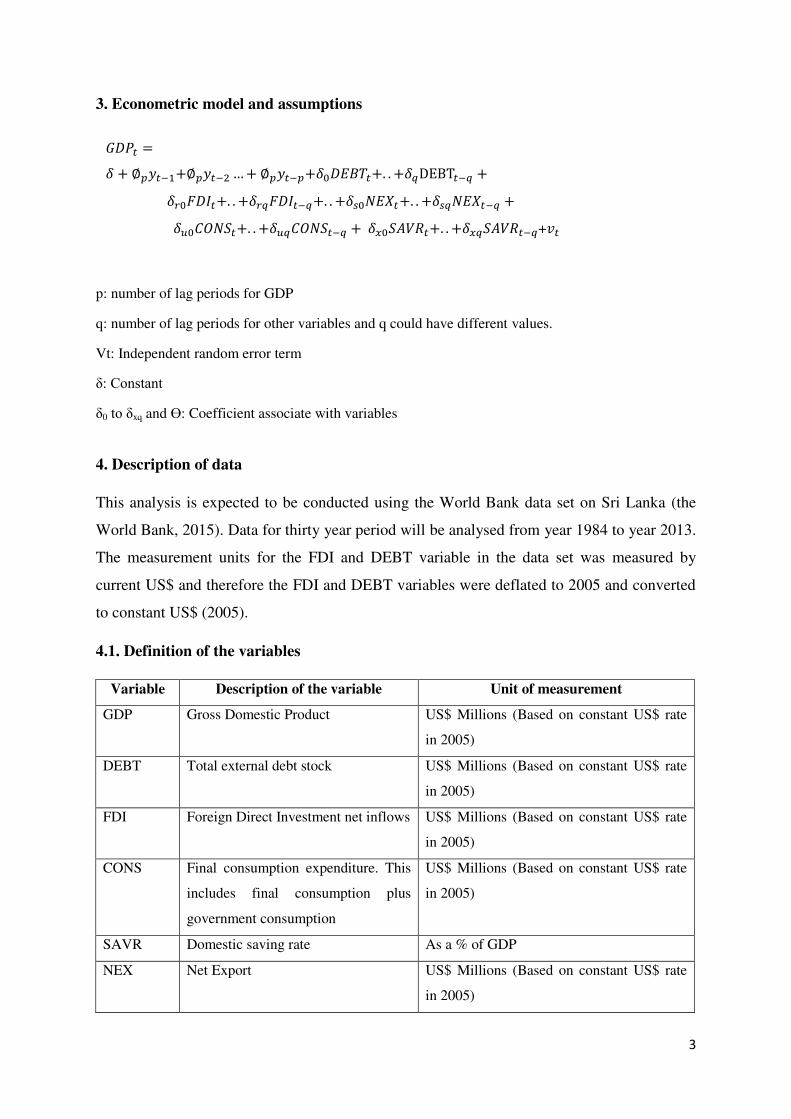
3. Econometric model and assumptions
3.1. Proposed Econometric Model
p: number of lag periods for GDP
q: number of lag periods for other variables and q could have different values.
Vt: Independent random error term
δ: Constant
δ0 to δxq and ϴ: Coefficient associate with variables
4. Description of data
This analysis is expected to be conducted using the World Bank data set on Sri Lanka (the
World Bank, 2015). Data for thirty year period will be analysed from year 1984 to year 2013.
The measurement units for the FDI and DEBT variable in the data set was measured by
current US$ and therefore the FDI and DEBT variables were deflated to 2005 and converted
to constant US$ (2005).
4.1. Definition of the variables
Variable Description of the variable Unit of measurement
GDP Gross Domestic Product US$ Millions (Based on constant US$ rate
in 2005)
DEBT Total external debt stock US$ Millions (Based on constant US$ rate
in 2005)
FDI Foreign Direct Investment net inflows US$ Millions (Based on constant US$ rate
in 2005)
CONS Final consumption expenditure. This
includes final consumption plus
government consumption
US$ Millions (Based on constant US$ rate
in 2005)
SAVR Domestic saving rate As a % of GDP
NEX Net Export US$ Millions (Based on constant US$ rate
in 2005)
𝐺𝐷𝑃𝑡 =𝛿 + ∅𝑝𝑦𝑡−1+∅𝑝𝑦𝑡−2…+ ∅𝑝𝑦𝑡−𝑝+𝛿0𝐷𝐸𝐵𝑇𝑡+. . +𝛿𝑞DEBT𝑡−𝑞 + 𝛿𝑟0𝐹𝐷𝐼𝑡+. . +𝛿𝑟𝑞𝐹𝐷𝐼𝑡−𝑞+. . +𝛿𝑠0𝑁𝐸𝑋𝑡+. . +𝛿𝑠𝑞𝑁𝐸𝑋𝑡−𝑞 + 𝛿𝑢0𝐶𝑂𝑁𝑆𝑡+. . +𝛿𝑢𝑞𝐶𝑂𝑁𝑆𝑡−𝑞 + 𝛿𝑥0𝑆𝐴𝑉𝑅𝑡+. . +𝛿𝑥𝑞𝑆𝐴𝑉𝑅𝑡−𝑞+𝑣𝑡
4
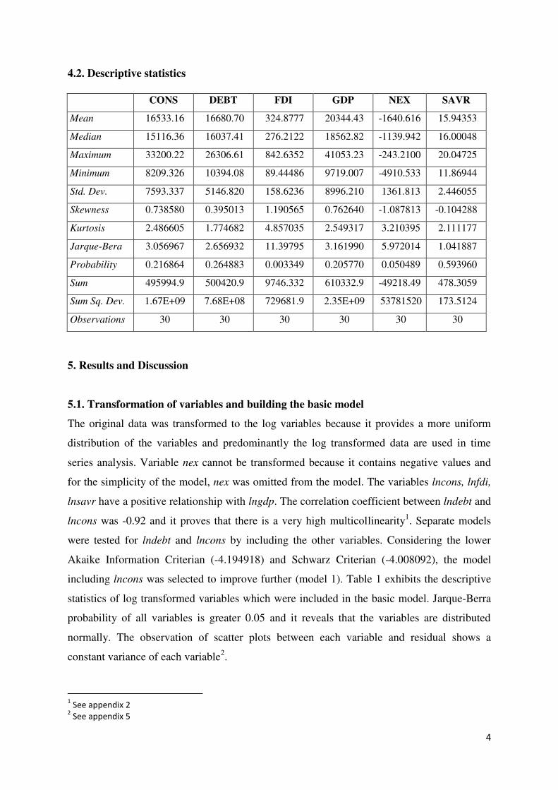
4.2. Descriptive statistics
CONS DEBT FDI GDP NEX SAVR
Mean 16533.16 16680.70 324.8777 20344.43 -1640.616 15.94353
Median 15116.36 16037.41 276.2122 18562.82 -1139.942 16.00048
Maximum 33200.22 26306.61 842.6352 41053.23 -243.2100 20.04725
Minimum 8209.326 10394.08 89.44486 9719.007 -4910.533 11.86944
Std. Dev. 7593.337 5146.820 158.6236 8996.210 1361.813 2.446055
Skewness 0.738580 0.395013 1.190565 0.762640 -1.087813 -0.104288
Kurtosis 2.486605 1.774682 4.857035 2.549317 3.210395 2.111177
Jarque-Bera 3.056967 2.656932 11.39795 3.161990 5.972014 1.041887
Probability 0.216864 0.264883 0.003349 0.205770 0.050489 0.593960
Sum 495994.9 500420.9 9746.332 610332.9 -49218.49 478.3059
Sum Sq. Dev. 1.67E+09 7.68E+08 729681.9 2.35E+09 53781520 173.5124
Observations 30 30 30 30 30 30
5. Results and Discussion
5.1. Transformation of variables and building the basic model
The original data was transformed to the log variables because it provides a more uniform
distribution of the variables and predominantly the log transformed data are used in time
series analysis. Variable nex cannot be transformed because it contains negative values and
for the simplicity of the model, nex was omitted from the model. The variables lncons, lnfdi,
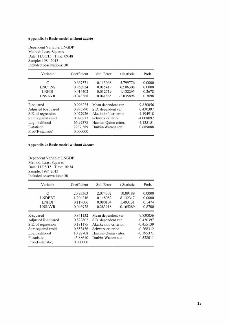
lnsavr have a positive relationship with lngdp. The correlation coefficient between lndebt and
lncons was -0.92 and it proves that there is a very high multicollinearity1. Separate models
were tested for lndebt and lncons by including the other variables. Considering the lower
Akaike Information Criterian (-4.194918) and Schwarz Criterian (-4.008092), the model
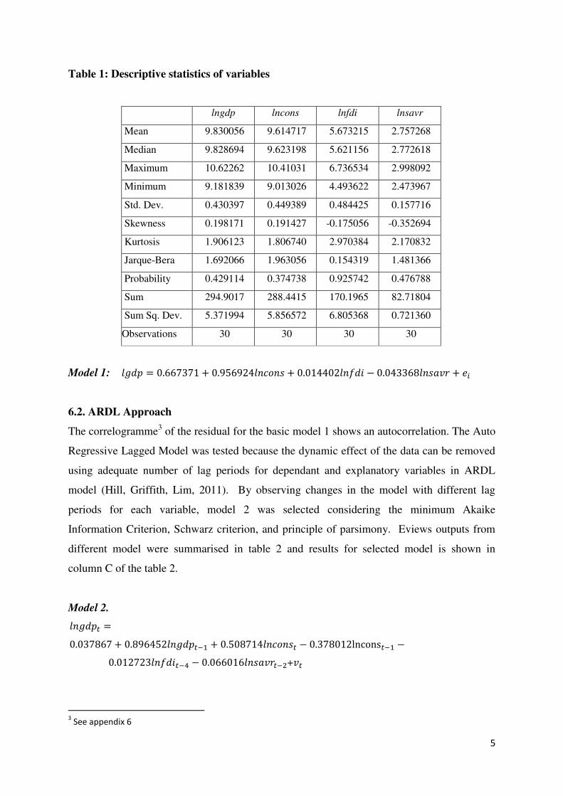
including lncons was selected to improve further (model 1). Table 1 exhibits the descriptive
statistics of log transformed variables which were included in the basic model. Jarque-Berra
probability of all variables is greater 0.05 and it reveals that the variables are distributed
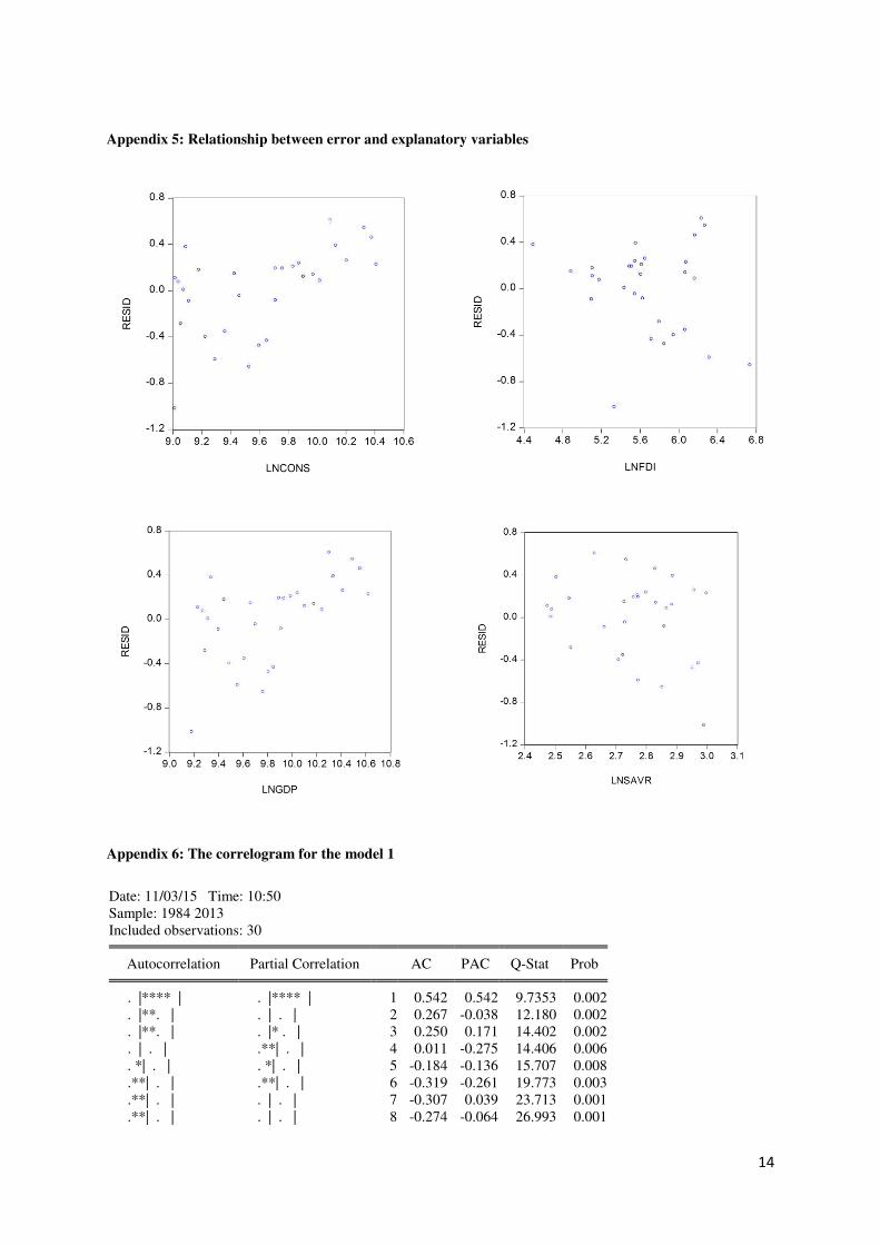
normally. The observation of scatter plots between each variable and residual shows a
constant variance of each variable2.
1 See appendix 2
2 See appendix 5
5
Table 1: Descriptive statistics of variables
lngdp lncons lnfdi lnsavr
Mean 9.830056 9.614717 5.673215 2.757268
Median 9.828694 9.623198 5.621156 2.772618
Maximum 10.62262 10.41031 6.736534 2.998092
Minimum 9.181839 9.013026 4.493622 2.473967
Std. Dev. 0.430397 0.449389 0.484425 0.157716
Skewness 0.198171 0.191427 -0.175056 -0.352694
Kurtosis 1.906123 1.806740 2.970384 2.170832
Jarque-Bera 1.692066 1.963056 0.154319 1.481366
Probability 0.429114 0.374738 0.925742 0.476788
Sum 294.9017 288.4415 170.1965 82.71804
Sum Sq. Dev. 5.371994 5.856572 6.805368 0.721360
Observations 30 30 30 30
Model 1: = . + . + . . +
6.2. ARDL Approach
The correlogramme3 of the residual for the basic model 1 shows an autocorrelation. The Auto
Regressive Lagged Model was tested because the dynamic effect of the data can be removed
using adequate number of lag periods for dependant and explanatory variables in ARDL
model (Hill, Griffith, Lim, 2011). By observing changes in the model with different lag
periods for each variable, model 2 was selected considering the minimum Akaike
Information Criterion, Schwarz criterion, and principle of parsimony. Eviews outputs from
different model were summarised in table 2 and results for selected model is shown in
column C of the table 2.
Model 2.
3.Model1. Proposed Econometric Model
3 See appendix 6
𝑙𝑛𝑔𝑑𝑝𝑡 = . + . 𝑙𝑛𝑔𝑑𝑝𝑡−1 + . 𝑙𝑛𝑐𝑜𝑛𝑠𝑡 . lncons𝑡−1 . 𝑙𝑛𝑓𝑑𝑖𝑡−4 . 𝑙𝑛𝑠𝑎𝑣𝑟𝑡−2+𝑣𝑡
6
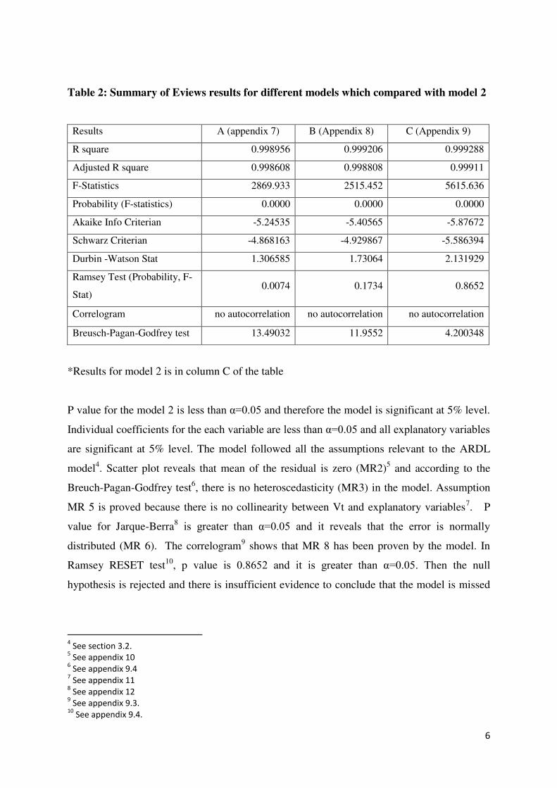
Table 2: Summary of Eviews results for different models which compared with model 2
Results A (appendix 7) B (Appendix 8) C (Appendix 9)
R square 0.998956 0.999206 0.999288
Adjusted R square 0.998608 0.998808 0.99911
F-Statistics 2869.933 2515.452 5615.636
Probability (F-statistics) 0.0000 0.0000 0.0000
Akaike Info Criterian -5.24535 -5.40565 -5.87672
Schwarz Criterian -4.868163 -4.929867 -5.586394
Durbin -Watson Stat 1.306585 1.73064 2.131929
Ramsey Test (Probability, F-
Stat) 0.0074 0.1734 0.8652
Correlogram no autocorrelation no autocorrelation no autocorrelation
Breusch-Pagan-Godfrey test 13.49032 11.9552 4.200348
*Results for model 2 is in column C of the table
P value for the model 2 is less than α=0.05 and therefore the model is significant at 5% level.
Individual coefficients for the each variable are less than α=0.05 and all explanatory variables
are significant at 5% level. The model followed all the assumptions relevant to the ARDL
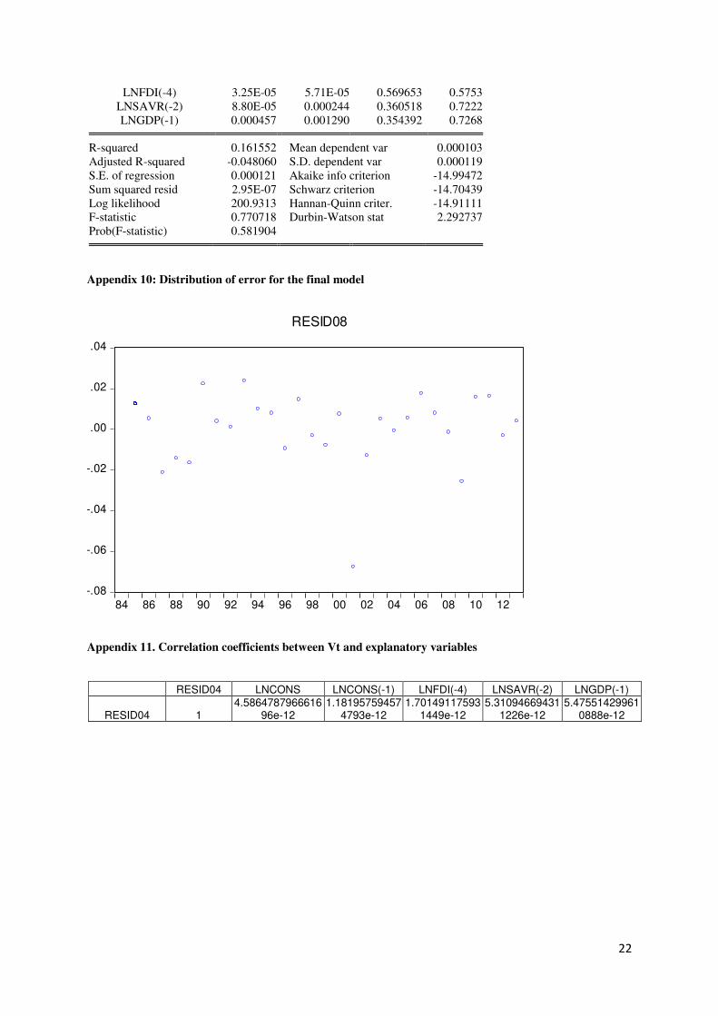
model4. Scatter plot reveals that mean of the residual is zero (MR2)5 and according to the
Breuch-Pagan-Godfrey test6, there is no heteroscedasticity (MR3) in the model. Assumption
MR 5 is proved because there is no collinearity between Vt and explanatory variables7. P
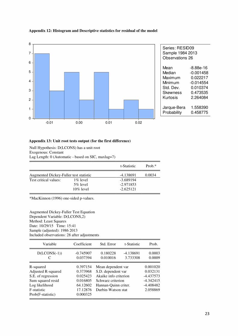
value for Jarque-Berra8 is greater than α=0.05 and it reveals that the error is normally
distributed (MR 6). The correlogram9 shows that MR 8 has been proven by the model. In
Ramsey RESET test10, p value is 0.8652 and it is greater than α=0.05. Then the null
hypothesis is rejected and there is insufficient evidence to conclude that the model is missed
4 See section 3.2.
5 See appendix 10
6 See appendix 9.4
7 See appendix 11
8 See appendix 12
9 See appendix 9.3.
10 See appendix 9.4.
7
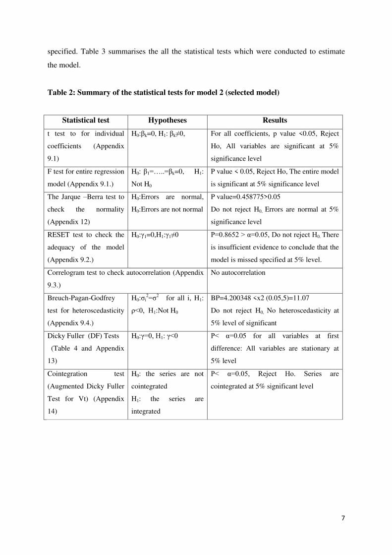
specified. Table 3 summarises the all the statistical tests which were conducted to estimate
the model.
Table 2: Summary of the statistical tests for model 2 (selected model)
Statistical test Hypotheses Results
t test to for individual
coefficients (Appendix
9.1)
H0:βk=0, H1: βk≠0, For all coefficients, p value <0.05, Reject
Ho, All variables are significant at 5%
significance level
F test for entire regression
model (Appendix 9.1.)
H0: β1=…..=βk=0, H1:
Not H0
P value < 0.05, Reject Ho, The entire model
is significant at 5% significance level
The Jarque –Berra test to
check the normality
(Appendix 12)
H0:Errors are normal,
H0:Errors are not normal
P value=0.458775>0.05
Do not reject H0, Errors are normal at 5%
significance level
RESET test to check the
adequacy of the model
(Appendix 9.2.)
H0:γ1=0,H1:γ1≠0
P=0.8652 > α=0.05, Do not reject H0. There
is insufficient evidence to conclude that the
model is missed specified at 5% level.
Correlogram test to check autocorrelation (Appendix
9.3.)
No autocorrelation
Breuch-Pagan-Godfrey
test for heteroscedasticity
(Appendix 9.4.)
H0:σi2=σ2 for all i, H1:
ρ<0, H1:Not H0
BP=4.200348 <x2 (0.05,5)=11.07
Do not reject H0, No heteroscedasticity at
5% level of significant
Dicky Fuller (DF) Tests
(Table 4 and Appendix
13)
H0:γ=0, H1: γ<0
P< α=0.05 for all variables at first
difference: All variables are stationary at
5% level
Cointegration test
(Augmented Dicky Fuller
Test for Vt) (Appendix
14)
H0: the series are not
cointegrated
H1: the series are
integrated
P< α=0.05, Reject Ho. Series are
cointegrated at 5% significant level
8
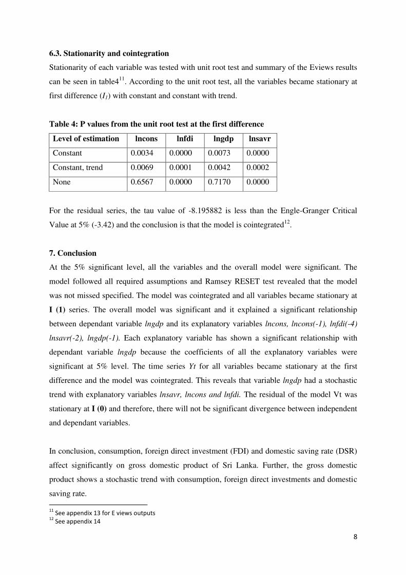
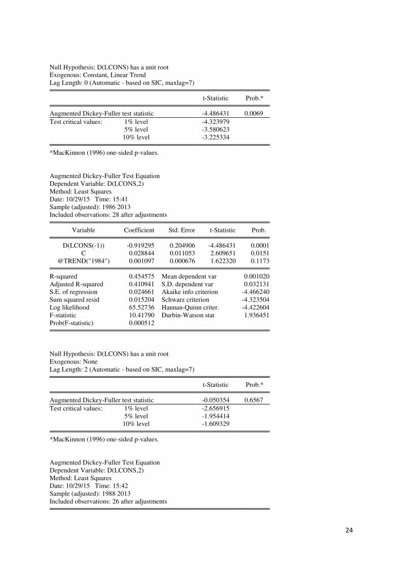
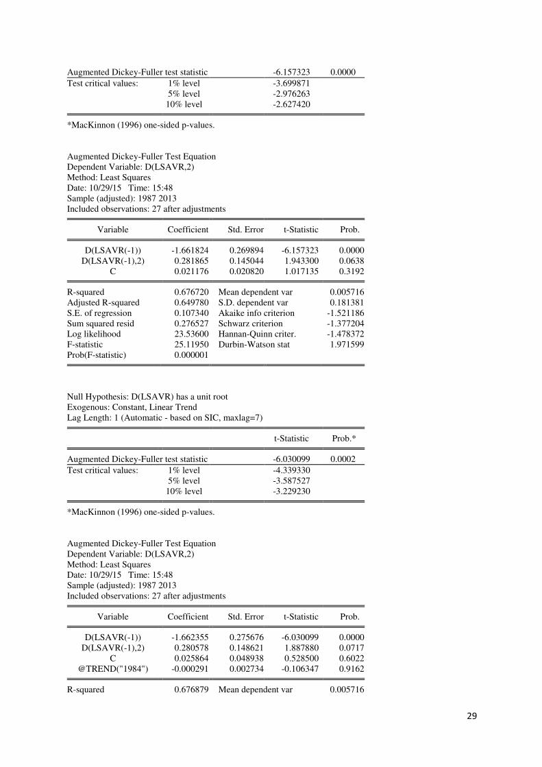
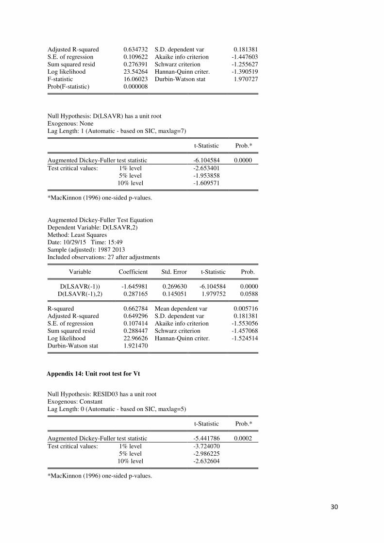
6.3. Stationarity and cointegration
Stationarity of each variable was tested with unit root test and summary of the Eviews results
can be seen in table411. According to the unit root test, all the variables became stationary at
first difference (I1) with constant and constant with trend.
Table 4: P values from the unit root test at the first difference
Level of estimation lncons lnfdi lngdp lnsavr
Constant 0.0034 0.0000 0.0073 0.0000
Constant, trend 0.0069 0.0001 0.0042 0.0002
None 0.6567 0.0000 0.7170 0.0000
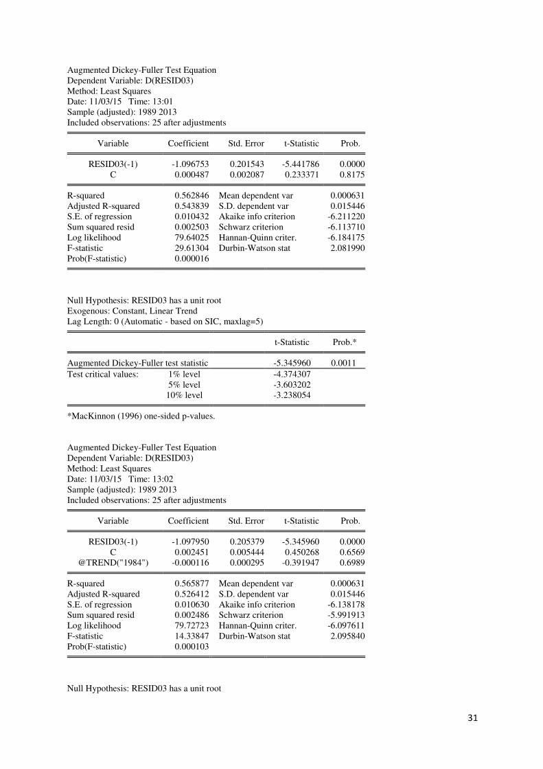
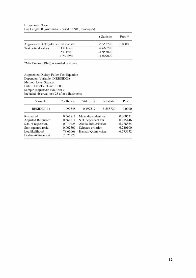
For the residual series, the tau value of -8.195882 is less than the Engle-Granger Critical
Value at 5% (-3.42) and the conclusion is that the model is cointegrated12.
7. Conclusion
At the 5% significant level, all the variables and the overall model were significant. The
model followed all required assumptions and Ramsey RESET test revealed that the model
was not missed specified. The model was cointegrated and all variables became stationary at
I (1) series. The overall model was significant and it explained a significant relationship
between dependant variable lngdp and its explanatory variables lncons, lncons(-1), lnfdi(-4)
lnsavr(-2), lngdp(-1). Each explanatory variable has shown a significant relationship with
dependant variable lngdp because the coefficients of all the explanatory variables were
significant at 5% level. The time series Yt for all variables became stationary at the first
difference and the model was cointegrated. This reveals that variable lngdp had a stochastic
trend with explanatory variables lnsavr, lncons and lnfdi. The residual of the model Vt was
stationary at I (0) and therefore, there will not be significant divergence between independent
and dependant variables.
In conclusion, consumption, foreign direct investment (FDI) and domestic saving rate (DSR)
affect significantly on gross domestic product of Sri Lanka. Further, the gross domestic
product shows a stochastic trend with consumption, foreign direct investments and domestic
saving rate.
11
See appendix 13 for E views outputs 12
See appendix 14
9
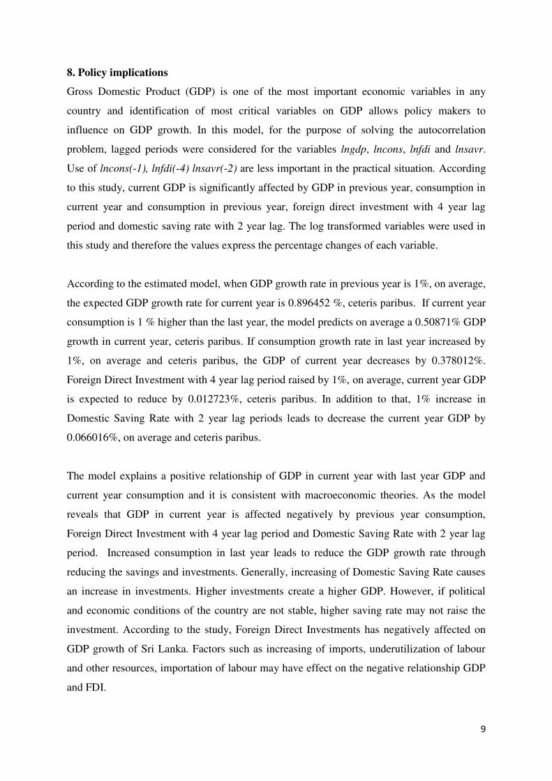
8. Policy implications
Gross Domestic Product (GDP) is one of the most important economic variables in any
country and identification of most critical variables on GDP allows policy makers to
influence on GDP growth. In this model, for the purpose of solving the autocorrelation
problem, lagged periods were considered for the variables lngdp, lncons, lnfdi and lnsavr.
Use of lncons(-1), lnfdi(-4) lnsavr(-2) are less important in the practical situation. According
to this study, current GDP is significantly affected by GDP in previous year, consumption in
current year and consumption in previous year, foreign direct investment with 4 year lag
period and domestic saving rate with 2 year lag. The log transformed variables were used in
this study and therefore the values express the percentage changes of each variable.
According to the estimated model, when GDP growth rate in previous year is 1%, on average,
the expected GDP growth rate for current year is 0.896452 %, ceteris paribus. If current year
consumption is 1 % higher than the last year, the model predicts on average a 0.50871% GDP
growth in current year, ceteris paribus. If consumption growth rate in last year increased by
1%, on average and ceteris paribus, the GDP of current year decreases by 0.378012%.
Foreign Direct Investment with 4 year lag period raised by 1%, on average, current year GDP
is expected to reduce by 0.012723%, ceteris paribus. In addition to that, 1% increase in
Domestic Saving Rate with 2 year lag periods leads to decrease the current year GDP by
0.066016%, on average and ceteris paribus.
The model explains a positive relationship of GDP in current year with last year GDP and
current year consumption and it is consistent with macroeconomic theories. As the model
reveals that GDP in current year is affected negatively by previous year consumption,
Foreign Direct Investment with 4 year lag period and Domestic Saving Rate with 2 year lag
period. Increased consumption in last year leads to reduce the GDP growth rate through
reducing the savings and investments. Generally, increasing of Domestic Saving Rate causes
an increase in investments. Higher investments create a higher GDP. However, if political
and economic conditions of the country are not stable, higher saving rate may not raise the
investment. According to the study, Foreign Direct Investments has negatively affected on
GDP growth of Sri Lanka. Factors such as increasing of imports, underutilization of labour
and other resources, importation of labour may have effect on the negative relationship GDP
and FDI.
10
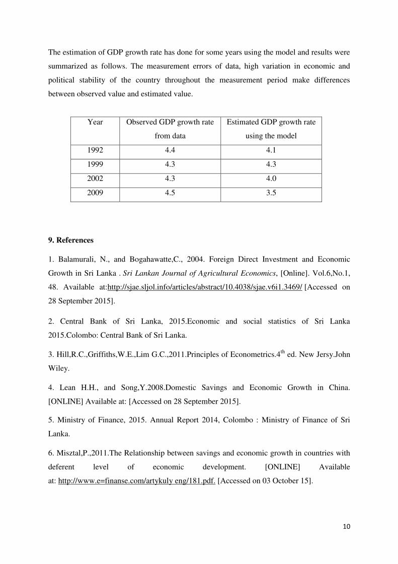
The estimation of GDP growth rate has done for some years using the model and results were
summarized as follows. The measurement errors of data, high variation in economic and
political stability of the country throughout the measurement period make differences
between observed value and estimated value.
Year Observed GDP growth rate
from data
Estimated GDP growth rate
using the model
1992 4.4 4.1
1999 4.3 4.3
2002 4.3 4.0
2009 4.5 3.5
9. References
1. Balamurali, N., and Bogahawatte,C., 2004. Foreign Direct Investment and Economic
Growth in Sri Lanka . Sri Lankan Journal of Agricultural Economics, [Online]. Vol.6,No.1,
48. Available at:http://sjae.sljol.info/articles/abstract/10.4038/sjae.v6i1.3469/ [Accessed on
28 September 2015].
2. Central Bank of Sri Lanka, 2015.Economic and social statistics of Sri Lanka
2015.Colombo: Central Bank of Sri Lanka.
3. Hill,R.C.,Griffiths,W.E.,Lim G.C.,2011.Principles of Econometrics.4th ed. New Jersy.John
Wiley.
4. Lean H.H., and Song,Y.2008.Domestic Savings and Economic Growth in China.
[ONLINE] Available at: [Accessed on 28 September 2015].
5. Ministry of Finance, 2015. Annual Report 2014, Colombo : Ministry of Finance of Sri
Lanka.
6. Misztal,P.,2011.The Relationship between savings and economic growth in countries with
deferent level of economic development. [ONLINE] Available
at: http://www.e=finanse.com/artykuly eng/181.pdf. [Accessed on 03 October 15].
11
7. Ngo,T.H.D., 2012. Statistics and Data Analysis, SAS global forum 2012, [Online]. Paper
333-2012. Available at: http://support.sas.com/resources/papers/proceedings12/333-
2012.pdf [Accessed on 11 October 2015].
8. Rahman, MM, and Shahbaz,M.,2011. Do Imports and Foreign Capital Inflows Lead
Economic Growth? Cointegration and Causality Analysis in Pakistan. Munich Personal
RePEc Archive, [Online]. paper no.29805, 22. Available
at: http://core.ac.uk/download/pdf/6915909.pdf [Accessed on 28 September 2015].
9. Ranasinghe,R.A.S.K., and Ichihashi,M.2014. The composition of government expenditure
and economic growth:The case of Sri Lanka. [ONLINE] Available at: http://ir.lib.hiroshima-
u.ac.jp/files/public/36105/IDEC-DP2 04-7.pdf.[Accessed on 28 September 2015].
10. The World Bank,2015.Country and Lending Groups. [ONLINE] Available
at:http://data.worldbank.org/about/country-and-lending-groups#Lower_middle_income.
[Accessed 27 September 15].
11. The World Bank. 2015. Data,Sri Lanka. [ONLINE] Available
at: http://data.worldbank.org/country/sri-lanka. [Accessed on 25 September 15].
12. Velnampy,T. and Achchuthan,S.,2013.Export, Import and Economic Growth: Evidence
from Sri Lanka.Journal of Economics and Sustainable Development. [ONLINE] Available at:
http://www.researhgate.net/publication/253233477 Export Import and Economic Growth
Evidence from Sri Lanka. [Accessed on 28 September 2015].
12
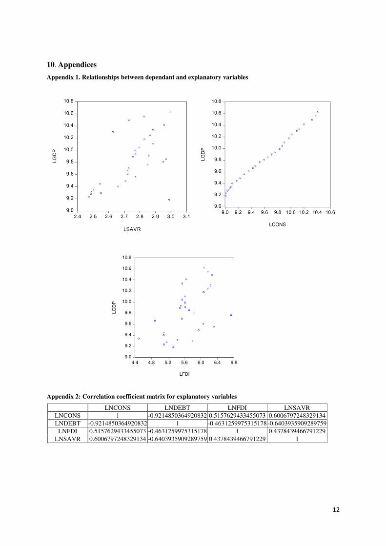
10. Appendices
Appendix 1. Relationships between dependant and explanatory variables
9.0
9.2
9.4
9.6
9.8
10.0
10.2
10.4
10.6
10.8
4.4 4.8 5.2 5.6 6.0 6.4 6.8
LFDI
LG
DP
Appendix 2: Correlation coefficient matrix for explanatory variables
LNCONS LNDEBT LNFDI LNSAVR LNCONS 1 -0.9214850364920832 0.5157629433455073 0.6006797248329134 LNDEBT -0.9214850364920832 1 -0.4631259975315178 -0.6403935909289759
LNFDI 0.5157629433455073 -0.4631259975315178 1 0.4378439466791229 LNSAVR 0.6006797248329134 -0.6403935909289759 0.4378439466791229 1
13
Appendix 3: Basic model without lndebt
Dependent Variable: LNGDP Method: Least Squares Date: 11/03/15 Time: 09:48 Sample: 1984 2013 Included observations: 30
Variable Coefficient Std. Error t-Statistic Prob. C 0.667371 0.115068 5.799776 0.0000
LNCONS 0.956924 0.015419 62.06308 0.0000 LNFDI 0.014402 0.012719 1.132295 0.2678
LNSAVR -0.043368 0.041865 -1.035898 0.3098 R-squared 0.996225 Mean dependent var 9.830056
Adjusted R-squared 0.995790 S.D. dependent var 0.430397 S.E. of regression 0.027926 Akaike info criterion -4.194918 Sum squared resid 0.020277 Schwarz criterion -4.008092 Log likelihood 66.92378 Hannan-Quinn criter. -4.135151 F-statistic 2287.389 Durbin-Watson stat 0.689088 Prob(F-statistic) 0.000000
Appendix 4: Basic model without lncons
Dependent Variable: LNGDP Method: Least Squares Date: 11/03/15 Time: 10:34 Sample: 1984 2013 Included observations: 30
Variable Coefficient Std. Error t-Statistic Prob. C 20.93363 2.074302 10.09189 0.0000
LNDEBT -1.204246 0.148082 -8.132317 0.0000 LNFDI 0.119606 0.080104 1.493131 0.1474
LNSAVR -0.046928 0.283918 -0.165289 0.8700 R-squared 0.841132 Mean dependent var 9.830056
Adjusted R-squared 0.822802 S.D. dependent var 0.430397 S.E. of regression 0.181175 Akaike info criterion -0.455139 Sum squared resid 0.853436 Schwarz criterion -0.268312 Log likelihood 10.82708 Hannan-Quinn criter. -0.395371 F-statistic 45.88610 Durbin-Watson stat 0.528011 Prob(F-statistic) 0.000000
14
Appendix 5: Relationship between error and explanatory variables
Appendix 6: The correlogram for the model 1
Date: 11/03/15 Time: 10:50 Sample: 1984 2013 Included observations: 30
Autocorrelation Partial Correlation AC PAC Q-Stat Prob . |**** | . |**** | 1 0.542 0.542 9.7353 0.002
. |**. | . | . | 2 0.267 -0.038 12.180 0.002 . |**. | . |* . | 3 0.250 0.171 14.402 0.002 . | . | .**| . | 4 0.011 -0.275 14.406 0.006 . *| . | . *| . | 5 -0.184 -0.136 15.707 0.008 .**| . | .**| . | 6 -0.319 -0.261 19.773 0.003 .**| . | . | . | 7 -0.307 0.039 23.713 0.001 .**| . | . | . | 8 -0.274 -0.064 26.993 0.001
15
.**| . | . *| . | 9 -0.305 -0.080 31.249 0.000 .**| . | .**| . | 10 -0.313 -0.211 35.939 0.000 .**| . | .**| . | 11 -0.330 -0.257 41.432 0.000 .**| . | . *| . | 12 -0.274 -0.148 45.444 0.000 . *| . | . | . | 13 -0.172 -0.060 47.109 0.000 . | . | . |* . | 14 -0.021 0.107 47.136 0.000 . |* . | . | . | 15 0.102 -0.011 47.805 0.000 . |* . | . *| . | 16 0.165 -0.088 49.672 0.000
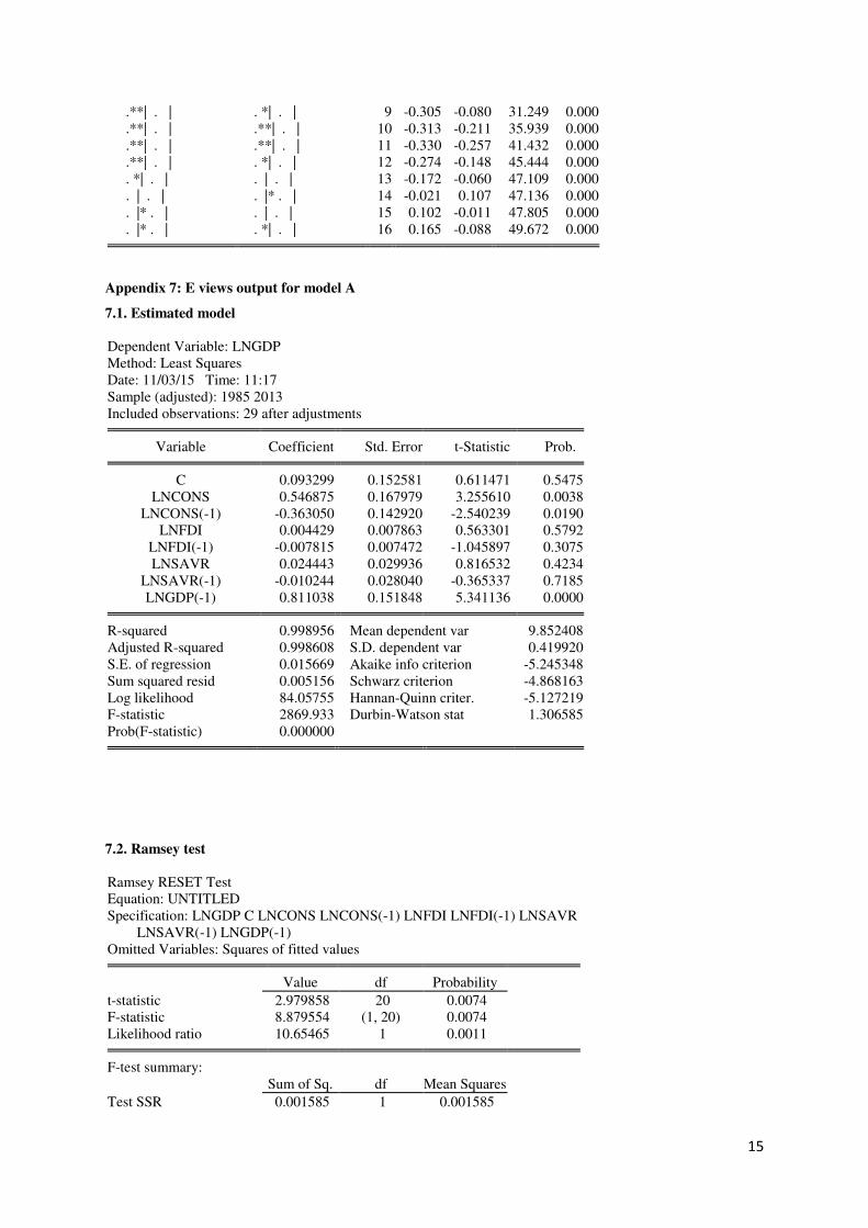
Appendix 7: E views output for model A
7.1. Estimated model
Dependent Variable: LNGDP Method: Least Squares Date: 11/03/15 Time: 11:17 Sample (adjusted): 1985 2013 Included observations: 29 after adjustments
Variable Coefficient Std. Error t-Statistic Prob. C 0.093299 0.152581 0.611471 0.5475
LNCONS 0.546875 0.167979 3.255610 0.0038 LNCONS(-1) -0.363050 0.142920 -2.540239 0.0190
LNFDI 0.004429 0.007863 0.563301 0.5792 LNFDI(-1) -0.007815 0.007472 -1.045897 0.3075 LNSAVR 0.024443 0.029936 0.816532 0.4234
LNSAVR(-1) -0.010244 0.028040 -0.365337 0.7185 LNGDP(-1) 0.811038 0.151848 5.341136 0.0000
R-squared 0.998956 Mean dependent var 9.852408
Adjusted R-squared 0.998608 S.D. dependent var 0.419920 S.E. of regression 0.015669 Akaike info criterion -5.245348 Sum squared resid 0.005156 Schwarz criterion -4.868163 Log likelihood 84.05755 Hannan-Quinn criter. -5.127219 F-statistic 2869.933 Durbin-Watson stat 1.306585 Prob(F-statistic) 0.000000
7.2. Ramsey test
Ramsey RESET Test Equation: UNTITLED Specification: LNGDP C LNCONS LNCONS(-1) LNFDI LNFDI(-1) LNSAVR LNSAVR(-1) LNGDP(-1) Omitted Variables: Squares of fitted values
Value df Probability
t-statistic 2.979858 20 0.0074 F-statistic 8.879554 (1, 20) 0.0074 Likelihood ratio 10.65465 1 0.0011
F-test summary: Sum of Sq. df Mean Squares
Test SSR 0.001585 1 0.001585
16
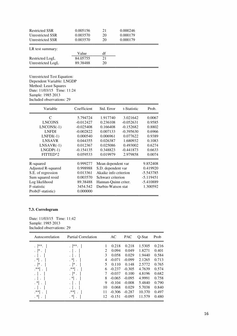
Restricted SSR 0.005156 21 0.000246 Unrestricted SSR 0.003570 20 0.000179 Unrestricted SSR 0.003570 20 0.000179
LR test summary: Value df
Restricted LogL 84.05755 21 Unrestricted LogL 89.38488 20
Unrestricted Test Equation: Dependent Variable: LNGDP Method: Least Squares Date: 11/03/15 Time: 11:24 Sample: 1985 2013 Included observations: 29
Variable Coefficient Std. Error t-Statistic Prob. C 5.794724 1.917740 3.021642 0.0067
LNCONS -0.012427 0.236108 -0.052631 0.9585 LNCONS(-1) -0.025408 0.166408 -0.152682 0.8802
LNFDI -0.002822 0.007133 -0.395630 0.6966 LNFDI(-1) 0.000540 0.006961 0.077622 0.9389 LNSAVR 0.044355 0.026387 1.680932 0.1083
LNSAVR(-1) 0.012367 0.025086 0.493002 0.6274 LNGDP(-1) -0.154135 0.348823 -0.441873 0.6633 FITTED^2 0.059533 0.019979 2.979858 0.0074
R-squared 0.999277 Mean dependent var 9.852408
Adjusted R-squared 0.998988 S.D. dependent var 0.419920 S.E. of regression 0.013361 Akaike info criterion -5.543785 Sum squared resid 0.003570 Schwarz criterion -5.119451 Log likelihood 89.38488 Hannan-Quinn criter. -5.410889 F-statistic 3454.542 Durbin-Watson stat 1.300592 Prob(F-statistic) 0.000000
7.3. Correlogram
Date: 11/03/15 Time: 11:42 Sample: 1985 2013 Included observations: 29
Autocorrelation Partial Correlation AC PAC Q-Stat Prob . |**. | . |**. | 1 0.218 0.218 1.5305 0.216
. |* . | . | . | 2 0.094 0.049 1.8271 0.401 . | . | . | . | 3 0.058 0.029 1.9440 0.584 . *| . | . *| . | 4 -0.071 -0.099 2.1265 0.713 . |* . | . |* . | 5 0.110 0.148 2.5772 0.765 .**| . | .**| . | 6 -0.237 -0.305 4.7639 0.574 . | . | . |* . | 7 -0.037 0.100 4.8196 0.682 . | . | . *| . | 8 -0.065 -0.095 4.9991 0.758 . *| . | . | . | 9 -0.104 -0.008 5.4840 0.790 . | . | . | . | 10 0.068 0.029 5.7038 0.840 .**| . | .**| . | 11 -0.306 -0.287 10.370 0.497 . *| . | . *| . | 12 -0.151 -0.095 11.579 0.480
17
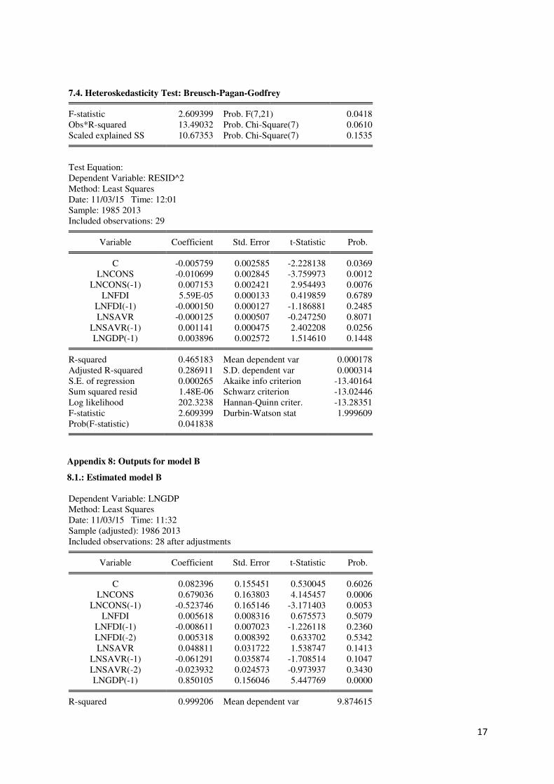
7.4. Heteroskedasticity Test: Breusch-Pagan-Godfrey F-statistic 2.609399 Prob. F(7,21) 0.0418
Obs*R-squared 13.49032 Prob. Chi-Square(7) 0.0610 Scaled explained SS 10.67353 Prob. Chi-Square(7) 0.1535
Test Equation: Dependent Variable: RESID^2 Method: Least Squares Date: 11/03/15 Time: 12:01 Sample: 1985 2013 Included observations: 29
Variable Coefficient Std. Error t-Statistic Prob. C -0.005759 0.002585 -2.228138 0.0369
LNCONS -0.010699 0.002845 -3.759973 0.0012 LNCONS(-1) 0.007153 0.002421 2.954493 0.0076
LNFDI 5.59E-05 0.000133 0.419859 0.6789 LNFDI(-1) -0.000150 0.000127 -1.186881 0.2485 LNSAVR -0.000125 0.000507 -0.247250 0.8071
LNSAVR(-1) 0.001141 0.000475 2.402208 0.0256 LNGDP(-1) 0.003896 0.002572 1.514610 0.1448
R-squared 0.465183 Mean dependent var 0.000178
Adjusted R-squared 0.286911 S.D. dependent var 0.000314 S.E. of regression 0.000265 Akaike info criterion -13.40164 Sum squared resid 1.48E-06 Schwarz criterion -13.02446 Log likelihood 202.3238 Hannan-Quinn criter. -13.28351 F-statistic 2.609399 Durbin-Watson stat 1.999609 Prob(F-statistic) 0.041838
Appendix 8: Outputs for model B
8.1.: Estimated model B
Dependent Variable: LNGDP Method: Least Squares Date: 11/03/15 Time: 11:32 Sample (adjusted): 1986 2013 Included observations: 28 after adjustments
Variable Coefficient Std. Error t-Statistic Prob. C 0.082396 0.155451 0.530045 0.6026
LNCONS 0.679036 0.163803 4.145457 0.0006 LNCONS(-1) -0.523746 0.165146 -3.171403 0.0053
LNFDI 0.005618 0.008316 0.675573 0.5079 LNFDI(-1) -0.008611 0.007023 -1.226118 0.2360 LNFDI(-2) 0.005318 0.008392 0.633702 0.5342 LNSAVR 0.048811 0.031722 1.538747 0.1413
LNSAVR(-1) -0.061291 0.035874 -1.708514 0.1047 LNSAVR(-2) -0.023932 0.024573 -0.973937 0.3430 LNGDP(-1) 0.850105 0.156046 5.447769 0.0000
R-squared 0.999206 Mean dependent var 9.874615
18
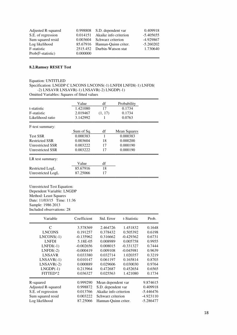
Adjusted R-squared 0.998808 S.D. dependent var 0.409918 S.E. of regression 0.014151 Akaike info criterion -5.405655 Sum squared resid 0.003604 Schwarz criterion -4.929867 Log likelihood 85.67916 Hannan-Quinn criter. -5.260202 F-statistic 2515.452 Durbin-Watson stat 1.730640 Prob(F-statistic) 0.000000
8.2.Ramsey RESET Test Equation: UNTITLED Specification: LNGDP C LNCONS LNCONS(-1) LNFDI LNFDI(-1) LNFDI( -2) LNSAVR LNSAVR(-1) LNSAVR(-2) LNGDP(-1) Omitted Variables: Squares of fitted values
Value df Probability
t-statistic 1.421080 17 0.1734 F-statistic 2.019467 (1, 17) 0.1734 Likelihood ratio 3.142992 1 0.0763
F-test summary: Sum of Sq. df Mean Squares
Test SSR 0.000383 1 0.000383 Restricted SSR 0.003604 18 0.000200 Unrestricted SSR 0.003222 17 0.000190 Unrestricted SSR 0.003222 17 0.000190
LR test summary: Value df
Restricted LogL 85.67916 18 Unrestricted LogL 87.25066 17
Unrestricted Test Equation: Dependent Variable: LNGDP Method: Least Squares Date: 11/03/15 Time: 11:36 Sample: 1986 2013 Included observations: 28
Variable Coefficient Std. Error t-Statistic Prob. C 3.578369 2.464726 1.451832 0.1648
LNCONS 0.191257 0.378432 0.505392 0.6198 LNCONS(-1) -0.135962 0.316662 -0.429362 0.6731
LNFDI 5.18E-05 0.008989 0.005758 0.9955 LNFDI(-1) -0.002656 0.008015 -0.331327 0.7444 LNFDI(-2) -0.000419 0.009108 -0.045981 0.9639 LNSAVR 0.033380 0.032714 1.020357 0.3219
LNSAVR(-1) 0.010147 0.061197 0.165814 0.8703 LNSAVR(-2) 0.000889 0.029606 0.030030 0.9764 LNGDP(-1) 0.213964 0.472687 0.452654 0.6565 FITTED^2 0.036327 0.025563 1.421080 0.1734
R-squared 0.999290 Mean dependent var 9.874615
Adjusted R-squared 0.998872 S.D. dependent var 0.409918 S.E. of regression 0.013766 Akaike info criterion -5.446476 Sum squared resid 0.003222 Schwarz criterion -4.923110 Log likelihood 87.25066 Hannan-Quinn criter. -5.286477
19
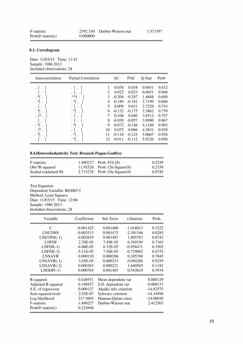
F-statistic 2392.330 Durbin-Watson stat 1.571597 Prob(F-statistic) 0.000000
8.3. Correlogram
Date: 11/03/15 Time: 11:41 Sample: 1986 2013 Included observations: 28
Autocorrelation Partial Correlation AC PAC Q-Stat Prob . | . | . | . | 1 0.038 0.038 0.0451 0.832
. | . | . | . | 2 0.025 0.023 0.0651 0.968 . *| . | .**| . | 3 -0.204 -0.207 1.4688 0.689 . *| . | . *| . | 4 -0.189 -0.181 2.7199 0.606 . | . | . | . | 5 0.009 0.031 2.7228 0.743 . *| . | . *| . | 6 -0.132 -0.175 3.3862 0.759 . |* . | . | . | 7 0.108 0.040 3.8512 0.797 . | . | . | . | 8 -0.030 -0.057 3.8900 0.867 . *| . | . *| . | 9 -0.072 -0.146 4.1188 0.903 . |* . | . | . | 10 0.075 0.066 4.3831 0.928 . *| . | . *| . | 11 -0.118 -0.124 5.0667 0.928 . | . | . *| . | 12 -0.011 -0.112 5.0726 0.956
8.4.Heteroskedasticity Test: Breusch-Pagan-Godfrey
F-statistic 1.490227 Prob. F(9,18) 0.2249
Obs*R-squared 11.95520 Prob. Chi-Square(9) 0.2158 Scaled explained SS 2.715278 Prob. Chi-Square(9) 0.9745
Test Equation: Dependent Variable: RESID^2 Method: Least Squares Date: 11/03/15 Time: 12:06 Sample: 1986 2013 Included observations: 28
Variable Coefficient Std. Error t-Statistic Prob. C -0.001425 0.001400 -1.018013 0.3222
LNCONS -0.003513 0.001475 -2.381546 0.0285 LNCONS(-1) 0.002819 0.001487 1.895783 0.0742
LNFDI 2.76E-05 7.49E-05 0.369194 0.7163 LNFDI(-1) -6.06E-05 6.32E-05 -0.958471 0.3505 LNFDI(-2) -5.51E-05 7.56E-05 -0.729082 0.4753 LNSAVR 0.000110 0.000286 0.385398 0.7045
LNSAVR(-1) 3.05E-05 0.000323 0.094266 0.9259 LNSAVR(-2) 0.000363 0.000221 1.640565 0.1182 LNGDP(-1) 0.000764 0.001405 0.543619 0.5934
R-squared 0.426971 Mean dependent var 0.000129
Adjusted R-squared 0.140457 S.D. dependent var 0.000137 S.E. of regression 0.000127 Akaike info criterion -14.82575 Sum squared resid 2.92E-07 Schwarz criterion -14.34996 Log likelihood 217.5605 Hannan-Quinn criter. -14.68030 F-statistic 1.490227 Durbin-Watson stat 2.412503 Prob(F-statistic) 0.224948
20
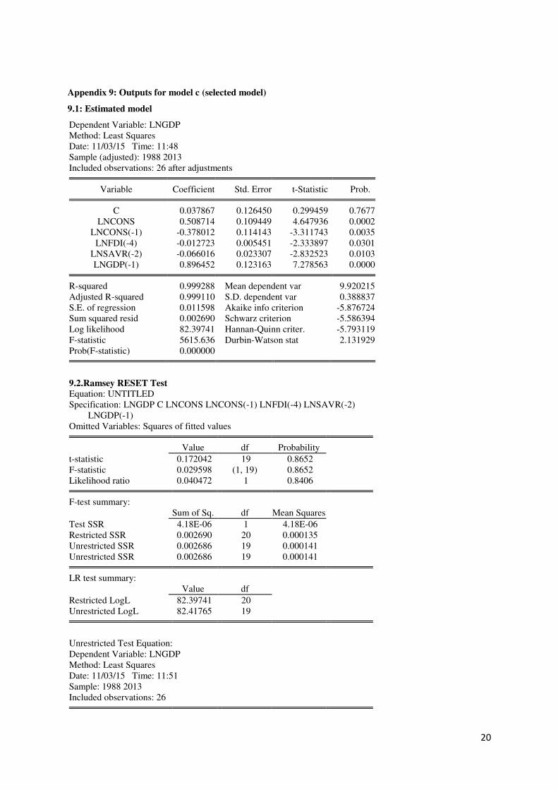
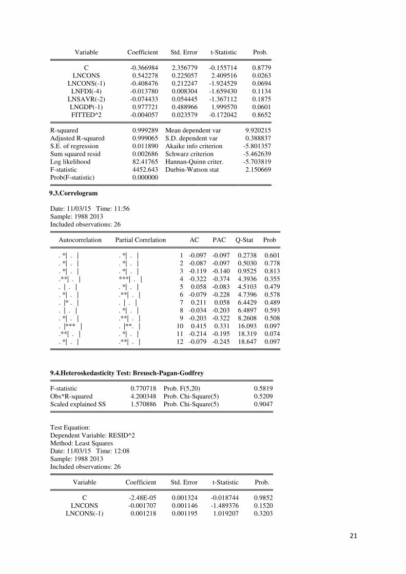
Appendix 9: Outputs for model c (selected model)
9.1: Estimated model
Dependent Variable: LNGDP Method: Least Squares Date: 11/03/15 Time: 11:48 Sample (adjusted): 1988 2013 Included observations: 26 after adjustments
Variable Coefficient Std. Error t-Statistic Prob. C 0.037867 0.126450 0.299459 0.7677
LNCONS 0.508714 0.109449 4.647936 0.0002 LNCONS(-1) -0.378012 0.114143 -3.311743 0.0035
LNFDI(-4) -0.012723 0.005451 -2.333897 0.0301 LNSAVR(-2) -0.066016 0.023307 -2.832523 0.0103 LNGDP(-1) 0.896452 0.123163 7.278563 0.0000
R-squared 0.999288 Mean dependent var 9.920215
Adjusted R-squared 0.999110 S.D. dependent var 0.388837 S.E. of regression 0.011598 Akaike info criterion -5.876724 Sum squared resid 0.002690 Schwarz criterion -5.586394 Log likelihood 82.39741 Hannan-Quinn criter. -5.793119 F-statistic 5615.636 Durbin-Watson stat 2.131929 Prob(F-statistic) 0.000000
9.2.Ramsey RESET Test Equation: UNTITLED Specification: LNGDP C LNCONS LNCONS(-1) LNFDI(-4) LNSAVR(-2) LNGDP(-1) Omitted Variables: Squares of fitted values
Value df Probability
t-statistic 0.172042 19 0.8652 F-statistic 0.029598 (1, 19) 0.8652 Likelihood ratio 0.040472 1 0.8406
F-test summary: Sum of Sq. df Mean Squares
Test SSR 4.18E-06 1 4.18E-06 Restricted SSR 0.002690 20 0.000135 Unrestricted SSR 0.002686 19 0.000141 Unrestricted SSR 0.002686 19 0.000141
LR test summary: Value df
Restricted LogL 82.39741 20 Unrestricted LogL 82.41765 19
Unrestricted Test Equation: Dependent Variable: LNGDP Method: Least Squares Date: 11/03/15 Time: 11:51 Sample: 1988 2013 Included observations: 26
21
Variable Coefficient Std. Error t-Statistic Prob. C -0.366984 2.356779 -0.155714 0.8779
LNCONS 0.542278 0.225057 2.409516 0.0263 LNCONS(-1) -0.408476 0.212247 -1.924529 0.0694
LNFDI(-4) -0.013780 0.008304 -1.659430 0.1134 LNSAVR(-2) -0.074433 0.054445 -1.367112 0.1875 LNGDP(-1) 0.977721 0.488966 1.999570 0.0601 FITTED^2 -0.004057 0.023579 -0.172042 0.8652
R-squared 0.999289 Mean dependent var 9.920215
Adjusted R-squared 0.999065 S.D. dependent var 0.388837 S.E. of regression 0.011890 Akaike info criterion -5.801357 Sum squared resid 0.002686 Schwarz criterion -5.462639 Log likelihood 82.41765 Hannan-Quinn criter. -5.703819 F-statistic 4452.643 Durbin-Watson stat 2.150669 Prob(F-statistic) 0.000000
9.3.Correlogram Date: 11/03/15 Time: 11:56 Sample: 1988 2013 Included observations: 26
Autocorrelation Partial Correlation AC PAC Q-Stat Prob . *| . | . *| . | 1 -0.097 -0.097 0.2738 0.601
. *| . | . *| . | 2 -0.087 -0.097 0.5030 0.778 . *| . | . *| . | 3 -0.119 -0.140 0.9525 0.813 .**| . | ***| . | 4 -0.322 -0.374 4.3936 0.355 . | . | . *| . | 5 0.058 -0.083 4.5103 0.479 . *| . | .**| . | 6 -0.079 -0.228 4.7396 0.578 . |* . | . | . | 7 0.211 0.058 6.4429 0.489 . | . | . *| . | 8 -0.034 -0.203 6.4897 0.593 . *| . | .**| . | 9 -0.203 -0.322 8.2608 0.508 . |*** | . |**. | 10 0.415 0.331 16.093 0.097 .**| . | . *| . | 11 -0.214 -0.195 18.319 0.074 . *| . | .**| . | 12 -0.079 -0.245 18.647 0.097
9.4.Heteroskedasticity Test: Breusch-Pagan-Godfrey
F-statistic 0.770718 Prob. F(5,20) 0.5819
Obs*R-squared 4.200348 Prob. Chi-Square(5) 0.5209 Scaled explained SS 1.570886 Prob. Chi-Square(5) 0.9047
Test Equation: Dependent Variable: RESID^2 Method: Least Squares Date: 11/03/15 Time: 12:08 Sample: 1988 2013 Included observations: 26
Variable Coefficient Std. Error t-Statistic Prob. C -2.48E-05 0.001324 -0.018744 0.9852
LNCONS -0.001707 0.001146 -1.489376 0.1520 LNCONS(-1) 0.001218 0.001195 1.019207 0.3203
22
LNFDI(-4) 3.25E-05 5.71E-05 0.569653 0.5753 LNSAVR(-2) 8.80E-05 0.000244 0.360518 0.7222 LNGDP(-1) 0.000457 0.001290 0.354392 0.7268
R-squared 0.161552 Mean dependent var 0.000103
Adjusted R-squared -0.048060 S.D. dependent var 0.000119 S.E. of regression 0.000121 Akaike info criterion -14.99472 Sum squared resid 2.95E-07 Schwarz criterion -14.70439 Log likelihood 200.9313 Hannan-Quinn criter. -14.91111 F-statistic 0.770718 Durbin-Watson stat 2.292737 Prob(F-statistic) 0.581904
Appendix 10: Distribution of error for the final model
-.08
-.06
-.04
-.02
.00
.02
.04
84 86 88 90 92 94 96 98 00 02 04 06 08 10 12
RESID08
Appendix 11. Correlation coefficients between Vt and explanatory variables
RESID04 LNCONS LNCONS(-1) LNFDI(-4) LNSAVR(-2) LNGDP(-1)
RESID04 1 4.5864787966616
96e-12 1.18195759457
4793e-12 1.70149117593
1449e-12 5.31094669431
1226e-12 5.47551429961
0888e-12
23
Appendix 12: Histogram and Descriptive statistics for residual of the model
0
1
2
3
4
5
6
7
8
-0.01 0.00 0.01 0.02
Series: RESID09
Sample 1984 2013
Observations 26
Mean -8.88e-16
Median -0.001458
Maximum 0.022217
Minimum -0.014554
Std. Dev. 0.010374
Skewness 0.473535
Kurtosis 2.264084
Jarque-Bera 1.558390
Probability 0.458775
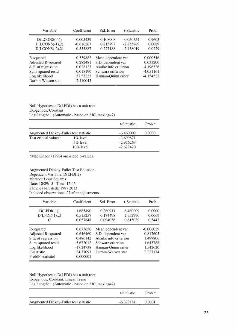
Appendix 13: Unit root tests output (for the first difference)
Null Hypothesis: D(LCONS) has a unit root Exogenous: Constant Lag Length: 0 (Automatic - based on SIC, maxlag=7)
t-Statistic Prob.* Augmented Dickey-Fuller test statistic -4.138691 0.0034
Test critical values: 1% level -3.689194 5% level -2.971853 10% level -2.625121 *MacKinnon (1996) one-sided p-values.
Augmented Dickey-Fuller Test Equation Dependent Variable: D(LCONS,2) Method: Least Squares Date: 10/29/15 Time: 15:41 Sample (adjusted): 1986 2013 Included observations: 28 after adjustments
Variable Coefficient Std. Error t-Statistic Prob. D(LCONS(-1)) -0.745907 0.180228 -4.138691 0.0003
C 0.037394 0.010016 3.733308 0.0009 R-squared 0.397154 Mean dependent var 0.001020
Adjusted R-squared 0.373968 S.D. dependent var 0.032131 S.E. of regression 0.025423 Akaike info criterion -4.437573 Sum squared resid 0.016805 Schwarz criterion -4.342415 Log likelihood 64.12602 Hannan-Quinn criter. -4.408482 F-statistic 17.12876 Durbin-Watson stat 2.058869 Prob(F-statistic) 0.000325
24
Null Hypothesis: D(LCONS) has a unit root Exogenous: Constant, Linear Trend Lag Length: 0 (Automatic - based on SIC, maxlag=7)
t-Statistic Prob.* Augmented Dickey-Fuller test statistic -4.486431 0.0069
Test critical values: 1% level -4.323979 5% level -3.580623 10% level -3.225334 *MacKinnon (1996) one-sided p-values.
Augmented Dickey-Fuller Test Equation Dependent Variable: D(LCONS,2) Method: Least Squares Date: 10/29/15 Time: 15:41 Sample (adjusted): 1986 2013 Included observations: 28 after adjustments
Variable Coefficient Std. Error t-Statistic Prob. D(LCONS(-1)) -0.919295 0.204906 -4.486431 0.0001
C 0.028844 0.011053 2.609651 0.0151 @TREND("1984") 0.001097 0.000676 1.622320 0.1173
R-squared 0.454575 Mean dependent var 0.001020
Adjusted R-squared 0.410941 S.D. dependent var 0.032131 S.E. of regression 0.024661 Akaike info criterion -4.466240 Sum squared resid 0.015204 Schwarz criterion -4.323504 Log likelihood 65.52736 Hannan-Quinn criter. -4.422604 F-statistic 10.41790 Durbin-Watson stat 1.936451 Prob(F-statistic) 0.000512
Null Hypothesis: D(LCONS) has a unit root Exogenous: None Lag Length: 2 (Automatic - based on SIC, maxlag=7)
t-Statistic Prob.* Augmented Dickey-Fuller test statistic -0.050354 0.6567
Test critical values: 1% level -2.656915 5% level -1.954414 10% level -1.609329 *MacKinnon (1996) one-sided p-values.
Augmented Dickey-Fuller Test Equation Dependent Variable: D(LCONS,2) Method: Least Squares Date: 10/29/15 Time: 15:42 Sample (adjusted): 1988 2013 Included observations: 26 after adjustments
25
Variable Coefficient Std. Error t-Statistic Prob. D(LCONS(-1)) -0.005439 0.108008 -0.050354 0.9603
D(LCONS(-1),2) -0.616267 0.215797 -2.855769 0.0089 D(LCONS(-2),2) -0.553887 0.227188 -2.438019 0.0229
R-squared 0.339882 Mean dependent var 0.000546
Adjusted R-squared 0.282481 S.D. dependent var 0.033200 S.E. of regression 0.028123 Akaike info criterion -4.196326 Sum squared resid 0.018190 Schwarz criterion -4.051161 Log likelihood 57.55223 Hannan-Quinn criter. -4.154523 Durbin-Watson stat 2.110043
Null Hypothesis: D(LFDI) has a unit root Exogenous: Constant Lag Length: 1 (Automatic - based on SIC, maxlag=7)
t-Statistic Prob.* Augmented Dickey-Fuller test statistic -6.460009 0.0000
Test critical values: 1% level -3.699871 5% level -2.976263 10% level -2.627420 *MacKinnon (1996) one-sided p-values.
Augmented Dickey-Fuller Test Equation Dependent Variable: D(LFDI,2) Method: Least Squares Date: 10/29/15 Time: 15:45 Sample (adjusted): 1987 2013 Included observations: 27 after adjustments
Variable Coefficient Std. Error t-Statistic Prob. D(LFDI(-1)) -1.685490 0.260911 -6.460009 0.0000
D(LFDI(-1),2) 0.515257 0.174498 2.952790 0.0069 C 0.057848 0.094056 0.615039 0.5443 R-squared 0.673656 Mean dependent var -0.006029
Adjusted R-squared 0.646460 S.D. dependent var 0.817605 S.E. of regression 0.486142 Akaike info criterion 1.499806 Sum squared resid 5.672012 Schwarz criterion 1.643788 Log likelihood -17.24738 Hannan-Quinn criter. 1.542620 F-statistic 24.77097 Durbin-Watson stat 2.227174 Prob(F-statistic) 0.000001
Null Hypothesis: D(LFDI) has a unit root Exogenous: Constant, Linear Trend Lag Length: 1 (Automatic - based on SIC, maxlag=7)
t-Statistic Prob.* Augmented Dickey-Fuller test statistic -6.322181 0.0001
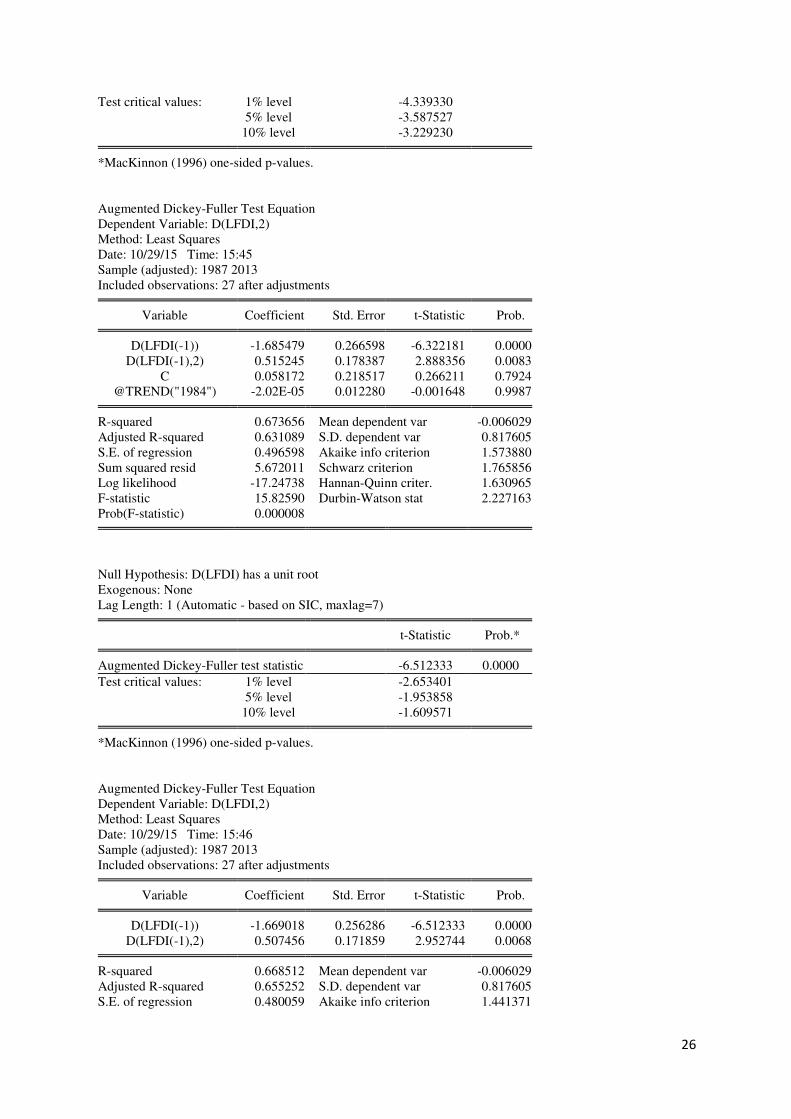
26
Test critical values: 1% level -4.339330 5% level -3.587527 10% level -3.229230 *MacKinnon (1996) one-sided p-values.
Augmented Dickey-Fuller Test Equation Dependent Variable: D(LFDI,2) Method: Least Squares Date: 10/29/15 Time: 15:45 Sample (adjusted): 1987 2013 Included observations: 27 after adjustments
Variable Coefficient Std. Error t-Statistic Prob. D(LFDI(-1)) -1.685479 0.266598 -6.322181 0.0000
D(LFDI(-1),2) 0.515245 0.178387 2.888356 0.0083 C 0.058172 0.218517 0.266211 0.7924
@TREND("1984") -2.02E-05 0.012280 -0.001648 0.9987 R-squared 0.673656 Mean dependent var -0.006029
Adjusted R-squared 0.631089 S.D. dependent var 0.817605 S.E. of regression 0.496598 Akaike info criterion 1.573880 Sum squared resid 5.672011 Schwarz criterion 1.765856 Log likelihood -17.24738 Hannan-Quinn criter. 1.630965 F-statistic 15.82590 Durbin-Watson stat 2.227163 Prob(F-statistic) 0.000008
Null Hypothesis: D(LFDI) has a unit root Exogenous: None Lag Length: 1 (Automatic - based on SIC, maxlag=7)
t-Statistic Prob.* Augmented Dickey-Fuller test statistic -6.512333 0.0000
Test critical values: 1% level -2.653401 5% level -1.953858 10% level -1.609571 *MacKinnon (1996) one-sided p-values.
Augmented Dickey-Fuller Test Equation Dependent Variable: D(LFDI,2) Method: Least Squares Date: 10/29/15 Time: 15:46 Sample (adjusted): 1987 2013 Included observations: 27 after adjustments
Variable Coefficient Std. Error t-Statistic Prob. D(LFDI(-1)) -1.669018 0.256286 -6.512333 0.0000
D(LFDI(-1),2) 0.507456 0.171859 2.952744 0.0068 R-squared 0.668512 Mean dependent var -0.006029
Adjusted R-squared 0.655252 S.D. dependent var 0.817605 S.E. of regression 0.480059 Akaike info criterion 1.441371
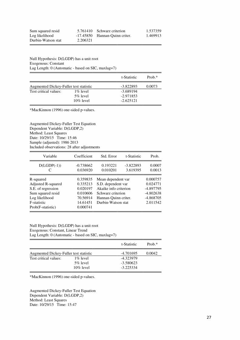
27
Sum squared resid 5.761410 Schwarz criterion 1.537359 Log likelihood -17.45850 Hannan-Quinn criter. 1.469913 Durbin-Watson stat 2.206321
Null Hypothesis: D(LGDP) has a unit root Exogenous: Constant Lag Length: 0 (Automatic - based on SIC, maxlag=7)
t-Statistic Prob.* Augmented Dickey-Fuller test statistic -3.822893 0.0073
Test critical values: 1% level -3.689194 5% level -2.971853 10% level -2.625121 *MacKinnon (1996) one-sided p-values.
Augmented Dickey-Fuller Test Equation Dependent Variable: D(LGDP,2) Method: Least Squares Date: 10/29/15 Time: 15:46 Sample (adjusted): 1986 2013 Included observations: 28 after adjustments
Variable Coefficient Std. Error t-Statistic Prob. D(LGDP(-1)) -0.738662 0.193221 -3.822893 0.0007
C 0.036920 0.010201 3.619395 0.0013 R-squared 0.359835 Mean dependent var 0.000757
Adjusted R-squared 0.335213 S.D. dependent var 0.024771 S.E. of regression 0.020197 Akaike info criterion -4.897795 Sum squared resid 0.010606 Schwarz criterion -4.802638 Log likelihood 70.56914 Hannan-Quinn criter. -4.868705 F-statistic 14.61451 Durbin-Watson stat 2.011542 Prob(F-statistic) 0.000741
Null Hypothesis: D(LGDP) has a unit root Exogenous: Constant, Linear Trend Lag Length: 0 (Automatic - based on SIC, maxlag=7)
t-Statistic Prob.* Augmented Dickey-Fuller test statistic -4.701695 0.0042
Test critical values: 1% level -4.323979 5% level -3.580623 10% level -3.225334 *MacKinnon (1996) one-sided p-values.
Augmented Dickey-Fuller Test Equation Dependent Variable: D(LGDP,2) Method: Least Squares Date: 10/29/15 Time: 15:47
28
Sample (adjusted): 1986 2013 Included observations: 28 after adjustments
Variable Coefficient Std. Error t-Statistic Prob. D(LGDP(-1)) -0.927698 0.197311 -4.701695 0.0001
C 0.029063 0.010063 2.887971 0.0079 @TREND("1984") 0.001104 0.000483 2.287937 0.0309
R-squared 0.470669 Mean dependent var 0.000757
Adjusted R-squared 0.428323 S.D. dependent var 0.024771 S.E. of regression 0.018729 Akaike info criterion -5.016480 Sum squared resid 0.008770 Schwarz criterion -4.873744 Log likelihood 73.23072 Hannan-Quinn criter. -4.972844 F-statistic 11.11472 Durbin-Watson stat 2.009126 Prob(F-statistic) 0.000352
Null Hypothesis: D(LGDP) has a unit root Exogenous: None Lag Length: 2 (Automatic - based on SIC, maxlag=7)
t-Statistic Prob.* Augmented Dickey-Fuller test statistic 0.136214 0.7170
Test critical values: 1% level -2.656915 5% level -1.954414 10% level -1.609329 *MacKinnon (1996) one-sided p-values.
Augmented Dickey-Fuller Test Equation Dependent Variable: D(LGDP,2) Method: Least Squares Date: 10/29/15 Time: 15:47 Sample (adjusted): 1988 2013 Included observations: 26 after adjustments
Variable Coefficient Std. Error t-Statistic Prob. D(LGDP(-1)) 0.011798 0.086611 0.136214 0.8928
D(LGDP(-1),2) -0.586188 0.201144 -2.914271 0.0078 D(LGDP(-2),2) -0.348249 0.196484 -1.772401 0.0896
R-squared 0.289849 Mean dependent var 0.002034
Adjusted R-squared 0.228096 S.D. dependent var 0.025129 S.E. of regression 0.022078 Akaike info criterion -4.680299 Sum squared resid 0.011211 Schwarz criterion -4.535134 Log likelihood 63.84389 Hannan-Quinn criter. -4.638497 Durbin-Watson stat 2.114261
Null Hypothesis: D(LSAVR) has a unit root Exogenous: Constant Lag Length: 1 (Automatic - based on SIC, maxlag=7)
t-Statistic Prob.*
29
Augmented Dickey-Fuller test statistic -6.157323 0.0000 Test critical values: 1% level -3.699871
5% level -2.976263 10% level -2.627420 *MacKinnon (1996) one-sided p-values.
Augmented Dickey-Fuller Test Equation Dependent Variable: D(LSAVR,2) Method: Least Squares Date: 10/29/15 Time: 15:48 Sample (adjusted): 1987 2013 Included observations: 27 after adjustments
Variable Coefficient Std. Error t-Statistic Prob. D(LSAVR(-1)) -1.661824 0.269894 -6.157323 0.0000
D(LSAVR(-1),2) 0.281865 0.145044 1.943300 0.0638 C 0.021176 0.020820 1.017135 0.3192 R-squared 0.676720 Mean dependent var 0.005716
Adjusted R-squared 0.649780 S.D. dependent var 0.181381 S.E. of regression 0.107340 Akaike info criterion -1.521186 Sum squared resid 0.276527 Schwarz criterion -1.377204 Log likelihood 23.53600 Hannan-Quinn criter. -1.478372 F-statistic 25.11950 Durbin-Watson stat 1.971599 Prob(F-statistic) 0.000001
Null Hypothesis: D(LSAVR) has a unit root Exogenous: Constant, Linear Trend Lag Length: 1 (Automatic - based on SIC, maxlag=7)
t-Statistic Prob.* Augmented Dickey-Fuller test statistic -6.030099 0.0002
Test critical values: 1% level -4.339330 5% level -3.587527 10% level -3.229230 *MacKinnon (1996) one-sided p-values.
Augmented Dickey-Fuller Test Equation Dependent Variable: D(LSAVR,2) Method: Least Squares Date: 10/29/15 Time: 15:48 Sample (adjusted): 1987 2013 Included observations: 27 after adjustments
Variable Coefficient Std. Error t-Statistic Prob. D(LSAVR(-1)) -1.662355 0.275676 -6.030099 0.0000
D(LSAVR(-1),2) 0.280578 0.148621 1.887880 0.0717 C 0.025864 0.048938 0.528500 0.6022
@TREND("1984") -0.000291 0.002734 -0.106347 0.9162 R-squared 0.676879 Mean dependent var 0.005716
30
Adjusted R-squared 0.634732 S.D. dependent var 0.181381 S.E. of regression 0.109622 Akaike info criterion -1.447603 Sum squared resid 0.276391 Schwarz criterion -1.255627 Log likelihood 23.54264 Hannan-Quinn criter. -1.390519 F-statistic 16.06023 Durbin-Watson stat 1.970727 Prob(F-statistic) 0.000008
Null Hypothesis: D(LSAVR) has a unit root Exogenous: None Lag Length: 1 (Automatic - based on SIC, maxlag=7)
t-Statistic Prob.* Augmented Dickey-Fuller test statistic -6.104584 0.0000
Test critical values: 1% level -2.653401 5% level -1.953858 10% level -1.609571 *MacKinnon (1996) one-sided p-values.
Augmented Dickey-Fuller Test Equation Dependent Variable: D(LSAVR,2) Method: Least Squares Date: 10/29/15 Time: 15:49 Sample (adjusted): 1987 2013 Included observations: 27 after adjustments
Variable Coefficient Std. Error t-Statistic Prob. D(LSAVR(-1)) -1.645981 0.269630 -6.104584 0.0000
D(LSAVR(-1),2) 0.287165 0.145051 1.979752 0.0588 R-squared 0.662784 Mean dependent var 0.005716
Adjusted R-squared 0.649296 S.D. dependent var 0.181381 S.E. of regression 0.107414 Akaike info criterion -1.553056 Sum squared resid 0.288447 Schwarz criterion -1.457068 Log likelihood 22.96626 Hannan-Quinn criter. -1.524514 Durbin-Watson stat 1.921470
Appendix 14: Unit root test for Vt
Null Hypothesis: RESID03 has a unit root Exogenous: Constant Lag Length: 0 (Automatic - based on SIC, maxlag=5)
t-Statistic Prob.* Augmented Dickey-Fuller test statistic -5.441786 0.0002
Test critical values: 1% level -3.724070 5% level -2.986225 10% level -2.632604 *MacKinnon (1996) one-sided p-values.
31
Augmented Dickey-Fuller Test Equation Dependent Variable: D(RESID03) Method: Least Squares Date: 11/03/15 Time: 13:01 Sample (adjusted): 1989 2013 Included observations: 25 after adjustments
Variable Coefficient Std. Error t-Statistic Prob. RESID03(-1) -1.096753 0.201543 -5.441786 0.0000
C 0.000487 0.002087 0.233371 0.8175 R-squared 0.562846 Mean dependent var 0.000631
Adjusted R-squared 0.543839 S.D. dependent var 0.015446 S.E. of regression 0.010432 Akaike info criterion -6.211220 Sum squared resid 0.002503 Schwarz criterion -6.113710 Log likelihood 79.64025 Hannan-Quinn criter. -6.184175 F-statistic 29.61304 Durbin-Watson stat 2.081990 Prob(F-statistic) 0.000016
Null Hypothesis: RESID03 has a unit root Exogenous: Constant, Linear Trend Lag Length: 0 (Automatic - based on SIC, maxlag=5)
t-Statistic Prob.* Augmented Dickey-Fuller test statistic -5.345960 0.0011
Test critical values: 1% level -4.374307 5% level -3.603202 10% level -3.238054 *MacKinnon (1996) one-sided p-values.
Augmented Dickey-Fuller Test Equation Dependent Variable: D(RESID03) Method: Least Squares Date: 11/03/15 Time: 13:02 Sample (adjusted): 1989 2013 Included observations: 25 after adjustments
Variable Coefficient Std. Error t-Statistic Prob. RESID03(-1) -1.097950 0.205379 -5.345960 0.0000
C 0.002451 0.005444 0.450268 0.6569 @TREND("1984") -0.000116 0.000295 -0.391947 0.6989
R-squared 0.565877 Mean dependent var 0.000631
Adjusted R-squared 0.526412 S.D. dependent var 0.015446 S.E. of regression 0.010630 Akaike info criterion -6.138178 Sum squared resid 0.002486 Schwarz criterion -5.991913 Log likelihood 79.72723 Hannan-Quinn criter. -6.097611 F-statistic 14.33847 Durbin-Watson stat 2.095840 Prob(F-statistic) 0.000103
Null Hypothesis: RESID03 has a unit root
32
Exogenous: None Lag Length: 0 (Automatic - based on SIC, maxlag=5)
t-Statistic Prob.* Augmented Dickey-Fuller test statistic -5.555720 0.0000
Test critical values: 1% level -2.660720 5% level -1.955020 10% level -1.609070 *MacKinnon (1996) one-sided p-values.
Augmented Dickey-Fuller Test Equation Dependent Variable: D(RESID03) Method: Least Squares Date: 11/03/15 Time: 13:03 Sample (adjusted): 1989 2013 Included observations: 25 after adjustments
Variable Coefficient Std. Error t-Statistic Prob. RESID03(-1) -1.097348 0.197517 -5.555720 0.0000 R-squared 0.561811 Mean dependent var 0.000631
Adjusted R-squared 0.561811 S.D. dependent var 0.015446 S.E. of regression 0.010225 Akaike info criterion -6.288855 Sum squared resid 0.002509 Schwarz criterion -6.240100 Log likelihood 79.61068 Hannan-Quinn criter. -6.275332 Durbin-Watson stat 2.075922


