Hybrid Systems with Finite Bisimulations?

Gerardo Lafferriere1, George J. Pappas2, and Shankar Sastry2

1 Department of Mathematical SciencesPortland State University, Portland, OR 97207, USA

gerardo@mth.pdx.edu2 Department of Electrical Engineering and Computer SciencesUniversity of California at Berkeley, Berkeley, CA 94720, USA

{gpappas,sastry}@eecs.berkeley.edu

Abstract. The theory of formal verification is one of the main approach-es to hybrid system analysis. Decidability questions for verification algo-rithms are obtained by constructing finite, reachability preserving quo-tient systems called bisimulations. In this paper, we use recent resultsfrom stratification theory, subanalytic sets, and model theory in order toextend the state-of-the-art results on the existence of bisimulations forcertain classes of planar hybrid systems.

1 Introduction

Hybrid systems consist of finite state machines interacting with differential equa-tions. Various modeling formalisms, analysis, design and control methodologies,as well as applications, can be found in [3,4,5,10,17]. Formal verification is themain computational approach for analyzing properties of hybrid systems. One ofthe most important verification problems for hybrid systems is the reachabilityproblem which asks whether trajectories of the hybrid system can reach certainundesirable regions of the state space. Since hybrid systems have infinite statespaces, the decidability of verification algorithms is very important.

A uniform framework for tackling the decidability issue is provided by thenotion of bisimulation. Bisimulations are quotients of the original hybrid systemthat are reachability preserving. Showing that an infinite state hybrid system hasa finite state bisimulation is the first step in proving decidability. This approachhas been successfully applied to timed automata [2], multirate automata [1], andinitialized rectangular automata [19,12]. It should be mentioned that the notionof bisimulation is closely related to the various consistency notions for discreteand continuous systems [7,8,18].

Since the discrete dynamics are already finite, it is clear that decidabilityresults for hybrid systems depend crucially on the success of obtaining finitebisimulations for continuous dynamics. The cases considered so far in the lit-erature dealt with simple dynamics: x = 1 for timed automata [2], x = a for? Research supported by the Army Research Office under grants DAAH 04-95-1-0588

and DAAH 04-96-1-0341.

P. Antsaklis et al. (Eds.): Hybrid Systems V, LNCS 1567, pp. 186–203, 1999.c© Springer-Verlag Berlin Heidelberg 1999

Hybrid Systems with Finite Bisimulations 187

multirate automata [1], x ∈ [a, b] for rectangular automata [19], and Ax ≤ b forlinear hybrid automata [11]. In this paper, we extend the bisimulation method-ology to hybrid systems with more general dynamics. We first present the s-tandard bisimulation algorithm which, upon termination, provides the desiredfinite bismilarity quotient. In [15], we used purely geometric methods to showthat the bisimulation algorithm terminates for a class of hybrid systems with pla-nar linear dynamics. In this paper, we combine mathematical techniques fromdifferential geometry and recent results in logic model theory in ordet to proveexistence of finite bisimulations for various new classes of hybrid systems withplanar continuous dynamics. This convergence of mathematical logic and differ-ential geometry also provides a natural framework for extending the decidabilityfrontier for more general classes of hybrid systems. Such extensions will requirepushing the boundary of decidable theories in mathematical logic.

Abstracting a discrete graph from a hybrid system requires the analysis oftrajectories of vector fields and their intersection properties relative to a givencollection of sets. Considering hybrid systems with arbitrary dynamics and ar-bitrary state partitions would soon lead to pathological situations. Subanalyticsets [6,13,21] provide a rich class of sets which have many desirable local inter-section properties with trajectories of analytic vector fields. Subanalytic sets canalso be partitioned into smooth embedded submanifolds in a form suitable forconstructing a bisimulation. Such partitions are called stratifications. Moreover,we show that relaxing the class of vector fields or sets in some naive ways leadsto pathological situations. On the other hand, the concept of o-minimal theo-ries in logic [24,25,26] identifies classes of sets with good intersection propertiessuitable for the global study of trajectories of vector fields. The combination oftechniques from both fields highlights the kind of properties of sets that play acentral role in obtaining discrete abstractions.

The outline of the paper is as follows: In Section 2 we review the notion ofbisimulations of transitions systems. In Section 3 we define the class of hybridsystems under study and describe the main bisimulation algorithm. Section 4presents some basic facts about stratification theory and subanalytic sets andrelates them to the construction of bisimulations. In Section 5 we present recentresults in model theory which are used in Section 6 in order to obtain classesof systems for which the bisimulation algorithm terminates. Section 7 containsconclusions and issues for further research.

2 Bisimulations of Transition Systems

A transition system T = (Q, Σ,→, QO, QF ) consists of a (not necessarily finite)set Q of states, an alphabet Σ of events, a transition relation →⊆ Q × Σ × Q,a set QO ⊆ Q of initial states, and a set QF ⊆ Q of final states. A transition(q1, σ, q2) ∈→ is denoted as q1

σ→ q2. The transition system is finite if thecardinality of Q is finite and it is infinite otherwise. A region is a subset P ⊆ Q.Given σ ∈ Σ we define the predecessor Preσ(P ) of a region P as

Preσ(P ) = {q ∈ Q | ∃p ∈ P and qσ→ p} (1)

188 G. Lafferriere, G.J. Pappas, and S. Sastry

Given an equivalence relation ∼⊆ Q×Q, we define a quotient transition systemt/ ∼ as follows: Let Q/∼ denote the quotient space. For a region P we denote byP/∼ the collection of all equivalence classes which intersect P . The transitionrelation →∼ on the quotient space is defined as follows: for Q1,Q2 ∈ Q/ ∼,Q1

σ→∼ Q2 iff there exist q1 ∈ Q1 and q2 ∈ Q2 such that q1σ→ q2. The quotient

transition system is then T/∼= (Q/∼, Σ,→∼, Q0/∼, QF /∼).Given a partition ∼ on Q, we call a set a ∼-block if it is a union of equivalence

classes. The partition ∼ is a bisimulation of T iff QO, QF are ∼-blocks and forall σ ∈ Σ and all ∼-blocks P , the region Preσ(P ) is a ∼-block. In this case thesystems T and T/∼ are called bisimilar. A bisimulation is called finite if it hasa finite number of equivalence classes. Bisimulations are very important becausechecking reachability on the bisimilar transition system is equivalent to checkingreachability of the original transition system [11]. Therefore, if T is infinite andT/∼ is a finite bisimulation, then verification algorithms for infinite systems areguaranteed to terminate. If ∼ is a bisimulation, it can be easily shown that ifp ∼ q then

B1 p ∈ QF iff q ∈ QF , and p ∈ QO iff q ∈ QO

B2 if pσ→ p′ then there exists q′ such that q

σ→ q′ and p′ ∼ q′

Based on the above characterization, given a transition system T , the followingalgorithm computes increasingly finer partitions of the state space Q.

Algorithm 1 (Bisimulation Algorithm for Transition Systems)Set Q/∼= {QO ∩ QF , QO \ QF , QF \ QO, Q \ (QO ∪ QF )}while ∃ P ,P ′ ∈ Q/∼ and σ ∈ Σ such that ∅ 6= P ∩ Preσ(P ′) 6= P

set P1 = P ∩ Preσ(P ′), P2 = P \ Preσ(P ′)refine Q/∼= (Q/∼ \{P}) ∪ {P1, P2}

end while

If the algorithm terminates, then the resulting quotient transition system is afinite bisimulation. The goal of the next sections is to show that the abovealgorithm terminates for transition systems generated by a class of planar hybridsystems.

3 Bisimulations of Hybrid Systems

In this paper, we focus on transition systems generated by the following class ofhybrid systems.

Definition 1. A hybrid system H = (X, X0, XF , F, E, I, G, R) consists of

– X = XD×XC is the state space with XD = {q1, . . . , qn} and XC an analyticmanifold.

– X0 ⊆ X is the set of initial states– XF ⊆ X is the set of final states– F : X −→ TXC assigns to each discrete state q ∈ XD an analytic vector

field F (q, ·)

Hybrid Systems with Finite Bisimulations 189

– E ⊆ XD × XD is the set of discrete transitions– I : XD −→ 2XC assigns to each discrete state a set I(q) ⊆ XC called the

invariant.– G : E −→ XD×2XC assigns to e = (q1, q2) ∈ E a guard of the form {q1}×U ,

U ⊆ I(q1).– R : E −→ XD×2XC assigns to e = (q1, q2) ∈ E a reset of the form {q2}×V ,

V ⊆ I(q2).

Trajectories of H start at any (q, x) ∈ X0 and consist of continuous evolutions ordiscrete jumps. Continuous trajectories evolve according to the continuous flowF (q, ·) as long as the state remains in the invariant set I(q). If the flow exits I(q),then a discrete transition is forced. If, during the continuous evolution, the state(q, x) enters a region G(e) for some e ∈ E, then discrete transition e is enabled,and the state may instantaneously jump from (q, x) to any (q′, x′) ∈ R(e). Thenthe system evolves according to F (q′, ·). Notice that the discrete transitionsallowed in our model are similar to the type allowed in initialized rectangularautomata [19]. Finally, we assume that our hybrid system model is non-blocking,that is from every state either a continuous evolution or a discrete transition ispossible.

Every hybrid system H = (X, X0, XF , F, E, I, G, R) generates a transitionsystem T = (Q, Σ,→, QO, QF ) by setting Q = X , Q0 = X0, QF = XF , Σ =E ∪ {τ}, and →= (∪e∈E

e→)∪ τ→ where

Discrete Transitions (q, x) e→ (q′, x′) for e ∈ E iff (q, x) ∈ G(e) and (q′, x′) ∈R(e)

Continuous Transitions (q1, x1)τ→ (q2, x2) iff q1 = q2 and there exists δ ≥ 0

and a curve x : [0, δ] −→ M with x(0) = x1, x(δ) = x2 and for all t ∈ [0, δ]it satisfies x′ = F (q1, x(t)) and x(t) ∈ I(q1).

The continuous τ transitions are time-abstract transitions, in the sense thatthe time it takes to reach one state from another is ignored. Having definedthe continuous and discrete transitions τ→ and e→ allows us to formally definePreτ (P ) and Pree(P ) for e ∈ E and any region P ⊆ X using (1). Furthermore,the discrete transitions allowed in our hybrid system model result in

Pree(P ) =

{∅ if P ∩ R(e) = ∅G(e) if P ∩ R(e) 6= ∅ (2)

for all discrete transitions e ∈ E and regions P . Therefore, if the sets R(e) andG(e) are blocks of any partition of the state space, then no partition refinementis necessary in the bisimulation algorithm due to any discrete transitions e ∈E. This fact, decouples the continuous and discrete components of the hybridsystem as long as the initial partition in the bisimulation algorithm contain theinvariants, guards and reset sets, in addition to the initial and final sets. Thisallows us to carry out the bisimulation algorithm independently for each discretestate.

190 G. Lafferriere, G.J. Pappas, and S. Sastry

More precisely, define for any region P ⊆ X and q ∈ XD the set Pq = {x ∈XC : (q, x) ∈ P}. For each discrete state q ∈ XD consider the finite collection ofsets

Aq = {I(q), (X0)q, (XF )q} ∪ {G(e)q, R(e)q : e ∈ E} (3)

which describes all the relevant sets associated with discrete state q. Let Sq bethe coarsest partition of XC compatible with the collection Aq (by compatiblewe mean that each set in Aq is a union of sets in Sq). The (finite) partition Sq

can be easily computed by successively finding the intersections between each ofthe sets in Aq and their complements. These collections Sq will be the startingpartitions of the following bisimulation algorithm for hybrid systems.

Algorithm 2 (Bisimulation Algorithm for Hybrid Systems)Set X/∼ =

⋃q Sq

for q ∈ XD

while ∃ P ,P ′ ∈ Sq such that ∅ 6= P ∩ Preτ (P ′) 6= PSet P1 = P ∩ Preτ (P ′); P2 = P \ Preτ (P ′)refine Sq = (Sq \ {P}) ∪ {P1, P2}

end whileend for

A few comments are in order here. The key problem is to investigate howthe flow of F (q, ·) interacts with the sets Sq for a single discrete state q. Thisrequires that the trajectories of the vector field F (q, ·) have “nice” intersectionproperties with such sets. Since the goal is to obtain finite partitions, it willbecome important that we restrict the study to classes of sets with good “finite-ness” properties, for example, sets with finitely many connected components. Inthe subsequent sections we identify classes of sets and vector fields which exhibitsuch properties and for which Algorithm 2 terminates.

One can also view the partitions in the algorithm as a way of discretizingthe system trajectories. This suggests studying the continuous transitions bylooking only at the points at which the trajectories move from one set in Sq toan “adjacent” one. This is in general not possible because sets could have ratherpathological boundaries (see also Example 4). We will see in the next sectionthat subanalytic sets are free from such pathologies and that in fact one canformalize the idea of trajectory discretization associated to the partition in thatcase.

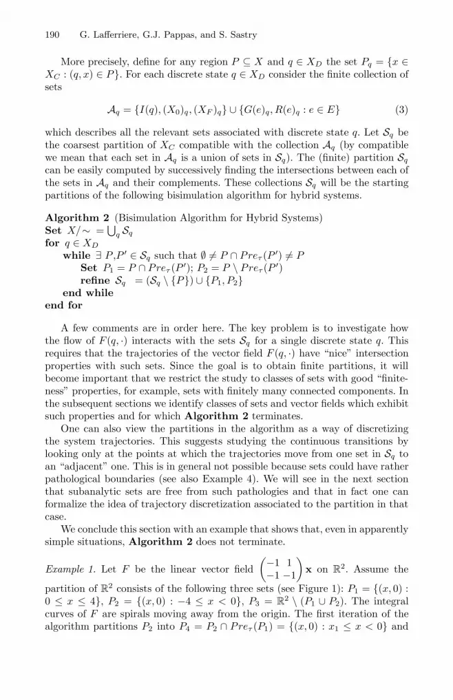
We conclude this section with an example that shows that, even in apparentlysimple situations, Algorithm 2 does not terminate.

Example 1. Let F be the linear vector field(−1 1−1 −1

)x on R

2. Assume the

partition of R2 consists of the following three sets (see Figure 1): P1 = {(x, 0) :

0 ≤ x ≤ 4}, P2 = {(x, 0) : −4 ≤ x < 0}, P3 = R2 \ (P1 ∪ P2). The integral

curves of F are spirals moving away from the origin. The first iteration of thealgorithm partitions P2 into P4 = P2 ∩ Preτ (P1) = {(x, 0) : x1 ≤ x < 0} and

Hybrid Systems with Finite Bisimulations 191

−6 −4 −2 0 2 4 6

−4

−2

0

2

4

Fig. 1. Algorithm 2 does not terminate

P2 \ Preτ (P1). Here x1 < 0 is the x-coordinate of the first intersection pointof the spiral through (4, 0) with P2. The second iteration subdivides P1 intoP5 = P1 ∩ Preτ (P4) = {(x, 0) : 0 ≤ x ≤ x2} and P1 \ Preτ (P4) where x2 > 0is the x-coordinate of the next point of intersection of the spiral with P1. Thisprocess continues indefinitely since the spiral intersects P1 in infinitely manypoints, and therefore the algorithm does not terminate.

4 Subanalytic Sets and Stratifications

In this section we describe some fundamental properties of subanalytic sets(see [6,13,21] for more details). A differentiable manifold is real analytic (Cω)if the transition maps between local coordinate charts are analytic functions ontheir domains (which are open subsets of R

n). An embedded submanifold S of amanifold M is a topological subspace of M together with a differentiable struc-ture such that the inclusion from S into M is a smooth immersion (i.e. has fullrank at every point). A vector field F on the real analytic manifold M is analyticif its coordinates in any local chart are analytic. If F is an analytic vector fieldthen any integral curve of F is analytic.

Let M and N be real analytic manifolds and let Cω(M, N) denote the setof analytic functions from M into N . If f ∈ Cω(M, N) we say f is of class Cω.Given an analytic manifold U , we denote by Σ(Cω(U, R)) the Boolean algebragenerated by the sets of the form {x : f(x) = 0} or {x : f(x) > 0}, wheref ∈ Cω(U, R).

Definition 2. Let M be a real analytic manifold. A subset A of M is semi-analytic in M if for every p ∈ M , there is an open neighborhood U of p inM such that U ∩ A ∈ Σ(Cω(U, R)). If A ⊆ M is semianalytic in M we writeA ∈ SMAN(M).

192 G. Lafferriere, G.J. Pappas, and S. Sastry

Definition 3. Let M be a real analytic manifold. Define SBANrc(M) andSBAN(M) by1. A ∈ SBANrc(M) if and only if there is (N, f, A∗) such that N is a real

analytic manifold, f ∈ Cω(N, M), A∗ ∈ SMAN(N), A∗ is relatively compactand A = f(A∗);

2. A ∈ SBAN(M) if and only if A is the union of a locally finite collectionof members of SBANrc(M). (A collection of sets C is locally finite if anycompact set intersect only finitely many sets in C.)

We say that A is subanalytic in M if A ∈ SBAN(M). It is easy to see thatA ∈ SBANrc(M) if and only if A is subanalytic in M and relatively compact. Thefollowing properties of subanalytic sets are easily derived from the definitions.

1. SBAN(M) is closed under locally finite unions and intersections.2. If A ∈ SBAN(M) and f : M −→ N is of class Cω and proper on A, the

closure of A, then f(A) ∈ SBAN(N). (A function f is proper if f−1(K) iscompact whenever K is.)

3. If A ∈ SBAN(N) and f : M −→ N is of class Cω , then f−1(A) ∈ SBAN(M).

The following two properties require more subtle proofs, but they give thefirst indication that this will be a suitable class of sets for our studies.

4. If A ∈ SBAN(M) then M \ A ∈ SBAN(M).5. A subanalytic set has a locally finite number of connected components, each

of which is subanalytic.

Example 2. Points are subanalytic, and so is any locally finite union of points,for example Z

n as subset of Rn. The empty set and M are both in SBAN(M).

Let a, b ∈ R, a < b, then [a, b], [a, b), (a, b] and (a, b) are subanalytic in R. Theopen ball B(p, r) centered at p of radius r in R

n is in SBAN(Rn).

Definition 4. Let M be a real analytic manifold. An analytic (Cω) stratificationof M is a partition S of M with the following properties:1. each S ∈ S is a connected, real analytic, embedded submanifold of M ,2. S is locally finite,3. given two sets S, P ∈ S, P 6= S, such that S ∩ P 6= ∅ then S ⊂ P and

dimS < dimP .The sets in a stratification are called strata.

The central result on stratifications for our analysis is the following. For aproof see [20].

Theorem 1. Let A be a locally finite family of nonempty subanalytic subsetsof a real analytic manifold M . For each A ∈ A, let F (A) be a finite set of realanalytic vector fields on M . Then there exists a subanalytic stratification S ofM , compatible with A, and having the property that, whenever S ∈ S, S ⊆ A,A ∈ A, X ∈ F (A), then either (i) F is everywhere tangent to S or (ii) F isnowhere tangent to S. (S is compatible with A is every set in A is a union ofsets in S.)

Hybrid Systems with Finite Bisimulations 193

Theorem 1 is illustrated by the following example.

Example 3. Let F be the following analytic vector field on R2

x = x2 + y2

y = 0

which has an isolated equilibrium at the origin and points in the positive x-direction otherwise. Consider the following two subanalytic sets

S1 = {(x, y) ∈ R2 | y ≥ 0 and (x − 1)2 + y2 = 1}

S2 = {(x, y) ∈ R2 | y = 0 and 0 ≤ x ≤ 2}

shown in Figure 2. A subanalytic stratification of R2 which is compatible with

the sets S1, S2 and the vector field F is also shown in Figure 2. It consists of

– 0-dimensional strata• P1 = (0, 0), P2 = (2, 0), and P3 = (1, 1)

– 1-dimensional strata• C1 = {(x, y) ∈ R

2 | y = 0 and 0 < x < 2}• C2 = {(x, y) ∈ R

2 | y > 0 and 1 < x < 2 and (x − 1)2 + y2 = 1}• C3 = {(x, y) ∈ R

2 | y > 0 and 0 < x < 1 and (x − 1)2 + y2 = 1}– 2-dimensional strata

• D1 = {(x, y) ∈ R2 | y > 0 and (x − 1)2 + y2 < 1}

• D2 = R2 \ {P1, P2, P3, C1, C2, C3, D1}

Notice that the vector field is tangent to P1 since it is an equilibrium as well as toC1, D1 and D2. The vector field is transverse to all the other strata. Moreover,S1 = P1 ∪ P2 ∪ P3 ∪ C2 ∪ C3 and S2 = P1 ∪ P2 ∪ C1.

S1

S2

D1

D2

P1 P2

P3

C1

C2C3F F

x x

yy

Fig. 2. Subanalytic stratification example

In view of the above properties we will restrict our study to hybrid systemsfor which the relevant sets are all relatively compact and subanalytic.

194 G. Lafferriere, G.J. Pappas, and S. Sastry

Assumption 1 : For each discrete state q the collection Aq consists of rela-tively compact subanalytic sets. In particular, we assume there exists a compactset K such that if A ∈ Aq then A ⊆ K.

The partition Sq which serves as the initialization step of Algorithm 2 cannow be assumed to be a subanalytic stratification compatible with Aq and thevector field F (q, ·) (as given by Theorem 1).

The following proposition illustrates some of the good intersection propertiesthat analytic curves have with subanalytic sets. The “finiteness” property indi-cated in the proposition makes it possible to define transitions between adjacentstrata in a natural way.

Proposition 1. Let I be an open interval, M a real analytic manifold andγ : I → M a real analytic function. Let S be a Cω stratification of M by suban-alytic sets If [a, b] ⊂ I then there exists a finite partition {x1, . . . , xn} of [a, b]with the property that for each i = 1, . . . , n − 1 there exists a stratum Si ∈ Ssuch that γ((xi, xi+1)) ⊆ Si.

Proof. The family I ={γ−1(S) ∩ [a, b] : S ∈ S}

is a finite partition of [a, b] bysubanalytic sets. Each such set consists of a finite number of points and openintervals. Using all such points and the endpoints of such intervals gives thedesired partition.

The following example shows the type of pathological situations that can beencountered if the assumption on subanalyticity is even slightly relaxed.

Example 4. Consider the stratification of R2 by the following five sets:

S1 = {(0, 0)}S2 =

{(x, y) : x > 0 ∧ y = x sin

1x

}

S3 ={

(x, y) : x < 0 ∧ y = x sin1x

}

S4 ={

(x, y) : x 6= 0 ∧ y > x sin1x

}⋃{(0, y) : y > 0}

S5 ={

(x, y) : x 6= 0 ∧ y < x sin1x

}⋃{(0, y) : y < 0}

Notice that S1, S2 and S3 form the graph of the function f(x) = x sin 1x

(f(0) = 0), while S4 and S5 denote the region above and the below the graph,respectively. Each set is a Cω, embedded submanifold of R

2 and they clearly sat-isfy the condition on the dimension of the strata in the closure of other strata.Finally, consider the constant vector field F = ∂

∂x . Then the integral curve γ ofF through (0, 0) is the x-axis (parameterized by x itself). Therefore, the imageby γ of any interval containing 0 intersects both S4 and S5 an infinite numberof times. This is reminiscent of the undesirable zeno property which allows aninfinite number of switches in finite time.

Hybrid Systems with Finite Bisimulations 195

Fig. 3. Infinite crossings on a compact interval

Since the algorithm considers one discrete state at a time, we will simplifythe notation by assuming that the discrete state q is fixed and drop it as asubscript. In particular we will consider a vector field F and a stratification Sof XC by subanalytic sets as provided by Theorem 1. By XC/∼ we will meanthe partition of XC induced by S. We will denote by γx the integral curve of Fwhich passes through x at time 0, i.e. with γx(0) = x.

We now proceed to formalize the notion of a discretization of the continuoustransitions relative to a given partition S. We do this mainly it simplifies thearguments in the proof of the main theorem (Theorem 2). In addition it sup-ports the intuitive picture we have that a trajectory can be decomposed as aconcatenation of pieces in each of the sets in S.

Definition 5 (Transition relative to S: version 1). Given x, y ∈ XC wesay x

S→ y iff there is t > 0 such that γx(t) = y and there exists S ∈ S such thatγx(s) ∈ S for 0 < s < t and at least one of x, y is in S.

To clarify this concept and to facilitate further discussions and proofs weintroduce additional definitions.

Definition 6. Given two subsets S1, S2 of XC , and a real analytic curve γ :I → XC where I is an open interval, we say that γ leaves S1 through S2 (orenters S2 from S1) if one of the following exiting conditions is satisfied:

E1 there exist a, b ∈ I, a < b, such that γ(t) ∈ S1 for all t ∈ (a, b) and γ(b) ∈ S2

E2 there exist a, b ∈ I, a < b, such that γ(a) ∈ S1 and γ(t) ∈ S2 for all t ∈ (a, b).

When x ∈ S1 we say that γx leaves S1 trough S2 if either E1 or E2 holds witha = 0.

The following proposition is a simple application of Proposition 1 and showsthat Definition 6 covers all possible “exiting” situations for strata of S.

196 G. Lafferriere, G.J. Pappas, and S. Sastry

Proposition 2. Let S1 ∈ S and γ be as above. If there exists t0, t1 ∈ I suchthat γ(t0) ∈ S1 and γ(t1) 6∈ S1 then there exists a stratum S2 ( 6= S1) such thateither E1 or E2 holds.

It is clear from Definition 6 that in case E1, S2 ∩ S1 6= ∅. By the properties ofstratifications, we conclude S2 ⊂ S1 and dimS2 < dim S1. Therefore, the flowexits the stratum S1 though a stratum of lower dimension. Similarly in case E2,S1 ⊂ S2 and dim S1 < dimS2 and the flow enters S2 from a stratum of lowerdimension. The following proposition further clarifies the possible exit situations.

Definition 7. We call a stratum S ∈ S tangential if the vector field F is tangentto S at every point of S. We call a stratum transversal otherwise.

Proposition 3. Let S1, S2 be strata in S and γ an integral curve of F whichleaves S1 through S2. Then one (and only one) of the following holds:

1. condition E1 holds, S1 is a tangential stratum and S2 is a transversal stra-tum.

2. condition E2 holds, S1 is a transversal stratum and S2 is a tangential stra-tum.

We can now give the alternative definition of relative transitions.

Definition 8 (Transition relative to S: version 2). For each x ∈ XC letS(x) denote the unique stratum in S which contains x. Given x, y ∈ XC we sayx

S→ y iff γx leaves S(x) through S(y).

It is clear from Proposition 1 that xτ→ y iff there exist x1, . . . , xn such that

xS→ x1

S→ . . .S→ xn

S→ y. We will denote the Pre operator associated to S→ byPreS . The above remark also implies that we can substitute PreS for Preτ inAlgorithm 2 in the sense that if the algorithm terminates using PreS then italso terminates when using Preτ .

As the stratification Theorem 1 shows, issues of transversality of trajectoriescan be analyzed within the context of subanalytic sets and analytic vector field-s. However, the study of continuous transitions requires that we investigate theglobal behavior of trajectories. In general, trajectories of analytic vector field-s (and much less their full flows) are not subanalytic. Identifying vector fieldswhose flows belong to a suitable class is the main obstacle in the study of bisim-ulations of hybrid systems. Recent developments in logic model theory providesome answers as well as suggest the proper context in which to carry on furtherstudies.

5 Model Theory

Model theory studies structures through properties of their definable sets(see [14,23] for general background). The basic structures of interest for this

Hybrid Systems with Finite Bisimulations 197

paper are that of the real numbers as a complete ordered field, symbolized by(R, +,−,×, <, 0, 1), and its extensions. Every such structure L has an associ-ated language L of formulas. The (first order) formulas over L are the well-formed logical expressions obtained by using logical connectives, quantifiers ∃∀, real numbers as constants, the operations of additions and multiplication,and the relations < and = (quantification is allowed over variables). All for-mulas will be interpreted over the real numbers. A definable set in the lan-guage L (or of the structure L) is a subset of R

n (for some n) of the form{(a1, . . . , an) ∈ R

n : Φ(a1, . . . , an)}, where Φ(x1, . . . , xn) is a formula in L andx1, . . . , xn are free (i.e. not quantified) variables in Φ. A function f is definableif its graph is a definable set.

While many of the concepts here apply to more general structures, in all thatfollows we consider only structures over the real numbers.

Definition 9. The theory of L is o-minimal (“order minimal”) if every defin-able subset of R is a finite union of points and intervals (possibly unbounded).

Tarski [22] was interested in the extension of the theory of the real numbersby the exponential function, (R, +,−,×, <, 0, 1, exp) (i.e., there is an additionalsymbol in the language for the exponential function). We denote this structureby Rexp. While such theory does not admit elimination of quantifiers, it wasshown in [25] that such theory is model complete, which in turns implies thatit is o-minimal. Another important extension is obtained as follows. Assume fis a real-analytic function in a neighborhood of the cube [−1, 1]n ⊂ R

n. Letf : R

n → R be the function defined by

f(x) =

{f(x) if x ∈ [−1, 1]n

0 otherwise

We call such functions restricted analytic functions. The structure Rexp,an =(R, +,−,×, <, 0, 1, exp, {f}) is then an extension of Rexp where there is a symbolfor each restricted analytic function. One reason this structure is relevant forthis paper is that all relatively compact subanalytic sets are definable in Rexp,an.Moreover, if F is a linear vector field in R

n with real eigenvalues, then thetrajectories of F are definable in Rexp,an. In [24], it was shown that Rexp.an isalso o-minimal. Finally, there are a few consequences of o-minimality that arecrucial for our results. We list them below under one proposition. The proofs arecontained in the various references mentioned above.

Proposition 4. Assume L is an o-minimal structure. Then

1. Any definable set has a finite number of connected components, each of whichis a definable set.

2. If A is definable, then so is its (topological) closure. Moreover, dimFr(A) <dimA, where Fr(A) = A \ A is the frontier of A and the dimension of aset B ⊂ R

n is the maximum integer d for which there is an embedded C1

manifold of Rn contained in B.

198 G. Lafferriere, G.J. Pappas, and S. Sastry

3. Given definable sets A1, . . . , Ak in Rn (and for any integer p), there is a

finite Cp stratification of Rn compatible with {A1, . . . , Ak}. In fact, for the

structure Rexp,an the strata are definable (real) analytic manifolds.

We are now ready to apply these results to prove that Algorithm 2 termi-nates for certain classes of planar systems.

6 Finiteness Results

In this section we use the model theoretic tools of Section 5 in order to obtainclasses of systems for which the Bisimulation Algorithm of Section 3 terminates.

Recall that given the family of sets A as in Assumption 1, and the vector fieldF we first obtain a stratification S compatible with A as given by Theorem 1.We will also assume that S is compatible with a compact subanalytic set Kwhich contains all sets in A. We define SK = {S ∈ S : S ∩ K 6= ∅} (which istherefore finite).

Theorem 2. Let XC = R2, F be the linear vector field Ax and assume that the

eigenvalues of A are real. Then the bisimulation algorithm for hybrid systems(Algorithm 2), initialized with SK , terminates.

Proof. We will consider the case when the origin is the only equilibrium of F .(The other cases require minor modifications.) We assume without loss of gen-erality that {(0, 0)} ∈ SK.

As indicated in Section 3 it suffices to study only the evolution of the con-tinuous variables and use PreS in Algorithm 2. To simplify notation we willsimply refer to it as Pre. In order to show that the bisimulation algorithm ter-minates we will construct a finite refinement of SK which is “invariant” underthe Pre operation and which is a refinement of XC/∼ at each step.

For each stratum S ∈ SK with (0, 0) ∈ S we consider the set

S∞ = {x ∈ S : ∀ t ≥ 0 γx(t) ∈ S}As mentioned earlier, since the eigenvalues of A are real, the flow of F ,

Φ(x, t) = γx(t) = etAx is definable in Rexp,an (the entries in etA involve poly-nomials and real exponential functions). Therefore, the set S∞ is definable. Foreach stratum T of dimension one with T ⊂ S, T 6= S, we consider the set

T∗ = {x ∈ T : γx leaves T through S∞}The set T∗ is also definable in Rexp,an and therefore can be written as a finite,disjoint union of definable sets each of which is either a point or homeomorphicto an open interval. We may assume, by refining the original SK if necessarythat the finitely many points in the decomposition of T∗ are already strata ofSK .

For each x ∈ R2 let Γx denote the trajectory of F passing through x, that is

Γx = {γx(t) : t ∈ R}.

Hybrid Systems with Finite Bisimulations 199

For each stratum S ∈ S and x ∈ S, let Γx(S) denote the connected componentof Γx ∩S which contains x. It is clear, from the definition of S∞, that if x ∈ S∞then Γx(S) ⊂ S∞. From this it follows that if x ∈ T and γx leaves T through Sthen γx either leaves T though S∞ or leaves T through S \ S∞.

Let {p1}, . . . ,{pl} be all the 0-dimensional strata of SK . Notice that foreach i, j, if Γpi ∩ Γpj 6= ∅, then Γpi = Γpj . We will eliminate redundancies andassume that the Γpi are pairwise disjoint. For each set S ∈ SK and each Γpi ,the sets S ∩Γpi and S \∪iΓpi are definable in Rexp,an (Intuitively, these sets arepartitions of S “in the direction of the flow of F”). By o-minimality, we get thateach such set has a finite number of connected components. Let B denote the(finite) collection of all such connected components. The collection B is then apartition of K compatible with S (every set in S is a union of sets in B).

Claim: At each step of the bisimulation algorithm, B is compatible withM/∼.

The claim shows that B is finer than all partitions obtained at each step.Since B is finite, this proves that the algorithm terminates.

To prove the claim we first show that if Bi ∈ B for i = 1, . . . , n then

Pre(∪Bi) = ∪Pre(Bi) (4)

We will call a set B ∈ B tangential if B is contained in a tangential stratum of S(i.e. B is a connected component of either S ∩Γq or S \∪Γpi with S tangential).The set B will be called transversal otherwise. Notice that if B is tangential andx ∈ B then Γx(S(x)) ⊂ B.

Let x ∈ Pre(Bi) for some i = 1, . . . , n and x 6∈ Bi. Suppose γx(t) ∈ S(x)for 0 ≤ t < δ and γx(δ) ∈ Bi (i.e. exit condition E1). In particular, S(x) is atangential stratum. If γx(t) 6∈ ∪Bi for t < δ, then x ∈ Pre(∪Bi). If γx(t) ∈ ∪Bi

for some t < δ, then for some j, Bj is tangential, so Γx(S(x)) ⊂ Bj and x ∈Pre(∪Bi). If, instead, γx(t) ∈ Bi for 0 < t < δ (exit condition E2), then clearlyx ∈ Pre(∪Bi).

Conversely, let x ∈ Pre(∪Bi). If γx(t) ∈ S(x) for 0 ≤ t < δ, γx(δ) ∈ ∪Bi,let i0 be such that γx(δ) ∈ Bi0 . Then x ∈ Pre(Bi0 ) ⊂ ∪Pre(Bi). If, instead,γx(t) ∈ ∪Bi for 0 < t < δ, then there is a δ0 > 0 and a Bi0 which contains γx(t)for 0 < t < δ0 (here we used o-minimality again to conclude that Γx intersectseach Bi in a finite disjoint union of points and arcs). Therefore, x ∈ Pre(Bi0 ).This conclude the proof of (4).

By construction, B is compatible with SK . At each step of the bisimulationalgorithm we need to show that if B = ∪n

i=1Bi and B′ = ∪mj=1B

′i with Bi, B

′i ∈ B

then B ∩Pre(B′) is again a finite union of sets in B. Based on (4) it will sufficeto show that for B, B′ ∈ B, either B ∩ Pre(B′) = ∅ or B ∩ Pre(B′) = B.

We consider several cases. The set B is of one of the two forms: (a) a con-nected component of S ∩ Γpi , or (b) a connected component of S \ ∪Γpi .

If S is 0-dimensional there is nothing to show because B contains a singlepoint.

If S is 1-dimensional and B is of type (a), then either S is transversal andB consists of a single point or S is tangential and so B = Γx(S) for any x ∈ B.

200 G. Lafferriere, G.J. Pappas, and S. Sastry

The first case is again clear. In the second case, if there is x ∈ B ∩Pre(B′) thenthere exists δ > 0 such that γx(t) ∈ S for 0 ≤ t < δ and γx(δ) ∈ B′. But thenfor all y ∈ Γx(S), γy leaves S through B′. So B = Γx(S) ⊂ Pre(B′).

If S is 1-dimensional and B is of type (b) then we again consider separatelythe cases when S is tangential and when S is transversal. In the first case weproceed as before. Assume now, that S is transversal. Notice that if x ∈ B ∩Pre(B′) then Γx intersects both B and B′. Therefore B′ is also a connectedcomponent of S′ \ ∪Γpi (for some S′). By transversality, γx leaves S intro S′

under exit condition E2 and so S ⊂ Fron(S′) (= S′\S′) and S′ is 2-dimensional.By continuity of the flow of F , there is an open neighborhood N of x such thatfor y ∈ N ∩ B, γy leaves S through S′. Moreover, since there are finitely manyΓpi we may assume (by taking N smaller) that γy leaves S through B′. Wehave then showed that the set E = {x ∈ B : γx leaves S through B′} is openin B. Suppose E 6= B. Then there is y ∈ B in the frontier of E. We can find aneighborhood W of y such that W ∩ Γpi = ∅ for all i. Since S′ is open in R

2,and S is transversal, we can find a neighborhood W0 ⊂ W of y and ε > 0 suchthat for z ∈ W0 ∩ S and 0 < t < ε we have γx(t) ∈ W ∩ S′. But then every suchz belongs to E. This contradicts the fact that y is a frontier point. Therefore, Eis also closed in B and so it must equal B (since B is connected). We concludein this case that B = B ∩ Pre(B′).

There is only one case remaining: S of dimension 2 (and hence tangential).If B is of type (a) then Γx(S) = B and we are done as before.

Assume then that B is a connected component of S \ ∪Γpi , B′ a connectedcomponent of S′ \ ∪Γpi , S′ is transversal, and dimS′ = 1. (The case with S′

0-dimensional is excluded since in that case S′ ∩ Γpi 6= ∅ for some i.)Let x ∈ B ∩Pre(B′) and assume there is y ∈ B \Pre(B′). We want to show

that this leads to a contradiction. Let α : [0, 1] → B be a curve connecting xto y. Let t0 be the smallest t ∈ [0, 1] such that γα(t)(s) 6∈ B′ for some s > 0.If γα(t0)(s) ∈ S for all s > 0 then α(t0) ∈ S∞. By the choice of t0 we in facthave α(t0) ∈ Γp0 for some p0 (see the initial subdivision caused by S∞). But thiscontradicts the fact that B is of type (b). Assume then that γα(t0)(s) 6∈ S forsome s > 0. For each t ∈ [0, t0] let s(t) be the smallest s such that γα(t)(s) 6∈ S.For each t ∈ [0, t0] set p(t) = γα(t)(s(t)). There are two possibilities: eitherp(t0) ∈ S′ or p(t0) ∈ S′ \ S.

In the first case choose a local chart (N, ϕ) centered at p(t0) so that in ϕ-coordinates we have N ∩ S′ = N ∩ B′ = {(x, 0)} and N ∩ S = {(x, y) : y >0} (therefore F points into the lower half plane at every point of N ∩ B′. Bycontinuity of the flow and transversality, we still have that γα(t) crosses N ∩ B′

from the upper to the lower half plane for t0 < t < t0 + ε. But this contradictsthe choice of t0.

In the second case, we have p(t0) ∈ Γq0 for some q0. But this contradicts thefact that B is of type (b).

All this implies that every y in B must also be in Pre(B′). That is, B =B ∩ Pre(B′). This concludes the proofs of the claim and the theorem.

Hybrid Systems with Finite Bisimulations 201

As the proof above suggests the termination of the algorithm depends on thefact that the integral curves of the vector field intersects relatively compact sub-analytic sets in at most finitely many points. This allows us to get the followinggeneralization.

Theorem 3. If F is an analytic vector field in R2 which admits an analytic

family of first integrals, then the bisimulation algorithm terminates. (Here, by ananalytic family of first integrals we mean a non-constant (real) analytic functionf : R

2 → R such that for each trajectory γ of F the function f(γ(t)) is constant.)

Proof. Notice that each level curve of f is an analytic set and therefore itsintersection with any relatively compact definable set (in Rexp,an) is definablein Rexp,an. The proof then follows the lines of the previous one but replacingthe sets Γpi , with the corresponding level set of f (level sets of f are at most1-dimensional since f is not constant on any open set).

Corollary 1. If F is a linear vector field in R2 with purely imaginary eigenval-

ues and SK is as in the theorem, then the bisimulation algorithm terminates.

Proof. Unless A = 0, in which case the result is trivial, there exists an (invertible)matrix P such that ‖Px‖2 is constant along trajectories of F .

Corollary 2. If F is an analytic Hamiltonian vector field in R2 and SK is as

above, then the bisimulation algorithm terminates.

Proof. The Hamiltonian is constant along the trajectories.

Remark 1. As is clear from the proofs above, the key is that all the objectsinvolved (the vector field F , the initial family of sets, the flow of F ) be definablein some o-minimal extension of the field of real numbers. We presented abovejust two specific instances of such a situation which can be easily characterized.A more recent o-minimal extension of the reals, by so called Pfaffian functions,was found in [26].

7 Conclusions

In this paper, we presented new classes of planar hybrid systems with finite bisim-ulations. This was achieved by combining the geometric framework of subanalyticsets with model theoretic concepts from mathematical logic. The mathematicaltools used in this paper provide the natural platform for studying decidabilityof computational algorithms for hybrid systems.

Issues for future research, include the extention of these results to Rn as well

as to hybrid systems whose relevant sets and flows are definable in o-minimalstructures. In addition, the issue of decidability requires not only termination ofthe bisimulation algorithm but also constructive decision methods for each step.

202 G. Lafferriere, G.J. Pappas, and S. Sastry

Even though decision methods exist for (R, +,−,×, <, 0, 1) [22], it is not knownif the theory of Rexp is decidable, although in [16] it was shown that it would be aconsequence of Schanuel’s conjecture in number theory. The results we obtainedin this paper suggest how to find some restricted classes of vector fields for whichthe algorithm is constructive. Indeed, if all the relevant sets are semialgebraic(for example if F is a Hamiltonian vector field on the plane with a polynomialHamiltonian and the initial conditions, guards, etc., are semialgebraic), thenthey are definable in (R, +,−,×, <, 0, 1). Such a decidability result is obtainedin [9].

References

1. R. Alur, C. Coucoubetis, N. Halbwachs, T.A. Henzinger, P.H. Ho, X. Nicolin,A. Olivero, J. Sifakis, and S. Yovine, The algorithmic analysis of hybrid systems,Theoretical Computer Science 138 (1995), 3–34.

2. R. Alur and D.L. Dill, A theory of timed automata, Theoretical Computer Science126 (1994), 183–235.

3. R. Alur, T.A. Henzinger, and E.D. Sontag (eds.), Hybrid systems III, Lecture Notesin Computer Science, vol. 1066, Springer-Verlag, 1996.

4. P. Antsaklis, W. Kohn, A. Nerode, and S. Sastry (eds.), Hybrid systems II, LectureNotes in Computer Science, vol. 999, Springer-Verlag, 1995.

5. P. Antsaklis, W. Kohn, A. Nerode, and S. Sastry (eds.), Hybrid systems IV, LectureNotes in Computer Science, vol. 1273, Springer-Verlag, 1997.

6. E. Bierstone and P.D. Milman, Semianalytic and subanalytic sets, Inst. HautesEtudes Sci. Publ. Math. 67 (1988), 5–42.

7. P.E. Caines and Y.J. Wei, The hierarchical lattices of a finite state machine, Sys-tems and Control Letters 25 (1995), 257–263.

8. , Hierarchical hybrid control systems: A lattice theoretic formulation, IEEETransactions on Automatic Control : Special Issue on Hybrid Systems 43 (1998),no. 4, 501–508.

9. K. Cerans and J. Viksna, Deciding reachability for planar multi-polynomial systems,Hybrid Systems III (R. Alur, T. Henzinger, and E.D. Sontag, eds.), Lecture Notesin Computer Science, vol. 1066, Springer Verlag, Berlin, Germany, 1996, pp. 389–400.

10. R. L. Grossman, A. Nerode, A. P. Ravn, and H. Rischel (eds.), Hybrid systems,Lecture Notes in Computer Science, vol. 736, Springer-Verlag, 1993.

11. T.A. Henzinger, Hybrid automata with finite bisimulations, ICALP 95: Automata,Languages, and Programming (Z. Fulop and F. Gecseg, eds.), Springer-Verlag,1995, pp. 324–335.

12. T.A. Henzinger, P.W. Kopke, A. Puri, and P. Varaiya, What’s decidable abouthybrid automata?, Proceedings of the 27th Annual Symposium on Theory of Com-puting, ACM Press, 1995, pp. 373–382.

13. H. Hironaka, Subanalytic sets, In Number Theory, Algebraic Geometry, and Com-mutative Algebra, in honor of Y. Akizuki, Kinokuniya Publications, 1973, pp. 453–493.

14. W. Hodges, A shorter model theory, Cambridge University Press, 1997.

Hybrid Systems with Finite Bisimulations 203

15. G. Lafferriere, G.J. Pappas, and S. Sastry, Subanalytic stratifications and bisimu-lations, Hybrid Systems : Computation and Control (T. Henzinger and S. Sastry,eds.), Lecture Notes in Computer Science, vol. 1386, Springer Verlag, Berlin, 1998,pp. 205–220.

16. A. Macintyre and A.J. Wilkie, On the decidability of the real exponential field,Kreiseliana: About and around Georg Kreisel, A.K. Peters, 1996, pp. 441–467.

17. O. Maler (ed.), Hybrid and real-time systems, Lecture Notes in Computer Science,vol. 1201, Springer-Verlag, 1997.

18. G.J. Pappas, G. Lafferriere, and S. Sastry, Hierarchically consistent control systems,Proceedings of the 37th IEEE Conference in Decision and Control, Tampa, FL,December 1998, Submitted.

19. A. Puri and P. Varaiya, Decidability of hybrid systems with rectangular differentialinclusions, Computer Aided Verification, 1994, pp. 95–104.

20. Hector J. Sussmann, Subanalytic sets and feedback control, Journal of DifferentialEquations 31 (1979), no. 1, 31–52.

21. , Real-analytic desingularization and subanalytic sets: An elementary ap-proach, Transactions of the American Mathematical Society 317 (1990), no. 2,417–461.

22. A. Tarski, A decision method for elementary algebra and geometry, second ed.,University of California Press, 1951.

23. D. van Dalen, Logic and structure, third ed., Springer-Verlag, 1994.24. L. van den Dries and C. Miller, On the real exponential field with restricted analytic

functions, Israel Journal of Mathematics 85 (1994), 19–56.25. A. J. Wilkie, Model completeness results for expansions of the ordered field of real

numbers by restricted pfaffian functions and the exponential function, Journal ofthe American Mathematical Society 9 (1996), no. 4, 1051–1094.

26. A.J. Wilkie, A general theorem of the complement and some new o-minimal struc-tures, Preprint, 1997.