How big a problem is noise pollution? A brief happiness analysis by a perturbable economist 

     

Diana Weinholdψ LSE   

April 2010 Preliminary draft, comments welcome 

            Abstract:   This paper approaches the question of the costs of everyday residential noise pollution by examining a series of ‘happiness regressions.’  We control for the possibility that an unobservable characteristic (which we denote ‘complainer type’) may lead people both to complain more and cause them to declare themselves to be less happy.  We further control for the possibility that a standard estimate of the marginal utility of income may suffer from endogeneity and will be under‐estimated if ‘effort’ is not adequately taken into account. We find perceived noise pollution to exert a negative and highly significant effect on happiness.  We then calculate the required income transfer to compensate for the noise and find the costs of noise pollution to be on the order of €146 per month per household.      Key words: happiness, hedonic regression, noise pollution JEL codes:  R21, R41, Q51 Introduction                                                         ψ Correspondence to: d.weinhold@lse.ac.uk.   The paper benefitted greatly from comments and suggestions from Giulia Ferrari, Guy Mayraz and an anonymous referee.  All the errors are the author’s. 

  2

 1. Introduction  Noise pollution has been a source of concern for doctors, psychologists, and economists for some time.   Perhaps due to the broad public policy implications, much of the attention has focussed on noise from roads and especially airports.  For example, multiple studies have demonstrated the significant negative physical, psychological and economic effects of chronic aircraft noise exposure (see, for example, Stansfeld et. al. (2005), Van Praag and Baarsma (2005)).   Diaz‐Serrano (2006) shows that noise complaints are a significant factor in housing satisfaction.  In economics, there is naturally an interest in calculating the costs of noise pollution and comparing these to the costs of noise abatement policies.  While the latter exercise is straightforward, there are a number of difficulties associated with summing up the economic and psychological effects of noise.  One set of approaches to this problem includes contingent valuation or ‘stated choice’ methods where subjects are asked to give their willingness‐to‐pay for alternative levels of different attributes, or are asked to choose between alternative combinations whose monetary equivalence is known to the researchers (see, for example, Galilea and Ortuzar (2005), Wardman and Bristow (2007)).  These methods are prone to various forms of strategic bias, however, and thus remain somewhat controversial (see Carson et. al. (2001) for a good review).     Since Walters (1975) it has become more common to use hedonic house price regressions to analyze the relationship between house prices and proximity to noise sources (usually airports) in order to estimate a shadow price of noise from the market data; all else equal, if similar homes sell for less the closer they are to the airport, the conditional difference in price is interpreted as the market discount attributed to the noise problem.   The imputed noise costs found by many of these studies are substantial: for example, Nelson (2004) finds a $200,000 house would sell for $20,000 to $24,000 less if exposed to airplane noise.     In theory, with perfect information and free and costless mobility, in equilibrium house prices should completely compensate the noise differentials and the average home‐owner should be left observationally indifferent between house X with noise level A and house Y with noise level B.  However, Van Praag and Baarsma (2005) point out that these assumptions for housing markets are far from realistic as moving costs are relatively high, both economically and socially.  Many people who optimally chose a home 10 years ago may find themselves in a suboptimal situation years later for a number of reasons: increases in local traffic, changes in airplane flight paths, or noisy new neighbours next door.  Nevertheless, high moving costs combined with the social and psychological costs of re‐establishing a social network and leaving one’s home of many years1, many home owners may simply hunker down and stay put.  Furthermore, many housing markets are highly regulated with a large amount of 

                                                        1 For example, a home owner may have recently renovated their bathroom using Pietra de Luna natural limestone tiles and be loathe to either trade down or go through the ordeal again. 

  3

rationing (such as the market studied by Van Praag and Baarsma2).  If the housing market is not in equilibrium, house prices may not fully compensate for undesirable characteristics and there will be residual welfare costs.  A further complication arises when one considers that there may be considerable heterogeneity in individuals’ tolerance towards noise.  Walters (1975) distinguishes between ‘perturbable’ and ‘imperturbable’ people.  Arsenio et. al. (2006) indeed does find evidence of self‐selection, where those with higher marginal values of noise self select into quieter apartments.   In the presence of such heterogeneity, noise tolerant people will be more likely to self‐select into noisy areas (taking advantage of the lower prices) which in turn leads to a downward bias in any estimate of the average welfare costs of noise; those closest to the noise source are the least bothered by it!   Endogenous selection implies that we cannot necessarily interpret the difference in house prices attributed to noise differentials as the total cost that would be imposed on an average individual exposed to that noise.    A third alternative, adopted here, is to use data from the many ‘happiness’ or life satisfaction surveys that are now available, many of which also ask questions about income and various other relevant things (including noise), making it possible, in principle, to calculate the income transfer required to compensate happiness‐reducing factors.   For example, Clark and Oswald (2002) use happiness data to generate estimates of the monetized ‘costs’ of various life events.   Van Praag and Baarsma (2005) use a combination of life‐satisfaction data (including detailed questions on exposure to different kinds of noise), house prices, and actual objective aircraft noise measurements by postcode to estimate the costs of airport noise around Amsterdam airport.  As Van Praag and Baarsma do not find any relationship between noise and house price, all of the costs of airport noise in their case are derived from the happiness survey data and they thus use this method to recover the residual costs of noise from the airport.  However the ‘happiness regression’ approach faces several problems of its own.   For example, if people who generally complain a lot are less happy3 and also report more noise problems than average, then there will be an omitted variable bias and our estimates of the happiness costs of noise will be overstated.   In addition, it may be difficult to estimate the marginal utility of money if we observe income but do not control for unobservable (and happiness decreasing) factors such as the effort that had to be exerted to generate that income.  Finally, income and happiness may be endogenous if happier people earn more.  This paper’s contribution is thus two‐fold.  We make a small contribution to the literature on noise pollution by using happiness regressions to impute a monetized value of residential noise complaints.  By using data from across Europe that includes 

                                                        2 The Amersterdam market under study was so far out of equilibrium that Van Praag and Baarsma found no relationship between noise exposure and price! 3 Whether the unhappiness causes the increased complaints, or whether the two characteristics, unhappiness and whininess, are simply correlated is a question best left to psychologists and neuroscientists.  For the purposes of this study we must assume the latter as the EQLS data leaves us no means to address the causal question. 

  4

information on nuisance noise of any origin, we ask a more general (and therefore less precise) question than do Van Praag and Baarsma (2005).  In particular, we consider what, on average, given the existing disequilibrium in housing markets and the actual distribution of perturbable and imperturbable individuals, is the welfare impact of all sources of noise pollution?     Second, in the process of estimating our happiness regressions we address several problems of omitted variable and endogeneity bias in novel ways.  In particular, we control for ‘complainer’ personalities among the respondents, and we estimate our marginal utility of income on a sample of housewives, thus de‐linking the production of household income from the effort or intrinsic happiness of the respondent.  The paper proceeds as follows.  In section 2 we describe the data and in section 3 we outline the method, including our approach to address omitted variable and endogeneity biases.  Section 4 discusses the results and section 5 concludes.  Tables are presented in the Tables Appendix and detailed information on the data set is presented in the Data Appendix.   2. Data   In order to evaluate the welfare effects of noise we take advantage of a comprehensive stratified random sample survey undertaken by the European Foundation for the Improvement of Living and Working Conditions, set up by the European Council in 1975 to “contribute to the planning and design of better living and working conditions in Europe”.   The European quality of life survey (EQLS) was carried out in 2003, covered 28 countries, and involved interviewing 26,000 people. The survey examined a range of issues, such as employment, income, education, housing, family, health, work‐life balance, life satisfaction and perceived quality of society.   In addition to all the standard socio‐economic and housing quality variables, respondents were asked to rank their overall life satisfaction, or happiness as some call it, on a scale of 1 to 10. They were also asked their frequency of exposure to complaint‐warranting noise from all sources (from none to very many).   At first blush many economists might rightly be suspicious of surveys asking people how satisfied they are with life.   As Di Tella and MacCulloch (2006) so succinctly put it, “economists are trained to infer preferences from observed choices… they watch what people do, rather than listening to what people say” (p. 25).  However, since the work of Richard Easterlin (1974), the use of life satisfaction, or happiness, survey data has become increasingly common among economists.   Despite some issues of concern4, numerous studies have shown these rankings to be surprisingly robust over time and across space, and correlated with the right signs to observables that we might expect to affect happiness (for a nice survey see Di Tella and MacCulloch (2006)).  

                                                        4 For example, the bounded nature of the satisfaction ranking can impose an illusion of diminishing marginal returns.  

  5

Our primary dependent variable is the average of two answers from (identical) questions in which respondents were asked to rank their overall life satisfaction on a scale from 1 to 10 (see below for a discussion of why we chose to average the two).  The mean ‘happiness score’ in the usable sample was 6.94, with a standard deviation of 1.96.      Our measure of noise is the response to the question of whether, in the area where the respondent lives, there are ‘very many’, ‘many’, ‘a few’, or no reasons to complain about noise.  For most of the analysis we classify respondents who answered ‘very many’ or ‘many’ as living in a noisy situation (noise)5.   We do not collect any information about the source of the noise, nor do we have any way of objectively measuring the actual decibel level of the offending noise.   In the usable sample 1486 people (7.4% of the sample) claimed to have ‘very many’ complaints about noise, 2060 (10.2%) had ‘many’, 5427 (27%) had ‘a few’ and 11,143 (55.4%) people had no complaints about noise.     Respondents were further asked if they had complaints about air quality, availability of green space and water quality.  Although none of these would seem to be correlated with noise pollution, we will exploit their responses to generate a measure of ‘complainer personality’, as explained further below.  Our measure of income is after‐tax household net monthly income, which respondents categorized into one of 19 possible income brackets (see table A2 in the data appendix).   Following Layard, Mayraz and Nickell (2008) we assign income to be the mean of each bracket6 and include both the log of income and the square of the log of income in all our regressions.   We also include average weekly hours worked as one (but ultimately not our primary) measure of ‘effort’.    Following the literature, other control variables include sex, age, marital status, parenthood status, education, employment status, family size, and various dwelling characteristics.  In addition we include a full set of country fixed effects which will control for the average level of happiness within each country due to both observable and unobservable characteristics.  Thus all our overall estimates should be interpreted as a weighted average of the within country estimates.  A full list of all the variables and their definitions is provided in table A1 in the Appendix.   3. Method  The empirical approach we adopt here is quite straightforward: by including our survey measure of perceived noise pollution in a regression analysis, along with a comprehensive set of control variables that may relate to reported happiness levels, we estimate the marginal effect on reported happiness of different degrees of noise pollution.   As we can also measure the effect on happiness of (rough) income level from the same regression, we can then calculate how much income would have to 

                                                        5 We later parse these out for robustness checks. 6 For the last open‐ended bracket of €4500+ we assign a value of €5000. 

  6

increase/decrease to produce the equivalent effect on reported happiness.  We call this derived figure the income‐equivalent cost of noise pollution.   More specifically,  let ui denote true utility of individual i, Xi denote the vector of individual‐specific external factors that effect utility (such as income, sex, marital status etc., as well as exposure to noise pollution), and Hi denote our index measure of happiness.  Then, following Layard et. al. (2008) we assume that equal intervals on the reported happiness scale reflect equal intervals of true utility7, in other words that f1(⋅)  is linear in equation (1).  Thus observed happiness is equal to a linear function of our true utility and a random error:  (1)    Hi = f1(ui) + ν i   The conditions under which we can map ‘life satisfaction’ scores to (unobserved) true utility levels has been explored in depth in the literature (for example, see Layard et. al. (2008), Di Tella and MacCulloch (2006)) and we do not revisit the issue here except to note, again, that numerous studies have demonstrated the systematic correspondence between these ‘happiness’ indices and both observable external conditions as well as neurological brain images (Davidson et. al. 2000).   We further assume that individual utility is a function of individual external factors Xi and a country‐specific  term, γ k , and residual εi which is uncorrelated with Xi and γ k .  (2)    uik = f2(Xi) + γ k + εik   (3)    cov Xi,γ k( )εik( )= 0   Following the literature we allow  f2(⋅)  to be nonlinear in some elements of Xi, such as income and age, but assume this can be captured by logarithmic and polynomial transformations of these variables.  Thus our basic estimating equation is written:  (4)   Hik = γ k + β1 ln(income) + β2noise + βq Xqi

q∑ + ω ik ,    where ωik = υ i + εik  

 From equation (4) it is straightforward to calculate the additional income necessary to compensate for a decrease in happiness brought about by noise pollution.  Clearly, the level of compensation will vary with income level:   

(5)  1

12

ˆˆoncompensati−

⎟⎟⎠

⎞⎜⎜⎝

⎛=

incomeββ  

 This basic strategy is not novel, for example Clark and Oswald (2002), and Frey, Luechinger and Stutzer (2004) adopt just such an approach for valuing life events such as marriage, illness or unemployment, or terrorism, respectively.  Furthermore, our strategy is quite a bit simpler than in Van Praag and Baarsma (2005), who isolate 

                                                        7 Layard et. al. (2008) test, and reject, the hypothesis that u maps nonlinearly to H. 

  7

the utility‐compensation costs of objective increases in aircraft noise, controlling for other factors that affect perception of noise.    As mentioned above, some of the assumptions underlying equation (4) are problematic, however.  In particular, if u is a function of both observable factors,  Xi

O , and unobservable factors  Xi

U  and cov(XiO , Xi

U ) ≠ 0  then our estimates will be biased8.  The two primary omitted variables of concern here are ‘effort,’ which may be correlated with both utility (negatively) and income (positively), as well as the possible existence of a ‘complaining personality’ that is correlated with both a lower level of life satisfaction and with more noise complaints.   The former will tend to bias our estimate of β1  downwards, while the latter will lead us to overestimate the utility costs of noise.  Finally, equation (3) will be violated if happiness itself plays a causal role in generating higher income.  These two problems are well understood in the literature and have been addressed in a number of ways.  For example, Clark et. al. (2008) reviews the results from studies that have used fixed effects to control for personality type, and lottery winnings and bequests to isolate the utility gain from an exogenous increase in income.  We add to this pool of possible solutions by adopting two novel (to the author’s knowledge) strategies to control for these possible biases using only cross sectional ‘life satisfaction’ survey data.   In the first case, we attempt to address the problem of an unobservable ‘complainer’ type by exploiting the fact that respondents listed complaints not just about noise, but also about (unrelated to noise) air pollution, green space and water quality.    Those respondents who list ‘many’ or ‘very many’ complaints about all three of these factors are designated as ‘complainers’.  The complainer dummy variable will thus capture the overall lower level of happiness of especially whiny respondents.   To address the problem of unobservable effort in the estimate of the marginal utility of income we attempt to de‐link income from effort by separately estimating a happiness regression for a sample of housewives only.  As housewives’ effort is arguably uncorrelated to household income, this should produce more accurate estimates of the coefficient on income.  Using a sample of housewives may also address the possible first‐order endogeneity problem that happier people, for a variety of reasons, may command higher incomes9.   

                                                        8 However, unobserved preference heterogeneity by itself is not a problem here.  For example, ‘perturbable’ people may both report more noise and lower happiness, but as long as the lower happiness is due to the fact that they are more perturbed by noise, then as long as we are consistent in interpreting our results as the effect on happiness of perceived noise (not actual noise), our results will not be biased and will in fact capture the overall average impact on happiness of the noise that is actually out there on the actual distribution of perturbable and imperturbable people, whatever that may be. 9 However there could still be a problem if happier women marry richer men, but we consider this possibility to be a second‐order issue compared to the happiness‐income link. 

  8

Two possible issues remain that could effect our estimates of β2 , but these arguably work in opposite directions and thus may partially cancel each other out.  Self‐selection of imperturbable people towards noisier areas will tend to downward bias our estimate of the costs of noise compared to one that measures the impact of an exogenous noise shock.  However, the inclusion of the ‘complainer’ dummy will capture the average lower happiness of both complainers as well as those unfortunates with legitimate reasons to complain, thus over‐estimating the effect of being whiny but leading to under‐estimates of the happiness cost of noise complaints.  Finally, we must settle on a method of estimation.  As the dependent variable, a reported level of happiness, is a reported rank from 1 to 10, a common estimator used in the literature is an ordered probit (O‐probit).    However the EQLS survey asked (in identical fashion) respondents to rank their happiness levels from 1 to 10 twice during the course of the survey, presumably for strategic reasons.  Thus we have two highly correlated, but often non‐identical, happiness rankings for each individual.    Averaging these two responses should give us a more robust measure, but it also results in a variable with 19 possible values rather than 10.  Thus it was not obvious whether ordered probit or simple OLS would be more suitable.     To further investigate we ran a number of basic happiness regressions using all three measures of happiness and both O‐probit and OLS regressions.   Results were quantitatively and qualitatively extremely similar regardless of whether we used the first happiness measure, the second happiness measure or the average of the two.  They were also similarly comparable whether we used an O‐probit or an OLS estimator.  Furthermore, we found that the proportional log ratios assumption was rejected for the O‐probit specification.  One solution is to use a generalized ordered logit (GO‐logit) instead, but we found that the GO‐logit approach became extremely difficult to estimate and complex to interpret with so many possible outcomes.    Other studies have also examined the question of the most appropriate estimation method for the typical (ranking from 1‐10) happiness data.  Lu (1999) examines the question of using O‐logit or OLS specification in the context of ordered residential satisfaction data.  Although he finds the former preferable on first principles, in practice Lu also finds the results derived from the two approaches are the same.   Thus our preferred estimation approach is to use the more robust average of the two happiness measures as the dependent variable with a robust OLS estimator10.     4. Results  4a.   Estimating happiness regressions 

 Table 1 presents the results from our 3 baseline happiness regressions.  All regressions control for country fixed effects (not reported) and report robust standard errors in parentheses.  We follow the happiness literature for guidance on our basic set of control variables, X, and their choice is intuitive (a list of all control variables and definitions is included in the appendix).    

                                                        10 As mentioned above, none of our results seem at all sensitive to this choice. 

  9

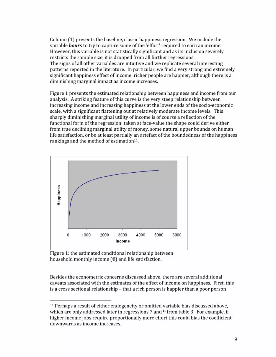
 Column (1) presents the baseline, classic happiness regression.  We include the variable hours to try to capture some of the ‘effort’ required to earn an income.  However, this variable is not statistically significant and as its inclusion severely restricts the sample size, it is dropped from all further regressions.  The signs of all other variables are intuitive and we replicate several interesting patterns reported in the literature.  In particular, we find a very strong and extremely significant happiness effect of income: richer people are happier, although there is a diminishing marginal impact as income increases.    Figure 1 presents the estimated relationship between happiness and income from our analysis.  A striking feature of this curve is the very steep relationship between increasing income and increasing happiness at the lower ends of the socio‐economic scale, with a significant flattening out at relatively moderate income levels.  This sharply diminishing marginal utility of income is of course a reflection of the functional form of the regression; taken at face‐value the shape could derive either from true declining marginal utility of money, some natural upper bounds on human life satisfaction, or be at least partially an artefact of the boundedness of the happiness rankings and the method of estimation11.    

 Figure 1: the estimated conditional relationship between  household monthly income (€) and life satisfaction.   Besides the econometric concerns discussed above, there are several additional caveats associated with the estimates of the effect of income on happiness.  First, this is a cross sectional relationship – that a rich person is happier than a poor person 

                                                        11 Perhaps a result of either endogeneity or omitted variable bias discussed above, which are only addressed later in regressions 7 and 9 from table 3.  For example, if higher income jobs require proportionally more effort this could bias the coefficient downwards as income increases. 

  10

does not automatically imply that the poor person would be made equally happy if they too were as rich.  For example, it could be that what really matters is relative wealth.  In fact, it is much harder to detect an effect of increasing income on happiness in a time series analysis (the famous Easterlin Paradox12), although recently Stevenson and Wolfers (2008) present evidence that there is indeed such an effect.    Layard et. al. (2008) also analyze the EQLS, as well as seven other ‘happiness’ datasets, in order to estimate an elasticity of marginal utility with respect to income, which they denote ρ.  Given the focus of their research, in order to focus on ‘permanent income’ they restrict their analysis to those between the age of 30 and 55, and delete the top and bottom 5% of outliers.   Despite the difference in the samples, as with our analysis, Layard et. al. find that both log_income and (log_income) squared have explanatory power13, and thus reject the hypothesis that happiness depends only linearly on the log of income (i.e. ρ=1).  Layard et. al. go on then to estimate ρ using maximum likelihood, and their results suggest values of ρ that are reassuringly similar across countries and time and fall into the region of 1.19‐1.34 with an overall average of 1.26.   Although we do not directly estimate ρ ourselves, we can use these Layard et. al. results to compare against our own direct utility‐compensating estimates as a robustness check (see discussion below and table 4).  Another interesting relationship that has drawn some attention recently is the correlation between happiness and age.  Thus, following some recent research (see, for example, Yang Yang (2008), Oswald and Blanchflower (2008)), we also control for age, age‐squared and age‐cubed.    Mirroring the findings of others, we find a striking dip in happiness around middle age, which then heads upwards again as people age further14.  This relationship holds true controlling for health, income, marital status, country of residence, etc. and has received quite a bit of interest from sociologists, psychologists and economists in the last year.  Figure 2 illustrates this estimated cubic inverted‐U relationship from our baseline regression.   

                                                        12 See Easterlin (1974), Stevenson and Wolfers (2008), Clark et. al. (2008) 13 Although Layard et. al. (2008) find a much less significant coefficient on the squared log of income for the EQLS data, which is probably due to their much narrower data set. 14 Thank goodness. 

  11

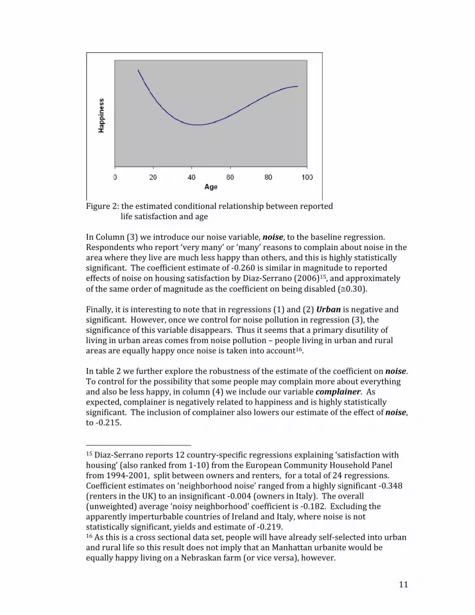
 Figure 2: the estimated conditional relationship between reported                    life satisfaction and age  In Column (3) we introduce our noise variable, noise, to the baseline regression.  Respondents who report ‘very many’ or ‘many’ reasons to complain about noise in the area where they live are much less happy than others, and this is highly statistically significant.  The coefficient estimate of ‐0.260 is similar in magnitude to reported effects of noise on housing satisfaction by Diaz‐Serrano (2006)15, and approximately of the same order of magnitude as the coefficient on being disabled (≅0.30).    Finally, it is interesting to note that in regressions (1) and (2) Urban is negative and significant.  However, once we control for noise pollution in regression (3), the significance of this variable disappears.  Thus it seems that a primary disutility of living in urban areas comes from noise pollution – people living in urban and rural areas are equally happy once noise is taken into account16.  In table 2 we further explore the robustness of the estimate of the coefficient on noise.  To control for the possibility that some people may complain more about everything and also be less happy, in column (4) we include our variable complainer.  As expected, complainer is negatively related to happiness and is highly statistically significant.  The inclusion of complainer also lowers our estimate of the effect of noise, to ‐0.215.                                                             15 Diaz‐Serrano reports 12 country‐specific regressions explaining ‘satisfaction with housing’ (also ranked from 1‐10) from the European Community Household Panel from 1994‐2001,  split between owners and renters,  for a total of 24 regressions.   Coefficient estimates on ‘neighborhood noise’ ranged from a highly significant ‐0.348 (renters in the UK) to an insignificant ‐0.004 (owners in Italy).  The overall (unweighted) average ‘noisy neighborhood’ coefficient is ‐0.182.  Excluding the apparently imperturbable countries of Ireland and Italy, where noise is not statistically significant, yields and estimate of ‐0.219. 16 As this is a cross sectional data set, people will have already self‐selected into urban and rural life so this result does not imply that an Manhattan urbanite would be equally happy living on a Nebraskan farm (or vice versa), however. 

  12

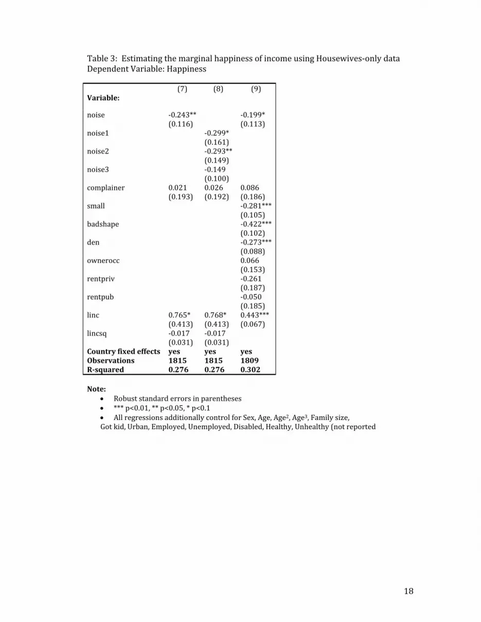
In column (5) we parse out our noise variable into its component parts: noise1 corresponds to ‘very many’ noise complaints, noise2 ‘many’, and noise3 denotes only ‘a few’ complaints (the excluded category is ‘no complaints’).   As expected, the coefficients on the three variables declines monotonically from ‐0.329 (worse than being disabled!) for the most noise to ‐0.230 for relatively fewer complaints (the omitted category is ‘no complaints’).  In column (6) of table 2 we consider whether our noise variable could be proxying for other characteristics of the respondent’s dwelling.   For example, poorly constructed housing can lack acoustic insulation, causing more noise complaints, as well as decrease happiness more directly.  Thus in regression (6) we control for the state of the dwelling: whether it is considered too small, how high the density (family size/number of rooms) is, whether it is in bad shape (with rot or no indoor plumbing), and whether the respondent owns the property, privately rents or lives in public housing.   Once we have controlled for all these housing factors, the magnitude of the coefficient estimate on noise falls to ‐0.158, but is still negative and highly statistically significant.  4b.  Utility compensating income estimates  We have found noise pollution to have a relatively large and statistically significantly negative effect on life satisfaction.   However we would also like to calculate the monetary equivalent impact: by how much would income have to increase to compensate for the negative effect on happiness that noise pollution creates?  To generate estimates of the happiness‐compensating money (income) value of noise pollution, it is essential to generate accurate estimates of the marginal happiness of income.  However, as discussed above, there are two primary problems, both well understood in the literature.  First, if happier people command higher incomes there will be endogeneity bias.  Second, if we fail to control for the (happiness reducing) effort required to earn that income, we will understate the true happiness benefit of extra income.  In table 3 we address both these problems by re‐estimating our happiness regressions in a sample of housewives.  As discussed above, housewives’ effort level is arguably uncorrelated with household income.  Furthermore, by de‐linking the respondent from the source of the income, we also address the first‐order endogeneity of happiness and income.    In column (7) of table 3 we reproduce our basic noise‐happiness regression in the housewife‐only sample.  The sample size is greatly reduced, but still sizable at 1815.  The coefficient on noise, ‐0.24, is negative, statistically significant and only slightly larger in magnitude than in the full sample.  In regressions (8) we parse out the noise variable and again find that the negative effect on happiness declines monotonically with degree of noise.  In column (9) we drop log‐income‐squared and additionally control for dwelling attributes that might be correlated with noise and creating an omitted variable bias.   As in the full sample, the magnitude of the coefficient on noise drops (to ‐0.199) but is still statistically significant.    We use regression (9) to derive our final estimates of the increase in income required to compensate for a loss of happiness due to noise pollution (at least for  housewives).   

  13

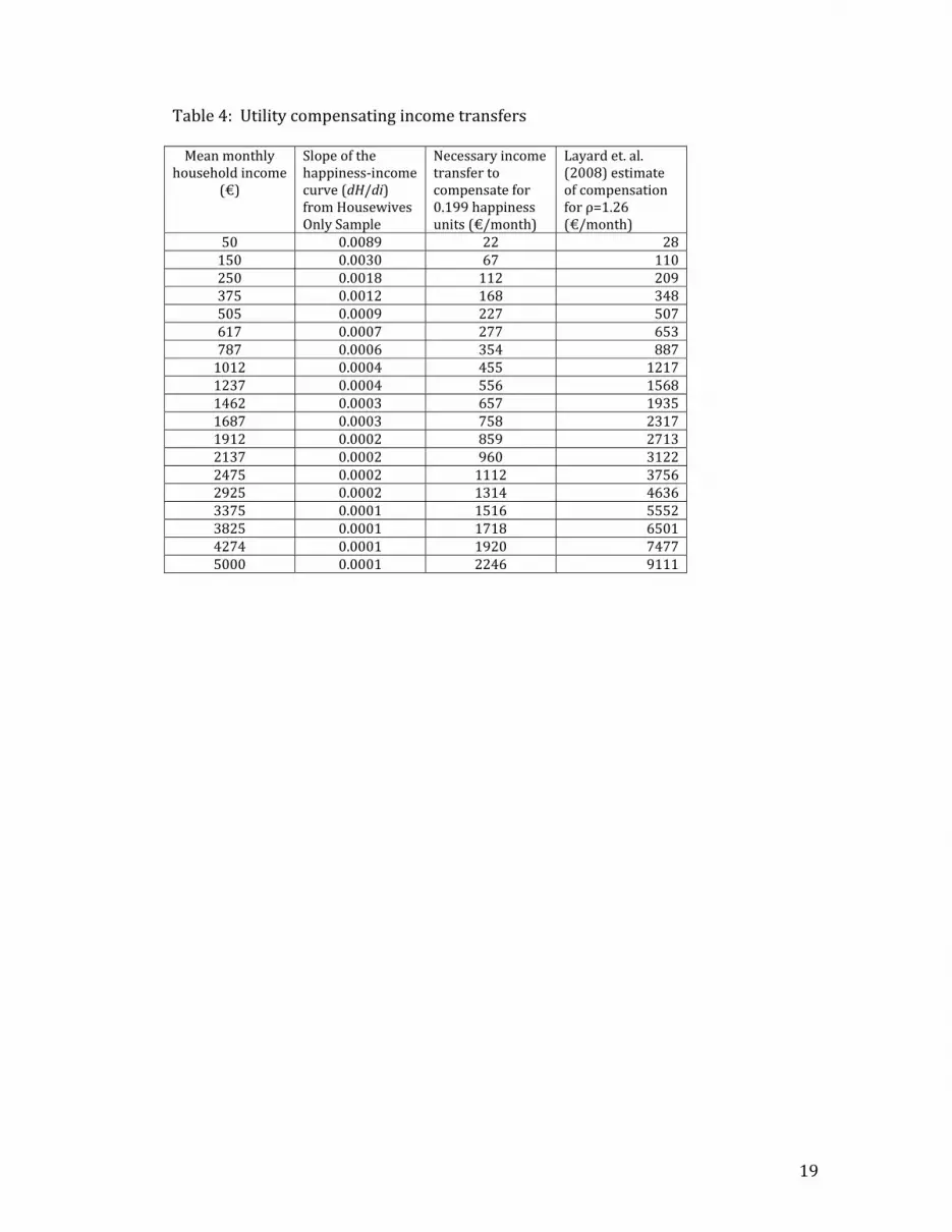
As we control for dwelling characteristics, estimates of the happiness cost of noise from equation (9) are the most conservative.  In addition, as regression (9) is run on the  housewife‐only sample, the estimates of the marginal happiness of income should be less endogenous and biased by effort effects, as discussed above. The coefficients on log of income and noise from column (9) are, respectively, ˆ β 1  = 0.443, and for  ˆ β 2= ‐0.199.    Following equation (5), table 4 presents the required compensatory income for each of the 19 income levels in the EQLS survey.   The amount varies from €22/month for the lowest income bracket, up to €2246 for the top group.  There are several interesting points to note.  First, the general relationship outlined in table 4 is not overly sensitive to the choice of functional form for the happiness‐income parameterization.  In separate robustness checks using level income brackets (1‐19), dividing the sample into three income groups, and allowing separate intercepts and slope coefficients for each, we found very similar results (not reported but available upon request).    Second, taking the compensation amounts presented in columns 3 and 4 of table 4 as the amount required to compensate for noise pollution assumes that a noisy environment reduces happiness in equal amounts for all income cohorts.   For wealthy people, spending to reduce noise pollution is a good deal in happiness terms, so we would expect them to ‘buy’ themselves out of a lot of the noise (and other) problems that less wealthy individuals face.   In fact, if we break up the noise variable, noise, by income bracket, we find that the wealthiest third do not suffer17 from noise (even if they complain about it), suggesting that what they consider to be ‘noise’ is not the same as it is for the lower income classes.     If we thus omit the top third of the income scale from consideration (they do not suffer from noise pollution!), we are still faced with relatively high compensation rates for the middle‐income group.   This of course is simply a direct result of the declining marginal returns to income reflected in the estimated happiness‐income curve.  However, it is probably politically, and possibly ethically, infeasible to consider making larger compensation payments to wealthier individuals for noise pollution (although this is routinely done in wrongful death cases, for different reasons).  Thus on the basis of our results for the lowest third of income levels (taking the average of the six lowest brackets), given the estimates for the (conservative) utility costs of noise from regression (9) we adopt a very rough estimate of a monetary equivalent cost of relatively severe noise pollution to be on the order of €146 per month for a household.  Finally, as we have discussed above, Layard, Mayraz and Nickell (2008) calculate the elasticity of happiness with respect to income (ρ) for 8 different data sets, and column 4 of table 4 presents the implied compensation for each income bracket from their mean overall estimate of ρ=1.26.    As is apparent, the Layard et. al estimates, which do not control for effort and are subject to endogeneity biases discussed above, are quite a bit higher than ours.  This is to be expected as their estimate for the EQLS of ρ=1.19 was the lowest of all the datasets.  However, estimates of the compensating income                                                         17 The coefficient on noise for the top 6 income brackets was ‐0.07 with a robust t‐statistic of ‐1.01.  Full results available upon request. 

  14

required at ρ=1.19 are still higher than ours.  This in turn suggests that omitted variable bias from unobservable effort, as well as possibly endogeneity, may account for some of the difference18.   5.  Discussion  This paper presents a simple empirical exercise that adds to the increasing amount of evidence that noise pollution can have a serious detrimental affect on people’s life satisfaction.  In fact, in our data the negative impact on happiness associated with urban life was entirely eliminated once we controlled for noise.  As urbanization rates increase dramatically around the globe and high housing costs compel people to live in ever closer quarters, overall welfare will suffer if builders and policy makers do not pay sufficient attention to acoustic insulation of dwellings.  However, noise pollution is often an externality and not easily priced in the market, leaving it to be easily under‐considered in the planning process.  We approach the problem of quantifying the lost utility of noise by examining a series of ‘happiness regressions’ in which we use a range of socio‐economic data to explain respondent’s declared level of life satisfaction on a scale from 1 to 10.  In the process we replicate the observed patterns from other studies of this type and find that noise complaints significantly decrease declared levels of life satisfaction.  In the process of estimating our happiness regressions we must address several major estimation problems of omitted variable and endogeneity biases.  While other studies have grappled with these issues, our contribution here is to propose solutions that can be implemented using solely the single cross sectional survey data that is much more ubiquitously available than the time‐series panel and other more difficult‐to‐find (i.e. lottery winners) data sets.   In particular,  first we control for the possibility that an unobservable characteristic (which we denote ‘complainer type’) may lead people both to complain more and cause them to be less happy.  Second, in the absence of some exogenous form of variation in income, estimates of the marginal utility of income may suffer from endogeneity and will be under‐estimated if ‘effort’ is not adequately controlled for.  By estimating the marginal utility of income on a sample of housewives, we make some progress in addressing both of these problems. Furthermore, while a number of other studies have used hedonic methods to monetize the costs of traffic and airport noise (which are substantial), this paper makes uses a general reduced form strategy to estimate the monetized costs of everyday neighbourhood noise of all types (even imaginary noise!).    Consistent with the literature, we find a substantial decline in the marginal impact of income on happiness at very moderate levels of income, even after attempting to control for omitted variables and endogeneity.  While this could be a true reflection of people’s underlying preferences, it may also be due to estimation bias or be an artefact of the bounded nature of the happiness rankings themselves.  At any rate, taken at face value a low elasticity of happiness with respect to income automatically implies that quite large monetary transfers must be made to compensate a given fall 

                                                        18 Layard et. al. also restrict the sample to people between 30 and 55 years old and omit the top and bottom 5% of outliers. 

  15

in ‘happiness,’ leading to infeasible estimates of the value of noise abatement for higher income individuals.  However our results also suggest that higher income households make those trade‐offs they see as worthwhile and ‘buy’ themselves out of serious noise problems19.   Among the wealthiest cohort of our sample, even those having ‘many’ or ‘very many’ reasons to complain about noise did not experience lower happiness by a statistically significant amount as a result, suggesting that their perception of noise is quite different from those with less income.  In the end, we adopt the estimates from the bottom third income cohort of the sample.  For this group, we estimate that the monetary equivalent of relatively severe noise pollution would be on average about €146 per month per household.  Clearly these are large costs, which, if taken at face value, can easily justify significant investment in noise abatement policies and infrastructure.  How do our estimates of the costs of noise compare with those generated using other methods?  Van Praag and Baarsma (2005) find that an Amsterdam‐area household with monthly income of €1500 would require (monthly) compensation of €57 for an increase in aircraft noise from 20 to 40 Ku.   As mentioned earlier, Nelson (2004) finds a US$200,000 house would sell for $20,000 to $24,000 less if exposed to airplane noise.  $24,000 amortized over 20 years at 4% comes to about $145/month.   Galilea and Ortuzar (2005) use a stated preference approach and find a (conservative) estimate of willingness‐to‐pay (WTP) of US$2.12 per decibel (dB(A)) per month.  Double glazing reduces noise levels by approximately 30 dB(A), so their results suggest a WTP of $64/month to reduce noise to a degree equivalent to that achieved by double glazing.    It is difficult to see how to directly compare these disparate estimates, but the general order of magnitude does not seem too out of line.   Our estimates are a bit higher, but other studies have focussed on single sources of noise, whereas here we attempt to capture the effect of all sources of irritating neighbourhood noise.  Furthermore, psychological studies suggest that people often under‐predict how unhappy a future bad event will make them (see Gilbert (2006)), suggesting that the WTP estimates be considered lower bounds20.    In sum, then, our primary conclusion is that noise pollution seems to be a cause of significant personal dissatisfaction (especially in urban areas) and that this disutility is not wholly immune from quantification.  Clearly, more research would be welcome.      

                                                        19 This strategy turns out to be much more difficult in extraordinarily expensive cities, such as central London. 20 Many thanks to Guy Mayraz who helpfully pointed this out. 

  16

Tables Appendix  Table 1:  Happiness OLS Regressions, Dep. Variable: Happiness    

(1)  

(2)  

(3)  

Variable: 

Noise      ‐0.260*** (0.032) 

Log income  0.661*** (0.111) 

0.727*** (0.103) 

0.736*** (0.103) 

(Log income)2  ‐0.023*** (0.009) 

‐0.028*** (0.008) 

‐0.029*** (0.008) 

Sex  ‐0.136*** (0.025) 

‐0.130*** (0.024) 

‐0.129*** (0.024) 

Age  ‐0.125*** (0.020) 

‐0.120*** (0.018) 

‐0.118*** (0.018) 

Age2  0.002*** (0.000) 

0.002*** (0.000) 

0.002*** (0.000) 

Age3  ‐0.000*** (0.000) 

‐0.000*** (0.000) 

‐0.000*** (0.000) 

Family size  ‐0.027** (0.012) 

‐0.029*** (0.011) 

‐0.029*** (0.011) 

Got kid  0.080** (0.039) 

0.079** (0.037) 

0.076** (0.037) 

Married  0.573*** (0.036) 

0.577*** (0.034) 

0.576*** (0.034) 

Single  0.138*** (0.052) 

0.154*** (0.050) 

0.151*** (0.049) 

Urban  ‐0.045* (0.025) 

‐0.047** (0.024) 

‐0.020 (0.024) 

University  0.220*** (0.031) 

0.218*** (0.030) 

0.217*** (0.030) 

Employed  0.083 (0.103) 

‐0.139* (0.084) 

‐0.138* (0.083) 

Unemployed  ‐0.609*** (0.116) 

‐0.790*** (0.097) 

‐0.787*** (0.096) 

In school  ‐0.038 (0.101) 

0.020 (0.085) 

0.021 (0.085) 

Retired  0.162 (0.111) 

0.002 (0.092) 

0.005 (0.092) 

Housewife  0.077 (0.118) 

‐0.116 (0.094) 

‐0.108 (0.094) 

Disabled  ‐0.108 (0.144) 

‐0.320** (0.126) 

‐0.318** (0.126) 

Healthy  0.744*** (0.031) 

0.801*** (0.030) 

0.794*** (0.030) 

Unhealthy  ‐0.882*** (0.053) 

‐0.880*** (0.049) 

‐0.872*** (0.049) 

Hours  0.005 (0.009) 

 

Country Fixed Effects 

yes  yes  yes 

Observations  17119  20113  20113 R­squared  0.352  0.346  0.349 Note: Robust standard errors in parentheses             *** p<0.01, ** p<0.05, * p<0.1   

  17

Table 2:  Estimating the happiness cost of noise pollution Dependent Variable: Happiness    (4) 

 (5)  

(6)  

Variable:   

Noise  ‐0.215*** (0.034) 

  ‐0.158*** (0.033) 

Complainer  ‐0.280*** (0.061) 

‐0.263*** (0.061) 

‐0.236*** (0.061) 

Noise1  ‐0.329*** (0.052) 

Noise2  ‐0.283*** (0.041) 

Noise3  ‐0.230*** (0.026) 

 

Small  ‐0.198*** (0.031) 

Bad shape  ‐0.384*** (0.029) 

Density  ‐0.179*** (0.031) 

Owner occupied  0.080 (0.052) 

Rent private   

‐0.147** (0.060) 

Rent public 

 

 

‐0.015 (0.060) 

Log income  0.741*** (0.102) 

0.756*** (0.102) 

0.709*** (0.102) 

(Log income)2  ‐0.030*** (0.008) 

‐0.031*** (0.008) 

‐0.033*** (0.008) 

Country Fixed Effects 

yes  yes  Yes 

Observations  20113  20113  20016 R­squared  0.349  0.352  0.364 Note: •  Robust standard errors in parentheses             • *** p<0.01, ** p<0.05, * p<0.1 • All regressions additionally control for Sex, Age, Age2, Age3, Family size,  

Got kid, Married, Single, Urban, Employed, Unemployed, In school,  Retired, Housewife, Disabled, Healthy, Unhealthy (not reported) 

 

        

  18

Table 3:  Estimating the marginal happiness of income using Housewives‐only data Dependent Variable: Happiness    (7)  (8)  (9) Variable:   

noise  ‐0.243**(0.116) 

  ‐0.199* (0.113) 

noise1    ‐0.299* (0.161) 

 

noise2    ‐0.293**(0.149) 

 

noise3    ‐0.149 (0.100) 

 

complainer  0.021 (0.193) 

0.026 (0.192) 

0.086 (0.186) 

small      ‐0.281***(0.105) 

badshape      ‐0.422***(0.102) 

den      ‐0.273***(0.088) 

ownerocc      0.066 (0.153) 

rentpriv      ‐0.261 (0.187) 

rentpub      ‐0.050 (0.185) 

linc  0.765* (0.413) 

0.768* (0.413) 

0.443*** (0.067) 

lincsq  ‐0.017 (0.031) 

‐0.017 (0.031) 

 

Country fixed effects  yes  yes  yes Observations  1815  1815  1809 R­squared  0.276  0.276  0.302  Note: 

• Robust standard errors in parentheses             • *** p<0.01, ** p<0.05, * p<0.1 • All regressions additionally control for Sex, Age, Age2, Age3, Family size,  Got kid, Urban, Employed, Unemployed, Disabled, Healthy, Unhealthy (not reported 

       

  19

Table 4:  Utility compensating income transfers  Mean monthly 

household income (€) 

Slope of the happiness‐income curve (dH/di) from Housewives Only Sample 

Necessary income transfer to compensate for  0.199 happiness units (€/month) 

Layard et. al. (2008) estimate of compensation for ρ=1.26 (€/month) 

50  0.0089  22  28 150  0.0030  67  110 250  0.0018  112  209 375  0.0012  168  348 505  0.0009  227  507 617  0.0007  277  653 787  0.0006  354  887 1012  0.0004  455  1217 1237  0.0004  556  1568 1462  0.0003  657  1935 1687  0.0003  758  2317 1912  0.0002  859  2713 2137  0.0002  960  3122 2475  0.0002  1112  3756 2925  0.0002  1314  4636 3375  0.0001  1516  5552 3825  0.0001  1718  6501 4274  0.0001  1920  7477 5000  0.0001  2246  9111 

   

  20

 References  Baranzini, Andrea and Jose V. Ramirez, 2005. “Paying for Quietness. The Impact of Noise on Geneva Rents”  Urban Studies, Vol. 42, No. 4, pp. 1‐14  Carson, Richard, Nicholas E. Flores and Norman F. Meade, 2001. “Contingent Valuation: Controversies and Evidence"  Environmental and Resource Economics, vol. 19: pp. 173-210  Clark, Andrew and Andrew Oswald, 2002. “A simple statistical method for measuring how life events affect happiness”  Unpublished manuscript, University of Warwick, January   Clark, Andrew,  Paul Frijters, and Michael A. Shields, 2008 “Relative Income, Happiness, and Utility: An Explanation for the Easterlin Paradox and Other Puzzles” Journal of Economic Literature, V. 96 ol. XLVI March   Davidson, R., Jackson, D. and Kalin, N. 2000. “Emotion, plasticity, context and regulation: Perspectives from affective neuroscience”, Psychological Bulletin 126, pp. 890–906  Day, Brett, Ian Bateman and Iain Lake, 2007. “Beyond implicit prices: recovering theoretically consistent and transferable values for noise avoidance from a hedonic property price model”, Environmental and Resource Economics, Volume 37, Number 1 May, pp. 211‐232  Diaz‐Serrano, Luis, 2006. “Housing Satisfaction, Homeownership and Housing Mobility: A Panel Data Analysis for Twelve EU Countries”  IZA Discussion Paper No. 2318, September   Di Tella, Rafael and Robert MacCulloch, 2006. “Some Uses of Happiness Data in Economics” Journal of Economic Perspectives Vol. 20(1) Winter pp.25‐46  Easterlin, Richard A. 1974. "Does economic growth improve the human lot? Some empirical evidence." In Nations and Households in Economic Growth: Essays in Honor of Moses Abramowitz, by Paul A David and Melvin W. Reder. New York: Academic Press  European Foundation for the Improvement of Living and Working Conditions and Wissenschaftszentrum Berlin fuer Sozialforschung, 2006. European Quality of Life Survey, 2003 [computer file]. Colchester, Essex: UK Data Archive [distributor], SN: 5260. Frey, Bruno S., Simon Leunchinger and Alois Stutzer, 2004. “Valuing public goods: the life satisfaction approach” CESifo working paper no. 1158, March Galilea, P. and Juan de Dios Ortuzar, 2005. “Valuing noise level reductions in a residential location context,” Transportation Research Part D 10: 305–322 Gilbert, Daniel, 2006. Stumbling on Happiness Knopf

  21

Layard, Richard, G. Mayraz and S. Nickell, 2008. “The marginal utility of income” Journal of Public Economics 92, pp.1846-1857 Lu, Max , 1999, “Determinants of Residential Satisfaction: Ordered Logit vs. Regression Models”, Growth and Change 30, pp.264-287  Nelson, Jon P., 2004. “Meta‐analysis of airport noise and hedonic property values: problems and prospects”  Journal of Transport Economics and Policy, January.  Oswald, Andrew and David Blanchflower, 2008. “Is Well‐Being U‐Shaped over the Life Cycle?" Social Science & Medicine, 66(6), 1733‐1749   Oswald, Andrew and Nattavudh Powdthavee, 2007. “Death, Happiness, and the Calculation of Compensatory Damages", forthcoming Journal of Legal Studies Stansfeld, S A, B Berglund, C Clark, I Lopez‐Barrio, P Fischer, E Öhrström, MMHaines, J Head, S Hygge, I van Kamp, B F Berry,  2005. “Aircraft and road traffic noise and children’s cognition and health: a cross‐national study”, The Lancet Vol. 365 June 4.  Stevenson, Betsy and Justin Wolfers, 2008.  “Economic Growth and Subjective Well‐Being:  Reassessing the Easterlin Paradox,”  Unpublished manuscript, University of Pennsylvania Wharton School of Business, May 9.  Van Praag, Bernard M.S. and Barbara E. Baarsma, 2005. “Using Happiness Surveys to Value Intangibles: The Case of Airport Noise”  The Economic Journal, Volume 115 Issue 500 Page 224‐246, January  Walters, A.A., 1975. Noise and Prices, Oxford University Press, London.  Wardman, Mark and Abigail Bristow, 2008. “Valuations of aircraft noise: experiments in stated preference” Environmental and Resource Economics, Volume 39, Number 4, April.  Yang Yang, 2008. "Social Inequalities in Happiness in the U.S. 1972‐2004: An Age‐Period‐Cohort Analysis." American Sociological Review 73:204‐226.      

  22

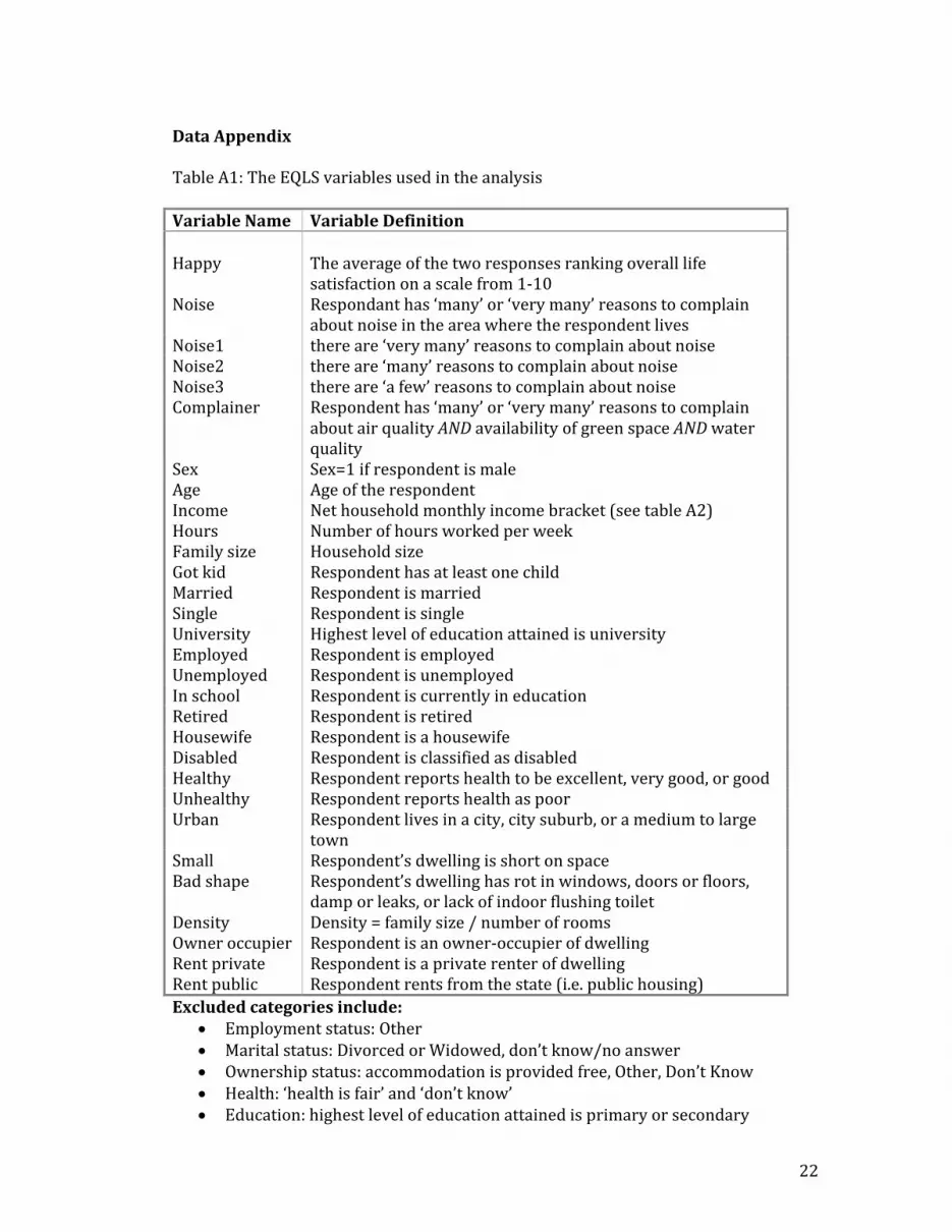
 Data Appendix  Table A1: The EQLS variables used in the analysis  Variable Name  Variable Definition    Happy  The average of the two responses ranking overall life 

satisfaction on a scale from 1‐10 Noise  Respondant has ‘many’ or ‘very many’ reasons to complain 

about noise in the area where the respondent lives Noise1  there are ‘very many’ reasons to complain about noise  Noise2  there are ‘many’ reasons to complain about noise Noise3  there are ‘a few’ reasons to complain about noise Complainer  Respondent has ‘many’ or ‘very many’ reasons to complain 

about air quality AND availability of green space AND water quality 

Sex  Sex=1 if respondent is male Age  Age of the respondent Income  Net household monthly income bracket (see table A2)  Hours  Number of hours worked per week Family size  Household size Got kid  Respondent has at least one child Married  Respondent is married Single   Respondent is single University  Highest level of education attained is university Employed  Respondent is employed Unemployed  Respondent is unemployed In school  Respondent is currently in education Retired  Respondent is retired Housewife  Respondent is a housewife Disabled  Respondent is classified as disabled Healthy  Respondent reports health to be excellent, very good, or good Unhealthy  Respondent reports health as poor Urban  Respondent lives in a city, city suburb, or a medium to large 

town Small  Respondent’s dwelling is short on space Bad shape  Respondent’s dwelling has rot in windows, doors or floors, 

damp or leaks, or lack of indoor flushing toilet Density  Density = family size / number of rooms Owner occupier  Respondent is an owner‐occupier of dwelling Rent private  Respondent is a private renter of dwelling Rent public  Respondent rents from the state (i.e. public housing) Excluded categories include:  

• Employment status: Other • Marital status: Divorced or Widowed, don’t know/no answer  • Ownership status: accommodation is provided free, Other, Don’t Know • Health: ‘health is fair’ and ‘don’t know’  • Education: highest level of education attained is primary or secondary  

  23

   Appendix (cont.)  Table A2:  Income brackets  Income is net monthly household income, divided into 19 non‐uniform brackets:  Value  Income bracket     1  Less than 100 euro     2   100 to 199 euro      3   200 to 299 euro     4   300 to 449 euro     5   450 to 559 euro     6   560 to 674 euro     7   675 to 899 euro     8   900 to 1124 euro     9   1125 to 1349 euro     10  1350 to 1574 euro      11  1575 to 1799 euro      12  1800 to 2024 euro      13  2025 to 2249 euro      14  2250 to 2699 euro      15  2700 to 3149 euro      16  3150 to 3599 euro      17  3600 to 4049 euro      18  4050 to 4499 euro      19  4500 euro or more      Table A3: Countries in EQLS Sample  Austria  Italy Belgium  Latvia Bulgaria  Lithuania Cyprus  Luxembourg Czech Republic  Malta Denmark  Netherlands Estonia  Poland Finland  Romania France  Slovakia Germany  Slovenia UK  Spain Greece  Sweden Hungary  Turkey Ireland  Portugal