Embed Size (px)
Citation preview
HOLISTIC OPTIMIZATION OF EMBEDDEDCOMPUTER VISION SYSTEMS
A Dissertation
Presented to the Faculty of the Graduate School
of Cornell University
in Partial Fulfillment of the Requirements for the Degree of
Doctor of Philosophy
by
Mark Andrew Buckler
August 2019

© 2019 Mark Andrew Buckler
ALL RIGHTS RESERVED
HOLISTIC OPTIMIZATION OF EMBEDDED COMPUTER VISION SYSTEMS
Mark Andrew Buckler, Ph.D.
Cornell University 2019
Despite strong interest in embedded computer vision, the computational demands of
Convolutional Neural Network (CNN) inference far exceed the resources available in
embedded devices. Thankfully, the typical embedded device has a number of desirable
properties that can be leveraged to significantly reduce the time and energy required
for CNN inference. This thesis presents three independent and synergistic methods
for optimizing embedded computer vision: 1) Reducing the time and energy needed to
capture and preprocess input images by optimizing the image capture pipeline for the
needs of CNNs rather than humans. 2) Exploiting temporal redundancy within incoming
video streams to perform computationally cheap motion estimation and compensation in
lieu of full CNN inference for the majority of frames. 3) Leveraging the sparsity of CNN
activations within the frequency domain to significantly reduce the number of operations
needed for inference. Collectively these techniques significantly reduce the time and
energy needed for vision at the edge, enabling a wide variety of new applications.
BIOGRAPHICAL SKETCH
Mark Buckler was born to Andrew and Elizabeth Buckler in a small town in Mas-
sachusetts, USA on August 18th, 1990. A performer at heart, he began studying the violin
at the age of 4. As Mark matured he developed an affinity for science and engineering,
culminating in a first place award for his high school science fair project which proposed
a novel video conferencing system. Partnering with Fish and Richardson PC, this project
eventually developed into Mark’s first patent.
Inspired by his father’s choice of undergraduate engineering discipline, Mark earned a
bachelors degree in electrical engineering while attended Rensselaer Polytechnic Institute
(RPI). Seeking to specialize and improve his design capabilities he then attended a masters
program in electrical and computer engineering at University of Massachusetts Amherst.
Due in part to encouragement and guidance from his advisor Prof. Wayne Burleson,
he secured an internship working with Advanced Micro Devices’ (AMD’s) exascale
supercomputing team. It was here that he developed a taste for research, spinning his
work on clock domain synchronizers into three separate publications. Around this time
Mark also founded his first company, Firebrand Innovations LLC, which focused on
selling the intellectual property he developed in high school.
Eager to continue pushing the boundaries of what is possible in computing, Mark
applied for PhD programs and secured a research assistantship with Cornell University.
Reclaiming his desire to perform, Mark also took up stand-up comedy. Writing jokes,
planning for shows, and making people laugh helped take the edge off the emotion-devoid
world of engineering. After some time searching for the right advisor, Prof. Adrian
Sampson selected Mark as his first PhD student. Adrian’s keen eye for promising research
directions and wealth of knowledge about the entire computing stack helped guide Mark’s
passion for research into concrete contributions in the field of embedded computer vision.
iii

This dissertation is dedicated to my loving wife, Becky.
You are my connection to all that is beautiful, playful, and joyful in this life.
iv
ACKNOWLEDGEMENTS
I am incredibly grateful to have so many amazing people in my life. We are all largely
a product of our environments, and as such I feel thankful and privileged to have been
surrounded by so many talented and supportive people over the years.
It seems most appropriate to begin by thanking my advisor, Prof. Adrian Sampson.
Even after working with you for so long I remain in awe of your knowledge, focus,
levelheadedness, and ability to communicate. I’m not entirely sure why you saw promise
in me when we got started, but your faith in my abilities is the reason why I can write
this document now. Thank you for humoring my flights of fancy when times were
good and thank you for assuring me that I could handle it when times were hard. I feel
exceptionally proud to be the first student to graduate from your research group and I
look forward to seeing many more students walk in my footsteps.
I also want to thank my committee for their guidance and understanding as my
research evolved in new and interesting ways. Chris Batten, you have been my one
constant at Cornell through all of the changes, and your support means the world to me.
Chris De Sa, your course taught me the intricacies of efficient machine learning, and
Bharath Hariharan your feedback has kept my research on an even keel.
I am thankful that so many talented researchers have been willing to collaborate on
my projects. Suren Jayasuriya, you were my advisor when I had none. I didn’t have even
the smallest amount of surprise when you landed your academic position. ASU is lucky
to have you. Phil Bedoukian, we both worked so damn hard on EVA2 that you pulled
your first all-nighter with me. May you never have to taste 7/11 coffee ever again. You’re
a talented researcher, and I can’t wait to see where your PhD takes you. Neil Adit, this
past year has been amazing and your willingness to jump into your work is inspiring.
Your ability to ask questions and think deeply will take you far. Yuwei Hu, we’ve only
just begun collaboration but you’ve already proven yourself to be remarkably perceptive
v
and a talented programmer.
In my younger years I may have shunned friendship in favor of work, but the Cornell
student community has been too great to let that happen. I especially want to thank
everyone in the Computer Systems Laboratory and the Molnar Research Group. The
early days saw the old guard like Stephen Longfield and Shreesha Srinath who were
able to give me context and temper my hubris. I also want to thank Tayyar Rzayev and
Nicholas Kramer for being great friends in the early years. It feels like only yesterday
that we were all sitting around Nick’s table making grand plans for the next big thing.
Ed Szoka, you intercepted me when I was about to leave Cornell and you couldn’t have
been a better best man. There are too many friends to list, but I especially want to thank
Khalid Al-Hawaj, Ritchie Zhao, Tristan Wang, Skand Hurkat, and Zach Boynton. You
guys kept me sane.
Beyond Cornell I am incredibly thankful for those in my masters program and those
in DeepScale. Prof Wayne Burleson, you were the perfect advisor for me at UMass.
Your tutelage launched me from being an average student to being a curious researcher.
Xiaobin Liu and Nithesh Kurella I will never forget our late nights studying and our
ridiculous time cooking chicken wings. I also want to thank Forrest Iandola and the
entire team at DeepScale. Forrest, its crazy to think how close our research became after
having first met so long ago. Thank you for giving me the opportunity to learn from your
team and to share my knowledge with them as well.
Of course, it all started with Mom and Dad. Thank you for handling my precocious
and obstinate behavior when I was a child. Mom, you taught me to be kind to others and
that its OK to enjoy the simple pleasures, like your cooking! I’m so thankful for your
support of my work even as it continues to get more and more esoteric. Dad, how crazy
is it that you’re beginning your PhD as I’m finishing mine? I cherish our relationship
dearly, and I’m so glad to have you in my life even after you raised me. Any success
vi
I have in work or relationships is only because I am channeling your approach to life.
Hannah and Mary, you guys have become even better sisters as we’ve gotten older. While
I’ve been stuck in college for over 10 years you’ve both grown up to be amazing women.
Finally and most importantly I want to thank my wife, the newly minted Becky
Buckler. You are the kindest and most loving person I know. I can’t believe that you’re
willing to spend even an afternoon with a curmudgeon like me, let alone a lifetime. You
have stuck with me through all the dramatic highs and lows that graduate school has to
offer and you have always been there to offer support. Your smile, your cooking, and
your playful nature make me giggle and remember that there’s more to life than just raw
analytics. I can’t wait to turn the page in the book that is our life, starting the new chapter
entitled ”Seattle”.
Financially my work has been supported by gifts from Google and Huawei, while
NVIDIA was generous enough to donate equipment.
vii
TABLE OF CONTENTS
Biographical Sketch . . . . . . . . . . . . . . . . . . . . . . . . . . . . . . . iiiDedication . . . . . . . . . . . . . . . . . . . . . . . . . . . . . . . . . . . . ivAcknowledgements . . . . . . . . . . . . . . . . . . . . . . . . . . . . . . . vTable of Contents . . . . . . . . . . . . . . . . . . . . . . . . . . . . . . . . viiiList of Tables . . . . . . . . . . . . . . . . . . . . . . . . . . . . . . . . . . xList of Figures . . . . . . . . . . . . . . . . . . . . . . . . . . . . . . . . . . xi
1 Introduction 11.1 Background . . . . . . . . . . . . . . . . . . . . . . . . . . . . . . . . 1
1.1.1 The Imaging Pipeline . . . . . . . . . . . . . . . . . . . . . . . 31.1.2 Camera Sensor . . . . . . . . . . . . . . . . . . . . . . . . . . 51.1.3 Image Signal Processor . . . . . . . . . . . . . . . . . . . . . . 6
1.2 Convolutional Neural Networks . . . . . . . . . . . . . . . . . . . . . 91.3 Hardware Accelerators for Computer Vision . . . . . . . . . . . . . . . 91.4 Key Observations and Contributions . . . . . . . . . . . . . . . . . . . 101.5 Collaborators and Previous Papers . . . . . . . . . . . . . . . . . . . . 11
2 Efficient Imaging for Computer Vision 122.0.1 Pipeline Simulation Tool . . . . . . . . . . . . . . . . . . . . . 152.0.2 Benchmarks . . . . . . . . . . . . . . . . . . . . . . . . . . . . 17
2.1 Image Sensor Design . . . . . . . . . . . . . . . . . . . . . . . . . . . 182.2 Sensitivity to ISP Stages . . . . . . . . . . . . . . . . . . . . . . . . . 212.3 Sensitivity to Sensor Parameters . . . . . . . . . . . . . . . . . . . . . 242.4 Quantifying Power Savings . . . . . . . . . . . . . . . . . . . . . . . . 282.5 Discussion . . . . . . . . . . . . . . . . . . . . . . . . . . . . . . . . . 312.6 Proposed Pipelines . . . . . . . . . . . . . . . . . . . . . . . . . . . . 312.7 Approximate Demosaicing . . . . . . . . . . . . . . . . . . . . . . . . 322.8 Resolution . . . . . . . . . . . . . . . . . . . . . . . . . . . . . . . . . 342.9 Quantization . . . . . . . . . . . . . . . . . . . . . . . . . . . . . . . . 352.10 ISP Profiling . . . . . . . . . . . . . . . . . . . . . . . . . . . . . . . . 37
3 Reduced Temporal Redundancy 393.1 Activation Motion Compensation . . . . . . . . . . . . . . . . . . . . . 41
3.1.1 AMC Overview . . . . . . . . . . . . . . . . . . . . . . . . . . 423.1.2 Warping CNN Activations . . . . . . . . . . . . . . . . . . . . 443.1.3 Design Decisions for AMC . . . . . . . . . . . . . . . . . . . . 49
3.2 The Embedded Vision Accelerator Accelerator . . . . . . . . . . . . . 533.2.1 Receptive Field Block Motion Estimation . . . . . . . . . . . . 553.2.2 Warp Engine . . . . . . . . . . . . . . . . . . . . . . . . . . . 59
3.3 Evaluation . . . . . . . . . . . . . . . . . . . . . . . . . . . . . . . . . 623.3.1 First-Order Efficiency Comparison . . . . . . . . . . . . . . . . 623.3.2 Experimental Setup . . . . . . . . . . . . . . . . . . . . . . . . 64
viii
3.3.3 Energy and Performance . . . . . . . . . . . . . . . . . . . . . 663.3.4 Accuracy–Efficiency Trade-Offs . . . . . . . . . . . . . . . . . 673.3.5 Design Choices . . . . . . . . . . . . . . . . . . . . . . . . . . 68
3.4 Related Work . . . . . . . . . . . . . . . . . . . . . . . . . . . . . . . 733.5 Conclusion . . . . . . . . . . . . . . . . . . . . . . . . . . . . . . . . 75
4 Structured Sparsity in the Frequency Domain 764.1 Background . . . . . . . . . . . . . . . . . . . . . . . . . . . . . . . . 81
4.1.1 Depthwise Separable CNNs . . . . . . . . . . . . . . . . . . . 814.1.2 Frequency Domain CNNs . . . . . . . . . . . . . . . . . . . . 83
4.2 Methodology . . . . . . . . . . . . . . . . . . . . . . . . . . . . . . . 854.2.1 Frequency-Domain 1×1 Convolutions . . . . . . . . . . . . . . 854.2.2 Frequency Band Pruning . . . . . . . . . . . . . . . . . . . . . 874.2.3 Profiled vs. Learned Pruning . . . . . . . . . . . . . . . . . . . 904.2.4 Dense Frequency-Domain 1×1 Computation . . . . . . . . . . 954.2.5 Interleaving Transforms into the Network . . . . . . . . . . . . 96
4.3 Experimental Setup . . . . . . . . . . . . . . . . . . . . . . . . . . . . 984.4 Evaluation . . . . . . . . . . . . . . . . . . . . . . . . . . . . . . . . . 99
4.4.1 CIFAR-10 . . . . . . . . . . . . . . . . . . . . . . . . . . . . . 994.4.2 ImageNet . . . . . . . . . . . . . . . . . . . . . . . . . . . . . 1044.4.3 Wall-Clock Speedup . . . . . . . . . . . . . . . . . . . . . . . 106
4.5 Implementation Details . . . . . . . . . . . . . . . . . . . . . . . . . . 1074.6 Conclusion . . . . . . . . . . . . . . . . . . . . . . . . . . . . . . . . 108
5 Conclusion 1095.1 Future Work . . . . . . . . . . . . . . . . . . . . . . . . . . . . . . . . 1095.2 Desired Impact . . . . . . . . . . . . . . . . . . . . . . . . . . . . . . 111
5.2.1 Direct Adoption . . . . . . . . . . . . . . . . . . . . . . . . . 1115.2.2 Computing on Compressed Data . . . . . . . . . . . . . . . . . 1125.2.3 Holistic Design and Specialization . . . . . . . . . . . . . . . . 112
ix
LIST OF TABLES
2.1 Vision applications used in our evaluation. . . . . . . . . . . . . . . . 172.2 Profiling statistics for software implementations of each ISP pipeline
stage. . . . . . . . . . . . . . . . . . . . . . . . . . . . . . . . . . . . 34
3.1 The trade-off space between accuracy and resource efficiency withEVA2. For the original baseline and three key configurations, we showthe vision task accuracy score (acc), the fraction of frames that are keyframes (keys), and the average latency and energy cost per frame. . . . 68
3.2 The accuracy impact of targeting different layers for EVA2’s predictionat various key frame intervals. The orig rows show the baseline accuracyfor each network. . . . . . . . . . . . . . . . . . . . . . . . . . . . . . 71
3.3 The accuracy impact of training to fine-tune CNNs for execution onwarped data. The accuracy column shows the network’s score whenprocessing plain, unwarped activation data. . . . . . . . . . . . . . . . 71
4.1 High-level results including CIFAR-10 top-1 accuracy degradation, com-putational savings, and expected CPU wall-clock speedups when usingour per channel frequency band pruning. Unlike Figures 4.11 and 4.12,this table shows accuracy of the network not only after pruning but alsoafter retraining. . . . . . . . . . . . . . . . . . . . . . . . . . . . . . . 99
x
LIST OF FIGURES
1.1 Legacy Computer Vision Pipeline . . . . . . . . . . . . . . . . . . . . 21.2 The standard imaging pipeline (a) and our proposed pipeline (b) for our
design’s vision mode. . . . . . . . . . . . . . . . . . . . . . . . . . . . 4
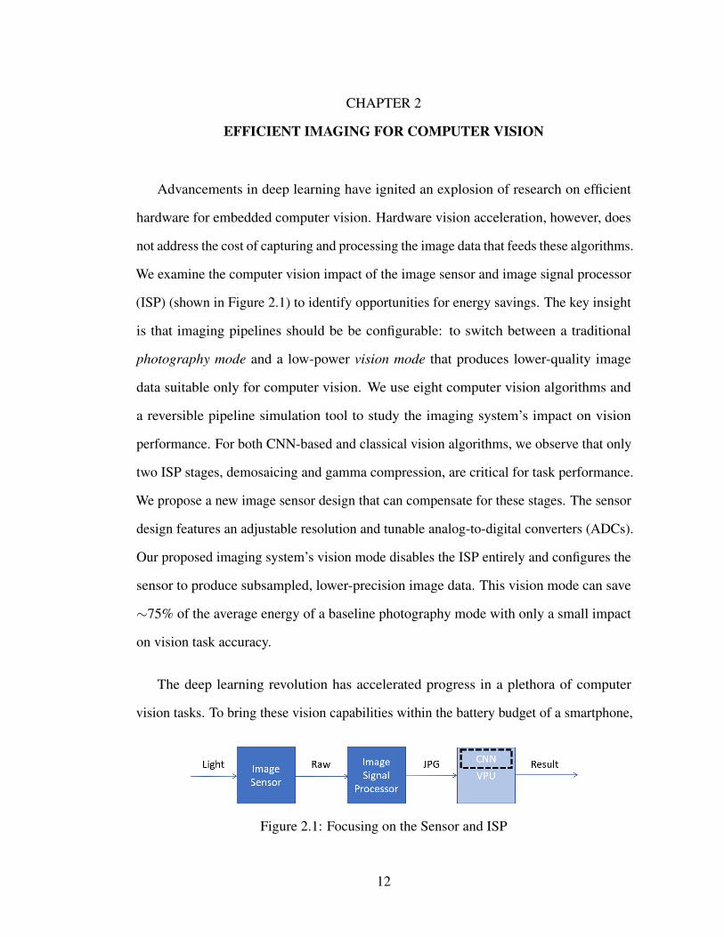
2.1 Focusing on the Sensor and ISP . . . . . . . . . . . . . . . . . . . . . 122.2 Configurable & Reversible Imaging Pipeline . . . . . . . . . . . . . . 152.3 Our proposed camera sensor circuitry, including power gating at the
column level (a) and our configurable logarithmic/linear SAR ADC (b). 182.4 Disabling a single ISP stage. . . . . . . . . . . . . . . . . . . . . . . . 232.5 Enabling a single ISP stage and disabling the rest. . . . . . . . . . . . 242.6 Each algorithm’s vision error, normalized to the original error on plain
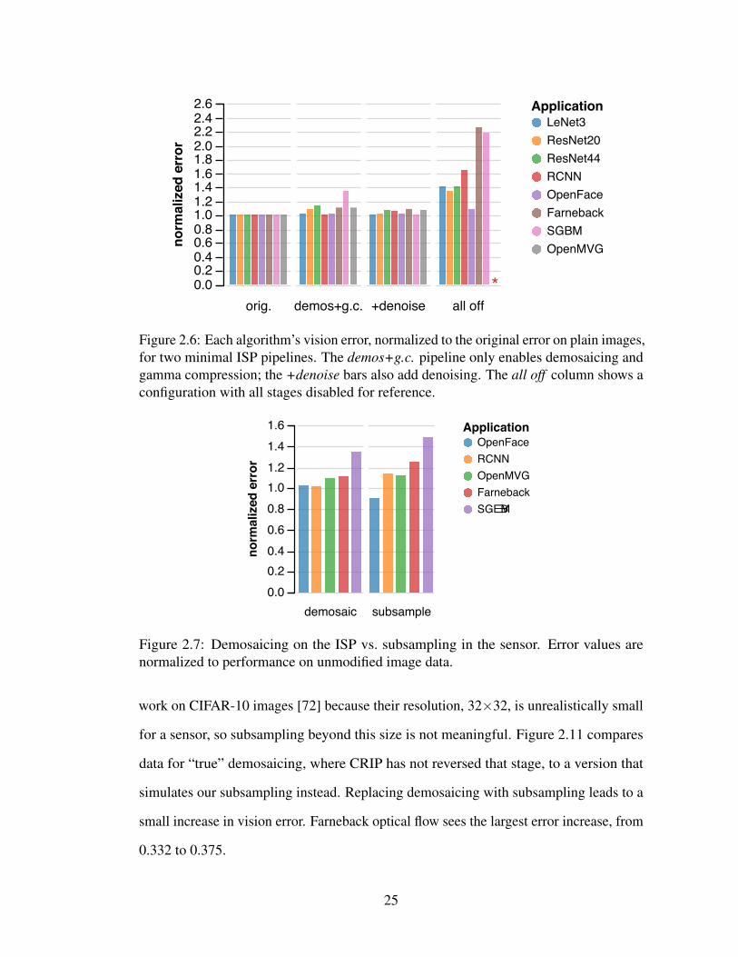
images, for two minimal ISP pipelines. The demos+g.c. pipeline onlyenables demosaicing and gamma compression; the +denoise bars alsoadd denoising. The all off column shows a configuration with all stagesdisabled for reference. . . . . . . . . . . . . . . . . . . . . . . . . . . 25
2.7 Demosaicing on the ISP vs. subsampling in the sensor. Error values arenormalized to performance on unmodified image data. . . . . . . . . . 25
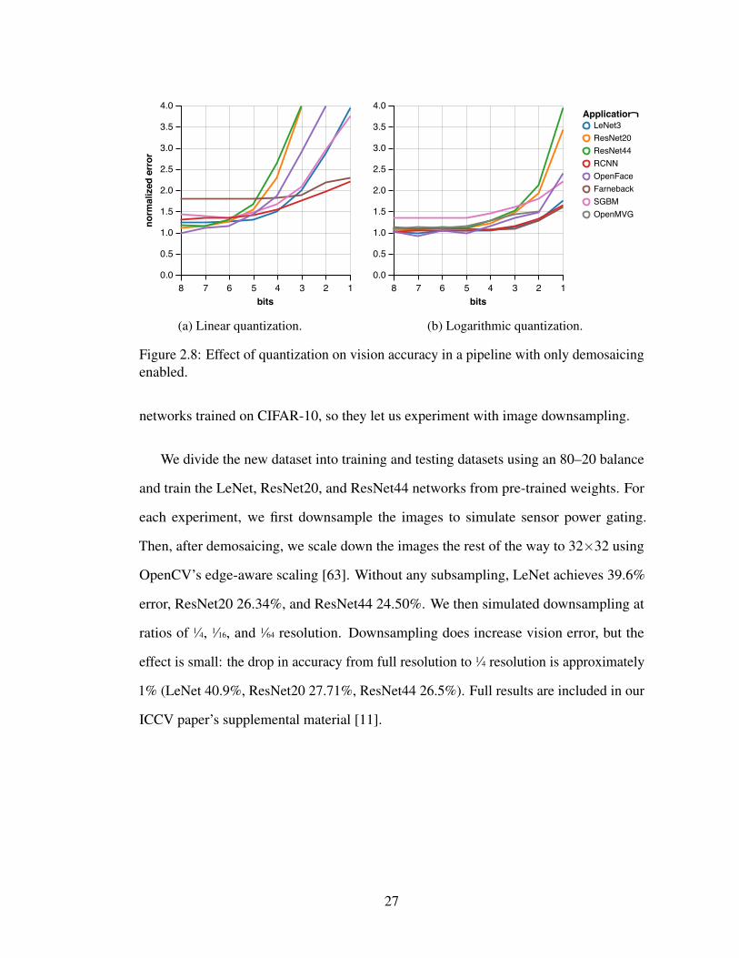
2.8 Effect of quantization on vision accuracy in a pipeline with only demo-saicing enabled. . . . . . . . . . . . . . . . . . . . . . . . . . . . . . 27
2.9 Vision accuracy for two proposed pipelines. . . . . . . . . . . . . . . . 322.10 Visualizations for the approximate forms of demosaicing: subsampling,
bilinear interpolation, and a nearest-neighbor algorithm. . . . . . . . . 332.11 Normalized task error for four demosaicing strategies. Each cluster
shows a configuration simulating a pipeline with only gamma com-pression enabled. The demosaic cluster shows the original demosaiceddata (i.e., all stages were reversed except for demosaicing). The othersshow images with simulated demosaicing using subsampling, nearest-neighbor demosaicing, and bilinear interpolation. . . . . . . . . . . . . 33
2.12 Impact of resolution on three CNNs for object recognition. Using acustom data set consisting of higher-resolution images from ImageNetmatching the CIFAR-10 categories, we simulate pixel binning in thesensor, which produces downsampled images. The y-axis shows thetop-1 error for each network. . . . . . . . . . . . . . . . . . . . . . . . 35
2.13 Histograms of the light intensity distribution for CRIP-converted rawCIFAR-10 data (top) and CDF quantized CIFAR-10 data (bottom). . . 36
2.14 Effect of the image quantization strategy on vision accuracy in a pipelinewith only demosaicing enabled. This figure shows logarithmic quantiza-tion and a second strategy based on measuring the cumulative distribu-tion function (CDF) of the input data. . . . . . . . . . . . . . . . . . . 37
3.1 Focusing on the Vision Processing Unit . . . . . . . . . . . . . . . . . 39
xi
3.2 Activation motion compensation (AMC) runs the CNN precisely forperiodic key frames and uses an approximately incremental update formore frequent predicted frames. For predicted frames, the algorithmestimates motion in the input and uses the resulting vector field to updatea saved CNN activation from the last key frame. . . . . . . . . . . . . 40
3.3 A convolutional layer applies filters to regions in the input. The inputregion corresponding to a given activation value is called its receptive field. 44
3.4 Convolutional layers and translations are commutative, so f (δ (x)) =δ ′( f (x)) where δ ′ is a scaled version of the translation δ . . . . . . . . 44
3.5 An example convolutional layer and pooling layer applied to transfor-mations of an input image. . . . . . . . . . . . . . . . . . . . . . . . . 47
3.6 EVA2 as a part of a complete vision processing unit (VPU). CNNsconsist primarily of convolutional layers and fully-connected layers; thisexample VPU uses ASIC designs from the architecture literature foreach of the two layer types [24, 45] and adds EVA2. . . . . . . . . . . 53
3.7 The architecture of EVA2. . . . . . . . . . . . . . . . . . . . . . . . . 553.8 A set of example receptive fields with size 6, stride 2, and padding 2.
Nearby receptive fields overlap significantly, and receptive fields nearthe edge overlap enclose out-of-bounds pixels. . . . . . . . . . . . . . 55
3.9 The architecture of the diff tile consumer used for receptive field blockmotion estimation (RFBME). . . . . . . . . . . . . . . . . . . . . . . 58
3.10 The architecture of the warp engine. . . . . . . . . . . . . . . . . . . . 593.11 The warp engine’s datapath for loading sparse activation data from the
key activation memory. . . . . . . . . . . . . . . . . . . . . . . . . . . 603.12 The warp engine’s bilinear interpolation logic. . . . . . . . . . . . . . 613.13 Hardware area on a 65 nm process for EVA2 compared to deep learning
ASICs: Eyeriss [24] for convolutional layers and EIE [45] for fully-connected layers. . . . . . . . . . . . . . . . . . . . . . . . . . . . . . 65
3.14 Performance (a) and energy (b) impact of EVA2. Orig shows the baselineCNN execution, pred shows the cost of predicted frames with EVA2,and avg shows the overall average cost per frame. . . . . . . . . . . . . 67
3.15 Accuracy impact of motion estimation techniques. New key frame showsthe ideal baseline accuracy when computing the full CNN precisely,old key frame shows the worst-case accuracy for using the previouskey frame without updating it at all, and the rest are motion estimationalgorithms. RFBME is our new algorithm. . . . . . . . . . . . . . . . 70
3.16 The impact of adaptive key frame selection strategy on vision accuracy.Each data point contains the same number of frames but with a differentpercentage of predicted frames. The y-axes show overall accuracy, andthe time gap between key frames and predicted frames is fixed at 198 msfor Faster16 and FasterM, and 4891 ms for AlexNet. . . . . . . . . . . 72
4.1 Focusing on the CNN Architecture . . . . . . . . . . . . . . . . . . . 764.2 Impact of 1×1 Convolutional Layers on Computational Efficiency . . . 82
xii
4.3 Various pruning strategies for frequency-domain 1×1 convolutions.Each figure depicts a pruning mask that the strategy applies to frequency-domain activations with 50% pruning. Gray areas are preserved(nonzero) and white areas are pruned (zero). . . . . . . . . . . . . . . 87
4.4 Computing Per-Coefficient Masks from Learned Contiguous FrequencyBand Parameter . . . . . . . . . . . . . . . . . . . . . . . . . . . . . 91
4.5 Example learned contiguous frequency band mask (MobiletNet v2 Block2) . . . . . . . . . . . . . . . . . . . . . . . . . . . . . . . . . . . . . 93
4.6 Example learned contiguous frequency band mask (MobiletNet v2 Block10) . . . . . . . . . . . . . . . . . . . . . . . . . . . . . . . . . . . . 93
4.7 MobileNetv2 Layer-Wise Frequency Coefficient Pruning . . . . . . . . 944.8 Quantizing Channel-Specific Masks Into Frequency Band Masks . . . 954.9 Dense Frequency Band Pruning . . . . . . . . . . . . . . . . . . . . . 964.10 Residual blocks for two CNN architectures with the onebyone convolu-
tion computed in the frequency domain. Shading indicates frequency-domain computation. . . . . . . . . . . . . . . . . . . . . . . . . . . . 97
4.11 Comparison of pruning methods for ResNeXt on CIFAR-10 (beforeretraining). . . . . . . . . . . . . . . . . . . . . . . . . . . . . . . . . 100
4.12 Comparison of pruning methods for MobileNetV2 on CIFAR-10 (beforeretraining). . . . . . . . . . . . . . . . . . . . . . . . . . . . . . . . . 102
4.13 Comparison of pruning methods for MobileNetV2 on ImageNet (beforeretraining). . . . . . . . . . . . . . . . . . . . . . . . . . . . . . . . . 104
4.14 Comparison of pruning methods for Xception on ImageNet (beforeretraining). . . . . . . . . . . . . . . . . . . . . . . . . . . . . . . . . 105
4.15 Efficiency of the Proposed Per-Channel Coefficient Masking . . . . . . 106
5.1 Comparing image pipelines before and after this work . . . . . . . . . 110
xiii
CHAPTER 1
INTRODUCTION
The advent of deep convolutional neural networks (CNNs) has made practical com-
puter vision a reality. Interest in computer vision research has been renewed and world
records for vision task accuracy on meaningful benchmarks are consistently being beaten.
Computer vision is the perfect poster child for machine learning as humans can perform
vision tasks with great ease (and thus can annotate training data easily), but program-
mers struggle to write explicit algorithms to perform vision tasks. The computational
demands of CNNs can be significant however, and so which computing system to use
when building and deploying CNNs is an important consideration.
Vision research and development is still generally performed using GPU-enabled data
centers since speed is more important than energy efficiency during training. When de-
ploying CNNs in battery-powered embedded systems, however, this trade of performance
for energy is no longer acceptable. Computer architects have stepped up to this challenge
and so just as CNNs have inspired a wave of new computer vision algorithms, CNNs have
given rise to a plethora of new hardware accelerator designs. While CNN accelerator
research has made great strides in recent years, much of this work has two key limitations:
(1) Focusing entirely on CNN execution ignores the rest of the vision pipeline, and (2)
assuming that the structure of the CNN cannot be changed leaves significant savings on
the table.
1.1 Background
Real-world applications which leverage computer vision algorithms include autonomous
cars [35], augmented reality [114], facial recognition [100], robotic control [7], and many
1
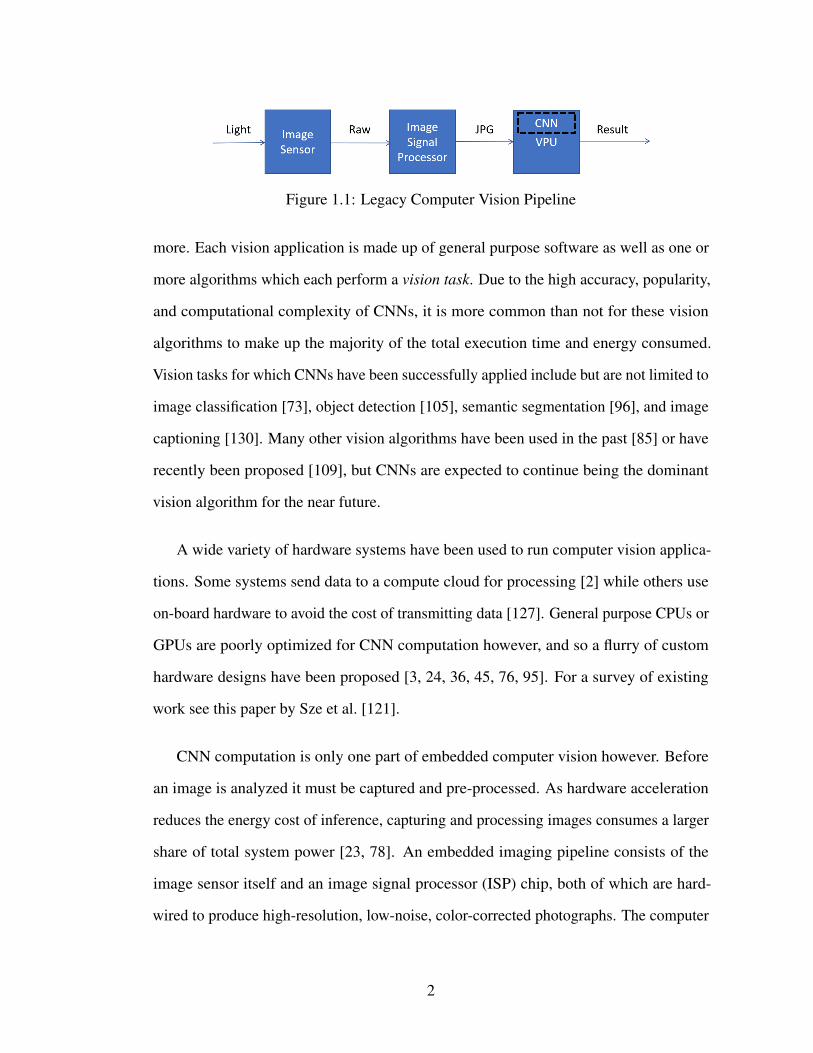
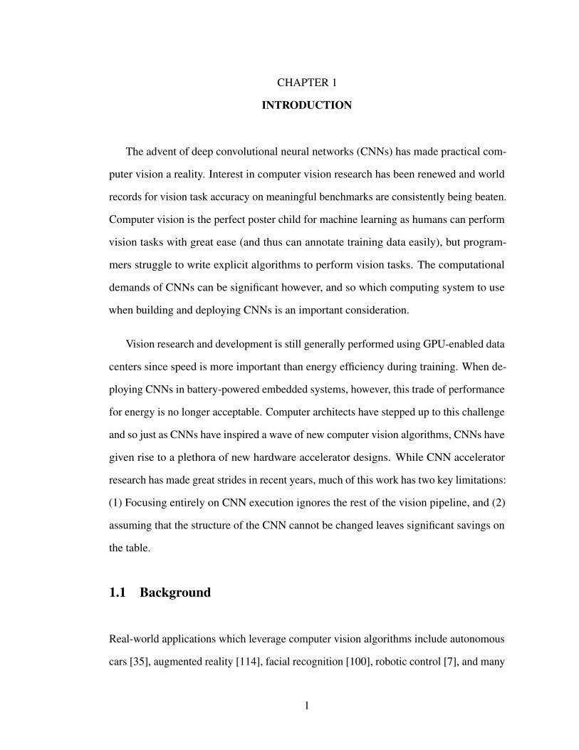
Figure 1.1: Legacy Computer Vision Pipeline
more. Each vision application is made up of general purpose software as well as one or
more algorithms which each perform a vision task. Due to the high accuracy, popularity,
and computational complexity of CNNs, it is more common than not for these vision
algorithms to make up the majority of the total execution time and energy consumed.
Vision tasks for which CNNs have been successfully applied include but are not limited to
image classification [73], object detection [105], semantic segmentation [96], and image
captioning [130]. Many other vision algorithms have been used in the past [85] or have
recently been proposed [109], but CNNs are expected to continue being the dominant
vision algorithm for the near future.
A wide variety of hardware systems have been used to run computer vision applica-
tions. Some systems send data to a compute cloud for processing [2] while others use
on-board hardware to avoid the cost of transmitting data [127]. General purpose CPUs or
GPUs are poorly optimized for CNN computation however, and so a flurry of custom
hardware designs have been proposed [3, 24, 36, 45, 76, 95]. For a survey of existing
work see this paper by Sze et al. [121].
CNN computation is only one part of embedded computer vision however. Before
an image is analyzed it must be captured and pre-processed. As hardware acceleration
reduces the energy cost of inference, capturing and processing images consumes a larger
share of total system power [23, 78]. An embedded imaging pipeline consists of the
image sensor itself and an image signal processor (ISP) chip, both of which are hard-
wired to produce high-resolution, low-noise, color-corrected photographs. The computer
2
vision algorithms of today are trained and tested on these human-readable photographs.
1.1.1 The Imaging Pipeline
Figure 1.1 depicts a traditional imaging pipeline that feeds a vision application, and
Figure 1.2a shows the stages in more detail. The main components are an image sensor,
which reacts to light and produces a RAW image; an image signal processor (ISP) unit,
which transforms, enhances, and compresses the signal to produce a complete image,
usually in JPEG format; and the vision application itself.
ISPs consist of a series of signal processing stages. While the precise makeup of
an ISP pipeline varies, we consider a typical set of stages common to all ISP pipelines:
denoising, demosaicing, color transformations, gamut mapping, tone mapping, and image
compression. This simple pipeline is idealized: modern ISPs can comprise hundreds of
proprietary stages. For example, tone mapping and denoising can use complex, adaptive
operations that are customized for specific camera hardware. In this paper, we consider a
simple form of global tone mapping that performs gamma compression. We also omit
analyses that control the sensor, such as autoexposure and autofocus, and specialized
stages such as burst photography or high dynamic range (HDR) modes. We select these
simple, essential ISP stages because we believe they represent the common functionality
that may impact computer vision.
ISPs for Vision: While most ISPs are fixed-function designs, Vasilyev et al. [126]
propose to use a programmable CGRA architecture to make them more flexible, and other
work has synthesized custom ISPs onto FPGAs [50, 51]. Mainstream cameras, including
smartphones [6], can bypass the ISP to produce RAW images, but the associated impact
on vision is not known. Liu et al. [79] propose an ISP that selectively disables stages
3
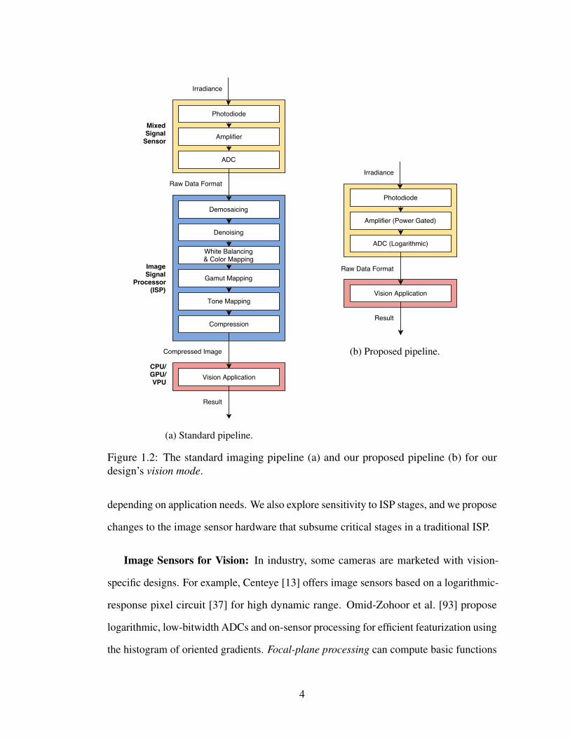
(a) Standard pipeline.
(b) Proposed pipeline.
Figure 1.2: The standard imaging pipeline (a) and our proposed pipeline (b) for ourdesign’s vision mode.
depending on application needs. We also explore sensitivity to ISP stages, and we propose
changes to the image sensor hardware that subsume critical stages in a traditional ISP.
Image Sensors for Vision: In industry, some cameras are marketed with vision-
specific designs. For example, Centeye [13] offers image sensors based on a logarithmic-
response pixel circuit [37] for high dynamic range. Omid-Zohoor et al. [93] propose
logarithmic, low-bitwidth ADCs and on-sensor processing for efficient featurization using
the histogram of oriented gradients. Focal-plane processing can compute basic functions
4
such as edge detection in analog on the sensor [29, 86]. RedEye [76] computes initial
convolutions for a CNN using a custom sensor ADC, and Chen et al. [19] approximate
the first layer optically using angle-sensitive pixels. Event-based vision sensors detect
temporal motion with custom pixels [8, 62]. Chakrabarti [16] proposes to learn novel,
non-Bayer sensor layouts using backpropagation. We focus instead on minimally invasive
changes to existing camera pipelines. To our knowledge, this is the first work to measure
vision applications’ sensitivity to design decisions in a traditional ISP pipeline. Our
proposed pipeline can support both computer vision and traditional photography.
Other work has measured the energy of image sensing: there are potential energy
savings when adjusting a sensor’s frame rate and resolution [78]. Lower-powered image
sensors have been used to decide when to activate traditional cameras and full vision
computations [44].
1.1.2 Camera Sensor
The first step in statically capturing a scene is to convert light into an electronic form.
Both CCD and CMOS image sensors use solid state devices which take advantage of
the photoelectric effect to convert light into voltage. Most modern devices use CMOS
sensors, which use active arrays of photodiodes to convert light to charge, and then to
convert charge to voltage. These pixels are typically the size of a few microns, with
modern mobile image sensors reaching sizes of 1.1 µm, and are configured in arrays
consisting of several megapixels.
CMOS photodiodes have a broadband spectral response in visible light, so they can
only capture monochrome intensity data by themselves. To capture color, sensors add
photodiode-sized filters that allow specific wavelengths of light to pass through. Each
5
photodiode is therefore statically allocated to sense a specific color: typically red, green,
or blue. The layout of these filters is called the mosaic. The most common mosaic is the
Bayer filter [98], which is a 2×2 pattern consisting of two green pixels, one red pixel,
and one blue pixel. The emphasis on green emulates the human visual system, which is
more sensitive to green wavelengths.
During capture, the camera reads out a row of the image sensor where each pixel
voltage is amplified at the column level and then quantized with an ADC. A frame rate
determines the time it takes to read and quantize a complete image. The camera emits a
digital signal referred to as a RAW image, and sends it to the ISP for processing.
1.1.3 Image Signal Processor
Modern mobile devices couple the image sensor with a specialized image signal processor
(ISP) chip, which is responsible for transforming the RAW data to a final, compressed
image—typically, a JPEG file. ISPs consist of a series of signal processing stages that are
designed to make the images more palatable for human vision. While the precise makeup
of an ISP pipeline varies, we describe a typical set of stages found in most designs here.
Denoising. RAW images suffer from three sources of noise: shot noise, due to the
physics of light detection; thermal noise in the pixels, and read noise from the readout
circuitry. The ISP uses a denoising algorithm such as BM3D [30] or NLM [9] to improve
the image’s SNR without blurring important image features such as edges and textures.
Denoising algorithms are typically expensive because they utilize spatial context, and it
is particularly difficult in low-light scenarios.
6
Demosaicing. The next stage compensates for the image sensor’s color filter mosaic. In
the Bayer layout, each pixel in the RAW image contains either red, green, or blue data; in
the output image, each pixel must contain all three channels. The demosaicing algorithm
fills in the missing color channels for each pixel by interpolating values from neighboring
pixels. Simple interpolation algorithms such as nearest-neighbor or averaging lead to
blurry edges and other artifacts, so more advanced demosaicing algorithms use gradient-
based information at each pixel to help preserve sharp edge details.
Color transformations and gamut mapping. A series of color transformation stages
translate the image into a color space that is visually pleasing. These color transformations
are local, per-pixel operations given by a 3×3 matrix multiplication. For a given pixel
p ∈ R3, a linear color transformation is a matrix multiplication:
p′ = Mp (1.1)
where M ∈ R3×3.
The first transformations are color mapping and white balancing. Color mapping
reduces the intensity of the green channel to match that of blue and red and includes
modifications for artistic effect. The white balancing transformation converts the image’s
color temperature to match that of the lighting in the scene. The matrix values for
these transformations are typically chosen specifically by each camera manufacturer for
aesthetic effect.
The next stage is gamut mapping, which converts color values captured outside of a
display’s acceptable color range (but still perceivable to human vision) into acceptable
color values. Gamut mapping, unlike the prior stages, is nonlinear (but still per-pixel).
ISPs may also transform the image into a non-RGB color space, such as YUV or
HSV [98].
7
Tone mapping. The next stage, tone mapping, is a nonlinear, per-pixel function with
multiple responsibilities. It compresses the image’s dynamic range and applies additional
aesthetic effects. Typically, this process results in aesthetically pleasing visual contrast
for an image, making the dark areas brighter while not overexposing or saturating the
bright areas. One type of global tone mapping called gamma compression transforms
the luminance of a pixel p (in YUV space):
p′ = Apγ (1.2)
where A > 0 and 0 < γ < 1. However, most modern ISPs use more computationally
expensive, local tone mapping based on contrast or gradient domain methods to enhance
image quality, specifically for high dynamic range scenes such as outdoors and bright
lighting.
Compression. In addition to reducing storage requirements, compression helps reduce
the amount of data transmitted between chips. In many systems, all three components—
the image sensor, ISP, and application logic—are on physically separate integrated
circuits, so communication requires costly off-chip transmission.
The most common image compression standard is JPEG, which uses the discrete
cosine transform quantization to exploit signal sparsity in the high-frequency space.
Other algorithms, such as JPEG 2000, use the wavelet transform, but the idea is the same:
allocate more stage to low-frequency information and omit high-frequency information
to sacrifice detail for space efficiency. This JPEG algorithm is typically physically
instantiated as a codec that forms a dedicated block of logic on the ISP.
8
1.2 Convolutional Neural Networks
Since the advent of competitive convolutional neural networks for vision, computational
efficiency has been a primary concern. A broad swath of techniques have successfully
decreased the time and space required for CNN inference, such as model compression
and pruning [46, 60], frequency-domain computation [80], and depthwise separable
convolutions [28]. The resulting highly efficient networks are particularly relevant to
industrial deployments of vision, especially in embedded and mobile settings where
energy is a scarce resource.
Error Tolerance in CNNs: Recent work by Diamond et al. [32] studies the impact
of sensor noise and blurring on CNN accuracy and develops strategies to tolerate it. Our
focus is broader: we consider a range of sensor and ISP stages, and we measure both
CNN-based and “classical” computer vision algorithms.
Energy-efficient Deep Learning: Recent research has focused on dedicated ASICs
for deep learning [24, 36, 45, 68, 76, 102] to reduce the cost of forward inference
compared to a GPU or CPU. Our work complements this agenda by focusing on energy
efficiency in the rest of the system: we propose to pair low-power vision implementations
with low-power sensing circuitry.
1.3 Hardware Accelerators for Computer Vision
A significant trend in computer architecture is machine learning accelerators [24, 36,
45, 68, 76, 102]. The excitement over these accelerators is well warranted as the spe-
cific properties of training and testing learned models are better served by these cus-
tom architectures than CPUs or GPUs. Improvements include commercial hardware
9
with customized vector and low-precision instructions [41, 118], ASICs which target
convolutional and fully-connected layers [4, 12, 20, 24, 26, 36, 102], and FPGA de-
signs [97, 115, 120, 135]. Recently, accelerators have focused on extreme quantization
to ternary or binary values [59, 101, 139] or exploiting sparsity in model weights and
activations [3, 45, 95, 134].
1.4 Key Observations and Contributions
This dissertation aims to optimize the entire computer vision pipeline from sensor to
vision result. In this document I expose and then exploit three opportunities for optimizing
embedded vision systems, outlined in the following core contributions.
• Efficient Imaging for Computer Vision: Traditional embedded systems use legacy
imaging pipelines optimized for the needs of humans. When images are captured
exclusively for computers this is wasteful. We propose an alternative pipeline
which saves significant energy while maintaining the same high level of vision task
accuracy.
• Reduced Temporal Redundancy: Vision systems such as self-driving vehicles and
augmented reality headsets process streaming video rather than individual image
frames. We exploit the inherent redundancy between frames of natural video to
save significantly on the cost for vision computation.
• Structured Sparsity in the Frequency Domain: As efficient CNN algorithms have
evolved they have become more reliant on dot products (1×1 convolutions) and
less reliant on traditional spatial convolutions. In this chapter we measure CNN
dot product’s sensitivity to frequency filtering and find that sensitivity varies
significantly between channels. We propose an alternative method for computing
10
dot products which performs per-channel truncated frequency transformation to the
input and then the output. The truncated nature of the transformation reduces total
data volume, saving dot product computation as fewer inputs must be processed
and fewer outputs must be produced.
1.5 Collaborators and Previous Papers
I am thankful to have received concrete help from a variety of collaborators during my
PhD. My first paper focused on optimizing the image capture pipeline and was published
with Suren Jayasuria and Adrian Sampson in ICCV 2017 [11]. While I wrote the entirety
of the code for this project, Suren was crucial to this work as he introduced me to the
basics of the imaging pipeline. My next paper focused on reducing temporal redundancy
in computer vision, and was published with Phil Bedoukian, Suren Jayasuria, and Adrian
Sampson in ISCA 2018 [10]. I completed all of the algorithmic development, network
training, and dataset management for this project. Phil wrote the entirety of the RTL
necessary for our hardware evaluation, managed our synthesis pipeline, and performed
post-layout simulations. The third project focuses on structured sparsity in the frequency
domain and is yet to be published. I conducted the majority of the experiments related to
algorithm design and I developed the core algorithm proposed in this chapter, specifically
the concept of structured sparsity in the frequency domain. Neil Adit has conducted
a variety of experiments including feature correlation in the frequency domain, sparse
library speed, and speedup experiments in PyTorch. Yuwei Hu recently joined the project
and has spent his time working on implementing the structured sparsity computation
methodology both in PyTorch and TVM. Chris De Sa has been consulted throughout the
project and has provided machine learning guidance.
11
CHAPTER 2
EFFICIENT IMAGING FOR COMPUTER VISION
Advancements in deep learning have ignited an explosion of research on efficient
hardware for embedded computer vision. Hardware vision acceleration, however, does
not address the cost of capturing and processing the image data that feeds these algorithms.
We examine the computer vision impact of the image sensor and image signal processor
(ISP) (shown in Figure 2.1) to identify opportunities for energy savings. The key insight
is that imaging pipelines should be be configurable: to switch between a traditional
photography mode and a low-power vision mode that produces lower-quality image
data suitable only for computer vision. We use eight computer vision algorithms and
a reversible pipeline simulation tool to study the imaging system’s impact on vision
performance. For both CNN-based and classical vision algorithms, we observe that only
two ISP stages, demosaicing and gamma compression, are critical for task performance.
We propose a new image sensor design that can compensate for these stages. The sensor
design features an adjustable resolution and tunable analog-to-digital converters (ADCs).
Our proposed imaging system’s vision mode disables the ISP entirely and configures the
sensor to produce subsampled, lower-precision image data. This vision mode can save
∼75% of the average energy of a baseline photography mode with only a small impact
on vision task accuracy.
The deep learning revolution has accelerated progress in a plethora of computer
vision tasks. To bring these vision capabilities within the battery budget of a smartphone,
Figure 2.1: Focusing on the Sensor and ISP
12
a wave of recent work has designed custom hardware for inference in deep neural
networks [36, 45, 76]. This work, however, only addresses part of the whole cost:
embedded vision involves the entire imaging pipeline, from photons to task result. As
hardware acceleration reduces the energy cost of inference, the cost to capture and
process images will consume a larger share of total system power [23, 78].
We study the potential for co-design between camera systems and vision algorithms
to improve their end-to-end efficiency. Existing imaging pipelines are designed for
photography: they produce high-quality images for human consumption. An imaging
pipeline consists of the image sensor itself and an image signal processor (ISP) chip,
both of which are hard-wired to produce high-resolution, low-noise, color-corrected
photographs. Modern computer vision algorithms, however, do not require the same
level of quality that humans do. Our key observation is that mainstream, photography-
oriented imaging hardware wastes time and energy to provide quality that computer
vision algorithms do not need.
We propose to make imaging pipelines configurable. The pipeline should support
both a traditional photography mode and an additional, low-power vision mode. In vision
mode, the sensor can save energy by producing lower-resolution, lower-precision image
data, and the ISP can skip stages or disable itself altogether. We examine the potential
for a vision mode in imaging systems by measuring its impact on the hardware efficiency
and vision accuracy. We study vision algorithms’ sensitivity to sensor parameters and
to individual ISP stages, and we use the results to propose an end-to-end design for an
imaging pipeline’s vision mode.
Contributions: This chapter proposes a set of modifications to a traditional camera
sensor to support a vision mode. The design uses variable-accuracy analog-to-digital
converters (ADCs) to reduce the cost of pixel capture and power-gated selective readout
13
to adjust sensor resolution. The sensor’s subsampling and quantization hardware approxi-
mates the effects of two traditional ISP stages, demosaicing and gamma compression.
With this augmented sensor, we propose to disable the ISP altogether in vision mode.
We also describe a methodology for studying the imaging system’s role in computer
vision performance. We have developed a tool that simulates a configurable imaging
pipeline and its inverse to convert plain images to approximate raw signals. This tool
is critical for generating training data for learning-based vision algorithms that need
examples of images produced by a hypothetical imaging pipeline. Section 2.0.1 describes
the open-source simulation infrastructure.
We use our methodology to examine eight vision applications, including classical
algorithms for stereo, optical flow, and structure-from-motion; and convolutional neural
networks (CNNs) for object recognition and detection. For these applications, we find
that:
• Most traditional ISP stages are unnecessary when targeting computer vision. For
all but one application we tested, only two stages had significant effects on vision
accuracy: demosaicing and gamma compression.
• Our image sensor can approximate the effects of demosaicing and gamma com-
pression in the mixed-signal domain. Using these in-sensor techniques eliminates
the need for a separate ISP for most vision applications.
• Our image sensor can reduce its bitwidth from 12 to 5 by replacing linear ADC
quantization with logarithmic quantization while maintaining the same level of
task performance.
Altogether, the proposed vision mode can use roughly a quarter of the imaging-pipeline
energy of a traditional photography mode without significantly affecting the performance
14
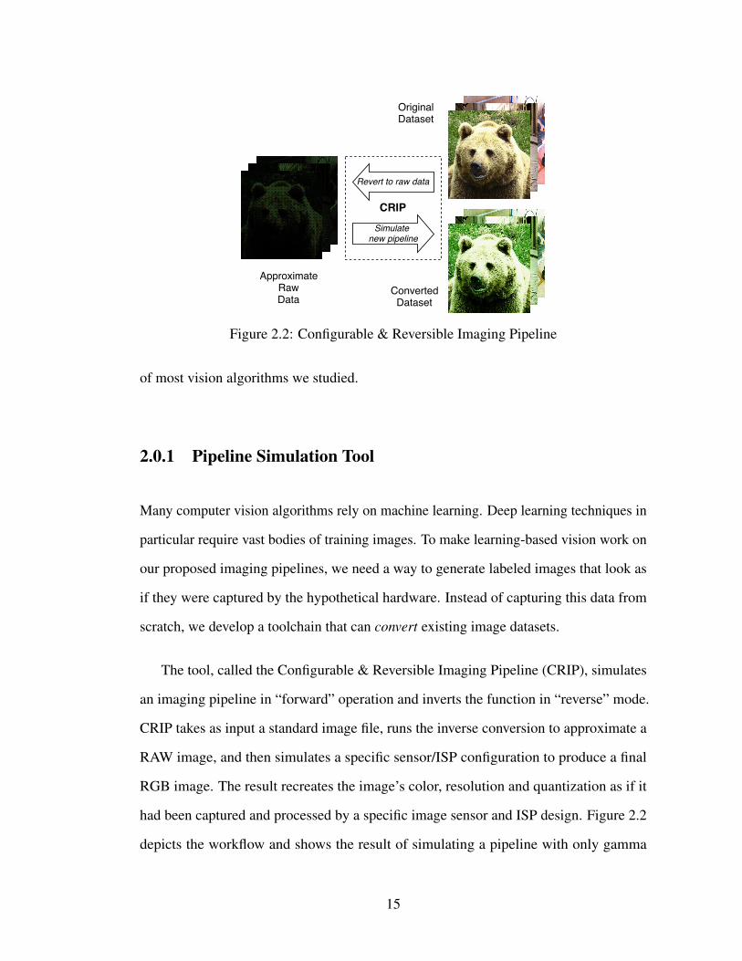
Figure 2.2: Configurable & Reversible Imaging Pipeline
of most vision algorithms we studied.
2.0.1 Pipeline Simulation Tool
Many computer vision algorithms rely on machine learning. Deep learning techniques in
particular require vast bodies of training images. To make learning-based vision work on
our proposed imaging pipelines, we need a way to generate labeled images that look as
if they were captured by the hypothetical hardware. Instead of capturing this data from
scratch, we develop a toolchain that can convert existing image datasets.
The tool, called the Configurable & Reversible Imaging Pipeline (CRIP), simulates
an imaging pipeline in “forward” operation and inverts the function in “reverse” mode.
CRIP takes as input a standard image file, runs the inverse conversion to approximate a
RAW image, and then simulates a specific sensor/ISP configuration to produce a final
RGB image. The result recreates the image’s color, resolution and quantization as if it
had been captured and processed by a specific image sensor and ISP design. Figure 2.2
depicts the workflow and shows the result of simulating a pipeline with only gamma
15
compression and demosaicing. Skipping color transformations leads to a green hue in
the output.
The inverse conversion uses an implementation of Kim et al.’s reversible ISP
model [71] augmented with new stages for reverse denoising and demosaicing as well
as re-quantization. To restore noise to a denoised image, we use Chehdi et al.’s sensor
noise model [124]. To reverse the demosaicing process, we remove channel data from
the image according to the Bayer filter. The resulting RAW image approximates the
unprocessed output of a camera sensor, but some aspects cannot be reversed: namely,
sensors typically digitize 12 bits per pixel, but ordinary 8-bit images have lost this detail
after compression. For this reason, we only report results for quantization levels with 8
bits or fewer.
CRIP implements the reverse stages from Kim et al. [71], so its model linearization
error is the same as in that work: namely, less than 1%. To quantify CRIP’s error when
reconstructing RAW images, we used it to convert a Macbeth color chart photograph and
compared the result with its original RAW version. The average pixel error was 1.064%
and the PSNR was 28.81 dB. Qualitatively, our tool produces simulated RAW images
that are visually indistinguishable from their real RAW counterparts.
CRIP’s reverse pipeline implementation can use any camera model specified by Kim
et al. [71], but for consistency, this work uses the Nikon D7000 pipeline. We have
implemented the entire tool in the domain-specific language Halide [99] for speed. For
example, CRIP can convert the entire CIFAR-10 dataset [72] in one hour on an 8-core
machine. CRIP is available as open source: https://github.com/cucapra/
approx-vision
16
Algorithm Dataset Vision Task
3 Deep LeNet [74] CIFAR-10 [72]
Obj.Classification
20 Deep ResNet [48] CIFAR-10 Obj.Classification
44 Deep ResNet [48] CIFAR-10 Obj.Classification
Faster R-CNN [105] VOC-2007 [39]
Object Detection
OpenFace [5] CASIA [132]and LFW [57]
FaceIdentification
OpenCVFarneback [63]
Middlebury [113]Optical Flow
OpenCV SGBM [63] Middlebury Stereo Matching
OpenMVG SfM [89] Strecha [119] Structure fromMotion
Table 2.1: Vision applications used in our evaluation.
2.0.2 Benchmarks
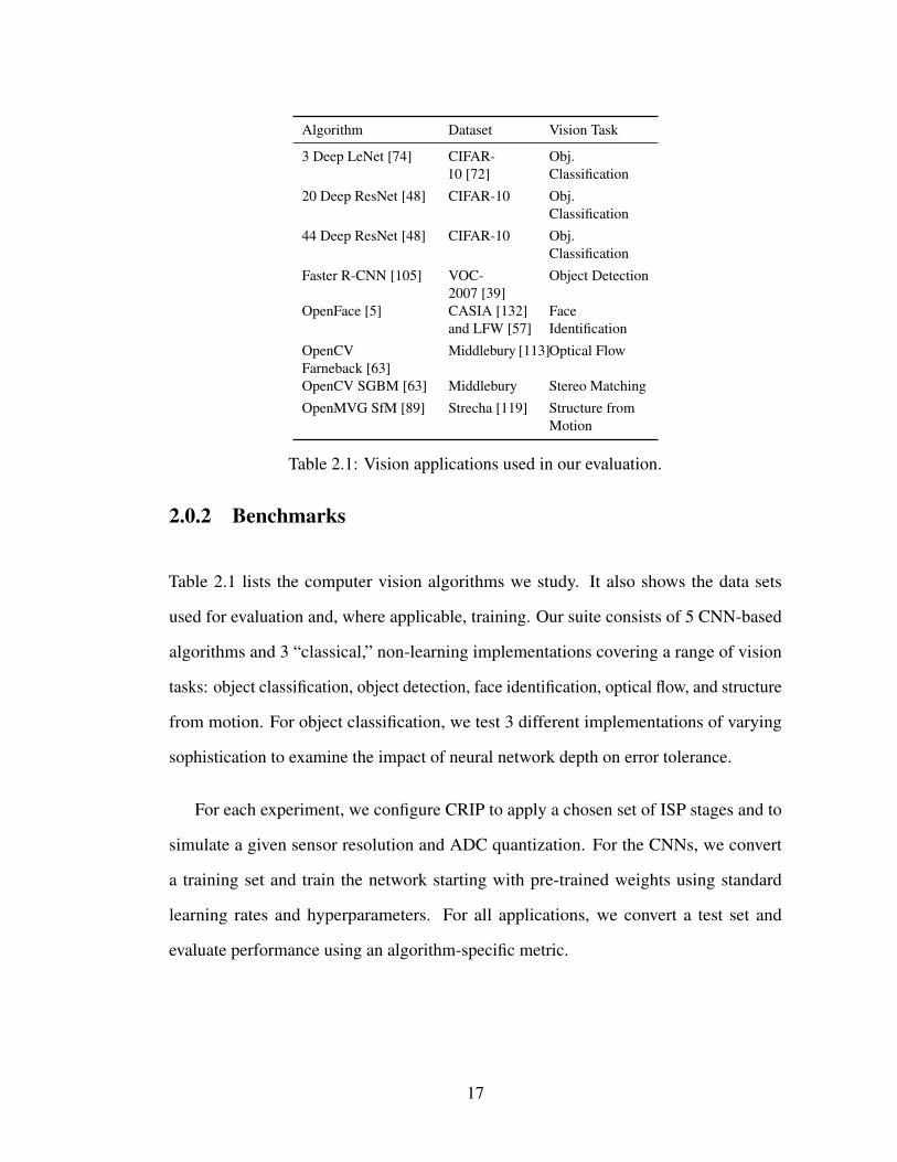
Table 2.1 lists the computer vision algorithms we study. It also shows the data sets
used for evaluation and, where applicable, training. Our suite consists of 5 CNN-based
algorithms and 3 “classical,” non-learning implementations covering a range of vision
tasks: object classification, object detection, face identification, optical flow, and structure
from motion. For object classification, we test 3 different implementations of varying
sophistication to examine the impact of neural network depth on error tolerance.
For each experiment, we configure CRIP to apply a chosen set of ISP stages and to
simulate a given sensor resolution and ADC quantization. For the CNNs, we convert
a training set and train the network starting with pre-trained weights using standard
learning rates and hyperparameters. For all applications, we convert a test set and
evaluate performance using an algorithm-specific metric.
17
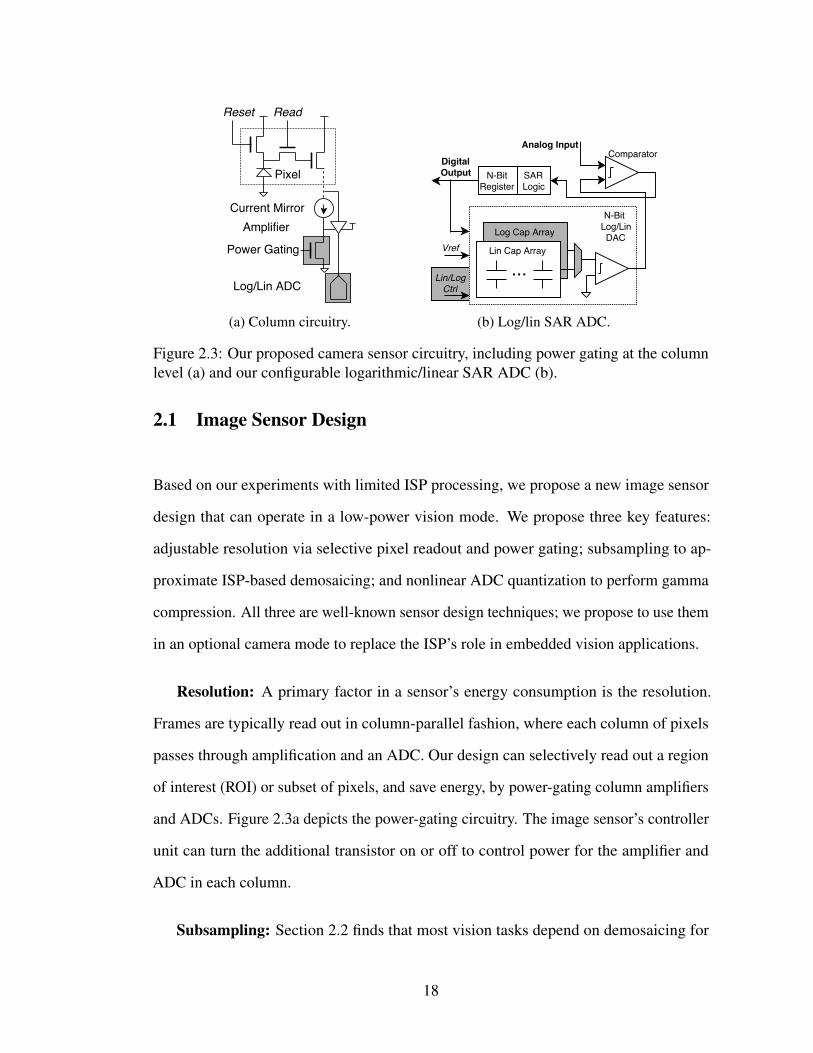
(a) Column circuitry. (b) Log/lin SAR ADC.
Figure 2.3: Our proposed camera sensor circuitry, including power gating at the columnlevel (a) and our configurable logarithmic/linear SAR ADC (b).
2.1 Image Sensor Design
Based on our experiments with limited ISP processing, we propose a new image sensor
design that can operate in a low-power vision mode. We propose three key features:
adjustable resolution via selective pixel readout and power gating; subsampling to ap-
proximate ISP-based demosaicing; and nonlinear ADC quantization to perform gamma
compression. All three are well-known sensor design techniques; we propose to use them
in an optional camera mode to replace the ISP’s role in embedded vision applications.
Resolution: A primary factor in a sensor’s energy consumption is the resolution.
Frames are typically read out in column-parallel fashion, where each column of pixels
passes through amplification and an ADC. Our design can selectively read out a region
of interest (ROI) or subset of pixels, and save energy, by power-gating column amplifiers
and ADCs. Figure 2.3a depicts the power-gating circuitry. The image sensor’s controller
unit can turn the additional transistor on or off to control power for the amplifier and
ADC in each column.
Subsampling: Section 2.2 finds that most vision tasks depend on demosaicing for
18
good accuracy. There are many possible demosaicing techniques, but they are typically
costly algorithms optimized for perceived image quality. We hypothesize that, for vision
algorithms, the nuances of advanced demosaicing techniques are less important than the
image format: raw images exhibit the Bayer pattern, while demosaiced images use a
standard RGB format.
We propose to modify the image sensor to achieve the same format-change effect
as demosaicing without any signal processing. Specifically, our camera’s vision mode
subsamples the raw image to collapse each 2×2 block of Bayer-pattern pixels into a
single RGB pixel. Each such block contains one red pixel, two green pixels, and one blue
pixel; our technique drops one green pixel and combines it with the remaining values
to form the three output channels. The design power-gates one of the two green pixels
interprets resulting red, green, and blue values as a single pixel.
Nonlinear Quantization: In each sensor column, an analog-to-digital (ADC) con-
verter is responsible for quantizing the analog output of the amplifier to a digital repre-
sentation. A typical linear ADC’s energy cost is exponential in the number of bits in its
output: an 12-bit ADC costs roughly twice as much energy as a 11-bit ADC. There is an
opportunity to drastically reduce the cost of image capture by reducing the number of
bits.
As with resolution, ADC quantization is typically fixed at design time. We propose
to make the number of bits configurable for a given imaging mode. Our proposed image
sensor uses successive-approximation (SAR) ADCs, which support a variable bit depth
controlled by a clock and control signal [125].
ADC design can also provide a second opportunity: to change the distribution of
quantization levels. Nonlinear quantization can be better for representing images because
19
their light intensities are not uniformly distributed: the probability distribution function
for intensities in natural images is log-normal [106]. To preserve more information
about the analog signal, SAR ADCs can use quantization levels that map the intensities
uniformly among digital values. (See the supplementary material for a more complete
discussion of intensity distributions.) We propose an ADC that uses logarithmic quanti-
zation in vision mode. Figure 2.3b shows the ADC design, which can switch between
linear quantization levels for photography mode and logarithmic quantization for vision
mode. The design uses a separate capacitor bank for each quantization scheme.
Logarithmic quantization lets the camera capture the same amount of image infor-
mation using fewer bits, which is the same goal usually accomplished by the gamma
compression stage in the ISP. Therefore, we eliminate the need for a separate ISP block
to perform gamma compression.
System Considerations: Our proposed vision mode controls three sensor parameters:
it enables subsampling to produce RGB images; it allows reduced-resolution readout;
and it enables a lower-precision logarithmic ADC configuration. The data is sent off-chip
directly to the application on the CPU, the GPU, or dedicated vision hardware without
being compressed. This mode assumes that the vision task is running in real time, so the
image does not need to be saved.
In the traditional photography mode, we configure the ADCs to be at high precision
with linear quantization levels. Then the image is sent to the separate ISP chip to perform
all the processing needed to generate high quality images. These images are compressed
using the JPEG codec on-chip and stored in memory for access by the application
processor.
20
2.2 Sensitivity to ISP Stages
We next present an empirical analysis of our benchmark suite’s sensitivity to stages
in the ISP. The goal is to measure, for each algorithm, the relative difference in task
performance between running on the original image data and running on data converted
by CRIP.
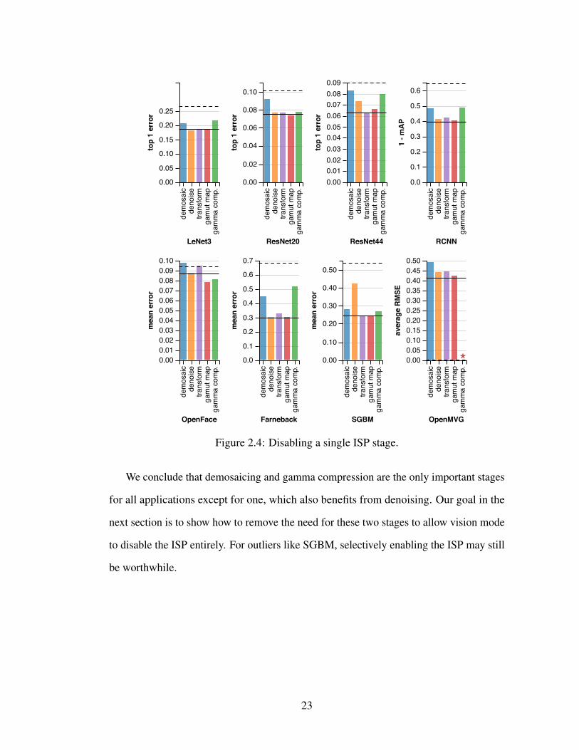
Individual Stages: First, we examine the sensitivity to each ISP stage in isolation.
Testing the exponential space of all possible stage combinations is intractable, so we start
with two sets of experiments: one that disables a single ISP stage and leaves the rest of
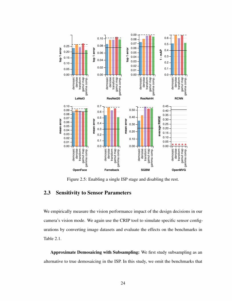
the pipeline intact (Figure 2.4); and one that enables a single ISP stage and disables the
rest (Figure 2.5).
In these experiments, gamut mapping and color transformations have a minimal
effect on all benchmarks. The largest effects are on ResNet44, where classification error
increases from 6.3% in the baseline to 6.6% without gamut mapping, and OpenMVG,
where removing the color transform stage increases RMSE from 0.408 to 0.445. This
finding confirms that features for vision are not highly sensitive to color.
There is a strong sensitivity, in contrast, to gamma compression and demosaicing.
The OpenMVG Structure from Motion (SfM) implementation fails entirely when gamma
compression is disabled: it was unable to find sufficient features using either of its
feature extractors, SIFT and AKAZE. Meanwhile, removing demosaicing worsens the
error for Farneback optical flow by nearly half, from 0.227 to 0.448. Both of these
classical (non-CNN) algorithms use hand-tuned feature extractors, which do not take the
Bayer pattern into account. The CIFAR-10 benchmarks (LeNet3, ResNet20, ResNet44)
use low-resolution data (32×32), which is disproportionately affected by the removal
of color channels in mosaiced data. While gamma-compressed data follows a normal
21
distribution, removing gamma compression reverts the intensity scale to its natural log-
normal distribution, which makes features more difficult to detect for both classical
algorithms and CNNs.
Unlike the other applications, Stereo SGBM is sensitive to noise. Adding sensor
noise increases its mean error from 0.245 to 0.425, an increase of over 70%. Also unlike
other applications, OpenFace counter-intuitively performs better than the baseline when
the simulated pipeline omits gamut mapping or gamma compression. OpenFace’s error
is 8.65% on the original data and 7.9% and 8.13%, respectively, when skipping those
stages. We attribute the difference to randomness inherent in the training process. Across
10 training runs, OpenFace’s baseline error rate varied from 8.22% to 10.35% with a
standard deviation of 0.57%.
In Figures 2.4 and 2.5 you can see the impact on vision accuracy when adding and
removing stages from the standard ISP pipeline. The solid line shows the baseline error
with all ISP stages enabled, and the dotted line shows the error when all ISP stages are
disabled. Asterisks denote aborted runs where no useful output was produced.
Minimal Pipelines: Based on these results, we study the effect of combining the
most important stages: demosaicing, gamma compression, and denoising. Figure 2.6
shows two configurations that enable only the first two and all three of these stages.
Accuracy for the minimal pipeline with only demosaicing and gamma compression
is similar to accuracy on the original data. The largest impact, excluding SGBM, is
ResNet44, whose top-1 error increases only from 6.3% to 7.2%. Stereo SGBM, however,
is noise sensitive: without denoising, its mean error is 0.33; with denoising, its error
returns to its baseline of 0.25. Overall, the CNNs are able to rely on retraining themselves
to adapt to changes in the capture pipeline, while classical benchmarks are less flexible
and can depend on specific ISP stages.
22
��������
�������
���������
�����
����
�����������
������
������������������������
���������
��������
�������
���������
�����
����
�����������
��������
����
����
����
����
����
����
���������
��������
�������
���������
�����
����
�����������
��������
����������������������������������������
���������
��������
�������
���������
�����
����
�����������
����
���
���
���
���
���
���
���
���
��
��������
�������
���������
�����
����
�����������
��������
��������������������������������������������
���������
��������
�������
���������
�����
����
�����������
���������
������������������������
���������
��������
�������
���������
�����
����
�����������
����
����
����
����
����
����
����
���������
��������
�������
���������
�����
����
�����������
�������
��������������������������������������������
���������
��
�
Figure 2.4: Disabling a single ISP stage.
We conclude that demosaicing and gamma compression are the only important stages
for all applications except for one, which also benefits from denoising. Our goal in the
next section is to show how to remove the need for these two stages to allow vision mode
to disable the ISP entirely. For outliers like SGBM, selectively enabling the ISP may still
be worthwhile.
23
��������
�������
���������
�����
����
�����������
������
������������������������
���������
��������
�������
���������
�����
����
�����������
��������
����
����
����
����
����
����
���������
��������
�������
���������
�����
����
�����������
��������
����������������������������������������
���������
��������
�������
���������
�����
����
�����������
����
���
���
���
���
���
���
���
���
��
��������
�������
���������
�����
����
�����������
��������
��������������������������������������������
���������
��������
�������
���������
�����
����
�����������
���������
������������������������
���������
��������
�������
���������
�����
����
�����������
����
����
����
����
����
����
����
���������
��������
�������
���������
�����
����
�����������
�������
����������������������������������������
���������
��
�����
Figure 2.5: Enabling a single ISP stage and disabling the rest.
2.3 Sensitivity to Sensor Parameters
We empirically measure the vision performance impact of the design decisions in our
camera’s vision mode. We again use the CRIP tool to simulate specific sensor config-
urations by converting image datasets and evaluate the effects on the benchmarks in
Table 2.1.
Approximate Demosaicing with Subsampling: We first study subsampling as an
alternative to true demosaicing in the ISP. In this study, we omit the benchmarks that
24
����� ���������� �������� ��� ���������������������������������������������
���������������
�����������������������������������������������������������������
*
Figure 2.6: Each algorithm’s vision error, normalized to the original error on plain images,for two minimal ISP pipelines. The demos+g.c. pipeline only enables demosaicing andgamma compression; the +denoise bars also add denoising. The all off column shows aconfiguration with all stages disabled for reference.
�������� ������������������������������������
���������������
�������������������������������������������
Figure 2.7: Demosaicing on the ISP vs. subsampling in the sensor. Error values arenormalized to performance on unmodified image data.
work on CIFAR-10 images [72] because their resolution, 32×32, is unrealistically small
for a sensor, so subsampling beyond this size is not meaningful. Figure 2.11 compares
data for “true” demosaicing, where CRIP has not reversed that stage, to a version that
simulates our subsampling instead. Replacing demosaicing with subsampling leads to a
small increase in vision error. Farneback optical flow sees the largest error increase, from
0.332 to 0.375.
25
Quantization: Next, we study the impact of signal quantization in the sensor’s
ADCs. There are two parameters: the number of bits and the level distribution (linear or
logarithmic). Figure 2.14 shows our vision applications’ sensitivity to both bitwidth and
distribution. Both sweeps use an ISP pipeline with demosiacing but without gamma com-
pression to demonstrate that the logarithmic ADC, like gamma compression, compresses
the data distribution.
The logarithmic ADC yields higher accuracy on all benchmarks than the linear ADC
with the same bitwidth. Farneback optical flow’s sensitivity is particularly dramatic:
using a linear ADC, its mean error is 0.54 and 0.65 for 8 and 2 bits, respectively; while
with a logarithmic ADC, the error drops to 0.33 and 0.38.
Switching to a logarithmic ADC also increases the applications’ tolerance to smaller
bitwidths. All applications exhibit minimal error increases down to 5 bits, and some can
even tolerate 4- or 3-bit quantization. OpenMVG’s average RMSE only increases from
0.454 to 0.474 when reducing 8 bit logarithmic sampling to 5 bits, and ResNet20’s top-1
error increases from 8.2% to 8.42%. To fit all of these applications, we propose a 5-bit
logarithmic ADC design in vision mode.
Resolution: We next measure the impact of resolution adjustment using column
power gating. Modern image sensors use multi-megapixel resolutions, while the input
dimensions for most convolutional neural networks are often 256×256 or smaller. While
changing the input dimensions of the network itself may also be an option, we focus here
on downsampling images to match the network’s published input size.
To test the downsampling technique, we concocted a new higher-resolution dataset
by selecting a subset of ImageNet [31] which contains the CIFAR-10 [72] object classes
(∼15,000 images). These images are higher resolution than the input resolution of
26
12345678
bits
0.0
0.5
1.0
1.5
2.0
2.5
3.0
3.5
4.0
normalizederror
(a) Linear quantization.
������������
���
���
���
���
���
���
���
���
��������������
������������������������������������������������������
(b) Logarithmic quantization.
Figure 2.8: Effect of quantization on vision accuracy in a pipeline with only demosaicingenabled.
networks trained on CIFAR-10, so they let us experiment with image downsampling.
We divide the new dataset into training and testing datasets using an 80–20 balance
and train the LeNet, ResNet20, and ResNet44 networks from pre-trained weights. For
each experiment, we first downsample the images to simulate sensor power gating.
Then, after demosaicing, we scale down the images the rest of the way to 32×32 using
OpenCV’s edge-aware scaling [63]. Without any subsampling, LeNet achieves 39.6%
error, ResNet20 26.34%, and ResNet44 24.50%. We then simulated downsampling at
ratios of 1⁄4, 1⁄16, and 1⁄64 resolution. Downsampling does increase vision error, but the
effect is small: the drop in accuracy from full resolution to 1⁄4 resolution is approximately
1% (LeNet 40.9%, ResNet20 27.71%, ResNet44 26.5%). Full results are included in our
ICCV paper’s supplemental material [11].
27
2.4 Quantifying Power Savings
Here we estimate the potential power efficiency benefits of our proposed vision mode as
compared to a traditional photography-oriented imaging pipeline. Our analysis covers
the sensor’s analog-to-digital conversion, the sensor resolution, and the ISP chip.
Image Sensor ADCs: Roughly half of a camera sensor’s power budget goes to
readout, which is dominated by the cost of analog-to-digital converters (ADCs) [15].
While traditional sensors use 12-bit linear ADCs, our proposal uses a 5-bit logarithmic
ADC.
To compute the expected value of the energy required for each ADC’s readout, we
quantify the probability and energy cost of each digital level that the ADC can detect.
The expected value for a single readout is:
E [ADC energy] =2n
∑m=1
pmem
where n is the number of bits, 2n is the total number of levels, m is the level index, pm is
the probability of level m occuring, and em is the energy cost of running the ADC at level
m.
To find pm for each level, we measure the distribution of values from images in the
CIFAR-10 dataset [72] in raw data form converted by CRIP (Section 2.0.1). To find
a relative measure for em, we simulate the operation of the successive approximation
register (SAR) ADC in charging and discharging the capacitors in its bank. This capacitor
simulation is a simple first-order model of a SAR ADC’s power that ignores fixed
overheads such as control logic.
In our simulations, the 5-bit logarithmic ADC uses 99.95% less energy than the
baseline 12-bit linear ADC. As the ADCs in an image sensor account for 50% of the
28
energy budget [15], this means that the cheaper ADCs save approximately half of the
sensor’s energy cost.
Image Sensor Resolution: An image sensor’s readout, I/O, and pixel array together
make up roughly 95% of its power cost [15]. These costs are linearly related to the
sensor’s total resolution. As Section 2.1 describes, our proposed image sensor uses
selective readout circuitry to power off the pixel, amplifier, and ADC for subsets of the
sensor array. The lower-resolution results can be appropriate for vision algorithms that
have low-resolution inputs (Section 2.3). Adjusting the proposed sensor’s resolution
parameter therefore reduces the bulk of its power linearly with the pixel count.
ISP: While total power consumption numbers are available for commercial and
research ISP designs, we are unaware of a published breakdown of power consumed per
stage. To approximate the relative cost for each stage, we measured software implemen-
tations of each using OpenCV 2.4.8 [63] and profile them when processing a 4288×2848
image on an Intel Ivy Bridge i7-3770K CPU. We report the number of dynamic instruc-
tions executed, the CPU cycle count, the number of floating-point operations, and the L1
data cache references in a table in our supplementary material.
While this software implementation does not directly reflect hardware costs in a real
ISP, we can draw general conclusions about relative costs. The denoising stage is by
far the most expensive, requiring more than two orders of magnitude more dynamic
instructions. Denoising—here, non-local means [9]—involves irregular and non-local
references to surrounding pixels. JPEG compression is also expensive; it uses a costly
discrete cosine transform for each macroblock.
Section 2.2 finds that most stages of the ISP are unnecessary in vision mode, and Sec-
tion 2.1 demonstrates how two remaining stages—gamma compression and demosaicing—
29
can be approximated using in-sensor techniques. The JPEG compression stage is also
unnecessary in computer vision mode: because images do not need to be stored, they do
not need to be compressed for efficiency. Therefore, the pipeline can fully bypass the ISP
when in vision mode. Power-gating the integrated circuit would save all of the energy
needed to run it.
Total Power Savings: The two components of an imaging pipeline, the sensor and
the ISP, have comparable total power costs. For sensors, typical power costs range from
137.1 mW for a security camera to 338.6 mW for a mobile device camera [78]. Industry
ISPs can range from 130 mW to 185 mW when processing 1.2 MP at 45 fps [94], while
Hegarty et al. [50] simulated an automatically synthesized ISP which consumes 250 mW
when processing 1080p video at 60 fps. This power consumption is comparable to recent
CNN ASICs such as TrueNorth at 204 mW [38] and EIE at 590 mW [45].
In vision mode, the proposed image sensor uses half as much energy as a traditional
sensor by switching to a 5-bit logarithmic ADC. The ISP can be disabled entirely. Because
the two components contribute roughly equal parts to the pipeline’s power, the entire
vision mode saves around 75% of a traditional pipeline’s energy. If resolution can be
reduced, energy savings can be higher.
This first-order energy analysis does not include overheads for power gating, addi-
tional muxing, or off-chip communication. We plan to measure complete implementations
in future work.
30
2.5 Discussion
We advocate for adding a vision mode to the imaging pipelines in mobile devices. We
show that design choices in the sensor’s circuitry can obviate the need for an ISP when
supplying a computer vision algorithm.
This work uses an empirical approach to validate our design for a vision-mode
imaging pipeline. This limits our conclusions to pertain to specific algorithms and specific
datasets. Follow-on work should take a theoretical approach to model the statistical effect
of each ISP stage. Future work should also complete a detailed hardware design for the
proposed sensor modifications. This work uses a first-order energy evaluation that does
not quantify overheads; a full design would contend with the area costs of additional
components and the need to preserve pixel pitch in the column architecture. Finally, the
proposed vision mode consists of conservative changes to a traditional camera design
and no changes to vision algorithms themselves. This basic framework suggests future
work on deeper co-design between camera systems and computer vision algorithms.
By modifying the abstraction boundary between hardware and software, co-designed
systems can make sophisticated vision feasible in energy-limited mobile devices.
2.6 Proposed Pipelines
We described two potential simplified ISP pipelines including only the stages that are
essential for all algorithms we studied: demosaicing, gamma compression, and denoising.
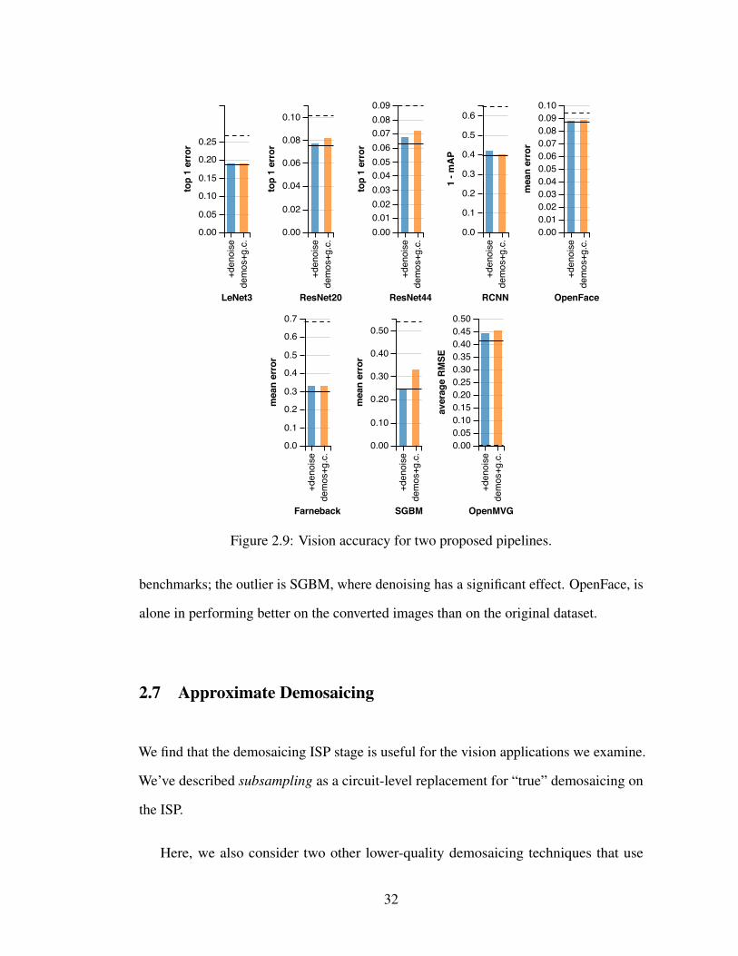
Normalized data was shown to make more efficient use of space, but here in Figure 2.9
we show the absolute error for each benchmark. As depicted before, the pipeline with
just demosaicing and gamma compression performs close to the baseline for most
31
�������
�����������
������
������������������������
���������
�������
�����������
��������
����
����
����
����
����
����
���������
�������
�����������
��������
����������������������������������������
���������
�������
�����������
����
���
���
���
���
���
���
���
���
��
�������
�����������
��������
��������������������������������������������
���������
�������
�����������
���������
������������������������
���������
�������
�����������
����
����
����
����
����
����
����
���������
�������
�����������
�������
��������������������������������������������
���������
��
Figure 2.9: Vision accuracy for two proposed pipelines.
benchmarks; the outlier is SGBM, where denoising has a significant effect. OpenFace, is
alone in performing better on the converted images than on the original dataset.
2.7 Approximate Demosaicing
We find that the demosaicing ISP stage is useful for the vision applications we examine.
We’ve described subsampling as a circuit-level replacement for “true” demosaicing on
the ISP.
Here, we also consider two other lower-quality demosaicing techniques that use
32
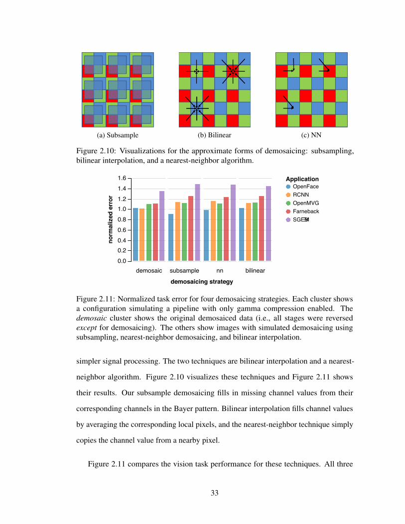
(a) Subsample (b) Bilinear (c) NN
Figure 2.10: Visualizations for the approximate forms of demosaicing: subsampling,bilinear interpolation, and a nearest-neighbor algorithm.
�������� ��������� �� ����������������������������
���������������������������
���������������
�������������������������������������������
Figure 2.11: Normalized task error for four demosaicing strategies. Each cluster showsa configuration simulating a pipeline with only gamma compression enabled. Thedemosaic cluster shows the original demosaiced data (i.e., all stages were reversedexcept for demosaicing). The others show images with simulated demosaicing usingsubsampling, nearest-neighbor demosaicing, and bilinear interpolation.
simpler signal processing. The two techniques are bilinear interpolation and a nearest-
neighbor algorithm. Figure 2.10 visualizes these techniques and Figure 2.11 shows
their results. Our subsample demosaicing fills in missing channel values from their
corresponding channels in the Bayer pattern. Bilinear interpolation fills channel values
by averaging the corresponding local pixels, and the nearest-neighbor technique simply
copies the channel value from a nearby pixel.
Figure 2.11 compares the vision task performance for these techniques. All three
33
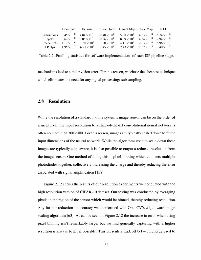
Demosaic Denoise Color Tform Gamut Map Tone Map JPEG
Instructions 3.45×10⁸ 4.84×10¹¹ 2.40×10⁸ 5.38×10⁸ 4.63×10⁸ 6.74×10⁸
Cycles 3.62×10⁸ 3.06×10¹¹ 2.26×10⁸ 8.09×10⁸ 4.84×10⁸ 2.94×10⁸
Cache Refs 4.17×10⁶ 1.60×10⁸ 1.80×10⁶ 4.11×10⁶ 2.63×10⁶ 6.96×10⁵
FP Ops 1.95×10⁵ 6.77×10⁸ 1.45×10⁵ 2.43×10⁵ 1.52×10⁵ 9.40×10³
Table 2.2: Profiling statistics for software implementations of each ISP pipeline stage.
mechanisms lead to similar vision error. For this reason, we chose the cheapest technique,
which eliminates the need for any signal processing: subsampling.
2.8 Resolution
While the resolution of a standard mobile system’s image sensor can be on the order of
a megapixel, the input resolution to a state-of-the-art convolutional neural network is
often no more than 300×300. For this reason, images are typically scaled down to fit the
input dimensions of the neural network. While the algorithms used to scale down these
images are typically edge aware, it is also possible to output a reduced resolution from
the image sensor. One method of doing this is pixel-binning which connects multiple
photodiodes together, collectively increasing the charge and thereby reducing the error
associated with signal amplification [138].
Figure 2.12 shows the results of our resolution experiments we conducted with the
high resolution version of CIFAR-10 dataset. Our testing was conducted by averaging
pixels in the region of the sensor which would be binned, thereby reducing resolution.
Any further reduction in accuracy was performed with OpenCV’s edge aware image
scaling algorithm [63]. As can be seen in Figure 2.12 the increase in error when using
pixel binning isn’t remarkably large, but we find generally capturing with a higher
resultion is always better if possible. This presents a tradeoff between energy used to
34
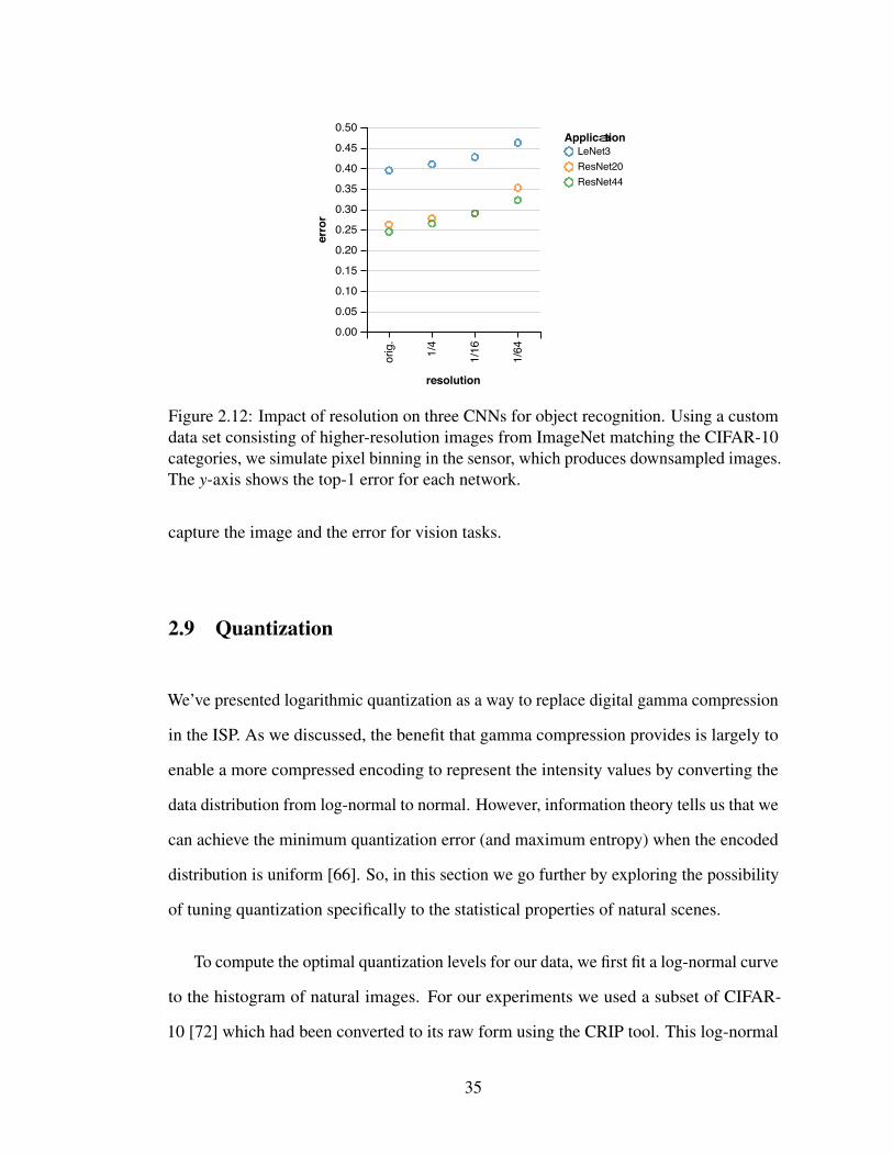
��������������������������������������������
�����
����� ���
����
����
����������
���������������������������������
Figure 2.12: Impact of resolution on three CNNs for object recognition. Using a customdata set consisting of higher-resolution images from ImageNet matching the CIFAR-10categories, we simulate pixel binning in the sensor, which produces downsampled images.The y-axis shows the top-1 error for each network.
capture the image and the error for vision tasks.
2.9 Quantization
We’ve presented logarithmic quantization as a way to replace digital gamma compression
in the ISP. As we discussed, the benefit that gamma compression provides is largely to
enable a more compressed encoding to represent the intensity values by converting the
data distribution from log-normal to normal. However, information theory tells us that we
can achieve the minimum quantization error (and maximum entropy) when the encoded
distribution is uniform [66]. So, in this section we go further by exploring the possibility
of tuning quantization specifically to the statistical properties of natural scenes.
To compute the optimal quantization levels for our data, we first fit a log-normal curve
to the histogram of natural images. For our experiments we used a subset of CIFAR-
10 [72] which had been converted to its raw form using the CRIP tool. This log-normal
35
0 50 100 150 200 250Encoded Channel Intensity
0.00
0.01
0.02
0.03
0.04
0.05
Pro
babili
ty
0 50 100 150 200 250Encoded Channel Intensity
0.000
0.001
0.002
0.003
0.004
0.005
Pro
babili
ty
Figure 2.13: Histograms of the light intensity distribution for CRIP-converted rawCIFAR-10 data (top) and CDF quantized CIFAR-10 data (bottom).
curve served as our probability density function (PDF), which we then integrated to
compute our cumulative density function (CDF). We then inverted the CDF to determine
the distribution of quantization levels. Using uniformly distributed values across the CDF
results in uniformly distributed encoded (digital) values. Figure 2.13 shows both the
input and quantized distributions.
This CDF-based technique approximates the minimum-entropy quantization distribu-
tion. An even more precise distribution of levels may be derived using the Lloyd-Max
algorithm [42].
Figure 2.14 compares the vision task performance using this CDF technique with the
simpler, data-agnostic logarithmic quantization. The error across all applications tends
to be lower. While the logarithmic quantization strategy is less sensitive to bit-width
reduction than linear quantization, the CDF technique is even less sensitive. Where 5 bits
suffice for most benchmarks under logarithmic quantization, 4 bits generally suffice with
CDF-based quantization.
Our main proposal focuses on logarithmic quantization, however, because of hardware
36
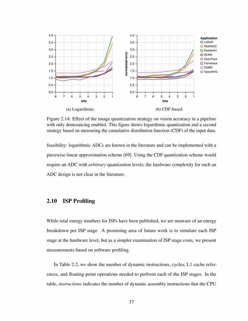
������������
���
���
���
���
���
���
���
���
���
(a) Logarithmic.
������������
���
���
���
���
���
���
���
���
���
���������������
�����������������������������������������������������������������
(b) CDF-based.
Figure 2.14: Effect of the image quantization strategy on vision accuracy in a pipelinewith only demosaicing enabled. This figure shows logarithmic quantization and a secondstrategy based on measuring the cumulative distribution function (CDF) of the input data.
feasibility: logarithmic ADCs are known in the literature and can be implemented with a
piecewise-linear approximation scheme [69]. Using the CDF quantization scheme would
require an ADC with arbitrary quantization levels; the hardware complexity for such an
ADC design is not clear in the literature.
2.10 ISP Profiling
While total energy numbers for ISPs have been published, we are unaware of an energy
breakdown per ISP stage. A promising area of future work is to simulate each ISP
stage at the hardware level, but as a simpler examination of ISP stage costs, we present
measurements based on software profiling.
In Table 2.2, we show the number of dynamic instructions, cycles, L1 cache refer-
ences, and floating-point operations needed to perform each of the ISP stages. In the
table, instructions indicates the number of dynamic assembly instructions that the CPU
37
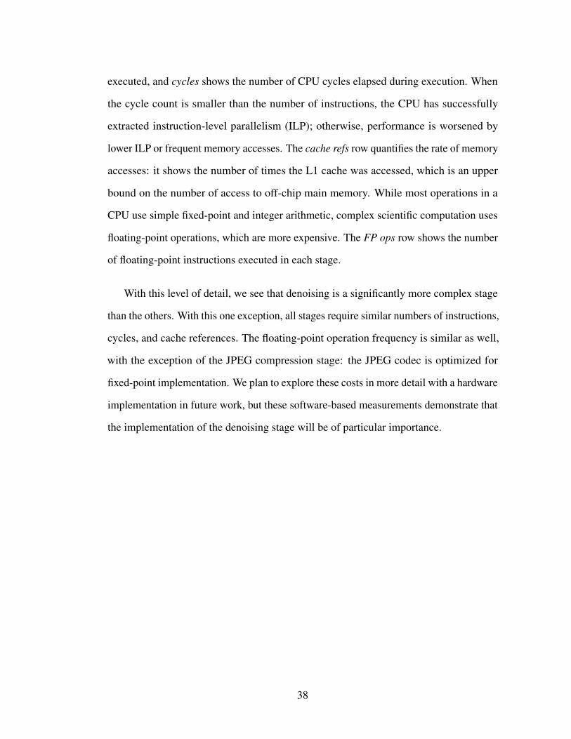
executed, and cycles shows the number of CPU cycles elapsed during execution. When
the cycle count is smaller than the number of instructions, the CPU has successfully
extracted instruction-level parallelism (ILP); otherwise, performance is worsened by
lower ILP or frequent memory accesses. The cache refs row quantifies the rate of memory
accesses: it shows the number of times the L1 cache was accessed, which is an upper
bound on the number of access to off-chip main memory. While most operations in a
CPU use simple fixed-point and integer arithmetic, complex scientific computation uses
floating-point operations, which are more expensive. The FP ops row shows the number
of floating-point instructions executed in each stage.
With this level of detail, we see that denoising is a significantly more complex stage
than the others. With this one exception, all stages require similar numbers of instructions,
cycles, and cache references. The floating-point operation frequency is similar as well,
with the exception of the JPEG compression stage: the JPEG codec is optimized for
fixed-point implementation. We plan to explore these costs in more detail with a hardware
implementation in future work, but these software-based measurements demonstrate that
the implementation of the denoising stage will be of particular importance.
38
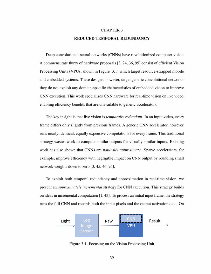
CHAPTER 3
REDUCED TEMPORAL REDUNDANCY
Deep convolutional neural networks (CNNs) have revolutionized computer vision.
A commensurate flurry of hardware proposals [3, 24, 36, 95] consist of efficient Vision
Processing Units (VPUs, shown in Figure 3.1) which target resource-strapped mobile
and embedded systems. These designs, however, target generic convolutional networks:
they do not exploit any domain-specific characteristics of embedded vision to improve
CNN execution. This work specializes CNN hardware for real-time vision on live video,
enabling efficiency benefits that are unavailable to generic accelerators.
The key insight is that live vision is temporally redundant. In an input video, every
frame differs only slightly from previous frames. A generic CNN accelerator, however,
runs nearly identical, equally expensive computations for every frame. This traditional
strategy wastes work to compute similar outputs for visually similar inputs. Existing
work has also shown that CNNs are naturally approximate. Sparse accelerators, for
example, improve efficiency with negligible impact on CNN output by rounding small
network weights down to zero [3, 45, 46, 95].
To exploit both temporal redundancy and approximation in real-time vision, we
present an approximately incremental strategy for CNN execution. This strategy builds
on ideas in incremental computation [1, 43]. To process an initial input frame, the strategy
runs the full CNN and records both the input pixels and the output activation data. On
Figure 3.1: Focusing on the Vision Processing Unit
39
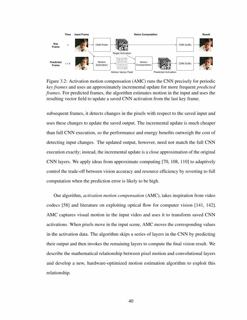
t
t + k
Time Input Frame
MotionEstimation
Motion Vector Field
CNN Prefix
Target Activation
CNN Suffix
Motion Compensation
Predicted Activation
CNN Suffix
Vision Computation
KeyFrame
PredictedFrame
Result
Figure 3.2: Activation motion compensation (AMC) runs the CNN precisely for periodickey frames and uses an approximately incremental update for more frequent predictedframes. For predicted frames, the algorithm estimates motion in the input and uses theresulting vector field to update a saved CNN activation from the last key frame.
subsequent frames, it detects changes in the pixels with respect to the saved input and
uses these changes to update the saved output. The incremental update is much cheaper
than full CNN execution, so the performance and energy benefits outweigh the cost of
detecting input changes. The updated output, however, need not match the full CNN
execution exactly; instead, the incremental update is a close approximation of the original
CNN layers. We apply ideas from approximate computing [70, 108, 110] to adaptively
control the trade-off between vision accuracy and resource efficiency by reverting to full
computation when the prediction error is likely to be high.
Our algorithm, activation motion compensation (AMC), takes inspiration from video
codecs [58] and literature on exploiting optical flow for computer vision [141, 142].
AMC captures visual motion in the input video and uses it to transform saved CNN
activations. When pixels move in the input scene, AMC moves the corresponding values
in the activation data. The algorithm skips a series of layers in the CNN by predicting
their output and then invokes the remaining layers to compute the final vision result. We
describe the mathematical relationship between pixel motion and convolutional layers
and develop a new, hardware-optimized motion estimation algorithm to exploit this
relationship.
40
We design a new hardware module, the Embedded Vision Accelerator Accelerator
(EVA2*), that implements the AMC algorithm. Instead of designing a CNN accelerator
from scratch, we show how to apply EVA2 to any generic CNN accelerator to improve
its efficiency for live computer vision. EVA2 adds new logic and memories to a baseline
accelerator to skip the majority of CNN layer executions for the majority of frames.
EVA2 uses an adaptive control scheme to decide which frames to run precisely.
We implement EVA2 and synthesize the design on a 65 nm process. We augment
state-of-the-art designs for accelerating convolutional and fully-connected layers [24, 45]
and find that EVA2 makes up 3.5% of a full ASIC’s area. On three CNN-based vision
workloads, using EVA2 reduces the average energy cost per frame by 54%, 62%, and
87% and decreases the average frame latency by similar amounts with less than 1% loss
in vision task accuracy.
3.1 Activation Motion Compensation
This section introduces activation motion compensation (AMC), our strategy for ex-
ploiting temporal redundancy in CNNs for efficient real-time computer vision. The
central idea is to use saved outputs from earlier key frames to predict the output for
later predicted frames. As in traditional incremental computing [1, 43], the challenge
is finding an algorithm for updating saved results that is much cheaper than running
the entire computation “from scratch” on the new input. Unlike traditional strategies,
however, our approach for vision is approximately incremental: the updated output need
not match the original output values precisely. Instead, predicted frames need only yield
equivalently high vision accuracy results.
One natural strategy for approximately incremental CNN execution would exploit the
*Pronounced ee-vah squared.
41
differentiability of neural network layers. If f (x) is a layer, then there must be another
function df such that f (x+dx)≈ f (x)+df (dx). Delta networks operate by storing the
old activation, f (x), for every layer, computing df (dx) for new layers, and adding it to the
stored data [91, 92]. While delta updates are straightforward to implement, they do not
address the primary efficiency bottlenecks in CNN execution. First, the hardware must
store the activation data for every network layer to apply per-layer deltas, significantly
increasing the memory requirements for CNN execution. Second, to compute df (dx)
for every layer, the hardware must load the full set of model weights, and previous
work shows that the cost of loading weights can dominate the computation cost in
CNNs [24, 26]. Finally, using pixelwise derivatives to represent changes in video frames
assumes that individual pixels change their color slowly over time. If the camera pans or
objects move in the scene, however, most pixels will change abruptly.
Instead of relying on a pixel-level derivative, our technique uses visual motion in
the input scene. The intuition is the same as in video compression: most frames are
approximately equal to the previous frame with some blocks of pixels moved around.
AMC detects pixel motion and compensates for it in the output of a single target layer in
the CNN. AMC builds on recent computer vision work to warp the target CNN activation
data based on motion information [142]. Unlike delta updating, AMC bypasses the
computation and memory accesses for an entire sequence of CNN layers.
3.1.1 AMC Overview
Figure 3.2 illustrates AMC’s approximately incremental execution strategy for real-time
vision using CNNs. AMC processes the input video as as a mixture of key frames,
which undergo full and precise CNN execution, and predicted frames, which use cheaper,
42
approximate execution. AMC saves intermediate results during key frames and incre-
mentally updates them for predicted frames. Section 3.1.3 describes how to decide which
frames should be key frames.
To apply the strategy to a new CNN architecture, the system splits the CNN’s series
of layers into two contiguous regions: a larger prefix that only executes for key frames,
and a smaller suffix that executes on every frame. The final layer in the prefix is called
the target layer: AMC saves the output from this layer during key frames and predicts its
output during predicted frames. Intuitively, the convolutional and pooling layers in the
prefix have a spatial relationship to the input, while the suffix contains fully-connected
layers and other computations where scene motion can have unpredictable effects. The
prefix typically performs more generic feature extraction, while the functionality in later
layers varies more between vision tasks [133]. Section 3.1.3 describes how to choose the
target layer in more detail.
During key frames, AMC stores the network’s input and the target layer’s output for
reuse during predicted frames. While the input image is typically small, CNN activa-
tions can have high dimensionality and occupy multiple megabytes [95]. Section 3.1.3
describes how to exploit activation sparsity to efficiently store key frame outputs.
During predicted frames, AMC detects the motion between the last stored key frame
and the new input frame. Motion estimation is the problem of computing a vector
field describing the visual displacement between two input frames. Motion estimation
algorithms offer different trade-offs between granularity, accuracy, and efficiency [40,
53, 61, 75, 83, 104, 140]. AMC requires an efficient motion estimation technique that
is aligned with the CNN’s convolutional structure. Section 3.1.3 describes receptive
field block motion estimation (RFBME), our new algorithm optimized for the hardware
implementation of AMC.
43
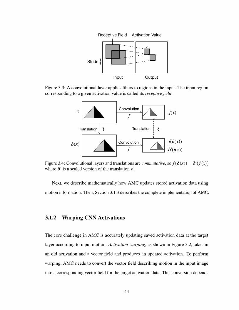
Input Output
Activation ValueReceptive Field
Stride
Figure 3.3: A convolutional layer applies filters to regions in the input. The input regioncorresponding to a given activation value is called its receptive field.
Convolution
Convolution
Translation Translation
f
f
δ δʹ
x
δ(x)
f(x)
f(∂(x))δʹ(f(x))
Figure 3.4: Convolutional layers and translations are commutative, so f (δ (x)) = δ ′( f (x))where δ ′ is a scaled version of the translation δ .
Next, we describe mathematically how AMC updates stored activation data using
motion information. Then, Section 3.1.3 describes the complete implementation of AMC.
3.1.2 Warping CNN Activations
The core challenge in AMC is accurately updating saved activation data at the target
layer according to input motion. Activation warping, as shown in Figure 3.2, takes in
an old activation and a vector field and produces an updated activation. To perform
warping, AMC needs to convert the vector field describing motion in the input image
into a corresponding vector field for the target activation data. This conversion depends
44
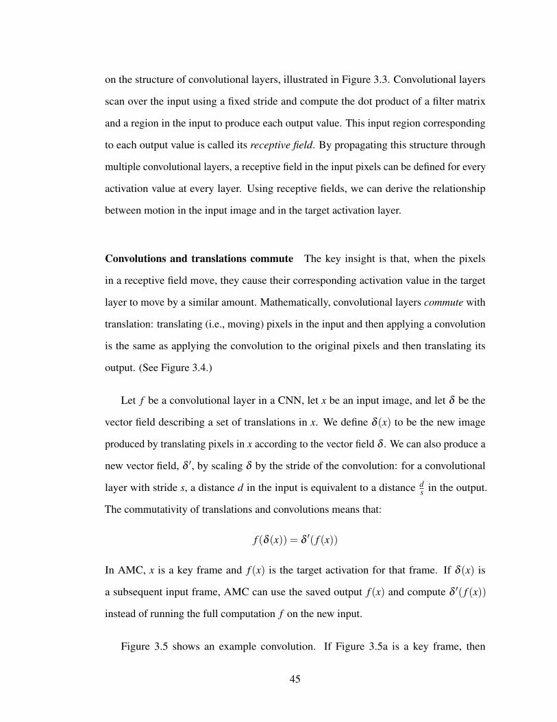
on the structure of convolutional layers, illustrated in Figure 3.3. Convolutional layers
scan over the input using a fixed stride and compute the dot product of a filter matrix
and a region in the input to produce each output value. This input region corresponding
to each output value is called its receptive field. By propagating this structure through
multiple convolutional layers, a receptive field in the input pixels can be defined for every
activation value at every layer. Using receptive fields, we can derive the relationship
between motion in the input image and in the target activation layer.
Convolutions and translations commute The key insight is that, when the pixels
in a receptive field move, they cause their corresponding activation value in the target
layer to move by a similar amount. Mathematically, convolutional layers commute with
translation: translating (i.e., moving) pixels in the input and then applying a convolution
is the same as applying the convolution to the original pixels and then translating its
output. (See Figure 3.4.)
Let f be a convolutional layer in a CNN, let x be an input image, and let δ be the
vector field describing a set of translations in x. We define δ (x) to be the new image
produced by translating pixels in x according to the vector field δ . We can also produce a
new vector field, δ ′, by scaling δ by the stride of the convolution: for a convolutional
layer with stride s, a distance d in the input is equivalent to a distance ds in the output.
The commutativity of translations and convolutions means that:
f (δ (x)) = δ′( f (x))
In AMC, x is a key frame and f (x) is the target activation for that frame. If δ (x) is
a subsequent input frame, AMC can use the saved output f (x) and compute δ ′( f (x))
instead of running the full computation f on the new input.
Figure 3.5 shows an example convolution. If Figure 3.5a is a key frame, then
45
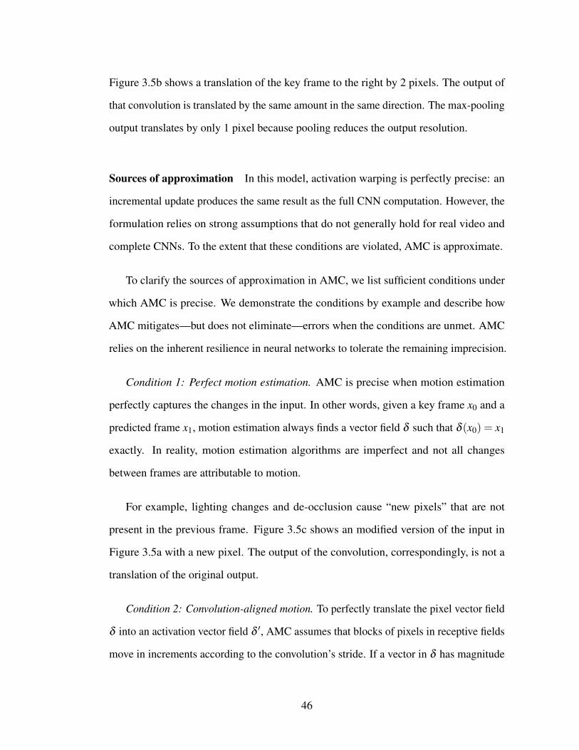
Figure 3.5b shows a translation of the key frame to the right by 2 pixels. The output of
that convolution is translated by the same amount in the same direction. The max-pooling
output translates by only 1 pixel because pooling reduces the output resolution.
Sources of approximation In this model, activation warping is perfectly precise: an
incremental update produces the same result as the full CNN computation. However, the
formulation relies on strong assumptions that do not generally hold for real video and
complete CNNs. To the extent that these conditions are violated, AMC is approximate.
To clarify the sources of approximation in AMC, we list sufficient conditions under
which AMC is precise. We demonstrate the conditions by example and describe how
AMC mitigates—but does not eliminate—errors when the conditions are unmet. AMC
relies on the inherent resilience in neural networks to tolerate the remaining imprecision.
Condition 1: Perfect motion estimation. AMC is precise when motion estimation
perfectly captures the changes in the input. In other words, given a key frame x0 and a
predicted frame x1, motion estimation always finds a vector field δ such that δ (x0) = x1
exactly. In reality, motion estimation algorithms are imperfect and not all changes
between frames are attributable to motion.
For example, lighting changes and de-occlusion cause “new pixels” that are not
present in the previous frame. Figure 3.5c shows an modified version of the input in
Figure 3.5a with a new pixel. The output of the convolution, correspondingly, is not a
translation of the original output.
Condition 2: Convolution-aligned motion. To perfectly translate the pixel vector field
δ into an activation vector field δ ′, AMC assumes that blocks of pixels in receptive fields
move in increments according to the convolution’s stride. If a vector in δ has magnitude
46
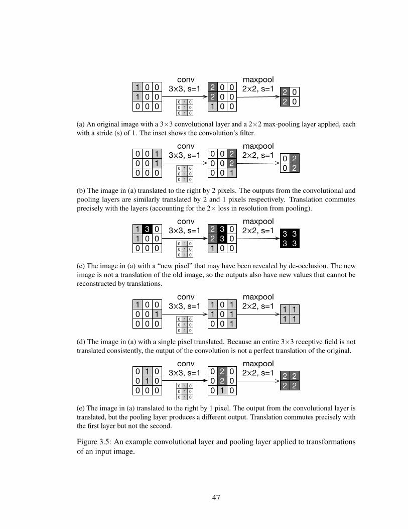
1 0 01 0 00 0 0
0 1 00 1 00 1 0
2 0 02 0 01 0 0
conv3⨉3, s=1 2 0
2 0
maxpool2⨉2, s=1
(a) An original image with a 3×3 convolutional layer and a 2×2 max-pooling layer applied, eachwith a stride (s) of 1. The inset shows the convolution’s filter.
0 0 10 0 10 0 0
0 1 00 1 00 1 0
0 0 20 0 20 0 1
conv3⨉3, s=1 0 2
0 2
maxpool2⨉2, s=1
(b) The image in (a) translated to the right by 2 pixels. The outputs from the convolutional andpooling layers are similarly translated by 2 and 1 pixels respectively. Translation commutesprecisely with the layers (accounting for the 2× loss in resolution from pooling).
1 3 01 0 00 0 0
0 1 00 1 00 1 0
2 3 02 3 01 0 0
conv3⨉3, s=1 3 3
3 3
maxpool2⨉2, s=1
(c) The image in (a) with a “new pixel” that may have been revealed by de-occlusion. The newimage is not a translation of the old image, so the outputs also have new values that cannot bereconstructed by translations.
1 0 00 0 10 0 0
0 1 00 1 00 1 0
1 0 11 0 10 0 1
conv3⨉3, s=1 1 1
1 1
maxpool2⨉2, s=1
(d) The image in (a) with a single pixel translated. Because an entire 3×3 receptive field is nottranslated consistently, the output of the convolution is not a perfect translation of the original.
0 1 00 1 00 0 0
0 1 00 1 00 1 0
0 2 00 2 00 1 0
conv3⨉3, s=1 2 2
2 2
maxpool2⨉2, s=1
(e) The image in (a) translated to the right by 1 pixel. The output from the convolutional layer istranslated, but the pooling layer produces a different output. Translation commutes precisely withthe first layer but not the second.
Figure 3.5: An example convolutional layer and pooling layer applied to transformationsof an input image.
47
d, the corresponding vector in δ ′ has magnitude ds where s is the convolutional layer’s
stride. If d is not a multiple of s, the translation ends at a fractional coordinate in the
activation and perfect reconstruction is impossible. Similarly, if pixels within a single
receptive field move differently, a translation in the activation cannot perfectly capture
the change.
Figure 3.5d shows a version of Figure 3.5a with a single pixel translated. Because the
translation’s granularity is smaller than a receptive field, the output of the convolution is
not a perfect translation of its original output.
Condition 3: Nonlinearities preserve motion. Translation is commutative with
convolution, but CNNs have other kinds of layers, such as pooling, that are not perfectly
commutative. For example, Figures 3.5b and 3.5e show translated versions of the input
in Figure 3.5a. In the first translation, a max-pooling layer produces an output that is a
perfect translation of the original output. In the second, however, the max-pooling layer
creates a non-translated output.
Real video and real CNNs violate all three of these conditions, so AMC’s activation
warping is an approximation of plain CNN execution. The central challenge in the design
of the rest of the AMC algorithm is avoiding and suppressing these potential errors.
AMC’s adaptive key frame selection (Section 3.1.3) mitigates motion estimation errors
by falling back to precise execution; interpolated warping (Section 3.1.3) addresses
unaligned motion; and careful target layer selection (Section 3.1.3) avoids too much error
accumulation due to nonlinear layers.
48
3.1.3 Design Decisions for AMC
This section outlines our approaches to motion estimation, activation storage, warp
interpolation, key frame selection, and target layer selection. AMC is a design space
with a range of possible choices for each of these factors. We describe both the general
requirements and the specific tactic we use in our hardware implementation.
Efficient Motion Estimation
The first step in executing an AMC predicted frame is motion estimation. Motion
estimation takes two input frames and produces a 2D vector field describing the visual
displacement between the frames. Motion estimation algorithms in the literature include
block matching [75, 140], phase correlation in the Fourier domain [104], traditional
optical flow algorithms such as Lucas–Kanade [83] and Horn–Schunck [53], and deep
learning methods [40, 61]. A primary difference is the motion granularity: optical flow
algorithms produce dense, pixel-level vector fields, while block matching detects coarser
motion but can often be cheaper. Previous work on exploiting motion for efficient vision
has used pixel-level optical flow [142]. For AMC, however, pixel-level motion estimation
yields unnecessary detail: activation warping can only handle motion at the granularity
of receptive fields. Another alternative is to use the motion vectors stored in compressed
video data [14, 137], but real-time vision systems can save energy by skipping the ISP
and video codec [11] to process uncompressed video streams.
Block matching algorithms, often used in video codecs, work by taking a block of
pixels and comparing it to a window of nearby blocks in the reference (key) frame. The
location of the closest matching reference block determines the motion vector for the
block. Critical parameters include the choice of search window, the search organization,
49
and the metric for comparing two candidate blocks [58].
We develop a new block matching algorithm, receptive field block motion estimation
(RFBME), that is specialized for AMC. RFBME estimates the motion of entire recep-
tive fields. The resulting displacement vector for each input receptive field maps to a
corresponding displacement vector for a value in the target activation. RFBME avoids
redundant work by dividing the input into square tiles whose size is equal to the receptive
field stride and reusing tile-level differences. Section 3.2.1 describes the algorithm in
detail and its hardware implementation.
Compressed Activation Storage
AMC needs to store the target activation data for the key frame so that subsequent
predicted frames can reuse it. Activations for CNNs, however, can be large: storing an
activation naively would require multiple megabytes of on-chip memory. To mitigate
storage costs, we exploit sparsity in CNN activations. Many CNN accelerator proposals
also exploit sparsity: most values in CNN weights and activations are close to zero, so
they can be safely ignored without a significant impact on output accuracy [3, 24, 45, 95].
We use the same property to avoid storing near-zero values. Section 3.2.2 describes our
hardware design for encoding and decoding sparse data.
Interpolated Warping
AMC’s activation warping step takes a vector field δ and an old CNN activation and
updates the activation according to the translations in the vector field δ ′. It works by
scaling the magnitudes of the vector field to match the dimensions of the activation data.
This scaling can produce vectors that are unaligned to activation coordinates. To translate
50
by a fractional distance, AMC needs to interpolate the values of nearby activations.
There are a range of possible strategies for interpolation, from cheap techniques,
such as nearest neighbor and bilinear interpolation, to more computationally expensive
but accurate interpolation methods that preserve edge or gradient boundaries. For this
work, we choose bilinear interpolation to average neighboring pixels in 2D space while
maintaining high performance. In our experiments, bilinear interpolation improves vision
accuracy by 1–2% over nearest-neighbor matching on average for one CNN benchmark
(FasterM).
Selecting Key Frames
The primary control that AMC has over vision accuracy and execution efficiency is
the allocation of key frames, which are both more expensive and more accurate than
predicted frames. Several strategies exist to decide when to use each type of frame.
The simplest is a static key frame rate: every nth frame is a key frame, and the rest are
predicted frames. A adaptive strategy, however, can allocate more key frames when the
scene is chaotic and unpredictable and fewer when AMC’s predictions are more likely to
succeed. To implement an adaptive strategy, the accelerator must measure some feature
of the input scene that correlates with the probability of a successful AMC prediction.
We consider two possible features:
Pixel compensation error. AMC can produce a poor prediction when the motion
estimation fails to accurately reflect the changes in the scene. To measure motion
accuracy, we can reuse the internal bookkeeping of a block matching algorithm, which
must compute the match error for each pixel block in the scene. When the aggregate error
across all blocks is high, this strategy allocates a new key frame. When large occlusions
51
occur, for example, this method will identify the inadequacy of the motion information.
Total motion magnitude. AMC’s predictions are more accurate when there is less
motion in the input scene. To measure the amount of motion, this simple strategy sums
the magnitude of the vectors produced by motion estimation. This policy uses a key
frame when the total amount of motion is large.
We implement and measure both techniques to compare their effectiveness. Sec-
tion 3.3.5 quantitatively compares their effects on overall accuracy.
Choosing the Target Layer
To apply AMC to a given CNN, the system needs to choose a target layer. This choice
controls both AMC’s potential efficiency benefits and its error rate. A later target layer
lets AMC skip more computation during predicted frames, but a larger CNN prefix can
also compound the influence of layers that make activation warping imperfect. Some
kinds of layers, including fully-connected layers, make activation warping impossible:
they have no 2D spatial structure and no meaningful relationship with motion in the input.
These non-spatial layers must remain in the CNN suffix, after the target layer. Fortunately,
these non-spatial layers are typically located later in CNNs, in the more task-specific
segment of the network [133]. AMC also cannot predict through stateful structures in
recurrent neural networks and LSTMs [52]. However, even these specialized networks
tend to contain early sets of stateless convolutional layers for feature extraction [67, 131],
where AMC can apply.
As with key frame selection, the system can use a static or adaptive policy to select the
target layer. In our evaluation, we measure the impact of choosing earlier and later CNN
layers, up to the last spatial layer (Section 3.3.5) and find that the accuracy difference is
52
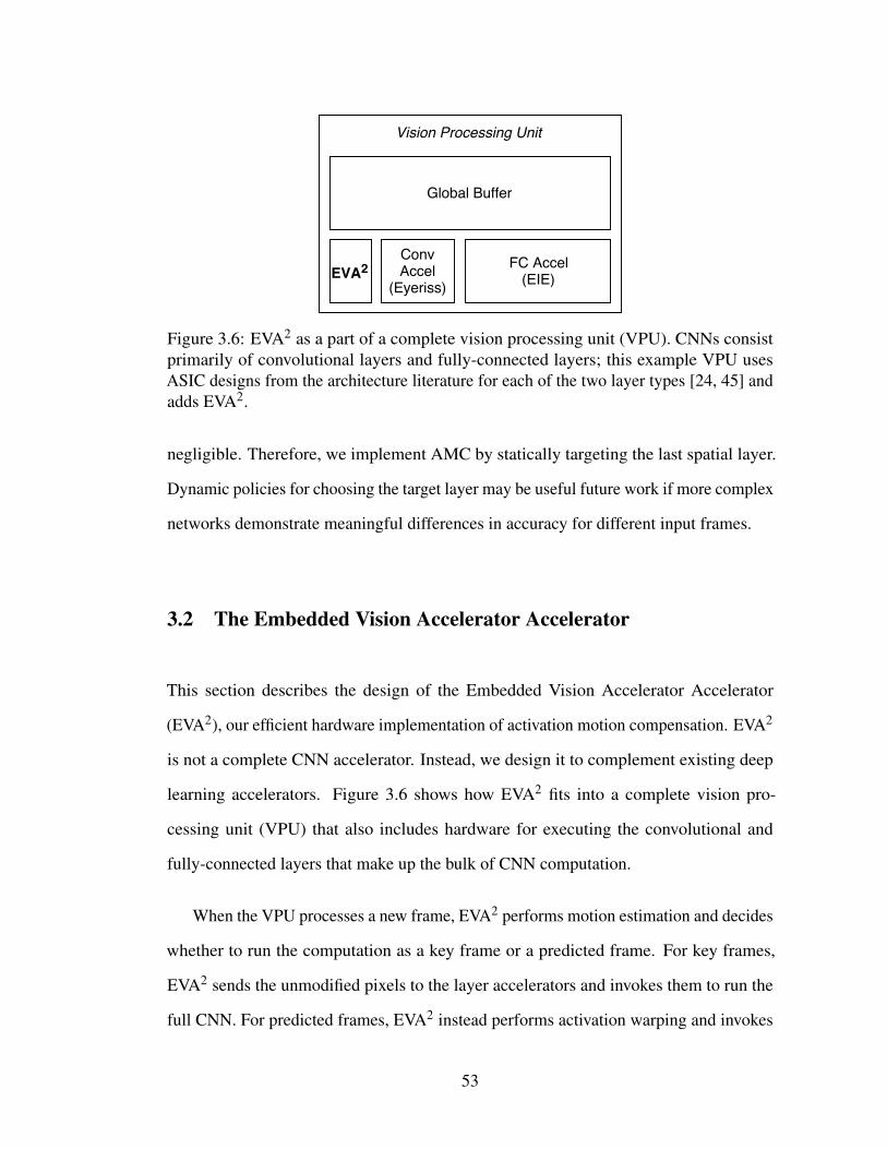
Figure 3.6: EVA2 as a part of a complete vision processing unit (VPU). CNNs consistprimarily of convolutional layers and fully-connected layers; this example VPU usesASIC designs from the architecture literature for each of the two layer types [24, 45] andadds EVA2.
negligible. Therefore, we implement AMC by statically targeting the last spatial layer.
Dynamic policies for choosing the target layer may be useful future work if more complex
networks demonstrate meaningful differences in accuracy for different input frames.
3.2 The Embedded Vision Accelerator Accelerator
This section describes the design of the Embedded Vision Accelerator Accelerator
(EVA2), our efficient hardware implementation of activation motion compensation. EVA2
is not a complete CNN accelerator. Instead, we design it to complement existing deep
learning accelerators. Figure 3.6 shows how EVA2 fits into a complete vision pro-
cessing unit (VPU) that also includes hardware for executing the convolutional and
fully-connected layers that make up the bulk of CNN computation.
When the VPU processes a new frame, EVA2 performs motion estimation and decides
whether to run the computation as a key frame or a predicted frame. For key frames,
EVA2 sends the unmodified pixels to the layer accelerators and invokes them to run the
full CNN. For predicted frames, EVA2 instead performs activation warping and invokes
53
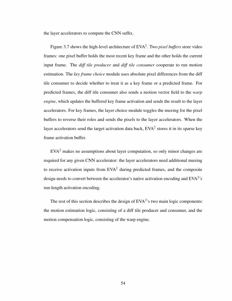
the layer accelerators to compute the CNN suffix.
Figure 3.7 shows the high-level architecture of EVA2. Two pixel buffers store video
frames: one pixel buffer holds the most recent key frame and the other holds the current
input frame. The diff tile producer and diff tile consumer cooperate to run motion
estimation. The key frame choice module uses absolute pixel differences from the diff
tile consumer to decide whether to treat it as a key frame or a predicted frame. For
predicted frames, the diff tile consumer also sends a motion vector field to the warp
engine, which updates the buffered key frame activation and sends the result to the layer
accelerators. For key frames, the layer choice module toggles the muxing for the pixel
buffers to reverse their roles and sends the pixels to the layer accelerators. When the
layer accelerators send the target activation data back, EVA2 stores it in its sparse key
frame activation buffer.
EVA2 makes no assumptions about layer computation, so only minor changes are
required for any given CNN accelerator: the layer accelerators need additional muxing
to receive activation inputs from EVA2 during predicted frames, and the composite
design needs to convert between the accelerator’s native activation encoding and EVA2’s
run-length activation encoding.
The rest of this section describes the design of EVA2’s two main logic components:
the motion estimation logic, consisting of a diff tile producer and consumer, and the
motion compensation logic, consisting of the warp engine.
54
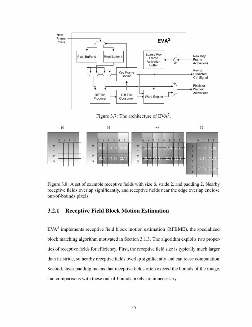
Figure 3.7: The architecture of EVA2.
Figure 3.8: A set of example receptive fields with size 6, stride 2, and padding 2. Nearbyreceptive fields overlap significantly, and receptive fields near the edge overlap encloseout-of-bounds pixels.
3.2.1 Receptive Field Block Motion Estimation
EVA2 implements receptive field block motion estimation (RFBME), the specialized
block matching algorithm motivated in Section 3.1.3. The algorithm exploits two proper-
ties of receptive fields for efficiency. First, the receptive field size is typically much larger
than its stride, so nearby receptive fields overlap significantly and can reuse computation.
Second, layer padding means that receptive fields often exceed the bounds of the image,
and comparisons with these out-of-bounds pixels are unnecessary.
55
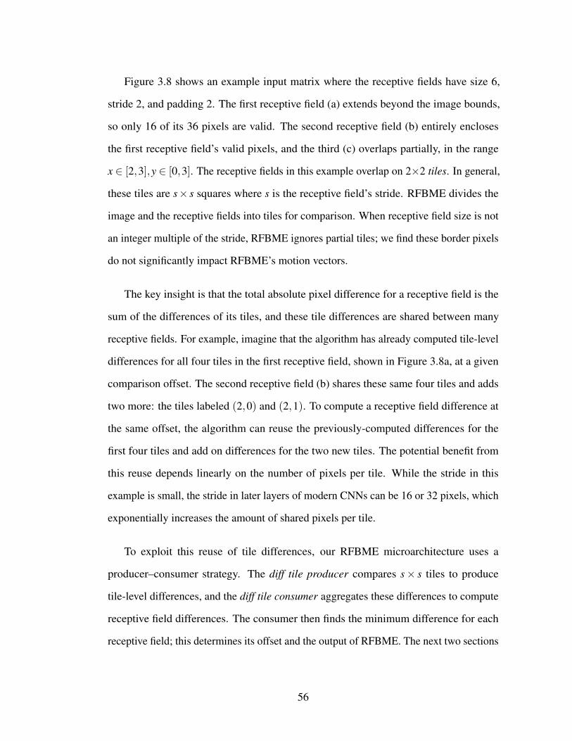
Figure 3.8 shows an example input matrix where the receptive fields have size 6,
stride 2, and padding 2. The first receptive field (a) extends beyond the image bounds,
so only 16 of its 36 pixels are valid. The second receptive field (b) entirely encloses
the first receptive field’s valid pixels, and the third (c) overlaps partially, in the range
x ∈ [2,3],y ∈ [0,3]. The receptive fields in this example overlap on 2×2 tiles. In general,
these tiles are s× s squares where s is the receptive field’s stride. RFBME divides the
image and the receptive fields into tiles for comparison. When receptive field size is not
an integer multiple of the stride, RFBME ignores partial tiles; we find these border pixels
do not significantly impact RFBME’s motion vectors.
The key insight is that the total absolute pixel difference for a receptive field is the
sum of the differences of its tiles, and these tile differences are shared between many
receptive fields. For example, imagine that the algorithm has already computed tile-level
differences for all four tiles in the first receptive field, shown in Figure 3.8a, at a given
comparison offset. The second receptive field (b) shares these same four tiles and adds
two more: the tiles labeled (2,0) and (2,1). To compute a receptive field difference at
the same offset, the algorithm can reuse the previously-computed differences for the
first four tiles and add on differences for the two new tiles. The potential benefit from
this reuse depends linearly on the number of pixels per tile. While the stride in this
example is small, the stride in later layers of modern CNNs can be 16 or 32 pixels, which
exponentially increases the amount of shared pixels per tile.
To exploit this reuse of tile differences, our RFBME microarchitecture uses a
producer–consumer strategy. The diff tile producer compares s× s tiles to produce
tile-level differences, and the diff tile consumer aggregates these differences to compute
receptive field differences. The consumer then finds the minimum difference for each
receptive field; this determines its offset and the output of RFBME. The next two sections
56
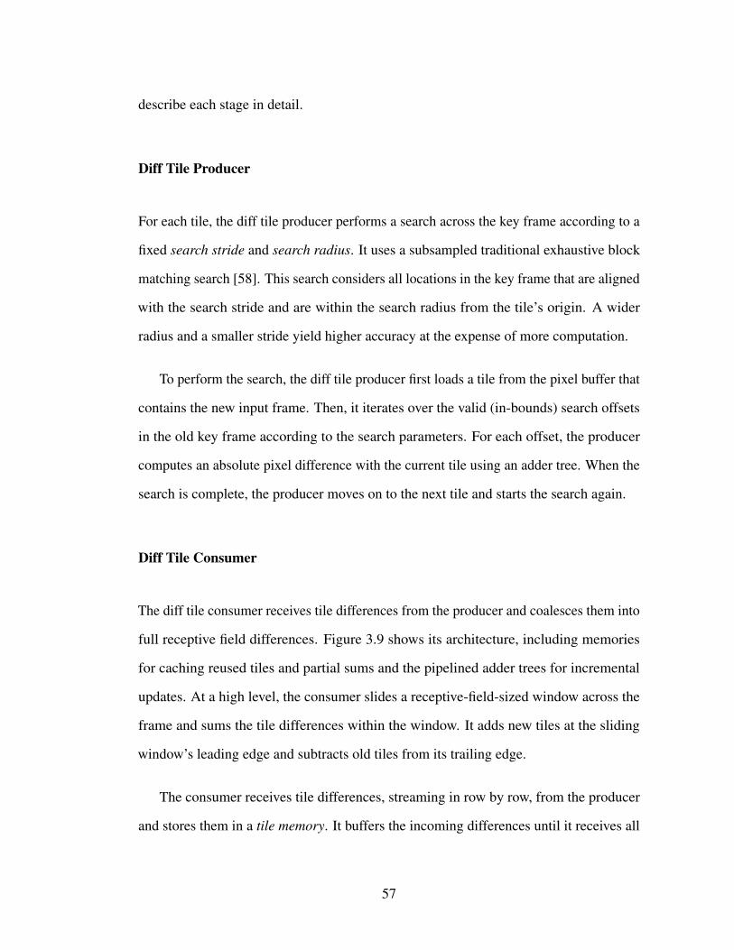
describe each stage in detail.
Diff Tile Producer
For each tile, the diff tile producer performs a search across the key frame according to a
fixed search stride and search radius. It uses a subsampled traditional exhaustive block
matching search [58]. This search considers all locations in the key frame that are aligned
with the search stride and are within the search radius from the tile’s origin. A wider
radius and a smaller stride yield higher accuracy at the expense of more computation.
To perform the search, the diff tile producer first loads a tile from the pixel buffer that
contains the new input frame. Then, it iterates over the valid (in-bounds) search offsets
in the old key frame according to the search parameters. For each offset, the producer
computes an absolute pixel difference with the current tile using an adder tree. When the
search is complete, the producer moves on to the next tile and starts the search again.
Diff Tile Consumer
The diff tile consumer receives tile differences from the producer and coalesces them into
full receptive field differences. Figure 3.9 shows its architecture, including memories
for caching reused tiles and partial sums and the pipelined adder trees for incremental
updates. At a high level, the consumer slides a receptive-field-sized window across the
frame and sums the tile differences within the window. It adds new tiles at the sliding
window’s leading edge and subtracts old tiles from its trailing edge.
The consumer receives tile differences, streaming in row by row, from the producer
and stores them in a tile memory. It buffers the incoming differences until it receives all
57
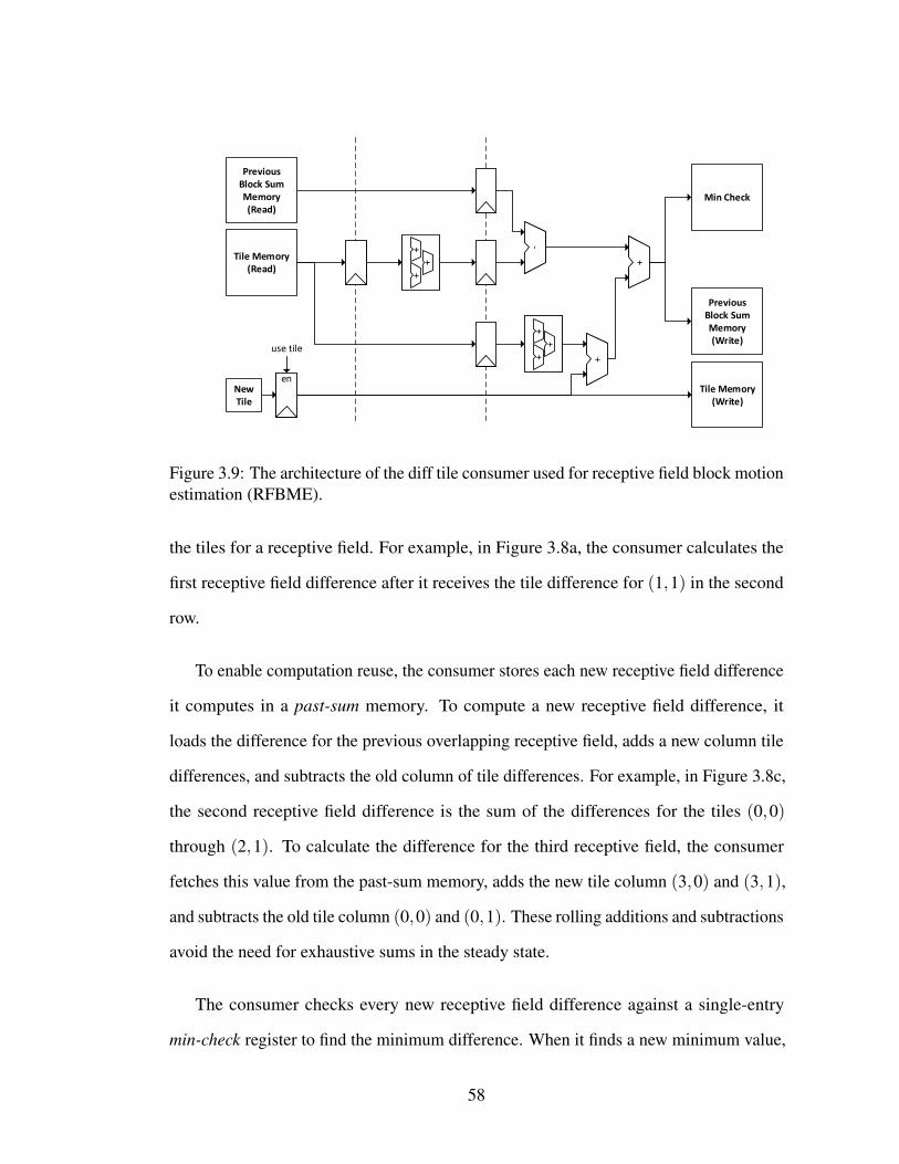
++
Previous Block Sum Memory(Write)
++
--
Min Check
Tile Memory (Write)
Tile Memory (Read)
Previous Block Sum Memory (Read)
New Tile
enen
use tile
++++
+++
++
++++
+++
++
Figure 3.9: The architecture of the diff tile consumer used for receptive field block motionestimation (RFBME).
the tiles for a receptive field. For example, in Figure 3.8a, the consumer calculates the
first receptive field difference after it receives the tile difference for (1,1) in the second
row.
To enable computation reuse, the consumer stores each new receptive field difference
it computes in a past-sum memory. To compute a new receptive field difference, it
loads the difference for the previous overlapping receptive field, adds a new column tile
differences, and subtracts the old column of tile differences. For example, in Figure 3.8c,
the second receptive field difference is the sum of the differences for the tiles (0,0)
through (2,1). To calculate the difference for the third receptive field, the consumer
fetches this value from the past-sum memory, adds the new tile column (3,0) and (3,1),
and subtracts the old tile column (0,0) and (0,1). These rolling additions and subtractions
avoid the need for exhaustive sums in the steady state.
The consumer checks every new receptive field difference against a single-entry
min-check register to find the minimum difference. When it finds a new minimum value,
58
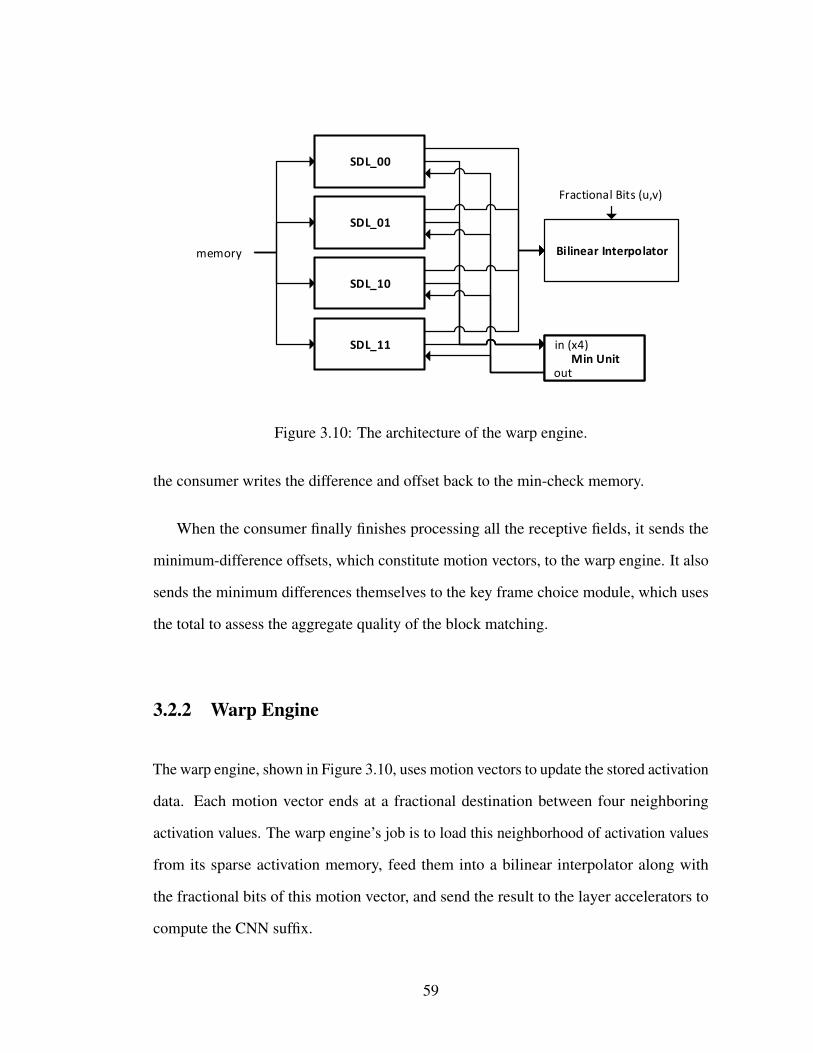
Fractional Bits (u,v)
memory
SDL_11
SDL_10
SDL_01
SDL_00
Min Unitin (x4)
outMin Unit
in (x4)
out
Bilinear Interpolator
Figure 3.10: The architecture of the warp engine.
the consumer writes the difference and offset back to the min-check memory.
When the consumer finally finishes processing all the receptive fields, it sends the
minimum-difference offsets, which constitute motion vectors, to the warp engine. It also
sends the minimum differences themselves to the key frame choice module, which uses
the total to assess the aggregate quality of the block matching.
3.2.2 Warp Engine
The warp engine, shown in Figure 3.10, uses motion vectors to update the stored activation
data. Each motion vector ends at a fractional destination between four neighboring
activation values. The warp engine’s job is to load this neighborhood of activation values
from its sparse activation memory, feed them into a bilinear interpolator along with
the fractional bits of this motion vector, and send the result to the layer accelerators to
compute the CNN suffix.
59
!load & deq
load deq
zero_gap
value
check_deq_ok
0
en
deq
deq
en
deactivate
max_zero
deq
FIFO
-1 --
Zero Compare
memory line
bilinear interpolator
min input
min output
Sparsity Decoder Lane (SDL)
Figure 3.11: The warp engine’s datapath for loading sparse activation data from the keyactivation memory.
The first step is to load the activation data. EVA2 uses run-length encoding (RLE)
for activations. RLE is critical to enabling on-chip activation storage: for Faster16, for
example, sparse storage reduces memory requirements by more than 80%. However, the
sparse data representation complicates the task of loading individual values.
To load sets of four activation values, the warp engine uses four sparsity decoder
lanes (Figure 3.11) to skip zeros shared among all four activations. Once activations are
loaded into the FIFO, each lane sends its zero gap for its first activation. The min unit
checks the zero gap in each lane and sends the minimum to all of the lanes. Each lane
then decrements its zero gap by this amount, thereby jumping forward in the channel.
All lanes with zero gaps of zero after the min subtraction provide their value register as
input to the bilinear interpolator. Lanes with positive zero gaps provide zero as the input
to the interpolator.
60
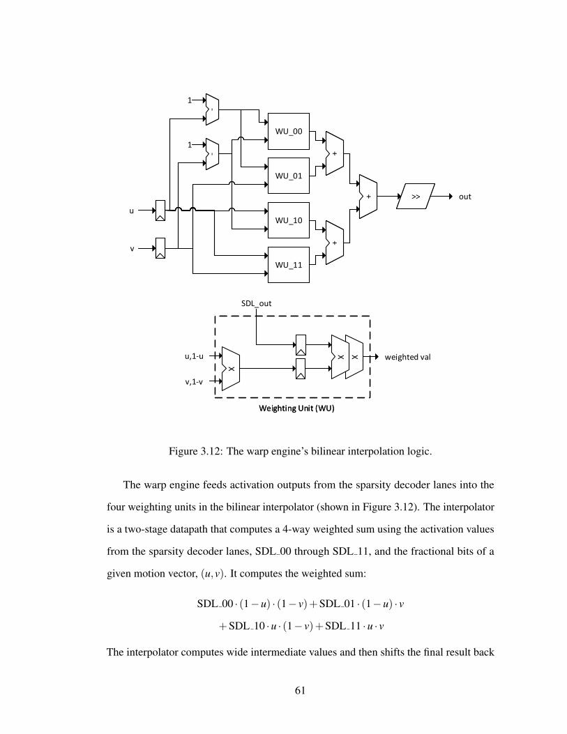
XXXX
SDL_out
XX
v,1-v
u,1-u weighted val
Weighting Unit (WU)
XX
SDL_out
X
v,1-v
u,1-u weighted val
Weighting Unit (WU)
--
1
++
++>>
++
out
v
u
WU_00
WU_01
WU_10
WU_11
--
1
-
1
+
+>>
+
out
v
u
WU_00
WU_01
WU_10
WU_11
-
1
Figure 3.12: The warp engine’s bilinear interpolation logic.
The warp engine feeds activation outputs from the sparsity decoder lanes into the
four weighting units in the bilinear interpolator (shown in Figure 3.12). The interpolator
is a two-stage datapath that computes a 4-way weighted sum using the activation values
from the sparsity decoder lanes, SDL 00 through SDL 11, and the fractional bits of a
given motion vector, (u,v). It computes the weighted sum:
SDL 00 · (1−u) · (1− v)+SDL 01 · (1−u) · v
+SDL 10 ·u · (1− v)+SDL 11 ·u · v
The interpolator computes wide intermediate values and then shifts the final result back
61
to a 16-bit fixed-point representation. The warp engine sends the output activations to the
layer accelerators to begin the CNN suffix computation.
3.3 Evaluation
This section studies EVA2’s impacts on vision accuracy and efficiency and explores its
implementation trade-offs. We begin with a simple first-order model to build intuition
and then proceed to a full, empirical evaluation.
3.3.1 First-Order Efficiency Comparison
As Section 3.1 describes, AMC relies on a fundamental efficiency trade-off: for predicted
frames, it eliminates the CNN prefix computation in exchange for incurring the cost of
motion estimation and compensation. The technique succeeds if the former is much more
expensive than the latter. To provide intuition for this advantage, we build a first-order
model for these computation costs.
The cost of computation in the CNN prefix is dominated by the multiply-and-
accumulate operations (MACs) in the convolutional layers. Each layer computes a
number of outputs dictated by its size and filter count (channels):
outputs = layer width× layer height×out channels
Each output is the weighted sum of inputs within an area given by the filters’ width and
height:
MACs per output = in channels×filter height×filter width
62
We sum the total number of MACs for all convolutional layers in the prefix:
prefix MACs =prefix layers
∑i
outputsi×MACs per outputi
For a Faster16 prefix ending at layer conv5 3 on 1000×562 images, for example, the
total is 1.7×10¹¹ MACs.
AMC’s cost for predicted frames, in contrast, consists mainly of motion estimation
and compensation. The compensation step is a simple linear-time interpolation, so motion
estimation dominates. Our motion estimation algorithm, RFBME (Section 3.2.1), consists
primarily of the additions and subtractions that accumulate absolute pixel differences.
We first analyze an unoptimized variant of RFBME that does not exploit tile-level
computation reuse. The algorithm sweeps a receptive field over a search region in
the input image with a given radius and stride. At each point, the algorithm takes the
difference for every pixel in the receptive field’s area, so the total number of operations is
given by:
unoptimized ops = (layer width× layer height)×(2× search radius
search stride
)2
× rfield size2
The full RFBME algorithm reuses computations from tiles whose size is equal to the
receptive field stride. It then incurs additional operations to combine the differences from
tiles:
RFBME ops =unoptimized ops
rfield stride2 +
(layer width× layer height)×(
rfield sizerfield stride
)2
Again using Faster16 as an example, an unoptimized version requires 3× 10⁹ add
operations while RFBME requires 1.3×10⁷. Overall, for this example, AMC eliminates
∼1011 MACs in the CNN prefix and incurs only ∼107 additions for motion estimation.
AMC’s advantages stem from this large difference between savings and overhead.
63
3.3.2 Experimental Setup
We implement EVA2 in RTL and synthesize our design using the Synopsys toolchain,
including the Design Compiler, IC Compiler, and PrimeTime, in the TSMC 65 nm
process technology. For energy and timing, we run simulations of the full EVA2 design.
The EVA2 implementation uses eDRAM memories for the three larger buffers: the two
pixel buffers and the activation buffer. We use CACTI 6.5 [90] to measure the memories’
power, performance, and area. CACTI includes both an eDRAM model and an SRAM
model, which we use for EVA2’s smaller buffers.
Baseline accelerator We apply EVA2 to a model of a state-of-the-art deep learning
accelerator based on recent architecture papers. We model Eyeriss [24] for convolutional
layers and EIE [45] for fully-connected layers by gathering published per-layer results
from each paper. A journal paper about Eyeriss [25] reports both power and latency
numbers for each layer in the VGG-16 [117] and AlexNet [73] networks. The EIE results
only include latency numbers for these two networks, so we use the total design power to
estimate energy. Because EIE is implemented on a TSMC 45 nm process, we normalize
by scaling up the power, latency, and area for EIE according to the technology scaling
factor. Eyeriss is implemented in the same TSMC 65 nm technology and thus requires no
scaling. The total latency and energy for a CNN execution in our model is the sum of the
individual layer costs. To quantify the cost of layers not present in AlexNet and VGG-16,
the model scales the average layer costs based on the number of multiply–accumulate
operations required for each layer, which we find to correlate closely with cost in both
accelerators [111].
64
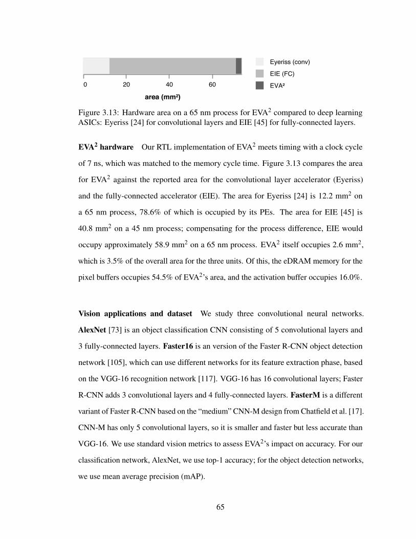
Eyeriss (conv)
EIE (FC)
EVA²0 20 40 60
area (mm²)
Figure 3.13: Hardware area on a 65 nm process for EVA2 compared to deep learningASICs: Eyeriss [24] for convolutional layers and EIE [45] for fully-connected layers.
EVA2 hardware Our RTL implementation of EVA2 meets timing with a clock cycle
of 7 ns, which was matched to the memory cycle time. Figure 3.13 compares the area
for EVA2 against the reported area for the convolutional layer accelerator (Eyeriss)
and the fully-connected accelerator (EIE). The area for Eyeriss [24] is 12.2 mm2 on
a 65 nm process, 78.6% of which is occupied by its PEs. The area for EIE [45] is
40.8 mm2 on a 45 nm process; compensating for the process difference, EIE would
occupy approximately 58.9 mm2 on a 65 nm process. EVA2 itself occupies 2.6 mm2,
which is 3.5% of the overall area for the three units. Of this, the eDRAM memory for the
pixel buffers occupies 54.5% of EVA2’s area, and the activation buffer occupies 16.0%.
Vision applications and dataset We study three convolutional neural networks.
AlexNet [73] is an object classification CNN consisting of 5 convolutional layers and
3 fully-connected layers. Faster16 is an version of the Faster R-CNN object detection
network [105], which can use different networks for its feature extraction phase, based
on the VGG-16 recognition network [117]. VGG-16 has 16 convolutional layers; Faster
R-CNN adds 3 convolutional layers and 4 fully-connected layers. FasterM is a different
variant of Faster R-CNN based on the “medium” CNN-M design from Chatfield et al. [17].
CNN-M has only 5 convolutional layers, so it is smaller and faster but less accurate than
VGG-16. We use standard vision metrics to assess EVA2’s impact on accuracy. For our
classification network, AlexNet, we use top-1 accuracy; for the object detection networks,
we use mean average precision (mAP).
65
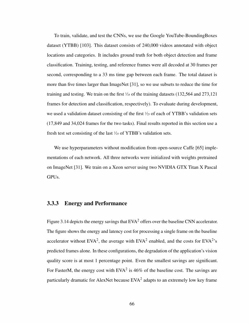
To train, validate, and test the CNNs, we use the Google YouTube-BoundingBoxes
dataset (YTBB) [103]. This dataset consists of 240,000 videos annotated with object
locations and categories. It includes ground truth for both object detection and frame
classification. Training, testing, and reference frames were all decoded at 30 frames per
second, corresponding to a 33 ms time gap between each frame. The total dataset is
more than five times larger than ImageNet [31], so we use subsets to reduce the time for
training and testing. We train on the first 1⁄25 of the training datasets (132,564 and 273,121
frames for detection and classification, respectively). To evaluate during development,
we used a validation dataset consisting of the first 1⁄25 of each of YTBB’s validation sets
(17,849 and 34,024 frames for the two tasks). Final results reported in this section use a
fresh test set consisting of the last 1⁄25 of YTBB’s validation sets.
We use hyperparameters without modification from open-source Caffe [65] imple-
mentations of each network. All three networks were initialized with weights pretrained
on ImageNet [31]. We train on a Xeon server using two NVIDIA GTX Titan X Pascal
GPUs.
3.3.3 Energy and Performance
Figure 3.14 depicts the energy savings that EVA2 offers over the baseline CNN accelerator.
The figure shows the energy and latency cost for processing a single frame on the baseline
accelerator without EVA2, the average with EVA2 enabled, and the costs for EVA2’s
predicted frames alone. In these configurations, the degradation of the application’s vision
quality score is at most 1 percentage point. Even the smallest savings are significant.
For FasterM, the energy cost with EVA2 is 46% of the baseline cost. The savings are
particularly dramatic for AlexNet because EVA2 adapts to an extremely low key frame
66
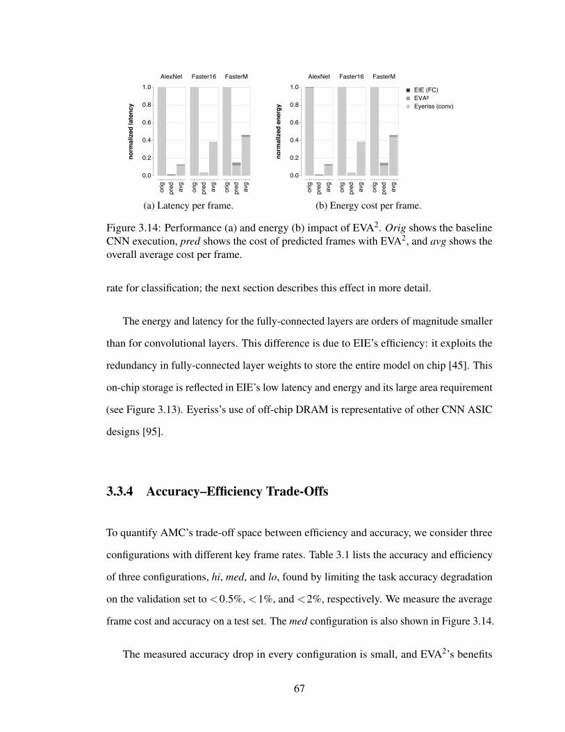
0.0
0.2
0.4
0.6
0.8
1.0
normalized
latency
AlexNet Faster16 FasterM
orig
pred
avg
orig
pred
avg
orig
pred
avg
(a) Latency per frame.
0.0
0.2
0.4
0.6
0.8
1.0
normalized
energy
AlexNet Faster16 FasterM
orig
pred
avg
orig
pred
avg
orig
pred
avg
EIE (FC)
EVA²
Eyeriss (conv)
(b) Energy cost per frame.
Figure 3.14: Performance (a) and energy (b) impact of EVA2. Orig shows the baselineCNN execution, pred shows the cost of predicted frames with EVA2, and avg shows theoverall average cost per frame.
rate for classification; the next section describes this effect in more detail.
The energy and latency for the fully-connected layers are orders of magnitude smaller
than for convolutional layers. This difference is due to EIE’s efficiency: it exploits the
redundancy in fully-connected layer weights to store the entire model on chip [45]. This
on-chip storage is reflected in EIE’s low latency and energy and its large area requirement
(see Figure 3.13). Eyeriss’s use of off-chip DRAM is representative of other CNN ASIC
designs [95].
3.3.4 Accuracy–Efficiency Trade-Offs
To quantify AMC’s trade-off space between efficiency and accuracy, we consider three
configurations with different key frame rates. Table 3.1 lists the accuracy and efficiency
of three configurations, hi, med, and lo, found by limiting the task accuracy degradation
on the validation set to <0.5%, <1%, and <2%, respectively. We measure the average
frame cost and accuracy on a test set. The med configuration is also shown in Figure 3.14.
The measured accuracy drop in every configuration is small, and EVA2’s benefits
67
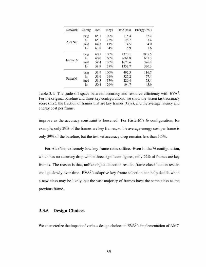
Network Config Acc. Keys Time (ms) Energy (mJ)
AlexNet
orig 65.1 100% 115.4 32.2hi 65.1 22% 26.7 7.4
med 64.3 11% 14.5 4.0lo 63.8 4% 5.9 1.6
Faster16
orig 60.1 100% 4370.1 1035.5hi 60.0 60% 2664.8 631.3
med 59.4 36% 1673.6 396.4lo 58.9 29% 1352.7 320.3
FasterM
orig 51.9 100% 492.3 116.7hi 51.6 61% 327.2 77.4
med 51.3 37% 226.4 53.4lo 50.4 29% 194.7 45.9
Table 3.1: The trade-off space between accuracy and resource efficiency with EVA2.For the original baseline and three key configurations, we show the vision task accuracyscore (acc), the fraction of frames that are key frames (keys), and the average latency andenergy cost per frame.
improve as the accuracy constraint is loosened. For FasterM’s lo configuration, for
example, only 29% of the frames are key frames, so the average energy cost per frame is
only 39% of the baseline, but the test-set accuracy drop remains less than 1.5%.
For AlexNet, extremely low key frame rates suffice. Even in the hi configuration,
which has no accuracy drop within three significant figures, only 22% of frames are key
frames. The reason is that, unlike object detection results, frame classification results
change slowly over time. EVA2’s adaptive key frame selection can help decide when
a new class may be likely, but the vast majority of frames have the same class as the
previous frame.
3.3.5 Design Choices
We characterize the impact of various design choices in EVA2’s implementation of AMC.
68
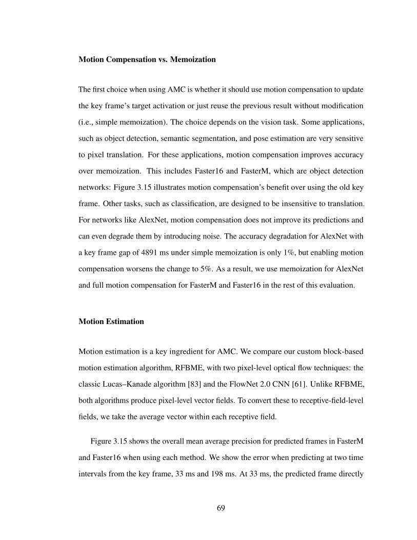
Motion Compensation vs. Memoization
The first choice when using AMC is whether it should use motion compensation to update
the key frame’s target activation or just reuse the previous result without modification
(i.e., simple memoization). The choice depends on the vision task. Some applications,
such as object detection, semantic segmentation, and pose estimation are very sensitive
to pixel translation. For these applications, motion compensation improves accuracy
over memoization. This includes Faster16 and FasterM, which are object detection
networks: Figure 3.15 illustrates motion compensation’s benefit over using the old key
frame. Other tasks, such as classification, are designed to be insensitive to translation.
For networks like AlexNet, motion compensation does not improve its predictions and
can even degrade them by introducing noise. The accuracy degradation for AlexNet with
a key frame gap of 4891 ms under simple memoization is only 1%, but enabling motion
compensation worsens the change to 5%. As a result, we use memoization for AlexNet
and full motion compensation for FasterM and Faster16 in the rest of this evaluation.
Motion Estimation
Motion estimation is a key ingredient for AMC. We compare our custom block-based
motion estimation algorithm, RFBME, with two pixel-level optical flow techniques: the
classic Lucas–Kanade algorithm [83] and the FlowNet 2.0 CNN [61]. Unlike RFBME,
both algorithms produce pixel-level vector fields. To convert these to receptive-field-level
fields, we take the average vector within each receptive field.
Figure 3.15 shows the overall mean average precision for predicted frames in FasterM
and Faster16 when using each method. We show the error when predicting at two time
intervals from the key frame, 33 ms and 198 ms. At 33 ms, the predicted frame directly
69
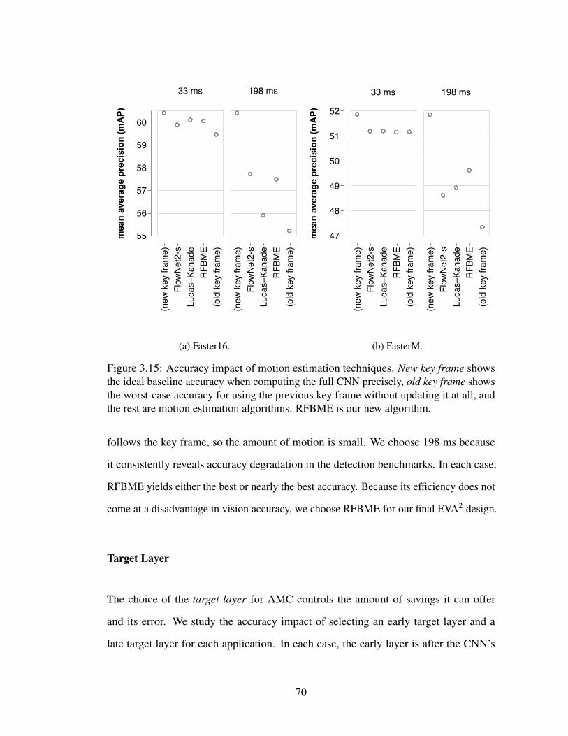
55
56
57
58
59
60mean
average
precision
(mAP)
33 ms 198 ms
(new
key frame)
FlowNet2-s
Lucas–Kanade
RFBME
(old
key frame)
(new
key frame)
FlowNet2-s
Lucas–Kanade
RFBME
(old
key frame)
(a) Faster16.
47
48
49
50
51
52
mean
average
precision
(mAP)
33 ms 198 ms
(new
key frame)
FlowNet2-s
Lucas–Kanade
RFBME
(old
key frame)
(new
key frame)
FlowNet2-s
Lucas–Kanade
RFBME
(old
key frame)
(b) FasterM.
Figure 3.15: Accuracy impact of motion estimation techniques. New key frame showsthe ideal baseline accuracy when computing the full CNN precisely, old key frame showsthe worst-case accuracy for using the previous key frame without updating it at all, andthe rest are motion estimation algorithms. RFBME is our new algorithm.
follows the key frame, so the amount of motion is small. We choose 198 ms because
it consistently reveals accuracy degradation in the detection benchmarks. In each case,
RFBME yields either the best or nearly the best accuracy. Because its efficiency does not
come at a disadvantage in vision accuracy, we choose RFBME for our final EVA2 design.
Target Layer
The choice of the target layer for AMC controls the amount of savings it can offer
and its error. We study the accuracy impact of selecting an early target layer and a
late target layer for each application. In each case, the early layer is after the CNN’s
70
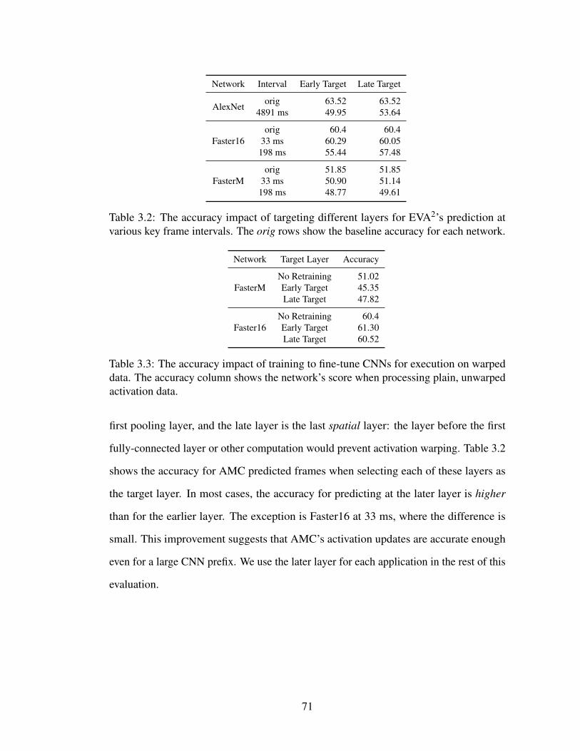
Network Interval Early Target Late Target
AlexNetorig 63.52 63.52
4891 ms 49.95 53.64
Faster16orig 60.4 60.4
33 ms 60.29 60.05198 ms 55.44 57.48
FasterMorig 51.85 51.85
33 ms 50.90 51.14198 ms 48.77 49.61
Table 3.2: The accuracy impact of targeting different layers for EVA2’s prediction atvarious key frame intervals. The orig rows show the baseline accuracy for each network.
Network Target Layer Accuracy
FasterMNo Retraining 51.02Early Target 45.35Late Target 47.82
Faster16No Retraining 60.4Early Target 61.30Late Target 60.52
Table 3.3: The accuracy impact of training to fine-tune CNNs for execution on warpeddata. The accuracy column shows the network’s score when processing plain, unwarpedactivation data.
first pooling layer, and the late layer is the last spatial layer: the layer before the first
fully-connected layer or other computation would prevent activation warping. Table 3.2
shows the accuracy for AMC predicted frames when selecting each of these layers as
the target layer. In most cases, the accuracy for predicting at the later layer is higher
than for the earlier layer. The exception is Faster16 at 33 ms, where the difference is
small. This improvement suggests that AMC’s activation updates are accurate enough
even for a large CNN prefix. We use the later layer for each application in the rest of this
evaluation.
71
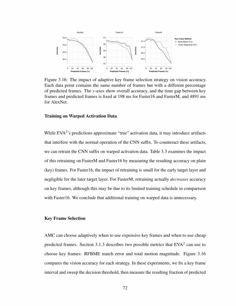
AlexNet Faster16 FasterM
0 20 40 60 80 100
Predicted Frames (%)
0 20 40 60 80 100
Predicted Frames (%)
0 20 40 60 80 100
Predicted Frames (%)
62.5
63.0
63.5
64.0
accuracy
57
58
59
60
61
accuracy
50.0
50.5
51.0
51.5
accuracy
Block Match Error
Vector Magnitude Sum
Key Frame Method
Figure 3.16: The impact of adaptive key frame selection strategy on vision accuracy.Each data point contains the same number of frames but with a different percentageof predicted frames. The y-axes show overall accuracy, and the time gap between keyframes and predicted frames is fixed at 198 ms for Faster16 and FasterM, and 4891 msfor AlexNet.
Training on Warped Activation Data
While EVA2’s predictions approximate “true” activation data, it may introduce artifacts
that interfere with the normal operation of the CNN suffix. To counteract these artifacts,
we can retrain the CNN suffix on warped activation data. Table 3.3 examines the impact
of this retraining on FasterM and Faster16 by measuring the resulting accuracy on plain
(key) frames. For Faster16, the impact of retraining is small for the early target layer and
negligible for the later target layer. For FasterM, retraining actually decreases accuracy
on key frames, although this may be due to its limited training schedule in comparison
with Faster16. We conclude that additional training on warped data is unnecessary.
Key Frame Selection
AMC can choose adaptively when to use expensive key frames and when to use cheap
predicted frames. Section 3.1.3 describes two possible metrics that EVA2 can use to
choose key frames: RFBME match error and total motion magnitude. Figure 3.16
compares the vision accuracy for each strategy. In these experiments, we fix a key frame
interval and sweep the decision threshold, then measure the resulting fraction of predicted
72
frames and the output accuracy. For a fair comparison between the two metrics, each
data point contains the same percentage of predicted frames and key frames for each
metric. A fixed key frame rate would appear as a straight line from the 0% predicted
frames point to the 100%. The curves for both metrics are above this fixed-rate line, so
both are viable strategies. We use the block error metric in our hardware implementation
because it is computationally cheap: block errors are byproducts of RFBME.
3.4 Related Work
EVA2 builds on a wave of recent architectural work on efficient hardware for deep
learning. For a survey of the state of the art, see the tutorial by Sze et al. [121]. Com-
mercial hardware efforts include GPUs and manycores with customized vector and
low-precision instructions [41, 118]. In research, many recent ASICs target convo-
lutional and fully-connected layers [4, 12, 20, 24, 26, 36, 102], as do some FPGA
designs [97, 115, 120, 135]. Recently, accelerators have focused on exploiting sparsity
in model weights and activations [3, 45, 95, 134] and extreme quantization to ternary
or binary values [59, 101, 139]. EVA2’s benefits are orthogonal to these design choices.
Because it skips entire layers during forward execution, it can apply to any underlying
CNN accelerator architecture.
The AMC algorithm uses insights from video compression. Specifically, our RFBME
algorithm builds on a large body of work on the block-matching motion estimation
algorithms that are central to video codecs [64, 75, 140] and their ASIC implementa-
tions [122, 123].
In vision, the most closely related work is deep feature flow (DFF) [141, 142]. DFF
is a neural network design that grafts an optical flow network, FlowNet [40], onto a
73
subset of a feature network, ResNet [48], via a spatial warping layer. The goal is similar
to AMC: DFF uses motion information to avoid computing a prefix of convolutional
layers involved in feature extraction. AMC’s focus on hardware efficiency provides
four key benefits over DFF. (1) While RFBME performs coarse-grained computation at
the receptive-field level, DFF uses a full CNN (FlowNet) to compute per-pixel motion,
which is far more expensive. (2) DFF uses a fixed key frame rate calibrated to the
“worst-case scenario” for scene motion. AMC’s adaptive key frame rate spends less
time and energy when frames are more predictable. (3) AMC’s activation compression
reduces the intermediate data size enough for on-chip storage (80–87%). (4) EVA2’s
warp engine skips over zero entries when performing interpolation, reducing the motion
compensation cost proportionally to the activations’ sparsity.
Other vision work has sought to exploit temporal redundancy for efficiency. Zhang
et al. leverage motion vectors and residuals in compressed video to speed up super-
resolution algorithms [137]. Future work may adapt AMC to replace RFBME with these
precomputed motion vectors. Clockwork convnets [116] exploit the observation that the
values in deeper, more semantic layers change at a slower rate than earlier, noisier layers.
The execution strategy uses fixed update rates, however, and does not adapt to changes in
the input video. Delta networks [91, 92] compute the temporal derivative of the input and
propagate the change through a network, layer by layer. Using pixel-level derivatives,
however, is a poor match for real video data, where even small movements can cause
large changes in pixel values. Section 3.1 discusses delta networks and their efficiency
drawbacks in more detail.
74
3.5 Conclusion
Generic CNN accelerators leave efficiency on the table when they run real-time computer
vision workloads. While this work exploits temporal redundancy to avoid CNN layer
computation, AMC also suggests opportunities for savings in the broader system. Future
work can integrate camera sensors that avoid spending energy to capture redundant
data [11, 18, 77, 88], and end-to-end visual applications can inform the system about
which semantic changes are relevant for their task. A change-oriented visual system
could exploit the motion vectors that hardware video codecs already produce, as recent
work has done for super-resolution [137]. Through holistic co-design, approximately
incremental vision can enable systems that spend resources in proportion to relevant
events in the environment.
75
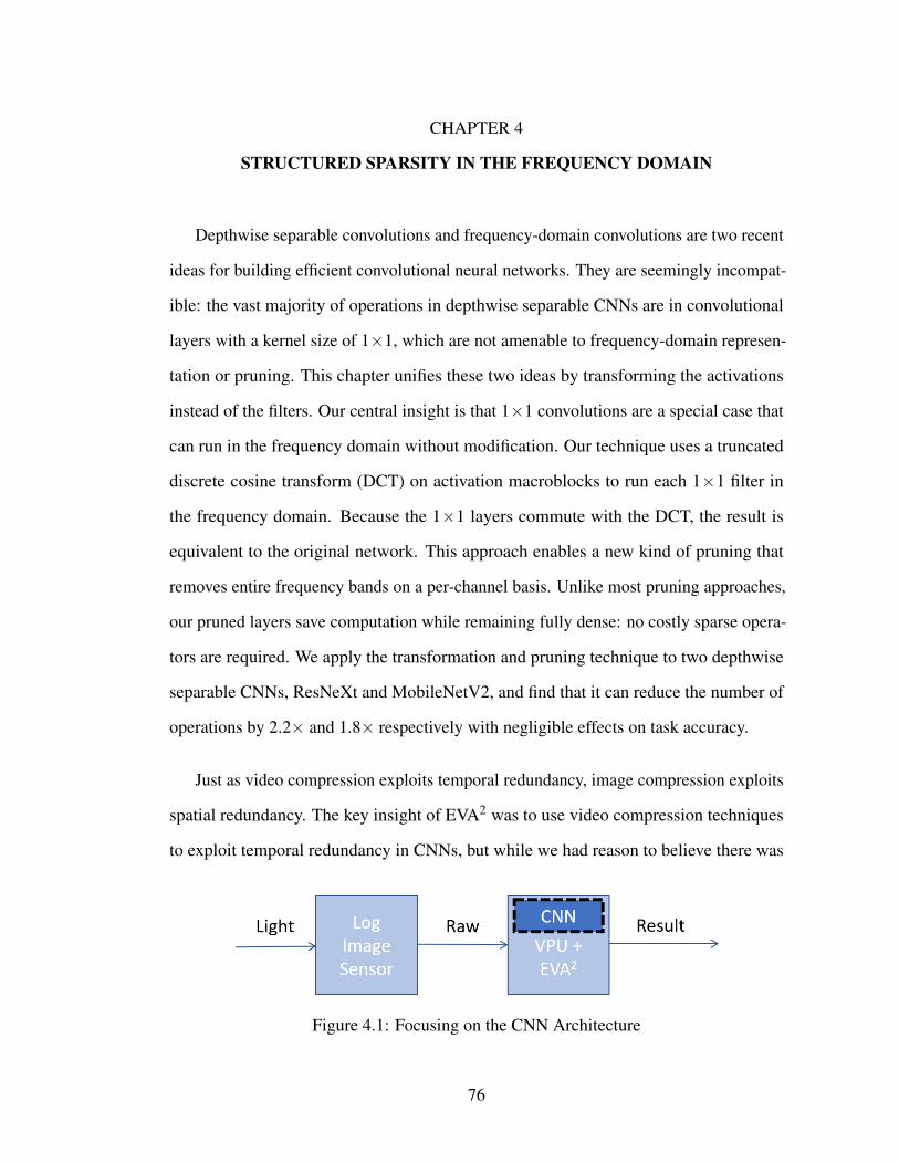
CHAPTER 4
STRUCTURED SPARSITY IN THE FREQUENCY DOMAIN
Depthwise separable convolutions and frequency-domain convolutions are two recent
ideas for building efficient convolutional neural networks. They are seemingly incompat-
ible: the vast majority of operations in depthwise separable CNNs are in convolutional
layers with a kernel size of 1×1, which are not amenable to frequency-domain represen-
tation or pruning. This chapter unifies these two ideas by transforming the activations
instead of the filters. Our central insight is that 1×1 convolutions are a special case that
can run in the frequency domain without modification. Our technique uses a truncated
discrete cosine transform (DCT) on activation macroblocks to run each 1×1 filter in
the frequency domain. Because the 1×1 layers commute with the DCT, the result is
equivalent to the original network. This approach enables a new kind of pruning that
removes entire frequency bands on a per-channel basis. Unlike most pruning approaches,
our pruned layers save computation while remaining fully dense: no costly sparse opera-
tors are required. We apply the transformation and pruning technique to two depthwise
separable CNNs, ResNeXt and MobileNetV2, and find that it can reduce the number of
operations by 2.2× and 1.8× respectively with negligible effects on task accuracy.
Just as video compression exploits temporal redundancy, image compression exploits
spatial redundancy. The key insight of EVA2 was to use video compression techniques
to exploit temporal redundancy in CNNs, but while we had reason to believe there was
Figure 4.1: Focusing on the CNN Architecture
76
spatial redundancy in CNNs, no techniques to exploit this yet existed. For this reason, the
natural follow-up to EVA2 was to move from video compression to image compression.
Image compression techniques generally begin with spatial transformation (such as the
DCT) and quantization to decrease the number of non-zeros required to encode the data.
With the assumption that CNN activations would also require fewer non-zeros to be
represented in the frequency domain, we built and evaluated two techniques to exploit
this property: 1) increase the effectiveness of sparse computational methods by first trans-
forming the input activations, and 2) expose static structured sparsity within activations
by performing truncated frequency transformations before each 1×1 convolution. While
the first technique achieved minimal improvement, the second technique managed to
achieve theoretical speedups of 1.8-2.2×.
Static spatial redundancy refers to the idea that convolutional filters have a heteroge-
neous sensitivity to the spatial frequencies of their inputs despite having a homogeneous
sampling rate. This form of spatial redundancy is a particularly attractive research path
since it exploits frequency based redundancy but doesn’t require any overhead due to
sparse computation. Static spatial redundancy was first observed when per-frequency
pruning of weights exhibited a heavy preference for low frequencies [21]. Two papers
have since taken this observation and used it to save computation. The first is the multi-
scale CNN which purposefully allocates more channels to the low resolution scale, thus
saving on computation [56]. Another paper follows on from the original frequency
based pruning work and computes convolutions in the frequency domain to save on
computation [81]. While these proposals are interesting and relevant, none of them have
paid attention to the dominance of depthwise separable CNNs.
Depthwise separable CNNs pose challenges and offer opportunities simultaneously
when considering the exploitation of frequency based spatial redundancy. 1×1 convolu-
77
tions represent 95% of the total computational cost in depthwise separable CNNs [112],
but 1×1 convolutional filters don’t have any spatial content and thus are incompatible
with frequency based pruning techniques [21, 81]. On the other hand, computing convo-
lutions in the frequency domain requires k2 transformations where k is the width of the
convolutional kernel [33]. This means that 1×1 convolutions are particularly well suited
for computation in the frequency domain as they only require a single transformation and
thus incur low overhead. It is for this reason that I see opportunity.
This chapter is about further increasing the efficiency of a modern category of high-
efficiency CNNs that make heavy use of 1×1 convolution layers [28, 54, 60, 84, 112,
128, 129, 136]. Our key insight is that a 1×1 convolution on an activation image in the
spatial domain is equivalent to the same 1×1 convolution in the frequency domain: as a
result, we can replace any 1×1 convolution in a CNN with a discrete cosine transform
(DCT) followed by the same 1×1 convolution followed by the inverse DCT. We use
this to develop a novel form of pruning, per-channel frequency band pruning, that
prunes the activation image in the frequency domain (after the DCT) by preserving
only contiguous frequency bands that typically yield significant coefficients: as in other
work on frequency-domain computation for CNNs [80], we exploit the fact that some
frequencies matter more than others to reduce computation. By focusing the pruning on
a contiguous band of important frequencies, our pruning technique results in fully dense
computation for the transformed and pruned computations. At similar pruning levels,
dense computation is far more efficient than sparse computation [134], so our technique
outperforms traditional weight pruning, which produces sparse weights by pruning in the
spatial domain. This improves the architecture of the CNN itself, as shown in Figure ??
High-efficiency CNNs have recently trended toward 1×1 convolutions because of
the high cost of larger kernels: the computational cost of convolutional layers scales
78
quadratically with the kernel width. SqueezeNet [60], for example, replaced many 3×3
kernels in a traditional architecture with 1×1 kernels, but it preserved some larger kernels
to extract spatial context from images. Depthwise separable CNNs take this approach a
step farther by emulating traditional 3×3 convolutions, which both incorporate spatial
context and combine data across channels, using a combination of 1×1 convolutions and
depthwise 3×3 convolutions. Depthwise convolutions differ from traditional convolutions
because they are only two dimensional (kernel width by kernel height): each kernel
receives input from only a single channel and produces only one channel of output. A
depthwise convolution may also be seen as a grouped convolution where the number
of groups equals the number of channels. Together, the 1×1 convolutions incorporate
cross-channel information while 3×3 depthwise convolutions capture spatial information,
and their combination can have fewer parameters than the equivalent standard 3×3
convolutional layer. The recent proliferation of depthwise separable CNNs [28, 54, 84,
112, 129, 136] has demonstrated the effectiveness of this approach. In these networks, 1×
1 convolutions overwhelmingly dominate the computational cost: for example, MobileNet
spends 95% of its time in these 1×1 layers [54].
A concurrent but independent research direction has focused on weight pruning as
a mechanism for compressing CNNs. Deep compression [46], for example, removes
near-zero parameters from models without reducing task accuracy. Other work has
used a frequency-domain representation to improve model compression. This category
of work demonstrates that CNNs are more sensitive to low frequencies than to high
frequencies: weight sharing [22], for example, performs better when allocating more
parameters to low frequencies than to high ones. While differences between CNNs
and the human perception system abound, this is one respect in which they are similar:
humans’ lower sensitivity to high spatial frequencies is the assumption that underlies
lossy image compression techniques like JPEG, for instance. More recent work on CNN
79
compression has exploited this imbalanced frequency sensitivity to prune traditional
3×3 convolutional filters [80]. However, weight pruning—whether in the spatial domain
or in a frequency domain—typically results in a sparse model, where zeros appear in
unpredictable locations. Sparse computation can be counterintuitively slower than the
dense computations found in unpruned models: a recent study found, for example, that
even pruning 89% of AlexNet’s [73] weights resulted in a 25% slowdown over the dense,
unpruned network [134]. As a result, current approaches to pruning need to achieve very
high sparsity levels to overcome the overheads of sparse execution.
While depthwise separable networks and frequency-based weight pruning both reduce
parameter volume and computational cost, they are not trivially compatible. The 1×1
filters that dominate computation in these architectures are not amenable to a frequency-
domain transform because they contain no spatial context, and the 3×3 filters account for
an order of magnitude less computation—so pruning them will have a negligible impact
on overall performance. The central goal in this chapter is to properly combine these two
trends by using frequency-domain computation and pruning to speed up the costly 1×1
convolutions. In doing so, we make the following contributions:
• We observe that 1×1 convolutions, which are the primary computational bottleneck
in modern efficiency-focused CNNs, admit frequency-domain computation without
modification.
• We use this style of frequency-domain computation to introduce per-channel
frequency band pruning, which can greatly reduce 1×1 computation costs without
introducing sparsity.
• We show how to apply DCT-based frequency-domain computation in the context
of the residual blocks for two popular depthwise separable CNNs, ResNeXt [129]
and MobileNetV2 [112].
80
In our experiments (Section 4.4), we find that the computational savings for
ResNeXt [129] and MobileNetV2 [112] significantly outstrip the overhead associated
with the DCT conversion. While maintaining task accuracy and keeping all computation
dense, our technique reduces the number of multiply–accumulate (MAC) operations for
these two networks by 2.2× and 1.8× respectively.
4.1 Background
Our work builds upon and combines three lines of work on making CNN inference
efficient: one that develops CNN architectures that can be trained from scratch for small
model sizes and fast inference; one that lowers model sizes of an already trained network
by pruning weights; and one that uses frequency-domain methods to compute CNNs more
efficiently, mostly by leveraging the convolution theorem. We have already discussed
frequency domain CNNs, so here we will discuss efficient CNNs and weight pruning in
more detail.
4.1.1 Depthwise Separable CNNs
While all convolutional CNN feature maps exhibit some spatial redundancy in some
way, the work in this chapter focuses primarily on depthwise separable convolutions.
SqueezeNet [60] demonstrated that 1×1 convolutions were viable and saved significant
computation over 3×3 convolutions, but papers like Xception [28], ResNext [129],
MobileNet [55], ShuffleNet [136], MobileNet v2 [112] and ShuffleNet v2 [84] have all
demonstrated that a traditional 3×3 convolution can be replaced with a 1×1 convolution
followed by a fully grouped (also known as depthwise) 3×3 convolution to form a
81
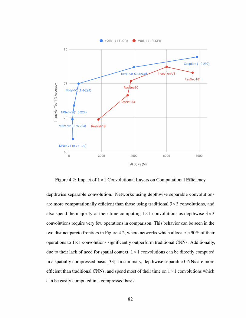
MNet-V1 (0.75-192)
MNet-V2 (0.75-224)
MNet-V2 (1.0-224)
MNet-V2 (1.4-224)
ResNeXt-50-32x4d
Xception (1.0-299)
ResNet-18
ResNet-34
ResNet-50
Inception-V3
ResNet-101
#FLOPs (M)
Imag
eNet
Top
-1 %
Acc
urac
y
65
70
75
80
0 2000 4000 6000 8000
>90% 1x1 FLOPs <90% 1x1 FLOPs
Figure 4.2: Impact of 1×1 Convolutional Layers on Computational Efficiency
depthwise separable convolution. Networks using depthwise separable convolutions
are more computationally efficient than those using traditional 3×3 convolutions, and
also spend the majority of their time computing 1×1 convolutions as depthwise 3×3
convolutions require very few operations in comparison. This behavior can be seen in the
two distinct pareto frontiers in Figure 4.2, where networks which allocate >90% of their
operations to 1×1 convolutions significantly outperform traditional CNNs. Additionally,
due to their lack of need for spatial context, 1×1 convolutions can be directly computed
in a spatially compressed basis [33]. In summary, depthwise separable CNNs are more
efficient than traditional CNNs, and spend most of their time on 1×1 convolutions which
can be easily computed in a compressed basis.
82
4.1.2 Frequency Domain CNNs
One well known method to perform convolutions in the frequency domain is to leverage
the Fourier transforms convolution theorem [87]. This method applies the DFT to both
the convolutional kernel and the input image. Then, the layer multiplies the corresponding
frequency components element-wise. While this method can significantly reduce the
total number of operations required, its benefit isn’t applicable to 1×1 convolutions.
Our work takes inspiration from work that leverages the discrete wavelet transform
(DWT). The DWT has been applied for image compression because natural images
tend to be sparse in the wavelet domain. Drori and Lischinski [34] show that any linear
combination of matrices may be computed in the wavelet domain because the DWT is an
invertible linear operator. Because convolution is commutative and distributive, it may be
computed as a sum of k2 matrices where k is the width of the convolutional filter. This is
desirable for image convolution when computation is performed on a processor which has
a small vector width or a hardware accelerator for sparse matrix multiplication because
image data is highly sparse in the wavelet domain. Just as lossy image compression
with the DWT can significantly reduce image size, lossy convolution with the DWT can
significantly reduce the number of operations required to perform convolution.
[80] use frequency-domain computation to prune models. While both that work and
our static spatial redundancy proposal prune in the frequency domain, the difference is
that that prior work prunes weights while our work prunes activations. In addition, that
earlier technique is designed to prune standard networks like LeNet, AlexNet, and ResNet
that rely on ordinary convolutions. This proposal focuses on improving the inference
efficiency of an emerging class of networks that are already designed for highly efficient
inference: namely, depthwise separable CNNs such as MobileNet and ResNeXt.
83
Efficient CNN architectures. This chapter builds on a line of work on designing CNN
architectures that support efficient inference. One of the earliest of these architectures
was Squeezenet [60], which achieved accuracy comparable to a state-of-the-art CNN
(AlexNet [73]) with substantially fewer weights. MobileNet achieved an even greater
reduction in computation by leveraging depthwise separable convolutions (which were
first introduced in another parameter-efficient architecture, Xception [28]) and a heavy
use of 1×1 convolutions. According to the authors, “Our model structure puts nearly
all of the computation into dense 1×1 convolutions. . . MobileNet spends 95% of its
computation time in 1×1 convolutions which also has 75% of the parameters” [54].
Since then, several other architectures have been built with similar structure, including
MobileNetV2 [112], ShuffleNet [136], ShuffleNetV2 [84], and ResNeXt [129]. In this
chapter, we develop ways to further reduce the cost of inference for an already-trained
network in this class.
Weight pruning. A second approach to efficient inference that we leverage in this
chapter is pruning, in which some of the signals in a neural network are removed after the
network is trained. This is typically done by pruning the weights, in which case it is a type
of model compression [47]. Like the efficient CNN architectures, approaches like deep
compression [46] have matched the performance of AlexNet with substantially fewer
weights. Importantly, as a result of the pruning process, the weights of these networks
become sparse, which can have a negative impact on the inference speed. For example,
pruning with deep compression achieved “3× to 4× speedup over the dense network
on average” while decreasing the number of parameters by 9–13× [46]. Subsequent
works have proposed to use specialized hardware to accelerate the sparse computations
that result from inference on pruned networks; examples of techniques in this class
include EIE [45] and Scalpel [134]. While our work does prune the computations in
84
network inference, we prune the activations, not the weights as is usually done in network
pruning. Additionally, our pruning method results in dense computations, which avoids
the overhead of sparse computations.
4.2 Methodology
This section describes our technique for running 1×1 convolutions in a DCT-based
frequency space. We then show how to prune the transformed network according to
frequency bands in the transformed data. Finally, we show how to practically apply the
technique to existing architectures for depthwise separable CNNs.
4.2.1 Frequency-Domain 1×1 Convolutions
Our approach to frequency-domain computation is to compress activation data using the
same approach as JPEG image compression: we divide an activation tensor into small,
fixed-size, square tiles called macroblocks and apply the discrete cosine transform (DCT)
to each. The key observation is that running a onebyone convolution on this transformed
data is equivalent to running it on the original activation, i.e.:
Conv1×1(X) = DCT−1(Conv1×1(DCT(X)))
where X is an activation tensor, DCT is the macroblocked discrete cosine transform, and
DCT−1 is the inverse transformation. This is possible because the DCT is an invertible
linear operator just like the DWT. Therefore, frequency-domain computation of 1×1
convolutions does not require frequency-domain training: we can train the entire network
normally, without the transformations, and then insert DCT and inverse DCT “layers” to
obtain an equivalent network.
85
To implement the DCT, we need to choose a macroblock size. The JPEG standard,
for example, uses 8×8-pixel macroblocks to localize frequency information to specific
locations within the image. In our setting, macroblock size represents a trade-off between
the precision of frequency-domain pruning and the performance overhead. With larger
macroblocks, the transformation can more effectively separate frequency components
from one another, which leads to better potential for pruning. On the other hand, the DCT
forms the overhead cost for our technique, and the cost of the DCT for k×k macroblocks
scales with k2. In our experiments, we find that 4×4 macroblocks work well across both
networks we evaluate.
Choosing the DCT macroblock width is also important because it determines the
overhead required to transform the activations into the frequency domain. As each channel
is transformed into the frequency domain independently, the DCT can be computed as
a depthwise convolution with the kernel size and stride equal to the macroblock width.
Each macroblock is multiplied by frequency filters (of size k2) for each coefficient (of
which there are k2). With this implementation of the DCT, the number of required
operations is:
DCT MACs = cin ∗hk∗ w
k∗ k4 = cin ∗h∗w∗ k2
Processing the same input with a 1×1 convolution with a stride of 1 would require the
following operations
1×1 MACs = cin ∗h∗w∗ cout
From these two equations it can be seen that the number of operations for a 4×4 DCT
would be equivalent to a 1×1 convolution with 16 output channels. Thankfully most
network layers produce far more than 16 channels, and so in the general case our overhead
is an insignificantly small portion of the total network operations.
86
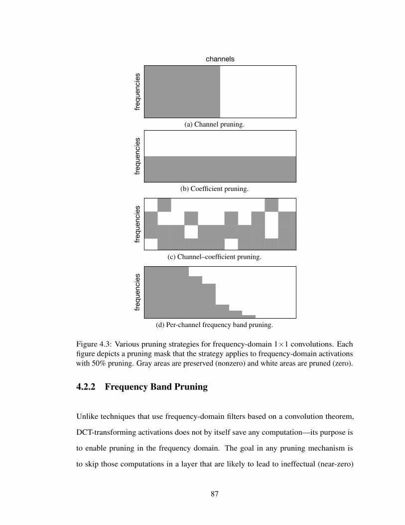
frequ
encie
s
channels
(a) Channel pruning.
frequ
encie
s
(b) Coefficient pruning.
frequ
encie
s
(c) Channel–coefficient pruning.
frequ
encie
s
(d) Per-channel frequency band pruning.
Figure 4.3: Various pruning strategies for frequency-domain 1×1 convolutions. Eachfigure depicts a pruning mask that the strategy applies to frequency-domain activationswith 50% pruning. Gray areas are preserved (nonzero) and white areas are pruned (zero).
4.2.2 Frequency Band Pruning
Unlike techniques that use frequency-domain filters based on a convolution theorem,
DCT-transforming activations does not by itself save any computation—its purpose is
to enable pruning in the frequency domain. The goal in any pruning mechanism is
to skip those computations in a layer that are likely to lead to ineffectual (near-zero)
87
activation results. The standard approach, weight pruning, rounds small weights down to
zero and removes them from the model. Weight pruning’s primary drawback is that it
results in sparse computation, since while many weights may be zero, zero weights are
not typically grouped together. Sparse computation is significantly slower than dense
computation even as it reduces the overall number of operations required because of its
need for frequent branches [134]. An alternative, channel pruning, removes nodes from
the neural network by zeroing out entire filters. Figure 4.3a depicts channel pruning.
Because channel pruning works at a larger granularity than weight pruning, it does not
require sparse computation, but the granularity also limits the amount of computation it
can eliminate.
Our goal is to prune contiguous components of a frequency-domain 1×1 convolution.
This techniques enables a large amount of pruning while also enforcing contiguity and
hence allowing dense computation. The rest of this section describes three approaches
to pruning in increasing order of sophistication: a simple sparse coefficient pruning
approach; a per-channel, per-coefficient technique that can adapt to the varying frequency
sensitivity among different channels; and the proposed frequency band pruning approach
that prunes a contiguous range of high-frequency components.
Coefficient pruning. The first and simplest approach prunes entire coefficients, inde-
pendent of the layer’s output channels. Figure 4.3b depicts a coefficient pruning mask: all
channels preserve the same set of “important” frequencies. For each layer, we compute
the average coefficient magnitude by aggregating across all output channels in the layer.
To prune, we select a percentile under which the smallest coefficients are removed in each
layer. After pruning, the coefficients whose average magnitude is below the threshold are
never computed.
88
This approach results in dense computation because the unpruned frequencies can
be reordered and packed into a dense tensor. However, this approach expresses the
(incorrect) assumption that all output channels are equally sensitive to each frequency in
the activation data. We find that channels are not uniformly sensitive to frequencies in
practice, which motivates a more nuanced approach.
Like our other pruning techniques, coefficient pruning can reduce both the cost
of the 1×1 convolution and the overhead associated with the DCT and inverse-DCT
computations. It is not necessary to produce frequency coefficients that will never be
used during the pruned 1×1 layer. Our technique truncates the DCT to produce only the
unpruned coefficients.
Channel–coefficient pruning. Channel–coefficient pruning removes the assumption
that all channels within a layer are uniformly sensitive to each frequency. Instead, it
acknowledges that some channels need different frequency information from others.
Intuitively, some channels represent features that require more detail (and hence higher
frequencies) than others. Channel–coefficient pruning does not average across chan-
nels but instead prunes a percentile of coefficients within each channel for each layer.
Figure 4.3c depicts the result: each channel receives a subset of the frequency coefficients.
We find that this per-channel sensitivity significantly increases the amount of pruning
that is possible for a given accuracy budget. However, the additional flexibility comes at
a cost: the “random” effect of the pruning means that the 1×1 filter computation must be
sparse. It is not generally possible to reorder channels and coefficients to pack them into
a dense tensor for fast computation.
89
Frequency band pruning. Our final approach extends frequency–coefficient pruning
to remove contiguous ranges of frequencies, thereby recovering dense computation. The
key idea relies on the insight from prior work that CNNs are more sensitive to low
frequencies than to high frequencies [22, 80, 82]. Put differently, coefficient importance
is monotonic with frequency—so if a given coefficient is pruned, all the higher-frequency
coefficients are also likely to be pruned. Frequency band pruning restricts pruning to a
contiguous range of the highest frequencies. Like channel–coefficient pruning, it prunes
coefficients within a given channel; unlike the unrestricted version, however, it preserves
the lowest-frequency coefficients up to the last (i.e., highest-frequency) coefficient whose
average magnitude exceeds the threshold. Figure 4.3d shows the resulting mask: each
channel receives a contiguous range of frequencies starting at the lowest frequency.
These contiguous ranges of frequencies correspond to the diagonals in the 2D DCT
transformation. The zigzag pattern commonly associated with JPEG is another use of
this frequency banding when using the DCT.
With this strategy, each channel’s computation in the 1×1 filter is dense. We find that
this technique prunes nearly the same set of channels as unrestricted channel–coefficient
pruning: significant frequencies naturally tend to be nearly contiguous. So this technique
loses only a few pruned coefficients while making computation dense and therefore far
more efficient.
4.2.3 Profiled vs. Learned Pruning
Channel, coefficient, channel–coefficient, and per-channel frequency band pruning each
represent different methods for coefficient/channel masks, but how exactly to set these
masks is non-trivial. Which coefficients should be masked for which channels ultimately
90
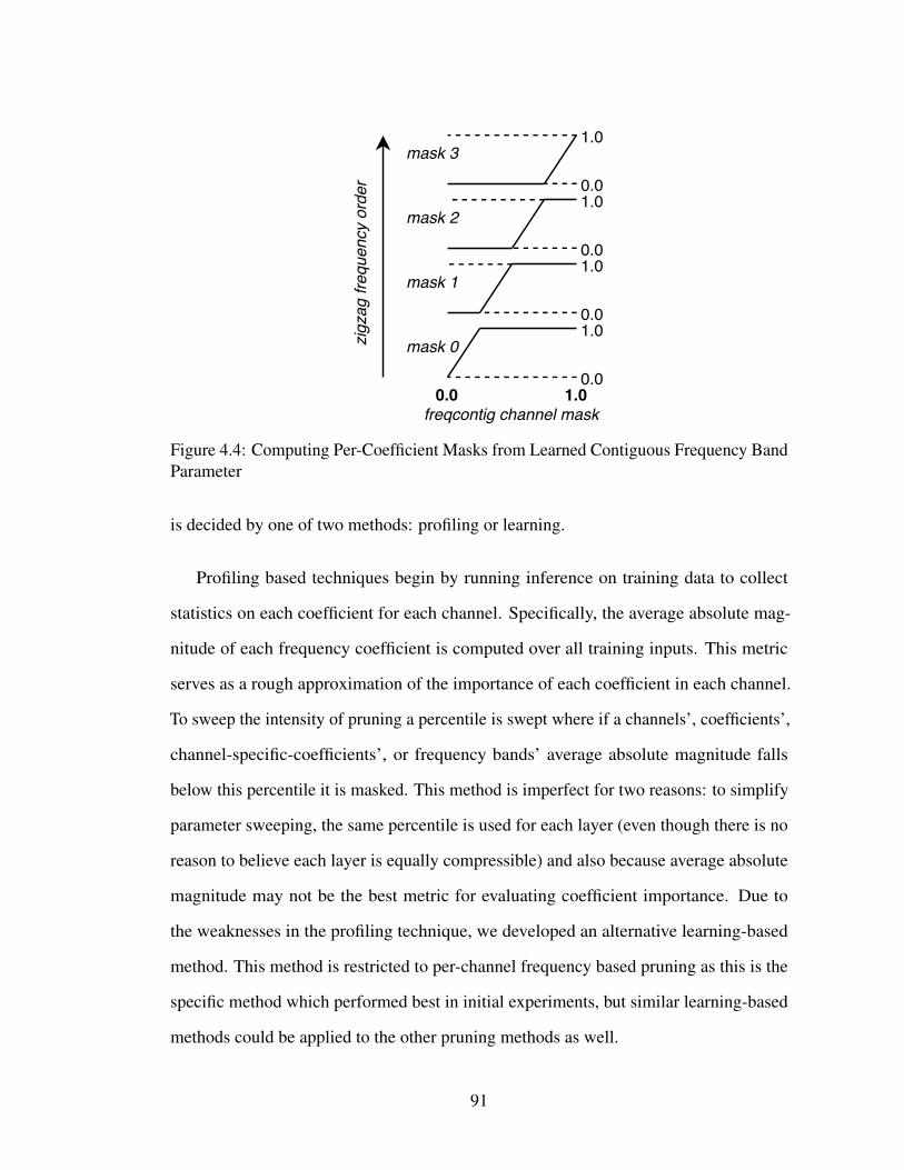
mask 0
mask 1
mask 2
mask 3
zigz
ag fr
eque
ncy
orde
r
0.0 1.00.0
0.0
0.0
0.0
1.0
1.0
1.0
1.0
freqcontig channel mask
Figure 4.4: Computing Per-Coefficient Masks from Learned Contiguous Frequency BandParameter
is decided by one of two methods: profiling or learning.
Profiling based techniques begin by running inference on training data to collect
statistics on each coefficient for each channel. Specifically, the average absolute mag-
nitude of each frequency coefficient is computed over all training inputs. This metric
serves as a rough approximation of the importance of each coefficient in each channel.
To sweep the intensity of pruning a percentile is swept where if a channels’, coefficients’,
channel-specific-coefficients’, or frequency bands’ average absolute magnitude falls
below this percentile it is masked. This method is imperfect for two reasons: to simplify
parameter sweeping, the same percentile is used for each layer (even though there is no
reason to believe each layer is equally compressible) and also because average absolute
magnitude may not be the best metric for evaluating coefficient importance. Due to
the weaknesses in the profiling technique, we developed an alternative learning-based
method. This method is restricted to per-channel frequency based pruning as this is the
specific method which performed best in initial experiments, but similar learning-based
methods could be applied to the other pruning methods as well.
91
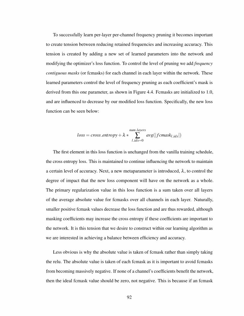
To successfully learn per-layer per-channel frequency pruning it becomes important
to create tension between reducing retained frequencies and increasing accuracy. This
tension is created by adding a new set of learned parameters into the network and
modifying the optimizer’s loss function. To control the level of pruning we add frequency
contiguous masks (or fcmasks) for each channel in each layer within the network. These
learned parameters control the level of frequency pruning as each coefficient’s mask is
derived from this one parameter, as shown in Figure 4.4. Fcmasks are initialized to 1.0,
and are influenced to decrease by our modified loss function. Specifically, the new loss
function can be seen below:
loss = cross entropy+λ ∗num layers
∑l idx=0
avg(| f cmaskl idx|)
The first element in this loss function is unchanged from the vanilla training schedule,
the cross entropy loss. This is maintained to continue influencing the network to maintain
a certain level of accuracy. Next, a new metaparameter is introduced, λ , to control the
degree of impact that the new loss component will have on the network as a whole.
The primary regularization value in this loss function is a sum taken over all layers
of the average absolute value for fcmasks over all channels in each layer. Naturally,
smaller positive fcmask values decrease the loss function and are thus rewarded, although
masking coefficients may increase the cross entropy if these coefficients are important to
the network. It is this tension that we desire to construct within our learning algorithm as
we are interested in achieving a balance between efficiency and accuracy.
Less obvious is why the absolute value is taken of fcmask rather than simply taking
the relu. The absolute value is taken of each fcmask as it is important to avoid fcmasks
from becoming massively negative. If none of a channel’s coefficients benefit the network,
then the ideal fcmask value should be zero, not negative. This is because if an fcmask
92
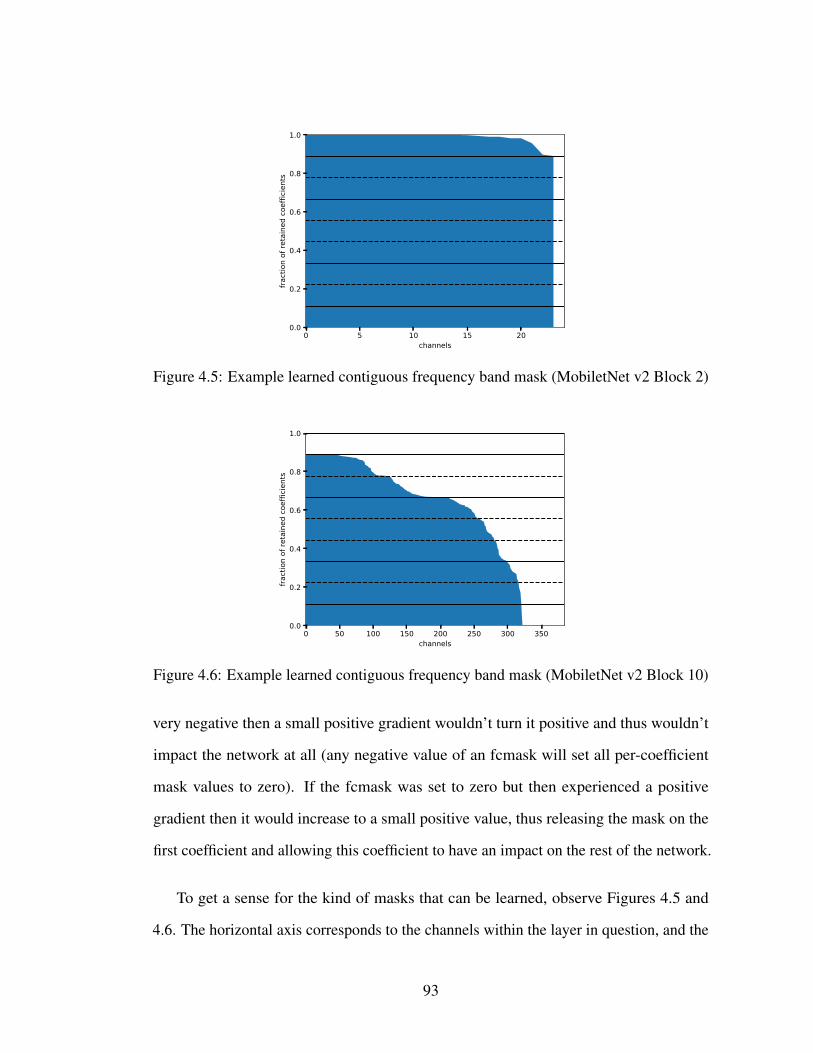
0 5 10 15 20channels
0.0
0.2
0.4
0.6
0.8
1.0
fract
ion
of re
tain
ed c
oeffi
cient
s
Figure 4.5: Example learned contiguous frequency band mask (MobiletNet v2 Block 2)
0 50 100 150 200 250 300 350channels
0.0
0.2
0.4
0.6
0.8
1.0
fract
ion
of re
tain
ed c
oeffi
cient
s
Figure 4.6: Example learned contiguous frequency band mask (MobiletNet v2 Block 10)
very negative then a small positive gradient wouldn’t turn it positive and thus wouldn’t
impact the network at all (any negative value of an fcmask will set all per-coefficient
mask values to zero). If the fcmask was set to zero but then experienced a positive
gradient then it would increase to a small positive value, thus releasing the mask on the
first coefficient and allowing this coefficient to have an impact on the rest of the network.
To get a sense for the kind of masks that can be learned, observe Figures 4.5 and
4.6. The horizontal axis corresponds to the channels within the layer in question, and the
93
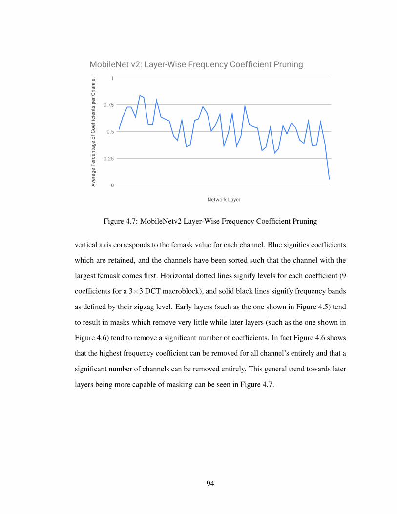
Network Layer
Aver
age
Perc
enta
ge o
f Coe
ffic
ient
s pe
r Cha
nnel
0
0.25
0.5
0.75
1
MobileNet v2: Layer-Wise Frequency Coefficient Pruning
Figure 4.7: MobileNetv2 Layer-Wise Frequency Coefficient Pruning
vertical axis corresponds to the fcmask value for each channel. Blue signifies coefficients
which are retained, and the channels have been sorted such that the channel with the
largest fcmask comes first. Horizontal dotted lines signify levels for each coefficient (9
coefficients for a 3×3 DCT macroblock), and solid black lines signify frequency bands
as defined by their zigzag level. Early layers (such as the one shown in Figure 4.5) tend
to result in masks which remove very little while later layers (such as the one shown in
Figure 4.6) tend to remove a significant number of coefficients. In fact Figure 4.6 shows
that the highest frequency coefficient can be removed for all channel’s entirely and that a
significant number of channels can be removed entirely. This general trend towards later
layers being more capable of masking can be seen in Figure 4.7.
94
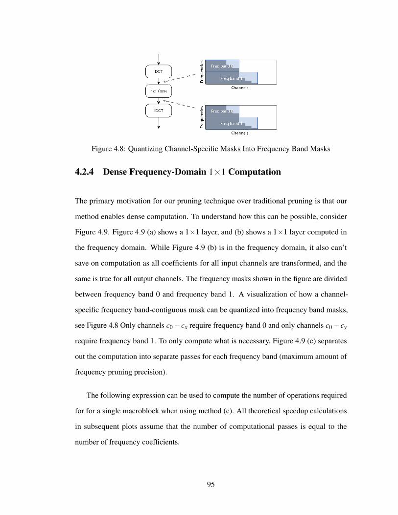
Figure 4.8: Quantizing Channel-Specific Masks Into Frequency Band Masks
4.2.4 Dense Frequency-Domain 1×1 Computation
The primary motivation for our pruning technique over traditional pruning is that our
method enables dense computation. To understand how this can be possible, consider
Figure 4.9. Figure 4.9 (a) shows a 1×1 layer, and (b) shows a 1×1 layer computed in
the frequency domain. While Figure 4.9 (b) is in the frequency domain, it also can’t
save on computation as all coefficients for all input channels are transformed, and the
same is true for all output channels. The frequency masks shown in the figure are divided
between frequency band 0 and frequency band 1. A visualization of how a channel-
specific frequency band-contiguous mask can be quantized into frequency band masks,
see Figure 4.8 Only channels c0− cx require frequency band 0 and only channels c0− cy
require frequency band 1. To only compute what is necessary, Figure 4.9 (c) separates
out the computation into separate passes for each frequency band (maximum amount of
frequency pruning precision).
The following expression can be used to compute the number of operations required
for for a single macroblock when using method (c). All theoretical speedup calculations
in subsequent plots assume that the number of computational passes is equal to the
number of frequency coefficients.
95
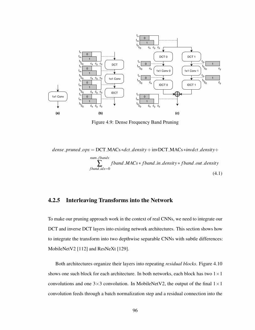
1x1 Conv
DCT
IDCT
1x1 Conv 0
DCT 0
IDCT 0
1x1 Conv 1
DCT 1
IDCT 1
10
fnfmf0ĉ0 ĉx ĉy ĉz
10
fnfmf0c0 cx cy cz
0fnfmc0 cx
1fmf0c0 cy
0fnfmĉ0 ĉx
1fmf0ĉ0 ĉy
10
fnfmf0ĉ0 ĉx ĉy ĉz
10
fnfmf0ĉ0 ĉx ĉy ĉz
10
fnfmf0c0 cx cy cz
10
fnfmf0c0 cx cy cz
(b) (c)
1x1 Conv
(a)
Figure 4.9: Dense Frequency Band Pruning
dense pruned ops = DCT MACs∗dct density+ invDCT MACs∗invdct density+
num f bands
∑f band idx=0
f band MACs∗ f band in density∗ f band out density
(4.1)
4.2.5 Interleaving Transforms into the Network
To make our pruning approach work in the context of real CNNs, we need to integrate our
DCT and inverse DCT layers into existing network architectures. This section shows how
to integrate the transform into two depthwise separable CNNs with subtle differences:
MobileNetV2 [112] and ResNeXt [129].
Both architectures organize their layers into repeating residual blocks. Figure 4.10
shows one such block for each architecture. In both networks, each block has two 1×1
convolutions and one 3×3 convolution. In MobileNetV2, the output of the final 1×1
convolution feeds through a batch normalization step and a residual connection into the
96
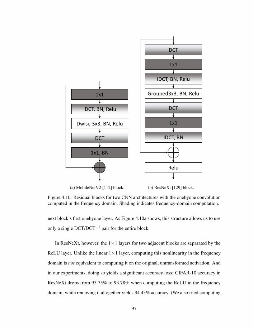
1x1
IDCT, BN, Relu
Dwise 3x3, BN, Relu
DCT
1x1, BN
(a) MobileNetV2 [112] block.
1x1
IDCT, BN, Relu
Grouped3x3, BN, Relu
DCT
1x1
DCT
IDCT, BN
Relu
(b) ResNeXt [129] block.
Figure 4.10: Residual blocks for two CNN architectures with the onebyone convolutioncomputed in the frequency domain. Shading indicates frequency-domain computation.
next block’s first onebyone layer. As Figure 4.10a shows, this structure allows us to use
only a single DCT/DCT−1 pair for the entire block.
In ResNeXt, however, the 1×1 layers for two adjacent blocks are separated by the
ReLU layer. Unlike the linear 1×1 layer, computing this nonlinearity in the frequency
domain is not equivalent to computing it on the original, untransformed activation. And
in our experiments, doing so yields a significant accuracy loss: CIFAR-10 accuracy in
ResNeXt drops from 95.75% to 93.78% when computing the ReLU in the frequency
domain, while removing it altogether yields 94.43% accuracy. (We also tried computing
97
the ReLU only on the DC component of the frequency-domain data, but the accuracy
still dropped to 95.01%.) Figure 4.10b shows how to insert two DCT/inverse-DCT
pairs into ResNeXt, with one around each 1×1 layer and with all ReLUs computed on
untransformed inputs. As we find in Section 4.4.1, the additional overhead from doubling
the transformations does not result in significant performance cost.
4.3 Experimental Setup
We evaluate the effectiveness of our frequency band activation pruning on two state-of-
the-art networks, MobileNetV2 [112] and ResNeXt [129]. For ResNeXt we chose a
cardinality of 32 and a bottleneck width of 4. Section 4.5 gives further network details. We
evaluate both networks on the CIFAR-10 [72] classification dataset, which is sufficiently
complex to demonstrate our technique while being small enough to enable rapid design
iteration. The top-1 CIFAR-10 accuracy for the baseline, unpruned configuration is
94.02% for MobileNetV2 and 95.75% for ResNeXt.
We evaluate computation savings by measuring the number of multiply–accumulate
(MAC) operations among all convolutional layers. In the baseline configuration for
CIFAR-10, ResNeXt uses 7.7×10⁸ MACs and MobileNetV2 uses 8.9×10⁷. We add
DCT and inverse-DCT transformation layers to each using 4×4 macroblocks, which
increases the MAC counts to 8.4×10⁸ for ResNeXt and 1.1×10⁸ for MobileNetV2.
98
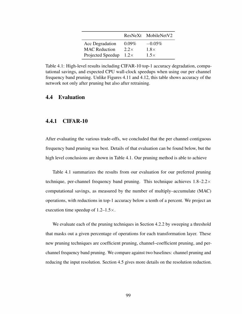
ResNeXt MobileNetV2
Acc Degradation 0.09% −0.05%MAC Reduction 2.2× 1.8×Projected Speedup 1.2× 1.5×
Table 4.1: High-level results including CIFAR-10 top-1 accuracy degradation, compu-tational savings, and expected CPU wall-clock speedups when using our per channelfrequency band pruning. Unlike Figures 4.11 and 4.12, this table shows accuracy of thenetwork not only after pruning but also after retraining.
4.4 Evaluation
4.4.1 CIFAR-10
After evaluating the various trade-offs, we concluded that the per channel contiguous
frequency band pruning was best. Details of that evaluation can be found below, but the
high level conclusions are shown in Table 4.1. Our pruning method is able to achieve
Table 4.1 summarizes the results from our evaluation for our preferred pruning
technique, per-channel frequency band pruning. This technique achieves 1.8–2.2×
computational savings, as measured by the number of multiply–accumulate (MAC)
operations, with reductions in top-1 accuracy below a tenth of a percent. We project an
execution time speedup of 1.2–1.5×.
We evaluate each of the pruning techniques in Section 4.2.2 by sweeping a threshold
that masks out a given percentage of operations for each transformation layer. These
new pruning techniques are coefficient pruning, channel–coefficient pruning, and per-
channel frequency band pruning. We compare against two baselines: channel pruning and
reducing the input resolution. Section 4.5 gives more details on the resolution reduction.
99
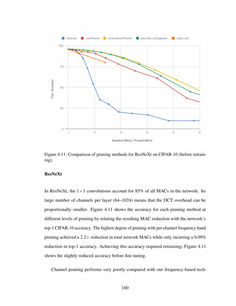
Baseline MACs / Pruned MACs
Top1
Acc
urac
y
0
25
50
75
100
1 2 3 4 5 6
channel coefficient channelcoefficient perchan_contigband input_res
Figure 4.11: Comparison of pruning methods for ResNeXt on CIFAR-10 (before retrain-ing).
ResNeXt
In ResNeXt, the 1×1 convolutions account for 85% of all MACs in the network. Its
large number of channels per layer (64–1024) means that the DCT overhead can be
proportionally smaller. Figure 4.11 shows the accuracy for each pruning method at
different levels of pruning by relating the resulting MAC reduction with the network’s
top-1 CIFAR-10 accuracy. The highest degree of pruning with per channel frequency band
pruning achieved a 2.2× reduction in total network MACs while only incurring a 0.09%
reduction in top-1 accuracy. Achieving this accuracy required retraining; Figure 4.11
shows the slightly reduced accuracy before fine tuning.
Channel pruning performs very poorly compared with our frequency-based tech-
100
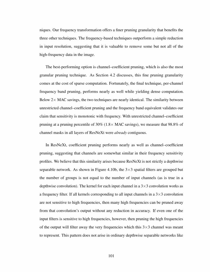
niques. Our frequency transformation offers a finer pruning granularity that benefits the
three other techniques. The frequency-based techniques outperform a simple reduction
in input resolution, suggesting that it is valuable to remove some but not all of the
high-frequency data in the image.
The best-performing option is channel–coefficient pruning, which is also the most
granular pruning technique. As Section 4.2 discusses, this fine pruning granularity
comes at the cost of sparse computation. Fortunately, the final technique, per-channel
frequency band pruning, performs nearly as well while yielding dense computation.
Below 2×MAC savings, the two techniques are nearly identical. The similarity between
unrestricted channel–coefficient pruning and the frequency band equivalent validates our
claim that sensitivity is monotonic with frequency. With unrestricted channel–coefficient
pruning at a pruning percentile of 30% (1.8×MAC savings), we measure that 98.8% of
channel masks in all layers of ResNeXt were already contiguous.
In ResNeXt, coefficient pruning performs nearly as well as channel–coefficient
pruning, suggesting that channels are somewhat similar in their frequency sensitivity
profiles. We believe that this similarity arises because ResNeXt is not strictly a depthwise
separable network. As shown in Figure 4.10b, the 3×3 spatial filters are grouped but
the number of groups is not equal to the number of input channels (as is true in a
depthwise convolution). The kernel for each input channel in a 3×3 convolution works as
a frequency filter. If all kernels corresponding to all input channels in a 3×3 convolution
are not sensitive to high frequencies, then many high frequencies can be pruned away
from that convolution’s output without any reduction in accuracy. If even one of the
input filters is sensitive to high frequencies, however, then pruning the high frequencies
of the output will filter away the very frequencies which this 3×3 channel was meant
to represent. This pattern does not arise in ordinary depthwise separable networks like
101
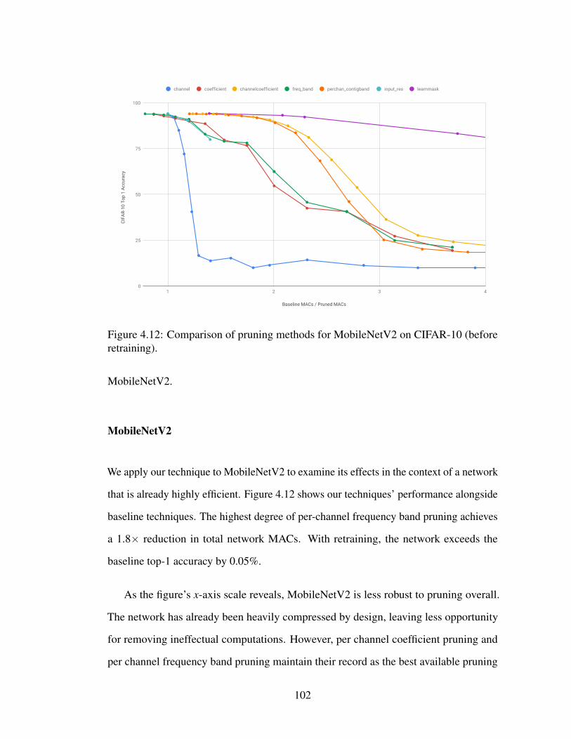
Baseline MACs / Pruned MACs
CIFA
R-10
Top
1 A
ccur
acy
0
25
50
75
100
1 2 3 4
channel coefficient channelcoefficient freq_band perchan_contigband input_res learnmask
Figure 4.12: Comparison of pruning methods for MobileNetV2 on CIFAR-10 (beforeretraining).
MobileNetV2.
MobileNetV2
We apply our technique to MobileNetV2 to examine its effects in the context of a network
that is already highly efficient. Figure 4.12 shows our techniques’ performance alongside
baseline techniques. The highest degree of per-channel frequency band pruning achieves
a 1.8× reduction in total network MACs. With retraining, the network exceeds the
baseline top-1 accuracy by 0.05%.
As the figure’s x-axis scale reveals, MobileNetV2 is less robust to pruning overall.
The network has already been heavily compressed by design, leaving less opportunity
for removing ineffectual computations. However, per channel coefficient pruning and
per channel frequency band pruning maintain their record as the best available pruning
102
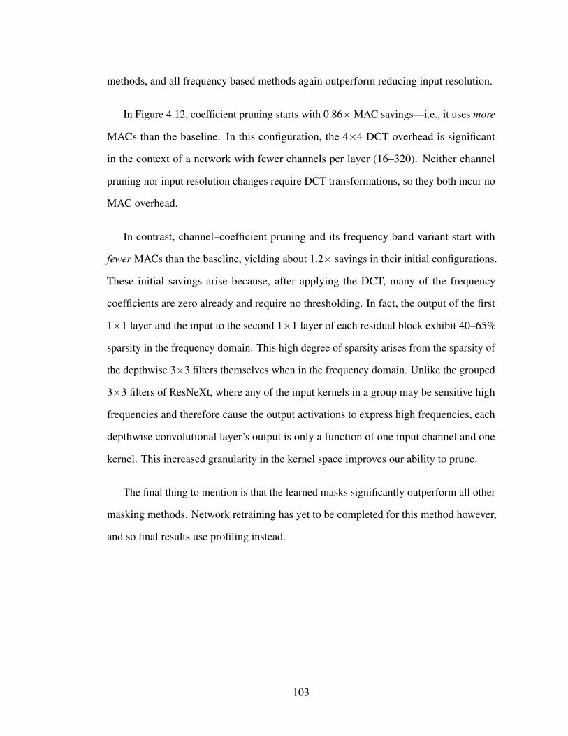
methods, and all frequency based methods again outperform reducing input resolution.
In Figure 4.12, coefficient pruning starts with 0.86×MAC savings—i.e., it uses more
MACs than the baseline. In this configuration, the 4×4 DCT overhead is significant
in the context of a network with fewer channels per layer (16–320). Neither channel
pruning nor input resolution changes require DCT transformations, so they both incur no
MAC overhead.
In contrast, channel–coefficient pruning and its frequency band variant start with
fewer MACs than the baseline, yielding about 1.2× savings in their initial configurations.
These initial savings arise because, after applying the DCT, many of the frequency
coefficients are zero already and require no thresholding. In fact, the output of the first
1×1 layer and the input to the second 1×1 layer of each residual block exhibit 40–65%
sparsity in the frequency domain. This high degree of sparsity arises from the sparsity of
the depthwise 3×3 filters themselves when in the frequency domain. Unlike the grouped
3×3 filters of ResNeXt, where any of the input kernels in a group may be sensitive high
frequencies and therefore cause the output activations to express high frequencies, each
depthwise convolutional layer’s output is only a function of one input channel and one
kernel. This increased granularity in the kernel space improves our ability to prune.
The final thing to mention is that the learned masks significantly outperform all other
masking methods. Network retraining has yet to be completed for this method however,
and so final results use profiling instead.
103
Baseline MACs / Pruned MACs
Top1
Acc
urac
y
0
20
40
60
80
0.9 1 1.1 1.2 1.3 1.4 1.5
perchan_contigband channelcoefficient channel freq_band coefficient learnmask
Figure 4.13: Comparison of pruning methods for MobileNetV2 on ImageNet (beforeretraining).
4.4.2 ImageNet
While CIFAR-10 is useful for early experiments, final results for this technique will need
to include ImageNet. ImageNet is a significantly more complex task as it contains 1000
instead of 10 classes, and perhaps more importantly for our method, the resolution is
typically 224 instead of 32. Early ImageNet results for MobileNet v2 (a small depthwise
separable network) and Xception (a large depthwise separable network) can be seen in
Figures 4.13 and 4.14. Unfortunately, the profiling based techniques do not perform
very well on ImageNet. This is possibly because the average absolute magnitude is no
longer a good metric for evaluating the importance of channel coefficients. Thankfully,
our learning based masking technique is certainly effective as can be seen by the one
evaluated point in Figure 4.13.
104
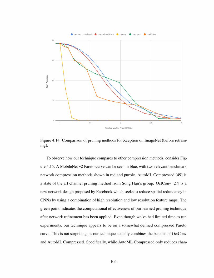
Baseline MACs / Pruned MACs
Top1
Acc
urac
y
0
20
40
60
80
1 1.5 2 2.5 3
perchan_contigband channelcoefficient channel freq_band coefficient
Figure 4.14: Comparison of pruning methods for Xception on ImageNet (before retrain-ing).
To observe how our technique compares to other compression methods, consider Fig-
ure 4.15. A MobileNet v2 Pareto curve can be seen in blue, with two relevant benchmark
network compression methods shown in red and purple. AutoML Compressed [49] is
a state of the art channel pruning method from Song Han’s group. OctConv [27] is a
new network design proposed by Facebook which seeks to reduce spatial redundancy in
CNNs by using a combination of high resolution and low resolution feature maps. The
green point indicates the computational effectiveness of our learned pruning technique
after network refinement has been applied. Even though we’ve had limited time to run
experiments, our technique appears to be on a somewhat defined compressed Pareto
curve. This is not surprising, as our technique actually combines the benefits of OctConv
and AutoML Compressed. Specifically, while AutoML Compressed only reduces chan-
105
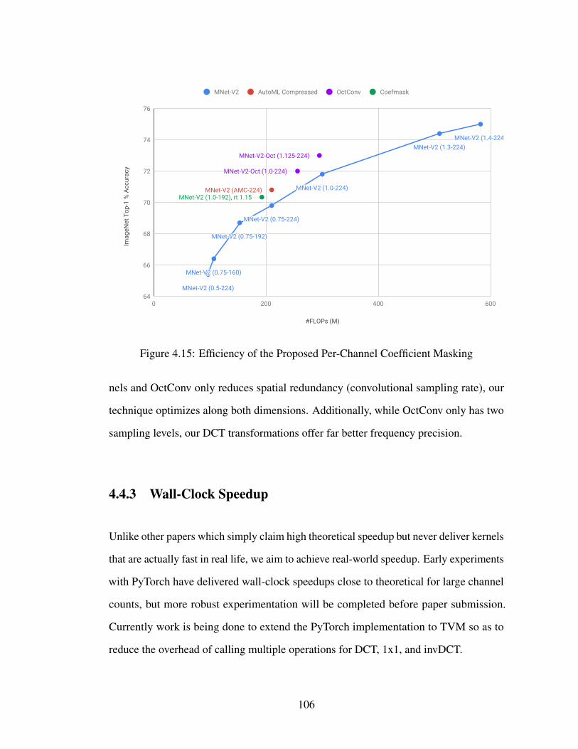
MNet-V2 (0.5-224)
MNet-V2 (0.75-160)
MNet-V2 (0.75-192)
MNet-V2 (0.75-224)
MNet-V2 (1.0-224)
MNet-V2 (1.3-224)MNet-V2 (1.4-224)
MNet-V2 (AMC-224)
MNet-V2-Oct (1.0-224)
MNet-V2-Oct (1.125-224)
MNet-V2 (1.0-192), rt 1.15
#FLOPs (M)
Imag
eNet
Top
-1 %
Acc
urac
y
64
66
68
70
72
74
76
0 200 400 600
MNet-V2 AutoML Compressed OctConv Coefmask
Figure 4.15: Efficiency of the Proposed Per-Channel Coefficient Masking
nels and OctConv only reduces spatial redundancy (convolutional sampling rate), our
technique optimizes along both dimensions. Additionally, while OctConv only has two
sampling levels, our DCT transformations offer far better frequency precision.
4.4.3 Wall-Clock Speedup
Unlike other papers which simply claim high theoretical speedup but never deliver kernels
that are actually fast in real life, we aim to achieve real-world speedup. Early experiments
with PyTorch have delivered wall-clock speedups close to theoretical for large channel
counts, but more robust experimentation will be completed before paper submission.
Currently work is being done to extend the PyTorch implementation to TVM so as to
reduce the overhead of calling multiple operations for DCT, 1x1, and invDCT.
106
4.5 Implementation Details
We built and trained CIFAR-10 versions of ResNeXt and MobileNetV2 using PyTorch.
Our evaluation platform used four Nvidia GTX Titan X GPUs.
The architecture for ResNeXt was taken directly from the original paper [129], which
already includes CIFAR-10 experiments. The version used in this chapter has a cardinality
of 32 and a bottleneck width of 4. Training hyperparameters are the same as those used
in the original paper.
For MobileNetV2 we built a modified version of the 1.0×wide ImageNet architecture.
The network contained 7 bottleneck stages, with each stage containing 1, 2, 3, 4, 3, 3,
and 1 residual blocks respectively. We modified the initial 2D 3×3 convolutional layer
to have a stride of 1, and we used strides of 2 in the first stage of the 3rd, 4th, and 6th
bottlenecks. The network was trained with the same hyperparameters as those used in
the paper, with the exception that the learning rate was scaled by 0.98 for every epoch
instead of every 2.5 epochs.
As mentioned in the evaluation section, we also trained versions of ResNeXt and
MobileNetV2 on reduced-resolution input. To produce this input, we began with the
standard 32×32 resolution CIFAR-10 data and used PyTorch’s interpolation layer using
the area algorithm to reduce its size to 16 or 8 pixels wide. When receiving 16-pixel
input, the first layer in each network with a stride of 2 was changed to have stride 1; when
receiving 8-pixel input, both of the first two layers in each network with a stride of 2
were changed to have stride 1.
107
4.6 Conclusion
This proposal does two things that at first seem paradoxical: it prunes CNNs without
introducing sparsity, and it applies frequency-based methods to save computation on
kernels with no spatial context. While these initial results are very exciting, two key steps
need to be taken before this work is ready for publication. Firstly, a thorough ablation
study and metaparameter sweep should be completed to fully explore the design space.
A part of this work would involve diving deeper into the complexities associated with
optimizing for either channel pruning or frequency pruning. Secondly, real wall clock
speedup evaluations need to be completed at the layer level and also at the full network
level. This would involve heavily optimizing our new kernels within TVM. Future work
could involve introducing quantization to the frequency pruning, as well as many other
suggestions in the future work section of this dissertation.
108
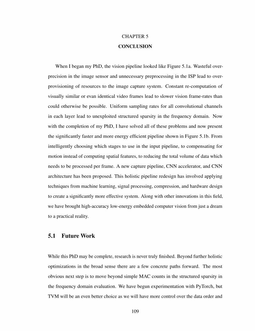
CHAPTER 5
CONCLUSION
When I began my PhD, the vision pipeline looked like Figure 5.1a. Wasteful over-
precision in the image sensor and unnecessary preprocessing in the ISP lead to over-
provisioning of resources to the image capture system. Constant re-computation of
visually similar or evan identical video frames lead to slower vision frame-rates than
could otherwise be possible. Uniform sampling rates for all convolutional channels
in each layer lead to unexploited structured sparsity in the frequency domain. Now
with the completion of my PhD, I have solved all of these problems and now present
the significantly faster and more energy efficient pipeline shown in Figure 5.1b. From
intelligently choosing which stages to use in the input pipeline, to compensating for
motion instead of computing spatial features, to reducing the total volume of data which
needs to be processed per frame. A new capture pipeline, CNN accelerator, and CNN
architecture has been proposed. This holistic pipeline redesign has involved applying
techniques from machine learning, signal processing, compression, and hardware design
to create a significantly more effective system. Along with other innovations in this field,
we have brought high-accuracy low-energy embedded computer vision from just a dream
to a practical reality.
5.1 Future Work
While this PhD may be complete, research is never truly finished. Beyond further holistic
optimizations in the broad sense there are a few concrete paths forward. The most
obvious next step is to move beyond simple MAC counts in the structured sparsity in
the frequency domain evaluation. We have begun experimentation with PyTorch, but
TVM will be an even better choice as we will have more control over the data order and
109
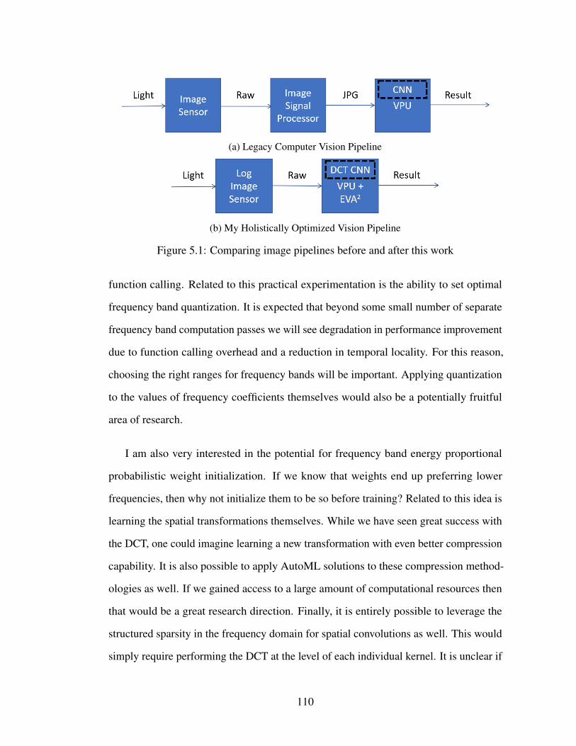
(a) Legacy Computer Vision Pipeline
(b) My Holistically Optimized Vision Pipeline
Figure 5.1: Comparing image pipelines before and after this work
function calling. Related to this practical experimentation is the ability to set optimal
frequency band quantization. It is expected that beyond some small number of separate
frequency band computation passes we will see degradation in performance improvement
due to function calling overhead and a reduction in temporal locality. For this reason,
choosing the right ranges for frequency bands will be important. Applying quantization
to the values of frequency coefficients themselves would also be a potentially fruitful
area of research.
I am also very interested in the potential for frequency band energy proportional
probabilistic weight initialization. If we know that weights end up preferring lower
frequencies, then why not initialize them to be so before training? Related to this idea is
learning the spatial transformations themselves. While we have seen great success with
the DCT, one could imagine learning a new transformation with even better compression
capability. It is also possible to apply AutoML solutions to these compression method-
ologies as well. If we gained access to a large amount of computational resources then
that would be a great research direction. Finally, it is entirely possible to leverage the
structured sparsity in the frequency domain for spatial convolutions as well. This would
simply require performing the DCT at the level of each individual kernel. It is unclear if
110
the overhead would be worth it, but that is worth determining experimentally as it will
dramatically broaden the appeal of our frequency domain structured sparsity work.
5.2 Desired Impact
I see two kinds of potential impact of this work: near-term industry adoption and longer-
term research influence. First, our new pipeline’s efficiency and generality warrants its
integration into the next generation of embedded vision systems. At a larger scale, I see
this pipeline as the first in a new line of machine learning optimizations that increase their
efficiency by leveraging data redundancy. This can also influence new general strategies
for design that leverage holistic understanding and specialization.
5.2.1 Direct Adoption
There is no shortage of papers proposing efficiency tweaks to deep learning. This work’s
distinguishing feature is its generality: it makes no assumptions about the underlying
vision task or the way that its steps are implemented. AMC and EVA2 can augment
any existing CNN implementation, including CPUs and GPUs as well as the ASICs
we evaluate in the paper. Our vision capture system can even work with traditional
vision, and while our work on structured sparsity in the frequency domain does focus
on depthwise separable networks in particular, these can be used as general featurizers
in nearly any CNN. This work complements any of the wide variety of CNN inference
optimizations proposed in architecture conferences each year, ensuring its longevity.
Because EVA2 works by manipulating intermediate activations, AMC applies to any
vision task—including ones without obvious spatial context, such as classification or
111
scene labeling networks. This generality makes my work ready for direct adoption in the
next generation of vision processors and systems as a whole.
5.2.2 Computing on Compressed Data
AMC and EVA2 are not the final word on exploiting temporal redundancy in vision,
machine learning, and beyond. The field of video compression research is old and
deep, and we see EVA2 as a first step toward exploiting its insights for computation
instead of storage. Other approaches to temporal redundancy are limited to bounding box
movement [143] or use simple delta-based encoding for frame differences [91, 92, 107].
These initial implementations represent an early stage in this new direction. The same
can be said of optimizing image capture for vision and spatial redundancy for structured
sparsity in the frequency domain.
5.2.3 Holistic Design and Specialization
This work also introduces the general concept of approximately incremental computation
in its exploitation of temporal redundancy. This approach represents a strategy for
exploiting approximate computing even when a direct approximation of the original
may be infeasible: instead, the approximate implementation only needs to update stored
outputs produced in a previous iteration. Other areas, especially workloads that involve
on-line processing of time series data, can apply the same paradigm to unlock new
approximation opportunities.
More broadly, I see this work as an example of full-stack co-optimization of hardware
and software that organizes the system around an application-level goal. It embodies
112
the advice from Hennessy and Patterson’s Turing Lecture: to eschew general-purpose,
piecemeal system design in favor of understanding the entire stack to create holistically
optimized systems. Future work can take inspiration from this design approach to find
new cross-stack optimizations in computation-heavy applications.
As a concrete example, consider a camera-equipped embedded device that breaks
down the abstraction between image capture and vision processing. By organizing the
entire pipeline around end-to-end vision tasks, future work in this direction can unlock
new sources of efficiency that are unavailable when designing general components.
Taking our temporal approach to the extreme, a change-oriented visual system can avoid
paying the cost to sense pixels that will be irrelevant for computing a desired vision
result. Using compressive sensing, simple subsampling, or even change-sensitive sensor
pixels, a co-designed visual system could capture only the information necessary for
a specific task. By applying these design principles based on our work, future “smart
camera” systems can spend energy on data capture proportional to relevant events in their
environment.
113
BIBLIOGRAPHY
[1] Umut A. Acar. Self-adjusting Computation. PhD thesis, Carnegie Mellon Univer-
sity, Pittsburgh, PA, USA, 2005.
[2] Harsh Agrawal, Clint Solomon Mathialagan, Yash Goyal, Neelima Chavali,
Prakriti Banik, Akrit Mohapatra, Ahmed Osman, and Dhruv Batra. Cloudcv:
Large-scale distributed computer vision as a cloud service. In Mobile cloud visual
media computing, pages 265–290. Springer, 2015.
[3] Jorge Albericio, Patrick Judd, Tayler Hetherington, Tor Aamodt, Natalie Enright
Jerger, and Andreas Moshovos. Cnvlutin: Ineffectual-neuron-free deep neural
network computing. In International Symposium on Computer Architecture (ISCA),
2016.
[4] Manoj Alwani, Han Chen, Michael Ferdman, and Peter Milder. Fused-layer CNN
accelerators. 2016.
[5] Brandon Amos, Bartosz Ludwiczuk, and Mahadev Satyanarayanan. OpenFace:
A general-purpose face recognition library with mobile applications. Technical
Report CMU-CS-16-118, CMU School of Computer Science, 2016.
[6] Apple Inc. AVCapturePhotoOutput. https://developer.apple.com/
reference/avfoundation/avcapturephotooutput.
[7] E. Azimi, B. Jiang, E. Tang, P. Kazanzides, and I. Iordachita. Teleoperative control
of intraocular robotic snake: Vision-based angular calibration. In 2017 IEEE
SENSORS, pages 1–3, Oct 2017.
[8] David Borer and Thomas Rosgen. Large-scale particle tracking with dynamic
vision sensors. In International Symposium on Flow Visualization (ISFV), 2014.
114
[9] A. Buades, B. Coll, and J. M. Morel. A review of image denoising algorithms,
with a new one. Multiscale Model Simulation, 4(2):490–530, 2005.
[10] Mark Buckler, Philip Bedoukian, Suren Jayasuriya, and Adrian Sampson. Eva2 :
Exploiting temporal redundancy in live computer vision. CoRR, abs/1803.06312,
2018.
[11] Mark Buckler, Suren Jayasuriya, and Adrian Sampson. Reconfiguring the imaging
pipeline for computer vision. In IEEE International Conference on Computer
Vision (ICCV), 2017.
[12] Lukas Cavigelli, David Gschwend, Christoph Mayer, Samuel Willi, Beat Muheim,
and Luca Benini. Origami: A convolutional network accelerator. In Great Lakes
Symposium on VLSI, 2015.
[13] Centeye, Inc. Logarithmic pixels. http://www.centeye.com/
technology/47-2/.
[14] Aaron Chadha, Alhabib Abbas, and Yiannis Andreopoulos. Video classification
with CNNs: Using the codec as a spatio-temporal activity sensor, 2017. https:
//arxiv.org/abs/1710.05112.
[15] Y. Chae, J. Cheon, S. Lim, M. Kwon, K. Yoo, W. Jung, D. H. Lee, S. Ham, and
G. Han. A 2.1 M pixels, 120 frame/s CMOS image sensor with column-parallel δσ
ADC architecture. IEEE Journal of Solid-State Circuits, 46(1):236–247, January
2011.
[16] Ayan Chakrabarti. Learning sensor multiplexing design through backpropagation.
In Advances in Neural Information Processing Systems (NIPS), 2016.
[17] Ken Chatfield, Karen Simonyan, Andrea Vedaldi, and Andrew Zisserman. Return
115
of the devil in the details: Delving deep into convolutional nets. In British Machine
Vision Conference, 2014.
[18] Huaijin G Chen, Suren Jayasuriya, Jiyue Yang, Judy Stephen, Sriram Sivara-
makrishnan, Ashok Veeraraghavan, and Alyosha Molnar. ASP vision: Optically
computing the first layer of convolutional neural networks using angle sensitive
pixels. In Conference on Computer Vision and Pattern Recognition (CVPR), pages
903–912, 2016.
[19] Huaijin G. Chen, Suren Jayasuriya, Jiyue Yang, Judy Stephen, Sriram Sivaramakr-
ishnan, Ashok Veeraraghavan, and Alyosha C. Molnar. ASP vision: Optically
computing the first layer of convolutional neural networks using angle sensitive
pixels. In Conference on Computer Vision and Pattern Recognition (CVPR), 2016.
[20] Tianshi Chen, Zidong Du, Ninghui Sun, Jia Wang, Chengyong Wu, Yunji Chen,
and Olivier Temam. DianNao: A small-footprint high-throughput accelerator
for ubiquitous machine-learning. In International Conference on Architectural
Support for Programming Languages and Operating Systems (ASPLOS), 2014.
[21] Wenlin Chen, James Wilson, Stephen Tyree, Kilian Q. Weinberger, and Yixin
Chen. Compressing convolutional neural networks in the frequency domain. In
Proceedings of the 22Nd ACM SIGKDD International Conference on Knowledge
Discovery and Data Mining, KDD ’16, pages 1475–1484, New York, NY, USA,
2016. ACM.
[22] Wenlin Chen, James T. Wilson, Stephen Tyree, Kilian Q. Weinberger, and Yixin
Chen. Compressing convolutional neural networks. CoRR, abs/1506.04449, 2015.
[23] Xiang Chen, Yiran Chen, Zhan Ma, and Felix C. A. Fernandes. How is energy
consumed in smartphone display applications? In HotMobile, 2013.
116
[24] Yu-Hsin Chen, Tushar Krishna, Joel Emer, and Vivienne Sze. Eyeriss: An energy-
efficient reconfigurable accelerator for deep convolutional neural networks. In
IEEE International Solid-State Circuits Conference (ISSCC), 2015.
[25] Yu-Hsin Chen, Tushar Krishna, Joel S. Emer, and Vivienne Sze. Eyeriss: An
energy-efficient reconfigurable accelerator for deep convolutional neural networks.
J. Solid-State Circuits, 52:127–138, January 2017.
[26] Yunji Chen, Tao Luo, Shaoli Liu, Shijin Zhang, Liqiang He, Jia Wang, Ling Li,
Tianshi Chen, Zhiwei Xu, Ninghui Sun, and Olivier Temam. DaDianNao: A
machine-learning supercomputer. 2014.
[27] Yunpeng Chen, Haoqi Fang, Bing Xu, Zhicheng Yan, Yannis Kalantidis, Marcus
Rohrbach, Shuicheng Yan, and Jiashi Feng. Drop an octave: Reducing spatial
redundancy in convolutional neural networks with octave convolution. arXiv
preprint arXiv:1904.05049, 2019.
[28] Francois Chollet. Xception: Deep learning with depthwise separable convolutions.
In Proceedings of the IEEE conference on computer vision and pattern recognition,
pages 1251–1258, 2017.
[29] Matthew A. Clapp, Viktor Gruev, and Ralph Etienne-Cummings. Focal-Plane
Analog Image Processing, pages 141–202. Springer US, Boston, MA, 2004.
[30] K. Dabov, A. Foi, V. Katkovnik, and K. Egiazarian. Image denoising by sparse 3-D
transform-domain collaborative filtering. IEEE Transactions on Image Processing,
16(8):2080–2095, August 2007.
[31] J. Deng, W. Dong, R. Socher, L.-J. Li, K. Li, and L. Fei-Fei. ImageNet: A
Large-Scale Hierarchical Image Database. In Conference on Computer Vision and
Pattern Recognition (CVPR), 2009.
117
[32] Steven Diamond, Vincent Sitzmann, Stephen Boyd, Gordon Wetzstein, and Felix
Heide. Dirty pixels: Optimizing image classification architectures for raw sensor
data, 2017. https://arxiv.org/abs/1701.06487.
[33] I. Drori and D. Lischinski. Fast multiresolution image operations in the wavelet
domain. IEEE Transactions on Visualization and Computer Graphics, 9(3):395–
411, July 2003.
[34] Iddo Drori and Dani Lischinski. Fast multiresolution image operations in the
wavelet domain. IEEE Trans. Vis. Comput. Graph., 9(3):395–411, 2003.
[35] X. Du, M. H. Ang, and D. Rus. Car detection for autonomous vehicle: Lidar
and vision fusion approach through deep learning framework. In 2017 IEEE/RSJ
International Conference on Intelligent Robots and Systems (IROS), pages 749–
754, Sept 2017.
[36] Zidong Du, Robert Fasthuber, Tianshi Chen, Paolo Ienne, Ling Li, Tao Luo,
Xiaobing Feng, Yunji Chen, and Olivier Temam. ShiDianNao: Shifting vision pro-
cessing closer to the sensor. In International Symposium on Computer Architecture
(ISCA), 2015.
[37] P. E. J. Duhamel, C. O. Perez-Arancibia, G. L. Barrows, and R. J. Wood. Bio-
logically inspired optical-flow sensing for altitude control of flapping-wing mi-
crorobots. IEEE/ASME Transactions on Mechatronics, 18(2):556–568, April
2013.
[38] Steven K. Esser, Paul A. Merolla, John V. Arthur, Andrew S. Cassidy, Rathinaku-
mar Appuswamy, Alexander Andreopoulos, David J. Berg, Jeffrey L. McKinstry,
Timothy Melano, Davis R. Barch, Carmelo di Nolfo, Pallab Datta, Arnon Amir,
Brian Taba, Myron D. Flickner, and Dharmendra S. Modha. Convolutional net-
118
works for fast, energy-efficient neuromorphic computing. Proceedings of the
National Academy of Sciences, 113(41):11441–11446, 2016.
[39] M. Everingham, L. Van Gool, C. K. I. Williams, J. Winn, and A. Zisserman. The
PASCAL visual object classes challenge 2007 (VOC2007) results.
[40] Philipp Fischer, Alexey Dosovitskiy, Eddy Ilg, Philip Hausser, Caner Hazirbas,
Vladimir Golkov, Patrick van der Smagt, Daniel Cremers, and Thomas Brox.
FlowNet: Learning optical flow with convolutional networks. In IEEE Interna-
tional Conference on Computer Vision (ICCV), 2015.
[41] Denis Foley and John Danskin. Ultra-performance Pascal GPU and NVLink
interconnect. IEEE Micro, 37(2):7–17, March 2017.
[42] M. Garey, D. Johnson, and H. Witsenhausen. The complexity of the generalized
Lloyd–Max problem. IEEE Transactions on Information Theory, 28(2):255–256,
March 1982.
[43] Matthew A. Hammer, Khoo Yit Phang, Michael Hicks, and Jeffrey S. Foster. Adap-
ton: Composable, demand-driven incremental computation. In ACM Conference
on Programming Language Design and Implementation (PLDI), 2014.
[44] Seungyeop Han, Rajalakshmi Nandakumar, Matthai Philipose, Arvind Krishna-
murthy, and David Wetherall. GlimpseData: Towards continuous vision-based
personal analytics. In Workshop on Physical Analytics (WPA), 2014.
[45] Song Han, Xingyu Liu, Huizi Mao, Jing Pu, Ardavan Pedram, Mark A. Horowitz,
and William J. Dally. EIE: Efficient inference engine on compressed deep neural
network. In International Symposium on Computer Architecture (ISCA), 2016.
[46] Song Han, Huizi Mao, and William J. Dally. Deep compression: Compressing
119
deep neural networks with pruning, trained quantization and huffman coding. In
International Conference on Learning Representations (ICLR), 2016.
[47] Song Han, Jeff Pool, John Tran, and William Dally. Learning both weights and
connections for efficient neural network. In Advances in neural information
processing systems, pages 1135–1143, 2015.
[48] Kaiming He, Xiangyu Zhang, Shaoqing Ren, and Jian Sun. Deep residual learning
for image recognition, 2015. https://arxiv.org/abs/1512.03385.
[49] Yihui He, Ji Lin, Zhijian Liu, Hanrui Wang, Li-Jia Li, and Song Han. Amc: Automl
for model compression and acceleration on mobile devices. In Proceedings of the
European Conference on Computer Vision (ECCV), pages 784–800, 2018.
[50] James Hegarty, John Brunhaver, Zachary DeVito, Jonathan Ragan-Kelley, Noy
Cohen, Steven Bell, Artem Vasilyev, Mark Horowitz, and Pat Hanrahan. Dark-
room: Compiling high-level image processing code into hardware pipelines. In
SIGGRAPH, 2014.
[51] James Hegarty, Ross Daly, Zachary DeVito, Jonathan Ragan-Kelley, Mark
Horowitz, and Pat Hanrahan. Rigel: Flexible multi-rate image processing hard-
ware. In SIGGRAPH, 2016.
[52] Sepp Hochreiter and Jurgen Schmidhuber. Long short-term memory. Neural
computation, 9(8):1735–1780, 1997.
[53] Berthold KP Horn and Brian G Schunck. Determining optical flow. Artificial
intelligence, 17(1-3):185–203, 1981.
[54] Andrew G Howard, Menglong Zhu, Bo Chen, Dmitry Kalenichenko, Weijun Wang,
Tobias Weyand, Marco Andreetto, and Hartwig Adam. Mobilenets: Efficient
120
convolutional neural networks for mobile vision applications. arXiv preprint
arXiv:1704.04861, 2017.
[55] Andrew G. Howard, Menglong Zhu, Bo Chen, Dmitry Kalenichenko, Weijun
Wang, Tobias Weyand, Marco Andreetto, and Hartwig Adam. Mobilenets: Ef-
ficient convolutional neural networks for mobile vision applications. CoRR,
abs/1704.04861, 2017.
[56] Gao Huang, Danlu Chen, Tianhong Li, Felix Wu, Laurens van der Maaten, and
Kilian Q. Weinberger. Multi-scale dense convolutional networks for efficient
prediction. CoRR, abs/1703.09844, 2017.
[57] Gary B. Huang, Manu Ramesh, Tamara Berg, and Erik Learned-Miller. Labeled
faces in the wild: A database for studying face recognition in unconstrained
environments. Technical Report 07-49, University of Massachusetts, Amherst,
October 2007.
[58] Yu-Wen Huang, Ching-Yeh Chen, Chen-Han Tsai, Chun-Fu Shen, and Liang-Gee
Chen. Survey on block matching motion estimation algorithms and architectures
with new results. J. VLSI Signal Processing Systems for Signal, Image and Video
Technology, 42(3):297–320, March 2006.
[59] Itay Hubara, Matthieu Courbariaux, Daniel Soudry, Ran El-Yaniv, and Yoshua
Bengio. Binarized neural networks. In Advances in Neural Information Processing
Systems (NeurIPS), 2016.
[60] Forrest N Iandola, Song Han, Matthew W Moskewicz, Khalid Ashraf, William J
Dally, and Kurt Keutzer. SqueezeNet: AlexNet-level accuracy with 50x fewer
parameters and <0.5 MB model size. arXiv preprint arXiv:1602.07360, 2016.
121
[61] Eddy Ilg, Nikolaus Mayer, Tonmoy Saikia, Margret Keuper, Alexey Dosovitskiy,
and Thomas Brox. FlowNet 2.0: Evolution of optical flow estimation with deep
networks. In Conference on Computer Vision and Pattern Recognition (CVPR),
2017.
[62] iniLabs Ltd. Dynamic vision sensor. https://inilabs.com/products/
dynamic-vision-sensors/.
[63] Itseez. OpenCV. http://opencv.org.
[64] Changsoo Je and Hyung-Min Park. Optimized hierarchical block matching for
fast and accurate image registration. Signal Processing: Image Communication,
28(7):779–791, 2013.
[65] Yangqing Jia, Evan Shelhamer, Jeff Donahue, Sergey Karayev, Jonathan Long,
Ross Girshick, Sergio Guadarrama, and Trevor Darrell. Caffe: Convolutional
architecture for fast feature embedding, 2014. http://arxiv.org/abs/
1408.5093.
[66] H.K. Kesavan J.N. Kapur. Entropy Optimization Principles and Their Applications,
volume 9. Water Science and Technology Library, 1992.
[67] Justin Johnson, Andrej Karpathy, and Li Fei-Fei. DenseCap: Fully convolutional
localization networks for dense captioning. In Conference on Computer Vision
and Pattern Recognition (CVPR), 2016.
[68] Norman P. Jouppi, Cliff Young, Nishant Patil, David Patterson, Gaurav Agrawal,
Raminder Bajwa, Sarah Bates, Suresh Bhatia, Nan Boden, Al Borchers, Rick
Boyle, Pierre luc Cantin, Clifford Chao, Chris Clark, Jeremy Coriell, Mike Da-
ley, Matt Dau, Jeffrey Dean, Ben Gelb, Tara Vazir Ghaemmaghami, Rajendra
Gottipati, William Gulland, Robert Hagmann, C. Richard Ho, Doug Hogberg,
122
John Hu, Robert Hundt, Dan Hurt, Julian Ibarz, Aaron Jaffey, Alek Jaworski,
Alexander Kaplan, Harshit Khaitan, Andy Koch, Naveen Kumar, Steve Lacy,
James Laudon, James Law, Diemthu Le, Chris Leary, Zhuyuan Liu, Kyle Lucke,
Alan Lundin, Gordon MacKean, Adriana Maggiore, Maire Mahony, Kieran Miller,
Rahul Nagarajan, Ravi Narayanaswami, Ray Ni, Kathy Nix, Thomas Norrie, Mark
Omernick, Narayana Penukonda, Andy Phelps, Jonathan Ross, Matt Ross, Amir
Salek, Emad Samadiani, Chris Severn, Gregory Sizikov, Matthew Snelham, Jed
Souter, Dan Steinberg, Andy Swing, Mercedes Tan, Gregory Thorson, Bo Tian,
Horia Toma, Erick Tuttle, Vijay Vasudevan, Richard Walter, Walter Wang, Eric
Wilcox, and Doe Hyun Yoon. In-datacenter performance analysis of a Tensor
Processing Unit. In International Symposium on Computer Architecture (ISCA),
2017.
[69] M. Judy, A. M. Sodagar, R. Lotfi, and M. Sawan. Nonlinear signal-specific adc
for efficient neural recording in brain-machine interfaces. IEEE Transactions on
Biomedical Circuits and Systems, 8(3):371–381, June 2014.
[70] Daya S. Khudia, Babak Zamirai, Mehrzad Samadi, and Scott Mahlke. Rumba: An
online quality management system for approximate computing. In International
Symposium on Computer Architecture (ISCA), 2015.
[71] S. J. Kim, H. T. Lin, Z. Lu, S. Susstrunk, S. Lin, and M. S. Brown. A new
in-camera imaging model for color computer vision and its application. IEEE
Transactions on Pattern Analysis and Machine Intelligence, 34(12):2289–2302,
December 2012.
[72] Alex Krizhevsky and Geoffrey Hinton. Learning multiple layers of features from
tiny images. Technical report, University of Toronto, 2009.
[73] Alex Krizhevsky, Ilya Sutskever, and Geoffrey E. Hinton. ImageNet classification
123
with deep convolutional neural networks. In Advances in Neural Information
Processing Systems (NIPS). 2012.
[74] Y. Lecun, L. Bottou, Y. Bengio, and P. Haffner. Gradient-based learning applied
to document recognition. Proceedings of the IEEE, 86(11):2278–2324, 1998.
[75] Reoxiang Li, Bing Zeng, and Ming L Liou. A new three-step search algorithm
for block motion estimation. Trans. Circuits and Systems for Video Technology,
4(4):438–442, 1994.
[76] Robert LiKamWa, Yunhui Hou, Julian Gao, Mia Polansky, and Lin Zhong. Red-
Eye: Analog ConvNet image sensor architecture for continuous mobile vision. In
International Symposium on Computer Architecture (ISCA), 2016.
[77] Robert LiKamWa, Yunhui Hou, Julian Gao, Mia Polansky, and Lin Zhong. Red-
Eye: Analog convnet image sensor architecture for continuous mobile vision. In
International Symposium on Computer Architecture (ISCA), pages 255–266. IEEE
Press, 2016.
[78] Robert LiKamWa, Bodhi Priyantha, Matthai Philipose, Lin Zhong, and Paramvir
Bahl. Energy characterization and optimization of image sensing toward continu-
ous mobile vision. In Conference on Mobile Systems, Applications, and Services
(MobiSys), 2013.
[79] Z. Liu, T. Park, H. S. Park, and N. S. Kim. Ultra-low-power image signal processor
for smart camera applications. Electronics Letters, 51(22):1778–1780, 2015.
[80] Zhenhua Liu, Jizheng Xu, Xiulian Peng, and Ruiqin Xiong. Frequency-domain
dynamic pruning for convolutional neural networks. In Advances in Neural
Information Processing Systems (NeurIPS), 2018.
124
[81] Zhenhua Liu, Jizheng Xu, Xiulian Peng, and Ruiqin Xiong. Frequency-domain
dynamic pruning for convolutional neural networks. NeurIPS, 2018.
[82] Zihao Liu, Tao Liu, Wujie Wen, Lei Jiang, Jie Xu, Yanzhi Wang, and Gang Quan.
DeepN-JPEG: A deep neural network favorable JPEG-based image compression
framework. In Design Automation Conference (DAC), 2018.
[83] Bruce D. Lucas and Takeo Kanade. An iterative image registration technique with
an application to stereo vision. In International Joint Conferences on Artificial
Intelligence (IJCAI), 1981.
[84] Ningning Ma, Xiangyu Zhang, Hai-Tao Zheng, and Jian Sun. ShuffleNet V2:
Practical guidelines for efficient CNN architecture design. In European Conference
on Computer Vision (ECCV), pages 116–131, 2018.
[85] Yunqian Ma and Guodong Guo. Support vector machines applications. Springer,
2014.
[86] N. Massari, M. Gottardi, L. Gonzo, D. Stoppa, and A. Simoni. A CMOS image
sensor with programmable pixel-level analog processing. IEEE Transactions on
Neural Networks, 16(6):1673–1684, November 2005.
[87] Michael Mathieu, Mikael Henaff, and Yann LeCun. Fast training of convolutional
networks through FFTs. In International Conference on Learning Representations
(ICLR), 2014.
[88] Amrita Mazumdar, Thierry Moreau, Sung Kim, Meghan Cowan, Armin
Alaghi, Luis Ceze, Mark Oskin, and Visvesh Sathe. Exploring computation–
communication tradeoffs in camera systems. In IEEE International Symposium
on Workload Characterization (IISWC), 2017.
125
[89] Pierre Moulon, Pascal Monasse, Renaud Marlet, and Others. OpenMVG: An
open multiple view geometry library. https://github.com/openMVG/
openMVG.
[90] Naveen Muralimanohar, Ali Shafiee, and Vaishnav Srinivas. CACTI 6.5. https:
//github.com/HewlettPackard/cacti.
[91] Daniel Neil, Jun Haeng Lee, Tobi Delbruck, and Shih-Chii Liu. Delta networks
for optimized recurrent network computation. In International Conference on
Machine Learning (ICML), 2017.
[92] Peter O’Connor and Max Welling. Sigma delta quantized networks. In Interna-
tional Conference on Learning Representations (ICLR), 2017.
[93] A. Omid-Zohoor, C. Young, D. Ta, and B. Murmann. Towards always-on mobile
object detection: Energy vs. performance tradeoffs for embedded HOG feature
extraction. IEEE Transactions on Circuits and Systems for Video Technology,
PP(99):1–1, 2017.
[94] ON Semiconductor. Image processors. Commercial Website, http://www.
onsemi.com/PowerSolutions/parametrics.do?id=16880.
[95] Angshuman Parashar, Minsoo Rhu, Anurag Mukkara, Antonio Puglielli, Ranghara-
jan Venkatesan, Brucek Khailany, Joel Emer, Stephen W. Keckler, and William J.
Dally. SCNN: An accelerator for compressed-sparse convolutional neural net-
works. In International Symposium on Computer Architecture (ISCA), 2017.
[96] Pedro H. O. Pinheiro, Tsung-Yi Lin, Ronan Collobert, and Piotr Dollar. Learning
to refine object segments, 2016. http://arxiv.org/abs/1603.08695.
[97] Jiantao Qiu, Jie Wang, Song Yao, Kaiyuan Guo, Boxun Li, Erjin Zhou, Jincheng
Yu, Tianqi Tang, Ningyi Xu, Sen Song, Yu Wang, and Huazhong Yang. Going
126
deeper with embedded FPGA platform for convolutional neural network. In
International Symposium on Field-Programmable Gate Arrays (FPGA), 2016.
[98] Richard E. Woods Rafael C. Gonzalez. Digital Image Processing (4th Edition).
Pearson, 2017.
[99] Jonathan Ragan-Kelley, Connelly Barnes, Andrew Adams, Sylvain Paris, Fredo
Durand, and Saman Amarasinghe. Halide: A language and compiler for optimizing
parallelism, locality, and recomputation in image processing pipelines. In ACM
Conference on Programming Language Design and Implementation (PLDI), 2013.
[100] R. Ranjan, V. M. Patel, and R. Chellappa. Hyperface: A deep multi-task learning
framework for face detection, landmark localization, pose estimation, and gender
recognition. IEEE Transactions on Pattern Analysis and Machine Intelligence,
pages 1–1, 2017.
[101] Mohammad Rastegari, Vicente Ordonez, Joseph Redmon, and Ali Farhadi. XNOR-
Net: ImageNet classification using binary convolutional neural networks. In
European Conference on Computer Vision (ECCV), 2016.
[102] Brandon Reagen, Paul N. Whatmough, Robert Adolf, Saketh Rama, Hyunkwang
Lee, Sae Kyu Lee, Jose Miguel Hernandez-Lobato, Gu-Yeon Wei, and David M.
Brooks. Minerva: Enabling low-power, highly-accurate deep neural network
accelerators. In International Symposium on Computer Architecture (ISCA), 2016.
[103] Esteban Real, Jonathon Shlens, Stefano Mazzocchi, Xin Pan, and Vincent Van-
houcke. YouTube-BoundingBoxes: A large high-precision human-annotated data
set for object detection in video. 2017.
[104] B Srinivasa Reddy and Biswanath N Chatterji. An FFT-based technique for trans-
127
lation, rotation, and scale-invariant image registration. Trans. Image Processing,
5(8):1266–1271, 1996.
[105] Shaoqing Ren, Kaiming He, Ross Girshick, and Jian Sun. Faster R-CNN: Towards
real-time object detection with region proposal networks. In Advances in Neural
Information Processing Systems (NIPS), 2015.
[106] W. A. Richards. Lightness scale from image intensity distributions. Appl Opt,
21(14):2569–2582, July 1982.
[107] M. Riera, J. Arnau, and A. Gonzalez. Computation reuse in dnns by exploiting
input similarity. In 2018 ACM/IEEE 45th Annual International Symposium on
Computer Architecture (ISCA), pages 57–68, June 2018.
[108] Michael Ringenberg, Adrian Sampson, Isaac Ackerman, Luis Ceze, and Dan
Grossman. Monitoring and debugging the quality of results in approximate
programs. In International Conference on Architectural Support for Programming
Languages and Operating Systems (ASPLOS), 2015.
[109] Sara Sabour, Nicholas Frosst, and Geoffrey E. Hinton. Dynamic routing between
capsules. CoRR, abs/1710.09829, 2017.
[110] Mehrzad Samadi, Janghaeng Lee, Davoud Anoushe Jamshidi, Amir Hormati, and
Scott Mahlke. SAGE: Self-tuning approximation for graphics engines. 2013.
[111] Adrian Sampson and Mark Buckler. FODLAM, a first-order deep learning
accelerator model. https://github.com/cucapra/fodlam. Commit
cde53fd.
[112] Mark B. Sandler, Andrew G. Howard, Menglong Zhu, Andrey Zhmoginov, and
Liang-Chieh Chen. MobileNetV2: Inverted residuals and linear bottlenecks. In
Conference on Computer Vision and Pattern Recognition (CVPR), 2018.
128
[113] Daniel Scharstein, Heiko Hirschmuller, York Kitajima, Greg Krathwohl, Nera
Nesic, Xi Wang, and Porter Westling. High-resolution stereo datasets with
subpixel-accurate ground truth. In German Conference on Pattern Recognition
(GCPR), 2014.
[114] D. Schmalstieg and T. Hllerer. Augmented reality: Principles and practice. In
2017 IEEE Virtual Reality (VR), pages 425–426, March 2017.
[115] Hardik Sharma, Jongse Park, Divya Mahajan, Emmanuel Amaro, Joon Kyung
Kim, Chenkai Shao, Asit Mishra, and Hadi Esmaeilzadeh. From high-level deep
neural models to FPGAs. 2016.
[116] Evan Shelhamer, Kate Rakelly, Judy Hoffman, and Trevor Darrell. Clockwork
convnets for video semantic segmentation. In Video Semantic Segmentation
Workshop at European Conference in Computer Vision (ECCV), 2016.
[117] Karen Simonyan and Andrew Zisserman. Very deep convolutional networks
for large-scale image recognition, 2014. http://arxiv.org/abs/1409.
1556.
[118] Avinash Sodani. Knights Landing (KNL): 2nd generation Intel Xeon Phi processor.
In HotChips, 2015.
[119] C. Strecha, W. von Hansen, L. Van Gool, P. Fua, and U. Thoennessen. On bench-
marking camera calibration and multi-view stereo for high resolution imagery. In
Conference on Computer Vision and Pattern Recognition (CVPR), 2008.
[120] Naveen Suda, Vikas Chandra, Ganesh Dasika, Abinash Mohanty, Yufei Ma,
Sarma Vrudhula, Jae-sun Seo, and Yu Cao. Throughput-optimized OpenCL-based
FPGA accelerator for large-scale convolutional neural networks. In International
Symposium on Field-Programmable Gate Arrays (FPGA), 2016.
129
[121] Vivienne Sze, Yu-Hsin Chen, Tien-Ju Yang, and Joel Emer. Efficient processing
of deep neural networks: A tutorial and survey, 2017. https://arxiv.org/
abs/1703.09039.
[122] M. Tikekar, V. Sze, and A. Chandrakasan. A fully-integrated energy-efficient
H.265/HEVC decoder with eDRAM for wearable devices. In 2017 Symposium on
VLSI Circuits, pages C230–C231, June 2017.
[123] Mehul Tikekar, Chao-Tsung Huang, Chiraag Juvekar, Vivienne Sze, and Anantha P
Chandrakasan. A 249-Mpixel/s HEVC video-decoder chip for 4K ultra-HD
applications. J. Solid-State Circuits, 49(1):61–72, 2014.
[124] Mykhail L. Uss, Benoit Vozel, Vladimir V. Lukin, and Kacem Chehdi. Image
informative maps for component-wise estimating parameters of signal-dependent
noise. Journal of Electronic Imaging, 22(1):013019–013019, 2013.
[125] Rudy J Van de Plassche. CMOS integrated analog-to-digital and digital-to-analog
converters, volume 742. Springer Science & Business Media, 2013.
[126] Artem Vasilyev, Nikhil Bhagdikar, Ardavan Pedram, Stephen Richardson, Sha-
har Kvatinsky, and Mark Horowitz. Evaluating programmable architectures for
imaging and vision applications. In MICRO, 2016.
[127] Guohui Wang, Yingen Xiong, Jay Yun, and Joseph R Cavallaro. Accelerating com-
puter vision algorithms using opencl framework on the mobile gpu-a case study.
In Acoustics, Speech and Signal Processing (ICASSP), 2013 IEEE International
Conference on, pages 2629–2633. IEEE, 2013.
[128] Bichen Wu, Forrest Iandola, Peter H Jin, and Kurt Keutzer. Squeezedet: Unified,
small, low power fully convolutional neural networks for real-time object detection
130
for autonomous driving. In Proceedings of the IEEE Conference on Computer
Vision and Pattern Recognition Workshops, pages 129–137, 2017.
[129] Saining Xie, Ross B. Girshick, Piotr Dollar, Zhuowen Tu, and Kaiming He.
Aggregated residual transformations for deep neural networks. Conference on
Computer Vision and Pattern Recognition (CVPR), 2017.
[130] Kelvin Xu, Jimmy Ba, Ryan Kiros, Kyunghyun Cho, Aaron C. Courville, Ruslan
Salakhutdinov, Richard S. Zemel, and Yoshua Bengio. Show, attend and tell:
Neural image caption generation with visual attention. CoRR, abs/1502.03044,
2015.
[131] Serena Yeung, Olga Russakovsky, Greg Mori, and Li Fei-Fei. End-to-end learning
of action detection from frame glimpses in videos. In Conference on Computer
Vision and Pattern Recognition (CVPR), 2016.
[132] Dong Yi, Zhen Lei, Shengcai Liao, and Stan Z. Li. Learning face representation
from scratch, 2014. http://arxiv.org/abs/1411.7923.
[133] Jason Yosinski, Jeff Clune, Yoshua Bengio, and Hod Lipson. How transferable are
features in deep neural networks? In Advances in Neural Information Processing
Systems (NeurIPS), 2014.
[134] Jiecao Yu, Andrew Lukefahr, David Palframan, Ganesh Dasika, Reetuparna Das,
and Scott Mahlke. Scalpel: Customizing DNN pruning to the underlying hardware
parallelism. In International Symposium on Computer Architecture (ISCA), 2017.
[135] Chen Zhang, Peng Li, Guangyu Sun, Yijin Guan, Bingjun Xiao, and Jason Cong.
Optimizing FPGA-based accelerator design for deep convolutional neural net-
works. In International Symposium on Field-Programmable Gate Arrays (FPGA),
2015.
131
[136] Xiangyu Zhang, Xinyu Zhou, Mengxiao Lin, and Jian Sun. Shufflenet: An ex-
tremely efficient convolutional neural network for mobile devices. In Proceedings
of the IEEE Conference on Computer Vision and Pattern Recognition, pages
6848–6856, 2018.
[137] Zhengdong Zhang and Vivienne Sze. FAST: A framework to accelerate super-
resolution processing on compressed videos. In CVPR Workshop on New Trends
in Image Restoration and Enhancement, 2017.
[138] Zhimin Zhou, B. Pain, and E. R. Fossum. Frame-transfer cmos active pixel sensor
with pixel binning. IEEE Transactions on Electron Devices, 44(10):1764–1768,
October 1997.
[139] Chenzhuo Zhu, Song Han, Huizi Mao, and William J Dally. Trained ternary
quantization. In International Conference on Learning Representations (ICLR),
2017.
[140] Shan Zhu and Kai-Kuang Ma. A new diamond search algorithm for fast block
matching motion estimation. Trans. Image Processing, 9:287–290, February 1997.
[141] Xizhou Zhu, Yujie Wang, Jifeng Dai, Lu Yuan, and Yichen Wei. Flow-guided
feature aggregation for video object detection. In IEEE International Conference
on Computer Vision (ICCV), 2017.
[142] Xizhou Zhu, Yuwen Xiong, Jifeng Dai, Lu Yuan, and Yichen Wei. Deep fea-
ture flow for video recognition. In Conference on Computer Vision and Pattern
Recognition (CVPR), 2016.
[143] Yuhao Zhu, Anand Samajdar, Matthew Mattina, and Paul Whatmough. Euphrates:
Algorithm-soc co-design for low-power mobile continuous vision. In Proceedings
132

of the 45th Annual International Symposium on Computer Architecture, ISCA ’18,
pages 547–560, Piscataway, NJ, USA, 2018. IEEE Press.
133


