Fourth International Symposium on Marine Propulsors SMP’15, Austin, Texas, USA, June 2015

High-fidelity Hydrodynamic Shape Optimization of a 3-D Morphing Hydrofoil

Nitin Garg1, Zhoujie Lyu2, Tristan Dhert2, Joaquim Martins2, Yin Lu Young1,* 1 Department of Naval Architecture and Marine Engineering, University of Michigan

2 Department of Aerospace Engineering, University of Michigan

*Corresponding author: ylyoung@umich.edu

ABSTRACT In spite of the widespread use of computational fluid dynamics (CFD) in the prediction of propulsors performance such as for hydrofoils, propellers, and turbines, there is lack of an efficient and robust CFD-based design optimization tool that can handle large number of shape design variables. To address this, a high-fidelity, efficient hydrodynamic shape optimization tool, with consideration for cavitation inception, is presented in this paper. A previously developed compressible computational fluid dynamics (CFD) solver is extended to solve for nearly incompressible flows, using a low-speed preconditioner. A gradient-based optimizer based on the adjoint method is used to carry out the optimization. Validation study of the modified CFD solver is presented for a tapered NACA 0009 hydrofoil with the experimental results from Zarruk et al. [1]. Comparison of Euler and Reynolds-Averaged Navier–Stokes (RANS)-based shape optimization results are shown for a tapered RAE 2822 hydrofoil. A total of 73 design variables are used, which include the angle of attack and geometric shape variables. For lift coefficient (CL) in the range of 0.3 to 1.0, the drag coefficient (CD) for a given lift coefficient can be reduced by at least 20%. The optimized hydrofoil is found to have much lower negative suction peak and hence delayed cavitation inception compared to the original foil. The need for a high-fidelity solver and large numbers of design variables are demonstrated.

KEYWORDS Shape Optimization, low-speed preconditioner, gradient-based optimizer, cavitation number, hydrofoil, shape morphing.

1 INTRODUCTION A robust CFD-based design optimization tool should be capable of handling large number of design variables efficiently. A large number of design variables are required because of the complex 3-D geometry of marine propulsors. The hydrodynamic performance of propulsors is also highly sensitive to the detailed surface geometry, particularly at the leading edge, trailing edge, and tip regions. Additional care is needed to prevent or control laminar to turbulent transition, separation and cavitation.

Cavitation can occur for marine propulsors operating at high speeds, operating near the free surface, or both, which leads to undesirable effects such as performance decay, erosion, vibration and noise. Thus, design optimization tools must also be able to enforce constraints to avoid or delay cavitation. Most of the studies carried out so far for the hydrofoil design optimization either (1) use potential based flow solvers or (2) use CFD techniques with a low number of design variables. However, there is a need of a RANS CFD solver as there are physics that cannot be captured using Euler or potential flow solvers, such as transition, separation, and stall. The objective of this work is to present an efficient, high-fidelity, hydrodynamic shape optimization tool for 3-D lifting bodies operating in viscous and nearly incompressible fluids with consideration for cavitation.

In recent studies [2], it was found that continuous dynamic shape change (morphing) of the trailing edge geometry of a foil can lead to fuel savings in the range of 5%-12% throughout the operation of a commercial fixed wing aircraft. Lyu et al. [3] carried out multipoint gradient-based aerodynamic shape optimization based on RANS CFD. They used the adjoint method to compute the gradients and carried out the shape optimization of the Common Research Model (CRM) wing. They minimized the drag coefficient subject to lift, pitch moment, and geometric constraints. The optimization reduced the drag coefficient by 8.5% for a given lift coefficient. However, while the advantage in aerial operation is relatively well studied, maritime applications of morphing surfaces bring several other challenges such as higher loading, stronger fluid structure interaction, as well as potential susceptibility to free surface and cavitation related instabilities. The goal of this paper is to study the potential advantages of an active shape-morphing hydrofoil (or control surface) as a function of the operating conditions (speed and angle of attack) for moderate to high Reynolds number flow.

A range of maritime design optimization tools exists in literature. However, they either use low-fidelity methods, or high-fidelity methods with low number of design variables. Ching–Yeh Hsin [4] studied two-

dimensional foil sections using a panel method assuming potential flow. They later performed RANS-based optimization for a 2-D hydrofoil using the Lagrange multiplier method for the optimization of the section [5]. Only two design variables were considered: the angle of attack and the camber ratio. Recently, several authors carried out high-fidelity hydrodynamic shape optimization for naval vehicles and catamarans (e.g. [6], [7]); they either used gradient-free methods or simulation based design (SBD) methods for optimization, which resulted in a very low number of design variables (less than 15) due to the high computational cost associated with large number of function evaluations, particularly for high-fidelity solvers.

Cavitation is the formation of bubbles in a liquid, when the local pressure drops to near the saturated vapor pressure. Cavitation can lead to undesirable effects such as performance decay, erosion, vibration and noise. This makes cavitation one of the main drivers in marine propulsors design. Mishima et al. [8] presented one of the first studies optimizing hydrofoil performance while considering cavitation. They carried out optimization for the 2-D hydrofoil to minimize the drag for a given lift and cavitation number. However, they used low-order potential-based panel method for the hydrodynamic model, and accounted for viscous effects by applying a uniform friction coefficient on the wetted foil surface. Zeng et al. [9] developed a design technique using genetic algorithm on 2-D sections, and used a potential-based lifting surface method to incorporate the 2-D section for 3-D propeller blade design. The above studies were based on the potential flow methods, which are not valid for cases with flow separation, or when the physics is dominated by large-scale vortices. Thus, there is a need for an efficient, high-fidelity 3-D design optimization tool that can handle a large number of design variables and can enforce constraints to avoid or delay cavitation.

2 METHODOLOGY

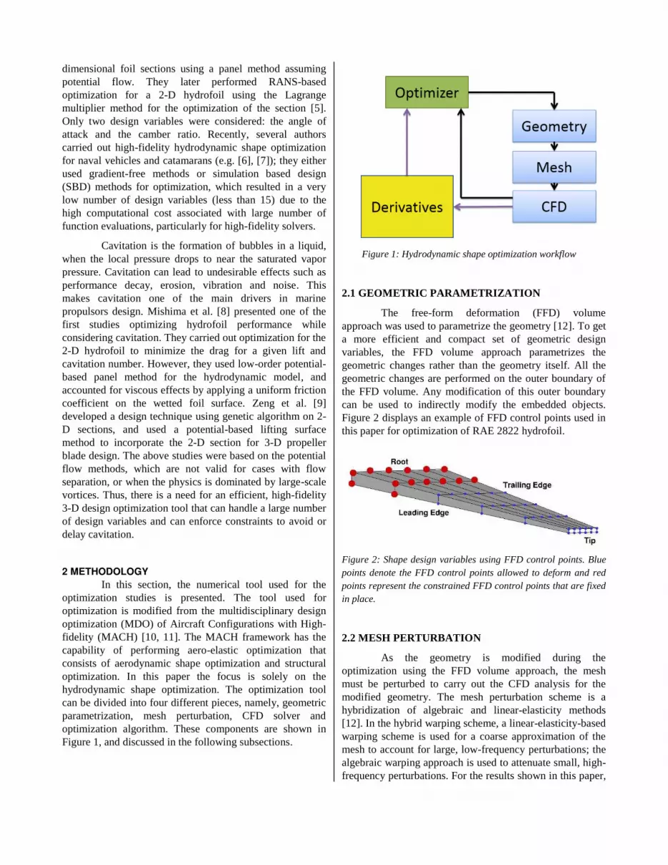
In this section, the numerical tool used for the optimization studies is presented. The tool used for optimization is modified from the multidisciplinary design optimization (MDO) of Aircraft Configurations with High-fidelity (MACH) [10, 11]. The MACH framework has the capability of performing aero-elastic optimization that consists of aerodynamic shape optimization and structural optimization. In this paper the focus is solely on the hydrodynamic shape optimization. The optimization tool can be divided into four different pieces, namely, geometric parametrization, mesh perturbation, CFD solver and optimization algorithm. These components are shown in Figure 1, and discussed in the following subsections.

2.1 GEOMETRIC PARAMETRIZATION

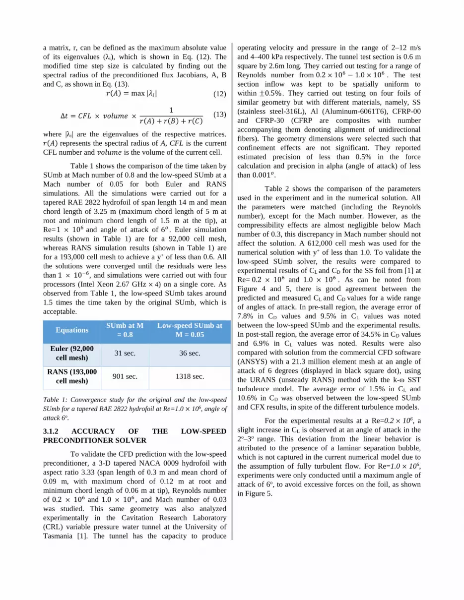
The free-form deformation (FFD) volume approach was used to parametrize the geometry [12]. To get a more efficient and compact set of geometric design variables, the FFD volume approach parametrizes the geometric changes rather than the geometry itself. All the geometric changes are performed on the outer boundary of the FFD volume. Any modification of this outer boundary can be used to indirectly modify the embedded objects. Figure 2 displays an example of FFD control points used in this paper for optimization of RAE 2822 hydrofoil.

Figure 2: Shape design variables using FFD control points. Blue points denote the FFD control points allowed to deform and red points represent the constrained FFD control points that are fixed in place.

2.2 MESH PERTURBATION

As the geometry is modified during the optimization using the FFD volume approach, the mesh must be perturbed to carry out the CFD analysis for the modified geometry. The mesh perturbation scheme is a hybridization of algebraic and linear-elasticity methods [12]. In the hybrid warping scheme, a linear-elasticity-based warping scheme is used for a coarse approximation of the mesh to account for large, low-frequency perturbations; the algebraic warping approach is used to attenuate small, high-frequency perturbations. For the results shown in this paper,

Figure 1: Hydrodynamic shape optimization workflow

the hybrid scheme is not required, and only the algebraic scheme is used because only small mesh perturbations were needed to optimize the geometry.

2.3 CFD SOLVER

The CFD solver used in this research is SUmb (Stanford University multi-block), an in-house CFD solver, capable of solving compressible Euler and RANS (Reynolds-Averaged Navier–Stokes) equations [16]. The 3-D compressible RANS equations without body forces in control volume, is demonstrated in Eq. (1). SUmb is a finite-volume, cell centered multiblock solver, already coupled with an adjoint solver for optimization studies [22]. The Jameson–Schmidt–Turkel [17] scheme (JST) augmented with artificial dissipation is used for spatial discretization. An explicit multi-stage Runge–Kutta method is used for temporal discretization. The one-equation Spalart–Allmaras (SA) [18] turbulence model is used.

�� + ∮ ∙ ̂ − ∮ � ∙ ̂ = (1)

The state variable vector s, inviscid flux vector Fin and viscous flux vector Fv are defined as, = [ ��� ]; = [ �� + �+ ]; � = [ �� − ] (2)

where � is the fluid shear stress tensor and qi is the heat flux vector. The focus of this paper is on nearly incompressible flows. Compressible flow equations can be used to solve incompressible flows, where the Mach number is very close to zero, say in the range of 0.01 or less. However, there are many numerical issues that arise when trying to solve the compressible equations at low Mach number (in order of 0.01). This is because, at low Mach numbers, there is large

disparity between the acoustic wave speed, i.e., u+c (where u is the fluid speed and c is the sound speed) and the waves convection speed, i.e., u. In this paper, the low-speed Turkel preconditioner [14] for Euler and RANS equations was implemented, such that the compressible flow solver can be applied to cases with nearly incompressible flows.

To implement the preconditioner, the system is made well-conditioned by pre-multiplying time derivatives of the flow governing equations by a preconditioner matrix, D, which slows down the speed of the acoustic waves towards the fluid speed by changing the eigenvalues of the system. The simplified RANS equation for the 3-D viscous flows with the preconditioner matrix can be written as,

− + + + = (3)

where st is the time derivative of the state variables, sx (or sy

and sz) is the x (or y and z)-derivative of the state variables and A (or B and C) is the flux Jacobian. To accommodate the compressible formulation in SUmb, the preconditioner matrix, D, is defined as,

= �� �� (4)

where = [ , , , , �]� , = [�, � , � , � , � ]� and D0 is defined in Eq. (5).

The main property of this preconditioner matrix, D, is to reduce the stiffness of the eigenvalues. The acoustic wave speed ‘c’ is replaced by a pseudo-wave speed of the same order of magnitude as the fluid speed. To be efficient, the selected preconditioning should be valid for inviscous computations as well as for viscous computations.

There are various low-speed preconditioners available in literature. Some of the most important ones are Turkel [13], Choi–Merkle [14] and Van leer [15]. A general preconditioner with two free parameters, α and δ, is given in Eqs. (5), (6) and (7).

=[ � − ��−� ��−� ��−� �� ]

(5)

� = min [max + + , (+ + ), ] (6)

= [ + −� �0� �0 ] (7)

Figure 3: RAE 2822 hydrofoil mesh (193,000 cells) used for the RANS-based design optimization at Re=1.0 × 106.

If δ = 1 and α = 0, the preconditioner suggested by Choi and Merkle [14] is represented. With δ = 0 and α = 0, the Turkel [13] preconditioner is recovered.

The present method uses α = 0, δ = 0. Here, c is the speed of sound, ρ is the density of the fluid, u, v and w are the speeds along x, y, and z, respectively. M is the free stream Mach number, is a constant set by the user to decide the specific Mach number to activate the preconditioner, , , , are the free-stream velocities. For > , � = . is fixed as 0.2 in our case, such that preconditioner is active only when the Mach number is below 0.2. was set as 1.05 and as 0.6, which are within the range suggested by Turkel [13]. Note that the preconditioning matrix shown in Eq. (5) becomes singular at = . Thus, this preconditioner will not work for Mach number very close to 0. The preconditioner was tested for Mach number as low as 0.01. Below that, it runs into some numerical difficulties depending on the problem. Typically, in marine applications, the Mach number ranges from 0.001 to 0.033, i.e., 1 m/s to 50 m/s. Thus, the higher end of the range can be easily solved using the modified solver, but numerical issues can be encountered near the lower end. However, in the lower end, the Mach number is so low that there will not be any compressibility effects, and hence the actual solution would be practically the same as the M=0.01 case.

2.4 OPTIMIZATION ALGORITHM

The evaluation of CFD models are the most expensive component of hydrodynamic shape optimization algorithms, which can take up to several hours, days or even months. Thus, for large-scale optimization problems, the challenge is to solve the problem to an acceptable level of accuracy with as few CFD evaluations as possible. There are two broad categories of optimization, namely, gradient-free methods and gradient-based methods. Gradient-free methods, such as genetic algorithms (GAs) and particle swarm optimization (PSO), have a higher probability of getting close to the global minima for problems with the multiple local minima. However, gradient-free methods lead to slower convergence and require larger number of function calls, especially with large number of design variables (of the order of hundreds). To reduce the number of function evaluations for cases with large number of design variables, gradient-based optimization algorithm should be used. Efficient gradient-based optimization requires accurate and efficient gradients. There are some straight forward algorithms like finite difference; they are neither accurate nor efficient. Complex-step methods yields accurate gradients, but are not efficient for large-scale optimization [21]. Thus, for gradient calculations, the adjoint method is used in this paper. The adjoint method is efficient as well as accurate, but can be slightly complicated to implement.

The optimization algorithm used in this paper is called SNOPT (sparse nonlinear optimizer) [19]. SNOPT is a gradient-based optimizer that implements a sequential quadratic programming method. It is capable of solving large-scale nonlinear optimization problems with thousands of constraints and design variables.

2.5 DESIGN CONSTRAINT ON CAVITATION

As explained earlier in section 1, cavitation is one of the most critical aspects of marine propulsors design. Hence, constraint on the pressure coefficient, CP, was developed to avoid cavitation. Cavitation takes place when � �� , or − � � (cavitation number), as explained in Eqs. 8, 9 and 10. Pref is the absolute hydrostatic pressure upstream, Pvap is the saturated vapor pressure of the fluid, V is the relative velocity of the body, and Plocal is the pressure at the point where CP is being evaluated.

� = � − �. � � (8)

Cavitation number, � = �� − ����. � � (9)

Constraint, − � − � < (10)

With change in design variables, this constraint function for a cell will either be inactive (− � − � < ) or active (− � − � , resulting in a step function, which is not continuously differentiable. This violates the continuously differentiable assumption for gradient-based optimization method. To overcome this issue, a Heaviside function (Eq. 11) was applied over each cell to make it smooth and continuously differentiable.

� − � − � = + − −��− � (11)

The smoothing parameter ‘k’ of 10 is used in this paper. The Heaviside function helps in smoothing out the constraint function and also embeds an automatic safety factor in the constraint function.

3 RESULTS AND DISCUSSION

3.1 CONVERGENCE AND VALIDATION

3.1.1 CONVERGENCE BEHAVIOR WITH THE LOW-SPEED PRECONDITIONER The low-speed preconditioner usually reduces the speed of the system significantly and thus, the convergence speed also reduces. This slow convergence rate makes it difficult to be used for analysis, leave aside optimization. To overcome this issue, the spectral radius method used to calculate the time step size in the RK4 (Runge–Kutta 4th order) solver, was modified to reflect the state variables after preconditioning. The spectral radius of

a matrix, r, can be defined as the maximum absolute value of its eigenvalues (λi), which is shown in Eq. (12). The modified time step size is calculated by finding out the spectral radius of the preconditioned flux Jacobians, A, B and C, as shown in Eq. (13). = max |� | (12)

Δ = × × + + (13)

where |λi| are the eigenvalues of the respective matrices. represents the spectral radius of A, CFL is the current

CFL number and is the volume of the current cell.

Table 1 shows the comparison of the time taken by SUmb at Mach number of 0.8 and the low-speed SUmb at a Mach number of 0.05 for both Euler and RANS simulations. All the simulations were carried out for a tapered RAE 2822 hydrofoil of span length 14 m and mean chord length of 3.25 m (maximum chord length of 5 m at root and minimum chord length of 1.5 m at the tip), at Re= × and angle of attack of . Euler simulation results (shown in Table 1) are for a 92,000 cell mesh, whereas RANS simulation results (shown in Table 1) are for a 193,000 cell mesh to achieve a y+ of less than 0.6. All the solutions were converged until the residuals were less than × − , and simulations were carried out with four processors (Intel Xeon 2.67 GHz × 4) on a single core. As observed from Table 1, the low-speed SUmb takes around 1.5 times the time taken by the original SUmb, which is acceptable.

Equations SUmb at M

= 0.8 Low-speed SUmb at

M = 0.05

Euler (92,000 cell mesh)

31 sec. 36 sec.

RANS (193,000 cell mesh)

901 sec. 1318 sec.

Table 1: Convergence study for the original and the low-speed SUmb for a tapered RAE 2822 hydrofoil at Re=1.0 × 106, angle of attack 6o.

3.1.2 ACCURACY OF THE LOW-SPEED PRECONDITIONER SOLVER

To validate the CFD prediction with the low-speed preconditioner, a 3-D tapered NACA 0009 hydrofoil with aspect ratio 3.33 (span length of 0.3 m and mean chord of 0.09 m, with maximum chord of 0.12 m at root and minimum chord length of 0.06 m at tip), Reynolds number of . × and . × , and Mach number of 0.03 was studied. This same geometry was also analyzed experimentally in the Cavitation Research Laboratory (CRL) variable pressure water tunnel at the University of Tasmania [1]. The tunnel has the capacity to produce

operating velocity and pressure in the range of 2–12 m/s and 4–400 kPa respectively. The tunnel test section is 0.6 m square by 2.6m long. They carried out testing for a range of Reynolds number from . × − . × . The test section inflow was kept to be spatially uniform to within ± . % . They carried out testing on four foils of similar geometry but with different materials, namely, SS (stainless steel-316L), Al (Aluminum-6061T6), CFRP-00 and CFRP-30 (CFRP are composites with number accompanying them denoting alignment of unidirectional fibers). The geometry dimensions were selected such that confinement effects are not significant. They reported estimated precision of less than 0.5% in the force calculation and precision in alpha (angle of attack) of less than . . Table 2 shows the comparison of the parameters used in the experiment and in the numerical solution. All the parameters were matched (including the Reynolds number), except for the Mach number. However, as the compressibility effects are almost negligible below Mach number of 0.3, this discrepancy in Mach number should not affect the solution. A 612,000 cell mesh was used for the numerical solution with y+ of less than 1.0. To validate the low-speed SUmb solver, the results were compared to experimental results of CL and CD for the SS foil from [1] at Re= . × and . × . As can be noted from Figure 4 and 5, there is good agreement between the predicted and measured CL and CD values for a wide range of angles of attack. In pre-stall region, the average error of 7.8% in CD values and 9.5% in CL values was noted between the low-speed SUmb and the experimental results. In post-stall region, the average error of 34.5% in CD values and 6.9% in CL values was noted. Results were also compared with solution from the commercial CFD software (ANSYS) with a 21.3 million element mesh at an angle of attack of 6 degrees (displayed in black square dot), using the URANS (unsteady RANS) method with the k-ω SST turbulence model. The average error of 1.5% in CL and 10.6% in CD was observed between the low-speed SUmb and CFX results, in spite of the different turbulence models.

For the experimental results at a Re=0.2 × 106, a slight increase in CL is observed at an angle of attack in the 2o–3o range. This deviation from the linear behavior is attributed to the presence of a laminar separation bubble, which is not captured in the current numerical model due to the assumption of fully turbulent flow. For Re=1.0 × 106, experiments were only conducted until a maximum angle of attack of 6o, to avoid excessive forces on the foil, as shown in Figure 5.

Table 2: Problem setup for validation of the modified low-speed solver for a tapered NACA 0009 hydrofoil with the experimental results from [1].

3.2 DESIGN PROBLEM FORMULATION

To demonstrate the advantages of using the active shape-morphing hydrofoil, an example of the tapered RAE 2822 hydrofoil is presented. Optimization was carried out for a 3-D tapered RAE 2822 foil; with an aspect ratio of 4.3 (span of 14 m and a mean chord of 3.25 m, with maximum chord of 5 m at the root and minimum chord of 1.5 m at the tip), Re= . × , and a Mach number of 0.05. The optimization problem is described in Table 3. The drag coefficient CD is minimized for a given CL and a given cavitation number. The design variables consist of 72 shape design variables and one angle of attack. The constraints on the minimum volume and minimum thickness are also detailed in Table 3. CL

* is the target CL, � is the volume of the optimized foil, � is the volume of the original foil, is the thickness of the original foil at a given section.

Figure 3 shows the mesh used for the computation, with an approximately 193,000 cells. Figure 2 depicts the FFD volume used for optimization, where the blue dots correspond to the points that are constrained from moving. These constrained points are in the first 20% of the foil from the root because for an actively morphed foil, only the outer section of the foil is deformable using embedded smart materials or small mechanical actuators. Additional simulations are currently being conducted to first perform a completely free optimization of the entire foil geometry at the design condition, and then carry out the morphing optimization.

Parameter Experiment [1] Low-speed

SUmb

Geometry NACA 0009 NACA 0009

Aspect ratio 3.33 3.33

Reynolds number

1 × 106 & 0.2 × 106

1 × 106 & 0.2 × 106

Mach number

0.008 0.03

Figure 5: Comparison observed between CL and CD values at various angle of attack for the low-speed SUmb and the experimental results from [1] for a tapered NACA 0009 hydrofoil (key parameters for which are shown in Table 2). Presented low-speed SUmb results are for tapered NACA 0009 foil of aspect ratio 3.33 at Re=1.0 × 106 for Mach number of 0.03 with 612,000 cells with the SA turbulence model. Black square symbols represent the solution from the commercial CFD solver, ANSYS, with the k-ω SST model with 21.3 M cells.

Figure 4: Comparison between CL and CD values at various angle of attack for the low-speed SUmb and the experimental results from [1] for a tapered NACA 0009 hydrofoil (key parameters for which are shown in Table 2). Presented low-speed SUmb results are for tapered NACA 0009 foil of aspect ratio 3.33 at Re= 0.2 × 106 for Mach number of 0.03 with 612,000 cells with the SA turbulence model. Black square symbols represent the solution from the commercial CFD solver, ANSYS, with the k-ω SST model with 21.3 M cells.

Re – 0.2 × 106 106

Re – 1.0 × 106 106

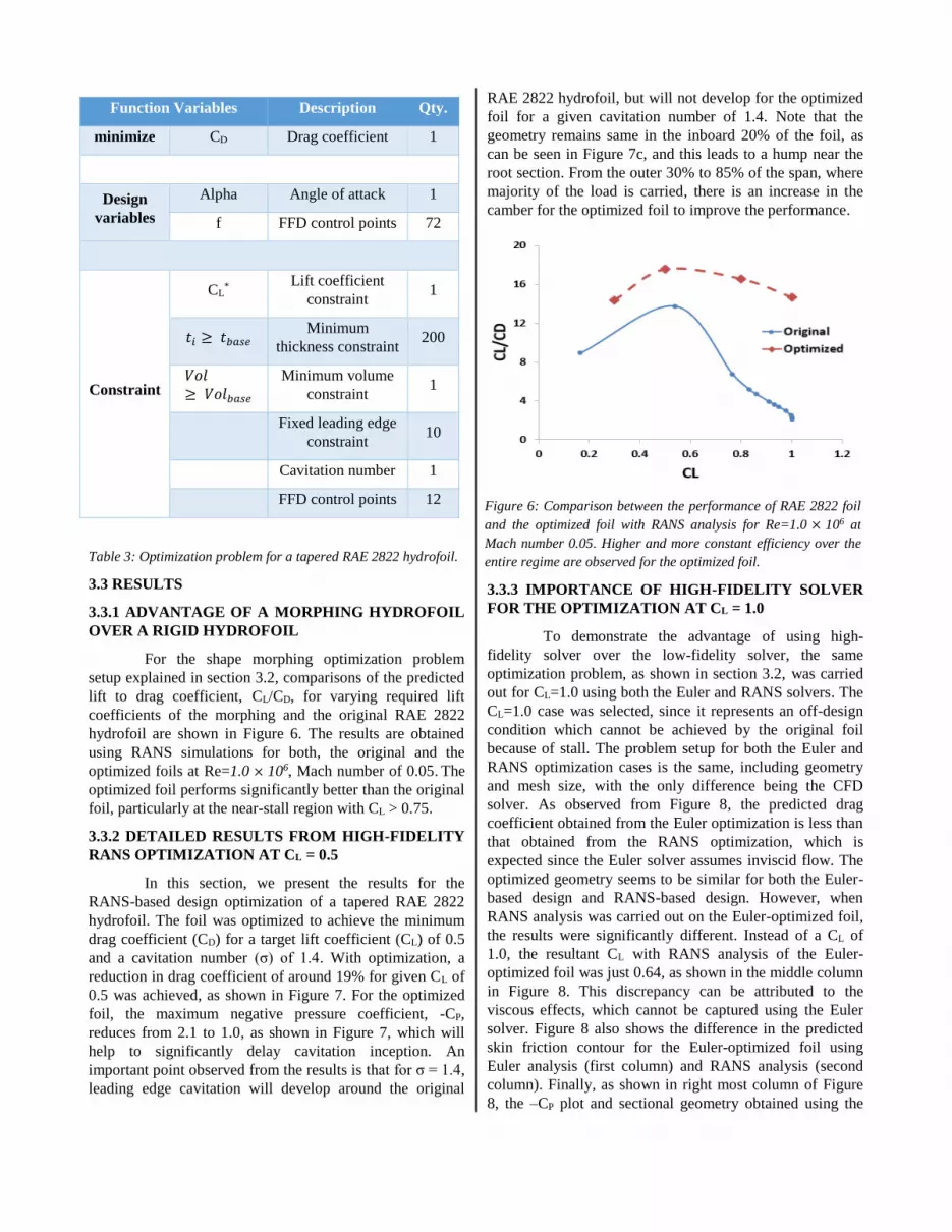
Table 3: Optimization problem for a tapered RAE 2822 hydrofoil.

3.3 RESULTS

3.3.1 ADVANTAGE OF A MORPHING HYDROFOIL OVER A RIGID HYDROFOIL

For the shape morphing optimization problem setup explained in section 3.2, comparisons of the predicted lift to drag coefficient, CL/CD, for varying required lift coefficients of the morphing and the original RAE 2822 hydrofoil are shown in Figure 6. The results are obtained using RANS simulations for both, the original and the optimized foils at Re=1.0 × 106, Mach number of 0.05. The optimized foil performs significantly better than the original foil, particularly at the near-stall region with CL > 0.75.

3.3.2 DETAILED RESULTS FROM HIGH-FIDELITY RANS OPTIMIZATION AT CL = 0.5

In this section, we present the results for the RANS-based design optimization of a tapered RAE 2822 hydrofoil. The foil was optimized to achieve the minimum drag coefficient (CD) for a target lift coefficient (CL) of 0.5 and a cavitation number (σ) of 1.4. With optimization, a reduction in drag coefficient of around 19% for given CL of 0.5 was achieved, as shown in Figure 7. For the optimized foil, the maximum negative pressure coefficient, -CP, reduces from 2.1 to 1.0, as shown in Figure 7, which will help to significantly delay cavitation inception. An important point observed from the results is that for σ = 1.4, leading edge cavitation will develop around the original

RAE 2822 hydrofoil, but will not develop for the optimized foil for a given cavitation number of 1.4. Note that the geometry remains same in the inboard 20% of the foil, as can be seen in Figure 7c, and this leads to a hump near the root section. From the outer 30% to 85% of the span, where majority of the load is carried, there is an increase in the camber for the optimized foil to improve the performance.

3.3.3 IMPORTANCE OF HIGH-FIDELITY SOLVER FOR THE OPTIMIZATION AT CL = 1.0

To demonstrate the advantage of using high-fidelity solver over the low-fidelity solver, the same optimization problem, as shown in section 3.2, was carried out for CL=1.0 using both the Euler and RANS solvers. The CL=1.0 case was selected, since it represents an off-design condition which cannot be achieved by the original foil because of stall. The problem setup for both the Euler and RANS optimization cases is the same, including geometry and mesh size, with the only difference being the CFD solver. As observed from Figure 8, the predicted drag coefficient obtained from the Euler optimization is less than that obtained from the RANS optimization, which is expected since the Euler solver assumes inviscid flow. The optimized geometry seems to be similar for both the Euler-based design and RANS-based design. However, when RANS analysis was carried out on the Euler-optimized foil, the results were significantly different. Instead of a CL of 1.0, the resultant CL with RANS analysis of the Euler-optimized foil was just 0.64, as shown in the middle column in Figure 8. This discrepancy can be attributed to the viscous effects, which cannot be captured using the Euler solver. Figure 8 also shows the difference in the predicted skin friction contour for the Euler-optimized foil using Euler analysis (first column) and RANS analysis (second column). Finally, as shown in right most column of Figure 8, the –CP plot and sectional geometry obtained using the

Function Variables Description Qty.

minimize CD Drag coefficient 1

Design variables

Alpha Angle of attack 1

f FFD control points 72

Constraint

CL* Lift coefficient

constraint 1

Minimum

thickness constraint 200 � �

Minimum volume constraint

1

Fixed leading edge

constraint 10

Cavitation number 1

FFD control points 12 Figure 6: Comparison between the performance of RAE 2822 foil and the optimized foil with RANS analysis for Re=1.0 × 106 at Mach number 0.05. Higher and more constant efficiency over the entire regime are observed for the optimized foil.

RANS optimized foil and RANS analysis of Euler-optimized foil are significantly different. This comparison clearly illustrates the need of high-fidelity solver to carry out hydrodynamic optimization for off-design conditions.

3.3.3 GRID CONVERGENCE STUDY AT CL=1.0

To ensure that the optimization results are independent of the mesh size, RANS-based optimization was repeated for the same foil with the same setup for CL= 1.0 using a 1.5 million cell mesh. As shown in Table 4 and Figure 9, the results obtained using the 1.5 million cell mesh and the 193,000 cell mesh are almost identical for the pressure distribution, skin friction distribution, and optimized geometry, although a small difference is noted in the total drag coefficient presented in Table 4.

Mesh Size CL CD

193,000 cells 1.0 0.0682

1.5 M cells 1.0 0.0611

Table 4: Grid convergence study for the RANS-optimization of the RAE 2822 hydrofoil at Re=1.0 × 106, CL=1.0.

4 CONCLUSIONS

In this work, a low-speed preconditioner is implemented in an existing compressible CFD solver, SUmb, to solve problems involving nearly incompressible flows for Mach numbers as low as 0.01. The low-speed SUmb solver was validated against the experimental results for a tapered stainless steel NACA 0009 hydrofoil from [1]. In pre-stall region, the average error of 7.8% in CD values and 9.5% in CL values was noted between the low-speed SUmb and the experimental results.

A design constraint on the cavitation number was developed to delay the cavitation inception for the optimized foil. The combination of this constraint and the low-speed solver resulted in a design optimization tool for 3-D lifting bodies operating in viscous and incompressible fluids with consideration for cavitation inception. Optimization results using the adjoint method were presented for both an Euler and a RANS solver for a tapered RAE 2822 hydrofoil at Re=1.0 × 106 and Mach number of 0.05. The problem setup is shown in section 3.2. In the presented results, 72 shape design variables were used to optimize the detailed geometry. The current tool is capable of handling much larger number of design variables. Currently, we are running optimizations to thoroughly study the effect of number of shape design variables on the optimization result.

The advantage of the RANS-based design optimization over Euler-based design optimization was demonstrated for the tapered RAE 2822 hydrofoil at a CL of 1.0 (i.e., at a near-stall condition). Results show that the Euler-based design optimization is significantly different from RANS-based design optimization, as Euler-based methods do not consider viscous effects. Thus, there is a need for high-fidelity, efficient design optimization tools to carry out design optimization at the intermediate stage, especially for off-design conditions.

The results show that active or passive continuous morphing of the RAE hydrofoil can lead to a decrease in drag of at least 20% for a given lift and help to significantly delay cavitation inception. A thorough study of the active or passive shape morphing in the marine propulsors can help to dramatically improve fuel efficiency, agility, and performance at off-design conditions (such as crash-stop maneuvers, hard turns, and maneuvering), while at the same time delaying cavitation inception.

5 FUTURE WORK

After a systematic hydrodynamic shape optimization study, the obvious next step is to check whether the optimized foil can satisfy structural strength and stability requirements. To check for structural strength and complete the design tool-kit, hydro-elastic optimization needs to be carried out, similar to what has been done for aircraft wings [10, 11]. Hydro-elastic optimization can help in optimizing the geometry and material configuration of the hydrofoil to control and tailor the fluid structure interaction (FSI) response, to reduce the structural weight, and to ensure structural integrity. Examples where hydro-elastic optimization can be critical include composite propellers and shape morphing propellers and hydrofoils. In composite propellers or hydrofoils, the load-dependent transformations can be tailored to reduce dynamic load variations, delay cavitation inception, and improve fuel efficiency by adjusting the blade or foil shape in off-design conditions or in spatially varying flow [20]. Thus, it will be interesting to see if optimizer can optimize both the geometry and material configurations to improve the overall hydrodynamic performance while satisfying structural and stability constraints.

ACKNOWLEDGMENTS The computations were performed on the Flux HPC

cluster at the University of Michigan Center of Advanced Computing.

Support for this research was provided by the U.S. Office of Naval Research (Contract N00014-13-1-0763), managed by Ms. Kelly Cooper.

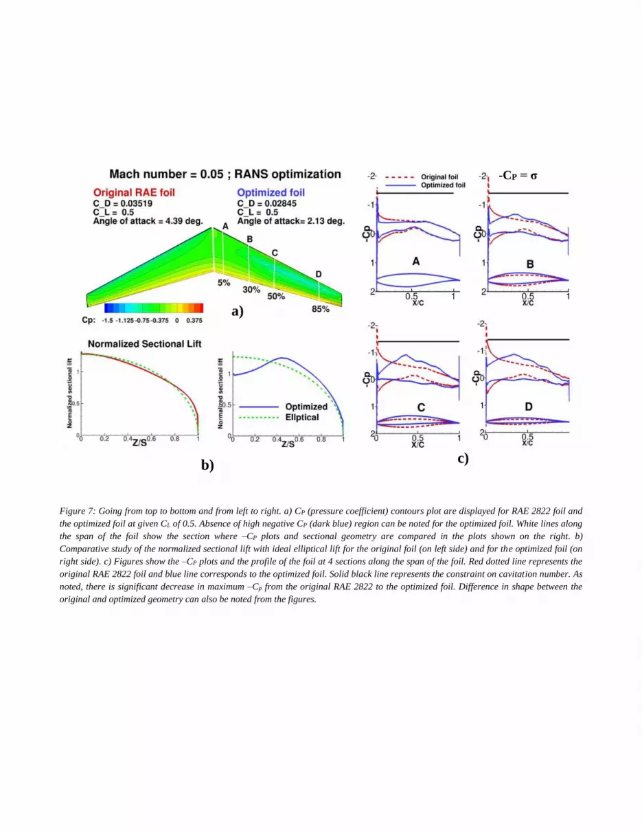
Figure 7: Going from top to bottom and from left to right. a) CP (pressure coefficient) contours plot are displayed for RAE 2822 foil and the optimized foil at given CL of 0.5. Absence of high negative CP (dark blue) region can be noted for the optimized foil. White lines along the span of the foil show the section where –CP plots and sectional geometry are compared in the plots shown on the right. b) Comparative study of the normalized sectional lift with ideal elliptical lift for the original foil (on left side) and for the optimized foil (on right side). c) Figures show the –CP plots and the profile of the foil at 4 sections along the span of the foil. Red dotted line represents the original RAE 2822 foil and blue line corresponds to the optimized foil. Solid black line represents the constraint on cavitation number. As noted, there is significant decrease in maximum –Cp from the original RAE 2822 to the optimized foil. Difference in shape between the original and optimized geometry can also be noted from the figures.

a)

b) c)

-CP = σ

Figure 8: Figure showing the difference in Euler-based optimization and RANS-based optimization for RAE 2822 hydrofoil at CL of 1.0 for Re=1.0 × 106. Comparisons are shown for the pressure contour, friction coefficient, sectional geometry, CL and CD values. Column 1 shows the Euler-based design optimized foil, column 2 represents the RANS analysis of the Euler-optimized foil, and column 3 displays the RANS optimized foil. The difference in the friction coefficient, pressure contours, CL and CD values can be easily seen between the Euler-optimized foil and RANS analysis of the Euler-optimized foil. Important points observed from the result are: (1) RANS analysis of the Euler-optimized foil showed that Euler-optimized foil will not be achieve the target lift. and (2) there are significant differences in the skin friction magnitude for the Euler-optimized foil with Euler analysis and RANS analysis. In the third row, comparison of -CP plots between the Euler-analysis and RANS-analysis of Euler-optimized foil is plotted. Difference between the CP plots for the same geometry but different solver) can be easily noted from the plots. In the last column of third row, comparison of geometry from RANS-based design optimization and RANS analysis of Euler-based design optimization is presented.

Euler-based optimized foil RANS-based optimized foil

Euler analysis RANS analysis RANS analysis

Pressure contours (suction

side)

Friction coefficient (pressure

side)

-CP plots and

geometry comparison

CL 1.0 0.6426 1.0

CD 0.0482 0.0554 0.0681

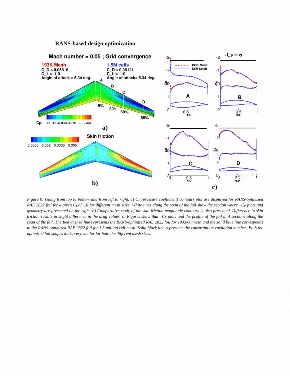
Figure 9: Going from top to bottom and from left to right. a) CP (pressure coefficient) contours plot are displayed for RANS-optimized RAE 2822 foil for a given CL of 1.0 for different mesh sizes. White lines along the span of the foil show the section where –CP plots and geometry are presented on the right. b) Comparative study of the skin friction magnitude contours is also presented. Difference in skin friction results in slight difference in the drag values. c) Figures show that –CP plots and the profile of the foil at 4 sections along the span of the foil. The Red dashed line represents the RANS-optimized RAE 2822 foil for 193,000 mesh and the solid blue line corresponds to the RANS-optimized RAE 2822 foil for 1.5 million cell mesh. Solid black line represents the constraint on cavitation number. Both the optimized foil shapes looks very similar for both the different mesh sizes.

c)

RANS-based design optimization

a)

-CP = σ

b)

REFERENCES

1. Zarruk, G. A., Brandner, P. A., Pearce, B. W., and Phillips, A. W. (2014). Experimental study of the steady fluid–structure interaction of flexible hydrofoils. Journal of Fluids and Structures, 51, 326-343.

2. Kota, S., Osborn, R., Ervin, G., Maric, D., Flick, P., and Paul, D. (2009). Mission adaptive compliant wing-design fabrication and flight test. Morphing vehicles, number RTO-MP-AVT-168-18. NATO research and Technology Organization.

3. Lyu, Z., Kenway, G. K., and Martins, J. R. R. A. (2014). Aerodynamic Shape Optimization Investigations of the Common Research Model Wing Benchmark. AIAA Journal, 1-18.

4. Hsin, C. Y. (1994). Application of the panel method to the design of two-dimensional foil sections. Journal of Chinese society of Naval Architects and Marine Engineers, Vol. 13, No.2pp. 1-11.

5. Hsin, C. Y., Wu, J. L., and Chang, S. F. (2006). Design and optimization method for a two-dimensional hydrofoil. Journal of Hydrodynamics, Ser. B, 18(3), 323-329.

6. Wilson, W., Gorski, J., Kandasamy, M., Takai, T., He, W., Stern, F., and Tahara, Y. (2010, June). Hydrodynamic shape optimization for naval vehicles. In High Performance Computing Modernization Program Users Group Conference (HPCMP-UGC), 2010 DoD (pp. 161-168). IEEE.

7. Campana, E. F., Peri, D., Tahara, Y., and Stern, F. (2006). Shape optimization in ship hydrodynamics using computational fluid dynamics. Computer methods in applied mechanics and engineering, 196(1), 634-651.

8. Mishima, S., and Kinnas, S. A. (1996). A numerical optimization technique applied to the design of two-dimensional cavitating hydrofoil sections. Journal of ship research, 40(1), 28-38.

9. ZENG, Z. B., and Kuiper, G. (2012). Blade section design of marine propellers with maximum cavitation inception speed. Journal of Hydrodynamics, Ser. B, 24(1), 65-75.

10. Kenway, G. K., Kennedy, G. J., and Martins, J. R. R. A. (2014). Scalable parallel approach for high-fidelity steady-state aeroelastic analysis and adjoint derivative computations. AIAA Journal, 52(5), 935-951.

11. Kenway, G. K., and Martins, J. R. R. A. (2014). Multipoint High-Fidelity Aerostructural

Optimization of a Transport Aircraft Configuration. Journal of Aircraft, 51(1), 144-160.

12. Reuther, J. J., Jameson, A., Alonso, J. J., Rimlinger, M. J., and Saunders, D. (1999). Constrained multipoint aerodynamic shape optimization using an adjoint formulation and parallel computers, part 1. Journal of Aircraft, 36(1), 51-60.

13. Turkel, E., Radespiel, R., and Kroll, N. (1997). Assessment of preconditioning methods for multidimensional aerodynamics. Computers & Fluids, 26(6), 613-634.

14. Choi, Y. H., and Merkle, C. L. (1993). The application of preconditioning in viscous flows. Journal of Computational Physics, 105(2), 207-223.

15. Van Leer, B., Lee, W. T., and Roe, P. L. (1991). Characteristic time-stepping or local preconditioning of the Euler equations. In 10th Computational Fluid Dynamics Conference (Vol. 1, pp. 260-282).

16. van der Weide, E., Kalitzin, G., Schluter, J., and Alonso, J. J. (2006). Unsteady turbomachinery computations using massively parallel platforms. AIAA paper, 421, 2006.

17. Jameson, A., Schmidt, W., and Turkel, E. (1981). Numerical solutions of the Euler equations by finite volume methods using Runge-Kutta time-stepping schemes. AIAA paper, 1259, 1981.

18. Spalart, P. and Allmaras, S. (1992). A One-Equation Turbulence Model for Aerodynamic Flows. 30th Aerospace Sciences Meeting and Exhibit. doi:10.2514/6.1992-439.

19. Gill, P. E., Murray, W., and Saunders, M. A. (2002). SNOPT: An SQP algorithm for large-scale constrained optimization. SIAM journal on optimization, 12(4), 979-1006.

20. Young, Y. L. (2008). Fluid–structure interaction analysis of flexible composite marine propellers. Journal of Fluids and Structures, 24(6), 799-818. Chicago.

21. Martins, J. R. R. A., Sturdza, P., and Alonso, J. J. (2003). The complex-step derivative approximation. ACM Transactions on Mathematical Software (TOMS), 29(3), 245-262.

22. Lyu, Z., Kenway, G. K., Paige, C., and Martins, J. R. R. A. (2013, July). Automatic differentiation adjoint of the Reynolds-averaged Navier–Stokes equations with a turbulence model. In 43rd AIAA Fluid Dynamics Conference and Exhibit.