Embed Size (px)
Citation preview


HEMLINE THEORY: TESTING THE RELATIONSHIP BETWEEN FASHION
TRENDS AND THE STOCK MARKET
A thesis submitted to the
Kent State University Honors College
in partial fulfillment of the requirements
for University Honors
by
Gabriella Humes
May, 2021


ii
Thesis written by
Gabriella Humes
Approved by
_____________________________________________________________________,
Advisor
______________________________________________, Chair, Department of Finance
Accepted by
___________________________________________________, Dean, Honors College

iii
TABLE OF CONTENTS
LIST OF EXHIBITS.....……………………………………………………………….....v
LIST OF TABLES………..……………………………………………………………..vi
ACKNOWLEDGMENTS……………….……………………………………………..vii
CHAPTER
I. INTRODUCTION……………………………………………….………1
II. PREVIOUS STUDIES…………………………………………….…….7
III. DATA COLLECTION………………………………………………….13
IV. GRAPHICAL REPRESENTATION OF THE HEMLINE THEORY…17
1920s.…………………………………..……………………………….19
1930s……………………………………………………………………21
1940s……………………………………………………………………23
1950s……………………………………………………………………26
1960s……………………………………………………………………27
1970s……………………………………………………………………30
1980s……………………………………………………………………33
1990s……………………………………………………………………35
2000s……………………………………………………………………37
V. REGRESSION TESTING……………………………………………...40
VI. CONCLUSIONS……………………………………………………….59
iv
REFERENCES…………………………………………………………………….…..61
APPENDIX
1. MONTHLY HEMLINE DATA FROM 1925 TO 2010...…………….63
2. MONTHLY PANTS DATA FROM 1960 TO 2010…...……………..65
3. MACROECONOMIC VARIABLE DESCRIPTIONS……………….67
4. REFERENCE IMAGES FOR HEMLINE LENGTHS..……………...69
5. REFERENCE IMAGES FOR PANTS LENGTHS..…………………70

v
LIST OF EXHIBITS
Exhibit 1. Hemlines, pants, and stock returns from 1925 to 2010……………………….18
Exhibit 2. Hemlines and stock returns from 1925 to 1929……………………………….19
Exhibit 3. Hemlines and stock returns from 1930 to 1939……………………………….21
Exhibit 4. Hemlines and stock returns from 1940 to 1949……………………………….23
Exhibit 5. Hemlines and stock returns from 1950 to 1959……………………………….26
Exhibit 6. Hemlines, pants, and stock returns from 1960 to 1969……………………….27
Exhibit 7. Hemlines, pants, and stock returns from 1970 to 1979……………………….30
Exhibit 8. Hemlines, pants, and stock returns from 1980 to 1989……………………….33
Exhibit 9. Hemlines, pants, and stock returns from 1990 to 1999……………………….35
Exhibit 10. Hemlines, pants, and stock returns from 2000 to 2010……………………...37
Exhibit 11. Monthly hemline data from 1925 to 2010…………………………………..63
Exhibit 12. Monthly pants data from 1960 to 2010……………………………………..65
Exhibit 13. Reference images for hemline lengths……………………………………...69
Exhibit 14. Reference images for pants lengths………………………………………...70
vi
LIST OF TABLES
Table 1. Regression Results for Stock Market Returns and Hemlines…………..…..….43
Table 2. Regression Results for Fashion Companies Stock Returns and Hemlines..…...45
Table 3. Regression Results for Stock Market Returns and Pants……………………....47
Table 4. Regression Results for Fashion Companies Stock Returns and Pants…………49
Table 5. Regression Results for Hemlines and Stock Returns…………………………..51
Table 6. Regression Results for Hemlines and Fashion Companies Stock Returns…….53
Table 7. Regression Results for Pants and Stock Returns………………………………55
Table 8. Regression Results for Pants and Fashion Companies Stock Returns………...57
Table 9. Macroeconomic variable descriptions………………………………………...67

vii
ACKNOWLEDGMENTS
Thank you to my advisors and oral defense committee members for the time and
effort you put into this thesis alongside me. Thank you to my family for supporting me
and believing in me, even when I did not believe in myself.
1
Chapter 1: Introduction
Fashion is a phenomenon that transcends time and culture. Fashion derives from
human’s universal instinct to decorate one’s self, and therefore can encompass clothing,
makeup, hairstyles, etc. (Welters, L., & Lillethun, A., 2018, p. 1-10). However, for the
purpose of this thesis, I will focus solely on the clothing part of fashion. According to
Linda Welters and Abby Lillethun, fashion can be defined as “changing styles of dress
and appearance that are adopted by a group of people at any given time and place”
(Welters, L., & Lillethun, A., 2018, p. 16). This definition encompasses the reality of
fashion being dynamic and ever changing. These changes in fashion can be the direct or
indirect result of numerous influences including social, cultural, and economic
characteristics as well as matters of class, gender, and sexuality (Gilbert, D., 2017, pgs.
487-488). Fashion also acts as an influence on numerous outside factors. Oscar Wilde
sums up the innovative nature of fashion well: “After all, what is fashion? It is usually a
form of ugliness so intolerable that we have to alter it every six months” (Laver, J., 1969
p. 25).
There are several theories that relate to the evolution of fashion and how it moves
through society. According to Robert Elms: “It [fashion] is cyclical, but the circle is
never completed because it is also evolutionary, therefore patterns repeat but they are
never quite the same” (Gilbert, D., 2017, p. 493). In 1937, Agnes Brooks Young claimed
that fashion has its own laws and cycles, free from external forces.
2
On the other side, James Laver embraced the notion that designers are not the masters of
their own fate and “can only introduce an innovation if it happens to be in accordance
with the spirit of the age” (Gilbert, D., 2017, p. 487). Laver also popularized the
“erogenous-zone” theory, first advanced by psychologist J.C. Flüegl, in his book Modesty
in Dress (Welters, L., & Lillethun, A., 2018, p. 38). This theory suggested that women’s
fashion trends follow whichever part of the body attracted the most sexual interest at that
point in time. For example, the 1920s focused on the legs, the 1930s on the back, the
1940s on the waist, the 1950s on the bust, and circled back around to the legs again in the
1960s (as cited in Mabry, 1971, p. 3). The most commonly accepted theory is that fashion
is cyclical but is also impacted by numerous external forces. An example of fashion’s
cyclical nature is shifts in hemlines. Midi skirts, which fall a little higher than mid-calf,
were a woman’s uniform in the 40s, and the length came back into style recently in 2018
and 2019. New fashions may be introduced that are considered novel, but over time, they
too become part of fashion’s cycle. For example, it was a shock when women began to
wear pants outside the house in the 1960s. However, as years passed, women’s pants
became common and were eventually accepted as part of the fashion cycle.
As for the flow of fashion trends through society, three theories are most
commonly assumed; the trickle-up theory, trickle-down theory, and trickle-across theory.
The trickle-up theory states that fashion trends start as street wear and travel up until the
trend is considered high fashion. The concept of the trickle-down theory is that trends
start on the runways as high fashion, move through the classes, and trickle down until the
trend is considered street wear. The trickle-across theory assumes that trends move
3
horizontally across groups of similar status with little lag time between them. The trickle-
down theory is the oldest and most widely accepted fashion flow theory. An example of
the trickle-down theory would be if a silhouette or pattern appeared on the runway for
Gucci and then appeared in fast fashion stores a few weeks later. Despite the widely
accepted trickle-down theory, some fashion historians believe that change can move
upwards, downwards, or crosswise, with no theory being distinctly superior (Welters, L.,
& Lillethun, A., 2018, p. 40). These theories on the fashion cycle are an important
influence on how we look at fashion innovation in society.
As Oscar Wilde so eloquently stated, fashion is constantly evolving from one
trend to the next, and one of the most common and noticeable changes in fashion is shifts
in hemline length. With these changes occurring so frequently, outside variables have
sometimes been suggested to have a relationship with hemlines. One such variable is the
stock market, which has been hypothesized to have a relationship with shifts in hemline
length. This theory is popularly referred to as the hemline theory, skirt length theory,
hemline index, and other similar names. George Taylor, an economist at Wharton School
of Business, was the first one to observe the relationship between hemlines and the stock
market in 1926 (Cole, D. J., & Deihl, N., 2015, p. 139). During his studies on women’s
silk hosiery, Taylor noted women’s skirts were shorter in thriving financial times so they
could show off their silk stockings. In economic downturns, women’s skirts fell lower to
hide the fact that some women could not afford stockings. By noticing these patterns in
his studies, Taylor became credited for the suggestion that hemline lengths were
correlated with the stock market, even though it was not his area of study (Cole, D. J., &
4
Deihl, N., 2015, p. 139). There are a few instances of this supposed correlation that seem
to support the theorized relationship between hemlines and stocks, the most commonly
known in the late 1920s, early 1930s. In the 1920s, hemlines rose to the knee, showing
off more leg than had ever been acceptable before. Women began to defy societal norms
by showing skin, drinking, clubbing, and fully embracing the new flapper culture. The
economy was doing well, as insinuated by the decade’s title: “The Roaring Twenties,”
and consumers were happy to indulge. Next came the Crash of 1929, which led to the
Great Depression. The new lavish fashions of the early 20s were left behind for plainer,
and therefore cheaper, styles, prompting hemlines to drop again. Despite the little
evidence seen in recent decades, this theoretical link between hemlines and the stock
market continues to fascinate people.
Due to the hemline index being more of an observation than a hard theory, there
are multiple interpretations of the supposed relationship between stock movements and
hemline trends. Some people believe that hemlines predict the stock market. Others
believe that the stock market predicts shifts in hemlines. The hemline theory remains a
point of interest in the fashion industry and studies have been conducted on the
correlation between these two variables. One study, completed in 2012 by Marjolein van
Baardwijk and Philip Hans Franses, looks at the stock market as the predictor of hemline
changes and the lag time that occurs between movements in the two variables (Van
Baardwijk, M., & Franses, P.H., 2012, p. 25-26). The other study, a master’s thesis,
completed by Mary Ann Mabry, looks at the relationship between the stock market and
5
hemlines and how it relates to the upper and middle classes (Mabry, M.A., 1971, p. 1-
101). These two studies will be discussed at further length in the next chapter.
The original purpose of this thesis was to research and test the relationship
between hem length and the stock market from 1925 to 2010. However, through the
process of gathering data, which will be discussed more in detail later, a pattern emerged
around the 1960s, where pants became a large part of women’s fashion and skirts fell to
the wayside. Due to this shift, trends in pant length were also studied from 1960 to 2010
alongside the original analysis of hemlines and the stock market. The stock returns for
fashion companies specifically, were also gathered and investigated, as the fashion trends
may exhibit a closer correlation to stock returns within their own industry. Given the
existing research on the hemline theory, the goal of this thesis is to determine whether
there is a relationship between hemline or pant lengths and the returns of either the entire
stock market or fashion company stocks. This thesis also explores whether fashion trends
or the stock market are reliable predictors of the other. As will be discussed later in
chapter 5, the results of the analysis and testing did indicate that there is no causal
relationship with stocks or hemlines as the dependent variable.
These relationships will be graphed by each decade and tested through a
regression analysis. To examine the effect of fashion changes on stock movements, the
independent variable or “x” will be annual hemline and pants data. The dependent
variable or “y” will be the stock returns. To assess the opposite side of the theory, the
independent variable will be stock returns, and the dependent variable will be hemlines
and pants data. Pant and hemline data will be collected from the fashion illustration
6
Vogue magazine, which has an archive of issues dating back to the 1890s (Vogue, n.d.).
Vogue is a well-known fashion publication and is revered at the forefront of high fashion
trends in the industry for representing fashion innovation. Vogue showcases new trends
early in its lifecycle. The publication can breathe life into trends, sometimes launching
them into the mass market and shortening their time to adoption by consumers.
Macroeconomic controls will also be included in the regression analyses as variables that
may have impacts on the main variables, hemlines, pants, and stocks. Some examples of
macroeconomic controls include unemployment rate, gross domestic product, annual
Treasury yields, and similar economic measures.
Chapter 2 of this thesis will discuss previous studies completed, their results, and
explain how my study will be different by researching new areas that have not been
previously examined. Chapter 3 will explain how I collected and utilized my raw data for
hemline trends, pant length trends, overall stock returns, fashion companies’ stock
returns, and macroeconomic control variables. Chapter 4 will include all the graphs
created to visually represent the data for the fashion trends and stock return movements.
This chapter will also include explanations of what is being observed in the graphs.
Chapter 5 will discuss the regression model further in depth and report the regression test
results. Chapter 6 will summarize the ending conclusions.
7
Chapter 2: Previous Studies
Several studies have been conducted on the hemline theory and the relationship
between hemlines and the economy or stock market. A study was completed on the
hemline theory by Mary Ann Mabry as a master’s thesis in 1971. The purpose of Mabry’s
thesis was to investigate the relationship between hemline and stock market fluctuations
from 1921 to 1970, and how both are affected by underlying economic factors. Mabry
also explored any time lag present in the acceptance of hemline fluctuations by the
middle and upper classes. The hemline data was collected from four fashion publications:
Vogue, Harper’s Bazaar, Good Housekeeping, and Ladies’ Home Journal. Stock market
data was collected from examination of the Dow Jones Stock Average Chart 1921 –
1970. Economic events that occurred during the 50-year period were also analyzed,
including recessions, depressions, inflationary periods, and wars (Mabry, M.A., 1971, p.
1-101).
Mabry graphed the hemline and stock market movements during the 1921-1970
period. Stock movements were graphed using the Dow Jones’ monthly highs and lows.
Hemline data from Vogue and Harper’s Bazaar were combined as the upper-class
publications, and Good Housekeeping and Ladies’ Home Journal were combined as the
middle-class publications. Mabry discovered through mathematical testing and visual
comparison that hemline fluctuations of both the upper and middle classes and stock
market movements did not correspond to each other. As for the hypothesized time lag for
8
hemline acceptance in the middle and upper classes, no such lag was found in Mabry’s
study except for the 1950s and 1960s, the last two decades that were studied (Mabry,
M.A., 1971, p. 1-101).
Another one of the most referenced studies was completed by Marjolein van
Baardwijk and Philip Hans Franses and published in 2012 in Foresight: The International
Journal of Applied Forecasting (Van Baardwijk, M., & Franses, P.H., 2012, p. 25-26).
Baardwijk and Franses realized that although the hemline theory remained prevalent in
the news and in the fashion industry, there had not been extensive research completed on
the supposed connection between hem lengths and the stock market. They set out to
change this in 2010. The pair collected monthly hemline data from the French fashion
magazine, L’Officiel. In the years where less than 12 issues were published, the missing
months were assumed to be the same figure as the previous month. Hem lengths were
recorded and grouped in 5 distinct lengths, and they are as follows: 1 – Mini, 2 –
Ballerina-length (above-the-knee, cocktail), 3 – Below the knee, 4 – Full-length (ankle),
and 5 – Floor-length. The monthly hemline data was then annualized for analysis by
taking an average. For the economic data, instead of using stock return fluctuations, the
pair investigated recessions, using the U.S. business chronology as provided by the
National Bureau of Economic Research (NBER). The monthly NBER chronology was
annualized by assigning values of 0-1 to a year depending on the months with a
recession. A value of 0 was assigned if a year had 0 or 1 month with a recession, a value
of 0.25 if a year had 2, 3, or 4 months with a recession, 0.5 if a year had 5, 6, or 7
recession months, 0.75 when there are 8, 9, or 10 months with a recession, and a value of
9
1 if a year had 11 or 12 months with a recession (Van Baardwijk, M., & Franses, P.H.,
2012, p. 25-26).
Baardwijk and Franses then created a regression model in order to explain the
hem length as a function of the prior year’s length, a trend logged to allow for leveling
off over time, and the NBER economic-cycle metric for a few years before and after. In
the last term of the equation, the symbol k was included to determine the length of the
lag. If k was a positive value, that indicates that the economic cycle led the hemline
length index. If k was a negative value, then the hem length leads the economy. By
experimenting with various values between -3 to 3 for k, the pair was able to examine
results for leading and lagging issues. The best model was where k was equal to 3. This
model had an R-squared of 0.310 and the coefficient on the NBER variable was
substantially positive. With this output, Baardwijk and Franses were able to conclude that
the economic cycle leads hemline trends by three years (Van Baardwijk, M., & Franses,
P.H., 2012, p. 25-26). By finding the economic cycle to be ahead of hemlines, it shows
that stock movements may be more predictive of hemline changes than the reverse.
However, this study looked only at the surface correlation, not the possible causality of
the relationship between the two variables. This correlation could be due to changes in
underlying variables that stocks and hemlines react similarly to, not necessarily one
variable directly affecting the other.
Both of the studies discussed above found different results on the relationship
between hemline and economic measures. Mabry found that the hemline and stock return
fluctuations analyzed did not correspond to each other’s movements (Mabry, M.A., 1971,
10
p. 1-101). Baardwijk and Franses found that hemline changes lag behind economic
movements by three years (Van Baardwijk, M., & Franses, P.H., 2012, p. 25-26). Due to
the results of these previous studies, the hemline theory may seem like a redundant topic
for this thesis. However, these studies looked only at hemlines and the overall stock
market. There are other facets to this theory that have yet to be studied.
The relationship between hemlines and the overall stock market will still be
investigated in this thesis, but it will not end there. The 85-year period that is being
investigated in this thesis can be split into two parts. The first part is from 1925 to 1959.
This is a time when the fashion industry abided by many rules. One example of these
unspoken rules was that women did not wear pants as a fashion choice. Pants for women
were first introduced as beachwear and loungewear, but they were not worn on the street,
less they cause a scandal. Another example rule is that hemlines stayed below the knee to
maintain modesty. Even the below-the-knee skirt length was novel in the 20s, as
hemlines had never risen high enough to show that much leg before. Due to these
traditional rules, the fashion industry did not see much unprecedented change. Hemlines
fluctuated, but only to lengths that were below the knee or longer.
The second part of the time period is 1960 to 2010. This was a time of significant
change. The fashion industry began to evolve in the 60s, throwing the old rules out the
window and allowing for individuality. This is seen in hemlines through the shocking
development of the miniskirt, which will be discussed further in chapter 4. This change is
also seen as women begin wearing pants. Women began to embrace the practicality and
comfort of a silhouette that was traditionally menswear during this time. However, this
11
practice was still shocking to some, and women that chose to wear pants often ran into
problems from others, sometimes even being refused entry into formal establishments
(Worsley, H., 2011, p. 42). This movement started to gain traction in 1966 when Yves
Saint Laurent designed “Le Smoking,” a sleek-tailored pantsuit. Although still
controversial at first, Le Smoking would eventually be recognized as the garment that
sealed the acceptability of pants as an alternative fashion choice for women (Worsley, H.,
2011, p. 42).
As pants became more popular as a women’s fashion choice, skirts began to fall
slightly behind. This trend, coupled with the new emphasis on individuality instead of
following macro-trends, caused hemline data to become more scattered after 1960. The
rise of numerous micro-trends made it difficult to discern specific hemline movements.
Due to this fundamental shift in the fashion industry, and that pant length has never been
studied before, I thought it was important to include pant lengths in the analysis. Pants
also change length based on trends, so this proposed relationship between trends and the
stock market could have been present. Pant length data was thus collected from 1960 to
2010 and was included in the final regression testing to see if there is a relationship
between pant lengths and the stock market.
Another interesting facet of the hemline theory is the stock market itself. The
overall stock market, which has been included in previous studies of the hemline theory,
can be broken down into different categories of companies. Virtually every industry in
the world has at least one publicly held company that will be a part of the whole stock
market, including the fashion industry. As the topic of hem and pant length is directly
12
associated with fashion and the fashion industry, I decided to gather data on the stock of
fashion companies as well. The relationship between hemlines, pants, and the return on
fashion companies’ stocks will also be investigated and tested. While the overall stock
market performance has been analyzed in previous studies and shown to have a weak
correlation with hemlines, there might be a closer correlation between fashion trends and
the stock of fashion companies.
13
Chapter 3: Data Collection
Data was collected in order to graph and test the relationship between stocks,
stocks for fashion companies, hemlines, and pants. Monthly data for hem length shifts
from 1925 to 2010 were collected from Vogue magazine’s digital archives. For the
months where multiple issues were published, the first issue of the month was used.
Hemlines were obtained by observing primarily editorial images. In the early issues,
photographs were rare, so fashion drawings were used to observe hemline trends.
Advertisements were not included in the data collection. Images and drawings were
found mainly in the fashion and lifestyle sections of the magazine. If there was more than
one hem length trend in the same month, the average was taken as the monthly figure.
Pant length trends were observed in monthly issues of Vogue magazine from 1960 to
2010. The data collection process was the same as for the hemline data. By the time pants
data was being collected, editorial images had replaced fashion drawings, therefore only
editorial photographs were used to collect pant length data. Only images with easily
discernable hem and pant lengths were used. If models were posed in a way that
obstructed the view of the length, the image was not used. Both hem and pant length data
were based on women’s street dress. Clothing categories such as sportswear, sleepwear,
and evening wear were excluded from the analysis. Hemline and pant fluctuation data
was collected through stratified sampling. In each Vogue issue examined, the first four
fashion illustrations that met the specified requirements were used.
14
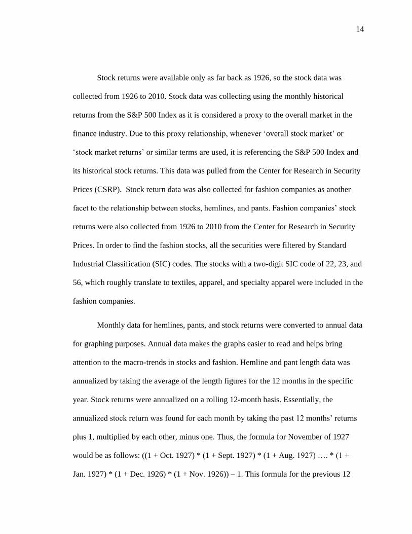
Stock returns were available only as far back as 1926, so the stock data was
collected from 1926 to 2010. Stock data was collecting using the monthly historical
returns from the S&P 500 Index as it is considered a proxy to the overall market in the
finance industry. Due to this proxy relationship, whenever ‘overall stock market’ or
‘stock market returns’ or similar terms are used, it is referencing the S&P 500 Index and
its historical stock returns. This data was pulled from the Center for Research in Security
Prices (CSRP). Stock return data was also collected for fashion companies as another
facet to the relationship between stocks, hemlines, and pants. Fashion companies’ stock
returns were also collected from 1926 to 2010 from the Center for Research in Security
Prices. In order to find the fashion stocks, all the securities were filtered by Standard
Industrial Classification (SIC) codes. The stocks with a two-digit SIC code of 22, 23, and
56, which roughly translate to textiles, apparel, and specialty apparel were included in the
fashion companies.
Monthly data for hemlines, pants, and stock returns were converted to annual data
for graphing purposes. Annual data makes the graphs easier to read and helps bring
attention to the macro-trends in stocks and fashion. Hemline and pant length data was
annualized by taking the average of the length figures for the 12 months in the specific
year. Stock returns were annualized on a rolling 12-month basis. Essentially, the
annualized stock return was found for each month by taking the past 12 months’ returns
plus 1, multiplied by each other, minus one. Thus, the formula for November of 1927
would be as follows: ((1 + Oct. 1927) * (1 + Sept. 1927) * (1 + Aug. 1927) …. * (1 +
Jan. 1927) * (1 + Dec. 1926) * (1 + Nov. 1926)) – 1. This formula for the previous 12
15
months was used for each month starting from December of 1926, as that is how far back
the stock return data went. The annual return was then taken from December, the twelfth
month of that year. Stock returns for fashion companies specifically were annualized with
the same formula on a similar rolling 12-month basis. The annual data for stock returns
for fashion companies and the S&P 500 Index as well as hem and pant lengths can be
seen in the graphs in chapter 4. Monthly data for hemlines and pants can be seen in
exhibits 11 and 12 in the appendix.
Macroeconomic variables are important to the regression testing and act as a
control in the equation. A total of 14 macroeconomic variables were included in the
regression analysis. The specific macroeconomic variables were chosen based on the core
variables found in “The Impact of Macroeconomic Variables on the Stock Market: A
Taxonomic Approach,” which will be discussed further in depth in Chapter 5. The core
variables were as follows: industrial production index, producer price index, consumer
credit, consumer price index, corporate profits, real gross domestic product,
unemployment rate, civilian labor rate, bank prime loan rate, capacity utilization, M1
money stock, vehicle sales, retail sales, and the 1-month Treasury Bill rate (Chang, S. J.,
& Ha, D., 1997, p. 111). Table 9 in the appendix has a list of all the definitions for the
macroeconomic variables used. Macroeconomic data was collected monthly from the
Federal Reserve Economic Data (FRED) database published by the Federal Reserve
Bank of St. Louis. Only the Industrial Production Index and Producer Price Index had
data available from 1925 (Federal Reserve Bank of St. Louis, n.d.). For the other
variables, data was collected as far back as recorded. Due to not all of the data being

16
available over the whole period, the regression tests needed to be staggered to be able to
include what controls were available. This will be discussed further in chapter 5. The
macroeconomic controls are only used for empirical testing and are not included in the
graphs.
17
Chapter 4: Graphical Representation of the Hemline Theory
In this section, hemline and pant trends will be graphed along with the returns of
the S&P 500 Index and the mean stock returns of fashion companies. The first graph
consists of all the years from 1925 to 2010. Each graph thereafter will correspond to a
decade within the 1925-2010 period studied. Influences of trends and returns will be
discussed after each graph. The hemline data is based on a scale from 1 to 9 and can be
interpreted as follows: 1 – Micro, 2 – Mini, 3 – Above Knee, 4 – Knee, 5 – Below Knee,
6 – Midi, 7 – Ballerina, 8 – Maxi, 9 – Floor. As touched on in the introduction, pant
length is also being studied as a potential component in the relationship between fashion
trends and the stock market. The hemline theory only discusses dresses and skirts, most
likely because women did not wear pants in 1925, when the theory was first suggested.
However, in today’s society, pants have replaced skirts and dresses as the dominant attire
for women. Due to this change, the correlation between pant length and the stock market
will also be investigated, graphed, and tested in this thesis. The pant length data was
collected on a similar 1 to 9 scale and can be interpreted as follows: 1 – Boy Shorts, 2 –
Jamaica, 3 – Bermuda, 4 – Surfer, 5 – Pedal Pushers, 6 – Clam Diggers, 7 – Seven-
eighths, 8 – Classic, 9 – Stirrup. Reference images of hem lengths and pant lengths are
included in the appendix. Hem and pant length correspond to the left-hand scale on the
graphs. Both stock returns correspond to the right-hand scale on the graph from positive
150% to negative 150%. This range was chosen in order to incorporate the majority of
the stock return fluctuations in both the S&P 500 Index and the fashion companies.
18
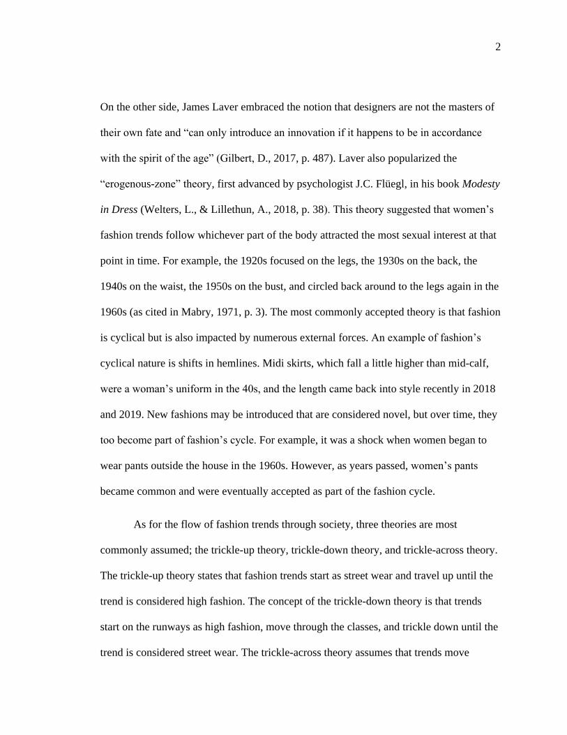
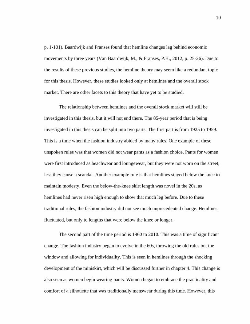
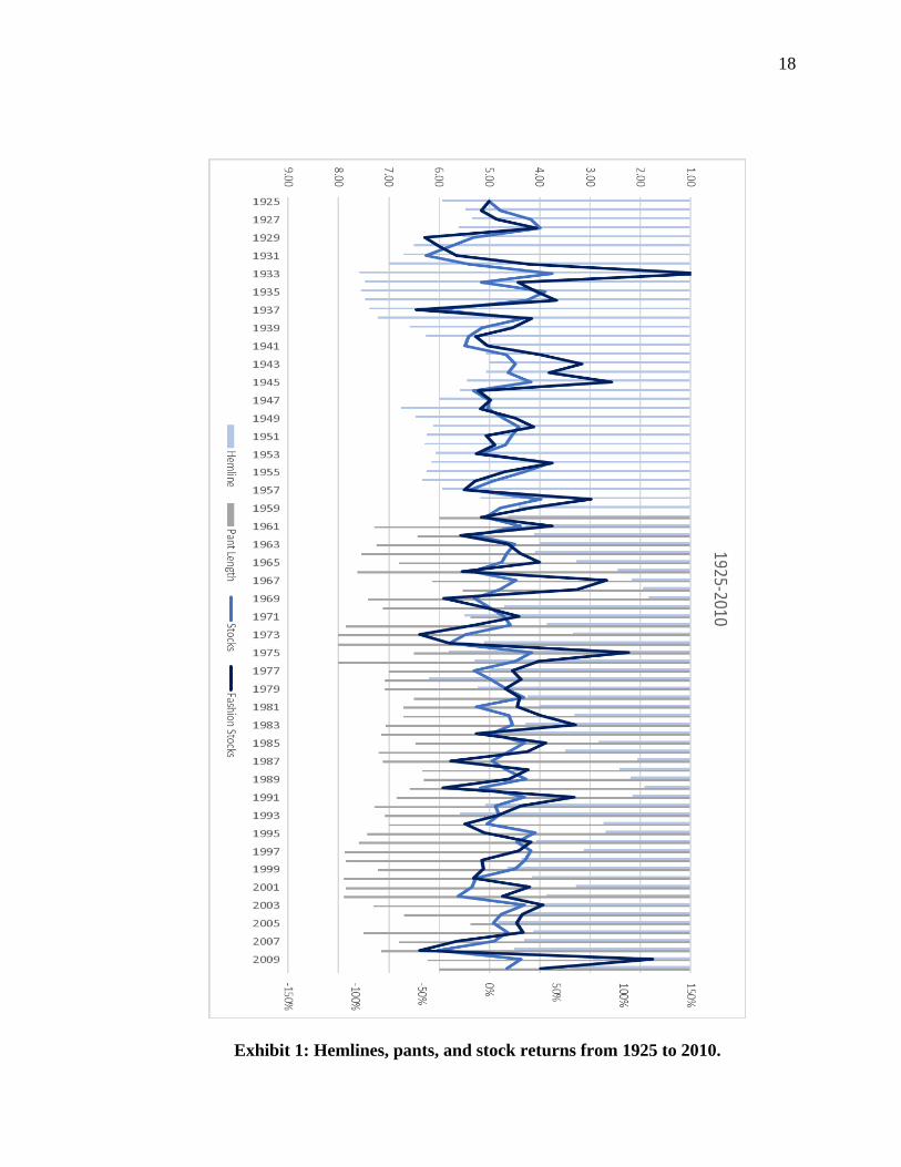
Exhibit 1: Hemlines, pants, and stock returns from 1925 to 2010.
19
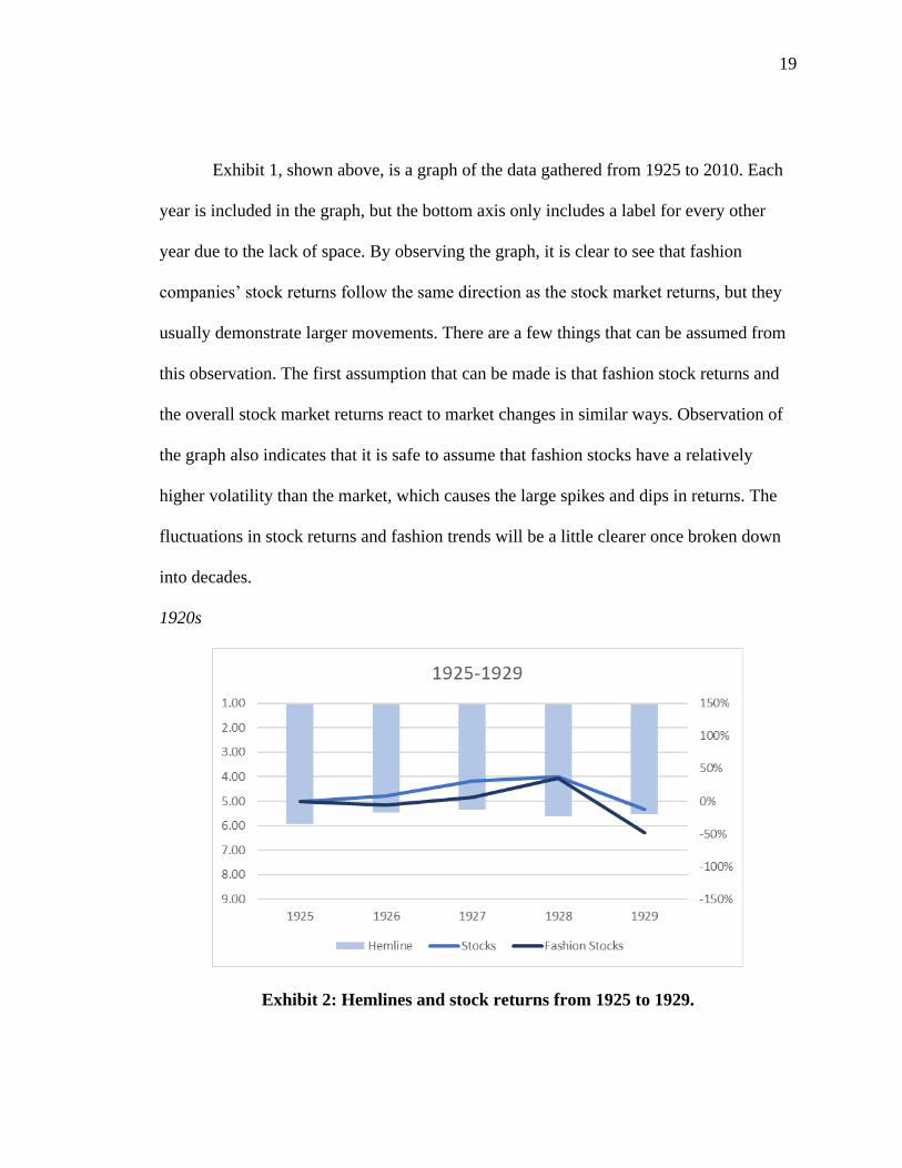
Exhibit 1, shown above, is a graph of the data gathered from 1925 to 2010. Each
year is included in the graph, but the bottom axis only includes a label for every other
year due to the lack of space. By observing the graph, it is clear to see that fashion
companies’ stock returns follow the same direction as the stock market returns, but they
usually demonstrate larger movements. There are a few things that can be assumed from
this observation. The first assumption that can be made is that fashion stock returns and
the overall stock market returns react to market changes in similar ways. Observation of
the graph also indicates that it is safe to assume that fashion stocks have a relatively
higher volatility than the market, which causes the large spikes and dips in returns. The
fluctuations in stock returns and fashion trends will be a little clearer once broken down
into decades.
1920s
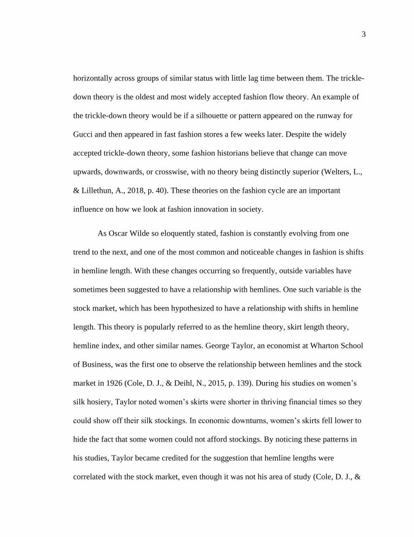
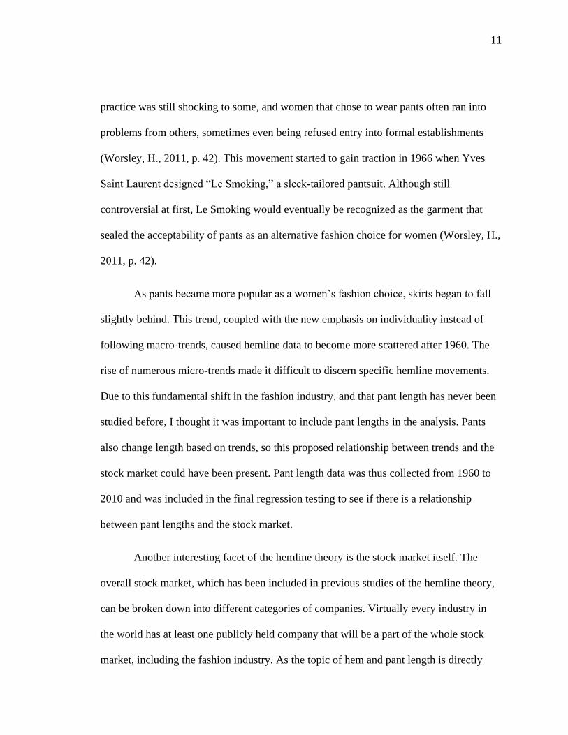
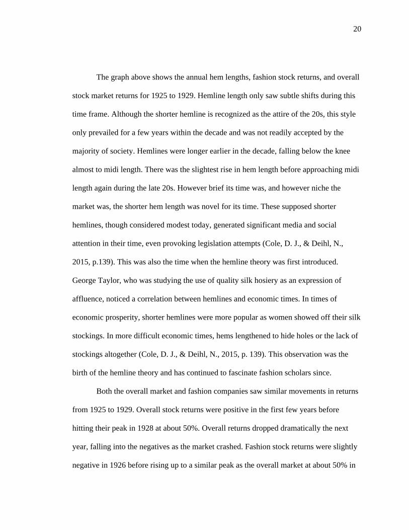
Exhibit 2: Hemlines and stock returns from 1925 to 1929.
20
The graph above shows the annual hem lengths, fashion stock returns, and overall
stock market returns for 1925 to 1929. Hemline length only saw subtle shifts during this
time frame. Although the shorter hemline is recognized as the attire of the 20s, this style
only prevailed for a few years within the decade and was not readily accepted by the
majority of society. Hemlines were longer earlier in the decade, falling below the knee
almost to midi length. There was the slightest rise in hem length before approaching midi
length again during the late 20s. However brief its time was, and however niche the
market was, the shorter hem length was novel for its time. These supposed shorter
hemlines, though considered modest today, generated significant media and social
attention in their time, even provoking legislation attempts (Cole, D. J., & Deihl, N.,
2015, p.139). This was also the time when the hemline theory was first introduced.
George Taylor, who was studying the use of quality silk hosiery as an expression of
affluence, noticed a correlation between hemlines and economic times. In times of
economic prosperity, shorter hemlines were more popular as women showed off their silk
stockings. In more difficult economic times, hems lengthened to hide holes or the lack of
stockings altogether (Cole, D. J., & Deihl, N., 2015, p. 139). This observation was the
birth of the hemline theory and has continued to fascinate fashion scholars since.
Both the overall market and fashion companies saw similar movements in returns
from 1925 to 1929. Overall stock returns were positive in the first few years before
hitting their peak in 1928 at about 50%. Overall returns dropped dramatically the next
year, falling into the negatives as the market crashed. Fashion stock returns were slightly
negative in 1926 before rising up to a similar peak as the overall market at about 50% in
21
1928. Stock returns for fashion companies saw the same crash in 1929 as the market, but
on a larger magnitude. Where the market returns dipped to about a negative 10%, fashion
stocks fell to around a negative 50% return. This market crash was the initial event that
would lead the economy into the Great Depression. Due to the relative stability of
hemlines, there does not appear to be a strong correlation between hemlines and stock
movements. The gradual rise of hem length in 1925, 1926, and 1927 follows a similar
rise in overall and fashion stock returns; however, hemlines fell slightly in 1928 when
stocks hit their peak.
1930s
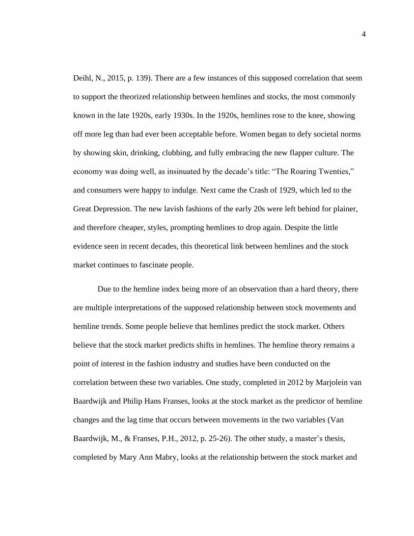
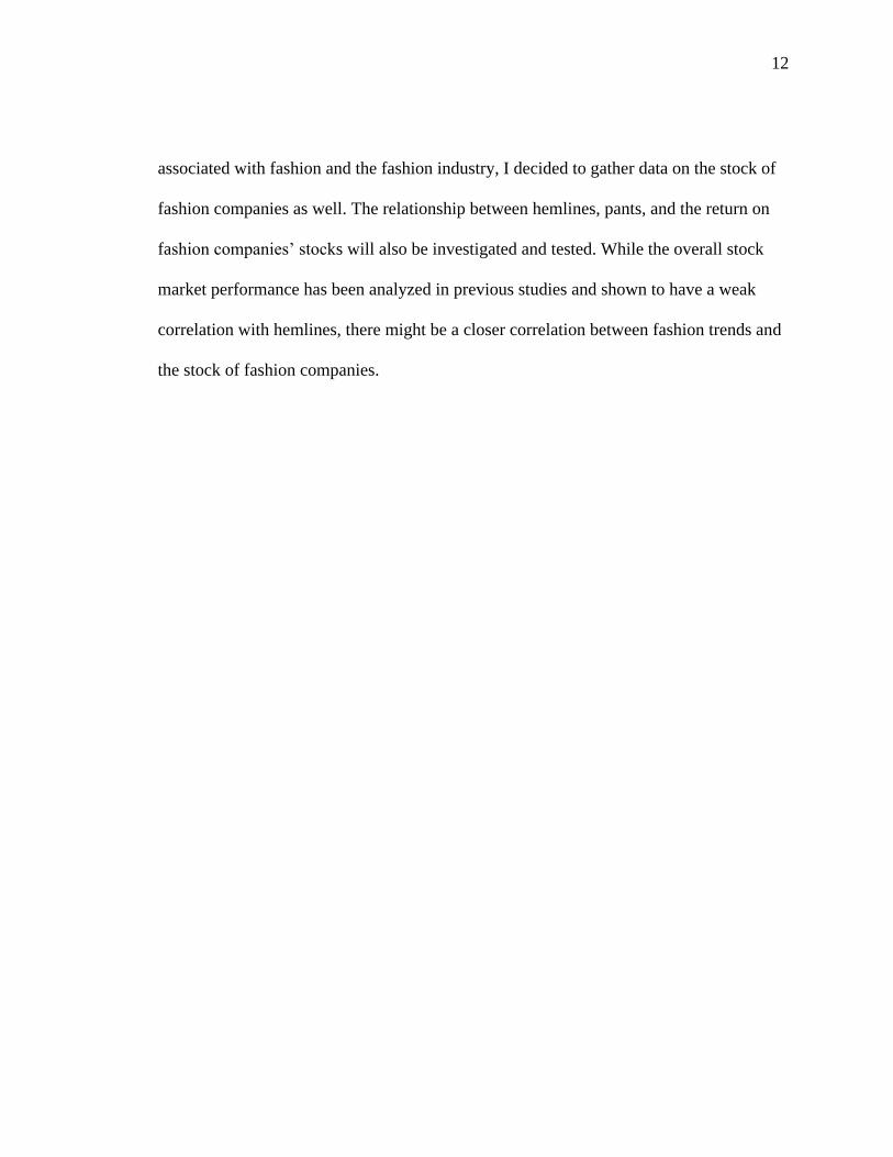
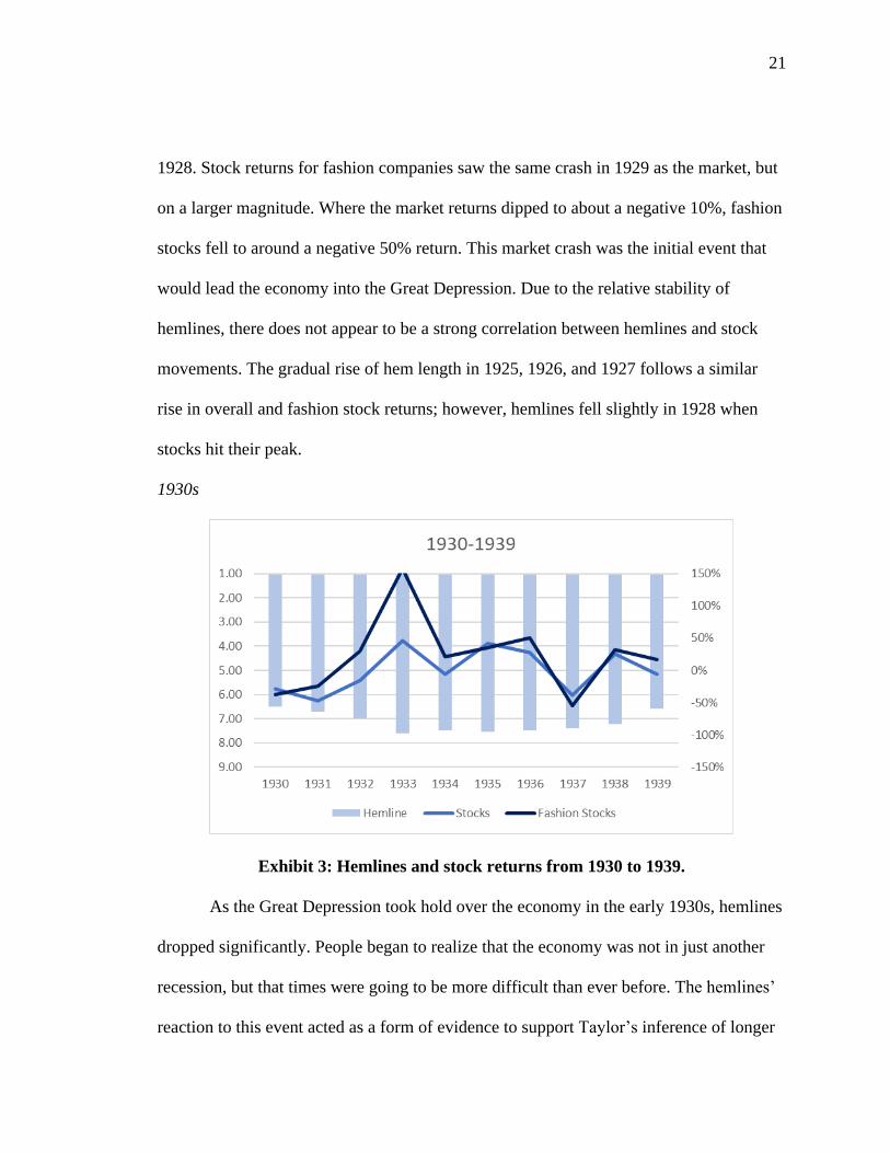
Exhibit 3: Hemlines and stock returns from 1930 to 1939.
As the Great Depression took hold over the economy in the early 1930s, hemlines
dropped significantly. People began to realize that the economy was not in just another
recession, but that times were going to be more difficult than ever before. The hemlines’
reaction to this event acted as a form of evidence to support Taylor’s inference of longer
22
hemlines in times of hardship to hide the lack of quality hosiery. Skirt lengths were still a
little short early in the decade following the below the knee style from the late 20s.
Starting in 1933, hemlines fell into the ballerina length area, even approaching the maxi
length. This longer style prevailed for a large portion of the decade up until 1938. In the
last year of the decade, as the national economy healed from the Great Depression,
hemlines began to rise again, leaving behind the long, sleek style for a midi look
accentuated with fluttery details (Cole, D. J., & Deihl, N., 2015, pp. 165-167).
Stock returns were very volatile during the 1930s. There were plenty of ups and
downs in returns as the market attempted to correct itself after the initial crash of 1929.
Both the market and fashion stocks started the decade off in the red, at about a negative
50% return. The market return dipped even further to below negative 50% in 1931 before
gradually moving into the black mid-1932. Fashion stocks continued to rise after 1930,
moving out of the negative numbers in mid-1931 and reaching almost a 50% return in
1932. The overall market spiked up in 1933 reaching a 50% return. Fashion stocks also
saw a spike, reaching a peak of 158% return, which is off the scale in exhibit 3. Both the
overall market and fashion stocks saw an equally aggressive drop in the next year, with
the market dipping slightly below 0% again and fashion stocks bottoming out around
22%. The market recovered quickly and saw a positive 50% return in 1935 before
gradually falling over the next two years to hit negative 50% again in 1937. Fashion
stocks grew slowly up to a 50% return in 1936 before falling sharply in 1937, hitting a
low of almost negative 60%. Both fashion stocks and the market jumped up again in 1938
before finishing the decade with fashion stocks in the black at about a 16% and the
23
market in the red at about a negative 5%. Hemlines and overall stock market returns
moved in sync in 1930 and 1931, but shifts did not move together for the rest of the
decade. Most notably, hemlines dropped in 1933 when the market was at its all-time high
for the decade. Fashion stock returns and hemlines did not demonstrate any correlation at
all in the 30s.
1940s
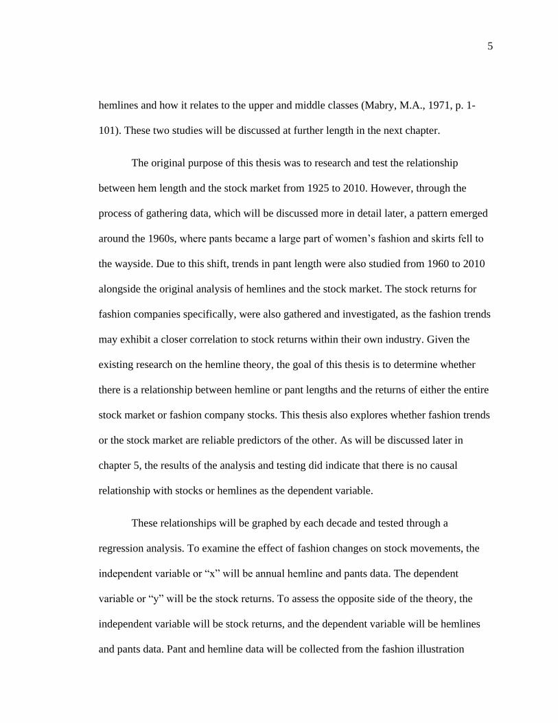
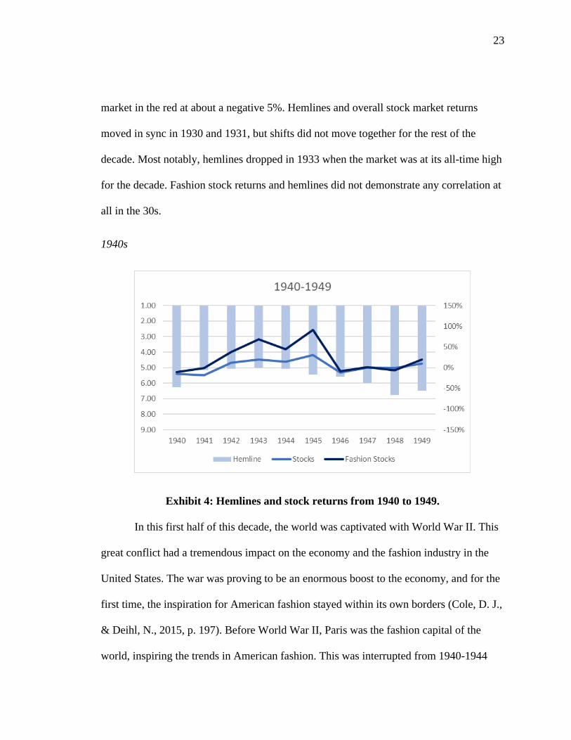
Exhibit 4: Hemlines and stock returns from 1940 to 1949.
In this first half of this decade, the world was captivated with World War II. This
great conflict had a tremendous impact on the economy and the fashion industry in the
United States. The war was proving to be an enormous boost to the economy, and for the
first time, the inspiration for American fashion stayed within its own borders (Cole, D. J.,
& Deihl, N., 2015, p. 197). Before World War II, Paris was the fashion capital of the
world, inspiring the trends in American fashion. This was interrupted from 1940-1944
24
when German forces occupied Paris. Due to this newfound self-sufficiency, the American
fashion industry witnessed a time of unprecedented development and expansion, only
fueled more by the economic boom (Cole, D. J., & Deihl, N., 2015, p. 197). Now that the
fashion industry in the United States was self-sufficient, limitations were placed on
designers in an effort to conserve resources during the war. General Limitation Order L-
85 went into effect on April 8, 1942, regulating the amount of materials that clothing
manufacturers could use. An example of these restrictions was that wool skirts could be
no longer than 28 inches or 71 centimeters (Cole, D. J., & Deihl, N., 2015, pp. 202-203).
Despite these restrictions, fashion became an expression of nationalism and propaganda.
Publications like Vogue encouraged women to do their part to support the United States
during the war. For example, the September 1st issue in 1943 implored women to “Take a
Job! Release a Man to Fight!” (Vogue, 1943).
Hemlines in 1940 had not yet left the midi range that was popular in the late 30s,
but the following year, skirt lengths jumped up to directly below the knee. This shift
could be the result of textile restrictions as well as the promising economic landscape of
the day. This below-the-knee skirt trend lasted from 1941 to 1944 before falling slightly
in 1945 and 1946. 1945 also marked the end of World War II. As the world began to heal
from the fallout of the war, designers were free to create without limitations. Gone were
the restrictions previously imposed. A French designer, Christian Dior, was shot to fame
in the late 40s. By creating his famous “New Look” in 1947, Dior placed not only himself
at the center of international fashion but revived Paris as the fashion capital of the world.
Dior’s New Look is characterized by a fuller, midi length skirt (Cole, D. J., & Deihl, N.,
25
2015, pp. 209-210). This length became the dominant hemline trend for 1947 and
inspired even longer lengths in 1948 and 1949, with hemlines falling below midi length
and approaching the ballerina style range.
Stocks were relatively calm during the 1940s compared to the previous decade.
There were a few spikes seen in the market and fashion stocks, but not nearly as many or
as substantial. The market started in the red in 1940, still struggling to bounce back from
the negative return in the previous year. The market finally found its way to the black in
1942 and remained there, reaching its peak for the decade in 1945 at about a 30% return.
The following year, the market plummeted, toeing the line between 0% and a negative
return until finally returning to positive territory in 1949. Fashion stocks followed a
similar direction, starting off negative but rising into positive returns in 1941. Returns
stayed positive and reached a peak of about 90% in 1945. Once again, stocks crashed in
1946 and remained between 0% and slightly negative until reaching a 20% return in the
last year of the decade. Hemlines shifted similarly to fashion companies’ and overall
stock returns up until 1944. In 1945, all stocks hit their peak while hemlines dropped.
From 1946 to 1949, all stocks remained stable; however, hemlines continued to drop.
26
1950s
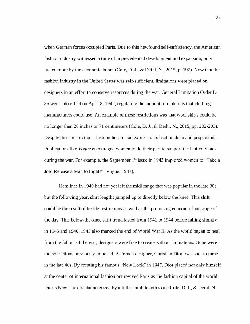
Exhibit 5: Hemlines and stock returns from 1950 to 1959.
Once Paris was catapulted into the spotlight by Christian Dior’s New Look,
American fashion began to look to them again for trend direction. Skirt suits became
exceedingly popular for women early in the decade, showcasing a tailored look with a
longer hemline. This tailored style dominated the fashion industry for almost the whole
decade (Cole, D. J., & Deihl, N., 2015, pp. 235-240). Hemlines hovered around the midi
length from 1950 to 1957. The last two years of the decade saw hemlines shortened to
unprecedented lengths. In 1959, the accepted length was at the knee, shorter than any of
the styles seen in the years prior. This novel length was only the beginning of the changes
in fashion, as we will see when we reach the 1960s.
Stocks saw some considerable changes in returns during this decade. The S&P
500 Index and fashion stocks had similar movements early to mid-decade, until 1957,
27
when fashion stocks began to react more strongly to changes than the overall market. In
1950, returns for the market and fashion stocks were in positive territory, registering
around 20% and 30% returns, respectively. Both gradually declined to slightly negative
figures in 1953 before spiking to more than 50% in returns in 1954. Returns for all stocks
fell again from 1955 to 1957, ending with around negative 15% returns. The overall
market quickly increased again to a 50% return in 1958 before falling to an 8% return at
the end of the decade. Fashion stocks saw a bigger jump in 1958, reaching a high point of
almost 80%, before decreasing again to a 30% return to close the 50s. Hemlines did not
see much movement from 1950 to 1957, whereas stocks saw quite a bit of activity.
However, from 1957 to 1958, hemlines and stocks jumped upwards together, but this is
the only time in the 50s where the variables alluded to a correlation.
1960s
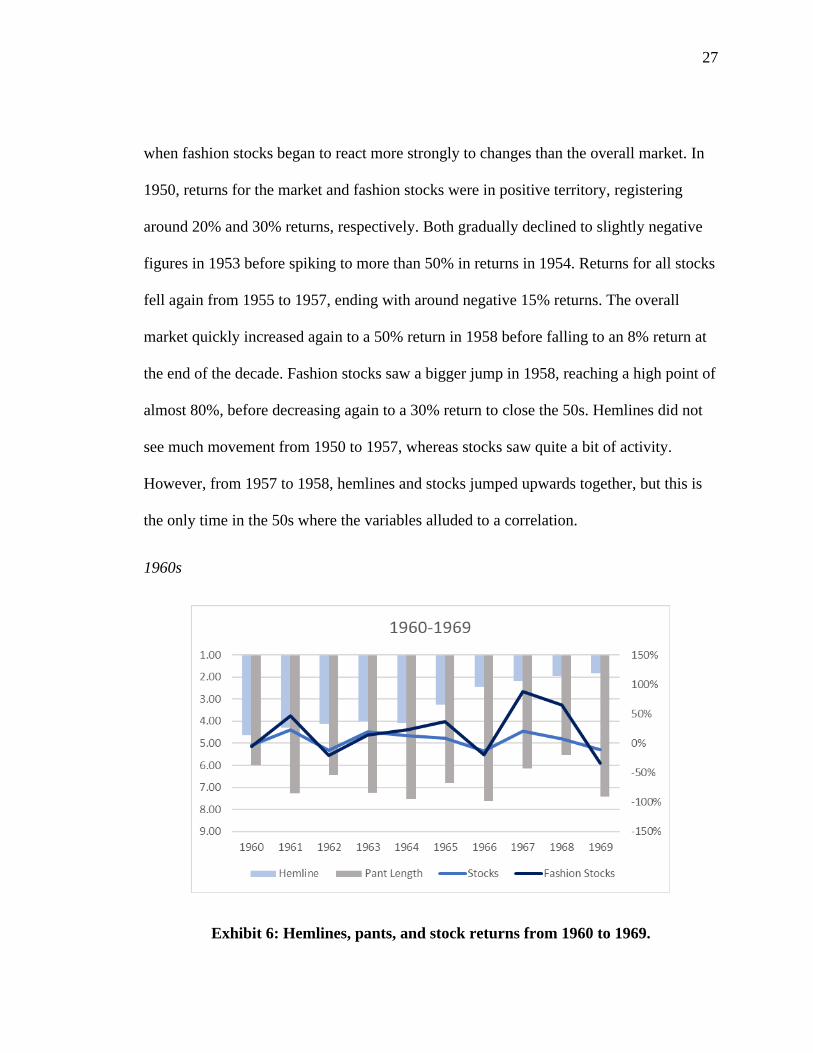
Exhibit 6: Hemlines, pants, and stock returns from 1960 to 1969.
28
The 1960s were a time of substantial change in the fashion industry. There were
several significant shifts, the most groundbreaking being the gradual introduction of pants
as part of women’s everyday wear. Up to this point, pants were mainly confined to
sportswear, beachwear, or pajamas. It was very uncommon to see a woman wearing pants
outside of these confines. Due to this shift in fashion, I began to collect the pants data in
1960, which is shown in gray on the graph. Another shift that took place was a movement
with more emphasis on individualized style rather than macro fashion trends (Cole, D. J.,
& Deihl, N., 2015, pp. 273-275). Macro fashion trends still occurred in the 60s, such as
the “Mod” and hippie style. However, the spotlight slowly moved from macro-trends to
individual style, which became even more prevalent in the next few decades. One trend
from this decade that stands out is the miniskirt (Cole, D. J., & Deihl, N., 2015, p. 278).
Despite the 60s being well known for this style, the miniskirt did not become mainstream
until later in the decade. During the early 60s, there was a struggle between youthfulness
and maintaining the status quo as the dominant fashion trend (Cole, D. J., & Deihl, N.,
2015, p. 278). By 1965, youthfulness had won, and the miniskirt became a mainstay of
the 60s.
In the early part of the decade, hemlines were at or below the knee, still being
dictated by the seemingly unbreakable tradition of fashion. From 1962 to 1964, hemlines
did not budge from knee-length. This was a time of conflicting interests in fashion, and
the industry waited to see if youthful rebellion would win out over tradition. Skirt lengths
hiked up above the knee in 1965, proving that the youthful, “mod” fashion style was here
to stay. By 1966, women embraced this new trend and began to show off their thighs.
29
The miniskirt held a dominant position in the industry until the end of the decade and was
effectively carved into fashion history (Cole, D. J., & Deihl, N., 2015, pp. 273-278).
Pants saw quite a few changes in lengths over the course of the 1960s. These changes
stayed above the classic length, focusing primarily on the clam digger and seven-eighths
lengths. In 1960, pant length was dominated by the clam digger style, which lands a little
above mid-calf, before falling in 1961 to a seven-eighths length, which hits above the
ankle. These two lengths continue to duel one another as the dominant trend for the
remainder of the decade. Some outliers came into play in 1964 and 1966, when pant
lengths began to approach the classic style, which lands at or slightly below the ankle, as
well as in 1968, when lengths creep toward pedal pusher area, which falls right below the
knee.
Fashion stock returns were a little unpredictable in this decade, with several
spikes and dips as seen in exhibit 6. The overall market was slightly less volatile. The
S&P 500 Index return started off slightly negative before increasing to around 25% in
1961. Overall market returns took a hit in 1963, falling back into negative territory in
1962 before going, and staying positive in 1963 through 1965. 1966 saw another negative
dip before finding positive returns from 1967 to 1968. The overall market ended the
decade with a negative return of about 11%. Fashion stocks saw a similar spike in 1961,
reaching over a 50% return before dipping to negative 20% in 1962. Fashion stocks saw
positive returns once again in 1963 and remained positive until the market took another
dip, reaching negative 20% in 1966. The next year saw a substantial spike to an 87%
return before falling slightly to a 65% return in 1968. The end of the decade saw more
30
negative returns for fashion stocks, finishing with a negative 33% return. 1960 and 1961
saw a slight correlation between all stock returns and hemlines as both saw a movement
upwards. However, the two do not remain in sync throughout the rest of the decade.
There was a slight correlation between stocks and pants in 1965 to 1966 and 1968 to
1969, but there is no other apparent correlation.
1970s
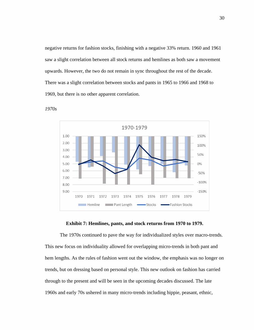
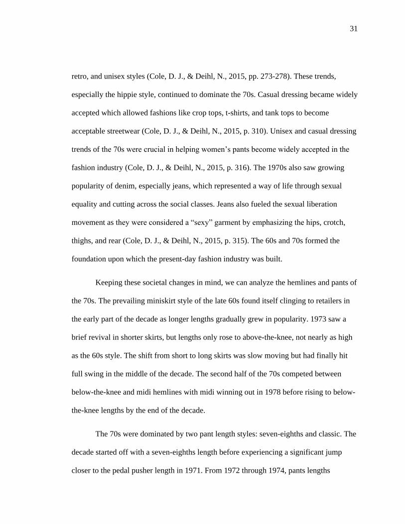
Exhibit 7: Hemlines, pants, and stock returns from 1970 to 1979.
The 1970s continued to pave the way for individualized styles over macro-trends.
This new focus on individuality allowed for overlapping micro-trends in both pant and
hem lengths. As the rules of fashion went out the window, the emphasis was no longer on
trends, but on dressing based on personal style. This new outlook on fashion has carried
through to the present and will be seen in the upcoming decades discussed. The late
1960s and early 70s ushered in many micro-trends including hippie, peasant, ethnic,
31
retro, and unisex styles (Cole, D. J., & Deihl, N., 2015, pp. 273-278). These trends,
especially the hippie style, continued to dominate the 70s. Casual dressing became widely
accepted which allowed fashions like crop tops, t-shirts, and tank tops to become
acceptable streetwear (Cole, D. J., & Deihl, N., 2015, p. 310). Unisex and casual dressing
trends of the 70s were crucial in helping women’s pants become widely accepted in the
fashion industry (Cole, D. J., & Deihl, N., 2015, p. 316). The 1970s also saw growing
popularity of denim, especially jeans, which represented a way of life through sexual
equality and cutting across the social classes. Jeans also fueled the sexual liberation
movement as they were considered a “sexy” garment by emphasizing the hips, crotch,
thighs, and rear (Cole, D. J., & Deihl, N., 2015, p. 315). The 60s and 70s formed the
foundation upon which the present-day fashion industry was built.
Keeping these societal changes in mind, we can analyze the hemlines and pants of
the 70s. The prevailing miniskirt style of the late 60s found itself clinging to retailers in
the early part of the decade as longer lengths gradually grew in popularity. 1973 saw a
brief revival in shorter skirts, but lengths only rose to above-the-knee, not nearly as high
as the 60s style. The shift from short to long skirts was slow moving but had finally hit
full swing in the middle of the decade. The second half of the 70s competed between
below-the-knee and midi hemlines with midi winning out in 1978 before rising to below-
the-knee lengths by the end of the decade.
The 70s were dominated by two pant length styles: seven-eighths and classic. The
decade started off with a seven-eighths length before experiencing a significant jump
closer to the pedal pusher length in 1971. From 1972 through 1974, pants lengths
32
dropped to a classic length before another hike to clam digger length in 1975. There was
a brief return to the classic length for pants in 1976 before the seven-eighths style won
out for the last three years of the decade.
The overall stock market started off slightly negative in 1970 before rising to a
positive return in 1971 and 1972. The next two years saw a large dip in market returns,
hitting a low point of almost negative 30% in 1974. In 1975, the market jumped up
significantly to a positive 30% return and remained in the black until mid-1976. The
market fell slightly, straining to find positive ground, finally returning to a positive figure
in 1978 and finishing out decade with a 12% return. Fashion stocks were more volatile
throughout the decade. Starting off slightly negative, there was a slight increase in 1971
to a 20% return. The next year saw returns drop into negative territory, bottoming out at
negative 52% before finding its way back to a remarkable 103% return in 1975. Fashion
stocks remained below a 50% return, but still positive until the end of the 70s. Hemlines
did not appear to have any correlation with fashion stock or stock market returns.
However, pants and both types of stock returns seemed to move in tandem for a few
years. From 1970 to 1976, movements in all stock returns and pant lengths mirrored each
other. From 1976 to 1977, stocks fell, but pant length rose and stayed at that length for
the rest of the decade.
33
1980s
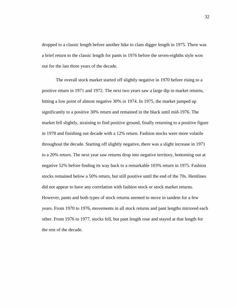
Exhibit 8: Hemlines, pants, and stock returns from 1980 to 1989.
Early 80s fashion was still influenced by the 70s style. However, as the decade
began to develop its own identity, several styles emerged that would characterize the 80s.
One of these styles was “power dressing” (Cole, D. J., & Deihl, N., 2015, pp. 352-353).
Power dressing played a large part in the skirt and pant trends seen in this decade. Blazers
were paired with a variety of bottoms. The 80s were a time of continued personalization
in style that was popularized in the previous decade, allowing many trends and hem
lengths to overlap. This decade became one of excess. Bigger and bolder was always
better, which set the tone for all the individual trends throughout the 80s (Cole, D. J., &
Deihl, N., 2015, pp. 352-353).
Hemlines in the early 1980s were still affected by the loose, flowing style and
longer hemlines characterized by the dominant hippie style of the 70s. Hem lengths hit at
34
or slightly below the knee in the early 80s, before rising above the knee shortly in 1982.
Skirts dropped below the knee again in 1983-1984 as fashion staged a revival of the 40s
style (Cole, D. J., & Deihl, N., 2015, pp. 352-353). 1985 saw a significant movement
upwards to above-the-knee lengths before falling closer to the knee in 1986. The last
three years of the decade were dominated by the miniskirt, falling at or above mid-thigh,
reminiscent of the 60s. Pant lengths in the 80s were heavily influenced by the “power
dressing” trend. Suit jackets were paired mainly with cropped styles, causing pants to
remain above the ankle for the entire decade (Cole, D. J., & Deihl, N., 2015, pp. 352-
353). For the majority of the 80s, pant lengths vacillated between the clam digger and
seven-eighths styles. However, the seven-eighths style dominated the decade from 1981
to 1987. The only exceptions are seen in 1980, 1985, and 1988-89, where lengths start to
creep upwards towards the clam digger length.
The stock market stayed relatively calm during the 80s. Market returns started off
around 25% in 1980 before tanking to a negative 10% return in 1981. The market picked
itself up, returning to positive territory again the next year and remained positive for the
rest of the decade. There were a few close calls in 1984 and 1987 where returns dipped
dangerously close to the red again but managed to remain positive at about a 2% return.
Fashion stock returns remained positive for the majority of the decade, save a few
downward spikes. 1980 through 1983 saw positive figures reaching a peak in 1983 at
almost 65%. Returns plummeted downward the next year to negative 10% before
rebounding in 1985 with a 42% return. 1986 also experienced positive returns before
another sharp drop to a negative 30% return in 1987 in the fashion market. Both 1988 and
35
1989 returned to positive territory with fashion stocks ending the decade with a 15%
return. 1983 to 1986 saw similar movements in hemlines and stock returns. Overall stock
return movements were minimal, whereas fashion stock returns were a little more
volatile, making their movements more obvious. However, both fashion and overall
returns moved synchronously with hemlines. Outside this three-year period, there is no
correlation revealed between the returns and hemlines. As for pants, the only areas where
similar shifts can be seen is in a rise in pant length and stock returns from 1984 to 1985,
as well as a slight decrease in both variables in 1986.
1990s
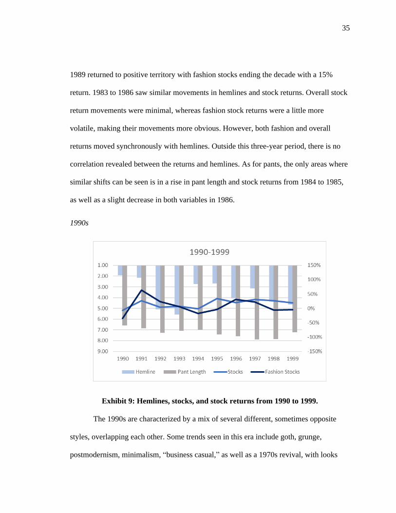
Exhibit 9: Hemlines, stocks, and stock returns from 1990 to 1999.
The 1990s are characterized by a mix of several different, sometimes opposite
styles, overlapping each other. Some trends seen in this era include goth, grunge,
postmodernism, minimalism, “business casual,” as well as a 1970s revival, with looks
36
from only two decades earlier already being considered retro (Cole, D. J., & Deihl, N.,
2015, pp. 393-395). Due to the increasing emphasis placed on individual designers
instead of macro-trends, women’s fashion was remarkably diverse and segmented,
especially in hem lengths. Denim was still popular, and trousers became increasingly
prevalent among women as well aligning with the “business casual” movement, which
heavily influenced the pant trends seen in this decade (Cole, D. J., & Deihl, N., 2015, pp.
352-353).
Hemlines saw both ends of the spectrum during this decade. 1990 and 1991 were
dominated by miniskirts before dropping significantly to a length below the knee in 1992.
Skirt lengths began to approach a midi length in 1993 before bouncing back to above the
knee lengths in 1994 and 1995. Hems fell to the knee and lower at the end of the decade,
with one exception in 1997 where lengths rose to an above-the-knee style. Pants saw
competing trends as well. Pant lengths were cropped in the early 90s, hovering around the
seven-eighths style. Later in the decade, around 1995 to 1998, pants began to approach
the classic length. At the end of the decade, pants sprang upwards to the seven-eighths
length which finished out the decade.
The 90s was another decade of overwhelmingly positive returns for the market
overall. Only 1990 and 1994 saw negative market returns of 6% and 1%, respectively.
1991 had a positive 26% return before dropping to lower returns of 4% and 7% in 1992
and 1993. Market returns topped out at 35% in 1995 and stayed positive until 1999.
Fashion stock returns started the decade off in the red with a negative 35% return before
catapulting in 1991 to an almost 65% return, the highest return seen in the 90s. Returns
37
fell gradually into the negatives in 1994 achieving a negative 18% return and remained
negative through 1995. Both 1996 and 1997 saw favorable returns of 31% and 22%,
respectively, before falling and staying in the negatives through the end of the decade.
Hemlines and overall stock market returns did not see any similarities in movements
during this decade. However, hemlines and fashion companies’ stock returns did appear
to move together from 1991 to 1993 and again from 1997 to 1999. Pants did not
demonstrate any correlated movements with either the overall stock market or fashion
stocks.
2000s
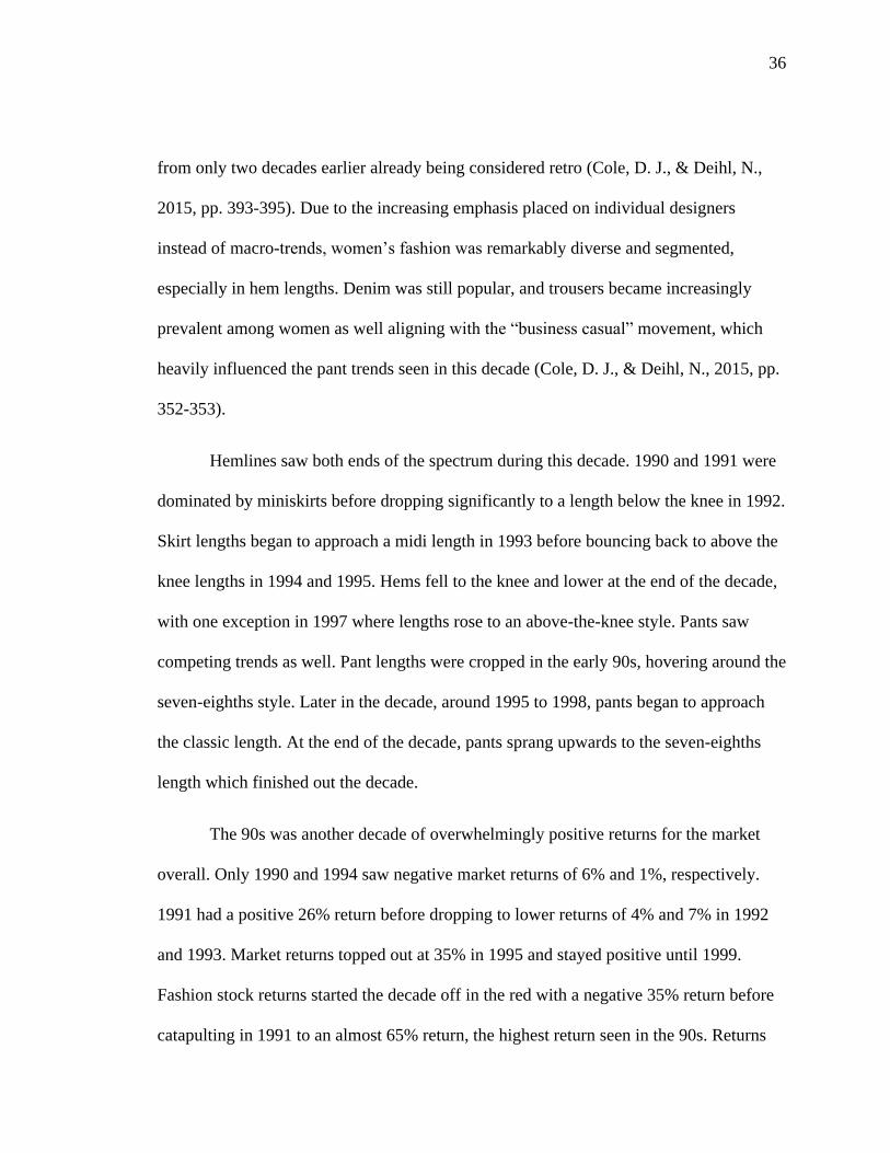
Exhibit 10: Hemlines, stocks, and stock returns from 2000 to 2010.
The 2000s era was a time of multiple divergent, sometimes contradictory, fashion
niches. These styles included hipster, so called “geek chic,” steampunk, and the largest of
the trends, “boho-chic” (Cole, D. J., & Deihl, N., 2015, pp. 431-434). These different
38
trends generated many shifts in hemline and pant lengths as exhibited from the graph
above. The early part of the decade saw similar hem lengths as that of the late 90s,
lingering around the knee. In 2001, hemlines rose to above-the-knee lengths before
dropping again to the knee in 2004 and below the knee in 2005. Hemlines hovered
around the knee again in 2006 before moving below-the-knee in 2007 and 2008. The last
few years of the decade saw a big jump to above-the-knee hemlines in 2009 before
sliding down the knee again in 2010. Pant lengths were static throughout the first few
years of the 2000s, hovering around the classic length until 2002. 2003 through 2005 saw
a significant rise from the seven-eighths length, below mid-calf, to the pedal pushers
length, which lands right below the knee. Lengths fell dramatically again in 2006,
approaching the classic length, before slowly climbing to the clam digger length at the
end of the decade.
The overall market suffered negative returns in the first few years of the decade,
finally attaining positive ground again in 2003 with a 26% return. Returns fell gradually,
dipping dangerously close to negative territory in 2005, but managed to stay positive until
2007. However, in 2008, market returns sank to an all-time low for the decade, realizing
a negative 38% before bouncing back to 23% in 2009. The stock market maintained its
positive return to 2010, ending at 12%. Fashion stock returns also began the decade in
negative territory but had pulled itself into positive numbers again in 2001 with a 30%
return. Fashion stocks fell slightly to a 9% return in 2002 before managing to maintain
returns in the range of 20-30% from 2003 to 2006. The next two years saw a significant
decline in fashion stock returns, bottoming out at a negative 51% return in 2008. Fashion
39
stocks experienced an extraordinary spike skyward landing returns at 121% in 2009
before settling back down to a solid 38% return in 2010. Hemlines and fashion
companies’ stock returns seemed to follow each other throughout the decade. The only
divergence occurred in 2003 as stock returns rose and hem lengths fell. Hemlines and the
overall stock market return also seemed to move in tandem from 2004 to 2010. Pant
lengths, on the other hand, did not reveal any movement in accordance with overall stock
returns or fashion stock returns.
40
Chapter 5: Regression Testing
Empirical testing was needed in order to analyze the relationship between hem
and pant length trends and stock returns to discover if there is any relationship present
between the variables. This type of testing required a regression model, which included
the two variables being tested, stocks and fashion trends, as well as some control
variables. The control variables were chosen based on “The Impact of Macroeconomic
Variables on Stock Market Performance: A Taxonomic Approach” (Chang, S. J., & Ha,
D., 1997, pp. 104-114). This study was completed by S.J. Chang and Daesung Ha to
answer the question of which of the numerous economic variables prevalent in the market
have the most significant impact on stock portfolios. Chang and Ha investigated 27
different economic activity measures and ran a correlation analysis among the economic
measures and the market (Chang, S. J., & Ha, D., 1997, pp. 104-114). This correlation
analysis showed which variables were considered “core variables,” or the ones that were
closest related to the market. As mentioned in Chapter 3, there were 14 core variables
found in this study: industrial production index, producer price index, consumer credit,
consumer price index, corporate profits, real gross domestic product, unemployment rate,
civilian labor rate, bank prime loan rate, capacity utilization, M1 money stock, vehicle
sales, retail sales, and the 1-month Treasury Bill rate (Chang, S. J., & Ha, D., 1997, p.
111). With all the monthly data collected and organized, regression testing began.
41
All the regression analyses were ran through the statistical software, R. There
were four different types of regression analyses completed. The first type was with the
market returns and hemlines, the second with fashion companies stock returns and
hemlines, the third with market returns and pants, and the fourth with fashion companies
stock returns and pants. Each type of regression was ran with the stock returns as the
dependent variable and then the hemline/pant data as the dependent variable. By
switching the different variables out as the dependent variable, I was able to examine any
correlation between hemlines/pants and stock returns going either way. For the
regressions that were ran with the hemlines and pants as the dependent variable, the
fashion trends were tested with the prior year’s stock return data. This lag was
intentionally included with the thought that fashion trends would take more time to adjust
to any changes possibly caused by the stock market movements. The regression analyses
also needed to be staggered as a result of not all the chosen macroeconomic variables
being available back to 1925. Tests were completed for the following years: 1926, 1948,
1955, 1960, 1976, 1992, and 2001.
A multiple regression model was used to incorporate all the necessary variables.
The formula includes the dependent variable, the one that is being changed, the
independent variable, the one supposedly causing those changes, and the control
variables. For example, to test if hemlines caused changes in stock returns in 1926, the
formula would be: lm(Stocks ~ Hemlines + Industrial Production Index + Producer Price
Index). Lm is the regression formula in R, stocks is the dependent variable, hemlines is
the independent variable, and Industrial Production Index and Producer Price Index are
42
the macroeconomic control variables. The formula is very similar for testing if stock
movements caused changes in hemlines in 1926: lm(Hemlines ~ Stocks + Industrial
Production Index + Producer Price Index).
Due to the staggered nature of the calculations and the different types of analysis
needed, a total of 44 regression analyses were ran. The results of the regression analyses,
including coefficients, corresponding t-values, coefficients’ significance, adjusted r-
squared, and observations are outlined in Tables 1 through 8. Each coefficient’s
corresponding t-value is reported directly under the coefficient and is italicized for
distinction. The adjusted r-squared and observations are reported at the bottom of each
column. The significance codes are as follows: ‘***’ 0.001, ‘**’ 0.01, ‘*’ 0.05, ‘.’ 0.1, ‘ ’
1. These codes are also listed at the bottom of each table for ease of referencing. The
significance of the coefficients is what is most important in this type of testing. These
codes will reveal if the coefficients are statistically significant enough to indicate a causal
relationship between the variables being tested. In the tests where hemlines and pants
were the independent variable, only the hem and pant lengths that were recorded will
appear in the regression results. Therefore, if a particular length was not recorded as a
trend in a specific year, that length will not have any output.
43
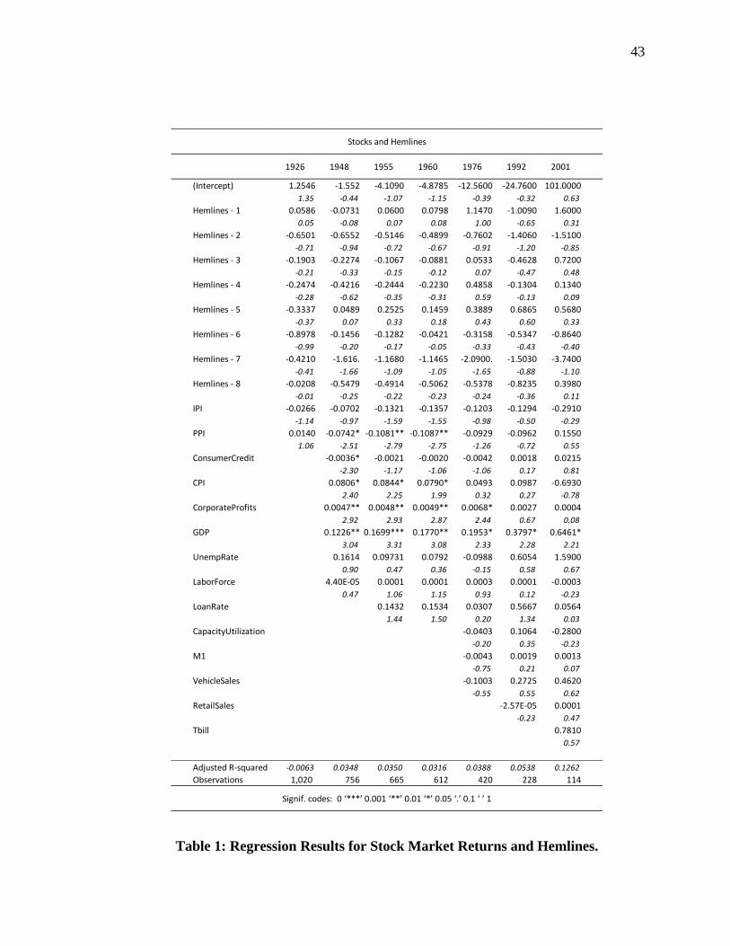
Table 1: Regression Results for Stock Market Returns and Hemlines.
(Intercept) 1.2546 -1.552 -4.1090 -4.8785 -12.5600 -24.7600 101.0000
1.35 -0.44 -1.07 -1.15 -0.39 -0.32 0.63
Hemlines - 1 0.0586 -0.0731 0.0600 0.0798 1.1470 -1.0090 1.6000
0.05 -0.08 0.07 0.08 1.00 -0.65 0.31
Hemlines - 2 -0.6501 -0.6552 -0.5146 -0.4899 -0.7602 -1.4060 -1.5100
-0.71 -0.94 -0.72 -0.67 -0.91 -1.20 -0.85
Hemlines - 3 -0.1903 -0.2274 -0.1067 -0.0881 0.0533 -0.4628 0.7200
-0.21 -0.33 -0.15 -0.12 0.07 -0.47 0.48
Hemlines - 4 -0.2474 -0.4216 -0.2444 -0.2230 0.4858 -0.1304 0.1340
-0.28 -0.62 -0.35 -0.31 0.59 -0.13 0.09
Hemlines - 5 -0.3337 0.0489 0.2525 0.1459 0.3889 0.6865 0.5680
-0.37 0.07 0.33 0.18 0.43 0.60 0.33
Hemlines - 6 -0.8978 -0.1456 -0.1282 -0.0421 -0.3158 -0.5347 -0.8640
-0.99 -0.20 -0.17 -0.05 -0.33 -0.43 -0.40
Hemlines - 7 -0.4210 -1.616. -1.1680 -1.1465 -2.0900. -1.5030 -3.7400
-0.41 -1.66 -1.09 -1.05 -1.65 -0.88 -1.10
Hemlines - 8 -0.0208 -0.5479 -0.4914 -0.5062 -0.5378 -0.8235 0.3980
-0.01 -0.25 -0.22 -0.23 -0.24 -0.36 0.11
IPI -0.0266 -0.0702 -0.1321 -0.1357 -0.1203 -0.1294 -0.2910
-1.14 -0.97 -1.59 -1.55 -0.98 -0.50 -0.29
PPI 0.0140 -0.0742* -0.1081** -0.1087** -0.0929 -0.0962 0.1550
1.06 -2.51 -2.79 -2.75 -1.26 -0.72 0.55
ConsumerCredit -0.0036* -0.0021 -0.0020 -0.0042 0.0018 0.0215
-2.30 -1.17 -1.06 -1.06 0.17 0.81
CPI 0.0806* 0.0844* 0.0790* 0.0493 0.0987 -0.6930
2.40 2.25 1.99 0.32 0.27 -0.78
CorporateProfits 0.0047** 0.0048** 0.0049** 0.0068* 0.0027 0.0004
2.92 2.93 2.87 2.44 0.67 0.08
GDP 0.1226** 0.1699*** 0.1770** 0.1953* 0.3797* 0.6461*
3.04 3.31 3.08 2.33 2.28 2.21
UnempRate 0.1614 0.09731 0.0792 -0.0988 0.6054 1.5900
0.90 0.47 0.36 -0.15 0.58 0.67
LaborForce 4.40E-05 0.0001 0.0001 0.0003 0.0001 -0.0003
0.47 1.06 1.15 0.93 0.12 -0.23
LoanRate 0.1432 0.1534 0.0307 0.5667 0.0564
1.44 1.50 0.20 1.34 0.03
CapacityUtilization -0.0403 0.1064 -0.2800
-0.20 0.35 -0.23
M1 -0.0043 0.0019 0.0013
-0.75 0.21 0.07
VehicleSales -0.1003 0.2725 0.4620
-0.55 0.55 0.62
RetailSales -2.57E-05 0.0001
-0.23 0.47
Tbill 0.7810
0.57
Adjusted R-squared -0.0063 0.0348 0.0350 0.0316 0.0388 0.0538 0.1262
Observations 1,020 756 665 612 420 228 114
Signif. codes: 0 ‘***’ 0.001 ‘**’ 0.01 ‘*’ 0.05 ‘.’ 0.1 ‘ ’ 1
Stocks and Hemlines
1926 1948 1955 1960 1976 1992 2001
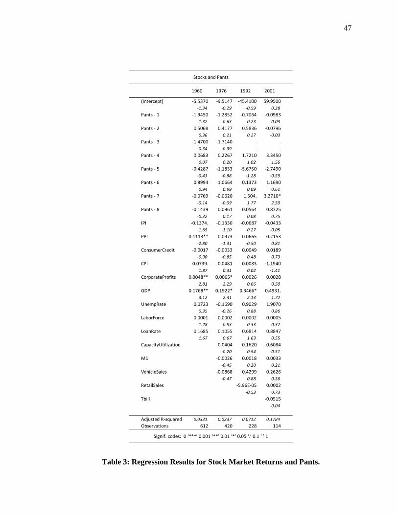
44
This table reports the results from the regression analyses of the overall stock market returns and
hemline lengths. The dependent variable ,overall stock returns, are the annualized figures for
returns on the S&P 500 Index from 1926 to 2010. The independent variables are the hemline
lengths, 1 through 8, that were collected through stratified sampling from Vogue. Other independent
variables were the various macroeconomic controls that were closely related to the stock market.
The limited availability of the macroeconomic control data during the time period caused the need
for staggered regression analyses. Each column corresponds to a regression analysis ran with new
variables included each time. T-values are reported in italics under the estimated coefficients.
Number of observations and the adjusted r-squared is reported at the bottom of each column.
Significance codes are shown at the bottom of the table. Definitions of macroeconomic controls
are included in Table 9 in the appendix.
Table 1 shows the results for each regression analysis conducted between stock
market returns and hemlines. The regression results for 1926, 1955, 1960, 1992, and 2001
do not show statistical significance for any of the hemline lengths. In the 1948 and 1976
results, hemline length 7 (ballerina length) shows a statistical significance of 0.1, as
indicated by the ‘.’ significance code. Several of the macroeconomic controls have
statistically significant relationships with the overall stock market. The producer price
index shows a negative statistically significant relationship with stocks in the 1948, 1955,
and 1960 regression results. Consumer credit also indicates a negative relationship with
stocks in the 1948 results with a statistical significance of 0.05. The consumer price index
showed a positive relationship with the stock market in the years 1948, 1955, and 1960.
Corporate profits also showed a positive statistically significant relationship in the 1948,
1955, 1960, and 1976 regression results. The stock market and gross domestic product
also appear to have a statistically significant positive relationship shown in each
regression output from 1948 to 2001.
45
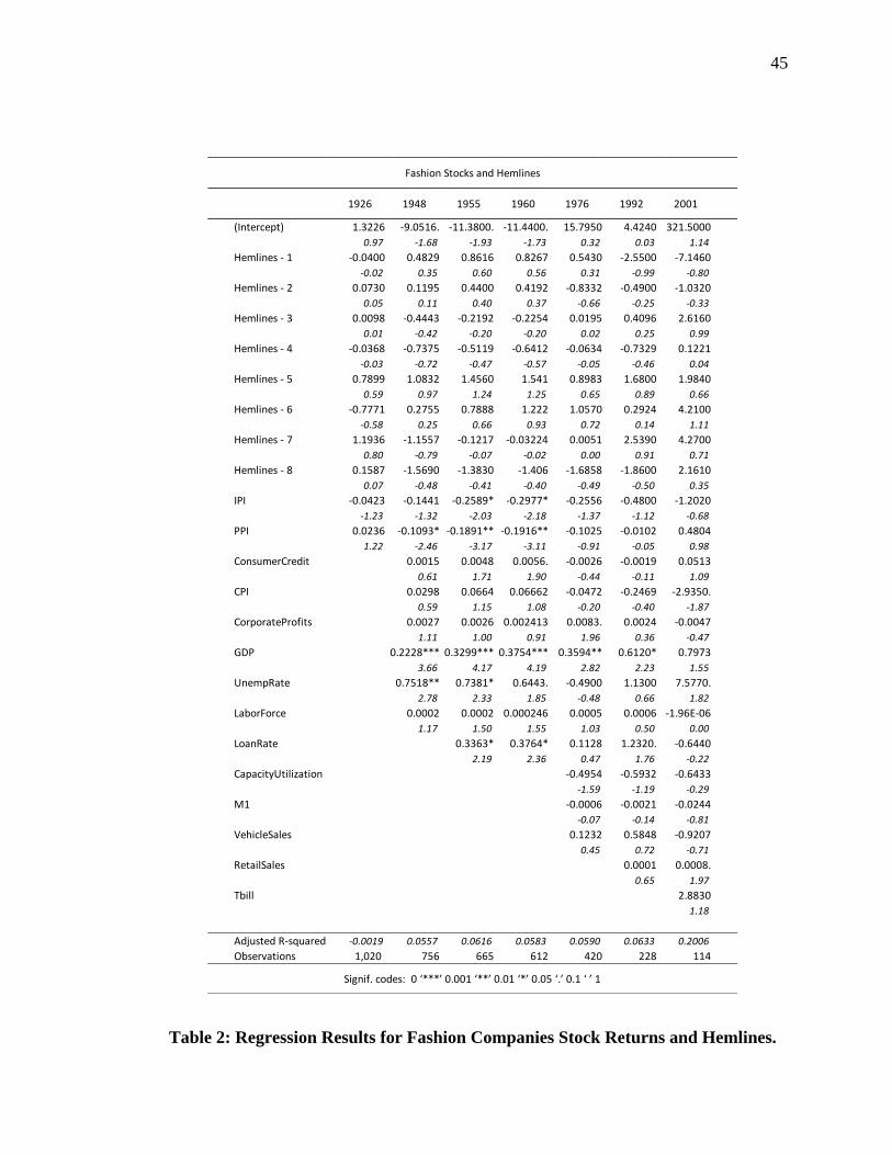
Table 2: Regression Results for Fashion Companies Stock Returns and Hemlines.
(Intercept) 1.3226 -9.0516. -11.3800. -11.4400. 15.7950 4.4240 321.5000
0.97 -1.68 -1.93 -1.73 0.32 0.03 1.14
Hemlines - 1 -0.0400 0.4829 0.8616 0.8267 0.5430 -2.5500 -7.1460
-0.02 0.35 0.60 0.56 0.31 -0.99 -0.80
Hemlines - 2 0.0730 0.1195 0.4400 0.4192 -0.8332 -0.4900 -1.0320
0.05 0.11 0.40 0.37 -0.66 -0.25 -0.33
Hemlines - 3 0.0098 -0.4443 -0.2192 -0.2254 0.0195 0.4096 2.6160
0.01 -0.42 -0.20 -0.20 0.02 0.25 0.99
Hemlines - 4 -0.0368 -0.7375 -0.5119 -0.6412 -0.0634 -0.7329 0.1221
-0.03 -0.72 -0.47 -0.57 -0.05 -0.46 0.04
Hemlines - 5 0.7899 1.0832 1.4560 1.541 0.8983 1.6800 1.9840
0.59 0.97 1.24 1.25 0.65 0.89 0.66
Hemlines - 6 -0.7771 0.2755 0.7888 1.222 1.0570 0.2924 4.2100
-0.58 0.25 0.66 0.93 0.72 0.14 1.11
Hemlines - 7 1.1936 -1.1557 -0.1217 -0.03224 0.0051 2.5390 4.2700
0.80 -0.79 -0.07 -0.02 0.00 0.91 0.71
Hemlines - 8 0.1587 -1.5690 -1.3830 -1.406 -1.6858 -1.8600 2.1610
0.07 -0.48 -0.41 -0.40 -0.49 -0.50 0.35
IPI -0.0423 -0.1441 -0.2589* -0.2977* -0.2556 -0.4800 -1.2020
-1.23 -1.32 -2.03 -2.18 -1.37 -1.12 -0.68
PPI 0.0236 -0.1093* -0.1891** -0.1916** -0.1025 -0.0102 0.4804
1.22 -2.46 -3.17 -3.11 -0.91 -0.05 0.98
ConsumerCredit 0.0015 0.0048 0.0056. -0.0026 -0.0019 0.0513
0.61 1.71 1.90 -0.44 -0.11 1.09
CPI 0.0298 0.0664 0.06662 -0.0472 -0.2469 -2.9350.
0.59 1.15 1.08 -0.20 -0.40 -1.87
CorporateProfits 0.0027 0.0026 0.002413 0.0083. 0.0024 -0.0047
1.11 1.00 0.91 1.96 0.36 -0.47
GDP 0.2228*** 0.3299*** 0.3754*** 0.3594** 0.6120* 0.7973
3.66 4.17 4.19 2.82 2.23 1.55
UnempRate 0.7518** 0.7381* 0.6443. -0.4900 1.1300 7.5770.
2.78 2.33 1.85 -0.48 0.66 1.82
LaborForce 0.0002 0.0002 0.000246 0.0005 0.0006 -1.96E-06
1.17 1.50 1.55 1.03 0.50 0.00
LoanRate 0.3363* 0.3764* 0.1128 1.2320. -0.6440
2.19 2.36 0.47 1.76 -0.22
CapacityUtilization -0.4954 -0.5932 -0.6433
-1.59 -1.19 -0.29
M1 -0.0006 -0.0021 -0.0244
-0.07 -0.14 -0.81
VehicleSales 0.1232 0.5848 -0.9207
0.45 0.72 -0.71
RetailSales 0.0001 0.0008.
0.65 1.97
Tbill 2.8830
1.18
Adjusted R-squared -0.0019 0.0557 0.0616 0.0583 0.0590 0.0633 0.2006
Observations 1,020 756 665 612 420 228 114
Signif. codes: 0 ‘***’ 0.001 ‘**’ 0.01 ‘*’ 0.05 ‘.’ 0.1 ‘ ’ 1
Fashion Stocks and Hemlines
1926 1948 1955 1960 1976 1992 2001
46
This table reports the results from the regression analyses of the stock market returns for fashion
companies and hemline lengths. The dependent variable, fashion stock returns, are the mean
annualized figures for returns on stocks with an SIC code of 22, 23, and 56 from 1926 to 2010. The
independent variables are the hemline lengths, 1 through 8, that were collected through stratified
sampling from Vogue. Other independent variables were the various macroeconomic controls that
were closely related to the stock market. The limited availability of the macroeconomic control
data during the time period caused the need for staggered regression analyses. Each column
corresponds to a regression analysis ran with new variables included each time. T-values are
reported in italics under the estimated coefficients. Number of observations and the adjusted r-
squared is reported at the bottom of each column. Significance codes are shown at the bottom of
the table. Definitions of macroeconomic controls are included in Table 9 in the appendix.
Table 2 displays the regression output for each test completed between fashion
companies stock returns and hemlines. None of the hem lengths in any of the years
demonstrate a statistically significant relationship with fashion companies stock returns.
However, several of the macroeconomic controls do reflect a statistically significant
relationship with fashion companies’ stock returns. The industrial production index
indicated a negative relationship with fashion stock returns in the 1955 and 1960 output.
The producer price index also showed a negative relationship with fashion stock returns
in the years 1948, 1955, and 1960. Consumer credit revealed a positive relationship to
fashion stocks in 1960 with a statistical significance of 0.1. The consumer price index
showed a slight significance in its negative relationship with fashion stocks. Corporate
profits also illustrated a positive relationship in 1976 with 0.1 statistical significance.
Gross domestic profit reflected a positive relationship with fashion stocks in the 1948,
1955, 1960, 1976, and 1992 results. Unemployment rate indicated a positive relationship
with diminishing statistical significance in the years 1948, 1955, 1960, and 2001. Fashion
stocks and loan rate were shown to have a positive relationship in the 1955, 1960, and
1992 outputs. The last macroeconomic variable to exhibit a positive relationship with
fashion stocks was retail sales in 2001 with a 0.1 statistical significance.
47
Table 3: Regression Results for Stock Market Returns and Pants.
(Intercept) -5.5370 -9.5147 -45.4100 59.9500
-1.34 -0.29 -0.59 0.38
Pants - 1 -1.9450 -1.2852 -0.7064 -0.0983
-1.32 -0.63 -0.23 -0.03
Pants - 2 0.5068 0.4177 0.5836 -0.0796
0.36 0.21 0.27 -0.03
Pants - 3 -1.4700 -1.7140 - -
-0.34 -0.39 - -
Pants - 4 0.0683 0.2267 1.7210 3.3450
0.07 0.20 1.02 1.56
Pants - 5 -0.4287 -1.1833 -5.6750 -2.7490
-0.43 -0.88 -1.28 -0.59
Pants - 6 0.8994 1.0664 0.1373 1.1690
0.94 0.99 0.09 0.61
Pants - 7 -0.0769 -0.0620 1.504. 3.2710*
-0.14 -0.09 1.77 2.50
Pants - 8 -0.1439 0.0961 0.0564 0.8725
-0.32 0.17 0.08 0.75
IPI -0.1374. -0.1330 -0.0687 -0.0433
-1.65 -1.10 -0.27 -0.05
PPI -0.1113** -0.0973 -0.0665 0.2153
-2.80 -1.31 -0.50 0.81
ConsumerCredit -0.0017 -0.0033 0.0049 0.0189
-0.90 -0.85 0.48 0.73
CPI 0.0739. 0.0481 0.0083 -1.1940
1.87 0.31 0.02 -1.41
CorporateProfits 0.0048** 0.0065* 0.0026 0.0028
2.81 2.29 0.66 0.50
GDP 0.1768** 0.1922* 0.3466* 0.4931.
3.12 2.31 2.13 1.72
UnempRate 0.0723 -0.1690 0.9029 1.9070
0.35 -0.26 0.88 0.86
LaborForce 0.0001 0.0002 0.0002 0.0005
1.28 0.83 0.33 0.37
LoanRate 0.1685 0.1055 0.6814 0.8847
1.67 0.67 1.63 0.55
CapacityUtilization -0.0404 0.1620 -0.6084
-0.20 0.54 -0.51
M1 -0.0026 0.0018 0.0033
-0.45 0.20 0.21
VehicleSales -0.0868 0.4299 0.2626
-0.47 0.88 0.36
RetailSales -5.96E-05 0.0002
-0.53 0.73
Tbill -0.0515
-0.04
Adjusted R-squared 0.0331 0.0237 0.0712 0.1784
Observations 612 420 228 114
Signif. codes: 0 ‘***’ 0.001 ‘**’ 0.01 ‘*’ 0.05 ‘.’ 0.1 ‘ ’ 1
Stocks and Pants
1960 1976 1992 2001
48
This table reports the results from the regression analyses of the overall stock market returns and
pant lengths. The dependent variable, overall stock returns, are the annualized figures for returns
on the S&P 500 Index from 1960 to 2010. The independent variables are the pant lengths, 1 through
8, that were collected through stratified sampling from Vogue. Other independent variables were
the various macroeconomic controls that were closely related to the stock market. The limited
availability of the macroeconomic control data during the time period caused the need for staggered
regression analyses. Each column corresponds to a regression analysis ran with new variables
included each time. T-values are reported in italics under the estimated coefficients. Number of
observations and the adjusted r-squared is reported at the bottom of each column. Significance
codes are shown at the bottom of the table. Definitions of macroeconomic controls are included in
Table 9 in the appendix.
Table 3 presents the results of the regression analyses run between stock market
returns and pants. Due to the fact that pants data was collected starting in the 1960s, the
regression analyses are only conducted in the years 1960, 1976, 1992, and 2001. The
results in the years 1960 and 1976 do not show statistical significance for any of the pant
lengths. In the 1992 results, only pant length 7 (seven-eighths) is shown to have a
statistical significance of 0.1 as indicated by the ‘.’ next to the coefficient. The 2001
results demonstrate a stronger statistical significance of 0.05 for pant length 7 as
indicated by the ‘*’ next to the coefficient. The macroeconomic variables also indicated
some relationships of varying significance. The industrial production index showed a
negative relationship to stocks with 0.1 statistical significance in the 1960 output.
Producer price index and stocks also reflected a negative relationship in the 1960 output,
but with a statistical significance of 0.01. The consumer price index showed a positive
relationship with stocks in the 1960 regression results with a significance of 0.1.
Corporate profits revealed a stronger positive relationship with the stock market in the
years 1960 and 1976. Gross domestic profit indicated a positive relationship with
decreasing statistical significance in each year’s output from 1960 to 2001.
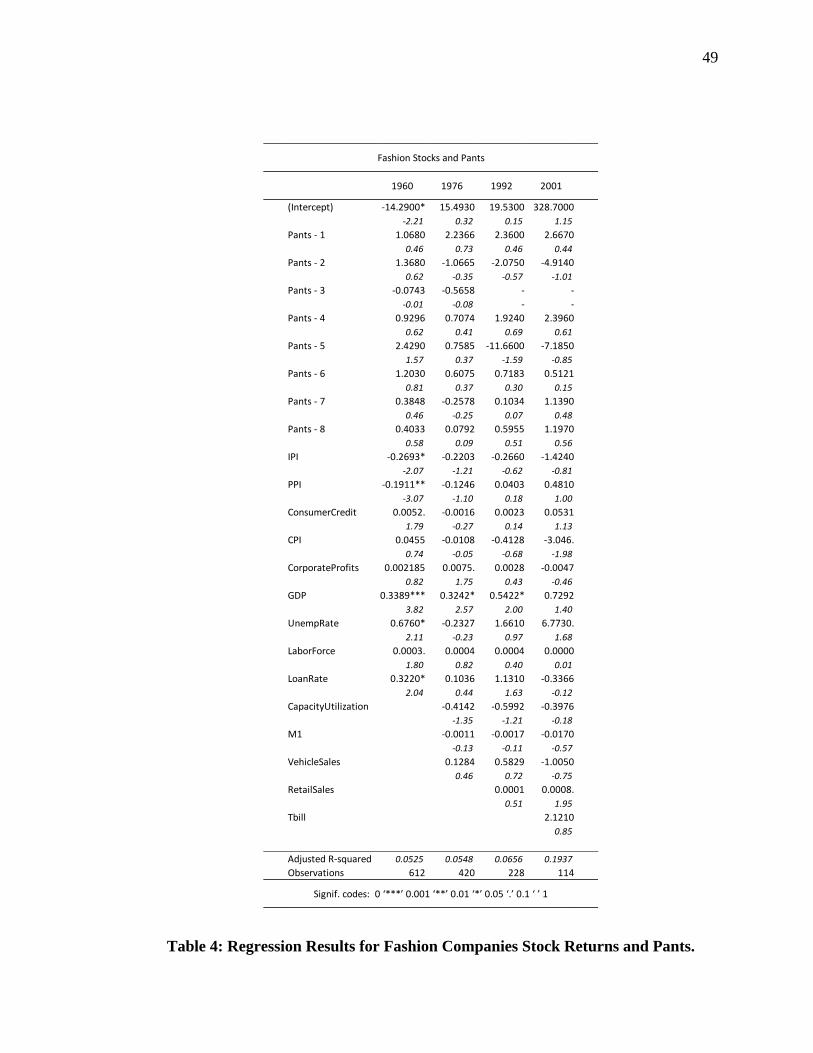
49
Table 4: Regression Results for Fashion Companies Stock Returns and Pants.
(Intercept) -14.2900* 15.4930 19.5300 328.7000
-2.21 0.32 0.15 1.15
Pants - 1 1.0680 2.2366 2.3600 2.6670
0.46 0.73 0.46 0.44
Pants - 2 1.3680 -1.0665 -2.0750 -4.9140
0.62 -0.35 -0.57 -1.01
Pants - 3 -0.0743 -0.5658 - -
-0.01 -0.08 - -
Pants - 4 0.9296 0.7074 1.9240 2.3960
0.62 0.41 0.69 0.61
Pants - 5 2.4290 0.7585 -11.6600 -7.1850
1.57 0.37 -1.59 -0.85
Pants - 6 1.2030 0.6075 0.7183 0.5121
0.81 0.37 0.30 0.15
Pants - 7 0.3848 -0.2578 0.1034 1.1390
0.46 -0.25 0.07 0.48
Pants - 8 0.4033 0.0792 0.5955 1.1970
0.58 0.09 0.51 0.56
IPI -0.2693* -0.2203 -0.2660 -1.4240
-2.07 -1.21 -0.62 -0.81
PPI -0.1911** -0.1246 0.0403 0.4810
-3.07 -1.10 0.18 1.00
ConsumerCredit 0.0052. -0.0016 0.0023 0.0531
1.79 -0.27 0.14 1.13
CPI 0.0455 -0.0108 -0.4128 -3.046.
0.74 -0.05 -0.68 -1.98
CorporateProfits 0.002185 0.0075. 0.0028 -0.0047
0.82 1.75 0.43 -0.46
GDP 0.3389*** 0.3242* 0.5422* 0.7292
3.82 2.57 2.00 1.40
UnempRate 0.6760* -0.2327 1.6610 6.7730.
2.11 -0.23 0.97 1.68
LaborForce 0.0003. 0.0004 0.0004 0.0000
1.80 0.82 0.40 0.01
LoanRate 0.3220* 0.1036 1.1310 -0.3366
2.04 0.44 1.63 -0.12
CapacityUtilization -0.4142 -0.5992 -0.3976
-1.35 -1.21 -0.18
M1 -0.0011 -0.0017 -0.0170
-0.13 -0.11 -0.57
VehicleSales 0.1284 0.5829 -1.0050
0.46 0.72 -0.75
RetailSales 0.0001 0.0008.
0.51 1.95
Tbill 2.1210
0.85
Adjusted R-squared 0.0525 0.0548 0.0656 0.1937
Observations 612 420 228 114
Signif. codes: 0 ‘***’ 0.001 ‘**’ 0.01 ‘*’ 0.05 ‘.’ 0.1 ‘ ’ 1
Fashion Stocks and Pants
1960 1976 1992 2001
50
This table reports the results from the regression analyses of the stock market returns for fashion
companies and pant lengths. The dependent variable, fashion stock returns, are the mean annualized
figures for returns on stocks with an SIC code of 22, 23, and 56 from 1960 to 2010. The independent
variables are the pant lengths, 1 through 8, that were collected through stratified sampling from
Vogue. Other independent variables were the various macroeconomic controls that were closely
related to the stock market. The limited availability of the macroeconomic control data during the
time period caused the need for staggered regression analyses. Each column corresponds to a
regression analysis ran with new variables included each time. T-values are reported in italics under
the estimated coefficients. Number of observations and the adjusted r-squared is reported at the
bottom of each column. Significance codes are shown at the bottom of the table. Definitions of
macroeconomic controls are included in Table 9 in the appendix.
Table 4 includes the regression results for fashion companies’ stock returns and
pants. There was no statistical significance recorded for any of the pant lengths in any of
the regressions completed. There were a few statistically significant coefficients for the
macroeconomic variables. Both the industrial production index and the producer price
index indicated a negative relationship with fashion stocks in the 1960 regression output.
The consumer credit coefficient showed a positive correlation to fashion companies’
stock returns in 1960 with a statistical significance of 0.1. The consumer price index had
a 0.1 statistically significant coefficient in the 2001 results. Corporate profits indicated a
positive relationship with fashion stocks in the 1976 output. Gross domestic profit also
revealed a positive relationship of varying significance with fashion stocks in the 1960,
1976, and 1992 regression results. Unemployment rate signaled another positive
relationship with fashion stocks in the 1960 and 2001 outputs. Finally, loan rate and labor
force both showed a positive relationship with fashion stocks in 1960.
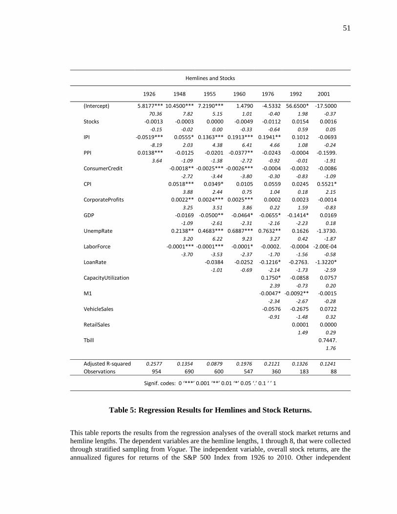
51
Table 5: Regression Results for Hemlines and Stock Returns.
This table reports the results from the regression analyses of the overall stock market returns and
hemline lengths. The dependent variables are the hemline lengths, 1 through 8, that were collected
through stratified sampling from Vogue. The independent variable, overall stock returns, are the
annualized figures for returns of the S&P 500 Index from 1926 to 2010. Other independent
(Intercept) 5.8177*** 10.4500*** 7.2190*** 1.4790 -4.5332 56.6500* -17.5000
70.36 7.82 5.15 1.01 -0.40 1.98 -0.37
Stocks -0.0013 -0.0003 0.0000 -0.0049 -0.0112 0.0154 0.0016
-0.15 -0.02 0.00 -0.33 -0.64 0.59 0.05
IPI -0.0519*** 0.0555* 0.1363*** 0.1913*** 0.1941** 0.1012 -0.0693
-8.19 2.03 4.38 6.41 4.66 1.08 -0.24
PPI 0.0138*** -0.0125 -0.0201 -0.0377** -0.0243 -0.0004 -0.1599.
3.64 -1.09 -1.38 -2.72 -0.92 -0.01 -1.91
ConsumerCredit -0.0018** -0.0025*** -0.0026*** -0.0004 -0.0032 -0.0086
-2.72 -3.44 -3.80 -0.30 -0.83 -1.09
CPI 0.0518*** 0.0349* 0.0105 0.0559 0.0245 0.5521*
3.88 2.44 0.75 1.04 0.18 2.15
CorporateProfits 0.0022** 0.0024*** 0.0025*** 0.0002 0.0023 -0.0014
3.25 3.51 3.86 0.22 1.59 -0.83
GDP -0.0169 -0.0500** -0.0464* -0.0655* -0.1414* 0.0169
-1.09 -2.61 -2.31 -2.16 -2.23 0.18
UnempRate 0.2138** 0.4683*** 0.6887*** 0.7632** 0.1626 -1.3730.
3.20 6.22 9.23 3.27 0.42 -1.87
LaborForce -0.0001*** -0.0001*** -0.0001* -0.0002. -0.0004 -2.00E-04
-3.70 -3.53 -2.37 -1.70 -1.56 -0.58
LoanRate -0.0384 -0.0252 -0.1216* -0.2763. -1.3220*
-1.01 -0.69 -2.14 -1.73 -2.59
CapacityUtilization 0.1750* -0.0858 0.0757
2.39 -0.73 0.20
M1 -0.0047* -0.0092** -0.0015
-2.34 -2.67 -0.28
VehicleSales -0.0576 -0.2675 0.0722
-0.91 -1.48 0.32
RetailSales 0.0001 0.0000
1.49 0.29
Tbill 0.7447.
1.76
Adjusted R-squared 0.2577 0.1354 0.0879 0.1976 0.2121 0.1326 0.1241
Observations 954 690 600 547 360 183 88
Signif. codes: 0 ‘***’ 0.001 ‘**’ 0.01 ‘*’ 0.05 ‘.’ 0.1 ‘ ’ 1
Hemlines and Stocks
1926 1948 1955 1960 1976 1992 2001
52
variables were the various macroeconomic controls that were closely related to the stock market.
The limited availability of the macroeconomic control data during the time period caused the need
for staggered regression analyses. Each column corresponds to a regression analysis ran with new
variables included each time. T-values are reported in italics under the estimated coefficients.
Number of observations and the adjusted r-squared is reported at the bottom of each column.
Significance codes are shown at the bottom of the table. Definitions of macroeconomic controls
are included in Table 9 in the appendix.
Table 5 contains the regression results between stock returns and hemlines with
hemlines as the dependent variable. The stock returns coefficient was not statistically
significant in any of the tests ran from 1926 to 2001. However, almost all of the
macroeconomic variables were statistically significant enough to indicate a relationship
to hemlines. The industrial production index showed a negative correlation to hemlines in
the 1926 output, but a positive correlation in 1948, 1955, 1960, and 1976. The producer
price index indicated a positive relationship with hemlines in 1926, but a negative
correlation in later outputs from the 1960 and 2001 tests. The coefficients for consumer
credit revealed a negative correlation with hemlines in the 1948, 1955, and 1960
regressions. Consumer price index and hemlines also showed a positive correlation in
1948, 1955, and 2001. Moreover, corporate profits signaled a positive relationship with
hemlines in the first three regression tests. Gross domestic profit indicated a statistically
significant negative correlation in 1955, 1960, 1976, and 1992. Hemlines and
unemployment rate were shown to have a positive correlation from 1948 to 1976 and a
negative correlation in 2001. The labor force coefficient suggested a negative relationship
of declining statistical significance from 1948 to 1976. Loan rate coefficients implied a
negative relationship with hemlines in the last three years. Capacity utilization and
hemlines indicated a positive statistically significant relationship in 1976, while the M1
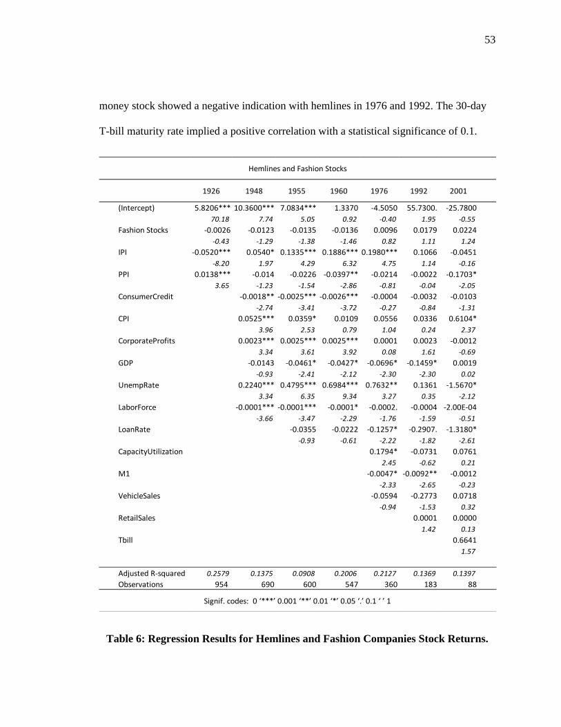
53
money stock showed a negative indication with hemlines in 1976 and 1992. The 30-day
T-bill maturity rate implied a positive correlation with a statistical significance of 0.1.
Table 6: Regression Results for Hemlines and Fashion Companies Stock Returns.
(Intercept) 5.8206*** 10.3600*** 7.0834*** 1.3370 -4.5050 55.7300. -25.7800
70.18 7.74 5.05 0.92 -0.40 1.95 -0.55
Fashion Stocks -0.0026 -0.0123 -0.0135 -0.0136 0.0096 0.0179 0.0224
-0.43 -1.29 -1.38 -1.46 0.82 1.11 1.24
IPI -0.0520*** 0.0540* 0.1335*** 0.1886*** 0.1980*** 0.1066 -0.0451
-8.20 1.97 4.29 6.32 4.75 1.14 -0.16
PPI 0.0138*** -0.014 -0.0226 -0.0397** -0.0214 -0.0022 -0.1703*
3.65 -1.23 -1.54 -2.86 -0.81 -0.04 -2.05
ConsumerCredit -0.0018** -0.0025*** -0.0026*** -0.0004 -0.0032 -0.0103
-2.74 -3.41 -3.72 -0.27 -0.84 -1.31
CPI 0.0525*** 0.0359* 0.0109 0.0556 0.0336 0.6104*
3.96 2.53 0.79 1.04 0.24 2.37
CorporateProfits 0.0023*** 0.0025*** 0.0025*** 0.0001 0.0023 -0.0012
3.34 3.61 3.92 0.08 1.61 -0.69
GDP -0.0143 -0.0461* -0.0427* -0.0696* -0.1459* 0.0019
-0.93 -2.41 -2.12 -2.30 -2.30 0.02
UnempRate 0.2240*** 0.4795*** 0.6984*** 0.7632** 0.1361 -1.5670*
3.34 6.35 9.34 3.27 0.35 -2.12
LaborForce -0.0001*** -0.0001*** -0.0001* -0.0002. -0.0004 -2.00E-04
-3.66 -3.47 -2.29 -1.76 -1.59 -0.51
LoanRate -0.0355 -0.0222 -0.1257* -0.2907. -1.3180*
-0.93 -0.61 -2.22 -1.82 -2.61
CapacityUtilization 0.1794* -0.0731 0.0761
2.45 -0.62 0.21
M1 -0.0047* -0.0092** -0.0012
-2.33 -2.65 -0.23
VehicleSales -0.0594 -0.2773 0.0718
-0.94 -1.53 0.32
RetailSales 0.0001 0.0000
1.42 0.13
Tbill 0.6641
1.57
Adjusted R-squared 0.2579 0.1375 0.0908 0.2006 0.2127 0.1369 0.1397
Observations 954 690 600 547 360 183 88
Signif. codes: 0 ‘***’ 0.001 ‘**’ 0.01 ‘*’ 0.05 ‘.’ 0.1 ‘ ’ 1
Hemlines and Fashion Stocks
1926 1948 1955 1960 1976 1992 2001
54
This table reports the results from the regression analyses of the stock market returns for fashion
companies and hemline lengths. The dependent variables are the hemline lengths, 1 through 8, that
were collected through stratified sampling from Vogue. The independent variable, fashion stock
returns, are the mean annualized figures for returns of stocks with an SIC code of 22, 23, and 56
from 1926 to 2010. Other independent variables were the various macroeconomic controls that
were closely related to the stock market. The limited availability of the macroeconomic control
data during the time period caused the need for staggered regression analyses. Each column
corresponds to a regression analysis ran with new variables included each time. T-values are
reported in italics under the estimated coefficients. Number of observations and the adjusted r-
squared is reported at the bottom of each column. Significance codes are shown at the bottom of
the table. Definitions of macroeconomic controls are included in Table 9 in the appendix.
Table 6 shows the regression output for hemlines and fashion companies’ stock
returns with hemlines as the dependent variable. The fashion companies’ stock returns
did not indicate any statistically significant relationship with hemlines in the regression
outputs from 1926 to 2001. However, all the macroeconomic variables other than vehicle
sales, retail sales, and T-bill maturity rate, indicated a statistically significant relationship
with hemlines. The industrial production index showed a negative correlation in the 1926
output and a positive correlation in the 1948 through 1976 results. The producer price
index implied a positive correlation in the 1926 results, but a negative correlation in the
1960 and 2001 outputs. Consumer credit showed a negative relationship with hemlines in
1948, 1955, and 1960. The consumer price index coefficients indicated a positive
correlation in 1948, 1955, and 2001. Corporate profits also suggested a positive
relationship with hemlines in the first three test outputs. Gross domestic product and
hemlines showed a negative correlation in the 1955, 1960, 1976, and 1992 outputs.
Unemployment rate implied a positive relationship with hemlines from 1955 to 1976 and
a negative relationship in 2001. The labor force and loan rate coefficients also indicated
negative correlations with hemlines. Capacity utilization suggests a statistically
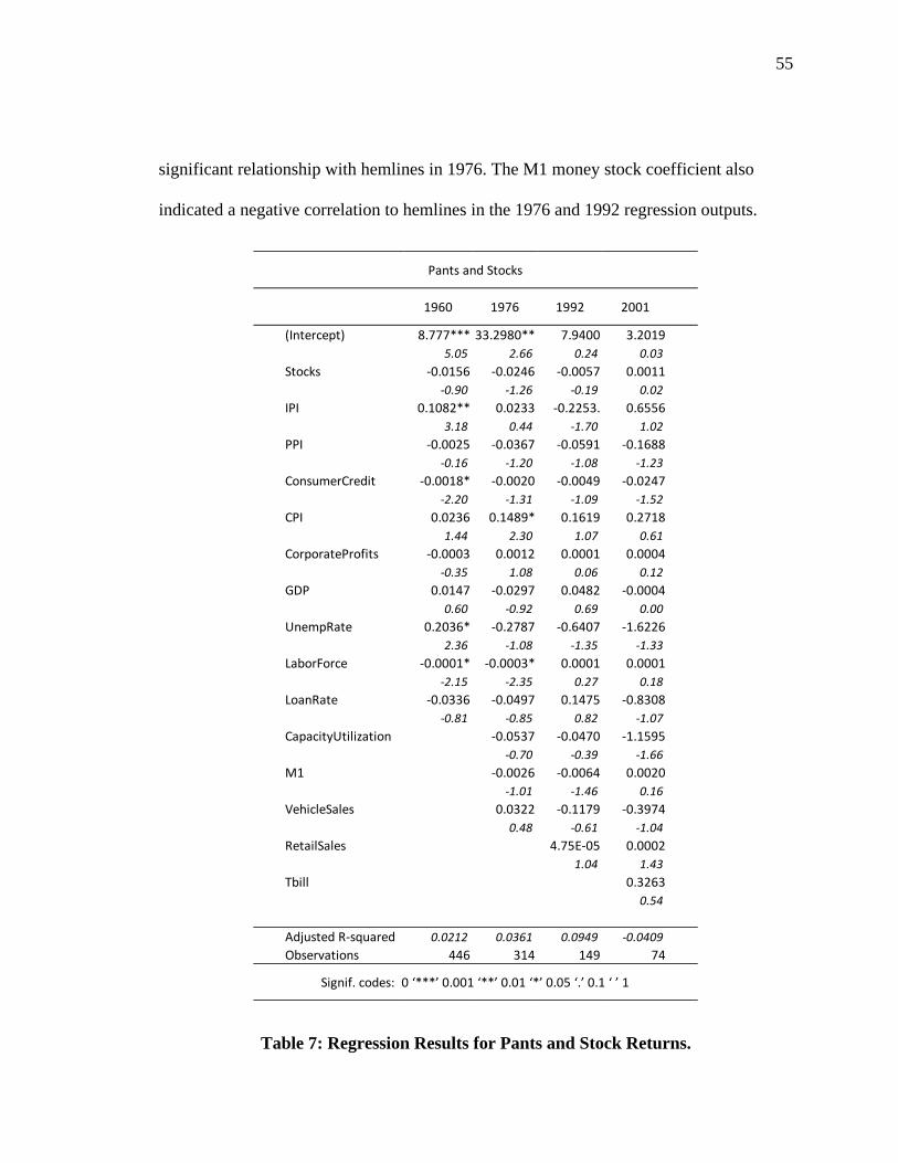
55
significant relationship with hemlines in 1976. The M1 money stock coefficient also
indicated a negative correlation to hemlines in the 1976 and 1992 regression outputs.
Table 7: Regression Results for Pants and Stock Returns.
(Intercept) 8.777*** 33.2980** 7.9400 3.2019
5.05 2.66 0.24 0.03
Stocks -0.0156 -0.0246 -0.0057 0.0011
-0.90 -1.26 -0.19 0.02
IPI 0.1082** 0.0233 -0.2253. 0.6556
3.18 0.44 -1.70 1.02
PPI -0.0025 -0.0367 -0.0591 -0.1688
-0.16 -1.20 -1.08 -1.23
ConsumerCredit -0.0018* -0.0020 -0.0049 -0.0247
-2.20 -1.31 -1.09 -1.52
CPI 0.0236 0.1489* 0.1619 0.2718
1.44 2.30 1.07 0.61
CorporateProfits -0.0003 0.0012 0.0001 0.0004
-0.35 1.08 0.06 0.12
GDP 0.0147 -0.0297 0.0482 -0.0004
0.60 -0.92 0.69 0.00
UnempRate 0.2036* -0.2787 -0.6407 -1.6226
2.36 -1.08 -1.35 -1.33
LaborForce -0.0001* -0.0003* 0.0001 0.0001
-2.15 -2.35 0.27 0.18
LoanRate -0.0336 -0.0497 0.1475 -0.8308
-0.81 -0.85 0.82 -1.07
CapacityUtilization -0.0537 -0.0470 -1.1595
-0.70 -0.39 -1.66
M1 -0.0026 -0.0064 0.0020
-1.01 -1.46 0.16
VehicleSales 0.0322 -0.1179 -0.3974
0.48 -0.61 -1.04
RetailSales 4.75E-05 0.0002
1.04 1.43
Tbill 0.3263
0.54
Adjusted R-squared 0.0212 0.0361 0.0949 -0.0409
Observations 446 314 149 74
Signif. codes: 0 ‘***’ 0.001 ‘**’ 0.01 ‘*’ 0.05 ‘.’ 0.1 ‘ ’ 1
Pants and Stocks
1960 1976 1992 2001
56
This table reports the results from the regression analyses of the overall stock market returns and
pant lengths. The dependent variables are the pant lengths, 1 through 8, that were collected through
stratified sampling from Vogue. The independent variable, overall stock returns, are the annualized
figures for returns of the S&P 500 Index from 1960 to 2010. Other independent variables were the
various macroeconomic controls that were closely related to the stock market. The limited
availability of the macroeconomic control data during the time period caused the need for staggered
regression analyses. Each column corresponds to a regression analysis ran with new variables
included each time. T-values are reported in italics under the estimated coefficients. Number of
observations and the adjusted r-squared is reported at the bottom of each column. Significance
codes are shown at the bottom of the table. Definitions of macroeconomic controls are included in
Table 9 in the appendix.
The above table shows the regression output between pants and stock returns with
pants as the dependent variable. The stock return coefficient did not indicate any
statistically significant relationship with pant length trends. Only a few of the
macroeconomic variables were revealed to have a correlation with pants that was
statistically significant. The industrial production index implied a relatively strong
positive correlation with pants in the 1960 output but implied a negative correlation in the
1992 result. The consumer credit coefficient showed a negative relationship with pants in
1960 with a statistical significance of 0.05. Consumer price index indicated a positive
correlation in the 1992 output. Unemployment rate also implied a positive relationship
with pants in 1960 with a 0.05 statistical significance. The labor force coefficient
revealed a negative statistically significant correlation in the 1960 and 1976 outputs.
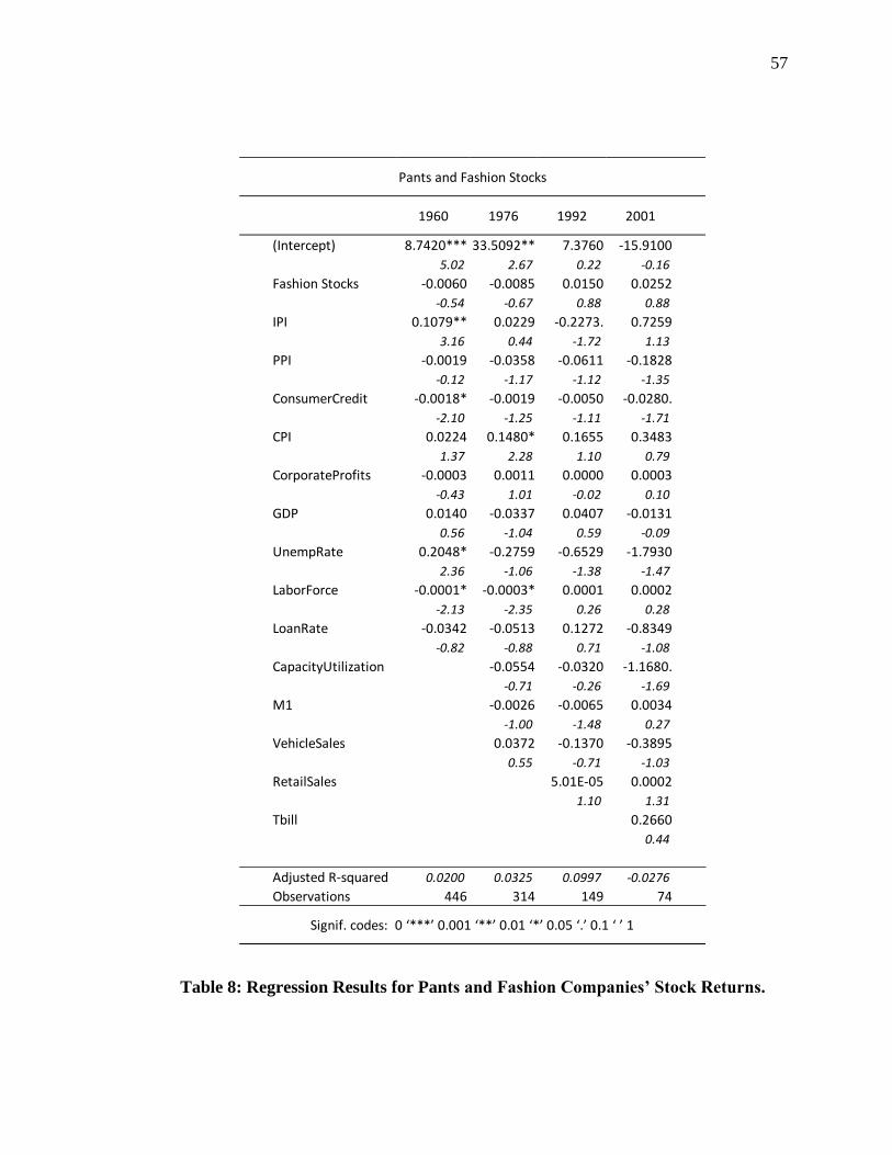
57
Table 8: Regression Results for Pants and Fashion Companies’ Stock Returns.
(Intercept) 8.7420*** 33.5092** 7.3760 -15.9100
5.02 2.67 0.22 -0.16
Fashion Stocks -0.0060 -0.0085 0.0150 0.0252
-0.54 -0.67 0.88 0.88
IPI 0.1079** 0.0229 -0.2273. 0.7259
3.16 0.44 -1.72 1.13
PPI -0.0019 -0.0358 -0.0611 -0.1828
-0.12 -1.17 -1.12 -1.35
ConsumerCredit -0.0018* -0.0019 -0.0050 -0.0280.
-2.10 -1.25 -1.11 -1.71
CPI 0.0224 0.1480* 0.1655 0.3483
1.37 2.28 1.10 0.79
CorporateProfits -0.0003 0.0011 0.0000 0.0003
-0.43 1.01 -0.02 0.10
GDP 0.0140 -0.0337 0.0407 -0.0131
0.56 -1.04 0.59 -0.09
UnempRate 0.2048* -0.2759 -0.6529 -1.7930
2.36 -1.06 -1.38 -1.47
LaborForce -0.0001* -0.0003* 0.0001 0.0002
-2.13 -2.35 0.26 0.28
LoanRate -0.0342 -0.0513 0.1272 -0.8349
-0.82 -0.88 0.71 -1.08
CapacityUtilization -0.0554 -0.0320 -1.1680.
-0.71 -0.26 -1.69
M1 -0.0026 -0.0065 0.0034
-1.00 -1.48 0.27
VehicleSales 0.0372 -0.1370 -0.3895
0.55 -0.71 -1.03
RetailSales 5.01E-05 0.0002
1.10 1.31
Tbill 0.2660
0.44
Adjusted R-squared 0.0200 0.0325 0.0997 -0.0276
Observations 446 314 149 74
Signif. codes: 0 ‘***’ 0.001 ‘**’ 0.01 ‘*’ 0.05 ‘.’ 0.1 ‘ ’ 1
Pants and Fashion Stocks
1960 1976 1992 2001
58
This table reports the results from the regression analyses of the stock market returns for fashion
companies and pant lengths. The dependent variables are the pant lengths, 1 through 8, that were
collected through stratified sampling from Vogue. The independent variable, fashion stock returns,
are the mean annualized figures for returns of stocks with an SIC code of 22, 23, and 56 from 1960
to 2010. Other independent variables were the various macroeconomic controls that were closely
related to the stock market. The limited availability of the macroeconomic control data during the
time period caused the need for staggered regression analyses. Each column corresponds to a
regression analysis ran with new variables included each time. T-values are reported in italics under
the estimated coefficients. Number of observations and the adjusted r-squared is reported at the
bottom of each column. Significance codes are shown at the bottom of the table. Definitions of
macroeconomic controls are included in Table 9 in the appendix.
Table 8 reflects the results of the regression analyses ran between pants and
fashion companies’ stock returns with pants as the dependent variable. The coefficient for
fashion stock returns did not indicate a statistically significant relationship with pant
trends in any of the regression results. However, 6 out of the 14 macroeconomic variables
showed a statistically significant correlation with pants in at least one of the regression
results. Industrial production index indicated a similar relationship with fashion stock
returns as it did with overall stock returns, with a positive coefficient in 1960 and a
negative coefficient in 1992. Consumer credit also showed a similar negative relationship
with fashion stocks with a statistical significance of 0.05 in the 1960 result. The
consumer price index coefficient implies a positive correlation with fashion stock returns
in the 1976 output. Unemployment rate also indicates a positive relationship in 1960 with
a 0.05 statistical significance. Labor force again reveals a negative correlation with
fashion stocks in the 1960 and 1976 returns. Capacity utilization shows a negative
relationship in 2001 with a statistical significance of 0.1.
59
Chapter 6: Conclusions
After completing several regression analyses which revealed no statistical
significance, and a thorough observation of graphed movements between hem lengths,
overall stock returns, and fashion companies’ stock returns, it is clear that there is no
causal relationship indicated between these variables. The same can be said between
pants, stock returns, and fashion companies’ stock returns. Due to the fact that there is no
causality between the variables, neither one of the variables can successfully predict the
other for extended periods of time. These results, reflective of Mabry’s study results of no
correlation (Mabry, M. A., 1971, pp. 1-101), provide evidence against the hemline
theory.
Although there were a few instances where a hemline or pant coefficient was
found to be slightly statistically significant, there were not enough significant coefficients
in order to indicate a pattern between the variables. There were also points on the graphs
where it appeared that hem and pant length trends moved together with stock returns.
However, these points were few and far between, and there are not enough of these
instances to indicate a pattern. These occurrences could be purely coincidental. There
could also be a reason to these seemingly in sync movements. Both fashion trends and
stock returns could be reacting in similar ways to changes in underlying variables.
Looking into these possible underlying variables could be an area for future research.
60
Another possible area for future research would be to look into a longer lag time
between stock movements and hem or pant length changes. As mentioned in chapter 2,
the study completed by Marjolein van Baardwijk and Philip Hans Franses found that
hemlines lag behind economic cycles for 3 years (Van Baardwijk, M., & Franses, P.H.,
2012, p. 25-26). This thesis only looked into a 1-year lag between stock and hemline
fluctuations. While this short lag time did not reveal any causality or apparent correlation
between the two variables, perhaps something different could be identified by moving
hemline data out further to test a longer lag time. Looking into a 3-year lag to compare to
Baardwijk and Franses’ results would be an interesting addition to this study and a
noteworthy area for potential future research.
Along with a longer lag time, Baardwijk and Franses’ study examined the
relationship between hemlines and economic cycles, instead of stock market movements.
As their study found a correlation between these two variables, it would be valuable to
test hemlines with overall economic movements as an area of future research. Stock
market movements are not always indicative of what is going on with the economy. As
was found in the regression test results, there were several economic measures that were
statistically significant in the tests with hemlines. This indicates that there could be a
correlation between the economy and hemline movements.
61
References
Chang, S. J., & Ha, D. (1997). The impact of macroeconomic variables on stock market
performance: A taxonomic approach. American Business Review, 15(2), 104.
Cole, D. J., & Deihl, N. (2015). The History of Modern Fashion From 1850. (F.
Maunder, Ed.). Laurence King Publisher Ltd.
Fashion Design Body Drawing. (n.d.). [Photograph]. Pixy Org. https://pixy.org/957767/.
Federal Reserve Bank of St. Louis. (n.d.) FRED Economic Data.
https://fred.stlouisfed.org/.
Gilbert, D. (2017). The looks of austerity: Fashions for hard times. Fashion Theory, The
Journal of Dress, Body & Culture, 21(4), 477-499. https://doi-
org.proxy.library.kent.edu/10.1080/1362704X.2017.1316057.
Laver, J. (1969). Modesty in Dress. Houghton Mifflin Company.
Mabry, M. A. (1971). The relationship between fluctuations in hemlines and stock market
averages from 1921 to 1971. (Publication No. 12-1971). [Master’s thesis,
University of Tennessee]. Trace: Tennessee Research and Creative Exchange.
Milford-Cottam, D. (2018). Fashion in the 1970s. Bloomsbury Publishing Plc.
Van Baardwijk, M., & Franses P.H. (2012). Hemlines and the economy: Which goes
down first? Foresight: The International Journal of Applied Forecasting, 26, 25-
26.
62
Vogue. (n.d.). Vogue Archive. Vogue Archive. https://archive.vogue.com/.
Vogue. 1, Sept. 1943, https://archive.vogue.com/issue/19430901.
Welters, L., & Lillethun, A. (2018). Fashion History: A Global View. (J.B. Eicher, Ed.).
Bloomsbury Academic.
Worsley, H. (2011). 100 Ideas That Changed Fashion. Laurence King Publishing Ltd.
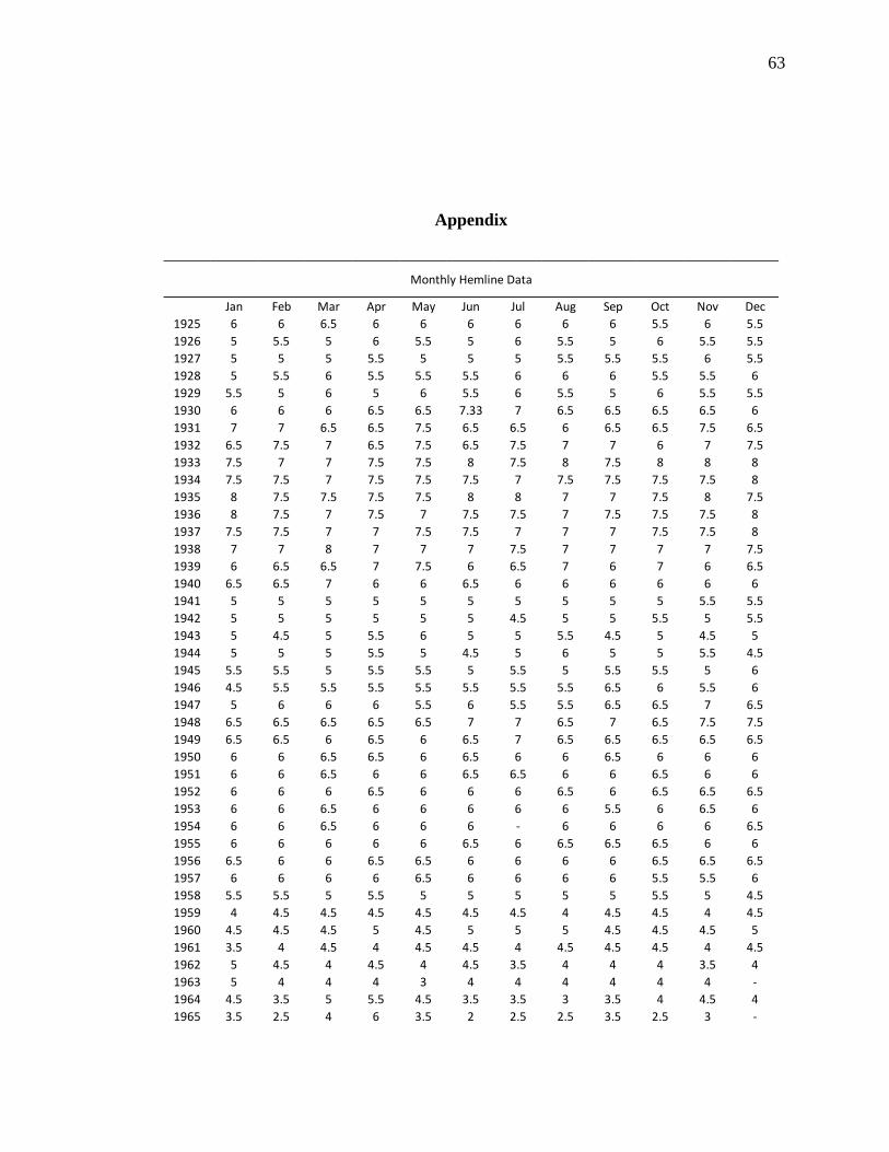
63
Appendix
Jan Feb Mar Apr May Jun Jul Aug Sep Oct Nov Dec
1925 6 6 6.5 6 6 6 6 6 6 5.5 6 5.5
1926 5 5.5 5 6 5.5 5 6 5.5 5 6 5.5 5.5
1927 5 5 5 5.5 5 5 5 5.5 5.5 5.5 6 5.5
1928 5 5.5 6 5.5 5.5 5.5 6 6 6 5.5 5.5 6
1929 5.5 5 6 5 6 5.5 6 5.5 5 6 5.5 5.5
1930 6 6 6 6.5 6.5 7.33 7 6.5 6.5 6.5 6.5 6
1931 7 7 6.5 6.5 7.5 6.5 6.5 6 6.5 6.5 7.5 6.5
1932 6.5 7.5 7 6.5 7.5 6.5 7.5 7 7 6 7 7.5
1933 7.5 7 7 7.5 7.5 8 7.5 8 7.5 8 8 8
1934 7.5 7.5 7 7.5 7.5 7.5 7 7.5 7.5 7.5 7.5 8
1935 8 7.5 7.5 7.5 7.5 8 8 7 7 7.5 8 7.5
1936 8 7.5 7 7.5 7 7.5 7.5 7 7.5 7.5 7.5 8
1937 7.5 7.5 7 7 7.5 7.5 7 7 7 7.5 7.5 8
1938 7 7 8 7 7 7 7.5 7 7 7 7 7.5
1939 6 6.5 6.5 7 7.5 6 6.5 7 6 7 6 6.5
1940 6.5 6.5 7 6 6 6.5 6 6 6 6 6 6
1941 5 5 5 5 5 5 5 5 5 5 5.5 5.5
1942 5 5 5 5 5 5 4.5 5 5 5.5 5 5.5
1943 5 4.5 5 5.5 6 5 5 5.5 4.5 5 4.5 5
1944 5 5 5 5.5 5 4.5 5 6 5 5 5.5 4.5
1945 5.5 5.5 5 5.5 5.5 5 5.5 5 5.5 5.5 5 6
1946 4.5 5.5 5.5 5.5 5.5 5.5 5.5 5.5 6.5 6 5.5 6
1947 5 6 6 6 5.5 6 5.5 5.5 6.5 6.5 7 6.5
1948 6.5 6.5 6.5 6.5 6.5 7 7 6.5 7 6.5 7.5 7.5
1949 6.5 6.5 6 6.5 6 6.5 7 6.5 6.5 6.5 6.5 6.5
1950 6 6 6.5 6.5 6 6.5 6 6 6.5 6 6 6
1951 6 6 6.5 6 6 6.5 6.5 6 6 6.5 6 6
1952 6 6 6 6.5 6 6 6 6.5 6 6.5 6.5 6.5
1953 6 6 6.5 6 6 6 6 6 5.5 6 6.5 6
1954 6 6 6.5 6 6 6 - 6 6 6 6 6.5
1955 6 6 6 6 6 6.5 6 6.5 6.5 6.5 6 6
1956 6.5 6 6 6.5 6.5 6 6 6 6 6.5 6.5 6.5
1957 6 6 6 6 6.5 6 6 6 6 5.5 5.5 6
1958 5.5 5.5 5 5.5 5 5 5 5 5 5.5 5 4.5
1959 4 4.5 4.5 4.5 4.5 4.5 4.5 4 4.5 4.5 4 4.5
1960 4.5 4.5 4.5 5 4.5 5 5 5 4.5 4.5 4.5 5
1961 3.5 4 4.5 4 4.5 4.5 4 4.5 4.5 4.5 4 4.5
1962 5 4.5 4 4.5 4 4.5 3.5 4 4 4 3.5 4
1963 5 4 4 4 3 4 4 4 4 4 4 -
1964 4.5 3.5 5 5.5 4.5 3.5 3.5 3 3.5 4 4.5 4
1965 3.5 2.5 4 6 3.5 2 2.5 2.5 3.5 2.5 3 -
Monthly Hemline Data
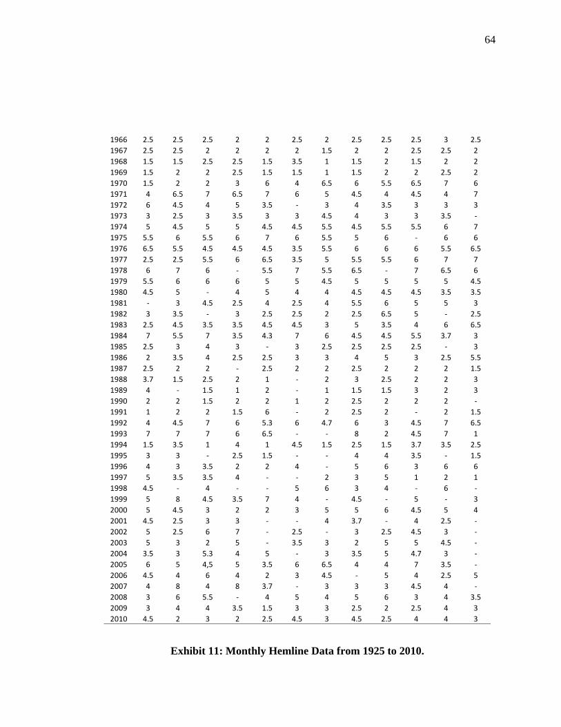
64
Exhibit 11: Monthly Hemline Data from 1925 to 2010.
1965 3.5 2.5 4 6 3.5 2 2.5 2.5 3.5 2.5 3 -
1966 2.5 2.5 2.5 2 2 2.5 2 2.5 2.5 2.5 3 2.5
1967 2.5 2.5 2 2 2 2 1.5 2 2 2.5 2.5 2
1968 1.5 1.5 2.5 2.5 1.5 3.5 1 1.5 2 1.5 2 2
1969 1.5 2 2 2.5 1.5 1.5 1 1.5 2 2 2.5 2
1970 1.5 2 2 3 6 4 6.5 6 5.5 6.5 7 6
1971 4 6.5 7 6.5 7 6 5 4.5 4 4.5 4 7
1972 6 4.5 4 5 3.5 - 3 4 3.5 3 3 3
1973 3 2.5 3 3.5 3 3 4.5 4 3 3 3.5 -
1974 5 4.5 5 5 4.5 4.5 5.5 4.5 5.5 5.5 6 7
1975 5.5 6 5.5 6 7 6 5.5 5 6 - 6 6
1976 6.5 5.5 4.5 4.5 4.5 3.5 5.5 6 6 6 5.5 6.5
1977 2.5 2.5 5.5 6 6.5 3.5 5 5.5 5.5 6 7 7
1978 6 7 6 - 5.5 7 5.5 6.5 - 7 6.5 6
1979 5.5 6 6 6 5 5 4.5 5 5 5 5 4.5
1980 4.5 5 - 4 5 4 4 4.5 4.5 4.5 3.5 3.5
1981 - 3 4.5 2.5 4 2.5 4 5.5 6 5 5 3
1982 3 3.5 - 3 2.5 2.5 2 2.5 6.5 5 - 2.5
1983 2.5 4.5 3.5 3.5 4.5 4.5 3 5 3.5 4 6 6.5
1984 7 5.5 7 3.5 4.3 7 6 4.5 4.5 5.5 3.7 3
1985 2.5 3 4 3 - 3 2.5 2.5 2.5 2.5 - 3
1986 2 3.5 4 2.5 2.5 3 3 4 5 3 2.5 5.5
1987 2.5 2 2 - 2.5 2 2 2.5 2 2 2 1.5
1988 3.7 1.5 2.5 2 1 - 2 3 2.5 2 2 3
1989 4 - 1.5 1 2 - 1 1.5 1.5 3 2 3
1990 2 2 1.5 2 2 1 2 2.5 2 2 2 -
1991 1 2 2 1.5 6 - 2 2.5 2 - 2 1.5
1992 4 4.5 7 6 5.3 6 4.7 6 3 4.5 7 6.5
1993 7 7 7 6 6.5 - - 8 2 4.5 7 1
1994 1.5 3.5 1 4 1 4.5 1.5 2.5 1.5 3.7 3.5 2.5
1995 3 3 - 2.5 1.5 - - 4 4 3.5 - 1.5
1996 4 3 3.5 2 2 4 - 5 6 3 6 6
1997 5 3.5 3.5 4 - - 2 3 5 1 2 1
1998 4.5 - 4 - - 5 6 3 4 - 6 -
1999 5 8 4.5 3.5 7 4 - 4.5 - 5 - 3
2000 5 4.5 3 2 2 3 5 5 6 4.5 5 4
2001 4.5 2.5 3 3 - - 4 3.7 - 4 2.5 -
2002 5 2.5 6 7 - 2.5 - 3 2.5 4.5 3 -
2003 5 3 2 5 - 3.5 3 2 5 5 4.5 -
2004 3.5 3 5.3 4 5 - 3 3.5 5 4.7 3 -
2005 6 5 4,5 5 3.5 6 6.5 4 4 7 3.5 -
2006 4.5 4 6 4 2 3 4.5 - 5 4 2.5 5
2007 4 8 4 8 3.7 - 3 3 3 4.5 4 -
2008 3 6 5.5 - 4 5 4 5 6 3 4 3.5
2009 3 4 4 3.5 1.5 3 3 2.5 2 2.5 4 3
2010 4.5 2 3 2 2.5 4.5 3 4.5 2.5 4 4 3
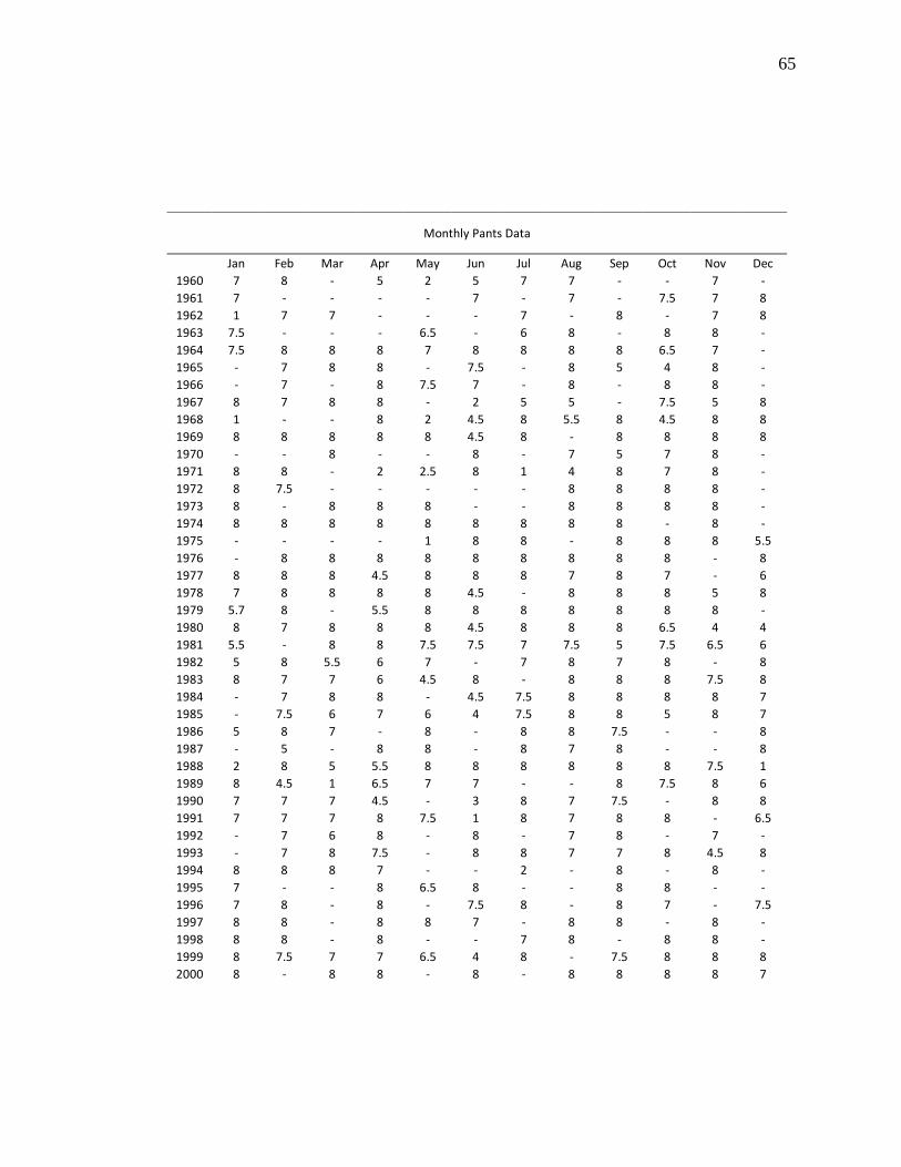
65
Jan Feb Mar Apr May Jun Jul Aug Sep Oct Nov Dec
1960 7 8 - 5 2 5 7 7 - - 7 -
1961 7 - - - - 7 - 7 - 7.5 7 8
1962 1 7 7 - - - 7 - 8 - 7 8
1963 7.5 - - - 6.5 - 6 8 - 8 8 -
1964 7.5 8 8 8 7 8 8 8 8 6.5 7 -
1965 - 7 8 8 - 7.5 - 8 5 4 8 -
1966 - 7 - 8 7.5 7 - 8 - 8 8 -
1967 8 7 8 8 - 2 5 5 - 7.5 5 8
1968 1 - - 8 2 4.5 8 5.5 8 4.5 8 8
1969 8 8 8 8 8 4.5 8 - 8 8 8 8
1970 - - 8 - - 8 - 7 5 7 8 -
1971 8 8 - 2 2.5 8 1 4 8 7 8 -
1972 8 7.5 - - - - - 8 8 8 8 -
1973 8 - 8 8 8 - - 8 8 8 8 -
1974 8 8 8 8 8 8 8 8 8 - 8 -
1975 - - - - 1 8 8 - 8 8 8 5.5
1976 - 8 8 8 8 8 8 8 8 8 - 8
1977 8 8 8 4.5 8 8 8 7 8 7 - 6
1978 7 8 8 8 8 4.5 - 8 8 8 5 8
1979 5.7 8 - 5.5 8 8 8 8 8 8 8 -
1980 8 7 8 8 8 4.5 8 8 8 6.5 4 4
1981 5.5 - 8 8 7.5 7.5 7 7.5 5 7.5 6.5 6
1982 5 8 5.5 6 7 - 7 8 7 8 - 8
1983 8 7 7 6 4.5 8 - 8 8 8 7.5 8
1984 - 7 8 8 - 4.5 7.5 8 8 8 8 7
1985 - 7.5 6 7 6 4 7.5 8 8 5 8 7
1986 5 8 7 - 8 - 8 8 7.5 - - 8
1987 - 5 - 8 8 - 8 7 8 - - 8
1988 2 8 5 5.5 8 8 8 8 8 8 7.5 1
1989 8 4.5 1 6.5 7 7 - - 8 7.5 8 6
1990 7 7 7 4.5 - 3 8 7 7.5 - 8 8
1991 7 7 7 8 7.5 1 8 7 8 8 - 6.5
1992 - 7 6 8 - 8 - 7 8 - 7 -
1993 - 7 8 7.5 - 8 8 7 7 8 4.5 8
1994 8 8 8 7 - - 2 - 8 - 8 -
1995 7 - - 8 6.5 8 - - 8 8 - -
1996 7 8 - 8 - 7.5 8 - 8 7 - 7.5
1997 8 8 - 8 8 7 - 8 8 - 8 -
1998 8 8 - 8 - - 7 8 - 8 8 -
1999 8 7.5 7 7 6.5 4 8 - 7.5 8 8 8
2000 8 - 8 8 - 8 - 8 8 8 8 7
Monthly Pants Data
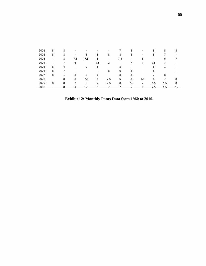
66
Exhibit 12: Monthly Pants Data from 1960 to 2010.
2001 8 8 - - - - 7 8 - 8 8 8
2002 8 8 - 8 8 8 8 8 - 8 7 -
2003 - 8 7.5 7.5 8 - 7.5 - 8 - 6 7
2004 - 7 6 - 7.5 2 - 7 7 7.5 7 -
2005 8 4 - 2 8 - 8 - - 6 1 -
2006 8 7 - - - 8 6 8 - 8 - -
2007 8 1 8 7 6 - 8 8 - 7 8 -
2008 - 8 8 7.5 8 7.5 6 8 4.5 8 7 8
2009 8 8 7 8 7 2.5 8 7.5 7 4.5 4.5 8
2010 - 8 4 6.5 8 7 7 5 4 7.5 4.5 7.5
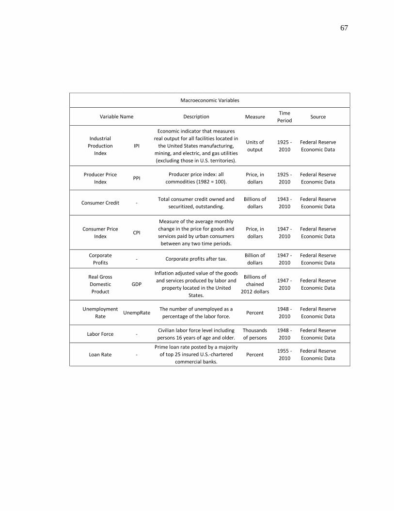
67
MeasureTime
PeriodSource
Industrial
Production
Index
IPIUnits of
output
1925 -
2010
Federal Reserve
Economic Data
Producer Price
IndexPPI
Price, in
dollars
1925 -
2010
Federal Reserve
Economic Data
Consumer Credit -Billions of
dollars
1943 -
2010
Federal Reserve
Economic Data
Consumer Price
IndexCPI
Price, in
dollars
1947 -
2010
Federal Reserve
Economic Data
Corporate
Profits-
Billion of
dollars
1947 -
2010
Federal Reserve
Economic Data
Real Gross
Domestic
Product
GDP
Billions of
chained
2012 dollars
1947 -
2010
Federal Reserve
Economic Data
Unemployment
RateUnempRate Percent
1948 -
2010
Federal Reserve
Economic Data
Labor Force -Thousands
of persons
1948 -
2010
Federal Reserve
Economic Data
Loan Rate - Percent1955 -
2010
Federal Reserve
Economic Data
Total consumer credit owned and
securitized, outstanding.
Measure of the average monthly
change in the price for goods and
services paid by urban consumers
between any two time periods.
Corporate profits after tax.
Macroeconomic Variables
The number of unemployed as a
percentage of the labor force.
Civilian labor force level including
persons 16 years of age and older.
Prime loan rate posted by a majority
of top 25 insured U.S.-chartered
commercial banks.
Inflation adjusted value of the goods
and services produced by labor and
property located in the United
States.
Variable Name Description
Economic indicator that measures
real output for all facilities located in
the United States manufacturing,
mining, and electric, and gas utilities
(excluding those in U.S. territories).
Producer price index: all
commodities (1982 = 100).
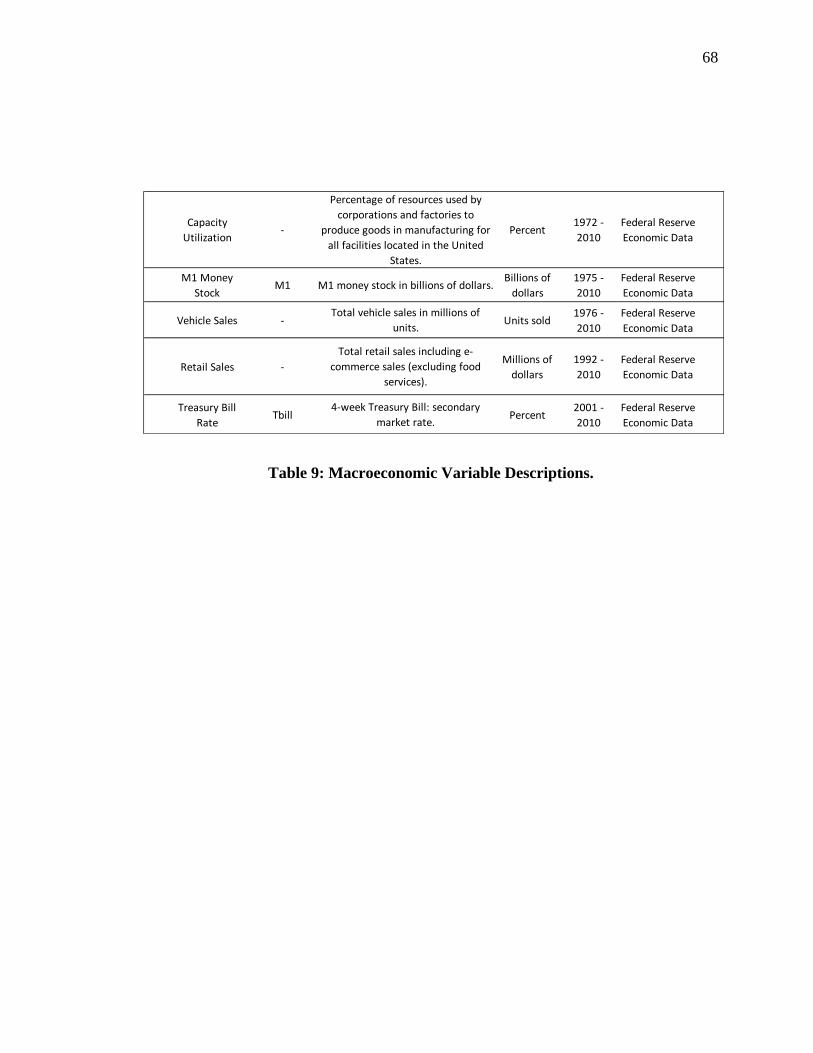
68
Table 9: Macroeconomic Variable Descriptions.
Capacity
Utilization- Percent
1972 -
2010
Federal Reserve
Economic Data
M1 Money
StockM1
Billions of
dollars
1975 -
2010
Federal Reserve
Economic Data
Vehicle Sales - Units sold1976 -
2010
Federal Reserve
Economic Data
Retail Sales -Millions of
dollars
1992 -
2010
Federal Reserve
Economic Data
Treasury Bill
RateTbill Percent
2001 -
2010
Federal Reserve
Economic Data
Total retail sales including e-
commerce sales (excluding food
services).
4-week Treasury Bill: secondary
market rate.
Percentage of resources used by
corporations and factories to
produce goods in manufacturing for
all facilities located in the United
States.
M1 money stock in billions of dollars.
Total vehicle sales in millions of
units.
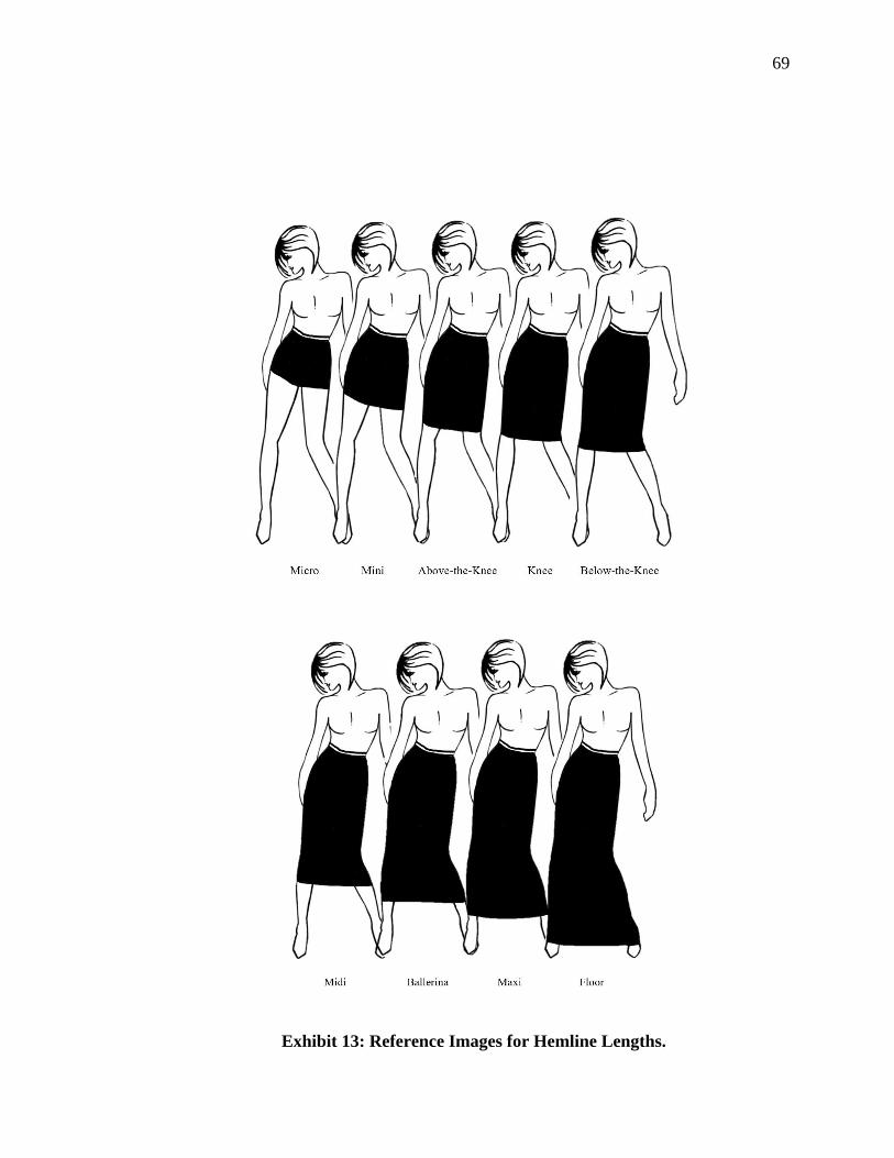
69
Exhibit 13: Reference Images for Hemline Lengths.
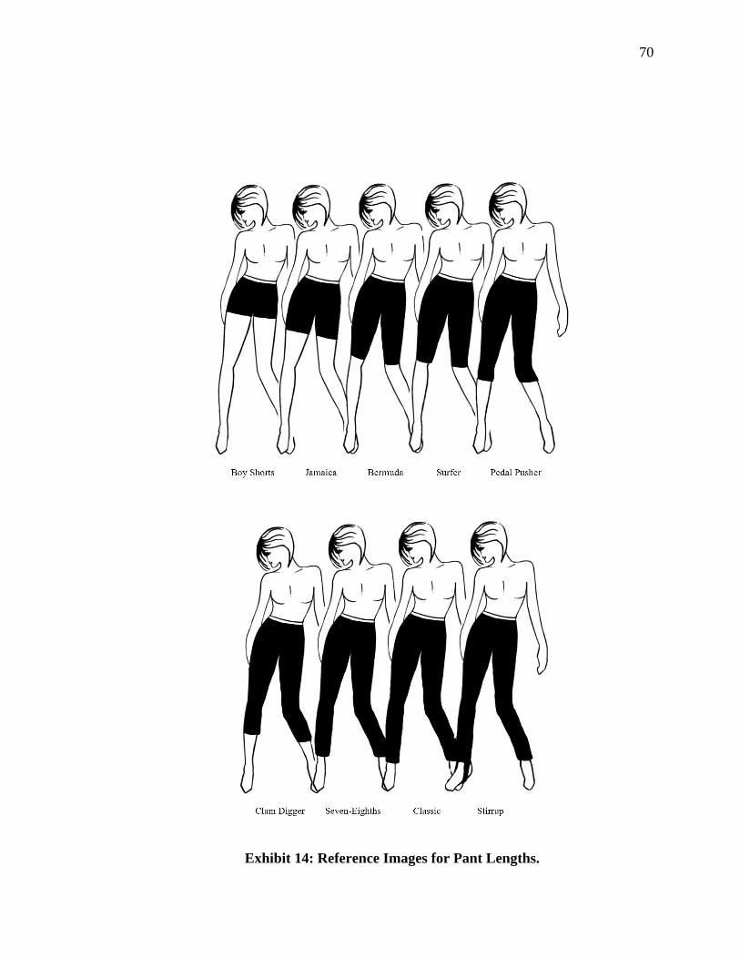
70
Exhibit 14: Reference Images for Pant Lengths.


