Embed Size (px)
Citation preview
HEAT CONDUCTION
Heat conduction modelling ........................................................................................................................... 1
Case studies ........................................................................................................................................... 2
Analytical solutions....................................................................................................................................... 2
Conduction shape factor (steady state) ..................................................................................................... 3
Reduction to the main dimension (steady state) ....................................................................................... 5
Planar, cylindrical, and spherical energy sources, internal or interfacial ............................................. 5
Multilayer composite walls ................................................................................................................... 7
Critical radius ........................................................................................................................................ 7
Rods and fins ......................................................................................................................................... 7
Heat source moving at steady state along a rod .................................................................................... 9
Reduction by dimension similarity (unsteady state) ............................................................................... 10
Energy deposition in unbounded media .............................................................................................. 11
Thermal contact in semi-infinite media .............................................................................................. 14
Freezing and thawing .......................................................................................................................... 16
Reduction by separation of variables ...................................................................................................... 17
Unsteady problems in 1-D .................................................................................................................. 17
Steady problems in 2-D....................................................................................................................... 22
Other analytical methods to solve partial differential equations ............................................................. 26
Duhamel`s theorem ............................................................................................................................. 26
Numerical solutions .................................................................................................................................... 27
Global fitting ........................................................................................................................................... 29
Lumped network ..................................................................................................................................... 30
Residual fitting ........................................................................................................................................ 31
Collocation method ............................................................................................................................. 33
Least square method (LSM) ................................................................................................................ 33
Galerkin method .................................................................................................................................. 33
Finite differences..................................................................................................................................... 33
Finite elements ........................................................................................................................................ 37
Boundary elements .................................................................................................................................. 37
HEAT CONDUCTION MODELLING
Heat transfer by conduction (also known as diffusion heat transfer) is the flow of thermal energy within
solids and non-flowing fluids, driven by thermal non-equilibrium (i.e. the effect of a non-uniform
temperature field), commonly measured as a heat flux (vector), i.e. the heat flow per unit time (and
usually unit normal area) at a control surface. The basics of Heat Transfer (what is it, what for, its
nomenclature, case studies, and the general view on how heat-transfer problems are solved and analysed),
is to be found aside, and assumed already covered. As explained there, the solution to heat-transfer
problems can be directly applied, with the appropriate change of variables, to mass-transfer problems.
The general equations for heat conduction are the energy balance for a control mass, d dE t Q W , and
the constitutive equations for heat conduction (Fourier's law) which relates heat flux to temperature
gradient, q k T . Their combination:
dd d
d d dd
p A
p A V
HQ KA T q n A H
t Q k T n A k T At
q k T
(1)
when applied to an infinitesimal volume, yield the partial differential equation (PDE) known as heat
equation, or diffusion equation, as explained aside:
2Tc k T cv T
t
(2)
where the last two terms in (2) come from separating enthalpy changes in a temperature-dependent term
(dH=VcdT), and the rest dH=Vdt (to account for a possible energy dissipation term, [W/m3]), and a
possible choice of coordinate system moving relative to the material at velocity v (i.e., by splitting the
convective derivative d dH t H t v H ). Many times, thermal conductivity in (2) is to be found
under the thermal diffusivity variable: a≡k/(c).
In this presentation we embark into generic analytical and numerical methods to solve the heat conduction
equations (2) within the bounding conditions of each particular problem (i.e., a PDE with some initial and
boundary conditions, BC). It is worth to mention now that, in the theory of Heat Transfer, initial and
boundary conditions are always neatly drawn, and great effort is devoted to solving the heat equation,
whereas, in real Heat Transfer practice, initial and boundary conditions are so loosely defined that well-
founded heat-transfer knowledge is needed to model then, and solving the equations is just a computer
chore.
Case studies
To better illustrate the different methods of solving heat-conduction problems, we are considering the two
following paradigms:
Rod-heated-at-one-end. This is the heating-up of a metal rod in ambient air by an energy source
at one end, as when holding a wire with our fingers from one end. To be more precise, we may
think of an aluminium rod of length L=0.1 m and diameter D=0.01 m, being heated at one end
with 0Q =10 W (from an inserted small electrical heater), while being exposed to a ambient air at
T∞=15 ºC with an estimated convective coefficient h=20 W/(m2∙K), and take for aluminium k=200
W/(m∙K), =2700 kg/m3 and c=900 J/(kg·K). The name rod usually refers to centimetric-size
elements; for much smaller rods, the word wire (or spine), is more common, and the word beam
for much larger elements. This example is a quasi-one-dimensional unsteady heat-transfer
problem, which has a non-trivial steady state temperature profile and demonstrates the tricky
approximations used in modelling real problems (e.g. grasping a long thermometer at the sensitive
end).
Cylinder-cooling-in-a-bath. This is the cooling-down of a hot cylinder in a water bath. To be
more precise, we may think of a food can of length L=0.1 m and D=0.05 m in diameter, taken out
of a bath at T1=100 ºC (e.g. boiling water) and submerged in a bath of ambient water at T∞=15 ºC
with an estimated convective coefficient of h=500 W/(m2∙K), taking for the food k=1 W/(m∙K),
=1000 kg/m3 and c=4000 J/(kg·K), and neglecting the effect of the thin metal cover. This is a
three-dimensional unsteady problem of practical relevance in materials processing.
ANALYTICAL SOLUTIONS
Analytical solutions are, in principle, the best outcome for a problem, not because they are more accurate
than numerical solutions (exactness is outside the physical realm), but because they are stricter, in the
sense that the influence of the parameters is explicitly shown in the answer (i.e. they have far more
information content).
Analytical solutions to heat transfer problems reduce to solving the PDE (2), i.e. the heat equation, within
a homogeneous solid, under appropriate initial and boundary conditions (IC and BC, which may include
convective and radiative interactions with the environment). Many analytical solutions refer just to the
simple one-dimensional planar problem obtained from (2) when dropping the dissipation and the
convective terms, i.e. to the classical parabolic PDE:
2
2
10
T T
x a t
(3)
and practically all analytical solutions refer to the much richer two-dimensional equation with heat
sources and a possible relative coordinate-motion:
2
2
1 ( , , ) 10n
n
T T cv T r z t Tr
r r r z k z k a t
(4)
where n=1 for cylindrical geometries and n=2 for spherical geometries (n=0 for planar geometries like in
(3)), and v is the velocity of the solid material relative to a z-moving reference frame (e.g. a travelling
sample in a furnace, or o moving heater along a sample at rest).
Several different approaches may be used to find analytical solutions to PDEs like (3) and (4): dimension
reduction, reduction by similarity, separation of variables, Green's function integrals, Laplace transforms,
etc., and, although this might be thought just a mathematical burden, it teaches a lot on thermal
modelling, shows with little effort the key effect of boundary conditions, and provides reliable patterns
against which practical numerical solutions (full of initial uncertainties) can be checked with confidence.
Conduction shape factor (steady state)
The generic aim in heat conduction problems (both analytical and numerical) is at getting the temperature
field, T(x,t), and later use it to compute heat flows by derivation. However, for steady heat conduction
between two isothermal surfaces in 2D or 3D problems, particularly for unbound domains, the simplest
way to present analytical solutions is by means of the so-called conduction shape factor S, defined by
Q kS T , that separates geometrical effects (S), from material effects (k), which appear mixed-up in the
general equation Q KA T . For instance, the shape factor between two parallel plates of frontal area A,
separated a distance L (with A>>L2), is S=A/L, meaning that the heat transfer rate through a planar wall of
thickness L is 1 2 1 2Q kS T T k A L T T , as Fourier's law teaches.
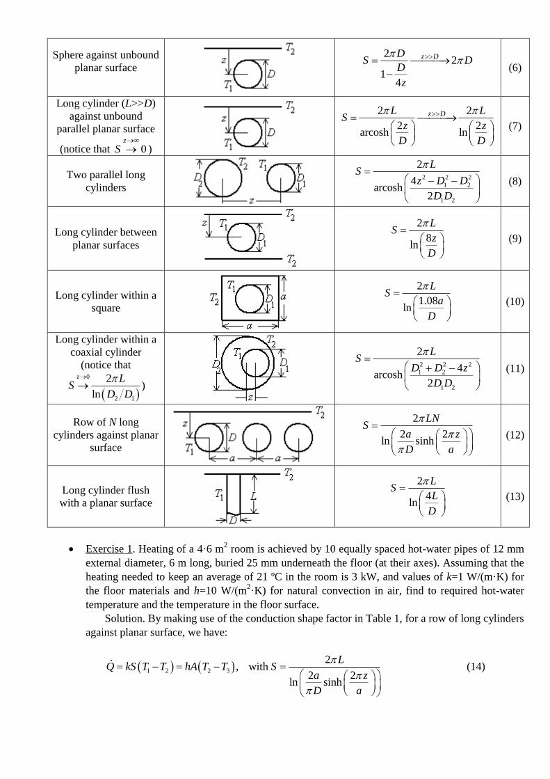
Table 1 gives some such shape factors, what may serve as recipes to solve some canonical heat-
conduction problems, but teach nothing on the subject (provide no insight for non-tabulated cases).
Notice that symmetry can be applied to extend applications; e.g. we may wonder how hot would become
a small electronic device sandwiched between two media, one of thermal conductivity k, and the other
insulating (i.e. with a much lower k), when dissipating a power W ; the answer is that, at the steady state,
the component will reach a temperature T1 such that 1 2W Q kS T T , with S-values from (5) for a
semi-infinity configuration, i.e. S=D for a hemispherical component, or S=2D for a thin disc shape (e.g.
if a D=1 cm disc-shape chip dissipates W =10 W through a much larger silicon substrate of k=150
W/(m·K) (with the other semi space made of insulating plastic), the chip temperature will rise T=
W kS =10/(150·0.02)=3.3 K.
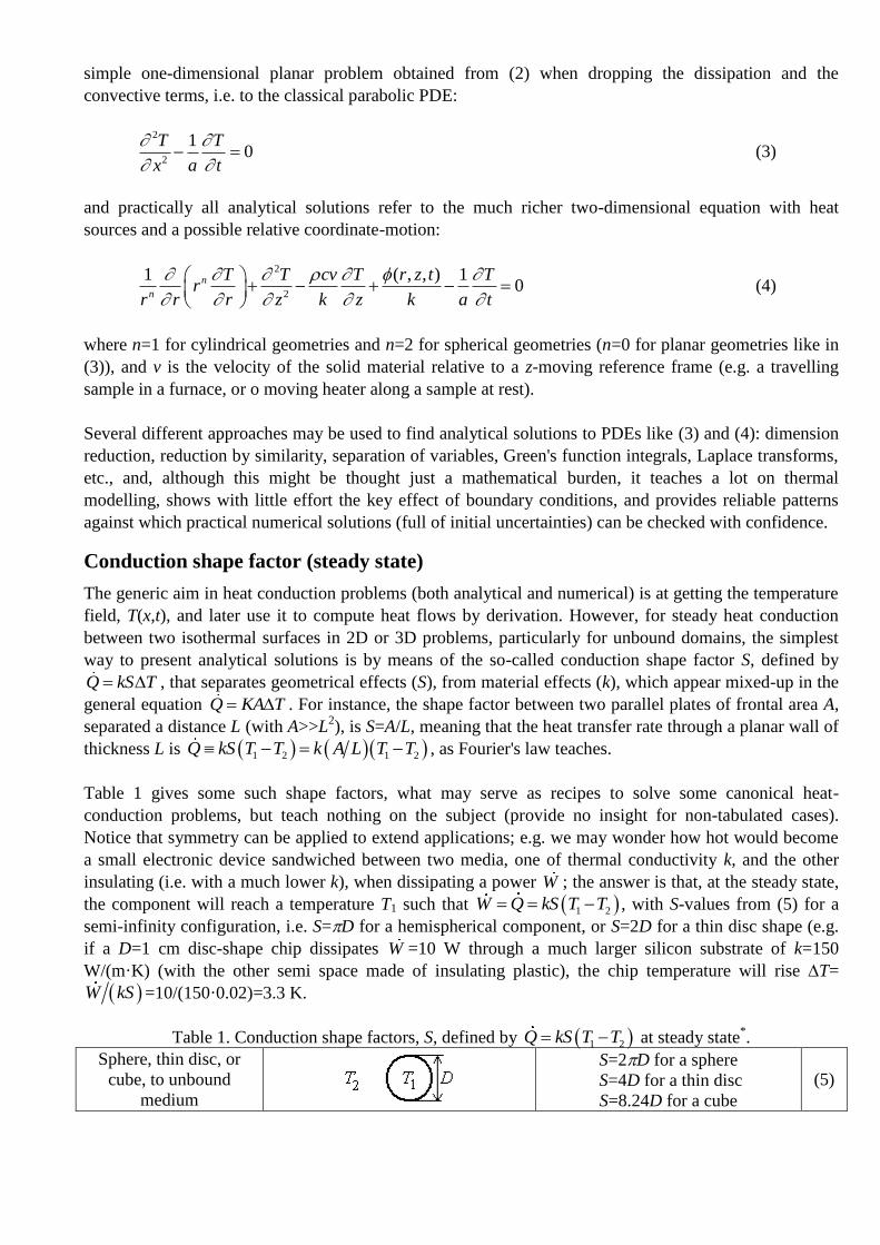
Table 1. Conduction shape factors, S, defined by 1 2Q kS T T at steady state*.
Sphere, thin disc, or
cube, to unbound
medium
S=2D for a sphere
S=4D for a thin disc
S=8.24D for a cube
(5)
Sphere against unbound
planar surface
22
14
z DDS D
D
z
(6)
Long cylinder (L>>D)
against unbound
parallel planar surface
(notice that 0z
S
)
2 2
2 2arcosh ln
z DL LS
z z
D D
(7)
Two parallel long
cylinders
2 2 2
1 2
1 2
2
4arcosh
2
LS
z D D
D D
(8)
Long cylinder between
planar surfaces
2
8ln
LS
z
D
(9)
Long cylinder within a
square
2
1.08ln
LS
a
D
(10)
Long cylinder within a
coaxial cylinder
(notice that
0
2 1
2
ln
z LS
D D
)
2 2 2
1 2
1 2
2
4arcosh
2
LS
D D z
D D
(11)
Row of N long
cylinders against planar
surface
2
2 2ln sinh
LNS
a z
D a
(12)
Long cylinder flush
with a planar surface
2
4ln
LS
L
D
(13)
Exercise 1. Heating of a 4·6 m2 room is achieved by 10 equally spaced hot-water pipes of 12 mm
external diameter, 6 m long, buried 25 mm underneath the floor (at their axes). Assuming that the
heating needed to keep an average of 21 ºC in the room is 3 kW, and values of k=1 W/(m·K) for
the floor materials and h=10 W/(m2·K) for natural convection in air, find to required hot-water
temperature and the temperature in the floor surface.
Solution. By making use of the conduction shape factor in Table 1, for a row of long cylinders
against planar surface, we have:
1 2 2 3
2, with
2 2ln sinh
LQ kS T T hA T T S
a z
D a
(14)
with the unknowns being T1 (pipe temperature) and T1 (floor temperature), and the data:
3000 WQ , k=1 W/(m·K), L=6 m, a=4/10=0.4 m, and h=10 W/(m2·K), what yields S=175 m,
A=4·6=24 m2, and finally T1=50.6 ºC and T1=33.5 ºC.
Reduction to the main dimension (steady state)
We here refer to the simplification of real heat transfer problems when one can reduce the three-
dimensional spatial variations and time variation to just one dimension, usually one spatial dimension in
the steady state (the spatially-homogeneous, time-changing problem is simpler). By the way, notice how
different the bounding conditions in space and time can be; to the richness of 1D-spatial problems,
conditions in time usually reduce to an initial value of the function at some time t=t0; that is why almost
all numerical methods deal with time in the same simple manner of a time-advancing scheme.
The heat equation (2), in steady state and one spatial dimension, reduces to
1 d d ( )0
d d
n
n
T rr
r r r k
(15)
which has as fundamental solutions, assuming the volumetric energy-source independent on position,
those compiled in Table 2. Particular solutions are obtained by imposing two boundary conditions on the
generic T(r)-expression, as done for the case with no sources (then the heat flow is the same through any
distance), and for the case of sources with symmetrical boundary conditions. These solutions teach that
one-dimensional temperature profiles are:
In the absence of internal sources:
o Linear for planar geometry.
o Logarithmic for cylindrical geometry.
o Hyperbolic for spherical geometry.
Planar, cylindrical, and spherical energy sources, internal or interfacial
With a constant volumetric heat source, [W/m3], a parabolic additional term must be added in all three
cases just described, as compiled shown Table 2.
Table 2. Basic solutions for one-dimensional steady heat conduction, i.e. for Eq. (15).
Geometry Generic T(r) Heat flow Central temperature*
Planar (slab) 2( )
2T x Ax B x
k
01 2
12 12
12
T TQ k A
L
1 22
08
sT T T
s
LT T
k
(16)
Cylindrical 2( ) ln
4T r A r B r
k
0
1 212 12
1
2
2
ln
T TQ k L
R
R
2
04
s
RT T
k
(17)
Spherical 2( )
6
AT r B r
r k
0
1 212 12
1 2
1 2
4T T
Q kR R
R R
2
06
s
RT T
k
(18)
*Central temperature, T0=T|r=0, for a given imposed surface temperature, Ts=T|r=R; centred
coordinates for slabs, i.e. T0=T|x=0 and Ts=T|x=L/2.
One application of these simple solutions may be to the heat flow through slender solid supports between
two walls under vacuum, as for a conical stiffener between walls in a dewar flask. The one-dimensional
approximation means that the planar frustum cone may be approximated to a spherical-caps frustum cone
and, with reference to the cone apex, the cross-section area is A(r)=A1(r/r1)2, and the temperature profile
2
1 1 1 11 1T r T Qr kA r r , where r1 is the radial position of the small face (of area A1 and
temperature T1); notice that the heat flow is independent of r: 1 2 2 1 2 1Q r krr T T r r , where r2 is
the radial position of the larger face, at temperature T2.
If the heat source were interfacial instead of volumetric (i.e. [W/m2].instead of [W/m
3]), and in case
of symmetry, the steady solutions would be those presented in Table 3, obtained from (15) as before, but
now with =0 and the boundary condition =kdT/dr|R+ at the interface, located at r=R.
Table 3. Steady solutions for one-dimensional heat conduction with a symmetric interfacial heat source
[W/m2]; in all cases T(rR)=TR=constant, and thus 0Q r R .
Geometry Temperature profile Heat flux Heat flow
Planar* ( ) RT r R T r Rk
q r R Q r R A (19)
Cylindrical ( ) lnR
R rT r R T
k R
Rq r R
r 2Q r R RL (20)
Spherical 2 1 1
( ) R
RT r R T
k R r
2
2
Rq r R
r 24Q r R R (21)
*The planar case refers to a semi-infinite solid with adiabatic wall at r=0 (or to a slab of thickness L
with two symmetric interfacial dissipation at |r|=R<L/2), and x is often used instead of r as
independent variable (centred midway in a finite slab).
Exercise 2. Find the temperature profile in our rod-heated-at-one-end problem, if lateral heat
losses to ambient air could be neglected (i.e. by a non-conducting shroud), and the only way out is
through the other end.
Solution. This is just a planar one-dimensional case, entirely similar to the slab-case in (16) from
Table 2, with =0, which leads to a linear temperature profile and the boundary conditions of our
case-study: 0Q =kA(T0TL)/L=10 W and kAdT/dx|x=L=kA(T0TL)/L=Ah(TLT), with our data:
k=200 W/(m∙K), A=D2/4=78·10
-6 m
2, h=20 W/(m
2∙K) and T=15 ºC; i.e. two equations with two
unknowns that yield T0=19 000 ºC and TL=6300 ºC, a great nonsense that one should have
anticipated, since, the basic heat rate at the sink being 20 W/(m2∙K), one needs a T and an active
surface A, satisfying 20.5 m ·KA T Q h , and we have just a disc of D=1 cm to evacuate that
heat.
Exercise 3. Find the maximum temperature difference between the axis and the lateral surface, in
our original rod-heated-at-one-end problem.
Solution. This difference is expected to be negligible (that is why we approximate rods and fins by
one-dimensional heat-transfer problems). This is a cylindrical one-dimensional problem, as in (17)
, but with coefficient A=0 to avoid the singularity at the axis. We reasoned above (Exercise 8 in
Heat and Mass Tranfer) that a lateral heat loss from a rod slice is equivalent to an internal heat
sink in the way Adx=hpdx(TT∞), what can be directly substituted in (17):
2 2 2
0 2
/ 2
4 4 4 2
R R
R R
hp T T A h R T T hRT T R R R T T
k k k R k
(22)
for instance, if the surface temperature is TR=100 ºC, the radial jump from the centre to the
periphery would be:
0
20 0.01/ 2373 288 0.021 K
2 2 200R R
hRT T T T
k
(23)
i.e., a negligible temperature difference, as expected.
Multilayer composite walls
Up to now, and in most of what follows on analytical methods, we have focused on simple homogeneous
systems. When the system under study comprises several different materials, one must solve each
homogeneous part with unknown interface conditions and match the solutions for temperature and heat
flow continuity. For one-dimensional configurations, two cases can be considered:
Layers in series. This is the normal case where heat flows through a layer and then through the
next (i.e. perpendicular to the layers). An example was presented in Exercise 5 of Heat transfer,
and another follows here. The general rule is that thermal resistances R T Q add, like
electrical resistances (R=V/I) in series, R=Ri; e.g. for heat flow across planar layers of thickness
i and conductivities ki, the overall conductivity is k=i/i/ki). The ‘Critical radio’ analysis that
follows gives additional examples of series resistances for non-planar geometries.
Layers in parallel. This is the case where heat flows parallel to several superimposed layers. The
general rule in this case is that the inverse of thermal resistances 1G R Q T add, like for
electrical resistances in parallel, 1/R=1/Ri; e.g. for heat flow parallel to several layers of
thickness i and conductivities ki, the overall conductivity is k=iki)/i.
Example 1. Dew on window panes
Critical radius
An interesting effect in non-planar geometries may occur when adding an 'insulating' layer over a hot thin
wire or small sphere, cooled to an ambient fluid; in those cases, it might happen that the increase in heat-
transfer area by the additional layer overcomes the effect of a small thermal conductivity of the shroud,
giving way to a phenomenon known as critical radius. For instance, for a hot wire of radius R with a fixed
temperature TR, exposed to an environment at temperature T, with which the convective coefficient is
assumed constant, h, adding an insulating layer of conductivity k between R and r>R:
( )
2 2 ( ) 21 1
ln ln
R RT T r T TQ r R k L h rL T r T L
r r
R k R rh
min
2
1 10 0
Q
Q kr
r rk r h h
(24)
The critical radius for spherical geometry is min
2Q
r k h . As said before, these critical radii only matter
when insulating small cylinders (R<k/h) and spheres (R<2k/h); e.g., for typical insulators (k=0.1
W/(m·K)) in ambient air (h=10 W/(m2·K)), it only matters for wires and pipes smaller than
k/h=0.1/10=10 mm.
Rods and fins
Many practical heat-transfer problems are not strictly one-dimensional and/or steady, but can be
approximated as if they were. A common case is the heat transfer on rods, fins, and other extended
surfaces often used to increase the heat-release rate.
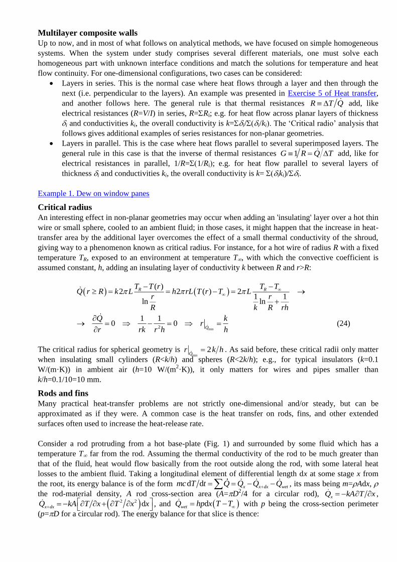
Consider a rod protruding from a hot base-plate (Fig. 1) and surrounded by some fluid which has a
temperature T far from the rod. Assuming the thermal conductivity of the rod to be much greater than
that of the fluid, heat would flow basically from the root outside along the rod, with some lateral heat
losses to the ambient fluid. Taking a longitudinal element of differential length dx at some stage x from
the root, its energy balance is of the form d d x x dx wetmc T t Q Q Q Q , its mass being m=Adx,
the rod-material density, A rod cross-section area (A=D2/4 for a circular rod), xQ kA T x ,
2 2 dx dxQ kA T x T x x
, and dwetQ hp x T T with p being the cross-section perimeter
(p=D for a circular rod). The energy balance for that slice is thence:
2 2d d dT
A xc kA T x kA T x T x x hp x T Tt
2 2
2
2 2
d,
d
steadyc T T hp T hpT T m T T m
k t x kA x kA
(25)
Fig. 1. Heat flow in a circular rod protruding from a hot base-plate and surrounded by a fluid, with
sketches for the cross-section, and a generic longitudinal differential element.
Solving the differential equation (25) in the steady state is straightforward, yielding a exponential
function T(x)=Aexp(mx)+Bexp(mx), whose coefficients are obtained by establishing the appropriate
boundary conditions. Table 4 presents the most important cases.
Table 4. Some analytical solutions for the heat equation (25) along a rod, bar or wire, immersed in a fluid.
Case Conditions Temperature profile End results
1
T(0)=T0
d0
d x L
T
x
0
cosh( )
cosh
m L xT x T
T T mL
0
0
tanhQ
mLT T phkA
0LQ
2 T(0)=T0
T(L)=TL
0
sinh( )
sinh
m L xT x T
T T mL
0
sinh
sinh
LmxT T
T T mL
0
00
1 1
tanh sinh
LQ T T
mL T T mLT T phkA
00
1 1
sinh tanh
L LQ T T
mL T T mLT T phkA
3 0(0)Q Q
( ) 0Q L
0
cosh( )
sinh
m L xT x T
mLQ phkA
0
(0) 1
tanh
T T
mLQ phkA
0
( ) 1
sinh
T L T
mLQ phkA
4 0(0)Q Q
( ) LQ L Q
0
cosh( )
sinh
m L xT x T
mLQ phkA
0
1
tanh
LQ
Q mL
00
(0) 1 1
tanh sinh
LT T Q
mL Q mLQ phkA
00
( ) 1 1
sinh tanh
LT L T Q
mL Q mLQ phkA
It is not difficult to extend the previous analysis to other fin configurations. For instance, the effect of a
uniform heat release of volumetric power [W/m3] along the fin (e.g. to model a one-dimensional heater)
can easily be added to (25); e.g., the solution of d2T/dx
2=m
2(TT∞)+/k for Case 1 in Table 4 changes
from (TT∞)/(T0T∞)=cosh(m(Lx))/cosh(mL)f to (TT∞)/(T0T∞)=f+(1f)/(km2(T0T∞)). For more
general configurations, as non-uniform heat-source distributions (x), slowly-varying cross-section area
A(x), variation on material properties (e.g. k(x)), and so on, the solution of the differential equation gets so
complicated that it is wiser to resort to numerical simulation.
Exercise 4. Find the steady temperature profile in our rod-heated-at-one-end problem.
Solution. This is just case 3 in Table 4, here re-elaborated as an exercise. We consider this
problem to be one-dimensional and planar for heat conduction (along the axial direction), with
internal heat sinks to account for the actual lateral heat losses by convection (i.e. with
Adx=hpdx(TT∞), p being the cross-section perimeter and A the cross-section area), and apply
(3) to an infinitesimal slice:
2
2
2
dd d d 0
d
tT T hpcA x kA x T hp x T T T T
t x kA
(26)
with:
00
0
coshd d& 0 ( )
d d sinhx x L
m L xQT TQ kA kA T x T
x x mkA mL
(27)
where /( )m hp kA , h being the convective coefficient, p the perimeter of the rod cross-section
(D if circular), A the cross-section area (D2/4 if circular), and L the rod length.
Exercise 5. A method to measure the thermal conductivity of non-metal slabs, consists on having a
small copper disc (like a coin) lodged at level into a high-insulating wall, with thermocouples at
both sides of the copper disc. When a thin sample slab (a plate), is sandwiched between a heat
source at constant temperature (e.g. with boiling water), and the mentioned 'heat-meter', a
transient heat-up takes place on the copper disc. If the temperature profile within the sample plate
is assumed linear as in a quasi-steady state, and the temperature within the copper disc uniform,
the energy balance of the latter yields:
sample Cu0 CuCu 0 Cu
Cu Cu sample Cu
sample 0 Cu Cu Cu sample
dd
d
k AT TT T Tm c k A
t L T T m c L
sample Cu0 Cu
0 Cu,initial Cu Cu sample
( )exp
k AT T tt
T T m c L
(28)
which allows the computation of the thermal conductivity of the sample, ksample, by a simple linear
fitting of the logarithm of cooper-temperatures versus time.
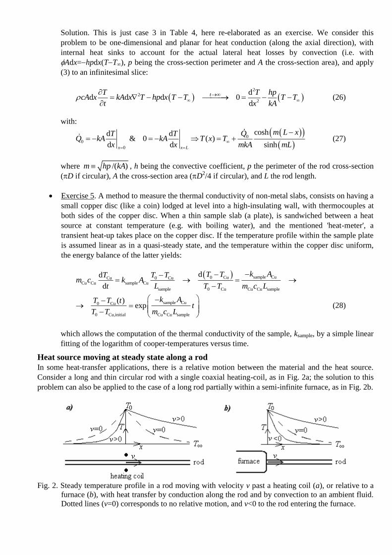
Heat source moving at steady state along a rod
In some heat-transfer applications, there is a relative motion between the material and the heat source.
Consider a long and thin circular rod with a single coaxial heating-coil, as in Fig. 2a; the solution to this
problem can also be applied to the case of a long rod partially within a semi-infinite furnace, as in Fig. 2b.
Fig. 2. Steady temperature profile in a rod moving with velocity v past a heating coil (a), or relative to a
furnace (b), with heat transfer by conduction along the rod and by convection to an ambient fluid.
Dotted lines (v=0) corresponds to no relative motion, and v<0 to the rod entering the furnace.
The heat equation (2), for the steady case of a rod moving past a heating coil, and the corresponding
boundary conditions, may be set like that:
2
2
0
00
d d0
d d
for 0 = , =
for 0 = , =
x x
x x
hp T TT Tk cv
x A x
x T T T T
x T T T T
(29)
which has the solution:
2 2
0 0
0
2 2exp 1 1 , 1 1
2 2
T T xv am v amQ mkA T T
T T a v a v
(30)
where the '' means that '+' should be taken for x>0 and '' applies for x<0, and, as before, /( )m hp kA ,
h being the convective coefficient, p the perimeter of the rod cross-section (D if circular), and A the
cross-section area (D2/4 if circular). It can be verified that, in the limit of no relative motion (v=0), there
heat flow in (30) becomes 0 0Q T T phkA at each side of the origin, corresponding to case 1 of
Table 4 for very long rods (mL>>1).
Reduction by dimension similarity (unsteady state)
Reduction by dimension similarity occurs when a partial differential equation can be converted to an
ordinary differential equation in a combined variable, due to lack of characteristic lengths and times. For
instance, for v==0, the partial differential equation (PDE) (3) transforms to an ordinary differential
equation (ODE):
2
2
,41 1 d ( ) d ( )
0 2 0d d
n
n
rr t
atT T T n Tr
r r r a t
(31)
which can be solved in general in terms of hypergeometric functions, and, in particular, for each space
dimension, in terms of the error function, 2
0erf ( ) 2 exp d
x
x x x , and the exponential integral,
x
-Ei( ) exp dx x x x
, as detailed below.
Planar solutions. Solving (31) with n=0 yields T()=A+Berf(), but, because of the linearity of
ad2T/dx
2dT/dt=0, not only that function but its partial derivatives to any order in x and t will be
solutions to (31),and in particular ∂erf()/∂x and ∂erf()/∂t, namely:
2
2
, erf4
, exp4
, exp44
xT x t A B
at
A xT x t
att
A x xT x t
t atat
(32)
Cylindrical solutions. Solving (31) with n=1 yields T()=A+BEi(2), where Ei(x) is the
exponential integral, but now only its partial derivatives in t will be solutions too; in particular:
2
2
, Ei4
, exp4
rT r t A B
at
A rT r t
t at
(33)
Spherical solutions. Solving (31) with n=2 yields 2( ) erf ( ) expT A B , but
again only its partial derivatives in t will be solutions too; in particular:
2
2
, erf exp4 44
, exp4
r r rT r t A B
at atat
A rT r t
atr t
(34)
Energy deposition in unbounded media
A most basic application of similarity solutions is the temperature field due to a thermal pulse in an
unbounded medium, i.e. the instantaneous release of an amount of energy Q at the origin; in mathematical
terms, this can be formulated in two different ways, here shown for the planar case:
As a singular initial-value problem in temperature without sources:
2
2
At 0 ( , ) δ( , )
( , ) 1 ( , )For 0 0
Qt T x t T x t
c
T x t T x tt
x a t
(35)
As a singular-source regular problem in temperature:
2
2
( , ) ( , ) 1 ( , )For ( , ) 0
with ( , ) δ( , )
T x t x t T x tx t
x k a t
x t Q x t
(36)
The solution can be expressed in a compact form valid for multiple geometries:
2
01 1
2 2
exp4
( , ) , (0, ) ,
4 4n n V
rQ
at Q QT r t T t T T dV
cc at c at
(37)
where the last integral extends to the whole space in the variable considered (one-dimensional, two-
dimensional, or three-dimensional volume), according to the n-value:
o n=0 for the planar geometry, where r should be understood as the x-coordinate, and Q is the
energy released at x=0 and t=0 per unit area.
o n=1 for the cylindrical geometry, where Q is the energy released per unit length, and the
o n=2 for the spherical geometry, where Q is the total energy released initially at the centre.
Exercise 6. For an analysis of the temperature field in a brake pad of thickness L=0.02 m (the
other dimensions being much larger), when suddenly rubbed on one face, consider an
instantaneous deposition of Q=10 MJ/m2 on one side of a slab of conductivity k=1 W/(m·K),
density =2000 kg/m3, thermal capacity c=1000 J/(kg·K), and no heat losses to the ambient, and
find the temperature history in the middle of the slab. Formulate the problem as an unbounded
medium, and quantify the constraints imposed by this simplification.
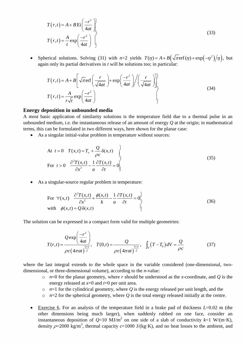
Solution. The general solution has been given in (35), here to be applied to n=0; i.e., at a point x1,
T(t) becomes:
227 1
6
6
10 expexp4 0.5 104
( , )4 2000 1000 4 0.5 10
xxQ
tatT x t
c at t
(38)
what has been plotted in Fig. 3 for the desired point x1=L/2=0.01 m, and two other locations, at
half and double distance to the heated surface; notice that the latter, being at precisely the other
end of the slab, which has been assumed adiabatic, is incompatible with the approximation of
semi-infinite-thick slab, although it helps to quantify that for the two first minute or so, the semi-
infinite solution may be valid at the middle point.
Fig. 3. Temperature history at three points in a semi-infinite slab with a heat pulse.
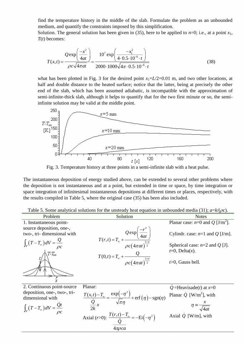
The instantaneous deposition of energy studied above, can be extended to several other problems where
the deposition is not instantaneous and at a point, but extended in time or space, by time integration or
space integration of infinitesimal instantaneous depositions at different times or places, respectively, with
the results compiled in Table 5, where the original case (35) has been also included.
Table 5. Some analytical solutions for the unsteady heat equation in unbounded media (31); a=k/(c).
Problem Solution Notes
1. Instantaneous point-
source deposition, one-,
two-, tri- dimensional with
V
QT T dV
c
2
1
2
exp4
( , )
4n
rQ
atT r t T
c at
1
2
(0, )
4n
QT t T
c at
Planar case: n=0 and Q [J/m2].
Cylindr. case: n=1 and Q [J/m].
Spherical case: n=2 and Q [J].
t=0, Delta(x).
t>0, Gauss bell.
2. Continuous point-source
deposition, one-, two-, tri-
dimensional with
V
QtT T dV
c
Planar:
2exp( , )erf sgn( )
2
T x t T
Qx
k
Axial (r>0): 2( , )Ei
4
T r t T
Q
ca
Q =Heavisade(t) at x=0
Planar Q [W/m2], with
4
x
at
Axial Q [W/m], with
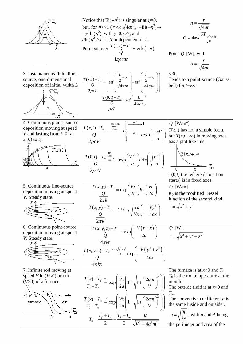
Notice that Ei(2) is singular at =0,
but, for <<1 ( 4r at ), Ei(2)
ln(2), with =0.577, and
ln(2)/t=t, independent of r
Point source: ( , )
erfc
4
T r t T
Q
car
4
r
at
2 44 r at
TQ k
t
Point Q [W], with
4
r
at
3. Instantaneous finite line-
source, one-dimensional
deposition of initial width L
( , ) 2 2erf erf4 4
2
L Lx x
T x t T
Q at at
cL
(0, )erf
4
T t T L
Q at
cL
t>0.
Tends to a point-source (Gauss
bell) for t
4. Continuous planar-source
deposition moving at speed
V and lasting from t=0 (at
x=0) to t1.
0moving axes
0
1( , )
exp
2
x
t
x
T x t TxV
Qa
cV
fix
2 2axes(0, )1 exp erfc
2
T t T V t V t
Q a a
cV
Q [W/m2].
T(x,t) has not a simple form,
but T(x,t→) in moving axes
has a plot like this:
T(0,t) (i.e. where deposition
starts) is in fixed axes.
5. Continuous line-source
deposition moving at speed
V. Steady state.
0
( , )exp
2 2
2
T x y T Vx VrK
Q a a
k
2( , )1
4
2
x yT x y T a Vy
Q Vx ax
k
Q [W/m].
K0 is the modified Bessel
function of the second kind. 2 2r x y
6. Continuous point-source
deposition moving at speed
V. Steady state.
( , , )exp
2
4
V r xT x y z T
Q a
kr
2 2 2 2
( , , )exp
4
4
x y z V y zT x y z T
Q ax
kx
Q [W].
2 2 2r x y z
7. Infinite rod moving at
speed V in (V<0) or out
(V>0) of a furnace.
20
0
( ) 2exp 1 1
2
xf
f
T x T Vx am
T T a V
20
0
( ) 2exp 1 1
2
xT x T Vx am
T T a V
02 2 22 2 4
f fT T T T VT
V a m
The furnace is at x<0 and Tf.
T0 is the rod temperature at the
mouth.
The outside fluid is at x>0 and
T.
The convective coefficient h is
the same inside and outside..
hpm
kA , with p and A being
the perimeter and area of the
rod cross-section.
8. Continuous spherical-
source kept at fixed-T.
( , )erfc
4R
T r t T R r R
T T r at
Only valid for r>R.
The heat supplied to the sphere
must be controlled to match
2 1 1( ) 4 RQ t k R T T
R at
Thermal contact in semi-infinite media
Another important kind of thermal problems where similarity in the variables make them amenable to
analytical solution is a sudden change in the boundary condition of semi-infinite bodies, which can be
applied to practical geometries of finite thickness L for short-enough times, because for t<<L2/a (Fo<<1)
the solid can be supposed semi-infinite.
For instance, for the sudden thermal change in a the face of a planar semi-infinite body (as developed in
Exercise 7 in the Introduction), the transient temperature profiles are given by (32). The following
example illustrates an imposed-convection case.
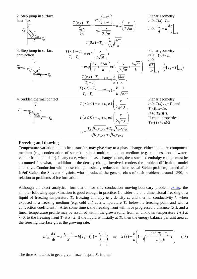
Exercise 7. Find for how long air-freezing temperatures of 10 ºC can be tolerated, without
freezing penetration to 1 m depth in soil, assuming and initial T-field at 15 ºC, a sudden change in
air temperature from 15 ºC to 10 ºC (with no further variation), a convective coefficient of h=10
W/(m2·K), and the soil having =2000 kg/m
3, c=2000 J/(kg·K), k=0.5 W/(m·K), and without
freezing effects.
Solution. Applying the initial and boundary conditions for the soil, to the general solution (32),
one gets:
1 2 000
erf ( ), with & ( ,0)x
x
TT c c k h T T T x T
x
2
0 0 2( , ) erfc exp erfc
2 2
x hx h at x h atT x t T T T
k k kat at
(39)
and the desired time-period is obtained by solving (39) for T(x,t)=0 ºC (water freezing) at x=1 m,
with T0=15 ºC and T=15 ºC, an implicit equation that yields t=9.7·106 s (i.e. some 110 days).
Figure 4 shows the temperature profile at several times.
Fig. 4. Temperature profiles at several time intervals in a solid material initially at 15 ºC, suddenly
exposed to air at 15 ºC with constant convective coefficient.
Another important application of similarity solutions is the evaluation of the contact temperature when
two solids at different temperature get into contact. Let solid A extend from x=0 to +∞, initially at TA, and
solid B extend from x=0 to ∞, initially at TB, and let T0 be the contact temperature (at x=0). Applying the
initial and boundary conditions to the general solution (32) for solid A:
1 2 0 0 0erf ( ), with ( ,0) & (0, ) ( , ) erf ( )2
A A A
A
xT c c T x T T t T T x t T T T
a t
0
0
with A AA
A A
x A
k T TTq k
x a t
(40)
whereas for solid B:
1 2 0 0 0erf ( ), with ( ,0) & (0, ) ( , ) erf ( )2
B B B
B
xT c c T x T T t T T x t T T T
a t
0
0
with B BB
B B
x B
k T TTq k
x a t
(41)
Now, the energy balance at the interface (continuity of heat flux) implies:
0 0
00A A B B A A A A B B B B
A B A A A B B B
k T T k T T T k c T k cT
a t a t k c k c
(42)
where the parameter k c is called thermal effusivity. The following exercise presents a concrete
application.
Exercise 8. Find the contact temperature between a bare foot and a floor at 10 ºC, for the case of
wooden floor and for the case of ceramic floor.
Solution. For our flesh we estimate its thermal data by approximation to those of leather in Solid
thermal data: k=0.4 W/(m·K), =1000 kg/m3, c=1500 J/(kg·K), what yields
-1 5/ 20.4 1000 1500 770 kg Kk c s . For wood, a look-up in the same table (for oak
wood) gives: -1 5/ 20.17 750 2400 550 kg Kk c s , and for ceramic tiles (with marble
data): -1 5/ 22.6 2700 880 2500 kg Kk c s , so that, if we assume our body at 37 ºC (feet
are always a few degrees colder) and the floor at 10 ºC, the skin in contact with wood will face
(nearly instantaneously) a temperature of (8): (37·770+10·550)/(770+550)=22 ºC, whereas in
contact with ceramic tiles will have (37·770+10·2500)/(770+2500)=16.4 ºC, what makes a great
difference (we may feel variations in our skin temperature of a few tenths of a degree!).
A compilation of similarity solutions for semi-infinite bodies is presented in Table 6.
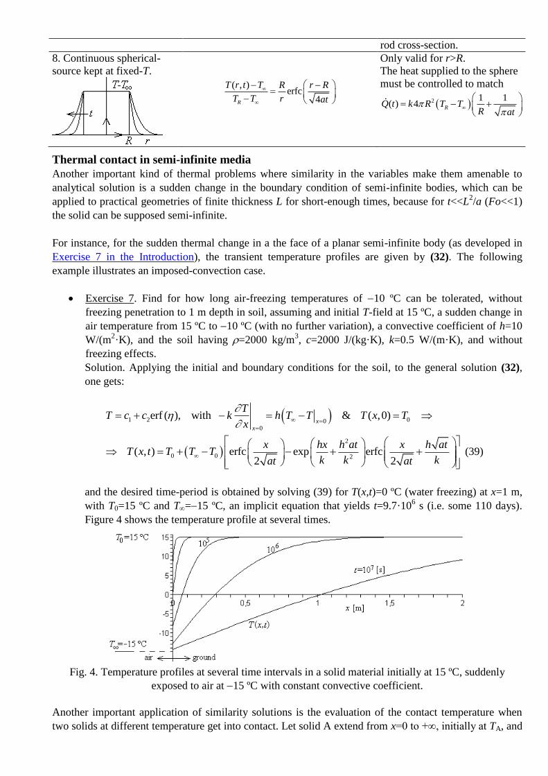
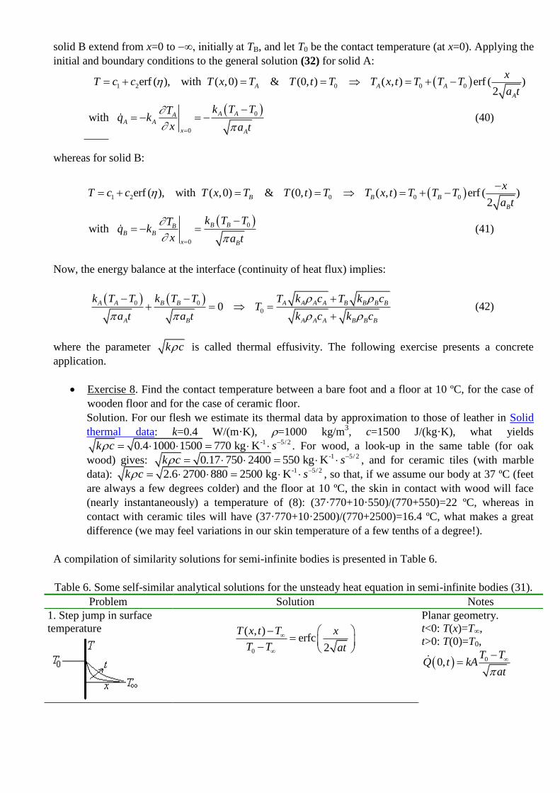
Table 6. Some self-similar analytical solutions for the unsteady heat equation in semi-infinite bodies (31).
Problem Solution Notes
1. Step jump in surface
temperature
0
( , )erfc
2
T x t T x
T T at
Planar geometry.
t<0: T(x)=T∞,
t>0: T(0)=T0,
00,T T
Q t kAat
2. Step jump in surface
heat flux
2
0
exp4( , )
erfc2
2
x
atT x t T x
xQ x at
atkA
0 4(0, )
Q atT t T
kA
Planar geometry.
t<0: T(x)=T∞,
t>0: 0
0
d
d x
Q Tk
A x
3. Step jump in surface
convection
0
2
2
( , )erfc
2
exp erfc2
T x t T x
T T at
hx h at x h at
k k kat
t 0
0
( , ) 4T x t T h at
T T k
,
t
0
( , ) 11
T x t T k
T T h at
Planar geometry.
t<0: T(x)=T∞,
t>0:
0 00
d
d xx
T hT T
x k
4. Sudden thermal contact
1 20 erf2 A
xT x c c
a t
3 40 erf2 B
xT x c c
a t
0
A A A A B B B B
A A A B B B
T k c T k cT
k c k c
Planar geometry.
t<0: T(x)|x>0=TA and
T(x)|x<0=TB.
t>0: T0f(t).
If equal properties:
T0=(TA+TB)/2
Freezing and thawing
Temperature variation due to heat transfer, may give way to a phase change, either in a pure-component
medium (e.g. condensation of steam), or in a multi-component medium (e.g. condensation of water-
vapour from humid air). In any case, when a phase change occurs, the associated enthalpy change must be
accounted for, what, in addition to the density change involved, renders the problem difficult to model
and solve. Conduction with phase change basically reduces to the classical Stefan problem, named after
Jožef Stefan, the Slovene physicist who introduced the general class of such problems around 1890, in
relation to problems of ice formation.
Although an exact analytical formulation for this conduction moving-boundary problem exists, the
simpler following approximation is good enough in practice. Consider the one-dimensional freezing of a
liquid of freezing temperature Tf, freezing enthalpy hSL, density , and thermal conductivity k, when
exposed to a freezing medium (e.g. cold air) at a temperature T below its freezing point and with a
convection coefficient h. After some time t, the freezing front will have progressed a distance X(t), and a
linear temperature profile may be assumed within the grown solid, from an unknown temperature T0(t) at
x=0, to the freezing front Tf at x=X. If the liquid is initially at Tf, then the energy balance per unit area at
the freezing interface gives the growing rate:
2
ff 0 f0
2d1 1
1dSL
SL
h T TT T T TX kh k h T T X t t
Xt X h h k
k h
(43)
The time t it takes to get a given frozen depth, X, is then:
f
1
2
SLh Xt X
T T h k
(44)
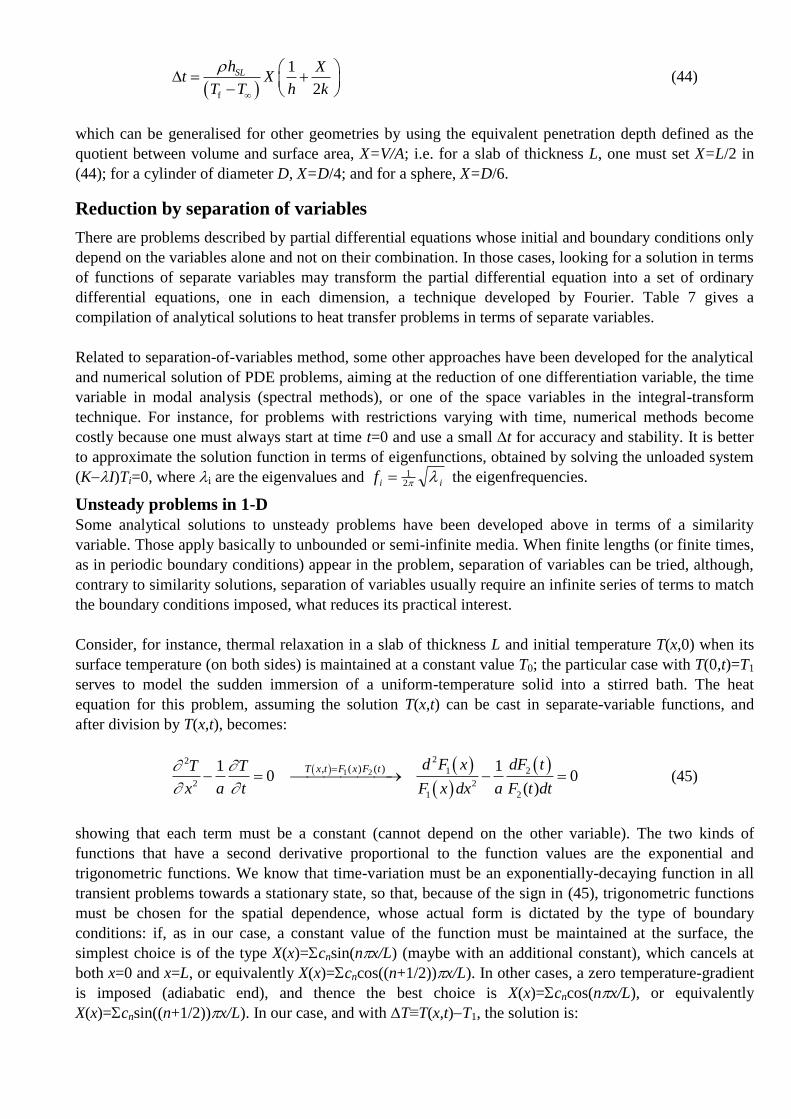
which can be generalised for other geometries by using the equivalent penetration depth defined as the
quotient between volume and surface area, X=V/A; i.e. for a slab of thickness L, one must set X=L/2 in
(44); for a cylinder of diameter D, X=D/4; and for a sphere, X=D/6.
Reduction by separation of variables
There are problems described by partial differential equations whose initial and boundary conditions only
depend on the variables alone and not on their combination. In those cases, looking for a solution in terms
of functions of separate variables may transform the partial differential equation into a set of ordinary
differential equations, one in each dimension, a technique developed by Fourier. Table 7 gives a
compilation of analytical solutions to heat transfer problems in terms of separate variables.
Related to separation-of-variables method, some other approaches have been developed for the analytical
and numerical solution of PDE problems, aiming at the reduction of one differentiation variable, the time
variable in modal analysis (spectral methods), or one of the space variables in the integral-transform
technique. For instance, for problems with restrictions varying with time, numerical methods become
costly because one must always start at time t=0 and use a small t for accuracy and stability. It is better
to approximate the solution function in terms of eigenfunctions, obtained by solving the unloaded system
(KI)Ti=0, where i are the eigenvalues and f i i 12 the eigenfrequencies.
Unsteady problems in 1-D
Some analytical solutions to unsteady problems have been developed above in terms of a similarity
variable. Those apply basically to unbounded or semi-infinite media. When finite lengths (or finite times,
as in periodic boundary conditions) appear in the problem, separation of variables can be tried, although,
contrary to similarity solutions, separation of variables usually require an infinite series of terms to match
the boundary conditions imposed, what reduces its practical interest.
Consider, for instance, thermal relaxation in a slab of thickness L and initial temperature T(x,0) when its
surface temperature (on both sides) is maintained at a constant value T0; the particular case with T(0,t)=T1
serves to model the sudden immersion of a uniform-temperature solid into a stirred bath. The heat
equation for this problem, assuming the solution T(x,t) can be cast in separate-variable functions, and
after division by T(x,t), becomes:
1 2
221 2
2 2
1 2
, ( ) ( )1 10 0
( )
T x t F x F t d F x dF tT T
x a t F x dx a F t dt
(45)
showing that each term must be a constant (cannot depend on the other variable). The two kinds of
functions that have a second derivative proportional to the function values are the exponential and
trigonometric functions. We know that time-variation must be an exponentially-decaying function in all
transient problems towards a stationary state, so that, because of the sign in (45), trigonometric functions
must be chosen for the spatial dependence, whose actual form is dictated by the type of boundary
conditions: if, as in our case, a constant value of the function must be maintained at the surface, the
simplest choice is of the type X(x)=cnsin(nx/L) (maybe with an additional constant), which cancels at
both x=0 and x=L, or equivalently X(x)=cncos((n+1/2))x/L). In other cases, a zero temperature-gradient
is imposed (adiabatic end), and thence the best choice is X(x)=cncos(nx/L), or equivalently
X(x)=cnsin((n+1/2))x/L). In our case, and with T≡T(x,t)T1, the solution is:
12 2
21
,0 sin
, sin exp with 0, 0
, 0
n
n
n
n
n xT x c
Ln x n at
T x t c T tL L
T L t
(46)
Notice that the two boundary conditions T(0,t)=T(L,t)=0 are automatically fulfilled by our choice of
spatial base functions, whereas matching the generic initial boundary condition demands a Fourier-series
expansion; the series coefficients are computed by minimisation of the function-projection over each of
the base functions:
0
2,0 sin , 1,2,3...
L
n
n xc T x dx n
L L
(47)
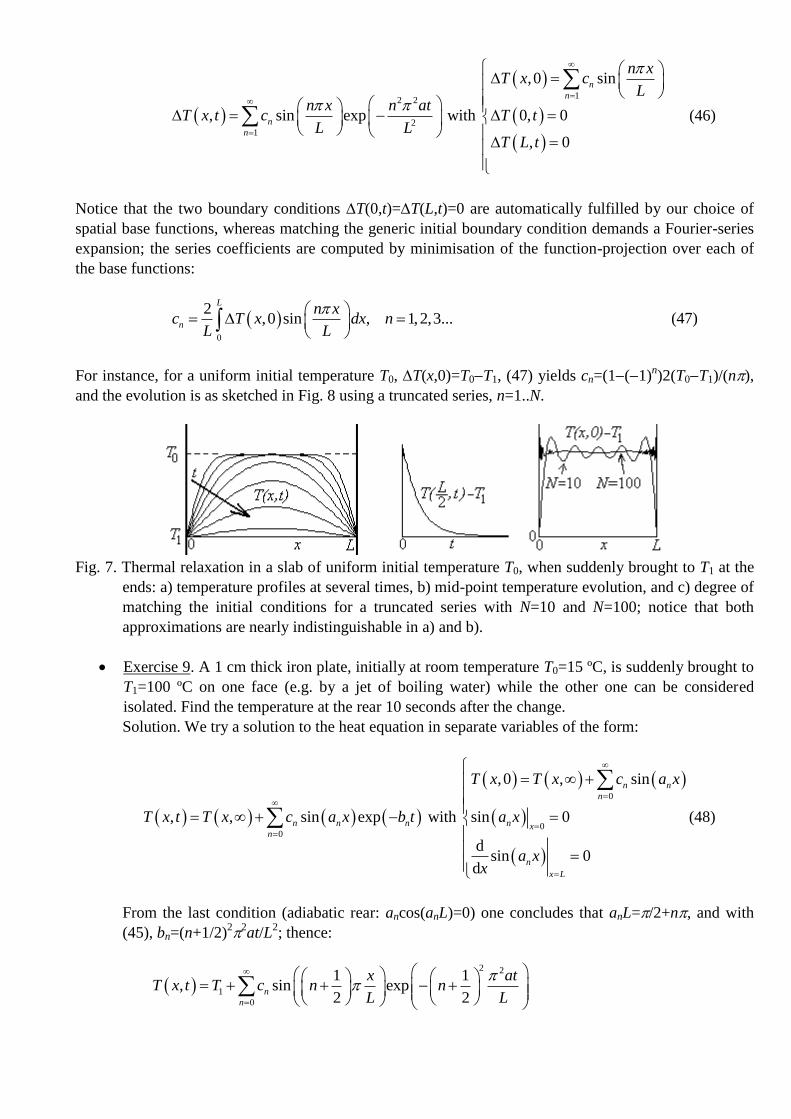
For instance, for a uniform initial temperature T0, T(x,0)=T0T1, (47) yields cn=(1(1)n)2(T0T1)/(n),
and the evolution is as sketched in Fig. 8 using a truncated series, n=1..N.
Fig. 7. Thermal relaxation in a slab of uniform initial temperature T0, when suddenly brought to T1 at the
ends: a) temperature profiles at several times, b) mid-point temperature evolution, and c) degree of
matching the initial conditions for a truncated series with N=10 and N=100; notice that both
approximations are nearly indistinguishable in a) and b).
Exercise 9. A 1 cm thick iron plate, initially at room temperature T0=15 ºC, is suddenly brought to
T1=100 ºC on one face (e.g. by a jet of boiling water) while the other one can be considered
isolated. Find the temperature at the rear 10 seconds after the change.
Solution. We try a solution to the heat equation in separate variables of the form:
0
00
,0 , sin
, , sin exp with sin 0
dsin 0
d
n n
n
n n n n xn
n
x L
T x T x c a x
T x t T x c a x b t a x
a xx
(48)
From the last condition (adiabatic rear: ancos(anL)=0) one concludes that anL=/2+n, and with
(45), bn=(n+1/2)22
at/L2; thence:
2 2
1
0
1 1, sin exp
2 2n
n
x atT x t T c n n
L L
0 1
0 1
0
21 with sin
12
2
n n
n
T Txc n T T c
Ln
(49)
The rear temperature, plotted in Fig. 9 (as well as several spatial profiles), is then approximated by
the truncated series (as seen in Fig. 9, the first term is already good enough for not too-short
times):
2 21
200 1
2 2 6
22
, 2 1 1exp
1 2
2
4 4 13.7 10 10exp exp 0.547
4 4 0.02
nN
n
T L t T atn
T T Ln
at
L
(50)
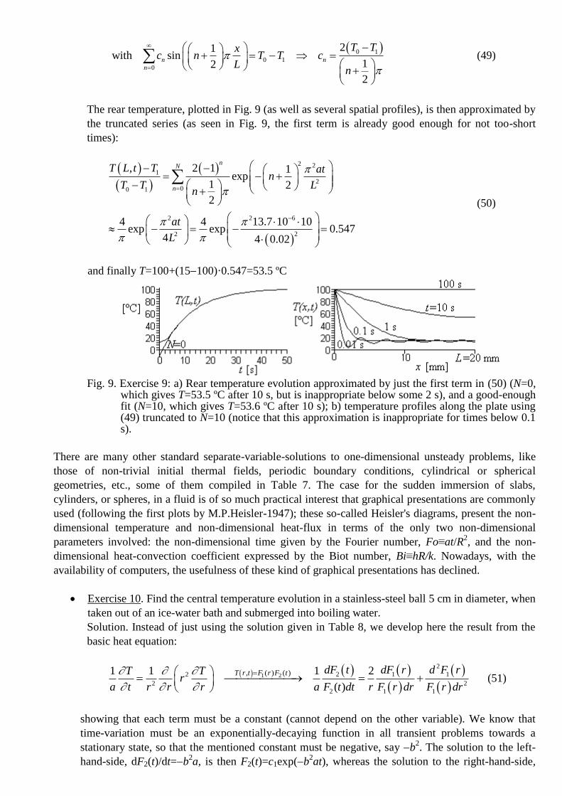
and finally T=100+(15100)·0.547=53.5 ºC
Fig. 9. Exercise 9: a) Rear temperature evolution approximated by just the first term in (50) (N=0,
which gives T=53.5 ºC after 10 s, but is inappropriate below some 2 s), and a good-enough fit (N=10, which gives T=53.6 ºC after 10 s); b) temperature profiles along the plate using (49) truncated to N=10 (notice that this approximation is inappropriate for times below 0.1 s).
There are many other standard separate-variable-solutions to one-dimensional unsteady problems, like
those of non-trivial initial thermal fields, periodic boundary conditions, cylindrical or spherical
geometries, etc., some of them compiled in Table 7. The case for the sudden immersion of slabs,
cylinders, or spheres, in a fluid is of so much practical interest that graphical presentations are commonly
used (following the first plots by M.P.Heisler-1947); these so-called Heisler's diagrams, present the non-
dimensional temperature and non-dimensional heat-flux in terms of the only two non-dimensional
parameters involved: the non-dimensional time given by the Fourier number, Fo≡at/R2, and the non-
dimensional heat-convection coefficient expressed by the Biot number, Bi≡hR/k. Nowadays, with the
availability of computers, the usefulness of these kind of graphical presentations has declined.
Exercise 10. Find the central temperature evolution in a stainless-steel ball 5 cm in diameter, when
taken out of an ice-water bath and submerged into boiling water.
Solution. Instead of just using the solution given in Table 8, we develop here the result from the
basic heat equation:
1 2
2
2 1 12
2 2
2 1 1
, ( ) ( )1 1 1 2
( )
T r t F r F t dF t dF r d F rT Tr
a t r r r a F t dt r F r dr F r dr
(51)
showing that each term must be a constant (cannot depend on the other variable). We know that
time-variation must be an exponentially-decaying function in all transient problems towards a
stationary state, so that the mentioned constant must be negative, say b2. The solution to the left-
hand-side, dF2(t)/dt=b2a, is then F2(t)=c1exp(b
2at), whereas the solution to the right-hand-side,
with the change G(r)=F1(r)/r, becomes, d2G(r)/d
2r=b
2, and thus has as solutions F1(r)=
c2sin(br)/r+c2sin(br)/r, although only the sin-term is appropriate here since F1(r)|r=0 must be finite.
The general solution to (51) is then:
2
1
sin, , exp
n
n n
n
b rT r t T r c b at
r
(52)
where the constants cn and bn are obtained by imposing initial and boundary conditions.
If we model the convective boiling process by the limit h→, then the initial and boundary
conditions are:
0 1
1
sin,0
n
n
n
b rT r T T c
r
(53)
0
d ,0
dr
T r t
r
(54)
2
1
1
sin, exp
n
n n
n
b RT R t T c b at
R
(55)
From (55) we deduce that bnR=n; (54) is automatically verified, and from (53), with the value for
bn, we get cn=2(1)n(T1T0)/(n), finally yielding:
1 2 2
10 1
2 1 sin,
exp
n
N
n
n r
T r t T Rn at
n rT T
R
(56)
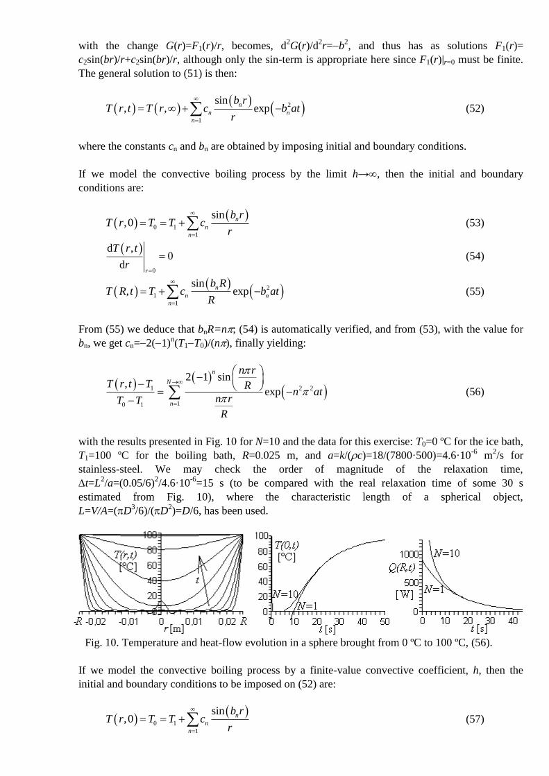
with the results presented in Fig. 10 for N=10 and the data for this exercise: T0=0 ºC for the ice bath,
T1=100 ºC for the boiling bath, R=0.025 m, and a=k/(c)=18/(7800·500)=4.6·10-6
m2/s for
stainless-steel. We may check the order of magnitude of the relaxation time,
t=L2/a=(0.05/6)
2/4.6·10
-6=15 s (to be compared with the real relaxation time of some 30 s
estimated from Fig. 10), where the characteristic length of a spherical object,
L=V/A=(D3/6)/(D
2)=D/6, has been used.
Fig. 10. Temperature and heat-flow evolution in a sphere brought from 0 ºC to 100 ºC, (56).
If we model the convective boiling process by a finite-value convective coefficient, h, then the
initial and boundary conditions to be imposed on (52) are:
0 1
1
sin,0
n
n
n
b rT r T T c
r
(57)
0
d ,0
dr
T r t
r
(58)
1
d ,,
dr R
T r tk h T R t T
r
(59)
Developing (55) we get:
2 2
21 1
cos sin sinexp exp
n n n n
n n n n
n n
b b R b R b Rk c b at h c b at
R R R
cos1
sin
n n
n
b R b R hRBi
b R k (60)
and we cannot proceed any further analytically since the values for bn must be obtained by
numerically solving (60). Once this is done, values for cn are obtained by cancelling the projection
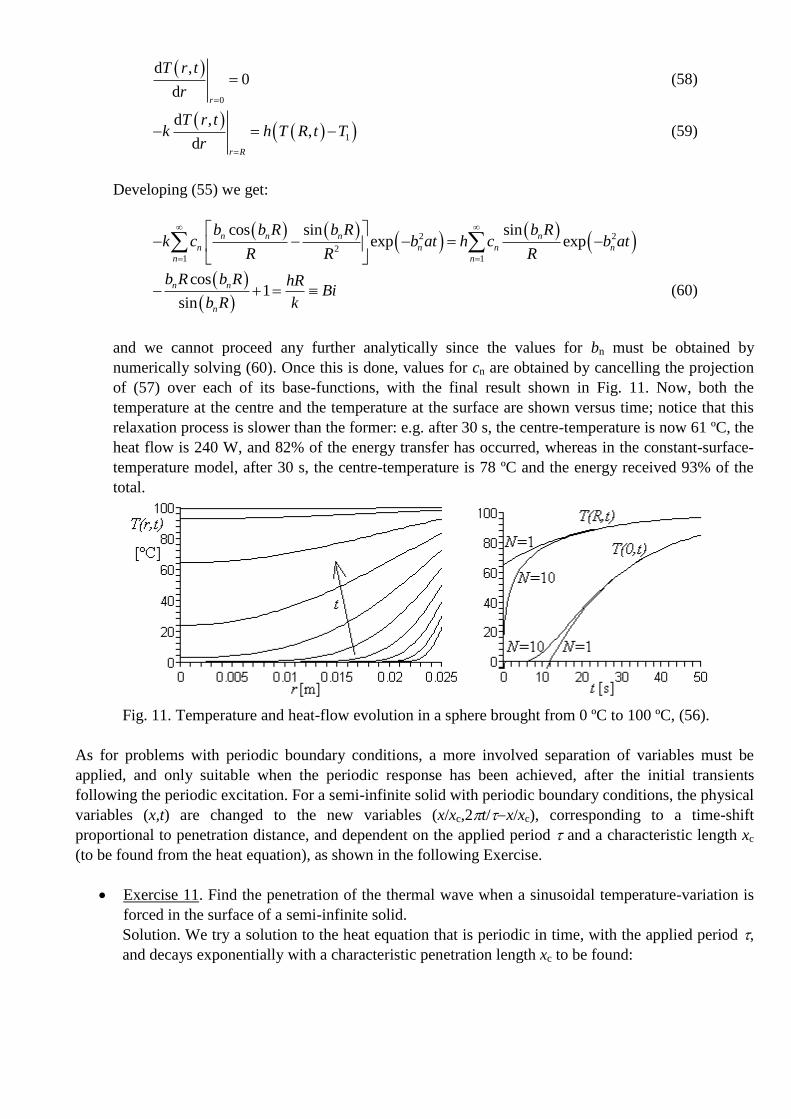
of (57) over each of its base-functions, with the final result shown in Fig. 11. Now, both the
temperature at the centre and the temperature at the surface are shown versus time; notice that this
relaxation process is slower than the former: e.g. after 30 s, the centre-temperature is now 61 ºC, the
heat flow is 240 W, and 82% of the energy transfer has occurred, whereas in the constant-surface-
temperature model, after 30 s, the centre-temperature is 78 ºC and the energy received 93% of the
total.
Fig. 11. Temperature and heat-flow evolution in a sphere brought from 0 ºC to 100 ºC, (56).
As for problems with periodic boundary conditions, a more involved separation of variables must be
applied, and only suitable when the periodic response has been achieved, after the initial transients
following the periodic excitation. For a semi-infinite solid with periodic boundary conditions, the physical
variables (x,t) are changed to the new variables (x/xc,2t/x/xc), corresponding to a time-shift
proportional to penetration distance, and dependent on the applied period and a characteristic length xc
(to be found from the heat equation), as shown in the following Exercise.
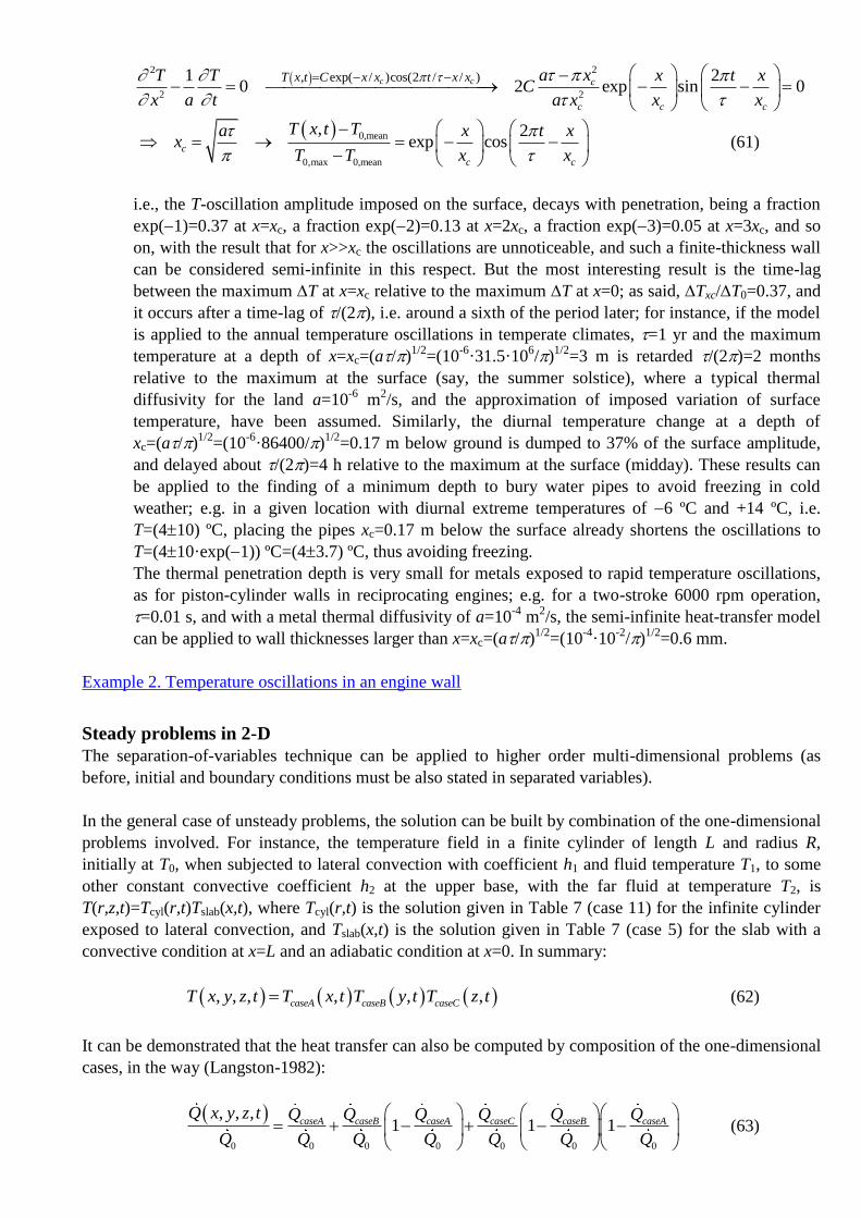
Exercise 11. Find the penetration of the thermal wave when a sinusoidal temperature-variation is
forced in the surface of a semi-infinite solid.
Solution. We try a solution to the heat equation that is periodic in time, with the applied period ,
and decays exponentially with a characteristic penetration length xc to be found:
22
2 2
, exp( / )cos(2 / / )1 20 2 exp sin 0c c c
c c c
T x t C x x t x x a xT T x t xC
x a t a x x x
0,mean
0,max 0,mean
, 2exp cosc
c c
T x t Ta x t xx
T T x x
(61)
i.e., the T-oscillation amplitude imposed on the surface, decays with penetration, being a fraction
exp(1)=0.37 at x=xc, a fraction exp(2)=0.13 at x=2xc, a fraction exp(3)=0.05 at x=3xc, and so
on, with the result that for x>>xc the oscillations are unnoticeable, and such a finite-thickness wall
can be considered semi-infinite in this respect. But the most interesting result is the time-lag
between the maximum T at x=xc relative to the maximum T at x=0; as said, Txc/T0=0.37, and
it occurs after a time-lag of /(2), i.e. around a sixth of the period later; for instance, if the model
is applied to the annual temperature oscillations in temperate climates, =1 yr and the maximum
temperature at a depth of x=xc=(a/)1/2
=(10-6
·31.5·106/)
1/2=3 m is retarded /(2)=2 months
relative to the maximum at the surface (say, the summer solstice), where a typical thermal
diffusivity for the land a=10-6
m2/s, and the approximation of imposed variation of surface
temperature, have been assumed. Similarly, the diurnal temperature change at a depth of
xc=(a/)1/2
=(10-6
·86400/)1/2
=0.17 m below ground is dumped to 37% of the surface amplitude,
and delayed about /(2)=4 h relative to the maximum at the surface (midday). These results can
be applied to the finding of a minimum depth to bury water pipes to avoid freezing in cold
weather; e.g. in a given location with diurnal extreme temperatures of 6 ºC and +14 ºC, i.e.
T=(410) ºC, placing the pipes xc=0.17 m below the surface already shortens the oscillations to
T=(410·exp(1)) ºC=(43.7) ºC, thus avoiding freezing.
The thermal penetration depth is very small for metals exposed to rapid temperature oscillations,
as for piston-cylinder walls in reciprocating engines; e.g. for a two-stroke 6000 rpm operation,
=0.01 s, and with a metal thermal diffusivity of a=10-4
m2/s, the semi-infinite heat-transfer model
can be applied to wall thicknesses larger than x=xc=(a/)1/2
=(10-4
·10-2
/)1/2
=0.6 mm.
Example 2. Temperature oscillations in an engine wall
Steady problems in 2-D
The separation-of-variables technique can be applied to higher order multi-dimensional problems (as
before, initial and boundary conditions must be also stated in separated variables).
In the general case of unsteady problems, the solution can be built by combination of the one-dimensional
problems involved. For instance, the temperature field in a finite cylinder of length L and radius R,
initially at T0, when subjected to lateral convection with coefficient h1 and fluid temperature T1, to some
other constant convective coefficient h2 at the upper base, with the far fluid at temperature T2, is
T(r,z,t)=Tcyl(r,t)Tslab(x,t), where Tcyl(r,t) is the solution given in Table 7 (case 11) for the infinite cylinder
exposed to lateral convection, and Tslab(x,t) is the solution given in Table 7 (case 5) for the slab with a
convective condition at x=L and an adiabatic condition at x=0. In summary:
, , , , , ,caseA caseB caseCT x y z t T x t T y t T z t (62)
It can be demonstrated that the heat transfer can also be computed by composition of the one-dimensional
cases, in the way (Langston-1982):
0 0 0 0 0 0 0
, , ,1 1 1caseA caseB caseA caseC caseB caseA
Q x y z t Q Q Q Q Q Q
Q Q Q Q Q Q Q
(63)
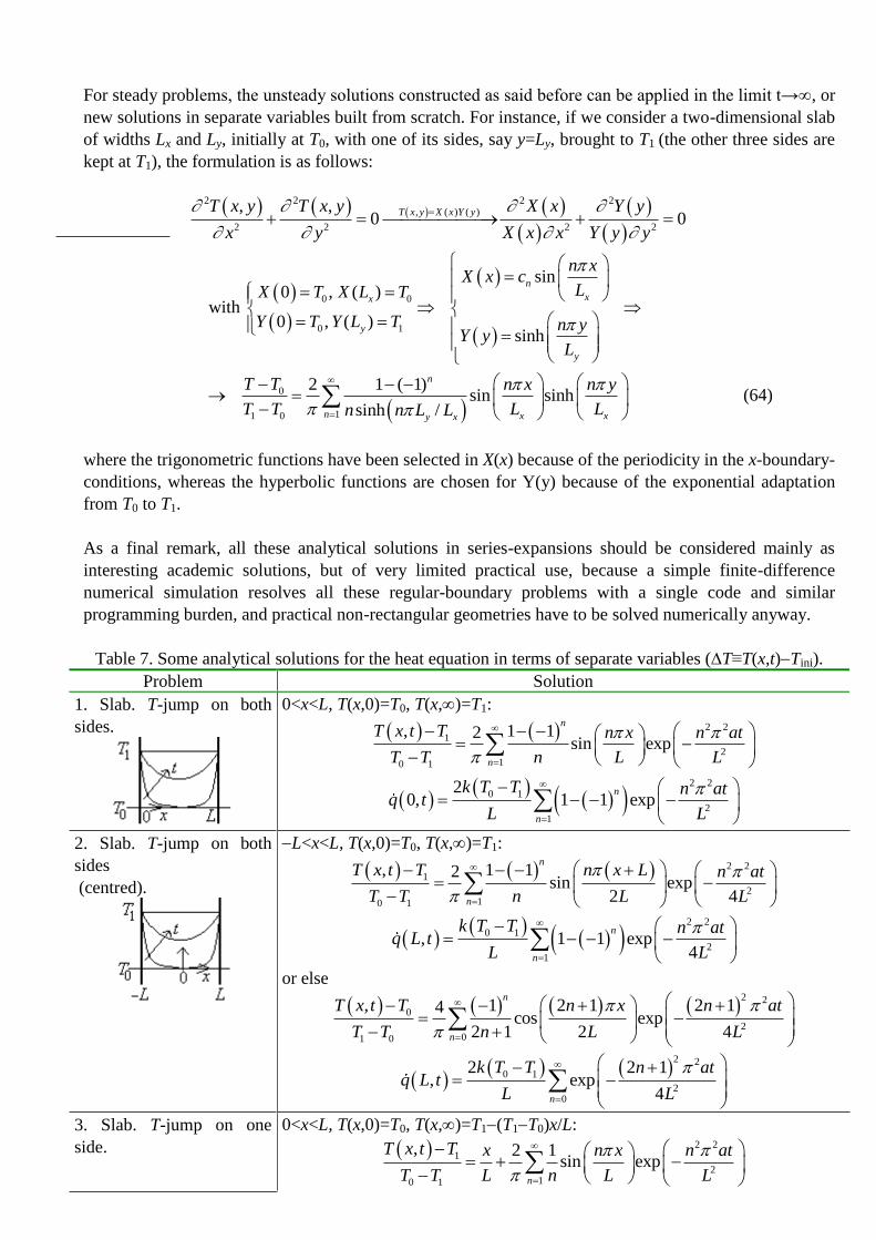
For steady problems, the unsteady solutions constructed as said before can be applied in the limit t→, or
new solutions in separate variables built from scratch. For instance, if we consider a two-dimensional slab
of widths Lx and Ly, initially at T0, with one of its sides, say y=Ly, brought to T1 (the other three sides are
kept at T1), the formulation is as follows:
2 2 2 2, ( ) ( )
2 2 2 2
, ,0 0
T x y X x Y yT x y T x y X x Y y
x y X x x Y y y
0 0
0 1
sin0 , ( )
with 0 , ( )
sinh
n
xx
y
y
n xX x c
LX T X L T
Y T Y L T n yY y
L
0
11 0
2 1 ( 1)sin sinh
sinh /
n
n x xy x
T T n x n y
T T L Ln n L L
(64)
where the trigonometric functions have been selected in X(x) because of the periodicity in the x-boundary-
conditions, whereas the hyperbolic functions are chosen for Y(y) because of the exponential adaptation
from T0 to T1.
As a final remark, all these analytical solutions in series-expansions should be considered mainly as
interesting academic solutions, but of very limited practical use, because a simple finite-difference
numerical simulation resolves all these regular-boundary problems with a single code and similar
programming burden, and practical non-rectangular geometries have to be solved numerically anyway.
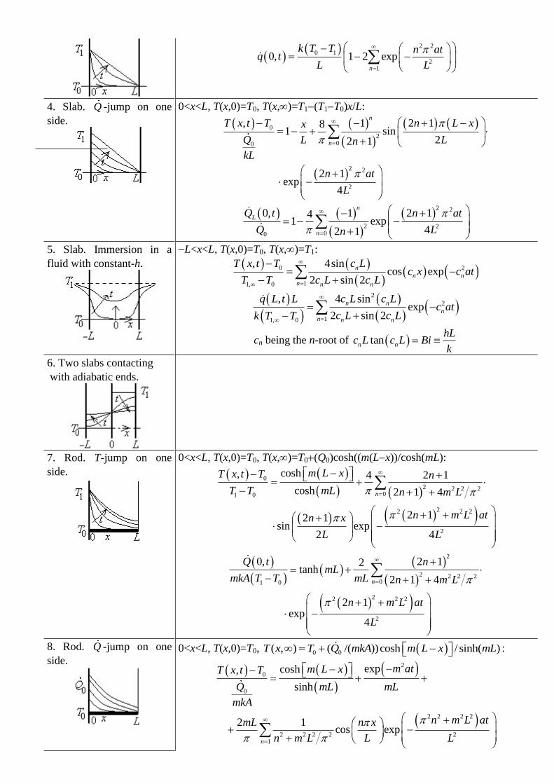
Table 7. Some analytical solutions for the heat equation in terms of separate variables (T≡T(x,t)Tini).
Problem Solution
1. Slab. T-jump on both
sides.
0<x<L, T(x,0)=T0, T(x,)=T1:
2 21
210 1
, 1 12sin exp
n
n
T x t T n x n at
T T n L L
2 2
0 1
21
20, 1 1 exp
n
n
k T T n atq t
L L
2. Slab. T-jump on both
sides
(centred).
L<x<L, T(x,0)=T0, T(x,)=T1:
2 21
210 1
, 1 12sin exp
2 4
n
n
T x t T n x L n at
T T n L L
2 2
0 1
21
, 1 1 exp4
n
n
k T T n atq L t
L L
or else
2 2
0
201 0
, 1 2 1 2 14cos exp
2 1 2 4
n
n
T x t T n x n at
T T n L L
2 2
0 1
20
2 2 1, exp
4n
k T T n atq L t
L L
3. Slab. T-jump on one
side.
0<x<L, T(x,0)=T0, T(x,)=T1(T1T0)x/L:
2 21
210 1
, 2 1sin exp
n
T x t T x n x n at
T T L n L L
2 2
0 1
21
0, 1 2 expn
k T T n atq t
L L
4. Slab. Q -jump on one
side.
0<x<L, T(x,0)=T0, T(x,)=T1(T1T0)x/L:
0
200
2 2
2
, 1 2 181 sin
22 1
2 1exp
4
n
n
T x t T n L xx
Q L Ln
kL
n at
L
2 2
2 200
0, 1 2 141 exp
42 1
n
L
n
Q t n at
Q Ln
5. Slab. Immersion in a
fluid with constant-h.
L<x<L, T(x,0)=T0, T(x,)=T1:
0 2
11, 0
, 4sincos exp
2 sin 2
n
n n
n n n
T x t T c Lc x c at
T T c L c L
2
2
11, 0
, 4 sinexp
2 sin 2
n n
n
n n n
q L t L c L c Lc at
c L c Lk T T
cn being the n-root of tann n
hLc L c L Bi
k
6. Two slabs contacting
with adiabatic ends.
7. Rod. T-jump on one
side.
0<x<L, T(x,0)=T0, T(x,)=T0(Q0)cosh((m(Lx))/cosh(mL):
0
2 2 2 201 0
22 2 2
2
cosh, 4 2 1
cosh 2 1 4
2 12 1sin exp
2 4
n
m L xT x t T n
T T mL n m L
n m L atn x
L L
2
2 2 2 201 0
22 2 2
2
0, 2 12tanh
2 1 4
2 1exp
4
n
Q t nmL
mkA T T mL n m L
n m L at
L
8. Rod. Q -jump on one
side.
0<x<L, T(x,0)=T0, 0 0( , ) ( /( ))cosh / sinh( )T x T Q mkA m L x mL :
2
0
0
2 2 2 2
2 2 2 2 21
expcosh,
sinh
2 1cos exp
n
m atm L xT x t T
Q mL mL
mkA
n m L atmL n x
n m L L L
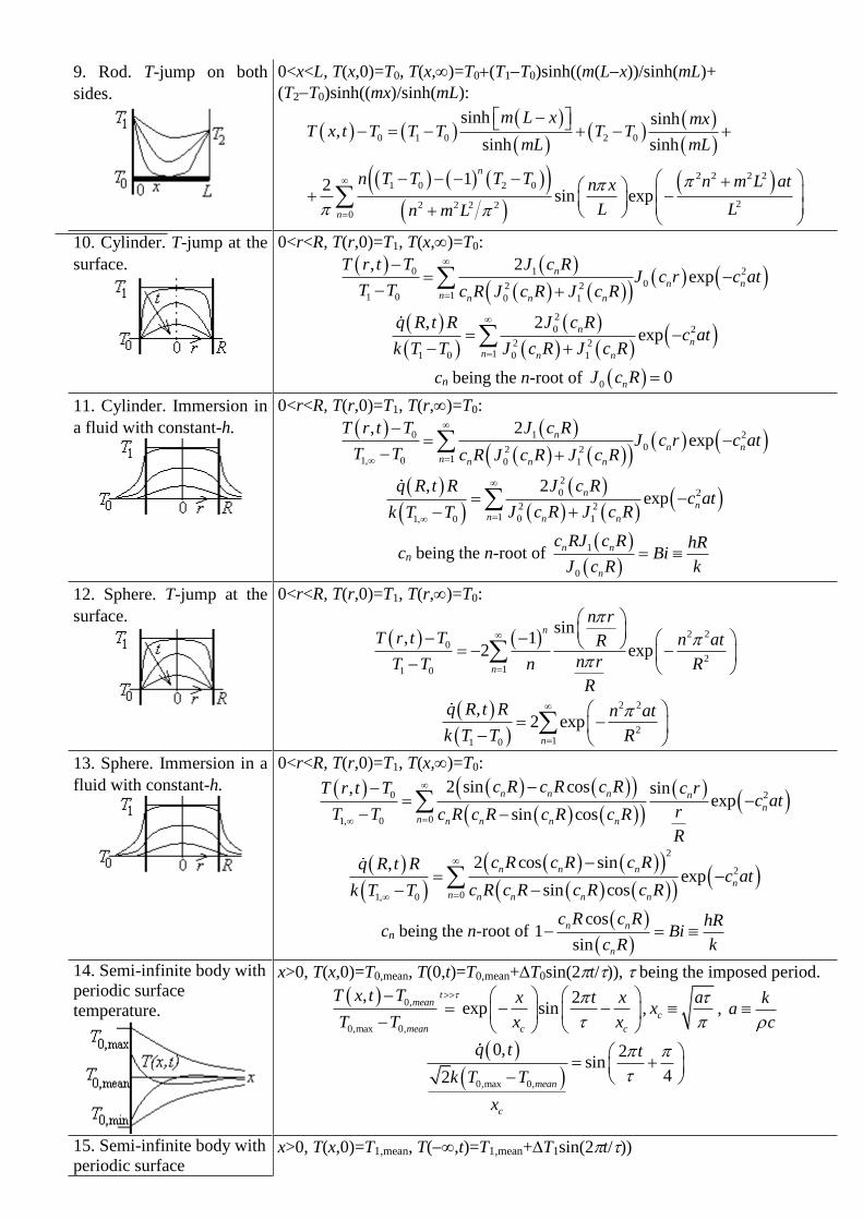
9. Rod. T-jump on both
sides.
0<x<L, T(x,0)=T0, T(x,)=T0(T1T0)sinh((m(Lx))/sinh(mL)+
(T2T0)sinh((mx)/sinh(mL):
0 1 0 2 0
2 2 2 21 0 2 0
22 2 2 20
sinh sinh,
sinh sinh
12sin exp
n
n
m L x mxT x t T T T T T
mL mL
n T T T T n m L atn x
L Ln m L
10. Cylinder. T-jump at the
surface.
0<r<R, T(r,0)=T1, T(x,)=T0:
0 1 2
02 211 0 0 1
, 2exp
n
n n
n n n n
T r t T J c RJ c r c at
T T c R J c R J c R
2
0 2
2 211 0 0 1
, 2exp
n
n
n n n
q R t R J c Rc at
k T T J c R J c R
cn being the n-root of 0 0nJ c R
11. Cylinder. Immersion in
a fluid with constant-h.
0<r<R, T(r,0)=T1, T(r,)=T0:
0 1 2
02 211, 0 0 1
, 2exp
n
n n
n n n n
T r t T J c RJ c r c at
T T c R J c R J c R
2
0 2
2 21 0 11, 0
, 2exp
n
n
n n n
q R t R J c Rc at
J c R J c Rk T T
cn being the n-root of
1
0
n n
n
c RJ c R hRBi
J c R k
12. Sphere. T-jump at the
surface.
0<r<R, T(r,0)=T1, T(r,)=T0:
2 20
211 0
sin, 1
2 exp
n
n
n r
T r t T n atR
n rT T n R
R
2 2
211 0
,2 exp
n
q R t R n at
k T T R
13. Sphere. Immersion in a
fluid with constant-h.
0<r<R, T(r,0)=T1, T(x,)=T0:
0 2
01, 0
2 sin cos, sinexp
sin cos
n n n n
n
n n n n n
c R c R c RT r t T c rc at
rT T c R c R c R c R
R
2
2
01, 0
2 cos sin,exp
sin cos
n n n
n
n n n n n
c R c R c Rq R t Rc at
c R c R c R c Rk T T
cn being the n-root of
cos1
sin
n n
n
c R c R hRBi
c R k
14. Semi-infinite body with
periodic surface
temperature.
x>0, T(x,0)=T0,mean, T(0,t)=T0,mean+T0sin(2t/)), being the imposed period.
0,
0,max 0,
, 2exp sin
tmean
mean c c
T x t T x t x
T T x x
, c
ax
,
ka
c
0,max 0,
0, 2sin
42 mean
c
q t t
k T T
x
15. Semi-infinite body with
periodic surface x>0, T(x,0)=T1,mean, T(,t)=T1,mean+T1sin(2t/))
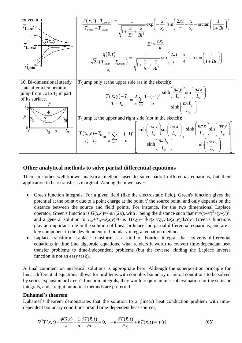
convection.
1,
1,max 1,
2
, 1 2 1exp sin arctan
12 21
tmean
mean c c
T x t T x t x
T T x x Bi
Bi Bi
chxBi
k
1,max 1,
2
0, 1 2 1sin arctan
4 12 2 21mean
c
q t t
Bik T T
Bi Bix
16. Bi-dimensional steady
state after a temperature-
jump from T0 to T1 in part
of its surface.
T-jump only at the upper side (as in the sketch):
0
11 0
sinh sin, 2 1 ( 1)
sinh
nx x
n y
x
n y n x
L LT x y T
n LT T n
L
T-jump at the upper and right side (not in the sketch):
0
11 0
sinh sinsinh sin, 2 1 ( 1)
sinh sinh
ny yx x
n y x
x y
n x n yn y n x
L LL LT x y T
n LT T n n L
L L
Other analytical methods to solve partial differential equations
There are other well-known analytical methods used to solve partial differential equations, but their
application in heat transfer is marginal. Among them we have:
Green function integrals. For a given field (like the electrostatic field), Green's function gives the
potential at the point x due to a point charge at the point x' the source point, and only depends on the
distance between the source and field points. For instance, for the two dimensional Laplace
operator, Green's function is G(x,x')=-lnr/(2), with r being the distance such that r2=(xx')
2+(yy')
2,
and a general solution to Txx+Tyy(x,y)=0 is T(x,y)= ∫∫G(x,x',y,y')(x',y')dx'dy'. Green's functions
play an important role in the solution of linear ordinary and partial differential equations, and are a
key component to the development of boundary integral equation methods.
Laplace transform. Laplace transform is a kind of Fourier integral that converts differential
equations in time into algebraic equations, what renders it worth to convert time-dependant heat
transfer problems to time-independent problems (but the reverse, finding the Laplace inverse
function is not an easy task).
A final comment on analytical solutions is appropriate here. Although the superposition principle for
linear differential equations allows for problems with complex boundary or initial conditions to be solved
by series expansion or Green's function integrals, they would require numerical evaluation for the sums or
integrals, and straight numerical methods are preferred
Duhamel`s theorem
Duhamel`s theorem demonstrates that the solution to a (linear) heat conduction problem with time-
dependent boundary conditions or/and time-dependent heat-sources,
2 ( , ) 1 ( , ) ( , )( , ) 0, ( , ) ( )
i
x t T x t T x tT x t k hT x t f t
k a t x
(65)
can be computed from the solution to a the time-independent problem:
2 ( , ) 1 ( , , ) ( , , )( , , ) 0, ( , , ) ( )
i
x x t x tx t k h x t f
k a t x
(66)
where t is now a parameter (not time), with the relation:
0
( , ) ( , , )
t
T x t x t dt
(67)
NUMERICAL SOLUTIONS
Numerical solutions are the rule in solving practical heat transfer problems, as well as in mass and
momentum transfer, because the analytical formulation in terms of partial differential equations is not
analytically solvable except for very simple configurations, as seen above. Numerical methods transform
the continuous problem to a discrete problem, thus, instead of yielding a continuous solution valid at
every point in the system and every instant in time, and every value of the parameters, numerical methods
only yield discrete solutions, valid only at discrete points in the system, at discrete time intervals, and for
discrete values of the parameters. However gloom the numerical approach may sound, it has two crucial
advantages:
Can provide a solution to any practical problem, however complicated it may be (not just steady
one-dimensional, constant-property ideal models). In any case, it is most important to realise that
any practical problem is at the end an intermediate idealisation aiming at practical answers (e.g.
nobody takes account of the infinite figures in ; 3 may be a good-enough approximation, and
3.1416 already an accuracy illusion).
The discretization can be refined as much as wanted (of course, at the expense in computing time
and memory, and operator's burden). In any case, it is wise to start with as few unknowns as
feasible, for an efficient feedback (most of the first trials suffer from infancy problems that are
independent on the finesse of the discretisation). Any good practitioner knows that refinements
should follow coarse work, and not the contrary.
All numerical approaches transform the continuous problem, that we may write as PDE(T)=F meaning
that a partial differential operator applied to the temperature field should equal the force-field imposing
the thermal non-equilibrium, to a discrete problem that we may write, at a given instant in time, as
K*T=F, where, instead of one differential equation, we have for each time step a set of N algebraic
equations involving the unknown temperatures at N points in the system (to our choice), a set of known
applied stimuli at N points (to be computed in a particular way), and a set of N*N coefficients to be
computed also in a particular way, depending on the numerical method. Numerical methods differ in the
way they yield this system of algebraic equations, but a general baseline exists. The problem may be
generally stated as:
0 0, 0, , 0, , 0PDE T x t BC T x t IC T x t (68)
where PDE, BC and IC represent functionals related to the partial differential equation, boundary
conditions and initial conditions, respectively. Numerical methods approximate the infinite-degrees-of-
freedom continuous solution by a finite N-degrees-of-freedom solution of the form:
1
, , ( ) ( )N
approx IBC
i i
i
T x t T x t T t x
(69)
where ,IBCT x t is a known function (chosen by the modeller) satisfying all the initial and boundary
conditions, ( )iT t are unknown coefficients (varying with time for transient problems) to be numerically
found, and i x( )
are known trial functions, the base functions the modeller chooses as a function space
of the solution. Notice the separation of variables in time and space in (69); in practice, the time-
dependence is also discretized, but this is a simpler problem because time is is one-dimensional and
unidirectional, and we forget it for the moment. Notice also that, in spite of the fact that physical
uncertainty comes from different idealisations (geometrical, material, temporal, interactions...), it is
customary to look for solutions that approximate the PDE but exactly verifying the initial and boundary
conditions.
Several numerical methods have been developed, each with its own advantages and complexities, from
simple ones like the lumped method or the finite difference method, which can be developed from scratch
for every new problem (but becoming too cumbersome in complex cases), to the standard finite element
method that, once developed (it demands much more effort), can be routinely applied to whatever
complex case we have at hand.
Steady state problems in heat transfer are boundary-value problems (elliptic problems), more difficult to
solve numerically than initial-value problems (parabolic problems), thus, even for steady state problems,
it is advisable to solve the initial value transient until sufficiently-small changes indicate the steady state
is reached.
The most common numerical methods, from simpler to more complex, may be grouped as:
Integral methods, where the integral energy equation d dE t Q W is solved, instead of the
(differential) heat equation (3). Among them, the most used are:
o Global fitting, where and ad-hoc continuous T-field function is fitted.
o Lumped network, where the system is partitioned in a number of isothermal lumps (a
discrete step-wise T-field).
Differential methods, where the heat equation is solved (sometimes by integration, but the PDE is
apparent), instead of the integral energy equation. Among them, the most used are:
o Residual minimization.
o Finite differences.
o Finite elements.
o Boundary elements.
Another classification may be in terms of the continuity of the base functions as: global methods (global
fitting and residual minimization), and local methods (or partition methods; all the others). The great
advantage of local methods is that the base functions can be very simple (often linear). The first step in all
local methods is a spatial discretisation of the domain, followed by node assignment (one central or
boundary node in the finite difference method, several nodes in the finite element method, at least one at
each end), and the choice of base functions, to be explained below.
There are other integral methods, like the Rayleigh-Ritz method, which are based on a variational
formulation of the problem if it exists (e.g. minimising the potential energy in mechanical problems or
minimising the generation of entropy in thermal problems). The variational functional contains all the
information (PDE plus boundary conditions), e.g. E=∫f(x,y,y')dx=min, and the unknown coefficients in the
temperature fitting are found by directly minimization of the variational, instead of through the equivalent
Lagrange equation, f/yd(f/y')/dx=0.
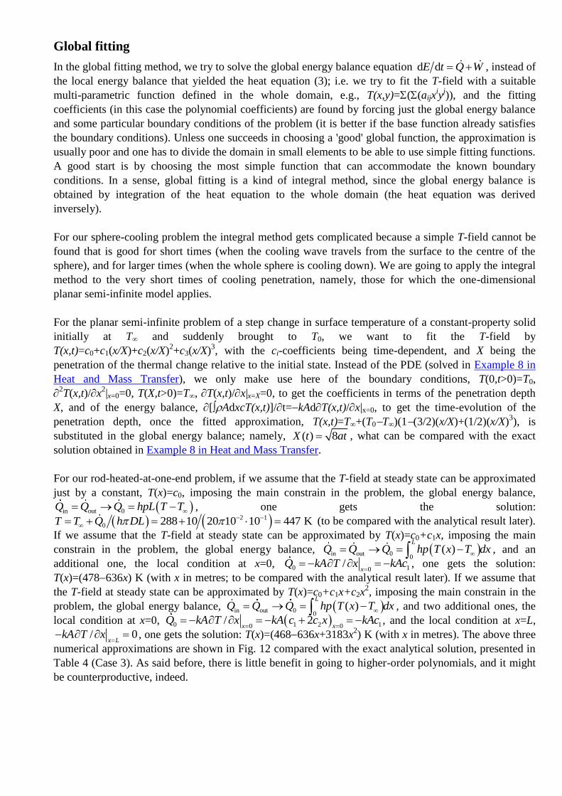
Global fitting
In the global fitting method, we try to solve the global energy balance equation d dE t Q W , instead of
the local energy balance that yielded the heat equation (3); i.e. we try to fit the T-field with a suitable
multi-parametric function defined in the whole domain, e.g., T(x,y)=((aijxiy
j)), and the fitting
coefficients (in this case the polynomial coefficients) are found by forcing just the global energy balance
and some particular boundary conditions of the problem (it is better if the base function already satisfies
the boundary conditions). Unless one succeeds in choosing a 'good' global function, the approximation is
usually poor and one has to divide the domain in small elements to be able to use simple fitting functions.
A good start is by choosing the most simple function that can accommodate the known boundary
conditions. In a sense, global fitting is a kind of integral method, since the global energy balance is
obtained by integration of the heat equation to the whole domain (the heat equation was derived
inversely).
For our sphere-cooling problem the integral method gets complicated because a simple T-field cannot be
found that is good for short times (when the cooling wave travels from the surface to the centre of the
sphere), and for larger times (when the whole sphere is cooling down). We are going to apply the integral
method to the very short times of cooling penetration, namely, those for which the one-dimensional
planar semi-infinite model applies.
For the planar semi-infinite problem of a step change in surface temperature of a constant-property solid
initially at T∞ and suddenly brought to T0, we want to fit the T-field by
T(x,t)=c0+c1(x/X)+c2(x/X)2+c3(x/X)
3, with the ci-coefficients being time-dependent, and X being the
penetration of the thermal change relative to the initial state. Instead of the PDE (solved in Example 8 in
Heat and Mass Transfer), we only make use here of the boundary conditions, T(0,t>0)=T0,
2T(x,t)/x
2|x=0=0, T(X,t>0)=T∞, T(x,t)/x|x=X=0, to get the coefficients in terms of the penetration depth
X, and of the energy balance, [AdxcT(x,t)]/t=kAdT(x,t)/x|x=0, to get the time-evolution of the
penetration depth, once the fitted approximation, T(x,t)=T∞+(T0T∞)(1(3/2)(x/X)+(1/2)(x/X)3), is
substituted in the global energy balance; namely, ( ) 8X t at , what can be compared with the exact
solution obtained in Example 8 in Heat and Mass Transfer.
For our rod-heated-at-one-end problem, if we assume that the T-field at steady state can be approximated
just by a constant, T(x)=c0, imposing the main constrain in the problem, the global energy balance,
in out 0Q Q Q hpL T T , one gets the solution:
2 1
0 288 10 20 10 10 447 KT T Q h DL
(to be compared with the analytical result later).
If we assume that the T-field at steady state can be approximated by T(x)=c0+c1x, imposing the main
constrain in the problem, the global energy balance, in out 00
( )L
Q Q Q hp T x T dx , and an
additional one, the local condition at x=0, 0 10/
xQ kA T x kAc
, one gets the solution:
T(x)=(478636x) K (with x in metres; to be compared with the analytical result later). If we assume that
the T-field at steady state can be approximated by T(x)=c0+c1x+c2x2, imposing the main constrain in the
problem, the global energy balance, in out 00
( )L
Q Q Q hp T x T dx , and two additional ones, the
local condition at x=0, 0 1 2 100/ 2
xxQ kA T x kA c c x kAc
, and the local condition at x=L,
/ 0x L
kA T x
, one gets the solution: T(x)=(468636x+3183x2) K (with x in metres). The above three
numerical approximations are shown in Fig. 12 compared with the exact analytical solution, presented in
Table 4 (Case 3). As said before, there is little benefit in going to higher-order polynomials, and it might
be counterproductive, indeed.
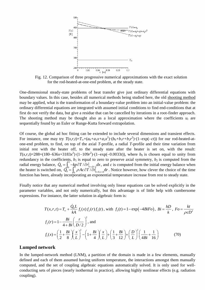
Fig. 12. Comparison of three progressive numerical approximations with the exact solution
for the rod-heated-at-one-end problem, at the steady state.
One-dimensional steady-state problems of heat transfer give just ordinary differential equations with
boundary values. In this case, besides all numerical methods being studied here, the old shooting method
may be applied, what is the transformation of a boundary-value problem into an initial-value problem: the
ordinary differential equations are integrated with assumed initial conditions to find end-conditions that at
first do not verify the data, but give a residue that can be cancelled by iterations in a root-finder approach.
The shooting method may be thought also as a local approximation where the coefficients ui are
sequentially found by an Euler or Runge-Kutta forward extrapolation.
Of course, the global ad hoc fitting can be extended to include several dimensions and transient effects.
For instance, one may try T(x,r,t)=T∞+(a0+a1x+a2x2)·(b0+b1r+b2r
2)·(1exp(ct)) for our rod-heated-at-
one-end problem, to find, on top of the axial T-profile, a radial T-profile and their time variation from
initial rest with the heater off, to the steady state after the heater is set on, with the result:
T(x,r,t)=288+(180636x+3183x2)·(1109r
2)·(1exp(0.0033t)), where b0 is chosen equal to unity from
redundancy in the coefficients, b1 is equal to zero to preserve axial symmetry, b2 is computed from the
radial energy balance, 0 / 20/
L
r DQ kp T r dx
, and c is computed from the initial energy balance when
the heater is switched on, 0 0, 00/ d
L
t rQ Ac T t r
. Notice however, how clever the choice of the time
function has been, already incorporating an exponential temperature increase from rest to steady state.
Finally notice that any numerical method involving only linear equations can be solved explicitly in the
parameter variables, and not only numerically, but this advantage is of little help with cumbersome
expressions. For instance, the latter solution in algebraic form is:
01 2 3( , , ) ( ) ( ) ( )
Q LT x r t T f x f r f t
kA , with 3( ) 1 exp 4f t BiFo ,
hDBi
k ,
2
ktFo
cD
2
2 ( ) 14 / 2
Bi rf r
Bi D
, and
2 2
1
1 1 1 1( ) 1
2 8 4 3 12 4 16
Bi x Bi x Bi Df x
L L L Bi
(70)
Lumped network
In the lumped-network method (LNM), a partition of the domain is made in a few elements, manually
defined and each of them assumed having uniform temperature, the interactions amongst them manually
computed, and the set of coupling algebraic equations automatically solved. It is only used for well-
conducting sets of pieces (nearly isothermal in practice), allowing highly nonlinear effects (e.g. radiation
coupling).
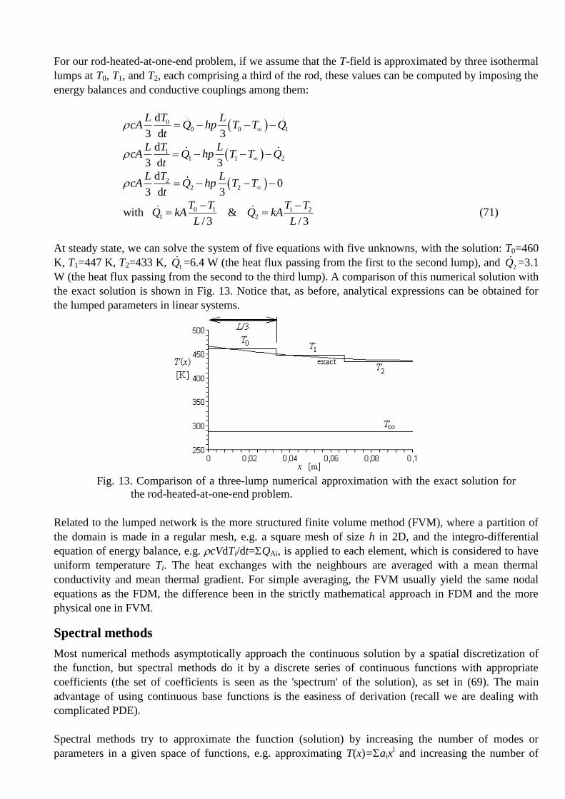
For our rod-heated-at-one-end problem, if we assume that the T-field is approximated by three isothermal
lumps at T0, T1, and T2, each comprising a third of the rod, these values can be computed by imposing the
energy balances and conductive couplings among them:
00 0 1
d
3 d 3
TL LcA Q hp T T Q
t
11 1 2
d
3 d 3
TL LcA Q hp T T Q
t
22 2
d0
3 d 3
TL LcA Q hp T T
t
0 1 1 21 2with &
/ 3 / 3
T T T TQ kA Q kA
L L
(71)
At steady state, we can solve the system of five equations with five unknowns, with the solution: T0=460
K, T1=447 K, T2=433 K, 1Q =6.4 W (the heat flux passing from the first to the second lump), and
2Q =3.1
W (the heat flux passing from the second to the third lump). A comparison of this numerical solution with
the exact solution is shown in Fig. 13. Notice that, as before, analytical expressions can be obtained for
the lumped parameters in linear systems.
Fig. 13. Comparison of a three-lump numerical approximation with the exact solution for
the rod-heated-at-one-end problem.
Related to the lumped network is the more structured finite volume method (FVM), where a partition of
the domain is made in a regular mesh, e.g. a square mesh of size h in 2D, and the integro-differential
equation of energy balance, e.g. cVdTi/dt=QAi, is applied to each element, which is considered to have
uniform temperature Ti. The heat exchanges with the neighbours are averaged with a mean thermal
conductivity and mean thermal gradient. For simple averaging, the FVM usually yield the same nodal
equations as the FDM, the difference been in the strictly mathematical approach in FDM and the more
physical one in FVM.
Spectral methods
Most numerical methods asymptotically approach the continuous solution by a spatial discretization of
the function, but spectral methods do it by a discrete series of continuous functions with appropriate
coefficients (the set of coefficients is seen as the 'spectrum' of the solution), as set in (69). The main
advantage of using continuous base functions is the easiness of derivation (recall we are dealing with
complicated PDE).
Spectral methods try to approximate the function (solution) by increasing the number of modes or
parameters in a given space of functions, e.g. approximating T(x)=aixi and increasing the number of
terms i, or better using orthogonal functions like T(x)=aisin(ix), etc. Although any function can be
approximated by an infinite series expansion of any kind, if the base functions are orthogonal the
coefficients in the series are uncoupled and a lot of work is saved (they can be found independently, and
if their number is increased, only the added ones must be computed).
Spectral methods usually take the domain globally (i.e. one element with multi-parametric base function),
but some new methods take a local approach, in combination with spatial methods. The handicap of
spectral methods is that for a multi-parametric fit of a global base function, unless one succeeds in
choosing a ‘good’ global function, the approximation is usually poor and misleading (e.g. with ripples),
and it is better to divide the domain in small elements to be able to use simple fitting functions (spatial
methods), e.g. piece-wise linear polynomials for second order PDE.
Residual fitting
As in the global fitting method, we try to fit the T-field with a suitable multi-parametric function defined
in the whole domain, ( , ) ( ) ( )i iT x t c t x , but the coefficients now are determined by minimization of
the residuals obtained when the fitting function is substituted into the differential form of the problem:
1
( ) ( ) , min, for independent N
i i i
i
PDE c t x R x t c
(72)
where the minimization of the N-degree-of-freedom residual is accomplished by weighted averaging in
the spatial domain:
, , 0, 1..iw x R x t i N (73)
where wi are the weighting functions and <wi,R> is the projection or scalar product.
For instance, for our rod-heated-at-one-end problem at the steady state, the differential problem was
stated as (25):
2
02
0
d d d0 with & 0
d d dx x L
T hp T TT T Q kA kA
x kA x x
(74)
If we chose as fitting function T(x)=c0+c1x+c2x2, imposing the two boundary conditions we get
2 0 /(2 )c Q kLA and 1 0 /( )c Q kA , and the other coefficients (only c0 here) are obtained by proper
minimization of the following weighted residual, R(ci):
2
2
0
d ( )( ) ( )
d
x L
i i
x
T x hpR c T x T w x dx
x kA
(75)
obtained by integration, over the whole domain (here the length of the rod), of the differential equation
that should be zero if exact, multiplied by some appropriate weighting functions, wi(x), which can be
chosen following different approaches, to be explained below:
method of collocation, and finite differences (FDM)
/ method of least squares (LSM)
( ) method of finite elements of Galerkin (FEM)
i i
i i
i i
w x x x
w x R u
w x x
(76)
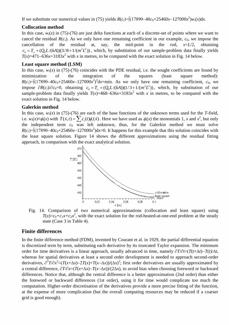
If we substitute our numerical values in (75) yields R(ci)=∫(1789040c0+25460x127000x2)wi(x)dx.
Collocation method
In this case, wi(x) in (75)-(76) are just delta functions at each of a discrete-set of points where we want to
cancel the residual R(ci). As we only have one remaining coefficient in our example, c0, we impose the
cancellation of the residual at, say, the mid-point in the rod, x=L/2, obtaining 2 2
0 0( /( ))(3/8 1/( ))c T Q L kA m L , which, by substitution of our sample-problem data finally yields
T(x)=471636x+3183x2 with x in metres, to be compared with the exact solution in Fig. 14 below.
Least square method (LSM)
In this case, wi(x) in (75)-(76) coincides with the PDE residual, i.e. the sought coefficients are found by
minimization of the integration of the squares (least square method):
R(ci)=∫(1789040c0+25460x127000x2)2dx=min. As we only have one remaining coefficient, c0, we
impose R(ci)/c0=0, obtaining 2 2
0 0( /( ))(1/3 1/( ))c T Q L kA m L , which, by substitution of our
sample-problem data finally yields T(x)=468636x+3183x2 with x in metres, to be compared with the
exact solution in Fig. 14 below.
Galerkin method
In this case, wi(x) in (75)-(76) are each of the base functions of the unknown terms used for the T-field,
i.e. wi(x)≡i(x) with ( , ) ( ) ( )i iT x t c t x . Here we have used as i(x) the monomials 1, x and x2, but only
the independent term c0 was left unknown, thus, for the Galerkin method we must solve
R(ci)=∫(1789040c0+25460x127000x2)dx=0. It happens for this example that this solution coincides with
the least square solution. Figure 14 shows the different approximations using the residual fitting
approach, in comparison with the exact analytical solution.
Fig. 14. Comparison of two numerical approximations (collocation and least square) using
T(x)=c0+c1x+c2x2, with the exact solution for the rod-heated-at-one-end problem at the steady
state (Case 3 in Table 4).
Finite differences
In the finite difference method (FDM), invented by Courant et al. in 1929, the partial differential equation
is discretized term by term, substituting each derivative by its truncated Taylor expansion. The minimum
order for time derivatives is a linear approach, usually advanced in time, namely T/t≈(T(t+t)T(t)/t,
whereas for spatial derivatives at least a second order development is needed to approach second-order
derivatives, 2T/x
2≈(T(x+x)T(x)+T(xx))/(x)
2; first order derivatives are usually approximated by
a central difference, T/x≈(T(x+x)T(xx))/(2x), to avoid bias when choosing foreword or backward
differences. Notice that, although the central difference is a better approximation (2nd order) than either
the foreword or backward differences (1st order), using it for time would complicate too much the
computation. Higher-order discretisation of the derivatives provide a more precise fitting of the function,
at the expense of more complication (but the overall computing resources may be reduced if a coarser
grid is good enough).
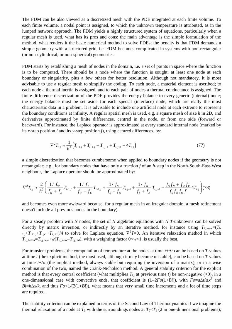
The FDM can be also viewed as a discretized mesh with the PDE integrated at each finite volume. To
each finite volume, a nodal point is assigned, to which the unknown temperature is attributed, as in the
lumped network approach. The FDM yields a highly structured system of equations, particularly when a
regular mesh is used, what has its pros and cons: the main advantage is the simple formulation of the
method, what renders it the basic numerical method to solve PDEs; the penalty is that FDM demands a
simple geometry with a structured grid, i.e. FDM becomes complicated in systems with non-rectangular
(or non-cylindrical, or non-spherical) geometries.
FDM starts by establishing a mesh of nodes in the domain, i.e. a set of points in space where the function
is to be computed. There should be a node where the function is sought; at least one node at each
boundary or singularity, plus a few others for better resolution. Although not mandatory, it is most
advisable to use a regular mesh to simplify the coding. To each node, a material element is ascribed; to
each node a thermal inertia is assigned, and to each pair of nodes a thermal conductance is assigned. The
finite difference discretization of the PDE provides the energy balance to every generic (internal) node;
the energy balance must be set aside for each special (interface) node, which are really the most
characteristic data in a problem. It is advisable to include one artificial node at each extreme to represent
the boundary conditions at infinity. A regular spatial mesh is used, e.g. a square mesh of size h in 2D, and
derivatives approximated by finite differences, centred in the node, or from one side (forward or
backward). For instance, the Laplace operator is approximated at every standard internal node (marked by
its x-step position i and its y-step position j), using centred differences, by:
2
2 1 1 1 1
14T
hT T T T Ti j i j i j i j i j i j, , , , , ,d i (77)
a simple discretization that becomes cumbersome when applied to boundary nodes if the geometry is not
rectangular; e.g., for boundary nodes that have only a fraction f of an h-step in the North-South-East-West
neighbour, the Laplace operator should be approximated by:
F
HGIKJ
2
2 1 1 1 1
2 1 1 1 14T
h
f
f fT
f
f fT
f
f fT
f
f fT
f f f f
f f f fTi j
W
W E
i jE
W E
i jS
S N
i jN
S N
i jS N W E
S N W
i j, , , , , ,
/ / / /(78)
and becomes even more awkward because, for a regular mesh in an irregular domain, a mesh refinement
doesn't include all previous nodes in the boundary).
For a steady problem with N nodes, the set of N algebraic equations with N T-unknowns can be solved
directly by matrix inversion, or indirectly by an iterative method, for instance using Ti,j,new=(Ti-
1,j+Ti+1,j+Ti,j-1+Ti,j+1)/4 to solve for Laplace equation, 2T=0. An iterative relaxation method in which
Ti,j,better=Ti,j,new+w(Ti,j,newTi,j,old), with a weighting factor 0<w<1, is usually the best.
For transient problems, the computation of temperature at the nodes at time t+t can be based on T-values
at time t (the explicit method, the most used, although it may become unstable), can be based on T-values
at time t+t (the implicit method, always stable but requiring the inversion of a matrix), or in a wise
combination of the two, named the Crank-Nicholson method. A general stability criterion for the explicit
method is that every central coefficient (what multiplies Ti,j at previous time t) be non-negative (≥0); in a
one-dimensional case with convective ends, that coefficient is (12Fo(1+Bi)), with Fo=at/x2 and
Bi=hx/k, and thus Fo<1/(2(1+Bi)), what means that very small time increments and a lot of time steps
are required.
The stability criterion can be explained in terms of the Second Law of Thermodynamics if we imagine the
thermal relaxation of a node at T1 with the surroundings nodes at T0<T1 (2 in one-dimensional problems);
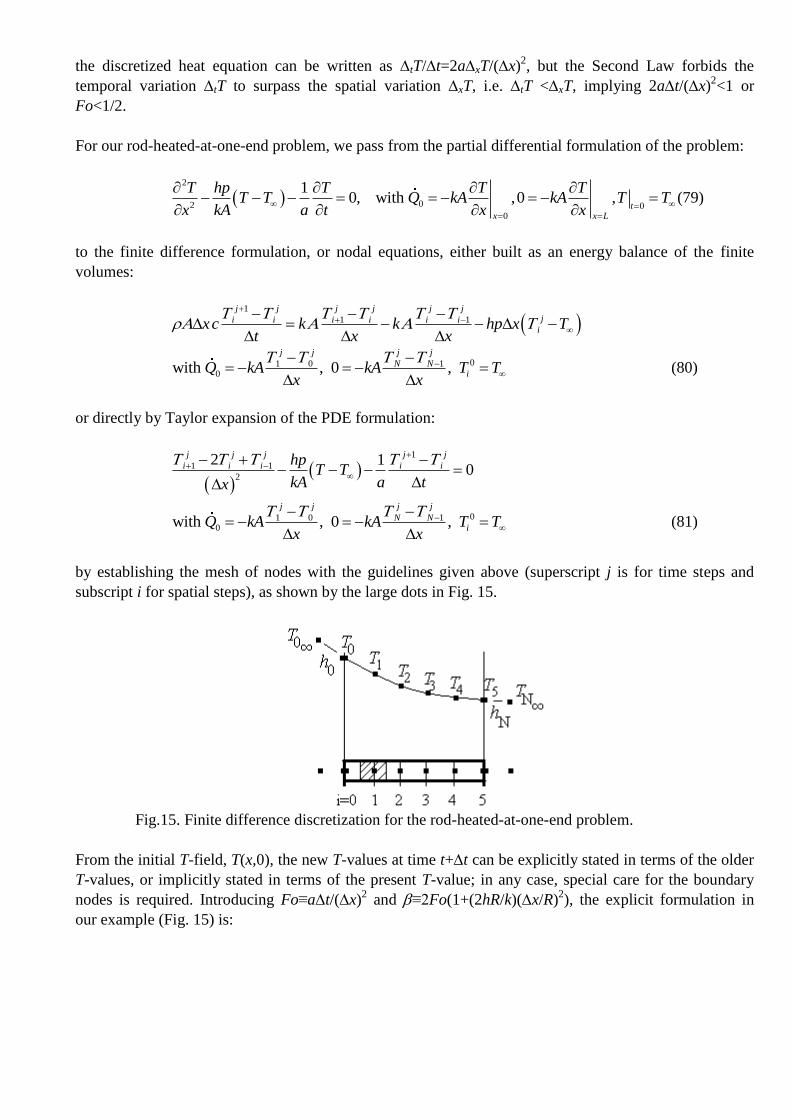
the discretized heat equation can be written as tT/t=2axT/(x)2, but the Second Law forbids the
temporal variation tT to surpass the spatial variation xT, i.e. tT <xT, implying 2at/(x)2<1 or
Fo<1/2.
For our rod-heated-at-one-end problem, we pass from the partial differential formulation of the problem:
2
02 00
10, with ,0 ,
tx x L
T hp T T TT T Q kA kA T T
x kA a t x x
(79)
to the finite difference formulation, or nodal equations, either built as an energy balance of the finite
volumes:
1
1 1
j j j j j jji i i i i i
ixc k k hp x Tt x x
01 0 10with , 0 ,
j j j j
N NiQ kA kA T T
x x
(80)
or directly by Taylor expansion of the PDE formulation:
1
1 1
2
2 10
j j j j j
i i i i ihpT T
kA a tx
01 0 10with , 0 ,
j j j j
N NiQ kA kA T T
x x
(81)
by establishing the mesh of nodes with the guidelines given above (superscript j is for time steps and
subscript i for spatial steps), as shown by the large dots in Fig. 15.
Fig.15. Finite difference discretization for the rod-heated-at-one-end problem.
From the initial T-field, T(x,0), the new T-values at time t+t can be explicitly stated in terms of the older
T-values, or implicitly stated in terms of the present T-value; in any case, special care for the boundary
nodes is required. Introducing Fo≡at/(x)2 and ≡2Fo(1+(2hR/k)(x/R)
2), the explicit formulation in
our example (Fig. 15) is:
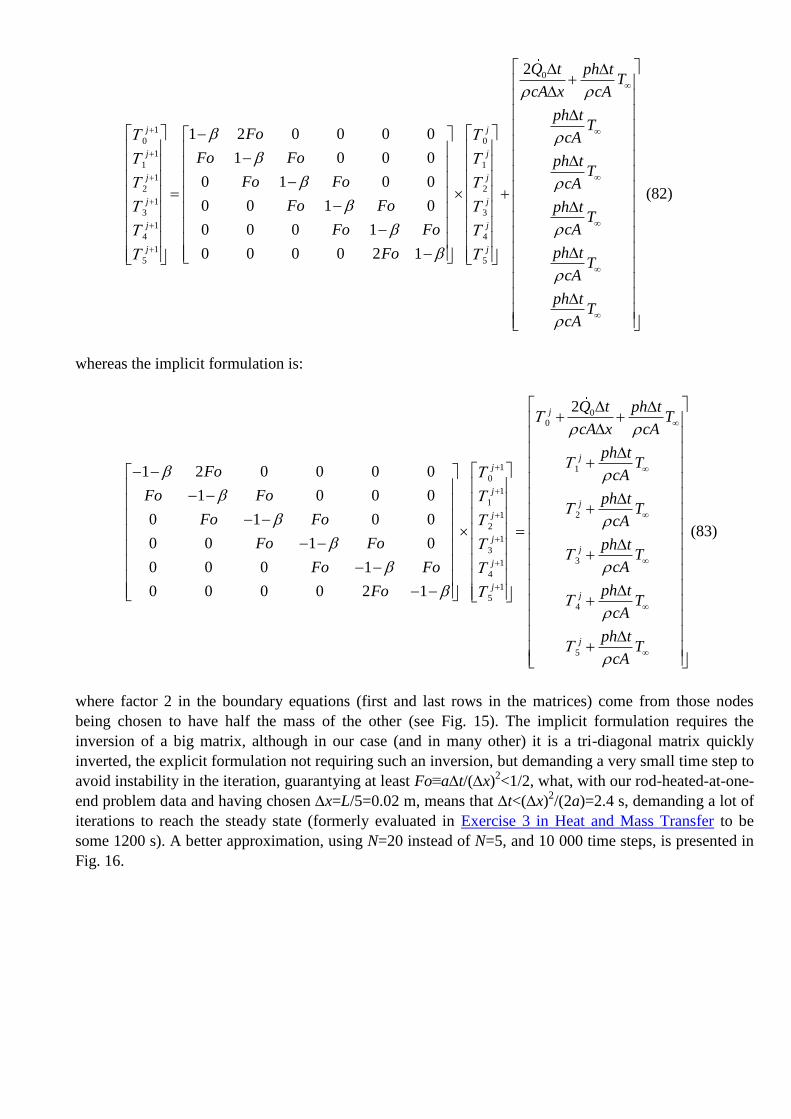
0
1
0 0
1
1 1
1
2 2
1
3 3
1
4 4
1
5 5
2
1 2 0 0 0 0
1 0 0 0
0 1 0 0
0 0 1 0
0 0 0 1
0 0 0 0 2 1
j j
j j
j j
j j
j j
j j
Q t ph tT
cA x cA
ph tT
Fo cA
Fo Fo
Fo Fo
Fo Fo
Fo Fo
Fo
ph tT
cA
ph tT
cA
ph tT
cA
ph tT
cA
(82)
whereas the implicit formulation is:
00
1 10
1
1
21
2
1
3
31
4
1
5
2
1 2 0 0 0 0
1 0 0 0
0 1 0 0
0 0 1 0
0 0 0 1
0 0 0 0 2 1
j
jj
j
j
j
jj
j
j
Q t ph tT
cA x cA
ph tT
Fo cA
Fo Fo ph tT
Fo Fo cA
Fo Fo ph t
cAFo Fo
Fo
4
5
j
j
T
ph tT
cA
ph tT
cA
(83)
where factor 2 in the boundary equations (first and last rows in the matrices) come from those nodes
being chosen to have half the mass of the other (see Fig. 15). The implicit formulation requires the
inversion of a big matrix, although in our case (and in many other) it is a tri-diagonal matrix quickly
inverted, the explicit formulation not requiring such an inversion, but demanding a very small time step to
avoid instability in the iteration, guarantying at least Fo≡at/(x)2<1/2, what, with our rod-heated-at-one-
end problem data and having chosen x=L/5=0.02 m, means that t<(x)2/(2a)=2.4 s, demanding a lot of
iterations to reach the steady state (formerly evaluated in Exercise 3 in Heat and Mass Transfer to be
some 1200 s). A better approximation, using N=20 instead of N=5, and 10 000 time steps, is presented in
Fig. 16.
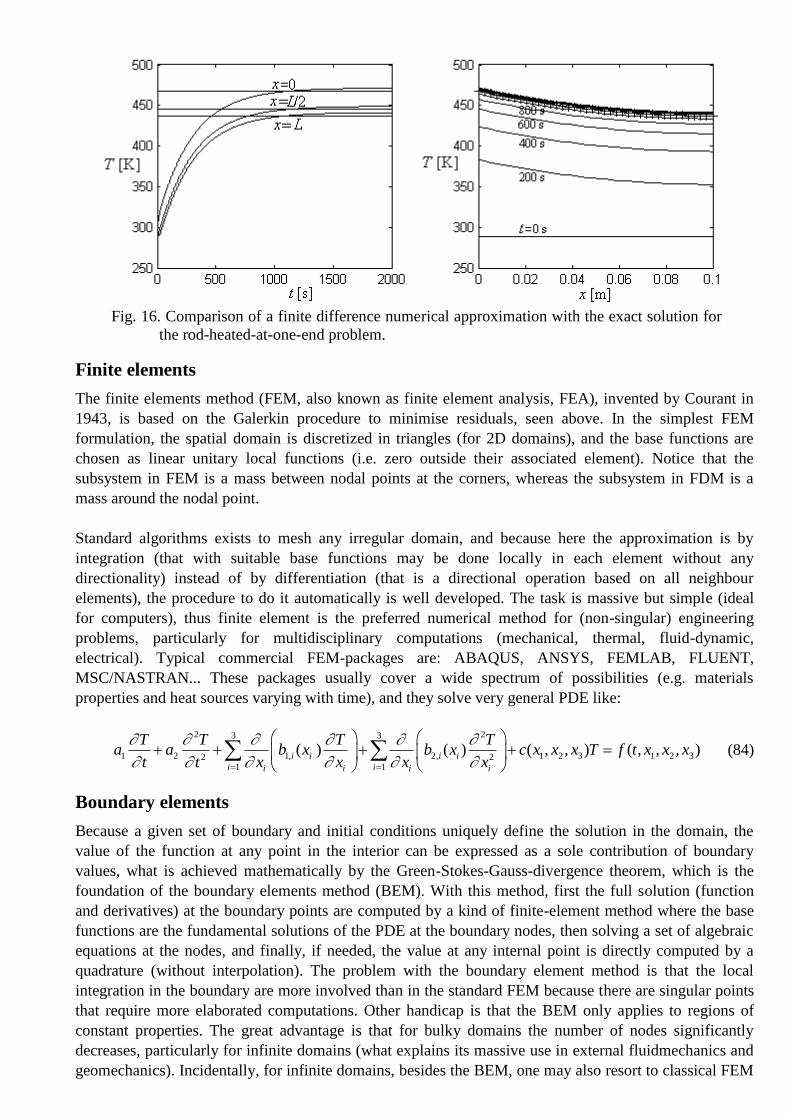
Fig. 16. Comparison of a finite difference numerical approximation with the exact solution for
the rod-heated-at-one-end problem.
Finite elements
The finite elements method (FEM, also known as finite element analysis, FEA), invented by Courant in
1943, is based on the Galerkin procedure to minimise residuals, seen above. In the simplest FEM
formulation, the spatial domain is discretized in triangles (for 2D domains), and the base functions are
chosen as linear unitary local functions (i.e. zero outside their associated element). Notice that the
subsystem in FEM is a mass between nodal points at the corners, whereas the subsystem in FDM is a
mass around the nodal point.
Standard algorithms exists to mesh any irregular domain, and because here the approximation is by
integration (that with suitable base functions may be done locally in each element without any
directionality) instead of by differentiation (that is a directional operation based on all neighbour
elements), the procedure to do it automatically is well developed. The task is massive but simple (ideal
for computers), thus finite element is the preferred numerical method for (non-singular) engineering
problems, particularly for multidisciplinary computations (mechanical, thermal, fluid-dynamic,
electrical). Typical commercial FEM-packages are: ABAQUS, ANSYS, FEMLAB, FLUENT,
MSC/NASTRAN... These packages usually cover a wide spectrum of possibilities (e.g. materials
properties and heat sources varying with time), and they solve very general PDE like:
2 23 3
1 2 1, 2, 1 2 3 1 2 32 21 1
( ) ( ) ( , , ) ( , , , )i i i i
i ii i i i
T T T Ta a b x b x c x x x T f t x x x
t t x x x x
(84)
Boundary elements
Because a given set of boundary and initial conditions uniquely define the solution in the domain, the
value of the function at any point in the interior can be expressed as a sole contribution of boundary
values, what is achieved mathematically by the Green-Stokes-Gauss-divergence theorem, which is the
foundation of the boundary elements method (BEM). With this method, first the full solution (function
and derivatives) at the boundary points are computed by a kind of finite-element method where the base
functions are the fundamental solutions of the PDE at the boundary nodes, then solving a set of algebraic
equations at the nodes, and finally, if needed, the value at any internal point is directly computed by a
quadrature (without interpolation). The problem with the boundary element method is that the local
integration in the boundary are more involved than in the standard FEM because there are singular points
that require more elaborated computations. Other handicap is that the BEM only applies to regions of
constant properties. The great advantage is that for bulky domains the number of nodes significantly
decreases, particularly for infinite domains (what explains its massive use in external fluidmechanics and
geomechanics). Incidentally, for infinite domains, besides the BEM, one may also resort to classical FEM

with a truncated domain progressively enlarged, or matched to an asymptotic analytical expansion, or
stretching the external elements with a log-transformation.
Back to Heat and mass transfer


