Analytical solution of 2D SPL heat conduction model

International Journal of Latest Research in Engineering and Technology (IJLRET)

ISSN: 2454-5031(Online)

www.ijlret.comǁ Volume 1 Issue 4ǁSeptember 2015 ǁ PP 47-54

www.ijlret.com 47 | Page

Analytical solution of 2D SPL heat conduction model

T. N. Mishra1

1(DST-CIMS, BHU, Varanasi, India)

ABSTRACT : The heat transport at microscale is vital important in the field of micro-technology. In this

paper heat transport in a two-dimensional thin plate based on single-phase-lagging (SPL) heat conduction model

is investigated. The solution was obtained with the help of superposition techniques and solution structure

theorem. The effect of internal heat source on temperature profile is studied by utilizing the solution structure

theorem. The whole analysis is presented in dimensionless form. A numerical example of particular interest has

been studied and discussed in details.

KEYWORDS – SPL heat conduction model, superposition technique, solution structure theorem, internal

heat source

1. INTRODUCTION

Cattaneo [1] and Vernotte [2] removed the deficiency [3]-[6] occurs in the classical heat conduction

equation based on Fourier's law and independently proposed a modified version of heat conduction equation by

adding a relaxation term to represent the lagging behavior of energy transport within the solid, which takes the

form

q k Tt

qq

1

where k is the thermal conductivity of medium and q

is a material property called the relaxation time. This

model characterizes the combined diffusion and wave like behavior of heat conduction and predicts a finite

speed

1

2

b q

kc

c

2

for heat propagation [7], where is the density and bc is the specific heat capacity. This model addresses

short time scale effects over a spatial macroscale. Detailed reviews of thermal relaxation in wave theory of heat

propagation were performed by Joseph and Preziosi [8], and Ozisik and Tzou [9]. The natural extension of CV

model is

( , ) ( , )qt k T t q r r

3

which is called the single-phase-lagging (SPL) heat conduction model [10]-[14]. According to SPL heat

conduction model, there is a finite built-up time q for onset of heat flux at r , after a temperature gradient is

imposed there i.e. q represents the time lag needed to establish the heat flux (the result) when a temperature

gradient (the cause) is suddenly imposed.

Due to the complexity of the SPL model, the exact solution can be obtained only for specific initial

and boundary conditions. The most popular solution methodology has resorted to either finite-difference or

finite-element methods. Only a few simple cases can be solved analytically. In the literature most popular

analytical solutions are the method of Laplace transformation [15], Fourier solution technique [16], Green’s

function solution [17], and the integral equation method by Wu [18] for the solution of the hyperbolic heat

conduction equation.

Recently, Lam and Fong [19] and Lam [20] conducted studies by employing the superposition

technique along with solution structure theorems for the analysis of the CV hyperbolic heat conduction equation

and one dimensional generalized heat conduction model. The temperature profile inside a one-dimensional



region was obtained in the form of a series solution. The method is relatively simple and requires only a basic

background in applied mathematics. However, it was noted that solution structure theorems concentrated only

on physical problems subjected to homogeneous boundary conditions. It was pointed out that there is a way to

solve problems with non-homogeneous boundary conditions by performing appropriate functional

transformations, namely by using auxiliary functions.

The purpose of this study is to apply solution structure theorems to study two dimensional SPL heat

conduction in a finite plate subjected to homogeneous boundary conditions. The SPL heat conduction equation

is solved using the superposition principle in conjunction with solution structure theorems. The outline of the

paper is as follows. SPL heat conduction model is given in section 2. Section 3 deals solution of single-phase-

lagging heat conduction model. Section 4 contains result and discussion. Conclusion is given in section 6.

2. 2D SPL HEAT CONDUCTION MODEL The combination of Fourier’s law of heat conduction

Tq k

y

4

and law of conservation of energy [21]

*

b

T qc g

t y

5

provides the law of heat conduction as follows

2 *

b

Tc k T g

t

6

where *g denotes the internal energy generation rate per unit volume inside the medium. In two dimension (6)

can be written as

2 2*

*2 *2b

T T Tc k g

t x y

7

The above (7) is the classical diffusion model which governs thermal energy transport in solids. By

introducing dimensionless parameters

* * 2

0, , ,2 2 2r

kcT cx cy cx y F t

f

. Equation (7) can be

expressed in dimensionless form as

2 2

2 2

0

2T T

gF x y

8

where Fourier number 0F represents dimensionless time. The CV constitutive relation (1) together with the

energy conservation (5) gives the equation governing propagation of thermal energy

2 2 2 **

2 *2 *2q q

T T T T gg

t t x y k t

9

where is the thermal diffusivity of the material and the relaxation time 2

/q

c . On the left hand side of

above equation, the second order time derivative term indicates that heat propagates as a wave with a

characteristic speed given by (2) and the first order time derivative corresponds to a diffusive process, which

damps spatially the heat wave. One can see that if energy travels at an infinite propagation speed (i.e. c ),

then (9) reduces to the two dimensional parabolic heat conduction equation (based on Fourier law). The (9) can

be expressed in dimensionless form as

2 2 2

2 2 2

0 0 0

12

2

gg

F F x y F

10

The above (10) can be written in simplified form as



2 2 2

2 2 2

0 0

2 GF F x y

11

In present study, an isotropic thin plate, 0 , 1,x y with uniform thickness and constant thermo-

physical properties, is assumed. Initially, the thin plate is at temperature 2( , ,0) ,x y which is a function of

positions within the thin plate and rate of change in temperature is3 . For time 0 0,F the following boundary

conditions will be considered

2 3

0

( , ,0)( , ,0) ,

x yx y

F

12

0 0(0, , ) 0, (1, , ) 0y F y F

13

0 0( ,0, ) 0, ( ,1, ) 0x F x F

14

3. SOLUTION The superposition technique can be applied to solve linear heat transfer problem with non-

homogeneous term [7, 22, 23]. With the application of superposition principle, the original problem (11) can be

divided into three sub-problems by setting initial conditions and 0( , , )G x y F as (1) 2 0,G (2)

3 0,G and (3) 2 3 0 . Solution to these sub-problems is designated as31 2, ,S S S . Therefore, the

general solution of the original hyperbolic SPL heat conduction model is 1 2 3S S S S .

3.1. Solution Structure Theorem

With the help of solution structure theorem [7], once the solution of sub-problem (1) is known, solution

of sub-problems (2) and (3) can be obtained as follows

2 0 2 0 , 2

0

2 , , , , , , m nS x y F B x y FF

F F

0

3 0

0

, , , ( , , )

F

S x y F G x y d F

where 0 3, , ,x y F F be the solution of sub-problem (1).

3.2. Solution of 2D-SPL Heat Conduction Model

This section only devoted to the solution of the sub-problem (1) of SPL heat conduction model. For the

given initial and boundary conditions, one can write solution to the governing equation by using Fourier series

as

0 , 0

,

( , , ) ( ) ( ) ( )m n m n

m n

x y F F Cos x Cos y

15

By substituting above (15) into (11) and after some manipulation we get following

,

2, ,

,20 0

2 0m n

m n m nm n

F F

16

The Solution of above takes the form

, 0

, 0 , , 0 , , 0( ) ( ) ( )m nF

m n m n m n m n m nF e a Sin F b Cos F

17

where ,m n and ,m n are defined as follows

, , , ,1, 1m n m n m n 2 2, ; ,m n m n m nm n .

By substituting above (17) into (15) solution of the sub-problem (1) can be expressed as follows



, 0

1 0 , , 0 , , 0

,

( , , ) ( ) ( )m nF

m n m n m n m n

m n

S x y F e a Sin F b Cos F

( ) ( )m nCos x Cos y

18

Now to find the coefficients ,m na and ,m nb we consider initial conditions 2 0, then , 0m nb and

,m na may be obtained as

11

, 30, 0

( ) ( )2

m nm nm n

a Cos x Cos y dxdy

.

Hence the solution of the problem is complete for , 0m n . Since the solution contains Cosine terms at

the end of (18), therefore for , 0m n there is also a solution of the problem. For , 0m n , (16) becomes

20 02

0 0

2 0F F

With the application of initial conditions, solution of above is

02

0 0 3

1( , , ) (1 )

2

Fx y F e

19

Thus the final solution of the two dimensional SPL heat conduction model is

0,0 0 0 0 3( , ,

1) ( , , ) ( , , ) (1 ) 2

2

Fm nx y F x y F x y F e

, 0

, 0

11

30

, 1 , 0

( ) ( )( )( , ) ( ) ( )m n

m nm n

F

m nm n m n

Cos x Cos ySin Fe

Cos Cos d d

20

4. RESULTS AND DISCUSSION

This section presents complete solution of two dimensional SPL heat conduction model under different

initial and boundary conditions. By utilizing the solution structure theorem, the effect of internal heat source on

temperature profile has been studied and is given in case 2. The figures presented in this study, only the

parameters whose values different from the reference value are indicated.

Case 1:2 3

0, ( ), 0Sin xy G .

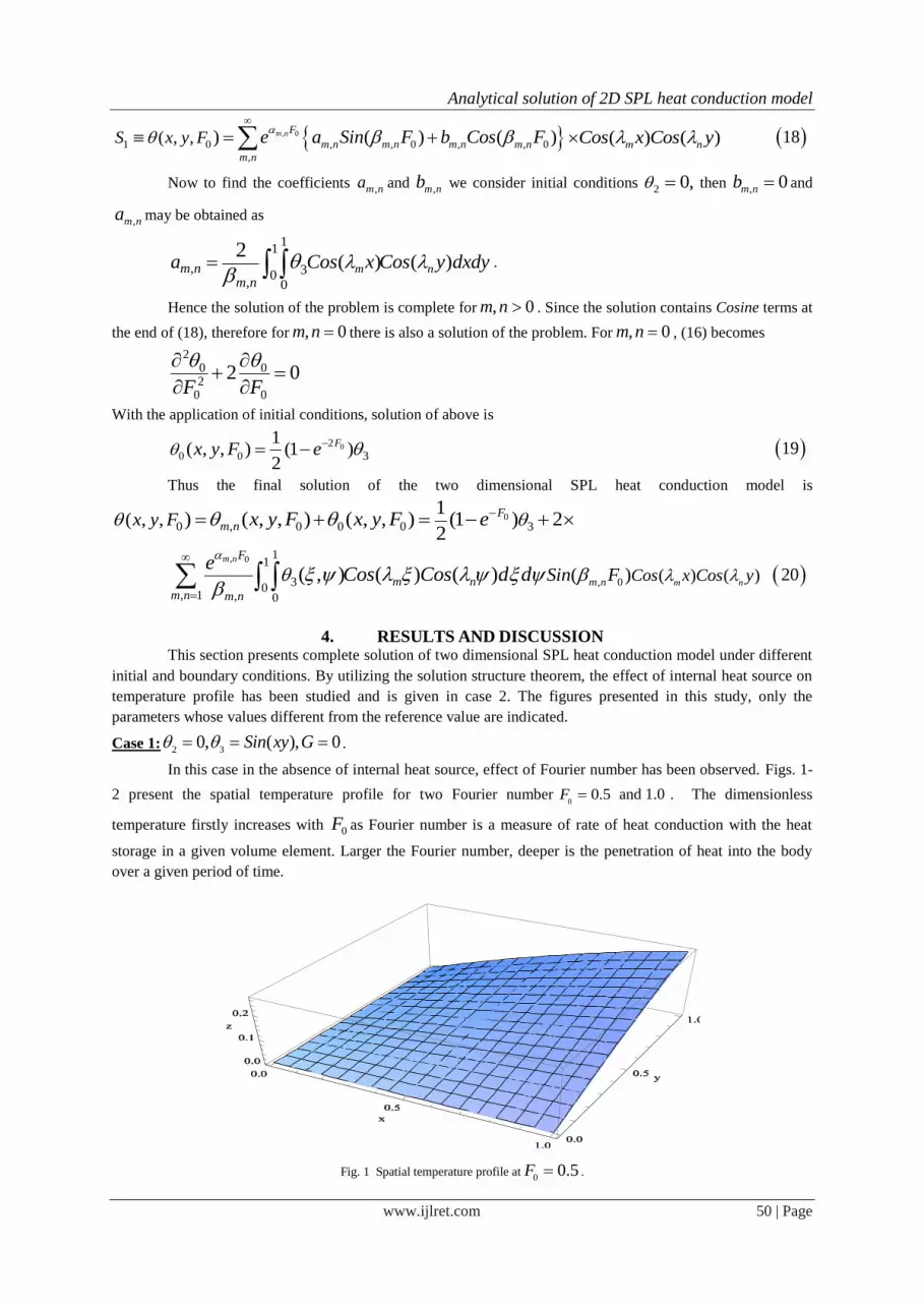
In this case in the absence of internal heat source, effect of Fourier number has been observed. Figs. 1-

2 present the spatial temperature profile for two Fourier number0

0.5F and 1.0 . The dimensionless

temperature firstly increases with 0F as Fourier number is a measure of rate of heat conduction with the heat

storage in a given volume element. Larger the Fourier number, deeper is the penetration of heat into the body

over a given period of time.

Fig. 1 Spatial temperature profile at0

0.5F .




2.0F .


1.0, 0.5, 5F .


1.0, 0.5, 15F .



Fig. 5 Spatial temperature profile at 0

1.0, 10, 0.1F .

Fig. 6 Spatial temperature profile at 0

1.0, 10, 1.0F .

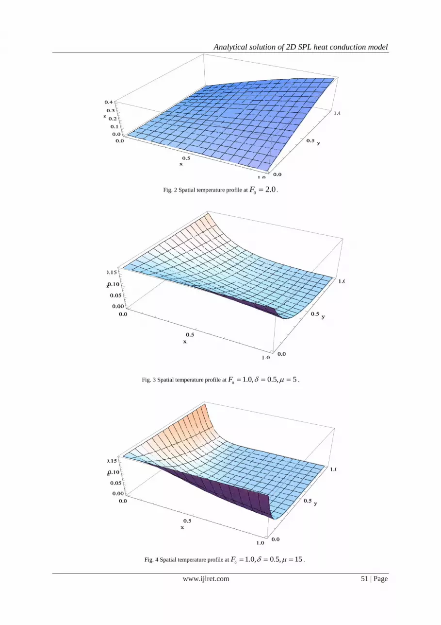
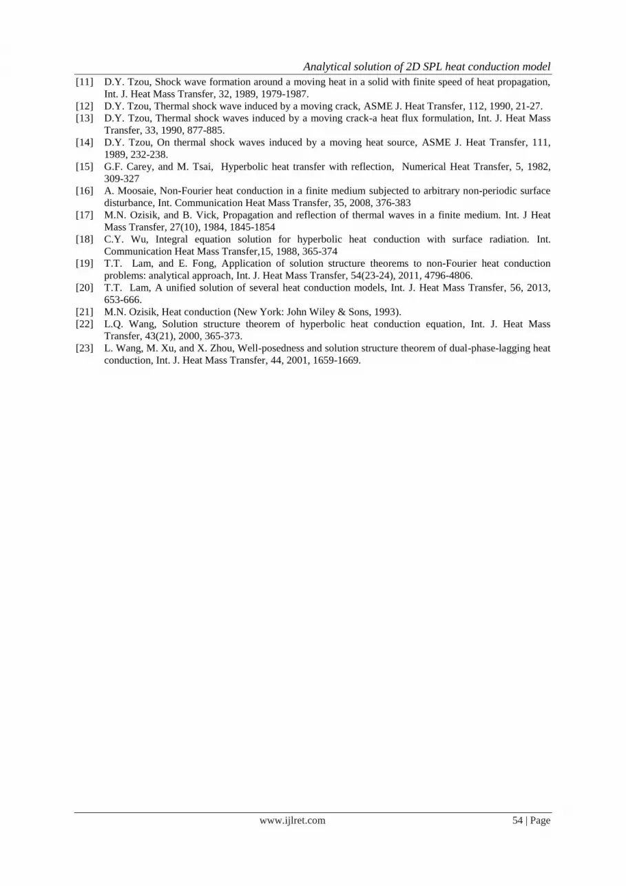
Case 2: 0

2 30, 0,

FxyG e e

.

This case is devoted to the effect of internal heat source on the temperature profile. Heat source is

modelled as time varying and spatially decaying. The spatial temperature profile for various absorption

coefficients at fixed Fourier number0

1.0F and laser pulse fall-time 0.5 is given in Figs. 3-4. Due

to the spatially decaying nature of heat source, if we move towards end of both the spatial direction of thin plate,

then the amount of heat entered into the body decreases and hence dimensionless temperature decreases with

increase of absorption coefficient, as shown in Figs. 3-4.

Figs. 5-6 present the effect of laser pulse fall-time on spatial temperature profile at fixed absorption

coefficient and Fourier number. For fixed Fourier number, as laser pulse fall-time increases the amount of heat

entered into the body decreases, due to which dimensional temperature into the body decreases.

5. CONCLUSION The mathematical model describing heat transfer in a thin plate based on single-phase-lagging heat

conduction is solved by superposition technique. The solution was obtained by utilizing superposition technique,

structure theorem and Fourier series expansion. The effect of Fourier number, absorption coefficient and laser



pulse fall time parameter on temperature profile has been observed. The temperature increases with increase of

Fourier number and laser pulse fall time parameter but decreases with absorption coefficient.

This technique is very applicable for solving non-homogeneous partial differential equation under

most generalized boundary conditions and may be applicable for solving the higher dimensional SPL heat

conduction model of general body.

6. NOMENCLATURE c Thermal wave propagation speed

/m s

bc Specific heat capacity / .J kg K

rf Reference heat flux / *q q

0F Fourier number 2

/ 2c t

*g Internal heat source 3/W m

g Dimensionless heat source

4 * /r

g cf

k Thermal conductivity / .W m K

*q Dimensionless heat flux /

rfq

r Position vector

t Time s

T Temperature K

T Temperature gradient /K m

*x Spatial coordinate m

x Dimensionless spatial

coordinate */ 2cx

*y Dimensionless spatial

coordinate */ 2cy

y Spatial coordinate m

Thermal diffusivity 2/m s

* Thermal diffusivity 1/ s

Dimensionless laser pulse fall-

time parameter *2

q

Dimensionless Temperature

/r

kcT f

* Thermal diffusivity 1/ m

Dimensionless absorption

coefficient *2 qc

Density 3/kg m

q Phase-lag of heat flux s

7. Acknowledgement Author is thankful to DST-CIMS, BHU for providing necessary facilities during the manuscript.

REFERENCES [1] C. Cattaneo, Sur une forme de I'Equation de la chaleur elinant le paradox d'une propagation instantance,

C. R. Acad. Sci. 247, 1958, 431-433.

[2] M.P. Vernotte, Les paradoxes de la theorie continue de I’ equation de la chleur, C. R. Acad. Sci., 246,

1958, 3154-3155.

[3] D.Y. Tzou, Macro-to-microscale heat transfer: the lagging behavior (Washington: Taylor & Francis,

1996).

[4] D.G. Cahill, W.K. Ford, K.E. Goodson, G.D. Mahan, A. Majumdar, H.J. Maris, R. Merlin, and S.R.

Phillpot, Nanoscale thermal transport, J. Appl. Phys., 93, 2003, 793-818.

[5] A.A. Joshi, and A. Majumdar, Transient ballistic and diffusive phonon heat transport in thin films, J.

Appl. Phys., 74, 1993, 31-39.

[6] C.L. Tien, A. Majumdar, and F.M. Gerner, Microscale energy transport (Washington: Taylor & Francis,

1998).

[7] L.Q. Wang, Xu Zhou, and X. Wei, Heat conduction: mathematical models and analytical solutions

(Berlin: Springer-Verlag, 2008).

[8] D.D. Joseph, and L. Preziosi, Heat waves, Rev. Mod. Phys., 61, 1989, 41-73.

[9] M.N. Ozisik, and D.Y. Tzou, On the wave theory in heat conduction, ASME J. Heat Transfer, 116(3),

1994, 526-535.

[10] D.Y. Tzou, Thermal shock phenomena under high rate response in solids, Annual Review of Heat

Transfer, 4, 1992, 111-185.



[11] D.Y. Tzou, Shock wave formation around a moving heat in a solid with finite speed of heat propagation,

Int. J. Heat Mass Transfer, 32, 1989, 1979-1987.

[12] D.Y. Tzou, Thermal shock wave induced by a moving crack, ASME J. Heat Transfer, 112, 1990, 21-27.

[13] D.Y. Tzou, Thermal shock waves induced by a moving crack-a heat flux formulation, Int. J. Heat Mass

Transfer, 33, 1990, 877-885.

[14] D.Y. Tzou, On thermal shock waves induced by a moving heat source, ASME J. Heat Transfer, 111,

1989, 232-238.

[15] G.F. Carey, and M. Tsai, Hyperbolic heat transfer with reflection, Numerical Heat Transfer, 5, 1982,

309-327

[16] A. Moosaie, Non-Fourier heat conduction in a finite medium subjected to arbitrary non-periodic surface

disturbance, Int. Communication Heat Mass Transfer, 35, 2008, 376-383

[17] M.N. Ozisik, and B. Vick, Propagation and reflection of thermal waves in a finite medium. Int. J Heat

Mass Transfer, 27(10), 1984, 1845-1854

[18] C.Y. Wu, Integral equation solution for hyperbolic heat conduction with surface radiation. Int.

Communication Heat Mass Transfer,15, 1988, 365-374

[19] T.T. Lam, and E. Fong, Application of solution structure theorems to non-Fourier heat conduction

problems: analytical approach, Int. J. Heat Mass Transfer, 54(23-24), 2011, 4796-4806.

[20] T.T. Lam, A unified solution of several heat conduction models, Int. J. Heat Mass Transfer, 56, 2013,

653-666.

[21] M.N. Ozisik, Heat conduction (New York: John Wiley & Sons, 1993).

[22] L.Q. Wang, Solution structure theorem of hyperbolic heat conduction equation, Int. J. Heat Mass

Transfer, 43(21), 2000, 365-373.

[23] L. Wang, M. Xu, and X. Zhou, Well-posedness and solution structure theorem of dual-phase-lagging heat

conduction, Int. J. Heat Mass Transfer, 44, 2001, 1659-1669.

Documents

Analytical solution of 2D SPL heat conduction model