.

GROUND-ROLL ATTENUATION USING A 2D TIME

DERIVATIVE FILTER

Paulo E. M. Melo

Milton J. Porsani

Michelangelo G. Silva

Centro de Pesquisa em Geofısica e Geologia.

Instituto de Geociencias, Universidade Federal da Bahia.

Campus Universitario da Federacao

Salvador, Bahia, Brasil.

1

ABSTRACT

We present a new filtering method for attenuation of ground-roll. The method

is based on the application of a bi-dimensional filter for obtaining the time-

derivative of the seismograms. Before convolving the filter with the input data

matrix, the normal move-out (NMO) correction is applied to the seismograms

with the purpose of flattening the reflections. The method can locally attenu-

ate the amplitude of data of low frequency (in the ground-roll and stretch NMO

region) and enhance flat events (reflections). The filtered seismograms can re-

veal horizontal or sub-horizontal reflections while vertical or sub-vertical events,

associated with ground-roll, are attenuated. A regular set of samples around

each neighborhood data sample of the seismogram is used to estimate the time-

derivative. A numerical approximation of the derivative is computed by taking

the difference between the interpolated values calculated in both the positive

and the negative neighborhood of the desired position. The coefficients of the

2D time-derivative filter are obtained by taking the difference between two fil-

ters that interpolate at positive and negative times. Numerical results which use

real seismic data, show that the proposed method is effective and can reveal re-

flections masked by the ground-roll. Another benefit of the method is that the

stretch mute, normally applied after the normal move-out correction, is unnec-

essary. The new filtering approach provides results of outstanding quality, when

compared to results obtained from the conventional FK filtering method.

2

INTRODUCTION

In seismic exploration, the noise present in seismograms with trace-to-trace reg-

ularity is classified as coherent noise. Among these types of noise, ground-roll,

present in land and ocean bottom seismic surveys, is responsible for a signifi-

cant reduction in the signal-to-noise ratio. The ground-roll is associated with

Rayleigh-type surface waves that occur in the zone of low velocity near the sur-

face (Yilmaz, 1987). It occurs in land and ocean bottom seismic data dominating

some portions of the seismograms, interfering and, therefore masking the seismic

reflections of interest. The attenuation or removal of this kind of noise represents

a serious obstacle to the processing of seismic data. The main characteristics of

this noise are its high amplitude, low velocity, dispersion and the concentration

of energy in the low frequencies.

Several papers have been published in the geophysics literature investigating

methods for attenuation of the ground roll. Some of them show that the ground

roll can be attenuated during the acquisition, through special source and receiver

arrays (Anstey, 1986; Pritchett, 1991). Such a strategy may have logistical limi-

tations or be unusable on data already acquired (Harlan et al., 1984; Shieh and

Herrmann, 1990). Other authors have tried new approaches based on filtering

methods applied in the frequency, Radon or wavelet domains, or have applied

numerical transformations such as Karhunen-Loeve and SVD, or have used po-

larization filters and multi-component data (Claerbout, 1983; Saatcilar, 1988;

Song and Stewart, 1993; Liu, 1999, Henley, 2003, Kendall et al, 2005; Yarham et

al 2006). One of the simplest filtering approaches used in the ground roll atten-

uation problem, is FK filtering, based on the 2D Fourier transform (Embree et

al., 1963; Wiggins, 1966). The ground-roll, represented by linear events with low

velocities, is mapped as lines in the FK domain and consequently can be filtered

by using a 2D band-pass filter.

Although the FK method is effective in the removal of linear events, it also

3

attenuates any primary reflected signals present in the frequency band and dip

range of the ground-roll.

This paper presents a new filtering method for ground-roll attenuation using

a 2D time-derivative filter. Before convolving the filter with the data matrix,

the normal move-out (NMO) correction is applied to the seismograms with the

purpose of flattening the reflections. We illustrate the method by using land

seismic data from the Tacutu basin, located in the northeast of Brazil. The

seismic data was acquired by PETROBRAS, in 1981 (Eiras and Kinoshita, 1990).

This paper is organized in the following way: First we present the method which

is used to generate the 2D derivative filter. Next we present numerical results

using real seismic data. Finally, we present the conclusions.

A 2D TIME DERIVATIVE FILTER

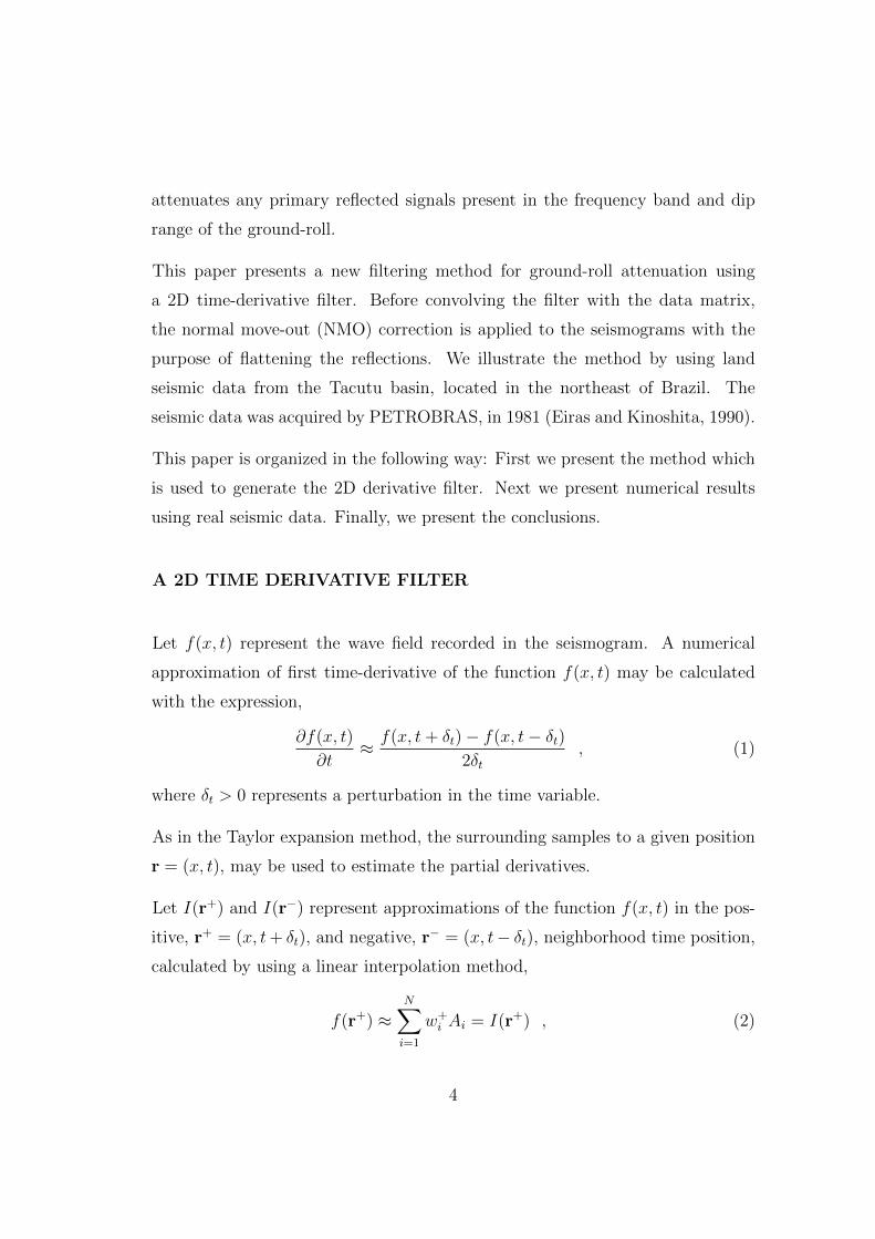
Let f(x, t) represent the wave field recorded in the seismogram. A numerical

approximation of first time-derivative of the function f(x, t) may be calculated

with the expression,

∂f(x, t)

∂t≈ f(x, t+ δt)− f(x, t− δt)

2δt, (1)

where δt > 0 represents a perturbation in the time variable.

As in the Taylor expansion method, the surrounding samples to a given position

r = (x, t), may be used to estimate the partial derivatives.

Let I(r+) and I(r−) represent approximations of the function f(x, t) in the pos-

itive, r+ = (x, t+ δt), and negative, r− = (x, t− δt), neighborhood time position,

calculated by using a linear interpolation method,

f(r+) ≈N∑i=1

w+i Ai = I(r+) , (2)

4

f(r−) ≈N∑i=1

w−i Ai = I(r−) , (3)

where:

N is the number of data samples used in the linear interpolation;

Ai represents the amplitude of the input data matrix at position ri, taken in the

neighborhood of the desired position r, and

{w+i , w

−i } represents the coefficients used in the interpolation at positions r+

and r− respectively.

Using equations (2) and (3) in equation (1) we obtain,

∂f(x, t)

∂t≈ I(r+)− I(r−)

2δt=

N∑i=1

(w+i − w−

i )

2δtAi . (4)

Equation (4) gives a numerical approximation of the time derivative, from the

difference between the interpolated values taken at two positions close to the

desired position. In order to evaluate directly the time-derivative by using only

one 2D filter, we combine the coefficients of the two interpolation operators into

one,

Dt = O+ −O− =

{(w+

i − w−i )

2δt, i = 1, . . . , N

}. (5)

The computational implementation is simplified by considering the data matrix

(seismograms) as corresponding to a regular grid. In this case we may design

a 2D filter and the derivative may be obtained by convolving it with the data

matrix. The first derivative with respect to time is given by,

A′

t = A ∗Dt , (6)

where ∗ represents the convolution, Dt represents the 2D filter to evaluate the

first derivative, and A represents the (Nt×Nx) input data matrix associated with

5

the seismograms. The first derivative filter can be applied in cascade to generate

higher order derivatives.

The derivative with respect to the spatial variable (x), if desired, may be obtained

in a similar way. In the case of a regular grid, with equal x and t sampling interval,

we can use the transpose of the operator, or the transpose of the data matrix to

obtain the derivative with respect to the x variable,

A′

x = DTt ∗A = Dt ∗AT . (7)

Obtaining the interpolation weights

A very simple approach to compute the weights wi, required in equations (2) and

(3), is given by the Shepard method (Shepard, 1968). By using this method we

can compute the interpolation weights based on the inverse of the distance,

wj =

1

dj∑Ni=1

1

di

. (8)

where di = |r− ri| represents the distance between the position (r) of the desired

output where we want to interpolate, and the data position (ri). It can be shown

that the Shepard method reproduces the data values at its original positions, i.e.,

I(ri) = Ai.

In case of a regular grid, the coefficients wi of an N ×N interpolation operator

need to be generated only once, and applied to all data matrix by means of con-

volution, making the interpolation method simple and computationally efficient.

Equation (8) may be used in the computation of the weights w+i and w−

i required

in equation (5). We point out that the proposed method may be used to generate

2D operators to evaluate the derivative in any direction.

6

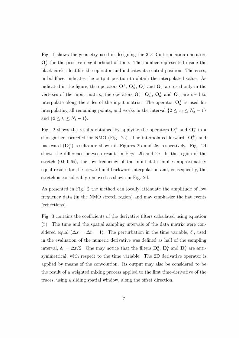
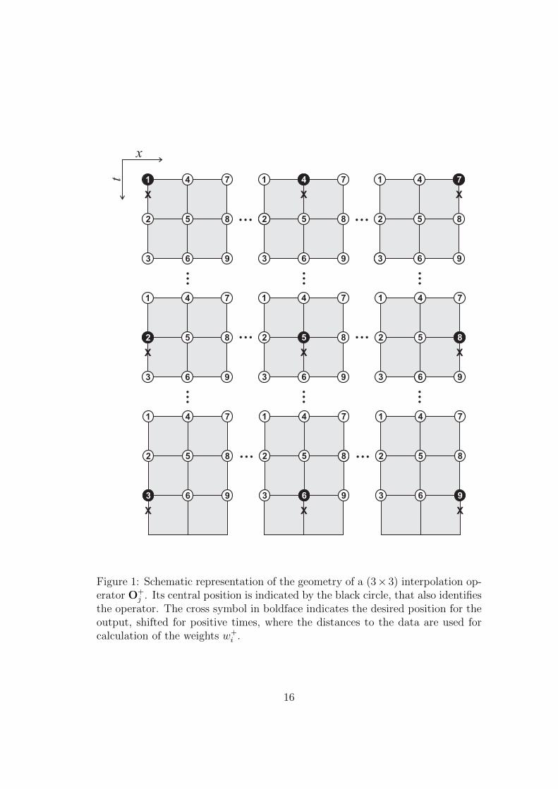
Fig. 1 shows the geometry used in designing the 3 × 3 interpolation operators

O+j for the positive neighborhood of time. The number represented inside the

black circle identifies the operator and indicates its central position. The cross,

in boldface, indicates the output position to obtain the interpolated value. As

indicated in the figure, the operators O+1 , O+

3 , O+7 and O+

9 are used only in the

vertexes of the input matrix; the operators O+2 , O+

4 , O+6 and O+

8 are used to

interpolate along the sides of the input matrix. The operator O+5 is used for

interpolating all remaining points, and works in the interval {2 ≤ xi ≤ Nx − 1}and {2 ≤ ti ≤ Nt − 1}.

Fig. 2 shows the results obtained by applying the operators O+j and O−

j in a

shot-gather corrected for NMO (Fig. 2a). The interpolated forward (O+j ) and

backward (O−j ) results are shown in Figures 2b and 2c, respectively. Fig. 2d

shows the difference between results in Figs. 2b and 2c. In the region of the

stretch (0.0-0.6s), the low frequency of the input data implies approximately

equal results for the forward and backward interpolation and, consequently, the

stretch is considerably removed as shown in Fig. 2d.

As presented in Fig. 2 the method can locally attenuate the amplitude of low

frequency data (in the NMO stretch region) and may emphasize the flat events

(reflections).

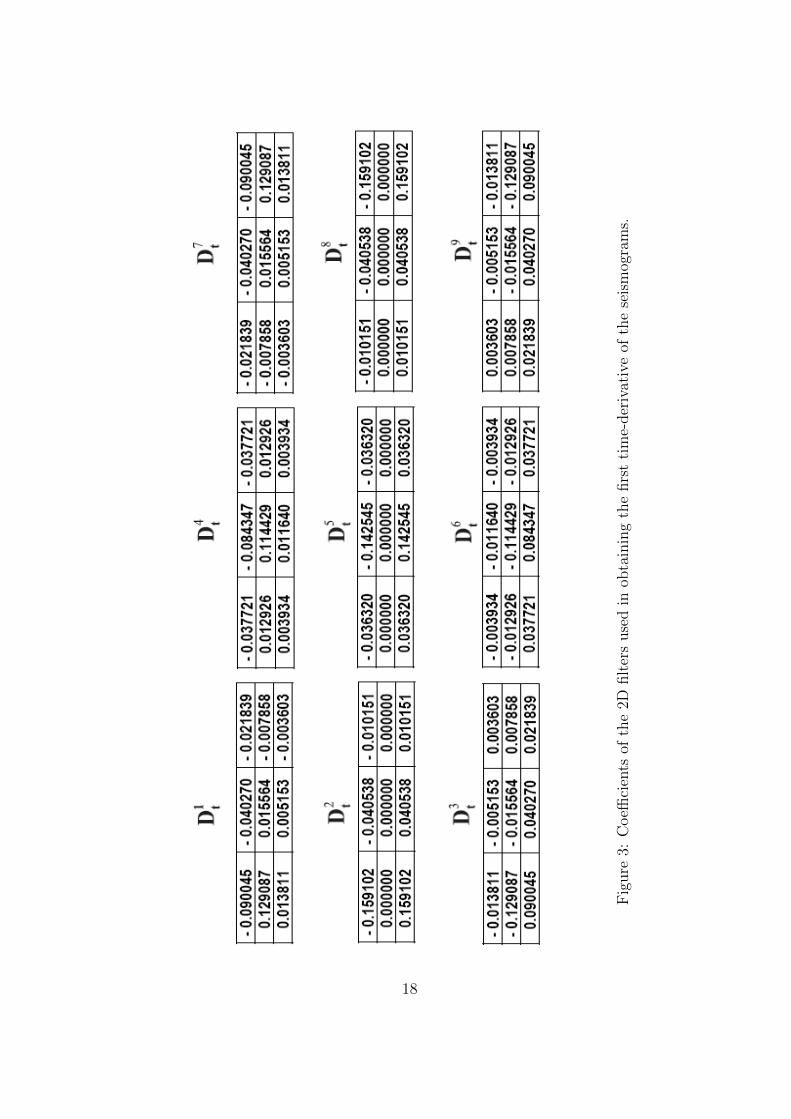
Fig. 3 contains the coefficients of the derivative filters calculated using equation

(5). The time and the spatial sampling intervals of the data matrix were con-

sidered equal (∆x = ∆t = 1). The perturbation in the time variable, δt, used

in the evaluation of the numeric derivative was defined as half of the sampling

interval, δt = ∆t/2. One may notice that the filters D2t , D5

t and D8t are anti-

symmetrical, with respect to the time variable. The 2D derivative operator is

applied by means of the convolution. Its output may also be considered to be

the result of a weighted mixing process applied to the first time-derivative of the

traces, using a sliding spatial window, along the offset direction.

7

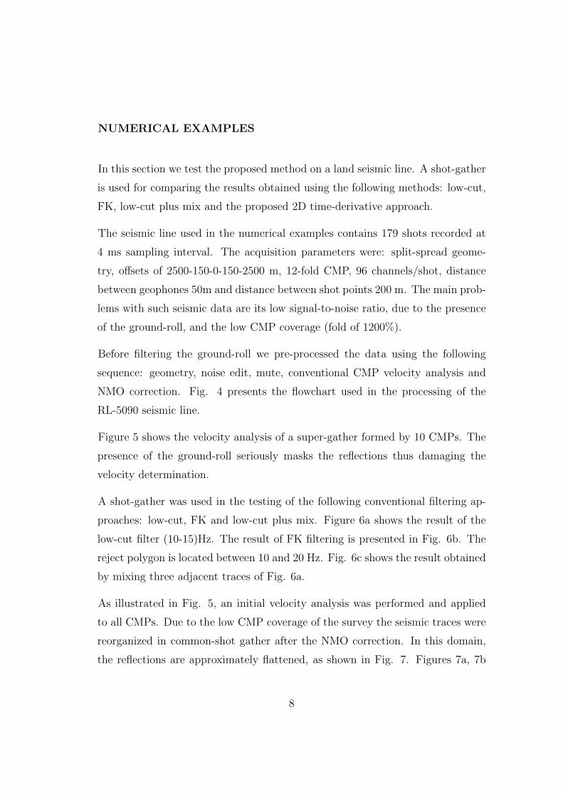
NUMERICAL EXAMPLES

In this section we test the proposed method on a land seismic line. A shot-gather

is used for comparing the results obtained using the following methods: low-cut,

FK, low-cut plus mix and the proposed 2D time-derivative approach.

The seismic line used in the numerical examples contains 179 shots recorded at

4 ms sampling interval. The acquisition parameters were: split-spread geome-

try, offsets of 2500-150-0-150-2500 m, 12-fold CMP, 96 channels/shot, distance

between geophones 50m and distance between shot points 200 m. The main prob-

lems with such seismic data are its low signal-to-noise ratio, due to the presence

of the ground-roll, and the low CMP coverage (fold of 1200%).

Before filtering the ground-roll we pre-processed the data using the following

sequence: geometry, noise edit, mute, conventional CMP velocity analysis and

NMO correction. Fig. 4 presents the flowchart used in the processing of the

RL-5090 seismic line.

Figure 5 shows the velocity analysis of a super-gather formed by 10 CMPs. The

presence of the ground-roll seriously masks the reflections thus damaging the

velocity determination.

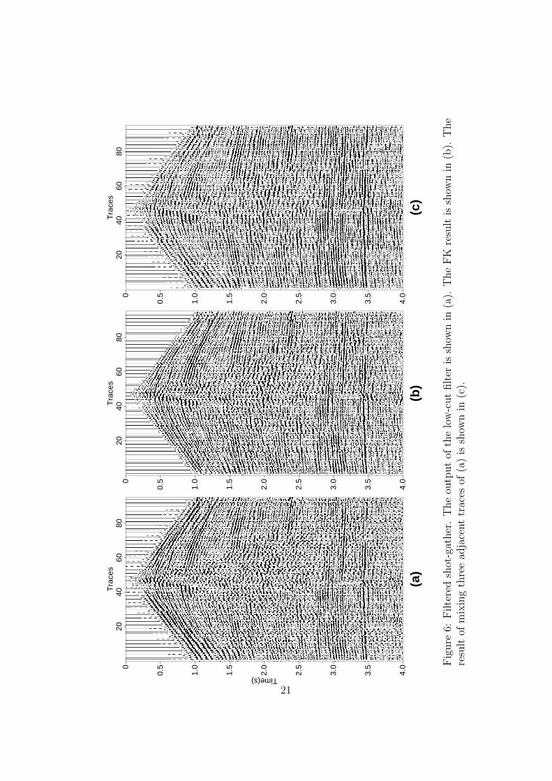
A shot-gather was used in the testing of the following conventional filtering ap-

proaches: low-cut, FK and low-cut plus mix. Figure 6a shows the result of the

low-cut filter (10-15)Hz. The result of FK filtering is presented in Fig. 6b. The

reject polygon is located between 10 and 20 Hz. Fig. 6c shows the result obtained

by mixing three adjacent traces of Fig. 6a.

As illustrated in Fig. 5, an initial velocity analysis was performed and applied

to all CMPs. Due to the low CMP coverage of the survey the seismic traces were

reorganized in common-shot gather after the NMO correction. In this domain,

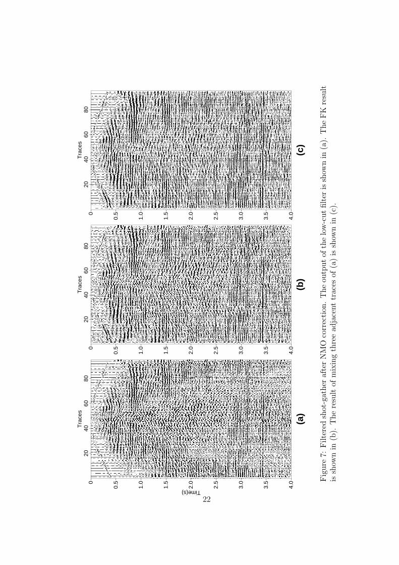
the reflections are approximately flattened, as shown in Fig. 7. Figures 7a, 7b

8

and 7c show the output of the low-cut, FK and the trace mix approach applied

to the shot-gather with NMO correction. We observe that the stretched data in

the interval 0.0-0.6s was considerably attenuated.

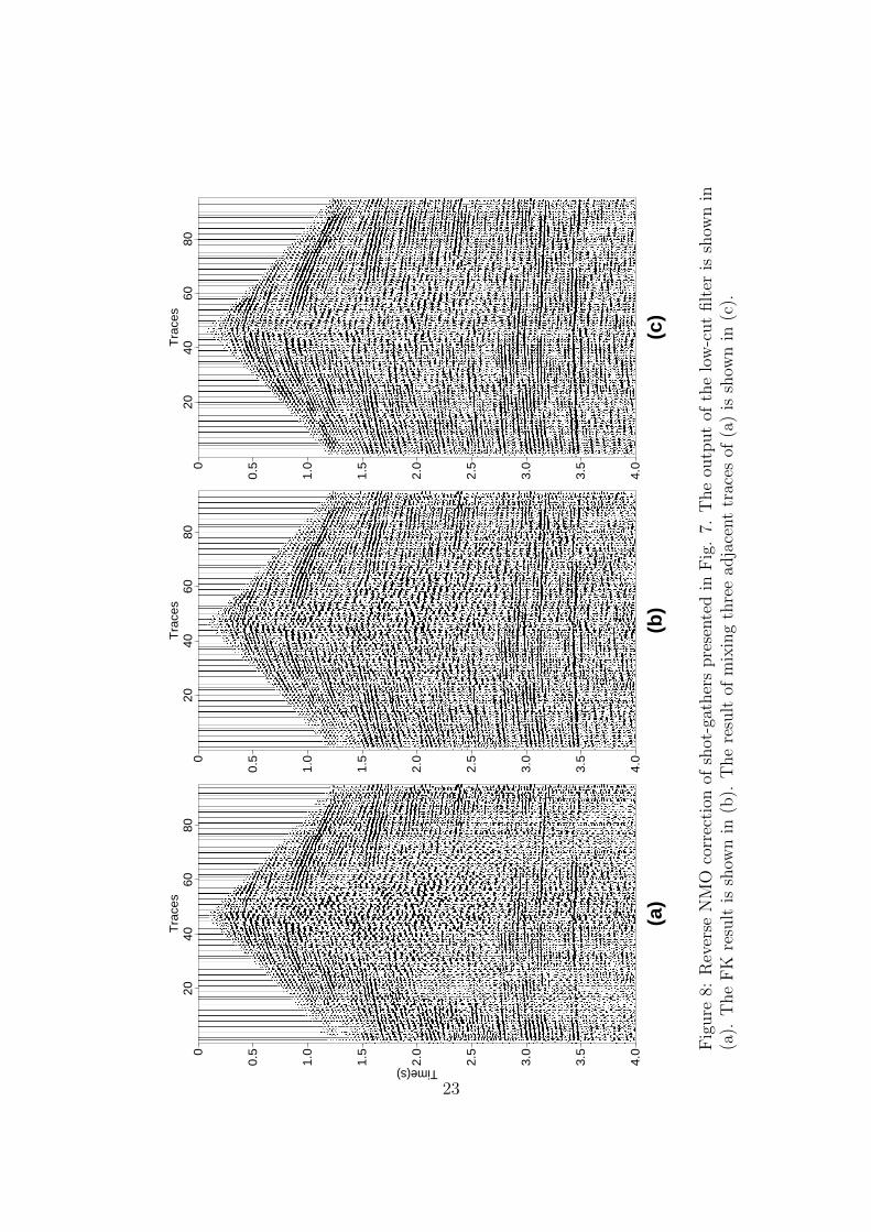
By applying the reverse NMO to the data shown in Fig. 7 we obtain the filtered

shot-gathers shown in Fig. 8. These results should be compared with Fig. 6.

The improvement in the signal-to-noise ratio, obtained specially in the region of

the shallow reflections, between 0.0-1.3s may be observed in Figs. 8a, 8b, and

8c. All three filtering approaches give better results when applied after the NMO

correction. They take advantage of the horizontal coherence of the reflections

generated by the NMO correction. As the ground-roll is not flattened by the

NMO correction, it is partially attenuated during the 2D filtering process, as

indicated by the low-cut plus mix results, shown in Fig. 8c.

In the next examples we illustrate the application of the 2D time-derivative ap-

proach to attenuate ground-roll and at the same time to reinforce the reflections.

The filtering was applied to shot-gathers after NMO correction. We used the

initial velocity obtained from the velocity analysis of super-gathers formed by 10

CMPs, as presented in Fig. 5.

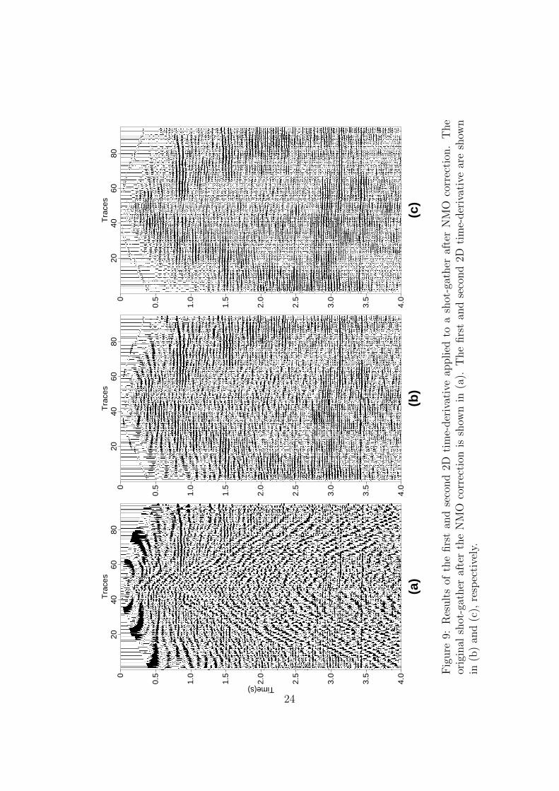
Fig. 9 shows the results of the 2D first and second time-derivative of the shot-

gather used in the numerical experiments. The input data matrix, formed by

the shot-gather corrected from the NMO, is shown in Fig. 9a. The filtered

seismograms, using the first and second 2D time-derivative, are shown in Figs.

9b and 9c, respectively. Fig. 9b was used as input data to compute the second

derivative. In addition to the attenuation of the ground-roll and the enhancement

of the underlying reflections, a reduction of NMO stretch can be seen.

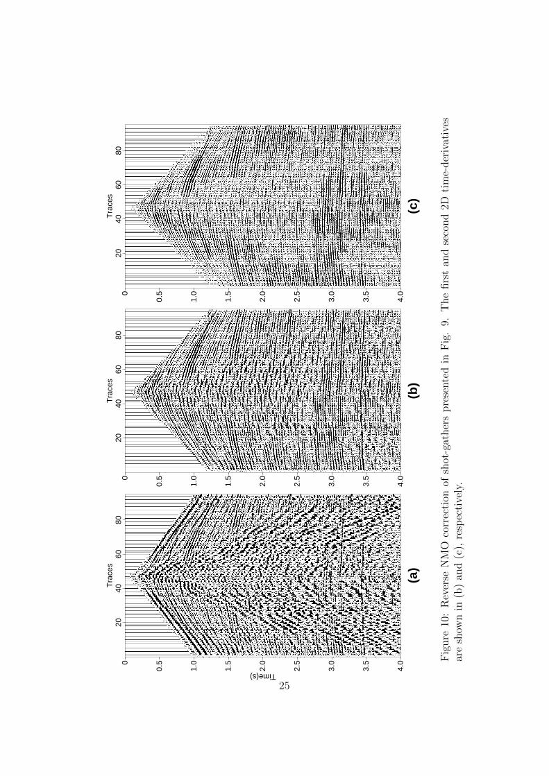
Fig. 10 shows the original and the filtered common-shot gathers after applying

the reverse NMO correction. The original seismograms are shown in Fig. 10a

and the results obtained using the first and second 2D time-derivatives are shown

in Fig. 10b and Fig. 10c, respectively. The ground-roll was practically removed,

9

thus improving the signal-to-noise ratio and the lateral continuity of the reflection,

formerly masked by noise.

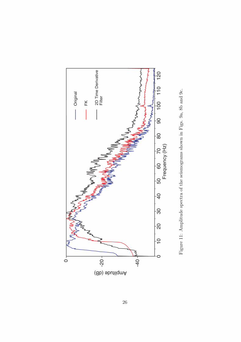
Fig. 11 shows the amplitude spectrum of the original and the filtered seismograms

obtained using the FK and the time-derivative methods. When comparing the

curves of Fig. 11, one notices that the new 2D time-derivative filtering approach

produces attenuation of the amplitude spectrum in the frequency band of the

ground-roll and an increase of high frequency signal. This is not seen in the

amplitude spectrum after FK filtering, which produces a severe cut in the low

frequency band of the ground-roll.

As a consequence of the computational manipulation of the original seismograms

(direct NMO, 2D time-derivative and reverse NMO) the waveform was affected

and an additional filtering step can be applied to recover the original wavelet.

That transformation may be performed by using the conventional least-squares

shaping filter following the steps: (i) estimate the autocorrelation coefficients

associated with the bandwidth frequency of the wavelet 15-50Hz, of the input

(Fig. 10a) and output seismograms (Fig. 10c); (ii) compute the minimum-phase

wavelets associated with the original and the filtered seismograms; compute the

shaping filter to recover the minimum-phase wavelet of the input seismograms,

and (iv) convolve the shaping filter with the filtered seismograms (Robinson and

Treitel, 1980; Porsani, 1996).

Figure 12 shows the super-gather presented in Fig. 5, after applying the 2D

filtering method, and its corresponding velocity analysis. A better definition of

the velocities in the semblance plot may be observed. Results as good as this

could probably be obtained by using the low-cut plus mix and the FK filtering

approaches.

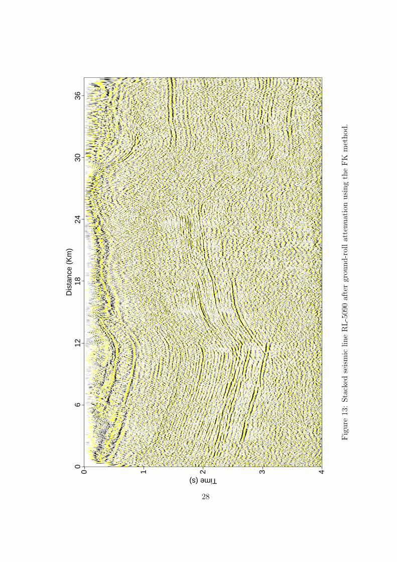
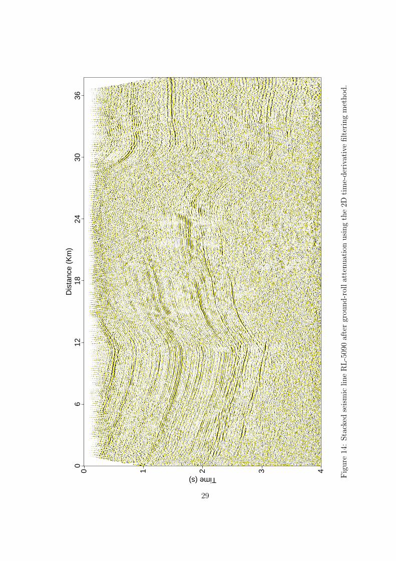
Figures 13 and 14 show respectively the stacked seismic section after ground-

roll attenuation using the FK method and the new approach. A mute was not

applied to the data, before the stacking. The same velocity function was used for

10

the CMP stacking. The improvement in the definition of the reflectors is visible

throughout the whole section. Better resolution and better lateral continuity can

be seen in Fig. 14.

CONCLUSIONS

We present a new filtering method for the attenuation of ground-roll. The new

method is based on the 2D time-derivative of the seismograms applied after NMO

correction. The NMO correction makes the reflections approximately horizontal,

thus generating ideal conditions for 2D or multichannel filters, which take advan-

tage of the lateral coherence between the reflections. As the ground-roll is not

flattened by the NMO correction, its contribution will be reduced after the 2D

filtering process. The main problem with the NMO correction, is the difficulty of

making the initial velocity analysis in the presence of the ground-roll.

The 2D filter coefficients are calculated once, and the filter is applied to the

whole data set by means of convolution, making the method computationally

very efficient. Numerical results using real data demonstrate its effectiveness for

the attenuation of the ground-roll. Additionally, the 2D time-derivative filtering

method also attenuates NMO stretch, increases the signal-to-noise ratio, and

improves resolution. The attenuation of the ground-roll and the recovery of the

underlying reflections can lead to improved velocity analysis on filtered CMPs.

The final stacked section has higher resolution and lateral continuity, compared

to the results obtained using the conventional FK method. New applications and

extensions of the method for 2D or multidimensional directional filtering, using

pre or post-stacking data, can be implemented.

11

ACKNOWLEDGEMENTS

The authors wish to express their gratitude to the Editor in Chief Dr. Tij-

men J. Moser and the Associate Editor Dr. John Sunderland as well as the

anonymous referees for constructive comments. We also thank FINEP, FAPESB,

PETROBRAS, ANP and CNPq, Brazil, for financial support and PARADIGM,

LANDMARK and SEISMIC-MICRO TECHNOLOGY for educational licenses

granted to the Centro de Pesquisa em Geofısica e Geologia (CPGG-UFBA).

REFERENCES

Anstey, N. 1986. Whatever happened to ground-roll? The Leading Edge 5, 40-46.

Claerbout, J. F. 1983. Ground Roll and radial traces. Stanford Exploration Project

Report, SEP-35, 43-53.

Eiras, J. F. and Kinoshita, E. M. 1990. Geologia e perspectivas petrolıferas da

Bacia do Tacutu, Origem e Evolucao das Bacias Sedimentares. PETROBRAS,

Anais, 197-220.

Embree, P., Burg, J. P. and Backus, M. M. 1963. Wide-band velocity filtering -

the pie-slice process. Geophysics 28, 948-974.

Harlan, W. S., Claerbout J. F. and Rocca F. 1984. Signal/noise separation and

velocity estimation. Geophysics 49, 1869-1880.

Henley, D. C. 2003. Coherent noise attenuation in the radial trace domain. Geo-

physics 68, 1408-1416.

Kendall, R., Jin, S. and Ronen, S. 2005. An SVD-polarization filter for ground

roll attenuation on multicomponent data. SEG meeting, Expanded Abstracts,

928-931.

12

Liu, X. 1999. Ground roll suppression using the Karhunen-Loeve transform. Geo-

physics 64, 564.

Porsani, M., 1996. Fast algorithms to design discrete Wiener filters in lag and

length coordinates. Geophysics, bf 61, 882-890.

Pritchett, W. 1991. System design for better seismic data. The Leading Edge 11,

30-35.

Robinson, E. A. and Treitel, S. 1980. Geophysical signal analysis. Prentice-Hall,

Inc.

Saatcilar, R. and Canitez, N. 1988. A method of ground-roll elimination. Geo-

physics 53, 894.

Shepard, D. 1968. A two-dimensional interpolation function for irregularly spaced

data. Proc. 23rd nat. Conf. ACM, 517-523 Brandon/Systems Press Inc., Prince-

ton.

Shieh, C. and Herrmann, R. B. 1990. Ground roll: Rejection using polarization

filters: Geophysics 55.

Song, Y. and Stewart, R. R. 1993. Ground roll rejection via f-v filtering: CREWES

Research Report, 5.

Wiggins, R. A. 1966. W-K Filter design. Geophysical Prospecting 14, 427-440.

Yarham, C., Boeniger, U. and Herrmann, f. 2006. Curvelet-based ground roll

removal. SEG meeting, New Orleans, Expanded Abstracts, 2777-2780.

Yilmaz, O. 1987. Seismic Data Processing: Society of Exploration Geophysicists.

13

FIGURES

FIG. 1. Schematic representation of the geometry of a (3 × 3) interpolation

operator O+j . Its central position is indicated by the black circle, that also

identifies the operator. The cross symbol in boldface indicates the desired

position for the output, shifted for positive times, where the distances to

the data are used for calculation of the weights w+i .

FIG. 2. Original shot-gather after NMO correction in (a). Forward interpola-

tion using O+j in (b). Backward interpolation using O−

j in (c). Difference

between results in (b) and (c) is shown in (d).

FIG. 3. Coefficients of the 2D filters used in obtaining the first time-derivative

of the seismograms.

FIG. 4.Flowchart of the seismic processing used in obtaining of the stacked

section.

FIG. 5. Super-gather formed by 10 CMPs in (a) and its corresponding velocity

analysis in (b).

FIG. 6. Filtered shot-gather. The output of the low-cut filter is shown in (a).

The FK result is shown in (b). The result of mixing three adjacent traces

of (a) is shown in (c).

FIG. 7. Filtered shot-gather after NMO correction. The output of the low-cut

filter is shown in (a). The FK result is shown in (b). The result of mixing

three adjacent traces of (a) is shown in (c).

FIG. 8. Reverse NMO correction of shot-gathers presented in Fig. 7. The

output of the low-cut filter is shown in (a). The FK result is shown in (b).

The result of mixing three adjacent traces of (a) is shown in (c).

14

FIG. 9. Results of the first and second 2D time-derivative applied to a shot-

gather after NMO correction. The original shot-gather after the NMO

correction is shown in (a). The first and second 2D time-derivative are

shown in (b) and (c), respectively.

FIG. 10. Reverse NMO correction of shot-gathers presented in Fig. 9. The first

and second 2D time-derivatives are shown in (b) and (c), respectively.

FIG. 11. Amplitude spectra of the seismograms shown in Figs. 9a, 8b and 9c.

FIG. 12. Super-gather shown in Fig. 5 filtered using the 2D derivative approach

is shown in (a) and its corresponding velocity analysis in (b).

FIG. 13. Stacked seismic line RL-5090 after ground-roll attenuation using the

FK method.

FIG. 14. Stacked seismic line RL-5090 after ground-roll attenuation using the

2D time-derivative filtering method.

15

1

2

3

4

5

6

7

8

9

1

2

3

4

5

6

7

8

9

4 1

2

3

4

5

6

7

8

9

7

x

t

2

3

X X X

... ...

1

2

3

5

6

7

8

9

1

2

3

4

5

6

7

8

9

1

2

3

4

5

6

7

8

9

2 8

6

4

X X X

... ...

1

2

3

4

5

6

8

9

1

2

3

4

5

6

7

8

9

1

2

3

4

5

6

7

8

93

8

6

7

X X X

... ...

...

...

...

...

...

...

Figure 1: Schematic representation of the geometry of a (3× 3) interpolation op-erator O+

j . Its central position is indicated by the black circle, that also identifiesthe operator. The cross symbol in boldface indicates the desired position for theoutput, shifted for positive times, where the distances to the data are used forcalculation of the weights w+

i .

16

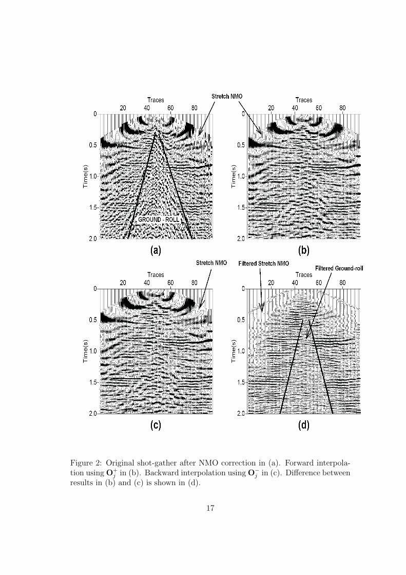
Figure 2: Original shot-gather after NMO correction in (a). Forward interpola-tion using O+

j in (b). Backward interpolation using O−j in (c). Difference between

results in (b) and (c) is shown in (d).

17

Fig

ure

3:C

oeffi

cien

tsof

the

2Dfilt

ers

use

din

obta

inin

gth

efirs

tti

me-

der

ivat

ive

ofth

ese

ism

ogra

ms.

18

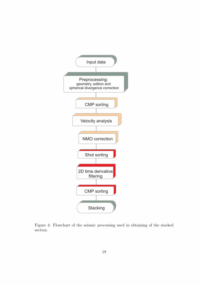
Figure 4: Flowchart of the seismic processing used in obtaining of the stackedsection.

19

Figure 5: Super-gather formed by 10 CMPs in (a) and its corresponding velocityanalysis in (b).

20

0

0.5

1.0

1.5

2.0

2.5

3.0

3.5

4.0

Time(s)

2040

6080

Tra

ces

(a)

0

0.5

1.0

1.5

2.0

2.5

3.0

3.5

4.0

2040

6080

Tra

ces

(b)

0

0.5

1.0

1.5

2.0

2.5

3.0

3.5

4.0

2040

6080

Tra

ces

(c)

Fig

ure

6:F

ilte

red

shot

-gat

her

.T

he

outp

ut

ofth

elo

w-c

ut

filt

eris

show

nin

(a).

The

FK

resu

ltis

show

nin

(b).

The

resu

ltof

mix

ing

thre

ead

jace

nt

trac

esof

(a)

issh

own

in(c

).

21

0

0.5

1.0

1.5

2.0

2.5

3.0

3.5

4.0

Time(s)

2040

6080

Tra

ces

(a)

0

0.5

1.0

1.5

2.0

2.5

3.0

3.5

4.0

2040

6080

Tra

ces

(b)

0

0.5

1.0

1.5

2.0

2.5

3.0

3.5

4.0

2040

6080

Tra

ces

(c)

Fig

ure

7:F

ilte

red

shot

-gat

her

afte

rN

MO

corr

ecti

on.

The

outp

ut

ofth

elo

w-c

ut

filt

eris

show

nin

(a).

The

FK

resu

ltis

show

nin

(b).

The

resu

ltof

mix

ing

thre

ead

jace

nt

trac

esof

(a)

issh

own

in(c

).

22

0

0.5

1.0

1.5

2.0

2.5

3.0

3.5

4.0

Time(s)

2040

6080

Tra

ces

(a)

0

0.5

1.0

1.5

2.0

2.5

3.0

3.5

4.0

2040

6080

Tra

ces

(b)

0

0.5

1.0

1.5

2.0

2.5

3.0

3.5

4.0

2040

6080

Tra

ces

(c)

Fig

ure

8:R

ever

seN

MO

corr

ecti

onof

shot

-gat

her

spre

sente

din

Fig

.7.

The

outp

ut

ofth

elo

w-c

ut

filt

eris

show

nin

(a).

The

FK

resu

ltis

show

nin

(b).

The

resu

ltof

mix

ing

thre

ead

jace

nt

trac

esof

(a)

issh

own

in(c

).

23

0

0.5

1.0

1.5

2.0

2.5

3.0

3.5

4.0

Time(s)

2040

6080

Tra

ces

(a)

0

0.5

1.0

1.5

2.0

2.5

3.0

3.5

4.0

2040

6080

Tra

ces

(b)

0

0.5

1.0

1.5

2.0

2.5

3.0

3.5

4.0

2040

6080

Tra

ces

(c)

Fig

ure

9:R

esult

sof

the

firs

tan

dse

cond

2Dti

me-

der

ivat

ive

applied

toa

shot

-gat

her

afte

rN

MO

corr

ecti

on.

The

orig

inal

shot

-gat

her

afte

rth

eN

MO

corr

ecti

onis

show

nin

(a).

The

firs

tan

dse

cond

2Dti

me-

der

ivat

ive

are

show

nin

(b)

and

(c),

resp

ecti

vely

.

24

0

0.5

1.0

1.5

2.0

2.5

3.0

3.5

4.0

Time(s)

2040

6080

Tra

ces

(a)

0

0.5

1.0

1.5

2.0

2.5

3.0

3.5

4.0

2040

6080

Tra

ces

(b)

0

0.5

1.0

1.5

2.0

2.5

3.0

3.5

4.0

2040

6080

Tra

ces

(c)

Fig

ure

10:

Rev

erse

NM

Oco

rrec

tion

ofsh

ot-g

ather

spre

sente

din

Fig

.9.

The

firs

tan

dse

cond

2Dti

me-

der

ivat

ives

are

show

nin

(b)

and

(c),

resp

ecti

vely

.

25

Fig

ure

11:

Am

plitu

de

spec

tra

ofth

ese

ism

ogra

ms

show

nin

Fig

s.9a

,8b

and

9c.

26

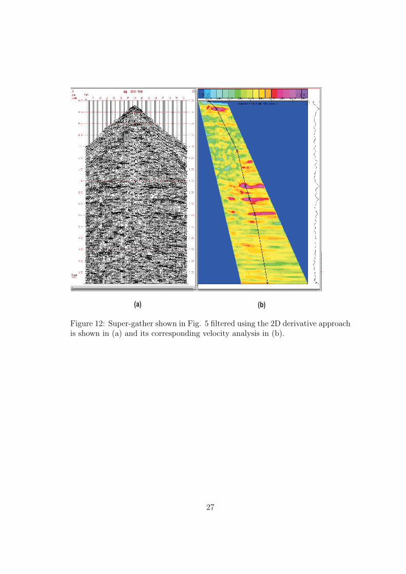
Figure 12: Super-gather shown in Fig. 5 filtered using the 2D derivative approachis shown in (a) and its corresponding velocity analysis in (b).

27

0 1 2 3 4

Time (s)0

612

1824

3036

Dis

tanc

e (K

m)

F

igure

13:

Sta

cked

seis

mic

line

RL

-509

0af

ter

grou

nd-r

oll

atte

nuat

ion

usi

ng

the

FK

met

hod.

28

0 1 2 3 4

Time (s)0

612

1824

3036

Dis

tanc

e (K

m)

F

igure

14:

Sta

cked

seis

mic

line

RL

-509

0af

ter

grou

nd-r

oll

atte

nuat

ion

usi

ng

the

2Dti

me-

der

ivat

ive

filt

erin

gm

ethod.

29