Graph Structure Estimation Neural Networks - Chuan Shi

Graph Structure Estimation Neural NetworksRuijia Wang∗

Beijing University of Posts andTelecommunications

Beijing, [email protected]

Shuai MouTencent TEG

Shenzhen, [email protected]

Xiao Wang∗Beijing University of Posts and

TelecommunicationsBeijing, China

[email protected]

Wanpeng Xiao, Qi Ju†[email protected]@tencent.com

Tencent TEGShenzhen, China

Chuan Shi†Beijing University of Posts and

TelecommunicationsBeijing, China

[email protected]

Xing XieMicrosoft Research

Beijing, [email protected]

ABSTRACTGraph Neural Networks (GNNs) have drawn considerable attentionin recent years and achieved outstanding performance in manytasks. Most empirical studies of GNNs assume that the observedgraph represents a complete and accurate picture of node rela-tionship. However, this fundamental assumption cannot alwaysbe satisfied, since the real-world graphs from complex systemsare error-prone and may not be compatible with the propertiesof GNNs. Therefore, GNNs solely relying on original graph maycause unsatisfactory results, one typical example of which is thatGNNs perform well on graphs with homophily while fail on thedisassortative situation. In this paper, we propose graph estimationneural networks GEN, which estimates graph structure for GNNs.Specifically, our GEN presents a structure model to fit the mecha-nism of GNNs by generating graphs with community structure, andan observation model that injects multifaceted observations intocalculating the posterior distribution of graphs and is the first to in-corporate multi-order neighborhood information. With above twomodels, the estimation of graph is implemented based on Bayesianinference to maximize the posterior probability, which attains mu-tual optimization with GNN parameters in an iterative framework.To comprehensively evaluate the performance of GEN, we performa set of experiments on several benchmark datasets with differenthomophily and a synthetic dataset, where the experimental resultsdemonstrate the effectiveness of our GEN and rationality of theestimated graph.

CCS CONCEPTS• Computing methodologies → Neural networks; • Theoryof computation → Social networks.

∗Both authors contributed equally to this research.†Corresponding author.

This paper is published under the Creative Commons Attribution 4.0 International(CC-BY 4.0) license. Authors reserve their rights to disseminate the work on theirpersonal and corporate Web sites with the appropriate attribution.WWW ’21, April 19–23, 2021, Ljubljana, Slovenia© 2021 IW3C2 (International World Wide Web Conference Committee), publishedunder Creative Commons CC-BY 4.0 License.ACM ISBN 978-1-4503-8312-7/21/04.https://doi.org/10.1145/3442381.3449952

KEYWORDSGraph Neural Networks, Graph Structure Learning, Network Rep-resentation Learning

ACM Reference Format:Ruijia Wang, Shuai Mou, Xiao Wang, Wanpeng Xiao, Qi Ju, Chuan Shi,and Xing Xie. 2021. Graph Structure Estimation Neural Networks. In Pro-ceedings of the Web Conference 2021 (WWW ’21), April 19–23, 2021, Ljubl-jana, Slovenia. ACM, New York, NY, USA, 12 pages. https://doi.org/10.1145/3442381.3449952

1 INTRODUCTIONGraphs are ubiquitous across application domains ranging fromchemo- and bioinformatics to image and social network analysis.With their prevalence, it is particularly important to learn effectiverepresentations of graphs and apply them to downstream tasks [13].Recently, there has been a surge of interest in Graph Neural Net-works (GNNs) [14, 21, 25, 41] for representation learning of graphs,which broadly follow a recursive message passing scheme [11]where local neighborhood information is aggregated and passedon to the neighbors. These GNNs have achieved state-of-the-artperformance in many analytical tasks such as node classification[47, 48] and recommender systems [44, 49].

Although existing GNNs have been successfully applied in a widevariety of scenarios, they rely on one fundamental assumption thatthe observed topology is ground-truth information and consistentwith the properties of GNNs. But in fact, as graphs are usuallyextracted from complex interaction systems, such assumption couldalways be violated. One reason is that these interaction systemsusually contain uncertainty or error [27]. For instance, in proteininteraction graphs, traditional laboratory experimental error is aprimary source of inaccuracy. The another reason is that the issue ofmissing data is inevitable. As another instance, the graph of Internetis determined by examining either router tables or collections oftraceroute paths, both of which give only subsets of the edges. It hasbeen revealed that unreliable error-prone graphs could significantlylimit the representation capability of GNNs [10, 37, 51], one typicalexample of which is that the performance of GNNs can greatlydegrade on the disassortative graphs [31] where homophily (i.e.,nodes within the same community tend to connect with each other)does not hold. In short, missing, meaningless or even spurious edgesare prevalent in real graphs, which results in inconsistency with

https://doi.org/10.1145/3442381.3449952

https://doi.org/10.1145/3442381.3449952

https://doi.org/10.1145/3442381.3449952

WWW ’21, April 19–23, 2021, Ljubljana, Slovenia Ruijia Wang, Shuai Mou, Xiao Wang, Wanpeng Xiao, Qi Ju, Chuan Shi, and Xing Xie

the properties of GNNs and casts doubts about the accuracy orcorrectness of their results. Therefore, it is imperative to explorean optimal graph for GNNs.

Nevertheless, it is technically challenging to effectively learn anoptimal graph structure for GNNs. Particularly, two obstacles needto be addressed. (1) The graph generation mechanism should betaken into consideration. It is well established in network scienceliterature [34] that the graph generation is potentially governed bysome underlying principles, e.g., the configuration model [33]. Con-sidering these principles fundamentally drives the learned graph tomaintain a regular global structure and be more robust to noise inreal observations. Unfortunately, the majority of current methodsparameterize each edge locally [5, 10, 18] and do not account forthe underlying generation of graph, so that the resulted graph has alower tolerance for noise and sparsity. (2) multifaceted informationshould be injected to reduce bias. Learning graph structure fromone information source inevitably leads to bias and uncertainty. Itmakes sense that the confidence of an edge would be greater if thisedge exists under multiple measurements. Thus, a reliable graphstructure ought to make allowance for comprehensive information,although it is complicated to obtain multi-view measurements anddepict their relationship with GNNs. Existing approaches [19, 51]mainly utilize the feature similarity, making the learned graph moresusceptible to the bias of single view.

To address the aforementioned issues, in this paper, we proposeGraph structure Estimation neural Networks (GEN) to improve thenode classification performance through estimating an appropriategraph structure for GNNs.We firstly analyze the properties of GNNsto match proper graph generation mechanism. GNNs, as low-passfilters [1, 23, 45] which smooth neighborhood to make the repre-sentations of proximal nodes similar, are suitable to graphs withcommunity structure [12]. Therefore, we attach a structure modelto the graph generation, hypothesizing that the estimated graphis drawn from Stochastic Block Model (SBM) [17]. Furthermore,in addition to the observed graph and node feature, we creativelyinject multi-order neighborhood information to circumvent biasand present an observation model to jointly treat above multi-viewinformation as observations of the optimal graph. In order to es-timate the optimal graph, we construct observations during GNNtraining, then apply Bayesian inference based on structure andobservation models to infer the entire posterior distribution overgraph structure. Finally, the estimated graph and the parameters ofGNNs achieve mutual, positive reinforcement through elaboratelyiterative optimization.

In summary, the contributions of this paper are three-fold:

• Concerning graph structure learning for GNNs, we are the firstto simultaneously consider the generation of learned graph tofit the mechanism of GNNs, and comprehensively employ themultifaceted information to give a more precise and nuancedpicture of the proper graph structure.

• We propose novel graph structure estimation neural networksGEN, which designs a structure model characterizing the un-derlying graph generation and an observation model injectingmulti-order neighborhood information to accurately infer thegraph structure based on Bayesian inference.

• We validate the effectiveness of GEN via thorough comparisonswith state-of-the-art methods on several challenging benchmarks.Additionally, we also analyze the properties of GEN and verifythe rationality of estimated graph on a synthetic dataset.The rest of the paper is organized as follows. In Section 2, we re-

view some of the related work. In Section 3, we introduce notationsand formally explain our proposed GEN. We report experimentalresults in Section 4 and conclude the work in Section 5.

2 RELATEDWORKIn line with the focus of our work, we briefly review the mostrelated work on GNNs and graph structure learning.

2.1 Graph Neural NetworksOver the past few years, graph neural networks have achieved greatsuccess in solving machine learning problems on graph-structureddata. Most current GNNs can be generally divided into two families,i.e., spectral methods and spatial methods.

Specifically, the first family learns node representation based ongraph spectral theory. [2] first proposes a spectral graph-based ex-tension of convolutional networks using the Fourier basis. ChebNet[6] defines graph convolution based on Chebyshev polynomials toremove the computationally expensive Laplacian eigendecomposi-tion. GCN [21] further simplifies ChebNet by using its first-orderapproximation. In a follow-up work, SGC [45] reduces the graphconvolution to a linear model but still achieves competitive per-formance. The second family of methods directly define graphconvolution in the spatial domain as aggregating and transforminglocal information. GraphSAGE [14] learns aggregators by samplingand aggregating neighbor information. GAT [41] assigns differ-ent edge weights based on node features during aggregation. Forbetter efficiency, FastGCN [4] performs importance sampling oneach layer to sample a fixed number of nodes and APPNP [22]uses the relationship between GCN and PageRank [36] to derivean improved propagation scheme based on personalized PageRank.

There are many other graph neural models, we please refer thereaders to recent surveys [46, 52] for a more comprehensive review.But almost all these GNNs treat the observed graphs, derived fromnoisy data or modelling assumptions, as ground-truth information,which significantly limits their capability to handle uncertainty inthe graph structure.

2.2 Graph Structure LearningGraph structure learning is not a newly born topic, and there hasbeen a considerable body of previous work in network science[16, 26, 28, 32] dedicated to it. To process raw graph data into moreaccurate and nuanced estimates of graph quantities, some meth-ods learn graph structure from measurements of the evolutionalgraphed dynamical systems such as coupled oscillators [43] orspreading processes [24]. There are also work [3, 15, 42] on errorcorrection strategies for missing or extraneous nodes. However, thegoal of these work departs from graph representation learning.

As GNNs become the most eye-catching tools for graph rep-resentation learning, several efforts have been made to combinegraph structure learning and GNNs for boosting performance ofdownstream tasks. Bayesian GCNN [51] views the observed graph

Graph Structure Estimation Neural Networks WWW ’21, April 19–23, 2021, Ljubljana, Slovenia

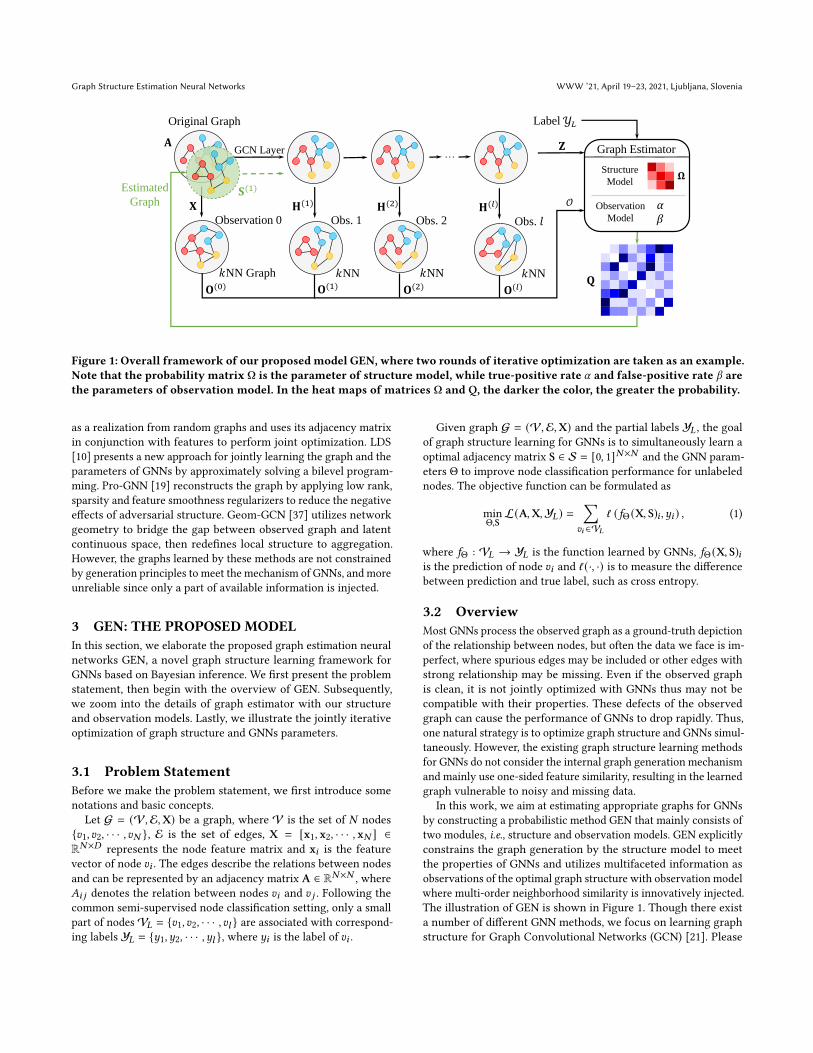
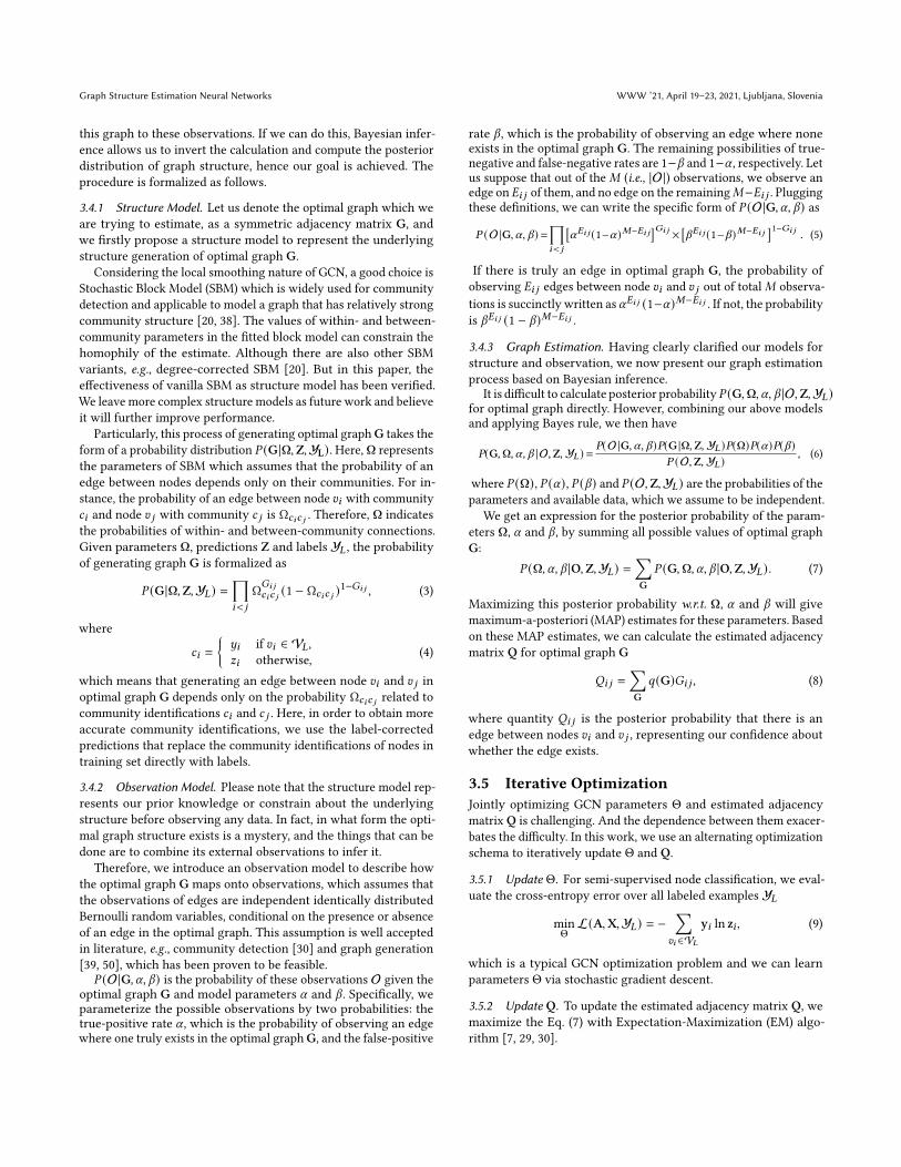
GCN Layer

Original Graph

𝐗 𝐇(1)

…𝐙 Graph Estimator

𝛀

𝛼𝛽

Label 𝒴𝐿

𝐐

𝐇(2) 𝐇(𝑙)

𝑘NN Graph

Observation 0 Obs. 1 Obs. 2 Obs. 𝑙

Estimated

Graph

𝑘NN 𝑘NN 𝑘NN

𝐀

𝐒(1)

𝐎(0) 𝐎(1) 𝐎(2) 𝐎(𝑙)

𝒪

Structure

Model

Observation

Model

Figure 1: Overall framework of our proposed model GEN, where two rounds of iterative optimization are taken as an example.Note that the probability matrix Ω is the parameter of structure model, while true-positive rate 𝛼 and false-positive rate 𝛽 arethe parameters of observation model. In the heat maps of matrices Ω and Q, the darker the color, the greater the probability.

as a realization from random graphs and uses its adjacency matrixin conjunction with features to perform joint optimization. LDS[10] presents a new approach for jointly learning the graph and theparameters of GNNs by approximately solving a bilevel program-ming. Pro-GNN [19] reconstructs the graph by applying low rank,sparsity and feature smoothness regularizers to reduce the negativeeffects of adversarial structure. Geom-GCN [37] utilizes networkgeometry to bridge the gap between observed graph and latentcontinuous space, then redefines local structure to aggregation.However, the graphs learned by these methods are not constrainedby generation principles to meet the mechanism of GNNs, and moreunreliable since only a part of available information is injected.

3 GEN: THE PROPOSED MODELIn this section, we elaborate the proposed graph estimation neuralnetworks GEN, a novel graph structure learning framework forGNNs based on Bayesian inference. We first present the problemstatement, then begin with the overview of GEN. Subsequently,we zoom into the details of graph estimator with our structureand observation models. Lastly, we illustrate the jointly iterativeoptimization of graph structure and GNNs parameters.

3.1 Problem StatementBefore we make the problem statement, we first introduce somenotations and basic concepts.

Let G = (V, E,X) be a graph, where V is the set of 𝑁 nodes𝑣1, 𝑣2, · · · , 𝑣𝑁 , E is the set of edges, X = [x1, x2, · · · , x𝑁 ] ∈R𝑁×𝐷 represents the node feature matrix and x𝑖 is the featurevector of node 𝑣𝑖 . The edges describe the relations between nodesand can be represented by an adjacency matrix A ∈ R𝑁×𝑁 , where𝐴𝑖 𝑗 denotes the relation between nodes 𝑣𝑖 and 𝑣 𝑗 . Following thecommon semi-supervised node classification setting, only a smallpart of nodes V𝐿 = 𝑣1, 𝑣2, · · · , 𝑣𝑙 are associated with correspond-ing labels Y𝐿 = 𝑦1, 𝑦2, · · · , 𝑦𝑙 , where 𝑦𝑖 is the label of 𝑣𝑖 .

Given graph G = (V, E,X) and the partial labels Y𝐿 , the goalof graph structure learning for GNNs is to simultaneously learn aoptimal adjacency matrix S ∈ S = [0, 1]𝑁×𝑁 and the GNN param-eters Θ to improve node classification performance for unlabelednodes. The objective function can be formulated as

minΘ,S

L(A,X,Y𝐿) =∑

𝑣𝑖 ∈V𝐿

ℓ (𝑓Θ (X, S)𝑖 , 𝑦𝑖 ) , (1)

where 𝑓Θ : V𝐿 → Y𝐿 is the function learned by GNNs, 𝑓Θ (X, S)𝑖is the prediction of node 𝑣𝑖 and ℓ (·, ·) is to measure the differencebetween prediction and true label, such as cross entropy.

3.2 OverviewMost GNNs process the observed graph as a ground-truth depictionof the relationship between nodes, but often the data we face is im-perfect, where spurious edges may be included or other edges withstrong relationship may be missing. Even if the observed graphis clean, it is not jointly optimized with GNNs thus may not becompatible with their properties. These defects of the observedgraph can cause the performance of GNNs to drop rapidly. Thus,one natural strategy is to optimize graph structure and GNNs simul-taneously. However, the existing graph structure learning methodsfor GNNs do not consider the internal graph generation mechanismand mainly use one-sided feature similarity, resulting in the learnedgraph vulnerable to noisy and missing data.

In this work, we aim at estimating appropriate graphs for GNNsby constructing a probabilistic method GEN that mainly consists oftwo modules, i.e., structure and observation models. GEN explicitlyconstrains the graph generation by the structure model to meetthe properties of GNNs and utilizes multifaceted information asobservations of the optimal graph structure with observation modelwhere multi-order neighborhood similarity is innovatively injected.The illustration of GEN is shown in Figure 1. Though there exista number of different GNN methods, we focus on learning graphstructure for Graph Convolutional Networks (GCN) [21]. Please


note that it is straightforward to extend the proposed frameworkto other GNNs [41, 45].

To infer the graph structure for GCN, we have the followingtwo insights. (1) The underlying graph generation that facilitatesthe node classification performance of GCN tends to maintain ho-mophily among neighbors. (2) The optimal graph might be mea-sured in multiple ways using observed interactions, feature similar-ity andmulti-order neighborhood similarity, which are multifacetedobservations that reflect the optimal graph from different views.These observations may be error-prone when viewed separately,but can be ensembled to circumvent bias. Therefore, our GEN firstlyutilizes available information to construct an observation set forthe optimal graph, then estimates the graph based on these obser-vations with explicitly constraining the underlying structure.

Specifically, we feed the original graph A and node feature Xinto 𝑙-layer vanilla GCN. In the light of that node representationsin different layers reveal multi-order neighborhood information,we utilize node representations H(𝑖) of every layer 𝑖 to construct𝑘-Nearest Neighbor (𝑘NN) graph O(𝑖) as the observation of optimalgraph, as well as the original graph A, to form observation set O =

A,O(0) ,O(1) , · · · ,O(𝑙) . Afterwards, we put these observations O,predictions Z and labelsY𝐿 into graph estimator, which is based onour proposed structure and observation models to infer adjacencymatrix Q with underlying community structure, where𝑄𝑖 𝑗 denotesthe probability that there is an edge between node 𝑣𝑖 and node𝑣 𝑗 . The entire framework is implemented by iterative optimizationbetween GCN parameters and graph estimation. Firstly, we tuneGCN parameters until the cross-entropy loss converges. Secondly,we hold GCN parameters constant to obtain estimated adjacencymatrix Q based on Expectation-Maximization (EM) algorithm, andset a threshold Y on Q to get estimated graph S. Lastly, we feedthe estimated graph S back to the vanilla GCN to perform the nextround of iterative optimization. The better estimated graph wouldthen force GCN to produce more accurate observations, and theprocess is repeated. During such iterations, the learning of GCNand the inference of graph structure enhance each other.

It is worth noting that the estimated graph is not only generatedby the original graph, but also by prior knowledge and multifacetedinformation. Thus the proposed GEN alleviates the problem ofmissing or erroneous data from three aspects. (1) Structure modelintroduces prior knowledge to constrain community structure ofthe estimated graph, thereby prompting the completion of missingedges inside communities and the deletion of erroneous edgesbetween communities. (2)We construct kNN graphs as observationsto infer the optimal graph, and different kNN graphs capture localstructures with different orders. Even original graph (first-orderstructure) may be erroneous, other structures can provide auxiliaryinformation. Based on these multifaceted observations, informativeedges may appear multiple times, while erroneous edges are onlyobserved accidentally. (3) With the iterative optimization of GEN,updated node embeddings are learned from the estimated graph.Therefore, the optimization of graph structure and GNN parametersachieve mutual reinforcement, which further resolves the problem.

3.3 Observation ConstructionWithout loss of generality, we choose representative GCN as back-bone. To begin with, we feed the original graph G = (V, E,X) intovanilla GCN to construct the initial observation set O for subse-quent graph estimation.

Specifically, GCN follows a neighborhood aggregation strategy,which iteratively updates the presentation of a node by aggregatingrepresentations of its neighbors. Formally, the 𝑘𝑡ℎ layer aggregationrule of GCN is

H(𝑘) = 𝜎

(D− 1

2 AD− 12 H(𝑘−1)W(𝑘)

). (2)

Here, A is the normalized adjacency matrix and 𝑖𝑖 =∑

𝑗 𝑖 𝑗 . W(𝑘)

is a layer-wise trainable weight matrix, and 𝜎 denotes an activationfunction. H(𝑘) ∈ R𝑁×𝑑 is the matrix of node representations in the𝑘𝑡ℎ layer, and H(0) = X. In terms of 𝑙-layer GCN, the activationfunction of the last layer 𝑙 is row-wise softmax and predictionsZ = H(𝑙) . The GCN parameters Θ = (W(1) ,W(2) , · · · ,W(𝑙) ) canbe trained via gradient descent.

The current GCN acts directly on the observed graph A whichis extracted from the real-world complex systems and is usuallynoisy. To estimate an optimal graph structure for GCN, we needto construct multifaceted observations that could be ensembled toresist bias. Fortunately, after 𝑘 iterations of aggregation, node rep-resentation captures the structural information within its 𝑘-ordergraph neighborhood which provides local to global information. Onthe other hand, node pairs with similar neighborhood are possiblyfar away in the graph but apt to the same communities. If these in-formative node pairs are employed, they could provide useful cluesfor downstream classification. Therefore, we attempt to connectthese distant but similar nodes in our estimated graph to enhancethe classification performance of GCN.

Specifically, we fix the GCN parameters Θ and take out thenode representationsH = H(0) ,H(1) , · · · ,H(𝑙) to construct 𝑘NNgraphs O(0) ,O(1) , · · · ,O(𝑙) as observations of the optimal graph,where O(𝑖) is the adjacency matrix of 𝑘NN graph generated by H(𝑖)

and characterizes the similarity of 𝑖-order neighborhood. Obviously,the original graph A is also an important external observation ofthe optimal graph, thus we combine it with 𝑘NN graphs to formthe complete observation set O = A,O(0) ,O(1) , · · · ,O(𝑙) . Theseobservations reflect the optimal graph structure from varied viewsand can be ensembled to infer a more reliable graph structure.

As preliminary preparations, these observations O, predictions Zand labelsY𝐿 will be fed into estimator to accurately infer the poste-rior distribution of the graph structure. In the following subsection,we will introduce the inference in detail.

3.4 Graph EstimatorUntil now, the question we would like to answer is: given theseavailable observations O, what is the best estimated graph for GCN?These observations reveal the optimal graph structure from differ-ent perspectives, but they may be unreliable or incomplete, andwe do not have a priori that how accurate any of the informationis. Under this daunting circumstance, it is not straightforward toanswer this question directly, but it is relatively easy to answer thereverse question. Imagining that a graph with community structurehas been generated, we could calculate the probability of mapping


this graph to these observations. If we can do this, Bayesian infer-ence allows us to invert the calculation and compute the posteriordistribution of graph structure, hence our goal is achieved. Theprocedure is formalized as follows.

3.4.1 Structure Model. Let us denote the optimal graph which weare trying to estimate, as a symmetric adjacency matrix G, andwe firstly propose a structure model to represent the underlyingstructure generation of optimal graph G.

Considering the local smoothing nature of GCN, a good choice isStochastic Block Model (SBM) which is widely used for communitydetection and applicable to model a graph that has relatively strongcommunity structure [20, 38]. The values of within- and between-community parameters in the fitted block model can constrain thehomophily of the estimate. Although there are also other SBMvariants, e.g., degree-corrected SBM [20]. But in this paper, theeffectiveness of vanilla SBM as structure model has been verified.We leave more complex structure models as future work and believeit will further improve performance.

Particularly, this process of generating optimal graph G takes theform of a probability distribution 𝑃 (G|Ω,Z,YL). Here, Ω representsthe parameters of SBM which assumes that the probability of anedge between nodes depends only on their communities. For in-stance, the probability of an edge between node 𝑣𝑖 with community𝑐𝑖 and node 𝑣 𝑗 with community 𝑐 𝑗 is Ω𝑐𝑖𝑐 𝑗 . Therefore, Ω indicatesthe probabilities of within- and between-community connections.Given parameters Ω, predictions Z and labels Y𝐿 , the probabilityof generating graph G is formalized as

𝑃 (G|Ω,Z,Y𝐿) =∏𝑖< 𝑗

Ω𝐺𝑖 𝑗

𝑐𝑖𝑐 𝑗 (1 − Ω𝑐𝑖𝑐 𝑗 )1−𝐺𝑖 𝑗 , (3)

where

𝑐𝑖 =

𝑦𝑖 if 𝑣𝑖 ∈ V𝐿,

𝑧𝑖 otherwise, (4)

which means that generating an edge between node 𝑣𝑖 and 𝑣 𝑗 inoptimal graph G depends only on the probability Ω𝑐𝑖𝑐 𝑗 related tocommunity identifications 𝑐𝑖 and 𝑐 𝑗 . Here, in order to obtain moreaccurate community identifications, we use the label-correctedpredictions that replace the community identifications of nodes intraining set directly with labels.

3.4.2 Observation Model. Please note that the structure model rep-resents our prior knowledge or constrain about the underlyingstructure before observing any data. In fact, in what form the opti-mal graph structure exists is a mystery, and the things that can bedone are to combine its external observations to infer it.

Therefore, we introduce an observation model to describe howthe optimal graph G maps onto observations, which assumes thatthe observations of edges are independent identically distributedBernoulli random variables, conditional on the presence or absenceof an edge in the optimal graph. This assumption is well acceptedin literature, e.g., community detection [30] and graph generation[39, 50], which has been proven to be feasible.

𝑃 (O|G, 𝛼, 𝛽) is the probability of these observations O given theoptimal graph G and model parameters 𝛼 and 𝛽 . Specifically, weparameterize the possible observations by two probabilities: thetrue-positive rate 𝛼 , which is the probability of observing an edgewhere one truly exists in the optimal graph G, and the false-positive

rate 𝛽 , which is the probability of observing an edge where noneexists in the optimal graph G. The remaining possibilities of true-negative and false-negative rates are 1−𝛽 and 1−𝛼 , respectively. Letus suppose that out of the𝑀 (i.e., |O|) observations, we observe anedge on 𝐸𝑖 𝑗 of them, and no edge on the remaining𝑀−𝐸𝑖 𝑗 . Pluggingthese definitions, we can write the specific form of 𝑃 (O|G, 𝛼, 𝛽) as

𝑃 (O |G, 𝛼, 𝛽) =∏𝑖< 𝑗

[𝛼𝐸𝑖 𝑗 (1−𝛼)𝑀−𝐸𝑖 𝑗]𝐺𝑖 𝑗 ×

[𝛽𝐸𝑖 𝑗 (1−𝛽)𝑀−𝐸𝑖 𝑗 ]1−𝐺𝑖 𝑗

. (5)

If there is truly an edge in optimal graph G, the probability ofobserving 𝐸𝑖 𝑗 edges between node 𝑣𝑖 and 𝑣 𝑗 out of total𝑀 observa-tions is succinctly written as 𝛼𝐸𝑖 𝑗 (1−𝛼)𝑀−𝐸𝑖 𝑗 . If not, the probabilityis 𝛽𝐸𝑖 𝑗 (1 − 𝛽)𝑀−𝐸𝑖 𝑗 .

3.4.3 Graph Estimation. Having clearly clarified our models forstructure and observation, we now present our graph estimationprocess based on Bayesian inference.

It is difficult to calculate posterior probability 𝑃 (G,Ω, 𝛼, 𝛽 |O,Z,Y𝐿)for optimal graph directly. However, combining our above modelsand applying Bayes rule, we then have

𝑃(G,Ω, 𝛼, 𝛽 |O,Z,Y𝐿) =𝑃(O |G, 𝛼, 𝛽)𝑃(G |Ω,Z,Y𝐿)𝑃(Ω)𝑃(𝛼)𝑃(𝛽)

𝑃 (O,Z,Y𝐿), (6)

where 𝑃 (Ω), 𝑃 (𝛼), 𝑃 (𝛽) and 𝑃 (O,Z,Y𝐿) are the probabilities of theparameters and available data, which we assume to be independent.

We get an expression for the posterior probability of the param-eters Ω, 𝛼 and 𝛽 , by summing all possible values of optimal graphG:

𝑃 (Ω, 𝛼, 𝛽 |O,Z,Y𝐿) =∑G

𝑃 (G,Ω, 𝛼, 𝛽 |O,Z,Y𝐿). (7)

Maximizing this posterior probability w.r.t. Ω, 𝛼 and 𝛽 will givemaximum-a-posteriori (MAP) estimates for these parameters. Basedon these MAP estimates, we can calculate the estimated adjacencymatrix Q for optimal graph G

𝑄𝑖 𝑗 =∑G

𝑞(G)𝐺𝑖 𝑗 , (8)

where quantity 𝑄𝑖 𝑗 is the posterior probability that there is anedge between nodes 𝑣𝑖 and 𝑣 𝑗 , representing our confidence aboutwhether the edge exists.

3.5 Iterative OptimizationJointly optimizing GCN parameters Θ and estimated adjacencymatrix Q is challenging. And the dependence between them exacer-bates the difficulty. In this work, we use an alternating optimizationschema to iteratively update Θ and Q.

3.5.1 Update Θ. For semi-supervised node classification, we eval-uate the cross-entropy error over all labeled examples Y𝐿

minΘ

L(A,X,Y𝐿) = −∑

𝑣𝑖 ∈V𝐿

y𝑖 ln z𝑖 , (9)

which is a typical GCN optimization problem and we can learnparameters Θ via stochastic gradient descent.

3.5.2 Update Q. To update the estimated adjacency matrix Q, wemaximize the Eq. (7) with Expectation-Maximization (EM) algo-rithm [7, 29, 30].


E-step. Since it is convenient to maximize not the probabilityitself but its logarithm, we apply Jensen’s inequality to the log ofEq. (7)

log 𝑃 (Ω, 𝛼, 𝛽 |O,Z,Y𝐿) ≥∑G𝑞(G) log 𝑃 (G,Ω, 𝛼, 𝛽 |O,Z,Y𝐿)

𝑞(G) , (10)

where 𝑞(G) is any nonnegative function of G satisfying∑

G 𝑞(G) =1, which can be seen as a probability distribution over G.

The right-hand side of the inequality Eq. (10) is maximized whenthe exact equality is achieved

𝑞(G) = 𝑃 (G,Ω, 𝛼, 𝛽 |O,Z,Y𝐿)∑G 𝑃 (G,Ω, 𝛼, 𝛽 |O,Z,Y𝐿)

. (11)

Substituting Eq. (3) and Eq. (5) into Eq. (11), and eliminating theconstants in fraction, we find the following expression for 𝑞(G):

𝑞 (G) =

∏𝑖< 𝑗

[Ω𝑐𝑖𝑐 𝑗

𝛼𝐸𝑖 𝑗 (1−𝛼)𝑀−𝐸𝑖 𝑗

]𝐺𝑖 𝑗[(1−Ω𝑐𝑖𝑐 𝑗

)𝛽𝐸𝑖 𝑗 (1−𝛽)𝑀−𝐸𝑖 𝑗]1−𝐺𝑖 𝑗

∑G∏

𝑖< 𝑗





=∏𝑖< 𝑗





Ω𝑐𝑖𝑐 𝑗𝛼𝐸𝑖 𝑗 (1−𝛼)𝑀−𝐸𝑖 𝑗 + (1−Ω𝑐𝑖𝑐 𝑗

)𝛽𝐸𝑖 𝑗 (1−𝛽)𝑀−𝐸𝑖 𝑗.

(12)Then further maximizing the right-hand side of Eq. (10) will giveus the MAP estimates.

M-step. We can find the maximum over the parameters by differ-entiating. Taking derivatives of the right-hand side of Eq. (10) whileholding 𝑞(G) constant, and assuming that the priors are uniform,we have ∑

G𝑞(G)

∑𝑖< 𝑗

[𝐺𝑖 𝑗

Ω𝑐𝑖𝑐 𝑗

−1 −𝐺𝑖 𝑗

1 − Ω𝑐𝑖𝑐 𝑗

]= 0, (13)

∑G

𝑞(G)∑𝑖< 𝑗

𝐺𝑖 𝑗

[𝐸𝑖 𝑗

𝛼−𝑀 − 𝐸𝑖 𝑗

1 − 𝛼

]= 0, (14)

∑G

𝑞(G)∑𝑖< 𝑗

(1 −𝐺𝑖 𝑗

) [𝐸𝑖 𝑗𝛽

−𝑀 − 𝐸𝑖 𝑗

1 − 𝛽

]= 0. (15)

The solution of these equations gives us MAP estimates for Ω, 𝛼and 𝛽 . Note that Eq. (13) depends only on the SBM and its solutiongives the parameter values for structure model. Similarly, Eq. (14)and Eq. (15) depend only on the observation model.

For specific calculations, we swap the order of the summationsand find that

Ω𝑟𝑠 =

𝑀𝑟𝑠

𝑛𝑟𝑛𝑠if 𝑟 ≠ 𝑠,

2𝑀𝑟𝑟

𝑛𝑟 (𝑛𝑟−1) otherwise,(16)

where 𝑛𝑟 =∑𝑖 𝛿𝑐𝑖 ,𝑟 and 𝑀𝑟𝑠 =

∑𝑖< 𝑗 𝑄𝑖 𝑗𝛿𝑐𝑖 ,𝑟𝛿𝑐 𝑗 ,𝑠 . Thus Eq. (16)

has the simple interpretation that the probability Ω𝑟𝑠 of an edgebetween community 𝑟 and 𝑠 is the average probabilities of the indi-vidual edges between all nodes in these two communities. Similarcalculations are done for 𝛼 and 𝛽

𝛼 =

∑𝑖< 𝑗 𝑄𝑖 𝑗𝐸𝑖 𝑗

𝑀∑𝑖< 𝑗 𝑄𝑖 𝑗

, (17)

𝛽 =

∑𝑖< 𝑗

(1 −𝑄𝑖 𝑗

)𝐸𝑖 𝑗

𝑀∑𝑖< 𝑗

(1 −𝑄𝑖 𝑗

) . (18)

Algorithm 1:Model training for GENInput :adjacency matrix A, feature matrix X, labels Y𝐿

𝑘 in 𝑘NN, tolerance _, threshold Y, iterations 𝜏Output :estimated graph S, GCN parameters Θ

1 Initialize Θ, Ω, 𝛼 and 𝛽 ;2 for 𝑖 = 1 to 𝜏 do3 Update Θ with Eq. (9);4 Construct the observation set O with 𝑘NN graph;5 while |𝛼 − 𝛼𝑜𝑙𝑑 | > _ or |𝛽 − 𝛽𝑜𝑙𝑑 | > _ do6 Ω𝑜𝑙𝑑 = Ω, 𝛼𝑜𝑙𝑑 = 𝛼 , 𝛽𝑜𝑙𝑑 = 𝛽 ;7 Calculate Ω, 𝛼 and 𝛽 with Eq. (16), (17) and (18);8 Update Q with Eq. (19);

9 Extract S(𝑖) from Q by threshold Y with Eq. (21);A = S(𝑖) ;

10 return S(𝜏) and Θ;

To calculate the value of 𝑄𝑖 𝑗 , we substitute Eq. (12) into Eq. (8):

𝑄𝑖 𝑗 =Ω𝑐𝑖𝑐 𝑗𝛼

𝐸𝑖 𝑗 (1 − 𝛼)𝑀−𝐸𝑖 𝑗

Ω𝑐𝑖𝑐 𝑗𝛼𝐸𝑖 𝑗 (1−𝛼)𝑀−𝐸𝑖 𝑗 + (1−Ω𝑐𝑖𝑐 𝑗 )𝛽𝐸𝑖 𝑗 (1−𝛽)𝑀−𝐸𝑖 𝑗

. (19)

The posterior distribution 𝑞(G) can be conveniently rewritten interms of 𝑄𝑖 𝑗 as

𝑞(G) =∏𝑖< 𝑗

𝑄𝐺𝑖 𝑗

𝑖 𝑗

(1 −𝑄𝑖 𝑗

)1−𝐺𝑖 𝑗 . (20)

To put that another way, the probability distribution over optimalgraph is the product of independent Bernoulli distributions of theindividual edges, with Bernoulli parameters𝑄𝑖 𝑗 which capture boththe graph structure itself and the uncertainty in that structure.

This leads to a natural EM algorithm for determining the valuesof the parameters and posterior distribution over possible graphstructures. We perform the E-step by maximizing first over 𝑞(G)with the parameters held constant; then go to the M-step overparameters Ω, 𝛼 and 𝛽 with 𝑞(G) held constant; and repeat theseiterations until convergence.

Sparsification. Note that the elements in estimated adjacencymatrix Q range between [0, 1]. However, a fully connected graphstructure is not only computationally expensive but also makeslittle sense for most applications. We hence proceed to extract asparse adjacency matrix S from G, by masking off those elementssmaller than certain non-negative threshold Y:

𝑆𝑖 𝑗 =

𝑄𝑖 𝑗 if 𝑄𝑖 𝑗 > Y,

0 otherwise. (21)

3.5.3 Training Algorithm. With the aforementioned updating andinference rules, the training algorithm is shown in Algorithm 1.Specifically, we first randomly initialize all the parameters for GEN.Then we update Θ to form observations, and estimate S basedon observations to boost the optimization of Θ in turn. Throughsuch alternative and iterative updates, the more accurate estimatedgraph S leads to better optimized parameters Θ, while the better Θproduces more precise observations for estimating S.


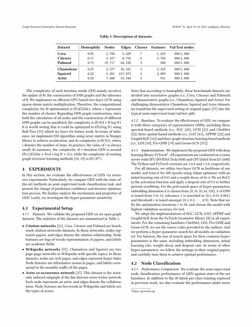
Table 1: Description of datasets.

Dataset Homophily Nodes Edges Classes Features Val/Test nodes

Cora 0.83 2, 708 5, 429 7 1, 433 500/1, 000Citeseer 0.71 3, 327 4, 732 6 3, 703 500/1, 000Pubmed 0.79 19, 717 44, 338 3 500 500/1, 000

Chameleon 0.25 2, 277 36, 101 5 2, 325 500/1, 000Squirrel 0.22 5, 201 217, 073 5 2, 089 500/1, 000Actor 0.24 7, 600 33, 544 5 931 500/1, 000

The complexity of each iteration inside GEN mainly involvesthe update of Θ, the construction of 𝑘NN graphs and the inferenceof S. We implement an efficient GPU-based two-layer GCN usingsparse-dense matrix multiplication. Therefore, the computationalcomplexity for Θ optimization is O(|E|𝐷𝑑𝑐), where 𝑐 representsthe number of classes. Regarding 𝑘NN graph construction, sinceboth the calculation of all nodes and the construction of different𝑘NN graphs can be paralleled, the complexity is O(𝑁𝑑 + 𝑁 log𝑁 ).It is worth noting that it could be optimized to O(𝑑 log𝑁 ) usingBall-Tree [35] which we leave for future work. In terms of infer-ence, we implement EM algorithm using array matrix in Numpylibrary to achieve acceleration, and its complexity is O(𝑁𝑖), where𝑖 denotes the number of steps. In practice, the value of 𝑖 is alwayssmall. In summary, the complexity of 𝜏-iteration GEN is aroundO(𝜏 ( |E |𝐷𝑑𝑐 + 𝑁 (𝑑 + log𝑁 + 𝑖))), while the complexity of existinggraph structure learning methods [10, 19] is O(𝜏𝑁 2).

4 EXPERIMENTSIn this section, we evaluate the effectiveness of GEN via exten-sive experiments. Particularly, we compare GEN with the-state-of-the-art methods on semi-supervised node classification task, andpresent the change of prediction confidence and iterative optimiza-tion process. We further analyze the mechanism and properties ofGEN. Lastly, we investigate the hyper-parameter sensitivity.

4.1 Experimental Setup4.1.1 Datasets. We validate the proposed GEN on six open graphdatasets. The statistics of the datasets are summarized in Table 1.

• Citation networks [21]. Cora, Citeseer and Pubmed are bench-mark citation networks datasets. In these networks, nodes rep-resent papers, and edges denote the citation relationship. Nodefeatures are bag-of-words representation of papers, and labelsare academic fields.

• Wikipedia networks [37]. Chameleon and Squirrel are twopage-page networks in Wikipedia with specific topics. In thosedatasets, nodes are web pages, and edges represent hyper-links.Node features are informative nouns in pages, and labels corre-spond to the monthly traffic of the pages.

• Actor co-occurrence network [37]. This dataset is the actor-only induced subgraph of the fim-director-actor-writer network.Each node represents an actor, and edges denote the collabora-tions. Node features are keywords in Wikipedia and labels arethe types of actors.

Note that according to homophily, these benchmark datasets aredivided into assortative graphs (i.e., Cora, Citeseer and Pubmed)and disassortative graphs (i.e., Chameleon, Squirrel and Actor). Forchallenging disassortative Chameleon, Squirrel and Actor datasets,we transform the supervised setting in original paper [37] into thetypical semi-supervised train/val/test split.

4.1.2 Baselines. To evaluate the effectiveness of GEN, we compareit with three categories of representative GNNs, including threespectral-based methods (i.e., SGC [45], GCN [21] and ChebNet[6]), three spatial-based methods (i.e., GAT [41], APPNP [22] andGraphSAGE [14]) and three graph structure learning based methods(i.e., LDS [10], Pro-GNN [19] and Geom-GCN [37]).

4.1.3 Implementation. We implement the proposed GENwith deeplearning library PyTorch1. All experiments are conducted on a Linuxserver with GPU (NVIDIA Tesla M40) and CPU (Intel Xeon E5-2680).The Python and PyTorch versions are 3.6.8 and 1.5.0, respectively.

For all datasets, we utilize two-layer GCN as backbone of ourmodel, and train it for 200 epochs using Adam optimizer with aninitial learning rate of 0.01 and a weight decay of 5e-4. We set ReLUas the activation function and apply a dropout rate of 0.5 to furtherprevent overfitting. For the grid search space of hyper-parameters,embedding dimension 𝑑 is chosen from 8, 16, 32, 64, 128, 𝑘 of 𝑘NNis tuned from 3 to 15, tolerance _ is searched in 0.1, 0.01, 0.001and threshold Y is tuned amongst 0.1, 0.2, · · · , 0.9. Note that wefix the optimization iterations 𝜏 to 50, and choose the model withhighest validation accuracy for test.

We adopt the implementations of SGC, GCN, GAT, APPNP andGraphSAGE from the PyTorch Geometric library [8] in all experi-ments. For the remaining baselines ChebNet, LDS, Pro-GNN andGeom-GCN, we use the source codes provided by the authors. Andwe perform a hyper-parameter search for all models on validationset. For fairness, the size of search space for their common hyper-parameters is the same, including embedding dimension, initiallearning rate, weight decay and dropout rate. In terms of otherhyper-parameters, we follow the settings in their original papers,and carefully tune them to achieve optimal performance.

4.2 Node Classification4.2.1 Performance Comparison. We evaluate the semi-supervisednode classification performance of GEN against state-of-the-artbaselines. In addition to the 20 labels per class training exploredin previous work, we also evaluate the performance under more

1https://pytorch.org/


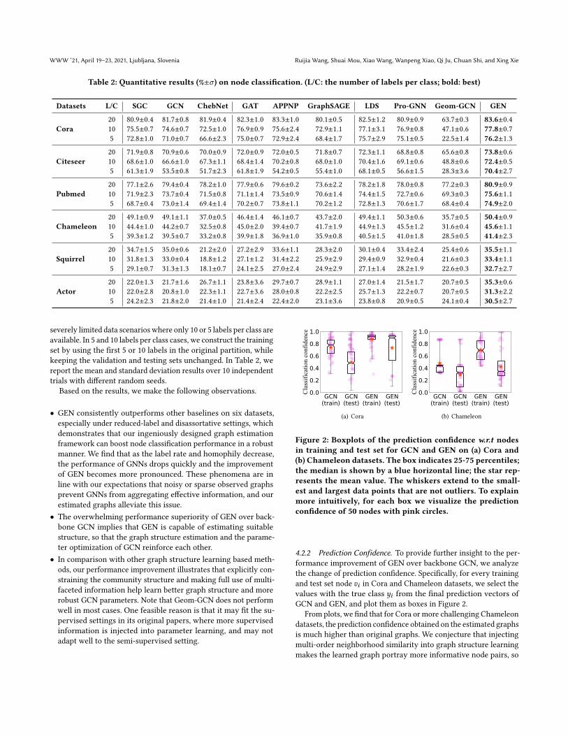
Table 2: Quantitative results (%±𝜎) on node classification. (L/C: the number of labels per class; bold: best)

Datasets L/C SGC GCN ChebNet GAT APPNP GraphSAGE LDS Pro-GNN Geom-GCN GEN

Cora20 80.9±0.4 81.7±0.8 81.9±0.4 82.3±1.0 83.3±1.0 80.1±0.5 82.5±1.2 80.9±0.9 63.7±0.3 83.6±0.410 75.5±0.7 74.6±0.7 72.5±1.0 76.9±0.9 75.6±2.4 72.9±1.1 77.1±3.1 76.9±0.8 47.1±0.6 77.8±0.75 72.8±1.0 71.0±0.7 66.6±2.3 75.0±0.7 72.9±2.4 68.4±1.7 75.7±2.9 75.1±0.5 22.5±1.4 76.2±1.3

Citeseer20 71.9±0.8 70.9±0.6 70.0±0.9 72.0±0.9 72.0±0.5 71.8±0.7 72.3±1.1 68.8±0.8 65.6±0.8 73.8±0.610 68.6±1.0 66.6±1.0 67.3±1.1 68.4±1.4 70.2±0.8 68.0±1.0 70.4±1.6 69.1±0.6 48.8±0.6 72.4±0.55 61.3±1.9 53.5±0.8 51.7±2.3 61.8±1.9 54.2±0.5 55.4±1.0 68.1±0.5 56.6±1.5 28.3±3.6 70.4±2.7

Pubmed20 77.1±2.6 79.4±0.4 78.2±1.0 77.9±0.6 79.6±0.2 73.6±2.2 78.2±1.8 78.0±0.8 77.2±0.3 80.9±0.910 71.9±2.3 73.7±0.4 71.5±0.8 71.1±1.4 73.5±0.9 70.6±1.4 74.4±1.5 72.7±0.6 69.3±0.3 75.6±1.15 68.7±0.4 73.0±1.4 69.4±1.4 70.2±0.7 73.8±1.1 70.2±1.2 72.8±1.3 70.6±1.7 68.4±0.4 74.9±2.0

Chameleon20 49.1±0.9 49.1±1.1 37.0±0.5 46.4±1.4 46.1±0.7 43.7±2.0 49.4±1.1 50.3±0.6 35.7±0.5 50.4±0.910 44.4±1.0 44.2±0.7 32.5±0.8 45.0±2.0 39.4±0.7 41.7±1.9 44.9±1.3 45.5±1.2 31.6±0.4 45.6±1.15 39.3±1.2 39.5±0.7 33.2±0.8 39.9±1.8 36.9±1.0 35.9±0.8 40.5±1.5 41.0±1.8 28.5±0.5 41.4±2.3

Squirrel20 34.7±1.5 35.0±0.6 21.2±2.0 27.2±2.9 33.6±1.1 28.3±2.0 30.1±0.4 33.4±2.4 25.4±0.6 35.5±1.110 31.8±1.3 33.0±0.4 18.8±1.2 27.1±1.2 31.4±2.2 25.9±2.9 29.4±0.9 32.9±0.4 21.6±0.3 33.4±1.15 29.1±0.7 31.3±1.3 18.1±0.7 24.1±2.5 27.0±2.4 24.9±2.9 27.1±1.4 28.2±1.9 22.6±0.3 32.7±2.7

Actor20 22.0±1.3 21.7±1.6 26.7±1.1 23.8±3.6 29.7±0.7 28.9±1.1 27.0±1.4 21.5±1.7 20.7±0.5 35.3±0.610 22.0±2.8 20.8±1.0 22.3±1.1 22.7±3.6 28.0±0.8 22.2±2.5 25.7±1.3 22.2±0.7 20.7±0.5 31.3±2.25 24.2±2.3 21.8±2.0 21.4±1.0 21.4±2.4 22.4±2.0 23.1±3.6 23.8±0.8 20.9±0.5 24.1±0.4 30.5±2.7

severely limited data scenarioswhere only 10 or 5 labels per class areavailable. In 5 and 10 labels per class cases, we construct the trainingset by using the first 5 or 10 labels in the original partition, whilekeeping the validation and testing sets unchanged. In Table 2, wereport the mean and standard deviation results over 10 independenttrials with different random seeds.

Based on the results, we make the following observations.

• GEN consistently outperforms other baselines on six datasets,especially under reduced-label and disassortative settings, whichdemonstrates that our ingeniously designed graph estimationframework can boost node classification performance in a robustmanner. We find that as the label rate and homophily decrease,the performance of GNNs drops quickly and the improvementof GEN becomes more pronounced. These phenomena are inline with our expectations that noisy or sparse observed graphsprevent GNNs from aggregating effective information, and ourestimated graphs alleviate this issue.

• The overwhelming performance superiority of GEN over back-bone GCN implies that GEN is capable of estimating suitablestructure, so that the graph structure estimation and the parame-ter optimization of GCN reinforce each other.

• In comparison with other graph structure learning based meth-ods, our performance improvement illustrates that explicitly con-straining the community structure and making full use of multi-faceted information help learn better graph structure and morerobust GCN parameters. Note that Geom-GCN does not performwell in most cases. One feasible reason is that it may fit the su-pervised settings in its original papers, where more supervisedinformation is injected into parameter learning, and may notadapt well to the semi-supervised setting.

GCN(train)

GCN(test)

GEN(train)

GEN(test)

0.00.20.40.60.81.0

Cla

ssifi

catio

n co

nfid

ence

(a) Cora

GCN(train)

GCN(test)

GEN(train)

GEN(test)

0.00.20.40.60.81.0

Cla

ssifi

catio

n co

nfid

ence

(b) Chameleon

Figure 2: Boxplots of the prediction confidence w.r.t nodesin training and test set for GCN and GEN on (a) Cora and(b) Chameleon datasets. The box indicates 25-75 percentiles;the median is shown by a blue horizontal line; the star rep-resents the mean value. The whiskers extend to the small-est and largest data points that are not outliers. To explainmore intuitively, for each box we visualize the predictionconfidence of 50 nodes with pink circles.

4.2.2 Prediction Confidence. To provide further insight to the per-formance improvement of GEN over backbone GCN, we analyzethe change of prediction confidence. Specifically, for every trainingand test set node 𝑣𝑖 in Cora and Chameleon datasets, we select thevalues with the true class 𝑦𝑖 from the final prediction vectors ofGCN and GEN, and plot them as boxes in Figure 2.

From plots, we find that for Cora or more challenging Chameleondatasets, the prediction confidence obtained on the estimated graphsis much higher than original graphs. We conjecture that injectingmulti-order neighborhood similarity into graph structure learningmakes the learned graph portray more informative node pairs, so


(a) Original graph (b) Neighbors in original graph (c) Estimated graph (d) Neighbors in estimated graph

Figure 3: Visualization of the graph structures for (a) original graph and (c) estimated graph, where color indicates the com-munities of nodes and the node diameter is proportional to the PageRank score. We fade the remaining nodes and edges toemphasize the neighbors of selected node in (b) original graph and (d) estimated graph.

4 8 12 16Step

0.1

0.2

0.3

0.4

0.001

0.002

0.003

0.004

(a) Cora

6 12 18 24Step

0.010.020.030.040.05

0.001

0.002

0.003

0.004

(b) Chameleon

Figure 4: Curves of parameter change during estimation on(a) Cora and (b) Chameleon datasets. The coordinate of X-axis represents the alternate step of expectation and maxi-mization in EM algorithm, and the pink dashed lines sepa-rate the different iterations of GEN.

that the classification distribution becomes more peaked and armthe vanilla GCN with the ability to correct misclassified nodes.

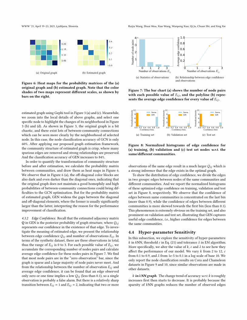
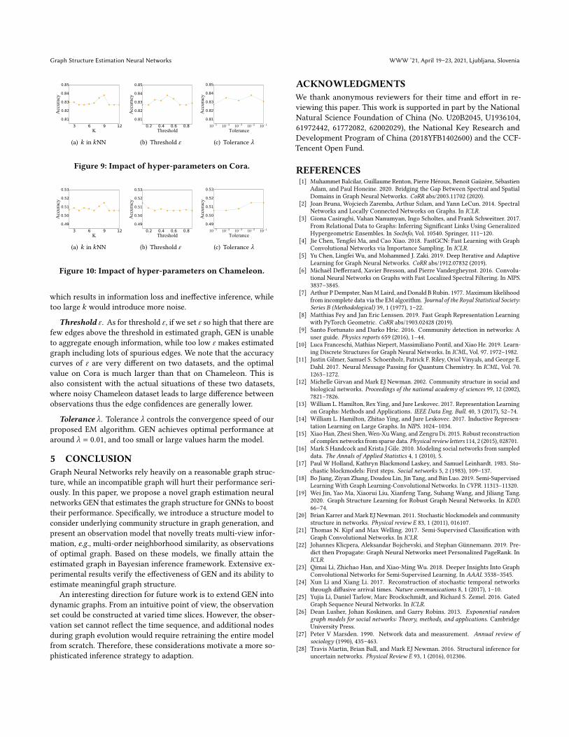
4.2.3 Optimization Analysis. To understand the iterative estima-tion process of GEN, we present the value change curves of true-positive rate 𝛼 and false-positive rate 𝛽 in Eq. (5) on Cora andChameleon datasets. Particularly, we fix the tolerance _ to 0.001and show the value change of several successive iterations in Figure4. We observe that the deduced EM algorithm always meets theconvergence condition within 6 steps, illustrating an extremelyefficient optimization. In addition, during the iterative process, thetrue-positive rate 𝛼 gradually increases, implying that the observa-tions built by backbone GCN become more and more accurate.

We further compare the convergence speed of GEN and othergraph structure learning baselines, as shown in Figure 5. Please notethat Geom-GCN is outside the scope of comparison, since it doesnot follow an iterative framework. It can be observed that GENhas faster convergence speed and better validation accuracy onboth datasets, demonstrating the efficiency and effectiveness of ourproposed GEN. Moreover, for disassortative Chameleon dataset,the validation accuracy of LDS and Pro-GNN fluctuates greatlywhile GEN improves accuracy steadily, which once again confirms

0 5 10 15 20 25 30Iteration

0.2

0.4

0.6

0.8

Acc

urac

yLDS

Pro-GNN

GEN

(a) Cora

0 5 10 15 20 25 30Iteration

0.1

0.2

0.3

0.4

0.5

Acc

urac

y

LDS

Pro-GNN

GEN

(b) Chameleon

Figure 5: Curves of validation accuracy w.r.t. the number ofiterations on (a) Cora and (b) Chameleon datasets.

the robustness of considering the graph generation principles andmultifaceted information.

4.3 Analysis of Estimated GraphIn the previous subsection, we have demonstrated the effectivenessof the proposed framework on real-world datasets. In this section,we aim at understanding the mechanism of GEN and the propertiesof estimated graph.

To better explore the mechanism of our GEN, we perform studieson a synthetic graph using an attributed stochastic block model,which has been used extensively to benchmark graph clusteringmethods [9, 40]. For better visualization and analysis, in our versionof SBM there are 5 communities and each with 20 nodes. We ran-domly initialize the symmetric probability matrix to generate edges,and the diagonal element is the largest in corresponding row undermost circumstances to ensure a certain degree of homophily. The8-dimensional features of nodes are generated using a multivariatenormal distribution, where nodes in different communities sharethe random covariance matrix but have different means accordingto their own communities. In terms of train/val/test split, we uti-lize 5 nodes per class for training, 5 nodes for validation and theremaining as test.

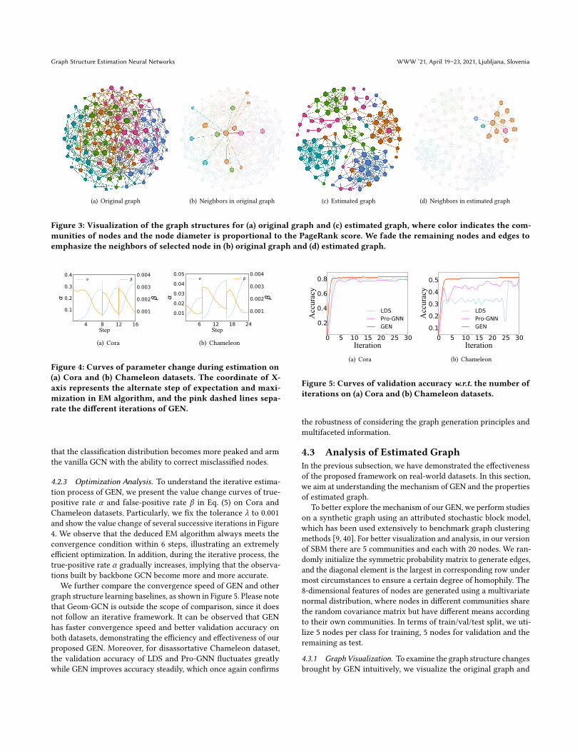
4.3.1 Graph Visualization. To examine the graph structure changesbrought by GEN intuitively, we visualize the original graph and


(a) Original graph (b) Estimated graph

Figure 6: Heat maps for the probability matrices of the (a)original graph and (b) estimated graph. Note that the colorshades of two maps represent different scales, as shown bybars on the right.

estimated graph using Gephi tool in Figure 3 (a) and (c). Meanwhile,we zoom into the local details of above graphs, and select onespecific node to highlight the changes of its neighborhood in Figure3 (b) and (d). As shown in Figure 3, the original graph is a bitchaotic, and there exist lots of between-community connectionswhich can be seen more clearly by the neighborhood of selectednode. In this case, the node classification accuracy of GCN is only60%. After applying our proposed graph estimation framework,the community structure of estimated graph is crisp, where manyspurious edges are removed and strong relationships are preserved.And the classification accuracy of GEN increases to 84%.

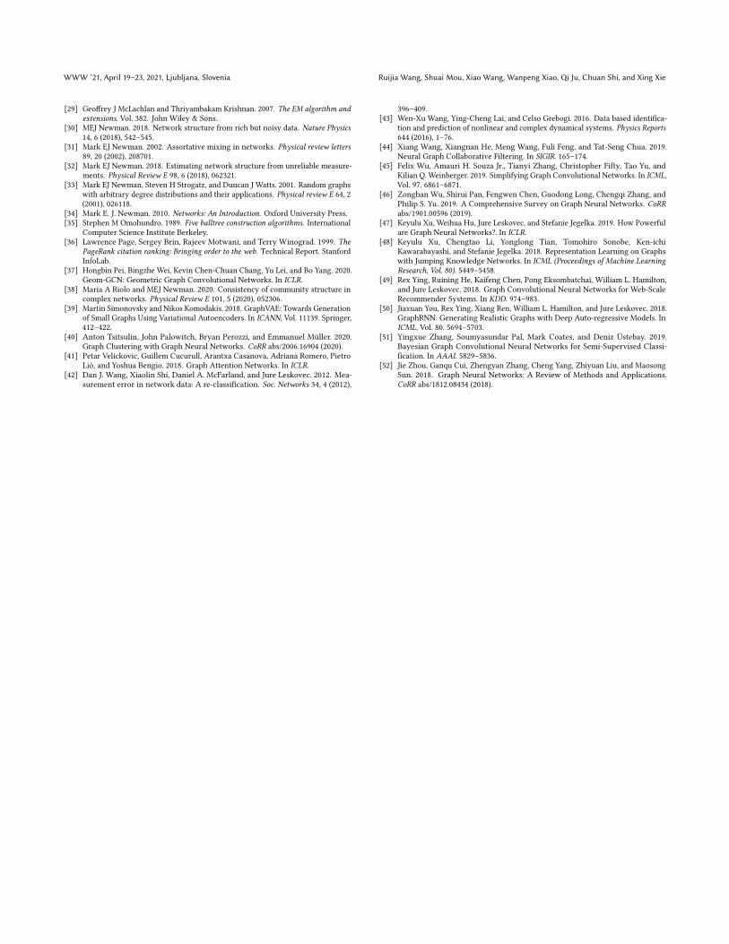
In order to quantify the transformation of community structurebefore and after estimation, we calculate the probability matrixbetween communities, and draw them as heat maps in Figure 6.We observe that in Figure 6 (a), the off-diagonal color blocks arealso dark and even darker than the diagonal ones, indicating thatthe original graph does not maintain a good homophily and highprobabilities of between-community connections could bring dif-ficulties to the GCN optimization. But for the probability matrixof estimated graph, GEN widens the gaps between the diagonaland off-diagonal elements, where the former is usually significantlylarger than the latter, interpreting the reason for the performanceimprovement of classification.

4.3.2 Edge Confidence. Recall that the estimated adjacency matrixQ in GEN is the posterior probability of graph structure, where𝑄𝑖 𝑗

represents our confidence in the existence of that edge. To inves-tigate the meaning of estimated edge, we present the relationshipbetween edge confidence 𝑄𝑖 𝑗 and number of observations 𝐸𝑖 𝑗 . Interms of the synthetic dataset, there are three observations in total,thus the range of 𝐸𝑖 𝑗 is 0 to 3. For each possible value of 𝐸𝑖 𝑗 , weaccumulate the corresponding number of nodes pairs and calculateaverage edge confidence for these nodes pairs in Figure 7. We findthat most node pairs are in the “zero observation” bar, since thegraph is sparse and a large majority of node pairs never meet. Andfrom the relationship between the number of observation 𝐸𝑖 𝑗 andaverage edge confidence, it can be found that an edge observedonly zero or one time implies a low 𝑄𝑖 𝑗 (less than 0.1), so a singleobservation is probably a false alarm. But there is a relatively sharptransition between 𝐸𝑖 𝑗 = 1 and 𝐸𝑖 𝑗 = 2, indicating that two or more

0 1 2 3Number of observations Eij

1

2

3

4

Num

ber o

f nod

e pa

irs

1e3

(a) Statistics of observations

0 1 2 3Number of observations Eij

0.2

0.4

0.6

0.8

1.0

Ave

rage

edg

e co

nfid

ence

(b) Relationship between edge confidenceand observations

Figure 7: The bar chart (a) shows the number of node pairswith each possible value of 𝐸𝑖 𝑗 , and the polyline (b) repre-sents the average edge confidence for every value of 𝐸𝑖 𝑗 .

0.0 0.2 0.4 0.6 0.8 1.0Confidence bins

3

6

9

12

Nor

mal

ized

den

sity

SameDiff.

(a) Training set

0.0 0.2 0.4 0.6 0.8 1.0Confidence bins

3

6

9

12

Nor

mal

ized

den

sity

SameDiff.

(b) Validation set

0.0 0.2 0.4 0.6 0.8 1.0Confidence bins

3

6

9

12

Nor

mal

ized

den

sity

SameDiff.

(c) Test set

Figure 8: Normalized histograms of edge confidence for(a) training, (b) validation and (c) test set nodes w.r.t. thesame/different communities.

observations of the same edge result in a much larger 𝑄𝑖 𝑗 which isa strong inference that the edge exists in the optimal graph.

To show the distribution of edge confidence, we divide the edgesin two groups: edges between nodes of the same communities anddifferent communities. And we report the normalized histogramsof these optimized edge confidence on training, validation and testset in Figure 8, respectively. We observe that the confidence ofedges between same communities is concentrated on the last bin(more than 0.9), while the confidence of edges between differentcommunities is more skewed towards the first bin (less than 0.1).This phenomenon is extremely obvious on the training set, and alsoprominent on validation and test set, illustrating that GEN capturesuseful edge confidence, i.e., higher confidence for edges betweenthe same communities.

4.4 Hyper-parameter SensitivityIn this subsection, we explore the sensitivity of hyper-parameters:𝑘 in 𝑘NN, threshold Y in Eq. (21) and tolerance _ in EM algorithm.More specifically, we alter the value of 𝑘 , Y and _ to see how theyaffect the performance of our model. We vary 𝑘 from 2 to 12, Yfrom 0.1 to 0.9, and _ from 1e-5 to 0.1 in a log scale of base 10. Weonly report the node classification results on Cora and Chameleondatasets in Figure 9 and 10, since similar observations are made inother datasets.

𝑘 in𝑘NN graph. The change trend of accuracyw.r.t.𝑘 is roughlyincreases first then starts to decrease. It is probably because thesparsity of 𝑘NN graphs reduces the number of observed edges


3 6 9 12K

0.81

0.82

0.83

0.84

0.85

Acc

urac

y

(a) 𝑘 in 𝑘NN

0.2 0.4 0.6 0.8Threshold

0.81

0.82

0.83

0.84

0.85

Acc

urac

y

(b) Threshold Y

10−5 10−4 10−3 10−2 10−1

Tolerance

0.81

0.82

0.83

0.84

0.85

Acc

urac

y

(c) Tolerance _

Figure 9: Impact of hyper-parameters on Cora.

3 6 9 12K

0.49

0.50

0.51

0.52

0.53

Acc

urac

y

(a) 𝑘 in 𝑘NN

0.2 0.4 0.6 0.8Threshold

0.49

0.50

0.51

0.52

0.53

Acc

urac

y

(b) Threshold Y

10−5 10−4 10−3 10−2 10−1

Tolerance

0.49

0.50

0.51

0.52

0.53

Acc

urac

y

(c) Tolerance _

Figure 10: Impact of hyper-parameters on Chameleon.

which results in information loss and ineffective inference, whiletoo large 𝑘 would introduce more noise.

Threshold Y. As for threshold Y, if we set Y so high that there arefew edges above the threshold in estimated graph, GEN is unableto aggregate enough information, while too low Y makes estimatedgraph including lots of spurious edges. We note that the accuracycurves of Y are very different on two datasets, and the optimalvalue on Cora is much larger than that on Chameleon. This isalso consistent with the actual situations of these two datasets,where noisy Chameleon dataset leads to large difference betweenobservations thus the edge confidences are generally lower.

Tolerance _. Tolerance _ controls the convergence speed of ourproposed EM algorithm. GEN achieves optimal performance ataround _ = 0.01, and too small or large values harm the model.

5 CONCLUSIONGraph Neural Networks rely heavily on a reasonable graph struc-ture, while an incompatible graph will hurt their performance seri-ously. In this paper, we propose a novel graph estimation neuralnetworks GEN that estimates the graph structure for GNNs to boosttheir performance. Specifically, we introduce a structure model toconsider underlying community structure in graph generation, andpresent an observation model that novelly treats multi-view infor-mation, e.g., multi-order neighborhood similarity, as observationsof optimal graph. Based on these models, we finally attain theestimated graph in Bayesian inference framework. Extensive ex-perimental results verify the effectiveness of GEN and its ability toestimate meaningful graph structure.

An interesting direction for future work is to extend GEN intodynamic graphs. From an intuitive point of view, the observationset could be constructed at varied time slices. However, the obser-vation set cannot reflect the time sequence, and additional nodesduring graph evolution would require retraining the entire modelfrom scratch. Therefore, these considerations motivate a more so-phisticated inference strategy to adaption.

ACKNOWLEDGMENTSWe thank anonymous reviewers for their time and effort in re-viewing this paper. This work is supported in part by the NationalNatural Science Foundation of China (No. U20B2045, U1936104,61972442, 61772082, 62002029), the National Key Research andDevelopment Program of China (2018YFB1402600) and the CCF-Tencent Open Fund.

REFERENCES[1] Muhammet Balcilar, Guillaume Renton, Pierre Héroux, Benoit Gaüzère, Sébastien

Adam, and Paul Honeine. 2020. Bridging the Gap Between Spectral and SpatialDomains in Graph Neural Networks. CoRR abs/2003.11702 (2020).

[2] Joan Bruna, Wojciech Zaremba, Arthur Szlam, and Yann LeCun. 2014. SpectralNetworks and Locally Connected Networks on Graphs. In ICLR.

[3] Giona Casiraghi, Vahan Nanumyan, Ingo Scholtes, and Frank Schweitzer. 2017.From Relational Data to Graphs: Inferring Significant Links Using GeneralizedHypergeometric Ensembles. In SocInfo, Vol. 10540. Springer, 111–120.

[4] Jie Chen, Tengfei Ma, and Cao Xiao. 2018. FastGCN: Fast Learning with GraphConvolutional Networks via Importance Sampling. In ICLR.

[5] Yu Chen, Lingfei Wu, and Mohammed J. Zaki. 2019. Deep Iterative and AdaptiveLearning for Graph Neural Networks. CoRR abs/1912.07832 (2019).

[6] Michaël Defferrard, Xavier Bresson, and Pierre Vandergheynst. 2016. Convolu-tional Neural Networks on Graphs with Fast Localized Spectral Filtering. In NIPS.3837–3845.

[7] Arthur P Dempster, NanM Laird, and Donald B Rubin. 1977. Maximum likelihoodfrom incomplete data via the EM algorithm. Journal of the Royal Statistical Society:Series B (Methodological) 39, 1 (1977), 1–22.

[8] Matthias Fey and Jan Eric Lenssen. 2019. Fast Graph Representation Learningwith PyTorch Geometric. CoRR abs/1903.02428 (2019).

[9] Santo Fortunato and Darko Hric. 2016. Community detection in networks: Auser guide. Physics reports 659 (2016), 1–44.

[10] Luca Franceschi, Mathias Niepert, Massimiliano Pontil, and Xiao He. 2019. Learn-ing Discrete Structures for Graph Neural Networks. In ICML, Vol. 97. 1972–1982.

[11] Justin Gilmer, Samuel S. Schoenholz, Patrick F. Riley, Oriol Vinyals, and George E.Dahl. 2017. Neural Message Passing for Quantum Chemistry. In ICML, Vol. 70.1263–1272.

[12] Michelle Girvan and Mark EJ Newman. 2002. Community structure in social andbiological networks. Proceedings of the national academy of sciences 99, 12 (2002),7821–7826.

[13] William L. Hamilton, Rex Ying, and Jure Leskovec. 2017. Representation Learningon Graphs: Methods and Applications. IEEE Data Eng. Bull. 40, 3 (2017), 52–74.

[14] William L. Hamilton, Zhitao Ying, and Jure Leskovec. 2017. Inductive Represen-tation Learning on Large Graphs. In NIPS. 1024–1034.

[15] XiaoHan, Zhesi Shen,Wen-XuWang, and Zengru Di. 2015. Robust reconstructionof complex networks from sparse data. Physical review letters 114, 2 (2015), 028701.

[16] Mark S Handcock and Krista J Gile. 2010. Modeling social networks from sampleddata. The Annals of Applied Statistics 4, 1 (2010), 5.

[17] Paul W Holland, Kathryn Blackmond Laskey, and Samuel Leinhardt. 1983. Sto-chastic blockmodels: First steps. Social networks 5, 2 (1983), 109–137.

[18] Bo Jiang, Ziyan Zhang, Doudou Lin, Jin Tang, and Bin Luo. 2019. Semi-SupervisedLearning With Graph Learning-Convolutional Networks. In CVPR. 11313–11320.

[19] Wei Jin, Yao Ma, Xiaorui Liu, Xianfeng Tang, Suhang Wang, and Jiliang Tang.2020. Graph Structure Learning for Robust Graph Neural Networks. In KDD.66–74.

[20] Brian Karrer and Mark EJ Newman. 2011. Stochastic blockmodels and communitystructure in networks. Physical review E 83, 1 (2011), 016107.

[21] Thomas N. Kipf and Max Welling. 2017. Semi-Supervised Classification withGraph Convolutional Networks. In ICLR.

[22] Johannes Klicpera, Aleksandar Bojchevski, and Stephan Günnemann. 2019. Pre-dict then Propagate: Graph Neural Networks meet Personalized PageRank. InICLR.

[23] Qimai Li, Zhichao Han, and Xiao-Ming Wu. 2018. Deeper Insights Into GraphConvolutional Networks for Semi-Supervised Learning. In AAAI. 3538–3545.

[24] Xun Li and Xiang Li. 2017. Reconstruction of stochastic temporal networksthrough diffusive arrival times. Nature communications 8, 1 (2017), 1–10.

[25] Yujia Li, Daniel Tarlow, Marc Brockschmidt, and Richard S. Zemel. 2016. GatedGraph Sequence Neural Networks. In ICLR.

[26] Dean Lusher, Johan Koskinen, and Garry Robins. 2013. Exponential randomgraph models for social networks: Theory, methods, and applications. CambridgeUniversity Press.

[27] Peter V Marsden. 1990. Network data and measurement. Annual review ofsociology (1990), 435–463.

[28] Travis Martin, Brian Ball, and Mark EJ Newman. 2016. Structural inference foruncertain networks. Physical Review E 93, 1 (2016), 012306.


[29] Geoffrey J McLachlan and Thriyambakam Krishnan. 2007. The EM algorithm andextensions. Vol. 382. John Wiley & Sons.

[30] MEJ Newman. 2018. Network structure from rich but noisy data. Nature Physics14, 6 (2018), 542–545.

[31] Mark EJ Newman. 2002. Assortative mixing in networks. Physical review letters89, 20 (2002), 208701.

[32] Mark EJ Newman. 2018. Estimating network structure from unreliable measure-ments. Physical Review E 98, 6 (2018), 062321.

[33] Mark EJ Newman, Steven H Strogatz, and Duncan J Watts. 2001. Random graphswith arbitrary degree distributions and their applications. Physical review E 64, 2(2001), 026118.

[34] Mark E. J. Newman. 2010. Networks: An Introduction. Oxford University Press.[35] Stephen M Omohundro. 1989. Five balltree construction algorithms. International

Computer Science Institute Berkeley.[36] Lawrence Page, Sergey Brin, Rajeev Motwani, and Terry Winograd. 1999. The

PageRank citation ranking: Bringing order to the web. Technical Report. StanfordInfoLab.

[37] Hongbin Pei, Bingzhe Wei, Kevin Chen-Chuan Chang, Yu Lei, and Bo Yang. 2020.Geom-GCN: Geometric Graph Convolutional Networks. In ICLR.

[38] Maria A Riolo and MEJ Newman. 2020. Consistency of community structure incomplex networks. Physical Review E 101, 5 (2020), 052306.

[39] Martin Simonovsky and Nikos Komodakis. 2018. GraphVAE: Towards Generationof Small Graphs Using Variational Autoencoders. In ICANN, Vol. 11139. Springer,412–422.

[40] Anton Tsitsulin, John Palowitch, Bryan Perozzi, and Emmanuel Müller. 2020.Graph Clustering with Graph Neural Networks. CoRR abs/2006.16904 (2020).

[41] Petar Velickovic, Guillem Cucurull, Arantxa Casanova, Adriana Romero, PietroLiò, and Yoshua Bengio. 2018. Graph Attention Networks. In ICLR.

[42] Dan J. Wang, Xiaolin Shi, Daniel A. McFarland, and Jure Leskovec. 2012. Mea-surement error in network data: A re-classification. Soc. Networks 34, 4 (2012),

396–409.[43] Wen-Xu Wang, Ying-Cheng Lai, and Celso Grebogi. 2016. Data based identifica-

tion and prediction of nonlinear and complex dynamical systems. Physics Reports644 (2016), 1–76.

[44] Xiang Wang, Xiangnan He, Meng Wang, Fuli Feng, and Tat-Seng Chua. 2019.Neural Graph Collaborative Filtering. In SIGIR. 165–174.

[45] Felix Wu, Amauri H. Souza Jr., Tianyi Zhang, Christopher Fifty, Tao Yu, andKilian Q. Weinberger. 2019. Simplifying Graph Convolutional Networks. In ICML,Vol. 97. 6861–6871.

[46] Zonghan Wu, Shirui Pan, Fengwen Chen, Guodong Long, Chengqi Zhang, andPhilip S. Yu. 2019. A Comprehensive Survey on Graph Neural Networks. CoRRabs/1901.00596 (2019).

[47] Keyulu Xu, Weihua Hu, Jure Leskovec, and Stefanie Jegelka. 2019. How Powerfulare Graph Neural Networks?. In ICLR.

[48] Keyulu Xu, Chengtao Li, Yonglong Tian, Tomohiro Sonobe, Ken-ichiKawarabayashi, and Stefanie Jegelka. 2018. Representation Learning on Graphswith Jumping Knowledge Networks. In ICML (Proceedings of Machine LearningResearch, Vol. 80). 5449–5458.

[49] Rex Ying, Ruining He, Kaifeng Chen, Pong Eksombatchai, William L. Hamilton,and Jure Leskovec. 2018. Graph Convolutional Neural Networks for Web-ScaleRecommender Systems. In KDD. 974–983.

[50] Jiaxuan You, Rex Ying, Xiang Ren, William L. Hamilton, and Jure Leskovec. 2018.GraphRNN: Generating Realistic Graphs with Deep Auto-regressive Models. InICML, Vol. 80. 5694–5703.

[51] Yingxue Zhang, Soumyasundar Pal, Mark Coates, and Deniz Üstebay. 2019.Bayesian Graph Convolutional Neural Networks for Semi-Supervised Classi-fication. In AAAI. 5829–5836.

[52] Jie Zhou, Ganqu Cui, Zhengyan Zhang, Cheng Yang, Zhiyuan Liu, and MaosongSun. 2018. Graph Neural Networks: A Review of Methods and Applications.CoRR abs/1812.08434 (2018).

Documents

Graph Structure Estimation Neural Networks - Chuan Shi