Embed Size (px)
Citation preview
Goal Programming Approach for
Channel Assignment Formulation
and Schemes
N G Cho Y iu
A Thesis Submitted in Partial Fulfilment
of the Requirements for the Degree of
Master of Philosophy
in
Information Engineering
Supervised by
Prof. L O K Tat Ming
©The Chinese University of Hong Kong
July 2005
The Chinese University of Hong Kong holds the copyright of this thesis. Any person(s) intending
to use a part or whole of the materials in the thesis in a proposed publication must seek copyright
release from the Dean of the Graduate School.

统系
H 1 8 DK j i ~UNIVERSITY
^^S^UBRARY SYSTEM
Abstract of thesis entitled:
Goal Programming Approach for Channel Assignment Formulation and Schemes
Submitted by NG Cho Yiu
for the degree of Master of Philosophy
at The Chinese University of Hong Kong in July 2005
In this thesis, a goal programming model is proposed for general downlink channel
assignment scheme. Unlike many current channel assignment schemes with quality
of service (QoS) requirements modeled as system constraints, QoS requirements are
formulated as mathematical functions, which are called unsatisfactory functions,
in the objective function of our schemes. With this formulation, when there is
insufficient amount of resource, the proposed schemes can provide the compromise
solutions more conveniently without explicit admission controls. Moreover, QoS
requirements can be modeled in a more flexible and detailed manner. The system
can substitute any QoS function for each user based on his/her application. In this
formulation, there are no assumptions about the underlying multiple access scheme
except the orthogonality of the logical channels.
Since it is proved to be an NP-hard problem, an iterative algorithm and a greedy
algorithm are proposed to provide near-optimal solutions. In addition, two special
cases of this model are studied. For these cases, it is proved that optimal solutions
can be obtained by polynomial-time algorithms. Simulation results show that with
the proposed algorithms, less channel resource is required to meet the client demand.
i
摘要
這篇論文爲下行線路通道分配問題(downlink channel assignment)提出一個目
標規劃(goal programming)模型。許多現今考慮服務質量(QoS)的通道分配
策略,把用戶的服務質量要求表達爲模型中的約束條件(system constraint)。不
同於這些策略,我把這些服務質量要求模擬成一個名爲「非滿意函數」
(unsatisfactory function )的函數,並放S令模型中的目標函數(ob jec t i ve function)
中。即使當系統沒有足夠的資源’根據我所提出的模型和相應的策略’我們可
以更方便地而又不需要利用額外的接納控制(admission control)得出一個妥協
解答(compromise solution)。除此之外,服務質量要求也可以在這個模型中有
一個更靈活和細緻的表達。在這個模型中’系統可以根據每個用戶的應用程式
代入適合的非滿意函數。在這個模型中,除了要求每一條邏輯通道( log ica l
channel)要其他邏輯通道正交(orthogonal)外’我沒有假設任何多工存取技術
(multiple access scheme)。
由於這是一個NP-hard問題’我提出一個疊代的流程(iterative algorithm)和一
個貪梦的策略(greedy algorithm)以提供一個接近最佳的解答。此外,我亦探
討了兩個特例。這些特例被證明了可以用多項式時間流程(polynomial-time
algorithm)得出最佳解答。電腦模擬結果也顯示了本論文提出的策略可以減少
滿足用戶需求所需的資源。
ii

Acknowledgement
I would like to express my gratitude to all those who gave me the possibility to
complete this thesis. I am grateful to the Almighty God who is my source of strength
throughout my study. "The LORD is my shepherd, I shall not be in want." (Psalm
23:1)
I take this opportunity to thank my supervisor, Prof. Tat Ming Lok. I am deeply
indebted to your stimulating suggestions and encouragement during my research.
You did not only help my research work, but you also broadened my horizon.
I would like to thank my family members who has supported me all the time. The
encouragement of my parents motivated me to face the difficulties in my research.
The prayers from my brother provided the power for me in the research.
I want to thank my brothers and sisters in my cell group in the Shatin Baptist
Church. The prayers, the sharings, the motivations and the encouragement are the
crucial backup for my research. It is my pleasure to have about twenty angels who
remind me, "My help comes from the LORD, the Maker of heaven and earth."
(Psalm 121:2) Although I did not pray for each of you, each of you has prayed for
my research many times.
I also want to thank my previous and present colleagues in the Information and
Systems Laboratory and Wireless Communications Laboratory II. Your comments
are valuable in this thesis. Thank you for spending your precious time to answer my
questions and providing suggestions.
iii

This work is dedicated to the Almighty God and my family.
iv
Contents
Abstract i
• • •
Acknowledgement iii
Preface x
1 Introduction 1
1.1 Multiple Access 1
1.1.1 Time Division Multiple Access 2
1.1.2 Frequency Division Multiple Access 3
1.1.3 Code Division Multiple Access 3
1.1.4 Hybrid Multiple Access Scheme 4
1.2 Goal Programming 5
2 Previous Works in Channel Assignment 10
2.1 Voice Service Network 10
2.2 Data Network 11
2.2.1 Throughput Optimization 13
2.2.2 Channel Assignment Schemes with QoS Consideration . . . . 14
3 General Channel Assignment Scheme 16
3.1 Baseline Model • 17
3.2 Goal Ranking 22
V
3.3 Model Transformation 22
3.4 Proposed Algorithms 23
3.4.1 Channel Swapping Algorithm 24
3.4.2 Best-First-Assign Algorithm 26
4 Special Case Algorithms 28
4.1 Single Order of Selection Diversity 28
4.1.1 System Model 29
4.1.2 Proposed Algorithm 30
4.1.3 Extension of Algorithm 31
4.2 Single Channel Assignment 32
4.2.1 System Model 33
4.2.2 Proposed Algorithms 34
5 Performance Evaluation 37
5.1 General Channel Assignment and Single Channel Assignment . . . . 37
5.1.1 System Model 38
5.1.2 Lower Bound of Weighted Sum of Unsatisfactory Function . . 40
5.1.3 Performance Evaluation I 41
5.1.4 Discussion 44
5.1.5 Performance Evaluation II 44
5.2 Single Order of Selection Diversity Algorithm 47
5.2.1 System Model 47
5.2.2 Performance Evaluation I 49
5.2.3 Performance Evaluation II 53
6 Conclusion and Future Works 58
6.1 Conclusion 58
6.2 Future Works 60
6.2.1 Multi-cell Channel Assignment 60
vi

6.2.2 Theoretical Studies 62
6.2.3 Adaptive Algorithms 62
6.2.4 Assignment of Non-orthogonal Channels 63
A Proof of Proposition 3.1 64
B Proof of Proposition 4.1 66
C Assignment Problem 68
Bibliography 74
vii

List of Figures
3.1 Relationship between weighted sum of unsatisfactory function and
number of iterations 26
5.1 Relationship between the proportion of deficient throughput and num-
ber of channels 41
5.2 Relationship between the proportion of deficient throughput and num-
ber of clients 43
5.3 Relationship between the proportion of deficient throughput and num-
ber of channels 45
5.4 Relationship between the proportion of deficient throughput and num-
ber of clients 46
5.5 Relationship between proportion of deficient throughput and number
of clients for fixed N 49
5.6 Relationship between weighted sum of bonus function and number of
clients for fixed N 50
5.7 Relationship between proportion of deficient throughput and number
of channels for fixed K 51
5.8 Relationship between weighted sum of bonus function and number of
channels for fixed K 52
5.9 Relationship between proportion of deficient throughput and number
of clients for fixed N 54
viii

5.10 Relationship between weighted sum of bonus function and number of
clients for fixed N 55
5.11 Relationship between proportion of deficient throughput and number
of channels for fixed K 56
5.12 Relationship between weighted sum of bonus function and number of
channels for fixed K 57
ix

List of Tables
1.1 Multiple Access Techniques Used in Different Wireless Communica-
tion Systems 2
V
Preface
In the third and future generation wireless systems, operators and service providers
have been introducing more and more variations of data applications. Examples
include video conferencing, video streaming and various kinds of multimedia services.
Quality of service (QoS) requirements have larger variations than previous generation
wireless systems which only provide voice services. Therefore, more sophisticated
resource allocation schemes are needed so that QoS requirements are satisfied in a
more effective way. In this thesis, we consider the allocation of one important type
of wireless resource, which is wireless channel.
Many current channel assignment schemes [19] [20] [39] have been proposed to opti-
mize throughput or latency in many wireless data networks. However, client demands
or QoS requirements are ignored in these schemes. As a result, unfair and inefficient
assignment is resulted. Some clients may not be able to obtain their desired through-
put while some may obtain far beyond their needs. Some channels are wasted in this
case.
Some other schemes like [2] are proposed to improve the above situation by formu-
lating user requirements as system constraints. However, in practice, there may not
be enough number of channels or the channels do not have the desired high quality
(like low signal-to-noise ratio). In the operations research terminology, there may be
110 feasible solutions.
One possible way to alleviate this problem is to perform admission control. Ad-
mitted data streams are guaranteed to meet the QoS requirements [36]. Then, we
xi
perform the throughput maximization or latency minimization for these admitted
data streams. Another way to tackle this problem is to seek foi. a compromise solu-
tion. In this case, user requirements are no longer modelled as the system constraints
of our problem. Instead, for each user, a function, called unsatisfactory function, is
introduced which measures the deviation of the performance below the minimum
requirement. By minimizing the sum of these functions, a compromise solution is
obtained. In this compromise solution, on average, the performance of each client is
close to the minimum requirement. This approach is more flexible so we consider it
throughout this thesis.
In this thesis, we propose a goal programming [12] model for a general downlink
channel assignment scheme. Goal programming is an operations research technique
in seeking for compromise solutions. In our model, it does not only formulates the
channel properties, but also introduces two functions, namely, the unsatisfactory
function and the bonus function, to model the clients' QoS requirements and per-
formance. For each user, these functions are chosen based on their application layer
specification. In this model, there are no assumptions in the underlying multiple
access schemes. It can be time division multiple access (TDMA), frequency division
multiple access (FDMA), code division multiple access (CDMA) or the hybrid of
them. The only requirement is that each logical channel must be orthogonal to one
another. That means, the multiple access interference (MAI) is 0. Therefore, this
model is general enough for most downlink transmission systems with a large variety
of user applications.
In this thesis, it is shown that the problem is an NP-hard problem [11]. Hence,
we propose two near-optimal polynomial-time algorithms, namely, channel-swapping
algorithm and the best-first-assign algorithm. Simulation results show that our pro-
posed algorithms assign the channels in a more effective way than throughput op-
timization schemes. Fewer channels are required to meet the same set of QoS re-
quirements. This suggests our proposed algorithms are more economical than the
xii
throughput optimization approaches. In addition, in this thesis, we also compare
these two proposed algorithms in terms of weighted sum of unsatisfactory function
and time complexity. These are the two main concerns for the operators. This
provides the hints on the choice of algorithm.
Our work does not end here. We also study two common subsets of problems
where optimal solutions can be obtained by polynomial-time algorithms. In the first
subset of problems, it is assumed that the order of selection diversity of the multiple
access scheme is 1. On the other hand, in the second subset of problems, it is
assumed that each client can be assigned at most 1 channel. Simulations results show
that in the first subset of the problem, compared with the throughput optimization
scheme, our proposed algorithm does not only have much smaller weighted sum of
unsatisfactory function, but also the throughput of our proposed algorithm is close to
the throughput optimization scheme. The proposed algorithm in the second subset of
problem is used in obtaining a lower bound of weighted sum of unsatisfactory function
in the performance evaluation of channel-swapping algorithm and best-first-assign
algorithm.
Finally, we carry out the performance evaluation via simulations. As mentioned
above, we compare our proposed algorithms and the throughput optimization schemes.
In the simulations, the proposed algorithms outperform the throughput optimization
scheme. We end this thesis with a conclusion and some future research directions.
This thesis is organized as follows. In Chapter 1, basic knowledge about multiple
access schemes and goal programming are introduced. In chapter 2, previous works
about channel assignment are reviewed. In Chapter 3, the general formulation for the
channel assignment problem is proposed. Two algorithms are proposed accordingly.
In Chapter 4, the two special cases are investigated and the optimal algorithms are
proposed. In Chapter 5, performances of proposed algorithms in Chapter 3 and 4 are
analyzed through simulations. In Chapter 6,I will conclude the thesis and discuss
some future research directions.
xiii
Chapter 1
Introduction
The main theme of this thesis is the application of goal programming in channel
assignment problem. Goal programming is a multi-objective optimization technique
which is useful in seeking for compromise solution when no feasible solutions exist.
Before we can formulate the problem as a goal programming model, we need to know
how the spectrum is partitioned into different channels. This is the known as the
multiple access scheme.
In this chapter, we will go through the two fundamental concepts of this thesis,
namely, multiple access and goal programming. In multiple access, we will describe
some common multiple access schemes like TDMA, FDMA, CDMA, etc. For goal
programming, we will discuss how a problem can be formulated as a goal program-
ming model. An example is given in the end of this chapter to illustrate the idea.
1.1 Multiple Access
In wireless communications, operators should allow multiple users to transmit and
receive information simultaneously in a shared spectrum. This is the purpose of
multiple access schemes. The base station (or access point for the case in wireless
LAN) multiplexes all the data streams in a way that each user should be able to
extract his or her desired data stream from the signal in the spectrum. In a multiple
1
CHAPTER 1. INTRODUCTION 2
access scheme, the whole spectrum is divided into several logical channels. Each
logical channel is dedicated to a one-way transmission (either uplink or downlink)
between the base station and a client. In this thesis, for simplicity, the term channel
refers to a logical channel of a multiple access scheme.
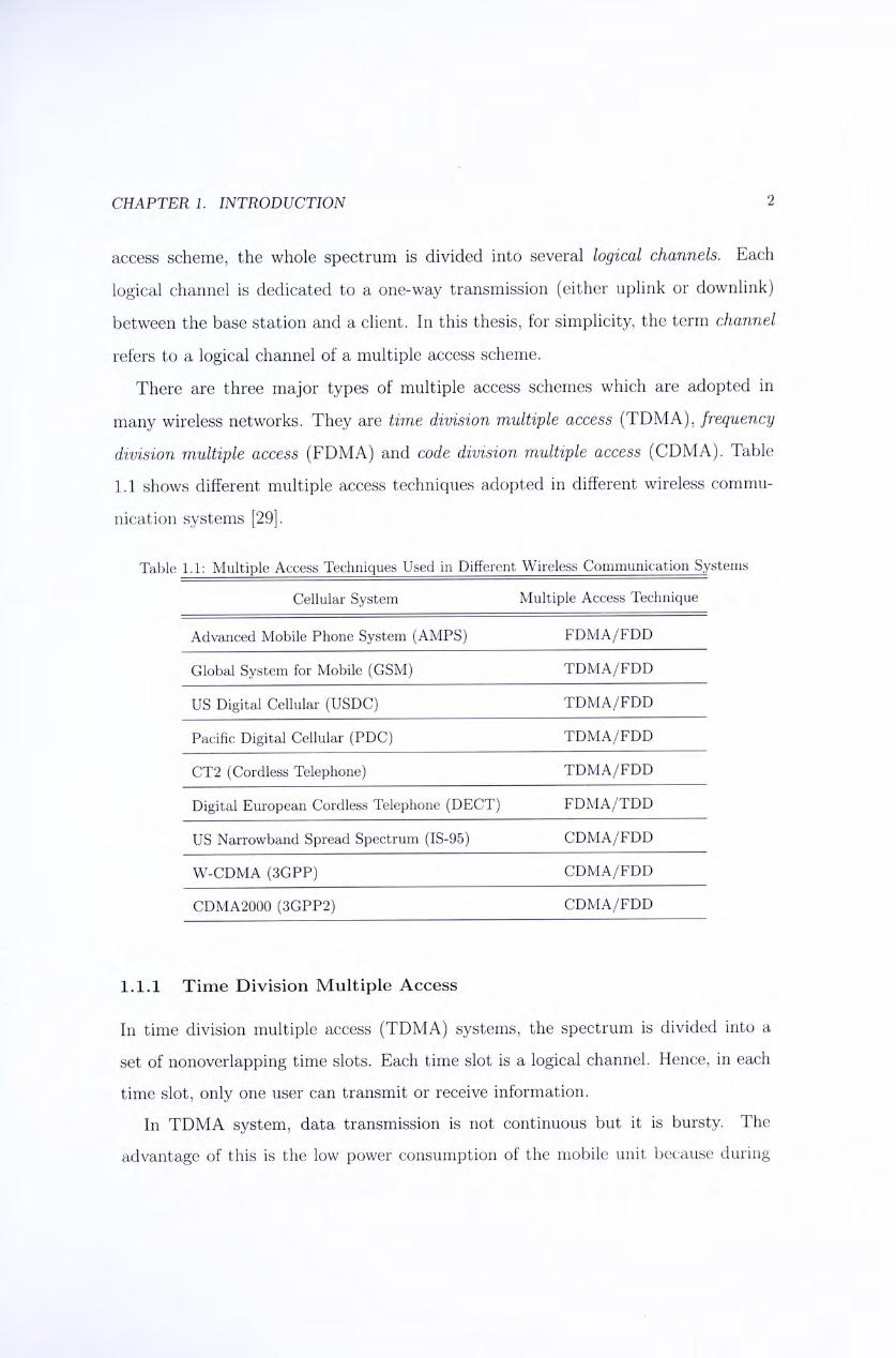
There are three major types of multiple access schemes which are adopted in
many wireless networks. They are time division multiple access (TDMA), frequency
division multiple access (FDMA) and code division multiple access (CDMA). Table
1.1 shows different multiple access techniques adopted in different wireless commu-
nication systems [29 .
Table 1.1: Multiple Access Techniques Used in Different Wireless Communication Systems
Cellular System Multiple Access Technique
Advanced Mobile Phone System (AMPS) FDMA/FDD
Global System for Mobile (GSM) TDMA/FDD
US Digital Cellular (USDC) TDMA/FDD
Pacific Digital Cellular (PDC) TDMA/FDD
CT2 (Cordless Telephone) TDMA/FDD
Digital European Cordless Telephone (DECT) FDMA/TDD
US Narrowband Spread Spectrum (IS-95) CDMA/FDD
W-CDMA (3GPP) CDMA/FDD
CDMA2000 (3GPP2) CDMA/FDD
1.1.1 Time Division Mult iple Access
In time division multiple access (TDMA) systems, the spectrum is divided into a
set of nonoverlapping time slots. Each time slot is a logical channel. Hence, in each
time slot, only one user can transmit or receive information.
In TDMA system, data transmission is not continuous but it is bursty. The
advantage of this is the low power consumption of the mobile unit because during
CHAPTER 1. INTRODUCTION 3
other users' time slots, the transmitter and receiver can be switched off. However, the
cost is the synchronization overhead. Guard time is needed so that the transmitter
and receiver are synchronized.
1.1.2 Frequency Division Mult ip le Access
In frequency division multiple access (FDMA) systems, the spectrum is divided into
a number of frequency bands. Each frequency band corresponds to a logical channel.
Therefore, different users can transmit or receive information in different frequency
bands simultaneously.
Unlike TDMA, in which all users can use the whole spectrum during their data
transmission, in FDMA, the bandwidth of each channel is much smaller. The symbol
time of narrowband signal is large compared to the average delay spread. Thus,
the intersymbol interference (ISI) is low and hence, the system does not require
sophisticated equalization techniques. Nonetheless, FDMA systems require tight
radio frequency (RF) filtering to minimize adjacent channel interference.
1.1.3 Code Division Mult iple Access
In code division multiple access (CDMA) systems, each logical channel is a signature
sequence (also known as spreading sequence). The correlation between the signature
sequences is low and by using this property, receivers can differentiate signals of
different logical channels by either the matched filter [27] (for zero correlation, i.e.
orthogonal sequences) or multiuser detectors [37] (for non-zero correlation, i.e. non-
orthogonal sequences).
There are many ways to implement CDMA. Two important examples of CDMA
systems are direct-sequence CDMA (DS-CDMA) systems [26] and multicarrier CDMA
(MC-CDMA) [21] systems.
In DS-CDMA systems, transmitted signals of different users are multiplied by
CHAPTER 1. INTRODUCTION 4
different spreading signal. The spreading signal is of the form:
N
键—ITc) (1.1)
1=0
where {aJ is the signature sequence and ip{t) is the chip waveform, which is time-
limited to [0, Tc) where T。is the chip interval. Since the correlation between distinct
sequences is low, to extract the desired signal, we can adopt a correlator receiver [42
to multiply and integrate the received signal with the spreading signal.
On the other hand, in MC-CDMA systems, instead of multiplying the user signal
by the spreading signal in the time domain, the multiplication is carried out in
frequency domain. As its name implies, in MC-CDMA systems, every user makes
use of all the carriers in the system. Each carrier is orthogonal to one another. The
user signal is multiplied by every carrier. For each carrier, the modulated signal is
multiplied by an element of the signature sequence. The transmitted signal is the
aggregation of the modulated signals of all the carriers.
1.1.4 Hybrid Mult ip le Access Scheme
Apart from the above multiple access schemes, there are some schemes called hybrid
multiple access schemes. They are combinations of multiple access schemes. After
dividing the spectrum into logical channels by the first multiple access scheme, each
logical channel is further divided into a new set of logical channels by the second
multiple access scheme.
One example is the time division CDMA (TCDMA) [29] system. In TCDMA
system, different signature sequences are assigned to different set of users. Within
the same set of users, only one user can transmit or receive the signal in a time slot
with that signature sequence. In this case, a logical channel is the signature sequence
in a time slot.
CHAPTER 1. INTRODUCTION 5
1.2 Goal Programming
111 many common optimization models, a single objective function is optimized. The
optimization may be performed subject to a certain set of constraints. However, in
reality, we may encounter problems involving more than one objective function which
may conflict with one another. Furthermore, feasible solutions may not exist. In this
situation, we may interest in seeking some compromise solutions so that the final
decision is close to the minimum requirements of everybody involved. Therefore, we
need some formulations which facilitate us to seek for compromise solutions in these
scenarios.
To alleviate the above problems, Charnes and Cooper proposed an approach called
goal programming in [5]. The principal idea is to combine all the objective functions
and the soft constraints into a single objective function. Soft constraints refer to
those constraints that we should try our best to fulfill but we are allowed to pro-
vide solutions which do not satisfy these constraints. For example, in some network
resource allocation problems, every user's application has its own quality of service
(QoS) requirements according to the application layer specification. If there is avail-
able amount of resource, those QoS requirements should be satisfied. However, in
reality, there exist some situations that the system does not have enough resource for
the QoS requirements. Therefore, to have a more realistic formulation, those QoS
requirements should be modelled as soft constraints. Actually, this is one important
point in the channel assignment formulation proposed in this thesis.
After that, we transform all the soft constraints in the following way. For the
z-th soft constraint, we define a function f制,where x is the vector of decision
variables. This function is a measurement of deviation from the requirement of
the constraint. For example, if constraint i is < a” where a is a constant,
one possible choice of f! can be fi{x) = max{0,队(f) - a j . That means, if this
constraint is satisfied, f^{x) is 0. Otherwise, it is 识(x) - a” that is the deviation of
from its required upper limit.
CHAPTER 1. INTRODUCTION 6
Now, the soft constraints become functions of decision variables. Since the func-
tions {fi} are deviations from the problem requirement, we would like to minimize
them. Therefore, for each we create a new objective function:
Minimize (1.2)
Together with the above set of new objective functions, we now have a multi-
objective optimization problem. In general, these constraints may conflict with one
another. Thus, we need to combine them into a single objective function in the
following manner first.
To begin with, we classify the objective functions into different groups according
to their priorities in decision making. A higher priority objective function dominates
the lower priority objective function in decision making. The objective functions
in the same group do not dominate one another in decision making. Usually, the
objective functions for the soft constraints are in the highest priority [12 .
Next, we define a term called lexicographic minimum as below [12]:
Definition 1.1. For two vectors a^^^ = ( 。 ( 八 4”,. •.,ai^i)广 and S⑶=(“(丄。),a;?),. • 乂 丄 ? ) ) ^ ,
IS preferred to a⑵ if there exists an integer k such that a[?) < a、:、and all higher
order terms (i.e. 0,1,0,2,.. . are equal. If no other vectors is preferred to a,
then a is the lexicographic minimum.
With the ranking of the objective functions and Definition 1.1, we can combine the
objective functions into a single objective function as follows. Firstly, the objective
functions in the same priority group is combined linearly into one objective function.
The coefficients in this linear combination correspond to the relative importance of
the objective functions in decision making. Now, for each priority group, there is one
combined objective function. We put all these objective functions into a vector. The
first component is for the most important objective function, the second component
is for the second most important objective function and so on. Our final objective
CHAPTER 1. INTRODUCTION 7
function becomes:
lexmin (仍(f),仍(f), •. •)『 (1.3)
where 认 is the objective function for the 2-th priority group and x is the vector of
the decision variables.
According to the properties of the objective functions, there are different algo-
rithms to solve the goal programming problem. For example, if all the components
are linear functions, the problem can be solved by multiphase Simplex-method [12],
which is an extension to the two-phase method [10] used in linear programming prob-
lems. For nonlinear goal programming problems, approaches have been summarized
in [32:.
We end this chapter with the following example quoted from [35] to illustrate how
to formulate a goal programming model. Since this thesis is not dedicated to the
topic goal programming, interested parties may refer to [12] for further details.
Example 1.1. Fairville is a small city with a population of about 20,000 residents.
The city council is in the process of developing an equitable tax rate table. The annual
taxation base for real estate property is $550 million. The annual taxation bases for
food and drugs and for general sales are $55 million and $35 million, respectively.
Annual local gasoline consumption is estimated at 7.5 million gallons. The city
council wants to maximize the tax revenue by developing the tax rates based on three
main goals
• Food and drug taxes cannot exceed 10% of all taxes collected.
• General sales taxes cannot exceed 20% of all taxes collected.
• Gasoline tax cannot exceed 2 cents per gallon.
Let the variables Xp.Xf, and Xs represent the tax rates (expressed as proportions) for
property, food and drug, and general sales and define the variable Xg as the gasoline
CHAPTER 1. INTRODUCTION 8
tax m cents per gallon. The problem can be formulated as
Maximize 500xp + 35x/ + 55a:, + O.OTSa: (1.4)
subject to
3bxf < 0.1(5502p + + 55x-, + 0.075xg (1.5)
55j:, < 0.2(550.Xp + 35:,/ + 55a:, + 0.075xg) (1.6)
< 2 (1.7)
Xp,Xf,Xs,Xg > 0 ( 1 . 8 )
Each of the first three inequalities represents a goal that the city council aspires to
satisfy. However, these goals may be m conflict and the best we can do is try to reach
a compromise solution.
Firstly, we convert the first three inequalities as follows:
55xp - 31.5x/ + + 0.0075x5 + 5+ - 5]; = 0 (1.9)
llOxp + 7xf - 44x, + + sf - sf 二 0 (1.10)
Xg + S^ - S^ = 0 (1.11)
5+,5- > 0 z = 1,2,3 (1.12)
These constraints replace the old set of system constraints. In addition, we have the
following three new objective functions now:
Minimize s^ (1.13)
Minimize s j (1-14)
Minimize S3 (1.15)
These three objective functions dominate the objective function (I.4) in decision mak-
ing. Furthermore, these three objective functions do not dominate one another m
decision making and they are equally important. Therefore, these objective functions
are combined into the following single objective function:
丁’
lexmin (s+ + 4 + 53 ,500a;p + 35x/ + + 0.075xg) (1.16)

CHAPTER 1. INTRODUCTION 9
subject to the constraints (1.9) to (1.12).
Chapter 2
Previous Works in Channel
Assignment
111 this chapter, we will review some previous works in channel assignment. We
will discuss the disadvantage of these channel assignment schemes and the rationale
behind as a background study and motivation of proposing new channel assignment
models and schemes in this thesis.
2.1 Voice Service Network
In the second generation (2G) cellular network, only voice service is provided. Hence,
if the wireless channel has a signal-to-noise ratio (SNR) above certain threshold, it
can be assigned to a user. Thus, for every user, all channels above the SNR threshold
are identical. The base station only needs to assign any of these channels which is
available. This is the channel assignment scheme in 2G systems.
The grade of service (GOS) is the blocking probability of the network. There are
two types of trunked systems which have two different formulas for the GOS. The
first type offers no queueing for the call requests. For each user who requests service,
it is assumed there is no setup time. If a channel is available, the suer can access
it immediately. Otherwise, that user is blocked without access and is free to try
10
CHAPTER 2. PREVIOUS WORKS IN CHANNEL ASSIGNMENT 26
again later. The inter-arrival time of the users is assumed to be Poisson distributed
and the service time of each user is assumed to be exponentially distributed. The
problem is modelled by an M/M/C queueing system [31]. In this case, the GOS is
given by the Erlang B formula [3
Pr {blocking} = — ^ ^ (2.1)
where C is the number of channels in the cell and A is the offered load, which is the
product of mean arrival rate and mean service time.
In the second type trunked system, a queue is provided to hold the blocked calls.
Call requests are delayed until a channel is available. In this case, the GOS is
defined as the probability that a call is blocked after waiting a specific length of time
in the queue. Before determining the GOS, the probability that a call not having an
immediate access to a channel is determined by the Erlang C formula [29
沖 e l 砂〉0} 二 f + 旬 E 二 要 (2.2)
The probability that a delayed call is forced to wait more than t seconds is given
by the probability that the call is delayed, multiplied by the conditional probability
that the delay is greater than t seconds. Hence, the GOS is given by
Pr {delay > t} = Pr {delay > 0} Pr {delay > delay > 0} (2.3)
=Pr {delay > 0} e-“"『 (2.4)
where H is the mean service time.
2.2 Data Network 丫
In the third generation and future generation wireless networks, there are not only
the voice services but also more and more data applications. For data applications,
common choices of performance measures are throughput and latency [28]. The
quality of service (QoS) of the network is no longer the blocking probability only.
CHAPTER 2. PREVIOUS WORKS IN CHANNEL ASSIGNMENT 12
According to Shannon's Channel Coding Theorem [33], for a channel with band-
width B and signal-to-noise ratio (SNR) 7, there exists a channel coding scheme
such that the coding rate is any C, C < R, where R is given by
二 Blog2(l + 7). (2.5)
This theorem implies that for a given amount of bandwidth, the maximum achievable
throughput of a channel depends on its SNR. In general, each channel has different
SNR. It is because the fading experience of each channel is different. In addition, for
the same channel, the fading experience of different users is different. Fading affects
the received signal power and thus the SNR at the receiver side.
For some multiple access schemes, for the same user, the fading experience of
different channels is the same but this is not the case for other multiple access
schemes. For instance, in a narrowband direct sequence CDMA (DS-CDMA) system
with Hadamard signature sequences [38], for the same user, the fading experience of
different channels is the same [20]. On the other hand, if we use random orthogonal
signature sequences, for the same user, the fading experience of different channels is
different.
We will define a term order of selection diversity in Chapter 3 for this phenom-
enon. This is a key property in designing special case algorithms in Chapter 4
By assigning different channels, the data applications may have different per-
formance because the throughputs of different channels are different. Unlike voice
service networks, we should not assign an available channel arbitrarily because the
performance measure of the system is no longer the blocking probability. In this case,
channel estimations have to be performed and then channels are assigned based on
these estimated values. The channels are assigned to optimize certain performance
measures. Some channel assignment schemes in data networks are reviewed below.
CHAPTER 2. PREVIOUS WORKS IN CHANNEL ASSIGNMENT 13
2.2.1 Throughput Opt imiza t ion
Since throughput and latency are typical choices of performance measures, some
channel assignment schemes [19] [20] [39] are proposed to optimize these two mea-
surements in different networks or multiple-access schemes. Since latency is the
reciprocal of the throughput, for channel assignment schemes which only assign one
channel to each user like [20], the same scheme also minimizes the total latency of
the users.
We can have a general formulation for the throughput optimization scheme. Let
N and K be the number of channels and users respectively. Let Xij be the binary
decision variable such that it is 1 if channel i is assigned to client j . Otherwise, Xy. is
0. Let R、i be the throughput of channel i for client j , which is obtained by equation
(2.5). The formulation of the problem is as follows.
N K
Maximize ^ ^ (2.6)
i=l j.=l
subject to
N
< 1, Vj- (2.7)
i=l K
V^ (2.8)
.7 = 1
e {0 , l } (2.9)
where the objective function is the total throughput of the users.
It can be seen that it is an assignment problem [10] and it can be solved by the
Hungarian method [16]. Alternatively, it can also be solved by common mathematical
software.
The major drawback of these schemes is that the application layer specifications,
such as minimum required throughput, are not considered. An unfair channel as-
signment may be resulted. The reason is that to optimize the total throughput,
the base station tends to assign more channels to users with higher average SNR.
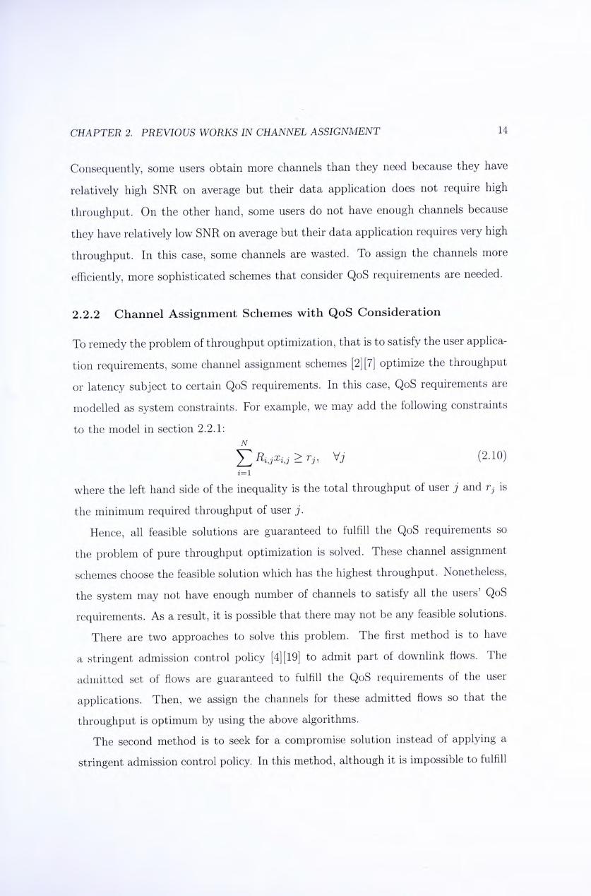
CHAPTER 2. PREVIOUS WORKS IN CHANNEL ASSIGNMENT 14
Consequently, some users obtain more channels than they need because they have
relatively high SNR on average but their data application does not require high
throughput. On the other hand, some users do not have enough channels because
they have relatively low SNR on average but their data application requires very high
throughput. In this case, some channels are wasted. To assign the channels more
efficiently, more sophisticated schemes that consider QoS requirements are needed.
2.2.2 Channel Assignment Schemes with QoS Consideration
To remedy the problem of throughput optimization, that is to satisfy the user applica-
tion requirements, some channel assignment schemes [2] [7] optimize the throughput
or latency subject to certain QoS requirements. In this case, QoS requirements are
modelled as system constraints. For example, we may add the following constraints
to the model in section 2.2.1:
f > , , 一 ” Vj (2.10)
where the left hand side of the inequality is the total throughput of user j and r] is
the minimum required throughput of user j .
Hence, all feasible solutions are guaranteed to fulfill the QoS requirements so
the problem of pure throughput optimization is solved. These channel assignment
schemes choose the feasible solution which has the highest throughput. Nonetheless,
the system may not have enough number of channels to satisfy all the users' QoS
requirements. As a result, it is possible that there may not be any feasible solutions.
There are two approaches to solve this problem. The first method is to have
a stringent admission control policy [4] [19] to admit part of downlink flows. The
admitted set of flows are guaranteed to fulfill the QoS requirements of the user
applications. Then, we assign the channels for these admitted flows so that the
throughput is optimum by using the above algorithms.
The second method is to seek for a compromise solution instead of applying a
stringent admission control policy. In this method, although it is impossible to fulfill

CHAPTER 2. PREVIOUS WORKS IN CHANNEL ASSIGNMENT 15
the user requirements, on average, the performance is very close to the minimal QoS
requirements. In this case, QoS requirements are met as much as possible. In this
thesis, the proposed channel assignment schemes adopt the second approach as it is
a more flexible approach.
As mentioned in Chapter 1, one purpose of using goal programming is to seek for
a compromise solution when there are no feasible solutions. Therefore, in the second
approach, goal programming is a candidate for tools of the second approach.
Chapter 3
General Channel Assignment
Scheme
In section 2.2.2, it mentioned two approaches of channel assignment to deal with
the case that there is no feasible solutions. One approach is to seek for a com-
promise solution so that on average, the performance is close to the minimal QoS
requirements.
In section 1.2, it introduced an optimization technique known as goal program-
ming to seek for compromise solutions when no feasible solutions exist. In this
chapter, we propose a goal programming model for a general downlink channel as-
signment scheme. This model not only formulates the channel properties, but also
introduces two functions, the unsatisfactory function and the bonus function, to
model the clients' requirements and performance. For each user, these functions are
chosen based on the user application specification. In this model, there is no assump-
tions for the underlying multiple access schemes. The only requirement is that each
logical channel must be orthogonal to one another. That means, the multiple access
interference (MAI) is 0. Therefore, this model is general enough for most downlink
transmission systems with a large variety of user applications.
It is shown that the problem is an NP-hard problem, so we propose two near-
16
CHAPTER, 3. GENERAL CHANNEL ASSIGNMENT SCHEME 17
optimal polynomial-time algorithms, the channel-swapping algorithm and the best-
first-assign algorithm, based on this formulation. The content of this chapter is also
published in [25 .
3.1 Baseline Model
We consider a system with N channels and K clients. Here, the meaning of a client
is not constrained to be a single user with his/her mobile terminal. For a single user,
if he/she has more than one user applications which require parallel and independent
transmissions, we can also model each user application as an independent client. On
the other hand, in chapter 4, in some special cases, we would like to combine a group
of clients into one virtual client to reduce the computational time of the channel
assignment scheme. Another example of combining a group of clients is in example
3.3.
Let Xi j be a binary decision variable such that
1,if channel i is assigned to client j = (3-1)
0, otherwise \
For client j , due to the system constraint of the mobile unit of him/her, at most
n? channels can be assigned to him/her. If there is no such constraint for that user,
n,j can be set to N, which is the number of channels of the whole system. However,
in many current communication system, rij is equal to 1. On the other hand, each
channel can be assigned to at most one client. Thus, we obtain the following two
system constraints:
(3.2)
5 1 Vz (3.3)
.7 = 1

CHAPTER, 3. GENERAL CHANNEL ASSIGNMENT SCHEME 18
The first inequality means that user j can have not more than Uj channels. The
second inequality means that each channel cannot be assigned to more than 1 user.
We assume that the channels are orthogonal, i.e. multiple access interference
(MAI) is zero. For each channel i to each client j , we define a value called quality
index, R计 This value describes the quality of the 2-th channel enjoyed by the j-th
client. The choice of value depends on the client's application. One example of this
value is the throughput obtained by client j when channel i is assigned to him/her.
This can be the quality index of a channel for a video conferencing application.
Another example of this value is the SNR of that channel. This can be the quality
index of a channel for a voice communication. The higher the quality index, the
better the channel.
For each of client j, there are two functions associated with him/her, the un-
satwfactory function, d^[TJLi R。、3、, and the bonus function, d;R、]工、])•
The unsatisfactory function is a monotonic decreasing function of RzjX^^j while
the bonus function is a monotonic increasing function of 〒二〜Rij^ij- These two
functions are the specifications of the user applications. Briefly speaking, the unsat-
isfactory function is a measurement of the performance below the user's minimum
requirement for a given channel assignment. On the other hand, the bonus func-
tion is a, measurement of the performance beyond the user's minimum requirement.
Similar to the quality index, the choice of explicit form unsatisfactory function and
bonus function depends on the application layer requirement of that user. Below are
three simple examples to illustrate the choice and the meaning of both functions.
Example 3.1. We consider a mulU-carrier CDMA (MC-CDMA) system [21] with
orthogonal signature sequences [38]. Since the signature sequences are orthogonal to
one another, the MAI is zero.
The i-th signature sequence is denoted by s^. Each sequence is normalized to unit
norm. Let g] be the large path loss of client j • The background noise is assumed to
be the additive white Gaussian noise (AWGN) with zero mean and variance The
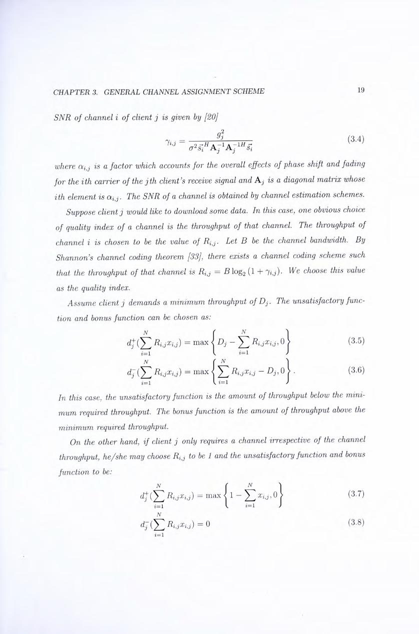
CHAPTER, 3. GENERAL CHANNEL ASSIGNMENT SCHEME 19
SNR of channel i of client j is given by [20]
T . 二 ^ (3.4)
where is a factor which accounts for the overall effects of phase shift and fading
for the ith earner of the jth client's receive signal and Aj is a diagonal matrix whose
ith element is a。. The SNR of a channel is obtained by channel estimation schemes.
Suppose client j would like to download some data. In this case, one obvious choice
of quality index of a channel is the throughput of that channel. The throughput of
channel i is chosen to be the value of R。. Let B be the channel bandwidth. By
Shannon's channel coding theorem [33], there exists a channel coding scheme such
that the throughput of that channel is R、] = Blog^ (1 +1。、. We choose this value
as the quality index.
Assume client j demands a minimum throughput of Dj. The unsatisfactory func-
tion and bonus function can be chosen as:
N ( N \
丑q.r。) 二 max \Dj-J2 ^M^M'O (3-5)
N ( N 、
d j { J 2 二 max ; ^ — D”0 I . (3.6)
i=l Ii=l J
In this case, the unsatisfactory function is the amount of throughput below the mini-
mum required throughput. The bonus function is the amount of throughput above the
minimum required throughput.
On the other hand, if client j only requires a channel irrespective of the channel
throughput, he/she may choose R^j to be 1 and the unsatisfactory function and bonus
function to be:
N ( ^ ]
尺 ! , J 二 m a x — f x.。,0 \ ( 3 . 7 )
z=l I J
N
i = l
CHAPTER, 3. GENERAL CHANNEL ASSIGNMENT SCHEME 20
An example of it is the traditional voice service. The user only requires a channel
with high enough SNR.
Example 3.2. This example shows how our model can generalize some previous
•models channel assignment problems. In this example, we would like to use our
model for throughput optimization.
To perform the throughput optimization, the unsatisfactory function and bonus
function can be chosen as below:
4(f>,.?而’和 0 (3.9)
N N
= (3.10)
i二 1 t=l
where R、] is chosen as the throughput of channel i for user j. In throughput op-
timization problem, we do not have any throughput requirement so we choose the
unsatisfactory function to be 0. Then, we choose the bonus function as the total
throughput of that user.
For latency minimization, you may choose R^^j to be the negative of latency of
channel i for user j and the same unsatisfactory function and bonus function. Al-
ternatively, you may choose R“ to be the latency of channel i for user j. Then, the
unsatisfactory function and bonus function can be chosen as:
N N
dt、Y^Ri’]、3、= Y2R讽] (3.11) i=l i=l
= 0 (3-12) i=l
Example 3.3. In this example, we consider the case of broadcasting a signal to
a group of users. Suppose users 1 ,2,. . . ,m would like to watch the same stream
of video. We would like these users’ mobile terminal to listen to the same set of
channels so that more channels can be assigned to other users. In this case, we
can group all the users into one virtual user. Since the users are using the same
CHAPTER, 3. GENERAL CHANNEL ASSIGNMENT SCHEME 21
application, the explicit form of the unsatisfactory function and bonus function is
the same for all of them except the quality indices due to different Jading experience
of the users. Then, the choice of the quality index of each channel i of this virtual
user can be the minimum of the quality index of the corresponding group of users.
The choice of unsatisfactory function and bonus function of this virtual user is the
same as the ones of each member of that group of user.
As shown in the above examples, for different types of client applications, the
choices of quality index, unsatisfactory function and bonus function are different.
In addition, from the above example, it can be seen that for client j , the value of
R、] may or may not depend on i. In some special cases, such as using Hadamard
signature sequence in narrowband DS-CDMA systems, the SNR of each channel is
the same so R!,] is the same for all i. In the second case, the value of R ,] is clearly
independent of i if the transmitted power of each channel is very high. In [20], the
term order of selection diversity is defined. We can further generalize the definition
as below:
Definition 3.1. For client j, the order of selection diversity of client j is the number
of distinct values in the set {R“ : 1 < z < N}.
If we choose R、] to be the throughput of channel i of client j , we can obtain the
same meaning of order of selection diversity as [20]. However, in definition 3.1,the
order of selection diversity does not only depend on the fading characteristics, but
also depends on the client application. This property is crucial when we try to seek
for special case algorithms in chapter 4.
Now, for client j, there are two objective functions:
N
Minimize 工。) (3.13)
N
Maximize 丑 m • 而 , ( 3 - 1 4 ) i=l
CHAPTER, 3. GENERAL CHANNEL ASSIGNMENT SCHEME 22
Now, we have an optimization problem with 2K objective functions. In general,
this set of 2K objective functions may conflict with each other. This baseline model
is then transformed to a goal programming model to resolve this conflict.
3.2 Goal Ranking
To begin with, we rank the objective functions of the clients. The objective functions
are divided into several priority classes. In chapter 1, it says that an objective
function in a higher priority class dominates another one in a lower priority class in
decision making.
Since the unsatisfactory function is the deficiency of performance below the min-
imum requirement of the user, minimizing the unsatisfactory function is much more
important than maximizing the bonus function. Therefore, the objective functions
111 (3.13) dominate the ones in (3.14). Thus, the objective functions in (3.13) is a
higher priority class while the remaining ones are in a lower priority class. In this
case, we divide the objective functions into two priority classes.
However, among the objective functions of each priority class, none of them dom-
inates another objective function. Therefore, we do not further divide the priority
classes. Hence, in our problem, we only have the two priority classes mentioned
above.
3.3 Model Transformation
III section 1.2, we have defined the term lexicographic minimum in Definition 1.1. By
using the model transformation technique in section 1.2 and the division of objective
functions into priority classes in section 3.2, we can transform the baseline model
into a goal programming model.
Now, the baseline model introduced in the section 3.1 can be converted into a
single-objective model as follows. Firstly, we aggregate the objective functions in
CHAPTER, 3. GENERAL CHANNEL ASSIGNMENT SCHEME 23
a priority class into a single objective function by a linear combination. Then, we
place these two new objective functions (one for unsatisfactory functions and another
one for bonus function) into a vector. The lexicographic minimum of this vector is
the final objective function. Since we would like to maximize the bonus functions, a
minus sign should be added to the weighted sum of them as minimizing the negative
of the weighted sum of them is equivalent to maximizing the weighted sum of them.
So, we obtain the goal programming model for the channel assignment problem as
below: K N K N
lexmin = 丑".而’」,_ 力—(E 尺。而,))广 (3.15)
subject to
Vj (3.16)
< 1 Vz (3.17)
E {0,1} (3.18)
where (3j are predefined constants.
The new objective function in equation (3.15) is called the achievement function
ill goal programming terminology. Inside the achievement function, the values pj
denotes the relative importance of user j's objective function. For instance, if client
J pays for a more expensive service plan, his/her value of [3j will be higher.
In addition, these constants can also be used to ensure some fairness criteria. For
example, if a user, on average, has relatively high value of the unsatisfactory function
compared to other users, we may assign a higher value of ft- to him/her.
3.4 Proposed Algorithms
Proposition 3.1. The opUmizaUon problem formulated in equations (3.15) to (3.18)
IS an NP-hard problem [11].
CHAPTER, 3. GENERAL CHANNEL ASSIGNMENT SCHEME 24
The proof of this proposition is provided in Appendix A. Briefly speaking, one
special case of our problem is the number partitioning problem which has been shown
to be NP-complete [9 .
Since this problem is shown to be an NP-hard problem, for practicality, we seek
for near-optimal polynomial-time algorithms in this chapter.
3.4.1 Channel Swapping Algorithm
As shown above, the optimization problem is NP-hard. Therefore, we propose a
suboptimal scheme called channel swapping algorithm. This algorithm is divided
into two parts. It is outlined as follows. Firstly, we obtain an initial feasible solution
by an arbitrary assignment. Then, we try to improve this solution by swapping
assignments between users in each iteration.
In the second part of the algorithm, we do not only consider pairwise swapping,
but we also consider a sequence of swapping so that for each iteration, the improve-
ment is higher. The algorithm of the second part is similar to the shortest path
algorithm. Each channel is represented by a node and the change by swapping the
assignment of two clients in the objective function is the distance between each pair
of the node. Each node would keep its own information about the channel assign-
ment. The distance between each pair of node is updated according to the current
information available in each node. The starting channel is the initial node. And we
compare the total change of objective 5D to this initial node. The information would
be updated according to (5D. For each channel, the following steps are executed in
each iteration.
1. Set SD of each node to be infinite except the initial node.
2. Calculate the change in the objective if this channel is assigned to a different
user.
3. If the new SD of a node is smaller, update the node's information including its
assignment and its 5D.
CHAPTER, 3. GENERAL CHANNEL ASSIGNMENT SCHEME 25
4. If the node is updated, go to step 2.
5. Stop when there are no updated node remain or a negative SD is detected in
the initial node.
6. If a negative 6D is found, change the assignment according to it.
At each iteration, we consider all the N nodes as the initial nodes. Therefore, we
have N shortest path problems. For each of the shortest path problem, it can be
solved by the Dijkstra's Algorithm [40]. Since the time complexity of the Dijkstra's
Algorithm is 0(N'^) [40], the time complexity for the whole iteration is 0{N^).
This iterative algorithm converges. It is because after each iteration, the weighted
sum of unsatisfactory functions decreases and the channel assignment is still a feasible
solution. That means, the weighted sum of unsatisfactory functions decrease and is
bounded below by the optimal solution for every iteration. Therefore, this algorithm
converges.
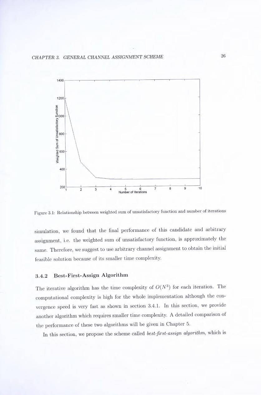
Figure 3.1 shows an example which illustrates the convergence of this algorithm.
Ill this example, we consider a MC-CDMA system with 32 channels and 16 clients.
The sequences are random orthogonal sequences. They are generated by a random
matrix followed by the QR decomposition [15]. The row vectors are the orthogonal
sequences. Each client can support at most 2 channels (i.e. n] = 2). The unsatisfac-
tory function and bonus function considered are equation (3.5) and (3.6) respectively.
Then, we plot the sum of unsatisfactory function (in this example, we simply set [5]
to be 1 for all j ) against the iterations in figure 3.1 for the first 10 iterations.
It can be seen that the algorithm converges within 3 to 4 iterations. From the
simulations results of other scenarios, it is found that typically, the algorithm con-
verges within 4 to 5 iterations. This shows that the algorithm has a high convergence
speed.
For the first part of the algorithm, instead of arbitrary assignment, we may also
choose other methods to obtain an initial feasible solution. One possible candidate
can be the solution from the throughput optimization scheme. However, from the
CHAPTER, 3. GENERAL CHANNEL ASSIGNMENT SCHEME 26
1400 I 1 1 1 I 1 1 1 ‘
1200 - _
i5iooo - \ _
I \ ^ 800 - \ % \ E \
- \ "S 6 0 0 - \ 一
备 \ V 400 - _
V
2 3 4 5 6 7 8 9 10 Number of Iterations
Figure 3.1: Relationship between weighted sum of unsatisfactory function and number of iterations
simulation, we found that the final performance of this candidate and arbitrary
assignment, i.e. the weighted sum of unsatisfactory function, is approximately the
same. Therefore, we suggest to use arbitrary channel assignment to obtain the initial
feasible solution because of its smaller time complexity.
3.4.2 Best-First-Assign Algorithm
The iterative algorithm has the time complexity of 0{N^) for each iteration. The
computational complexity is high for the whole implementation although the con-
vergence speed is very fast as shown in section 3.4.1. In this section, we provide
another algorithm which requires smaller time complexity. A detailed comparison of
the performance of these two algorithms will be given in Chapter 5.
In this section, we propose the scheme called best-first-assign algorithm, which is

CHAPTER, 3. GENERAL CHANNEL ASSIGNMENT SCHEME 27
a, greedy approach [6], as outlined below:
Step 1: For each client j , sort the value R、] in descending order.
Step 2: For each client j , evaluate the reduction of d^ if a unassigned channel
with highest value oi Ri,] is assigned to him/her.
Step 3: Among these clients, choose the client has the greatest reduction calcu-
lated in step 2 and perform the corresponding channel assignment.
Step 4: If there are still some channels can be assigned to the clients, go to step
2.
In step 1, the sorting can be processed by parallel processing as each client's
sorting list is independent from the others. The time complexity for the sorting is
0(N log N) [6]. The time complexity for step 2 and 3 for each iteration is 0{K).
There are at most N iterations as in each iteration, one channel is assigned. There-
fore, the time complexity of this algorithm is 0[NK), which is smaller than the one
of channel swapping algorithm. In chapter 5, it can be seen that the cost of having
smaller time complexity is the increment of the weighted sum of unsatisfactory func-
tion. However, also in chapter 5, it shows that this increment is small. Hence, the
best-first-assign algorithm is also a good choice for our general channel assignment
problem.
Chapter 4
Special Case Algorithms
In Chapter 3, we have formulated a goal programming model for a general channel
assignment problem. In this chapter, we will go through two special cases of this
general channel assignment problem. The first case is that the order of selection
diversity (see Definition 3.1) is 1. The second case is that every user can support at
most one channel (i.e. n] 二 1 for all j).
In Chapter 3,we have mentioned that the general channel assignment problem
is NP-hard. Nevertheless, for these two special cases, optimum solutions can be ob-
tained by means of polynomial-time algorithms. This is the purpose of this chapter.
The details of these two cases are provided below.
4.1 Single Order of Selection Diversity
In this section, we consider the case that the order of selection diversity of all users
is 1. According to Definition 3.1, for a user j , the quality indices R、] is the same
for all channels. That means, for each user, all channels are the same. On the other
hand, for each channel, different users experience different performances.
Such behavior is typical in the downlink of a cellular system. One example is
a narrowband DS-CDMA system with Hadamard signature sequences [38]. In this
case, the SNR of each signature sequence is the same. Another example is a special
28
CHAPTER. 4. SPECIAL CASE ALGORITHMS 29
case of Example 3.1. If the network only provides voice services, Il、j 二 1 for all i and
J. So the order of selection diversity of the system depends on the multiple access
scheme and the user application. Therefore, for each user, he/she only concerns
about how many channels are assigned to him/her. The system model in Chapter 3
can be simplified as below.
The content of this section is also published in [24 .
4.1.1 System Model
Since for each client, the channels are identical, the problem is reduced to decide how
many channels should be assigned to each client. That means, we need to change the
decision variables. Let Xj be the number of channels assigned to client j . Thus, the
unsatisfactory function and bonus function of a user j can be modelled as functions
of X j .
Now, the system model can be modified as below:
/ K K 入 T
lexmin (巧) (4.1)
subject to
<7V (4.2)
0 < < n, Vj (4.3)
X, G N Vj (4.4)
Constraint (4.2) means there are totally N channels which are available. Constraint
(4.3) is the system constraint of the mobile terminal of each client which is the
maximum number of channels can be assigned to client j. It also ensures that the
decision variables are non-negative.
C H A P T E R . 4. SPECIAL CASE ALGORITHMS 30
4.1.2 Proposed A lgor i thm
To solve the goal programming problem above, we propose the following algorithm,
called inductive assignment algorithm which is a dynamic programming [6] approach.
Let /(n, k) be the optimal value of (E)二i ft母(工"),_ 工 w h e n —* —t
n channels are assigned to the first k clients only. When /c 二 0, f ( j i ,k ) 二 0.
Let gk{n) = (d^(n),—dj(n)f and N' = min {Y:^^, n,, n}. Un) is the vector
of unsatisfactory function and bonus function of user j if we assign n channels to
him/her. The recursive relation of /(n, k) is given by
f{n, k) 二 lexmin<[/(n —n',/c- 1) + 歹fcO') : 0 < n < min{nfc,n}| (4.5)
where 0 < n < TV' and 0 < /c < X . By using this recursive relation, the assignment
is obtained by means of evaluating f{N',K).
Proposit ion 4.1. The inductive assignment algorithm provides the optimal assign-
ment.
The proof of proposition 4.1 is given in Appendix B.
In fact, the proof of proposition 4.1 is similar to the algorithm of obtaining
f{N',K). The way to obtain the optimal f{N',K) and the corresponding chan-
nel assignment is outlined as follows. We can use a TV' x (K + 1) table to store each
instance of /(n, k). The value of /(n, k) is stored in the n-th row and A;-th column
of the table.
Firstly, we put the zero vectors to column 0 because /(n, 0) = 0 for all n. Then, we
evaluate the entries in column 1 by using the recursive relation in equation (4.5) and
the column O's information. Next, we compute the entries in column 2 in a similar
way based on column I's information. Then, we continue this process column by
column until we reach the entry of f{N', K). By backtracking from column K, we
can obtain the optimal number of channels to be assigned for each user.
In the calculation of each entry [n, k), we have to make use of the information of
entries (0, k - 1),(1, A: — 1),...,(n, k - 1). There are totally {K + 1)N' entries to be
CHAPTER. 4. SPECIAL CASE ALGORITHMS 31
evaluated. Therefore, the time complexity for the inductive assignment algorithm is
4.1.3 Extension of A lgor i thm
As mentioned in Section 4.1.2, the time complexity for the inductive assignment
algorithm is 0{N'^K). However, when the system is large, the time required to
implement the proposed algorithm for the whole system may be too large for practical
use. For example, if we are assigning channels to more than one cells which are
adjacent to one another, then the number of users involved can be very large.
This problem can be solved by a parallel processing implementation as follows.
We can divide all the users into several groups. For example, if we are performing
the dynamic channel assignment [29] for multiple cells which are adjacent to one
another, we can divide the users according to the cell they reside.
We can compute the set of values of /(n, k) among the users in each group with
the inductive assignment algorithm simultaneously. Then, we treat each group as
a, virtual user. Let = [jf (n, k),-jf\n,kjf be the value of f[n,k) for
the j-th group. Suppose Kj is the number of users in group j. The unsatisfactory
function and the bonus function for each virtual user are
彻 二 / 作 ” 〜 (4.6)
= (4.7)
Now, the unsatisfactory function, ^ ( x , ) , of group ] is the minimum weighted sum
of unsatisfactory function of all users in group j when we assign Xj channels to them.
The bonus function, dj{xj), of group j is the weighted sum of bonus function of all
users in group j when we optimally assign xj channels to them. As mentioned in
section 4.1.2,we use a table to store every instances of /(n, k) in the implementation
of the inductive assignment algorithm . From the last column of the table for the
channel assignment of each group, we can obtain the function values in equations
(4.6) and (4.7).
CHAPTER. 4. SPECIAL CASE ALGORITHMS 32
Then, we can apply the proposed algorithm again for those groups to complete the
channel assignment. In this case, we consider each group as a virtual user with the
unsatisfactory function and bonus function being (4.6) and (4.7). We perform the
optimal channel assignments for these virtual users. We can then obtain the optimal
number of channels assigned to each group. From the dynamic programming table
of each group, we can backtrack the optimal number of channels assigned to each
user eventually.
Since we compute the values for each user group in parallel first, the time com-
plexity can be reduced although the amount of computation is the same. It can be
easily proved that this parallel implementation can also provide the optimal solution
for the larger system by induction in the same way as the proof for the inductive
assignment algorithm.
In addition, if there are some new users joining the network, we can use similar
method to adaptively assign the channels. Each new user is a group and all the old
users are gathered into another group. Then, use the above method to assign the
channels to all these 'groups' according to the old inductive assignment algorithm
table of the network. In this case, when new users arrive at the system, we can have
a more effective way to assign the channels.
4.2 Single Channel Assignment
We look into another special case in this section. In this section, we consider the
scenario that at most one channel can be assigned to each user. That means, n] = 1
for all J. This is the case for most of the current cellular system. Fortunately, as
mentioned at the very beginning of this chapter, polynomial-time optimal algorithms
are found for this case. Furthermore, we will adopt the optimal algorithm in Chapter
5 to obtain a lower bound of performance analysis. This is the reason why we consider
this special case in this chapter.
CHAPTER. 4. SPECIAL CASE ALGORITHMS 33
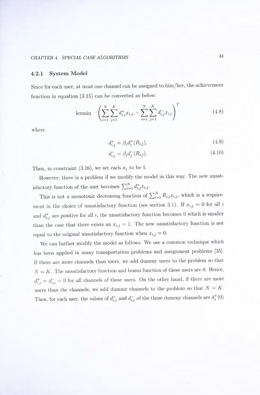
4.2.1 System Model
Since for each user, at most one channel can be assigned to him/her, the achievement
function in equation (3.15) can be converted as below:
/ N K N K \ ^
lexmin ^ ^ ^ < ; 产 … 《 。 工 ^ , ] (4.8)
\ z = l j ^ l i二 1 j = l /
where
私,力, (4.9)
d-. = (4.10)
Then, in constraint (3.16), we set each rij to be 1.
However, there is a problem if we modify the model in this way. The new unsat-
isfactory function of the user becomes d j工
This is not a monotonic decreasing function of Ri,jX…which is a require-
ment in the choice of unsatisfactory function (see section 3.1). If a:,口 = 0 for all i
and are positive for all z, the unsatisfactory function becomes 0 which is smaller
than the case that there exists an 工。=1. The new unsatisfactory function is not
equal to the original unsatisfactory function when x^j = 0.
We can further modify the model as follows. We use a common technique which
has been applied in many transportation problems and assignment problems [35 .
If there are more channels than users, we add dummy users to the problem so that
N 二 K. The unsatisfactory function and bonus function of these users are 0. Hence,
d+. 二 d: = 0 for all channels of these users. On the other hand, if there are more
users than the channels, we add dummy channels to the problem so that N 二 K.
Then, for each user, the values of and d;。of the those dummy channels are d^{0)
C H A P T E R . 4. SPECIAL CASE ALGORITHMS 24
and d~(0) respectively. Finally, we use the following system constraints:
f 2、3 = l, Vj (4.11)
i=l
j y 一 , Vz (4-12)
Now, both component of the achievement function are linear functions of oc、].
Hence, we can now have a linear binary goal programming problem. That means,
we can apply the multiphase simplex algorithm [12], Alternatively, we can have the
following two algorithms.
4.2.2 Proposed Algorithms
There are two more approaches to solve this problem. One is to extend the Hungarian
Method [16]. Another one is to extend the linear programming algorithms.
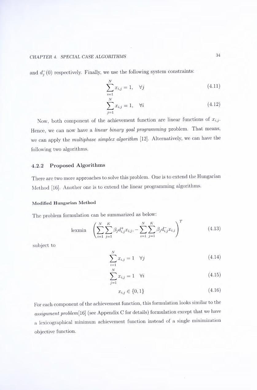
Modi f ied Hunga r i an M e t h o d
The problem formulation can be summarized as below:
lexmm ( f : f : / K 内 , " E E 眺]、^ (4.13) \i=l j=l i二 1 j = l )
subject to
j y 、 3 = l Vj (4.14)
f > ’ 「 l V2 (4.15)
(4.16)
For each component of the achievement function, this formulation looks similar to the
assignment problem[l6] (see Appendix C for details) formulation except that we have
a lexicographical minimum achievement function instead of a single minimization
objective function.

CHAPTER. 4. SPECIAL CASE ALGORITHMS 35
To solve the problem, firstly, we only consider the minimization of weighted sum
of unsatisfactory function in the achievement function (4.13). Then, we perform the
Hungarian method (see Appendix C) to solve this single-objective problem. If there
is only one combination from the modified cost matrix in such a way that the sum
IS zero, we can terminate according to the way of comparison in Definition 1.1.
Otherwise, we need to consider the maximization of the weighted sum of bonus
functions. In the minimization of the weighted sum of unsatisfactory functions,
there are zero entries in the modified cost matrix. Actually, these entries are the
candidate assignments. Therefore, we constraint ourselves to these assignments in
the maximization of the weighted sum of bonus functions. The way to do so is to
construct another cost matrix based on the modified cost matrix in the previous steps
and the values 眺Since we do not consider those nonzero entries in the modified
cost matrix, in the new cost matrix, those corresponding entries are negative infinity.
For other entries, in the new cost matrix, their values are f3jd~j.
Since assignment problems are minimization problems but we want to maximize
the weighted sum of bonus functions, we need to change the cost matrix before
implementing the Hungarian method. We only need to multiply each entry by -1 so
that the Hungarian method will minimize the negative of the weighted sum of bonus
functions which is equivalent to maximizing the weighted sum of bonus functions.
Linear Programming Approach
The second approach is to apply linear programming algorithms twice. As men-
tioned above, the problem can be viewed as two assignment problems. In fact, each
assignment problem can be solved by linear programming algorithms directly due to
the integer solution property [10]. We can solve the problem as follows.
Firstly, we replace the integer solution constraint with 0 < ; < 1. Then, we
ignore the second component of the achievement function in (4.13). We only consider
the weighted sum of unsatisfactory function. Next, we apply any linear programming

CHAPTER. 4. SPECIAL CASE ALGORITHMS 36
algorithms to minimize the weighed sum of unsatisfactory function. This can be done
by common mathematical software. After that, we add the following constraint to
the problem:
f : f x 〒 化 i n (4.17)
where is the minimum value of weighted sum of unsatisfactory function obtained
in the previous steps. Now, we change the objective function to the weighted sum of
bonus function. We treat it as another linear programming problem again and solve
it by mathematical software. Then, we can obtain the final solution.
Chapter 5
Performance Evaluation
In this chapter, we will evaluate the performance of proposed algorithms in chapter
3 and 4 by means of computer simulations. We will compare the proposed algo-
rithms with throughput optimization schemes. Since minimizing the weighted sum
of unsatisfactory function is the most important objective in our channel assignment
scheme, we will adopt it as a measure of performance.
5.1 General Channel Assignment and Single Channel As-
signment
In this section, we would like to compare the performances of the throughput opti-
mization scheme, two proposed algorithms in chapter 3,namely, the channel swap-
ping algorithm and the best-first-assign algorithm, via simulations. We compare the
performances by varying the number of clients and channels in the system. A lower
bound of weighted sum of unsatisfactory function is provided for a reference. We
will see later for the cases ofN <K, rij = 1, the lower bound of weighted sum of un-
satisfactory function is obtained by the algorithm described in Section 4.2. Hence,
we also compare this algorithm with other proposed channel assignment schemes
and the throughput optimization scheme. In this simulation, we consider two sets of
37
CHAPTER, 5. PERFORMANCE EVALUATION 38
unsatisfactory function and bonus function.
5.1.1 System Mode l
We consider an MC-CDMA system with random orthogonal sequences. In this sys-
tem, sequences are first generated randomly and then by using QR decomposition
15] or Gram-Schmidt procedure [17], the sequences become orthonormal. We as-
sume large scale path loss is compensated by downlink power control methods [30 .
The small scale fading is assumed to be Rayleigh fading and the background noise
is assumed to be the additive white Gaussian noise (AWGN). We choose R、] to be
the throughput obtained by client j when channel i is assigned to him/her. In this
simulation, R、] is chosen to be the channel capacity of the channel. For each client
j,he/she demands a throughput of Dj.
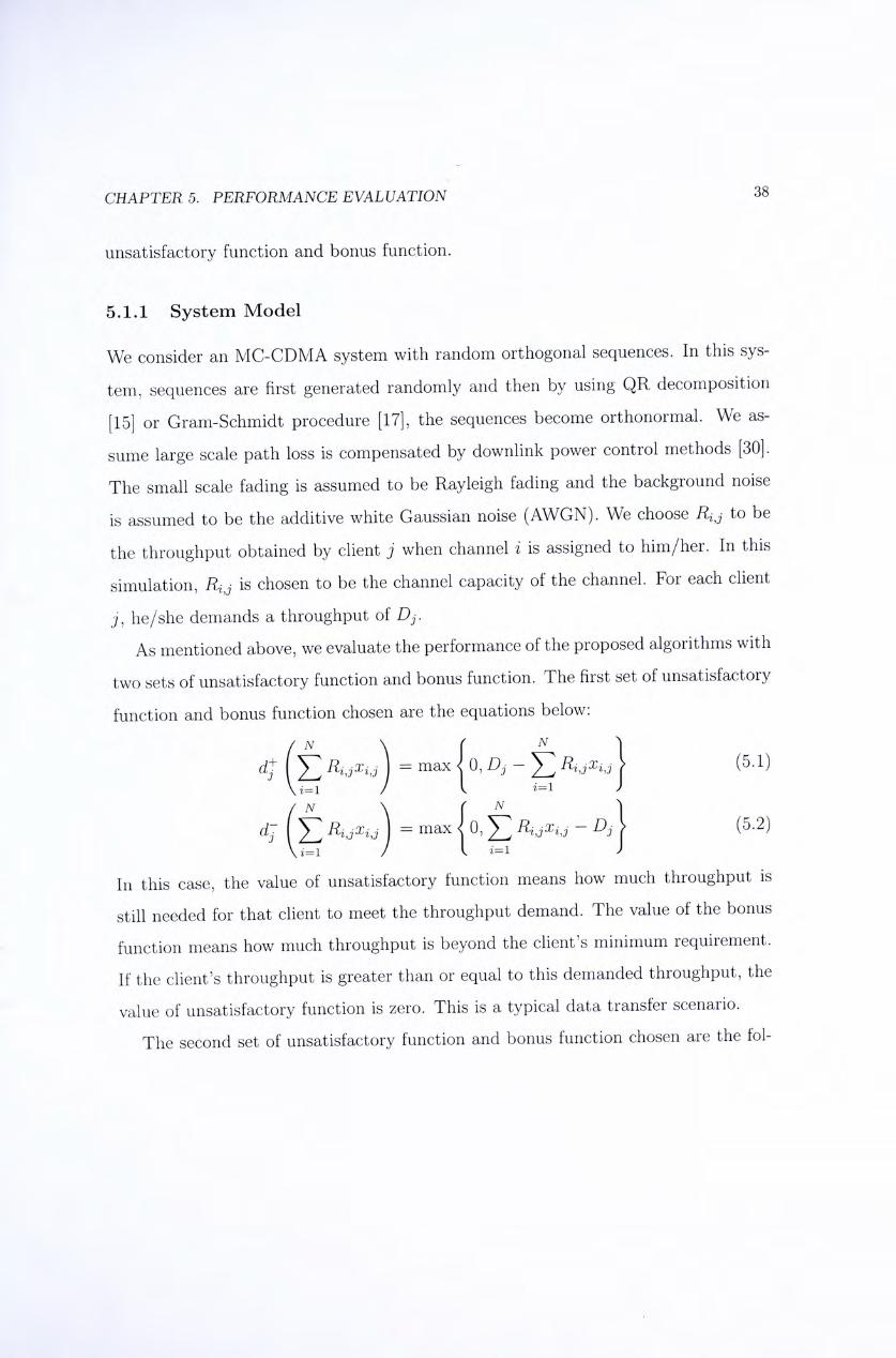
As mentioned above, we evaluate the performance of the proposed algorithms with
two sets of unsatisfactory function and bonus function. The first set of unsatisfactory
function and bonus function chosen are the equations below:
/ N \ N 1
4 Y ^ I k ; 。 = max 0, D] - R^ ,]、] (5.1)
\i=i ) I “1 >
(N \ ( N 1
dJ Y. R。工 I,] = max j o , 一 D] (5.2)
/ I 口 1 >
In this case, the value of unsatisfactory function means how much throughput is
still needed for that client to meet the throughput demand. The value of the bonus
function means how much throughput is beyond the client's minimum requirement.
If the client's throughput is greater than or equal to this demanded throughput, the
value of unsatisfactory function is zero. This is a typical data transfer scenario.
The second set of unsatisfactory function and bonus function chosen are the fol-
CHAPTER, 5. PERFORMANCE EVALUATION 39
lowing equations:
4 ( t … ’ ) 二 钟 + - ( 巧 ; 私 , 而 ( 5 . 3 )
\z=l / / N \ r ^ 1
d- 代, • ^工。=max 一 D, J (5.4)
This is a typical choice of unsatisfactory function and bonus function for video
streaming. The function sgn(x) is the signum function where it is 1 if x is pos-
itive, 0 if X is 0 and -1 if x is negative. If the client's throughput is below the
minimum requirement Dj, the unsatisfactory function is Dj because in this situa-
tion, no matter how high is the throughput, the buffer is starving [18] and it affects
the playback of the video. Otherwise, it is 0. The bonus function is the same as the
previous case.
For simplicity, we set /3j 二 1 for all j which means the objective function of
each user is equally important. The value of n] is chosen to be「警^ for N > K.
Otherwise, we set rij 二 1.
In the performance evaluation in this section, we consider the proportion of de-
ficient throughput, which is defined as follows, as the performance measure in our
simulation.
Definition 5.1. The proportion of deficient throughput of a channel assignment
scheme is the weighted sum of unsatisfactory function this scheme divided by the
weighted sum of unsatisfactory function without assigning any channels.
Roughly speaking, this value is the proportion of the total client demand which
has not been satisfied. In our choice of unsatisfactory function for this simulation, we
are considering the proportion of throughput demand which has not been satisfied.
For the channel swapping algorithm, which is an iterative algorithm, we repeat the
iterations until the solution cannot be further improved. That means, the algorithm
terminates when the local optimal is reached. As mentioned in Section 3.4.1, the
algorithm typically converges within 4 to 5 iterations in our simulations.
CHAPTER, 5. PERFORMANCE EVALUATION 40
5.1.2 Lower Bound of Weighted Sum of Unsatisfactory Function
Apart from plotting the curves for the throughput optimization schemes, we also
obtain a lower bound of the optimal weighted sum of unsatisfactory function as a
benchmark for the performance evaluation. The lower bound is divided into two
parts. The first part is for the case when N 〉 K , i.e. rij > 1. The second part is for
the case when N < K, i.e. n] 二 1. Below is the description of how we obtain the
lower bound.
When N > K, Uj > 1. The lower bound in this case is obtained by an algorithm
which is likely to give an infeasible solution. In this algorithm, each client j inde-
pendently obtains the ly channels which have the highest throughput. Obviously,
this gives the upper bound of the throughput of a user so this gives the lower bound
of the unsatisfactory function of each client and thus the lower bound of weighted
sum of unsatisfactory function. However, in this scheme, a channel may be assigned
to more than one client so in general, the solution is infeasible as it violates the
constraint (3.17). Hence, it is also a lower bound of the optimal weighted sum of
unsatisfactory function.
When N < K, rij = 1. In chapter 4, we have seen that for n] 二 1,there is a
polynomial-time algorithm to give the optimal solution. Hence, we can make use of
that algorithm to obtain the optimal solution as our lower bound. At the same time,
we can compare the performance of that algorithm with other proposed algorithms
and the throughput optimization scheme in this simulation.
Alternatively, since we only consider the weighted sum of unsatisfactory function,
we can simply treat the problem as an assignment problem (see Appendix C). This
is a single objective optimization problem and the objective function is a linear
function. Although the decision variables are binary, by the integer solution property
10], we can simply relax the integer constraint and treat the decision variables as
continuous variables from 0 to 1. Hence, we can obtain the lower bound for this
case by the Hungarian method [16] or using some common mathematical software
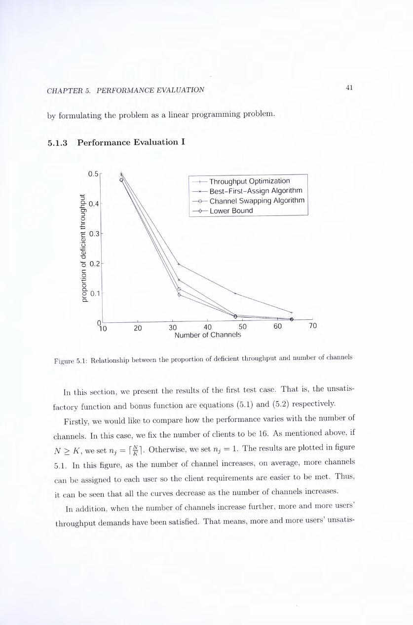
CHAPTER, 5. PERFORMANCE EVALUATION 41
by formulating the problem as a linear programming problem.
5.1.3 Performance Evaluation I
0 . 5 厂 \
- f— Throughput Optimization
一 ^ ^ —Best-First-Assign Algorithm
Q. Q 4 Channel Swapping Algorithm
\ \ — ^ Lower Bound
n , : . — — — — ‘
% 2 0 3 0 4 0 5 0 6 0 7 0
Number of Channels
Figure 5.1; Relationship between the proportion of deficient throughput and number of channels
In this section, we present the results of the first test case. That is, the unsatis-
factory function and bonus function are equations (5.1) and (5.2) respectively.
Firstly, we would like to compare how the performance varies with the number ot
channels. In this case, we fix the number of clients to be 16. As mentioned above, if
N>K,we set Uj = 「 f Otherwise, we set n] = 1. The results are plotted in figure
5.1. In this figure, as the number of channel increases, on average, more channels
can be assigned to each user so the client requirements are easier to be met. Thus,
it can be seen that all the curves decrease as the number of channels increases.
In addition, when the number of channels increase further, more and more users'
throughput demands have been satisfied. That means, more and more users' unsatis-

CHAPTER, 5. PERFORMANCE EVALUATION 42
factory functions become zero which is the minimum possible value of unsatisfactory
functions. In this case, fewer and fewer users' unsatisfactory functions can decrease
further. Therefore, it can be seen that in figure 5.1, all the curves decrease with a
smaller and smaller rate. This accounts for the shapes of the curve in figure 5.1.
In figure 5.1, it can be seen that the channel swapping algorithm and the best-
first-assign algorithm perform better than the throughput optimization scheme. The
curves for both of the channel swapping algorithm and the best-first-assign algorithm
fall with higher rate than the one of the throughput optimization scheme. In addition,
for N > 48, the curve of the channel swapping algorithm overlaps with our lower
bound. That means, in those cases, the channel swapping algorithm converge to
the optimal solution in those cases. This is a nice feature of the channel swapping
algorithm.
What's more, it is observed that the curve of the best-first-assign algorithm is
close to the one of channel swapping algorithm. This is an important feature for
the choice of algorithms. When we consider the trade-off between computational
complexity and the weighted sum of unsatisfactory function, this can give some
hints on the choice of the algorithm. It will be discussed in more details in section
5.1.4.
Next, we would like to compare the variation of performance with respect to the
number of clients. In this case, we fix the number of channels to be 16. Similar to
the above case, we choose n] 二「f 1 for N > K and choose n] = 1 for TV < K.
The results are plotted in figure 5.2. As the number of client increases, on average,
fewer channels are assigned to each user so the proportion of deficient throughput
becomes larger. Hence, it can be seen that those curves increase as the number of
clients increase.
Moreover, it is observed that all the curves are concave which means the rate of
increment is decreasing with the number of clients. When K > 16, since N is fixed
to be 16, that means, some of the users do not have any channels. For these clients,
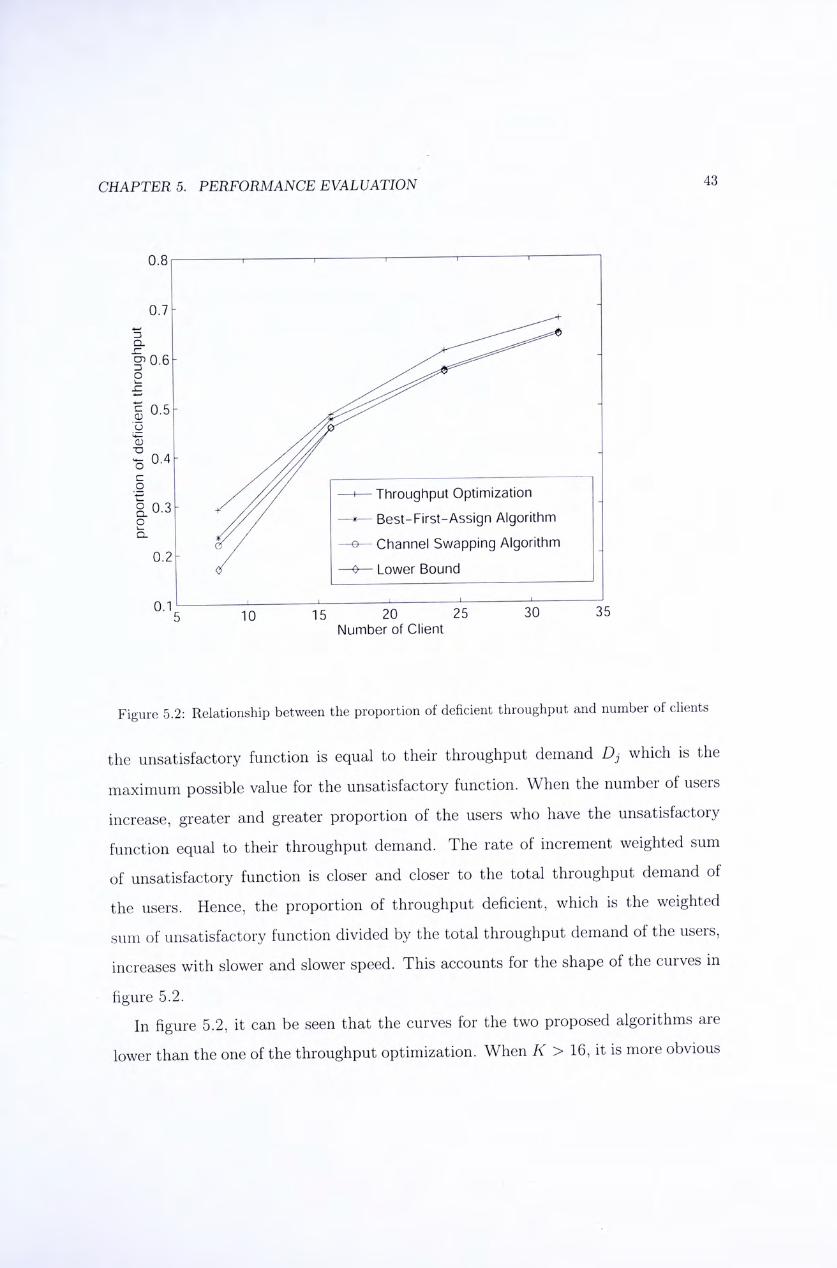
CHAPTER 5. PERFORMANCE EVALUATION 43
0.81 ' ‘ ^ ‘ ‘ “~
t : 1" jf「 'i // I ^ Throughput Optimization _
|"〇.3 ^ / / / ——*一一 Best—First-Assig门 Algorithm
a i / / —e--Channel Swapping Algorithm 0 . 2 - / _
^ 0 L o w e r Bound
^•''s 10 15 20 25 30 35
Number of Client
Figure 5.2: Relationship between the proportion of deficient throughput and number of clients
the unsatisfactory function is equal to their throughput demand D] which is the
maximum possible value for the unsatisfactory function. When the number of users
increase, greater and greater proportion of the users who have the unsatisfactory
function equal to their throughput demand. The rate of increment weighted sum
of unsatisfactory function is closer and closer to the total throughput demand of
the users. Hence, the proportion of throughput deficient, which is the weighted
sum of unsatisfactory function divided by the total throughput demand of the users,
increases with slower and slower speed. This accounts for the shape of the curves in
figure 5.2.
In figure 5.2, it can be seen that the curves for the two proposed algorithms are
lower than the one of the throughput optimization. When K > 16, it is more obvious
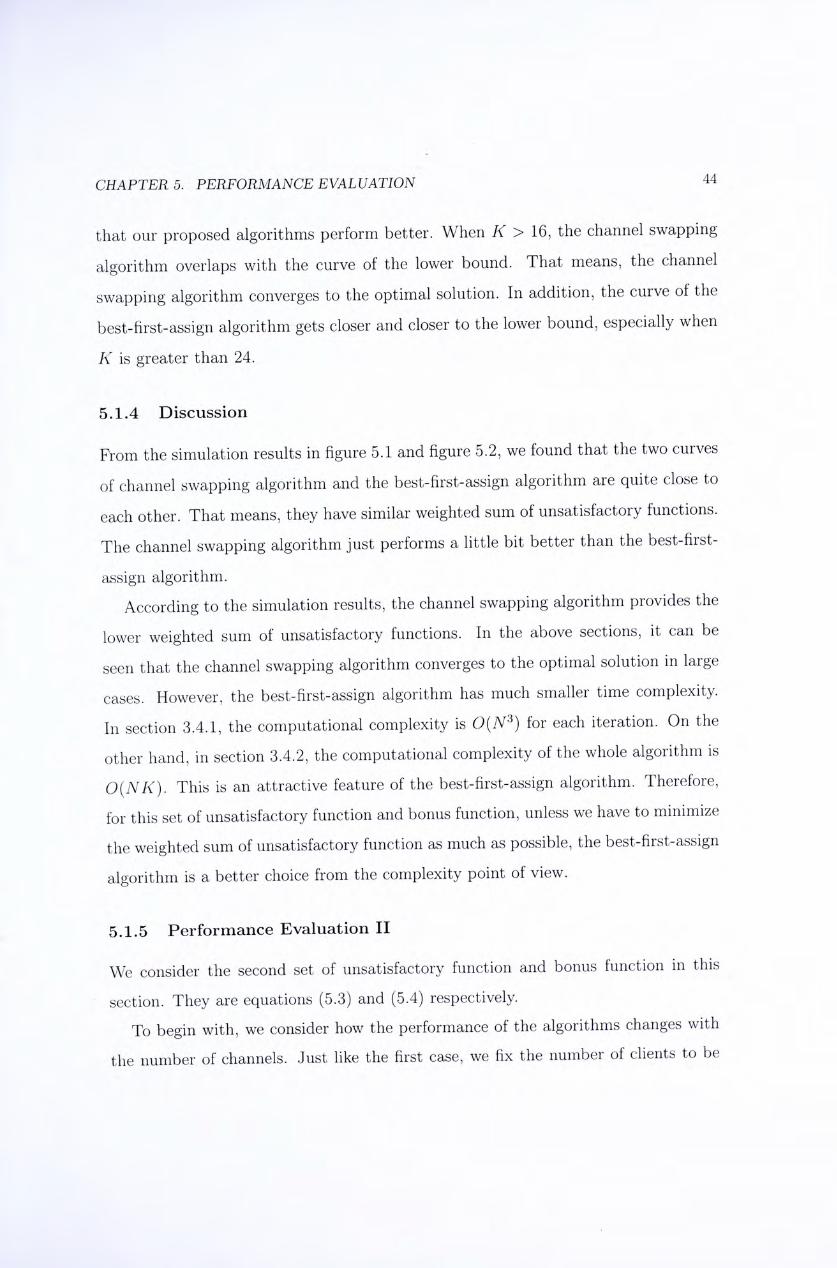
C H A P T E R , 5. PERFORMANCE EVALUATION 44
that our proposed algorithms perform better. When K > 16, the channel swapping
algorithm overlaps with the curve of the lower bound. That means, the channel
swapping algorithm converges to the optimal solution. In addition, the curve of the
best-first-assign algorithm gets closer and closer to the lower bound, especially when
K is greater than 24.
5.1.4 Discussion
From the simulation results in figure 5.1 and figure 5.2, we found that the two curves
of channel swapping algorithm and the best-first-assign algorithm are quite close to
each other. That means, they have similar weighted sum of unsatisfactory functions.
The channel swapping algorithm just performs a little bit better than the best-first-
assign algorithm.
According to the simulation results, the channel swapping algorithm provides the
lower weighted sum of unsatisfactory functions. In the above sections, it can be
seen that the channel swapping algorithm converges to the optimal solution in large
cases. However, the best-first-assign algorithm has much smaller time complexity.
Ill section 3.4.1, the computational complexity is 0{N^) for each iteration. On the
other hand, in section 3.4.2,the computational complexity of the whole algorithm is
0{NK). This is an attractive feature of the best-first-assign algorithm. Therefore,
for this set of unsatisfactory function and bonus function, unless we have to minimize
the weighted sum of unsatisfactory function as much as possible, the best-first-assign
algorithm is a better choice from the complexity point of view.
5.1.5 Performance Evaluation I I
We consider the second set of unsatisfactory function and bonus function in this
section. They are equations (5.3) and (5.4) respectively.
To begin with, we consider how the performance of the algorithms changes with
the number of channels. Just like the first case, we fix the number of clients to be
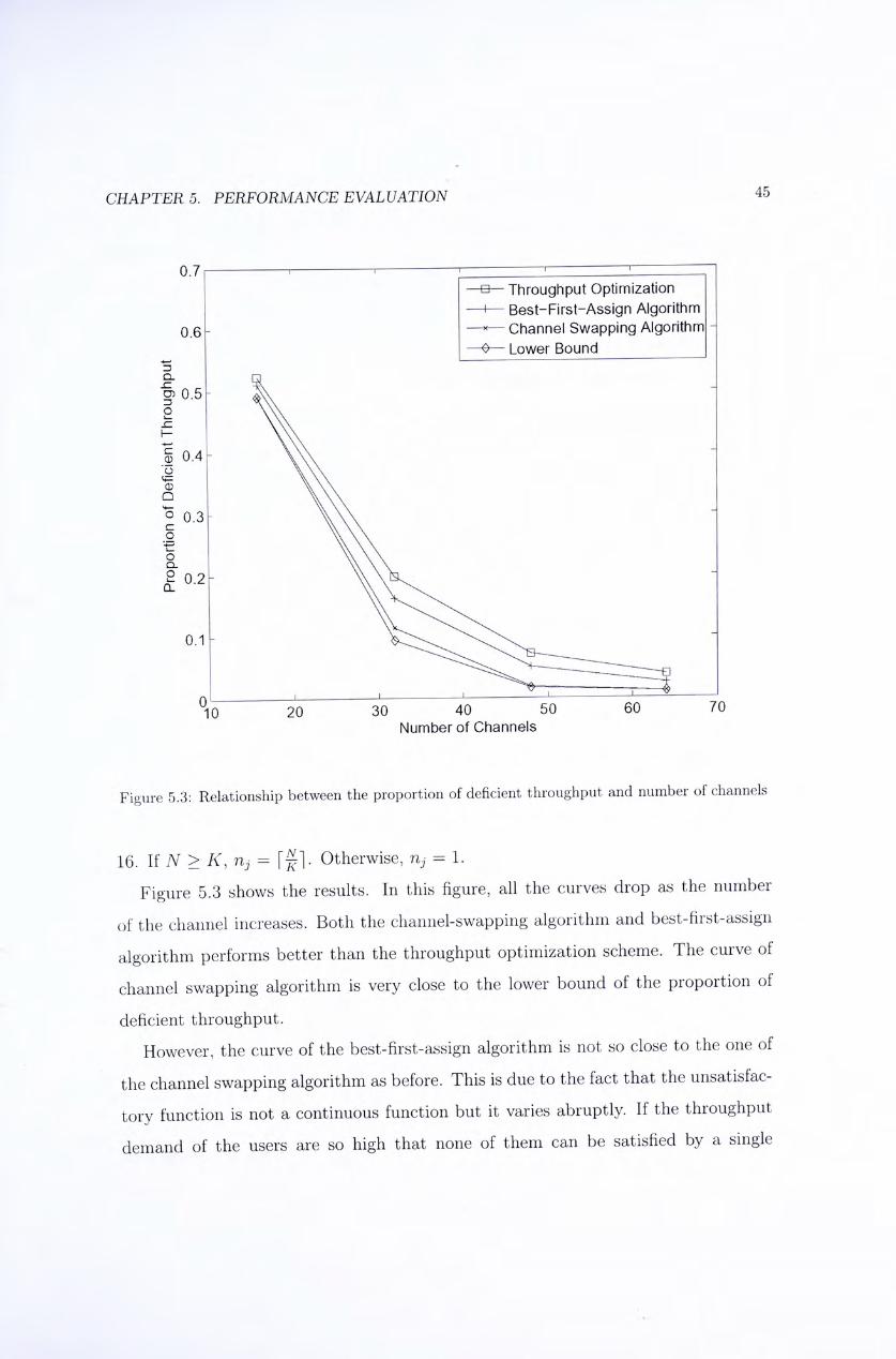
CHAPTER, 5. PERFORMANCE EVALUATION 45
0.7| 丨 ‘ I I • I
• Throughput Optimization
~ I ~ Best-First-Assign Algorithm
0.6 - ^ ^ ^ Channel Swapping Algorithm -
• Lower Bound
I: \ :
20 30 40 50 60 70
Number of Channels
Figure 5.3: Relationship between the proportion of deficient throughput and number of channels
16. If N > K, rij =「 f1. Otherwise, n] = 1.
Figure 5.3 shows the results. In this figure, all the curves drop as the number
of the channel increases. Both the channel-swapping algorithm and best-first-assign
algorithm performs better than the throughput optimization scheme. The curve of
channel swapping algorithm is very close to the lower bound of the proportion of
deficient throughput.
However, the curve of the best-first-assign algorithm is not so close to the one of
the channel swapping algorithm as before. This is due to the fact that the unsatisfac-
tory function is not a continuous function but it varies abruptly. If the throughput
demand of the users are so high that none of them can be satisfied by a single
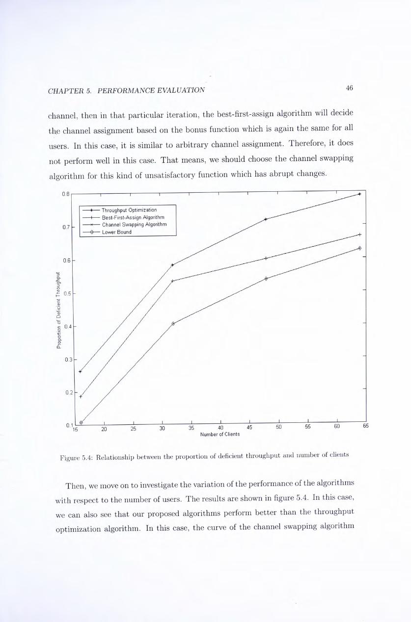
CHAPTER, 5. PERFORMANCE EVALUATION 46
channel, then in that particular iteration, the best-first-assign algorithm will decide
the channel assignment based on the bonus function which is again the same for all
users. In this case, it is similar to arbitrary channel assignment. Therefore, it does
not perform well in this case. That means, we should choose the channel swapping
algorithm for this kind of unsatisfactory function which has abrupt changes.
0.8 I 1 1 1 1 T I I I “~丨 ^ ^ ^
——*~ Throughput Optimization
——I——Best-First-Assign Algorithm
Q j _ « ~ C h a n n e l SwafDping Algorithm ^ ^ -
~ Lower Bound ^ ^
0.2 - / /
. / /
¥ I I I I I I I 1 1
U.1i5 20 25 30 35 40 45 50 55 60 65 Number of Clients
Figure 5.4: Relationship between the proportion of deficient throughput and number of clients
Then, we move on to investigate the variation of the performance of the algorithms
with respect to the number of users. The results are shown in figure 5.4. In this case,
we can also see that our proposed algorithms perform better than the throughput
optimization algorithm. In this case, the curve of the channel swapping algorithm
CHAPTER, 5. PERFORMANCE EVALUATION 47
touches the lower bound of proportion of deficient throughput. That means, the
channel swapping algorithm reaches the optimal solution. When the number of users
is greater than 32, the curve of the best-first-assign algorithm becomes closer and
closer to the lower bound but this does not happen for the throughput optimization
scheme.
5.2 Single Order of Selection Diversity Algorithm
In this section, we would like to evaluate the performance of the proposed algorithm
for the special case of order of section diversity being 1, which is described in chapter
4. The performance is evaluated via simulations. In our simulations, we would like
to compare how the performances of that proposed algorithm and a throughput
optimization scheme vary with number of clients and number of channels. In this
section, we will also show the performance of the proposed algorithm and throughput
optimization scheme in terms of weighted sum of bonus functions. Unlike the general
case considered in the previous sections, when the order of selection diversity is 1,
from the curves of the weighted sum of bonus functions, we can see some nice features
of the proposed algorithm. This is the reason why although the weighted sum of the
bonus function is not the most important objective function under our formulation,
we also show the simulation results of the weighted sum of bonus function in this
section. Just like in the performance evaluation of the general case algorithms, in
this section, we will also evaluate the proposed algorithm by two similar sets of
unsatisfactory function and bonus function.
5.2.1 System Model
Two scenarios of a narrowband DS-CDMA system with Hadamard signature se-
quences are considered. The first one is that the number of channel is fixed to be 16
while the number of clients varies. The second one is that the number of clients is
fixed to be 16 while the number of channels varies.
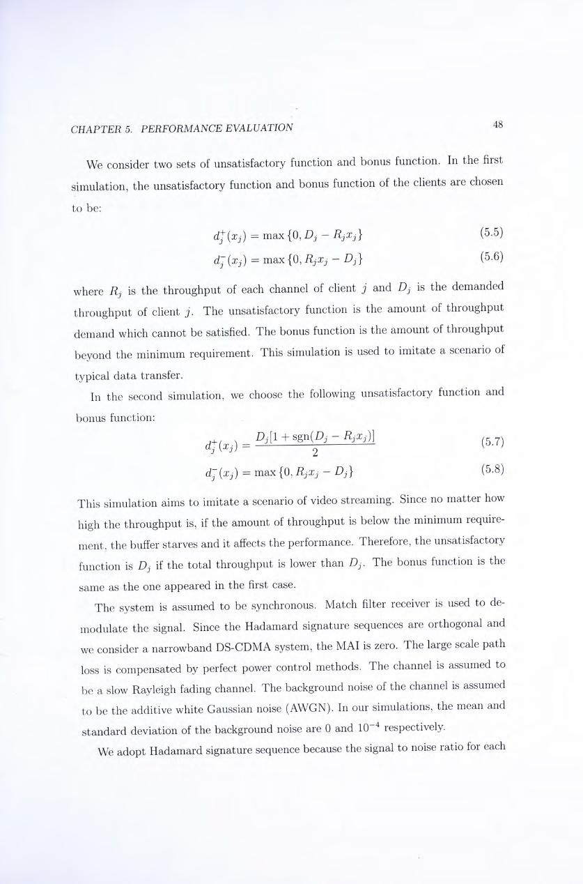
CHAPTER, 5. PERFORMANCE EVALUATION 48
We consider two sets of unsatisfactory function and bonus function. In the first
simulation, the unsatisfactory function and bonus function of the clients are chosen
to be:
二 max {0, D] 一 RjXj} (5.5)
d-{xj) = max {0,R,Xj — Dj} (5.6)
where R] is the throughput of each channel of client j and D] is the demanded
throughput of client j . The unsatisfactory function is the amount of throughput
demand which cannot be satisfied. The bonus function is the amount of throughput
beyond the minimum requirement. This simulation is used to imitate a scenario of
typical data transfer.
In the second simulation, we choose the following unsatisfactory function and
bonus function:
(〜)二 DAl + sgn{D,-R,x,)] (5.7)
3 2
djixj) = max {0, RjX, - Dj} (5.8)
This simulation aims to imitate a scenario of video streaming. Since no matter how
high the throughput is, if the amount of throughput is below the minimum require-
ment, the buffer starves and it affects the performance. Therefore, the unsatisfactory
function is D] if the total throughput is lower than D]. The bonus function is the
same as the one appeared in the first case.
The system is assumed to be synchronous. Match filter receiver is used to de-
modulate the signal. Since the Hadamard signature sequences are orthogonal and
we consider a narrowband DS-CDMA system, the MAI is zero. The large scale path
loss is compensated by perfect power control methods. The channel is assumed to
be a slow Rayleigh fading channel. The background noise of the channel is assumed
to be the additive white Gaussian noise (AWGN). In our simulations, the mean and
standard deviation of the background noise are 0 and 10-4 respectively.
We adopt Hadamard signature sequence because the signal to noise ratio for each
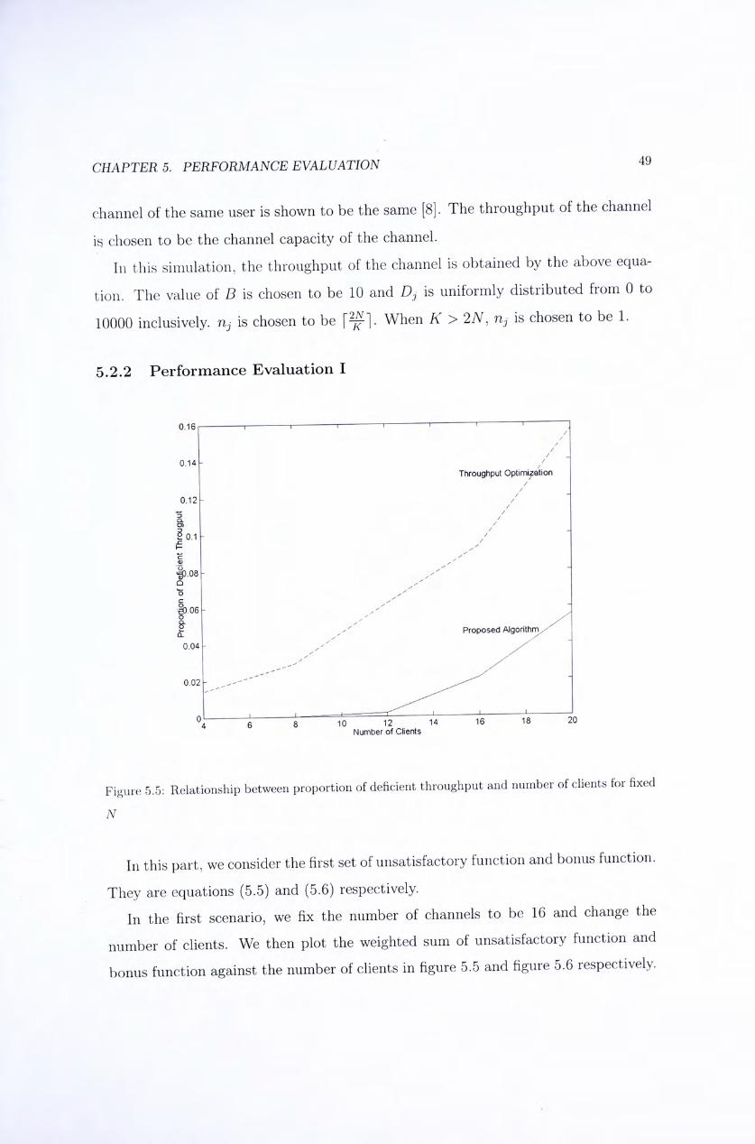
CHAPTER, 5. PERFORMANCE EVALUATION 49
channel of the same user is shown to be the same [8]. The throughput of the channel
is chosen to be the channel capacity of the channel.
In this simulation, the throughput of the channel is obtained by the above equa-
tion. The value of B is chosen to be 10 and D] is uniformly distributed from 0 to
10000 inclusively, n] is chosen to be「警 1. When K > 2N, n] is chosen to be 1.
5.2.2 Performance Evaluation I
0.16 I 1 1 1 1 ‘“ “ ‘ ‘ /
/ /
/
0.14 - / — Throughput Optimization
/ /
0.12 - / ‘
1 / ZD / 2 0.1 - / H Z i 3-08- _ Q Z
Z § Z -
- Z /
I Z z
H Proposed Algorithm/-
0.04 - z',, / _ z 乂 Z _
0.02-zz'z z ^ Z
— I , ,
6 8 ^ 16 18 20 Number of Clients
Figure 5.5: Relationship between proportion of deficient throughput and number of clients for fixed
N
III this part, we consider the first set of unsatisfactory function and bonus function.
They are equations (5.5) and (5.6) respectively.
In the first scenario, we fix the number of channels to be 16 and change the
number of clients. We then plot the weighted sum of unsatisfactory function and
bonus function against the number of clients in figure 5.5 and figure 5.6 respectively.
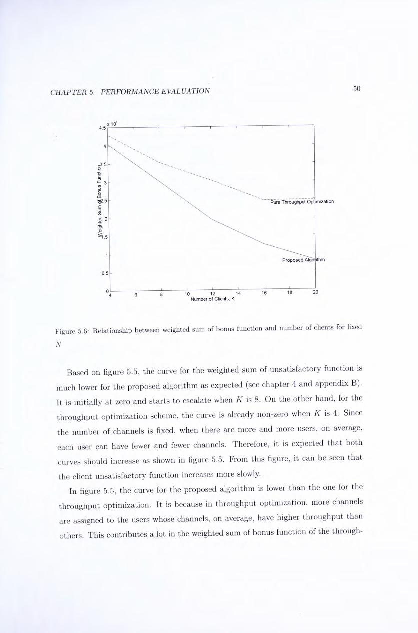
CHAPTER, 5. PERFORMANCE EVALUATION 50
X 10' , ,
4.5 I 1 1 1 1 ‘ ‘ ‘ 、、
、 -
r— \ : \ \ 、 \ 、
^ 3- \ \、、\ -B \ CO \
- \ 一一Pure Throughput Opt mization
I \ _ I 2- \\ 一 . 5 - 、 \ \ -
1 -
Proposed Algol ithm
0.5 - 一
6 8 to 12 14 W 18 20 Number of Clients, K
Figure 5.6: Relationship between weighted sum of bonus function and number of clients for fixed
N
Based on figure 5.5, the curve for the weighted sum of unsatisfactory function is
much lower for the proposed algorithm as expected (see chapter 4 and appendix B).
It is initially at zero and starts to escalate when K is 8. On the other hand, for the
throughput optimization scheme, the curve is already non-zero when K is 4. Since
the number of channels is fixed, when there are more and more users, on average,
each user can have fewer and fewer channels. Therefore, it is expected that both
curves sliould increase as shown in figure 5.5. From this figure, it can be seen that
the client unsatisfactory function increases more slowly.
In figure 5.5,the curve for the proposed algorithm is lower than the one for the
throughput optimization. It is because in throughput optimization, more channels
are assigned to the users whose channels, on average, have higher throughput than
others. This contributes a lot in the weighted sum of bonus function of the through-
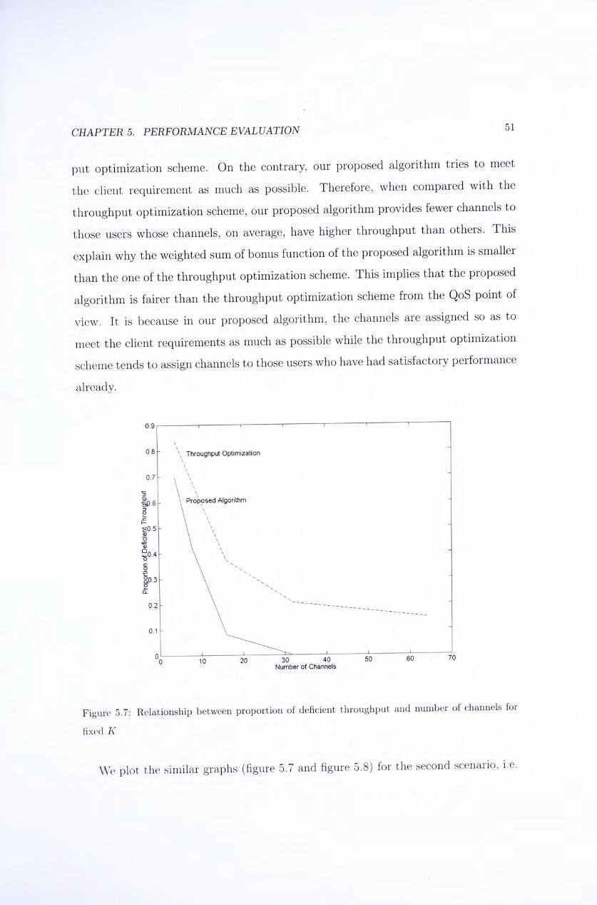
CHAPTER, 5. PERFORMANCE EVALUATION 51
put optimization scheme. On the contrary, our proposed algorithm tries to meet
the client requirement as much as possible. Therefore, when compared with the
throughput optimization scheme, our proposed algorithm provides fewer channels to
those users whose channels, on average, have higher throughput than others. This
explain why the weighted sum of bonus function of the proposed algorithm is smaller
than the one of the throughput optimization scheme. This implies that the proposed
algorithm is fairer than the throughput optimization scheme from the QoS point of
view. It IS because in our proposed algorithm, the channels are assigned so as to
meet the client requirements as much as possible while the throughput optimization
scheme tends to assign channels to those users who have had satisfactory performance
already.
0.9 I 1 1 1 1 ‘
\ \ -
0.8 - \ Throughput Optimization 、 \ \ _
0 . 7 - 、, \ -.\ \ ^ Q \ Proposed Algorithm -
I • \ \ H \ \ -r- \ \ % \ \ ? 。 . 4 - \ \ § \ \\
\ \\、 _ 。 . 2 \ 、 、 … … … … 一 … 一 … … -
0.1 - \ ‘
0(3 10 20 30 40 50 60 70 Number of Channels
Figure 5.7: Relationship between proportion of deficient throughput and number of channels for
fixed K
We plot the similar graphs (figure 5.7 and figure 5.8) for the second scenario, i.e.
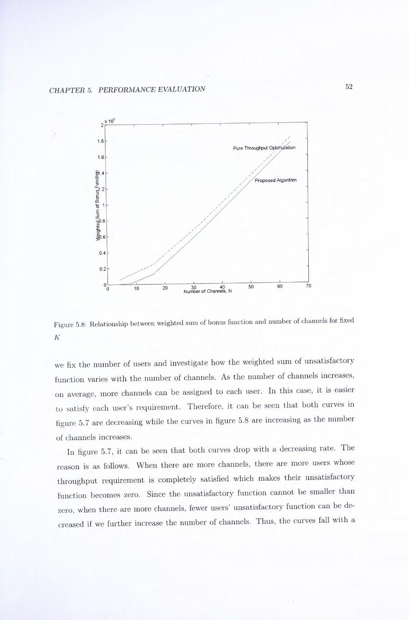
CHAPTER, 5. PERFORMANCE EVALUATION 52
X 10® . ^ 2 r 1 1 1 1 ‘ ^
1 . 8 - ‘
Pure Throughput Optir^zation
1.6- / V -, // _ .01.4 - , Z
^ Proposed Algorithm
r 一
CD / X -11 - , 7
- / / ‘
I / ' /
0 . 4 - / /
0.2- Z 乂 Z -
„ “ I I I I i
° 0 ^ 3 0 ^ 5 0 6 0 7 0
Number of Channels, N
Figure 5.8: Relationship between weighted sum of bonus function and number of channels for fixed
K
we fix the number of users and investigate how the weighted sum of unsatisfactory
function varies with the number of channels. As the number of channels increases,
on average, more channels can be assigned to each user. In this case, it is easier
to satisfy each user's requirement. Therefore, it can be seen that both curves in
figure 5.7 are decreasing while the curves in figure 5.8 are increasing as the number
of channels increases.
In figure 5.7, it can be seen that both curves drop with a decreasing rate. The
reason is as follows. When there are more channels, there are more users whose
throughput requirement is completely satisfied which makes their unsatisfactory
function becomes zero. Since the unsatisfactory function cannot be smaller than
zero, when there are more channels, fewer users' unsatisfactory function can be de-
creased if we further increase the number of channels. Thus, the curves fall with a
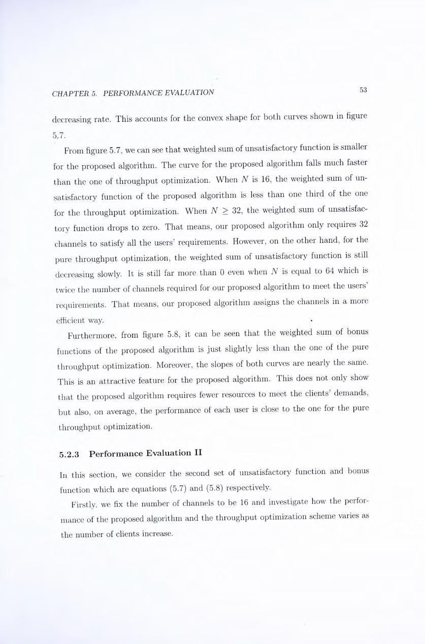
CHAPTER, 5. PERFORMANCE EVALUATION 53
decreasing rate. This accounts for the convex shape for both curves shown in figure
5.7.
From figure 5.7, we can see that weighted sum of unsatisfactory function is smaller
for the proposed algorithm. The curve for the proposed algorithm falls much faster
than the one of throughput optimization. When N is 16, the weighted sum of un-
satisfactory function of the proposed algorithm is less than one third of the one
for the throughput optimization. When N > 32, the weighted sum of unsatisfac-
tory function drops to zero. That means, our proposed algorithm only requires 32
channels to satisfy all the users' requirements. However, on the other hand, for the
pure throughput optimization, the weighted sum of unsatisfactory function is still
decreasing slowly. It is still far more than 0 even when N is equal to 64 which is
twice the number of channels required for our proposed algorithm to meet the users'
requirements. That means, our proposed algorithm assigns the channels in a more
efficient way. •
Furthermore, from figure 5.8, it can be seen that the weighted sum of bonus
functions of the proposed algorithm is just slightly less than the one of the pure
throughput optimization. Moreover, the slopes of both curves are nearly the same.
This is an attractive feature for the proposed algorithm. This does not only show
that the proposed algorithm requires fewer resources to meet the clients' demands,
but also, on average, the performance of each user is close to the one for the pure
throughput optimization.
5.2.3 Performance Evaluation I I
In this section, we consider the second set of unsatisfactory function and bonus
function which are equations (5.7) and (5.8) respectively.
Firstly, we fix the number of channels to be 16 and investigate how the perfor-
mance of the proposed algorithm and the throughput optimization scheme varies as
the number of clients increase.
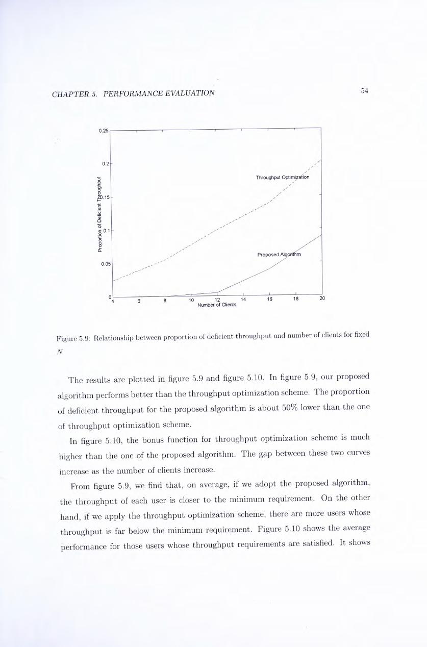
CHAPTER, 5. PERFORMANCE EVALUATION 54
0.25 I 1 1 1 1 r- ‘
0.2 - , /
/ /
3 Throughput Optimi/afion
Cl Z
O) Z |D.15 - / _ I— /
I , z 0 Z
Q Z •h Z —
§0.1-% z Z
1 , z / Proposed A l^ i t hm
0.05 - ' Z ‘
„ I I — ^ ^ I I 1 1 °4 6 8 10 12 14 16 18 20
Number of Clients
Figure 5.9: Relationship between proportion of deficient throughput and number of clients for fixed
N
The results are plotted in figure 5.9 and figure 5.10. In figure 5.9, our proposed
algorithm performs better than the throughput optimization scheme. The proportion
of deficient throughput for the proposed algorithm is about 50% lower than the one
of throughput optimization scheme.
In figure 5.10, the bonus function for throughput optimization scheme is much
higher than the one of the proposed algorithm. The gap between these two curves
increase as the number of clients increase.
From figure 5.9, we find that, on average, if we adopt the proposed algorithm,
the throughput of each user is closer to the minimum requirement. On the other
hand, if we apply the throughput optimization scheme, there are more users whose
throughput is far below the minimum requirement. Figure 5.10 shows the average
performance for those users whose throughput requirements are satisfied. It shows
CHAPTER, 5. PERFORMANCE EVALUATION 70
x10' ,
4.5 I 1 1 1 1 1 ‘ ‘
_ [o3.5- \ 、\、、 -1 \ 、 、 小 \ 、、 -
1 \ \ (D \ \ 、\ Throughput Optimization
e \ 、\、
I \\ \\\ _
、\\、 Proposed Algorithm
1.5 - ““一~~~~
, , I I I I 1 1 % 6 8 ^ ^ 18 20
Number of Users
Figure 5.10: Relationship between weighted sum of bonus function and number of clients for fixed
N
that for the throughput optimization, the average throughput of these users are
much higher. However, just as what we have seen in figure 5.9, it tends to be
more users whose throughput is far below the minimum requirement for throughput
optimization scheme. That means, for throughput optimization, some users whose
performance is far beyond the minimum requirement but there are also some users
whose performance is far below the minimum requirement simultaneously. That
means, compared to the throughput optimization scheme, the proposed algorithm is
fairer.
Now, we move on to investigate how the performance of the proposed algorithm
and throughput optimization scheme changes when we change the number of chan-
nels. We fix the number of users to be 16. The results are illustrated in figure 5.11
and 5.12.
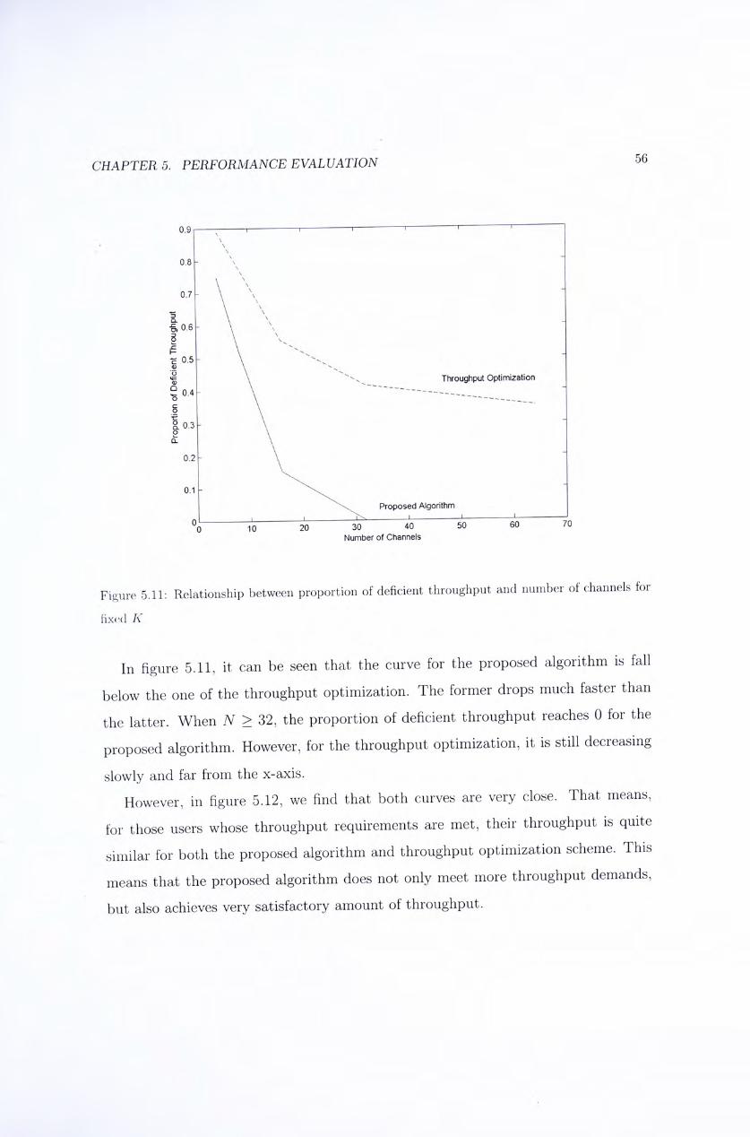
CHAPTER, 5. PERFORMANCE EVALUATION 56
0.9 I 1 r ‘ ‘ ^ ‘
\ \
\
0.8 - \ _ \
\
0.7 - \ \ -
.\ \ -o \ 、 ^ \ \ \ -c 0 .5- \ \ 、
\ 、\、 Throughput Optimization
H \ 一 s s … . -
In \ -。+2- V _
0 .1 -
\\\ Proposed Algorithm „ I I 、>\ _ I I 1 ‘ °0 10 20 30 40 50 60 70
Number of Channels
Figure 5.11: Relationship between proportion of deficient throughput and number of channels for
fixed K
In figure 5.11, it can be seen that the curve for the proposed algorithm is fall
below the one of the throughput optimization. The former drops much faster than
the latter. When N > 32,the proportion of deficient throughput reaches 0 for the
proposed algorithm. However, for the throughput optimization, it is still decreasing
slowly and far from the x-axis.
However, in figure 5.12, we find that both curves are very close. That means,
for those users whose throughput requirements are met, their throughput is quite
similar for both the proposed algorithm and throughput optimization scheme. This
means that the proposed algorithm does not only meet more throughput demands,
but also achieves very satisfactory amount of throughput.
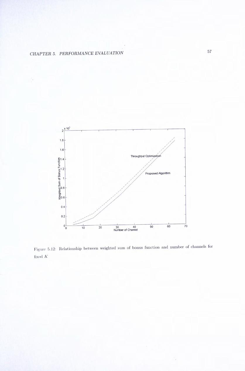
CHAPTER 5. PERFORMANCE EVALUATION 57
x105 ,
2 I 1 1 1 “ I ‘ ‘
1 .8 _ ,/〉 一
1.6 _ Throughput Optimi^^tipn _
\ / / 售 1.2- / / _ g / / Proposed Algorithm CD / / -
I / / — ”0.8- z Z
14 /义 -1 , , :
% ^ ^ ^ ^ 50 60 70
Number of Channel
Figure 5.12: Relationship between weighted sum of bonus function and number of channels for
fixed K
Chapter 6
Conclusion and Future Works
6.1 Conclusion
111 this thesis, we focus on applying goal programming technique in channel assign-
ment problem. Firstly, we formulate the goal programming model for the general
channel assignment problem and then we propose two corresponding channel assign-
ment schemes. Secondly, we consider two special cases of the channel assignment
yeheines. The goal programming models for these two special cases are modified
and new optimal polynomial-time channel assignment schemes are proposed. Simu-
lations have been performed to compare our proposed schemes with the throughput
optimization scheme. Based on the simulations results, we compare the two channel
assignment schemes of the general case.
To begin with, we consider the general channel assignment problem. In this
model, we do not assume the underlying multiple access scheme except we only re-
quire each logical channel should be orthogonal to one another, i.e. the MAI is 0.
The property of channel for the user application is specified by the quality index.
The QoS requirements of each client are specified by a pair of functions, namely,
the unsatisfactory function and the bonus function. Each user has two objective
functions (minimizing the unsatisfactory function and maximizing the bonus func-
58
CHAPTER, 6. CONCLUSION AND FUTURE WORKS 59
tion) and all these objective functions conflict with one another in general. Goal
programming technique is then applied to tackle this problem and then we have the
goal programming formulation for the general channel assignment problem.
It is shown that the problem is an NP-hard problem. Therefore, we propose
two near-optimal polynomial-time channel assignment schemes, namely the channel-
s'wapping algorithm and the best-first-assign algorithm. The channel-swapping algo-
nthni has slightly better values for the achievement function while the best-first-
assign algorithm has much smaller time complexity (although the channel-swapping
algorithm usually converges within 4 to 5 iterations). However, according to the
simulation results, the weighted sum of unsatisfactory function provided by both
algorithms are very close. Therefore, the choice of algorithm is concluded as follows.
Unless the weighted sum of unsatisfactory function is much more important than
the time complexity, the best-first-assign algorithm is preferred.
Our work does not end here. Since the algorithms mentioned above are only near-
optimal algorithms and the general case is an NP-hard problem, we then move on to
seek for optimal algorithms in some special cases which are typical in communication
systems. In the first special case, the order of selection diversity of all the users is
equal to 1. In the second case, we consider the case of single channel assignment (i.e.
we assign at most 1 channel to each user).
In the first special case, since the order of selection diversity of the system is
1,that means for each user, the channels are homogenous. However, for the same
channel, the performance for different client is different in general. The problem is
then reduced to how many channels should be assigned to each user. A dynamic
programming algorithm is proposed to provide the optimal solution. It is also noted
that this algorithm is not only applicable to single cell systems, but also can be
extended to multi-cell systems in which each cell is adjacent to one another. Parallel
processing implementation of this extension is also described to reduce the time
complexity of the whole assignment. In addition, it is found that when there are
CHAPTER, 6. CONCLUSION AND FUTURE WORKS 60
new users requesting for channels, we can adaptively perform the assignment. From
the simulation results, it found that the proposed algorithm does not only have lower
weighted sum of unsatisfactory function, but also in some cases, the weighted sum
of bonus function is very close to the throughput optimization. This is an attractive
feature of the proposed algorithm.
In the second special case, each user can be assigned to at most 1 channels which
is a very common scenario in present communication systems. It is also useful in
obtaining the lower bound of the weighted sum of unsatisfactory function for the
performance evaluation in the general case.
The problem is transformed into two assignment problems and we can solve it
with two approaches. Firstly, as assignment problems can be solved by linear pro-
gramming algorithms by relaxing the integer solution constraint, we can use some
common mathematical software to solve the assignment problems one-by-one by
adding a constraint when solving the second problem.
Alternatively, assignment problems can also be solved by Hungarian methods.
Therefore, we can apply the Hungarian methods twice to obtain the optimal solution
with two different cost matrices.
6.2 Future Works
The goal programming approach provides a new outlook in the channel assignment
problem. There are still a lot of problems that require our effort to investigate. In
this section, some suggested research directions are provided.
6.2.1 Multi-cell Channel Assignment
In this thesis, most of the systems that we consider are single cell systems. In
practice, operators concern more about the multi-cell channel assignment. In multi-
cell channel assignment scenario, if all the cells are adjacent to one another, we can
consider the whole system as a larger cell and directly apply the proposed algorithms
CHAPTER, 6. CONCLUSION AND FUTURE WORKS 61
in this thesis. However, in most of the cases, channel reuse [29] is possible as the
operators have a large number of cells covering a large area. A channel can be
assigned to more than one users if they are far enough to have sufficiently small
co-channel interference. To model this problem, we cannot impose constraint (3.17).
A more general model and scheme may be needed.
There are two main types of channel assignment schemes for multi-cell channel
assignment [29]. The first type is known as fixed channel assignment (FCA). In FCA,
a predetermined set of channels is assigned to each cell. Thus, we can directly apply
the proposed algorithms for each cell to have independent channel assignments.
However, the main drawback of FCA is lack of flexibility. Users can only be
assigned to the available channels in their resided cell. In this case, some channels
are not used while in some other cells, the users are blocked. Resource is wasted in
this case. To solve this problem, the second type of multi-cell channel assignment
scheme is introduced, which is known as dynamic channel assignment (DCA) [14 .
Ill DCA, when a channel request is made, the serving base station of the cell re-
quests for a channel from the mobile switching center (MSG). The switching center
then allocates a channel to the requested cell according to a certain channel assign-
ment algorithm. In this case, the channel assignment scheme is more flexible and
efficient. The blocking probability can also be greatly reduced.
In DCA, a channel assignment scheme called sequential packing [34] is used in
traditional voice network. However, this algorithm only takes care of number of
requested channels in each cell but ignores the QoS requirements of each user. But
for data network, QoS requirement plays an important role in resource allocation.
That means, we need to have a new channel assignment scheme.
The challenge of multi-cell channel assignment is that the number of users and
channels involved is much larger. In the single cell case, the problem is NP-hard
already. That means, the multi-cell channel assignment problem is much harder to
be solved as the problem size is greater. This is the main challenge of this problem.
CHAPTER, 6. CONCLUSION AND FUTURE WORKS 62
6.2.2 Theoretical Studies
Another research direction is to obtain some theoretical limits of the amount of
resource required to provide certain grade of service. This can give the operators
a picture of how much resource they need to invest to provide a particular grade
of service. Examples are the Erlang B or C formulas in traditional cellular network
which only provides voice services. In addition, if the operators would like to upgrade
their present services, they also need to know how much the minimum additional
cost they need to pay to decide whether it is worth to have this investment. It is
similar to the sensitivity analysis in some operations research problems.
In chapter 4,we proposed the optimal algorithms for two special cases. From the
operator point of view, the next question is how many channels are required so that
we can support certain user requirements based on the proposed algorithm. This
depends on the traffic models and the specifications of the user applications (i.e. the
unsatisfactory function and bonus function).
For the general case, the optimal polynomial-time algorithm is hard to obtain as
It is an NP-hard problem. In this case, one possible direction of research is to obtain
some bounds of the number of channels required to meet the user requirements.
6.2.3 Adaptive Algorithms
All the proposed algorithms in this thesis are not adaptive algorithms. They all
need to perform the channel assignment in each time slot independently. They never
make use of the results in the previous time slots and the relationship between the
problems in consecutive time slots.
In practical situations, the channel conditions between two consecutive time slots
do not vary too much if the time between two consecutive time slots is smaller than
the coherence time of the channel. In addition, it is expected that the number of
users and their user requirements seldom have drastic changes in the next time slot.
We can have faster implementations by making good use of the correlation between
CHAPTER, 6. CONCLUSION AND FUTURE WORKS 63
the consecutive time slots. To reduce the time complexity, we may perform the
channel assignment based on the results in the previous time slots and the change
hi the current time slot. This is the motivation of investigating adaptive algorithms
for the channel assignment problem.
6.2.4 Assignment of Non-orthogonal Channels
111 the formulation of this thesis, we assume that the channels are orthogonal to each
other. That means, the MAI of the channels is zero. However, this assumption limits
the number of the channels that can be assigned.
There are many research works in multiple access schemes which have non-
orthogonal channels but they have satisfactory signal-to-interference ratio. One
example is the introduction of carrier interferometry (CI) signal in multiple access
schemes which have orthogonal channels [1] [22] [23] [41]. With these techniques, we
can have more channels to be assigned to the users.
Hence, a possible research direction is in the channel assignment for multiple
access schemes with non-orthogonal channels. Besides the multi-cell channel as-
signment, this IS another direction of generalization of channel assignment problem.
However, in this case, we do not only need to consider the assignment of channels,
but also other parameters like transmitted power in each channel because the MAI
in these cases is no longer zero. Some other techniques like downlink power control
13] and multiuser detection [37] may be applied jointly as well.
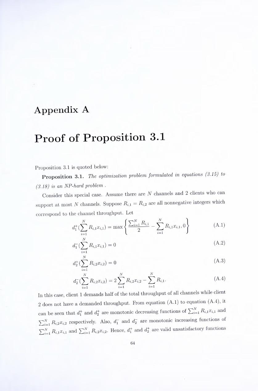
Appendix A
Proof of Proposition 3.1
Proposition 3.1 is quoted below:
Proposit ion 3.1. The optimization problem formulated in equations (3.15) to
(3.18) IS an NP-hard problem .
Consider this special case. Assume there are N channels and 2 clients who can
support at most N channels. Suppose 二 R、2 are all nonnegative integers which
correspond to the channel throughput. Let
4 ( E 二 max I 一 E 讽 1, o } (A . l )
i二1 I
d 「 ( f > _ ) = 0 (A.2)
i=i
N
= 0 (A.3)
1=1
N N N
1=1 i=l
In this case, client 1 demands half of the total throughput of all channels while client
2 does not have a demanded throughput. From equation (A.l) to equation (A.4),it
can be seen that df and 4 are monotonic decreasing functions of 二 i?u.A,i and
R。工respectively. Also, d : and d ; are monotonic increasing functions of
e S I i and Ef=i 尺 而 ’ 2 . Hence, 4 and 4 are valid unsatisfactory functions 64
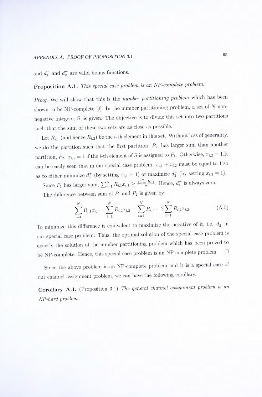
APPENDIX A. PROOF OF PROPOSITION 3.1 65
and d]; and d^ are valid bonus functions.
Proposition A . l . This special case problem is an NP-complete problem.
Proof. We will show that this is the number partitioning problem which has been
shown to be NP-complete [9]. In the number partitioning problem, a set of N non-
negative integers, 5•’ is given. The objective is to divide this set into two partitions
such that the sum of these two sets are as close as possible.
Let (and hence i?,,2) be the 2 - t h element in this set. Without loss of generality,
we do the partition such that the first partition, Pi, has larger sum than another
partition, JV 二 1 if the z-th element of S is assigned to P:. Otherwise, = 1-It
can be easily seen that in our special case problem, + 工。must be equal to 1 so
as to either minimize 4 (by setting = 1) or maximize d ; (by setting 二 1).
Since Pi has larger sum, E t i > Hence, 4 is always zero.
The difference between sum of Pi and P2 is given by
f : - E 丑':,2、2 = E I k i - 2 E … , 2 . (A.5) 口 1
To minimize this difference is equivalent to maximize the negative of it, i.e. d ; in
our special case problem. Thus, the optimal solution of the special case problem is
exactly the solution of the number partitioning problem which has been proved to
be NP-complete. Hence, this special case problem is an NP-complete problem. •
Since the above problem is an NP-complete problem and it is a special case of
our channel assignment problem, we can have the following corollary.
Corollary A . l . (Proposition 3.1) The general channel assignment problem is an
NP-hard problem.
Appendix B
Proof of Proposition 4.1
Proposition 4.1 is quoted below:
Proposit ion 4.1. The inductive assignment algorithm in Chapter 4 provides the
optimal assignment.
In this chapter, I will provide the proof of Proposition 4.1. It shows that the
inductive assignment algorithm in Section 4.1.2 is an optimal algorithm for the case
of single order of selection diversity.
Firstly, we prove that the recursive relation of /(n, k) is true for all n and k by
induction. If it is true, from the meaning of this function, the inductive assignment
algorithm must give the optimal solution. It is obviously true for both n and k are
0. Also, when /c 二 0, there are zero terms in the summations of both components in
equation (4.1). Therefore, it is also true for all values of n when /c 二 0.
Assume it is true for 0 < n < and /c = /c' where n' and k' are positive
integers such that 0 < n' < and 0 < k' < K. Now, we show that it is also
true for n = n' + 1 and k ^ k'+ 1. In this case, we are deciding the number of
channels to be assigned to the {k' + l)-th client out of these n' + 1 channels. We can
assign 0 to mm { n ^ i , + 1} channels to the {k' + 1)-th client. If we assign xv+i
channels to the {k' + l)-th client, the optimal value for equation (4.1) is the sum
of ( 4 ( 工 ; ^ ' + 1 ) , 《 ( 工 叫 ) ) 了 and / V + 1 - � + 1 , " ) ’ which IS the optimal value for
66

APPENDIX B. PROOF OF PROPOSITION 4.1 67
assigning (n + 1 — Xk'+i) channels to the first k' clients. Therefore, f{n' + 1, A:, + 1)
is obtained by considering all possible values of [ d ^ ( x k ' + i ) Y + / 0 ' + 丄—
’T,:'仆 it') for 0 < < mm {n 叫 n/ + 1}. Hence, f{n' + 1 , + 1) is obtained by
choosing the lexicographic minimum oi{d1l'{xk'+i),dj(xk'+i)V + / ( " + 1 _ 工、 ‘ + i ,)
for 0 < Xk'+i < min {n/^'+iX + 1}, which is the recursive expression described in the
inductive assignment algorithm in Section 4.1.2. Hence, the expression for f[n, k) is
also true for n 二 + 1 and /c 二 /c' + 1.
By mathematical induction, this expression is true for all n and k. Therefore,
by using the recursive relations for all /(n, /c), the optimal solution solution can be
found from f{N', K).
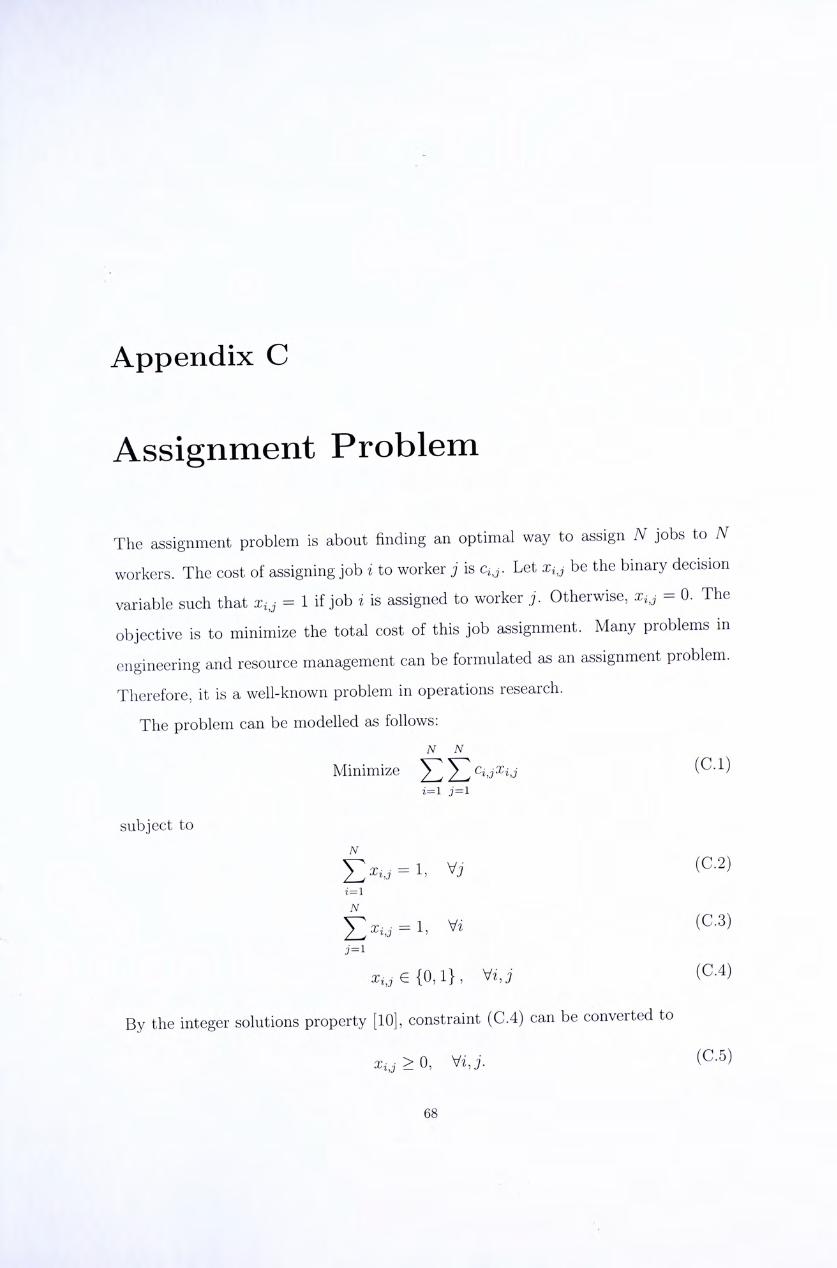
Appendix C
Assignment Problem
The assignment problem is about finding an optimal way to assign N jobs to N
workers. The cost of assigning job z to worker j is c斤 Let x,, be the binary decision
variable such that 二 1 if job i is assigned to worker j . Otherwise, 二 0. The
objective is to minimize the total cost of this job assignment. Many problems in
engineering and resource management can be formulated as an assignment problem.
Therefore, it is a well-known problem in operations research.
The problem can be modelled as follows:
N N
Minimize > > c“工i’7. ( c . i )
i二 1 j=i
subject to
£ � = 1, V , (C.2)
1=1
= Vz (C.3)
6 {0,1} , V U (C.4)
By the integer solutions property [10], constraint (C.4) can be converted to
> 0, Vz,j. (C.5)
68

APPENDIX C. ASSIGNMENT PROBLEM
Now, the problem is a standard linear programming problem which can be solved
with common mathematical software.
Another way to solve the problem is by using the Hungarian Method [16]. This
algorithm is outlined as below.
To begin with, we let C be the matrix
/ \ Ci,i Ci’2 • . • Ci’iV
C 二 C2,l C2,2 ••• C2,N (C.6)
. • . *
. . • • • . • •
y CN,1 Civ,2 . . • CN,N
Then, we follow the steps below:
1. Subtract the entries of each row of C by the row minimum. As a result, each
row has at least one zero and all entries are nonnegative.
2. Subtract the entries of each column by the column minimum. Now, each row
and each column has at least one zero.
3. Select rows and columns across which you draw lines, in such a way that all the
zeros are covered and that no more lines have been drawn than necessary.
4. If the number of the lines is N, choose a combination from the modified cost
matrix in such a way that the sum is zero. Otherwise, that is, the number of
lines is less than TV, go to step 5.
5. Find the smallest element which is not covered by any of the lines. Then
subtract it from each entry which is not covered by the lines and add it to each
entry which is covered by a vertical and a horizontal line. Go back to step 3.
Bibliography
[1] p. R. Barbosa, Z. Wu, and C. R. Nassar. High-performance mimo-ofdm via ear-
ner interferometry. In IEEE Global Telecommunications Conference, Globecom
2003, Vol: 2, pages 711-715, Dec. 2003.
2] S. Borst and P. Whiting. Dynamic rate control algorithms for hdr throughput
optimization. In INFOCOM 2001. Twentieth Annual Joint Conference of the
IEEE Computer and Communications Societies. Proceedings. IEEE, Volume: 2,
pages 976-985, Apr. 2001.
.3] J. R. Boucher. Voice Teletraffic Systems Engineering. Artech House, 1988.
[4] M. Carsoni, G. Immovilli, and M. L. Merani. Admission control in t/cdma sys-
tems supporting voice and data applications. Wireless Communications, IEEE
Transactions on, Vol: 1 , Issue: 3, pages 540-548,July 2002.
[5] A. Charnes and W. W. Cooper. Goal programming and multiple objective
optimizations. European Journal of Operational Research i, 1975.
[6] T. H. Gormen, C. E. Leiserson, R. L. Rivest, and C. Stein. Introduction to
Algorithms, volume 2nd edition. MIT Press, 2001.
[7] M.-S. Do, Y. Park, and J.-Y. Lee. Channel assignment with qos guarantees for
a multiclass multicode cdma system. Vehicular Technology, IEEE Transactions
on , Vol: 51,Issue: 5, pages 935-948, Sept. 2002.
70
BIBLIOGRAPHY 飞飞
[8] I. Ghauri and D. T. M. Slock. Linear receivers for the ds-cdma downlink ex-
ploiting orthogonality of spreading sequences.
9] B. Hayes. The easiest hard problem. American Scientist, Vol. 90, pages 113—117,
Mar-Apr 2002.
10] F. S. Hillerm and G. J. Lieberman. Introduction to Operations Research.
McGraw-Hill, 1995.
[11] J. E. Hopcroft, R. Motwani, and J. D. Ullman. Introduction to Automata Theory,
Languages and Computation, volume 2nd Edition. Addison Wesley, 2000.
12] J. p. Ignizio. Introduction to Linear Goal Programming. SAGE Publications,
Inc, 1985.
[13] A. Jalali and P. Mermelstein. Power control and diversity for the downlink of
cdma systems. In 2nd International Conference on Universal Persona/ Commu-
nications, 1993,Vol: 2, Oct.
14] Y. Jang and S. Cheng. A new dynamic channel assignment strategy in cellular
mobile communication systems.
15] E. Kreyszig. Advanced Engineering Mathematics. John Wiley k Sons, Inc.
[16] H. W. Kuhn. The hungarian method for the assignment problems. Naval Re-
search Logistics Quarterly, pages 83-97, 1955.
[17] S. J. Leon. Linear Algebra with Applications, volume 6th Edition. Prentice Hall,
Inc, 2002.
[18] A. Leon-Garcia and I. Widjaja. Communication Networks Fundamental Con-
cepts and Key Architectures. McGraw-Hill, 2000.
[19] G. Li. Throughput maximization with buffer constraints in broadband ofdma
networks. In AcousUcs, Speech, and Signal Processing, 2003. Proceedings.
BIBLIOGRAPHY 飞飞
(ICASSP 03). 2003 IEEE International Conference on, Vol. 4, pages 197-200,
Apr. 2003.
[20] T. M. Lok. Downlink code assignment for throughput or latency optimization
in multicarrier cdma systems. In Personal, Indoor and Mobile Radio Commu-
nications, 2003. PIMRC 2003. Uth IEEE Proceedings on, Volume:忍,pages
1365-1369, Sept. 2003.
21] T. M. Lok and T. F. Wong. Transmitter and receiver optimization in multicarrier
cdma systems. IEEE Trans. Commun., vol. 48, no. 7, July 2000.
[22] B. Natarajan,,Z. Wu, C. R. Nassar, and S. Shattil. Large set of ci spreading
codes for high-capacity mc-cdma. IEEE Transactions on Communications, Vol
52, Issue: 11, pages 1862-1866, Nov. 2004.
[23] B. Natarajan, C. R. Nassar, and S. Shattil. High-throughput high-performance
tdma through pseudo-orthogonal carrier interferometry. IEEE Transactions on
Wireless Communications, Vol 3, Issue: 3, pages 689-694, May 2004.
[24] C. Y. Ng and T. M. Lok. A goal programming approach for downlink channel
assignment. In VTC 2004 fall, Sept. 2004.
[25] C. Y. Ng, H. M. Tse, and T. M. Lok. A goal programming model and schemes
for channel assignment in general downlink transmission system. In IEEE In-
ternational Conference on Communications, ICC 2005, May 2005.
[26] R. L. Peterson, R. E. Ziemer, and D. E. Borth. Introduction to Spread Spectrum
Communications. Prentice Hall, Inc, 1995.
[27] J. G. Proakis and M. Salehi. CommumcaUon Systems Engineering, volume 2nd
Edition. Prentice-Hall, 2002.
[28] X. Qiu, K. Chawla, J. C.-I. Chuang, and N. Sollenberger. Network-assisted
resource management for wireless data networks. Selected Areas m Communi-
cations, IEEE Journal on, Volume: 19 Issue: 7, pages 1222-1234, July 2001.
73 BIBLIOGRAPHY
[29] T. S. Rappaport. Wireless Communications Principles and Practice, volume
2nd Edition. Prentice Hall, 2002.
[30] F. Rashid-Farrokhi, K. J. R. Liu, and L. Tassiulas. Downlink power control and
base station assignment. CommumcaUons Letter, IEEE, Vol. 1, Issue: I pages
96-98, July 1997.
[31] S. M. Ross. Introduction to ProbabUity Models, volume 8th Edition. Academic
Press, 2003.
[32] H. M. Saber and A. Ravindran. Nonlinear goal programming theory and prac-
tice: A survey. Computers and Operations Research, Vol. 20, pages 275-291,
1993.
33] c . E. Shannon. A mathematical theory of communication. Bell Syst. Tech. J.,
Vol 27, pages 623-656,Oct. 1948.
[34] C. W. Sung and W. S. Wong. Sequential packing algorithm for channel assign-
ment under cochannel and adjacent-channel interference constraint.
[35] H. A. Taha. Operations Research An Introduction, volume 6th Edition. Prentice-
Hall, 1997.
[36] X. Tian and C. Ji. Qos provisioning with distributed call admission control in
wireless networks. In Commumcatwns, 1998. ICC 98. Conference Record. 1998
IEEE International Conference on,Volume: pages 797-801’ June 1998.
[37] S. Verdu. Multiuser Detection. Cambridge University Press, 1998.
[38] A. J. Viterbi. CDMA Principles of Spread Spectrum CommumcaUon. Addison
Wesley, 1995.
[39] V. Vitsas and A. C. Boucouvalas. Optimization of irda irlap link access protocol.
Wireless CommumcaUons, IEEE Transactions on, Volume: 2 Issue: Sept.
2003.
BIBLIOGRAPHY 飞飞
[40] M. A. Weiss. Data Structures and Algorithm Analysis in C, volume 2th Edition.
Addison Wesley, 1999.
[41] D. A. Wiegandt and C. R. Nassar. Higher-speed, higher-performance 802.11a
wireless Ian via carrier-interferometry orthogonal frequency division multiplex-
ing. In IEEE International Conference on Communications, ICC 2002, Vol. U
2002.
[42] R. E. Ziemar and R. L. Peterson. Introduction to Digital Communication. Pren-
tice Hall, Inc, 2001.

‘
I
• ..•
I I
=• •
I
.
. .
.
-
-
.
...--
•
.:
•
.
i,- u.
::
?
-
声
一
I
‘
1
...
-
:
J、>T:. ---. •.
••-
•
•
/
「
-
.
.
:
•
.
-
.
•
•
•
•
:
•
•
•
V. ;.-.«.,、
一.「-:-?•..• -
.
.
^
,...•
.
>
.
.
-
i
-
W
I
::-,
.
.:.:..•
•.」
-....
-
V.
--.「._ :
..
..
、
\
r.
-•,•-. .
.
•
-
一
.
i
.
/-:《.: ..
L
- _
r--..
.•: -
/
;
.
•
.
「:-•_••
V-
.-
二
.
“J"
:.
•
.
:
:•
.1
“::
•
,
I
i
^^
.
.•.:.,」一
:.
-•—-,
t .
:.iv这k.
---- •
.
-
_
•
,-‘
v t
J
•• ".v,
• ' •
、
--
•
.1
...
Lr .. yr ..
.vu.
:•. .
•
/:>
-J-.c^.
=
-
hi fr」
... •
•
I
•:•—
rp“ -
--
.:
:
:
••
,>_:i:
- •
• •
.....
i
.
:
.
•
:
•
.
. .
, ---
.
-
,.「1
---一
,
一
^
r、-
:‘
:
、.
•
-厂
£
. .
:
V
.
. .
:
v.
. )
J
3
」」
;-
- .
/- .
vs
l.l II.
.
’ •
V.
•
I
- -
-
J
•• •
u
...
f.
tt ^ ^
.V
- =
.
-
.
-r
心
V::。.
/
.、
?.
、-络
驟梦( V
:
.
「、妙个
J
冒爹::、:::::Y::.
_

C U H K L i b r a r i e s
004280685


