Geologic Storage of CO2

Subsurface Monitoring of CO2 Sequestration in Coal

GCEP Annual Report May, 2008

Investigators Jerry M. Harris, Professor, Geophysics Youli Quan, Research Associate, Geophysics Eduardo Santos, Postdoc, Geophysics Tope Akinbehinje, Adeyemi Arogunmati, Jolene Robin-McCaskill, and Evan S. Um, Graduate Research Assistants, Geophysics Abstract

Dynamic imaging provides an effective way to integrate previous time-lapse data with current data in order to estimate a current model. We present two methods useful for continuous dynamic reservoir and subsurface monitoring. The first method is a stochastic method for the inversion of geophysical data. It uses the ensemble Kalman filter (EnKF) that we demonstrate using time-lapse surface seismic data. We use reflection waveform and traveltime data plus sonic log information as input to the EnKF inversion. Unlike conventional seismic methods that give relative impedance, the EnKF inversion yields absolute seismic velocity. The second method is a specific dynamic imaging algorithm we call DynaSIRT. DynaSIRT integrates data from previous surveys in an efficient way, without the reprocessing older data. It preserves state variables that store the temporally damped effective illumination of previous surveys and timestamps to track parameter updates. We show results of DynaSIRT applied to synthetic time-lapse diffraction tomography data, where it provides a clear detection of a CO2 leak even for sparse survey geometry. Lastly, we introduce the method of data evolution to supplement sparse data surveys for continuous monitoring. Data evolution may be used with any dynamic imaging stream to supplement sparse data recordings with predicted data based on spatio-temporal interpolation. And finally, we report herein a feasibility study for the use controlled-source electromagnetics (CSEM) for monitoring geological CO2 storage in coal. We conducted the CSEM study in both the frequency domain and time domain. In order to test various monitoring methods and strategies, we used relatively realistic time-lapse seismic and electrical models that were constructed from flow simulation and rock physics.

-2-

Contents Investigators ………………………………………………………………………….. (1)

Abstract ……………………...……………………………………………………….. (1)

1. Introduction ……………………………………………………………………….. (3)

2. The Ensemble Kalman Filter for Inversion of Waveform and Traveltime Data ..… (4)

3. DynaSIRT: A Robust Dynamic Imaging Method for Time-lapse Monitoring …… (13)

4. Data Evolution for Continuous Monitoring ………………………………………. (20)

5. A Feasibility Study on the Controlled Source Electromagnetic Method for Monitoring

of Geological CO2 Sequestration ……………………………………………….. (24)

6. Future Work ……………………………………………………………………… (33)

Publications ………………………………………………………………………….. (33)

References ……………………………………………………………………………. (34)

Contacts ……………………………………………………………………………... (35)

-3-

1. Introduction

Seismic and electromagnetic methods are developed for monitoring geological CO2 storage. CO2 sequestration provides a possible solution for reducing green gas emissions to the atmosphere. For safety and operational reasons, we need to monitor the containment of the CO2 in the subsurface. This report summarizes a continuation of last year’s research on subsurface monitoring. In the 2007 report, we reviewed the seismic properties of coalbeds, discussed the concept of continuous monitoring with sparse data, and proposed a monitoring method using feature-enhanced adaptive meshes with spatio-temporal regularization. In this year’s report, we focus on a realistic full seismic simulation of dynamic imaging using surface reflection data. By “realistic”, we mean (1) a flow model built from real field parameters for coal beds; (2) a sequence of time-lapse models simulated for CO2 storage in dual porosity coal model with adsorption in coal; (3) a sequence of seismic models generated from rock physics; (4) full waveform seismic data generated with the finite difference method for surface reflection surveys; (5) Inversion of the simulated data using the robust EnKF statistical algorithm and DynaSIRT. This full scale simulation provides a reality check before field data experiments can be run. We also present a data evolution approach that is an important step towards continuous spatio-temporal tomography from sparse time-datasets. In addition to seismic monitoring techniques, we also investigated the controlled-source electromagnetic (CSEM) method. Coalbeds are relatively shallow; therefore, the CSEM technique seems promising for monitoring of CO2 sequestration in coalbeds. Since the CSEM method is preferentially sensitive to thin electrical resistors, we expect this method to be suitable for CO2 leakage detection. We have carried out two numerical simulations in the frequency domain and the time domain to test the responses to the leakage models. Various survey configurations are examined for sensitivity tests.

-4-

2. The Application of Ensemble Kalman Filter for Inversion of Waveform and

Traveltime Seismic Data Introduction

Subsurface monitoring is a dynamic process. Seismic monitoring data observed at the surface change with time and consist of a series of time-lapse datasets. We want to integrate the temporal information captured by time-lapse datasets into the spatial seismic inversion (or imaging) method and develop the spatio-temporal seismic inversion for the monitoring. The Kalman filter is a classical method for integrating temporal and spatial information. The standard Kalman, however, has problems with a large number of model parameters as we have in seismic inversion. To overcome this problem, Evensen introduced the ensemble Kalman filter (EnKF). A complete introduction to EnKF can be found in Evensen (2007). EnKF is a stochastic version of the Kalman filter. EnFK can be used for linear and non-linear stochastic inversion. It can also integrate different types of data in the inversion. Taking advantage of these features, we combine waveform data and travel time data for seismic inversion. The waveform inversion in our study is non-linear. The use of travel time data improves the estimation of the absolute seismic velocity. The purpose of inversion is to recover the subsurface seismic properties e.g., acoustic impedance and velocity. For example, Oldenburg et al. (1983) discussed a deterministic approach for impedance inversion; Hass and Dubrule (1994) introduced a stochastic impedance inversion; Cao et al. (1989) presented an inversion method to estimate the background velocity and impedance simultaneously. Francis (2005) and Sancevero et al. (2005) compared deterministic and stochastic impedance inversion using examples. In general, stochastic seismic inversion has higher vertical resolution than deterministic inversion. We first introduce the EnKF method and then use surface seismic data simulated for CO2 monitoring in coal to demonstrate the monitoring method. The method can also be used for general stationary reservoir characterization. Model

Consider the seismic signal d recorded at surface as a function of subsurface model vector m. In this seismic experiment, d is normal incidence reflection data obtained after all necessary signal processing, and m is the 1-D seismic velocity model directly below the receiver. Data d and model m are related through an observation matrix G for the linear case:

d = Gm. (1)

A more general observation function g includes non-linear cases:

d = g(m). (2)

-5-

We want to estimate model m from observed data d by a stochastic inversion procedure implemented with the ensemble Kalman filter. We follow the derivation in Evensen (2003) and apply the general EnFK theory to our monitoring problem, i.e., joint inversion using both waveform and traveltime data. In our case, m is an n-dimensional model vector composed with discretized 1-D velocity below the receiver; d is an m-dimensional data vector having m1 waveform data points and m2 traveltime data points, where m=m1+m2. A proper scaling factor is needed to normalize the two types of data. Assume model m has a Gaussian probability distribution with mean m0 and covariance C, and data d also has a Gaussian probability distribution with mean d0 and covariance R. We create a model ensemble

M = [m1, …, mN] (3)

that has the mean m0 and the covariance C, and a data ensemble

D = [d1, …, dN] (4)

that has the mean d0 and the covariance R. Here, mi and di are ensemble members; N is the ensemble size that should be large enough to provide a good approximation to the probability distribution for the model and the data. The EnKF gives the statistical solution for a linear problem shown in equation (1):

)(ˆ GMDKMM −+= , (5)

where

1)( −+= RGCGCGK TT (6)

is called the Kalman gain. The EnKF solution for a non-linear version equation (2) will be discussed in next section. The matrix M̂ is an n × N matrix; each column represents a realization from the posterior probability distribution. The average of all columns (or realizations) forms the solution for the model estimation. In a time-lapse inversion problem, new data are coming in continuously, and the model can be continuously updated by repeating the procedure above, equations (3)-(5), using the estimated model obtained in current step as the initial model for next time step. Implementation

We start with an initial model m0 created from prior knowledge, e.g., sonic logs and their interpolations, or just a constant model in the worst case. Then we construct the model ensemble in equation (3) as mi = m0 + ε i , where εi is a n-dimensional random vector with Gaussian statistics. Convolution is used as the observation function for waveform data modeling, that is, we calculate reflection coefficients from 1-D velocity and convolve the reflection profile with a wavelet extracted from the normal incidence seismogram and a sonic log. The observation function in this study is not a linear function, and we cannot directly use equation (6),

-6-

because it is difficulty to find an observation matrix G for this convolution modeling operation. Instead we have to use a matrix-free implementation (Mandel, 2006) for this inversion. The model covariance C in equation (6) can be approximated by the ensemble covariance as

)1/( −= NTAAC , (7)

where

. 1)(1∑=

−=−=N

iiN

E mMMMA

Then model update equation (5) can be performed with

, )]([)(1

1ˆ 1 MDPGAAMM gN

T −−

+= − (8)

where

, RGAGAP +−

= T

N)(

11 (9)

and the ith column of matrix GA can be obtained from

.gN

gN

jjii ∑

=

−=1

)(1)(][ mmGA (10)

For the data ensemble D, we perturb the observed data d and have

di = d + γ i .

Here, γ i is an m-dimensional random vector from Gaussian statistics. The data covariance R required in equation (9) can be obtained from the ensemble covariance

R = γγ T / (N − 1).

We next apply the procedure described above to a synthetic example. An Example of Time-lapse Seismic Monitoring

This is an integrated simulation study for seismic monitoring of CO2 sequestration in coalbeds. The primary goal of this simulation is to create a series of relatively realistic CO2 storage models and the corresponding surface reflection seismic data for monitoring tests. Time-lapse Models

We first build a 2-D reservoir flow model according to the geology and flow parameters of unmineable coalbeds in the Powder River Basin. Over a period of 10 years, 175 time-lapse models are generated using the flow simulator GEM. Various cases, e.g., CO2 storage with or without leakage, are simulated. In the coalbed, matrix porosity

-7-

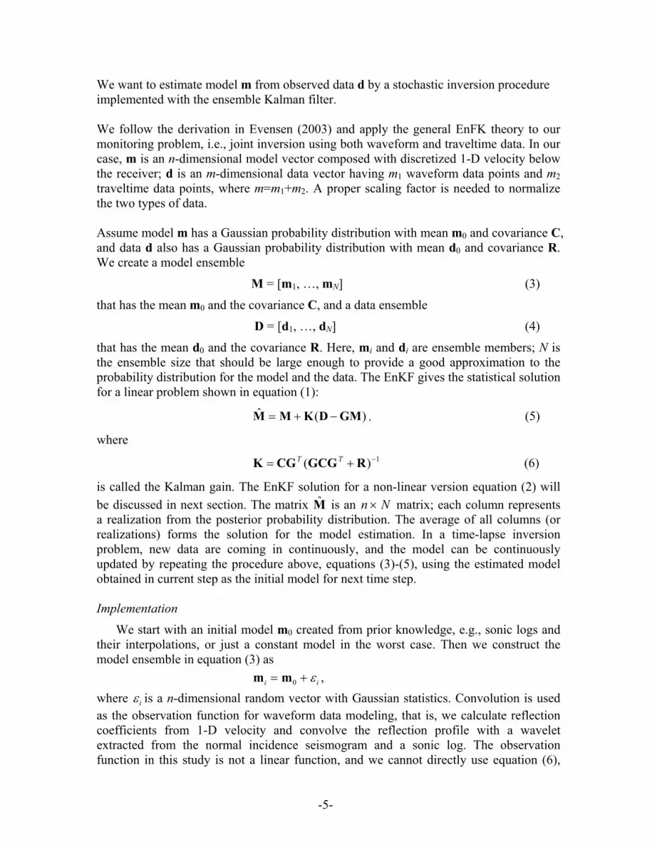
equals 5%, cleat porosity equals 1-5%, matrix permeability equals 0.5md and cleat permeability equals 100md. Next, we convert the flow simulation results to time-lapse P-wave velocity models with the help of a rock physics model. Figure 1 shows four velocity models at time =0, 3 months, 1 year, and 3 years. It can be seen that the P-wave velocity decreases due to the CO2 saturation. The methods discussed in previous sections are applied to these models to test if we can track the CO2 front using EnKF.

Figure 1: Four time-lapse P-wave velocity modes created based on CO2 flow simulation in the coalbeds. A: time=0; B: time=3 months; C: time=1 year; D: time=3 years.

Seismic Data

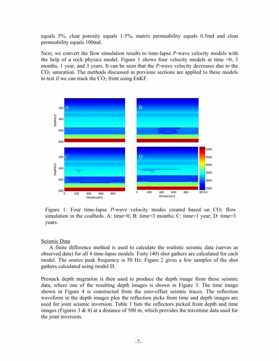
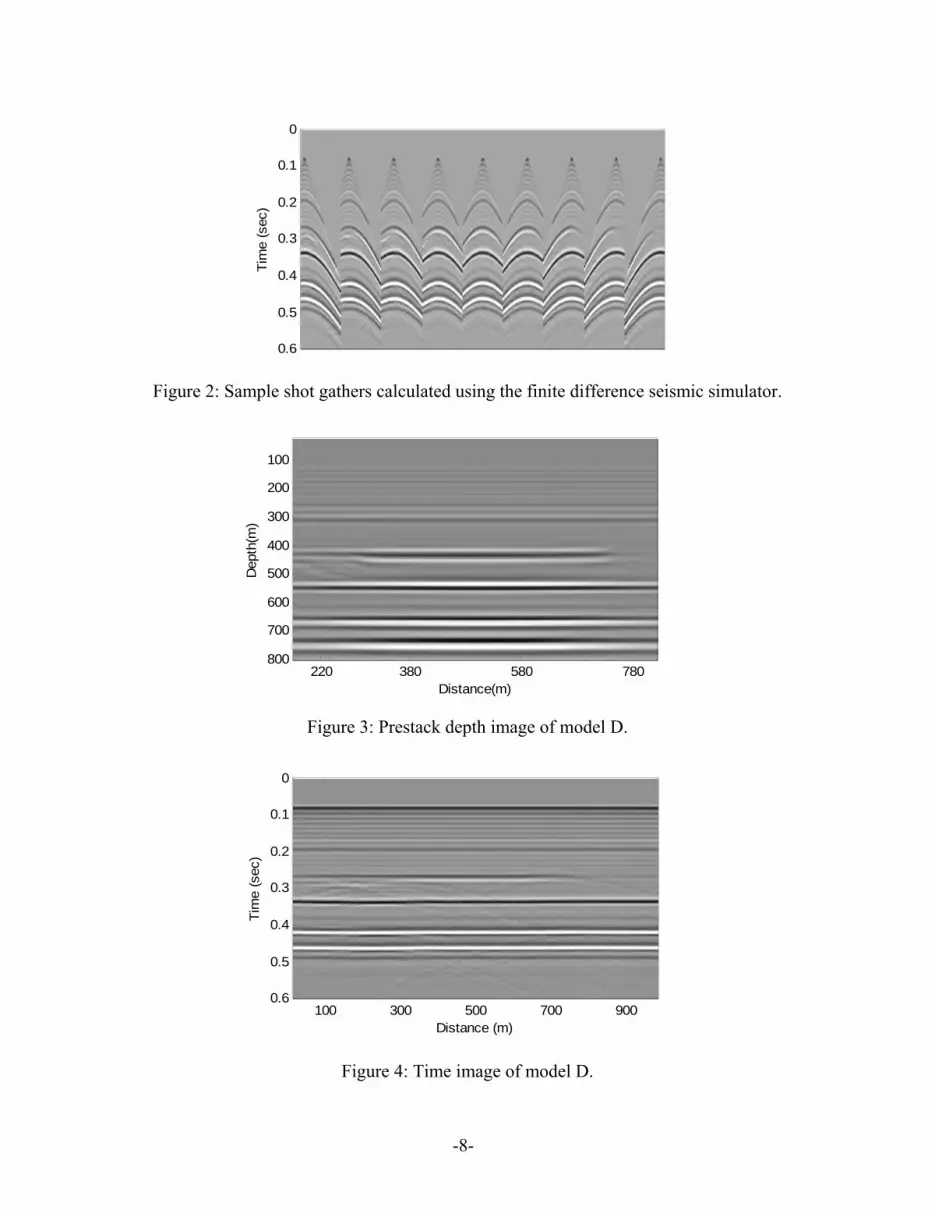
A finite difference method is used to calculate the realistic seismic data (serves as observed data) for all 4 time-lapse models. Forty (40) shot gathers are calculated for each model. The source peak frequency is 50 Hz. Figure 2 gives a few samples of the shot gathers calculated using model D. Prestack depth migration is then used to produce the depth image from these seismic data, where one of the resulting depth images is shown in Figure 3. The time image shown in Figure 4 is constructed from the zero-offset seismic traces. The reflection waveform in the depth images plus the reflection picks from time and depth images are used for joint seismic inversion. Table 1 lists the reflectors picked from depth and time images (Figures 3 & 4) at a distance of 500 m, which provides the travetime data used for the joint inversion.

Dep

th(m

)

200

400

600

800

Distance(m)0 200 400 600 800

2500

3000

3500

4000

4500

5000

v(m/s)

Distance(m)

Dep

th(m

)

0 200 400 600 800

200

400

600

800

A B

C D

-8-

Tim

e (s

ec)

0

0.1

0.2

0.3

0.4

0.5

0.6

Figure 2: Sample shot gathers calculated using the finite difference seismic simulator.

Distance(m)

Dep

th(m

)

220 380 580 780

100

200

300

400

500

600

700

800

Figure 3: Prestack depth image of model D.

Tim

e (s

ec)

Distance (m)100 300 500 700 900

0

0.1

0.2

0.3

0.4

0.5

0.6

Figure 4: Time image of model D.

-9-

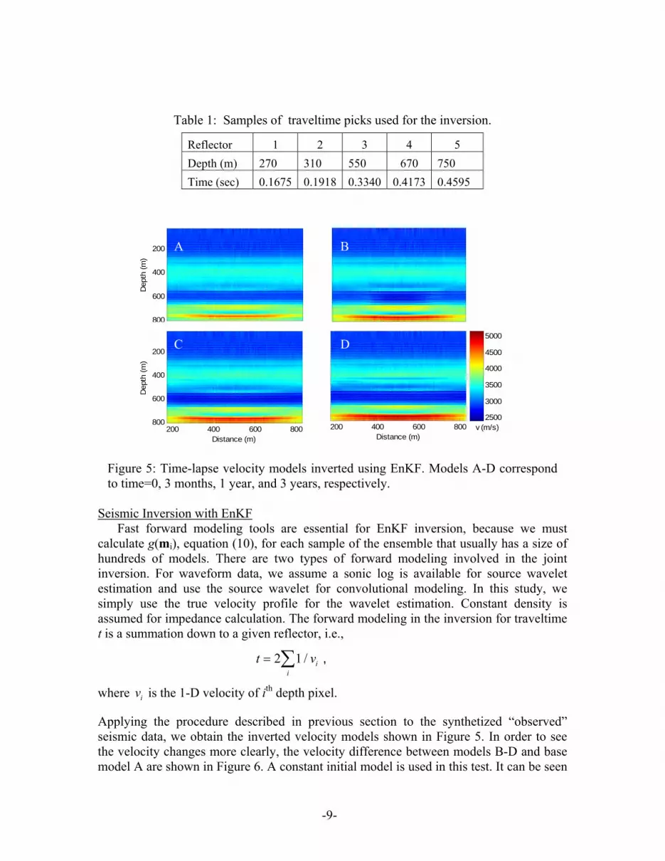
Table 1: Samples of traveltime picks used for the inversion.

Reflector 1 2 3 4 5 Depth (m) 270 310 550 670 750 Time (sec) 0.1675 0.1918 0.3340 0.4173 0.4595

Figure 5: Time-lapse velocity models inverted using EnKF. Models A-D correspond to time=0, 3 months, 1 year, and 3 years, respectively.

Seismic Inversion with EnKF

Fast forward modeling tools are essential for EnKF inversion, because we must calculate g(mi), equation (10), for each sample of the ensemble that usually has a size of hundreds of models. There are two types of forward modeling involved in the joint inversion. For waveform data, we assume a sonic log is available for source wavelet estimation and use the source wavelet for convolutional modeling. In this study, we simply use the true velocity profile for the wavelet estimation. Constant density is assumed for impedance calculation. The forward modeling in the inversion for traveltime t is a summation down to a given reflector, i.e.,

t = 2 1 / vi

i∑ ,

where vi is the 1-D velocity of ith depth pixel. Applying the procedure described in previous section to the synthetized “observed” seismic data, we obtain the inverted velocity models shown in Figure 5. In order to see the velocity changes more clearly, the velocity difference between models B-D and base model A are shown in Figure 6. A constant initial model is used in this test. It can be seen

Dep

th (m

)

200

400

600

800

Distance (m)200 400 600 800

2500

3000

3500

4000

4500

5000

v (m/s)Distance (m)

Dep

th (m

)

200 400 600 800

200

400

600

800

A B

C D

-10-

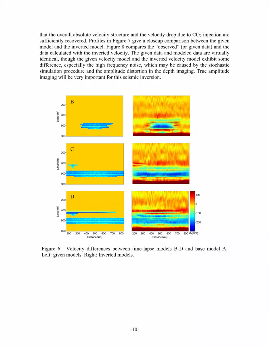
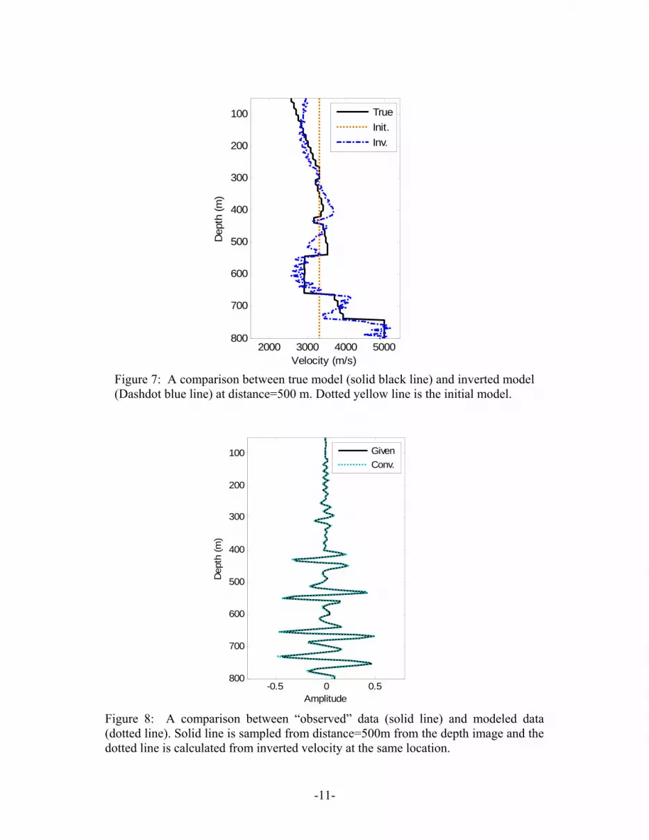
that the overall absolute velocity structure and the velocity drop due to CO2 injection are sufficiently recovered. Profiles in Figure 7 give a closeup comparison between the given model and the inverted model. Figure 8 compares the “observed” (or given data) and the data calculated with the inverted velocity. The given data and modeled data are virtually identical, though the given velocity model and the inverted velocity model exhibit some difference, especially the high frequency noise, which may be caused by the stochastic simulation procedure and the amplitude distortion in the depth imaging. True amplitude imaging will be very important for this seismic inversion.

Figure 6: Velocity differences between time-lapse models B-D and base model A. Left: given models. Right: Inverted models.

Distance(m)200 300 400 500 600 700 800

-200

-100

0

100

dv(m/s)

Dep

th(m

)

200

400

600

800

Dep

th(m

)

200

400

600

800

Distance(m)

Dep

th(m

)

200 300 400 500 600 700 800

200

400

600

800

B

C

D

-11-

2000 3000 4000 5000

100

200

300

400

500

600

700

800

Velocity (m/s)

Dep

th (m

)

TrueInit.Inv.

Figure 7: A comparison between true model (solid black line) and inverted model (Dashdot blue line) at distance=500 m. Dotted yellow line is the initial model.

-0.5 0 0.5

100

200

300

400

500

600

700

800

Amplitude

Dep

th (m

)

GivenConv.

Figure 8: A comparison between “observed” data (solid line) and modeled data (dotted line). Solid line is sampled from distance=500m from the depth image and the dotted line is calculated from inverted velocity at the same location.

-12-

Conclusions

The ensemble Kalman filter provides a powerful tool for stochastic seismic inversion, especially for dynamic inversion in seismic monitoring. Integrating travetime data into the inversion makes the estimation of absolute velocity possible. Waveform data alone in the joint inversion gives the short wavelength (spatial) components of inverted velocity.

-13-

3. DynaSIRT: A Robust Dynamic Imaging Method for Time-lapse Monitoring Dynamic Imaging

Dynamic imaging incorporates the temporal dimension into time-lapse seismic inversion. Instead of considering independent inversions for each time-lapse image, the temporal dynamics of the model are incorporated into inversion method, becoming a true spatio-temporal approach. This section describes a new algorithm for inversion of time-lapse seismic data named DynaSIRT. While conventional methods solve a system of equations independently for each survey for each snapshot in time, DynaSIRT incorporates information of previous surveys to estimate the current model without the reprocessing of previous data. Continuous or quasi-continuous monitoring present some special challenges for geophysical imaging. The amount of processing in case of joint inversion using data from older surveys or cross-equalization (Rickett and Lumley, 2001) can be excessively large and will grow in time. Practical implementation of dynamic imaging methods for seismic imaging must deal with memory and processing constraints. It can be done by incrementally solving the inversion problem and preserving solver state for later updates, keeping the problem tractable. Regularization (Tikhonov and Arsenin, 1977) is usually applied to improve seismic imaging. Many conventional seismic imaging methods use spatial similarity along axes as additional information to perform inversion, applying spatial regularization (Santos, 2006). Analogously, similarities occur along time axes and can be used as well by means of temporal regularization (Ajo-Franklin et al., 2005). Dynamic imaging goes one step further beyond separated spatial and temporal regularization. It treats the evolution of the imaged area as a dynamic process, an integrated approach that intrinsically includes spatio-temporal dynamics on inversion method. Although medical imaging has successfully applied dynamic imaging methods, geophysics still widely uses static methods adapted for time-lapse imaging. This is due to the larger amount of data to be processed, the long time between geophysical surveys, and the larger number of parameters to be estimated from geophysical inversion methods. DynaSIRT extends the static snapshot inversion method in order to incorporate temporal dynamic imaging. This method is efficient, processing equation by equation to incrementally update a previous model from new data. This incremental update is further explored for an additional advantage. The current state of the solver is saved for the next survey inversion, thus optimizing processing of sparse time-lapse data. Thus, DynaSIRT provides an efficient method for dynamic imaging, incorporating previous data into inversion without the burden caused by re-processing all the previous data. These features make DynaSIRT well suited for continuous monitoring of CO2 injection. DynaSIRT reduces computational effort by saving the solver state of last time-lapse inversion, avoiding increasing amounts of data to be processed along time. It can also provide snapshots of updated image during acquisition, due to its incremental way of processing and update.

-14-

Row-action Solvers

Row-action solvers compute an inversion problem solution iteratively, processing a linear system row by row, which means the updates are calculated equation by equation. These methods are the starting points for a practical implementation of dynamic imaging. A classic row-action method called ART (Algebraic Reconstruction Technique) computes parameter updates based on the difference between observed and computed data for each row (Peterson et al., 1985). The ART update equation for a linear system d=Gm is given by

( )( 1) ( )

2

kk k i

l l ilij

j

dm m gg

+ Δ= +

∑.

Here, di is the i-th data element; gij is a kernel matrix element, and ml is the parameter element. Artifacts may occur due to the row nature of ART since updates are computed separately for each row. Artifacts can be reduced by computing an average update from all equation updates. SIRT (Simultaneous Iterative Reconstruction Technique) averages the update using the expression (Stewart, 1992)

( )( 1) ( )

21

1 knk k i

l l ilil ij

j

dm m gN g

+

=

Δ= + ∑ ∑

.

The iterative nature of these methods, dealing with each equation separately to update the model allows us to save the solver state and restart later from this saved state. This feature was implemented on DynaSIRT, avoiding reprocessing previous surveys data. Other row-action methods or methods that act on subsets of data may be used as well. DynaSIRT

The continuous imaging/inversion approach must address three important questions:

1-How to preserve the influence of older survey equations on current model estimation? 2-How to balance influence between older and newer surveys equations? 3-How to avoid reprocessing older surveys equations?

DynaSIRT addresses these questions through the incorporation of three upgrades over original SIRT method:

1-Apply updates during computation, instead of later averaging and updating; 2-Apply temporal damping penalty effects for earlier surveys because the model

changes with time (aging effects); 3-Save linear solver state for future surveys, thus avoiding reprocessing of older surveys equations.

-15-

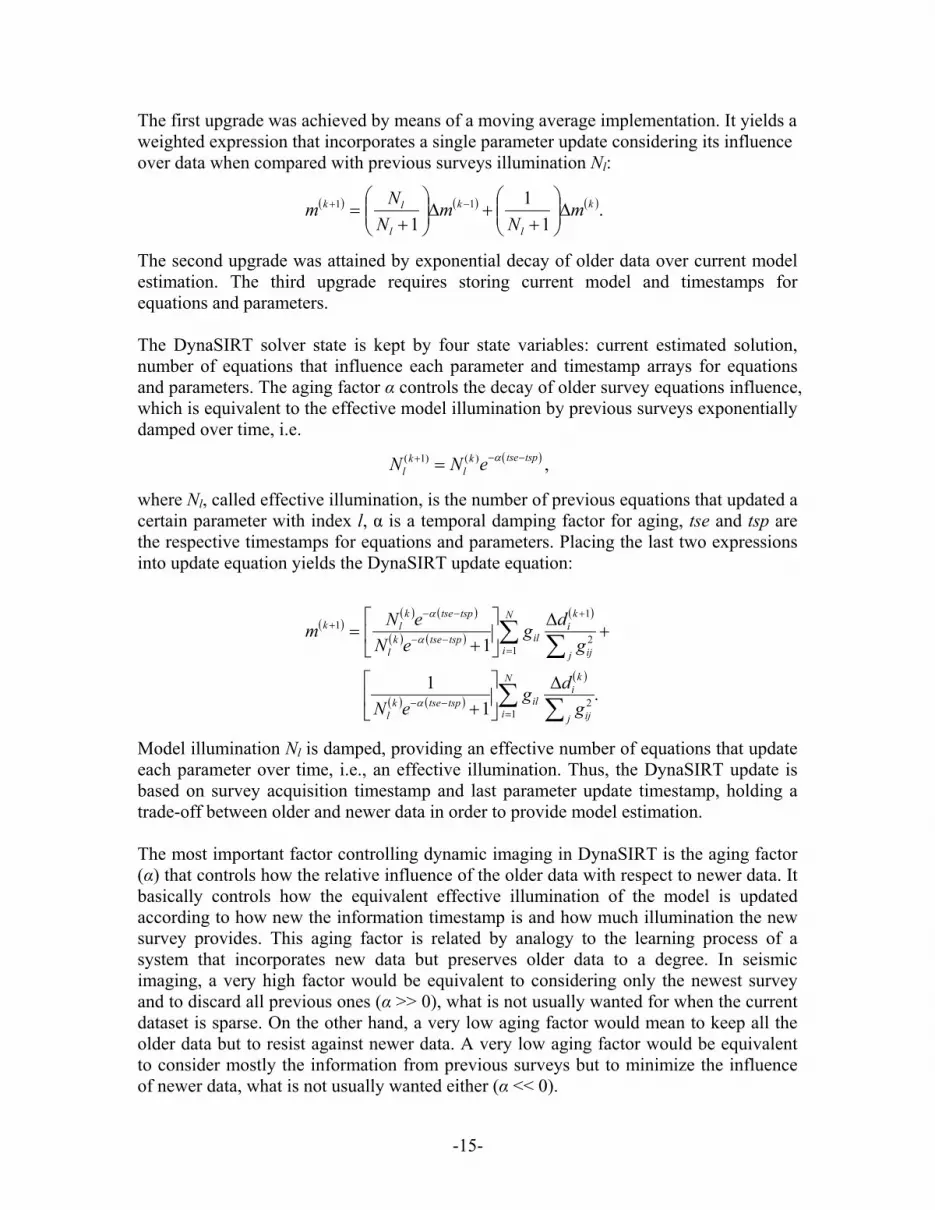
The first upgrade was achieved by means of a moving average implementation. It yields a weighted expression that incorporates a single parameter update considering its influence over data when compared with previous surveys illumination Nl:

( ) ( ) ( ).1

11

11 k

l

k

l

lk mN

mN

Nm Δ⎟⎟⎠

⎞⎜⎜⎝

⎛+

+Δ⎟⎟⎠

⎞⎜⎜⎝

⎛+

= −+

The second upgrade was attained by exponential decay of older data over current model estimation. The third upgrade requires storing current model and timestamps for equations and parameters. The DynaSIRT solver state is kept by four state variables: current estimated solution, number of equations that influence each parameter and timestamp arrays for equations and parameters. The aging factor α controls the decay of older survey equations influence, which is equivalent to the effective model illumination by previous surveys exponentially damped over time, i.e.

( )( 1) ( ) tse tspk kl lN N e α− −+ = ,

where Nl, called effective illumination, is the number of previous equations that updated a certain parameter with index l, α is a temporal damping factor for aging, tse and tsp are the respective timestamps for equations and parameters. Placing the last two expressions into update equation yields the DynaSIRT update equation:

( )( ) ( )

( ) ( )

( )

( ) ( )

( ).

11

1

12

12

11

∑ ∑

∑ ∑

=−−

=

+

−−

−−+

Δ⎥⎦

⎤⎢⎣

⎡+

+Δ

⎥⎦

⎤⎢⎣

⎡+

=

N

i j ij

ki

iltsptsekl

N

i j ij

ki

iltsptsekl

tsptseklk

gdg

eN

gdg

eNeNm

α

α

α

Model illumination Nl is damped, providing an effective number of equations that update each parameter over time, i.e., an effective illumination. Thus, the DynaSIRT update is based on survey acquisition timestamp and last parameter update timestamp, holding a trade-off between older and newer data in order to provide model estimation. The most important factor controlling dynamic imaging in DynaSIRT is the aging factor (α) that controls how the relative influence of the older data with respect to newer data. It basically controls how the equivalent effective illumination of the model is updated according to how new the information timestamp is and how much illumination the new survey provides. This aging factor is related by analogy to the learning process of a system that incorporates new data but preserves older data to a degree. In seismic imaging, a very high factor would be equivalent to considering only the newest survey and to discard all previous ones (α >> 0), what is not usually wanted for when the current dataset is sparse. On the other hand, a very low aging factor would mean to keep all the older data but to resist against newer data. A very low aging factor would be equivalent to consider mostly the information from previous surveys but to minimize the influence of newer data, what is not usually wanted either (α << 0).

-16-

Two particular cases are theoretically interesting. The first one happens when α is infinite, which would be analog to a system without memory. For this particular case, DynaSIRT becomes equivalent to SIRT applied only to the latest survey. Another particular case happens when α is zero, which means that the influence of older surveys is not damped and that all surveys are equally important, what is usually incorrect since the imaged area is usually changing over time. Since the extremes are not desired, α should be chosen within a limited range. Lower α emphasizes older surveys influence. Higher α emphasizes newer surveys influence. The effects associated to intermediary values of α are somehow analog to control the regularization factor of temporal regularization in a very sophisticated and adaptive way. It means that conventional tools for regularization factor selection can be adapted for this purpose, such as L-curve (Hansen, 1992) or θ-curve (Santos and Bassrei, 2007). Numerical Simulation

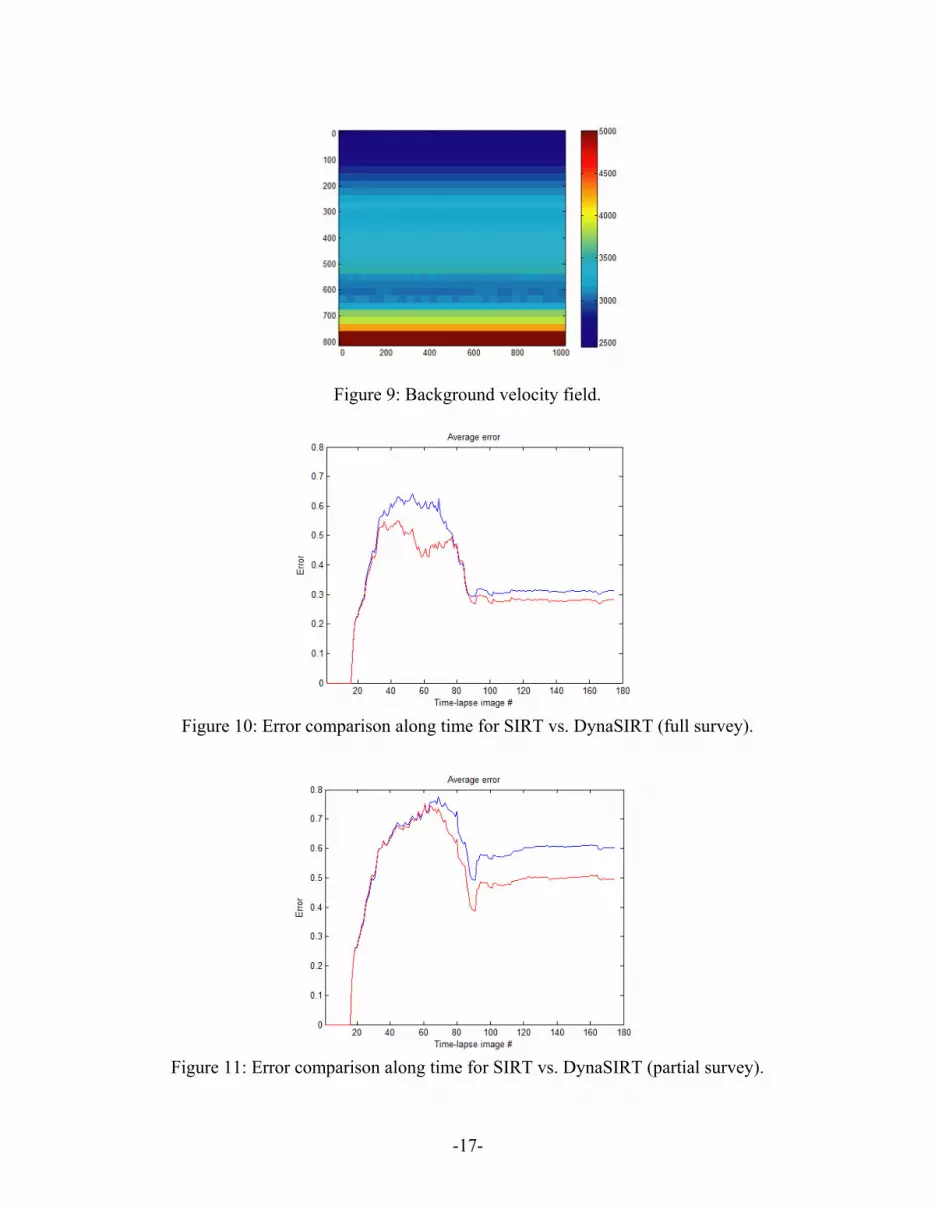
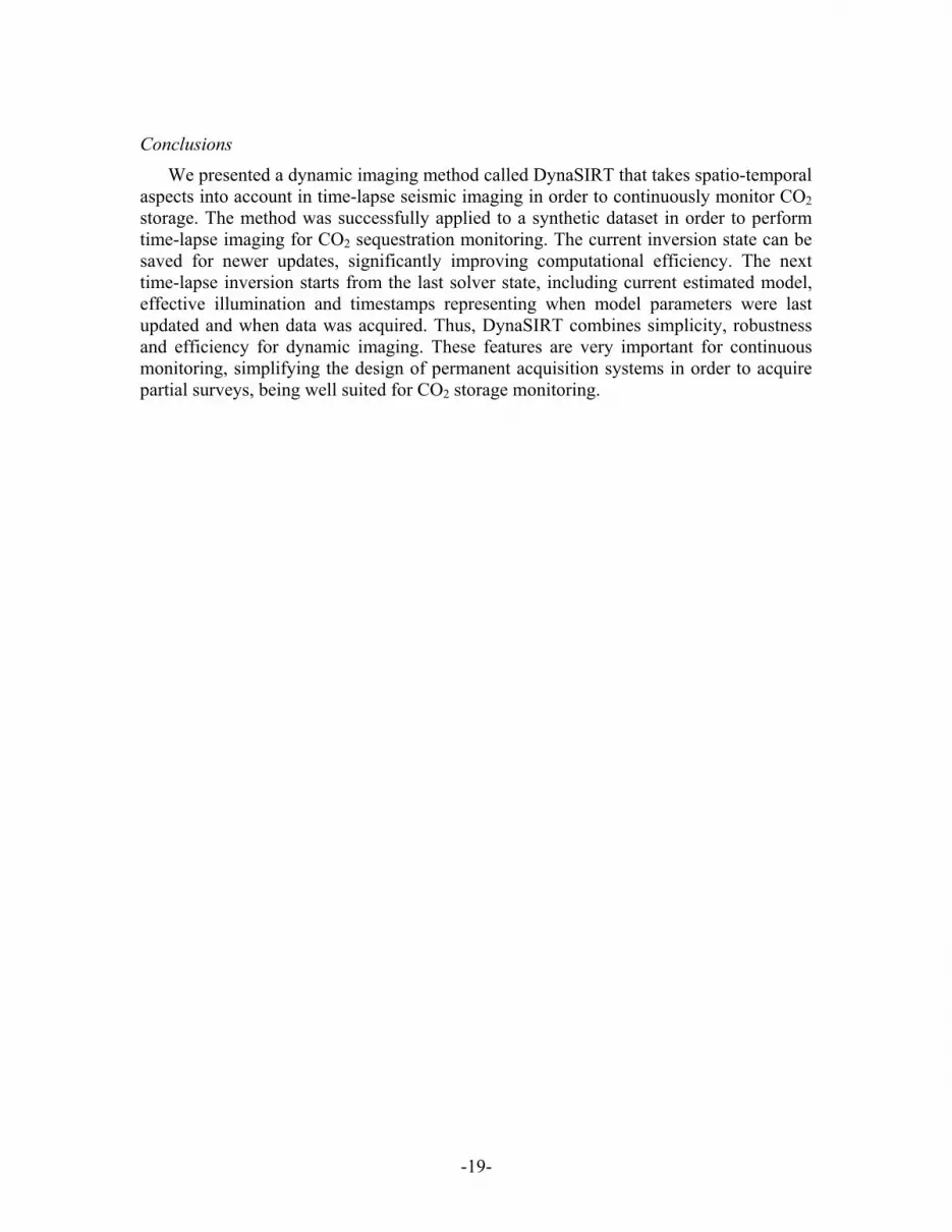
We applied DynaSIRT to a synthetic dataset generated with crosswell tomography surveys computed for 175 time-lapse 30×30 velocity models. The models show an expanding CO2 leakage computed using the reservoir simulator (GEM) and monitored by a permanently emplaced crosswell acquisition system. The background velocity model (Figure 9 shows a coalbed between 550m and 650m of depth where the CO2 is injected, causing a negative velocity contrast. All figures show distances in meters and velocities in m/s. Each time-lapse tomographic inversion was performed using diffraction tomography (Devaney, 1984) (Harris, 1987) (Wu and Toksöz, 1987). The discretization of the original continuous formulation leads to a linear system, which has to be inverted in order to estimate the velocity field (Rocha Filho, 1997) (Santos and Bassrei, 2007). DynaSIRT was applied to estimate each time-lapse tomography solution, incrementally updating the estimated velocity field without reprocessing of previous surveys data. The error comparison between a conventional approach using SIRT and the proposed approach using DynaSIRT is shown on Figure 10 for the full survey (30 sources × 15 receivers) and on Figure 11 for sparse partial survey (6 sources × 15 receivers) along 175 time-lapse images for α=2. Good results were achieved and they show that inversion error is notably reduced when comparing DynaSIRT with SIRT for sparse partial surveys. Even when SIRT provides good results, the DynaSIRT method performs well, making SIRT an upper bound for its error. The true velocity models for six time-lapse images equally spaced in time are shown on Figure 12 as absolute velocity contrast relatively to the background velocity field. The respective estimated models computed using DynaSIRT for sparse partial surveys are shown in the same way in Figure 13. Although this partial survey has only 20% of the data from the full survey, the DynaSIRT results still show good agreement with true models as expected from error comparison with SIRT.

-17-

Figure 9: Background velocity field.

Figure 10: Error comparison along time for SIRT vs. DynaSIRT (full survey).

Figure 11: Error comparison along time for SIRT vs. DynaSIRT (partial survey).

-18-

Figure 12: True model (CO2 sequestration leakage modeling): velocity field contrast modulus. Time-lapse number shown on image top.

Figure13: Time-lapse tomographic inversion using DynaSIRT (partial survey): velocity field contrast modulus. Time-lapse number shown on image top.

-19-

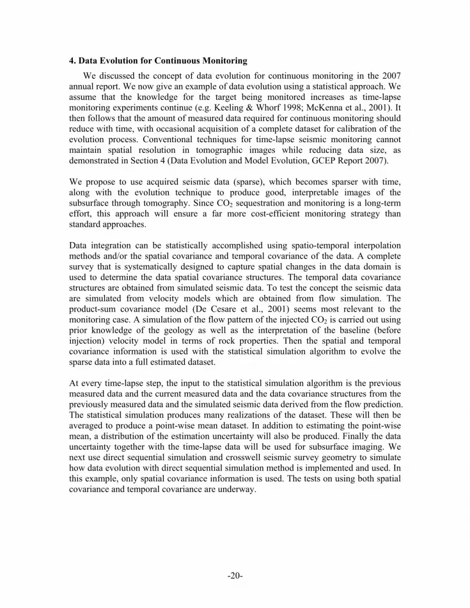
Conclusions

We presented a dynamic imaging method called DynaSIRT that takes spatio-temporal aspects into account in time-lapse seismic imaging in order to continuously monitor CO2 storage. The method was successfully applied to a synthetic dataset in order to perform time-lapse imaging for CO2 sequestration monitoring. The current inversion state can be saved for newer updates, significantly improving computational efficiency. The next time-lapse inversion starts from the last solver state, including current estimated model, effective illumination and timestamps representing when model parameters were last updated and when data was acquired. Thus, DynaSIRT combines simplicity, robustness and efficiency for dynamic imaging. These features are very important for continuous monitoring, simplifying the design of permanent acquisition systems in order to acquire partial surveys, being well suited for CO2 storage monitoring.

-20-

4. Data Evolution for Continuous Monitoring

We discussed the concept of data evolution for continuous monitoring in the 2007 annual report. We now give an example of data evolution using a statistical approach. We assume that the knowledge for the target being monitored increases as time-lapse monitoring experiments continue (e.g. Keeling & Whorf 1998; McKenna et al., 2001). It then follows that the amount of measured data required for continuous monitoring should reduce with time, with occasional acquisition of a complete dataset for calibration of the evolution process. Conventional techniques for time-lapse seismic monitoring cannot maintain spatial resolution in tomographic images while reducing data size, as demonstrated in Section 4 (Data Evolution and Model Evolution, GCEP Report 2007). We propose to use acquired seismic data (sparse), which becomes sparser with time, along with the evolution technique to produce good, interpretable images of the subsurface through tomography. Since CO2 sequestration and monitoring is a long-term effort, this approach will ensure a far more cost-efficient monitoring strategy than standard approaches. Data integration can be statistically accomplished using spatio-temporal interpolation methods and/or the spatial covariance and temporal covariance of the data. A complete survey that is systematically designed to capture spatial changes in the data domain is used to determine the data spatial covariance structures. The temporal data covariance structures are obtained from simulated seismic data. To test the concept the seismic data are simulated from velocity models which are obtained from flow simulation. The product-sum covariance model (De Cesare et al., 2001) seems most relevant to the monitoring case. A simulation of the flow pattern of the injected CO2 is carried out using prior knowledge of the geology as well as the interpretation of the baseline (before injection) velocity model in terms of rock properties. Then the spatial and temporal covariance information is used with the statistical simulation algorithm to evolve the sparse data into a full estimated dataset. At every time-lapse step, the input to the statistical simulation algorithm is the previous measured data and the current measured data and the data covariance structures from the previously measured data and the simulated seismic data derived from the flow prediction. The statistical simulation produces many realizations of the dataset. These will then be averaged to produce a point-wise mean dataset. In addition to estimating the point-wise mean, a distribution of the estimation uncertainty will also be produced. Finally the data uncertainty together with the time-lapse data will be used for subsurface imaging. We next use direct sequential simulation and crosswell seismic survey geometry to simulate how data evolution with direct sequential simulation method is implemented and used. In this example, only spatial covariance information is used. The tests on using both spatial covariance and temporal covariance are underway.

-21-

(a) (b)

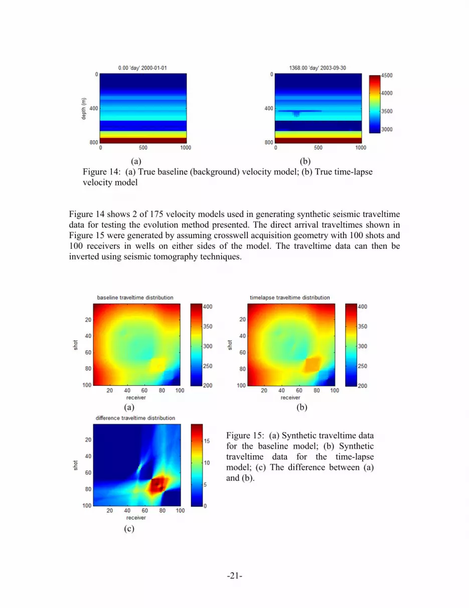
Figure 14: (a) True baseline (background) velocity model; (b) True time-lapse velocity model

Figure 14 shows 2 of 175 velocity models used in generating synthetic seismic traveltime data for testing the evolution method presented. The direct arrival traveltimes shown in Figure 15 were generated by assuming crosswell acquisition geometry with 100 shots and 100 receivers in wells on either sides of the model. The traveltime data can then be inverted using seismic tomography techniques.

(a) (b)

(c)

Figure 15: (a) Synthetic traveltime data for the baseline model; (b) Synthetic traveltime data for the time-lapse model; (c) The difference between (a) and (b).

-22-

Direct sequential simulation implementation

Consider a variable )( rκ with a global cumulative distribution function Fκ(z) = prob{κ(r) < z} and stationary spatiotemporal variogram, γ(r), with which we intend to reproduce γ(r) and Fκ(z), direct sequential simulation will be implemented in the following way:

1. Select randomly, the location of a node r in a grid of nodes to be simulated 2. Get the neighborhood data, both original data, )( αrκ , and simulated data, )( irκ 3. Calculate the conditional mean and conditional variance using simple kriging 4. Build a conditional cumulative distribution function (ccdf) at r with the moments

obtained in step 3 5. Draw a value )( irκ from the local ccdf 6. Return to step 1 until all nodes have been visited

Direct sequential simulation (dssim) was carried out on the data presented earlier, but decimated to about 10% (Figure 16b), using the variogram obtained from the complete data (from the full baseline dataset). Accurate estimates of the data are obtained by calculating the point-wise data average. Data uncertainties are obtained by calculating the point-wise data standard deviation. Selected realizations and the e-type (point-wise average) data are shown in Figure 17. Results compare reasonably well to the complete dataset.

(a) (b) Figure 16: (a) Complete time-lapse difference dataset (same as Figure 15(c)); (b) Sparse 10% time-lapse difference dataset.

-23-

(a) (b)

(c) (d)

Figure 17: (a) and (b) are 2 realizations from 100 generated after running direct sequential simulation (dssim); (c) E-type (average) of all realizations obtained from running dssim on the dataset shown in Figure 16(b); (d) point-wise variance of all dssim realizations.

-24-

5. A Feasibility Study on the Controlled Source Electromagnetic Method for

Monitoring of Geological CO2 Sequestration Introduction

The controlled-source electromagnetic (CSEM) method was first developed in academia more than 30 years ago to investigate the electrical conductivity structures of the deep ocean lithosphere and terrestrial basin (Strack, 1984 and Cox et al., 1986). Since the method is preferentially sensitive to thin electrical resistors such as hydrocarbon and gas reservoirs in depth, the method has recently demonstrated its commercial ability to evaluate the electrical resistivity of potential offshore hydrocarbon reservoirs before drilling (Eidesmo et al., 2002). The method is also being changed rapidly from a simple reservoir detecting tool to a multi-dimensional electromagnetic (EM) imaging and monitoring tool, trying to push the boundary of the EM monitoring capabilities (Gribenko and Zhdanov, 2007). In this study, we investigate the feasibility of the CSEM method as a supplementary monitoring tool in water-saturated coalbed environments, though we continue our efforts to develop efficient time-lapse seismic techniques as a primary subsurface monitoring tool. Before we present CSEM numerical modeling works and their analysis over the coalbed environment, we briefly summarize the basic rock physics and electromagnetics. Rock Physics and Basic Electromagnetics

Electrical resistivity of rocks is highly sensitive to changes in brine saturation, as can be seen from plotting of Archie’s law shown in Figure 18. As the electrically conductive pore fluid within a rock is replaced by the leaked CO2 gas or other by-product gas, the electrical resistivity increases exponentially, resulting in a strong resistivity contrast between gas-saturated and brine-saturated geological media. For this type of geophysical scenario, the CSEM method would serve as an effective geophysical tool to monitor CO2 leakage from a reservoir and supplement seismic methods with relatively low cost.

Figure 18: Archie’s law and its plot (Gasperikova and Hoversten, 2006).

1.0E+00

1.0E+01

1.0E+02

1.0E+03

1.0E+04

0 0.1 0.2 0.3 0.4 0.5 0.6 0.7 0.8 0.9 1

Gas saturation (Sg)

Bul

k re

sist

ivity

(Ohm

-m)

2 2( ) (1 )

0.25, 0.33rock g g brine

brine

S S

m

ρ φ ρ

φ ρ

− −= −

= = Ω

-25-

Secondary fields

Primary fields

CO2 saturated coal bed

- - -- - -+ + + ++ +

Electric dipole EM receivers

Air waveAir wave

Secondary fields

Primary fields

CO2 saturated coal bed

- - -- - -+ + + ++ +

Electric dipole EM receivers

Air waveAir wave

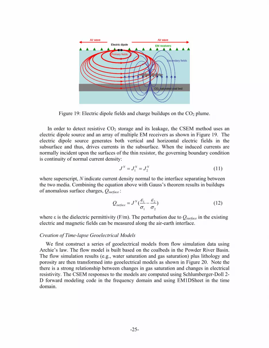
Figure 19: Electric dipole fields and charge buildups on the CO2 plume.

In order to detect resistive CO2 storage and its leakage, the CSEM method uses an

electric dipole source and an array of multiple EM receivers as shown in Figure 19. The electric dipole source generates both vertical and horizontal electric fields in the subsurface and thus, drives currents in the subsurface. When the induced currents are normally incident upon the surfaces of the thin resistor, the governing boundary condition is continuity of normal current density:

1 2N N NJ J J= = (11)

where superscript, N indicate current density normal to the interface separating between the two media. Combining the equation above with Gauss’s theorem results in buildups of anomalous surface charges, Qsurface :

1 2

1 2

( )NsurfaceQ J ε ε

σ σ= − (12)

where ε is the dielectric permittivity (F/m). The perturbation due to Qsurface in the existing electric and magnetic fields can be measured along the air-earth interface. Creation of Time-lapse Geoelectrical Models

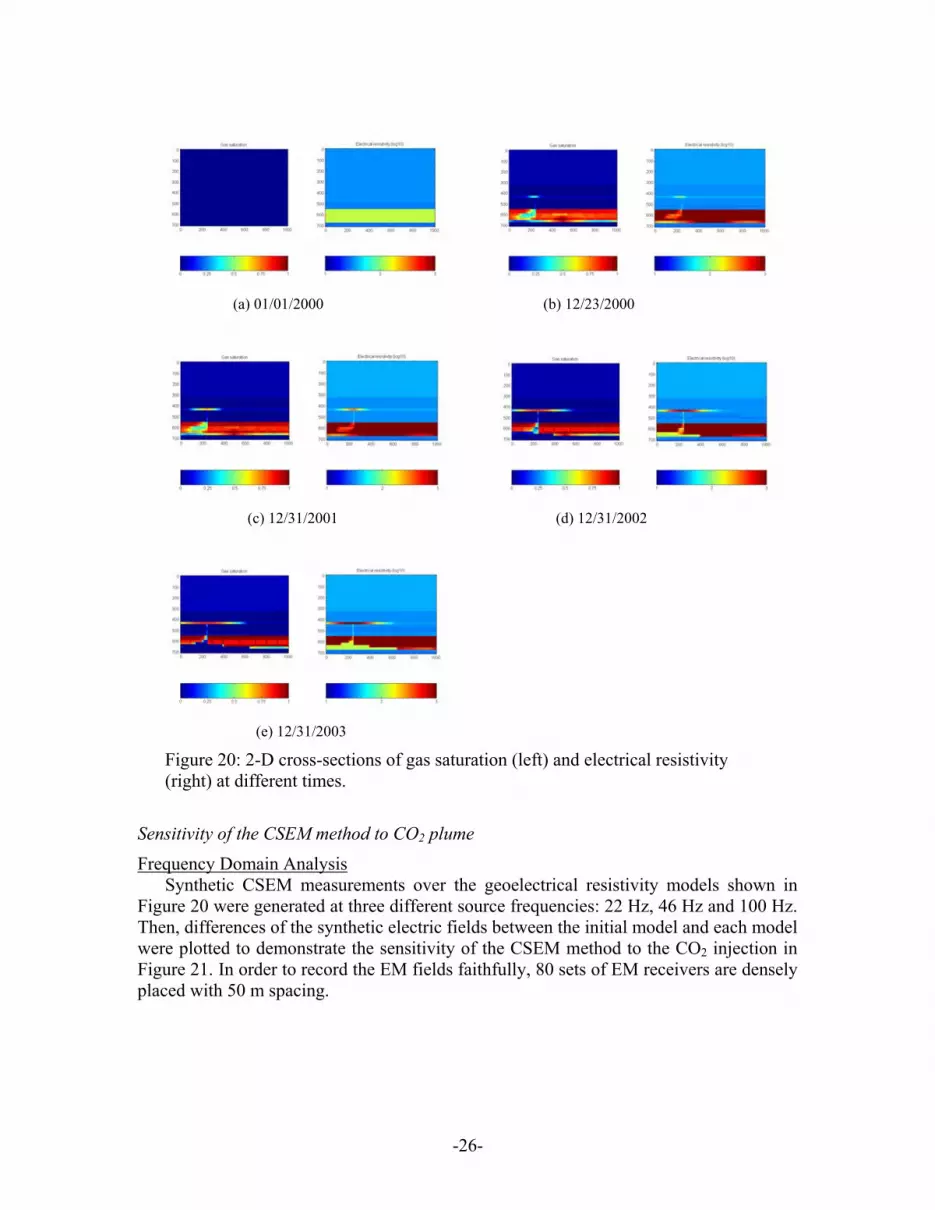
We first construct a series of geoelectrical models from flow simulation data using Archie’s law. The flow model is built based on the coalbeds in the Powder River Basin. The flow simulation results (e.g., water saturation and gas saturation) plus lithology and porosity are then transformed into geoelectrical models as shown in Figure 20. Note the there is a strong relationship between changes in gas saturation and changes in electrical resistivity. The CSEM responses to the models are computed using Schlumberger-Doll 2-D forward modeling code in the frequency domain and using EM1DSheet in the time domain.

-26-

(a) 01/01/2000 (b) 12/23/2000

(c) 12/31/2001 (d) 12/31/2002

(e) 12/31/2003

Figure 20: 2-D cross-sections of gas saturation (left) and electrical resistivity (right) at different times.

Sensitivity of the CSEM method to CO2 plume

Frequency Domain Analysis Synthetic CSEM measurements over the geoelectrical resistivity models shown in

Figure 20 were generated at three different source frequencies: 22 Hz, 46 Hz and 100 Hz. Then, differences of the synthetic electric fields between the initial model and each model were plotted to demonstrate the sensitivity of the CSEM method to the CO2 injection in Figure 21. In order to record the EM fields faithfully, 80 sets of EM receivers are densely placed with 50 m spacing.

-27-

Electric Field Perturbation

0

10

20

30

40

50

60

70

-2000 -1500 -1000 -500 0 500 1000 1500 2000X distance (km)

Diff

eren

ce (5

)12/23/2000

12/31/2001

12/31/2002

12/31/2003

Electric Field Perturbation

0

5

10

15

20

25

30

35

-2000 -1500 -1000 -500 0 500 1000 1500 2000X distance (km)

Diff

eren

ce (5

)

(a) Electric dipole source at (-255m, 0m, 0m) (b) (255m, 0m, 0m)

Electric Field Perturbation

0

5

10

15

20

25

30

35

-2000 -1500 -1000 -500 0 500 1000 1500 2000X distance (km)

Diff

eren

ce (5

)

Electric Field Perturbation

0

10

20

30

40

50

60

70

-2000 -1500 -1000 -500 0 500 1000 1500 2000X distance (km)

Diff

eren

ce (5

)

(c) (755m, 0m, 0m) (d) (1155m, 0m, 0m).

Figure 21: Difference (%) of the electric fields between the initial model and each model at four source positions.

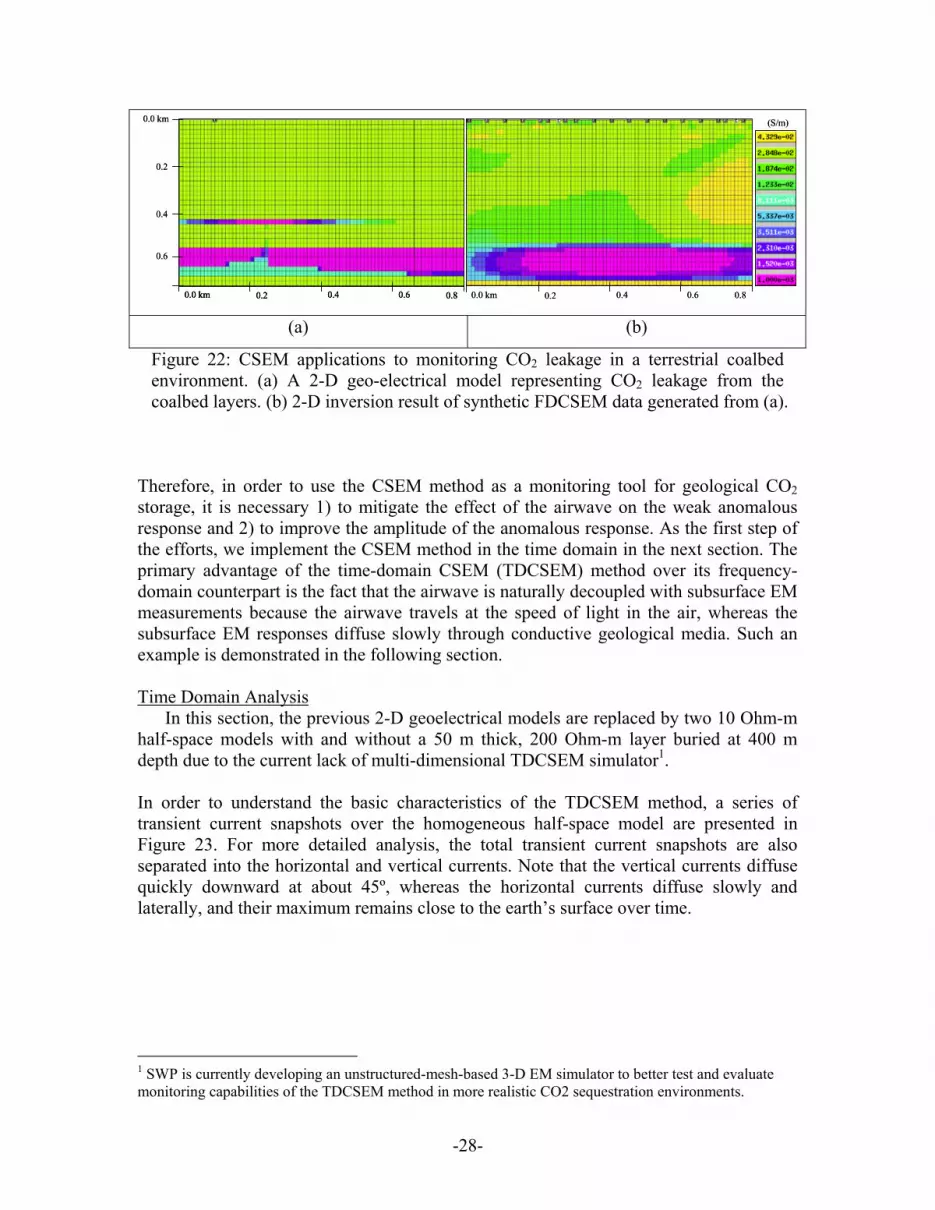
Note that the CSEM method clearly detects the injection of the CO2 gas into the coalbed in the first year. However, in the next following years, the relatively-small perturbations were observed. In order to examine how well the leakage can be imaged, the synthetic data were inverted. The background model without the injection is used as a starting model during the inversion process. The true model and inversion result are compared in Figure 22; the CSEM method fails to detect the thin CO2 plume at 440 m depth, whereas it reasonably delineates the thick coalbed saturated with CO2. Even though there exists sharp difference in electrical resistivity between the CO2 plume and the background environment, the CSEM method is nearly blind to the thin leakage because of the following two reasons:

• Airwave that does not include any information about the subsurface dominates the subsurface responses, masking the weak anomalous response to the CO2 leakage.

• Perturbation in electric field due to the coalbed is much larger than that due to the leakage, masking the weak anomalous response to the leakage.

-28-

�(S/m)0.0 km

0.2

0.4

0.6

0.0 km 0.2 0.4 0.6 0.8 0.0 km 0.2 0.4 0.6 0.8

�(S/m)0.0 km

0.2

0.4

0.6

0.0 km 0.2 0.4 0.6 0.80.0 km 0.2 0.4 0.6 0.8 0.0 km 0.2 0.4 0.6 0.8

(a) (b)

Figure 22: CSEM applications to monitoring CO2 leakage in a terrestrial coalbed environment. (a) A 2-D geo-electrical model representing CO2 leakage from the coalbed layers. (b) 2-D inversion result of synthetic FDCSEM data generated from (a).

Therefore, in order to use the CSEM method as a monitoring tool for geological CO2 storage, it is necessary 1) to mitigate the effect of the airwave on the weak anomalous response and 2) to improve the amplitude of the anomalous response. As the first step of the efforts, we implement the CSEM method in the time domain in the next section. The primary advantage of the time-domain CSEM (TDCSEM) method over its frequency-domain counterpart is the fact that the airwave is naturally decoupled with subsurface EM measurements because the airwave travels at the speed of light in the air, whereas the subsurface EM responses diffuse slowly through conductive geological media. Such an example is demonstrated in the following section. Time Domain Analysis

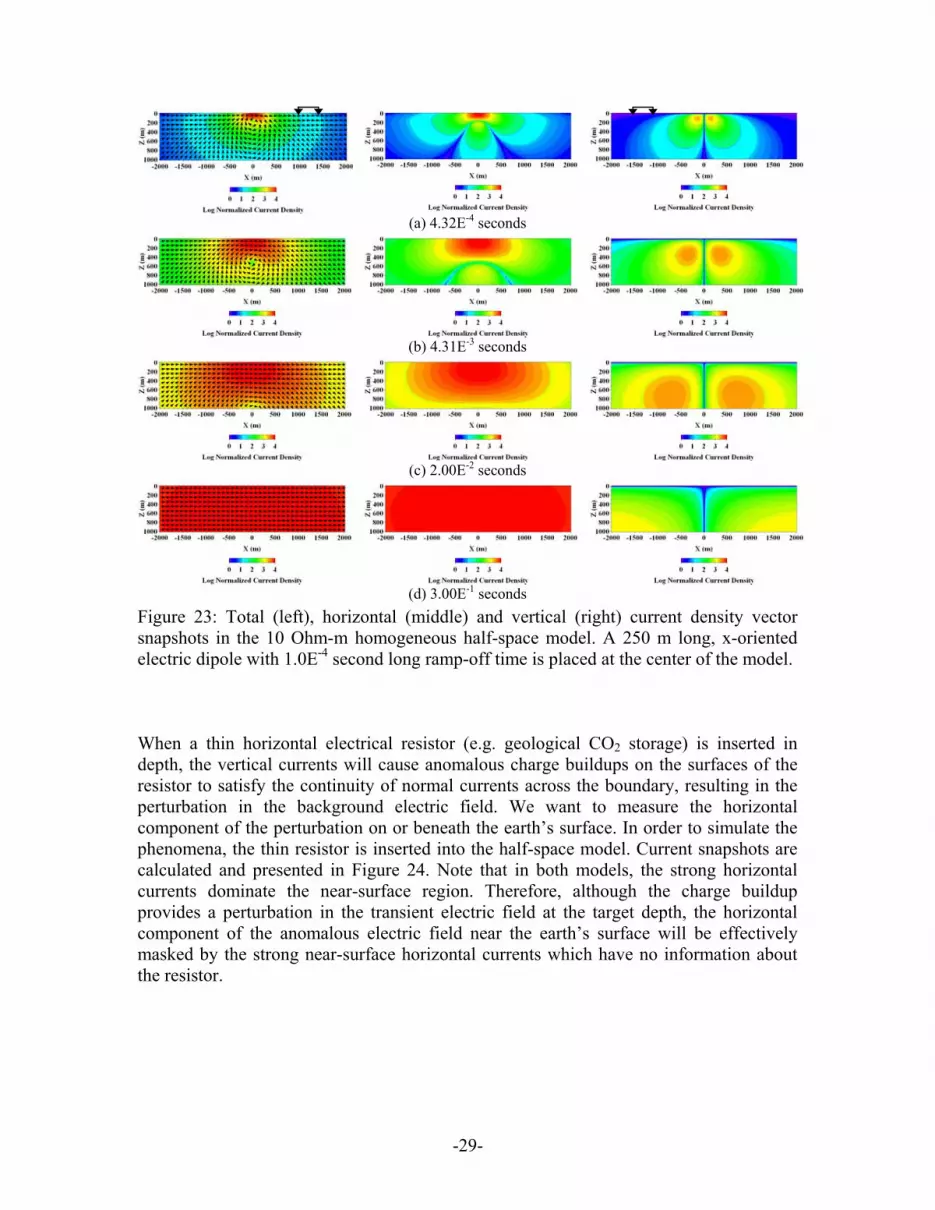
In this section, the previous 2-D geoelectrical models are replaced by two 10 Ohm-m half-space models with and without a 50 m thick, 200 Ohm-m layer buried at 400 m depth due to the current lack of multi-dimensional TDCSEM simulator1. In order to understand the basic characteristics of the TDCSEM method, a series of transient current snapshots over the homogeneous half-space model are presented in Figure 23. For more detailed analysis, the total transient current snapshots are also separated into the horizontal and vertical currents. Note that the vertical currents diffuse quickly downward at about 45º, whereas the horizontal currents diffuse slowly and laterally, and their maximum remains close to the earth’s surface over time.

1 SWP is currently developing an unstructured-mesh-based 3-D EM simulator to better test and evaluate monitoring capabilities of the TDCSEM method in more realistic CO2 sequestration environments.

-29-

(a) 4.32E-4 seconds

(b) 4.31E-3 seconds

(c) 2.00E-2 seconds

(d) 3.00E-1 seconds Figure 23: Total (left), horizontal (middle) and vertical (right) current density vector snapshots in the 10 Ohm-m homogeneous half-space model. A 250 m long, x-oriented electric dipole with 1.0E-4 second long ramp-off time is placed at the center of the model.

When a thin horizontal electrical resistor (e.g. geological CO2 storage) is inserted in depth, the vertical currents will cause anomalous charge buildups on the surfaces of the resistor to satisfy the continuity of normal currents across the boundary, resulting in the perturbation in the background electric field. We want to measure the horizontal component of the perturbation on or beneath the earth’s surface. In order to simulate the phenomena, the thin resistor is inserted into the half-space model. Current snapshots are calculated and presented in Figure 24. Note that in both models, the strong horizontal currents dominate the near-surface region. Therefore, although the charge buildup provides a perturbation in the transient electric field at the target depth, the horizontal component of the anomalous electric field near the earth’s surface will be effectively masked by the strong near-surface horizontal currents which have no information about the resistor.

-30-

(a) 4.32E-4 seconds

(b) 4.31E-3 seconds

(c) 2.00E-2 seconds

(d) 3.00E-1 seconds

Figure 24: Total (left), horizontal (middle) and vertical (right) current density vector snapshots in the half-space model with the 50 m thick, 200 Ohm-m gas storage layer (denoted as the double black solid lines) at a depth of 400. Consequently, the difference between the two models is clearly observed at the target depth in the vertical current snapshots, but is not obvious along the earth’s surface in the horizontal current snapshots. As a result, when the surface electric fields are simulated over the half-space models with and without the resistor and plotted, the TDCSEM method does not distinguish between the two models as shown in Figure 25a. A classic method for increasing the differences in the electric field measurements between the two models is to convert standard step-off responses into impulse responses by calculating the time-derivative of the recorded step responses (Edwards, 1997; Hördt et al., 2000). The time-derivatives of the step-off sounding curves shown in Figure 25a are presented in Figure 25b. Since an impulse source has a larger amount of high frequency contents than a standard step-off source, the near-surface horizontal currents are increasingly attenuated with source-receiver offsets over time; therefore, their masking effect on the anomalous electric field can be diminished.

-31-

1.E-13

1.E-12

1.E-11

1.E-10

1.E-09

1.E-08

1.E-07

1.E-06

1.E-04 1.E-03 1.E-02 1.E-01 1.E+00 1.E+01

Time (sec)

Ele

ctri

c fie

ld (V

/m)

Background model1D resistor model

-5.0E-08

0.0E+00

5.0E-08

1.0E-07

1.5E-07

1.E-04 1.E-03 1.E-02 1.E-01 1.E+00 1.E+01

Time (sec)

Ele

ctri

c fie

ld (V

/m/s

ec)

(a) (b)

Figure 25: The inline horizontal electric field sounding curves over the half-space models with/without the CO2 storage layer. (a) The inline electric field measurements excited by a step-off source waveform and (b) the time-derivative of the sounding curves in (a) to mimic the corresponding impulse responses.

1.E-14

1.E-13

1.E-12

1.E-11

1.E-10

1.E-09

1.E-08

1.E-07

1.E-06

1.E-04 1.E-03 1.E-02 1.E-01 1.E+00 1.E+01

Time (sec)

Ele

ctri

c fie

ld (V

/m)

1D resistor model, dual TX

Background model, dual TX

1D resistor model, single TX

Background model, single TX

(a) (b)

Figure 26: Sounding results over a 10 Ohm-m half-space with and without a 50 m thick, 200 Ohm-m gas storage buried at 400 m depth. (a) A dual source TDCSEM configuration with a synchronized step-off excitation. The arrows on the dipoles represent the direction of source polarization, and the fat arrows in the earth are transient currents. (b) Electric field measurements 300 m away from the center of the model (the center of the sources). The electric field measurements completed with a single 250 m-long source are superimposed for a direct comparison.

Another way to improve the sensitivity to the CO2 storage is to split a single large electric dipole source into multiple smaller electric dipole sources and configure them concentrically. In such a configuration, transient vertical currents responsible for the galvanic response are constructively superimposed, producing larger galvanic responses

50 m50 m 200 m

Constructive superposition

Destructive superposition

-32-

at a region in which the CO2 storage lies. In contrast, near-surface horizontal currents from each source will interact destructively with each other at measurement points, reducing their masking effect on the useful galvanic responses. The simplest form of a multi-source TDCSEM configuration proposed here and its sounding curves are presented in Figure 26.

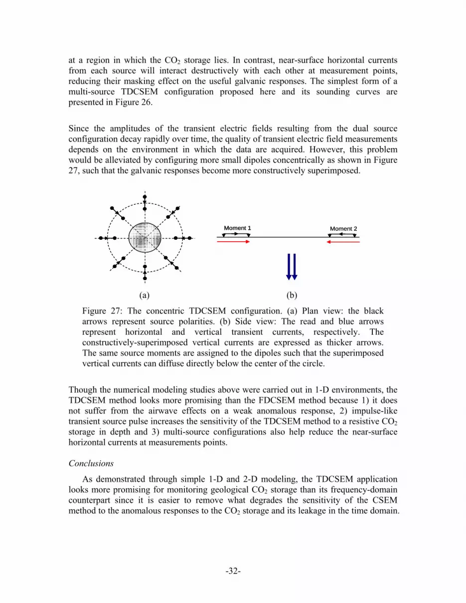
Since the amplitudes of the transient electric fields resulting from the dual source configuration decay rapidly over time, the quality of transient electric field measurements depends on the environment in which the data are acquired. However, this problem would be alleviated by configuring more small dipoles concentrically as shown in Figure 27, such that the galvanic responses become more constructively superimposed.

Moment 1 Moment 2Moment 1Moment 1 Moment 2

(a) (b)

Figure 27: The concentric TDCSEM configuration. (a) Plan view: the black arrows represent source polarities. (b) Side view: The read and blue arrows represent horizontal and vertical transient currents, respectively. The constructively-superimposed vertical currents are expressed as thicker arrows. The same source moments are assigned to the dipoles such that the superimposed vertical currents can diffuse directly below the center of the circle.

Though the numerical modeling studies above were carried out in 1-D environments, the TDCSEM method looks more promising than the FDCSEM method because 1) it does not suffer from the airwave effects on a weak anomalous response, 2) impulse-like transient source pulse increases the sensitivity of the TDCSEM method to a resistive CO2 storage in depth and 3) multi-source configurations also help reduce the near-surface horizontal currents at measurements points. Conclusions

As demonstrated through simple 1-D and 2-D modeling, the TDCSEM application looks more promising for monitoring geological CO2 storage than its frequency-domain counterpart since it is easier to remove what degrades the sensitivity of the CSEM method to the anomalous responses to the CO2 storage and its leakage in the time domain.

-33-

6. Future Work

We plan to test the EnKF seismic inversion method to continuously monitor and develop a localized imaging technique. In this way, data can be acquired or sorted by patches as shown in Figure 28, and the data in each patch may be sorted as a common reflection gather and stacked as a single trace for the seismic inversion. We will apply data evolution it to transmission and reflection seismic tomography. The CSEM research has just started. We are developing a 3-D finite-element time-domain EM diffusion simulator to better handle complex subsurface geology and subtle geometric changes in CO2 storage.

Publications Quan, Y. and J.M. Harris, 2008, Stochastic Seismic Inversion using both Waveform and

Traveltime Data and Its Application to Time-lapse Monitoring: SEG Expanded Abstracts 28 (2008)

Santos, Eduardo T. F. and Jerry M. Harris, DynaSIRT, 2008, A Robust Dynamic Imaging Method Applied to CO2 Sequestration Monitoring, SEG Extended Abstracts 28 (2008).

Santos, E.T.F., Harris, J., Bassrei, A., Costa, J.C., 2007, Regularized diffraction tomography for trigonal meshes applied to reservoir monitoring. In: X Congresso Internacional da Sociedade Brasileira de Geofísica, 2007, Rio de Janeiro.

Santos, Eduardo T. F. and Harris, Jerry M., 2007, Time-lapse diffraction tomography for trigonal meshes with temporal data Integration applied to CO2 sequestration monitoring, SEG Extended Abstracts 26, 2959 (2007).

Figure 28: Incremental data acquisition for continuous subsurface monitoring

Subsurface target to be monitored

Datasets collected at different times

-34-

References Ajo-Franklin, J. B., J. A. Urban, and J. M. Harris, 2005, Temporal integration of seismic

traveltime tomography: 75th Annual International Meeting, SEG, Expanded Abstracts, 2468-2471.

Cao, D., W.B. Bevdoun, S.C. Singn and A. Tarantola, A simultaneous inversion for background velocity and impedance maps: Geophysics, 55, 458–469.

Cox, C., S. Constable, A. Chave and S. Webb, 1986, Controlled-source electromagnetic sounding of the oceanic lithosphere, Nature, Vol. 320, 52-54.

De Cesare, L., Myers, D. E., & Posa, D. (2001). Product-sum covariance for space-time modeling: an environmental application. Environmetrics, vol. 12 , 11-23.

Devaney, A. J., 1984, Geophysical diffraction tomography: IEEE Transactions on Geoscience and Remote Sensing, 22, 3-13.

Eidesmo, T., S. Ellingsrud, L. MacGregor, S. Constable, M. Sinha, S. Johansen, F. Kong, and H. Westerdahl, 2002, Sea bed logging (SBL), a new method for remote and direct identification of hydrocarbon filled layers in deepwater areas: First Break, 20, 144–152. Evensen, G., 2003, The ensemble Kalman filter: Theoretical formulation and practical

implementation: Ocean Dynamics, 53, 343–367. Evensen, G. 2007, Data Assimilation – the Ensemble Kalman Filter: Springer Francis, A., 2005, Limitations of deterministic and advantages of stochastic inversion:

CSEG Recorder, February 2005. Gasperikova, E. and M. Hoversten, 2006, A feasibility study of nonseismic geophysical

methods for monitoring geologic CO2 sequestration, The Leading Edge, Vol. 25, No. 10, 1282-1288.

Geologic Storage of CO2, 2007, GCEP Annual Report. Gribenko, A. and M. Zhdanov, 2007, Rigorous 3D inversion of marine CSEM data on the

integral equation method, Geophysics, Vol. 72, No. 2, WA73-WA84. Haas, A., and O. Dubrule, 1994, Geostatistical inversion — A sequential method of

stochastic reservoir modeling constrained by seismic data: First Break, 12, 561–569.

Hansen, P. C., 1992, Analysis of discrete ill-posed problems by means of the l-curve, SIAM Review, 34, 561-580.

Harris, J. M., 1987, Diffraction tomography with discrete arrays of sources and receivers, IEEE Transactions on Geoscience and Remote Sensing, V. GE-25, n. 4, p. 448-455.

Keeling, C. D., & Whorf, T. P., 2005, Atmospheric CO2 records from sites in the SIO air sampling network. In Trends: A Compendium of Data on Global Change. Laboratory, Carbon Dioxide Information Analysis Center Oak Ridge National, Oak Ridge, Tenn., U.S.A.: U.S. Department of Energy.

Mandel, J., 2006, Efficient implementation of the ensemble Kalman filter: CCM Report 231, University of Colorado at Denver and Health Sciences Center.

McKenna, J., Sherlock, D., & Evans, B., 2001, Time-lapse 3-D seismic imaging of shallow subsurface contaminant flow: Journal of Contaminant Hydrology, vol. 53, 133-150.

Oldenburg, D. W., T. Scheuer, and S. Levy, 1983, Recovery of the acoustic impedance from reflection seismograms: Geophysics, 48, 1318–1337.

-35-

Peterson, J. E., B. J. P. Paulsson, and T. V. McEvilly, 1985, Applications of algebraic reconstruction techniques to crosshole seismic data: Geophysics, v. 50. no. 10, p. 1566-1580.

Rickett, J., and D. Lumley, 2001, Cross-equalization data processing for time-lapse seismic reservoir monitoring: A case study from the Gulf of Mexico: Geophysics, 66, 1015-1025.

Rocha Filho, A. A., 1997, Geophysical diffraction tomography: multifrequency matrix formulation and integrated inversion (in Portuguese): M.Sc. Dissertation, Federal University of Bahia.

Sancevero, S.S, A.Z. Remacre, R. S. Portugal, 2005, Comparing deterministic and stochastic seismic inversion for thin-bed reservoir characterization in a turbidite synthetic reference model of Campos Basin, Brazil: The Leading Edge, February 2005, 1168–1172.

Santos, E. T. F., 2006, Anisotropic seismic tomographic inversion with optimal regularization (in Portuguese): D.Sc. Thesis, Federal University of Bahia.

Santos, E. T. F., and J. M. Harris, 2007, Time-lapse Diffraction Tomography for Trigonal Meshes with Temporal Data Integration Applied to CO2 Sequestration Monitoring: 77th Annual International Meeting, SEG, Expanded Abstracts, 2959-2963.

Santos, E. T. F., and A. Bassrei, 2007, L- and Theta-curve approaches for the selection of regularization parameter in geophysical diffraction tomography: Computers & Geosciences, 33, 618-629.

Strack, K.M., 1984, The deep transient electromagnetic sounding technique: first field test in Australia, Exploration Geophysics, Vol. 15,251-259.

Stewart, R. R., 1992, Exploration seismic tomography-fundamentals, Course Notes Series, V. 3: Tulsa, Oklahoma, Society of Exploration Geophysicists.

Tikhonov, A. N., and V. Y. Arsenin, 1977, Solution of Ill-Posed Problems: Wiley. Wu, R-S, and M. N. Toksöz, 1987, Diffraction tomography and multisource holography

applied to seismic imaging. Geophysics, 52, 11-25.

Contacts Jerry M. Harris: jerry.harris@stanford.edu Youli Quan: quany@stanford.edu Eduardo Santos: eduardo.telmo@terra.com.br Tope Akinbehinje: topeakin@stanford.edu Adeyemi Arogunmati: aadeyemi@stanford.edu Jolene Robin-McCaskill: jmrobin@stanford.edu Evan Um: eum@stanford.edu