Embed Size (px)
Citation preview
AAllmmaa MMaatteerr SSttuuddiioorruumm –– UUnniivveerrssiittàà ddii BBoollooggnnaa
DOTTORATO DI RICERCA IN
GEOFISICA
Ciclo XXXII
Settore Concorsuale: 02/C1
Settore Scientifico Disciplinare: FIS/06
CHARACTERIZATION OF TURBULENT EXCHANGE PROCESSES
IN REAL URBAN STREET CANYONS WITH AND WITHOUT
VEGETATION
Presentata da: Francesco Barbano
Coordinatore Dottorato Supervisore
Prof.ssa Nadia Pinardi Prof.ssa Silvana Di Sabatino
Esame finale anno 2020

Abstract
Recent studies on turbulent exchange processes between the urban canopy layer and theatmosphere above have focused primarily on mechanical effects and less so on thermal ones,mostly by means of laboratory and numerical investigations and rarely in the real environment.More recently, these studies have been adopted to investigate city breathability, urban comfortand citizen health, with the aim to find new mitigation or adaptation solutions to air pollutionand urban heat island, to enhance the citizen wellness. To investigate the small-scale proces-ses characterizing vegetative and non-vegetative urban canopies, two field campaigns have beencarried out within the city of Bologna, Italy. New mechanical and thermal time scales, and theirratios (rates), associated with inertial and thermal flow circulations, have been derived to thisscope. In the non-vegetated canopy, mechanical time scales are found to describe fast exchangesat the rooftop and slow within the canopy, while thermal ones to describe fast mixing in thewhole canopy. Faster processes are found in the vegetative canopy, with rapidly mixed mecha-nical time scales and varying thermal ones. The exchange rates are found to identify favorablemixing conditions in the 50-75% of the investigated period, but extreme disadvantageous eventscan totally suppress the exchanges. The exchange rates are also found to drive the pollutantremoval from vegetated and non-vegetated canopies, with an efficacy which depends on the in-canyon circulation. The impacts of real trees in a real neighborhood of the city is tackled witha simplified fluid-dynamics model, where mean flow and turbulence are studied with differentvegetation configurations, topological and morphological characteristics. Vegetation is foundto increase both blocking and channeling effects on the mean flow and to modify the produc-tion/dissipation rate of turbulence, depending on the wind direction and topology. Nevertheless,buildings maintain a predominant impact on the atmospheric flows.
i

Contents
1 Introduction 1
2 The Urban Boundary Layer: an Overview 52.1 The Urban Boundary Layer . . . . . . . . . . . . . . . . . . . . . . . . . . . . . . 5
2.1.1 The Roughness Sublayer . . . . . . . . . . . . . . . . . . . . . . . . . . . . 82.1.2 The Inertial Sublayer . . . . . . . . . . . . . . . . . . . . . . . . . . . . . 9
2.2 The Urban Canopy Layer . . . . . . . . . . . . . . . . . . . . . . . . . . . . . . . 102.2.1 Inertial and Thermal Circulations . . . . . . . . . . . . . . . . . . . . . . 11
2.3 Exchange Processes and City Breathability . . . . . . . . . . . . . . . . . . . . . 152.4 Vegetation in the Urban Environment . . . . . . . . . . . . . . . . . . . . . . . . 212.5 Summary and Conclusions . . . . . . . . . . . . . . . . . . . . . . . . . . . . . . . 25
3 The "Bologna Project": the Experimental Field Campaigns 273.1 The Experimental Sites . . . . . . . . . . . . . . . . . . . . . . . . . . . . . . . . 27
3.1.1 Non Vegetated Street Canyon - Marconi Street . . . . . . . . . . . . . . . 303.1.2 Vegetated Street Canyon - Laura Bassi Street . . . . . . . . . . . . . . . . 35
3.2 Supporting Instrumentation . . . . . . . . . . . . . . . . . . . . . . . . . . . . . . 393.3 Summary and Conclusions . . . . . . . . . . . . . . . . . . . . . . . . . . . . . . . 42
4 Data Processing and Methodology 434.1 Data processing . . . . . . . . . . . . . . . . . . . . . . . . . . . . . . . . . . . . . 43
4.1.1 Experimental protocol and despiking procedure . . . . . . . . . . . . . . . 434.1.2 Coordinate system rotation . . . . . . . . . . . . . . . . . . . . . . . . . . 44
4.2 Data analysis . . . . . . . . . . . . . . . . . . . . . . . . . . . . . . . . . . . . . . 454.2.1 The period selection based on the analysis of synoptic conditions . . . . . 454.2.2 Exchange processes: time scales and rates . . . . . . . . . . . . . . . . . . 494.2.3 Pollutant concentration normalization . . . . . . . . . . . . . . . . . . . . 53
4.3 Numerical simulations . . . . . . . . . . . . . . . . . . . . . . . . . . . . . . . . . 564.3.1 QUIC-URB model description . . . . . . . . . . . . . . . . . . . . . . . . 56
v
CONTENTS4.3.2 QUIC-PLUME model description . . . . . . . . . . . . . . . . . . . . . . . 634.3.3 Vegetation Parametrization . . . . . . . . . . . . . . . . . . . . . . . . . . 654.3.4 Model setup . . . . . . . . . . . . . . . . . . . . . . . . . . . . . . . . . . . 67
4.4 Summary and Conclusions . . . . . . . . . . . . . . . . . . . . . . . . . . . . . . . 70
5 Results and Discussion: Observations and Campaign Comparison 735.1 Mean Characteristics of the Summer Campaign . . . . . . . . . . . . . . . . . . . 73
5.1.1 Pollutant Concentrations . . . . . . . . . . . . . . . . . . . . . . . . . . . 735.1.2 Background and Mean Flow Fields Characteristics . . . . . . . . . . . . . 775.1.3 Local Flow Field and Turbulence . . . . . . . . . . . . . . . . . . . . . . . 78
5.2 Mean Characteristics of the Winter Campaign . . . . . . . . . . . . . . . . . . . . 855.2.1 Pollutant Concentrations . . . . . . . . . . . . . . . . . . . . . . . . . . . 855.2.2 Background and Mean Flow Fields Characteristics . . . . . . . . . . . . . 875.2.3 Local Flow Field and Turbulence . . . . . . . . . . . . . . . . . . . . . . . 88
5.3 Summary and Conclusions . . . . . . . . . . . . . . . . . . . . . . . . . . . . . . . 94
6 Results and Discussion: Exchange Processes between the Canopy Layer andthe Urban Boundary Layer 976.1 Exchange Processes: Time Scales and Rates . . . . . . . . . . . . . . . . . . . . . 98
6.1.1 Time Scales Evaluation . . . . . . . . . . . . . . . . . . . . . . . . . . . . 986.1.2 Exchange Rates Evaluation . . . . . . . . . . . . . . . . . . . . . . . . . . 1026.1.3 Comparison between the Exchange Rates and the Normalized Pollutant
Concentrations . . . . . . . . . . . . . . . . . . . . . . . . . . . . . . . . . 1056.1.4 The Circulation Regime Identification: use of New Parametrizations to
Compare Different Street Canyon Flow Characteristics . . . . . . . . . . . 1106.2 The Impact of Trees on Exchange Processes Variables: a Multi-Seasonal Com-
parative Analysis . . . . . . . . . . . . . . . . . . . . . . . . . . . . . . . . . . . . 1146.3 Summary and Conclusions . . . . . . . . . . . . . . . . . . . . . . . . . . . . . . . 117
7 Results and Discussion: Modeling the Impacts of Trees on the ExchangeProcesses 1197.1 Qualitative Code Verification: u∗ associated to the Unperturbed Flow . . . . . . 1197.2 Model Verification among Different Wind Direction Ensembles . . . . . . . . . . 126
7.2.1 Vegetated Street Canyon - Laura Bassi Street . . . . . . . . . . . . . . . . 1267.2.2 Non Vegetated Street Canyon - Marconi Street . . . . . . . . . . . . . . . 133
7.3 The Impact of Trees in Laura Bassi Neighborhood under the Input Wind Direc-tion Perpendicular from East to the Street Canyon Orientation . . . . . . . . . . 1397.3.1 Vegetation Impact Distributions and Topological Discretization . . . . . . 143
vi
CONTENTS
7.3.2 The Effects of Morphology . . . . . . . . . . . . . . . . . . . . . . . . . . 1517.4 The Effect of Wind Direction and Surface Roughness on the Vegetation Impact . 155
7.4.1 Vegetation Impact Distributions and Topological Discretization . . . . . . 1567.4.2 The Effects of Morphology . . . . . . . . . . . . . . . . . . . . . . . . . . 170
7.5 Summary and Conclusions . . . . . . . . . . . . . . . . . . . . . . . . . . . . . . . 177
8 Conclusions and Further Remarks 1818.1 Future Perspectives . . . . . . . . . . . . . . . . . . . . . . . . . . . . . . . . . . . 185
Appendices
A Technical Specifications for the Instrumentation 189
B Application of Buckingham Theorem 199
C Generalized Extreme Value Distribution Theory 201
Bibliography 203
vii

List of Figures
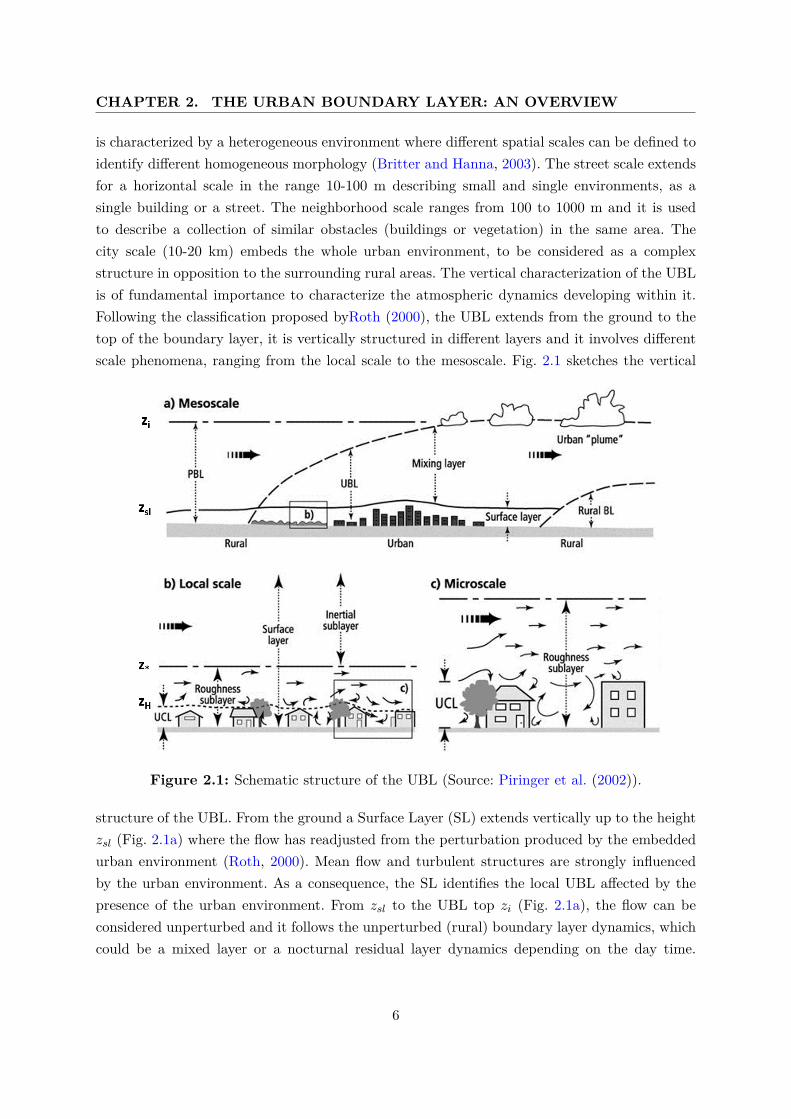
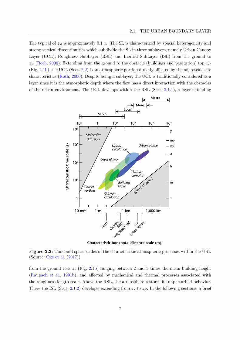
2.1 Schematic structure of the UBL (Source: Piringer et al. (2002)). . . . . . . . . . . 62.2 Time and space scales of the characteristic atmospheric processes within the UBL
(Source: Oke et al. (2017)) . . . . . . . . . . . . . . . . . . . . . . . . . . . . . . . 72.3 Idealized 2D sketches of the in-canyon flow regimes from Oke (1987) classification.
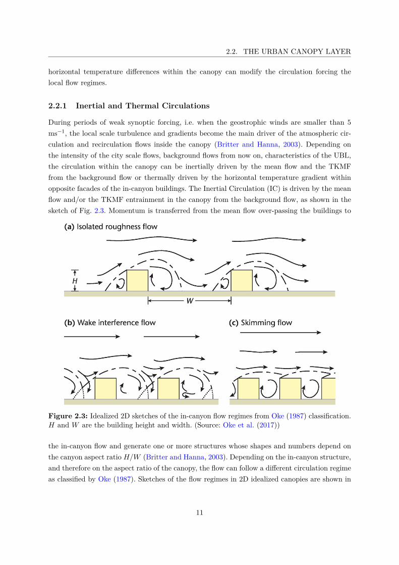
H and W are the building height and width. (Source: Oke et al. (2017)) . . . . . 112.4 Idealized 2D sketches of the in-canyon flow regimes in irregular street canyons
originally from Xiaomin et al. (2006). h1 and h2 are the leeward and windwardbuilding height respectively, and g is the canyon width. (Source: Zajic et al. (2011)) 12
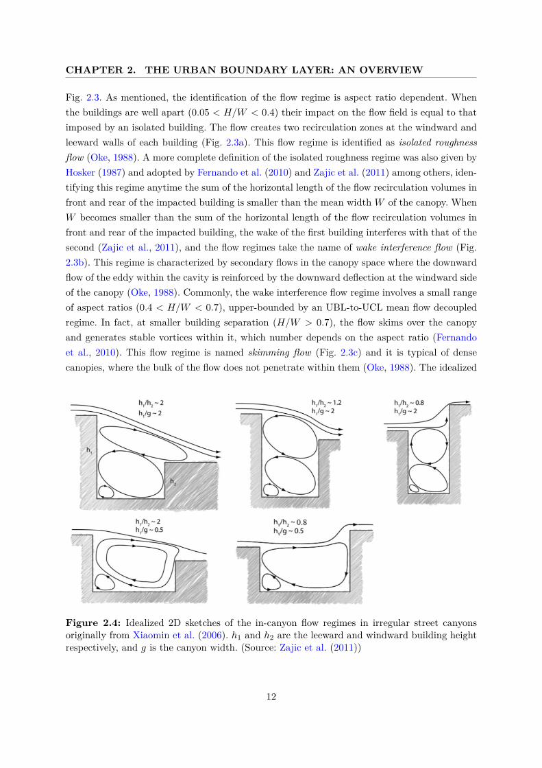
2.5 Sketches of the (a) IC and (b) TC inside an idealized SC. H andW are the meanbuilding height and width of the canyon, T1 and T2 the building facade tempera-tures, Ub and θb the background wind speed and air potential temperature, w′u′
and w′θ′ the TKMF and the TKSHF evaluated inside the canyon (subscript S)and at the rooftop level (subscript H). . . . . . . . . . . . . . . . . . . . . . . . . 13
2.6 Simplified velocity profiles within and above the urban canopy. H is the meanbuilding height, UC the canopy layer velocity, Uref the velocity above the canopylayer and UE the exchange velocity between at the rooftop interface. (Source:Bentham and Britter (2003)) . . . . . . . . . . . . . . . . . . . . . . . . . . . . . 17
3.1 Satellite view of the Po Valley and Bologna historical center. (Source: GoogleEarth). . . . . . . . . . . . . . . . . . . . . . . . . . . . . . . . . . . . . . . . . . . 28
3.2 Top view of Bologna city center (a, ©Comune di Bologna) and the surroundingarea (b). . . . . . . . . . . . . . . . . . . . . . . . . . . . . . . . . . . . . . . . . . 29
3.3 Map of Bologna with localization of the campaign sampling sites. In order: (a)SI, (b) PSF, (c) MA, (d) GM, (e) LB, (f) AT and (g) IR. (Source: Google Earth). 30
3.4 Top (a) and frontal (b) views of MA. . . . . . . . . . . . . . . . . . . . . . . . . . 313.5 Measurement sites locations at the three levels inside and above MA canyon.
Colors link the location (dots) to the corresponding measurement site (boxes).Instrumentation at each level is reported on table 3.1. (Source: Google Earth). . 32
3.6 Top (a) and frontal (b) views of LB. . . . . . . . . . . . . . . . . . . . . . . . . . 35
ix
LIST OF FIGURES
3.7 Measurement sites locations at the three levels inside and above LB canyon. Col-ors link the location (dots) to the corresponding measurement site (boxes). Instru-mentation at each level is reported on table 3.2. (Source: https://earth.google.com/web/). 36
3.8 PSF (a) and GM (b) air quality monitoring sites. . . . . . . . . . . . . . . . . . . 39
3.9 The Vaisala Ceilometer CL31 located on the rooftop of the Physics and Astron-omy department in IS. . . . . . . . . . . . . . . . . . . . . . . . . . . . . . . . . . 40
4.1 Three dimensional coordinate rotations for alignment of coordinate axes to theflow field over sloping terrain. Modified from figure 6.20 of Kaimal and Finnigan(1994). . . . . . . . . . . . . . . . . . . . . . . . . . . . . . . . . . . . . . . . . . . 44
4.2 GFS analysis of the surface isobars (white lines) superimposed on the geopotentialat 500 hPa (colormap). Each panel shows the midnight UTC of a single day withinthe summer period. Bologna is identified by the black dot. . . . . . . . . . . . . . 46
4.3 Wind velocity, air temperature and dew point temperature profiles retrieved fromsounding data measured during (a) 20, (b) 21, (c) 22 and (d) 23 September fromSan Pietro in Capofiume, a small village 30 km to the north-east of Bologna (Datasource: University of Wyoming, http://weather.uwyo.edu/upperair/sounding.html). 47
4.4 GFS analysis of the surface isobars (white lines) superimposed on the geopotentialat 500 hPa (colormap). Each panel shows the midnight UTC of a single day withinthe winter period. Bologna is identified by the black dot. . . . . . . . . . . . . . . 48
4.5 Wind velocity, air temperature and dew point temperature profiles retrieved fromsounding data measured during (a) 08 and (b) 09 February from San Pietro inCapofiume, a small village 30 km to the north-east of Bologna (Data source:University of Wyoming, http://weather.uwyo.edu/upperair/sounding.html). . . . 48
4.6 Wind velocity streamlines retrieved from CFD simulations of MA, in conditionof background wind direction perpendicular (a) and parallel (b) to the canyonorientation. H and W are the mean building height and width of the canyon, T1
and T2 the building facade temperatures, Ub and θb the background wind speedand air potential temperature, w′u′ and w′θ′ the TKMF and TKSHF respectivelyevaluated inside the canyon (GL and ML, subscript S) and at the RL (subscriptH). . . . . . . . . . . . . . . . . . . . . . . . . . . . . . . . . . . . . . . . . . . . . 50
4.7 Comparison between CO concentrations (red line) measured in (a) MA and (b)LB and the respective traffic rates (blue line) expressed as the number of carspassing through the street during the summer period. Data are averaged over a30 minutes window. The shadowed areas highlight nighttime periods. On averagesun rises at 6:00 AM and sets at 18:00 PM (GMT+1). . . . . . . . . . . . . . . . 54
x
LIST OF FIGURES
4.8 Comparison between CO concentrations (red line) measured in (a) MA and (b)LB and the respective traffic rates (blue line) expressed as the number of carspassing through the street during the winter period. Data are averaged over a 30minutes window. The shadowed areas highlight nighttime periods. On averagesun rises at 7:30 AM and sets at 17:30 PM (GMT+1). . . . . . . . . . . . . . . . 55
4.9 2D simplified schematic of the interaction of an incident boundary layer flow withthe front face of a rectangular obstacle and the initial wind field for the rooftoprecirculation scheme. In the upwind region, the boundary layer first adjusts tothe adverse pressure gradient associated with the obstacle in the displacementzone where wind speeds are retarded. This zone is followed by flow separationand the formation of a frontal eddy. In the rooftop region, the model producesa monotonically decreasing profile with high velocities (opposite in direction tothe incident boundary layer) near the roof and zero velocity at the core of therecirculation region. Above the vortex core, the velocities are specified to be thesame as the upstream incident boundary layer. (Source: Gowardhan et al. (2010)) 58
4.10 Schematic illustrating the flow regions and initial velocity fields associated withthe street canyon parametrization in the vertical plane. (Source: Gowardhan et al.(2010)) . . . . . . . . . . . . . . . . . . . . . . . . . . . . . . . . . . . . . . . . . . 61
4.11 Schematic illustrating the flow regions and initial velocity fields associated withthe street canyon parametrization in the horizontal plane. (Source: Gowardhanet al. (2010)) . . . . . . . . . . . . . . . . . . . . . . . . . . . . . . . . . . . . . . 62
4.12 (a) MA and (b) LB domains. . . . . . . . . . . . . . . . . . . . . . . . . . . . . . 67
5.1 Boxplot of the summer campaign (a) NO2, (b) CO, (c) PM10, (d) PM2.5, (e)O3 concentrations and (f) air temperature T within the reference canyons andthe supporting sites. . . . . . . . . . . . . . . . . . . . . . . . . . . . . . . . . . . 75
5.2 Typical day for NO and NO2 concentrations in MA, LB and PSF during thesummer campaign. . . . . . . . . . . . . . . . . . . . . . . . . . . . . . . . . . . . 75
5.3 Typical relative concentrations of NO, NO2 and O3 in (a) MA and (b) LB duringthe summer campaign. . . . . . . . . . . . . . . . . . . . . . . . . . . . . . . . . . 76
5.4 Wind roses of the summer campaign within (a) MA, (b) LB and (c) on thesupporting site of SI. . . . . . . . . . . . . . . . . . . . . . . . . . . . . . . . . . . 77
5.5 1 hour average wind speed (a), wind direction (b) and temperature (c) measuredabove the UCL. Colors indicate the following sites: (•) AT at 100 m agl, (•) SI at35 m agl, (•) RL at 33 m agl in MA and (•) RL at 20 m agl in LB. The shadowedareas highlight nighttime periods. On average sun rises at 06:00 AM and sets at18:00 PM (GMT+1). . . . . . . . . . . . . . . . . . . . . . . . . . . . . . . . . . . 78
xi
LIST OF FIGURES
5.6 Daytime (a) and nighttime (b) typical wind speed profiles in MA and LB relativeto the period 20-23 September. Measurements are taken from the respective GLs,MLs and RLs and coupled with SI. Profiles are the hourly average over theinvestigated period taken at the 12:00, 14:00 and 16:00 GMT+1 during the dayand the 00:00, 02:00 and 04:00 GMT+1 during the night. . . . . . . . . . . . . . 79
5.7 Time evolution of the wind speed in (a) MA and (b) LB during the period 20-23September. Measurements are taken from the respective GLs (blue), MLs (red)and RLs (green) of the canyons. The shadowed areas highlight nighttime periods.On average sun rises at 06:00 AM and sets at 18:00 PM (GMT+1). . . . . . . . . 80
5.8 Time evolution of the air temperature (a) in MA and LB, and their in-canyoncomparison (b) during the period 20-23 September. Measurements are taken fromthe respective GLs (blue), MLs (red) and RLs (green) of the canyons. In (b) redasterisks correspond to MA, the blue ones to LB. The shadowed areas high-light nighttime periods. On average sun rises at 06:00 AM and sets at 18:00 PM(GMT+1). . . . . . . . . . . . . . . . . . . . . . . . . . . . . . . . . . . . . . . . 80
5.9 Time evolution of the TKMF measured in (a) MA and (b) LB during the period20-23 September. Measurements are taken from the respective GLs (blue), MLs(red) and RLs (green) of the canyons. The shadowed areas highlight nighttimeperiods. On average sun rises at 06:00 AM and sets at 18:00 PM (GMT+1). . . . 81
5.10 Time evolution of the TKSHF measured in (a) MA and (b) LB during the period20-23 September. Measurements are taken from the respective GLs (blue), MLs(red) and RLs (green) of the canyons. The shadowed areas highlight nighttimeperiods. On average sun rises at 06:00 AM and sets at 18:00 PM (GMT+1). . . . 82
5.11 Time evolution of the Tke measured in (a) MA and (b) LB during the period20-23 September. Measurements are taken from the respective GLs (blue), MLs(red) and RLs (green) of the canyons. The shadowed areas highlight nighttimeperiods. On average sun rises at 06:00 AM and sets at 18:00 PM (GMT+1). . . . 82
5.12 Time evolution of the stability parameter H−d/LO measured in (a) MA and (b)LB at the RLs of the canyons during the period 20-23 September. The shadowedareas highlight nighttime periods. On average sun rises at 06:00 AM and sets at18:00 PM (GMT+1). . . . . . . . . . . . . . . . . . . . . . . . . . . . . . . . . . . 83
5.13 Time evolution of the 5-minute average normalized carbon monoxide concen-trations CO+ in MA (red) and LB (blue) during the analyzed period (20-23September). The shadowed areas highlight nighttime periods. On average sunrises at 6:00 AM and sets at 18:00 PM (GMT+1). . . . . . . . . . . . . . . . . . 84
5.14 Normalized CO+ concentration as function of the emission source Qe in (a) MAand (c) LB, and the rooftop wind speed UH in (b) and (d) respectively. . . . . . 85
xii
LIST OF FIGURES
5.15 Typical day for NO and NO2 concentrations in MA, LB and PSF during thewinter campaign. . . . . . . . . . . . . . . . . . . . . . . . . . . . . . . . . . . . . 85
5.16 Boxplot of the winter campaign (a) NO2, (b) CO, (c) PM10, (d) PM2.5, (e) O3
concentrations and (f) air temperature T within the reference canyons and thesupporting sites. . . . . . . . . . . . . . . . . . . . . . . . . . . . . . . . . . . . . 87
5.17 Wind roses of the winter campaign within (a) MA, (b) LB and (c) on the sup-porting site of SI. . . . . . . . . . . . . . . . . . . . . . . . . . . . . . . . . . . . . 88
5.18 1 hour average wind speed (a), wind direction (b) and temperature (c) measuredabove the canopy layer. Colors indicate the following sites: (•) AT at 100 m agl,(•) SI at 35 m agl, (•) RL at 33 m agl in MA and (•) RL at 18 m agl in LB. Theshadowed areas highlight nighttime periods. On average sun rises at 07:30 AMand sets at 17:30 PM (GMT+1). . . . . . . . . . . . . . . . . . . . . . . . . . . . 88
5.19 Daytime (a) and nighttime (b) typical wind speed profiles in MA and LB relativeto the period 08-09 February. Measurements are taken from the respective GLs(blue), MLs (red) and RLs (green) of the canyons. Profiles are the hourly averageover the investigated period taken at the 12:00, 14:00 and 16:00 GMT+1 duringthe day and the 00:00, 02:00 and 04:00 GMT+1 during the night. . . . . . . . . . 89
5.20 Time evolution of the wind speed in (a) MA and (b) LB during the period 08-09February. Measurements are taken from the respective GLs (blue), MLs (red),RLs (green) and extrapolated rooftop levels (cyan, specific for LB) of the canyons.The shadowed areas highlight nighttime periods. On average sun rises at 07:30AM and sets at 17:30 PM (GMT+1). . . . . . . . . . . . . . . . . . . . . . . . . . 89
5.21 Time evolution of the air temperature (a) in MA and LB, and their in-canyoncomparison (b) during the period 08-09 February. Measurements are taken fromthe respective GLs (blue), MLs (red) and RLs (green) of the canyons. In (b)red asterisks correspond to MA, the blue ones to LB. The shadowed areas high-light nighttime periods. On average sun rises at 07:30 AM and sets at 17:30 PM(GMT+1). . . . . . . . . . . . . . . . . . . . . . . . . . . . . . . . . . . . . . . . 90
5.22 Time evolution of the TKMF measured in (a) MA and (b) LB during the period08-09 February.Measurements are taken from the respective GLs (blue), MLs(red), RLs (green) and extrapolated rooftop levels (cyan, specific for LB) of thecanyons. The shadowed areas highlight nighttime periods. On average sun risesat 07:30 AM and sets at 17:30 PM (GMT+1). . . . . . . . . . . . . . . . . . . . . 91
xiii
LIST OF FIGURES
5.23 Time evolution of the TKSHF measured in (a) MA and (b) LB during the period08-09 February. Measurements are taken from the respective GLs (blue), MLs(red), RLs (green) and extrapolated rooftop levels (cyan, specific for LB) of thecanyons. The shadowed areas highlight nighttime periods. On average sun risesat 07:30 AM and sets at 17:30 PM (GMT+1). . . . . . . . . . . . . . . . . . . . . 91
5.24 Time evolution of the Tke measured in (a) MA and (b) LB during the period08-09 February. Measurements are taken from the respective GLs (blue), MLs(red), RLs (green) and extrapolated rooftop level (cyan, specific for LB) of thecanyons. The shadowed areas highlight nighttime periods. On average sun risesat 07:30 AM and sets at 17:30 PM (GMT+1). . . . . . . . . . . . . . . . . . . . . 92
5.25 Time evolution of the stability parameter H−d/LO measured in (a) MA and (b)LB during the period 08-09 February. Measurements are taken from the respectiveRLs (green) of the canyons. The shadowed areas highlight nighttime periods. Onaverage sun rises at 07:30 AM and sets at 17:30 PM (GMT+1). . . . . . . . . . . 92
5.26 Time evolution of the 5-minute average normalized carbon monoxide concen-trations CO+ in MA (red) and LB (blue) during the analyzed period (08-09February). The shadowed areas highlight nighttime periods. On average sun risesat 7:30 AM and sets at 17:30 PM (GMT+1). . . . . . . . . . . . . . . . . . . . . 93
5.27 Normalized CO+ concentration as function of the emission source Qe in (a) Mar-coni Street and (c) LB, and the rooftop wind speed UH in (b) and (d) respectively. 94
6.1 Normalized density distributions of the 5 minutes average τd (a) and τh (b) datainside and above MA during the analyzed period (20-23 September 2017). Allthe wind direction cases are considered together at each level. . . . . . . . . . . . 98
6.2 Normalized density distributions of the 5 minutes average τd (a) and τh (b) datainside and above LB during the analyzed period (20-23 September 2017). All thewind direction cases are considered together at each level. . . . . . . . . . . . . . 99
6.3 Generalized extreme value density functions of τd (a) and τh (b) distributionsin Fig. 6.1 inside and above MA during the analyzed period (20-23 September2017). All the wind direction cases are considered together at each level. . . . . . 99
6.4 Generalized extreme value density functions of τd (a) and τh (b) distributions inFig. 6.2 inside and above LB during the analyzed period (20-23 September 2017).All the wind direction cases are considered together at each level. . . . . . . . . . 100
6.5 Normalized density distributions of ηd (a) and ηh (b) data inside and above MAduring the analyzed period (20-23 September 2017). All the wind direction casesare considered together at each level. . . . . . . . . . . . . . . . . . . . . . . . . . 103
xiv
LIST OF FIGURES
6.6 Normalized density distributions of ηd (a) and ηh (b) data inside and above LBduring the analyzed period (20-23 September 2017). All the wind direction casesare considered together at each level. . . . . . . . . . . . . . . . . . . . . . . . . . 104
6.7 Data distributions and relative fits for the normalized CO+ concentrations in (a)MA and (b) LB. . . . . . . . . . . . . . . . . . . . . . . . . . . . . . . . . . . . . 106
6.8 Wind speed ratios UC/Ub as a function of B in (a) MA and (b) LB. Windspeed ratios are averaged over B bins and the errorbars represent the standarddeviation computed in each bin. Dashed lines are the trends from which Eq. (6.2)are extrapolated, black the one associated with the IC and red the one associatedwith the TC. . . . . . . . . . . . . . . . . . . . . . . . . . . . . . . . . . . . . . . 107
6.9 Time evolution of the buoyancy parameter B defined by Eq. (6.1) in (a) MA and(b) LB. The dashed lines highlight the critical values Bc. The shadowed areashighlight nighttime periods. On average sun rises at 6:00 AM and sets at 18:00PM (GMT+1) . . . . . . . . . . . . . . . . . . . . . . . . . . . . . . . . . . . . . 109
6.10 Evolution comparison between CO+ (blue) and ηt (red) for (a) the GL to RLand (b) the ML to RL exchange rates in MA. . . . . . . . . . . . . . . . . . . . . 109
6.11 Evolution comparison between CO+ (blue) and ηt (red) for (a) the GL to RLand (b) the ML to RL exchange rates in LB. . . . . . . . . . . . . . . . . . . . . 110
6.12 Experiment setup, with aspect ratio shown. The view is looking towards north(Source: Dallman et al. (2014)). . . . . . . . . . . . . . . . . . . . . . . . . . . . . 111
6.13 Wind speed ratios UC/Ub as a function of B in (a) MA and (b) LB modifiedaccording to Eq. (6.5a) and (6.5b) to compare with Dallman et al. (2014). Windspeed ratios are averaged over B bins and the errorbars represent the standarddeviation computed in each bin. . . . . . . . . . . . . . . . . . . . . . . . . . . . . 113
6.14 Wind speed ratios UC/Ub as a function of B in LB modified according to Eq.(6.5a) and (6.5b) to account for the effective aspect ratio defined considering treesinstead of buildings to compare with Dallman et al. (2014). Wind speed ratiosare averaged over B bins and the errorbars represent the standard deviationcomputed in each bin. . . . . . . . . . . . . . . . . . . . . . . . . . . . . . . . . . 113
7.1 Simulated u∗ in (a) MA and (b) LB at the three monitoring levels as it wascomputed by the original version of the model. . . . . . . . . . . . . . . . . . . . 120
7.2 Simulated Tke in (a) MA and (b) LB at the three monitoring levels as it wascomputed by the original version of the model. . . . . . . . . . . . . . . . . . . . 120
xv
LIST OF FIGURES
7.3 Simple domain for testing the newly computed u∗. xi identify the locations wherethe simulated u∗ profiles are taken, and represent specific morphological struc-tures depending on the input wind direction. Domain size (XxY xZ): 20x20x100m; Domain resolution: 1x1x0.5 m. Dark blue building size: 10x2x20 m; light bluebuilding size: 8x2x25 m; red tower size (diameter d and height h): d=3 m, h=50m; trees sizes: d=2 m, h=15 m, attenuation coefficient a=1.7. . . . . . . . . . . . 121
7.4 Simulated u∗ profiles with the original QUIC (blue line) and the new computation(red line) for the Case 2 (Tab. 7.1). Each panel shows one location from the list(Fig. 7.3). . . . . . . . . . . . . . . . . . . . . . . . . . . . . . . . . . . . . . . . . 123
7.5 Simulated u∗ in (a) MA and (b) LB at the three monitoring levels using the newcomputation for u∗. . . . . . . . . . . . . . . . . . . . . . . . . . . . . . . . . . . 125
7.6 Simulated Tke in (a) MA and (b) LB at the three monitoring levels using thenew computation for u∗. . . . . . . . . . . . . . . . . . . . . . . . . . . . . . . . . 125
7.7 Simulated U , Tke and | w′u′ | at (a) GL, (b) ML, (c) RL and (d) canyon centerlocations for the EP wind direction ensemble in LB. The blue profile representsthe 90◦ wind direction to the canyon orientation, while the shadowed area is thewind direction ensemble. The black dots and error bars refer to the averagedmeasured value and standard deviation within the selected period. . . . . . . . . 127
7.8 Simulated U , Tke and | w′u′ | at (a) GL, (b) ML, (c) RL and (d) canyon centerlocations for the WP wind direction ensemble in LB. The blue profile representsthe 270◦ wind direction to the canyon orientation, while the shadowed area isthe wind direction ensemble. The black dots and error bars refer to the averagedmeasured value and standard deviation within the selected period. . . . . . . . . 129
7.9 Simulated U , Tke and | w′u′ | at (a) GL, (b) ML, (c) RL and (d) canyon centerlocations for the NP wind direction ensemble in LB. The blue profile representsthe 0◦ wind direction to the canyon orientation, while the shadowed area is thewind direction ensemble. The black dots and error bars refer to the averagedmeasured value and standard deviation within the selected period. . . . . . . . . 130
7.10 Simulated U , Tke and | w′u′ | at (a) GL, (b) ML, (c) RL and (d) canyon centerlocations for the SP wind direction ensemble in LB. The blue profile representsthe 180◦ wind direction to the canyon orientation, while the shadowed area isthe wind direction ensemble. The black dots and error bars refer to the averagedmeasured value and standard deviation within the selected period. . . . . . . . . 132
xvi
LIST OF FIGURES
7.11 Simulated U , Tke and | w′u′ | at (a) GL, (b) ML, (c) RL and (d) canyon centerlocations for the EP wind direction ensemble in MA. The blue profile representsthe 90◦ wind direction to the canyon orientation, while the shadowed area is thewind direction ensemble. The black dots and error bars refer to the averagedmeasured value and standard deviation within the selected period. . . . . . . . . 134
7.12 Simulated U , Tke and | w′u′ | at (a) GL, (b) ML, (c) RL and (d) canyon centerlocations for the WP wind direction ensemble in MA. The blue profile representsthe 270◦ wind direction to the canyon orientation, while the shadowed area isthe wind direction ensemble. The black dots and error bar refer to the averagedmeasured value and standard deviation within the selected period. . . . . . . . . 135
7.13 Simulated U , Tke and | w′u′ | at (a) GL, (b) ML, (c) RL and (d) canyon centerlocations for the NP wind direction ensemble in MA. The blue profile representsthe 0◦ wind direction to the canyon orientation, while the shadowed area is thewind direction ensemble. The black dots and error bars refer to the averagedmeasured value and standard deviation within the selected period. . . . . . . . . 137
7.14 Simulated U , Tke and | w′u′ | at (a) GL, (b) ML, (c) RL and (d) canyon centerlocations for the SP wind direction ensemble in MA. The blue profile representsthe 180◦ wind direction to the canyon orientation, while the shadowed area isthe wind direction ensemble. The black dots and error bars refer to the averagedmeasured value and standard deviation within the selected period. . . . . . . . . 138
7.15 Cross sections of the wind speed simulated at the GL (a-b) and ML (c-d) mon-itoring sites of LB. (a-c) simulate the real environment of the street while (b-d)represent the scenario where vegetation has been removed. Solid boundaries aredisplayed in white, trees are represented as white towers of dashed lines. . . . . . 140
7.16 Cross sections of the Tke simulated at the GL (a-b) and the ML (c-d) monitoringsites of LB. (a-c) simulate the real environment of the street while (b-d) representthe scenario where vegetation has been removed. Solid boundaries are displayedin white, trees are represented as white towers of dashed lines. . . . . . . . . . . 141
7.17 Cross sections of the TKMF | w′u′ | simulated at the GL (a-b) and the ML (c-d)monitoring sites of LB. (a-c) simulate the real environment of the street while(b-d) represent the scenario where vegetation has been removed. Solid boundariesare displayed in white, trees are represented as white towers of dashed lines. . . . 142
7.18 Wind speed U distributions evaluated in the (a) UCL and (b) UBL above for theREF-scen (in blue), the NOVEG-scen (in green) and the VEG50-scen (in cyan). 144
7.19 Tke distributions, normalized on the squared wind speed U , evaluated in the (a)UCL and (b) UBL above for the REF-scen (in blue), the NOVEG-scen (in green)and the VEG50-scen (in cyan). . . . . . . . . . . . . . . . . . . . . . . . . . . . . 145
xvii
LIST OF FIGURES
7.20 TKMF | w′u′ | distributions, normalized on the squared wind speed U , evaluatedin the (a) UCL and (b) UBL above for the REF-scen (in blue), the NOVEG-scen(in green) and the VEG50-scen (in cyan). Ground layer in (a) has a differentordinate tick to make the distribution differences appreciable. . . . . . . . . . . . 146
7.21 Wind speed U variation factor distributions evaluated in the (a) UCL and (b)UBL above for the difference between REF-scen VEG-scen for the EWcanopy(blue), NScanopy (green) and Intersect (red) topological categories. . . . . . . . . 147
7.22 Tke variation factor distributions, normalized on the squared wind speed U (<Tke >), evaluated in the (a) UCL and (b) UBL above for the difference betweenREF-scen and NOVEG-scen for the EWcanopy (blue), NScanopy (green) andIntersect (red) topological categories. . . . . . . . . . . . . . . . . . . . . . . . . . 148
7.23 TKMF | w′u′ | variation factor distributions, normalized on the squared windspeed U (<| w′u′ |>), evaluated in the (a) UCL and (b) UBL above for the dif-ference between REF-scen and NOVEG-scen for the EWcanopy (blue), NScanopy(green) and Intersect (red) topological categories. . . . . . . . . . . . . . . . . . . 149
7.24 Wind speed U variation factor distributions evaluated in the (a) UCL and (b)UBL above for the difference between REF-scen and VEG50-scen for the EW-canopy (blue), NScanopy (green) and Intersect (red) topological categories. . . . 150
7.25 Tke variation factor distributions, normalized on the squared wind speed U
(< Tke >), evaluated in the (a) UCL and (b) UBL above for the differencebetween REF-scen and VEG50-scen for the EWcanopy (blue), NScanopy (green)and Intersect (red) topological categories. . . . . . . . . . . . . . . . . . . . . . . 150
7.26 TKMF | w′u′ | variation factor distributions, normalized on the squared windspeed U (<| w′u′ |>), evaluated in the (a) UCL and (b) UBL above for the dif-ference between REF-scen and VEG50-scen for the EWcanopy (blue), NScanopy(green) and Intersect (red) topological categories. . . . . . . . . . . . . . . . . . . 151
7.27 Wind speed as a function of the planar (λp) and frontal (λf ) area fraction coef-ficients retrieved at (a) ground, (b) mid-canyon, (c) rooftop and (d) roughnesslayers respectively. Wind speeds are normalized over their maximum values ineach layer to enhance the comparability. Blue circles identify to the REF-scen,the green ones the NOVEG-scen and the black ones the VEG50-scen. Each dotis the wind speed averaged over each λp or λf bin 0.01 large, and the error barsare the standard deviation in each bin. . . . . . . . . . . . . . . . . . . . . . . . . 152
xviii
LIST OF FIGURES
7.28 Tke, normalized on the squared wind speed U , as a function of the planar (λp)and frontal (λf ) area coefficients retrieved at (a) ground, (b) mid-canyon, (c)rooftop and (d) roughness layers respectively. Tke/U2s are normalized over theirmaximum values in each layer to enhance the comparability. Blue circles identifyto the REF-scen, the green ones the NOVEG-scen and the black ones the VEG50-scen. Each dot is the Tke/U2 averaged over each λp or λf bin 0.01 large and theerror bars are the standard deviation in each bin. . . . . . . . . . . . . . . . . . . 153
7.29 TKMF, normalized on the squared wind speed U , as a function of the planar(λp) and frontal (λf ) area coefficients retrieved at (a) ground, (b) mid-canyon,(c) rooftop and (d) roughness layers respectively. | w′u′ |s are normalized overtheir maximum values in each layer to enhance the comparability. Blue circlesidentify to the REF-scen, the green ones the NOVEG-scen and the black onesthe VEG50-scen. Each dot is the | w′u′ | averaged over each λp or λf bin 0.01large and the error bars are the standard deviation in each bin. . . . . . . . . . . 154
7.30 Wind speed U distributions evaluated in the (a) UCL and (b) UBL above forREF-scen (in blue), NOVEG-scen (in green) and VEG50-scen (in cyan). Groundlayer in (a) has a different ordinate tick to make the distribution differencesappreciable. . . . . . . . . . . . . . . . . . . . . . . . . . . . . . . . . . . . . . . . 156
7.31 Tke distributions, normalized on the squared wind speed U , evaluated in the (a)UCL and (b) UBL above for REF-scen (in blue), NOVEG-scen (in green) andVEG50-scen (in cyan). Ground layer in (a) has a different ordinate tick to makethe distribution differences appreciable. . . . . . . . . . . . . . . . . . . . . . . . 157
7.32 TKMF | w′u′ | distributions, normalized on the squared wind speed U , evaluatedin the (a) UCL and (b) UBL above for REF-scen (in blue), NOVEG-scen (ingreen) and VEG50-scen (in cyan). Ground layer in (a) has a different ordinatetick to make the distribution differences appreciable. . . . . . . . . . . . . . . . . 158
7.33 Wind speed U variation factor distributions evaluated in the (a) UCL and (b)UBL above for the difference between REF-scen and NOVEG-scen for the EW-canopy (blue), NScanopy (green) and Intersect (red) topological categories. . . . 159
7.34 Tke variation factor distributions, normalized on the squared wind speed U (<Tke >), evaluated in the (a) UCL and (b) UBL above for the difference betweenREF-scen and NOVEG-scen for the EWcanopy (blue), NScanopy (green) andIntersect (red) topological categories. . . . . . . . . . . . . . . . . . . . . . . . . . 159
7.35 TKMF | w′u′ | variation factor distributions, normalized on the squared windspeed U (<| w′u′ |>), evaluated in the (a) UCL and (b) UBL above for the dif-ference between REF-scen and NOVEG-scen for the EWcanopy (blue), NScanopy(green) and Intersect (red) topological categories. . . . . . . . . . . . . . . . . . . 160
xix
LIST OF FIGURES
7.36 Wind speed U variation factor distributions evaluated in the (a) UCL and (b)UBL above for the difference between REF-scen and VEG50-scen for the EW-canopy (blue), NScanopy (green) and Intersect (red) topological categories. . . . 161
7.37 Tke variation factor distributions, normalized on the squared wind speed U
(< Tke >), evaluated in the (a) UCL and (b) UBL above for the differencebetween REF-scen and VEG50-scen for the EWcanopy (blue), NScanopy (green)and Intersect (red) topological categories. . . . . . . . . . . . . . . . . . . . . . . 162
7.38 TKMF | w′u′ | variation factor distributions, normalized on the squared windspeed U (<| w′u′ |>), evaluated in the (a) UCL and (b) UBL above for the dif-ference between REF-scen and VEG50-scen for the EWcanopy (blue), NScanopy(green) and Intersect (red) topological categories. . . . . . . . . . . . . . . . . . . 163
7.39 Wind speed U distributions evaluated in the (a) UCL and (b) UBL above forREF-scen (in blue), NOVEG-scen (in green) and VEG50-scen (in cyan). Groundlayer in (a) has a different ordinate tick to make the distribution differencesappreciable. . . . . . . . . . . . . . . . . . . . . . . . . . . . . . . . . . . . . . . . 164
7.40 Tke distributions, normalized on the squared wind speed U , evaluated in the (a)UCL and (b) UBL above for REF-scen (in blue), NOVEG-scen (in green) andVEG50-scen (in cyan). Ground layer in (a) has a different ordinate tick to makethe distribution differences appreciable. . . . . . . . . . . . . . . . . . . . . . . . 165
7.41 TKMF | w′u′ | distributions, normalized on the squared wind speed U , evaluatedin the (a) UCL and (b) UBL above for REF-scen (in blue), NOVEG-scen (ingreen) and VEG50-scen (in cyan). Ground layer in (a) has a different ordinatetick to make the distribution differences appreciable. . . . . . . . . . . . . . . . . 166
7.42 Wind speed U variation factor distributions evaluated in the (a) UCL and (b)UBL above for the difference between REF-scen and NOVEG-scen for the EW-canopy (blue), NScanopy (green) and Intersect (red) topological categories. . . . 166
7.43 Tke variation factor distributions, normalized on the squared wind speed U (<Tke >), evaluated in the (a) UCL and (b) UBL above for the difference betweenREF-scen and NOVEG-scen for the EWcanopy (blue), NScanopy (green) andIntersect (red) topological categories. . . . . . . . . . . . . . . . . . . . . . . . . . 167
7.44 TKMF | w′u′ | variation factor distributions, normalized on the squared windspeed U (<| w′u′ |>), evaluated in the (a) UCL and (b) UBL above for the dif-ference between REF-scen and NOVEG-scen for the EWcanopy (blue), NScanopy(green) and Intersect (red) topological categories. . . . . . . . . . . . . . . . . . . 168
7.45 Wind speed U variation factor distributions evaluated in the (a) UCL and (b)UBL above for the difference between REF-scen and VEG50-scen for the EW-canopy (blue), NScanopy (green) and Intersect (red) topological categories. . . . 169
xx
LIST OF FIGURES
7.46 Tke variation factor distributions, normalized on the squared wind speed U
(< Tke >), evaluated in the (a) UCL and (b) UBL above for the differencebetween REF-scen and VEG50-scen for the EWcanopy (blue), NScanopy (green)and Intersect (red) topological categories. . . . . . . . . . . . . . . . . . . . . . . 169
7.47 TKMF | w′u′ | variation factor distributions, normalized on the squared windspeed U (<| w′u′ |>), evaluated in the (a) UCL and (b) UBL above for the dif-ference between REF-scen and VEG50-scen for the EWcanopy (blue), NScanopy(green) and Intersect (red) topological categories. . . . . . . . . . . . . . . . . . . 170
7.48 Wind speed as a function of the planar (λp) and frontal (λf ) area coefficientsretrieved at (a) ground, (b) mid-canyon, (c) rooftop and (d) roughness layers re-spectively. Wind speeds are normalized over their maximum values to enhance thecomparability. Blue circles identify to the REF-scen, the green ones the NOVEG-scen and the black ones the VEG50-scen. Each dot is the wind speed averagedover each λp or λf bin 0.01 large and the error bars are the standard deviationin each bin. . . . . . . . . . . . . . . . . . . . . . . . . . . . . . . . . . . . . . . . 171
7.49 Tke, normalized on the squared wind speed U , as a function of the planar (λp)and frontal (λf ) area coefficients retrieved at (a) ground, (b) mid-canyon, (c)rooftop and (d) roughness layers respectively. Tkes are normalized over theirmaximum values to enhance the comparability. Blue circles identify to the REF-scen, the green ones the NOVEG-scen and the black ones the VEG50-scen. Eachdot is the Tke averaged over each λp or λf bin 0.01 large and the error bars arethe standard deviation in each bin. . . . . . . . . . . . . . . . . . . . . . . . . . . 172
7.50 TKMF, normalized on the squared wind speed U , as a function of the planar(λp) and frontal (λf ) area coefficients retrieved at (a) ground, (b) mid-canyon,(c) rooftop and (d) roughness layers respectively. | w′u′ |s are normalized overtheir maximum values to enhance the comparability. Blue circles identify to theREF-scen, the green ones the NOVEG-scen and the black ones the VEG50-scen.Each dot is the | w′u′ | averaged over each λp or λf bin 0.01 large and the errorbars are the standard deviation in each bin. . . . . . . . . . . . . . . . . . . . . . 173
7.51 Wind speed as a function of the planar (λp) and frontal (λf ) area coefficientsretrieved at (a) ground, (b) mid-canyon, (c) rooftop and (d) roughness layers re-spectively. Wind speeds are normalized over their maximum values to enhance thecomparability. Blue circles identify to the REF-scen, the green ones the NOVEG-scen and the black ones the VEG50-scen. Each dot is the wind speed averagedover each λp or λf bin 0.01 large and the error bars are the standard deviationin each bin. . . . . . . . . . . . . . . . . . . . . . . . . . . . . . . . . . . . . . . . 175
xxi
LIST OF FIGURES
7.52 Tke, normalized on the squared wind speed U , as a function of the planar (λp)and frontal (λf ) area coefficients retrieved at (a) ground, (b) mid-canyon, (c)rooftop and (d) roughness layers respectively. Tkes are normalized over theirmaximum values to enhance the comparability. Blue circles identify to the REF-scen, the green ones the NOVEG-scen and the black ones the VEG50-scen. Eachdot is the Tke averaged over each λp or λf bin 0.01 large and the error bars arethe standard deviation in each bin. . . . . . . . . . . . . . . . . . . . . . . . . . . 176
7.53 TKMF, normalized on the squared wind speed U , as a function of the planar(λp) and frontal (λf ) area coefficients retrieved at (a) ground, (b) mid-canyon,(c) rooftop and (d) roughness layers respectively. | w′u′ |s are normalized overtheir maximum values to enhance the comparability. Blue circles identify to theREF-scen, the green ones the NOVEG-scen and the black ones the VEG50-scen.Each dot is the | w′u′ | averaged over each λp or λf bin 0.01 large and the errorbars are the standard deviation in each bin. . . . . . . . . . . . . . . . . . . . . . 177
xxii
List of Tables
3.1 Table summarizing the instrumentation setup deployed in MA. . . . . . . . . . . 34
3.2 Table summarizing the instrumentation setup deployed in LB. . . . . . . . . . . . 38
3.3 Table summarizing the instrumentation setup deployed at the supporting sites. . 41
4.1 Setup configuration for the QUIC simulations. . . . . . . . . . . . . . . . . . . . . 68
4.2 Setup quantities for Marconi and Laura Bassi domains. Between brackets is re-ported the inlet wind direction considered (when important). . . . . . . . . . . . 69
5.1 Significant statistics for the air quality and air temperature within the referenceSCs and the supporting monitoring sites during the summer campaign. Left toright: mean, standard deviation, 25th percentile, 50th percentile, 75th percentile . 74
5.2 Significant statistics for the air quality and air temperature within the referenceSCs and the supporting monitoring sites during the winter campaign. Left toright: mean, standard deviation, 25th percentile, 50th percentile, 75th percentile. . 86
6.1 Table summarizing the characteristic time scales τ in MA derived from the modesof the probability density functions computed for the whole period overall flow,NP, SP and EWP background wind direction cases. . . . . . . . . . . . . . . . . 101
6.2 Table summarizing the characteristic time scales τ in LB derived from the modesof the probability density functions computed for the whole period overall flow,NP, SP and EWP background wind direction cases. . . . . . . . . . . . . . . . . 102
6.3 Table summarizing the characteristic exchange rates η in MA derived from themodes of the probability density functions computed for the whole period overallflow, NP, SP and EWP background wind direction cases. . . . . . . . . . . . . . 104
6.4 Table summarizing the characteristic exchange rates η in LB derived from themodes of the probability density functions computed for the whole period overallflow, NP, SP and EWP background wind direction cases. . . . . . . . . . . . . . 105
xxiii
LIST OF TABLES
6.5 Ratios between the summer (subscript s) and the winter (subscript w) mean windspeed, TKMF, TKSHF and Tke for different background wind direction classesunder near-neutral atmospheric stability condition at the three levels of LB. . . . 115
6.6 Ratios between the summer (subscript s) and the winter (subscript w) mean windspeed, TKMF, TKSHF and Tke for different background wind direction classesunder strongly unstable atmospheric stability condition at the three levels of LB. 116
7.1 Input variables for the seven test cases used to assess the reliability of the newu∗ computation. . . . . . . . . . . . . . . . . . . . . . . . . . . . . . . . . . . . . 122
7.2 Retrieved wrong u∗ values, together with the newly computed ones with theupdated method and the corresponding wind speeds for each grid point. . . . . . 124
7.3 Retrieved wrong u∗ values, together with the newly computed ones with theupdated method in MA and LB neighborhoods. . . . . . . . . . . . . . . . . . . . 124
A.1 Technical specifications of sonic anemometers. . . . . . . . . . . . . . . . . . . . . 189A.2 Technical specifications of sonic anemometers. . . . . . . . . . . . . . . . . . . . . 190A.3 Technical specifications of the open path gas analyzer. . . . . . . . . . . . . . . . 191A.4 Technical specifications of HCS2S3 thermohygrometer, CNR4 net radiometer and
PTB110 barometer. . . . . . . . . . . . . . . . . . . . . . . . . . . . . . . . . . . 192A.5 Technical specifications of CO, NOx and SO2 gas analyzers. . . . . . . . . . . . 193A.6 Technical specifications of O3 and BTX gas analyzers. . . . . . . . . . . . . . . . 194A.7 Technical specifications of PM10 and PM2.5 particulate samplers. . . . . . . . . . 195A.8 Technical specifications of thermohygrometers inside the mobile laboratories. . . 195A.9 Technical specifications of the cup and vane anemometers inside the mobile lab-
oratories. . . . . . . . . . . . . . . . . . . . . . . . . . . . . . . . . . . . . . . . . 196A.10 Technical specifications of the ceilometer CL31. . . . . . . . . . . . . . . . . . . . 196A.11 Technical specifications of thermohygrometers in Silvani Street and Asinelli Tower.197A.12 Technical specifications of the cup and vane anemometers in Silvani Street and
Asinelli Tower. . . . . . . . . . . . . . . . . . . . . . . . . . . . . . . . . . . . . . 198
xxiv
Acronyms
ACI Italian Car Club. 56
ARPAE Environmental and Energy Regional Protection Agency. 28, 31, 34, 37–42
AT Asinelli Tower. 29, 40, 78, 128–131, 137
BT Buckingham Theorem. 51, 52
CB City Breathability. 16–19, 21, 23, 25
CFD Computational Fluid Dynamics. 18, 25, 50, 56, 70, 102, 139, 177
CNR National Council of Researches. 28, 34, 38
DIFA-UNIBO Department of Physics and Astronomy of the University of Bologna. 27, 28,34, 38, 40–42
EMEP/EEA European Monitoring and Evaluation Program of the European EnvironmentAgency. 56
EP East Perpendicular. 114, 116, 121, 126, 128, 133–135, 139, 143, 155–157, 174, 177–179
EWcanopy East-West Oriented Street Canyons. 146–150, 158–163, 165, 167, 179
EWP East-West Perpendicular. 97, 101, 102, 104, 114, 117, 134, 137
GEV Generalize Extreme Value. 100, 101, 103, 106, 117
GL Ground Level. vi, viii–xi, xiii, 31, 37, 50, 52, 79–82, 89–92, 98, 100–103, 107–110, 112, 117,128, 129, 131, 134, 135, 137–139, 141
GM Giardini Margherita. 29, 39, 40, 76, 86
IC Inertial Circulation. 11, 14, 15, 21, 79, 81, 82, 92, 105–110, 114, 157
xxv
Acronyms
Intersect Major Intersections. xvii, 146, 147, 150, 158–163, 165–167, 169, 179
IS Irnerio Street. 29, 40, 70
iSCAPE Improving the Smart Control of Air Pollution in Europe. 2, 42
ISL Inertial SubLayer. 7–10, 16, 139
ISTAT National Institute of Statistics. 28
LB Laura Bassi Street. 27, 35, 36, 39, 42, 54, 55, 66, 67, 71, 75–84, 86–88, 90–92, 94, 95, 98–109,111, 112, 115, 117–121, 125, 126, 128, 130, 131, 137–139, 143, 149, 155, 156, 163, 177, 178
MA Marconi Street. vi, ix, 27, 30, 31, 35–37, 42, 50, 54, 55, 67, 71, 74–77, 79–81, 83, 84, 86–88,90–92, 94, 95, 98–101, 103–112, 114, 117–121, 125, 126, 133, 134, 136–138, 177
ML Mid-canyon Level. vi, viii–xi, xiii, 31, 33, 37, 50, 52, 79–82, 89–92, 98, 100–105, 107–110,112, 117, 128, 129, 131, 137, 139, 141
NOVEG-scen No Vegetation Scenario. 143, 144, 146, 151, 153–158, 163–165, 168, 170, 171,173, 175, 176, 178, 179
NP Northerly Parallel. 97, 101, 102, 104, 116–118, 130, 136, 155, 158, 170, 177–179
NScanopy North-South Oriented Street Canyons. 146, 147, 150, 158–163, 165, 167–169, 179
PBL Planetary Boundary Layer. 5
PSF Porta San Felice. 29, 39, 40, 74–76, 85, 87
QUIC Quick Urban & Industrial Complex. 56, 67, 70, 71, 119, 126, 134, 138, 177, 178, 183
QUIC-PLUME Quick Urban & Industrial Complex Lagrangian random-walk dispersion model.56, 63, 67, 70, 71
QUIC-URB Quick Urban & Industrial Complex mass-conserved wind solver. 56, 58, 64, 67,71
REF-scen Reference Scenario. 143–146, 148, 151, 153–158, 160, 163–168, 170, 171, 173, 175–178
RL Rooftop Level. vi–xi, 25, 31, 33, 37, 50–53, 66, 78–84, 88–94, 98, 100–105, 109, 110, 117,126–129, 131, 134, 135, 138
xxvi
Acronyms
RSL Roughness SubLayer. 7–9, 15, 17
ShL Shear Layer. 9, 13, 16, 25, 50, 52, 61, 121, 126, 134
SI Silvani Street. 29, 40, 67, 70, 77, 78, 87, 107, 112, 121, 127–130, 133, 134, 136, 137
SL Surface Layer. 6–9, 25, 49, 70
SP Southerly Parallel. 97, 101, 102, 104, 116, 117, 131, 137, 155, 177
SW 45◦ Oblique from SouthWest. 155, 163, 167, 173, 178
TC Thermal Circulation. 14, 15, 21, 81, 105–110, 114
TKE Turbulence Kinetic Energy. 177–179, 184
TKMF Turbulent Kinematic Momentum Flux. vi, xiii, xvi, 8, 11, 13, 16, 17, 25, 50, 51, 79,81, 82, 92, 100, 101, 105, 108, 115, 126, 128, 131, 134, 139, 141–143, 145, 146, 148, 150,151, 154, 155, 157, 159, 160, 162–170, 172, 173, 176–179, 184
TKSHF Turbulent Kinematic Sensible Heat Flux. vi, 8, 25, 50, 51, 81, 82, 92, 100, 101, 105,109, 115, 118
UBL Urban Boundary Layer. 5, 6, 8–12, 15, 24, 25, 40, 70, 79, 120, 123–125, 127, 128, 131,134, 137–139, 143, 150, 177, 178, 183
UCL Urban Canopy Layer. vii, 7–10, 12, 15, 18, 24, 25, 49, 70, 78, 79, 120, 123–125, 127, 129,131, 134, 137, 143, 149, 150, 166, 177, 178, 183
VEG50-scen 50% Vegetation Increase Scenario. 143, 144, 146, 149, 151, 153–157, 160, 161,163–165, 167, 168, 171, 173, 175, 176, 178, 179
WP West Perpendicular. 114, 116, 118, 128, 134, 177
WRF Weather Research and Forecasting. 58
xxvii
Chapter 1
Introduction
The basic physical processes underlying the small scale atmospheric circulations in urban en-vironment have been widely explored for few decades now. A rising number of investigationsconcerning the urban environment have been tackled in view in the recent years. Microme-teorology, fluid dynamics, air quality, thermal comfort are some of the studied topic of theurban atmosphere. Local flow circulations, coherent and transient turbulent structures, inter-action processes and local thermal budget are the key investigated aspects that drive or havean implication on the majority of the local atmospheric issues. Of particular interest in recentyears are the application of these fundamental aspects of the local processes to investigate citybreathability and thermal comfort in the urban canopy, with the aim to mitigate air pollutionand urban heat island effects and rise the livability of the urban environment. In this contest,it is fundamental to fully understand the processes at the basis or that drive the local atmo-spheric flow and turbulent phenomena responsible for the city livability enhancement. A largeeffort has been spent in the recent past on city breathability investigations, focusing on theventilation processes and their implication on the pollutant removal and thermal comfort ofthe urban canopy. Key aspects of the exchange processes have been investigated as fundamen-tal phenomena regulating the exchanges of momentum and heat between the canopy and theatmosphere above through the rooftop interface. Of large interest is also the evaluation of theimpacts the presence of vegetation causes to different aspects of the urban atmosphere, from theaerodynamics effects to the implication on pollutant deposition and resuspension and thermalcomfort. In this context, the present work aims to suggest new simple diagnostic quantities to berepresentative of fundamental aspects of the flow circulations within the urban canopies, suchas the exchange processes developing within real street canyons and at the interface betweenthe canopy and the outer layers. The scope of these new quantities is twofold: to quantify du-ration and efficacy of mechanical and thermal exchange processes associated respectively withthe inertial and thermal circulations, and to identify the key mechanisms of pollutant removalfrom the canopy. When dealing with real urban environments, complexity can be added by the
1
CHAPTER 1. INTRODUCTION
different type and location of obstacles within the urban network. The purpose of this work isalso to quantify the impact of vegetation within urban canopies on the mean flow and turbulentfields at the basis of the evaluation of the diagnostic quantities. The investigations proposed inthis thesis are conducted on data collected from field measurements and numerical simulationsperformed in a real urban environment by means of two experimental field campaigns core ofthis work. The campaigns were designed and developed within and thanks to the H2020 Eu-ropean founded project Improving the Smart Control of Air Pollution in Europe (iSCAPE), amultidisciplinary project with the aim to integrate and advance the control of air quality andcarbon emissions in European cities in the context of climate change through the developmentof sustainable and passive air pollution remediation strategies, policy interventions and behav-ioral change initiatives. Within the project, the field investigation conducted in Bologna wereaimed to reveal the local circulations, ventilation, air quality and thermal aspects in a typicalEuropean city, and assess the impact of vegetation on these processes through the present andfuture climatic challenges. To this aim, a great instrumental effort has been arranged to satisfythe research aims, providing good datasets to be used for data analysis or to validate numericalsimulation both in the present and in other topic-related works.The present thesis develops as follow: after this brief introduction, Chapter 2 will give thereader an insight on the literature review that inspires the current analysis, by adding to themost fundamental milestones the recent updates from field, laboratory and numerical investi-gations. A brief description of the urban boundary layers directly involved or influenced by theurban canopy is followed by more fundamental insights on the exchange processes and theirapplication to city breathability and the most recent technique to reveal the vegetation rolein urban environment. Chapter 3 will be dedicated to the description of the experimental fieldcampaigns, reveling the experimental design and focusing on the main or reference sites, i.e. thetwo street canyons, within the city of Bologna. Chapter 4 will be used to illustrate the basic dataprocessing technique commonly used for high temporal resolution data, like gap filling, despik-ing and wind speed coordinate rotation, followed by a description of the methodology and themodel used for the analysis. Methodology will account for the period identification based on theadopted criterion, and the presentation of the investigation method, including the evaluationof the new diagnostic quantities and the application of the normalization technique to the realenvironment. Chapter 5, 6 and 7 are dedicated to the results and discussion. Chapter 5 detailsthe results concerning the main observations from the two experimental campaigns, allowingto compare the representative quantities. Particular effort has been given to the identificationof the city and local scales circulations, the characterization of the thermal properties of thecanopy and the air quality issues given by the traffic related pollution. Chapter 6 focuses on thecore of the exchange processes investigation through the characterization of the new diagnosticquantities and their use as key factor to reveal in-canyon pollutant concentration and its re-
2
moval properties. A bulk comparison between the key variables defining the exchange processesretrieved during the two campaigns is used to broadly address the impact of tree crowns fromthe measured data. Chapter 7 details the modeling results concerning the impact of trees onthe exchange processes. After a brief inshight on the code modification, the model is verifiedamong the summer experimental campaign data for the four cardinal wind directions. Detailon the tree impact is performed for different scenarios in terms of wind direction and vegeta-tion amount, analyzing topological and morphological parameters dependency of the differentsimulated scenarios. Finally, Chapter 8 provides the final conclusive remarks to the thesis.
3

Chapter 2
The Urban Boundary Layer: anOverview
The majority of the world population lives in urban areas, a proportion that is expected toincrease to 68% by the 2050 (UN DESA, 2018). Long term projections indicate that urban-ization, along with the overall growth of the world’s population, could add further 2.5 billionpeople to urban areas by 2050, with percentages reaching 90% in Asia and Africa (UN DESA,2018). Increasing urbanization can deeply affect regional and local scale meteorology and airquality, modifying the mass, momentum and energy exchange processes at the interfaces (Liet al., 2019). It is therefore fundamental to characterize the urban atmosphere to fully under-stand the processes developing within it. A brief literature review on the urban atmosphereand its characteristic processes is presented in the following sections. First, some milestonesas well as recent developments in the field of urban environment involving exchange processes,pollutant removal and evaluation of the vegetation role are reported. The key characteristics ofthe atmospheric boundary layer in urban environment will guide the reader to the identifica-tion of the relevant boundary layer depths for the current investigation, and their properties.Then the focus will shift toward an insight on the key aspects of the exchange processes asfundamental phenomena regulating the exchanges of momentum and heat between the canopyand the atmosphere above through the rooftop interface, and their implication on pollutantremoval from the canopy. Finally, a brief review will highlight the major impacts the presenceof vegetation causes to different aspects of the urban atmosphere, from the aerodynamics effectsto the implication on pollutant deposition and resuspension and thermal comfort.
2.1 The Urban Boundary Layer
The Urban Boundary Layer (UBL) is the portion of the Planetary Boundary Layer (PBL) whosecharacteristics are affected by the presence of an urban area at its lower boundary (Oke, 1976). It
5
CHAPTER 2. THE URBAN BOUNDARY LAYER: AN OVERVIEW
is characterized by a heterogeneous environment where different spatial scales can be defined toidentify different homogeneous morphology (Britter and Hanna, 2003). The street scale extendsfor a horizontal scale in the range 10-100 m describing small and single environments, as asingle building or a street. The neighborhood scale ranges from 100 to 1000 m and it is usedto describe a collection of similar obstacles (buildings or vegetation) in the same area. Thecity scale (10-20 km) embeds the whole urban environment, to be considered as a complexstructure in opposition to the surrounding rural areas. The vertical characterization of the UBLis of fundamental importance to characterize the atmospheric dynamics developing within it.Following the classification proposed byRoth (2000), the UBL extends from the ground to thetop of the boundary layer, it is vertically structured in different layers and it involves differentscale phenomena, ranging from the local scale to the mesoscale. Fig. 2.1 sketches the vertical
Figure 2.1: Schematic structure of the UBL (Source: Piringer et al. (2002)).
structure of the UBL. From the ground a Surface Layer (SL) extends vertically up to the heightzsl (Fig. 2.1a) where the flow has readjusted from the perturbation produced by the embeddedurban environment (Roth, 2000). Mean flow and turbulent structures are strongly influencedby the urban environment. As a consequence, the SL identifies the local UBL affected by thepresence of the urban environment. From zsl to the UBL top zi (Fig. 2.1a), the flow can beconsidered unperturbed and it follows the unperturbed (rural) boundary layer dynamics, whichcould be a mixed layer or a nocturnal residual layer dynamics depending on the day time.
6
2.1. THE URBAN BOUNDARY LAYER
The typical of zsl is approximately 0.1 zi. The SL is characterized by spacial heterogeneity andstrong vertical discontinuities which subdivide the SL in three sublayers, namely Urban CanopyLayer (UCL), Roughness SubLayer (RSL) and Inertial SubLayer (ISL) from the ground tozsl (Roth, 2000). Extending from the ground to the obstacle (buildings and vegetation) top zH(Fig. 2.1b), the UCL (Sect. 2.2) is an atmospheric portion directly affected by the microscale sitecharacteristics (Roth, 2000). Despite being a sublayer, the UCL is traditionally considered as alayer since it is the atmospheric depth where the flow has a direct interaction with the obstaclesof the urban environment. The UCL develops within the RSL (Sect. 2.1.1), a layer extending
Figure 2.2: Time and space scales of the characteristic atmospheric processes within the UBL(Source: Oke et al. (2017))
from the ground to a z∗ (Fig. 2.1b) ranging between 2 and 5 times the mean building height(Raupach et al., 1991b), and affected by mechanical and thermal processes associated withthe roughness length scale. Above the RSL, the atmosphere restores its unperturbed behavior.There the ISL (Sect. 2.1.2) develops, extending from z∗ to zsl. In the following sections, a brief
7
CHAPTER 2. THE URBAN BOUNDARY LAYER: AN OVERVIEW
focus on the SL will be given to better detail the urban environment key characteristics for thecurrent investigations.Depending on the spatial and temporal scales characterizing their evolution, a large and variousquantities of atmospheric phenomena can develop in the UBL. Fig. 2.2 summarizes the mostimportant atmospheric processes developing in the UBL as function of time and space scales.The genesis and evolution of these processes must be searched in the interaction between theatmospheric flow with the urban obstacles, the restoring forces that drive the perturbed flowsto the unperturbed conditions and the further complexity introduced by an environment thatmodifies the surface energy budget. The flow dynamics, and the consequent development ofturbulent structures, change with the atmospheric height, and it will be better assess in thespecific layer section. Also the modified surface energy budget changes the flow characteristicsthrough the Turbulent Kinematic Momentum Flux (TKMF) and the Turbulent KinematicSensible Heat Flux (TKSHF) from the heterogeneous surface (Arnfield, 2003). The TKSHFes areenhanced by the storage-emission capacity of the different obstacles in the urban environment(Grimmond and Oke, 2002) which are mostly made of non reflective materials, like concreteand tarmac, with large thermal inertia. The latent heat fluxes are lowered due to the smallfraction of vegetation (Barlow, 2014), except for parks and largely vegetated neighborhoods,which however have an impact only at small scales. The human activities also provide a sourceof heat for the urban energy budget. Finally, the radiation budget is perturbed by the shadowingeffect of buildings and vegetative elements, resulting in the formation of local radiative fluxesand temperature gradients which can drive local flow circulations. In the following subsections,a brief focus on the sublayers of the UBL is presented pointing out the main features of theRSL and the ISL in terms of vertical extension and characteristic flows dynamics. A stand alonesection will be dedicated to the UCL which is of fundamental importance for the current study,despite being a sublayer of the RSL.
2.1.1 The Roughness Sublayer
The atmospheric layer influenced by the mechanical and thermal length scales associated withthe roughness is the RSL (Roth, 2000). It is a transition layer between the ground and the ISL(Ground-z∗, Fig. 2.1b), characterized by three dimensional turbulent flow fields (Roth and Oke,1995), driven by the momentum and heat transport source and sink and the wake diffusion(Schmid et al., 1991), as schematically represented by the chaotic behavior of the wind vectorsin Fig. 2.1c. The vertical depth of the RSL can vary according to the different local geometricaland atmospheric conditions, since z∗ is not a fixed depth but is defined as the height wherethe horizontal homogeneity of the flow is achieved (Kastner-Klein and Rotach, 2004), i.e. wherethe ISL begins. Geometrically, z∗ is found to depend on the roughness length of the obstaclesand their horizontal spacing (Roth, 2000). Atmospheric stability is also found to modify the
8
2.1. THE URBAN BOUNDARY LAYER
RSL depth, with an increase of z∗ with an increasing unstable stratification (Garratt, 1980).Raupach et al. (1991a) found the RSL depth oscillates between 2 and 5 times the mean buildingheight, but it can also extend for the whole SL superimposing the ISL in presence of particularmorphological conditions such as a tall building (Rotach, 1999) or sparse canopies (Cheng et al.,2007). The height z∗ is usually estimated from the turbulent fluxes or the wind speed profiles.In the first case, z∗ is identified as the base of the ISL, i.e. where the fluxes become constantwith the height (Grimmond et al., 2004). In the second case, z∗ is the lowest height wherewind speed profiles measured simultaneously at different domain locations are equal above thecanopy (Kastner-Klein and Rotach, 2004). To enhance the degree of complexity, a Shear Layer(ShL) can overlap the RSL at the building rooftops, modifying the interface turbulence kineticenergy and the outward inward turbulent transport. Due to the roughness dependency of theatmospheric flows in the layer, the wind velocity profile does not satisfy neither the logarithmicwall law in the RSL nor the exponential law (Cionco, 1965) typical of the UCL containedwithin it, at least not above the canopy displacement height. Kastner-Klein and Rotach (2004)suggested an empirical wind speed profile valid for the portion of the RSL bounded by thecanopy and the ISL as
URSL(z) = u∗0.6k
[1− 0.6 ln 0.12− exp 0.6− 0.072z − d
z0
],
where u∗ (ms−1) is the friction velocity, k is the Von Karman constant equal to 0.4, d (m)is the displacement height and z0 (m) the roughness length. The RSL profile was obtainedfrom laboratory investigations, but found to apply to the real environment, despite it is not socommonly used.
2.1.2 The Inertial Sublayer
The atmospheric depth between the RSL and the remnant of the UBL (mixed or residual layer) iscalled the ISL and it is characterized by the atmospheric flow that has restored the perturbationgiven by the roughness elements of the canopy and turbulent eddyies influenced by the urbanreduced atmospheric volume (Barlow, 2014). It is also defined as the region where turbulentfluxes are constant with the height, which is also a main feature that enables the identificationof this sublayer (Grimmond et al., 2004). The vertical depth of the ISL is determined by thedevelopment of the whole surface layer which responds to the larger scale dynamics (Roth,2000). As already depicted in Sect. 2.1.1, the existence and depth of the ISL is also tied to theextension of the RSL, and in tun to the geometrical roughness and stability conditions of theRSL itself. When the RSL does not involve the whole SL, the mean flow in the ISL has restoredto the unperturbed boundary layer values at least in the near-neutral stability condition. Inthis condition, the wind speed profile follows the wall law (Barlow, 2014) as in a rural boundary
9
CHAPTER 2. THE URBAN BOUNDARY LAYER: AN OVERVIEW
layer over flat terrain but displaced to account for the presence of the canopy:
UISL(z) = u∗k
ln z − dz0
,
where u∗ (ms−1) is the friction velocity, k is the Von Karman constant equal to 0.4, d (m) isthe displacement height and z0 (m) the roughness length. Turbulence intensity in near-neutralconditions is instead larger in the ISL than at similar layers in the rural boundary layer (Barlow,2014), caused by the presence of the canopy.
2.2 The Urban Canopy Layer
The UCL is the atmospheric depth extending from the ground to the building and tree heights.In real environments, its depth is not constant since its upper limit follows the shape of the cityrooftops. A representative constant height to identify the canopy layer is given by the meanrooftop height H, defined as the level beneath which the local scale dynamics and turbulenceare largely perturbed by the canopy morphology, obstacles porosity and structural materialcomposition and human activities (Oke, 1976). The drag force generated by large and irregularobstacles, the heat and moisture injections from human activities and the heat storage capacityof non reflective materials, like concrete or tarmac, modify the wind circulation (Britter andHanna, 2003) and the thermal budget (Grimmond and Oke, 2002) of this layer. The ensembleof obstacles displaced in an urban environment constitutes the morphology of the city, whichcontributes to identify the roughness properties of the canopy. Morphology is mainly quantifiedthroughout two coefficients evaluating the normalized cross section of the obstacles the incomingwind impacts against. The planar area coefficient λp = Ap/At is the plan area of the obstaclesnormalized on the total domain area. The frontal area coefficient λf = Af/At is the frontalarea of the obstacles normalized on the total domain area. The most high-impact morphologyon the atmospheric flows is the street canyon. The street canyon constrains the atmosphericflows within an air volume defined by the canyon length, height and width. In fact, the mostimportant geometrical parameter that influences the flow regime within a street canyon is thecanyon aspect ratio AR = H/W , i.e. the ratio between the mean obstacle heightH and the meancanyon width W . Despite the complexity associated with the morphology and the necessity toapproximate its representation, the mean wind speed has a simple and verified equation givenby Cionco (1965) as
UUCL(z) = UH exp[a
(z
H− 1
)],
where UH (ms−1) is the mean wind speed at the mean rooftop height H and a is the attenuationcoefficient. As the mean flow behavior is described by the Cionco (1965) equation, the flowcirculation regime is driven by the momentum transport from the UBL eddies. Moreover, the
10
2.2. THE URBAN CANOPY LAYER
horizontal temperature differences within the canopy can modify the circulation forcing thelocal flow regimes.
2.2.1 Inertial and Thermal Circulations
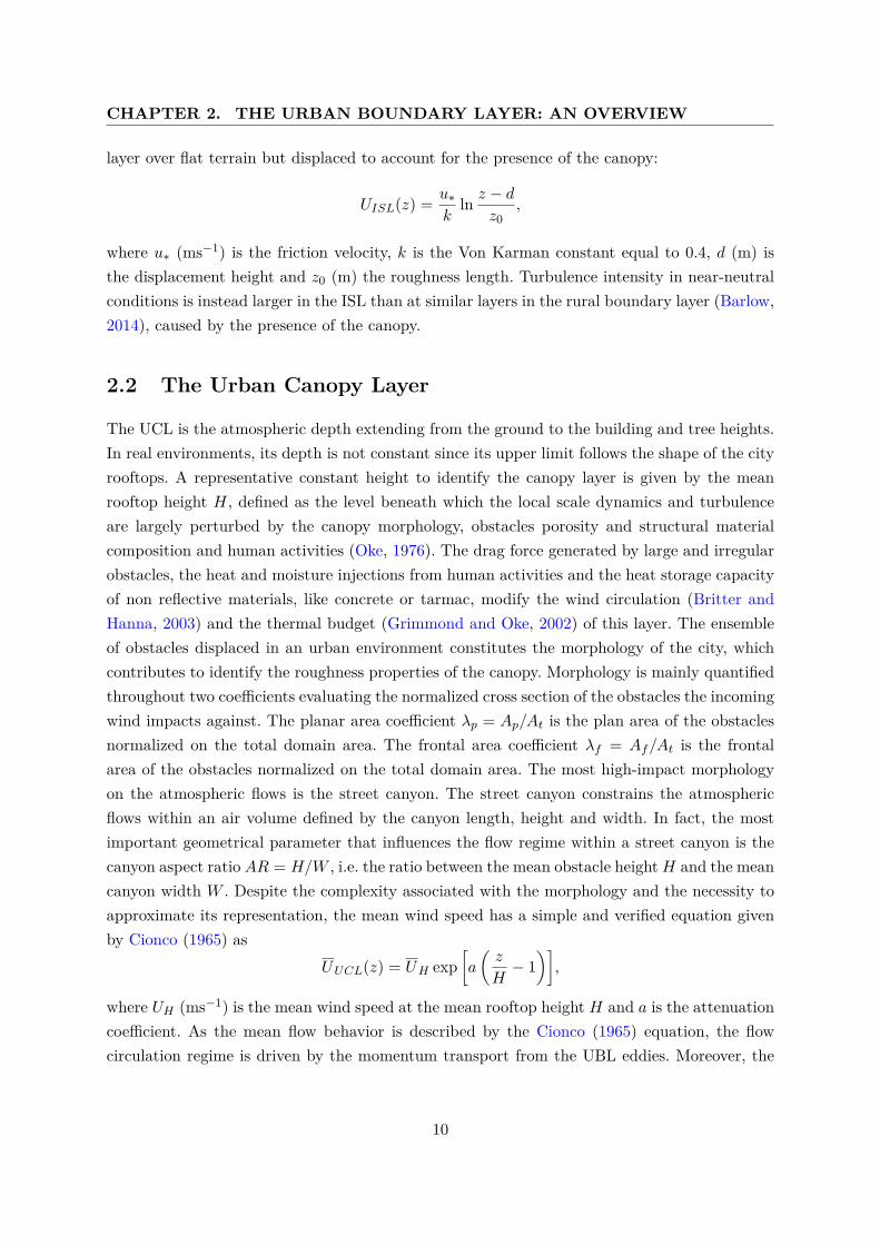
During periods of weak synoptic forcing, i.e. when the geostrophic winds are smaller than 5ms−1, the local scale turbulence and gradients become the main driver of the atmospheric cir-culation and recirculation flows inside the canopy (Britter and Hanna, 2003). Depending onthe intensity of the city scale flows, background flows from now on, characteristics of the UBL,the circulation within the canopy can be inertially driven by the mean flow and the TKMFfrom the background flow or thermally driven by the horizontal temperature gradient withinopposite facades of the in-canyon buildings. The Inertial Circulation (IC) is driven by the meanflow and/or the TKMF entrainment in the canopy from the background flow, as shown in thesketch of Fig. 2.3. Momentum is transferred from the mean flow over-passing the buildings to
Figure 2.3: Idealized 2D sketches of the in-canyon flow regimes from Oke (1987) classification.H and W are the building height and width. (Source: Oke et al. (2017))
the in-canyon flow and generate one or more structures whose shapes and numbers depend onthe canyon aspect ratio H/W (Britter and Hanna, 2003). Depending on the in-canyon structure,and therefore on the aspect ratio of the canopy, the flow can follow a different circulation regimeas classified by Oke (1987). Sketches of the flow regimes in 2D idealized canopies are shown in
11
CHAPTER 2. THE URBAN BOUNDARY LAYER: AN OVERVIEW
Fig. 2.3. As mentioned, the identification of the flow regime is aspect ratio dependent. Whenthe buildings are well apart (0.05 < H/W < 0.4) their impact on the flow field is equal to thatimposed by an isolated building. The flow creates two recirculation zones at the windward andleeward walls of each building (Fig. 2.3a). This flow regime is identified as isolated roughnessflow (Oke, 1988). A more complete definition of the isolated roughness regime was also given byHosker (1987) and adopted by Fernando et al. (2010) and Zajic et al. (2011) among others, iden-tifying this regime anytime the sum of the horizontal length of the flow recirculation volumes infront and rear of the impacted building is smaller than the mean width W of the canopy. WhenW becomes smaller than the sum of the horizontal length of the flow recirculation volumes infront and rear of the impacted building, the wake of the first building interferes with that of thesecond (Zajic et al., 2011), and the flow regimes take the name of wake interference flow (Fig.2.3b). This regime is characterized by secondary flows in the canopy space where the downwardflow of the eddy within the cavity is reinforced by the downward deflection at the windward sideof the canopy (Oke, 1988). Commonly, the wake interference flow regime involves a small rangeof aspect ratios (0.4 < H/W < 0.7), upper-bounded by an UBL-to-UCL mean flow decoupledregime. In fact, at smaller building separation (H/W > 0.7), the flow skims over the canopyand generates stable vortices within it, which number depends on the aspect ratio (Fernandoet al., 2010). This flow regime is named skimming flow (Fig. 2.3c) and it is typical of densecanopies, where the bulk of the flow does not penetrate within them (Oke, 1988). The idealized
Figure 2.4: Idealized 2D sketches of the in-canyon flow regimes in irregular street canyonsoriginally from Xiaomin et al. (2006). h1 and h2 are the leeward and windward building heightrespectively, and g is the canyon width. (Source: Zajic et al. (2011))
12
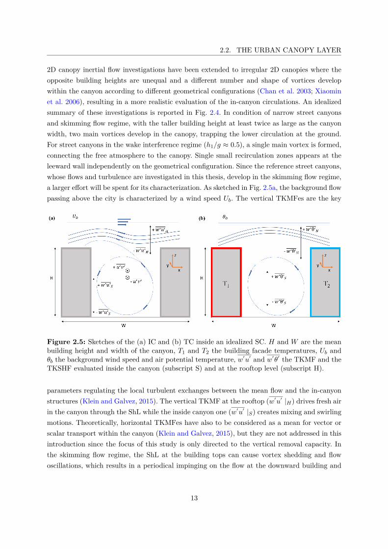
2.2. THE URBAN CANOPY LAYER
2D canopy inertial flow investigations have been extended to irregular 2D canopies where theopposite building heights are unequal and a different number and shape of vortices developwithin the canyon according to different geometrical configurations (Chan et al. 2003; Xiaominet al. 2006), resulting in a more realistic evaluation of the in-canyon circulations. An idealizedsummary of these investigations is reported in Fig. 2.4. In condition of narrow street canyonsand skimming flow regime, with the taller building height at least twice as large as the canyonwidth, two main vortices develop in the canopy, trapping the lower circulation at the ground.For street canyons in the wake interference regime (h1/g ≈ 0.5), a single main vortex is formed,connecting the free atmosphere to the canopy. Single small recirculation zones appears at theleeward wall independently on the geometrical configuration. Since the reference street canyons,whose flows and turbulence are investigated in this thesis, develop in the skimming flow regime,a larger effort will be spent for its characterization. As sketched in Fig. 2.5a, the background flowpassing above the city is characterized by a wind speed Ub. The vertical TKMFes are the key
Figure 2.5: Sketches of the (a) IC and (b) TC inside an idealized SC. H and W are the meanbuilding height and width of the canyon, T1 and T2 the building facade temperatures, Ub andθb the background wind speed and air potential temperature, w′u′ and w′θ′ the TKMF and theTKSHF evaluated inside the canyon (subscript S) and at the rooftop level (subscript H).
parameters regulating the local turbulent exchanges between the mean flow and the in-canyonstructures (Klein and Galvez, 2015). The vertical TKMF at the rooftop (w′u′ |H) drives fresh airin the canyon through the ShL while the inside canyon one (w′u′ |S) creates mixing and swirlingmotions. Theoretically, horizontal TKMFes have also to be considered as a mean for vector orscalar transport within the canyon (Klein and Galvez, 2015), but they are not addressed in thisintroduction since the focus of this study is only directed to the vertical removal capacity. Inthe skimming flow regime, the ShL at the building tops can cause vortex shedding and flowoscillations, which results in a periodical impinging on the flow at the downward building and
13
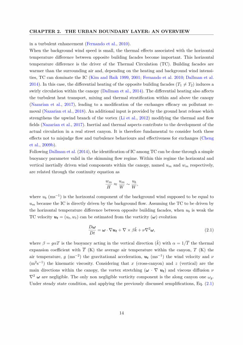
CHAPTER 2. THE URBAN BOUNDARY LAYER: AN OVERVIEW
in a turbulent enhancement (Fernando et al., 2010).When the background wind speed is small, the thermal effects associated with the horizontaltemperature difference between opposite building facades become important. This horizontaltemperature difference is the driver of the Thermal Circulation (TC). Building facades arewarmer than the surrounding air and, depending on the heating and background wind intensi-ties, TC can dominate the IC (Kim and Baik 1999, 2001; Fernando et al. 2010; Dallman et al.2014). In this case, the differential heating of the opposite building facades (T1 6= T2) induces aswirly circulation within the canopy (Dallman et al., 2014). The differential heating also affectsthe turbulent heat transport, mixing and thermal stratification within and above the canopy(Nazarian et al., 2017), leading to a modification of the exchanges efficacy on pollutant re-moval (Nazarian et al., 2018). An additional input is provided by the ground heat release whichstrengthens the upwind branch of the vortex (Li et al., 2012) modifying the thermal and flowfields (Nazarian et al., 2017). Inertial and thermal aspects contribute to the development of theactual circulation in a real street canyon. It is therefore fundamental to consider both theseeffects not to misjudge flow and turbulence behaviours and effectiveness for exchanges (Chenget al., 2009b).Following Dallman et al. (2014), the identification of IC among TC can be done through a simplebuoyancy parameter valid in the skimming flow regime. Within this regime the horizontal andvertical inertially driven wind components within the canopy, named um and wm respectively,are related through the continuity equation as
wmH≈ umW∼ ubW,
where ub (ms−1) is the horizontal component of the background wind supposed to be equal toum because the IC is directly driven by the background flow. Assuming the TC to be driven bythe horizontal temperature difference between opposite building facades, when ub is weak theTC velocity ut = (ut, wt) can be estimated from the vorticity (ω) evolution
Dω
Dt= ω · ∇ut +∇× βk + ν∇2ω, (2.1)
where β = gαT is the buoyancy acting in the vertical direction (k) with α = 1/T the thermalexpansion coefficient with T (K) the average air temperature within the canyon, T (K) theair temperature, g (ms−2) the gravitational acceleration, ut (ms−1) the wind velocity and ν
(m2s−1) the kinematic viscosity. Considering that x (cross-canyon) and z (vertical) are themain directions within the canopy, the vortex stretching (ω · ∇ ut) and viscous diffusion ν
∇2 ω are negligible. The only non negligible vorticity component is the along canyon one ωy.Under steady state condition, and applying the previously discussed semplifications, Eq. (2.1)
14
2.3. EXCHANGE PROCESSES AND CITY BREATHABILITY
becomesut · ∇ωy ∼ −gα
∂T
∂x. (2.2)
Using once again the dimensional analysis on the vorticity component on the left hand side ofEq. (2.2) the following approximation is retrieved
ωy = ∂u
∂z− ∂w
∂x∼[utH
+ wtW
]∼[utH
+ ut
H (H/W )2
]∼(utH
)[1 +
(H
W
)2], (2.3)
where ut/W ≈ wt/H as for the IC case. Substituting Eq. (2.3) into (2.2), the vorticity equationbecomes
utW
utH
[1 +
(H
W
)2]∼ gα∆T
W, (2.4)
where ∆T = T1−T2 is the horizontal temperature difference between opposite building facades.From Eq. (2.4), the velocity scale for the TC becomes
ut ∼
gα∆TH[1 +
(HW
)2]
1/2
. (2.5)
When both IC and TC divers are present, the first dominates the second if ub � ut. To evaluatethis condition, the buoyancy parameter B is defined from Eq. (2.5) as
B =
gα∆TH
u2b
[1 +
(HW
)2]
1/2
� Bc, (2.6)
where Bc is the critical value of the buoyancy parameter discerning the inertial (B < Bc)from the thermal (B > Bc) circulations. From this parameter the identification of the canopycirculation is performed to characterize the flow and assess the dominant processes correlated tothem. In the next section, the characteristics of the exchange processes developing in conditionsof IC and TC are introduced.
2.3 Exchange Processes and City Breathability
The term exchange processis used in boundary-layer meteorology to identify all the atmosphericphenomena involving the outward and inward exchange of both vector and scalar quantitiesbetween the UCL and the UBL above through the rooftop interface. The understanding andgood representation of these processes is fundamental to correctly predict flow and turbulentfields within the RSL. Milestones in the understanding of the exchange processes have been
15
CHAPTER 2. THE URBAN BOUNDARY LAYER: AN OVERVIEW
given by Barlow and Belcher (2002), Bentham and Britter (2003) and Harman et al. (2004))at the beginning of the 21st century, revealing the intricacy of momentum and heat exchangesthrough the canopy interface. In the same period, several studies have focused on the nature ofthe exchange processes, by means of field, laboratory and numerical investigations. Key findingsconcluded that exchange processes are driven and scale with the vertical TKMF at the canopyinterface (Louka et al. 1998; Barlow et al. 2004; Solazzo and Britter 2007), especially in presenceof a ShL dynamics. The efficacy of the exchange processes increases with the intensity of thebackground wind in the ISL (Barlow and Belcher 2002; Harman et al. 2004), the turbulentmomentum (Kim and Baik, 2003) and turbulent kinetic heat (Salizzoni et al., 2011) transportsfrom the ShL to the street canyon. The efficacy also varies according to local morphologycharacteristics such as the street canyon aspect ratio (Barlow and Belcher, 2002) and the roofgeometry (Kastner-Klein et al., 2004).In more recent years, the exchange processes focus has shifted from the fundamental natureinvestigation to their implication on more practical problems such as air quality and pollutantdispersion or removal from the urban canopy. The application of the exchange processes to thepollutant removal from an urban canopy takes the terminology of City Breathability (CB), asadopted by several authors (Buccolieri et al. 2010; Panagiotou et al. 2013; Chen et al. 2017),which incorporates any scalar (e.g. heat, moisture, pollutant concentration) ejection from groundlevel, transport throughout a canopy interface or turnover time scales. The CB concept hasbeen applied to different spatial scales of the urban environment, ranging from street canyon(Cheng et al. 2009a; Liu and Wong 2014; Di Bernardino et al. 2018) to neighbourhood (Soulhacand Salizzoni 2010; Buccolieri et al. 2015) and city (Hang et al. 2012) scales, corroborated bylaboratory and numerical investigations. Despite several field experimental campaigns have beenrealized in the last two decades (Louka et al. 2000; Rotach et al. 2005; Eliasson et al. 2006;Kanda and Moriwaki 2006; Nelson et al. 2011; Zajic et al. 2011; Dallman et al. 2013), CB hasbeen poorly investigated in real environments due to the complex interactions between differentatmospheric phenomena and the irregular morphology of the real cities.Following Lo and Ngan (2017), CB is assessed by two categories of diagnostic parameters. Thefirst category is based on the evaluation of turbulent mass exchange between the canopy andthe overlying atmosphere, typically quantified by exchange velocities or exchange rates. Thesecond category is based on the evaluation of diagnostic time scales associated with pollutantremoval or in-canyon circulations. Diagnostic time scales enable the characterization of CB fordifferent background conditions (e.g. change in mean wind direction), aspect ratios, canyonorientation and exposure to solar radiation, domain size and morphology, pollutant emissionsand turbulence regimes. The investigations conducted in the current study focus on the secondcategory, but it is worth mentioning at least two examples of exchange velocity and rate tobetter qualify the research effort in the field of the CB. The first is the exchange velocity that
16
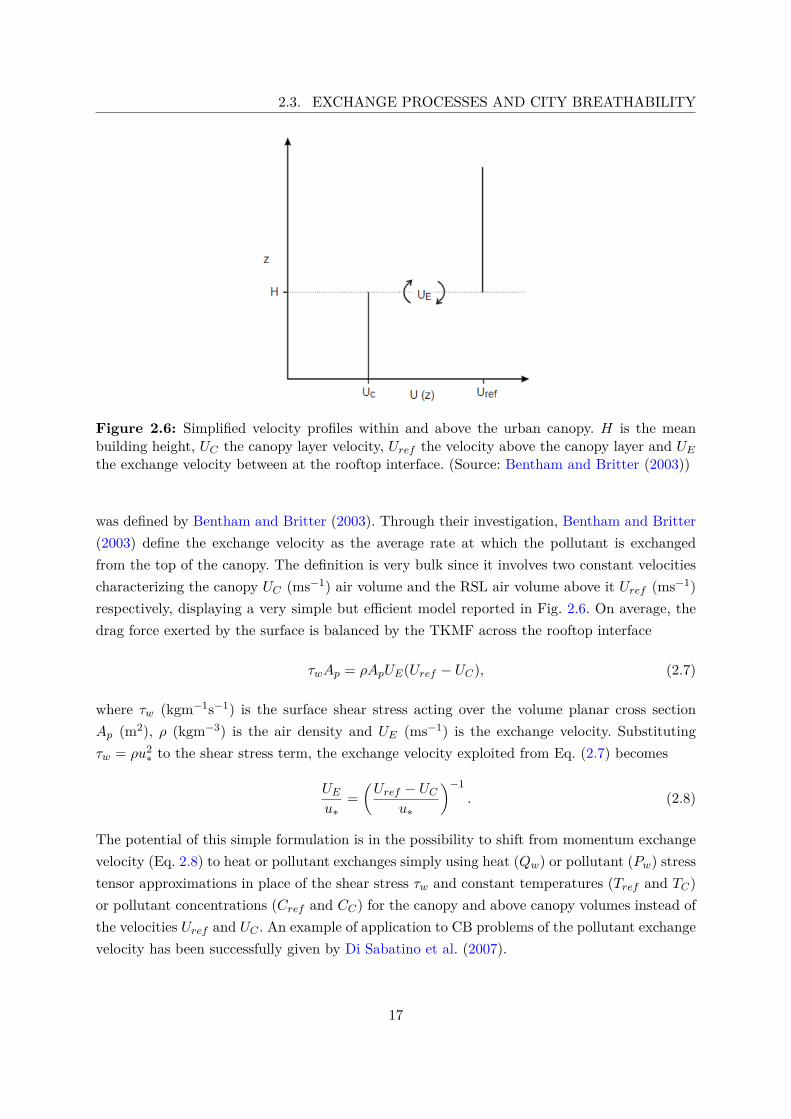
2.3. EXCHANGE PROCESSES AND CITY BREATHABILITY
Figure 2.6: Simplified velocity profiles within and above the urban canopy. H is the meanbuilding height, UC the canopy layer velocity, Uref the velocity above the canopy layer and UEthe exchange velocity between at the rooftop interface. (Source: Bentham and Britter (2003))
was defined by Bentham and Britter (2003). Through their investigation, Bentham and Britter(2003) define the exchange velocity as the average rate at which the pollutant is exchangedfrom the top of the canopy. The definition is very bulk since it involves two constant velocitiescharacterizing the canopy UC (ms−1) air volume and the RSL air volume above it Uref (ms−1)respectively, displaying a very simple but efficient model reported in Fig. 2.6. On average, thedrag force exerted by the surface is balanced by the TKMF across the rooftop interface
τwAp = ρApUE(Uref − UC), (2.7)
where τw (kgm−1s−1) is the surface shear stress acting over the volume planar cross sectionAp (m2), ρ (kgm−3) is the air density and UE (ms−1) is the exchange velocity. Substitutingτw = ρu2
∗ to the shear stress term, the exchange velocity exploited from Eq. (2.7) becomes
UEu∗
=(Uref − UC
u∗
)−1. (2.8)
The potential of this simple formulation is in the possibility to shift from momentum exchangevelocity (Eq. 2.8) to heat or pollutant exchanges simply using heat (Qw) or pollutant (Pw) stresstensor approximations in place of the shear stress τw and constant temperatures (Tref and TC)or pollutant concentrations (Cref and CC) for the canopy and above canopy volumes instead ofthe velocities Uref and UC . An example of application to CB problems of the pollutant exchangevelocity has been successfully given by Di Sabatino et al. (2007).
17
CHAPTER 2. THE URBAN BOUNDARY LAYER: AN OVERVIEW
A comprehensive definition for the exchange rate is given by (Liu et al., 2005). Exchange rate wasclassified in air and pollutant exchange rates to respectively account for the vertical velocity andpollutant concentration transport fluctuations through the rooftop level interface of the UCL.Again, the formulations are simple but they enclose the essence of the canopy to free atmosphereinteraction. The air exchange rate (ACH) is defined as the integral over planar cross section ofthe canopy volume Ap (m2) of the vertical wind velocity fluctuations at the rooftop interfacew′(t) |interface (ms−1):
ACH(t) =∫Apw′(t) |interface dAp.
The sign of the air exchange rate is directly given by the vertical velocity fluctuations, so thata positive ACH value describes air removal from the canopy while a negative one identifies anentrainment.Similarly, the pollutant exchange rate PCH describes the pollutant concentration transportw′(t) |interface C(t) |interface (µgm−3 ms−1) through the rooftop interface
PCH(t) =∫Apw′(t) |interface C(t) |interface dAp.
The sign of the pollutant exchange rate follows the behavior of the air exchange rate with posi-tive PCH values describing pollutant removal from the canopy while negative ones identifyingan entrainment. Simple as they are, they can easily be used to describe a time dependent re-freshment or stagnation of the air in the UCL.The second category of Lo and Ngan (2017) describes the diagnostic parameters by which theexchange processes can be characterized. Particularly used from this ensemble, the diagnostictime scales enable the characterization of CB for different background conditions (e.g. change inmean wind direction), aspect ratios, canyon orientation and exposure to solar radiation, domainsize and morphology, pollutant emissions and turbulence regimes. In the recent past, differenttime scales have been derived using Computational Fluid Dynamics (CFD) models and windtunnel experiments. Below, a brief summary of the most used and work-inspiring time scalesis presented. A retention time τa |V is defined by Liu et al. (2005) as the average pollutantconcentration C |V (µgm−3) within the canyon mean volume V = W · H · L (m3) and thepollutant emission rate Qe |V (µgm−3s−1) of the source
τa |V = C |VQe |V
.
The pollutant retention time expresses the time a certain pollutant remains in the canopybefore from its emission. The retention time is found to be dependent on the aspect ratioH/W , with a time scale increase as the aspect ratio increases. As the aspect ratio increases,the pollutant transport from the ground sources to the canopy top becomes more and more
18
2.3. EXCHANGE PROCESSES AND CITY BREATHABILITY
inefficient, since multiple independent vortices can form within the canopy. In this last scenario,the retention time scale is enhanced by this transport inefficiency. Similar to the retention timeis the mean age of the air defined by Hang et al. (2009). The definition follows exactly theretention time of Liu et al. (2005), expressing the ratio between the pollutant concentrationand the emission rate of its source. Again the lower the local mean age of air is, the moreefficiently the local exchange processes remove the pollutant concentrations from the canopy.Being of simple practical use especially in laboratory and numerical investigations, the meanage of air (or retention time, since they are equally defined) has been used for several analysisto characterize different aspects of the removal processes in different conditions. In fact, thecity shape, the configuration of streets and the approaching wind conditions are all aspectsthat influence the age of air and the air exchange efficiency of the urban canopies. Hang et al.(2012) first confirms the direct proportionality between the time scale and the single streetcanyon aspect ratio found by Liu et al. (2005), extending the analysis to the neighborhoodand city scales with contrasting results. At the city scale, the dependency of the age of theair on the street canyon aspect ratio is again found to by directly proportional, while at theneighborhood scale the proportionality was inverse. This inverse behavior of the time scale atthe neighborhood scale is confirmed by Hang et al. (2013) who suggested the dependency onthe planar area fraction coefficient (not retrieved at the city scale) to be the cause. Hang et al.(2013) also investigates the variation of the age of the air with the background wind direction,founding an improvement of the CB with an increasing background wind direction in the range0◦-45◦ to the canyon orientation.The average residence time τ r was introduced by Bady et al. (2008) and used by Kato andHuang (2009) to assess the ventilation performance of the street canyon exchange processes byrepresenting the time of permanence of pollutants in the canopy volume. It is defined as theratio between the canopy volume V (m3) and the product between the purging flow rate Pr(m3s−1) and the adimensional visitation frequency fV
τ r = V
PrfV
The purging flow rate represents the effective airflow rate required to remove or purge the airpollutants from the volume and it is computed as Pr = Qe/
(1000Cρ
), where Qe (gs−1) is the
pollutant source rate, Cq (kgkg−1) is the volume averaged canopy concentration and ρ (kgm−3)is the air density. The visitation frequency describes the history of a pollutant particle in thecanopy volume by establishing the number of times the particle enters and exits the canopyvolume. It is defined as fV = 1 + ∆Qe/Qe, where ∆Qe (kgs−1) is the inflow flux of pollutantsinto the canopy volume. Therefore, the average residence time describes the time a pollutantparticle takes between its entrance in and exit from the canopy volume, and therefore it is anindication of the pollutant dilution capability of the volume itself operated by the atmospheric
19
CHAPTER 2. THE URBAN BOUNDARY LAYER: AN OVERVIEW
exchange processes. The average residence time was found by both Bady et al. (2008) and Katoand Huang (2009) to increase as the street canyon aspect ratio increases, as it was for theretention time and age of the air.Salizzoni et al. (2009) define an exchange time scale τe to account for the pollutant masstransport through the rooftop interface in dependency on the mean building height H (m)of the canopy. It is defined as the ratio between the square value of the mean building height,the averaged pollutant concentration within the canopy C (µgm−3) and the inflow mass ratefrom the canopy rooftop Mq (µgm−1s−1)
τe = H2C
Mq.
The exchange time scale describes the wash-out of pollutants from the canopy. From Salizzoniet al. (2009) investigations, it is found to increase as the aspect ratio of the single street canyonincreases, confirming the previously introduced time scales.More recently, time scales related to the exchange processes have been addressed by Lagrangianmodels, directly describing the trajectories of single fluid particles from the source to the sink orremoval. An example of time scales derived from Lagrangian model investigations is presentedby Lo and Ngan (2017). Two Lagrangian time scales, namely the residence τLr and exposure τLetimes, have been evaluated to establish the time required for a pollutant particle to exit thecanopy and the time spent by a pollutant particle in a region of interest respectively. Withinthe canopy cavity volume V (m3), the residence time is defined as
DτLrDt|V = 1,
with τLr (0) = 0 at the open frontier ∂V of the volume, i.e. the rooftop interface in the case of asingle street canyon. The exposure time scale is defined in a volume of interest Ve ∈ V (m3) as
DτLeDt|Ve=
1 if x 6∈ Ve0 if x ∈ Ve,
with τLe (0) = 0 at the open frontier ∂Ve of the volume, and where x is the position vector.It accounts for the overall time a particle stays within the volume Ve, summing all multipleenter/exit situations. Both the Lagrangian time scales have been found to be in agreement withthe in-canyon recirculation time in the case of pure diffusion.All the previously mentioned time scales relate directly to pollutant concentrations, emissionsand mass transport through the canyon interface, giving the purpose of this work to find new di-agnostic quantities to characterize the fundamental nature of the momentum and heat exchange
20
2.4. VEGETATION IN THE URBAN ENVIRONMENT
processes associated with the in-canyon IC and TC.
2.4 Vegetation in the Urban Environment
Investigations on CB of urban environment have rapidly developed an interest in the impact ofvegetation on the flow and turbulent fields. Within the last two decades, different approacheshave been tried to tackle the problem, mostly involving laboratory and (especially) numeri-cal investigations. Common results have led to the conclusion that the vegetation in urbanenvironment exerts a drag force that reduces the flow field intensity by causing a net loss ofmomentum, with a consequent modification of both production (transfer from the mean flow)and destruction (the eddy fragmentation can enhance the dissipation) of the turbulent field.As a consequence of the flow and turbulent field modifications, scalar transport and removalare affected, with primary implications on the air quality and thermal comfort of the urbanenvironment. Other impacts generated by vegetation concern the enhancement of the particledeposition on the vegetation leaves, the transpiration and evaporation processes, and the shad-owing effect. In this section, a brief description of the role of vegetation on the fluid dynamics,thermodynamics and air quality investigations is given, focusing only on the most widely usedvegetation type in urban environment, the tree. Only the vegetation embedded in street canyonenvironments will be considered, excluding designated green areas such as parks.A vastly used way to consider trees in fluid dynamics investigations establishes to decomposethe tree in two parts. A solid trunk, defined as a long and thin cylinder of non reflective material,on top of which the tree crown is simulated as a solid geometry (generally a cube or a sphere)of porous medium (Gromke and Ruck 2008; Gromke and Ruck 2009). This configuration allowsto capture both the flow channeling beneath the crown and the flow intensity reduction causedby the crown porosity, resulting in an overall wind speed modification due to the exerted dragforce the tree. The drag force Fdrag (N) employed by the tree crown is simply evaluated as thefriction force exerted by a medium against the motion of the fluid:
Fdrag = 12Cvρu
2xA
vf ,
where ρ (kgm−3) is the air density, ux (ms−1) is the flow velocity component directed towardthe tree, Cv is the vegetation drag coefficient and Avf (m2) is the vegetated frontal area. Thevegetation drag coefficient is an indication of the aerodynamic drag exerted by the crown onthe flow. Commonly it is considered as a property of the tree species and the season, and it isgiven as an averaged value representative of the full crown (Di Sabatino et al. 2015; Jeanjeanet al. 2017). A more sophisticated and computational costly evaluation of the vegetation dragcoefficient has been proposed by Chester et al. (2007), which trees are represented as a fractalgeometry of increasing order with the increasing branching. A drag coefficient is evaluated for
21
CHAPTER 2. THE URBAN BOUNDARY LAYER: AN OVERVIEW
each ramification order m with branching resolving simulations as
Cnv (m) = −2∑m
r=1
(F n,rdrag(Cn−1
v · V n,r | V n,r | Avf ))
∑mr=1 ρ | V n,r |4
(Avf
)2
where V (ms−1) is the spatially averaged wind velocity vector, r is the ramification level andn is the iteration index. The first iteration of Cv is an a priori guess. Despite the mathematicalaccuracy and detailed precision in the evaluation of this drag coefficient, its value seems to besimilar to those reported in look-up tables relative to the single tree species. Therefore, it isbarely used due to the large computational costs and the very detailed simulation grid required.As a consequence of the drag force application, the tree exerts a pressure modification on theenvironment consisting in a reduction of the pressure itself when the air flow passes through theporous crown. This pressure drop is generally computed as a coefficient λ (m−1), normalizingthe static pressure difference ∆pstat (hPa) between the static pressure retrieved at the windwardpwind and leeward plee sides of the crown with the drag pressure pdrag = Fdrag/A
vf (hPa) of the
porous medium of extent X (m) (Buccolieri et al., 2011):
λ = ∆pstatpdragX
= pwind − plee0.5ρu2
xX(2.9)
This pressure loss coefficient is a useful piece of information that gives the aerodynamic charac-teristics of the tree crown, but it is not always simple to compute since it involve measurementsof pressure all around the tree to account for all the possible wind directions. An alternativeand commonly adopted way (by Van Renterghem and Botteldooren 2008 for instance) is tocompute the pressure drop in dependency of a pressure resistance coefficient kr as
∆pstat = 12krρu
2x. (2.10)
The pressure resistance coefficient is simply the aerodynamic drag of the tree crown weightedon the leaf area density LAD (m2m−3), the total area of the leafs per unit volume of the canopy,and it can be evaluated following Wilson (1985) as
kr =∫ X
0CvLADdx, (2.11)
Substituting Eq. (2.11) into (2.10) and back into Eq. (2.9), the pressure loss coefficient simplybecomes
λ = CvLAD. (2.12)
This method of estimating the impact of the trees on the mean flow was largely used in recentnumerical and laboratory investigations (Gromke et al. 2008; Van Renterghem and Botteldooren
22
2.4. VEGETATION IN THE URBAN ENVIRONMENT
2008; Buccolieri et al. 2011; Jeanjean et al. 2017). Due to its simplicity, Eq. (2.12) can be adoptedalso as a bulk estimation of the tree effect in field experiment. As largely discussed in the reviewof Buccolieri et al. (2019), the other very common parametrization of the tree largely used innumerical simulation employs the evaluation of a mean momentum sink Sui (hPam−1) to beadded for each velocity component of the momentum equation as
Sui = −ρLADCv | u | ui, (2.13)
where the subscript i identifies the three Cartesian directions and ui is the i-th wind veloc-ity component. The negative sign enables Sui to be interpreted as a momentum sink in theNavier-Stokes equations, where the larger the foliage density and wind speed are, the larger themomentum sink will be. This approach based on the momentum sink in Eq. 2.13 is equivalent tothe pressure loss coefficient method in Eq. (2.12), but it is preferred by several authors (Katulet al. 2004; Gromke et al. 2008, 2015; Buccolieri et al. 2009, 2018; Rafael et al. 2018; Li andWang 2018 among others) because it is generally followed by a computation of the turbulentfield modification. In fact, the vegetation subtracts momentum and energy from the mean flowinto wake turbulence. At the same time, the smaller length scales of turbulence generated by theshear induced by the vegetation are rapidly dissipation (Buccolieri et al., 2019). These processesare usually parameterized as source and sink terms of Turbulence Kinetic Energy (TKE), asits value Tke gives the source-sink term STke (kgm−1s−3), and turbulent dissipation rate ε (Sε,kgm−1s−4) as
Stke = ρLADCv(βp | u |3 −βd | u | Tke
)Sε = ρLADCv
(Cε,4βp
ε
Tke| u |3 −Cε,5βd | u | ε
),
where βp is the fraction of mean kinetic energy converted into Tke by means of the drag force andhas a value in the range 0-1, βd is the short-circuiting coefficient of the turbulent cascade and Cε,iare model constants, with the second controlling the destruction of dissipation induced by thefoliage (Buccolieri et al., 2019). Although it is certain that the mean flow momentum is consumedby the vegetation, the impact of turbulence is more uncertain due to the source/sink balanceoperated by the Tke production and dissipation. This ambivalent behavior of the turbulent fieldis also at the basis of the recent investigation on the advantage/disadvantage balance the treecan induce on the CB.Despite the aerodynamic effects of vegetation on the mean flow and turbulent fields correspondto the major impact generated by trees in urban canopies (Buccolieri et al., 2019), particledeposition and resuspension, thermal and shadowing effects must be taken into account too.The deposition and resuspension effects are important, since they are the second factor ofpollutant removal after the aerodynamic effects related to the exchange processes. Deposition
23
CHAPTER 2. THE URBAN BOUNDARY LAYER: AN OVERVIEW
is active as a sink Sd (kgm−3s−1) of atmospheric pollutant concentrations C(x, y, z) (kgm−3)caused by the particle capture of the tree leaves (Vos et al. 2013; Jeanjean et al. 2017; Buccolieriet al. 2018):
Sd = −LADudC(x, y, z),
where ud (ms−1) is the deposition velocity associated with the investigated pollutant type.Resuspension is instead a source of pollution, especially for the particulate matters (Nowaket al., 2013) and provides an increase of the pollutant concentrations in the urban environmentby detaching particles from the tree leaves. The most recent parametrization for the resuspensioneffect is given by Hong et al. (2018), and it provides a source of particulate concentrations as
Sr = LADurCsinked(x, y, z),
where ur (ms−1) is the resuspension velocity from the tree foliage associated with the investi-gated pollutant particulate type and Csinked(x, y, z) (kgm−3) is the particulate matter concen-tration deposited on the plant foliage, i.e. the available particle concentration for resuspension.Thermal and shadowing effects are also important for the regulation of the air temperature andthe thermal comfort of the UCL but they have been poorly investigated so far. This categoryaccounts for two factors: the shadowing effect of the tree crown, that reduces the amount of solarradiation reaching the buildings and the street surfaces, and the thermal cooling provided bytree foliage evapotranspiration. The overall effect is a temperature variation δT (K) caused bythe sensible heat variation rate H (W) induced by a mass flow rate m (kgs−1) passing throughthe vegetated crown (Gromke et al. 2015; Moradpour et al. 2017) as
δT = H
mcp,
where cp (JK−1kg−1) is the specific heat capacity at constant pressure. Notably on the shad-owing effects of the trees, infrared imaging is a useful measurement technique to evaluate theemission temperature reduction of solid obstacles covered by trees as it allows to retrieve theobstacles infrared brightness temperatures. This technique is used during field campaigns (forexample Di Sabatino et al. 2015) where a spatial computation of the thermal cooling is difficultto obtain.All these effects define vegetation from its interaction with the urban canopy atmosphere, ac-counting for the different modification vegetation can introduce in the environment.
24
2.5. SUMMARY AND CONCLUSIONS
2.5 Summary and Conclusions
A brief literature review has been given to contestualize the argument of this thesis. First, aclassical description of the UBL is presented, focusing on the lower atmospheric layers directlyinvolved in the investigation, which are the UCL and the ShL. The focus then shifted on present-ing the most meaningful and recent works characterizing the exchange processes within the UCLand with the atmosphere above. The fundamental aspects describing the role of the exchangeporcesses in regulating momentum and energy transport in street canyons have provided a base-line for the current work computations. In particular the importance of TKMF and TKSHF asdriver and regulative factors of the transport through the RL interface becomes a key factor inthe current investigation, where these behaviors will be extended to assess the in-canyon mixingefficacy. The geometrical and background flow constraints have also been considered to be offundamental importance for the current work, as mitigating factors of the excahnge processesintensityFollowing investigations in the field of CB, the different time scales reported in literature hasprovided useful information on the pollutant removal time from the UCL. A considerable num-ber of different time scales have been presented to show the spectra of possible investigationapproaches to the same problem. All the reported time scales have in common their use of pol-lutant eimssion source rates, removal or entrainment velocities. On the contrary, this thesis willfocus on computing the time scales for the momentum and heat exchanges between differentatmospheric layers, using only the fundamental aspects of the exchange processes to describethe transport and mixing characteristics of the SL, in dependency on the observed in-canyoncirculation. Subsequently, the time scales will be used to evaluate the impact of the exchangeprocesses on pollutant removal.Finally, this literature review described the most recent update concerning vegetation simula-tion using CFD models, introducing the second part of the current work tackling the impact oftrees on the mean flow and turbulence in UCL. Evaluation of the vegetation impact is foundto assess different aspects of the atmospheric flow in the UBL. Most of the CFD simulationsfocused on the attenuation of the mean flow velocity exerted by the vegetation, but several otherimpacts have been tackled. In particular, vegetation is founded to play the dual role of sourceand sink for turbulence, as the mechanical Tke production is balanced by turbulent dissipation.A dual role is also associated with deposition and resuspention of the particulate matter. Atlast, the shadowing effet of the tree crowns is associated with a strong modification of the heatcapacity of the ground, causing a modification in the circulation intensity.Given this overview of the fundamental studies and recent improvements, the aim of this workis to present new and alternative formulations or investigations of both exchange processes andvegetation impact in a real urban environment by means of simple quantities and operativemodel.
25

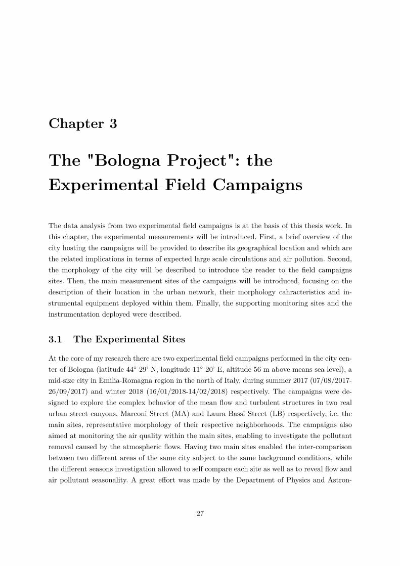
Chapter 3
The "Bologna Project": theExperimental Field Campaigns
The data analysis from two experimental field campaigns is at the basis of this thesis work. Inthis chapter, the experimental measurements will be introduced. First, a brief overview of thecity hosting the campaigns will be provided to describe its geographical location and which arethe related implications in terms of expected large scale circulations and air pollution. Second,the morphology of the city will be described to introduce the reader to the field campaignssites. Then, the main measurement sites of the campaigns will be introduced, focusing on thedescription of their location in the urban network, their morphology cahracteristics and in-strumental equipment deployed within them. Finally, the supporting monitoring sites and theinstrumentation deployed were described.
3.1 The Experimental Sites
At the core of my research there are two experimental field campaigns performed in the city cen-ter of Bologna (latitude 44◦ 29’ N, longitude 11◦ 20’ E, altitude 56 m above means sea level), amid-size city in Emilia-Romagna region in the north of Italy, during summer 2017 (07/08/2017-26/09/2017) and winter 2018 (16/01/2018-14/02/2018) respectively. The campaigns were de-signed to explore the complex behavior of the mean flow and turbulent structures in two realurban street canyons, Marconi Street (MA) and Laura Bassi Street (LB) respectively, i.e. themain sites, representative morphology of their respective neighborhoods. The campaigns alsoaimed at monitoring the air quality within the main sites, enabling to investigate the pollutantremoval caused by the atmospheric flows. Having two main sites enabled the inter-comparisonbetween two different areas of the same city subject to the same background conditions, whilethe different seasons investigation allowed to self compare each site as well as to reveal flow andair pollutant seasonality. A great effort was made by the Department of Physics and Astron-
27
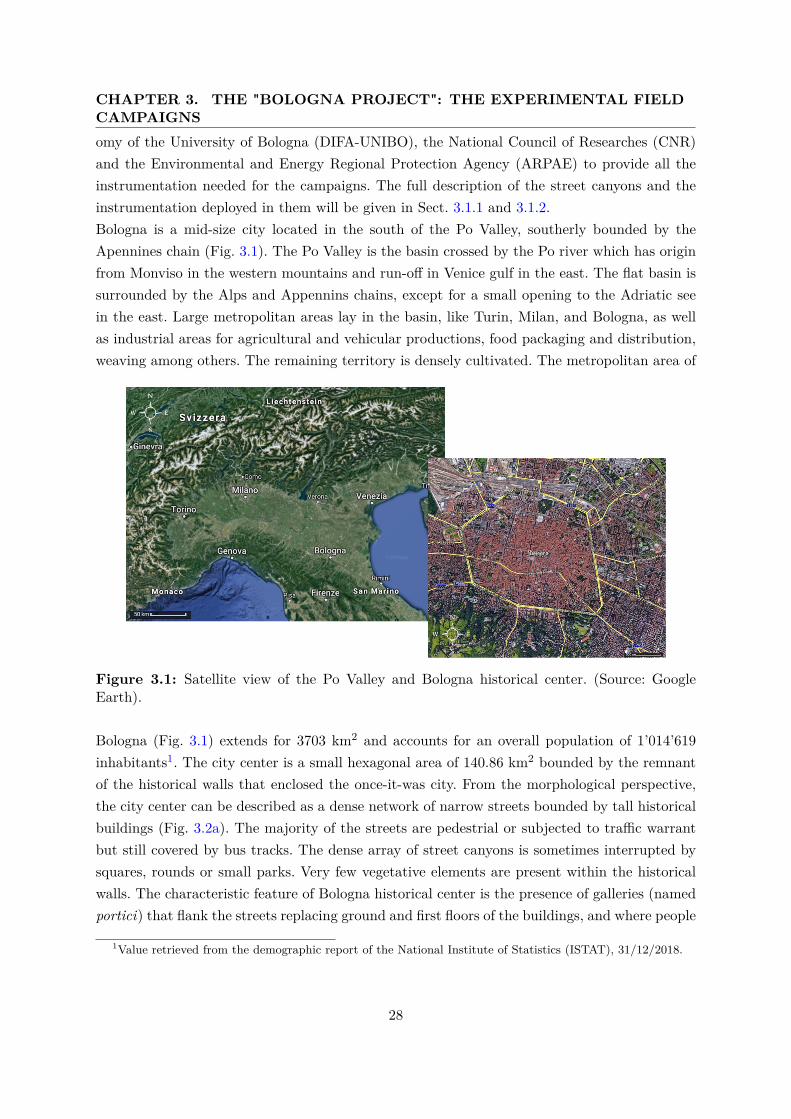
CHAPTER 3. THE "BOLOGNA PROJECT": THE EXPERIMENTAL FIELDCAMPAIGNSomy of the University of Bologna (DIFA-UNIBO), the National Council of Researches (CNR)and the Environmental and Energy Regional Protection Agency (ARPAE) to provide all theinstrumentation needed for the campaigns. The full description of the street canyons and theinstrumentation deployed in them will be given in Sect. 3.1.1 and 3.1.2.Bologna is a mid-size city located in the south of the Po Valley, southerly bounded by theApennines chain (Fig. 3.1). The Po Valley is the basin crossed by the Po river which has originfrom Monviso in the western mountains and run-off in Venice gulf in the east. The flat basin issurrounded by the Alps and Appennins chains, except for a small opening to the Adriatic seein the east. Large metropolitan areas lay in the basin, like Turin, Milan, and Bologna, as wellas industrial areas for agricultural and vehicular productions, food packaging and distribution,weaving among others. The remaining territory is densely cultivated. The metropolitan area of
Figure 3.1: Satellite view of the Po Valley and Bologna historical center. (Source: GoogleEarth).
Bologna (Fig. 3.1) extends for 3703 km2 and accounts for an overall population of 1’014’619inhabitants1. The city center is a small hexagonal area of 140.86 km2 bounded by the remnantof the historical walls that enclosed the once-it-was city. From the morphological perspective,the city center can be described as a dense network of narrow streets bounded by tall historicalbuildings (Fig. 3.2a). The majority of the streets are pedestrial or subjected to traffic warrantbut still covered by bus tracks. The dense array of street canyons is sometimes interrupted bysquares, rounds or small parks. Very few vegetative elements are present within the historicalwalls. The characteristic feature of Bologna historical center is the presence of galleries (namedportici) that flank the streets replacing ground and first floors of the buildings, and where people
1Value retrieved from the demographic report of the National Institute of Statistics (ISTAT), 31/12/2018.
28
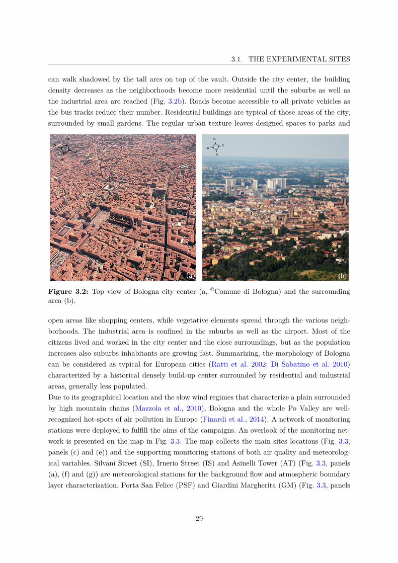
3.1. THE EXPERIMENTAL SITES
can walk shadowed by the tall arcs on top of the vault. Outside the city center, the buildingdensity decreases as the neighborhoods become more residential until the suburbs as well asthe industrial area are reached (Fig. 3.2b). Roads become accessible to all private vehicles asthe bus tracks reduce their number. Residential buildings are typical of those areas of the city,surrounded by small gardens. The regular urban texture leaves designed spaces to parks and
Figure 3.2: Top view of Bologna city center (a, ©Comune di Bologna) and the surroundingarea (b).
open areas like shopping centers, while vegetative elements spread through the various neigh-borhoods. The industrial area is confined in the suburbs as well as the airport. Most of thecitizens lived and worked in the city center and the close surroundings, but as the populationincreases also suburbs inhabitants are growing fast. Summarizing, the morphology of Bolognacan be considered as typical for European cities (Ratti et al. 2002; Di Sabatino et al. 2010)characterized by a historical densely build-up center surrounded by residential and industrialareas, generally less populated.Due to its geographical location and the slow wind regimes that characterize a plain surroundedby high mountain chains (Mazzola et al., 2010), Bologna and the whole Po Valley are well-recognized hot-spots of air pollution in Europe (Finardi et al., 2014). A network of monitoringstations were deployed to fulfill the aims of the campaigns. An overlook of the monitoring net-work is presented on the map in Fig. 3.3. The map collects the main sites locations (Fig. 3.3,panels (c) and (e)) and the supporting monitoring stations of both air quality and meteorolog-ical variables. Silvani Street (SI), Irnerio Street (IS) and Asinelli Tower (AT) (Fig. 3.3, panels(a), (f) and (g)) are meteorological stations for the background flow and atmospheric boundarylayer characterization. Porta San Felice (PSF) and Giardini Margherita (GM) (Fig. 3.3, panels
29
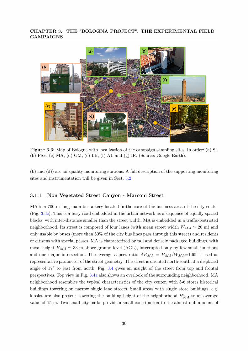
CHAPTER 3. THE "BOLOGNA PROJECT": THE EXPERIMENTAL FIELDCAMPAIGNS
Figure 3.3: Map of Bologna with localization of the campaign sampling sites. In order: (a) SI,(b) PSF, (c) MA, (d) GM, (e) LB, (f) AT and (g) IR. (Source: Google Earth).
(b) and (d)) are air quality monitoring stations. A full description of the supporting monitoringsites and instrumentation will be given in Sect. 3.2.
3.1.1 Non Vegetated Street Canyon - Marconi Street
MA is a 700 m long main bus artery located in the core of the business area of the city center(Fig. 3.3c). This is a busy road embedded in the urban network as a sequence of equally spacedblocks, with inter-distance smaller than the street width. MA is embedded in a traffic-restrictedneighborhood. Its street is composed of four lanes (with mean street width WMA ' 20 m) andonly usable by buses (more than 50% of the city bus lines pass through this street) and residentsor citizens with special passes. MA is characterized by tall and densely packaged buildings, withmean height HMA ' 33 m above ground level (AGL), interrupted only by few small junctionsand one major intersection. The average aspect ratio ARMA = HMA/WMA=1.65 is used asrepresentative parameter of the street geometry. The street is oriented north-south at a displacedangle of 17◦ to east from north. Fig. 3.4 gives an insight of the street from top and frontalperspectives. Top view in Fig. 3.4a also shows an overlook of the surrounding neighborhood. MAneighborhood resembles the typical characteristics of the city center, with 5-6 stores historicalbuildings towering on narrow single lane streets. Small areas with single store buildings, e.g.kiosks, are also present, lowering the building height of the neighborhood Hn
MA to an averagevalue of 15 m. Two small city parks provide a small contribution to the almost null amount of
30
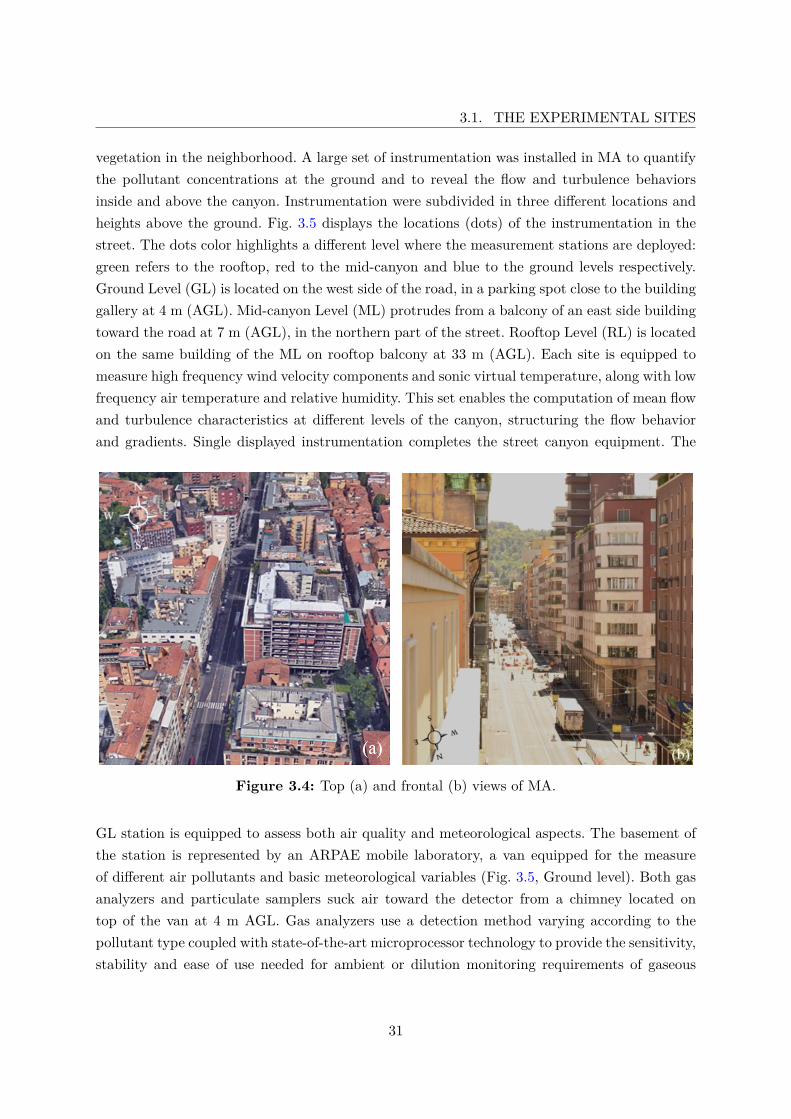
3.1. THE EXPERIMENTAL SITES
vegetation in the neighborhood. A large set of instrumentation was installed in MA to quantifythe pollutant concentrations at the ground and to reveal the flow and turbulence behaviorsinside and above the canyon. Instrumentation were subdivided in three different locations andheights above the ground. Fig. 3.5 displays the locations (dots) of the instrumentation in thestreet. The dots color highlights a different level where the measurement stations are deployed:green refers to the rooftop, red to the mid-canyon and blue to the ground levels respectively.Ground Level (GL) is located on the west side of the road, in a parking spot close to the buildinggallery at 4 m (AGL). Mid-canyon Level (ML) protrudes from a balcony of an east side buildingtoward the road at 7 m (AGL), in the northern part of the street. Rooftop Level (RL) is locatedon the same building of the ML on rooftop balcony at 33 m (AGL). Each site is equipped tomeasure high frequency wind velocity components and sonic virtual temperature, along with lowfrequency air temperature and relative humidity. This set enables the computation of mean flowand turbulence characteristics at different levels of the canyon, structuring the flow behaviorand gradients. Single displayed instrumentation completes the street canyon equipment. The
Figure 3.4: Top (a) and frontal (b) views of MA.
GL station is equipped to assess both air quality and meteorological aspects. The basement ofthe station is represented by an ARPAE mobile laboratory, a van equipped for the measureof different air pollutants and basic meteorological variables (Fig. 3.5, Ground level). Both gasanalyzers and particulate samplers suck air toward the detector from a chimney located ontop of the van at 4 m AGL. Gas analyzers use a detection method varying according to thepollutant type coupled with state-of-the-art microprocessor technology to provide the sensitivity,stability and ease of use needed for ambient or dilution monitoring requirements of gaseous
31
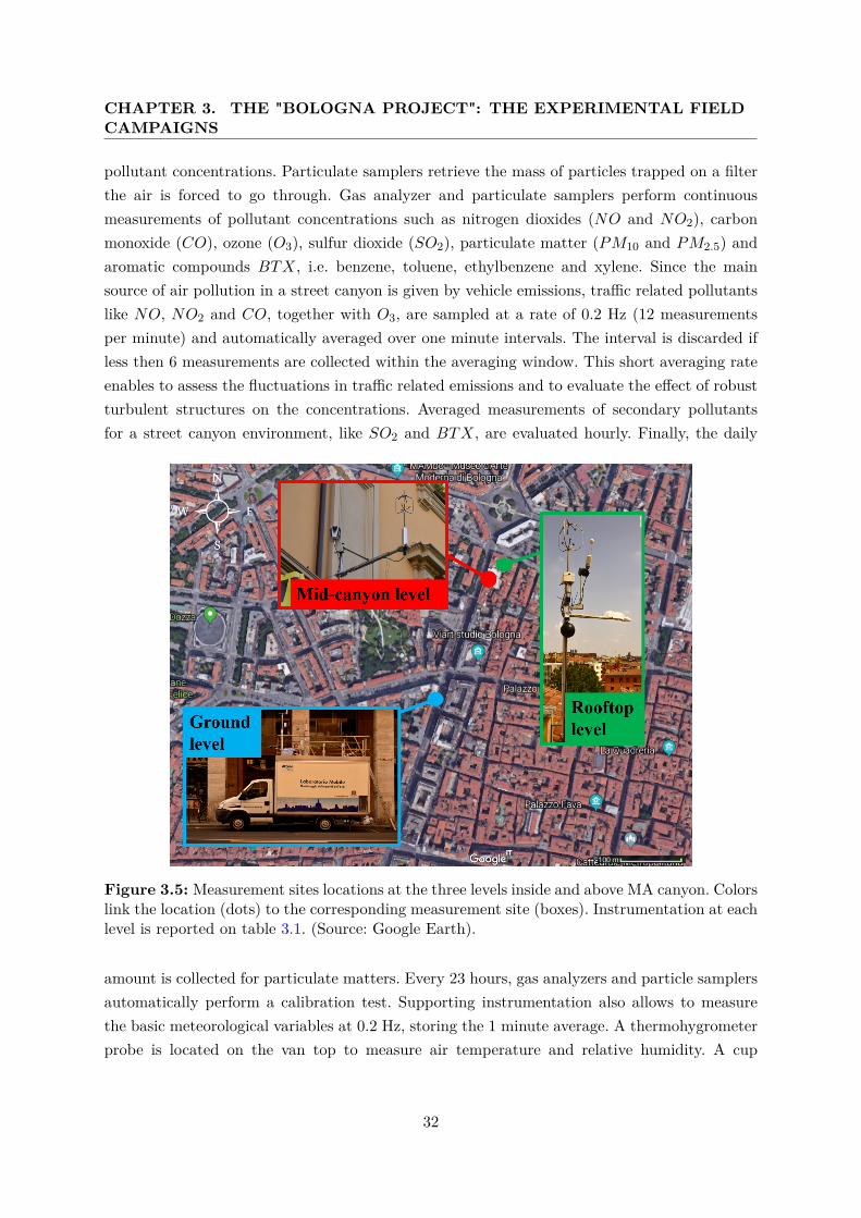
CHAPTER 3. THE "BOLOGNA PROJECT": THE EXPERIMENTAL FIELDCAMPAIGNS
pollutant concentrations. Particulate samplers retrieve the mass of particles trapped on a filterthe air is forced to go through. Gas analyzer and particulate samplers perform continuousmeasurements of pollutant concentrations such as nitrogen dioxides (NO and NO2), carbonmonoxide (CO), ozone (O3), sulfur dioxide (SO2), particulate matter (PM10 and PM2.5) andaromatic compounds BTX, i.e. benzene, toluene, ethylbenzene and xylene. Since the mainsource of air pollution in a street canyon is given by vehicle emissions, traffic related pollutantslike NO, NO2 and CO, together with O3, are sampled at a rate of 0.2 Hz (12 measurementsper minute) and automatically averaged over one minute intervals. The interval is discarded ifless then 6 measurements are collected within the averaging window. This short averaging rateenables to assess the fluctuations in traffic related emissions and to evaluate the effect of robustturbulent structures on the concentrations. Averaged measurements of secondary pollutantsfor a street canyon environment, like SO2 and BTX, are evaluated hourly. Finally, the daily
Figure 3.5: Measurement sites locations at the three levels inside and above MA canyon. Colorslink the location (dots) to the corresponding measurement site (boxes). Instrumentation at eachlevel is reported on table 3.1. (Source: Google Earth).
amount is collected for particulate matters. Every 23 hours, gas analyzers and particle samplersautomatically perform a calibration test. Supporting instrumentation also allows to measurethe basic meteorological variables at 0.2 Hz, storing the 1 minute average. A thermohygrometerprobe is located on the van top to measure air temperature and relative humidity. A cup
32
3.1. THE EXPERIMENTAL SITES
and vane anemometer is also collocated on the van top collecting the 2D wind velocity anddirection. Wind velocity is retrieved from a measurement of cup spins per second, given by themechanical torque generated by the flow on the cups. This characteristic of the instrumentationinvolves an activation threshold of approximately 0.5 ms−1 to overpower the static frictionof the rotation mechanisms. Moreover, cups have a slow response to flow variations due tothe inertia of the rotation. Therefore cup and vane anemometer is not suitable for turbulenceestimation. To cover this gap, supplementary instrumentation was installed on the van top. Asonic anemometer was set to collect high frequency measurements of the three wind velocitycomponents, together with the sonic temperature (a quantity close to the virtual temperature).The operative method, based on the retrieval of a sonic wave perturbation generated by thevelocity of the medium the waves goes through, allows to collect data at a sampling rate of20 Hz, corresponding to 20 measurements per second. This fast sampling rate is sufficient forthe evaluation of turbulent quantities, necessary to fulfill the aims of the whole investigation.Sonic anemometers are also coupled with a thermohygrometer and a barometer sampling at 1Hz, to access the fast variation of air temperature, relative humidity and pressure. The ML wasequipped with the essential core of each site, i.e. the sonic anemometer for the measurements ofmean flow velocity and direction and turbulence, and the thermohygrometer for air temperatureand relative humidity. As for the ground level, the sonic anemometer sampled at 20 Hz whilethe thermohygrometer samples at 1 Hz. The instrumentation was mounted on an ad-hoc metalstructure at the edge of a balcony facing the street from the eastern side (Fig. 3.5, Mid-canyonlevel). To minimize the building facade and balcony perturbation effect on the atmosphericflow, the sonic anemometer was mounted on a branch of the metal structure 0.5 m above thebalcony rail protruding approximately 2 m from the balcony edge toward the street center.The RL was located on the rooftop balcony of the same building hosting the ML (Fig. 3.5,Rooftop level). The site was equipped by a sonic anemometer coupled with an open path gasanalyzer and a net radiometer. The sonic anemometer differs from the in-canyon ones since itensures measurement stability over a wider temperature range, but reduces the sampling rateto 10 Hz. The open path gas analyzer is an optical instrument which enables the retrieval ofwater vapor H2O and carbon dioxide CO2 concentrations at a sampling rate of 10 Hz from thebackscatter of a laser beam. When coupled with a sonic anemometer, CO2 and H2O fluxes canbe determined combining the gas concentrations to the wind velocity components by meansof the eddy covariance technique. The net radiometer is an optical instrumentation formed by2 couples of sensors for the evaluation of the radiative energy balance. Each sensors couple isformed by a pyranometer to measure the shortwave (0.3-2.8 µm) radiation and a pyrgeometerto measure the longwave (4.5-42 µm) radiation. A couple is set on top of the instrumentationfacing the sky to retrieve the incoming solar radiation; the other couple is set on the bottomfacing the ground to retrieve the surface longwave emission and shortwave scatter.
33
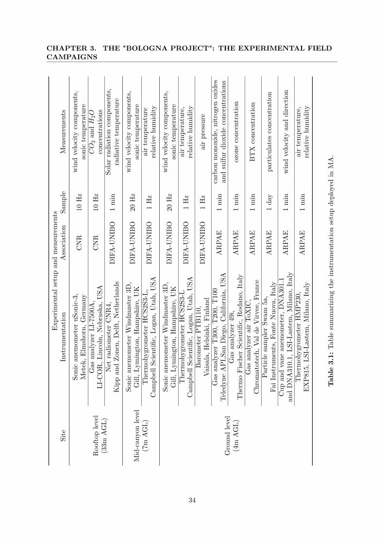
CHAPTER 3. THE "BOLOGNA PROJECT": THE EXPERIMENTAL FIELDCAMPAIGNS
Expe
rimentals
etup
andmeasurements
Site
Instrumentatio
nAssociatio
nSa
mple
Measurements
Roo
ftoplevel
Sonican
emom
eter
uSon
ic-3,
CNR
10Hz
windvelocity
compo
nents,
(33m
AGL)
Metek,E
lmshorn,
German
ysonictempe
rature
Gas
analyzer
LI-750
0A,
CNR
10Hz
CO
2an
dH
2OLI-C
OR,L
incoln,N
ebraska,
USA
conc
entrations
Net
radiom
eter
CNR4,
DIFA-U
NIB
O1min
Solarradiationcompo
nents,
Kippan
dZo
nen,
Delft,
Nethe
rland
sradiativetempe
rature
Mid-can
yonlevel
Sonican
emom
eter
Windm
aster3D
,DIFA-U
NIB
O20
Hz
windvelocity
compo
nents,
(7m
AGL)
Gill,L
ymington
,Ham
pshire,U
Ksonictempe
rature
The
rmoh
ygrometer
HCS2
S3-L,
DIFA-U
NIB
O1Hz
airtempe
rature
Cam
pbellS
cientifi
c,Lo
gan,
Utah,
USA
relativ
ehu
midity
Groun
dlevel
Sonican
emom
eter
Windm
aster3D
,DIFA-U
NIB
O20
Hz
windvelocity
compo
nents,
(4m
AGL)
Gill,L
ymington
,Ham
pshire,U
Ksonictempe
rature
The
rmoh
ygrometer
HCS2
S3-L
DIFA-U
NIB
O1Hz
airtempe
rature,
Cam
pbellS
cientifi
c,Lo
gan,
Utah,
USA
relativ
ehu
midity
Barometer
PTB1
10,
DIFA-U
NIB
O1Hz
airpressure
Vaisa
la,H
elsin
ki,F
inland
Gas
analyzer
T30
0,T20
0,T10
0ARPA
E1min
carbon
mon
oxide,
nitrog
enoxides
Teledy
neAPI
,San
Diego
,Califo
rnia,U
SAan
dsulfu
rdioxideconc
entrations
Gas
analyzer
49i,
ARPA
E1min
ozon
econc
entration
The
rmoFische
rSc
ientific,
Rod
ano,
Italy
Gas
analyzer
airTo
XIC
,ARPA
E1min
BTX
conc
entration
Chrom
atotech,
Vald
eVirv
ee,F
ranc
ePa
rticle
sampler
Swam
5a,
ARPA
E1da
ypa
rticulates
conc
entration
FaiInstrum
ents,F
onte
Nuo
va,Italy
Cup
andvane
anem
ometer,D
NA30
1.1
ARPA
E1min
windvelocity
anddirection
andDNA31
0.1,
LSI-L
astem,M
ilano
,Italy
The
rmoh
ygrometer
HMP2
30,
ARPA
E1min
airtempe
rature,
EXP8
15,L
SI-Lastem,M
ilano
,Italy
relativ
ehu
midity
Tab
le3.1:
Tablesummarizingtheinstrumentatio
nsetupde
ployed
inMA.
34
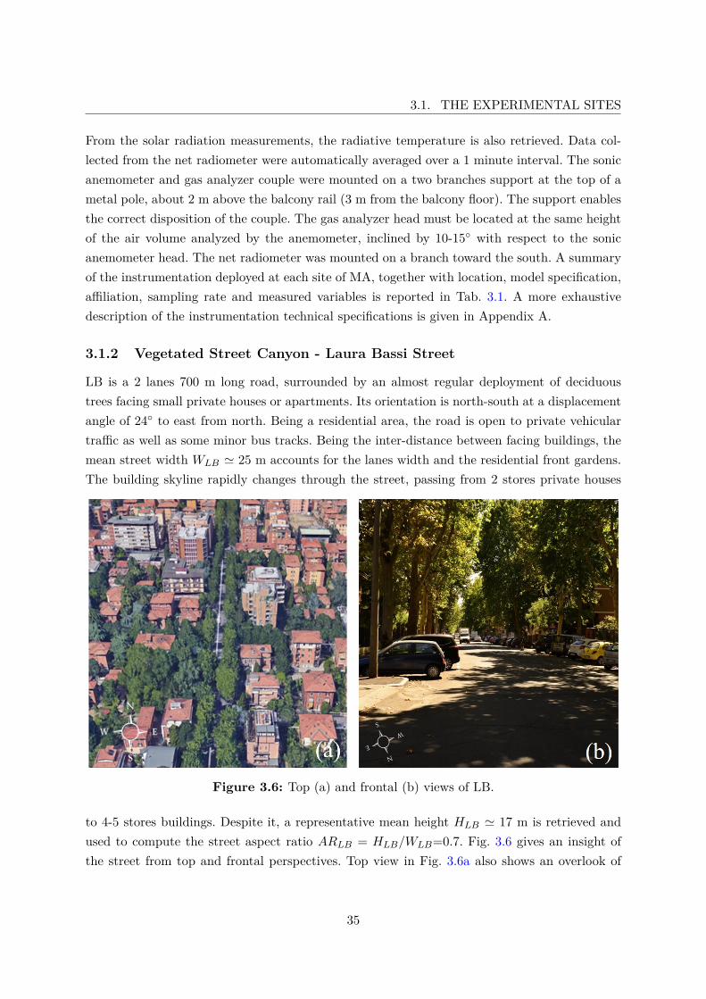
3.1. THE EXPERIMENTAL SITES
From the solar radiation measurements, the radiative temperature is also retrieved. Data col-lected from the net radiometer were automatically averaged over a 1 minute interval. The sonicanemometer and gas analyzer couple were mounted on a two branches support at the top of ametal pole, about 2 m above the balcony rail (3 m from the balcony floor). The support enablesthe correct disposition of the couple. The gas analyzer head must be located at the same heightof the air volume analyzed by the anemometer, inclined by 10-15◦ with respect to the sonicanemometer head. The net radiometer was mounted on a branch toward the south. A summaryof the instrumentation deployed at each site of MA, together with location, model specification,affiliation, sampling rate and measured variables is reported in Tab. 3.1. A more exhaustivedescription of the instrumentation technical specifications is given in Appendix A.
3.1.2 Vegetated Street Canyon - Laura Bassi Street
LB is a 2 lanes 700 m long road, surrounded by an almost regular deployment of deciduoustrees facing small private houses or apartments. Its orientation is north-south at a displacementangle of 24◦ to east from north. Being a residential area, the road is open to private vehiculartraffic as well as some minor bus tracks. Being the inter-distance between facing buildings, themean street width WLB ' 25 m accounts for the lanes width and the residential front gardens.The building skyline rapidly changes through the street, passing from 2 stores private houses
Figure 3.6: Top (a) and frontal (b) views of LB.
to 4-5 stores buildings. Despite it, a representative mean height HLB ' 17 m is retrieved andused to compute the street aspect ratio ARLB = HLB/WLB=0.7. Fig. 3.6 gives an insight ofthe street from top and frontal perspectives. Top view in Fig. 3.6a also shows an overlook of
35
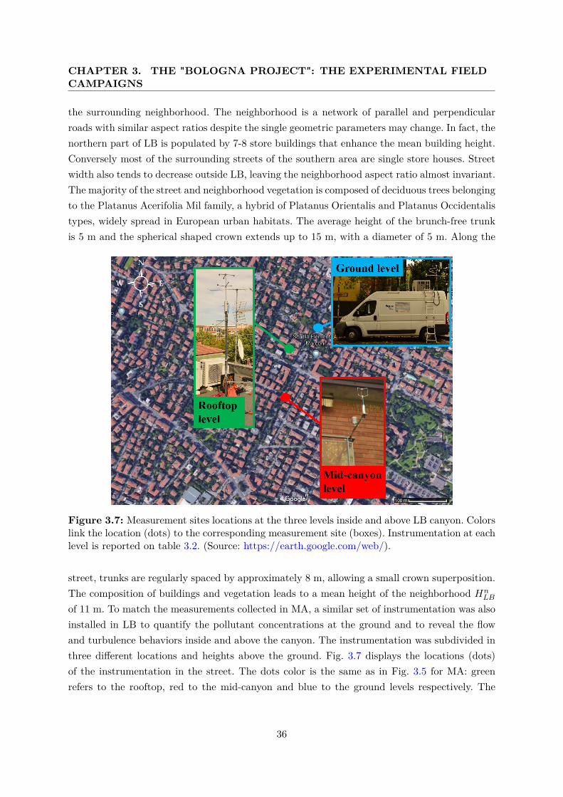
CHAPTER 3. THE "BOLOGNA PROJECT": THE EXPERIMENTAL FIELDCAMPAIGNS
the surrounding neighborhood. The neighborhood is a network of parallel and perpendicularroads with similar aspect ratios despite the single geometric parameters may change. In fact, thenorthern part of LB is populated by 7-8 store buildings that enhance the mean building height.Conversely most of the surrounding streets of the southern area are single store houses. Streetwidth also tends to decrease outside LB, leaving the neighborhood aspect ratio almost invariant.The majority of the street and neighborhood vegetation is composed of deciduous trees belongingto the Platanus Acerifolia Mil family, a hybrid of Platanus Orientalis and Platanus Occidentalistypes, widely spread in European urban habitats. The average height of the brunch-free trunkis 5 m and the spherical shaped crown extends up to 15 m, with a diameter of 5 m. Along the
Figure 3.7: Measurement sites locations at the three levels inside and above LB canyon. Colorslink the location (dots) to the corresponding measurement site (boxes). Instrumentation at eachlevel is reported on table 3.2. (Source: https://earth.google.com/web/).
street, trunks are regularly spaced by approximately 8 m, allowing a small crown superposition.The composition of buildings and vegetation leads to a mean height of the neighborhood Hn
LB
of 11 m. To match the measurements collected in MA, a similar set of instrumentation was alsoinstalled in LB to quantify the pollutant concentrations at the ground and to reveal the flowand turbulence behaviors inside and above the canyon. The instrumentation was subdivided inthree different locations and heights above the ground. Fig. 3.7 displays the locations (dots)of the instrumentation in the street. The dots color is the same as in Fig. 3.5 for MA: greenrefers to the rooftop, red to the mid-canyon and blue to the ground levels respectively. The
36
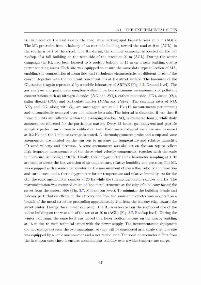
3.1. THE EXPERIMENTAL SITES
GL is placed on the east side of the road, in a parking spot beneath trees at 3 m (AGL).The ML protrudes from a balcony of an east side building toward the road at 9 m (AGL), inthe southern part of the street. The RL during the summer campaign is located on the flatrooftop of a tall building on the west side of the street at 20 m (AGL). During the wintercampaign the RL had been lowered to a rooftop balcony at 15 m on a near building due topower sourcing issues. Each site was equipped to ensure the same data type collection of MA,enabling the computation of mean flow and turbulence characteristics at different levels of thecanyon, together with the pollutant concentrations at the street surface. The basement of theGL station is again represented by a mobile laboratory of ARPAE (Fig. 3.7, Ground level). Thegas analyzer and particulate samplers within it perfom continuous measurements of pollutantconcentrations such as nitrogen dioxides (NO and NO2), carbon monoxide (CO), ozone (O3),sulfur dioxide (SO2) and particulate matter (PM10 and PM2.5). The sampling rates of NO,NO2 and CO, along with O3, are once again set at 0.2 Hz (12 measurements per minute)and automatically averaged over one minute intervals. The interval is discarded if less then 6measurements are collected within the averaging window. SO2 is evaluated hourly, while dailyamounts are collected for the particulate matter. Every 23 hours, gas analyzers and particlesamplers perform an automatic calibration test. Basic meteorological variables are measuredat 0.2 Hz and the 1 minute average is stored. A thermohygrometer probe and a cup and vaneanemometer are located on the van top to measure air temperature and relative humidity,2D wind velocity and direction. A sonic anemometer was also set on the van top to collecthigh frequency measurements of the three wind velocity components, together with the sonictemperature, sampling at 20 Hz. Finally, thermohygrometer and a barometer sampling at 1 Hzare used to access the fast variation of air temperature, relative humidity and pressure. The MLwas equipped with a sonic anemometer for the measurement of mean flow velocity and directionand turbulence, and a thermohygrometer for air temperature and relative humidity. As for theGL, the sonic anemometer samples at 20 Hz while the thermohygrometer samples at 1 Hz. Theinstrumentation was mounted on an ad-hoc metal structure at the edge of a balcony facing thestreet from the eastern side (Fig. 3.7, Mid-canyon level). To minimize the building facade andbalcony perturbation effects on the atmospheric flow, the sonic anemometer was mounted on abranch of the metal structure protruding approximately 2 m from the balcony edge toward thestreet center. During the summer campaign, the RL was located on the rooftop of one of thetallest building on the west side of the street at 20 m (AGL) (Fig. 3.7, Rooftop level). During thewinter campaign, the same level was moved to a lower rooftop balcony on the nearby buildingat 15 m due to risen technical issues with the power supply. The instrumentation equipmentdid not change between the two campaigns, so they will be considered as a single site. The sitewas equipped by a sonic anemometer and a net radiometer. The sonic anemometer differs fromthe in-canyon ones since it ensures measurement stability over a wider temperature range.
37
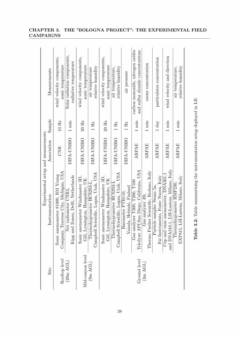
CHAPTER 3. THE "BOLOGNA PROJECT": THE EXPERIMENTAL FIELDCAMPAIGNS
Expe
rimentals
etup
andmeasurements
Site
Instrumentatio
nAssociatio
nSa
mple
Measurements
Roo
ftoplevel
Sonican
emom
eter
8100
0,RM
Youn
gCNR
10Hz
windvelocity
compo
nents,
(20m
AGL)
Com
pany,T
raverseCity
,Mich
igan
,USA
sonictempe
rature
Net
radiom
eter
CNR4,
DIFA-U
NIB
O1min
Solarradiationcompo
nents,
Kippan
dZo
nen,
Delft,
Nethe
rland
sradiativetempe
rature
Mid-can
yonlevel
Sonican
emom
eter
Windm
aster3D
,DIFA-U
NIB
O20
Hz
windvelocity
compo
nents,
(9m
AGL)
Gill,L
ymington
,Ham
pshire,U
Ksonictempe
rature
The
rmoh
ygrometer
HCS2
S3-L,
DIFA-U
NIB
O1Hz
airtempe
rature
Cam
pbellS
cientifi
c,Lo
gan,
Utah,
USA
relativ
ehu
midity
Groun
dlevel
Sonican
emom
eter
Windm
aster3D
,DIFA-U
NIB
O20
Hz
windvelocity
compo
nents,
(3m
AGL)
Gill,L
ymington
,Ham
pshire,U
Ksonictempe
rature
The
rmoh
ygrometer
HCS2
S3-L
DIFA-U
NIB
O1Hz
airtempe
rature,
Cam
pbellS
cientifi
c,Lo
gan,
Utah,
USA
relativ
ehu
midity
Barometer
PTB1
10,
DIFA-U
NIB
O1Hz
airpressure
Vaisa
la,H
elsin
ki,F
inland
Gas
analyzer
T30
0,T20
0,T10
0ARPA
E1min
carbon
mon
oxide,
nitrog
enoxides
Teledy
neAPI
,San
Diego
,Califo
rnia,U
SAan
dsulfu
rdioxideconc
entrations
Gas
analyzer
49i,
ARPA
E1min
ozon
econc
entration
The
rmoFische
rSc
ientific,
Rod
ano,
Italy
Particle
sampler
Swam
5a,
ARPA
E1da
ypa
rticulates
conc
entration
FaiInstrum
ents,F
onte
Nuo
va,Italy
Cup
andvane
anem
ometer,D
NA30
1.1
ARPA
E1min
windvelocity
anddirection
andDNA31
0.1,
LSI-L
astem,M
ilano
,Italy
The
rmoh
ygrometer
HMP2
30,
ARPA
E1min
airtempe
rature,
EXP8
15,L
SI-Lastem,M
ilano
,Italy
relativ
ehu
midity
Tab
le3.2:
Tablesummarizingtheinstrumentatio
nsetupde
ployed
inLB
.
38
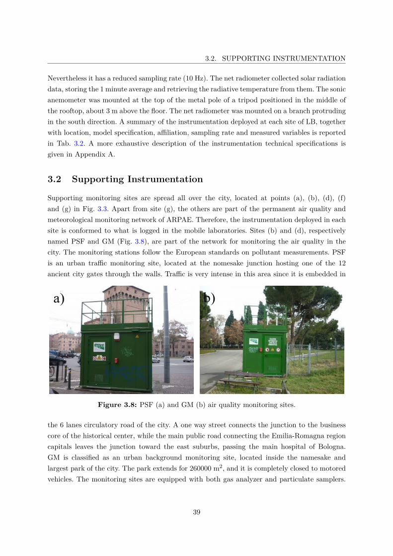
3.2. SUPPORTING INSTRUMENTATION
Nevertheless it has a reduced sampling rate (10 Hz). The net radiometer collected solar radiationdata, storing the 1 minute average and retrieving the radiative temperature from them. The sonicanemometer was mounted at the top of the metal pole of a tripod positioned in the middle ofthe rooftop, about 3 m above the floor. The net radiometer was mounted on a branch protrudingin the south direction. A summary of the instrumentation deployed at each site of LB, togetherwith location, model specification, affiliation, sampling rate and measured variables is reportedin Tab. 3.2. A more exhaustive description of the instrumentation technical specifications isgiven in Appendix A.
3.2 Supporting Instrumentation
Supporting monitoring sites are spread all over the city, located at points (a), (b), (d), (f)and (g) in Fig. 3.3. Apart from site (g), the others are part of the permanent air quality andmeteorological monitoring network of ARPAE. Therefore, the instrumentation deployed in eachsite is conformed to what is logged in the mobile laboratories. Sites (b) and (d), respectivelynamed PSF and GM (Fig. 3.8), are part of the network for monitoring the air quality in thecity. The monitoring stations follow the European standards on pollutant measurements. PSFis an urban traffic monitoring site, located at the nomesake junction hosting one of the 12ancient city gates through the walls. Traffic is very intense in this area since it is embedded in
Figure 3.8: PSF (a) and GM (b) air quality monitoring sites.
the 6 lanes circulatory road of the city. A one way street connects the junction to the businesscore of the historical center, while the main public road connecting the Emilia-Romagna regioncapitals leaves the junction toward the east suburbs, passing the main hospital of Bologna.GM is classified as an urban background monitoring site, located inside the namesake andlargest park of the city. The park extends for 260000 m2, and it is completely closed to motoredvehicles. The monitoring sites are equipped with both gas analyzer and particulate samplers.
39
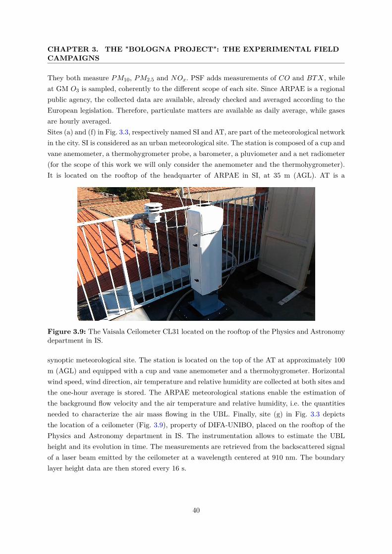
CHAPTER 3. THE "BOLOGNA PROJECT": THE EXPERIMENTAL FIELDCAMPAIGNS
They both measure PM10, PM2.5 and NOx. PSF adds measurements of CO and BTX, whileat GM O3 is sampled, coherently to the different scope of each site. Since ARPAE is a regionalpublic agency, the collected data are available, already checked and averaged according to theEuropean legislation. Therefore, particulate matters are available as daily average, while gasesare hourly averaged.Sites (a) and (f) in Fig. 3.3, respectively named SI and AT, are part of the meteorological networkin the city. SI is considered as an urban meteorological site. The station is composed of a cup andvane anemometer, a thermohygrometer probe, a barometer, a pluviometer and a net radiometer(for the scope of this work we will only consider the anemometer and the thermohygrometer).It is located on the rooftop of the headquarter of ARPAE in SI, at 35 m (AGL). AT is a
Figure 3.9: The Vaisala Ceilometer CL31 located on the rooftop of the Physics and Astronomydepartment in IS.
synoptic meteorological site. The station is located on the top of the AT at approximately 100m (AGL) and equipped with a cup and vane anemometer and a thermohygrometer. Horizontalwind speed, wind direction, air temperature and relative humidity are collected at both sites andthe one-hour average is stored. The ARPAE meteorological stations enable the estimation ofthe background flow velocity and the air temperature and relative humidity, i.e. the quantitiesneeded to characterize the air mass flowing in the UBL. Finally, site (g) in Fig. 3.3 depictsthe location of a ceilometer (Fig. 3.9), property of DIFA-UNIBO, placed on the rooftop of thePhysics and Astronomy department in IS. The instrumentation allows to estimate the UBLheight and its evolution in time. The measurements are retrieved from the backscattered signalof a laser beam emitted by the ceilometer at a wavelength centered at 910 nm. The boundarylayer height data are then stored every 16 s.
40
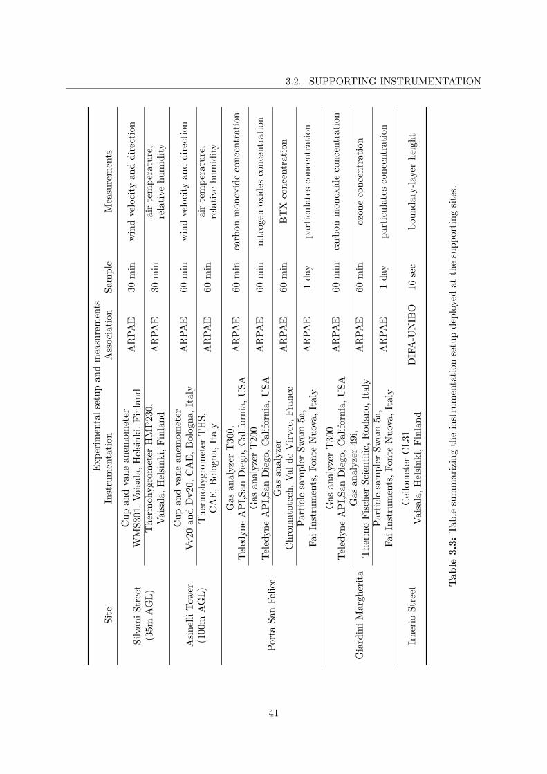
3.2. SUPPORTING INSTRUMENTATIONEx
perim
entals
etup
andmeasurements
Site
Instrumentatio
nAssociatio
nSa
mple
Measurements
Silvan
iStreet
Cup
andvane
anem
ometer
ARPA
E30
min
windvelocity
anddirection
(35m
AGL)
WMS3
01,V
aisala,H
elsin
ki,F
inland
The
rmoh
ygrometer
HMP2
30,
ARPA
E30
min
airtempe
rature,
Vaisa
la,H
elsin
ki,F
inland
relativ
ehu
midity
Asin
elliTo
wer
Cup
andvane
anem
ometer
ARPA
E60
min
windvelocity
anddirection
(100
mAGL)
Vv20
andDv2
0,CAE,
Bologn
a,Italy
The
rmoh
ygrometer
THS,
ARPA
E60
min
airtempe
rature,
CAE,
Bologn
a,Italy
relativ
ehu
midity
PortaSa
nFe
lice
Gas
analyzer
T30
0,ARPA
E60
min
carbon
mon
oxideconc
entration
Teledy
neAPI
,San
Diego
,Califo
rnia,U
SAGas
analyzer
T20
0ARPA
E60
min
nitrog
enox
ides
conc
entration
Teledy
neAPI
,San
Diego
,Califo
rnia,U
SAGas
analyzer
ARPA
E60
min
BTX
conc
entration
Chrom
atotech,
Vald
eVirv
ee,F
ranc
ePa
rticle
sampler
Swam
5a,
ARPA
E1da
ypa
rticulates
conc
entration
FaiInstrum
ents,F
onte
Nuo
va,Italy
GiardiniM
argh
erita
Gas
analyzer
T30
0ARPA
E60
min
carbon
mon
oxideconc
entration
Teledy
neAPI
,San
Diego
,Califo
rnia,U
SAGas
analyzer
49i,
ARPA
E60
min
ozon
econc
entration
The
rmoFische
rSc
ientific,
Rod
ano,
Italy
Particle
sampler
Swam
5a,
ARPA
E1da
ypa
rticulates
conc
entration
FaiInstrum
ents,F
onte
Nuo
va,Italy
Irne
rioStreet
Ceilometer
CL3
1DIFA-U
NIB
O16
sec
boun
dary-la
yerhe
ight
Vaisa
la,H
elsin
ki,F
inland
Tab
le3.3:
Tablesummarizingtheinstrumentatio
nsetupde
ployed
atthesupp
ortin
gsit
es.
41
CHAPTER 3. THE "BOLOGNA PROJECT": THE EXPERIMENTAL FIELDCAMPAIGNS
A summary of the instrumentation deployed at each ARPAE and DIFA-UNIBO monitoring site,along with location, model specification, affiliation, sampling rate and measured variables is re-ported in Tab. 3.3. A more exhaustive description of the instrumentation technical specificationsis given in Appendix A.
3.3 Summary and Conclusions
In this section, the experimental field campaigns have been presented, focusing on the charac-terization of the field domains and the instrumentation deployed. It worth recalling that twoexperimental field campaigns have been performed, investigating both summer (07/08/2017-26/09/2017) and winter (16/01/2018-14/02/2018) seasons. The field campaigns investigationswere supported and financed by the iSCAPE project.The city of Bologna, host of the campaigns, has been described revealing its hot-spot conditionregarding air pollution, as a consequence of the low natural ventilation provided by its geo-graphical collocation within the Po Valley. The network of narrow street canyons that composesthe city center is known to exacerbate this low ventilation condition, worsening the air pollutionproblem. To investigate the ventilation processes in presence and absence of vegetation, and toreveal their impacts on pollutant removal, the two street canyons of MA and LB have beenselected as main sites of the experimental field campaigns. The street canyons description fo-cused on the instrumentation deployed at three different levels inside and above each canyon tomeasure mean flow and turbulence characteristics, along with air pollutants. The instrumentalsetup was then completed by the permanent monitoring station in the city, establishing thesupporting measurement sites necessary to evaluate the background flow conditions.
42
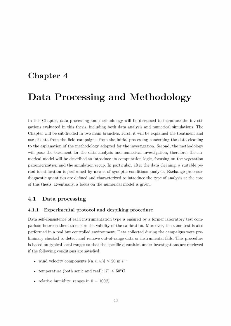
Chapter 4
Data Processing and Methodology
In this Chapter, data processing and methodology will be discussed to introduce the investi-gations evaluated in this thesis, including both data analysis and numerical simulations. TheChapter will be subdivided in two main branches. First, it will be explained the treatment anduse of data from the field campaigns, from the initial processing concerning the data cleaningto the esplanation of the methodology adopted for the investigation. Second, the methodologywill pose the basement for the data analysis and numerical investigation; therefore, the nu-merical model will be described to introduce its computation logic, focusing on the vegetationparametrization and the simulation setup. In particular, after the data cleaning, a suitable pe-riod identification is performed by means of synoptic conditions analysis. Exchange processesdiagnostic quantities are defined and characterized to introduce the type of analysis at the coreof this thesis. Eventually, a focus on the numerical model is given.
4.1 Data processing
4.1.1 Experimental protocol and despiking procedure
Data self-consistence of each instrumentation type is ensured by a former laboratory test com-parison between them to ensure the validity of the calibration. Moreover, the same test is alsoperformed in a real but controlled environment. Data collected during the campaigns were pre-liminary checked to detect and remove out-of-range data or instrumental fails. This procedureis based on typical local ranges so that the specific quantities under investigations are retrievedif the following conditions are satisfied:
• wind velocity components |(u, v, w)| ≤ 20 m s−1
• temperature (both sonic and real): |T | ≤ 50◦C
• relative humidity: ranges in 0 − 100%
43
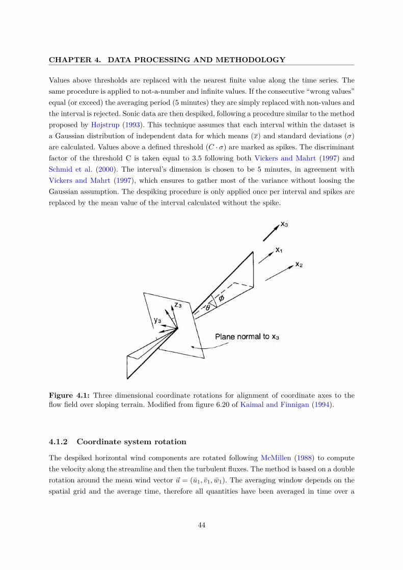
CHAPTER 4. DATA PROCESSING AND METHODOLOGY
Values above thresholds are replaced with the nearest finite value along the time series. Thesame procedure is applied to not-a-number and infinite values. If the consecutive “wrong values”equal (or exceed) the averaging period (5 minutes) they are simply replaced with non-values andthe interval is rejected. Sonic data are then despiked, following a procedure similar to the methodproposed by Højstrup (1993). This technique assumes that each interval within the dataset isa Gaussian distribution of independent data for which means (x) and standard deviations (σ)are calculated. Values above a defined threshold (C · σ) are marked as spikes. The discriminantfactor of the threshold C is taken equal to 3.5 following both Vickers and Mahrt (1997) andSchmid et al. (2000). The interval’s dimension is chosen to be 5 minutes, in agreement withVickers and Mahrt (1997), which ensures to gather most of the variance without loosing theGaussian assumption. The despiking procedure is only applied once per interval and spikes arereplaced by the mean value of the interval calculated without the spike.
Figure 4.1: Three dimensional coordinate rotations for alignment of coordinate axes to theflow field over sloping terrain. Modified from figure 6.20 of Kaimal and Finnigan (1994).
4.1.2 Coordinate system rotation
The despiked horizontal wind components are rotated following McMillen (1988) to computethe velocity along the streamline and then the turbulent fluxes. The method is based on a doublerotation around the mean wind vector ~u = (u1, v1, w1). The averaging window depends on thespatial grid and the average time, therefore all quantities have been averaged in time over a
44
4.2. DATA ANALYSIS
period of 5 minutes. The whole transformation refers to the diagram in figure (4.1). The firsttransformation swings the x1 and y1 axes around z1 to produce a new set of axes (x2, y2, z2)with x2 in the plane spanned by ~u and z1:
u2 = u1 cosψ + v1 sinχ
v2 = −u1 sinψ + v1 cosχ
w2 = w1
ψ = tan−1(v1/u1);
where χ is the angle along the projection of the mean stream on the instrumental plane. Thisway, the coordinate system is oriented along with the mean stream direction, computing arotation in χ. As a consequence, the rotation constrains advection to be null (v2 = 0) andthe main stream to project along u2, letting w2 = w1. The second rotation maintains v2 = 0,swinging x2 and z2 of the elevation angle from the surface φ into new directions (x3, y3, z3). Sox3 is the direction of the streamline, y3 is the cross-streamline direction and z3 is the verticalnormal to the inclined surface:
u3 = u2 cosφ+ w2 sinφ
v3 = v2
w3 = −u2 sinφ+ w2 cosφ
φ = tan−1(w2/u2).
Since the elevation angle is small the variation between the first to the second rotation isnegligible. After the whole rotation procedure, the final velocity vector is uf = (u3, 0, 0).Once data have been despiked and rotated, both mean flow quantities and kinematic turbulentfluxes are computed at all levels inside and above the canyon. To ensure a general robustnessof the analysis, without losing small scales processes, all quantities have been averaged in timeover a period of 5 minutes.
4.2 Data analysis
4.2.1 The period selection based on the analysis of synoptic conditions
Long-lasting experimental field campaigns enable to continuously collect local data throughoutdifferent meteorological synoptic conditions. Large scale horizontal gradients induce the synop-tic circulation and drive the small scale dynamics. In a close environment such as the Po Valley(see Sect. 3.1), these large scale gradients are easily inhibited by the presence of the mountainchains. This inhibition is more visible when the region is not perturbed by fronts or instabilities,
45
CHAPTER 4. DATA PROCESSING AND METHODOLOGY
Figure 4.2: GFS analysis of the surface isobars (white lines) superimposed on the geopotentialat 500 hPa (colormap). Each panel shows the midnight UTC of a single day within the summerperiod. Bologna is identified by the black dot.
and leads to the development of local circulations.Local circulation flows are driven by small scale gradients and perturbed by the network of ob-stacles of an urban environment. The transport of momentum, heat and other scalars like massand moisture, are regulated by local mean flow gradients and turbulent processes (Britter andHanna, 2003). Given that the aim of this work is to assess the behavior of turbulent exchangeprocesses in street canyons and the role of vegetation on local circulations, it is fundamentalto ensure that local circulation can establish and be perturbed as little as possible. Suitableperiods have been selected, one from each campaign, when weak synoptic conditions are found.These periods are identified following an analysis of synoptic maps and soundings. The firstgives an overview on the horizontal patterns, in order to avoid instabilities or frontal passages.The second retrieves the wind velocity along the atmospheric column and ensures no local in-stabilities are present.
46
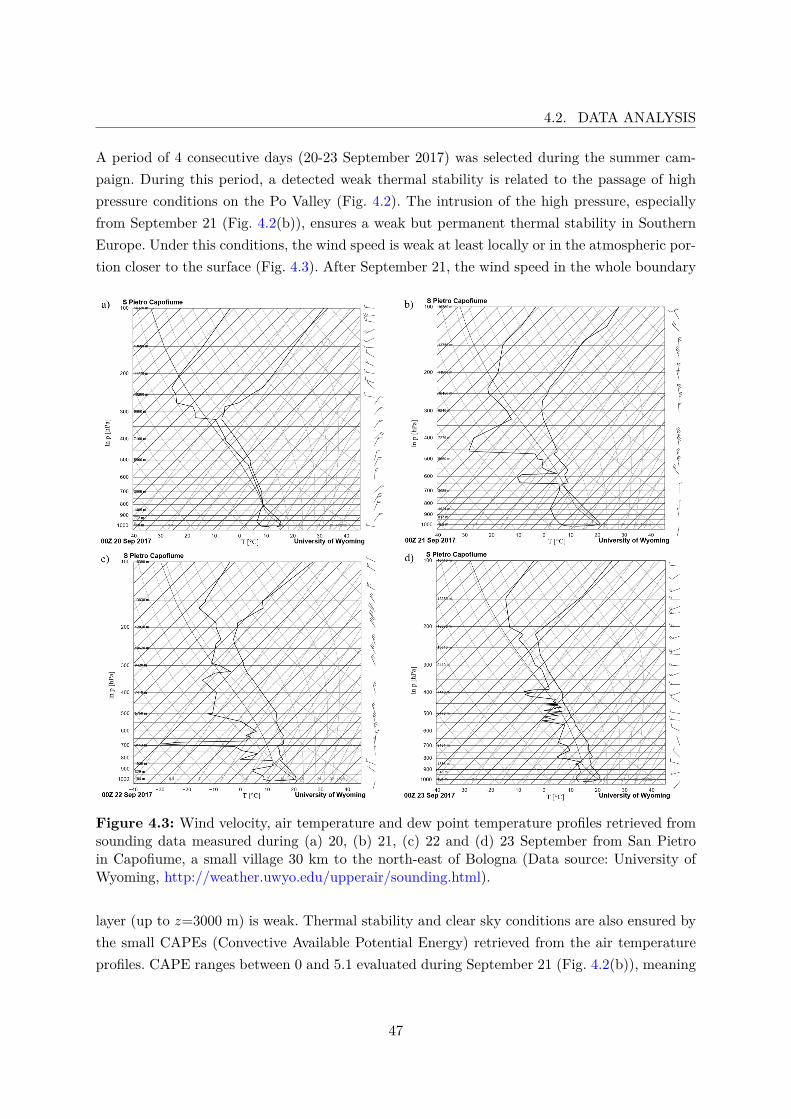
4.2. DATA ANALYSIS
A period of 4 consecutive days (20-23 September 2017) was selected during the summer cam-paign. During this period, a detected weak thermal stability is related to the passage of highpressure conditions on the Po Valley (Fig. 4.2). The intrusion of the high pressure, especiallyfrom September 21 (Fig. 4.2(b)), ensures a weak but permanent thermal stability in SouthernEurope. Under this conditions, the wind speed is weak at least locally or in the atmospheric por-tion closer to the surface (Fig. 4.3). After September 21, the wind speed in the whole boundary
Figure 4.3: Wind velocity, air temperature and dew point temperature profiles retrieved fromsounding data measured during (a) 20, (b) 21, (c) 22 and (d) 23 September from San Pietroin Capofiume, a small village 30 km to the north-east of Bologna (Data source: University ofWyoming, http://weather.uwyo.edu/upperair/sounding.html).
layer (up to z=3000 m) is weak. Thermal stability and clear sky conditions are also ensured bythe small CAPEs (Convective Available Potential Energy) retrieved from the air temperatureprofiles. CAPE ranges between 0 and 5.1 evaluated during September 21 (Fig. 4.2(b)), meaning
47
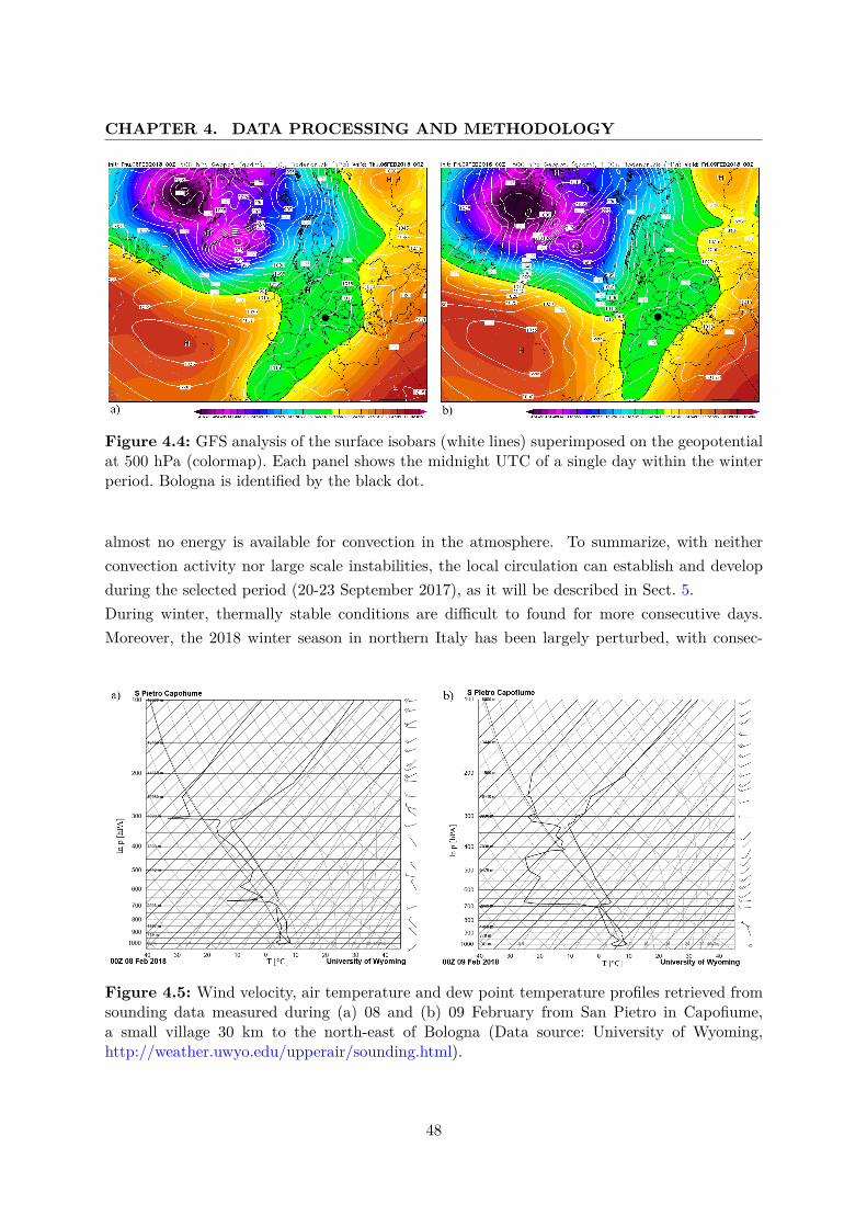
CHAPTER 4. DATA PROCESSING AND METHODOLOGY
Figure 4.4: GFS analysis of the surface isobars (white lines) superimposed on the geopotentialat 500 hPa (colormap). Each panel shows the midnight UTC of a single day within the winterperiod. Bologna is identified by the black dot.
almost no energy is available for convection in the atmosphere. To summarize, with neitherconvection activity nor large scale instabilities, the local circulation can establish and developduring the selected period (20-23 September 2017), as it will be described in Sect. 5.During winter, thermally stable conditions are difficult to found for more consecutive days.Moreover, the 2018 winter season in northern Italy has been largely perturbed, with consec-
Figure 4.5: Wind velocity, air temperature and dew point temperature profiles retrieved fromsounding data measured during (a) 08 and (b) 09 February from San Pietro in Capofiume,a small village 30 km to the north-east of Bologna (Data source: University of Wyoming,http://weather.uwyo.edu/upperair/sounding.html).
48
4.2. DATA ANALYSIS
utive periods of heavy rains and snows. Within the campaign only few consecutive days werefound to be in clear sky conditions and slightly stable stability. Among them, days 08 and 09of February were constantly stable (Fig. 4.4). Both days were under a very weak surface lowpressure coupled to a geopotential branch extending from the polar vortex. This geopotentialbranch is also wide enough to involve the whole Europe and perdure almost unperturbed forboth days. These synoptic conditions are not ideal but sufficient to weaken the wind velocityalong the profile (Fig. 4.5) up to 9000 m. Local circulations can develop among an atmosphericdepth much larger than the whole boundary layer depth. Moreover, the different wind directionsof the weak velocity depth from the atmosphere above ensures a strong decoupling of the localand SL from the large scale flow. Thermal stability and clear sky conditions are again ensuredby the small CAPEs retrieved from the air temperature profiles. CAPE ranges between 0 and18.2 evaluated during the 09 February (Fig. 4.2(b)), meaning almost no energy is available forconvection in the atmosphere. To summarize also during winter period, the local circulation canestablish and develop among the chosen period (08-09 February 2018), as it will be describedin Sect. 5, since neither convection activity nor large scale instabilities are detected.
4.2.2 Exchange processes: time scales and rates
In Sect. 2.3, the widely used time scales associated with the exchange processes in street canyonhave been presented. As it was described, these time scales always directly involve the pollutantconcentrations or the emission rate from the pollutant source, and can be independent on theflow circulation developing in the canopies. However one goal of this thesis is to evaluate newtime scales which can be a characteristic of the exchange processes between the UCL and theatmosphere above it. As a consequence, our new time scales are chosen to be characterized bythe flow and turbulent fields and to be independent on the pollutant concentrations or emissionsources, in opposition to the literature described in Sect. 2.3. With this choice, these time scalesand the subsequent diagnostic quantities derived from them will be used to assess the pollutantconcentration removal only associated to the atmospheric exchange processes, without fallinginto self-correlation problems. To fullfil this aim, it is fundamental to characterize both flow andturbulent fields in connection with the urban morphology of the investigated area.Following the classification proposed by Oke (1987), flows in street canyons of typical Europeancities belong to the skimming flow regime (Ratti et al. 2002; Di Sabatino et al. 2010), whereturbulence dominates local exchange processes (Oke 1988; Louka et al. 2000). As already re-viewed in Sect. 2.3, turbulent kinematic fluxes regulate the transfer of momentum, heat andother scalars within and above the street canyon. During periods of weak synoptic forcing,turbulent fluxes become the main driver of the atmospheric circulation and recirculation flowsinside the canyon (Britter and Hanna, 2003). Given that one element of the work is to derivenew original diagnostic time scales for real urban flows in a street canyon, it worths to assess
49
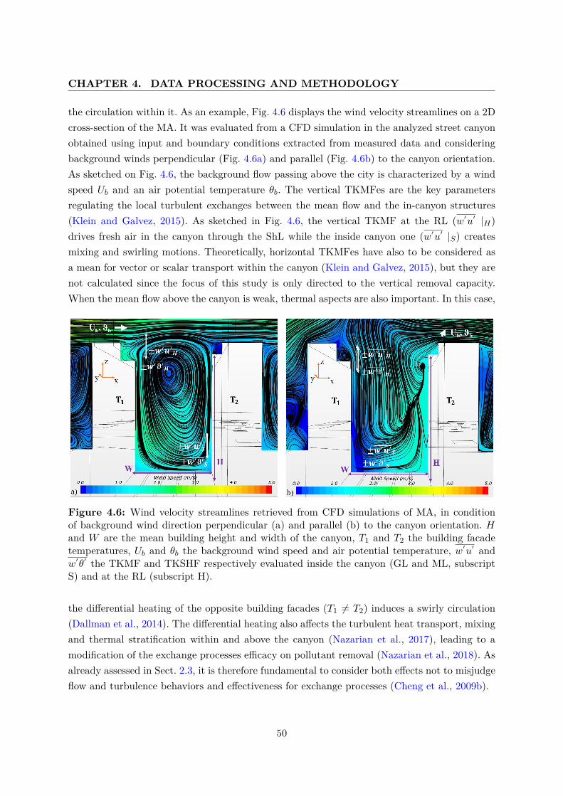
CHAPTER 4. DATA PROCESSING AND METHODOLOGY
the circulation within it. As an example, Fig. 4.6 displays the wind velocity streamlines on a 2Dcross-section of the MA. It was evaluated from a CFD simulation in the analyzed street canyonobtained using input and boundary conditions extracted from measured data and consideringbackground winds perpendicular (Fig. 4.6a) and parallel (Fig. 4.6b) to the canyon orientation.As sketched on Fig. 4.6, the background flow passing above the city is characterized by a windspeed Ub and an air potential temperature θb. The vertical TKMFes are the key parametersregulating the local turbulent exchanges between the mean flow and the in-canyon structures(Klein and Galvez, 2015). As sketched in Fig. 4.6, the vertical TKMF at the RL (w′u′ |H)drives fresh air in the canyon through the ShL while the inside canyon one (w′u′ |S) createsmixing and swirling motions. Theoretically, horizontal TKMFes have also to be considered asa mean for vector or scalar transport within the canyon (Klein and Galvez, 2015), but they arenot calculated since the focus of this study is only directed to the vertical removal capacity.When the mean flow above the canyon is weak, thermal aspects are also important. In this case,
Figure 4.6: Wind velocity streamlines retrieved from CFD simulations of MA, in conditionof background wind direction perpendicular (a) and parallel (b) to the canyon orientation. Hand W are the mean building height and width of the canyon, T1 and T2 the building facadetemperatures, Ub and θb the background wind speed and air potential temperature, w′u′ andw′θ′ the TKMF and TKSHF respectively evaluated inside the canyon (GL and ML, subscriptS) and at the RL (subscript H).
the differential heating of the opposite building facades (T1 6= T2) induces a swirly circulation(Dallman et al., 2014). The differential heating also affects the turbulent heat transport, mixingand thermal stratification within and above the canyon (Nazarian et al., 2017), leading to amodification of the exchange processes efficacy on pollutant removal (Nazarian et al., 2018). Asalready assessed in Sect. 2.3, it is therefore fundamental to consider both effects not to misjudgeflow and turbulence behaviors and effectiveness for exchange processes (Cheng et al., 2009b).
50
4.2. DATA ANALYSIS
The momentum and heat cascades from the mean flow to turbulence dictate the time scales ofexchange processes, which in turn are constrained by the canyon geometry. These time scalesare new local factors dependent on both local (canopy scale) and non local (city scale) quan-tities. The new four different time scales can be evaluated, distinguishing inertial and thermalprocesses, rooftop and in-canyon locations. Time scales are defined as the time required formomentum and heat to be vertically exchanged between two atmospheric layers. At the RL,they describe the time taken by the external flow to infiltrate the canyon through momentumtransport and heat loss. Inside the canyon, time scales assess the mixing efficacy of fresh airwith stagnant air and the upward particle removal time from the street.These new time scales are derived using the Buckingham Theorem (BT), a key property ofthe similarity theory (Durst, 2008)1. The BT states that if a certain number of variables canbe related in a physically meaningful equation, then a set of parameters can be constructedfrom the original variables. The theorem provides a method for computing sets of parametersfrom the given variables, even if the form of the equation is still unknown. These variables canthen be combined with the appropriate powers given through the theorem application to re-trieve the final equation. Following the previous considerations on the mean flow and turbulenceimportance for the in-canyon circulation, the momentum and heat time scales at the RL
τHd = f(w′u′ |H , H,W,L,∆Ub∆z ) (4.1a)
τHh = f(w′θ′ |H , H,W,L,∆θb∆z ) (4.1b)
are considered to be functions respectively of the TKMF w′u′ |H (m2s−2), the TKSHF w′θ′ |H(mKs−1) taken at the RL, the thermal stratification (represented by the vertical gradient of themean speed ∆Ub/∆z (s−1) and potential temperature ∆θb/∆z (Ks−1)) of the background flowimpinging on the canyon and the geometric parameters H (m) the mean buildings height, W(m) the mean street width, and L (m) the street length. Making use of the BT on both Eq.(4.1a) and (4.1b), following the example given in Appendix B, the time scales become:
τHd = H3
w′u′ |H W
∆Ub∆z (4.2a)
τHh = H3
w′θ′ |H W
∆θb∆z . (4.2b)
Equations (4.2a) and (4.2b) represent only one of the possible solutions of the BT due to thepresence of arbitrary coefficients, as described in Appendix A. Time scales increase as the canyon
1An example application of the BT is presented in Appendix B.
51
CHAPTER 4. DATA PROCESSING AND METHODOLOGY
height increases, as well as the thermal stratification increases, with the latter inhibiting mixing.Conversely, time scales decrease as canyon width increases, as well as the fluxes intensitiesincrease. The equations Eq. (4.2a) and (4.2b) do not depend on L since time scales are basedonly on vertical transport or vertical flow variation. These quantities are confined on the bi-dimensional plane defined by the vertical and cross-canyon directions and delimited by thegeometric parameter H and W of the canyon. Therefore, they are not supposed to be anextensive variable of canyon length.Time scales inside the canyon describe the required time for exchange processes to mix fresh aircoming from the rooftop interface with the stagnant air of the canopy. Time scales inside thecanyon are functions of the merging flow from the ShL into the inner circulation, and presentthe following dependencies:
τSd = f(w′u′ |S ,W,L,H, uH∗ ) (4.3a)
τSh = f(w′θ′ |S ,W,L,H, uH∗ , θH∗ ), (4.3b)
where the fluxes are computed inside the canyon (GL and ML, subscript S), W , L and H arethe geometric parameters, while the friction velocity uH∗ = (w′u′ |2H +w′v′ |2H)1/4 (ms−1) andtemperature θH∗ = w′θ′ |H
uH∗(K) are constant values computed at the RL for each wind direction
configuration. As for the rooftop ones, these time scales depend on the momentum and heattransport provided by the in-canyon momentum w′u′ |S (m2s−2) and heat w′θ′ |S (mKs−1)fluxes, which dictate the mixing time of the canopy, and are constrained by the canyon geometry.The fresh air is driven in the canopy by the momentum and heat transfers sustaining thecirculation within the canyon and modulated by the shear layer intensity, the latter parametrisedby the friction velocity uH∗ (ms−1) and temperature θH∗ (K). Using again the BT, with theprocedure in Appendix B, Eq. (4.3a) and (4.3b) become:
τSd = H2uH∗
w′u′ |S W(4.4a)
τSh = H2θH∗
w′θ′ |S W. (4.4b)
Equations (4.4a) and (4.4b) describe the time associated to momentum and heat transportwithin the canyon. These time scales increase in stagnant conditions, that occur when air istrapped within the canyon, and decrease when mixing with fresh air entered from the RL isfavored by the exchange processes. Time scales do not depend on L, neither it was for the timescales evaluated at the RL. τSh in Eq. (4.4b) does not depend on uH∗ either because frictionvelocity contribution is provided by θH∗ .
52
4.2. DATA ANALYSIS
The ratios between the time scales evaluated inside and above the canyon provide the followingrelations:
ηd = τSdτHd
(4.5a)
ηh = τShτHh
. (4.5b)
These ratios provide information about the rate of mixing of fresh and stagnant air within thecanyon, by comparing turbulent exchange efficacy at different heights. As long as τH>τS , theair within the canyon is supposed to efficiently mix with fresh air from the rooftop. The airwithin the canyon is well mixed. Momentum and heat are efficiently transported toward higherlevels and exchanged with the free atmosphere. When τH<τS , mixing inside the canyon is lessefficient than the rooftop one. Turbulent structures in the canyon are not prone to transportmomentum and heat, enhancing stagnant conditions. At the RL, a well mixed air mass isseparated from the inner canyon, behaving as a cap for vertical exchanges. Air in the canyonstagnates trapped within the canopy. Since Eq. (4.5a) and (4.5b) provide information aboutthe refreshing properties of the canyon, they will be referred to as transport or exchange rates.The aim of this study is to prove that these diagnostic quantities are useful to characterize theexchange processes and to interpret pollutant removal from real urban street canyons.
4.2.3 Pollutant concentration normalization
Pollutant concentrations in real environments are strongly affected by several aspects such asthe canyon geometry, the wind velocity above the canopy, local flow structures and the sourceemission rates. Particularly, the source treatment can be challenging due to the different compo-sition and time dependency of emission sources, and the presence of multiple sources especiallyduring the winter period when domestic heating is a non negligible emission component. Unfor-tunately, the estimation of domestic heating emission is still a challenge as well as the availabilityof heat consumption databases from the public administrations. Therefore emissions are esti-mated considering vehicular traffic as the only source of pollutant concentrations inside thecanyon. This approximation is good for the summer period, when the cooling systems are asmall emissions source compared to traffic, but it is a bad approximation during winter. Tominimize the heating system contribution to the overall emission, we select the carbon monox-ide CO as pollutant tracer for this investigation, since CO is considered a criteria to estimatepollutant emitted by internal combustion engines (Winkler et al., 2018). CO emissions fromvehicular traffic is retrieved from the analysis of the fleet composition of the vehicles passedthrough the canyons during the analyzed periods. Traffic counts were obtained from counting
53
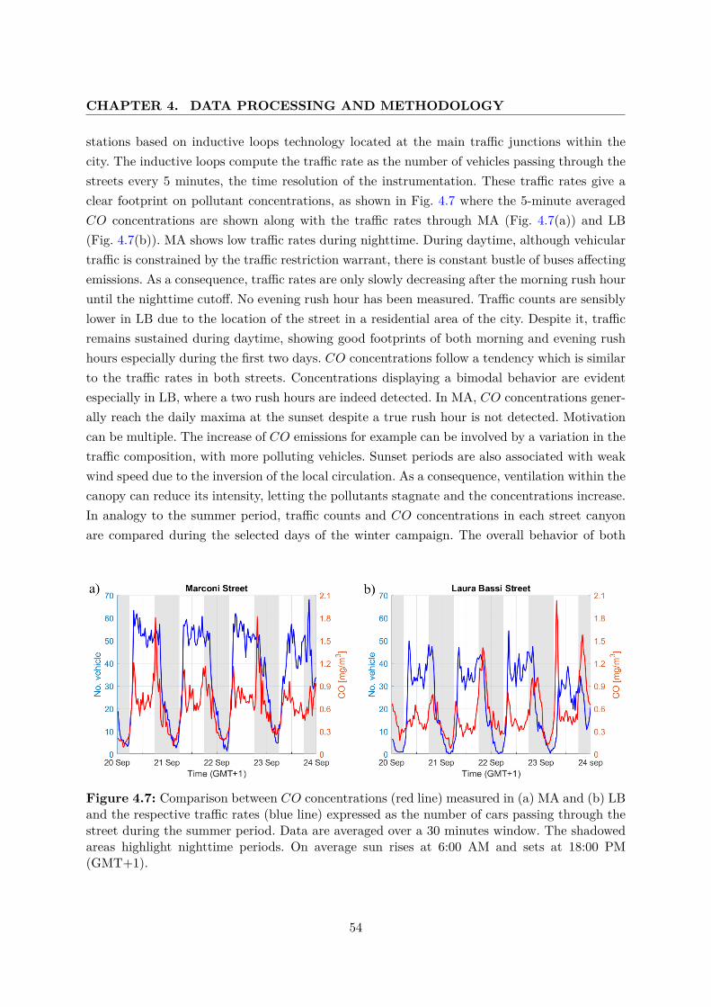
CHAPTER 4. DATA PROCESSING AND METHODOLOGY
stations based on inductive loops technology located at the main traffic junctions within thecity. The inductive loops compute the traffic rate as the number of vehicles passing through thestreets every 5 minutes, the time resolution of the instrumentation. These traffic rates give aclear footprint on pollutant concentrations, as shown in Fig. 4.7 where the 5-minute averagedCO concentrations are shown along with the traffic rates through MA (Fig. 4.7(a)) and LB(Fig. 4.7(b)). MA shows low traffic rates during nighttime. During daytime, although vehiculartraffic is constrained by the traffic restriction warrant, there is constant bustle of buses affectingemissions. As a consequence, traffic rates are only slowly decreasing after the morning rush houruntil the nighttime cutoff. No evening rush hour has been measured. Traffic counts are sensiblylower in LB due to the location of the street in a residential area of the city. Despite it, trafficremains sustained during daytime, showing good footprints of both morning and evening rushhours especially during the first two days. CO concentrations follow a tendency which is similarto the traffic rates in both streets. Concentrations displaying a bimodal behavior are evidentespecially in LB, where a two rush hours are indeed detected. In MA, CO concentrations gener-ally reach the daily maxima at the sunset despite a true rush hour is not detected. Motivationcan be multiple. The increase of CO emissions for example can be involved by a variation in thetraffic composition, with more polluting vehicles. Sunset periods are also associated with weakwind speed due to the inversion of the local circulation. As a consequence, ventilation within thecanopy can reduce its intensity, letting the pollutants stagnate and the concentrations increase.In analogy to the summer period, traffic counts and CO concentrations in each street canyonare compared during the selected days of the winter campaign. The overall behavior of both
Figure 4.7: Comparison between CO concentrations (red line) measured in (a) MA and (b) LBand the respective traffic rates (blue line) expressed as the number of cars passing through thestreet during the summer period. Data are averaged over a 30 minutes window. The shadowedareas highlight nighttime periods. On average sun rises at 6:00 AM and sets at 18:00 PM(GMT+1).
54
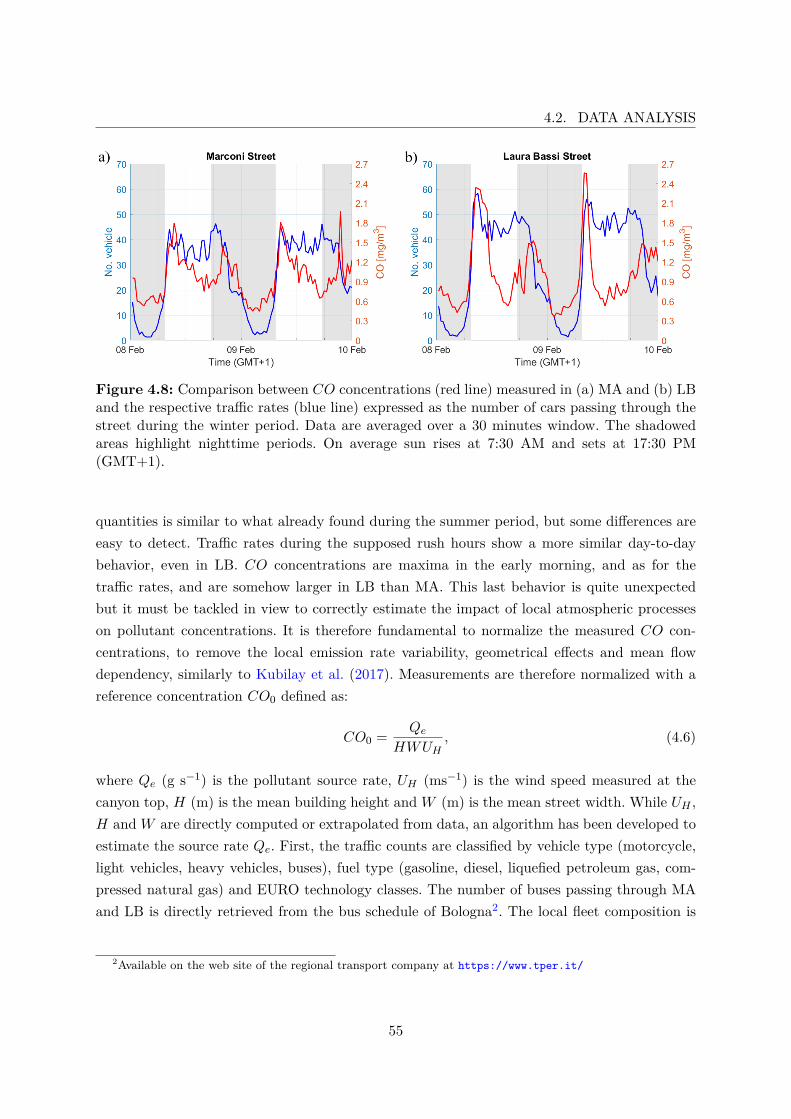
4.2. DATA ANALYSIS
Figure 4.8: Comparison between CO concentrations (red line) measured in (a) MA and (b) LBand the respective traffic rates (blue line) expressed as the number of cars passing through thestreet during the winter period. Data are averaged over a 30 minutes window. The shadowedareas highlight nighttime periods. On average sun rises at 7:30 AM and sets at 17:30 PM(GMT+1).
quantities is similar to what already found during the summer period, but some differences areeasy to detect. Traffic rates during the supposed rush hours show a more similar day-to-daybehavior, even in LB. CO concentrations are maxima in the early morning, and as for thetraffic rates, and are somehow larger in LB than MA. This last behavior is quite unexpectedbut it must be tackled in view to correctly estimate the impact of local atmospheric processeson pollutant concentrations. It is therefore fundamental to normalize the measured CO con-centrations, to remove the local emission rate variability, geometrical effects and mean flowdependency, similarly to Kubilay et al. (2017). Measurements are therefore normalized with areference concentration CO0 defined as:
CO0 = QeHWUH
, (4.6)
where Qe (g s−1) is the pollutant source rate, UH (ms−1) is the wind speed measured at thecanyon top, H (m) is the mean building height and W (m) is the mean street width. While UH ,H andW are directly computed or extrapolated from data, an algorithm has been developed toestimate the source rate Qe. First, the traffic counts are classified by vehicle type (motorcycle,light vehicles, heavy vehicles, buses), fuel type (gasoline, diesel, liquefied petroleum gas, com-pressed natural gas) and EURO technology classes. The number of buses passing through MAand LB is directly retrieved from the bus schedule of Bologna2. The local fleet composition is
2Available on the web site of the regional transport company at https://www.tper.it/
55
CHAPTER 4. DATA PROCESSING AND METHODOLOGY
extracted from the regional inventory of circulating vehicles3 and used to divide the remainingvehicular traffic following the vehicular type classification. Pollutant emission rates (g km−1)per class (vehicle, fuel and EURO technology) are estimated from the European Monitoring andEvaluation Program of the European Environment Agency (EMEP/EEA) air pollutant emis-sion inventory for each vehicle category (Ntziachristos et al., 2009). Pollutant emission rates arefinally converted in pollutant source rates Qe (g s−1) applying a representative vehicle meanurban speed of 19 km h−1 (Ntziachristos et al., 2009) as a conversion factor. The normalizedCO concentrations, named CO+, are simply retrieved from the ratio between the measuredconcentrations CO in each street canyon and the reference concentration CO0 from Eq. (4.6).
4.3 Numerical simulations
The numerical evaluation part of this work is tackled using Quick Urban & Industrial Complex(QUIC) dispersion modeling system. QUIC is a fast-response model that runs on a laptop, com-bining a mass-conserved wind solver (QUIC-URB) with a Lagrangian random-walk dispersionmodel (QUIC-PLUME). The QUIC system was primarily developed to rapidly tackle impulsiveproblems such as accidental releases of substances within the urban environment. Its primarscope was to obtain a reliable but approximated result of an atmospheric dynamics problem inthe smallest time possible, in order to be used as an operative nowcasting model to tackle emer-gency situations. Since the model first application, it has been improved to update and improvethe approximations used to solve the complex interaction between the atmospheric flows andthe terrain obstacles, without increasing the computational costs. Today it is used to rapidlydiagnose flow and turbulence characteristics in complex urban and vegetated environments.In the context of this thesis work, QUIC is preferred among the most widely adopted andcomputationally costly CFD models because it combines high computation performances tothe evaluation of approximated but consistent results. The small computational costs enableto perform a wide ensemble of simulations for every given case study in few hours, allowing tocapture all the different shades of the problem. This last consideration is extremely valuablein real environments, where homogeneous and stationary conditions are rarely achieved andsustained for long periods.
4.3.1 QUIC-URB model description
QUIC-URB is a 3D wind solver that uses a mass consistent wind model to resolve the windfield around obstacles for a representative time interval (Singh et al., 2008). Mass consistencymethod forces the initial wind velocity field u0=(u0i + v0j + w0k) generated from the input
3Available as an open data on the Italian Car Club (ACI) web site (http://www.aci.it/laci/studi-e-ricerche/dati-e-statistiche/open-data.html)
56
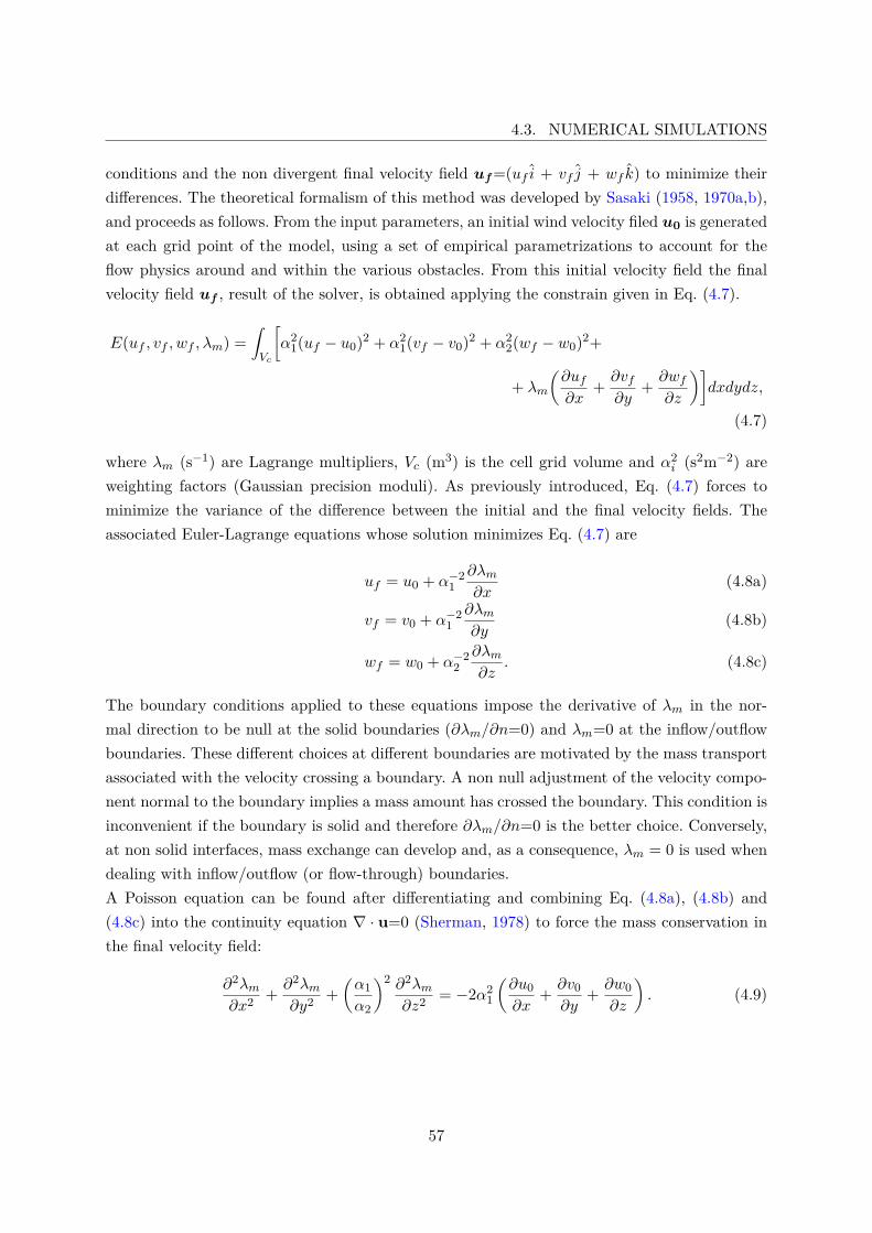
4.3. NUMERICAL SIMULATIONS
conditions and the non divergent final velocity field uf=(uf i + vf j + wf k) to minimize theirdifferences. The theoretical formalism of this method was developed by Sasaki (1958, 1970a,b),and proceeds as follows. From the input parameters, an initial wind velocity filed u0 is generatedat each grid point of the model, using a set of empirical parametrizations to account for theflow physics around and within the various obstacles. From this initial velocity field the finalvelocity field uf , result of the solver, is obtained applying the constrain given in Eq. (4.7).
E(uf , vf , wf , λm) =∫Vc
[α2
1(uf − u0)2 + α21(vf − v0)2 + α2
2(wf − w0)2+
+ λm
(∂uf∂x
+ ∂vf∂y
+ ∂wf∂z
)]dxdydz,
(4.7)
where λm (s−1) are Lagrange multipliers, Vc (m3) is the cell grid volume and α2i (s2m−2) are
weighting factors (Gaussian precision moduli). As previously introduced, Eq. (4.7) forces tominimize the variance of the difference between the initial and the final velocity fields. Theassociated Euler-Lagrange equations whose solution minimizes Eq. (4.7) are
uf = u0 + α−21∂λm∂x
(4.8a)
vf = v0 + α−21∂λm∂y
(4.8b)
wf = w0 + α−22∂λm∂z
. (4.8c)
The boundary conditions applied to these equations impose the derivative of λm in the nor-mal direction to be null at the solid boundaries (∂λm/∂n=0) and λm=0 at the inflow/outflowboundaries. These different choices at different boundaries are motivated by the mass transportassociated with the velocity crossing a boundary. A non null adjustment of the velocity compo-nent normal to the boundary implies a mass amount has crossed the boundary. This condition isinconvenient if the boundary is solid and therefore ∂λm/∂n=0 is the better choice. Conversely,at non solid interfaces, mass exchange can develop and, as a consequence, λm = 0 is used whendealing with inflow/outflow (or flow-through) boundaries.A Poisson equation can be found after differentiating and combining Eq. (4.8a), (4.8b) and(4.8c) into the continuity equation ∇ · u=0 (Sherman, 1978) to force the mass conservation inthe final velocity field:
∂2λm∂x2 + ∂2λm
∂y2 +(α1α2
)2 ∂2λm∂z2 = −2α2
1
(∂u0∂x
+ ∂v0∂y
+ ∂w0∂z
). (4.9)
57
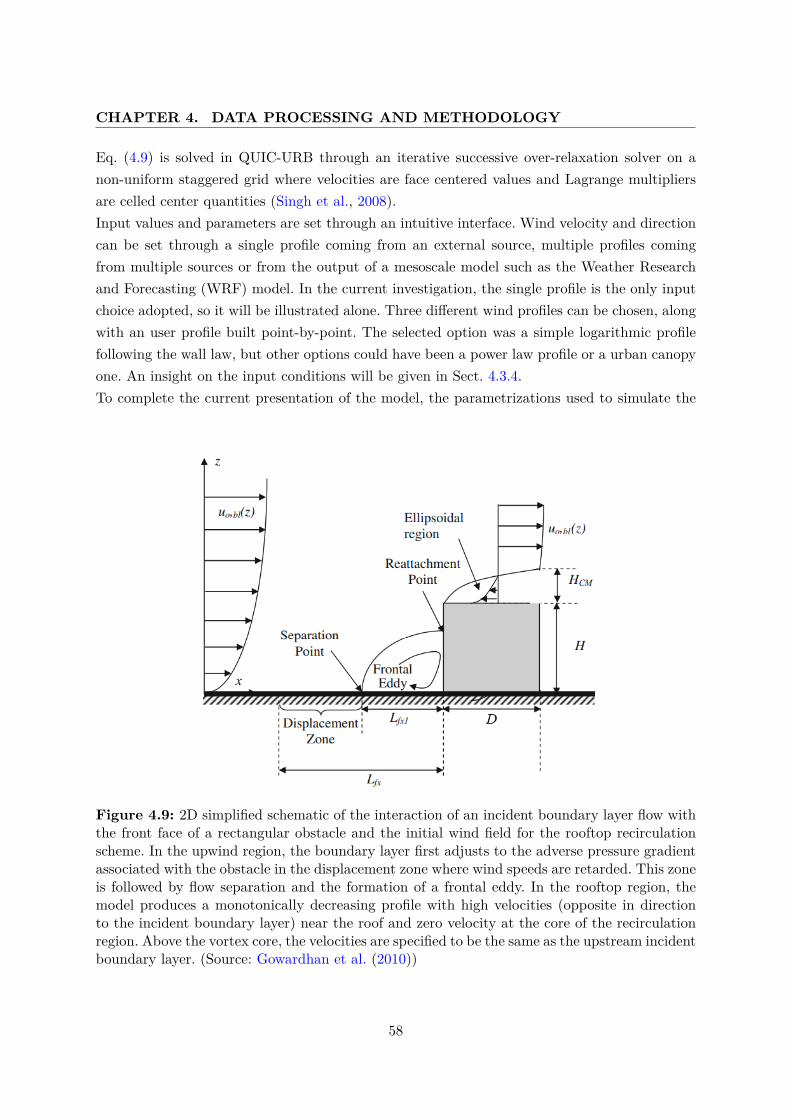
CHAPTER 4. DATA PROCESSING AND METHODOLOGY
Eq. (4.9) is solved in QUIC-URB through an iterative successive over-relaxation solver on anon-uniform staggered grid where velocities are face centered values and Lagrange multipliersare celled center quantities (Singh et al., 2008).Input values and parameters are set through an intuitive interface. Wind velocity and directioncan be set through a single profile coming from an external source, multiple profiles comingfrom multiple sources or from the output of a mesoscale model such as the Weather Researchand Forecasting (WRF) model. In the current investigation, the single profile is the only inputchoice adopted, so it will be illustrated alone. Three different wind profiles can be chosen, alongwith an user profile built point-by-point. The selected option was a simple logarithmic profilefollowing the wall law, but other options could have been a power law profile or a urban canopyone. An insight on the input conditions will be given in Sect. 4.3.4.To complete the current presentation of the model, the parametrizations used to simulate the
Figure 4.9: 2D simplified schematic of the interaction of an incident boundary layer flow withthe front face of a rectangular obstacle and the initial wind field for the rooftop recirculationscheme. In the upwind region, the boundary layer first adjusts to the adverse pressure gradientassociated with the obstacle in the displacement zone where wind speeds are retarded. This zoneis followed by flow separation and the formation of a frontal eddy. In the rooftop region, themodel produces a monotonically decreasing profile with high velocities (opposite in directionto the incident boundary layer) near the roof and zero velocity at the core of the recirculationregion. Above the vortex core, the velocities are specified to be the same as the upstream incidentboundary layer. (Source: Gowardhan et al. (2010))
58
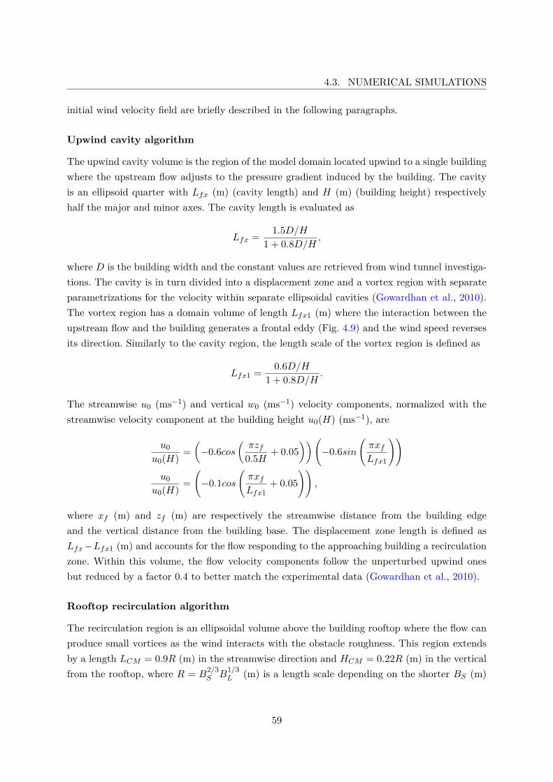
4.3. NUMERICAL SIMULATIONS
initial wind velocity field are briefly described in the following paragraphs.
Upwind cavity algorithm
The upwind cavity volume is the region of the model domain located upwind to a single buildingwhere the upstream flow adjusts to the pressure gradient induced by the building. The cavityis an ellipsoid quarter with Lfx (m) (cavity length) and H (m) (building height) respectivelyhalf the major and minor axes. The cavity length is evaluated as
Lfx = 1.5D/H1 + 0.8D/H ,
where D is the building width and the constant values are retrieved from wind tunnel investiga-tions. The cavity is in turn divided into a displacement zone and a vortex region with separateparametrizations for the velocity within separate ellipsoidal cavities (Gowardhan et al., 2010).The vortex region has a domain volume of length Lfx1 (m) where the interaction between theupstream flow and the building generates a frontal eddy (Fig. 4.9) and the wind speed reversesits direction. Similarly to the cavity region, the length scale of the vortex region is defined as
Lfx1 = 0.6D/H1 + 0.8D/H .
The streamwise u0 (ms−1) and vertical w0 (ms−1) velocity components, normalized with thestreamwise velocity component at the building height u0(H) (ms−1), are
u0u0(H) =
(−0.6cos
(πzf
0.5H + 0.05))(
−0.6sin(πxfLfx1
))u0
u0(H) =(−0.1cos
(πxfLfx1
+ 0.05))
,
where xf (m) and zf (m) are respectively the streamwise distance from the building edgeand the vertical distance from the building base. The displacement zone length is defined asLfx−Lfx1 (m) and accounts for the flow responding to the approaching building a recirculationzone. Within this volume, the flow velocity components follow the unperturbed upwind onesbut reduced by a factor 0.4 to better match the experimental data (Gowardhan et al., 2010).
Rooftop recirculation algorithm
The recirculation region is an ellipsoidal volume above the building rooftop where the flow canproduce small vortices as the wind interacts with the obstacle roughness. This region extendsby a length LCM = 0.9R (m) in the streamwise direction and HCM = 0.22R (m) in the verticalfrom the rooftop, where R = B
2/3S B
1/3L (m) is a length scale depending on the shorter BS (m)
59
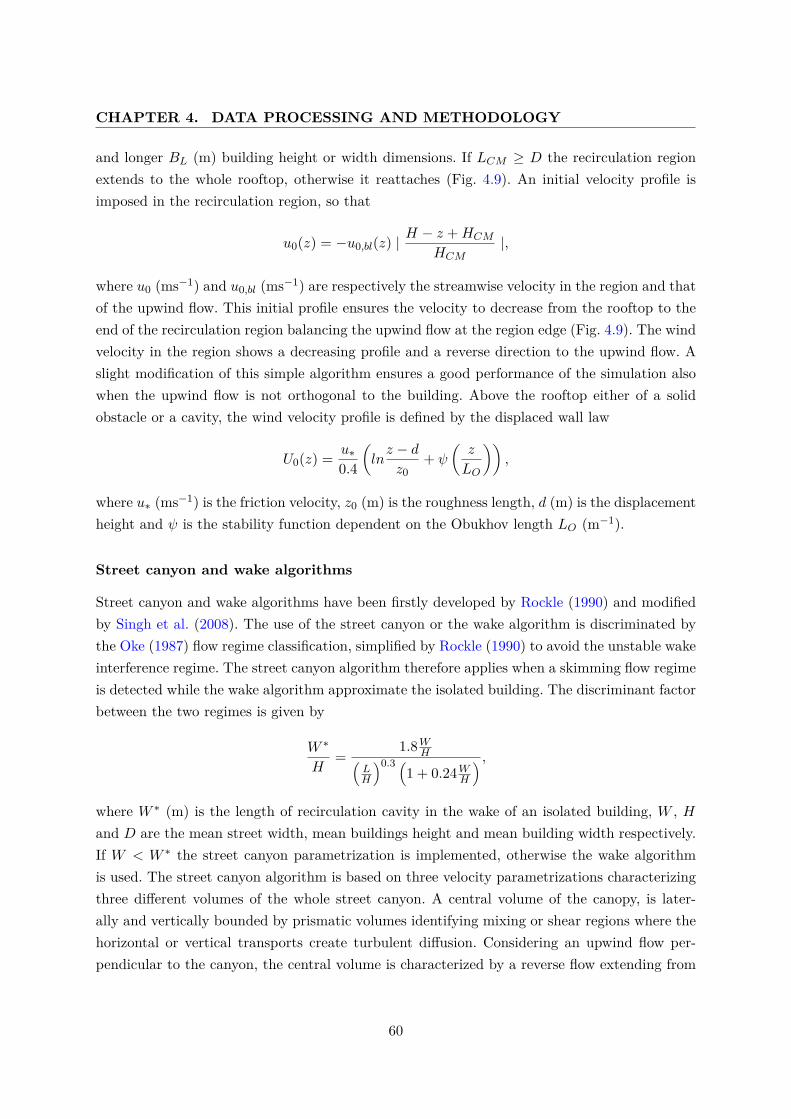
CHAPTER 4. DATA PROCESSING AND METHODOLOGY
and longer BL (m) building height or width dimensions. If LCM ≥ D the recirculation regionextends to the whole rooftop, otherwise it reattaches (Fig. 4.9). An initial velocity profile isimposed in the recirculation region, so that
u0(z) = −u0,bl(z) |H − z +HCM
HCM|,
where u0 (ms−1) and u0,bl (ms−1) are respectively the streamwise velocity in the region and thatof the upwind flow. This initial profile ensures the velocity to decrease from the rooftop to theend of the recirculation region balancing the upwind flow at the region edge (Fig. 4.9). The windvelocity in the region shows a decreasing profile and a reverse direction to the upwind flow. Aslight modification of this simple algorithm ensures a good performance of the simulation alsowhen the upwind flow is not orthogonal to the building. Above the rooftop either of a solidobstacle or a cavity, the wind velocity profile is defined by the displaced wall law
U0(z) = u∗0.4
(lnz − dz0
+ ψ
(z
LO
)),
where u∗ (ms−1) is the friction velocity, z0 (m) is the roughness length, d (m) is the displacementheight and ψ is the stability function dependent on the Obukhov length LO (m−1).
Street canyon and wake algorithms
Street canyon and wake algorithms have been firstly developed by Rockle (1990) and modifiedby Singh et al. (2008). The use of the street canyon or the wake algorithm is discriminated bythe Oke (1987) flow regime classification, simplified by Rockle (1990) to avoid the unstable wakeinterference regime. The street canyon algorithm therefore applies when a skimming flow regimeis detected while the wake algorithm approximate the isolated building. The discriminant factorbetween the two regimes is given by
W ∗
H=
1.8WH(LH
)0.3 (1 + 0.24WH
) ,where W ∗ (m) is the length of recirculation cavity in the wake of an isolated building, W , Hand D are the mean street width, mean buildings height and mean building width respectively.If W < W ∗ the street canyon parametrization is implemented, otherwise the wake algorithmis used. The street canyon algorithm is based on three velocity parametrizations characterizingthree different volumes of the whole street canyon. A central volume of the canopy, is later-ally and vertically bounded by prismatic volumes identifying mixing or shear regions where thehorizontal or vertical transports create turbulent diffusion. Considering an upwind flow per-pendicular to the canyon, the central volume is characterized by a reverse flow extending from
60
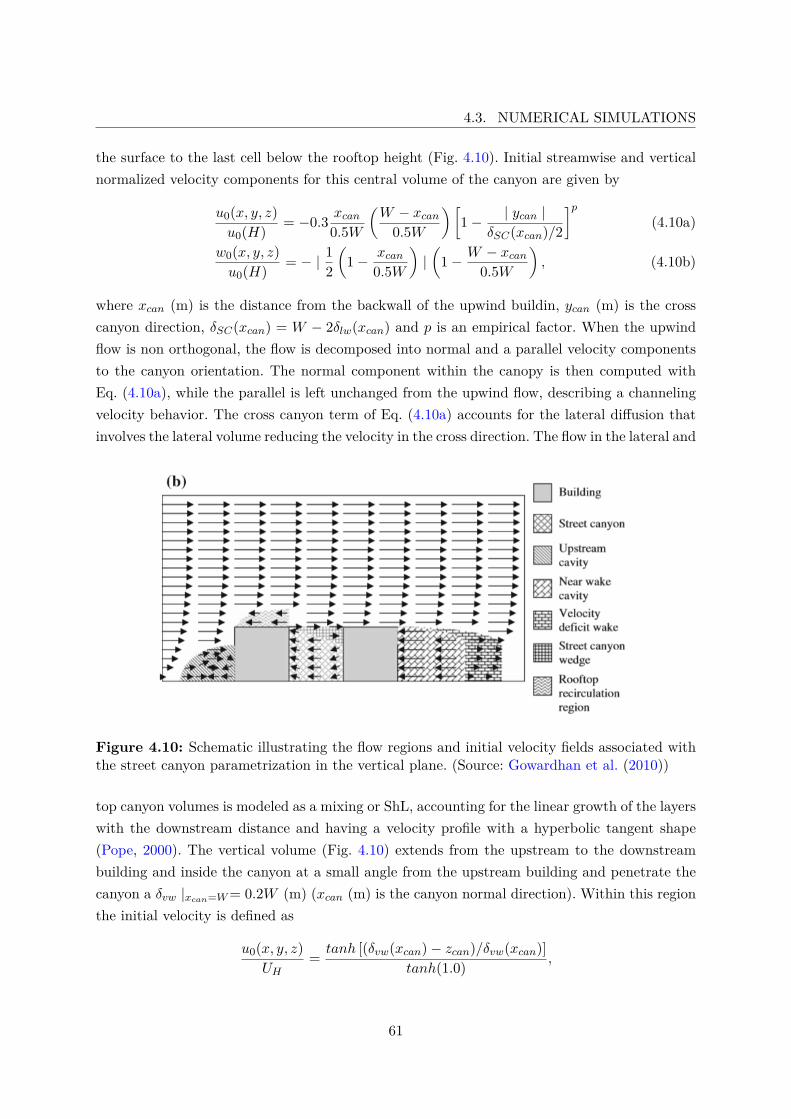
4.3. NUMERICAL SIMULATIONS
the surface to the last cell below the rooftop height (Fig. 4.10). Initial streamwise and verticalnormalized velocity components for this central volume of the canyon are given by
u0(x, y, z)u0(H) = −0.3 xcan0.5W
(W − xcan
0.5W
)[1− | ycan |
δSC(xcan)/2
]p(4.10a)
w0(x, y, z)u0(H) = − | 1
2
(1− xcan
0.5W
)|(
1− W − xcan0.5W
), (4.10b)
where xcan (m) is the distance from the backwall of the upwind buildin, ycan (m) is the crosscanyon direction, δSC(xcan) = W − 2δlw(xcan) and p is an empirical factor. When the upwindflow is non orthogonal, the flow is decomposed into normal and a parallel velocity componentsto the canyon orientation. The normal component within the canopy is then computed withEq. (4.10a), while the parallel is left unchanged from the upwind flow, describing a channelingvelocity behavior. The cross canyon term of Eq. (4.10a) accounts for the lateral diffusion thatinvolves the lateral volume reducing the velocity in the cross direction. The flow in the lateral and
Figure 4.10: Schematic illustrating the flow regions and initial velocity fields associated withthe street canyon parametrization in the vertical plane. (Source: Gowardhan et al. (2010))
top canyon volumes is modeled as a mixing or ShL, accounting for the linear growth of the layerswith the downstream distance and having a velocity profile with a hyperbolic tangent shape(Pope, 2000). The vertical volume (Fig. 4.10) extends from the upstream to the downstreambuilding and inside the canyon at a small angle from the upstream building and penetrate thecanyon a δvw |xcan=W= 0.2W (m) (xcan (m) is the canyon normal direction). Within this regionthe initial velocity is defined as
u0(x, y, z)UH
= tanh [(δvw(xcan)− zcan)/δvw(xcan)]tanh(1.0) ,
61
CHAPTER 4. DATA PROCESSING AND METHODOLOGY
Figure 4.11: Schematic illustrating the flow regions and initial velocity fields associated withthe street canyon parametrization in the horizontal plane. (Source: Gowardhan et al. (2010))
where UH (ms−1) is the reference velocity in the streamwise direction at the rooftop obtainedfrom a displaced logarithmic profile, zcan (m) is the vertical canyon direction and δvw |xcan=0.2xcan (m) is the linear approximation of the volume penetration depth. The lateral volume(Fig. 4.11) has the same shape of the vertical with maximum horizontal penetration widthδlw |xcan=W= 0.2W (m). Within this region the initial velocity is defined as
u0(x, y, z)u0,bl(z)
= 0.3 tanh [Ylw/δlw(xcan)]tanh(1.0) ,
where u0,bl(z) (ms−1) is the upwind velocity profile, δlw |xcan= 0.2xcan (m) is the width of thelateral volume and Ylw =| ycan | −δSC(xcan)/2 (m) is the isoline delimiting the street canyonvolume penetration into lateral volume.Downwind to the street canyon or an isolated building a wake region develops as a turbulentlayer (Kaplan and Dinar, 1996). The wake region develops as the upwind cavity region, witha near and a far volume based on the same principle but defined with a single velocity profile.The near volume has a streamwise dimension
Lw = W ∗
√√√√(1−(zcanH
)2)(
1−(ycanW
)2)− 0.5D
where the wind flow direction is reversed with respect to the upwind flow. The wake regionstreamwise length is defined as 3W ∗ and within this region the velocity is deflected with respect
62
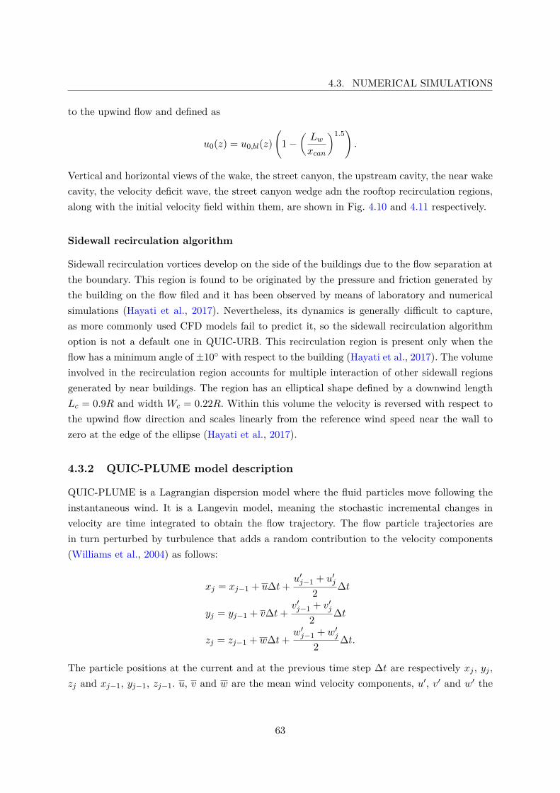
4.3. NUMERICAL SIMULATIONS
to the upwind flow and defined as
u0(z) = u0,bl(z)(
1−(Lwxcan
)1.5).
Vertical and horizontal views of the wake, the street canyon, the upstream cavity, the near wakecavity, the velocity deficit wave, the street canyon wedge adn the rooftop recirculation regions,along with the initial velocity field within them, are shown in Fig. 4.10 and 4.11 respectively.
Sidewall recirculation algorithm
Sidewall recirculation vortices develop on the side of the buildings due to the flow separation atthe boundary. This region is found to be originated by the pressure and friction generated bythe building on the flow filed and it has been observed by means of laboratory and numericalsimulations (Hayati et al., 2017). Nevertheless, its dynamics is generally difficult to capture,as more commonly used CFD models fail to predict it, so the sidewall recirculation algorithmoption is not a default one in QUIC-URB. This recirculation region is present only when theflow has a minimum angle of ±10◦ with respect to the building (Hayati et al., 2017). The volumeinvolved in the recirculation region accounts for multiple interaction of other sidewall regionsgenerated by near buildings. The region has an elliptical shape defined by a downwind lengthLc = 0.9R and width Wc = 0.22R. Within this volume the velocity is reversed with respect tothe upwind flow direction and scales linearly from the reference wind speed near the wall tozero at the edge of the ellipse (Hayati et al., 2017).
4.3.2 QUIC-PLUME model description
QUIC-PLUME is a Lagrangian dispersion model where the fluid particles move following theinstantaneous wind. It is a Langevin model, meaning the stochastic incremental changes invelocity are time integrated to obtain the flow trajectory. The flow particle trajectories arein turn perturbed by turbulence that adds a random contribution to the velocity components(Williams et al., 2004) as follows:
xj = xj−1 + u∆t+u′j−1 + u′j
2 ∆t
yj = yj−1 + v∆t+v′j−1 + v′j
2 ∆t
zj = zj−1 + w∆t+w′j−1 + w′j
2 ∆t.
The particle positions at the current and at the previous time step ∆t are respectively xj , yj ,zj and xj−1, yj−1, zj−1. u, v and w are the mean wind velocity components, u′, v′ and w′ the
63
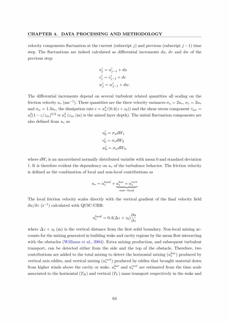
CHAPTER 4. DATA PROCESSING AND METHODOLOGY
velocity components fluctuation at the current (subscript j) and previous (subscript j−1) timestep. The fluctuations are indeed calculated as differential increments du, dv and dw of theprevious step:
u′j = u′j−1 + du
v′j = v′j−1 + dv
w′j = w′j−1 + dw.
The differential increments depend on several turbulent related quantities all scaling on thefriction velocity u∗ (ms−1). These quantities are the three velocity variances σu = 2u∗, σv = 2u∗and σw = 1.3u∗, the dissipation rate ε = u3
∗/(0.4(z+ z0)) and the shear stress component τuw =u2∗(1− z/zm)3/2 ≈ u2
∗ (zm (m) is the mixed layer depth). The initial fluctuation components arealso defined from u∗ as
u′0 = σudW1
v′0 = σvdW2
w′0 = σwdW3,
where dWi is an uncorrelated normally distributed variable with mean 0 and standard deviation1. It is therefore evident the dependency on u∗ of the turbulence behavior. The friction velocityis defined as the combination of local and non-local contributions as
u∗ = ulocal∗ + uhor∗ + uvert∗︸ ︷︷ ︸non−local
The local friction velocity scales directly with the vertical gradient of the final velocity field∂u/∂z (s−1) calculated with QUIC-URB:
ulocal∗ = 0.4(∆z + z0)∂u∂z
where ∆z + z0 (m) is the vertical distance from the first solid boundary. Non-local mixing ac-counts for the mixing generated in building wake and cavity regions by the mean flow interactingwith the obstacles (Williams et al., 2004). Extra mixing production, and subsequent turbulenttransport, can be detected either from the side and the top of the obstacle. Therefore, twocontributions are added to the total mixing to detect the horizontal mixing (uhor∗ ) produced byvertical axis eddies, and vertical mixing (uvert∗ ) produced by eddies that brought material downfrom higher winds above the cavity or wake. uhor∗ and uvert∗ are estimated from the time scaleassociated to the horizontal (TH) and vertical (TV ) mass transport respectively in the wake and
64
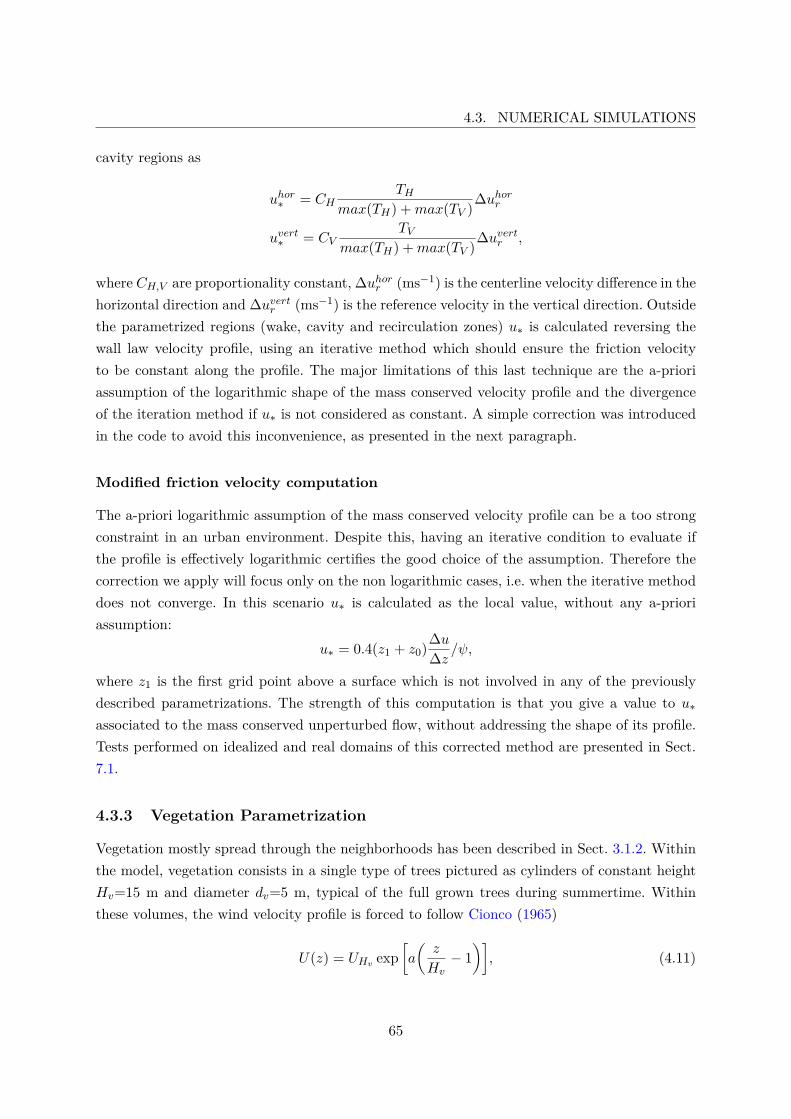
4.3. NUMERICAL SIMULATIONS
cavity regions as
uhor∗ = CHTH
max(TH) +max(TV )∆uhorr
uvert∗ = CVTV
max(TH) +max(TV )∆uvertr ,
where CH,V are proportionality constant, ∆uhorr (ms−1) is the centerline velocity difference in thehorizontal direction and ∆uvertr (ms−1) is the reference velocity in the vertical direction. Outsidethe parametrized regions (wake, cavity and recirculation zones) u∗ is calculated reversing thewall law velocity profile, using an iterative method which should ensure the friction velocityto be constant along the profile. The major limitations of this last technique are the a-prioriassumption of the logarithmic shape of the mass conserved velocity profile and the divergenceof the iteration method if u∗ is not considered as constant. A simple correction was introducedin the code to avoid this inconvenience, as presented in the next paragraph.
Modified friction velocity computation
The a-priori logarithmic assumption of the mass conserved velocity profile can be a too strongconstraint in an urban environment. Despite this, having an iterative condition to evaluate ifthe profile is effectively logarithmic certifies the good choice of the assumption. Therefore thecorrection we apply will focus only on the non logarithmic cases, i.e. when the iterative methoddoes not converge. In this scenario u∗ is calculated as the local value, without any a-prioriassumption:
u∗ = 0.4(z1 + z0)∆u∆z /ψ,
where z1 is the first grid point above a surface which is not involved in any of the previouslydescribed parametrizations. The strength of this computation is that you give a value to u∗associated to the mass conserved unperturbed flow, without addressing the shape of its profile.Tests performed on idealized and real domains of this corrected method are presented in Sect.7.1.
4.3.3 Vegetation Parametrization
Vegetation mostly spread through the neighborhoods has been described in Sect. 3.1.2. Withinthe model, vegetation consists in a single type of trees pictured as cylinders of constant heightHv=15 m and diameter dv=5 m, typical of the full grown trees during summertime. Withinthese volumes, the wind velocity profile is forced to follow Cionco (1965)
U(z) = UHv exp[a
(z
Hv− 1
)], (4.11)
65
CHAPTER 4. DATA PROCESSING AND METHODOLOGY
where UHv (ms−1) is the velocity above the top of the cylinder and a is the attenuation co-efficient. The attenuation coefficient is estimated from measurements, reversing the Eq. (4.11)
a =ln(U(z)/UH
)z/H − 1 , (4.12)
where U(z) (ms−1) is the average wind speed within RL during the analyzed period and UH(ms−1) is the average wind speed at the RL of LB during the analyzed period. The retrievedattenuation coefficient takes the value a=(1.7±0.3). To check the reliability of the coefficientvalue, a is used to calculate the vegetative drag coefficient Cv of an isolated tree in the domain.The integral of the difference between the mass conserved velocity profiles in a bare domainand within a tree retrieved from the same input conditions, gives a good estimation of the totaldrag force Ftot generated by the tree on the wind. From basic laws of fluid mechanics, the dragforce is proportional to the unperturbed wind velocity through a drag coefficient, which in thiscase is relative to the vegetation. From this law, Cv is retrieved as
Cv = 2FtotρAvfU
2tot
,
where ρ (kgm−3) is the air density, Avf (m2) is the frontal area of the tree and Utot is theunperturbed wind velocity integrated along the profile. Using this method, Cv=(0.24±0.4) inagreement with Jeanjean et al. (2017) and Di Sabatino et al. (2015), who found a value for Cvequal to 0.25 for the same tree species. Cv is then used to evaluate the vegetation porosity as
P =(1− Cv/1.08
)1/1.8,
as defined by Guan et al. (2003). Trees are found to be largely porous medium with P=(0.56±0.05).Both the porosity and the vegetation drag coefficient are used to calculate the total area fractioncoefficients following Kent et al. (2017), as it will be shown in Sect. 4.3.4. Here we will onlyfocus on the computation of the vegetation planar and frontal area Avp (m2) and Avf (m2). Avp isdefined as the circumference (radius r=2.5 m) area times the number n of trees in the domain,while Avf is taken as the maximum cylinder cross section
Avp = π · r2 · n
Avf = Hv · 2r · n.
Vegetation areas will be used in the following section to compute the total area fraction coeffi-cients.
66
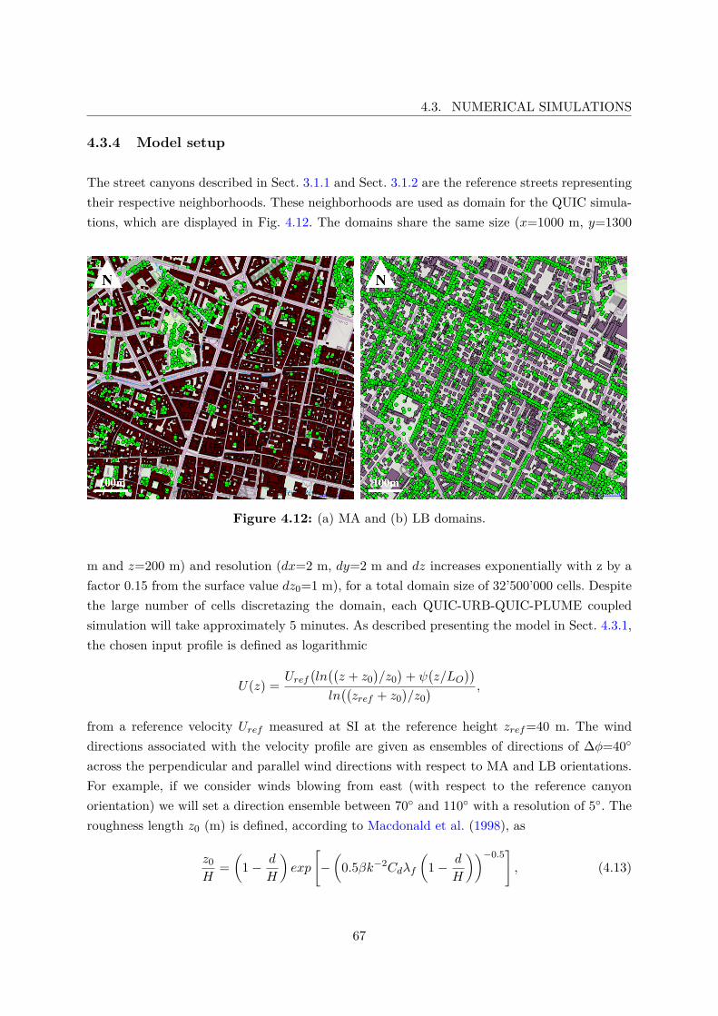
4.3. NUMERICAL SIMULATIONS
4.3.4 Model setup
The street canyons described in Sect. 3.1.1 and Sect. 3.1.2 are the reference streets representingtheir respective neighborhoods. These neighborhoods are used as domain for the QUIC simula-tions, which are displayed in Fig. 4.12. The domains share the same size (x=1000 m, y=1300
Figure 4.12: (a) MA and (b) LB domains.
m and z=200 m) and resolution (dx=2 m, dy=2 m and dz increases exponentially with z by afactor 0.15 from the surface value dz0=1 m), for a total domain size of 32’500’000 cells. Despitethe large number of cells discretazing the domain, each QUIC-URB-QUIC-PLUME coupledsimulation will take approximately 5 minutes. As described presenting the model in Sect. 4.3.1,the chosen input profile is defined as logarithmic
U(z) =Uref
(ln((z + z0
)/z0)
+ ψ(z/LO
))ln((zref + z0
)/z0) ,
from a reference velocity Uref measured at SI at the reference height zref=40 m. The winddirections associated with the velocity profile are given as ensembles of directions of ∆φ=40◦
across the perpendicular and parallel wind directions with respect to MA and LB orientations.For example, if we consider winds blowing from east (with respect to the reference canyonorientation) we will set a direction ensemble between 70◦ and 110◦ with a resolution of 5◦. Theroughness length z0 (m) is defined, according to Macdonald et al. (1998), as
z0H
=(
1− d
H
)exp
[−(
0.5βk−2Cdλf
(1− d
H
))−0.5], (4.13)
67
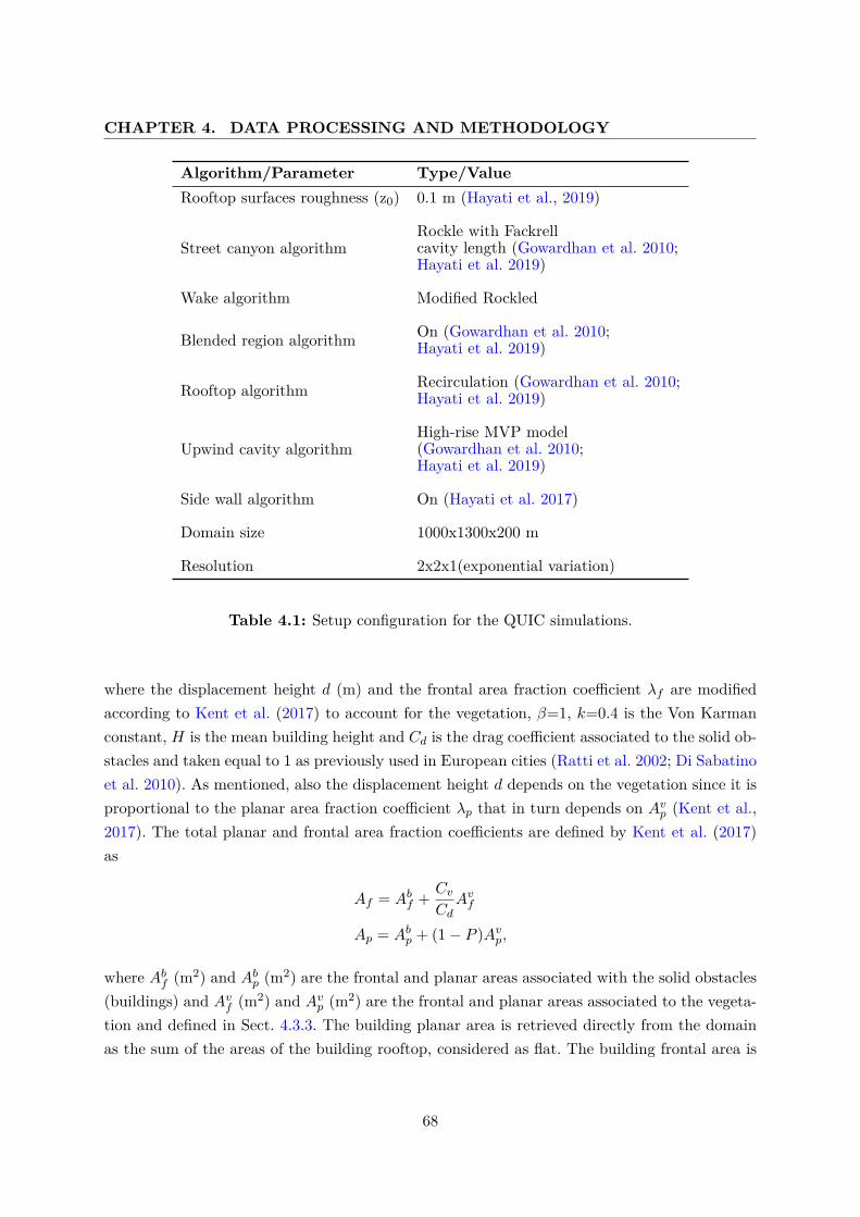
CHAPTER 4. DATA PROCESSING AND METHODOLOGY
Algorithm/Parameter Type/ValueRooftop surfaces roughness (z0) 0.1 m (Hayati et al., 2019)
Street canyon algorithmRockle with Fackrellcavity length (Gowardhan et al. 2010;Hayati et al. 2019)
Wake algorithm Modified Rockled
Blended region algorithm On (Gowardhan et al. 2010;Hayati et al. 2019)
Rooftop algorithm Recirculation (Gowardhan et al. 2010;Hayati et al. 2019)
Upwind cavity algorithmHigh-rise MVP model(Gowardhan et al. 2010;Hayati et al. 2019)
Side wall algorithm On (Hayati et al. 2017)
Domain size 1000x1300x200 m
Resolution 2x2x1(exponential variation)
Table 4.1: Setup configuration for the QUIC simulations.
where the displacement height d (m) and the frontal area fraction coefficient λf are modifiedaccording to Kent et al. (2017) to account for the vegetation, β=1, k=0.4 is the Von Karmanconstant, H is the mean building height and Cd is the drag coefficient associated to the solid ob-stacles and taken equal to 1 as previously used in European cities (Ratti et al. 2002; Di Sabatinoet al. 2010). As mentioned, also the displacement height d depends on the vegetation since it isproportional to the planar area fraction coefficient λp that in turn depends on Avp (Kent et al.,2017). The total planar and frontal area fraction coefficients are defined by Kent et al. (2017)as
Af = Abf + CvCdAvf
Ap = Abp + (1− P )Avp,
where Abf (m2) and Abp (m2) are the frontal and planar areas associated with the solid obstacles(buildings) and Avf (m2) and Avp (m2) are the frontal and planar areas associated to the vegeta-tion and defined in Sect. 4.3.3. The building planar area is retrieved directly from the domainas the sum of the areas of the building rooftop, considered as flat. The building frontal area is
68
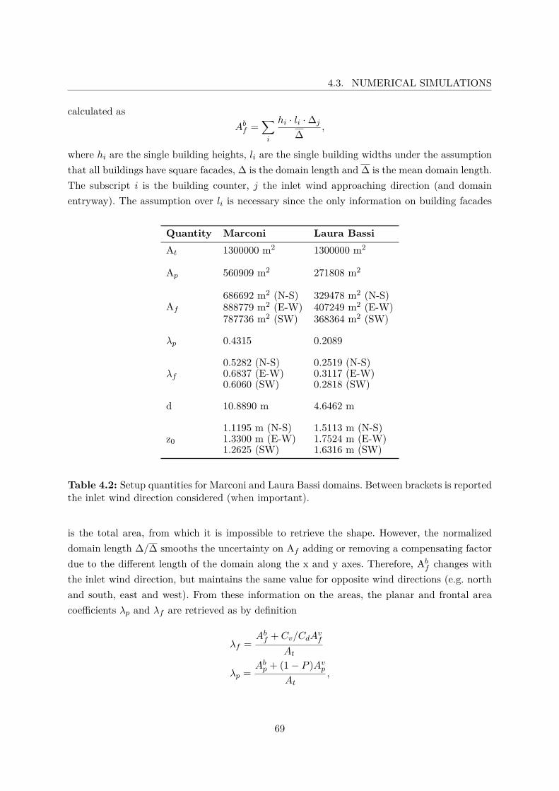
4.3. NUMERICAL SIMULATIONS
calculated asAbf =
∑i
hi · li ·∆j
∆,
where hi are the single building heights, li are the single building widths under the assumptionthat all buildings have square facades, ∆ is the domain length and ∆ is the mean domain length.The subscript i is the building counter, j the inlet wind approaching direction (and domainentryway). The assumption over li is necessary since the only information on building facades
Quantity Marconi Laura BassiAt 1300000 m2 1300000 m2
Ap 560909 m2 271808 m2
Af686692 m2 (N-S) 329478 m2 (N-S)888779 m2 (E-W) 407249 m2 (E-W)787736 m2 (SW) 368364 m2 (SW)
λp 0.4315 0.2089
λf
0.5282 (N-S) 0.2519 (N-S)0.6837 (E-W) 0.3117 (E-W)0.6060 (SW) 0.2818 (SW)
d 10.8890 m 4.6462 m
z01.1195 m (N-S) 1.5113 m (N-S)1.3300 m (E-W) 1.7524 m (E-W)1.2625 (SW) 1.6316 m (SW)
Table 4.2: Setup quantities for Marconi and Laura Bassi domains. Between brackets is reportedthe inlet wind direction considered (when important).
is the total area, from which it is impossible to retrieve the shape. However, the normalizeddomain length ∆/∆ smooths the uncertainty on Af adding or removing a compensating factordue to the different length of the domain along the x and y axes. Therefore, Abf changes withthe inlet wind direction, but maintains the same value for opposite wind directions (e.g. northand south, east and west). From these information on the areas, the planar and frontal areacoefficients λp and λf are retrieved as by definition
λf =Abf + Cv/CdA
vf
At
λp =Abp + (1− P )Avp
At,
69
CHAPTER 4. DATA PROCESSING AND METHODOLOGY
where At (m2) is the total area of the domain. λp is then used to compute the displacementheight d as defined by Macdonald et al. (1998)
d = H[1 + 4.43−λp (λp − 1)
].
Tab. 4.2 stores the values computed for the defined quantities.QUIC-PLUME needs input values to compute realistic turbulent quantities. Reference surfacetemperatures are retrieved from the ground level thermohygrometers deployed in the streets.Reference air temperature and humidity are taken from SI. Eventually, the boundary layerheight is measured with the ceilometer located in IS. A list of the parametrizations used in themodel is given in Tab. 4.1.
4.4 Summary and Conclusions
In this chapter, the approach to data analysis and modeling was described. Data processing hasbeen briefly described to define the experimental protocol used to check, clean and (for windvelocity components) rotate the measured data. After an initial check on the reliable ranges ofthe raw data, data gaps and unmeasured values have been replaced by the mean on the 5-minuteinterval they are included in. 5-minute interval which has also been chosen as averaging periodto ensure the robustness of the results without loosing the quick turbulent events. A despikingprocedure has been performed to remove the outliers from the high resolution sonic anemometerdata, which has subsequently been double rotated to align the coordinate system to the windstreamline direction.Following the data processing, the methodology for the data analysis has been presented. Firstthe most suitable period has been identify for both experimental field campaigns, based on thechoice of weak synoptic conditions characterized by thermal stability at large scale and smalllocal wind speed in the UBL. Then the analysis method has been described, introducing thediagnostic time scales and exchange rates that will characterize the analysis of the exchangeprocesses and their implications on normalized CO concentrations removal. The time scales havebeen defined as the mixing times associated with the momentum and heat exchanges betweendifferent atmospheric layers within the canopy and throughout the rooftop interface. The ex-change rates have been defined as the ratios between the time scales within the canopy and theones above it, addressing the mixing efficacy of momentum and heat in the SL. The exchangerates have also been identified as describing factors of pollutant removal from the UCL. Toevalute the previous hypothesis, the pollutant concentration has been normalization to removethe emission source, mean flow and geometrical contributions on the measurements. The wholemethodology will be used for the data analysis in Sect. 6After the methodology for the data analysis, the approximated CFD model QUIC used to eval-
70
4.4. SUMMARY AND CONCLUSIONS
uate the numerical investigation of this study have been introduced. Both its main components,i.e. QUIC-URB and QUIC-PLUME, have been described, focusing on the physical principlesthat regulates their functioning and on the algorithms required to combine reliable results tohigh computational performances. Being the focus of the numerical investigation, a dedicatedsection has been used to fully describe the parametrization of vegetation in the model, whichis represented as porous cylinder where the wind speed profile is attenuated by the flow-leavesinteractions.Finally, the model setup for the numerical investigations has been given. To enhance the re-liability of the simulations, the most updated alghoritms and parametrizations in QUIC havebeen used, along with the choice of simulating a large domain around the reference MA and LBcanyons to capture the neighborhood scale dynamics. Wind direction ensembles have been cho-sen to be representative of each input wind directions, to better capture most of the variabilityassociated to the measured wind direction oscillations. Given the described model and setup,the results from the numerical simulations will be shown in Sect. 7.
71

Chapter 5
Results and Discussion: Observationsand Campaign Comparison
In this chapter, an overview of the campaigns results is presented and detailed focusing on themean characteristics of the background flow, local circulation, turbulence and air quality in thetwo reference street canyons. The mean behaviors of the most representative meteorologicaland air quality variables will be presented to characterize the reference street canyons andsurrounding neighborhoods during both the investigated seasons. A preliminary inter-seasonalcomparison is also presented, to address the seasonal dependency of the investigated quantities.For what concern air quality, the pollutant concentrations are compared with the permanentmonitoring network data to assess the impact of a close environment, such as the urban canyon,to the measured concentrations. The background flow will be compared to the local in-canyonmean meteorological characteristics, to address the implication of the investigated environmenton the mean atmospheric flows. Meteorological and turbulent data measured within the referencecanyons will focus on the weak synoptic periods defined in Sect. 4.2.1, so that summer campaigndata corresponds to the 20-23 September and winter campaign data to 08-09 February, to assessthe local flow and turbulence characteristics and behaviors during weak synoptic conditions.Conversely, to have a more complete and general assessment of the city scale dynamics, itworths to present a comparison of the selected period characteristics with the mean campaignones.
5.1 Mean Characteristics of the Summer Campaign
5.1.1 Pollutant Concentrations
Characteristic pollutant concentrations for the whole campaigns are presented by means ofboxplot and usefull statistics (summarized in Tab. 5.1 and 5.2 for the summer and winter cam-
73
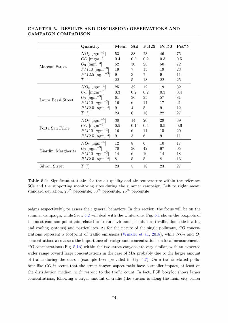
CHAPTER 5. RESULTS AND DISCUSSION: OBSERVATIONS ANDCAMPAIGN COMPARISON
Quantity Mean Std Pct25 Pct50 Pct75
Marconi Street
NO2 [µgm−3] 53 38 23 46 75CO [mgm−3] 0.4 0.3 0.2 0.3 0.5O3 [µgm−3] 52 30 28 50 72PM10 [µgm−3] 19 7 15 19 23PM2.5 [µgm−3] 9 3 7 9 11T [◦] 22 5 18 22 25
Laura Bassi Street
NO2 [µgm−3] 25 32 12 19 32CO [mgm−3] 0.3 0.2 0.2 0.3 0.4O3 [µgm−3] 61 36 35 57 81PM10 [µgm−3] 16 6 11 17 21PM2.5 [µgm−3] 9 4 5 9 12T [◦] 23 6 18 22 27
Porta San Felice
NO2 [µgm−3] 30 14 20 29 39CO [mgm−3] 0.5 0.14 0.4 0.5 0.6PM10 [µgm−3] 16 6 11 15 20PM2.5 [µgm−3] 9 3 6 9 11
Giardini Margherita
NO2 [µgm−3] 12 8 6 10 17O3 [µgm−3] 70 36 42 67 95PM10 [µgm−3] 14 6 10 14 18PM2.5 [µgm−3] 8 5 5 8 13
Silvani Street T [◦] 23 5 18 23 27
Table 5.1: Significant statistics for the air quality and air temperature within the referenceSCs and the supporting monitoring sites during the summer campaign. Left to right: mean,standard deviation, 25th percentile, 50th percentile, 75th percentile
paigns respectively), to assess their general behaviors. In this section, the focus will be on thesummer campaign, while Sect. 5.2 will deal with the winter one. Fig. 5.1 shows the boxplots ofthe most common pollutants related to urban environment emissions (traffic, domestic heatingand cooling systems) and particulates. As for the nature of the single pollutant, CO concen-trations represent a footprint of traffic emissions (Winkler et al., 2018), while NO2 and O3
concentrations also assess the importance of background concentrations on local measurements.CO concentrations (Fig. 5.1b) within the two street canyons are very similar, with an expectedwider range toward large concentrations in the case of MA probably due to the larger amountof traffic during the season (example been provided in Fig. 4.7). On a traffic related pollu-tant like CO it seems that the street canyon aspect ratio have a smaller impact, at least onthe distribution median, with respect to the traffic count. In fact, PSF boxplot shows largerconcentrations, following a larger amount of traffic (the station is along the main city center
74
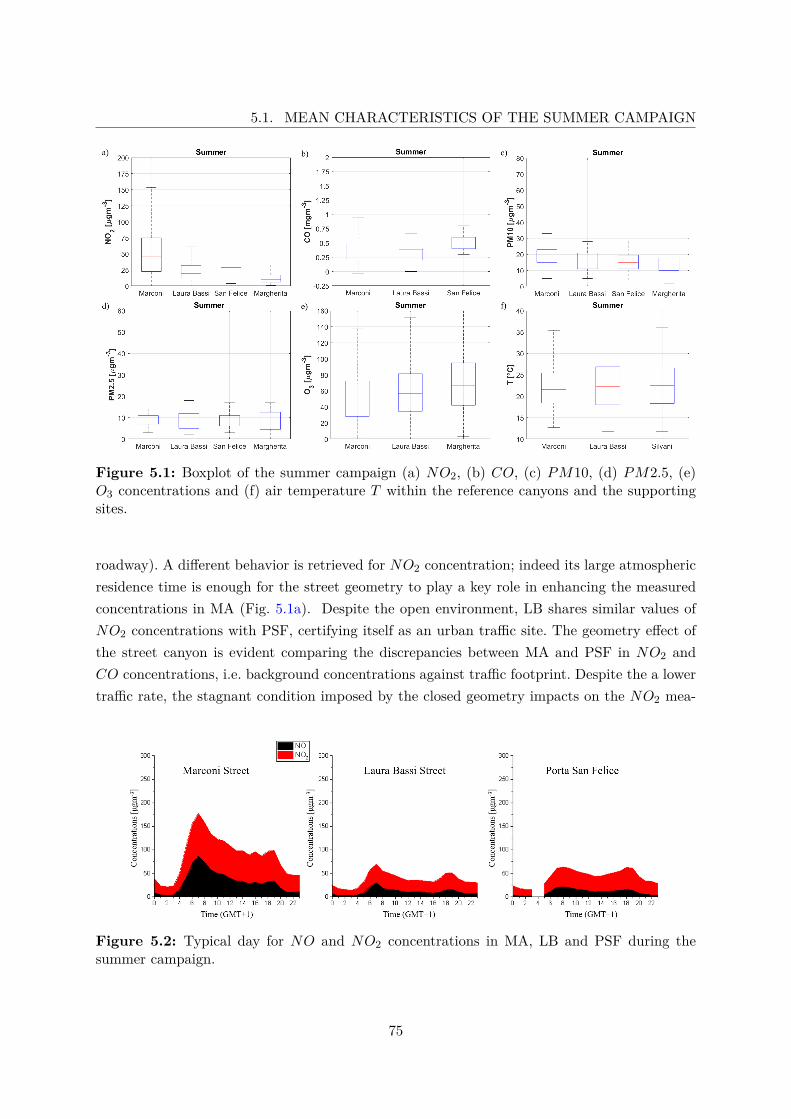
5.1. MEAN CHARACTERISTICS OF THE SUMMER CAMPAIGN
Figure 5.1: Boxplot of the summer campaign (a) NO2, (b) CO, (c) PM10, (d) PM2.5, (e)O3 concentrations and (f) air temperature T within the reference canyons and the supportingsites.
roadway). A different behavior is retrieved for NO2 concentration; indeed its large atmosphericresidence time is enough for the street geometry to play a key role in enhancing the measuredconcentrations in MA (Fig. 5.1a). Despite the open environment, LB shares similar values ofNO2 concentrations with PSF, certifying itself as an urban traffic site. The geometry effect ofthe street canyon is evident comparing the discrepancies between MA and PSF in NO2 andCO concentrations, i.e. background concentrations against traffic footprint. Despite the a lowertraffic rate, the stagnant condition imposed by the closed geometry impacts on the NO2 mea-
Figure 5.2: Typical day for NO and NO2 concentrations in MA, LB and PSF during thesummer campaign.
75
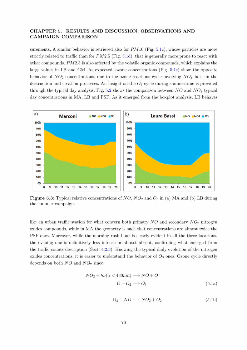
CHAPTER 5. RESULTS AND DISCUSSION: OBSERVATIONS ANDCAMPAIGN COMPARISON
surements. A similar behavior is retrieved also for PM10 (Fig. 5.1c), whose particles are morestrictly related to traffic than for PM2.5 (Fig. 5.1d), that is generally more prone to react withother compounds. PM2.5 is also affected by the volatile organic compounds, which explains thelarge values in LB and GM. As expected, ozone concentrations (Fig. 5.1e) show the oppositebehavior of NO2 concentrations, due to the ozone reactions cycle involving NOx both in thedestruction and creation processes. An insight on the O3 cycle during summertime is providedthrough the typical day analysis. Fig. 5.2 shows the comparison between NO and NO2 typicalday concentrations in MA, LB and PSF. As it emerged from the boxplot analysis, LB behaves
Figure 5.3: Typical relative concentrations of NO, NO2 and O3 in (a) MA and (b) LB duringthe summer campaign.
like an urban traffic station for what concern both primary NO and secondary NO2 nitrogenoxides compounds, while in MA the geometry is such that concentrations are almost twice thePSF ones. Moreover, while the morning rush hour is clearly evident in all the three locations,the evening one is definitively less intense or almost absent, confirming what emerged fromthe traffic counts description (Sect. 4.2.3). Knowing the typical daily evolution of the nitrogenoxides concentrations, it is easier to understand the behavior of O3 ones. Ozone cycle directlydepends on both NO and NO2 since
NO2 + hν(λ < 430nm) −→ NO +O
O +O2 −→ O3 (5.1a)
O3 +NO −→ NO2 +O2 (5.1b)
76
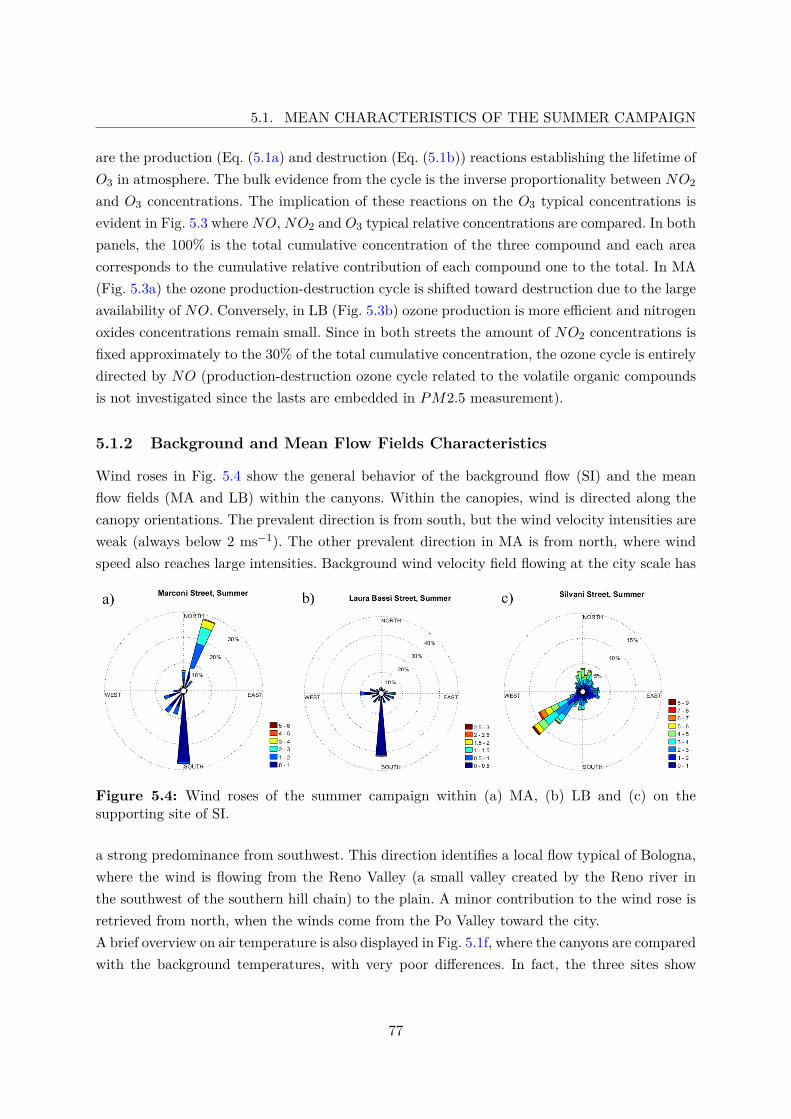
5.1. MEAN CHARACTERISTICS OF THE SUMMER CAMPAIGN
are the production (Eq. (5.1a) and destruction (Eq. (5.1b)) reactions establishing the lifetime ofO3 in atmosphere. The bulk evidence from the cycle is the inverse proportionality between NO2
and O3 concentrations. The implication of these reactions on the O3 typical concentrations isevident in Fig. 5.3 where NO, NO2 and O3 typical relative concentrations are compared. In bothpanels, the 100% is the total cumulative concentration of the three compound and each areacorresponds to the cumulative relative contribution of each compound one to the total. In MA(Fig. 5.3a) the ozone production-destruction cycle is shifted toward destruction due to the largeavailability of NO. Conversely, in LB (Fig. 5.3b) ozone production is more efficient and nitrogenoxides concentrations remain small. Since in both streets the amount of NO2 concentrations isfixed approximately to the 30% of the total cumulative concentration, the ozone cycle is entirelydirected by NO (production-destruction ozone cycle related to the volatile organic compoundsis not investigated since the lasts are embedded in PM2.5 measurement).
5.1.2 Background and Mean Flow Fields Characteristics
Wind roses in Fig. 5.4 show the general behavior of the background flow (SI) and the meanflow fields (MA and LB) within the canyons. Within the canopies, wind is directed along thecanopy orientations. The prevalent direction is from south, but the wind velocity intensities areweak (always below 2 ms−1). The other prevalent direction in MA is from north, where windspeed also reaches large intensities. Background wind velocity field flowing at the city scale has
Figure 5.4: Wind roses of the summer campaign within (a) MA, (b) LB and (c) on thesupporting site of SI.
a strong predominance from southwest. This direction identifies a local flow typical of Bologna,where the wind is flowing from the Reno Valley (a small valley created by the Reno river inthe southwest of the southern hill chain) to the plain. A minor contribution to the wind rose isretrieved from north, when the winds come from the Po Valley toward the city.A brief overview on air temperature is also displayed in Fig. 5.1f, where the canyons are comparedwith the background temperatures, with very poor differences. In fact, the three sites show
77
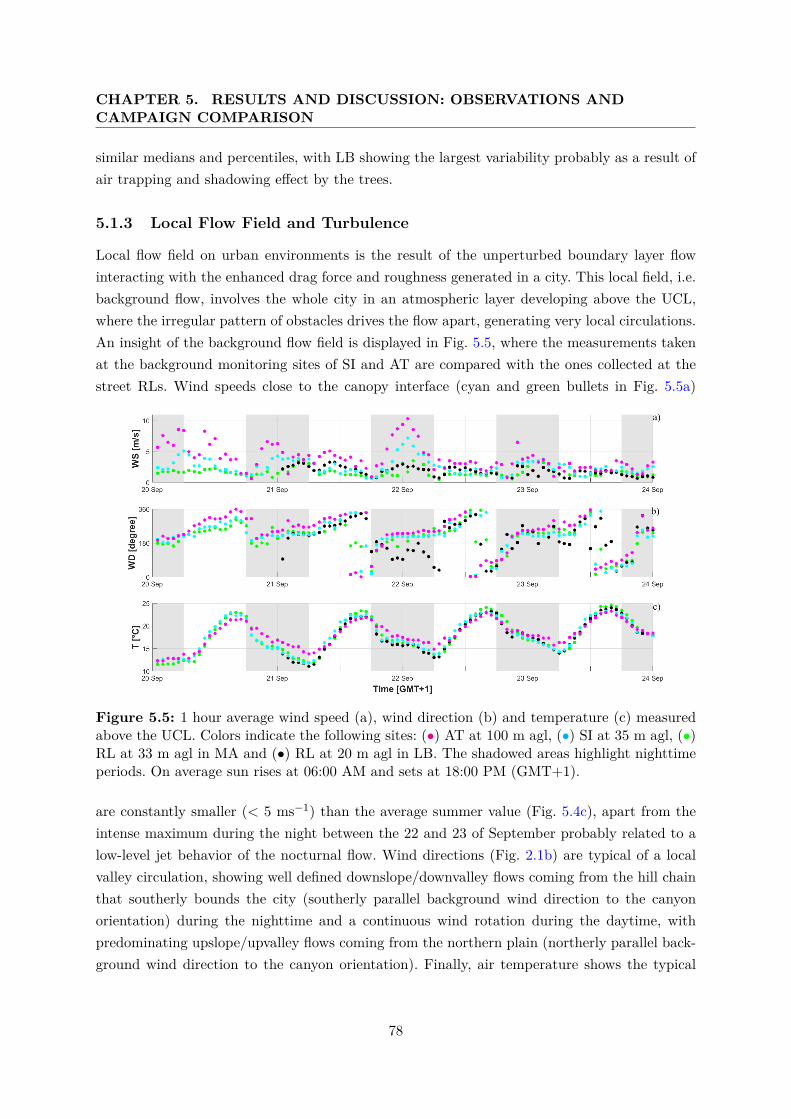
CHAPTER 5. RESULTS AND DISCUSSION: OBSERVATIONS ANDCAMPAIGN COMPARISON
similar medians and percentiles, with LB showing the largest variability probably as a result ofair trapping and shadowing effect by the trees.
5.1.3 Local Flow Field and Turbulence
Local flow field on urban environments is the result of the unperturbed boundary layer flowinteracting with the enhanced drag force and roughness generated in a city. This local field, i.e.background flow, involves the whole city in an atmospheric layer developing above the UCL,where the irregular pattern of obstacles drives the flow apart, generating very local circulations.An insight of the background flow field is displayed in Fig. 5.5, where the measurements takenat the background monitoring sites of SI and AT are compared with the ones collected at thestreet RLs. Wind speeds close to the canopy interface (cyan and green bullets in Fig. 5.5a)
Figure 5.5: 1 hour average wind speed (a), wind direction (b) and temperature (c) measuredabove the UCL. Colors indicate the following sites: (•) AT at 100 m agl, (•) SI at 35 m agl, (•)RL at 33 m agl in MA and (•) RL at 20 m agl in LB. The shadowed areas highlight nighttimeperiods. On average sun rises at 06:00 AM and sets at 18:00 PM (GMT+1).
are constantly smaller (< 5 ms−1) than the average summer value (Fig. 5.4c), apart from theintense maximum during the night between the 22 and 23 of September probably related to alow-level jet behavior of the nocturnal flow. Wind directions (Fig. 2.1b) are typical of a localvalley circulation, showing well defined downslope/downvalley flows coming from the hill chainthat southerly bounds the city (southerly parallel background wind direction to the canyonorientation) during the nighttime and a continuous wind rotation during the daytime, withpredominating upslope/upvalley flows coming from the northern plain (northerly parallel back-ground wind direction to the canyon orientation). Finally, air temperature shows the typical
78
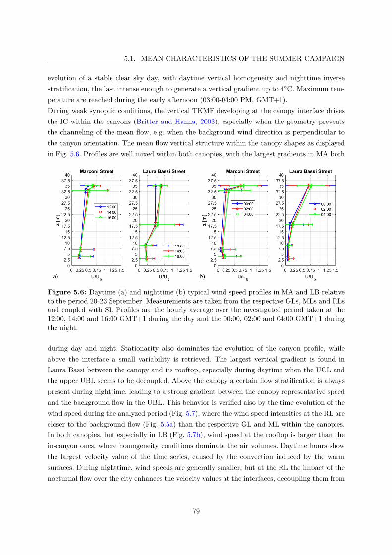
5.1. MEAN CHARACTERISTICS OF THE SUMMER CAMPAIGN
evolution of a stable clear sky day, with daytime vertical homogeneity and nighttime inversestratification, the last intense enough to generate a vertical gradient up to 4◦C. Maximum tem-perature are reached during the early afternoon (03:00-04:00 PM, GMT+1).During weak synoptic conditions, the vertical TKMF developing at the canopy interface drivesthe IC within the canyons (Britter and Hanna, 2003), especially when the geometry preventsthe channeling of the mean flow, e.g. when the background wind direction is perpendicular tothe canyon orientation. The mean flow vertical structure within the canopy shapes as displayedin Fig. 5.6. Profiles are well mixed within both canopies, with the largest gradients in MA both
Figure 5.6: Daytime (a) and nighttime (b) typical wind speed profiles in MA and LB relativeto the period 20-23 September. Measurements are taken from the respective GLs, MLs and RLsand coupled with SI. Profiles are the hourly average over the investigated period taken at the12:00, 14:00 and 16:00 GMT+1 during the day and the 00:00, 02:00 and 04:00 GMT+1 duringthe night.
during day and night. Stationarity also dominates the evolution of the canyon profile, whileabove the interface a small variability is retrieved. The largest vertical gradient is found inLaura Bassi between the canopy and its rooftop, especially during daytime when the UCL andthe upper UBL seems to be decoupled. Above the canopy a certain flow stratification is alwayspresent during nighttime, leading to a strong gradient between the canopy representative speedand the background flow in the UBL. This behavior is verified also by the time evolution of thewind speed during the analyzed period (Fig. 5.7), where the wind speed intensities at the RL arecloser to the background flow (Fig. 5.5a) than the respective GL and ML within the canopies.In both canopies, but especially in LB (Fig. 5.7b), wind speed at the rooftop is larger than thein-canyon ones, where homogeneity conditions dominate the air volumes. Daytime hours showthe largest velocity value of the time series, caused by the convection induced by the warmsurfaces. During nighttime, wind speeds are generally smaller, but at the RL the impact of thenocturnal flow over the city enhances the velocity values at the interfaces, decoupling them from
79
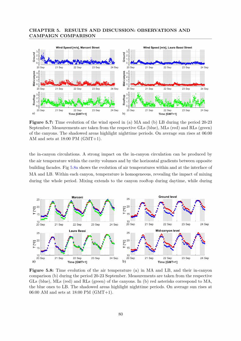
CHAPTER 5. RESULTS AND DISCUSSION: OBSERVATIONS ANDCAMPAIGN COMPARISON
Figure 5.7: Time evolution of the wind speed in (a) MA and (b) LB during the period 20-23September. Measurements are taken from the respective GLs (blue), MLs (red) and RLs (green)of the canyons. The shadowed areas highlight nighttime periods. On average sun rises at 06:00AM and sets at 18:00 PM (GMT+1).
the in-canyon circulations. A strong impact on the in-canyon circulation can be produced bythe air temperature within the cavity volumes and by the horizontal gradients between oppositebuilding facades. Fig 5.8a shows the evolution of air temperatures within and at the interface ofMA and LB. Within each canyon, temperature is homogeneous, revealing the impact of mixingduring the whole period. Mixing extends to the canyon rooftop during daytime, while during
Figure 5.8: Time evolution of the air temperature (a) in MA and LB, and their in-canyoncomparison (b) during the period 20-23 September. Measurements are taken from the respectiveGLs (blue), MLs (red) and RLs (green) of the canyons. In (b) red asterisks correspond to MA,the blue ones to LB. The shadowed areas highlight nighttime periods. On average sun rises at06:00 AM and sets at 18:00 PM (GMT+1).
80
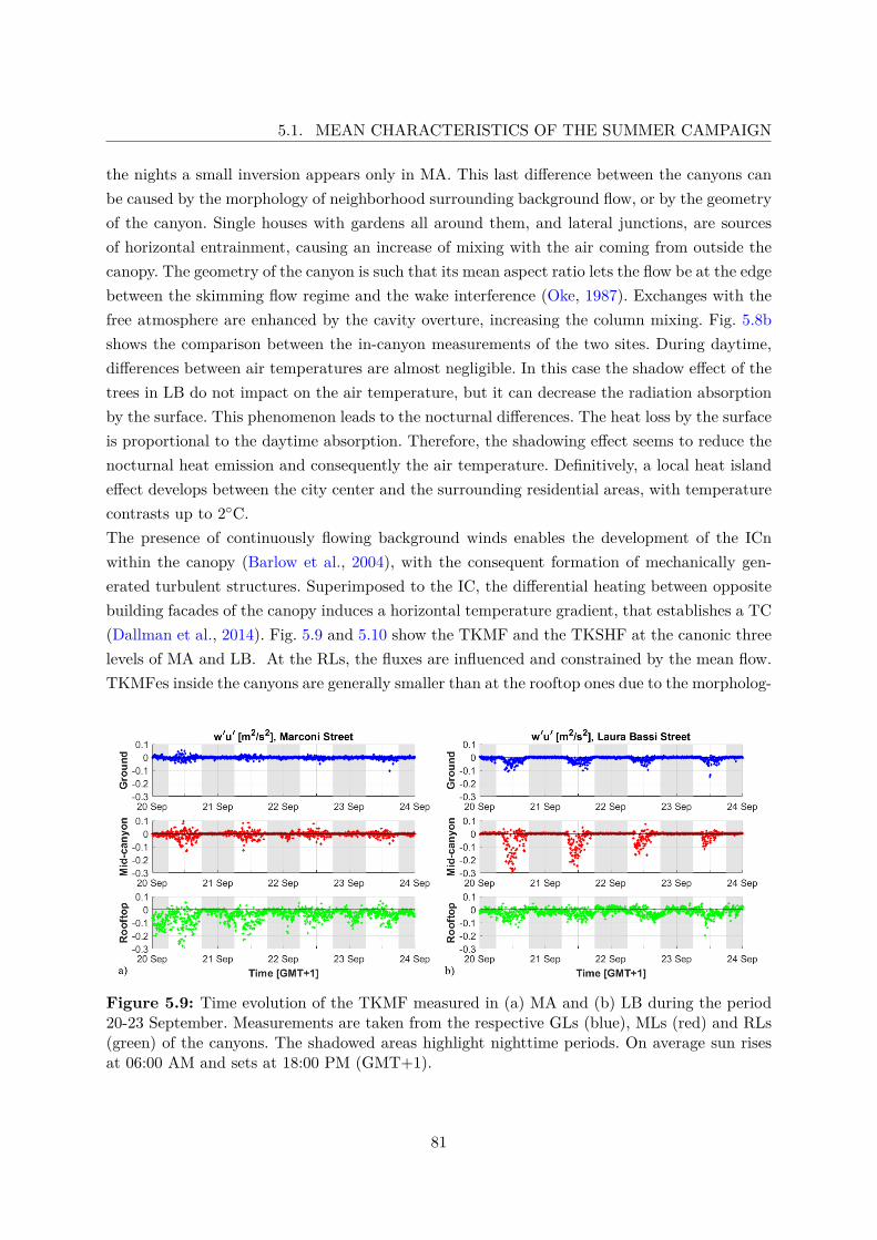
5.1. MEAN CHARACTERISTICS OF THE SUMMER CAMPAIGN
the nights a small inversion appears only in MA. This last difference between the canyons canbe caused by the morphology of neighborhood surrounding background flow, or by the geometryof the canyon. Single houses with gardens all around them, and lateral junctions, are sourcesof horizontal entrainment, causing an increase of mixing with the air coming from outside thecanopy. The geometry of the canyon is such that its mean aspect ratio lets the flow be at the edgebetween the skimming flow regime and the wake interference (Oke, 1987). Exchanges with thefree atmosphere are enhanced by the cavity overture, increasing the column mixing. Fig. 5.8bshows the comparison between the in-canyon measurements of the two sites. During daytime,differences between air temperatures are almost negligible. In this case the shadow effect of thetrees in LB do not impact on the air temperature, but it can decrease the radiation absorptionby the surface. This phenomenon leads to the nocturnal differences. The heat loss by the surfaceis proportional to the daytime absorption. Therefore, the shadowing effect seems to reduce thenocturnal heat emission and consequently the air temperature. Definitively, a local heat islandeffect develops between the city center and the surrounding residential areas, with temperaturecontrasts up to 2◦C.The presence of continuously flowing background winds enables the development of the ICnwithin the canopy (Barlow et al., 2004), with the consequent formation of mechanically gen-erated turbulent structures. Superimposed to the IC, the differential heating between oppositebuilding facades of the canopy induces a horizontal temperature gradient, that establishes a TC(Dallman et al., 2014). Fig. 5.9 and 5.10 show the TKMF and the TKSHF at the canonic threelevels of MA and LB. At the RLs, the fluxes are influenced and constrained by the mean flow.TKMFes inside the canyons are generally smaller than at the rooftop ones due to the morpholog-
Figure 5.9: Time evolution of the TKMF measured in (a) MA and (b) LB during the period20-23 September. Measurements are taken from the respective GLs (blue), MLs (red) and RLs(green) of the canyons. The shadowed areas highlight nighttime periods. On average sun risesat 06:00 AM and sets at 18:00 PM (GMT+1).
81
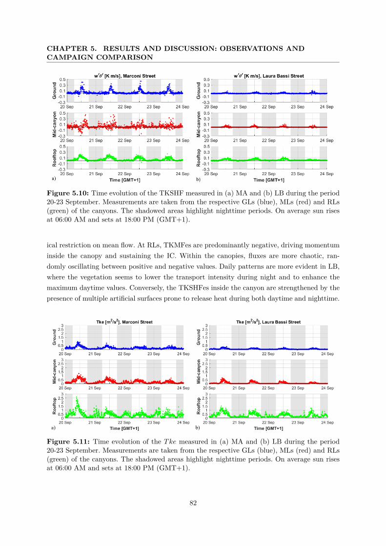
CHAPTER 5. RESULTS AND DISCUSSION: OBSERVATIONS ANDCAMPAIGN COMPARISON
Figure 5.10: Time evolution of the TKSHF measured in (a) MA and (b) LB during the period20-23 September. Measurements are taken from the respective GLs (blue), MLs (red) and RLs(green) of the canyons. The shadowed areas highlight nighttime periods. On average sun risesat 06:00 AM and sets at 18:00 PM (GMT+1).
ical restriction on mean flow. At RLs, TKMFes are predominantly negative, driving momentuminside the canopy and sustaining the IC. Within the canopies, fluxes are more chaotic, ran-domly oscillating between positive and negative values. Daily patterns are more evident in LB,where the vegetation seems to lower the transport intensity during night and to enhance themaximum daytime values. Conversely, the TKSHFes inside the canyon are strengthened by thepresence of multiple artificial surfaces prone to release heat during both daytime and nighttime.
Figure 5.11: Time evolution of the Tke measured in (a) MA and (b) LB during the period20-23 September. Measurements are taken from the respective GLs (blue), MLs (red) and RLs(green) of the canyons. The shadowed areas highlight nighttime periods. On average sun risesat 06:00 AM and sets at 18:00 PM (GMT+1).
82
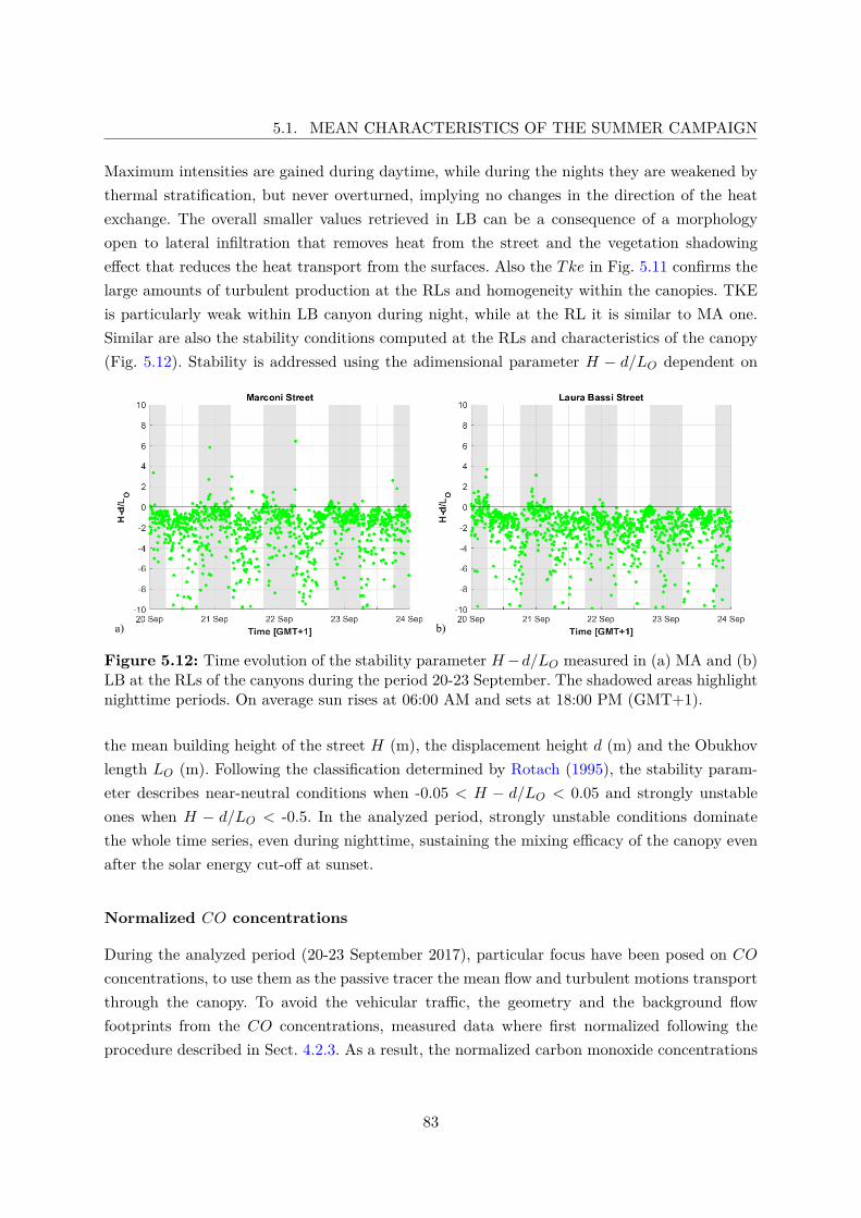
5.1. MEAN CHARACTERISTICS OF THE SUMMER CAMPAIGN
Maximum intensities are gained during daytime, while during the nights they are weakened bythermal stratification, but never overturned, implying no changes in the direction of the heatexchange. The overall smaller values retrieved in LB can be a consequence of a morphologyopen to lateral infiltration that removes heat from the street and the vegetation shadowingeffect that reduces the heat transport from the surfaces. Also the Tke in Fig. 5.11 confirms thelarge amounts of turbulent production at the RLs and homogeneity within the canopies. TKEis particularly weak within LB canyon during night, while at the RL it is similar to MA one.Similar are also the stability conditions computed at the RLs and characteristics of the canopy(Fig. 5.12). Stability is addressed using the adimensional parameter H − d/LO dependent on
Figure 5.12: Time evolution of the stability parameter H−d/LO measured in (a) MA and (b)LB at the RLs of the canyons during the period 20-23 September. The shadowed areas highlightnighttime periods. On average sun rises at 06:00 AM and sets at 18:00 PM (GMT+1).
the mean building height of the street H (m), the displacement height d (m) and the Obukhovlength LO (m). Following the classification determined by Rotach (1995), the stability param-eter describes near-neutral conditions when -0.05 < H − d/LO < 0.05 and strongly unstableones when H − d/LO < -0.5. In the analyzed period, strongly unstable conditions dominatethe whole time series, even during nighttime, sustaining the mixing efficacy of the canopy evenafter the solar energy cut-off at sunset.
Normalized CO concentrations
During the analyzed period (20-23 September 2017), particular focus have been posed on COconcentrations, to use them as the passive tracer the mean flow and turbulent motions transportthrough the canopy. To avoid the vehicular traffic, the geometry and the background flowfootprints from the CO concentrations, measured data where first normalized following theprocedure described in Sect. 4.2.3. As a result, the normalized carbon monoxide concentrations
83
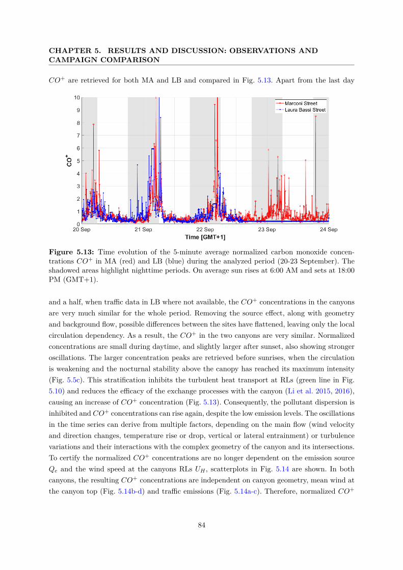
CHAPTER 5. RESULTS AND DISCUSSION: OBSERVATIONS ANDCAMPAIGN COMPARISON
CO+ are retrieved for both MA and LB and compared in Fig. 5.13. Apart from the last day
Figure 5.13: Time evolution of the 5-minute average normalized carbon monoxide concen-trations CO+ in MA (red) and LB (blue) during the analyzed period (20-23 September). Theshadowed areas highlight nighttime periods. On average sun rises at 6:00 AM and sets at 18:00PM (GMT+1).
and a half, when traffic data in LB where not available, the CO+ concentrations in the canyonsare very much similar for the whole period. Removing the source effect, along with geometryand background flow, possible differences between the sites have flattened, leaving only the localcirculation dependency. As a result, the CO+ in the two canyons are very similar. Normalizedconcentrations are small during daytime, and slightly larger after sunset, also showing strongeroscillations. The larger concentration peaks are retrieved before sunrises, when the circulationis weakening and the nocturnal stability above the canopy has reached its maximum intensity(Fig. 5.5c). This stratification inhibits the turbulent heat transport at RLs (green line in Fig.5.10) and reduces the efficacy of the exchange processes with the canyon (Li et al. 2015, 2016),causing an increase of CO+ concentration (Fig. 5.13). Consequently, the pollutant dispersion isinhibited and CO+ concentrations can rise again, despite the low emission levels. The oscillationsin the time series can derive from multiple factors, depending on the main flow (wind velocityand direction changes, temperature rise or drop, vertical or lateral entrainment) or turbulencevariations and their interactions with the complex geometry of the canyon and its intersections.To certify the normalized CO+ concentrations are no longer dependent on the emission sourceQe and the wind speed at the canyons RLs UH , scatterplots in Fig. 5.14 are shown. In bothcanyons, the resulting CO+ concentrations are independent on canyon geometry, mean wind atthe canyon top (Fig. 5.14b-d) and traffic emissions (Fig. 5.14a-c). Therefore, normalized CO+
84
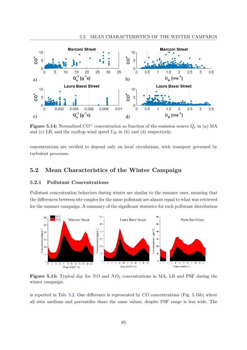
5.2. MEAN CHARACTERISTICS OF THE WINTER CAMPAIGN
Figure 5.14: Normalized CO+ concentration as function of the emission source Qe in (a) MAand (c) LB, and the rooftop wind speed UH in (b) and (d) respectively.
concentrations are verified to depend only on local circulations, with transport governed byturbulent processes.
5.2 Mean Characteristics of the Winter Campaign
5.2.1 Pollutant Concentrations
Pollutant concentration behaviors during winter are similar to the summer ones, meaning thatthe differences between site couples for the same pollutant are almost equal to what was retrievedfor the summer campaign. A summary of the significant statistics for each pollutant distribution
Figure 5.15: Typical day for NO and NO2 concentrations in MA, LB and PSF during thewinter campaign.
is reported in Tab. 5.2. One difference is represented by CO concentrations (Fig. 5.16b) whereall sites medians and percentiles share the same values, despite PSF range is less wide. The
85
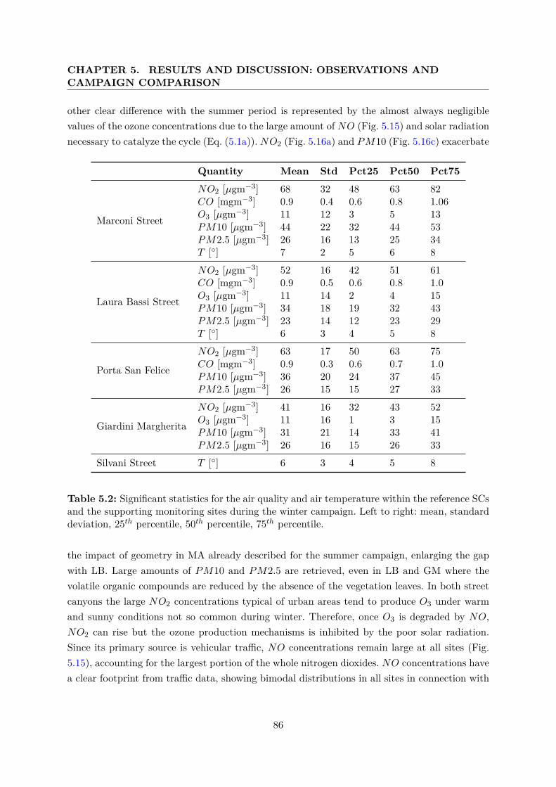
CHAPTER 5. RESULTS AND DISCUSSION: OBSERVATIONS ANDCAMPAIGN COMPARISON
other clear difference with the summer period is represented by the almost always negligiblevalues of the ozone concentrations due to the large amount of NO (Fig. 5.15) and solar radiationnecessary to catalyze the cycle (Eq. (5.1a)). NO2 (Fig. 5.16a) and PM10 (Fig. 5.16c) exacerbate
Quantity Mean Std Pct25 Pct50 Pct75
Marconi Street
NO2 [µgm−3] 68 32 48 63 82CO [mgm−3] 0.9 0.4 0.6 0.8 1.06O3 [µgm−3] 11 12 3 5 13PM10 [µgm−3] 44 22 32 44 53PM2.5 [µgm−3] 26 16 13 25 34T [◦] 7 2 5 6 8
Laura Bassi Street
NO2 [µgm−3] 52 16 42 51 61CO [mgm−3] 0.9 0.5 0.6 0.8 1.0O3 [µgm−3] 11 14 2 4 15PM10 [µgm−3] 34 18 19 32 43PM2.5 [µgm−3] 23 14 12 23 29T [◦] 6 3 4 5 8
Porta San Felice
NO2 [µgm−3] 63 17 50 63 75CO [mgm−3] 0.9 0.3 0.6 0.7 1.0PM10 [µgm−3] 36 20 24 37 45PM2.5 [µgm−3] 26 15 15 27 33
Giardini Margherita
NO2 [µgm−3] 41 16 32 43 52O3 [µgm−3] 11 16 1 3 15PM10 [µgm−3] 31 21 14 33 41PM2.5 [µgm−3] 26 16 15 26 33
Silvani Street T [◦] 6 3 4 5 8
Table 5.2: Significant statistics for the air quality and air temperature within the reference SCsand the supporting monitoring sites during the winter campaign. Left to right: mean, standarddeviation, 25th percentile, 50th percentile, 75th percentile.
the impact of geometry in MA already described for the summer campaign, enlarging the gapwith LB. Large amounts of PM10 and PM2.5 are retrieved, even in LB and GM where thevolatile organic compounds are reduced by the absence of the vegetation leaves. In both streetcanyons the large NO2 concentrations typical of urban areas tend to produce O3 under warmand sunny conditions not so common during winter. Therefore, once O3 is degraded by NO,NO2 can rise but the ozone production mechanisms is inhibited by the poor solar radiation.Since its primary source is vehicular traffic, NO concentrations remain large at all sites (Fig.5.15), accounting for the largest portion of the whole nitrogen dioxides. NO concentrations havea clear footprint from traffic data, showing bimodal distributions in all sites in connection with
86
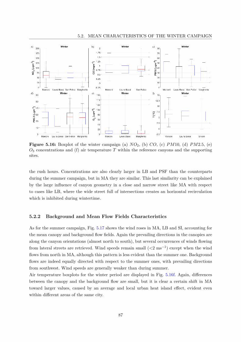
5.2. MEAN CHARACTERISTICS OF THE WINTER CAMPAIGN
Figure 5.16: Boxplot of the winter campaign (a) NO2, (b) CO, (c) PM10, (d) PM2.5, (e)O3 concentrations and (f) air temperature T within the reference canyons and the supportingsites.
the rush hours. Concentrations are also clearly larger in LB and PSF than the counterpartsduring the summer campaign, but in MA they are similar. This last similarity can be explainedby the large influence of canyon geometry in a close and narrow street like MA with respectto cases like LB, where the wide street full of intersections creates an horizontal recirculationwhich is inhibited during wintertime.
5.2.2 Background and Mean Flow Fields Characteristics
As for the summer campaign, Fig. 5.17 shows the wind roses in MA, LB and SI, accounting forthe mean canopy and background flow fields. Again the prevailing directions in the canopies arealong the canyon orientations (almost north to south), but several occurrences of winds flowingfrom lateral streets are retrieved. Wind speeds remain small (<2 ms−1) except when the windflows from north in MA, although this pattern is less evident than the summer one. Backgroundflows are indeed equally directed with respect to the summer ones, with prevailing directionsfrom southwest. Wind speeds are generally weaker than during summer.Air temperature boxplots for the winter period are displayed in Fig. 5.16f. Again, differencesbetween the canopy and the background flow are small, but it is clear a certain shift in MAtoward larger values, caused by an average and local urban heat island effect, evident evenwithin different areas of the same city.
87
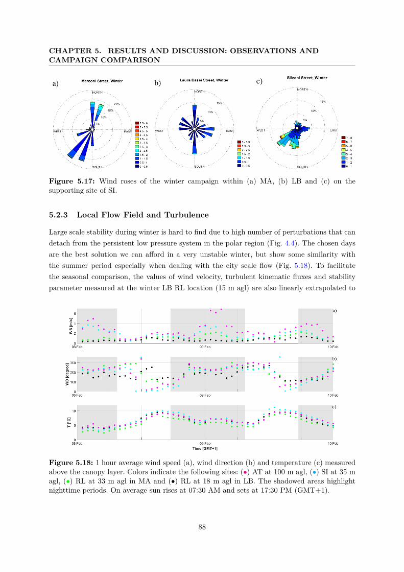
CHAPTER 5. RESULTS AND DISCUSSION: OBSERVATIONS ANDCAMPAIGN COMPARISON
Figure 5.17: Wind roses of the winter campaign within (a) MA, (b) LB and (c) on thesupporting site of SI.
5.2.3 Local Flow Field and Turbulence
Large scale stability during winter is hard to find due to high number of perturbations that candetach from the persistent low pressure system in the polar region (Fig. 4.4). The chosen daysare the best solution we can afford in a very unstable winter, but show some similarity withthe summer period especially when dealing with the city scale flow (Fig. 5.18). To facilitatethe seasonal comparison, the values of wind velocity, turbulent kinematic fluxes and stabilityparameter measured at the winter LB RL location (15 m agl) are also linearly extrapolated to
Figure 5.18: 1 hour average wind speed (a), wind direction (b) and temperature (c) measuredabove the canopy layer. Colors indicate the following sites: (•) AT at 100 m agl, (•) SI at 35 magl, (•) RL at 33 m agl in MA and (•) RL at 18 m agl in LB. The shadowed areas highlightnighttime periods. On average sun rises at 07:30 AM and sets at 17:30 PM (GMT+1).
88
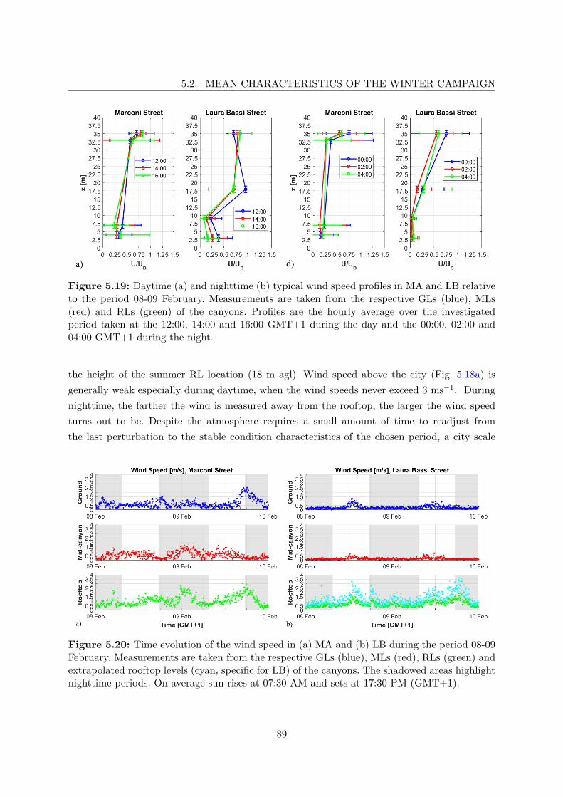
5.2. MEAN CHARACTERISTICS OF THE WINTER CAMPAIGN
Figure 5.19: Daytime (a) and nighttime (b) typical wind speed profiles in MA and LB relativeto the period 08-09 February. Measurements are taken from the respective GLs (blue), MLs(red) and RLs (green) of the canyons. Profiles are the hourly average over the investigatedperiod taken at the 12:00, 14:00 and 16:00 GMT+1 during the day and the 00:00, 02:00 and04:00 GMT+1 during the night.
the height of the summer RL location (18 m agl). Wind speed above the city (Fig. 5.18a) isgenerally weak especially during daytime, when the wind speeds never exceed 3 ms−1. Duringnighttime, the farther the wind is measured away from the rooftop, the larger the wind speedturns out to be. Despite the atmosphere requires a small amount of time to readjust fromthe last perturbation to the stable condition characteristics of the chosen period, a city scale
Figure 5.20: Time evolution of the wind speed in (a) MA and (b) LB during the period 08-09February. Measurements are taken from the respective GLs (blue), MLs (red), RLs (green) andextrapolated rooftop levels (cyan, specific for LB) of the canyons. The shadowed areas highlightnighttime periods. On average sun rises at 07:30 AM and sets at 17:30 PM (GMT+1).
89
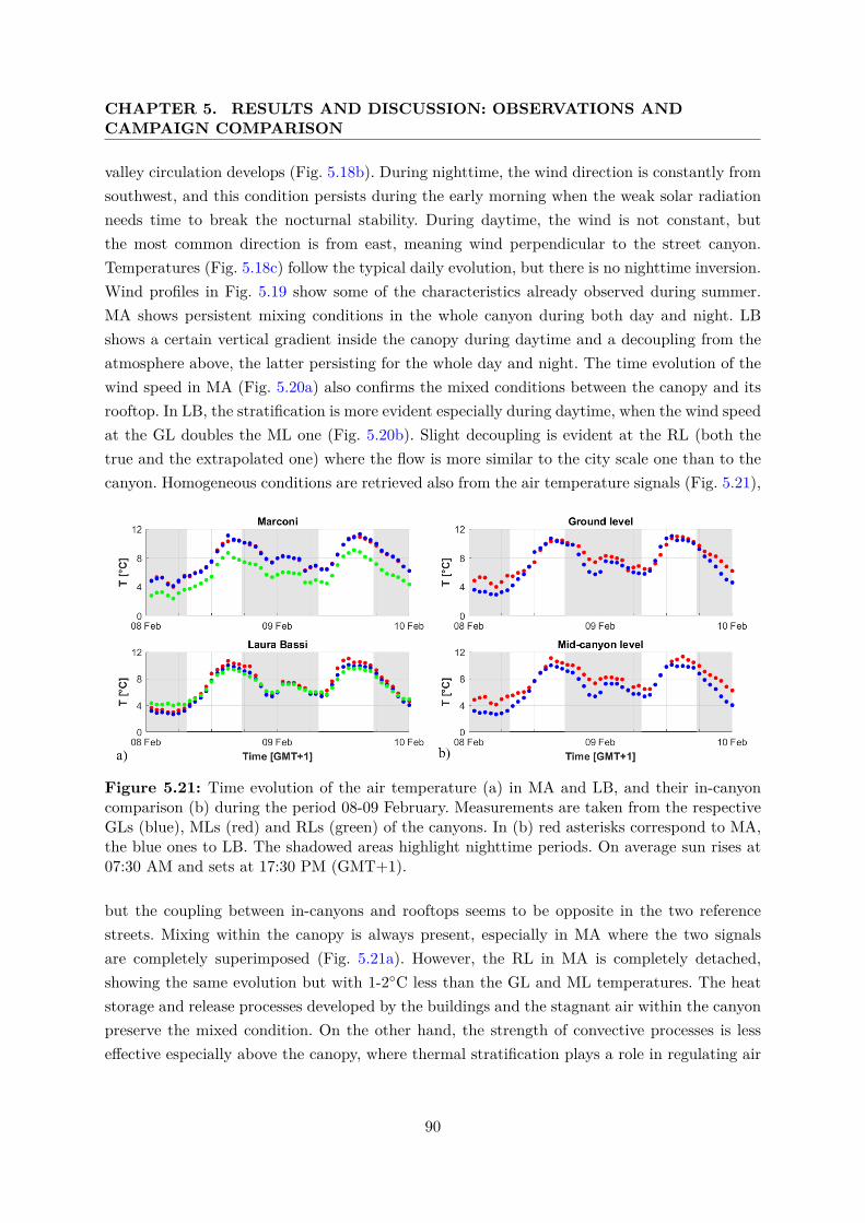
CHAPTER 5. RESULTS AND DISCUSSION: OBSERVATIONS ANDCAMPAIGN COMPARISON
valley circulation develops (Fig. 5.18b). During nighttime, the wind direction is constantly fromsouthwest, and this condition persists during the early morning when the weak solar radiationneeds time to break the nocturnal stability. During daytime, the wind is not constant, butthe most common direction is from east, meaning wind perpendicular to the street canyon.Temperatures (Fig. 5.18c) follow the typical daily evolution, but there is no nighttime inversion.Wind profiles in Fig. 5.19 show some of the characteristics already observed during summer.MA shows persistent mixing conditions in the whole canyon during both day and night. LBshows a certain vertical gradient inside the canopy during daytime and a decoupling from theatmosphere above, the latter persisting for the whole day and night. The time evolution of thewind speed in MA (Fig. 5.20a) also confirms the mixed conditions between the canopy and itsrooftop. In LB, the stratification is more evident especially during daytime, when the wind speedat the GL doubles the ML one (Fig. 5.20b). Slight decoupling is evident at the RL (both thetrue and the extrapolated one) where the flow is more similar to the city scale one than to thecanyon. Homogeneous conditions are retrieved also from the air temperature signals (Fig. 5.21),
Figure 5.21: Time evolution of the air temperature (a) in MA and LB, and their in-canyoncomparison (b) during the period 08-09 February. Measurements are taken from the respectiveGLs (blue), MLs (red) and RLs (green) of the canyons. In (b) red asterisks correspond to MA,the blue ones to LB. The shadowed areas highlight nighttime periods. On average sun rises at07:30 AM and sets at 17:30 PM (GMT+1).
but the coupling between in-canyons and rooftops seems to be opposite in the two referencestreets. Mixing within the canopy is always present, especially in MA where the two signalsare completely superimposed (Fig. 5.21a). However, the RL in MA is completely detached,showing the same evolution but with 1-2◦C less than the GL and ML temperatures. The heatstorage and release processes developed by the buildings and the stagnant air within the canyonpreserve the mixed condition. On the other hand, the strength of convective processes is lesseffective especially above the canopy, where thermal stratification plays a role in regulating air
90
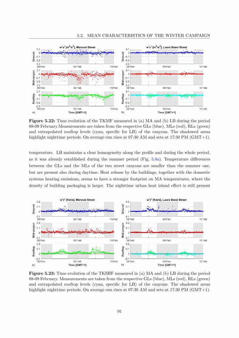
5.2. MEAN CHARACTERISTICS OF THE WINTER CAMPAIGN
Figure 5.22: Time evolution of the TKMF measured in (a) MA and (b) LB during the period08-09 February.Measurements are taken from the respective GLs (blue), MLs (red), RLs (green)and extrapolated rooftop levels (cyan, specific for LB) of the canyons. The shadowed areashighlight nighttime periods. On average sun rises at 07:30 AM and sets at 17:30 PM (GMT+1).
temperature. LB maintains a clear homogeneity along the profile and during the whole period,as it was already established during the summer period (Fig. 5.8a). Temperature differencesbetween the GLs and the MLs of the two street canyons are smaller than the summer one,but are present also during daytime. Heat release by the buildings, together with the domesticsystems heating emissions, seems to have a stronger footprint on MA temperatures, where thedensity of building packaging is larger. The nighttime urban heat island effect is still present
Figure 5.23: Time evolution of the TKSHF measured in (a) MA and (b) LB during the period08-09 February. Measurements are taken from the respective GLs (blue), MLs (red), RLs (green)and extrapolated rooftop levels (cyan, specific for LB) of the canyons. The shadowed areashighlight nighttime periods. On average sun rises at 07:30 AM and sets at 17:30 PM (GMT+1).
91
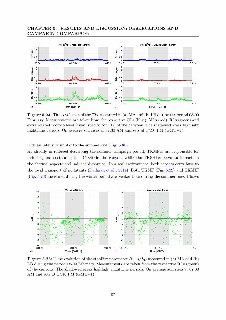
CHAPTER 5. RESULTS AND DISCUSSION: OBSERVATIONS ANDCAMPAIGN COMPARISON
Figure 5.24: Time evolution of the Tkemeasured in (a) MA and (b) LB during the period 08-09February. Measurements are taken from the respective GLs (blue), MLs (red), RLs (green) andextrapolated rooftop level (cyan, specific for LB) of the canyons. The shadowed areas highlightnighttime periods. On average sun rises at 07:30 AM and sets at 17:30 PM (GMT+1).
with an intensity similar to the summer one (Fig. 5.8b).As already introduced describing the summer campaign period, TKMFes are responsible forinducing and sustaining the IC within the canyon, while the TKSHFes have an impact onthe thermal aspects and induced dynamics. In a real environment, both aspects contribute tothe local transport of pollutants (Dallman et al., 2014). Both TKMF (Fig. 5.22) and TKSHF(Fig. 5.23) measured during the winter period are weaker than during the summer ones. Fluxes
Figure 5.25: Time evolution of the stability parameter H−d/LO measured in (a) MA and (b)LB during the period 08-09 February. Measurements are taken from the respective RLs (green)of the canyons. The shadowed areas highlight nighttime periods. On average sun rises at 07:30AM and sets at 17:30 PM (GMT+1).
92
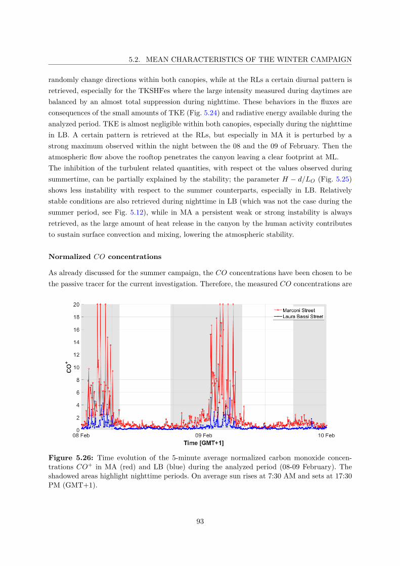
5.2. MEAN CHARACTERISTICS OF THE WINTER CAMPAIGN
randomly change directions within both canopies, while at the RLs a certain diurnal pattern isretrieved, especially for the TKSHFes where the large intensity measured during daytimes arebalanced by an almost total suppression during nighttime. These behaviors in the fluxes areconsequences of the small amounts of TKE (Fig. 5.24) and radiative energy available during theanalyzed period. TKE is almost negligible within both canopies, especially during the nighttimein LB. A certain pattern is retrieved at the RLs, but especially in MA it is perturbed by astrong maximum observed within the night between the 08 and the 09 of February. Then theatmospheric flow above the rooftop penetrates the canyon leaving a clear footprint at ML.The inhibition of the turbulent related quantities, with respect ot the values observed duringsummertime, can be partially explained by the stability; the parameter H − d/LO (Fig. 5.25)shows less instability with respect to the summer counterparts, especially in LB. Relativelystable conditions are also retrieved during nighttime in LB (which was not the case during thesummer period, see Fig. 5.12), while in MA a persistent weak or strong instability is alwaysretrieved, as the large amount of heat release in the canyon by the human activity contributesto sustain surface convection and mixing, lowering the atmospheric stability.
Normalized CO concentrations
As already discussed for the summer campaign, the CO concentrations have been chosen to bethe passive tracer for the current investigation. Therefore, the measured CO concentrations are
Figure 5.26: Time evolution of the 5-minute average normalized carbon monoxide concen-trations CO+ in MA (red) and LB (blue) during the analyzed period (08-09 February). Theshadowed areas highlight nighttime periods. On average sun rises at 7:30 AM and sets at 17:30PM (GMT+1).
93
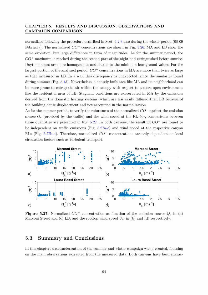
CHAPTER 5. RESULTS AND DISCUSSION: OBSERVATIONS ANDCAMPAIGN COMPARISON
normalized following the procedure described in Sect. 4.2.3 also during the winter period (08-09February). The normalized CO+ concentrations are shown in Fig. 5.26. MA and LB show thesame evolution, but large differences in term of magnitudes. As for the summer period, theCO+ maximum is reached during the second part of the night and extinguished before sunrise.Daytime hours are more homogeneous and flatten to the minimum background values. For thelargest portion of the analyzed period, CO+ concentrations in MA are more than twice as largeas that measured in LB. In a way, this discrepancy is unexpected, since the similarity foundduring summer (Fig. 5.13). Nevertheless, a densely built area like MA and its neighborhood canbe more prone to entrap the air within the canopy with respect to a more open environmentlike the residential area of LB. Stagnant conditions are exacerbated in MA by the emissionsderived from the domestic heating systems, which are less easily diffused than LB because ofthe building dense displacement and not accounted in the normalization.As for the summer period, to verify the robustness of the normalized CO+ against the emissionsource Qe (provided by the traffic) and the wind speed at the RL UH , comparisons betweenthose quantities are presented in Fig. 5.27. In both canyons, the resulting CO+ are found tobe independent on traffic emissions (Fig. 5.27a-c) and wind speed at the respective canyonRLs (Fig. 5.27b-d). Therefore, normalized CO+ concentrations are only dependent on localcirculation factors such as turbulent transport.
Figure 5.27: Normalized CO+ concentration as function of the emission source Qe in (a)Marconi Street and (c) LB, and the rooftop wind speed UH in (b) and (d) respectively.
5.3 Summary and Conclusions
In this chapter, a characterization of the summer and winter campaign was presented, focusingon the main observations extracted from the measured data. Both canyons have been charac-
94
5.3. SUMMARY AND CONCLUSIONS
terized in terms of air quality and typical meteorological patterns and then focusing on someaspects more crucial for the following investigations, as the normalized pollutant concentra-tion evolution, the local circulation features and turbulent behavior. The seasonality and streetcanyons comparisons have highlighted the similar and dissimilar behaviors of the referencecanyons. In particular, the behavior of the different pollutants certifies the importance of thestreet canyon effect in both locations (especially in MA), while the seasonality exacerbates thedifferent impacts of multiple emission sources and local atmospheric conditions on the pollu-tant concentrations. Local atmospheric conditions that indeed show the larger importance ofthe location rather than the seasonality. Similarity evolution of the mean flow and turbulent re-lated quantities have been retrieved comparing summer and winter periods under weak synopticforcing, both within and above the canopy, where the majority of the inter-seasonal differencesare caused by the different amounts of available energy in the environment. On the contrary,the different morphology and presence of vegetation of the two street canyons have supportedregimes of sustained turbulence and mixing in MA, less intense in LB. Atmospheric stabilityhas also forced a seasonality footprint on local flow and turbulent behaviors, weakening thewinter wind speed, mechanical and thermal related turbulence magnitudes, while enhancingthe same quantities intensity favoring summertime convection and mixing. The results obtainedfrom these observations will provide a baseline for the next chapter analyses on the local char-acteristics of the urban flows, with the aim of revealing interesting diagnoses on the turbulentexchange processes and their impact on air quality.
95

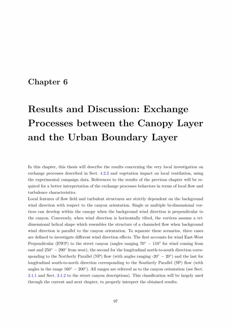
Chapter 6
Results and Discussion: ExchangeProcesses between the Canopy Layerand the Urban Boundary Layer
In this chapter, this thesis will describe the results concerning the very local investigation onexchange processes described in Sect. 4.2.2 and vegetation impact on local ventilation, usingthe experimental campaign data. References to the results of the previous chapter will be re-quired for a better interpretation of the exchange processes behaviors in terms of local flow andturbulence characteristics.Local features of flow field and turbulent structures are strictly dependent on the backgroundwind direction with respect to the canyon orientation. Single or multiple bi-dimensional vor-tices can develop within the canopy when the background wind direction is perpendicular tothe canyon. Conversely, when wind direction is horizontally tilted, the vortices assume a tri-dimensional helical shape which resembles the structure of a channeled flow when backgroundwind direction is parallel to the canyon orientation. To separate these scenarios, three casesare defined to investigate different wind direction effects. The first accounts for wind East-WestPerpendicular (EWP) to the street canyon (angles ranging 70◦ − 110◦ for wind coming fromeast and 250◦ − 290◦ from west), the second for the longitudinal north-to-south direction corre-sponding to the Northerly Parallel (NP) flow (with angles ranging -20◦ − 20◦) and the last forlongitudinal south-to-north direction corresponding to the Southerly Parallel (SP) flow (withangles in the range 160◦ − 200◦). All ranges are referred as to the canyon orientation (see Sect.3.1.1 and Sect. 3.1.2 to the street canyon descriptions). This classification will be largely usedthrough the current and next chapter, to properly interpret the obtained results.
97
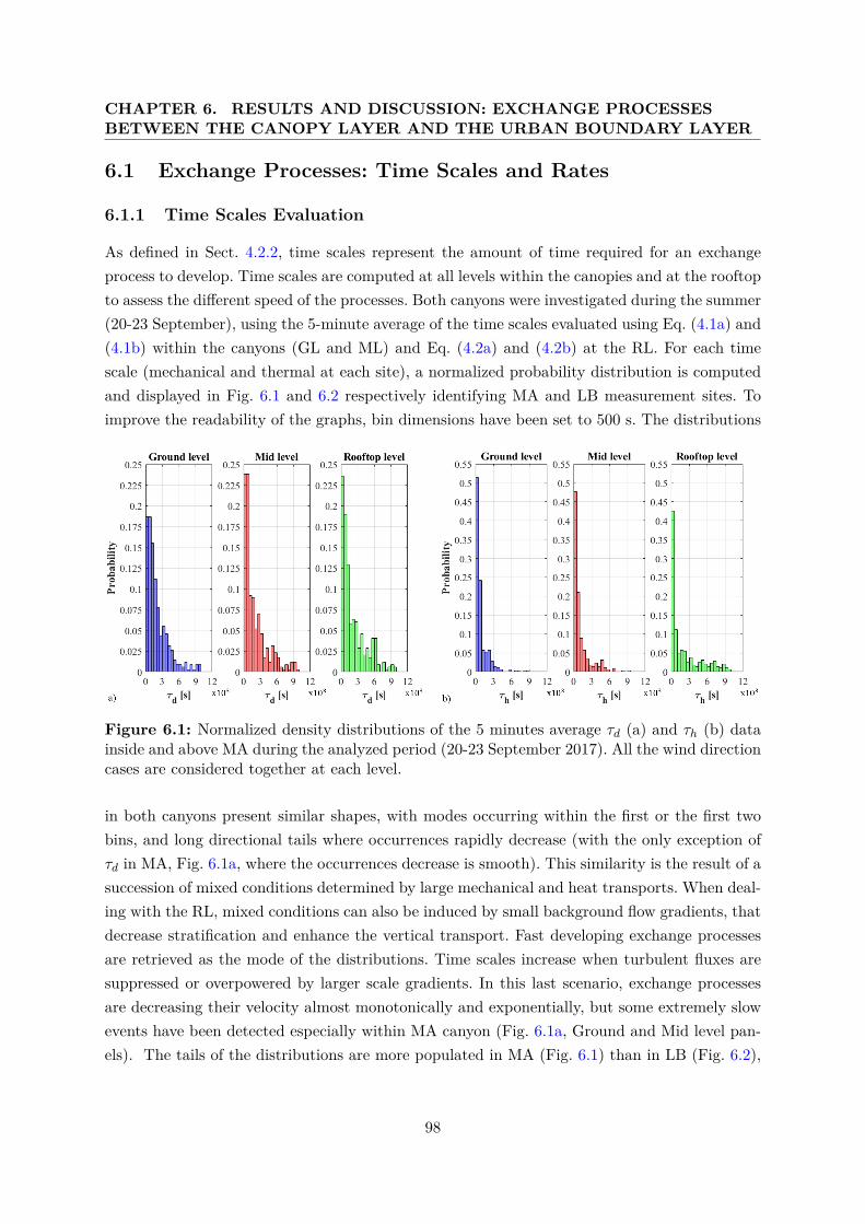
CHAPTER 6. RESULTS AND DISCUSSION: EXCHANGE PROCESSESBETWEEN THE CANOPY LAYER AND THE URBAN BOUNDARY LAYER
6.1 Exchange Processes: Time Scales and Rates
6.1.1 Time Scales Evaluation
As defined in Sect. 4.2.2, time scales represent the amount of time required for an exchangeprocess to develop. Time scales are computed at all levels within the canopies and at the rooftopto assess the different speed of the processes. Both canyons were investigated during the summer(20-23 September), using the 5-minute average of the time scales evaluated using Eq. (4.1a) and(4.1b) within the canyons (GL and ML) and Eq. (4.2a) and (4.2b) at the RL. For each timescale (mechanical and thermal at each site), a normalized probability distribution is computedand displayed in Fig. 6.1 and 6.2 respectively identifying MA and LB measurement sites. Toimprove the readability of the graphs, bin dimensions have been set to 500 s. The distributions
Figure 6.1: Normalized density distributions of the 5 minutes average τd (a) and τh (b) datainside and above MA during the analyzed period (20-23 September 2017). All the wind directioncases are considered together at each level.
in both canyons present similar shapes, with modes occurring within the first or the first twobins, and long directional tails where occurrences rapidly decrease (with the only exception ofτd in MA, Fig. 6.1a, where the occurrences decrease is smooth). This similarity is the result of asuccession of mixed conditions determined by large mechanical and heat transports. When deal-ing with the RL, mixed conditions can also be induced by small background flow gradients, thatdecrease stratification and enhance the vertical transport. Fast developing exchange processesare retrieved as the mode of the distributions. Time scales increase when turbulent fluxes aresuppressed or overpowered by larger scale gradients. In this last scenario, exchange processesare decreasing their velocity almost monotonically and exponentially, but some extremely slowevents have been detected especially within MA canyon (Fig. 6.1a, Ground and Mid level pan-els). The tails of the distributions are more populated in MA (Fig. 6.1) than in LB (Fig. 6.2),
98
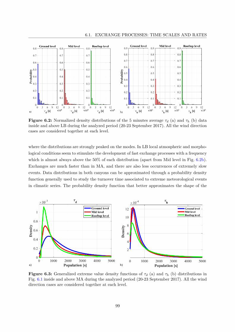
6.1. EXCHANGE PROCESSES: TIME SCALES AND RATES
Figure 6.2: Normalized density distributions of the 5 minutes average τd (a) and τh (b) datainside and above LB during the analyzed period (20-23 September 2017). All the wind directioncases are considered together at each level.
where the distributions are strongly peaked on the modes. In LB local atmospheric and morpho-logical conditions seem to stimulate the development of fast exchange processes with a frequencywhich is almost always above the 50% of each distribution (apart from Mid level in Fig. 6.2b).Exchanges are much faster than in MA, and there are also less occurrences of extremely slowevents. Data distributions in both canyons can be approximated through a probability densityfunction generally used to study the turnover time associated to extreme meteorological eventsin climatic series. The probability density function that better approximates the shape of the
Figure 6.3: Generalized extreme value density functions of τd (a) and τh (b) distributions inFig. 6.1 inside and above MA during the analyzed period (20-23 September 2017). All the winddirection cases are considered together at each level.
99
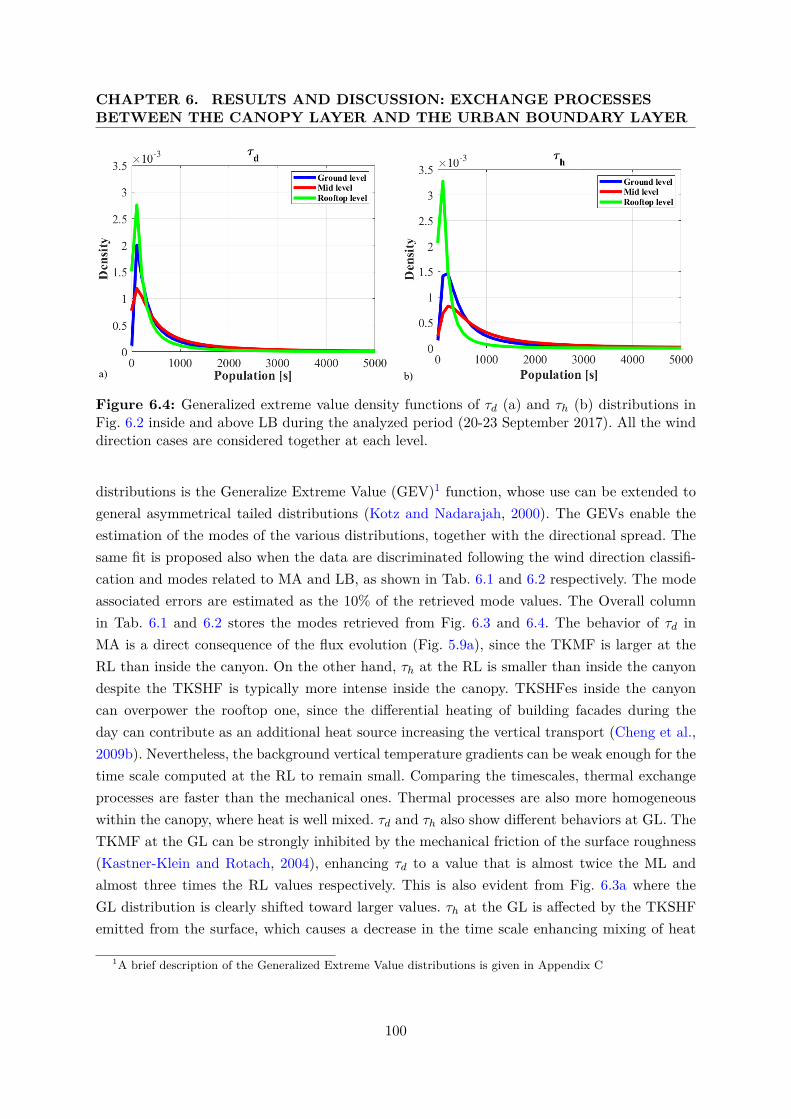
CHAPTER 6. RESULTS AND DISCUSSION: EXCHANGE PROCESSESBETWEEN THE CANOPY LAYER AND THE URBAN BOUNDARY LAYER
Figure 6.4: Generalized extreme value density functions of τd (a) and τh (b) distributions inFig. 6.2 inside and above LB during the analyzed period (20-23 September 2017). All the winddirection cases are considered together at each level.
distributions is the Generalize Extreme Value (GEV)1 function, whose use can be extended togeneral asymmetrical tailed distributions (Kotz and Nadarajah, 2000). The GEVs enable theestimation of the modes of the various distributions, together with the directional spread. Thesame fit is proposed also when the data are discriminated following the wind direction classifi-cation and modes related to MA and LB, as shown in Tab. 6.1 and 6.2 respectively. The modeassociated errors are estimated as the 10% of the retrieved mode values. The Overall columnin Tab. 6.1 and 6.2 stores the modes retrieved from Fig. 6.3 and 6.4. The behavior of τd inMA is a direct consequence of the flux evolution (Fig. 5.9a), since the TKMF is larger at theRL than inside the canyon. On the other hand, τh at the RL is smaller than inside the canyondespite the TKSHF is typically more intense inside the canopy. TKSHFes inside the canyoncan overpower the rooftop one, since the differential heating of building facades during theday can contribute as an additional heat source increasing the vertical transport (Cheng et al.,2009b). Nevertheless, the background vertical temperature gradients can be weak enough for thetime scale computed at the RL to remain small. Comparing the timescales, thermal exchangeprocesses are faster than the mechanical ones. Thermal processes are also more homogeneouswithin the canopy, where heat is well mixed. τd and τh also show different behaviors at GL. TheTKMF at the GL can be strongly inhibited by the mechanical friction of the surface roughness(Kastner-Klein and Rotach, 2004), enhancing τd to a value that is almost twice the ML andalmost three times the RL values respectively. This is also evident from Fig. 6.3a where theGL distribution is clearly shifted toward larger values. τh at the GL is affected by the TKSHFemitted from the surface, which causes a decrease in the time scale enhancing mixing of heat
1A brief description of the Generalized Extreme Value distributions is given in Appendix C
100
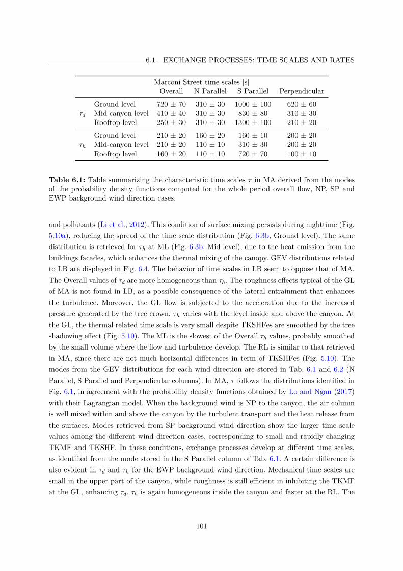
6.1. EXCHANGE PROCESSES: TIME SCALES AND RATES
Marconi Street time scales [s]Overall N Parallel S Parallel Perpendicular
τd
Ground level 720 ± 70 310 ± 30 1000 ± 100 620 ± 60Mid-canyon level 410 ± 40 310 ± 30 830 ± 80 310 ± 30Rooftop level 250 ± 30 310 ± 30 1300 ± 100 210 ± 20
τh
Ground level 210 ± 20 160 ± 20 160 ± 10 200 ± 20Mid-canyon level 210 ± 20 110 ± 10 310 ± 30 200 ± 20Rooftop level 160 ± 20 110 ± 10 720 ± 70 100 ± 10
Table 6.1: Table summarizing the characteristic time scales τ in MA derived from the modesof the probability density functions computed for the whole period overall flow, NP, SP andEWP background wind direction cases.
and pollutants (Li et al., 2012). This condition of surface mixing persists during nighttime (Fig.5.10a), reducing the spread of the time scale distribution (Fig. 6.3b, Ground level). The samedistribution is retrieved for τh at ML (Fig. 6.3b, Mid level), due to the heat emission from thebuildings facades, which enhances the thermal mixing of the canopy. GEV distributions relatedto LB are displayed in Fig. 6.4. The behavior of time scales in LB seem to oppose that of MA.The Overall values of τd are more homogeneous than τh. The roughness effects typical of the GLof MA is not found in LB, as a possible consequence of the lateral entrainment that enhancesthe turbulence. Moreover, the GL flow is subjected to the acceleration due to the increasedpressure generated by the tree crown. τh varies with the level inside and above the canyon. Atthe GL, the thermal related time scale is very small despite TKSHFes are smoothed by the treeshadowing effect (Fig. 5.10). The ML is the slowest of the Overall τh values, probably smoothedby the small volume where the flow and turbulence develop. The RL is similar to that retrievedin MA, since there are not much horizontal differences in term of TKSHFes (Fig. 5.10). Themodes from the GEV distributions for each wind direction are stored in Tab. 6.1 and 6.2 (NParallel, S Parallel and Perpendicular columns). In MA, τ follows the distributions identified inFig. 6.1, in agreement with the probability density functions obtained by Lo and Ngan (2017)with their Lagrangian model. When the background wind is NP to the canyon, the air columnis well mixed within and above the canyon by the turbulent transport and the heat release fromthe surfaces. Modes retrieved from SP background wind direction show the larger time scalevalues among the different wind direction cases, corresponding to small and rapidly changingTKMF and TKSHF. In these conditions, exchange processes develop at different time scales,as identified from the mode stored in the S Parallel column of Tab. 6.1. A certain difference isalso evident in τd and τh for the EWP background wind direction. Mechanical time scales aresmall in the upper part of the canyon, while roughness is still efficient in inhibiting the TKMFat the GL, enhancing τd. τh is again homogeneous inside the canyon and faster at the RL. The
101
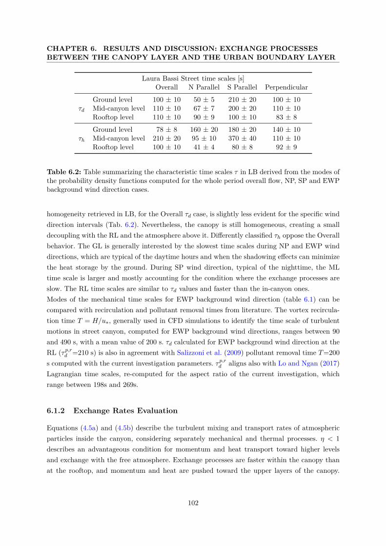
CHAPTER 6. RESULTS AND DISCUSSION: EXCHANGE PROCESSESBETWEEN THE CANOPY LAYER AND THE URBAN BOUNDARY LAYER
Laura Bassi Street time scales [s]Overall N Parallel S Parallel Perpendicular
τd
Ground level 100 ± 10 50 ± 5 210 ± 20 100 ± 10Mid-canyon level 110 ± 10 67 ± 7 200 ± 20 110 ± 10Rooftop level 110 ± 10 90 ± 9 100 ± 10 83 ± 8
τh
Ground level 78 ± 8 160 ± 20 180 ± 20 140 ± 10Mid-canyon level 210 ± 20 95 ± 10 370 ± 40 110 ± 10Rooftop level 100 ± 10 41 ± 4 80 ± 8 92 ± 9
Table 6.2: Table summarizing the characteristic time scales τ in LB derived from the modes ofthe probability density functions computed for the whole period overall flow, NP, SP and EWPbackground wind direction cases.
homogeneity retrieved in LB, for the Overall τd case, is slightly less evident for the specific winddirection intervals (Tab. 6.2). Nevertheless, the canopy is still homogeneous, creating a smalldecoupling with the RL and the atmosphere above it. Differently classified τh oppose the Overallbehavior. The GL is generally interested by the slowest time scales during NP and EWP winddirections, which are typical of the daytime hours and when the shadowing effects can minimizethe heat storage by the ground. During SP wind direction, typical of the nighttime, the MLtime scale is larger and mostly accounting for the condition where the exchange processes areslow. The RL time scales are similar to τd values and faster than the in-canyon ones.Modes of the mechanical time scales for EWP background wind direction (table 6.1) can becompared with recirculation and pollutant removal times from literature. The vortex recircula-tion time T = H/u∗, generally used in CFD simulations to identify the time scale of turbulentmotions in street canyon, computed for EWP background wind directions, ranges between 90and 490 s, with a mean value of 200 s. τd calculated for EWP background wind direction at theRL (τp,rd =210 s) is also in agreement with Salizzoni et al. (2009) pollutant removal time T=200s computed with the current investigation parameters. τp,rd aligns also with Lo and Ngan (2017)Lagrangian time scales, re-computed for the aspect ratio of the current investigation, whichrange between 198s and 269s.
6.1.2 Exchange Rates Evaluation
Equations (4.5a) and (4.5b) describe the turbulent mixing and transport rates of atmosphericparticles inside the canyon, considering separately mechanical and thermal processes. η < 1describes an advantageous condition for momentum and heat transport toward higher levelsand exchange with the free atmosphere. Exchange processes are faster within the canopy thanat the rooftop, and momentum and heat are pushed toward the upper layers of the canopy.
102
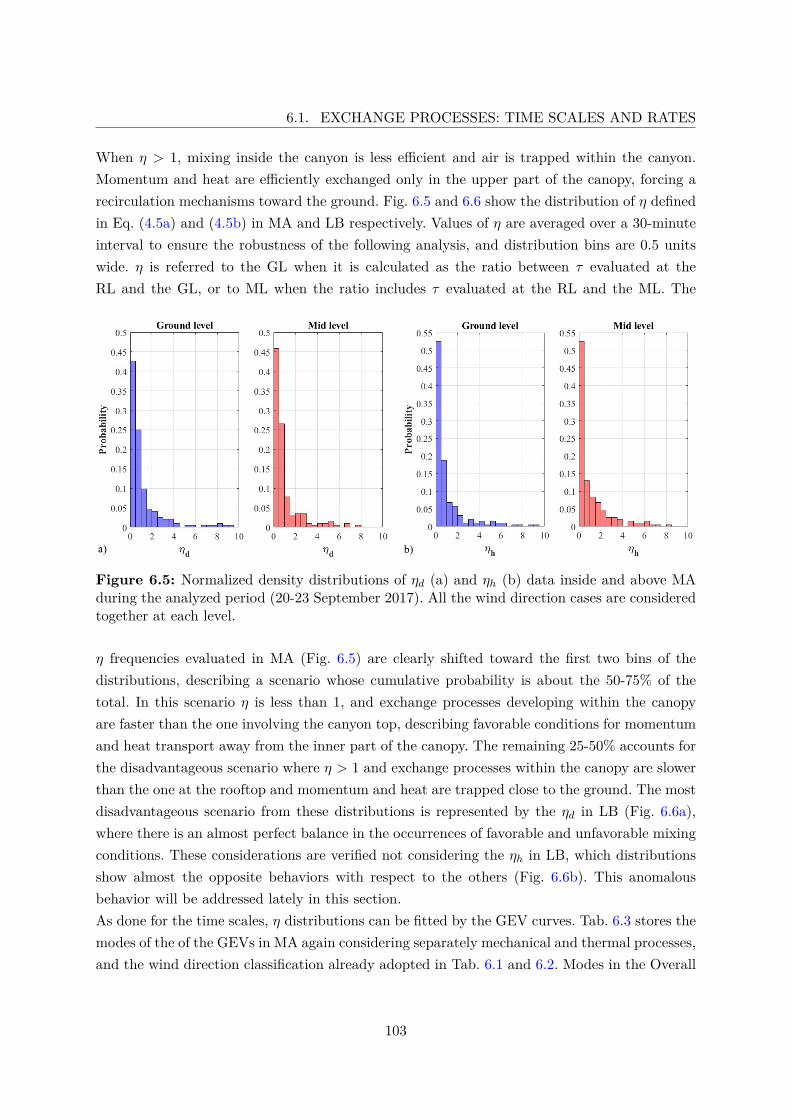
6.1. EXCHANGE PROCESSES: TIME SCALES AND RATES
When η > 1, mixing inside the canyon is less efficient and air is trapped within the canyon.Momentum and heat are efficiently exchanged only in the upper part of the canopy, forcing arecirculation mechanisms toward the ground. Fig. 6.5 and 6.6 show the distribution of η definedin Eq. (4.5a) and (4.5b) in MA and LB respectively. Values of η are averaged over a 30-minuteinterval to ensure the robustness of the following analysis, and distribution bins are 0.5 unitswide. η is referred to the GL when it is calculated as the ratio between τ evaluated at theRL and the GL, or to ML when the ratio includes τ evaluated at the RL and the ML. The
Figure 6.5: Normalized density distributions of ηd (a) and ηh (b) data inside and above MAduring the analyzed period (20-23 September 2017). All the wind direction cases are consideredtogether at each level.
η frequencies evaluated in MA (Fig. 6.5) are clearly shifted toward the first two bins of thedistributions, describing a scenario whose cumulative probability is about the 50-75% of thetotal. In this scenario η is less than 1, and exchange processes developing within the canopyare faster than the one involving the canyon top, describing favorable conditions for momentumand heat transport away from the inner part of the canopy. The remaining 25-50% accounts forthe disadvantageous scenario where η > 1 and exchange processes within the canopy are slowerthan the one at the rooftop and momentum and heat are trapped close to the ground. The mostdisadvantageous scenario from these distributions is represented by the ηd in LB (Fig. 6.6a),where there is an almost perfect balance in the occurrences of favorable and unfavorable mixingconditions. These considerations are verified not considering the ηh in LB, which distributionsshow almost the opposite behaviors with respect to the others (Fig. 6.6b). This anomalousbehavior will be addressed lately in this section.As done for the time scales, η distributions can be fitted by the GEV curves. Tab. 6.3 stores themodes of the of the GEVs in MA again considering separately mechanical and thermal processes,and the wind direction classification already adopted in Tab. 6.1 and 6.2. Modes in the Overall
103
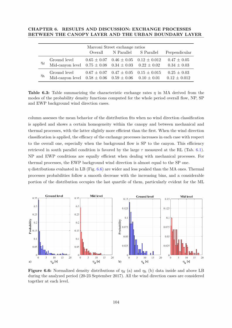
CHAPTER 6. RESULTS AND DISCUSSION: EXCHANGE PROCESSESBETWEEN THE CANOPY LAYER AND THE URBAN BOUNDARY LAYER
Marconi Street exchange ratiosOverall N Parallel S Parallel Perpendicular
ηdGround level 0.65 ± 0.07 0.46 ± 0.05 0.12 ± 0.012 0.47 ± 0.05Mid-canyon level 0.75 ± 0.08 0.34 ± 0.03 0.22 ± 0.02 0.34 ± 0.03
ηhGround level 0.67 ± 0.07 0.47 ± 0.05 0.15 ± 0.015 0.25 ± 0.03Mid-canyon level 0.58 ± 0.06 0.59 ± 0.06 0.10 ± 0.01 0.12 ± 0.012
Table 6.3: Table summarizing the characteristic exchange rates η in MA derived from themodes of the probability density functions computed for the whole period overall flow, NP, SPand EWP background wind direction cases.
column assesses the mean behavior of the distribution fits when no wind direction classificationis applied and shows a certain homogeneity within the canopy and between mechanical andthermal processes, with the latter slightly more efficient than the first. When the wind directionclassification is applied, the efficacy of the exchange processes increases in each case with respectto the overall one, especially when the background flow is SP to the canyon. This efficiencyretrieved in south parallel condition is favored by the large τ measured at the RL (Tab. 6.1).NP and EWP conditions are equally efficient when dealing with mechanical processes. Forthermal processes, the EWP background wind direction is almost equal to the SP one.η distributions evaluated in LB (Fig. 6.6) are wider and less peaked than the MA ones. Thermalprocesses probabilities follow a smooth decrease with the increasing bins, and a considerableportion of the distribution occupies the last quartile of them, particularly evident for the ML
Figure 6.6: Normalized density distributions of ηd (a) and ηh (b) data inside and above LBduring the analyzed period (20-23 September 2017). All the wind direction cases are consideredtogether at each level.
104
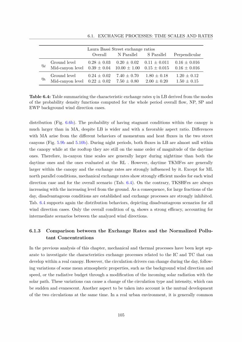
6.1. EXCHANGE PROCESSES: TIME SCALES AND RATES
Laura Bassi Street exchange ratiosOverall N Parallel S Parallel Perpendicular
ηdGround level 0.28 ± 0.03 0.20 ± 0.02 0.11 ± 0.011 0.16 ± 0.016Mid-canyon level 0.39 ± 0.04 10.00 ± 1.00 0.15 ± 0.015 0.16 ± 0.016
ηhGround level 0.24 ± 0.02 7.40 ± 0.70 1.80 ± 0.18 1.20 ± 0.12Mid-canyon level 0.22 ± 0.02 7.50 ± 0.80 2.00 ± 0.20 1.50 ± 0.15
Table 6.4: Table summarizing the characteristic exchange rates η in LB derived from the modesof the probability density functions computed for the whole period overall flow, NP, SP andEWP background wind direction cases.
distribution (Fig. 6.6b). The probability of having stagnant conditions within the canopy ismuch larger than in MA, despite LB is wider and with a favorable aspect ratio. Differenceswith MA arise from the different behaviors of momentum and heat fluxes in the two streetcanyons (Fig. 5.9b and 5.10b). During night periods, both fluxes in LB are almost null withinthe canopy while at the rooftop they are still on the same order of magnitude of the daytimeones. Therefore, in-canyon time scales are generally larger during nighttime than both thedaytime ones and the ones evaluated at the RL . However, daytime TKMFes are generallylarger within the canopy and the exchange rates are strongly influenced by it. Except for MLnorth parallel conditions, mechanical exchange rates show strongly efficient modes for each winddirection case and for the overall scenario (Tab. 6.4). On the contrary, TKSHFes are alwaysincreasing with the increasing level from the ground. As a consequence, for large fractions of theday, disadvantageous conditions are established and exchange processes are strongly inhibited.Tab. 6.4 supports again the distribution behaviors, depicting disadvantageous scenarios for allwind direction cases. Only the overall condition of ηh shows a strong efficacy, accounting forintermediate scenarios between the analyzed wind directions.
6.1.3 Comparison between the Exchange Rates and the Normalized Pollu-tant Concentrations
In the previous analysis of this chapter, mechanical and thermal processes have been kept sep-arate to investigate the characteristics exchange processes related to the IC and TC that candevelop within a real canopy. However, the circulation drivers can change during the day, follow-ing variations of some mean atmospheric properties, such as the background wind direction andspeed, or the radiative budget through a modification of the incoming solar radiation with thesolar path. These variations can cause a change of the circulation type and intensity, which canbe sudden and evanescent. Another aspect to be taken into account is the mutual developmentof the two circulations at the same time. In a real urban environment, it is generally common
105
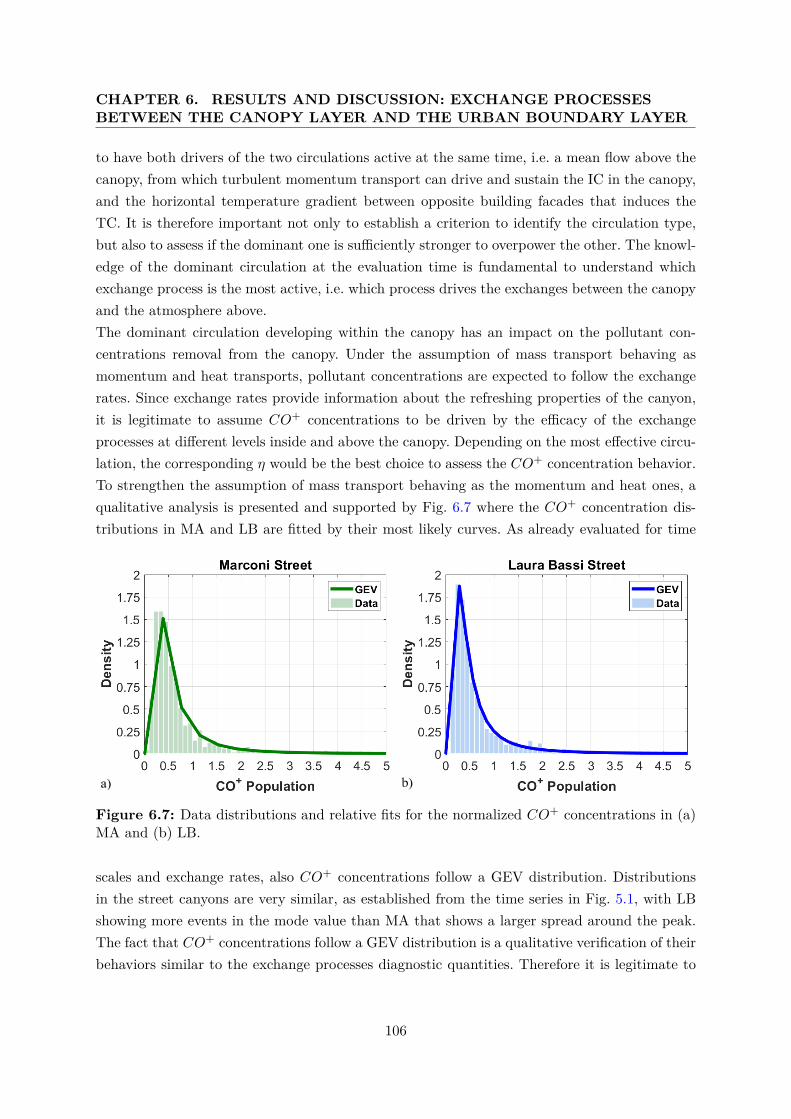
CHAPTER 6. RESULTS AND DISCUSSION: EXCHANGE PROCESSESBETWEEN THE CANOPY LAYER AND THE URBAN BOUNDARY LAYER
to have both drivers of the two circulations active at the same time, i.e. a mean flow above thecanopy, from which turbulent momentum transport can drive and sustain the IC in the canopy,and the horizontal temperature gradient between opposite building facades that induces theTC. It is therefore important not only to establish a criterion to identify the circulation type,but also to assess if the dominant one is sufficiently stronger to overpower the other. The knowl-edge of the dominant circulation at the evaluation time is fundamental to understand whichexchange process is the most active, i.e. which process drives the exchanges between the canopyand the atmosphere above.The dominant circulation developing within the canopy has an impact on the pollutant con-centrations removal from the canopy. Under the assumption of mass transport behaving asmomentum and heat transports, pollutant concentrations are expected to follow the exchangerates. Since exchange rates provide information about the refreshing properties of the canyon,it is legitimate to assume CO+ concentrations to be driven by the efficacy of the exchangeprocesses at different levels inside and above the canopy. Depending on the most effective circu-lation, the corresponding η would be the best choice to assess the CO+ concentration behavior.To strengthen the assumption of mass transport behaving as the momentum and heat ones, aqualitative analysis is presented and supported by Fig. 6.7 where the CO+ concentration dis-tributions in MA and LB are fitted by their most likely curves. As already evaluated for time
Figure 6.7: Data distributions and relative fits for the normalized CO+ concentrations in (a)MA and (b) LB.
scales and exchange rates, also CO+ concentrations follow a GEV distribution. Distributionsin the street canyons are very similar, as established from the time series in Fig. 5.1, with LBshowing more events in the mode value than MA that shows a larger spread around the peak.The fact that CO+ concentrations follow a GEV distribution is a qualitative verification of theirbehaviors similar to the exchange processes diagnostic quantities. Therefore it is legitimate to
106
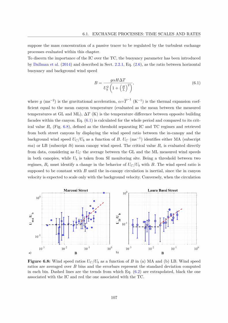
6.1. EXCHANGE PROCESSES: TIME SCALES AND RATES
suppose the mass concentration of a passive tracer to be regulated by the turbulent exchangeprocesses evaluated within this chapter.To discern the importance of the IC over the TC, the buoyancy parameter has been introducedby Dallman et al. (2014) and described in Sect. 2.2.1, Eq. (2.6), as the ratio between horizontalbuoyancy and background wind speed
B = gαH∆T
U2b
(1 +
(HL
)2) , (6.1)
where g (ms−2) is the gravitational acceleration, α=T−1 (K−1) is the thermal expansion coef-ficient equal to the mean canyon temperature (evaluated as the mean between the measuredtemperatures at GL and ML), ∆T (K) is the temperature difference between opposite buildingfacades within the canyon. Eq. (6.1) is calculated for the whole period and compared to its crit-ical value Bc (Fig. 6.8), defined as the threshold separating IC and TC regimes and retrievedfrom both street canyons by displaying the wind speed ratio between the in-canopy and thebackground wind speed UC/Ub as a function of B. UC (ms−1) identifies either MA (subscriptma) or LB (subscript lb) mean canopy wind speed. The critical value Bc is evaluated directlyfrom data, considering as UC the average between the GL and the ML measured wind speedsin both canopies, while Ub is taken from SI monitoring site. Being a threshold between tworegimes, Bc must identify a change in the behavior of UC/Ub with B. The wind speed ratio issupposed to be constant with B until the in-canopy circulation is inertial, since the in canyonvelocity is expected to scale only with the background velocity. Conversely, when the circulation
Figure 6.8: Wind speed ratios UC/Ub as a function of B in (a) MA and (b) LB. Wind speedratios are averaged over B bins and the errorbars represent the standard deviation computedin each bin. Dashed lines are the trends from which Eq. (6.2) are extrapolated, black the oneassociated with the IC and red the one associated with the TC.
107
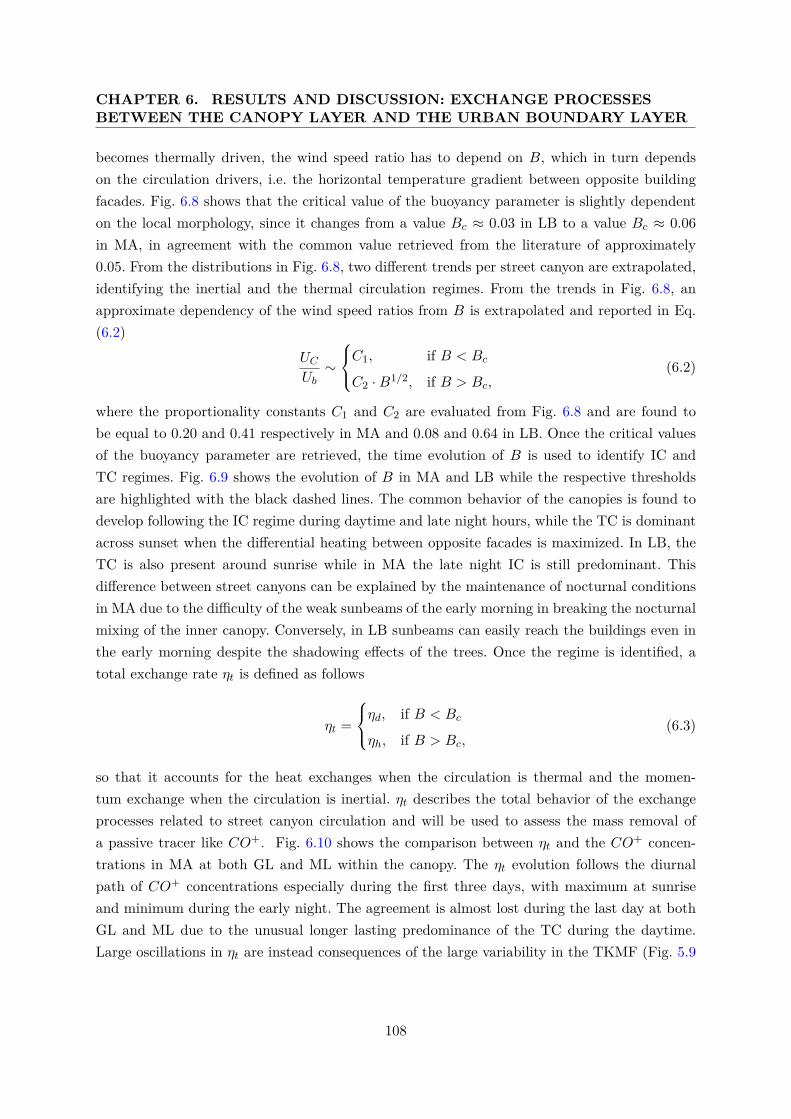
CHAPTER 6. RESULTS AND DISCUSSION: EXCHANGE PROCESSESBETWEEN THE CANOPY LAYER AND THE URBAN BOUNDARY LAYER
becomes thermally driven, the wind speed ratio has to depend on B, which in turn dependson the circulation drivers, i.e. the horizontal temperature gradient between opposite buildingfacades. Fig. 6.8 shows that the critical value of the buoyancy parameter is slightly dependenton the local morphology, since it changes from a value Bc ≈ 0.03 in LB to a value Bc ≈ 0.06in MA, in agreement with the common value retrieved from the literature of approximately0.05. From the distributions in Fig. 6.8, two different trends per street canyon are extrapolated,identifying the inertial and the thermal circulation regimes. From the trends in Fig. 6.8, anapproximate dependency of the wind speed ratios from B is extrapolated and reported in Eq.(6.2)
UCUb∼
C1, if B < Bc
C2 ·B1/2, if B > Bc,(6.2)
where the proportionality constants C1 and C2 are evaluated from Fig. 6.8 and are found tobe equal to 0.20 and 0.41 respectively in MA and 0.08 and 0.64 in LB. Once the critical valuesof the buoyancy parameter are retrieved, the time evolution of B is used to identify IC andTC regimes. Fig. 6.9 shows the evolution of B in MA and LB while the respective thresholdsare highlighted with the black dashed lines. The common behavior of the canopies is found todevelop following the IC regime during daytime and late night hours, while the TC is dominantacross sunset when the differential heating between opposite facades is maximized. In LB, theTC is also present around sunrise while in MA the late night IC is still predominant. Thisdifference between street canyons can be explained by the maintenance of nocturnal conditionsin MA due to the difficulty of the weak sunbeams of the early morning in breaking the nocturnalmixing of the inner canopy. Conversely, in LB sunbeams can easily reach the buildings even inthe early morning despite the shadowing effects of the trees. Once the regime is identified, atotal exchange rate ηt is defined as follows
ηt =
ηd, if B < Bc
ηh, if B > Bc,(6.3)
so that it accounts for the heat exchanges when the circulation is thermal and the momen-tum exchange when the circulation is inertial. ηt describes the total behavior of the exchangeprocesses related to street canyon circulation and will be used to assess the mass removal ofa passive tracer like CO+. Fig. 6.10 shows the comparison between ηt and the CO+ concen-trations in MA at both GL and ML within the canopy. The ηt evolution follows the diurnalpath of CO+ concentrations especially during the first three days, with maximum at sunriseand minimum during the early night. The agreement is almost lost during the last day at bothGL and ML due to the unusual longer lasting predominance of the TC during the daytime.Large oscillations in ηt are instead consequences of the large variability in the TKMF (Fig. 5.9
108
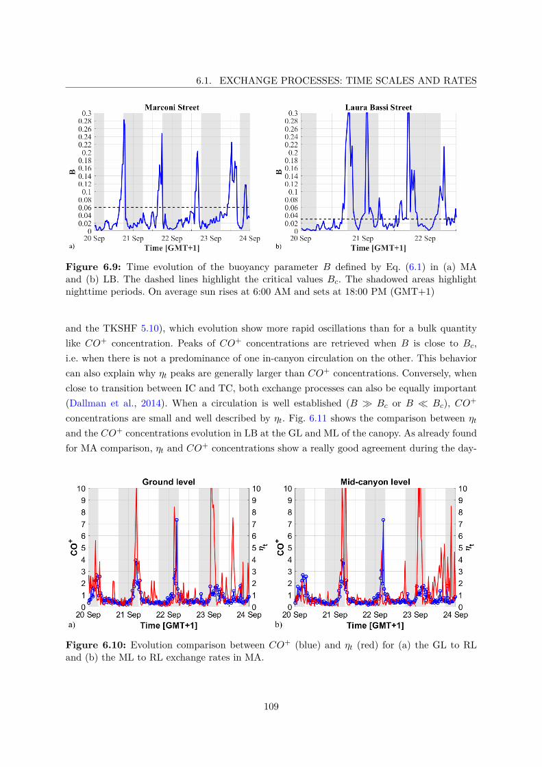
6.1. EXCHANGE PROCESSES: TIME SCALES AND RATES
Figure 6.9: Time evolution of the buoyancy parameter B defined by Eq. (6.1) in (a) MAand (b) LB. The dashed lines highlight the critical values Bc. The shadowed areas highlightnighttime periods. On average sun rises at 6:00 AM and sets at 18:00 PM (GMT+1)
and the TKSHF 5.10), which evolution show more rapid oscillations than for a bulk quantitylike CO+ concentration. Peaks of CO+ concentrations are retrieved when B is close to Bc,i.e. when there is not a predominance of one in-canyon circulation on the other. This behaviorcan also explain why ηt peaks are generally larger than CO+ concentrations. Conversely, whenclose to transition between IC and TC, both exchange processes can also be equally important(Dallman et al., 2014). When a circulation is well established (B � Bc or B � Bc), CO+
concentrations are small and well described by ηt. Fig. 6.11 shows the comparison between ηtand the CO+ concentrations evolution in LB at the GL and ML of the canopy. As already foundfor MA comparison, ηt and CO+ concentrations show a really good agreement during the day-
Figure 6.10: Evolution comparison between CO+ (blue) and ηt (red) for (a) the GL to RLand (b) the ML to RL exchange rates in MA.
109
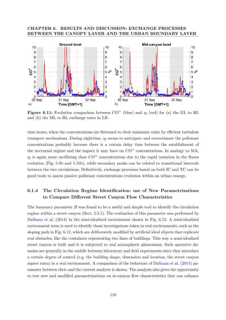
CHAPTER 6. RESULTS AND DISCUSSION: EXCHANGE PROCESSESBETWEEN THE CANOPY LAYER AND THE URBAN BOUNDARY LAYER
Figure 6.11: Evolution comparison between CO+ (blue) and ηt (red) for (a) the GL to RLand (b) the ML to RL exchange rates in LB.
time hours, when the concentrations are flattened to their minimum value by efficient turbulenttransport mechanisms. During nighttime, ηt seems to anticipate and overestimate the pollutantconcentrations probably because there is a certain delay time between the establishment ofthe nocturnal regime and the impact it may have on CO+ concentrations. In analogy to MA,ηt is again more oscillating than CO+ concentrations due to the rapid variation in the fluxesevolution (Fig. 5.9b and 5.10b), while secondary peaks can be related to transitional intervalsbetween the two circulations. Definitively, exchange processes based on both IC and TC can begood tools to assess passive pollutant concentrations evolution within an urban canopy.
6.1.4 The Circulation Regime Identification: use of New Parametrizationsto Compare Different Street Canyon Flow Characteristics
The buoyancy parameter B was found to be a useful and simple tool to identify the circulationregime within a street canyon (Sect. 2.2.1). The evaluation of this parameter was performed byDallman et al. (2014) in the semi-idealized environment shown in Fig. 6.12. A semi-idealizedenvironment term is used to identify those investigations taken in real environments, such as thesloping park in Fig. 6.12, which are deliberately modified by artificial ideal objects that replicatereal obstacles, like the containers representing two lines of buildings. This way a semi-idealizedstreet canyon is built and it is subjected to real atmospheric phenomena. Such operative do-mains are generally in the middle between laboratory and field experiments since they introducea certain degree of control (e.g. the building shape, dimension and location, the street canyonaspect ratio) in a real environment. A comparison of the behaviors of Dallman et al. (2014) pa-rameter between their and the current analysis is shown. The analysis also gives the opportunityto test new and modified parametrizations on in-canyon flow characteristics that can enhance
110
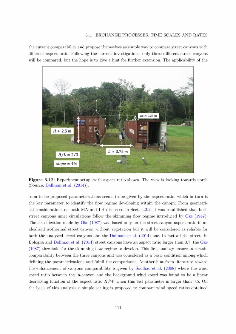
6.1. EXCHANGE PROCESSES: TIME SCALES AND RATES
the current comparability and propose themselves as simple way to compare street canyons withdifferent aspect ratio. Following the current investigations, only three different street canyonswill be compared, but the hope is to give a hint for further extension. The applicability of the
Figure 6.12: Experiment setup, with aspect ratio shown. The view is looking towards north(Source: Dallman et al. (2014)).
soon to be proposed parametrizations seems to be given by the aspect ratio, which in turn isthe key parameter to identify the flow regime developing within the canopy. From geometri-cal considerations on both MA and LB discussed in Sect. 4.2.2, it was established that bothstreet canyons inner circulations follow the skimming flow regime introduced by Oke (1987).The classification made by Oke (1987) was based only on the street canyon aspect ratio in anidealized isothermal street canyon without vegetation but it will be considered as reliable forboth the analyzed street canyons and the Dallman et al. (2014) one. In fact all the streets inBologna and Dallman et al. (2014) street canyons have an aspect ratio larger than 0.7, the Oke(1987) threshold for the skimming flow regime to develop. This first analogy ensures a certaincomparability between the three canyons and was considered as a basic condition among whichdefining the parametrizations and fulfill the comparisons. Another hint from literature towardthe enhancement of canyons comparability is given by Soulhac et al. (2008) where the windspeed ratio between the in-canyon and the background wind speed was found to be a lineardecreasing function of the aspect ratio H/W when this last parameter is larger than 0.5. Onthe basis of this analysis, a simple scaling is proposed to compare wind speed ratios obtained
111
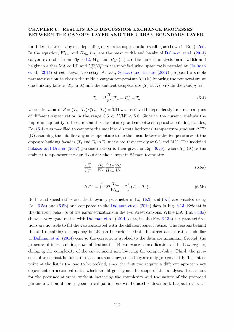
CHAPTER 6. RESULTS AND DISCUSSION: EXCHANGE PROCESSESBETWEEN THE CANOPY LAYER AND THE URBAN BOUNDARY LAYER
for different street canyons, depending only on an aspect ratio rescaling as shown in Eq. (6.5a).In the equation, WDa and HDa (m) are the mean width and height of Dallman et al. (2014)canyon extracted from Fig. 6.12, WC and HC (m) are the current analysis mean width andheight in either MA or LB and UmC /Umb is the modified wind speed ratio rescaled on Dallmanet al. (2014) street canyon geometry. At last, Solazzo and Britter (2007) proposed a simpleparametrization to obtain the middle canyon temperature Tc (K) knowing the temperature atone building facade (Tw in K) and the ambient temperature (Ta in K) outside the canopy as
Tc = RH
W(Tw − Ta) + Ta, (6.4)
where the value of R = (Tc−Ta)/(Tw−Ta) = 0.11 was retrieved independently for street canyonsof different aspect ratios in the range 0.5 < H/W < 5.0. Since in the current analysis theimportant quantity is the horizontal temperature gradient between opposite building facades,Eq. (6.4) was modified to compute the modified discrete horizontal temperature gradient ∆Tm
(K) assuming the middle canyon temperature to be the mean between the temperatures at theopposite building facades (T1 and T2 in K, measured respectively at GL and ML). The modifiedSolazzo and Britter (2007) parametrization is then given in Eq. (6.5b), where Ta (K) is theambient temperature measured outside the canopy in SI monitoring site.
UmCUmb
= HC
WC
WDa
HDa
UCUb
(6.5a)
∆Tm =(
0.22HDa
WDa− 2
)(T1 − Ta) , (6.5b)
Both wind speed ratios and the buoyancy parameter in Eq. (6.2) and (6.1) are rescaled usingEq. (6.5a) and (6.5b) and compared to the Dallman et al. (2014) data in Fig. 6.13. Evident isthe different behavior of the parametrizations in the two street canyons. While MA (Fig. 6.13a)shows a very good match with Dallman et al. (2014) data, in LB (Fig. 6.13b) the parametriza-tions are not able to fill the gap associated with the different aspect ratios. The reasons behindthe still remaining discrepancy in LB can be various. First, the street aspect ratio is similarto Dallman et al. (2014) one, so the corrections applied to the data are minimum. Second, thepresence of intra-building flow infiltration in LB can cause a modification of the flow regime,changing the complexity of the environment and lowering the comparability. Third, the pres-ence of trees must be taken into account somehow, since they are only present in LB. The latterpoint of the list is the one to be tackled, since the first two require a different approach notdependent on measured data, which would go beyond the scope of this analysis. To accountfor the presence of trees, without increasing the complexity and the nature of the proposedparametrization, different geometrical parameters will be used to describe LB aspect ratio. Ef-
112
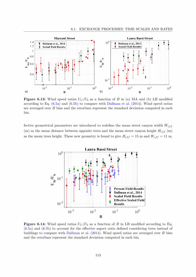
6.1. EXCHANGE PROCESSES: TIME SCALES AND RATES
Figure 6.13: Wind speed ratios UC/Ub as a function of B in (a) MA and (b) LB modifiedaccording to Eq. (6.5a) and (6.5b) to compare with Dallman et al. (2014). Wind speed ratiosare averaged over B bins and the errorbars represent the standard deviation computed in eachbin.
fective geometrical parameters are introduced to redefine the mean street canyon width Weff
(m) as the mean distance between opposite trees and the mean street canyon height Heff (m)as the mean trees height. These new geometry is found to give Heff = 15 m and Weff = 11 m,
Figure 6.14: Wind speed ratios UC/Ub as a function of B in LB modified according to Eq.(6.5a) and (6.5b) to account for the effective aspect ratio defined considering trees instead ofbuildings to compare with Dallman et al. (2014). Wind speed ratios are averaged over B binsand the errorbars represent the standard deviation computed in each bin.
113
CHAPTER 6. RESULTS AND DISCUSSION: EXCHANGE PROCESSESBETWEEN THE CANOPY LAYER AND THE URBAN BOUNDARY LAYER
leading to an effective aspect ratio Heff/Weff = 1.36. The basic assumption for this evaluationis to consider the trees as solid obstacles like buildings, so that they become the boundaries ofthe street canyon. Although this approximation is certainly rough because for example it doesnot account for the tree crown porosity or the trunk, it is a simple solution to account for thepresence of trees. Substituting the effective geometrical parameters in Eq. (6.5a) and (6.5b),the wind speed ratio as a function of the buoyancy parameter displays as in Fig. 6.14 withthe previous scaling (Fig. 6.13b) and the real results. The comparison is still far from being asgood as in MA (Fig. 6.13a) but there are improvement taking the effective geometry. Scaleddata are closer to Dallman et al. (2014) ones despite the distinction between the IC and TCregimes is deteriorated especially in the vicinity of the transition value, as somehow the reducedcanopy air volume imposed by the trees dismantles the circulation differences. As anticipated,the introduced correction to account for the presence of the trees is weak but simple, and givesbetter results than the case where trees are totally neglected. A discrepancy remains due to thepresence of the tree contribution within the measurements of wind speed and air temperaturestaken within the canopy. To magnify the comparability it will probably be necessary to intro-duce further parametrization in these two variables to account for the tree impact on both flowfield and temperature.
6.2 The Impact of Trees on Exchange Processes Variables: aMulti-Seasonal Comparative Analysis
In Sect. 3.1 and during the introduction of this chapter, it was highlighted the importance ofthe canopy atmospheric stability and the background wind direction with respect to the canyonorientation in driving the circulation regimes within the canopy. In Sect. 4.2.2, the backgroundwind direction was stressed to be a fundamental indicator of the circulatory motion withinthe canyon, as retrieved from literature. Atmospheric stability is also important in determiningthe strength and characteristics of mean flow and turbulent structures within the canopy. Tocompare summer and winter campaign’s mean flow and turbulence during the weak synopticperiods it is therefore fundamental to classify different regimes based on atmospheric stabilityand background wind direction. This way, mean flow and turbulence within the canopy areindependent on both atmospheric stability and background wind direction, enabling the com-parison to better highlight the possible impact of tree crowns. The background wind directionclassification was defined at the beginning of this chapter and used throughout the presentedanalysis, but it presents a slight modification to the EWP wind direction. In fact, the EWPwind direction is further divided in East Perpendicular (EP) and West Perpendicular (WP)to search for possible discrepancies in having the monitoring site on the windward or leewardbuilding rooftop of the canyon. The atmospheric stability classification relies on the stability
114
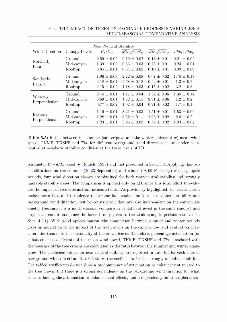
6.2. THE IMPACT OF TREES ON EXCHANGE PROCESSES VARIABLES: AMULTI-SEASONAL COMPARATIVE ANALYSIS
Near-Neutral StabilityWind Direction Canopy Levels Us/Uw w′u′s/w′u′w w′θ′s/w′θ′w Tkes/Tkew
Northerly Ground 0.59 ± 0.02 0.19 ± 0.02 0.13 ± 0.01 0.21 ± 0.02
Parallel Mid-canyon 1.39 ± 0.02 0.36 ± 0.03 0.25 ± 0.01 0.23 ± 0.01Rooftop 0.85 ± 0.01 0.64 ± 0.02 0.10 ± 0.01 0.99 ± 0.06
Southerly Ground 1.96 ± 0.03 2.22 ± 0.08 0.67 ± 0.02 1.78 ± 0.17
Parallel Mid-canyon 3.18 ± 0.04 2.68 ± 0.18 0.42 ± 0.01 1.3 ± 0.2Rooftop 2.15 ± 0.02 1.18 ± 0.03 0.15 ± 0.02 3.2 ± 0.3
Westerly Ground 0.75 ± 0.01 1.17 ± 0.04 1.34 ± 0.05 1.35 ± 0.14
Perpendicular Mid-canyon 0.69 ± 0.01 1.52 ± 0.15 2.91 ± 0.06 1.2 ± 0.2Rooftop 0.77 ± 0.02 1.02 ± 0.04 0.21 ± 0.02 1.7 ± 0.1
Easterly Ground 1.16 ± 0.01 3.21 ± 0.03 1.51 ± 0.01 1.53 ± 0.09
Perpendicular Mid-canyon 1.28 ± 0.01 8.52 ± 0.11 1.93 ± 0.02 2.0 ± 0.2Rooftop 1.23 ± 0.01 3.96 ± 0.02 0.59 ± 0.02 1.94 ± 0.02
Table 6.5: Ratios between the summer (subscript s) and the winter (subscript w) mean windspeed, TKMF, TKSHF and Tke for different background wind direction classes under near-neutral atmospheric stability condition at the three levels of LB.
parameter H − d/LO used by Rotach (1995) and first presented in Sect. 3.3. Applying this twoclassifications on the summer (20-23 September) and winter (08-09 February) weak synopticperiods, four wind direction classes are obtained for both near-neutral stability and stronglyunstable stability cases. The comparison is applied only on LB, since this is an effort to evalu-ate the impact of tree crowns from measured data. As previously highlighted, the classificationmakes mean flow and turbulence to become independent on local atmospheric stability andbackground wind direction, but by construction they are also independent on the canyon ge-ometry (because it is a multi-seasonal comparison of data retrieved in the same canopy) andlarge scale conditions (since the focus is only given to the weak synoptic periods retrieved inSect. 4.2.1). With good approximation, the comparison between summer and winter periodsgives an indication of the impact of the tree crowns on the canyon flow and ventilation char-acteristics thanks to the seasonality of the crown leaves. Therefore, percentage attenuation (orenhancement) coefficients of the mean wind speed, TKMF, TKSHF and Tke associated withthe presence of the tree crowns are calculated as the ratio between the summer and winter quan-tities. The coefficient values for near-neutral stability are reported in Tab. 6.5 for each class ofbackground wind direction. Tab. 6.6 stores the coefficients for the strongly unstable condition.The tabled coefficients do not show a predominance of attenuation or enhancement related tothe tree crown, but there is a strong dependency on the background wind direction for whatconcern having the attenuation or enhancement effects, and a dependency on atmospheric sta-
115
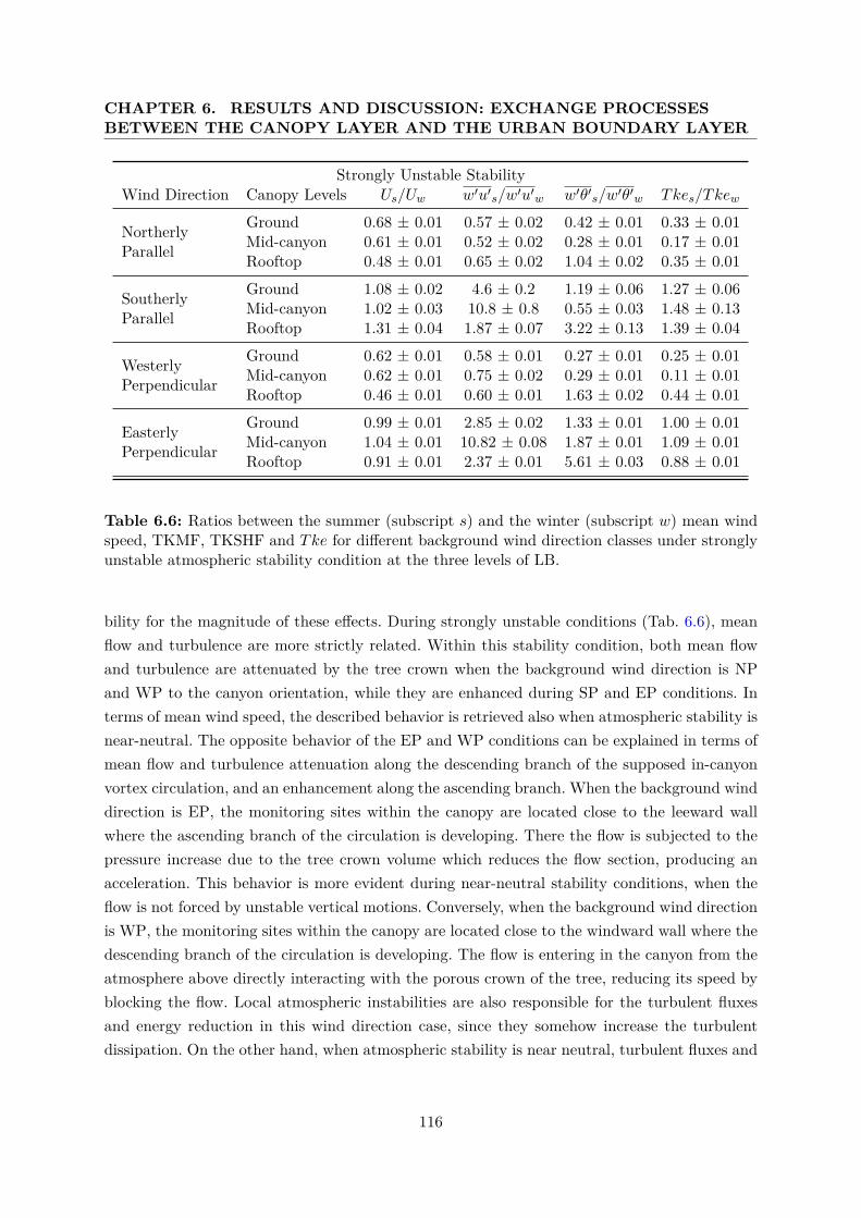
CHAPTER 6. RESULTS AND DISCUSSION: EXCHANGE PROCESSESBETWEEN THE CANOPY LAYER AND THE URBAN BOUNDARY LAYER
Strongly Unstable StabilityWind Direction Canopy Levels Us/Uw w′u′s/w′u′w w′θ′s/w′θ′w Tkes/Tkew
Northerly Ground 0.68 ± 0.01 0.57 ± 0.02 0.42 ± 0.01 0.33 ± 0.01
Parallel Mid-canyon 0.61 ± 0.01 0.52 ± 0.02 0.28 ± 0.01 0.17 ± 0.01Rooftop 0.48 ± 0.01 0.65 ± 0.02 1.04 ± 0.02 0.35 ± 0.01
Southerly Ground 1.08 ± 0.02 4.6 ± 0.2 1.19 ± 0.06 1.27 ± 0.06
Parallel Mid-canyon 1.02 ± 0.03 10.8 ± 0.8 0.55 ± 0.03 1.48 ± 0.13Rooftop 1.31 ± 0.04 1.87 ± 0.07 3.22 ± 0.13 1.39 ± 0.04
Westerly Ground 0.62 ± 0.01 0.58 ± 0.01 0.27 ± 0.01 0.25 ± 0.01
Perpendicular Mid-canyon 0.62 ± 0.01 0.75 ± 0.02 0.29 ± 0.01 0.11 ± 0.01Rooftop 0.46 ± 0.01 0.60 ± 0.01 1.63 ± 0.02 0.44 ± 0.01
Easterly Ground 0.99 ± 0.01 2.85 ± 0.02 1.33 ± 0.01 1.00 ± 0.01
Perpendicular Mid-canyon 1.04 ± 0.01 10.82 ± 0.08 1.87 ± 0.01 1.09 ± 0.01Rooftop 0.91 ± 0.01 2.37 ± 0.01 5.61 ± 0.03 0.88 ± 0.01
Table 6.6: Ratios between the summer (subscript s) and the winter (subscript w) mean windspeed, TKMF, TKSHF and Tke for different background wind direction classes under stronglyunstable atmospheric stability condition at the three levels of LB.
bility for the magnitude of these effects. During strongly unstable conditions (Tab. 6.6), meanflow and turbulence are more strictly related. Within this stability condition, both mean flowand turbulence are attenuated by the tree crown when the background wind direction is NPand WP to the canyon orientation, while they are enhanced during SP and EP conditions. Interms of mean wind speed, the described behavior is retrieved also when atmospheric stability isnear-neutral. The opposite behavior of the EP and WP conditions can be explained in terms ofmean flow and turbulence attenuation along the descending branch of the supposed in-canyonvortex circulation, and an enhancement along the ascending branch. When the background winddirection is EP, the monitoring sites within the canopy are located close to the leeward wallwhere the ascending branch of the circulation is developing. There the flow is subjected to thepressure increase due to the tree crown volume which reduces the flow section, producing anacceleration. This behavior is more evident during near-neutral stability conditions, when theflow is not forced by unstable vertical motions. Conversely, when the background wind directionis WP, the monitoring sites within the canopy are located close to the windward wall where thedescending branch of the circulation is developing. The flow is entering in the canyon from theatmosphere above directly interacting with the porous crown of the tree, reducing its speed byblocking the flow. Local atmospheric instabilities are also responsible for the turbulent fluxesand energy reduction in this wind direction case, since they somehow increase the turbulentdissipation. On the other hand, when atmospheric stability is near neutral, turbulent fluxes and
116
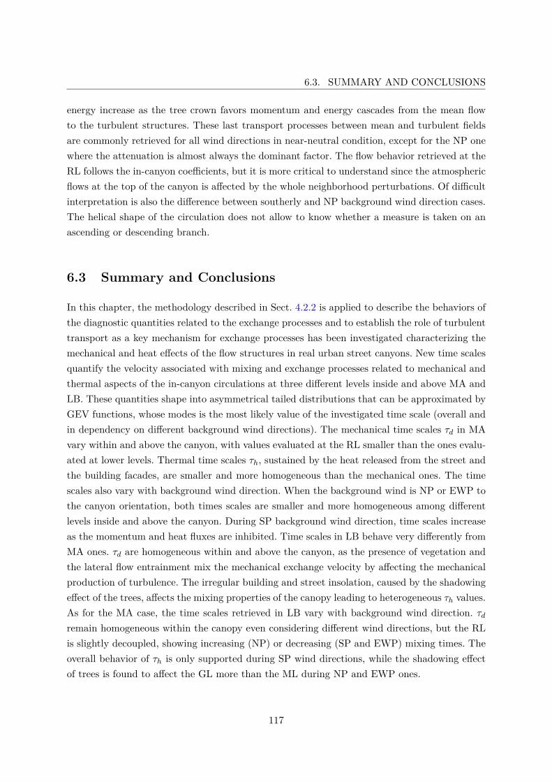
6.3. SUMMARY AND CONCLUSIONS
energy increase as the tree crown favors momentum and energy cascades from the mean flowto the turbulent structures. These last transport processes between mean and turbulent fieldsare commonly retrieved for all wind directions in near-neutral condition, except for the NP onewhere the attenuation is almost always the dominant factor. The flow behavior retrieved at theRL follows the in-canyon coefficients, but it is more critical to understand since the atmosphericflows at the top of the canyon is affected by the whole neighborhood perturbations. Of difficultinterpretation is also the difference between southerly and NP background wind direction cases.The helical shape of the circulation does not allow to know whether a measure is taken on anascending or descending branch.
6.3 Summary and Conclusions
In this chapter, the methodology described in Sect. 4.2.2 is applied to describe the behaviors ofthe diagnostic quantities related to the exchange processes and to establish the role of turbulenttransport as a key mechanism for exchange processes has been investigated characterizing themechanical and heat effects of the flow structures in real urban street canyons. New time scalesquantify the velocity associated with mixing and exchange processes related to mechanical andthermal aspects of the in-canyon circulations at three different levels inside and above MA andLB. These quantities shape into asymmetrical tailed distributions that can be approximated byGEV functions, whose modes is the most likely value of the investigated time scale (overall andin dependency on different background wind directions). The mechanical time scales τd in MAvary within and above the canyon, with values evaluated at the RL smaller than the ones evalu-ated at lower levels. Thermal time scales τh, sustained by the heat released from the street andthe building facades, are smaller and more homogeneous than the mechanical ones. The timescales also vary with background wind direction. When the background wind is NP or EWP tothe canyon orientation, both times scales are smaller and more homogeneous among differentlevels inside and above the canyon. During SP background wind direction, time scales increaseas the momentum and heat fluxes are inhibited. Time scales in LB behave very differently fromMA ones. τd are homogeneous within and above the canyon, as the presence of vegetation andthe lateral flow entrainment mix the mechanical exchange velocity by affecting the mechanicalproduction of turbulence. The irregular building and street insolation, caused by the shadowingeffect of the trees, affects the mixing properties of the canopy leading to heterogeneous τh values.As for the MA case, the time scales retrieved in LB vary with background wind direction. τdremain homogeneous within the canopy even considering different wind directions, but the RLis slightly decoupled, showing increasing (NP) or decreasing (SP and EWP) mixing times. Theoverall behavior of τh is only supported during SP wind directions, while the shadowing effectof trees is found to affect the GL more than the ML during NP and EWP ones.
117
CHAPTER 6. RESULTS AND DISCUSSION: EXCHANGE PROCESSESBETWEEN THE CANOPY LAYER AND THE URBAN BOUNDARY LAYER
The exchange rates associated with mechanical (ηd) and thermal (ηh) processes evaluate the in-canopy flow capability to exchange momentum and heat with the atmosphere above. Both MAand LB are found to be favourable environment for exchange processes to develop for approxi-mately the 50− 75% of the rates cases, but the long tails of the distributions describe scenarioswhere the exchanges are totally suppressed, particularly common in LB. The only exception isretrieved for ηh in LB, where the vegetation inhibits the exchanges at the surface by loweringthe TKSHF. As the exchange rates modes agree in decribing efficient mixing characteristics inMA for all the wind direction cases and for mechanical processes in LB, the ηh in LB mostlydescribe very poor mixing and and heat exchange.From the combination of ηd and ηh, a total exchange rate ηt is evaluated to assess the normal-ized CO+ concentrations removal capacity of the canyon. The buoyancy parameter B retrievedfrom Dallman et al. (2014) has been used as distinguishing factor to combine the mechanicaland thermal rates into the total one. The comparisons between ηt and CO+ show a very goodagreement in both canopies, verifying the a priori hypothesis of mass transport to be driven bymomentum or heat transports, depending on the most dominant in-canyon circulation.Furthermore, the validation of the reproducibility of Dallman et al. (2014) in-canyon circulationdetection on the current investigated canyons enabled the introduction of simple parametriza-tions for in-canyon wind speed and temperature horizontal gradient as functions of the meancanyon aspect ratio H/W . These parametrizations allow to estimate and compare flow char-acteristics in real street canyons with different aspect ratios, if the airflow within the canyonbehaves as expected by the skimming flow regime.Finally a multi-seasonal analysis is presented to retrieve attenuation and enhancement coeffi-cients associated to the impact the tree crowns have on the mean flow and turbulent character-istics under different stability conditions. Both mean flow and turbulent momentum transportdepend strongly on the background wind direction for what discern attenuation and enhance-ment impacts, and depend on atmospheric stability for the magnitude of the coefficients. At-tenuation coefficients are retrieved for the mean flow when background wind directions are NPand WP. The relationship applies also to the turbulent quantities when dealing with stronglyunstable conditions, while a general enhancement is retrieved when atmospheric stability is near-neutral. The results from this last analysis will provide an useful verification for the numericalinvestigations of the following chapter.
118
Chapter 7
Results and Discussion: Modelingthe Impacts of Trees on theExchange Processes
In this chapter, the results obtained from the numerical investigation using the QUIC model willbe presented to simulate the impact of trees on the ventilation, enrinching the characterizationof the excahnge processes in the real urban environment described in Chapter 3 and alreadyinvestigated in Chapter 5 and 6. After a short description of the modification method (see Sect.4.3.2) application, the improved model will be tested on the MA and LB domain among differentinput wind conditions, classified by wind direction ensemble, and verified with the measureddata retreived from the summer campaign. Comparative studies among three different winddirection ensembles will be presented to evaluate the impact of trees in the urban neighborhoodssurrounding MA and LB, focusing on the topological differences of the urban structures withinit and the morphological dependency of the exchagne processes when trees are added or removedfrom the domain.
7.1 Qualitative Code Verification: u∗ associated to the Unper-turbed Flow
As described in Sect. 4.3.2, the friction velocity u∗ is the fundamental variable at the basis ofthe computation of the initial turbulent field. The variable is computed at each grid point of thedomain from the sum of a local, directly related to the mass conserved mean flow, and a non-localparts. The value of u∗ already accounts for the various parametrizations that characterize themodel and, as said, the mass conservation constraint. When dealing with such complex domains,as in typical European urban environments, the mean flow dynamics is strongly perturbed by
119
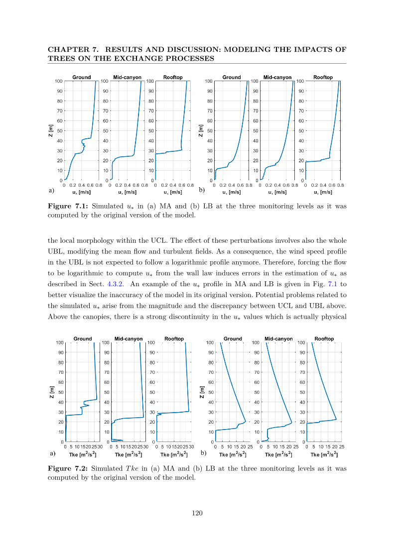
CHAPTER 7. RESULTS AND DISCUSSION: MODELING THE IMPACTS OFTREES ON THE EXCHANGE PROCESSES
Figure 7.1: Simulated u∗ in (a) MA and (b) LB at the three monitoring levels as it wascomputed by the original version of the model.
the local morphology within the UCL. The effect of these perturbations involves also the wholeUBL, modifying the mean flow and turbulent fields. As a consequence, the wind speed profilein the UBL is not expected to follow a logarithmic profile anymore. Therefore, forcing the flowto be logarithmic to compute u∗ from the wall law induces errors in the estimation of u∗ asdescribed in Sect. 4.3.2. An example of the u∗ profile in MA and LB is given in Fig. 7.1 tobetter visualize the inaccuracy of the model in its original version. Potential problems related tothe simulated u∗ arise from the magnitude and the discrepancy between UCL and UBL above.Above the canopies, there is a strong discontinuity in the u∗ values which is actually physical
Figure 7.2: Simulated Tke in (a) MA and (b) LB at the three monitoring levels as it wascomputed by the original version of the model.
120
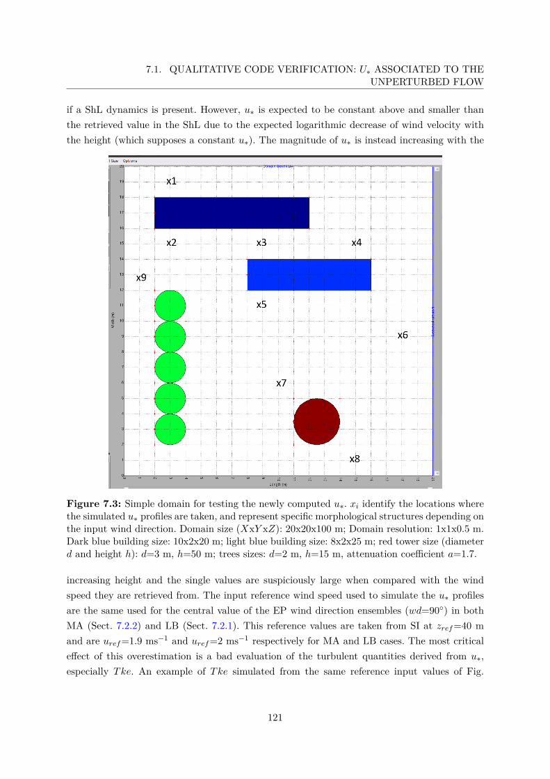
7.1. QUALITATIVE CODE VERIFICATION: U∗ ASSOCIATED TO THEUNPERTURBED FLOW
if a ShL dynamics is present. However, u∗ is expected to be constant above and smaller thanthe retrieved value in the ShL due to the expected logarithmic decrease of wind velocity withthe height (which supposes a constant u∗). The magnitude of u∗ is instead increasing with the
Figure 7.3: Simple domain for testing the newly computed u∗. xi identify the locations wherethe simulated u∗ profiles are taken, and represent specific morphological structures depending onthe input wind direction. Domain size (XxY xZ): 20x20x100 m; Domain resolution: 1x1x0.5 m.Dark blue building size: 10x2x20 m; light blue building size: 8x2x25 m; red tower size (diameterd and height h): d=3 m, h=50 m; trees sizes: d=2 m, h=15 m, attenuation coefficient a=1.7.
increasing height and the single values are suspiciously large when compared with the windspeed they are retrieved from. The input reference wind speed used to simulate the u∗ profilesare the same used for the central value of the EP wind direction ensembles (wd=90◦) in bothMA (Sect. 7.2.2) and LB (Sect. 7.2.1). This reference values are taken from SI at zref=40 mand are uref=1.9 ms−1 and uref=2 ms−1 respectively for MA and LB cases. The most criticaleffect of this overestimation is a bad evaluation of the turbulent quantities derived from u∗,especially Tke. An example of Tke simulated from the same reference input values of Fig.
121
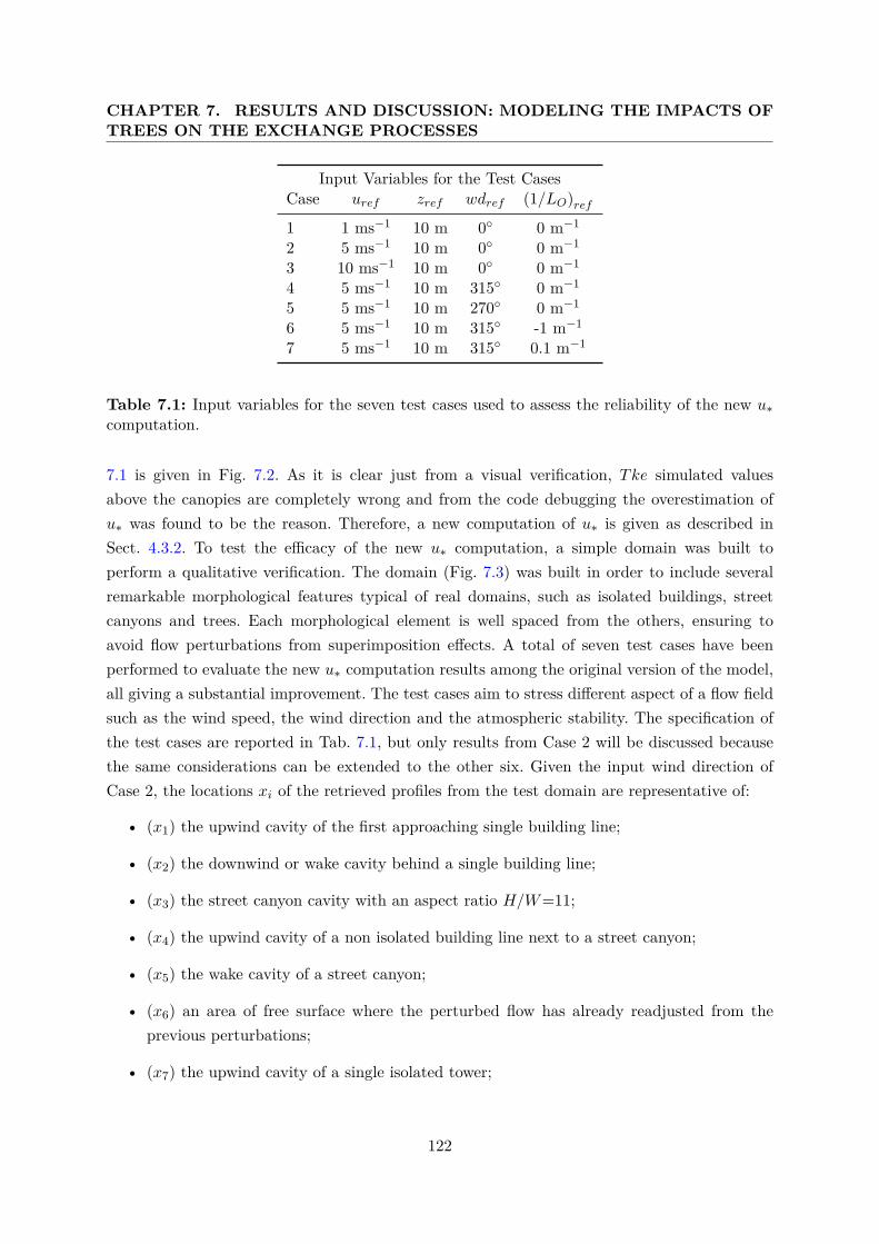
CHAPTER 7. RESULTS AND DISCUSSION: MODELING THE IMPACTS OFTREES ON THE EXCHANGE PROCESSES
Input Variables for the Test CasesCase uref zref wdref (1/LO)ref1 1 ms−1 10 m 0◦ 0 m−1
2 5 ms−1 10 m 0◦ 0 m−1
3 10 ms−1 10 m 0◦ 0 m−1
4 5 ms−1 10 m 315◦ 0 m−1
5 5 ms−1 10 m 270◦ 0 m−1
6 5 ms−1 10 m 315◦ -1 m−1
7 5 ms−1 10 m 315◦ 0.1 m−1
Table 7.1: Input variables for the seven test cases used to assess the reliability of the new u∗computation.
7.1 is given in Fig. 7.2. As it is clear just from a visual verification, Tke simulated valuesabove the canopies are completely wrong and from the code debugging the overestimation ofu∗ was found to be the reason. Therefore, a new computation of u∗ is given as described inSect. 4.3.2. To test the efficacy of the new u∗ computation, a simple domain was built toperform a qualitative verification. The domain (Fig. 7.3) was built in order to include severalremarkable morphological features typical of real domains, such as isolated buildings, streetcanyons and trees. Each morphological element is well spaced from the others, ensuring toavoid flow perturbations from superimposition effects. A total of seven test cases have beenperformed to evaluate the new u∗ computation results among the original version of the model,all giving a substantial improvement. The test cases aim to stress different aspect of a flow fieldsuch as the wind speed, the wind direction and the atmospheric stability. The specification ofthe test cases are reported in Tab. 7.1, but only results from Case 2 will be discussed becausethe same considerations can be extended to the other six. Given the input wind direction ofCase 2, the locations xi of the retrieved profiles from the test domain are representative of:
• (x1) the upwind cavity of the first approaching single building line;
• (x2) the downwind or wake cavity behind a single building line;
• (x3) the street canyon cavity with an aspect ratio H/W=11;
• (x4) the upwind cavity of a non isolated building line next to a street canyon;
• (x5) the wake cavity of a street canyon;
• (x6) an area of free surface where the perturbed flow has already readjusted from theprevious perturbations;
• (x7) the upwind cavity of a single isolated tower;
122
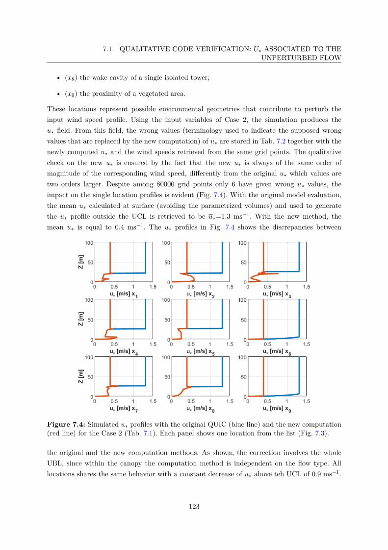
7.1. QUALITATIVE CODE VERIFICATION: U∗ ASSOCIATED TO THEUNPERTURBED FLOW
• (x8) the wake cavity of a single isolated tower;
• (x9) the proximity of a vegetated area.
These locations represent possible environmental geometries that contribute to perturb theinput wind speed profile. Using the input variables of Case 2, the simulation produces theu∗ field. From this field, the wrong values (terminology used to indicate the supposed wrongvalues that are replaced by the new computation) of u∗ are stored in Tab. 7.2 together with thenewly computed u∗ and the wind speeds retrieved from the same grid points. The qualitativecheck on the new u∗ is ensured by the fact that the new u∗ is always of the same order ofmagnitude of the corresponding wind speed, differently from the original u∗ which values aretwo orders larger. Despite among 80000 grid points only 6 have given wrong u∗ values, theimpact on the single location profiles is evident (Fig. 7.4). With the original model evaluation,the mean u∗ calculated at surface (avoiding the parametrized volumes) and used to generatethe u∗ profile outside the UCL is retrieved to be u∗=1.3 ms−1. With the new method, themean u∗ is equal to 0.4 ms−1. The u∗ profiles in Fig. 7.4 shows the discrepancies between
Figure 7.4: Simulated u∗ profiles with the original QUIC (blue line) and the new computation(red line) for the Case 2 (Tab. 7.1). Each panel shows one location from the list (Fig. 7.3).
the original and the new computation methods. As shown, the correction involves the wholeUBL, since within the canopy the computation method is independent on the flow type. Alllocations shares the same behavior with a constant decrease of u∗ above teh UCL of 0.9 ms−1.
123
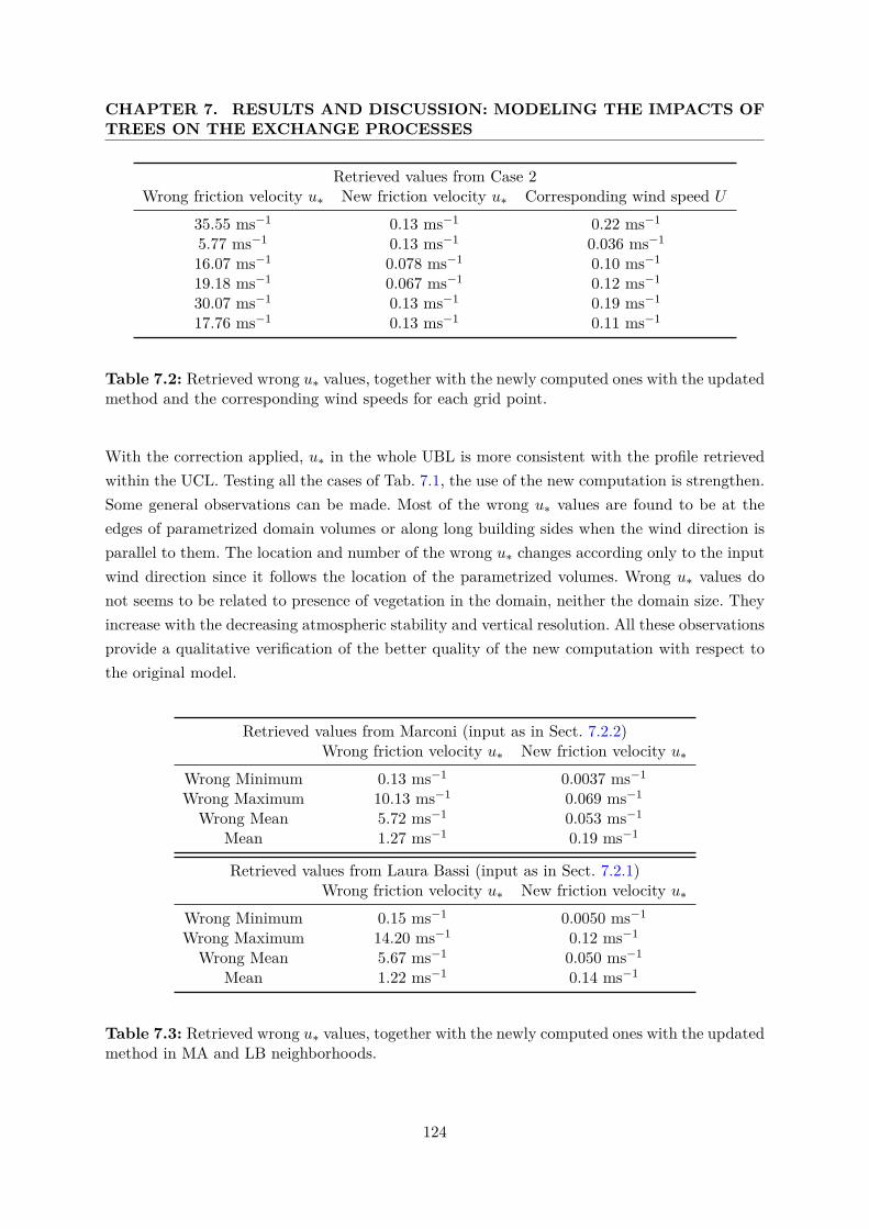
CHAPTER 7. RESULTS AND DISCUSSION: MODELING THE IMPACTS OFTREES ON THE EXCHANGE PROCESSES
Retrieved values from Case 2Wrong friction velocity u∗ New friction velocity u∗ Corresponding wind speed U
35.55 ms−1 0.13 ms−1 0.22 ms−1
5.77 ms−1 0.13 ms−1 0.036 ms−1
16.07 ms−1 0.078 ms−1 0.10 ms−1
19.18 ms−1 0.067 ms−1 0.12 ms−1
30.07 ms−1 0.13 ms−1 0.19 ms−1
17.76 ms−1 0.13 ms−1 0.11 ms−1
Table 7.2: Retrieved wrong u∗ values, together with the newly computed ones with the updatedmethod and the corresponding wind speeds for each grid point.
With the correction applied, u∗ in the whole UBL is more consistent with the profile retrievedwithin the UCL. Testing all the cases of Tab. 7.1, the use of the new computation is strengthen.Some general observations can be made. Most of the wrong u∗ values are found to be at theedges of parametrized domain volumes or along long building sides when the wind direction isparallel to them. The location and number of the wrong u∗ changes according only to the inputwind direction since it follows the location of the parametrized volumes. Wrong u∗ values donot seems to be related to presence of vegetation in the domain, neither the domain size. Theyincrease with the decreasing atmospheric stability and vertical resolution. All these observationsprovide a qualitative verification of the better quality of the new computation with respect tothe original model.
Retrieved values from Marconi (input as in Sect. 7.2.2)Wrong friction velocity u∗ New friction velocity u∗
Wrong Minimum 0.13 ms−1 0.0037 ms−1
Wrong Maximum 10.13 ms−1 0.069 ms−1
Wrong Mean 5.72 ms−1 0.053 ms−1
Mean 1.27 ms−1 0.19 ms−1
Retrieved values from Laura Bassi (input as in Sect. 7.2.1)Wrong friction velocity u∗ New friction velocity u∗
Wrong Minimum 0.15 ms−1 0.0050 ms−1
Wrong Maximum 14.20 ms−1 0.12 ms−1
Wrong Mean 5.67 ms−1 0.050 ms−1
Mean 1.22 ms−1 0.14 ms−1
Table 7.3: Retrieved wrong u∗ values, together with the newly computed ones with the updatedmethod in MA and LB neighborhoods.
124
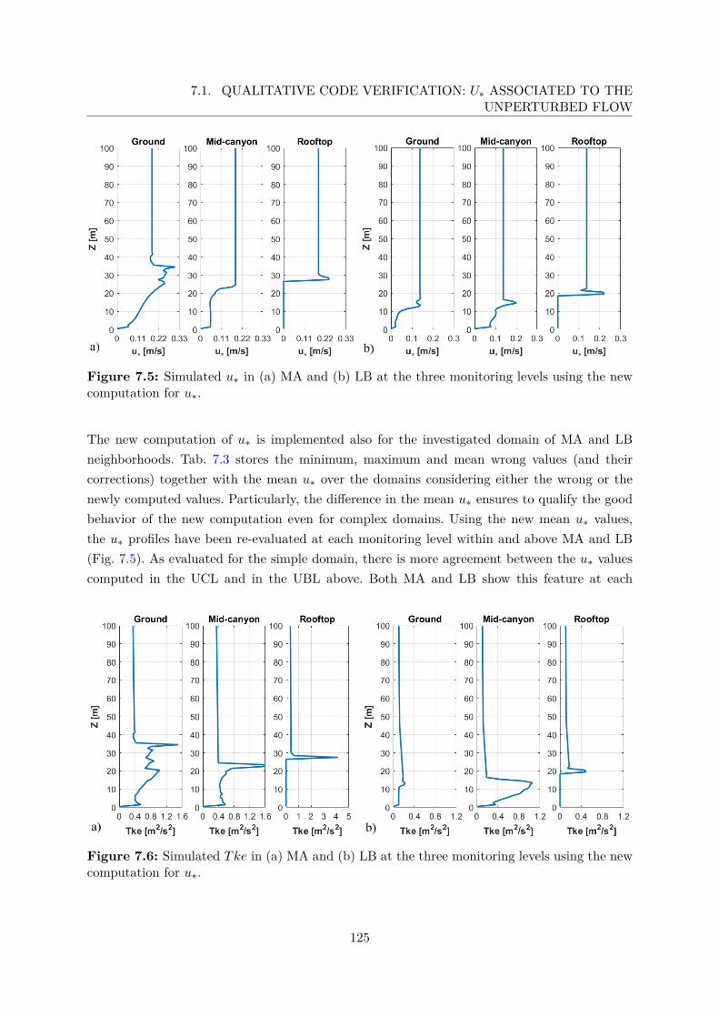
7.1. QUALITATIVE CODE VERIFICATION: U∗ ASSOCIATED TO THEUNPERTURBED FLOW
Figure 7.5: Simulated u∗ in (a) MA and (b) LB at the three monitoring levels using the newcomputation for u∗.
The new computation of u∗ is implemented also for the investigated domain of MA and LBneighborhoods. Tab. 7.3 stores the minimum, maximum and mean wrong values (and theircorrections) together with the mean u∗ over the domains considering either the wrong or thenewly computed values. Particularly, the difference in the mean u∗ ensures to qualify the goodbehavior of the new computation even for complex domains. Using the new mean u∗ values,the u∗ profiles have been re-evaluated at each monitoring level within and above MA and LB(Fig. 7.5). As evaluated for the simple domain, there is more agreement between the u∗ valuescomputed in the UCL and in the UBL above. Both MA and LB show this feature at each
Figure 7.6: Simulated Tke in (a) MA and (b) LB at the three monitoring levels using the newcomputation for u∗.
125
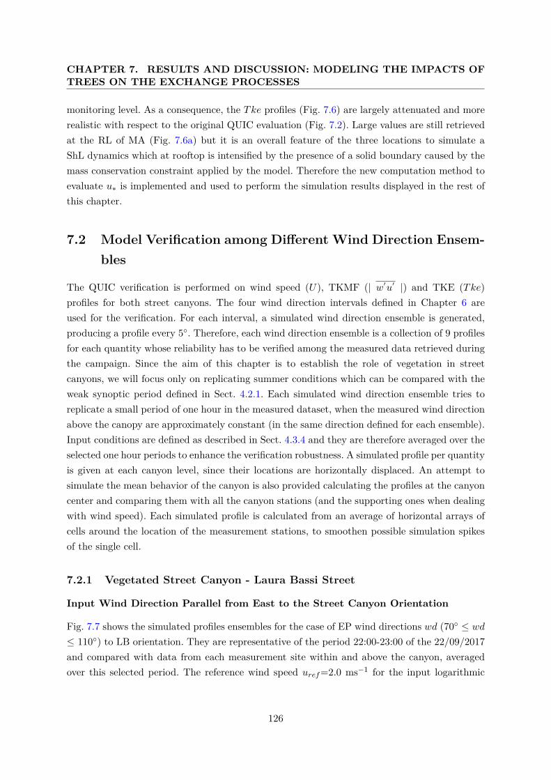
CHAPTER 7. RESULTS AND DISCUSSION: MODELING THE IMPACTS OFTREES ON THE EXCHANGE PROCESSES
monitoring level. As a consequence, the Tke profiles (Fig. 7.6) are largely attenuated and morerealistic with respect to the original QUIC evaluation (Fig. 7.2). Large values are still retrievedat the RL of MA (Fig. 7.6a) but it is an overall feature of the three locations to simulate aShL dynamics which at rooftop is intensified by the presence of a solid boundary caused by themass conservation constraint applied by the model. Therefore the new computation method toevaluate u∗ is implemented and used to perform the simulation results displayed in the rest ofthis chapter.
7.2 Model Verification among Different Wind Direction Ensem-bles
The QUIC verification is performed on wind speed (U), TKMF (| w′u′ |) and TKE (Tke)profiles for both street canyons. The four wind direction intervals defined in Chapter 6 areused for the verification. For each interval, a simulated wind direction ensemble is generated,producing a profile every 5◦. Therefore, each wind direction ensemble is a collection of 9 profilesfor each quantity whose reliability has to be verified among the measured data retrieved duringthe campaign. Since the aim of this chapter is to establish the role of vegetation in streetcanyons, we will focus only on replicating summer conditions which can be compared with theweak synoptic period defined in Sect. 4.2.1. Each simulated wind direction ensemble tries toreplicate a small period of one hour in the measured dataset, when the measured wind directionabove the canopy are approximately constant (in the same direction defined for each ensemble).Input conditions are defined as described in Sect. 4.3.4 and they are therefore averaged over theselected one hour periods to enhance the verification robustness. A simulated profile per quantityis given at each canyon level, since their locations are horizontally displaced. An attempt tosimulate the mean behavior of the canyon is also provided calculating the profiles at the canyoncenter and comparing them with all the canyon stations (and the supporting ones when dealingwith wind speed). Each simulated profile is calculated from an average of horizontal arrays ofcells around the location of the measurement stations, to smoothen possible simulation spikesof the single cell.
7.2.1 Vegetated Street Canyon - Laura Bassi Street
Input Wind Direction Parallel from East to the Street Canyon Orientation
Fig. 7.7 shows the simulated profiles ensembles for the case of EP wind directions wd (70◦ ≤ wd≤ 110◦) to LB orientation. They are representative of the period 22:00-23:00 of the 22/09/2017and compared with data from each measurement site within and above the canyon, averagedover this selected period. The reference wind speed uref=2.0 ms−1 for the input logarithmic
126
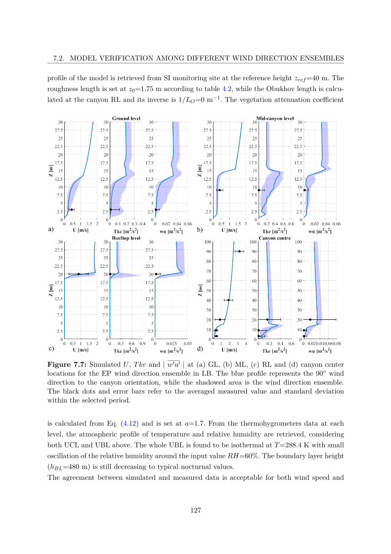
7.2. MODEL VERIFICATION AMONG DIFFERENT WIND DIRECTION ENSEMBLES
profile of the model is retrieved from SI monitoring site at the reference height zref=40 m. Theroughness length is set at z0=1.75 m according to table 4.2, while the Obukhov length is calcu-lated at the canyon RL and its inverse is 1/LO=0 m−1. The vegetation attenuation coefficient
Figure 7.7: Simulated U , Tke and | w′u′ | at (a) GL, (b) ML, (c) RL and (d) canyon centerlocations for the EP wind direction ensemble in LB. The blue profile represents the 90◦ winddirection to the canyon orientation, while the shadowed area is the wind direction ensemble.The black dots and error bars refer to the averaged measured value and standard deviationwithin the selected period.
is calculated from Eq. (4.12) and is set at a=1.7. From the thermohygrometers data at eachlevel, the atmospheric profile of temperature and relative humidity are retrieved, consideringboth UCL and UBL above. The whole UBL is found to be isothermal at T=288.4 K with smalloscillation of the relative humidity around the input value RH=60%. The boundary layer height(hBL=480 m) is still decreasing to typical nocturnal values.The agreement between simulated and measured data is acceptable for both wind speed and
127
CHAPTER 7. RESULTS AND DISCUSSION: MODELING THE IMPACTS OFTREES ON THE EXCHANGE PROCESSES
turbulence related quantities. Within the canyon, wind speed is underestimated by the model,but still within the error bars. This behavior can be consequence of the wind acceleration dueto the reduced air volume and increased pressure between the tree crown and the surface (atGL) or the building facade (at ML) not sufficiently accounted by the model. TKE and TKMFwithin the canyon are well captured, despite a certain overestimation at ML. Turbulent relatedquantities are less in agreement with data for what concern the RL (Fig. 7.7c). Since measure-ments are taken directly above the rooftop, the profiles are cut at the building height. Despitethe good agreement for wind speed values, turbulence is roughly overestimated, describing aturbulent layer which does not find confirmation in the measured data. Despite these small dis-agreements, data from measurements are well simulated by the model. Agreement is still goodif a single representative profile is computed for the canyon (Fig. 7.7d). These last profiles arenot meant to match perfectly the data, but to assess how representative could measurements beof the flow behavior. Poor agreement was expected inside the canopy, where local morphologicalfeatures and the vicinity of trees may have a role in the modification of the profile. However, theagreement is good for both mean flow and turbulent quantities, confirming the results found ateach measurement site. Wind speed is also compared to SI and AT monitoring sites to assess theflow behavior at larger scale. SI is perfectly represented, verifying the logarithmic shape of thewind velocity profile outside the canopy layer. However, wind speed at AT is poorly captured.This behavior can be the consequence of the possible perturbations of the logarithmic profileby the larger scale flow, which enhances the wind speed in the upper part of the UBL.
Input Wind Direction Perpendicular from West to the Street Canyon Orientation
Profiles simulated for the WP wind direction ensemble (250◦ ≤ wd ≤ 290◦) to LB orientation aredisplayed in Fig. 7.8, representing the interval 09:00-10:00 of the 21/09/2017. Reference windspeed uref=2.1 ms−1 for the input profile is again collected at SI monitoring site at zref=40 m.As for the EP case, z0=1.75 m and a=1.7. The inverse Obukhov length is 1/LO=-0.0242 m−1,describing a near neutral stability condition. Temperature is uniform inside the canopy (Tc=292K) and almost equal to the ambient temperature Ta=291 K. Relative humidity ranges betweenthe RHc=50% of the canopy to the RHa=40% at the AT monitoring site. A rising boundarylayer reaches a height of hBL=750 m.Fig. 7.8 shows an even better agreement between simulations and measurements than the EPensemble. Each profile stays within the error bar of the measurements, even considering thecanyon center panel in Fig. 7.8d. However, a certain underestimation can be found inside thecanopy (Fig. 7.8a-b) where both wind speed and TKMF are smaller than the measurements.Wind speed is slightly underestimated by the model (Fig. 7.8a-b) as it was already found forthe EP wind direction ensemble (Fig. 7.7a-b). The reduced air volume between the tree crownand the ground or the building facade increases the local pressure and produces an acceleration
128
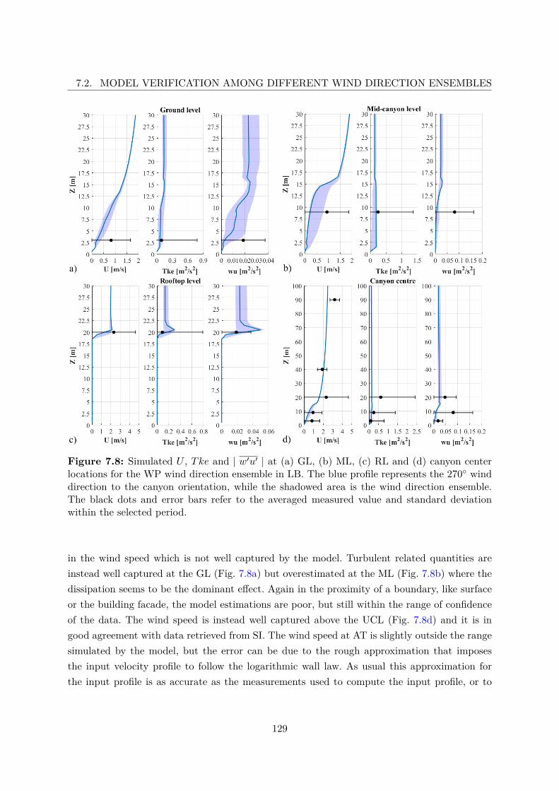
7.2. MODEL VERIFICATION AMONG DIFFERENT WIND DIRECTION ENSEMBLES
Figure 7.8: Simulated U , Tke and | w′u′ | at (a) GL, (b) ML, (c) RL and (d) canyon centerlocations for the WP wind direction ensemble in LB. The blue profile represents the 270◦ winddirection to the canyon orientation, while the shadowed area is the wind direction ensemble.The black dots and error bars refer to the averaged measured value and standard deviationwithin the selected period.
in the wind speed which is not well captured by the model. Turbulent related quantities areinstead well captured at the GL (Fig. 7.8a) but overestimated at the ML (Fig. 7.8b) where thedissipation seems to be the dominant effect. Again in the proximity of a boundary, like surfaceor the building facade, the model estimations are poor, but still within the range of confidenceof the data. The wind speed is instead well captured above the UCL (Fig. 7.8d) and it is ingood agreement with data retrieved from SI. The wind speed at AT is slightly outside the rangesimulated by the model, but the error can be due to the rough approximation that imposesthe input velocity profile to follow the logarithmic wall law. As usual this approximation forthe input profile is as accurate as the measurements used to compute the input profile, or to
129
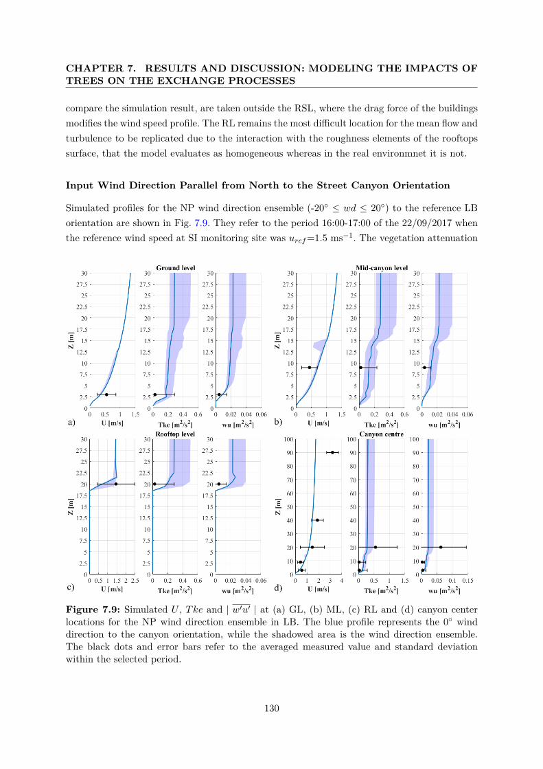
CHAPTER 7. RESULTS AND DISCUSSION: MODELING THE IMPACTS OFTREES ON THE EXCHANGE PROCESSES
compare the simulation result, are taken outside the RSL, where the drag force of the buildingsmodifies the wind speed profile. The RL remains the most difficult location for the mean flow andturbulence to be replicated due to the interaction with the roughness elements of the rooftopssurface, that the model evaluates as homogeneous whereas in the real environmnet it is not.
Input Wind Direction Parallel from North to the Street Canyon Orientation
Simulated profiles for the NP wind direction ensemble (-20◦ ≤ wd ≤ 20◦) to the reference LBorientation are shown in Fig. 7.9. They refer to the period 16:00-17:00 of the 22/09/2017 whenthe reference wind speed at SI monitoring site was uref=1.5 ms−1. The vegetation attenuation
Figure 7.9: Simulated U , Tke and | w′u′ | at (a) GL, (b) ML, (c) RL and (d) canyon centerlocations for the NP wind direction ensemble in LB. The blue profile represents the 0◦ winddirection to the canyon orientation, while the shadowed area is the wind direction ensemble.The black dots and error bars refer to the averaged measured value and standard deviationwithin the selected period.
130
7.2. MODEL VERIFICATION AMONG DIFFERENT WIND DIRECTION ENSEMBLES
coefficient is always a=1.7, while z0=1.51 m according to table 4.2. The inverse of the Obukhovlength (1/LO=-0.0223 m−1) accounts for a near neutral condition. The in-canyon temperature(Tc=296 K) is slightly larger than the ambient (Ta=295 K), while relative humidity decreasesfrom RHc=43% to RHa=33% from the canyon surface to the AT monitoring site. The boundarylayer height (hBL=1336 m) is typical of daytime hours.TKE and TKMF are overestimated in comparison with the data from measurements. Onceagain the proximity of a boundary, like the surface or the building facade, is poorly representedby the model, but still within the range of confidence of the data. Moreover the channellingeffect of the flow parallel to the street canyon, somehow enhances the turbulence productionof both TKE and TKMF. The mean wind speed is underestimated at the GL (Fig. 7.9a) dueto the poor representation of the flow acceleration between the tree crown and the surface.Conversely, the wind speed is overestimated at ML (Fig. 7.9b). The channelling effect at thestreet surface is underestimated, since the trunk portion of the tree can create a flow accelerationnot captured by the model. Nevertheless, the speed reduction due to the enhanced roughness ofthe small environment between the tree crown and the building facades in instead interpretedby the model as a simple sidewall on which the flow can accelarate due to the increased volumepressure. In both cases, wind speed profiles are independent of wind direction, as a consequenceof the channeling behavior of the flow. The canyon center profiles (Fig. 7.9d) overestimatethe daytime typical behavior of the mean flow and turbulence accounting for well mixed airand small gradients, larger than what it is resembled by data from measurements. This lastpoor comparison is indeed a consequence of the sum of the problematic already described forthe single sensors locations, and it is expected to increase due to the bulk estimation of thecenter canyon profile. Nevertheless the data from measurements stay within the wind directionensembles retrieved from the model.
Input Wind Direction Parallel from South to the Street Canyon Orientation
Fig. 7.10 shows the simulated profiles for the SP wind direction ensemble (160◦ ≤ wd ≤ 200◦)to the LB orientation, referring to the period 03:00-04:00 of the 22/09/2017. This last scenariopresents some differences with the previously analyzed ones. Reference wind speed is more in-tense (uref=5.3 ms−1) due to the possible development of a nocturnal jet at the city scale. Aninverse thermal stratification affects the UBL above the canopy, where a ∆T=2 K is retrievedbetween 40 m and 100 m. Nevertheless, air within the canopy and at the rooftop interfaceremains mixed due to the heat loss from the building facades, and a weak unstable conditiondevelops inside the canyon (1/LO=-0.0816 m−1). The result is a strong thermal and stabilitydecoupling between the UCL and the UBL above it. Relative humidity does not follow thetemperature inversion and ranges between the RHc=69% value inside the canyon to RHa=50%at the AT monitoring site. A boundary layer height of hBL=455 m is retrieved.
131
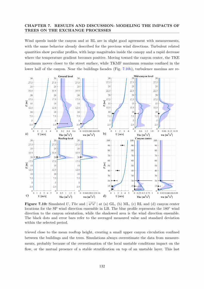
CHAPTER 7. RESULTS AND DISCUSSION: MODELING THE IMPACTS OFTREES ON THE EXCHANGE PROCESSES
Wind speeds inside the canyon and at RL are in slight good agreement with measurements,with the same behavior already described for the previous wind directions. Turbulent relatedquantities show peculiar profiles, with large magnitudes inside the canopy and a rapid decreasewhere the temperature gradient becomes positive. Moving toward the canyon center, the TKEmaximum moves closer to the street surface, while TKMF maximum remains confined in thelower half of the canyon. Near the buildings facades (Fig. 7.10b), turbulence maxima are re-
Figure 7.10: Simulated U , Tke and | w′u′ | at (a) GL, (b) ML, (c) RL and (d) canyon centerlocations for the SP wind direction ensemble in LB. The blue profile represents the 180◦ winddirection to the canyon orientation, while the shadowed area is the wind direction ensemble.The black dots and error bars refer to the averaged measured value and standard deviationwithin the selected period.
trieved close to the mean rooftop height, creating a small upper canyon circulation confinedbetween the buildings and the trees. Simulations always overestimate the data from measure-ments, probably because of the overestimation of the local unstable conditions impact on theflow, or the mutual presence of a stable stratification on top of an unstable layer. This last
132
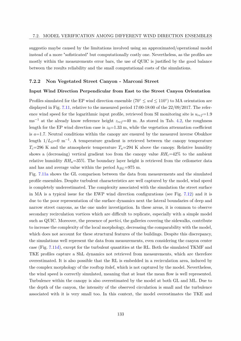
7.2. MODEL VERIFICATION AMONG DIFFERENT WIND DIRECTION ENSEMBLES
suggestio maybe caused by the limitations involved using an approximated/operational modelinstead of a more "sofisticated" but computationally costly one. Nevertheless, as the profiles aremostly within the measurements error bars, the use of QUIC is justified by the good balancebetween the results reliability and the small computational costs of the simulations.
7.2.2 Non Vegetated Street Canyon - Marconi Street
Input Wind Direction Perpendicular from East to the Street Canyon Orientation
Profiles simulated for the EP wind direction ensemble (70◦ ≤ wd ≤ 110◦) to MA orientation aredisplayed in Fig. 7.11, relative to the measured period 17:00-18:00 of the 22/09/2017. The refer-ence wind speed for the logarithmic input profile, retrieved from SI monitoring site is uref=1.9ms−1 at the already know reference height zref=40 m. As stored in Tab. 4.2, the roughnesslength for the EP wind direction case is z0=1.33 m, while the vegetation attenuation coefficientis a=1.7. Neutral conditions within the canopy are ensured by the measured inverse Obukhovlength 1/LO=0 m−1. A temperature gradient is retrieved between the canopy temperatureTc=296 K and the atmospheric temperature Ta=294 K above the canopy. Relative humidityshows a (decreasing) vertical gradient too from the canopy value RHc=42% to the ambientrelative humidity RHa=35%. The boundary layer height is retrieved from the ceilometer dataand has and average value within the period hBL=975 m.Fig. 7.11a shows the GL comparison between the data from measurements and the simulatedprofile ensembles. Despite turbulent characteristics are well captured by the model, wind speedis completely underestimated. The complexity associated with the simulation the street surfacein MA is a typical issue for the EWP wind direction configurations (see Fig. 7.12) and it isdue to the poor representation of the surface dynamics next the lateral boundaries of deep andnarrow street canyons, as the one under investigation. In these areas, it is common to observesecondary recirculation vortices which are difficult to replicate, especially with a simple modelsuch as QUIC. Moreover, the presence of portici, the galleries covering the sidewalks, contributeto increase the complexity of the local morphology, decreasing the comparability with the model,which does not account for these structural features of the buildings. Despite this discrepancy,the simulations well represent the data from measurements, even considering the canyon centercase (Fig. 7.11d), except for the turbulent quantities at the RL. Both the simulated TKMF andTKE profiles capture a ShL dynamics not retrieved from measurements, which are thereforeoverestimated. It is also possible that the RL is embedded in a recirculation area, induced bythe complex morphology of the rooftop itslef, which is not captured by the model. Nevertheless,the wind speed is correctly simulated, meaning that at least the mean flow is well represented.Turbulence within the canopy is also overestimated by the model at both GL and ML. Due tothe depth of the canyon, the intensity of the observed circulation is small and the turbulenceassociated with it is very small too. In this context, the model overestimates the TKE and
133
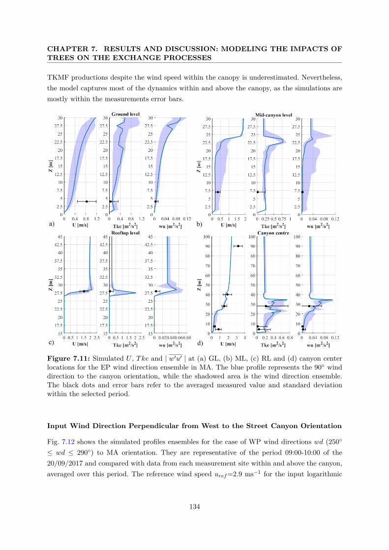
CHAPTER 7. RESULTS AND DISCUSSION: MODELING THE IMPACTS OFTREES ON THE EXCHANGE PROCESSES
TKMF productions despite the wind speed within the canopy is underestimated. Nevertheless,the model captures most of the dynamics within and above the canopy, as the simulations aremostly within the measurements error bars.
Figure 7.11: Simulated U , Tke and | w′u′ | at (a) GL, (b) ML, (c) RL and (d) canyon centerlocations for the EP wind direction ensemble in MA. The blue profile represents the 90◦ winddirection to the canyon orientation, while the shadowed area is the wind direction ensemble.The black dots and error bars refer to the averaged measured value and standard deviationwithin the selected period.
Input Wind Direction Perpendicular from West to the Street Canyon Orientation
Fig. 7.12 shows the simulated profiles ensembles for the case of WP wind directions wd (250◦
≤ wd ≤ 290◦) to MA orientation. They are representative of the period 09:00-10:00 of the20/09/2017 and compared with data from each measurement site within and above the canyon,averaged over this period. The reference wind speed uref=2.9 ms−1 for the input logarithmic
134
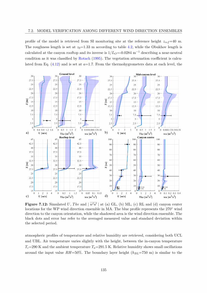
7.2. MODEL VERIFICATION AMONG DIFFERENT WIND DIRECTION ENSEMBLES
profile of the model is retrieved from SI monitoring site at the reference height zref=40 m.The roughness length is set at z0=1.33 m according to table 4.2, while the Obukhov length iscalculated at the canyon rooftop and its inverse is 1/LO=-0.0284 m−1 describing a near-neutralcondition as it was classified by Rotach (1995). The vegetation attenuation coefficient is calcu-lated from Eq. (4.12) and is set at a=1.7. From the thermohygrometers data at each level, the
Figure 7.12: Simulated U , Tke and | w′u′ | at (a) GL, (b) ML, (c) RL and (d) canyon centerlocations for the WP wind direction ensemble in MA. The blue profile represents the 270◦ winddirection to the canyon orientation, while the shadowed area is the wind direction ensemble. Theblack dots and error bar refer to the averaged measured value and standard deviation withinthe selected period.
atmospheric profiles of temperature and relative humidity are retrieved, considering both UCLand UBL. Air temperature varies slightly with the height, between the in-canyon temperatureTc=290 K and the ambient temperature Ta=291.5 K. Relative humidity shows small oscillationsaround the input value RH=50%. The boundary layer height (hBL=750 m) is similar to the
135
CHAPTER 7. RESULTS AND DISCUSSION: MODELING THE IMPACTS OFTREES ON THE EXCHANGE PROCESSES
condition retrieved for the EP wind direction ensemble.Simulated profiles are in good agreement with the data from measurements at all locations. Theonly discrepancy is retrieved in the wind speed at the GL location (Fig. 7.12a), as already ob-served for the EP wind direction ensemble (Fig. 7.11a). In the current case, the underestimationis less pronounced, but it is still present, since the circulation within the canopy is expected tobe similar to the EP case. Despite being on the opposite side of the circulation with respect tothe EP wind direction case, secondary vortices are still expected to develop. Turbulence quan-tities are instead well captured by the model, as the measurements data are not as small asduring the EP wind direction case. The discrepancy in terms of turbulence intensity betweenthe WP and EP wind directions are a consequence of the different turbulence production atthe opposite branches of the canopy circulation. At the RL, turbulent related quantities arestill slightly overestimated, but the profiles fall within the measurement error bars, as the ShLdynamics is much less pronunced than during the EP case. The canyon center simulations areable to capture the behaviors of both mean flow and turbulence within and above the canopy.
Input Wind Direction Parallel from North to the Street Canyon Orientation
The verification procedure for the NP wind direction ensemble (-20◦ ≤ wd ≤ 20◦) to MAorientation is displayed in Fig. 7.13 and represents the interval 10:00-11:00 of the 23/09/2017.The input wind speed profile is defined from the reference wind speed uref=1.1 ms−1 at thereference height zref=40 m of SI monitoring site. As for the previous cases, the vegetationattenuation coefficient is a=1.7, while the roughness length is z0=1.12 m. Neutral atmosphericstability is ensured by the inverse Obukhov length, which was evaluated to be 1/LO=0 m−1.Despite the neutral stability of the canopy, the whole atmospheric column shows a temperaturevertical gradient which ensures the canyon temperature Tc=293 K to be smaller than the ambientone Ta=296 K above it. Relative humidity shows the inverse tendency with RHc=54% andRHa=46%. The large temperatures above the canopy enable the boundary layer height to riseto hBL=1240 m.A good agreement between the simulated profiles and the measurements is found at all locations(Fig. 7.13). Wind speed at GL (Fig. 7.13a) is better represented than the EP cases withoutdeteriorating the agreement with the turbulent quantities. The ML (Fig. 7.13b) shows the worstagreement in terms of wind speed due to a general underestimation of the flow velocity. A poorrepresentation of the wind speed is also found above the canopy at SI (z=40 m) and AT (z=90m) heights (Fig. 7.13d). The vertical gradient of the wind speed from the simulations is too largewith respect to what is shown by measurements. As a consequence, a general underestimationof the wind speed within the canopy is obtained at each level (Fig. 7.13). The absence of adisplacement in the wind speed profiles within the canopy suggested the channeling behavior ofthe mean flow, which finds a good agreement with measurements (Fig. 7.13d).
136
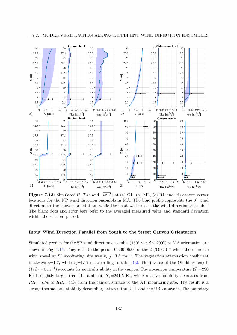
7.2. MODEL VERIFICATION AMONG DIFFERENT WIND DIRECTION ENSEMBLES
Figure 7.13: Simulated U , Tke and | w′u′ | at (a) GL, (b) ML, (c) RL and (d) canyon centerlocations for the NP wind direction ensemble in MA. The blue profile represents the 0◦ winddirection to the canyon orientation, while the shadowed area is the wind direction ensemble.The black dots and error bars refer to the averaged measured value and standard deviationwithin the selected period.
Input Wind Direction Parallel from South to the Street Canyon Orientation
Simulated profiles for the SP wind direction ensemble (160◦ ≤ wd ≤ 200◦) to MA orientation areshown in Fig. 7.14. They refer to the period 05:00-06:00 of the 21/09/2017 when the referencewind speed at SI monitoring site was uref=3.5 ms−1. The vegetation attenuation coefficientis always a=1.7, while z0=1.12 m according to table 4.2. The inverse of the Obukhov length(1/LO=0 m−1) accounts for neutral stability in the canyon. The in-canyon temperature (Tc=290K) is slightly larger than the ambient (Ta=291.5 K), while relative humidity decreases fromRHc=51% to RHa=44% from the canyon surface to the AT monitoring site. The result is astrong thermal and stability decoupling between the UCL and the UBL above it. The boundary
137
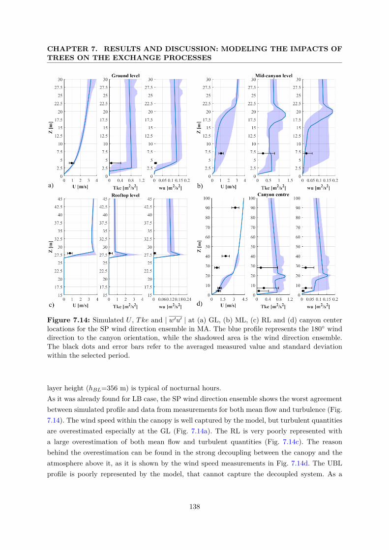
CHAPTER 7. RESULTS AND DISCUSSION: MODELING THE IMPACTS OFTREES ON THE EXCHANGE PROCESSES
Figure 7.14: Simulated U , Tke and | w′u′ | at (a) GL, (b) ML, (c) RL and (d) canyon centerlocations for the SP wind direction ensemble in MA. The blue profile represents the 180◦ winddirection to the canyon orientation, while the shadowed area is the wind direction ensemble.The black dots and error bars refer to the averaged measured value and standard deviationwithin the selected period.
layer height (hBL=356 m) is typical of nocturnal hours.As it was already found for LB case, the SP wind direction ensemble shows the worst agreementbetween simulated profile and data from measurements for both mean flow and turbulence (Fig.7.14). The wind speed within the canopy is well captured by the model, but turbulent quantitiesare overestimated especially at the GL (Fig. 7.14a). The RL is very poorly represented witha large overestimation of both mean flow and turbulent quantities (Fig. 7.14c). The reasonbehind the overestimation can be found in the strong decoupling between the canopy and theatmosphere above it, as it is shown by the wind speed measurements in Fig. 7.14d. The UBLprofile is poorly represented by the model, that cannot capture the decoupled system. As a
138
7.3. THE IMPACT OF TREES IN LAURA BASSI NEIGHBORHOOD UNDER THEINPUT WIND DIRECTION PERPENDICULAR FROM EAST TO THE STREET
CANYON ORIENTATIONconsequence, the driven wind speed at the RL is overestimated as it is overestimated the UBLprofile above the canyon. Being directly related to the mean flow, the turbulent quantities atRL are overestimated too.
7.3 The Impact of Trees in Laura Bassi Neighborhood underthe Input Wind Direction Perpendicular from East to theStreet Canyon Orientation
Following the aim of the research, QUIC is used to assess the impact of trees in an urbanneighborhood of the city of Bologna, considered as an example of European city among whichtesting the efficacy of a model developed for typical American cities. The selected simulated areais the residential neighborhood surrounding LB (Fig. 4.12b). The choice is motivated by thepresence of measurements which can help to set the input parameters and to have a comparisonwith the results from simulations, and because this neighborhood more than the one surroundingMA has a large disposal of vegetation in the real scenario (which will be used as reference totest the impact of vegetation). The setup for the reference simulation is the same as for theEP wind direction ensemble verification (Sect. 7.2.1), and follows the morphological parameterimplementation of Sect. 4.3.4. Fig. 7.15, 7.16 and 7.17 display two cross sections of the windspeed, TKE and TKMF within LB in the vicinity of the GL (panels a-b) and ML (panels c-d)locations respectively. Each quantity is simulated using the same domain size, resolution andsolid obstacles, with the exception of trees, which are present in the real amount in panels a-cand completely removed in panels b-d. The location for the cross sections computation waschosen to evaluate the impact of trees in two of the most representative geometries of realurban environments, i.e. the wake region on the leeward side of a building (panels a-b) and thestreet canyon (c-d) whose flow develops in the skimming regime of Oke (1987). In the wakeregion (Fig. 7.15a) the mean flow perturbation generated by the trees results in a wavelikemotion, whose period depends on the distance between adjacent trees. This wavelike motion isgenerated because the flow speed inside the tree is reduced by the drag force exerted by theporous crown. This wind speed reduction propagate vertically above the trees due to the massconservation, imposing a wavelike motion also in the ISL. Adding trees means adding obstacleswhich generate a local increase of pressure on the flow field that in turn has to adapt and adjust.This adaptation creates a wavelike motion since the flow is pushed upward when it passes abovethe tree, or decelerates when it flows through the tree. The wavelike motion can either be apressure driven wave or a wake generated by the coolision between the flow and the trees. Eitherway, the mass conservation sustains this wavelike motion and allows it to propagate vertically,generating a column of slower wind speed with respect to the surroundings. This wavelike motionis retrieved in the street canyon environment (Fig. 7.15c), but it is characterized by a smaller
139
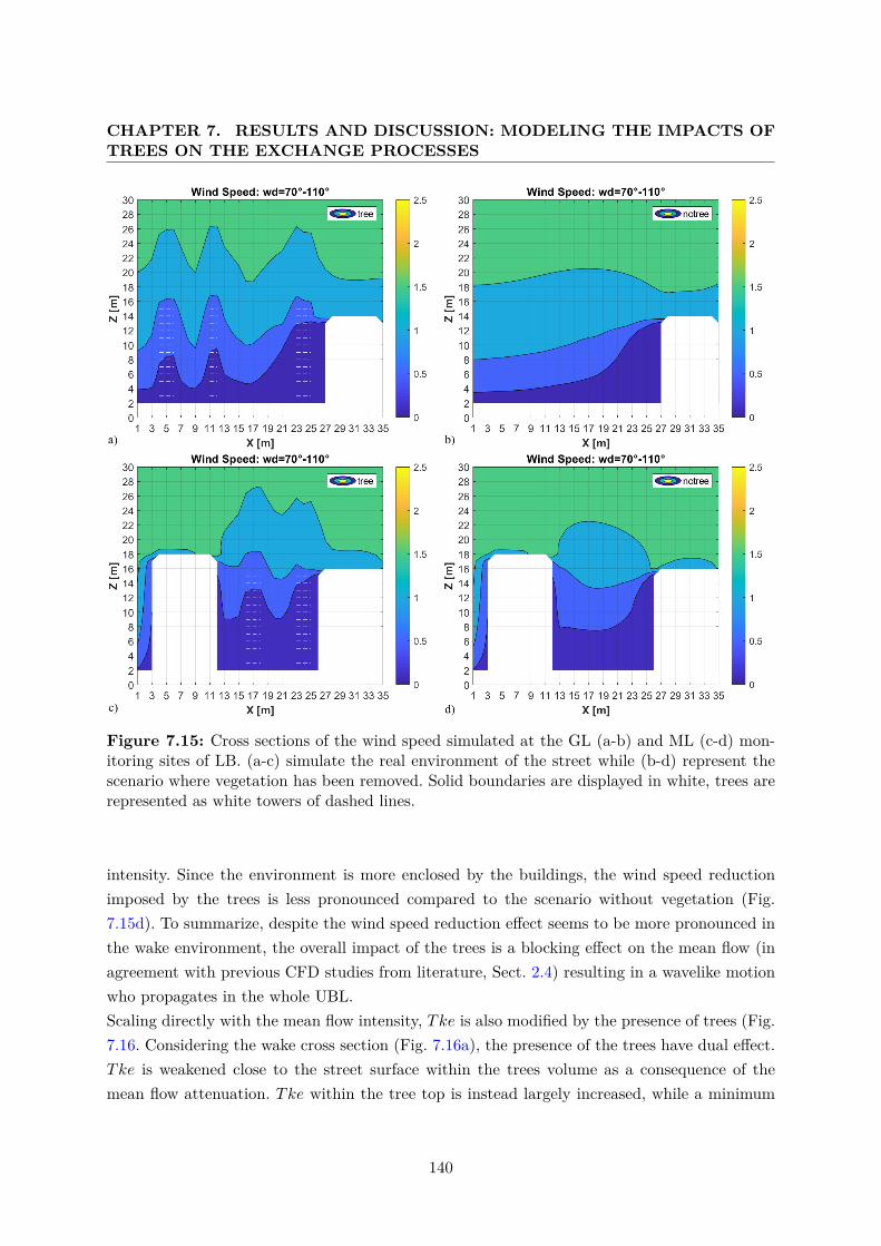
CHAPTER 7. RESULTS AND DISCUSSION: MODELING THE IMPACTS OFTREES ON THE EXCHANGE PROCESSES
Figure 7.15: Cross sections of the wind speed simulated at the GL (a-b) and ML (c-d) mon-itoring sites of LB. (a-c) simulate the real environment of the street while (b-d) represent thescenario where vegetation has been removed. Solid boundaries are displayed in white, trees arerepresented as white towers of dashed lines.
intensity. Since the environment is more enclosed by the buildings, the wind speed reductionimposed by the trees is less pronounced compared to the scenario without vegetation (Fig.7.15d). To summarize, despite the wind speed reduction effect seems to be more pronounced inthe wake environment, the overall impact of the trees is a blocking effect on the mean flow (inagreement with previous CFD studies from literature, Sect. 2.4) resulting in a wavelike motionwho propagates in the whole UBL.Scaling directly with the mean flow intensity, Tke is also modified by the presence of trees (Fig.7.16. Considering the wake cross section (Fig. 7.16a), the presence of the trees have dual effect.Tke is weakened close to the street surface within the trees volume as a consequence of themean flow attenuation. Tke within the tree top is instead largely increased, while a minimum
140
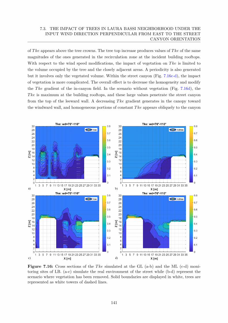
7.3. THE IMPACT OF TREES IN LAURA BASSI NEIGHBORHOOD UNDER THEINPUT WIND DIRECTION PERPENDICULAR FROM EAST TO THE STREET
CANYON ORIENTATION
of Tke appears above the tree crowns. The tree top increase produces values of Tke of the samemagnitudes of the ones generated in the recirculation zone at the incident building rooftops.With respect to the wind speed modifications, the impact of vegetation on Tke is limited tothe volume occupied by the tree and the closely adjacent areas. A periodicity is also generatedbut it involves only the vegetated volume. Within the street canyon (Fig. 7.16c-d), the impactof vegetation is more complicated. The overall effect is to decrease the homogeneity and modifythe Tke gradient of the in-canyon field. In the scenario without vegetation (Fig. 7.16d), theTke is maximum at the building rooftops, and these large values penetrate the street canyonfrom the top of the leeward wall. A decreasing Tke gradient generates in the canopy towardthe windward wall, and homogeneous portions of constant Tke appears obliquely to the canyon
Figure 7.16: Cross sections of the Tke simulated at the GL (a-b) and the ML (c-d) moni-toring sites of LB. (a-c) simulate the real environment of the street while (b-d) represent thescenario where vegetation has been removed. Solid boundaries are displayed in white, trees arerepresented as white towers of dashed lines.
141
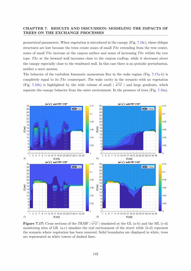
CHAPTER 7. RESULTS AND DISCUSSION: MODELING THE IMPACTS OFTREES ON THE EXCHANGE PROCESSES
geometrical parameters. When vegetation is introduced in the canopy (Fig. 7.16c), these obliquestructures are lost because the trees create zones of small Tke extending from the tree center,zones of small Tke increase at the canyon surface and zones of increasing Tke within the treetops. Tke at the leeward wall increases close to the canyon rooftop, while it decreases abovethe canopy especially close to the windward wall. In this case there is no periodic perturbation,neither a wave motion.The behavior of the turbulent kinematic momentum flux in the wake regime (Fig. 7.17a-b) iscompletely equal to its Tke counterpart. The wake cavity in the scenario with no vegetation(Fig. 7.16b) is highlighted by the wide volume of small | w′u′ | and large gradients, whichseparate the canopy behavior from the outer environment. In the presence of trees (Fig. 7.16a),
Figure 7.17: Cross sections of the TKMF | w′u′ | simulated at the GL (a-b) and the ML (c-d)monitoring sites of LB. (a-c) simulate the real environment of the street while (b-d) representthe scenario where vegetation has been removed. Solid boundaries are displayed in white, treesare represented as white towers of dashed lines.
142
7.3. THE IMPACT OF TREES IN LAURA BASSI NEIGHBORHOOD UNDER THEINPUT WIND DIRECTION PERPENDICULAR FROM EAST TO THE STREET
CANYON ORIENTATION
the wake cavity is extended away from the building, while maxima of | w′u′ | are retrievedat the tree top. The impact of vegetation in the street canyon scenario (Fig. 7.16c-d) showssimilarities and dissimilarities with the TKE simulations. The behavior of the TKMF in therecirculation zone of the building rooftops in the scenario with no vegetation is similar, butno intense entrainment is retrieved. A certain penetration through the street is also evidentin the leeward half of the canopy. This penetration is completely lost when trees are present(Fig. 7.16c), and it is replaced by small values of | w′u′ | extending above the canopy. Anintensification of the TKMFes within the tree top is induced by the momentum transport fromthe mean flow colliding with the crown to turbulence. The presence of trees does not seem toproduce an effect on the in-canyon momentum flux.From these qualitative investigation, it is evident the blocking effect of the trees on the meanflow field, while the turbulent quantities show a dual behavior: a dissipation of the turbulentfields at the surface and an increase of them within the trees top. Wavelike motions are alsoretrieved when dealing with the mean flow, while perturbations on the turbulent fields are moreconstrained in the vicinity of the trees. More quantitative analyses of the impact of trees aregiven in the following sections, where the distributions of wind speed, TKE and TKMF fromthe whole domain are detailed.
7.3.1 Vegetation Impact Distributions and Topological Discretization
To extend the observations made in the previous section to the whole neighborhood and general-ize the results for densely vegetated urban areas, an analysis based on the wind speed, Tke and| w′u′ | distributions is presented to evaluate the overall impact of trees in LB neighborhood.The same analysis is also refined to account for the different behavior of specific topologicalfeatures of the neighborhood, such as differently oriented street canyons or intersections, whenthe total vegetation amount is modified. The proposed distributions will cover the whole hori-zontal domain and will be representative of five different layers within the UBL. Distributionsare normalized on each total number of occurrences and displayed in a percentage ordinate scalefrom 0 (0%) to 1 (100%). The first two layers represent the average behavior of the mean flowand turbulent fields at ground and mid-canyon layers of the UCL, within whom the analyzedquantities are averaged. The depth of the layers are 1.5-4.5 m for the ground layer and 5.5-9.5 mfor the mid layer. The roof layer (10.5-14.5 m) is the interface layer between the canopy and theUBL above it. Above the rooftop height, a roughness layer (15.5-20.5 m) is generally observedwhere the flow is adjusting from the perturbation generated by the canopy. The last layer is theinertial layer extending in the depth 25.5-30.5 m. It generally refers to the layer where the flowhas already readjusted from the perturbation given by the canopy, but in this case there wasno analysis to identify the height where a possible inertial layer develops, so it simply identifiesthe top layer of the first half of the vertical domain.
143
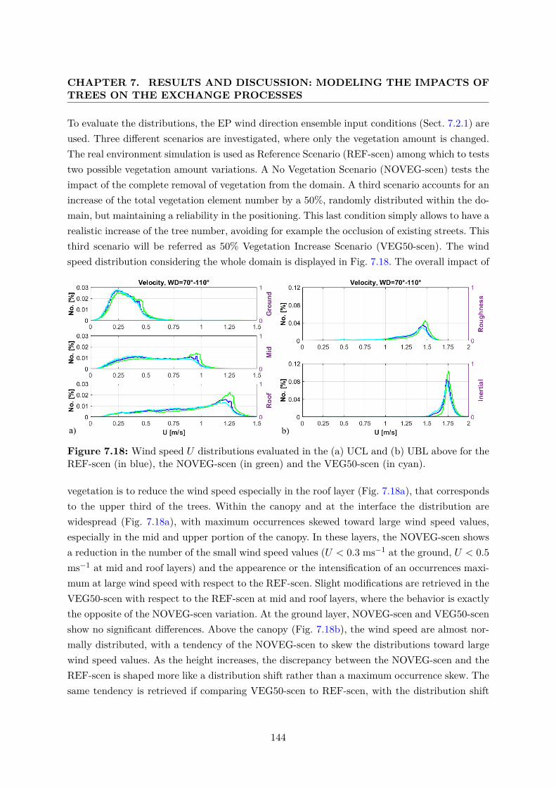
CHAPTER 7. RESULTS AND DISCUSSION: MODELING THE IMPACTS OFTREES ON THE EXCHANGE PROCESSES
To evaluate the distributions, the EP wind direction ensemble input conditions (Sect. 7.2.1) areused. Three different scenarios are investigated, where only the vegetation amount is changed.The real environment simulation is used as Reference Scenario (REF-scen) among which to teststwo possible vegetation amount variations. A No Vegetation Scenario (NOVEG-scen) tests theimpact of the complete removal of vegetation from the domain. A third scenario accounts for anincrease of the total vegetation element number by a 50%, randomly distributed within the do-main, but maintaining a reliability in the positioning. This last condition simply allows to have arealistic increase of the tree number, avoiding for example the occlusion of existing streets. Thisthird scenario will be referred as 50% Vegetation Increase Scenario (VEG50-scen). The windspeed distribution considering the whole domain is displayed in Fig. 7.18. The overall impact of
Figure 7.18: Wind speed U distributions evaluated in the (a) UCL and (b) UBL above for theREF-scen (in blue), the NOVEG-scen (in green) and the VEG50-scen (in cyan).
vegetation is to reduce the wind speed especially in the roof layer (Fig. 7.18a), that correspondsto the upper third of the trees. Within the canopy and at the interface the distribution arewidespread (Fig. 7.18a), with maximum occurrences skewed toward large wind speed values,especially in the mid and upper portion of the canopy. In these layers, the NOVEG-scen showsa reduction in the number of the small wind speed values (U < 0.3 ms−1 at the ground, U < 0.5ms−1 at mid and roof layers) and the appearence or the intensification of an occurrences maxi-mum at large wind speed with respect to the REF-scen. Slight modifications are retrieved in theVEG50-scen with respect to the REF-scen at mid and roof layers, where the behavior is exactlythe opposite of the NOVEG-scen variation. At the ground layer, NOVEG-scen and VEG50-scenshow no significant differences. Above the canopy (Fig. 7.18b), the wind speed are almost nor-mally distributed, with a tendency of the NOVEG-scen to skew the distributions toward largewind speed values. As the height increases, the discrepancy between the NOVEG-scen and theREF-scen is shaped more like a distribution shift rather than a maximum occurrence skew. Thesame tendency is retrieved if comparing VEG50-scen to REF-scen, with the distribution shift
144
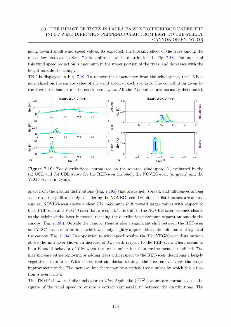
7.3. THE IMPACT OF TREES IN LAURA BASSI NEIGHBORHOOD UNDER THEINPUT WIND DIRECTION PERPENDICULAR FROM EAST TO THE STREET
CANYON ORIENTATION
going toward small wind speed values. As expected, the blocking effect of the trees among themean flow observed in Sect. 7.3 is confirmed by the distributions in Fig. 7.18. The impact ofthis wind speed reduction is maximum in the upper portion of the trees, and decreases with theheight outside the canopy.TKE is displayed in Fig. 7.19. To remove the dependency from the wind speed, the TKE isnormalized on the square value of the wind speed of each scenario. The contribution given bythe tree is evident at all the considered layers. All the Tke values are normally distributed,
Figure 7.19: Tke distributions, normalized on the squared wind speed U , evaluated in the(a) UCL and (b) UBL above for the REF-scen (in blue), the NOVEG-scen (in green) and theVEG50-scen (in cyan).
apart from the ground distributions (Fig. 7.19a) that are largely spread, and differences amongscenarios are significant only considering the NOVEG-scen. Despite the distributions are almostsimilar, NOVEG-scen shows a clear Tke maximum shift toward larger values with respect toboth REF-scen and VEG50-scen that are equal. This shift of the NOVEG-scen becomes cleareras the height of the layer increases, reaching the distribution maximum separation outside thecanopy (Fig. 7.19b). Outside the canopy, there is also a significant shift between the REF-scenand VEG50-scen distributions, which was only slightly appreciable at the mid and roof layers ofthe canopy (Fig. 7.19a). In opposition to wind speed results, the Tke VEG50-scen distributionsabove the mid layer shows an increase of Tke with respect to the REF-scen. There seems tobe a bimodal behavior of Tke when the tree number in urban environment is modified. Tkemay increase either removing or adding trees with respect to the REF-scen, describing a largelyvegetated urban area. With the current simulation settings, the tree removal gives the largerimprovement to the Tke increase, but there may be a critical tree number by which this situa-tion is overturned.The TKMF shows a similar behavior to Tke. Again the | w′u′ | values are normalized on thesquare of the wind speed to ensure a correct comparability between the distributions. The
145
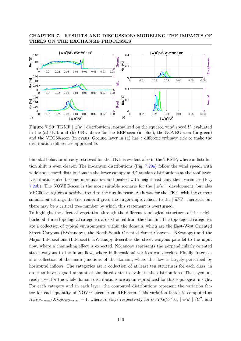
CHAPTER 7. RESULTS AND DISCUSSION: MODELING THE IMPACTS OFTREES ON THE EXCHANGE PROCESSES
Figure 7.20: TKMF | w′u′ | distributions, normalized on the squared wind speed U , evaluatedin the (a) UCL and (b) UBL above for the REF-scen (in blue), the NOVEG-scen (in green)and the VEG50-scen (in cyan). Ground layer in (a) has a different ordinate tick to make thedistribution differences appreciable.
bimodal behavior already retrieved for the TKE is evident also in the TKMF, where a distribu-tion shift is even clearer. The in-canyon distributions (Fig. 7.20a) follow the wind speed, withwide and skewed distributions in the lower canopy and Gaussian distributions at the roof layer.Distributions also become more narrow and peaked with height, reducing their variances (Fig.7.20b). The NOVEG-scen is the most suitable scenario for the | w′u′ | development, but alsoVEG50-scen gives a positive trend to the flux increase. As it was for the TKE, with the currentsimulation settings the tree removal gives the larger improvement to the | w′u′ | increase, butthere may be a critical tree number by which this statement is overturned.To highlight the effect of vegetation through the different topological structures of the neigh-borhood, three topological categories are extracted from the domain. The topological categoriesare a collection of typical environments within the domain, which are the East-West OrientedStreet Canyons (EWcanopy), the North-South Oriented Street Canyons (NScanopy) and theMajor Intersections (Intersect). EWcanopy describes the street canyons parallel to the inputflow, where a channeling effect is expected. NScanopy represents the perpendicularly orientedstreet canyons to the input flow, where bidimensional vortices can develop. Finally Intersectis a collection of the main junctions of the domain, where the flow is largely perturbed byhorizontal inflows. The categories are a collection of at least ten structures for each class, inorder to have a good amount of simulated data to evaluate the distributions. The layers al-ready used for the whole domain distributions are again reproduced for this topological insight.For each category and in each layer, the computed distributions represent the variation fac-tor for each quantity of NOVEG-scen from REF-scen. This variation factor is computed asXREF−scen/XNOV EG−scen − 1, where X stays respectively for U , Tke/U2 or | w′u′ | /U2, and
146
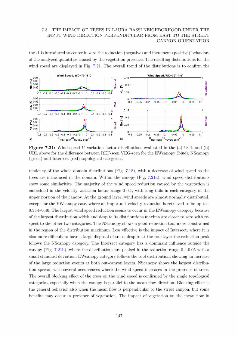
7.3. THE IMPACT OF TREES IN LAURA BASSI NEIGHBORHOOD UNDER THEINPUT WIND DIRECTION PERPENDICULAR FROM EAST TO THE STREET
CANYON ORIENTATION
the -1 is introduced to center in zero the reduction (negative) and increment (positive) behaviorsof the analyzed quantities caused by the vegetation presence. The resulting distributions for thewind speed are displayed in Fig. 7.21. The overall trend of the distributions is to confirm the
Figure 7.21: Wind speed U variation factor distributions evaluated in the (a) UCL and (b)UBL above for the difference between REF-scen VEG-scen for the EWcanopy (blue), NScanopy(green) and Intersect (red) topological categories.
tendency of the whole domain distributions (Fig. 7.18), with a decrease of wind speed as thetrees are introduced in the domain. Within the canopy (Fig. 7.21a), wind speed distributionsshow some similarities. The majority of the wind speed reduction caused by the vegetation isembedded in the velocity variation factor range 0-0.1, with long tails in each category in theupper portion of the canopy. At the ground layer, wind speeds are almost normally distributed,except for the EWcanopy case, where an important velocity reduction is retrieved to be up to -0.35÷-0.40. The largest wind speed reduction seems to occur in the EWcanopy category becauseof the largest distribution width and despite its distributions maxima are closer to zero with re-spect to the other two categories. The NScanopy shows a good reduction too, more constrainedin the region of the distribution maximum. Less effective is the impact of Intersect, where it isalso more difficult to have a large disposal of trees, despite at the roof layer the reduction peakfollows the NScanopy category. The Intersect category has a dominant influence outside thecanopy (Fig. 7.21b), where the distributions are peaked in the reduction range 0÷-0.05 with asmall standard deviation. EWcanopy category follows the roof distribution, showing an increaseof the large reduction events at both out-canyon layers. NScanopy shows the largest distribu-tion spread, with several occurrences where the wind speed increases in the presence of trees.The overall blocking effect of the trees on the wind speed is confirmed by the single topologicalcategories, especially when the canopy is parallel to the mean flow direction. Blocking effect isthe general behavior also when the mean flow is perpendicular to the street canyon, but somebenefits may occur in presence of vegetation. The impact of vegetation on the mean flow in
147
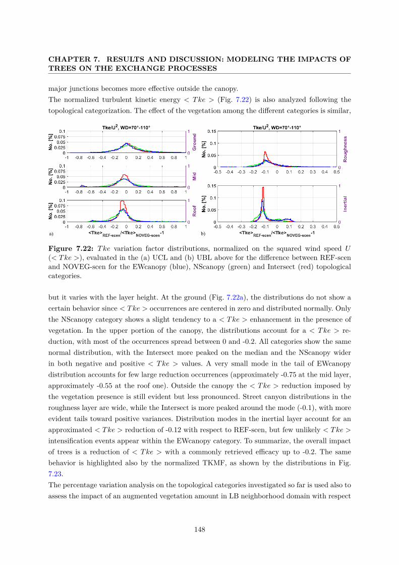
CHAPTER 7. RESULTS AND DISCUSSION: MODELING THE IMPACTS OFTREES ON THE EXCHANGE PROCESSES
major junctions becomes more effective outside the canopy.The normalized turbulent kinetic energy < Tke > (Fig. 7.22) is also analyzed following thetopological categorization. The effect of the vegetation among the different categories is similar,
Figure 7.22: Tke variation factor distributions, normalized on the squared wind speed U(< Tke >), evaluated in the (a) UCL and (b) UBL above for the difference between REF-scenand NOVEG-scen for the EWcanopy (blue), NScanopy (green) and Intersect (red) topologicalcategories.
but it varies with the layer height. At the ground (Fig. 7.22a), the distributions do not show acertain behavior since < Tke > occurrences are centered in zero and distributed normally. Onlythe NScanopy category shows a slight tendency to a < Tke > enhancement in the presence ofvegetation. In the upper portion of the canopy, the distributions account for a < Tke > re-duction, with most of the occurrences spread between 0 and -0.2. All categories show the samenormal distribution, with the Intersect more peaked on the median and the NScanopy widerin both negative and positive < Tke > values. A very small mode in the tail of EWcanopydistribution accounts for few large reduction occurrences (approximately -0.75 at the mid layer,approximately -0.55 at the roof one). Outside the canopy the < Tke > reduction imposed bythe vegetation presence is still evident but less pronounced. Street canyon distributions in theroughness layer are wide, while the Intersect is more peaked around the mode (-0.1), with moreevident tails toward positive variances. Distribution modes in the inertial layer account for anapproximated < Tke > reduction of -0.12 with respect to REF-scen, but few unlikely < Tke >
intensification events appear within the EWcanopy category. To summarize, the overall impactof trees is a reduction of < Tke > with a commonly retrieved efficacy up to -0.2. The samebehavior is highlighted also by the normalized TKMF, as shown by the distributions in Fig.7.23.The percentage variation analysis on the topological categories investigated so far is used also toassess the impact of an augmented vegetation amount in LB neighborhood domain with respect
148
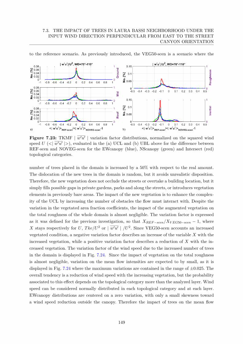
7.3. THE IMPACT OF TREES IN LAURA BASSI NEIGHBORHOOD UNDER THEINPUT WIND DIRECTION PERPENDICULAR FROM EAST TO THE STREET
CANYON ORIENTATION
to the reference scenario. As previously introduced, the VEG50-scen is a scenario where the
Figure 7.23: TKMF | w′u′ | variation factor distributions, normalized on the squared windspeed U (<| w′u′ |>), evaluated in the (a) UCL and (b) UBL above for the difference betweenREF-scen and NOVEG-scen for the EWcanopy (blue), NScanopy (green) and Intersect (red)topological categories.
number of trees placed in the domain is increased by a 50% with respect to the real amount.The dislocation of the new trees in the domain is random, but it avoids unrealistic disposition.Therefore, the new vegetation does not occlude the streets or overtake a building location, but itsimply fills possible gaps in private gardens, parks and along the streets, or introduces vegetationelements in previously bare areas. The impact of the new vegetation is to enhance the complex-ity of the UCL by increasing the number of obstacles the flow must interact with. Despite thevariation in the vegetated area fraction coefficients, the impact of the augmented vegetation onthe total roughness of the whole domain is almost negligible. The variation factor is expressedas it was defined for the previous investigation, so that XREF−scen/XV EG50−scen − 1, whereX stays respectively for U , Tke/U2 or | w′u′ | /U2. Since VEG50-scen accounts an increasedvegetated condition, a negative variation factor describes an increase of the variable X with theincreased vegetation, while a positive variation factor describes a reduction of X with the in-creased vegetation. The variation factor of the wind speed due to the increased number of treesin the domain is displayed in Fig. 7.24. Since the impact of vegetation on the total roughnessis almost negligible, variation on the mean flow intensities are expected to by small, as it isdisplayed in Fig. 7.24 where the maximum variations are contained in the range of ±0.025. Theoverall tendency is a reduction of wind speed with the increasing vegetation, but the probabilityassociated to this effect depends on the topological category more than the analyzed layer. Windspeed can be considered normally distributed in each topological category and at each layer.EWcanopy distributions are centered on a zero variation, with only a small skewness towarda wind speed reduction outside the canopy. Therefore the impact of trees on the mean flow
149
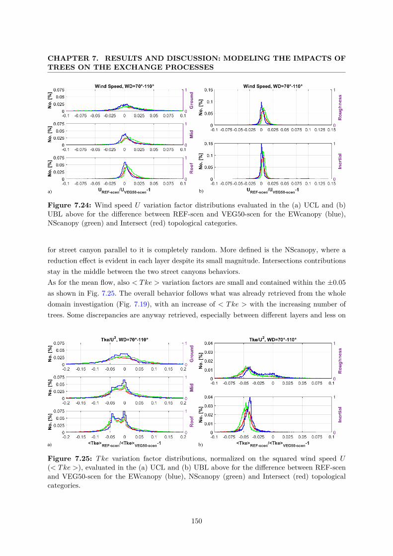
CHAPTER 7. RESULTS AND DISCUSSION: MODELING THE IMPACTS OFTREES ON THE EXCHANGE PROCESSES
Figure 7.24: Wind speed U variation factor distributions evaluated in the (a) UCL and (b)UBL above for the difference between REF-scen and VEG50-scen for the EWcanopy (blue),NScanopy (green) and Intersect (red) topological categories.
for street canyon parallel to it is completely random. More defined is the NScanopy, where areduction effect is evident in each layer despite its small magnitude. Intersections contributionsstay in the middle between the two street canyons behaviors.As for the mean flow, also < Tke > variation factors are small and contained within the ±0.05as shown in Fig. 7.25. The overall behavior follows what was already retrieved from the wholedomain investigation (Fig. 7.19), with an increase of < Tke > with the increasing number oftrees. Some discrepancies are anyway retrieved, especially between different layers and less on
Figure 7.25: Tke variation factor distributions, normalized on the squared wind speed U(< Tke >), evaluated in the (a) UCL and (b) UBL above for the difference between REF-scenand VEG50-scen for the EWcanopy (blue), NScanopy (green) and Intersect (red) topologicalcategories.
150
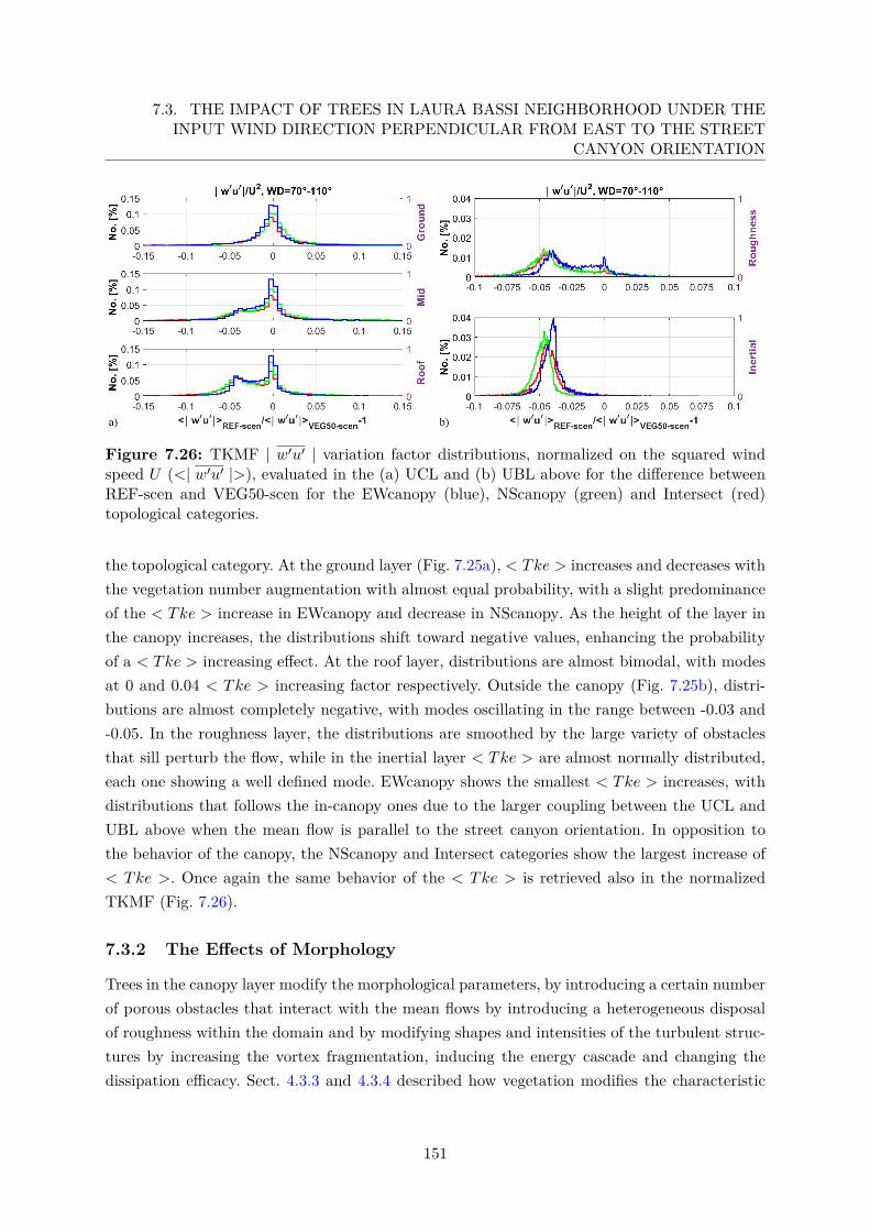
7.3. THE IMPACT OF TREES IN LAURA BASSI NEIGHBORHOOD UNDER THEINPUT WIND DIRECTION PERPENDICULAR FROM EAST TO THE STREET
CANYON ORIENTATION
Figure 7.26: TKMF | w′u′ | variation factor distributions, normalized on the squared windspeed U (<| w′u′ |>), evaluated in the (a) UCL and (b) UBL above for the difference betweenREF-scen and VEG50-scen for the EWcanopy (blue), NScanopy (green) and Intersect (red)topological categories.
the topological category. At the ground layer (Fig. 7.25a), < Tke > increases and decreases withthe vegetation number augmentation with almost equal probability, with a slight predominanceof the < Tke > increase in EWcanopy and decrease in NScanopy. As the height of the layer inthe canopy increases, the distributions shift toward negative values, enhancing the probabilityof a < Tke > increasing effect. At the roof layer, distributions are almost bimodal, with modesat 0 and 0.04 < Tke > increasing factor respectively. Outside the canopy (Fig. 7.25b), distri-butions are almost completely negative, with modes oscillating in the range between -0.03 and-0.05. In the roughness layer, the distributions are smoothed by the large variety of obstaclesthat sill perturb the flow, while in the inertial layer < Tke > are almost normally distributed,each one showing a well defined mode. EWcanopy shows the smallest < Tke > increases, withdistributions that follows the in-canopy ones due to the larger coupling between the UCL andUBL above when the mean flow is parallel to the street canyon orientation. In opposition tothe behavior of the canopy, the NScanopy and Intersect categories show the largest increase of< Tke >. Once again the same behavior of the < Tke > is retrieved also in the normalizedTKMF (Fig. 7.26).
7.3.2 The Effects of Morphology
Trees in the canopy layer modify the morphological parameters, by introducing a certain numberof porous obstacles that interact with the mean flows by introducing a heterogeneous disposalof roughness within the domain and by modifying shapes and intensities of the turbulent struc-tures by increasing the vortex fragmentation, inducing the energy cascade and changing thedissipation efficacy. Sect. 4.3.3 and 4.3.4 described how vegetation modifies the characteristic
151
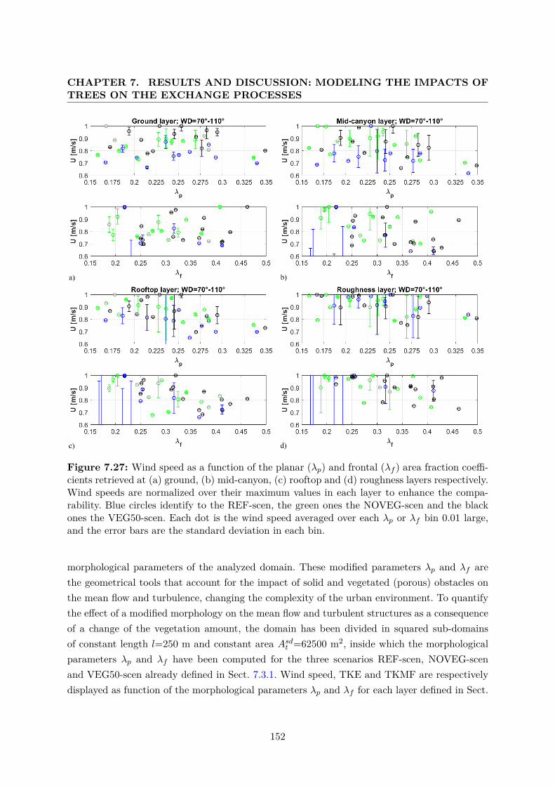
CHAPTER 7. RESULTS AND DISCUSSION: MODELING THE IMPACTS OFTREES ON THE EXCHANGE PROCESSES
Figure 7.27: Wind speed as a function of the planar (λp) and frontal (λf ) area fraction coeffi-cients retrieved at (a) ground, (b) mid-canyon, (c) rooftop and (d) roughness layers respectively.Wind speeds are normalized over their maximum values in each layer to enhance the compa-rability. Blue circles identify to the REF-scen, the green ones the NOVEG-scen and the blackones the VEG50-scen. Each dot is the wind speed averaged over each λp or λf bin 0.01 large,and the error bars are the standard deviation in each bin.
morphological parameters of the analyzed domain. These modified parameters λp and λf arethe geometrical tools that account for the impact of solid and vegetated (porous) obstacles onthe mean flow and turbulence, changing the complexity of the urban environment. To quantifythe effect of a modified morphology on the mean flow and turbulent structures as a consequenceof a change of the vegetation amount, the domain has been divided in squared sub-domainsof constant length l=250 m and constant area Asdt =62500 m2, inside which the morphologicalparameters λp and λf have been computed for the three scenarios REF-scen, NOVEG-scenand VEG50-scen already defined in Sect. 7.3.1. Wind speed, TKE and TKMF are respectivelydisplayed as function of the morphological parameters λp and λf for each layer defined in Sect.
152
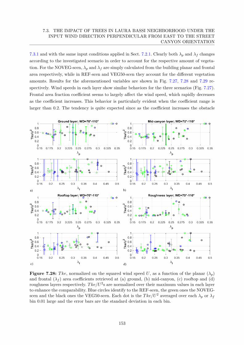
7.3. THE IMPACT OF TREES IN LAURA BASSI NEIGHBORHOOD UNDER THEINPUT WIND DIRECTION PERPENDICULAR FROM EAST TO THE STREET
CANYON ORIENTATION
7.3.1 and with the same input conditions applied in Sect. 7.2.1. Clearly both λp and λf changesaccording to the investigated scenario in order to account for the respective amount of vegeta-tion. For the NOVEG-scen, λp and λf are simply calculated from the building planar and frontalarea respectively, while in REF-scen and VEG50-scen they account for the different vegetationamounts. Results for the aforementioned variables are shown in Fig. 7.27, 7.28 and 7.29 re-spectively. Wind speeds in each layer show similar behaviors for the three scenarios (Fig. 7.27).Frontal area fraction coefficient seems to largely affect the wind speed, which rapidly decreasesas the coefficient increases. This behavior is particularly evident when the coefficient range islarger than 0.2. The tendency is quite expected since as the coefficient increases the obstacle
Figure 7.28: Tke, normalized on the squared wind speed U , as a function of the planar (λp)and frontal (λf ) area coefficients retrieved at (a) ground, (b) mid-canyon, (c) rooftop and (d)roughness layers respectively. Tke/U2s are normalized over their maximum values in each layerto enhance the comparability. Blue circles identify to the REF-scen, the green ones the NOVEG-scen and the black ones the VEG50-scen. Each dot is the Tke/U2 averaged over each λp or λfbin 0.01 large and the error bars are the standard deviation in each bin.
153
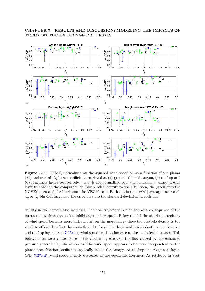
CHAPTER 7. RESULTS AND DISCUSSION: MODELING THE IMPACTS OFTREES ON THE EXCHANGE PROCESSES
Figure 7.29: TKMF, normalized on the squared wind speed U , as a function of the planar(λp) and frontal (λf ) area coefficients retrieved at (a) ground, (b) mid-canyon, (c) rooftop and(d) roughness layers respectively. | w′u′ |s are normalized over their maximum values in eachlayer to enhance the comparability. Blue circles identify to the REF-scen, the green ones theNOVEG-scen and the black ones the VEG50-scen. Each dot is the | w′u′ | averaged over eachλp or λf bin 0.01 large and the error bars are the standard deviation in each bin.
density in the domain also increases. The flow trajectory is modified as a consequence of theinteraction with the obstacles, inhibiting the flow speed. Below the 0.2 threshold the tendencyof wind speed becomes more independent on the morphology since the obstacle density is toosmall to efficiently affect the mean flow. At the ground layer and less evidently at mid-canyonand rooftop layers (Fig. 7.27a-b), wind speed tends to increase as the coefficient increases. Thisbehavior can be a consequence of the channeling effect on the flow caused by the enhancedpressure generated by the obstacles. The wind speed appears to be more independent on theplanar area fraction coefficient especially inside the canopy. At rooftop and roughness layers(Fig. 7.27c-d), wind speed slightly decreases as the coefficient increases. As retrieved in Sect.
154
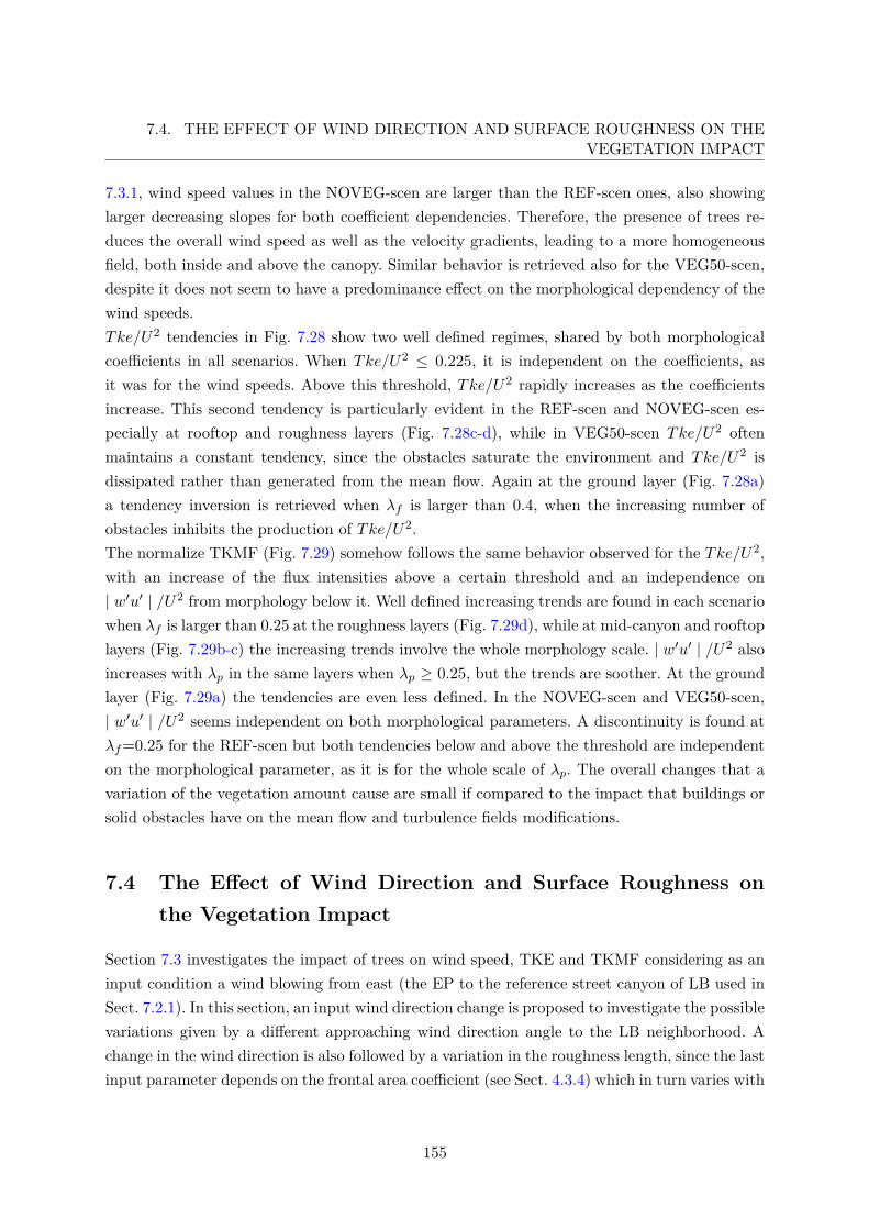
7.4. THE EFFECT OF WIND DIRECTION AND SURFACE ROUGHNESS ON THEVEGETATION IMPACT
7.3.1, wind speed values in the NOVEG-scen are larger than the REF-scen ones, also showinglarger decreasing slopes for both coefficient dependencies. Therefore, the presence of trees re-duces the overall wind speed as well as the velocity gradients, leading to a more homogeneousfield, both inside and above the canopy. Similar behavior is retrieved also for the VEG50-scen,despite it does not seem to have a predominance effect on the morphological dependency of thewind speeds.Tke/U2 tendencies in Fig. 7.28 show two well defined regimes, shared by both morphologicalcoefficients in all scenarios. When Tke/U2 ≤ 0.225, it is independent on the coefficients, asit was for the wind speeds. Above this threshold, Tke/U2 rapidly increases as the coefficientsincrease. This second tendency is particularly evident in the REF-scen and NOVEG-scen es-pecially at rooftop and roughness layers (Fig. 7.28c-d), while in VEG50-scen Tke/U2 oftenmaintains a constant tendency, since the obstacles saturate the environment and Tke/U2 isdissipated rather than generated from the mean flow. Again at the ground layer (Fig. 7.28a)a tendency inversion is retrieved when λf is larger than 0.4, when the increasing number ofobstacles inhibits the production of Tke/U2.The normalize TKMF (Fig. 7.29) somehow follows the same behavior observed for the Tke/U2,with an increase of the flux intensities above a certain threshold and an independence on| w′u′ | /U2 from morphology below it. Well defined increasing trends are found in each scenariowhen λf is larger than 0.25 at the roughness layers (Fig. 7.29d), while at mid-canyon and rooftoplayers (Fig. 7.29b-c) the increasing trends involve the whole morphology scale. | w′u′ | /U2 alsoincreases with λp in the same layers when λp ≥ 0.25, but the trends are soother. At the groundlayer (Fig. 7.29a) the tendencies are even less defined. In the NOVEG-scen and VEG50-scen,| w′u′ | /U2 seems independent on both morphological parameters. A discontinuity is found atλf=0.25 for the REF-scen but both tendencies below and above the threshold are independenton the morphological parameter, as it is for the whole scale of λp. The overall changes that avariation of the vegetation amount cause are small if compared to the impact that buildings orsolid obstacles have on the mean flow and turbulence fields modifications.
7.4 The Effect of Wind Direction and Surface Roughness onthe Vegetation Impact
Section 7.3 investigates the impact of trees on wind speed, TKE and TKMF considering as aninput condition a wind blowing from east (the EP to the reference street canyon of LB used inSect. 7.2.1). In this section, an input wind direction change is proposed to investigate the possiblevariations given by a different approaching wind direction angle to the LB neighborhood. Achange in the wind direction is also followed by a variation in the roughness length, since the lastinput parameter depends on the frontal area coefficient (see Sect. 4.3.4) which in turn varies with
155
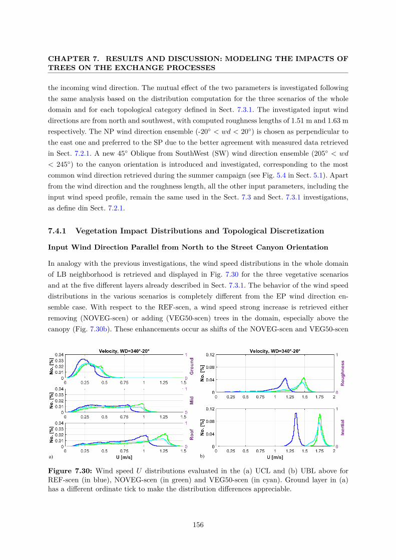
CHAPTER 7. RESULTS AND DISCUSSION: MODELING THE IMPACTS OFTREES ON THE EXCHANGE PROCESSES
the incoming wind direction. The mutual effect of the two parameters is investigated followingthe same analysis based on the distribution computation for the three scenarios of the wholedomain and for each topological category defined in Sect. 7.3.1. The investigated input winddirections are from north and southwest, with computed roughness lengths of 1.51 m and 1.63 mrespectively. The NP wind direction ensemble (-20◦ < wd < 20◦) is chosen as perpendicular tothe east one and preferred to the SP due to the better agreement with measured data retrievedin Sect. 7.2.1. A new 45◦ Oblique from SouthWest (SW) wind direction ensemble (205◦ < wd
< 245◦) to the canyon orientation is introduced and investigated, corresponding to the mostcommon wind direction retrieved during the summer campaign (see Fig. 5.4 in Sect. 5.1). Apartfrom the wind direction and the roughness length, all the other input parameters, including theinput wind speed profile, remain the same used in the Sect. 7.3 and Sect. 7.3.1 investigations,as define din Sect. 7.2.1.
7.4.1 Vegetation Impact Distributions and Topological Discretization
Input Wind Direction Parallel from North to the Street Canyon Orientation
In analogy with the previous investigations, the wind speed distributions in the whole domainof LB neighborhood is retrieved and displayed in Fig. 7.30 for the three vegetative scenariosand at the five different layers already described in Sect. 7.3.1. The behavior of the wind speeddistributions in the various scenarios is completely different from the EP wind direction en-semble case. With respect to the REF-scen, a wind speed strong increase is retrieved eitherremoving (NOVEG-scen) or adding (VEG50-scen) trees in the domain, especially above thecanopy (Fig. 7.30b). These enhancements occur as shifts of the NOVEG-scen and VEG50-scen
Figure 7.30: Wind speed U distributions evaluated in the (a) UCL and (b) UBL above forREF-scen (in blue), NOVEG-scen (in green) and VEG50-scen (in cyan). Ground layer in (a)has a different ordinate tick to make the distribution differences appreciable.
156
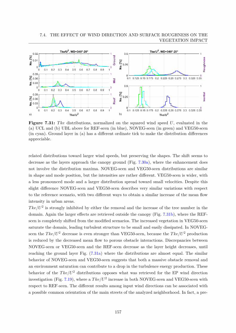
7.4. THE EFFECT OF WIND DIRECTION AND SURFACE ROUGHNESS ON THEVEGETATION IMPACT
Figure 7.31: Tke distributions, normalized on the squared wind speed U , evaluated in the(a) UCL and (b) UBL above for REF-scen (in blue), NOVEG-scen (in green) and VEG50-scen(in cyan). Ground layer in (a) has a different ordinate tick to make the distribution differencesappreciable.
related distributions toward larger wind speeds, but preserving the shapes. The shift seems todecrease as the layers approach the canopy ground (Fig. 7.30a), where the enhancement doesnot involve the distribution maxima. NOVEG-scen and VEG50-scen distributions are similarin shape and mode position, but the intensities are rather different. VEG50-scen is wider, witha less pronounced mode and a larger distribution spread toward small velocities. Despite thisslight difference NOVEG-scen and VEG50-scen describes very similar variations with respectto the reference scenario, with two different ways to obtain a similar increase of the mean flowintensity in urban areas.Tke/U2 is strongly inhibited by either the removal and the increase of the tree number in thedomain. Again the larger effects are retrieved outside the canopy (Fig. 7.31b), where the REF-scen is completely shifted from the modified scenarios. The increased vegetation in VEG50-scensaturate the domain, leading turbulent structure to be small and easily dissipated. In NOVEG-scen the Tke/U2 decrease is even stronger than VEG50-scen, because the Tke/U2 productionis reduced by the decreased mean flow to porous obstacle interactions. Discrepancies betweenNOVEG-scen or VEG50-scen and the REF-scen decrease as the layer height decreases, untilreaching the ground layer Fig. (7.31a) where the distributions are almost equal. The similarbehavior of NOVEG-scen and VEG50-scen suggests that both a massive obstacle removal andan environment saturation can contribute to a drop in the turbulence energy production. Thesebehavior of the Tke/U2 distributions opposes what was retrieved for the EP wind directioninvestigation (Fig. 7.19), where a Tke/U2 increase in both NOVEG-scen and VEG50-scen withrespect to REF-scen. The different results among input wind directions can be associated witha possible common orientation of the main streets of the analyzed neighborhood. In fact, a pre-
157
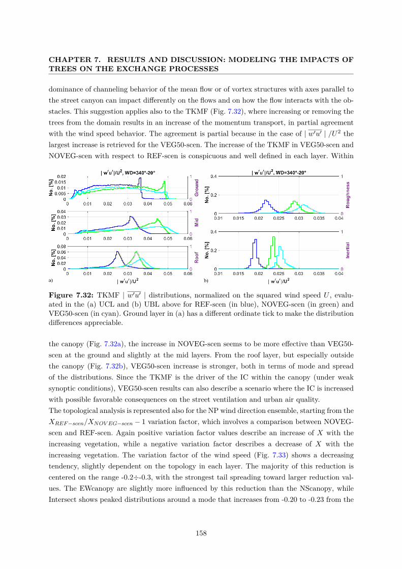
CHAPTER 7. RESULTS AND DISCUSSION: MODELING THE IMPACTS OFTREES ON THE EXCHANGE PROCESSES
dominance of channeling behavior of the mean flow or of vortex structures with axes parallel tothe street canyon can impact differently on the flows and on how the flow interacts with the ob-stacles. This suggestion applies also to the TKMF (Fig. 7.32), where increasing or removing thetrees from the domain results in an increase of the momentum transport, in partial agreementwith the wind speed behavior. The agreement is partial because in the case of | w′u′ | /U2 thelargest increase is retrieved for the VEG50-scen. The increase of the TKMF in VEG50-scen andNOVEG-scen with respect to REF-scen is conspicuous and well defined in each layer. Within
Figure 7.32: TKMF | w′u′ | distributions, normalized on the squared wind speed U , evalu-ated in the (a) UCL and (b) UBL above for REF-scen (in blue), NOVEG-scen (in green) andVEG50-scen (in cyan). Ground layer in (a) has a different ordinate tick to make the distributiondifferences appreciable.
the canopy (Fig. 7.32a), the increase in NOVEG-scen seems to be more effective than VEG50-scen at the ground and slightly at the mid layers. From the roof layer, but especially outsidethe canopy (Fig. 7.32b), VEG50-scen increase is stronger, both in terms of mode and spreadof the distributions. Since the TKMF is the driver of the IC within the canopy (under weaksynoptic conditions), VEG50-scen results can also describe a scenario where the IC is increasedwith possible favorable consequences on the street ventilation and urban air quality.The topological analysis is represented also for the NP wind direction ensemble, starting from theXREF−scen/XNOV EG−scen − 1 variation factor, which involves a comparison between NOVEG-scen and REF-scen. Again positive variation factor values describe an increase of X with theincreasing vegetation, while a negative variation factor describes a decrease of X with theincreasing vegetation. The variation factor of the wind speed (Fig. 7.33) shows a decreasingtendency, slightly dependent on the topology in each layer. The majority of this reduction iscentered on the range -0.2÷-0.3, with the strongest tail spreading toward larger reduction val-ues. The EWcanopy are slightly more influenced by this reduction than the NScanopy, whileIntersect shows peaked distributions around a mode that increases from -0.20 to -0.23 from the
158
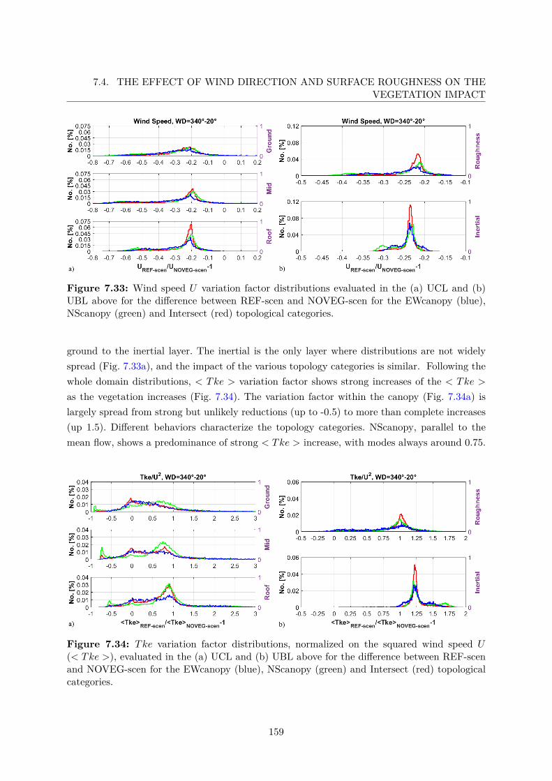
7.4. THE EFFECT OF WIND DIRECTION AND SURFACE ROUGHNESS ON THEVEGETATION IMPACT
Figure 7.33: Wind speed U variation factor distributions evaluated in the (a) UCL and (b)UBL above for the difference between REF-scen and NOVEG-scen for the EWcanopy (blue),NScanopy (green) and Intersect (red) topological categories.
ground to the inertial layer. The inertial is the only layer where distributions are not widelyspread (Fig. 7.33a), and the impact of the various topology categories is similar. Following thewhole domain distributions, < Tke > variation factor shows strong increases of the < Tke >
as the vegetation increases (Fig. 7.34). The variation factor within the canopy (Fig. 7.34a) islargely spread from strong but unlikely reductions (up to -0.5) to more than complete increases(up 1.5). Different behaviors characterize the topology categories. NScanopy, parallel to themean flow, shows a predominance of strong < Tke > increase, with modes always around 0.75.
Figure 7.34: Tke variation factor distributions, normalized on the squared wind speed U(< Tke >), evaluated in the (a) UCL and (b) UBL above for the difference between REF-scenand NOVEG-scen for the EWcanopy (blue), NScanopy (green) and Intersect (red) topologicalcategories.
159
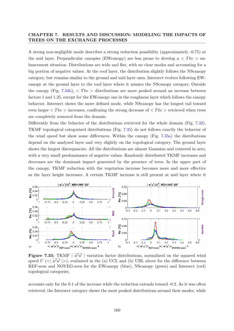
CHAPTER 7. RESULTS AND DISCUSSION: MODELING THE IMPACTS OFTREES ON THE EXCHANGE PROCESSES
A strong non-negligible mode describes a strong reduction possibility (approximately -0.75) atthe mid layer. Perpendicular canopies (EWcanopy) are less prone to develop a < Tke > en-hancement situation. Distributions are wide and flat, with no clear modes and accounting for abig portion of negative values. At the roof layer, the distribution slightly follows the NScanopycategory, but remains similar to the ground and mid layer ones. Intersect evolves following EW-canopy at the ground layer to the roof layer where it mimics the NScanopy category. Outsidethe canopy (Fig. 7.34b), < Tke > distributions are more peaked around an increase betweenfactors 1 and 1.25, except for the EWcanopy one in the roughness layer which follows the canopybehavior. Intersect shows the more defined mode, while NScanopy has the longest tail towardeven larger < Tke > increases, confirming the strong decrease of < Tke > retrieved when treesare completely removed from the domain.Differently from the behavior of the distributions retrieved for the whole domain (Fig. 7.32),TKMF topological categorized distributions (Fig. 7.35) do not follows exactly the behavior ofthe wind speed but show some differences. Within the canopy (Fig. 7.35a) the distributionsdepend on the analyzed layer and very slightly on the topological category. The ground layershows the largest discrepancies. All the distributions are almost Gaussian and centered in zero,with a very small predominance of negative values. Randomly distributed TKMF increases anddecreases are the dominant impact generated by the presence of trees. In the upper part ofthe canopy, TKMF reduction with the vegetation increase becomes more and more effectiveas the layer height increases. A certain TKMF increase is still present at mid layer where it
Figure 7.35: TKMF | w′u′ | variation factor distributions, normalized on the squared windspeed U (<| w′u′ |>), evaluated in the (a) UCL and (b) UBL above for the difference betweenREF-scen and NOVEG-scen for the EWcanopy (blue), NScanopy (green) and Intersect (red)topological categories.
accounts only for the 0.1 of the increase while the reduction extends toward -0.2. As it was oftenretrieved, the Intersect category shows the most peaked distributions around their modes, while
160
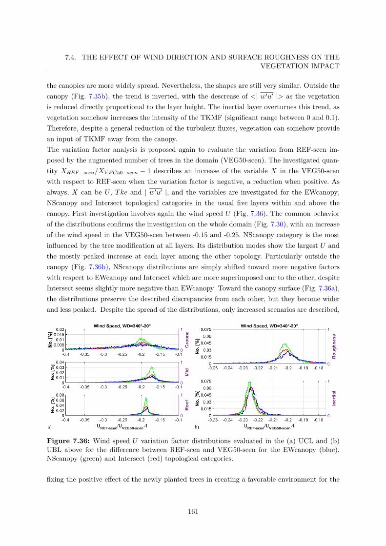
7.4. THE EFFECT OF WIND DIRECTION AND SURFACE ROUGHNESS ON THEVEGETATION IMPACT
the canopies are more widely spread. Nevertheless, the shapes are still very similar. Outside thecanopy (Fig. 7.35b), the trend is inverted, with the descrease of <| w′u′ |> as the vegetationis reduced directly proportional to the layer height. The inertial layer overturnes this trend, asvegetation somehow increases the intensity of the TKMF (significant range between 0 and 0.1).Therefore, despite a general reduction of the turbulent fluxes, vegetation can somehow providean input of TKMF away from the canopy.The variation factor analysis is proposed again to evaluate the variation from REF-scen im-posed by the augmented number of trees in the domain (VEG50-scen). The investigated quan-tity XREF−scen/XV EG50−scen − 1 describes an increase of the variable X in the VEG50-scenwith respect to REF-scen when the variation factor is negative, a reduction when positive. Asalways, X can be U , Tke and | w′u′ |, and the variables are investigated for the EWcanopy,NScanopy and Intersect topological categories in the usual five layers within and above thecanopy. First investigation involves again the wind speed U (Fig. 7.36). The common behaviorof the distributions confirms the investigation on the whole domain (Fig. 7.30), with an increaseof the wind speed in the VEG50-scen between -0.15 and -0.25. NScanopy category is the mostinfluenced by the tree modification at all layers. Its distribution modes show the largest U andthe mostly peaked increase at each layer among the other topology. Particularly outside thecanopy (Fig. 7.36b), NScanopy distributions are simply shifted toward more negative factorswith respect to EWcanopy and Intersect which are more superimposed one to the other, despiteIntersect seems slightly more negative than EWcanopy. Toward the canopy surface (Fig. 7.36a),the distributions preserve the described discrepancies from each other, but they become widerand less peaked. Despite the spread of the distributions, only increased scenarios are described,
Figure 7.36: Wind speed U variation factor distributions evaluated in the (a) UCL and (b)UBL above for the difference between REF-scen and VEG50-scen for the EWcanopy (blue),NScanopy (green) and Intersect (red) topological categories.
fixing the positive effect of the newly planted trees in creating a favorable environment for the
161
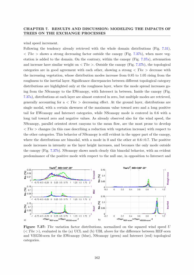
CHAPTER 7. RESULTS AND DISCUSSION: MODELING THE IMPACTS OFTREES ON THE EXCHANGE PROCESSES
wind speed increment.Following the tendency already retrieved with the whole domain distributions (Fig. 7.31),< Tke > shows a strong decreasing factor outside the canopy (Fig. 7.37b), when more veg-etation is added to the domain. On the contrary, within the canopy (Fig. 7.37a), attenuationand increase have similar weight on < Tke >. Outside the canopy (Fig. 7.37b), the topologicalcategories are in good agreement with each other, showing a strong < Tke > decrease withthe increasing vegetation, whose distribution modes increase from 0.85 to 1.05 rising from theroughness to the inertial layer. Significance discrepancies between different topological categorydistributions are highlighted only at the roughness layer, where the mode spread increases go-ing from the NScanopy to the EWcanopy, with Intersect in between. Inside the canopy (Fig.7.37a), distributions at each layer are almost centered in zero, but multiple modes are retrieved,generally accounting for a < Tke > decreasing effect. At the ground layer, distributions aresingle modal, with a certain skewness of the maximum value toward zero and a long positivetail for EWcanopy and Intersect categories, while NScanopy mode is centered in 0.6 with along tail toward zero and negative values. As already observed also for the wind speed, theNScanopy, parallel oriented street canyons to the mean flow, are the most prone to develop< Tke > changes (in this case describing a reduction with vegetation increase) with respect tothe other categories. This behavior of NScanopy is still evident in the upper part of the canopy,where the distributions are bimodal, with a mode in 0 and the other at 0.6÷0.7. The positivemode increases in intensity as the layer height increases, and becomes the only mode outsidethe canopy (Fig. 7.37b). NScanopy shows much clearly this bimodal behavior, with an evidentpredominance of the positive mode with respect to the null one, in opposition to Intersect and
Figure 7.37: Tke variation factor distributions, normalized on the squared wind speed U(< Tke >), evaluated in the (a) UCL and (b) UBL above for the difference between REF-scenand VEG50-scen for the EWcanopy (blue), NScanopy (green) and Intersect (red) topologicalcategories.
162
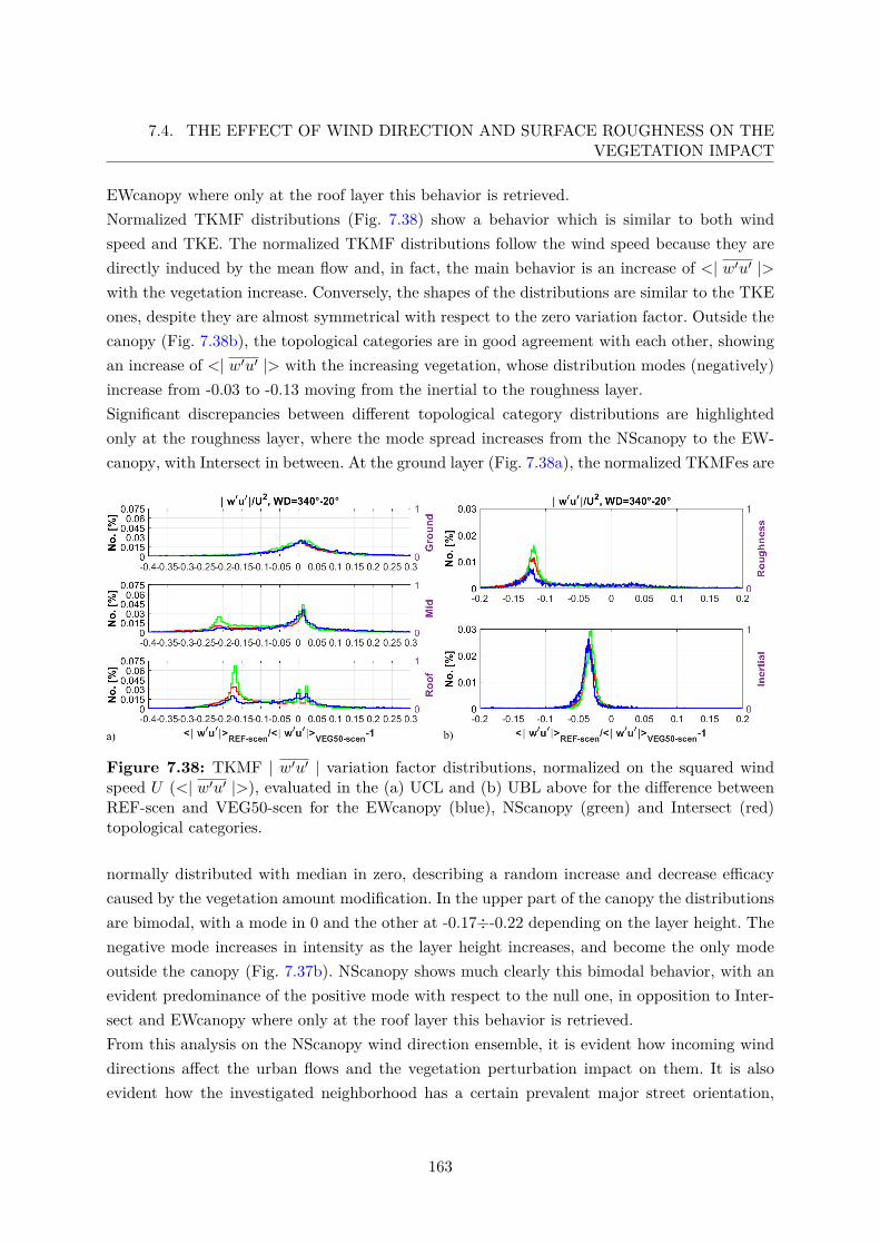
7.4. THE EFFECT OF WIND DIRECTION AND SURFACE ROUGHNESS ON THEVEGETATION IMPACT
EWcanopy where only at the roof layer this behavior is retrieved.Normalized TKMF distributions (Fig. 7.38) show a behavior which is similar to both windspeed and TKE. The normalized TKMF distributions follow the wind speed because they aredirectly induced by the mean flow and, in fact, the main behavior is an increase of <| w′u′ |>with the vegetation increase. Conversely, the shapes of the distributions are similar to the TKEones, despite they are almost symmetrical with respect to the zero variation factor. Outside thecanopy (Fig. 7.38b), the topological categories are in good agreement with each other, showingan increase of <| w′u′ |> with the increasing vegetation, whose distribution modes (negatively)increase from -0.03 to -0.13 moving from the inertial to the roughness layer.Significant discrepancies between different topological category distributions are highlightedonly at the roughness layer, where the mode spread increases from the NScanopy to the EW-canopy, with Intersect in between. At the ground layer (Fig. 7.38a), the normalized TKMFes are
Figure 7.38: TKMF | w′u′ | variation factor distributions, normalized on the squared windspeed U (<| w′u′ |>), evaluated in the (a) UCL and (b) UBL above for the difference betweenREF-scen and VEG50-scen for the EWcanopy (blue), NScanopy (green) and Intersect (red)topological categories.
normally distributed with median in zero, describing a random increase and decrease efficacycaused by the vegetation amount modification. In the upper part of the canopy the distributionsare bimodal, with a mode in 0 and the other at -0.17÷-0.22 depending on the layer height. Thenegative mode increases in intensity as the layer height increases, and become the only modeoutside the canopy (Fig. 7.37b). NScanopy shows much clearly this bimodal behavior, with anevident predominance of the positive mode with respect to the null one, in opposition to Inter-sect and EWcanopy where only at the roof layer this behavior is retrieved.From this analysis on the NScanopy wind direction ensemble, it is evident how incoming winddirections affect the urban flows and the vegetation perturbation impact on them. It is alsoevident how the investigated neighborhood has a certain prevalent major street orientation,
163
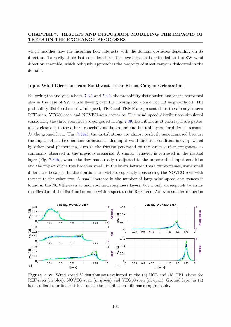
CHAPTER 7. RESULTS AND DISCUSSION: MODELING THE IMPACTS OFTREES ON THE EXCHANGE PROCESSES
which modifies how the incoming flow interacts with the domain obstacles depending on itsdirection. To verify these last considerations, the investigation is extended to the SW winddirection ensemble, which obliquely approaches the majority of street canyons dislocated in thedomain.
Input Wind Direction from Southwest to the Street Canyon Orientation
Following the analysis in Sect. 7.3.1 and 7.4.1, the probability distribution analysis is performedalso in the case of SW winds flowing over the investigated domain of LB neighborhood. Theprobability distributions of wind speed, TKE and TKMF are presented for the already knownREF-scen, VEG50-scen and NOVEG-scen scenarios. The wind speed distributions simulatedconsidering the three scenarios are compared in Fig. 7.39. Distributions at each layer are partic-ularly close one to the others, especially at the ground and inertial layers, for different reasons.At the ground layer (Fig. 7.39a), the distributions are almost perfectly superimposed becausethe impact of the tree number variation in this input wind direction condition is overpoweredby other local phenomena, such as the friction generated by the street surface roughness, ascommonly observed in the previous scenarios. A similar behavior is retrieved in the inertiallayer (Fig. 7.39b), where the flow has already readjusted to the unperturbed input conditionand the impact of the tree becomes small. In the layers between these two extremes, some smalldifferences between the distributions are visible, especially considering the NOVEG-scen withrespect to the other two. A small increase in the number of large wind speed occurrences isfound in the NOVEG-scen at mid, roof and roughness layers, but it only corresponds to an in-tensification of the distribution mode with respect to the REF-scen. An even smaller reduction
Figure 7.39: Wind speed U distributions evaluated in the (a) UCL and (b) UBL above forREF-scen (in blue), NOVEG-scen (in green) and VEG50-scen (in cyan). Ground layer in (a)has a different ordinate tick to make the distribution differences appreciable.
164
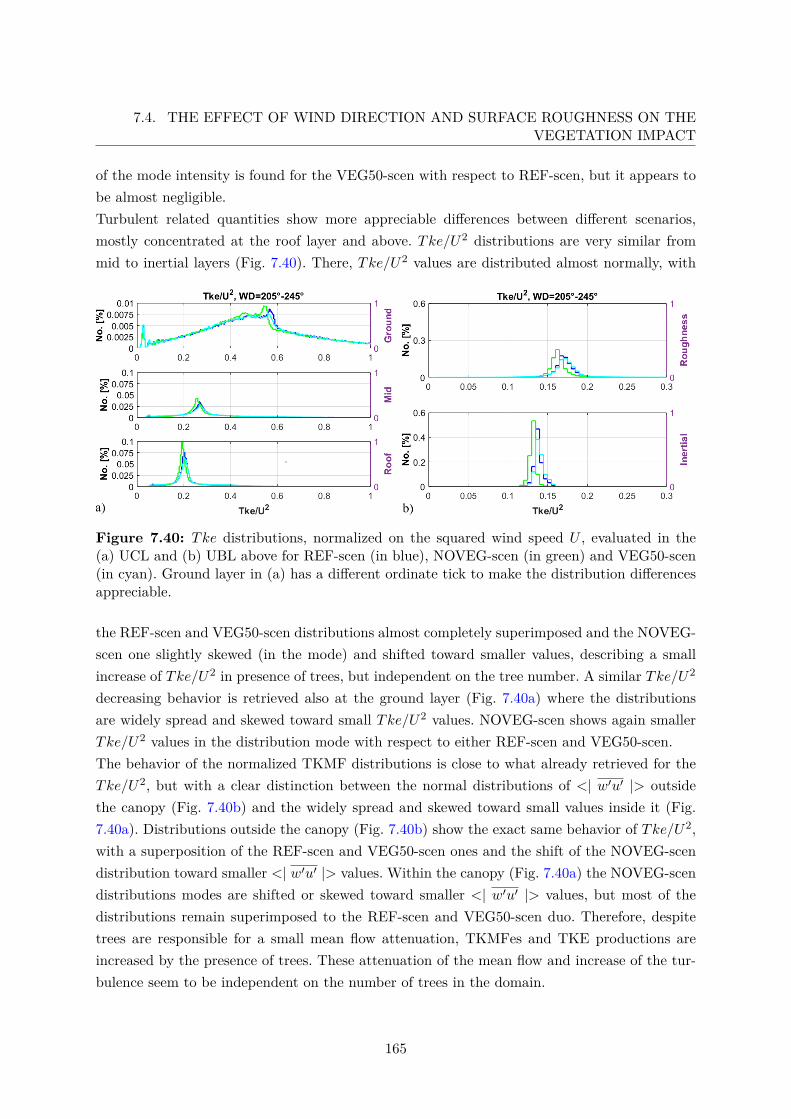
7.4. THE EFFECT OF WIND DIRECTION AND SURFACE ROUGHNESS ON THEVEGETATION IMPACT
of the mode intensity is found for the VEG50-scen with respect to REF-scen, but it appears tobe almost negligible.Turbulent related quantities show more appreciable differences between different scenarios,mostly concentrated at the roof layer and above. Tke/U2 distributions are very similar frommid to inertial layers (Fig. 7.40). There, Tke/U2 values are distributed almost normally, with
Figure 7.40: Tke distributions, normalized on the squared wind speed U , evaluated in the(a) UCL and (b) UBL above for REF-scen (in blue), NOVEG-scen (in green) and VEG50-scen(in cyan). Ground layer in (a) has a different ordinate tick to make the distribution differencesappreciable.
the REF-scen and VEG50-scen distributions almost completely superimposed and the NOVEG-scen one slightly skewed (in the mode) and shifted toward smaller values, describing a smallincrease of Tke/U2 in presence of trees, but independent on the tree number. A similar Tke/U2
decreasing behavior is retrieved also at the ground layer (Fig. 7.40a) where the distributionsare widely spread and skewed toward small Tke/U2 values. NOVEG-scen shows again smallerTke/U2 values in the distribution mode with respect to either REF-scen and VEG50-scen.The behavior of the normalized TKMF distributions is close to what already retrieved for theTke/U2, but with a clear distinction between the normal distributions of <| w′u′ |> outsidethe canopy (Fig. 7.40b) and the widely spread and skewed toward small values inside it (Fig.7.40a). Distributions outside the canopy (Fig. 7.40b) show the exact same behavior of Tke/U2,with a superposition of the REF-scen and VEG50-scen ones and the shift of the NOVEG-scendistribution toward smaller <| w′u′ |> values. Within the canopy (Fig. 7.40a) the NOVEG-scendistributions modes are shifted or skewed toward smaller <| w′u′ |> values, but most of thedistributions remain superimposed to the REF-scen and VEG50-scen duo. Therefore, despitetrees are responsible for a small mean flow attenuation, TKMFes and TKE productions areincreased by the presence of trees. These attenuation of the mean flow and increase of the tur-bulence seem to be independent on the number of trees in the domain.
165
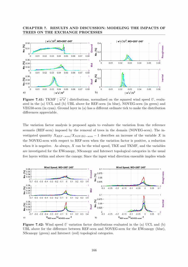
CHAPTER 7. RESULTS AND DISCUSSION: MODELING THE IMPACTS OFTREES ON THE EXCHANGE PROCESSES
Figure 7.41: TKMF | w′u′ | distributions, normalized on the squared wind speed U , evalu-ated in the (a) UCL and (b) UBL above for REF-scen (in blue), NOVEG-scen (in green) andVEG50-scen (in cyan). Ground layer in (a) has a different ordinate tick to make the distributiondifferences appreciable.
The variation factor analysis is proposed again to evaluate the variation from the referencescenario (REF-scen) imposed by the removal of trees in the domain (NOVEG-scen). The in-vestigated quantity XREF−scen/XNOV EG−scen − 1 describes an increase of the variable X inthe NOVEG-scen with respect to REF-scen when the variation factor is positive, a reductionwhen it is negative. As always, X can be the wind speed, TKE and TKMF, and the variablesare investigated for the EWcanopy, NScanopy and Intersect topological categories in the usualfive layers within and above the canopy. Since the input wind direction ensemble implies winds
Figure 7.42: Wind speed U variation factor distributions evaluated in the (a) UCL and (b)UBL above for the difference between REF-scen and NOVEG-scen for the EWcanopy (blue),NScanopy (green) and Intersect (red) topological categories.
166
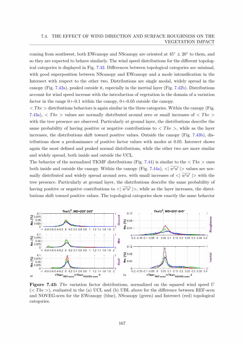
7.4. THE EFFECT OF WIND DIRECTION AND SURFACE ROUGHNESS ON THEVEGETATION IMPACT
coming from southwest, both EWcanopy and NScanopy are oriented at 45◦ ± 20◦ to them, andso they are expected to behave similarly. The wind speed distributions for the different topolog-ical categories is displayed in Fig. 7.42. Differences between topological categories are minimal,with good superposition between NScanopy and EWcanopy and a mode intensification in theIntersect with respect to the other two. Distributions are single modal, widely spread in thecanopy (Fig. 7.42a), peaked outside it, especially in the inertial layer (Fig. 7.42b). Distributionsaccount for wind speed increase with the introduction of vegetation in the domain of a variationfactor in the range 0÷-0.1 within the canopy, 0÷-0.05 outside the canopy.< Tke > distributions behaviors is again similar in the three categories. Within the canopy (Fig.7.43a), < Tke > values are normally distributed around zero or small increases of < Tke >
with the tree presence are observed. Particularly at ground layer, the distributions describe thesame probability of having positive or negative contributions to < Tke >, while as the layerincreases, the distributions shift toward positive values. Outside the canopy (Fig. 7.43b), dis-tributions show a predominance of positive factor values with modes at 0.05. Intersect showsagain the most defined and peaked normal distributions, while the other two are more similarand widely spread, both inside and outside the UCL.The behavior of the normalized TKMF distributions (Fig. 7.44) is similar to the < Tke > onesboth inside and outside the canopy. Within the canopy (Fig. 7.44a), <| w′u′ |> values are nor-mally distributed and widely spread around zero, with small increases of <| w′u′ |> with thetree presence. Particularly at ground layer, the distributions describe the same probability ofhaving positive or negative contributions to <| w′u′ |>, while as the layer increases, the distri-butions shift toward positive values. The topological categories show exactly the same behavior
Figure 7.43: Tke variation factor distributions, normalized on the squared wind speed U(< Tke >), evaluated in the (a) UCL and (b) UBL above for the difference between REF-scenand NOVEG-scen for the EWcanopy (blue), NScanopy (green) and Intersect (red) topologicalcategories.
167
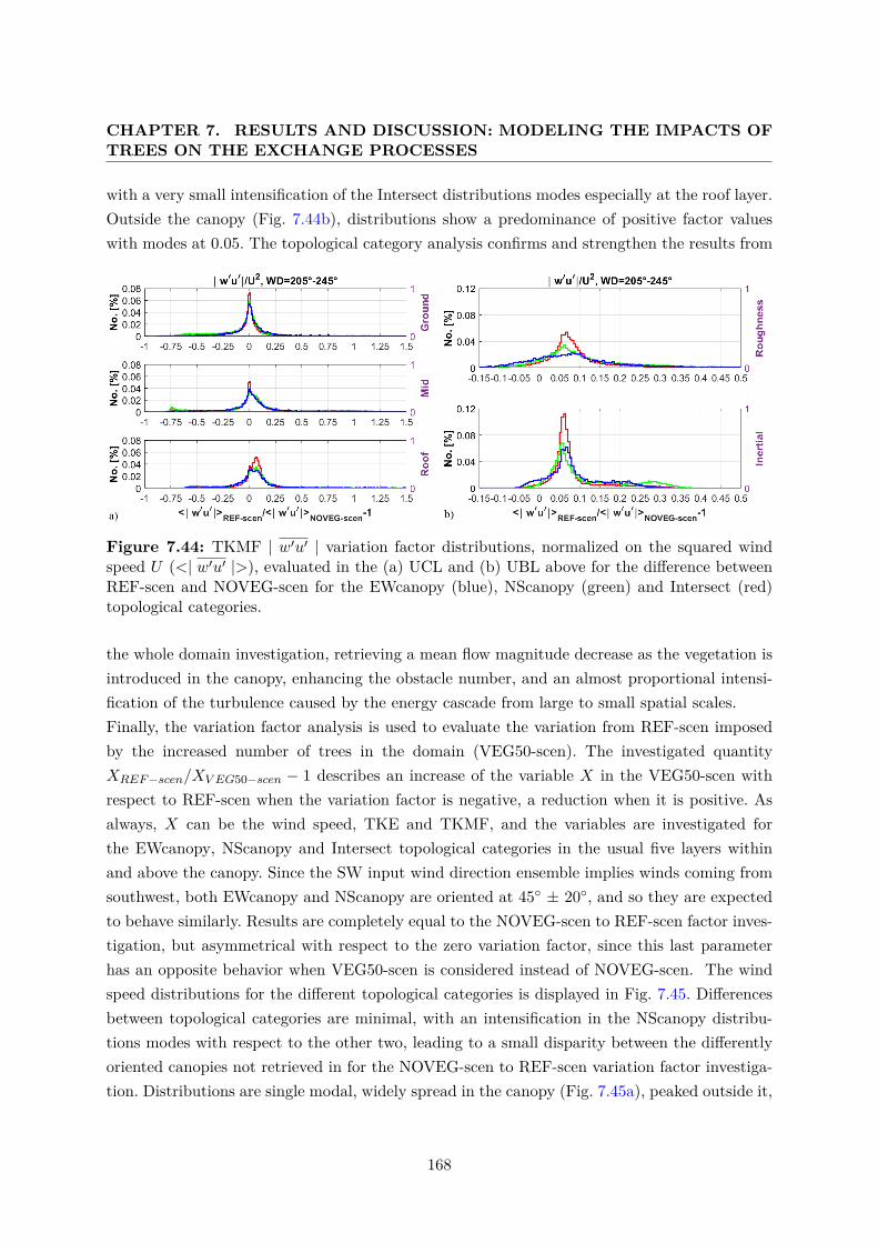
CHAPTER 7. RESULTS AND DISCUSSION: MODELING THE IMPACTS OFTREES ON THE EXCHANGE PROCESSES
with a very small intensification of the Intersect distributions modes especially at the roof layer.Outside the canopy (Fig. 7.44b), distributions show a predominance of positive factor valueswith modes at 0.05. The topological category analysis confirms and strengthen the results from
Figure 7.44: TKMF | w′u′ | variation factor distributions, normalized on the squared windspeed U (<| w′u′ |>), evaluated in the (a) UCL and (b) UBL above for the difference betweenREF-scen and NOVEG-scen for the EWcanopy (blue), NScanopy (green) and Intersect (red)topological categories.
the whole domain investigation, retrieving a mean flow magnitude decrease as the vegetation isintroduced in the canopy, enhancing the obstacle number, and an almost proportional intensi-fication of the turbulence caused by the energy cascade from large to small spatial scales.Finally, the variation factor analysis is used to evaluate the variation from REF-scen imposedby the increased number of trees in the domain (VEG50-scen). The investigated quantityXREF−scen/XV EG50−scen − 1 describes an increase of the variable X in the VEG50-scen withrespect to REF-scen when the variation factor is negative, a reduction when it is positive. Asalways, X can be the wind speed, TKE and TKMF, and the variables are investigated forthe EWcanopy, NScanopy and Intersect topological categories in the usual five layers withinand above the canopy. Since the SW input wind direction ensemble implies winds coming fromsouthwest, both EWcanopy and NScanopy are oriented at 45◦ ± 20◦, and so they are expectedto behave similarly. Results are completely equal to the NOVEG-scen to REF-scen factor inves-tigation, but asymmetrical with respect to the zero variation factor, since this last parameterhas an opposite behavior when VEG50-scen is considered instead of NOVEG-scen. The windspeed distributions for the different topological categories is displayed in Fig. 7.45. Differencesbetween topological categories are minimal, with an intensification in the NScanopy distribu-tions modes with respect to the other two, leading to a small disparity between the differentlyoriented canopies not retrieved in for the NOVEG-scen to REF-scen variation factor investiga-tion. Distributions are single modal, widely spread in the canopy (Fig. 7.45a), peaked outside it,
168
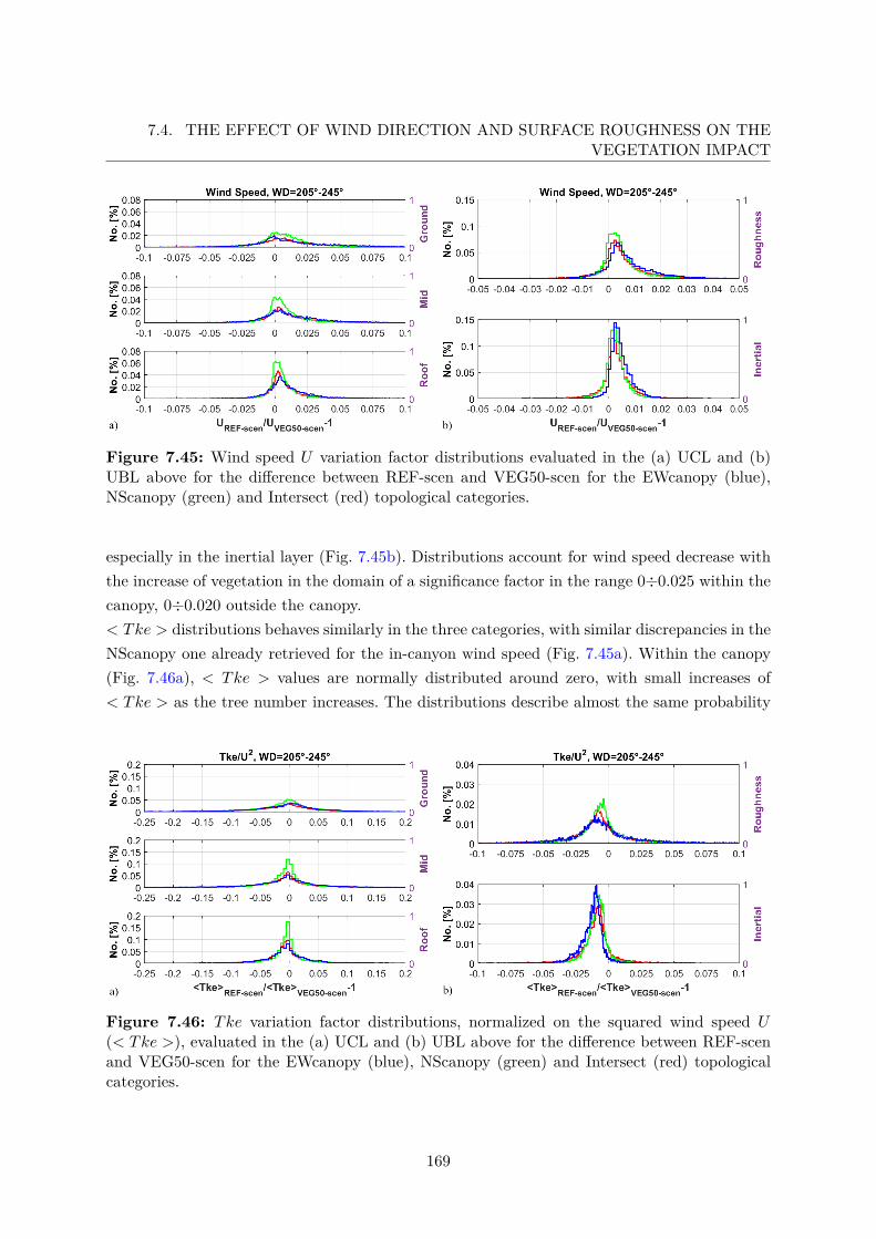
7.4. THE EFFECT OF WIND DIRECTION AND SURFACE ROUGHNESS ON THEVEGETATION IMPACT
Figure 7.45: Wind speed U variation factor distributions evaluated in the (a) UCL and (b)UBL above for the difference between REF-scen and VEG50-scen for the EWcanopy (blue),NScanopy (green) and Intersect (red) topological categories.
especially in the inertial layer (Fig. 7.45b). Distributions account for wind speed decrease withthe increase of vegetation in the domain of a significance factor in the range 0÷0.025 within thecanopy, 0÷0.020 outside the canopy.< Tke > distributions behaves similarly in the three categories, with similar discrepancies in theNScanopy one already retrieved for the in-canyon wind speed (Fig. 7.45a). Within the canopy(Fig. 7.46a), < Tke > values are normally distributed around zero, with small increases of< Tke > as the tree number increases. The distributions describe almost the same probability
Figure 7.46: Tke variation factor distributions, normalized on the squared wind speed U(< Tke >), evaluated in the (a) UCL and (b) UBL above for the difference between REF-scenand VEG50-scen for the EWcanopy (blue), NScanopy (green) and Intersect (red) topologicalcategories.
169
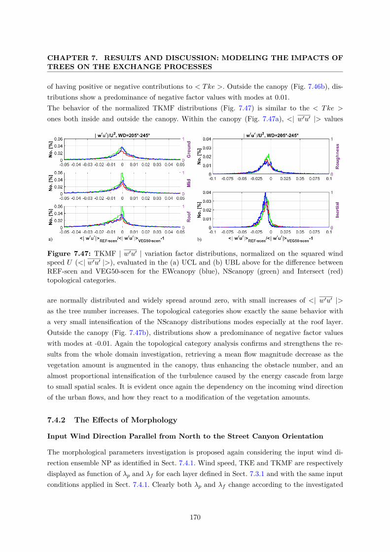
CHAPTER 7. RESULTS AND DISCUSSION: MODELING THE IMPACTS OFTREES ON THE EXCHANGE PROCESSES
of having positive or negative contributions to < Tke >. Outside the canopy (Fig. 7.46b), dis-tributions show a predominance of negative factor values with modes at 0.01.The behavior of the normalized TKMF distributions (Fig. 7.47) is similar to the < Tke >
ones both inside and outside the canopy. Within the canopy (Fig. 7.47a), <| w′u′ |> values
Figure 7.47: TKMF | w′u′ | variation factor distributions, normalized on the squared windspeed U (<| w′u′ |>), evaluated in the (a) UCL and (b) UBL above for the difference betweenREF-scen and VEG50-scen for the EWcanopy (blue), NScanopy (green) and Intersect (red)topological categories.
are normally distributed and widely spread around zero, with small increases of <| w′u′ |>as the tree number increases. The topological categories show exactly the same behavior witha very small intensification of the NScanopy distributions modes especially at the roof layer.Outside the canopy (Fig. 7.47b), distributions show a predominance of negative factor valueswith modes at -0.01. Again the topological category analysis confirms and strengthens the re-sults from the whole domain investigation, retrieving a mean flow magnitude decrease as thevegetation amount is augmented in the canopy, thus enhancing the obstacle number, and analmost proportional intensification of the turbulence caused by the energy cascade from largeto small spatial scales. It is evident once again the dependency on the incoming wind directionof the urban flows, and how they react to a modification of the vegetation amounts.
7.4.2 The Effects of Morphology
Input Wind Direction Parallel from North to the Street Canyon Orientation
The morphological parameters investigation is proposed again considering the input wind di-rection ensemble NP as identified in Sect. 7.4.1. Wind speed, TKE and TKMF are respectivelydisplayed as function of λp and λf for each layer defined in Sect. 7.3.1 and with the same inputconditions applied in Sect. 7.4.1. Clearly both λp and λf change according to the investigated
170
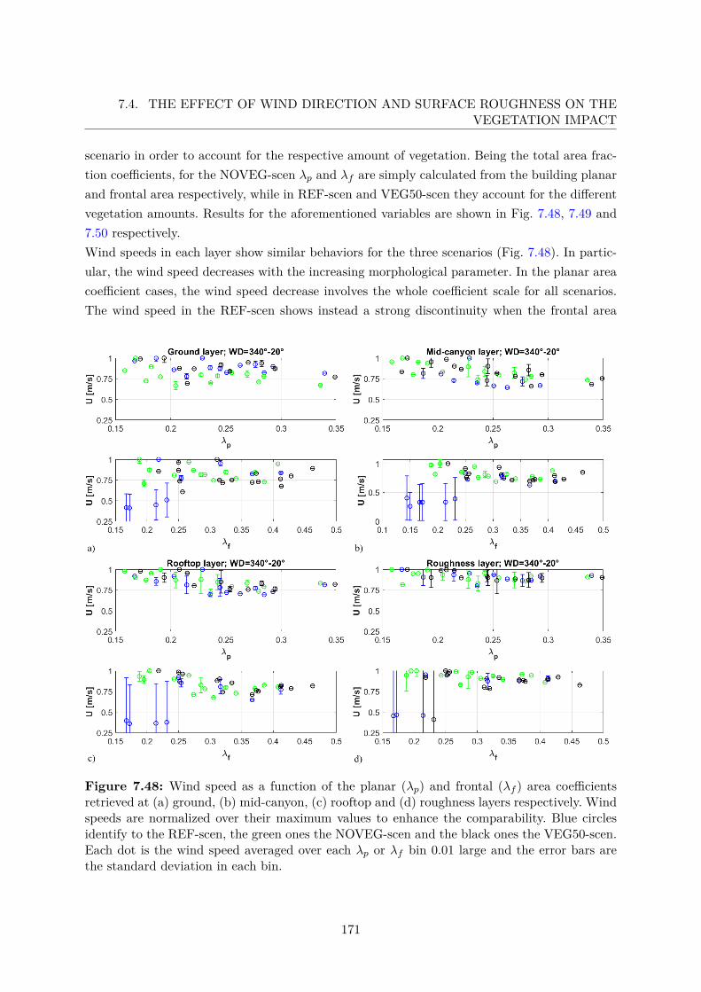
7.4. THE EFFECT OF WIND DIRECTION AND SURFACE ROUGHNESS ON THEVEGETATION IMPACT
scenario in order to account for the respective amount of vegetation. Being the total area frac-tion coefficients, for the NOVEG-scen λp and λf are simply calculated from the building planarand frontal area respectively, while in REF-scen and VEG50-scen they account for the differentvegetation amounts. Results for the aforementioned variables are shown in Fig. 7.48, 7.49 and7.50 respectively.Wind speeds in each layer show similar behaviors for the three scenarios (Fig. 7.48). In partic-ular, the wind speed decreases with the increasing morphological parameter. In the planar areacoefficient cases, the wind speed decrease involves the whole coefficient scale for all scenarios.The wind speed in the REF-scen shows instead a strong discontinuity when the frontal area
Figure 7.48: Wind speed as a function of the planar (λp) and frontal (λf ) area coefficientsretrieved at (a) ground, (b) mid-canyon, (c) rooftop and (d) roughness layers respectively. Windspeeds are normalized over their maximum values to enhance the comparability. Blue circlesidentify to the REF-scen, the green ones the NOVEG-scen and the black ones the VEG50-scen.Each dot is the wind speed averaged over each λp or λf bin 0.01 large and the error bars arethe standard deviation in each bin.
171
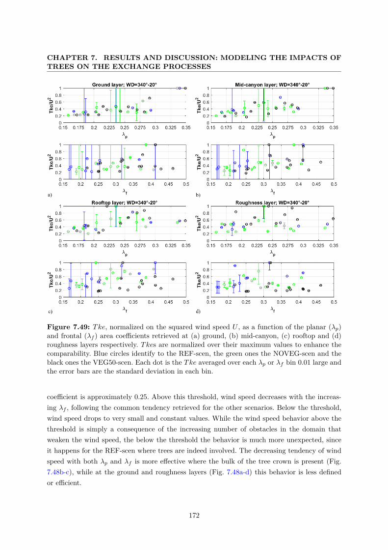
CHAPTER 7. RESULTS AND DISCUSSION: MODELING THE IMPACTS OFTREES ON THE EXCHANGE PROCESSES
Figure 7.49: Tke, normalized on the squared wind speed U , as a function of the planar (λp)and frontal (λf ) area coefficients retrieved at (a) ground, (b) mid-canyon, (c) rooftop and (d)roughness layers respectively. Tkes are normalized over their maximum values to enhance thecomparability. Blue circles identify to the REF-scen, the green ones the NOVEG-scen and theblack ones the VEG50-scen. Each dot is the Tke averaged over each λp or λf bin 0.01 large andthe error bars are the standard deviation in each bin.
coefficient is approximately 0.25. Above this threshold, wind speed decreases with the increas-ing λf , following the common tendency retrieved for the other scenarios. Below the threshold,wind speed drops to very small and constant values. While the wind speed behavior above thethreshold is simply a consequence of the increasing number of obstacles in the domain thatweaken the wind speed, the below the threshold the behavior is much more unexpected, sinceit happens for the REF-scen where trees are indeed involved. The decreasing tendency of windspeed with both λp and λf is more effective where the bulk of the tree crown is present (Fig.7.48b-c), while at the ground and roughness layers (Fig. 7.48a-d) this behavior is less definedor efficient.
172
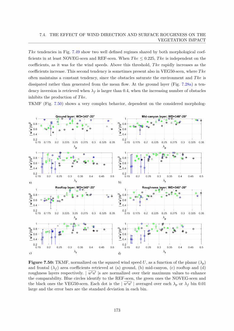
7.4. THE EFFECT OF WIND DIRECTION AND SURFACE ROUGHNESS ON THEVEGETATION IMPACT
Tke tendencies in Fig. 7.49 show two well defined regimes shared by both morphological coef-ficients in at least NOVEG-scen and REF-scen. When Tke ≤ 0.225, Tke is independent on thecoefficients, as it was for the wind speeds. Above this threshold, Tke rapidly increases as thecoefficients increase. This second tendency is sometimes present also in VEG50-scen, where Tkeoften maintains a constant tendency, since the obstacles saturate the environment and Tke isdissipated rather than generated from the mean flow. At the ground layer (Fig. 7.28a) a ten-dency inversion is retrieved when λf is larger than 0.4, when the increasing number of obstaclesinhibits the production of Tke.TKMF (Fig. 7.50) shows a very complex behavior, dependent on the considered morpholog-
Figure 7.50: TKMF, normalized on the squared wind speed U , as a function of the planar (λp)and frontal (λf ) area coefficients retrieved at (a) ground, (b) mid-canyon, (c) rooftop and (d)roughness layers respectively. | w′u′ |s are normalized over their maximum values to enhancethe comparability. Blue circles identify to the REF-scen, the green ones the NOVEG-scen andthe black ones the VEG50-scen. Each dot is the | w′u′ | averaged over each λp or λf bin 0.01large and the error bars are the standard deviation in each bin.
173
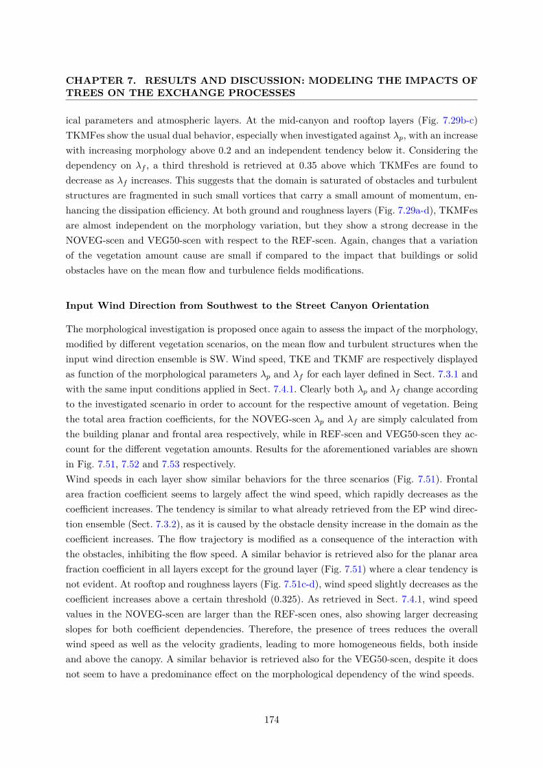
CHAPTER 7. RESULTS AND DISCUSSION: MODELING THE IMPACTS OFTREES ON THE EXCHANGE PROCESSES
ical parameters and atmospheric layers. At the mid-canyon and rooftop layers (Fig. 7.29b-c)TKMFes show the usual dual behavior, especially when investigated against λp, with an increasewith increasing morphology above 0.2 and an independent tendency below it. Considering thedependency on λf , a third threshold is retrieved at 0.35 above which TKMFes are found todecrease as λf increases. This suggests that the domain is saturated of obstacles and turbulentstructures are fragmented in such small vortices that carry a small amount of momentum, en-hancing the dissipation efficiency. At both ground and roughness layers (Fig. 7.29a-d), TKMFesare almost independent on the morphology variation, but they show a strong decrease in theNOVEG-scen and VEG50-scen with respect to the REF-scen. Again, changes that a variationof the vegetation amount cause are small if compared to the impact that buildings or solidobstacles have on the mean flow and turbulence fields modifications.
Input Wind Direction from Southwest to the Street Canyon Orientation
The morphological investigation is proposed once again to assess the impact of the morphology,modified by different vegetation scenarios, on the mean flow and turbulent structures when theinput wind direction ensemble is SW. Wind speed, TKE and TKMF are respectively displayedas function of the morphological parameters λp and λf for each layer defined in Sect. 7.3.1 andwith the same input conditions applied in Sect. 7.4.1. Clearly both λp and λf change accordingto the investigated scenario in order to account for the respective amount of vegetation. Beingthe total area fraction coefficients, for the NOVEG-scen λp and λf are simply calculated fromthe building planar and frontal area respectively, while in REF-scen and VEG50-scen they ac-count for the different vegetation amounts. Results for the aforementioned variables are shownin Fig. 7.51, 7.52 and 7.53 respectively.Wind speeds in each layer show similar behaviors for the three scenarios (Fig. 7.51). Frontalarea fraction coefficient seems to largely affect the wind speed, which rapidly decreases as thecoefficient increases. The tendency is similar to what already retrieved from the EP wind direc-tion ensemble (Sect. 7.3.2), as it is caused by the obstacle density increase in the domain as thecoefficient increases. The flow trajectory is modified as a consequence of the interaction withthe obstacles, inhibiting the flow speed. A similar behavior is retrieved also for the planar areafraction coefficient in all layers except for the ground layer (Fig. 7.51) where a clear tendency isnot evident. At rooftop and roughness layers (Fig. 7.51c-d), wind speed slightly decreases as thecoefficient increases above a certain threshold (0.325). As retrieved in Sect. 7.4.1, wind speedvalues in the NOVEG-scen are larger than the REF-scen ones, also showing larger decreasingslopes for both coefficient dependencies. Therefore, the presence of trees reduces the overallwind speed as well as the velocity gradients, leading to more homogeneous fields, both insideand above the canopy. A similar behavior is retrieved also for the VEG50-scen, despite it doesnot seem to have a predominance effect on the morphological dependency of the wind speeds.
174
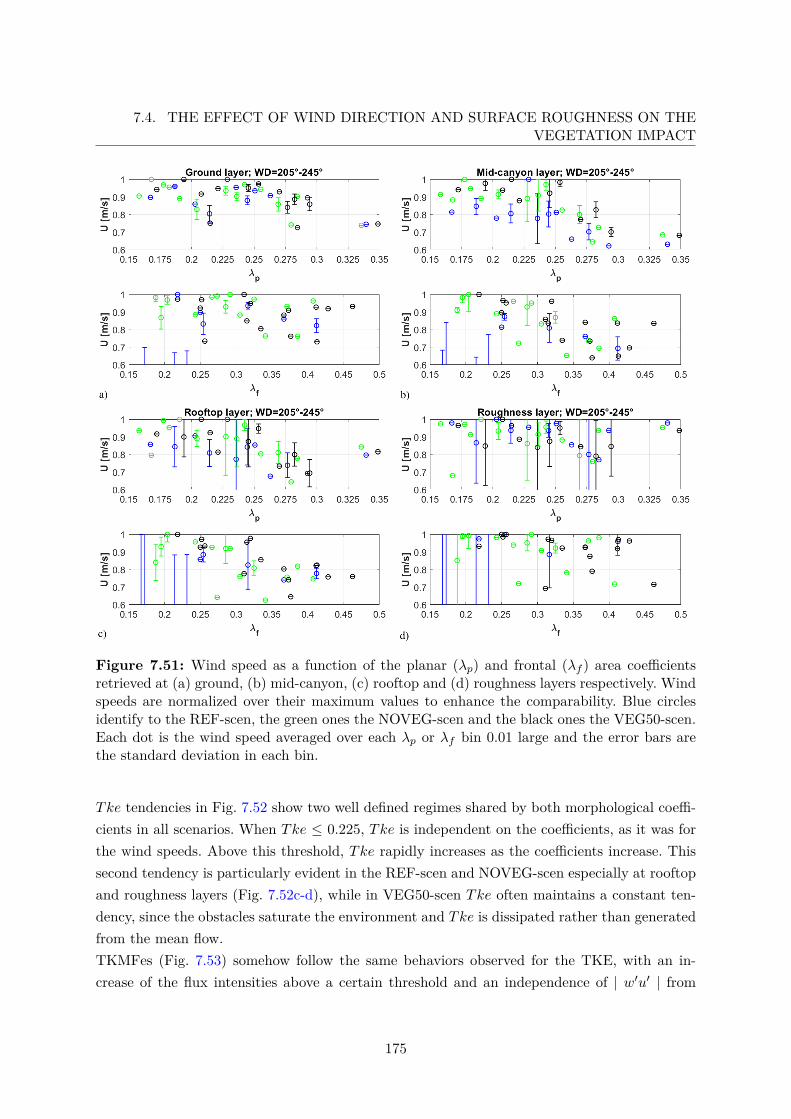
7.4. THE EFFECT OF WIND DIRECTION AND SURFACE ROUGHNESS ON THEVEGETATION IMPACT
Figure 7.51: Wind speed as a function of the planar (λp) and frontal (λf ) area coefficientsretrieved at (a) ground, (b) mid-canyon, (c) rooftop and (d) roughness layers respectively. Windspeeds are normalized over their maximum values to enhance the comparability. Blue circlesidentify to the REF-scen, the green ones the NOVEG-scen and the black ones the VEG50-scen.Each dot is the wind speed averaged over each λp or λf bin 0.01 large and the error bars arethe standard deviation in each bin.
Tke tendencies in Fig. 7.52 show two well defined regimes shared by both morphological coeffi-cients in all scenarios. When Tke ≤ 0.225, Tke is independent on the coefficients, as it was forthe wind speeds. Above this threshold, Tke rapidly increases as the coefficients increase. Thissecond tendency is particularly evident in the REF-scen and NOVEG-scen especially at rooftopand roughness layers (Fig. 7.52c-d), while in VEG50-scen Tke often maintains a constant ten-dency, since the obstacles saturate the environment and Tke is dissipated rather than generatedfrom the mean flow.TKMFes (Fig. 7.53) somehow follow the same behaviors observed for the TKE, with an in-crease of the flux intensities above a certain threshold and an independence of | w′u′ | from
175
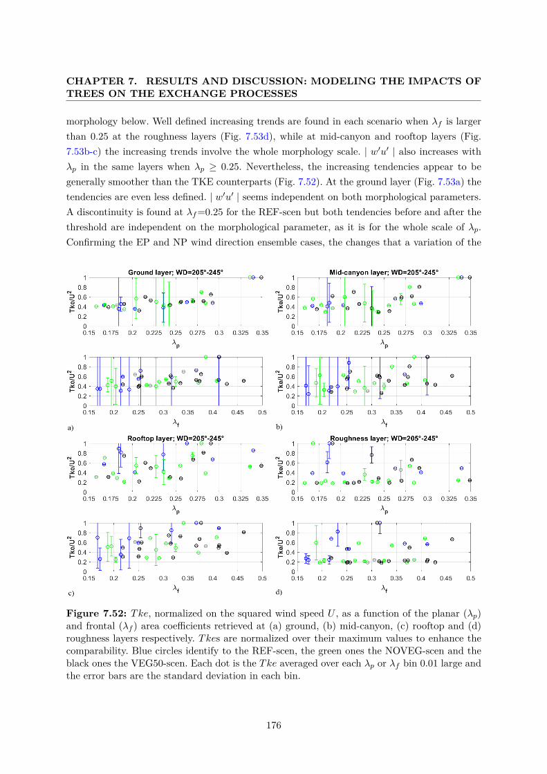
CHAPTER 7. RESULTS AND DISCUSSION: MODELING THE IMPACTS OFTREES ON THE EXCHANGE PROCESSES
morphology below. Well defined increasing trends are found in each scenario when λf is largerthan 0.25 at the roughness layers (Fig. 7.53d), while at mid-canyon and rooftop layers (Fig.7.53b-c) the increasing trends involve the whole morphology scale. | w′u′ | also increases withλp in the same layers when λp ≥ 0.25. Nevertheless, the increasing tendencies appear to begenerally smoother than the TKE counterparts (Fig. 7.52). At the ground layer (Fig. 7.53a) thetendencies are even less defined. | w′u′ | seems independent on both morphological parameters.A discontinuity is found at λf=0.25 for the REF-scen but both tendencies before and after thethreshold are independent on the morphological parameter, as it is for the whole scale of λp.Confirming the EP and NP wind direction ensemble cases, the changes that a variation of the
Figure 7.52: Tke, normalized on the squared wind speed U , as a function of the planar (λp)and frontal (λf ) area coefficients retrieved at (a) ground, (b) mid-canyon, (c) rooftop and (d)roughness layers respectively. Tkes are normalized over their maximum values to enhance thecomparability. Blue circles identify to the REF-scen, the green ones the NOVEG-scen and theblack ones the VEG50-scen. Each dot is the Tke averaged over each λp or λf bin 0.01 large andthe error bars are the standard deviation in each bin.
176
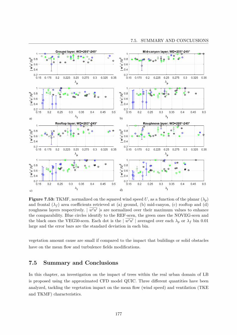
7.5. SUMMARY AND CONCLUSIONS
Figure 7.53: TKMF, normalized on the squared wind speed U , as a function of the planar (λp)and frontal (λf ) area coefficients retrieved at (a) ground, (b) mid-canyon, (c) rooftop and (d)roughness layers respectively. | w′u′ |s are normalized over their maximum values to enhancethe comparability. Blue circles identify to the REF-scen, the green ones the NOVEG-scen andthe black ones the VEG50-scen. Each dot is the | w′u′ | averaged over each λp or λf bin 0.01large and the error bars are the standard deviation in each bin.
vegetation amount cause are small if compared to the impact that buildings or solid obstacleshave on the mean flow and turbulence fields modifications.
7.5 Summary and Conclusions
In this chapter, an investigation on the impact of trees within the real urban domain of LBis proposed using the approximated CFD model QUIC. Three different quantities have beenanalyzed, tackling the vegetation impact on the mean flow (wind speed) and ventilation (TKEand TKMF) characteristics.
177
CHAPTER 7. RESULTS AND DISCUSSION: MODELING THE IMPACTS OFTREES ON THE EXCHANGE PROCESSES
Before the analysis to be made, a code modification is introduced and validated on a simple do-main to better simulate the friction velocity and therefore the turbulent related quantities. Thecode modification theory was introduced in Sect. 7.1 to overcome some wrong values obtainedfor the TKE profiles from simulations. The validation of the modified code has been proven towork better than the original one for the simple and most common obstacles and morphology inurban environments, such as isolated trees and buildings, street canyons, frontal and rear wakevolumes. The modified code has been succesfully validated for different input wind directionsand speeds, and atmospheric stability. Finally, a successful validation has been obtained alsofor the MA and LB domains, considering real input conditions retrieved from measurements.After the implementation of the u∗ modified computation into QUIC, simulations of wind speed,TKE and TKMF for four different wind direction ensembles have been verified on the experi-mental field campaign in MA and LB. The choice to have wind direction ensembles, i.e. a rangeof simulations taken for different wind direction under the same input conditions, was made tobetter account for the strong variability of the wind direction and to choose a representativeinterval of at least one hour that could ensure some robustness to the simulation results. Theverification of the different simulaitons gave very good results in all the three analyzed variables,when the NP, WP and EP wind direction ensembles are considered. Conversely, the simulationsfor the SP wind directions ensemble gave a poor comparison with the data from measurements.This last ensemble was associated with nocturnal conditions, when a stably stratified UBLdeveloping above a neutrally stable UCL, and a small boundary layer height provided someoverestimation in the model computation. Nevertheless, QUIC is found to provide reliable andaccurate estimations of the mean flow and turbulence developing within complex urban envi-ronments typical of European cities, especially when the UCL unstable or neutral stability iscoupled with the rest of the UBL.From the verification, the input conditions of the EP wind direction ensemble are chosen toinvestigate the vegetation impact on wind speed, TKE and TKMF in the building wake volumeand the deep and narrow street canyon of LB. The overall impact of vegetation on the windspeed is found to be a blocking effect, reducing the wind speed in the UCL and propagatingthis reduction in the UBL above. The reduction propagation bove the canopy resulted in awavelike motion. TKE is found to increase its heterogeneous spatial distribution as the treesare introduced in the domains, both in the canopy and above it. TKE increased at the baseof the trees and at their top, while decreased above them. TKE production is limited to thevolumes where an intense flow interact with the tree, generating more dissipation elsewhere.TKMF is found to behave similarly to the TKE, except for the tree base and the inner-canopyregion, where the vegetation was insignificant or reduced the flux.The vegetation impact was then detailed as a function of the wind direction, by means of thecharacteristic quantities distributions computed for the different vertical layers LB neighbor-
178
7.5. SUMMARY AND CONCLUSIONS
hood domain has been divided into. Three different input wind directions (EP, NP and SW)were chosen for the investigation, but they all used the same input conditions of the EP winddirection ensemble, except of course the wind direction. Among these input conditions, threedifferent topological scenarios have been investigated to detail the differences between the ref-erence or real domain (REF-scen) and a non vegetative domain (NOVEG-scen) or a scenariowhere the vegetation amount is randomly increased by a 50% (VEG50-scen). Wind speed isfound to increase as the vegetation is removed from the domain for all the investigated thewind direction ensembles, confirming the blocking effect of vegetation on the mean flow. Asa verification, wind speed is found to decrease when the tree number is increased for the EPand SW wind directions. However, the NP wind direction revealed an increased wind speed inthe VEG50-scen with respect to the REF-scen, as the vegetation may increase the channelingeffect of the wind. TKE is found to show similar behaviors if vegetation is added or removedfrom REF-scen, but drastically change with the input wind direction. TKE is found to increasewhen vegetation is either removed or added, and to increase from SW to EP wind directions, inagreement with the wind speed behaviors. On the contrary, TKE is strongly reduced when thewind is NP to the canyon, for both modified scenarios, as the channeling effect on the flow tendsto favor direction rather than isotropic turbulence. The similar behavior of NOVEG-scen andVEG50-scen suggested the existance of a threshold in the number of trees added in the domain,by which the TKE dissipation dominates the production. Finally, the TKMFes are generallyfound to follow the wind speed behaviors since these two quantities are strictly related one to theother. The strong increase of TKMF under NP wind directions supported the directional tur-bulence production theory suggested for the channeling flows. As the behaviors of VEG50-scenand NOVEG-scen are again coupled, the hypothesis on the turbulence dissipation-productionthreshold based on the number of trees in the domain is supported.Similar results are also retrieved detailing the analysis to account for different topological cate-gories defined within the domain. In particular, wind speed, TKE and TKMF are investigated asfunction of the three vegetation scenarios in an ensemble of street canyons north-south oriented(NScanopy), east-west oriented (EWcanopy) and inside the major intersections (Intersect). Re-sults for each input wind direction ensemble confirm the overall behaviors discovered with thewhole domain distribution analysis, with an increase of the channeling effect of street canyonsparallel to the flow as vegetation is added in the domain, and a general flow reduction else-where. Turbulent quantities confirmed the whole domain distribution analysis, with the TKMFfollowing more strictly the mean flow behaviors and TKE behaving in opposition. Moreover itappears evident how the domain has a prevalent orientation, which can also explain the differentbehaviors when wind directions are EP and NP.Finally, a morphological analysis is presented, showing the dependency of the three atmosphericquantities on the morphological parameters λp and λf as the vegetation scenarios are changed.
179

CHAPTER 7. RESULTS AND DISCUSSION: MODELING THE IMPACTS OFTREES ON THE EXCHANGE PROCESSES
Both mean flow and turbulent fields are found to decrease their magnitudes as the obstacledensity increases in the domain, but the largest impact is given by the building dispositionrather than the vegetation amounts. Below certain obstacle densities, mean flow and especiallyturbulence are found to be independent on the morphological parameters.
180
Chapter 8
Conclusions and Further Remarks
Local atmopsheric processes, such as flow circulations, coherent and transient turbulent struc-tures, interaction processes and local thermal budget are the key investigated aspects that driveor have an impact on the majority of the local atmospheric issues concerning the urban en-vironment. In recent years, these fundamental aspects have been tackled to investigate citybreathability and thermal comfort in the urban canopies, with the aim to find solutions formitigating air pollution and urban heat island effects and for rising the livability of the urbanenvironment. Of large interest is also the presence of vegetation in urban environments and howit impacts different aspects of the atmospheric processes, from the aerodynamics effects to theimplication on pollutant deposition and resuspension and thermal comfort.
The present thesis was inspired by these past investigations, to focus on the analysis the ven-tilation processes in different real urban canopies modified by vegetative elements, and theirapplications to air pollutant removal. In particular, exchange processes have been investigatedfrom measured data in real urban street canyons by means of new diagnostic quantities evalu-ated using the Buckingham theorem, fundamental mathematical tool of the similarity theory,with the aim to characterize mechanical and thermal aspects of the in-canyon circulation, torepresent the chemically passive pollutant removal from the canopy and to evaluate the role ofvegetation on the local flows and turbulent structures at the basis of the diagnostic quantitiesformulation. At the core of the investigation there are the two experimental field campaigns con-ducted in two street canyons of the city of Bologna (Italy), namely Marconi Street and LauraBassi Street, covering part of the late summer/early fall (August-September 2017) and winter(January-February 2018) periods. Three sites located at different height in each street canyonhave been fully equipped to detail the minimum variations in the flow and turbulent fields,together with a detailed measure of the principal traffic pollutant concentrations. Supportingmeteorological and air quality monitoring sites have been added to establish a measurementnetwork ensuring a good characterization of the urban boundary layer processes.
181
CHAPTER 8. CONCLUSIONS AND FURTHER REMARKS
The diagnostic quantities are derived from processed data during a period of weak synopticconditions and thermal circulation developing at the urban boundary layer scale. Despite thedetailed analyses for the diagnostic quantities have been conducted only for the summer cam-paign, the similar conditions characterizing the two season’s periods at the synoptic scale grantfor the possible analysis extension to the winter period. As expected from two similar synopticconditions, summer and winter periods showed some similarity, such as the time evolution ofthe mean flow and turbulent related quantities both within and above the canopies, where themajority of the inter seasonal differences are caused by the different amounts of available energyin the environment.
Newly developed diagnostic quantities included four time scales characterizing the time as-sociated to mechanical and thermal exchanges between different atmospheric layers within andat the interface of the urban canopy. The time scales separately assess the momentum and heatexchange contributions, including the combined impact of mean flow and turbulent aspectsrelated to the upward/downward transport processes. Therefore the time scales are represen-tative of the key mechanisms regulating the exchange processes, and their values vary withthe wind direction of the background flow. Detailed findings associated with the time scalesanalysis in the non-vegetated canyon revealed that mechanical time scales τd vary within andabove the canyon, with values evaluated at the rooftop level smaller than the ones evaluatedat lower levels. Thermal time scales τh, sustained by the heat released from the street and thebuilding facades, are smaller and more homogeneous than the mechanical ones. In a vegetatedcanopy, τd are homogeneous within and above the canyon, as the presence of vegetation andthe lateral flow entrainment mix the mechanical exchange velocity by affecting the mechanicalproduction of turbulence. The irregular building and street insolation, caused by the shadowingeffect of the trees, affects the mixing properties of the canopy leading to heterogeneous τh values.
From the time scales, another couple of new diagnostic quantities have been evaluated as theratio between interface and in-canyon time scales, always keeping mechanical and thermal as-pects separated. These new quantities have been named exchange rates η as they evaluate thecapacity of a canopy in exchanging momentum and heat with the outer layer. When η < 1, thecanopy circulation rapidly transports momentum or heat toward the interface, favoring the ex-changes with the outer layers. When η > 1, the circulation is faster at the interface, which trapsmomentum and heat to recirculate downward and limits the exchange efficacy. Both vegetatedand non-vegetated canopies are found to be favourable environment for exchange processes todevelop for approximately the 50−75% of the rates cases, but the long tails of the distributionsdescribe scenarios where the exchanges are totally suppressed, particularly common in the veg-
182
etated canyon. The only exception is retrieved for the thermal rates in the vegetated canyon,where the vegetation inhibits the exchanges at the surface by lowering the sensible heat fluxes.
A new total circulation dependent exchange rate ηt has been computed supposing the largerefficiency of mechanical processes when the in-canyon circulation is inertially driven or of thethermal processes when the circulation is thermal. Discrimination has been made using thebuoyancy parameter B (the ratio between thermal and inertial circulations drivers), to findan exchange rate representative of a real environment where both circulations can be present.The total exchange rate is succesfully used to reproduce the CO concentration (normalized onthe canopy geometry, mean flow velocity and source emission) tendency within the canopies,revealing momentum and heat transports to be most efficient driver of mass transport within astreet canyon under weak synoptic conditions.
Finally, the buoyancy parameter B enables the introduction of a new simple parametrizationfor in-canyon wind speed and to modify an existing one for the temperature horizontal gradientas functions of the mean canyon aspect ratio H/W . These parametrizations allow to estimateand compare flow characteristics in real street canyons with different aspect ratios, if the airflowregime within the canyon is in the skimming flow.
The bulk of the investigation on the impact of vegetation on the mean flow, turbulence kineticenergy and momentum flux is performed using the fast-responding operational computationalfluid dynamics model Quick Urban & Industrial Complex (QUIC). First, a code modification wasintroduced to better simulate the friction velocity and therefore the turbulent related quantities.The improved code has been successfully validated among a simple idealized domain, and thenproved more accurate for the investigated vegetated and non-vegetated neighborhoods domains.
The model was then verified on both domains, testing real conditions characterized by fourdifferent wind direction ensembles to the reference canyons orientations as input for the simula-tions The choice of simulating ensembles of wind directions minimized the uncertainties of themodel and associated with the transient nature of the wind direction. The model verificationgave very good results in all the three analyzed variables when the northerly, westerly and east-erly wind direction ensembles are considered, while the southerly comparison with measureddata is poor, as a stably stratified UBL developing above a neutrally stable UCL, and a smallboundary layer height provided some overestimation in the model computation. Definitively,QUIC is proved to perform reliable and accurate estimations of the mean flow and turbulencedeveloping within complex urban environments typical of European cities, especially when theurban canopy unstable or neutral stability is coupled with the rest of the boundary layer.
183
CHAPTER 8. CONCLUSIONS AND FURTHER REMARKS
A qualitative impact of vegetation is addressed by simulating representative volumes of thevegetated street canyon in presence and absence of trees. The overall impact of vegetation onthe wind speed is found to be a blocking effect, reducing the wind speed in the whole boundarylayer. The reduction propagation bove the canopy resulted in a wavelike motion. Turbulenceis found to increase its heterogeneous spatial distribution as the trees are introduced in thedomains, both in the canopy and above it. A turbulence production is found to be limited tothe volumes where an intense flow interact with the tree, generating more dissipation elsewhere.
A quantitative investigation is then proposed to assess the vegetation impact in the wholedomain on the mean flow and turbulence under different input wind directions, comparing thereal environment to scenarios with no vegetation and more vegetation. Wind speed is foundto increase as the vegetation is removed from the domain for all the investigated the wind di-rections, confirming the blocking effect of vegetation on the mean flow. As a verification, windspeed is found to decrease when the tree number is increased for perpendicular and obliquewind directions. However, the parallel wind direction revealed an increased wind speed as thenumber of trees increase in the domain, as the vegetation may increase the channeling effect ofthe wind. TKE is found to increase when vegetation is either removed or added, and to increasefrom oblique to perpendicular wind directions, in agreement with the wind speed behaviors.On the contrary, TKE is strongly reduced when the wind is parallel to the canyon, for bothmodified scenarios, as the channeling effect on the flow tends to favor direction rather thanisotropic turbulence. The existance of a threshold in the number of trees added in the domainis speculated, by which the TKE dissipation dominates the production. Finally, the TKMFesare generally found to follow the wind speed behaviors since these two quantities are strictlyrelated one to the other. The strong increase of TKMF under parallel wind directions supportedthe directional turbulence production theory suggested for the channeling flows. Since the tur-bulent quantities showed similar behaviors for the non-vegetated and more vegetated scenarios,the existance of a threshold in the number of trees added in the domain is speculated, by whichthe turbulence dissipation dominates on the production.
Similar results are also retrieved detailing the analysis to account for different topological cat-egories defined within the domain. Results for each input wind direction confirm the overallbehaviors discovered with the whole domain distribution analysis, with an increase of the chan-neling effect of street canyons parallel to the flow as vegetation is added in the domain, anda general flow reduction elsewhere. Also turbulent quantities confirmed the whole domain dis-tribution analysis, with the TKMF following more strictly the mean flow behaviors and TKEbehaving in opposition.
184
8.1. FUTURE PERSPECTIVES
Finally, a morphological analysis is presented, showing the dependency of the three atmosphericquantities on the morphological parameters λp and λf as the vegetation scenarios are changed.Both mean flow and turbulent fields are found to decrease their magnitudes as the obstacledensity increases in the domain, but the largest impact is given by the building dispositionrather than the vegetation amounts. Below certain obstacle densities, mean flow and especiallyturbulence are found to be independent on the morphological parameters.
8.1 Future Perspectives
Several aspects of the urban canopy flows and ventilation processes have been tackled in thisthesis and more generally during the last two decades. Through the challenges of the worldpopulation growth and rising urbanization, the investigations concerning the urban environmentare expected to further increase and embrace a wider range of aspects from the fundamentalprocess investigation to the citizen adaptation strategies. In this context, our investigationtackles fundamental aspects of the canopy flow and turbulence in real urban environments andextend them to the more practical topic of air pollution mitigation. Further application of thecurrent method must be done for the winter campaign where the local atmospheric stability isespected to play a key role on the exchanges, while the absence of the vegetation leaves can offeranother clue to establish the impact of tree crowns. Further studies are expected and suggestedin the recent future following this approach.The capitalization of experimental field campaigns is fundamental to extend as much as possibleall numerical and laboratory studies of idealized scenarios in real environment, to study theimplication of transient behaviors of the atmospheric flows on local aspects, given the complexityof a real city morphology. In the context of the exchange processes, further studies are needed totest the implication of an irregular skyline, also in terms of rooftop shape, and dense real streetnetworks on the city breathability. Moreover, the majority of the recent studies, as the currentone, has focused on synoptically stable conditions, leaving a large spectrum of backgroundconditions to be investigated. In these scenarios, must be included the effects of vegetations,whose roles needs further and more detailed investigations especially in real environments.Last suggestion involves the complex interaction between chemically or photochemically activepollutants, the transport and exchange atmospheric processes and the vegetation depositionand transpiration processes which still provide a contemporary challenging research topic.
185


Appendices
187

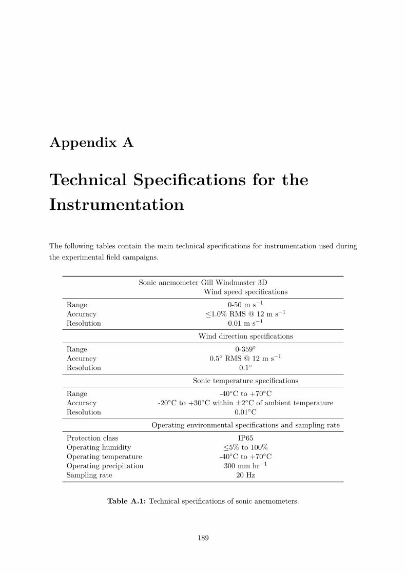
Appendix A
Technical Specifications for theInstrumentation
The following tables contain the main technical specifications for instrumentation used duringthe experimental field campaigns.
Sonic anemometer Gill Windmaster 3DWind speed specifications
Range 0-50 m s−1
Accuracy ≤1.0% RMS @ 12 m s−1
Resolution 0.01 m s−1
Wind direction specificationsRange 0-359◦Accuracy 0.5◦ RMS @ 12 m s−1
Resolution 0.1◦
Sonic temperature specificationsRange -40◦C to +70◦CAccuracy -20◦C to +30◦C within ±2◦C of ambient temperatureResolution 0.01◦C
Operating environmental specifications and sampling rateProtection class IP65Operating humidity ≤5% to 100%Operating temperature -40◦C to +70◦COperating precipitation 300 mm hr−1
Sampling rate 20 Hz
Table A.1: Technical specifications of sonic anemometers.
189
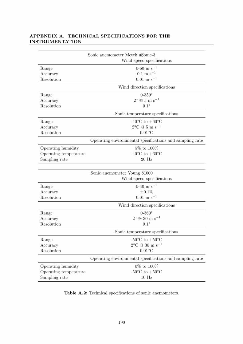
APPENDIX A. TECHNICAL SPECIFICATIONS FOR THEINSTRUMENTATION
Sonic anemometer Metek uSonic-3Wind speed specifications
Range 0-60 m s−1
Accuracy 0.1 m s−1
Resolution 0.01 m s−1
Wind direction specificationsRange 0-359◦Accuracy 2◦ @ 5 m s−1
Resolution 0.1◦
Sonic temperature specificationsRange -40◦C to +60◦CAccuracy 2◦C @ 5 m s−1
Resolution 0.01◦COperating environmental specifications and sampling rate
Operating humidity 5% to 100%Operating temperature -40◦C to +60◦CSampling rate 20 Hz
Sonic anemometer Young 81000Wind speed specifications
Range 0-40 m s−1
Accuracy ±0.1%Resolution 0.01 m s−1
Wind direction specificationsRange 0-360◦Accuracy 2◦ @ 30 m s−1
Resolution 0.1◦
Sonic temperature specificationsRange -50◦C to +50◦CAccuracy 2◦C @ 30 m s−1
Resolution 0.01◦COperating environmental specifications and sampling rate
Operating humidity 0% to 100%Operating temperature -50◦C to +50◦CSampling rate 10 Hz
Table A.2: Technical specifications of sonic anemometers.
190
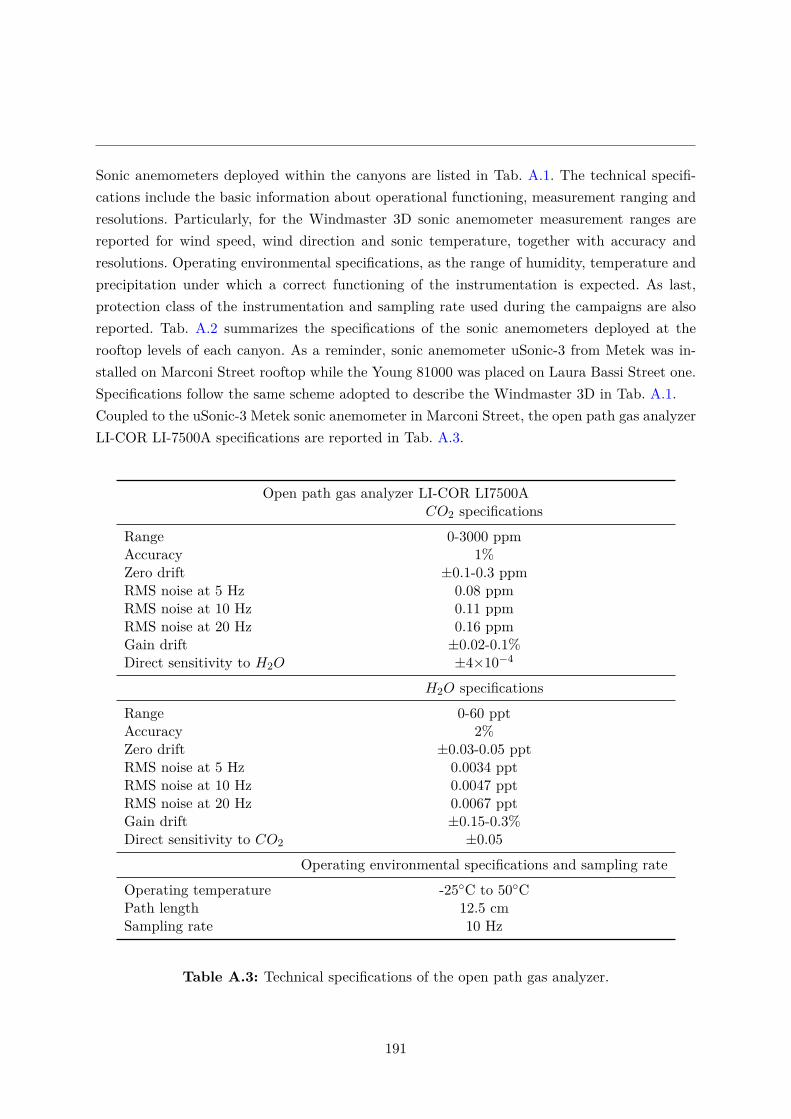
Sonic anemometers deployed within the canyons are listed in Tab. A.1. The technical specifi-cations include the basic information about operational functioning, measurement ranging andresolutions. Particularly, for the Windmaster 3D sonic anemometer measurement ranges arereported for wind speed, wind direction and sonic temperature, together with accuracy andresolutions. Operating environmental specifications, as the range of humidity, temperature andprecipitation under which a correct functioning of the instrumentation is expected. As last,protection class of the instrumentation and sampling rate used during the campaigns are alsoreported. Tab. A.2 summarizes the specifications of the sonic anemometers deployed at therooftop levels of each canyon. As a reminder, sonic anemometer uSonic-3 from Metek was in-stalled on Marconi Street rooftop while the Young 81000 was placed on Laura Bassi Street one.Specifications follow the same scheme adopted to describe the Windmaster 3D in Tab. A.1.Coupled to the uSonic-3 Metek sonic anemometer in Marconi Street, the open path gas analyzerLI-COR LI-7500A specifications are reported in Tab. A.3.
Open path gas analyzer LI-COR LI7500ACO2 specifications
Range 0-3000 ppmAccuracy 1%Zero drift ±0.1-0.3 ppmRMS noise at 5 Hz 0.08 ppmRMS noise at 10 Hz 0.11 ppmRMS noise at 20 Hz 0.16 ppmGain drift ±0.02-0.1%Direct sensitivity to H2O ±4×10⁻⁴
H2O specificationsRange 0-60 pptAccuracy 2%Zero drift ±0.03-0.05 pptRMS noise at 5 Hz 0.0034 pptRMS noise at 10 Hz 0.0047 pptRMS noise at 20 Hz 0.0067 pptGain drift ±0.15-0.3%Direct sensitivity to CO2 ±0.05
Operating environmental specifications and sampling rateOperating temperature -25◦C to 50◦CPath length 12.5 cmSampling rate 10 Hz
Table A.3: Technical specifications of the open path gas analyzer.
191
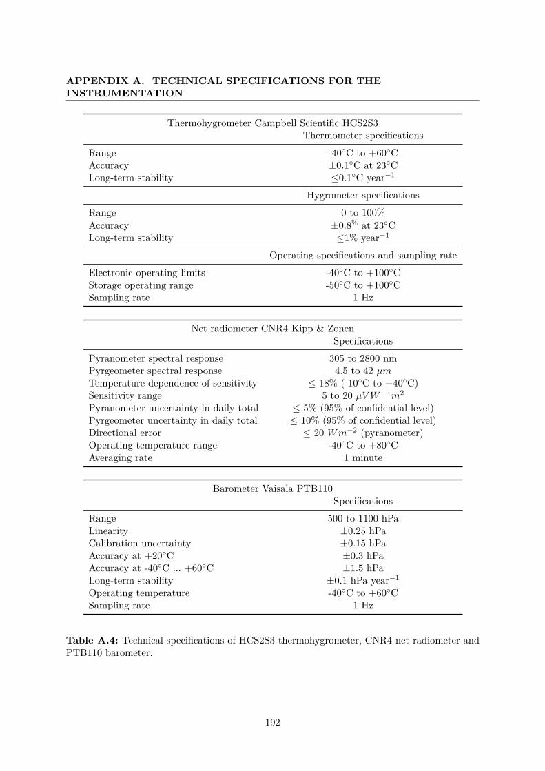
APPENDIX A. TECHNICAL SPECIFICATIONS FOR THEINSTRUMENTATION
Thermohygrometer Campbell Scientific HCS2S3Thermometer specifications
Range -40◦C to +60◦CAccuracy ±0.1◦C at 23◦CLong-term stability ≤0.1◦C year−1
Hygrometer specificationsRange 0 to 100%Accuracy ±0.8% at 23◦CLong-term stability ≤1% year−1
Operating specifications and sampling rateElectronic operating limits -40◦C to +100◦CStorage operating range -50◦C to +100◦CSampling rate 1 Hz
Net radiometer CNR4 Kipp & ZonenSpecifications
Pyranometer spectral response 305 to 2800 nmPyrgeometer spectral response 4.5 to 42 µmTemperature dependence of sensitivity ≤ 18% (-10◦C to +40◦C)Sensitivity range 5 to 20 µVW−1m2
Pyranometer uncertainty in daily total ≤ 5% (95% of confidential level)Pyrgeometer uncertainty in daily total ≤ 10% (95% of confidential level)Directional error ≤ 20 Wm−2 (pyranometer)Operating temperature range -40◦C to +80◦CAveraging rate 1 minute
Barometer Vaisala PTB110Specifications
Range 500 to 1100 hPaLinearity ±0.25 hPaCalibration uncertainty ±0.15 hPaAccuracy at +20◦C ±0.3 hPaAccuracy at -40◦C ... +60◦C ±1.5 hPaLong-term stability ±0.1 hPa year−1
Operating temperature -40◦C to +60◦CSampling rate 1 Hz
Table A.4: Technical specifications of HCS2S3 thermohygrometer, CNR4 net radiometer andPTB110 barometer.
192
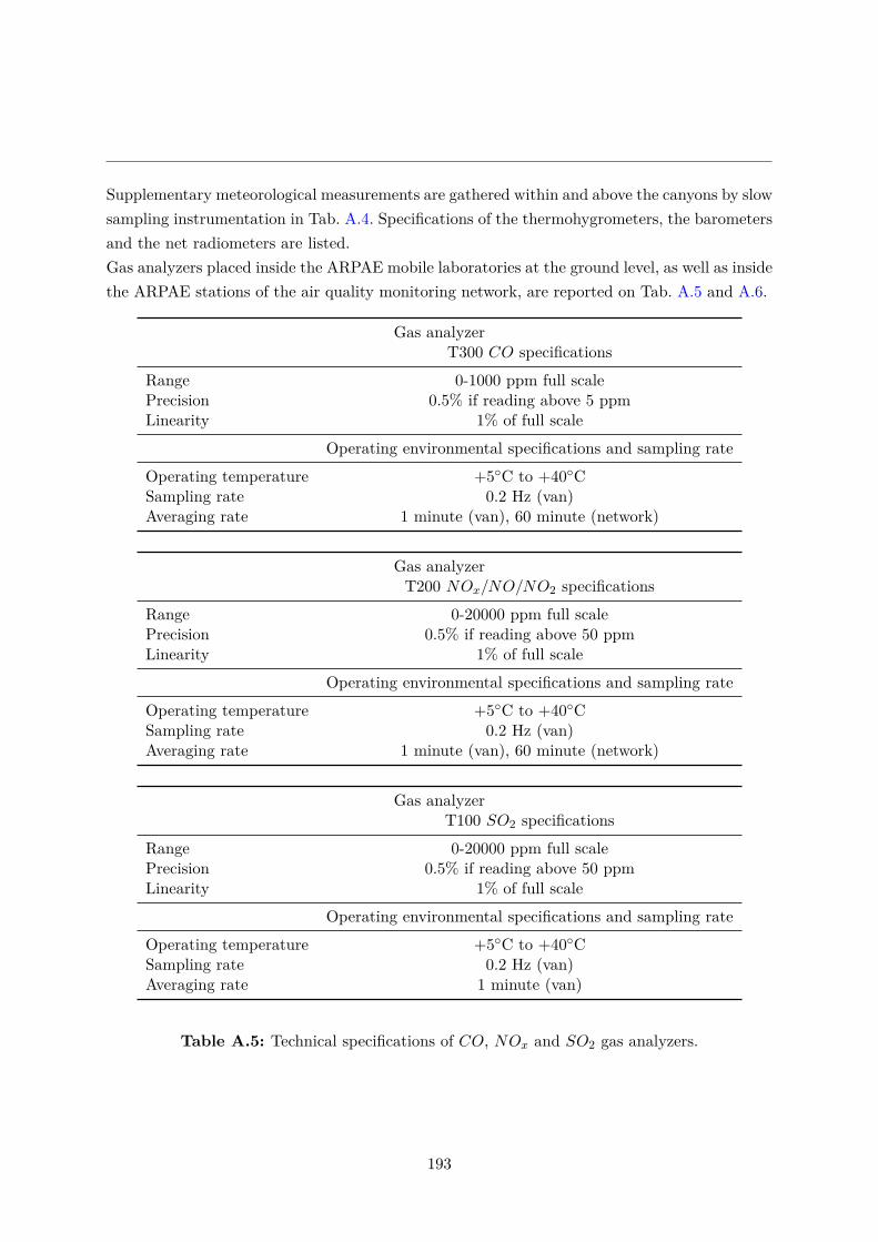
Supplementary meteorological measurements are gathered within and above the canyons by slowsampling instrumentation in Tab. A.4. Specifications of the thermohygrometers, the barometersand the net radiometers are listed.Gas analyzers placed inside the ARPAE mobile laboratories at the ground level, as well as insidethe ARPAE stations of the air quality monitoring network, are reported on Tab. A.5 and A.6.
Gas analyzerT300 CO specifications
Range 0-1000 ppm full scalePrecision 0.5% if reading above 5 ppmLinearity 1% of full scale
Operating environmental specifications and sampling rateOperating temperature +5◦C to +40◦CSampling rate 0.2 Hz (van)Averaging rate 1 minute (van), 60 minute (network)
Gas analyzerT200 NOx/NO/NO2 specifications
Range 0-20000 ppm full scalePrecision 0.5% if reading above 50 ppmLinearity 1% of full scale
Operating environmental specifications and sampling rateOperating temperature +5◦C to +40◦CSampling rate 0.2 Hz (van)Averaging rate 1 minute (van), 60 minute (network)
Gas analyzerT100 SO2 specifications
Range 0-20000 ppm full scalePrecision 0.5% if reading above 50 ppmLinearity 1% of full scale
Operating environmental specifications and sampling rateOperating temperature +5◦C to +40◦CSampling rate 0.2 Hz (van)Averaging rate 1 minute (van)
Table A.5: Technical specifications of CO, NOx and SO2 gas analyzers.
193
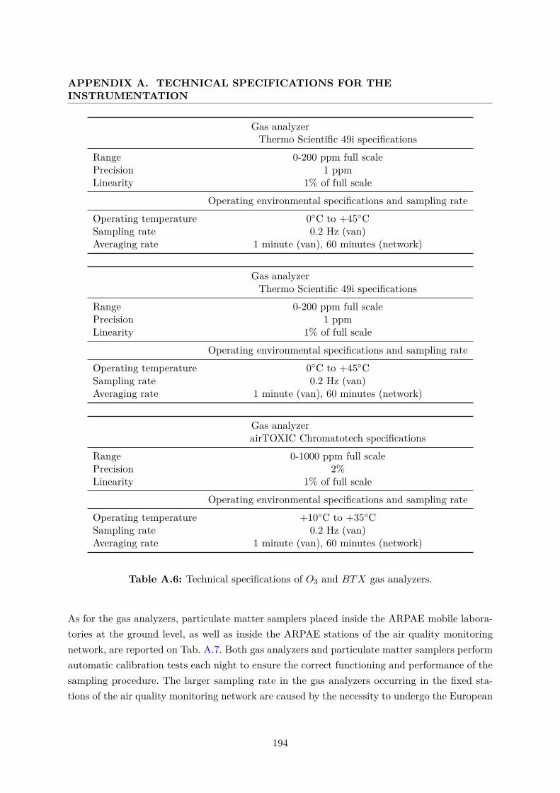
APPENDIX A. TECHNICAL SPECIFICATIONS FOR THEINSTRUMENTATION
Gas analyzerThermo Scientific 49i specifications
Range 0-200 ppm full scalePrecision 1 ppmLinearity 1% of full scale
Operating environmental specifications and sampling rateOperating temperature 0◦C to +45◦CSampling rate 0.2 Hz (van)Averaging rate 1 minute (van), 60 minutes (network)
Gas analyzerThermo Scientific 49i specifications
Range 0-200 ppm full scalePrecision 1 ppmLinearity 1% of full scale
Operating environmental specifications and sampling rateOperating temperature 0◦C to +45◦CSampling rate 0.2 Hz (van)Averaging rate 1 minute (van), 60 minutes (network)
Gas analyzerairTOXIC Chromatotech specifications
Range 0-1000 ppm full scalePrecision 2%Linearity 1% of full scale
Operating environmental specifications and sampling rateOperating temperature +10◦C to +35◦CSampling rate 0.2 Hz (van)Averaging rate 1 minute (van), 60 minutes (network)
Table A.6: Technical specifications of O3 and BTX gas analyzers.
As for the gas analyzers, particulate matter samplers placed inside the ARPAE mobile labora-tories at the ground level, as well as inside the ARPAE stations of the air quality monitoringnetwork, are reported on Tab. A.7. Both gas analyzers and particulate matter samplers performautomatic calibration tests each night to ensure the correct functioning and performance of thesampling procedure. The larger sampling rate in the gas analyzers occurring in the fixed sta-tions of the air quality monitoring network are caused by the necessity to undergo the European
194
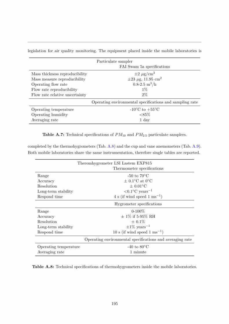
legislation for air quality monitoring. The equipment placed inside the mobile laboratories is
Particulate samplerFAI Swam 5a specifications
Mass thickness reproducibility ±2 µg/cm2
Mass measure reproducibility ±23 µg, 11.95 cm2
Operating flow rate 0.8-2.5 m3/hFlow rate reproducibility 1%Flow rate relative uncertainty 2%
Operating environmental specifications and sampling rateOperating temperature -10◦C to +55◦COperating humidity <85%Averaging rate 1 day
Table A.7: Technical specifications of PM10 and PM2.5 particulate samplers.
completed by the thermohygrometers (Tab. A.8) and the cup and vane anemometers (Tab. A.9).Both mobile laboratories share the same instrumentation, therefore single tables are reported.
Theromhygrometer LSI Lastem EXP815Thermometer specifications
Range -50 to 70◦CAccuracy ± 0.1◦C at 0◦CResolution ± 0.01◦CLong-term stability <0.1◦C years−1
Respond time 4 s (if wind speed 1 ms−1)Hygrometer specifications
Range 0-100%Accuracy ± 1% if 5-95% RHResolution ± 0.1%Long-term stability ±1% years−1
Respond time 10 s (if wind speed 1 ms−1)Operating environmental specifications and averaging rate
Operating temperature -40 to 80◦CAveraging rate 1 minute
Table A.8: Technical specifications of thermohygrometers inside the mobile laboratories.
195
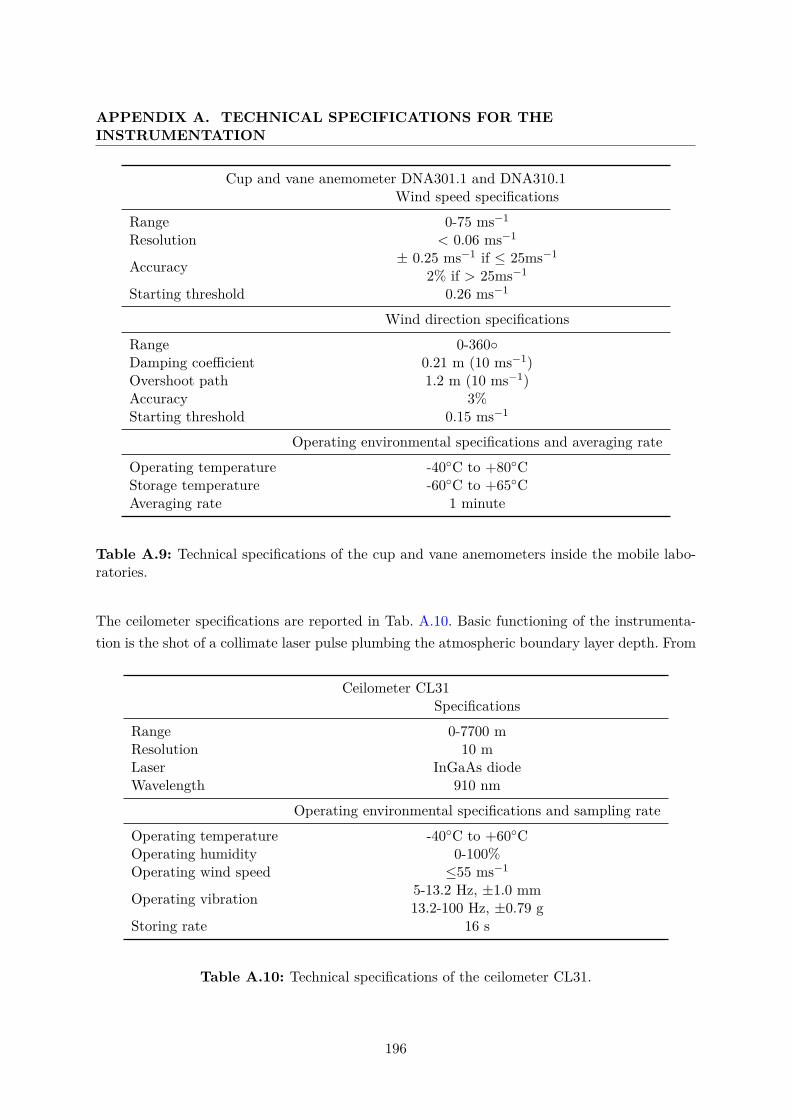
APPENDIX A. TECHNICAL SPECIFICATIONS FOR THEINSTRUMENTATION
Cup and vane anemometer DNA301.1 and DNA310.1Wind speed specifications
Range 0-75 ms−1
Resolution < 0.06 ms−1
Accuracy ± 0.25 ms−1 if ≤ 25ms−1
2% if > 25ms−1
Starting threshold 0.26 ms−1
Wind direction specificationsRange 0-360◦Damping coefficient 0.21 m (10 ms−1)Overshoot path 1.2 m (10 ms−1)Accuracy 3%Starting threshold 0.15 ms−1
Operating environmental specifications and averaging rateOperating temperature -40◦C to +80◦CStorage temperature -60◦C to +65◦CAveraging rate 1 minute
Table A.9: Technical specifications of the cup and vane anemometers inside the mobile labo-ratories.
The ceilometer specifications are reported in Tab. A.10. Basic functioning of the instrumenta-tion is the shot of a collimate laser pulse plumbing the atmospheric boundary layer depth. From
Ceilometer CL31Specifications
Range 0-7700 mResolution 10 mLaser InGaAs diodeWavelength 910 nm
Operating environmental specifications and sampling rateOperating temperature -40◦C to +60◦COperating humidity 0-100%Operating wind speed ≤55 ms−1
Operating vibration 5-13.2 Hz, ±1.0 mm13.2-100 Hz, ±0.79 g
Storing rate 16 s
Table A.10: Technical specifications of the ceilometer CL31.
196
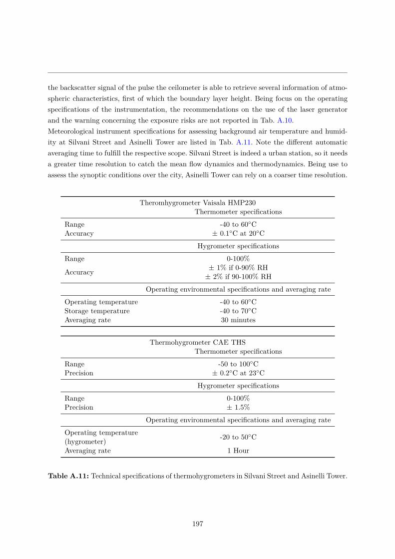
the backscatter signal of the pulse the ceilometer is able to retrieve several information of atmo-spheric characteristics, first of which the boundary layer height. Being focus on the operatingspecifications of the instrumentation, the recommendations on the use of the laser generatorand the warning concerning the exposure risks are not reported in Tab. A.10.Meteorological instrument specifications for assessing background air temperature and humid-ity at Silvani Street and Asinelli Tower are listed in Tab. A.11. Note the different automaticaveraging time to fulfill the respective scope. Silvani Street is indeed a urban station, so it needsa greater time resolution to catch the mean flow dynamics and thermodynamics. Being use toassess the synoptic conditions over the city, Asinelli Tower can rely on a coarser time resolution.
Theromhygrometer Vaisala HMP230Thermometer specifications
Range -40 to 60◦CAccuracy ± 0.1◦C at 20◦C
Hygrometer specificationsRange 0-100%
Accuracy ± 1% if 0-90% RH± 2% if 90-100% RH
Operating environmental specifications and averaging rateOperating temperature -40 to 60◦CStorage temperature -40 to 70◦CAveraging rate 30 minutes
Thermohygrometer CAE THSThermometer specifications
Range -50 to 100◦CPrecision ± 0.2◦C at 23◦C
Hygrometer specificationsRange 0-100%Precision ± 1.5%
Operating environmental specifications and averaging rateOperating temperature -20 to 50◦C(hygrometer)Averaging rate 1 Hour
Table A.11: Technical specifications of thermohygrometers in Silvani Street and Asinelli Tower.
197
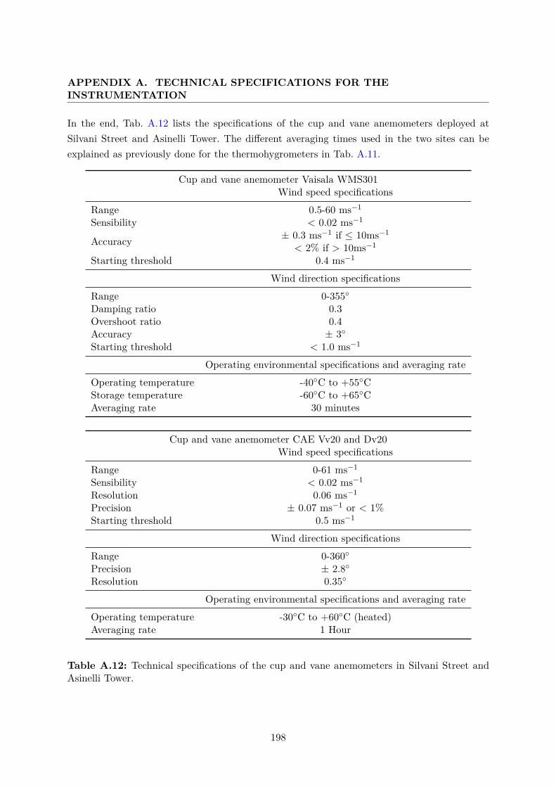
APPENDIX A. TECHNICAL SPECIFICATIONS FOR THEINSTRUMENTATION
In the end, Tab. A.12 lists the specifications of the cup and vane anemometers deployed atSilvani Street and Asinelli Tower. The different averaging times used in the two sites can beexplained as previously done for the thermohygrometers in Tab. A.11.
Cup and vane anemometer Vaisala WMS301Wind speed specifications
Range 0.5-60 ms−1
Sensibility < 0.02 ms−1
Accuracy ± 0.3 ms−1 if ≤ 10ms−1
< 2% if > 10ms−1
Starting threshold 0.4 ms−1
Wind direction specificationsRange 0-355◦Damping ratio 0.3Overshoot ratio 0.4Accuracy ± 3◦Starting threshold < 1.0 ms−1
Operating environmental specifications and averaging rateOperating temperature -40◦C to +55◦CStorage temperature -60◦C to +65◦CAveraging rate 30 minutes
Cup and vane anemometer CAE Vv20 and Dv20Wind speed specifications
Range 0-61 ms−1
Sensibility < 0.02 ms−1
Resolution 0.06 ms−1
Precision ± 0.07 ms−1 or < 1%Starting threshold 0.5 ms−1
Wind direction specificationsRange 0-360◦Precision ± 2.8◦Resolution 0.35◦
Operating environmental specifications and averaging rateOperating temperature -30◦C to +60◦C (heated)Averaging rate 1 Hour
Table A.12: Technical specifications of the cup and vane anemometers in Silvani Street andAsinelli Tower.
198

Appendix B
Application of Buckingham Theorem
In this appendix, the Buckingham Theorem is applied to evaluate the time scale τHd . The samecomputation is then used for the other τ extrapolated in Sect. 4.2.2. The equation in Eq. (4.1a)states that τHd is a function of w′u′ |H , H, W , L and ∆Ub
∆z :
τHd = f(w′u′ |H , H, L,W,∆Ub∆z ). (B.1)
The dimensional analysis is performed for each term, so that
[τHd ] = s, (B.2a)
[w′u′ |H ] = m2s−2, (B.2b)
[H] = m, (B.2c)
[L] = m, (B.2d)
[W ] = m, (B.2e)
[∆Ub∆z ] = s−1. (B.2f)
The theorem states that the product of the variable dimensions on the right hand side of Eq.(B.1) powered to real coefficients must be equal to the actual dimension of the term on the leftof the same equation. Therefore,
s1 = (m2s−2)a(m)b(m)c(m)d(s−1)e, (B.3a)
[τHd ]1 = [w′u′ |H ]a[H]b[L]c[W ]d[∆Ub∆z ]e. (B.3b)
The number of possible combinations of the variables whose τHd is function is given by the num-ber of independent variables (5) minus the number of dimensions (2). To find this combination,the coefficients have to be extrapolated considering separately the contribution of each variable
199

APPENDIX B. APPLICATION OF BUCKINGHAM THEOREM
dimension on the desired result. In particular:
[m] 0 = 2a+ b+ c+ d (B.4a)
[s] 1 = −2a− e, (B.4b)
that gives the following result
e = −2a− 1 (B.5a)
c = −2a− d− b. (B.5b)
Since a, b and d are arbitrary coefficients, a and d are set equal to -1 while b equals 3. Therefore,
a = −1, d = −1 and b = 3→ c = 0 and e = 1. (B.6)
Substituting the coefficient in Eq. (B.3b)
(τHd )1 = (w′u′ |H)−1W−1L0H3(∆Ub∆z )1, (B.7)
and eventually
τHd = H3∆Ubw′u′ |H W∆z
. (B.8)
200
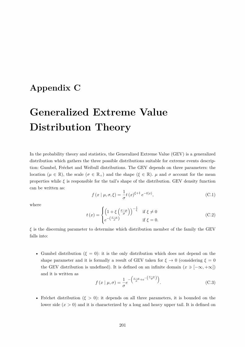
Appendix C
Generalized Extreme ValueDistribution Theory
In the probability theory and statistics, the Generalized Extreme Value (GEV) is a generalizeddistribution which gathers the three possible distributions suitable for extreme events descrip-tion: Gumbel, Fréchet and Weibull distributions. The GEV depends on three parameters: thelocation (µ ∈ R), the scale (σ ∈ R+) and the shape (ξ ∈ R). µ and σ account for the meanproperties while ξ is responsible for the tail’s shape of the distribution. GEV density functioncan be written as:
f (x | µ, σ, ξ) = 1σt (x)ξ+1 e−t(x), (C.1)
where
t (x) =
(1 + ξ
(x−µσ
))− 1ξ if ξ 6= 0
e−(x−µσ ) if ξ = 0.(C.2)
ξ is the discerning parameter to determine which distribution member of the family the GEVfalls into:
• Gumbel distribution (ξ = 0): it is the only distribution which does not depend on theshape parameter and it is formally a result of GEV taken for ξ → 0 (considering ξ = 0the GEV distribution is undefined). It is defined on an infinite domain (x 3 [−∞,+∞])and it is written as
f (x | µ, σ) = 1σe−(x−µσ
+e−(x−µσ )). (C.3)
• Fréchet distribution (ξ > 0): it depends on all three parameters, it is bounded on thelower side (x > 0) and it is characterized by a long and heavy upper tail. It is defined on
201
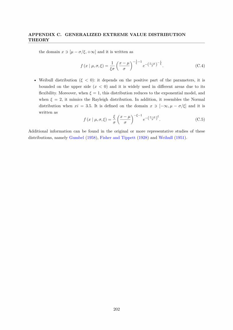
APPENDIX C. GENERALIZED EXTREME VALUE DISTRIBUTIONTHEORY
the domain x 3 [µ− σ/ξ,+∞] and it is written as
f (x | µ, σ, ξ) = 1ξσ
(x− µσ
)− 1ξ−1e−(x−µσ )−
1ξ. (C.4)
• Weibull distribution (ξ < 0): it depends on the positive part of the parameters, it isbounded on the upper side (x < 0) and it is widely used in different areas due to itsflexibility. Moreover, when ξ = 1, this distribution reduces to the exponential model, andwhen ξ = 2, it mimics the Rayleigh distribution. In addition, it resembles the Normaldistribution when xi = 3.5. It is defined on the domain x 3 [−∞, µ − σ/ξ] and it iswritten as
f (x | µ, σ, ξ) = ξ
σ
(x− µσ
)−ξ−1e−(x−µσ )ξ . (C.5)
Additional information can be found in the original or more representative studies of thesedistributions, namely Gumbel (1958), Fisher and Tippett (1928) and Weihull (1951).
202
Bibliography
Arnfield AJ (2003) Two decades of urban climate research: A review of turbulence, exchanges ofenergy and water, and the urban heat island. Intern J Clim 23(1):1–26, DOI 10.1002/joc.859
Bady M, Kato S, Huang H (2008) Towards the application of indoor ventilation efficiency indicesto evaluate the air quality of urban areas. Build Environ 43(12):1991–2004
Barlow JF (2014) Progress in observing and modelling the urban boundary layer. Urban Clim10(P2):216–240, DOI 10.1016/j.uclim.2014.03.011
Barlow JF, Belcher SE (2002) A wind tunnel model for quantifying fluxes in the urban boundarylayer. Boundary-Layer Meteorol 104:131–150
Barlow JF, Harman IN, Belcher SE (2004) Scalar fluxes from urban street canyons. Part I:laboratory simulation. Boundary-Layer Meteorol 113:369–385
Bentham T, Britter R (2003) Spatially averaged flow within obstacle arrays. Atmos Environ37(15):2037–2043
Britter RE, Hanna SR (2003) Flow and Dispersion in Urban Areas. Annual Review of FluidMechanics 35(1):469
Buccolieri R, Gromke C, Di Sabatino S, Ruck B (2009) Aerodynamic effects of trees onpollutant concentration in street canyons. Scien Tot Environ 407(19):5247–5256, DOI10.1016/j.scitotenv.2009.06.016
Buccolieri R, Sandberg M, Di Sabatino S (2010) City breathability and its link to pollutantconcentration distribution within urban-like geometries. Atmos Environ 44(15):1894–1903
Buccolieri R, Salim SM, Leo LS, Di Sabatino S, Chan A, Ielpo P, de Gennaro G, GromkeC (2011) Analysis of local scale tree-atmosphere interaction on pollutant concentration inidealized street canyons and application to a real urban junction. Atmos Environ 45(9):1702–1713, DOI 10.1016/j.atmosenv.2010.12.058
203
BIBLIOGRAPHY
Buccolieri R, Salizzoni P, Soulhac L, Garbero V, Di Sabatino S (2015) The breathability ofcompact cities. Urban Clim 13:73–93
Buccolieri R, Jeanjean AP, Gatto E, Leigh RJ (2018) The impact of trees on street ventila-tion, NOx and PM2.5 concentrations across heights in Marylebone Rd street canyon, centralLondon. Sust Cities Soc 41:227–241, DOI 10.1016/j.scs.2018.05.030
Buccolieri R, Santiago JL, Rivas E, Sáanchez B (2019) Reprint of: Review on urban tree mod-elling in CFD simulations: Aerodynamic, deposition and thermal effects. Urb Fore Urb Green37:56–64, DOI 10.1016/j.ufug.2018.07.004
Chan AT, Au WT, So ES (2003) Strategic guidelines for street canyon geometry to achievesustainable street air quality—part II: multiple canopies and canyons. Atmos Environ37(20):2761–2772, DOI 10.1016/S1352-2310(03)00252-8
Chen L, Hang J, Sandberg M, Claesson L, Di Sabatino S, Wigo H (2017) The impacts of buildingheight variations and building packing densities on flow adjustment and city breathability inidealized urban models. Build Environ 118:344–361, DOI 10.1016/j.buildenv.2017.03.042
Cheng H, Hayden P, Robins A, Castro I (2007) Flow over cube arrays of different packingdensities. J Wind Eng Ind Aerodyn 95(8):715–740, DOI 10.1016/j.jweia.2007.01.004
Cheng WC, Liu CH, Leung DYC (2009a) On the comparison of the ventilation performance ofstreet canyons of different aspect ratios and Richardson number. Build Simul 2(1):53–61
Cheng WC, Liu CH, Leung DYC (2009b) On the correlation of air and pollutant exchange forstreet canyons in combined wind-buoyancy-driven flow. Atmos Environ 43(24):3682–3690
Chester S, Meneveau C, Parlange MB (2007) Modeling turbulent flow over fractal trees withrenormalized numerical simulation. J Comput Phys 225(1):427–448, DOI 10.1016/j.jcp.2006.12.009
Cionco MR (1965) A mathematical model for air flow in vegetative canopy. J Appl Meteorol4:517–522
Dallman A, Di Sabatino S, Fernando HJ (2013) Flow and turbulence in an industrial/suburbanroughness canopy. Environ Fluid Mech 13(3):279–307
Dallman A, Magnusson S, Britter R, Norford L, Entekhabi D, Fernando HJS (2014) Conditionsfor thermal circulation in urban street canyons. Build Environ 80:184–191
Di Bernardino A, Monti P, Leuzzi G, Querzoli G (2018) Pollutant fluxes in two-dimensionalstreet canyons. Urban Clim 24:80–93
204
BIBLIOGRAPHY
Di Sabatino S, Buccolieri R, Pulvirenti B, Britter RE (2007) Simulations of pollutant disper-sion within idealised urban-type geometries with CFD and integral models. Atmos Environ41(37):8316–8329
Di Sabatino S, Leo LS, Cataldo R, Britter RE (2010) Construction of Digital Elevation Modelsfor a Southern European City and a Comparative Morphological Analysis with Respect toNorthern European and North American Cities. J Appl Meteorol Clim 49:1377–1396
Di Sabatino S, Buccolieri R, Pappaccogli G, Leo LS (2015) The effects of trees on microme-teorology in a real street canyon: consequences for local air quality. Intern J Environ Poll58(1/2):100, DOI 10.1504/ijep.2015.076587
Durst F (2008) Similarity Theory. In: Fluid Mechanics, Springer Berlin Heidelberg, chap 7, pp193–219
Eliasson I, Offerle B, Grimmond CSB, Lindqvist S (2006) Wind fields and turbulence statisticsin an urban street canyon. Atmos Environ 40:1–16
Fernando H, Zajic D, Di Sabatino S, Dimitrova R, Hedquist B, Dallman A (2010) Flow, turbu-lence, and pollutant dispersion in urban atmospheres. Phys Fluids 22:1–20
Finardi S, Silibello C, D Allura A, Radice P (2014) Analysis of pollutants exchange betweenthe Po Valley and the surrounding European region. Urb Clim 10:682–702, DOI 10.1016/j.uclim.2014.02.002
Fisher RA, Tippett LHC (1928) Limiting forms of the frequency distribution of the largest orsmallest member of a sample. Math Proc Cambridge Philosophical Society 24(2):180–190
Garratt JR (1980) Surface influence upon vertical profiles in the atmospheric near-surface layer.Quart J Royal Meteorol Soc 106(450):803–819, DOI 10.1002/qj.49710645011
Gowardhan AA, Brown MJ, Pardyjak ER (2010) Evaluation of a fast response pressuresolver for flow around an isolated cube. Environ Fluid Mech 10:311–328, DOI 10.1007/s10652-009-9152-5
Grimmond CS, Oke TR (2002) Turbulent heat fluxes in urban areas: Observations and a local-scale urban meteorological parameterization scheme (LUMPS). J Appl Meteorol 41(7):792–810, DOI 10.1175/1520-0450(2002)041<0792:THFIUA>2.0.CO;2
Grimmond CS, Salmond JA, Oke TR, Offerle B, Lemonsu A (2004) Flux and turbulence mea-surements at a densely built-up site in Marseille: Heat, mass (water and carbon dioxide), andmomentum. J Geophys Res 109(24):1–19, DOI 10.1029/2004JD004936
205
BIBLIOGRAPHY
Gromke C, Blocken B (2015) Influence of avenue-trees on air quality at the urban neighborhoodscale. Part I: Quality assurance studies and turbulent Schmidt number analysis for RANSCFD simulations. Environ Poll 196:214–223, DOI 10.1016/j.envpol.2014.10.016
Gromke C, Ruck B (2008) Aerodynamic modelling of trees for small-scale wind tunnel studies.Forestry 81(3):243–258, DOI 10.1093/forestry/cpn027
Gromke C, Ruck B (2009) On the impact of trees on dispersion processes of traffic emissions instreet canyons. Boundary-Layer Meteorol 131(1):19–34, DOI 10.1007/s10546-008-9301-2
Gromke C, Buccolieri R, Di Sabatino S, Ruck B (2008) Dispersion study in a street canyon withtree planting by means of wind tunnel and numerical investigations - Evaluation of CFD datawith experimental data. Atmos Environ 42(37):8640–8650, DOI 10.1016/j.atmosenv.2008.08.019
Gromke C, Blocken B, Janssen W, Merema B, van Hooff T, Timmermans H (2015) CFD analysisof transpirational cooling by vegetation: Case study for specific meteorological conditionsduring a heat wave in Arnhem, Netherlands. Build Environ 83:11–26, DOI 10.1016/j.buildenv.2014.04.022
Guan D, Zhang Y, Zhu T (2003) A wind-tunnel study of windbreak drag. Agric Fore Meteorol118(1-2):75–84, DOI 10.1016/S0168-1923(03)00069-8
Gumbel E (1958) Statistics of extremes. Columbia University press, New York, USA
Hang J, Sandberg M, Li Y (2009) Age of air and air exchange efficiency in idealized city models.Build Environ 44(8):1714–1723
Hang J, Li Y, Buccolieri R, Sandberg M, Di Sabatino S (2012) On the contribution of meanflow and turbulence to city breathability: The case of long streets with tall buildings. Sci TotEnviron 416:362–373
Hang J, Luo Z, Sandberg M, Gong J (2013) Natural ventilation assessment in typical open andsemi-open urban environments under various wind directions. Build Environ 70:318–333
Harman IN, Barlow JF, Belcher SE (2004) Scalar Fluxes from Urban Street Canyons Part II:Model. Boundary-Layer Meteorol 113(3):387–410
Hayati AN, Stoll R, Kim JJ, Harman T, Nelson MA, Brown MJ, Pardyjak ER, Brown MJ (2017)Comprehensive Evaluation of Fast-Response, Reynolds-Averaged Navier-Stokes, and Large-Eddy Simulation Methods Against High-Spatial-Resolution Wind-Tunnel Data in Step-DownStreet Canyons. Boundary-Layer Meteorol 164:217–247, DOI 10.1007/s10546-017-0245-2
206
BIBLIOGRAPHY
Hayati AN, Stoll R, Pardyjak ER, Harman T, Kim J (2019) Comparative metrics for com-putational approaches in non-uniform street-canyon flows. Build Environ 158:16–27, DOI10.1016/j.buildenv.2019.04.028
Højstrup J (1993) Statistical data screening procedure. Meas Sci Technol 4(2):153–157
Hong B, Qin H, Lin B (2018) Prediction of wind environment and indoor/outdoor rela-tionships for PM2.5 in different building-tree grouping patterns. Atmosphere 9(2), DOI10.3390/atmos9020039
Hosker R (1987) Effects of buildings on local dispersion. Modeling the urban boundary layer.Amer Meteorol Soc pp 95–159
Jeanjean A, Buccolieri R, Eddy J, Monks P, Leigh R (2017) Air quality affected by trees inreal street canyons: The case of Marylebone neighbourhood in central London. Urb Fore UrbGreen 22:41–53, DOI 10.1016/j.ufug.2017.01.009
Kaimal J, Finnigan J (1994) Atmospheric boundary layer flows, their structure and measure-ment, vol 41. Oxford University Press, DOI 10.1016/0169-8095(95)00045-3
Kanda M, Moriwaki R (2006) Spatial variability of both turbulent fluxes and temperatureprofiles in an urban roughness layer. Boundary-Layer Meteorol 121(2):339–350
Kaplan H, Dinar N (1996) A lagrangian dispersion model for calculating concentration distribu-tion within a built-up domain. Atmos Environ 30(24):4197–4207, DOI 10.1016/1352-2310(96)00144-6
Kastner-Klein P, Rotach MW (2004) Mean flow and turbulence characterisitcs in a urban rough-ness sublayer. Boundary-Layer Meteorol 111:55–84
Kastner-Klein P, Berkowicz R, Britter R (2004) The influence of street architecture on flow anddispersion in street canyons. Meteorol Atmos Phys 87:121–131
Kato S, Huang H (2009) Ventilation efficiency of void space surrounded by buildings with windblowing over built-up urban area. J Wind Eng Ind Aerodyn 97(7-8):358–367
Katul GG, Mahrt L, Poggi D, Sanz C (2004) One- and two-equation models for canopy turbu-lence. Boundary-Layer Meteorol 113:81–109
Kent WC, Grimmond S, Gatey D (2017) Aerodynamic roughness parameters in cities: inclusionof vegetation. J Wind Engin Ind Aerodyn 169:168–176
Kim J, Baik J (1999) A numerical study of thermal effects on flow and pollutant dispersion inurban street canyons. J Appl Meteorol 38:1249–1261
207
BIBLIOGRAPHY
Kim JJ, Baik JJ (2001) Urban street-canyon flows with bottom heating. Atmos Environ35(20):3395–3404, DOI 10.1016/S1352-2310(01)00135-2
Kim JJ, Baik JJ (2003) Effects of inflow turbulence intensity on flow and pollutant dispersionin an urban street canyon. J Wind Eng Ind Aerodyn 91(3):309–329
Klein PM, Galvez JM (2015) Flow and turbulence characteristics in a suburban street canyon.Environ Fluid Mech 15:419–438
Kotz S, Nadarajah S (2000) Extreme value distributions: theory and applications. World Sci-entific
Kubilay A, Neophytou MK, Matsentides S, Loizou M, Carmeliet J (2017) The Pollutant RemovalCapacity of an Urban Street Canyon and its Link to the Breathability and Exchange Velocity.Proc Eng 180:443–451
Li Q, Wang ZH (2018) Large-eddy simulation of the impact of urban trees on momentum andheat fluxes. Agricult Forest Meteorol 255:44–56, DOI 10.1016/j.agrformet.2017.07.011
Li XX, Britter RE, Norford LK, Koh TY, Entekhabi D (2012) Flow and Pollutant Transportin Urban Street Canyons of Different Aspect Ratios with Ground Heating: Large-Eddy Sim-ulation. Boundary-Layer Meteorol 142(2):289–304
Li XX, Britter RE, Norford LK (2015) Transport processes in and above two-dimensional urbanstreet canyons under different stratification conditions: results from numerical simulation.Environ Fluid Mech 15(2):399–417
Li XX, Britter R, Norford LK (2016) Effect of stable stratification on dispersion within urbanstreet canyons: A large-eddy simulation. Atmos Environ 144:47–59
Li Y, Zhang J, Sailor DJ, Ban-Weiss GA (2019) Effects of urbanization on regional meteorologyand air quality in Southern California. Atmos Chem Phys 19(7):4439–4457, DOI 10.5194/acp-19-4439-2019
Liu CH, Wong CC (2014) On the pollutant removal, dispersion, and entrainment over two-dimensional idealized street canyons. Atmos Res 135:128–142
Liu CH, Leung DYC, Barth MC (2005) On the prediction of air and pollutant exchangerates in street canyons of different aspect ratios using large-eddy simulation. Atmos Envi-ron 39(9):1567–1574
Lo KW, Ngan K (2017) Characterizing ventilation and exposure in street canyons using La-grangian particles. J Appl Meteorol Clim 56(5):1177–1194
208
BIBLIOGRAPHY
Louka P, Belcher S, Harrison R (1998) Modified street canyon flow. J Wind Eng Ind Aerodyn74:485–493
Louka P, Belcher SE, Harrison RG (2000) Coupling between air flow in streets and the well-developed boundary layer aloft. Atmos Environ 34(16):2613–2621
Macdonald RW, Griffiths RF, Hall DJ (1998) An improved method for the estimation of surfaceroughness of obstacle arrays. Atmos Environ 32(11):1857–1864
Mazzola M, Lanconelli C, Lupi A, Busetto M, Vitale V, Tomasi C (2010) Columnar aerosoloptical properties in the Po Valley, Italy, from MFRSR data. J of Geophys Res Atmos DOI10.1029/2009JD013310
McMillen R (1988) An eddy correlation technique with extended applicability to non-simpleterrain. Boundary-Layer Meteorol 43(3):231–245
Moradpour M, Afshin H, Farhanieh B (2017) A numerical investigation of reactive air pollutantdispersion in urban street canyons with tree planting. Atmos Poll Res 8:253–266
Nazarian N, Martilli A, Kleissl J (2017) Impacts of Realistic Urban Heating, Part I: SpatialVariability of Mean Flow, Turbulent Exchange and Pollutant Dispersion. Boundary-LayerMeteorol 166:367–393
Nazarian N, Martilli A, Norford L, Kleissl J (2018) Impacts of Realistic Urban Heating. PartII: Air Quality and City Breathability. Boundary-Layer Meteorol 168:321–341
Nelson MA, Pardyjak ER, Klein P (2011) Momentum and Turbulent Kinetic Energy Bud-gets Within the Park Avenue Street Canyon During the Joint Urban 2003 Field Campaign.Boundary-Layer Meteorol 140:143–162
Nowak DJ, Hirabayashi S, Bodine A, Hoehn R (2013) Modeled PM2.5 removal by trees in tenU.S. cities and associated health effects. Environ Poll 178:395–402
Ntziachristos, Leonidas, Boulter P (2009) EMEP/EEA air pollutant emissions inventory guide-book 2009: road vehicle tyre and brake wear; road surface wear
Oke T (1987) Boundary-layer climates, 2nd edn. Routledge, London
Oke TR (1976) The distinction between canopy and boundary-layer urban heat Islands. Atmo-sphere 14(4):268–277, DOI 10.1080/00046973.1976.9648422
Oke TR (1988) Street Design and Urban Canopy Layer Climate. Energy Build 11(1-3):103–113
Oke TR, Mills G, Christen A, Voogt JA (2017) Urban Climates. Cambridge University Press,Cambridge, DOI 10.1017/9781139016476
209
BIBLIOGRAPHY
Panagiotou I, Neophytou MKA, Hamlyn D, Britter RE (2013) City breathability as quantifiedby the exchange velocity and its spatial variation in real inhomogeneous urban geometries:An example from central London urban area. Sci Tot Environ 442:466–477
Piringer M, Grimmond CSB, Joffre SM, Mestayer P, Middleton DR, Rotach MW, BaklanovA, De Ridder K, Ferreira J, Guilloteau E, Karppinen A, Martilli A, Masson V, Tombrou M(2002) Investigating the Surface Energy Budget in Urban Areas-Recent Advances and FutureNeeds. Water, Air Soil Poll (2):1–16, DOI 10.1023/A:1021302824331
Pope S (2000) Turbulent flows. Cambridge University Press, Cambridge
Rafael S, Vicente B, Rodrigues V, Miranda AI, Borrego C, Lopes M (2018) Impacts of greeninfrastructures on aerodynamic flow and air quality in Porto’s urban area. Atmos Environ190:317–330, DOI 10.1016/j.atmosenv.2018.07.044
Ratti C, Di Sabatino S, Britter R, Brown M, Caton F, Burian S (2002) Analysis of 3-D urbandatabases with respect to pollutant dispersion for a number of European and American cities.Water Air Soil Pollut 2:459–469
Raupach M, Antonia R, Rajagopalan S (1991a) Rough-wall turbulent boundary layer. ApplMech Rev 44(1):1–25
Raupach MR, Antonia RA, Rajagopalan S (1991b) Rough-Wall Turbulent Boundary Layers.Appl Mech Rev 44(1):1–25, DOI 10.1115/1.3119492
Rockle R (1990) Bestimmung der Stromungsverhaltnisse im Bereich komplexer Bebauungsstruk-turen. PhD thesis, der Technischen Hochschule Darmstadt, Germany
Rotach M (1995) Profiles of turbulence statistics in and above an urban street canyon. AtmosEnviron 29(13):1473–1486, DOI 10.1016/1352-2310(95)00084-C
Rotach MW (1999) On the influence of the urban roughness sublayer on turbulence and disper-sion. Atmos Environ 33(24-25):4001–4008, DOI 10.1016/S1352-2310(99)00141-7
Rotach MW, Vogt R, Bernhofer C, Batchvarova E, Christen A, Clappier A, Feddersen B, Gryn-ing SE, Martucci G, Mayer H, Mitev V, Oke TR, Parlow E, Richner H, Roth M, Roulet YA,Ruffieux D, Salmond JA, Schatzmann M, Voogt JA (2005) BUBBLE-an Urban BoundaryLayer Meteorology Project. Theor Appl Climatol 81:231–261
Roth M (2000) Review of atmospheric turbulence over cities. Q J R Meteorol Soc 126:941–990
Roth M, Oke T (1995) Relative efficiencies of turbulent transfer of heat, massm and momentumover a patchy urban surface. American Meteorol Soc 52(11):1863–1874
210
BIBLIOGRAPHY
Salizzoni P, Soulhac L, Mejean P (2009) Street canyon ventilation and atmospheric turbulence.Atmos Environ 43(32):5056–5067
Salizzoni P, Marro M, Soulhac L, Grosjean N, Perkins RJ (2011) Turbulent Transfer BetweenStreet Canyons and the Overlying Atmospheric Boundary Layer. Boundary-Layer Meteorol141(3):393–414
Sasaki Y (1958) An ObJective Analysis Based on the Variational Method. J Meteorol Soc Japan36(3):77–88
Sasaki Y (1970) Numerical variational analysis formulated under the constraints as determinedby longwave equations and a low-pass filter. Monthly Weather Rev 98(12):884–898
Schmid H, Cleugh H, Grimmond C, Oke T (1991) Spatial variability of energy fluxes in suburbanterrain. Boundary-Layer Meteorol 54:249–276
Schmid HP, Grimmond CB, Cropley F, Offerle B, Su HB (2000) Measurements of CO2 andenergy fluxes over a mixed hardwood forest in the mid-western United States. Agric ForMeteorol 103(4):357–374
Sherman CA (1978) A mass-consistent model for wind fields over complex terrain. J ApplMeteorol 17:312–319
Singh B, Hansen BS, Brown MJ, Pardyjak ER (2008) Evaluation of the QUIC-URB fast responseurban wind model for a cubical building array and wide building street canyon. Environ FluidMech 8:281–312, DOI 10.1007/s10652-008-9084-5
Solazzo E, Britter RE (2007) Transfer processes in a simulated urban street canyon. Boundary-Layer Meteorol 124:43–60, DOI 10.1007/s10546-007-9176-7
Soulhac L, Salizzoni P (2010) Dispersion in a street canyon for a wind direction parallel to thestreet axis. J Wind Eng Ind Aerodyn 98(12):903–910
Soulhac L, Perkins RJ, Salizzoni P (2008) Flow in a Street Canyon for any External WindDirection. Boundary-Layer Meteorol 126:365–388
UN DESA (2018) Revision of the World Urbanization Prospects
Van Renterghem T, Botteldooren D (2008) Numerical evaluation of tree canopy shape nearnoise barriers to improve downwind shielding. J Acoust Soc Amer 123(2):648–657, DOI10.1121/1.2828052
Vickers D, Mahrt L (1997) Quality Control and Flux Sampling Problems for Tower and AircraftData. J Atmos Ocean Technol 14(3):512–526
211
BIBLIOGRAPHY
Vos PE, Maiheu B, Vankerkom J, Janssen S (2013) Improving local air quality in cities: To treeor not to tree? Environ Poll 183:113–122, DOI 10.1016/j.envpol.2012.10.021
Weihull W (1951) A statistical distribution function of wide applicability. J Appl Mech 18:290–293
Williams MD, Brown MJ, Boswell D, Singh B, Pardyjak ER (2004) Testing of the QUIC-PLUME model with wind-tunnel measurements for a high-rise building. In: Ame MeteorSoc (ed) Testing of the QUIC-PLUME model with wind-tunnel measurements for a high-risebuilding, Vancouver, BC, Canada, p 10
Wilson JD (1985) Numerical studies of flow through a windbreak. J Wind Eng Ind Aerodyn21(2):119–154, DOI 10.1016/0167-6105(85)90001-7
Winkler SL, Anderson JE, Garza L, Ruona WC, Vogt R, Wallington TJ (2018) Vehicle criteriapollutant (PM, NOx, CO, HCs) emissions: how low should we go? Clim Atmos Science 1:26,DOI 10.1038/s41612-018-0037-5
Xiaomin X, Zhen H, Jiasong W (2006) The impact of urban street layout on local atmosphericenvironment. Build Environ 41(10):1352–1363, DOI 10.1016/j.buildenv.2005.05.028
Zajic D, Fernando HJ, Calhoun R, Princevac M, Brown MJ, Pardyjak ER (2011) Flow andturbulence in an urban canyon. J Appl Meteorol Clim 50(1):203–223
212

Acknowledgements
I wish to acknowledge everyone who helped me, contributed to my growth through this ad-venture, supported me and sustained me all the time.
I wish to acknowledge my supervisor, Professor Silvana Di Sabatino, for the trust she gaveme (together with some very good help) since the beginning of this PhD. The role of a super-visor is to guide the a student through is growth as a researcher and she embraces this role asalways in her own personal way. She has been fleeing more than ones, but I could always counton her when I needed most. No matter how difficult was the task, she was always able to offerme all the tools I needed to find the best solution but following my own thoughts and knowledge.
I wish also to acknowledge Professor Eric Pardyjak who hosted me for few months in hisresearch group, giving me the opportunity to enjoy a similar but totally different research expe-rience in the US. To him goes all my gratitude as it goes to the people (professors and researchers)who helped me embracing the atmospheric modeling world.
I acknowledge the iSCAPE project for having granted me the economical support for thePhD and all the participant I was given the pleasure to work and interact with.
I acknowledge all the people who have somehow contributed to the experimental campaigns.Carla Barbieri and Luca Torreggiani from ARPAE for the deployment and maintenance of the in-strumentation for air quality measurements and their constant support to the best developmentof the research. Marianna Nardino from CNR for the deployment and installation of part of theinstrumentation for the measurement of turbulence. Beatrice Pulvirenti from the Departmentof Industrial Engineering of the University of Bologna and Enrico Minguzzi from ARPAE for allthe support given during the realization of the campaign and the fruitful discussions to finalizethe research. The CGIL (Confederazione Generale Italiana del Lavoro) and private citizens forhaving host part of the instrumentation on private balcony or rooftop.
I want to thanks the guys of the laboratory (Francesca, Erika, Laura, Leonardo, Marco,Carlo, Davide and William), and the students who have passed by having the bad idea to askany help from us. Thanks for your help, for the good moments, for the lunches, but also theyelling and outbursts. I know most of the time I’m stubborn and tricky but i really like all of

you and I’m proud to be part of the group.
I really want to thanks Massimo, he allows me to survive in the field and taught me there isalways a solution for everything. My PhD would have been much different without you.
I want also to thanks Thomas, James, Andrea and Federico because I could have and stillcan always count on them. More than once they have saved my day, adding colors when myeyes had only see shades of black.
I want to thanks my families, my kinsman for the support and the faith in me and my choi-ces. Thanks to my adoptive family, my roommates, for everything. I will miss you.
Last but not least I want to thanks Silvia for convincing me that giving a possibility to whodeserves it is the best you can do.


