Gaussian Processes for Object Categorization

Noname manuscript No.(will be inserted by the editor)

Gaussian Processes for Object Categorization

Ashish Kapoor · Kristen Grauman · Raquel Urtasun · Trevor Darrell

Received: date / Accepted: date

Abstract Discriminative methods for visual object categoryrecognition are typically non-probabilistic, predicting classlabels but not directly providing an estimate of uncertainty.Gaussian Processes (GPs) provide a framework for derivingregression techniques with explicit uncertainty models; weshow here how Gaussian Processes with covariance func-tions defined based on a Pyramid Match Kernel (PMK) canbe used for probabilistic object category recognition. Ourprobabilistic formulation provides a principled way to learnhyperparameters, which we utilize to learn an optimal com-bination of multiple covariance functions. It also offers con-fidence estimates at test points, and naturally allows for anactive learning paradigm in which points are optimally se-lected for interactive labeling. We show that with an appro-priate combination of kernels a significant boost in classi-fication performance is possible. Further, our experimentsindicate the utility of active learning with probabilistic pre-dictive models, especially when the amount of training datalabels that may be sought for a category is ultimately verysmall.

Keywords Object Recognition · Gaussian Process · KernelCombination · Active Learning

Ashish KapoorMicrosoft Research, Redmond WA 98052, USAE-mail: [email protected]

Kristen GraumanUniversity of Texas at Austin, TX 78712, USAE-mail: [email protected]

Raquel UrtasunUC Berkeley EECS & ICSI, Berkeley, CA 94720, USAE-mail: [email protected]

Trevor DarrellUC Berkeley EECS & ICSI, Berkeley, CA 94720, USAE-mail: [email protected]

1 Introduction

Object categorization is a fundamental problem in imageunderstanding. It remains a challenging learning task givenboth the variability of images that objects from the sameclass can produce, as well as the substantial expense of pro-viding high quality image annotations needed to train ac-curate models. Discriminative methods for visual categorylearning have yielded promising results in recent years, in-cluding various approaches based on support vector machinesor nearest neighbor classification [14,49,46,30,21,43,5,13,19]. However, such methods typically are not explicitly prob-abilistic, which makes them inadequate when estimates ofuncertainty are required. At the same time, probabilistic gen-erative methods that attempt to directly model the joint dis-tribution of object classes and their features—though ap-pealing for their ability to estimate uncertainty during infere-nce—can be impractical for image recognition applicationsdue to the complexity of representing the data’s underlyingdensity.

In this work we provide a probabilistic discriminativeapproach to object categorization, with the goal of exercis-ing the advantages of both types of methods. We introducea new Gaussian Process (GP) regression method for objectcategory recognition using a local feature correspondencekernel. Local feature-based object recognition has severalimportant advantages, including invariance to various trans-lational, rotational, affine and photometric transformationsand robustness to partial occlusions. Our method is basedon a GP with a covariance function derived from a PyramidMatch Kernel [14], which offers an efficient approximationto a partial-match distance function and can therefore han-dle outliers and occlusions. Our model offers some of theknown benefits of probabilistic techniques, while still main-taining the power of a discriminative learner. In particular,we show how it enables both active visual category learn-

2

ing, as well as learning from multiple image feature sourceswith an optimal combination of covariance functions.

Collecting training data for large-scale image categorymodels is a potentially expensive process. While certain cat-egories may have a large number of training images avail-able, many more will have relatively few. A number of inge-nious schemes have been developed to obtain labeled datafrom people performing other tasks (e.g., [45,44]), or di-rectly labeling objects in images [1]. To make the most ofscarce human labeling resources it is imperative to carefullyselect points for user labeling. The paradigm of active learn-ing has been introduced in the machine learning communityto address this issue [12,39,25,29,50]; with an active learn-ing method, generally new test points are selected so as tominimize the model entropy.

GPs have received limited attention in the computer vi-sion literature to date perhaps due to the fact that they areconventionally limited to modest amounts of training data:the learning complexity is O(n3), cubic in the number oftraining examples. While recent advances in sparse GPs arepromising (e.g., [20,34,37,40]), we focus here on the caseof active learning with relatively small numbers of labeledexamples (10-100), which is feasible with existing imple-mentations. In this realm, we show that active learning pro-vides significantly more accurate estimates per labeled pointthan does a conventional random selection of training points.

Specific choices made regarding image representationsand kernel parameters can greatly influence a classifier’s po-tential. Even within the domain of local image features andmatching kernels, a variety of alternative interest point de-tectors, descriptors, match criteria, and feature space quanti-zation strategies are available. Rather than require a user todecide a priori which particular items will define the GP’scovariance function, we show how to automatically optimizethe combination of kernels for the recognition task using theGP marginal likelihood function. As a result, one can com-pute a set of potential kernels using a variety of local fea-ture types, and then directly learn a weight for each suchthat the final combination is highly discriminative. Whilerecent work has considered multiple kernel learning [43,19]and cross-validation approaches [5] to combine image fea-ture types within SVM classifiers, to our knowledge our ap-proach is the first to consider kernel combinations in a prob-abilistic setting.

The three main contributions of this paper are (1) a prob-abilistic discriminative category recognition scheme basedon a Gaussian Process prior with a covariance function de-fined using the Pyramid Match Kernel, (2) the introductionof an active learning paradigm for object category learningwhich optimally selects unlabeled test points for interactivelabeling, and (3) a probabilistic approach to learn discrim-inative kernel combinations for multiple local feature typeswithin a GP framework. We show that with active learning

small amounts of interactively labeled data can provide veryaccurate category recognition performance, while with co-variance functions that optimally combine multiple match-ing kernels our method obtains state-of-the-art results withbenchmark datasets.

2 Previous Work

Object category recognition has been a topic of active inter-est in the computer vision literature. Methods based on localfeature descriptors (c.f. [23,26]) have been shown to offerinvariance across a range of geometric and photometric con-ditions. Early models captured appearance and shape varia-tion in a generative probabilistic framework [11], but morerecent techniques have typically exploited methods based onSVMs or Nearest Neighbors in a bag-of-visual-words fea-ture space [36,30,49,9].

Several authors have explored correspondence-based ker-nels [49,46], where the distance between a set of local fea-ture descriptors—potentially including appearance and shape/ position—is computed based on associating pairs of de-scriptors. However, the polynomial-time computational costof correspondence-based distance measures makes them un-suitable for domains where there are large databases or largenumbers of features per image. In [14] the authors intro-duced the Pyramid Match Kernel (PMK), an efficient linear-time approximation to a partial match correspondence, andin [21] it was demonstrated that a spatial variant—which ef-ficiently represents the distinction between appearance andimage location features—outperformed many competing m-ethods.

Semi-supervised or unsupervised visual category learn-ing methods are related to active learning, in that they alsoleverage unlabeled examples to learn more accurately whenlimited labeled examples are available. Generative modelswhich model visual words as arising from a set of underlyingobjects or “topics” based on recently introduced methods forLatent Dirichlet Allocation have been developed [35,38] butas yet have not been applied to active learning nor evaluatedon purely supervised tasks. A semi-supervised method us-ing normalized cuts to cluster a graph defined by PyramidMatch distances between examples was presented in [16],but this method is not probabilistic nor does it provide foran active learning formalism.

In the machine learning literature active learning has beena topic of recent interest, and numerous schemes have beenproposed for choosing unlabeled points for tagging. For ex-ample, in [12] the authors propose using the disagreementamong the committee of classifiers as a criterion for activelearning, and show an application to image classification [2].In [39], unlabeled examples to query are selected based onminimizing the version space within the SVM formulation,

3

while in [7] an SVM-based active learner is applied for im-age retrieval using color and texture features.

Within the Gaussian Process framework, the method ofchoice has been to look at the expected informativeness ofan unlabeled data point [20,24]. Specifically, the idea is tochoose to query cases that are expected to maximally in-fluence the posterior distribution over the set of possibleclassifiers. Additional studies have sought to combine ac-tive learning with semi-supervised learning [25,29,50]. Ourwork is significantly different as we focus on local featureapproaches for the task of object categorization. We explorethe GP models, which provide estimates for uncertainty inprediction and can be easily extended to active learning.

Recent work has shown the value of combining multiplelocal image feature types into a single kernel matrix, eitherby using cross-validation with a held-out set of labeled im-ages to adjust the weight attached to each [5], or by optimiz-ing the weights to align the combined kernel with the idealkernel matrix reflecting the labels on the training data [43,19]. Both tactics have yielded impressive results in prac-tice. Our proposed method to optimize kernel weights fitsdirectly within our GP learning framework, and is distinctin that rather than target the labels of training examples, itmaximizes the evidence of the probabilistic model.

Gaussian Processes have been recently introduced to thecomputer vision literature. While they have been used in [41,42] for human motion modeling and in [48] for stereo seg-mentation, we are unaware of any prior work on visual ob-ject recognition in a Gaussian Process framework.1

3 Approach Overview

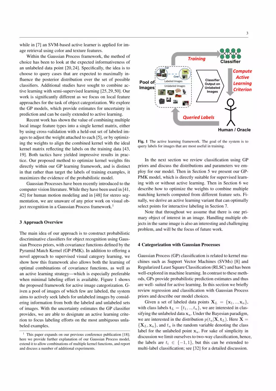
The main idea of our approach is to construct probabilisticdiscriminative classifiers for object recognition using Gaus-sian Process priors, with covariance functions defined by thePyramid Match Kernel (GP-PMK). In addition to offering anovel approach to supervised visual category learning, weshow how this framework also allows both the learning ofoptimal combinations of covariance functions, as well asan active learning strategy—which is especially preferablewhen minimal labeling effort is available. Figure 1 showsthe proposed framework for active image categorization. G-iven a pool of images of which few are labeled, the systemaims to actively seek labels for unlabeled images by consid-ering information from both the labeled and unlabeled setsof images. With the uncertainty estimates the GP classifierprovides, we are able to designate an active learning crite-rion to focus labeling efforts on the most ambiguous unla-beled examples.

1 This paper expands on our previous conference publication [18];here we provide further explanation of our Gaussian Process model,extend it to allow combinations of multiple kernel functions, and reportand discuss a number of additional experiments.

Fig. 1 The active learning framework. The goal of the system is toquery labels for images that are most useful in training.

In the next section we review classification using GPpriors and discuss the distributions and parameters we em-ploy for our model. Then in Section 5 we present our GP-PMK model, which is directly suitable for supervised learn-ing with or without active learning. Then in Section 6 wedescribe how to optimize the weights to combine multiplematching kernels computed from different feature sets. Fi-nally, we derive an active learning variant that can optimallyselect points for interactive labeling in Section 7.

Note that throughout we assume that there is one pri-mary object of interest in an image. Handling multiple ob-jects in the same image is also an interesting and challengingproblem, and will be the focus of future work.

4 Categorization with Gaussian Processes

Gaussian Process (GP) classification is related to kernel ma-chines such as Support Vector Machines (SVMs) [8] andRegularized Least Square Classification (RLSC) and has beenwell-explored in machine learning. In contrast to these meth-ods, GPs provide probabilistic prediction estimates and thusare well- suited for active learning. In this section we brieflyreview regression and classification with Gaussian Processpriors and describe our model choices.

Given a set of labeled data points XL = {x1, ..,xn},with class labels tL = {t1, .., tn}, we are interested in clas-sifying the unlabeled data xu. Under the Bayesian paradigm,we are interested in the distribution p(tu|X, tL). Here X ={XL,xu}, and tu is the random variable denoting the classlabel for the unlabeled point xu. For sake of simplicity indiscussion we limit ourselves to two-way classification, hence,the labels are ti ∈ {−1, 1}, but this can be extended tomulti-label classification; see [32] for a detailed discussion.

4

(a) (b)

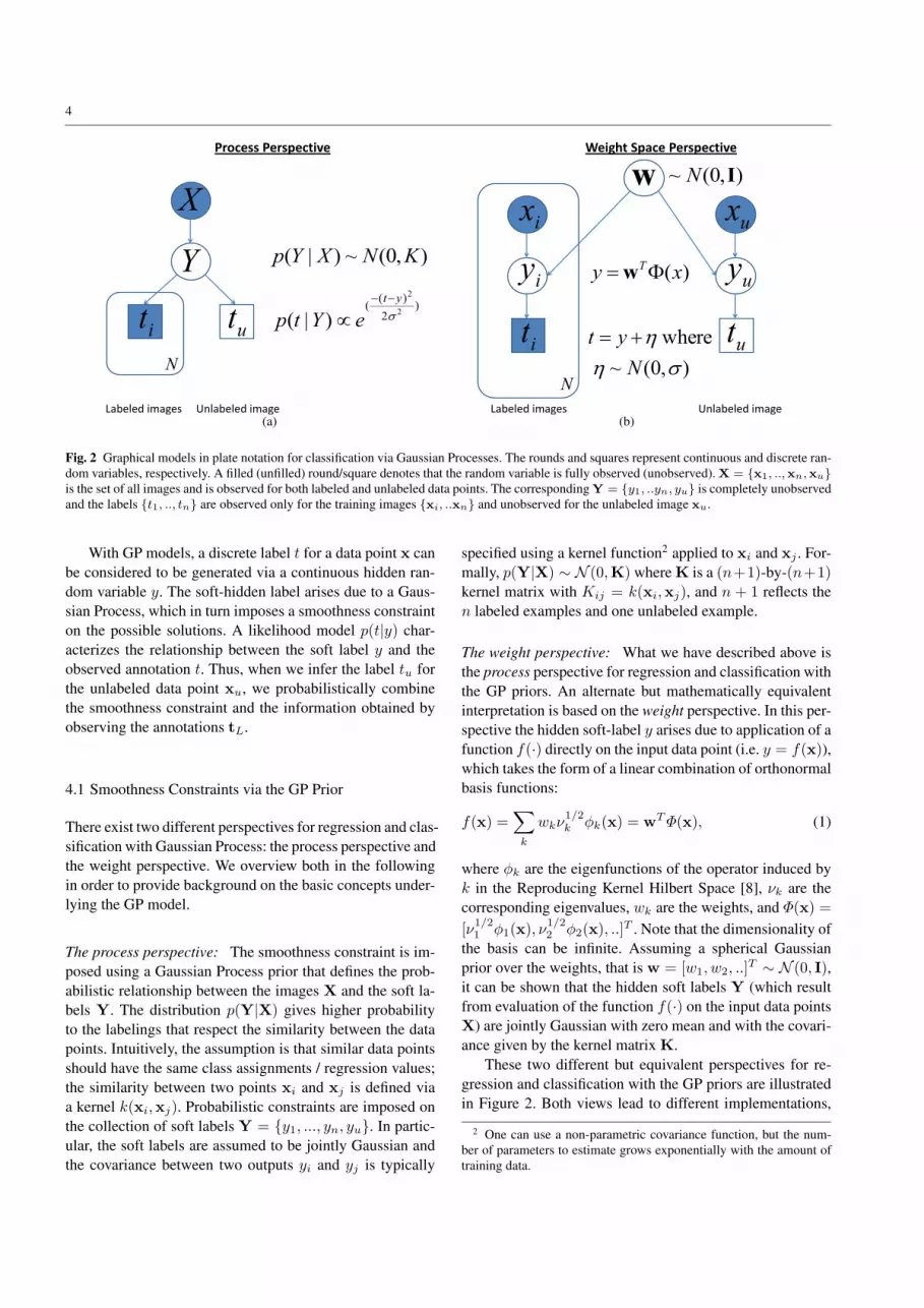
Fig. 2 Graphical models in plate notation for classification via Gaussian Processes. The rounds and squares represent continuous and discrete ran-dom variables, respectively. A filled (unfilled) round/square denotes that the random variable is fully observed (unobserved). X = {x1, ..,xn,xu}is the set of all images and is observed for both labeled and unlabeled data points. The corresponding Y = {y1, ..yn, yu} is completely unobservedand the labels {t1, .., tn} are observed only for the training images {xi, ..xn} and unobserved for the unlabeled image xu.

With GP models, a discrete label t for a data point x canbe considered to be generated via a continuous hidden ran-dom variable y. The soft-hidden label arises due to a Gaus-sian Process, which in turn imposes a smoothness constrainton the possible solutions. A likelihood model p(t|y) char-acterizes the relationship between the soft label y and theobserved annotation t. Thus, when we infer the label tu forthe unlabeled data point xu, we probabilistically combinethe smoothness constraint and the information obtained byobserving the annotations tL.

4.1 Smoothness Constraints via the GP Prior

There exist two different perspectives for regression and clas-sification with Gaussian Process: the process perspective andthe weight perspective. We overview both in the followingin order to provide background on the basic concepts under-lying the GP model.

The process perspective: The smoothness constraint is im-posed using a Gaussian Process prior that defines the prob-abilistic relationship between the images X and the soft la-bels Y. The distribution p(Y|X) gives higher probabilityto the labelings that respect the similarity between the datapoints. Intuitively, the assumption is that similar data pointsshould have the same class assignments / regression values;the similarity between two points xi and xj is defined viaa kernel k(xi,xj). Probabilistic constraints are imposed onthe collection of soft labels Y = {y1, ..., yn, yu}. In partic-ular, the soft labels are assumed to be jointly Gaussian andthe covariance between two outputs yi and yj is typically

specified using a kernel function2 applied to xi and xj . For-mally, p(Y|X) ∼ N (0,K) where K is a (n+1)-by-(n+1)kernel matrix with Kij = k(xi,xj), and n + 1 reflects then labeled examples and one unlabeled example.

The weight perspective: What we have described above isthe process perspective for regression and classification withthe GP priors. An alternate but mathematically equivalentinterpretation is based on the weight perspective. In this per-spective the hidden soft-label y arises due to application of afunction f(·) directly on the input data point (i.e. y = f(x)),which takes the form of a linear combination of orthonormalbasis functions:

f(x) =∑

k

wkν1/2k φk(x) = wT Φ(x), (1)

where φk are the eigenfunctions of the operator induced byk in the Reproducing Kernel Hilbert Space [8], νk are thecorresponding eigenvalues, wk are the weights, and Φ(x) =[ν1/2

1 φ1(x), ν1/22 φ2(x), ..]T . Note that the dimensionality of

the basis can be infinite. Assuming a spherical Gaussianprior over the weights, that is w = [w1, w2, ..]T ∼ N (0, I),it can be shown that the hidden soft labels Y (which resultfrom evaluation of the function f(·) on the input data pointsX) are jointly Gaussian with zero mean and with the covari-ance given by the kernel matrix K.

These two different but equivalent perspectives for re-gression and classification with the GP priors are illustratedin Figure 2. Both views lead to different implementations,

2 One can use a non-parametric covariance function, but the num-ber of parameters to estimate grows exponentially with the amount oftraining data.

5

but are conceptually equivalent. In this work, we follow theprocess perspective. For details, please see [33].

4.2 The Likelihood Model

The likelihood models the probabilistic relationship betweenthe observed label t and the hidden label y. The majorityof the likelihood models proposed for GP classification useadditional latent “squashing” variables that transform un-constrained variables into labels. A wide range of squash-ing functions have been developed in the literature [32] andexamples include the logisitic and the probit functions. Tomake predictions based on the training set for a test set inthese models (i.e., probit and logit) one has to integrate outthe prediction over the posterior. Since the likelihood is notGaussian, neither the posterior, the marginal likelihood, northe predictions can be computed analytically. Instead, onehas to rely on numerical methods, such as MCMC [47], orapproximations of the posterior, e.g. Laplace and Expecta-tion Propagation [28].

In contrast to GP classification, GP regression leads toefficient analytic solutions for prediction. For Gaussian Pro-cess regression using a Gaussian noise model, the relationbetween t and y is given by

p(t|y) =1√

2πσ2e−

(t−y)2

2σ2 , (2)

where σ is the noise model variance. Since this likelihoodmodel is Gaussian, it leads to a closed form solution for in-ference. Although originally developed for regression, theGaussian noise model has also proven effective for classi-fication,3 and its performance typically matches the morecomplex probit and logit likelihood models noted above.Due to its simplicity and good performance, in our exper-iments we use regression (i.e., the Gaussian noise model) tolabel variables. Non-Gaussian noise models could also beapplied within the proposed framework, and exploring themis a topic of interest for future work.

4.3 Inference

Given the labeled and unlabeled data points, our goal is thento infer p(tu|X, tL). Specifically:

p(tu|X, tL) ∝∫

Y

p(tu|Y)p(Y|X, tL). (3)

For a Gaussian noise model we can compute this integralusing closed form expressions. Note that the key quantity to

3 This method is referred to as least-squares classification in the lit-erature (see Section 6.5 of [32]) and often demonstrates performancecompetitive with more expensive Gaussian Process classification meth-ods that require approximate inference.

compute is the posterior p(Y|X, tL), which can be writtenas:

p(Y|X, tL) ∝ p(Y|X)p(tL|Y) = p(Y|X)n∏

i=1

p(ti|yi). (4)

This equation probabilistically combines the smoothnessconstraints p(Y|X) imposed via the GP prior and the infor-mation provided in the labels (p(tL|Y)). The posterior asshown in Equation 4 is simply a product of Gaussians, andthe posterior over the soft label yu has a particularly simpleform. Specifically, p(yu|X, tL) ∼ N (yu, σ2

u), where:

yu = k(xu)T (σ2I + KLL)−1tL (5)

Σu = k(xu,xu)− k(xu)T (σ2I + KLL)−1k(xu). (6)

Here, k(xu) is the vector of kernel function evaluations withn training points, and KLL = {k(xi,xj)}, is the trainingcovariance, with xi,xj ∈ Xu. Further, due to the Gaussiannoise model that links tu to yu, the predictive distributionover the unknown label tu is also a Gaussian: p(tu|X, tL) ∼N (yu, Σu + σ2).

Note that the posterior mean for both tu and yu is thesame; thus, the unlabeled point xu can be classified accord-ing to the sign of yu. Unlike the Regularized Least SquareClassification (RLSC) methods, we also get the variance inprediction. As we will show in Section 7, we can exploitthese measures of uncertainty to guide an active learningprocedure. The computationally costly operation in GP in-ference is the inversion of (σ2I + KLL) which has a timecomplexity of O(n3) for n training examples. In additionto reducing manual labeling effort, an active learning for-mulation can help us reduce the computational overhead ininference by reducing the number of needed training points.

4.4 Training with the Gaussian Process Models

The performance of Gaussian Process-based classificationdepends upon the chosen kernel used to capture the similar-ity between examples, as well as the kernel’s hyperparame-ters, such as the length-scale, the noise variance, and otherparameters determining local feature-based image similar-ity. Finding the right set of all these parameters can be achallenge. Many discriminative models (including SVMs)often use cross-validation, which is a robust measure butcan be prohibitively expensive and problematic when wehave few labeled data points. Learning in a Gaussian Processframework is equivalent to choosing the kernel hyperparam-eters of the covariance function. Ideally we would like tomarginalize over these hyperparameters. While approachesbased on Hybrid Monte Carlo have been explored to performthis marginalization [47], such techniques are relatively ex-pensive.

6

Empirical Bayes is a more computationally efficient al-ternative where the idea is to maximize the marginal like-lihood or the evidence, which is nothing but the constantp(tL|X) that normalizes the posterior. This methodologyof tuning the hyperparameter is often called evidence maxi-mization, and has been one of the favorite tools for perform-ing model selection. Evidence is a numerical quantity andsignifies how well a model fits the given data. By comparingthe evidence corresponding to the different models (or hy-perparameters that determine the model), we can choose themodel and the hyperparameters suitable for the task.

The idea is to choose a set of hyperparameters Θ thatmaximize the evidence: Θ = arg maxΘ log[p(tL|X, Θ)].Note that the log evidence log(p(tL|X, Θ)) can be writtenas a closed form equation for the Gaussian noise model (GPregression):

log p(tL|X, Θ) =− 12tTL(σ2I + KLL)−1tL−

12

log |σ2I + KLL| − Const.

This objective can be maximized using non-linear optimiza-tion techniques, such as gradient descent. In this work, weuse gradient-descent to maximize evidence. The optimiza-tion procedure can perform multiple searches with differ-ent initializations to deal with the fact that the evidence willhave multiple local optima.

This scheme of learning hyperparameters by maximiz-ing evidence lets us find the correct parameters without theneed of cross-validation. Further, this procedure can also beused to learn an ideal linear combination of covariance func-tions, which is a useful tool in practice to combine variouslocal feature object categorization schemes. We show thiscombination strategy in Section 6.

5 Pyramid Match Kernel Gaussian Processes(GP-PMK)

To use GPs for object categorization, we need to define asuitable covariance function. We would like to exploit lo-cal feature methods for object and image representations.However, GP priors require covariance functions which arepositive semi-definite (a Mercer kernel) and traditional co-variance functions (e.g., RBF) are not suitable for represen-tations that are comprised of sets of features.

We wish to define a GP with a covariance function basedon a partial match distance function. The idea is to first rep-resent an image as an unordered set of local features, andthen use a matching over these sets of features to computea smoothness prior between images. The optimal least-costpartial matching takes two sets of features, possibly of vary-ing sizes, and pairs each point in the smaller set to a uniquepoint in the larger one, such that the sum of the distances

between the matched points is minimized. The cubic costof the optimal matching makes it prohibitive for recognitionwith a large number of local image features, yet rich imagedescriptions comprised of densely sampled local features areknown to often yield better recognition accuracy [31].

Therefore, rather than adopt a full partial match kernelfor the GP prior, we use the Pyramid Match [14]. The Pyra-mid Match is a linear-time kernel function over unorderedfeature sets that approximates the similarity measured bythe optimal partial matching, and it forms a Mercer ker-nel. A multi-resolution partition (pyramid) carves the featurespace into increasingly larger regions. At the finest resolu-tion level in the pyramid, the partitions are very small; atsuccessive levels they continue to grow in size until a sin-gle partition encompasses the entire feature space. The in-sight of the Pyramid Match algorithm is to treat points whichshare a bin in this pyramid as being matched, and to use thehistograms to read off the number of possible matches with-out explicitly searching for correspondences. Histogram in-tersection (the sum of the minimum number of points in agiven histogram bin) is used to count the number of newmatches that occur at each resolution level.

The input space S contains sets of feature vectors drawnfrom feature space F : S = {F|F = {f1, . . . , fm}}, whereeach feature fi ∈ F ⊆ <d, and m = |F|. For example, Fmight be the space of SIFT [23] descriptors (d = 128), orimage coordinate positions (d = 2), etc.; a set F containsa collection of these descriptors extracted from a single im-age or object. An L-level histogram pyramid for input exam-ple F ∈ S is defined as: Ψ(F) = [H0(F), . . . ,HL−1(F)],where Hi(F) is a histogram vector formed over points in Fusing multi-dimensional bins.

The Pyramid Match Kernel (PMK) value between twoinput sets F1, F2 ∈ S is defined as the weighted sum ofthe number of feature matches found at each level of theirpyramids [14]:

K∆ (Ψ(F1), Ψ(F2)) =

L−1∑

i=0

wi

(I (Hi(F1),Hi(F2))−I(Hi−1(F1),Hi−1(F2))

),

where I denotes histogram intersection, and the differencein intersections across levels serves to count the number ofnew matches formed at level i that were not already countedat any finer resolution level. Note that bins at level i are al-ways larger than those at level i − 1. The weights are setto be inversely proportional to the size of the bins, in orderto reflect the maximal distance two matched points couldbe from one another. As long as wi ≥ wi+1, the kernel isMercer.

We thus define a Pyramid Match Gaussian Process model(GP-PMK) using the prior

p(Y|X) ∼ N (0,K∆). (7)

7

In contrast to previous GP priors, this prior is well-suited forvisual category recognition as it naturally handles represen-tations based on sets of local image features.

A variety of Pyramid Match Kernels (and thus GP pri-ors) are possible, given that we have flexibility in choosingthe interest operator used to sample local image regions, thetype of descriptor used to describe each region, and the par-titioning strategy used to form the pyramid histogram bins.To extract local features, we can exploit a wealth of interestoperators designed to detect a sparse set of salient regions(e.g., [23,27,17]), or simply sample densely at regular in-tervals and at multiple scales. To describe each region orpatch, we can choose from an array of descriptors designedto capture local texture while maintaining some invarianceto small shifts and rotations, such as SIFT [23], shape con-text [3], or geometric blur [4].

For low-dimensional feature spaces, the partitions withineach histogram Hi may be placed at uniform intervals to di-vide the feature space into equally sized grid cells, as in [14,21]. For higher-dimensional feature spaces it is better to placethe partitions non-uniformly in a data-dependent manner, asdescribed in [15]. To encode spatial position together withthe region appearance, each feature fi can be expanded toinclude both the image descriptor concatenated with the nor-malized image coordinate at which it occurred; however, do-ing so requires standardizing the dimensions carefully. Anefficient way to incorporate both feature channels is to usethe spatial pyramid match [21], a variant of the PMK thatfirst quantizes the appearance feature descriptors to form abag-of-words representation, and then sums over the PMKvalues for each word in the space of image coordinates. De-pending on the image data, such choices are likely to influ-ence the accuracy of the GP-PMK model. In the next sec-tion, we describe a technically sound strategy to combineall of these different kernels such that the resulting kernel ishighly discriminatory.

6 Combining Multiple Covariance Functions

Given multiple kernels K(1), · · · ,K(k) we seek a linear com-bination of the base kernels such that the resulting kernel Khas a good discriminatory power. Formally, we have

K =k∑

i=1

αiK(i), (8)

where α = {α1, .., αk} are the weight parameters that wewish to optimize. We can take an evidence maximization ap-proach as described in Section 4.4 to solve for these weights.In this case, the objective function L(α) that we wish tominimize is the negative log evidence (that is, the marginal

likelihood) of the model:

arg minα− log p(tL|X,α)

subject to: αi ≥ 0 for i ∈ {0, .., k}.

The non-negativity constraints on α ensure that the re-sulting K is positive-semidefinite and can be used in an GPformulation (or other kernel-based methods).

The proposed objective is a non-linear program and canbe solved using any gradient-descent based procedure. Inour implementation we use a gradient descent procedurebased on the projected BFGS method using a simple linesearch. The gradients of the objective are efficient to com-pute and can be written as:

δL(α)δαi

= −12tTLA−1K(i)

LLA−1tL +12

Tr(A−1K(i)LL),

where A = σ2I + KLL.Once the parameters α are found, then the resulting lin-

ear combination of kernels (K) can be used for classification.By selecting the kernel weights within the GP framework,we allow a user to provide several feature choices and PMKkernel variants that seem plausible, with the system itselfselecting the most discriminative combination.

7 Active Learning for Object Categorization

In this section we consider the scenario where our visual cat-egory learner has access to a pool of unlabeled data XU ={xn+1, ..,xn+m}. The task in active learning is to seek thelabel for one of these examples and then update the classi-fication model by incorporating it into the existing trainingset. The goal is to select the sample that would maximizethe benefit in terms of the discriminatory capability of thesystem.

With non-probabilistic classification schemes, a popu-lar heuristic for establishing the confidence of estimates andidentifying points for active learning is to simply use thedistance from the classification boundary (margin). This ap-proach can also be used with GP classification models, byinspecting the magnitude of the posterior mean yu: one wouldthen choose the next point x∗ as arg maxxu∈XU

yu.However, GP classification provides us with both the

posterior mean as well as the posterior variance for the un-known label tu. An alternative criteria could be to look at thevariances and select the point that has the maximum vari-ance, i.e. x∗ = arg maxxu∈XU Σu. However such an ap-proach does not consider the mean yu at all! Further, the ex-pression for Σu does not consider labels from the annotatedtraining data; this scheme uses only a very limited amountof information.

8

Table 1 Active Learning Criteria

Method CriteriaDistancefrom Boundary (SVM) x∗ = arg minxu∈XU

|yu|

Variance x∗ = arg maxxu∈XUΣu

Uncertainty (GP) x∗ = arg minxu∈XU

|yu|√Σu+σ2

We therefore propose an approach which considers boththe posterior mean as well as the posterior variance. Specif-ically, we select the next point according to:

x∗ = arg minxu∈XU

|yu|√Σu + σ2

, (9)

where σ2 is the noise model variance. This formulation con-siders uncertainty in the labeling xu as ±1. Note that thepredictive distribution for tu is a Gaussian; however, weare interested in the binary label decided according to thesign of tu. To this end we should consider the value p(tu ≥0) = φ( yu√

Σu+σ2 ), where φ(·) denotes the cdf of a standardnormal distribution, to provide the hard label ±1. Further,we are interested in selecting those samples where the un-certainty is maximum. The points where the classificationmodel is most uncertain should have a value for p(tu ≥ 0)that is close to 0.5—equivalently, a value of |yu|√

Σu+σ2 that isvery close to zero. Thus, the criterion in Equation 9 choosesthe unlabeled point where the classification is the most un-certain.

We summarize the methods for identifying points to belabeled in Table 1, with our strategy given in the third row.Our active learning approach looks at all the points beforechoosing the points to actively label; thus it considers thewhole dataset instead of just looking at individual points.Further, this scheme considers both the distance from theboundary as well as the variance in selecting the points; thisis only possible due to the availability of the predictive dis-tribution in GP regression. In results below we show thatin practice we can effectively choose useful examples to la-bel, allowing our active GP approach to fare much betterwith minimal labeled data than a “passive” random selec-tion scheme.

8 Experiments and Results

In this section we report results from experiments to demon-strate 1) the effectiveness of the GP-PMK classification frame-work, 2) the ability of the proposed framework to do goodkernel combination, and 3) how active learning can guide thelearning procedure to select critical examples to be labeled.

Table 2 Recognition accuracy on the Caltech-101 using 15 labeledpoints per class.

Method GP SVM 1-NN1-vs-All 1-vs-All

Dense PMK 52.13 ± 0.69 48.77 ± 0.95 24.20 ± 0.48Spatial PMK 51.90 ± 0.78 54.26 ± 0.65 41.10 ± 0.78AppColour 44.54 ± 1.05 44.88 ± 1.09 37.42 ± 0.88AppGray 56.04 ± 1.10 57.87 ± 1.00 46.82 ± 0.58Shape 180 49.64 ± 0.70 48.86 ± 1.00 35.35 ± 0.79Shape 360 50.92 ± 0.90 51.80 ± 0.75 34.34 ± 0.84GB 64.15 ± 0.76 65.87 ± 0.92 45.58 ± 0.79GBDist 58.81 ± 0.58 65.91 ± 0.66 50.23 ± 0.66Combination 88.65 ± 0.53 -NA- -NA-

We show how kernel combination and active learning withGaussian Process priors yield classifiers which can learn ob-ject categories from relatively few examples.

Datasets and Implementation Details

We performed supervised and active learning experimentson two different datasets that are considered standards forthe object categorization task: the Caltech-4 dataset and theCaltech-101 dataset (which is a superset of Caltech-4). Wecompute the similarity between all pairs of images in eachdatabase using the PMK. We used LIBSVM [6] for the SVMbaseline tests. In our experiments we set the noise modelvariance σ = 10−5 for the Gaussian Process models andfix C = 10000 for SVM models. These parameter valuesworked well; we experimented with other values but foundthat both SVM and GP classification schemes were fairlyinsensitive to the choice of these parameters.

The object categorization task is a multi-class problem(nclass = 101 and nclass = 4 for the Caltech-101 and theCaltech-4, respectively). To handle multiple classes we usethe one-vs-all formulation, where we choose the label corre-sponding to the class with maximum value of the soft labely. For kernel combination under the one-vs-all classificationscheme we assume a joint model by summing the log evi-dence over all the binary classification problems. For multi-class active learning in every round we select one examplefrom each of the one-vs-all classifiers, thus adding nclass

examples every time.The Caltech-4 database contains 3188 images with four

object classes. There are 1155 rear views of cars, 800 im-ages of airplanes, 435 images of frontal faces, and 798 im-ages of motorcycles. The second database is the Caltech-101 database of 101 object categories [10]; there are 8677images in this data set, with between 31 to 800 images foreach of the 101 categories. Our experiments for kernel com-bination use 30 images per class (3030 images in total), andare exactly same as the ones used in [43]. We perform ac-tive learning experiments using the complete Caltech-101dataset.

9

0 2 4 6 8 10 12 14 160.1

0.15

0.2

0.25

0.3

0.35

0.4

0.45

0.5

0.55

0.6

Number of Labeled Examples per Class

Acc

urac

y

Caltech−101 with Dense PMK

SVMGP

0 2 4 6 8 10 12 14 16

0.2

0.25

0.3

0.35

0.4

0.45

0.5

0.55


Acc

urac

y

Caltech−101 with Spatial PMK

SVMGP

0 2 4 6 8 10 12 14 16

0.2

0.25

0.3

0.35

0.4

0.45

0.5


Acc

urac

y

Caltech−101 with AppColour

SVMGP

0 2 4 6 8 10 12 14 160.2

0.25

0.3

0.35

0.4

0.45

0.5

0.55

0.6

0.65


Acc

urac

y

Caltech−101 with AppGray

SVMGP

0 2 4 6 8 10 12 14 160.2

0.25

0.3

0.35

0.4

0.45

0.5


Acc

urac

y

Caltech−101 with Shape 180

SVMGP

0 2 4 6 8 10 12 14 160.2

0.25

0.3

0.35

0.4

0.45

0.5

0.55


Acc

urac

y

Caltech−101 with Shape 360

SVMGP

0 2 4 6 8 10 12 14 160.2

0.25

0.3

0.35

0.4

0.45

0.5

0.55

0.6

0.65

0.7

Number of Labeled Examples per ClassA

ccur

acy

Caltech−101 with GB

SVMGP

0 2 4 6 8 10 12 14 160.25

0.3

0.35

0.4

0.45

0.5

0.55

0.6

0.65

0.7


Acc

urac

y

Caltech−101 with GBdist

SVMGP

Fig. 3 Performance comparison of GP and SVM classification on each of the eight different kernels used in this work. The figures show thatusing the GP framework with supervised learning achieves comparable performance to that of SVMs, but with the additional benefit of retaining aprobabilistic formulation.

Further, we consider various shape and appearance fea-tures and sampling strategies, which are useful to capturethe intra-class variation present in the Caltech-101 images.Specifically, we look at the following eight combinations ofmatching kernels and features:

– Dense PMK: the PMK with uniformly shaped pyra-mid bins, using SIFT descriptors extracted densely fromthe images at every 8th pixel in the image from a re-gion of 16 pixels in diameter, with each SIFT descriptorconcatenated with its normalized image position. We usePCA to reduce the dimensionality of the SIFT descrip-tors to 10 before adding the position, yielding featureshaving a total of 12 dimensions. See [14] for details.

– Spatial PMK: The spatial variant of Dense-PMK. Wetake the same raw SIFT features, but quantize them intovisual words, and then build one pyramid per word, eachwith uniform bins in the space of image coordinates.See [21] for details.

– AppColour: SIFT descriptors are extracted for eachcomponent of the HSV color space representation of theimage, with all features sampled on a regular grid and atfour fixed scales. As above, these are quantized into vi-sual words, and the pyramid kernel is applied per wordin the space of image coordinates. See [5] for details.

– AppGray: Same as AppColour, except features are ex-tracted from the grayscale images.

– Shape 180: Histograms of oriented gradients are matchedusing a spatial pyramid kernel. Edges are computed us-ing the Canny edge detector followed by Sobel filteringfor gradients; the gradients are discretized into orienta-

tion histogram bins in the range [0, 180] with soft voting.See [5] for details.

– Shape 360: Same as Shape 180 except that the orienta-tion bins are in the range [0, 360].

– GB: The Geometric Blur feature of [4] is extracted atsampled edge points. For the kernel values, the exactcorrespondences are computed based on the average min-imum distance between points in the two input sets offeatures, as in [49].

– GBdist: Same as GB, except the feature representationhas an additional geometric distortion term.

The kernel matrices for this dataset using each of thesevariants were provided directly by the authors. All kernelsreflect variations on the PMK and feature spaces, except forthe two using the geometric blur; these kernels do not ap-proximate the matching, but rather compute an explicit cor-respondence between the features.

In all our experiments in which comparisons are madeagainst other methods, we follow the standard testing proto-col, where a given number of training images (say 15) aretaken from each class at random, and the rest of the datais used for testing. The mean recognition rate per class isused as a metric of performance. Note that this metric en-sures that the recognition accuracies are such that classeswith large numbers of examples are not favored. This pro-cess is repeated 10 times and the average correctness rate isreported.

10

0 5 10 15 20 25 300

10

20

30

40

50

60

70

80

90

number of training examples per class

mea

n re

cogn

ition

rat

e pe

r cl

ass

Caltech 101 Categories Data Set

GP−Muti−KernelGP−PMKJain, Kulis, & Grauman (CVPR08)Varma and Ray (ICCV07)Bosch, Zisserman, & Munoz (ICCV07)Frome, Singer, Sha, & Malik (ICCV07)Zhang, Berg, Maire, & Malik(CVPR06)Lazebnik, Schmid, & Ponce (CVPR06)Berg (thesis)Mutch, & Lowe(CVPR06)Grauman & Darrell(ICCV 2005)Berg, Berg, & Malik(CVPR05)Zhang, Marszalek, Lazebnik, & SchmidWang, Zhang, & Fei−Fei (CVPR06)Holub, Welling, & Perona(ICCV05)Serre, Wolf, & Poggio(CVPR05)Fei−Fei, Fergus, & PeronaSSD baseline

Fig. 4 Performance comparison of GP-PMK and GP-Multi-Kernel classification with reported results from the literature. Using the same PMKkernel and features, our GP-PMK approach outperforms earlier SVM-PMK results [14]. Furthermore, with an appropriate combination of variouskernels (GP-Multi-Kernel), we obtain recognition performance very competitive with the state-of-the-art. In fact, we believe our approach isyielding the highest accuracy to-date on this dataset when learning with few training examples (1 to 10 labeled examples per class).

Classification and Kernel Combination

First, we explore classification performance on individualkernels using different classification strategies. Figure 3 graph-ically shows the performance of classification with GaussianProcess as compared to an SVM classifier. From the eightgraphs we can observe that overall the performance obtainedusing either the GP or the SVM is very similar. However,we note some deviations in performance: for example GP issignificantly better on the Dense-PMK, whereas SVM per-forms very well with GBdist. We also compare performanceof these methods with 1-Nearest Neighbor as a baseline;Table 2 summarizes the accuracy obtained with 15 labeledpoints per class. Both GP and SVM perform significantly

better than the 1-Nearest Neighbor classifier. We find theseexperiments encouraging, since they indicates that we neednot give up the accuracy of other well-used discriminativemethods (like the SVM) in order to gain the other benefitsof having the probabilistic GP model.

In general, the superior performance of a particular clas-sification algorithm with a specific kernel might be due toseveral reasons. For any classification strategy to work well,the underlying data must support the assumptions made bythe model; whenever the data is favorable to the assumptionsof a method, then we can hope that the algorithm will per-form well. The point we wish to make here is that GP classi-fication can often provide comparable or slightly improvedclassification performance when compared to SVMs; we do

11

−10 −9 −8 −7 −6 −5 −4 −3 −2 −1

PMK

Spatial PMK

AppColour

AppGray

Shape 180

Shape 360

GB

GBDist

Log wi (5 labels per class)

Distribution of Log Weights

−10 −9 −8 −7 −6 −5 −4 −3 −2 −1

PMK

Spatial PMK

AppColour

AppGray

Shape 180

Shape 360

GB

GBDist


−10 −9 −8 −7 −6 −5 −4 −3 −2 −1

PMK

Spatial PMK

AppColour

AppGray

Shape 180

Shape 360

GB

GBDist


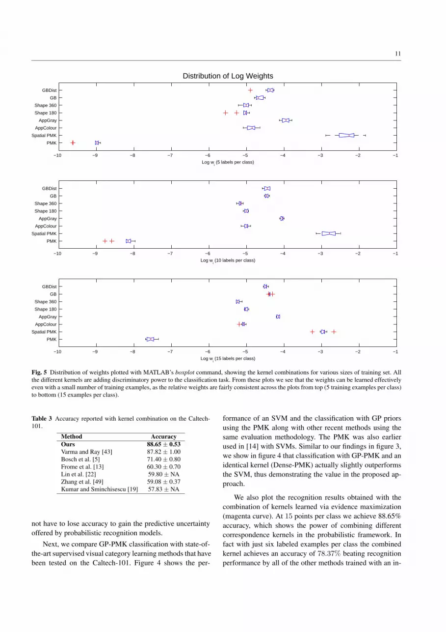
Fig. 5 Distribution of weights plotted with MATLAB’s boxplot command, showing the kernel combinations for various sizes of training set. Allthe different kernels are adding discriminatory power to the classification task. From these plots we see that the weights can be learned effectivelyeven with a small number of training examples, as the relative weights are fairly consistent across the plots from top (5 training examples per class)to bottom (15 examples per class).

Table 3 Accuracy reported with kernel combination on the Caltech-101.

Method AccuracyOurs 88.65 ± 0.53Varma and Ray [43] 87.82 ± 1.00Bosch et al. [5] 71.40 ± 0.80Frome et al. [13] 60.30 ± 0.70Lin et al. [22] 59.80 ± NAZhang et al. [49] 59.08 ± 0.37Kumar and Sminchisescu [19] 57.83 ± NA

not have to lose accuracy to gain the predictive uncertaintyoffered by probabilistic recognition models.

Next, we compare GP-PMK classification with state-of-the-art supervised visual category learning methods that havebeen tested on the Caltech-101. Figure 4 shows the per-

formance of an SVM and the classification with GP priorsusing the PMK along with other recent methods using thesame evaluation methodology. The PMK was also earlierused in [14] with SVMs. Similar to our findings in figure 3,we show in figure 4 that classification with GP-PMK and anidentical kernel (Dense-PMK) actually slightly outperformsthe SVM, thus demonstrating the value in the proposed ap-proach.

We also plot the recognition results obtained with thecombination of kernels learned via evidence maximization(magenta curve). At 15 points per class we achieve 88.65%accuracy, which shows the power of combining differentcorrespondence kernels in the probabilistic framework. Infact with just six labeled examples per class the combinedkernel achieves an accuracy of 78.37% beating recognitionperformance by all of the other methods trained with an in-

12

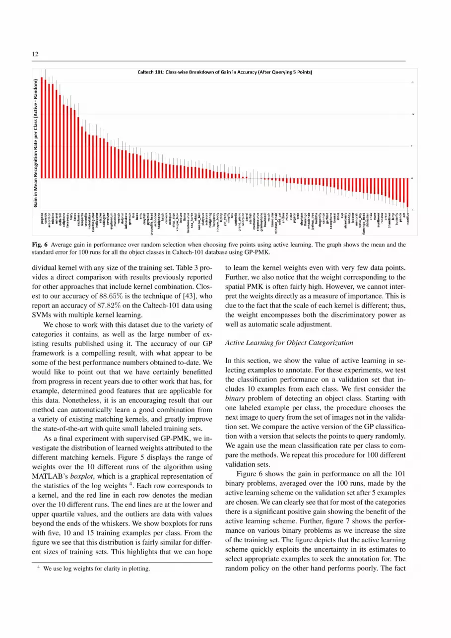
Fig. 6 Average gain in performance over random selection when choosing five points using active learning. The graph shows the mean and thestandard error for 100 runs for all the object classes in Caltech-101 database using GP-PMK.

dividual kernel with any size of the training set. Table 3 pro-vides a direct comparison with results previously reportedfor other approaches that include kernel combination. Clos-est to our accuracy of 88.65% is the technique of [43], whoreport an accuracy of 87.82% on the Caltech-101 data usingSVMs with multiple kernel learning.

We chose to work with this dataset due to the variety ofcategories it contains, as well as the large number of ex-isting results published using it. The accuracy of our GPframework is a compelling result, with what appear to besome of the best performance numbers obtained to-date. Wewould like to point out that we have certainly benefittedfrom progress in recent years due to other work that has, forexample, determined good features that are applicable forthis data. Nonetheless, it is an encouraging result that ourmethod can automatically learn a good combination froma variety of existing matching kernels, and greatly improvethe state-of-the-art with quite small labeled training sets.

As a final experiment with supervised GP-PMK, we in-vestigate the distribution of learned weights attributed to thedifferent matching kernels. Figure 5 displays the range ofweights over the 10 different runs of the algorithm usingMATLAB’s boxplot, which is a graphical representation ofthe statistics of the log weights 4. Each row corresponds toa kernel, and the red line in each row denotes the medianover the 10 different runs. The end lines are at the lower andupper quartile values, and the outliers are data with valuesbeyond the ends of the whiskers. We show boxplots for runswith five, 10 and 15 training examples per class. From thefigure we see that this distribution is fairly similar for differ-ent sizes of training sets. This highlights that we can hope

4 We use log weights for clarity in plotting.

to learn the kernel weights even with very few data points.Further, we also notice that the weight corresponding to thespatial PMK is often fairly high. However, we cannot inter-pret the weights directly as a measure of importance. This isdue to the fact that the scale of each kernel is different; thus,the weight encompasses both the discriminatory power aswell as automatic scale adjustment.

Active Learning for Object Categorization

In this section, we show the value of active learning in se-lecting examples to annotate. For these experiments, we testthe classification performance on a validation set that in-cludes 10 examples from each class. We first consider thebinary problem of detecting an object class. Starting withone labeled example per class, the procedure chooses thenext image to query from the set of images not in the valida-tion set. We compare the active version of the GP classifica-tion with a version that selects the points to query randomly.We again use the mean classification rate per class to com-pare the methods. We repeat this procedure for 100 differentvalidation sets.

Figure 6 shows the gain in performance on all the 101binary problems, averaged over the 100 runs, made by theactive learning scheme on the validation set after 5 examplesare chosen. We can clearly see that for most of the categoriesthere is a significant positive gain showing the benefit of theactive learning scheme. Further, figure 7 shows the perfor-mance on various binary problems as we increase the sizeof the training set. The figure depicts that the active learningscheme quickly exploits the uncertainty in its estimates toselect appropriate examples to seek the annotation for. Therandom policy on the other hand performs poorly. The fact

13

0 2 4 6 8 10 1270

75

80

85

90

95

100

Number of Examples Queried

Mea

n R

ecog

nitio

n R

ate

per

Cla

ss

faces vs rest

GP ActiveGP Random

0 2 4 6 8 10 1260

65

70

75

80

85

90


Mea

n R

ecog

nitio

n R

ate

per

Cla

ss

faces easy vs rest

GP ActiveGP Random

0 2 4 6 8 10 1275

80

85

90

95

100


Mea

n R

ecog

nitio

n R

ate

per

Cla

ss

leopards vs rest

GP ActiveGP Random

0 2 4 6 8 10 1276

78

80

82

84

86

88

90

92

94


Mea

n R

ecog

nitio

n R

ate

per

Cla

ss

motorbikes vs rest

GP ActiveGP Random

0 2 4 6 8 10 1252

53

54

55

56

57

58

59

60


Mea

n R

ecog

nitio

n R

ate

per

Cla

ss

ketch vs rest

GP ActiveGP Random

0 2 4 6 8 10 1255

60

65

70

75

80

85

90

95


Mea

n R

ecog

nitio

n R

ate

per

Cla

ss

airplanes vs rest

GP ActiveGP Random

0 2 4 6 8 10 1245

46

47

48

49

50

51

52

53

54


Mea

n R

ecog

nitio

n R

ate

per

Cla

ss

bass vs rest

GP ActiveGP Random

0 2 4 6 8 10 1260

65

70

75

80

85

90

95


Mea

n R

ecog

nitio

n R

ate

per

Cla

ss

car side vs rest

GP ActiveGP Random

0 2 4 6 8 10 1242

44

46

48

50

52

54


Mea

n R

ecog

nitio

n R

ate

per

Cla

ss

ceiling fan vs rest

GP ActiveGP Random

0 2 4 6 8 10 1245

46

47

48

49

50

51

52

53

54

55


Mea

n R

ecog

nitio

n R

ate

per

Cla

ss

mandolin vs rest

GP ActiveGP Random

0 2 4 6 8 10 1260

65

70

75

80

85

90

95


Mea

n R

ecog

nitio

n R

ate

per

Cla

ss

minaret vs rest

GP ActiveGP Random

0 2 4 6 8 10 1246

47

48

49

50

51

52

53

54


Mea

n R

ecog

nitio

n R

ate

per

Cla

ss

dolphin vs rest

GP ActiveGP Random

0 2 4 6 8 10 1248

50

52

54

56

58

60


Mea

n R

ecog

nitio

n R

ate

per

Cla

ss

electric guitar vs rest

GP ActiveGP Random

0 2 4 6 8 10 1244

46

48

50

52

54

56


Mea

n R

ecog

nitio

n R

ate

per

Cla

ss

euphonium vs rest

GP ActiveGP Random

0 2 4 6 8 10 1246

47

48

49

50

51

52

53

54

55


Mea

n R

ecog

nitio

n R

ate

per

Cla

ss

pyramid vs rest

GP ActiveGP Random

0 2 4 6 8 10 1248

50

52

54

56

58

60

62

64


Mea

n R

ecog

nitio

n R

ate

per

Cla

ss

ferry vs rest

GP ActiveGP Random

0 2 4 6 8 10 1244

46

48

50

52

54

56

58


Mea

n R

ecog

nitio

n R

ate

per

Cla

ss

helicopter vs rest

GP ActiveGP Random

0 2 4 6 8 10 1258

60

62

64

66

68

70

72


Mea

n R

ecog

nitio

n R

ate

per

Cla

ss

inline skate vs rest

GP ActiveGP Random

Fig. 7 Performance comparison of GP classification with active learning and GP with random supervision for various object detection problems(binary) in the Caltech-101 database.

that the Caltech-101 dataset has unbalanced numbers of ex-amples per category affects the random sampling policy; itdoes not work well in these unbalanced scenarios becausethe training set will usually be skewed towards one class,resulting in poor accuracy. However, selecting points via ac-tive learning focuses on points with maximum uncertainty,irrespective of their label, making the procedure highly ef-fective.

Next we describe active learning experiments with theCaltech-4 dataset using multiple feature sampling and pyra-mid partitioning strategies. The goal here was to investigatethe benefits of the proposed scheme across the spectrum ofkernels available for the task of object categorization. Forthis experiment we again experimented with three differ-ent flavors of the Pyramid Match Kernel. Besides DensePMK, we also used PMK computed using only sparse in-terest points where salient points in the images are detectedwith a Harris-Affine interest operator (Harris PMK). Thethird PMK variant was vocabulary guided (Vocabulary GuidedPMK) where the features were binned non-uniformly in adata-dependent manner, as in [15].

Figure 8 compares different classification approaches onthe Caltech-4 database for different kinds of kernels. Essen-tially, the plot shows mean classification accuracy per classas we vary the total number of examples in the training data.The images not in the training set are considered as the testset to compute the classification performance. We plot theperformance of the SVM and the GP classification with andwithout active learning. We start with zero labeled points.For the SVM and supervised GP without active learning, werandomly select points as we increase the size of the train-ing set, whereas for the active learning GP classification we

use uncertainty to guide its sample selection process. Thisprocess was repeated 40 times and figure 8 shows the meanperformance. The errorbars denote the standard error andnon-overlapping errorbars signify difference in performancelevels with 95% confidence.

From figure 8 we observe that GP classification againperforms competitively with the SVM, and using active learn-ing further improves the performance. In fact we can seethat a mean accuracy per class close to 90% can be obtainedwith just 20 labeled examples, whereas the non-active learn-ers achieve around 85% accuracy for the same amount oflabeled data. This demonstrates that active learning can pro-vide a significant boost in accuracy across different flavorsof kernels and feature types used in object categorization.Further, the scheme also makes it possible for the learningalgorithm to learn the object classes even with very few la-beled examples.

Table 4 shows the confusion matrix resulting after incor-porating only 120 examples in the training set using the ac-tive learning methodology with Dense PMK. We obtain anoverall accuracy of 98.48%, which demonstrates the effec-tiveness of the framework. The completely supervised GPclassification and SVM achieved a mean classification ac-curacy per class of 95.6% and 95.19%, respectively. Thisshows that our active learning strategy allows us to learnobject categories much more effectively than traditional su-pervised classification.

9 Discussion

The experiments in this paper indicate that classification us-ing GP priors performs competitively with SVM on the ob-

14

0 20 40 60 80 100 120 14070

75

80

85

90

95

100

Size of Active Set

Mea

n R

ecog

nitio

n R

ate

per

Cla

ss

Caltech−4 with Dense PMK

SVMGPGP Active Learning (Uncertainty)

0 20 40 60 80 100 120 14040

50

60

70

80

90

100

Size of Active SetM

ean

Rec

ogni

tion

Rat

e pe

r C

lass

Caltech−4 with Harris PMK


0 20 40 60 80 100 120 14030

40

50

60

70

80

90

100

Size of Active Set

Mea

n R

ecog

nitio

n R

ate

per

Cla

ss

Caltech−4 with Vocabulary Guided PMK


Fig. 8 Active learning on the Caltech-4 database using different kinds of Pyramid Match Kernels and feature types. In each case, our active learningapproach provides significant gains over traditional passive approaches that label points at random, while the GP classification even shows somegains over the SVM.

Table 4 Confusion matrix obtained for Caltech-4 database using activelearning with the Pyramid Match Kernel (Dense PMK). (120 labeledimages, mean accuracy over all the classes = 98.48%).

Recognized Class

True Class Cars Faces Airplanes MotorbikesCars 1121 0 0 1Faces 0 416 0 2Airplanes 0 2 753 20Motorbikes 10 0 10 733

ject categorization task with Caltech-101 and Caltech-4 data.Of course, these experiments cannot serve as conclusive proofthat classification using a GP prior is inherently superiorthan other classification techniques or vice-versa. Yet forthis object categorization task and data, the underlying datadensity is favorable to the assumptions of the classificationmodel we are using. The experiments in this paper stronglysuggest that there is a value in looking at GP classificationmodels for object categorization.

Another important aspect of our framework lies in itsseamless extension to kernel combination and active learn-ing. The probabilistic paradigm allows us to exploit the evi-dence maximization framework to principally combine dif-ferent correspondence kernels. Furthermore, the Bayesianformulation lets us incorporate measures such as uncertainty,variance, and expected information gain that could be highlyvaluable in guiding a supervised learning procedure. One ofthe challenges in computer vision is the ability to learn ob-ject categories with a low number of examples. Humans areable to learn object categories and generalize from a verysmall number of examples. However, current machine visionsystems are far from achieving performance akin to humans.One of the principal differences among humans and existingobject classification systems is that humans have the abil-ity to actively seek supervision from the environment andother sources of information. We believe that active learningmight enable us to move towards vision systems that requirefew examples to learn successfully.

10 Conclusion and Future Work

We have presented a discriminative probabilistic frameworkbased on Gaussian Process priors and the local feature-basedcorrespondence kernels, and have shown its utility for vi-sual category recognition. Gaussian Process regression pro-vides a principled framework to combine different corre-spondence kernels, which results in performance superiorto individual kernels. Further, the modeling with GaussianProcess priors provides direct estimates of prediction uncer-tainty using a smoothness prior that captures a correspondence-based notion of similarity between sets of local image fea-tures. We introduced an active learning method for visualcategory recognition based on the GP-PMK uncertainty es-timates, and showed empirically that active learning can beused to achieve very good recognition results using far fewertraining images than standard supervised learning approaches.

We plan to extend the framework to adopt non-Gaussiannoise models, and investigate other active learning formu-lations such as value of information and/or criteria previ-ously developed for sparsifying GPs [20]. By incorporatingdecision-theoretic formulations we should be able to learnobject categories within a given budget. We also plan toextend the model to handle multiple objects in the sameimage, incorporate semi-supervised learning, and exploresparse GP techniques for large training sets.

Acknowledgements We thank the following for providing kernel ma-trices: Alex Berg, Anna Bosch, Jitendra Malik and Andrew Zisserman.We also wish to thank Manik Varma for his help in obtaining the re-quired data and for many helpful discussions.

References

1. http ://labelme.csail.mit.edu/.2. Y. Abramson and Y. Freund. Active learning for visual object

recognition. Technical report, UCSD, 2004.3. S. Belongie, J. Malik, and J. Puzicha. Matching shapes. In ICCV,

2001.

15

4. A. Berg and J. Malik. Geometric blur for template matching. InCVPR, 2001.

5. A. Bosch, A. Zisserman, and X. Munoz. Representing shape witha spatial pyramid kernel. In CIVR, 2007.

6. C. Chang and C. Lin. LIBSVM: a library for SVMs, 2001.7. E. Y. Chang, S. Tong, K. Goh, and C. Chang. Support vector ma-

chine concept-dependent active learning for image retrieval. IEEETransactions on Multimedia, 2005.

8. T. Evgeniou, M. Pontil, and T. Poggio. Regularization networksand support vector machines. Advances in Computational Mathe-matics, 13(1), 2000.

9. B. T. F. Moosmann and F. Jurie. Fast discriminative visual code-books using randomized clustering forests. In NIPS, 2007.

10. L. Fei-Fei, R. Fergus, and P. Perona. One-shot learning of objectcategories. IEEE Transaction on Pattern Recognition and Ma-chine Intelligence, 2006.

11. R. Fergus, P. Perona, and A. Zisserman. Object class recognitionby unsupervised scale-invariant learning. In CVPR, 2003.

12. Y. Freund, H. S. Seung, E. Shamir, and N. Tishby. Selective sam-pling using the query by committee algorithm. Machine Learning,28(2-3), 1997.

13. A. Frome, Y. Singer, F. Sha, and J. Malik. Learning globally-consistent local distance functions for shape-based image retrievaland classification. In ICCV, 2007.

14. K. Grauman and T. Darrell. The pyramid match kernel: Discrimi-native classification with sets of image features. In ICCV, 2005.

15. K. Grauman and T. Darrell. Approximate correspondences in highdimensions. In NIPS, 2006.

16. K. Grauman and T. Darrell. Unsupervised learning of categoriesfrom sets of partially matching image features. In CVPR, 2006.

17. T. Kadir and M. Brady. Scale saliency : A novel approach to salientfeature and scale selection. In International Conference VisualInformation Engineering, 2003.

18. A. Kapoor, K. Grauman, R. Urtasun, and T. Darrell. Active learn-ing with Gaussian Processes for object categorization. In ICCV,2007.

19. A. Kumar and C. Sminchisescu. Support kernel machines for ob-ject recognition. In ICCV, 2007.

20. N. Lawrence, M. Seeger, and R. Herbrich. Fast sparse GaussianProcess method: Informative vector machines. NIPS, 2002.

21. S. Lazebnik, C. Schmid, and J. Ponce. Beyond bags of fea-tures: Spatial pyramid matching for recognizing natural scene cat-egories. In CVPR, 2006.

22. Y. Y. Lin, T. Y. Liu, and C. S. Fuh. Local ensemble kern el learningfor object category recognition. In CVPR, 2007.

23. D. Lowe. Distinctive image features from scale-invariant key-points. IJCV, 60(2), 2004.

24. D. MacKay. Information-based objective functions for active dataselection. Neural Computation, 4(4), 1992.

25. A. K. McCallum and K. Nigam. Employing EM in pool-basedactive learning for text classification. In ICML, 1998.

26. K. Mikolajczyk and C. Schmid. Indexing Based on Scale InvariantInterest Points. In ICCV, 2001.

27. K. Mikolajczyk and C. Schmid. Scale and Affine Invariant InterestPoint Detectors. IJCV, 1(60):63–86, October 2004.

28. T. P. Minka. A Family of Algorithms for Approximate BayesianInference. PhD thesis, MIT, 2001.

29. I. Muslea, S. Minton, and C. A. Knoblock. Active + semi-supervised learning = robust multi-view learning. In ICML, 2002.

30. D. Nister and H. Stewenius. Scalable Recognition with a Vocabu-lary Tree. In CVPR, 2006.

31. E. Nowak, F. Jurie, and B. Triggs. Sampling strategies for bag-of-features image classification. In ECCV, 2006.

32. C. E. Rasmusen and C. Williams. Gaussian Processes for MachineLearning. MIT Press, 2006.

33. M. Seeger. Gaussian Processes for machine learning. Interna-tional Journal of Neural Systems, 14(2), 2004.

34. Y. Shen, A. Ng, and M. Seeger. Fast Gaussian Process regressionusing kd-trees. In NIPS, 2006.

35. J. Sivic, B. Russell, A. Efros, A. Zisserman, and W. Freeman. Dis-covering object categories in image collections. In ICCV, 2005.

36. J. Sivic and A. Zisserman. Video Google: a text retrieval approachto object matching in videos. In ICCV, 2003.

37. E. Snelson and Z. Ghahramani. Sparse Gaussian Processes usingpseudo-inputs. In NIPS, 2006.

38. E. Sudderth, A. Torralba, W. Freeman, and A. Willsky. Describ-ing visual scenes using transformed dirichlet processes. In NIPS,2005.

39. S. Tong and D. Koller. Support vector machine active learningwith applications to text classification. In ICML, 2000.

40. R. Urtasun and T. Darrell. Local probabilistic regression foractivity-independent human pose inference. In CVPR, 2008.

41. R. Urtasun, D. J. Fleet, and P. Fua. Gaussian Process dynamicalmodels for 3d people tracking. In CVPR, 2006.

42. R. Urtasun, D. J. Fleet, A. Hertzman, and P. Fua. Priors for peopletracking from small training sets. In ICCV, 2005.

43. M. Varma and D. Ray. Learning the discriminative power-invariance trade-off. In ICCV, 2007.

44. L. von Ahn and L. Dabbish. Labeling images with a computergame. In ACM CHI, 2004.

45. L. von Ahn, R. Liu, and M. Blum. Peekaboom: A game for locat-ing objects in images. In ACM CHI, 2006.

46. C. Wallraven, B. Caputo, and A. Graf. Recognition with localfeatures: the kernel recipe. In ICCV, 2003.

47. C. Williams and D. Barber. Bayesian classification with GaussianProcesses. IEEE Transaction on Pattern Recognition and MachineIntelligence, 20(12):1342–1351, 1998.

48. O. Williams. A switched Gaussian Process for estimating disparityand segmentation in binocular stereo. In NIPS, 2006.

49. H. Zhang, A. Berg, M. Maire, and J. Malik. SVM-KNN: Discrim-inative nearest neighbor classification for visual category recogni-tion. In CVPR, 2006.

50. X. Zhu, J. Lafferty, and Z. Ghahramani. Combining active learn-ing and semi-supervised learning using Gaussian fields and har-monic functions. In Workshop on The Continuum from Labeled toUnlabeled Data in Machine Learning and Data Mining at ICML,2003.

Documents

Gaussian Processes for Object Categorization