Gauss Newton method for image reconstruction in diffuse optical tomography

INSTITUTE OF PHYSICS PUBLISHING PHYSICS IN MEDICINE AND BIOLOGY

Phys. Med. Biol. 50 (2005) 2365–2386 doi:10.1088/0031-9155/50/10/013

Gauss–Newton method for image reconstruction indiffuse optical tomography

Martin Schweiger1, Simon R Arridge1 and Ilkka Nissila2

1 Department of Computer Science, University College London, Gower Street London,WC1E 6BT, UK2 Laboratory of Biomedical Engineering, Helsinki University of Technology, Finland

Received 21 January 2005, in final form 30 March 2005Published 5 May 2005Online at stacks.iop.org/PMB/50/2365

AbstractWe present a regularized Gauss–Newton method for solving the inverseproblem of parameter reconstruction from boundary data in frequency-domaindiffuse optical tomography. To avoid the explicit formation and inversion of theHessian which is often prohibitively expensive in terms of memory resourcesand runtime for large-scale problems, we propose to solve the normal equationat each Newton step by means of an iterative Krylov method, which accesses theHessian only in the form of matrix–vector products. This allows us to representthe Hessian implicitly by the Jacobian and regularization term. Further weintroduce transformation strategies for data and parameter space to improvethe reconstruction performance. We present simultaneous reconstructions ofabsorption and scattering distributions using this method for a simulated testcase and experimental phantom data.

1. Introduction

1.1. Optical tomography

Diffuse optical tomography is a new medical imaging modality with potential applications infunctional imaging of the brain and in breast cancer detection, amongst other applications. Thismethod seeks to recover optical parameters of blood and tissue from boundary measurementsof light transmission in the visible and near-infrared range. The reconstructed images of thespatial distribution of tissue parameters can be related directly to physiologically importantproperties such as blood and tissue oxygenation state. Instrumentation for optical tomographyis portable and relatively inexpensive, and can provide a viable alternative to currently availablesystems such as functional magnetic resonance imaging.

Data acquisition systems consist of a light source such as an infrared laser, illuminatingthe body surface at different source locations in succession. The light which has propagatedthrough the tissue is then measured at multiple detector locations on the surface. Biological

0031-9155/05/102365+22$30.00 © 2005 IOP Publishing Ltd Printed in the UK 2365

http://dx.doi.org/10.1088/0031-9155/50/10/013

http://stacks.iop.org/pb/50/2365

2366 M Schweiger et al

tissue is strongly scattering at the wavelengths used in optical tomography, which generallymakes the recovery of tissue parameters from the boundary data a highly nonlinear problem.

The experimental systems in use today utilize either ultrashort input pulses (time domainsystems) or continuous intensity-modulated input (frequency-domain systems). In the formercase, measurements consist of the temporal dispersion of the transmitted pulse, measured ata resolution in the order of pico-seconds. In the latter case, the measurements consist of thecomplex intensity of the transmitted photon density wave, most commonly measured in termsof the phase shift and modulation amplitude. The frequency domain version of the problem isthe one considered in this paper.

1.2. Image reconstruction in optical tomography

Image reconstruction methods in optical tomography differ in the type of data being considered,the type of solutions being sought, the physical model assumed for light propagation, and in thealgorithmic details; for reviews see Arridge (1993, 1999), Yodh and Chance (1995), Hebdenet al (1997), Arridge and Hebden (1997), Hawysz and Sevick-Muraca (2000), Boas et al(2001) and Gibson et al (2005). Two main distinctions are between linear methods basedon inverse scattering theory, and non-linear methods based on model fitting. In the formercategory, a perturbation model is postulated which corresponds to the first term in a Bornor Rytov expansion of the Lippman–Schwinger equation (Arridge et al 1991, O’Leary et al1995, O’Leary 1996, Schotland et al 1993, Schotland 1997, Schotland and Markel 2001,Markel and Schotland 2001, 2002). This model can be constructed using Green’s functionsfor the diffusion equation, either in infinite space or in the presence of boundaries, or by anumerical technique such as Monte Carlo, finite difference or finite elements. The resultantlinear system is usually solved by an iterative method such as the Kaczmarz method, conjugategradients or projection onto convex sets (Barbour et al 1990, Wang et al 1992, Walker et al1997, Ripoll et al 2001). The second approach considers the model in terms of explicitparameters and adjusts these parameters in order to optimize an objective function combininga data fitting and regularization term (Arridge et al 1992, Schweiger et al 1993, Paulsenand Jiang 1995, Klose and Hielscher 1999, Ye et al 2001). These methods, based eitheron the diffusion equation or on the radiative transfer equation, use a variety of algorithms,including Levenberg–Marquardt (Schweiger et al 1993), quasi-Newton (Klose and Hielscher2003), truncated Newton (Roy and Sevick-Muraca 1999) and non-linear conjugate gradients(Arridge and Schweiger 1998) to minimize the objective function over the search space ofmodel parameters.

1.3. Contribution of this paper

In this paper we compare some implementation strategies for a Gauss–Newton approach tothe inverse solver in optical tomography. In this approach the non-linear forward model islinearized to produce a Jacobian, and a system of normal equations is developed wherein theHessian of the forward model is approximated by the Jacobian transposed with itself, plus aregularization term. This approach has to be combined with a globalization strategy to ensureconvergence. When the dimension of the problem is large the representation of the Hessiancan be infeasible in terms of available memory, whereas the representation of the Jacobianis possible. However, if the solution of the normal equations is carried out with an iterativeprocedure, the Hessian is only utilized in terms of matrix–vector products. Therefore wepropose a method to implicitly represent the Hessian in a functional form that proves to becomputationally efficient.

Gauss–Newton method for optical tomography 2367

We use this representation to compare both a Levenberg–Marquardt, and damped Gauss–Newton globalization strategy and show that the latter has better convergence. In addition,performance of the reconstruction technique is strongly dependent on transformation of thedata and conditioning of the Jacobian.

2. Formulation of the problem

Let � ⊂ Rn be a simply connected domain containing two real positive scalar functions

µa(r), κ(r). Let f (m;ω) eiωt be a time-harmonic incoming radiation boundary condition.Then the photon density �(r;ω) inside the domain satisfies

−∇ · κ(r)∇�(r;ω) +(µa(r) +

iω

c

)�(r;ω) = 0 r ∈ �\∂� (1)

�(m;ω) + 2ζκ(m)∂�(m;ω)

∂ν= f (m;ω) m ∈ ∂� (2)

where ζ is a boundary term which incorporates the refractive index mismatch at the tissue-airboundary (Moulton 1990, Schweiger et al 1995), and ν is the outward normal of the boundary∂� at m. In the literature, the optical coefficients are often expressed in terms of absorptionand scattering. The scattering coefficient, µs , is related to µa and κ by

κ = 1

3(µa + µ′s)

. (3)

The distribution of scattering angles for individual scattering events in biological tissues isgenerally not isotropic, but strongly biased towards small angles. If we assume that all lightcontributing to measurements has undergone a large number of scattering events, then wecan introduce an equivalent isotropic scattering coefficient (often called transport or reducedscattering coefficient) µ′

s = (1 − g)µs , where g is the average cosine of the single scatteringphase function, with a typical range of g = 0.9, . . . , 0.99.

The measurable exitance is the (diffuse) outgoing radiation and corresponds to theNeumann data

y(m;ω) = −κ(m)∂�(m;ω)

∂ν, m ∈ ∂�. (4)

We use X to denote the function space of the parameters, Q the function space of thesources and Y the function space of the data. Some discussion of the form of these spaces canbe found in Arridge (1999) and Dorn (1998).

The Robin-to-Neumann (RtN) map

�(µa, κ;ω) : Q → Y (5)

is a linear mapping from the incoming radiation f to the outgoing radiation y, for any givenpair of functions in the solution space {µa, κ}:

y(m;ω) = �(µa, κ;ω)f (m;ω), m ∈ ∂�. (6)

The forward operator

Fs : X → Y (7)

is a non-linear mapping from pairs of functions in the solution space to the data on theboundary, for given incoming radiation fs , where index s is introduced to allow specificindexing of different sources. The direct Frechet derivative

F ′s (µa, κ;ω) : X → Y (8)


is a linear mapping from pairs of functions in the solution space to the data on the boundary,for given incoming radiation fs . F ′

s is the linearization of Fs around the solution point {µa, κ}that maps changes

{µδ

a, κδ} ≡ {α, β} in solution space functions to changes yδ

s in data. Thevalue of the mapping

yδs (m;ω) = F ′

s (µa, κ;ω)

(α

β

)(9)

is given by{−∇ · κ(r)∇ +

(µa(r) +

iω

c

)}�δ

s(r;ω) ={∇ · β(r)∇ −

(α(r) +

iω

c

)}�s(r;ω)

r ∈ �\∂� (10)

�δs(m;ω) + 2ζκ(m)

∂�δs(m;ω)

∂ν= 0 m ∈ ∂� (11)

yδs (m;ω) = −κ(m)

∂�δs(m;ω)

∂ν, m ∈ ∂�. (12)

The adjoint Frechet derivative

F ′∗s (µa, κ;ω) : Y → X (13)

is a linear mapping from functions on the boundary to pairs of functions in the solution space,for given incoming radiation fs . The value of the mapping(

α

β

)= F ′∗

s (µa, κ;ω)yδs (m;ω) (14)

is given by {−∇ · κ(r)∇ +

(µa(r) − iω

c

)}� +

s (r;ω) = 0 r ∈ �\∂� (15)

� +s (m;ω) + 2ζκ(m)

∂ � +s (m;ω)

∂ν= yδ

s (m;ω) m ∈ ∂� (16)

(α

β

)= Re

(− � +

s �s

−∇ � +s · ∇�s

)r ∈ �\∂�. (17)

We assume a finite number of incoming radiation sources S = {fs(m); s = 1, . . . , S},where fs(m) is a function of local support on ∂� representing the finite width and profile ofthe sth source. The forward operator is now considered as a stacked set of operators

y(m;ω) =

y1(m;ω)

y2(m;ω)

...

yS(m;ω)

= F (µa, κ;ω) =

F1(µa, κ;ω)

F2(µa, κ;ω)

...

FS(µa, κ;ω)

. (18)

We also consider a finite sampling of the outgoing distributions ys(m;ω), leading to ameasurement model:

ys,i(ω) = Mi[ys(m;ω)] =∫

∂�

wi(m)ys(m;ω) (19)

where wi(m) represents the finite aperture of a detector. In the following we will useW = {wi(m); i = 1, . . . , D} to assume a finite number D of detectors, with Ws ⊂ W the


subset of size Ds � D of detectors that see source s. An ideal choice for the functions insets S, W would form a basis for the set of complete functions on ∂� that could be used torepresent the Robin-to-Neumann operator �. In this paper we use Hanning functions withfinite width chosen to span ∂�. These functions can be analytically integrated with the FEMbasis functions used for the discrete forward model (section 4.1).

The discrete data in (18) is complex, and inversion would lead to a complex parameterupdate. For this reason the data vector is usually split into real and imaginary parts with acommensurate splitting of the linearized derivative operators. In the following we assumey ∈ R

2M where = ∑Ss=1 Ds . In addition, when considering log of the data the splitting

associates the real part with logarithmic amplitude, and the imaginary part with phase. Thisis discussed further below in section 4.4.

3. Approaches to the inverse problem

3.1. Output least-squares approach

In the following we combine the two scalar functions into one symbol

x :=(

µa

κ

), x ∈ R

N, (20)

with N = 2Pb, where Pb is the dimension of the basis expansion used for representing theoptical parameter distributions in the context of the inverse solver. We consider the regularizedoutput least-squares approach to the inverse problem. We seek the solution

x = argminx

�(x), (21)

where

�(x) = 1

2

∑i,s

|ys,i(ω) − Fs,i(x;ω)|2 + τR(x) (22)

is the objective function and R(x) is a regularizing functional whose relative contribution isgoverned by hyperparameter τ . The Newton scheme for solving equation (21) is given by theiteration

x(k+1) = x(k) + ςk(F′∗(x(k);ω)F ′(x(k);ω) + H(x(k);ω) + τR′′(x(k)))−1

× [F ′∗(x(k);ω)(y(ω) − F (x(k);ω)) − τR′(x(k))] (23)

starting from an initial estimate x(0), where H = 〈y − F ,F ′′〉 is a term depending on boththe data and the second derivative of the forward model. Because this term is difficult tocompute, and can also lead to a loss of positive-definiteness of the Hessian, it is left out in theGauss–Newton scheme at the cost of potential loss of the local quadratic convergence of thestandard Newton iteration.

3.2. Globalization

There are two common approaches to restore local convergence (Dennis and Schnabel 1983):(i) a trust region approach which leads to the Levenberg–Marquardt (LM) method

x(k+1)LM = x(k) + (F ′∗(x(k);ω)F ′(x(k);ω) + τR′′(x(k)) + λk I)−1

× [F ′∗(x(k);ω)(y(ω) − F (x(k);ω)) − τR′(x(k))], (24)


where the control parameter λk > 0 is adjusted at each iteration, and (ii) a damped Gauss–Newton (DGN) approach given by

x(k+1)DGN = x(k) + ςk(F

′∗(x(k);ω)F ′(x(k);ω) + τR′′(x(k)))−1

× [F ′∗(x(k);ω)(y(ω) − F (x(k);ω)) − τR′(x(k))], (25)

where ςk is a step length parameter obtained by an inexact line search at each iteration. Forsimplification we introduce the following notation for the Hessian and gradient terms:

H(λk)k = F ′∗(x(k);ω)F ′(x(k);ω) + τR′′(x(k)) + λk I (26)

and

gk = F ′∗(x(k);ω)(F (x(k);ω) − y(ω)) + τR′(x(k)). (27)

A conventional way to implement these schemes is to build the explicit JacobianJ ∈ R

2M×N as the discrete representation of F ′, and solve the linear normal equations

(JT J + τR′′(x(k)) + λk I)xδ = gk. (28)

3.3. Solution of normal equations

Solution of a linear system such as (28) can be approached in a number of ways. For arelatively small solution space, the system is considered overdetermined and solved directlyusing Gaussian substitution or indirectly using an iterative solution scheme.

If the regularization functional is quadratic we have the relations

R(x(k)) = ‖L(x(k) − xg)‖22

R′(x(k)) = LT L(x(k) − xg)

R′′(x(k)) = LT L

where xg is a given reference state. In the Bayesian framework and for quadratic regularizationfunctionals xg is the mean of a Gaussian prior distribution. Note that xg is not necessarilyidentical to the initial estimate x(0). The normal equations can then be expressed as(

Jτ 1/2L

)xδ =

(y − F (x(k))

τ 1/2L(x(k) − xg)

)(29)

which are usually solved by QR decomposition. The matrix in (29) is of dimension(2M + N) × N . A standard QR algorithm decomposes into a rectangular (2M + N) × N

matrix Q and a square N × N matrix R, thus requiring storage for N(2M + 2N) floating pointvalues.

Alternatively, an underdetermined form can be constructed using the matrix inversionlemma (Eppstein et al 2001, Dehghani et al 2003):

(JT J + τLT L)−1JT = JT (J(LT L)−1JT + τ I)−1.

Typically the regularization functional is in terms of a PDE and its inverse is non-sparse andequivalent to a smoothing operation. For this reason the regularization is sometimes replacedby an image filtering operation.

None of these methods take account of the particular structure of the Hessian. It containsa part that is a dense representation of a compact operator and a part that is sparse, representinga local operator which may have a non-trivial null space. In general the regularizer may not bequadratic, or even convex. In this paper we consider an inexact Gauss–Newton approach tosolve equation (28). We use a Krylov method for the Hessian inversion that computes a smallnumber of matrix–vector products. These products are efficiently calculated by applying the


forward and adjoint Frechet derivatives plus the explicit Hessian of the regularizer. In thispaper we consider that the Frechet derivative is explicitly represented by a Jacobian matrix,although if this is infeasible, it could be replaced by an operator involving additional solutionsof the original PDE.

4. Implementation

4.1. Finite element method forward solver

We employ a finite element discretization for numerically computing the forward problemdefined in equations (1) and (2). We divide the domain � into an unstructured mesh ofnonoverlapping elements of simple shape, and define a basis in � which is polynomialwithin each element, and continuous across elements. Given Ph nodal points with associatedbasis functions ui(r), i = 1, . . . , Ph, of limited support, a function � defined in � is thenapproximated in this basis by the piecewise polynomial interpolation �h(r) = ∑Ph

i=1 �iui(r),where Φ = {�i} is a Ph-dimensional array of basis coefficients. We use superscript h todenote the finite element mesh basis expansion. The coefficients κ(r) and µa(r) are expandedin the same manner into κh(r) and µh

a(r). As developed previously (Arridge et al 1993,Schweiger et al 1995), the basis representation transforms the continuous problem (1), (2)into a linear system which is expressed in terms of the nodal values of the coefficients andfield: (

K(κh) + C(µh

a

)+ γ A + iωB

)Φ(ω) = Q(ω) (30)

with Φ,Q ∈ RPh and system matrices K, C, A, B ∈ R

Ph×Ph given by

Kij =∫

�

κh(r)∇ui(r) · ∇uj (r) dr, Cij =∫

�

µha(r)ui(r)uj (r) dr,

Aij =∫

∂�

ui(r)uj (r) dr, Bij = 1

c

∫�

ui(r)uj (r) dr.

(31)

Analytic solutions for the integrals of polynomial basis functions over simple elements suchas triangles or tetrahedra are readily available (Zienkiewicz and Taylor 1987). In the generalcase, e.g. for elements with curved boundaries, numerical quadrature rules must be applied.

4.2. Krylov solution of the Gauss–Newton step

When solving the LM problem (24) or DGN problem (25), the explicit computation andstorage of the approximate Hessian JT J is often intractable in large-scale problems. Instead,we use a Krylov method as an iterative solver for the linearized problem (28) at each Newtonstep k. The computational advantage of using a Krylov solver lies in the fact that H is onlyaccessed for matrix–vector products. This approach avoids the explicit formation of H. Insteadwe can evaluate matrix–vector operations directly by applying the right-hand side of (26). Wecan therefore represent H formally by its components as an operator H = H[J,R′′, τ, λ] andreplace all instances of operations Hx by the subroutine

proc Hx (J,R′′, τ, λ,x)

z = Jx

return JT z + τR′′x + λx

end

To estimate the computational efficiency of the implicit formulation of H we note thatthe product Hx requires N2 floating point multiplications when H is given explicitly, while in


the implicit representation the calculation of JT J requires 4NM floating point multiplications.Assuming that the computational cost of the product R′′x is small due to its sparsity we findthat the implicit formulation is more efficient when 2M < N

2 .

4.3. GMRES linear solver

Equation (28) defines a linear system of the form Hx = g, where GN iteration subscript k andsuperscript δ have been omitted for simplicity. In this paper we use the generalized minimalresidual (GMRES) Krylov method (Saad and Schultz 1986) to solve this system.

At iteration j of the GMRES solver an approximation x(j) of x is produced from a Krylovspace generated by a vector c:

Kj (H, c) = span{c, Hc, . . . , Hj−1c} (32)

where c = g is commonly used, and the matrix power is defined by H 1 = H,Hi+1 =HHi(i � 1).

GMRES finds in iteration j a solution x(j) which solves the least-squares problem

x(j) = arg minx∈Kj (H,g)

‖g − Hx‖ (33)

by constructing an orthonormal basis {v1,v2, . . . ,vj } for Kj (H, g) using Arnoldi’s method(Arnoldi 1951). Starting from v1 = g/‖g‖, the basis for Kj+1(H, g) is built recursively by

vj+1 = vj+1/‖vj+1‖ (34)

where

vj+1 = Hvj − (h1jv1 + · · · + hjjvj ) (35)

and hij = v∗i Hvj . The basis vectors for Kj (H, g) are collected in a matrix Vj = {v1, . . . ,vj }

which leads to a decomposition

HVj = Vj+1Uj (36)

where Uj is an upper Hessenberg matrix of size (j + 1) × j storing coefficients hij and norms‖vj‖. We can now represent x as x = Vjw for some w, and thus

Hx = Vj+1Ujw, g = ‖g‖Vj+1e1 (37)

where e1 is the first column of the identity matrix. The least-squares problem in (33) atiteration j reduces therefore to

w = arg minw

‖(‖g‖e1) − Ujw‖, x(j) = Vj w. (38)

A standard method to reduce memory requirements for GMRES is to employ a restartingstrategy, where after m iterations the accumulated data in U and V are cleared and theintermediate results are used as the starting values for the next m iterations, until convergenceis achieved. For the calculations in this paper we used m = 10, and a stopping criteriondefined by

‖g − Hx(j)‖L2 � η‖g‖L2 (39)

for a prescribed tolerance η. We find that H is referenced only in (35) and (39) forvector multiplication operations, and can therefore be represented implicitly as discussed insection 4.2.


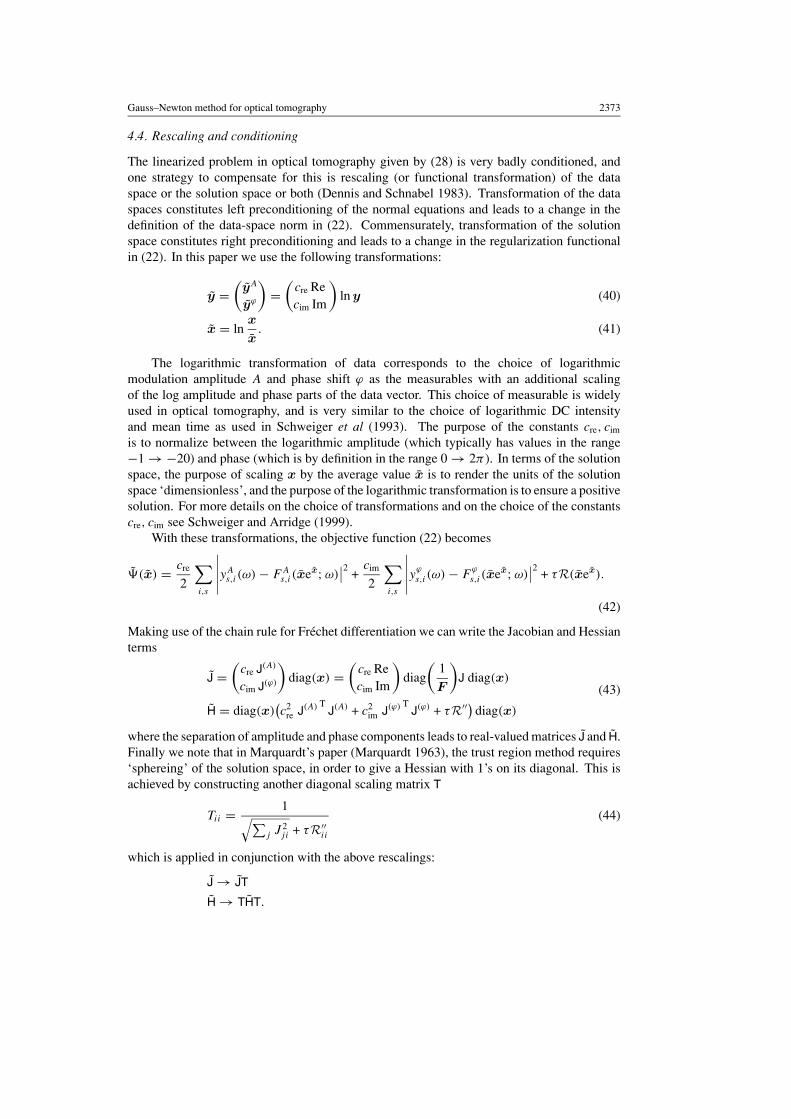
4.4. Rescaling and conditioning

The linearized problem in optical tomography given by (28) is very badly conditioned, andone strategy to compensate for this is rescaling (or functional transformation) of the dataspace or the solution space or both (Dennis and Schnabel 1983). Transformation of the dataspaces constitutes left preconditioning of the normal equations and leads to a change in thedefinition of the data-space norm in (22). Commensurately, transformation of the solutionspace constitutes right preconditioning and leads to a change in the regularization functionalin (22). In this paper we use the following transformations:

y =(

yA

yϕ

)=

(cre Recim Im

)ln y (40)

x = lnx

x. (41)

The logarithmic transformation of data corresponds to the choice of logarithmicmodulation amplitude A and phase shift ϕ as the measurables with an additional scalingof the log amplitude and phase parts of the data vector. This choice of measurable is widelyused in optical tomography, and is very similar to the choice of logarithmic DC intensityand mean time as used in Schweiger et al (1993). The purpose of the constants cre, cim

is to normalize between the logarithmic amplitude (which typically has values in the range−1 → −20) and phase (which is by definition in the range 0 → 2π ). In terms of the solutionspace, the purpose of scaling x by the average value x is to render the units of the solutionspace ‘dimensionless’, and the purpose of the logarithmic transformation is to ensure a positivesolution. For more details on the choice of transformations and on the choice of the constantscre, cim see Schweiger and Arridge (1999).

With these transformations, the objective function (22) becomes

�(x) = cre

2

∑i,s

∣∣∣∣∣yAs,i(ω) − FA

s,i(xex;ω)∣∣2

+cim

2

∑i,s

∣∣∣∣∣yϕ

s,i(ω) − Fϕ

s,i(xex;ω)∣∣2

+ τR(xex).

(42)

Making use of the chain rule for Frechet differentiation we can write the Jacobian and Hessianterms

J =(

cre J(A)

cim J(ϕ)

)diag(x) =

(cre Recim Im

)diag

(1

F

)J diag(x)

H = diag(x)(c2

re J(A) TJ(A) + c2

im J(ϕ) TJ(ϕ) + τR′′) diag(x)

(43)

where the separation of amplitude and phase components leads to real-valued matrices J and H.Finally we note that in Marquardt’s paper (Marquardt 1963), the trust region method requires‘sphereing’ of the solution space, in order to give a Hessian with 1’s on its diagonal. This isachieved by constructing another diagonal scaling matrix T

Tii = 1√∑j J 2

ji + τR′′ii

(44)

which is applied in conjunction with the above rescalings:

J → JT

H → THT.


��

��

��

��

��

��

��

��

��

��

��

��

��

xg xb

xh

DD−1

BB−1

E

E−1

Representation

of fields

Representation

of image

Representation

of mesh

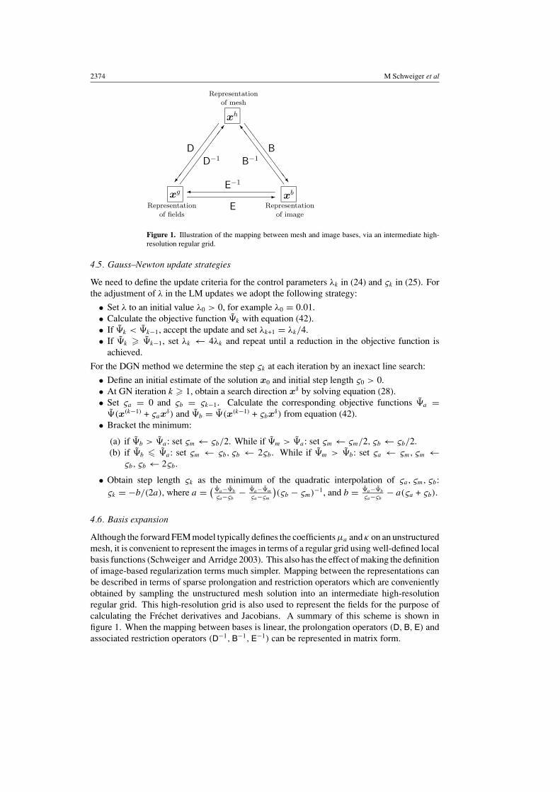
Figure 1. Illustration of the mapping between mesh and image bases, via an intermediate high-resolution regular grid.

4.5. Gauss–Newton update strategies

We need to define the update criteria for the control parameters λk in (24) and ςk in (25). Forthe adjustment of λ in the LM updates we adopt the following strategy:

• Set λ to an initial value λ0 > 0, for example λ0 = 0.01.• Calculate the objective function �k with equation (42).• If �k < �k−1, accept the update and set λk+1 = λk/4.• If �k � �k−1, set λk ← 4λk and repeat until a reduction in the objective function is

achieved.

For the DGN method we determine the step ςk at each iteration by an inexact line search:

• Define an initial estimate of the solution x0 and initial step length ς0 > 0.• At GN iteration k � 1, obtain a search direction xδ by solving equation (28).• Set ςa = 0 and ςb = ςk−1. Calculate the corresponding objective functions �a =

�(x(k−1) + ςaxδ) and �b = �(x(k−1) + ςbx

δ) from equation (42).• Bracket the minimum:

(a) if �b > �a: set ςm ← ςb/2. While if �m > �a: set ςm ← ςm/2, ςb ← ςb/2.(b) if �b � �a: set ςm ← ςb, ςb ← 2ςb. While if �m > �b: set ςa ← ςm, ςm ←

ςb, ςb ← 2ςb.

• Obtain step length ςk as the minimum of the quadratic interpolation of ςa, ςm, ςb:ςk = −b/(2a), where a = (

�a−�b

ςa−ςb− �a−�m

ςa−ςm

)(ςb − ςm)−1, and b = �a−�b

ςa−ςb− a(ςa + ςb).

4.6. Basis expansion

Although the forward FEM model typically defines the coefficients µa and κ on an unstructuredmesh, it is convenient to represent the images in terms of a regular grid using well-defined localbasis functions (Schweiger and Arridge 2003). This also has the effect of making the definitionof image-based regularization terms much simpler. Mapping between the representations canbe described in terms of sparse prolongation and restriction operators which are convenientlyobtained by sampling the unstructured mesh solution into an intermediate high-resolutionregular grid. This high-resolution grid is also used to represent the fields for the purpose ofcalculating the Frechet derivatives and Jacobians. A summary of this scheme is shown infigure 1. When the mapping between bases is linear, the prolongation operators (D, B, E) andassociated restriction operators (D−1, B−1, E−1) can be represented in matrix form.


4.7. Regularization

We use a first-order Tikhonov prior of the form

R(xk) = ‖L�xk‖22 (45)

where LT L ∈ RN×N denotes the Laplacian, and �xk = xk − x0. We define LT L as

(LT L)ij =

nn if i = j

−1 if j is neighbour of i

0 otherwise(46)

where nn is the number of neighbours of basis component i. In this paper we use a regularpixel (in 2D) or voxel (in 3D) grid basis, and use the four-connected neighbourhood in2D or six-connected neighbourhood in 3D. An alternative, not presented here, is to definea neighbourhood radius r, such that all pixels (voxels) inside r are considered neighboursof i. To obtain a value for the regularization parameter τ we use the L-curve method(Hansen and O’Leary 1993, Vogel 2002).

4.8. Calculation of the Jacobian

For the sth source and ith detector we calculate the forward field �s(r, ω) from equation (1),with boundary condition fs(m) in (2) and the adjoint field �+

i from (15) with boundarycondition wi(m) in equation (16). These fields are mapped from the nodal basis of theforward solver into the high-resolution grid basis expansion g:

�gs = D�h

s , �g+i = D�h+

i (47)

and used to define the complex photon measurement density functions (Arridge 1995)

ρ(µ)

is = −�gs �

g+i

ys,i

ρ(κ)is = −∇�

gs · ∇�

g+s

ys,i

. (48)

These vectors are mapped back into the image basis and split into real and imaginary parts toconstruct the Jacobian

J(A,µ)

is = Re[Eρ

(µ)

is

]J(A,κ)is = Re

[Eρ

(κ)is

]J(ϕ,µ)

is = Im[Eρ

(µ)

is

]J(ϕ,κ)

is = Im[Eρ

(κ)is

].

5. Numerical results

5.1. Simulated test case

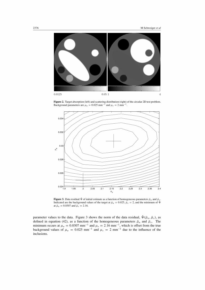
We first consider a 2D test problem of recovering the parameter distributions of µa and µs

in a circular object of radius 25 mm, shown in figure 2. A total of 32 source sites areplaced at equidistant angular spacing along the surface, and 32 detector sites are placed sothat each detector is located between two source sites. For each source, measurements areproduced at all detector sites except the two sites closest to the source, leading to a total of 960measurements. We consider sources to be intensity modulated with a frequency of 50 MHz,and each measurement consisting of the logarithmic modulation amplitude yA

i and phase shifty

ϕ

i . The target data y = (yA, yϕ) are calculated with the FEM diffusion forward modelusing a mesh consisting of 7261 ten-noded triangles and 32 971 nodes, defining a piecewisequadratic unstructured basis expansion. Both yA and yϕ are then contaminated with 1%additive Gaussian random noise.

For the reconstruction we use homogeneous distributions for the initial estimates of opticalcoefficients, µ(0)

a (r) = µa and µ(0)s (r) = µs , which are obtained from a global fit of the two


0.0125 0.05 1 4

Figure 2. Target absorption (left) and scattering distribution (right) of the circular 2D test problem.Background parameters are µa = 0.025 mm−1 and µs = 2 mm−1.

1.9 1.95 2 2.05 2.1 2.15 2.2 2.25 2.3 2.35 2.40.024

0.026

0.028

0.03

0.032

0.034

µs

µ a

Figure 3. Data residual � of initial estimate as a function of homogeneous parameters µa and µs .Indicated are the background values of the target at µa = 0.025, µs = 2, and the minimum of �

at µa = 0.0307 and µs = 2.16.

parameter values to the data. Figure 3 shows the norm of the data residual, �(µa, µs), asdefined in equation (42), as a function of the homogeneous parameters µa and µs . Theminimum occurs at µa = 0.0307 mm−1 and µs = 2.16 mm−1, which is offset from the truebackground values of µa = 0.025 mm−1 and µs = 2 mm−1 due to the influence of theinclusions.


0.0125 0.05 1 4

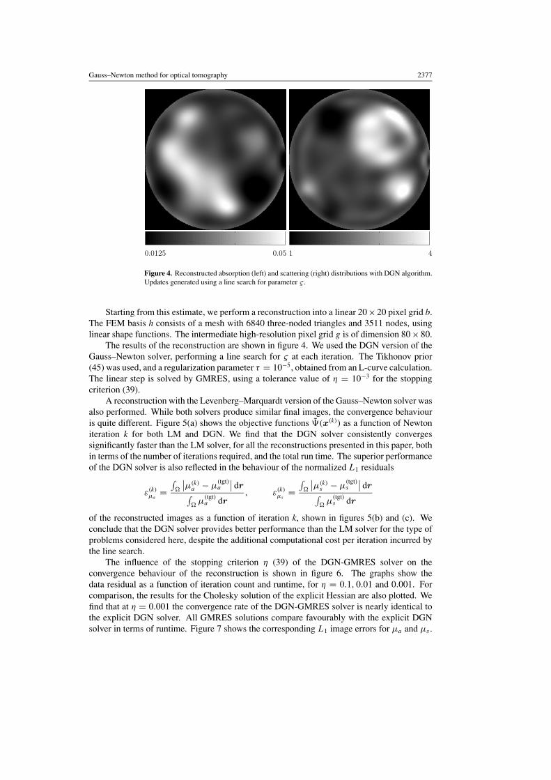
Figure 4. Reconstructed absorption (left) and scattering (right) distributions with DGN algorithm.Updates generated using a line search for parameter ς .

Starting from this estimate, we perform a reconstruction into a linear 20×20 pixel grid b.The FEM basis h consists of a mesh with 6840 three-noded triangles and 3511 nodes, usinglinear shape functions. The intermediate high-resolution pixel grid g is of dimension 80 × 80.

The results of the reconstruction are shown in figure 4. We used the DGN version of theGauss–Newton solver, performing a line search for ς at each iteration. The Tikhonov prior(45) was used, and a regularization parameter τ = 10−5, obtained from an L-curve calculation.The linear step is solved by GMRES, using a tolerance value of η = 10−3 for the stoppingcriterion (39).

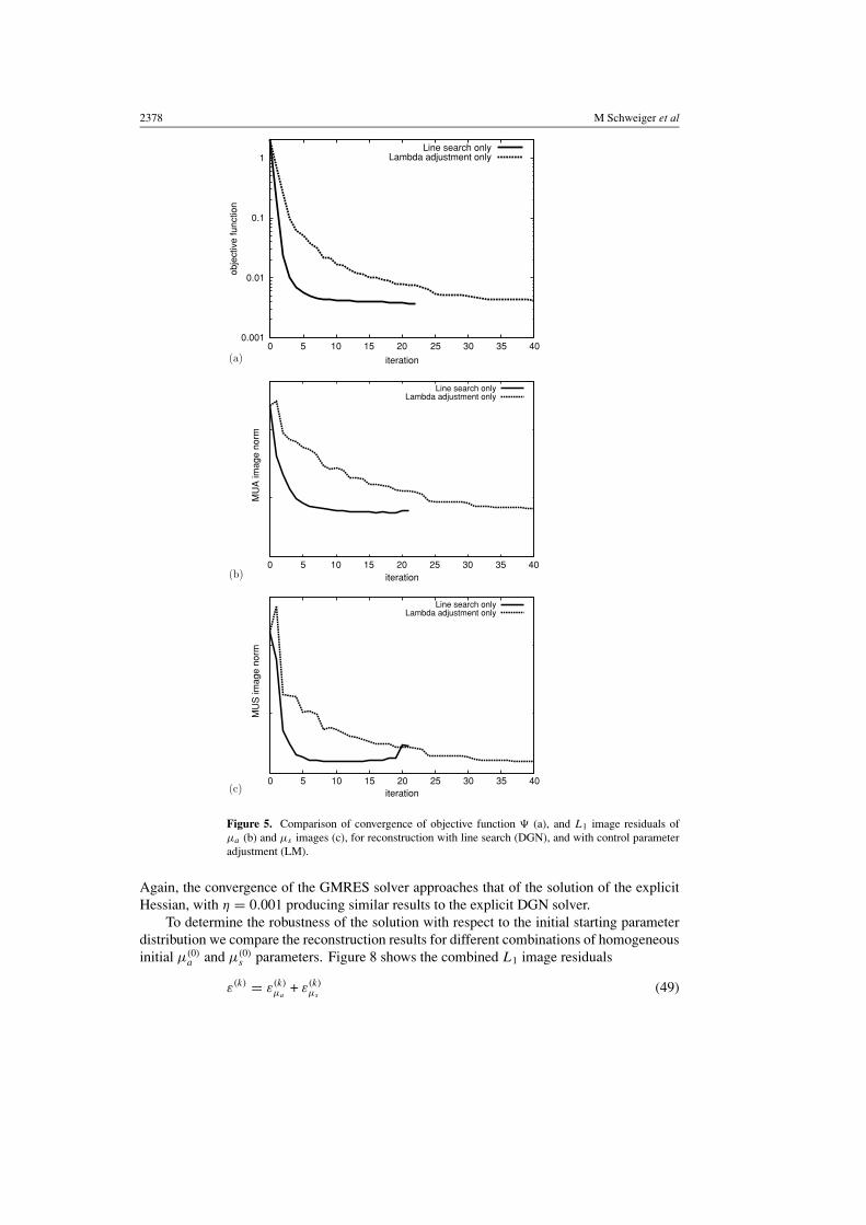
A reconstruction with the Levenberg–Marquardt version of the Gauss–Newton solver wasalso performed. While both solvers produce similar final images, the convergence behaviouris quite different. Figure 5(a) shows the objective functions �(x(k)) as a function of Newtoniteration k for both LM and DGN. We find that the DGN solver consistently convergessignificantly faster than the LM solver, for all the reconstructions presented in this paper, bothin terms of the number of iterations required, and the total run time. The superior performanceof the DGN solver is also reflected in the behaviour of the normalized L1 residuals

ε(k)µa

=∫�

∣∣µ(k)a − µ

(tgt)a

∣∣ dr∫�

µ(tgt)a dr

, ε(k)µs

=∫�

∣∣µ(k)s − µ

(tgt)s

∣∣ dr∫�

µ(tgt)s dr

of the reconstructed images as a function of iteration k, shown in figures 5(b) and (c). Weconclude that the DGN solver provides better performance than the LM solver for the type ofproblems considered here, despite the additional computational cost per iteration incurred bythe line search.

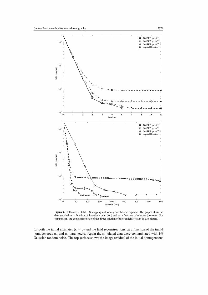
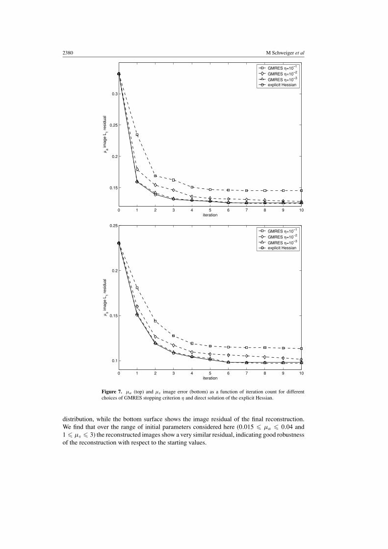
The influence of the stopping criterion η (39) of the DGN-GMRES solver on theconvergence behaviour of the reconstruction is shown in figure 6. The graphs show thedata residual as a function of iteration count and runtime, for η = 0.1, 0.01 and 0.001. Forcomparison, the results for the Cholesky solution of the explicit Hessian are also plotted. Wefind that at η = 0.001 the convergence rate of the DGN-GMRES solver is nearly identical tothe explicit DGN solver. All GMRES solutions compare favourably with the explicit DGNsolver in terms of runtime. Figure 7 shows the corresponding L1 image errors for µa and µs .


(a)

(b)

(c)

0.001

0.01

0.1

1

0 5 10 15 20 25 30 35 40

obje

ctiv

e fu

nctio

n

iteration

iteration

iteration

Line search onlyLambda adjustment only

0 5 10 15 20 25 30 35 40

MU

A im

age

norm


0 5 10 15 20 25 30 35 40

MU

S im

age

norm


Figure 5. Comparison of convergence of objective function � (a), and L1 image residuals ofµa (b) and µs images (c), for reconstruction with line search (DGN), and with control parameteradjustment (LM).

Again, the convergence of the GMRES solver approaches that of the solution of the explicitHessian, with η = 0.001 producing similar results to the explicit DGN solver.

To determine the robustness of the solution with respect to the initial starting parameterdistribution we compare the reconstruction results for different combinations of homogeneousinitial µ(0)

a and µ(0)s parameters. Figure 8 shows the combined L1 image residuals

ε(k) = ε(k)µa

+ ε(k)µs

(49)


0 1 2 3 4 5 6 7 8 9 1010

–3

10–2

10–1

100

iteration

data

res

idua

l

GMRES η=10–1

GMRES η=10–2

GMRES η=10–3

explicit Hessian

0 100 200 300 400 500 600 700 80010

–3

10–2

10–1

100

run time [sec]

data

res

idua

l

GMRES η=10–1

GMRES η=10–2

GMRES η=10–3

explicit Hessian

Figure 6. Influence of GMRES stopping criterion η on LM convergence. The graphs show thedata residual as a function of iteration count (top) and as a function of runtime (bottom). Forcomparison, the convergence rate of the direct solution of the explicit Hessian is also plotted.

for both the initial estimates (k = 0) and the final reconstructions, as a function of the initialhomogeneous µa and µs parameters. Again the simulated data were contaminated with 1%Gaussian random noise. The top surface shows the image residual of the initial homogeneous


0 1 2 3 4 5 6 7 8 9 10

0.15

0.2

0.25

0.3

iteration

µ a imag

e L 1 r

esid

ual

GMRES η=10–1

GMRES η=10–2

GMRES η=10–3

explicit Hessian

0 1 2 3 4 5 6 7 8 9 10

0.1

0.15

0.2

0.25

iteration

µ s imag

e L 1 r

esid

ual

GMRES η=10–1

GMRES η=10–2

GMRES η=10–3

explicit Hessian

Figure 7. µa (top) and µs image error (bottom) as a function of iteration count for differentchoices of GMRES stopping criterion η and direct solution of the explicit Hessian.

distribution, while the bottom surface shows the image residual of the final reconstruction.We find that over the range of initial parameters considered here (0.015 � µa � 0.04 and1 � µs � 3) the reconstructed images show a very similar residual, indicating good robustnessof the reconstruction with respect to the starting values.


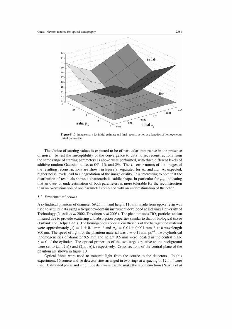
Figure 8. L1 image error ε for initial estimate and final reconstruction as a function of homogeneousinitial parameters.

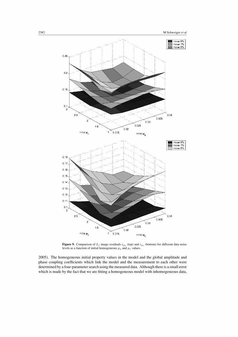
The choice of starting values is expected to be of particular importance in the presenceof noise. To test the susceptibility of the convergence to data noise, reconstructions fromthe same range of starting parameters as above were performed, with three different levels ofadditive random Gaussian noise, at 0%, 1% and 2%. The L1 error norms of the images ofthe resulting reconstructions are shown in figure 9, separated for µa and µs . As expected,higher noise levels lead to a degradation of the image quality. It is interesting to note that thedistribution of residuals shows a characteristic saddle shape, in particular for µs , indicatingthat an over- or underestimation of both parameters is more tolerable for the reconstructionthan an overestimation of one parameter combined with an underestimation of the other.

5.2. Experimental results

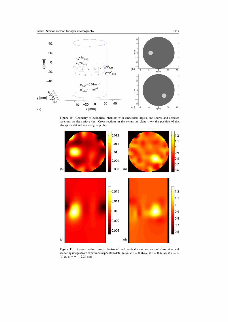
A cylindrical phantom of diameter 69.25 mm and height 110 mm made from epoxy resin wasused to acquire data using a frequency-domain instrument developed at Helsinki University ofTechnology (Nissila et al 2002, Tarvainen et al 2005). The phantom uses TiO2 particles and aninfrared dye to provide scattering and absorption properties similar to that of biological tissue(Firbank and Delpy 1993). The homogeneous optical coefficients of the background materialwere approximately µ′

s = 1 ± 0.1 mm−1 and µa = 0.01 ± 0.001 mm−1 at a wavelength800 nm. The speed of light for the phantom material was c = 0.19 mm ps−1. Two cylindricalinhomogeneities of diameter 9.5 mm and height 9.5 mm were located in the central planez = 0 of the cylinder. The optical properties of the two targets relative to the backgroundwere set to (µa, 2µ′

s) and (2µa,µ′s), respectively. Cross sections of the central plane of the

phantom are shown in figure 10.Optical fibres were used to transmit light from the source to the detectors. In this

experiment, 16 source and 16 detector sites arranged in two rings at a spacing of 12 mm wereused. Calibrated phase and amplitude data were used to make the reconstructions (Nissila et al


Figure 9. Comparison of L1 image residuals εµa (top) and εµs (bottom) for different data noiselevels as a function of initial homogeneous µa and µs values.

2005). The homogeneous initial property values in the model and the global amplitude andphase coupling coefficients which link the model and the measurement to each other weredetermined by a four-parameter search using the measured data. Although there is a small errorwhich is made by the fact that we are fitting a homogeneous model with inhomogeneous data,


(a)

–40 –20 0 20 40–40–20

020

40

–40

–20

0

20

40

µa=µ

a,bg

µ’s=2µ’

s,bg

x [mm]

µa,bg

≈ 0.01mm–1

µ’s,bg

≈ 1mm–1

µa=2µ

a,bg

µ’s=µ’

s,bg

y [mm]

z [m

m]

(b) –40 –20 0 20 40

–30

–20

–10

0

10

20

30

x [mm]

y [m

m]

(c) –40 –20 0 20 40

–30

–20

–10

0

10

20

30

x [mm]

y [m

m]

Figure 10. Geometry of cylindrical phantom with embedded targets, and source and detectorlocations on the surface (a). Cross sections in the central xy plane show the position of theabsorption (b) and scattering target (c).

(a) (b)

(c) (d)

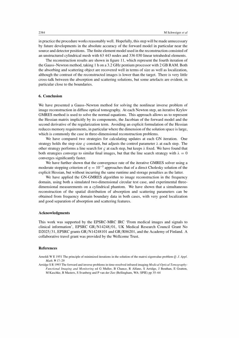
Figure 11. Reconstruction results: horizontal and vertical cross sections of absorption andscattering images from experimental phantom data. (a) µa at z = 0, (b) µs at z = 0, (c) µa at y = 0,(d) µs at y = −12.24 mm.


in practice the procedure works reasonably well. Hopefully, this step will be made unnecessaryby future developments in the absolute accuracy of the forward model in particular near thesource and detector positions. The finite element model used in the reconstruction consisted ofan unstructured cylindrical mesh with 63 443 nodes and 336 030 linear tetrahedral elements.

The reconstruction results are shown in figure 11, which represent the fourth iteration ofthe Gauss–Newton method, taking 1 h on a 3.2 GHz pentium processor with 2 GB RAM. Boththe absorbing and scattering object are recovered well in terms of size as well as localization,although the contrast of the reconstructed images is lower than the target. There is very littlecross-talk between the absorption and scattering solutions, but some artefacts are evident, inparticular close to the boundaries.

6. Conclusion

We have presented a Gauss–Newton method for solving the nonlinear inverse problem ofimage reconstruction in diffuse optical tomography. At each Newton step, an iterative KrylovGMRES method is used to solve the normal equations. This approach allows us to representthe Hessian matrix implicitly by its components, the Jacobian of the forward model and thesecond derivative of the regularization term. Avoiding an explicit formulation of the Hessianreduces memory requirements, in particular where the dimension of the solution space is large,which is commonly the case in three-dimensional reconstruction problems.

We have compared two strategies for calculating updates at each GN iteration. Onestrategy holds the step size ς constant, but adjusts the control parameter λ at each step. Theother strategy performs a line search for ς at each step, but keeps λ fixed. We have found thatboth strategies converge to similar final images, but that the line search strategy with λ = 0converges significantly faster.

We have further shown that the convergence rate of the iterative GMRES solver using amoderate stopping criterion of η = 10−3 approaches that of a direct Cholesky solution of theexplicit Hessian, but without incurring the same runtime and storage penalties as the latter.

We have applied the GN-GMRES algorithm to image reconstruction in the frequencydomain, using both a simulated two-dimensional circular test case, and experimental three-dimensional measurements on a cylindrical phantom. We have shown that a simultaneousreconstruction of the spatial distribution of absorption and scattering parameters can beobtained from frequency domain boundary data in both cases, with very good localizationand good separation of absorption and scattering features.

Acknowledgments

This work was supported by the EPSRC-MRC IRC ‘From medical images and signals toclinical information’, EPSRC GR/N14248/01, UK Medical Research Council Grant NoD2025/31, EPSRC grants GR/N14248101 and GR/R86201, and the Academy of Finland. Acollaborative travel grant was provided by the Wellcome Trust.

References

Arnoldi W E 1951 The principle of minimized iterations in the solution of the matrxi eigenvalue problem Q. J. Appl.Math. 9 17–29

Arridge S R 1993 The forward and inverse problems in time-resolved infrared imaging Medical Optical Tomography:Functional Imaging and Monitoring ed G Muller, B Chance, R Alfano, S Arridge, J Beuthan, E Gratton,M Kaschke, B Masters, S Svanberg and P van der Zee (Bellingham, WA: SPIE) pp 35–64


Arridge S R 1995 Photon measurement density functions: Part 1. Analytical forms Appl. Opt. 34 7395–409Arridge S R 1999 Optical tomography in medical imaging Inverse Problems 15 R41–92Arridge S R and Hebden J C 1997 Optical imaging in medicine: II. Modelling and reconstruction Phys. Med. Biol.

42 841–53Arridge S R and Schweiger M 1998 A gradient-based optimisation scheme for optical tomography Opt. Express 2

213–26 (http://www.epubs.osa.org/oearchive/source/4014htm)Arridge S R, Schweiger M and Delpy D T 1992 Iterative reconstruction of near-infrared absorption images Inverse

Problems in Scattering and Imaging (Proc. SPIE vol 1767) ed M A Fiddy pp 372–83Arridge S R, Schweiger M, Hiraoka M and Delpy D T 1993 A finite element approach for modeling photon transport

in tissue Med. Phys. 20 299–309Arridge S R, van der Zee P, Delpy D T and Cope M 1991 Reconstruction methods for infra-red absorption imaging

Time-Resolved Spectroscopy and Imaging of Tissues (Proc. SPIE vol 1431) ed B Chance and A Katzirpp 204–15

Barbour R L, Graber H L, Lubowsky J and Aronson R 1990 Model for 3-D optical imaging of tissue 10th AnnualIEEE International Geoscience and Remote Sensing Symposium (IGARSS) vol 2 ed J Ormsby pp 1395–9

Boas D A, Brooks D H, Miller E L, DiMarzio C A, Kilmer M, Gaudette R J and Zhang Q 2001 Imaging the bodywith diffuse optical tomography IEEE Signal Process. Mag. 57–75

Dehghani H, Pogue B W, Poplack S P and Paulsen K D 2003 Multiwavelength three-dimensional near-infraredtomography of the breast: initial simulation, phantom, and clinical results Appl. Opt. 42

Dennis J E and Schnabel R B 1983 Numerical Methods for Unconstrained Optimization and Nonlinear Equations(Englewood Cliffs, NJ: Prentice-Hall)

Dorn O 1998 A transport-backtransport method for optical tomography Inverse Problems 14 1107–30Eppstein M J, Dougherty D E, Hawysz D J and Sevick-Muraca E M 2001 Three-dimensional Bayesian optical image

reconstruction with domain decomposition IEEE Trans. Med. Imaging 20 147–63Firbank M and Delpy D T 1993 A design for a stable and reproducible phantom for use in near infrared imaging and

spectroscopy Phys. Med. Biol. 38 847–53Gibson A, Hebden J C and Arridge S R 2005 Recent advances in diffuse optical tomography Phys. Med. Biol. 50

R1–43Hansen P C and O’Leary D P 1993 The use of the L-curve in the regularization of discrete ill-posed problems

SIAM J. Sci. Comput. 14 1487–503Hawysz D and Sevick-Muraca E M 2000 Developments towards diagnostic breast cancer imaging using near-infrared

optical measurements and fluorescent contrast agents Neoplasia 2 388–417Hebden J C, Arridge S R and Delpy D T 1997 Optical imaging in medicine: I. Experimental techniques Phys. Med.

Biol. 42 825–40Klose A D and Hielscher A H 1999 Iterative reconstruction scheme for optical tomography based on the equation of

radiative transfer Med. Phys. 26 1698–707Klose A D and Hielscher A H 2003 Quasi-Newton methods in optical tomographic image reconstruction Inverse

Problems 19 387–409Markel V A and Schotland J C 2001 Inverse problem in optical diffusion tomography: I. Fourier Laplace inversion

formulas J. Opt. Soc. Am. A 18 1336–47Markel V and Schotland J C 2002 Inverse problem in optical diffusion tomography: II. Role of boundary conditions

J. Opt. Soc. Am. A 19 558–66Marquardt D W 1963 An algorithm for least-squares estimation of nonlinear parameters J. SIAM 11 431–41Moulton J D 1990 Diffusion modelling of picosecond laser pulse propagation in turbid media M. Eng. Thesis

McMaster University, Hamilton, OntarioNissila I, Kotilahti K, Fallstrom K and Katila T 2002 Instrumentation for the accurate measurement of phase and

amplitude in optical tomography Rev. Sci. Instrum. 73 3306–12Nissila I, Noponen T, Kotilahti K, Tarvainen T, Schweiger M, Lipiainen L, Arridge S R and Katila T 2005

Instrumentation and calibration methods for the multichannel measurement of phase and amplitude in opticaltomography Rev. Sci. Instrum. 76 044302

O’Leary M A 1996 Imaging with diffuse photon density waves PhD Thesis University of PennsylvaniaO’Leary M A, Boas D A, Chance B and Yodh A G 1995 Experimental images of heterogeneous turbid media by

frequency-domain diffusing-photon tomography Opt. Lett. 20 426–8Paulsen K D and Jiang H 1995 Spatially-varying optical property reconstruction using a finite element diffusion

equation approximation Med. Phys. 22 691–701Ripoll J, Ntziachristos V and Nieto-Vesperinas M 2001 The Kirchoff approximation for diffusive waves Phys. Rev. E

64 1–8Roy R and Sevick-Muraca E M 1999 Truncated Newton’s optimization scheme for absorption and fluorescence optical

tomography: Part I. Theory and formulation Opt. Express 4 353–71


Saad Y and Schultz M H 1986 GMRES: a generalized minimal residual algorithm for solving nonsymmetric linearsystems SIAM J. Sci. Stat. Comput. 7 856–69

Schotland J C 1997 Continuous-wave diffusion imaging J. Opt. Soc. Am. A 14 275–9Schotland J C, Haselgrove J C and Leigh J S 1993 Photon hitting density Appl. Opt. 32 448–53Schotland J C and Markel V 2001 Inverse scattering with diffusing waves J. Opt. Soc. Am. A 18 2767–77Schweiger M and Arridge S R 1999 Application of temporal filters to time resolved data in optical tomgraphy

Phys. Med. Biol. 44 1699–717Schweiger M and Arridge S R 2003 Image reconstruction in optical tomography using local basis functions J. Electron.

Imaging 12 583–93Schweiger M, Arridge S R and Delpy D T 1993 Application of the finite-element method for the forward and inverse

models in optical tomography J. Math. Imag. Vision 3 263–83Schweiger M, Arridge S R, Hiraoka M and Delpy D T 1995 The finite element model for the propagation of light in

scattering media: boundary and source conditions Med. Phys. 22 1779–92Tarvainen T, Kolehmainen V, Vauhkonen M, Vanne A, Gibson A P, Schweiger M, Arridge S R and Kaipio J P 2005

Computational calibration method for optical tomography Appl. Opt. 44 1879–88Vogel C 2002 Computational Methods for Inverse Problems (Society for Industrial and Applied Mathematics)Walker S A, Fantini S and Gratton E 1997 Image reconstruction by backprojection from frequency-domain optical

measurements in highly scattering media Appl. Opt. 36 170–9Wang Y, Chang J-H, Aronson R, Barbour R L, Graber H L and Lubowsky J 1992 Imaging of scattering media

by diffusion tomography: an iterative perturbation approach Physiological Monitoring and Early DetectionDiagnostic Methods (Proc. SPIE vol 1641) ed T S Mang pp 58–71

Yodh A and Chance B 1995 Spectroscopy and imaging with diffusing light Phys. Today 48 34–40Ye J C, Bouman C A, Webb K J and Millane R P 2001 Nonlinear multigrid algorithms for bayesian optical diffusion

tomography IEEE Trans. Image Proc. 10 909–22Zienkiewicz O C and Taylor R L 1987 The Finite Element Method 4th edn (London: McGraw-Hill)

Documents

Gauss Newton method for image reconstruction in diffuse optical tomography