Embed Size (px)
Citation preview
arX
iv:h
ep-t
h/05
0521
1v3
12
Dec
200
5
Preprint typeset in JHEP style. - HYPER VERSION
MIT-CTP-3646, CERN-PH-TH/2005-084, HUTP-05/A0027
Gauge Theories from Toric Geometry and Brane
Tilings
Sebastian Franco1, Amihay Hanany1, Dario Martelli2, James Sparks3, David Vegh1,
and Brian Wecht1
1. Center for Theoretical Physics, Massachusetts Institute of Technology,
Cambridge, MA 02139, USA.
2. Department of Physics, CERN Theory Division, 1211 Geneva 23, Switzerland.
3. Department of Mathematics, Harvard University,
One Oxford Street, Cambridge, MA 02318, U.S.A.
and
Jefferson Physical Laboratory, Harvard University, Cambridge, MA 02138, U.S.A.
[email protected], [email protected], [email protected],
[email protected], [email protected], [email protected]
Abstract: We provide a general set of rules for extracting the data defining a quiver gauge
theory from a given toric Calabi–Yau singularity. Our method combines information from the
geometry and topology of Sasaki–Einstein manifolds, AdS/CFT, dimers, and brane tilings.
We explain how the field content, quantum numbers, and superpotential of a superconformal
gauge theory on D3–branes probing a toric Calabi–Yau singularity can be deduced. The
infinite family of toric singularities with known horizon Sasaki–Einstein manifolds La,b,c is
used to illustrate these ideas. We construct the corresponding quiver gauge theories, which
may be fully specified by giving a tiling of the plane by hexagons with certain gluing rules.
As checks of this construction, we perform a-maximisation as well as Z-minimisation to
compute the exact R-charges of an arbitrary such quiver. We also examine a number of
examples in detail, including the infinite subfamily La,b,a, whose smallest member is the
Suspended Pinch Point.
1
Contents
1. Introduction 1
2. Quiver content from toric geometry 4
2.1 General geometrical set–up 4
2.2 Quantum numbers of fields 7
2.2.1 Multiplicities 8
2.2.2 Baryon charges 9
2.2.3 Flavour charges 11
2.2.4 R–charges 12
3. The La,b,c toric singularities 13
3.1 The sub–family La,b,a 16
3.2 Quantum numbers of fields 18
3.3 The geometry 19
4. Superpotential and gauge groups 24
4.1 The superpotential 24
4.2 The gauge groups 25
5. R–charges from a–maximisation 26
6. Constructing the gauge theories using brane tilings 28
6.1 Seiberg duality and transformations of the tiling 29
6.2 Explicit examples 30
6.2.1 Gauge theory for L2,6,3 31
6.2.2 Generating D hexagons by Seiberg duality: L2,6,4 32
6.2.3 The La,b,a sub–family 33
7. Conclusions 37
8. Acknowledgements 38
0
9. Appendix: More examples 39
9.1 Brane tiling and quiver for L1,5,2 39
9.2 Brane tiling and quiver for L1,7,3 40
1. Introduction
Gauge theories arise within string theory in a variety of different ways. One possible ap-
proach, which is particularly interesting due to its relationship with different branches of
geometry, is to use D–branes to probe a singularity. The geometry of the singularity then
determines the amount of supersymmetry, the gauge group structure, the matter content
and the superpotential interactions on the worldvolume of the D–branes. The richest of
such examples which are both tractable, using current techniques, and also non–trivial, are
given by the d = 4 N = 1 gauge theories that arise on a stack of D3–branes probing a
singular Calabi–Yau 3–fold. There has been quite remarkable progress over the last year in
understanding these theories, especially in the case where the Calabi–Yau singularity is also
toric. In this case one can use toric geometry, which by now is an extremely well–developed
subject, to study the gauge theories. In fact part of this paper is devoted to pushing this
further and we will show how one can use arguments in toric geometry and topology to
derive much of the field content of a D3–brane probing a toric Calabi–Yau singularity in a
very simple manner, using essentially only the toric diagram and associated gauged linear
sigma model.
At low energies the theory on the D3–brane is expected to flow to a superconformal fixed
point. The AdS/CFT correspondence [1, 2, 3] connects the strong coupling regime of such
gauge theories with supergravity in a mildly curved geometry. For the case of D3–branes
placed at the tips of Calabi–Yau cones over five–dimensional geometries Y5, the gravity dual
is of the form AdS5 × Y5, where Y5 is a Sasaki–Einstein manifold [4, 5, 6, 7]. There has
been considerable progress in this subject recently: for a long time, there was only one
non–trivial Sasaki–Einstein five–manifold, T 1,1, where the metric was known. Thanks to
recent progress, we now have an infinite family of explicit metrics which, when non–singular
and simply–connected, have topology S2 × S3. The most general such family is specified
by 3 positive integers a, b, c, with the metrics denoted La,b,c [8, 9]1. When a = p − q, b =
1We have changed the notation to La,b,c to avoid confusion with the p and q of Y p,q. In our notation,
Y p,q is Lp+q,p−q,p.
1
p + q, c = p these reduce to the Y p,q family of metrics, which have an enhanced SU(2)
isometry [10, 11, 12]. Aided by the toric description in [12], the entire infinite family of gauge
theories dual to these metrics was constructed in [13]. These theories have subsequently been
analysed in considerable detail [14, 15, 16, 17, 18, 19, 20, 21, 22, 23, 24, 25, 26]. There has also
been progress on the non–conformal extensions of these theories (and others) both from the
supergravity [14, 22] and gauge theory sides [20, 21, 23, 24, 26, 27]. These extensions exhibit
many interesting features, such as cascades [28] and dynamical supersymmetry breaking.
In addition to the Y p,q spaces, there are also several other interesting infinite families of
geometries which have been studied recently: theXp,q spaces [29], deformations of geometries
with U(1)×U(1) isometry [18], and deformations of geometries with U(1)3 isometry [30, 31].
Another key ingredient in obtaining the gauge theories dual to singular Calabi–Yau
manifolds is the principle of a–maximisation [32], which permits the determination of exact
R–charges of superconformal field theories. Recall that all d = 4 N = 1 gauge theories
possess a U(1)R symmetry which is part of the superconformal group SU(2, 2|1). If this
superconformal R–symmetry is correctly identified, many properties of the gauge theory may
be determined. a–maximisation [32] is a simple procedure – maximizing a cubic function
– that allows one to identify the R–symmetry from among the set of global symmetries of
any given gauge theory. Plugging the superconformal R-charges into this cubic function
gives exactly the central charge a of the SCFT [33, 34, 35]. Although here we will focus on
superconformal theories with known geometric duals, a–maximization is a general procedure
which applies to any N = 1 d = 4 superconformal field theory, and has been studied in
this context in a number of recent works, with much emphasis on its utility for proving the
a–theorem [38, 39, 40, 41, 42, 43, 44].
In the case that the gauge theory has a geometric dual, one can use the AdS/CFT
correspondence to compute the volume of the dual Sasaki–Einstein manifold, as well as
the volumes of certain supersymmetric 3–dimensional submanifolds, from the R–charges.
For example, remarkable agreement was found for these two computations in the case of
the Y p,q singularities [45, 13]. Moreover, a general geometric procedure that allows one to
compute the volume of any toric Sasaki–Einstein manifold, as well as its toric supersymmetric
submanifolds, was then given in [46]. In [46] it was shown that one can determine the Reeb
vector field, which is dual to the R–symmetry, of any toric Sasaki–Einstein manifold by
minimising a function Z that depends only on the toric data that defines the singularity.
For example, the volumes of the Y p,q manifolds are easily reproduced this way. Remarkably,
one can also compute the volumes of manifolds for which the metric is not known explicitly.
In all cases agreement has been found between the geometric and field theoretic calculations.
2
This was therefore interpreted as a geometric dual of a–maximisation in [46], although to date
there is no general proof that the two extremal problems, within the class of superconformal
gauge theories dual to toric Sasaki–Einstein manifolds, are in fact equivalent.
Another important step was achieved recently by the introduction of dimer technololgy
as a tool for studying N = 1 gauge theories. Although it has been known in principle how
to compute toric data dual to a given SCFT and vice versa [36, 37], these computations
are often very computationally expensive, even for fairly small quivers. Dimer technology
greatly simplifies this process, and turns previously intractable calculations into easily solved
problems. The initial connection between toric geometry and dimers was suggested in [47];
the connection to N = 1 theories was proposed and explored in [48]. A crucial realization
that enables one to use this tool is that all the data for an N = 1 theory can be simply
represented as a periodic tiling (“brane tiling”) of the plane by polygons with an even
number of sides: the faces represent gauge groups, the edges represent bifundamentals, and
the vertices represent superpotential terms. This tiling has a physical meaning in Type
IIB string theory as an NS5–brane wrapping a holomorphic curve (the edges of the tiling)
with D5–branes (the faces) ending on the NS5–brane. The fact that the polygons have an
even number of sides is equivalent to the requirement that the theories be anomaly free;
by choosing an appropriate periodicity, one can color the vertices of such a graph with two
colours (say, black and white) so that a black vertex is adjacent only to white vertices. Edges
that stretch between black and white nodes are the dimers, and there is a simple prescription
for computing a weighted adjacency matrix (the Kasteleyn matrix) which gives the partition
function for a given graph. This partition function encodes the toric diagram for the dual
geometry in a simple way, thus enabling one to have access to many properties of both the
gauge theory and the geometry. The tiling construction of a gauge theory is a much more
compact way of describing the theory than the process of specifying both a quiver and the
superpotential, and we will use this newfound simplicitly rather extensively in this paper.
In this paper, we will use this recent progress in geometry, field theory, and dimer
models to obtain a lot of information about gauge theories dual to general toric Calabi-
Yau cones. Our geometrical knowledge will specify many requirements of the gauge theory,
and we describe how one can read off gauge theory quantities rather straightforwardly from
the geometry. As a particular example of our methods, we construct the gauge theories
dual to the recently discovered La,b,c geometries. We will realize the geometrically derived
requirements by using the brane tiling approach. Since the La,b,c spaces are substantially
more complicated than the Y p,q’s, we will not give a closed form expression for the gauge
theory. We will, however, specify all the necessary building blocks for the brane tiling, and
3
discuss how these building blocks are related to quantities derived from the geometry.
The plan of the paper is as follows: In Section 2, we discuss how to read gauge theory data
from a given toric geometry. In particular, we give a detailed prescription for computing the
quantum numbers (e.g. baryon charges, flavour charges, and R–charges) and multiplicities
for the different fields in the gauge theory. Section 3 applies these results to the La,b,c spaces.
We derive the toric diagram for a general La,b,c geometry, and briefly review the metrics [8, 9]
for these theories. We compute the volumes of the supersymmetric 3–cycles in these Sasaki–
Einstein spaces, and discuss the constraints these put on the gauge theories. In Section
4 we discuss how our geometrical computations constrain the superpotential, and describe
how one may always find a phase of the gauge theory with at most only three different
types of interactions. In Section 5, we prove that a–maximisation reduces to the same
equations required by the geometry for computing R-charges and central charges. Thus we
show that a–maximisation and the geometric computation agree. In Section 6, we construct
the gauge theories dual to the La,b,c spaces by using the brane tiling perspective, and give
several examples of interesting theories. In particular, we describe a particularly simple
infinite subclass of theories, the La,b,a theories, for which we can simply specify the toric
data and brane tiling. We check via Z–minimisation and a–maximisation that all volumes
and dimensions reproduce the results expected from AdS/CFT. Finally, in the Appendix,
we give some more interesting examples which use our construction.
Note: While this paper was being finalised, we were made aware of other work in [49],
which has some overlap with our results. Similar conclusions have been reached in [50].
2. Quiver content from toric geometry
In this section we explain how one can extract a considerable amount of information about the
gauge theories on D3–branes probing toric Calabi–Yau singularities using simple geometric
methods. In particular, we show that there is always a distinguished set of fields whose
multiplicities, baryon charges, and flavour charges can be computed straightforwardly using
the toric data.
2.1 General geometrical set–up
Let us first review the basic geometrical set–up. For more details, the reader is referred to
[46]. Let (X,ω) be a toric Calabi–Yau cone of complex dimension n, where ω is the Kahler
form on X. In particular X = C(Y ) ∼= IR+×Y has an isometry group containing an n–torus,
T n. A conical metric on X which is both Ricci–flat and Kahler then gives a Sasaki–Einstein
4
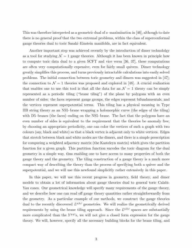
metric on the base of the cone, Y . The moment map for the torus action exhibits X as a
Lagrangian T n fibration over a strictly convex rational polyhedral cone C ⊂ IRn. This is a
subset of IRn of the form
C = y ∈ IRn | (y, vA) ≥ 0, A = 1, . . . , D . (2.1)
Thus C is made by intersecting D hyperplanes through the origin in order to make a convex
polyhedral cone. Here y ∈ IRn are coordinates on IRn and vA are the inward pointing normal
vectors to the D hyperplanes, or facets, that define the polyhedral cone. The normals are
rational and hence one can normalise them to be primitive2 elements of the lattice ZZn. We
also assume this set of vectors is minimal in the sense that removing any vector vA in the
definition (2.1) changes C. The condition that C be strictly convex is simply the condition
that it is a cone over a convex polytope.
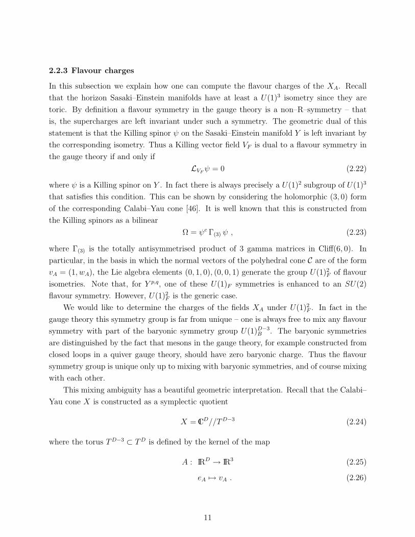
Figure 1: A four–faceted polyhedral cone in IR3.
The condition that X is Calabi–Yau, c1(X) = 0, implies that the vectors vA may, by
an appropriate SL(n; ZZ) transformation of the torus, be all written as vA = (1, wA). In
particular, in complex dimension n = 3 we may therefore represent any toric Calabi–Yau
cone by a convex lattice polytope in ZZ2, where the vertices are simply the vectors wA. This
is usually called the toric diagram.
From the vectors vA one can reconstruct X as a Kahler quotient or, more physically, as
the classical vacuum moduli space of a gauged linear sigma model (GLSM). To explain this,
denote by Λ ⊂ ZZn the span of the normals vA over ZZ. This is a lattice of maximal rank
since C is strictly convex. Consider the linear map
A : IRD → IRn
eA 7→ vA (2.2)
2A vector v ∈ ZZn is primitive if it cannot be written as mv′ with v′ ∈ ZZn and ZZ ∋ m > 1.
5
which maps each standard orthonormal basis vector eA of IRD to the vector vA. This induces
a map of tori
TD ∼= IRD/ZZD → IRn/Λ . (2.3)
In general the kernel of this map is A ∼= TD−n × Γ where Γ is a finite abelian group. Then
X is given by the Kahler quotient
X = CD//A . (2.4)
Recall we may write this more explicitly as follows. The torus TD−n ⊂ TD is specified by a
charge matrix QAI with integer coefficients, I = 1, . . . , D − n, and we define
K ≡
(Z1, . . . , ZD) ∈CD |∑
A
QAI |ZA|2 = 0
⊂CD (2.5)
where ZA denote complex coordinates on CD. In GLSM language, K is simply the space of
solutions to the D–term equations. Dividing out by gauge transformations gives the quotient
X = K/TD−n × Γ . (2.6)
We also denote by L the link of K with the sphere S2D−1 ⊂CD. We then have a fibration
A → L→ Y (2.7)
where Y is the Sasakian manifold which is the base of the cone X = C(Y ). For a general set
of vectors vA, the space Y will not be smooth. In fact typically one has orbifold singularities.
Y is smooth if and only if the polyhedral cone is good [51], although we will not enter into
the general details of this here – see, for example, [46].
Finally in this subsection we note some topological properties of Y , in the case that Y is
a smooth manifold. In [52] it is shown that L has trivial homotopy groups in dimensions 0,
1 and 2. From the long exact homotopy sequence for the fibration (2.7) one concludes that
[52]
π1(Y ) ∼= π0(A) ∼= Γ ∼= ZZn/Λ (2.8)
π2(Y ) ∼= π1(A) ∼= ZZD−n .
In particular, Y is simply–connected if and only if the vA span ZZn over ZZ. In fact we will
assume this throughout this paper – any finite quotient of a toric singularity will correspond
to an orbifold of the corresponding gauge theory, and this process is well–understood by
now.
6
From now on we also restrict to the physical case of complex dimension n = 3. Moreover,
throughout this section we assume that the Sasaki–Einstein manifold Y is smooth. The
reason for this assumption is firstly to simplify the geometrical and topological analysis, and
secondly because the physics in the case that Y is an orbifold which is not a global quotient of
a smooth manifold is not well–understood. However, as we shall see later, one can apparently
relax this assumption with the results essentially going through without modification. The
various cohomology groups that we introduce would then need replacing by their appropriate
orbifold versions.
2.2 Quantum numbers of fields
In this subsection we explain how one can deduce the quantum numbers for a certain dis-
tinguished set of fields in any toric quiver gauge theory. Recall that, quite generally, N
D3–branes placed at a toric Calabi–Yau singularity have an AdS/CFT dual that may be
described by a toric quiver gauge theory. In particular, the matter content is specified by
giving the number of gauge groups, Ng, and number of fields Nf , together with the charge
assignments of the fields. In fact these fields are always bifundamentals (or adjoints). This
means that the matter content may be neatly summarised by a quiver diagram.
We may describe the toric singularity as a convex lattice polytope in ZZ2 or by giving
the GLSM charges, as described in the previous section. By setting each complex coordinate
ZA = 0, A = 1, . . . , D, one obtains a toric divisor DA in the Calabi–Yau cone. This is also
a cone, with DA = C(ΣA) where ΣA is a 3–dimensional supersymmetric submanifold of Y .
Thus in particular wrapping a D3–brane over ΣA gives rise to a BPS state, which via the
AdS/CFT correspondence is conjectured to be dual to a dibaryonic operator in the dual
gauge theory. We claim that there is always a distinguished subset of the fields, for any toric
quiver gauge theory, which are associated to these dibaryonic states. To explain this, recall
that given any bifundamental field X, one can construct the dibaryonic operator
B[X] = ǫα1...αNXβ1
α1. . .XβN
αNǫβ1...βN
(2.9)
using the epsilon tensors of the corresponding two SU(N) gauge groups. This is dual to
a D3–brane wrapped on a supersymmetric submanifold, for example one of the ΣA. In
fact to each toric divisor ΣA let us associate a bifundamental field XA whose corresponding
dibaryonic operator (2.9) is dual to a D3–brane wrapped on ΣA. These fields in fact have
multiplicities, as we explain momentarily. In particular each field in such a multiplet has the
same baryon charge, flavour charge, and R–charge.
7
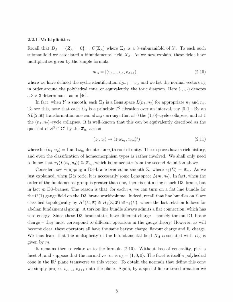
2.2.1 Multiplicities
Recall that DA = ZA = 0 = C(ΣA) where ΣA is a 3–submanifold of Y . To each such
submanifold we associated a bifundamental field XA. As we now explain, these fields have
multiplicities given by the simple formula
mA = |(vA−1, vA, vA+1)| (2.10)
where we have defined the cyclic identification vD+1 = v1, and we list the normal vectors vA
in order around the polyhedral cone, or equivalently, the toric diagram. Here (·, ·, ·) denotes
a 3 × 3 determinant, as in [46].
In fact, when Y is smooth, each ΣA is a Lens space L(n1, n2) for appropriate n1 and n2.
To see this, note that each ΣA is a principle T 2 fibration over an interval, say [0, 1]. By an
SL(2; ZZ) transformation one can always arrange that at 0 the (1, 0)–cycle collapses, and at 1
the (n1, n2)–cycle collapses. It is well–known that this can be equivalently described as the
quotient of S3 ⊂C2 by the ZZn1action
(z1, z2) → (z1ωn1, z2ω
n2n1
) (2.11)
where hcf(n1, n2) = 1 and ωn1denotes an n1th root of unity. These spaces have a rich history,
and even the classification of homeomorphism types is rather involved. We shall only need
to know that π1(L(n1, n2)) ∼= ZZn1, which is immediate from the second definition above.
Consider now wrapping a D3–brane over some smooth Σ, where π1(Σ) = ZZm. As we
just explained, when Σ is toric, it is necessarily some Lens space L(m,n2). In fact, when the
order of the fundamental group is greater than one, there is not a single such D3–brane, but
in fact m D3–branes. The reason is that, for each m, we can turn on a flat line bundle for
the U(1) gauge field on the D3–brane worldvolume. Indeed, recall that line bundles on Σ are
classified topologically by H2(Σ; ZZ) ∼= H1(Σ; ZZ) ∼= π1(Σ), where the last relation follows for
abelian fundamental group. A torsion line bundle always admits a flat connection, which has
zero energy. Since these D3–brane states have different charge – namely torsion D1–brane
charge – they must correspond to different operators in the gauge theory. However, as will
become clear, these operators all have the same baryon charge, flavour charge and R–charge.
We thus learn that the multiplicity of the bifundamental field XA associated with DA is
given by m.
It remains then to relate m to the formula (2.10). Without loss of generality, pick a
facet A, and suppose that the normal vector is vA = (1, 0, 0). The facet is itself a polyhedral
cone in the IR2 plane transverse to this vector. To obtain the normals that define this cone
we simply project vA−1, vA+1 onto the plane. Again, by a special linear transformation we
8
may take these 2–vectors to be (0, 1), (n1,−n2), respectively, for some integers n1 and n2.
One can then verify that this toric diagram indeed corresponds to the cone over L(n1, n2),
as defined above. By direct calculation we now see that
|(vA−1, vA, vA+1)| = |(0, 1) × (n1,−n2)| = n1 (2.12)
which is the order of π1(ΣA). The determinant is independent of the choice of basis we
have made, and thus this relation is true in general, thus proving the formula (2.10). One
can verify this formula in a large number of examples where the gauge theories are already
known.
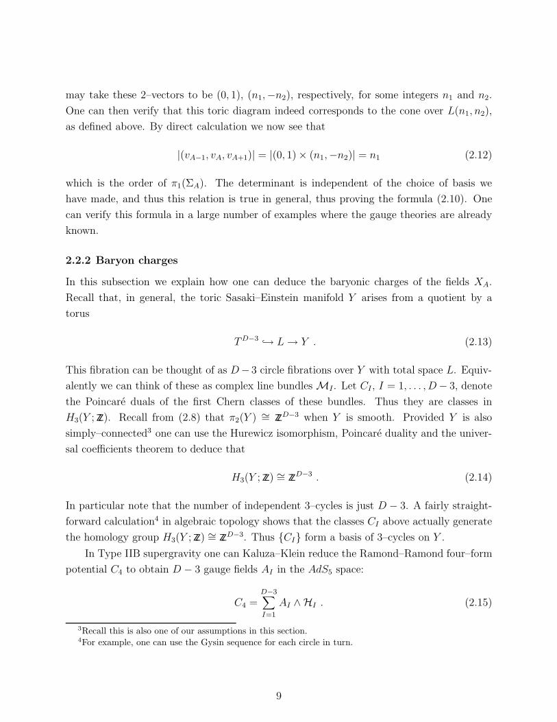
2.2.2 Baryon charges
In this subsection we explain how one can deduce the baryonic charges of the fields XA.
Recall that, in general, the toric Sasaki–Einstein manifold Y arises from a quotient by a
torus
TD−3 → L→ Y . (2.13)
This fibration can be thought of as D− 3 circle fibrations over Y with total space L. Equiv-
alently we can think of these as complex line bundles MI . Let CI , I = 1, . . . , D− 3, denote
the Poincare duals of the first Chern classes of these bundles. Thus they are classes in
H3(Y ; ZZ). Recall from (2.8) that π2(Y ) ∼= ZZD−3 when Y is smooth. Provided Y is also
simply–connected3 one can use the Hurewicz isomorphism, Poincare duality and the univer-
sal coefficients theorem to deduce that
H3(Y ; ZZ) ∼= ZZD−3 . (2.14)
In particular note that the number of independent 3–cycles is just D − 3. A fairly straight-
forward calculation4 in algebraic topology shows that the classes CI above actually generate
the homology group H3(Y ; ZZ) ∼= ZZD−3. Thus CI form a basis of 3–cycles on Y .
In Type IIB supergravity one can Kaluza–Klein reduce the Ramond–Ramond four–form
potential C4 to obtain D − 3 gauge fields AI in the AdS5 space:
C4 =D−3∑
I=1
AI ∧HI . (2.15)
3Recall this is also one of our assumptions in this section.4For example, one can use the Gysin sequence for each circle in turn.
9
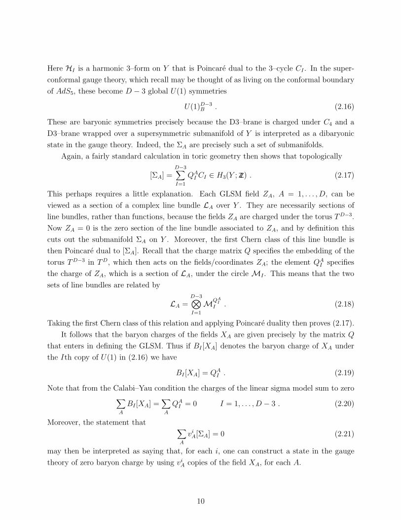
Here HI is a harmonic 3–form on Y that is Poincare dual to the 3–cycle CI . In the super-
conformal gauge theory, which recall may be thought of as living on the conformal boundary
of AdS5, these become D − 3 global U(1) symmetries
U(1)D−3B . (2.16)
These are baryonic symmetries precisely because the D3–brane is charged under C4 and a
D3–brane wrapped over a supersymmetric submanifold of Y is interpreted as a dibaryonic
state in the gauge theory. Indeed, the ΣA are precisely such a set of submanifolds.
Again, a fairly standard calculation in toric geometry then shows that topologically
[ΣA] =D−3∑
I=1
QAI CI ∈ H3(Y ; ZZ) . (2.17)
This perhaps requires a little explanation. Each GLSM field ZA, A = 1, . . . , D, can be
viewed as a section of a complex line bundle LA over Y . They are necessarily sections of
line bundles, rather than functions, because the fields ZA are charged under the torus TD−3.
Now ZA = 0 is the zero section of the line bundle associated to ZA, and by definition this
cuts out the submanifold ΣA on Y . Moreover, the first Chern class of this line bundle is
then Poincare dual to [ΣA]. Recall that the charge matrix Q specifies the embedding of the
torus TD−3 in TD, which then acts on the fields/coordinates ZA; the element QAI specifies
the charge of ZA, which is a section of LA, under the circle MI . This means that the two
sets of line bundles are related by
LA =D−3⊗
I=1
MQA
I
I . (2.18)
Taking the first Chern class of this relation and applying Poincare duality then proves (2.17).
It follows that the baryon charges of the fields XA are given precisely by the matrix Q
that enters in defining the GLSM. Thus if BI [XA] denotes the baryon charge of XA under
the Ith copy of U(1) in (2.16) we have
BI [XA] = QAI . (2.19)
Note that from the Calabi–Yau condition the charges of the linear sigma model sum to zero∑
A
BI [XA] =∑
A
QAI = 0 I = 1, . . . , D − 3 . (2.20)
Moreover, the statement that∑
A
viA[ΣA] = 0 (2.21)
may then be interpreted as saying that, for each i, one can construct a state in the gauge
theory of zero baryon charge by using viA copies of the field XA, for each A.
10
2.2.3 Flavour charges
In this subsection we explain how one can compute the flavour charges of the XA. Recall
that the horizon Sasaki–Einstein manifolds have at least a U(1)3 isometry since they are
toric. By definition a flavour symmetry in the gauge theory is a non–R–symmetry – that
is, the supercharges are left invariant under such a symmetry. The geometric dual of this
statement is that the Killing spinor ψ on the Sasaki–Einstein manifold Y is left invariant by
the corresponding isometry. Thus a Killing vector field VF is dual to a flavour symmetry in
the gauge theory if and only if
LVFψ = 0 (2.22)
where ψ is a Killing spinor on Y . In fact there is always precisely a U(1)2 subgroup of U(1)3
that satisfies this condition. This can be shown by considering the holomorphic (3, 0) form
of the corresponding Calabi–Yau cone [46]. It is well known that this is constructed from
the Killing spinors as a bilinear
Ω = ψc Γ(3) ψ , (2.23)
where Γ(3) is the totally antisymmetrised product of 3 gamma matrices in Cliff(6, 0). In
particular, in the basis in which the normal vectors of the polyhedral cone C are of the form
vA = (1, wA), the Lie algebra elements (0, 1, 0), (0, 0, 1) generate the group U(1)2F of flavour
isometries. Note that, for Y p,q, one of these U(1)F symmetries is enhanced to an SU(2)
flavour symmetry. However, U(1)2F is the generic case.
We would like to determine the charges of the fields XA under U(1)2F . In fact in the
gauge theory this symmetry group is far from unique – one is always free to mix any flavour
symmetry with part of the baryonic symmetry group U(1)D−3B . The baryonic symmetries
are distinguished by the fact that mesons in the gauge theory, for example constructed from
closed loops in a quiver gauge theory, should have zero baryonic charge. Thus the flavour
symmetry group is unique only up to mixing with baryonic symmetries, and of course mixing
with each other.
This mixing ambiguity has a beautiful geometric interpretation. Recall that the Calabi–
Yau cone X is constructed as a symplectic quotient
X = CD//TD−3 (2.24)
where the torus TD−3 ⊂ TD is defined by the kernel of the map
A : IRD → IR3 (2.25)
eA 7→ vA . (2.26)
11
More precisely the kernel of A is generated by the matrix QAI , which in turn defines a
sublattice Υ of ZZD of rank D−3. The torus is then TD−3 = IRD−3/Υ. We may also consider
the quotient ZZD/Υ. The map induced from A then maps this quotient space isomorphically
onto ZZ3 and the corresponding torus T 3 = TD/TD−3 is then precisely the torus isometry of
X.
Let us pick two elements α1, α2 of ZZD that map to the basis vectors (0, 1, 0), (0, 0, 1)
under A. From the last paragraph these are defined only up to elements of the lattice Υ,
and thus may be considered as elements of the quotient ZZD/Υ. Geometrically, α1, α2 define
circle subgroups of TD that descend to the two U(1) flavour isometries generated by (0, 1, 0)
and (0, 0, 1). The charges of the complex coordinates ZA on CD are then simply αA1 , αA
2 for
each A = 1, . . . , D. However, as discussed in the last subsection, the ZA descend to complex
line bundles on Y whose Poincare duals are precisely the submanifolds ΣA. Thus the flavour
charges of XA may be identified with αA1 , αA
2 . Moreover, by construction, each α was unique
only up to addition by some element in the lattice Υ generated by QAI . But as we just saw
in the previous subsection, this is precisely the set of baryon charges in the gauge theory.
We thus see that the ambiguity in the choice of flavour symmetries in the gauge theory is in
1–1 correspondence with the ambiguity in choosing α1, α2.
2.2.4 R–charges
The R–charges were treated in reference [46], so we will be brief here. Let us begin by
emphasising that all the quantities computed so far can be extracted in a simple way from
the toric data, or equivalently from the charges of the gauged linear sigma model, without
the need of an explicit metric. In [46], it was shown that the total volume of any toric
Sasaki–Einstein manifold, as well as the volumes of its supersymmetric toric submanifolds,
can be computed by solving a simple extremal problem which is defined in terms of the
polyhedral cone C. This toric data is encoded in a function Z, which depends on a “trial”
Reeb vector living in IR3. Minimising Z determines the Reeb vector for the Sasaki–Einstein
metric on Y uniquely, and as a result one can compute the volumes of the ΣA. This is a
geometric analogue of a–maximisation [32]. Indeed, recall that the volumes are related to
the R–charges of the corresponding fields XA by the simple formula
R[XA] =π
3
vol(ΣA)
vol(Y ). (2.27)
This formula has been used in many AdS/CFT calculations to compare the R–charges of
dibaryons with their corresponding 3–manifolds [53, 54, 55, 56].
12
Moreover, in [46] a general formula relating the volume of supersymmetric submanifolds
to the total volume of the toric Sasaki–Einstein manifold was given. This reads
πD∑
A=1
vol(ΣA) = 6 vol(Y ) . (2.28)
Then the physical interpretation of (2.28) is that the R–charges of the bifundamental fields
XA sum to 2:
∑
A
R[XA] = 2 . (2.29)
This is related to the fact that each term in the superpotential is necessarily the sum
D∑
A=1
ΣA (2.30)
and the superpotential has R–charge 2 by definition. We shall discuss this further in Section
4.
3. The La,b,c toric singularities
In the remainder of this paper we will be interested in the specific GLSM with charges
Q = (a,−c, b,−d) (3.1)
where of course d = a + b − c in order to satisfy the Calabi–Yau condition. We will define
this singularity to be La,b,c. The reason we choose this family is two–fold: firstly, the Sasaki–
Einstein metrics are known explicitly in this case [8, 9] and, secondly, this family is sufficiently
simple that we will be able to give a general prescription for constructing the gauge theories.
Let us begin by noting that this is essentially the most general GLSM with four charges,
and hence the most general toric quiver gauge theories with a single U(1)B symmetry, up
to orbifolding. Indeed, provided all the charges are non–zero, either two have the same sign
or else three have the same sign. The latter are in fact just orbifolds of S5, and this case
where all but one of the charges have the same sign is slightly degenerate. Specifically, the
charges (e, f, g,−e− f − g) describe the orbifold of S5 ⊂C3 by ZZe+f+g with weights (e, f, g).
The polyhedral cones therefore have three facets, and not four, or equivalently the (p, q) web
has 3 external legs. By our general analysis there is therefore no U(1) baryonic symmetry,
as expected. Indeed, note that setting Z4 = 0 does not give a divisor in this case, since the
remaining charges are all positive and there is no solultion to the remaining D–terms. The
13
Sasaki–Einstein metrics are just the quotients of the round metric on S5 and these theories
are therefore not particularly interesting. In the case that one of the charges is zero, we
instead obtain N = 2 orbifolds of S5, which are also well–studied.
We are therefore left with the case that two charges have the same sign. In (3.1) we
therefore take all integers to be positive. Without loss of generality we may of course take
0 < a ≤ b. Also, by swapping c and d if necessary, we can always arrange that c ≤ b. By
definition hcf(a, b, c, d) = 1 in order that the U(1) action specified by (3.1) is effective, and
it then follows that any three integers are coprime. The explicit Sasaki–Einstein metrics on
the horizons of these singularities were constructed in [8]. The toric description above was
then given in [9]. The manifolds were named Lp,q,r in reference [8] but, following [9], we
have renamed these La,b,c in order to avoid confusion with Y p,q. Indeed, notice that these
spaces reduce to Y p,q when c = d = p, and then a = p− q, b = p + q. In particular there is
an enhanced SU(2) symmetry in the metric in this limit. It is straightforward to determine
when the space Y = La,b,c is non–singular: each of the pair a, b must be coprime to each
of c, d. This condition is necessary to avoid codimension four orbifold singularities on Y .
To see this, consider setting Z1 = Z4 = 0. If b and c had a common factor h, then the
circle action specified by (3.1) would factor through a cyclic group ZZh of order h, and this
would descend to a local orbifold group on the quotient space. In fact it is simple to see that
this subspace is just an S1 family of ZZh orbifold singularities. All such singularities arise in
this way. When Y = La,b,c is non–singular it follows from the last section that π2(Y ) ∼= ZZ
and hence H2(Y ; ZZ) ∼= ZZ. By Smale’s theorem Y is therefore diffeomorphic to S2 × S3. In
particular there is one 3–cycle and hence one U(1)B for these theories.
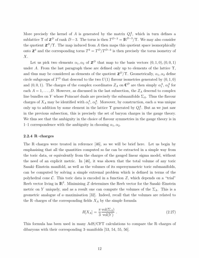
The toric diagram can be described by an appropriate set of four vectors vA = (1, wA).
We take the following set
w1 = [1, 0] w2 = [ak, b] w3 = [−al, c] w4 = [0, 0] (3.2)
where k and l are two integers satisfying
c k + b l = 1 (3.3)
and we have assumed for simplicity of exposition that hcf(b, c) = 1. This toric diagram is
depicted in Figure 2.
The solution to the above equation always exists by Euclid’s algorithm. Moreover, there
is a countable infinity of solutions to this equation, where one shifts k and l by −tb and
tc, respectively, for any integer t. However, it is simple to check that different solutions are
14
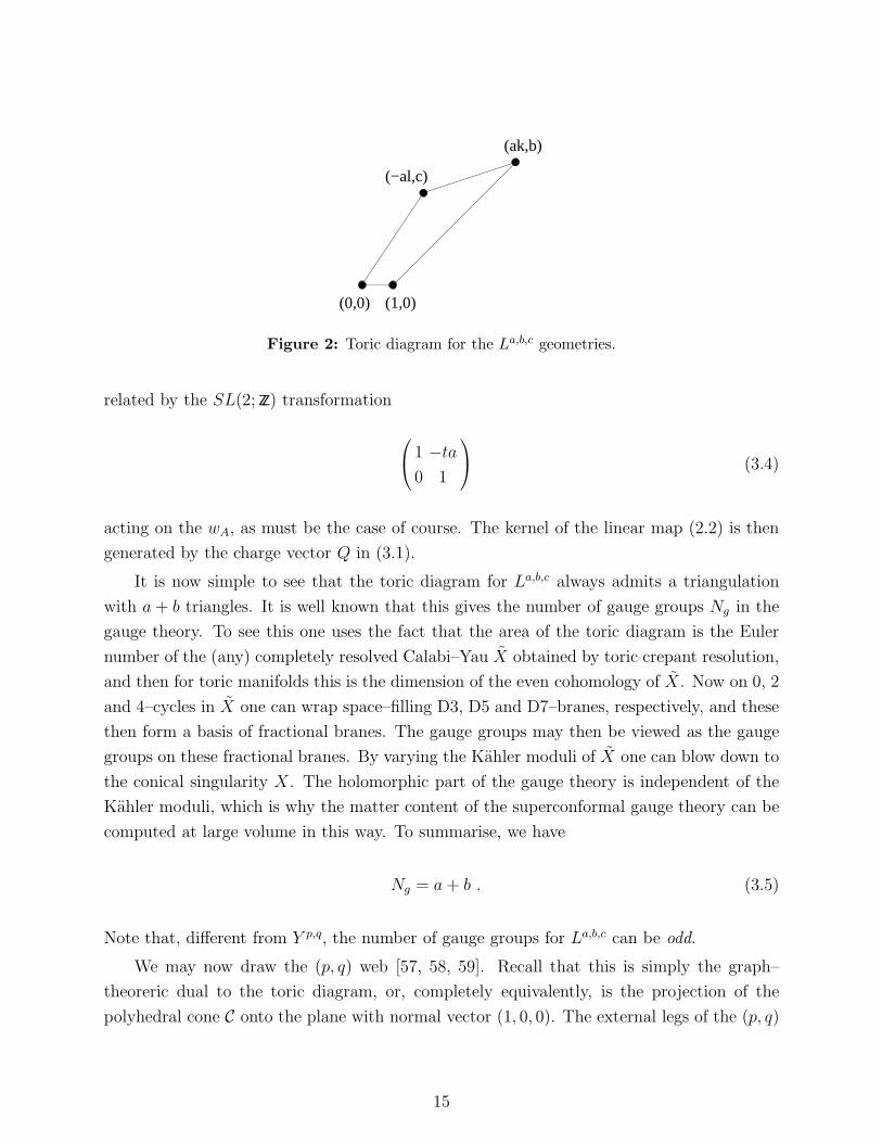
(1,0)(0,0)
(ak,b)
(−al,c)
Figure 2: Toric diagram for the La,b,c geometries.
related by the SL(2; ZZ) transformation
1 −ta0 1
(3.4)
acting on the wA, as must be the case of course. The kernel of the linear map (2.2) is then
generated by the charge vector Q in (3.1).
It is now simple to see that the toric diagram for La,b,c always admits a triangulation
with a + b triangles. It is well known that this gives the number of gauge groups Ng in the
gauge theory. To see this one uses the fact that the area of the toric diagram is the Euler
number of the (any) completely resolved Calabi–Yau X obtained by toric crepant resolution,
and then for toric manifolds this is the dimension of the even cohomology of X. Now on 0, 2
and 4–cycles in X one can wrap space–filling D3, D5 and D7–branes, respectively, and these
then form a basis of fractional branes. The gauge groups may then be viewed as the gauge
groups on these fractional branes. By varying the Kahler moduli of X one can blow down to
the conical singularity X. The holomorphic part of the gauge theory is independent of the
Kahler moduli, which is why the matter content of the superconformal gauge theory can be
computed at large volume in this way. To summarise, we have
Ng = a + b . (3.5)
Note that, different from Y p,q, the number of gauge groups for La,b,c can be odd.
We may now draw the (p, q) web [57, 58, 59]. Recall that this is simply the graph–
theoreric dual to the toric diagram, or, completely equivalently, is the projection of the
polyhedral cone C onto the plane with normal vector (1, 0, 0). The external legs of the (p, q)
15
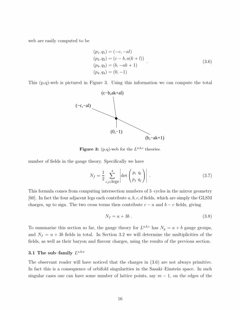
web are easily computed to be
(p1, q1) = (−c,−al)(p2, q2) = (c− b, a(k + l))
(p3, q3) = (b,−ak + 1)
(p4, q4) = (0,−1)
. (3.6)
This (p,q)-web is pictured in Figure 3. Using this information we can compute the total
(−c,−al)
(0,−1)
(c−b,ak+al)
(b,−ak+1)
Figure 3: (p,q)-web for the La,b,c theories.
number of fields in the gauge theory. Specifically we have
Nf =1
2
4∑
i,j∈legs
∣
∣
∣
∣
∣
∣
det
pi qi
pj qj
∣
∣
∣
∣
∣
∣
. (3.7)
This formula comes from computing intersection numbers of 3–cycles in the mirror geometry
[60]. In fact the four adjacent legs each contribute a, b, c, d fields, which are simply the GLSM
charges, up to sign. The two cross terms then contribute c− a and b− c fields, giving
Nf = a+ 3b . (3.8)
To summarise this section so far, the gauge theory for La,b,c has Ng = a + b gauge groups,
and Nf = a + 3b fields in total. In Section 3.2 we will determine the multiplicities of the
fields, as well as their baryon and flavour charges, using the results of the previous section.
3.1 The sub–family La,b,a
The observant reader will have noticed that the charges in (3.6) are not always primitive.
In fact this is a consequence of orbifold singularities in the Sasaki–Einstein space. In such
singular cases one can have some number of lattice points, say m − 1, on the edges of the
16
toric diagram, and then the corresponding leg of the (p, q) web in (3.6) is not a primitive
vector. One should then really write the primitive vector, and associate to that leg the label,
or multiplicity, m. Each leg of the (p, q) web corresponds to a circle on Y which is a locus
of singular points if m > 1, where m gives the order of the orbifold group. Nevertheless,
the charges (3.6) as written above give the correct numbers of fields. In fact this discussion
is rather similar to the classification of compact toric orbifolds in [61], where each facet is
assigned a positive integer label that describes the order of an orbifold group. Moreover, the
non–primitive vectors are then used in the symplectic quotient.
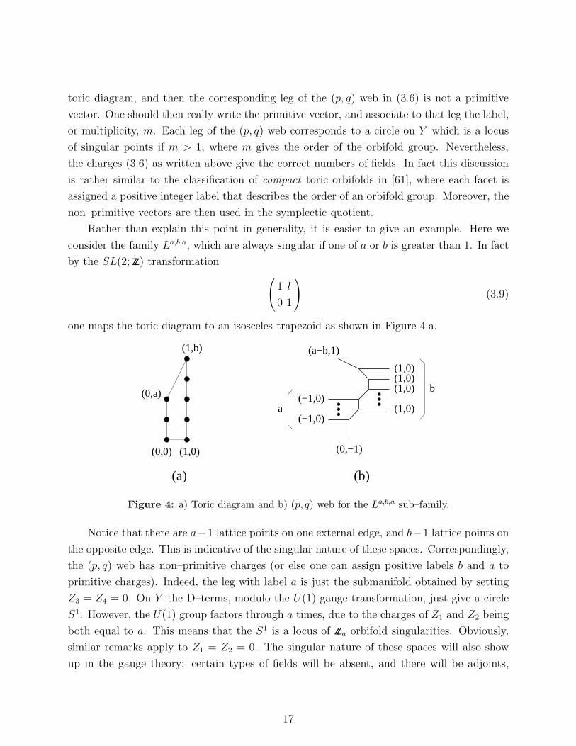
Rather than explain this point in generality, it is easier to give an example. Here we
consider the family La,b,a, which are always singular if one of a or b is greater than 1. In fact
by the SL(2; ZZ) transformation
1 l
0 1
(3.9)
one maps the toric diagram to an isosceles trapezoid as shown in Figure 4.a.
(a)
(1,0)(0,0)
(0,a)
(1,b)
(b)
(a−b,1)
(0,−1)
(1,0)
(1,0)(1,0)(1,0)
(−1,0)
(−1,0)a
b
Figure 4: a) Toric diagram and b) (p, q) web for the La,b,a sub–family.
Notice that there are a−1 lattice points on one external edge, and b−1 lattice points on
the opposite edge. This is indicative of the singular nature of these spaces. Correspondingly,
the (p, q) web has non–primitive charges (or else one can assign positive labels b and a to
primitive charges). Indeed, the leg with label a is just the submanifold obtained by setting
Z3 = Z4 = 0. On Y the D–terms, modulo the U(1) gauge transformation, just give a circle
S1. However, the U(1) group factors through a times, due to the charges of Z1 and Z2 being
both equal to a. This means that the S1 is a locus of ZZa orbifold singularities. Obviously,
similar remarks apply to Z1 = Z2 = 0. The singular nature of these spaces will also show
up in the gauge theory: certain types of fields will be absent, and there will be adjoints,
17
as well as bifundamentals. The La,b,a family will be revisited in Section 6.2.3, where we
will construct their associated brane tilings, gauge theories and compare the computations
performed in the field theories with those in the dual supergravity backgrounds.
3.2 Quantum numbers of fields
Let us denote the distinguished fields as
X1 = Y X2 = U1 X3 = Z X4 = U2 . (3.10)
In the limit c = d = p we have that La,b,c reduces to a Y p,q. Specifically, b = p + q and
a = p−q. Then this notation for the fields coincides with that of reference [13]. In particular,
the Ui become a doublet under the SU(2) isometry/flavour symmetry in this limit.
The multiplicities of the fields can be read off from the results of the last section:
mult[Y ] = b mult[U1] = d mult[Z] = a mult[U2] = c . (3.11)
This accounts for 2(a+ b) fields, which means that there are b− a fields missing. The (p, q)
web suggests that there are two more fields V1 and V2 with multiplicities
mult[V1] = c− a mult[V2] = b− c . (3.12)
Indeed, this also reproduces a Y p,q theory in the limit c = d, where the fields Vi again become
an SU(2) doublet.
It is now simple to work out which toric divisors these additional fields are associated
to. As will be explained later, each divisor must appear precisely b times in the list of fields.
Roughly, this is because there are necessarily a+3b−(a+b) = 2b terms in the superpotential,
and every field must appear precisely twice by the quiver toric condition [62]. From this we
deduce that we may view the remaining fields V1, V2 as “composites” — more precisely, we
identify them with unions of adjacent toric divisors Di∪Dj in the Calabi–Yau, or equivalently
in terms of supersymmetric 3–submanifolds in the Sasaki–Einstein space:
V1 : Σ3 ∪ Σ4
V2 : Σ2 ∪ Σ3 . (3.13)
We may now compute the baryon and flavour charges of all the fields. The charges for
the fields V1, V2 can be read off from their relation to the divisors ΣA above. We summarise
the various quantum numbers in Table 1.
18

Field SUSY submanifold number U(1)B U(1)F1U(1)F2
Y Σ1 b a 1 0
U1 Σ2 d −c 0 l
Z Σ3 a b 0 k
U2 Σ4 c −d −1 −k − l
V1 Σ3 ∪ Σ4 b− c c− a −1 −lV2 Σ2 ∪ Σ3 c− a b− c 0 k + l
Table 1: Charge assignments for the six different types of fields present in the general quiver
diagram for La,b,c.
Notice that the SL(2; ZZ) transformation (3.4) that shifts k and l is equivalent to redefin-
ing the flavour symmetry
U(1)F2→ U(1)F2
− tU(1)B + taU(1)F1. (3.14)
Note also that each toric divisor appears precisely b times in the table. This fact automati-
cally ensures that the linear traces vanish
TrU(1)B = 0 and TrU(1)F1= TrU(1)F2
= 0 , (3.15)
as must be the case. As a non–trivial check of these assignments, one can compute that the
cubic baryonic trace vanishes as well
TrU(1)3B = ba3 − dc3 + ab3 − cd3 + (b− c)(c− a)3 + (c− a)(b− c)3 = 0 . (3.16)
3.3 The geometry
In this subsection we summarise some aspects of the geometry of the toric Sasaki–Einstein
manifolds La,b,c. First, we recall the metrics [8], and how these are associated to the toric
singularities discussed earlier [9]. We also discuss supersymmetric submanifolds, compute
their volumes, and use these results to extract the R–charges of the dual field theory.
The local metrics were given in [8] in the form
ds2 =ρ2dx2
4∆x
+ρ2dθ2
∆θ
+∆x
ρ2
(
sin2 θ
αdφ+
cos2 θ
βdψ
)2
+∆θ sin2 θ cos2 θ
ρ2
(
α− x
αdφ− β − x
βdψ
)2
+ (dτ + σ)2 (3.17)
19
where
σ =α− x
αsin2 θdφ+
β − x
βcos2 θdψ
∆x = x(α − x)(β − x) − µ, ρ2 = ∆θ − x
∆θ = α cos2 θ + β sin2 θ . (3.18)
Here α, β, µ are a priori arbitrary constants. These local metrics are Sasaki–Einstein which
can be equivalently stated by saying that the metric cone dr2 + r2ds2 is Ricci–flat and
Kahler, or that the four–dimensional part of the metric (suppressing the τ direction) is a
local Kahler–Einstein metric of positive curvature. These local metrics were also found in [9].
The coordinates in (3.17) have the following ranges: 0 ≤ θ ≤ π/2, 0 ≤ φ ≤ 2π, 0 ≤ ψ ≤ 2π,
and x1 ≤ x ≤ x2, where x1, x2 are the smallest two roots of the cubic polynomial ∆x. The
coordinate τ , which parameterises the orbits of the Reeb Killing vector ∂/∂τ is generically
non–periodic. In particular, generically the orbits of the Reeb vector field do not close,
implying that the Sasaki–Einstein manifolds are in general irregular.
The metrics are clearly toric, meaning that there is a U(1)3 contained in the isometry
group. Three commuting Killing vectors are simply given by ∂/∂ψ, ∂/∂ψ, ∂/∂τ . The global
properties of the spaces are then conveniently described in terms of those linear combinations
of the vector fields that vanish over real codimension two fixed point sets. This will corre-
spond to toric divisors in the Calabi–Yau cone — see e.g. [12]. It is shown in [8] that there
are precisely four such vector fields, and in particular these are ∂/∂φ and ∂/∂ψ, vanishing
on θ = 0 and θ = π/2 respectively, and two additional vectors
ℓi = ai∂
∂φ+ bi
∂
∂ψ+ ci
∂
∂τi = 1, 2 (3.19)
which vanish over x = x1 and x = x2, respectively. The constants are given by [8]
ai =αci
xi − α, bi =
βcixi − β
,
ci =(α− xi)(β − xi)
2(α + β)xi − αβ − 3x2i
. (3.20)
In order that the corresponding space is globally well–defined, there must be a linear relation
between the four Killing vector fields
a ℓ1 + b ℓ2 + c∂
∂φ+ d
∂
∂ψ= 0 (3.21)
20
where (a, b, c, d) are relatively prime integers. It is shown in [8] that for appropriately chosen
coefficients ai, bi, ci there are then countably infinite families of complete Sasaki–Einstein
manifolds.
The fact that there are four Killing vector fields that vanish on codimension 2 submani-
folds implies that the image of the Calabi–Yau cone under the moment map for the T 3 action
is a four faceted polyhedral cone in IR3 [12]. Using the linear relation among the vectors
(3.21) one can show that the normal vectors to this polyhedral cone satisfy the relation
a v1 − c v2 + b v3 − (a+ b− c) v4 = 0 (3.22)
where vA, A = 1, 2, 3, 4 are the primitive vectors in IR3 that define the cone. Note that
we have listed the vectors according to the order of the facets of the polyhedral cone. As
explained in [9], it follows that, for a, b, c relatively prime, the Sasaki–Einstein manifolds
arise from the symplectic quotient
C4//(a,−c, b,−a− b+ c) (3.23)
which is precisely the gauged linear sigma model considered in the previous subsection.
The volume of the Sasaki–Einstein manifolds/orbifolds is given by [8]
vol(Y ) =π2
2kαβ(x2 − x1)(α+ β − x1 − x2)∆τ (3.24)
where here k =gcd(a, b) and
∆τ =2πk|c1|
b. (3.25)
This can also be written as
vol(Y ) =π3(a+ b)3
8abcdW (3.26)
where W is a root of certain quartic polynomial given in [8]. This shows that the central
charges of the dual conformal field theory will be generically quartic irrational.
In order to compute the R–charges from the metric, we need to know the volumes of
the four supersymmetric 3–submanifolds ΣA. These volumes were not given in [8] but it is
straightforward to compute them. We obtain
vol(Σ1) =π
k
∣
∣
∣
∣
c1a1b1
∣
∣
∣
∣
∆τ vol(Σ2) =π
kβ(x2 − x1)∆τ
vol(Σ3) =π
k
∣
∣
∣
∣
c2a2b2
∣
∣
∣
∣
∆τ vol(Σ4) =π
kα(x2 − x1)∆τ . (3.27)
21
We can now complete the charge assignments of all the fields in the quiver by giving their
R–charges purely from the geometry. The charges of the distinguished fields Y, U1, Z, U2 are
obtained from the geometry using the formula
R[XA] =π
3
vol(ΣA)
vol(Y ), (3.28)
while those of the V1, V2 fields are simply deduced from (3.13). In particular
R[V1] = R[Z] +R[U2] R[V2] = R[Z] +R[U1] . (3.29)
It will be convenient to note that the constants α, β, µ appearing in ∆x are related to
its roots as follows
µ = x1x2x3
α+ β = x1 + x2 + x3
αβ = x1x2 + x1x3 + x2x3 , (3.30)
where x3 is the third root of the cubic, and x3 ≥ x2 ≥ x1 ≥ 0. Using the volumes in (3.27),
we then obtain the following set of R–charges
R[Y ] =2
3x3(x3 − x1) R[U1] =
2α
3x3
R[Z] =2
3x3
(x3 − x2) R[U2] =2β
3x3
. (3.31)
To obtain explicit expressions, one should now write the constants xi, α, β in terms of the
integers a, b, c. This can be done, using the equations (9) in [8]. We have
x1(x3 − x1)
x2(x3 − x2)=a
b(3.32)
α(x3 − α)
β(x3 − β)=c
d. (3.33)
Notice that α = β implies c = d, as claimed in [8]. Combining these two equations with
(3.30), one obtains a complicated system of quartic polynomials, which in principle can be
solved. However, we will proceed differently. Our aim is simply to show that the resulting
R–charges will match with the a–maximisation computation in the field theory. Therefore,
using the relations above, we can write down a system of equations involving the R–charges
22
and the integers a, b, c, d. We obtain the following:
R[Y ](2 − 3R[Y ])
R[Z](2 − 3R[Z])=a
b
R[U1](2 − 3R[U1])
R[U2](2 − 3R[U2])=c
d
3
4(R[U1]R[U2] −R[Y ]R[Z]) +R[Z] +R[Y ] = 1
R[Y ] +R[U1] +R[Z] +R[U2] = 2 . (3.34)
With the aid of a computer program, one can check that the solutions to this system are
given in terms of roots of various quartic polynomials involving a, b, c. For the case of La,b,a
the polynomials reduce to quadratics and the R–charges can be given in closed form. These
in fact match precisely with the values that we will compute later using a–maximisation, as
well as Z–minimisation. Therefore we won’t record them here.
In the general case, instead of giving the charges in terms of unwieldy quartic roots, we
can more elegantly show that the system (3.34) can be recast into an equivalent form which
is obtained from a–maximisation. In order to do so, we can use the last equation to solve for
R[U1]. Expressing the first three equations in terms of R[U2] = x, R[Y ] = y and R[z] = z,
we haveb(2 − 3y) + az(3z − 2) = 0
c(x+ y − 2)(3x+ 3y − 4) − (a + b− c)(x− z)(3x− 3z − 2) = 0
3x2 − 4y + 2(z + 2) + x(3y − 3z − 6) = 0 .
(3.35)
Interestingly, the third equation does not involve any of the parameters. For later comparison
with the results coming from a–maximisation, it is important to find a way to reduce this
system of three coupled quadratic equations in three variables to a standard form. The
simplest way of doing so is to ‘solve’ for one of the variables x, y or z and two of the
parameters. A particularly simple choice is to solve for y, a and b. The simplicity follows
from the fact that it is possible to use the third equation to solve for y and the parameters
then appear linearly in all the equations. Doing this, we obtain
a =c(3x− 2) (3x(x− z − 2) + 2(2 + z))
(3x− 4)2(x− z)
b =cz(3z − 2)
(3x− 3z − 2)(x− z)
y =−2(2 + z) − 3x(x− z − 2)
(3x− 4). (3.36)
23
This system of equations is equivalent to the original one, and is the one we will compare
with the results of a–maximisation.
Of course, one could also compute these R–charges using Z–minimisation [46]. The al-
gebra encountered in tackling the minimisation problem is rather involved, but it is straight-
forward to check agreement of explicit results on a case by case basis.
4. Superpotential and gauge groups
In the previous sections we have already described how rather generally one can obtain the
number of gauge groups, and the field content of a quiver whose vacuum moduli space should
reproduce the given toric variety. In particular, we have listed the multiplicities of every field
and their complete charge assignments, namely their baryonic, flavour, and R–charges. In
the following we go further and predict the form of the superpotential as well as the nature
of the gauge groups, that is, the types of nodes appearing in the quivers.
4.1 The superpotential
First, we recall that in [48] a general formula was derived relating the number of gauge
groups Ng, the number of fields Nf , and the number of terms in the superpotential NW .
This follows from applying Euler’s formula to a brane tiling that lives on the surface of a
2–torus, and reads
NW = Nf −Ng . (4.1)
Using this we find that the number of superpotential terms for La,b,c is NW = 2b. Now we
use the fact each term in the superpotential W must be
∪4A=1ΣA . (4.2)
In fact this is just the canonical class of X – a standard result in toric geometry. One can
justify the above form as follows. Each term in W is a product of fields, and each field is
associated to a union of toric divisors. The superpotential has R–charge 2, and is uncharged
under the baryonic and flavour symmetries. This is true, using the results of Section 2 and
(4.2).
A quick inspection of Table 1 then allows us to identify three types of monomials that
may appear in the superpotential
Wq = TrY U1ZU2 Wc1 = Tr Y U1V1 Wc2 = TrY U2V2 . (4.3)
24
Furthermore, their number is uniquely fixed by the mutiplicities of the fields, and the fact
that NW = 2b. The schematic form of the superpotential for a general La,b,c quiver theory
is then
W = 2 [aWq + (b− c)Wc1 + (c− a)Wc2 ] . (4.4)
In the language of dimer models, this is telling us the types of vertices in the brane tilings
[48]. In particular, in each fundamental domain of the tiling we must have 2a four–valent
vertices, 2(b− c) three–valent vertices of type 1, and 2(c− a) three–valent vertices of type 2.
4.2 The gauge groups
Finally, we discuss the nature of the Ng = a + b gauge groups of the gauge theory, i.e. we
determine the types of nodes in the quiver. This information, together with the above, will
be used to construct the brane tilings. First, we will identify the allowed types of nodes, and
then we will determine the number of times each node appears in the quiver.
The allowed types of nodes can be deduced by requiring that at any given node
1. the total baryonic and flavour charge is zero:∑
i∈node U(1)i = 0
2. the beta function vanishes:∑
i∈node(Ri − 1) + 2 = 0
3. there are an even number of legs.
These requirements are physically rather obvious. The first property is satisfied if we
construct a node out of products (and powers) of the building blocks of the superpotential
(4.3). Moreover, using (2.29), this also guarantees that the total R–charge at the node is
even.
Imposing these three requirements turns out to be rather restrictive, and we obtain four
different types of nodes that we list below:
A : U1Y V1 · U1Y V1 B : V2Y V1 · U1Y U2 D : U2Y V2 · U2Y V2 C : U1Y U2Z (4.5)
Next, we determine the number of times each node appears in the quiver. Denote these
numbers nA, nB, nD, 2nC respectively. Taking into account the multiplicities of all the fields
imposes six linear relations. However, it turns out that these do not uniquely fix the number
of different nodes. We have
nC = a
nB + 2nA = 2(b− c)
nB + 2nD = 2(c− a) . (4.6)
25
Although the number of fields and schematic form of superpotential terms are fixed by
the geometry, the number of A, B and D nodes are not. We can then have different types
of quivers that are nevertheless described by the same toric singularity. This suggests that
the theories with different types of nodes are related by Seiberg dualities. We will show that
this is the case in Section 6.
It is interesting to see what happens for the La,b,a geometries discussed in Section 3.1.
In this case c − a = 0 (the case that b − c = 0 is symmetric with this) and the theory has
some peculiar properties. Recall that this corresponds to a linear sigma model with charges
(a,−a, b,−b). These theories have no V2 fields, while the b − a V1 fields have zero baryonic
charge, and must therefore be adjoints. Moreover, from (4.6), we see that nB = nD = 0, so
that there aren’t any B and D type nodes, while there are b − a A–type nodes. In terms
of tilings, these theories are then just constructed out of C–type quadrilaterals and A–type
hexagons. We will consider in detail these models in Section 6.2.3.
Finally, we note that the general conclusions derived for La,b,c quivers in Sections 4.1
and 4.2 are based on the underlying assumption that we are dealing with a generic theory
(i.e. one in which the R–charges of different types of fields are not degenerate). It is always
possible to find at least one generic phase for a given La,b,c, and thus the results discussed
so far apply. Non–generic phases can be generated by Seiberg duality transformations. In
these cases, new types of superpotential interactions and quiver nodes may emerge, as well
as new types of fields. This was for instance the case for the toric phases of the Y p,q theories
[15].
5. R–charges from a–maximisation
A remarkable check of the AdS/CFT correspondence consists of matching the gauge theory
computation of R–charges and central charge with the corresponding calculations of vol-
umes of the dual Sasaki–Einstein manifold and supersymmetric submanifolds on the gravity
side. This is perhaps the most convincing evidence that the dual field theory is the correct
one. Since explicit expressions for the Sasaki–Einstein metrics are available, it is natural to
attempt such a check. Actually, the volumes of toric manifolds and supersymmetric sub-
manifolds thereof can also be computed from the toric data [46], without using a metric.
This gives a third independent check that everything is indeed consistent.
Here we will calculate the R–charges and central charge a for an arbitrary La,b,c quiver
gauge theory using a–maximisation. From the field theory point of view, initially, there are
six different R–charges, corresponding to the six types of bifundamental fields U1, U2, V1, V2,
26
Y and Z. Since the field theories are superconformal, these R–charges are such that the beta
functions for the gauge and superpotential couplings vanish. Using the constraints (4.3) and
(4.5) it is possible to see that these conditions always leave us with a three–dimensional space
of possible R–charges. This is in precise agreement with the fact that the non–R abelian
global symmetry is U(1)3 ≃ U(1)2F × U(1)B. It is convenient to adopt the parametrization
of R–charges of Section 3.3:
R[U1] = x− z R[U2] = 2 − x− y
R[V1] = 2 − x− y + z R[V2] = x
R[Y ] = y R[Z] = z .
(5.1)
This guarantees that all beta functions vanish. Using the multiplicities in Table 1, we can
check that trR(x, y, z) = 0. This is expected, since this trace is proportional to the sum of
all the beta functions. In addition, the trial a central charge can be written as
trR3(x, y, z) =1
3[a (9(2 − x)(x− z)z − 2) + b (9 x y (2 − x− y) − 2)
+ 9(b− c) y z (2x+ y − z − 2)] . (5.2)
The R–charges are determined by maximising (5.2) with respect to x, y and z. This corre-
sponds to the following equations
∂x trR3(x, y, z) = 0 = −3 b y (2x+ y − 2z − 2) + 3 z (a(2 − 2x+ z − 2cy))
∂y trR3(x, y, z) = 0 = −3 b (x− z)(x+ 2y − z − 2) − 3 c z(2x+ 2y − z − 2)
∂z trR3(x, y, z) = 0 = −3 a (x− 2)(x− 2z) + 3(b− c) y (2x+ y − 2z − 2)
. (5.3)
It is straightforward to show that this system of equations is equivalent to (3.36). In fact,
proceeding as in Section 3.3, we reduce (5.3) to an equivalent system by ‘solving’ for y, a
and b. In this case, there are three solutions, although only one of them does not produce
zero R–charges for some of the fields, and indeed corresponds to the local maximum of (5.2).
This solution corresponds to the following system of equations
a =c(3x− 2) (3x(x− z − 2) + 2(2 + z))
(3x− 4)2(x− z)
b =cz(3z − 2)
(3x− 3z − 2)(x− z)
y =−2(2 + z) − 3x(x− z − 2)
(3x− 4)(5.4)
which is identical to (3.36). We conclude that, for the entire La,b,c family, the gauge theory
computation of R–charges and central charge using a–maximisation agrees precisely with the
27
values determined using geometric methods on the gravity side of the AdS/CFT correspon-
dence.
6. Constructing the gauge theories using brane tilings
In Sections 3 and 4 we derived detailed information regarding the gauge theory on D3–
branes transverse to the cone over an arbitrary La,b,c space. Table 1 gives the types of
fields along with their multiplicities and global U(1) charges, (4.3) presents the possible
superpotential interactions and (4.5) and (4.6) give the types of nodes in the quiver along
with some constraints on their multiplicities.
This information is sufficient for constructing the corresponding gauge theories. We have
used it in Section 5 to prove perfect agreement between the geometric and gauge theory
computations of R–charges and central charges. Nevertheless, it is usually a formidable task
to combine all these pieces of information to generate the gauge theory. In this section
we introduce a simple set of rules for the construction of the gauge theories for the La,b,c
geometries. In particular, our goal is to find a simple procedure in the spirit of the ‘impurity
idea’ of [13, 15].
Our approach uses the concept of a brane tiling, which was introduced in [48], following
the discovery of the connection between toric geometry and dimer models of [47]. Brane
tilings encode both the quiver diagram and the superpotential of gauge theories on D–
branes probing toric singularities. Because of this simplicity, they provide the most suitable
language for describing complicated gauge theories associated with toric geometries. We
refer the reader to [48] for a detailed explanation of brane tilings and their relation to dimer
models.
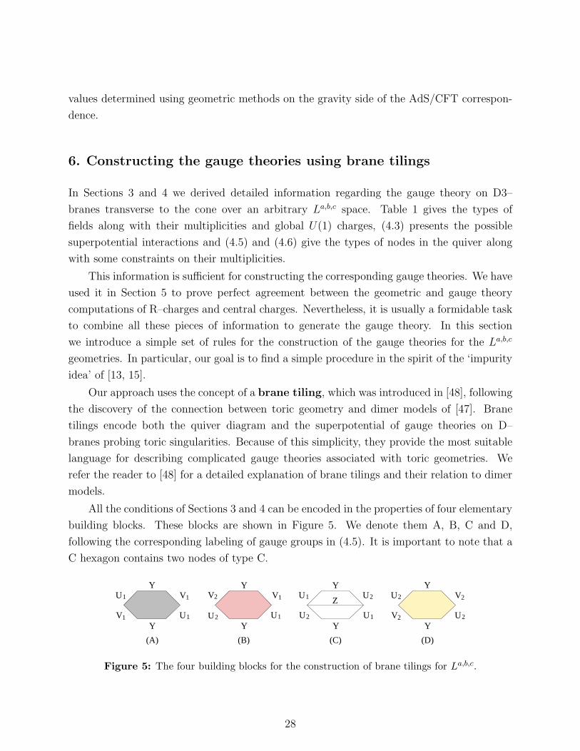
All the conditions of Sections 3 and 4 can be encoded in the properties of four elementary
building blocks. These blocks are shown in Figure 5. We denote them A, B, C and D,
following the corresponding labeling of gauge groups in (4.5). It is important to note that a
C hexagon contains two nodes of type C.
V2
U2 U2
U1V1
U1
U2
U1V1
U1 V1
U1
Y
Y
(A)
V2
U2 V2
U2
Z
YY
YY
(B) (C)
Y
Y
(D)
Figure 5: The four building blocks for the construction of brane tilings for La,b,c.
28
Every edge in the elementary hexagons is associated with a particular type of field.
These edge labels fully determine the way in which hexagons can be glued together along
their edges to form a periodic tiling. The quiver diagram and superpotential can then be read
off from the resulting tiling using the results of [48]. The elementary hexagons automatically
incorporate the three superpotential interactions of (4.3). The number of A, B, C and D
hexagons is nA, nB, nC and nD, respectively. Taking their values as given by (4.6), the
multiplicities in Table 1 are reproduced.
Following the discussion in Section 4, the number of A, B, C and D hexagons is not
fixed for a given La,b,c geometry. There is a one parameter space of solutions to (4.6), which
we can take to be indexed by nD. It is possible to go from one solution of (4.6) to another
one by decreasing the number of B hexagons by two and introducing one A and one D,
i.e. (nA, nB, nC , nD) → (nA + 1, nB − 2, nC , nD + 1). We show in the next section that this
freedom in the number of each type of hexagon is associated with Seiberg duality.
6.1 Seiberg duality and transformations of the tiling
We now study Seiberg duality [63] transformations that produce ‘toric quivers’ 5. We can go
from one toric quiver to another one by applying Seiberg duality to the so–called self–dual
nodes. These are nodes for which the number of flavours is twice the number of colours, thus
ensuring that the rank of the dual gauge group does not change after Seiberg duality. Such
nodes are represented by squares in the brane tiling [48]. Hence, for La,b,c theories, we only
have to consider dualizing C nodes. Seiberg duality on a self–dual node corresponds to a
local transformation of the brane tiling [48]. This is important, since it means that we can
focus on the sub–tilings surrounding the nodes of interest in order to analyse the possible
behavior of the tiling.
We will focus on cases in which the tiling that results from dualizing a self–dual node can
also be described in terms of A, B, C and D hexagons. There are some cases in which Seiberg
duality generates tilings that are not constructed using the elementary building blocks of
Figure 5. In these cases, the assumption of the six types of fields being non–degenerate does
not hold. We present an example of this non-generic case below, corresponding to L2,6,3.
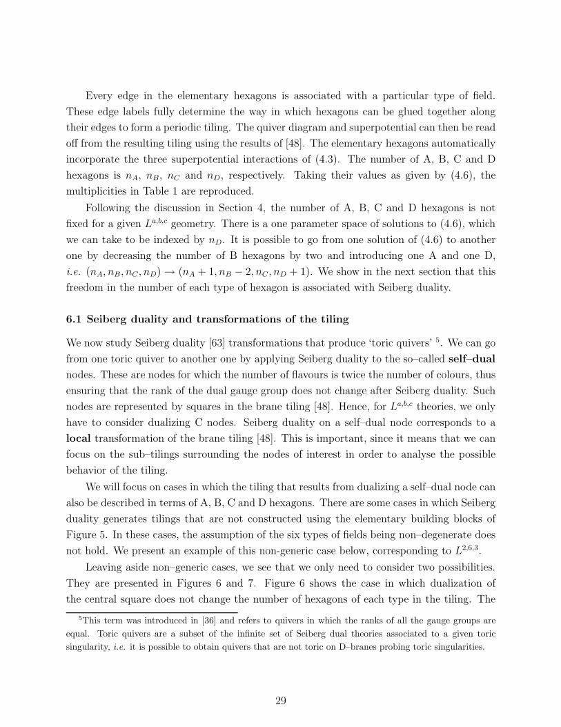
Leaving aside non–generic cases, we see that we only need to consider two possibilities.
They are presented in Figures 6 and 7. Figure 6 shows the case in which dualization of
the central square does not change the number of hexagons of each type in the tiling. The
5This term was introduced in [36] and refers to quivers in which the ranks of all the gauge groups are
equal. Toric quivers are a subset of the infinite set of Seiberg dual theories associated to a given toric
singularity, i.e. it is possible to obtain quivers that are not toric on D–branes probing toric singularities.
29
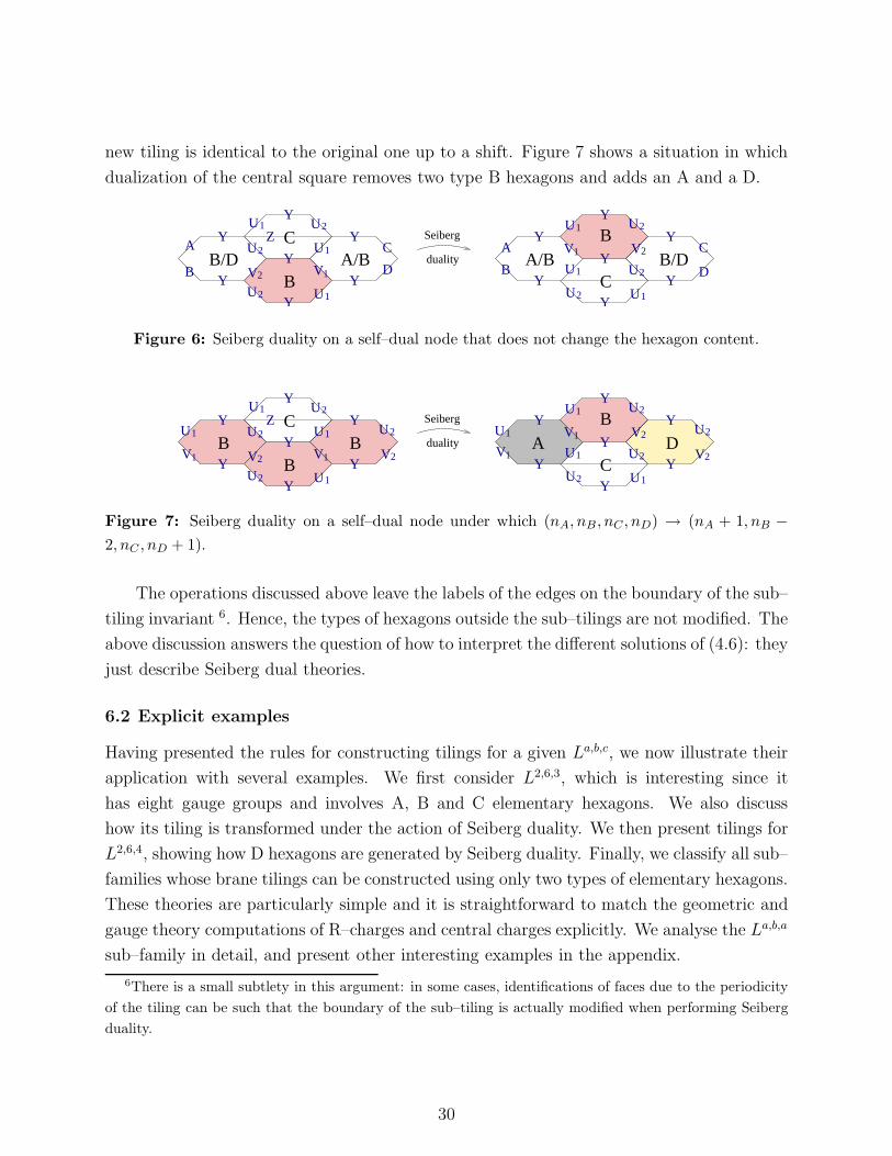
new tiling is identical to the original one up to a shift. Figure 7 shows a situation in which
dualization of the central square removes two type B hexagons and adds an A and a D.
U2
U2
U1 U2
V2
U1
V1
U1
U2U1
U1 U2
U2
V1 V2
U1
Seiberg
duality
B
CZ
Y
Y
Y
Y
Y
Y
Y
B
C
Y
Y
Y
Y
Y
Y
Y
B/D A/B B/DA/BA
B
C
D
A
B
C
D
Figure 6: Seiberg duality on a self–dual node that does not change the hexagon content.
U2U1 U2
U2
U1 U2
V1 V2
U1
V1
U1
V2B
BB
CZ
Y
Y
Y
Y
Y
Y
Y
U1 U2
U2U1
U1 U2
U2
V1
V1 V2
U1
V2A
BD
C
Y
Y
Y
Y
Y
Y
Y
Seiberg
duality
Figure 7: Seiberg duality on a self–dual node under which (nA, nB , nC , nD) → (nA + 1, nB −2, nC , nD + 1).
The operations discussed above leave the labels of the edges on the boundary of the sub–
tiling invariant 6. Hence, the types of hexagons outside the sub–tilings are not modified. The
above discussion answers the question of how to interpret the different solutions of (4.6): they
just describe Seiberg dual theories.
6.2 Explicit examples
Having presented the rules for constructing tilings for a given La,b,c, we now illustrate their
application with several examples. We first consider L2,6,3, which is interesting since it
has eight gauge groups and involves A, B and C elementary hexagons. We also discuss
how its tiling is transformed under the action of Seiberg duality. We then present tilings for
L2,6,4, showing how D hexagons are generated by Seiberg duality. Finally, we classify all sub–
families whose brane tilings can be constructed using only two types of elementary hexagons.
These theories are particularly simple and it is straightforward to match the geometric and
gauge theory computations of R–charges and central charges explicitly. We analyse the La,b,a
sub–family in detail, and present other interesting examples in the appendix.
6There is a small subtlety in this argument: in some cases, identifications of faces due to the periodicity
of the tiling can be such that the boundary of the sub–tiling is actually modified when performing Seiberg
duality.
30
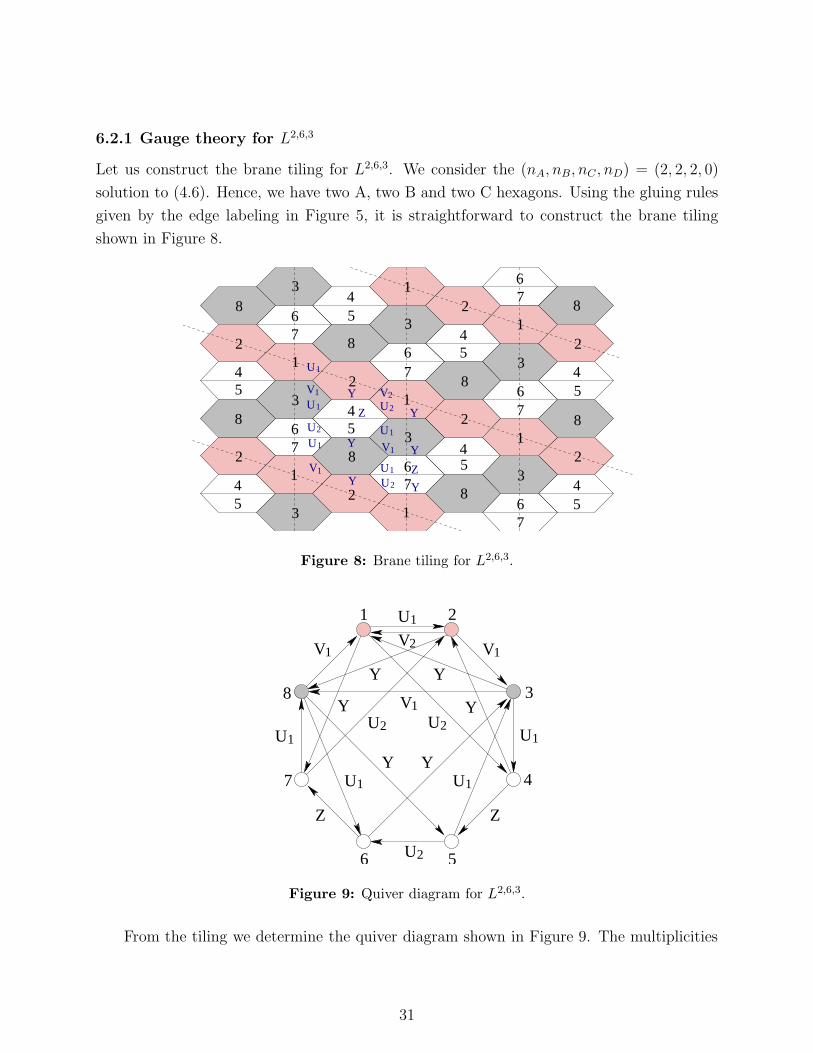
6.2.1 Gauge theory for L2,6,3
Let us construct the brane tiling for L2,6,3. We consider the (nA, nB, nC , nD) = (2, 2, 2, 0)
solution to (4.6). Hence, we have two A, two B and two C hexagons. Using the gluing rules
given by the edge labeling in Figure 5, it is straightforward to construct the brane tiling
shown in Figure 8.
U1
U2
U1
V1
U2
V2
U1
V1
U2
U1
V1
U1
8
67
2
2
1
1
21
21
2
21
2
12
3
3
3
3
3
3
3
5
45
545
45
454
45
45
467
67
67
67
67
67
8
8
8
8
8
8
8
1
Y
Z
Z
Y
Y
Y
Y
Y
Figure 8: Brane tiling for L2,6,3.
V
U
VV
U U
UU
U
U U
V
Y Y
Y Y
Y Y
ZZ
7
8 3
4
1 2
6 5
2
1
11
2 2
11
2
1 1
1
Figure 9: Quiver diagram for L2,6,3.
From the tiling we determine the quiver diagram shown in Figure 9. The multiplicities
31
of each type of field are in agreement with the values in Table 2. In addition, we can also
read off the corresponding superpotential
W = Y31U(1)12 V
(1)23 − Y42V
(1)23 U
(1)34 + Y42V
(2)21 U
(2)12 + Y85U
(1)53 V
(1)38
+ Y17U(1)78 V
(1)81 − Y63V
(1)38 U
(1)86 − Y28V
(1)81 U
(1)12 − Y17U
(2)72 V
(2)21
+ Z45U(2)56 Y63U
(1)34 − Z45U
(1)53 Y31U
(2)14 − Z67U
(1)78 Y85U
(2)56 + Z67U
(2)72 Y28U
(1)86
(6.1)
where for simplicity we have indicated the type of U and V fields with a superscript and
have used subscripts for the gauge groups under which the bifundamental fields are charged.
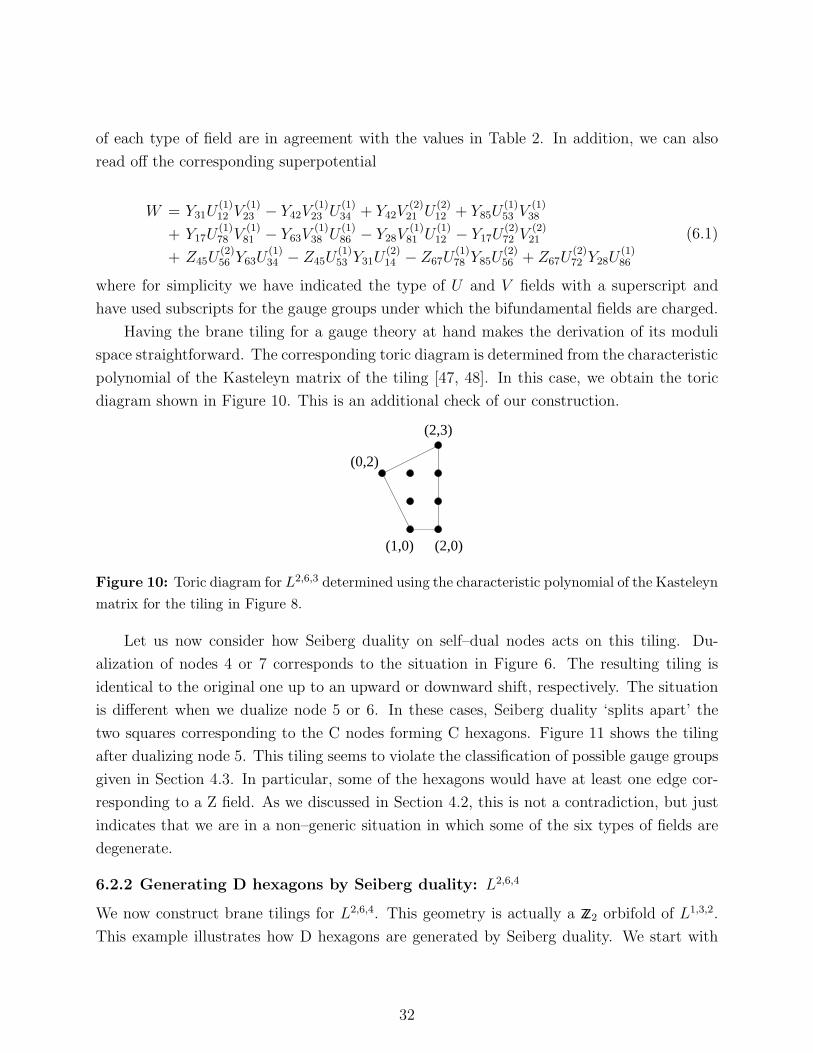
Having the brane tiling for a gauge theory at hand makes the derivation of its moduli
space straightforward. The corresponding toric diagram is determined from the characteristic
polynomial of the Kasteleyn matrix of the tiling [47, 48]. In this case, we obtain the toric
diagram shown in Figure 10. This is an additional check of our construction.
(0,2)
(2,3)
(2,0)(1,0)
Figure 10: Toric diagram for L2,6,3 determined using the characteristic polynomial of the Kasteleyn
matrix for the tiling in Figure 8.
Let us now consider how Seiberg duality on self–dual nodes acts on this tiling. Du-
alization of nodes 4 or 7 corresponds to the situation in Figure 6. The resulting tiling is
identical to the original one up to an upward or downward shift, respectively. The situation
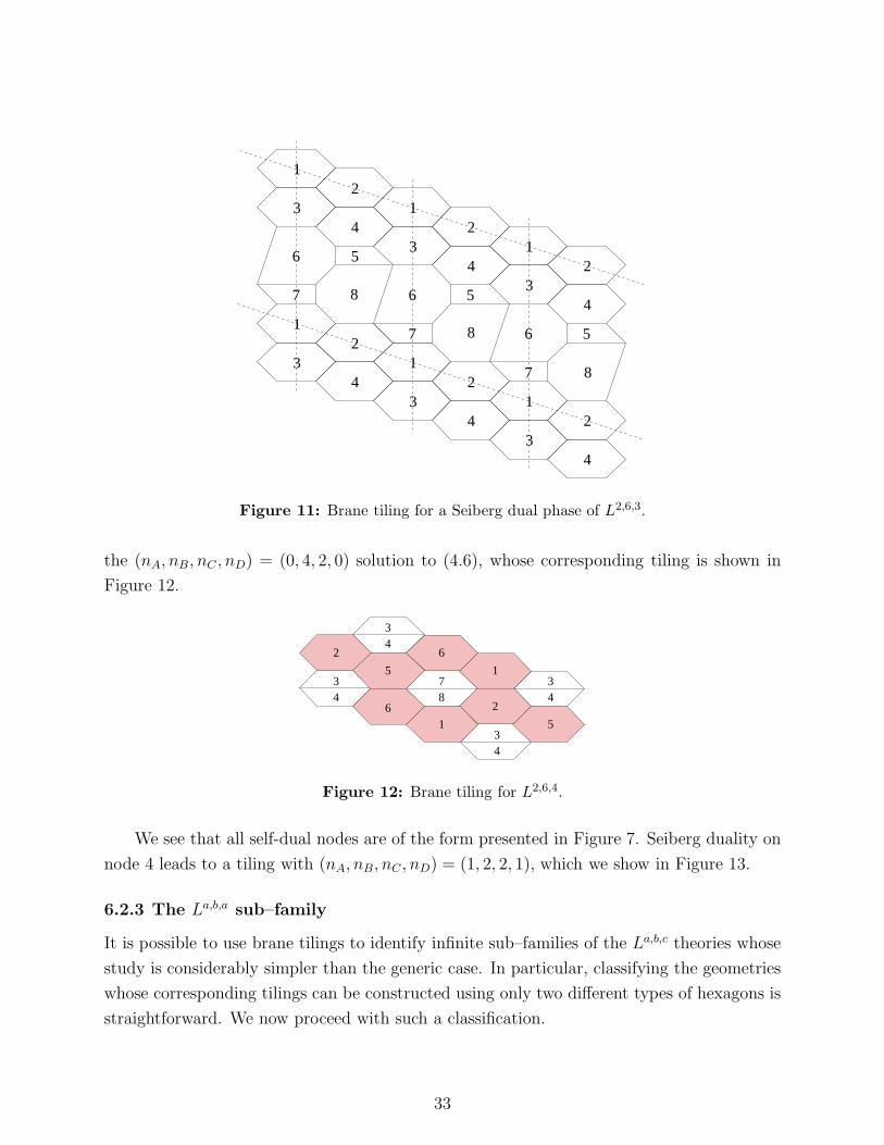
is different when we dualize node 5 or 6. In these cases, Seiberg duality ‘splits apart’ the
two squares corresponding to the C nodes forming C hexagons. Figure 11 shows the tiling
after dualizing node 5. This tiling seems to violate the classification of possible gauge groups
given in Section 4.3. In particular, some of the hexagons would have at least one edge cor-
responding to a Z field. As we discussed in Section 4.2, this is not a contradiction, but just
indicates that we are in a non–generic situation in which some of the six types of fields are
degenerate.
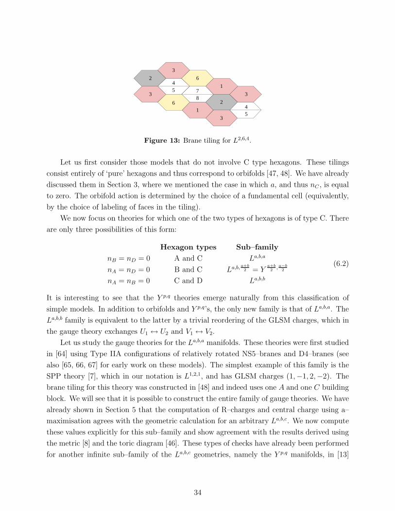
6.2.2 Generating D hexagons by Seiberg duality: L2,6,4
We now construct brane tilings for L2,6,4. This geometry is actually a ZZ2 orbifold of L1,3,2.
This example illustrates how D hexagons are generated by Seiberg duality. We start with
32
43
41
21
21
2
12
12
12
34
3
34
34
34
5
5
7
7
7
6
6
6
8
8
8
5
Figure 11: Brane tiling for a Seiberg dual phase of L2,6,3.
the (nA, nB, nC , nD) = (0, 4, 2, 0) solution to (4.6), whose corresponding tiling is shown in
Figure 12.
1
6
34
2
578
2
16
434
35
4
3
Figure 12: Brane tiling for L2,6,4.
We see that all self-dual nodes are of the form presented in Figure 7. Seiberg duality on
node 4 leads to a tiling with (nA, nB, nC , nD) = (1, 2, 2, 1), which we show in Figure 13.
6.2.3 The La,b,a sub–family
It is possible to use brane tilings to identify infinite sub–families of the La,b,c theories whose
study is considerably simpler than the generic case. In particular, classifying the geometries
whose corresponding tilings can be constructed using only two different types of hexagons is
straightforward. We now proceed with such a classification.
33
1
62
78
2
16
5
45
4
3
3
3
3
Figure 13: Brane tiling for L2,6,4.
Let us first consider those models that do not involve C type hexagons. These tilings
consist entirely of ‘pure’ hexagons and thus correspond to orbifolds [47, 48]. We have already
discussed them in Section 3, where we mentioned the case in which a, and thus nC , is equal
to zero. The orbifold action is determined by the choice of a fundamental cell (equivalently,
by the choice of labeling of faces in the tiling).
We now focus on theories for which one of the two types of hexagons is of type C. There
are only three possibilities of this form:
Hexagon types Sub–family
nB = nD = 0 A and C La,b,a
nA = nD = 0 B and C La,b, a+b
2 = Ya+b
2, a−b
2
nA = nB = 0 C and D La,b,b
(6.2)
It is interesting to see that the Y p,q theories emerge naturally from this classification of
simple models. In addition to orbifolds and Y p,q’s, the only new family is that of La,b,a. The
La,b,b family is equivalent to the latter by a trivial reordering of the GLSM charges, which in
the gauge theory exchanges U1 ↔ U2 and V1 ↔ V2.
Let us study the gauge theories for the La,b,a manifolds. These theories were first studied
in [64] using Type IIA configurations of relatively rotated NS5–branes and D4–branes (see
also [65, 66, 67] for early work on these models). The simplest example of this family is the
SPP theory [7], which in our notation is L1,2,1, and has GLSM charges (1,−1, 2,−2). The
brane tiling for this theory was constructed in [48] and indeed uses one A and one C building
block. We will see that it is possible to construct the entire family of gauge theories. We have
already shown in Section 5 that the computation of R–charges and central charge using a–
maximisation agrees with the geometric calculation for an arbitrary La,b,c. We now compute
these values explicitly for this sub–family and show agreement with the results derived using
the metric [8] and the toric diagram [46]. These types of checks have already been performed
for another infinite sub–family of the La,b,c geometries, namely the Y p,q manifolds, in [13]
34
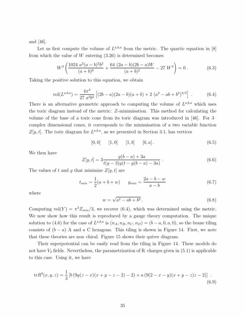
and [46].
Let us first compute the volume of La,b,a from the metric. The quartic equation in [8]
from which the value of W entering (3.26) is determined becomes
W 2
(
1024 a2(a− b)2b2
(a+ b)6+
64 (2a− b)(2b− a)W
(a+ b)2− 27 W 2
)
= 0 . (6.3)
Taking the positive solution to this equation, we obtain
vol(La,b,a) =4π3
27 a2b2
[
(2b− a)(2a− b)(a + b) + 2 (a2 − ab+ b2)3/2]
. (6.4)
There is an alternative geometric approach to computing the volume of La,b,a which uses
the toric diagram instead of the metric: Z-minimisation. This method for calculating the
volume of the base of a toric cone from its toric diagram was introduced in [46]. For 3–
complex dimensional cones, it corresponds to the minimisation of a two variable function
Z[y, t]. The toric diagram for La,b,a, as we presented in Section 3.1, has vertices
[0, 0] [1, 0] [1, b] [0, a] . (6.5)
We then have
Z[y, t] = 3y(b− a) + 3a
t(y − 3)y(t− y(b− a) − 3a). (6.6)
The values of t and y that minimize Z[y, t] are
tmin =1
2(a+ b+ w) ymin =
2a− b− w
a− b(6.7)
where
w =√a2 − ab+ b2 . (6.8)
Computing vol(Y ) = π3Zmin/3, we recover (6.4), which was determined using the metric.
We now show how this result is reproduced by a gauge theory computation. The unique
solution to (4.6) for the case of La,b,a is (nA, nB, nC , nD) = (b− a, 0, a, 0), so the brane tiling
consists of (b − a) A and a C hexagons. This tiling is shown in Figure 14. First, we note
that these theories are non–chiral. Figure 15 shows their quiver diagram.
Their superpotential can be easily read from the tiling in Figure 14. These models do
not have V2 fields. Nevertheless, the parametrization of R–charges given in (5.1) is applicable
to this case. Using it, we have
trR3(x, y, z) =1
3[b (9y(z − x)(x+ y − z − 2) − 2) + a (9(2 − x− y)(x+ y − z)z − 2)] .
(6.9)
35

bb
b
121
212
2a
2a−1
2a−12a−1
2a2a
2a+12a+1
2a+1
a
(b−a)
a+ba+b
a+b
Figure 14: Brane tiling for La,b,a.
(b−a)2a
Figure 15: Quiver diagram for La,b,a. It consists of 2a C nodes and (b − a) A nodes. The last
node is connected to the first one by a bidirectional arrow.
Maximising (6.9), we obtain the R–charges
R[U1] = 13
b−2a+wb−a
R[U2] = 13
2b−a−wb−a
R[V1] = 23
2b−a−wb−a
R[Y ] = 13
b−2a+wb−a
R[Z] = 13
2b−a−wb−a
. (6.10)
The central charge a is then
a(Laba) =27 a2b2
16
[
(2b− a)(2a− b)(a + b) + 2 (a2 − ab+ b2)3/2]
−1(6.11)
which reproduces (6.4) on using a = π3/4 vol(Y ).
36
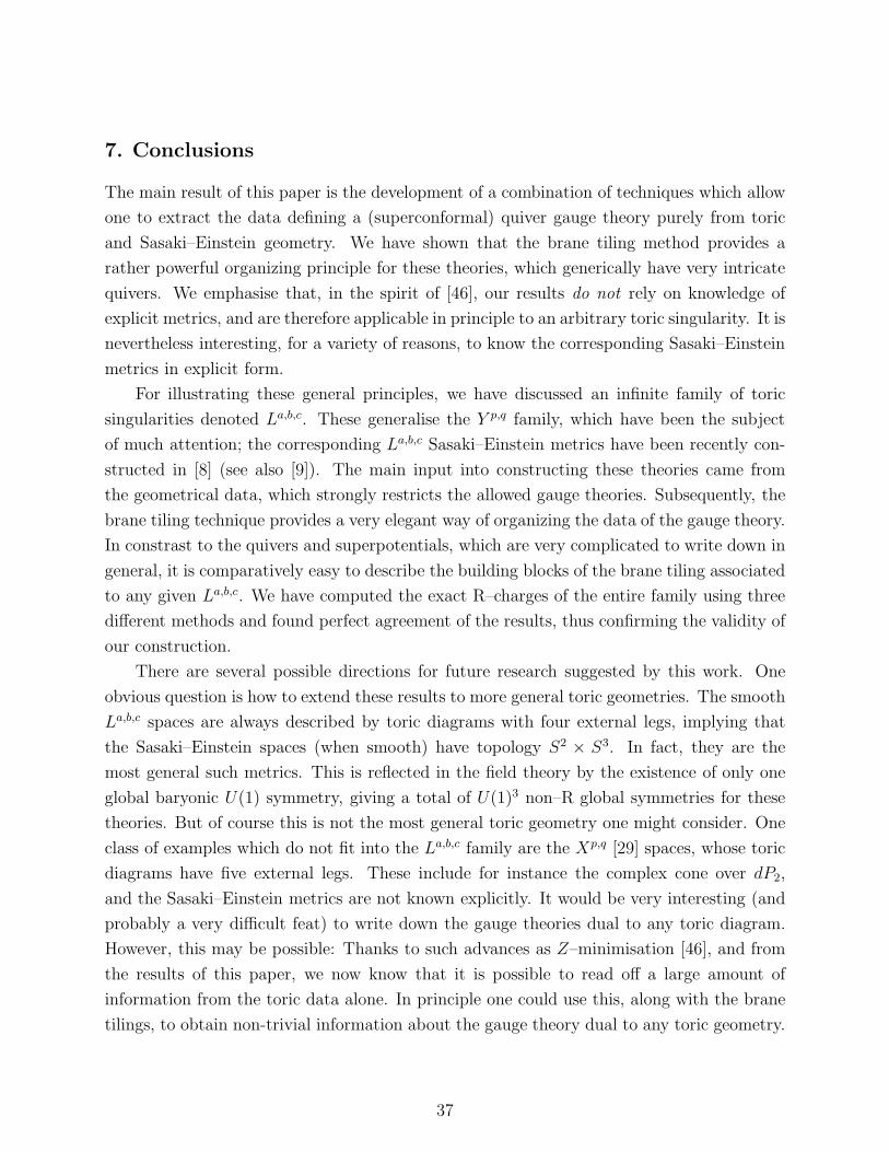
7. Conclusions
The main result of this paper is the development of a combination of techniques which allow
one to extract the data defining a (superconformal) quiver gauge theory purely from toric
and Sasaki–Einstein geometry. We have shown that the brane tiling method provides a
rather powerful organizing principle for these theories, which generically have very intricate
quivers. We emphasise that, in the spirit of [46], our results do not rely on knowledge of
explicit metrics, and are therefore applicable in principle to an arbitrary toric singularity. It is
nevertheless interesting, for a variety of reasons, to know the corresponding Sasaki–Einstein
metrics in explicit form.
For illustrating these general principles, we have discussed an infinite family of toric
singularities denoted La,b,c. These generalise the Y p,q family, which have been the subject
of much attention; the corresponding La,b,c Sasaki–Einstein metrics have been recently con-
structed in [8] (see also [9]). The main input into constructing these theories came from
the geometrical data, which strongly restricts the allowed gauge theories. Subsequently, the
brane tiling technique provides a very elegant way of organizing the data of the gauge theory.
In constrast to the quivers and superpotentials, which are very complicated to write down in
general, it is comparatively easy to describe the building blocks of the brane tiling associated
to any given La,b,c. We have computed the exact R–charges of the entire family using three
different methods and found perfect agreement of the results, thus confirming the validity of
our construction.
There are several possible directions for future research suggested by this work. One
obvious question is how to extend these results to more general toric geometries. The smooth
La,b,c spaces are always described by toric diagrams with four external legs, implying that
the Sasaki–Einstein spaces (when smooth) have topology S2 × S3. In fact, they are the
most general such metrics. This is reflected in the field theory by the existence of only one
global baryonic U(1) symmetry, giving a total of U(1)3 non–R global symmetries for these
theories. But of course this is not the most general toric geometry one might consider. One
class of examples which do not fit into the La,b,c family are the Xp,q [29] spaces, whose toric
diagrams have five external legs. These include for instance the complex cone over dP2,
and the Sasaki–Einstein metrics are not known explicitly. It would be very interesting (and
probably a very difficult feat) to write down the gauge theories dual to any toric diagram.
However, this may be possible: Thanks to such advances as Z–minimisation [46], and from
the results of this paper, we now know that it is possible to read off a large amount of
information from the toric data alone. In principle one could use this, along with the brane
tilings, to obtain non-trivial information about the gauge theory dual to any toric geometry.
37
One could also proceed by analogy to the progress made on the Y p,q spaces. Since we
know the La,b,c metrics, it is possible to seek deformations of these theories on both the su-
pergravity and gauge theory sides. Indeed there have been many exciting new developments
thanks to the study of the Y p,q theories and their cascading solutions. For the La,b,c family,
the study of the supergravity side of the cascades has been initiated in [9]. Here we have
not attempted to elaborate on these deformations, but doing so would be very interesting.
Additionally, the recent progress in Sasaki-Einstein spaces opens up the question of what
other metrics we can derive for other infinite families of spaces.
Although the toric data specifies much information, it is still important in many cases
to know the metric. This is true for example if one wishes to compute the Kaluza–Klein
spectrum of a given background. Another example is given by the problem of constructing
non-conformal deformations, or cascading solutions. It will be interesting to see whether
the program initiated in [46] can be developed further, so that for instance one can extract
information on the spectrum of the Laplacian operator purely from the toric data.
Another interesting question that arises in the context of our work is how to prove the
equivalence of a–maximisation and Z–minimisation. Although both procedures yield the
same numbers in all known examples (of which there are infinitely many), it is nevertheless
not a priori obvious that this should be the case. In particular, the function one extremizes
during a–maximisation is simply a cubic, whereas the function used in Z–minimisation is
a rational function. Furthermore, Z–minimisation is a statement about Sasaki-Einstein
spaces in any dimension, while a–maximisation appears to be unique to four dimensions.
Intuitively, we suspect (thanks to AdS/CFT) that these two procedures are equivalent, but
this statement is far from obvious. It would be wonderful to have a general proof that
Z–minimisation is the same as a–maximisation.
8. Acknowledgements
D. M. and J. F. S. would like to thank S.–T. Yau for discussions. S. F. and A. H. would
like to thank Bo Feng, Yang-Hui He and Kris Kennaway for discussions. A.H. would like to
thank Sergio Benvenuti for conversations. J. F. S. would also like to thank CalTech, KITP
and the University of Cambridge for hospitality. He is supported by NSF grants DMS–
0244464, DMS–0074329 and DMS–9803347. D. M. would like to thank his parents for warm
hospitality while this work has been completed. B.W. thanks the University of Chicago,
where some of this work was completed. S.F., A.H., D.V., and B.W. are supported in part
by the CTP and LNS of MIT, DOE contract #DE-FC02-94ER40818, and NSF grant PHY-
38
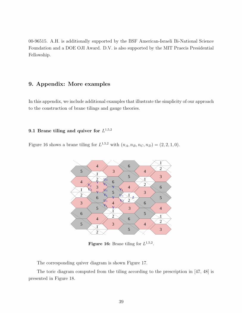
00-96515. A.H. is additionally supported by the BSF American-Israeli Bi-National Science
Foundation and a DOE OJI Award. D.V. is also supported by the MIT Praecis Presidential
Fellowship.
9. Appendix: More examples
In this appendix, we include additional examples that illustrate the simplicity of our approach
to the construction of brane tilings and gauge theories.
9.1 Brane tiling and quiver for L1,5,2
Figure 16 shows a brane tiling for L1,5,2 with (nA, nB, nC , nD) = (2, 2, 1, 0).
2U
1U
V2
1V
1U
1U
1U
1V
2U
1V
1V
1
4
Z
Y
Y
Y
Y
Y
1
3
6
5
4
2
34
5
6
3
21
45
4
1
3
6
53
2
4
35
3
6
5
21
4
5
6
3
4
21
6
6
5
2
22
11
Figure 16: Brane tiling for L1,5,2.
The corresponding quiver diagram is shown Figure 17.
The toric diagram computed from the tiling according to the prescription in [47, 48] is
presented in Figure 18.
39
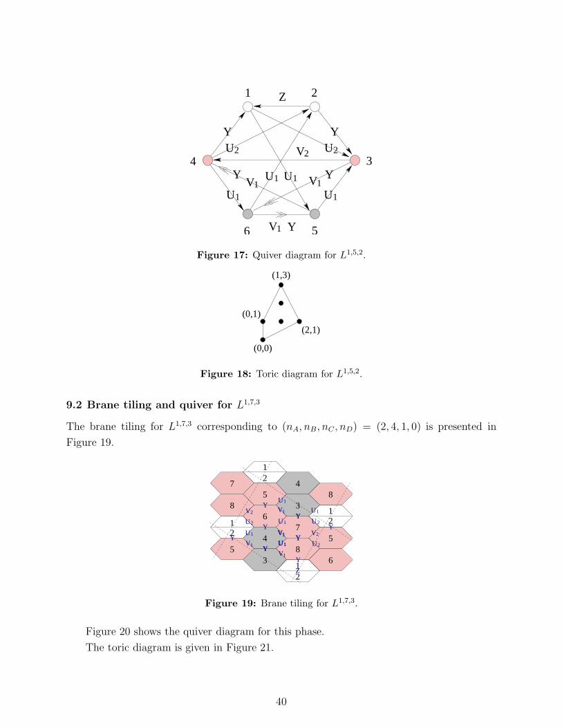
V
UV
UVU
U U
U
V
Y
Y Y
YY
6 5
4 3
21 Z
1
11
1
11
2 2
1
2
Figure 17: Quiver diagram for L1,5,2.
(0,1)
(1,3)
(0,0)
(2,1)
Figure 18: Toric diagram for L1,5,2.
9.2 Brane tiling and quiver for L1,7,3
The brane tiling for L1,7,3 corresponding to (nA, nB, nC , nD) = (2, 4, 1, 0) is presented in
Figure 19.
V2
U1
V1 V2
U1
U1
V1
U1
U2
U1
V1
V1
V1
U1
U2
U2
Y
Y Y
YY
Y
YY
Y
Y
Z
Y1
1
1
12
2
2
2
3
3
4
45
55
6
6
7
78
8
8
Figure 19: Brane tiling for L1,7,3.
Figure 20 shows the quiver diagram for this phase.
The toric diagram is given in Figure 21.
40
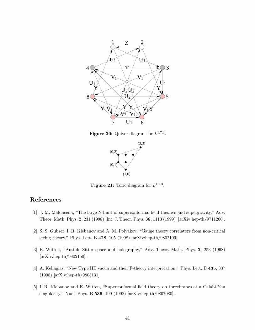
V
U
V
V
U
U
VUU
U
U
V
U
VY
Y
Y
8
7 6
5
4
21
3
Z
YY Y
Y
2
2
1
1
1
2
111
1
2
1
1
2
Figure 20: Quiver diagram for L1,7,3.
(1,0)
(0,2)
(0,1)
(3,3)
Figure 21: Toric diagram for L1,7,3.
References
[1] J. M. Maldacena, “The large N limit of superconformal field theories and supergravity,” Adv.
Theor. Math. Phys. 2, 231 (1998) [Int. J. Theor. Phys. 38, 1113 (1999)] [arXiv:hep-th/9711200].
[2] S. S. Gubser, I. R. Klebanov and A. M. Polyakov, “Gauge theory correlators from non-critical
string theory,” Phys. Lett. B 428, 105 (1998) [arXiv:hep-th/9802109].
[3] E. Witten, “Anti-de Sitter space and holography,” Adv. Theor. Math. Phys. 2, 253 (1998)
[arXiv:hep-th/9802150].
[4] A. Kehagias, “New Type IIB vacua and their F-theory interpretation,” Phys. Lett. B 435, 337
(1998) [arXiv:hep-th/9805131].
[5] I. R. Klebanov and E. Witten, “Superconformal field theory on threebranes at a Calabi-Yau
singularity,” Nucl. Phys. B 536, 199 (1998) [arXiv:hep-th/9807080].
41
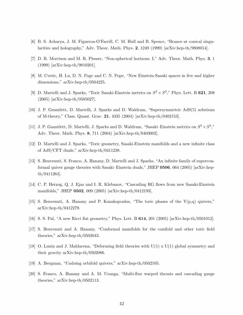
[6] B. S. Acharya, J. M. Figueroa-O’Farrill, C. M. Hull and B. Spence, “Branes at conical singu-
larities and holography,” Adv. Theor. Math. Phys. 2, 1249 (1999) [arXiv:hep-th/9808014].
[7] D. R. Morrison and M. R. Plesser, “Non-spherical horizons. I,” Adv. Theor. Math. Phys. 3, 1
(1999) [arXiv:hep-th/9810201].
[8] M. Cvetic, H. Lu, D. N. Page and C. N. Pope, “New Einstein-Sasaki spaces in five and higher
dimensions,” arXiv:hep-th/0504225.
[9] D. Martelli and J. Sparks, “Toric Sasaki-Einstein metrics on S2 ×S3,” Phys. Lett. B 621, 208
(2005) [arXiv:hep-th/0505027].
[10] J. P. Gauntlett, D. Martelli, J. Sparks and D. Waldram, “Supersymmetric AdS(5) solutions
of M-theory,” Class. Quant. Grav. 21, 4335 (2004) [arXiv:hep-th/0402153].
[11] J. P. Gauntlett, D. Martelli, J. Sparks and D. Waldram, “Sasaki–Einstein metrics on S2×S3,”
Adv. Theor. Math. Phys. 8, 711 (2004) [arXiv:hep-th/0403002].
[12] D. Martelli and J. Sparks, “Toric geometry, Sasaki-Einstein manifolds and a new infinite class
of AdS/CFT duals,” arXiv:hep-th/0411238.
[13] S. Benvenuti, S. Franco, A. Hanany, D. Martelli and J. Sparks, “An infinite family of supercon-
formal quiver gauge theories with Sasaki–Einstein duals,” JHEP 0506, 064 (2005) [arXiv:hep-
th/0411264].
[14] C. P. Herzog, Q. J. Ejaz and I. R. Klebanov, “Cascading RG flows from new Sasaki-Einstein
manifolds,” JHEP 0502, 009 (2005) [arXiv:hep-th/0412193].
[15] S. Benvenuti, A. Hanany and P. Kazakopoulos, “The toric phases of the Y(p,q) quivers,”
arXiv:hep-th/0412279.
[16] S. S. Pal, “A new Ricci flat geometry,” Phys. Lett. B 614, 201 (2005) [arXiv:hep-th/0501012].
[17] S. Benvenuti and A. Hanany, “Conformal manifolds for the conifold and other toric field
theories,” arXiv:hep-th/0502043.
[18] O. Lunin and J. Maldacena, “Deforming field theories with U(1) x U(1) global symmetry and
their gravity arXiv:hep-th/0502086.
[19] A. Bergman, “Undoing orbifold quivers,” arXiv:hep-th/0502105.
[20] S. Franco, A. Hanany and A. M. Uranga, “Multi-flux warped throats and cascading gauge
theories,” arXiv:hep-th/0502113.
42
[21] J. F. G. Cascales, F. Saad and A. M. Uranga, “Holographic dual of the standard model on
the throat,” arXiv:hep-th/0503079.
[22] B. A. Burrington, J. T. Liu, M. Mahato and L. A. Pando Zayas, “Towards supergravity duals
of chiral symmetry breaking in Sasaki-Einstein arXiv:hep-th/0504155.
[23] D. Berenstein, C. P. Herzog, P. Ouyang and S. Pinansky, “Supersymmetry breaking from a
Calabi-Yau singularity,” arXiv:hep-th/0505029.
[24] S. Franco, A. Hanany, F. Saad and A. M. Uranga, “Fractional branes and dynamical super-
symmetry breaking,” arXiv:hep-th/0505040.
[25] S. Benvenuti and M. Kruczenski, “Semiclassical strings in Sasaki-Einstein manifolds and long
operators in N = 1 gauge theories,” arXiv:hep-th/0505046.
[26] M. Bertolini, F. Bigazzi and A. L. Cotrone, “Supersymmetry breaking at the end of a cascade
of Seiberg dualities,” arXiv:hep-th/0505055.
[27] S. Franco, Y. H. He, C. Herzog and J. Walcher, “Chaotic duality in string theory,” Phys. Rev.
D 70, 046006 (2004) [arXiv:hep-th/0402120].
[28] I. R. Klebanov and M. J. Strassler, “Supergravity and a confining gauge theory: Duality
cascades and JHEP 0008, 052 (2000) [arXiv:hep-th/0007191].
[29] A. Hanany, P. Kazakopoulos and B. Wecht, “A new infinite class of quiver gauge theories,”
arXiv:hep-th/0503177.
[30] C. Ahn and J. F. Vazquez-Poritz, “Marginal Deformations with U(1)3 Global Symmetry,”
arXiv:hep-th/0505168.
[31] Jerome P. Gauntlett, Sangmin Lee, Toni Mateos, Daniel Waldram, “Marginal Deformations
of Field Theories with AdS4 Duals,” arXiv:hep-th/0505207.
[32] K. Intriligator and B. Wecht, “The exact superconformal R-symmetry maximizes a,” Nucl.
Phys. B 667, 183 (2003) [arXiv:hep-th/0304128].
[33] D. Anselmi, D. Z. Freedman, M. T. Grisaru and A. A. Johansen, “Nonperturbative formulae for
central functions of supersymmetric gauge theories”, Nucl. Phys. B526, 543 (1998), [arXiv:hep-
th/9708042].
[34] D. Anselmi, J. Erlich, D. Z. Freedman and A. A. Johansen, “Positivity constraints on anomalies
in supersymmetric gauge theories”, Phys. Rev. D57, 7570 (1998), [arXiv:hep-th/9711035].
[35] M. Henningson and K. Skenderis, “The holographic Weyl anomaly,” JHEP 9807, 023 (1998)
[arXiv:hep-th/9806087].
43
[36] B. Feng, A. Hanany and Y. H. He, “D-brane gauge theories from toric singularities and toric
duality,” Nucl. Phys. B 595, 165 (2001) [arXiv:hep-th/0003085].
[37] B. Feng, A. Hanany and Y. H. He, “Phase structure of D-brane gauge theories and toric
duality,” JHEP 0108, 040 (2001) [arXiv:hep-th/0104259].
[38] D. Kutasov, A. Parnachev and D. A. Sahakyan, “Central charges and U(1)R symmetries in N
= 1 super Yang-Mills,” JHEP 0311, 013 (2003) [arXiv:hep-th/0308071].
[39] K. Intriligator and B. Wecht, “RG fixed points and flows in SQCD with adjoints,” Nucl. Phys.
B 677, 223 (2004) [arXiv:hep-th/0309201].
[40] D. Kutasov, “New results on the ’a-theorem’ in four dimensional supersymmetric field
arXiv:hep-th/0312098.
[41] C. Csaki, P. Meade and J. Terning, “A mixed phase of SUSY gauge theories from a-
maximization,” JHEP 0404, 040 (2004) [arXiv:hep-th/0403062].
[42] E. Barnes, K. Intriligator, B. Wecht and J. Wright, “Evidence for the strongest version of the
4d a-theorem, via a-maximization along RG flows,” Nucl. Phys. B 702, 131 (2004) [arXiv:hep-
th/0408156].
[43] D. Kutasov and A. Schwimmer, “Lagrange multipliers and couplings in supersymmetric field
theory,” Nucl. Phys. B 702, 369 (2004) [arXiv:hep-th/0409029].
[44] E. Barnes, K. Intriligator, B. Wecht and J. Wright, “N = 1 RG flows, product groups, and
a-maximization,” Nucl. Phys. B 716, 33 (2005) [arXiv:hep-th/0502049].
[45] M. Bertolini, F. Bigazzi and A. L. Cotrone, “New checks and subtleties for AdS/CFT and
a-maximization,” JHEP 0412, 024 (2004s [arXiv:hep-th/0411249].
[46] D. Martelli, J. Sparks and S. T. Yau, “The geometric dual of a-maximization for toric Sasaki-
Einstein manifolds,” arXiv:hep-th/0503183.
[47] A. Hanany and K. D. Kennaway, “Dimer models and toric diagrams,” arXiv:hep-th/0503149.
[48] S. Franco, A. Hanany, K. D. Kennaway, D. Vegh and B. Wecht, “Brane dimers and quiver
gauge theories,” arXiv:hep-th/0504110.
[49] S. Benvenuti and M. Kruczenski, “From Sasaki-Einstein spaces to quivers via BPS geodesics:
Lpqr,” arXiv:hep-th/0505206.
[50] A. Butti, D. Forcella and A. Zaffaroni, “The dual superconformal theory for L(p,q,r) mani-
folds,” arXiv:hep-th/0505220.
44
[51] E. Lerman, “Contact Toric Manifolds”, J. Symplectic Geom. 1 (2003), no. 4, 785–828
arXiv:math.SG/0107201.
[52] E. Lerman, “Homotopy Groups of K-Contact Toric Manifolds,” Trans. Amer. Math. Soc. 356
(2004), no. 10, 4075–4083 math.SG/0204064.
[53] D. Berenstein, C. P. Herzog and I. R. Klebanov, “Baryon spectra and AdS/CFT correspon-
dence,” JHEP 0206, 047 (2002) [arXiv:hep-th/0202150].
[54] K. Intriligator and B. Wecht, “Baryon charges in 4D superconformal field theories and their
AdS duals,” Commun. Math. Phys. 245, 407 (2004) [arXiv:hep-th/0305046].
[55] C. P. Herzog and J. McKernan, “Dibaryon spectroscopy,” JHEP 0308, 054 (2003) [arXiv:hep-
th/0305048].
[56] C. P. Herzog and J. Walcher, “Dibaryons from exceptional collections,” JHEP 0309, 060
(2003) [arXiv:hep-th/0306298].
[57] O. Aharony, A. Hanany and B. Kol, “Webs of (p,q) 5-branes, five dimensional field theories
and grid diagrams,” JHEP 9801, 002 (1998) [arXiv:hep-th/9710116].
[58] O. Aharony and A. Hanany, “Branes, superpotentials and superconformal fixed points,” Nucl.
Phys. B 504, 239 (1997) [arXiv:hep-th/9704170].
[59] N. C. Leung and C. Vafa, “Branes and toric geometry,” Adv. Theor. Math. Phys. 2, 91 (1998)
[arXiv:hep-th/9711013].
[60] A. Hanany and A. Iqbal, “Quiver theories from D6-branes via mirror symmetry,” JHEP 0204,
009 (2002) [arXiv:hep-th/0108137].
[61] E. Lerman, S. Tolman, ”Symplectic Toric Orbifolds”, arXiv: dg-ga/9412005
[62] B. Feng, S. Franco, A. Hanany and Y. H. He, “Symmetries of toric duality,” JHEP 0212, 076
(2002) [arXiv:hep-th/0205144].
[63] N. Seiberg, “Electric - magnetic duality in supersymmetric nonAbelian gauge theories,” Nucl.
Phys. B 435, 129 (1995) [arXiv:hep-th/9411149].
[64] A. M. Uranga, “Brane configurations for branes at conifolds,” JHEP 9901, 022 (1999)
[arXiv:hep-th/9811004].
[65] S. Gubser, N. Nekrasov and S. Shatashvili, “Generalized conifolds and four dimensional N =
1 superconformal theories,” JHEP 9905, 003 (1999) [arXiv:hep-th/9811230].
45
[66] E. Lopez, “A family of N = 1 SU(N)**k theories from branes at singularities,” JHEP 9902,
019 (1999) [arXiv:hep-th/9812025].
[67] R. von Unge, “Branes at generalized conifolds and toric geometry,” JHEP 9902, 023 (1999)
[arXiv:hep-th/9901091].
46


