From Regular BoundaryGraphs to AntipodalDistance-Regular Graphs*

M. A. Fiol, E. Garriga, and J. L. A. YebraDEPARTAMENT DE MATEMATICA APLICADA I TELEMATICA

UNIVERSITAT POLITECNICA DE CATALUNYAE-mails: f iol@mat.upc.es, garriga@mat.upc.es, yebra@mat.upc.es

Received April 10, 1995; revised October 16, 1997

Abstract: Let Γ be a regular graph with n vertices, diameter D, and d + 1different eigenvalues λ > λ1 > · · · > λd. In a previous paper, the authorsshowed that if P (λ) > n − 1, then D ≤ d − 1, where P is the polynomial ofdegree d−1 which takes alternating values±1 atλ1, . . . , λd. The graphs satisfyingP (λ) = n − 1, called boundary graphs, have shown to deserve some attentionbecause of their rich structure. This paper is devoted to the study of this caseand, as a main result, it is shown that those extremal (D = d) boundary graphswhere each vertex have maximum eccentricity are, in fact, 2-antipodal distance-regular graphs. The study is carried out by using a new sequence of orthogonalpolynomials, whose special properties are shown to be induced by their intrinsicsymmetry. c© 1998 John Wiley & Sons, Inc. J Graph Theory 27: 123–140, 1998

Keywords: antinodal distance-regular graphs, boundary graphs, eigenvalues, orthogonal

polynomials

1. INTRODUCTION

A general problem which has deserved much attention among graph theorists is to

*Work supported in part by the Spanish Research Council (Comision Interministerialde Ciencia y Tecnologia, CICYT) under projects TIC 92-1228-E and TIC 94-0592.

c© 1998 John Wiley & Sons, Inc. CCC 0364-9024/98/030123-18

124 JOURNAL OF GRAPH THEORY

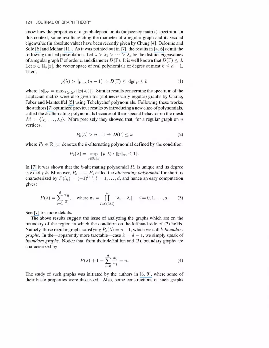
know how the properties of a graph depend on its (adjacency matrix) spectrum. Inthis context, some results relating the diameter of a regular graph and its secondeigenvalue (in absolute value) have been recently given by Chung [4], Delorme andSole [6] and Mohar [11]. As it was pointed out in [7], the results in [4, 6] admit thefollowing unified presentation. Let λ > λ1 > · · · > λd be the distinct eigenvaluesof a regular graph Γ of order n and diameterD(Γ). It is well known thatD(Γ) ≤ d.Let p ∈ Rk[x], the vector space of real polynomials of degree at most k ≤ d − 1.Then,

p(λ) > ‖p‖∞(n− 1)⇒ D(Γ) ≤ dgr p ≤ k (1)

where ‖p‖∞ = max1≤l≤d|p(λl)|. Similar results concerning the spectrum of theLaplacian matrix were also given for (not necessarily regular) graphs by Chung,Faber and Manteuffel [5] using Tchebychef polynomials. Following these works,the authors [7] optimized previous results by introducing a new class of polynomials,called the k-alternating polynomials because of their special behavior on the meshM = λ1, . . . , λd. More precisely they showed that, for a regular graph on nvertices,

Pk(λ) > n− 1⇒ D(Γ) ≤ k (2)

where Pk ∈ Rk[x] denotes the k-alternating polynomial defined by the condition:

Pk(λ) = supp∈Rk[x]

p(λ) : ‖p‖∞ ≤ 1.

In [7] it was shown that the k-alternating polynomial Pk is unique and its degreeis exactly k. Moreover, Pd−1 ≡ P , called the alternating polynomial for short, ischaracterized by P (λl) = (−1)l+1, l = 1, . . . , d, and hence an easy computationgives:

P (λ) =d∑i=1

π0

πi, where πi =

d∏l=0(l /=i)

|λi − λl|, i = 0, 1, . . . , d. (3)

See [7] for more details.The above results suggest the issue of analyzing the graphs which are on the

boundary of the region in which the condition on the lefthand side of (2) holds.Namely, those regular graphs satisfying Pk(λ) = n−1, which we call k-boundarygraphs. In the—apparently more tractable—case k = d − 1, we simply speak ofboundary graphs. Notice that, from their definition and (3), boundary graphs arecharacterized by

P (λ) + 1 =d∑l=0

π0

πl= n. (4)

The study of such graphs was initiated by the authors in [8, 9], where some oftheir basic properties were discussed. Also, some constructions of such graphs

ANTIPODAL DISTANCE-REGULAR GRAPHS 125

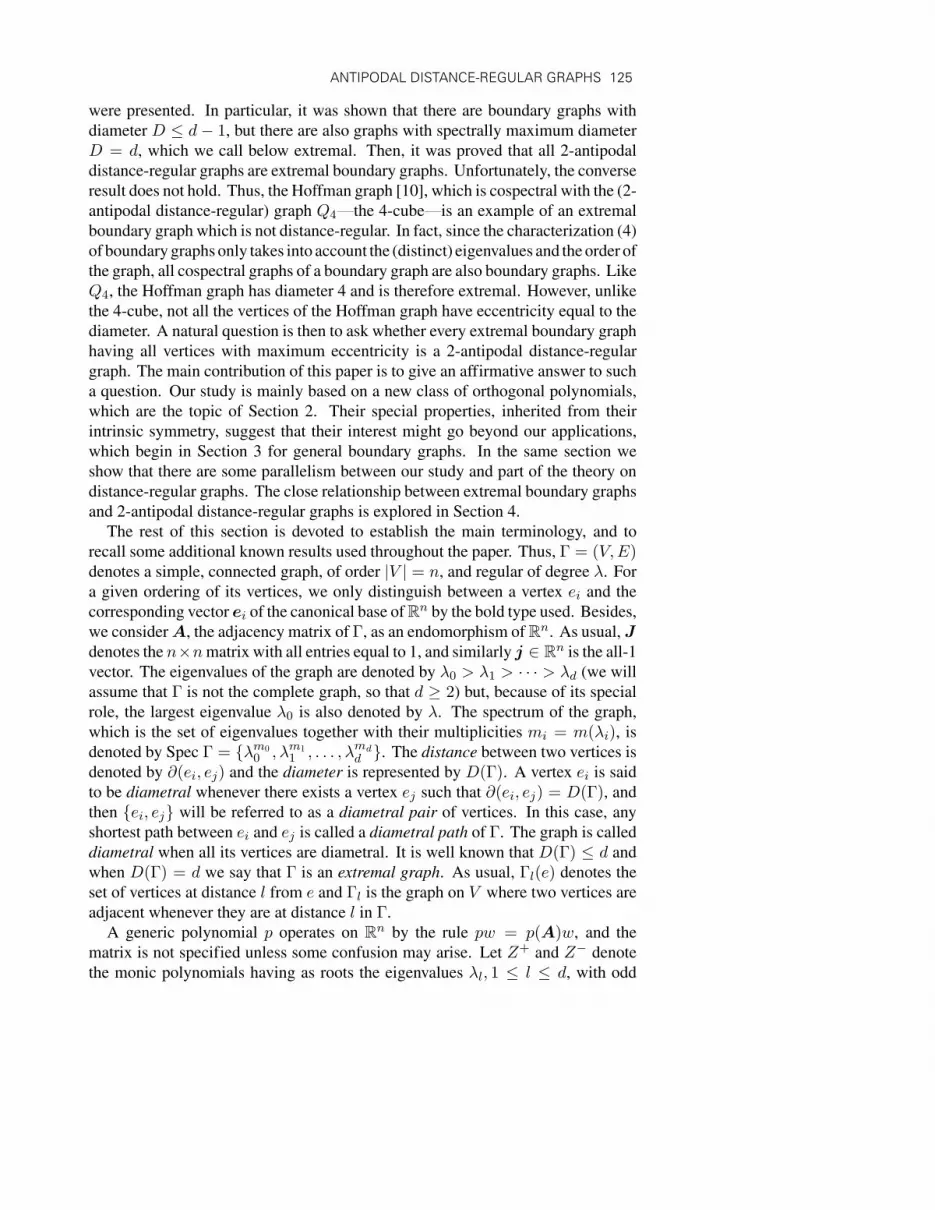
were presented. In particular, it was shown that there are boundary graphs withdiameter D ≤ d− 1, but there are also graphs with spectrally maximum diameterD = d, which we call below extremal. Then, it was proved that all 2-antipodaldistance-regular graphs are extremal boundary graphs. Unfortunately, the converseresult does not hold. Thus, the Hoffman graph [10], which is cospectral with the (2-antipodal distance-regular) graph Q4—the 4-cube—is an example of an extremalboundary graph which is not distance-regular. In fact, since the characterization (4)of boundary graphs only takes into account the (distinct) eigenvalues and the order ofthe graph, all cospectral graphs of a boundary graph are also boundary graphs. LikeQ4, the Hoffman graph has diameter 4 and is therefore extremal. However, unlikethe 4-cube, not all the vertices of the Hoffman graph have eccentricity equal to thediameter. A natural question is then to ask whether every extremal boundary graphhaving all vertices with maximum eccentricity is a 2-antipodal distance-regulargraph. The main contribution of this paper is to give an affirmative answer to sucha question. Our study is mainly based on a new class of orthogonal polynomials,which are the topic of Section 2. Their special properties, inherited from theirintrinsic symmetry, suggest that their interest might go beyond our applications,which begin in Section 3 for general boundary graphs. In the same section weshow that there are some parallelism between our study and part of the theory ondistance-regular graphs. The close relationship between extremal boundary graphsand 2-antipodal distance-regular graphs is explored in Section 4.

The rest of this section is devoted to establish the main terminology, and torecall some additional known results used throughout the paper. Thus, Γ = (V,E)denotes a simple, connected graph, of order |V | = n, and regular of degree λ. Fora given ordering of its vertices, we only distinguish between a vertex ei and thecorresponding vector ei of the canonical base ofRn by the bold type used. Besides,we considerA, the adjacency matrix of Γ, as an endomorphism ofRn. As usual, Jdenotes the n×nmatrix with all entries equal to 1, and similarly j ∈ Rn is the all-1vector. The eigenvalues of the graph are denoted by λ0 > λ1 > · · · > λd (we willassume that Γ is not the complete graph, so that d ≥ 2) but, because of its specialrole, the largest eigenvalue λ0 is also denoted by λ. The spectrum of the graph,which is the set of eigenvalues together with their multiplicities mi = m(λi), isdenoted by Spec Γ = λm0

0 , λm11 , . . . , λmdd . The distance between two vertices is

denoted by ∂(ei, ej) and the diameter is represented by D(Γ). A vertex ei is saidto be diametral whenever there exists a vertex ej such that ∂(ei, ej) = D(Γ), andthen ei, ej will be referred to as a diametral pair of vertices. In this case, anyshortest path between ei and ej is called a diametral path of Γ. The graph is calleddiametral when all its vertices are diametral. It is well known that D(Γ) ≤ d andwhen D(Γ) = d we say that Γ is an extremal graph. As usual, Γl(e) denotes theset of vertices at distance l from e and Γl is the graph on V where two vertices areadjacent whenever they are at distance l in Γ.

A generic polynomial p operates on Rn by the rule pw = p(A)w, and thematrix is not specified unless some confusion may arise. Let Z+ and Z− denotethe monic polynomials having as roots the eigenvalues λl, 1 ≤ l ≤ d, with odd

126 JOURNAL OF GRAPH THEORY

and even subindex l, respectively. Then, we will make ample use of the followingspectral decompositions of the canonical vector ei.

ei =1nj + zi =

1nj + zi1 + · · ·+ zid =

1nj + z+

i + z−i (5)

where zi ∈ j⊥,zil ∈ Ker (x− λl),z+i ∈ Ker Z+ and z−i ∈ Ker Z−.

Since for a boundary graph the inequality in the righthand side of (2) (withk = d − 1) does not hold, the matrix P (A) may have entries equal to zero. Thatis, it may happen that 〈Pe, e〉 = 0 for some pair of vertices e, e. We say in thiscase that each one is a conjugate vertex and, when they are different, that they forma pair of conjugate vertices. Thus, every diametral pair of an extremal graph is aconjugate pair. If 〈Pe, e〉 = 0 we say that e is a selfconjugate vertex.

In some cases, condition (4) characterizing boundary graphs is strong enough todetermine the entries of the matrix P (A), from where some of the main propertiesof such graphs follow. Indeed, since the alternating polynomial satisfies P (λl) =(−1)l+1, 1 ≤ l ≤ d, we have ‖Pzi‖2 = ‖zi‖2 = 1 − ‖ 1

nj‖2 = 1 − 1n , and this

decomposition allows us to give a generic expression for the ij entry of the matrixP (A), as follows:

(P (A))ij = 〈Pei, ej〉 =⟨P (λ)nj + Pzi,

1nj + zj

⟩=

n− 1n

+ ‖Pzi‖ ‖zj‖ cos γij

=n− 1n

(1 + cos γij) (6)

where γij represents the angle formed by Pzi and zj .As a straightforward consequence of (6), note that all the entries of P (A) satisfy

0 ≤ (P (A))ij < 2(1− 1n). Furthermore,

(P (A))ij = 0 ⇔ Pzi = −zj (7)

⇔ z+i = −z+

j ,z−i = z−j ⇔ zil = (−1)lzjl, (1 ≤ l ≤ d) (8)

⇔ei = 1

nj + zi1 + zi2 + zi3 + · · ·+ zidej = 1

nj − zi1 + zi2 − zi3 + · · ·+ (−1)dzid(9)

since, in j⊥, Pz = z iff z ∈ Ker Z+, and Pz = −z iff z ∈ Ker Z−.Notice that, by (9), the spectral decompositions of the conjugate vertices ei, ej

have the same components, except for their signs which are alternatively equal ordistinct. As we will see, the polynomials studied in the next section show a similarbehavior at the points of the mesh and, we could say that, in a sense, each one hasalso a ‘‘conjugate.’’ For instance, consider the pair (P, I) formed by the alternatingand the identity polynomials respectively. Then, using (9) we get

Pei + Iej =1n

(Pj + j) = j. (10)

ANTIPODAL DISTANCE-REGULAR GRAPHS 127

That is, if Pei has a zero component, all its other components are 1, and henceeach vertex can only belong to a pair of conjugate vertices. Let V ∗ denote the setof conjugate vertices and let Γ∗ be its induced subgraph in V ∗. Let σ : V ∗ → V ∗be the mapping defined by σe = (J −P (A))e. From the above, σ is well definedand it is an involutive permutation of V ∗. Then, in [8] the following result wasproved.

Proposition 1.1. In a boundary graph Γ the mapping σ is an automorphism ofΓ∗. Moreover, in Γ, ∂(σei, σej) = ∂(ei, ej),∀ei, ej ∈ V ∗.

2. A CLASS OF ORTHOGONAL POLYNOMIALS

LetM = x1 > · · · > xm be a mesh of m real points. For i = 1, . . . ,m, setMi = 1, . . . ,m \ i and

νi(M) =∏l∈Mi

(xi − xl), πi(M) = (−1)i+1νi = |νi(M)|.

Using the fact that each polynomial of degree ≤ m − 1 can be identified by itsvalues onM, we introduce in Rm−1[x] a scalar product by

〈p, q〉 =m∑i=1

1πi(M)

p(xi)q(xi),

and a linear mapping T by

(Tp)(xi) = (−1)i+1p(xi), i = 1, . . . ,m.

Clearly, T is an involutive automorphism of Rm−1[x], and for this scalar productwe have:

(a) T is symmetric, 〈Tp, q〉 =∑mi=1

(−1)i+ 1

πi(M) p(xi)q(xi) = 〈p, Tq〉;(b) T is an isometry, 〈Tp, Tq〉 = 〈T 2p, q〉 = 〈p, q〉. In particular, ‖Tp‖ = ‖p‖.

In order to establish the main results of this section we first need the following.

Lemma 2.1.m∑i=1

xkiνi(M)

=

0 for k = 0, 1, . . . ,m− 21 for k = m− 1.

Proof. Since for polynomials of degree≤ m−1 interpolation troughm pointsis exact, using Lagrange interpolation with Ri =

∏j∈Mi

(x− xj) we have

p =m∑i=1

p(xi)Ri(xi)

Ri =m∑i=1

p(xi)νi(M)

Ri =

(m∑i=1

p(xi)νi(M)

)xm−1 + · · ·

and for p = xk the result follows.

128 JOURNAL OF GRAPH THEORY

Noticing that 〈Txr, xs〉 =∑mi=1

1πi(M)(−1)i+1xrix

si =

∑mi=1

xr+si

νi(M) , we mayrestate the above lemma in the following way:

〈Txr, xs〉 =

0 for r + s = 0, 1, . . . ,m− 21 for r + s = m− 1. (11)

We next use T to characterize some systems of orthogonal polynomials for thescalar product above.

Proposition 2.2. Let pk, k = 0, . . . ,m − 1, be polynomials with dgr pk = k.Then, the following statements are equivalent:

(i) pk, k = 0, . . . ,m− 1 is an orthogonal system;(ii) Tpk is proportional to pm−1−k, k = 0, 1, . . . ,m− 1.

Proof. Since dgr pk = k, (11) implies

〈Tpk, pl〉 = 0 for k + l < m− 1.

Let pk, k = 0, . . . ,m− 1 be an orthogonal system. Then,

Tpk =m−1∑l=0

cklpl =m−1∑

l=m−1−kcklpl,

since for l < m − 1 − k we have ckl‖pl‖2 = 〈Tpk, pl〉 = 0. For k = 0 wealready obtain that Tp0 is proportional to pm−1. Using induction, let us assumethat Tp0 = γ0pm−1, . . . , Tpk−1 = γk−1pm−k. Consider now l > m−1−k. SinceT is involutive andm−1−l < k, we obtain pm−1−l = T 2(pm−1−l) = γm−1−lTpl,so that

ckl‖pl‖2 = 〈Tpk, pl〉 = 〈pk, Tpl〉 =1

γm−1−l〈pk, pm−1−l〉 = 0.

Therefore, ckl = 0 for l > m− 1− k and Tpk is proportional to pm−1−k.Reciprocally, assume now that Tpk = γkpm−1−k, for k = 0, 1, . . . ,m− 1. For

0 ≤ j < i ≤ m− 1 we have m− 1− i+ j < m− 1, so that

〈pi, pj〉 = 〈Tpi, Tpj〉 = γi〈pm−1−i, Tpj〉 = 0.

From this proposition we obtain, for k = 0, 1, . . . ,m− 1,

‖pk‖2 = 〈Tpk, Tpk〉 = γ2k‖pm−1−k‖2, (12)

‖pk‖2 = 〈Tpk, γkpm−1−k〉= γk〈T (αkxk + · · ·), αm−1−kxm−1−k + · · ·〉 = γkαkαm−1−k, (13)

where αk is the leading coefficient of pk, 0 ≤ k ≤ m− 1.

Proposition 2.3. For any given x0 > x1 and any constant n there exists aunique system of orthogonal polynomials on the meshM, w0, w1, . . . , wm−1, withdgr wk = k, such that, for k = 0, 1, . . . ,m− 1,

ANTIPODAL DISTANCE-REGULAR GRAPHS 129

(a) Twk = wm−1−k;(b) wk(x0) + wm−1−k(x0) = n.

Proof. The Gram-Schmidt procedure assures the existence of a unique systemof orthonormal polynomials q0, q1, . . . , qm−1, such that dgr qk = k and the leadingcoefficient of each qk is positive. From the theory of orthogonal polynomials weknow that all their roots are real and belong to the interval (xm, x1). It followsthat qk(x0) > 0 for all k. From (12) and (13) we obtain Tqk = qm−1−k. Settingwk = ξkqk we have

Twk = ξkTqk = ξkqm−1−k =ξk

ξm−1−kwm−1−k.

Now (a) is equivalent to ξk = ξm−1−k and (b) becomes

n = ξkqk(x0) + ξm−1−kqm−1−k(x0) = (qk(x0) + qm−1−k(x0))ξk,

which determines ξk for k = 0, 1, . . . ,m− 1.In particular, (a) gives

‖wk‖2 = αkαm−1−k, , k = 0, 1, . . . ,m− 1, (14)

where αk is the leading coefficient of wk. Denoting by PM the polynomial ofdegree m− 1 such that PM(xi) = (−1)i+1, i = 1, . . . ,m, we have: wm−1(xi) =Tw0(xi) = (−1)i+1α0, so that wm−1 = α0PM. Moreover, α0 +α0PM(x0) = n,and

w0 =n

1 + PM(x0), wm−1 =

n

1 + PM(x0)PM. (15)

Notice that whenM, x0, n are such that PM(x0) = n− 1, equation (15) becomesw0 = 1 and wm−1 = PM. We will consider this case in the context of graphs inthe next section.

Consider now two meshes

M∗ = λ1 > · · · > λd, M = λ0(= λ) > λ1 > · · · > λd.For the meshM∗ (resp. M) we define the involutive automorphism T ∗ (resp. T )and consider the scalar product 〈 , 〉∗ (resp. 〈 , 〉) and the norm ‖ · ‖∗ (resp. ‖ · ‖.)We also write π∗i = πi(M∗) and πi = πi(M).

For a fixed constant n let w0, w1, . . . , wd−1 be the orthogonal system of Propo-sition 2.3 for the mesh M∗ with x0 = λ, that is T ∗wk = wd−1−k, wk(λ) +wd−1−k(λ) = n for k = 0, 1, . . . , d − 1. We next introduce the polynomialsin Rd[x]:

vk = wk − wk−1, k = 0, 1, . . . , d,

by defining w−1 = 0, wd = nπ0

∏di=1(x− λi), so that we still have: T ∗w−1 = wd

and w−1(λ) + wd(λ) = n.

130 JOURNAL OF GRAPH THEORY

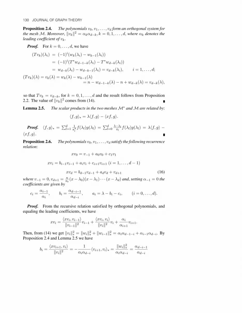
Proposition 2.4. The polynomials v0, v1, . . . , vd form an orthogonal system forthe meshM. Moreover, ‖vk‖2 = αkαd−k, k = 0, 1, . . . , d, where αk denotes theleading coefficient of vk.

Proof. For k = 0, . . . , d, we have

(Tvk)(λi) = (−1)i(wk(λi)− wk−1(λi))

= (−1)i(T ∗wd−1−k(λi)− T ∗wd−k(λi))= wd−k(λi)− wd−k−1(λi) = vd−k(λi), i = 1, . . . , d;

(Tvk)(λ) = vk(λ) = wk(λ)− wk−1(λ)= n− wd−1−k(λ)− n+ wd−k(λ) = vd−k(λ),

so that Tvk = vd−k, for k = 0, 1, . . . , d and the result follows from Proposition2.2. The value of ‖vk‖2 comes from (14).

Lemma 2.5. The scalar products in the two meshesM∗ andM are related by:

〈f, g〉∗ = λ〈f, g〉 − 〈xf, g〉.

Proof. 〈f, g〉∗ =∑dl=1

1π∗lf(λl)g(λl) =

∑dl=0

λ−λlπl

f(λl)g(λl) = λ〈f, g〉 −〈xf, g〉.Proposition 2.6. The polynomials v0, v1, . . . , vd satisfy the following recurrencerelation:

xv0 = v−1 + a0v0 + c1v1

xvi = bi−1vi−1 + aivi + ci+1vi+1 (i = 1, . . . , d− 1)

xvd = bd−1vd−1 + advd + vd+1 (16)

where v−1 = 0, vd+1 = nπ0

(x− λ0)(x− λ1) · · · (x− λd) and, setting α−1 = 0 thecoefficients are given by

ci =αi−1

αi, bi =

αd−i−1

αd−i, ai = λ− bi − ci, (i = 0, . . . , d).

Proof. From the recursive relation satisfied by orthogonal polynomials, andequaling the leading coefficients, we have

xvi =〈xvi, vi−1〉‖vi−1‖2 vi−1 +

〈xvi, vi〉‖vi‖2 vi +

αiαi+1

vi+1.

Then, from (14) we get ‖vi‖2∗ = ‖wi‖2∗ + ‖wi−1‖2∗ = αiαd−1−i + αi−1αd−i. ByProposition 2.4 and Lemma 2.5 we have

bi =〈xvi+1, vi〉‖vi‖2 = − 1

αiαd−i〈vi+1, vi〉∗ =

‖wi‖2∗αiαd−i

=αd−i−1

αd−i

ANTIPODAL DISTANCE-REGULAR GRAPHS 131

ai =〈xvi, vi〉‖vi‖2 =

1αiαd−i

(λ‖vi‖2 − ‖vi‖2∗) = λ− αd−i−1

αd−i− αi−1

ai= λ− bi − ci

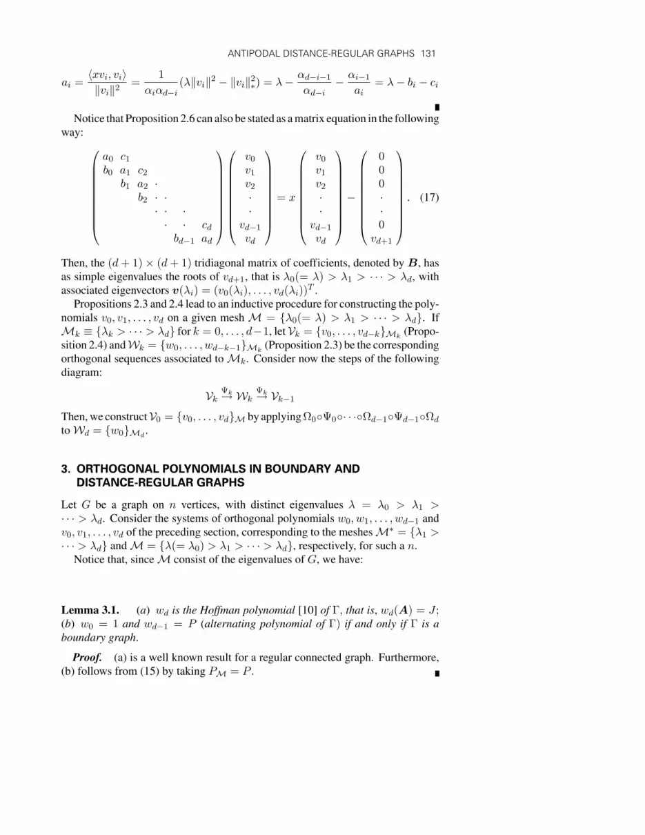
Notice that Proposition 2.6 can also be stated as a matrix equation in the followingway:

a0 c1b0 a1 c2

b1 a2 ·b2 · ·· · ·· · cdbd−1 ad

v0v1v2··

vd−1vd

= x

v0v1v2··

vd−1vd

−

000··0

vd+1

. (17)

Then, the (d+ 1)× (d+ 1) tridiagonal matrix of coefficients, denoted by B, hasas simple eigenvalues the roots of vd+1, that is λ0(= λ) > λ1 > · · · > λd, withassociated eigenvectors v(λi) = (v0(λi), . . . , vd(λi))T .

Propositions 2.3 and 2.4 lead to an inductive procedure for constructing the poly-nomials v0, v1, . . . , vd on a given mesh M = λ0(= λ) > λ1 > · · · > λd. IfMk ≡ λk > · · · > λd for k = 0, . . . , d−1, let Vk = v0, . . . , vd−kMk

(Propo-sition 2.4) andWk = w0, . . . , wd−k−1Mk

(Proposition 2.3) be the correspondingorthogonal sequences associated toMk. Consider now the steps of the followingdiagram:

Vk Ψk→WkΨk→ Vk−1

Then, we constructV0 = v0, . . . , vdM by applying Ω0Ψ0· · ·Ωd−1Ψd−1Ωd

toWd = w0Md.

3. ORTHOGONAL POLYNOMIALS IN BOUNDARY ANDDISTANCE-REGULAR GRAPHS

Let G be a graph on n vertices, with distinct eigenvalues λ = λ0 > λ1 >· · · > λd. Consider the systems of orthogonal polynomials w0, w1, . . . , wd−1 andv0, v1, . . . , vd of the preceding section, corresponding to the meshesM∗ = λ1 >· · · > λd andM = λ(= λ0) > λ1 > · · · > λd, respectively, for such a n.

Notice that, sinceM consist of the eigenvalues of G, we have:

Lemma 3.1. (a) wd is the Hoffman polynomial [10] of Γ, that is, wd(A) = J ;(b) w0 = 1 and wd−1 = P (alternating polynomial of Γ) if and only if Γ is aboundary graph.

Proof. (a) is a well known result for a regular connected graph. Furthermore,(b) follows from (15) by taking PM = P .

132 JOURNAL OF GRAPH THEORY

Now, define the numbers ki, i = 0, 1, . . . , kd recursively by ki = bi−1ciki−1,

initialized with k0 = v0(λ) = 1. Then,

ki =bi−1

ciki−1 =

bi−1 · · · b0ci · · · c1

=αd−iαiαdα0

=π0

n‖vi‖2. (18)

Let us now turn our attention to distance-regular graphs. As it is well known,a graph Γ, with adjacency matrix A and eigenvalues λ > λ1 > · · · > λd, isa distance-regular graph if and only if its adjacency algebra (that is, the algebragenerated by its adjacency matrix) contains the adjacency matrix of Γk, for any1 ≤ k ≤ d, and this matrix is a polynomial of degree k in A, see Biggs [2]and Brouwer et al. [3]. In other words, there exists a sequence of polynomialsvk, 0 ≤ k ≤ d such that dgr vk = k and

(vk(A))ij =

1, if ∂(ei, ej) = k0, otherwise,

(19)

which are usually called the (k-)distance polynomials. These polynomials satisfythe recurrence relation (16), where the coefficients ai, bi, ci are now the entriesof the so-called intersection array of Γ. Besides, the matrix B associated to therecurrence relation (17) is now the collapsed adjacency matrix of Γ. See [2, 3] formore details.

A known, but seldom explicited, result states that the distance polynomials con-stitute an orthogonal basis ofRd[x] with the scalar product

〈f, g〉 =d∑l=0

m(λl)n

f(λl)g(λl). (20)

An easy proof of such result goes as follows. By (19), all entries of the maindiagonal of vi(A)vj(A), i /= j, are equal to zero, and hence Tr(vi(A)vj(A)) = 0.On the other hand, since each vi(A) is a polynomial in A so is vi(A)vj(A), andtherefore

0 = Tr(vi(A)vj(A)) =d∑l=0

m(λl)vi(λl)vj(λl) = n〈vi, vj〉.

Furthermore, for i = j we get

‖vi‖2 = 〈vi, vi〉 =1n

Tr(vi(A)vi(A)) =1n

∑v∈V (Γ)

|Γi(v)| = ki.

The reader has already probably noted the similarities between the recurrencerelation (16) satisfied by the polynomials vi of both boundary graphs and distance-regular graphs. This will lead to a unified formula for both type of graphs, which isthe main result of this section. Before proceeding with our study, however, we mustrecall some basic facts on orthogonal polynomials of a discrete variable. For moredetails see, for instance, [12]. Let pi be a sequence of polynomials satisfying the

ANTIPODAL DISTANCE-REGULAR GRAPHS 133

following recurrence, initiated with p−1 = 0, p0 = 1:

xpi = bi−1pi−1 + aipi + ci+1pi+1

where bi−1, ai, ci+1 are real numbers such that ci+1 /= 0 and bi−1ci+1 > 0, 1 ≤i ≤ d. Then, the following orthogonality property holds:

d∑l=0

pi(xl)pj(xl)ρl = δijki, (0 ≤ i, j < d+ 1) (21)

where the points xl are the (real and different) roots of pd+1, k0 is any given positivenumber, ki = bi−1

ciki−1, 1 ≤ i ≤ d, and

1ρl

=d∑i=0

p2i (xl)ki

=αd

αd+1kdp′d+1(xl)pd(xl) (22)

with αi the leading coefficient of pi. Moreover, these polynomials satisfy also theso-called dual orthogonality property:

d∑i=0

pi(xl)pi(xm)1ki

= δlm1ρl, (0 ≤ l,m < d+ 1). (23)

The polynomials p∗l ∈ Rd[x] defined on the meshM = x0, . . . , xd by p∗l (xi) =pi(xl) are called the dual polynomials of the pi.

Let us see some consequences of these results for boundary graphs and distance-regular graphs.

Theorem 3.2. Let Γ be a distance-regular graph or a boundary graph on nvertices, with eigenvalues λ0 = λ > λ1 > · · · > λd, and let vd be the polynomialof degree d of the corresponding sequence of orthogonal polynomials. Then,

1ρl

= ‖v∗l ‖2 =d∑i=0

v2i (λl)ki

= nµlvd(λl)µ0vd(λ)

, (24)

where µl = µ′(λl), µ(x) = vd+1(x) =∏dl=0(x− λl).

Proof. We have seen that, in both cases, the polynomials vi satisfy a recurrencerelation of the type

xvi = bi−1vi−1 + aivi + ci+1vi+1 (25)

with v−1 = 0, v0 = 1, and c1, . . . , cd, a0, . . . , ad, b0, . . . , bd−1 being constantssatisfying ai = λ − bi − ci (cd+1 /= 0 and b−1 can be conveniently chosen). Wehave also seen that they satisfy an orthogonal property:

d∑l=0

vi(λl)vj(λl)ρl = δijki (26)

134 JOURNAL OF GRAPH THEORY

with k0 = 1 and ki = bi−1ciki−1, 1 ≤ i ≤ d. Then, by applying (22) with αd = n

µ0

(the leading coefficient of the Hoffman polynomial) and vd+1(x) = µ(x), we get

‖v∗i ‖2 =d∑i=0

v2i (λl)ki

= nµlvd(λl)µ0kd

. (27)

Hence, it suffices to show that kd = ‖vd‖2 = vd(λ). By induction, k−1 = 0 =v−1(λ) (by convention), and k0 = 1 = v0(λ). Let us then assume that the resultholds for ki−1 and ki. Evaluating (25) at λ and solving for vi+1(λ), we obtain

vi+1(λ) =(λ− ai)ki − bi−1ki−1

ci+1=

bici+1

ki = ki+1,

where we have used that bi−1ki−1 = ciki and ai = λ− bi − ci.In particular, we can obtain the following known result for the multiplicities of

a distance-regular graph (see Bannai and Ito [1]):

Corollary 3.3. Let Γ be a distance-regular graph with eigenvalues λ0 = k >λ1 > · · · > λd, and let vd the d-distance polynomial. Then,

m(λl) =µ0vd(λ)µlvd(λl)

(0 ≤ l ≤ d) (28)

Proof. From (20), we have ρl = m(λl)n . Then the result follows from (24).

By (28) note that, since µ0vd(λ) = µ0kd > 0, we must also have µlvd(λl) > 0.Moreover, we also have n

m(λi)= ‖v∗i ‖2, that is,

m(λi) =n

〈u(λi),v(λi)〉 (0 ≤ i ≤ d) (29)

which corresponds to the formula given by Biggs [2, Th.21.4] for the multiplici-ties of the eigenvalues of Γ. In this formula, v(λi) = (v0(λi), . . . , vd(λi))T andu(λi) = ( 1

k0v0(λi), . . . , 1

kdvd(λi)) are respectively the right and left eigenvalues of

B, corresponding to the eigenvalue λi, and with first component 1. For any i /= j,the vectors v(λi) and u(λj) are orthogonal.

With respect to the consequences of Theorem 3.2 for boundary graphs, we havethe following result.

Corollary 3.4. Let Γ be a boundary graph with eigenvalues λ0 > λ1 > · · · >λd. Then,

d∑i=0

v2i (λl)ki

=nπlπ0

. (30)

Proof. Now, vd is the polynomial of Rd[x] defined by vd(λl) = (−1)l, 0 ≤l ≤ d (the Hoffman polynomial minus the alternating polynomial), so that αd =

ANTIPODAL DISTANCE-REGULAR GRAPHS 135∑dl=0

1πl

= nπ0

. Then, applying (24) with v′d+1(λl)vd(λl) = µl(−1)l = πl, andkd = k0 = 1, the result follows. Alternatively, the comparison between (18) and(26) gives ρl = π0

πln, so that (30) is just 1

ρl.

We have already seen that, in the case of distance-regular graphs, the value of kicorresponds to the number of vertices |Γi(v)| for any v. But, clearly, such a valueis also the sum of the entries of every row or column of vi(A). The following resultshows that this last property is also shared by boundary graphs.

Lemma 3.5. Let A be the adjacency matrix of a distance-regular graph ora boundary graph, and let vi, 0 ≤ i ≤ d be the corresponding sequence oforthogonal polynomials. Then, the sum of the entries of each row or column ofvi(A) is ki.

Proof. Using previous results, we have:

〈viei, j〉 = 〈ei, vij〉 = 〈ei, vi(λ)j〉 = vi(λ) = ki.

4. EXTREMAL BOUNDARY GRAPHS ANDDISTANCE-REGULAR GRAPHS

We devote this last section to study the relationship between extremal boundarygraphs and distance-regular graphs. First, we recall that a graph Γ is antipodalwhen the relation ei ∼ ej iff ei = ej or ∂(ei, ej) = D(Γ) is an equivalence rela-tion. In particular, Γ is 2-antipodal when all equivalence classes have 2 elements.Alternatively, Γ is 2-antipodal when every connected component of ΓD(Γ) is K2.In [8], as a consequence of a more general result about r-antipodal graphs, it wasproved the following result:

Lemma 4.1. All 2-antipodal distance-regular graphs are extremal boundarygraphs.

This section is mainly devoted to examine the additional conditions under whichthe reciprocal statement holds. We begin by studying the structure of the graph as‘‘seen from a diametral vertex.’’ Notice that, to say that e is a diametral vertex of anextremal boundary graph Γ is equivalent to saying that Γd(e) consists of just onevertex (e). We will use again the results on orthogonal polynomials of Section 2.

Lemma 4.2. Let Γ be a boundary graph with a pair of conjugate vertices e, e.Then, for k = −1, 0, . . . , d,

wke+ wd−1−ke = j.

Proof. For k = −1 and k = d the result is straightforward. Then, let us con-sider the remaining cases k = 0, 1, . . . , d−1. By using the spectral decompositions

136 JOURNAL OF GRAPH THEORY

of e and e:

e =1nj +

d∑l=1

zl, e =1nj +

d∑l=1

(−1)lzl, with zl ∈ Ker (A− λlI),

we get

wke+ wd−1−ke =wk(λ)n

j +d∑l=1

wk(λl)zl +wd−1−k(λ)

nj

+d∑l=1

(−1)l(T ∗wk)(λl)zl

=1n

(wk(λ) + wd−1−k(λ))j

+d∑l=1

(wk(λl) + (−1)l(−1)l+1wkkk(λl))zl = j

as claimed.Notice that, for k = 0, Lemma 4.2 corresponds to (10) in Section 2.Let Γ be a boundary graph with a pair of conjugate vertices e, e. From Lemma

4.2 we have, for any vertex v ∈ V (Γ),

〈wke,v〉+ 〈wd−1−ke,v〉 = 1. (31)

We are now ready to present the main result of this section.

Theorem 4.3. An extremal boundary graph Γ is distance-regular 2-antipodalaround any diametral vertex e, and the corresponding local intersection array isindependent of such a vertex.

Proof. Let k = 0, 1, . . . , d and v ∈ Γk(e). Then, 〈wke,v〉 = αk〈Ake,v〉, and〈wd−1−ke,v〉 = 0 since ∂(v, e) ≥ d− k. From (31) we obtain,

〈Ake,v〉 =1αk

(32)

for any v ∈ Γk(e). Now, let k = −1, 0, . . . , d − 1 and v ∈ Γk+1(e). Then,〈wke,v〉 = 0, and 〈wd−1−ke,v〉 = αd−1−k〈Ad−1−ke,v〉, because ∂(v, e) ≥d− k − 1. Applying again (31) we have

〈Ad−1−ke,v〉 =1

αd−1−k(33)

for any v ∈ Γk+1(e).For a given vertex v ∈ Γk(e), 0 ≤ k ≤ d, let ak(v), bk(v), and ck(v) denote

the number of vertices adjacent to v and belonging to Γk(e),Γk+1(e), and Γk−1(e)respectively. Then, for any k, we clearly have ak(v) + bk(v) + ck(v) = λ, where

ANTIPODAL DISTANCE-REGULAR GRAPHS 137

a0(v) = ad(v) = 0, b0(v) = cd(v) = λ and, by convention, c0(v) = 0 andbd(v) = 0.

Denoting by u1, . . . , uck(v) the vertices of Γk−1(e) which are adjacent to v,equation (32) yields:

1αk

= 〈Ake,v〉 =ck(v)∑l=1

〈Ak−1e,ul〉 =ck(v)αk−1

. (34)

Similarly, if w1, . . . , wbk(v) represent the vertices in Γk+1(e) which are adjacent tov, equation (33) leads to

1αd−k

= 〈Ad−ke,v〉 =bk(v)∑l=1

〈Ad−k−1e,wl〉 =bk(v)αd−1−k

. (35)

As a consequence of (34) and (35) notice, in particular, that the numbers bk =bk(v) and ck = ck(v) do not depend on the considered vertex v ∈ Γk(e). Moreover,

bk =αd−1−kαd−k

, ck =αk−1

αk, ak = λ− bk − ck, (36)

are also independent of the chosen diametral vertex e.From Theorem 4.3 and Corollary 4.1 we reach the following characterization of

those extremal boundary graphs all of whose vertices are diametral.

Theorem 4.4. A graph Γ is distance-regular 2-antipodal if and only if it is adiametral extremal boundary graph.

By (29) and (30), an immediate consequence of this characterization is:

Proposition 4.5. The multiplicities of the eigenvalues of a distance-regular 2-antipodal graph (diametral extremal boundary graph) are given by

m(λi) =π0

πi(i = 0, 1, . . . , d).

Reasoning as in (32) we get that, for any diametral vertex e of an extremalboundary graph, 〈wie,v〉 = 1 if and only if ∂(v, e) ≤ i. Hence, the polynomialsvi = wi − wi−1 satisfy the following result.

Corollary 4.6. Let e be a diametral vertex of an extremal boundary graph. Then,for any 1 ≤ j ≤ n, the vector vie has jth component equal to 1 if ∂(e, ej) = i,and 0 otherwise.

So, we could say that vi, 0 ≤ i ≤ d, is the ‘‘locally’’ i-distance polynomial ofthe graph.

We end the section by giving some more results on (general) extremal boundarygraphs. To begin with, note that, given a diametral vertex e of Γ, the numbers

138 JOURNAL OF GRAPH THEORY

ki defined by k0 = 1 and bi−1ki−1 = ciki(i = 1, . . . , d) correspond now toki = |Γi(e)|. Then, we have bi−1ki−1 +aiki + ci+1ki+1 = λki and the tridiagonalmatrix B of Section 2 has the eigenvector (k0, k1, . . . , kd)T with correspondingeigenvalue λ. Since k0 = v0(λ) = 1, we have ki = vi(λ) (i = 0, 1, . . . , d), as wealready know. Hence, (18) yields the following result:

Proposition 4.7. Let e be a diametral vertex of an extremal boundary graph.Then,

|Γi(e)| = vi(λ) =π0

n‖vi‖2.

From previous results, the local intersection array of an extremal boundary graph(and hence the intersection array of a distance-regular 2-antipodal graph) is deter-mined by its eigenvalues. Indeed, from the equalities

(T ∗wk)(λi) = wd−1−k(λi) (1 ≤ i ≤ d),

wk(λ) + wd−1−k(λ) = n,

we get a linear system of equations with the coefficients of wk and wd−1−k asunknowns. Then, Cramer's rule yields:

αd−1−k = (−1)k+1 Hk(λ1, . . . , λd)Hk(λ, λ1, . . . , λd)

n (0 ≤ k ≤ d− 2)

where Hk(x1, . . . , xm) stands for the determinant of order m∣∣∣∣∣∣∣∣∣∣

1 x1 x21 · · · xk1 1 x1 x2

1 · · · xm−2−k1

1 x2 x22 · · · xk2 −1 −x2 −x2

2 · · · −xm−2−k2

1 x3 x23 · · · xk3 1 x3 x2

3 · · · xm−2−k3

......

......

......

... · · ·...

1 xm x2m · · · xkm (−1)m+ 1 (−1)m+ 1xm (−1)m+ 1x2

m · · · (−1)m+ 1xm−2−km

∣∣∣∣∣∣∣∣∣∣By (34) and (35) we get bk = cd−k, and an explicit formula for such coefficients,as stated in the next Corollary.

Corollary 4.8. The entries of the local intersection array of an extremal bound-ary graph Γ are univocally determined by their eigenvalues, λ > λ1 > · · · > λd,through the formulas:

bk = cd−k = −Hk(λ1, . . . , λd)Hk−1(λ, λ1, . . . , λd)Hk(λ, λ1, . . . , λd)Hk−1(λ1, . . . , λd)

(1 ≤ k ≤ d− 2)

b0 = cd = λ, bd−1 = c1 = 1, ak = λ− bk − ck.

Keeping in mind our description of an extremal boundary graph as a localdistance-regular 2-antipodal graph, we come back to the subgraph Γ∗ induced bythe conjugate vertices. Then,

ANTIPODAL DISTANCE-REGULAR GRAPHS 139

Proposition 4.9. Let Γ be an extremal boundary graph with 1 +λ1 + · · ·+λd <0. Then, either every vertex of each connected component of Γ∗ is diametral, orneither is.

Proof. Let e be a diametral vertex of Γ, and let ei be a conjugate vertex adjacentto e. Let e and ei be their respective conjugate vertices which are also adjacentvertices by Proposition 1.1. Therefore, ∂(ei, ei) ≥ d− 2.

Moreover, in [8] it was shown that the first two terms of the alternating polyno-mial of an extremal boundary graph (d ≥ 2) are:

P = λn

π0[xd−1 − (1 + λ1 + · · ·+ λd)xd−2 + · · ·].

Hence, we have

〈Pei, ei〉 = λn

π0(〈Ad−1ei, ei〉 − (1 + λ1 + · · ·+ λd)〈Ad−2ei, ei〉) = 0

so that ∂(ei, ei) = d and ei is also diametral.There are boundary graphs with self-conjugate vertices, but the examples of

extremal boundary graphs known by the authors [8] have no such vertices. In theway of studying their possible existence, it could be worth considering the followingfacts:

(1) If d is odd such vertices cannot exist. Indeed, By Proposition 1.1 and theproperty of being locally distance-regular, a self-conjugate vertex ewould beon a diametral path, and at the same distance of its end vertices, but this onlycan happen if d is even.

(2) Assuming that d is even, say d = 2d′, Lemma 4.2 with k = d′ and for aself-conjugate vertex e yields: wd′e+wd′−1e = j. Therefore, the graph hasradius d′, the self-conjugate vertices are in the center of the graph, and Γd′(e)contains all the pairs of diametral vertices.

References

[1] E. Bannai and T. Ito, Algebraic combinatorics I: Association schemes,Benjamin-Cummings Lecture Note Ser. 58, London (1993).

[2] N. Biggs, Algebraic graph theory, Cambridge University Press, Cambridge(1993).

[3] A. E. Brouwer, A. M. Cohen, and A. Neumaier, Distance regular graphs,Springer-Verlag (1989).

[4] F. R. K. Chung, Diameter and eigenvalues, J. Amer. Math. Soc. 2 (2) (1989),187–196.

[5] F. R. K. Chung, V. Faber, and T. H. Manteuffel, An upper bound on thediameter of a graph from eigenvalues associated with its laplacian. SIAM J.Disc. Math. 7 (3) (1994), 443–457.

140 JOURNAL OF GRAPH THEORY

[6] C. Delorme and P. Sole, Diameter, covering index, covering radius and eigen-values. European J. Combin. 12 (1991), 95–108.

[7] M. A. Fiol, E. Garriga, and J. L. A. Yebra, On a class of polynomials and itsrelation with the spectra and diameters of graphs. J. Combin. Theory Ser. B67 (1996), 48–61.

[8] M. A. Fiol, E. Garriga, and J. L. A. Yebra, Boundary graphs: The limit caseof a spectral property (I), submitted, 1995.

[9] M. A. Fiol, E. Garriga, and J. L. A. Yebra, Boundary graphs: The limit caseof a spectral property (II). Discrete Math., to appear.

[10] A. J. Hoffman, On the polinomial of a graph. Amer. Math. Monthly 70 (1963),30–36.

[11] B. Mohar, Eigenvalues, diameter and mean distance in graphs. Graphs Com-bin. 7 (1991), 53–64.

[12] A. F. Nikiforov, S. K. Suslov, and V. B. Uvarov, Classical orthogonal poly-nomials of a discrete variable, Springer-Verlag, Berlin (1991).