Free-Form Object Reconstruction from Silhouettes, Occluding Edges and Texture Edges: A Unified and Robust Operator Based on Duality

Free-form Object Reconstruction from Silhouettes, Occluding

Edges and Texture Edges: A Unified and Robust Operator based

on Duality

Shubao Liu, Kongbin Kang, Jean-Philippe Tarel, Member, IEEE, and David B. Cooper, Fellow, IEEE

Abstract

In this paper, the duality in differential form is developed between a 3D primal surface and its

dual manifold formed by the surface’s tangent planes, i.e., each tangent plane of the primal surface is

represented as a four-dimensional vector which constitutes a point on the dual manifold. The iterated

dual theorem shows that each tangent plane of the dual manifold corresponds to a point on the original

3D surface, i.e., the “dual” of the “dual” goes back to the “primal”. This theorem can be directly used

to reconstruct 3D surface from image edges by estimating the dual manifold from these edges. In this

paper we further develop the work in our original conference papers resulting in the robust differential

dual operator. We argue that the operator makes good use of the information available in the image data,

by using both points of intensity discontinuity and their edge directions; we provide a simple physical

interpretation of what the abstract algorithm is actually estimating and why it makes sense in terms

of estimation accuracy; our algorithm operates on all edges in the images, including silhouette edges,

self occlusion edges, and texture edges, without distinguishing their types (thus resulting in improved

accuracy and handling locally concave surface estimation if texture edges are present); the algorithm

automatically handles various degeneracies; and the algorithm incorporates new methodologies for

implementing the required operations such as appropriately relating edges in pairs of images, evaluating

and using the algorithm’s sensitivity to noise to determine the accuracy of an estimated 3D point.

Experiments with both synthetic and real images demonstrate that the operator is accurate, robust to

degeneracies and noise, and general for reconstructing free-form objects from occluding edges and

S. Liu, K. Kang and D.B. Cooper are with the Laboratory for Engineering Man/Machine System (LEMS), Division of

Engineering, Brown University, Providence, RI 02912. Email: shubao [email protected], {kk, cooper}@lems.brown.edu.

J.-P. Tarel is with DESE, Laboratoire Central des Ponts et Chaussees (LCPC), 58, Boulevard Lefebvre, 75015 Paris, France.

E-mail: [email protected].

March 28, 2007 DRAFT

1

texture edges detected in calibrated images or video sequences.

Index Terms

3D reconstruction robust to degeneracies and noise, duality in differential form, dual manifold, multi-view

reconstruction, shape from silhouettes, shape from occlusions and textures, dynamic programming.

I. INTRODUCTION

This paper, further developing the dual-space approach to 3D surface reconstruction from the

edge curves in sets of calibrated images, includes the following five important contributions.

1) Estimation of a 3D point (expressed in homogeneous coordinates) on the primal surface is

treated as determination of a 1-dimensional null space in a four dimensional space, where the

other three dimensions are spanned by vectors that are dual to the surface to be reconstructed.

The physical interpretation of this representation is that the estimated point lies on three planes

in the primal space, each plane being one of the aforementioned dual vectors, and is therefore the

intersection of three planes that have simple interpretations with respect to the 3D surface that is

being estimated. The surface estimation is built around using both measured planes and measured

rays that are tangent to the primal surface. Why is this a good approach to 3D reconstruction?

The reason is that we assume the primal surface is piecewise C2. A tangent plane contains surface

normal and thus more information than does a ray. It can also be estimated more accurately in

the presence of noise than can a ray. We also use interpolation among tangent planes and rays

which incorporates additional information about assumed primal surface shape and additional

smoothing for combating noise. In general, the type of interpolation employed can be tailored

to the assumptions about the properties of the primal surface. This enables us to do accurate

reconstruction of dense 3D points on a surface from sparse silhouettes and images of apparent

contours of self occlusions.

2) The epipolar parametrization as incorporated into our surface reconstruction operator provides

a fourth plane in our dual formulation which automatically handles degenerate cases such as

frontier points.

3) The reconstruction algorithm operates on edges detected in the images. These edges can be

silhouette edges, edges from self occlusion, or texture edges (due to albedo discontinuities, shad-

ows, or lighting) on the 3D surface. The reconstruction algorithm treats these types uniformly,


2

i.e., it does not distinguish them by type.

4) Central to the surface reconstruction is establishing a two parameter parametrization on the

dual manifold, the surface in the four dimensional space of vectors, each vector representing a

plane tangent to the primal surface. Since the baseline between successive camera positions in

a sequence may be large, a matching algorithm is introduced for creating this parametrization

so that it is stable and effective. This problem is essentially that of finding pairs of edges, one

in each of two successive images, that correspond.

5) A confidence measure is associated with each estimated 3D surface point. This provides a

good mechanism for discarding estimated points which are likely to be outliers.

Our proposed operator is developed from shape from silhouettes, so we will first review the

progress in this branch in detail. Due to the difficulty in extracting the occluding edges in

an image, most of the previous works discuss silhouettes only — the occluding edges due to

occlusion between object and background, although from the reconstruction algorithm viewpoint,

all the occluding edges can be treated as the same. Recent progress in the field of computer

graphics makes shape from occluding contours more interesting: in [1], Raskar et. al. designed

a multi-flash camera to automatically extract depth edges from images for non-photorealistic

rendering. Taubin et. al [2] immediately realized its importance and applied it to the field

of 3D reconstruction. They used a refined method in [1] to automatically extract occluding

contours, and with implicit surface fitting they showed that occluding contours can be used to

recover complicated shape with high confidence. That study shows the rich geometric information

contained in occluding edges.

Previous approaches to the problem of 3D reconstruction from silhouettes can be categorized

into three groups: the discrete approach (also called visual hull approach), the differential

approach, and the dual approach. The discrete approach takes the 3D reconstruction from

silhouettes as a problem of computing the intersection of the volumetric cones back-projected

from silhouettes in different views [3]–[10]. The main drawback of this approach is that it

can not deal with the self-occluding edges and the reconstructed surface is not smooth. The

differential approach is based on the assumption that the object surface is smooth enough to

allow a differential analysis of the properties of the 2D silhouettes and of the 3D surface to be

reconstructed [11]–[15]. In this method, strong assumptions are usually made about the motion

of the camera and the local shape of the object to get a closed-form solution, and it cannot


3

deal with sparse views. The work in [2] mentioned above is based on this method with dense

sampling. The main idea of the dual approach is to use the duality principle to have better insight

in how to perform the 3D reconstruction by taking advantage of more information, especially

the local information in tangent planes, and in the viewing ray. The duality property says that

the primal surface and the dual manifold are equivalent in the sense that given one we can get

the other through the dual mapping. The dual approach was first introduced with algebraic local

curve estimation in [16]. Then the dual and algebraic approach was improved in [17] to handle

singular cases.

Dual and differential approaches started to converge with the insights brought up in [18], [19],

where the dual operator in its differential form was introduced for the first time for direct 3D

reconstruction. Moreover, the arc-length parametrization of the silhouettes was used to rewrite

this dual operator in a more robust way for 3D reconstruction from silhouettes. This study

resulted in the dual operator with the ray constraint. One problem with the algorithm proposed

in [18], [19] was that the search for the connectivity between views was relatively complicated.

Thanks to [20], the epipolar constraint was introduced for improving the matching between

views. However, only the epipolar constraint was used and the epipolar parametrization of the

3D object that comes from the differential approach was not fully used and fused with the dual

approach. In this paper, we introduce a clear unification of the dual and differential approaches

with new insights, which results in a robust differential dual operator.

None of those approaches address the problem of inferring objects’ 3D structure from both

texture edges and occluding edges in the same algorithm. Texture edges reflect the sharp changes

in the intensity of the object surface, e.g., surface markings and texture patterns; Occluding edges

are formed due to surface discontinuity in specific direction, i.e. occlusion, with silhouettes as

a special case. The difference between these two kinds of edges include: (i) texture edges

are viewpoint independent while the occluding edges are viewpoint dependent; (ii) texture

edges usually provide detailed shape information, e.g., shape information about locally concave

surfaces, while occluding edges usually can only provide rough but critical shape information

and contain no information about the concave part of the surface; (iii) texture edge detections are

usually sensitive to the environmental conditions, such as lighting, surface reflectance, shading,

etc., while occluding edge detections are much more stable in images and video sequences,

where the both image intensity discontinuity and motion discontinuity can be used to get the


4

occluding edges, e.g. [29]. In a word, these two kinds of edges complement each other to provide

rich geometric information about the object surface. But until now in 3D reconstruction they

are usually treated separately and with different methods. The texture contours on the surface,

corresponding to texture edges in images, are usually recovered by triangulation and its variants,

which are common techniques in stereo vision and multi-view vision [21]–[23]. In stereo vision,

the existence of occluding edges creates significant difficulty in current procedures for matching

two stereo images, and considerable effort has been put into developing matching algorithms

robust to the disturbance of occluding edges, e.g. [24]–[28]. This makes the algorithms complex

and computationally intensive.

Neither texture edges nor occluding edges can be used alone to handle all kinds of situations:

for example, the concave part of an object surface cannot be recovered from contour edges;

on the other hand, texture edges are not present on surfaces with uniform intensity or highly

reflective mirror-like surfaces. The more general algorithm should incorporate both kinds of

information to robustly and accurately infer the objects’ 3D structure. There have been a few

studies which try to fuse these two kinds of information, e.g. [30], [31]. In [30], a visual hull is

constructed from silhouettes first, and then it is taken as the initial condition for the evolution

of a PDE, which is evolved using the texture information. The core idea of [31] is fusing the

texture and silhouettes information into a deformable model, where each kind of information

corresponds to an external force, respectively texture driven force and silhouette driven force. In

this paper, we fuse these two kinds of information using a different approach — handling them

in one single reconstruction operator. With the developed robust differential dual operator, we

build a connection between the differential dual approach developed in shape from silhouettes

and the triangulation approach used in standard stereo reconstruction, or more generally, the

multi-view reconstruction. This results in an operator capable of reconstructing 3D objects from

general edge-maps, not only from silhouettes.

The remainder of this paper is organized as follows. In Sec. II, we discuss the duality in

differential form and the robust differential dual operator. Then in Sec. III, we propose an

algorithm for estimating each term in the operator from multiple images. And both the operator

and the estimation algorithm are tested by comprehensive experiments in Sec. IV.


5

II. DUALITY IN DIFFERENTIAL FORM

The problem of 3D reconstruction from occluding edges taken in different views consists of

making an inference about the shape of the 3D object so that it is as consistent with the given

occluding edges as possible. When the camera is calibrated for the different views, it is easy

from each occluding edge to estimate a series of planes tangent to the unknown 3D object by

back-projecting the tangent lines of the edge curve. This fact leads us to study these sets of

planes and introduce the duality as an important concept for doing the 3D reconstruction from

silhouettes, which was first proposed in [16]. The types of duality we investigate include: duality

between points and hyper-planes, duality between 2D curves, duality between surfaces, and how

these duality properties fit well with the epipolar parametrization in the context of multiple view

reconstruction. Let us start with the basic duality between points and hyper-planes.

Given a 3D point P ∝ (x, y, z, 1)t expressed in homogeneous coordinates, and a hyperplane

P∗ ∝ (Nt, d)t, where N is a unit vector perpendicular to the plane and d is the distance from

the plane to the origin, the point P is on the hyperplane if and only if P∗tP = 0. This last

equation can be interpreted in two different ways:

• The first interpretation is to consider that this equation defines the set of points along the

hyperplane P∗.

• After transposition, we get PtP∗ = 0. This equation defines the set of hyper-planes going

through P. In the space of hyper-planes, the so-called dual space, P ∗ is a point and P is

a hyperplane. Thus in the dual space, the equation can also be interpreted in a very similar

way as before in the primal space.

Instead of studying the simple duality between point and hyperplanes, to discuss the duality

for curves and surfaces we need to express it in differential form. For this purpose we assume

standard normalization, in homogeneous coordinates, for points, straight lines and planes. In the

appendix, we prove that the choice of normalization method doesn’t affect the reconstruction

result in theory.

A. Duality for 2D Curves

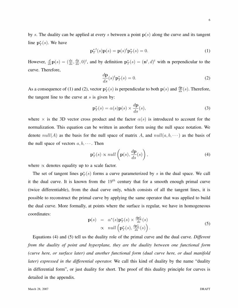
In 2D (d = 2), the duality between points and lines leads to the duality between a curve and

the set of its tangent lines, the so called dual curve. Let us assume that the curve is parameterized


6

by s. The duality can be applied at every s between a point p(s) along the curve and its tangent

line p∗T (s). We have

p∗T

t(s)p(s) = p(s)tp∗T (s) = 0. (1)

However, dds

p(s) = (dxds

, dyds

, 0)t, and by definition p∗T (s) = (nt, d)t with n perpendicular to the

curve. Therefore,dp

ds(s)tp∗

T (s) = 0. (2)

As a consequence of (1) and (2), vector p∗T (s) is perpendicular to both p(s) and dp

ds(s). Therefore,

the tangent line to the curve at s is given by:

p∗T (s) = α(s)p(s)× dp

ds(s), (3)

where × is the 3D vector cross product and the factor α(s) is introduced to account for the

normalization. This equation can be written in another form using the null space notation. We

denote null(A) as the basis for the null space of matrix A, and null(a, b, · · · ) as the basis of

the null space of vectors a, b, · · · . Then

p∗T (s) ∝ null

(p(s),

dp

ds(s)

), (4)

where ∝ denotes equality up to a scale factor.

The set of tangent lines p∗T (s) forms a curve parameterized by s in the dual space. We call

it the dual curve. It is known from the 19th century that for a smooth enough primal curve

(twice differentiable), from the dual curve only, which consists of all the tangent lines, it is

possible to reconstruct the primal curve by applying the same operator that was applied to build

the dual curve. More formally, at points where the surface is regular, we have in homogeneous

coordinates:p(s) = α∗(s)p∗

T (s)× dp∗T

ds(s)

∝ null(p∗

T (s),dp∗

T

ds(s)

).

(5)

Equations (4) and (5) tell us the duality role of the primal curve and the dual curve. Different

from the duality of point and hyperplane, they are the duality between one functional form

(curve here, or surface later) and another functional form (dual curve here, or dual manifold

later) expressed in the differential operator. We call this kind of duality by the name “duality

in differential form”, or just duality for short. The proof of this duality principle for curves is

detailed in the appendix.


7

In practice, to remove the unknown factor α(s) in the homogeneous representation, the point

p(s) is always normalized such that its third component is one. And the line p∗T (s) is normalized

such that the vector of its two first components has norm one. In fact, surprisingly in the appendix,

we prove in the theory that the choice of α(s) doesn’t affect the reconstruction result.

B. Duality for 3D Surfaces

In 3D (d = 3), the duality between points and planes leads to the duality between a surface

S and its dual manifold S∗, which is formed by the tangent planes of S. Let us assume that the

surface is parameterized by s and v. The duality can be applied at every (s, v) between a point

P(s, v) along the surface and its tangent plane P∗T (s, v). Similarly to the previous section, we

have

P(s, v)tP∗T (s, v) = 0. (6)

By definition, P∗T (s, v) as a function of (s, v), is tangent to the surface at P(s, v) and therefore

we have∂P

∂s(s, v)tP∗

T (s, v) = 0, (7)

and∂P

∂v(s, v)tP∗

T (s, v) = 0. (8)

As a consequence of equations (6), (7), (8), vector P∗T (s, v) is perpendicular to the three vectors

P(s, v), ∂P∂s

(s, v) and ∂P∂v

(s, v).

Therefore, the tangent plane to the surface at (s, v) is given by:

P∗T (s, v) = α(s, v)P(s, v) ∧ ∂P

∂s(s, v) ∧ ∂P

∂v(s, v)

∝ null((P(s, v), ∂P∂s

(s, v), ∂P∂v

(s, v))(9)

where ∧ and ¯ are respectively the exterior product and complement operator defined in exterior

algebra, also called Grassmann algebra [32]. The term a∧b∧c can be interpreted as a span space

of a, b and c. Its complement a ∧ b ∧ c can be seen as a generalization of the cross product from

3D to 4D, which is also called the meet operation in [23] because of its geometric meaning. The

set of tangent planes P∗T (s, v) forms a dual manifold S∗, also parameterized by (s, v). Similarly

to the previous section, for smooth enough primal surfaces the same operator can be used in


8

the dual manifold to derive the set of tangent planes and thus to reconstruct the primal surface.

More formally, we have in homogeneous coordinates:

P(s, v) = α∗(s, v)P∗T (s, v) ∧ ∂P∗

T

∂s(s, v) ∧ ∂P∗

T

∂v(s, v)

∝ null(P∗T (s, v),

∂P∗T

∂s(s, v),

∂P∗T

∂v(s, v))

(10)

The proof of the duality property for surfaces is detailed in the appendix.

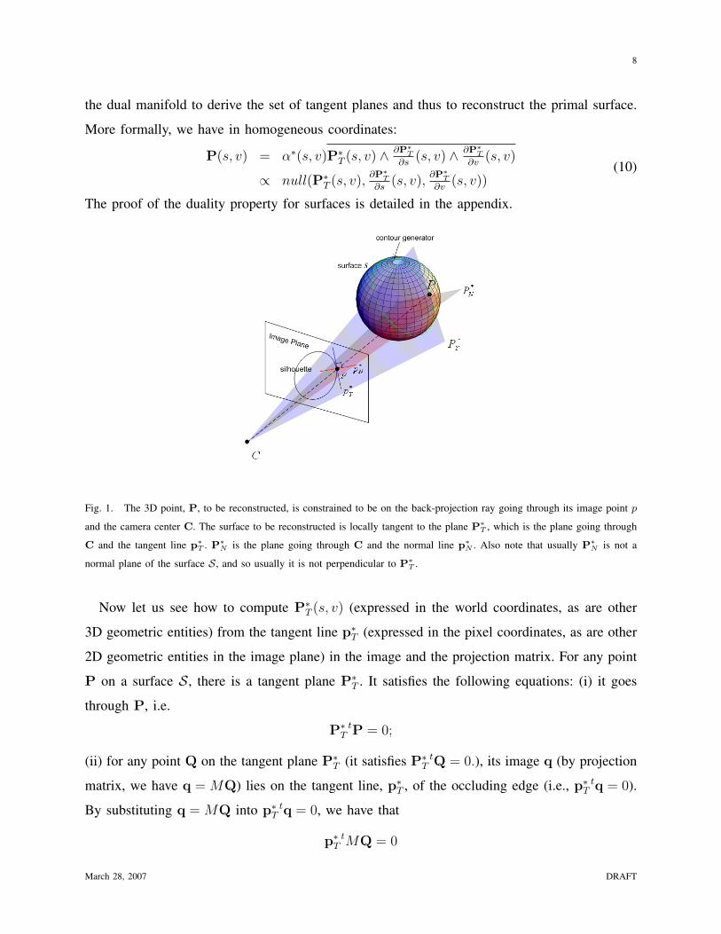
Fig. 1. The 3D point, P, to be reconstructed, is constrained to be on the back-projection ray going through its image point p

and the camera center C. The surface to be reconstructed is locally tangent to the plane P∗T , which is the plane going through

C and the tangent line p∗T . P∗

N is the plane going through C and the normal line p∗N . Also note that usually P∗

N is not a

normal plane of the surface S, and so usually it is not perpendicular to P∗T .

Now let us see how to compute P∗T (s, v) (expressed in the world coordinates, as are other

3D geometric entities) from the tangent line p∗T (expressed in the pixel coordinates, as are other

2D geometric entities in the image plane) in the image and the projection matrix. For any point

P on a surface S, there is a tangent plane P∗T . It satisfies the following equations: (i) it goes

through P, i.e.

P∗T

tP = 0;

(ii) for any point Q on the tangent plane P∗T (it satisfies P∗

TtQ = 0.), its image q (by projection

matrix, we have q = MQ) lies on the tangent line, p∗T , of the occluding edge (i.e., p∗

Ttq = 0).

By substituting q = MQ into p∗T

tq = 0, we have that

p∗T

tMQ = 0


9

holds for any Q lying on the tangent plane P∗T . Therefore, p∗

TtMQ = 0 holds for any Q which

satisfies P∗T

tQ = 0. This implies that the two linear equations are equivalent. From this, we can

derive that the coefficients of the linear equations, i.e., P∗T and M tp∗

T , are equal up to a scalar

multiplier β. That is,

P∗T = βM tp∗

T ∝ M tp∗T . (11)

This relationship and the equation (10) give a clear way of reconstructing 3D points P from

occluding edges. But it is not an optimal way, as shown in the next two subsections.

C. Ray Constraint

Occluding edges in a image give us not only tangent planes but stronger information — the

viewing rays. The reconstructed points should lie on these viewing rays. This is a constraint that

is not utilized in (10), but can be used to improve accuracy generally and to handle an important

kind of degeneracy in particular.

Assume that each occluding edge is parameterized by s which is not necessarily the arc-

length. Denote by t(s, v) the two component unit tangent vector of the silhouette at s, for

viewing position v. We also introduce n(s, v) as the unit normal of the silhouette at s. We thus

have by definition tt(s, v)n(s, v) = 0 and nt(s, v)n(s, v) = 1. By differentiating the last equation

w.r.t. s, we deduce nt(s, v)∂n∂s

(s, v) = 0. Since we are in 2D, ∂n∂s

(s, v) = k(s, v)t(s, v), where

k(s, v) is a scalar factor.

With the previous notation, the tangent line is:

p∗T (s, v) =

n(s, v)

−n(s, v)tp(s, v)

(12)

By differentiating w.r.t. s, we obtain:

∂p∗T

∂s(s, v) =

∂n∂s

(s, v)

−∂n∂s

(s, v)tp(s, v)− n(s, v)t ∂p∂s

(s, v)

= k(s, v)

t(s, v)

−t(s, v)tp(s, v) + 0

.

Denote the vector in the previous equation as p∗N(s, v), i.e.,

p∗N(s, v) =

t(s, v)

−t(s, v)tp(s, v)

. (13)


10

From its definition, p∗N(s, v) is the line perpendicular to the tangent line and crossing the curve

at the same position. By taking the derivative of (11) w.r.t. s, we obtain

∂P∗T

∂s(s, v) = β(s, v)M(v)t ∂p∗

T

∂s(s, v) +

∂β

∂sM(v)tp∗

T (s, v). (14)

And by using (13), we deduce that ∂P∗T

∂s(s, v) is a linear combination of M(v)tp∗

N(s, v) and

P∗T (s, v). Define

P∗N(s, v) ∝ M(v)tp∗

N(s, v).

With the same derivation as P∗T (s, v) in Sec. II-B, we can see that P∗

N(s, v) is the plane going

through both the camera center and the normal line p∗N . Putting the above definition into (14), we

can get that ∂P∗T

∂s(s, v) is a linear combination of P∗

N(s, v) and P∗T (s, v). This means that for 3D

reconstruction from silhouettes, in the operator (10), we can substitute P∗N(s, v) for ∂P∗

T

∂s(s, v).

The operator (10) is thus rewritten as:

P(s, v) ∝ null(P∗T (s, v),P∗

N(s, v),∂P∗

T

∂v(s, v)). (15)

These geometric quantities, including p, p∗T , p∗

N , P, P∗T , P∗

N , and their relationships are shown

in Fig. 1.

The operator (15) is better than (10) in practice since it substitutes P∗N , which is easily

estimated from the silhouettes, for the partial derivative vector ∂P∗T

∂s. Moreover, notice that from

(3) and (11),∂P∗

T

∂s∝ M(v)t ∂p∗

T

∂s∝ M(v)t ∂

∂s(p× ∂p

∂s)

is a second order derivative, while P∗N is only first order. In practice, a second order derivative

is often too noisy to be used. By substitution of a first order derivative, we get a more robust

operator. Another practical interesting property is that it provides a solution for degenerate cases,

e.g., reconstructing cylinders where ∂∂s

p∗T = 0 for the vertical line, see Fig. 4. In operator (15),

planes P∗T (s, v) and P∗

N(s, v) specify the ray going through image point p and the camera

center, and the intersection of this ray and plane ∂P∗T

∂v(s, v) specify 3D point P. Note, (15) is

also interpreted as the specification of 3D point P as the intersection of three planes. Notice

that in [16], the ray constraint was already introduced in the algebraic approach of the 3D

reconstruction from silhouettes in the same spirit; in [18], [19], it was incorporated into the

differential operator, but in an indirect way.


11

D. Epipolar Parametrization

In the previous subsection, differential operator (10) is rewritten in the better form (15).

However, another source of improvement is to take full advantage of the epipolar parametrization

of the surface introduced in [12]. In [20], the epipolar constraint was introduced into the dual

approach but only to improve the matching between two views. In [12], the “t-parameter curves

are defined to lie instantaneously in the epipolar plane defined by the ray and direction of

translation”. Here we use v instead of notation t. With the above definition and the fact that the

tangent vector of the “v-parameter curve” should lie on the tangent plane, we get the conclusion

that the tangent vector of the “v-parameter curve” goes in the direction of the viewing ray. That is,

with the epipolar parametrization, ∂P∂v

is on the ray going through point P and the camera center

C, see Fig. 2. Since the ray is defined by the intersection of two planes P∗T and P∗

N , therefore

P∗T

t ∂P∂v

= 0 and P∗N

t ∂P∂v

= 0. From the last equation and the derivative of P∗N

t(s, v)P(s, v) = 0

w.r.t. v, we therefore deduce ∂P∗N

∂v

t(s, v)P(s, v) = 0. The vector P is thus also perpendicular to

∂P∗N

∂v. This implies that a new operator can be proposed:

P(s, v)

∝ null(P∗

T (s, v),P∗N(s, v),

∂P∗T

∂v(s, v),

∂P∗N

∂v(s, v)

) (16)

The intuitive geometric interpretation of operator (16) is that the four planes, P∗T , P∗

N ,∂P∗

T

∂v,

∂P∗N

∂v

all go through one point that we want to recover. This relationship is illustrated in Fig. 3. The

operator (16) is more robust than (15) because it uses more information and it is robust against

the noise. Especially, it is still valid for the so called frontier points [33], which occur when the

tangent plane is identical to the epipolar plane. In that case, ∂P∗T

∂v(s, v) degenerates to be zero,

see Fig. 4. For this reason, this operator is called the robust differential dual operator, which

is used in the following 3D reconstruction algorithm. Note that each term in the operator is

estimated based on assumptions about the object shape.

Another very interesting property of this new operator (16) is that the 3D point reconstruction

by classical triangulation can be seen as the a special case of (16). Indeed, if the two derivatives


12

Fig. 2. Illustration of the epipolar parametrization of a 3D surface.

Fig. 3. The geometric interpretation of operator (16): four planes P∗T , P∗

N , ∂P∗T

∂v, ∂P∗

N∂v

all go through one point P.

in (16) are approximated by a simple first order difference scheme, we obtain:

P(s, v)

∼=null(P∗

T (s, v),P∗N(s, v),

P∗T (s,v′)−P∗

T (s,v)

v′−v,

P∗N (s,v′)−P∗

N (s,v)

v′−v)

∝ null (P∗T (s, v),P∗

N(s, v),P∗T (s, v′),P∗

N(s, v′))

The last equation is equivalent of the classical triangulation by two rays characterized by

(P∗T (s, v),P∗

N(s, v)) and (P∗T (s, v′),P∗

N(s, v′)), respectively. This relationship shows the con-


13

(a) (b)

−0.25−0.2

−0.15−0.1

−0.050

−0.2

−0.15

−0.1

−0.05

0

0.05

0.1

0.15

0.2−0.1

−0.05

0

0.05

0.1

xy

z

(c)

−0.25−0.2

−0.15−0.1

−0.050

−0.2

−0.15

−0.1

−0.05

0

0.05

0.1

0.15

0.2−0.1

−0.05

0

0.05

0.1

xy

z

(d)

−0.25−0.2

−0.15−0.1

−0.050

−0.2

−0.15

−0.1

−0.05

0

0.05

0.1

0.15

0.2−0.1

−0.05

0

0.05

0.1

xy

z

(e)

Fig. 4. In this figure, to remove the influence of the matching errors, we have worked with a synthetic object with surface

of revolution. In this case, ∂P∗T

∂v= ∂M

∂vp∗

T + M∂p∗T∂v

= ∂M∂v

p∗T . Indeed, ∂p∗T

∂v= 0 because of the same silhouettes in all view

directions. Similarly, we have ∂P∗N

∂v= ∂M

∂vp∗

N . (a) surface of revolution (b) the silhouette (c) the reconstruction of contour

generator with operator (10); (d) the result using operator (15) which is better since it enforces the ray constraint, but it is still

not good at frontier points; (e) the reconstruction using operator (16) is even more robust and nearly perfect.

(a) (b) (c)

Fig. 5. Comparison between results obtained with operator (16) and direct triangulation. Given 8 silhouettes of a sphere with

radius 100cm, the reconstructed contours with direct triangulation are shown in green points, and the reconstructed contours

with the proposed new operator are shown in red. The average error for the proposed operator is 0.37cm, while it is 4.14cm

for the direct triangulation. From (a,b), visually we can see that the red points lie on the sphere, while the green points lie away

from the sphere surface. (c) shows the interpolated point cloud (result from direct triangulation is not interpolated).

nection and difference between the proposed operator (16) and the direct triangulation. In some

sense, (16) can be seen to be a generalization of classical triangulation to the case of occluding

edges where continuity is enforced for the shape to be reconstructed. In practice, continuity

assumptions are of main importance during interpolation of the 3D shape to be reconstructed.

Fig. 5 shows the comparison between results obtained from (16) and direct classical triangulation.

The proposed approach clearly achieves more accurate results.

More generally, suppose ∂P∗T

∂vand ∂P∗

N

∂vare estimated as linear combinations of the samples of

P∗T (s, vi) and P∗

N(s, vi), i = 0, 1, 2, · · · and v0 = v as usually does. More specifically, suppose

∂P∗T

∂v(s, v) = β0P

∗T (s, v0) + β1P

∗T (s, v1) + β2P

∗T (s, v2) + · · · ,

where {βi} are the set of scalar coefficients depending on the sample set {vi}. Similarly for


14

∂P∗N

∂v(s, v). Then if they are texture edges, that is, they all come from the same curve on the

surface, the reconstruction operator is equivalent to

P(s, v) ∝ null(P∗T (s, v),P∗

N(s, v),P∗T (s, v1),

P∗N(s, v1),P

∗T (s, v2),P

∗N(s, v2), · · · ).

This is the generalized triangulation for multi-view reconstruction.

The fact that triangulation is included in operator (16) has a very important consequence: it

means that this operator should be able to reconstruct 3D surface from not only occluding edges

but also the texture edges in the same setting. And different from the fusion approach in [30],

[31], by using this operator, there is no need to discriminate these two kinds of edges which is

often difficult. This will be shown in Sec. IV. This fact is very useful in 3D reconstruction from

2D images because:

1) In our approach the basic feature is the edge element (edgel) and its orientation instead of

only edge point. In the proposed operator based on this feature, the occlusion is no longer

a trouble but of which an advantage can be taken.

2) There is no need to discriminate the edge types, and every type of edge is treated in exactly

the same way.

3) By using the orientation information, although the reconstruction is also based on the

local information it is much more stable than using just the point information. Indeed, the

orientation contains very important local information.

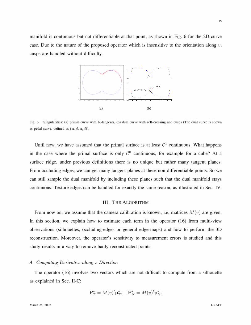
E. The Structure of the Dual Manifold

Actually the dual manifold crosses itself wherever the primal surface has bi-tangents as shown

in Fig. 6. The self-crossing singular points on the dual manifold correspond to tangent planes in

the primal surface that kiss the primal surface at more than one point. These kinds of singularities

used to be a source of trouble for computing the derivatives because there are more than

one possible tangent to these points. This problem is solved naturally using the connectivity

information on the primal surface (the parametrization along s and v). With this connectivity

the derivatives can be computed at the neighborhood of self-crossing points. This is illustrated

in a 2D case shown in Fig. 6.

There is another kind of singularity on the dual manifold: cusps. It happens when the primal

curve has an inflexion point or when the primal surface has a parabolic point, and thus the dual


15

manifold is continuous but not differentiable at that point, as shown in Fig. 6 for the 2D curve

case. Due to the nature of the proposed operator which is insensitive to the orientation along v,

cusps are handled without difficulty.

−2.5 −2 −1.5 −1 −0.5 0 0.5 1 1.5 2 2.5−1.5

−1

−0.5

0

0.5

1

1.5

(a) (b)

Fig. 6. Singularities: (a) primal curve with bi-tangents, (b) dual curve with self-crossing and cusps (The dual curve is shown

as pedal curve, defined as (nxd,nyd)).

Until now, we have assumed that the primal surface is at least C1 continuous. What happens

in the case where the primal surface is only C0 continuous, for example for a cube? At a

surface ridge, under previous definitions there is no unique but rather many tangent planes.

From occluding edges, we can get many tangent planes at these non-differentiable points. So we

can still sample the dual manifold by including these planes such that the dual manifold stays

continuous. Texture edges can be handled for exactly the same reason, as illustrated in Sec. IV.

III. THE ALGORITHM

From now on, we assume that the camera calibration is known, i.e, matrices M(v) are given.

In this section, we explain how to estimate each term in the operator (16) from multi-view

observations (silhouettes, occluding-edges or general edge-maps) and how to perform the 3D

reconstruction. Moreover, the operator’s sensitivity to measurement errors is studied and this

study results in a way to remove badly reconstructed points.

A. Computing Derivative along s Direction

The operator (16) involves two vectors which are not difficult to compute from a silhouette

as explained in Sec. II-C:

P∗T = M(v)tp∗

T , P∗N = M(v)tp∗

N .


16

To compute the tangent line p∗T and tangent vectors p∗

N , each edge curve is fitted by B-splines

along the edgel linking. The required derivatives are then computed from the fitted curve.

B. Edge-map Matching

The other two vectors in operator (16), the derivatives ∂P∗T

∂vand ∂P∗

N

∂v, should be carefully

estimated. These two vectors are derivatives with respect to v. Different from the dense sampling

in the s direction, the sampling in the v direction is usually sparse, and thus interpolation is

required. The task is to interpolate the planes (P∗T (s, v) and P∗

N(s, v)) between views, then

derivatives w.r.t. v can be estimated. Contrary to the case in the s direction, the connection

between points along v is not direct. A matching step between views is thus required.

In [20], given a point p(s, v) on the silhouette of the view v, the matching is performed by

searching for the corresponding point p(s′, v′) in view v′ which is at the crossing of the epipolar

line associated with p(s, v) and of the silhouette in the view v′. For a complicated object with

branches, for instance, there is a matching ambiguity with this procedure: usually several points

satisfy the previous constraints. This is why, following [8], it is better to compute the so-called

viewing edge. This viewing edge can be defined as the segment of the ray (P∗T (s, v),P∗

N(s, v))

going through p(s, v) and the camera center C(v) which is hidden by the object in all the other

views.

The problem with the previous viewing edge approach is that we have to discriminate between

texture edges and occluding edges which is a difficult task to perform in images. This problem

drives us to perform matching between pairs of views using dynamic programming and then to

remove badly matched points by testing reconstruction consistency during the 3D reconstruc-

tion, as described in the following sections. Silhouettes are closed curves, but in general the

occluding edges and the texture edges are open curves. So it is not possible to use inside/outside

discrimination for doing the matching as is the case for silhouettes.

In practice, we first rectify consecutive edge-map pairs to make the epipolar lines horizontal,

then the matching is reduced to a one-dimensional alignment for each row. Each edgel in this row

is described by three quantities, its relative position l ∈ [0, 1] within that row, its edge gradient

magnitude g ∈ [0, 1], and edge orientation r ∈ [0, π]. Edgels in each row are represented as a

vector. Then the matching in each row consists in aligning the vector pairs from two images.

The basic idea is to introduce a similarity measure between two edgels and to find the best


17

alignment which makes the total similarities maximal. The optimization is performed using the

Needleman-Wunsch algorithm [34], which guarantees optimal alignment. The similarity between

two edgels is defined as:

sij = 1−√

γl(∆lij)2 + γg(∆gij)2 + γr(∆rij)2,

where ∆lij = li − lj , ∆gij = gi − gj , ∆rij =|ri−rj |

π/2− [

|ri−rj |π/2

], γl + γg + γr = 1, and γl, γg, γr

are scalar parameters controlling the weighting of the edgel three properties, [·] is the round

operation. In our experiments, we select γl = 0.5, γg = 0.3, γr = 0.2, and the skip penalty is

chosen to be d = 0.4. More complex similarity measures may be needed for outdoor scenes.

C. Computing Derivatives along v Direction

After the matching between edge-maps in different views is performed, there are several ways

for interpolating the rays (P∗T (s, v),P∗

N(s, v)) between different values of v.

The simplest way is to directly interpolate tangent planes P∗T (v) and normal planes P∗

N(v).

For instance each plane can be interpolated using B-splines on each of its two angles and on

the distance to the origin. The drawback is that the interpolation result depends on the origin

location of the reference system.

Fig. 7. Illustration of the edge-map interpolation. The matched results for four consecutive edge-maps are shown on the left.

Parts of the interpolated edge curve through cubic splines are shown on the right marked with red color.

A different way of interpolation is to interpolate the camera motion and the change of

edge-maps separately. First, the camera centers C(v) are interpolated in 3D and m virtual

camera centers are generated. Also from the interpolation, ∂M∂v

is computed. The edge curves


18

are interpolated along the v directions with the matching results. Then m virtual edge-maps

are generated through equally spaced sampling the interpolated spline, see Fig. 7. With the

interpolated curve (e.g., interpolated spline), ∂p∗T

∂vand ∂p∗

N

∂vfor each s, v and also the new

interpolated edgels can be estimated. Then ∂P∗T

∂vand ∂P∗

N

∂vare computed as

∂P∗T

∂v∝ ∂M

∂vp∗

T + M∂p∗

T

∂v,

∂P∗N

∂v∝ ∂M

∂vp∗

N + M∂p∗

N

∂v.

The interpolation requires knowing the v values for each view. Different from the s parameter,

which is chosen to be the arc-length along the edge curve, the arc-length of the epipolar curve

is not a good choice for the v parameter. As an extreme case, for example, in the case of cube,

the same edge is viewed in several images, where the arc-length along epipolar curve doesn’t

change but the tangent plane changes as discussed in Sec. II-E. In this case, the derivative of

the tangent plane over arc-length along epipolar curve is not defined. The point is that since

we are computing the change of the tangent planes which are points on the dual manifold, we

should make v parameter meaningful on the dual manifold, instead of on the primal surface. In

the normal setup where the object depth is larger than the object size and the origin of the world

coordinate locates around the object center, the change of the tangent plane is mainly influenced

by the change of the angle between the camera center and the object center, and less influenced

by the object shape as shown in Fig. 8. So usually we take the angle change between the object

center (estimated approximately) and the camera center as the v parameter.

D. Oriented Point Cloud Reconstruction

For each edge point p(s, v), we have estimated the four vectors P∗T , P∗

N , dP∗T

dvand dP∗

N

dv, which

are involved in operator (16). In theory, the matrix composed of the above four vectors should

be rank 3, with the null vector being the reconstructed point position. But in practice, due to

errors from curve detection, interpolation and matching, the 4× 4 matrix

A(s, v)

=[

P ∗T (s, v) P ∗

N(s, v)dP ∗

T

dv(s, v)

dP ∗N

dv(s, v)

]t (17)

is only of rank 3 approximately. In this case, the equation A(s, v)P(s, v) = 0 can be robustly

solved using the Singular Value Decomposition (SVD). In SVD, matrix A can be decomposed


19

(a) (b)

Fig. 8. Illustration of the fact that tangent plane change is mainly influenced by the change of the angle between the camera

center and the object center; the shape of the object has less influence on the tangent plane change. For simplicity, this figure

shows only the 2D case.

as

A = UΛV t,

where U tU = I , V tV = I , and Λ = diag(λ1, λ2, λ3, λ4) with (λ1, λ2, λ3, λ4) being the singular

values of the A(s, v) matrix in the decreasing order. Also denote ui as the ith column of U , and

vi as the ith column of V . Note that λi ≥ 0, i = 1, · · · , 4. Then the solution using SVD is to

take the column of V (called the right singular vector) corresponding to the smallest singular

value in Λ, i.e., v4. And the result is optimal in the least square error sense [35].

The normal of the reconstructed points is useful information for surface reconstruction, where

the orientation information can be utilized to fill holes and generate smooth surfaces. For the

silhouette only, the orientation is easy to compute since the foreground and the background are

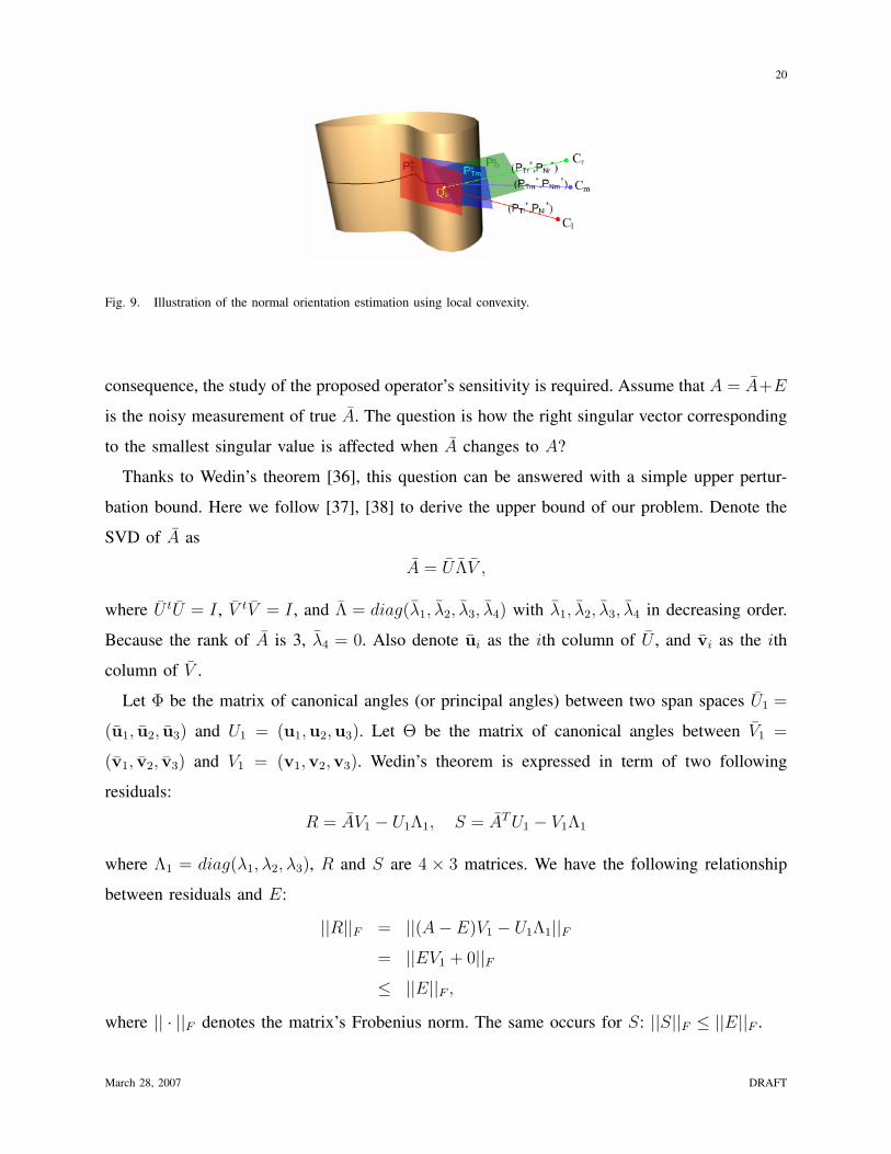
known in images. But this is not applicable to self-occluding edges. We thus propose another

approach based on the fact that if a point is on an occluding edge, then the corresponding

viewing curve along v is locally convex, as shown in Fig. 9. When the shape is locally convex,

the rays on the previous and next views cross outside the object, and this point is used to orient

the normal vector towards the outside.

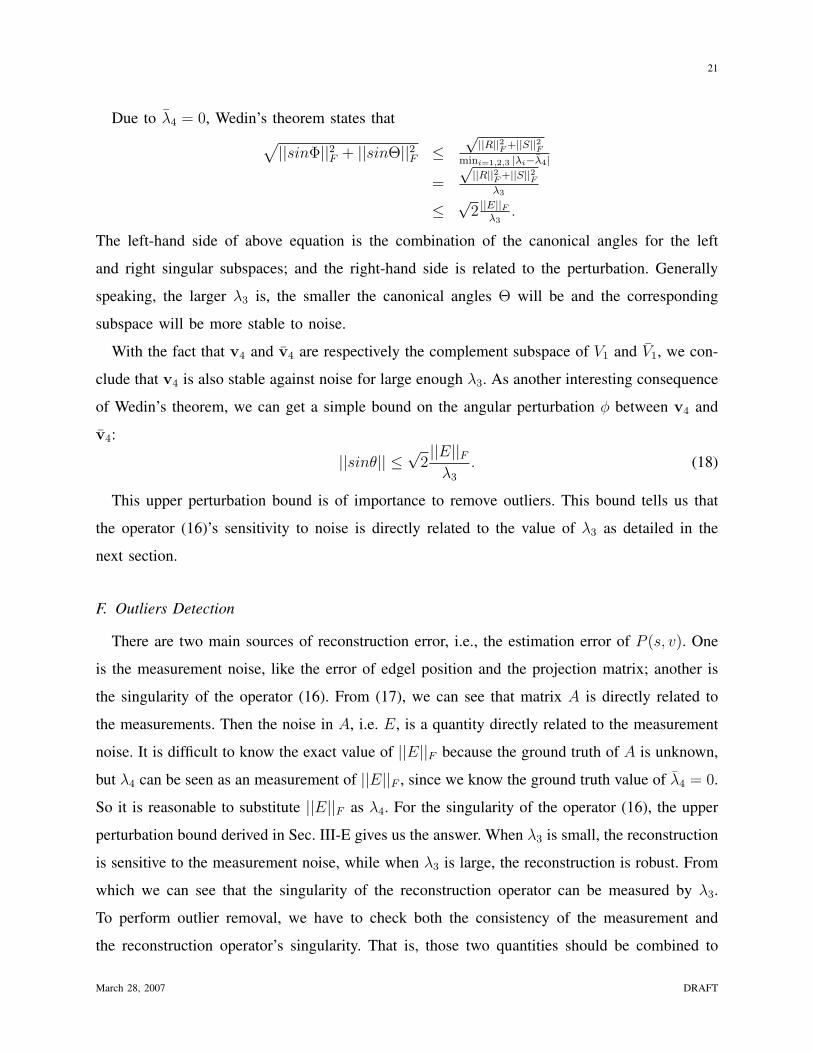
E. Stability Analysis

The matrix A(s, v) is subject to the measurement errors of edge detection, inaccurate pro-

jection matrices, matching errors, errors of estimating the derivatives along v direction. As a


20

Fig. 9. Illustration of the normal orientation estimation using local convexity.

consequence, the study of the proposed operator’s sensitivity is required. Assume that A = A+E

is the noisy measurement of true A. The question is how the right singular vector corresponding

to the smallest singular value is affected when A changes to A?

Thanks to Wedin’s theorem [36], this question can be answered with a simple upper pertur-

bation bound. Here we follow [37], [38] to derive the upper bound of our problem. Denote the

SVD of A as

A = U ΛV ,

where U tU = I , V tV = I , and Λ = diag(λ1, λ2, λ3, λ4) with λ1, λ2, λ3, λ4 in decreasing order.

Because the rank of A is 3, λ4 = 0. Also denote ui as the ith column of U , and vi as the ith

column of V .

Let Φ be the matrix of canonical angles (or principal angles) between two span spaces U1 =

(u1, u2, u3) and U1 = (u1,u2,u3). Let Θ be the matrix of canonical angles between V1 =

(v1, v2, v3) and V1 = (v1,v2,v3). Wedin’s theorem is expressed in term of two following

residuals:

R = AV1 − U1Λ1, S = AT U1 − V1Λ1

where Λ1 = diag(λ1, λ2, λ3), R and S are 4 × 3 matrices. We have the following relationship

between residuals and E:

||R||F = ||(A− E)V1 − U1Λ1||F= ||EV1 + 0||F≤ ||E||F ,

where || · ||F denotes the matrix’s Frobenius norm. The same occurs for S: ||S||F ≤ ||E||F .


21

Due to λ4 = 0, Wedin’s theorem states that√||sinΦ||2F + ||sinΘ||2F ≤

√||R||2F +||S||2F

mini=1,2,3 |λi−λ4|

=

√||R||2F +||S||2F

λ3

≤√

2 ||E||Fλ3

.

The left-hand side of above equation is the combination of the canonical angles for the left

and right singular subspaces; and the right-hand side is related to the perturbation. Generally

speaking, the larger λ3 is, the smaller the canonical angles Θ will be and the corresponding

subspace will be more stable to noise.

With the fact that v4 and v4 are respectively the complement subspace of V1 and V1, we con-

clude that v4 is also stable against noise for large enough λ3. As another interesting consequence

of Wedin’s theorem, we can get a simple bound on the angular perturbation φ between v4 and

v4:

||sinθ|| ≤√

2||E||F

λ3

. (18)

This upper perturbation bound is of importance to remove outliers. This bound tells us that

the operator (16)’s sensitivity to noise is directly related to the value of λ3 as detailed in the

next section.

F. Outliers Detection

There are two main sources of reconstruction error, i.e., the estimation error of P (s, v). One

is the measurement noise, like the error of edgel position and the projection matrix; another is

the singularity of the operator (16). From (17), we can see that matrix A is directly related to

the measurements. Then the noise in A, i.e. E, is a quantity directly related to the measurement

noise. It is difficult to know the exact value of ||E||F because the ground truth of A is unknown,

but λ4 can be seen as an measurement of ||E||F , since we know the ground truth value of λ4 = 0.

So it is reasonable to substitute ||E||F as λ4. For the singularity of the operator (16), the upper

perturbation bound derived in Sec. III-E gives us the answer. When λ3 is small, the reconstruction

is sensitive to the measurement noise, while when λ3 is large, the reconstruction is robust. From

which we can see that the singularity of the reconstruction operator can be measured by λ3.

To perform outlier removal, we have to check both the consistency of the measurement and

the reconstruction operator’s singularity. That is, those two quantities should be combined to


22

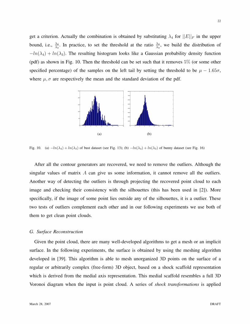
get a criterion. Actually the combination is obtained by substituting λ4 for ||E||F in the upper

bound, i.e., λ4

λ3. In practice, to set the threshold at the ratio λ4

λ3, we build the distribution of

−ln(λ4) + ln(λ3). The resulting histogram looks like a Gaussian probability density function

(pdf) as shown in Fig. 10. Then the threshold can be set such that it removes 5% (or some other

specified percentage) of the samples on the left tail by setting the threshold to be µ − 1.65σ,

where µ, σ are respectively the mean and the standard deviation of the pdf.

2 4 6 8 10 12 14 16 180

50

100

150

200

250

(a)

0 2 4 6 8 10 12 14 16 180

1000

2000

3000

4000

5000

6000

7000

8000

(b)

Fig. 10. (a) −ln(λ4) + ln(λ3) of bust dataset (see Fig. 13); (b) −ln(λ4) + ln(λ3) of bunny dataset (see Fig. 16)

After all the contour generators are recovered, we need to remove the outliers. Although the

singular values of matrix A can give us some information, it cannot remove all the outliers.

Another way of detecting the outliers is through projecting the recovered point cloud to each

image and checking their consistency with the silhouettes (this has been used in [2]). More

specifically, if the image of some point lies outside any of the silhouettes, it is a outlier. These

two tests of outliers complement each other and in our following experiments we use both of

them to get clean point clouds.

G. Surface Reconstruction

Given the point cloud, there are many well-developed algorithms to get a mesh or an implicit

surface. In the following experiments, the surface is obtained by using the meshing algorithm

developed in [39]. This algorithm is able to mesh unorganized 3D points on the surface of a

regular or arbitrarily complex (free-form) 3D object, based on a shock scaffold representation

which is derived from the medial axis representation. This medial scaffold resembles a full 3D

Voronoi diagram when the input is point cloud. A series of shock transformations is applied


23

iteratively to the medial scaffold to simplify it, while on the other hand re-meshing the surface,

in that the pruning of a medial branch implies filling the gap between surface points.

We are building surfaces to illustrate the good quality of the obtained 3D reconstructions

despite that the chosen algorithm may not perfectly fit our particular kind of point clouds. In

fact, the normal direction of each point is not used to generate smooth surfaces and to fill holes

in the adopted algorithms. Presently, the orientation of each point is used only at the rendering

stage to get a better visual result. Although there are other algorithms which fully utilize the

normal information, they are not directly applicable to our case, since our point clouds are only

partially oriented in the sense that occluding contours have normal direction but texture contours

do not.

The final algorithm is summarized in Algorithm 1.

IV. EXPERIMENTS

In this part, with both real and synthetic data, comprehensive experiments have been performed

to show various aspects of the proposed algorithm, including its ability to deal with both

occluding edges and texture edges, to deal with degenerate cases, and its capability of recovering

complex objects. To show the accuracy of the reconstruction, the distribution of the outlier points

are shown through coloring each recovered point with its confidence value defined as a linear

function of conf = −ln(λ4) + ln(λ3), with red indicating outliers (when conf = 0) and blue

indicating normal points (when conf = 1). To visualize the dual manifold in a 3D space, we

exploit the fact that the points are normalized in the sense that the first three elements denote the

plane’s orientation vector nx, ny, nz and the fourth element denotes the negative of the distance

between the tangent plane and the origin, −d. With the relation between orientation vector and

its spherical coordinate (ρ, φ, θ) 1, the dual manifold can be visualized in the spherical coordinate

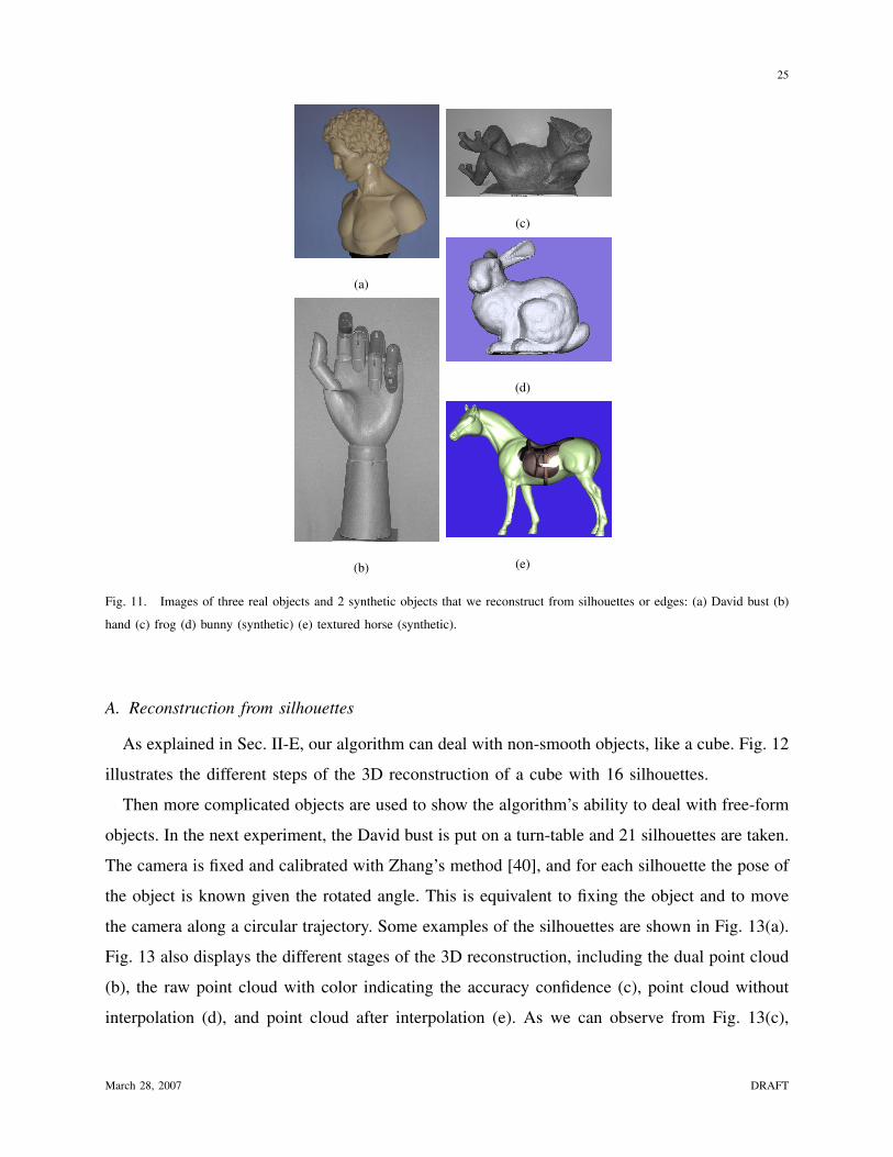
system. Here three real datasets, respectively David bust, hand and frog (thanks to [2].) and two

synthetic datasets, Stanford bunny and textured horse (as shown in Fig. 11) are representative

shapes of objects.

1The transformation relation is d = ρ, nx = sin(φ)cos(θ), ny = sin(φ)cos(θ), nz = cos(φ)


24

Algorithm 1 3D reconstruction from silhouettes, occluding edges and/or general edge mapsInput: image sequences Ii, (i = 1, · · · , N) and their calibration matrix Mi, (i = 1, · · · , N).

Output: 3D point cloud and surface.

Procedure:

1) Turn the images Ii into edge maps Ei with gradient and orientation.

a) Get the edge sub-pixel position through edge detection, like Canny; Or get the

silhouette curve through segmentation; Or other possible ways of converting images

into useful edge-maps.

b) Link the edge points and fit a spline for each edge curve.

c) Get the orientation of each edge point through computing the derivative of the spline

representation of edge curve (for instance with cubic approximate spline.)

2) Match the consecutive edge-maps.

a) Rectify the consecutive edge-maps to make the epipolar lines horizontal in the

rectified images.

b) Match each row of the rectified edge-maps through one-dimensional alignment with

dynamic programming, as discussed in Sec. III-B.

c) Transform the matching results in the rectified edge-maps back to the original edge-

maps.

3) Estimate each quantity in operator (16).

a) Compute p∗T and p∗

N with (12) and (13).

b) Compute P∗T and P∗

N with (11), and normalize them.

c) Fit splines for P∗T and P∗

N over v direction, i.e., through the matched points, and

compute their derivatives ∂P∗T

∂vand ∂P∗

N

∂vas discussed in Sec. III-C (using for instance

cubic fitting spline).

4) Reconstruct the 3D points with the operator (16) by using SVD as discussed in Sec. III-D.

If the input are silhouettes or occluding edges, also compute the normal vector.

5) Detect and remove outlier points through re-projection to the image planes and confidence

thresholding of the reconstructed points using singular values as described in Sec. III-F.

6) Generate surface from oriented point clouds as discussed in Sec. III-G or with other

proper surface reconstruction algorithms.


25

(a)

(b)

(c)

(d)

(e)

Fig. 11. Images of three real objects and 2 synthetic objects that we reconstruct from silhouettes or edges: (a) David bust (b)

hand (c) frog (d) bunny (synthetic) (e) textured horse (synthetic).

A. Reconstruction from silhouettes

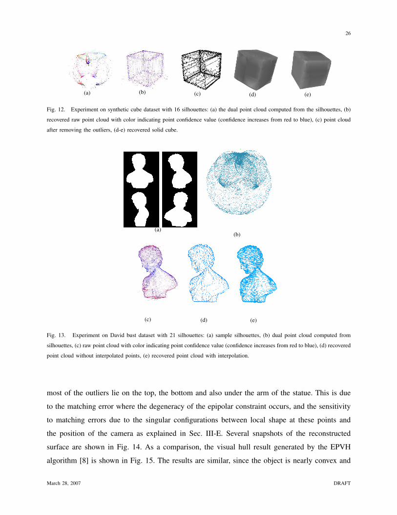
As explained in Sec. II-E, our algorithm can deal with non-smooth objects, like a cube. Fig. 12

illustrates the different steps of the 3D reconstruction of a cube with 16 silhouettes.

Then more complicated objects are used to show the algorithm’s ability to deal with free-form

objects. In the next experiment, the David bust is put on a turn-table and 21 silhouettes are taken.

The camera is fixed and calibrated with Zhang’s method [40], and for each silhouette the pose of

the object is known given the rotated angle. This is equivalent to fixing the object and to move

the camera along a circular trajectory. Some examples of the silhouettes are shown in Fig. 13(a).

Fig. 13 also displays the different stages of the 3D reconstruction, including the dual point cloud

(b), the raw point cloud with color indicating the accuracy confidence (c), point cloud without

interpolation (d), and point cloud after interpolation (e). As we can observe from Fig. 13(c),


26

(a) (b) (c) (d) (e)

Fig. 12. Experiment on synthetic cube dataset with 16 silhouettes: (a) the dual point cloud computed from the silhouettes, (b)

recovered raw point cloud with color indicating point confidence value (confidence increases from red to blue), (c) point cloud

after removing the outliers, (d-e) recovered solid cube.

(a)(b)

(c) (d) (e)

Fig. 13. Experiment on David bust dataset with 21 silhouettes: (a) sample silhouettes, (b) dual point cloud computed from

silhouettes, (c) raw point cloud with color indicating point confidence value (confidence increases from red to blue), (d) recovered

point cloud without interpolated points, (e) recovered point cloud with interpolation.

most of the outliers lie on the top, the bottom and also under the arm of the statue. This is due

to the matching error where the degeneracy of the epipolar constraint occurs, and the sensitivity

to matching errors due to the singular configurations between local shape at these points and

the position of the camera as explained in Sec. III-E. Several snapshots of the reconstructed

surface are shown in Fig. 14. As a comparison, the visual hull result generated by the EPVH

algorithm [8] is shown in Fig. 15. The results are similar, since the object is nearly convex and


27

(a) (b) (c)

Fig. 14. Experiment on David bust dataset with 21 silhouettes: recovered solid object from different views.

(a) (b) (c)

Fig. 15. The result of EPVH approach with the same dataset as Fig. 14.

has nearly no self occluding parts.

Another experiment is simulated to take 20 silhouettes of the Stanford bunny with a virtual

moving camera. As above, different stages of the reconstruction are shown in Fig. 16. Some

snapshots of the reconstructed mesh are shown in Fig. 17. Observe that although the ear part

of the bunny in different views is not correctly matched due to occlusion, the algorithm can

still recovers it correctly, thanks to the outlier detection. The concave and nearly flat part of the

bunny body are not recovered (see Fig. 16(d) and Fig. 16(e)) due to the inherent limitation of

shape from silhouettes. This part is meshed with flat surface at surface reconstruction stage (see

Fig. 17). The same data is used to generate the visual hull with EPVH algorithm as shown in

Fig. 18. Comparing the results from two approaches, we can see that our proposed approach

gives us generally more natural looking surfaces due to its interpolation capabilities, espcially

for strong self-occluding parts.

B. Reconstruction from Occluding Edges

With the reconstruction from occluding edges, we show the rich additional information pro-

vided compared with silhouettes only. First, the hand dataset is taken with a multi-flash to

detect the occluding edges. Although in our system, there is no need to use this special device


28

(a)(b)

(c)(d) (e)

Fig. 16. Experiment on Stanford bunny dataset with 20 silhouettes: (a) sample silhouettes, (b) dual point cloud computed

from silhouettes, (c) raw point cloud with color indicating point confidence value (confidence increases from red to blue), (d)

recovered point cloud without interpolated points, (e) recovered point cloud with interpolation.

(a) (b) (c)

Fig. 17. Experiment on Bunny dataset with 20 silhouettes: recovered solid objects from different views.

because our system deals with general edges. We use this dataset to observe the benefits of

reconstructing from occluding edges instead of just silhouettes. The obtained point clouds are

shown in Fig. 19. Figures (a-d) show results of reconstruction from silhouettes only, and figures

(e-h) show results from occluding edges. Notice that with the occluding edges, our matching

algorithm can still match the more complicated edge-map accurately and the matching results

in much more complete reconstruction than with silhouettes only.

The effect of recovering shapes from all occluding edges instead of only silhouettes are better

shown in Fig. 20, which shows the recovered surfaces from all occluding edges with our proposed


29

(a) (b) (c)

Fig. 18. Results of the EPVH approach with the same dataset as Fig. 17.

(a) (b) (c) (d) (e) (f) (g) (h)

Fig. 19. (a-d) are using silhouettes only, and (e-h) are using all occluding edges. (a) silhouette with tangent vectors, (b) two

consecutive silhouette matched, (c,d) two views of the reconstruction from silhouettes, (e) occluding edges with tangent vectors,

(f) two consecutive edge-maps matched (g,h) two views of the reconstruction using all occluding edges. 21 images used.

algorithm. From the results we can observe that the details of the object surface is recovered,

like the complex hairs, the concave parts of the arm and etc., which are impossible from only

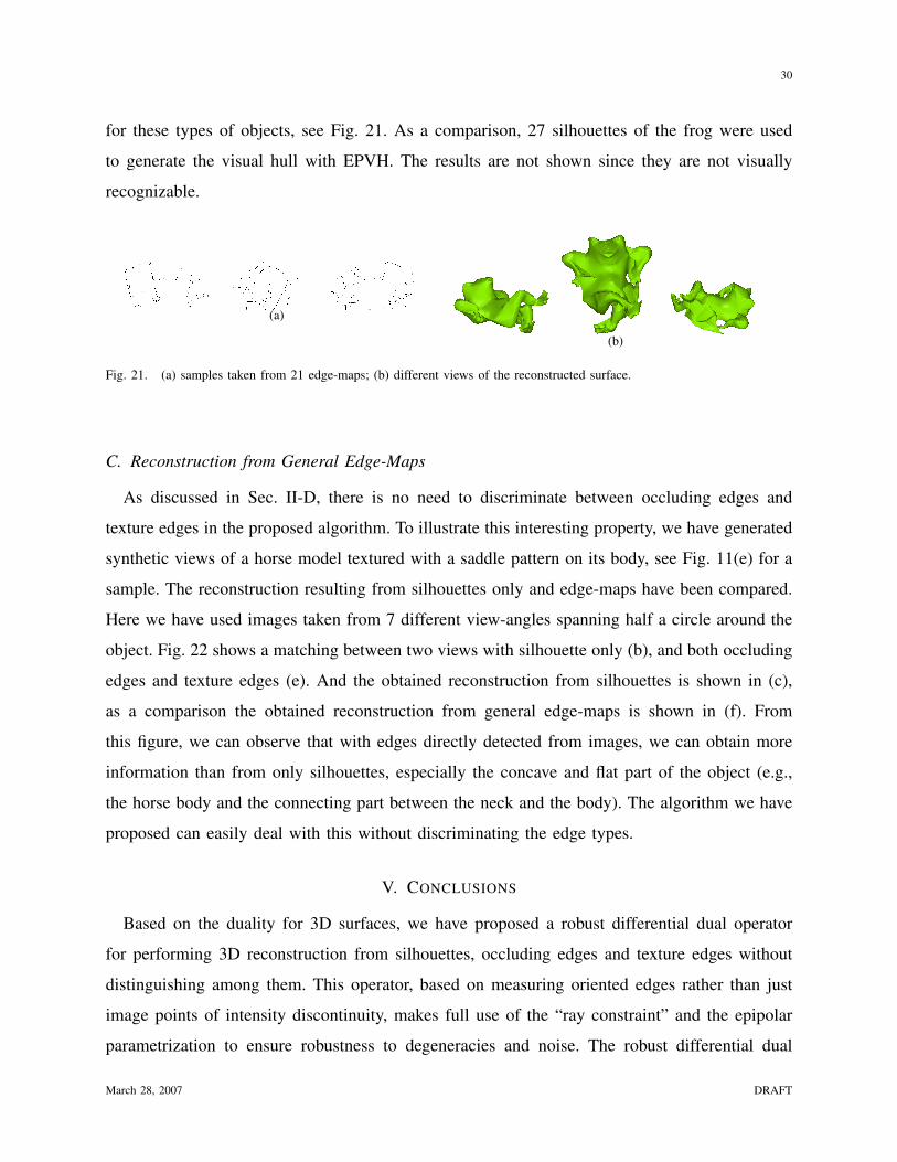
silhouettes. The results for the frog dataset are shown in Fig. 21. Notice that the frog is an

object with strong self-occlusion, and its geometry is more complex than the David bust and

the Stanford bunny in terms of number of holes and strong concavities. The results show that

the proposed algorithm can generate fairly good surfaces, based only on the edge information

(a) (b) (c) (d) (e) (f)

Fig. 20. (a-c) samples taken from 42 edge-maps; (d-f) recovered surface using the proposed algorithm.


30

for these types of objects, see Fig. 21. As a comparison, 27 silhouettes of the frog were used

to generate the visual hull with EPVH. The results are not shown since they are not visually

recognizable.

(a)

(b)

Fig. 21. (a) samples taken from 21 edge-maps; (b) different views of the reconstructed surface.

C. Reconstruction from General Edge-Maps

As discussed in Sec. II-D, there is no need to discriminate between occluding edges and

texture edges in the proposed algorithm. To illustrate this interesting property, we have generated

synthetic views of a horse model textured with a saddle pattern on its body, see Fig. 11(e) for a

sample. The reconstruction resulting from silhouettes only and edge-maps have been compared.

Here we have used images taken from 7 different view-angles spanning half a circle around the

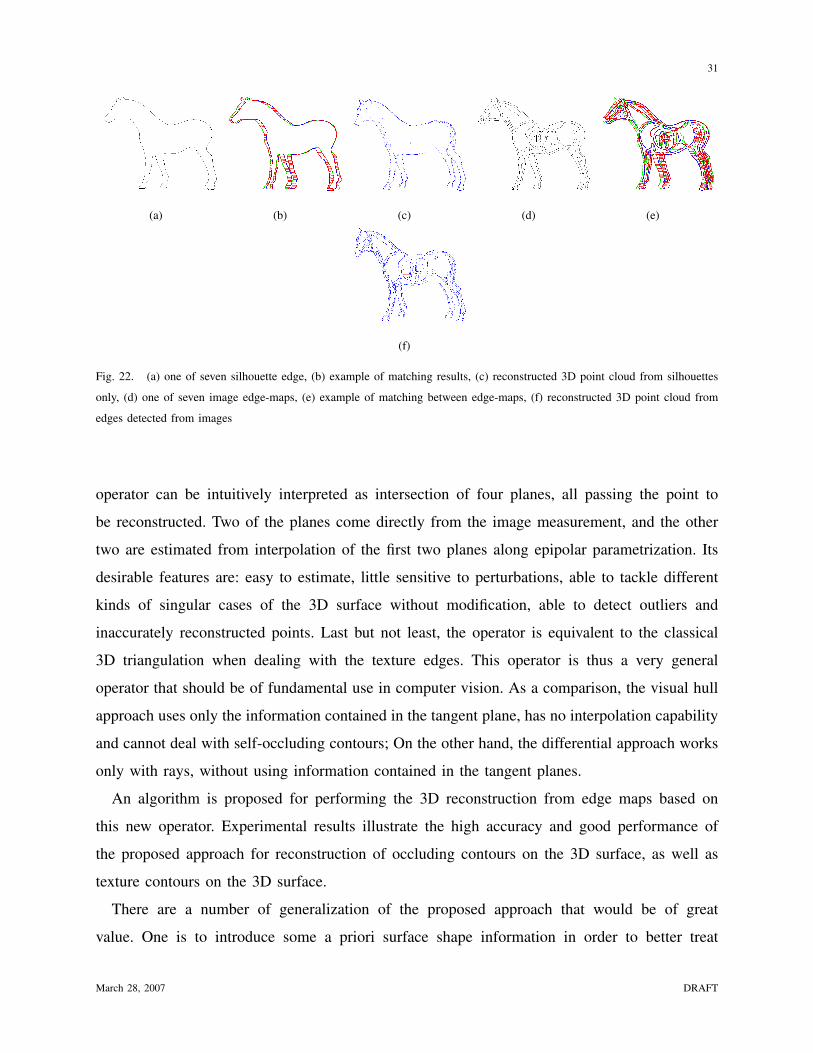
object. Fig. 22 shows a matching between two views with silhouette only (b), and both occluding

edges and texture edges (e). And the obtained reconstruction from silhouettes is shown in (c),

as a comparison the obtained reconstruction from general edge-maps is shown in (f). From

this figure, we can observe that with edges directly detected from images, we can obtain more

information than from only silhouettes, especially the concave and flat part of the object (e.g.,

the horse body and the connecting part between the neck and the body). The algorithm we have

proposed can easily deal with this without discriminating the edge types.

V. CONCLUSIONS

Based on the duality for 3D surfaces, we have proposed a robust differential dual operator

for performing 3D reconstruction from silhouettes, occluding edges and texture edges without

distinguishing among them. This operator, based on measuring oriented edges rather than just

image points of intensity discontinuity, makes full use of the “ray constraint” and the epipolar

parametrization to ensure robustness to degeneracies and noise. The robust differential dual


31

(a) (b) (c) (d) (e)

(f)

Fig. 22. (a) one of seven silhouette edge, (b) example of matching results, (c) reconstructed 3D point cloud from silhouettes

only, (d) one of seven image edge-maps, (e) example of matching between edge-maps, (f) reconstructed 3D point cloud from

edges detected from images

operator can be intuitively interpreted as intersection of four planes, all passing the point to

be reconstructed. Two of the planes come directly from the image measurement, and the other

two are estimated from interpolation of the first two planes along epipolar parametrization. Its

desirable features are: easy to estimate, little sensitive to perturbations, able to tackle different

kinds of singular cases of the 3D surface without modification, able to detect outliers and

inaccurately reconstructed points. Last but not least, the operator is equivalent to the classical

3D triangulation when dealing with the texture edges. This operator is thus a very general

operator that should be of fundamental use in computer vision. As a comparison, the visual hull

approach uses only the information contained in the tangent plane, has no interpolation capability

and cannot deal with self-occluding contours; On the other hand, the differential approach works

only with rays, without using information contained in the tangent planes.

An algorithm is proposed for performing the 3D reconstruction from edge maps based on

this new operator. Experimental results illustrate the high accuracy and good performance of

the proposed approach for reconstruction of occluding contours on the 3D surface, as well as

texture contours on the 3D surface.

There are a number of generalization of the proposed approach that would be of great

value. One is to introduce some a priori surface shape information in order to better treat


32

the problem of large camera baseline between successive views. Another arises because the

matching of consecutive edge-maps is treated as a one-dimensional alignment problem, which

can be implemented with dynamic programming. But the limitation of this method is that the

matching is only optimal locally in the sense that the matching of edge points in different rows

are totally independent, without using their connection information. So a global matching of

edge maps is a research topic for the future. A third is the surface reconstruction from point

cloud when only partial orientation information is available.

ACKNOWLEDGEMENT

This work was partial supported by NSF Grants NO. 0205477 and NO. BCS-9980091. The

authors thank Professor Gabriel Taubin’s group for providing their datasets, and their help for

setting up the experimental device. The authors would also like to thank Ming-ching Chang for

providing the mesh code and Dr. Matthew Brand for providing support for the initial version of

the research.

APPENDIX

A. Proof of Duality for Curves

Following is the proof of the proposition that the dual of the dual manifold is the primal

surface, see [18].

Proof: See equation (19).

B. Proof of Duality for Surfaces

Following is the proof that the dual of the dual manifold is the primal surface. Here we omit

the parameters to make the proof clear, e.g., P(s, v) is denoted by P. In this proof, we use the

Grassmann algebra and the duality properties between the exterior product (denoted as ∧) and

the regressive product (denoted as ∨). We denote by ¯ the complement operator. Details about

those operators can be found in [32], [41].

With the use of Grassmann algebra, we can easily generalize the proof from 2D curves to 3D

surfaces. To do so, we first derive a rule which is similar to the 3D cross product rule used in


33

p∗T (s)× dp∗

T

ds(s) =

(α(s)p(s)× dp

ds(s)

)× d

ds

(α(s)p(s)× dp

ds(s)

)= α(s)

(p(s)× dp

ds(s)

)×

(dαds

(s)p(s)× dpds

(s) + α(s) dds

(p(s)× dp

ds(s)

))= 0 + α(s)

(p(s)× dp

ds(s)

)× α(s) d

ds

(p(s)× dp

ds(s)

)= α2(s)

(p(s)× dp

ds(s)

)×

(dpds

(s)× dpds

(s) + p(s)× d2pds2 (s)

)= α2(s)

(p(s)× dp

ds(s)

)×

(0 + p(s)× d2p

ds2 (s))

= α2(s) det(p(s), dpds

(s), d2pds2 (s))p(s)

= α∗(s)p(s)(19)

using the 3d cross product rule (a× b)× (a× c) = det(a, b, c)a.

the previous section, but which applies for 4D vectors. For 4D vectors a, b, c, d, we have:

(a ∧ b ∧ c) ∨ (a ∧ b ∧ d) ∨ (a ∧ c ∧ e)

= det(a, b, c, d)det(a, b, c, e)a.

This rule is derived by applying two times the common factor axiom [32]:

(αm ∧ γp) ∨ (βk ∧ γp) = (αm ∧ βk ∧ γp) ∨ γp,

where αm, βk, γp are elements of grade m, k and p respectively, and with m+k+p = 4. Notice

that in the following, we also use the following property for 4D vectors:

(a ∧ b ∧ c ∧ d) = det(a, b, c, d).

and the anti-commutativity axiom:

(a ∧ b) = −(b ∧ a).

Proof:(a ∧ b ∧ c) ∨ (a ∧ b ∧ d) ∨ (a ∧ c ∧ e)

= ( c︸︷︷︸α1

∧ a ∧ b︸︷︷︸γ2

) ∨ ( d︸︷︷︸β1

∧ a ∧ b︸︷︷︸γ2

) ∨ (a ∧ c ∧ e)

= (c ∧ d ∧ a ∧ b) ∨ (a ∧ b) ∨ (a ∧ c ∧ e)

= −det(c, d, a, b)( b︸︷︷︸α1

∧ a︸︷︷︸γ1

) ∨ (c ∧ e︸︷︷︸β2

∧ a︸︷︷︸γ1

)

= −det(a, b, c, d)(b ∧ c ∧ e ∧ a) ∨ a

= det(a, b, c, d)det(a, b, c, e)a.

(20)


34

Similarly, we deduce a second rule for 4D vectors:

(a ∧ b ∧ c) ∨ (a ∧ b ∧ d) ∨ (a ∧ b ∧ e) = 0.

With all the previous properties, we are now able to prove that the dual of the dual manifold

is the primal surface in 3D:

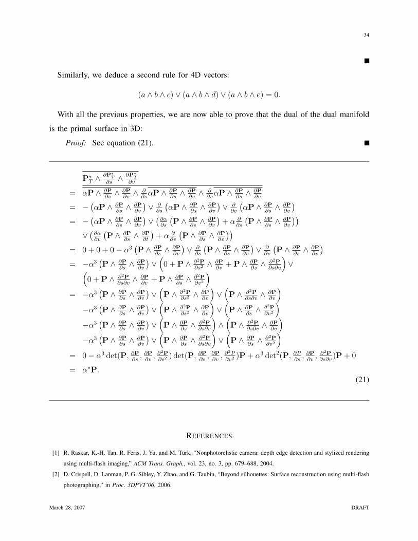
Proof: See equation (21).

P∗T ∧

∂P∗T

∂s∧ ∂P∗

T

∂v

= αP ∧ ∂P∂s∧ ∂P

∂v∧ ∂

∂sαP ∧ ∂P

∂s∧ ∂P

∂v∧ ∂

∂vαP ∧ ∂P

∂s∧ ∂P

∂v

= −(αP ∧ ∂P

∂s∧ ∂P

∂v

)∨ ∂

∂s

(αP ∧ ∂P

∂s∧ ∂P

∂v

)∨ ∂

∂v

(αP ∧ ∂P

∂s∧ ∂P

∂v

)= −

(αP ∧ ∂P

∂s∧ ∂P

∂v

)∨

(∂α∂s

(P ∧ ∂P

∂s∧ ∂P

∂v

)+ α ∂

∂s

(P ∧ ∂P

∂s∧ ∂P

∂v

))∨

(∂α∂v

(P ∧ ∂P

∂s∧ ∂P

∂t

)+ α ∂

∂v

(P ∧ ∂P

∂s∧ ∂P

∂v

))= 0 + 0 + 0− α3

(P ∧ ∂P

∂s∧ ∂P

∂v

)∨ ∂

∂s

(P ∧ ∂P

∂s∧ ∂P

∂v

)∨ ∂

∂v

(P ∧ ∂P

∂s∧ ∂P

∂v

)= −α3

(P ∧ ∂P

∂s∧ ∂P

∂v

)∨

(0 + P ∧ ∂2P

∂s2 ∧ ∂P∂v

+ P ∧ ∂P∂s∧ ∂2P

∂s∂v

)∨(

0 + P ∧ ∂2P∂s∂v

∧ ∂P∂v

+ P ∧ ∂P∂s∧ ∂2P

∂v2

)= −α3

(P ∧ ∂P

∂s∧ ∂P

∂v

)∨

(P ∧ ∂2P

∂s2 ∧ ∂P∂v

)∨

(P ∧ ∂2P

∂s∂v∧ ∂P

∂v

)−α3

(P ∧ ∂P

∂s∧ ∂P

∂v

)∨

(P ∧ ∂2P

∂s2 ∧ ∂P∂v

)∨

(P ∧ ∂P

∂s∧ ∂2P

∂v2

)−α3

(P ∧ ∂P

∂s∧ ∂P

∂v

)∨

(P ∧ ∂P

∂s∧ ∂2P

∂s∂v

)∧

(P ∧ ∂2P

∂s∂v∧ ∂P

∂v

)−α3

(P ∧ ∂P

∂s∧ ∂P

∂v

)∨

(P ∧ ∂P

∂s∧ ∂2P

∂s∂v

)∨

(P ∧ ∂P

∂s∧ ∂2P

∂v2

)= 0− α3 det(P, ∂P

∂s, ∂P

∂v, ∂2P

∂s2 ) det(P, ∂P∂s

, ∂P∂v

, ∂2P∂v2 )P + α3 det2(P, ∂P

∂s, ∂P

∂v, ∂2P

∂s∂v)P + 0

= α∗P.(21)

REFERENCES

[1] R. Raskar, K.-H. Tan, R. Feris, J. Yu, and M. Turk, “Nonphotorelistic camera: depth edge detection and stylized rendering

using multi-flash imaging,” ACM Trans. Graph., vol. 23, no. 3, pp. 679–688, 2004.

[2] D. Crispell, D. Lanman, P. G. Sibley, Y. Zhao, and G. Taubin, “Beyond silhouettes: Surface reconstruction using multi-flash

photographing,” in Proc. 3DPVT’06, 2006.


35

[3] A. Laurentini, “The visual hull concept for silhouette-based image understanding,” IEEE Trans. PAMI, vol. 16, pp. 150–162,

February 1994.

[4] E. Boyer and M.-O. Berger, “3d surface reconstruction using occluding contours,” Int. Journal of Computer Vision, vol. 22,

pp. 219–233, Mar 1997.

[5] S. Sullivan and J. Ponce, “Automatic model construction and pose estimation from photographs using triangular splines,”

IEEE Trans. PAMI, vol. 20, pp. 1091–1096, October 1998.

[6] K. N. Kutulakos and S. M. Seitz, “A theory of shape by space carving,” IEEE Trans. PAMI, vol. 38, no. 3, pp. 199–218,

2000.

[7] S. Lazebnik, E. Boyer, and J. Ponce, “On computing exact visual hulls of solids bounded by smooth surfaces,” in Computer

Vision and Pattern Recognition (CVPR ’01), pp. 156–161, 2001.

[8] J.-S. Franco and E. Boyer, “Exact polyhedral visual hulls,” in Proceedings of the Fourteenth British Machine Vision

Conference, pp. 329–338, September 2003. Norwich, UK.

[9] J.-S. Franco, M. Lapierre, and E. Boyer, “Visual shapes of silhouette sets,” in Proc. 3DPVT’06, 2006.

[10] L. Guan, S. Sinha, J.-S. Franco, and M. Pollefeys, “Visual hull construction in the presence of partial occlusion,” in Proc.

3DPVT’6, June 2006.

[11] R. Cipolla and A. Blake, “Surface shape from deformation of apparent contours,” Int. Journal of Computer Vision, vol. 9,

no. 2, pp. 83–112, 1992.

[12] R. Cipolla and P. Giblin, Visual Motion of Curves and Surfaces. Cambridge University Press, 2000.

[13] P. J. Giblin and R. S. Weiss, “Reconstructions of surfaces from profiles,” in International Conference on Computer Vision

(ICCV ’87), pp. 136–144, 1987.

[14] R. Vaillant and O. Faugeras, “Using extremal boundaries for 3-d object modeling,” IEEE Trans. PAMI, vol. 14, pp. 157–173,

February 1992.

[15] K. Wong, P. Mendonca, and R. Cipolla, “Structure and motion estimation from apparent contours under circular motion,”

Image and Vision Computing, vol. 20, pp. 441–448, April 2002.

[16] K. Kang, J.-P. Tarel, R. Fishman, and D. B. Cooper, “A linear dual-space approach to 3d surface reconstruction from

occluding contours using algebraic surface,” in International Conference on Computer Vision (ICCV ’01), vol. 1, pp. 198–

204, 2001.

[17] K. Kang, J.-P. Tarel, and D. B. Cooper, “A unified linear fitting approach for singular and non-singular 3d quadrics from

occluding contours,” in HLK’2003, (Nice, France), pp. 48–57, 2003.

[18] K. Kang, Three-Dimensional Free Form Surface Reconstruction from Occluding Contours in a Sequence Images or Video.

PhD thesis, Division of Engineering at Brown University, Providence, RI, United States, May 2004.

[19] M. Brand, K. Kang, and D. B. Cooper, “Algebraic solution for the visual hull,” in IEEE Conference on Computer Vision

and Pattern Recognition (CVPR ’04), pp. 30–35, 2004.

[20] C. Liang and K.-Y. K. Wong, “Complex 3d shape recovery using a dual-space approach,” in IEEE Conference on Computer

Vision and Pattern Recognition (CVPR ’05), vol. 2, pp. 878–884, 2005.

[21] R. I. Hartley and A. Zisserman, Multiple View Geometry in Computer Vision. Cambridge University Press, second ed.,

2004.

[22] H. H. Baker and R. C. Bolles, “Generalizing epipolar-plane image analysis on the spatiotemporal surface,” Int. Journal of

Computer Vision, vol. 3, no. 1, pp. 33–49, 1989.

[23] Q.-T. Luong and O. Faugeras, The Geometry of Multiple Images. MIT Press, 2004.


36

[24] C. L. Zitnick and T. Kanade, “A cooperative algorithm for stereo matching and occlusion detection,” IEEE Trans. PAMI,

vol. 22, no. 7, pp. 675–684, 2000.

[25] Y. Nakamura, T. Matsuura, K. Satoh, and Y. Ohta, “Occlusion detectable stereo-occlusion patterns in camera matrix,” in

IEEE Conference on Computer Vision and Pattern Recognition (CVPR ’96), pp. 371–378, 1996.

[26] A. F. Bobick and S. S. Intille, “Large occlusion stereo,” International Journal of Computer Vision, vol. 33, no. 3, pp. 181–

200, 1999.

[27] S. B. Kang, R. Szeliski, and J. Chai, “Handling occlusions in dense multi-view stereo,” in IEEE Conference on Computer

Vison and Pattern Recognition (CVPR ’01), vol. 01, (Los Alamitos, CA, USA), p. 103, IEEE Computer Society, 2001.

[28] A. S. Ogale and Y. Aloimonos, “Shape and the stereo correspondence problem,” Int. Journal of Computer Vision, vol. 65,

October 2005.

[29] A. S. Ogale, C. Fermuller, and Y. Aloimonos, “Motion segmentation using occlusions,” IEEE Transactions on Pattern

Analysis and Machine Intelligence, vol. 27, no. 6, pp. 988–992, 2005.

[30] R. Szeliski and R. Weiss, “Robust shape recovery from occluding contours using a linear smoother,” Int. Journal of

Computer Vision, vol. 28, no. 1, pp. 27–44, 1998.

[31] C. Esteban and F. Schmitt, “Silhouette and stereo fusion for 3d object modeling,” Computer Vision and Image

Understanding, vol. 96, pp. 367–392, December 2004.

[32] J. Browne, “Glassmann algebra - exploring applications of extended vector algebra with mathematica.” Incomplete draft

on http://www.ses.swin.edu.au/homes/browne/grassmannalgebra/book/, January 2001.

[33] P. Giblin and R. Weiss, “Epipolar fields on surfaces,” in Proc. 3rd European Conf. on Computer Vision, vol. 1, pp. 14–23,

May 1994.

[34] S. Needleman and C. Wunsch, “A general method applicable to the search for similarities in the amino acid sequence of

two proteins,” J. Mol. Bio., vol. 48, pp. 443–453, 1970.

[35] G. H. Golub and C. F. VanLoan, Matrix Computations. Johns Hopkins University, 1996.

[36] P. Wedin, “Perturbation bounds in connection with singular value decomposition,” BIT, vol. 12, pp. 99–111, 1972.

[37] G. W. Stewart, “Perturbation theory for the singular value decomposition,” Tech. Rep. CS-TR-2539, 1990.

[38] F. M. Dopico, “A note on sinθ theorems for singular subspace variations,” BIT, vol. 40, pp. 395–403, 2000.

[39] F. Leymarie, Three-Dimensional Shape Representation via Shock Flows. PhD thesis, Division of Engineering at Brown

University, Providence, RI, United States, May 2003.

[40] Z. Zhang, “Flexible camera calibration by viewing a plane from unknown orientations,” in International Conference on

Computer Vision (ICCV ’99), vol. 1, pp. 666–673, 1999.

[41] H. Barton, “A modern presentation of grassmann’s tensor analysis,” American Journal of Mathematics, vol. XLIX, pp. 598–

614, 1927.


Documents

Free-Form Object Reconstruction from Silhouettes, Occluding Edges and Texture Edges: A Unified and Robust Operator Based on Duality