arX

iv:c

ond-

mat

/030

9481

v1 [

cond

-mat

.mtr

l-sc

i] 2

1 Se

p 20

03

Free energy and configurational entropy of liquid silica: fragile-to-strong crossover and

polyamorphism

Ivan Saika-Voivod,1, 2 Francesco Sciortino,2 and Peter H. Poole1, 3

1Department of Applied Mathematics, University of Western Ontario, London, Ontario N6A 5B7, Canada2Dipartimento di Fisica and Istituto Nazionale per la Fisica della Materia,

Universita’ di Roma La Sapienza, Piazzale Aldo Moro 2, I-00185, Roma, Italy3Department of Physics, St. Francis Xavier University, Antigonish, Nova Scotia B2G 2W5, Canada

(Dated: February 2, 2008)

Recent molecular dynamics (MD) simulations of liquid silica, using the “BKS” model [Van Beest,Kramer and van Santen, Phys. Rev. Lett. 64, 1955 (1990)], have demonstrated that the liq-uid undergoes a dynamical crossover from super-Arrhenius, or “fragile” behavior, to Arrhenius, or“strong” behavior, as temperature T is decreased. From extensive MD simulations, we show thatthis fragile-to-strong crossover (FSC) can be connected to changes in the properties of the potentialenergy landscape, or surface (PES), of the liquid. To achieve this, we use thermodynamic integra-tion to evaluate the absolute free energy of the liquid over a wide range of density and T . We usethis free energy data, along with the concept of “inherent structures” of the PES, to evaluate theabsolute configurational entropy Sc of the liquid. We find that the temperature dependence of thediffusion coefficient and of Sc are consistent with the prediction of Adam and Gibbs, including inthe region where we observe the FSC to occur. We find that the FSC is related to a change in theproperties of the PES explored by the liquid, specifically an inflection in the T dependence of theaverage inherent structure energy. In addition, we find that the high T behavior of Sc suggests thatthe liquid entropy might approach zero at finite T , behavior associated with the so-called Kauz-mann paradox. However, we find that the change in the PES that underlies the FSC is associatedwith a change in the T dependence of Sc that elucidates how the Kauzmann paradox is avoidedin this system. Finally, we also explore the relation of the observed PES changes to the recentlydiscussed possibility that BKS silica exhibits a liquid-liquid phase transition, a behavior that hasbeen proposed to underlie the observed polyamorphism of amorphous solid silica.

PACS numbers: 64.70.Pf, 66.20.+d, 65.40.Gr, 65.20+w

I. INTRODUCTION

Liquid silica is the archetypal “strong liquid,” that is, aliquid whose viscosity η and other measures of relaxationfollow closely an Arrhenius behavior, log η ∼ 1/T [1, 2],where T is the temperature. For most liquids, η in-creases significantly faster than an Arrhenius law as Tapproaches the glass transition temperature Tg; these liq-uids are referred to as “fragile.”

Strong liquids such as silica are important as glass-forming systems. In a strong liquid, η varies less rapidlywith T near Tg, compared to a fragile liquid. As a conse-quence, a strong liquid can be held in a desired range ofη over a wider range of T than a fragile liquid. As everyglassblower knows, this makes silica-based systems easierto manipulate just above Tg than any other commonlyavailable liquid.

The fundamental origins of strong behavior in glass-forming liquids is also a subject of continuing interest.We note in particular two recent developments. First,computer simulation work of Horbach and Kob [3] usingthe “BKS” model of silica [4] has demonstrated that athigh T , the model liquid exhibits fragile behavior, andthen crosses over to a regime of strong behavior uponcooling. The work of La Nave and coworkers, based oninstantaneous normal mode analysis, has shown that sucha crossover is connected to a progressive reduction in the

number of diffusive directions in phase space accessedby the system [5]. Such a “fragile-to-strong crossover”(FSC) may be a general mechanism underlying the emer-gence of strong behavior, and has since been studiedfor a number of systems [6]. We note that a crossoverfrom a super-Arrhenius to Arrhenius dynamics may bea general feature of liquids around the so-called mode-coupling temperature [7], as is appearing to emerge inrecent numerical studies, thanks to the the larger dynam-ical window made available by current computationalpower [8, 9, 10]. However, the T region where equilibriumsimulations can be performed is still limited, and does notallow for a precise statement of the T -dependence belowthe crossover temperature, as required to make final con-tact with models for the glass transition [11, 12, 13].

Second, a growing body of computer simulation re-search has established the importance of the potentialenergy landscape or surface (PES) for understanding thedynamics of liquids near Tg [9, 14, 15, 16, 17, 18, 19,20, 21, 22, 23, 24, 25]. The PES refers specifically toU , the instantaneous potential energy hypersurface ofthe system, expressed as a function of the 3N coordi-nates qi that specify the positions of the N atoms of thesystem; i.e. U = U(q1, q2, ..., q3N ). The properties andtopology of the PES have been carefully studied in theabove cited works, predominantly in the case of fragileliquids, resulting in important insights into the equilib-rium [26] and out-of-equilibrium [27, 28] thermodynamics

2

of supercooled states, and the connection between ther-modynamics and transport propertie [21, 29]. However,the relationship of the PES to the dynamic properties ofstrong liquids is less well understood. In this paper, ourfocus is to clarify this relationship, and in particular, todetermine if the FSC proposed for liquid silica can beconnected to properties of the PES.

Following previous studies of fragile liquids, our ap-proach is to apply the “inherent structure” formalism ofStillinger and Weber [15] to molecular dynamics (MD)computer simulation data obtained for the BKS model ofliquid silica. In this approach, the PES is partitioned intobasins associated with the local minima of U [14, 15, 16].Each minimum corresponds to a particular configurationof atoms and is called an inherent structure (IS). Wedenote by eIS the average potential energy of the IS’sassociated with the basins sampled by the equilibriumliquid at a given T and volume V . An IS and its energycan be obtained in computer simulation by carrying outa local minimization of U starting from an equilibriumliquid configuration.

As we will describe in detail below, the evaluation ofeIS , combined with free energy calculations, allows usto calculate the configurational entropy, Sc, of the sys-tem [9, 18, 20, 21, 24]. Sc determines the number of dis-tinct configurations explored by the system, in this casethe basins of the PES. In a liquid, diffusion is associatedwith the exploration by the system of different basins ofthe PES. The work of Adam and Gibbs (AG) predicts arelationship (in the low T limit) between the character-istic relaxation time of the system and Sc [30]. The AGrelation has been recently derived in a novel way [12].Generalizing the AG relation to the diffusion coefficientD, the AG relation can be written as,

D

T= µ0 exp

(

− A

TSc

)

, (1)

where µ0 and A are presumed to be constant with respectto T . In the context of liquid silica, an interesting test ofthe robustness of the AG relation is possible by checkingif Eq. 1 is obeyed throughout the region in which the FSCoccurs. If so, the AG relation then provides a basis forconnecting transport behavior (quantified by D) to theproperties of the PES (quantified by Sc and eIS).

In a recent letter [31], we showed that liquid BKS sil-ica behaves in a manner that allows Sc to be calculatedfrom eIS, and that D and Sc are related as predictedby the AG relation. We were thereby able to show thatthe FSC in liquid silica is associated with a change inthe T dependence of eIS, i.e. a change in the nature ofthe PES explored by the system as T decreases. We alsofound that this observation in turn has implications forother behavior observed in BKS silica, in particular, thepossible occurrence of a liquid-liquid transition, and thebehavior of the liquid as related to the so-called Kauz-mann paradox.

To reach such conclusions, extensive MD simulations

are required over a wide range of V and T , to calcu-late thermodynamic and transport properties, as well ascareful examination of the IS properties. In addition, theabsolute free energy of the liquid must be evaluated. Inthe present work, we provide a detailed description ofthe methods used to obtain the results summarized inRef. [31], and also provide an expanded analysis and dis-cussion of the results. This work is organized as follows.In Section II we describe our MD simulations, includ-ing the interaction potential used. Section III provides adetailed description of the techniques we use to evaluateeIS, Sc, and the total free energy of the liquid. Section IVpresents the results of these calculations and provides adiscussion of their implications.

II. MOLECULAR DYNAMICS SIMULATIONS

We carry out MD simulations at constant V . Most ofour results are for a system of 444 Si atoms and 888 Oatoms. A few simulations are carried out with a reducednumber of particles (333 Si and 666 O atoms) in order toaccess longer physical times scales. Our MD simulationprogram is based on the “MDCSPC2” source code [32].We also reproduce a subset of our results using a codewe have written independently of MDCSPC2. Note thatall molar quantities are reported here in moles of atoms.

Our model of atomic interactions in silica, denoted hereas ΦBKS, is based on the BKS potential, modified in twoways. First, the BKS potential energy for both the Si-Oand O-O interactions diverges unphysically to negativeinfinity at sufficiently small distances, allowing “fusion”events to occur during simulation of high T systems. Toprevent this, ΦBKS consists of the standard BKS poten-tial plus a short range term given by

4ǫµν

[

(

σµν

rij

)30

−(

σµν

rij

)6]

(2)

where rij is the interatomic separation between an atomi of species µ, and an atom j of species ν. To choosethe parameters ǫµν and σµν (see Table I) we first identifythe value rij = r∗ij at which the inflection of the stan-dard BKS potential occurs, below which the divergenceto negative infinity develops. The parameters are chosenso that the new potential increases monotonically, andwithout inflections, as rij decreases for rij < r∗ij ; and sothat the difference between the new and the old poten-tials is small for rij > r∗ij . Similar approaches have beenused in other works [33, 34].

The second modification to the standard BKS poten-tial included in ΦBKS relates to the treatment of longerrange interactions. As is common in implementations ofthe BKS potential, we calculate the long range contribu-tions to the Coulombic potential energy using the Ewaldsummation technique, with the dipole surface term setto zero [35]. The reciprocal space summation is carriedout to a radius of six reciprocal lattice cell widths. In

3

this approach, the real space contributions to the BKSpotential are usually cut off discontinuously at a specifieddistance, often chosen as L/2, where L is the length of anedge of the simulation cell. However, we study systemsover a wide range of density ρ, and we desire a poten-tial for which the cut-off is independent of L. Also, foraccurate determination of inherent structures, we wishto remove discontinuities in the potential energy arisingfrom cut-offs, and to remove any L dependence from longrange corrections associated with the cut-off.

To achieve these goals, instead of discontinuously cut-ting off the real space potential contributions, we intro-duce a switching function. At a fixed distance Rs =0.77476 nm the real space terms of the standard BKSpotential are replaced by a 5th degree polynomial thattapers smoothly to zero over the range Rs < rij < Rc,where Rc = 1 nm. The polynomial coefficients and thevalue of Rs are chosen so that the potential is continuousup to and including second derivatives at both rij = Rs

and rij = Rc; and so that the potential and its first twoderivatives are monotonic for Rs < rij < Rc, and go tozero as rij → Rc. These choices depend on the Ewaldparameter α that occurs in both the real and reciprocalspace contributions to the potential energy. For all L, wechoose α = 2.5 nm−1 to ensure sufficient convergence ofthe potential energy in the reciprocal space summationfor the densities studied. The value Rc = 1 nm where theswitching function reaches zero is chosen to include thirdSi-Si neighbor interactions at most densities studied.

The real space contribution to ΦBKS , denoted here asφ, is therefore a piece-wise defined function of the form,

φ(rij ≤ Rs) =qµqν

4πε

erfc(αrij)

rij

+ Aµνe−Bµνrij +Cµν

r6ij

+ 4ǫµν

[

(

σµν

rij

)30

−(

σµν

rij

)6]

(3)

φ(Rs < rij < Rc) = Dµν(rij − Rs)5

+ Eµν(rij − Rs)4

+ Fµν(rij − Rs)3 (4)

φ(rij ≥ Rc) = 0 (5)

where erfc(x) is the complementary error function and εis the permittivity constant. The parameters are givenin Table I.

Note that the above modifications have the conse-quence that the average potential energy U and pressureP obtained using ΦBKS differ from those obtained usingthe standard BKS potential. We find that the differencesare approximately independent of T along isochores. AtT = 4000 K and ρ = 2.3072 g/cm3, we find that ΦBKS

gives a P value 0.25 GPa greater than the standard BKSpotential, and U is 2.5 kJ/mol higher. At the same T andρ = 3.8995 g/cm3, the respective differences are 0.9 GPaand 4.4 kJ/mol higher. These are not large differences

on the scale of our measurements, and the qualitative be-havior of the system is, as shown below, consistent withthat found in other studies based on the BKS model.

For the free energy calculation to be described below,we also perform MD simulations using a binary Lennard-Jones (LJ) potential, in which two atomic species (alsolabeled “Si” and “O”) occur in the same 1 : 2 proportionas in SiO2. The LJ pair potential is of the form

ΦLJ = 4gµν

[

(

sµν

rij

)12

−(

sµν

rij

)6]

− Φshiftµν (6)

The pair potential is cut off at rij = 2.5sµν and Φshiftµν

is determined so that ΦLJ(rij = 2.5sµν) = 0. Thesepotential parameters are given in Table I.

In order to obtain equilibrium properties we use the fol-lowing procedure. We equilibrate the liquid using veloc-ity rescaling for a time τ long enough to allow Si atoms todiffuse an average of 0.2 nm, after significant relaxationof P and U have disappeared from the system history.The interval of velocity rescaling varies from 10 to 1000time steps depending on T . The time step for all runsis 1 fs, except for T = 7000 K, where the time step is0.5 fs. Velocity scaling is then turned off and the systemis evolved in a constant (N, V, E) ensemble for at least10τ . (E is the total energy.) Using this approach, thereis no appreciable drift in E during the constant (N, V, E)phase, over which we calculate equilibrium quantities.

For the lowest T where relaxation is slowest we modifythis procedure to improve our sampling of phase space:we conduct up to five independent runs, with the con-stant (N, V, E) phase of each run lasting at least 2τ . Thereported properties (including T ) are averages over bothtime and over the independent runs. Thus averages forlow T state points are also calculated over a total of 10τ ,while at the same time the danger of an undetected trap-ping in an out-of-equilibrium state is reduced throughcomparison of the independent runs.

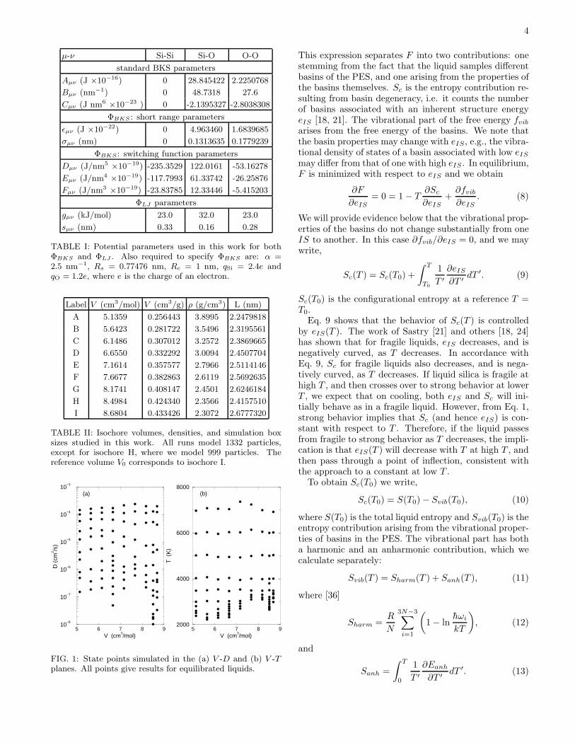
The densities of the isochores simulated are given inTable II, while the state points studied are shown inFig. 1. Note that we have studied the isochore at density2.3566 g/cm3 in order to compare with previously pub-lished work [3]. The simulations along this isochore arethose that involve only 999 atoms; all others model 1332atoms.

III. CONFIGURATIONAL ENTROPY

CALCULATION

In this section we calculate Sc from knowledge of eIS

and the vibrational properties of the basins of the PES.Similar calculations have been carried out for water [20],binary LJ mixtures [21] and orthoterphenyl [9].

We begin by writing the Helmholtz free energy F ofthe liquid along an isochore as [18],

F = eIS(T ) − TSc(eIS(T )) + fvib(T, eIS(T )). (7)

4

µ-ν Si-Si Si-O O-O

standard BKS parameters

Aµν (J ×10−16) 0 28.845422 2.2250768

Bµν (nm−1) 0 48.7318 27.6

Cµν (J nm6 ×10−23 ) 0 -2.1395327 -2.8038308

ΦBKS : short range parameters

ǫµν (J ×10−22) 0 4.963460 1.6839685

σµν (nm) 0 0.1313635 0.1779239

ΦBKS : switching function parameters

Dµν (J/nm5 ×10−19) -235.3529 122.0161 -53.16278

Eµν (J/nm4 ×10−19) -117.7993 61.33742 -26.25876

Fµν (J/nm3 ×10−19) -23.83785 12.33446 -5.415203

ΦLJ parameters

gµν (kJ/mol) 23.0 32.0 23.0

sµν (nm) 0.33 0.16 0.28

TABLE I: Potential parameters used in this work for bothΦBKS and ΦLJ . Also required to specify ΦBKS are: α =2.5 nm−1, Rs = 0.77476 nm, Rc = 1 nm, qSi = 2.4e andqO = 1.2e, where e is the charge of an electron.

Label V (cm3/mol) V (cm3/g) ρ (g/cm3) L (nm)

A 5.1359 0.256443 3.8995 2.2479818

B 5.6423 0.281722 3.5496 2.3195561

C 6.1486 0.307012 3.2572 2.3869665

D 6.6550 0.332292 3.0094 2.4507704

E 7.1614 0.357577 2.7966 2.5114146

F 7.6677 0.382863 2.6119 2.5692635

G 8.1741 0.408147 2.4501 2.6246184

H 8.4984 0.424340 2.3566 2.4157510

I 8.6804 0.433426 2.3072 2.6777320

TABLE II: Isochore volumes, densities, and simulation boxsizes studied in this work. All runs model 1332 particles,except for isochore H, where we model 999 particles. Thereference volume V0 corresponds to isochore I.

5 6 7 8 9V (cm

3/mol)

10−8

10−7

10−6

10−5

10−4

10−3

D (

cm2 /s

)

5 6 7 8 9V (cm

3/mol)

2000

4000

6000

8000

T (

K)

(b)(a)

FIG. 1: State points simulated in the (a) V -D and (b) V -Tplanes. All points give results for equilibrated liquids.

This expression separates F into two contributions: onestemming from the fact that the liquid samples differentbasins of the PES, and one arising from the properties ofthe basins themselves. Sc is the entropy contribution re-sulting from basin degeneracy, i.e. it counts the numberof basins associated with an inherent structure energyeIS [18, 21]. The vibrational part of the free energy fvib

arises from the free energy of the basins. We note thatthe basin properties may change with eIS, e.g., the vibra-tional density of states of a basin associated with low eIS

may differ from that of one with high eIS . In equilibrium,F is minimized with respect to eIS and we obtain

∂F

∂eIS= 0 = 1 − T

∂Sc

∂eIS+

∂fvib

∂eIS. (8)

We will provide evidence below that the vibrational prop-erties of the basins do not change substantially from oneIS to another. In this case ∂fvib/∂eIS = 0, and we maywrite,

Sc(T ) = Sc(T0) +

∫ T

T0

1

T ′

∂eIS

∂T ′dT ′. (9)

Sc(T0) is the configurational entropy at a reference T =T0.

Eq. 9 shows that the behavior of Sc(T ) is controlledby eIS(T ). The work of Sastry [21] and others [18, 24]has shown that for fragile liquids, eIS decreases, and isnegatively curved, as T decreases. In accordance withEq. 9, Sc for fragile liquids also decreases, and is nega-tively curved, as T decreases. If liquid silica is fragile athigh T , and then crosses over to strong behavior at lowerT , we expect that on cooling, both eIS and Sc will ini-tially behave as in a fragile liquid. However, from Eq. 1,strong behavior implies that Sc (and hence eIS) is con-stant with respect to T . Therefore, if the liquid passesfrom fragile to strong behavior as T decreases, the impli-cation is that eIS(T ) will decrease with T at high T , andthen pass through a point of inflection, consistent withthe approach to a constant at low T .

To obtain Sc(T0) we write,

Sc(T0) = S(T0) − Svib(T0), (10)

where S(T0) is the total liquid entropy and Svib(T0) is theentropy contribution arising from the vibrational proper-ties of basins in the PES. The vibrational part has botha harmonic and an anharmonic contribution, which wecalculate separately:

Svib(T ) = Sharm(T ) + Sanh(T ), (11)

where [36]

Sharm =R

N

3N−3∑

i=1

(

1 − lnhωi

kT

)

, (12)

and

Sanh =

∫ T

0

1

T ′

∂Eanh

∂T ′dT ′. (13)

5

Here Sharm is the entropy in the harmonic approxima-tion of the IS’s obtained at a given T . The set ωidescribes the vibrational density of states of the IS’s (de-tails below), h is Planck’s constant over 2π, R is the gasconstant, and k is Boltzmann’s constant. Eanh is givenby

Eanh(T ) = E(T ) − Eharm(T ) − eIS(T ), (14)

where Eharm is the harmonic contribution to the energy,given by Eharm = 3RT (N − 1)/N .

To obtain eIS we select 100 equilibrated liquid config-urations over the course of the MD run, perform a con-jugate gradient minimization [37] of U , and then averagethe results. As a stopping criterion for the conjugategradient minimizations, we specify a relative tolerance of10−8 along line minimizations and a relative tolerance of10−15 between line minimizations. In the case of isochoreH our runs are the longest, and so we average over 1000configurations.

In order to evaluate Sc and Sanh (using Eqs. 9 and 13respectively) we first fit average values of eIS and Eanh

to polynomials in T , and then evaluate the required in-tegrals analytically. The Eanh fit is constrained so thatat T = 0, the value of Eanh and its first derivative arezero. This is consistent with Eanh being a correction tothe harmonic approximation.

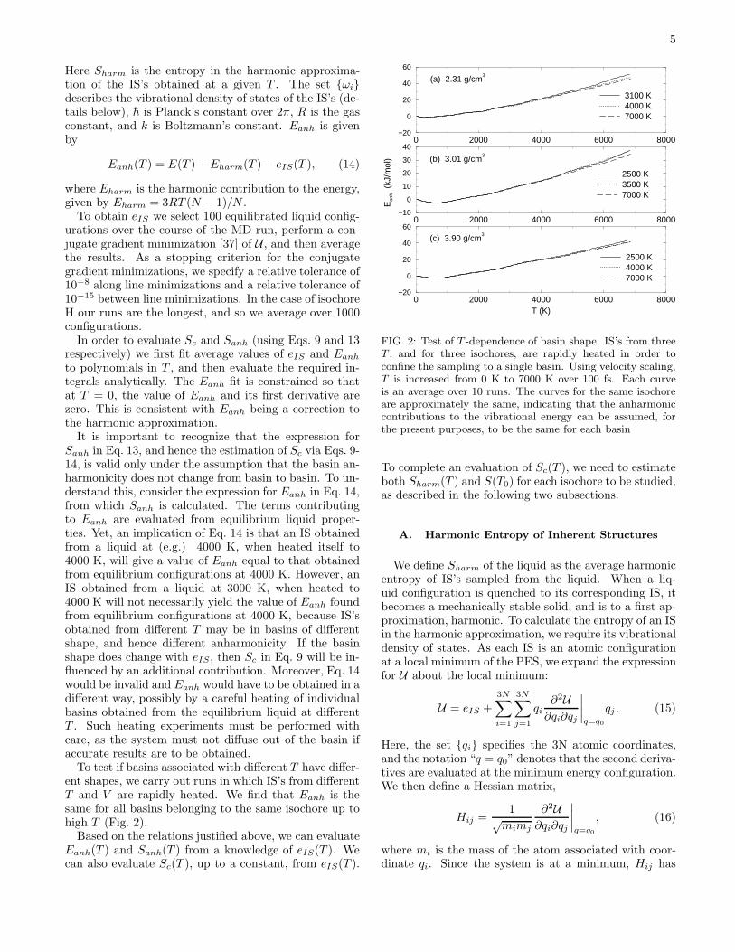
It is important to recognize that the expression forSanh in Eq. 13, and hence the estimation of Sc via Eqs. 9-14, is valid only under the assumption that the basin an-harmonicity does not change from basin to basin. To un-derstand this, consider the expression for Eanh in Eq. 14,from which Sanh is calculated. The terms contributingto Eanh are evaluated from equilibrium liquid proper-ties. Yet, an implication of Eq. 14 is that an IS obtainedfrom a liquid at (e.g.) 4000 K, when heated itself to4000 K, will give a value of Eanh equal to that obtainedfrom equilibrium configurations at 4000 K. However, anIS obtained from a liquid at 3000 K, when heated to4000 K will not necessarily yield the value of Eanh foundfrom equilibrium configurations at 4000 K, because IS’sobtained from different T may be in basins of differentshape, and hence different anharmonicity. If the basinshape does change with eIS, then Sc in Eq. 9 will be in-fluenced by an additional contribution. Moreover, Eq. 14would be invalid and Eanh would have to be obtained in adifferent way, possibly by a careful heating of individualbasins obtained from the equilibrium liquid at differentT . Such heating experiments must be performed withcare, as the system must not diffuse out of the basin ifaccurate results are to be obtained.

To test if basins associated with different T have differ-ent shapes, we carry out runs in which IS’s from differentT and V are rapidly heated. We find that Eanh is thesame for all basins belonging to the same isochore up tohigh T (Fig. 2).

Based on the relations justified above, we can evaluateEanh(T ) and Sanh(T ) from a knowledge of eIS(T ). Wecan also evaluate Sc(T ), up to a constant, from eIS(T ).

0 2000 4000 6000 8000T (K)

−20

0

20

40

60

2500 K4000 K7000 K

0 2000 4000 6000 8000−10

0

10

20

30

40

Ean

h (

kJ/m

ol)

2500 K3500 K7000 K

0 2000 4000 6000 8000−20

0

20

40

60

3100 K4000 K7000 K

(c) 3.90 g/cm3

(b) 3.01 g/cm3

(a) 2.31 g/cm3

FIG. 2: Test of T -dependence of basin shape. IS’s from threeT , and for three isochores, are rapidly heated in order toconfine the sampling to a single basin. Using velocity scaling,T is increased from 0 K to 7000 K over 100 fs. Each curveis an average over 10 runs. The curves for the same isochoreare approximately the same, indicating that the anharmoniccontributions to the vibrational energy can be assumed, forthe present purposes, to be the same for each basin

To complete an evaluation of Sc(T ), we need to estimateboth Sharm(T ) and S(T0) for each isochore to be studied,as described in the following two subsections.

A. Harmonic Entropy of Inherent Structures

We define Sharm of the liquid as the average harmonicentropy of IS’s sampled from the liquid. When a liq-uid configuration is quenched to its corresponding IS, itbecomes a mechanically stable solid, and is to a first ap-proximation, harmonic. To calculate the entropy of an ISin the harmonic approximation, we require its vibrationaldensity of states. As each IS is an atomic configurationat a local minimum of the PES, we expand the expressionfor U about the local minimum:

U = eIS +3N∑

i=1

3N∑

j=1

qi∂2U

∂qi∂qj

∣

∣

∣

∣

q=q0

qj . (15)

Here, the set qi specifies the 3N atomic coordinates,and the notation “q = q0” denotes that the second deriva-tives are evaluated at the minimum energy configuration.We then define a Hessian matrix,

Hij =1

√mimj

∂2U∂qi∂qj

∣

∣

∣

∣

q=q0

, (16)

where mi is the mass of the atom associated with coor-dinate qi. Since the system is at a minimum, Hij has

6

2000 4000 6000T (K)

32.142

32.147

32.152

32.200

32.205

32.210

Ω

32.290

32.295

32.300

5 6 7 8 9V (cm

3/mol)

32.14

32.19

32.24

32.29 (d)(a)

(b)

(c)

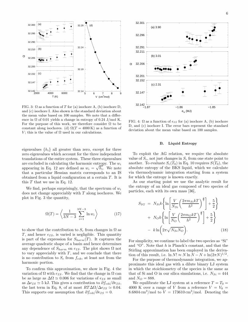
FIG. 3: Ω as a function of T for (a) isochore A, (b) isochore D,and (c) isochore I. Also shown is the standard deviation aboutthe mean value based on 100 samples. We note that a differ-ence in Ω of 0.01 yields a change in entropy of 0.24 J/mol K.For the purpose of this work, we therefore consider Ω to beconstant along isochores. (d) Ω(T = 4000 K) as a function ofV ; this is the value of Ω used in our calculations.

eigenvalues hi all greater than zero, except for threezero eigenvalues which account for the three independenttranslations of the entire system. These three eigenvaluesare excluded in calculating the harmonic entropy. The wi

appearing in Eq. 12 are defined as wi =√

hi. We notethat a particular Hessian matrix corresponds to an ISobtained from a liquid configuration at a certain T . It isthis T that we use in Eq. 12.

We find, perhaps surprisingly, that the spectrum of wi

does not change appreciably with T along isochores. Weplot in Fig. 3 the quantity,

Ω(T ) =

⟨

1

3N − 3

3N−3∑

i=1

lnwi

⟩

(17)

to show that the contribution to Sc from changes in Ω asT , and hence eIS , is varied is negligible. This quantityis part of the expression for Sharm(T ). It captures theaverage quadratic shape of a basin and hence determinesany dependence of Sharm on eIS. The plot shows Ω notto vary appreciably with T , and we conclude that thereis no contribution to Sc from fvib, at least not from theharmonic portion.

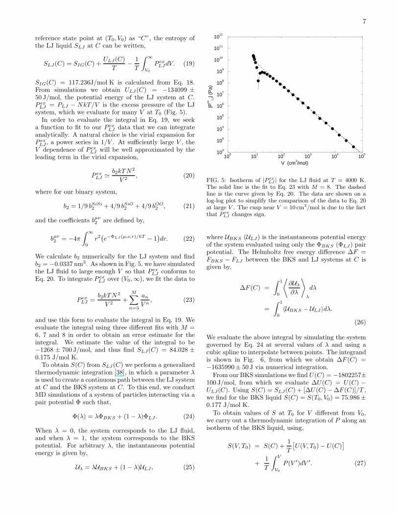
To confirm this approximation, we show in Fig. 4 thevariation of Ω with eIS . We find that the change in Ω canbe as large as ∆Ω ≃ 0.006 for variations of eIS as smallas ∆eIS ≃ 5 kJ. This gives a contribution to ∂fvib/∂eIS,the last term in Eq. 8, of at most RT∆Ω/∆eIS ≃ 0.04.This supports our assumption that ∂fvib/∂eIS = 0.

−1.87 −1.86 −1.85eIS (MJ)

32.142

32.147

32.152

32.201

32.206

32.211

Ω

32.291

32.296

32.301

(a) 3.90

(b) 3.01

(c) 2.31

FIG. 4: Ω as a function of eIS for (a) isochore A, (b) isochoreD, and (c) isochore I. The error bars represent the standarddeviation about the mean value based on 100 samples.

B. Liquid Entropy

To exploit the AG relation, we require the absolutevalue of Sc, not just changes in Sc from one state point toanother. To evaluate Sc(T0) in Eq. 10 requires S(T0), theabsolute entropy of the BKS liquid, which we calculatevia thermodynamic integration starting from a systemfor which the entropy is known exactly.

As our starting point we use the analytic result forthe entropy of an ideal gas composed of two species ofparticles, each with its own mass [36],

SIG = NSik

ln

[

V

NSi

(

2πmSikT

h2

)3

2

]

+5

2

+ NOk

ln

[

V

NO

(

2πmOkT

h2

)3

2

]

+5

2

− k ln

(

2π√

NSiNO

)

. (18)

For simplicity, we continue to label the two species as “Si”and “O”. Note that h is Planck’s constant, and that theStirling approximation has been employed in the deriva-tion of this result, i.e. lnN ! ≈ N lnN −N + ln(2πN)1/2.

For the purpose of thermodynamic integration, we ap-proximate this ideal gas with a dilute binary LJ systemin which the stoichiometry of the species is the same asthat of Si and O in our silica simulations, i.e. NSi = 444and NO = 888.

We equilibrate the LJ system at a reference T = T0 =4000 K over a range of V from a reference V = V0 =8.6804 cm3/mol to V = 173610 cm3/mol. Denoting the

7

reference state point at (T0, V0) as “C”, the entropy ofthe LJ liquid SLJ at C can be written,

SLJ(C) = SIG(C) +ULJ(C)

T− 1

T

∫

∞

V0

P exLJdV. (19)

SIG(C) = 117.236J/mol K is calculated from Eq. 18.From simulations we obtain ULJ(C) = −134099 ±50 J/mol, the potential energy of the LJ system at C.P ex

LJ = PLJ − NkT/V is the excess pressure of the LJsystem, which we evaluate for many V at T0 (Fig. 5).

In order to evaluate the integral in Eq. 19, we seeka function to fit to our P ex

LJ data that we can integrateanalytically. A natural choice is the virial expansion forP ex

LJ , a power series in 1/V . At sufficiently large V , theV dependence of P ex

LJ will be well approximated by theleading term in the virial expansion,

P exLJ ≃ b2kTN2

V 2, (20)

where for our binary system,

b2 = 1/9 bSiSi2 + 4/9 bSiO

2 + 4/9 bOO2 , (21)

and the coefficients bµν2 are defined by,

bµν2 = −4π

∫

∞

0

r2(

e−ΦLJ (µ,ν,r)/kT − 1)

dr. (22)

We calculate b2 numerically for the LJ system and findb2 = −0.0337 nm3. As shown in Fig. 5, we have simulatedthe LJ fluid to large enough V so that P ex

LJ conforms toEq. 20. To integrate P ex

LJ over (V0,∞), we fit the data to

P exLJ =

b2kTN2

V 2+

M∑

n=3

an

V n, (23)

and use this form to evaluate the integral in Eq. 19. Weevaluate the integral using three different fits with M =6, 7 and 8 in order to obtain an error estimate for theintegral. We estimate the value of the integral to be−1268 ± 700 J/mol, and thus find SLJ(C) = 84.028 ±0.175 J/mol K.

To obtain S(C) from SLJ(C) we perform a generalizedthermodynamic integration [38], in which a parameter λis used to create a continuous path between the LJ systemat C and the BKS system at C. To this end, we conductMD simulations of a system of particles interacting via apair potential Φ such that,

Φ(λ) = λΦBKS + (1 − λ)ΦLJ . (24)

When λ = 0, the system corresponds to the LJ fluid,and when λ = 1, the system corresponds to the BKSpotential. For arbitrary λ, the instantaneous potentialenergy is given by,

Uλ = λUBKS + (1 − λ)ULJ , (25)

100

101

102

103

104

105

V (cm3/mol)

102

103

104

105

106

107

108

109

1010

1011

1012

|Pex

LJ| (

Pa)

FIG. 5: Isotherm of |P exLJ | for the LJ fluid at T = 4000 K.

The solid line is the fit to Eq. 23 with M = 8. The dashedline is the curve given by Eq. 20. The data are shown on alog-log plot to simplify the comparison of the data to Eq. 20at large V . The cusp near V = 10 cm3/mol is due to the factthat P ex

LJ changes sign.

where UBKS (ULJ) is the instantaneous potential energyof the system evaluated using only the ΦBKS (ΦLJ) pairpotential. The Helmholtz free energy difference ∆F =FBKS − FLJ between the BKS and LJ systems at C isgiven by,

∆F (C) =

∫ 1

0

⟨

∂Uλ

∂λ

⟩

λ

dλ

=

∫ 1

0

〈UBKS − ULJ〉dλ.

(26)

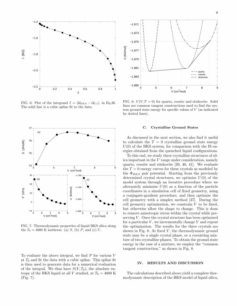
We evaluate the above integral by simulating the systemgoverned by Eq. 24 at several values of λ and using acubic spline to interpolate between points. The integrandis shown in Fig. 6, from which we obtain ∆F (C) =−1635990± 50 J via numerical integration.

From our BKS simulations we find U(C) = −1802257±100 J/mol, from which we evaluate ∆U(C) = U(C) −ULJ(C). Using S(C) = SLJ(C) + [∆U(C) − ∆F (C)]/T ,we find for the BKS liquid S(C) = S(T0, V0) = 75.986 ±0.177 J/mol K.

To obtain values of S at T0 for V different from V0,we carry out a thermodynamic integration of P along anisotherm of the BKS liquid, using,

S(V, T0) = S(C) +1

T

[

U(V, T0) − U(C)]

+1

T

∫ V

V0

P (V ′)dV ′. (27)

8

0 0.2 0.4 0.6 0.8 1 λ

−2.2

−2.0

−1.8

−1.6

−1.4I

(M

J)

FIG. 6: Plot of the integrand I = 〈UBKS − ULJ 〉, in Eq.26.The solid line is a cubic spline fit to the data.

5 6 7 8 9V (cm

3/mol)

−1.805

−1.800

−1.795

−1.790

U (

MJ/

mol

)

5 6 7 8 9V (cm

3/mol)

−10

0

10

20

30

P (

GP

a)

5 6 7 8 9 V (cm

3/mol)

74

75

76

77

S (

J/m

olK

)

(a)

(b) (c)

FIG. 7: Thermodynamic properties of liquid BKS silica alongthe T0 = 4000 K isotherm: (a) S, (b) P , and (c) U .

To evaluate the above integral, we find P for various Vat T0 and fit the data with a cubic spline. This spline fitis then used to generate data for a numerical evaluationof the integral. We thus have S(V, T0), the absolute en-tropy of the BKS liquid at all V studied, at T0 = 4000 K(Fig. 7).

4 5 6 7 8 9V (cm

3/mol)

−1.885

−1.883

−1.881

−1.879

−1.877

−1.875

−1.873

−1.871

U (

MJ/

mol

)

quartzcoesitestishovite

FIG. 8: U(V, T = 0) for quartz, coesite and stishovite. Solidlines are common tangent constructions used to find the sys-tem ground state energy for specific values of V (as indicatedby dotted lines).

C. Crystalline Ground States

As discussed in the next section, we also find it usefulto calculate the T = 0 crystalline ground state energyU(0) of the BKS system, for comparison with the IS en-ergies obtained from the quenched liquid configurations.

To this end, we study three crystalline structures of sil-ica important in the V range under consideration, namelyquartz, coesite and stishovite [39, 40, 41]. We evaluatethe T = 0 energy curves for these crystals as modeled bythe ΦBKS pair potential. Starting from the previouslydetermined crystal structures, we optimize U(0) of themodel system through an iterative procedure where wealternately minimize U(0) as a function of the particlecoordinates in a simulation cell of fixed geometry, usinga conjugate-gradient procedure; and then optimize thecell geometry with a simplex method [37]. During thecell geometry optimization, we constrain V to be fixed,but otherwise allow the shape to change. This is doneto remove anisotropic stress within the crystal while pre-serving V . Once the crystal structure has been optimizedfor a particular V , we incrementally change V and repeatthe optimization. The results for the three crystals areshown in Fig. 8. At fixed V , the thermodynamic groundstate may be a single crystal phase, or a coexisting mix-ture of two crystalline phases. To obtain the ground stateenergy in the case of a mixture, we employ the “commontangent construction,” as shown in Fig. 8.

IV. RESULTS AND DISCUSSION

The calculations described above yield a complete ther-modynamic description of the BKS model of liquid silica,

9

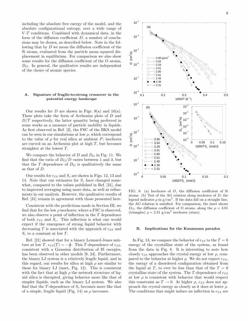
including the absolute free energy of the model, and theabsolute configurational entropy, over a wide range ofV -T conditions. Combined with dynamical data, in theform of the diffusion coefficient D, a number of conclu-sions may be drawn, as described below. Note in the fol-lowing that by D we mean the diffusion coefficient of theSi atoms, evaluated from the particle mean squared dis-placement in equilibrium. For comparison we also showsome results for the diffusion coefficient of the O atoms,DO. In general, the qualitative results are independentof the choice of atomic species.

A. Signature of fragile-to-strong crossover in the

potential energy landscape

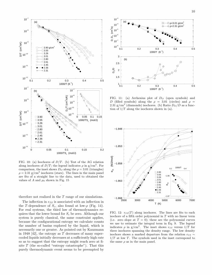
Our results for D are shown in Figs. 9(a) and 10(a).These plots take the form of Arrhenius plots of D andD/T respectively, the latter quantity being preferred insome works as a measure of particle mobility in liquids.As first observed in Ref. [3], the FSC of the BKS modelcan be seen in our simulations at low ρ, which correspondto the value of ρ for real silica at ambient P ; isochoresare curved on an Arrhenius plot at high T , but becomesstraighter at the lowest T .

We compare the behavior of D and DO in Fig. 11. Wefind that the ratio of DO/D varies between 1 and 3, butthat the T dependence of DO is qualitatively the sameas that of D.

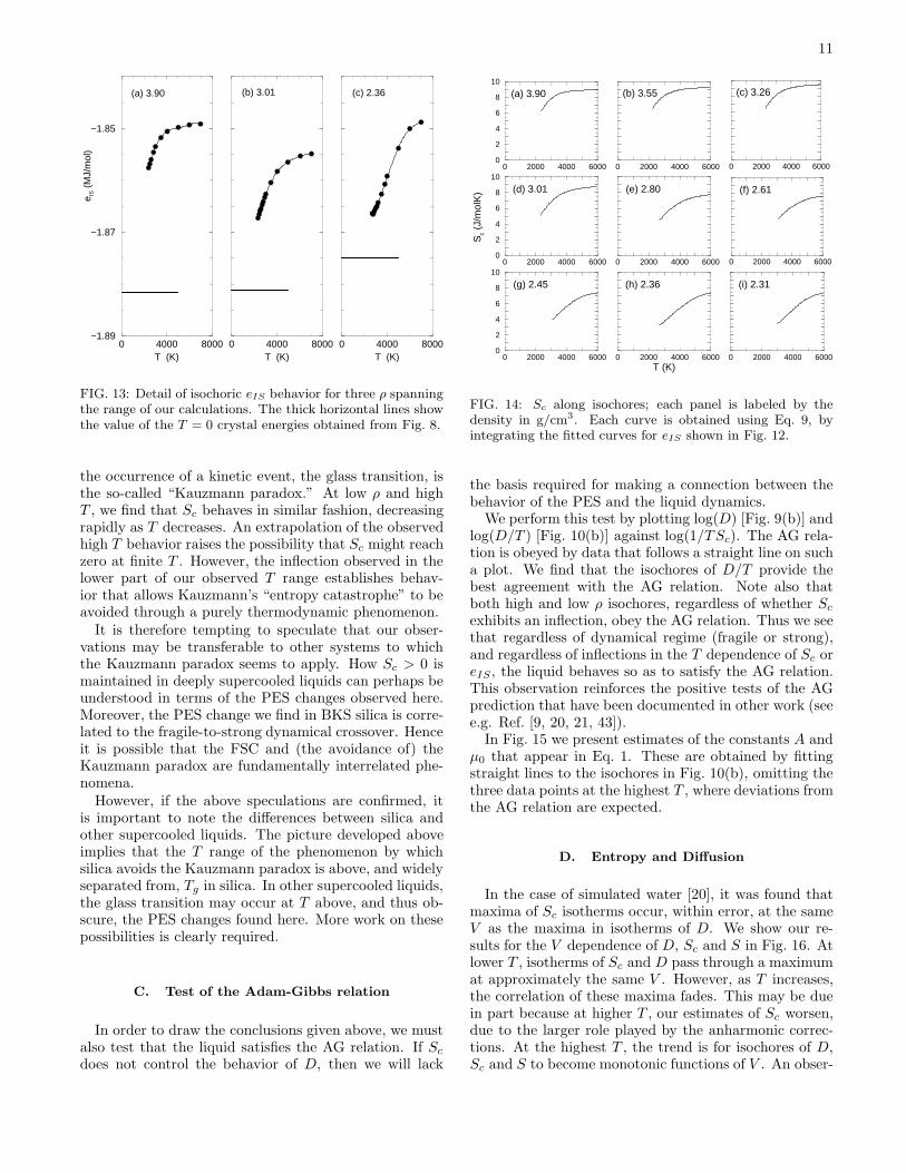
Our results for eIS and Sc are shown in Figs. 12, 13 and14. Note that our estimates for Sc have changed some-what, compared to the values published in Ref. [31], dueto improved averaging using more data, as well as refine-ments in our analysis. However, the qualitative results ofRef. [31] remain in agreement with those presented here.

Consistent with the predictions made in Section III, wefind that for the low ρ isochores, where a FSC is observed,we also observe a point of inflection in the T dependenceof both eIS and Sc. This inflection is what one wouldexpect if the emergence of strong liquid behavior withdecreasing T is associated with the approach of eIS andSc to a constant at low T .

Ref. [21] showed that for a binary Lennard-Jones mix-ture at low T , eIS(T ) ∼ − 1

T . This T -dependence of eIS,consistent with a Gaussian distribution of IS energies,has been observed in other models [9, 24]. Furthermore,the binary LJ system is a relatively fragile liquid, and inthis regard, our results for silica at high ρ are similar tothose for binary LJ (inset, Fig. 12). This is consistentwith the fact that at high ρ the network structure of liq-uid silica is disrupted, giving behavior more like that ofsimpler liquids, such as the binary LJ system. We alsofind that the T -dependence of Sc becomes more like thatof a simple, fragile liquid (Fig. 14) as ρ increases.

0.1 0.2 0.3 0.4 0.51000/T (K

−1)

10−8

10−7

10−6

10−5

10−4

10−3

D (

cm2 /s

)

3.90 g/cm3

3.553.263.012.802.612.452.362.31

(a)

0 0.05 0.1 0.15 0.21000/TSc (mol/J)

10−8

10−7

10−6

10−5

10−4

10−3

D (

cm2 /s

)

3.903.553.263.012.802.612.452.362.31

0 0.05 0.1 0.151000/TSc (mol/J)

10−8

10−7

10−6

10−5

10−4

10−3

DO (

cm2 /s

)

(b)

FIG. 9: (a) Isochores of D, the diffusion coefficient of Siatoms. (b) Test of the AG relation along isochores of D; thelegend indicates ρ in g/cm3. If the data fall on a straight line,the AG relation is satisfied. For comparison, the inset showsDO, the diffusion coefficient of O atoms, along the ρ = 3.01(triangles) ρ = 2.31 g/cm3 isochores (stars).

B. Implications for the Kauzmann paradox

In Fig. 13, we compare the behavior of eIS to the T = 0energy of the crystalline state of the system, as foundfrom the data in Fig. 8. It is interesting to note howclosely eIS approaches the crystal energy at low ρ, com-pared to the behavior at higher ρ. We do not expect eIS ,the energy of a disordered configuration obtained fromthe liquid at T , to ever be less than that of the T = 0crystalline state of the system. The T -dependence of eIS

at low ρ is consistent with behavior that would respectthis constraint as T → 0. At higher ρ, eIS does not ap-proach the crystal energy as closely as it does at lower ρ.The conditions that might induce an inflection in eIS are

10

0.1 0.2 0.3 0.4 0.51000/T (K

−1)

10−12

10−11

10−10

10−9

10−8

10−7

D/T

(cm

2 /sK

)

3.90 g/cm3

3.553.263.012.802.612.452.362.31

(a)

0 0.05 0.1 0.15 0.21000/TSc (mol/J)

10−12

10−11

10−10

10−9

10−8

10−7

D/T

(cm

2 /sK

)

3.903.553.263.012.802.612.452.362.31

0 0.05 0.1 0.151000/TSc (mol/J)

10−11

10−10

10−9

10−8

10−7

DO/T

(cm

2 /s/K

)

(b)

FIG. 10: (a) Isochores of D/T . (b) Test of the AG relationalong isochores of D/T ; the legend indicates ρ in g/cm3. Forcomparison, the inset shows DO along the ρ = 3.01 (triangles)ρ = 2.31 g/cm3 isochores (stars). The lines in the main panelare fits of a straight line to the data, used to obtained thevalues of A and µ0 shown in Fig. 15

.

therefore not realized in the T range of our simulations.

The inflection in eIS is associated with an inflection inthe T -dependence of Sc, also found at low-ρ (Fig. 14).For real systems, the third law of thermodynamics re-quires that the lower bound for Sc be zero. Although oursystem is purely classical, the same constraint applies,because the configurational entropy we calculate countsthe number of basins explored by the liquid, which isnecessarily one or greater. As pointed out by Kauzmannin 1948 [42], the entropy as T decreases of many super-cooled liquids initially decreases at a sufficiently high rateso as to suggest that the entropy might reach zero at fi-nite T (the so-called “entropy catastrophe”). That thispurely thermodynamic event seems to be preempted by

0.1 0.2 0.3 0.4 0.51000/T (K

−1)

1

1.5

2

2.5

3

DO/D

0.1 0.2 0.3 0.4 0.51000/T (K

−1)

10−8

10−7

10−6

10−5

10−4

10−3

D, D

O (

cm2 /s

)

ρ=3.01 g/cm3

ρ=2.31 g/cm3

(a)

(b)

FIG. 11: (a) Arrhenius plot of DO (open symbols) andD (filled symbols) along the ρ = 3.01 (circles) and ρ =2.31 g/cm3 (diamonds) isochores. (b) Ratio DO/D as a func-tion of 1/T along the isochores shown in (a).

2000 3000 4000 5000 6000 7000T (K)

−1.868

−1.863

−1.858

−1.853

−1.848

e IS

(MJ/

mol

)

3.903.553.263.012.802.612.452.362.31

0.1 0.41000/T

−1.87

−1.85

e IS

FIG. 12: eIS(T ) along isochores. The lines are fits to eachisochore of a fifth order polynomial in T with no linear term(i.e. zero slope at T = 0); these are the polynomial curveswe use to estimate the integral term in Eq. 9. The legendindicates ρ in g/cm3. The inset shows eIS versus 1/T forthree isochores spanning the density range. The low densityisochore shows a marked departure from the relation eIS ∼1/T at low T . The symbols used in the inset correspond tothe same ρ as in the main panel.

11

0 4000 8000T (K)

−1.89

−1.87

−1.85

e IS (

MJ/

mol

)

0 4000 8000T (K)

0 4000 8000T (K)

(c) 2.36(b) 3.01(a) 3.90

FIG. 13: Detail of isochoric eIS behavior for three ρ spanningthe range of our calculations. The thick horizontal lines showthe value of the T = 0 crystal energies obtained from Fig. 8.

the occurrence of a kinetic event, the glass transition, isthe so-called “Kauzmann paradox.” At low ρ and highT , we find that Sc behaves in similar fashion, decreasingrapidly as T decreases. An extrapolation of the observedhigh T behavior raises the possibility that Sc might reachzero at finite T . However, the inflection observed in thelower part of our observed T range establishes behav-ior that allows Kauzmann’s “entropy catastrophe” to beavoided through a purely thermodynamic phenomenon.

It is therefore tempting to speculate that our obser-vations may be transferable to other systems to whichthe Kauzmann paradox seems to apply. How Sc > 0 ismaintained in deeply supercooled liquids can perhaps beunderstood in terms of the PES changes observed here.Moreover, the PES change we find in BKS silica is corre-lated to the fragile-to-strong dynamical crossover. Henceit is possible that the FSC and (the avoidance of) theKauzmann paradox are fundamentally interrelated phe-nomena.

However, if the above speculations are confirmed, itis important to note the differences between silica andother supercooled liquids. The picture developed aboveimplies that the T range of the phenomenon by whichsilica avoids the Kauzmann paradox is above, and widelyseparated from, Tg in silica. In other supercooled liquids,the glass transition may occur at T above, and thus ob-scure, the PES changes found here. More work on thesepossibilities is clearly required.

C. Test of the Adam-Gibbs relation

In order to draw the conclusions given above, we mustalso test that the liquid satisfies the AG relation. If Sc

does not control the behavior of D, then we will lack

0 2000 4000 60000

2

4

6

8

100 2000 4000 6000

0

2

4

6

8

10

Sc (

J/m

olK

)

0 2000 4000 60000

2

4

6

8

10

0 2000 4000 6000T (K)

0 2000 4000 6000

0 2000 4000 6000

0 2000 4000 6000

0 2000 4000 6000

0 2000 4000 6000

(a) 3.90 (b) 3.55 (c) 3.26

(d) 3.01 (e) 2.80 (f) 2.61

(g) 2.45 (i) 2.31(h) 2.36

FIG. 14: Sc along isochores; each panel is labeled by thedensity in g/cm3. Each curve is obtained using Eq. 9, byintegrating the fitted curves for eIS shown in Fig. 12.

the basis required for making a connection between thebehavior of the PES and the liquid dynamics.

We perform this test by plotting log(D) [Fig. 9(b)] andlog(D/T ) [Fig. 10(b)] against log(1/TSc). The AG rela-tion is obeyed by data that follows a straight line on sucha plot. We find that the isochores of D/T provide thebest agreement with the AG relation. Note also thatboth high and low ρ isochores, regardless of whether Sc

exhibits an inflection, obey the AG relation. Thus we seethat regardless of dynamical regime (fragile or strong),and regardless of inflections in the T dependence of Sc oreIS, the liquid behaves so as to satisfy the AG relation.This observation reinforces the positive tests of the AGprediction that have been documented in other work (seee.g. Ref. [9, 20, 21, 43]).

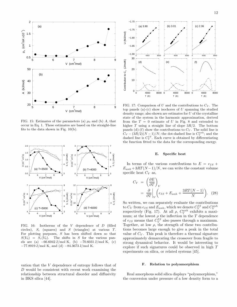
In Fig. 15 we present estimates of the constants A andµ0 that appear in Eq. 1. These are obtained by fittingstraight lines to the isochores in Fig. 10(b), omitting thethree data points at the highest T , where deviations fromthe AG relation are expected.

D. Entropy and Diffusion

In the case of simulated water [20], it was found thatmaxima of Sc isotherms occur, within error, at the sameV as the maxima in isotherms of D. We show our re-sults for the V dependence of D, Sc and S in Fig. 16. Atlower T , isotherms of Sc and D pass through a maximumat approximately the same V . However, as T increases,the correlation of these maxima fades. This may be duein part because at higher T , our estimates of Sc worsen,due to the larger role played by the anharmonic correc-tions. At the highest T , the trend is for isochores of D,Sc and S to become monotonic functions of V . An obser-

12

5 6 7 8 9V (cm

3/mol)

20

30

40

50

A (

kJ/m

ol)

5 6 7 8 9V (cm

3/mol)

0.5

1

1.5

2µ 0

(cm

2 /sK

x10

−7 )

(a)

(b)

FIG. 15: Estimates of the parameters (a) µ0 and (b) A, thatoccur in Eq. 1. These estimates are based on the straight-linefits to the data shown in Fig. 10(b).

5 6 7 8 9V (cm

3/mol)

0.0

0.5

1.0

1.5

2.0

D (

10−

5 cm

2 /s)

3

4

5

6

S, S

c (J/

mol

K)

5 6 7 8 9V (cm

3/mol)

0

1

2

3

D (

10−

5 cm

2 /s)

3

4

5

6

7

S, S

c (J/

mol

K)

5 6 7 8 9V (cm

3/mol)

4

5

6

7

D (

10−

5 cm

2 /s)

3

4

5

6

7

8

S, S

c(J/

mol

K)

5 6 7 8 9V (cm

3/mol)

9

10

11

12

D (

10−

5 cm

2 /s)

2

4

6

8

S, S

c (J/

mol

K)

(a) T=3500 (b) T=4000

(c) T=5000 (d) T=6000

FIG. 16: Isotherms of the V dependence of D (filledcircles), Sc (squares) and S (triangles) at various T .For plotting purposes, S has been shifted down so thatS(V0) = Sc(V0). The shifts in S for the various pan-els are (a) −66.6042 J/mol K, (b) −70.6031 J/mol K, (c)−77.8919 J/mol K, and (d) −84.3673 J/mol K.

vation that the V dependence of entropy follows that ofD would be consistent with recent work examining therelationship between structural disorder and diffusivityin BKS silica [44].

0 4000 8000T (K)

0

10

20

30

Con

trib

utio

n to

CV (

J/m

olK

)

0 4000 8000−1.90

−1.85

−1.80

−1.75

−1.70

U (

MJ/

mol

)

0 4000 8000T (K)

0 4000 8000

0 4000 8000T (K)

0 4000 8000

(a) 3.90 (b) 3.01 (c) 2.36

(d) (e) (f)

FIG. 17: Comparison of U and the contributions to CV . Thetop panels (a)-(c) show isochores of U spanning the studieddensity range; also shown are estimates for U of the crystallinestate of the system in the harmonic approximation, derivedfrom the T = 0 estimate of U in Fig. 8 and extended tohigher T using a straight line of slope 3R/2. The bottompanels (d)-(f) show the contributions to CV . The solid line isCV − (3R/2)(N − 1)/N ; the dot-dashed line is Canh

V ; and thedashed line is CIS

V . Each curve is obtained by differentiatingthe function fitted to the data for the corresponding energy.

E. Specific heat

In terms of the various contributions to E = eIS +Eanh +3RT (N−1)/N , we can write the constant volumespecific heat CV as,

CV =

(

∂E

∂T

)

V

=∂

∂T

∣

∣

∣

∣

V

(

eIS + Eanh +3RT (N − 1)

N

)

. (28)

So written, we can separately evaluate the contributionsto CV from eIS and Eanh, which we denote CIS

V and CanhV

respectively (Fig. 17). At all ρ, CanhV exhibits a maxi-

mum; at the lowest ρ the inflection in the T dependenceof eIS means that CIS

V also passes through a maximum.Together, at low ρ, the strength of these two contribu-tions becomes large enough to give a peak in the totalvalue of CV . This peak is therefore a thermal signatureapproximately demarcating the crossover from fragile tostrong dynamical behavior. It would be interesting toexplore if such signatures could be observed in high Texperiments on silica, or related systems [45].

F. Relation to polyamorphism

Real amorphous solid silica displays “polyamorphism,”the conversion under pressure of a low density form to a

13

high density form, that occurs in some ways as thoughit were a first-order phase transition. Computer sim-ulations of BKS silica have provided evidence that thispolyamorphic transition may correspond to a sub-Tg rem-nant of a liquid-liquid phase transition occurring in theequilibrium liquid [46].

Having found that the same model, BKS silica, ex-hibits a thermodynamic anomaly, in the form of a CV

peak associated with a FSC, it is natural to ask if thisphenomenon is related in some way to polyamorphism.It is difficult at present to answer this question decisively,since the region of the proposed liquid-liquid instabilityin BKS silica has only been approximately located, andseems to lie in a T range below that at which we canevaluate equilibrium liquid properties with current com-putational resources. However, several trends suggest aconnection.

First, we find that the T at which the peak of CV

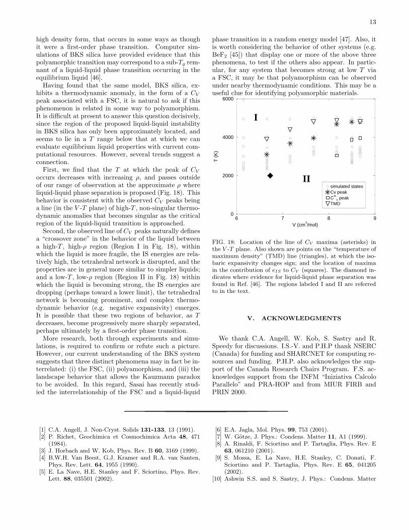
occurs decreases with increasing ρ, and passes outsideof our range of observation at the approximate ρ whereliquid-liquid phase separation is proposed (Fig. 18). Thisbehavior is consistent with the observed CV peaks beinga line (in the V -T plane) of high-T , non-singular thermo-dynamic anomalies that becomes singular as the criticalregion of the liquid-liquid transition is approached.

Second, the observed line of CV peaks naturally definesa “crossover zone” in the behavior of the liquid betweena high-T , high-ρ region (Region I in Fig. 18), withinwhich the liquid is more fragile, the IS energies are rela-tively high, the tetrahedral network is disrupted, and theproperties are in general more similar to simpler liquids;and a low-T , low-ρ region (Region II in Fig. 18) withinwhich the liquid is becoming strong, the IS energies aredropping (perhaps toward a lower limit), the tetrahedralnetwork is becoming prominent, and complex thermo-dynamic behavior (e.g. negative expansivity) emerges.It is possible that these two regions of behavior, as Tdecreases, become progressively more sharply separated,perhaps ultimately by a first-order phase transition.

More research, both through experiments and simu-lations, is required to confirm or refute such a picture.However, our current understanding of the BKS systemsuggests that three distinct phenomena may in fact be in-terrelated: (i) the FSC, (ii) polyamorphism, and (iii) thelandscape behavior that allows the Kauzmann paradoxto be avoided. In this regard, Sasai has recently stud-ied the interrelationship of the FSC and a liquid-liquid

phase transition in a random energy model [47]. Also, itis worth considering the behavior of other systems (e.g.BeF2 [45]) that display one or more of the above threephenomena, to test if the others also appear. In partic-ular, for any system that becomes strong at low T viaa FSC, it may be that polyamorphism can be observedunder nearby thermodynamic conditions. This may be auseful clue for identifying polyamorphic materials.

6 7 8 9V (cm

3/mol)

0

2000

4000

6000

T (

K)

simulated statesCv peakC

IS

V peakTMD

I

II

FIG. 18: Location of the line of CV maxima (asterisks) inthe V -T plane. Also shown are points on the “temperature ofmaximum density” (TMD) line (triangles), at which the iso-baric expansivity changes sign; and the location of maximain the contribution of eIS to CV (squares). The diamond in-dicates where evidence for liquid-liquid phase separation wasfound in Ref. [46]. The regions labeled I and II are referredto in the text.

V. ACKNOWLEDGMENTS

We thank C.A. Angell, W. Kob, S. Sastry and R.Speedy for discussions. I.S.-V. and P.H.P thank NSERC(Canada) for funding and SHARCNET for computing re-sources and funding. P.H.P. also acknowledges the sup-port of the Canada Research Chairs Program. F.S. ac-knowledges support from the INFM “Iniziativa CalcoloParallelo” and PRA-HOP and from MIUR FIRB andPRIN 2000.

[1] C.A. Angell, J. Non-Cryst. Solids 131-133, 13 (1991).[2] P. Richet, Geochimica et Cosmochimica Acta 48, 471

(1984).[3] J. Horbach and W. Kob, Phys. Rev. B 60, 3169 (1999).[4] B.W.H. Van Beest, G.J. Kramer and R.A. van Santen,

Phys. Rev. Lett. 64, 1955 (1990).[5] E. La Nave, H.E. Stanley and F. Sciortino, Phys. Rev.

Lett. 88, 035501 (2002).

[6] E.A. Jagla, Mol. Phys. 99, 753 (2001).[7] W. Gotze, J. Phys.: Condens. Matter 11, A1 (1999).[8] A. Rinaldi, F. Sciortino and P. Tartaglia, Phys. Rev. E

63, 061210 (2001).[9] S. Mossa, E. La Nave, H.E. Stanley, C. Donati, F.

Sciortino and P. Tartaglia, Phys. Rev. E 65, 041205(2002).

[10] Ashwin S.S. and S. Sastry, J. Phys.: Condens. Matter

14

15, S1253 (2003).[11] M. Mezard and G. Parisi, Phys. Rev. Lett. 82, 747

(1999).[12] X. Xia and P.G. Wolynes, Phys. Rev. Lett. 86, 5526

(2001).[13] J.P. Garrahan and D. Chandler, Phys. Rev. Lett. 89,

035704 (2002).[14] M. Goldstein, J. Chem. Phys. 51, 3728 (1969).[15] F.H. Stillinger and T.A. Weber, Science 225, 983 (1984).[16] F.H. Stillinger, Science 267, 1935 (1995).[17] S. Sastry, P.G. Debenedetti and F.H. Stillinger, Nature

393, 554 (1998).[18] F. Sciortino, W. Kob and P. Tartaglia, Phys. Rev. Lett.

83, 3214 (1999).[19] S. Buechner and A. Heuer, Phys. Rev. E 60, 6507 (1999).[20] A. Scala, F. Starr, E. La Nave, F. Sciortino and H.E.

Stanley, Nature 406, 166 (2000).[21] S. Sastry, Nature 409, 164 (2001).[22] L.-M. Martinez and C.A. Angell, Nature 410, 663 (2001).[23] P.G. Debenedetti and F.H. Stillinger, Nature 410, 259

(2001).[24] F.W. Starr, S. Sastry, E. La Nave, A. Scala, H.E. Stanley

and F. Sciortino, Phys. Rev. E 63, 041201 (2001).[25] E. La Nave, F. Sciortino, P. Tartaglia, C. De Michele and

S. Mossa, J. Phys.: Condens. Matter 15, S1085 (2003).[26] E. La Nave, S. Mossa and F. Sciortino, Phys. Rev. Lett.

88, 225701 (2002).[27] F. Sciortino and P. Tartaglia, Phys. Rev. Lett. 86, 107

(2001).[28] S. Mossa, E. La Nave, F. Sciortino and P. Tartaglia, Eur.

Phys. J. B 30, 351 (2002).[29] A. Saksaengwijit, B. Doliwa and A. Heuer, J. Phys.: Con-

dens. Matter 15, S1237 (2003).[30] G. Adam and J.H. Gibbs, J. Chem. Phys. 43, 139 (1965).[31] I. Saika-Voivod, P.H. Poole and F. Sciortino, Nature 412,

514 (2001).[32] MDCSPC2 is a MD program written by W. Smith,

Daresbury Laboratory, UK. This program is distributedby the CCP5 Project via www.ccp5.ac.uk.

[33] Y. Guissani and B. Guillot, J. Chem. Phys. 104, 7633(1996).

[34] K. Vollmayr, W. Kob and K. Binder, Phys. Rev. B 54,15808 (1996).

[35] M.P. Allen and D.J. Tildesley, Computer Simulation of

Liquids (Oxford University Press, Oxford, 1989).[36] R.K. Pathria, Statistical Mechanics (Butterworth-

Heinemann, Bodmin, U.K., 1996).[37] W.H. Press, S.A. Teukolsky, W.T. Vetterling, and

B.P. Flannery, Numerical Recipes (Cambridge UniversityPress, Cambridge, 1992).

[38] M. Mezei and D.L. Beveridge, Annals of the New YorkAcademy of Sciences 482, 1 (1986).

[39] P.J. Heaney, Reviews in Mineralogy 29, 1 (1994).[40] N.R. Keskar and J.R. Chelikowsky, Phys. Rev. B 46, 1

(1992).[41] J.R. Smyth, J.V. Smith, G. Artioli and A. Kvick, J.

Chem. Phys. 91, 988 (1987).[42] W. Kauzmann, Chem. Rev. 43, 219 (1948).[43] S. Corezzi, D. Fioretto and P. Rolla, Nature 420, 653

(2002).[44] M.S. Shell, P.G. Debenedetti and Z. Panagiotopoulos,

Molecular structural order and anomalies in liquid silica,Phys. Rev. E 66, 011202 (2002).

[45] M. Hemmati, C.T. Moynihan and C.A. Angell, J. Chem.Phys. 115, 6663 (2001).

[46] I. Saika-Voivod, F. Sciortino and P.H. Poole, Phys. Rev.E 63, 011202 (2001).

[47] M. Sasai, J. Chem. Phys. 118, 10651 (2003).