Forward irrelevance

Seediscussions,stats,andauthorprofilesforthispublicationat:https://www.researchgate.net/publication/228432113

Forwardirrelevance

ARTICLEinJOURNALOFSTATISTICALPLANNINGANDINFERENCE·FEBRUARY2009

ImpactFactor:0.68·DOI:10.1016/j.jspi.2008.01.012

CITATIONS

8

READS

16

3AUTHORS,INCLUDING:

GertDeCooman

GhentUniversity

164PUBLICATIONS1,898CITATIONS

SEEPROFILE

EnriqueMiranda

UniversityofOviedo

76PUBLICATIONS750CITATIONS

SEEPROFILE

Availablefrom:EnriqueMiranda

Retrievedon:04February2016

https://www.researchgate.net/publication/228432113_Forward_irrelevance?enrichId=rgreq-1ecf6d0b-3029-4e43-8f37-fcddf9212b1b&enrichSource=Y292ZXJQYWdlOzIyODQzMjExMztBUzoxMDMwNDk1NzM5NjE3MzdAMTQwMTU4MDM0MTQ1MA%3D%3D&el=1_x_2

https://www.researchgate.net/publication/228432113_Forward_irrelevance?enrichId=rgreq-1ecf6d0b-3029-4e43-8f37-fcddf9212b1b&enrichSource=Y292ZXJQYWdlOzIyODQzMjExMztBUzoxMDMwNDk1NzM5NjE3MzdAMTQwMTU4MDM0MTQ1MA%3D%3D&el=1_x_3

https://www.researchgate.net/?enrichId=rgreq-1ecf6d0b-3029-4e43-8f37-fcddf9212b1b&enrichSource=Y292ZXJQYWdlOzIyODQzMjExMztBUzoxMDMwNDk1NzM5NjE3MzdAMTQwMTU4MDM0MTQ1MA%3D%3D&el=1_x_1

https://www.researchgate.net/profile/Gert_De_Cooman?enrichId=rgreq-1ecf6d0b-3029-4e43-8f37-fcddf9212b1b&enrichSource=Y292ZXJQYWdlOzIyODQzMjExMztBUzoxMDMwNDk1NzM5NjE3MzdAMTQwMTU4MDM0MTQ1MA%3D%3D&el=1_x_4


https://www.researchgate.net/institution/Ghent_University?enrichId=rgreq-1ecf6d0b-3029-4e43-8f37-fcddf9212b1b&enrichSource=Y292ZXJQYWdlOzIyODQzMjExMztBUzoxMDMwNDk1NzM5NjE3MzdAMTQwMTU4MDM0MTQ1MA%3D%3D&el=1_x_6


https://www.researchgate.net/profile/Enrique_Miranda2?enrichId=rgreq-1ecf6d0b-3029-4e43-8f37-fcddf9212b1b&enrichSource=Y292ZXJQYWdlOzIyODQzMjExMztBUzoxMDMwNDk1NzM5NjE3MzdAMTQwMTU4MDM0MTQ1MA%3D%3D&el=1_x_4


https://www.researchgate.net/institution/University_of_Oviedo?enrichId=rgreq-1ecf6d0b-3029-4e43-8f37-fcddf9212b1b&enrichSource=Y292ZXJQYWdlOzIyODQzMjExMztBUzoxMDMwNDk1NzM5NjE3MzdAMTQwMTU4MDM0MTQ1MA%3D%3D&el=1_x_6


FORWARD IRRELEVANCE

GERT DE COOMAN AND ENRIQUE MIRANDA

ABSTRACT. We investigate how to combine marginal assessments about the values thatrandom variables assume separately into a model for the values that they assume jointly,when (i) these marginal assessments are modelled by means of coherent lower previsions,and (ii) we have the additional assumption that the random variables are forward epis-temically irrelevant to each other. We consider and provide arguments for two possiblecombinations, namely the forward irrelevant natural extension and the forward irrelevantproduct, and we study the relationships between them. Our treatment also uncovers aninteresting connection between the behavioural theory of coherent lower previsions, andShafer and Vovk’s game-theoretic approach to probability theory.

1. INTRODUCTION

In probability and statistics, assessments of independence are often useful as they allowus to reduce the complexity of inference problems. To give an example, and to set the stagefor the developments in this paper, we consider two random variables X1 and X2, takingvalues in the respective finite sets X1 and X2. Suppose that a subject is uncertain aboutthe values of these variables, but that he has some model expressing his beliefs about them.Then we say that X1 is epistemically irrelevant to X2 for the subject when he assesses thatlearning the actual value of X1 won’t change his beliefs (or belief model) about the value ofX2. We say that X1 and X2 are epistemically independent when X1 and X2 are epistemicallyirrelevant to one another; the terminology is borrowed from Walley (1991, Chapter 9).

Let us first look at what these general definitions yield when the belief models our sub-ject uses are precise probabilities. If the subject has a marginal probability mass functionp1(x1) for the first variable X1, and a conditional mass function q2(x2|x1) for the secondvariable X2 conditional on the first, then we can calculate his joint mass function p(x1,x2)using Bayes’s rule: p(x1,x2) = p1(x1)q2(x2|x1). Now consider any real-valued function fon X1×X2. We shall call such functions gambles, because they can be interpreted as un-certain rewards. We find for the prevision (or expectation, or fair price, we use de Finetti’s(1974–1975) terminology and notation throughout this paper.) of such a gamble f that:

P( f ) = ∑(x1,x2)∈X1×X2

f (x1,x2)p1(x1)q2(x2|x1)

= ∑x1∈X1

p1(x1) ∑x2∈X2

f (x1,x2)q2(x2|x1) = ∑x1∈X1

p1(x1)Q2( f (x1, ·)|x1)

= P1(Q2( f |X1)), (1)

Date: November 9, 2007.2000 Mathematics Subject Classification. 60A99,60G99,91A40.Key words and phrases. Imprecise probabilities, coherent lower previsions, forward irrelevance, game-

theoretic probability, epistemic irrelevance, epistemic independence, event trees.Supported by research grant G.0139.01 of the Flemish Fund for Scientific Research (FWO), and by MCYT,

projects MTM2004-01269, TSI2004-06801-C04-01.1

2 GERT DE COOMAN AND ENRIQUE MIRANDA

where we let Q2( f |X1) be the subject’s conditional prevision of f given X1, which is agamble on X1 whose value in x1,

Q2( f |x1) := Q2( f (x1, ·)|x1) = ∑x2∈X2

f (x1,x2)q2(x2|x1),

is the subject’s conditional prevision of f given that X1 = x1. We also let P1 be the subject’smarginal prevision (operator) for the first random variable, associated with the marginalmass function p1: P1(g) := ∑x1∈X1

g(x1)p1(x1) for all gambles g on X1.When the subject judges X1 to be (epistemically) irrelevant to X2, then we get for all

x1 ∈X1 and x2 ∈X2 thatq2(x2|x1) = p2(x2), (2)

where p2 is the subject’s marginal mass function for the second variable X2 that we canderive from the joint p using p2(x2) := ∑x1∈X1

p(x1,x2). The equality (2) expresses thatlearning that X1 = x1 doesn’t change the subject’s probability model for the value of thesecond variable. Condition (2) is equivalent to requiring that for all x1 ∈X and all gamblesf on X1×X2,

Q2( f (x1, ·)|x1) = P2( f (x1, ·)), (3)

where now P2 is the subject’s marginal prevision (operator) for the second variable, asso-ciated with the marginal mass function p2. We can then write for the joint prevision:

P( f ) = P1(P2( f )), (4)

where f is any gamble on X1×X2, and where we let P2( f ) be the gamble on X1 thatassumes the value P2( f (x1, ·)) in x1 ∈X1.

Similarly, when X2 is epistemically irrelevant to X1 for our subject, then

q1(x1|x2) = p1(x1) (5)

for all x1 ∈X1 and x2 ∈X2. Here q1(x1|x2) is the subject’s mass function for the first vari-able X1 conditional on the second. This leads to another expression for the joint prevision:

P( f ) = P2(P1( f )). (6)

Expressions (4) and (6) for the joint are equivalent, as generally P1(P2( f )) = P2(P1( f )).This is related to the fact that Conditions (2) and (5) are equivalent: if X1 is epistemicallyirrelevant to X2 then X2 is epistemically irrelevant to X1, and vice versa. In other words, forprecise probability models, epistemic irrelevance is equivalent to epistemic independence.

Some caution is needed here: this equivalence is only guaranteed if the marginal massfunctions are everywhere non-zero. If some events have zero probability, then it can stillbe guaranteed provided we slightly change the definition of epistemic irrelevance, and forinstance impose q2(x2|x1) = p2(x2) only when p1(x1) > 0.

All of this will seem tritely obvious to anyone with a basic knowledge of probabilitytheory, but the point we want to make, is that the situation changes dramatically whenwe use belief models that are more general (and arguably more realistic) than the precise(Bayesian) ones, such as Walley’s (1991) imprecise probability models.

On Walley’s view, a subject may not generally be disposed to specify a fair price P( f )for any gamble f , but we can always ask for his lower prevision P( f ), which is his supre-mum acceptable price for buying the uncertain reward f , and his upper prevision P( f ),which is his infimum acceptable price for selling f . We give a fairly detailed introductionto Walley’s theory in Section 2.

FORWARD IRRELEVANCE 3

On this new approach, if X1 is epistemically irrelevant to X2 for our subject, then [com-pare with Condition (3)]

Q2( f (x1, ·)|x1) = P2( f (x1, ·))for all gambles f on X1 ×X2 and all x1 ∈ X1. Here, similar to what we did before,P2 is the subject’s marginal lower prevision (operator) for X2, and Q2(·|X1) is his lowerprevision (operator) for X2 conditional on X1. We shall see in Section 3 that a reasonablejoint model1 for the value that (X1,X2) assumes in X1×X2 is then given by [comparewith Eqs. (1) and (4)]

P( f ) = P1(Q2( f |X1)) = P1(P2( f )) (7)for all gambles f on X1×X2, where P1 is the subject’s marginal lower prevision (op-erator) for X1, and where we also let P2( f ) be the gamble on X1 that assumes the valueP2( f (x1, ·)) in any x1 ∈X1.

On the other hand, when our subject judges X2 to be epistemically irrelevant to X1, weare eventually led to the joint model

P′( f ) = P2(P1( f )),

where now P1( f ) is the gamble on X2 that assumes the value P1( f (·,x2)) in any x2 ∈X1.Interestingly, it now is no longer guaranteed that P = P′, or in other words that P1(P2(·)) =P2(P1(·)). We give an example in Section 4, where we also argue that this asymmetry(i) isn’t caused by ‘pathological’ consequences involving zero probabilities, and can’t beremedied by simple tricks as the one mentioned above for (precise) probabilities; and (ii)is endemic, as it seems to be there for all imprecise models, apart from the extreme (linearor vacuous) ones. It results that, here, the notion of epistemic irrelevance is fundamentallyasymmetrical, and is no longer equivalent to the symmetrical notion of epistemic indepen-dence. This was discussed in much more detail by Couso et al. (2000).

But then, as the two notions are no longer equivalent here, it becomes quite important todistinguish between them when we actually represent beliefs using imprecise probabilitymodels. There are a number of reasons why a subject shouldn’t use the consequences ofepistemic independence automatically, when he is only assessing epistemic irrelevance.

First of all, an assessment of epistemic independence is stronger, and leads to higherjoint lower previsions. As lower previsions represent supremum buying prices, highervalues represent stronger commitments, and these may be unwarranted when it is onlyepistemic irrelevance that our subject wants to model.

Secondly, joint lower previsions based on an epistemic irrelevance assessment are gen-erally relatively straightforward to calculate, as Eq. (7) testifies. But calculating joint lowerprevisions from marginals based on an epistemic independence assessment is quite often avery complicated affair; see for instance the expressions in Section 9.3.2 of Walley (1991).

Moreover, there are special but nevertheless important situations where we want to ar-gue that it may be natural to make an epistemic irrelevance assessment, but not one ofindependence. Suppose, for instance that we consider two random variables, X1 and X2,where our subject knows that the value of X1 will be revealed to him before that of X2.2

Then assessing that X1 and X2 are epistemically independent amounts to assessing that(i) X1 is epistemically irrelevant to X2: getting to know the value of X1 doesn’t change

our subject’s beliefs about X2;

1This is the most conservative joint lower prevision that is coherent with P1 and Q2(·|X1), see also (Walley,1991, Section 6.7).

2The discussion that follows here, as well as the one in Appendix A, generalises naturally to random pro-cesses, where the values of a process are revealed at subsequent points in time.


(ii) X2 is epistemically irrelevant to X1: getting to know the value of X2 doesn’t changeour subject’s beliefs about X1.

But since the subject knows that he will always know the value of X1 before that of X2,(ii) is effectively a counter-factual statement for him: “if I got to the value of X2 first, thenlearning that value wouldn’t affect my beliefs about X1”. It’s not clear that making suchan assessment has any real value, and we feel it is much more natural in such situationscontext to let go of (ii) and therefore to resort to epistemic irrelevance.

This line of reasoning can also be related to Shafer’s (1985) idea that conditioningmust always be associated with a protocol. A subject can then only meaningfully update(or condition) a probability model on events that he envisages may happen (according tothe established protocol). In the specific situation described above, conditioning on thevariable X2 could only legitimately be done if it were possible to find out the value of X2without getting to know that of X1, quod non. Therefore, it isn’t legitimate to considerthe conditional lower prevision Q1(·|X2) expressing the beliefs about X1 conditional onX2, and we therefore can’t meaningfully impose (ii), as it requires that Q1(·|X2) = P1.Shafer has developed and formalised his ideas about protocols and conditioning using thenotion of an event tree, in an interesting book dealing with causal reasoning (Shafer, 1996).In Appendix A, we formulate a simple example, where X1 and X2 are the outcomes ofsuccessive coin tosses, in Shafer’s event-tree language. We show that in this specific case,the general notion of event-tree independence that he develops in his book, is effectivelyequivalent to the requirement that X1 should be epistemically irrelevant to X2.

For all these reasons, we feel that a study of the joint lower previsions that result fromepistemic irrelevance assessments is quite important, also from a practical point of view.We take the first steps towards such a study in this paper.

We shall consider a finite number of variables X1, . . . , XN taking values in respectivesets X1, . . . , XN . We are going to assume moreover that for k = 2, . . . ,N the variables X1,. . . , Xk−1 are epistemically irrelevant to Xk: we shall call such an assessment forward irrel-evance. It means that we aren’t learning from the ‘past’,3 and it will be in general weakerthan an assessment of epistemic independence. We shall study which are the inferencesthat can be made, based on such assessments.

In order to model the information we have about the variables X1, . . . , XN , we use thebehavioural theory of imprecise probabilities, developed mainly by Walley (1991), withinfluences from earlier work by de Finetti (1974–1975) and Williams (1975), amongstothers. This theory constitutes a generalisation of de Finetti’s account of subjective proba-bility, and uses (coherent) lower and upper previsions to represent a subject’s behaviouraldispositions. We give a brief introduction to the basic ideas behind coherent lower previ-sions in Section 2, and we explain how they can be identified with sets of (finitely additive)probability measures. This introductory section can be skipped by anyone with a reason-able working knowledge of coherent lower previsions.

It may appear at first sight that, because of this choice of model, the results we ob-tain have a limited interest for people working outside the field of imprecise probabil-ities. We think that this is not necessarily so, for two reasons: on the one hand, themathematical theory of coherent lower and upper previsions subsumes a number of ap-proaches to uncertainty modelling in the literature, like probability charges (Bhaskara Rao

3Of course, we can only speak of ‘the past’ in this context when the index k refers to the ‘time’ that the actualvalue of a variable Xk is revealed. This is the specific situation where we argue that the notion of epistemic irrele-vance is more natural than epistemic independence. But we don’t question the interest of epistemic independencein other contexts, of course.


and Bhaskara Rao, 1983), 2- and n-monotone set functions (Choquet, 1953–1954), pos-sibility measures (De Cooman, 2001; De Cooman and Aeyels, 1999, 2000; Dubois andPrade, 1988), and p-boxes (Ferson et al., 2003). This means that the results we establishhere will also be valid for any of these models.

Moreover, the behavioural theory of imprecise probabilities can also be given a Bayesiansensitivity analysis interpretation: we may assume the existence of a precise but unknownprobability model for the random variables X1, . . . , XN , and model our information aboutit by means of a set of possible models. As we shall see further on in Theorem 5, some ofthe results we shall find also make sense on such a sensitivity analysis interpretation.

In Section 3 we explain how a subject’s assessment that he doesn’t learn from the pastcan be used to combine a number of marginal lower previsions into a joint lower prevision,called their forward irrelevant natural extension. We study the properties of this combina-tion, and show later that it can be related to specific types of coherent probability protocolsintroduced by Shafer and Vovk (2001). We also discuss another interesting way of combin-ing marginal lower previsions into a joint, leading to their forward irrelevant product. Thisproduct has an interesting Bayesian sensitivity analysis interpretation. We also discuss itsproperties, and its relationship with the forward irrelevant natural extension. We show inparticular that the forward irrelevant product generally dominates—is less conservative ormore committal than—the forward irrelevant natural extension, and that these two coincidewhen the variables Xk we consider, can assume only a finite number of values.

As indicated above, our results also allow us to uncover a perhaps surprising relationshipbetween Walley’s (1991) behavioural theory of coherent lower previsions, and Shafer andVovk’s (2001) game-theoretic approach to probability theory. This is done in Section 5.In that same section, we also give an interesting financial interpretation for the forwardirrelevant natural extension in terms of an investment game involving futures. We havegathered the proofs of the main results in Appendix B.

2. COHERENT LOWER AND UPPER PREVISIONS

Here, we present a succinct overview of the relevant main ideas underlying the be-havioural theory of imprecise probabilities, in order to make it easier for the reader tounderstand the course of reasoning that we shall develop. We refer to Walley (1991) forextensive discussion and motivation.

2.1. Basic notation and rationality requirements. Consider a subject who is uncertainabout something, say, the value that a random variable X assumes in a set of possiblevalues4 X . Then, a bounded real-valued function on X is called a gamble on X (or onX), and the set of all gambles on X is denoted by L (X ). Given a real number µ , wealso use µ to denote the gamble that takes the constant value µ . A lower prevision P is areal-valued map (a functional) defined on some subset K of L (X ), called its domain.For any gamble f in K , P( f ) is called the lower prevision of f .

A subset A of X is called an event, and it can be identified with its indicator IA, whichis the gamble on X that assumes the value one on A and zero elsewhere. The lowerprobability P(A) of A is defined as the lower prevision P(IA) of its indicator IA. On theother hand, given a lower prevision P, its conjugate upper prevision P is defined on the setof gambles −K := {− f : f ∈K } by P( f ) := −P(− f ) for every − f in the domain ofP. This conjugacy relationship shows that we can restrict our attention to lower previsionsonly. If the domain of P contains only indicators, then we also call P an upper probability.

4We don’t require X to be a subset of the reals, nor that X satisfies any kind of measurability condition.


A lower prevision P with domain K is called coherent when for any natural numbersn≥ 0 and m≥ 0, and f0, . . . , fn in K :

supx∈X

[ n

∑k=1

[ fk(x)−P( fk)]−m[ f0(x)−P( f0)]]≥ 0. (8)

Coherent lower previsions share a number of basic properties. For instance, given gamblesf and g in K , real numbers µ and non-negative real numbers λ , coherence implies thatthe following properties hold, whenever the gambles are in the domain K of P:(C1) P( f )≥ infx∈X f (x);(C2) P( f +g)≥ P( f )+P(g) [super-additivity];(C3) P(λ f ) = λP( f ) [non-negative homogeneity];(C4) P( f + µ) = P( f )+ µ [constant additivity].Other properties can be found in Walley (1991, Section 2.6). It is important to mentionhere that when K is a linear space, coherence is equivalent to (C1)–(C3). More generally,a lower prevision on a general domain is coherent if and only if it can be extended to acoherent lower prevision on some linear space, i.e., a real functional satisfying (C1)–(C3).

2.2. Natural extension. We can always extend a coherent lower prevision P defined ona set of gambles K to a coherent lower prevision E on the set of all gambles L (X ),through a procedure called natural extension. The natural extension E of P is defined asthe point-wise smallest coherent lower prevision on L (X ) that coincides on K with P.It is given for all f in L (X ) by

E( f ) = supf1,..., fn∈K

µ1,...,µn≥0,n≥0

infx∈X

[f (x)−

n

∑k=1

µk[ fk(x)−P( fk)]], (9)

where the µ1, . . . , µn in the supremum are non-negative real numbers.

2.3. Relation to precise probabilities. A linear prevision P is a real-valued functionaldefined on a set of gambles K , that satisfies

sup[ n

∑i=1

fi−m

∑j=1

g j

]≥

n

∑i=1

P( fi)−m

∑j=1

P(g j) (10)

for all natural numbers n and m, and all gambles f1, . . . , fn, g1, . . . , gm in K .In particular, a linear prevision P on the set L (X ) is a real linear functional that is

positive (if f ≥ 0 then P( f ) ≥ 0) and has unit norm (P(IX ) = 1). Its restriction to eventsis a finitely additive probability. Moreover, any finitely additive probability defined on theset ℘(X ) of all events can be uniquely extended to a linear prevision on L (X ). For thisreason, we shall identify linear previsions on L (X ) with finitely additive probabilities on℘(X ). We denote by P(X ) the set of all linear previsions on L (X ).

Linear previsions are the precise probability models: they coincide with de Finetti’s(1974–1975) notion of a coherent prevision or fair price. We call coherent lower and upperprevisions imprecise probability models. That linear previsions are only required to befinitely additive, and not σ -additive, derives from the finitary character of the coherencerequirement in Eq. (10).

Consider a lower prevision P defined on a set of gambles K . Its set of dominatinglinear previsions M (P) is given by

M (P) = {P ∈ P(X ) : (∀ f ∈K )(P( f )≥ P( f ))}.


Then P is coherent if and only if M (P) 6= /0 and P( f ) = min{P( f ) : P ∈M (P)} for all fin K , i.e., if P is the lower envelope of M (P). And the natural extension E of a coherent Psatisfies E( f ) = min{P( f ) : P∈M (P)} for all f in L (X ). Moreover, the lower envelopeof any set of linear previsions is always a coherent lower prevision.

These relationships allow us to provide coherent lower previsions with a Bayesian sen-sitivity analysis interpretation, which is different from the behavioural interpretation dis-cussed below in Section 2.5: we might assume the existence of an ideal (but unknown)precise probability model PT on L (X ), and represent our imperfect knowledge aboutPT by means of a (convex closed) set M of possible candidates for PT . The informationgiven by this set is equivalent to the one provided by its lower envelope P, which is givenby P( f ) = minP∈M P( f ) for all f in L (X ). This lower envelope P is a coherent lowerprevision; and indeed, PT ∈M is equivalent to PT ≥ P.

2.4. Joint and marginal lower previsions. Now consider two random variables X1 andX2 that may assume values in the respective sets X1 and X2. We assume that these vari-ables are logically independent: the joint random variable (X1,X2) may assume all valuesin the product set X1×X2. A subject’s coherent lower prevision P on a subset K ofL (X1×X2) is a model for his uncertainty about the value that the joint random variable(X1,X2) assumes in X1×X2, and we call it a joint lower prevision.

We can associate with P its X1-marginal (lower prevision) P1, defined as follows:

P1(g) = P(g′)

for all gambles g on X1, such that the corresponding gamble g′ on X1×X2, defined byg′(x1,x2) := g(x1) for all (x1,x2) in X1×X2, belongs to K . The gamble g′ is constanton the sets {x1}×X2, and we call it X1-measurable. In what follows, we identify g andg′, and simply write P(g) rather than P(g′). The marginal P1 is the corresponding modelfor the subject’s uncertainty about the value that X1 assumes in X1, irrespective of whatvalue X2 assumes in X2. The X2-marginal P2 is defined similarly. The coherence of thejoint lower prevision P clearly implies the coherence of its marginals. If P is in particulara linear prevision on L (X1×X2), its marginals are linear previsions too.

Conversely, assume we start with two coherent marginal lower previsions P1 and P2,defined on the respective domains K1 ⊆ L (X1) and K2 ⊆ L (X2). We can interpretK1 as a set of gambles on X1×X2 that are X1-measurable, and similarly for K2. Anycoherent joint lower prevision defined on a set K of gambles on X1×X2 that includes K1and K2, and that coincides with P1 and P2 on their respective domains, i.e., has marginalsP1 and P2, will be called a product of P1 and P2. We shall investigate various ways ofdefining such products further on in the paper.5

2.5. The behavioural interpretation. The mathematical theory presented above can bebetter understood if we consider the following behavioural interpretation.

We interpret a gamble as an uncertain reward: if the value of the random variable Xturns out to be x ∈X , then the corresponding reward will be f (x) (positive or negative),expressed in units of some (predetermined) linear utility. A subject’s lower prevision P( f )for a gamble f is defined as his supremum acceptable price for buying f : it is the highestprice µ such that the subject will accept to buy f for all prices α < µ (buying f for a price

5It should be noted here that, in contradistinction with Walley (1991, Section 9.3.1), we don’t intend the mereterm ‘product’ to imply that the variables X1 and X2 are assumed to be independent in any way. On our approach,there may be many types of products, some of which may be associated with certain types of interdependencebetween the random variables X1 and X2. In other words, a product will be simply a joint distribution which iscompatible with the given marginals.


α is the same thing as accepting the uncertain reward f −α). A subject’s upper previsionP( f ) for f is his infimum acceptable selling price for f . Then P( f ) = −P(− f ), sinceselling f for a price α is the same thing as buying − f for the price −α .

A lower prevision P with domain K is then coherent when a finite combination ofacceptable buying transactions can’t lead to a sure loss, and when moreover for any f in K ,we can’t force the subject to accept f for a price strictly higher than his specified supremumbuying price P( f ), by exploiting buying transactions implicit in his lower previsions P( fk)for a finite number of gambles fk in K , which he is committed to accept. This is theessence of the mathematical requirement (8).

The natural extension of a coherent lower prevision P is the smallest coherent extensionto all gambles, and as such it summarises the behavioural implications of P: E( f ) is thesupremum buying price for f that can be derived from the lower prevision P by argumentsof coherence alone. We can see from its definition (9) that it is the supremum of all pricesthat the subject can be effectively forced to buy the gamble f for, by combining finitenumbers of buying transactions implicit in his lower prevision assessments P. In generalE won’t be the unique coherent extension of P to L (X ); but any other coherent exten-sion will point-wise dominate E and will therefore represent behavioural dispositions notimplied by the assessments P and coherence alone.

Finally, a linear prevision P with a negation invariant domain K = −K correspondsto the case where P( f ) = P( f ), i.e., when the subject’s supremum buying price coincideswith his infimum selling price, and this common value is a prevision or fair price for thegamble f , in the sense of de Finetti (1974–1975). This means that our subject is disposedto buy the gamble f for any price µ < P( f ), and to sell it for any price µ ′ > P( f ) (butnothing is said about his behaviour for µ = P( f )).

2.6. Conditional lower previsions and separate coherence. Consider a gamble h onX1×X2 and any value x1 ∈X1. Our subject’s conditional lower prevision P(h|X1 = x1),also denoted as P(h|x1), is the largest real number p for which the subject would buy thegamble h for any price strictly lower than p, if he knew in addition that the variable X1assumes the value x1 (and nothing more!).

We shall denote by P(h|X1) the gamble on X1 that assumes the value P(h|X1 = x1) =P(h|x1) in any x1 in X1. We can assume that P(h|X1) is defined for all gambles h in somesubset H of X1×X2, and we call P(·|X1) a conditional lower prevision on H . It isimportant to recognise that P(·|X1) maps any gamble h on X1×X2 to the gamble P(h|X1)on X1. We also use the notations

G(h|x1) := I{x1}×X2 [h−P(h|x1)], G(h|X1) = h−P(h|X1) := ∑x1∈X1

G(h|x1);

G(h|X1) is a gamble on X1 as well.That the domain of P(·|x1) is the same set H for all x1 ∈X1 is a consequence of the

notion of separate coherence that we shall introduce next (Walley, 1991, Section 6.2.4),and that we shall assume for all the conditional lower previsions in this paper. We say thatP(·|X1) is separately coherent if (i) for all x1 in X1, P(·|x1) is a coherent lower prevision onits domain, and if moreover (ii) P({x1}×X2|x1) = 1. It is a very important consequenceof this definition that for all x1 in X1 and all gambles h on the domain of P(·|x1),

P(h|x1) = P(h(x1, ·)|x1).

This implies that a separately coherent P(·|X1) is completely determined by the valuesP( f |X1) that it assumes in the gambles f on X2 alone. We shall use this very usefulproperty repeatedly throughout the paper.


2.7. Joint coherence and marginal extension. If besides the (separately coherent) con-ditional lower prevision P(·|X1) on some subset H of L (X1 ×X2), the subject hasalso specified a coherent joint (unconditional) lower prevision P on some subset K ofL (X1×X2), then P and P(·|X1) should in addition satisfy the consistency criterion ofjoint coherence, which is discussed and motivated at great length in Walley (1991, Chap-ter 6), and to a lesser extent in Appendix B (Section B.1).

Now, suppose our subject has specified a coherent marginal lower prevision P1 on somesubset K1 of L (X1), modelling the available information about the value that X1 assumesin X1. And, when modelling the available information about X2, he specifies a separatelycoherent conditional lower prevision P(·|X1) on some subset H of L (X1×X2). We canthen always extend P1 and P(·|X1) to a pair M and M(·|X1) defined on all of L (X1×X2),which is the point-wise smallest jointly coherent pair that coincides with P1 and P(·|X1)on their respective domains K1 and H . M and M(·|X1) are called the marginal extensionsof P1 and P(·|X1), and they are given, for all gambles f on X1×X2, by

M( f |x1) = E( f (x1, ·)|x1) and M( f ) = E1(E( f |X1)),

where for each x1 in X1, E(·|x1) is the (unconditional) natural extension of the coherentlower prevision P(·|x1) to all gambles on X2, and E1 is the (unconditional) natural exten-sion of P1 to all gambles on X1. This result is called the Marginal Extension Theorem inWalley (1991, Theorem 6.7.2). Note that M coincides with E1 on X1-measurable gambles,but also that M is not necessarily equal to the (unconditional) natural extension of P1 to allgambles on X1×X2, as it also has to take into account the behavioural consequences ofthe assessments that are present in P(·|X1). As is the case for unconditional natural exten-sion, the marginal extensions M and M(·|X1) summarise the behavioural implications of P1and P(·|X1), only taking into account the consequences of (separate and) joint coherence.

Further on, we consider a more general situation, where we work with N random vari-ables X1 ,. . . , XN taking values in the respective sets X1, . . . , XN , and we apply a general-isation of the Marginal Extension Theorem proved in Miranda and De Cooman (2007).

3. FORWARD IRRELEVANT NATURAL EXTENSION AND FORWARD IRRELEVANTPRODUCT

We are ready to begin our detailed discussion of how to combine marginal lower previ-sions into a joint, in such a way as to take into account epistemic irrelevance assessments.

3.1. Marginal information. Consider N random variables X1, . . . , XN taking values inthe respective non-empty sets X1, . . . , XN . We do not assume that these random variablesare real-valued, i.e., that the Xk are subsets of the set of real numbers R.

For each variable Xk, a subject has beliefs about the values that it assumes in Xk, ex-pressed in the form of a coherent marginal lower prevision Pk defined on some set ofgambles Kk ⊆L (Xk).

Now, if we know Pk( f ) for some f , then coherence implies that Pk(λ f +µ) = λPk( f )+µ for all λ ≥ 0 and µ ∈ R, so Pk can be uniquely extended to a coherent lower previsionon all λ f + µ . We may therefore assume, without loss of generality, that Pk is actuallydefined on the set of gambles K ∗

k (a cone containing all constant gambles), given by:

K ∗k := {λ f + µ : λ ≥ 0, µ ∈ R and f ∈Kk}. (11)

We can extend the marginal lower previsions Pk defined on Kk (or on K ∗k ) to marginal

lower previsions Ek defined on all of L (Xk), for 1 ≤ k ≤ N, through the procedure of


natural extension, as explained in Section 2.2. Applying (9), this yields:

Ek(h) = supgkik∈K ∗

kik=1,...,nk,nk≥0

infxk∈Xk

[h(xk)−

nk

∑ik=1

[gkik(xk)−Pk(gkik)]]

(12)

for all gambles h on Xk, also taking into account that K ∗k is a cone. Recall that Ek is

the point-wise smallest (least-committal) coherent extension of Pk: it is the extension thattakes into account only the consequences of coherence.

For any 1≤ k ≤ N, we define the set

X k :=×ki=1Xi = {(x1, . . . ,xk) : xi ∈Xi, i = 1, . . . ,k}

and the random variable Xk := (X1, . . . ,Xk) taking values in the set X k. Our subject judgesthe random variables X1, . . . , XN to be logically independent, which means that accordingto him, the Xk can assume all values in the corresponding Cartesian product sets X k.

3.2. Expressing forward irrelevance. We now express the following forward irrelevanceassessment: for each 2 ≤ k ≤ N, our subject assesses that his beliefs about the value thatthe variable Xk assumes in Xk will not be influenced by any additional information aboutthe value that the ‘previous’ variables Xk−1 = (X1, . . . ,Xk−1) assume in X k−1 =×k−1

i=1 Xi.To use Walley’s (1991) terminology, the variables X1, . . . , Xk−1 are epistemically irrelevantto the variable Xk, for 2≤ k ≤ N.

To make this forward irrelevance condition more explicit, we define the sets of gamblesK k on the product sets X k: let K 1 := K ∗

1 and for 2 ≤ k ≤ N, let K k be the set ofall gambles f on X k such that all partial maps f (x, ·) are in K ∗

k for x ∈ X k−1, i.e.,K k := { f ∈L (X k) : (∀x ∈X k−1)( f (x, ·) ∈K ∗

k )}. It follows from Eq. (11) that K k isa cone as well. In fact, we have something stronger: that λ f + µ ∈K k for all f in K k,and all gambles λ ≥ 0 and µ on X k−1. The forward irrelevance assessment can now beused to define conditional lower previsions P(·|Xk−1): let P( f |x1, . . . ,xk−1) := Pk( f ) forall f in Kk. Invoking separate coherence (Section 2.6), they can actually be defined on allg in K k by

P(g|x1, . . . ,xk−1) := Pk(g(x1, . . . ,xk−1, ·)) (13)

for all (x1, . . . ,xk−1) in X k−1, where 2≤ k ≤ N.In summary, we have the following assessments: an marginal lower prevision P1 defined

on K 1, and conditional lower previsions P(·|Xk−1) defined on K k, which are derivedfrom the marginals Pk and the forward irrelevance assessment (13), for 2≤ k ≤ N.

3.3. The forward irrelevant natural extension. We now investigate what are the mini-mal behavioural consequences of these (conditional) lower prevision assessments. In par-ticular, if a subject has specified the marginal lower previsions Pk summarising his dis-positions to buy gambles fk in Kk for prices up to Pk( fk), and if he makes the forwardirrelevance assessment expressed through Eq. (13), then what is the smallest (most conser-vative, or least-committal) price that these assessments and coherence imply he should bewilling to pay for a gamble f on the product space X N?

The lower prevision that represents these least-committal supremum acceptable buyingprices is identified in the following theorem, which is proved in Appendix B, Section B.2.


Theorem 1. The so-called natural extension EN of P1 and the P(·|Xk−1) to a lower previ-sion on L (X N), defined by

EN( f ) = supgkik∈K k,ik=1,...,nk

nk≥0,k=1,...,N

infx∈X N

[f (x)−

N

∑k=1

nk

∑ik=1

G(gkik |Xk−1)(x)

](14)

is the point-wise smallest coherent extension of the marginal lower prevision P1 to L (X N)that is jointly coherent with the conditional lower previsions P(·|X1), . . . , P(·|XN−1) ob-tained from the marginal lower previsions P2, . . . , PN through the forward irrelevanceassessments (13).

The expression generalises Walley’s definition of natural extension (Walley, 1991, Sec-tion 8.1) from linear spaces to more general domains (cones).

The joint lower prevision EN is actually a product of these marginal lower previsions:we shall see in Proposition 7 that its marginals coincide with the lower previsions P1,. . . , PN , on their respective domains K1, . . . , KN . In other words, EN provides a way tocombine the marginal lower previsions Pk into a joint lower prevision, taking into accountthe assessment of forward irrelevance. We call EN the forward irrelevant natural extensionof the given marginals. Above, we have used the following notations, for all x ∈X N :

G(g|X0)(x) = g(x1)−P1(g)

for any g in K 1 = K ∗1 , and

G(g|Xk−1)(x) = ∑y∈X k−1

I{y}(x1, . . . ,xk−1)[g(x1, . . . ,xk)−P(g|y)]

for all 2≤ k ≤ N and g ∈K k, which can be simplified to

G(g|Xk−1)(x) = g(x1, . . . ,xk)−Pk(g(x1, . . . ,xk−1, ·)),taking into account the forward irrelevance condition (13). This means that we can furthersimplify the given expression for the forward irrelevant natural extension EN , also takinginto account that each K k is a cone (and with some obvious abuse of notation for k = 1):

EN( f ) = supgkik∈K k,ik=1,...,nk

nk≥0,k=1,...,N

infx∈X N

[f (x)

−N

∑k=1

nk

∑ik=1

[gkik(x1, . . . ,xk)−Pk(gkik(x1, . . . ,xk−1, ·))]]. (15)

3.4. The forward irrelevant product. The forward irrelevant natural extension EN is thesmallest joint lower prevision on L (X N) that is coherent with the given assessments. Insome situations, we might be interested not only in coherently extending the given assess-ments to a joint lower prevision, but we also might want to coherently extend the condi-tional lower previsions P(·|Xk), defined on K k+1 (k = 1, . . . ,N−1), to all of L (X k+1),or to L (X N) for that matter.

We have shown in Miranda and De Cooman (2007) that it is always possible to co-herently extend any (separately) coherent (conditional) lower previsions P1, P(·|X1), . . . ,P(·|XN−1) in a least-committal way: there always are (separately and) jointly coherent(conditional) lower previsions MN , MN(·|X1), . . . , MN(·|XN−1), defined on L (X N),that coincide with the respective original (conditional) lower previsions P1, P(·|X1), . . . ,P(·|XN−1) on their respective domains K 1, K 2, . . . , K N , and that are the same time


point-wise dominated by (i.e., more conservative than) all the other (separately and) jointlycoherent extensions of the original (conditional) lower previsions. This is the essence ofour Marginal Extension Theorem (Miranda and De Cooman, 2007, Theorem 4 and Sec-tion 7). We refer to Miranda and De Cooman (2007) for a detailed introduction (withproofs) to the concept of marginal extension and its properties. If we apply our generalMarginal Extension Theorem to the special case considered here, where the P1, P(·|X1),. . . , P(·|XN−1) are constructed from the marginals P1, . . . , PN using the forward irrelevanceassessment (13), we come to the conclusions summarised in Theorem 2 below.

Consider, for 1 ≤ ` ≤ N, the (unconditional) natural extensions E` to L (X`) of themarginals P` on K`, and define the lower prevision M` on L (X `) by

M`(h) := E1(E2(. . .(E`(h)) . . .)),

for any gamble h on X `. We use the general convention that for any gamble g on X k,Ek(g) denotes the gamble on X k−1, whose value in an element (x1, . . . ,xk−1) of X k−1 isgiven by Ek(g(x1, . . . ,xk−1, ·)). In general, we have the following recursion formula

Mk( f ) = Mk−1(Ek( f ))

for k = 2, . . . ,N and f in L (X k). Observe that M1 = E1.We can now use the lower prevision MN to define the so-called marginal extensions

MN , MN(·|X1), . . . , MN(·|XN−1) to L (X N) of the original (conditional) lower previsionsP1, P(·|X1), . . . , P(·|XN−1). Consider any gamble f on X N . Then obviously6

MN( f ) = E1(E2(. . .(EN( f )) . . .)), (16)

and similarly, for any x = (x1, . . . ,xN) in X N ,

MN( f |x1) = MN( f (x1, ·)) = E2(E3(. . .(EN( f (x1, ·))) . . .))MN( f |x1,x2) = MN( f (x1,x2, ·)) = E3(E4(. . .(EN( f (x1,x2, ·))) . . .))

. . .

MN( f |x1, . . . ,xN−1) = MN( f (x1, . . . ,xN−1, ·)) = EN( f (x1, . . . ,xN−1, ·)).

(17)

Theorem 2. The marginal extensions MN , MN(·|X1), . . . , MN(·|XN−1) defined above inEqs. (16) and (17) are the point-wise smallest jointly coherent extensions to L (X N) ofthe (conditional) lower previsions P1, P(·|X1), . . . , P(·|XN−1), obtained from the marginallower previsions P1, . . . , PN through the forward irrelevance assessments (13) .

Since we shall see in Proposition 7 that the joint lower prevision MN coincides withP1, . . . , PN on their respective domains K1, . . . , KN , MN is a product of these marginallower previsions, and we shall call it their forward irrelevant product. It too provides away of combining the marginal lower previsions Pk into a joint lower prevision, takinginto account the assessment of forward irrelevance.

The procedure of marginal extension preserves forward irrelevance: the equalities (17)extend the equalities (13) to all gambles on X N , and not just the ones in the domains K k.

6To see that this expression makes sense, note that for any gamble f on X N , EN( f ) is a gamble on X N−1,and as such we can apply EN−1 to it; then EN−1(EN( f )) is a gamble on X N−2, to which we can apply EN−2;and, finally, E2(. . .(EN( f ))) is a gamble on X1, to which we can apply E1 to obtain the real value of MN( f ).


3.5. The relationship between the forward irrelevant natural extension and the for-ward irrelevant product. Perhaps surprisingly, the forward irrelevant product and theforward irrelevant natural extension don’t always coincide, unless the variables Xk may as-sume only a finite number of values, i.e., unless the sets Xk are finite. That they coincidein this case follows from Walley (1991, Theorem 8.1.9) or from Miranda and De Cooman(2007, Section 6). For an example showing that they don’t necessarily coincide when thespaces Xk are infinite, check Example 1 and Section 7 in Miranda and De Cooman (2007).We summarise this as follows.

Theorem 3. The forward irrelevant product dominates the forward natural extension:MN( f ) ≥ EN( f ) for all gambles f on X N . But EN and MN coincide if the sets Xk,k = 1, . . . ,N are finite.

The forward irrelevant natural extension and the forward irrelevant product also coin-cide when the initial domains Kk are actually equal to L (Xk), for k = 1, . . . ,N. Thisis stated in the following theorem, which is proved in Appendix B (Section B.3). WhenKk = L (Xk) for k = 1, . . . ,N, we obtain

MN( f ) = P1(P2(. . .(PN( f )) . . .)),

and, for any x = (x1, . . . ,xN) in X N ,

MN( f |x1) = P2(P3(. . .(PN( f (x1, ·))) . . .)). . .

MN( f |x1, . . . ,xN−1) = PN( f (x1, . . . ,xN−1, ·)).

Theorem 4. If the domain Kk of the marginal lower prevision Pk is L (Xk) for k =1, . . . ,N, then EN and MN coincide.

When EN doesn’t coincide with (i.e., is strictly dominated by) MN , it can’t, of course,be jointly coherent with the conditional lower previsions MN(·|X1), . . . , MN(·|XN−1), al-though it is, by Theorem 1, still coherent with their restrictions P(·|X1), . . . , P(·|XN−1)to the respective domains K 2, . . . , K N . So it is all right to use the forward irrelevantnatural extension if we are interested in coherently extending the given assessments to ajoint lower prevision on L (X N) only. If, however, we also want to coherently extend thegiven assessments to conditional lower previsions, we need the forward irrelevant product.In this sense, the forward irrelevant product seems to be the better extension.

3.6. Properties of the forward irrelevant natural extension and the forward irrelevantproduct. Let us now devote some attention to the properties of the forward irrelevant nat-ural extension EN and product MN . First of all, MN has an interesting Bayesian sensitivityanalysis interpretation. We can construct MN as a lower envelope of joint linear previsions,each of which can be obtained by combining the marginal linear previsions in the M (Pk)in a special way. There seems to be no analogous construction for EN . The followingtheorem is an immediate special case of the more general Lower Envelope Theorem wehave proved in (Miranda and De Cooman, 2007, Theorem 3).

Theorem 5 (Lower Envelope Theorem). Let P1 be any element of M (P1), and for 2≤ k≤N and any (x1, . . . ,xk−1) in X k−1, let Pk(·|x1, . . . ,xk−1) be any element of M (Pk). Define,for any gamble fk on X k, Pk( fk|Xk−1) as the gamble on X k−1 that assumes the valuePk( fk(x1, . . . ,xk−1, ·)|x1, . . . ,xk−1) in the element (x1, . . . ,xk−1) of X k−1, for 2 ≤ k ≤ N.Finally let, for any gamble f on X N , PN( f ) = P1(P2(. . .(PN( f |XN−1)) . . . |X1)), i.e., applyBayes’ rule (or marginal extension) to combine the linear prevision P1 and the conditional


linear previsions P2(·|X1), . . . , PN(·|XN−1) [see footnote 6]. Then the PN constructed inthis way is a linear prevision on L (X N). Moreover, MN is the lower envelope of allsuch linear previsions, and for any gamble f on X N there is such a linear prevision thatcoincides on f with MN .

This theorem allows us to relate the forward irrelevant product to other products ofmarginal lower previsions, extant in the literature. First of all, the so-called type-1 prod-uct, or strong product of the marginals P1, . . . , PN is obtained by choosing the samePk(·|x1, . . . ,xk−1) in M (Pk) for all (x1, . . . ,xk−1) in X k−1 in the above procedure, andthen taking the lower envelope; see for instance Walley (1991, Section 9.3.5) and Cousoet al. (2000). It therefore dominates the forward irrelevant product.

In case we have X1 = · · · = XN , and P1 = · · · = PN = P, the so-called type-2 productof the marginals P1, . . . , PN is obtained by choosing the same P1 and Pk(·|x1, . . . ,xk−1) inM (P) for all (x1, . . . ,xk−1) in X k−1 and for all 2 ≤ k ≤ N in the above procedure, andthen taking the lower envelope; again see Walley (1991, Section 9.3.5) and Couso et al.(2000). It therefore dominates both the type-1 product and the forward irrelevant product.

Next, we show that the forward irrelevant natural extension and the forward irrelevantproduct have a number of properties that are similar to (but sometimes weaker than) theusual product of linear previsions.

Proposition 6 (External linearity). Let fk be any gamble on Xk for 1≤ k ≤ N. Then

EN( N

∑k=1

fk

)= MN

( N

∑k=1

fk

)=

N

∑k=1

Ek( fk).

The forward irrelevant natural extension and product are indeed products: EN and MN areextensions of the marginals Pk.

Proposition 7. Let fk be any gamble on Xk. Then EN( fk) = MN( fk) = Ek( fk). If inparticular fk belongs to Kk, then EN( fk) = MN( fk) = Pk( fk), for all 1≤ k ≤ N.

The forward irrelevant natural extension and product also satisfy a (restricted) product rule.

Proposition 8 (Product rule). Let fk be a non-negative gamble on Xk for 1≤ k≤ N. Then

EN( f1 f2 . . . fN) = MN( f1 f2 . . . fN) = E1( f1)E2( f2) . . .EN( fN)

EN( f1 f2 . . . fN) = MN( f1 f2 . . . fN) = E1( f1)E2( f2) . . .EN( fN).

In particular, let Ak be any subset of Xk for 1≤ k ≤ N. Then

EN(A1×A2×·· ·×AN) = MN(A1×A2×·· ·×AN) = E1(A1)E2(A2) . . .EN(AN)

EN(A1×A2×·· ·×AN) = MN(A1×A2×·· ·×AN) = E1(A1)E2(A2) . . .EN(AN).

Finally, both the forward irrelevant product and the forward irrelevant natural extensionsatisfy the so-called forward factorising property. This property allows us to establishlaws of large numbers for these lower previsions (De Cooman and Miranda, 2006).

Proposition 9 (Forward factorisation). Let fk be a non-negative gamble on Xk for 1 ≤k ≤ N−1, and let fN be a gamble on XN . Then

EN( f1 f2 . . . fN−1[ fN−EN( fN)]) = MN( f1 f2 . . . fN−1[ fN−EN( fN)]) = 0.

The following proposition gives an equivalent formulation. We prove in De Cooman andMiranda (2006) that in the precise case the forward factorisation property is equivalent toEN(g fN) = EN(g)EN( fN) for all g ∈X N−1 and all fN ∈XN , hence its name.


Proposition 10. Let g be a non-negative gamble on X N−1, and let fN be a gamble onXN . Then EN(g[ fN−EN( fN)]) = MN(g[ fN−EN( fN)]) = 0.

We refer to Miranda and De Cooman (2007, Section 7) for the proofs of Propositions 6–8.Propositions 9 and 10 are proved in Appendix B (Sections B.4 and B.5).

3.7. Examples of forward irrelevant natural extension and product.

3.7.1. Linear marginals. Suppose our subject’s marginal lower previsions are precise inthe following sense: for each k = 1, . . . ,N, Pk = Pk is a linear prevision on Kk = L (Xk).Then it follows from Eq. (16) that the forward irrelevant product MN satisfies:

MN( f ) = MN( f ) = P1(P2(. . .(PN−1(PN( f ))) . . .))

for all gambles f on X N , or in other words, MN = MN = MN is a linear prevision onL (X N) that is the usual product7 of the marginals P1, . . . , PN .

Since here the domain of Pk is L (Xk), for k = 1, . . . ,n, we deduce from Theorem 4 thatthe forward irrelevant natural extension coincides with the forward irrelevant product.

3.7.2. Vacuous marginals. Suppose that our subject has the following information: thevariable Xk assumes a value in a non-empty subset Ak of Xk. It has been argued elsewhere(for instance, by Walley (1991) and De Cooman and Troffaes (2004)) that he can modelthis using the so-called vacuous lower prevision PAk

relative to Ak, where for any gamblef on Xk: PAk

( f ) = infxk∈Ak f (xk). Both forward irrelevant natural extension and productof these marginal lower previsions Pk = PAk

coincide with the vacuous lower previsionrelative to the Cartesian product A1×·· ·×AN :

MN( f ) = EN( f ) = PA1×···×AN( f ) = inf

(x1,...,xN)∈A1×···×ANf (x1, . . . ,xN)

for all gambles f on X N . For MN , this is an immediate consequence of Eq. (16). That thisresult also holds for EN follows from Theorem 4.

4. EPISTEMIC IRRELEVANCE VERSUS EPISTEMIC INDEPENDENCE

An assessment of forward irrelevance is actually weaker than one of epistemic inde-pendence. Indeed, an assessment of epistemic independence would mean that the subjectdoesn’t change his beliefs about any variable Xk after observing the values of a collectionof variables {X` : ` ∈ T}, where T is any non-empty subset of {1, . . . ,N} not containing k;see for instance Walley (1991, Section 9.3) and Couso et al. (2000).

Epistemic independence clearly implies both forward and backward irrelevance, whereof course, backward irrelevance simply means that the subject doesn’t change his beliefsabout any Xk after observing the variables Xk+1, . . . , XN . We now show neither forwardnor backward irrelevance generally imply epistemic independence.

Consider the special case of two random variables X1 and X2 taking values on the samefinite space X , with identical marginal lower previsions P1 = P2 = P. Clearly, they are

7Some care is needed here, however, since for general linear previsions, contrary to the σ -additive case(Fubini’s Theorem), this product is not necessarily ‘commutative’, meaning that ‘the order of integration’ cannotgenerally be ‘permuted’, unless the spaces Xk are finite. This means that if we consider a permutation π on{1, . . . ,n} and construct the forward irrelevant product Pπ(1)(Pπ(2)(. . .(Pπ(n)(·)))), it will not coincide in generalwith MN . In Walley’s (1991) words, we then say that the linear marginals P1, . . . , PN are incompatible, meaningthat there is no (jointly) coherent lower prevision with marginals P1, . . . , PN that furthermore expresses theepistemic independence of the random variables X1, . . . , XN ; see also Section 4 and Walley (1991, Section 9.3)for more details about epistemic independence.


epistemically independent if and only if there is both forward and backward irrelevance.Suppose that, in general, forward irrelevance implied epistemic independence, then theforward irrelevant product (or the forward irrelevant natural extension, since they coincideon finite spaces) P1(P2(·)) of P1 and P2 would generally coincide with the epistemic inde-pendent product and with the backward irrelevant product P2(P1(·)). The following simplecounterexample shows that this is not the case.

Let X = {a,b} and let the linear prevision P on X be determined by P({a}) = α andP({b}) = 1−α , where 0≤α ≤ 1. Let the coherent marginal lower previsions P1 = P2 = Pbe the so-called linear-vacuous mixture, or ε-contamination of P, given by

P( f ) = (1− ε)P( f )+ εPX ( f ) = (1− ε)[α f (a)+(1−α) f (b)]+ ε min{ f (a), f (b)}

for all gambles f on X , where 0 ≤ ε ≤ 1. It is, by the way, easy to see that all coherentlower previsions on a two-element space are such linear-vacuous mixtures, which impliesthat by varying α and ε we generate all possible coherent lower previsions on X .

Consider the gambles h1 = I{a}+ 2I{b} and h2 = I{a}− 2I{b} on X , and the gamble hon X ×X given by h(x,y) = h1(x)h2(y), i.e.,

h = I{(a,a)}−2I{(a,b)}+2I{(b,a)}−4I{(b,b)}

In Fig. 1 we have plotted the difference P1(P2(·))−P2(P1(·)) between the forward and thebackward irrelevant natural extensions/products of the marginal lower previsions P1 andP2, as a function of α and ε , for the gambles h and −h. These plots clearly show that,unless the marginals are precise (ε = 0) or completely vacuous (ε = 1), the forward andbackward irrelevant natural extensions/products are always different in some gamble. Thisexample also shows that the product rule of Proposition 8 cannot in general be extended togambles that don’t have constant sign (but see also Propositions 9 and 10).

We get this inequality even though the two marginals are the same. Moreover, since

P1({a}) = P2({a}) = α(1− ε) and P1({b}) = P2({b}) = (1−α)(1− ε),

the inequality is in no way caused by any ‘pathological’ consequences of conditioning onsets with probability zero.

We learn from this example that, generally speaking, in the context of the theory of co-herent lower previsions, the fact that one variable is irrelevant to another doesn’t imply theconverse! Epistemic irrelevance is an asymmetrical notion, but when we restrict ourselvesto precise models (linear previsions), the asymmetry usually collapses into symmetry; seealso Section 1 and footnote 7. For more detailed discussion, we refer to Couso et al. (2000).

The so-called independent natural extension of P1, . . . , PN is defined as the point-wisesmallest (most conservative) product for which there is epistemic independence (Walley,1991, Section 9.3). Since epistemic independence is generally a stronger requirement thanforward irrelevance, the independent natural extension will generally dominate the forwardirrelevant natural extension.

5. FURTHER DEVELOPMENTS OF THE MODEL

In the particular case that all the domains Kk are finite, or in other words, when themarginal lower previsions Pk are based on a finite number of assessments, we can simplifythe formula for the forward irrelevant natural extension EN :

EN( f ) = supgkhk∈L +(X k−1)

hk∈Kk,k=1,...,N

infx∈X N

[f (x)−

N

∑k=1

∑hk∈Kk

gkhk(x1, . . . ,xk−1)[hk(xk)−Pk(hk)]]

(18)


0

0.2

0.4

0.6

0.8

1

alpha

00.2

0.40.6

0.81epsilon

0

0.05

0.1

0.15

0.2

0.250

0.2

0.4

0.6

0.8

1

alpha

00.2

0.40.6

0.81epsilon

0

0.1

0.2

0.3

0.4

FIGURE 1. The difference P1(P2(·))−P2(P1(·)) between the forwardand the backward irrelevant natural extensions/products of the marginallower previsions P1 and P2, as a function of α and ε , for the gambles h(left) and −h (right).

where L +(X k) denotes the set of the non-negative gambles on X k for 1 ≤ k ≤ N− 1,and with some abuse of notation, L +(X 0) denotes the set of non-negative real numbers;see Appendix B, Section B.6 for a proof.

So EN( f ) is the solution of a special linear programming problem (with a possiblyinfinite number of linear constraints and variables). Interestingly, the dual form of thisproblem consists in minimising the linear expression P( f ) where the linear prevision P issubject to the linear constraints implicit in the condition P ∈M (EN).

It is instructive to compare this expression with the one for the natural extension of themarginals Pk without making any assumption about the interdependence of the variablesX1, . . . , XN . This is simply the natural extension FN to L (X N) of the lower prevision QN

defined on the gambles hk in Kk by QN(hk) = Pk(hk) for k = 1, . . . ,N, or in other words,the point-wise smallest coherent lower prevision on L (X N) that coincides with the Pk onKk. Using the expression (9) for natural extension given in Section 2.2, we easily find that

FN( f ) = supλkhk∈R+

hk∈Kk,k=1,...,N

infx∈X N

[f (x)−

N

∑k=1

∑hk∈Kk

λkhk [hk(xk)−Pk(hk)]]

for any gamble f on X N . We see that these formulae are quite similar, apart from thefact that the non-negative constants λkhk in the expression for FN( f ) are replaced in theexpression for EN( f ) by non-negative gambles gkhk that may depend on the first k− 1variables x1, . . . , xk−1. This makes sure that the forward irrelevant natural extension EN

dominates the natural extension FN : making an extra assessment of forward irrelevancemakes the resultant model more precise.


For the conjugate upper prevision EN of EN , we get

EN( f ) = infgkhk∈L +(X k−1)

hk∈Kk,k=1,...,N

supx∈X N

[f (x)+

N

∑k=1

∑hk∈Kk

gkhk(x1, . . . ,xk−1)[hk(xk)−Pk(hk)]]

(19)

But Eq. (19) also allows us to establish an intriguing relationship between the forward ir-relevant natural extension in the theory of coherent lower previsions and Shafer and Vovk’s(2001) game-theoretic approach to probability theory. To see how this comes about, let usshow how we can interpret EN in terms of a special investment game.

Assume that the random variable Xk represents some meaningful part of the state of themarket at times k = 1, . . . ,N. A gamble hk is a real-valued function of this variable: foreach possible state xk of the market at time k, it yields a (possibly negative) amount ofutility hk(xk). As an example, hk could be the unknown market value of a share at time k,and this value is determined by the (unknown) state of the market Xk at that time.

Now let us consider two players: Bank and Investor. These players are called Houseand Gambler in Shafer et al. (2003), and Forecaster and Skeptic in Shafer and Vovk (2001),respectively. Before time k = 1 (for instance, at time 0), Bank models his uncertainty aboutthe values of the random variable Xk in terms of lower prevision assessments Pk on finitesets of gambles Kk ⊆L (Xk), and this for all k = 1, . . . ,N.

Recall that the lower prevision Pk on Kk represents Bank’s commitments to buying thegambles hk in Kk for the price Pk(hk).8 In fact, Bank is also committed to buying λhkfor the price λPk(hk) for all non-negative λ . As an example, if hk is the uncertain marketvalue of a share at time k, then Pk(hk) is the supremum price, announced by the Bank attime 0, that he shall pay at time k for buying the share (at that time).

We assume that the actual value of the random variable Xk becomes known to Bank andInvestor at time k. Investor will now try to exploit Bank’s commitments in order to achievesome goal. At each time k− 1

2 , i.e., some time after the value of Xk−1 and before that ofXk becomes known, she chooses for each of the gambles hk in Kk (for each of the sharesBank has promised to buy at time k), a non-negative multiplier gkhk(x1, . . . ,xk−1), whichrepresents the number of shares she will sell to Bank at time k, for the price Pk(hk) thatBank has promised to pay for them. The number of shares gkhk(x1, . . . ,xk−1) that Investorsells at time k, can depend on the previously observed states of the market X1, . . . , Xk−1. Ifthe state of the market Xk at time k turns out to be xk, then the utility Investor derives fromthe transactions at time k is given by: −∑hk∈Kk

gkhk(x1, . . . ,xk−1)[hk(xk)−Pk(hk)].Investor could also specify the functions gkhk : X k→R+ in advance, i.e., at time 0, and

in that case these functions constitute her strategy for exploiting Bank’s commitments. IfInvestor starts at time 0 with an initial capital β , then by following this strategy her capitalat time N will be β −∑

Nk=1 ∑hk∈Kk

gkhk(x1, . . . ,xk−1)[hk(xk)−Pk(hk)].Now consider a gamble f on X N , that we shall interpret as an investment for Investor

at time N. The price f (x1, . . . ,xN) that Investor has to pay for it generally depends on thehistory of (x1, . . . ,xN) of the market. Clearly, Investor can hedge the investment f with thechosen strategy and an initial capital β if and only if for all x = (x1, . . . ,xN) in X N :

f (x)≤ β −N

∑k=1

∑hk∈Kk

gkhk(x1, . . . ,xk−1)[hk(xk)−Pk(hk)].

8Actually, Bank is only committed to buying hk for all prices Pk(hk)− ε , ε > 0. But it is simpler to assumethat this holds for ε = 0 as well, and this won’t affect the conclusions we reach.


And the infimum capital for which there is some strategy that allows her to hedge theinvestment f is called the upper price for f by Shafer and Vovk (2001), and given by

E( f ) = infgkhk∈L +(X k−1)

hk∈Kk,k=1,...,N

supx∈X N

[f (x)+

N

∑k=1

∑hk∈Kk

gkhk(x1, . . . ,xk−1)[hk(xk)−Pk(hk)]].

This is precisely equal to the upper prevision EN( f ) for f associated with the forwardirrelevant natural extension of Bank’s marginal lower previsions!

Theorem 11. The infimum capital for which Investor has some strategy that allows her tohedge an investment f is equal to Bank’s infimum selling price for f , based on his marginallower previsions Pk and on his assessment that he can’t learn about the current state of themarket by observing the previous states: E( f ) = EN( f ).

By itself, this is a surprising, non-trivial and interesting result. But the equality of upperprices and the (conjugate) forward irrelevant natural extension also allows us to bring to-gether two approaches to probability theory that until now were taken to be quite different:Walley’s (1991) behavioural theory of coherent lower previsions, and Shafer and Vovk’s(2001) game-theoretic approach to probability theory. On the one hand, our Theorem 11allows us to incorporate many of the results in Shafer and Vovk’s work into the theory ofcoherent lower previsions. And on the other hand, it shows that all the properties we haveproved for the forward irrelevant natural extension in Section 3 are also valid for Shaferand Vovk’s upper prices in this particular type of investment game.

6. DISCUSSION

Why do we believe that the results presented here merit attention?First of all, the material about forward irrelevance in Section 3 constitutes a significant

contribution to the theory of coherent lower previsions. We have shown that the forwardirrelevant product, given by the concatenation formula (16), is the appropriate way to com-bine marginal lower previsions into a joint lower prevision, based on an assessment of for-ward irrelevance; see the comments near the end of Section 3.5. Such a concatenation issometimes used to combine marginal lower previsions; see for instance Denneberg (1994,Chapter 12). The fact that, even on finite spaces, changing the order of the marginals inthe concatenation generally produces different joints, or in other words that a Fubini-likeresult doesn’t generally hold for lower previsions (unless they are linear or vacuous, seeSection 4), is related to the important observation that epistemic irrelevance (as opposed tothe more involved notion of epistemic independence) is an asymmetrical notion.

Besides the forward irrelevant product, we have also introduced the forward irrelevantnatural extension as a way to combine marginal into joint lower previsions, based on anassessment of forward irrelevance. This forward irrelevant natural extension turns out tocoincide with the upper prices for specific types of coherent probability protocols in Shaferand Vovk’s approach. This is our main reason for deeming the forward irrelevant naturalextension useful. It allows us to embed many of Shafer and Vovk’s ideas into the theory ofcoherent lower previsions. We feel, however, that our approach to interpreting the forwardirrelevant product has certain benefit. One of them is that it has a more direct behaviouralinterpretation. For one thing, in contradistinction with the general approach described byShafer and Vovk (2001) and Shafer et al. (2003), it has no need of Cournot’s bridge tolink upper and lower previsions and probabilities to behaviour (see Shafer and Vovk (2001,Section 2.2) for more details).


Both the forward irrelevant product and the forward irrelevant marginal extension can beregarded as joint lower previsions compatible with a number of given marginals under for-ward irrelevance. The forward irrelevant natural extension of P1, P(·|X1), . . . , P(·|XN−1)to L (X N) is the smallest coherent lower prevision that extends P1 and is coherent withP(·|X1), . . . , P(·|XN−1). But being coherent with P(·|Xk), k = 1, . . . ,N−1 means in par-ticular extending the marginals P2, . . . , PN . Hence, the forward irrelevant natural exten-sion is the smallest coherent joint lower prevision on X N that is coherent with the givenmarginals, also taking into account the assessment of forward irrelevance.

If we are only interested in coherently constructing a joint lower prevision from a num-ber of given marginals under forward irrelevance, the forward irrelevant natural extensionseems to be an appropriate choice. If on the other hand, we wish to coherently extend themarginals to joint and conditional lower previsions on all gambles that satisfy the condi-tions for forward irrelevance everywhere (see Section 3.4), then the procedure of marginalextension, leading to the forward irrelevant product, seems preferable.

Finally, we have also related the forward irrelevant natural extension and product to anumber of other ways of combining marginals into joints: they are more conservative thanindependent natural extension, type-1 and type-2 products.

APPENDIX A. EVENT-TREE INDEPENDENCE AND EPISTEMIC IRRELEVANCE

In this Appendix, we shed more light on why we believe that in certain contexts, andespecially in random processes, where the values of random variables become known oneafter the other, the notion of epistemic irrelevance (rather than epistemic independence) isa natural one to consider. In particular, we show that for a random process with only tworandom variables, Shafer’s (1996) notion of (event-tree) independence reduces to forwardepistemic irrelevance. This can be generalised to random processes with more than twoobservations (or time instants), but the derivation is cumbersome, and the essential ideasremain the same as in the special case we consider here.

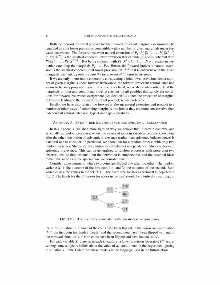
Consider an experiment, where two coins are flipped one after the other. The randomvariable X1 is the outcome of the first coin flip, and X2 the outcome of the second. Bothvariables assume values in the set {h, t}. The event tree for this experiment is depicted inFig. 2. The labels for the situations (or nodes in the tree) should be intuitively clear: e.g., in

?,?

t,?t, t

t,h

h,?h, t

h,h

FIGURE 2. The event tree associated with two successive coin tosses.

the initial situation ‘?,?’ none of the coins have been flipped, in the non-terminal situation‘h,?’ the first coin has landed ‘heads’ and the second coin hasn’t been flipped yet, and inthe terminal situation ‘t, t’ both coins have been flipped and have landed ‘tails’.

For each variable Xk there is, in each situation s, a lower prevision (operator) PXks repre-

senting some subject’s beliefs about the value of Xk conditional on the experiment gettingto situation s. Table 1 identifies these models in the language used in the Introduction.


PX1?,?( f ) PX1

h,?( f ) PX1t,?( f ) PX1

h,h( f ) PX1h,t( f ) PX1

t,h( f ) PX1t,t ( f )

P1( f ) f (h) f (t) f (h) f (h) f (t) f (t)

PX2?,?(g) PX2

h,?(g) PX2t,?(g) PX2

h,h(g) PX2h,t(g) PX2

t,h(g) PX2t,t (g)

P2(g) Q2(g|h) Q2(g|t) g(h) g(t) g(h) g(t)

TABLE 1. The conditional lower previsions PX1s and PX2

s . f is any gam-ble on the outcome of the first variable X1, and g any gamble on theoutcome of the second variable X2.

In Shafer’s (1996) language, (the experiment in a) situation s influences a variable X if shas at least one child situation c such that the subject’s model is changed if the experimentmoves from s to c: for our imprecise probability models this means that PX

s 6= PXc . Two

variables X and Y are then event-tree independent if there are no situations that influencethem both. Shafer proves in Section 8.1 of his book that for event trees with (precise)probabilistic models, event-tree independence implies the usual notion of independence asdiscussed in the Introduction.

Let us now investigate under what conditions the variables X1 and X2 will be event-treeindependent. It is obvious that the only situations that can influence these variables, arethe non-terminal situations, as these are the only ones with children. In Table 2, we usethe identifications of Table 1 to indicate if and when each of these situations influences X1and/or X2. It is clear from this table that X1 and X2 are event-tree independent if and onlyif Q2(·|X1) = P2, or in other words if X1 is epistemically irrelevant to X2.

?,? h,? t,?

X1 always never never

X2 if Q2(·|h) 6= P2 or Q2(·|t) 6= P2 always always

TABLE 2. When do the non-terminal situations influence the variablesX1 and X2?

APPENDIX B. PROOFS OF THEOREMS

B.1. Preliminaries. Let us begin by making a few preliminary remarks, and fixing a num-ber of notations. For 1≤ j ≤ N, let X N

j =×N`= jX`. For 1≤ j ≤ N−1, we call a gamble

f on X N X j-measurable if it is constant on the elements of {(x1, . . . ,x j)}×X Nj+1, for all

(x1, . . . ,x j) in X j.


We define the X j−1-support S j( f ) of a gamble f on X N , as the set of those subsets{(x1, . . . ,x j−1)}×X N

j of X N such that the gamble f is not identically zero on this set. Inparticular, S1( f ) = X N if f is not identically 0. If f happens to be X j-measurable, then

S j( f ) := {{(x1, . . . ,x j−1)}×X Nj : f (x1, . . . ,x j−1,x j) 6= 0 for some x j ∈X j}.

In what follows, we need to prove joint coherence of conditional lower previsions whosedomains are not necessarily linear spaces. Since Walley (1991, Section 8.1) has only givendefinitions of joint coherence for conditional lower previsions defined on linear spaces, wemust check the following, fairly straightforward, generalisation to non-linear domains ofWalley’s coherence condition. See Miranda and De Cooman (2005) for more details.

Consider a coherent lower prevision Q defined on a subset H 1 of L (X N), and sep-arately coherent conditional lower previsions Q(·|X1), . . . , Q(·|XN−1) defined on the re-spective subsets H 2, . . . , H N of L (X N). We may assume without loss of generalitythat these domains are cones (see the discussion in Section 3.2). Then these (conditional)lower previsions are called jointly coherent if for any g j

` in H `, j = 1, . . . ,n`, n` ≥ 0 and` = 1, . . . ,N and any k ∈ {1, . . . ,N} and g0 ∈H k, the following conditions are satisfied:

(JC1) If k = 1, we must have that

supx∈X N

[ n1

∑j=1

G(g j1)(x)+

N

∑`=2

n`

∑j=1

G(g j`|X

`−1)(x)−G(g0)(x)]≥ 0. (20)

(JC2) If k > 1, we must have that for any (y1, . . . ,yk−1) ∈X k−1, there is some B in

{{(y1, . . . ,yk−1)}×X Nk }∪

N⋃`=1

n⋃j=1

S`(gj`)

such that

supx∈B

[ n1

∑j=1

G(g j1)(x)+

N

∑`=2

n`

∑j=1

G(g j`|X

`−1)(x)−G(g0|y1, . . . ,yk−1)(x)]≥ 0. (21)

Here, for any x ∈X N , and g j` ∈H `,

G(g j`)(x) = g j

`(x)−Q(g j`) (22)

when ` = 1, and

G(g j`|X

`−1)(x) = g j`(x1, . . . ,x`)−Q(g j

`|(x1, . . . ,x`−1)) (23)

when ` > 1. The idea behind this condition is, as for (unconditional) coherence (seeSection 2), that we shouldn’t be able to raise the supremum acceptable buying price wehave given for a gamble f by considering the acceptable transactions implicit in othergambles in the domains. For instance, if condition (20) fails, then there is some δ > 0such that the gamble G( f0)− δ = f0− (Q( f0)+ δ ) dominates the acceptable transaction

∑n1j=1 G(g j

1)+ ∑N`=2 ∑

n`j=1 G(g j

`|X`−1)+ δ , meaning that Q( f0)+ δ must be an acceptable

buying price for f0.Using Eqs. (22) and (23), it is easy to see that conditions (20) and (21) are equivalent,

respectively, to

supx∈X N

[ n1

∑j=1

[g j1(x)−Q(g j

1)]+N

∑`=2

n`

∑j=1

[g j`(x)−Q(g j

`|x1, . . . ,x`−1)]− [g0(x)−Q(g0)]]≥ 0,


and

supx∈B

[ n1

∑j=1

[g j1(x)−Q(g j

1)]+N

∑`=2

n`

∑j=1

[g j`(x)−Q(g j

`|x1, . . . ,x`−1)]

− I{(y1,...,yk−1)}(x1, . . . ,xk−1)[g0(x)−Q(g0|y1, . . . ,yk−1)]]≥ 0.

B.2. Proof of Theorem 1. Theorem 1 is a consequence of the following three lemmas.

Lemma 12. The lower previsions P1, P(·|X1), . . . , P(·|XN) are jointly coherent.

Proof. We can prove independently (using the Marginal Extension Theorem, see Theo-rem 2) that P1, P(·|X1), . . . , P(·|XN) can be extended to jointly coherent (conditional)lower previsions on all of L (X N). This means that the restrictions P1, P(·|X1), . . . ,P(·|XN) to the respective domains K 1, . . . , K N of these jointly coherent (conditional)lower previsions, are of course jointly coherent as well. �

Lemma 13. The lower prevision EN is jointly coherent with the conditional lower previ-sions P(·|X1), . . . , P(·|XN−1).

Proof. We have to check that the immediate generalisation (see Section B.1) to non-lineardomains of Walley’s joint coherence requirements is satisfied. We use the fact that EN is acoherent lower prevision on the linear space L (X N), and that the domains K i are cones.Consider g1 ∈ L (X N) and g j

i ∈K i for i = 2, . . . ,N, j = 1, . . . ,ni. Let k ∈ {1, . . . ,N},g0 ∈K k and (y1, . . . ,yk−1) ∈X k−1. Assume first that k > 1, i.e., let us prove (JC2). Ifg1 = 0, then the result follows from the joint coherence of P(·|X1), . . . , P(·|XN−1).

Assume then that g1 6= 0. Then (JC2) is equivalent to

supx∈X N

[[g1(x)−EN(g1)]+

N

∑i=2

ni

∑j=1

G(g ji |X

i−1)(x)−G(g0|y1, . . . ,yk−1)(x)]≥ 0. (24)

From the definition of EN [see Eq. (14)] and the fact that all relevant domains are cones,we see that for any ε > 0, there are mi ≥ 0 and h j

i ∈K i for i = 1, . . . ,N and j = 1, . . . ,mi,such that

g1(x)−N

∑i=1

mi

∑j=1

G(h ji |X

i−1)(x)≥ EN(g1)− ε (25)

for all x ∈X N . Hence

supx∈X N

[[g1(x)−EN(g1)]+

N

∑i=2

ni

∑j=1

G(g ji |X

i−1)(x)−G(g0|y1, . . . ,yk−1)(x)]

≥ supx∈X N

[ N

∑i=1

mi

∑j=1

G(h ji |X

i−1)(x)+N

∑i=2

ni

∑j=1

G(g ji |X

i−1)(x)−G(g0|y1, . . . ,yk−1)(x)]− ε

≥−ε,

where the last inequality follows from the joint coherence of P1, P(·|X1), . . . , P(·|XN−1),by Lemma 12 [also see Eq. (21)]. Since this holds for any ε > 0, we deduce that Eq. (24)holds.

Next, we consider (JC1). Assume then that k = 1, i.e., g0 ∈L (X N). We show that

supx∈X N

[[g1(x)−EN(g1)]+

N

∑i=2

ni

∑j=1

G(g ji |X

i−1)(x)− [g0(x)−EN(g0)]]≥ 0. (26)


Assume ex absurdo that there is some δ > 0 such that this supremum is smaller than −δ .Then, using the approximation of EN(g1) given by Eq. (25) for ε = δ

2 , we deduce that

−δ > supx∈X N

[[g1(x)−EN(g1)]+

N

∑i=2

ni

∑j=1

G(g ji |X

i−1)(x)− [g0−EN(g0)]]

≥−δ

2+ sup

x∈X N

[ N

∑i=1

mi

∑j=1

G(h ji |X

i−1)(x)+N

∑i=2

ni

∑j=1

G(g ji |X

i−1)(x)− [g0(x)−EN(g0)]],

whence

infx∈X N

[g0(x)−

N

∑i=1

mi

∑j=1

G(h ji |X

i−1)(x)−N

∑i=2

ni

∑j=1

G(g ji |X

i−1)(x)]

> EN(g0)+δ

2,

and this contradicts the definition of EN(g0). Hence, Eq. (26) holds and we conclude thatthe (conditional) lower previsions EN , P(·|X1), . . . , P(·|XN−1) are jointly coherent. �

Lemma 14. EN is an extension of the lower prevision P1 to L (X N), i.e., EN( f ) = P1( f )for all f in K 1.

Proof. Consider f ∈K 1. From (15) we deduce that EN( f )≥ infx∈X N [ f (x)−G1( f )(x)] =P1( f ). Assume ex absurdo that EN( f ) > P1( f ). Then there are gambles g j

i ∈ Ki fori = 1, . . . ,N and j = 1, . . . ,ni, such that infx∈X N [ f (x)−∑

Ni=1 ∑

nij=1 G(g j

i |X i−1)(x)] > P1( f ).

But this means that supx∈X N [∑Ni=1 ∑

nij=1 G(g j

i |X i−1)(x)− [ f (x)−P1( f )]] < 0, and this con-tradicts the joint coherence of P1, P(·|X1), . . . , P(·|XN−1), which we have proved inLemma 12 [also see Eqs. (20) and (21)]. Consequently, EN( f ) = P1( f ). �

Proof of Theorem 1. Taking into account the previous lemmas, it only remains to provethat EN is the point-wise smallest coherent extension of P1 to L (X N) that is coherentwith P(·|X1), . . . , P(·|XN−1). Let therefore F be another coherent extension of P1 toL (X N) that is moreover jointly coherent with the conditional lower previsions P(·|X1),. . . , P(·|XN−1), and consider any f ∈L (X N). Then, for any ε > 0, the expression (14)for EN( f ) implies that there are h j

i ∈K i for i = 1, . . . ,N and j = 1, . . . ,ni such that

supx∈X N

[ N

∑i=1

ni

∑j=1

G(h ji |X

i−1)(x)− f (x)]≤−EN( f )+ ε.

On the other hand, the coherence of F , P(·|X1), . . . , P(·|XN−1) implies that

supx∈X N

[ N

∑i=1

ni

∑j=1

G(h ji |X

i−1)(x)− [ f (x)−F( f )]]≥ 0,

whence

−F( f )≤ supx∈X N

[ N

∑i=1

ni

∑j=1

G(h ji |X

i−1)(x)− f (x)]≤−EN( f )+ ε.

Therefore, F( f )≥ EN( f )− ε for any ε > 0, so F dominates EN on L (X N). �


B.3. Proof of Theorem 4. From Theorem 3 we infer that EN ≤MN , so we only need toprove the converse inequality. Note first of all that if Kk = L (Xk), then the domain K k

of P(·|Xk−1) is L (X k), for k = 1, . . . ,N.Consider any gamble f on X N , and recursively define fN := f , fN−1 := PN( fN), . . . ,

fk := Pk+1( fk+1), . . . , f1 := P2( f2). Then clearly fk belongs to L (X k), and P1( f1) =MN( f ), P( f2|X1) = P2( f2) = f1, . . . , P( fk|Xk−1) = Pk( fk) = fk−1, . . . , P( fN |XN−1) =PN( fN) = fN−1. Hence

f −N

∑k=1

G( fk|Xk−1) = f − [ f1−MN( f )]−N−1

∑k=2

[ fk− fk−1]− [ f − fN−1] = MN( f ).

We therefore deduce from Eq. (14) that indeed EN( f )≥MN( f ).

B.4. Proof of Proposition 9. First of all, we can assume without loss of generality thatfN is non-negative: otherwise, it suffices to take gN = fN − inf fN , which is non-negativeand satisfies gN−EN(gN) = fN−EN( fN).

From Proposition 8, we infer that

MN( f1 . . . fN) = EN( f1 . . . fN) = E1( f1) . . .EN( fN)

= MN( f1 . . . fN−1EN( fN)) = EN( f1 . . . fN−1EN( fN)),

taking into account that EN( fN) ≥ 0 because we are assuming fN to be non-negative, andthe non-negative homogeneity of a coherent lower prevision. Using the super-additivity[due to coherence] of MN and EN , we deduce that

MN( f1 . . . fN−1[ fN−EN( fN)])≤MN( f1 . . . fN)−MN( f1 . . . fN−1EN( fN)) = 0

EN( f1 . . . fN−1[ fN−EN( fN)])≤ EN( f1 . . . fN)−EN( f1 . . . fN−1EN( fN)) = 0.

We are now going to show that, conversely, EN( f1 . . . fN−1[ fN −EN( fN)]) ≥ 0. This willcomplete the proof, since we know that MN dominates EN , and it will therefore also followthat MN( f1 . . . fN−1[ fN −EN( fN)]) ≥ 0. So, fix ε > 0, then it follows from Eq. (12) thatthere are nN ≥ 0 and gambles g j

N in K ∗N for j = 1, . . . ,nN such that

infxN∈XN

[fN(xN)−

nN

∑j=1

[g jN(xN)−PN(g j

N)]]≥ EN( fN)− ε. (27)

Define the gambles h jN on X N by h j

N := f1 . . . fN−1g jN . All these gambles clearly belong to

K N , so, using Eq. (15), we get that EN( f1 . . . fN−1[ fN −EN( fN)]) is greater than or equalto

supgkik∈K k,ik=1,...,nk

nk≥0,k=1,...,N−1

infx∈X N

[f1 . . . fN−1[ fN−EN( fN)](x)

−N−1

∑k=1

nk

∑ik=1

[gkik(x1, . . . ,xk)−Pk(gkik(x1, . . . ,xk−1, ·))]

−nN

∑j=1

[h jN(x1, . . . ,xN)−PN(h j

N(x1, . . . ,xN−1, ·))]]


and after some manipulations, using the coherence of PN and the fact that all the fk arenon-negative, this can be rewritten as

supgkik∈K k,ik=1,...,nk

nk≥0,k=1,...,N−1

infx∈X N−1

[−

N−1

∑k=1

nk

∑ik=1

[gkik(x1, . . . ,xk)−Pk(gkik(x1, . . . ,xk−1, ·))]

+ f1(x1) . . . fN−1(xN−1) infxN∈XN

[fN(xN)−EN( fN)−

nN

∑j=1

[g jN(xN)−PN(gN j)]

]]Now if we use the inequality (27), we see that this is greater than or equal to

EN( f1 . . . fN−1[−ε]) =−εEN( f1 . . . fN−1)≥−ε sup f1 . . .sup fN−1,

where the last inequality is a consequence of coherence and the non-negativity of the fk.Since this holds for any ε > 0, we deduce that indeed EN( f1 . . . fN−1[ fN−EN( fN)])≥ 0.

B.5. Proof of Proposition 10. The proof of the inequality EN(g[ fN −EN( fN)]) ≥ 0 iscompletely analogous to that in Proposition 9, with g taking the role of f1 . . . fN−1. Wededuce from this that MN(g[ fN−EN( fN)])≥ EN(g[ fN−EN( fN)])≥ 0.

Conversely, we get from Theorem 5 that MN(g fN) = MN(g)MN( fN) = MN−1(g)EN( fN)for any non-negative gamble g on X N−1 and any fN ∈L (XN). By the super-additivity[coherence] of MN we get MN(g[ fN −EN( fN)]) ≤MN(g fN)−MN(gEN( fN)) ≤ 0, and asa consequence MN(g( fN−EN( fN))) = EN(g( fN−EN( fN))) = 0.

B.6. Proof of Eq. (18). Assume that for each Xk, we have a coherent lower previsionPk defined on a finite subset Kk = { f 1

k , . . . , f mkk } of L (Xk). We may assume without

loss of generality that the Kk contain no constant gambles. Then, for any gkhk ∈ K k

and (x1, . . . ,xk−1) ∈X k−1, the gamble gkhk(x1, . . . ,xk−1, ·) belongs by definition to K ∗k ,

and consequently there are non-negative λ(x1,...,xk−1)khk, real µ(x1,...,xk−1)khk

and gamblesg(x1,...,xk−1)khk

in Kk such that

gkhk(x1, . . . ,xk−1, ·) = λ(x1,...,xk−1)khkg(x1,...,xk−1)khk

+ µ(x1,...,xk−1)khk.

Hence

gkhk(x1, . . . ,xk−1, ·)−Pk(gkhk |x1, . . . ,xk−1)

= λ(x1,...,xk−1)khkg(x1,...,xk−1)khk

+ µ(x1,...,xk−1)khk

− [λ(x1,...,xk−1)khkPk(g(x1,...,xk−1)khk

)+ µ(x1,...,xk−1)khk]

= λ(x1,...,xk−1)khk[g(x1,...,xk−1)khk

−Pk(g(x1,...,xk−1)khk)].

Define the gamble λj

khkon X k−1 by

λj

khk(x1, . . . ,xk−1) =

{λ(x1,...,xk−1)khk

if g(x1,...,xk−1)khk= f j

k

0 otherwise,

for all (x1, . . . ,xk−1) in X k−1, j = 1, . . . ,mk. Let us show that λj

khkis indeed a gam-

ble, i.e., that it is bounded. Since f jk is not a constant gamble by assumption, there

are x1k and x2

k in Xk such that f jk (x1

k)− f jk (x2

k) > 0. Now, if λj

khk(x1, . . . ,xk−1) were not


bounded, there would exist, for any natural number M, some (x1, . . . ,xk−1) in X k−1 suchthat λ

jkhk

(x1, . . . ,xk−1) > M. But then

gkhk(x1, . . . ,xk−1,x1k)−gkhk(x1, . . . ,xk−1,x2

k)

= λj

khk(x1, . . . ,xk−1)( f j

k (x1k)− f j

k (x2k)) > M( f j

k (x1k)− f j

k (x2k)),

and this would imply that gkhk isn’t bounded, a contradiction. Now,

gkhk(x1, . . . ,xk)−Pk(gkhk |(x1, . . . ,xk−1)) =mk

∑j=1

λj

khk(x1, . . . ,xk−1)( f j

k (xk)−Pk( f jk )),

whencenk

∑hk=1

[gkhk(x1, . . . ,xk)−Pk(gkhk |(x1, . . . ,xk−1))]

=mk

∑j=1

[ f jk (xk)−Pk( f j

k )]nk

∑hk=1

λj

khk(x1, . . . ,xk−1)

and consequently

EN( f ) = supgkhk∈K k

hk=1,...,nk,k=1,...,N

infx∈X N

[f (x)−

N

∑k=1

nk

∑hk=1

G(gkhk |Xk−1)

]

≤ supλ

jkk ∈L

+(X k−1)jk=1,...,mk,k=1,...,N

infx∈X N

[f (x)−

N

∑k=1

mk

∑j=1

λjk

k (x1, . . . ,xk−1)[ f jk (xk)−Pk( f j

k )]].

The converse inequality follows taking into account that for any λjk

k in L +(X k−1), thegamble gk jk in X k given by gk jk = λ

jkk f j

k belongs to K k. This shows that we can indeedcalculate the forward irrelevant natural extension EN using Eq. (18).

ACKNOWLEDGEMENTS

We would like to thank the reviewers for their many comments, which were quite help-ful in making this paper clearer, shorter and more readable.

REFERENCES

K. P. S. Bhaskara Rao and M. Bhaskara Rao. Theory of Charges. Academic Press, London,1983.

G. Choquet. Theory of capacities. Annales de l’Institut Fourier, 5:131–295, 1953–1954.I. Couso, S. Moral, and P. Walley. Examples of independence for imprecise probabilities.

Risk Decision and Policy, 5:165–181, 2000.G. de Cooman. Integration and conditioning in numerical possibility theory. Annals of

Mathematics and Artificial Intelligence, 32:87–123, 2001.G. de Cooman and D. Aeyels. Supremum preserving upper probabilities. Information

Sciences, 118:173–212, 1999.G. de Cooman and D. Aeyels. A random set description of a possibility measure and

its natural extension. IEEE Transactions on Systems, Man and Cybernetics—Part A:Systems and Humans, 30:124–130, 2000.


G. de Cooman and E. Miranda. Laws of large numbers for coherent lower previsions.Journal of Statistical Planning and Inference, 2006. Submitted for publication.

G. de Cooman and M. C. M. Troffaes. Coherent lower previsions in systems modelling:products and aggregation rules. Reliability Engineering and System Safety, 85:113–134,2004.

B. de Finetti. Teoria delle Probabilita. Einaudi, Turin, 1970.B. de Finetti. Theory of Probability. John Wiley & Sons, Chichester, 1974–1975. English

translation of de Finetti (1970), two volumes.D. Denneberg. Non-Additive Measure and Integral. Kluwer Academic, Dordrecht, 1994.D. Dubois and H. Prade. Possibility Theory. Plenum Press, New York, 1988.S. Ferson, V. Kreinovich, L. Ginzburg, D. S. Myers, and K. Sentz. Constructing probabil-

ity boxes and Dempster-Shafer structures. Technical Report SAND2002–4015, SandiaNational Laboratories, January 2003.

E. Miranda and G. de Cooman. Coherence and independence in non-linearspaces. Technical report, Rey Juan Carlos University, TR05/10, May 2005.http://bayes.escet.urjc.es/publicaciones/wp05-10.pdf.

E. Miranda and G. de Cooman. Marginal extension in the theory of coherent lower previ-sions. International Journal of Approximate Reasoning, 46:(1), 188–225, 2007.

G. Shafer. Conditional probability. International Statistical Review, 53:261–277, 1985.G. Shafer. The Art of Causal Conjecture. The MIT Press, Cambridge, MA, 1996.G. Shafer and V. Vovk. Probability and Finance: It’s Only a Game. Wiley, New York,

2001.G. Shafer, P. R. Gillett, and R. B. Scherl. A new understanding of subjective probability and

its generalization to lower and upper prevision. International Journal of ApproximateReasoning, 33:1–49, 2003.

P. Walley. Statistical Reasoning with Imprecise Probabilities. Chapman and Hall, London,1991.

P. M. Williams. Notes on conditional previsions. Technical report, School of Mathematicaland Physical Science, University of Sussex, UK, 1975.

GHENT UNIVERSITY, SYSTEMS RESEARCH GROUP, TECHNOLOGIEPARK – ZWIJNAARDE 914, 9052ZWIJNAARDE, BELGIUM

E-mail address: [email protected]

REY JUAN CARLOS UNIVERSITY, DEPT. OF STATISTICS AND OPERATIONS RESEARCH – C-TULIPAN,S/N, 28933 MOSTOLES, SPAIN

E-mail address: [email protected]

Documents

Forward irrelevance