Embed Size (px)
Citation preview

Florida State University Libraries
Electronic Theses, Treatises and Dissertations The Graduate School
2010
Elastic Property Prediction and VariationQuantification for Buckypaper-PolymerNanocomposites: Modeling andExperimental ValidationChao-hsi Tsai
Follow this and additional works at the FSU Digital Library. For more information, please contact [email protected]

THE FLORIDA STATE UNIVERSITY
COLLEGE OF ENGINEERING
ELASTIC PROPERTY PREDICTION AND VARIATION QUANTIFICATION
FOR BUCKYPAPER-POLYMER NANOCOMPOSITES: MODELING AND
EXPERIMENTAL VALIDATION
By
CHAO-HSI TSAI
A Dissertation submitted to the Department of Industrial and Manufacturing Engineering
in partial fulfillment of the requirements for the degree of
Doctor of Philosophy
Degree Awarded: Summer Semester, 2010

ii
The members of the committee approve the dissertation of Chao-hsi Tsai defended on May 17th,
2010. __________________________________ Chuck Zhang Professor Directing Dissertation
__________________________________ William Oates University Representative
__________________________________ Ben Wang Committee Member
__________________________________
O. Arda Vanli Committee Member
Approved: _____________________________________ Chuck Zhang, Chair, Department of Industrial and Manufacturing Engineering
_____________________________________ Ching-Jen Chen, Dean, FAMU-FSU College of Engineering The Graduate School has verified and approved the above-named committee members.

iii
ACKNOWLEDGEMENTS
I would like to express my sincere gratitude and thanks to Dr. Chuck Zhang for his
extensive support throughout the program and his guidance as both advisor and friend. I would
also like to thank my committee members, Dr. Ben Wang, Dr. Arda Vanli and Dr. William Oates
for their suggestions and assistance during the preparation of this dissertation. A sincere
appreciation goes to all the PI‟s and co-workers at the High Performance Materials Institute
(HPMI) especially Dr. Richard Liang, Dr. David Cheng, Dr. Peter Chen, Dr. Qian Wu, Dr. Jin
Gyu Park and Frank Allen for their help and meaningful contribution to this dissertation. Deep
appreciation also goes to Chia-jung Chang and Dr. Jianjun Shi at Georgia Institute of
Technology for their help on multi-resolution project, as well as to Dr. David Jack at Baylor
University for his help on constructing micromechanical models. Finally, I would like to thank
my parents, my wife and children, my brother and my sister in law for their encouragement and
support throughout my life and education.

iv
TABLE OF CONTENTS
LIST OF TABLES .................................................................................................................................. viii
LIST OF FIGURES ................................................................................................................................... x
ABSTRACT ............................................................................................................................................. xiv
CHAPTER 1 INTRODUCTION ............................................................................................................ 1
1.1 Background .................................................................................................................................... 1
1.2 Problem Statement ........................................................................................................................ 1
1.3 Objectives ....................................................................................................................................... 4
1.4 Research Scope and Limitations ................................................................................................. 6
CHAPTER 2 LITERATURE REVIEW ................................................................................................ 7
2.1 Carbon Nanotubes and Carbon Nanotube Buckypapers .......................................................... 7
2.1.1 Mechanical properties of carbon nanotubes and carbon nanotube ropes ....................... 7
2.1.2 Carbon nanotube buckypaper ............................................................................................... 9
2.2 Buckypaper Nanostructure ......................................................................................................... 10
2.2.1 Characterization of nanotube bundle diameter ................................................................ 10
2.2.2 Characterization of nanotube bundle length ..................................................................... 12
2.2.3 Characterization of nanotube bundle orientation ............................................................. 14
2.2.4 Characterization of nanotube bundle curvature ............................................................... 15
2.3 Modeling Techniques for CNT-Reinforced Composites Stiffness ....................................... 17
2.3.1 Molecular models ................................................................................................................ 17
2.3.2 Micromechanical models for composites with unidirectional inclusions .................... 18
2.3.3 Modeling for effective composite stiffness with mis-aligned inclusions ..................... 23
2.3.4 Modeling for effective composite stiffness with wavy inclusions ................................ 25
2.3.5 Stiffness prediction using classical laminate theory ....................................................... 27
2.3.6 Reviews of application of micromechanics to CNT-reinforced composites ............... 30
2.3.7 Statistical analysis of composite properties...................................................................... 31
2.4 Interfacial Bonding of Carbon Nanotube/Polymer Composites ............................................ 32
2.4.1 Theoretical modeling techniques for CNT/polymer interface ....................................... 32
2.4.2 Experimental Investigations on CNT/polymer interface ................................................ 33
2.5 Modeling and Analysis of Computer Experiments ................................................................. 34

v
2.5.1 Design of computer experiments ....................................................................................... 35
2.5.2 Metamoding techniques for computer model .................................................................. 36
2.5.3 Computer model interpretation .......................................................................................... 39
2.6 Statistical Adjustment for Engineering Models ...................................................................... 43
CHAPTER 3 STOCHASTIC MODELING OF BUCKYPAPER-POLYEMR COMPOSITE ELASTIC PROPERTIES ........................................................................................................................ 47
3.1 Nanotube Bundle Nanostructure Characterization for SWNT-Buckypapers ...................... 47
3.1.1 Nanotube bundle orientation representation and characterization ................................ 48
3.1.2 Nanotube bundle waviness representation and characterization ................................... 51
3.2 Stiffness Prediction of BPP Composite Laminate with Straight Nanotube Bundles ......... 53
3.2.1 Stochastic simulation procedure ........................................................................................ 53
3.2.2 Monte-Carlo simulation results .......................................................................................... 57
3.3 Stiffness Prediction of BPP Composite Laminate with Wavy Nanotube Bundles ............. 63
3.3.1 Simulation procedure .......................................................................................................... 63
3.3.2 Simulation results of BPP composite laminate with measured bundle waviness distribution ........................................................................................................................................ 64
3.3.3 Simulation results of single BPP composite lamina with assumed bundle waviness distribution ........................................................................................................................................ 65
3.3.4 Experimental results comparison using assumed bundle waviness distribution ......... 66
3.4 Simulation Results for Multi-Layered BPP Composite Laminate with Assumed Waviness and Ply Thickness Distribution .......................................................................................................... 68
3.5 Summary ....................................................................................................................................... 69
CHAPTER 4 DISTRIBUTION EFFECTS OF STRUCTURAL PARAMETERS ON COMPOSITE ELASTIC PROPERTIES .............................................................................................. 70
4.1 Microstructure Distribution and Modeling .............................................................................. 71
4.1.1 Fiber orientation distribution function .............................................................................. 71
4.1.2 Fiber aspect ratio and waviness distribution .................................................................... 72
4.1.3 Microstructure distribution modeling ............................................................................... 74
4.2 Effects of Composite Microstructure Distribution .................................................................. 75
4.2.1 Effect of orientation distribution of fibers with constant aspect ratio and waviness .. 76
4.2.2 Effect of inclusion aspect ratio distribution with uniform fiber waviness ................... 79
4.2.3 Effect of Fiber Waviness Distribution with Constant Fiber Aspect Ratio ................... 80
4.2.4 Inclusion waviness effect on carbon nanotube-reinforced composites ........................ 83
4.3 Summary ....................................................................................................................................... 84

vi
CHAPTER 5 DEGREE OF NANOSTRUCTURE EFFECTS AND INTERACTIONS ON THE ELASTIC PORPERTIES OF BPP COMPOSITES ............................................................................ 86
5.1 Buckypaper Alignment and Nanotube Bundle Orientation Distribution ............................. 86
5.2 Polynomial Metamodeling of Micromechanics ...................................................................... 88
5.2.1 Single-walled buckypaper-polymer composite stiffness prediction model ................. 88
5.2.2 Factorial experiments .......................................................................................................... 89
5.2.3 Results for factorial design ................................................................................................. 90
5.2.4 Response surface method (RSM) design .......................................................................... 91
5.2.5 Results for Central Composite Design .............................................................................. 92
5.2.6 Polynomial modeling summary ......................................................................................... 96
5.3 Sensitivity Analysis of Buckypaper-Polymer Composite Nanostructures .......................... 97
5.3.1 Kriging based surrogate model .......................................................................................... 98
5.3.2 Sensitivity analysis results ................................................................................................ 100
5.4 Summary ..................................................................................................................................... 102
CHAPTER 6 VARIATION QUANTIFICATION AND PROPOGATION OF BUCKYPAPER-POLYMER COMPOSITES ................................................................................... 103
6.1 Analysis of Intra/Inter Buckypaper Variation ....................................................................... 104
6.1.1 Characterization of intra-buckypaper variation ............................................................. 104
6.1.2 Characterization of inter-buckypaper variation ............................................................. 106
6.2 Quantification of mean buckypaper nanostructure distribution .......................................... 107
6.3 Buckypaper-Polymer Composite Property Distribution After Variation Propagation .... 110
6.3.1 Modeling technique ........................................................................................................... 110
6.3.2 Simulation results .............................................................................................................. 111
6.4 Summary ..................................................................................................................................... 113
CHAPTER 7 EXPERIMENTAL VALIDATION AND MULTI-RESOLUTION DATA INTEGRATION ..................................................................................................................................... 114
7.1 Experimental Validation ........................................................................................................... 114
7.1.1 SWNTBP-epoxy composites ............................................................................................ 114
7.1.2 MWNT-BMI composites .................................................................................................. 116
7.2 Adjusting Micromechanical Models Using Physical Observations ................................... 121
7.2.1 Surrogate model for SWNT-epoxy nanocomposite tensile modulus.......................... 122
7.2.2 Surrogate model for MWNT-BMI nanocomposite tensile modulus .......................... 124
7.2.3 Updated experimental data for MWNT-BMI nanocomposites ................................... 126

vii
7.3 Summary ..................................................................................................................................... 128
CHAPTER 8 CONCLUSIONS AND SUGGESTED FUTURE WORKS ................................... 130
8.1 Conclusions ................................................................................................................................ 130
8.2 Suggested Future Works ........................................................................................................... 132
APPENDIX ............................................................................................................................................. 137
REFERENCE ......................................................................................................................................... 139
BIOGRAPHICAL SKETCH ................................................................................................................ 149

viii
LIST OF TABLES
Table 2.1 Halpin-Tsai parameters for short-fiber composites ...................................................... 22 Table 2.2 Love-Kirchhoff assumptions ........................................................................................ 27 Table 2.3 Perfect Bonding assumptions........................................................................................ 27 Table 3.1 Simulation results summary for single BPP composite lamina .................................... 58 Table 3.2 Simulation Results Summary for 16-Layered BPP Composite Laminate .................... 61 Table 3.3 Experimental data comparison ...................................................................................... 62 Table 3.4 Simulation results summary for single BPP composite lamina .................................... 66 Table 3.5 Experimental data comparison ...................................................................................... 67 Table 3.6 Simulation Results Summary for 16-Layered BPP Composite Laminate .................... 69 Table 5.1 High/low values for buckypaper nanosturctures .......................................................... 90 Table 5.2 Central Composite Design levels for the five nanostructure parameters...................... 93 Table 5.3 ANOVA tables for CCD after data transformation (a) E11 (b) E22 ............................... 94 Table 5.4 ANOVA tables for CCD after data transformation (a) G12 (b) 12 ............................... 95 Table 5.5 CCD approximated models summary (in coded unit) .................................................. 96 Table 5.6 Variable range for Latin Hypercube Design ................................................................. 98 Table 5.7 Kriging model result summary ..................................................................................... 99 Table 5.8 Sensitivity indices for first-order interaction terms .................................................... 102 Table 6.1 Nanotube bundle diameter measurement summary .................................................... 105 Table 6.β Levene‟s test result summary ..................................................................................... 105 Table 6.3 ANOVA results for intra-buckypaper diameter variation .......................................... 106 Table 6.4 ANOVA result for inter-buckypaper diameter variation ............................................ 107

ix
Table 6.5 Bundle diameter measurement of the five buckypapers ............................................. 108 Table 6.6 Simulation results for SWNT BP-epoxy composites ................................................. 112 Table 7.1 SWNTBP-epoxy composite sample nanostructure characterization results ............... 115 Table 7.2 MWNT-BMI composite sample nanostructure characterization results .................... 121 Table 7.3 Model Inadequacy and predictive improvement for SWNTBP-epoxy composites ... 123 Table 7.4 Summary for different modeling strategy ................................................................... 126 Table 8.1 Buckypaper-polymer composites: volume fraction, pristine buckypaper moduli, and resultant composite E11 ............................................................................................................... 134

x
LIST OF FIGURES
Figure 1.1 Sources of uncertainties of BPP composites …………………………………………..2 Figure 1.2 Source of uncertainties for BPP composite stiffness ..................................................... 4 Figure 2.1 Mechanical properties of SWNT bundles ..................................................................... 8 Figure 2.2 Measured reduced modulus, Er , for ten different SWNT ropes with diameters between 3 and 20 nm .................................................................................................................... 9 Figure 2.3 Multi-walled nanotube diameter measurement (a) TEM micrograph of a multi-walled carbon nanotube with measurements of outside diameter, inside diameter and wall thickness indicated (b) Histogram for the diameter distribution of carbon nanotubes ................................. 11 Figure 2.4 Weibull fit of nanotube bundle diameter (rope size) distribution ............................... 12 Figure 2.5 Measurement of SWNTs and rope length: (a) tapping mode amplitude AFM image (b) post-processed image for identifying SWNTs and bundles .......................................................... 12 Figure 2.6 Histogram of dispersed SWNT length ........................................................................ 13 Figure 2.7 Weibull fit for nanotube bundle length distribution .................................................... 13 Figure 2.8 Incident and scattered intensities on the SWNT and related angles in the polymer and laboratory frames .......................................................................................................................... 14 Figure 2.9 Normalized intensity of nanotube orientation within buckypapers ............................. 15 Figure 2.10 Illustration of lamina with fiber waviness ................................................................. 16 Figure 2.11 Illustrative example of evaluating nanotube waviness .............................................. 16 Figure 2.12 Coordinate system defining the fiber orientation in 3-D space ................................. 24 Figure 2.13 Representative volume and coordinates for a unidirectional composite with uniform waviness ...................................................................................................................................... 25 Figure 2.14 Geometry of an n-layered laminate ......................................................................... 28 Figure 2.15 Two LHSs with eight runs ....................................................................................... 36 Figure 2.16 Building strategy of the two-stage sequential modeling ........................................... 45

xi
Figure 3.1 Coordinate system defining the fiber orientation in 2-D space ................................... 48 Figure 3.2 SIMAGIS processed SEM image ................................................................................ 49 Figure 3.3 (a) Histogram of nanotube bundle orientation (b) Histogram with fitted Fourier series fittings ........................................................................................................................................... 50 Figure 3.4 (a) SEM image of buckypaper surface (b) Converted monochrome of SEM Image .. 51 Figure 3.5 Nano-bundle waviness identification and measurement ............................................. 52 Figure 3.6 (a) Waviness distribution fitted by 3-parameter lognormal distribution (b) Normal plot of waviness distribution fitted with 3-parameter lognormal distribution ..................................... 52 Figure 3.7 Stochastic modeling procedure.................................................................................... 54 Figure 3.8 Axial tensile modulus for SWNT bundles with respect to bundle diameter ............... 56 Figure 3.9 (a) Image of 16-layered SWNTBP-epoxy composite cross-section (resolution X500) (b) Simulation scheme for multi-layered buckypaper/epoxy composite laminate ....................... 59 Figure 3.10 Pure epoxy layer thickness effect plots (a) tensile moduli Ex and Ey (b) shear modulus Gxy (c) Poisson ratio xy .................................................................................................. 61 Figure 3.11 Modified simulation procedure ................................................................................. 63 Figure 3.12 Theoretical results and experimental data comparison ............................................. 64 Figure 3.13 Waviness factor effect plot ........................................................................................ 65 Figure 4.1 Planar orientation distribution function with different fiber alignment ...................... 72 Figure 4.2 Three dimensional orientation distribution function (a) m=0, n=0 (b) m=1, n=1 ....... 72 Figure 4.3 Illustration of fiber aspect ratio distribution with ar = 15 and ar = 5 ........................ 74 Figure 4.4 Illustration of Stochastic Composite Stiffness Prediction Methodology .................... 75 Figure 4.5 Fiber orientation distribution effects on composite stiffness (a) E11 (b) E22 ............... 77 Figure 4.6 Fiber orientation distribution effects on composite stiffness (a) G12 (b) v12 ............... 77 Figure 4.7 Fiber orientation distribution effects on composite stiffness (a) E11 (b) E22 ............... 78 Figure 4.8 Fiber orientation distribution effects on composite stiffness (a) G12 (b) v12 ............... 79

xii
Figure 4.9 Fiber aspect ratio distribution effects on composite stiffness (a) E11 (b) E22 .............. 80 Figure 4.10 Fiber aspect ratio distribution effects on composite stiffness (a) G12 (b) v12 ............ 80 Figure 4.11 Fiber waviness distribution effects on composite stiffness (a) E11 (b) E22 ................ 81 Figure 4.12 Fiber waviness distribution effects on composite stiffness (a) G12 (b) v12 ................ 82 Figure 4.13 Fiber waviness distribution effects on composite stiffness with different volume fraction (a) E11 (b) E22 ................................................................................................................... 82 Figure 4.14 Fiber waviness distribution effects on composite stiffness with different volume fraction (a) G12 (b) v12 ................................................................................................................... 83 Figure 4.15 Experimental data and simulation results comparison .............................................. 84 Figure 5.1 CNT orientation distribution functions ....................................................................... 87 Figure 5.2 Half-normal plot of axial tensile modulus (a) E11 (b) E22 ........................................... 90 Figure 5.3 Half-normal plot of shear modulus (a) G12 (b) 12 ...................................................... 91 Figure 5.4 Illustration of Central Composite Design .................................................................... 92 Figure 5.5 Significant interaction plots for E11 (a) diameter v.s. waviness (b) waviness v.s. volume fraction ............................................................................................................................. 95 Figure 5.6 Micromechanical predictions versus Kriging predictions ......................................... 100 Figure 5.7 Global sensitivity indices and total sensitivity indices .............................................. 101 Figure 6.1 Source of uncertainties for BPP composite stiffness ................................................. 107 Figure 6.2 Nanotube bundle waviness characterization ............................................................. 110 Figure 6.3 Simulated BP-epoxy composite elastic constants (Vf = 40%) ................................... 112 Figure 7.1 Scanning Electron Microscopic (SEM) image of MWNT-sheet surface .................. 117 Figure 7.2 (a) Relation between SWNT bundle diameter and its corresponding modulus (b) converted relation between number of tubes in each bundle and the corresponding bundle modulus ..................................................................................................................................... 118 Figure 7.3 (a) Schematic illustration of mechanical stretching to align nanotubes in the as-received random MWNT sheet (b) Effect of stretch ratio on degree of alignment.. ............. 119

xiii
Figure 7.4 Orientation distribution functions for different MWNT alignment .......................... 120 Figure 7.5 Performance comparison plot with physical experiments, micromechanics simulation model and adjusted surrogate model for SWNTBP-epoxy nanocomposites .............................. 123 Figure 7.6 Performance comparison plot with micromechanics simulation model and adjusted surrogate model ........................................................................................................................... 125 Figure 7.7 Young‟s modulus comparison for pristine MWNT-BMI composites, f-MWNT-BMI composites, and corresponding micromechanical predictions .................................................... 127 Figure 8.1 Scatter plot of neat buckypaper moduli and composite E11 ...................................... 135

xiv
ABSTRACT
A practical method to utilize carbon nanotubes (CNTs) in structural applications is to
fabricate them into buckypapers (BPs), a thin film containing two-dimensional CNT networks,
and combine them with a polymer matrix to make BP-polymer (BPP) composites. It has been
demonstrated that BPP composites have very good mechanical properties with multi-functional
capabilities. However, due to the uncertainties involved in different manufacturing stages, the
resulting BPP composites exhibit larger property variations when compared with traditional
metal or ceramic materials. As such, there is need for an improved modeling strategy that can
provide rapid property predictions and variation quantifications for BPP composites through
measurable buckypaper nanostructures and processing conditions. Due to high material costs and
long production cycle times, it is nearly impossible to construct a statistical-based model for BPP
composites purely from physical experiments. Theoretical (micromechanical) models are more
cost effective, but they also have some drawbacks. Namely, they are computationally intensive,
deterministic in nature, and have questionable accuracy due to underlying simplified assumptions.
Different sources of variations in BPP composite manufacturing also build on the inadequacy of
these micromechanical models for providing reasonable predictions without further adjustments.
Therefore, the main objective of this study is to provide a better modeling strategy for the
prediction of BPP composite stiffness. By integrating a series of statistical methods with
traditional micromechanical models, the variations observed in different stages were quantified,
and a better predictive surrogate modeling strategy was constructed as a result. The statistical
dispersions of buckypaper nanostructures (nanotube bundle length, diameter, orientation and
waviness) were first analyzed and characterized by applying image analysis to microscopic
images of buckypaper surface. It was found that the distribution of bundle length and diameter
can be reasonably described by a two-parameter Weibull distribution, and the orientation of
nanotubes can be represented by a periodic Fourier series. A stochastic based model was then
constructed to predict the theoretical dispersions of BPP composite stiffness through
experimentally measured nanostructure distributions by combining micromechanics with a
Monte-Carlo simulation. It was found that the distribution of BP nanostructures would bias the
resultant BPP composite modulus if a non-symmetric nanostructure distribution was present. The
degree of nanostructure effects and interactions was analyzed using polynomial modeling and

xv
sensitivity analysis. The diameter and waviness of nanotube bundles were found to be the most
influential factors for BPP composite modulus in most cases. The intra/inter buckypaper
variations were studied using an Analysis of Variance (ANOVA) test. Both variations were
tested as insignificant and can thus be statistically combined using the “mean nanostructure
distribution” with pooled mean and variance. Lastly, two different sets of BPP composite
experiments were used to validate the predictive capability of the constructed model. Preliminary
results exhibited a noticeable discrepancy between theoretical predictions and physical
observations due to the imperfections of the CNT-polymer interface. Therefore, statistical
two-stage sequential modeling was applied to calibrate the original micromechanical model, and
the resultant surrogate model was demonstrated to possess improved predictive capabilities.
Recently functionalized BPP composite data also showed a very good correspondence to the
theoretical predictions after the CNT-polymer interface was improved.

1
CHAPTER 1
INTRODUCTION
1.1 Background
Ever since carbon nanotubes (CNTs) were first discovered by Dr. Sumio Iijima in 1991 [1],
many researchers have considered them to be the most promising next generation reinforcement
materials for usage in high performance composites. CNTs have been found to have exceptional
mechanical properties, electrical properties and thermal properties [2-8]. Because of their
characteristics and multi-functional capabilities, carbon nanotubes have the potential for general
application into several different areas and industries.
However, fabricating carbon nanotube reinforced composites is a great challenge due to
poor tube dispersion under high nanotube loading. In order to effectively produce reinforced
CNTs parts, a multi-step manufacturing procedure was developed by the authors [9-11]. The raw
CNTs are first dispersed and fabricated into thin films called buckypapers (BPs). BPs are then
incorporated with polymer resin to form multi-layered buckypaper-polymer (BPP) composite
laminate. Researchers have discovered that BPP composites not only possess excellent elastic,
electrical, and thermal properties [12-14], but that they also have the potential for wider
industrial applications [15-17].
1.2 Problem Statement
Many issues first need to be resolved before industries can embrace BPP composites for
commercial applications. For instance, in order to use BPP composites as structural materials,
their mechanical properties need to be fully understood. Although some of the properties can be
measured instrumentally, (e.g., the elastic modulus and strength can be physically measured with
tensile tests or dynamic mechanical analysis [DMA]), the theoretical stiffness of bulk BPP
composites is still unknown. Also, large variations have been observed from the experimental
data of multi-layered BPP composites, which are largely derived from the different stages of
BPP composite manufacturing. Figure 1.1 shows all the possible sources of uncertainties for BPP
composites.

2
Figure 1.1 Sources of uncertainties of BPP composite
In order to optimize the properties of BPP composites, those uncertainties listed above need to be
studied and quantified for process controls. Researchers have studied the buckypaper fabrication
process by using statistical experiment design methods [10-11]. By controlling for different
manufacturing parameter levels (i.e. sonication time, filtration method, surfactant…etc.), a
standardized manufacturing process was developed. Researchers have also made efforts to
improve the process into a continual and automative system [18-20]. Wang et al. [9] studied the
BPP composite manufacturing process. They also physically investigated the mechanical
properties of the bulk BPP composite laminate produced. The variations between different
batches of raw CNTs were studied by Huang et al. [21] using the Taguchi method.
The nanostructure of buckypapers is another important source of uncertainties affecting the
resulting BPP composites. For traditional short-fiber reinforced composites, micromechanical
theories have been developed by researchers to predict the resultant composite properties with
structural parameters [22]. Recently, researchers have also adapted the micromechanical theory
in order to predict the stiffness of CNT-based composites [9, 23-33]. However, the revised
theory‟s predictive accuracy is largely questionable due to the over-simplified assumptions of
micromechanics. When viewed practically, the simulation results can sometimes be off by orders

3
of magnitude. In addition, the micromechanical models are known to be limited by the
deterministic capabilities of the computations. For example, fixed values of the constituent
material properties (i.e., the underlying CNT properties and nanostructure) are used as inputs,
even though in reality they exhibit considerable variations. Therefore, the statistical distribution
of the nanostructural parameters cannot be fully explored simply through the use of
micromechanical models.
Furthermore, several buckypaper nanostructures have been found to have significant effects
on the resulting BPP composite stiffness: nanotube (bundle) length, diameter, alignment,
curvature, and overall CNT volume fraction [23, 26, 34]. A practical challenge is to rank the
importance of these nanostructure parameters to achieve larger improvements in BPP composite
quality. However, due to the uniqueness of the buckypaper fabrication process, it is physically
impossible to control for the nanostructure of buckypaper by manipulating processing parameters;
therefore, methods like statistical design of experiments (DOE) are not suitable in this case.
From a simulation point of view, although these nanostructure parameters can be modeled by
combining different micromechanical models together, it is still very difficult to determine the
degree of their effects from this method due to the complicity of formula forms.
Buckypaper nanostructures are not the only contributors to the variations in BPP composite
stiffness, the intra/inter buckypaper variation is also a potential source of uncertainty. Although
researchers have intensively studied and set standardized the fabrication process of buckypapers
[10-11], the location (i.e. intra-BP) variation and part-to-part (i.e. inter-BP) variation of BP
nanostructures is still unclear. In summary, to achieve wider industrial applications for BPP
composites, their mechanical behavior needs to be better understood. A predictive model that can
provide rapid and accurate predictions on the properties of BPP composites is required. The
sources of uncertainties during manufacturing also need to be studied and quantified for better
quality control. Figure 1.2 is the illustration of the manufacturing process of BPP composites, as
well as the potential sources of uncertainties.

4
Figure 1.2 Source of uncertainties for BPP composite stiffness
Based on the problem statement noted above, we can categorize the sources of uncertainties for
BPP composite stiffness into four levels. The first level encompasses the variations originating
from buckypaper nanostructures; the second level defines the uniformity within buckypapers; the
third level defines the variations between different buckypapers; and the fourth level pertains to
the discrepancy between simulation and physical experiments.
1.3 Objectives
The objective of this research project is to conduct a comprehensive statistical analysis in
order to quantify all sources of uncertainties stated in the previous section. The major tasks are
listed as follows.
1) Investigating the statistical characteristics of buckypaper nanostructures. In this study we
selected four characteristics of buckypaper nanostructures as important parameters: nanotube
bundle length, diameter, alignment, and curvature. Techniques required to characterize these
nanostructures from physical samples also need to be developed. In addition, their statistical
properties need to be quantified in order to study their effects on the resultant BPP composites.

5
2) Developing a stochastic based stiffness prediction model. Micromechanical models are
commonly used as the basis for predicting BPP composite stiffness. However, due to the
deterministic nature of micromechanics, they are not able to significantly account for the
statistical variation of inputted nanostructures. Therefore, a stochastic based modeling technique
needs to be constructed.
3) Investigating the statistical effects of different structure distribution on the resultant composite
stiffness. The statistical variation of the inclusion structure is expected to affect the resulting
composite stiffness. Even when employing the same average structural parameters (e.g. same
average inclusion aspect ratio), different types or different degrees of variations will still lead to
totally different composite properties. Therefore, it is critical to study the statistical effects of the
inclusion structures on the resulting composite stiffness.
4) Investigating the degree of nanostructure effects and interactions on the resulting BPP
composite stiffness. To achieve better quality control, it is vital to identify the significant
nanostructural factors for BPP composites. As mentioned above, it is physically impossible to
control buckypaper nanostructures during the fabrication process. Therefore, a simulation based
analysis will be conducted to rank the importance of different buckypaper nanostructures.
5) Quantifying intra/inter buckypaper nanostructure variations and their effects on the resulting
BPP composite stiffness. Although the fabrication process of buckypaper is set standardized, it is
still necessary to investigate the possible location effects and part-to-part effects of different
buckypapers. However, characterizing buckypaper nanostructure is a relatively difficult and time
consuming task. The material cost is also very high, which means the quantity of test samples
may not be sufficient. Therefore, a systematic analysis procedure needs to be developed in order
to quantify the intra/inter part variations for buckypaper nanostructures while maintaining
affordable costs in both time and effort.
6) Adjusting the micromechanical model based on physical experiments. Although it is
well-accepted by researchers to apply micromechanical models on CNT-reinforced composites,
their predictive accuracy remains questionable, and the simulated results are usually different
from that of physical experiments. Therefore, a better modeling technique needs to be developed
in order to statistically adjust micromechanical models based on real observations, and thus
construct a better surrogate model with greater predictive capabilities.

6
1.4 Research Scope and Limitations
In this research project, we only study the relationship between buckypaper nanostructures
and the stiffness of the resulting BPP composites. As the manufacturing process of BPP
composites has been well-studied and set standardized [9-11], we assume that samples made by
the process are consistent. We also assume that every batch of raw materials is identical and
holds consistently. Human and instrumental errors are ignored as well.
In addition, the micromechanical models are applied as the basis for calculating the
effective stiffness of BPP composites. Therefore, the standard micromechanic assumptions are
followed, which can be found in many reviews (see, e.g., in [22]). We simply list the
assumptions here with proper modifications, while the „fiber‟ mentioned in the original
assumptions have been rephrased to „CNT bundles‟ in this study.
The CNT bundles and the isotropic matrix are linearly elastic. The CNT bundles are
assumed to be transversely isotropic.
The CNT bundles are rigid and axisymmetric, with each bundle having a unique aspect ratio
ar = l/d and curvature, where l is the bundle length and d is the bundle diameter. Their
orientation direction is sampled from the spatially homogeneous CNT bundle orientation
distribution function.
The CNT bundles and the surrounding matrix are well bonded at their interface, and remain
that way during deformation. Thus, we do not consider interfacial slip and bundle/matrix
debonding.

7
CHAPTER 2
LITERATURE REVIEW
2.1 Carbon Nanotubes and Carbon Nanotube Buckypapers
Carbon nanotubes (CNTs) are layers of graphite rolling into cylinder structure. They
possess exceptional material and mechanical properties, together with their strong, light weight,
and high toughness characteristics. The high elastic properties of CNTs make them specifically
suitable to be used as structural materials. However, due to high inter-tube van der Waals force,
it is difficult to manufacture CNT-reinforced composites with good tube dispersion under high
tube loading. In order to overcome this challenge, researchers have found it easier to control the
nanotube nanostructure and dispersion by fabricating nanotubes into texture structure [9-11]. The
pure nanotube sheet is known as carbon nanotube buckypapers (BPs). In this section, we first
introduced the mechanical properties of carbon nanotubes. Then the development and
manufacturing details of CNT buckypapers are summarized.
2.1.1 Mechanical properties of carbon nanotubes and carbon nanotube ropes
In order to apply CNTs as structural materials, their mechanical properties need to be fully
understood. Yu et al. [2] measured the tensile strengths of individual single-walled and
multi-walled carbon nanotubes with a "nanostressing stage" located within a scanning electron
microscope. The tensile-loading experiment was prepared and observed entirely within the
microscope and was recorded on video. The estimated tensile modulus of multi-walled
nanotubes ranged from 270 to 950 GPa, with the estimated tensile strength around 11 to 63 GPa.
Ruoff and Lorents [3] studied some aspects of the mechanical and thermal properties of carbon
nanotubes. The tensile and bending stiffness constants of ideal multi-walled and single-walled
carbon nanotubes are derived in terms of the known elastic properties of graphite. The tensile
strength of nanotubes was calculated to be about 20 GPa, with nanotube wall thickness around
0.34nm and tube diameter about 1nm.
Popov et al. [6] studied the elastic properties of single-walled carbon nanotubes ropes using
analytical expressions based on a force-constant lattice dynamical model. The elastic constants,

8
Young‟s moduli, bulk moduli and Poisson‟s ratio for various tube types are calculated. They
discovered that the Young‟s modulus of SWNT ropes becomes lower with the increase of
nanotube diameter. Based on their calculation, the theoretical axial tensile modulus of SWNT
ropes goes up to 850 GPa, with the transverse tensile modulus equating around 40 GPa. The bulk
modulus of SWNTs has a maximal value of 38 GPa at tube radius around 6Å. Liu et al. [5]
studied the mechanical properties of SWNT bundles using molecular dynamics (MD) simulation.
A complete set of five elastic moduli: in-plane bulk modulus, in-plane shear modulus, axial
Young‟s modulus, out-of-plane Poisson‟s ratio, and out-of-plane shear modulus, are predicted, as
shown in Figure 2.1. They also compute the highest CNT bundle axial tensile modulus to be
around 850 GPa, which is close to the results provided by Popov et al. [6].
Figure 2.1 Mechanical properties of SWNT bundles [5]
Salvetat et al. [4] discussed the relations between SWNT nanotube bundle diameter and
their tensile modulus using Atomic Force Microscope (AFM) and a special substrate. Their
results are shown in Figure 2.2. Their measured axial tensile modulus (Er in their notation) goes
up to 1310 GPa, which is higher than the results predicted by Popov et al. [6] and Liu et al. [5].
They are also one of the few studies to have the elastic properties of nanotube bundle with
bundle diameter up to 20nm.

9
Figure 2.2 Measured reduced modulus, Er , for ten different SWNT ropes with diameters between 3 and 20 nm [4]
2.1.2 Carbon nanotube buckypaper
The term “buckypapers” was first coined by Dr. Smalley‟s group [35]. It was originally a
fabrication method used to handle carbon nanotubes, but it is currently being studied and
developed into industrial applications. Several different buckypaper synthesis methods can be
found in the literatures [9, 35-36]. Sreekumar et al. [35] developed the isotropic carbon nanotube
films by applying filtration process. An optically homogeneous solution/dispersion of SWNTs in
oleum has been used to form isotropic films exhibiting fibrillar morphology. Tensile modulus,
strength, and strain to failure of the film are 8 GPa, 30 MPa, and 0.5%, respectively. The
electrical conductivity in the plane of the film is 1*105 S/m.
Zhang et al. [36] produced the carbon nanotube sheets by using nanotube assembly. These
self-supporting nanotube sheets are initially formed as a highly anisotropic electronically
conducting aerogel that can be densified into strong sheets that are as thin as 50 nanometers. The
measured gravimetric strength of orthogonally oriented sheet arrays exceeds that of sheets of
high-strength steel. These nanotube sheets have been used in laboratory demonstrations for the
microwave bonding of plastics and for making transparent, highly elastomeric electrodes; planar
sources of polarized broad-band radiation; conducting appliqués; and flexible organic
light-emitting diodes. Wang et al. [9] developed a new method to fabricate carbon nanotube

10
buckypapers with preformed nanotube networks and high tube loading. CNTs were first
dispersed in water-based suspension with the aid of surfactant and sonication. Through a
filtration process, CNTs were fabricated into thin membranes to form networks of CNT ropes.
By applying external magnetic fields, the alignment of CNTs in the buckypapers can also be
achieved. The buckypapers made by this process are found to have wide industrial applications,
such as structural materials [9], fuel cell component [17], field emission back light unit [16], and
smart materials and actuators [15].
2.2 Buckypaper Nanostructure
The properties of composites are determined by the constituent materials, their distribution
and their orientation. Therefore, it is critical to have a systematic way for characterizing
composites nanostructure. For buckypaper-polymer composites, the elastic properties are
affected largely by the following BP nanostructure parameters: nanotube bundle diameter, length,
orientation and waviness. In this section, we summarized some related studies regarding
buckypaper nanostructure characterization.
2.2.1 Characterization of nanotube bundle diameter
Carbon nanotubes are known to have exceptional elastic properties, while this usually refers
to individual tubes only [37]. CNTs tend to form bundles due to strong inter-tube van der Waals
force. Researchers have found that the elastic properties of CNT-reinforced composites will
decrease with the increase of nanotube bundle diameter [23]. In order to accurately predict the
elastic properties of BPP composite, as well as to control the manufacturing process, the
diameter distribution of nanotube bundle needs to be quantified.
The most popular ways used by the researchers are the microscopic techniques. Cheng et al.
[38] observed the synthesized SWNTs using high-resolution transmission electron microscope
(HRTTM). The diameter of SWNTs were measured and fitted into a Gaussian distribution with
mean 1.69nm and standard deviation 0.34nm. Rinzler et al. [39] also characterized the
purification process of SWNTs using scanning electron microscopy (SEM), transmission
electron microscopy (TEM), X-ray diffraction (XRD), Raman scattering, and thermal

11
gravimetric analysis (TGA). The diameter of SWNTs is measured, tough no statistical
distribution are fitted. Thostenson and Chou [40] measured the diameter of multi-walled
nanotubes via TEM images. As shown in Figure 2.3(a), the outside diameter, inside diameter,
and wall thickness of each individual multi-malled nanotube can be measured directly from the
image. In order to obtain a statistically meaningful distribution of nanotube diameters, the
diameter measurements were taken of the outside diameter of MWNTs of nearly seven hundred
nanotubes. Figure 2.3(b) shows the resulting histogram for the nanotube diameter distribution,
with the probability density function represented by either a double Lorentzian distribution or a
double Gaussian distribution.
Figure 2.3 Multi-walled nanotube diameter measurement (a) TEM micrograph of a multi-walled carbon nanotube with measurements of outside diameter, inside diameter and wall thickness
indicated (b) Histogram for the diameter distribution of carbon nanotubes [40]
Yeh [37] characterized single-walled nanotube diameter in buckypapers using SEM images
and imaging process software suite SIMAGIS. A Weibull distribution with parameter
α=8.ββ5nm, =1.6γ, is used to fit the diameter distribution of nanotube bundles, as shown in
Figure 2.4. The average nanotube bundle diameter is 9.42nm, and standard deviation is 4.42nm.

12
Figure 2.4 Weibull fit of nanotube bundle diameter (rope size) distribution [37]
2.2.2 Characterization of nanotube bundle length
Another important nanostructure for the CNT-reinforced composites is the nanotube length
distribution. The length distribution has direct effects on nanotubes‟ aspect ratio, as well as to the
elastic properties of resulting composite parts. Wang et al. [27] characterized the SWNT length
distribution using the tapping mode of Atomic Force Microscope (AFM) and the image
processing. The AFM images are taken from the SWNT-solvent suspension since it is difficult to
measure the SWNT length directly from buckypapers. The AFM images are then post-processing
by SIMAGIS software. The AFM image and the SIMAGIS post-processed image are illustrated
in Figure 2.5.
Figure 2.5 Measurement of SWNTs and rope length: (a) tapping mode amplitude AFM image, (b) post-processed image for identifying SWNTs and bundles [27]

13
The histogram of SWNT length distribution generated by the software is showed in Figure 2.6
[27]. The Weibull distribution is used to describe the length distribution.
Figure 2.6 Histogram of dispersed SWNT length [27]
Yeh [37] measured the length of nanotubes in the buckypapers using the same techniques.
The length distribution is fitted into a Weibull distribution with parameter α=1.8λ m, =1.λγ, as
shown in Figure 2.7. The average nanotube bundle length is β.1 m, and standard deviation is
0.λβ m.
Figure 2.7 Weibull fit for nanotube bundle length distribution [37]

14
2.2.3 Characterization of nanotube bundle orientation
Because of the transversely isotropic characteristic of carbon nanotubes, the
CNT-reinforced composites possess orthotropic property, with their properties depend highly on
the alignment of the nanotubes therein. Therefore, the nanotube alignment measurement and
characterization is critical for predicting the properties of CNT-reinforced composites. Some
recently studies applied polarized Raman spectrum for characterizing CNT alignment within the
composites [41-42]. Because carbon nanobutes constitute wonderful one-dimensional molecule
structures, and the polarization effects of the Raman scattering are commonly observed in
low-dimensional materials, the use of light that is polarized parallel or perpendicular to the tube
axis will show the low dimensionality of the nanotubes.
Figure 2.8 Incident and scattered intensities on the SWNT and related angles in the polymer and
laboratory frames [41]
Figure 2.8 is the general representation of a CNT-reinforce polymer composite. The
orientation of each individual SWNT can be represented by a set of Euler angles (α, , ). A
generic angle Φ is used to indicate the orientation of the nanocomposite specimen in the
laboratory frame (Xlab ,Ylab ,Zlab), and ei and es are unit vectors for the scattered and incident
directions, respectively [41]. By rotating the laboratory frame and measure the scattered intensity,
the SWNT orientation distribution can be formed.

15
The alignment characterization for buckypapers using Raman spectrum was done by Yeh
[37]. Figure 2.9 shows the normalized intensity of nanotube orientation for different kinds of
buckypapers. It can be seen that the random nanotube buckypaper has constant orientation
through 0 to βπ. Aligned buckypaper has a higher intensity along 0o, 180o and 360o, and intensity
along aligned direction increases with increasing magnetic field [37].
Figure 2.9 Normalized intensity of nanotube orientation within buckypapers [37]
2.2.4 Characterization of nanotube bundle curvature
The curvature of inclusions is a critical factor to affect the resulting composite stiffness.
This issue was studied by several researchers by introducing the idea of waviness to model the
curvature of inclusions (see, e.g., [43]). Similar idea was also adapted by the researchers to
model the curvature of CNTs recent years [34, 44-45]. In the modeling of inclusion waviness, it
is assumes that each inclusion forms a sinusoidal wave shape in the x-y plane, as shown in
Figure 2.10, where A is the amplitude, and is the wavelength. The waviness factor w is thus
defined as A/ . By incorporating the waviness of fiber, it has been shown that the composite
properties are often reduced, thus corresponding with the physical system under consideration
[43].

16
Figure 2.10 Illustration of lamina with fiber waviness
Imaging processing is the most common method used to characterize inclusion waviness in
physical samples. Fisher et al. [34] demonstrated a practical method to measure nanotube
waviness from microscopic images. By manually identifying nanotubes and measure the
corresponding amplitude and wavelength, the waviness factor w for each nanotube can be
calculated.
Figure 2.11 Illustrative example of evaluating nanotube waviness [34]

17
2.3 Modeling Techniques for CNT-Reinforced Composites Stiffness
The modeling techniques for the prediction of elastic properties of CNT-reinforced
composites have been studied intensively by several researchers over the last decade [46-48].
They can be categorized into two types: the molecular models and the micromechanical models
[47].
2.3.1 Molecular models
The molecular models, namely, construct the simulation model down to the molecular scale.
These types of models didn‟t draw much attention by the researchers until recent years because
of the increasing computational capabilities. The molecular models can be used to predict atomic
structure, interfacial bonding between atoms, load transfer and heat transfer, electrical properties,
and so on [46-50]. One of the advantages of the molecular models is no assumptions of a
material continuum are needed. Therefore, these models are ideal to study the properties of
materials in nano-scale. However, the downside is that it is difficult to predict the properties of a
bulk material using these models due to their discrete nature [47]. This is also a concern in the
development of nanostructured materials for structural applications [47].
The ab initio simulation and molecular dynamics (MD) are the two widely used molecular
models. Ab initio simulation is based on the first-principles density function theory and the
solution of Schrödinger‟s equation for each electron. It can be used for the systems with 1-40
atoms, depending on the power of the computational equipment available. It is suitable for the
simulation of single point simulation, geometry optimization, and frequency calculation [47].
MD is the most widely used modeling techniques for the simulation of nanostructured
materials. It is a computational technique in which a time evolution of a set of interacting atoms
is followed by integrating their equations of motion. The motion of the atoms is described by
Newton‟s Second Law of Motion [47]:
Fi = miai (2.1)

18
where Fi is the force vector acting on atom i, mi is the mass, and ai is the acceleration vector. The
forces acting on each atom are due to the interactions with the other atoms. The trajectory for
each atom is then calculated in the phase space. Typical MD simulations are performed on
systems containing thousands of atoms and for simulation time ranging from picoseconds to
nanoseconds [47].
2.3.2 Micromechanical models for composites with unidirectional inclusions
In the development and use of micromechanics models, it is assumed that the constituents
are continuous, and the properties of which can be mathematical described with continuum
mechanics [22]. These types of models were originally designed for the traditional
fiber-reinforced composites from the constitutive relations of composite constituents. Recently
they are also applied by the researchers to predict the properties of CNT-reinforced composites
[9, 24-33]. Several different micromechanical theories were derived by the researchers based on
different underlying assumptions. Notable theories include Eshelby‟s equivalent inclusion [51],
Mori-Tanaka method [52], self-consistent models [53], bounding models [54-59] and
Halpin-Tsai equations [60-62]. Tucker and Liang [22] wrote a detailed review on the modeling
techniques of micromechanics, and their paper is used to summarized the basic assumptions and
utilizations of different micromechanical models.
The goal of micromechanical models is to predict the average elastic properties of the
composite. Subject a representative volume V to surface displacements consistent with a uniform
strain, the stiffness tensor C of the composite is defined with respect to the average strain and
the average stress applied on the composite as:
εσ C (2.2)
One can then define a strain-concentration tensor A with respect to the average fiber strain and
the corresponding average in the composite as [63]:
εε f A (2.3)

19
Note that different micromechanical theories provide different ways to approximate the
strain-concentration tensor. The average composite stiffness can then be calculated in terms of A
and overall fiber volume fraction Vf as:
C = Cm
+ Vf (Cf – Cm
) A (2.4)
where the superscripts m and f denote the stiffness of matrix and fiber, respectively.
A fundamental theory used in several different models is Eshelby‟s equivalent inclusion
[51]. Eshelby showed that within an ellipsoidal inclusion the strain is uniform and is related to
the transformation strain by [51]
TC εε E (2.5)
where εC is the strain field within the inclusion, εT is the transformation strain, and E is the
Eshelby‟s tensor, which depends only on the inclusion aspect ratio and the matrix elastic
constants. Based on E at dilute concentration, one can define the Eshelby strain-concentration
tensor AEshelby as [51]:
AEshelby = [ I + ES
m (Cf – Cm) ]-1 (2.6)
where I is the identity tensor, and S is the compliance tensor.
Mori and Tanaka [52] proposed the concept of effective field theory, which assumed that
when many identical inclusions are introduced in a concentrated composite, the strain over each
inclusion is equal to the average strain in the matrix, and thus provided results applicable to
higher inclusion volume fractions [52]:
mEshelbyf εε A (2.7)
The Mori-Tanaka strain-concentration tensor AMT can thus be defined as [52]:

20
AMT
= AEshelby
[ (1-Vf) I + Vf AEshelby ]-1 (2.8)
Wakashim et al. [64] first introduced Mori-Tanaka model to study the properties prediction
of composite materials, while the original Mori and Tanaka‟s ideas deal only with the
homogeneous inclusion problem. Tendon and Weng [65] then developed the equations for the
elastic constants of short-fiber composites using Mori-Tanaka approach. The original
Tendon-Weng‟s equation for the plane-strain bulk modulus k23 and the major Possion‟s ratio 21
must be solved iteratively. This problem was later solved by Tucker and Liang [22] by deriving
alternative equations. Mori-Tanaka model has the advantages of handing both isotropic and
transversely isotropic fibers [52]. It is very accurate in low fiber volume fraction cases, but the
accuracy decrease with the increase of fiber volume fraction. Also, its accuracy gets lower if the
ratio of fiber tensile modulus and matrix tensile modulus (Ef /Em) gets higher [22].
Another theory to compute composite stiffness with finite fiber volume is the
self-consistent model, which was first introduced by Hill [53]. Similar to Eshelby‟s method, the
self-consistent model considered a single inclusion embedded in an infinite matrix, but assumed
that the matrix has the average properties of the composites. Therefore, the strain-concentration
tensor ASC of self-consistent model can be defined based on Eshelby‟s result by replacing the
matrix stiffness and compliance tensors by the corresponding properties of the composites as
[53]:
ASC = [ I + ES
(Cf – C) ]-1 (2.9)
Note that in practice the properties of composite (i.e. S and C) are initially unknown, therefore a
numerical iteration scheme is required. One starts with an initial gauss at the composite
properties, evaluate E and ASC from Equation (2.9), then substitutes the result into Equation (2.4)
to get an improved value for the composite stiffness. The process is repeated until the results for
C is converge.
A rather different approach to model composite stiffness is the bounding models, which
intend to find the upper and lower bounds of the composites moduli. All bounding method are
based on assuming an approximate field for either the stress or the strain in the composite. The

21
unknown field is then found through a variational principle, by minimizing or maximizing some
functional of the stress and strain. Depending on the variational principle, the bounding models
can generate either the theoretical upper bound or the lower bound. Voigt and Reuss averages
were the first models to provide rigorous upper and lower bounds [66]. The Voigt model
assumes that the fiber and matrix experiment the same uniform strain and then minimizes the
potential energy, which thus provide the theoretical upper bound for the actual composite
stiffness. The Reuss method, on the other hand, assumes that fiber and matrix have the same
uniform stress, and then maximizes the complementary energy. Therefore, the Reuss model
provides the theoretical lower bound for the actual stiffness. It is noted that the Voigt and Reuss
bounds provide isotropic results, when in fact the aligned-fiber composites possess highly
anisotropic properties. In addition, it is found when the fiber and matrix have substantially
different stiffness, the Voigt and Reuss bounds are quite far apart and thus unable to provide
useful information for actual composite stiffness [22].
Hashin and Shtrikman [54-55] developed an alternate variation principle for heterogeneous
material by introducing a reference material, and bases the subsequent development on the
difference between this reference material and the actual composite. By making appropriate
choice of the reference material, the H-S method can provide both upper and lower bounds for
actual composite stiffness. Similarly, the original H-S bounds apply to isotropic composites with
isotropic constituents only. Walpole re-derived the H-S bounds using classical energy principles
and extended them to anisotropic materials [56-57]. The resultant Hashin-Shtrikman-Walpole
bounds were later extended to short-fiber composite by Willis [58] and derived explicit formulae
for aligned inclusions by Weng [59], with the general bounding formula defined as:
1m
mf
fmm
mff
f ]V][VV[V QQQCQCC
where 10f00f )]([ CCSEIQ (2.10)
and 10m00m )]([ CCSEIQ
Here E0 is Eshelby‟s tensor associated with the properties of the reference material, which has
stiffness C0 and compliance S0. The strain-concentration tensor for lower and upper bound can

22
be obtained from Equation (2.10) by choosing, respectively, matrix and fiber as reference
materials [22]:
1mfmmlower )]([ˆ CCSEIA (2.11)
1mfffupper )]([ˆ CCSEIA (2.12)
Another popular analytical models for composite stiffness prediction is the Halpin-Tsai
equations [62]. They were originally derived from the self-consistent models of Hermans [61]
and Hill [60], and have known to be a empirical or semi-empirical based model [22]. Halpin-Tsai
equations are widely used to predict the effective stiffness for both long and short fiber
composites with perfect fiber alignment [22]. The details of derivation for the Halpin-Tsai
equations can be found in the review written by Halpin and Kardos [62]. The common form of
Halpin-Tsai equations have the following forms [62]:
f
f
V1V1
mP
P with
)/(
1)/(
mf
mf
PP
PP (2.13)
where P represents any one of the composite moduli listed in Table 2.1. Pf and Pm are the
corresponding fibers and matrix moduli, and Vf is the fiber volume fraction. is the geometry
parameter, which measures the reinforcement geometry, packing geometry, and loading
conditions. values for different composites moduli are also listed in Table 2.1.
Table 2.1 Halpin-Tsai parameters for short-fiber composites [62]
P Pf Pm ζ E11 Ef Em 2(l/d)
E22 Ef Em 2
G12 Gf Gm 1
G23 Gf Gm 243
1
mm
m

23
Here E11 and E22 represent the longitudinal and the transverse tensile modulus of the composites,
G12 and G23 are the in-plane and out-plane shear modulus of the composites, Ef and Gf are tensile
modulus and shear modulus of the fibers, respectively, while Em and Gm are the tensile and shear
modulus of the matrix. l and d represent the length and diameter of the fibers, meaning that l/d is
the aspect ratio. m is the Poisson ratio of the matrix.
Halpin-Tsai equations can deal with both isotropic and transversely isotropic fibers. They
are found to provide reasonable results at low fiber volume fraction cases, but tend to
under-predict those properties when the volume fraction gets higher [22].
2.3.3 Modeling for effective composite stiffness with mis-aligned inclusions
The elastic material behavior of a short-fiber composite is determined largely by the
orientation state of the fibers within the underlying matrix, therefore it is essential that the
relationship between the fiber orientation and material property is completely understood.
Practically the orientation problems are often studied through numerical analysis of processing
conditions (see, e.g., Folgar and Tucker [67]), but this kind of analysis usually requires great deal
of computational power. The orientation tensor and the averaging approach introduced by
Advani and Tucker [68] and Camacho et al. [69] are therefore became popular for industrial
applications. The averaging approach (also known as the orientation averaging [68]) predict the
composite stiffness through fiber orientation distribution function (ODF) and the two-step
Voigt-like procedure, which assumes a constant strain over the aggregate of non-aligned fibers.
Their work is summarized as follows.
In the three dimensional space, the orientation of a specific fiber can be described by a unit
vector p, as shown in Figure 2.12. The components of p are defined as:
cos
sinsin
cossin
,p
(2.14)

24
One can thus write the orientation distribution function as Ψ(p). The function Ψ must satisfy
certain physical conditions [68]. First, a fiber oriented at any angle ( , ) is indistinguishable
from a fiber oriented at the angles (π - , + π). Therefore Ψ must be periodic, with the
property Ψ(p) = Ψ(–p). Second, Ψ must be normalized, since every fiber has some orientation.
Third, Ψ must fulfill the continuity condition, which describes the change in Ψ with time when
the fibers are changing orientation (see, e.g., [68] for full discussion).
Figure 2.12 Coordinate system defining the fiber orientation in 3-D space
The effective composite stiffness with oriented inclusions, C , can be computed through Ψ
and p as [68]:
2
0 0sin)(Ψ)()(Ψ)( ddd ppCpppCC
(2.15)
where square backets denote orientation average of the corresponding tensors over all possible
directions.
Jack and Smith [70] derived the analytical expressions of material stiffness tensor by
expending the fiber orientation distribution function through the Laplace series of complex
spherical harmonics. Their results of predicting the expectation of stiffness tensor can be written
in the same form as Adavni and Tucker‟s model. In addition, the analytical form to evaluate the

25
variance of the stiffness tensor was derived, which required orientation tensor up through
eighth-order.
2.3.4 Modeling for effective composite stiffness with wavy inclusions
The curvature of fibers is an important factor to affect the resulting composite stiffness.
Several researchers introduced the concept of inclusion waviness to model the curvature effects
[34, 43-45, 71-72]. Chan and Wang [71] evaluate the influence of in-plane fiber waviness on
structural response and its sensitivity on a composite beam. Explicit forms of lamina and
laminate stiffness and their sensitivity analysis due to fiber waviness are formulated. Hsiao and
Daniel [43] derived analytical expressions for unidirectional composite stiffness with uniform
fiber waviness. A complete set of nine elastic constants were derived with respect to the defined
waviness parameters. In their definition of inclusion waviness, it is assumed that each inclusion
forms sinusoidal wave shape, as shown in Figure 2.13 [43]:
Figure 2.13 Representative volume and coordinates for a unidirectional composite with uniform
waviness [43]
where A is the amplitude and L is the wavelength. For uniform waviness, it is sufficient to
consider a representative volume element containing one period of the waviness. Assume axis x
being the direction along the aligned inclusion and applied load. The elastic properties of the

26
composites are determined from the average strain obtained in the representative volume, which
is the integration of the strain of every infinitesimal thickness over one wavelength in the loading
(x) direction. To get the effective stiffness of the uniform-waviness model, a waviness parameter
α is introduced as a function of amplitude and wavelength as α = βπA/L. The effective Young‟s
modulus along the loading direction, wavy
xE , can be computed with respect to the waviness
parameter as [43]:
52236612111 )2(
1
ISISSISE
wavy
x (2.16)
where 2
32
2
1
1
2/1
I ,
23
2
2
3
1
2/
I ,
23
2
2
5
1
2/31
I , and
A
2 . Here Sij‟s are the
components of unidirectional composite compliance with straight inclusions, and I‟s are scalar constants as functions of waviness factor α. The expressions and derivation details of the nine elastic constants and I‟s are omitted here. Please refer to Hsiao and Daniel [43] for detailed
discussions.
Fisher et al. [34] and Bradshaw et al. [72] demonstrated the waviness effects on
CNT-reinforced composites by constructing a numerical finite element RVE. They found that
even slight nanotube waviness significantly reduces the effective stiffness of resulting
composites. They also found that the degree of reduction is dependent on the ratio of the
sinusoidal wavelength to the diameter of nanotube. Similar approach was adapted by Anumandla
and Gibson [44] to construct a closed form micromechanics model for estimating the effective
stiffness of CNT-reinforced composites. An equivalent finite element model for effective
reinforcing modulus of the nanotubes was constructed and combined with micromechanics
model to provide analytical solutions for composite stiffness. They also concluded that the
waviness of CNT have strong effects to the resulting composites. Shi et al. [45] investigated the
effects of CNT waviness and agglomeration to the stiffness of CNT-reinforced composites.
Analytical expressions were derived for the composite with wavy and aggregated CNTs, and the
results indicated that both CNT waviness and agglomeration will significantly reduced the
resulting composite stiffness.

27
2.3.5 Stiffness prediction using classical laminate theory
The effective stiffness for a single composite ply can be predicted using micromechanics
models. But for a multi-layered composite laminate, one has to use laminate theory for stiffness
calculation. The details and derivation of laminate theory can be found in any composite
mechanics book, for example, the one written by Jones [73], which we used to summarize the
stiffness tensor formulation process for a multi-layered composite laminate.
A laminate theory is a two-dimensional presentation of and otherwise three-dimensional
problem describing the behavior of laminates. The simplest assumption is the Love-Kirchhoff
assumption widely used in the conventional plate theory, as showed in Table 2.2. The laminate
theory resulted from this assumption is called classical laminate theory (CLT) [74]. The theory
can be improved by introducing more accurate assumptions, but usually cost more complication
in the calculation. In addition, perfect bonding between layers is also assumed, as showed in
Table 2.3 [74].
Table 2.2 Love-Kirchhoff assumptions [74]
Love-Kirchhoff Assumptions
1. Normals remain straight (they do not bend)
2. Normals remain unstretched ( they keep the same length)
3. Normals remain normal (they always make a right angle to the neutral plane)
Table 2.3 Perfect Bonding assumptions [74]
Perfect Bonding
1. The bonding itself is infinitesimally small (there is no flow or gap between layers)
2. The bonding is non-shear-deformable (no lamina can slip relative to another)
3. The strength of bonding is as strong as it needs to be (the laminate acts as a single
lamina with special integrated properties)

28
Unlike plate theory usually assumes that the material is isotropic, the composite ply
discussed in CLT are usually orthotropic. The constitutive equation relating the lamina stresses
x, x and xy to the related strains εx, εy and xy can be expressed as [73]:
kxy
y
x
kkxy
y
x
QQQ
QQQ
QQQ
662616
262212
161211
(2.17)
Here ij
Q is called the transformed reduced stiffness tensor given in the laboratory reference
frame. The subscript k indicates the kth layer counting from the top of the laminate. as shown in
Figure 2.14 [73].
Figure 2.14 Geometry of an n-layered Laminate [73]
The strains of the lamina can be rewritten using the kinematics equations:

29
yx
w
y
wx
w
x
v
y
u
y
vx
u
z
xy
y
x
xy
y
x
xy
y
x
02
2
02
2
02
00
0
0
0
0
0
2
(2.18)
where u, v and w are the displacements along x, y and z axis, respectively. 0x , 0
y and 0xy
are the middle-surface strains, x , y and xy are the middle-surface curvatures. Also from
the resultant force and moment equations, we have [73]:
2/
2/1 1
t
t
n
k
z
z
kxy
y
x
xy
y
x
xy
y
xk
k
dzdz
N
N
N
(2.19)
2/
2/1 1
t
t
n
k
z
z
kxy
y
x
xy
y
x
xy
y
xk
k
zdzdzz
M
M
M
(2.20)
where Nx, Ny and Nxy are resultant forces, and Mx, My, Mxy resultant moments. Again, the
subscript k indicates the kth layer from the top of the laminate and n is the total number of layers.
Put constitutive and kinematics equations into resultants equations, we have the following
expression [73]:
n
k
z
z
z
z
xy
y
x
xy
y
x
kxy
y
xk
k
k
k
zdzdz
QQQ
QQQ
QQQ
N
N
N
1 0
0
0
662616
262212
161211
1
(2.21)
n
k
z
z
z
z
xy
y
x
xy
y
x
kxy
y
xk
k
k
k
dzzzdz
QQQ
QQQ
QQQ
M
M
M
1
2
0
0
0
662616
262212
161211
1
(2.22)

30
By applying the summation and integration operations to their respective components, the force
and moment resultants can be further simplified to [73]:
xy
y
x
xy
y
x
xy
y
x
BBB
BBB
BBB
AAA
AAA
AAA
N
N
N
662616
262212
161211
0
0
0
662616
262212
161211
(2.23)
xy
y
x
xy
y
x
xy
y
x
DDD
DDD
DDD
BBB
BBB
BBB
M
M
M
662616
262212
161211
0
0
0
662616
262212
161211
(2.24)
which may be simplified as
0
DB
BA
M
N (2.25)
Here the matrix
DB
BA is the effective stiffness tensor of the n-layer laminate. A is called the
extensional stiffness, B is called the bending extension coupling stiffness, and D is called the
bending stiffness of the laminate. The components of these three stiffness matrices are defined as
follows [73]:
n
k
kkkijij zzQA1
1 (2.26)
n
k
kkkijij zzQB1
21
2
21
(2.27)
n
k
kkkijij zzQD1
31
3
31
(2.28)
2.3.6 Reviews of application of micromechanics to CNT-reinforced composites
Several literatures have addressed that classical continuum mechanics theories could be
used to interpret the mechanical behavior of CNT-based structures. Valavala et al. [47] and Gou

31
et al. [46] both wrote a comprehensive review for the modeling of CNT/polymer composites.
The continuum-based models are mentioned in both articles.
For the specific micromechanics model applications, Li et al. [24] used Halpin-Tsai and
Mori-Tanaka models to predict the elastic properties of CNT/epoxy composites. They found the
calculated results have good agreement with the experimental data. They also claimed that these
two models are also applicable to other single-walled CNT-reinforced, amorphous-polymer
composites, given the existence of efficient load transfer. Other researchers who also compared
the experimental data to the micromechanics modeling results include McClory et al. [25], Wang
et al. [9], Zhupanska et al. [26], Wang et al. [27], Kanagaraj et al. [28], and Tai et al. [29].
Doghri et al. [30] applied the Mori-Tanaka model on the CNT-reinforced composites. They
extended the idea of M-T and constructed three different micromechanical models: the two-level
(M-T/M-T), two-step (M-T/M-T) and two-step (M-T/Voigt). They concluded that the two-level
(M-T/M-T) gives the best predictions in most cases. Song and Youn [31] compared the results of
analytical models to the control volume finite element method (CVFEM). They found that the
numerically calculated elastic modulus is in good agreement with that obtained by analytic
models. Similar results can also be found in the studies of Luo et al. [32] and Krzyzanowski et al.
[33].
2.3.7 Statistical analysis of composite properties
Unlike traditional structural materials, the mechanical properties of composite materials
exhibit intrinsic statistical dependence. Therefore, careful statistical analysis is essential for the
understanding of the mechanical properties of composite materials. Stock [75] developed a
probabilistic analysis procedure for fiber-reinforced composites using a special computer
program ICAN. The uncertainties for fiber misalignment, constituent volume fractions, and
constituent properties of graphite/epoxy ply were quantified. The probability distribution of
composite properties was generated using Monte-Carlo Simulation. Jiang et al. [23] studied the
effects of fiber orientation and aspect ratio to the composite elastic properties. Their results
showed that the use of average aspect ratio of the fibers to estimate resulting elastic properties is
not appropriate under some conditions. When the aspect ratio of the fibers does not follow a

32
symmetric distribution, the overall elastic properties obtained by the average aspect ratio of the
fibers may differ by more than 30% from those obtained by the method considering the aspect
ratio distribution.
Barbero et al. [76] used Weibull statistics in designing mechanical components made of
composite materials. They derived statistical formulae to analyze the variability of the
mechanical properties of composite materials. The two-parameter Weibull distribution was used
to describe statistically the strength properties of composite materials. Peponi et al. [77] studied
the tensile behavior of different natural fiber reinforced composite materials. The probability
density function estimation approach based on neural networks was applied to the Halpin-Tsai
equation to predict the properties of random discontinuous natural fiber reinforced composites.
Jack and Smith [70] derived the analytical expressions of expectation and variance of material
stiffness tensor for short-fiber composites from the fiber orientation distribution function. The
fiber orientation distribution function was expanded through Laplace series of complex spherical
harmonics. The Monte-Carlo simulation was also applied and the results were shown to agree
with the analytic expressions for material stiffness tensor expectation and variance.
2.4 Interfacial Bonding of Carbon Nanotube/Polymer Composites
The major mechanisms of load transfer in fiber-reinforced composites include mechanical
interlocking, chemical bonding, and nonbonded interactions between the fiber and polymer
matrix [46]. Although carbon nanotubes possess exceptional mechanical properties, the
mechanical properties of CNT-reinforced composites depend highly on the nanotube/polymer
interface and load transfer efficiency. Therefore, several researchers have studied the interfacial
bonding characteristics of CNT/polymer composites recent years. Their works can be divided
into two categories: the theoretical modeling techniques, and the experimental investigations.
2.4.1 Theoretical modeling techniques for CNT/polymer interface
The theoretical modeling techniques are widely used by the researchers to study the
interfacial characteristics of CNT-reinforced composites. Unlike conventional fiber-reinforced
composites, it is almost impossible to characterize the CNT/matrix interface from single fiber

33
pullout test due to nanotube dimension and technical difficulties. It is why the theoretical
modeling techniques like molecular mechanics and molecular dynamics draw many researchers‟
attentions.
The molecular mechanics study of interfacial binding of CNT/polymer composites was first
conducted by Lordi and Yao [78]. They used force-field-based molecular mechanics to calculate
the binding energies and sliding frictional stresses between the nanotubes and different polymer
matrices. Liang et al. [79] examined the molecular interactions between the nanotbues and epoxy
resin during composite processing. Liao and Li [80] studied the mechanical interlocking due to
the mismatch in the coefficient of thermal expansion between the nanotubes and polystyrene (PS)
in the composites. Their results showed that the interfacial shear stress between the nanotbues
and the PS matrix was calculated to be 160 MPa, which is significantly higher than most carbon
fiber-reinforced polymer composites [80].
Molecular dynamics (MD) simulation is another powerful tool used to study CNT/polymer
interface. Guo et al. [49-50] applied MD simulation to study the interfacial bonding and load
transfer problem in CNT/epoxy composites. Their results provided evidence of effective stress
transfer from the epoxy resin to the nanotubes. The simulation results also showed that
individual nanotubes had stronger interactions with epoxy resin and, therefore, provided better
load transfer than the nanotube rope. Frankland et al. [81-82] studied the interfacial sliding
during the entire pullout process of the nonfunctionalized and functionalized CNT/polyethylene
(PE) composite systems. Their results suggest that even a relatively low density of cross-link
could have a large influence on the properties of the nanotube/PE interface.
2.4.2 Experimental Investigations on CNT/polymer interface
Experimental investigations are also applied by several researchers on studying
CNT/polymer interface. Ajayan et al. [83] applied Raman spectroscopy to characterize the
SWNT/epoxy interface. They suggested that the nearly constant value of the Ramon peak in
tension is related to tube sliding within the nanotube ropes and indicated poor interfacial load
transfer between the nanotubes. Sandler et al. [84] studied the load transfer of MWNT/epoxy
composites in tension and compression. They found that the compressive modulus was higher

34
than the tensile modulus of the composites, and the Raman peak shifted only in compression.
These findings suggested that during load transfer, only the outer layers were stressed in tension
because of inner-wall sliding effects, whereas all layers responded in compression. Lau and Shi
[85] also investigated the fracture behavior of MWNT/polymer composites. They found that
MWNT were pulled out after a flexural property test on MWNT/epoxy composites. They
suggested that MWNT may not be a appropriate material used for advanced composite structures,
as only the outermost layer of the nanotubes takes all applied loads.
Wagner et al. [86] examined the fragmentation of MWNTs in the polymer films and
concluded that the interfacial bonding stress between the nanotubes and polymer matrix could be
as high as 500 MPa. Lourie et al. [87] studied the expansion of elliptical hole spanned by the
rope of SWNTs, which were well anchored at both ends. The fracture of the nanotubes occurred
in tension within the hole rather than in shear within the gripping polymer region at the ends of
the bundles. Cooper et al. [88] directly measured the interfacial strength by drawing out
individual SWNT ropes and MWNTs bridging across holes in an epoxy matrix using a scanning
probe microscope tip. Based on these experiments, the interfacial shear strength between the
MWNTs and the epoxy matrix were calculated to be in the range of 35–376 MPa, whereas most
of SWNT ropes were fractured instead of being pulled out of the epoxy matrix. Barber et al. [89]
also measured the adhesive interactions between the MWNT and the polyethylene–butene matrix
by performing reproducible nano-pullout experiments using atomic force microscopy. Their
experimental data resulted in a relatively high interfacial separation stress of 47 MPa.
2.5 Modeling and Analysis of Computer Experiments
The concept of experimental design is very important in the area of science and engineering.
Traditionally one refers the term “experiment” as physical experiments, which are usually
implemented in laboratory, factory, or agricultural field where the experimenters physically carry
out the experiments. Practically the physical experiments can be expensive or time consuming,
which creates complexity in data analysis and modeling due to the lack of sufficient data points.
On the other hand, the rapid increasing of computational power makes it possible to model the
real process by sophisticated computer codes [90]. In the past decades computer experiments or

35
computer-based simulation have become topics in statistics and engineering that have received a
lot of attention from both practitioners and the academic community [91].
Comparing to physical experiments which always possess random errors, the computer
experiment is deterministic and the underlying model is usually given. However, oftentimes the
computer model itself is too complicated to analyze, or maybe is computational intensive. An
alternative is to find an approximate model (sometimes called “metamodel” or “surrogate model”)
that is much simpler than the true one, and conduct analysis based on the metamodel constructed.
In this section, we briefly introduce the concepts of computer experiment design, modeling
techniques, and model analysis tools. Detailed discussions of modeling and analysis of computer
experiments can be found in Santner et al. [90] and Fang et al. [91].
2.5.1 Design of computer experiments
For computer experiments, selecting an appropriate experimental design is a key issue in
building an efficient and informative model. A popular design skill for computer experiments is
the space-filling design, which includes the Latin hypercube types design and the Uniform
design [91]. Here we briefly introduced the concept of Latin hypercube design. For details of
Uniform design, see Fang et al. [91].
A Latin hypercube design with n runs and s input variables, denoted by LHD (n, s), is a n by
s matrix, in which each column is a random permutation of [1, β,…, n]. The Latin hypercube
sampling (LHS), which was proposed by McKay et al. [92], is a sampling algorithm based on
LHD and random numbers. Assume one were willing to perform a n × s Latin hypercube
sampling, a LHD (n, s) and a n × s random numbers R(n, s) where R(i, j) ~ U(0, 1) are first
generated. Let ),...,( 1 s
kkk xxx where
n
jkjkx
j
k
),(R),(LHD (2.29)
where k = [1, β,…, n] and j = [1, β,…, s]. Then Xn = (x1, …, xn) is a Latin hypercube sampling
and is denoted by LHS (n, s). Figure 2.15 gives the plot of a LHS (8, 2) design, where eight

36
points are assigned in a grid of 64 = 82 cells, satisfying that each row and each column has one
and only one point, and each point is uniformly distributed in the corresponding cell.
McKay et al. [92] showed that LHS has a smaller variance of the sample mean than the
simply random sampling. Based on LHS, several extended methods include midpoint Latin
hypercube sampling (MLHS), randomized orthogonal array, symmetric Latin hypercube
sampling, and optimal Latin hypercube design. For detailed discussions of the extended methods,
please refer to Fang et al. [91].
Figure 2.15 Two LHSs with eight runs [91]
2.5.2 Metamoding techniques for computer model
Practically once the data have been collected from an experiment, one wishes to find a
metamodel f which describes empirical relationships between the inputs x and outputs Y. For
physical experiments, the relationships can be described in the mathematically form as:
)(xY f (2.30)
where metamodel f is unspecified and needs to be approximated, and ε is the random error. For
computer experiments, the mathematical relationship between inputs and outputs can also be

37
described by Equation (2.30). The only difference is that the random error is eliminated since the
experiment is deterministic. Therefore, modeling computer experiment can be viewed as
regression on data without random errors. This view suggests that many fundamental idea and
concepts in statistical modeling may be applied and extended to modeling computer experiments.
Most metamodels in the literature for modeling computer experiments have the follow form
[91]:
j
s
j
jFf
0
)()( xx (2.31)
where [F0(x),…, Fs(x)] is a set of basis functions defined on the experimental domain. Popular
basis functions in the computer experiment literature include the polynomial basis function,
spline basis function, radial basis function, Gaussian Kriging model, Bayesian based model, and
so forth [91]. Detailed discussions of different basis functions can be found in the literature
[90-91, 93-94]. Here we simply introduce the concepts of Gaussian Kriging model.
The Gaussian Kriging model (also known as Gaussian regression model or simply Kriging
model) was proposed by D. G. Krige in his master‟s thesis on analyzing mining data [95]. The
original applications of Kriging model is in the geostatistics area. Sacks et al. [94] first
introduced Kriging approach to model computer experiments, and it became very popular in this
area since then. Suppose that xi (i = 1, β,…, n) are design points over an s-dimensional
experimental domain, and yi = y(xi) is the associated output to xi, the Kriging model is defined
as:
)()()(0
xxx zFys
j
jj
(2.32)
where [Fj(x), j = 1,…, s] is a chosen basis over the experimental domain, s is number of input
variables, and z(x) is the random error. Instead of assuming the random error is independent and
identically distributed, the Kriging approach assumes that z(x) is a Gaussian process with zero
mean, variance 2, and correlation function

38
))(),((Corr),;( vuvuθ zzr (2.33)
here r(θ; u, v) is a pre-specified positive definite bivariate function of z(u) and z(v). The
following correlation function [90]:
s
k
q
kkk vur1
)(exp),;( vuθ for 20 q (2.34)
is the most commonly used one in practice.
To compute the Kriging predictors over any untried points, define R(θ) be a n by n matrix
whose component Rij is (θ, xi, xj). Under normality assumption on z(x), the best linear unbiased
predictor (BLUP) of y(x) can be written as [90]:
)ˆ()('ˆ)()(ˆ 1 FRxxx yrfy (2.35)
where the estimate of regression coefficients ̂ can be solved using generalized least squares
(with respect to R) as [90]:
y111 ')'(ˆ RFFRF (2.36)
which is also the maximum likelihood estimate (MLE) of for a given . Similarly, the MLE for
the process variance 2 is [90]:
)ˆ()'ˆ(1ˆ 12 FRF
yyn
σ (2.37)
Note that the estimation of correlation parameters θ requires computing the MLE of θ, which
requires maximizing the log likelihood function defined as [90]:
)]ˆ()'(21
))log(det(log[21
),,( 12
22 FRFRθ yy
σσnσL (2.38)

39
Substituting Equation (2.36) and (2.37) into (2.38), we obtain that the maximum of the log
likelihood function over and 2 is [90]:
])))(log(det()(log[21
),ˆ,ˆ( 22nσnσL θRθθ (2.39)
Therefore, the MLE choose θ̂ to minimize Equation (2.39).
Simpson et al. [93] presented a survey and conducted some empirical comparisons of
metamodeling techniques. They recommended Kriging model to be the best choice in the
situation in which the underlying function to be modeled is deterministic and highly nonlinear
with moderate number of factors.
2.5.3 Computer model interpretation
As mentioned in the previous section, computer models used to describe real process or
physical phenomena can sometimes be very complicated. Such models are therefore very
difficult to interpret. The metamodels, on the other hand, usually possess easier formula forms
and is able to provide much better model interpretation. Practically a investigator who intends to
interpret the models may concern with the following questions [91]:
Model validation: how well the metamodel resembles the system or the true model;
Factor ranking: which input factors and which interactions contribute most to the output
variability;
Factor screening: whether we can remove insignificant input factors to improve the
efficiency of the metamodel;
Optimization: which level-combination of the input variables can reach the maximum or
minimum of the outputs.
These questions are particularly important when one is interested in gaining insight into the
relationships and effects of input variables to the response variable. While it may be easy to
interpret low-order polynomial models using traditional ANOVA or by simply inspecting the
regression coefficients, it would be difficult to directly understand metamodels with
sophisticated basis functions such as Kriging model. The so-called sensitivity analysis (SA) is

40
motivated by this. Sensitivity analysis extends the idea of traditional ANOVA decomposition
and aims to quantify how much a model depends on its input variables. Popular sensitivity
analysis techniques include Sobol‟s sensitivity test [96] and Fourier amplitude sensitivity test
(FAST) [97]. A comprehensive review and detailed introduction to sensitivity analysis can be
found in Saltelli et al. [98]. Here we summarize the basic concepts of the two methods.
Sobol‟s method is based on variation decomposition, which is the basis of general ANOVA.
This method can be extended to decomposition of a metamodel by functional analysis of
variance. Suppose that the metamodel f(x) is a integrable function defined in the experimental
domain. It can be shown that f(x) can be represented in the following functional ANOVA form
[96]:
),...,(...),()()( 1...10 ss
ji
jiij
i
ii xxfxxfxffxf
(2.40)
The term ANOVA is used here because the representation of Equation (2.40) provides the same
interpretation as that of a classical ANOVA model. Integrate Equation (2.40) over the
experiment domain, one get [96]:
0)( fdxxf
)()( 0 ii
ik
k xffdxxf
(2.41)
),()()()( 0,
jiijjjii
jik
k xxfxfxffdxxf
and so on. Assume further that f(x) is square integrable, then all the components in Equation
(2.40) is square integrable. We thus define the total variance and partial variation, respectively,
by [96]:
20
2 )( fdxxfD and ssss iiiiiiii dxdxxxfD ...),...,(1111
2...... (2.42)

41
where
s
k
s
ii
ii
k
kDD
1 ......
1
1, which is similar to the decomposition in the traditional ANOVA. The
global sensitivity indices (also called Sobol‟s indices) are thus defined as [96]:
D
DS k
k
ii
ii
......
1
1 (2.43)
which can be used to rank the importance of input variables. In addition, when one is interested
in understanding the total effect of each variable including its interactions with other variables,
the total sensitivity index proposed by Homma and Saltelli can be employed [99]:
iiiii SSSST 1),( (2.44)
where S-i is the sum of all S‟s terms which do not include the ith variable, i.e., the total fraction
of variance complementary to variable xi.
Another popular method to rank the importance of input variables is the Fourier amplitude
sensitivity test (FAST) [97], which provides a way to estimate the expectation and variance of
the output and the contribution of individual input variables to this variance. The greatest
advantage of the FAST is that the evaluation of sensitivity estimates can be carried out
independently for each variable using just a single set of runs. The main idea of FAST is to
convert the k-dimensional integral in x into a one-dimensional integral in s by using the
transformation functions [97]:
)(sin sGx iii (2.45)
where ),( s is a scalar variable and ωi is a set of integer angular frequencies. For properly
chosen ωi and Gi the expectation of Y can be approximated by [97]:
dssfYE
)(
21
)( (2.46)

42
where f(s) = f(G1(sin ωis),…Gk(sin ωks)). By using the properties of Fourier series, an
approximation of the variance of Y is given by [97]:
22 )]([)(21
)( YEdssfYVar
)()( 20
20
22BABA j
j
j
(2.47)
DBA j
j
j
)( 2
1
2
where Aj and Bj are the Fourier coefficients and are defined as [97]:
dsjssfA j
cos)(
21
dsjssfB j
sin)(
21
(2.48)
The expressions in Equation (2.46) and (2.47) provide a means to estimate the expectation and
variation (i.e. total variation, D) associated with Y. Further define
)(2 2
1
2
iii p
p
p BAD
(2.49)
which is meant to include all the harmonics related to the frequency associated with the input
variable xi. Similar to Sobol‟s method, the coefficienti
D can be interpreted as the “main effect”
in the model. Therefore, the indices DDSii / is the fraction of the variance of f due to the
input variable xi, and can be used to rank the importance of input variables. Unfortunately, the
fraction of the total variance due to interactions cannot be computed by the presented technique
[97]. Saltelli et al. [98] proposed the total effect index to extend FAST, which allow full
quantification of the importance of each variable. Similar to Equation (2.44), the total effect
indices STi describe the total variance of main effect and interactions associated with variable xi.

43
The application of FAST involves defining the ωi and Gi, and evaluating the original model
at a sufficient number of points to allow numerical evaluation of Aj and Bj. For the choices of Gi,
see Saltelli et al. [98].
2.6 Statistical Adjustment for Engineering Models
Models that can provide rapid and robust property predictions are essential for process
control and optimization. In general, there are two different types of modeling techniques,
including the engineering/physical modeling and statistical modeling [100]. The engineering
model (e.g. micromechanical model in this study) is derived based on fundamental physical laws
with simplified assumptions, which usually leads to less accurate property predictions due to
additional factors not considered in the modeling assumptions. Therefore, many researches are
proposed to improve engineering models driven by physics laws via real experimental data using
statistical approaches [100-105].
To represent the adjustment and model calibration problem in more general and clearer
manner, denote Y as the output of the physical experimental data and x = (x1, x2, ... , xp)’ be the
input factors for the experiments. Due to the existence of uncontrollable noise factors and
measurement errors, the observed output is random and can be presented as:
( )Y x (2.50)
where (x) represents the mean function of Y, which is usually unknown but interested by users
for investigation; ε ~ σ(0, 2) is the uncontrollable error. What people have at hand is the
engineering model denoted as f(x; ) and the collection of paired input and output data from the
physical experiments (x1, y1),…,(xn, yn). Note that = ( 1… q) represents the set of unknown and
unobservable parameters to be calibrated or estimated from certain experiments data. For
example, the friction coefficient in a milling process is usually critical but unobservable and
therefore needs to be estimated. Here n stands for the sample size of physical experiments and q
refers to the number of the calibration parameters.

44
Kennedy and O‟Hagan [101] proposed an approach to capture the discrepancy between the
physical model and the true underlying unknown function, (x), by adding a bias term to the
given engineering model, f(x). They postulated Gaussian process prior distribution for (x) by
incorporating f(x) in its mean part. Other related works in this field include Reese et al. [102],
Higdon et al. [103], Bayarri et al. [104], Qian and Wu [105], among others. Note that all these
works addressed the adjustment problem from the Bayesian parameter estimation point of view.
Different from using Bayesian approach to postulate the prior for the mean part, Joseph and
Melkote [100] proposed a two-stage sequential modeling strategy, which helps identifying a
predictive model that makes minimal changes from the engineering model, so that the obtained
surrogate model will keep the original conceptual components of engineering model. To be more
specific, the engineering models are usually constructed under certain assumptions that may not
always hold in reality due to over simplifications. While calibrating the engineering model to
modify these incorrect model assumptions through sequential adjustment procedure, the
proposed surrogate model still holds the original concepts in engineering model with additional
location and scale changes. This characteristic is quite important and favored by many
professionals and engineers.
The two-stage sequential modeling procedures are: 1) perform a location and scale
adjustment (i.e. “constant adjustment”) in the initial stage to ensure the deviation from the
original engineering model induced by adjustment procedure is minimal; (2) analyze the
discrepancy pattern between physical experimental data and the proposed adjustment model and
determine the need of second-stage functional adjustment; (3) If there is a need for further
adjustment, functional adjustment will be applied sequentially to the adjusted model. The
building strategy for the two-stage modeling is illustrated in Figure 2.16.

45
Figure 2.16 Building strategy of the two-stage sequential modeling [100]
As shown in Joseph and Melkote [100], the simple location-scale adjustment model is
obtained by fitting the simple linear regression as follows:
0 1( ) ( ) ( ( ) )x f x f x f (2.51)
The left-hand side of equity measures the discrepancy between the engineering model and the
real observational data, while the 0 and 1 in right-hand side represent the location and scale
adjustments respectively. To be more specific, 0 stands for the intercept adjustment and 1 is the
adjusted scale change of engineering model itself. Note that both shrinkage estimates, j‟s, will
be forced as zero if the test-statistic for j is less than 2 , this relationship is derived explicitly
when approximating the frequentist procedure by empirical Bayes approach [100]. This
adjustment procedure is more computationally efficient and preferred by many users due to its
simplicity and ease of implementation. The adjusted model obtained here is also named as
constant-adjustment model because the two constants are used for adjustments.

46
A model inadequacy (MI) index [100] is defined to evaluate the model prediction
performance, which is determined by the average sum of squared difference between the true
observations and the predictions:
2
1
1 ˆ( )n
E
i i
i
MI yn
(2.52)
where ˆ E denotes the prediction obtained by engineering model at the current stage, and n is
the number of observational points. The rule is that if the calculated MI value is close to or less
than the natural production variability, 2, there is no need to perform further adjustments since
the current adjusted model is already good enough to reduce the inaccuracy to the magnitude of
natural variance [100]. In other words, when MI value of constant-adjustment model is small
enough, the adjustment procedure could be stopped at this stage due to its adequate prediction
performance. Otherwise, an additional functional adjustment should be applied and initiated by
analyzing the linear/nonlinear relationship of the residual calculated from the constant
adjustment model obtained in the first stage. The selected terms for functional adjustment could
be determined by variable selection technique or other domain knowledge along with the
analysis of residual pattern.
The two-stage modeling strategy has two major advantages [100]. First of all, it is easier to
be implemented in practice compared to the Bayesian stream approaches due to the ease of
computation. Secondly, Kennedy and O‟Hagan [101] and all other works fit the
function-adjustment model directly that may completely change the basic structure of the
original engineering model.

47
CHAPTER 3
STOCHASTIC MODELING OF BUCKYPAPER-POLYEMR COMPOSITE
ELASTIC PROPERTIES
The researchers at the High-Performance Materials Institute (HPMI) developed a new
method to fabricate carbon nanotube buckypapers with preformed nanotube networks and high
tube loading [9]. CNTs were first dispersed in a water-based suspension with the aid of
surfactant and sonication. Through a filtration process, CNTs were fabricated into thin
membranes to form networks of CNT ropes. By applying external magnetic fields, we achieved
the alignment of CNTs in the buckypapers. This approach will thus form a planar network of
carbon nanotubes that are not planar isotropic due to a preferential alignment state in the
direction of the applied magnetic field experienced during manufacturing.
3.1 Nanotube Bundle Nanostructure Characterization for SWNT-Buckypapers
One of the major objectives of this research is to study the relation between buckypaper
nanostructure and the elastic properties of buckypaper-polymer composites. In order to do so, the
nanostructures of buckypaper need to be quantified for future use. Four buckypaper
nanostructure parameters are considered by this research: nanotube bundle length, diameter,
orientation, and waviness. In addition, we need the complete statistical distribution information
for each nanostructure parameter to apply the statistical simulation. This can be achieved by
applying statistical characterization on nanostructure distributions.
Experimental investigations of the statistical characteristics of nanotube bundle length and
diameter were recently conducted by Wang et al. [27] and Yeh [37]. In Yeh‟s research, the
bundle length was measured through Atomic Force Microscopy (AFM) imaging; the diameter
was measured using Scanning Electron Microscopy (SEM) imaging; and both were analyzed
using the commercial image processing software suite, SIMAGIS. The nanotube bundle diameter
and length were both found to be reasonably represented by the two-parameter Weibull
probability distribution,

48
b
ax
b
bex
a
bbaxW
)(1),;( (3.1)
where ],0[ x and ],0[ a are of the same unit, and parameter b is unitless with ],0[ b .
The Weibull distribution parameters for the length of the nanotube bundles used in this research,
when measured in m, are described by parameters a = 1.8λ m and b = 1.93; and the diameters,
when measured in nm, can be described by Weibull parameters a = 8.225nm, b = 1.63 [37]. As
for the nanotube bundle orientation and waviness distribution, the characterization procedure is
discussed here.
3.1.1 Nanotube bundle orientation representation and characterization
This research introduced a new methodology for characterizing the planar nanotube bundle
orientation, where each bundle‟s orientation may be represented by the single angle , as shown
in Figure 3.1.
Figure 3.1 Coordinate system defining the fiber orientation in 2-D space
In order to gather the overall nanotube bundle orientation behavior, we define a
representative volume element (RVE). It is assumed that the nanostructure within the
buckypaper is spatially homogeneous, thus the position of the RVE is arbitrary. Conversely, the
size of the RVE must be sufficiently large such that the orientation characteristics are adequately
represented. We therefore selected the dimensions of the scanning electron microscopy (SEM)

49
images to be the RVE, which as noted in Figure 3.2, usually contains more than five hundred
individual nanotube bundles. Note that the original image was taken from a 17.3T
magnetic-aligned buckypaper.
Figure 3.2 SIMAGIS processed SEM image
The 2-D orientation of each bundle was found by obtaining the angle between each of the
bundles and the x1-axis using a special module of the software package SIMAGIS from several
SEM images. The software processes the image by revealing the contour mask and skeleton of
each bundle (as depicted in Figure 3.2), where the skeletal line is defined as passing through the
center of the bundle. The skeletal line is then approximated by a poly-line of several short
segments and the resulting angle for each segment line relative to the x1-axis is tabulated.
Figure 3.3(a) shows the resulting orientation distribution histogram. As observed in Figure
3.3(a), there is a noticeable dip in the orientation distribution near the angle = π/2, with peaks
along = 0 and π. The peaks correspond to a direction of preferential alignment and correspond
with the direction of the applied magnetic field, whereas the valleys indicate a reduced
probability of a nanotube being orientated in a direction perpendicular to the applied magnetic
field. The nanotube bundle orientation is assumed to be periodic and symmetric (i.e., one end of

50
a bundle is indistinguishable from the opposite end); due to this we selected a Fourier series
expansion since it satisfies our periodic criteria and is readily constructed to any desired order of
expansion. The Fourier series is a periodic function with period 2L (L=π in our case), and is
expressed as
1
0 )sin()cos(2
)(n
nnL
tnb
L
tna
atf
(3.2)
where the coefficients ,...2,1,0, iai and ,...2,1,0, ja j can be determined from a
least-squares fitting. The Fourier series fits to the experimental data are presented in Figure 3.3(b)
for a second-, fourth-, and sixth-order expansion. The quality of fit from each of the respective
expansions is given as R2 = 0.9079, R2 = 0.9305, and R2 = 0.9335, respectively and the peaks and
valleys of the experimentally observed orientation distribution are reasonably represented by the
4th- and the 6th-order Fourier series fit. It is noted that there was an improvement from the
sixth-order fit relative to the fourth-order function; however, the improvement is negligible.
Therefore, we selected the 4th-order Fourier series to represent the nanotube bundle orientation
distribution function.
Figure 3.3 (a) Histogram of nanotube bundle orientation (b) Histogram with fitted Fourier series fittings

51
3.1.2 Nanotube bundle waviness representation and characterization
A multi-step characterization procedure was developed to characterize the nanotube bundle
waviness within the buckypapers. The SEM image is used as the source of gathering waviness
information. In order to identify individual wavy nanotube bundles, the image is first convert
into monochrome with increased image contrast, as shown in Figure 3.4(b).
Figure 3.4 (a) SEM image of buckypaper surface (b) Converted monochrome of SEM Image
A marker is then used to manually approximate each individual wavy nanotube bundle, with the
waviness of each bundle measured by the build-in measurement tool of Adobe AcrobatTM
software. As shown in Figure 3.5, the red arcs are the approximated skeleton of the
corresponding nanotube bundles, and the waviness factor w of each bundle can then be computed
from the amplitude of the arc divided by its wavelength.

52
Figure 3.5 Nano-bundle waviness identification and measurement
The histogram of the waviness factor (as shown in Figure 3.6(a)) possesses skew distribution
characteristics, therefore a three-parameter lognormal distribution was used. Figure 3.6(b) is the
normal plot of the data, which indicates that the waviness data tend to form a straight line,
meaning that the chosen lognormal distribution fits the histogram fairly well.
Figure 3.6 (a) Waviness distribution fitted by 3-parameter lognormal distribution (b) Normal plot of waviness distribution fitted with 3-parameter lognormal distribution

53
3.2 Stiffness Prediction of BPP Composite Laminate with Straight Nanotube Bundles
3.2.1 Stochastic simulation procedure
The buckypaper-polymer composites made by the HPMI researchers were composed of
multiple layers of buckypapers bonded and infused with polymer matrix [9]. During the
fabrication process, acetone diluted epoxy resin (Epon 862/EPI Cure W system) was infiltrated
along the buckypaper thickness direction, and the composite was cured with hot press molding
(see e.g., Wang et al. [9] for a full description).
In order to predict the stiffness for the final processed buckypaper-polymer composites, a
step-by-step procedure from the nanoscale to the resulting macroscopic composite part behavior
is provided, which is illustrated in Figure 3.7. The procedure is summarized as follows:
1) The nanoscale inclusion stiffness is addressed through the Mori-Tanaka method to predict the
elastic properties of single-layered BPP composite lamina.
2) The link between the buckypaper/polymer layers is addressed via laminate theory to predict
the elastic response of the multi-layered BPP composite laminate.
3) The method of Monte-Carlo sampling is applied in both phases for obtaining the expectation
and the spread of the resulting stiffness response of the system. The inputs for the simulation of
the Mori-Tanaka method are the experimentally developed Weibull distributions of length and
diameter [37] and the nanotube bundle orientation distribution function provided in the previous
section. The resulting stiffness distribution for the BPP lamina is then used as inputs for the
Monte-Carlo simulation for the laminate theory.
It is worthwhile to note that if one were considering mis-aligned nanotube bundles of a
fixed aspect ratio, analytic expressions exist for both the expectation and the variance for the
resulting composite stiffness tensor (see e.g., Jack and Smith [70]). But to date, a form does not
exist for an analytic expression were one to consider the length and diameter to be sampled from
their own respective probability distribution functions. The Monte-Carlo simulation is a method
of numerical integration; therefore, it can be used for generating the statistical distribution for the
resulting stiffness tensor of BPP composites.

54
Figure 3.7 Stochastic modeling procedure
The analysis for the Monte-Carlo simulation random sampling was performed using the
base package of MATLAB, with the Statistical Toolbox being employed to generate the Weibull
distributions (i.e., the nanotube bundle length and diameter distributions). To randomly sample
the nanotube-bundle orientation data from the 4th-order Fourier series probability distribution
function of Equation (3.2) obtained from the imaging results, we employed the Accept-Reject
Generation Algorithm (ARGA). The complete discussion of ARGA can be found in many
mathematical statistics books, such as [106]. To summarize, ARGA can be expressed as a
method to sample a pseudo-random variable X from an arbitrary function f (in this research, f
was the 4th-order Fourier series), while only having the means to randomly sample a random
variable from a different, independent, probability distribution (such as a uniform number
generator). Then, a variable Y, a random variable from a probability distribution function g(y),
can be used to generate samples from f, if there exists a constant k, such that )()( xfxkg is
satisfied for every Rx (where R is the set of real numbers). The following algorithm can then
be used to generate a random variable from f:
1. Sample U from the uniform distribution u(x) and Y from g(y).
2. If kUYg
Yf
)()( , let Y=X. Otherwise, throw away Y and U, and return to step 1.
3. X is a random variable from the probability distribution function f(x).
For each of the i samples, samNi ,...,2,1 , we sampled, independently from each other, a
nanotube bundle length and diameter value from their corresponding Weibull distributions and

55
computed a value for the stiffness tensor using Equation (2.4). The properties for CNT and CM are
computed from the inputted nanotube and epoxy properties, where CNT depends on the length
and diameter values. This resulting value for the stiffness from the ith sample is labeled Ciprincipal
in recognition that the result of Equation (2.4) yields a stiffness tensor in the coordinate system
aligned along the nanotube axis. Next, we sampled an orientation value from the orientation
probability distribution function and constructed a rotation tensor, defined in three dimensions
as:
100
0cossin
0sincos
ii
ii
i
R (3.3)
which was used to rotate the stiffness tensor from the ith sample into the global coordinate frame
as:
Ciglobal = Ri
TRi
TC
iprincipalRiRi (3.4)
As the process is repeated Nsam times, a reasonable value of the expectation of i
globalC was
generated for the BPP composite lamina:
samN
i
i
global
samN 1
1CCBPP (3.5)
It is noted that the expectation of the CBPP computed using the Monte-Carlo simulation will
converge to its mean (expectation) for a sufficiently large enough sample set. However, in this
reported case, we selected a finite sample set similar in size to the number of samples one might
observe in a typical SEM image and duplicated the process Ncal times, thus providing a
distribution of expectations. Therefore, the results presented will be analogous to that one would
expect were multiple SEM images used to obtain the distribution of the expectation of the
stiffness. This paper presents results based on the average of the stiffness tensor expectations,

56
BPPC , where the standard deviations presented are dependent on the number of nanotube
bundles within the image. Were the number of samples used from the image to increase, the
standard deviation would decrease, and the converse would be true were the number of samples
to decrease.
As a final physical consideration, we recognize that the stiffness of a nanotube bundle will
be a function of the effective diameter of the bundle. Salvetat et al. [4] experimentally measured
the elastic modulus of SWNT bundles using AFM and a special substrate. They concluded that
the axial modulus of the nanotube bundle decreases with the increase of the corresponding
bundle diameter, as illustrated in Figure 2.2. Based on their data, we applied curve fitting to find
the representative polynomial to represent the relations between bundle diameter and the
corresponding elastic modulus. Therefore, for each Monte-Carlo sampling, one nanotube bundle
diameter is generated from the Weibull distribution, which thus determines the corresponding
bundle axial modulus based on the constructed polynomial.
Figure 3.8 Axial tensile modulus for SWNT bundles with respect to bundle diameter
It is also noted that nanotube bundles are highly transversely isotropic materials [5],
therefore, one requires five elastic constants (namely, axial modulus NTE11 , transversely modulus
NTE22 , shear modulus NT
G12 , and two Poisson‟s ratios NT
12 and NT
23 ) to construct the stiffness
tensor CNT used in Equation (2.4). We applied the theoretical predictions provided by Liu et
al.[5], with the transversely modulus equaling 2.67GPa, the shear modulus equaling 0.68GPa,

57
and two Poisson‟s ratios equaling 0.16 and 0.λ7, respectively. With respect to the properties of
the surrounding epoxy resin matrix, we used the data in Yamini and Young‟s paper [107], with
an elastic modulus of Em = 2.5 GPa, shear modulus Gm = 1.β GPa, and Poisson‟s ratio m = 0.3,
and thus completely defined the matrix‟s isotropic stiffness tensor CM expressed in Equation
(2.4).
3.2.2 Monte-Carlo simulation results
We selected a sample size for each of our Monte-Carlo simulations to be Nsam = 1000,
which is reasonably close to the number of nanotube bundle orientations observed in the SEM
images. Since different resolution of SEM images would result in different numbers of bundles
observed, the actual number of samples varied based on the number of available samples. This
simulation process was repeated 1000 times (Ncal = 1000) so that a reasonable distribution of
samples could be obtained for the expectation. The simulation results are presented in three parts:
1) the results for single-layered BPP composite lamina; 2) the results for the multi-layered BPP
composite laminate; and 3) a comparison between available experimental data and the simulation
results.
Simulation results for single-layered BPP composite lamina
Buckypaper-polymer composite laminas fabricated in a magnetic field will yield an
orthotropic material structure (i.e., three mutually orthogonal directions of material symmetry).
Therefore, nine independent elastic constants are required to uniquely define the stiffness tensor:
the tensile moduli, E11, E22 and E33, the shear moduli G12, G13 and G23, and Poisson‟s ratio 12, 13
and 23. The mean and standard deviation for these constants were generated using the
Mori-Tanaka method during the Monte-Carlo simulation for a nanotube volume fraction of 60%
(i.e., the average volume fraction of neat SWNT buckypaper [37]).
One of the major objectives of this research was to investigate the relevance of considering
the probability distribution of nanotube bundle aspect ratios on material stiffness predictions.
Table 3.1 compared the results of the two different bundle aspect ratio conditions. The first
column is the case having variable bundle aspect ratios. As stated in the second section, the

58
length and diameter distribution of nanotube bundles in the buckypapers can both be
characterized by Weibull distributions. What “varying aspect ratio” means here is that each
nanotube bundle has unique aspect ratio computed from the corresponding bundle
length/diameter distribution using the Monte-Carlo sampling technique. Therefore, in this case,
each bundle has a different length and diameter. This also refers to different bundle properties,
since the properties of SWNT bundles are directly related to their diameter, as shown in Figure
2.2.
Table 3.1 Simulation results summary for single BPP composite lamina
Varying Aspect Ratio Fixed Aspect Ratio Difference in mean (%)
E11 (GPa) 64±3 44±2 -31%
E22 (GPa) 41±2 28±1 -31%
E33 (GPa) 1±0.07 0.63±0.001 -37%
G12 (GPa) 23±0.9 16±0.4 -30%
G13 (GPa) 0.56±0.03 0.44±0.001 -21%
G23 (GPa) 0.54±0.02 0.42±0.001 -22%
12 0.48±0.03 0.48±0.02 -
13 0.23±0.02 0.21±0.01 -9%
23 0.28±0.02 0.28±0.01 -
Because of the deterministic nature of micromechanical models (i.e., only fixed values can
be used as model inputs), the typical method is to take the “average” length and diameter to get
the average aspect ratio, and apply this value to the model to get composite stiffness. The second
column of Table 3.1 shows the results that only consider the variations in stiffness from the
orientation effects on the network; the aspect ratio considered the uncorrelated mean of the
Weibull distributions for the length and the diameter. The average bundle aspect ratio was found
to be approximately 470 [37]. This also indicates constant properties of a nanotube bundle, since
only the average diameter was used to compute the five bundle elastic constants from Figure 2.2
and Ref [5].

59
Table 3.1 shows a considerable difference between the samples taken from a distribution of
aspect ratios versus those that assume a fixed aspect ratio. The differences were most drastic for
E33 where there was a 37% discrepancy, with the shear modulus, G12, difference being around
γ0%. Conversely, there was a negligible difference between values of Poisson‟s ratio from the
two differing approaches. Thus, the distribution of nanotube bundle aspect ratio apparently has a
nominal effect to the Poisson‟s ratio of a single-layered composite lamina. However, if one is
interested in the stiffness moduli, then stochastic nature of the bundle length and diameter must
be taken into consideration.
Simulation Results for Multi-layered BPP Composite Laminate
Due to the unique manufacturing process, buckypaper-polymer composites produced by
HPMI researchers possess layer-by-layer structures, where pure polymer layers remain between
neighboring buckypapers-polymer layers. In Figure 3.9(a), which is the SEM image of a
16-layered BP-epoxy composite cross-section, the pure epoxy layers are clearly observed. We
can therefore consider these BP-epoxy composites as multi-layered composite laminates
possessing two different kinds of layers, BP-epoxy layers and pure epoxy layers, as illustrated in
Figure 3.9(b). While the effective stiffness for the individual BP-epoxy ply was predicted using a
micromechanical model (i.e., the Mori-Tanaka method), the bulk laminate response for a
multi-layered BPP composite was modeled using the classical laminate theory outlined in
Section 2.3.5.
Figure 3.9 (a) Image of 16-layered SWNTBP-epoxy composite cross-section (resolution X500) (b) Simulation scheme for multi-layered buckypaper/epoxy composite laminate

60
The thickness of the pure epoxy layers is directly related to the overall BPP composite
volume fraction. If we assume the thickness of each epoxy layer is identical, the overall
composite volume fraction (Vf) is directly related to the thickness of the buckypaper/epoxy layer
(tBP), the volume fraction of pure buckypaper (VfBP), the number of buckypaper layers (N), and
the thickness of the pure epoxy layer (tepoxy):
epoxyBP
fBPBP
ftNNt
NVtV
)1(
(3.6)
Note we have assumed the average volume fraction of pure buckypaper (VfBP) is 60% as stated
for a neat buckypaper manufactured via a similar process [37]. The laminate properties are
computed from the laminate theory, where the stiffness behavior of each layer is the result from
one of the Monte-Carlo simulations for the single-layered BPP composite lamina and where it is
assumed that the properties of every BP-epoxy layer are consistent.
A 16-layered BPP composite laminate was used to demonstrate the versatility of the
prediction methodology proposed by this research. The buckypaper/resin layer thickness was
assumed to be β0 m. A plane stress state was assumed; therefore, the elastic behavior of the
multi-layered composite laminates can be described by four elastic constants, two tensile moduli
Ex and Ey, the shear modulus Gxy, and Poisson‟s ratio xy, each of which was computed directly
from the laminate theories once the individual lamina properties were obtained. The
Monte-Carlo procedure was performed for each lamina‟s stiffness response, and the 16-layer
laminate response was obtained from Laminate Theory. The procedure was repeated 1000 times.
Table 3.2 summarizes the mean and the standard deviation from the Monte-Carlo simulation.
For demonstration purposes, the pure epoxy layer thickness effect plots were constructed, as
shown in Figure 3.10. From the results, we observed that the existing of the pure epoxy layers do
affect the overall BPP composite properties. The BPP composite tensile moduli Ex, Ey, and Gxy
decrease dramatically with the increase of epoxy layer thickness. However, the thickness of
epoxy layer has nearly no effect on the BPP composite Poisson ratio xy.

61
Table 3.2 Simulation Results Summary for 16-Layered BPP Composite Laminate
Volume Fraction 0.1 0.2 0.3 0.4
Ex (GPa) 13±0.1 23±0.3 32±0.4 44±0.5
Ey (GPa) 8.9±0.1 15±0.2 22±0.3 35±0.5
Gxy (GPa) 4.7±0.4 8.4±0.07 12±0.1 20±0.2
xy 0.44±0.006 0.46±0.006 0.47±0.007 0.48±0.007
Figure 3.10 Pure epoxy layer thickness effect plots (a) tensile moduli Ex and Ey (b) shear modulus Gxy (c) Poisson ratio xy
Experimental data comparison
Wang et al. [9] manufactured multi-layered BPP composite laminates using a hand lay-up
process in conjunction with a hot press molding technique and they presented four composite
samples (depicted as Samples A-D). The tensile properties of the finished samples were tested
using dynamic mechanical analysis (DMA). Our simulation results were compared to those
presented in their work, as well as some a recent manufactured 16-layered BPP composite

62
sample. The original work of Wang‟s team did not provide the ply thickness directly, but it can
be inferred from their data by the use of the following equations. If the overall composite
thickness (t) is given, the thickness of buckypaper/epoxy layer can be computed as:
N
t
V
Vt
fBP
f
BP (3.7)
Thus the thickness of the epoxy layer is computed as
1
N
tNtt
BP
epoxy (3.8)
Table 3.5 shows the results from our simulation and the experimental data. It is observed that the
theoretical predictions are much higher than the experimental data, and the difference can be as
high as 172%. The discrepancy could be due to the lack of considering the CNT waviness and
interface between CNTs and matrix. Therefore, a modified simulation model is will be discussed
in the next section.
Table 3.3 Experimental data comparison

63
3.3 Stiffness Prediction of BPP Composite Laminate with Wavy Nanotube Bundles
3.3.1 Simulation procedure
From the previous section, it is found that the assumption of straight nanotube bundle lead
to over-predicted BPP composite properties. Since the waviness of the fibers within the
composites has found to have dramatic effect to the overall composite properties by the authors
[34, 43-45, 71-72], the application of nanotube waviness is an possible solution for model
improvement.
The modified Monte-Carlo simulation procedure is summarized in Figure 3.11. The
analytical expressions of fiber waviness were gathered from the study of Hsiao and Daniel [43].
In their expressions, once the waviness factor w is determined, the effective stiffness tensor Cwavy
can be computed directly from the unidirectional composite stiffness tensor (i.e. the bulk
composite stiffness computed from the Mori-Tanaka model). Although the original work of
Hsiao and Daniel can only be applied to the case of constant fiber waviness, this issue can easily
be improved by the Monte-Carlo simulation proposed by this research.
Figure 3.11 Modified simulation procedure

64
3.3.2 Simulation results of BPP composite laminate with measured bundle waviness
distribution
From section 3.1.2, the nanotube bundle waviness distribution was characterized by a
three-parameter lognormal distribution. To check the validity of this distribution, a simulation
was conducted using the same setting as section 3.2.2. The simulation results are also compared
to the experimental results provided by Wang et al. [9], as show in Figure 3.12. Unexpectedly,
after including the nanotube bundle waviness distribution, the simulation results tend to
under-predicted the BPP composite property by a factor of two, indicating the measured
distribution might be problematic.
Figure 3.12 Theoretical results and experimental data comparison
A waviness effect plot is used to check the validity of the measured nanotube bundle
waviness distribution. The waviness factor w was set to range from 0 to 0.3, as shown in Figure
3.13. It is observed that the tensile moduli of BBP composites, both Ex and Ey, decrease largely
with the increase of waviness factor w. It is also observed that the degree of decrease for both
moduli slows down when w is around 0.03, and they converge to each other after w is larger than
0.1. From Figure 3.6(a), it is found that the average nanotube bundle waviness is around 0.1,
which reaches the converge point observed in Figure 3.13. Therefore, it is reasonable to conclude
that the waviness distribution measured in section 3.1.3 is problematic. In other words, the
waviness characterization methodology proposed in section 3.1.3 needs to be improved.

65
Figure 3.13 Waviness factor effect plot
3.3.3 Simulation results of single BPP composite lamina with assumed bundle waviness
distribution
As discussed in the previous section, the measured nanotube bundle waviness distribution in
section 3.1.3 seems to be questionable, meaning the true waviness distribution within the
buckypaper is still unknown. In order to study the statistical effect of waviness distribution, we
simply assume it follows a normal distribution, with the average waviness factor w equals 0.01
and a standard deviation of 0.005.
The Monte-Carlo simulation is conducted using the same settings as mentioned in section
3.2.2. The mean and standard deviation of the nine elastic constants are computed from the
Monte-Carlo analysis and are presented in the first column of Table 3.4 when all of the
previously mentioned stochastic variables are included. As one of the objectives of this study is
to study the nanotube bundle waviness effect, the simulated results are compared to the
simulation results of straight bundles provided in section 3.2.3, and given in the second column
of Table 3.4. From the results, it is observed that relaxing the straight nanobundle assumption
drastically alters the effective moduli. The rigid assumption will lead to an increase in two of the
three elastic moduli and an increase in all of the shear moduli. The differences are most drastic
for E11, E22 and G12 ,where there is a reduction of nearly 30% for flexible inclusions. The
difference in the shear moduli G13 and G23 are nearly 20%. Conversely, the waviness of the

66
nanotube bundle tends to increase the Poisson ratio 13 and 23 by about 25% and 50%,
respectively. There is a negligible difference between values of E22 and Poisson‟s ratio 12 from
the two differing approaches, indicating the distribution of nanotube bundle waviness nearly has
no effect on them.
It is also worthwhile to test if the distribution of the waviness has the effect to the
simulation results. We simply replace the waviness distribution by its mean, and re-run the
simulation. It is observed that the results given in the third column of Table 3.4 are similar to
those obtained for a distribution of waviness results, indicating that the distribution of the bundle
waviness has a nominal effect on predicting the properties of BPP composites and it is more
important to obtain an accurate representation of the waviness mean.
Table 3.4 Simulation results summary for single BPP composite lamina
Wavy nanotube bundle Straight nanotube Wavy nanotube bundle
(Bundle waviness distribution) bundle (Fix bundle waviness)
E11 (GPa)
E22 (GPa)
E33 (GPa)
G12 (GPa)
G13 (GPa)
G23 (GPa)
12
13
23
3.3.4 Experimental results comparison using assumed bundle waviness distribution
To investigate the bundle waviness effect to the overall BPP composite stiffness, we used
the assumed waviness distribution introduced in the previous section, and computed the
corresponding theoretical predictions for the experimental samples provided by Wang et al. [9].

67
By considering the waviness distribution, it can be seen from Table 3.5 that the predicted results
are reasonably close to the experimental data.
Table 3.5 Experimental data comparison
The discrepancy between predicted results and actual data are hypothesized to be due to several
considerations. First, we assumed interfacial bonding between the nanobundles and the matrix is
perfect, which may not be valid for inclusions at the nanoscale. While this issue is very important
and can lead to possible future researches, it is beyond the scope of this work and will be
reserved for a future study. Secondly, the waviness factor used here was arbitrary selected to be
around 0.01, which represents a relatively slight nanotube bundle curvature. While the properties
of composites decrease largely with the increase of inclusion waviness [43], the over-predicted
theoretical results may result from the waviness factor selected. The actual nanotube bundle
waviness distribution within the buckypapers, however, needs to be characterized before the BPP
composite stiffness can be accurately predicted. The third consideration is attributed to the
quality of the manufacturing of the BPP composite lamina. As the composite samples provided
by Wang et al. [9] are relatively outdated, recent experimental results demonstrate a significant
increase in the elongation modulus as the number of voids in the processed part are removed and
the interface between nanotube and polymer are improved.

68
3.4 Simulation Results for Multi-Layered BPP Composite Laminate with Assumed
Waviness and Ply Thickness Distribution
As the statistical variability of the ply thickness is observed from the SEM images, it is
equally worthwhile to study the statistical effect of the ply thickness distribution. By adding
random sampling procedure for the classical laminate theory, the statistical effect of ply
thickness can be discussed. The same 16-layered BPP composite laminate was used to
demonstrate the versatility of the prediction methodology proposed by this research. As the ply
thickness distribution within the BPP composites are still unknown, it is assumed that the
BP/epoxy layer thickness (tBP) distribution follows a normal distribution with a mean of β0 m
and a standard deviation of β m. The pure epoxy layer thickness (tepoxy) is also assumed to follow
a normal distribution with mean and standard deviation equal β m and 0.β m, respectively. The
Monte-Carlo procedure is performed for each lamina‟s stiffness response, and provides the input
for the 16 layer laminate response. The procedure to obtain the BPP laminate stiffness response
is repeated 1000 times (Ncal = 1000) and the results are given in Table 3.6.
In order to study the effect from incorporating the thickness distribution, the Monte-Carlo
simulation is repeated for just the average ply thickness (i.e. tBP = β0 m and tepoxy = β m). The
results show that for low volume fractions (Vf = 0.1 and 0.2), the use of the average thickness
tends to under-predict the four elastic constants, but the differences are nominal. As for a higher
volume fraction (Vf = 0.3 and 0.4), the results are nearly indistinguishable. Thus, incorporating
variability in the thickness has a nominal effect on the outcome and it is recommended that the
distribution of thicknesses be replaced by their average value.

69
Table 3.6 Simulation Results Summary for 16-Layered BPP Composite Laminate
Volume Fraction 0.1 0.2 0.3 0.4
Ex Average (GPa) (Thickness distribution) 12 0.1 19 0.2 24 0.3 30 0.3
Ex Average (GPa) (Average thickness) 11 0.1 19 0.2 25 0.3 30 0.3
Ey Average (GPa) (Thickness distribution) 8.1 0.08 13 0.2 16 0.2 19 0.3
Ey Average (GPa) (Average thickness) 7.9 0.08 12 0.2 16 0.2 19 0.3
Gxy Average (GPa) (Thickness distribution) 4.2 0.03 7.0 0.05 8.9 0.08 11 0.09
Gxy Average (GPa) (Average thickness) 4.1 0.03 6.8 0.05 9.1 0.08 11 0.09
xy Average (Thickness distribution) 0.42 0.005 0.45 0.006 0.46 0.006 0.47 0.007
xy Average (Average thickness) 0.42 0.005 0.45 0.006 0.46 0.006 0.47 0.007
3.5 Summary
In this section, we studied the effect the nanostructure of a buckypaper on the elastic
properties of a BPP composite laminate. The nanotube-bundle orientation is characterized using
image processing techniques, and a 4th-order Fourier series was found to adequately describe the
bundle orientation distribution. Technique used to characterize waviness distribution of nanotube
bundles in the buckypapers was demonstrated. However, once the computed waviness
distribution was included in the simulation, the model seemed to under-predict the modulus of
BPP composites, indicating that the waviness distribution generated may be problematic.
The statistical relationships between buckypaper nanostructures and laminate elastic
properties were studied using a Monte-Carlo simulation procedure and found that the distribution
of nanotube-bundle aspect ratio has significant effect on the lamina tensile moduli and shear
moduli, and by extension the laminate composite behavior. The waviness of bundles and the pure
epoxy layers were found to decrease the overall elastic properties of a multi-layered BPP
composite laminate. However, by assuming normal distribution to bundle waviness and ply
thickness, it seemed that the distribution of them have only nominal effect to the resulting
composite properties. Lastly, by including assumed waviness distribution into the model, the
predictive results were reasonably close to the physical data.

70
CHAPTER 4
DISTRIBUTION EFFECTS OF STRUCTURAL PARAMETERS ON
COMPOSITE ELASTIC PROPERTIES
As reviewed in the previous sections, to compute composite stiffness via constituent
properties and corresponding microstructures is known as composite micromechanics. Although
the theory of micromechanics has been well-studied, most existing models are originally derived
for composites having unidirectional inclusions with constant inclusion structure and properties
[22]. In other words, those models were deterministic in nature, and the statistical variations of
the input variables were ignored. This may bias the results when using these models to predict
composite stiffness, especially for fiber-reinforced composites (e.g. BPP composites) with each
inclusion having different aspect ratio, orientation and waviness.
Researchers have been trying to solve these problems over the past decades. For instance,
some researches focused on investigating the effects of misaligned inclusions to the stiffness of
short-fiber reinforced composites [23, 68, 70, 108]. Many researchers also studied the variations
of inclusion aspect ratio [23, 109]. However, limited information on studies are available with
respect to the inclusion waviness variation. Some of the existing studies focused on deriving
analytical expressions for effective composite stiffness with wavy inclusions (e.g. Hsiao &
Daniel [43], Chan and Wang [71]). Some others applied finite element analysis to construct an
effective wavy inclusion element, and combined with traditional micromechanical models to
predict the overall effective stiffness of composites [34, 44, 72]. In the studies of Anumandla and
Gibson [44] and Bradshaw et al. [72], the inclusion waviness in the composites was assumed
homogeneous (i.e. all inclusions possess identical waviness), and thus the waviness distribution
effects were ignored. Fisher et al. [34] discussed the case where waviness distribution was
presented. However, the distribution they considered was assumed discrete, while in most real
cases the waviness is more likely to follow continuous probability distribution.
The objective of this Chapter was to conduct a comprehensive analysis focusing on the
stochastic effect of composite microstructure to the stiffness of general fiber-reinforced
composites. Critical microstructure parameters selected are inclusion aspect ratio, orientation and
waviness. Continuous microstructure distribution with both symmetric and asymmetric shapes

71
were considered, and the four composite elastic constants (elongation and transversely tensile
moduli E11 and E22, shear modulus G12, and Poisson‟s ratio 12) were computed and compared
under different conditions.
4.1 Microstructure Distribution and Modeling
Before the inclusion structure effects on the overall properties of composites can be
analyzed, its distribution function and modeling techniques must be defined. The three
microstructure parameters are fiber aspect ratio, orientation and waviness. Their distribution
functions and modeling are introduced as follows.
4.1.1 Fiber orientation distribution function
To describe the orientation state of fibers within the composites, it is convenient to introduce a
fiber orientation distribution function, which is also a probability distribution function, defined
as:
nmk
22 cossin),(Ψ (4.1)
where n and m are positive integers, ( , ) are Eular angles defined in Figure 2.12, and k is determined by satisfying normalized condition of Ψ. It is noted that m and n are related to the degree of fiber alignment, and higher the m, n values, higher the degree of fiber alignment along X1 corresponding to ( , ) = (π/2, 0) and ( , ) = (π/2, π).
The function form in Equation (4.1) can also be used to represent planar orientation state,
in which all fibers lie in a single plane. Taking the 1-2 plane as the plane of fiber orientation, the
distribution function in Equation (4.1) becomes
nkΨ 2cos)( (4.2)
where the out of plane angle is eliminated since = π/2 and thus cos = 1. Figure 4.1 is the
illustration of planar orientation distribution function with different fiber alignment (n=0, 1, 2, 5).
In most cases, however, one requires a three-dimensional orientation distribution function to

72
describe fiber orientation states. By changing different value combinations of m and n in
Equation (4.1), one can easily has different fiber orientation distribution. For instant, if m and n
both equal zero, as shown in Figure 4.2(a), the function represents three-dimensional random
oriented fibers. If one set m=1 and n=1, the function represents the orientation state with fibers
alignment along X1 axis, as shown in Figure 4.2(b).
Figure 4.1 Planar orientation distribution function with different fiber alignment
Figure 4.2 Three dimensional orientation distribution function (a) m=0, n=0 (b) m=1, n=1
4.1.2 Fiber aspect ratio and waviness distribution

73
As a physical consideration, a composite may contain inclusions having various structure
parameters (e.g. aspect ratio and waviness). Although the variations can be statistically
represented by their mean and variance, it is often insufficient if one does not consider the whole
probability distributions. For instance, a symmetric distribution and a non-symmetric distribution
can have totally different behavior, even if they have the same mean and variance.
Probability distribution can be roughly grouped into two types: normal (or symmetric)
distributions, and non-normal (or asymmetric) distributions [106]. A normal distribution function
with random variable X has the form of [106]:
2
21
exp2
1)(
σμX
πσXp (4.3)
where and are mean and variance of the distribution, respectively. However, many real
distributions fall into the category of asymmetric distribution, such as Gamma distribution and
exponential distribution. One of the objectives of this research is to study the distribution effects
of the inclusion waviness to the effective composite stiffness. We introduce a log-normal
distribution as the representation of asymmetric waviness distribution, which has the function
form of [106]:
2
22
lnexp
1
2
1)(
X
XXp (4.4)
where α and are distribution parameters and both have positive values. The mean and variance
of a log-normal distribution are exp(α + 2/2) and exp(2α +
2)(exp( 2)-1), respectively [106].
The probability distribution of fiber aspect ratio p(ar) and waviness p(wav), therefore, can
be represented by either normal distribution or lognormal distribution. Figure 4.3 is the
illustration of fiber aspect ratio distribution, with ar = 15 and ar = 5 for both distributions.

74
Figure 4.3 Illustration of fiber aspect ratio distribution with ar = 15 and ar = 5
4.1.3 Microstructure distribution modeling
As mentioned in the previous section, the micromechanical models (e.g. Mori-Tanaka
method and Hsiao-Daniel model) can only deal with uniform inclusion properties and
microstructures because of their deterministic nature. To address this issue, the Voigt method of
composite homogenization were often applied (see, e.g. Jack and Smith [70]), and the concepts
are described as follows. We first considered a simplified composite representation volume
element (RVE) with uniform inclusion aspect ratio and variable waviness, as shown in the left
section of Figure 4.4. The inclusion waviness within the RVE is assumed to follow a certain
distribution; therefore, the effective stiffness tensor of the RVE, RVEC , cannot be computed
directly through micromechanical models because of their deterministic limitations. The
composite homogenization process is thus applied to decompose the whole RVE into several
independent unit elements. Each unit element is assumed having unidirectional inclusions with
uniform (but unique) waviness, and the same concentration as the original RVE. The effective
stiffness tensor of the ith unit element, labeled Ci, can be computed through Mori-Tanaka method
and Hsiao-Daniel model. From the Voigt method, a constant mean strain over each unit element
was assumed, and the stiffness of the RVE is simply the expectation of the total unit elements
combined. If the number of total unit elements is N, the expectation for the effective
RVE stiffness tensor can be computed as:

75
N
i
iRVE
N 1
1CC (4.5)
Note that the numerical Monte-Carlo simulation is employed to randomly generate waviness
values from the corresponding waviness distribution used to compute Ci‟s in Equation (4.5).
Similar concept can also be applied for composite having non-uniform inclusion aspect ratio,
orientation and waviness. It is worthwhile to mention that the expectation of composite stiffness
with misaligned inclusions has been analytically solved (see, e.g. Advani and Tucker [68], Jack
and Smith [70]). However, for conjunction to non-uniform inclusion aspect ratio and waviness,
the analytical form of the composite stiffness has yet to be developed, and needs to be computed
numerically through Equation (4.5) or similar approaches.
Figure 4.4 Illustration of Stochastic Composite Stiffness Prediction Methodology
4.2 Effects of Composite Microstructure Distribution
In this section we conduct a comprehensive analysis on the effects of inclusion waviness
and its distribution to the stiffness of composites. Different microstructure combinations were
considered. First, we study the effect of orientation distribution of inclusions with constant

76
aspect ratio and waviness. Secondly, we consider a uniform inclusion waviness state with either
variable inclusion alignment or aspect ratio. Then the variation of inclusion waviness was
analyzed under uniform aspect ratio and unidirectional inclusions. Finally, the waviness
influence on a carbon nanotube-reinforce composite is discussed.
4.2.1 Effect of orientation distribution of fibers with constant aspect ratio and waviness
To discuss the orientation distribution effect on the composite stiffness, several different
fiber orientation states: perfect fiber alignment (unidirectional), planar fiber orientation state
(2-D orientation), and three-dimensional orientation state, are considered by this study. For the
later two orientation states, the fiber can either be randomly distributed or partially aligned.
For unidirectional fiber with constant fiber aspect ratio and waviness, the composite
stiffness tensor is computed directly through Mori-Tanaka method. Different fiber orientation
distribution functions, on the other hand, need to be chosen to compute effective composite
stiffness with misorientated fiber states. The orientation distribution function introduced in
Equation (4.2) is used to represent 2-D orientation state, with n = 0 and n = 1 describing 2-D
random and 2-D partially aligned state, respectively. 3-D orientation states are represented by
Equation (4.1), where n = m = 0 and n = m = 1 are used to describe 3-D random and 3-D partially
aligned state, respectively.
The material property parameters used by this study are described as follows. The fibers
are assumed isotropic, and the Young‟s modulus and Poisson‟s ratio are β0 GPa and 0.β,
respectively, and the matrix are 1 GPa and 0.38. The volume fraction of the fiber is 20%. Two
special cases are considered: (1) straight fibers with constant aspect ratio and (2) fibers with
constant aspect ratio and waviness. A plane stress state is assumed, therefore the elastic behavior
of the composite can be described by four elastic constants: two tensile moduli E11 and E22, shear
modulus G12, and Poisson ratio 12,
Figure 4.5 and Figure 4.6 demonstrated the fiber orientation effect on the composite with
straight fibers. It can be seen that in most cases, the increase of fiber aspect ratio leads to the
increase of composite moduli. The degree of increment, however, varies with different fiber

77
orientation states. Unidirectional fiber composite has the highest E11, but the lowest E22 and G12.
The alignment of the fibers, either two dimensional or three dimensional, result in the higher
value of E11 but lower value of E22. Random fiber orientated composites, on the other hand,
possess high shear modulus.
Figure 4.5 Fiber orientation distribution effects on composite stiffness (a) E11 (b) E22
Figure 4.6 Fiber orientation distribution effects on composite stiffness (a) G12 (b) v12
The effect of orientation distribution on composites with constant fiber aspect ratio and
waviness are demonstrated in Figure 4.7 and Figure 4.8. The fiber aspect ratio was set constant at
10, and the fiber volume fraction is 20%. It can be seen from Figure 4.7(a) that fiber waviness

78
has dramatic effect on axial tensile modulus (E11) for unidirectional composite, but the effects
are minor if the fibers are somewhat misorientated. Fiber waviness also has significant effects on
transverse tensile modulus (E22) and Poisson‟s ratio ( 12) for most of the fiber orientated states,
except for three-dimensional random composite, whose E22 and 12 stay nearly constants for
different fiber waviness levels. It is also observed that the increase of fiber waviness leads to the
increase of composite E22, if the fiber orientation is partially aligned or unidirectional. The fiber
waviness also affects the shear modulus of composites with different fiber orientation states, but
the effects are only significant when the fibers are either two-dimensional random or
unidirectional.
Figure 4.7 Fiber orientation distribution effects on composite stiffness (a) E11 (b) E22

79
Figure 4.8 Fiber orientation distribution effects on composite stiffness (a) G12 (b) v12
4.2.2 Effect of inclusion aspect ratio distribution with uniform fiber waviness
In this section, we discuss the effects of different fiber aspect ratio distributions on
unidirectional composites with constant fiber waviness. Three different fiber aspect ratio
conditions: 1) non-symmetric distribution (represented by Lognormal distribution), 2) symmetric
distribution (represented by Normal distribution), and 3) constant aspect ratio, were considered.
For all the three conditions, the average fiber aspect ratio was set to be either 10 or 100, with the
standard deviation equaling 50% of the mean.
Figure 4.9 and Figure 4.10 illustrated the effects of different fiber aspect ratio distribution on
the four composite elastic constants. It can be seen in most cases, different aspect ratio
distributions lead to different composite property predictions. When the fiber aspect ratio is
relatively large (i.e. ar = 100), the prediction results for composites with Lognormal aspect ratio
distribution and the constant one is very similar. However, the properties of composites would be
over-estimated if the fiber aspect ratio follows normal distribution. With respect to the
composites with smaller fiber aspect ratio (i.e. ar = 10), similar prediction results can also be
seen. If the aspect ratio follows normal distribution, the composite E11, E22, and G12, will be
over-estimated. On the contrary, the three of the four elastic properties will be under-estimated if
the composite has Lognormal fiber aspect ratio distribution. In summary, the distribution of fiber
aspect ratio has significant effects on composite property prediction. This also implies the lack of

80
prediction accuracy if one considers only the average fiber aspect ratio to predict the composite
stiffness using micromechanical models.
Figure 4.9 Fiber aspect ratio distribution effects on composite stiffness (a) E11 (b) E22
Figure 4.10 Fiber aspect ratio distribution effects on composite stiffness (a) G12 (b) v12
4.2.3 Effect of Fiber Waviness Distribution with Constant Fiber Aspect Ratio
The effect of different fiber waviness distributions on unidirectional composites stiffness is
also discussed. For the constant fiber aspect ratios, three different waviness distributions were

81
considered: non-symmetric distribution (represented by Lognormal distribution), symmetric
distribution (represented by Normal distribution), and constant fiber waviness. Similar to the
previous section, two different waviness means, 0.1 (high) and 0.01 (low), were assumed. The
standard deviation of the waviness distribution set were 50% of the mean.
Figure 4.11 and Figure 4.12 illustrated the effective composite properties with different
fiber waviness distributions. It was observed that at smaller fiber waviness conditions, the
predicted results for composite with Lognormal waviness distribution were nearly identical to the
one with constant waviness. On the other hand, under the current modeling assumption, if the
composite possesses normal distributed fiber waviness, it was very likely that three of the four
elastic constants (E11, E22, G12) would be over-estimated. With respect to the composites with
larger fiber waviness, the three different waviness distributions lead to different predictions for
composites E11, E22 and G12. Composites with Lognormal fiber waviness distribution had the
highest predictions on E11 and E22. On the other hand, composite with constant fiber waviness
had the highest predictions on G12 and 12. Normal distributed fiber waviness appeared to have
the tendency to result in lower composite property predictions.
Figure 4.11 Fiber waviness distribution effects on composite stiffness (a) E11 (b) E22

82
Figure 4.12 Fiber waviness distribution effects on composite stiffness (a) G12 (b) v12
Waviness distribution effects on composite stiffness at different volume fraction levels were
also investigated. Similar to the previous analysis, three different fiber waviness distributions
were assumed. The analysis was conducted based on different fiber aspect ratio and waviness
combinations; therefore, four different conditions were considered. Figure 4.13 and Figure 4.14
demonstrated the simulation results, and different fiber aspect ratio and waviness combination
are represented by different colors. It was observed that the distribution of fiber waviness had a
significant effect on composite properties. In most cases, the lack of fiber waviness distribution
assumption would lead to inaccurate composite stiffness predictions, especially for composite
with higher fiber volume fraction.
Figure 4.13 Fiber waviness distribution effects on composite stiffness with different volume
fraction (a) E11 (b) E22

83
Figure 4.14 Fiber waviness distribution effects on composite stiffness with different volume fraction (a) G12 (b) v12
4.2.4 Inclusion waviness effect on carbon nanotube-reinforced composites
In this section, we demonstrate the inclusion waviness effect on the tensile modulus of
carbon nanotube-reinforced composites. A unique manufacturing technique was employed in this
research to produce multi-layered CNT-reinforced composite laminates. This process was first
developed by Wang et al. [9]. An eight-layered buckypaper-polymer composite was produced
using randomly disperesed single-walled CNT buckypapers and Epon 862 polymer matrix. The
composite was cured at 177°C under vacuum to remove possible void formation. Five samples
were produced using the same process. The mechanical properties of the BP-polymer composites
were measured using Dynamic Mechanical Analysis (DMA). For each composite sample, the
DMA test was conducted three times to get the average tensile modulus.
We used the same simulation settings as ones used in Chapter 3. Specifically, the CNT and
resin properties and CNT bundle length and diameter distribution. The waviness distribution of
the CNT bundle within the buckypapers is not recognized yet. From the SEM image of
buckypaper surface, only slight bundle waviness was observed. Therefore, a normal waviness
distribution is assumed, with the mean ranges from 0.01 to 0.05, and the standard deviation
equals 50% of the mean. Figure 4.15 shows the tensile modulus comparison of experimental data
and micromechanical simulation predictions. The trend of DMA results seem to correspond with

84
the simulation quite well. With the assumption of normal CNT bundle waviness distribution with
the mean equal to 0.05, the micromechanical simulation results were very close to the
experimental data. However, as the CNT waviness distribution used here were arbitrarily
selection, no clear conclusion can be made from the results of Figure 4.15. The purpose of this
analysis is rather to demonstrate the possible CNT bundle waviness effects on the resulting BPP
composite modulus. More accurate simulation predictions can be made once the true CNT
waviness distribution within the buckypapers is recognized.
Figure 4.15 Experimental data and simulation results comparison
4.3 Summary
In this chapter we investigated the effect of inclusion waviness and its distribution to the
effective composite stiffness. Different waviness conditions: uniform waviness with variable
inclusion orientation or aspect ratio, uniform aspect ratio and variable waviness, were analyzed.
The inclusion waviness was found to have a great effect on tensile moduli and shear modulus for
unidirectional composites. However, if the inclusions were either randomly dispersed or only
partially aligned, the degree of waviness effect was smaller. With respect to unidirectional
composites with variable aspect ratio and uniform waviness, the composite properties tended to

85
be over-estimated if inclusion aspect ratio follows symmetric distribution. The elastic moduli
would also be over-estimated if variable inclusion waviness follows symmetric distribution. In
addition, the waviness distribution effect is larger when larger inclusion waviness was introduced
in the composite. The lack of fiber waviness distribution assumption was found to lead to
inaccurate composite stiffness predictions, especially for composite with higher fiber volume
fractions. We also demonstrated the inclusion waviness effect to the tensile modulus of carbon
nanotube-reinforced composites. The results show that the disparity between theoretical
predictions and experimental data could be due to different inclusion waviness conditions.
Several modeling limitations are listed here. As micromechanics were used as the basis of
computation, standard micromechanics assumptions (e.g. perfect interface) hold. It is also noted
that different micromechanical models could result in different waviness effects because of the
underlying assumption differences. Our results are only held under the models applied (i.e.
Mori-Tanaka method and Hsiao-Daniel model) in this study. Users who would like to refer to
our results must understand these limitations.

86
CHAPTER 5
DEGREE OF NANOSTRUCTURE EFFECTS AND INTERACTIONS ON
THE ELASTIC PORPERTIES OF BPP COMPOSITES
For buckypaper-polymer composites, several nanostructure parameters were found to be
influential to the resulting composite property: the aspect ratio and waviness of the inclusions,
their orientation, and the volume fraction. Although the constitutive relations between different
nanostructure parameters were well defined by micromechanical models, a huge drawback of
those models is the difficulty of quantifying the degree of nanostructure effects and interactions
due to the lack of analytical equations. Therefore in this chapter, we applied statistical methods
to overcome this issue. Two different methods were applied. A polynomial based metamodel
were first constructed using statistical design of experiment (DOE) and response surface method
(RSM) approaches, so that the degree of nanostructure effects and interactions can be
investigated from regression coefficients. Secondly, the sensitivity analysis (SA) was utilized to
rank the importance of different nanostructure based on variation decomposition. In order to
effectively apply sensitivity analysis, a Kriging model was constructed as a surrogate to the
micromechanical models.
5.1 Buckypaper Alignment and Nanotube Bundle Orientation Distribution
It has been revealed that the orientation of the inclusions have dramatic effects on the
overall composite properties. With respect to buckypapers, although the alignment of nanotube
bundles can be achieved by applying external magnetic force during the filtration process, it is
virtually impossible to produce perfectly aligned (i.e. unidirectional) buckyapers. Therefore,
nanotube bundle orientation distribution must be taken into account in determining the effective
properties of BPP composites.
As summarized in Section 2.3.3, the effective stiffness of composites with mis-aligned
fibers can be computed from fiber orientation distribution function using orientation averaging
method [68]. For BPP composites with planar orientation states, the effective stiffness CBPP is
simply computed as:

87
2
0)p()p( dBPPBPP CC
(5.1)
To describe the in-plane orientation of the nanotube bundles within the buckypaper, we chose a
two dimensional probability distribution function defined by [26]
2/
2/
2
2
)(cos
)(cos81
)(
d
n
n
(5.2)
where n is integer determinning the degree of alignment of nanotube bundles with respect to the
X1-axis ( =0 along the X1-axis), and larger the n, higher the degree of alignment is represented.
For example, if n = 0, the )( = 1/8π, which describes uniformly distributed nanotube bundles.
If n = 1, then 60% of bundles are oriented within –π/6≦≦π/6, from which ββ% are
within –π/18≦≦π/18 and 11% are within –π/γ6≦≦π/γ6 [26]. Figure 5.1 is the illustration
of orientation distribution functions with n = 0, 1, 2 and 5. Note that an ODF must be chosen to
ensure invariance C = C if C is an isotropic tensor and averaging is isotropic (randomly
distributed inclusions). The function )( from Equation (5.2) satisfies this requirement [26].
Figure 5.1 CNT orientation distribution functions

88
5.2 Polynomial Metamodeling of Micromechanics
The statistical design of experiments (DOE) is an efficient procedure for planning
experiments so that the data obtained can be analyzed to yield valid and objective conclusions. In
an experiment, one deliberately changes one or more process variables (or factors) in order to
observe the effect the changes have on one or more response variables [110]. In this section, the
experiments were conducted through a computer simulation model (i.e. micromechanical model),
and the objectives were to investigate the degree of nanostructure effects and interactions to the
overall BPP composite stiffness.
5.2.1 Single-walled buckypaper-polymer composite stiffness prediction model
To study the nanostructure effects and interactions on the properties of BPP composites, a
computer simulation model was first constructed to predict the elastic properties of BPP
composite through corresponding buckypaper nanostructures. Five nanostructure parameters are
considered as model inputs: nanotube bundle length, diameter, orientation, waviness, and volume
fraction. It is worthwhile to note that the bundle aspect ratio (defined as inclusion length over
diameter) was divided into two separate input variables because of the nanotube bundle size
effect (see, e.g. Salvetat et al. [4] and Figure 3.8). The effective BPP composite stiffness was
computed in three steps. The unidirectional stiffness, MT
BPPC , is first computed using
Mori-Takana method via selected nanotube bundle aspect ratio, bundle and resin stiffness CNT
and CM, and volume fraction Vf. The effective stiffness with wavy bundles, Wavy
BPPC , is then
computed using Hsiao and Daniel‟s equations [43] via the selected bundle waviness factor.
Lastly, the orientation averaged stiffness, C , is computed via Advani and Tucker‟s [68]
orientation averaging procedure using the selected bundle orientation distribution function. Note
that in the above calculations, we assumed that the bundles are transversely isotropic, identical in
shape (i.e. all bundles have identical length, diameter, and waviness), and the interface between
bundles and surrounding matrix are perfect.

89
5.2.2 Factorial experiments
Factorial experiments are used to study the effects of multiple factors by varying the factor
levels simultaneously [110]. They are the most efficient ways of exploratory data analysis (EDA)
to study factor effects and interactions between two or more factors. The main (factor) effect is
defined as the changes in the response due to the changes in the levels (treatments) of the factors,
while the interaction implies the failure of one factor to produce similar effects at different levels
of other factors [110]. A common factorial experiment is one with all factors set at two levels
each. These levels are called “high (+1)” or “low (-1)”, respectively. A design with all possible
high/low combinations of all the input factors is called a full factorial design in two levels [110].
If there are k factors, each at two levels, the full factorial design is denoted as 2k design. A huge
drawback of 2k design is the number of experiment runs required (2k
design requires 2k runs).
However, it also has the benefit of having the most complete information without having the
alias problems (see, e.g. [110] for full discussion). In this study, the experiments were conducted
via a computer simulation, and there is nearly no cost to perform each of the experiment runs.
Therefore, the full factorial designed was selected by this study.
Five important buckypaper nanostructure factors are selected: nanotube bundle length (A),
diameter (B), orientation (C), waviness (D), and volume fraction (E). The high/low values for
each factor are listed in Table 5.1. As there are five factors with each having two levels, it is a 25
full factorial design. Note that the constant n used in the values of bundle orientation is the one
appears in Equation (5.2). The modeling response is the effective stiffness of BPP composite
laminates. Specifically, a plane stress state is assumed. Therefore, the elastic behavior of the
composite laminates can be described by four response elastic constants, two tensile moduli E11
and E22, the shear modulus G12, and Poisson‟s ratio 12. The analysis is conducted using Design
ExpertTM software.

90
Table 5.1 High/low values for buckypaper nanosturctures
Low (-1) High (+1)
A: Bundle length (nm) 50 1000
B: Bundle diameter (nm) 0.5 20
C: Bundle orientation n = 0 n = 2
D: Bundle waviness W = 0 w = 0.05
E: Volume fraction 0% 40%
5.2.3 Results for factorial design
The factorial experiments are conducted for the four responses for factor screening purposes,
which are analyzed via half-normal plots to select significant factors and interactions. The
distance between a specific factor/interaction term and the line indicates the relative magnitude
of the corresponding factor/interaction. Figure 5.2 is the half-normal of tensile moduli E11 and
E22. It indicates that all the five main effects are significant, with factor B (bundle diameter)
found to be the most influential factor in both cases. However, several higher order interactions
are also found significant. This indicates that data transformation or higher-order estimation
models (e.g. a quadratic model) might be necessary [110].
Figure 5.2 Half-normal plot of axial tensile modulus (a) E11 (b) E22

91
From Figure 5.3(a), it can be seen that bundle diameter is also the most influential factor for
shear modulus G12. However, high order significant interaction terms also indicate the need of
data transformation or higher-order estimation model. Similar results can also be observed from
Figure 5.3(b), while the most influential factor for Poisson ratio 12 is bundle orientation.
In summary, the factorial experiment results show that the five selected nanostructure
factors are all significant for the four responses, although the degree of factor effects are vary. In
addition, higher-order interactions indicate the necessity of higher-order estimation models.
Therefore, the Central Composite Design is applied, with all five nanostructure factors included
in the new design.
Figure 5.3 Half-normal plot of shear modulus (a) G12 (b) 12
5.2.4 Response surface method (RSM) design
The response surface method (RSM) design allows one to estimate high-order main effects
and interactions, therefore it provides a more accurate description of the shape of the true
response surface [110]. They are usually conducted based on the exploratory results of factorial
experiments once significant factors are selected. As factorial experiments can only approximate
factor effects and interactions using first-order polynomials, a more complicated response
surface design, such as a Central Composite Design (CCD) [110], can then be implemented to

92
construct a second-order approximated polynomial model. In this study we selected CCD as our
response surface design. It contains an imbedded full factorial or fractional factorial design with
center points that is augmented with a group of “axial points” that allow estimation of curvature
[110], as shown in Figure 5.4.
If the distance from the center of the design space to a factorial point is ±1 unit for each
factor, distance from the center of the design space to the axial points is ±α with |α| > 1. The
precise value of α depends on certain properties desired for the design and on the number of
factors involved [110]. The axial points establish new extremes for the low and high settings for
all factors. In summary, to perform a CCD, each factor is required to have five levels: two
factorial points, two axial points, and a central point. The five levels of five buckypaper
nanostructures used in this research are listed in Table 5.2.
Figure 5.4 Illustration of Central Composite Design [110]
5.2.5 Results for Central Composite Design
The Central Composite Design is usually conducted based on the results of factorial
experiments. In this study, all five input nanostructure factors are significant to the four
responses, therefore CCD is conducted for the four response with all the input factors included.
Table 5.2 is the summary of CCD levels for the five nanostructure parameters. Note that the
original high/low points for the factorial experiments are now considered as the “axial points” in

93
CCD. Bundle orientation is the only exception, where n equals 0 and 4 are the new axial points
for CCD. We selected orthogonal quadratic design as our CCD design. For orthogonal quadratic
design with five factors and full factorial experiments, the corresponding α is β [110]. Stepwise
variable selection is used to determine the significant factors. The estimation models are tested
by ANOVA table and model fitness parameter R2.
Table 5.2 Central Composite Design levels for the five nanostructure parameters
Axial point
low
Factorial
point low Center point
Factorial
point high
Axial point
high
A: Bundle length (nm) 50 287.5 525 762.5 1000
B: Bundle diameter (nm) 0.5 5.375 10.25 15.125 20
C: Bundle orientation n = 0 n = 1 n = 2 n = 3 n = 4
D: Bundle waviness w = 0 w = 0.0125 w = 0.025 w = 0.0375 w = 0.05
E: Volume fraction 0% 10% 20% 30% 40%
It is worthwhile to note that the examining of model residuals is an important step before
determining the final approximated model. They are used to check if the basic statistical
modeling assumptions are violated, and one expects the residuals to be (roughly) normal and
(approximately) independently distribution with a mean of 0 and some constant variance [110].
The most common ways of examining model residuals are the graphical methods.
From the original CCD results, we observed non-constant variance from the residual plots
of E11, E22, and G12. Therefore, the Box-Cox statistics is applied to check if data transformation
is required [110]. It suggested us to apply logarithmic transformation on E11, and G12, and
inverse square root transformation for E22. It also suggested that no data transformation is
required for 12. The ANOVA tables after data transformation is summarized in Table 5.3 and
Table 5.4. Residual plots for transformed data can be found in Appendix.
The F statistics in ANOVA tables can be used to determine the magnitude of effect for a
specific term. For example, the most influential factor for E11 is E (volume fraction), followed by

94
B (bundle diameter) and D (bundle waviness). The least influencing factor of E11 is found to be C
(bundle orientation). The model F-value of 51.46 implies the model is significant, with adjusted
R2 equals 0.9295. It is also revealed that two interaction terms are significant to E11: BD and DE.
The interaction plots are shown in Figure 5.5. The BD interactions indicate that the increase of D
(diameter) will decrease E11, however, the degree of decrease is more significant when factor D
(waviness) is at low level. Similar interpretation can also be applied on DE interactions: the
increase of bundle waviness will decrease E11, but the degree of decrease if more significant
when volume fraction is low.
Table 5.3 ANOVA tables for CCD after data transformation (a) E11 (b) E22
From Table 5.3(b), it is observed that the most influencing for E22 is bundle orientation, followed
by bundle diameter and waviness. It is also note that factor E (volume fraction) is found
non-significant, but it is included in the model to support model hierarchy [110] The overall
model is also significant, with adjusted R2 equals 0.9086. Three interaction terms are found
significant: BE, CE, and DE, and it is revealed that high volume fraction will induce larger
impacts for bundle diameter, orientation, and waviness on E22. The interaction plots for E22 can
be found in Appendix.

95
Figure 5.5 Significant interaction plots for E11 (a) diameter v.s. waviness (b) waviness v.s.
volume fraction
Table 5.4 is the ANOVA tables for G12 and 12 after data transformation. It is observed that
bundle diameter, volume fraction and waviness are the top three influencing factors for G12, and
volume fraction, bundle orientation and waviness are the three most influential factors for 12.
Both models are found significant, with adjusted R2 equal 0.9239 and 0.9462, respectively. It is
also found that G12 has identical interaction terms as E11 with similar behavior. The increase of
bundle diameter and waviness will results in the decrease of G12, while the effects are more
significant when bundle waviness are and low level and volume fraction are at high value,
respectively. The interaction plots can also be found in Appendix.
Table 5.4 ANOVA tables for CCD after data transformation (a) G12 (b) 12

96
Table 5.5 summarizes the four approximated models produced by CCD. Note that the
factors are in coded unit (i.e. axial points equal ±2, factorial points equal ±1, and central point is
0). It is found that the five important nanostructure factors are all influential to the four response
elastic constants. Factor B (diameter) and D (waviness) can be concluded to be the most
influencing factors in most cases. The quadratic terms of length, diameter, and volume fraction
(i.e. A2, B2 and E2) are also significant in most cases. Several interaction terms are found to be
significant, therefore special attentions need to be made on them to achieve desired BPP
composite properties.
Table 5.5 CCD approximated models summary (in coded unit) (A: Length, B: Diameter, C: Orientation, D: Waviness, E: Volume fraction)
5.2.6 Polynomial modeling summary
In this section, the buckypaper nanostructure effects and interactions to the elastic
properties of BPP composites are investigated. By the use of factorial experiments and Central
Composite Designs, the approximated models for the four response BPP elastic constants: tensile
moduli E11 and E22, the shear modulus G12, and Poisson‟s ratio 12, are constructed. Among the
five important buckypaper nanostructures, the nanotube bundle diameter and waviness are found
to be the most influential factors in most cases. The interaction between bundle waviness and
volume fraction is also found significant for all the four responses. The approximated models can
also be used by the manufacturers to achieve optimum BPP composite properties. For example,
to get maximum BPP composite tensile properties, to apply higher nanotube volume fraction
with smaller bundle diameter and waviness are the most desirable conditions. Therefore, control

97
actions should be made specifically on optimizing these factors, even if some other factors need
to be sacrificed.
Several limitations need to be addressed here. As approximated models constructed by CCD
are interpolation models, they are only valid in the range selected. Also as micromechanics are
used as the basis of elastic properties prediction, the computed properties are valid only when the
standard micromechanical assumptions (e.g. perfect interfacial bonding) are correct.
5.3 Sensitivity Analysis of Buckypaper-Polymer Composite Nanostructures
Another effective method to rank the importance of different BPP composite nanostructure
is the sensitivity analysis (SA), which is based on variation decomposition as discussed in
Section 2.5.3. Here we applied Sobol‟s method [96] and its extension [99] to compute sensitivity
indices of the five important nanostructure parameters: nanotube bundle length, diameter,
orientation, waviness, and volume fraction, as well as their first-order interactions. Note that the
application of Sobol‟s method requires computing integrals of variations stated in Equation
(2.41), which usually requires numerical integration if the original function f(x) is not
analytically integrable. In this study, the micromechanical model was used as the computing
basis, and it requires numerical integration as its function form is not analytically integrable.
In practice the numerical integration can be easily done by Monte-Carlo approach: generate
random vectors x1,…,xN from the uniform distribution over the experimental domain. The
variation constants, D‟s, can then be estimated by [91]:
N
i
iiiii ssf
ND
1...... )(
1ˆ11
x (5.3)
A huge drawback of traditional Monte-Carlo method is the inefficient rate of converges. For
example, the estimate of equation (5.3) possesses a N converge rate [91]. As suggested in the
literature, the quasi-Monte Carlo approach, which generates a set of random points from a space
filling approach rather than a uniform distribution over the experimental domain, was thus used
in this study to improve the speed of converge. However, preliminary trials still observed

98
unexpected huge amount of computational time for numerically integrating micromechanical
models even using quasi-MC approach. Although micromechanical model is not a very
computational intensive model, it still requires about 30 seconds to generate one data point. In
other words, it takes days just to perform one integration for micromechanical model under
reasonable sample size (~106). A more computational efficient surrogate model is thus required
in this case.
In the following sections, we constructed a Kriging based surrogate model for
micromechanical model. The Sobol‟s sensitivity analysis was then applied to rank the
importance of different buckypaper nanostructures.
5.3.1 Kriging based surrogate model
As suggested by Simpson et al. [93] to be the best metamodeling method, the Kriging
model was used to construct a approximated surrogate model for micromechanical models in this
study to provide better computational efficiency for subsequent sensitivity analysis. General
Kriging equation contains a regression part and a stochastic part. Here we used a first-order
polynomial for the regression part, and q = 2 in Equation (2.34) for the stochastic part. Five
buckypaper nanostructures were used as modeling inputs: bundle length (len), diameter (dia),
waviness (wav), volume fraction (vf), and orientation (ori). Four BPP composite elastic constants
were considered as response variables: axial modulus (E11), transversely modulus (E22), shear
modulus (G12) and Poisson ratio ( 12), and the Kriging model was constructed respectively for
each response variable. Practically one usually requires a set of data points for model
construction and validation. Here we generated γ00 “training points” from a space filling Latin
Hypercube Design to construct Kriging model, and another 10 points for model validation. The
corresponding experimental domain (variable range) is listed in Table 5.6.
Table 5.6 Variable range for Latin Hypercube Design
Length (nm) Diameter (nm) Waviness Vfraction (%) Orientation
Low 500 5 0 10 0
High 1000 20 0.05 60 10

99
The computation and parameter estimation of Kriging model was conducted by MATLAB
and its toolbox DACE (Design and Analysis of Computer Experiments). The estimated Kriging
parameters, regression coefficients ‟s and correlation parameters ‟s, are summarized in Table
5.7. To evaluate the predictive capability of constructed model, the Mean Square Prediction
Error (MSPE) is usually applied, which is defined as follows:
n
i
ii yyn
MSPE1
2)ˆ(1
(5.4)
where n is the number of validation points. Table 5.7 also summarizes the computed MSPE for
the four constructed Kriging models, and it is concluded that Kriging models provide reasonable
predictions for the four elastic constants.
Table 5.7 Kriging model result summary
Figure 5.6 is the comparison of micromechanical outputs and the corresponding Kriging
predictions of the ten validation points for axial modulus E11. It can be seen that they correspond
with each other fairly well.

100
Figure 5.6 Micromechanical predictions versus Kriging predictions
5.3.2 Sensitivity analysis results
Sobol‟s sensitivity analysis was used to rank the importance of the five nanostructure
parameters. Quasi-MC method with sample size equating 106 was used to compute the sensitivity
indices Si‟s and total sensitivity indices STi‟s for the four composite elastic constants. The results
were illustrated in Figure 5.7. It can be seen that for E11, the most significant factor is the
waviness of bundles, followed by bundle diameter and volume fraction. The main effect of
bundle length is not significant at all, which is similar to the results we got from the polynomial
modeling in the previous section. Respect to the total effects, bundle waviness still plays the
most important role, followed by bundle diameter and volume fraction. The total effect of bundle
length is significant larger than its main effect, indicating that the interaction of bundle length
and other factors need to be considered. Different from E11, the most significant factor for E22 is
the orientation of nanotube, which also seems to be the most dominated factor. The rest four
factors don‟t seem to have much effect to E22. On the other hand, the total effects of the five
factors are all very significant for E22, indicating the interactions between factors play very
important role in this case. With respect to shear modulus, the most significant factor is again the
bundle waviness, following by bundle diameter and orientation. The length of the bundles is
again the least significant for G12. Similar to the trend of main effects, the total effects of bundle
waviness also is the largest in this case, followed by bundle diameter, orientation, volume
fraction, and length. Lastly, the Poisson‟s ratio of the composites is affected mostly by the

101
diameter of therein nanotube bundles. The main effects and total effects of bundle volume
fraction, waviness, and orientation, are also very significant.
Figure 5.7 Global sensitivity indices and total sensitivity indices
To further investigate the interactions between different factors, we computed the sensitivity
indices for the first-order interaction terms, as shown in Table 5.8. It can be seen that the
interaction between bundle diameter and waviness is very significant in all four cases. The
interaction of bundle waviness and volume fraction is also very significant. The interaction of
diameter and orientation is significant for E22 and v12. Quite a few interaction terms are
significant for E22, therefore they need to be fully understood before one can try to optimized the
transverse modulus of BPP composites.

102
Table 5.8 Sensitivity indices for first-order interaction terms
5.4 Summary
In the chapter, we investigated the effects and interactions of buckypaper nanostructure to
the elastic constants of resulting BPP composites. Two different methods, the polynomial
modeling and the sensitivity analysis, were conducted to fulfill this purpose. It is concluded that
bundle waviness and diameter are the two most significant factors in most cases. The orientation
of nanotube bundles is the most significant factor for transverse modulus. Unexpectedly, the
length of nanotube bundle is found insignificant in most cases based on the current modeling
settings. The interaction between bundle diameter and waviness, and interaction between
waviness and volume fraction, are also very important. The results of this chapter can provide a
useful guideline for the optimization of required BPP composite properties.

103
CHAPTER 6
VARIATION QUANTIFICATION AND PROPOGATION OF
BUCKYPAPER-POLYMER COMPOSITES
As discussed in the first Chapter, the variation of buckypaper-polymer composite properties
can come from several sources. As shown in Figure 1.2, the variation can be categorized into
four levels, the buckypaper nanostructure variation (Level 1), variation within a buckypaper
(Level 2), variation between different buckypapers (Level 3), and discrepancy between
simulation and physical experiments (Level 4). We already quantified the BP nanostructure
variation using stochastic modeling. In this chapter, we aim to further analyze the intra-BP
variation and inter-BP variation, as well as their effects to the resulting BPP composite
properties.
To analyze intra/inter buckypaper variations, the Analysis of Variance (ANOVA) and
Levene‟s test of equal variance [106] were used to test if the “average” nanostructure parameters
(i.e. nanotube bundle length, diameter, and waviness) are significantly different between
different locations of different buckypapers. In other words, we need to conduct physical
nanostructure measurement from different buckypapers, which requires efficient and repeatable
characterization techniques. As mentioned in Section 2.2, the buckypaper nanostructures can be
characterized by image processing. Unfortunately, to date only the bundle diameter
characterization method can be considered accuracy, efficient and repeatable. The measurement
of bundle length is a indirect method, therefore it cannot be used to study intra/inter buckypaper
length variation. The bundle waviness characterization is a immature method as it requires
manual bundle identification and measurement, the accuracy and repeatability is thus
questionable. Therefore in this chapter, we only physically conducted bundle diameter
measurement, and assumed that bundle length and waviness have similar degree of variation as
bundle diameter. The diameter analysis results can thus be used to represent intra/inter
buckypaper variation.
Five SWNT “random” buckypapers produced from the continuous process were used to
conduct the analysis. For each buckypaper, five locations are randomly picked to conduct

104
diameter measurement. The ANOVA and Levene‟s test were applied to study both intra/inter
buckypaper variation.
6.1 Analysis of Intra/Inter Buckypaper Variation
6.1.1 Characterization of intra-buckypaper variation
To study the intra-buckypaper variation, we aim to analysis if the average bundle diameter
of different locations on the same buckypaper is significantly different, which requires the use of
ANOVA test. In statistics, the ANOVA provides a statistical test of whether or not the means (i.e.
average bundle diameter in this case) of several groups (i.e. different locations) are all equal.
General assumptions of ANOVA include independent samples, normality, and equality of
variance [106]. In practice the independent assumption can be relaxed by random sampling, and
normality assumption can be relaxed by appealing to the Central Limit Theorem (CLT) when
sample size is large [106]. The equality of variation needs further analysis using Levene‟s test,
which computes a inferential Levene‟s statistic w used to assess the equality of variance in
different groups. The Levene‟s statistic is defined as follows [106]:
k
i
N
j
iij
k
i
ii
i
ZZk
ZZNkN
w
1 1
2.
1
2...
)()1(
)()( (6.1)
where N is the total number of samples, k is the number of groups, and Ni is the number of
samples in the ith group. Zij is defined as:
.iijij YYZ (6.2)
where .iY is the mean of the ith group.

105
Five “random” buckypapers were used to test the intra-BP diameter variation. For each
buckypaper, five locations were randomly selected to conduct diameter measurement using SEM
and SIMAGIS software, as mentioned in Section 2.2. For each location, 200 bundles were
randomly selected and measured.
Table 6.1 summarized the diameter measurement results.
Table 6.1 Nanotube bundle diameter measurement summary
Levene‟s test was first conducted to test if the equal variance assumption for ANOVA is satisfied.
Table 6.2 summarized the computed Levene‟s statistics for the five buckypapers, as well as the
corresponding p-values. It can be seen that the Levene‟s statistics are all significant, indicating
that the diameter variance can be considered equal for all five buckypapers.
Table 6.2 Levene‟s test result summary
Levene‟s Test for Equal Variance BP1 BP2 BP3 BP4 BP5
Levene's Statistics w 1.51 0.18 0.67 1.67 0.9
p-value 0.197 0.948 0.615 0.154 0.461

106
The ANOVA test was then conducted for the five buckypapers to test if there exists significant
intra-part diameter variation, and the results were summarized in Table 6.3. It can be seen that
the F-statistics are all significant, meaning that the average bundle diameter from different
locations can be considered equal. Therefore, we concluded that there doesn‟t exist significant
intra-buckypaper variation for bundle diameter.
Table 6.3 ANOVA results for intra-buckypaper diameter variation
ANOVA BP1 BP2 BP3 BP4 BP5
F Statistics 0.7 1.63 0.97 0.98 0.94
p-value 0.592 0.165 0.421 0.416 0.441
6.1.2 Characterization of inter-buckypaper variation
To test the inter-buckypaper variation, we aim to test if the average bundle diameter is
significantly different between different buckypapers, where the Levene‟s test and ANOVA can
also be used. We again took five “random” buckypapers and conducted diameter measurement
for five randomly selected locations on each buckypaper. 200 bundles were randomly selected
from each location and combined, in other words, each buckypaper has 1000 randomly selected
bundles from five independent locations to test the inter-buckypaper diameter variation.
The Levene‟s statistic was first computed to test if the equal variance assumption is satisfied.
The computed w is 1.86, which is smaller than the critical value F0.05,4,4997 = 2.37. We can thus
conclude that there is no significant difference in variance and all the assumptions for ANOVA
are satisfied. Table 6.4 summarizes the ANOVA results of inter-buckypaper bundle diameter.
Small F value and large p-value indicate insignificant average bundle diameter difference
between the five buckypapers. We therefore conclude that the inter-buckypaper variance is
insignificant.

107
Table 6.4 ANOVA result for inter-buckypaper diameter variation
Source DF SS MS F P-value Factor 4 74.9 18.7 1.48 0.205 Error 4995 63061 12.6
Total 4999 63145
6.2 Quantification of mean buckypaper nanostructure distribution
From the previous two sections, we concluded that there doesn‟t exist significant
intra-buckypaper and inter-buckypaper variation for bundle diameter. By assuming that bundle
length and waviness have similar degree of variation as bundle diameter, we can further
conclude that the buckypapers produced from the continuous process is quite consistent and
therefore the nanostructure parameters can be considered to follow the corresponding “mean”
nanostructure distribution. Revisit Figure 1.2 regarding the four levels of variation sources. As
the middle two levels were tested to be insignificant, they can be combined and replaced by a
single variation level defined as “mean nanostructure distribution,” as illustrated in Figure 6.1.
Figure 6.1 Source of uncertainties for BPP composite stiffness

108
By Central Limit Theorem, the population of mean nanostructures will follow a normal
distribution defined by a population mean and variance [106], which are usually estimated in
practice by sample mean and variance. In this case, the samples were selected from five different
groups (i.e. five different buckypapers), therefore the “pooled” mean and variance can be used to
estimate the population mean and variance. Take bundle diameter as an example, the image
processing results are summarized in Table 6.5:
Table 6.5 Bundle diameter measurement of the five buckypapers
The “pooled” mean and variance are defined as follows [106]:
k
k
i i
pool
1
and
k
i i
k
i iis
pool
n
sns
1
1
2
)1(
))1(( (6.3)
where k is the number of groups, and n is the sample size of the corresponding group. Based on
the bundle diameter measured, the pooled diameter mean and variance are computed using
Equation (6.3) as nm61.7_ diapool and 15.02_ diapools . We can therefore conclude that the
average of bundle diameter follows a normal distribution with mean 7.61nm and variance 0.15,
depicted as dia ~ Normal (7.61nm, 0.15).

109
With respect to bundle length and waviness, as we does not have enough data to estimate
the corresponding mean distribution, the only way is to assume that bundle length and waviness
have similar degree of variation as bundle diameter, though it is not a unreasonable assumption
in practice. We can therefore estimate the mean length/waviness distribution based on mean
diameter distribution computed. To be more specific, we assume that the variance of bundle
length/waviness is certain percent of the corresponding average length/waviness based on the
pooled diameter mean and variance. For example, the pooled diameter variance, which equals
0.15, is about 2% of the pooled diameter mean. We therefore assume that both the variance of
bundle length and waviness is also 2% of the corresponding length/waviness mean.
According to Yeh‟s results [37], the average bundle length for similar single-walled CNT
buckypapers is around 2.1 m. The corresponding mean length distribution can thus be assumed
as len ~ Normal (2.1 m, 0.042). With respect to the average bundle waviness, physical
measurement was conducted based on the characterization method introduced in Section 2.2.4,
and the characterization process is summarized as follows. The five “random” buckypapers were
again used to measure the waviness of bundle. For each buckypaper, three locations were
randomly picked to conduct waviness characterization through SEM images. As depicted in the
left panel of Figure 6.2, each SEM image is divided in three equal sections, and a diagonal is
drawn. In each section, nanotube bundles were selected randomly for measurement, and only
those bundles that passed through the diagonal were measured. For each bundle selected, a
representative wave was drawn manually, and the wavelength and amplitude were measured to
compute the waviness of the corresponding bundle. A waviness measurement example was
depicted in the right panel of Figure 6.2. Note that ten bundles were chosen from each section
randomly based on the random number table (i.e. a total of 30 bundles were selected from each
SEM images). The average waviness measured was 0.036. Therefore, we assume the variance of
average waviness as 2% of 0.036, and the mean waviness distribution can therefore be assumed
as wav ~ Normal (0.036, 7.2e-4).

110
Figure 6.2 Nanotube bundle waviness characterization
6.3 Buckypaper-Polymer Composite Property Distribution After Variation Propagation
6.3.1 Modeling technique
We introduced a buckypaper-epoxy composite to demonstrate the effects of the computed
mean nanostructure distribution. Three nanostructure parameters, bundle length, diameter, and
waviness, were used as simulation inputs. Different from the stochastic simulation introduced in
Chapter 3, here we introduced another loop of Monte-Carlo simulation to generation “average”
nanostructure from the corresponding mean distribution. The simulation was conducted using the
following steps:
1. Generate “average” nanostructure parameters from the corresponding mean distributions.
2. Generate the nanostructure distribution based on the “average” nanostructure and pre-defined
nanostructure variance.
3. Compute average composite properties using micromechanical models and stochastic
simulation proposed in Chapter 3.
4. Repeat Step 1.
5. Stop after Nsam times and generate composite property distribution.
Note that we have two different distributions here, the “nanostructure distribution” and the
“mean nanostructure distribution.” Their definitions are further clarified here. The “mean

111
nanostructure distribution” represents the distribution of the “average” nanostructure parameter,
which is resulted from the nanostructure variation of different buckypapers or different locations.
Based on Central Limit Theorem, the mean nanostructure distribution follows a normal
distribution with a population mean and variance. Also note that in the previous sections, we
observed insignificant intra/inter buckypaper variation, therefore the dispersion of the
nanostructure mean can simply be represented by the mean distribution. On the other hand, if
there existed significant intra/inter buckypaper variation, more sophisticated modeling model is
required.
Compare to the “mean distribution,” the “nanostructure distribution” represents the
nanostructure dispersion at a specific location, and it is not necessary to be a normal distribution.
For example, Yeh [37] discovered that bundle length and diameter within the buckypapers can
be reasonably represented by a right-skew distribution (e.g. Weibull distribution). Preliminary
observations also found that bundle waviness also follows a right-skew distribution. Therefore in
the section, we introduced a log-normal distribution to represent the distribution of bundle length,
diameter, and waviness. The probability density function of a two-parameter (α, ) log-normal
distribution can be found in Equation (4.4), with the mean and variance equating exp(α + 2/2)
and exp(2α + 2)(exp( 2)-1), respectively [106]. In practice, we can compute the corresponding
log-normal distribution inversely by solving the two parameters α and with pre-defined mean
and variance. From the statistical analysis conducted in the previous section, not only
insignificant intra/inter buckypaper variation was observed, we also discovered that the variance
of the diameter distribution is about 50% of the corresponding mean in average. Here we
assumed that bundle length and waviness have similar degree of variation as bundle diameter,
and the variance of them is about 50% of the corresponding mean. Therefore, in each
Monte-Carlo simulation loop, we first generate a mean nanostructure, and then use it to generate
the corresponding nanostructure distribution by assuming the variation to be 50% of the mean,
and then compute the average composite stiffness using the micromechanical models and
stochastic modeling introduced in Chapter 3.
6.3.2 Simulation results

112
We again considered the SWNT bundle effects introduced by Salvetat et al. [4], as well as
the Epoxy resin property introduced by Yamini and Young [107], with an elastic modulus of Em
= 2.5 GPa, shear modulus Gm = 1.2 GPa, and Poisson‟s ratio m = 0.3, respectively. In addition,
the nanotube bundle orientation was model through orientation averaging technique proposed by
Advani and Tucker [68], which is used to computed the effective composite stiffness with
misaligned inclusions. Note that “random” buckypaper was simulated, therefore the
two-dimensional orientation distribution function introduced in section 5.1 and Equation (5.1)
with n = 0 was used to compute the effective stiffness for the composites.
We set the simulation sample size Nsam to be 1000. Table 6.6 summarized the simulation
results for BP-epoxy composite properties with volume fraction ranged from 10% to 40%.
Compared to the simulation results in Chapter 3, it can be seen that the composite properties now
have larger variations due to the consideration of mean nanostructure distribution based on the
same size. Figure 6.3 is the generated histograms of the elastic constants of BP-epoxy
composites with volume fraction equating 40%. The larger spread of the composite elastic
constants is resulted from the mean nanostructure distributions.
Table 6.6 Simulation results for SWNT BP-epoxy composites
Vf = 10% Vf = 20% Vf = 30% Vf = 40%
E11 (GPa) 7.92±0.25 10.14±0.30 11.15±0.31 11.56±0.32
G12 (GPa) 3.01±0.09 3.82±0.11 4.18±0.12 4.32±0.12
12 0.31±0.001 0.33±0.001 0.33±0.001 0.34±0.001
Figure 6.3 Simulated BP-epoxy composite elastic constants (Vf = 40%)

113
6.4 Summary
In this chapter, we analyzed the intra/inter part variation of SWNT buckypapers made from
the continuous process. Based on the analysis results of bundle diameter, it was found that both
sources of variations was insignificant, and can therefore be replaced by the “mean nanostructure
distribution,” which was quantified using the concept of pooled mean and variance. A two-step
Monte-Carlo simulation was introduced based on the stochastic simulation constructed in
Chapter 3 to demonstrate the effects of mean nanostructure distribution. It was shown that the
resulting simulated composite properties have larger dispersion after the mean distribution was
considered.

114
CHAPTER 7
EXPERIMENTAL VALIDATION AND MULTI-RESOLUTION DATA
INTEGRATION
In this chapter, we first aim to validate the micromechanical models using physical
experiments. Two different sets of BPP composite experiments were discussed. The first set is
the SWNT buckypaper-epoxy composites. “Random” SWNTBPs made from continuous process
at HPMI were used to make 8-layered composite laminate. Total nine samples were produced,
and the tensile modulus was tested by Dynamic Mechanical Analysis (DMA), with each sample
having three replicates. The second set of experiments is the MWNT sheet-bismaleimide
nanocomposites produced by Cheng et al. [111]. Commercially available MWNT sheets were
used as prepregs to make MWNT-BMI composites with high CNT loading. The alignment of
MWNTs was achieved by applying mechanical stretch on MWNT sheets. Four different kinds of
composites were produced with different MWNT sheet stretch ratios. The mechanical properties
of the resulting composites were tested using tensile tests.
The second part of the chapter demonstrated the adjustment of micromechanical models
through physical data. As significant discrepancy between simulation and physical data were
observed, we proposed to use the two-stage sequential modeling proposed by Joseph and
Melkote [100] to construct a better predictive model for BPP composite modulus.
7.1 Experimental Validation
7.1.1 SWNTBP-epoxy composites
A unique continuous manufacturing technique was developed by the researchers at High
Performance Material Institute (HPMI) [18-20] to fabricate raw CNTs into buckypapers with
controlled nanostructure and dispersion through a series of sonication and filtration processes.
Buckypapers were then used as preforms to produce multi-layered buckypaper-polymer
composites. In this study, BPP composites were produced using randomly dispersed
single-walled CNT buckypapers and Epon 862 polymer matrix. For each composite sample,
eight pieces of pre-cut buckypapers (two by two inches in size) were stack layer-by-layer with

115
fluid resin, then cure at 177oC for two hours using hot press molding. Total nine composite
samples were produced, and the corresponding Young‟s modulus was characterized by Dynamic
Mechanical Analysis (DMA), with each sample having three measurements.
The theoretical composite Young‟s modulus was computed using micromechanics outlined
in Chapter 2. The input parameters for micromechanics are the properties of the nanotube bundle
and polymer matrix, as well as the buckypaper nanostructure parameters (i.e. bundle length,
diameter, waviness, and volume fraction). Note that the distribution of SWNT bundle length,
diameter, and waviness were characterized in the previous chapter using uncertainty propagation
technique. Therefore, the two-step Monte-Carlo simulation introduced in the previous chapter
were employed to predict the Young‟s modulus of SWNT-epoxy composite produced through
the nanostructure distribution and the mean nanostructure distribution. Same simulation inputs
such as SWNT bundle effects, epoxy resin properties, and random orientation distribution
function were also applied.
Table 7.1 summarized the buckypaper volume fraction, DMA results, and the theoretical
predicted tensile modulus for each BPP composite sample. Based on current modeling settings,
the theoretical prediction and physical experiments can have as much as 120.26% discrepancy.
The average discrepancy is 78.44%, with model inadequacy (MI) equals 24.31.
Table 7.1 SWNTBP-epoxy composite sample nanostructure characterization results
BPP Comp. Sample # 1 2 3 4 5 6 7 8 9
Volume fraction (%) 32.95 32.54 33.16 31.00 31.13 31.75 31.98 32.15 32.94
DMA test 1 (GPa) 7.60 4.60 6.20 4.32 5.21 7.16 4.96 9.16 8.49
DMA test 2 (GPa) 6.97 9.18 9.36 8.74 6.54 6.31 6.94 6.09 6.35
DMA test 3 (GPa) 4.14 4.65 4.37 5.69 3.53 5.78 5.89 8.59 6.08
DMA test average (GPa) 6.24 6.14 6.64 6.25 5.10 6.42 5.93 7.94 6.97
Theoretical E11 (GPa) 11.31 11.34 11.20 11.23 11.26 11.27 11.27 11.29 11.32
Discrepancy (%) 81.85 84.08 70.71 79.72 120.26 75.73 89.97 42.13 62.48

116
7.1.2 MWNT-BMI composites
Cheng et al. [111] produced multi-walled carbon nanotube (MWNT) reinforced
nanocomposites from commercially available MWNT sheet (manufactured by Nanocomp
Technologies Inc., Concord, NH) and bismaleimide (BMI) polymer matrix. By applying
mechanical stretching and prepregging (pre-resin impregnation) processes on initially randomly
dispersed MWNT sheets, the resultant nanocomposites demonstrated very good mechanical
properties with high nanotube loading (~60 wt%), good dispersion, high packing density, and
substantial nanotube alignment enhancement [111]. Four different kinds for MWNT-BMI
nanocomposites were considered including “random” MWNT nanocomposites (made from
randomly dispersed MWNT sheets) and “stretched” MWNT nanocomposites (made from
mechanical stretched MWNT sheets) with three different stretch ratios, 30%, 35% and 40%,
respectively.
Nanostructure characterization for MWNT sheets
The embedded MWNT nanostructures are expected to have a direct influence on the
properties of the resulting MWNT-BMI nanocomposite. From a micromechanics point of view,
several structure parameters are influential to the composite modulus: the aspect ratio of the
inclusions [22, 51-52], their orientation [68], waviness [34, 43-44, 72]. Preliminary study
reported that the original MWNT sheets consist of millimeter-long MWNTs with small diameter
(~3-8 namometers) with range of 2-5 walls, providing an aspect ratio up to 100,000 [112]. This
makes these MWNT-BMI nanocomposites acting like long-fiber reinforced composites. Many
researchers have micromechanically demonstrated that the inclusion aspect ratio only has limited
effect on the elongation modulus of long-fiber reinforced composites having a large inclusion
aspect ratio (>200) (see, e.g., [22]), which provides direct evidence that the MWNT aspect ratio
can be treated as an insignificant factor while predicting the resultant composite modulus. On the
other hand, from the microscopic images of MWNT sheet surface, we observed that MWNTs
tend to aggregate together to form bundles (see, e.g., Figure 7.1).

117
Figure 7.1 Scanning Electron Microscopic (SEM) image of MWNT-sheet surface
As mentioned above, the elastic properties of the nanotube bundles are directly related to
the corresponding bundle diameter [4], which thus leads to different resulting composite
modulus. Unfortunately, a study to characterize the relations between MWNT bundle diameter
and the resulting bundle modulus does not exist to date. We simply assume that SWNT and
MWNT bundles have similar elastic behaviors, and therefore the results of Salvetat et al. [4] can
also be applied to MWNT bundles with some careful considerations.
Salvetat et al. [4] characterized the relations between SWNT bundle diameter and resulting
bundle modulus (Er), as illustrated in Figure 7.2(a). To apply this relation to MWNT bundles, we
convert the original data from bundle diameter to the number of nanotubes in each bundle by
dividing bundle diameter with average nanotube diameter in the bundle. Liu et al. [5]
theoretically predicted that the average SWNT diameter in SWNT bundles is 1.4 nanometers.
Therefore, we divided the original SWNT bundle diameter data by 1.4 to generate the new
relations between bundle modulus and the number of nanotubes (for both SWNTs and MWNTs)
in each bundle, as illustrated in Figure 7.2(b). A power-series polynomial was then applied to
approximate this relation for later use.

118
Figure 7.2 (a) Relation between SWNT bundle diameter and its corresponding modulus (b) converted relation between number of tubes in each bundle and the corresponding bundle
modulus
To measure MWNT bundle diameter in the MWNT sheet, we utilized the commercial
image processing package suite SIMAGIS by Smart Imaging Technologies. Note that for each
composite sample, we took three different SEM images and conducted diameter measurement by
SIMAGIS. The average bundle diameter for each sample is summarized in Table 7.2. The
waviness measurement of the MWNT bundles was conducted using the same characterization
technique proposed in the previous chapter. Note that total 30 bundles were chosen from each
SEM image randomly, and a total of three SEM images were used for each composite sample.
The average bundle waviness for different samples can also be found in Table 7.2.
The alignment of nanotubes is also an important structural parameter to affect the effective
modulus for the resultant composites. Cheng et al. [111] applied mechanical-stretch method to
align MWNTs in the Nanocomp sheets, as illustrate in Figure 7.3(a). Three different stretch
ratios, 30%, 35%, and 40%, were applied to achieve different degree of MWNT alignment for
the post-stretch sheets. Polarized Ramon scattering tests were then conducted to further quantify
the degree of MWNT alignment [111]. By measuring polarized Raman intensity of the G-band
as a function of angle between laser polarized direction and nanotube alignment direction or
stretch axis, they concluded there are around 60% of MWNTs are aligned in the 30% stretched

119
sheet, and around 65% and 80% of MWNTs are aligned in 35% and 40% stretched sheets,
respectively, as depicted in Figure 7.3(b).
Figure 7.3 (a) Schematic illustration of mechanical stretching to align nanotubes in the
as-received random MWNT sheet. (b) Effect of stretch ratio on degree of alignment. The G-band intensity ratio of the polarized Raman spectrum along parallel and perpendicular (IG∥ and IG⊥) directions to the alignment (or stretching) direction indicates the extent of nanotube
alignment. The relative alignment degree of a randomly dispersed CNT sheet is 0, whereas the perfect axial alignment degree is defined as 1. Based on the ratio of IG∥/IG⊥, the effect of the
stretch ratio on the relative alignment degree was calculated [111].
To describe the in-plane orientation of the nanotubes within the MWNT sheet, we chose the
same orientation distribution function used in Section 5.1 and Equation (5.1). Here we selected n
= 0, 1, 2, and 3 to represent the alignment of MWNTs for original MWNT sheet, 30%, 35% and
40% stretched sheet, respectively. The corresponding orientation distribution functions are
illustrated in Figure 7.4.
(a) (b)

120
Figure 7.4 Orientation distribution functions for different MWNT alignment
Experimental and simulated tensile modulus for MWNT-BMI nanocomposites
The theoretical MWNT-BMI composite tensile moduli were computed using
micromechanics as outlined in Chapter 2. The input parameters for micromechanics are the
stiffness tensor of the MWNT bundle (CNT) and BMI resin (CM), as well as the MWNT-sheet
nanostructure parameters (i.e. bundle aspect ratio, waviness and orientation), and the overall
MWNT volume fraction. Note that carbon nanotube bundles were demonstrated to be highly
transversely isotropic [5], therefore, one requires five independent elastic constants (i.e. axial
modulus NTE11 , transversely modulus NT
E `22 , shear modulus NTG12 , and two Poisson‟s ratios NT
12
and NT
23 ) to construct the stiffness tensor for MWNT bundles. As the axial modulus of MWNT
bundle was shown to be the function of the corresponding bundle diameter, the resulting bundle
stiffness will also be a function of bundle diameter. Therefore, for each composite sample, the
average MWNT bundle diameter was measured by image processing, which was then employed
to determine the average bundle axial modulus using the fitted polynomial shown in Figure 7.2
(b). As for the remaining four constants, we used the theoretical predictions provided by Liu et al.
[5] by assuming SWNT bundles and MWNT bundles have similar elastic behaviors, with NTE `22
equaling 2.67GPa, NTG12 equaling 0.68GPa, and NT
12 and NT
23 equaling 0.16 and 0.97,

121
respectively. With respect to the properties of isotropic bismaleimide resin, the elastic modulus
Em, shear modulus Gm, and Poission‟s ratio m are 2.5 GPa, 1.2 GPa, and 0.3, respectively.
Table 7.2 summarized the nanostructure measurement results, experimentally tested tensile
modulus, and the theoretical predictions of tensile modulus for each MWNT-BMI composite
sample. The mechanical stretching and tensile tests were conducted using a Shimadzu machine
(AGS-J, Shimadzu Scientific Inc., Japan) [111]. The theoretical tensile modulus was predicted
using micromechanics from experimentally measured MWNT bundle diameter, waviness, and
orientation. Note that we only conducted MWNT bundle waviness measurement for original
MWNT sheets. While the MWNT bundles should all be straighten after mechanical stretching,
we should be able to ignore the bundle waviness in post-stretch sheets. Based on the current
model settings, the theoretical prediction and physical experiments can have as much as 147%
disparity. The average disparity is 118.78%, with model inadequacy (MI) equals to 16713.92.
Table 7.2 MWNT-BMI composite sample nanostructure characterization results
7.2 Adjusting Micromechanical Models Using Physical Observations
As demonstrated in the previous section, the micromechanical models can be used to predict
the properties of BPP composites, but the accuracy is questionable. Note that the outputs from
the simplified micromechanical models and physical experiments perform a set of

122
“multi-accuracy” datasets, reflecting similar physical properties from different perspectives. By
borrowing the strength of each dataset, an integrated modeling and analysis can produce better
results. Careful adjustment must be made to merge the systematic differences among simulation
predictions and experimental observations. Therefore, our objective of this section is to develop
a systematic modeling strategy that incorporates statistical strength with micromechanical
models to provide more accurate and realistic predictions for BPP composites. This new
surrogate model utilizes both physical experiments and micromechanical models simultaneously
to predict the tensile modulus of CNT-reinforced composites. The required physical
experimental sample size for a surrogate model is usually smaller than the model developed from
physical experiments alone, since the micromechanical model plays the role of a predictive
model to a certain degree. Moreover, the surrogate model is more reliable when it is used to
make predictions beyond the range of modeling data due to its nature of adopting multi-accuracy
datasets.
7.2.1 Surrogate model for SWNT-epoxy nanocomposite tensile modulus
As observed in Table 7.1, the theoretical predictions and physical data for the Young‟s
modulus of SWNTBP-epoxy composites are still very different from each, with discrepancy as
large as 120%. To calibrate the micromechanical model according to real observations, we
applied the two-stage sequential modeling [100] introduced in Section 2.6 to construct a better
surrogate model for this case. Note that the first step of the two-step sequential modeling is to
apply a “constant adjustment” by introducing the “scale” coefficient and “location” coefficient,
which need to be estimated using the empirical Baye‟s method [100]. After fitting the model, we
found that the scale term is not significant in this case, with the location (intercept) term equating
-4.854. In other words, the final surrogate model has the simple equation form defined as:
854.4)()(ˆ xfxy (7.1)
To evaluate the predictive capability of the constructed model, we computed Model Inadequacy
(MI) defined in Equation (2.52) for both micromechanical models and adjusted model and the
results are summarized in Table 7.3. Based on the computed MI, we concluded that the resulting
surrogate model has 98% of predictive capability improvement.

123
Table 7.3 Model Inadequacy (MI) and predictive improvement for SWNTBP-epoxy composites
SWNT-epoxy composites
MI_micromechanics 24.31
MI_adjustment model 0.51
Predictive improvement 98%
To further predict the possible variation of the composite modulus, we introduced the concept of
Bayesian prediction interval, which is defined as [100]:
12 2
2
1 ( ( ) )ˆ( ) 1f x f
y x zn S
(7.2)
where
n
i i ffS1
2)( . The resulting Bayesian interval illustrated in Figure 7.5, along with
experimental data and model predictions. It can be seen that the experimental data are all covered
by the constructed Bayesian interval, indicating that the resulting surrogate model is reasonable
and reliable.
Figure 7.5 Performance comparison plot with physical experiments, micromechanics simulation model and adjusted surrogate model for SWNTBP-epoxy nanocomposites

124
7.2.2 Surrogate model for MWNT-BMI nanocomposite tensile modulus
As summarized in Table 7.2, the tensile strength prediction data set contains both physical
experimental observations and micromechanical model simulations. Regarding to the ten
physical experimental observations, they are collected associated with four different
MWNT-BMI samples where two MWNT-BMIs have three measured specimen for each
MWNT-BMI while the other two only have two measured specimen for each one. Ten
simulation predictions of the same input variable set-ups are also generated from
micromechanical model. Besides, due to the commonly existed uncertainty in diameter and
waviness measurements, the micromechanical model also simulates the tensile modulus (E11)
with 20% deviation from given diameter and waviness measurements. Here the 20% variation is
determined by domain knowledge and lab measurement equipment capability. Based on the data
summarized in Table 7.2, the constant adjustment was applied to construct the surrogate model
for more accurate prediction. The resulting surrogate model is proposed as:
ˆ( ) ( ) 117.006 0.566( ( ) )y x f x f x f (7.3)
Here f is calculated as the mean of all predictions from micromechanical model. Besides, the
upper and lower bounds of surrogate model could be also inferred with the simulated bounds that
are shown as the dashed line in Figure 7.6. Based on this surrogate model developed through
adjustment methodology, we can reduce the existing discrepancy between micromechanics
model and true experimental observations. Note that the estimation of 0 in this case is
negative, which implies that the tensile strength is over estimated by micromechanics model, in
another word, the simulation model is generally more optimistic than the reality. This point is
supported by domain experts in MWNT-BMI manufacturing area as well.
Figure 7.6 illustrated the comparison the performances among the original micromechanical
predictions, tensile test results, and predictions calculated based on the surrogate model. The
micromechanical simulated E11‟s are illustrated as red squares, real experimental observations
are blue circles, and the surrogate model is green triangles along with the prediction intervals
(green dashed line). The model inadequacy (MI) of micromechanics model is 16713.92, while
the proposed adjusted surrogate model greatly reduces the MI to 82.759. In other words, the

125
efficiency of prediction accuracy improves about 99% through the constant adjustment approach.
Since the MI of the constant adjustment model obtained at this first stage is sufficiently small,
this implies that this constant adjustment model is adequate and there is no need to perform
further adjustment. Figure 7.6 also indicates that the predictions provided by the surrogate model
under different experimental conditions are all within the observational data range because all
real experimental data points fall into the predicted confidence interval of surrogate model.
Moreover, it also demonstrates that the predictions from the surrogate model are closer to the
real observations compared to those models obtained from pure micromechanical methods.
Figure 7.6 Performance comparison plot with micromechanics simulation model and adjusted surrogate model
For comparison purposes, we also implement the adjustment procedure with
cross-validation concept to validate the robustness of adjustment approach in MWNT-BMI
production process. The framework and analysis procedures of cross-validation concept are
summarized as follows. First of all, we randomly leave one MWNT-BMI out from the modeling
set and build up the surrogate prediction model only with the rest of sample points. Then based
on the developed surrogate model, the tensile modulus prediction for the leaved out sample is
calculated based on its corresponding nanostructure conditions. Note that we leave the three or
two sample points from MWNT-BMI under similar production conditions together instead of
only deleting one sample point at a time, because we want to validate the practical prediction

126
ability of applying surrogate model to estimate the tensile strength of unobservable MWNT-BMI.
By repeating these steps with leaving one different MWNT-BMI out each time, the predictions
based on four different surrogate models could be obtained respectively and iteratively.
Similarly, the model inadequacy is calculated to check the discrepancy between the true
observations and these predictions obtained under cross-validation procedures. The MI value of
cross-validation surrogate model is reported as 822.975, which is higher than MI value for the
surrogate model developed with whole sample points. However, the prediction improvement
efficiency is still around 95%, which shows the outstanding prediction ability of the proposed
surrogate model. Nevertheless, the proposed adjustment surrogate model with limited physical
experimental data performs good prediction ability demonstrated through this case study.
Table 7.4 Summary for different modeling strategy
7.2.3 Updated experimental data for MWNT-BMI nanocomposites
As observed in the previous sections, currently the theoretical predictions of BPP composite
modulus are still higher than physical measurements even with very careful simulation
conditions. This result is largely due to the inefficiency of load transfer from polymer matrix to
CNT reinforcements. As the degree of load transfer cannot be modeled in micromechanical
models, the simulation outputs always represent the cases where perfect interfacial bonding is
presented. Physically speaking, the interfacial bonding between carbon nanotubes and
surrounding polymer matrix can either be chemical bonding, mechanical interlocking, or
nonbonded interactions. A practical method to enhance the chemical bonding of CNTs and
polymer is the application of chemical functionalization, which has be studied intensively by the
researchers for the past decades (please refer to Wang [113] for a complete review of CNT
functionalization). More recently, Cheng et al. [114] applied epoxidation functionalization to

127
enhance the chemical bonding between MWNT and BMI polymer matrix. The commercially
available MWNT sheet provided by Nanocomp Inc. was again used to produce MWNT-BMI
nanocomposites. Pristine MWNT sheets were pre-treated by expoidation functionalization to
form active epoxy group on MWNT surface, which is then react with BMI molecular to form
covalent bonding (see Cheng et al. [114] for full discussions). The resulting functionalized
MWNT-BMI composite was found to possess extremely high mechanical and electrical
properties.
Three different kind of f-MWNT-BMI composites were produced: non-stretched one
(“random”), γ0% stretch ratio one, and 40% stretch ratio one. The corresponding theoretical
predictions were computed using the same simulation settings introduced in the previous section,
and the results are demonstrated in Figure 7.7. It can be seen that the theoretical predictions and
physical Young‟s modulus of functionalized MWNT-BMI composites correspond with each
other very well.
Figure 7.7 Young‟s modulus comparison for pristine MWNT-BMI composites, f-MWNT-BMI composites, and corresponding micromechanical predictions
We can therefore conclude that the modulus discrepancy between theoretical predictions and
non-functionalizaed composite samples is due to imperfect interface between CNT and polymer

128
matrix. We also are much confident that the current model settings can provide very reasonable
modulus predictions for general CNT-reinforced composites.
7.3 Summary
Understanding composite mechanical property is extremely important for real structural
applications. Traditionally researchers seek to either theoretically or statistically construct
predictive models to provide property predictions and implement quality control. However, due
to the high material cost and a long production cycle, the pure experimental-driven statistical
modeling is not suitable for carbon nanotube-reinforced nanocomposites. The micromechanical
modeling, though it is widely accepted, has problematic predictive accuracy. In this study, we
proposed a better modeling strategy to improve the predictive capability of traditional
micromechanical models on the elastic modulus of CNT-reinforced nanocomposites. By
employing a two-stage sequential modeling strategy, a better predictive surrogate model was
constructed with only a few experimental samples.
Two different sets of experiments, SWNT-epoxy composites, and MWNT-BMI composites,
were used as case studies to demonstrate the surrogate model construction procedure. The tensile
modulus was measured by tensile test, while the theoretical modulus was calculated using
micromechanical models. Specifically, the Mori-Tanaka model, Hsiao-Daniel‟s waviness model,
and Advani-Tucker‟s orientation averaging method were utilized by inputting buckypaper
nanostructures such as nanotube bundle aspect ratio, waviness and orientation. The MWNT
diameter and waviness were physically measured from SEM images of buckypaper surface, and
the MWNT alignment was measured by polarized Raman scattering tests. The micromechanical
computed modulus was found to have as much as 120.26% in disparity, with average disparity
equaling 78.44% for SWNT-epoxy composites and 88.3% MWNT-BMI composites, and model
inadequacy (MI) equaling 24.31 and 16713.92, respectively. By applying constant adjustment on
micromechanical modeling, the surrogate model provided 98% and 99% of MI reduction,
respectively. The cross-validation results also indicated good robustness of the constructed
surrogate model. When the prediction associated with input settings outside the range of training
data is required, the traditional statistical modeling techniques, such as the regression method,
may not work well due to the lack of a broader range of modeling data set constrained by

129
expensive experimental cost and time. However, by borrowing the strength of the
micromechanics model, the tensile modulus could be simulated and then plugged into the
surrogate model to obtain the modulus predictions. Due to the limited experimental data
collected at this moment, although we are confident about the superior predictive ability of the
proposed surrogate model, the validation of predictive ability with various and broad real input
data have not yet been finished; we leave it for further investigation while the data are accessible.

130
CHAPTER 8
CONCLUSIONS AND SUGGESTED FUTURE WORKS
8.1 Conclusions
In this research, we conducted a comprehensive statistical analysis in an effort to better
quantify the sources of the variations for buckypaper-polymer composites; including the
nanostructure variation, intra/inter buckypaper variations, and the inaccuracy of the simulation
model. We first studied the nanostructural effects of buckypaper on the elastic properties of a
BPP composite laminate. Five important characteristics of buckypaper nanostructures were
considered: nanotube bundle length, diameter, waviness, orientation, and waviness. Their
statistical dispersion was characterized using image processing techniques. It was found that the
distribution of bundle length and diameter can be reasonably represented by a two-parameter
Weibull distribution, and bundle orientation is represented by a 4th-order Fourier series.
Techniques used to characterize the waviness distribution of nanotube bundles in the
buckypapers were also demonstrated. The statistical relationships between buckypaper
nanostructures and laminate elastic properties were studied using the micromechanical modeling
strategy in conjunction with a Monte-Carlo simulation. It was found that the distribution of the
nanotube-bundle aspect ratio has significant effects on the lamina tensile moduli and the shear
moduli, and also, by extension, the laminate composite behavior. The waviness of bundles and
the pure epoxy layers were found to decrease the overall elastic properties of a multi-layered
BPP composite laminate. However, by assuming a normal distribution for bundle waviness and
ply thickness, it seemed that their distribution has only a nominal effect on the resulting
composite properties.
To further explore the statistical effects of composite structures, different structure
distributions with different scenarios were simulated. It was found that the waviness of
inclusions has a great effect on tensile moduli and the shear modulus for unidirectional
composites. However, if the inclusions were either randomly dispersed or only partially aligned,
then the degree of the waviness‟s effect was smaller as a result. With respect to unidirectional
composites with a variable aspect ratio and uniform waviness, the composite properties tended to
be over-estimated if the inclusion aspect ratio followed a symmetric distribution. The elastic

131
moduli would also be over-estimated if variable inclusion waviness followed a symmetric
distribution. In addition, the waviness distribution effect is significantly increased when a larger
inclusion waviness was introduced into the composite. The lack of a fiber waviness distribution
assumption was found to lead to inaccurate composite stiffness predictions, especially for
composites with higher fiber volume fractions. We also demonstrated the inclusion waviness‟s
effect on the tensile modulus of BPP composites. The results suggest that the disparity between
theoretical predictions and experimental data could be due to different inclusion waviness
conditions.
Furthermore, we investigated the effects and interactions of buckypaper nanostructure on
the elastic constants of resulting BPP composites. Two different methods, the polynomial
modeling strategy and sensitivity analysis, were conducted to fulfill this purpose. We concluded
that bundle waviness and diameter are the two most significant factors in most cases. The
orientation of nanotube bundles is the most significant factor affecting the transverse modulus.
Unexpectedly, using the current modeling settings, the length of the nanotube bundle is
insignificant in most cases. The interaction between bundle diameter and waviness, and the
interaction between waviness and volume fraction, are also very important.
The intra/inter part variations of SWNT buckypapers made from the continuous process
were studied using a series of statistical analysis. Based on the analyses‟ results on bundle
diameter, it was found that both sources of variations were insignificant, and can therefore be
replaced by the “mean nanostructure distribution,” which was quantified using the concept of
pooled mean and variance. A two-step Monte-Carlo simulation was introduced based on the
stochastic simulation constructed in Chapter 3 to demonstrate the effects of mean nanostructure
distribution. It was shown that the resulting simulated composite properties have larger
dispersions after the mean distribution was considered.
Lastly, we demonstrated a model adjustment technique to calibrate the engineering model
whenever large modeling inaccuracies are observed. Traditionally, researchers seek to either
theoretically or statistically construct predictive models in order to provide property predictions
and implement quality control. However, due to high material costs and a long production cycle,
pure experimental-driven statistical modeling is not suitable for carbon nanotube-reinforced

132
nanocomposites. The micromechanical modeling strategy, though it is widely accepted, has
questionable predictive accuracy. Therefore, we proposed a revised modeling strategy to
improve the predictive capability of traditional micromechanical models on the elastic modulus
of CNT-reinforced nanocomposites. By employing a two-stage sequential modeling strategy, a
better predictive surrogate model was constructed with only a few experimental samples.
Ten previously published multi-walled carbon nanotube sheet-bismaleimide nanocomposite
samples were used as a case study to demonstrate the surrogate model‟s construction procedure.
The tensile modulus was measured using a tensile test, while the theoretical modulus was
calculated using micromechanical models. Both the MWNT diameter and the waviness were
physically measured from SEM images of MWNT sheet surface, and the MWNT alignment was
measured using polarized Raman scattering tests. The micromechanical computed modulus was
found to have a disparity amounting to as much as 118.78%, with average disparity equaling
88.3%, and model inadequacy (MI) equaling 16713.92. By applying constant adjustments on
micromechanical modeling, the surrogate model provided for 99% of MI reduction, with an
average modulus disparity equaling 10.08%. The cross-validation results also indicated the
robustness of the constructed surrogate model. Whenever the prediction associated with input
settings outside the range of training data is required, the traditional statistical modeling
techniques, such as the regression method, may not work well due to cost and time constraints
along with the lack of a broader range of modeling data sets. However, by borrowing the
strengths of the micromechanics model, the tensile modulus could be simulated and then plugged
into the surrogate model in order to obtain the modulus predictions. Although we are confident
as to the superior predictive ability of the proposed surrogate model, the validation of its
predictive ability with a variety of broad real input data is not yet finished due to the limited
amount of experimental data collected at this moment; we, therefore, leave the proposed model
up for further investigation while the data is accessible.
8.2 Suggested Future Works
1. Better buckypaper nanostructure characterization methods for bundle length and waviness

133
We already demonstrated the significance effects of buckypaper nanostructure on the
resulting BPP composite properties. However, the efficiency and accuracy of current
nanostructure characterization methods are still questionable due to technical limitations.
Specifically, an improved characterization method for nanotube bundle length and waviness
needs to be developed. The quality of the BPP composites can only be controlled once the
nanostructure therein can be accurately measured.
2. Investigate BPP composite nanostructures and their effects
In this study, we mainly studied the nanostructural effects of buckypapers on the resulting
properties of BPP composites. The underlying assumption is that buckypapers hold their
nanostructures during the composite manufacturing process, which may not be true in reality.
Therefore, techniques that can provide for direct measurement of BPP composite nanostructures
need to be developed. In addition to the buckypaper nanostructure parameters considered in this
study (i.e. bundle length, diameter, orientation and waviness), other important factors such as
interfacial bonding, void fraction, void distribution, and uniformity, need to be characterized as
well.
3. Investigate the property relationship between neat buckypaper and resulting BPP composites
In this study, we only examined the structural effects of buckypapers on the resulting
properties of BPP composites. In other words, we only studied the “structure-property” relation,
when in fact the “property-property” relation, meaning the relationship between the property of
neat buckypapers and BPP composites, is also critical. Preliminary study has found that the
elastic modulus of neat buckypapers has direct effects on the resulting BPP composite modulus.
Three different kinds of buckypapers were used: SWNT buckypaper made from HPMI
continuous process, MWNT buckypaper made from HPMI batch process, and MWNT sheet
purchased from Nanocomp, Inc., with four different stretch ratios [111]. Their neat moduli were
tested using DMA, along with composite E11 tested from the resulting composites. The results
are listed in Table 8.1. It is found that the modulus of neat BPs and the resulting composites have
very high position correlation, with Pearson correlation coefficient equating 0.961. Figure 8.1 is

134
the scatter plot of neat BP modulus and composite E11. The data points tend to follow a straight
line, indicating the two variables have significant correlation.
Table 8.1 Buckypaper-polymer composites: volume fraction, pristine buckypaper moduli, and resultant composite E11
Volume fraction BP modulus (GPa) Comp E11 (GPa)
SWNT-1 0.330 1.143 6.237
SWNT-2 0.334 1.645 4.890
SWNT-3 0.325 2.418 6.143
SWNT-4 0.332 1.817 6.642
SWNT-5 0.310 2.026 6.251
SWNT-6 0.311 1.275 5.096
SWNT-7 0.318 1.231 6.415
SWNT-8 0.320 1.442 5.931
SWNT-9 0.322 1.255 7.945
SWNT-10 0.329 1.892 6.969
MWNT-1 0.103 0.124 2.598
MWNT-2 0.109 0.125 1.729
MWNT-3 0.093 0.294 2.628
MWNT-4 0.089 0.318 2.604
NanoC-R 0.510 1.1 48.520
NanoC-30 0.528 11.93 124.500
NanoC-35 0.515 18.21 150.300
NanoC-40 0.528 25.45 168.800
We conducted a linear regression to quantify the relations between composite E11, neat
buckypaper moduli and CNT volume fraction. The relation can be reasonably described by a
first-order linear function as:
(composite E11) = -15.4 + 6.66 * (buckypaper modulus) + 61.5 * (volume fraction) (8.1)
The adjusted R2 is 93.8%, indicating the model fits the data very well.

135
180160140120100806040200
25
20
15
10
5
0
Comp E11
BP
mo
du
lus
Scatterplot of BP modulus vs Comp E11
Figure 8.1 Scatter plot of neat buckypaper moduli and composite E11
The challenge here is the lack of fundamental theories to support this observation. Therefore, it is
worthwhile to further examine this issue.
4. Improve Micromechanical Models
Micromechanical models were used as the computational basis for BPP composite stiffness.
While they were originally derived for traditional micro-scale composites, their suitability in
CNT-reinforced composites will always be an issue. In addition, the current model cannot deal
with several critical factors such as interfacial bonding, void ratio, and so forth. Furthermore,
researchers have found that the properties of CNT-reinforced composites will improve
dramatically when the aspect ratio of CNTs is larger than a critical amount (~106). As the upper
limit of the fiber aspect ratio in micromechanics is around 200, we cannot model the effect of
long-CNT reinforced composites in this case. Therefore, the modification and improvement of
micromechanics is required and suggested as a possible future study.
5. Reduce variation for BPP composite
In this study, different sources of variation were studied and quantified through a series of
modeling, stochastic simulation, statistical analysis, and model calibration. The outcome of this

136
study is an improved capability to predict for variation in BPP composites. Once the effects of
variation were quantified, the next step is to physically reduce the variation by improving the
consistency and robustness of the manufacturing process. This requires detailed research on the
manufacturing itself, and is also suggested as a possible future study.

137
APPENDIX
Interaction plots for transformed E22
Interaction plots for transformed G12
Interaction plots for v12
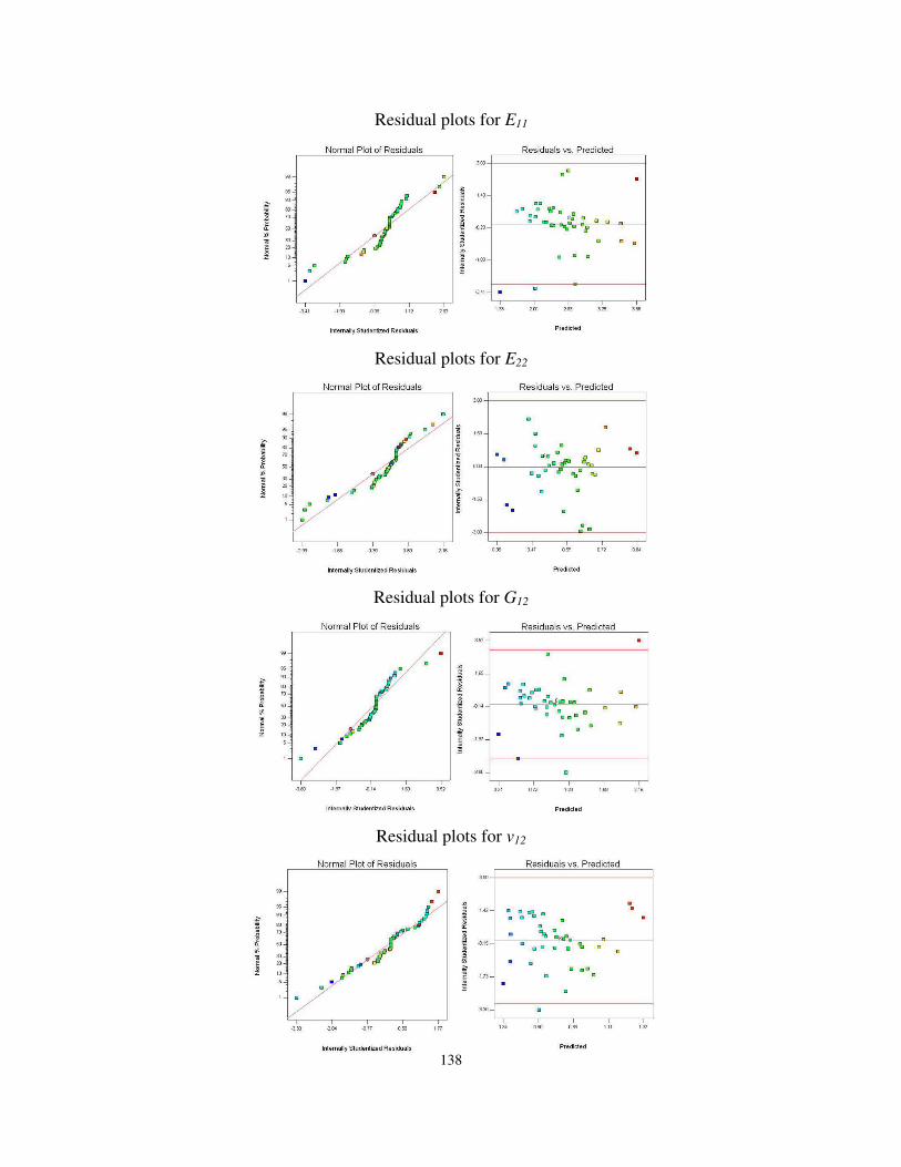
138
Residual plots for E11
Residual plots for E22
Residual plots for G12
Residual plots for v12

139
REFERENCE
[1] Iijima, S., "Helical Microtubules of Graphitic Carbon," Nature, vol. 354, pp. 56-58, 1991. [2] Yu, M. F., Lourie, O., Dyer, M. J., Moloni, K., Kelly, T. F., and Ruoff, R. S., "Strength
and Breaking Mechanism of Multiwalled Carbon Nanotubes under Tensile Load," Science, vol. 287, pp. 637-640, 2000.
[3] Ruoff, R. S. and Lorents, D. C., "Mechanical and Thermal-Properties of Carbon
Nanotubes," Carbon, vol. 33, pp. 925-930, 1995. [4] Salvetat, J. P., Briggs, G. A. D., Bonard, J. M., Bacsa, R. R., Kulik, A. J., Stockli, T.,
Burnham, N. A., and Forro, L., "Elastic and Shear Moduli of Single-Walled Carbon Nanotube Ropes," Physical Review Letters, vol. 82, pp. 944-947, 1999.
[5] Liu, J. Z., Zheng, Q. S., Wang, L. F., and Jiang, Q., "Mechanical Properties of
Single-Walled Carbon Nanotube Bundles as Bulk Materials," Journal of the Mechanics
and Physics of Solids, vol. 53, pp. 123-142, 2005. [6] Popov, V. N., Van Doren, V. E., and Balkanski, M., "Elastic Properties of Crystals of
Single-Walled Carbon Nanotubes," Solid State Communications, vol. 114, pp. 395-399, 2000.
[7] Reich, S., Thomsen, C., and Maultzsch, J., Carbon Nanotubes: Basic Concepts and
Physical Properties New York: Wiley-VCH 2004. [8] Wong, E. W., Sheehan, P. E., and Lieber, C. M., "Nanobeam Mechanics: Elasticity,
Strength, and Toughness of Nanorods and Nanotubes," Science, vol. 277, pp. 1971-1975, 1997.
[9] Wang, Z., Liang, Z. Y., Wang, B., Zhang, C., and Kramer, L., "Processing and Property
Investigation of Single-Walled Carbon Nanotube (Swnt) Buckypaper/Epoxy Resin Matrix Nanocomposites," Composites Part a-Applied Science and Manufacturing, vol. 35, pp. 1225-1232, 2004.
[10] Lin, C. Y., "Investigation and Characterization of Swnt Buckypaper Manufacturing
Process," Master Thesis, Industrial and Manufacturing Engineering, Florida State University, 2005.
[11] Yeh, C. S., "Characterization of Nanotube Buckypaper Manufacturing Processing,"
Master Thesis, Industrial and Manufacturing Engineering, Florida State University, 2004.

140
[12] Xue, Y., "Experimental Study of Electrical Conductivity of Carbon Nanotube, Nanofiber Buckypapers and Their Composites," Master Thesis, Industrial and Manufacturing Engineering, Florida State University, 2007.
[13] Wang, S. R., Liang, Z. Y., Wang, B., and Zhang, C., "High-Strength and Multifunctional
Macroscopic Fabric of Single-Walled Carbon Nanotubes," Advanced Materials, vol. 19, pp. 1257-+, 2007.
[14] Gonnet, P., Liang, S. Y., Choi, E. S., Kadambala, R. S., Zhang, C., Brooks, J. S., Wang,
B., and Kramer, L., "Thermal Conductivity of Magnetically Aligned Carbon Nanotube Buckypapers and Nanocomposites," Current Applied Physics, vol. 6, pp. 119-122, 2006.
[15] Tsai, S. Y., "Experimental Study and Modeling of Nanotube Buckypaper Composite
Actuator for Morphing Structure Applications," Ph.D. Dissertation, Industrial and Manufacturing Engineering, Florida State University, 2010.
[16] Chen, Y., Miao, H. Y., Zhang, M., Liang, R., Zhang, C., and Wang, B., "Analysis of a
Laser Post-Process on a Buckypaper Field Emitter for High and Uniform Electron Emission," Nanotechnology, vol. 20, p. 325302, 2009.
[17] Zhu, W., Zheng, J. P., Liang, R., Wang, B., Zhang, C., Au, G., and Plichta, E. J.,
"Durability Study on Swnt/Nanofiber Buckypaper Catalyst Support for Pemfcs," Journal
of the Electrochemical Society, vol. 156, pp. B1099-B1105, 2009. [18] Rodriguez, E., "Development of an Automated Continuous Buckypaper Production
Process," Master Thesis, Industrial and Manufacturing Engineering Florida State University, 2008.
[19] Ugarte, J., "Development of Continuous Manufacturing Process for Magnetically
Aligned and Random Nanotube Buckypapers," Master Thesis, Industrial and Manufacturing Engineering Florida State University, 2007.
[20] Young, J. P., "Continuous Buckypaper Manufacturing Process: Process Investigation and
Improvement," Master Thesis, Industrial and Manufacturing Engineering, Florida State University, 2009.
[21] Huang, P., Zhang, C., Wu, M., Liang, R., and Wang, B., "Improvement and Optimization
of Carbon Nanotube Buckypaper Fabrication Process with Taguchi Method," working
paper. [22] Tucker, C. L. and Liang, E., "Stiffness Predictions for Unidirectional Short-Fiber
Composites: Review and Evaluation," Composites Science and Technology, vol. 59, pp. 655-671, 1999.

141
[23] Jiang, B., Liu, C., Zhang, C., Wang, B., and Wang, Z., "The Effect of Non-Symmetric Distribution of Fiber Orientation and Aspect Ratio on Elastic Properties of Composites," Composites Part B-Engineering, vol. 38, pp. 24-34, 2007.
[24] Li, X. D., Gao, H. S., Scrivens, W. A., Fei, D. L., Xu, X. Y., Sutton, M. A., Reynolds, A.
P., and Myrick, M. L., "Reinforcing Mechanisms of Single-Walled Carbon Nanotube-Reinforced Polymer Composites," Journal of Nanoscience and
Nanotechnology, vol. 7, pp. 2309-2317, 2007. [25] McClory, C., McNally, T., Brennan, G. P., and Erskine, J., "Thermosetting Polyurethane
Multiwalled Carbon Nanotube Composites," Journal of Applied Polymer Science, vol. 105, pp. 1003-1011, 2007.
[26] Zhupanska, O. I., Liu, Q., Liang, Z., Wang, B., and Zhang, C., "Elastic Properties of
Buckypaper Nanocomposites: Studies on the Effects of Buckypaper Texture," in Proceeding of 52nd International SAMPE Symposium and Exhibition Baltimore, MD, 2007.
[27] Wang, S. R., Liang, Z. Y., Wang, B., and Zhang, C., "Statistical Characterization of
Single-Wall Carbon Nanotube Length Distribution," Nanotechnology, vol. 17, pp. 634-639, 2006.
[28] Kanagaraj, S., Varanda, F. R., Zhil'tsova, T. V., Oliveira, M. S. A., and Simoes, J. A. O.,
"Mechanical Properties of High Density Polyethylene/Carbon Nanotube Composites," Composites Science and Technology, vol. 67, pp. 3071-3077, 2007.
[29] Tai, N. H., Yeh, M. K., and Peng, T. H., "Experimental Study and Theoretical Analysis
on the Mechanical Properties of Swnts/Phenolic Composites," Composites Part
B-Engineering, vol. 39, pp. 926-932, 2008. [30] Doghri, I., Selmi, A., Friebel, C., and Hassis, H., "Prediction of the Elastic Properties of
Single Walled Carbon Nanotube Reinforced Polymers: A Comparative Study of Several Micromechanical Models," Composites Science and Technology, vol. 67, pp. 2071-84, 2007.
[31] Song, Y. S. and Youn, J. R., "Modeling of Effective Elastic Properties for Polymer Based
Carbon Nanotube Composites," Polymer, vol. 47, pp. 1741-1748, 2006. [32] Luo, D. M., Wang, W. X., and Takao, Y., "Application of Homogenization Method on
the Evaluation and Analysis of the Effective Stiffness for Noncontinuous Carbon Nanotube/Polymer Composites," Polymer Composites, vol. 28, pp. 688-695, 2007.
[33] Krzyzanowski, D. R., Chattopadhyay, A., and Wei, J., "Elastic and Viscoelastic
Modeling of Carbon Nanotube Reinforced Polystyrene," in Proceeding of 48th

142
AIAA/ASME/ASCE/AHS/ASC Structures, Structural Dynamics, and Materials
Conferences, Honolulu, Hawaii, 2007, pp. 4096-4110. [34] Fisher, F. T., Bradshaw, R. D., and Brinson, L. C., "Fiber Waviness in
Nanotube-Reinforced Polymer Composites-1: Modulus Predictions Using Effective Nanotube Properties," Composites Science and Technology, vol. 63, pp. 1689-1703, 2003.
[35] Sreekumar, T. V., Liu, T., Kumar, S., Ericson, L. M., Hauge, R. H., and Smalley, R. E.,
"Single-Wall Carbon Nanotube Films," Chemistry of Materials, vol. 15, pp. 175-178, 2003.
[36] Zhang, M., Fang, S. L., Zakhidov, A. A., Lee, S. B., Aliev, A. E., Williams, C. D.,
Atkinson, K. R., and Baughman, R. H., "Strong, Transparent, Multifunctional, Carbon Nanotube Sheets," Science, vol. 309, pp. 1215-1219, 2005.
[37] Yeh, C. S., "A Study of Nanostructure and Properties of Mixed Nanotube Buckypaper
Materials Fabrication, Process Modeling Characterization, and Property Modeling," Ph.D. Dissertation, Industrial and Manufacturing Engineering, Florida State University, 2007.
[38] Cheng, H. M., Li, F., Sun, X., Brown, S. D. M., Pimenta, M. A., Marucci, A.,
Dresselhaus, G., and Dresselhaus, M. S., "Bulk Morphology and Diameter Distribution of Single-Walled Carbon Nanotubes Synthesized by Catalytic Decomposition of Hydrocarbons," Chemical Physics Letters, vol. 289, pp. 602-610, 1998.
[39] Rinzler, A. G., Liu, J., Dai, H., Nikolaev, P., Huffman, C. B., Rodriguez-Macias, F. J.,
Boul, P. J., Lu, A. H., Heymann, D., Colbert, D. T., Lee, R. S., Fischer, J. E., Rao, A. M., Eklund, P. C., and Smalley, R. E., "Large-Scale Purification of Single-Wall Carbon Nanotubes: Process, Product, and Characterization," Applied Physics a-Materials Science
& Processing, vol. 67, pp. 29-37, 1998. [40] Thostenson, E. T. and Chou, T. W., "On the Elastic Properties of Carbon
Nanotube-Based Composites: Modelling and Characterization," Journal of Physics
D-Applied Physics, vol. 36, pp. 573-582, 2003. [41] Perez, R., Banda, S., and Ounaies, Z., "Determination of the Orientation Distribution
Function in Aligned Single Wall Nanotube Polymer Nanocomposites by Polarized Raman Spectroscopy," Journal of Applied Physics, vol. 103, 2008.
[42] Liu, P. J., Liu, L. Y., and Zhang, Y. F., "Alignment Characterization of Single-Wall
Carbon Nanotubes by Raman Scattering," Physics Letters A, vol. 313, pp. 302-306, 2003. [43] Hsiao, H. M. and Daniel, I. M., "Elastic Properties of Composites with Fiber Waviness,"
Composites Part a-Applied Science and Manufacturing, vol. 27, pp. 931-941, 1996.

143
[44] Anumandla, V. and Gibson, R. F., "A Comprehensive Closed Form Micromechanics Model for Estimating the Elastic Modulus of Nanotube-Reinforced Composites," Composites Part a-Applied Science and Manufacturing, vol. 37, pp. 2178-2185, 2006.
[45] Shi, D.-L., Feng, X.-Q., Huang, Y. Y., Keh-Chih, H., and Huajian, G., "The Effect of
Nanotube Waviness and Agglomeration on the Elastic Property of Carbon Nanotube-Reinforced Composites," Transactions of the ASME. Journal of Engineering
Materials and Technology, vol. 126, pp. 250-7, 2004. [46] Gou, J. and Lau, K. T., "Modeling and Simulation of Carbon Nanotube/Polymer
Composites," in Handbook of Theoretical and Computational Nanotechnology. vol. 1, Rieth, M. and Schommers, W., Eds., 1 ed: American Scientific Publishers, 2006, pp. 1-33.
[47] Valavala, P. K. and Odegard, G. M., "Modeling Techniques for Determination of
Mechanical Properties of Polymer Nanocomposites," Reviews on Advanced Materials
Science, vol. 9, pp. 34-44, 2005. [48] Odegard, G. M., Gates, T. S., Wise, K. E., Park, C., and Siochi, E. J., "Constitutive
Modeling of Nanotube-Reinforced Polymer Composites," Composites Science and
Technology, vol. 63, pp. 1671-1687, 2003. [49] Gou, J. H., Minaie, B., Wang, B., Liang, Z. Y., and Zhang, C., "Computational and
Experimental Study of Interfacial Bonding of Single-Walled Nanotube Reinforced Composites," Computational Materials Science, vol. 31, pp. 225-236, 2004.
[50] Gou, J. H., Liang, Z. Y., Zhang, C., and Wang, B., "Computational Analysis of Effect of
Single-Walled Carbon Nanotube Rope on Molecular Interaction and Load Transfer of Nanocomposites," Composites Part B-Engineering, vol. 36, pp. 524-533, 2005.
[51] Eshelby, J. D., "The Determination of the Elastic Field of an Ellipsoidal Inclusion, and
Related Problems," Proceedings of the Royal Society of London Series a-Mathematical
and Physical Sciences, vol. 241, pp. 376-396, 1957. [52] Mori, T. and Tanaka, K., "Average Stress in Matrix and Average Elastic Energy of
Materials with Misfitting Inclusions," Acta Metallurgica, vol. 21, pp. 571-574, 1973. [53] Hill, R., "Self-Consistent Mechanics of Composite Materials," Journal of Mechanics and
Physics of Solids, vol. 13, pp. 213-222, 1965. [54] Hashin, Z. and Shtrikman, S., "On Some Variational Principles in Anisotropic and
Nonhomogeneous Elasticity," Journal of Mechanics and Physics of Solids, vol. 10, pp. 335-342, 1962.

144
[55] Hashin, Z. and Shtrikman, S., "A Variational Approach to the Theory of the Elastic Behaviour of Multiphase Materials," Journal of the Mechanics and Physics of Solids, vol. 11, pp. 127-140, 1963.
[56] Walpole, L. J., "On Bounds for the Overall Elastic Moduli of Inhomogeneous
Systems--I," Journal of the Mechanics and Physics of Solids, vol. 14, pp. 151-162, 1966. [57] Walpole, L. J., "On Bounds for the Overall Elastic Moduli of Inhomogeneous
Systems--Ii," Journal of the Mechanics and Physics of Solids, vol. 14, pp. 289-301, 1966. [58] Willis, J. R., "Bounds and Self-Consistent Estimates for the Overall Properties of
Anisotropic Composites," Journal of the Mechanics and Physics of Solids, vol. 25, pp. 185-202, 1977.
[59] Weng, G. J., "Explicit Evaluation of Willis' Bounds with Ellipsoidal Inclusions,"
International Journal of Engineering Science, vol. 30, pp. 83-92, 1992. [60] Hill, R., "Theory of Mechanical Properties of Fibre-Strengthened Materials .1. Elastic
Behaviour," Journal of the Mechanics and Physics of Solids, vol. 12, pp. 199-212, 1964. [61] Hermans, J. J., "Elastic Properties of Fiber Reinforced Materials When Fibers Are
Aligned," Koninklijke Nederlandse Akademie Van Weteschappen-Proceedings Series
B-Physical Sciences, vol. 70, pp. 1-&, 1967. [62] Halpin, J. C. and Kardos, J. L., "Halpin-Tsai Equations - Review," Polymer Engineering
and Science, vol. 16, pp. 344-352, 1976. [63] Hill, R., "Elastic Properties of Reinforced Solids -- Some Theoretical Principles," Journal
of Mechanics and Physics of Solids, vol. 11, pp. 357-372, 1963. [64] Wakashim. K, Otsuka, M., and Umekawa, S., "Thermal Expansions of Heterogeneous
Solids Containing Aligned Ellipsoidal Inclusions," Journal of Composite Materials, vol. 8, pp. 391-404, 1974.
[65] Tandon, G. P. and Weng, G. J., "The Effect of Aspect Ratio of Inclusions on the Elastic
Properties of Unidirectionally Aligned Composites," Polymer Composites, vol. 5, pp. 327-333, 1984.
[66] Hill, R., "The Elastic Behaviour of a Crystalline Aggregate " Proceedings of the Physical
Society. Section A, vol. 65, pp. 349-354, 1952. [67] Folgar, F. and Tucker Iii, C. L., "Orientation Behavior of Fibers in Concentrated
Suspensions," Journal of Reinforced Plastics and Composites, vol. 3, pp. 98-119, 1984.

145
[68] Advani, S. G. and Tucker, C. L., "The Use of Tensors to Describe and Predict Fiber Orientation in Short Fiber Composites," Journal of Rheology, vol. 31, pp. 751-784, 1987.
[69] Camacho, C. W., Tucker, C. L., III, Yalvac, S., and McGee, R. L., "Stiffness and
Thermal Expansion Predictions for Hybrid Short Fiber Composites," Polymer
Composites, vol. 11, pp. 229-39, 1990. [70] Jack, D. A. and Smith, D. E., "Elastic Properties of Short-Fiber Polymer Composites,
Derivation and Demonstration of Analytical Forms for Expectation and Variance from Orientation Tensors," Journal of Composite Materials, vol. 42, pp. 277-308, 2008.
[71] Chan, W. S. and Wang, J. S., "Influence of Fiber Waviness on the Structural Response of
Composite Laminates," Journal of Thermoplastic Composite Materials, vol. 7, pp. 243-260, 1994.
[72] Bradshaw, R. D., Fisher, F. T., and Brinson, L. C., "Fiber Waviness in
Nanotube-Reinforced Polymer Composites-Ii: Modeling Via Numerical Approximation of the Dilute Strain Concentration Tensor," Composites Science and Technology, vol. 63, pp. 1705-1722, 2003.
[73] Jones, R., Mechanics of Composite Materials, 1 ed.: CRC, 1998. [74] Efunda: Classical Lamination Theory. Available:
http://www.efunda.com/formulae/solid_mechanics/composites/comp_laminate.cfm [75] Stock, T. A., "Probabilistic Fiber Composite Micromechanics," Master Thesis,
Department of Civil Engineering, Cleveland State University, 1983. [76] Barbero, E., Fernandez-Saez, J., and Navarro, C., "Statistical Analysis of the Mechanical
Properties of Composite Materials," Composites Part B-Engineering, vol. 31, pp. 375-381, 2000.
[77] Peponi, L., Biagiotti, J., Kenny, J. M., and Mondragon, I., "Statistical Analysis of the
Mechanical Properties of Natural Fibers and Their Composite Materials. Ii. Composite Materials," Polymer Composites, vol. 29, pp. 321-325, 2008.
[78] Lordi, V. and Yao, N., "Molecular Mechanics of Binding in Carbon-Nanotube-Polymer
Composites," Journal of Materials Research, vol. 15, pp. 2770-2779, 2000. [79] Liang, Z. Y., Gou, J. H., Zhang, C., Wang, B., and Kramer, L., "Investigation of
Molecular Interactions between (10,10) Single-Walled Nanotube and Epon 862 Resin/Detda Curing Agent Molecules," pp. 228-234.
[80] Liao, K. and Li, S., "Interfacial Characteristics of a Carbon Nanotube-Polystyrene
Composite System," Applied Physics Letters, vol. 79, pp. 4225-4227, 2001.

146
[81] Frankland, S. J. V. and Harik, V. M., "Analysis of Carbon Nanotube Pull-out from a Polymer Matrix," Surface Science, vol. 525, pp. L103-L108, 2003.
[82] Frankland, S. J. V., Caglar, A., Brenner, D. W., and Griebel, M., "Molecular Simulation
of the Influence of Chemical Cross-Links on the Shear Strength of Carbon Nanotube-Polymer Interfaces," Journal of Physical Chemistry B, vol. 106, pp. 3046-3048, 2002.
[83] Ajayan, P. M., Stephan, O., Colliex, C., and Trauth, D., "Aligned Carbon Nanotube
Arrays Formed by Cutting a Polymer Resin-Nanotube Composite," Science, vol. 265, pp. 1212-1214, 1994.
[84] Sandler, J., Shaffer, M. S. P., Prasse, T., Bauhofer, W., Schulte, K., and Windle, A. H.,
"Development of a Dispersion Process for Carbon Nanotubes in an Epoxy Matrix and the Resulting Electrical Properties," Polymer, vol. 40, pp. 5967-5971, 1999.
[85] Lau, K. T. and Shi, S. Q., "Failure Mechanisms of Carbon Nanotube/Epoxy Composites
Pretreated in Different Temperature Environments," Carbon, vol. 40, pp. 2965-2968, 2002.
[86] Wagner, H. D., Lourie, O., Feldman, Y., and Tenne, R., "Stress-Induced Fragmentation
of Multiwall Carbon Nanotubes in a Polymer Matrix," Applied Physics Letters, vol. 72, pp. 188-190, 1998.
[87] Lourie, O. and Wagner, H. D., "Transmission Electron Microscopy Observations of
Fracture of Single-Wall Carbon Nanotubes under Axial Tension," Applied Physics
Letters, vol. 73, pp. 3527-3529, 1998. [88] Cooper, C. A., Cohen, S. R., Barber, A. H., and Wagner, H. D., "Detachment of
Nanotubes from a Polymer Matrix," Applied Physics Letters, vol. 81, pp. 3873-3875, 2002.
[89] Barber, A. H., Cohen, S. R., and Wagner, H. D., "Measurement of Carbon
Nanotube-Polymer Interfacial Strength," Applied Physics Letters, vol. 82, pp. 4140-4142, 2003.
[90] Santner, T. J., Williams, B. J., and Notz, W., The Design and Analysis of Computer
Experiments: Springer, 2003. [91] Fang, K., Li, R., and Sudjianto, A., Design and Modeling for Computer Experiments, 1
ed.: Chapman and Hall/CRC, 2005. [92] Mckay, M. D., Beckman, R. J., and Conover, W. J., "A Comparison of Three Methods
for Selecting Values of Input Variables in the Analysis of Output from a Computer Code," Technometrics, vol. 20, pp. 239-245, 1979.

147
[93] Simpson, T. W., Peplinski, J. D., Koch, P. N., and Allen, J. K., "Metamodels for
Computer-Based Engineering Design: Survey and Recommendations," Engineering with
Computers, vol. 17, pp. 129-50, 2001. [94] Sacks, J., Welch, W. J., Mitchell, T. J., and Wynn, H. P., "Design and Analysis of
Computer Experiments" Statistical science, vol. 4, pp. 409-435, 1989. [95] Krige, D. G., "A Statistical Approach to Some Mine Valuations and Allied Problems at
the Witwatersrand," Master Thesis, University of Witwatersrand, 1951. [96] Sobol', I. M., "Sensitivity Estimates for Nonlinear Mathematical Models," Mathematical
Modeling and Computational Experiment, vol. 1, pp. 407-414, 1993. [97] Cukier, R. I., Levine, H. B., and Shuler, K. E., "Nonlinear Sensitivity Analysis of
Multiparameter Model Systems," Journal of Computational Physics, vol. 26, pp. 1-42, 1978.
[98] Saltelli, A., Chan, K., and Scott, E. M., Sensitivity Analysis: Wiley, 2008. [99] Homma, T. and Saltelli, A., "Importance Measures in Global Sensitivity Analysis of
Nonlinear Models," Reliability Engineering and System Safety, vol. 52, pp. 1-17, 1996. [100] Joseph, V. R. and Melkote, S. N., "Statistical Adjustments to Engineering Models,"
Journal of Quality Technology, vol. 41, pp. 362-375, 2009. [101] Kennedy, M. C. and O'Hagan, A., "Bayesian Calibration of Computer Models," Journal
of the Royal Statistical Society Series B-Statistical Methodology, vol. 63, pp. 425-450, 2001.
[102] Reese, C. S., Wilson, A. G., Hamada, M., Martz, H. F., and Ryan, K., "Integrated
Analysis of Computer and Physical Experiments," Technometrics, vol. 46, pp. 153-64, 2004.
[103] Higdon, D., Kennedy, M., Cavendish, J. C., Cafeo, J. A., and Ryne, R. D., "Combining
Field Data and Computer Simulations for Calibration and Prediction," SIAM Journal on
Scientific Computing, vol. 26, pp. 90-108, 2005. [104] Bayarri, M. J., Paulo, R., Berger, J., Sacks, J., Cafeo, J. A., Cavendish, J., Chin-Hsu, L.,
and Jian, T., "A Framework for Validation of Computer Models," Technometrics, vol. 49, pp. 138-54, 2007.
[105] Qian, P. Z. G. and Wu, C. F. J., "Bayesian Hierarchical Modeling for Integrating
Low-Accuracy and High-Accuracy Experiments," Technometrics, vol. 50, pp. 192-204, 2008.

148
[106] DeGroot, M. H. and Schervish, M. J., Probability and Statistics: Addison Wesley, 2001. [107] Yamini, S. and Young, R. J., "The Mechanical-Properties of Epoxy-Resins .1.
Mechanisms of Plastic-Deformation," Journal of Materials Science, vol. 15, pp. 1814-1822, 1980.
[108] Chen, C. H. and Cheng, C. H., "Effective Elastic Moduli of Misoriented Short-Fiber
Composites," International Journal of Solids and Structures, vol. 33, pp. 2519-2539, 1996.
[109] Hine, P. J., Lusti, H. R., and Gusev, A. A., "Numerical Simulation of the Effects of
Volume Fraction, Aspect Ratio and Fibre Length Distribution on the Elastic and Thermoelastic Properties of Short Fibre Composites," Composites Science and
Technology, vol. 62, pp. 1445-1453, 2002. [110] Montgomery, D. C., Design and Analysis of Experiments, 6 ed.: Wiley, 2004. [111] Cheng, Q. F., Bao, J. W., Park, J., Liang, Z. Y., Zhang, C., and Wang, B., "High
Mechanical Performance Composite Conductor: Multi-Walled Carbon Nanotube Sheet/Bismaleimide Nanocomposites," Advanced Functional Materials, vol. 19, pp. 3219-3225, 2009.
[112] Lashmore, D. S., "Supercapacitors and Methods of Manufacturing Same," US Patent No.
20080225464, 2008. [113] Wang, S. R., "Functionalization of Carbon Nanotubes:Characterization, Modeling and
Composite Applications," Ph.D. Dissertation, Department of Industrial and Manufacturing Engineering, Florida State University, 2006.
[114] Cheng, Q., Wang, B., Zhang, C., and Liang, Z., "Functionalized Carbon-Nanotube
Sheet/Bismaleimide Nanocomposites: Mechanical and Electrical Performance Beyond Carbon-Fiber Composites," Small, vol. 6, pp. 763-767, 2010.

149
BIOGRAPHICAL SKETCH
Chao-hsi (James) Tsai started his doctoral education in the Industrial and Manufacturing
Engineering Department at The Florida State University (Tallahassee, FL) in the Fall semester of
2006. His research area is the modeling and statistical analysis of elastic properties of CNT
buckypaper reinforced polymer composites. He received his baccalaureate in Chemistry at
National Sun Yat-sen University in Taiwan. He received his Master of Business Administration
at National Chia-yi University in Taiwan, where he conducted research in management
information systems and electronic commerce. He has co-authored three journal papers, two
peer-reviewed conference papers, and has participated in one NSF grant proposal.


