Embed Size (px)
Citation preview
FIXED INCOMEANALYSIS
Second Edition
Frank J. Fabozzi, PhD, CFA, CPA
with contributions from
Mark J.P. Anson, PhD, CFA, CPA, Esq.Kenneth B. Dunn, PhD
J. Hank Lynch, CFAJack Malvey, CFAMark Pitts, PhD
Shrikant RamamurthyRoberto M. Sella
Christopher B. Steward, CFA
John Wiley & Sons, Inc.


FIXED INCOMEANALYSIS

CFA Institute is the premier association for investment professionals around the world,with over 85,000 members in 129 countries. Since 1963 the organization has developedand administered the renowned Chartered Financial Analyst Program. With a rich historyof leading the investment profession, CFA Institute has set the highest standards in ethics,education, and professional excellence within the global investment community, and is theforemost authority on investment profession conduct and practice.
Each book in the CFA Institute Investment Series is geared toward industry practitionersalong with graduate-level finance students and covers the most important topics in theindustry. The authors of these cutting-edge books are themselves industry professionals andacademics and bring their wealth of knowledge and expertise to this series.

FIXED INCOMEANALYSIS
Second Edition
Frank J. Fabozzi, PhD, CFA, CPA
with contributions from
Mark J.P. Anson, PhD, CFA, CPA, Esq.Kenneth B. Dunn, PhD
J. Hank Lynch, CFAJack Malvey, CFAMark Pitts, PhD
Shrikant RamamurthyRoberto M. Sella
Christopher B. Steward, CFA
John Wiley & Sons, Inc.

Copyright c© 2004, 2007 by CFA Institute. All rights reserved.
Published by John Wiley & Sons, Inc., Hoboken, New Jersey.Published simultaneously in Canada.
No part of this publication may be reproduced, stored in a retrieval system, or transmitted in any form or by anymeans, electronic, mechanical, photocopying, recording, scanning, or otherwise, except as permitted under Section107 or 108 of the 1976 United States Copyright Act, without either the prior written permission of the Publisher, orauthorization through payment of the appropriate per-copy fee to the Copyright Clearance Center, Inc., 222Rosewood Drive, Danvers, MA 01923, (978) 750-8400, fax (978) 646-8600, or on the Web at www.copyright.com.Requests to the Publisher for permission should be addressed to the Permissions Department, John Wiley & Sons,Inc., 111 River Street, Hoboken, NJ 07030, (201) 748-6011, fax (201) 748-6008, or online athttp://www.wiley.com/go/permissions.
Limit of Liability/Disclaimer of Warranty: While the publisher and author have used their best efforts in preparingthis book, they make no representations or warranties with respect to the accuracy or completeness of the contents ofthis book and specifically disclaim any implied warranties of merchantability or fitness for a particular purpose. Nowarranty may be created or extended by sales representatives or written sales materials. The advice and strategiescontained herein may not be suitable for your situation. You should consult with a professional where appropriate.Neither the publisher nor author shall be liable for any loss of profit or any other commercial damages, including butnot limited to special, incidental, consequential, or other damages.
For general information on our other products and services or for technical support, please contact our CustomerCare Department within the United States at (800) 762-2974, outside the United States at (317) 572-3993 or fax(317) 572-4002.
Wiley also publishes its books in a variety of electronic formats. Some content that appears in print may not beavailable in electronic formats. For more information about Wiley products, visit our Web site at www.wiley.com.
Library of Congress Cataloging-in-Publication Data:
Fabozzi, Frank J.Fixed income analysis / Frank J. Fabozzi.—2nd ed.
p. cm.—(CFA Institute investment series)Originally published as: Fixed income analysis for the chartered financial
analyst program. New Hope, Pa. : F. J. Fabozzi Associates, c2000.Includes index.ISBN-13: 978-0-470-05221-1 (cloth)ISBN-10: 0-470-05221-X (cloth)
1. Fixed-income securities. I. Fabozzi, Frank J. Fixed income analysis forthe chartered financial analyst program. 2006. II. Title.
HG4650.F329 2006332.63’23—dc22
2006052818
Printed in the United States of America.
10 9 8 7 6 5 4 3 2 1
CONTENTS
Foreword xiii
Acknowledgments xvii
Introduction xxi
Note on Rounding Differences xxvii
CHAPTER 1Features of Debt Securities 1
I. Introduction 1II. Indenture and Covenants 2III. Maturity 2IV. Par Value 3V. Coupon Rate 4VI. Provisions for Paying Off Bonds 8VII. Conversion Privilege 13VIII. Put Provision 13IX. Currency Denomination 13X. Embedded Options 14XI. Borrowing Funds to Purchase Bonds 15
CHAPTER 2Risks Associated with Investing in Bonds 17
I. Introduction 17II. Interest Rate Risk 17III. Yield Curve Risk 23IV. Call and Prepayment Risk 26V. Reinvestment Risk 27VI. Credit Risk 28VII. Liquidity Risk 32VIII. Exchange Rate or Currency Risk 33IX. Inflation or Purchasing Power Risk 34X. Volatility Risk 34
v
vi Contents
XI. Event Risk 35XII. Sovereign Risk 36
CHAPTER 3Overview of Bond Sectors and Instruments 37
I. Introduction 37II. Sectors of the Bond Market 37III. Sovereign Bonds 39IV. Semi-Government/Agency Bonds 44V. State and Local Governments 53VI. Corporate Debt Securities 56VII. Asset-Backed Securities 67VIII. Collateralized Debt Obligations 69IX. Primary Market and Secondary Market for Bonds 70
CHAPTER 4Understanding Yield Spreads 74
I. Introduction 74II. Interest Rate Determination 74III. U.S. Treasury Rates 75IV. Yields on Non-Treasury Securities 82V. Non-U.S. Interest Rates 90VI. Swap Spreads 92
CHAPTER 5Introduction to the Valuation of Debt Securities 97
I. Introduction 97II. General Principles of Valuation 97III. Traditional Approach to Valuation 109IV. The Arbitrage-Free Valuation Approach 110V. Valuation Models 117
CHAPTER 6Yield Measures, Spot Rates, and Forward Rates 119
I. Introduction 119II. Sources of Return 119III. Traditional Yield Measures 120IV. Theoretical Spot Rates 135V. Forward Rates 147
CHAPTER 7Introduction to the Measurement of Interest Rate Risk 157
I. Introduction 157II. The Full Valuation Approach 157
Contents vii
III. Price Volatility Characteristics of Bonds 160IV. Duration 168V. Convexity Adjustment 180VI. Price Value of a Basis Point 182VII. The Importance of Yield Volatility 183
CHAPTER 8Term Structure and Volatility of Interest Rates 185
I. Introduction 185II. Historical Look at the Treasury Yield Curve 186III. Treasury Returns Resulting from Yield Curve Movements 189IV. Constructing the Theoretical Spot Rate Curve for Treasuries 190V. The Swap Curve (LIBOR Curve) 193VI. Expectations Theories of the Term Structure of Interest Rates 196VII. Measuring Yield Curve Risk 204VIII. Yield Volatility and Measurement 207
CHAPTER 9Valuing Bonds with Embedded Options 215
I. Introduction 215II. Elements of a Bond Valuation Model 215III. Overview of the Bond Valuation Process 218IV. Review of How to Value an Option-Free Bond 225V. Valuing a Bond with an Embedded Option Using the Binomial Model 226VI. Valuing and Analyzing a Callable Bond 233VII. Valuing a Putable Bond 240VIII. Valuing a Step-Up Callable Note 243IX. Valuing a Capped Floater 244X. Analysis of Convertible Bonds 247
CHAPTER 10Mortgage-Backed Sector of the Bond Market 256
I. Introduction 256II. Residential Mortgage Loans 257III. Mortgage Passthrough Securities 260IV. Collateralized Mortgage Obligations 273V. Stripped Mortgage-Backed Securities 294VI. Nonagency Residential Mortgage-Backed Securities 296VII. Commercial Mortgage-Backed Securities 298
CHAPTER 11Asset-Backed Sector of the Bond Market 302
I. Introduction 302II. The Securitization Process and Features of ABS 303
viii Contents
III. Home Equity Loans 313IV. Manufactured Housing-Backed Securities 317V. Residential MBS Outside the United States 318VI. Auto Loan-Backed Securities 320VII. Student Loan-Backed Securities 322VIII. SBA Loan-Backed Securities 324IX. Credit Card Receivable-Backed Securities 325X. Collateralized Debt Obligations 327
CHAPTER 12Valuing Mortgage-Backed and Asset-Backed Securities 335
I. Introduction 335II. Cash Flow Yield Analysis 336III. Zero-Volatility Spread 337IV. Monte Carlo Simulation Model and OAS 338V. Measuring Interest Rate Risk 351VI. Valuing Asset-Backed Securities 358VII. Valuing Any Security 359
CHAPTER 13Interest Rate Derivative Instruments 360
I. Introduction 360II. Interest Rate Futures 360III. Interest Rate Options 371IV. Interest Rate Swaps 377V. Interest Rate Caps and Floors 382
CHAPTER 14Valuation of Interest Rate Derivative Instruments 386
I. Introduction 386II. Interest Rate Futures Contracts 386III. Interest Rate Swaps 392IV. Options 403V. Caps and Floors 416
CHAPTER 15General Principles of Credit Analysis 421
I. Introduction 421II. Credit Ratings 421III. Traditional Credit Analysis 424IV. Credit Scoring Models 453V. Credit Risk Models 455
Appendix: Case Study 456
Contents ix
CHAPTER 16Introduction to Bond Portfolio Management 462
I. Introduction 462II. Setting Investment Objectives for Fixed-Income Investors 463III. Developing and Implementing a Portfolio Strategy 471IV. Monitoring the Portfolio 475V. Adjusting the Portfolio 475
CHAPTER 17Measuring a Portfolio’s Risk Profile 476
I. Introduction 476II. Review of Standard Deviation and Downside Risk Measures 476III. Tracking Error 482IV. Measuring a Portfolio’s Interest Rate Risk 487V. Measuring Yield Curve Risk 491VI. Spread Risk 492VII. Credit Risk 493VIII. Optionality Risk for Non-MBS 494IX. Risks of Investing in Mortgage-Backed Securities 495X. Multi-Factor Risk Models 498
CHAPTER 18Managing Funds against a Bond Market Index 503
I. Introduction 503II. Degrees of Active Management 503III. Strategies 507IV. Scenario Analysis for Assessing Potential Performance 513V. Using Multi-Factor Risk Models in Portfolio Construction 525VI. Performance Evaluation 528VII. Leveraging Strategies 531
CHAPTER 19Portfolio Immunization and Cash Flow Matching 541
I. Introduction 541II. Immunization Strategy for a Single Liability 541III. Contingent Immunization 551IV. Immunization for Multiple Liabilities 554V. Cash Flow Matching for Multiple Liabilities 557
CHAPTER 20Relative-Value Methodologies for Global Credit Bond
Portfolio Management (by Jack Malvey) 560
I. Introduction 560II. Credit Relative-Value Analysis 561
x Contents
III. Total Return Analysis 565IV. Primary Market Analysis 566V. Liquidity and Trading Analysis 567VI. Secondary Trade Rationales 568VII. Spread Analysis 572VIII. Structural Analysis 575IX. Credit Curve Analysis 579X. Credit Analysis 579XI. Asset Allocation/Sector Rotation 581
CHAPTER 21International Bond Portfolio Management (by Christopher B.
Steward, J. Hank Lynch, and Frank J. Fabozzi) 583
I. Introduction 583II. Investment Objectives and Policy Statements 584III. Developing a Portfolio Strategy 588IV. Portfolio Construction 595
Appendix 614
CHAPTER 22Controlling Interest Rate Risk with Derivatives (by Frank J. Fabozzi,
Shrikant Ramamurthy, and Mark Pitts) 617
I. Introduction 617II. Controlling Interest Rate Risk with Futures 617III. Controlling Interest Rate Risk with Swaps 633IV. Hedging with Options 637V. Using Caps and Floors 649
CHAPTER 23Hedging Mortgage Securities to Capture Relative Value
(by Kenneth B. Dunn, Roberto M. Sella, and Frank J. Fabozzi) 651
I. Introduction 651II. The Problem 651III. Mortgage Security Risks 655IV. How Interest Rates Change Over Time 660V. Hedging Methodology 661VI. Hedging Cuspy-Coupon Mortgage Securities 671
CHAPTER 24Credit Derivatives in Bond Portfolio Management (by Mark J.P. Anson
and Frank J. Fabozzi) 673
I. Introduction 673II. Market Participants 674III. Why Credit Risk Is Important 674

Contents xi
IV. Total Return Swap 677V. Credit Default Products 679VI. Credit Spread Products 687VII. Synthetic Collateralized Debt Obligations 691VIII. Basket Default Swaps 692
About the CFA Program 695
About the Author 697
About the Contributors 699
Index 703

FOREWORD
There is an argument that an understanding of any financial market must incorporate anappreciation of the functioning of the bond market as a vital source of liquidity. This argumentis true in today’s financial markets more than ever before, because of the central role that debtplays in virtually every facet of our modern financial markets. Thus, anyone who wants to bea serious student or practitioner in finance should at least become familiar with the currentspectrum of fixed income securities and their associated derivatives and structural products.
This book is a fully revised and updated edition of two volumes used earlier in preparationfor the Chartered Financial Analysts (CFA) program. However, in its current form, it goesbeyond the original CFA role and provides an extraordinarily comprehensive, and yet quitereadable, treatment of the key topics in fixed income analysis. This breadth and quality of itscontents has been recognized by its inclusion as a basic text in the finance curriculum of majoruniversities. Anyone who reads this book, either thoroughly or by dipping into the portionsthat are relevant at the moment, will surely reach new planes of knowledgeability about debtinstruments and the liquidity they provide throughout the global financial markets.
I first began studying the bond market back in the 1960s. At that time, bonds werethought to be dull and uninteresting. I often encountered expressions of sympathy abouthaving been misguided into one of the more moribund backwaters in finance. Indeed, adesigner of one of the early bond market indexes (not me) gave a talk that started with adeclaration that bonds were ‘‘dull, dull, dull!’’
In those early days, the bond market consisted of debt issued by US Treasury, agencies,municipalities, or high grade corporations. The structure of these securities was generally quite‘‘plain vanilla’’: fixed coupons, specified maturities, straightforward call features, and somesinking funds. There was very little trading in the secondary market. New issues of tax exemptbonds were purchased by banks and individuals, while the taxable offerings were taken downby insurance companies and pension funds. And even though the total outstanding footingswere quite sizeable relative to the equity market, the secondary market trading in bonds wasminiscule relative to stocks.
Bonds were, for the most part, locked away in frozen portfolios. The coupons werestill—literally—‘‘clipped,’’ and submitted to receive interest payments (at that time, scissorswere one of the key tools of bond portfolio management). This state of affairs reflected theenvironment of the day—the bond-buying institutions were quite traditional in their culture(the term ‘‘crusty’’ may be only slightly too harsh), bonds were viewed basically as a source ofincome rather than an opportunity for short-term return generation, and the high transactioncosts in the corporate and municipal sectors dampened any prospective benefit from trading.
However, times change, and there is no area of finance that has witnessed a more rapidevolution—perhaps revolution would be more apt—than the fixed income markets. Interestrates have swept up and down across a range of values that was previously thought to beunimaginable. New instruments were introduced, shaped into standard formats, and then
xiii
xiv Foreword
exploded to huge markets in their own right, both in terms of outstanding footings and themagnitude of daily trading. Structuring, swaps, and a variety of options have become integralcomponents of the many forms of risk transfer that make today’s vibrant debt market possible.
In stark contrast to the plodding pace of bonds in the 1960s, this book takes the readeron an exciting tour of today’s modern debt market. The book begins with descriptions ofthe current tableau of debt securities. After this broad overview, which I recommend toeveryone, the second chapter delves immediately into the fundamental question associatedwith any investment vehicle: What are the risks? Bonds have historically been viewed as alower risk instrument relative to other markets such as equities and real estate. However, intoday’s fixed income world, the derivative and structuring processes have spawned a veritablesmorgasbord of investment opportunities, with returns and risks that range across an extremelywide spectrum.
The completion of the Treasury yield curve has given a new clarity to term structure andmaturity risk. In turn, this has sharpened the identification of minimum risk investments forspecific time periods. The Treasury curve’s more precisely defined term structure can then helpin analyzing the spread behavior of non-Treasury securities. The non-Treasury market consistsof corporate, agency, mortgage, municipal, and international credits. Its total now far exceedsthe total supply of Treasury debt. To understand the credit/liquidity relationships across thevarious market segments, one must come to grips with the constellation of yield spreads thataffects their pricing. Only then can then one begin to understand how a given debt security isvalued and to appreciate the many-dimensional determinants of debt return and risk.
As one delves deeper into the multiple layers of fixed income valuation, it becomes evidentthat these same factors form the basis for analyzing all forms of investments, not just bonds. Inevery market, there are spot rates, forward rates, as well as the more aggregated yield measures.In the past, this structural approach may have been relegated to the domain of the arcane orthe academic. In the current market, these more sophisticated approaches to capital structureand term effects are applied daily in the valuation process.
Whole new forms of securitized fixed income instruments have come into existence andgrown to enormous size in the past few decades, for example, the mortgage backed, assetbacked, and structured-loan sectors. These sectors have become critical to the flow of liquidityto households and to the global economy at large. To trace how liquidity and credit availabilityfind their way through various channels to the ultimate demanders, it is critical to understandhow these assets are structured, how they behave, and why various sources of funds are attractedto them.
Credit analysis is another area that has undergone radical evolution in the past fewyears. The simplistic standard ratio measures of yesteryear have been supplemented by marketoriented analyses based upon option theory as well as new approaches to capital structure.
The active management of bond portfolios has become a huge business where sizeablefunds are invested in an effort to garner returns in excess of standard benchmark indices. Thefixed income markets are comprised of far more individual securities than the equity market.However, these securities are embedded in term structure/spread matrix that leads to muchtighter and more reliable correlations. The fixed income manager can take advantage of thesetighter correlations to construct compact portfolios to control the overall benchmark risk andstill have ample room to pursue opportunistic positive alphas in terms of sector selection, yieldcurve placement, or credit spreads. There is a widespread belief that exploitable inefficienciespersist within the fixed income market because of the regulatory and/or functional constraints
Foreword xv
placed upon many of the major market participants. In more and more instances, these so-called alpha returns from active bond management are being ‘‘ported’’ via derivative overlays,possibly in a leveraged fashion, to any position in a fund’s asset allocation structure.
In terms of managing credit spreads and credit exposure, the development of credit defaultswaps (CDS) and other types of credit derivatives has grown at such an incredible pace that itnow constitutes an important market in its own right. By facilitating the redistribution anddiversification of credit risk, the CDS explosion has played a critical role in providing ongoingliquidity throughout the economy. These structure products and derivatives may have evolvedfrom the fixed income market, but their role now reaches far afield, e.g., credit default swapsare being used by some equity managers as efficient alternative vehicles for hedging certaintypes of equity risks.
The worldwide maturing of pension funds in conjunction with a more stringentaccounting/regulatory environment has created new management approaches such as surplusmanagement, asset/liability management (ALM), or liability driven investment (LDI). Thesetechniques incorporate the use of very long duration portfolios, various types of swaps andderivatives, as well as older forms of cash matching and immunization to reduce the fund’sexposure to fluctuations in nominal and/or real interest rates. With pension fund assets ofboth defined benefit and defined contribution variety amounting to over $14 trillion in theUnited States alone, it is imperative for any student of finance to understand these liabilitiesand their relationship to various fixed income vehicles.
With its long history as the primary organization in educating and credentialing financeprofessionals, CFA Institute is the ideal sponsor to provide a balanced and objective overviewof this subject. Drawing upon its unique professional network, CFA Institute has been ableto call upon the most authoritative sources in the field to develop, review, and updateeach chapter. The primary author and editor, Frank Fabozzi, is recognized as one of themost knowledgeable and prolific scholars across the entire spectrum of fixed income topics.Dr. Fabozzi has held positions at MIT, Yale, and the University of Pennsylvania, and haswritten articles in collaboration with Franco Modigliani, Harry Markowitz, Gifford Fong,Jack Malvey, Mark Anson, and many other noted authorities in fixed income. One could nothope for a better combination of editor/author and sponsor. It is no wonder that they havemanaged to produce such a valuable guide into the modern world of fixed income.
Over the past three decades, the changes in the debt market have been arguably far morerevolutionary than that seen in equities or perhaps in any other financial market. Unfortunately,the broader development of this market and its extension into so many different arenas andforms has made it more difficult to achieve a reasonable level of knowledgeability. However,this highly readable, authoritative and comprehensive volume goes a long way towards thisgoal by enabling individuals to learn about this most fundamental of all markets. The morespecialized sections will also prove to be a resource that practitioners will repeatedly dip intoas the need arises in the course of their careers.
Martin L. LeibowitzManaging DirectorMorgan Stanley

ACKNOWLEDGMENTS
I would like to acknowledge the following individuals for their assistance.
First Edition (Reprinted from First Edition)Dr. Robert R. Johnson, CFA, Senior Vice President of AIMR, reviewed more than a dozen ofthe books published by Frank J. Fabozzi Associates. Based on his review, he provided me withan extensive list of chapters for the first edition that contained material that would be usefulto CFA candidates for all three levels. Rather than simply put these chapters together into abook, he suggested that I use the material in them to author a book based on explicit contentguidelines. His influence on the substance and organization of this book was substantial.
My day-to-day correspondence with AIMR regarding the development of the materialand related issues was with Dr. Donald L. Tuttle, CFA, Vice President. It would seem fittingthat he would serve as one of my mentors in this project because the book he co-edited,Managing Investment Portfolios: A Dynamic Process (first published in 1983), has played animportant role in shaping my thoughts on the investment management process; it also hasbeen the cornerstone for portfolio management in the CFA curriculum for almost two decades.The contribution of his books and other publications to the advancement of the CFA bodyof knowledge, coupled with his leadership role in several key educational projects, recentlyearned him AIMR’s highly prestigious C. Stewart Sheppard Award.
Before any chapters were sent to Don for his review, the first few drafts were sent toAmy F. Lipton, CFA of Lipton Financial Analytics, who was a consultant to AIMR forthis project. Amy is currently a member of the Executive Advisory Board of the CandidateCurriculum Committee (CCC). Prior to that she was a member of the Executive Committeeof the CCC, the Level I Coordinator for the CCC, and the Chair of the Fixed Income TopicArea of the CCC. Consequently, she was familiar with the topics that should be includedin a fixed income analysis book for the CFA Program. Moreover, given her experience inthe money management industry (Aetna, First Boston, Greenwich, and Bankers Trust), shewas familiar with the material. Amy reviewed and made detailed comments on all aspects ofthe material. She recommended the deletion or insertion of material, identified topics thatrequired further explanation, and noted material that was too detailed and showed how itshould be shortened. Amy not only directed me on content, but she checked every calculation,provided me with spreadsheets of all calculations, and highlighted discrepancies between thesolutions in a chapter and those she obtained. On a number of occasions, Amy added materialthat improved the exposition; she also contributed several end-of-chapter questions. Amy hasbeen accepted into the doctoral program in finance at both Columbia University and LehighUniversity, and will begin her studies in Fall of 2000.
xvii

xviii Acknowledgments
After the chapters were approved by Amy and Don, they were then sent to reviewersselected by AIMR. The reviewers provided comments that were the basis for further revisions.I am especially appreciative of the extensive reviews provided by Richard O. Applebach, Jr.,CFA and Dr. George H. Troughton, CFA. I am also grateful to the following reviewers:Dr. Philip Fanara, Jr., CFA; Brian S. Heimsoth, CFA; Michael J. Karpik, CFA; Daniel E.Lenhard, CFA; Michael J. Lombardi, CFA; James M. Meeth, CFA; and C. Ronald Sprecher,PhD, CFA.
I engaged William McLellan to review all of the chapter drafts. Bill has completed theLevel III examination and is now accumulating enough experience to be awarded the CFAdesignation. Because he took the examinations recently, he reviewed the material as if he werea CFA candidate. He pointed out statements that might be confusing and suggested ways toeliminate ambiguities. Bill checked all the calculations and provided me with his spreadsheetresults.
Martin Fridson, CFA and Cecilia Fok provided invaluable insight and direction for thechapter on credit analysis (Chapter 9 of Level II). Dr. Steven V. Mann and Dr. Michael Ferrireviewed several chapters in this book. Dr. Sylvan Feldstein reviewed the sections dealing withmunicipal bonds in Chapter 3 of Level I and Chapter 9 of Level II. George Kelger reviewedthe discussion on agency debentures in Chapter 3 of Level I.
Helen K. Modiri of AIMR provided valuable administrative assistance in coordinatingbetween my office and AIMR.
Megan Orem of Frank J. Fabozzi Associates typeset the entire book and provided editorialassistance on various aspects of this project.
Second EditionDennis McLeavey, CFA was my contact person at CFA Institute for the second edition. Hesuggested how I could improve the contents of each chapter from the first edition and readseveral drafts of all the chapters. The inclusion of new topics were discussed with him. Dennisis an experienced author, having written several books published by CFA Institute for the CFAprogram. Dennis shared his insights with me and I credit him with the improvement in theexposition in the second edition.
The following individuals reviewed chapters:
Stephen L. Avard, CFAMarcus A. Ingram, CFAMuhammad J. Iqbal, CFAWilliam L. Randolph, CFAGerald R. Root, CFARichard J. Skolnik, CFAR. Bruce Swensen, CFALavone Whitmer, CFA
Larry D. Guin, CFA consolidated the individual reviews, as well as reviewed chapters1–7. David M. Smith, CFA did the same for Chapters 8–15.
The final proofreaders were Richard O. Applebach, CFA, Dorothy C. Kelly, CFA, LouisJ. James, CFA and Lavone Whitmer.
Wanda Lauziere of CFA Institute coordinated the reviews. Helen Weaver of CFA Instituteassembled, summarized, and coordinated the final reviewer comments.

Acknowledgments xix
Jon Fougner, an economics major at Yale, provided helpful comments on Chapters 1and 2.
Finally, CFA Candidates provided helpful comments and identified errors in the firstedition.

INTRODUCTION
CFA Institute is pleased to provide you with this Investment Series covering major areas inthe field of investments. These texts are thoroughly grounded in the highly regarded CFAProgram Candidate Body of Knowledge (CBOK) that draws upon hundreds of practicinginvestment professionals and serves as the anchor for the three levels of the CFA Examinations.In the year this series is being launched, more than 120,000 aspiring investment professionalswill each devote over 250 hours of study to master this material as well as other elements ofthe Candidate Body of Knowledge in order to obtain the coveted CFA charter. We providethese materials for the same reason we have been chartering investment professionals for over40 years: to improve the competency and ethical character of those serving the capital markets.
PARENTAGE
One of the valuable attributes of this series derives from its parentage. In the 1940s, a handfulof societies had risen to form communities that revolved around common interests and workin what we now think of as the investment industry.
Understand that the idea of purchasing common stock as an investment—as opposed tocasino speculation—was only a couple of decades old at most. We were only 10 years past thecreation of the U.S. Securities and Exchange Commission and laws that attempted to level theplaying field after robber baron and stock market panic episodes.
In January 1945, in what is today CFA Institute Financial Analysts Journal , a funda-mentally driven professor and practitioner from Columbia University and Graham-NewmanCorporation wrote an article making the case that people who research and manage portfoliosshould have some sort of credential to demonstrate competence and ethical behavior. Thisperson was none other than Benjamin Graham, the father of security analysis and futurementor to a well-known modern investor, Warren Buffett.
The idea of creating a credential took a mere 16 years to drive to execution but by 1963,284 brave souls, all over the age of 45, took an exam and launched the CFA credential. Whatmany do not fully understand was that this effort had at its root a desire to create a professionwhere its practitioners were professionals who provided investing services to individuals inneed. In so doing, a fairer and more productive capital market would result.
A profession—whether it be medicine, law, or other—has certain hallmark characteristics.These characteristics are part of what attracts serious individuals to devote the energy of theirlife’s work to the investment endeavor. First, and tightly connected to this Series, there mustbe a body of knowledge. Second, there needs to be some entry requirements such as thoserequired to achieve the CFA credential. Third, there must be a commitment to continuingeducation. Fourth, a profession must serve a purpose beyond one’s direct selfish interest. Inthis case, by properly conducting one’s affairs and putting client interests first, the investment
xxi
xxii Introduction
professional can work as a fair-minded cog in the wheel of the incredibly productive globalcapital markets. This encourages the citizenry to part with their hard-earned savings to beredeployed in fair and productive pursuit.
As C. Stewart Sheppard, founding executive director of the Institute of Chartered FinancialAnalysts said, ‘‘Society demands more from a profession and its members than it does from aprofessional craftsman in trade, arts, or business. In return for status, prestige, and autonomy,a profession extends a public warranty that it has established and maintains conditions ofentry, standards of fair practice, disciplinary procedures, and continuing education for itsparticular constituency. Much is expected from members of a profession, but over time, moreis given.’’
‘‘The Standards for Educational and Psychological Testing,’’ put forth by the AmericanPsychological Association, the American Educational Research Association, and the NationalCouncil on Measurement in Education, state that the validity of professional credentialingexaminations should be demonstrated primarily by verifying that the content of the examina-tion accurately represents professional practice. In addition, a practice analysis study, whichconfirms the knowledge and skills required for the competent professional, should be the basisfor establishing content validity.
For more than 40 years, hundreds upon hundreds of practitioners and academics haveserved on CFA Institute curriculum committees sifting through and winnowing all the manyinvestment concepts and ideas to create a body of knowledge and the CFA curriculum. One ofthe hallmarks of curriculum development at CFA Institute is its extensive use of practitionersin all phases of the process.
CFA Institute has followed a formal practice analysis process since 1995. The effortinvolves special practice analysis forums held, most recently, at 20 locations around the world.Results of the forums were put forth to 70,000 CFA charterholders for verification andconfirmation of the body of knowledge so derived.
What this means for the reader is that the concepts contained in these texts were drivenby practicing professionals in the field who understand the responsibilities and knowledge thatpractitioners in the industry need to be successful. We are pleased to put this extensive effortto work for the benefit of the readers of the Investment Series.
BENEFITS
This series will prove useful both to the new student of capital markets, who is seriouslycontemplating entry into the extremely competitive field of investment management, and tothe more seasoned professional who is looking for a user-friendly way to keep one’s knowledgecurrent. All chapters include extensive references for those who would like to dig deeper intoa given concept. The workbooks provide a summary of each chapter’s key points to helporganize your thoughts, as well as sample questions and answers to test yourself on yourprogress.
For the new student, the essential concepts that any investment professional needs tomaster are presented in a time-tested fashion. This material, in addition to university studyand reading the financial press, will help you better understand the investment field. I believethat the general public seriously underestimates the disciplined processes needed for thebest investment firms and individuals to prosper. These texts lay the basic groundwork formany of the processes that successful firms use. Without this base level of understandingand an appreciation for how the capital markets work to properly price securities, you may
Introduction xxiii
not find competitive success. Furthermore, the concepts herein give a genuine sense of thekind of work that is to be found day to day managing portfolios, doing research, or relatedendeavors.
The investment profession, despite its relatively lucrative compensation, is not foreveryone. It takes a special kind of individual to fundamentally understand and absorb theteachings from this body of work and then convert that into application in the practitionerworld. In fact, most individuals who enter the field do not survive in the longer run. Theaspiring professional should think long and hard about whether this is the field for him- orherself. There is no better way to make such a critical decision than to be prepared by readingand evaluating the gospel of the profession.
The more experienced professional understands that the nature of the capital marketsrequires a commitment to continuous learning. Markets evolve as quickly as smart minds canfind new ways to create an exposure, to attract capital, or to manage risk. A number of theconcepts in these pages were not present a decade or two ago when many of us were startingout in the business. Hedge funds, derivatives, alternative investment concepts, and behavioralfinance are examples of new applications and concepts that have altered the capital markets inrecent years. As markets invent and reinvent themselves, a best-in-class foundation investmentseries is of great value.
Those of us who have been at this business for a while know that we must continuouslyhone our skills and knowledge if we are to compete with the young talent that constantlyemerges. In fact, as we talk to major employers about their training needs, we are oftentold that one of the biggest challenges they face is how to help the experienced professional,laboring under heavy time pressure, keep up with the state of the art and the more recentlyeducated associates. This series can be part of that answer.
CONVENTIONAL WISDOM
It doesn’t take long for the astute investment professional to realize two common characteristicsof markets. First, prices are set by conventional wisdom, or a function of the many variablesin the market. Truth in markets is, at its essence, what the market believes it is and how itassesses pricing credits or debits on those beliefs. Second, as conventional wisdom is a productof the evolution of general theory and learning, by definition conventional wisdom is oftenwrong or at the least subject to material change.
When I first entered this industry in the mid-1970s, conventional wisdom held thatthe concepts examined in these texts were a bit too academic to be heavily employed in thecompetitive marketplace. Many of those considered to be the best investment firms at thetime were led by men who had an eclectic style, an intuitive sense of markets, and a greattrack record. In the rough-and-tumble world of the practitioner, some of these concepts wereconsidered to be of no use. Could conventional wisdom have been more wrong? If so, I’m notsure when.
During the years of my tenure in the profession, the practitioner investment managementfirms that evolved successfully were full of determined, intelligent, intellectually curiousinvestment professionals who endeavored to apply these concepts in a serious and disciplinedmanner. Today, the best firms are run by those who carefully form investment hypothesesand test them rigorously in the marketplace, whether it be in a quant strategy, in comparativeshopping for stocks within an industry, or in many hedge fund strategies. Their goal is tocreate investment processes that can be replicated with some statistical reliability. I believe

xxiv Introduction
those who embraced the so-called academic side of the learning equation have been muchmore successful as real-world investment managers.
THE TEXTS
Approximately 35 percent of the Candidate Body of Knowledge is represented in the initialfour texts of the series. Additional texts on corporate finance and international financialstatement analysis are in development, and more topics may be forthcoming.
One of the most prominent texts over the years in the investment management industryhas been Maginn and Tuttle’s Managing Investment Portfolios: A Dynamic Process. The thirdedition updates key concepts from the 1990 second edition. Some of the more experiencedmembers of our community, like myself, own the prior two editions and will add thisto our library. Not only does this tome take the concepts from the other readings andput them in a portfolio context, it also updates the concepts of alternative investments,performance presentation standards, portfolio execution and, very importantly, managingindividual investor portfolios. To direct attention, long focused on institutional portfolios,toward the individual will make this edition an important improvement over the past.
Quantitative Investment Analysis focuses on some key tools that are needed for today’sprofessional investor. In addition to classic time value of money, discounted cash flowapplications, and probability material, there are two aspects that can be of value overtraditional thinking.
First are the chapters dealing with correlation and regression that ultimately figure intothe formation of hypotheses for purposes of testing. This gets to a critical skill that manyprofessionals are challenged by: the ability to sift out the wheat from the chaff. For mostinvestment researchers and managers, their analysis is not solely the result of newly createddata and tests that they perform. Rather, they synthesize and analyze primary research doneby others. Without a rigorous manner by which to understand quality research, not only canyou not understand good research, you really have no basis by which to evaluate less rigorousresearch. What is often put forth in the applied world as good quantitative research lacks rigorand validity.
Second, the last chapter on portfolio concepts moves the reader beyond the traditionalcapital asset pricing model (CAPM) type of tools and into the more practical world ofmultifactor models and to arbitrage pricing theory. Many have felt that there has been aCAPM bias to the work put forth in the past, and this chapter helps move beyond that point.
Equity Asset Valuation is a particularly cogent and important read for anyone involvedin estimating the value of securities and understanding security pricing. A well-informedprofessional would know that the common forms of equity valuation—dividend discountmodeling, free cash flow modeling, price/earnings models, and residual income models (oftenknown by trade names)—can all be reconciled to one another under certain assumptions.With a deep understanding of the underlying assumptions, the professional investor can betterunderstand what other investors assume when calculating their valuation estimates. In myprior life as the head of an equity investment team, this knowledge would give us an edge overother investors.
Fixed Income Analysis has been at the frontier of new concepts in recent years, greatlyexpanding horizons over the past. This text is probably the one with the most new material forthe seasoned professional who is not a fixed-income specialist. The application of option andderivative technology to the once staid province of fixed income has helped contribute to an

Introduction xxv
explosion of thought in this area. And not only does that challenge the professional to stay upto speed with credit derivatives, swaptions, collateralized mortgage securities, mortgage backs,and others, but it also puts a strain on the world’s central banks to provide oversight and therisk of a correlated event. Armed with a thorough grasp of the new exposures, the professionalinvestor is much better able to anticipate and understand the challenges our central bankersand markets face.
I hope you find this new series helpful in your efforts to grow your investment knowledge,whether you are a relatively new entrant or a grizzled veteran ethically bound to keep upto date in the ever-changing market environment. CFA Institute, as a long-term committedparticipant of the investment profession and a not-for-profit association, is pleased to give youthis opportunity.
Jeff Diermeier, CFAPresident and Chief Executive OfficerCFA InstituteSeptember 2006

NOTE ON ROUNDINGDIFFERENCES
It is important to recognize in working through the numerical examples and illustrationsin this book that because of rounding differences you may not be able to reproduce someof the results precisely. The two individuals who verified solutions and I used a spreadsheetto compute the solution to all numerical illustrations and examples. For some of the moreinvolved illustrations and examples, there were slight differences in our results.
Moreover, numerical values produced in interim calculations may have been rounded offwhen produced in a table and as a result when an operation is performed on the values shownin a table, the result may appear to be off. Just be aware of this. Here is an example of acommon situation that you may encounter when attempting to replicate results.
Suppose that a portfolio has four securities and that the market value of these foursecurities are as shown below:
Security Market value1 8,890,1002 15,215,0633 18,219,4044 12,173,200
54,497,767
Assume further that we want to calculate the duration of this portfolio. This value isfound by computing the weighted average of the duration of the four securities. This involvesthree steps. First, compute the percentage of each security in the portfolio. Second, multiplythe percentage of each security in the portfolio by its duration. Third, sum up the productscomputed in the second step.
Let’s do this with our hypothetical portfolio. We will assume that the duration for eachof the securities in the portfolio is as shown below:
Security Duration1 92 53 84 2
Using an Excel spreadsheet the following would be computed specifying that thepercentage shown in Column (3) below be shown to seven decimal places:
xxvii
xxviii Note on Rounding Differences
(1) (2) (3) (4) (5)Security Market value Percent of portfolio Duration Percent × duration
1 8,890,100 0.1631278 9 1.468152 15,215,063 0.2791869 5 1.3959353 18,219,404 0.3343147 8 2.6745184 12,173,200 0.2233706 2 0.446741
Total 54,497,767 1.0000000 5.985343
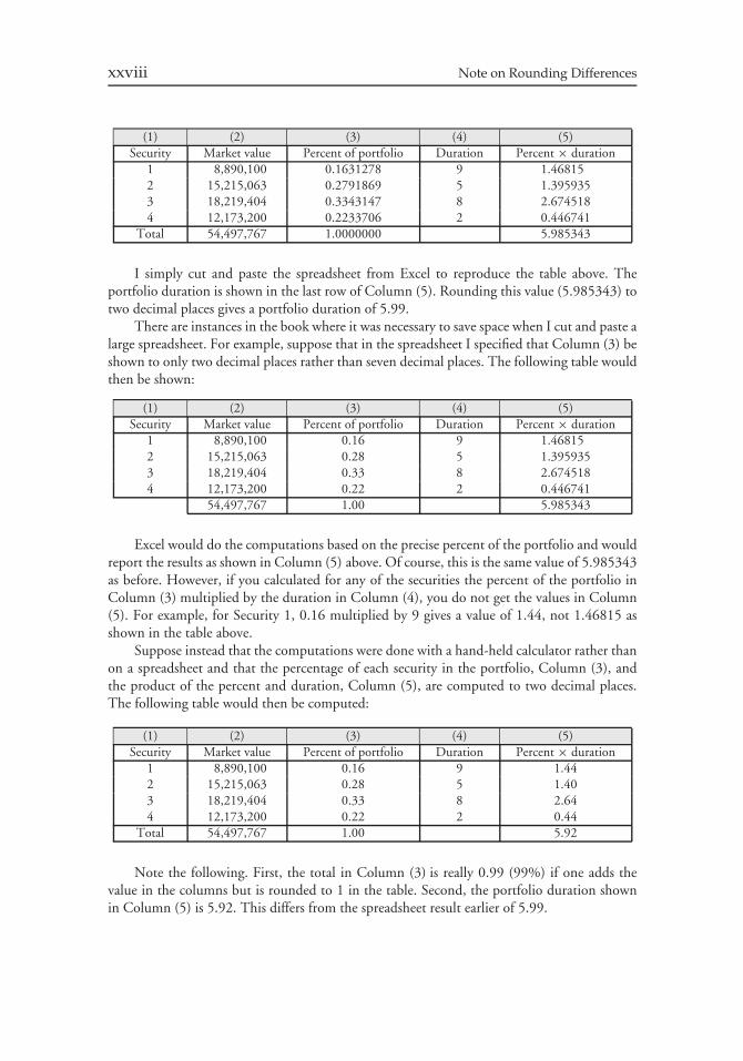
I simply cut and paste the spreadsheet from Excel to reproduce the table above. Theportfolio duration is shown in the last row of Column (5). Rounding this value (5.985343) totwo decimal places gives a portfolio duration of 5.99.
There are instances in the book where it was necessary to save space when I cut and paste alarge spreadsheet. For example, suppose that in the spreadsheet I specified that Column (3) beshown to only two decimal places rather than seven decimal places. The following table wouldthen be shown:
(1) (2) (3) (4) (5)Security Market value Percent of portfolio Duration Percent × duration
1 8,890,100 0.16 9 1.468152 15,215,063 0.28 5 1.3959353 18,219,404 0.33 8 2.6745184 12,173,200 0.22 2 0.446741
54,497,767 1.00 5.985343
Excel would do the computations based on the precise percent of the portfolio and wouldreport the results as shown in Column (5) above. Of course, this is the same value of 5.985343as before. However, if you calculated for any of the securities the percent of the portfolio inColumn (3) multiplied by the duration in Column (4), you do not get the values in Column(5). For example, for Security 1, 0.16 multiplied by 9 gives a value of 1.44, not 1.46815 asshown in the table above.
Suppose instead that the computations were done with a hand-held calculator rather thanon a spreadsheet and that the percentage of each security in the portfolio, Column (3), andthe product of the percent and duration, Column (5), are computed to two decimal places.The following table would then be computed:
(1) (2) (3) (4) (5)Security Market value Percent of portfolio Duration Percent × duration
1 8,890,100 0.16 9 1.442 15,215,063 0.28 5 1.403 18,219,404 0.33 8 2.644 12,173,200 0.22 2 0.44
Total 54,497,767 1.00 5.92
Note the following. First, the total in Column (3) is really 0.99 (99%) if one adds thevalue in the columns but is rounded to 1 in the table. Second, the portfolio duration shownin Column (5) is 5.92. This differs from the spreadsheet result earlier of 5.99.
Note on Rounding Differences xxix
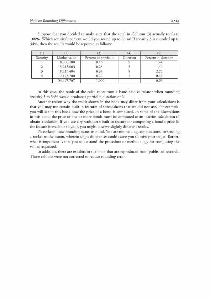
Suppose that you decided to make sure that the total in Column (3) actually totals to100%. Which security’s percent would you round up to do so? If security 3 is rounded up to34%, then the results would be reported as follows:
(1) (2) (3) (4) (5)Security Market value Percent of portfolio Duration Percent × duration
1 8,890,100 0.16 9 1.442 15,215,063 0.28 5 1.403 18,219,404 0.34 8 2.724 12,173,200 0.22 2 0.44
54,497,767 1.000 6.00
In this case, the result of the calculation from a hand-held calculator when roundingsecurity 3 to 34% would produce a portfolio duration of 6.
Another reason why the result shown in the book may differ from your calculations isthat you may use certain built-in features of spreadsheets that we did not use. For example,you will see in this book how the price of a bond is computed. In some of the illustrationsin this book, the price of one or more bonds must be computed as an interim calculation toobtain a solution. If you use a spreadsheet’s built-in feature for computing a bond’s price (ifthe feature is available to you), you might observe slightly different results.
Please keep these rounding issues in mind. You are not making computations for sendinga rocket to the moon, wherein slight differences could cause you to miss your target. Rather,what is important is that you understand the procedure or methodology for computing thevalues requested.
In addition, there are exhibits in the book that are reproduced from published research.Those exhibits were not corrected to reduce rounding error.

CHAPTER 1FEATURES OF DEBT
SECURITIES
I. INTRODUCTION
In investment management, the most important decision made is the allocation of fundsamong asset classes. The two major asset classes are equities and fixed income securities. Otherasset classes such as real estate, private equity, hedge funds, and commodities are referred to as‘‘alternative asset classes.’’ Our focus in this book is on one of the two major asset classes: fixedincome securities.
While many people are intrigued by the exciting stories sometimes found with equi-ties—who has not heard of someone who invested in the common stock of a small companyand earned enough to retire at a young age?—we will find in our study of fixed incomesecurities that the multitude of possible structures opens a fascinating field of study. While fre-quently overshadowed by the media prominence of the equity market, fixed income securitiesplay a critical role in the portfolios of individual and institutional investors.
In its simplest form, a fixed income security is a financial obligation of an entity thatpromises to pay a specified sum of money at specified future dates. The entity that promisesto make the payment is called the issuer of the security. Some examples of issuers are centralgovernments such as the U.S. government and the French government, government-relatedagencies of a central government such as Fannie Mae and Freddie Mac in the United States,a municipal government such as the state of New York in the United States and the city ofRio de Janeiro in Brazil, a corporation such as Coca-Cola in the United States and YorkshireWater in the United Kingdom, and supranational governments such as the World Bank.
Fixed income securities fall into two general categories: debt obligations and preferredstock. In the case of a debt obligation, the issuer is called the borrower. The investor whopurchases such a fixed income security is said to be the lender or creditor. The promised pay-ments that the issuer agrees to make at the specified dates consist of two components: interestand principal (principal represents repayment of funds borrowed) payments. Fixed incomesecurities that are debt obligations include bonds, mortgage-backed securities, asset-backedsecurities, and bank loans.
In contrast to a fixed income security that represents a debt obligation, preferred stockrepresents an ownership interest in a corporation. Dividend payments are made to thepreferred stockholder and represent a distribution of the corporation’s profit. Unlike investorswho own a corporation’s common stock, investors who own the preferred stock can onlyrealize a contractually fixed dividend payment. Moreover, the payments that must be madeto preferred stockholders have priority over the payments that a corporation pays to common
1
2 Fixed Income Analysis
stockholders. In the case of the bankruptcy of a corporation, preferred stockholders are givenpreference over common stockholders. Consequently, preferred stock is a form of equity thathas characteristics similar to bonds.
Prior to the 1980s, fixed income securities were simple investment products. Holdingaside default by the issuer, the investor knew how long interest would be received and whenthe amount borrowed would be repaid. Moreover, most investors purchased these securitieswith the intent of holding them to their maturity date. Beginning in the 1980s, the fixedincome world changed. First, fixed income securities became more complex. There are featuresin many fixed income securities that make it difficult to determine when the amount borrowedwill be repaid and for how long interest will be received. For some securities it is difficult todetermine the amount of interest that will be received. Second, the hold-to-maturity investorhas been replaced by institutional investors who actively trades fixed income securities.
We will frequently use the terms ‘‘fixed income securities’’ and ‘‘bonds’’ interchangeably. Inaddition, we will use the term bonds generically at times to refer collectively to mortgage-backedsecurities, asset-backed securities, and bank loans.
In this chapter we will look at the various features of fixed income securities and in thenext chapter we explain how those features affect the risks associated with investing in fixedincome securities. The majority of our illustrations throughout this book use fixed incomesecurities issued in the United States. While the U.S. fixed income market is the largest fixedincome market in the world with a diversity of issuers and features, in recent years there hasbeen significant growth in the fixed income markets of other countries as borrowers haveshifted from funding via bank loans to the issuance of fixed income securities. This is a trendthat is expected to continue.
II. INDENTURE AND COVENANTS
The promises of the issuer and the rights of the bondholders are set forth in great detail ina bond’s indenture. Bondholders would have great difficulty in determining from time totime whether the issuer was keeping all the promises made in the indenture. This problem isresolved for the most part by bringing in a trustee as a third party to the bond or debt contract.The indenture identifies the trustee as a representative of the interests of the bondholders.
As part of the indenture, there are affirmative covenants and negative covenants.Affirmative covenants set forth activities that the borrower promises to do. The most commonaffirmative covenants are (1) to pay interest and principal on a timely basis, (2) to pay all taxesand other claims when due, (3) to maintain all properties used and useful in the borrower’sbusiness in good condition and working order, and (4) to submit periodic reports to a trusteestating that the borrower is in compliance with the loan agreement. Negative covenants setforth certain limitations and restrictions on the borrower’s activities. The more commonrestrictive covenants are those that impose limitations on the borrower’s ability to incuradditional debt unless certain tests are satisfied.
III. MATURITY
The term to maturity of a bond is the number of years the debt is outstanding or the numberof years remaining prior to final principal payment. The maturity date of a bond refers to thedate that the debt will cease to exist, at which time the issuer will redeem the bond by paying
Chapter 1 Features of Debt Securities 3
the outstanding balance. The maturity date of a bond is always identified when describing abond. For example, a description of a bond might state ‘‘due 12/1/2020.’’
The practice in the bond market is to refer to the ‘‘term to maturity’’ of a bond as simplyits ‘‘maturity’’ or ‘‘term.’’ As we explain below, there may be provisions in the indenture thatallow either the issuer or bondholder to alter a bond’s term to maturity.
Some market participants view bonds with a maturity between 1 and 5 years as ‘‘short-term.’’ Bonds with a maturity between 5 and 12 years are viewed as ‘‘intermediate-term,’’ and‘‘long-term’’ bonds are those with a maturity of more than 12 years.
There are bonds of every maturity. Typically, the longest maturity is 30 years. However,Walt Disney Co. issued bonds in July 1993 with a maturity date of 7/15/2093, making them100-year bonds at the time of issuance. In December 1993, the Tennessee Valley Authorityissued bonds that mature on 12/15/2043, making them 50-year bonds at the time of issuance.
There are three reasons why the term to maturity of a bond is important:
Reason 1: Term to maturity indicates the time period over which the bondholder canexpect to receive interest payments and the number of years before the principal willbe paid in full.
Reason 2: The yield offered on a bond depends on the term to maturity. The relationshipbetween the yield on a bond and maturity is called the yield curve and will bediscussed in Chapter 4.
Reason 3: The price of a bond will fluctuate over its life as interest rates in the marketchange. The price volatility of a bond is a function of its maturity (among othervariables). More specifically, as explained in Chapter 7, all other factors constant, thelonger the maturity of a bond, the greater the price volatility resulting from a changein interest rates.
IV. PAR VALUE
The par value of a bond is the amount that the issuer agrees to repay the bondholder ator by the maturity date. This amount is also referred to as the principal value, face value,redemption value, and maturity value. Bonds can have any par value.
Because bonds can have a different par value, the practice is to quote the price of a bond as apercentage of its par value. A value of ‘‘100’’ means 100% of par value. So, for example, if a bondhas a par value of $1,000 and the issue is selling for $900, this bond would be said to be selling at90. If a bond with a par value of $5,000 is selling for $5,500, the bond is said to be selling for 110.
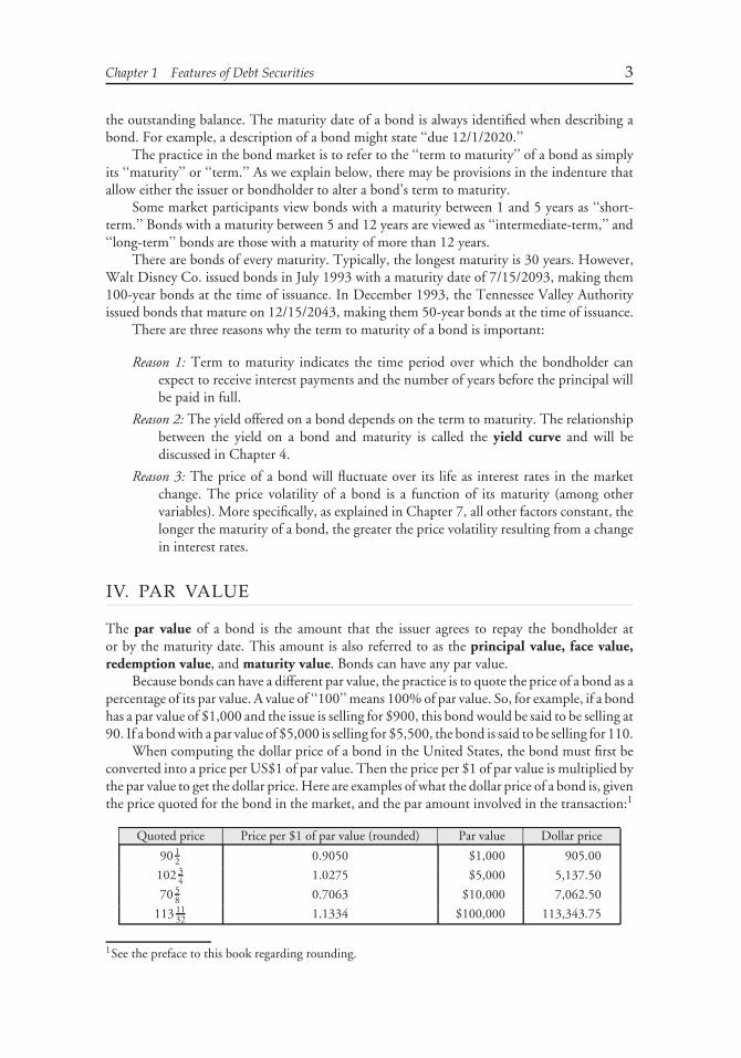
When computing the dollar price of a bond in the United States, the bond must first beconverted into a price per US$1 of par value. Then the price per $1 of par value is multiplied bythe par value to get the dollar price. Here are examples of what the dollar price of a bond is, giventhe price quoted for the bond in the market, and the par amount involved in the transaction:1
Quoted price Price per $1 of par value (rounded) Par value Dollar price
90 12 0.9050 $1,000 905.00
102 34 1.0275 $5,000 5,137.50
70 58 0.7063 $10,000 7,062.50
113 1132 1.1334 $100,000 113,343.75
1See the preface to this book regarding rounding.
4 Fixed Income Analysis
Notice that a bond may trade below or above its par value. When a bond trades below itspar value, it said to be trading at a discount. When a bond trades above its par value, it saidto be trading at a premium. The reason why a bond sells above or below its par value will beexplained in Chapter 2.
V. COUPON RATE
The coupon rate, also called the nominal rate, is the interest rate that the issuer agrees to payeach year. The annual amount of the interest payment made to bondholders during the termof the bond is called the coupon. The coupon is determined by multiplying the coupon rateby the par value of the bond. That is,
coupon = coupon rate × par value
For example, a bond with an 8% coupon rate and a par value of $1,000 will pay annualinterest of $80 (= $1, 000 × 0.08).
When describing a bond of an issuer, the coupon rate is indicated along with the maturitydate. For example, the expression ‘‘6s of 12/1/2020’’ means a bond with a 6% coupon ratematuring on 12/1/2020. The ‘‘s’’ after the coupon rate indicates ‘‘coupon series.’’ In ourexample, it means the ‘‘6% coupon series.’’
In the United States, the usual practice is for the issuer to pay the coupon in twosemiannual installments. Mortgage-backed securities and asset-backed securities typically payinterest monthly. For bonds issued in some markets outside the United States, couponpayments are made only once per year.
The coupon rate also affects the bond’s price sensitivity to changes in market interestrates. As illustrated in Chapter 2, all other factors constant, the higher the coupon rate, theless the price will change in response to a change in market interest rates.
A. Zero-Coupon Bonds
Not all bonds make periodic coupon payments. Bonds that are not contracted to make periodiccoupon payments are called zero-coupon bonds. The holder of a zero-coupon bond realizesinterest by buying the bond substantially below its par value (i.e., buying the bond at a discount).Interest is then paid at the maturity date, with the interest being the difference between the parvalue and the price paid for the bond. So, for example, if an investor purchases a zero-couponbond for 70, the interest is 30. This is the difference between the par value (100) and the pricepaid (70). The reason behind the issuance of zero-coupon bonds is explained in Chapter 2.
B. Step-Up Notes
There are securities that have a coupon rate that increases over time. These securities are calledstep-up notes because the coupon rate ‘‘steps up’’ over time. For example, a 5-year step-upnote might have a coupon rate that is 5% for the first two years and 6% for the last three years.Or, the step-up note could call for a 5% coupon rate for the first two years, 5.5% for the thirdand fourth years, and 6% for the fifth year. When there is only one change (or step up), as inour first example, the issue is referred to as a single step-up note. When there is more thanone change, as in our second example, the issue is referred to as a multiple step-up note.
Chapter 1 Features of Debt Securities 5
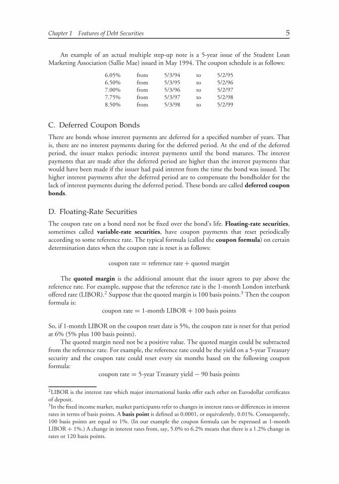
An example of an actual multiple step-up note is a 5-year issue of the Student LoanMarketing Association (Sallie Mae) issued in May 1994. The coupon schedule is as follows:
6.05% from 5/3/94 to 5/2/956.50% from 5/3/95 to 5/2/967.00% from 5/3/96 to 5/2/977.75% from 5/3/97 to 5/2/988.50% from 5/3/98 to 5/2/99
C. Deferred Coupon Bonds
There are bonds whose interest payments are deferred for a specified number of years. Thatis, there are no interest payments during for the deferred period. At the end of the deferredperiod, the issuer makes periodic interest payments until the bond matures. The interestpayments that are made after the deferred period are higher than the interest payments thatwould have been made if the issuer had paid interest from the time the bond was issued. Thehigher interest payments after the deferred period are to compensate the bondholder for thelack of interest payments during the deferred period. These bonds are called deferred couponbonds.
D. Floating-Rate Securities
The coupon rate on a bond need not be fixed over the bond’s life. Floating-rate securities,sometimes called variable-rate securities, have coupon payments that reset periodicallyaccording to some reference rate. The typical formula (called the coupon formula) on certaindetermination dates when the coupon rate is reset is as follows:
coupon rate = reference rate + quoted margin
The quoted margin is the additional amount that the issuer agrees to pay above thereference rate. For example, suppose that the reference rate is the 1-month London interbankoffered rate (LIBOR).2 Suppose that the quoted margin is 100 basis points.3 Then the couponformula is:
coupon rate = 1-month LIBOR + 100 basis points
So, if 1-month LIBOR on the coupon reset date is 5%, the coupon rate is reset for that periodat 6% (5% plus 100 basis points).
The quoted margin need not be a positive value. The quoted margin could be subtractedfrom the reference rate. For example, the reference rate could be the yield on a 5-year Treasurysecurity and the coupon rate could reset every six months based on the following couponformula:
coupon rate = 5-year Treasury yield − 90 basis points
2LIBOR is the interest rate which major international banks offer each other on Eurodollar certificatesof deposit.3In the fixed income market, market participants refer to changes in interest rates or differences in interestrates in terms of basis points. A basis point is defined as 0.0001, or equivalently, 0.01%. Consequently,100 basis points are equal to 1%. (In our example the coupon formula can be expressed as 1-monthLIBOR + 1%.) A change in interest rates from, say, 5.0% to 6.2% means that there is a 1.2% change inrates or 120 basis points.
6 Fixed Income Analysis
So, if the 5-year Treasury yield is 7% on the coupon reset date, the coupon rate is 6.1% (7%minus 90 basis points).
It is important to understand the mechanics for the payment and the setting of thecoupon rate. Suppose that a floater pays interest semiannually and further assume that thecoupon reset date is today. Then, the coupon rate is determined via the coupon formula andthis is the interest rate that the issuer agrees to pay at the next interest payment date six monthsfrom now.
A floater may have a restriction on the maximum coupon rate that will be paid at anyreset date. The maximum coupon rate is called a cap. For example, suppose for a floater whosecoupon formula is the 3-month Treasury bill rate plus 50 basis points, there is a cap of 9%. Ifthe 3-month Treasury bill rate is 9% at a coupon reset date, then the coupon formula wouldgive a coupon rate of 9.5%. However, the cap restricts the coupon rate to 9%. Thus, for ourhypothetical floater, once the 3-month Treasury bill rate exceeds 8.5%, the coupon rate iscapped at 9%. Because a cap restricts the coupon rate from increasing, a cap is an unattractivefeature for the investor. In contrast, there could be a minimum coupon rate specified for afloater. The minimum coupon rate is called a floor. If the coupon formula produces a couponrate that is below the floor, the floor rate is paid instead. Thus, a floor is an attractive featurefor the investor. As we explain in Section X, caps and floors are effectively embedded options.
While the reference rate for most floaters is an interest rate or an interest rate index, awide variety of reference rates appear in coupon formulas. The coupon for a floater could beindexed to movements in foreign exchange rates, the price of a commodity (e.g., crude oil),the return on an equity index (e.g., the S&P 500), or movements in a bond index. In fact,through financial engineering, issuers have been able to structure floaters with almost anyreference rate. In several countries, there are government bonds whose coupon formula is tiedto an inflation index.
The U.S. Department of the Treasury in January 1997 began issuing inflation-adjustedsecurities. These issues are referred to as Treasury Inflation Protection Securities (TIPS).The reference rate for the coupon formula is the rate of inflation as measured by the ConsumerPrice Index for All Urban Consumers (i.e., CPI-U). (The mechanics of the payment of thecoupon will be explained in Chapter 3 where these securities are discussed.) Corporationsand agencies in the United States issue inflation-linked (or inflation-indexed) bonds. Forexample, in February 1997, J. P. Morgan & Company issued a 15-year bond that pays theCPI plus 400 basis points. In the same month, the Federal Home Loan Bank issued a 5-yearbond with a coupon rate equal to the CPI plus 315 basis points and a 10-year bond with acoupon rate equal to the CPI plus 337 basis points.
Typically, the coupon formula for a floater is such that the coupon rate increases whenthe reference rate increases, and decreases when the reference rate decreases. There are issueswhose coupon rate moves in the opposite direction from the change in the reference rate.Such issues are called inverse floaters or reverse floaters.4 It is not too difficult to understandwhy an investor would be interested in an inverse floater. It gives an investor who believesinterest rates will decline the opportunity to obtain a higher coupon interest rate. The issuerisn’t necessarily taking the opposite view because it can hedge the risk that interest rates willdecline.5
4In the agency, corporate, and municipal markets, inverse floaters are created as structured notes. Wediscuss structured notes in Chapter 3. Inverse floaters in the mortgage-backed securities market arecommon and are created through a process that will be discussed in Chapter 10.5The issuer hedges by using financial instruments known as derivatives, which we cover in later chapters.
Chapter 1 Features of Debt Securities 7
The coupon formula for an inverse floater is:
coupon rate = K − L × (reference rate)
where K and L are values specified in the prospectus for the issue.For example, suppose that for a particular inverse floater, K is 20% and L is 2. Then the
coupon reset formula would be:
coupon rate = 20% − 2 × (reference rate)
Suppose that the reference rate is the 3-month Treasury bill rate, then the coupon formulawould be
coupon rate = 20% − 2 × (3-month Treasury bill rate)
If at the coupon reset date the 3-month Treasury bill rate is 6%, the coupon rate for the nextperiod is:
coupon rate = 20% − 2 × 6% = 8%
If at the next reset date the 3-month Treasury bill rate declines to 5%, the coupon rateincreases to:
coupon rate = 20% − 2 × 5% = 10%
Notice that if the 3-month Treasury bill rate exceeds 10%, then the coupon formulawould produce a negative coupon rate. To prevent this, there is a floor imposed on the couponrate. There is also a cap on the inverse floater. This occurs if the 3-month Treasury bill rate iszero. In that unlikely event, the maximum coupon rate is 20% for our hypothetical inversefloater.
There is a wide range of coupon formulas that we will encounter in our study of fixedincome securities.6 These are discussed below. The reason why issuers have been able to createfloating-rate securities with offbeat coupon formulas is due to derivative instruments. It is tooearly in our study of fixed income analysis and portfolio management to appreciate why someof these offbeat coupon formulas exist in the bond market. Suffice it to say that some of theseoffbeat coupon formulas allow the investor to take a view on either the movement of someinterest rate (i.e., for speculating on an interest rate movement) or to reduce exposure to therisk of some interest rate movement (i.e., for interest rate risk management). The advantageto the issuer is that it can lower its cost of borrowing by creating offbeat coupon formulas forinvestors.7 While it may seem that the issuer is taking the opposite position to the investor,this is not the case. What in fact happens is that the issuer can hedge its risk exposure by usingderivative instruments so as to obtain the type of financing it seeks (i.e., fixed rate borrowingor floating rate borrowing). These offbeat coupon formulas are typically found in ‘‘structurednotes,’’ a form of medium-term note that will be discussed in Chapter 3.
6In Chapter 3, we will describe other types of floating-rate securities.7These offbeat coupon bond formulas are actually created as a result of inquiries from clients of dealerfirms. That is, a salesperson will be approached by fixed income portfolio managers requesting a structurebe created that provides the exposure sought. The dealer firm will then notify the investment bankinggroup of the dealer firm to contact potential issuers.
8 Fixed Income Analysis
E. Accrued Interest
Bond issuers do not disburse coupon interest payments every day. Instead, typically in theUnited States coupon interest is paid every six months. In some countries, interest is paidannually. For mortgage-backed and asset-backed securities, interest is usually paid monthly.The coupon payment is made to the bondholder of record. Thus, if an investor sells a bondbetween coupon payments and the buyer holds it until the next coupon payment, then theentire coupon interest earned for the period will be paid to the buyer of the bond since thebuyer will be the holder of record. The seller of the bond gives up the interest from the timeof the last coupon payment to the time until the bond is sold. The amount of interest overthis period that will be received by the buyer even though it was earned by the seller is calledaccrued interest. We will see how to calculate accrued interest in Chapter 5.
In the United States and in many countries, the bond buyer must pay the bond seller theaccrued interest. The amount that the buyer pays the seller is the agreed upon price for thebond plus accrued interest. This amount is called the full price. (Some market participantsrefer to this as the dirty price.) The agreed upon bond price without accrued interest is simplyreferred to as the price. (Some refer to it as the clean price.)
A bond in which the buyer must pay the seller accrued interest is said to be tradingcum-coupon (‘‘with coupon’’). If the buyer forgoes the next coupon payment, the bond issaid to be trading ex-coupon (‘‘without coupon’’). In the United States, bonds are alwaystraded cum-coupon. There are bond markets outside the United States where bonds are tradedex-coupon for a certain period before the coupon payment date.
There are exceptions to the rule that the bond buyer must pay the bond seller accruedinterest. The most important exception is when the issuer has not fulfilled its promise to makethe periodic interest payments. In this case, the issuer is said to be in default. In such instances,the bond is sold without accrued interest and is said to be traded flat.
VI. PROVISIONS FOR PAYING OFF BONDS
The issuer of a bond agrees to pay the principal by the stated maturity date. The issuer canagree to pay the entire amount borrowed in one lump sum payment at the maturity date.That is, the issuer is not required to make any principal repayments prior to the maturity date.Such bonds are said to have a bullet maturity. The bullet maturity structure has become themost common structure in the United States and Europe for both corporate and governmentissuers.
Fixed income securities backed by pools of loans (mortgage-backed securities and asset-backed securities) often have a schedule of partial principal payments. Such fixed incomesecurities are said to be amortizing securities. For many loans, the payments are structuredso that when the last loan payment is made, the entire amount owed is fully paid.
Another example of an amortizing feature is a bond that has a sinking fund provision.This provision for repayment of a bond may be designed to pay all of an issue by the maturitydate, or it may be arranged to repay only a part of the total by the maturity date. We discussthis provision later in this section.
An issue may have a call provision granting the issuer an option to retire all or part ofthe issue prior to the stated maturity date. Some issues specify that the issuer must retire apredetermined amount of the issue periodically. Various types of call provisions are discussedin the following pages.
Chapter 1 Features of Debt Securities 9
A. Call and Refunding Provisions
An issuer generally wants the right to retire a bond issue prior to the stated maturity date. Theissuer recognizes that at some time in the future interest rates may fall sufficiently below theissue’s coupon rate so that redeeming the issue and replacing it with another lower coupon rateissue would be economically beneficial. This right is a disadvantage to the bondholder sinceproceeds received must be reinvested in the lower interest rate issue. As a result, an issuer whowants to include this right as part of a bond offering must compensate the bondholder whenthe issue is sold by offering a higher coupon rate, or equivalently, accepting a lower price thanif the right is not included.
The right of the issuer to retire the issue prior to the stated maturity date is referred to asa call provision. If an issuer exercises this right, the issuer is said to ‘‘call the bond.’’ The pricewhich the issuer must pay to retire the issue is referred to as the call price or redemptionprice.
When a bond is issued, typically the issuer may not call the bond for a number of years.That is, the issue is said to have a deferred call. The date at which the bond may first becalled is referred to as the first call date. The first call date for the Walt Disney 7.55s due7/15/2093 (the 100-year bonds) is 7/15/2023. For the 50-year Tennessee Valley Authority6 7
8 s due 12/15/2043, the first call date is 12/15/2003.Bonds can be called in whole (the entire issue) or in part (only a portion). When less
than the entire issue is called, the certificates to be called are either selected randomly or ona pro rata basis. When bonds are selected randomly, a computer program is used to selectthe serial number of the bond certificates called. The serial numbers are then published inThe Wall Street Journal and major metropolitan dailies. Pro rata redemption means that allbondholders of the issue will have the same percentage of their holdings redeemed (subject tothe restrictions imposed on minimum denominations). Pro rata redemption is rare for publiclyissued debt but is common for debt issues directly or privately placed with borrowers.
A bond issue that permits the issuer to call an issue prior to the stated maturity dateis referred to as a callable bond. At one time, the callable bond structure was common forcorporate bonds issued in the United States. However, since the mid-1990s, there has beensignificantly less issuance of callable bonds by corporate issuers of high credit quality. Instead,as noted above, the most popular structure is the bullet bond. In contrast, corporate issuers oflow credit quality continue to issue callable bonds.8 In Europe, historically the callable bondstructure has not been as popular as in the United States.
1. Call (Redemption) Price When the issuer exercises an option to call an issue, the callprice can be either (1) fixed regardless of the call date, (2) based on a price specified in the callschedule, or (3) based on a make-whole premium provision. We will use various debt issues ofAnheuser-Busch Companies to illustrate these three ways by which the call price is specified.
a. Single Call Price Regardless of Call Date On 6/10/97, Anheuser-Busch Companiesissued $250 million of notes with a coupon rate of 7.1% due June 15, 2007. The prospectusstated that:
8As explained in Chapter 2, high credit quality issuers are referred to as ‘‘investment grade’’ issuers andlow credit quality issuers are referred to as ‘‘non-investment grade’’ issuers. The reason why high creditquality issuers have reduced their issuance of callable bonds while it is still the more popular structurefor low credit quality issuers is explained later.
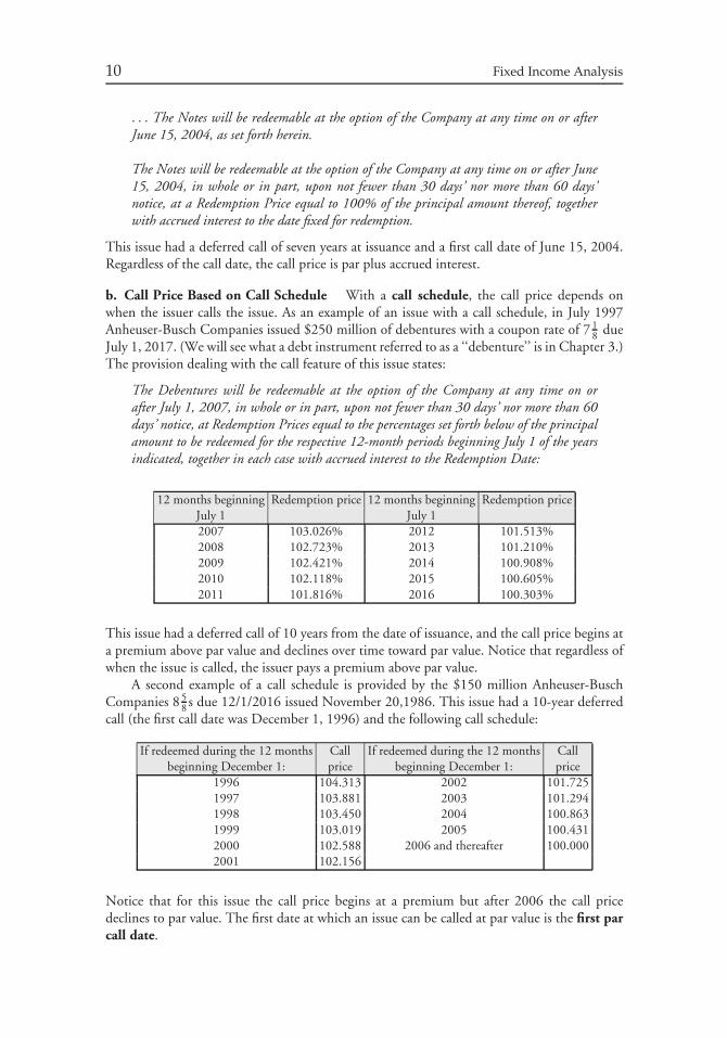
10 Fixed Income Analysis
. . . The Notes will be redeemable at the option of the Company at any time on or afterJune 15, 2004, as set forth herein.
The Notes will be redeemable at the option of the Company at any time on or after June15, 2004, in whole or in part, upon not fewer than 30 days’ nor more than 60 days’notice, at a Redemption Price equal to 100% of the principal amount thereof, togetherwith accrued interest to the date fixed for redemption.
This issue had a deferred call of seven years at issuance and a first call date of June 15, 2004.Regardless of the call date, the call price is par plus accrued interest.
b. Call Price Based on Call Schedule With a call schedule, the call price depends onwhen the issuer calls the issue. As an example of an issue with a call schedule, in July 1997Anheuser-Busch Companies issued $250 million of debentures with a coupon rate of 7 1
8 dueJuly 1, 2017. (We will see what a debt instrument referred to as a ‘‘debenture’’ is in Chapter 3.)The provision dealing with the call feature of this issue states:
The Debentures will be redeemable at the option of the Company at any time on orafter July 1, 2007, in whole or in part, upon not fewer than 30 days’ nor more than 60days’ notice, at Redemption Prices equal to the percentages set forth below of the principalamount to be redeemed for the respective 12-month periods beginning July 1 of the yearsindicated, together in each case with accrued interest to the Redemption Date:
12 months beginning Redemption price 12 months beginning Redemption priceJuly 1 July 12007 103.026% 2012 101.513%2008 102.723% 2013 101.210%2009 102.421% 2014 100.908%2010 102.118% 2015 100.605%2011 101.816% 2016 100.303%
This issue had a deferred call of 10 years from the date of issuance, and the call price begins ata premium above par value and declines over time toward par value. Notice that regardless ofwhen the issue is called, the issuer pays a premium above par value.
A second example of a call schedule is provided by the $150 million Anheuser-BuschCompanies 8 5
8 s due 12/1/2016 issued November 20,1986. This issue had a 10-year deferredcall (the first call date was December 1, 1996) and the following call schedule:
If redeemed during the 12 months Call If redeemed during the 12 months Callbeginning December 1: price beginning December 1: price
1996 104.313 2002 101.7251997 103.881 2003 101.2941998 103.450 2004 100.8631999 103.019 2005 100.4312000 102.588 2006 and thereafter 100.0002001 102.156
Notice that for this issue the call price begins at a premium but after 2006 the call pricedeclines to par value. The first date at which an issue can be called at par value is the first parcall date.
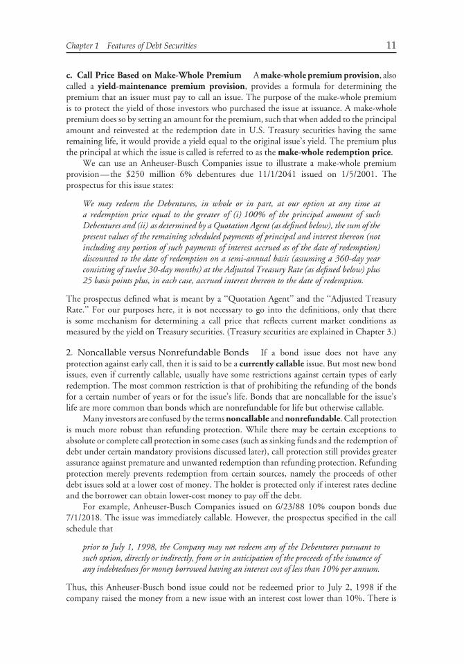
Chapter 1 Features of Debt Securities 11
c. Call Price Based on Make-Whole Premium A make-whole premium provision, alsocalled a yield-maintenance premium provision, provides a formula for determining thepremium that an issuer must pay to call an issue. The purpose of the make-whole premiumis to protect the yield of those investors who purchased the issue at issuance. A make-wholepremium does so by setting an amount for the premium, such that when added to the principalamount and reinvested at the redemption date in U.S. Treasury securities having the sameremaining life, it would provide a yield equal to the original issue’s yield. The premium plusthe principal at which the issue is called is referred to as the make-whole redemption price.
We can use an Anheuser-Busch Companies issue to illustrate a make-whole premiumprovision—the $250 million 6% debentures due 11/1/2041 issued on 1/5/2001. Theprospectus for this issue states:
We may redeem the Debentures, in whole or in part, at our option at any time ata redemption price equal to the greater of (i) 100% of the principal amount of suchDebentures and (ii) as determined by a Quotation Agent (as defined below), the sum of thepresent values of the remaining scheduled payments of principal and interest thereon (notincluding any portion of such payments of interest accrued as of the date of redemption)discounted to the date of redemption on a semi-annual basis (assuming a 360-day yearconsisting of twelve 30-day months) at the Adjusted Treasury Rate (as defined below) plus25 basis points plus, in each case, accrued interest thereon to the date of redemption.
The prospectus defined what is meant by a ‘‘Quotation Agent’’ and the ‘‘Adjusted TreasuryRate.’’ For our purposes here, it is not necessary to go into the definitions, only that thereis some mechanism for determining a call price that reflects current market conditions asmeasured by the yield on Treasury securities. (Treasury securities are explained in Chapter 3.)
2. Noncallable versus Nonrefundable Bonds If a bond issue does not have anyprotection against early call, then it is said to be a currently callable issue. But most new bondissues, even if currently callable, usually have some restrictions against certain types of earlyredemption. The most common restriction is that of prohibiting the refunding of the bondsfor a certain number of years or for the issue’s life. Bonds that are noncallable for the issue’slife are more common than bonds which are nonrefundable for life but otherwise callable.
Many investors are confused by the terms noncallable and nonrefundable. Call protectionis much more robust than refunding protection. While there may be certain exceptions toabsolute or complete call protection in some cases (such as sinking funds and the redemption ofdebt under certain mandatory provisions discussed later), call protection still provides greaterassurance against premature and unwanted redemption than refunding protection. Refundingprotection merely prevents redemption from certain sources, namely the proceeds of otherdebt issues sold at a lower cost of money. The holder is protected only if interest rates declineand the borrower can obtain lower-cost money to pay off the debt.
For example, Anheuser-Busch Companies issued on 6/23/88 10% coupon bonds due7/1/2018. The issue was immediately callable. However, the prospectus specified in the callschedule that
prior to July 1, 1998, the Company may not redeem any of the Debentures pursuant tosuch option, directly or indirectly, from or in anticipation of the proceeds of the issuance ofany indebtedness for money borrowed having an interest cost of less than 10% per annum.
Thus, this Anheuser-Busch bond issue could not be redeemed prior to July 2, 1998 if thecompany raised the money from a new issue with an interest cost lower than 10%. There is
12 Fixed Income Analysis
nothing to prevent the company from calling the bonds within the 10-year refunding protectedperiod from debt sold at a higher rate (although the company normally wouldn’t do so) or frommoney obtained through other means. And that is exactly what Anheuser-Busch did. BetweenDecember 1993 and June 1994, it called $68.8 million of these relatively high-coupon bondsat 107.5% of par value (the call price) with funds from its general operations. This waspermitted because funds from the company’s general operations are viewed as more expensivethan the interest cost of indebtedness. Thus, Anheuser-Busch was allowed to call this issueprior to July 1, 1998.
3. Regular versus Special Redemption Prices The call prices for the various issuescited above are called the regular redemption prices or general redemption prices. Noticethat the regular redemption prices are above par until the first par call date. There are alsospecial redemption prices for bonds redeemed through the sinking fund and through otherprovisions, and the proceeds from the confiscation of property through the right of eminentdomain or the forced sale or transfer of assets due to deregulation. The special redemptionprice is usually par value. Thus, there is an advantage to the issuer of being able to redeem anissue prior to the first par call date at the special redemption price (usually par) rather than atthe regular redemption price.
A concern of an investor is that an issuer will use all means possible to maneuver a call sothat the special redemption price applies. This is referred to as the par call problem. Therehave been ample examples, and subsequent litigation, where corporations have used the specialredemption price and bondholders have challenged the use by the issuer.
B. Prepayments
For amortizing securities that are backed by loans that have a schedule of principal payments,individual borrowers typically have the option to pay off all or part of their loan prior toa scheduled principal payment date. Any principal payment prior to a scheduled principalpayment date is called a prepayment. The right of borrowers to prepay principal is called aprepayment option.
Basically, the prepayment option is the same as a call option. However, unlike a calloption, there is not a call price that depends on when the borrower pays off the issue.Typically, the price at which a loan is prepaid is par value. Prepayments will be discussed whenmortgage-backed and asset-backed securities are discussed.
C. Sinking Fund Provision
An indenture may require the issuer to retire a specified portion of the issue each year. This isreferred to as a sinking fund requirement. The alleged purpose of the sinking fund provisionis to reduce credit risk (discussed in the next chapter). This kind of provision for debt paymentmay be designed to retire all of a bond issue by the maturity date, or it may be designed to payonly a portion of the total indebtedness by the end of the term. If only a portion is paid, theremaining principal is called a balloon maturity.
An example of an issue with a sinking fund requirement that pays the entire principal bythe maturity date is the $150 million Ingersoll Rand 7.20s issue due 6/1/2025. This bond,issued on 6/5/1995, has a sinking fund schedule that begins on 6/1/2006. Each year the issuermust retire $7.5 million.
Generally, the issuer may satisfy the sinking fund requirement by either (1) making a cashpayment to the trustee equal to the par value of the bonds to be retired; the trustee then calls
Chapter 1 Features of Debt Securities 13
the bonds for redemption using a lottery, or (2) delivering to the trustee bonds purchased inthe open market that have a total par value equal to the amount to be retired. If the bonds areretired using the first method, interest payments stop at the redemption date.
Usually, the periodic payments required for a sinking fund requirement are the samefor each period. Selected issues may permit variable periodic payments, where paymentschange according to certain prescribed conditions set forth in the indenture. Many bond issueindentures include a provision that grants the issuer the option to retire more than the sinkingfund requirement. This is referred to as an accelerated sinking fund provision. For example,the Anheuser-Busch 8 5
8 s due 12/1/2016, whose call schedule was presented earlier, has asinking fund requirement of $7.5 million each year beginning on 12/01/1997. The issuer ispermitted to retire up to $15 million each year.
Usually the sinking fund call price is the par value if the bonds were originally sold at par.When issued at a premium, the call price generally starts at the issuance price and scales downto par as the issue approaches maturity.
VII. CONVERSION PRIVILEGE
A convertible bond is an issue that grants the bondholder the right to convert the bond fora specified number of shares of common stock. Such a feature allows the bondholder to takeadvantage of favorable movements in the price of the issuer’s common stock. An exchangeablebond allows the bondholder to exchange the issue for a specified number of shares of commonstock of a corporation different from the issuer of the bond. These bonds are discussed laterwhere a framework for analyzing them is also provided.
VIII. PUT PROVISION
An issue with a put provision included in the indenture grants the bondholder the right tosell the issue back to the issuer at a specified price on designated dates. The specified price iscalled the put price. Typically, a bond is putable at par if it is issued at or close to par value.For a zero-coupon bond, the put price is below par.
The advantage of a put provision to the bondholder is that if, after the issuance date,market rates rise above the issue’s coupon rate, the bondholder can force the issuer to redeemthe bond at the put price and then reinvest the put bond proceeds at the prevailing higher rate.
IX. CURRENCY DENOMINATION
The payments that the issuer makes to the bondholder can be in any currency. For bonds issuedin the United States, the issuer typically makes coupon payments and principal repaymentsin U.S. dollars. However, there is nothing that forces the issuer to make payments in U.S.dollars. The indenture can specify that the issuer may make payments in some other specifiedcurrency.
An issue in which payments to bondholders are in U.S. dollars is called a dollar-denominated issue. A nondollar-denominated issue is one in which payments are notdenominated in U.S. dollars. There are some issues whose coupon payments are in onecurrency and whose principal payment is in another currency. An issue with this characteristicis called a dual-currency issue.
14 Fixed Income Analysis
X. EMBEDDED OPTIONS
As we have seen, it is common for a bond issue to include a provision in the indenture thatgives the issuer and/or the bondholder an option to take some action against the other party.These options are referred to as embedded options to distinguish them from stand aloneoptions (i.e., options that can be purchased on an exchange or in the over-the-counter market).They are referred to as embedded options because the option is embedded in the issue. In fact,there may be more than one embedded option in an issue.
A. Embedded Options Granted to Issuers
The most common embedded options that are granted to issuers or borrowers discussed in theprevious section include:
• the right to call the issue• the right of the underlying borrowers in a pool of loans to prepay principal above the
scheduled principal payment• the accelerated sinking fund provision• the cap on a floater
The accelerated sinking fund provision is an embedded option because the issuer cancall more than is necessary to meet the sinking fund requirement. An issuer usually takesthis action when interest rates decline below the issue’s coupon rate even if there are otherrestrictions in the issue that prevent the issue from being called.
The cap of a floater can be thought of as an option requiring no action by the issuer totake advantage of a rise in interest rates. Effectively, the bondholder has granted to the issuerthe right not to pay more than the cap.
Notice that whether or not the first three options are exercised by the issuer or borrowerdepends on the level of interest rates prevailing in the market relative to the issue’s coupon rateor the borrowing rate of the underlying loans (in the case of mortgage-backed and asset-backedsecurities). These options become more valuable when interest rates fall. The cap of a floateralso depends on the prevailing level of rates. But here the option becomes more valuable wheninterest rates rise.
B. Embedded Options Granted to Bondholders
The most common embedded options granted to bondholders are:
• conversion privilege• the right to put the issue• floor on a floater
The value of the conversion privilege depends on the market price of the stock relative tothe embedded purchase price held by the bondholder when exercising the conversion option.The put privilege benefits the bondholder if interest rates rise above the issue’s coupon rate.While a cap on a floater benefits the issuer if interest rates rise, a floor benefits the bondholderif interest rates fall since it fixes a minimum coupon rate payable.
Chapter 1 Features of Debt Securities 15
C. Importance of Understanding Embedded Options
At the outset of this chapter, we stated that fixed income securities have become more complex.One reason for this increased complexity is that embedded options make it more difficult toproject the cash flows of a security. The cash flow for a fixed income security is defined as itsinterest and the principal payments.
To value a fixed income security with embedded options, it is necessary to:
1. model the factors that determine whether or not an embedded option will be exercisedover the life of the security, and
2. in the case of options granted to the issuer/borrower, model the behavior of issuersand borrowers to determine the conditions necessary for them to exercise an embeddedoption.
For example, consider a callable bond issued by a corporation. Projecting the cash flowrequires (1) modeling interest rates (over the life of the security) at which the issuer can refundan issue and (2) developing a rule for determining the economic conditions necessary forthe issuer to benefit from calling the issue. In the case of mortgage-backed or asset-backedsecurities, again it is necessary to model how interest rates will influence borrowers to refinancetheir loan over the life of the security. Models for valuing bonds with embedded options willbe covered in Chapter 9.
It cannot be overemphasized that embedded options affect not only the value of a bondbut also the total return of a bond. In the next chapter, the risks associated with the presenceof an embedded option will be explained. What is critical to understand is that due to thepresence of embedded options it is necessary to develop models of interest rate movementsand rules for exercising embedded options. Any analysis of securities with embedded optionsexposes an investor to modeling risk. Modeling risk is the risk that the model analyzingembedded options produces the wrong value because the assumptions are not correct or theassumptions were not realized. This risk will become clearer when we describe models forvaluing bonds with embedded options.
XI. BORROWING FUNDS TO PURCHASE BONDS
In later chapters, we will discuss investment strategies an investor uses to borrow funds topurchase securities. The expectation of the investor is that the return earned by investing inthe securities purchased with the borrowed funds will exceed the borrowing cost. There areseveral sources of funds available to an investor when borrowing funds. When securities arepurchased with borrowed funds, the most common practice is to use the securities as collateralfor the loan. In such instances, the transaction is referred to as a collateralized loan. Twocollateralized borrowing arrangements are used by investors—margin buying and repurchaseagreements.
A. Margin Buying
In a margin buying arrangement, the funds borrowed to buy the securities are provided bythe broker and the broker gets the money from a bank. The interest rate banks charge brokersfor these transactions is called the call money rate (or broker loan rate). The broker charges
16 Fixed Income Analysis
the investor the call money rate plus a service charge. The broker is not free to lend as muchas it wishes to the investor to buy securities. In the United States, the Securities and ExchangeAct of 1934 prohibits brokers from lending more than a specified percentage of the marketvalue of the securities. The 1934 Act gives the Board of Governors of the Federal Reserve theresponsibility to set initial margin requirements, which it does under Regulations T and U.While margin buying is the most common collateralized borrowing arrangement for commonstock investors (both retail investors and institutional investors) and retail bond investors (i.e.,individual investors), it is not the common for institutional bond investors.
B. Repurchase Agreement
The collateralized borrowing arrangement used by institutional investors in the bond marketis the repurchase agreement. We will discuss this arrangement in more detail later. However,it is important to understand the basics of the repurchase agreement because it affects howsome bonds in the market are valued.
A repurchase agreement is the sale of a security with a commitment by the seller to buythe same security back from the purchaser at a specified price at a designated future date.The repurchase price is the price at which the seller and the buyer agree that the seller willrepurchase the security on a specified future date called the repurchase date. The differencebetween the repurchase price and the sale price is the dollar interest cost of the loan; based onthe dollar interest cost, the sales price, and the length of the repurchase agreement, an impliedinterest rate can be computed. This implied interest rate is called the repo rate. The advantageto the investor of using this borrowing arrangement is that the interest rate is less than thecost of bank financing. When the term of the loan is one day, it is called an overnight repo(or overnight RP); a loan for more than one day is called a term repo (or term RP). As will beexplained, there is not one repo rate. The rate varies from transaction to transaction dependingon a variety of factors.
CHAPTER 2RISKS ASSOCIATED WITH
INVESTING IN BONDS
I. INTRODUCTION
Armed with an understanding of the basic features of bonds, we now turn to the risks associatedwith investing in bonds. These risks include:
• interest rate risk• call and prepayment risk• yield curve risk• reinvestment risk• credit risk• liquidity risk• exchange-rate risk• volatility risk• inflation or purchasing power risk• event risk• sovereign risk
We will see how features of a bond that we described in Chapter 1—coupon rate, maturity,embedded options, and currency denomination—affect several of these risks.
II. INTEREST RATE RISK
As we will demonstrate in Chapter 5, the price of a typical bond will change in the oppositedirection to the change in interest rates or yields.1 That is, when interest rates rise, a bond’sprice will fall; when interest rates fall, a bond’s price will rise. For example, consider a 6%20-year bond. If the yield investors require to buy this bond is 6%, the price of this bondwould be $100. However, if the required yield increased to 6.5%, the price of this bond woulddecline to $94.4479. Thus, for a 50 basis point increase in yield, the bond’s price declines by5.55%. If, instead, the yield declines from 6% to 5.5%, the bond’s price will rise by 6.02% to$106.0195.
1At this stage, we will use the terms interest rate and yield interchangeably. We’ll see in Chapter 6 howto compute a bond’s yield.
17
18 Fixed Income Analysis
Since the price of a bond fluctuates with market interest rates, the risk that an investorfaces is that the price of a bond held in a portfolio will decline if market interest rates rise.This risk is referred to as interest rate risk and is the major risk faced by investors in the bondmarket.
A. Reason for the Inverse Relationship between Changes in InterestRates and Price
The reason for this inverse relationship between a bond’s price change and the change ininterest rates (or change in market yields) is as follows. Suppose investor X purchases ourhypothetical 6% coupon 20-year bond at a price equal to par (100). As explained in Chapter 6,the yield for this bond is 6%. Suppose that immediately after the purchase of this bond twothings happen. First, market interest rates rise to 6.50% so that if a bond issuer wishes to sella bond priced at par, it will require a 6.50% coupon rate to attract investors to purchase thebond. Second, suppose investor X wants to sell the bond with a 6% coupon rate. In attemptingto sell the bond, investor X would not find an investor who would be willing to pay parvalue for a bond with a coupon rate of 6%. The reason is that any investor who wanted topurchase this bond could obtain a similar 20-year bond with a coupon rate 50 basis pointshigher, 6.5%.
What can the investor do? The investor cannot force the issuer to change the coupon rateto 6.5%. Nor can the investor force the issuer to shorten the maturity of the bond to a pointwhere a new investor might be willing to accept a 6% coupon rate. The only thing that theinvestor can do is adjust the price of the bond to a new price where a buyer would realize ayield of 6.5%. This means that the price would have to be adjusted down to a price belowpar. It turns out, the new price must be 94.4479.2 While we assumed in our illustration aninitial price of par value, the principle holds for any purchase price. Regardless of the pricethat an investor pays for a bond, an instantaneous increase in market interest rates will resultin a decline in a bond’s price.
Suppose that instead of a rise in market interest rates to 6.5%, interest rates decline to5.5%. Investors would be more than happy to purchase the 6% coupon 20-year bond at par.However, investor X realizes that the market is only offering investors the opportunity to buya similar bond at par with a coupon rate of 5.5%. Consequently, investor X will increase theprice of the bond until it offers a yield of 5.5%. That price turns out to be 106.0195.
Let’s summarize the important relationships suggested by our example.
1. A bond will trade at a price equal to par when the coupon rate is equal to the yieldrequired by market. That is,3
coupon rate = yield required by market → price = par value
2. A bond will trade at a price below par (sell at a discount) or above par (sell at a premium)if the coupon rate is different from the yield required by the market. Specifically,
coupon rate < yield required by market → price < par value (discount)
coupon rate > yield required by market → price > par value (premium)
2We’ll see how to compute the price of a bond in Chapter 5.3The arrow symbol in the expressions means ‘‘therefore.’’
Chapter 2 Risks Associated with Investing in Bonds 19
3. The price of a bond changes in the opposite direction to the change in interest rates.So, for an instantaneous change in interest rates the following relationship holds:
if interest rates increase → price of a bond decreases
if interest rates decrease → price of a bond increases
B. Bond Features that Affect Interest Rate Risk
A bond’s price sensitivity to changes in market interest rates (i.e., a bond’s interest raterisk) depends on various features of the issue, such as maturity, coupon rate, and embeddedoptions.4 While we discuss these features in more detail in Chapter 7, we provide a briefdiscussion below.
1. The Impact of Maturity All other factors constant, the longer the bond’s maturity, thegreater the bond’s price sensitivity to changes in interest rates. For example, we know that for a6% 20-year bond selling to yield 6%, a rise in the yield required by investors to 6.5% willcause the bond’s price to decline from 100 to 94.4479, a 5.55% price decline. Similarly for a6% 5-year bond selling to yield 6%, the price is 100. A rise in the yield required by investorsfrom 6% to 6.5% would decrease the price to 97.8944. The decline in the bond’s price is only2.11%.
2. The Impact of Coupon Rate A property of a bond is that all other factors constant,the lower the coupon rate, the greater the bond’s price sensitivity to changes in interest rates. Forexample, consider a 9% 20-year bond selling to yield 6%. The price of this bond would be134.6722. If the yield required by investors increases by 50 basis points to 6.5%, the price ofthis bond would fall by 5.13% to 127.7605. This decline is less than the 5.55% decline forthe 6% 20-year bond selling to yield 6% discussed above.
An implication is that zero-coupon bonds have greater price sensitivity to interest ratechanges than same-maturity bonds bearing a coupon rate and trading at the same yield.
3. The Impact of Embedded Options In Chapter 1, we discussed the various embed-ded options that may be included in a bond issue. As we continue our study of fixed incomeanalysis, we will see that the value of a bond with embedded options will change dependingon how the value of the embedded options changes when interest rates change. For example,we will see that as interest rates decline, the price of a callable bond may not increase as muchas an otherwise option-free bond (that is, a bond with no embedded options).
For now, to understand why, let’s decompose the price of a callable bond into twocomponents, as shown below:
price of callable bond = price of option-free bond − price of embedded call option
The reason for subtracting the price of the embedded call option from the price of theoption-free bond is that the call option is a benefit to the issuer and a disadvantage to thebondholder. This reduces the price of a callable bond relative to an option-free bond.
4Recall from Chapter 1 that an embedded option is the feature in a bond issue that grants either theissuer or the investor an option. Examples include call option, put option, and conversion option.
20 Fixed Income Analysis
Now, when interest rates decline, the price of an option-free bond increases. However,the price of the embedded call option in a callable bond also increases because the call optionbecomes more valuable to the issuer. So, when interest rates decline both price componentsincrease in value, but the change in the price of the callable bond depends on the relativeprice change between the two components. Typically, a decline in interest rates will result inan increase in the price of the callable bond but not by as much as the price change of anotherwise comparable option-free bond.
Similarly, when interest rates rise, the price of a callable bond will not fall as much as anotherwise option-free bond. The reason is that the price of the embedded call option declines.So, when interest rates rise, the price of the option-free bond declines but this is partially offsetby the decrease in the price of the embedded call option component.
C. The Impact of the Yield Level
Because of credit risk (discussed later), different bonds trade at different yields, even if theyhave the same coupon rate, maturity, and embedded options. How, then, holding other factorsconstant, does the level of interest rates affect a bond’s price sensitivity to changes in interestrates? As it turns out, the higher a bond’s yield, the lower the price sensitivity.
To see this, we compare a 6% 20-year bond initially selling at a yield of 6%, and a 6%20-year bond initially selling at a yield of 10%. The former is initially at a price of 100, andthe latter 65.68. Now, if the yield for both bonds increases by 100 basis points, the first bondtrades down by 10.68 points (10.68%) to a price of 89.32. The second bond will trade downto a price of 59.88, for a price decline of only 5.80 points (or 8.83%). Thus, we see thatthe bond that trades at a lower yield is more volatile in both percentage price change andabsolute price change, as long as the other bond characteristics are the same. An implicationof this is that, for a given change in interest rates, price sensitivity is lower when the level ofinterest rates in the market is high, and price sensitivity is higher when the level of interestrates is low.
D. Interest Rate Risk for Floating-Rate Securities
The change in the price of a fixed-rate coupon bond when market interest rates change is dueto the fact that the bond’s coupon rate differs from the prevailing market interest rate. Fora floating-rate security, the coupon rate is reset periodically based on the prevailing marketinterest rate used as the reference rate plus a quoted margin. The quoted margin is set forthe life of the security. The price of a floating-rate security will fluctuate depending on threefactors.
First, the longer the time to the next coupon reset date, the greater the potential pricefluctuation.5 For example, consider a floating-rate security whose coupon resets every sixmonths and suppose the coupon formula is the 6-month Treasury rate plus 20 basis points.Suppose that on the coupon reset date the 6-month Treasury rate is 5.8%. If on the dayafter the coupon reset date, the 6-month Treasury rate rises to 6.1%, this security is paying a6-month coupon rate that is less than the prevailing 6-month rate for the next six months. Theprice of the security must decline to reflect this lower coupon rate. Suppose instead that thecoupon resets every month at the 1-month Treasury rate and that this rate rises immediately
5As explained in Chapter 1, the coupon reset formula is set at the reset date at the beginning of theperiod but is not paid until the end of the period.
Chapter 2 Risks Associated with Investing in Bonds 21
after the coupon rate is reset. In this case, while the investor would be realizing a sub-market1-month coupon rate, it is only for one month. The one month coupon bond’s price declinewill be less than the six month coupon bond’s price decline.
The second reason why a floating-rate security’s price will fluctuate is that the requiredmargin that investors demand in the market changes. For example, consider once again thesecurity whose coupon formula is the 6-month Treasury rate plus 20 basis points. If marketconditions change such that investors want a margin of 30 basis points rather than 20 basispoints, this security would be offering a coupon rate that is 10 basis points below the marketrate. As a result, the security’s price will decline.
Finally, a floating-rate security will typically have a cap. Once the coupon rate as specifiedby the coupon reset formula rises above the cap rate, the coupon will be set at the cap rateand the security will then offer a below-market coupon rate and its price will decline. In fact,once the cap is reached, the security’s price will react much the same way to changes in marketinterest rates as that of a fixed-rate coupon security. This risk for a floating-rate security iscalled cap risk.
E. Measuring Interest Rate Risk
Investors are interested in estimating the price sensitivity of a bond to changes in marketinterest rates. We will spend a good deal of time looking at how to quantify a bond’s interestrate risk in Chapter 7, as well as other chapters. For now, let’s see how we can get a rough ideaof how to quantify the interest rate risk of a bond.
What we are interested in is a first approximation of how a bond’s price will change wheninterest rates change. We can look at the price change in terms of (1) the percentage pricechange from the initial price or (2) the dollar price change from the initial price.
1. Approximate Percentage Price Change The most straightforward way to calculatethe percentage price change is to average the percentage price change resulting from an increaseand a decrease in interest rates of the same number of basis points. For example, suppose thatwe are trying to estimate the sensitivity of the price of bond ABC that is currently sellingfor 90 to yield 6%. Now, suppose that interest rates increase by 25 basis points from 6% to6.25%. The change in yield of 25 basis points is referred to as the ‘‘rate shock.’’ The questionis, how much will the price of bond ABC change due to this rate shock? To determine whatthe new price will be if the yield increases to 6.25%, it is necessary to have a valuation model.A valuation model provides an estimate of what the value of a bond will be for a given yieldlevel. We will discuss the various models for valuing simple bonds and complex bonds withembedded options in later chapters.
For now, we will assume that the valuation model tells us that the price of bond ABC willbe 88 if the yield is 6.25%. This means that the price will decline by 2 points or 2.22% of theinitial price of 90. If we divide the 2.22% by 25 basis points, the resulting number tells us thatthe price will decline by 0.0889% per 1 basis point change in yield.
Now suppose that the valuation model tells us that if yields decline from 6% to 5.75%,the price will increase to 92.7. This means that the price increases by 2.7 points or 3.00%of the initial price of 90. Dividing the 3.00% by 25 basis points indicates that the price willchange by 0.1200% per 1 basis point change in yield.
We can average the two percentage price changes for a 1 basis point change in yield upand down. The average percentage price change is 0.1044% [= (0.0889% + 0.1200%)/2].
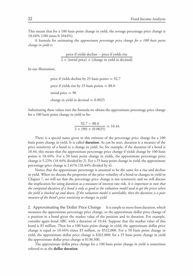
22 Fixed Income Analysis
This means that for a 100 basis point change in yield, the average percentage price change is10.44% (100 times 0.1044%).
A formula for estimating the approximate percentage price change for a 100 basis pointchange in yield is:
price if yields decline − price if yields rise
2 × (initial price) × (change in yield in decimal)
In our illustration,
price if yields decline by 25 basis points = 92.7
price if yields rise by 25 basis points = 88.0
initial price = 90
change in yield in decimal = 0.0025
Substituting these values into the formula we obtain the approximate percentage price changefor a 100 basis point change in yield to be:
92.7 − 88.0
2 × (90) × (0.0025)= 10.44
There is a special name given to this estimate of the percentage price change for a 100basis point change in yield. It is called duration. As can be seen, duration is a measure of theprice sensitivity of a bond to a change in yield. So, for example, if the duration of a bond is10.44, this means that the approximate percentage price change if yields change by 100 basispoints is 10.44%. For a 50 basis point change in yields, the approximate percentage pricechange is 5.22% (10.44% divided by 2). For a 25 basis point change in yield, the approximatepercentage price change is 2.61% (10.44% divided by 4).
Notice that the approximate percentage is assumed to be the same for a rise and declinein yield. When we discuss the properties of the price volatility of a bond to changes in yield inChapter 7, we will see that the percentage price change is not symmetric and we will discussthe implication for using duration as a measure of interest rate risk. It is important to note thatthe computed duration of a bond is only as good as the valuation model used to get the prices whenthe yield is shocked up and down. If the valuation model is unreliable, then the duration is a poormeasure of the bond’s price sensitivity to changes in yield.
2. Approximating the Dollar Price Change It is simple to move from duration, whichmeasures the approximate percentage price change, to the approximate dollar price change ofa position in a bond given the market value of the position and its duration. For example,consider again bond ABC with a duration of 10.44. Suppose that the market value of thisbond is $5 million. Then for a 100 basis point change in yield, the approximate dollar pricechange is equal to 10.44% times $5 million, or $522,000. For a 50 basis point change inyield, the approximate dollar price change is $261,000; for a 25 basis point change in yieldthe approximate dollar price change is $130,500.
The approximate dollar price change for a 100 basis point change in yield is sometimesreferred to as the dollar duration.
Chapter 2 Risks Associated with Investing in Bonds 23
III. YIELD CURVE RISK
We know that if interest rates or yields in the market change, the price of a bond will change.One of the factors that will affect how sensitive a bond’s price is to changes in yield is thebond’s maturity. A portfolio of bonds is a collection of bond issues typically with differentmaturities. So, when interest rates change, the price of each bond issue in the portfolio willchange and the portfolio’s value will change.
As you will see in Chapter 4, there is not one interest rate or yield in the economy. Thereis a structure of interest rates. One important structure is the relationship between yield andmaturity. The graphical depiction of this relationship is called the yield curve. As we will seein Chapter 4, when interest rates change, they typically do not change by an equal number ofbasis points for all maturities.
For example, suppose that a $65 million portfolio contains the four bonds shown inExhibit 1. All bonds are trading at a price equal to par value.
If we want to know how much the value of the portfolio changes if interest rates change,typically it is assumed that all yields change by the same number of basis points. Thus, if wewanted to know how sensitive the portfolio’s value is to a 25 basis point change in yields,we would increase the yield of the four bond issues by 25 basis points, determine the newprice of each bond, the market value of each bond, and the new value of the portfolio. Panel(a) of Exhibit 2 illustrates the 25 basis point increase in yield. For our hypothetical portfolio,the value of each bond issue changes as shown in panel (a) of Exhibit 1. The portfolio’s valuedecreases by $1,759,003 from $65 million to $63,240,997.
Suppose that, instead of an equal basis point change in the yield for all maturities, the20-year yield changes by 25 basis points, but the yields for the other maturities changes asfollows: (1) 2-year maturity changes by 10 basis points (from 5% to 5.1%), (2) 5-year maturitychanges by 20 basis points (from 5.25% to 5.45%), and (3) 30-year maturity changes by 45basis points (from 5.75% to 6.2%). Panel (b) of Exhibit 2 illustrates these yield changes. Wewill see in later chapters that this type of movement (or shift) in the yield curve is referredto as a ‘‘steepening of the yield curve.’’ For this type of yield curve shift, the portfolio’s valueis shown in panel (b) of Exhibit 1. The decline in the portfolio’s value is $2,514,375 (from$65 million to $62,485,625).
Suppose, instead, that if the 20-year yield changes by 25 basis points, the yields for theother three maturities change as follows: (1) 2-year maturity changes by 5 basis points (from5% to 5.05%), (2) 5-year maturity changes by 15 basis points (from 5.25% to 5.40%), and(3) 30-year maturity changes by 35 basis points (from 5.75% to 6.1%). Panel (c) of Exhibit2 illustrates this shift in yields. The new value for the portfolio based on this yield curve shiftis shown in panel (c) of Exhibit 1. The decline in the portfolio’s value is $2,096,926 (from$65 million to $62,903,074). The yield curve shift in the third illustration does not steepenas much as in the second, when the yield curve steepens considerably.
The point here is that portfolios have different exposures to how the yield curve shifts.This risk exposure is called yield curve risk. The implication is that any measure of interestrate risk that assumes that the interest rates changes by an equal number of basis points for allmaturities (referred to as a ‘‘parallel yield curve shift’’) is only an approximation.
This applies to the duration concept that we discussed above. We stated that the durationfor an individual bond is the approximate percentage change in price for a 100 basis pointchange in yield. A duration for a portfolio has the same meaning: it is the approximatepercentage change in the portfolio’s value for a 100 basis point change in the yield for allmaturities.
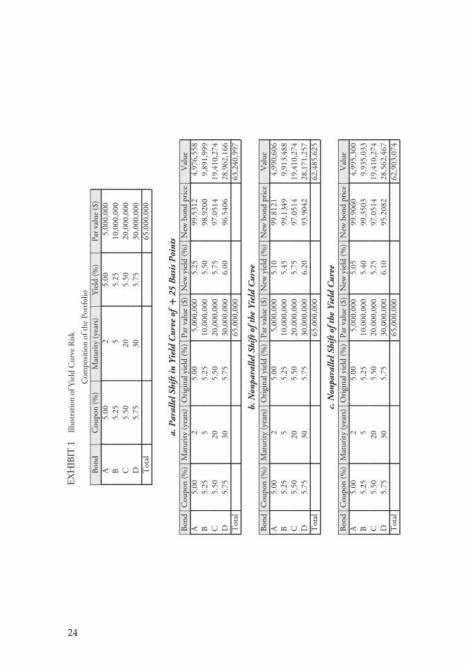
EX
HIB
IT1
Illu
stra
tion
ofY
ield
Cur
veR
isk
Com
posi
tion
ofth
ePo
rtfo
lioB
ond
Cou
pon
(%)
Mat
urit
y(y
ears
)Y
ield
(%)
Par
valu
e($
)A
5.00
25.
005,
000,
000
B5.
255
5.25
10,0
00,0
00C
5.50
205.
5020
,000
,000
D5.
7530
5.75
30,0
00,0
00T
otal
65,0
00,0
00
a.P
aral
lelS
hift
inY
ield
Cur
veof
+25
Bas
isP
oint
sB
ond
Cou
pon
(%)
Mat
urit
y(y
ears
)O
rigi
naly
ield
(%)
Par
valu
e($
)N
ewyi
eld
(%)
New
bond
pric
eV
alue
A5.
002
5.00
5,00
0,00
05.
2599
.531
24,
976,
558
B5.
255
5.25
10,0
00,0
005.
5098
.920
09,
891,
999
C5.
5020
5.50
20,0
00,0
005.
7597
.051
419
,410
,274
D5.
7530
5.75
30,0
00,0
006.
0096
.540
628
,962
,166
Tot
al65
,000
,000
63,2
40,9
97
b.N
onpa
ralle
lShi
ftof
the
Yie
ldC
urve
Bon
dC
oupo
n(%
)M
atur
ity
(yea
rs)
Ori
gina
lyie
ld(%
)Pa
rva
lue
($)
New
yiel
d(%
)N
ewbo
ndpr
ice
Val
ueA
5.00
25.
005,
000,
000
5.10
99.8
121
4,99
0,60
6B
5.25
55.
2510
,000
,000
5.45
99.1
349
9,91
3,48
8C
5.50
205.
5020
,000
,000
5.75
97.0
514
19,4
10,2
74D
5.75
305.
7530
,000
,000
6.20
93.9
042
28,1
71,2
57T
otal
65,0
00,0
0062
,485
,625
c.N
onpa
ralle
lShi
ftof
the
Yie
ldC
urve
Bon
dC
oupo
n(%
)M
atur
ity
(yea
rs)
Ori
gina
lyie
ld(%
)Pa
rva
lue
($)
New
yiel
d(%
)N
ewbo
ndpr
ice
Val
ueA
5.00
25.
005,
000,
000
5.05
99.9
060
4,99
5,30
0B
5.25
55.
2510
,000
,000
5.40
99.3
503
9,93
5,03
3C
5.50
205.
5020
,000
,000
5.75
97.0
514
19,4
10,2
74D
5.75
305.
7530
,000
,000
6.10
95.2
082
28,5
62,4
67T
otal
65,0
00,0
0062
,903
,074
24
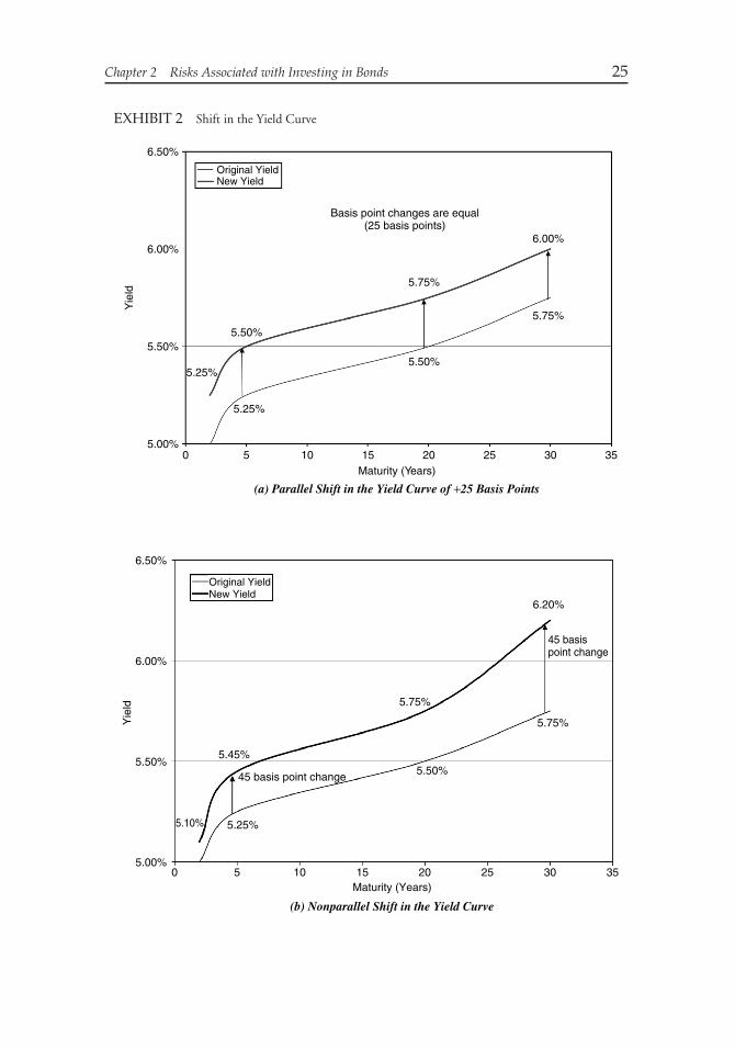
Chapter 2 Risks Associated with Investing in Bonds 25
EXHIBIT 2 Shift in the Yield Curve
6.50%
6.00%6.00%
5.75%
5.75%
5.50%
5.50%
5.25%
5.25%
5.50%
5.00%0 5 10 15 20 25 30 35
Yie
ld
Original Yield
Basis point changes are equal(25 basis points)
New Yield
Maturity (Years)
(a) Parallel Shift in the Yield Curve of +25 Basis Points
Original YieldNew Yield
6.50%
6.00%
5.50%
5.00%
Yie
ld
5.25%
0 5 10 15 20 25 30 35Maturity (Years)
5.45%
5.10%
5.50%
5.75%
5.75%
6.20%
45 basispoint change
45 basis point change
(b) Nonparallel Shift in the Yield Curve
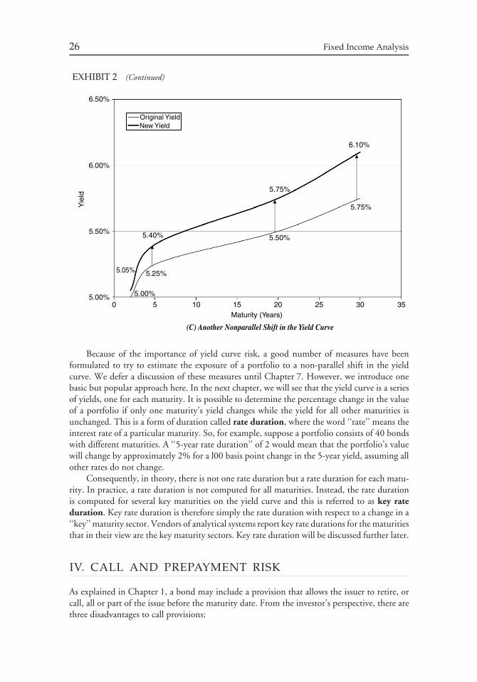
26 Fixed Income Analysis
EXHIBIT 2 (Continued)
6.50%
6.00%
5.75%
5.75%
5.50%
5.25%
5.50%
5.00%0 5 10 15 20 25 30 35
Yie
ld
Original YieldNew Yield
Maturity (Years)
6.10%
5.40%
5.00%
5.05%
(C) Another Nonparallel Shift in the Yield Curve
Because of the importance of yield curve risk, a good number of measures have beenformulated to try to estimate the exposure of a portfolio to a non-parallel shift in the yieldcurve. We defer a discussion of these measures until Chapter 7. However, we introduce onebasic but popular approach here. In the next chapter, we will see that the yield curve is a seriesof yields, one for each maturity. It is possible to determine the percentage change in the valueof a portfolio if only one maturity’s yield changes while the yield for all other maturities isunchanged. This is a form of duration called rate duration, where the word ‘‘rate’’ means theinterest rate of a particular maturity. So, for example, suppose a portfolio consists of 40 bondswith different maturities. A ‘‘5-year rate duration’’ of 2 would mean that the portfolio’s valuewill change by approximately 2% for a l00 basis point change in the 5-year yield, assuming allother rates do not change.
Consequently, in theory, there is not one rate duration but a rate duration for each matu-rity. In practice, a rate duration is not computed for all maturities. Instead, the rate durationis computed for several key maturities on the yield curve and this is referred to as key rateduration. Key rate duration is therefore simply the rate duration with respect to a change in a‘‘key’’ maturity sector. Vendors of analytical systems report key rate durations for the maturitiesthat in their view are the key maturity sectors. Key rate duration will be discussed further later.
IV. CALL AND PREPAYMENT RISK
As explained in Chapter 1, a bond may include a provision that allows the issuer to retire, orcall, all or part of the issue before the maturity date. From the investor’s perspective, there arethree disadvantages to call provisions:
Chapter 2 Risks Associated with Investing in Bonds 27
Disadvantage 1: The cash flow pattern of a callable bond is not known with certainty becauseit is not known when the bond will be called.
Disadvantage 2: Because the issuer is likely to call the bonds when interest rates have declinedbelow the bond’s coupon rate, the investor is exposed to reinvestment risk, i.e., theinvestor will have to reinvest the proceeds when the bond is called at interest rates lowerthan the bond’s coupon rate.
Disadvantage 3: The price appreciation potential of the bond will be reduced relative to anotherwise comparable option-free bond. (This is called price compression.)
We explained the third disadvantage in Section II when we discussed how the price of acallable bond may not rise as much as an otherwise comparable option-free bond when interestrates decline.
Because of these three disadvantages faced by the investor, a callable bond is said to exposethe investor to call risk. The same disadvantages apply to mortgage-backed and asset-backedsecurities where the borrower can prepay principal prior to scheduled principal payment dates.This risk is referred to as prepayment risk.
V. REINVESTMENT RISK
Reinvestment risk is the risk that the proceeds received from the payment of interest andprincipal (i.e., scheduled payments, called proceeds, and principal prepayments) that areavailable for reinvestment must be reinvested at a lower interest rate than the security thatgenerated the proceeds. We already saw how reinvestment risk is present when an investorpurchases a callable or principal prepayable bond. When the issuer calls a bond, it is typicallydone to lower the issuer’s interest expense because interest rates have declined after the bond isissued. The investor faces the problem of having to reinvest the called bond proceeds receivedfrom the issuer in a lower interest rate environment.
Reinvestment risk also occurs when an investor purchases a bond and relies on the yieldof that bond as a measure of return. We have not yet explained how to compute the ‘‘yield’’for a bond. When we do, it will be demonstrated that for the yield computed at the time ofpurchase to be realized, the investor must be able to reinvest any coupon payments at thecomputed yield. So, for example, if an investor purchases a 20-year bond with a yield of 6%,to realize the yield of 6%, every time a coupon interest payment is made, it is necessary toreinvest the payment at an interest rate of at 6% until maturity. So, it is assumed that the firstcoupon payment can be reinvested for the next 19.5 years at 6%; the second coupon paymentcan be reinvested for the next 19 years at 6%, and so on. The risk that the coupon paymentswill be reinvested at less than 6% is also reinvestment risk.
When dealing with amortizing securities (i.e., securities that repay principal periodically),reinvestment risk is even greater. Typically, amortizing securities pay interest and principalmonthly and permit the borrower to prepay principal prior to schedule payment dates. Nowthe investor is more concerned with reinvestment risk due to principal prepayments usuallyresulting from a decline in interest rates, just as in the case of a callable bond. However, sincepayments are monthly, the investor has to make sure that the interest and principal can bereinvested at no less than the computed yield every month as opposed to semiannually.
This reinvestment risk for an amortizing security is important to understand. Too often itis said by some market participants that securities that pay both interest and principal monthly
28 Fixed Income Analysis
are advantageous because the investor has the opportunity to reinvest more frequently andto reinvest a larger amount (because principal is received) relative to a bond that pays onlysemiannual coupon payments. This is not the case in a declining interest rate environment,which will cause borrowers to accelerate their principal prepayments and force the investor toreinvest at lower interest rates.
With an understanding of reinvestment risk, we can now appreciate why zero-couponbonds may be attractive to certain investors. Because there are no coupon payments toreinvest, there is no reinvestment risk. That is, zero-coupon bonds eliminate reinvestment risk.Elimination of reinvestment risk is important to some investors. That’s the plus side of therisk equation. The minus side is that, as explained in Section II, the lower the coupon rate thegreater the interest rate risk for two bonds with the same maturity. Thus, zero-coupon bondsof a given maturity expose investors to the greatest interest rate risk.
Once we cover our basic analytical tools in later chapters, we will see how to quantify abond issue’s reinvestment risk.
VI. CREDIT RISK
An investor who lends funds by purchasing a bond issue is exposed to credit risk. There arethree types of credit risk:
1. default risk2. credit spread risk3. downgrade risk
We discuss each type below.
A. Default Risk
Default risk is defined as the risk that the issuer will fail to satisfy the terms of the obligationwith respect to the timely payment of interest and principal.
Studies have examined the probability of issuers defaulting. The percentage of a populationof bonds that is expected to default is called the default rate. If a default occurs, this does notmean the investor loses the entire amount invested. An investor can expect to recover a certainpercentage of the investment. This is called the recovery rate. Given the default rate and therecovery rate, the estimated expected loss due to a default can be computed. We will explainthe findings of studies on default rates and recovery rates in Chapter 3.
B. Credit Spread Risk
Even in the absence of default, an investor is concerned that the market value of a bond willdecline and/or the price performance of a bond will be worse than that of other bonds. Tounderstand this, recall that the price of a bond changes in the opposite direction to the changein the yield required by the market. Thus, if yields in the economy increase, the price of abond declines, and vice versa.
As we will see in Chapter 3, the yield on a bond is made up of two components: (1) theyield on a similar default-free bond issue and (2) a premium above the yield on a default-freebond issue necessary to compensate for the risks associated with the bond. The risk premium
Chapter 2 Risks Associated with Investing in Bonds 29
is referred to as a yield spread. In the United States, Treasury issues are the benchmarkyields because they are believed to be default free, they are highly liquid, and they are notcallable (with the exception of some old issues). The part of the risk premium or yield spreadattributable to default risk is called the credit spread.
The price performance of a non-Treasury bond issue and the return over some time periodwill depend on how the credit spread changes. If the credit spread increases, investors say thatthe spread has ‘‘widened’’ and the market price of the bond issue will decline (assuming U.S.Treasury rates have not changed). The risk that an issuer’s debt obligation will decline due toan increase in the credit spread is called credit spread risk.
This risk exists for an individual issue, for issues in a particular industry or economicsector, and for all non-Treasury issues in the economy. For example, in general duringeconomic recessions, investors are concerned that issuers will face a decline in cash flows thatwould be used to service their bond obligations. As a result, the credit spread tends to widenfor U.S. non-Treasury issuers and the prices of all such issues throughout the economy willdecline.
C. Downgrade Risk
While portfolio managers seek to allocate funds among different sectors of the bond market tocapitalize on anticipated changes in credit spreads, an analyst investigating the credit qualityof an individual issue is concerned with the prospects of the credit spread increasing for thatparticular issue. But how does the analyst assess whether he or she believes the market willchange the credit spread associated with an individual issue?
One tool investors use to gauge the default risk of an issue is the credit ratings assignedto issues by rating companies, popularly referred to as rating agencies. There are three ratingagencies in the United States: Moody’s Investors Service, Inc., Standard & Poor’s Corporation,and Fitch Ratings.
A credit rating is an indicator of the potential default risk associated with a particularbond issue or issuer. It represents in a simplistic way the credit rating agency’s assessment of anissuer’s ability to meet the payment of principal and interest in accordance with the terms ofthe indenture. Credit rating symbols or characters are uncomplicated representations of morecomplex ideas. In effect, they are summary opinions. Exhibit 3 identifies the ratings assignedby Moody’s, S&P, and Fitch for bonds and the meaning of each rating.
In all systems, the term high grade means low credit risk, or conversely, a high probabilityof receiving future payments is promised by the issuer. The highest-grade bonds are designatedby Moody’s by the symbol Aaa, and by S&P and Fitch by the symbol AAA. The next highestgrade is denoted by the symbol Aa (Moody’s) or AA (S&P and Fitch); for the third grade,all three rating companies use A. The next three grades are Baa or BBB, Ba or BB, and B,respectively. There are also C grades. Moody’s uses 1, 2, or 3 to provide a narrower creditquality breakdown within each class, and S&P and Fitch use plus and minus signs for thesame purpose.
Bonds rated triple A (AAA or Aaa) are said to be prime grade; double A (AA or Aa)are of high quality grade; single A issues are called upper medium grade, and triple B arelower medium grade. Lower-rated bonds are said to have speculative grade elements or tobe distinctly speculative grade.
Bond issues that are assigned a rating in the top four categories (that is, AAA, AA, A,and BBB) are referred to as investment-grade bonds. Issues that carry a rating below thetop four categories are referred to as non-investment-grade bonds or speculative bonds, or
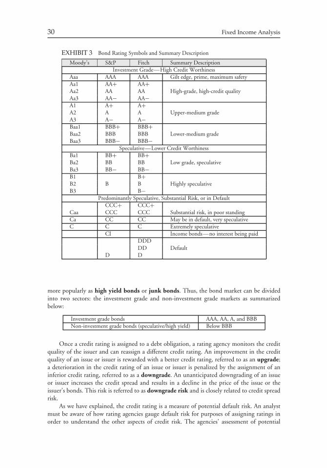
30 Fixed Income Analysis
EXHIBIT 3 Bond Rating Symbols and Summary Description
Moody’s S&P Fitch Summary DescriptionInvestment Grade—High Credit Worthiness
Aaa AAA AAA Gilt edge, prime, maximum safetyAa1 AA+ AA+Aa2 AA AA High-grade, high-credit qualityAa3 AA− AA−A1 A+ A+A2 A A Upper-medium gradeA3 A− A−Baa1 BBB+ BBB+Baa2 BBB BBB Lower-medium gradeBaa3 BBB− BBB−
Speculative—Lower Credit WorthinessBa1 BB+ BB+Ba2 BB BB Low grade, speculativeBa3 BB− BB−B1 B+B2 B B Highly speculativeB3 B−
Predominantly Speculative, Substantial Risk, or in DefaultCCC+ CCC+
Caa CCC CCC Substantial risk, in poor standingCa CC CC May be in default, very speculativeC C C Extremely speculative
CI Income bonds—no interest being paidDDDDD Default
D D
more popularly as high yield bonds or junk bonds. Thus, the bond market can be dividedinto two sectors: the investment grade and non-investment grade markets as summarizedbelow:
Investment grade bonds AAA, AA, A, and BBBNon-investment grade bonds (speculative/high yield) Below BBB
Once a credit rating is assigned to a debt obligation, a rating agency monitors the creditquality of the issuer and can reassign a different credit rating. An improvement in the creditquality of an issue or issuer is rewarded with a better credit rating, referred to as an upgrade;a deterioration in the credit rating of an issue or issuer is penalized by the assignment of aninferior credit rating, referred to as a downgrade. An unanticipated downgrading of an issueor issuer increases the credit spread and results in a decline in the price of the issue or theissuer’s bonds. This risk is referred to as downgrade risk and is closely related to credit spreadrisk.
As we have explained, the credit rating is a measure of potential default risk. An analystmust be aware of how rating agencies gauge default risk for purposes of assigning ratings inorder to understand the other aspects of credit risk. The agencies’ assessment of potential
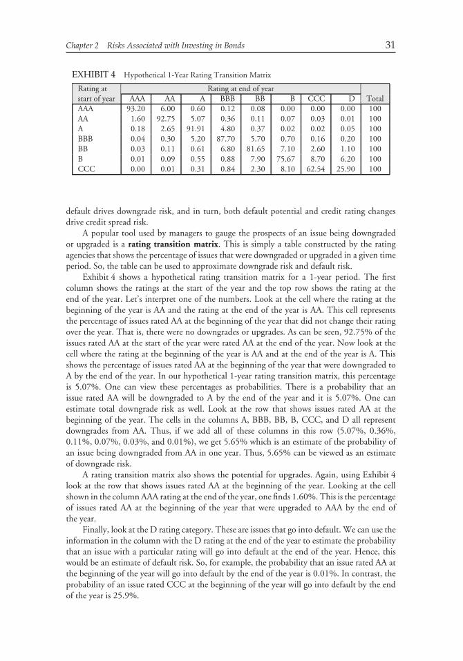
Chapter 2 Risks Associated with Investing in Bonds 31
EXHIBIT 4 Hypothetical 1-Year Rating Transition Matrix
Rating at Rating at end of yearstart of year AAA AA A BBB BB B CCC D TotalAAA 93.20 6.00 0.60 0.12 0.08 0.00 0.00 0.00 100AA 1.60 92.75 5.07 0.36 0.11 0.07 0.03 0.01 100A 0.18 2.65 91.91 4.80 0.37 0.02 0.02 0.05 100BBB 0.04 0.30 5.20 87.70 5.70 0.70 0.16 0.20 100BB 0.03 0.11 0.61 6.80 81.65 7.10 2.60 1.10 100B 0.01 0.09 0.55 0.88 7.90 75.67 8.70 6.20 100CCC 0.00 0.01 0.31 0.84 2.30 8.10 62.54 25.90 100
default drives downgrade risk, and in turn, both default potential and credit rating changesdrive credit spread risk.
A popular tool used by managers to gauge the prospects of an issue being downgradedor upgraded is a rating transition matrix. This is simply a table constructed by the ratingagencies that shows the percentage of issues that were downgraded or upgraded in a given timeperiod. So, the table can be used to approximate downgrade risk and default risk.
Exhibit 4 shows a hypothetical rating transition matrix for a 1-year period. The firstcolumn shows the ratings at the start of the year and the top row shows the rating at theend of the year. Let’s interpret one of the numbers. Look at the cell where the rating at thebeginning of the year is AA and the rating at the end of the year is AA. This cell representsthe percentage of issues rated AA at the beginning of the year that did not change their ratingover the year. That is, there were no downgrades or upgrades. As can be seen, 92.75% of theissues rated AA at the start of the year were rated AA at the end of the year. Now look at thecell where the rating at the beginning of the year is AA and at the end of the year is A. Thisshows the percentage of issues rated AA at the beginning of the year that were downgraded toA by the end of the year. In our hypothetical 1-year rating transition matrix, this percentageis 5.07%. One can view these percentages as probabilities. There is a probability that anissue rated AA will be downgraded to A by the end of the year and it is 5.07%. One canestimate total downgrade risk as well. Look at the row that shows issues rated AA at thebeginning of the year. The cells in the columns A, BBB, BB, B, CCC, and D all representdowngrades from AA. Thus, if we add all of these columns in this row (5.07%, 0.36%,0.11%, 0.07%, 0.03%, and 0.01%), we get 5.65% which is an estimate of the probability ofan issue being downgraded from AA in one year. Thus, 5.65% can be viewed as an estimateof downgrade risk.
A rating transition matrix also shows the potential for upgrades. Again, using Exhibit 4look at the row that shows issues rated AA at the beginning of the year. Looking at the cellshown in the column AAA rating at the end of the year, one finds 1.60%. This is the percentageof issues rated AA at the beginning of the year that were upgraded to AAA by the end ofthe year.
Finally, look at the D rating category. These are issues that go into default. We can use theinformation in the column with the D rating at the end of the year to estimate the probabilitythat an issue with a particular rating will go into default at the end of the year. Hence, thiswould be an estimate of default risk. So, for example, the probability that an issue rated AA atthe beginning of the year will go into default by the end of the year is 0.01%. In contrast, theprobability of an issue rated CCC at the beginning of the year will go into default by the endof the year is 25.9%.
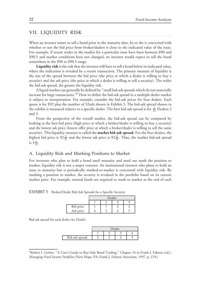
32 Fixed Income Analysis
VII. LIQUIDITY RISK
When an investor wants to sell a bond prior to the maturity date, he or she is concerned withwhether or not the bid price from broker/dealers is close to the indicated value of the issue.For example, if recent trades in the market for a particular issue have been between $90 and$90.5 and market conditions have not changed, an investor would expect to sell the bondsomewhere in the $90 to $90.5 range.
Liquidity risk is the risk that the investor will have to sell a bond below its indicated value,where the indication is revealed by a recent transaction. The primary measure of liquidity isthe size of the spread between the bid price (the price at which a dealer is willing to buy asecurity) and the ask price (the price at which a dealer is willing to sell a security). The widerthe bid-ask spread, the greater the liquidity risk.
A liquid market can generally be defined by ‘‘small bid-ask spreads which do not materiallyincrease for large transactions.’’6 How to define the bid-ask spread in a multiple dealer marketis subject to interpretation. For example, consider the bid-ask prices for four dealers. Eachquote is for $92 plus the number of 32nds shown in Exhibit 5. The bid-ask spread shown inthe exhibit is measured relative to a specific dealer. The best bid-ask spread is for 2
32 Dealers 2and 3.
From the perspective of the overall market, the bid-ask spread can be computed bylooking at the best bid price (high price at which a broker/dealer is willing to buy a security)and the lowest ask price (lowest offer price at which a broker/dealer is willing to sell the samesecurity). This liquidity measure is called the market bid-ask spread. For the four dealers, thehighest bid price is 92 2
32 and the lowest ask price is 92 232 . Thus, the market bid-ask spread
is 3 132 .
A. Liquidity Risk and Marking Positions to Market
For investors who plan to hold a bond until maturity and need not mark the position tomarket, liquidity risk is not a major concern. An institutional investor who plans to hold anissue to maturity but is periodically marked-to-market is concerned with liquidity risk. Bymarking a position to market, the security is revalued in the portfolio based on its currentmarket price. For example, mutual funds are required to mark to market at the end of each
EXHIBIT 5 Broker/Dealer Bid-Ask Spreads for a Specific Security
Dealer1 2 3 4
Bid price 1 1 2 2Ask price 4 3 4 5
Bid-ask spread for each dealer (in 32nds):
Dealer1 2 3 4
Bid-ask spread 3 2 2 3
6Robert I. Gerber, ‘‘A User’s Guide to Buy-Side Bond Trading,’’ Chapter 16 in Frank J. Fabozzi (ed.),Managing Fixed Income Portfolios (New Hope, PA: Frank J. Fabozzi Associates, 1997, p. 278.)
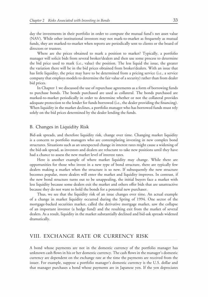
Chapter 2 Risks Associated with Investing in Bonds 33
day the investments in their portfolio in order to compute the mutual fund’s net asset value(NAV). While other institutional investors may not mark-to-market as frequently as mutualfunds, they are marked-to-market when reports are periodically sent to clients or the board ofdirectors or trustees.
Where are the prices obtained to mark a position to market? Typically, a portfoliomanager will solicit bids from several broker/dealers and then use some process to determinethe bid price used to mark (i.e., value) the position. The less liquid the issue, the greaterthe variation there will be in the bid prices obtained from broker/dealers. With an issue thathas little liquidity, the price may have to be determined from a pricing service (i.e., a servicecompany that employs models to determine the fair value of a security) rather than from dealerbid prices.
In Chapter 1 we discussed the use of repurchase agreements as a form of borrowing fundsto purchase bonds. The bonds purchased are used as collateral. The bonds purchased aremarked-to-market periodically in order to determine whether or not the collateral providesadequate protection to the lender for funds borrowed (i.e., the dealer providing the financing).When liquidity in the market declines, a portfolio manager who has borrowed funds must relysolely on the bid prices determined by the dealer lending the funds.
B. Changes in Liquidity Risk
Bid-ask spreads, and therefore liquidity risk, change over time. Changing market liquidityis a concern to portfolio managers who are contemplating investing in new complex bondstructures. Situations such as an unexpected change in interest rates might cause a widening ofthe bid-ask spread, as investors and dealers are reluctant to take new positions until they havehad a chance to assess the new market level of interest rates.
Here is another example of where market liquidity may change. While there areopportunities for those who invest in a new type of bond structure, there are typically fewdealers making a market when the structure is so new. If subsequently the new structurebecomes popular, more dealers will enter the market and liquidity improves. In contrast, ifthe new bond structure turns out to be unappealing, the initial buyers face a market withless liquidity because some dealers exit the market and others offer bids that are unattractivebecause they do not want to hold the bonds for a potential new purchaser.
Thus, we see that the liquidity risk of an issue changes over time. An actual exampleof a change in market liquidity occurred during the Spring of 1994. One sector of themortgage-backed securities market, called the derivative mortgage market, saw the collapseof an important investor (a hedge fund) and the resulting exit from the market of severaldealers. As a result, liquidity in the market substantially declined and bid-ask spreads wideneddramatically.
VIII. EXCHANGE RATE OR CURRENCY RISK
A bond whose payments are not in the domestic currency of the portfolio manager hasunknown cash flows in his or her domestic currency. The cash flows in the manager’s domesticcurrency are dependent on the exchange rate at the time the payments are received from theissuer. For example, suppose a portfolio manager’s domestic currency is the U.S. dollar andthat manager purchases a bond whose payments are in Japanese yen. If the yen depreciates
34 Fixed Income Analysis
relative to the U.S. dollar at the time a payment is made, then fewer U.S. dollars can beexchanged.
As another example, consider a portfolio manager in the United Kingdom. This manager’sdomestic currency is the pound. If that manager purchases a U.S. dollar denominated bond,then the manager is concerned that the U.S. dollar will depreciate relative to the British poundwhen the issuer makes a payment. If the U.S. dollar does depreciate, then fewer British poundswill be received on the foreign exchange market.
The risk of receiving less of the domestic currency when investing in a bond issue thatmakes payments in a currency other than the manager’s domestic currency is called exchangerate risk or currency risk.
IX. INFLATION OR PURCHASING POWER RISK
Inflation risk or purchasing power risk arises from the decline in the value of a security’scash flows due to inflation, which is measured in terms of purchasing power. For example,if an investor purchases a bond with a coupon rate of 5%, but the inflation rate is 3%, thepurchasing power of the investor has not increased by 5%. Instead, the investor’s purchasingpower has increased by only about 2%.
For all but inflation protection bonds, an investor is exposed to inflation risk because theinterest rate the issuer promises to make is fixed for the life of the issue.
X. VOLATILITY RISK
In our discussion of the impact of embedded options on the interest rate risk of a bond inSection II, we said that a change in the factors that affect the value of the embedded optionswill affect how the bond’s price will change. Earlier, we looked at how a change in the levelof interest rates will affect the price of a bond with an embedded option. But there are otherfactors that will affect the price of an embedded option.
While we discuss these other factors later, we can get an appreciation of one importantfactor from a general understanding of option pricing. A major factor affecting the valueof an option is ‘‘expected volatility.’’ In the case of an option on common stock, expectedvolatility refers to ‘‘expected price volatility.’’ The relationship is as follows: the greater theexpected price volatility, the greater the value of the option. The same relationship holds foroptions on bonds. However, instead of expected price volatility, for bonds it is the ‘‘expectedyield volatility.’’ The greater the expected yield volatility, the greater the value (price) ofan option. The interpretation of yield volatility and how it is estimated are explained at inChapter 8.
Now let us tie this into the pricing of a callable bond. We repeat the formula for thecomponents of a callable bond below:
Price of callable bond = Price of option-free bond − Price of embedded call option
If expected yield volatility increases, holding all other factors constant, the price of theembedded call option will increase. As a result, the price of a callable bond will decrease(because the former is subtracted from the price of the option-free bond).
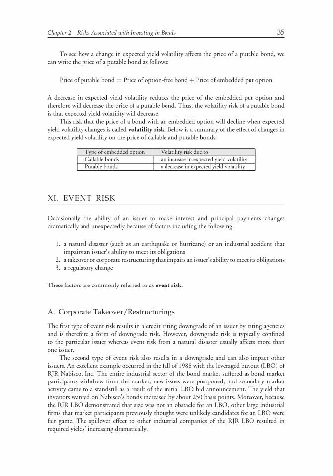
Chapter 2 Risks Associated with Investing in Bonds 35
To see how a change in expected yield volatility affects the price of a putable bond, wecan write the price of a putable bond as follows:
Price of putable bond = Price of option-free bond + Price of embedded put option
A decrease in expected yield volatility reduces the price of the embedded put option andtherefore will decrease the price of a putable bond. Thus, the volatility risk of a putable bondis that expected yield volatility will decrease.
This risk that the price of a bond with an embedded option will decline when expectedyield volatility changes is called volatility risk. Below is a summary of the effect of changes inexpected yield volatility on the price of callable and putable bonds:
Type of embedded option Volatility risk due toCallable bonds an increase in expected yield volatilityPutable bonds a decrease in expected yield volatility
XI. EVENT RISK
Occasionally the ability of an issuer to make interest and principal payments changesdramatically and unexpectedly because of factors including the following:
1. a natural disaster (such as an earthquake or hurricane) or an industrial accident thatimpairs an issuer’s ability to meet its obligations
2. a takeover or corporate restructuring that impairs an issuer’s ability to meet its obligations3. a regulatory change
These factors are commonly referred to as event risk.
A. Corporate Takeover/Restructurings
The first type of event risk results in a credit rating downgrade of an issuer by rating agenciesand is therefore a form of downgrade risk. However, downgrade risk is typically confinedto the particular issuer whereas event risk from a natural disaster usually affects more thanone issuer.
The second type of event risk also results in a downgrade and can also impact otherissuers. An excellent example occurred in the fall of 1988 with the leveraged buyout (LBO) ofRJR Nabisco, Inc. The entire industrial sector of the bond market suffered as bond marketparticipants withdrew from the market, new issues were postponed, and secondary marketactivity came to a standstill as a result of the initial LBO bid announcement. The yield thatinvestors wanted on Nabisco’s bonds increased by about 250 basis points. Moreover, becausethe RJR LBO demonstrated that size was not an obstacle for an LBO, other large industrialfirms that market participants previously thought were unlikely candidates for an LBO werefair game. The spillover effect to other industrial companies of the RJR LBO resulted inrequired yields’ increasing dramatically.

36 Fixed Income Analysis
B. Regulatory Risk
The third type of risk listed above is regulatory risk. This risk comes in a variety of forms.Regulated entities include investment companies, depository institutions, and insurancecompanies. Pension funds are regulated by ERISA. Regulation of these entities is in terms ofthe acceptable securities in which they may invest and/or the treatment of the securities forregulatory accounting purposes.
Changes in regulations may require a regulated entity to divest itself from certain types ofinvestments. A flood of the divested securities on the market will adversely impact the price ofsimilar securities.
XII. SOVEREIGN RISK
When an investor acquires a bond issued by a foreign entity (e.g., a French investor acquiringa Brazilian government bond), the investor faces sovereign risk. This is the risk that, as aresult of actions of the foreign government, there may be either a default or an adverse pricechange even in the absence of a default. This is analogous to the forms of credit risk describedin Section VI—credit risk spread and downgrade risk. That is, even if a foreign governmentdoes not default, actions by a foreign government can increase the credit risk spread sought byinvestors or increase the likelihood of a downgrade. Both of these will have an adverse impacton a bond’s price.
Sovereign risk consists of two parts. First is the unwillingness of a foreign government topay. A foreign government may simply repudiate its debt. The second is the inability to paydue to unfavorable economic conditions in the country. Historically, most foreign governmentdefaults have been due to a government’s inability to pay rather than unwillingness to pay.

CHAPTER 3OVERVIEW OF BOND
SECTORS ANDINSTRUMENTS
I. INTRODUCTION
Thus far we have covered the general features of bonds and the risks associated with investingin bonds. In this chapter, we will review the major sectors of a country’s bond marketand the securities issued. This includes sovereign bonds, semi-government bonds, municipalor province securities, corporate debt securities, mortgage-backed securities, asset-backedsecurities, and collateralized debt obligations. Our coverage in this chapter is to describe theinstruments found in these sectors.
II. SECTORS OF THE BOND MARKET
While there is no uniform system for classifying the sectors of the bond markets throughoutthe world, we will use the classification shown in Exhibit 1. From the perspective of a givencountry, the bond market can be classified into two markets: an internal bond market andan external bond market.
A. Internal Bond Market
The internal bond market of a country is also called the national bond market. It is dividedinto two parts: the domestic bond market and the foreign bond market. The domesticbond market is where issuers domiciled in the country issue bonds and where those bonds aresubsequently traded.
The foreign bond market of a country is where bonds of issuers not domiciled in thecountry are issued and traded. For example, in the United States. the foreign bond marketis the market where bonds are issued by non–U.S. entities and then subsequently traded inthe United States. In the U.K., a sterling-denominated bond issued by a Japanese corporationand subsequently traded in the U.K. bond market is part of the U.K. foreign bond market.Bonds in the foreign sector of a bond market have nicknames. For example, foreign bonds inthe U.S. market are nicknamed ‘‘Yankee bonds’’ and sterling-denominated bonds in the U.K.foreign bond market are nicknamed ‘‘Bulldog bonds.’’ Foreign bonds can be denominated in
37
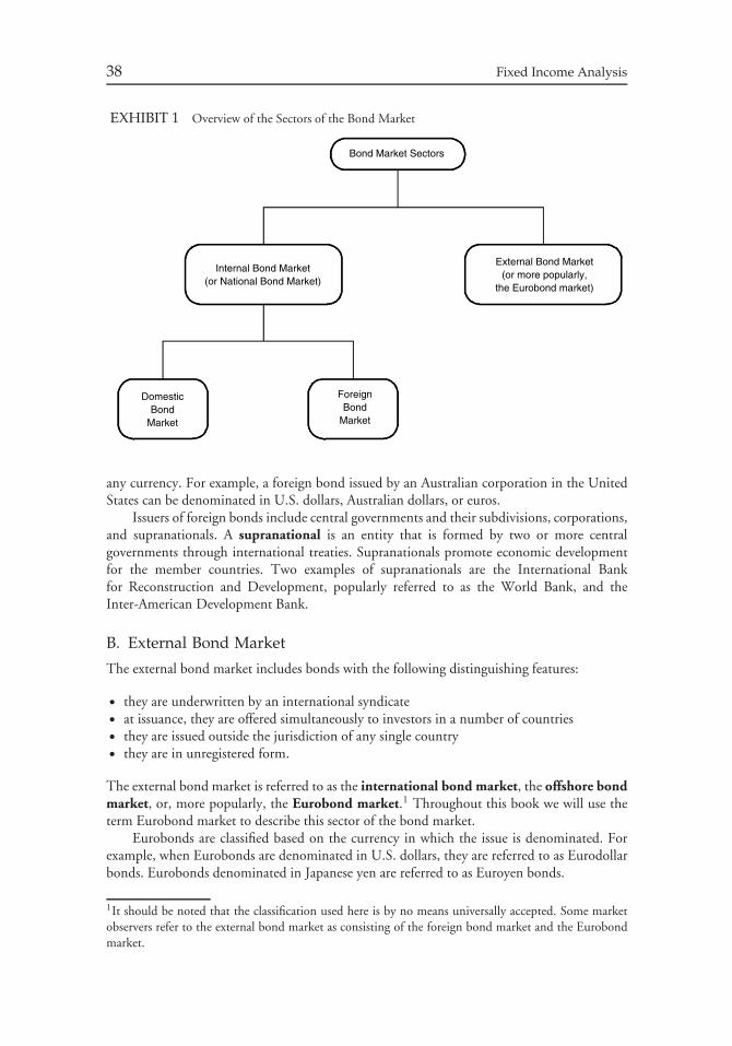
38 Fixed Income Analysis
EXHIBIT 1 Overview of the Sectors of the Bond Market
DomesticBond
Market
ForeignBond
Market
Bond Market Sectors
Internal Bond Market(or National Bond Market)
External Bond Market(or more popularly,
the Eurobond market)
any currency. For example, a foreign bond issued by an Australian corporation in the UnitedStates can be denominated in U.S. dollars, Australian dollars, or euros.
Issuers of foreign bonds include central governments and their subdivisions, corporations,and supranationals. A supranational is an entity that is formed by two or more centralgovernments through international treaties. Supranationals promote economic developmentfor the member countries. Two examples of supranationals are the International Bankfor Reconstruction and Development, popularly referred to as the World Bank, and theInter-American Development Bank.
B. External Bond Market
The external bond market includes bonds with the following distinguishing features:
• they are underwritten by an international syndicate• at issuance, they are offered simultaneously to investors in a number of countries• they are issued outside the jurisdiction of any single country• they are in unregistered form.
The external bond market is referred to as the international bond market, the offshore bondmarket, or, more popularly, the Eurobond market.1 Throughout this book we will use theterm Eurobond market to describe this sector of the bond market.
Eurobonds are classified based on the currency in which the issue is denominated. Forexample, when Eurobonds are denominated in U.S. dollars, they are referred to as Eurodollarbonds. Eurobonds denominated in Japanese yen are referred to as Euroyen bonds.
1It should be noted that the classification used here is by no means universally accepted. Some marketobservers refer to the external bond market as consisting of the foreign bond market and the Eurobondmarket.
Chapter 3 Overview of Bond Sectors and Instruments 39
A global bond is a debt obligation that is issued and traded in the foreign bond marketof one or more countries and the Eurobond market.
III. SOVEREIGN BONDS
In many countries that have a bond market, the largest sector is often bonds issued by acountry’s central government. These bonds are referred to as sovereign bonds. A governmentcan issue securities in its national bond market which are subsequently traded within thatmarket. A government can also issue bonds in the Eurobond market or the foreign sector ofanother country’s bond market. While the currency denomination of a government security istypically the currency of the issuing country, a government can issue bonds denominated inany currency.
A. Credit Risk
An investor in any bond is exposed to credit risk. The perception throughout the worldis that the credit risk of bonds issued by the U.S. government are virtually free of creditrisk. Consequently, the market views these bonds as default-free bonds. Sovereign bonds ofnon-U.S. central governments are rated by the credit rating agencies. These ratings are referredto as sovereign ratings. Standard & Poor’s and Moody’s rate sovereign debt. We will discussthe factors considered in rating sovereign bonds later.
The rating agencies assign two types of ratings to sovereign debt. One is a local currencydebt rating and the other a foreign currency debt rating. The reason for assigning tworatings is, historically, the default frequency differs by the currency denomination of the debt.Specifically, defaults have been greater on foreign currency denominated debt. The reason forthe difference in default rates for local currency debt and foreign currency debt is that if agovernment is willing to raise taxes and control its domestic financial system, it can generatesufficient local currency to meet its local currency debt obligation. This is not the case withforeign currency denominated debt. A central government must purchase foreign currency tomeet a debt obligation in that foreign currency and therefore has less control with respect toits exchange rate. Thus, a significant depreciation of the local currency relative to a foreigncurrency denominated debt obligation will impair a central government’s ability to satisfy thatobligation.
B. Methods of Distributing New Government Securities
Four methods have been used by central governments to distribute new bonds that theyissue: (1) regular auction cycle/multiple-price method, (2) regular auction cycle/single-pricemethod, (3) ad hoc auction method, and (4) tap method.
With the regular auction cycle/multiple-price method, there is a regular auction cycleand winning bidders are allocated securities at the yield (price) they bid. For the regularauction cycle/single-price method, there is a regular auction cycle and all winning biddersare awarded securities at the highest yield accepted by the government. For example, if thehighest yield for a single-price auction is 7.14% and someone bid 7.12%, that bidder would beawarded the securities at 7.14%. In contrast, with a multiple-price auction that bidder wouldbe awarded securities at 7.12%. U.S. government bonds are currently issued using a regularauction cycle/single-price method.
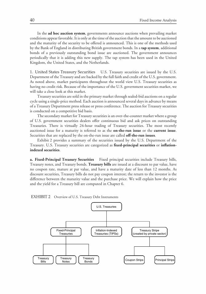
40 Fixed Income Analysis
In the ad hoc auction system, governments announce auctions when prevailing marketconditions appear favorable. It is only at the time of the auction that the amount to be auctionedand the maturity of the security to be offered is announced. This is one of the methods usedby the Bank of England in distributing British government bonds. In a tap system, additionalbonds of a previously outstanding bond issue are auctioned. The government announcesperiodically that it is adding this new supply. The tap system has been used in the UnitedKingdom, the United States, and the Netherlands.
1. United States Treasury Securities U.S. Treasury securities are issued by the U.S.Department of the Treasury and are backed by the full faith and credit of the U.S. government.As noted above, market participants throughout the world view U.S. Treasury securities ashaving no credit risk. Because of the importance of the U.S. government securities market, wewill take a close look at this market.
Treasury securities are sold in the primary market through sealed-bid auctions on a regularcycle using a single-price method. Each auction is announced several days in advance by meansof a Treasury Department press release or press conference. The auction for Treasury securitiesis conducted on a competitive bid basis.
The secondary market for Treasury securities is an over-the-counter market where a groupof U.S. government securities dealers offer continuous bid and ask prices on outstandingTreasuries. There is virtually 24-hour trading of Treasury securities. The most recentlyauctioned issue for a maturity is referred to as the on-the-run issue or the current issue.Securities that are replaced by the on-the-run issue are called off-the-run issues.
Exhibit 2 provides a summary of the securities issued by the U.S. Department of theTreasury. U.S. Treasury securities are categorized as fixed-principal securities or inflation-indexed securities.
a. Fixed-Principal Treasury Securities Fixed principal securities include Treasury bills,Treasury notes, and Treasury bonds. Treasury bills are issued at a discount to par value, haveno coupon rate, mature at par value, and have a maturity date of less than 12 months. Asdiscount securities, Treasury bills do not pay coupon interest; the return to the investor is thedifference between the maturity value and the purchase price. We will explain how the priceand the yield for a Treasury bill are computed in Chapter 6.
EXHIBIT 2 Overview of U.S. Treasury Debt Instruments
U.S. Treasuries
Fixed-PrincipalTreasuries
TreasuryBills
TreasuryNotes
TreasuryBonds
Inflation-IndexedTreasuries (TIPSs)
Treasury Stripe(created by private sector)
Coupon Strips Principal Strips
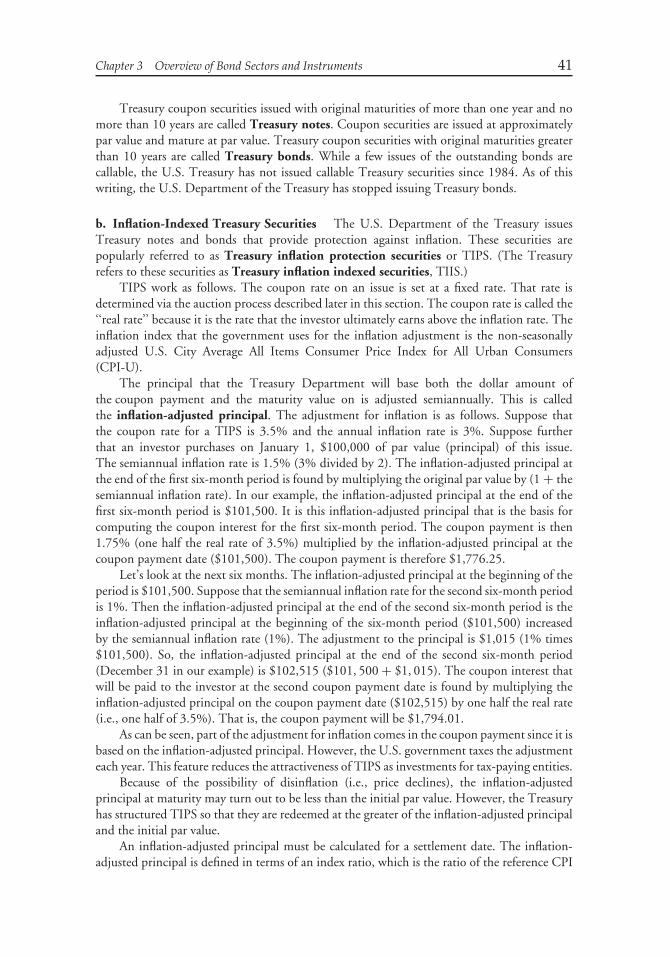
Chapter 3 Overview of Bond Sectors and Instruments 41
Treasury coupon securities issued with original maturities of more than one year and nomore than 10 years are called Treasury notes. Coupon securities are issued at approximatelypar value and mature at par value. Treasury coupon securities with original maturities greaterthan 10 years are called Treasury bonds. While a few issues of the outstanding bonds arecallable, the U.S. Treasury has not issued callable Treasury securities since 1984. As of thiswriting, the U.S. Department of the Treasury has stopped issuing Treasury bonds.
b. Inflation-Indexed Treasury Securities The U.S. Department of the Treasury issuesTreasury notes and bonds that provide protection against inflation. These securities arepopularly referred to as Treasury inflation protection securities or TIPS. (The Treasuryrefers to these securities as Treasury inflation indexed securities, TIIS.)
TIPS work as follows. The coupon rate on an issue is set at a fixed rate. That rate isdetermined via the auction process described later in this section. The coupon rate is called the‘‘real rate’’ because it is the rate that the investor ultimately earns above the inflation rate. Theinflation index that the government uses for the inflation adjustment is the non-seasonallyadjusted U.S. City Average All Items Consumer Price Index for All Urban Consumers(CPI-U).
The principal that the Treasury Department will base both the dollar amount ofthe coupon payment and the maturity value on is adjusted semiannually. This is calledthe inflation-adjusted principal. The adjustment for inflation is as follows. Suppose thatthe coupon rate for a TIPS is 3.5% and the annual inflation rate is 3%. Suppose furtherthat an investor purchases on January 1, $100,000 of par value (principal) of this issue.The semiannual inflation rate is 1.5% (3% divided by 2). The inflation-adjusted principal atthe end of the first six-month period is found by multiplying the original par value by (1 + thesemiannual inflation rate). In our example, the inflation-adjusted principal at the end of thefirst six-month period is $101,500. It is this inflation-adjusted principal that is the basis forcomputing the coupon interest for the first six-month period. The coupon payment is then1.75% (one half the real rate of 3.5%) multiplied by the inflation-adjusted principal at thecoupon payment date ($101,500). The coupon payment is therefore $1,776.25.
Let’s look at the next six months. The inflation-adjusted principal at the beginning of theperiod is $101,500. Suppose that the semiannual inflation rate for the second six-month periodis 1%. Then the inflation-adjusted principal at the end of the second six-month period is theinflation-adjusted principal at the beginning of the six-month period ($101,500) increasedby the semiannual inflation rate (1%). The adjustment to the principal is $1,015 (1% times$101,500). So, the inflation-adjusted principal at the end of the second six-month period(December 31 in our example) is $102,515 ($101, 500 + $1, 015). The coupon interest thatwill be paid to the investor at the second coupon payment date is found by multiplying theinflation-adjusted principal on the coupon payment date ($102,515) by one half the real rate(i.e., one half of 3.5%). That is, the coupon payment will be $1,794.01.
As can be seen, part of the adjustment for inflation comes in the coupon payment since it isbased on the inflation-adjusted principal. However, the U.S. government taxes the adjustmenteach year. This feature reduces the attractiveness of TIPS as investments for tax-paying entities.
Because of the possibility of disinflation (i.e., price declines), the inflation-adjustedprincipal at maturity may turn out to be less than the initial par value. However, the Treasuryhas structured TIPS so that they are redeemed at the greater of the inflation-adjusted principaland the initial par value.
An inflation-adjusted principal must be calculated for a settlement date. The inflation-adjusted principal is defined in terms of an index ratio, which is the ratio of the reference CPI
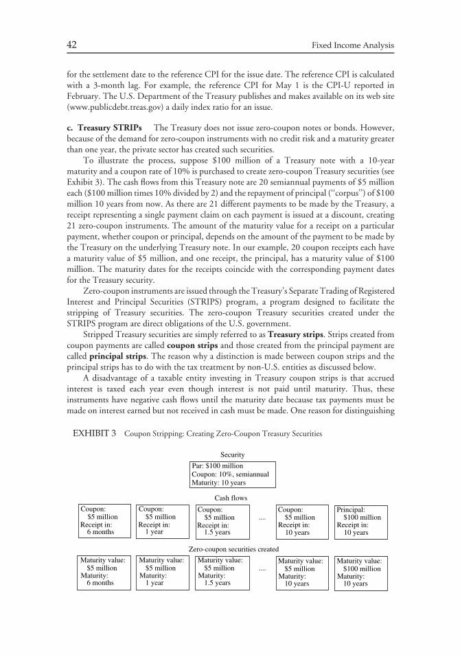
42 Fixed Income Analysis
for the settlement date to the reference CPI for the issue date. The reference CPI is calculatedwith a 3-month lag. For example, the reference CPI for May 1 is the CPI-U reported inFebruary. The U.S. Department of the Treasury publishes and makes available on its web site(www.publicdebt.treas.gov) a daily index ratio for an issue.
c. Treasury STRIPs The Treasury does not issue zero-coupon notes or bonds. However,because of the demand for zero-coupon instruments with no credit risk and a maturity greaterthan one year, the private sector has created such securities.
To illustrate the process, suppose $100 million of a Treasury note with a 10-yearmaturity and a coupon rate of 10% is purchased to create zero-coupon Treasury securities (seeExhibit 3). The cash flows from this Treasury note are 20 semiannual payments of $5 millioneach ($100 million times 10% divided by 2) and the repayment of principal (‘‘corpus’’) of $100million 10 years from now. As there are 21 different payments to be made by the Treasury, areceipt representing a single payment claim on each payment is issued at a discount, creating21 zero-coupon instruments. The amount of the maturity value for a receipt on a particularpayment, whether coupon or principal, depends on the amount of the payment to be made bythe Treasury on the underlying Treasury note. In our example, 20 coupon receipts each havea maturity value of $5 million, and one receipt, the principal, has a maturity value of $100million. The maturity dates for the receipts coincide with the corresponding payment datesfor the Treasury security.
Zero-coupon instruments are issued through the Treasury’s Separate Trading of RegisteredInterest and Principal Securities (STRIPS) program, a program designed to facilitate thestripping of Treasury securities. The zero-coupon Treasury securities created under theSTRIPS program are direct obligations of the U.S. government.
Stripped Treasury securities are simply referred to as Treasury strips. Strips created fromcoupon payments are called coupon strips and those created from the principal payment arecalled principal strips. The reason why a distinction is made between coupon strips and theprincipal strips has to do with the tax treatment by non-U.S. entities as discussed below.
A disadvantage of a taxable entity investing in Treasury coupon strips is that accruedinterest is taxed each year even though interest is not paid until maturity. Thus, theseinstruments have negative cash flows until the maturity date because tax payments must bemade on interest earned but not received in cash must be made. One reason for distinguishing
EXHIBIT 3 Coupon Stripping: Creating Zero-Coupon Treasury Securities
Security
Cash flows
....
....
Coupon:$5 million
Receipt in:
Coupon:$5 million
Receipt in:1 year
Coupon:$5 million
Receipt in:1.5 years
Coupon:$5 million
Receipt in:10 years
Principal:$100 million
Receipt in:10 years
Zero-coupon securities created
Maturity value:$5 million
Maturity:6 months
Maturity value:$5 million
Maturity:1 year
Maturity value:$5 million
Maturity:1.5 years
Maturity value:$5 million
Maturity:10 years
Maturity value:$100 million
Maturity:10 years
Par: $100 million
Maturity: 10 yearsCoupon: 10%, semiannual
6 months
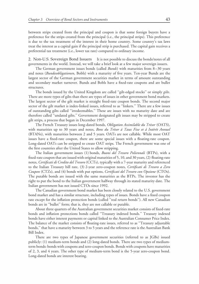
Chapter 3 Overview of Bond Sectors and Instruments 43
between strips created from the principal and coupon is that some foreign buyers have apreference for the strips created from the principal (i.e., the principal strips). This preferenceis due to the tax treatment of the interest in their home country. Some country’s tax lawstreat the interest as a capital gain if the principal strip is purchased. The capital gain receives apreferential tax treatment (i.e., lower tax rate) compared to ordinary income.
2. Non-U.S. Sovereign Bond Issuers It is not possible to discuss the bonds/notes of allgovernments in the world. Instead, we will take a brief look at a few major sovereign issuers.
The German government issues bonds (called Bunds) with maturities from 8–30 yearsand notes (Bundesobligationen, Bobls) with a maturity of five years. Ten-year Bunds are thelargest sector of the German government securities market in terms of amount outstandingand secondary market turnover. Bunds and Bobls have a fixed-rate coupons and are bulletstructures.
The bonds issued by the United Kingdom are called ‘‘gilt-edged stocks’’ or simply gilts.There are more types of gilts than there are types of issues in other government bond markets.The largest sector of the gilt market is straight fixed-rate coupon bonds. The second majorsector of the gilt market is index-linked issues, referred to as ‘‘linkers.’’ There are a few issuesof outstanding gilts called ‘‘irredeemables.’’ These are issues with no maturity date and aretherefore called ‘‘undated gilts.’’ Government designated gilt issues may be stripped to creategilt strips, a process that began in December 1997.
The French Treasury issues long-dated bonds, Obligation Assimilable du Trésor (OATS),with maturities up to 30 years and notes, Bons du Trésor á Taux Fixe et á Intérét Annuel(BTANs), with maturities between 2 and 5 years. OATs are not callable. While most OATissues have a fixed-rate coupon, there are some special issues with a floating-rate coupon.Long-dated OATs can be stripped to create OAT strips. The French government was one ofthe first countries after the United States to allow stripping.
The Italian government issues (1) bonds, Buoni del Tresoro Poliennali (BTPs), with afixed-rate coupon that are issued with original maturities of 5, 10, and 30 years, (2) floating-ratenotes, Certificati di Credito del Tresoro (CCTs), typically with a 7-year maturity and referencedto the Italian Treasury bill rate, (3) 2-year zero-coupon notes, Certificati di Tresoro a ZeroCoupon (CTZs), and (4) bonds with put options, Certificati del Tresoro con Opzione (CTOs).The putable bonds are issued with the same maturities as the BTPs. The investor has theright to put the bond to the Italian government halfway through its stated maturity date. TheItalian government has not issued CTOs since 1992.
The Canadian government bond market has been closely related to the U.S. governmentbond market and has a similar structure, including types of issues. Bonds have a fixed couponrate except for the inflation protection bonds (called ‘‘real return bonds’’). All new Canadianbonds are in ‘‘bullet’’ form; that is, they are not callable or putable.
About three quarters of the Australian government securities market consists of fixed-ratebonds and inflation protections bonds called ‘‘Treasury indexed bonds.’’ Treasury indexedbonds have either interest payments or capital linked to the Australian Consumer Price Index.The balance of the market consists of floating-rate issues, referred to as ‘‘Treasury adjustablebonds,’’ that have a maturity between 3 to 5 years and the reference rate is the Australian BankBill Index.
There are two types of Japanese government securities (referred to as JGBs) issuedpublicly: (1) medium-term bonds and (2) long-dated bonds. There are two types of medium-term bonds: bonds with coupons and zero-coupon bonds. Bonds with coupons have maturitiesof 2, 3, and 4 years. The other type of medium-term bond is the 5-year zero-coupon bond.Long-dated bonds are interest bearing.
44 Fixed Income Analysis
The financial markets of Latin America, Asia with the exception of Japan, and EasternEurope are viewed as ‘‘emerging markets.’’ Investing in the government bonds of emergingmarket countries entails considerably more credit risk than investing in the government bondsof major industrialized countries. A good amount of secondary trading of government debtof emerging markets is in Brady bonds which represent a restructuring of nonperformingbank loans to emerging market governments into marketable securities. There are two types ofBrady bonds. The first type covers the interest due on these loans (‘‘past-due interest bonds’’).The second type covers the principal amount owed on the bank loans (‘‘principal bonds’’).
IV. SEMI-GOVERNMENT/AGENCY BONDS
A central government can establish an agency or organization that issues bonds. The bonds ofsuch entities are not issued directly by the central government but may have either a direct orimplied government guarantee. These bonds are generically referred to as semi-governmentbonds or government agency bonds. In some countries, semi-government bonds includebonds issued by regions of the country.
Here are a few examples of semi-government bonds. In Australia, there are the bondsissued by Telstra or a State electric power supplier such as Pacific Power. These bonds areguaranteed by the full faith and credit of the Commonwealth of Australia. Government agencybonds are issued by Germany’s Federal Railway (Bundesbahn) and the Post Office (Bundespost)with the full faith and credit of the central government.
In the United States, semi-government bonds are referred to as federal agency securities.They are further classified by the types of issuer—those issued by federally related institutionsand those issued by government-sponsored enterprises. Our focus in the remainder of thissection is on U.S. federal agency securities. Exhibit 4 provides an overview of the U.S. federalagency securities market.
Federally related institutions are arms of the federal government. They include theExport-Import Bank of the United States, the Tennessee Valley Authority (TVA), theCommodity Credit Corporation, the Farmers Housing Administration, the General ServicesAdministration, the Government National Mortgage Association (Ginnie Mae), the MaritimeAdministration, the Private Export Funding Corporation, the Rural Electrification Adminis-tration, the Rural Telephone Bank, the Small Business Administration, and the WashingtonMetropolitan Area Transit Authority. With the exception of securities of the TVA and thePrivate Export Funding Corporation, the securities are backed by the full faith and credit ofthe U.S. government. In recent years, the TVA has been the only issuer of securities directlyinto the marketplace.
Government-sponsored enterprises (GSEs) are privately owned, publicly chartered enti-ties. They were created by Congress to reduce the cost of capital for certain borrowing sectorsof the economy deemed to be important enough to warrant assistance. The entities in thesesectors include farmers, homeowners, and students. The enabling legislation dealing with aGSE is reviewed periodically. GSEs issue securities directly in the marketplace. The marketfor these securities, while smaller than that of Treasury securities, has in recent years becomean active and important sector of the bond market.
Today there are six GSEs that currently issue securities: Federal National MortgageAssociation (Fannie Mae), Federal Home Loan Mortgage Corporation (Freddie Mac), FederalAgricultural Mortgage Corporation (Farmer Mac), Federal Farm Credit System, FederalHome Loan Bank System, and Student Loan Marketing Association (Sallie Mae). Fannie
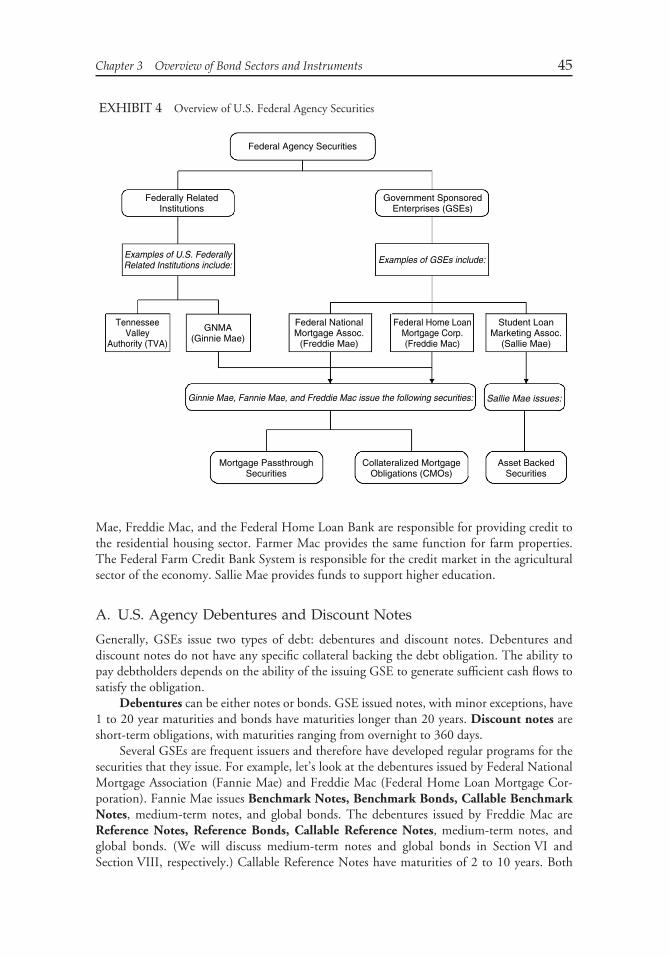
Chapter 3 Overview of Bond Sectors and Instruments 45
EXHIBIT 4 Overview of U.S. Federal Agency Securities
Federal Agency Securities
Federally RelatedInstitutions
TennesseeValley
Authority (TVA)
GNMA(Ginnie Mae)
Government SponsoredEnterprises (GSEs)
Examples of U.S. FederallyRelated Institutions include: Examples of GSEs include:
Ginnie Mae, Fannie Mae, and Freddie Mac issue the following securities: Sallie Mae issues:
Student LoanMarketing Assoc.
(Sallie Mae)
Federal Home LoanMortgage Corp.(Freddie Mac)
Federal NationalMortgage Assoc.
(Freddie Mae)
Mortgage PassthroughSecurities
Collateralized MortgageObligations (CMOs)
Asset BackedSecurities
Mae, Freddie Mac, and the Federal Home Loan Bank are responsible for providing credit tothe residential housing sector. Farmer Mac provides the same function for farm properties.The Federal Farm Credit Bank System is responsible for the credit market in the agriculturalsector of the economy. Sallie Mae provides funds to support higher education.
A. U.S. Agency Debentures and Discount Notes
Generally, GSEs issue two types of debt: debentures and discount notes. Debentures anddiscount notes do not have any specific collateral backing the debt obligation. The ability topay debtholders depends on the ability of the issuing GSE to generate sufficient cash flows tosatisfy the obligation.
Debentures can be either notes or bonds. GSE issued notes, with minor exceptions, have1 to 20 year maturities and bonds have maturities longer than 20 years. Discount notes areshort-term obligations, with maturities ranging from overnight to 360 days.
Several GSEs are frequent issuers and therefore have developed regular programs for thesecurities that they issue. For example, let’s look at the debentures issued by Federal NationalMortgage Association (Fannie Mae) and Freddie Mac (Federal Home Loan Mortgage Cor-poration). Fannie Mae issues Benchmark Notes, Benchmark Bonds, Callable BenchmarkNotes, medium-term notes, and global bonds. The debentures issued by Freddie Mac areReference Notes, Reference Bonds, Callable Reference Notes, medium-term notes, andglobal bonds. (We will discuss medium-term notes and global bonds in Section VI andSection VIII, respectively.) Callable Reference Notes have maturities of 2 to 10 years. Both
46 Fixed Income Analysis
Benchmark Notes and Bonds and Reference Notes and Bonds are eligible for stripping tocreate zero-coupon bonds.
B. U.S. Agency Mortgage-Backed Securities
The two GSEs charged with providing liquidity to the mortgage market—Fannie Mae andFreddie Mac—also issue securities backed by the mortgage loans that they purchase. That is,they use the mortgage loans they underwrite or purchase as collateral for the securities theyissue. These securities are called agency mortgage-backed securities and include mortgagepassthrough securities, collateralized mortgage obligations (CMOs), and stripped mortgage-backed securities. The latter two mortgage-backed securities are referred to as derivativemortgage-backed securities because they are created from mortgage passthrough securities.
While we confine our discussion to the U.S. mortgage-backed securities market, mostdeveloped countries have similar mortgage products.
1. Mortgage Loans A mortgage loan is a loan secured by the collateral of some specifiedreal estate property which obliges the borrower to make a predetermined series of payments.The mortgage gives the lender the right, if the borrower defaults, to ‘‘foreclose’’ on the loanand seize the property in order to ensure that the debt is paid off. The interest rate on themortgage loan is called the mortgage rate or contract rate.
There are many types of mortgage designs available in the United States. A mortgagedesign is a specification of the mortgage rate, term of the mortgage, and the manner in whichthe borrowed funds are repaid. For now, we will use the most common mortgage designto explain the characteristics of a mortgage-backed security: a fixed-rate, level-payment, fullyamortizing mortgage.
The basic idea behind this mortgage design is that each monthly mortgage payment isthe same dollar amount and includes interest and principal payment. The monthly paymentsare such that at the end of the loan’s term, the loan has been fully amortized (i.e., there is nomortgage principal balance outstanding).
Each monthly mortgage payment for this mortgage design is due on the first of eachmonth and consists of:
1. interest of 112 of the fixed annual interest rate times the amount of the outstanding
mortgage balance at the end of the previous month, and2. a payment of a portion of the outstanding mortgage principal balance.
The difference between the monthly mortgage payment and the portion of the payment thatrepresents interest equals the amount that is applied to reduce the outstanding mortgageprincipal balance. This amount is referred to as the amortization. We shall also refer to it asthe scheduled principal payment.
To illustrate this mortgage design, consider a 30-year (360-month), $100,000 mortgagewith an 8.125% mortgage rate. The monthly mortgage payment would be $742.50.2 Exhibit
2The calculation of the monthly mortgage payment is simply an application of the present value of anannuity. The formula as applied to mortgage payments is as follows:
MP = B[
r(1 + r)n
(1 + r)n − 1
]
Chapter 3 Overview of Bond Sectors and Instruments 47
5 shows for selected months how each monthly mortgage payment is divided between interestand scheduled principal payment. At the beginning of month 1, the mortgage balance is$100,000, the amount of the original loan. The mortgage payment for month 1 includesinterest on the $100,000 borrowed for the month. Since the interest rate is 8.125%, themonthly interest rate is 0.0067708 (0.08125 divided by 12). Interest for month 1 is therefore$677.08 ($100,000 times 0.0067708). The $65.41 difference between the monthly mortgagepayment of $742.50 and the interest of $677.08 is the portion of the monthly mortgagepayment that represents the scheduled principal payment (i.e., amortization). This $65.41 inmonth 1 reduces the mortgage balance.
The mortgage balance at the end of month 1 (beginning of month 2) is then $99,934.59($100,000 minus $65.41). The interest for the second monthly mortgage payment is $676.64,the monthly interest rate (0.0066708) times the mortgage balance at the beginning of month2 ($99,934.59). The difference between the $742.50 monthly mortgage payment and the$676.64 interest is $65.86, representing the amount of the mortgage balance paid off withthat monthly mortgage payment. Notice that the mortgage payment in month 360—the finalpayment—is sufficient to pay off the remaining mortgage principal balance.
As Exhibit 5 clearly shows, the portion of the monthly mortgage payment applied tointerest declines each month and the portion applied to principal repayment increases. Thereason for this is that as the mortgage balance is reduced with each monthly mortgage payment,the interest on the mortgage balance declines. Since the monthly mortgage payment is a fixeddollar amount, an increasingly larger portion of the monthly payment is applied to reduce themortgage principal balance outstanding in each subsequent month.
To an investor in a mortgage loan (or a pool of mortgage loans), the monthly mortgagepayments as described above do not equal an investor’s cash flow. There are two reasons forthis: (1) servicing fees and (2) prepayments.
Every mortgage loan must be serviced. Servicing of a mortgage loan involves collectingmonthly payments and forwarding proceeds to owners of the loan; sending payment noticesto mortgagors; reminding mortgagors when payments are overdue; maintaining records ofprincipal balances; administering an escrow balance for real estate taxes and insurance;initiating foreclosure proceedings if necessary; and, furnishing tax information to mortgagorswhen applicable. The servicing fee is a portion of the mortgage rate. If the mortgage rate is8.125% and the servicing fee is 50 basis points, then the investor receives interest of 7.625%.The interest rate that the investor receives is said to be the net interest.
Our illustration of the cash flow for a level-payment, fixed-rate, fully amortized mortgageassumes that the homeowner does not pay off any portion of the mortgage principal balance
where
MP = monthly mortgage paymentB = amount borrowed (i.e., original loan balance)r = monthly mortgage rate (annual rate divided by 12)n = number of months of the mortgage loanIn our example,B = $100, 000 r = 0.0067708 (0.08125/12) n = 360
Then
MP = $100, 000
[0.0067708 (1.0067708)360
(1.0067708)360 − 1
]= $742.50
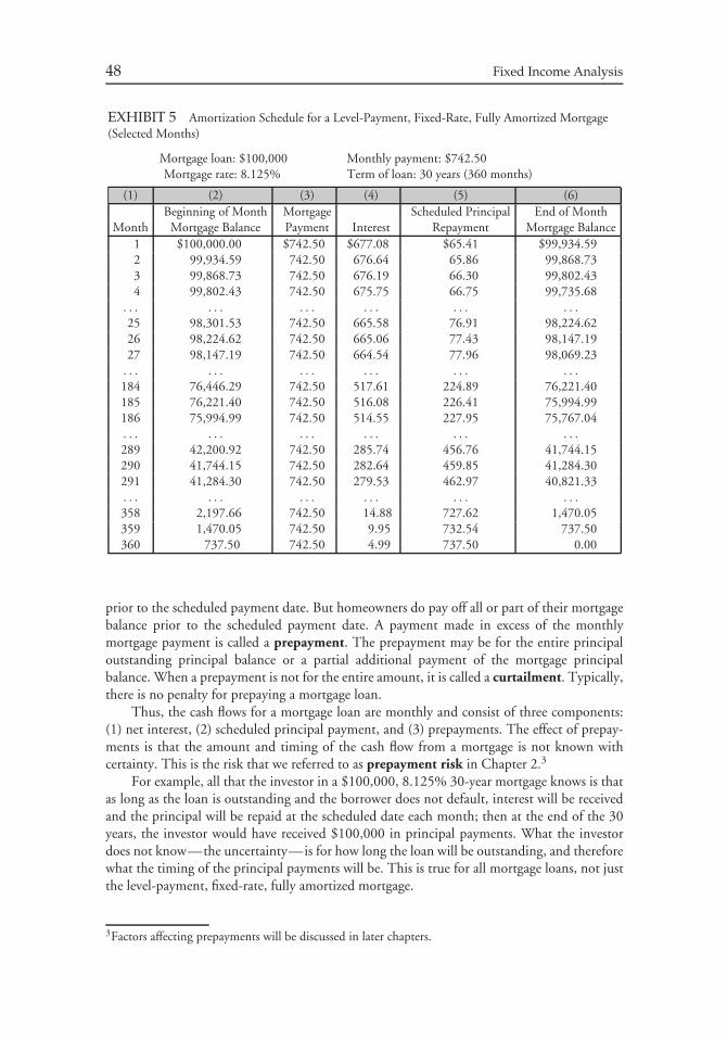
48 Fixed Income Analysis
EXHIBIT 5 Amortization Schedule for a Level-Payment, Fixed-Rate, Fully Amortized Mortgage(Selected Months)
Mortgage loan: $100,000 Monthly payment: $742.50Mortgage rate: 8.125% Term of loan: 30 years (360 months)
(1) (2) (3) (4) (5) (6)Beginning of Month Mortgage Scheduled Principal End of Month
Month Mortgage Balance Payment Interest Repayment Mortgage Balance1 $100,000.00 $742.50 $677.08 $65.41 $99,934.592 99,934.59 742.50 676.64 65.86 99,868.733 99,868.73 742.50 676.19 66.30 99,802.434 99,802.43 742.50 675.75 66.75 99,735.68
. . . . . . . . . . . . . . . . . .
25 98,301.53 742.50 665.58 76.91 98,224.6226 98,224.62 742.50 665.06 77.43 98,147.1927 98,147.19 742.50 664.54 77.96 98,069.23. . . . . . . . . . . . . . . . . .
184 76,446.29 742.50 517.61 224.89 76,221.40185 76,221.40 742.50 516.08 226.41 75,994.99186 75,994.99 742.50 514.55 227.95 75,767.04. . . . . . . . . . . . . . . . . .
289 42,200.92 742.50 285.74 456.76 41,744.15290 41,744.15 742.50 282.64 459.85 41,284.30291 41,284.30 742.50 279.53 462.97 40,821.33. . . . . . . . . . . . . . . . . .
358 2,197.66 742.50 14.88 727.62 1,470.05359 1,470.05 742.50 9.95 732.54 737.50360 737.50 742.50 4.99 737.50 0.00
prior to the scheduled payment date. But homeowners do pay off all or part of their mortgagebalance prior to the scheduled payment date. A payment made in excess of the monthlymortgage payment is called a prepayment. The prepayment may be for the entire principaloutstanding principal balance or a partial additional payment of the mortgage principalbalance. When a prepayment is not for the entire amount, it is called a curtailment. Typically,there is no penalty for prepaying a mortgage loan.
Thus, the cash flows for a mortgage loan are monthly and consist of three components:(1) net interest, (2) scheduled principal payment, and (3) prepayments. The effect of prepay-ments is that the amount and timing of the cash flow from a mortgage is not known withcertainty. This is the risk that we referred to as prepayment risk in Chapter 2.3
For example, all that the investor in a $100,000, 8.125% 30-year mortgage knows is thatas long as the loan is outstanding and the borrower does not default, interest will be receivedand the principal will be repaid at the scheduled date each month; then at the end of the 30years, the investor would have received $100,000 in principal payments. What the investordoes not know—the uncertainty—is for how long the loan will be outstanding, and thereforewhat the timing of the principal payments will be. This is true for all mortgage loans, not justthe level-payment, fixed-rate, fully amortized mortgage.
3Factors affecting prepayments will be discussed in later chapters.
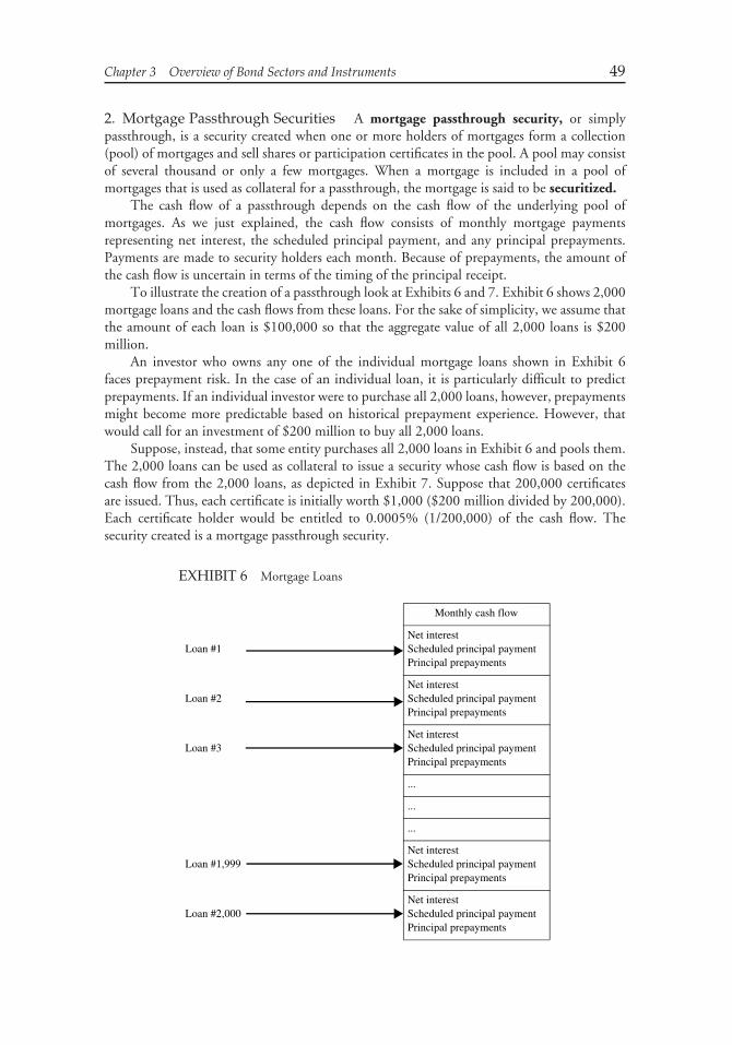
Chapter 3 Overview of Bond Sectors and Instruments 49
2. Mortgage Passthrough Securities A mortgage passthrough security, or simplypassthrough, is a security created when one or more holders of mortgages form a collection(pool) of mortgages and sell shares or participation certificates in the pool. A pool may consistof several thousand or only a few mortgages. When a mortgage is included in a pool ofmortgages that is used as collateral for a passthrough, the mortgage is said to be securitized.
The cash flow of a passthrough depends on the cash flow of the underlying pool ofmortgages. As we just explained, the cash flow consists of monthly mortgage paymentsrepresenting net interest, the scheduled principal payment, and any principal prepayments.Payments are made to security holders each month. Because of prepayments, the amount ofthe cash flow is uncertain in terms of the timing of the principal receipt.
To illustrate the creation of a passthrough look at Exhibits 6 and 7. Exhibit 6 shows 2,000mortgage loans and the cash flows from these loans. For the sake of simplicity, we assume thatthe amount of each loan is $100,000 so that the aggregate value of all 2,000 loans is $200million.
An investor who owns any one of the individual mortgage loans shown in Exhibit 6faces prepayment risk. In the case of an individual loan, it is particularly difficult to predictprepayments. If an individual investor were to purchase all 2,000 loans, however, prepaymentsmight become more predictable based on historical prepayment experience. However, thatwould call for an investment of $200 million to buy all 2,000 loans.
Suppose, instead, that some entity purchases all 2,000 loans in Exhibit 6 and pools them.The 2,000 loans can be used as collateral to issue a security whose cash flow is based on thecash flow from the 2,000 loans, as depicted in Exhibit 7. Suppose that 200,000 certificatesare issued. Thus, each certificate is initially worth $1,000 ($200 million divided by 200,000).Each certificate holder would be entitled to 0.0005% (1/200,000) of the cash flow. Thesecurity created is a mortgage passthrough security.
EXHIBIT 6 Mortgage Loans
Monthly cash flow
Loan #1Net interestScheduled principal paymentPrincipal prepayments
Loan #2Net interestScheduled principal paymentPrincipal prepayments
Loan #3Net interestScheduled principal paymentPrincipal prepayments
...
...
...
Loan #1,999Net interestScheduled principal paymentPrincipal prepayments
Loan #2,000Net interestScheduled principal paymentPrincipal prepayments
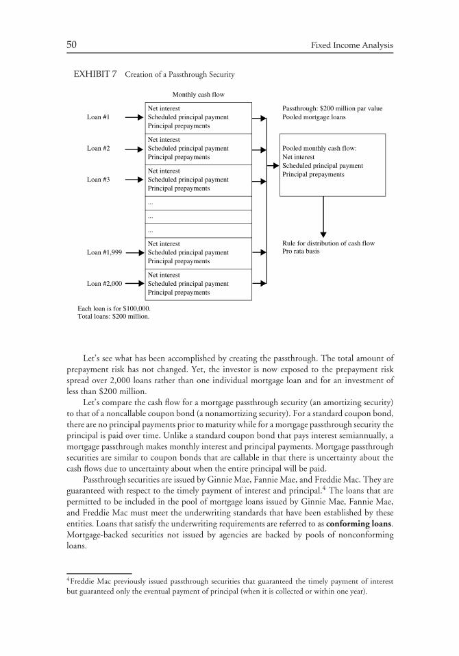
50 Fixed Income Analysis
EXHIBIT 7 Creation of a Passthrough Security
Monthly cash flow
Loan #1Net interestScheduled principal paymentPrincipal prepayments
Passthrough: $200 million par valuePooled mortgage loans
Loan #2Net interestScheduled principal paymentPrincipal prepayments
Pooled monthly cash flow:Net interestScheduled principal paymentPrincipal prepayments
Loan #3Net interestScheduled principal paymentPrincipal prepayments
...
...
...
Loan #1,999Net interestScheduled principal paymentPrincipal prepayments
Rule for distribution of cash flowPro rata basis
Loan #2,000Net interestScheduled principal paymentPrincipal prepayments
Each loan is for $100,000.Total loans: $200 million.
Let’s see what has been accomplished by creating the passthrough. The total amount ofprepayment risk has not changed. Yet, the investor is now exposed to the prepayment riskspread over 2,000 loans rather than one individual mortgage loan and for an investment ofless than $200 million.
Let’s compare the cash flow for a mortgage passthrough security (an amortizing security)to that of a noncallable coupon bond (a nonamortizing security). For a standard coupon bond,there are no principal payments prior to maturity while for a mortgage passthrough security theprincipal is paid over time. Unlike a standard coupon bond that pays interest semiannually, amortgage passthrough makes monthly interest and principal payments. Mortgage passthroughsecurities are similar to coupon bonds that are callable in that there is uncertainty about thecash flows due to uncertainty about when the entire principal will be paid.
Passthrough securities are issued by Ginnie Mae, Fannie Mae, and Freddie Mac. They areguaranteed with respect to the timely payment of interest and principal.4 The loans that arepermitted to be included in the pool of mortgage loans issued by Ginnie Mae, Fannie Mae,and Freddie Mac must meet the underwriting standards that have been established by theseentities. Loans that satisfy the underwriting requirements are referred to as conforming loans.Mortgage-backed securities not issued by agencies are backed by pools of nonconformingloans.
4Freddie Mac previously issued passthrough securities that guaranteed the timely payment of interestbut guaranteed only the eventual payment of principal (when it is collected or within one year).
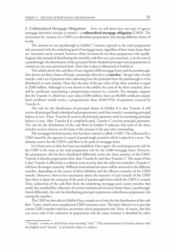
Chapter 3 Overview of Bond Sectors and Instruments 51
3. Collateralized Mortgage Obligations Now we will show how one type of agencymortgage derivative security is created—a collateralized mortgage obligation (CMO). Themotivation for creation of a CMO is to distribute prepayment risk among different classes ofbonds.
The investor in our passthrough in Exhibit 7 remains exposed to the total prepaymentrisk associated with the underlying pool of mortgage loans, regardless of how many loans thereare. Securities can be created, however, where investors do not share prepayment risk equally.Suppose that instead of distributing the monthly cash flow on a pro rata basis, as in the case ofa passthrough, the distribution of the principal (both scheduled principal and prepayments) iscarried out on some prioritized basis. How this is done is illustrated in Exhibit 8.
The exhibit shows the cash flow of our original 2,000 mortgage loans and the passthrough.Also shown are three classes of bonds, commonly referred to as tranches,5 the par value of eachtranche, and a set of payment rules indicating how the principal from the passthrough is to bedistributed to each tranche. Note that the sum of the par value of the three tranches is equalto $200 million. Although it is not shown in the exhibit, for each of the three tranches, therewill be certificates representing a proportionate interest in a tranche. For example, supposethat for Tranche A, which has a par value of $80 million, there are 80,000 certificates issued.Each certificate would receive a proportionate share (0.00125%) of payments received byTranche A.
The rule for the distribution of principal shown in Exhibit 8 is that Tranche A willreceive all principal (both scheduled and prepayments) until that tranche’s remaining principalbalance is zero. Then, Tranche B receives all principal payments until its remaining principalbalance is zero. After Tranche B is completely paid, Tranche C receives principal payments.The rule for the distribution of the cash flows in Exhibit 8 indicates that each of the threetranches receives interest on the basis of the amount of the par value outstanding.
The mortgage-backed security that has been created is called a CMO. The collateral for aCMO issued by the agencies is a pool of passthrough securities which is placed in a trust. Theultimate source for the CMO’s cash flow is the pool of mortgage loans.
Let’s look now at what has been accomplished. Once again, the total prepayment risk forthe CMO is the same as the total prepayment risk for the 2,000 mortgage loans. However,the prepayment risk has been distributed differently across the three tranches of the CMO.Tranche A absorbs prepayments first, then Tranche B, and then Tranche C. The result of thisis that Tranche A effectively is a shorter term security than the other two tranches; Tranche Cwill have the longest maturity. Different institutional investors will be attracted to the differenttranches, depending on the nature of their liabilities and the effective maturity of the CMOtranche. Moreover, there is less uncertainty about the maturity of each tranche of the CMOthan there is about the maturity of the pool of passthroughs from which the CMO is created.Thus, redirection of the cash flow from the underlying mortgage pool creates tranches thatsatisfy the asset/liability objectives of certain institutional investors better than a passthrough.Stated differently, the rule for distributing principal repayments redistributes prepayment riskamong the tranches.
The CMO we describe in Exhibit 8 has a simple set of rules for the distribution of the cashflow. Today, much more complicated CMO structures exist. The basic objective is to providecertain CMO tranches with less uncertainty about prepayment risk. Note, of course, that thiscan occur only if the reduction in prepayment risk for some tranches is absorbed by other
5‘‘Tranche’’ is from an old French word meaning ‘‘slice.’’ (The pronunciation of tranche rhymes withthe English word ‘‘launch,’’ as in launch a ship or a rocket.)
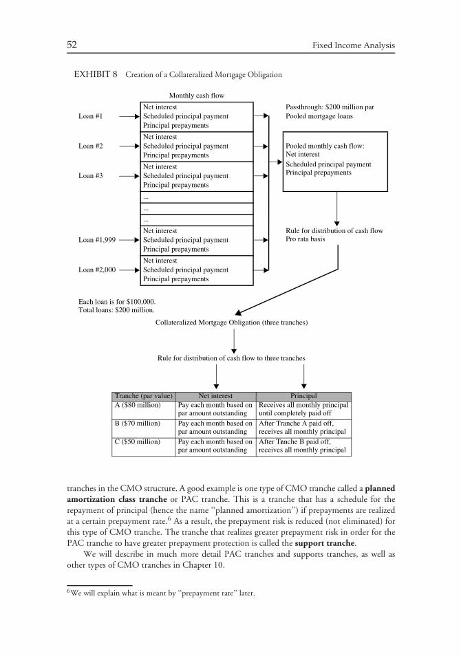
52 Fixed Income Analysis
EXHIBIT 8 Creation of a Collateralized Mortgage Obligation
Monthly cash flow
Loan #1Net interestScheduled principal paymentPrincipal prepayments
Passthrough: $200 million parPooled mortgage loans
Loan #2Net interestScheduled principal paymentPrincipal prepayments
Pooled monthly cash flow:Net interestScheduled principal paymentPrincipal prepaymentsLoan #3
Net interestScheduled principal paymentPrincipal prepayments
...
...
...
Loan #1,999Net interestScheduled principal paymentPrincipal prepayments
Rule for distribution of cash flowPro rata basis
Loan #2,000Net interestScheduled principal paymentPrincipal prepayments
Each loan is for $100,000.Total loans: $200 million.
Collateralized Mortgage Obligation (three tranches)
Rule for distribution of cash flow to three tranches
Tranche (par value) Net interest PrincipalA ($80 million) Pay each month based on
par amount outstandingReceives all monthly principaluntil completely paid off
B ($70 million) Pay each month based onpar amount outstanding
After Tranche A paid off,receives all monthly principal
C ($50 million) Pay each month based onpar amount outstanding
After Tanche B paid off,receives all monthly principal
r
tranches in the CMO structure. A good example is one type of CMO tranche called a plannedamortization class tranche or PAC tranche. This is a tranche that has a schedule for therepayment of principal (hence the name ‘‘planned amortization’’) if prepayments are realizedat a certain prepayment rate.6 As a result, the prepayment risk is reduced (not eliminated) forthis type of CMO tranche. The tranche that realizes greater prepayment risk in order for thePAC tranche to have greater prepayment protection is called the support tranche.
We will describe in much more detail PAC tranches and supports tranches, as well asother types of CMO tranches in Chapter 10.
6We will explain what is meant by ‘‘prepayment rate’’ later.
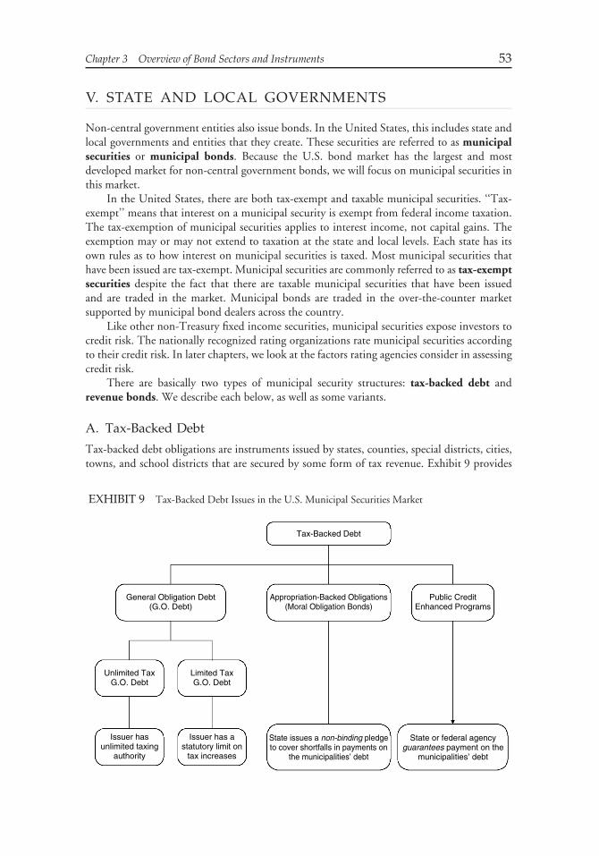
Chapter 3 Overview of Bond Sectors and Instruments 53
V. STATE AND LOCAL GOVERNMENTS
Non-central government entities also issue bonds. In the United States, this includes state andlocal governments and entities that they create. These securities are referred to as municipalsecurities or municipal bonds. Because the U.S. bond market has the largest and mostdeveloped market for non-central government bonds, we will focus on municipal securities inthis market.
In the United States, there are both tax-exempt and taxable municipal securities. ‘‘Tax-exempt’’ means that interest on a municipal security is exempt from federal income taxation.The tax-exemption of municipal securities applies to interest income, not capital gains. Theexemption may or may not extend to taxation at the state and local levels. Each state has itsown rules as to how interest on municipal securities is taxed. Most municipal securities thathave been issued are tax-exempt. Municipal securities are commonly referred to as tax-exemptsecurities despite the fact that there are taxable municipal securities that have been issuedand are traded in the market. Municipal bonds are traded in the over-the-counter marketsupported by municipal bond dealers across the country.
Like other non-Treasury fixed income securities, municipal securities expose investors tocredit risk. The nationally recognized rating organizations rate municipal securities accordingto their credit risk. In later chapters, we look at the factors rating agencies consider in assessingcredit risk.
There are basically two types of municipal security structures: tax-backed debt andrevenue bonds. We describe each below, as well as some variants.
A. Tax-Backed Debt
Tax-backed debt obligations are instruments issued by states, counties, special districts, cities,towns, and school districts that are secured by some form of tax revenue. Exhibit 9 provides
EXHIBIT 9 Tax-Backed Debt Issues in the U.S. Municipal Securities Market
Tax-Backed Debt
General Obligation Debt(G.O. Debt)
Unlimited TaxG.O. Debt
Limited TaxG.O. Debt
Issuer hasunlimited taxing
authority
Issuer has astatutory limit on
tax increases
State issues a non-binding pledgeto cover shortfalls in payments on
the municipalities’ debt
State or federal agencyguarantees payment on the
municipalities’ debt
Appropriation-Backed Obligations(Moral Obligation Bonds)
Public CreditEnhanced Programs
54 Fixed Income Analysis
an overview of the types of tax-backed debt issued in the U.S. municipal securities market.Tax-backed debt includes general obligation debt, appropriation-backed obligations, anddebt obligations supported by public credit enhancement programs. We discuss eachbelow.
1. General Obligation Debt The broadest type of tax-backed debt is general obligationdebt. There are two types of general obligation pledges: unlimited and limited. An unlimitedtax general obligation debt is the stronger form of general obligation pledge because it issecured by the issuer’s unlimited taxing power. The tax revenue sources include corporate andindividual income taxes, sales taxes, and property taxes. Unlimited tax general obligation debtis said to be secured by the full faith and credit of the issuer. A limited tax general obligationdebt is a limited tax pledge because, for such debt, there is a statutory limit on tax rates thatthe issuer may levy to service the debt.
Certain general obligation bonds are secured not only by the issuer’s general taxing powersto create revenues accumulated in a general fund, but also by certain identified fees, grants,and special charges, which provide additional revenues from outside the general fund. Suchbonds are known as double-barreled in security because of the dual nature of the revenuesources. For example, the debt obligations issued by special purpose service systems may besecured by a pledge of property taxes, a pledge of special fees/operating revenue from theservice provided, or a pledge of both property taxes and special fees/operating revenues. In thelast case, they are double-barreled.
2. Appropriation-Backed Obligations Agencies or authorities of several states haveissued bonds that carry a potential state liability for making up shortfalls in the issuing entity’sobligation. The appropriation of funds from the state’s general tax revenue must be approvedby the state legislature. However, the state’s pledge is not binding. Debt obligations withthis nonbinding pledge of tax revenue are called moral obligation bonds. Because a moralobligation bond requires legislative approval to appropriate the funds, it is classified as anappropriation-backed obligation. The purpose of the moral obligation pledge is to enhancethe credit worthiness of the issuing entity. However, the investor must rely on the best-effortsof the state to approve the appropriation.
3. Debt Obligations Supported by Public Credit Enhancement Programs Whilea moral obligation is a form of credit enhancement provided by a state, it is not a legallyenforceable or legally binding obligation of the state. There are entities that have issued debtthat carries some form of public credit enhancement that is legally enforceable. This occurswhen there is a guarantee by the state or a federal agency or when there is an obligation toautomatically withhold and deploy state aid to pay any defaulted debt service by the issuingentity. Typically, the latter form of public credit enhancement is used for debt obligations ofa state’s school systems.
Some examples of state credit enhancement programs include Virginia’s bond guaranteeprogram that authorizes the governor to withhold state aid payments to a municipality anddivert those funds to pay principal and interest to a municipality’s general obligation holdersin the event of a default. South Carolina’s constitution requires mandatory withholding ofstate aid by the state treasurer if a school district is not capable of meeting its general obligationdebt. Texas created the Permanent School Fund to guarantee the timely payment of principaland interest of the debt obligations of qualified school districts. The fund’s income is obtainedfrom land and mineral rights owned by the state of Texas.
Chapter 3 Overview of Bond Sectors and Instruments 55
More recently, states and local governments have issued increasing amounts of bondswhere the debt service is to be paid from so-called ‘‘dedicated’’ revenues such as sales taxes,tobacco settlement payments, fees, and penalty payments. Many are structured to mimic theasset-backed bonds that are discussed later in this chapter (Section VII).
B. Revenue Bonds
The second basic type of security structure is found in a revenue bond. Revenue bonds areissued for enterprise financings that are secured by the revenues generated by the completedprojects themselves, or for general public-purpose financings in which the issuers pledge tothe bondholders the tax and revenue resources that were previously part of the general fund.This latter type of revenue bond is usually created to allow issuers to raise debt outside generalobligation debt limits and without voter approval.
Revenue bonds can be classified by the type of financing. These include utility revenuebonds, transportation revenue bonds, housing revenue bonds, higher education revenuebonds, health care revenue bonds, sports complex and convention center revenue bonds,seaport revenue bonds, and industrial revenue bonds.
C. Special Bond Structures
Some municipal securities have special security structures. These include insured bonds andprerefunded bonds.
1. Insured Bonds Insured bonds, in addition to being secured by the issuer’s revenue, arealso backed by insurance policies written by commercial insurance companies. Insurance on amunicipal bond is an agreement by an insurance company to pay the bondholder principaland/or coupon interest that is due on a stated maturity date but that has not been paid by thebond issuer. Once issued, this municipal bond insurance usually extends for the term of thebond issue and cannot be canceled by the insurance company.
2. Prerefunded Bonds Although originally issued as either revenue or general obligationbonds, municipals are sometimes prerefunded and thus called prerefunded municipal bonds.A prerefunding usually occurs when the original bonds are escrowed or collateralized by directobligations guaranteed by the U.S. government. By this, it is meant that a portfolio of securitiesguaranteed by the U.S. government is placed in a trust. The portfolio of securities is assembledsuch that the cash flows from the securities match the obligations that the issuer must pay. Forexample, suppose that a municipality has a 7% $100 million issue with 12 years remaining tomaturity. The municipality’s obligation is to make payments of $3.5 million every six monthsfor the next 12 years and $100 million 12 years from now. If the issuer wants to prerefundthis issue, a portfolio of U.S. government obligations can be purchased that has a cash flow of$3.5 million every six months for the next 12 years and $100 million 12 years from now.
Once this portfolio of securities whose cash flows match those of the municipality’sobligation is in place, the prerefunded bonds are no longer secured as either general obligationor revenue bonds. The bonds are now supported by cash flows from the portfolio of securitiesheld in an escrow fund. Such bonds, if escrowed with securities guaranteed by the U.S.government, have little, if any, credit risk. They are the safest municipal bonds available.
The escrow fund for a prerefunded municipal bond can be structured so that the bonds tobe refunded are to be called at the first possible call date or a subsequent call date established
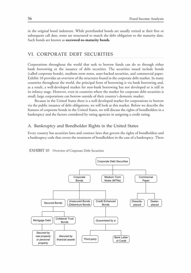
56 Fixed Income Analysis
in the original bond indenture. While prerefunded bonds are usually retired at their first orsubsequent call date, some are structured to match the debt obligation to the maturity date.Such bonds are known as escrowed-to-maturity bonds.
VI. CORPORATE DEBT SECURITIES
Corporations throughout the world that seek to borrow funds can do so through eitherbank borrowing or the issuance of debt securities. The securities issued include bonds(called corporate bonds), medium term notes, asset-backed securities, and commercial paper.Exhibit 10 provides an overview of the structures found in the corporate debt market. In manycountries throughout the world, the principal form of borrowing is via bank borrowing and,as a result, a well-developed market for non-bank borrowing has not developed or is still inits infancy stage. However, even in countries where the market for corporate debt securities issmall, large corporations can borrow outside of their country’s domestic market.
Because in the United States there is a well developed market for corporations to borrowvia the public issuance of debt obligations, we will look at this market. Before we describe thefeatures of corporate bonds in the United States, we will discuss the rights of bondholders in abankruptcy and the factors considered by rating agencies in assigning a credit rating.
A. Bankruptcy and Bondholder Rights in the United States
Every country has securities laws and contract laws that govern the rights of bondholders anda bankruptcy code that covers the treatment of bondholders in the case of a bankruptcy. There
EXHIBIT 10 Overview of Corporate Debt Securities
Corporate Debt Securities
Medium-TermNotes (MTNs)
CommercialPaper
Diresctly-placed
Dealer-placed
CorporateBonds
Unsecured Bonds(Debenture Bonds
Credit EnhancedBonds
Guaranteed by a:
Third-partyBank Letter
of Credit
Secured Bonds
Collateral TrustBonds
Mortgage Debt
Secured byfinancial assets
Secured byreal propertyor personal
property
Chapter 3 Overview of Bond Sectors and Instruments 57
are principles that are common in the legal arrangements throughout the world. Below wediscuss the features of the U.S. system.
The holder of a U.S. corporate debt instrument has priority over the equity owners in abankruptcy proceeding. Moreover, there are creditors who have priority over other creditors.The law governing bankruptcy in the United States is the Bankruptcy Reform Act of 1978 asamended from time to time. One purpose of the act is to set forth the rules for a corporationto be either liquidated or reorganized when filing bankruptcy.
The liquidation of a corporation means that all the assets will be distributed to the claimholders of the corporation and no corporate entity will survive. In a reorganization, a newcorporate entity will emerge at the end of the bankruptcy proceedings. Some security holdersof the bankrupt corporation will receive cash in exchange for their claims, others may receivenew securities in the corporation that results from the reorganization, and others may receivea combination of both cash and new securities in the resulting corporation.
Another purpose of the bankruptcy act is to give a corporation time to decide whetherto reorganize or liquidate and then the necessary time to formulate a plan to accomplisheither a reorganization or liquidation. This is achieved because when a corporation files forbankruptcy, the act grants the corporation protection from creditors who seek to collect theirclaims. The petition for bankruptcy can be filed either by the company itself, in which caseit is called a voluntary bankruptcy, or be filed by its creditors, in which case it is calledan involuntary bankruptcy. A company that files for protection under the bankruptcy actgenerally becomes a ‘‘debtor-in-possession’’ and continues to operate its business under thesupervision of the court.
The bankruptcy act is comprised of 15 chapters, each chapter covering a particular typeof bankruptcy. Chapter 7 deals with the liquidation of a company; Chapter 11 deals with thereorganization of a company.
When a company is liquidated, creditors receive distributions based on the absolutepriority rule to the extent assets are available. The absolute priority rule is the principle thatsenior creditors are paid in full before junior creditors are paid anything. For secured andunsecured creditors, the absolute priority rule guarantees their seniority to equity holders. Inliquidations, the absolute priority rule generally holds. In contrast, there is a good body ofliterature that argues that strict absolute priority typically has not been upheld by the courtsor the SEC in reorganizations.
B. Factors Considered in Assigning a Credit Rating
In the previous chapter, we explained that there are companies that assign credit ratings tocorporate issues based on the prospects of default. These companies are called rating agencies.In conducting a credit examination, each rating agency, as well as credit analysts employedby investment management companies, consider the four C’s of credit—character, capacity,collateral, and covenants.
It is important to understand that a credit analysis can be for an entire company ora particular debt obligation of that company. Consequently, a rating agency may assign adifferent rating to the various issues of the same corporation depending on the level of seniorityof the bondholders of each issue in the case of bankruptcy. For example, we will explain belowthat there is senior debt and subordinated debt. Senior debtholders have a better positionrelative to subordinated debtholders in the case of a bankruptcy for a given issuer. So, a ratingagency, for example, may assign a rating of ‘‘A’’ to the senior debt of a corporation and a lowerrating, ‘‘BBB,’’ to the subordinated debt of the same corporation.
58 Fixed Income Analysis
Character analysis involves the analysis of the quality of management. In discussing thefactors it considers in assigning a credit rating, Moody’s Investors Service notes the followingregarding the quality of management:
Although difficult to quantify, management quality is one of the most important factorssupporting an issuer’s credit strength. When the unexpected occurs, it is a management’sability to react appropriately that will sustain the company’s performance.7
In assessing management quality, the analysts at Moody’s, for example, try to understandthe business strategies and policies formulated by management. Moody’s considers thefollowing factors: (1) strategic direction, (2) financial philosophy, (3) conservatism, (4) trackrecord, (5) succession planning, and (6) control systems.8
In assessing the ability of an issuer to pay (i.e., capacity), the analysts conduct financialstatement analysis. In addition to financial statement analysis, the factors examined by analystsat Moody’s are (1) industry trends, (2) the regulatory environment, (3) basic operating andcompetitive position, (4) financial position and sources of liquidity, (5) company structure(including structural subordination and priority of claim), (6) parent company supportagreements, and (7) special event risk.9
The third C, collateral, is looked at not only in the traditional sense of assets pledgedto secure the debt, but also to the quality and value of those unpledged assets controlled bythe issuer. Unpledged collateral is capable of supplying additional sources of funds to supportpayment of debt. Assets form the basis for generating cash flow which services the debt in goodtimes as well as bad. We discuss later the various types of collateral used for a corporate debtissue and features that analysts should be cognizant of when evaluating an investor’s securedposition.
Covenants deal with limitations and restrictions on the borrower’s activities. Affirmativecovenants call upon the debtor to make promises to do certain things. Negative covenants arethose which require the borrower not to take certain actions. Negative covenants are usuallynegotiated between the borrower and the lender or their agents. Borrowers want the leastrestrictive loan agreement available, while lenders should want the most restrictive, consistentwith sound business practices. But lenders should not try to restrain borrowers from acceptedbusiness activities and conduct. A borrower might be willing to include additional restrictions(up to a point) if it can get a lower interest rate on the debt obligation. When borrowersseek to weaken restrictions in their favor, they are often willing to pay more interest or giveother consideration. We will see examples of positive and negative covenants later in thischapter.
C. Corporate Bonds
In Chapter 1, we discussed the features of bonds including the wide range of coupon types,the provisions for principal payments, provisions for early retirement, and other embeddedoptions. Also, in Chapter 2, we reviewed the various forms of credit risk and the ratingsassigned by rating agencies. In our discussion of corporate bonds here, we will discuss securedand unsecured debt and information about default and recovery rates.
7‘‘Industrial Company Rating Methodology,’’ Moody’s Investors Service: Global Credit Research (July1998), p. 6.8‘‘Industrial Company Rating Methodology,’’ p. 7.9‘‘Industrial Company Rating Methodology,’’ p. 3.
Chapter 3 Overview of Bond Sectors and Instruments 59
1. Secured Debt, Unsecured Debt, and Credit Enhancements A corporate debtobligation may be secured or unsecured. Secured debt means that there is some formof collateral pledged to ensure payment of the debt. Remove the pledged collateral and wehave unsecured debt.
It is important to recognize that while a superior legal status will strengthen a bondholder’schance of recovery in case of default, it will not absolutely prevent bondholders from sufferingfinancial loss when the issuer’s ability to generate sufficient cash flow to pay its obligations isseriously eroded. Claims against a weak borrower are often satisfied for less than par value.
a. Secured Debt Either real property or personal property may be pledged as securityfor secured debt. With mortgage debt, the issuer grants the bondholders a lien againstpledged assets. A lien is a legal right to sell mortgaged property to satisfy unpaid obligations tobondholders. In practice, foreclosure and sale of mortgaged property is unusual. If a defaultoccurs, there is usually a financial reorganization of the issuer in which provision is madefor settlement of the debt to bondholders. The mortgage lien is important, though, becauseit gives the mortgage bondholders a strong bargaining position relative to other creditors indetermining the terms of a reorganization.
Some companies do not own fixed assets or other real property and so have nothingon which they can give a mortgage lien to secure bondholders. Instead, they own securitiesof other companies; they are holding companies and the other companies are subsidiaries.To satisfy the desire of bondholders for security, the issuer grants investors a lien on stocks,notes, bonds or other kind of financial asset they own. Bonds secured by such assets are calledcollateral trust bonds. The eligible collateral is periodically marked to market by the trusteeto ensure that the market value has a liquidation value in excess of the amount needed to repaythe entire outstanding bonds and accrued interest. If the collateral is insufficient, the issuermust, within a certain period, bring the value of the collateral up to the required amount. Ifthe issuer is unable to do so, the trustee would then sell collateral and redeem bonds.
Mortgage bonds have many different names. The following names have been used: firstmortgage bonds (most common name), first and general mortgage bonds, first refundingmortgage bonds, and first mortgage and collateral trusts. There are instances (excludingprior lien bonds as mentioned above) when a company might have two or more layers ofmortgage debt outstanding with different priorities. This situation usually occurs becausecompanies cannot issue additional first mortgage debt (or the equivalent) under the existingindentures. Often this secondary debt level is called general and refunding mortgage bonds(G&R). In reality, this is mostly second mortgage debt. Some issuers may have third mortgagebonds.
Although an indenture may not limit the total amount of bonds that may be issuedwith the same lien, there are certain issuance tests that usually have to be satisfied before thecompany may sell more bonds. Typically there is an earnings test that must be satisfied beforeadditional bonds may be issued with the same lien.
b. Unsecured Debt Unsecured debt is commonly referred to as debenture bonds.Although a debenture bond is not secured by a specific pledge of property, that doesnot mean that bondholders have no claim on property of issuers or on their earnings. Deben-ture bondholders have the claim of general creditors on all assets of the issuer not pledgedspecifically to secure other debt. And they even have a claim on pledged assets to the extentthat these assets generate proceeds in liquidation that are greater than necessary to satisfysecured creditors. Subordinated debenture bonds are issues that rank after secured debt, afterdebenture bonds, and often after some general creditors in their claim on assets and earnings.
60 Fixed Income Analysis
One of the important protective provisions for unsecured debt holders is the negativepledge clause. This provision, found in most senior unsecured debt issues and a fewsubordinated issues, prohibits a company from creating or assuming any lien to secure a debtissue without equally securing the subject debt issue(s) (with certain exceptions).
c. Credit Enhancements Some debt issuers have other companies guarantee their loans.This is normally done when a subsidiary issues debt and the investors want the addedprotection of a third-party guarantee. The use of guarantees makes it easier and moreconvenient to finance special projects and affiliates, although guarantees are also extended tooperating company debt.
An example of a third-party (but related) guarantee was U.S. West Capital Funding, Inc.8% Guaranteed Notes that were due October 15, 1996 (guaranteed by U.S. West, Inc.).The principal purpose of Capital Funding was to provide financing to U.S. West and itsaffiliates through the issuance of debt guaranteed by U.S. West. PepsiCo, Inc. has guaranteedthe debt of its financing affiliate, PepsiCo Capital Resources, Inc., and The Standard OilCompany (an Ohio Corporation) has unconditionally guaranteed the debt of Sohio Pipe LineCompany.
Another credit enhancing feature is the letter of credit (LOC) issued by a bank. A LOCrequires the bank make payments to the trustee when requested so that monies will be availablefor the bond issuer to meet its interest and principal payments when due. Thus, the creditof the bank under the LOC is substituted for that of the debt issuer. Specialized insurancecompanies also lend their credit standing to corporate debt, both new issues and outstandingsecondary market issues. In such cases, the credit rating of the bond is usually no better thanthe credit rating of the guarantor.
While a guarantee or other type of credit enhancement may add some measure ofprotection to a debtholder, caution should not be thrown to the wind. In effect, one’s jobmay even become more complex as an analysis of both the issuer and the guarantor should beperformed. In many cases, only the latter is needed if the issuer is merely a financing conduitwithout any operations of its own. However, if both concerns are operating companies, itmay very well be necessary to analyze both, as the timely payment of principal and interestultimately will depend on the stronger party. Generally, a downgrade of the credit enhancer’sclaims-paying ability reduces the value of the credit-enhanced bonds.
2. Default Rates and Recovery Rates Now we turn our attention to the various aspectsof the historical performance of corporate issuers with respect to fulfilling their obligationsto bondholders. Specifically, we will review two aspects of this performance. First, we willreview the default rate of corporate borrowers. Second, we will review the default loss rateof corporate borrowers. From an investment perspective, default rates by themselves are notof paramount significance: it is perfectly possible for a portfolio of bonds to suffer defaultsand to outperform Treasuries at the same time, provided the yield spread of the portfolio issufficiently high to offset the losses from default. Furthermore, because holders of defaultedbonds typically recover some percentage of the face amount of their investment, the defaultloss rate is substantially lower than the default rate. Therefore, it is important to look atdefault loss rates or, equivalently, recovery rates.
a. Default Rates A default rate can be measured in different ways. A simple way to definea default rate is to use the issuer as the unit of study. A default rate is then measured asthe number of issuers that default divided by the total number of issuers at the beginning of
Chapter 3 Overview of Bond Sectors and Instruments 61
the year. This measure—referred to as the issuer default rate—gives no recognition to theamount defaulted nor the total amount of issuance. Moody’s, for example, uses this defaultrate statistic in its study of default rates. The rationale for ignoring dollar amounts is thatthe credit decision of an investor does not increase with the size of the issuer. The secondmeasure—called the dollar default rate—defines the default rate as the par value of all bondsthat defaulted in a given calendar year, divided by the total par value of all bonds outstandingduring the year. With either default rate statistic, one can measure the default for a given yearor an average annual default rate over a certain number of years.
There have been several excellent studies of corporate bond default rates. All of thestudies found that the lower the credit rating, the greater the probability of a corporate issuerdefaulting.
There have been extensive studies focusing on default rates for non-investment gradecorporate bonds (i.e., speculative-grade issuer or high yield bonds). Studies by EdwardAltman suggest that the annual default rate for speculative-grade corporate debt has beenbetween 2.15% and 2.4% per year.10 Asquith, Mullins, and Wolff, however, found thatnearly one out of every three speculative-grade bonds defaults.11 The large discrepancy arisesbecause researchers use three different definitions of ‘‘default rate’’; even if applied to thesame universe of bonds (which they are not), the results of these studies could be validsimultaneously.12
Altman defines the default rate as the dollar default rate. His estimates (2.15% and2.40%) are simple averages of the annual dollar default rates over a number of years. Asquith,Mullins, and Wolff use a cumulative dollar default rate statistic. While both measures areuseful indicators of bond default propensity, they are not directly comparable. Even whenrestated on an annualized basis, they do not all measure the same quantity. The defaultstatistics reported in both studies, however, are surprisingly similar once cumulative rates havebeen annualized. A majority of studies place the annual dollar default rates for all original issuehigh-yield bonds between 3% and 4%.
b. Recovery Rates There have been several studies that have focused on recovery rates ordefault loss rates for corporate debt. Measuring the amount recovered is not a simple task. Thefinal distribution to claimants when a default occurs may consist of cash and securities. Oftenit is difficult to track what was received and then determine the present value of any non-cashpayments received.
Here we review recovery information as reported in a study by Moody’s which uses thetrading price at the time of default as a proxy for the amount recovered.13 The recovery rate isthe trading price at that time divided by the par value. Moody’s found that the recovery ratewas 38% for all bonds. Moreover, the study found that the higher the level of seniority, thegreater the recovery rate.
10Edward I. Altman and Scott A. Nammacher, Investing in Junk Bonds (New York: John Wiley, 1987)and Edward I. Altman, ‘‘Research Update: Mortality Rates and Losses, Bond Rating Drift,’’ unpublishedstudy prepared for a workshop sponsored by Merrill Lynch Merchant Banking Group, High Yield Salesand Trading, 1989.11Paul Asquith, David W. Mullins, Jr., and Eric D. Wolff, ‘‘Original Issue High Yield Bonds: AgingAnalysis of Defaults, Exchanges, and Calls,’’ Journal of Finance (September 1989), pp. 923–952.12As a parallel, we know that the mortality rate in the United States is currently less than 1% per year,but we also know that 100% of all humans (eventually) die.13Moody’s Investors Service, Corporate Bond Defaults and Default Rates: 1970–1994, Moody’s SpecialReport, January 1995, p. 13.
62 Fixed Income Analysis
D. Medium-Term Notes
A medium-term note (MTN) is a debt instrument, with the unique characteristic that notesare offered continuously to investors by an agent of the issuer. Investors can select fromseveral maturity ranges: 9 months to 1 year, more than 1 year to 18 months, more than18 months to 2 years, and so on up to 30 years. Medium-term notes are registered withthe Securities and Exchange Commission under Rule 415 (the shelf registration rule) whichgives a borrower (corporation, agency, sovereign, or supranational) the maximum flexibilityfor issuing securities on a continuous basis. As with corporate bonds, MTNs are rated by thenationally recognized statistical rating organizations.
The term ‘‘medium-term note’’ used to describe this debt instrument is misleading.Traditionally, the term ‘‘note’’ or ‘‘medium-term’’ was used to refer to debt issues with amaturity greater than one year but less than 15 years. Certainly this is not a characteristic ofMTNs since they have been sold with maturities from nine months to 30 years, and evenlonger. For example, in July 1993, Walt Disney Corporation issued a security with a 100-yearmaturity off its medium-term note shelf registration. From the perspective of the borrower,the initial purpose of the MTN was to fill the funding gap between commercial paper andlong-term bonds. It is for this reason that they are referred to as ‘‘medium term.’’
Borrowers have flexibility in designing MTNs to satisfy their own needs. They can issuefixed- or floating-rate debt. The coupon payments can be denominated in U.S. dollars or in aforeign currency. MTNs have been designed with the same features as corporate bonds.
1. The Primary Market Medium-term notes differ from bonds in the manner in whichthey are distributed to investors when they are initially sold. Although some corporate bondissues are sold on a ‘‘best-efforts basis’’ (i.e., the underwriter does not purchase the securitiesfrom the issuer but only agrees to sell them),14 typically corporate bonds are underwritten byinvestment bankers. When ‘‘underwritten,’’ the investment banker purchases the bonds fromthe issuer at an agreed upon price and yield and then attempts to sell them to investors. Thisis discussed further in Section IX. MTNs have been traditionally distributed on a best-effortsbasis by either an investment banking firm or other broker/dealers acting as agents. Anotherdifference between bonds and MTNs is that when offered, MTNs are usually sold in relativelysmall amounts on either a continuous or an intermittent basis, while bonds are sold in large,discrete offerings.
An entity that wants to initiate a MTN program will file a shelf registration15 with theSEC for the offering of securities. While the SEC registration for MTN offerings are between$100 million and $1 billion, once completely sold, the issuer can file another shelf registrationfor a new MTN offering. The registration will include a list of the investment banking firms,usually two to four, that the borrower has arranged to act as agents to distribute the MTNs.
14The primary market for bonds is described in Section IX A.15SEC Rule 415 permits certain issuers to file a single registration document indicating that it intends tosell a certain amount of a certain class of securities at one or more times within the next two years. Rule415 is popularly referred to as the ‘‘shelf registration rule’’ because the securities can be viewed as sittingon the issuer’s ‘‘shelf’’ and can be taken off that shelf and sold to the public without obtaining additionalSEC approval. In essence, the filing of a single registration document allows the issuer to come to marketquickly because the sale of the security has been preapproved by the SEC. Prior to establishment of Rule415, there was a lengthy period required before a security could be sold to the public. As a result, in afast-moving market, issuers could not come to market quickly with an offering to take advantage of whatit perceived to be attractive financing opportunities.
Chapter 3 Overview of Bond Sectors and Instruments 63
The issuer then posts rates over a range of maturities: for example, nine months to oneyear, one year to 18 months, 18 months to two years, and annually thereafter. In an offeringrate schedule, an issuer will post rates as a spread over a Treasury security of comparablematurity. Rates will not be posted for maturity ranges that the issuer does not desire to sell.
The agents will then make the offering rate schedule available to their investor baseinterested in MTNs. An investor who is interested in the offering will contact the agent. Inturn, the agent contacts the issuer to confirm the terms of the transaction. Since the maturityrange in an offering rate schedule does not specify a specific maturity date, the investor canchose the final maturity subject to approval by the issuer.
The rate offering schedule can be changed at any time by the issuer either in response tochanging market conditions or because the issuer has raised the desired amount of funds at agiven maturity. In the latter case, the issuer can either not post a rate for that maturity rangeor lower the rate.
2. Structured MTNs At one time, the typical MTN was a fixed-rate debenture that wasnoncallable. It is common today for issuers of MTNs to couple their offerings with transactionsin the derivative markets (options, futures/forwards, swaps, caps, and floors) so they may createdebt obligations with more complex risk/return features than are available in the corporatebond market. Specifically, an issue can have a floating-rate over all or part of the life of thesecurity and the coupon formula can be based on a benchmark interest rate, equity index,individual stock price, foreign exchange rate, or commodity index. There are MTNs withinverse floating coupon rates and can include various embedded options.
MTNs created when the issuer simultaneously transacts in the derivative markets are calledstructured notes. The most common derivative instrument used in creating structured notes isa swap, an instrument described in Chapter 13. By using the derivative markets in combinationwith an offering, issuers are able to create investment vehicles that are more customized forinstitutional investors to satisfy their investment objectives, but who are forbidden from usingswaps for hedging or speculating. Moreover, it allows institutional investors who are restrictedto investing in investment grade debt issues the opportunity to participate in other asset classessuch as the equity market. Hence, structured notes are sometimes referred to as ‘‘rule busters.’’For example, an investor who buys an MTN whose coupon rate is tied to the performanceof the S&P 500 (the reference rate) is participating in the equity market without owningcommon stock. If the coupon rate is tied to a foreign stock index, the investor is participatingin the equity market of a foreign country without owning foreign common stock. In exchangefor creating a structured note product, issuers can reduce their funding costs.
Common structured notes include: step-up notes, inverse floaters, deleveraged floaters,dual-indexed floaters, range notes, and index amortizing notes.
a. Deleveraged Floaters A deleveraged floater is a floater that has a coupon formulawhere the coupon rate is computed as a fraction of the reference rate plus a quoted margin.The general formula for a deleveraged floater is:
coupon rate = b × (reference rate) + quoted margin
where b is a value between zero and one.
b. Dual-Indexed Floaters The coupon rate for a dual-indexed floater is typically a fixedpercentage plus the difference between two reference rates. For example, the Federal HomeLoan Bank System issued a floater whose coupon rate (reset quarterly) as follows:
(10-year Constant Maturity Treasury rate) − (3-month LIBOR) + 160 basis points
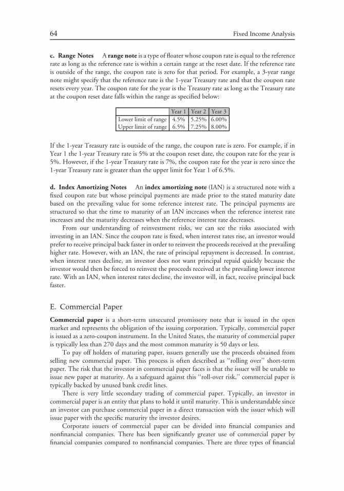
64 Fixed Income Analysis
c. Range Notes A range note is a type of floater whose coupon rate is equal to the referencerate as long as the reference rate is within a certain range at the reset date. If the reference rateis outside of the range, the coupon rate is zero for that period. For example, a 3-year rangenote might specify that the reference rate is the 1-year Treasury rate and that the coupon rateresets every year. The coupon rate for the year is the Treasury rate as long as the Treasury rateat the coupon reset date falls within the range as specified below:
Year 1 Year 2 Year 3Lower limit of range 4.5% 5.25% 6.00%Upper limit of range 6.5% 7.25% 8.00%
If the 1-year Treasury rate is outside of the range, the coupon rate is zero. For example, if inYear 1 the 1-year Treasury rate is 5% at the coupon reset date, the coupon rate for the year is5%. However, if the 1-year Treasury rate is 7%, the coupon rate for the year is zero since the1-year Treasury rate is greater than the upper limit for Year 1 of 6.5%.
d. Index Amortizing Notes An index amortizing note (IAN) is a structured note with afixed coupon rate but whose principal payments are made prior to the stated maturity datebased on the prevailing value for some reference interest rate. The principal payments arestructured so that the time to maturity of an IAN increases when the reference interest rateincreases and the maturity decreases when the reference interest rate decreases.
From our understanding of reinvestment risks, we can see the risks associated withinvesting in an IAN. Since the coupon rate is fixed, when interest rates rise, an investor wouldprefer to receive principal back faster in order to reinvest the proceeds received at the prevailinghigher rate. However, with an IAN, the rate of principal repayment is decreased. In contrast,when interest rates decline, an investor does not want principal repaid quickly because theinvestor would then be forced to reinvest the proceeds received at the prevailing lower interestrate. With an IAN, when interest rates decline, the investor will, in fact, receive principal backfaster.
E. Commercial Paper
Commercial paper is a short-term unsecured promissory note that is issued in the openmarket and represents the obligation of the issuing corporation. Typically, commercial paperis issued as a zero-coupon instrument. In the United States, the maturity of commercial paperis typically less than 270 days and the most common maturity is 50 days or less.
To pay off holders of maturing paper, issuers generally use the proceeds obtained fromselling new commercial paper. This process is often described as ‘‘rolling over’’ short-termpaper. The risk that the investor in commercial paper faces is that the issuer will be unable toissue new paper at maturity. As a safeguard against this ‘‘roll-over risk,’’ commercial paper istypically backed by unused bank credit lines.
There is very little secondary trading of commercial paper. Typically, an investor incommercial paper is an entity that plans to hold it until maturity. This is understandable sincean investor can purchase commercial paper in a direct transaction with the issuer which willissue paper with the specific maturity the investor desires.
Corporate issuers of commercial paper can be divided into financial companies andnonfinancial companies. There has been significantly greater use of commercial paper byfinancial companies compared to nonfinancial companies. There are three types of financial
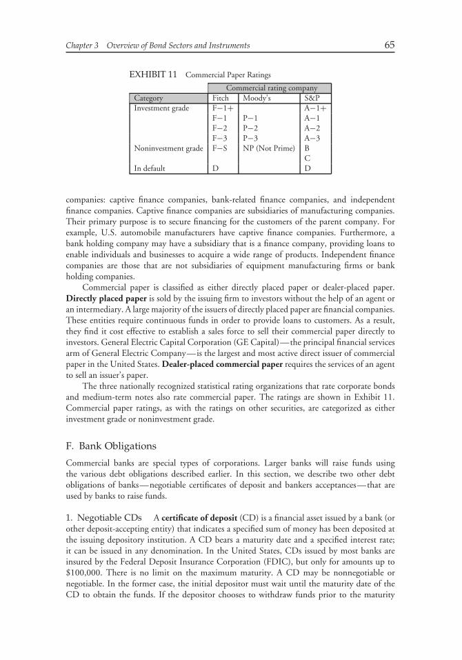
Chapter 3 Overview of Bond Sectors and Instruments 65
EXHIBIT 11 Commercial Paper Ratings
Commercial rating companyCategory Fitch Moody’s S&PInvestment grade F−1+ A−1+
F−1 P−1 A−1F−2 P−2 A−2F−3 P−3 A−3
Noninvestment grade F−S NP (Not Prime) BC
In default D D
companies: captive finance companies, bank-related finance companies, and independentfinance companies. Captive finance companies are subsidiaries of manufacturing companies.Their primary purpose is to secure financing for the customers of the parent company. Forexample, U.S. automobile manufacturers have captive finance companies. Furthermore, abank holding company may have a subsidiary that is a finance company, providing loans toenable individuals and businesses to acquire a wide range of products. Independent financecompanies are those that are not subsidiaries of equipment manufacturing firms or bankholding companies.
Commercial paper is classified as either directly placed paper or dealer-placed paper.Directly placed paper is sold by the issuing firm to investors without the help of an agent oran intermediary. A large majority of the issuers of directly placed paper are financial companies.These entities require continuous funds in order to provide loans to customers. As a result,they find it cost effective to establish a sales force to sell their commercial paper directly toinvestors. General Electric Capital Corporation (GE Capital)—the principal financial servicesarm of General Electric Company—is the largest and most active direct issuer of commercialpaper in the United States. Dealer-placed commercial paper requires the services of an agentto sell an issuer’s paper.
The three nationally recognized statistical rating organizations that rate corporate bondsand medium-term notes also rate commercial paper. The ratings are shown in Exhibit 11.Commercial paper ratings, as with the ratings on other securities, are categorized as eitherinvestment grade or noninvestment grade.
F. Bank Obligations
Commercial banks are special types of corporations. Larger banks will raise funds usingthe various debt obligations described earlier. In this section, we describe two other debtobligations of banks—negotiable certificates of deposit and bankers acceptances—that areused by banks to raise funds.
1. Negotiable CDs A certificate of deposit (CD) is a financial asset issued by a bank (orother deposit-accepting entity) that indicates a specified sum of money has been deposited atthe issuing depository institution. A CD bears a maturity date and a specified interest rate;it can be issued in any denomination. In the United States, CDs issued by most banks areinsured by the Federal Deposit Insurance Corporation (FDIC), but only for amounts up to$100,000. There is no limit on the maximum maturity. A CD may be nonnegotiable ornegotiable. In the former case, the initial depositor must wait until the maturity date of theCD to obtain the funds. If the depositor chooses to withdraw funds prior to the maturity

66 Fixed Income Analysis
date, an early withdrawal penalty is imposed. In contrast, a negotiable CD allows the initialdepositor (or any subsequent owner of the CD) to sell the CD in the open market prior tothe maturity date. Negotiable CDs are usually issued in denominations of $1 million or more.Hence, an investor in a negotiable CD issued by an FDIC insured bank is exposed to thecredit risk for any amount in excess of $100,000.
An important type of negotiable CD is the Eurodollar CD, which is a U.S. dollar-denominated CD issued primarily in London by U.S., European, Canadian, and Japanesebanks. The interest rates paid on Eurodollar CDs play an important role in the world financialmarkets because they are viewed globally as the cost of bank borrowing. This is due to thefact that these interest rates represent the rates at which major international banks offer topay each other to borrow money by issuing a Eurodollar CD with given maturities. Theinterest rate paid is called the London interbank offered rate (LIBOR). The maturities forthe Eurodollar CD range from overnight to five years. So, references to ‘‘3-month LIBOR’’indicate the interest rate that major international banks are offering to pay to other such bankson a Eurodollar CD that matures in three months. During the 1990s, LIBOR has increasinglybecome the reference rate of choice for borrowing arrangements—loans and floating-ratesecurities.
2. Bankers Acceptances Simply put, a bankers acceptance is a vehicle created tofacilitate commercial trade transactions. The instrument is called a bankers acceptance becausea bank accepts the ultimate responsibility to repay a loan to its holder. The use of bankersacceptances to finance a commercial transaction is referred to as ‘‘acceptance financing.’’ Inthe United States, the transactions in which bankers acceptances are created include (1) theimporting of goods; (2) the exporting of goods to foreign entities; (3) the storing and shippingof goods between two foreign countries where neither the importer nor the exporter is a U.S.firm; and (4) the storing and shipping of goods between two U.S. entities in the United States.Bankers acceptances are sold on a discounted basis just as Treasury bills and commercial paper.
The best way to explain the creation of a bankers acceptance is by an illustration. Severalentities are involved in our hypothetical transaction:
• Luxury Cars USA (Luxury Cars), a firm in Pennsylvania that sells automobiles• Italian Fast Autos Inc. (IFA), a manufacturer of automobiles in Italy• First Doylestown Bank (Doylestown Bank), a commercial bank in Doylestown, Pennsyl-
vania• Banco di Francesco, a bank in Naples, Italy• The Izzabof Money Market Fund, a U.S. mutual fund
Luxury Cars and IFA are considering a commercial transaction. Luxury Cars wants to import45 cars manufactured by IFA. IFA is concerned with the ability of Luxury Cars to makepayment on the 45 cars when they are received.
Acceptance financing is suggested as a means for facilitating the transaction. Luxury Carsoffers $900,000 for the 45 cars. The terms of the sale stipulate payment to be made to IFA 60days after it ships the 45 cars to Luxury Cars. IFA determines whether it is willing to acceptthe $900,000. In considering the offering price, IFA must calculate the present value of the$900,000, because it will not be receiving payment until 60 days after shipment. Suppose thatIFA agrees to these terms.
Luxury Cars arranges with its bank, Doylestown Bank, to issue a letter of credit. Theletter of credit indicates that Doylestown Bank will make good on the payment of $900,000
Chapter 3 Overview of Bond Sectors and Instruments 67
that Luxury Cars must make to IFA 60 days after shipment. The letter of credit, or time draft,will be sent by Doylestown Bank to IFA’s bank, Banco di Francesco. Upon receipt of the letterof credit, Banco di Francesco will notify IFA, which will then ship the 45 cars. After the cars areshipped, IFA presents the shipping documents to Banco di Francesco and receives the presentvalue of $900,000. IFA is now out of the picture.
Banco di Francesco presents the time draft and the shipping documents to DoylestownBank. The latter will then stamp ‘‘accepted’’ on the time draft. By doing so, DoylestownBank has created a bankers acceptance. This means that Doylestown Bank agrees to pay theholder of the bankers acceptance $900,000 at the maturity date. Luxury Cars will receive theshipping documents so that it can procure the 45 cars once it signs a note or some other typeof financing arrangement with Doylestown Bank.
At this point, the holder of the bankers acceptance is Banco di Francesco. It has two choices.It can continue to hold the bankers acceptance as an investment in its loan portfolio, or it canrequest that Doylestown Bank make a payment of the present value of $900,000. Let’s assumethat Banco di Francesco requests payment of the present value of $900,000. Now the holder ofthe bankers acceptance is Doylestown Bank. It has two choices: retain the bankers acceptanceas an investment as part of its loan portfolio or sell it to an investor. Suppose that DoylestownBank chooses the latter, and that The Izzabof Money Market Fund is seeking a high-qualityinvestment with the same maturity as that of the bankers acceptance. Doylestown Bank sellsthe bankers acceptance to the money market fund at the present value of $900,000. Ratherthan sell the instrument directly to an investor, Doylestown Bank could sell it to a dealer, whowould then resell it to an investor such as a money market fund. In either case, at the maturitydate, the money market fund presents the bankers acceptance to Doylestown Bank, receiving$900,000, which the bank in turn recovers from Luxury Cars.
Investing in bankers acceptances exposes the investor to credit risk and liquidity risk.Credit risk arises because neither the borrower nor the accepting bank may be able to paythe principal due at the maturity date. When the bankers acceptance market was growingin the early 1980s, there were over 25 dealers. By 1989, the decline in the amount ofbankers acceptances issued drove many one-time major dealers out of the business. Today,there are only a few major dealers and therefore bankers acceptances are considered illiquid.Nevertheless, since bankers acceptances are typically purchased by investors who plan to holdthem to maturity, liquidity risk is not a concern to such investors.
VII. ASSET-BACKED SECURITIES
In Section IVB we described how residential mortgage loans have been securitized. Whileresidential mortgage loans is by far the largest type of asset that has been securitized, the majortypes of assets that have been securitized in many countries have included the following:
• auto loans and leases• consumer loans• commercial assets (e.g., including aircraft, equipment leases, trade receivables)• credit cards• home equity loans• manufactured housing loans
Asset-backed securities are securities backed by a pool of loans or receivables. Ourobjective in this section is to provide a brief introduction to asset-backed securities.
68 Fixed Income Analysis
A. The Role of the Special Purpose Vehicle
The key question for investors first introduced to the asset-backed securities market is whydoesn’t a corporation simply issue a corporate bond or medium-term note rather than an asset-backed security? To understand why, consider a triple B rated corporation that manufacturesconstruction equipment. We will refer to this corporation as XYZ Corp. Some of its sales arefor cash and others are on an installment sales basis. The installment sales are assets on thebalance sheet of XYZ Corp., shown as ‘‘installment sales receivables.’’
Suppose XYZ Corp. wants to raise $75 million. If it issues a corporate bond, for example,XYZ Corp.’s funding cost would be whatever the benchmark Treasury yield is plus a yieldspread for BBB issuers. Suppose, instead, that XYZ Corp. has installment sales receivables thatare more than $75 million. XYZ Corp. can use the installment sales receivables as collateralfor a bond issue. What will its funding cost be? It will probably be the same as if it issued acorporate bond. The reason is if XYZ Corp. defaults on any of its obligations, the creditorswill have claim on all of its assets, including the installment sales receivables to satisfy paymentof their bonds.
However, suppose that XYZ Corp. can create another corporation or legal entity and sellthe installment sales receivables to that entity. We’ll refer to this entity as SPV Corp. If thetransaction is done properly, SPV Corp. owns the installment sales receivables, not XYZ Corp.It is important to understand that SPV Corp. is not a subsidiary of XYZ Corp.; therefore, theassets in SPV Corp. (i.e., the installment sales receivables) are not owned by XYZ Corp. Thismeans that if XYZ Corp. is forced into bankruptcy, its creditors cannot claim the installmentsales receivables because they are owned by SPV Corp. What are the implications?
Suppose that SPV Corp. sells securities backed by the installment sales receivables. Nowcreditors will evaluate the credit risk associated with collecting the receivables independent ofthe credit rating of XYZ Corp. What credit rating will be received for the securities issued bySPV Corp.? Whatever SPV Corp. wants the rating to be! It may seem strange that the issuer(SPV Corp.) can get any rating it wants, but that is the case. The reason is that SPV Corp. willshow the characteristics of the collateral for the security (i.e., the installment sales receivables)to a rating agency. In turn, the rating agency will evaluate the credit quality of the collateraland inform the issuer what must be done to obtain specific ratings.
More specifically, the issuer will be asked to ‘‘credit enhance’’ the securities. There arevarious forms of credit enhancement. Basically, the rating agencies will look at the potentiallosses from the pool of installment sales receivables and make a determination of how muchcredit enhancement is needed for it to issue a specific rating. The higher the credit ratingsought by the issuer, the greater the credit enhancement. Thus, XYZ Corp. which is BBBrated can obtain funding using its installment sales receivables as collateral to obtain a bettercredit rating for the securities issued. In fact, with enough credit enhancement, it can issue aAAA-rated security.
The key to a corporation issuing a security with a higher credit rating than the corporation’sown credit rating is using SPV Corp. as the issuer. Actually, this legal entity that a corporationsells the assets to is called a special purpose vehicle or special purpose corporation. It playsa critical role in the ability to create a security—an asset-backed security—that separates theassets used as collateral from the corporation that is seeking financing.16
16There are other advantages to the corporation having to do with financial accounting for the assetssold. We will not discuss this aspect of financing via asset securitization here since it is not significant forthe investor.
Chapter 3 Overview of Bond Sectors and Instruments 69
Why doesn’t a corporation always seek the highest credit rating (AAA) for its securitiesbacked by collateral? The answer is that credit enhancement does not come without a cost.Credit enhancement mechanisms increase the costs associated with a securitized borrowingvia an asset-backed security. So, the corporation must monitor the trade-off when seeking ahigher rating between the additional cost of credit enhancing the security versus the reductionin funding cost by issuing a security with a higher credit rating.
Additionally, if bankruptcy occurs, there is the risk that a bankruptcy judge may decidethat the assets of the special purpose vehicle are assets that the creditors of the corporationseeking financing (XYZ Corp. in our example) may claim after all. This is an important butunresolved legal issue in the United States. Legal experts have argued that this is unlikely.In the prospectus of an asset-backed security, there will be a legal opinion addressing thisissue. This is the reason why special purpose vehicles in the United States are referred to as‘‘bankruptcy remote’’ entities.
B. Credit Enhancement Mechanisms
Later, we will review how rating agencies analyze collateral in order to assign ratings. What isimportant to understand is that the amount of credit enhancement will be determined relativeto a particular rating. There are two general types of credit enhancement structures: externaland internal.
External credit enhancements come in the form of third-party guarantees. The mostcommon forms of external credit enhancements are (1) a corporate guarantee, (2) a letter ofcredit, and (3) bond insurance. A corporate guarantee could be from the issuing entity seekingthe funding (XYZ Corp. in our illustration above) or its parent company. Bond insuranceprovides the same function as in municipal bond structures and is referred to as an insurance‘‘wrap.’’
A disadvantage of an external credit enhancement is that it is subject to the credit riskof the third-party guarantor. Should the third-party guarantor be downgraded, the issue itselfcould be subject to downgrade even if the collateral is performing as expected. This is basedon the ‘‘weak link’’ test followed by rating agencies. According to this test, when evaluatinga proposed structure, the credit quality of the issue is only as good as the weakest link incredit enhancement regardless of the quality of the underlying loans. Basically, an externalcredit enhancement exposes the investor to event risk since the downgrading of one entity (thethird-party guarantor) can result in a downgrade of the asset-backed security.
Internal credit enhancements come in more complicated forms than external creditenhancements. The most common forms of internal credit enhancements are reserve funds,over collateralization, and senior/subordinate structures.
VIII. COLLATERALIZED DEBT OBLIGATIONS
A fixed income product that is also classified as part of the asset-backed securities market isthe collateralized debt obligation (CDO). CDOs deserve special attention because of theirgrowth since 2000. Moreover, while a CDO is backed by various assets, it is managed in away that is not typical in other asset-backed security transactions. CDOs have been issued inboth developed and developing countries.
A CDO is a product backed by a diversified pool of one or more of the following typesof debt obligations:
70 Fixed Income Analysis
• U.S. domestic investment-grade and high-yield corporate bonds• U.S. domestic bank loans• emerging market bonds• special situation loans and distressed debt• foreign bank loans• asset-backed securities• residential and commercial mortgage-backed securities• other CDOs
When the underlying pool of debt obligations consists of bond-type instruments (corporateand emerging market bonds), a CDO is referred to as a collateralized bond obligation (CBO).When the underlying pool of debt obligations are bank loans, a CDO is referred to as acollateralized loan obligation (CLO).
In a CDO structure, an asset manager is responsible for managing the portfolio of assets(i.e., the debt obligations in which it invests). The funds to purchase the underlying assets(i.e., the bonds and loans) are obtained from the issuance of a CDO. The CDO is structuredinto notes or tranches similar to a CMO issue. The tranches are assigned ratings by a ratingagency. There are restrictions as to how the manager manages the CDO portfolio, usually inthe form of specific tests that must be satisfied. If any of the restrictions are violated by theasset manager, the notes can be downgraded and it is possible that the trustee begin payingprincipal to the senior noteholders in the CDO structure.
CDOs are categorized based on the motivation of the sponsor of the transaction. If themotivation of the sponsor is to earn the spread between the yield offered on the fixed incomeproducts held in the portfolio of the underlying pool (i.e., the collateral) and the paymentsmade to the noteholders in the structure, then the transaction is referred to as an arbitragetransaction. (Moreover, a CDO is a vehicle for a sponsor that is an investment managementfirm to gather additional assets to manage and thereby generate additional management fees.)If the motivation of the sponsor is to remove debt instruments (primarily loans) from itsbalance sheet, then the transaction is referred to as a balance sheet transaction. Sponsorsof balance sheet transactions are typically financial institutions such as banks and insurancecompanies seeking to reduce their capital requirements by removing loans due to their higherrisk-based capital requirements.
IX. PRIMARY MARKET AND SECONDARYMARKET FOR BONDS
Financial markets can be categorized as those dealing with financial claims that are newlyissued, called the primary market, and those for exchanging financial claims previously issued,called the secondary market.
A. Primary Market
The primary market for bonds involves the distribution to investors of newly issued securitiesby central governments, its agencies, municipal governments, and corporations. Investmentbankers work with issuers to distribute newly issued securities. The traditional process forissuing new securities involves investment bankers performing one or more of the followingthree functions: (1) advising the issuer on the terms and the timing of the offering, (2) buying
Chapter 3 Overview of Bond Sectors and Instruments 71
the securities from the issuer, and (3) distributing the issue to the public. The advisor role mayrequire investment bankers to design a security structure that is more palatable to investorsthan a particular traditional instrument.
In the sale of new securities, investment bankers need not undertake the secondfunction—buying the securities from the issuer. An investment banker may merely act as anadvisor and/or distributor of the new security. The function of buying the securities from theissuer is called underwriting. When an investment banking firm buys the securities from theissuer and accepts the risk of selling the securities to investors at a lower price, it is referredto as an underwriter. When the investment banking firm agrees to buy the securities fromthe issuer at a set price, the underwriting arrangement is referred to as a firm commitment.In contrast, in a best efforts arrangement, the investment banking firm only agrees to use itsexpertise to sell the securities—it does not buy the entire issue from the issuer. The fee earnedfrom the initial offering of a security is the difference between the price paid to the issuer andthe price at which the investment bank reoffers the security to the public (called the reofferingprice).
1. Bought Deal and Auction Process Not all bond issues are underwritten using thetraditional firm commitment or best effort process we just described. Variations in the UnitedStates, the Euromarkets, and foreign markets for bonds include the bought deal and theauction process. The mechanics of a bought deal are as follows. The underwriting firm orgroup of underwriting firms offers a potential issuer of debt securities a firm bid to purchasea specified amount of securities with a certain coupon rate and maturity. The issuer is givena day or so (maybe even a few hours) to accept or reject the bid. If the bid is accepted, theunderwriting firm has ‘‘bought the deal.’’ It can, in turn, sell the securities to other investmentbanking firms for distribution to their clients and/or distribute the securities to its clients.Typically, the underwriting firm that buys the deal will have presold most of the issue to itsinstitutional clients. Thus, the risk of capital loss for the underwriting firm in a bought dealmay not be as great as it first appears. There are some deals that are so straightforward thata large underwriting firm may have enough institutional investor interest to keep the risks ofdistributing the issue at the reoffering price quite small. Moreover, hedging strategies usinginterest rate risk control tools can reduce or eliminate the risk of realizing a loss of selling thebonds at a price below the reoffering price.
In the auction process, the issuer announces the terms of the issue and interested partiessubmit bids for the entire issue. This process is more commonly referred to as a competitivebidding underwriting. For example, suppose that a public utility wishes to issue $400 millionof bonds. Various underwriters will form syndicates and bid on the issue. The syndicate thatbids the lowest yield (i.e., the lowest cost to the issuer) wins the entire $400 million bond issueand then reoffers it to the public.
2. Private Placement of Securities Public and private offerings of securities differ interms of the regulatory requirements that must be satisfied by the issuer. For example, in theUnited States, the Securities Act of 1933 and the Securities Exchange Act of 1934 requirethat all securities offered to the general public must be registered with the SEC, unless thereis a specific exemption. The Securities Acts allow certain exemptions from federal registration.Section 4(2) of the 1933 Act exempts from registration ‘‘transactions by an issuer not involvingany public offering.’’
The exemption of an offering does not mean that the issuer need not disclose informationto potential investors. The issuer must still furnish the same information deemed material by
72 Fixed Income Analysis
the SEC. This is provided in a private placement memorandum, as opposed to a prospectusfor a public offering. The distinction between the private placement memorandum and theprospectus is that the former does not include information deemed by the SEC as ‘‘non-material,’’ whereas such information is required in a prospectus. Moreover, unlike a prospectus,the private placement memorandum is not subject to SEC review.
In the United States, one restriction that was imposed on buyers of privately placedsecurities is that they may not be sold for two years after acquisition. Thus, there was noliquidity in the market for that time period. Buyers of privately placed securities must becompensated for the lack of liquidity which raises the cost to the issuer of the securities.SEC Rule 144A, which became effective in 1990, eliminates the two-year holding periodby permitting large institutions to trade securities acquired in a private placement amongthemselves without having to register these securities with the SEC. Private placements aretherefore now classified as Rule 144A offerings or non-Rule 144A offerings. The latter are morecommonly referred to as traditional private placements. Rule 144A offerings are underwrittenby investment bankers.
B. Secondary Market
In the secondary market, an issuer of a bond—whether it is a corporation or a governmentalunit—may obtain regular information about the bond’s value. The periodic trading of abond reveals to the issuer the consensus price that the bond commands in an open market.Thus, issuers can discover what value investors attach to their bonds and the implied interestrates investors expect and demand from them. Bond investors receive several benefits from asecondary market. The market obviously offers them liquidity for their bond holdings as wellas information about fair or consensus values. Furthermore, secondary markets bring togethermany interested parties and thereby reduces the costs of searching for likely buyers and sellersof bonds.
A bond can trade on an exchange or in an over-the-counter market. Traditionally, bondtrading has taken place predominately in the over-the-counter market where broker-dealertrading desks take principal positions to fill customer buy and sell orders. In recent years,however, there has been an evolution away from this form of traditional bond trading andtoward electronic bond trading. This evolution toward electronic bond trading is likely tocontinue.
There are several related reasons for the transition to the electronic trading of bonds.First, because the bond business has been a principal business (where broker-dealer firms risktheir own capital) rather than an agency business (where broker-dealer firms act merely as anagent or broker), the capital of the market makers is critical. The amount of capital availableto institutional investors to invest throughout the world has placed significant demands on thecapital of broker-dealer firms. As a result, making markets in bonds has become more risky forbroker-dealer firms. Second, the increase in bond market volatility has increased the capitalrequired of broker-dealer firms in the bond business. Finally, the profitability of bond markettrading has declined since many of the products have become more commodity-like and theirbid-offer spreads have decreased.
The combination of the increased risk and the decreased profitability of bond markettrading has induced the major broker-dealer firms to deemphasize this business in the allocationof capital. Broker-dealer firms have determined that it is more efficient to employ their capitalin other activities such as underwriting and asset management, rather than in principal-typemarket-making businesses. As a result, the liquidity of the traditionally principal-oriented bond
Chapter 3 Overview of Bond Sectors and Instruments 73
markets has declined, and this decline in liquidity has opened the way for other market-makingmechanisms. This retreat by traditional market-making firms opened the door for electronictrading. In fact, the major broker-dealer firms in bonds have supported electronic trading inbonds.
Electronic trading in bonds has helped fill this developing vacuum and provided liquidityto the bond markets. In addition to the overall advantages of electronic trading in providingliquidity to the markets and price discovery (particularly for less liquid markets) is the resultingtrading and portfolio management efficiencies that have been realized. For example, portfoliomanagers can load their buy/sell orders into a web site, trade from these orders, and then clearthese orders.
There are a variety of types of electronic trading systems for bonds. The two major typesof electronic trading systems are dealer-to-customer systems and exchange systems. Dealer-to-customer systems can be a single-dealer system or multiple-dealer system. Single-dealersystems are based on a customer dealing with a single, identified dealer over the computer.The single-dealer system simply computerizes the traditional customer-dealer market-makingmechanism. Multi-dealer systems provide some advancement over the single-dealer method.A customer can select from any of several identified dealers whose bids and offers are providedon a computer screen. The customer knows the identity of the dealer.
In an exchange system, dealer and customer bids and offers are entered into the system onan anonymous basis, and the clearing of the executed trades is done through a common process.Two different major types of exchange systems are those based on continuous trading and callauctions. Continuous trading permits trading at continuously changing market-determinedprices throughout the day and is appropriate for liquid bonds, such as Treasury and agencysecurities. Call auctions provide for fixed price auctions (that is, all the transactions orexchanges occur at the same ‘‘fixed’’ price) at specific times during the day and are appropriatefor less liquid bonds such as corporate bonds and municipal bonds.
CHAPTER 4UNDERSTANDING YIELD
SPREADS
I. INTRODUCTION
The interest rate offered on a particular bond issue depends on the interest rate that can beearned on (1) risk-free instruments and (2) the perceived risks associated with the issue. Werefer to the interest rates on risk-free instruments as the ‘‘level of interest rates.’’ The actions ofa country’s central bank influence the level of interest rates as does the state of the country’seconomy. In the United States, the level of interest rates depends on the state of the economy,the interest rate policies implemented by the Board of Governors of the Federal Reserve Board,and the government’s fiscal policies.
A casual examination of the financial press and dealer quote sheets shows a wide rangeof interest rates reported at any given point in time. Why are there differences in interestrates among debt instruments? We provided information on this topic in Chapters 1 and 2. InChapter 1, we explained the various features of a bond while in Chapter 2 we explained howthose features affect the risk characteristics of a bond relative to bonds without that feature.
In this chapter, we look more closely at the differences in yields offered by bonds indifferent sectors of the bond market and within a sector of the bond market. This informationis used by investors in assessing the ‘‘relative value’’ of individual securities within a bondsector, or among sectors of the bond market. Relative value analysis is a process of rankingindividual securities or sectors with respect to expected return potential. We will continue touse the terms ‘‘interest rate’’ and ‘‘yield’’ interchangeably.
II. INTEREST RATE DETERMINATION
Our focus in this chapter is on (1) the relationship between interest rates offered on differentbond issues at a point in time and (2) the relationships among interest rates offered in differentsectors of the economy at a given point in time. We will provide a brief discussion of the roleof the U.S. Federal Reserve (the Fed), the policy making body whose interest rate policy toolsdirectly influence short-term interest rates and indirectly influence long-term interest rates.
Once the Fed makes a policy decision it immediately announces the policy in a statementissued at the close of its meeting. The Fed also communicates its future intentions via publicspeeches or its Chairman’s testimony before Congress. Managers who pursue an active strategyof positioning a portfolio to take advantage of expected changes in interest rates watch closelythe same key economic indicators that the Fed watches in order to anticipate a change in
74
Chapter 4 Understanding Yield Spreads 75
the Fed’s monetary policy and to assess the expected impact on short-term interest rates. Theindicators that are closely watched by the Fed include non-farm payrolls, industrial production,housing starts, motor vehicle sales, durable good orders, National Association of PurchasingManagement supplier deliveries, and commodity prices.
In implementing monetary policy, the Fed uses the following interest rate policy tools:
1. open market operations2. the discount rate3. bank reserve requirements4. verbal persuasion to influence how bankers supply credit to businesses and consumers
Engaging in open market operations and changing the discount rate are the tools mostoften employed. Together, these tools can raise or lower the cost of funds in the economy.Open market operations do this through the Fed’s buying and selling of U.S. Treasurysecurities. This action either adds funds to the market (when Treasury securities are purchased)or withdraws funds from the market (when Treasury securities are sold). Fed open marketoperations influence the federal funds rate, the rate at which banks borrow and lend funds fromeach other. The discount rate is the interest rate at which banks can borrow on a collateralizedbasis at the Fed’s discount window. Increasing the discount rate makes the cost of funds moreexpensive for banks; the cost of funds is reduced when the discount rate is lowered. Changingbank reserve requirements is a less frequently used policy, as is the use of verbal persuasion toinfluence the supply of credit.
III. U.S. TREASURY RATES
The securities issued by the U.S. Department of the Treasury are backed by the full faith andcredit of the U.S. government. Consequently, market participants throughout the world viewthese securities as being ‘‘default risk-free’’ securities. However, there are risks associated withowning U.S. Treasury securities.
The Treasury issues the following securities:
Treasury bills: Zero-coupon securities with a maturity at issuance of one year or less. TheTreasury currently issues 1-month, 3-month, and 6-month bills.
Treasury notes: Coupon securities with maturity at issuance greater than 1 year but notgreater than 10 years. The Treasury currently issues 2-year, 5-year, and 10-year notes.
Treasury bonds: Coupon securities with maturity at issuance greater than 10 years.Although Treasury bonds have traditionally been issued with maturities up to 30years, the Treasury suspended issuance of the 30-year bond in October 2001.
Inflation-protection securities: Coupon securities whose principal’s reference rate is theConsumer Price Index.
The on-the-run issue or current issue is the most recently auctioned issue of Treasurynotes and bonds of each maturity. The off-the-run issues are securities that were previouslyissued and are replaced by the on-the-run issue. Issues that have been replaced by several morerecent issues are said to be ‘‘well off-the-run issues.’’
The secondary market for Treasury securities is an over-the-counter market where agroup of U.S. government securities dealers provides continuous bids and offers on specific
76 Fixed Income Analysis
outstanding Treasuries. This secondary market is the most liquid financial market in theworld. Off-the-run issues are less liquid than on-the-run issues.
A. Risks of Treasury Securities
With this brief review of Treasury securities, let’s look at their risks. We listed the generalrisks in Chapter 2 and repeat them here: (1) interest rate risk, (2) call and prepayment risk,(3) yield curve risk, (4) reinvestment risk, (5) credit risk, (6) liquidity risk, (7) exchange-raterisk, (8) volatility risk, (9) inflation or purchasing power risk, and (10) event risk.
All fixed income securities, including Treasury securities, expose investors to interest raterisk.1 However, the degree of interest rate risk is not the same for all securities. The reason isthat maturity and coupon rate affect how much the price changes when interest rates change.One measure of a security’s interest rate risk is its duration.2 Since Treasury securities, likeother fixed income securities, have different durations, they have different exposures to interestrate risk as measured by duration.
Technically, yield curve risk and volatility risk are risks associated with Treasury securities.However, at this early stage of our understanding of fixed income analysis, we will not attemptto explain these risks. It is not necessary to understand these risks at this point in order toappreciate the material that follows in this section.
Because Treasury securities are noncallable, there is no reinvestment risk due to an issuebeing called.3 Treasury coupon securities carry reinvestment risk because in order to realizethe yield offered on the security, the investor must reinvest the coupon payments received atan interest rate equal to the computed yield. So, all Treasury coupon securities are exposedto reinvestment risk. Treasury bills are not exposed to reinvestment risk because they arezero-coupon instruments.
As for credit risk, the perception in the global financial community is that Treasurysecurities have no credit risk. In fact, when market participants and the popular press statethat Treasury securities are ‘‘risk free,’’ they are referring to credit risk.
Treasury securities are highly liquid. However, on-the-run and off-the-run Treasurysecurities trade with different degrees of liquidity. Consequently, the yields offered byon-the-run and off-the-run issues reflect different degrees of liquidity.
Since U.S. Treasury securities are dollar denominated, there is no exchange-rate risk foran investor whose domestic currency is the U.S. dollar. However, non-U.S. investors whosedomestic currency is not the U.S. dollar are exposed to exchange-rate risk.
Fixed-rate Treasury securities are exposed to inflation risk. Treasury inflation protectionsecurities (TIPS) have a coupon rate that is effectively adjusted for the rate of inflation andtherefore have protection against inflation risk.
1Interest rate risk is the risk of an adverse movement in the price of a bond due to changes in interestrates.2Duration is a measure of a bond’s price sensitivity to a change in interest rates.3The Treasury no longer issues callable bonds. The Treasury issued callable bonds in the early 1980sand all of these issues will mature no later than November 2014 (assuming that they are not calledbefore then). Moreover, as of 2004, the longest maturity of these issues is 10 years. Consequently, whileoutstanding callable issues of the Treasury are referred to as ‘‘bonds,’’ based on their current maturitythese issues would not be compared to long-term bonds in any type of relative value analysis. Therefore,because the Treasury no longer issues callable bonds and the outstanding issues do not have the maturitycharacteristics of a long-term bond, we will ignore these callable issues and simply treat Treasury bondsas noncallable.
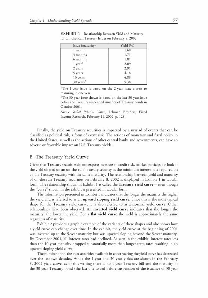
Chapter 4 Understanding Yield Spreads 77
EXHIBIT 1 Relationship Between Yield and Maturityfor On-the-Run Treasury Issues on February 8, 2002
Issue (maturity) Yield (%)1 month 1.683 months 1.716 months 1.811 year1 2.092 years 2.915 years 4.1810 years 4.8830 years2 5.38
1The 1-year issue is based on the 2-year issue closest tomaturing in one year.2The 30-year issue shown is based on the last 30-year issuebefore the Treasury suspended issuance of Treasury bonds inOctober 2001.
Source: Global Relative Value, Lehman Brothers, FixedIncome Research, February 11, 2002, p. 128.
Finally, the yield on Treasury securities is impacted by a myriad of events that can beclassified as political risk, a form of event risk. The actions of monetary and fiscal policy inthe United States, as well as the actions of other central banks and governments, can have anadverse or favorable impact on U.S. Treasury yields.
B. The Treasury Yield Curve
Given that Treasury securities do not expose investors to credit risk, market participants look atthe yield offered on an on-the-run Treasury security as the minimum interest rate required ona non-Treasury security with the same maturity. The relationship between yield and maturityof on-the-run Treasury securities on February 8, 2002 is displayed in Exhibit 1 in tabularform. The relationship shown in Exhibit 1 is called the Treasury yield curve—even thoughthe ‘‘curve’’ shown in the exhibit is presented in tabular form.
The information presented in Exhibit 1 indicates that the longer the maturity the higherthe yield and is referred to as an upward sloping yield curve. Since this is the most typicalshape for the Treasury yield curve, it is also referred to as a normal yield curve. Otherrelationships have been observed. An inverted yield curve indicates that the longer thematurity, the lower the yield. For a flat yield curve the yield is approximately the sameregardless of maturity.
Exhibit 2 provides a graphic example of the variants of these shapes and also shows howa yield curve can change over time. In the exhibit, the yield curve at the beginning of 2001was inverted up to the 5-year maturity but was upward sloping beyond the 5-year maturity.By December 2001, all interest rates had declined. As seen in the exhibit, interest rates lessthan the 10-year maturity dropped substantially more than longer-term rates resulting in anupward sloping yield curve.
The number of on-the-run securities available in constructing the yield curve has decreasedover the last two decades. While the 1-year and 30-year yields are shown in the February8, 2002 yield curve, as of this writing there is no 1-year Treasury bill and the maturity ofthe 30-year Treasury bond (the last one issued before suspension of the issuance of 30-year
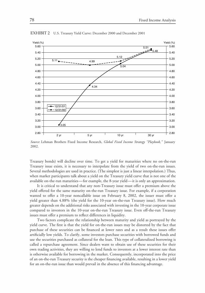
78 Fixed Income Analysis
EXHIBIT 2 U.S. Treasury Yield Curve: December 2000 and December 2001
Yield (%)5.60
5.40
5.20
5.00
4.80
4.60
4.40
4.20
4.00
3.80
3.60
3.40
3.20
3.00
2.80
Yield (%)5.60
5.40
5.20
5.00
4.80
4.60
4.40
4.20
4.00
3.80
3.60
3.40
3.20
3.00
2.80
5.11 4.99
5.12
5.515.48
5.04
4.34
3.05
12/31/0112/31/00
2 yr 5 yr 10 yr 30 yr
Source: Lehman Brothers Fixed Income Research, Global Fixed Income Strategy ‘‘Playbook,’’ January2002.
Treasury bonds) will decline over time. To get a yield for maturities where no on-the-runTreasury issue exists, it is necessary to interpolate from the yield of two on-the-run issues.Several methodologies are used in practice. (The simplest is just a linear interpolation.) Thus,when market participants talk about a yield on the Treasury yield curve that is not one of theavailable on-the-run maturities—for example, the 8-year yield—it is only an approximation.
It is critical to understand that any non-Treasury issue must offer a premium above theyield offered for the same maturity on-the-run Treasury issue. For example, if a corporationwanted to offer a 10-year noncallable issue on February 8, 2002, the issuer must offer ayield greater than 4.88% (the yield for the 10-year on-the-run Treasury issue). How muchgreater depends on the additional risks associated with investing in the 10-year corporate issuecompared to investors in the 10-year on-the-run Treasury issue. Even off-the-run Treasuryissues must offer a premium to reflect differences in liquidity.
Two factors complicate the relationship between maturity and yield as portrayed by theyield curve. The first is that the yield for on-the-run issues may be distorted by the fact thatpurchase of these securities can be financed at lower rates and as a result these issues offerartificially low yields. To clarify, some investors purchase securities with borrowed funds anduse the securities purchased as collateral for the loan. This type of collateralized borrowing iscalled a repurchase agreement. Since dealers want to obtain use of these securities for theirown trading activities, they are willing to lend funds to investors at a lower interest rate thanis otherwise available for borrowing in the market. Consequently, incorporated into the priceof an on-the-run Treasury security is the cheaper financing available, resulting in a lower yieldfor an on-the-run issue than would prevail in the absence of this financing advantage.
Chapter 4 Understanding Yield Spreads 79
The second factor complicating the comparison of on-the-run and off-the-run Treasuryissues (in addition to liquidity differences) is that they have different interest rate risks anddifferent reinvestment risks. So, for example, if the coupon rate for the 5-year on-the-runTreasury issue in February 2002 is 4.18% and an off-the-run Treasury issue with just less than5 years to maturity has a 5.25% coupon rate, the two bonds have different degrees of interestrate risk. Specifically, the on-the-run issue has greater interest rate risk (duration) because ofthe lower coupon rate. However, it has less reinvestment risk because the coupon rate is lower.
Because of this, when market participants talk about interest rates in the Treasury marketand use these interest rates to value securities they look at another relationship in the Treasurymarket: the relationship between yield and maturity for zero-coupon Treasury securities. Butwait, we said that the Treasury only issues three zero-coupon securities—1-month, 3-month,and 6-month Treasury bills. Where do we obtain the relationship between yield and maturityfor zero-coupon Treasury securities? We discuss this next.
1. Theories of the Term Structure of Interest Rates What information does the yieldcurve reveal? How can we explain and interpret changes in the yield curve? These questions areof great interest to anyone concerned with such tasks as the valuation of multiperiod securities,economic forecasting, and risk management. Theories of the term structure of interest rates4
address these questions. Here we introduce the three main theories or explanations of the termstructure. We shall present these theories intuitively.5
The three main term structure theories are:
• the pure expectations theory (unbiased expectations theory)• the liquidity preference theory (or liquidity premium theory)• the market segmentation theory
Each theory is explained below.
a. Pure Expectations Theory The pure expectations theory makes the simplest and mostdirect link between the yield curve and investors’ expectations about future interest rates,and, because long-term interest rates are plausibly linked to investor expectations about futureinflation, it also opens the door to some interesting economic interpretations.
The pure expectations theory explains the term structure in terms of expected futureshort-term interest rates. According to the pure expectations theory, the market sets the yieldon a two-year bond so that the return on the two-year bond is approximately equal to thereturn on a one-year bond plus the expected return on a one-year bond purchased one yearfrom today.
Under this theory, a rising term structure indicates that the market expects short-termrates to rise in the future. For example, if the yield on the two-year bond is higher than theyield on the one-year bond, according to this theory, investors expect the one-year rate a yearfrom now to be sufficiently higher than the one-year rate available now so that the two ways ofinvesting for two years have the same expected return. Similarly, a flat term structure reflects
4Term structure means the same as maturity structure—a description of how a bond’s yield changes asthe bond’s maturity changes. In other words, term structure asks the question: Why do long-term bondshave a different yield than short-term bonds?5Later, we provide a more mathematical treatment of these theories in terms of forward rates that wewill discuss in Chapter 6.
80 Fixed Income Analysis
an expectation that future short-term rates will be unchanged from today’s short-term rates,while a falling term structure reflects an expectation that future short-term rates will decline.This is summarized below:
Shape of term structure Implication according to pure expectations theoryupward sloping (normal) rates expected to risedownward sloping (inverted) rates expected to declineflat rates not expected to change
The implications above are the broadest interpretation of the theory.How does the pure expectations theory explain a humped yield curve? According to the
theory, this can result when investors expect the returns on one-year securities to rise for anumber of years, then fall for a number of years.
The relationships that the table above illustrates suggest that the shape of the yield curvecontains information regarding investors’ expectations about future inflation. A pioneer of thetheory of interest rates (the economist Irving Fisher) asserted that interest rates reflect the sumof a relatively stable real rate of interest plus a premium for expected inflation. Under thishypothesis, if short-term rates are expected to rise, investors expect inflation to rise as well.An upward (downward) sloping term structure would mean that investors expected rising(declining) future inflation. Much economic discussion in the financial press and elsewhere isbased on this interpretation of the yield curve.
The shortcoming of the pure expectations theory is that it assumes investors are indifferentto interest rate risk and any other risk factors associated with investing in bonds with differentmaturities.
b. Liquidity Preference Theory The liquidity preference theory asserts that marketparticipants want to be compensated for the interest rate risk associated with holding longer-term bonds. The longer the maturity, the greater the price volatility when interest rates changeand investors want to be compensated for this risk. According to the liquidity preferencetheory, the term structure of interest rates is determined by (1) expectations about futureinterest rates and (2) a yield premium for interest rate risk.6 Because interest rate risk increaseswith maturity, the liquidity preference theory asserts that the yield premium increases withmaturity.
Consequently, based on this theory, an upward-sloping yield curve may reflect expectationsthat future interest rates either (1) will rise, or (2) will be unchanged or even fall, but with ayield premium increasing with maturity fast enough to produce an upward sloping yield curve.Thus, for an upward sloping yield curve (the most frequently observed type), the liquiditypreference theory by itself has nothing to say about expected future short-term interest rates.For flat or downward sloping yield curves, the liquidity preference theory is consistent witha forecast of declining future short-term interest rates, given the theory’s prediction that theyield premium for interest rate risk increases with maturity.
Because the liquidity preference theory argues that the term structure is determined byboth expectations regarding future interest rates and a yield premium for interest rate risk, itis referred to as biased expectations theory.
6In the liquidity preference theory, ‘‘liquidity’’ is measured in terms of interest rate risk. Specifically, themore interest rate risk, the less the liquidity.
Chapter 4 Understanding Yield Spreads 81
c. Market Segmentation Theory Proponents of the market segmentation theory arguethat within the different maturity sectors of the yield curve the supply and demand for fundsdetermine the interest rate for that sector. That is, each maturity sector is an independentor segmented market for purposes of determining the interest rate in that maturity sector.Thus, positive sloping, inverted, and humped yield curves are all possible. In fact, the marketsegmentation theory can be used to explain any shape that one might observe for the yieldcurve.
Let’s understand why proponents of this theory view each maturity sector as independentor segmented. In the bond market, investors can be divided into two groups based on theirreturn needs: investors that manage funds versus a broad-based bond market index and thosethat manage funds versus their liabilities. The easiest case is for those that manage fundsagainst liabilities. Investors managing funds where liabilities represent the benchmark willrestrict their activities to the maturity sector that provides the best match with the maturityof their liabilities.7 This is the basic principle of asset-liability management. If these investorsinvest funds outside of the maturity sector that provides the best match against liabilities, theyare exposing themselves to the risks associated with an asset-liability mismatch. For example,consider the manager of a defined benefit pension fund. Since the liabilities of a defined benefitpension fund are long-term, the manager will invest in the long-term maturity sector of thebond market. Similarly, commercial banks whose liabilities are typically short-term focus onshort-term fixed-income investments. Even if the rate on long-term bonds were considerablymore attractive than that on short-term investments, according to the market segmentationtheory commercial banks will restrict their activities to investments at the short end of the yieldcurve. Reinforcing this notion of a segmented market are restrictions imposed on financialinstitutions that prevent them from mismatching the maturity of assets and liabilities.
A variant of the market segmentation theory is the preferred habitat theory. This theoryargues that investors prefer to invest in particular maturity sectors as dedicated by the natureof their liabilities. However, proponents of this theory do not assert that investors would beunwilling to shift out of their preferred maturity sector; instead, it is argued that if investorsare given an inducement to do so in the form of a yield premium they will shift out of theirpreferred habitat. The implication of the preferred habitat theory for the shape of the yieldcurve is that any shape is possible.
C. Treasury Strips
Although the U.S. Department of the Treasury does not issue zero-coupon Treasury securitieswith maturity greater than one year, government dealers can synthetically create zero-couponsecurities, which are effectively guaranteed by the full faith and credit of the U.S. government,with longer maturities. They create these securities by separating the coupon payments andthe principal payment of a coupon-bearing Treasury security and selling them off separately.The process, referred to as stripping a Treasury security, results in securities called Treasurystrips. The Treasury strips created from coupon payments are called Treasury coupon stripsand those created from the principal payment are called Treasury principal strips. We explainedthe process of creating Treasury strips in Chapter 3.
7One of the principles of finance is the ‘‘matching principle:’’ short-term assets should be financed with(or matched with) short-term liabilities; long-term assets should be financed with (or matched with)long-term sources of financing.
82 Fixed Income Analysis
Because zero-coupon instruments have no reinvestment risk, Treasury strips for differentmaturities provide a superior relationship between yield and maturity than do securitieson the on-the-run Treasury yield curve. The lack of reinvestment risk eliminates the biasresulting from the difference in reinvestment risk for the securities being compared. Anotheradvantage is that the duration of a zero-coupon security is approximately equal to its maturity.Consequently, when comparing bond issues against Treasury strips, we can compare them onthe basis of duration.
The yield on a zero-coupon security has a special name: the spot rate. In the case of aTreasury security, the yield is called a Treasury spot rate. The relationship between maturityand Treasury spot rates is called the term structure of interest rates. Sometimes discussionsof the term structure of interest rates in the Treasury market get confusing. The Treasuryyield curve and the Treasury term structure of interest rates are often used interchangeably.While there is a technical difference between the two, the context in which these terms areused should be understood.
IV. YIELDS ON NON-TREASURY SECURITIES
Despite the imperfections of the Treasury yield curve as a benchmark for the minimum interestrate that an investor requires for investing in a non-Treasury security, it is commonplace torefer to the additional yield over the benchmark Treasury issue of the same maturity as theyield spread. In fact, because non-Treasury sectors of the fixed income market offer a yieldspread to Treasury securities, non-Treasury sectors are commonly referred to as spread sectorsand non-Treasury securities in these sectors are referred to as spread products.
A. Measuring Yield Spreads
While it is common to talk about spreads relative to a Treasury security of the same maturity, ayield spread between any two bond issues can be easily computed. In general, the yield spreadbetween any two bond issues, bond X and bond Y, is computed as follows:
yield spread = yield on bond X − yield on bond Y
where bond Y is considered the reference bond (or benchmark) against which bond X ismeasured.
When a yield spread is computed in this manner it is referred to as an absolute yieldspread and it is measured in basis points. For example, on February 8, 2002, the yield onthe 10-year on-the-run Treasury issue was 4.88% and the yield on a single A rated 10-yearindustrial bond was 6.24%. If bond X is the 10-year industrial bond and bond Y is the 10-yearon-the-run Treasury issue, the absolute yield spread was:
yield spread = 6.24% − 4.88% = 1.36% or 136 basis points
Unless otherwise specified, yield spreads are typically measured in this way. Yield spreadscan also be measured on a relative basis by taking the ratio of the yield spread to the yield ofthe reference bond. This is called a relative yield spread and is computed as shown below,assuming that the reference bond is bond Y:
relative yield spread = yield on bond X − yield on bond Y
yield on bond Y
Chapter 4 Understanding Yield Spreads 83
Sometimes bonds are compared in terms of a yield ratio, the quotient of two bond yields,as shown below:
yield ratio = yield on bond X
yield on bond Y
Typically, in the U.S. bond market when these measures are computed, bond Y (thereference bond) is a Treasury issue. In that case, the equations for the yield spread measuresare as follows:
absolute yield spread = yield on bond X − yield of on-the-run Treasury
relative yield spread = yield on bond X − yield of on-the-run Treasuryyield of on-the-run Treasury
yield ratio = yield on bond Xyield of on-the-run Treasury
For the above example comparing the yields on the 10-year single A rated industrial bondand the 10-year on-the-run Treasury, the relative yield spread and yield ratio are computedbelow:
absolute yield spread = 6.24% − 4.88% = 1.36% = 136 basis points
relative yield spread = 6.24% − 4.88%
4.88%= 0.279 = 27.9%
yield ratio = 6.24%
4.88%= 1.279
The reason for computing yield spreads in terms of a relative yield spread or a yield ratiois that the magnitude of the yield spread is affected by the level of interest rates. For example,in 1957 the yield on Treasuries was about 3%. At that time, the absolute yield spread betweentriple B rated utility bonds and Treasuries was 40 basis points. This was a relative yield spreadof 13% (0.40% divided by 3%). However, when the yield on Treasuries exceeded 10% in1985, an absolute yield spread of 40 basis points would have meant a relative yield spread ofonly 4% (0.40% divided by 10%). Consequently, in 1985 an absolute yield spread greaterthan 40 basis points would have been required in order to produce a similar relative yieldspread.
In this chapter, we will focus on the yield spread as most commonly measured, theabsolute yield spread. So, when we refer to yield spread, we mean absolute yield spread.
Whether we measure the yield spread as an absolute yield spread, a relative yield spread,or a yield ratio, the question to answer is what causes the yield spread between two bondissues. Basically, active bond portfolio strategies involve assessing the factors that cause theyield spread, forecasting how that yield spread may change over an investment horizon, andtaking a position to capitalize on that forecast.
B. Intermarket Sector Spreads and Intramarket Spreads
The bond market is classified into sectors based on the type of issuer. In the United States,these sectors include the U.S. government sector, the U.S. government agencies sector, themunicipal sector, the corporate sector, the mortgage-backed securities sector, the asset-backed
84 Fixed Income Analysis
securities sector, and the foreign (sovereign, supranational, and corporate) sector. Differentsectors are generally perceived as offering different risks and rewards.
The major market sectors are further divided into sub-sectors reflecting common economiccharacteristics. For example, within the corporate sector, the subsectors are: (1) industrialcompanies, (2) utility companies, (3) finance companies, and (4) banks. In the market forasset-backed securities, the sub-sectors are based on the type of collateral backing the security.The major types are securities backed by pools of (1) credit card receivables, (2) home equityloans, (3) automobile loans, (4) manufactured housing loans, and (5) student loans. Excludingthe Treasury market sector, the other market sectors have a wide range of issuers, each withdifferent abilities to satisfy their contractual obligations. Therefore, a key feature of a debtobligation is the nature of the issuer.
The yield spread between the yields offered in two sectors of the bond market with thesame maturity is referred to as an intermarket sector spread. The most common intermarketsector spread calculated by market participants is the yield spread between a non-Treasurysector and Treasury securities with the same maturity.
The yield spread between two issues within a market sector is called an intramarketsector spread. As with Treasury securities, a yield curve can be estimated for a given issuer.The yield spread typically increases with maturity. The yield spreads for a given issuer canbe added to the yield for the corresponding maturity of the on-the-run Treasury issue. Theresulting yield curve is then an issuer’s on-the-run yield curve.
The factors other than maturity that affect the intermarket and intramarket yield spreadsare (1) the relative credit risk of the two issues, (2) the presence of embedded options, (3) theliquidity of the two issues, and (4) the taxability of interest received by investors.
C. Credit Spreads
The yield spread between non-Treasury securities and Treasury securities that are identicalin all respects except for credit rating is referred to as a credit spread or quality spread.‘‘Identical in all respects except credit rating’’ means that the maturities are the same and thatthere are no embedded options.
For example, Exhibit 3 shows information on the yield spread within the corporate sectorby credit rating and maturity, for the 90-day period ending February 8, 2002. The high, low,and average spreads for the 90-day period are reported. Note that the lower the credit rating,the higher the credit spread. Also note that, for a given sector of the corporate market and agiven credit rating, the credit spread increases with maturity.
It is argued that credit spreads between corporates and Treasuries change systematicallywith changes in the economy. Credit spreads widen (i.e., become larger) in a declining orcontracting economy and narrow (i.e., become smaller) during economic expansion. Theeconomic rationale is that, in a declining or contracting economy, corporations experiencedeclines in revenue and cash flow, making it more difficult for corporate issuers to service theircontractual debt obligations. To induce investors to hold spread products as credit qualitydeteriorates, the credit spread widens. The widening occurs as investors sell off corporates andinvest the proceeds in Treasury securities (popularly referred to as a ‘‘flight to quality’’). Theconverse is that, during economic expansion and brisk economic activity, revenue and cashflow increase, increasing the likelihood that corporate issuers will have the capacity to servicetheir contractual debt obligations.
Exhibit 4 provides evidence of the impact of the business cycle on credit spreads since1919. The credit spread in the exhibit is the difference between Baa rated and Aaa rated
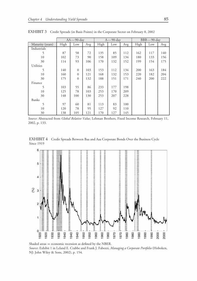
Chapter 4 Understanding Yield Spreads 85
EXHIBIT 3 Credit Spreads (in Basis Points) in the Corporate Sector on February 8, 2002
AA—90-day A—90-day BBB—90-dayMaturity (years) High Low Avg High Low Avg High Low AvgIndustrials
5 87 58 72 135 85 112 162 117 14010 102 73 90 158 109 134 180 133 15630 114 93 106 170 132 152 199 154 175
Utilities5 140 0 103 153 112 134 200 163 184
10 160 0 121 168 132 153 220 182 20430 175 0 132 188 151 171 240 200 222
Finance5 103 55 86 233 177 198
10 125 78 103 253 170 20930 148 100 130 253 207 228
Banks5 97 60 81 113 83 100
10 120 78 95 127 92 11030 138 105 121 170 127 145
Source: Abstracted from Global Relative Value, Lehman Brothers, Fixed Income Research, February 11,2002, p. 133.
EXHIBIT 4 Credit Spreads Between Baa and Aaa Corporate Bonds Over the Business CycleSince 1919
1920
0
1
2
3
4
(%)
5
6
1920
1930
1930
1940
1940
1940
1950
1950
1960
1960
1960
1970
1970
1980
1980
1980
1990
1990
2000
2000
Shaded areas = economic recession as defined by the NBER.Source: Exhibit 1 in Leland E. Crabbe and Frank J. Fabozzi, Managing a Corporate Portfolio (Hoboken,NJ: John Wiley & Sons, 2002), p. 154.
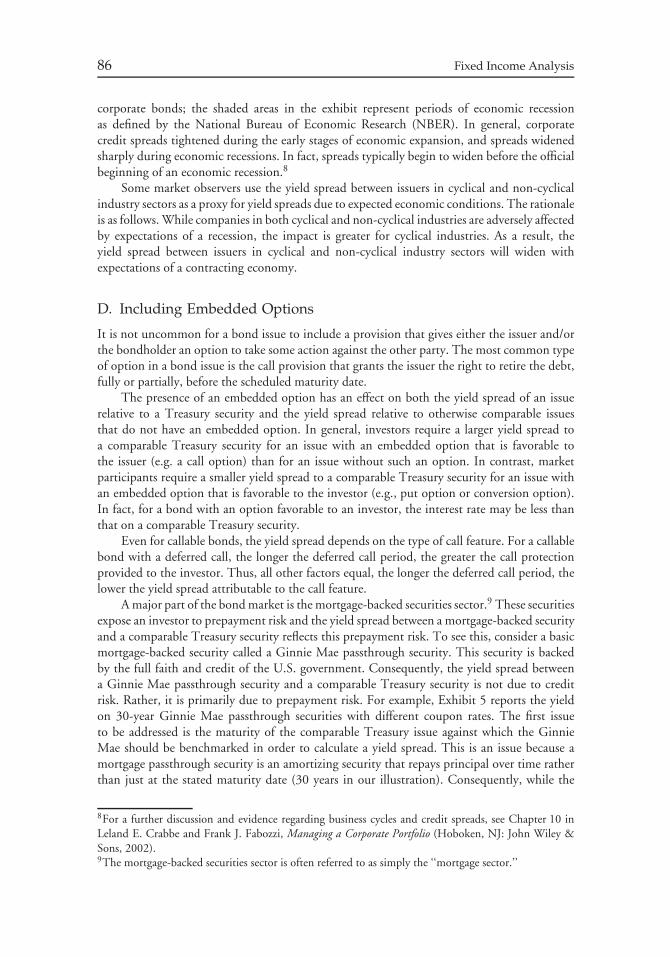
86 Fixed Income Analysis
corporate bonds; the shaded areas in the exhibit represent periods of economic recessionas defined by the National Bureau of Economic Research (NBER). In general, corporatecredit spreads tightened during the early stages of economic expansion, and spreads widenedsharply during economic recessions. In fact, spreads typically begin to widen before the officialbeginning of an economic recession.8
Some market observers use the yield spread between issuers in cyclical and non-cyclicalindustry sectors as a proxy for yield spreads due to expected economic conditions. The rationaleis as follows. While companies in both cyclical and non-cyclical industries are adversely affectedby expectations of a recession, the impact is greater for cyclical industries. As a result, theyield spread between issuers in cyclical and non-cyclical industry sectors will widen withexpectations of a contracting economy.
D. Including Embedded Options
It is not uncommon for a bond issue to include a provision that gives either the issuer and/orthe bondholder an option to take some action against the other party. The most common typeof option in a bond issue is the call provision that grants the issuer the right to retire the debt,fully or partially, before the scheduled maturity date.
The presence of an embedded option has an effect on both the yield spread of an issuerelative to a Treasury security and the yield spread relative to otherwise comparable issuesthat do not have an embedded option. In general, investors require a larger yield spread toa comparable Treasury security for an issue with an embedded option that is favorable tothe issuer (e.g. a call option) than for an issue without such an option. In contrast, marketparticipants require a smaller yield spread to a comparable Treasury security for an issue withan embedded option that is favorable to the investor (e.g., put option or conversion option).In fact, for a bond with an option favorable to an investor, the interest rate may be less thanthat on a comparable Treasury security.
Even for callable bonds, the yield spread depends on the type of call feature. For a callablebond with a deferred call, the longer the deferred call period, the greater the call protectionprovided to the investor. Thus, all other factors equal, the longer the deferred call period, thelower the yield spread attributable to the call feature.
A major part of the bond market is the mortgage-backed securities sector.9 These securitiesexpose an investor to prepayment risk and the yield spread between a mortgage-backed securityand a comparable Treasury security reflects this prepayment risk. To see this, consider a basicmortgage-backed security called a Ginnie Mae passthrough security. This security is backedby the full faith and credit of the U.S. government. Consequently, the yield spread betweena Ginnie Mae passthrough security and a comparable Treasury security is not due to creditrisk. Rather, it is primarily due to prepayment risk. For example, Exhibit 5 reports the yieldon 30-year Ginnie Mae passthrough securities with different coupon rates. The first issueto be addressed is the maturity of the comparable Treasury issue against which the GinnieMae should be benchmarked in order to calculate a yield spread. This is an issue because amortgage passthrough security is an amortizing security that repays principal over time ratherthan just at the stated maturity date (30 years in our illustration). Consequently, while the
8For a further discussion and evidence regarding business cycles and credit spreads, see Chapter 10 inLeland E. Crabbe and Frank J. Fabozzi, Managing a Corporate Portfolio (Hoboken, NJ: John Wiley &Sons, 2002).9The mortgage-backed securities sector is often referred to as simply the ‘‘mortgage sector.’’
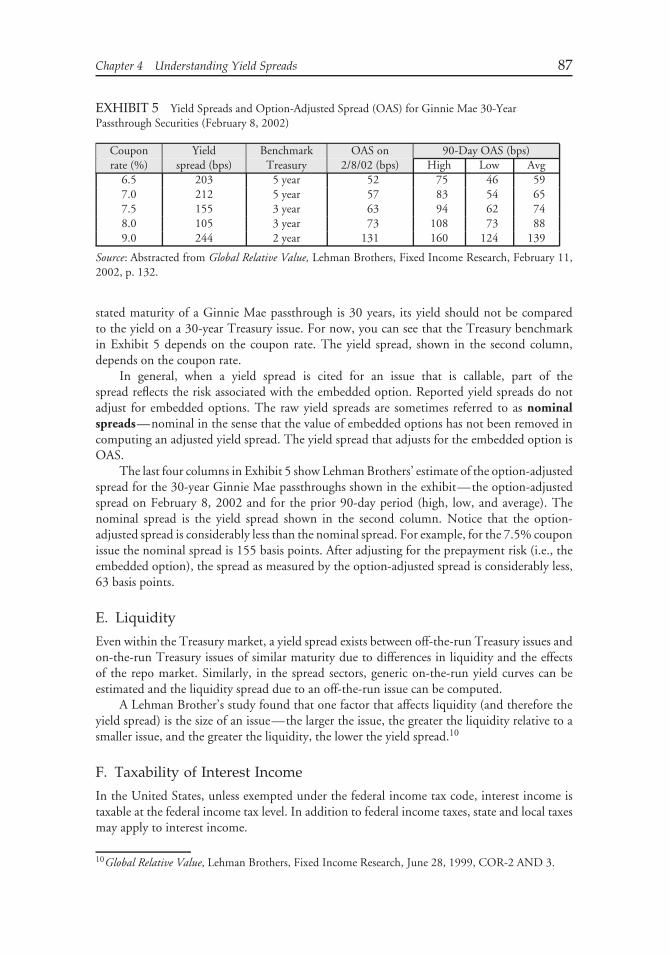
Chapter 4 Understanding Yield Spreads 87
EXHIBIT 5 Yield Spreads and Option-Adjusted Spread (OAS) for Ginnie Mae 30-YearPassthrough Securities (February 8, 2002)
Coupon Yield Benchmark OAS on 90-Day OAS (bps)rate (%) spread (bps) Treasury 2/8/02 (bps) High Low Avg
6.5 203 5 year 52 75 46 597.0 212 5 year 57 83 54 657.5 155 3 year 63 94 62 748.0 105 3 year 73 108 73 889.0 244 2 year 131 160 124 139
Source: Abstracted from Global Relative Value, Lehman Brothers, Fixed Income Research, February 11,2002, p. 132.
stated maturity of a Ginnie Mae passthrough is 30 years, its yield should not be comparedto the yield on a 30-year Treasury issue. For now, you can see that the Treasury benchmarkin Exhibit 5 depends on the coupon rate. The yield spread, shown in the second column,depends on the coupon rate.
In general, when a yield spread is cited for an issue that is callable, part of thespread reflects the risk associated with the embedded option. Reported yield spreads do notadjust for embedded options. The raw yield spreads are sometimes referred to as nominalspreads—nominal in the sense that the value of embedded options has not been removed incomputing an adjusted yield spread. The yield spread that adjusts for the embedded option isOAS.
The last four columns in Exhibit 5 show Lehman Brothers’ estimate of the option-adjustedspread for the 30-year Ginnie Mae passthroughs shown in the exhibit—the option-adjustedspread on February 8, 2002 and for the prior 90-day period (high, low, and average). Thenominal spread is the yield spread shown in the second column. Notice that the option-adjusted spread is considerably less than the nominal spread. For example, for the 7.5% couponissue the nominal spread is 155 basis points. After adjusting for the prepayment risk (i.e., theembedded option), the spread as measured by the option-adjusted spread is considerably less,63 basis points.
E. Liquidity
Even within the Treasury market, a yield spread exists between off-the-run Treasury issues andon-the-run Treasury issues of similar maturity due to differences in liquidity and the effectsof the repo market. Similarly, in the spread sectors, generic on-the-run yield curves can beestimated and the liquidity spread due to an off-the-run issue can be computed.
A Lehman Brother’s study found that one factor that affects liquidity (and therefore theyield spread) is the size of an issue—the larger the issue, the greater the liquidity relative to asmaller issue, and the greater the liquidity, the lower the yield spread.10
F. Taxability of Interest Income
In the United States, unless exempted under the federal income tax code, interest income istaxable at the federal income tax level. In addition to federal income taxes, state and local taxesmay apply to interest income.
10Global Relative Value, Lehman Brothers, Fixed Income Research, June 28, 1999, COR-2 AND 3.
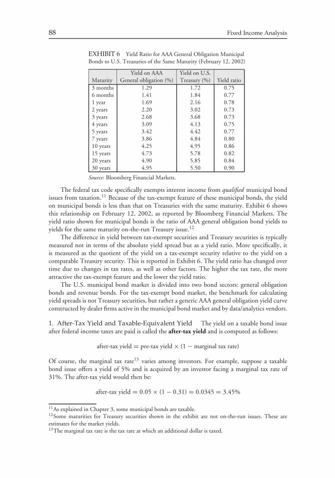
88 Fixed Income Analysis
EXHIBIT 6 Yield Ratio for AAA General Obligation MunicipalBonds to U.S. Treasuries of the Same Maturity (February 12, 2002)
Yield on AAA Yield on U.S.Maturity General obligation (%) Treasury (%) Yield ratio3 months 1.29 1.72 0.756 months 1.41 1.84 0.771 year 1.69 2.16 0.782 years 2.20 3.02 0.733 years 2.68 3.68 0.734 years 3.09 4.13 0.755 years 3.42 4.42 0.777 years 3.86 4.84 0.8010 years 4.25 4.95 0.8615 years 4.73 5.78 0.8220 years 4.90 5.85 0.8430 years 4.95 5.50 0.90
Source: Bloomberg Financial Markets.
The federal tax code specifically exempts interest income from qualified municipal bondissues from taxation.11 Because of the tax-exempt feature of these municipal bonds, the yieldon municipal bonds is less than that on Treasuries with the same maturity. Exhibit 6 showsthis relationship on February 12, 2002, as reported by Bloomberg Financial Markets. Theyield ratio shown for municipal bonds is the ratio of AAA general obligation bond yields toyields for the same maturity on-the-run Treasury issue.12
The difference in yield between tax-exempt securities and Treasury securities is typicallymeasured not in terms of the absolute yield spread but as a yield ratio. More specifically, itis measured as the quotient of the yield on a tax-exempt security relative to the yield on acomparable Treasury security. This is reported in Exhibit 6. The yield ratio has changed overtime due to changes in tax rates, as well as other factors. The higher the tax rate, the moreattractive the tax-exempt feature and the lower the yield ratio.
The U.S. municipal bond market is divided into two bond sectors: general obligationbonds and revenue bonds. For the tax-exempt bond market, the benchmark for calculatingyield spreads is not Treasury securities, but rather a generic AAA general obligation yield curveconstructed by dealer firms active in the municipal bond market and by data/analytics vendors.
1. After-Tax Yield and Taxable-Equivalent Yield The yield on a taxable bond issueafter federal income taxes are paid is called the after-tax yield and is computed as follows:
after-tax yield = pre-tax yield × (1 − marginal tax rate)
Of course, the marginal tax rate13 varies among investors. For example, suppose a taxablebond issue offers a yield of 5% and is acquired by an investor facing a marginal tax rate of31%. The after-tax yield would then be:
after-tax yield = 0.05 × (1 − 0.31) = 0.0345 = 3.45%
11As explained in Chapter 3, some municipal bonds are taxable.12Some maturities for Treasury securities shown in the exhibit are not on-the-run issues. These areestimates for the market yields.13The marginal tax rate is the tax rate at which an additional dollar is taxed.
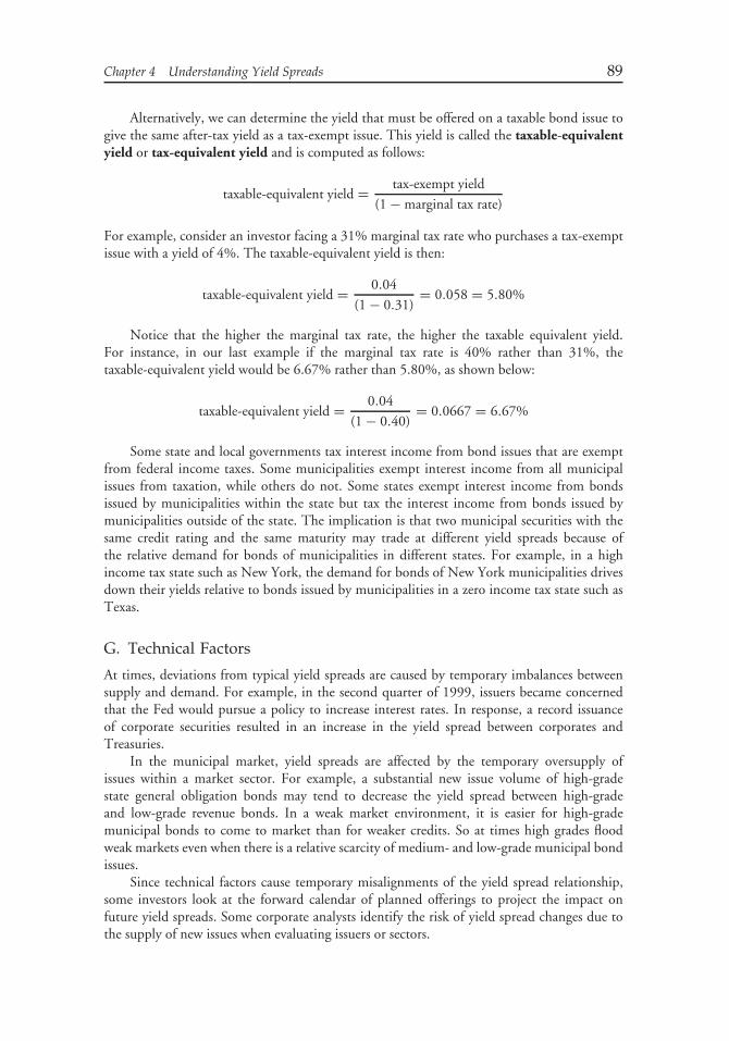
Chapter 4 Understanding Yield Spreads 89
Alternatively, we can determine the yield that must be offered on a taxable bond issue togive the same after-tax yield as a tax-exempt issue. This yield is called the taxable-equivalentyield or tax-equivalent yield and is computed as follows:
taxable-equivalent yield = tax-exempt yield
(1 − marginal tax rate)
For example, consider an investor facing a 31% marginal tax rate who purchases a tax-exemptissue with a yield of 4%. The taxable-equivalent yield is then:
taxable-equivalent yield = 0.04
(1 − 0.31)= 0.058 = 5.80%
Notice that the higher the marginal tax rate, the higher the taxable equivalent yield.For instance, in our last example if the marginal tax rate is 40% rather than 31%, thetaxable-equivalent yield would be 6.67% rather than 5.80%, as shown below:
taxable-equivalent yield = 0.04
(1 − 0.40)= 0.0667 = 6.67%
Some state and local governments tax interest income from bond issues that are exemptfrom federal income taxes. Some municipalities exempt interest income from all municipalissues from taxation, while others do not. Some states exempt interest income from bondsissued by municipalities within the state but tax the interest income from bonds issued bymunicipalities outside of the state. The implication is that two municipal securities with thesame credit rating and the same maturity may trade at different yield spreads because ofthe relative demand for bonds of municipalities in different states. For example, in a highincome tax state such as New York, the demand for bonds of New York municipalities drivesdown their yields relative to bonds issued by municipalities in a zero income tax state such asTexas.
G. Technical Factors
At times, deviations from typical yield spreads are caused by temporary imbalances betweensupply and demand. For example, in the second quarter of 1999, issuers became concernedthat the Fed would pursue a policy to increase interest rates. In response, a record issuanceof corporate securities resulted in an increase in the yield spread between corporates andTreasuries.
In the municipal market, yield spreads are affected by the temporary oversupply ofissues within a market sector. For example, a substantial new issue volume of high-gradestate general obligation bonds may tend to decrease the yield spread between high-gradeand low-grade revenue bonds. In a weak market environment, it is easier for high-grademunicipal bonds to come to market than for weaker credits. So at times high grades floodweak markets even when there is a relative scarcity of medium- and low-grade municipal bondissues.
Since technical factors cause temporary misalignments of the yield spread relationship,some investors look at the forward calendar of planned offerings to project the impact onfuture yield spreads. Some corporate analysts identify the risk of yield spread changes due tothe supply of new issues when evaluating issuers or sectors.
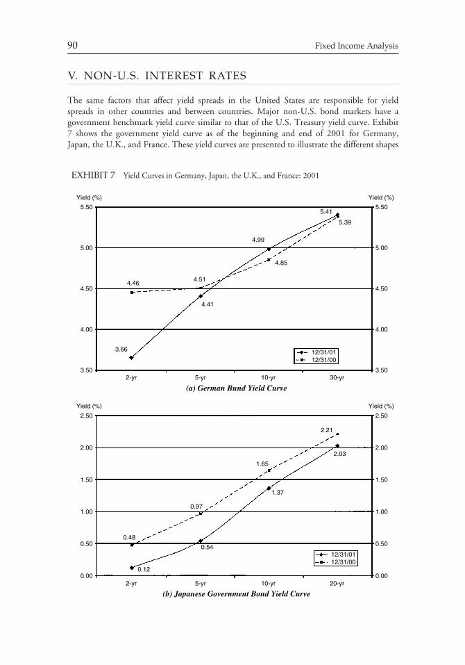
90 Fixed Income Analysis
V. NON-U.S. INTEREST RATES
The same factors that affect yield spreads in the United States are responsible for yieldspreads in other countries and between countries. Major non-U.S. bond markets have agovernment benchmark yield curve similar to that of the U.S. Treasury yield curve. Exhibit7 shows the government yield curve as of the beginning and end of 2001 for Germany,Japan, the U.K., and France. These yield curves are presented to illustrate the different shapes
EXHIBIT 7 Yield Curves in Germany, Japan, the U.K., and France: 2001
Yield (%)
5.50
5.00
4.50
4.00
3.50
Yield (%)
5.50
5.00
4.50
4.00
3.502-yr 5-yr 10-yr 30-yr
12/31/0112/31/00
3.66
4.41
4.51
4.85
4.99
5.41
5.39
4.46
Yield (%)
2.50
2.00
1.50
1.00
0.00
0.50
Yield (%)
2.50
2.00
1.50
1.00
0.50
0.002-yr 5-yr 10-yr 20-yr
(a) German Bund Yield Curve
(b) Japanese Government Bond Yield Curve
2.21
2.03
1.65
1.37
0.54
0.97
0.48
0.12
12/31/0112/31/00
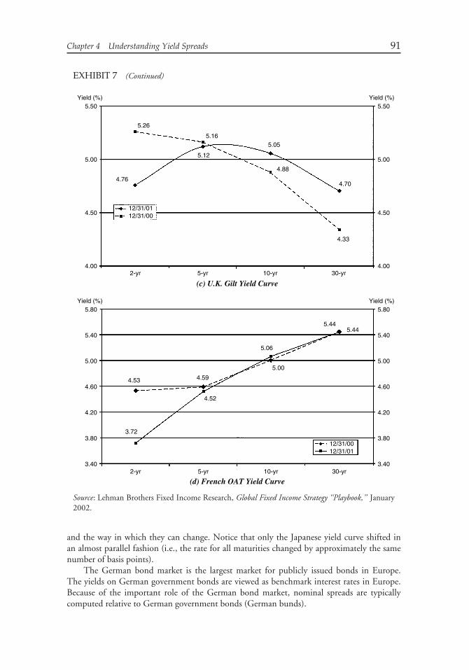
Chapter 4 Understanding Yield Spreads 91
EXHIBIT 7 (Continued)
Yield (%)5.50
5.00
4.50
4.00
Yield (%)5.50
5.00
4.50
4.00
12/31/0112/31/00
2-yr 5-yr 10-yr 30-yr
5.26
5.16
5.12
4.88
4.33
5.05
4.704.76
Yield (%)5.80
5.00
5.40
4.20
4.60
3.40
3.80
5.80
5.00
5.40
4.20
4.60
3.40
3.80
Yield (%)
12/31/0012/31/01
2-yr 5-yr 10-yr 30-yr
3.72
5.00
5.06
5.445.44
4.53 4.59
4.52
(c) U.K. Gilt Yield Curve
(d) French OAT Yield Curve
Source: Lehman Brothers Fixed Income Research, Global Fixed Income Strategy ‘‘Playbook,’’ January2002.
and the way in which they can change. Notice that only the Japanese yield curve shifted inan almost parallel fashion (i.e., the rate for all maturities changed by approximately the samenumber of basis points).
The German bond market is the largest market for publicly issued bonds in Europe.The yields on German government bonds are viewed as benchmark interest rates in Europe.Because of the important role of the German bond market, nominal spreads are typicallycomputed relative to German government bonds (German bunds).
92 Fixed Income Analysis
Institutional investors who borrow funds on a short-term basis to invest (referred to as‘‘funded investors’’) obviously desire to earn an amount in excess of their borrowing cost. Themost popular borrowing cost reference rate is the London interbank offered rate (LIBOR).LIBOR is the interest rate at which banks pay to borrow funds from other banks in theLondon interbank market. The borrowing occurs via a cash deposit of one bank (the lender)into a certificate of deposit (CD) in another bank (the borrower). The maturity of the CDcan be from overnight to five years. So, 3-month LIBOR represents the interest rate paid on aCD that matures in three months. The CD can be denominated in one of several currencies.The currencies for which LIBOR is reported are the U.S. dollar, the British pound, the Euro,the Canadian dollar, the Australian dollar, the Japanese yen, and Swiss francs. When it isdenominated in U.S. dollars, it is referred to as a Eurodollar CD. LIBOR is determined forevery London business day by the British Bank Association (BBA) by maturity and for eachcurrency and is reported by various services.
Entities seeking to borrow funds pays a spread over LIBOR and seek to earn a spreadover that funding cost when they invest the borrowed funds. So, for example, if the 3-monthborrowing cost for a funded investor is 3-month LIBOR plus 25 basis points and the investorcan earn 3-month LIBOR plus 125 basis points for three months, then the investor earns aspread of 100 basis points for three months (125 basis points-25 basis points).
VI. SWAP SPREADS
Another important spread measure is the swap spread.
A. Interest Rate Swap and the Swap Spread
In an interest rate swap, two parties (called counterparties) agree to exchange periodic interestpayments. The dollar amount of the interest payments exchanged is based on a predetermineddollar principal, which is called the notional principal or notional amount. The dollaramount each counterparty pays to the other is the agreed-upon periodic interest rate times thenotional principal. The only dollars exchanged between the parties are the interest payments,not the notional principal. In the most common type of swap, one party agrees to pay theother party fixed interest payments at designated dates for the life of the swap. This party isreferred to as the fixed-rate payer. The fixed rate that the fixed-rate payer pays is called theswap rate. The other party, who agrees to make interest rate payments that float with somereference rate, is referred to as the fixed-rate receiver.
The reference rates used for the floating rate in an interest rate swap is one of variousmoney market instruments: LIBOR (the most common reference rate used in swaps),Treasury bill rate, commercial paper rate, bankers’ acceptance rate, federal funds rate, andprime rate.
The convention that has evolved for quoting a swap rate is that a dealer sets the floatingrate equal to the reference rate and then quotes the fixed rate that will apply. The fixed ratehas a specified ‘‘spread’’ above the yield for a Treasury with the same term to maturity as theswap. This specified spread is called the swap spread. The swap rate is the sum of the yieldfor a Treasury with the same maturity as the swap plus the swap spread.
To illustrate an interest rate swap in which one party pays fixed and receives floating,assume the following:
Chapter 4 Understanding Yield Spreads 93
term of swap: 5 years
swap spread: 50 basis points
reference rate: 3-month LIBOR
notional amount: $50 million
frequency of payments: every three months
Suppose also that the 5-year Treasury rate is 5.5% at the time the swap is entered into. Thenthe swap rate will be 6%, found by adding the swap spread of 50 basis points to the 5-yearTreasury yield of 5.5%.
This means that the fixed-rate payer agrees to pay a 6% annual rate for the next five yearswith payments made quarterly and receive from the fixed-rate receiver 3-month LIBOR withthe payments made quarterly. Since the notional amount is $50 million, this means that everythree months, the fixed-rate payer pays $750,000 (6% times $50 million divided by 4). Thefixed-rate receiver pays 3-month LIBOR times $50 million divided by 4. The table belowshows the payment made by the fixed-rate receiver to the fixed-rate payer for different valuesof 3-month LIBOR:14
If 3-month LIBOR is Annual dollar amount Quarterly payment4% $2,000,000 $500,0005% 2,500,000 625,0006% 3,000,000 750,0007% 3,500,000 875,0008% 4,000,000 1,000,000
In practice, the payments are netted out. For example, if 3-month LIBOR is 4%, thefixed-rate receiver would receive $750,000 and pay to the fixed-rate payer $500,000. Nettingthe two payments, the fixed-rate payer pays the fixed-rate receiver $250,000 ($750, 000 −$500, 000).
B. Role of Interest Rate Swaps
Interest rate swaps have many important applications in fixed income portfolio managementand risk management. They tie together the fixed-rate and floating-rate sectors of the bondmarket. As a result, investors can convert a fixed-rate asset into a floating-rate asset with aninterest rate swap.
Suppose a financial institution has invested in 5-year bonds with a $50 million par valueand a coupon rate of 9% and that this bond is selling at par value. Moreover, this institutionborrows $50 million on a quarterly basis (to fund the purchase of the bonds) and its costof funds is 3-month LIBOR plus 50 basis points. The ‘‘income spread’’ between its assets(i.e., 5-year bonds) and its liabilities (its funding cost) for any 3-month period depends on3-month LIBOR. The following table shows how the annual spread varies with 3-monthLIBOR:
14The amount of the payment is found by dividing the annual dollar amount by four because paymentsare made quarterly. In a real world application, both the fixed-rate and floating-rate payments areadjusted for the number of days in a quarter, but it is unnecessary for us to deal with this adjustmenthere.
94 Fixed Income Analysis
Asset yield 3-month LIBOR Funding cost Annual income spread9.00% 4.00% 4.50% 4.50%9.00% 5.00% 5.50% 3.50%9.00% 6.00% 6.50% 2.50%9.00% 7.00% 7.50% 1.50%9.00% 8.00% 8.50% 0.50%9.00% 8.50% 9.00% 0.00%9.00% 9.00% 9.50% −0.50%9.00% 10.00% 10.50% −1.50%9.00% 11.00% 11.50% −2.50%
As 3-month LIBOR increases, the income spread decreases. If 3-month LIBOR exceeds 8.5%,the income spread is negative (i.e., it costs more to borrow than is earned on the bonds inwhich the borrowed funds are invested).
This financial institution has a mismatch between its assets and its liabilities. An interestrate swap can be used to hedge this mismatch. For example, suppose the manager ofthis financial institution enters into a 5-year swap with a $50 million notional amountin which it agrees to pay a fixed rate (i.e., to be the fixed-rate payer) in exchange for3-month LIBOR. Suppose further that the swap rate is 6%. Then the annual incomespread taking into account the swap payments is as follows for different values of 3-monthLIBOR:
Asset 3-month Funding Fixed rate 3-month LIBOR Annualyield LIBOR cost paid in swap rec. in swap income spread9.00% 4.00% 4.50% 6.00% 4.00% 2.50%9.00% 5.00% 5.50% 6.00% 5.00% 2.50%9.00% 6.00% 6.50% 6.00% 6.00% 2.50%9.00% 7.00% 7.50% 6.00% 7.00% 2.50%9.00% 8.00% 8.50% 6.00% 8.00% 2.50%9.00% 8.50% 9.00% 6.00% 8.50% 2.50%9.00% 9.00% 9.50% 6.00% 9.00% 2.50%9.00% 10.00% 10.50% 6.00% 10.00% 2.50%9.00% 11.00% 11.50% 6.00% 11.00% 2.50%
Assuming the bond does not default and is not called, the financial institution has locked in aspread of 250 basis points.
Effectively, the financial institution using this interest rate swap converted a fixed-rateasset into a floating-rate asset. The reference rate for the synthetic floating-rate asset is 3-monthLIBOR and the liabilities are in terms of 3-month LIBOR. Alternatively, the financialinstitution could have converted its liabilities to a fixed-rate by entering into a 5-year $50million notional amount swap by being the fixed-rate payer and the results would have beenthe same.
This simple illustration shows the critical importance of an interest rate swap. Investorsand issuers with a mismatch of assets and liabilities can use an interest rate swap to bettermatch assets and liabilities, thereby reducing their risk.
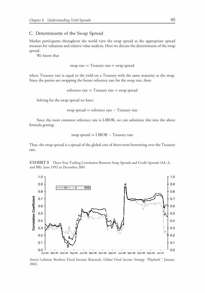
Chapter 4 Understanding Yield Spreads 95
C. Determinants of the Swap Spread
Market participants throughout the world view the swap spread as the appropriate spreadmeasure for valuation and relative value analysis. Here we discuss the determinants of the swapspread.
We know that
swap rate = Treasury rate + swap spread
where Treasury rate is equal to the yield on a Treasury with the same maturity as the swap.Since the parties are swapping the future reference rate for the swap rate, then:
reference rate = Treasury rate + swap spread
Solving for the swap spread we have:
swap spread = reference rate − Treasury rate
Since the most common reference rate is LIBOR, we can substitute this into the aboveformula getting:
swap spread = LIBOR − Treasury rate
Thus, the swap spread is a spread of the global cost of short-term borrowing over the Treasuryrate.
EXHIBIT 8 Three-Year Trailing Correlation Between Swap Spreads and Credit Spreads (AA, A,and BB): June 1992 to December 2001
1.0
0.9
0.8
0.7
0.6
0.5
0.4
0.3
0.2
0.1
0.0
1.0
0.9
0.8
0.7
0.6
0.5
0.4
0.3
0.2
0.1
0.0
Co
rrel
atio
n C
oef
fici
ent
AA A BBB
Jun-92 Mar-93 Dec-93 Sep-94 Jun-95 Mar-96 Dec-96 Sep-97 Jun-98 Mar-99 Dec-99 Sep-00 Jun-01
Source: Lehman Brothers Fixed Income Research, Global Fixed Income Strategy ‘‘Playbook,’’ January2002.
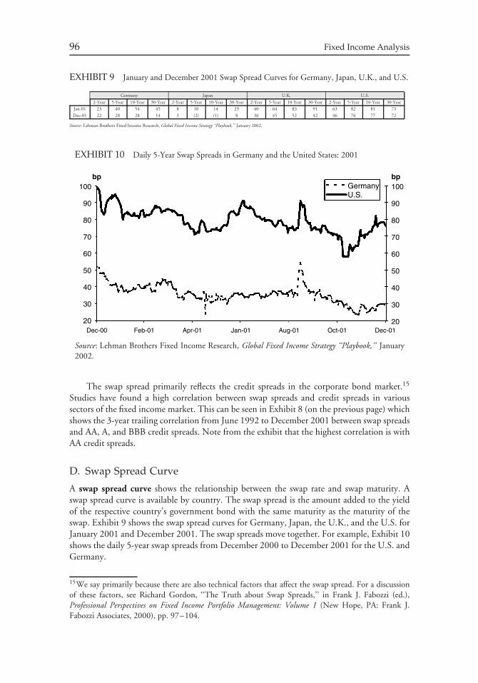
96 Fixed Income Analysis
EXHIBIT 9 January and December 2001 Swap Spread Curves for Germany, Japan, U.K., and U.S.
Germany Japan U.K. U.S.
2-Year 5-Year 10-Year 30-Year 2-Year 5-Year 10-Year 30-Year 2-Year 5-Year 10-Year 30-Year 2-Year 5-Year 10-Year 30-YearJan-01 23 40 54 45 8 10 14 29 40 64 83 91 63 82 81 73
Dec-01 22 28 28 14 3 (2) (1) 8 36 45 52 42 46 76 77 72
Source: Lehman Brothers Fixed Income Research, Global Fixed Income Strategy ‘‘Playbook,’’ January 2002.
EXHIBIT 10 Daily 5-Year Swap Spreads in Germany and the United States: 2001
bp100
90
80
70
60
50
40
30
20
bp100Germany
U.S.90
80
70
60
50
40
30
20Dec-00 Feb-01 Apr-01 Jan-01 Aug-01 Oct-01 Dec-01
Source: Lehman Brothers Fixed Income Research, Global Fixed Income Strategy ‘‘Playbook,’’ January2002.
The swap spread primarily reflects the credit spreads in the corporate bond market.15
Studies have found a high correlation between swap spreads and credit spreads in varioussectors of the fixed income market. This can be seen in Exhibit 8 (on the previous page) whichshows the 3-year trailing correlation from June 1992 to December 2001 between swap spreadsand AA, A, and BBB credit spreads. Note from the exhibit that the highest correlation is withAA credit spreads.
D. Swap Spread Curve
A swap spread curve shows the relationship between the swap rate and swap maturity. Aswap spread curve is available by country. The swap spread is the amount added to the yieldof the respective country’s government bond with the same maturity as the maturity of theswap. Exhibit 9 shows the swap spread curves for Germany, Japan, the U.K., and the U.S. forJanuary 2001 and December 2001. The swap spreads move together. For example, Exhibit 10shows the daily 5-year swap spreads from December 2000 to December 2001 for the U.S. andGermany.
15We say primarily because there are also technical factors that affect the swap spread. For a discussionof these factors, see Richard Gordon, ‘‘The Truth about Swap Spreads,’’ in Frank J. Fabozzi (ed.),Professional Perspectives on Fixed Income Portfolio Management: Volume 1 (New Hope, PA: Frank J.Fabozzi Associates, 2000), pp. 97–104.
CHAPTER 5INTRODUCTION TO THE
VALUATION OF DEBTSECURITIES
I. INTRODUCTION
Valuation is the process of determining the fair value of a financial asset. The process isalso referred to as ‘‘valuing’’ or ‘‘pricing’’ a financial asset. In this chapter, we will explainthe general principles of fixed income security valuation. In this chapter, we will limit ourdiscussion to the valuation of option-free bonds.
II. GENERAL PRINCIPLES OF VALUATION
The fundamental principle of financial asset valuation is that its value is equal to the presentvalue of its expected cash flows. This principle applies regardless of the financial asset. Thus,the valuation of a financial asset involves the following three steps:
Step 1: Estimate the expected cash flows.
Step 2: Determine the appropriate interest rate or interest rates that should be used todiscount the cash flows.
Step 3: Calculate the present value of the expected cash flows found in step 1 using theinterest rate or interest rates determined in step 2.
A. Estimating Cash Flows
Cash flow is simply the cash that is expected to be received in the future from an investment.In the case of a fixed income security, it does not make any difference whether the cash flowis interest income or payment of principal. The cash flows of a security are the collection ofeach period’s cash flow. Holding aside the risk of default, the cash flows for few fixed incomesecurities are simple to project. Noncallable U.S. Treasury securities have known cash flows.For Treasury coupon securities, the cash flows are the coupon interest payments every sixmonths up to and including the maturity date and the principal payment at the maturity date.
At times, investors will find it difficult to estimate the cash flows when they purchase afixed income security. For example, if
97
98 Fixed Income Analysis
1. the issuer or the investor has the option to change the contractual due date for thepayment of the principal, or
2. the coupon payment is reset periodically by a formula based on some value or values ofreference rates, prices, or exchange rates, or
3. the investor has the choice to convert or exchange the security into common stock.
Callable bonds, putable bonds, mortgage-backed securities, and asset-backed securitiesare examples of (1). Floating-rate securities are an example of (2). Convertible bonds andexchangeable bonds are examples of (3).
For securities that fall into the first category, future interest rate movements are the keyfactor to determine if the option will be exercised. Specifically, if interest rates fall far enough,the issuer can sell a new issue of bonds at the lower interest rate and use the proceeds to pay off(call) the older bonds that have the higher coupon rate. (This assumes that the interest savingsare larger than the costs involved in refunding.) Similarly, for a loan, if rates fall enough thatthe interest savings outweigh the refinancing costs, the borrower has an incentive to refinance.For a putable bond, the investor will put the issue if interest rates rise enough to drive themarket price below the put price (i.e., the price at which it must be repurchased by the issuer).
What this means is that to properly estimate the cash flows of a fixed income security, itis necessary to incorporate into the analysis how, in the future, changes in interest rates andother factors affecting the embedded option may affect cash flows.
B. Determining the Appropriate Rate or Rates
Once the cash flows for a fixed income security are estimated, the next step is to determinethe appropriate interest rate to be used to discount the cash flows. As we did in the previouschapter, we will use the terms interest rate and yield interchangeably. The minimum interestrate that an investor should require is the yield available in the marketplace on a default-freecash flow. In the United States, this is the yield on a U.S. Treasury security. This is one of thereasons that the Treasury market is closely watched. What is the minimum interest rate U.S.investors demand? At this point, we can assume that it is the yield on the on-the-run Treasurysecurity with the same as the security being valued.1 We will qualify this shortly.
For a security that is not issued by the U.S. government, investors will require a yieldpremium over the yield available on an on-the-run Treasury issue. This yield premium reflectsthe additional risks that the investor accepts.
For each cash flow estimated, the same interest rate can be used to calculate the presentvalue. However, since each cash flow is unique, it is more appropriate to value each cashflow using an interest rate specific to that cash flow’s maturity. In the traditional approach tovaluation a single interest rate is used. In Section IV, we will see that the proper approach tovaluation uses multiple interest rates each specific to a particular cash flow. In that section, wewill also demonstrate why this must be the case.
C. Discounting the Expected Cash Flows
Given expected (estimated) cash flows and the appropriate interest rate or interest rates to beused to discount the cash flows, the final step in the valuation process is to value the cash flows.
1As explained in Chapter 3, the on-the-run Treasury issues are the most recently auctioned Treasuryissues.
Chapter 5 Introduction to the Valuation of Debt Securities 99
What is the value of a single cash flow to be received in the future? It is the amount ofmoney that must be invested today to generate that future value. The resulting value is calledthe present value of a cash flow. (It is also called the discounted value.) The present valueof a cash flow will depend on (1) when a cash flow will be received (i.e., the timing of a cashflow) and (2) the interest rate used to calculate the present value. The interest rate used iscalled the discount rate.
First, we calculate the present value for each expected cash flow. Then, to determine thevalue of the security, we calculate the sum of the present values (i.e., for all of the security’sexpected cash flows).
If a discount rate i can be earned on any sum invested today, the present value of theexpected cash flow to be received t years from now is:
present valuet = expected cash flow in period t(1 + i)t
The value of a financial asset is then the sum of the present value of all the expected cashflows. That is, assuming that there are N expected cash flows:
value = present value1 + present value2 + · · · + present valueN
To illustrate the present value formula, consider a simple bond that matures in four years,has a coupon rate of 10%, and has a maturity value of $100. For simplicity, let’s assume thebond pays interest annually and a discount rate of 8% should be used to calculate the presentvalue of each cash flow. The cash flow for this bond is:
Year Cash flow1 $102 103 104 110
The present value of each cash flow is:
Year 1: present value1 = $10
(1.08)1= $9.2593
Year 2: present value2 = $10
(1.08)2= $8.5734
Year 3: present value3 = $10
(1.08)3= $7.9383
Year 4: present value4 = $110
(1.08)4= $80.8533
The value of this security is then the sum of the present values of the four cash flows.That is, the present value is $106.6243 ($9.2593 + $8.5734 + $7.9383 + $80.8533).
1. Present Value Properties An important property about the present value can be seenfrom the above illustration. For the first three years, the cash flow is the same ($10) and thediscount rate is the same (8%). The present value decreases as we go further into the future.This is an important property of the present value: for a given discount rate, the further into the
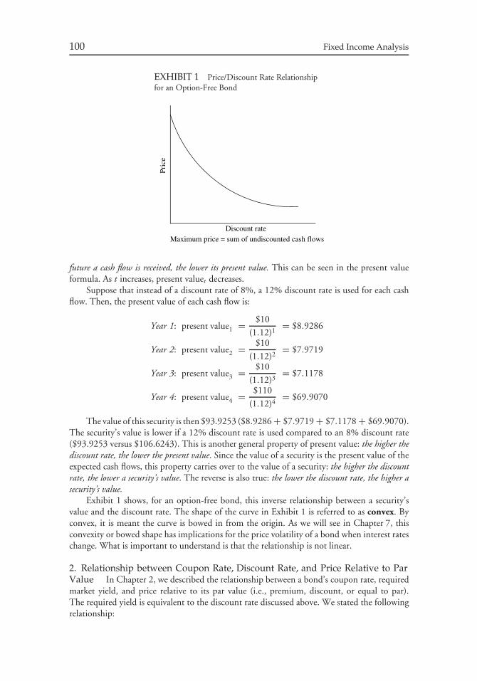
100 Fixed Income Analysis
EXHIBIT 1 Price/Discount Rate Relationshipfor an Option-Free Bond
Pric
e
Maximum price = sum of undiscounted cash flows
Discount rate
future a cash flow is received, the lower its present value. This can be seen in the present valueformula. As t increases, present valuet decreases.
Suppose that instead of a discount rate of 8%, a 12% discount rate is used for each cashflow. Then, the present value of each cash flow is:
Year 1: present value1 = $10
(1.12)1= $8.9286
Year 2: present value2 = $10
(1.12)2= $7.9719
Year 3: present value3 = $10
(1.12)3= $7.1178
Year 4: present value4 = $110
(1.12)4= $69.9070
The value of this security is then $93.9253 ($8.9286 + $7.9719 + $7.1178 + $69.9070).The security’s value is lower if a 12% discount rate is used compared to an 8% discount rate($93.9253 versus $106.6243). This is another general property of present value: the higher thediscount rate, the lower the present value. Since the value of a security is the present value of theexpected cash flows, this property carries over to the value of a security: the higher the discountrate, the lower a security’s value. The reverse is also true: the lower the discount rate, the higher asecurity’s value.
Exhibit 1 shows, for an option-free bond, this inverse relationship between a security’svalue and the discount rate. The shape of the curve in Exhibit 1 is referred to as convex. Byconvex, it is meant the curve is bowed in from the origin. As we will see in Chapter 7, thisconvexity or bowed shape has implications for the price volatility of a bond when interest rateschange. What is important to understand is that the relationship is not linear.
2. Relationship between Coupon Rate, Discount Rate, and Price Relative to ParValue In Chapter 2, we described the relationship between a bond’s coupon rate, requiredmarket yield, and price relative to its par value (i.e., premium, discount, or equal to par).The required yield is equivalent to the discount rate discussed above. We stated the followingrelationship:
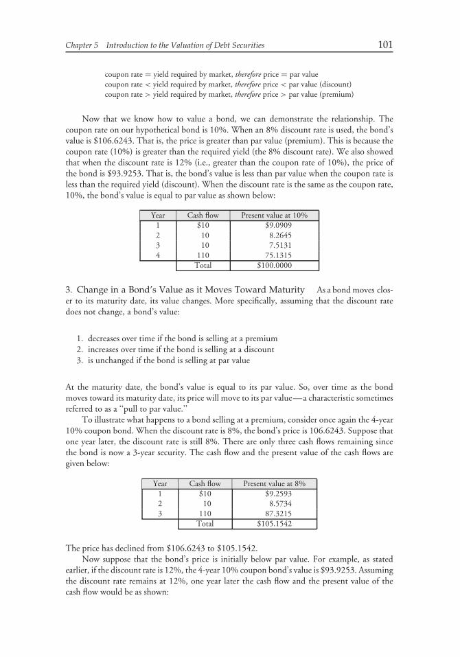
Chapter 5 Introduction to the Valuation of Debt Securities 101
coupon rate = yield required by market, therefore price = par valuecoupon rate < yield required by market, therefore price < par value (discount)coupon rate > yield required by market, therefore price > par value (premium)
Now that we know how to value a bond, we can demonstrate the relationship. Thecoupon rate on our hypothetical bond is 10%. When an 8% discount rate is used, the bond’svalue is $106.6243. That is, the price is greater than par value (premium). This is because thecoupon rate (10%) is greater than the required yield (the 8% discount rate). We also showedthat when the discount rate is 12% (i.e., greater than the coupon rate of 10%), the price ofthe bond is $93.9253. That is, the bond’s value is less than par value when the coupon rate isless than the required yield (discount). When the discount rate is the same as the coupon rate,10%, the bond’s value is equal to par value as shown below:
Year Cash flow Present value at 10%1 $10 $9.09092 10 8.26453 10 7.51314 110 75.1315
Total $100.0000
3. Change in a Bond’s Value as it Moves Toward Maturity As a bond moves clos-er to its maturity date, its value changes. More specifically, assuming that the discount ratedoes not change, a bond’s value:
1. decreases over time if the bond is selling at a premium2. increases over time if the bond is selling at a discount3. is unchanged if the bond is selling at par value
At the maturity date, the bond’s value is equal to its par value. So, over time as the bondmoves toward its maturity date, its price will move to its par value—a characteristic sometimesreferred to as a ‘‘pull to par value.’’
To illustrate what happens to a bond selling at a premium, consider once again the 4-year10% coupon bond. When the discount rate is 8%, the bond’s price is 106.6243. Suppose thatone year later, the discount rate is still 8%. There are only three cash flows remaining sincethe bond is now a 3-year security. The cash flow and the present value of the cash flows aregiven below:
Year Cash flow Present value at 8%1 $10 $9.25932 10 8.57343 110 87.3215
Total $105.1542
The price has declined from $106.6243 to $105.1542.Now suppose that the bond’s price is initially below par value. For example, as stated
earlier, if the discount rate is 12%, the 4-year 10% coupon bond’s value is $93.9253. Assumingthe discount rate remains at 12%, one year later the cash flow and the present value of thecash flow would be as shown:
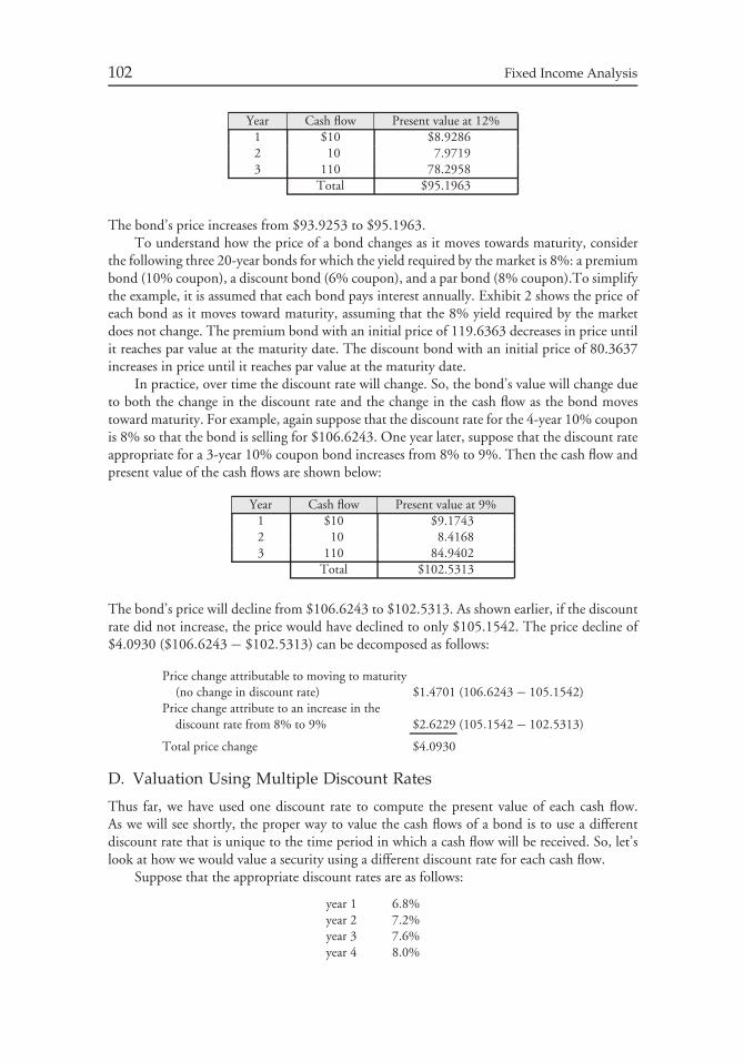
102 Fixed Income Analysis
Year Cash flow Present value at 12%1 $10 $8.92862 10 7.97193 110 78.2958
Total $95.1963
The bond’s price increases from $93.9253 to $95.1963.To understand how the price of a bond changes as it moves towards maturity, consider
the following three 20-year bonds for which the yield required by the market is 8%: a premiumbond (10% coupon), a discount bond (6% coupon), and a par bond (8% coupon).To simplifythe example, it is assumed that each bond pays interest annually. Exhibit 2 shows the price ofeach bond as it moves toward maturity, assuming that the 8% yield required by the marketdoes not change. The premium bond with an initial price of 119.6363 decreases in price untilit reaches par value at the maturity date. The discount bond with an initial price of 80.3637increases in price until it reaches par value at the maturity date.
In practice, over time the discount rate will change. So, the bond’s value will change dueto both the change in the discount rate and the change in the cash flow as the bond movestoward maturity. For example, again suppose that the discount rate for the 4-year 10% couponis 8% so that the bond is selling for $106.6243. One year later, suppose that the discount rateappropriate for a 3-year 10% coupon bond increases from 8% to 9%. Then the cash flow andpresent value of the cash flows are shown below:
Year Cash flow Present value at 9%1 $10 $9.17432 10 8.41683 110 84.9402
Total $102.5313
The bond’s price will decline from $106.6243 to $102.5313. As shown earlier, if the discountrate did not increase, the price would have declined to only $105.1542. The price decline of$4.0930 ($106.6243 − $102.5313) can be decomposed as follows:
Price change attributable to moving to maturity(no change in discount rate) $1.4701 (106.6243 − 105.1542)
Price change attribute to an increase in thediscount rate from 8% to 9% $2.6229 (105.1542 − 102.5313)
Total price change $4.0930
D. Valuation Using Multiple Discount Rates
Thus far, we have used one discount rate to compute the present value of each cash flow.As we will see shortly, the proper way to value the cash flows of a bond is to use a differentdiscount rate that is unique to the time period in which a cash flow will be received. So, let’slook at how we would value a security using a different discount rate for each cash flow.
Suppose that the appropriate discount rates are as follows:
year 1 6.8%year 2 7.2%year 3 7.6%year 4 8.0%
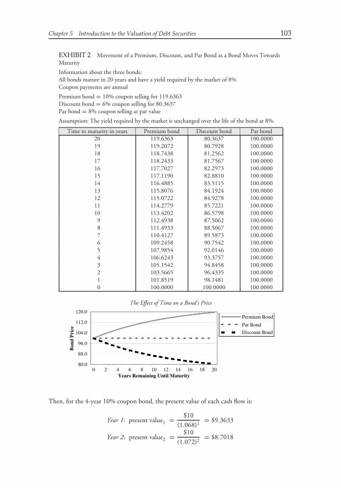
Chapter 5 Introduction to the Valuation of Debt Securities 103
EXHIBIT 2 Movement of a Premium, Discount, and Par Bond as a Bond Moves TowardsMaturity
Information about the three bonds:All bonds mature in 20 years and have a yield required by the market of 8%Coupon payments are annual
Premium bond = 10% coupon selling for 119.6363Discount bond = 6% coupon selling for 80.3637Par bond = 8% coupon selling at par value
Assumption: The yield required by the market is unchanged over the life of the bond at 8%.
Time to maturity in years Premium bond Discount bond Par bond20 119.6363 80.3637 100.000019 119.2072 80.7928 100.000018 118.7438 81.2562 100.000017 118.2433 81.7567 100.000016 117.7027 82.2973 100.000015 117.1190 82.8810 100.000014 116.4885 83.5115 100.000013 115.8076 84.1924 100.000012 115.0722 84.9278 100.000011 114.2779 85.7221 100.000010 113.4202 86.5798 100.00009 112.4938 87.5062 100.00008 111.4933 88.5067 100.00007 110.4127 89.5873 100.00006 109.2458 90.7542 100.00005 107.9854 92.0146 100.00004 106.6243 93.3757 100.00003 105.1542 94.8458 100.00002 103.5665 96.4335 100.00001 101.8519 98.1481 100.00000 100.0000 100.0000 100.0000
The Effect of Time on a Bond’s Price
120.0
112.0
104.0
Bon
d P
rice
Years Remaining Until Maturity
96.0
88.0
80.00 2 4 6 8 10 12 14 16 18 20
Premium Bond
Par Bond
Discount Bond
Then, for the 4-year 10% coupon bond, the present value of each cash flow is:
Year 1: present value1 = $10
(1.068)1= $9.3633
Year 2: present value2 = $10
(1.072)2= $8.7018
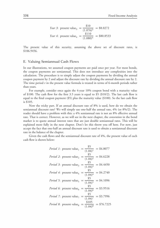
104 Fixed Income Analysis
Year 3: present value3 = $10
(1.076)3= $8.0272
Year 4: present value4 = $110
(1.080)4= $80.8533
The present value of this security, assuming the above set of discount rates, is$106.9456.
E. Valuing Semiannual Cash Flows
In our illustrations, we assumed coupon payments are paid once per year. For most bonds,the coupon payments are semiannual. This does not introduce any complexities into thecalculation. The procedure is to simply adjust the coupon payments by dividing the annualcoupon payment by 2 and adjust the discount rate by dividing the annual discount rate by 2.The time period t in the present value formula is treated in terms of 6-month periods ratherthan years.
For example, consider once again the 4-year 10% coupon bond with a maturity valueof $100. The cash flow for the first 3.5 years is equal to $5 ($10/2). The last cash flow isequal to the final coupon payment ($5) plus the maturity value ($100). So the last cash flowis $105.
Now the tricky part. If an annual discount rate of 8% is used, how do we obtain thesemiannual discount rate? We will simply use one-half the annual rate, 4% (or 8%/2). Thereader should have a problem with this: a 4% semiannual rate is not an 8% effective annualrate. That is correct. However, as we will see in the next chapter, the convention in the bondmarket is to quote annual interest rates that are just double semiannual rates. This will beexplained more fully in the next chapter. Don’t let this throw you off here. For now, justaccept the fact that one-half an annual discount rate is used to obtain a semiannual discountrate in the balance of the chapter.
Given the cash flows and the semiannual discount rate of 4%, the present value of eachcash flow is shown below:
Period 1: present value1 = $5
(1.04)1= $4.8077
Period 2: present value2 = $5
(1.04)2= $4.6228
Period 3: present value3 = $5
(1.04)3= $4.4450
Period 4: present value4 = $5
(1.04)4= $4.2740
Period 5: present value5 = $5
(1.04)5= $4.1096
Period 6: present value6 = $5
(1.04)6= $3.9516
Period 7: present value7 = $5
(1.04)7= $3.7996
Period 8: present value8 = $105
(1.04)8= $76.7225
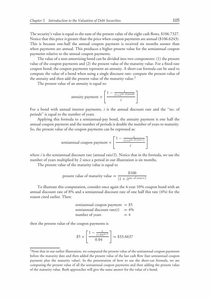
Chapter 5 Introduction to the Valuation of Debt Securities 105
The security’s value is equal to the sum of the present value of the eight cash flows, $106.7327.Notice that this price is greater than the price when coupon payments are annual ($106.6243).This is because one-half the annual coupon payment is received six months sooner thanwhen payments are annual. This produces a higher present value for the semiannual couponpayments relative to the annual coupon payments.
The value of a non-amortizing bond can be divided into two components: (1) the presentvalue of the coupon payments and (2) the present value of the maturity value. For a fixed-ratecoupon bond, the coupon payments represent an annuity. A short-cut formula can be used tocompute the value of a bond when using a single discount rate: compute the present value ofthe annuity and then add the present value of the maturity value.2
The present value of an annuity is equal to:
annuity payment ×[
1 − 1(1+i)no. of periods
i
]
For a bond with annual interest payments, i is the annual discount rate and the ‘‘no. ofperiods’’ is equal to the number of years.
Applying this formula to a semiannual-pay bond, the annuity payment is one half theannual coupon payment and the number of periods is double the number of years to maturity.So, the present value of the coupon payments can be expressed as:
semiannual coupon payment ×[
1 − 1(1+i)no. of years×2
i
]
where i is the semiannual discount rate (annual rate/2). Notice that in the formula, we use thenumber of years multiplied by 2 since a period in our illustration is six months.
The present value of the maturity value is equal to
present value of maturity value = $100
(1 + i)no. of years×2
To illustrate this computation, consider once again the 4-year 10% coupon bond with anannual discount rate of 8% and a semiannual discount rate of one half this rate (4%) for thereason cited earlier. Then:
semiannual coupon payment = $5semiannual discount rate(i) = 4%number of years = 4
then the present value of the coupon payments is
$5 ×[
1 − 1(1.04)4×2
0.04
]= $33.6637
2Note that in our earlier illustration, we computed the present value of the semiannual coupon paymentsbefore the maturity date and then added the present value of the last cash flow (last semiannual couponpayment plus the maturity value). In the presentation of how to use the short-cut formula, we arecomputing the present value of all the semiannual coupon payments and then adding the present valueof the maturity value. Both approaches will give the same answer for the value of a bond.
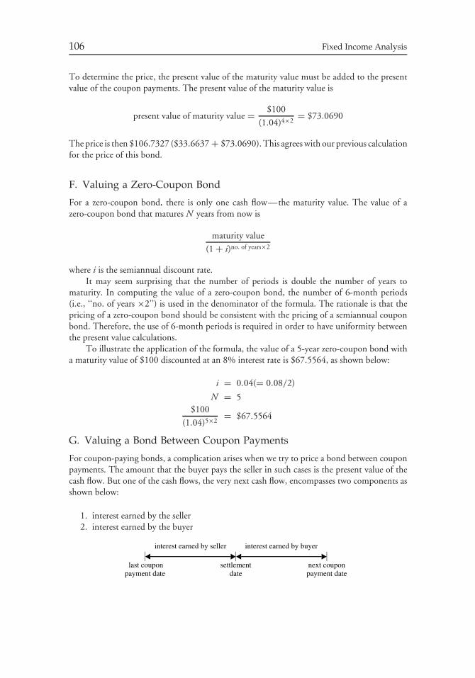
106 Fixed Income Analysis
To determine the price, the present value of the maturity value must be added to the presentvalue of the coupon payments. The present value of the maturity value is
present value of maturity value = $100
(1.04)4×2= $73.0690
The price is then $106.7327 ($33.6637 + $73.0690). This agrees with our previous calculationfor the price of this bond.
F. Valuing a Zero-Coupon Bond
For a zero-coupon bond, there is only one cash flow—the maturity value. The value of azero-coupon bond that matures N years from now is
maturity value
(1 + i)no. of years×2
where i is the semiannual discount rate.It may seem surprising that the number of periods is double the number of years to
maturity. In computing the value of a zero-coupon bond, the number of 6-month periods(i.e., ‘‘no. of years ×2’’) is used in the denominator of the formula. The rationale is that thepricing of a zero-coupon bond should be consistent with the pricing of a semiannual couponbond. Therefore, the use of 6-month periods is required in order to have uniformity betweenthe present value calculations.
To illustrate the application of the formula, the value of a 5-year zero-coupon bond witha maturity value of $100 discounted at an 8% interest rate is $67.5564, as shown below:
i = 0.04(= 0.08/2)
N = 5$100
(1.04)5×2= $67.5564
G. Valuing a Bond Between Coupon Payments
For coupon-paying bonds, a complication arises when we try to price a bond between couponpayments. The amount that the buyer pays the seller in such cases is the present value of thecash flow. But one of the cash flows, the very next cash flow, encompasses two components asshown below:
1. interest earned by the seller2. interest earned by the buyer
interest earned by seller interest earned by buyer
last couponpayment date
settlementdate
next couponpayment date

Chapter 5 Introduction to the Valuation of Debt Securities 107
The interest earned by the seller is the interest that has accrued3 between the last couponpayment date and the settlement date.4 This interest is called accrued interest. At the time ofpurchase, the buyer must compensate the seller for the accrued interest. The buyer recoversthe accrued interest when the next coupon payment is received.
When the price of a bond is computed using the present value calculations describedearlier, it is computed with accrued interest embodied in the price. This price is referred toas the full price. (Some market participants refer to it as the dirty price.) It is the full pricethat the buyer pays the seller. From the full price, the accrued interest must be deducted todetermine the price of the bond, sometimes referred to as the clean price.
Below, we show how the present value formula is modified to compute the full pricewhen a bond is purchased between coupon periods.
1. Computing the Full Price To compute the full price, it is first necessary to determinethe fractional periods between the settlement date and the next coupon payment date. This isdetermined as follows:
w periods = days between settlement date and next coupon payment date
days in coupon period
Then the present value of the expected cash flow to be received t periods from now usinga discount rate i assuming the first coupon payment is w periods from now is:
present valuet = expected cash flow
(1 + i)t−1+w
This procedure for calculating the present value when a security is purchased between couponpayments is called the ‘‘Street method.’’
To illustrate the calculation, suppose that there are five semiannual coupon paymentsremaining for a 10% coupon bond. Also assume the following:
1. 78 days between the settlement date and the next coupon payment date2. 182 days in the coupon period
Then w is 0.4286 periods (= 78/182). The present value of each cash flow assuming that eachis discounted at 8% annual discount rate is
Period 1: persent value1 = $5
(1.04)0.4286= $4.9167
Period 2: present value2 = $5
(1.04)1.4286= $4.7276
Period 3: present value3 = $5
(1.04)2.4286= $4.5457
Period 4: present value4 = $5
(1.04)3.4286= $4.3709
Period 5: present value5 = $105
(1.04)4.4286= $88.2583
3‘‘Accrued’’ means that the interest is earned but not distributed to the bondholder.4The settlement date is the date a transaction is completed.
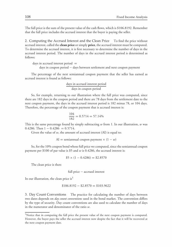
108 Fixed Income Analysis
The full price is the sum of the present value of the cash flows, which is $106.8192. Rememberthat the full price includes the accrued interest that the buyer is paying the seller.
2. Computing the Accrued Interest and the Clean Price To find the price withoutaccrued interest, called the clean price or simply price, the accrued interest must be computed.To determine the accrued interest, it is first necessary to determine the number of days in theaccrued interest period. The number of days in the accrued interest period is determined asfollows:
days in accrued interest period =days in coupon period − days between settlement and next coupon payment
The percentage of the next semiannual coupon payment that the seller has earned asaccrued interest is found as follows:
days in accrued interest period
days in coupon period
So, for example, returning to our illustration where the full price was computed, sincethere are 182 days in the coupon period and there are 78 days from the settlement date to thenext coupon payment, the days in the accrued interest period is 182 minus 78, or 104 days.Therefore, the percentage of the coupon payment that is accrued interest is:
104
182= 0.5714 = 57.14%
This is the same percentage found by simply subtracting w from 1. In our illustration, w was0.4286. Then 1 − 0.4286 = 0.5714.
Given the value of w, the amount of accrued interest (AI) is equal to:
AI = semiannual coupon payment × (1 − w)
So, for the 10% coupon bond whose full price we computed, since the semiannual couponpayment per $100 of par value is $5 and w is 0.4286, the accrued interest is:
$5 × (1 − 0.4286) = $2.8570
The clean price is then:
full price − accrued interest
In our illustration, the clean price is5
$106.8192 − $2.8570 = $103.9622
3. Day Count Conventions The practice for calculating the number of days betweentwo dates depends on day count conventions used in the bond market. The convention differsby the type of security. Day count conventions are also used to calculate the number of daysin the numerator and denominator of the ratio w.
5Notice that in computing the full price the present value of the next coupon payment is computed.However, the buyer pays the seller the accrued interest now despite the fact that it will be recovered atthe next coupon payment date.
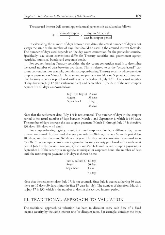
Chapter 5 Introduction to the Valuation of Debt Securities 109
The accrued interest (AI) assuming semiannual payments is calculated as follows:
AI = annual coupon
2× days in AI period
days in coupon period
In calculating the number of days between two dates, the actual number of days is notalways the same as the number of days that should be used in the accrued interest formula.The number of days used depends on the day count convention for the particular security.Specifically, day count conventions differ for Treasury securities and government agencysecurities, municipal bonds, and corporate bonds.
For coupon-bearing Treasury securities, the day count convention used is to determinethe actual number of days between two dates. This is referred to as the ‘‘actual/actual’’ daycount convention. For example, consider a coupon-bearing Treasury security whose previouscoupon payment was March 1. The next coupon payment would be on September 1. Supposethis Treasury security is purchased with a settlement date of July 17th. The actual numberof days between July 17 (the settlement date) and September 1 (the date of the next couponpayment) is 46 days, as shown below:
July 17 to July 31 14 daysAugust 31 daysSeptember 1 1 day
46 days
Note that the settlement date (July 17) is not counted. The number of days in the couponperiod is the actual number of days between March 1 and September 1, which is 184 days.The number of days between the last coupon payment (March 1) through July 17 is therefore138 days (184 days − 46 days).
For coupon-bearing agency, municipal, and corporate bonds, a different day countconvention is used. It is assumed that every month has 30 days, that any 6-month period has180 days, and that there are 360 days in a year. This day count convention is referred to as‘‘30/360.’’ For example, consider once again the Treasury security purchased with a settlementdate of July 17, the previous coupon payment on March 1, and the next coupon payment onSeptember 1. If the security is an agency, municipal, or corporate bond, the number of daysuntil the next coupon payment is 44 days as shown below:
July 17 to July 31 13 daysAugust 30 daysSeptember 1 1 day
44 days
Note that the settlement date, July 17, is not counted. Since July is treated as having 30 days,there are 13 days (30 days minus the first 17 days in July). The number of days from March 1to July 17 is 136, which is the number of days in the accrued interest period.
III. TRADITIONAL APPROACH TO VALUATION
The traditional approach to valuation has been to discount every cash flow of a fixedincome security by the same interest rate (or discount rate). For example, consider the three
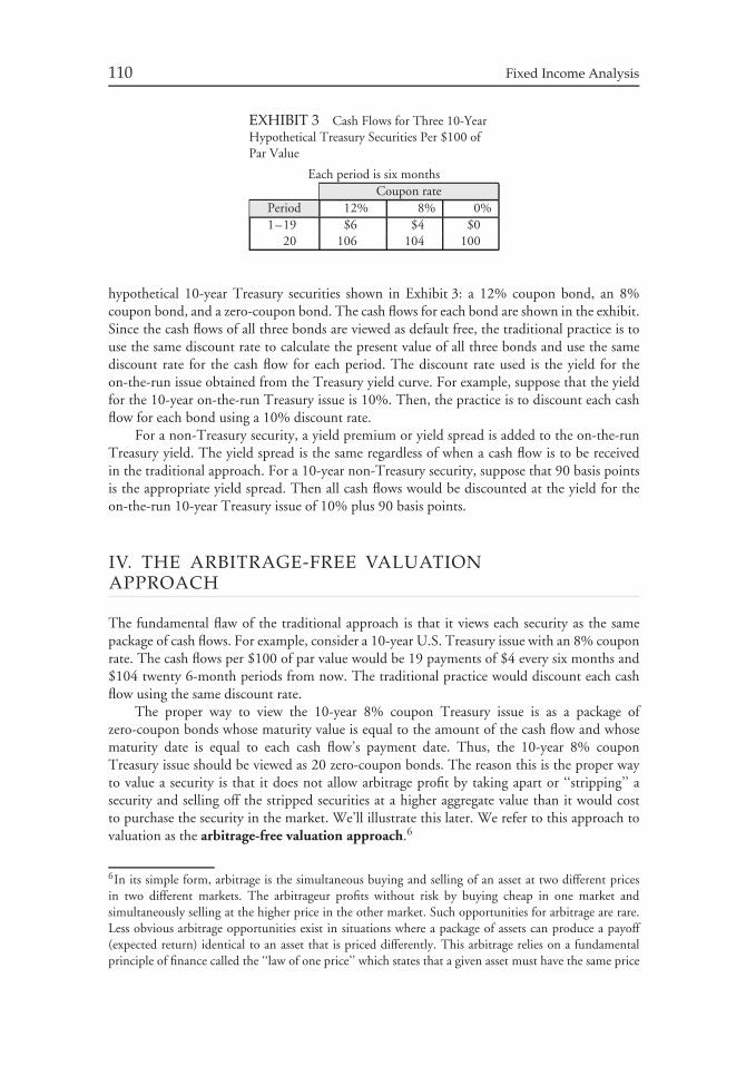
110 Fixed Income Analysis
EXHIBIT 3 Cash Flows for Three 10-YearHypothetical Treasury Securities Per $100 ofPar Value
Each period is six monthsCoupon rate
Period 12% 8% 0%1–19 $6 $4 $0
20 106 104 100
hypothetical 10-year Treasury securities shown in Exhibit 3: a 12% coupon bond, an 8%coupon bond, and a zero-coupon bond. The cash flows for each bond are shown in the exhibit.Since the cash flows of all three bonds are viewed as default free, the traditional practice is touse the same discount rate to calculate the present value of all three bonds and use the samediscount rate for the cash flow for each period. The discount rate used is the yield for theon-the-run issue obtained from the Treasury yield curve. For example, suppose that the yieldfor the 10-year on-the-run Treasury issue is 10%. Then, the practice is to discount each cashflow for each bond using a 10% discount rate.
For a non-Treasury security, a yield premium or yield spread is added to the on-the-runTreasury yield. The yield spread is the same regardless of when a cash flow is to be receivedin the traditional approach. For a 10-year non-Treasury security, suppose that 90 basis pointsis the appropriate yield spread. Then all cash flows would be discounted at the yield for theon-the-run 10-year Treasury issue of 10% plus 90 basis points.
IV. THE ARBITRAGE-FREE VALUATIONAPPROACH
The fundamental flaw of the traditional approach is that it views each security as the samepackage of cash flows. For example, consider a 10-year U.S. Treasury issue with an 8% couponrate. The cash flows per $100 of par value would be 19 payments of $4 every six months and$104 twenty 6-month periods from now. The traditional practice would discount each cashflow using the same discount rate.
The proper way to view the 10-year 8% coupon Treasury issue is as a package ofzero-coupon bonds whose maturity value is equal to the amount of the cash flow and whosematurity date is equal to each cash flow’s payment date. Thus, the 10-year 8% couponTreasury issue should be viewed as 20 zero-coupon bonds. The reason this is the proper wayto value a security is that it does not allow arbitrage profit by taking apart or ‘‘stripping’’ asecurity and selling off the stripped securities at a higher aggregate value than it would costto purchase the security in the market. We’ll illustrate this later. We refer to this approach tovaluation as the arbitrage-free valuation approach.6
6In its simple form, arbitrage is the simultaneous buying and selling of an asset at two different pricesin two different markets. The arbitrageur profits without risk by buying cheap in one market andsimultaneously selling at the higher price in the other market. Such opportunities for arbitrage are rare.Less obvious arbitrage opportunities exist in situations where a package of assets can produce a payoff(expected return) identical to an asset that is priced differently. This arbitrage relies on a fundamentalprinciple of finance called the ‘‘law of one price’’ which states that a given asset must have the same price

Chapter 5 Introduction to the Valuation of Debt Securities 111
EXHIBIT 4 Comparison of Traditional Approach and Arbitrage-Free Approach inValuing a Treasury Security
Each period is six monthsDiscount (base interest) rate Cash flows for∗
Period Traditional approach Arbitrage-free approach 12% 8% 0%1 10-year Treasury rate 1-period Treasury spot rate $6 $4 $02 10-year Treasury rate 2-period Treasury spot rate 6 4 03 10-year Treasury rate 3-period Treasury spot rate 6 4 04 10-year Treasury rate 4-period Treasury spot rate 6 4 05 10-year Treasury rate 5-period Treasury spot rate 6 4 06 10-year Treasury rate 6-period Treasury spot rate 6 4 07 10-year Treasury rate 7-period Treasury spot rate 6 4 08 10-year Treasury rate 8-period Treasury spot rate 6 4 09 10-year Treasury rate 9-period Treasury spot rate 6 4 0
10 10-year Treasury rate 10-period Treasury spot rate 6 4 011 10-year Treasury rate 11-period Treasury spot rate 6 4 012 10-year Treasury rate 12-period Treasury spot rate 6 4 013 10-year Treasury rate 13-period Treasury spot rate 6 4 014 10-year Treasury rate 14-period Treasury spot rate 6 4 015 10-year Treasury rate 15-period Treasury spot rate 6 4 016 10-year Treasury rate 16-period Treasury spot rate 6 4 017 10-year Treasury rate 17-period Treasury spot rate 6 4 018 10-year Treasury rate 18-period Treasury spot rate 6 4 019 10-year Treasury rate 19-period Treasury spot rate 6 4 020 10-year Treasury rate 20-period Treasury spot rate 106 104 100
∗Per $100 of par value.
By viewing any financial asset as a package of zero-coupon bonds, a consistent valuationframework can be developed. Viewing a financial asset as a package of zero-coupon bondsmeans that any two bonds would be viewed as different packages of zero-coupon bonds andvalued accordingly.
The difference between the traditional valuation approach and the arbitrage-free approachis illustrated in Exhibit 4, which shows how the three bonds whose cash flows are depictedin Exhibit 3 should be valued. With the traditional approach, the discount rate for all threebonds is the yield on a 10-year U.S. Treasury security. With the arbitrage-free approach, thediscount rate for a cash flow is the theoretical rate that the U.S. Treasury would have to pay ifit issued a zero-coupon bond with a maturity date equal to the maturity date of the cash flow.
Therefore, to implement the arbitrage-free approach, it is necessary to determine thetheoretical rate that the U.S. Treasury would have to pay on a zero-coupon Treasury securityfor each maturity. As explained in the previous chapter, the name given to the zero-couponTreasury rate is the Treasury spot rate. In Chapter 6, we will explain how the Treasury spotrate can be calculated. The spot rate for a Treasury security is the interest rate that should beused to discount a default-free cash flow with the same maturity. We call the value of a bondbased on spot rates the arbitrage-free value.
regardless of the means by which one goes about creating that asset. The law of one price implies that ifthe payoff of an asset can be synthetically created by a package of assets, the price of the package and theprice of the asset whose payoff it replicates must be equal.
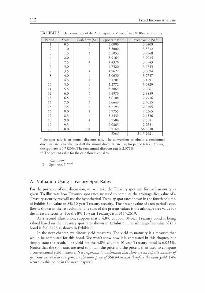
112 Fixed Income Analysis
EXHIBIT 5 Determination of the Arbitrage-Free Value of an 8% 10-year Treasury
Period Years Cash flow ($) Spot rate (%)∗ Present value ($) ∗∗
1 0.5 4 3.0000 3.94092 1.0 4 3.3000 3.87123 1.5 4 3.5053 3.79684 2.0 4 3.9164 3.70145 2.5 4 4.4376 3.58436 3.0 4 4.7520 3.47437 3.5 4 4.9622 3.36948 4.0 4 5.0650 3.27479 4.5 4 5.1701 3.1791
10 5.0 4 5.2772 3.082911 5.5 4 5.3864 2.986112 6.0 4 5.4976 2.888913 6.5 4 5.6108 2.791614 7.0 4 5.6643 2.705515 7.5 4 5.7193 2.620516 8.0 4 5.7755 2.536517 8.5 4 5.8331 2.453618 9.0 4 5.9584 2.358119 9.5 4 6.0863 2.263120 10.0 104 6.2169 56.3830
Total $115.2621∗The spot rate is an annual discount rate. The convention to obtain a semiannualdiscount rate is to take one-half the annual discount rate. So, for period 6 (i.e., 3 years),the spot rate is 4.7520%. The semiannual discount rate is 2.376%.∗∗ The present value for the cash flow is equal to:
Cash flow(1 + Spot rate/2)period
A. Valuation Using Treasury Spot Rates
For the purposes of our discussion, we will take the Treasury spot rate for each maturity asgiven. To illustrate how Treasury spot rates are used to compute the arbitrage-free value of aTreasury security, we will use the hypothetical Treasury spot rates shown in the fourth columnof Exhibit 5 to value an 8% 10-year Treasury security. The present value of each period’s cashflow is shown in the last column. The sum of the present values is the arbitrage-free value forthe Treasury security. For the 8% 10-year Treasury, it is $115.2619.
As a second illustration, suppose that a 4.8% coupon 10-year Treasury bond is beingvalued based on the Treasury spot rates shown in Exhibit 5. The arbitrage-free value of thisbond is $90.8428 as shown in Exhibit 6.
In the next chapter, we discuss yield measures. The yield to maturity is a measure thatwould be computed for this bond. We won’t show how it is computed in this chapter, butsimply state the result. The yield for the 4.8% coupon 10-year Treasury bond is 6.033%.Notice that the spot rates are used to obtain the price and the price is then used to computea conventional yield measure. It is important to understand that there are an infinite number ofspot rate curves that can generate the same price of $90.8428 and therefore the same yield. (Wereturn to this point in the next chapter.)
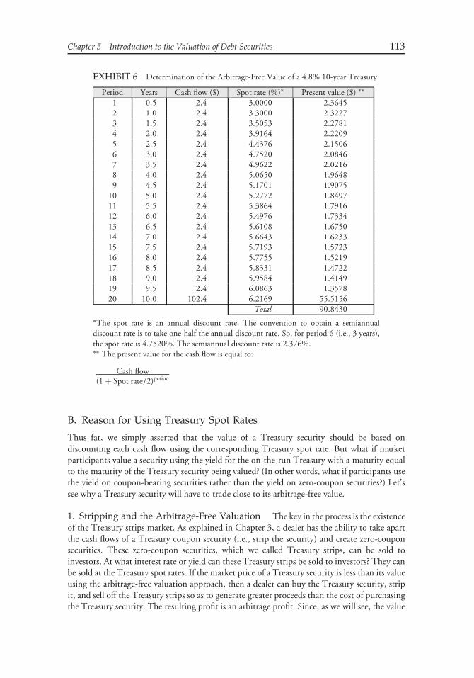
Chapter 5 Introduction to the Valuation of Debt Securities 113
EXHIBIT 6 Determination of the Arbitrage-Free Value of a 4.8% 10-year Treasury
Period Years Cash flow ($) Spot rate (%)∗ Present value ($) ∗∗
1 0.5 2.4 3.0000 2.36452 1.0 2.4 3.3000 2.32273 1.5 2.4 3.5053 2.27814 2.0 2.4 3.9164 2.22095 2.5 2.4 4.4376 2.15066 3.0 2.4 4.7520 2.08467 3.5 2.4 4.9622 2.02168 4.0 2.4 5.0650 1.96489 4.5 2.4 5.1701 1.9075
10 5.0 2.4 5.2772 1.849711 5.5 2.4 5.3864 1.791612 6.0 2.4 5.4976 1.733413 6.5 2.4 5.6108 1.675014 7.0 2.4 5.6643 1.623315 7.5 2.4 5.7193 1.572316 8.0 2.4 5.7755 1.521917 8.5 2.4 5.8331 1.472218 9.0 2.4 5.9584 1.414919 9.5 2.4 6.0863 1.357820 10.0 102.4 6.2169 55.5156
Total 90.8430∗The spot rate is an annual discount rate. The convention to obtain a semiannualdiscount rate is to take one-half the annual discount rate. So, for period 6 (i.e., 3 years),the spot rate is 4.7520%. The semiannual discount rate is 2.376%.∗∗ The present value for the cash flow is equal to:
Cash flow(1 + Spot rate/2)period
B. Reason for Using Treasury Spot Rates
Thus far, we simply asserted that the value of a Treasury security should be based ondiscounting each cash flow using the corresponding Treasury spot rate. But what if marketparticipants value a security using the yield for the on-the-run Treasury with a maturity equalto the maturity of the Treasury security being valued? (In other words, what if participants usethe yield on coupon-bearing securities rather than the yield on zero-coupon securities?) Let’ssee why a Treasury security will have to trade close to its arbitrage-free value.
1. Stripping and the Arbitrage-Free Valuation The key in the process is the existenceof the Treasury strips market. As explained in Chapter 3, a dealer has the ability to take apartthe cash flows of a Treasury coupon security (i.e., strip the security) and create zero-couponsecurities. These zero-coupon securities, which we called Treasury strips, can be sold toinvestors. At what interest rate or yield can these Treasury strips be sold to investors? They canbe sold at the Treasury spot rates. If the market price of a Treasury security is less than its valueusing the arbitrage-free valuation approach, then a dealer can buy the Treasury security, stripit, and sell off the Treasury strips so as to generate greater proceeds than the cost of purchasingthe Treasury security. The resulting profit is an arbitrage profit. Since, as we will see, the value
114 Fixed Income Analysis
determined by using the Treasury spot rates does not allow for the generation of an arbitrageprofit, this is the reason why the approach is referred to as an ‘‘arbitrage-free’’ approach.
To illustrate this, suppose that the yield for the on-the-run 10-year Treasury issue is 6%.(We will see in Chapter 6 that the Treasury spot rate curve in Exhibit 5 was generated froma yield curve where the on-the-run 10-year Treasury issue was 6%.) Suppose that the 8%coupon 10-year Treasury issue is valued using the traditional approach based on 6%. Exhibit7 shows the value based on discounting all the cash flows at 6% is $114.8775.
Consider what would happen if the market priced the security at $114.8775. The valuebased on the Treasury spot rates (Exhibit 5) is $115.2621. What can the dealer do? Thedealer can buy the 8% 10-year issue for $114.8775, strip it, and sell the Treasury strips at thespot rates shown in Exhibit 5. By doing so, the proceeds that will be received by the dealerare $115.2621. This results in an arbitrage profit of $0.3846 (= $115.2621 − $114.8775).7
Dealers recognizing this arbitrage opportunity will bid up the price of the 8% 10-year Treasuryissue in order to acquire it and strip it. At what point will the arbitrage profit disappear? Whenthe security is priced at $115.2621, the value that we said is the arbitrage-free value.
To understand in more detail where this arbitrage profit is coming from, look at Exhibit8.The third column shows how much each cash flow can be sold for by the dealer if it isstripped. The values in the third column are simply the present values in Exhibit 5 based ondiscounting the cash flows at the Treasury spot rates. The fourth column shows how muchthe dealer is effectively purchasing the cash flow if each cash flow is discounted at 6%. Thisis the last column in Exhibit 7. The sum of the arbitrage profit from each cash flow strippedis the total arbitrage profit.
2. Reconstitution and Arbitrage-Free Valuation We have just demonstrated howcoupon stripping of a Treasury issue will force its market value to be close to the valuedetermined by arbitrage-free valuation when the market price is less than the arbitrage-freevalue. What happens when a Treasury issue’s market price is greater than the arbitrage-freevalue? Obviously, a dealer will not want to strip the Treasury issue since the proceeds generatedfrom stripping will be less than the cost of purchasing the issue.
When such situations occur, the dealer will follow a procedure called reconstitution.8
Basically, the dealer can purchase a package of Treasury strips so as to create a synthetic(i.e., artificial) Treasury coupon security that is worth more than the same maturity and samecoupon Treasury issue.
To illustrate this, consider the 4.8% 10-year Treasury issue whose arbitrage-free valuewas computed in Exhibit 6. The arbitrage-free value is $90.8430. Exhibit 9 shows the priceassuming the traditional approach where all the cash flows are discounted at a 6% interest rate.The price is $91.0735. What the dealer can do is purchase the Treasury strip for each 6-monthperiod at the prices shown in Exhibit 6 and sell short the 4.8% 10-year Treasury couponissue whose cash flows are being replicated. By doing so, the dealer has the cash flow of a4.8% coupon 10-year Treasury security at a cost of $90.8430, thereby generating an arbitrageprofit of $0.2305 ($91.0735 − $90.8430). The cash flows from the package of Treasury strips
7This may seem like a small amount, but remember that this is for a single $100 par value bond. Multiplythis by thousands of bonds and you can see a dealer’s profit potential.8The definition of reconstitute is to provide with a new structure, often by assembling various parts into awhole. Reconstitution then, as used here, means to assemble the parts (the Treasury strips) in such a waythat a new whole (a Treasury coupon bond) is created. That is, it is the opposite of stripping a couponbond.
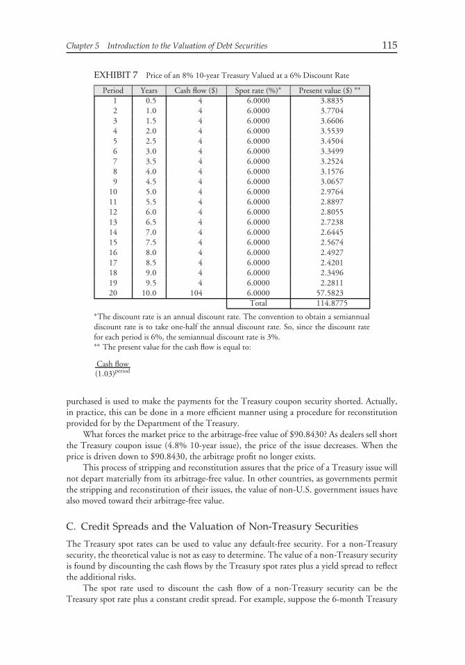
Chapter 5 Introduction to the Valuation of Debt Securities 115
EXHIBIT 7 Price of an 8% 10-year Treasury Valued at a 6% Discount Rate
Period Years Cash flow ($) Spot rate (%)∗ Present value ($) ∗∗1 0.5 4 6.0000 3.88352 1.0 4 6.0000 3.77043 1.5 4 6.0000 3.66064 2.0 4 6.0000 3.55395 2.5 4 6.0000 3.45046 3.0 4 6.0000 3.34997 3.5 4 6.0000 3.25248 4.0 4 6.0000 3.15769 4.5 4 6.0000 3.0657
10 5.0 4 6.0000 2.976411 5.5 4 6.0000 2.889712 6.0 4 6.0000 2.805513 6.5 4 6.0000 2.723814 7.0 4 6.0000 2.644515 7.5 4 6.0000 2.567416 8.0 4 6.0000 2.492717 8.5 4 6.0000 2.420118 9.0 4 6.0000 2.349619 9.5 4 6.0000 2.281120 10.0 104 6.0000 57.5823
Total 114.8775∗The discount rate is an annual discount rate. The convention to obtain a semiannualdiscount rate is to take one-half the annual discount rate. So, since the discount ratefor each period is 6%, the semiannual discount rate is 3%.∗∗ The present value for the cash flow is equal to:
Cash flow(1.03)period
purchased is used to make the payments for the Treasury coupon security shorted. Actually,in practice, this can be done in a more efficient manner using a procedure for reconstitutionprovided for by the Department of the Treasury.
What forces the market price to the arbitrage-free value of $90.8430? As dealers sell shortthe Treasury coupon issue (4.8% 10-year issue), the price of the issue decreases. When theprice is driven down to $90.8430, the arbitrage profit no longer exists.
This process of stripping and reconstitution assures that the price of a Treasury issue willnot depart materially from its arbitrage-free value. In other countries, as governments permitthe stripping and reconstitution of their issues, the value of non-U.S. government issues havealso moved toward their arbitrage-free value.
C. Credit Spreads and the Valuation of Non-Treasury Securities
The Treasury spot rates can be used to value any default-free security. For a non-Treasurysecurity, the theoretical value is not as easy to determine. The value of a non-Treasury securityis found by discounting the cash flows by the Treasury spot rates plus a yield spread to reflectthe additional risks.
The spot rate used to discount the cash flow of a non-Treasury security can be theTreasury spot rate plus a constant credit spread. For example, suppose the 6-month Treasury
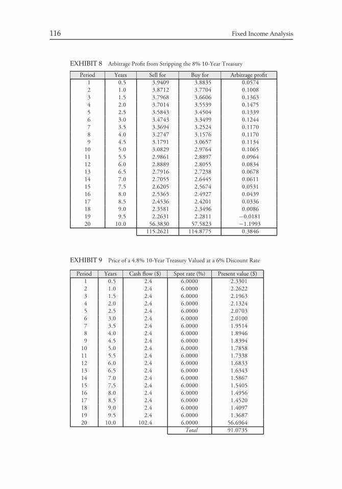
116 Fixed Income Analysis
EXHIBIT 8 Arbitrage Profit from Stripping the 8% 10-Year Treasury
Period Years Sell for Buy for Arbitrage profit1 0.5 3.9409 3.8835 0.05742 1.0 3.8712 3.7704 0.10083 1.5 3.7968 3.6606 0.13634 2.0 3.7014 3.5539 0.14755 2.5 3.5843 3.4504 0.13396 3.0 3.4743 3.3499 0.12447 3.5 3.3694 3.2524 0.11708 4.0 3.2747 3.1576 0.11709 4.5 3.1791 3.0657 0.1134
10 5.0 3.0829 2.9764 0.106511 5.5 2.9861 2.8897 0.096412 6.0 2.8889 2.8055 0.083413 6.5 2.7916 2.7238 0.067814 7.0 2.7055 2.6445 0.061115 7.5 2.6205 2.5674 0.053116 8.0 2.5365 2.4927 0.043917 8.5 2.4536 2.4201 0.033618 9.0 2.3581 2.3496 0.008619 9.5 2.2631 2.2811 −0.018120 10.0 56.3830 57.5823 −1.1993
115.2621 114.8775 0.3846
EXHIBIT 9 Price of a 4.8% 10-Year Treasury Valued at a 6% Discount Rate
Period Years Cash flow ($) Spot rate (%) Present value ($)1 0.5 2.4 6.0000 2.33012 1.0 2.4 6.0000 2.26223 1.5 2.4 6.0000 2.19634 2.0 2.4 6.0000 2.13245 2.5 2.4 6.0000 2.07036 3.0 2.4 6.0000 2.01007 3.5 2.4 6.0000 1.95148 4.0 2.4 6.0000 1.89469 4.5 2.4 6.0000 1.8394
10 5.0 2.4 6.0000 1.785811 5.5 2.4 6.0000 1.733812 6.0 2.4 6.0000 1.683313 6.5 2.4 6.0000 1.634314 7.0 2.4 6.0000 1.586715 7.5 2.4 6.0000 1.540516 8.0 2.4 6.0000 1.495617 8.5 2.4 6.0000 1.452018 9.0 2.4 6.0000 1.409719 9.5 2.4 6.0000 1.368720 10.0 102.4 6.0000 56.6964
Total 91.0735
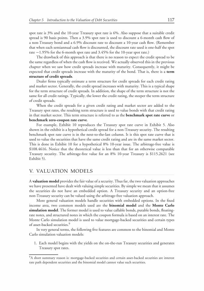
Chapter 5 Introduction to the Valuation of Debt Securities 117
spot rate is 3% and the 10-year Treasury spot rate is 6%. Also suppose that a suitable creditspread is 90 basis points. Then a 3.9% spot rate is used to discount a 6-month cash flow ofa non-Treasury bond and a 6.9% discount rate to discount a 10-year cash flow. (Rememberthat when each semiannual cash flow is discounted, the discount rate used is one-half the spotrate −1.95% for the 6-month spot rate and 3.45% for the 10-year spot rate.)
The drawback of this approach is that there is no reason to expect the credit spread to bethe same regardless of when the cash flow is received. We actually observed this in the previouschapter when we saw how credit spreads increase with maturity. Consequently, it might beexpected that credit spreads increase with the maturity of the bond. That is, there is a termstructure of credit spreads.
Dealer firms typically estimate a term structure for credit spreads for each credit ratingand market sector. Generally, the credit spread increases with maturity. This is a typical shapefor the term structure of credit spreads. In addition, the shape of the term structure is not thesame for all credit ratings. Typically, the lower the credit rating, the steeper the term structureof credit spreads.
When the credit spreads for a given credit rating and market sector are added to theTreasury spot rates, the resulting term structure is used to value bonds with that credit ratingin that market sector. This term structure is referred to as the benchmark spot rate curve orbenchmark zero-coupon rate curve.
For example, Exhibit 10 reproduces the Treasury spot rate curve in Exhibit 5. Alsoshown in the exhibit is a hypothetical credit spread for a non-Treasury security. The resultingbenchmark spot rate curve is in the next-to-the-last column. It is this spot rate curve that isused to value the securities that have the same credit rating and are in the same market sector.This is done in Exhibit 10 for a hypothetical 8% 10-year issue. The arbitrage-free value is$108.4616. Notice that the theoretical value is less than that for an otherwise comparableTreasury security. The arbitrage-free value for an 8% 10-year Treasury is $115.2621 (seeExhibit 5).
V. VALUATION MODELS
A valuation model provides the fair value of a security. Thus far, the two valuation approacheswe have presented have dealt with valuing simple securities. By simple we mean that it assumesthe securities do not have an embedded option. A Treasury security and an option-freenon-Treasury security can be valued using the arbitrage-free valuation approach.
More general valuation models handle securities with embedded options. In the fixedincome area, two common models used are the binomial model and the Monte Carlosimulation model. The former model is used to value callable bonds, putable bonds, floating-rate notes, and structured notes in which the coupon formula is based on an interest rate. TheMonte Carlo simulation model is used to value mortgage-backed securities and certain typesof asset-backed securities.9
In very general terms, the following five features are common to the binomial and MonteCarlo simulation valuation models:
1. Each model begins with the yields on the on-the-run Treasury securities and generatesTreasury spot rates.
9A short summary reason is: mortgage-backed securities and certain asset-backed securities are interestrate path dependent securities and the binomial model cannot value such securities.
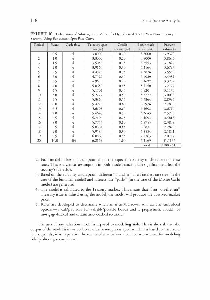
118 Fixed Income Analysis
EXHIBIT 10 Calculation of Arbitrage-Free Value of a Hypothetical 8% 10-Year Non-TreasurySecurity Using Benchmark Spot Rate Curve
Period Years Cash flow Treasury spot Credit Benchmark Presentrate (%) spread (%) spot (%) value ($)
1 0.5 4 3.0000 0.20 3.2000 3.93702 1.0 4 3.3000 0.20 3.5000 3.86363 1.5 4 3.5053 0.25 3.7553 3.78294 2.0 4 3.9164 0.30 4.2164 3.67975 2.5 4 4.4376 0.35 4.7876 3.55386 3.0 4 4.7520 0.35 5.1020 3.43897 3.5 4 4.9622 0.40 5.3622 3.32378 4.0 4 5.0650 0.45 5.5150 3.21779 4.5 4 5.1701 0.45 5.6201 3.117010 5.0 4 5.2772 0.50 5.7772 3.008811 5.5 4 5.3864 0.55 5.9364 2.899512 6.0 4 5.4976 0.60 6.0976 2.789613 6.5 4 5.6108 0.65 6.2608 2.679414 7.0 4 5.6643 0.70 6.3643 2.579915 7.5 4 5.7193 0.75 6.4693 2.481316 8.0 4 5.7755 0.80 6.5755 2.383817 8.5 4 5.8331 0.85 6.6831 2.287618 9.0 4 5.9584 0.90 6.8584 2.180119 9.5 4 6.0863 0.95 7.0363 2.073720 10.0 104 6.2169 1.00 7.2169 51.1835
Total $108.4616
2. Each model makes an assumption about the expected volatility of short-term interestrates. This is a critical assumption in both models since it can significantly affect thesecurity’s fair value.
3. Based on the volatility assumption, different ‘‘branches’’ of an interest rate tree (in thecase of the binomial model) and interest rate ‘‘paths’’ (in the case of the Monte Carlomodel) are generated.
4. The model is calibrated to the Treasury market. This means that if an ‘‘on-the-run’’Treasury issue is valued using the model, the model will produce the observed marketprice.
5. Rules are developed to determine when an issuer/borrower will exercise embeddedoptions—a call/put rule for callable/putable bonds and a prepayment model formortgage-backed and certain asset-backed securities.
The user of any valuation model is exposed to modeling risk. This is the risk that theoutput of the model is incorrect because the assumptions upon which it is based are incorrect.Consequently, it is imperative the results of a valuation model be stress-tested for modelingrisk by altering assumptions.
CHAPTER 6YIELD MEASURES, SPOTRATES, AND FORWARD
RATES
I. INTRODUCTION
Frequently, investors assess the relative value of a security by some yield or yield spreadmeasure quoted in the market. These measures are based on assumptions that limit their useto gauge relative value. This chapter explains the various yield and yield spread measures andtheir limitations.
In this chapter, we will see a basic approach to computing the spot rates from the on-the-run Treasury issues. We will see the limitations of the nominal spread measure and explain twomeasures that overcome these limitations—zero-volatility spread and option-adjusted spread.
II. SOURCES OF RETURN
When an investor purchases a fixed income security, he or she can expect to receive a dollarreturn from one or more of the following sources:
1. the coupon interest payments made by the issuer2. any capital gain (or capital loss—a negative dollar return) when the security matures, is
called, or is sold3. income from reinvestment of interim cash flows (interest and/or principal payments
prior to stated maturity)
Any yield measure that purports to measure the potential return from a fixed incomesecurity should consider all three sources of return described above.
A. Coupon Interest Payments
The most obvious source of return on a bond is the periodic coupon interest payments. Forzero-coupon instruments, the return from this source is zero. By purchasing a security below itspar value and receiving the full par value at maturity, the investor in a zero-coupon instrumentis effectively receiving interest in a lump sum.
119
120 Fixed Income Analysis
B. Capital Gain or Loss
An investor receives cash when a bond matures, is called, or is sold. If these proceeds aregreater than the purchase price, a capital gain results. For a bond held to maturity, there willbe a capital gain if the bond is purchased below its par value. For example, a bond purchasedfor $94.17 with a par value of $100 will generate a capital gain of $5.83 ($100−$94.17) ifheld to maturity. For a callable bond, a capital gain results if the price at which the bondis called (i.e., the call price) is greater than the purchase price. For example, if the bond inour previous example is callable and subsequently called at $100.5, a capital gain of $6.33($100.50 − $94.17) will be realized. If the same bond is sold prior to its maturity or beforeit is called, a capital gain will result if the proceeds exceed the purchase price. So, if ourhypothetical bond is sold prior to the maturity date for $103, the capital gain would be$8.83 ($103 − $94.17).
Similarly, for all three outcomes, a capital loss is generated when the proceeds received areless than the purchase price. For a bond held to maturity, there will be a capital loss if the bondis purchased for more than its par value (i.e., purchased at a premium). For example, a bondpurchased for $102.50 with a par value of $100 will generate a capital loss of $2.50 ($102.50− $100) if held to maturity. For a callable bond, a capital loss results if the price at whichthe bond is called is less than the purchase price. For example, if the bond in our example iscallable and subsequently called at $100.50, a capital loss of $2 ($102.50 − $100.50) will berealized. If the same bond is sold prior to its maturity or before it is called, a capital loss willresult if the sale price is less than the purchase price. So, if our hypothetical bond is sold priorto the maturity date for $98.50, the capital loss would be $4 ($102.50 −$98.50).
C. Reinvestment Income
Prior to maturity, with the exception of zero-coupon instruments, fixed income securities makeperiodic interest payments that can be reinvested. Amortizing securities (such as mortgage-backed securities and asset-backed securities) make periodic principal payments that can bereinvested prior to final maturity. The interest earned from reinvesting the interim cash flows(interest and/or principal payments) prior to final or stated maturity is called reinvestmentincome.
III. TRADITIONAL YIELD MEASURES
Yield measures cited in the bond market include current yield, yield to maturity, yield to call,yield to put, yield to worst, and cash flow yield. These yield measures are expressed as a percentreturn rather than a dollar return. Below we explain how each measure is calculated and itslimitations.
A. Current Yield
The current yield relates the annual dollar coupon interest to a bond’s market price. Theformula for the current yield is:
current yield = annual dollar coupon interest
price
Chapter 6 Yield Measures, Spot Rates, and Forward Rates 121
For example, the current yield for a 7% 8-year bond whose price is $94.17 is 7.43% as shownbelow:
annual dollar coupon interest = 0.07 × $100 = $7
price = $94.17
current yield = $7
$94.17= 0.0743 or 7.43%
The current yield will be greater than the coupon rate when the bond sells at a discount;the reverse is true for a bond selling at a premium. For a bond selling at par, the current yieldwill be equal to the coupon rate.
The drawback of the current yield is that it considers only the coupon interest andno other source for an investor’s return. No consideration is given to the capital gain aninvestor will realize when a bond purchased at a discount is held to maturity; nor is there anyrecognition of the capital loss an investor will realize if a bond purchased at a premium is heldto maturity. No consideration is given to reinvestment income.
B. Yield to Maturity
The most popular measure of yield in the bond market is the yield to maturity. The yieldto maturity is the interest rate that will make the present value of a bond’s cash flows equalto its market price plus accrued interest. To find the yield to maturity, we first determine theexpected cash flows and then search, by trial and error, for the interest rate that will makethe present value of cash flows equal to the market price plus accrued interest. (This is simplya special case of an internal rate of return (IRR) calculation where the cash flows are thosereceived if the bond is held to the maturity date.) In the illustrations presented in this chapter,we assume that the next coupon payment will be six months from now so that there is noaccrued interest.
To illustrate, consider a 7% 8-year bond selling for $94.17. The cash flows for this bondare (1) 16 payments every 6-months of $3.50 and (2) a payment sixteen 6-month periodsfrom now of $100. The present value using various semiannual discount (interest) rates is:
Semiannual interest rate 3.5% 3.6% 3.7% 3.8% 3.9% 4.0%Present value 100.00 98.80 97.62 96.45 95.30 94.17
When a 4.0% interest rate is used, the present value of the cash flows is equal to $94.17, whichis the price of the bond. Hence, 4.0% is the semiannual yield to maturity.
The market convention adopted to annualize the semiannual yield to maturity is todouble it and call that the yield to maturity. Thus, the yield to maturity for the above bondis 8% (2 times 4.0%). The yield to maturity computed using this convention—doubling thesemiannual yield—is called a bond-equivalent yield.
The following relationships between the price of a bond, coupon rate, current yield, andyield to maturity hold:
Bond selling at Relationshippar coupon rate = current yield = yield to maturitydiscount coupon rate < current yield < yield to maturitypremium coupon rate > current yield > yield to maturity
122 Fixed Income Analysis
1. The Bond-Equivalent Yield Convention The convention developed in the bondmarket to move from a semiannual yield to an annual yield is to simply double the semiannualyield. As just noted, this is called the bond-equivalent yield. In general, when one doublesa semiannual yield (or a semiannual return) to obtain an annual measure, one is said to becomputing the measure on a bond-equivalent basis.
Students of the bond market are troubled by this convention. The two questions mostcommonly asked are: First, why is the practice of simply doubling a semiannual yieldfollowed? Second, wouldn’t it be more appropriate to compute the effective annual yield bycompounding the semiannual yield?1
The answer to the first question is that it is simply a convention. There is no danger witha convention unless you use it improperly. The fact is that market participants recognize thata yield (or return) is computed on a semiannual basis by convention and adjust accordinglywhen using the number. So, if the bond-equivalent yield on a security purchased by an investoris 6%, the investor knows the semiannual yield is 3%. Given that, the investor can use thatsemiannual yield to compute an effective annual yield or any other annualized measure desired.For a manager comparing the yield on a security as an asset purchased to a yield required ona liability to satisfy, the yield figure will be measured in a manner consistent with that of theyield required on the liability.
The answer to the second question is that it is true that computing an effective annualyield would be better. But so what? Once we discover the limitations of yield measures ingeneral, we will question whether or not an investor should use a bond-equivalent yieldmeasure or an effective annual yield measure in making investment decisions. That is, whenwe identify the major problems with yield measures, the doubling of a semiannual yield is theleast of our problems.
So, don’t lose any sleep over this convention. Just make sure that you use a bond-equivalentyield measure properly.
2. Limitations of Yield-to-Maturity Measure The yield to maturity considers notonly the coupon income but any capital gain or loss that the investor will realize by holdingthe bond to maturity. The yield to maturity also considers the timing of the cash flows. It doesconsider reinvestment income; however, it assumes that the coupon payments can be reinvested at aninterest rate equal to the yield to maturity. So, if the yield to maturity for a bond is 8%, for example,to earn that yield the coupon payments must be reinvested at an interest rate equal to 8%.
The illustrations below clearly demonstrate this. In the illustrations, the analysis will bein terms of dollars. Be sure you keep in mind the difference between the total future dollars,which is equal to all the dollars an investor expects to receive (including the recovery of theprincipal), and the total dollar return, which is equal to the dollars an investor expects torealize from the three sources of return (coupon payments, capital gain/loss, and reinvestmentincome).
Suppose an investor has $94.17 and places the funds in a certificate of deposit (CD) thatmatures in 8 years. Let’s suppose that the bank agrees to pay 4% interest every six months.This means that the bank is agreeing to pay 8% on a bond equivalent basis (i.e., doublingthe semiannual yield). We can translate all of this into the total future dollars that will begenerated by this investment at the end of 8 years. From the standard formula for the future
1By compounding the semiannual yield it is meant that the annual yield is computed as follows:effective annual yield = (1 + semiannual yield)2 − 1
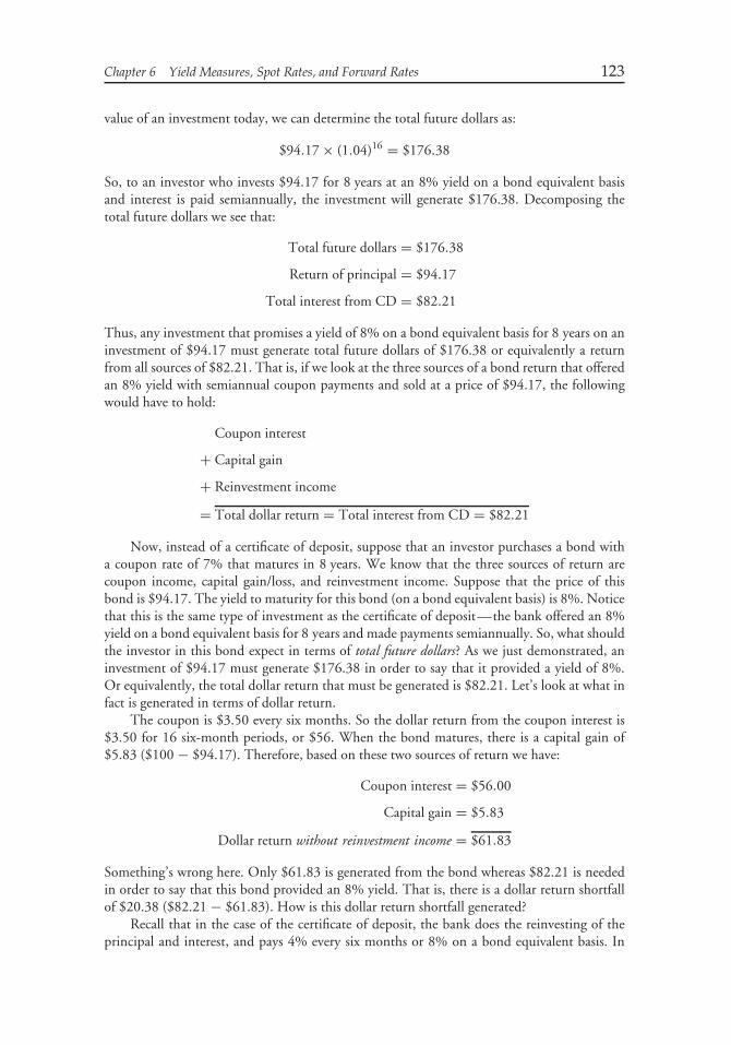
Chapter 6 Yield Measures, Spot Rates, and Forward Rates 123
value of an investment today, we can determine the total future dollars as:
$94.17 × (1.04)16 = $176.38
So, to an investor who invests $94.17 for 8 years at an 8% yield on a bond equivalent basisand interest is paid semiannually, the investment will generate $176.38. Decomposing thetotal future dollars we see that:
Total future dollars = $176.38
Return of principal = $94.17
Total interest from CD = $82.21
Thus, any investment that promises a yield of 8% on a bond equivalent basis for 8 years on aninvestment of $94.17 must generate total future dollars of $176.38 or equivalently a returnfrom all sources of $82.21. That is, if we look at the three sources of a bond return that offeredan 8% yield with semiannual coupon payments and sold at a price of $94.17, the followingwould have to hold:
Coupon interest
+ Capital gain
+ Reinvestment income
= Total dollar return = Total interest from CD = $82.21
Now, instead of a certificate of deposit, suppose that an investor purchases a bond witha coupon rate of 7% that matures in 8 years. We know that the three sources of return arecoupon income, capital gain/loss, and reinvestment income. Suppose that the price of thisbond is $94.17. The yield to maturity for this bond (on a bond equivalent basis) is 8%. Noticethat this is the same type of investment as the certificate of deposit—the bank offered an 8%yield on a bond equivalent basis for 8 years and made payments semiannually. So, what shouldthe investor in this bond expect in terms of total future dollars? As we just demonstrated, aninvestment of $94.17 must generate $176.38 in order to say that it provided a yield of 8%.Or equivalently, the total dollar return that must be generated is $82.21. Let’s look at what infact is generated in terms of dollar return.
The coupon is $3.50 every six months. So the dollar return from the coupon interest is$3.50 for 16 six-month periods, or $56. When the bond matures, there is a capital gain of$5.83 ($100 − $94.17). Therefore, based on these two sources of return we have:
Coupon interest = $56.00
Capital gain = $5.83
Dollar return without reinvestment income = $61.83
Something’s wrong here. Only $61.83 is generated from the bond whereas $82.21 is neededin order to say that this bond provided an 8% yield. That is, there is a dollar return shortfallof $20.38 ($82.21 − $61.83). How is this dollar return shortfall generated?
Recall that in the case of the certificate of deposit, the bank does the reinvesting of theprincipal and interest, and pays 4% every six months or 8% on a bond equivalent basis. In
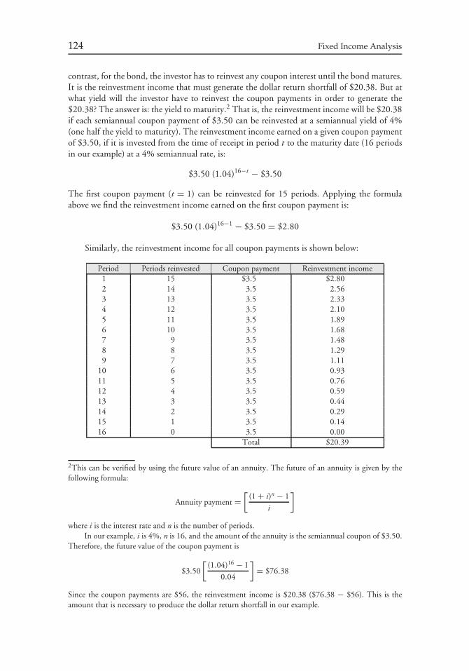
124 Fixed Income Analysis
contrast, for the bond, the investor has to reinvest any coupon interest until the bond matures.It is the reinvestment income that must generate the dollar return shortfall of $20.38. But atwhat yield will the investor have to reinvest the coupon payments in order to generate the$20.38? The answer is: the yield to maturity.2 That is, the reinvestment income will be $20.38if each semiannual coupon payment of $3.50 can be reinvested at a semiannual yield of 4%(one half the yield to maturity). The reinvestment income earned on a given coupon paymentof $3.50, if it is invested from the time of receipt in period t to the maturity date (16 periodsin our example) at a 4% semiannual rate, is:
$3.50 (1.04)16−t − $3.50
The first coupon payment (t = 1) can be reinvested for 15 periods. Applying the formulaabove we find the reinvestment income earned on the first coupon payment is:
$3.50 (1.04)16−1 − $3.50 = $2.80
Similarly, the reinvestment income for all coupon payments is shown below:
Period Periods reinvested Coupon payment Reinvestment income1 15 $3.5 $2.802 14 3.5 2.563 13 3.5 2.334 12 3.5 2.105 11 3.5 1.896 10 3.5 1.687 9 3.5 1.488 8 3.5 1.299 7 3.5 1.11
10 6 3.5 0.9311 5 3.5 0.7612 4 3.5 0.5913 3 3.5 0.4414 2 3.5 0.2915 1 3.5 0.1416 0 3.5 0.00
Total $20.39
2This can be verified by using the future value of an annuity. The future of an annuity is given by thefollowing formula:
Annuity payment =[
(1 + i)n − 1
i
]
where i is the interest rate and n is the number of periods.In our example, i is 4%, n is 16, and the amount of the annuity is the semiannual coupon of $3.50.
Therefore, the future value of the coupon payment is
$3.50[
(1.04)16 − 1
0.04
]= $76.38
Since the coupon payments are $56, the reinvestment income is $20.38 ($76.38 − $56). This is theamount that is necessary to produce the dollar return shortfall in our example.
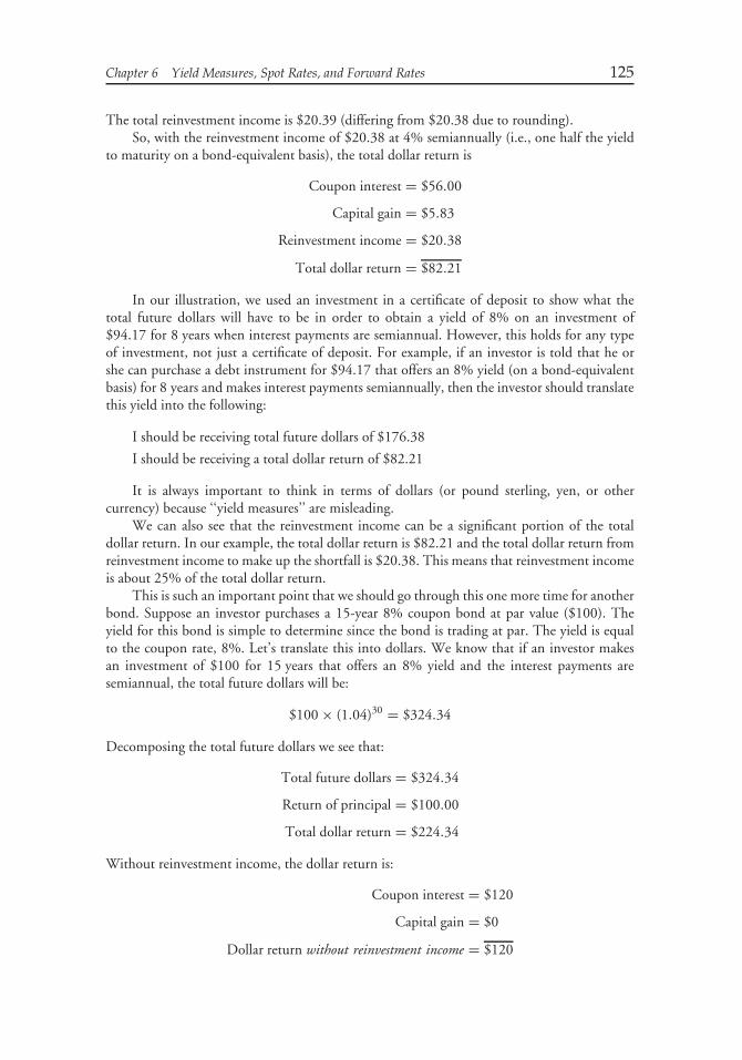
Chapter 6 Yield Measures, Spot Rates, and Forward Rates 125
The total reinvestment income is $20.39 (differing from $20.38 due to rounding).So, with the reinvestment income of $20.38 at 4% semiannually (i.e., one half the yield
to maturity on a bond-equivalent basis), the total dollar return is
Coupon interest = $56.00
Capital gain = $5.83
Reinvestment income = $20.38
Total dollar return = $82.21
In our illustration, we used an investment in a certificate of deposit to show what thetotal future dollars will have to be in order to obtain a yield of 8% on an investment of$94.17 for 8 years when interest payments are semiannual. However, this holds for any typeof investment, not just a certificate of deposit. For example, if an investor is told that he orshe can purchase a debt instrument for $94.17 that offers an 8% yield (on a bond-equivalentbasis) for 8 years and makes interest payments semiannually, then the investor should translatethis yield into the following:
I should be receiving total future dollars of $176.38
I should be receiving a total dollar return of $82.21
It is always important to think in terms of dollars (or pound sterling, yen, or othercurrency) because ‘‘yield measures’’ are misleading.
We can also see that the reinvestment income can be a significant portion of the totaldollar return. In our example, the total dollar return is $82.21 and the total dollar return fromreinvestment income to make up the shortfall is $20.38. This means that reinvestment incomeis about 25% of the total dollar return.
This is such an important point that we should go through this one more time for anotherbond. Suppose an investor purchases a 15-year 8% coupon bond at par value ($100). Theyield for this bond is simple to determine since the bond is trading at par. The yield is equalto the coupon rate, 8%. Let’s translate this into dollars. We know that if an investor makesan investment of $100 for 15 years that offers an 8% yield and the interest payments aresemiannual, the total future dollars will be:
$100 × (1.04)30 = $324.34
Decomposing the total future dollars we see that:
Total future dollars = $324.34
Return of principal = $100.00
Total dollar return = $224.34
Without reinvestment income, the dollar return is:
Coupon interest = $120
Capital gain = $0
Dollar return without reinvestment income = $120
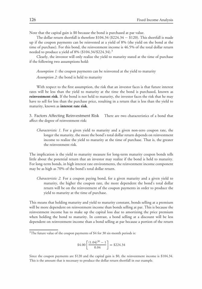
126 Fixed Income Analysis
Note that the capital gain is $0 because the bond is purchased at par value.The dollar return shortfall is therefore $104.34 ($224.34 − $120). This shortfall is made
up if the coupon payments can be reinvested at a yield of 8% (the yield on the bond at thetime of purchase). For this bond, the reinvestment income is 46.5% of the total dollar returnneeded to produce a yield of 8% ($104.34/$224.34).3
Clearly, the investor will only realize the yield to maturity stated at the time of purchaseif the following two assumptions hold:
Assumption 1: the coupon payments can be reinvested at the yield to maturity
Assumption 2: the bond is held to maturity
With respect to the first assumption, the risk that an investor faces is that future interestrates will be less than the yield to maturity at the time the bond is purchased, known asreinvestment risk. If the bond is not held to maturity, the investor faces the risk that he mayhave to sell for less than the purchase price, resulting in a return that is less than the yield tomaturity, known as interest rate risk.
3. Factors Affecting Reinvestment Risk There are two characteristics of a bond thataffect the degree of reinvestment risk:
Characteristic 1. For a given yield to maturity and a given non-zero coupon rate, thelonger the maturity, the more the bond’s total dollar return depends on reinvestmentincome to realize the yield to maturity at the time of purchase. That is, the greaterthe reinvestment risk.
The implication is the yield to maturity measure for long-term maturity coupon bonds tellslittle about the potential return that an investor may realize if the bond is held to maturity.For long-term bonds, in high interest rate environments, the reinvestment income componentmay be as high as 70% of the bond’s total dollar return.
Characteristic 2. For a coupon paying bond, for a given maturity and a given yield tomaturity, the higher the coupon rate, the more dependent the bond’s total dollarreturn will be on the reinvestment of the coupon payments in order to produce theyield to maturity at the time of purchase.
This means that holding maturity and yield to maturity constant, bonds selling at a premiumwill be more dependent on reinvestment income than bonds selling at par. This is because thereinvestment income has to make up the capital loss due to amortizing the price premiumwhen holding the bond to maturity. In contrast, a bond selling at a discount will be lessdependent on reinvestment income than a bond selling at par because a portion of the return
3The future value of the coupon payments of $4 for 30 six-month periods is:
$4.00[
(1.04)30 − 1
0.04
]= $224.34
Since the coupon payments are $120 and the capital gain is $0, the reinvestment income is $104.34.This is the amount that is necessary to produce the dollar return shortfall in our example.
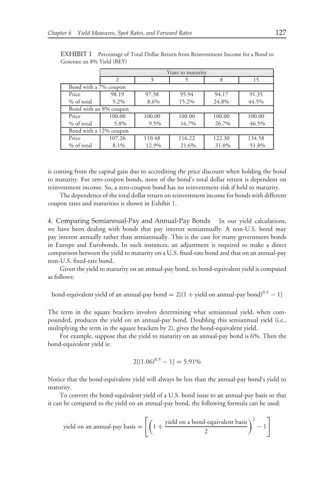
Chapter 6 Yield Measures, Spot Rates, and Forward Rates 127
EXHIBIT 1 Percentage of Total Dollar Return from Reinvestment Income for a Bond toGenerate an 8% Yield (BEY)
Years to maturity2 3 5 8 15
Bond with a 7% couponPrice 98.19 97.38 95.94 94.17 91.35% of total 5.2% 8.6% 15.2% 24.8% 44.5%Bond with an 8% couponPrice 100.00 100.00 100.00 100.00 100.00% of total 5.8% 9.5% 16.7% 26.7% 46.5%Bond with a 12% couponPrice 107.26 110.48 116.22 122.30 134.58% of total 8.1% 12.9% 21.6% 31.0% 51.8%
is coming from the capital gain due to accrediting the price discount when holding the bondto maturity. For zero-coupon bonds, none of the bond’s total dollar return is dependent onreinvestment income. So, a zero-coupon bond has no reinvestment risk if held to maturity.
The dependence of the total dollar return on reinvestment income for bonds with differentcoupon rates and maturities is shown in Exhibit 1.
4. Comparing Semiannual-Pay and Annual-Pay Bonds In our yield calculations,we have been dealing with bonds that pay interest semiannually. A non-U.S. bond maypay interest annually rather than semiannually. This is the case for many government bondsin Europe and Eurobonds. In such instances, an adjustment is required to make a directcomparison between the yield to maturity on a U.S. fixed-rate bond and that on an annual-paynon-U.S. fixed-rate bond.
Given the yield to maturity on an annual-pay bond, its bond-equivalent yield is computedas follows:
bond-equivalent yield of an annual-pay bond = 2[(1 + yield on annual-pay bond)0.5 − 1]
The term in the square brackets involves determining what semiannual yield, when com-pounded, produces the yield on an annual-pay bond. Doubling this semiannual yield (i.e.,multiplying the term in the square brackets by 2), gives the bond-equivalent yield.
For example, suppose that the yield to maturity on an annual-pay bond is 6%. Then thebond-equivalent yield is:
2[(1.06)0.5 − 1] = 5.91%
Notice that the bond-equivalent yield will always be less than the annual-pay bond’s yield tomaturity.
To convert the bond-equivalent yield of a U.S. bond issue to an annual-pay basis so thatit can be compared to the yield on an annual-pay bond, the following formula can be used:
yield on an annual-pay basis =[(
1 + yield on a bond-equivalent basis
2
)2
− 1
]
128 Fixed Income Analysis
By dividing the yield on a bond-equivalent basis by 2 in the above expression, the semiannualyield is computed. The semiannual yield is then compounded to get the yield on an annual-paybasis.
For example, suppose that the yield of a U.S. bond issue quoted on a bond-equivalentbasis is 6%. The yield to maturity on an annual-pay basis would be:
[(1.03)2 − 1] = 6.09%
The yield on an annual-pay basis is always greater than the yield on a bond-equivalent basisbecause of compounding.
C. Yield to Call
When a bond is callable, the practice has been to calculate a yield to call as well as a yieldto maturity. A callable bond may have a call schedule.4 The yield to call assumes the issuerwill call a bond on some assumed call date and that the call price is the price specified in thecall schedule. Typically, investors calculate a yield to first call or yield to next call, a yield tofirst par call, and a yield to refunding. The yield to first call is computed for an issue that isnot currently callable, while the yield to next call is computed for an issue that is currentlycallable.
Yield to refunding is used when bonds are currently callable but have some restrictionson the source of funds used to buy back the debt when a call is exercised. Namely, if a debtissue contains some refunding protection, bonds cannot be called for a certain period of timewith the proceeds of other debt issues sold at a lower cost of money. As a result, the bondholderis afforded some protection if interest rates decline and the issuer can obtain lower-cost fundsto pay off the debt. It should be stressed that the bonds can be called with funds derived fromother sources (e.g., cash on hand) during the refunded-protected period. The refunding dateis the first date the bond can be called using lower-cost debt.
The procedure for calculating any yield to call measure is the same as for any yieldto maturity calculation: determine the interest rate that will make the present value of theexpected cash flows equal to the price plus accrued interest. In the case of yield to first call,the expected cash flows are the coupon payments to the first call date and the call price. Forthe yield to first par call, the expected cash flows are the coupon payments to the first dateat which the issuer can call the bond at par and the par value. For the yield to refunding, theexpected cash flows are the coupon payments to the first refunding date and the call price atthe first refunding date.
To illustrate the computation, consider a 7% 8-year bond with a maturity value of $100selling for $106.36. Suppose that the first call date is three years from now and the call priceis $103. The cash flows for this bond if it is called in three years are (1) 6 coupon payments of$3.50 every six months and (2) $103 in six 6-month periods from now.
The present value for several semiannual interest rates is shown in Exhibit 2. Since asemiannual interest rate of 2.8% makes the present value of the cash flows equal to the price,2.8% is the yield to first call. Therefore, the yield to first call on a bond-equivalent basisis 5.6%.
4A call schedule shows the call price that the issuer must pay based on the date when the issue is called.An example of a call schedule is provided in Chapter 1.
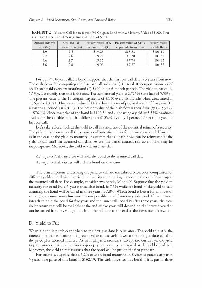
Chapter 6 Yield Measures, Spot Rates, and Forward Rates 129
EXHIBIT 2 Yield to Call for an 8-year 7% Coupon Bond with a Maturity Value of $100. FirstCall Date Is the End of Year 3, and Call Price of $103.
Annual interest Semiannual Present value of 6 Present value of $103 Present valuerate (%) interest rate (%) payments of $3.5 6 periods from now of cash flows
5.0 2.5 $19.28 $88.82 $108.105.2 2.6 19.21 88.30 107.515.4 2.7 19.15 87.78 106.935.6 2.8 19.09 87.27 106.36
For our 7% 8-year callable bond, suppose that the first par call date is 5 years from now.The cash flows for computing the first par call are then: (1) a total 10 coupon payments of$3.50 each paid every six months and (2) $100 in ten 6-month periods. The yield to par call is5.53%. Let’s verify that this is the case. The semiannual yield is 2.765% (one half of 5.53%).The present value of the 10 coupon payments of $3.50 every six months when discounted at2.765% is $30.22. The present value of $100 (the call price of par) at the end of five years (10semiannual periods) is $76.13. The present value of the cash flow is then $106.35 (= $30.22+ $76.13). Since the price of the bond is $106.36 and since using a yield of 5.53% producesa value for this callable bond that differs from $106.36 by only 1 penny, 5.53% is the yield tofirst par call.
Let’s take a closer look at the yield to call as a measure of the potential return of a security.The yield to call considers all three sources of potential return from owning a bond. However,as in the case of the yield to maturity, it assumes that all cash flows can be reinvested at theyield to call until the assumed call date. As we just demonstrated, this assumption may beinappropriate. Moreover, the yield to call assumes that
Assumption 1: the investor will hold the bond to the assumed call date
Assumption 2: the issuer will call the bond on that date
These assumptions underlying the yield to call are unrealistic. Moreover, comparison ofdifferent yields to call with the yield to maturity are meaningless because the cash flows stop atthe assumed call date. For example, consider two bonds, M and N. Suppose that the yield tomaturity for bond M, a 5-year noncallable bond, is 7.5% while for bond N the yield to call,assuming the bond will be called in three years, is 7.8%. Which bond is better for an investorwith a 5-year investment horizon? It’s not possible to tell from the yields cited. If the investorintends to hold the bond for five years and the issuer calls bond N after three years, the totaldollar return that will be available at the end of five years will depend on the interest rate thatcan be earned from investing funds from the call date to the end of the investment horizon.
D. Yield to Put
When a bond is putable, the yield to the first put date is calculated. The yield to put is theinterest rate that will make the present value of the cash flows to the first put date equal tothe price plus accrued interest. As with all yield measures (except the current yield), yieldto put assumes that any interim coupon payments can be reinvested at the yield calculated.Moreover, the yield to put assumes that the bond will be put on the first put date.
For example, suppose that a 6.2% coupon bond maturing in 8 years is putable at par in3 years. The price of this bond is $102.19. The cash flows for this bond if it is put in three
130 Fixed Income Analysis
years are: (1) a total of 6 coupon payments of $3.10 each paid every six months and (2) the$100 put price in six 6-month periods from now. The semiannual interest rate that will makethe present value of the cash flows equal to the price of $102.19 is 2.7%. Therefore, 2.7% isthe semiannual yield to put and 5.4% is the yield to put on a bond equivalent basis.
E. Yield to Worst
A yield can be calculated for every possible call date and put date. In addition, a yield tomaturity can be calculated. The lowest of all these possible yields is called the yield to worst.For example, suppose that there are only four possible call dates for a callable bond, that theyield to call assuming each possible call date is 6%, 6.2%, 5.8%, and 5.7%, and that the yieldto maturity is 7.5%. Then the yield to worst is the minimum of these yields, 5.7% in ourexample.
The yield to worst measure holds little meaning as a measure of potential return. Itsupposedly states that this is the worst possible yield that the investor will realize. However,as we have noted about any yield measure, it does not identify the potential return over someinvestment horizon. Moreover, the yield to worst does not recognize that each yield calculationused in determining the yield to worst has different exposures to reinvestment risk.
F. Cash Flow Yield
Mortgage-backed securities and asset-backed securities are backed by a pool of loans orreceivables. The cash flows for these securities include principal payment as well as interest.The complication that arises is that the individual borrowers whose loans make up the pooltypically can prepay their loan in whole or in part prior to the scheduled principal paymentdates. Because of principal prepayments, in order to project cash flows it is necessary to makean assumption about the rate at which principal prepayments will occur. This rate is called theprepayment rate or prepayment speed.
Given cash flows based on an assumed prepayment rate, a yield can be calculated. Theyield is the interest rate that will make the present value of the projected cash flows equal tothe price plus accrued interest. The yield calculated is commonly referred to as a cash flowyield.5
1. Bond-Equivalent Yield Typically, the cash flows for mortgage-backed and asset-backed securities are monthly. Therefore the interest rate that will make the present value ofprojected principal and interest payments equal to the market price plus accrued interest is amonthly rate. The monthly yield is then annualized as follows.
First, the semiannual effective yield is computed from the monthly yield by compoundingit for six months as follows:
effective semiannual yield = (1 + monthly yield)6 − 1
5Some firms such as Prudential Securities refer to this yield as yield to maturity rather than cash flowyield.
Chapter 6 Yield Measures, Spot Rates, and Forward Rates 131
Next, the effective semiannual yield is doubled to get the annual cash flow yield on abond-equivalent basis. That is,
cash flow yield = 2 × effective semiannual yield
= 2[(1 + monthly yield)6 − 1]
For example, if the monthly yield is 0.5%, then:
cash flow yield on a bond-equivalent basis = 2[(1.005)6 − 1] = 6.08%
The calculation of the cash flow yield may seem strange because it first requires thecomputing of an effective semiannual yield given the monthly yield and then doubling. Thisis simply a market convention. Of course, the student of the bond market can always askthe same two questions as with the yield to maturity: Why it is done? Isn’t it better to justcompound the monthly yield to get an effective annual yield? The answers are the same asgiven earlier for the yield to maturity. Moreover, as we will see next, this is the least of ourproblems in using a cash flow yield measure for an asset-backed and mortgage-backed security.
2. Limitations of Cash Flow Yield As we have noted, the yield to maturity has twoshortcomings as a measure of a bond’s potential return: (1) it is assumed that the couponpayments can be reinvested at a rate equal to the yield to maturity and (2) it is assumed thatthe bond is held to maturity. These shortcomings are equally present in application of thecash flow yield measure: (1) the projected cash flows are assumed to be reinvested at the cashflow yield and (2) the mortgage-backed or asset-backed security is assumed to be held untilthe final payoff of all the loans, based on some prepayment assumption. The significance ofreinvestment risk, the risk that the cash flows will be reinvested at a rate less than the cash flowyield, is particularly important for mortgage-backed and asset-backed securities since paymentsare typically monthly and include principal payments (scheduled and prepaid), and interest.Moreover, the cash flow yield is dependent on realizing of the projected cash flows accordingto some prepayment rate. If actual prepayments differ significantly from the prepayment rateassumed, the cash flow yield will not be realized.
G. Spread/Margin Measures for Floating-Rate Securities
The coupon rate for a floating-rate security (or floater) changes periodically according to areference rate (such as LIBOR or a Treasury rate). Since the future value for the referencerate is unknown, it is not possible to determine the cash flows. This means that a yield tomaturity cannot be calculated. Instead, ‘‘margin’’ measures are computed. Margin is simplysome spread above the floater’s reference rate.
Several spread or margin measures are routinely used to evaluate floaters. Two marginmeasures commonly used are spread for life and discount margin.6
6For a discussion of other traditional measures, see Chapter 3 in Frank J. Fabozzi and Steven V. Mann,Floating Rate Securities (New Hope, PA; Frank J. Fabozzi Associates, 2000).

132 Fixed Income Analysis
1. Spread for Life When a floater is selling at a premium/discount to par, investorsconsider the premium or discount as an additional source of dollar return. Spread for life(also called simple margin) is a measure of potential return that accounts for the accretion(amortization) of the discount (premium) as well as the constant quoted margin over thesecurity’s remaining life. Spread for life (in basis points) is calculated using the followingformula:
Spread for life =[
100(100 − Price)
Maturity+ Quoted margin
]×
(100
Price
)
wherePrice = market price per $100 of par value
Maturity = number of years to maturityQuoted margin = quoted margin in the coupon reset formula measured in basis points
For example, suppose that a floater with a quoted margin of 80 basis points is selling for99.3098 and matures in 6 years. Then,
Price = 99.3098
Maturity = 6
Quoted margin = 80
Spread for life =[
100(100 − 99.3098)
6+ 80
]×
(100
99.3098
)
= 92.14 basis points
The limitations of the spread for life are that it considers only the accretion/amortizationof the discount/premium over the floater’s remaining term to maturity and does not considerthe level of the coupon rate or the time value of money.
2. Discount Margin Discount margin estimates the average margin over the referencerate that the investor can expect to earn over the life of the security. The procedure forcalculating the discount margin is as follows:
Step 1. Determine the cash flows assuming that the reference rate does not change overthe life of the security.
Step 2. Select a margin.
Step 3. Discount the cash flows found in Step 1 by the current value of the reference rateplus the margin selected in Step 2.
Step 4. Compare the present value of the cash flows as calculated in Step 3 to the priceplus accrued interest. If the present value is equal to the security’s price plus accruedinterest, the discount margin is the margin assumed in Step 2. If the present valueis not equal to the security’s price plus accrued interest, go back to Step 2 and try adifferent margin.
For a security selling at par, the discount margin is simply the quoted margin in thecoupon reset formula.

Chapter 6 Yield Measures, Spot Rates, and Forward Rates 133
To illustrate the calculation, suppose that the coupon reset formula for a 6-year floating-rate security selling for $99.3098 is 6-month LIBOR plus 80 basis points. The coupon rate isreset every 6 months. Assume that the current value for the reference rate is 10%.
Exhibit 3 shows the calculation of the discount margin for this security. The secondcolumn shows the current value for 6-month LIBOR. The third column sets forth the cashflows for the security. The cash flow for the first 11 periods is equal to one-half the current6-month LIBOR (5%) plus the semiannual quoted margin of 40 basis points multiplied by$100. At the maturity date (i.e., period 12), the cash flow is $5.4 plus the maturity value of$100. The column headings of the last five columns show the assumed margin. The rowsbelow the assumed margin show the present value of each cash flow. The last row gives thetotal present value of the cash flows.
For the five assumed margins, the present value is equal to the price of the floating-ratesecurity ($99.3098) when the assumed margin is 96 basis points. Therefore, the discountmargin is 96 basis points. Notice that the discount margin is 80 basis points, the same as thequoted margin, when this security is selling at par.
There are two drawbacks of the discount margin as a measure of the potential return frominvesting in a floating-rate security. First, the measure assumes that the reference rate will notchange over the life of the security. Second, if the floating-rate security has a cap or floor, thisis not taken into consideration.
H. Yield on Treasury Bills
Treasury bills are zero-coupon instruments with a maturity of one year or less. The conventionin the Treasury bill market is to calculate a bill’s yield on a discount basis. This yield isdetermined by two variables:
1. the settlement price per $1 of maturity value (denoted by p)2. the number of days to maturity which is calculated as the number of days between the
settlement date and the maturity date (denoted by NSM )
The yield on a discount basis (denoted by d ) is calculated as follows:
d = (1 − p)
(360
NSM
)
We will use two actual Treasury bills to illustrate the calculation of the yield on a discountbasis assuming a settlement date in both cases of 8/6/97. The first bill has a maturity date of1/8/98 and a price of 0.97769722. For this bill, the number of days from the settlement dateto the maturity date, NSM , is 155. Therefore, the yield on a discount basis is
d = (1 − 0.97769722)
(360
155
)= 5.18%
For our second bill, the maturity date is 7/23/98 and the price is 0.9490075. Assuming asettlement date of 8/6/97, the number of days from the settlement date to the maturity dateis 351. The yield on a discount basis for this bill is
d = (1 − 0.9490075)
(360
351
)= 5.23%
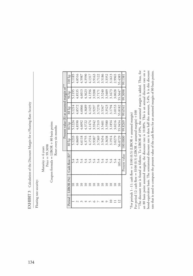
EX
HIB
IT3
Cal
cula
tion
ofth
eD
isco
untM
argi
nfo
ra
Floa
ting
-Rat
eSe
curi
ty
Floa
ting
rate
secu
rity
:
Mat
urit
y=
6ye
ars
Pric
e=
99.3
098
Cou
pon
form
ula
=LI
BO
R+
80ba
sis
poin
tsR
eset
ever
ysi
xm
onth
s
Pres
entv
alue
($)
atas
sum
edm
argi
nof
∗∗
Peri
odLI
BO
R(%
)C
ash
flow
($)∗
80bp
84bp
88bp
96bp
100
bp1
105.
45.
1233
5.12
245.
1214
5.11
955.
1185
210
5.4
4.86
094.
8590
4.85
724.
8535
4.85
163
105.
44.
6118
4.60
924.
6066
4.60
134.
5987
410
5.4
4.37
554.
3722
4.36
894.
3623
4.35
905
105.
44.
1514
4.14
744.
1435
4.13
564.
1317
610
5.4
3.93
873.
9342
3.92
973.
9208
3.91
637
105.
43.
7369
3.73
193.
7270
3.71
713.
7122
810
5.4
3.54
543.
5401
3.53
473.
5240
3.51
869
105.
43.
3638
3.35
803.
3523
3.34
093.
3352
1010
5.4
3.19
143.
1854
3.17
943.
1673
3.16
1311
105.
43.
0279
3.02
163.
0153
3.00
282.
9965
1210
105.
456
.072
955
.945
455
.818
255
.564
755
.438
5Pr
esen
tva
lue
100.
0000
99.8
269
99.6
541
99.3
098
99.1
381
∗ For
peri
ods
1–
11:c
ash
flow
=$1
00(0
.5)
(LIB
OR
+as
sum
edm
argi
n)Fo
rpe
riod
12:c
ash
flow
=$1
00(0
.5)
(LIB
OR
+as
sum
edm
argi
n)+1
00∗∗
The
disc
ount
rate
isfo
und
asfo
llow
s.T
oLI
BO
Rof
10%
,th
eas
sum
edm
argi
nis
adde
d.T
hus,
for
an80
basi
spo
int
assu
med
mar
gin,
the
disc
ount
rate
is10
.80%
.T
his
isan
annu
aldi
scou
ntra
teon
abo
nd-e
quiv
alen
tba
sis.
The
sem
iann
uald
isco
unt
rate
isth
enha
lfth
isam
ount
,5.4
%.I
tis
this
disc
ount
rate
that
isus
edto
com
pute
the
pres
entv
alue
ofth
eca
shflo
ws
for
anas
sum
edm
argi
nof
80ba
sis
poin
ts.
134
Chapter 6 Yield Measures, Spot Rates, and Forward Rates 135
Given the yield on a discount basis, the price of a bill (per $1 of maturity value) iscomputed as follows:
p = 1 − d (NSM/360)
For the 155-day bill selling for a yield on a discount basis of 5.18%, the price per $1 ofmaturity value is
p = 1 − 0.0518 (155/360) = 0.97769722
For the 351-day bill selling for a yield on a discount basis of 5.23%, the price per $1 ofmaturity value is
p = 1 − 0.0523 (351/360) = 0.9490075
The quoted yield on a discount basis is not a meaningful measure of the return fromholding a Treasury bill for two reasons. First, the measure is based on a maturity valueinvestment rather than on the actual dollar amount invested. Second, the yield is annualizedaccording to a 360-day year rather than a 365-day year, making it difficult to compare yieldson Treasury bills with Treasury notes and bonds which pay interest based on the actualnumber of days in a year. The use of 360 days for a year is a convention for money marketinstruments. Despite its shortcomings as a measure of return, this is the method dealers haveadopted to quote Treasury bills.
Market participants recognize this limitation of yield on a discount basis and consequentlymake adjustments to make the yield quoted on a Treasury bill comparable to that on a Treasurycoupon security. For investors who want to compare the yield on Treasury bills to that ofother money market instruments (i.e., debt obligations with a maturity that does not exceedone year), there is a formula to convert the yield on a discount basis to that of a money marketyield. The key point is that while the convention is to quote the yield on a Treasury bill interms of a yield on a discount basis, no one uses that yield measure other than to compute theprice given the quoted yield.
IV. THEORETICAL SPOT RATES
The theoretical spot rates for Treasury securities represent the appropriate set of interest ratesthat should be used to value default-free cash flows. A default-free theoretical spot rate curvecan be constructed from the observed Treasury yield curve. There are several approaches thatare used in practice. The approach that we describe below for creating a theoretical spotrate curve is called bootstrapping. (The bootstrapping method described here is also used inconstructing a theoretical spot rate curve for LIBOR.)
A. Bootstrapping
Bootstrapping begins with the yield for the on-the-run Treasury issues because there is nocredit risk and no liquidity risk. In practice, however, there is a problem of obtaining a sufficientnumber of data points for constructing the U.S. Treasury yield curve. In the United States, theU.S. Department of the Treasury currently issues 3-month and 6-month Treasury bills and
136 Fixed Income Analysis
2-year, 5-year, and 10-year Treasury notes. Treasury bills are zero-coupon instruments andTreasury notes are coupon-paying instruments. Hence, there are not many data points fromwhich to construct a Treasury yield curve, particularly after two years. At one time, the U.S.Treasury issued 30-year Treasury bonds. Since the Treasury no longer issues 30-year bonds,market participants currently use the last issued Treasury bond (which has a maturity less than30 years) to estimate the 30-year yield. The 2-year, 5-year, and 10-year Treasury notes and anestimate of the 30-year Treasury bond are used to construct the Treasury yield curve.
On September 5, 2003, Lehman Brothers reported the following values for these fouryields:
2 year 1.71%
5 year 3.25%
10 year 4.35%
30 year 5.21%
To fill in the yield for the 25 missing whole year maturities (3 year, 4 year, 6 year,7 year, 8 year, 9 year, 11 year, and so on to the 29-year maturity), the yield for the 25 wholeyear maturities are interpolated from the yield on the surrounding maturities. The simplestinterpolation, and the one most commonly used in practice, is simple linear interpolation.
For example, suppose that we want to fill in the gap for each one year of maturity.To determine the amount to add to the on-the-run Treasury yield as we go from the lowermaturity to the higher maturity, the following formula is used:
Yield at higher maturity − Yield at lower maturity
Number of years between two observed maturity points
The estimated on-the-run yield for all intermediate whole-year maturities is found by addingthe amount computed from the above formula to the yield at the lower maturity.
For example, using the September 5, 2003 yields, the 5-year yield of 3.25% and the10-year yield of 4.35% are used to obtain the interpolated 6-year, 7-year, 8-year, and 9-yearyields by first calculating:
4.35% − 3.25%
5= 0.22%
Then,
interpolated 6-year yield = 3.25% + 0.22% = 3.47%
interpolated 7-year yield = 3.47% + 0.22% = 3.69%
interpolated 8-year yield = 3.69% + 0.22% = 3.91%
interpolated 9-year yield = 3.91% + 0.22% = 4.13%
Thus, when market participants talk about a yield on the Treasury yield curve that is notone of the on-the-run maturities—for example, the 8-year yield—it is only an approximation.Notice that there is a large gap between maturity points. This may result in misleading yields
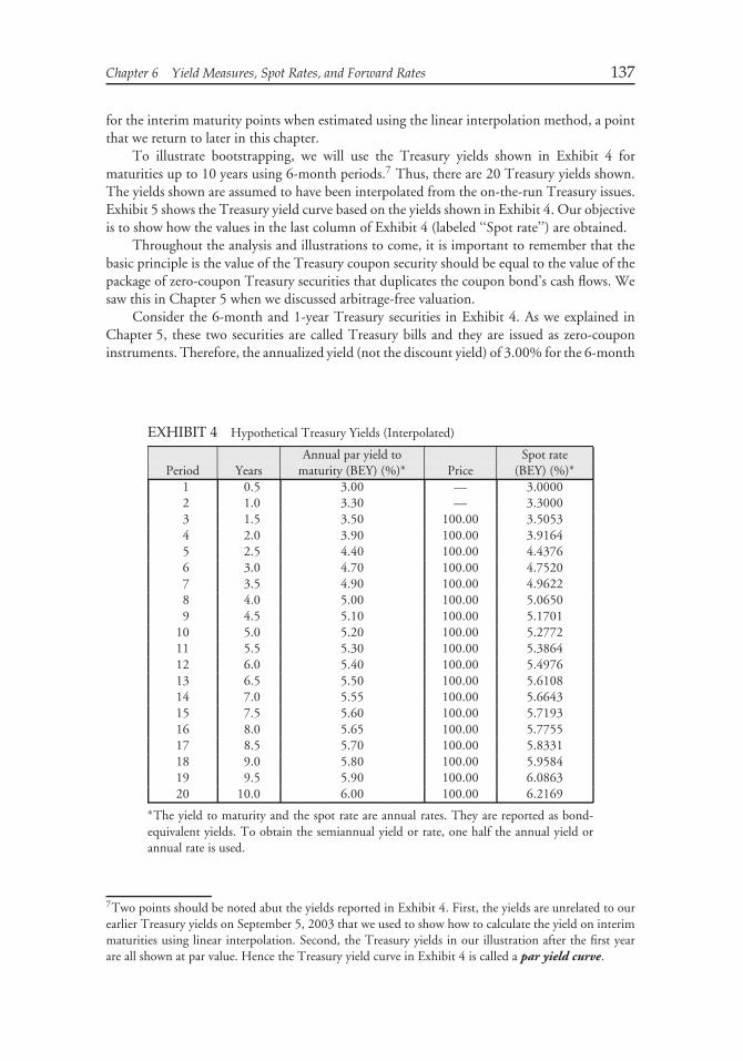
Chapter 6 Yield Measures, Spot Rates, and Forward Rates 137
for the interim maturity points when estimated using the linear interpolation method, a pointthat we return to later in this chapter.
To illustrate bootstrapping, we will use the Treasury yields shown in Exhibit 4 formaturities up to 10 years using 6-month periods.7 Thus, there are 20 Treasury yields shown.The yields shown are assumed to have been interpolated from the on-the-run Treasury issues.Exhibit 5 shows the Treasury yield curve based on the yields shown in Exhibit 4. Our objectiveis to show how the values in the last column of Exhibit 4 (labeled ‘‘Spot rate’’) are obtained.
Throughout the analysis and illustrations to come, it is important to remember that thebasic principle is the value of the Treasury coupon security should be equal to the value of thepackage of zero-coupon Treasury securities that duplicates the coupon bond’s cash flows. Wesaw this in Chapter 5 when we discussed arbitrage-free valuation.
Consider the 6-month and 1-year Treasury securities in Exhibit 4. As we explained inChapter 5, these two securities are called Treasury bills and they are issued as zero-couponinstruments. Therefore, the annualized yield (not the discount yield) of 3.00% for the 6-month
EXHIBIT 4 Hypothetical Treasury Yields (Interpolated)
Annual par yield to Spot ratePeriod Years maturity (BEY) (%)∗ Price (BEY) (%)∗
1 0.5 3.00 — 3.00002 1.0 3.30 — 3.30003 1.5 3.50 100.00 3.50534 2.0 3.90 100.00 3.91645 2.5 4.40 100.00 4.43766 3.0 4.70 100.00 4.75207 3.5 4.90 100.00 4.96228 4.0 5.00 100.00 5.06509 4.5 5.10 100.00 5.1701
10 5.0 5.20 100.00 5.277211 5.5 5.30 100.00 5.386412 6.0 5.40 100.00 5.497613 6.5 5.50 100.00 5.610814 7.0 5.55 100.00 5.664315 7.5 5.60 100.00 5.719316 8.0 5.65 100.00 5.775517 8.5 5.70 100.00 5.833118 9.0 5.80 100.00 5.958419 9.5 5.90 100.00 6.086320 10.0 6.00 100.00 6.2169
∗The yield to maturity and the spot rate are annual rates. They are reported as bond-equivalent yields. To obtain the semiannual yield or rate, one half the annual yield orannual rate is used.
7Two points should be noted abut the yields reported in Exhibit 4. First, the yields are unrelated to ourearlier Treasury yields on September 5, 2003 that we used to show how to calculate the yield on interimmaturities using linear interpolation. Second, the Treasury yields in our illustration after the first yearare all shown at par value. Hence the Treasury yield curve in Exhibit 4 is called a par yield curve.
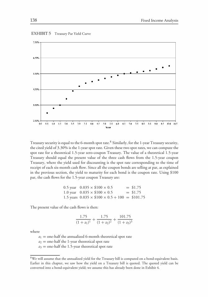
138 Fixed Income Analysis
EXHIBIT 5 Treasury Par Yield Curve
Treasury security is equal to the 6-month spot rate.8 Similarly, for the 1-year Treasury security,the cited yield of 3.30% is the 1-year spot rate. Given these two spot rates, we can compute thespot rate for a theoretical 1.5-year zero-coupon Treasury. The value of a theoretical 1.5-yearTreasury should equal the present value of the three cash flows from the 1.5-year couponTreasury, where the yield used for discounting is the spot rate corresponding to the time ofreceipt of each six-month cash flow. Since all the coupon bonds are selling at par, as explainedin the previous section, the yield to maturity for each bond is the coupon rate. Using $100par, the cash flows for the 1.5-year coupon Treasury are:
0.5 year 0.035 × $100 × 0.5 = $1.751.0 year 0.035 × $100 × 0.5 = $1.751.5 years 0.035 × $100 × 0.5 + 100 = $101.75
The present value of the cash flows is then:
1.75
(1 + z1)1+ 1.75
(1 + z2)2+ 101.75
(1 + z3)3
wherez1 = one-half the annualized 6-month theoretical spot ratez2 = one-half the 1-year theoretical spot ratez3 = one-half the 1.5-year theoretical spot rate
8We will assume that the annualized yield for the Treasury bill is computed on a bond-equivalent basis.Earlier in this chapter, we saw how the yield on a Treasury bill is quoted. The quoted yield can beconverted into a bond-equivalent yield; we assume this has already been done in Exhibit 4.
Chapter 6 Yield Measures, Spot Rates, and Forward Rates 139
Since the 6-month spot rate is 3% and the 1-year spot rate is 3.30%, we know that:
z1 = 0.0150 and z2 = 0.0165
We can compute the present value of the 1.5-year coupon Treasury security as:
1.75
(1 + z1)1+ 1.75
(1 + z2)2+ 101.75
(1 + z3)3= 1.75
(1.015)1+ 1.75
(1.0165)2+ 101.75
(1 + z3)3
Since the price of the 1.5-year coupon Treasury security is par value (see Exhibit 4), thefollowing relationship must hold:9
1.75
(1.015)1+ 1.75
(1.0165)2+ 101.75
(1 + z3)3= 100
We can solve for the theoretical 1.5-year spot rate as follows:
1.7241 + 1.6936 + 101.75
(1 + z3)3= 100
101.75
(1 + z3)3= 96.5822
(1 + z3)3 = 101.75
96.5822
z3 = 0.0175265 = 1.7527%
Doubling this yield, we obtain the bond-equivalent yield of 3.5053%, which is the theoretical1.5-year spot rate. That rate is the rate that the market would apply to a 1.5-year zero-couponTreasury security if, in fact, such a security existed. In other words, all Treasury cash flows tobe received 1.5 years from now should be valued (i.e., discounted) at 3.5053%.
Given the theoretical 1.5-year spot rate, we can obtain the theoretical 2-year spot rate.The cash flows for the 2-year coupon Treasury in Exhibit 3 are:
0.5 year 0.039 × $100 × 0.5 = $1.951.0 year 0.039 × $100 × 0.5 = $1.951.5 years 0.039 × $100 × 0.5 = $1.952.0 years 0.039 × $100 × 0.5 + 100 = $101.95
The present value of the cash flows is then:
1.95
(1 + z1)1+ 1.95
(1 + z2)2+ 1.95
(1 + z3)3+ 101.95
(1 + z4)4
where z4 = one-half the 2-year theoretical spot rate.
9If we had not been working with a par yield curve, the equation would have been set equal to whateverthe market price for the 1.5-year issue is.
140 Fixed Income Analysis
Since the 6-month spot rate, 1-year spot rate, and 1.5-year spot rate are 3.00%, 3.30%,and 3.5053%, respectively, then:
z1 = 0.0150 z2 = 0.0165 z3 = 0.017527
Therefore, the present value of the 2-year coupon Treasury security is:
1.95
(1.0150)1+ 1.95
(1.0165)2+ 1.95
(1.07527)3+ 101.95
(1 + z4)4
Since the price of the 2-year coupon Treasury security is par, the following relationship musthold:
1.95
(1.0150)1+ 1.95
(1.0165)2+ 1.95
(1.017527)3+ 101.95
(1 + z4)4= 100
We can solve for the theoretical 2-year spot rate as follows:
101.95
(1 + z4)4= 94.3407
(1 + z4)4 = 101.95
94.3407
z4 = 0.019582 = 1.9582%
Doubling this yield, we obtain the theoretical 2-year spot rate bond-equivalent yield of3.9164%.
One can follow this approach sequentially to derive the theoretical 2.5-year spot ratefrom the calculated values of z1, z2, z3, and z4 (the 6-month-, 1-year-, 1.5-year-, and 2-yearrates), and the price and coupon of the 2.5-year bond in Exhibit 4. Further, one could derivetheoretical spot rates for the remaining 15 half-yearly rates.
The spot rates thus obtained are shown in the last column of Exhibit 4. They representthe term structure of default-free spot rate for maturities up to 10 years at the particular timeto which the bond price quotations refer. In fact, it is the default-free spot rates shown inExhibit 4 that were used in our illustrations in the previous chapter.
Exhibit 6 shows a plot of the spot rates. The graph is called the theoretical spot ratecurve. Also shown on Exhibit 6 is a plot of the par yield curve from Exhibit 5. Notice thatthe theoretical spot rate curve lies above the par yield curve. This will always be the case whenthe par yield curve is upward sloping. When the par yield curve is downward sloping, thetheoretical spot rate curve will lie below the par yield curve.
B. Yield Spread Measures Relative to a Spot Rate Curve
Traditional analysis of the yield spread for a non-Treasury bond involves calculating thedifference between the bond’s yield and the yield to maturity of a benchmark Treasury couponsecurity. The latter is obtained from the Treasury yield curve. For example, consider thefollowing 10-year bonds:
Issue Coupon Price Yield to maturityTreasury 6% 100.00 6.00%Non-Treasury 8% 104.19 7.40%
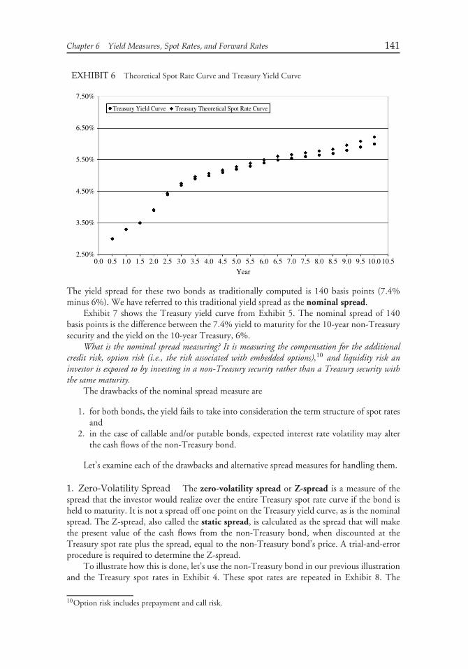
Chapter 6 Yield Measures, Spot Rates, and Forward Rates 141
EXHIBIT 6 Theoretical Spot Rate Curve and Treasury Yield Curve
7.50%
6.50%
5.50%
4.50%
3.50%
2.50%0.0 0.5 1.0 1.5 2.0 2.5 3.0 3.5 4.0 4.5 5.0 5.5 6.0 6.5 7.0 7.5 8.0 8.5 9.0 9.5 10.0 10.5
Year
Treasury Yield Curve Treasury Theoretical Spot Rate Curve
The yield spread for these two bonds as traditionally computed is 140 basis points (7.4%minus 6%). We have referred to this traditional yield spread as the nominal spread.
Exhibit 7 shows the Treasury yield curve from Exhibit 5. The nominal spread of 140basis points is the difference between the 7.4% yield to maturity for the 10-year non-Treasurysecurity and the yield on the 10-year Treasury, 6%.
What is the nominal spread measuring? It is measuring the compensation for the additionalcredit risk, option risk (i.e., the risk associated with embedded options),10 and liquidity risk aninvestor is exposed to by investing in a non-Treasury security rather than a Treasury security withthe same maturity.
The drawbacks of the nominal spread measure are
1. for both bonds, the yield fails to take into consideration the term structure of spot ratesand
2. in the case of callable and/or putable bonds, expected interest rate volatility may alterthe cash flows of the non-Treasury bond.
Let’s examine each of the drawbacks and alternative spread measures for handling them.
1. Zero-Volatility Spread The zero-volatility spread or Z-spread is a measure of thespread that the investor would realize over the entire Treasury spot rate curve if the bond isheld to maturity. It is not a spread off one point on the Treasury yield curve, as is the nominalspread. The Z-spread, also called the static spread, is calculated as the spread that will makethe present value of the cash flows from the non-Treasury bond, when discounted at theTreasury spot rate plus the spread, equal to the non-Treasury bond’s price. A trial-and-errorprocedure is required to determine the Z-spread.
To illustrate how this is done, let’s use the non-Treasury bond in our previous illustrationand the Treasury spot rates in Exhibit 4. These spot rates are repeated in Exhibit 8. The
10Option risk includes prepayment and call risk.
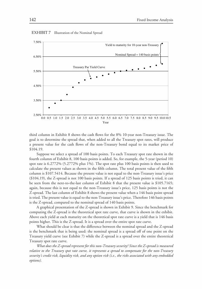
142 Fixed Income Analysis
EXHIBIT 7 Illustration of the Nominal Spread
7.50%
6.50%
5.50%
4.50%
3.50%
2.50%0.0 0.5 1.0 1.5 2.0 2.5 3.0 3.5 4.0 4.5 5.0 5.5 6.0 6.5 7.0 7.5 8.0 8.5 9.0 9.5 10.0 10.5
Year
Treasury Par Yield Curve
Yield to maturity for 10-year non-Treasury
Nominal Spread = 140 basis points
third column in Exhibit 8 shows the cash flows for the 8% 10-year non-Treasury issue. Thegoal is to determine the spread that, when added to all the Treasury spot rates, will producea present value for the cash flows of the non-Treasury bond equal to its market price of$104.19.
Suppose we select a spread of 100 basis points. To each Treasury spot rate shown in thefourth column of Exhibit 8, 100 basis points is added. So, for example, the 5-year (period 10)spot rate is 6.2772% (5.2772% plus 1%). The spot rate plus 100 basis points is then used tocalculate the present values as shown in the fifth column. The total present value of the fifthcolumn is $107.5414. Because the present value is not equal to the non-Treasury issue’s price($104.19), the Z-spread is not 100 basis points. If a spread of 125 basis points is tried, it canbe seen from the next-to-the-last column of Exhibit 8 that the present value is $105.7165;again, because this is not equal to the non-Treasury issue’s price, 125 basis points is not theZ-spread. The last column of Exhibit 8 shows the present value when a 146 basis point spreadis tried. The present value is equal to the non-Treasury issue’s price. Therefore 146 basis pointsis the Z-spread, compared to the nominal spread of 140 basis points.
A graphical presentation of the Z-spread is shown in Exhibit 9. Since the benchmark forcomputing the Z-spread is the theoretical spot rate curve, that curve is shown in the exhibit.Above each yield at each maturity on the theoretical spot rate curve is a yield that is 146 basispoints higher. This is the Z-spread. It is a spread over the entire spot rate curve.
What should be clear is that the difference between the nominal spread and the Z-spreadis the benchmark that is being used: the nominal spread is a spread off of one point on theTreasury yield curve (see Exhibit 7) while the Z-spread is a spread over the entire theoreticalTreasury spot rate curve.
What does the Z-spread represent for this non-Treasury security? Since the Z-spread is measuredrelative to the Treasury spot rate curve, it represents a spread to compensate for the non-Treasurysecurity’s credit risk, liquidity risk, and any option risk (i.e., the risks associated with any embeddedoptions).
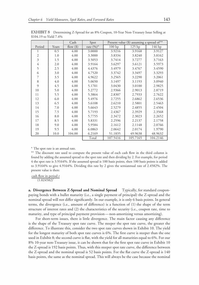
Chapter 6 Yield Measures, Spot Rates, and Forward Rates 143
EXHIBIT 8 Determining Z-Spread for an 8% Coupon, 10-Year Non-Treasury Issue Selling at$104.19 to Yield 7.4%
Cash Spot Present value ($) assuming a spread of ∗∗
Period Years flow ($) rate (%)∗ 100 bp 125 bp 146 bp1 0.5 4.00 3.0000 3.9216 3.9168 3.91272 1.0 4.00 3.3000 3.8334 3.8240 3.81623 1.5 4.00 3.5053 3.7414 3.7277 3.71634 2.0 4.00 3.9164 3.6297 3.6121 3.59735 2.5 4.00 4.4376 3.4979 3.4767 3.45906 3.0 4.00 4.7520 3.3742 3.3497 3.32937 3.5 4.00 4.9622 3.2565 3.2290 3.20618 4.0 4.00 5.0650 3.1497 3.1193 3.09409 4.5 4.00 5.1701 3.0430 3.0100 2.9825
10 5.0 4.00 5.2772 2.9366 2.9013 2.871911 5.5 4.00 5.3864 2.8307 2.7933 2.762212 6.0 4.00 5.4976 2.7255 2.6862 2.653613 6.5 4.00 5.6108 2.6210 2.5801 2.546314 7.0 4.00 5.6643 2.5279 2.4855 2.450415 7.5 4.00 5.7193 2.4367 2.3929 2.356816 8.0 4.00 5.7755 2.3472 2.3023 2.265217 8.5 4.00 5.8331 2.2596 2.2137 2.175818 9.0 4.00 5.9584 2.1612 2.1148 2.076619 9.5 4.00 6.0863 2.0642 2.0174 1.979020 10.0 104.00 6.2169 51.1835 49.9638 48.9632
Total 107.5416 105.7165 104.2146
∗ The spot rate is an annual rate.∗∗ The discount rate used to compute the present value of each cash flow in the third column isfound by adding the assumed spread to the spot rate and then dividing by 2. For example, for period4 the spot rate is 3.9164%. If the assumed spread is 100 basis points, then 100 basis points is addedto 3.9164% to give 4.9164%. Dividing this rate by 2 gives the semiannual rate of 2.4582%. Thepresent value is then:
cash flow in period t(1.024582)t
a. Divergence Between Z-Spread and Nominal Spread Typically, for standard coupon-paying bonds with a bullet maturity (i.e., a single payment of principal) the Z-spread and thenominal spread will not differ significantly. In our example, it is only 6 basis points. In generalterms, the divergence (i.e., amount of difference) is a function of (1) the shape of the termstructure of interest rates and (2) the characteristics of the security (i.e., coupon rate, time tomaturity, and type of principal payment provision—non-amortizing versus amortizing).
For short-term issues, there is little divergence. The main factor causing any differenceis the shape of the Treasury spot rate curve. The steeper the spot rate curve, the greater thedifference. To illustrate this, consider the two spot rate curves shown in Exhibit 10. The yieldfor the longest maturity of both spot rate curves is 6%. The first curve is steeper than the oneused in Exhibit 8; the second curve is flat, with the yield for all maturities equal to 6%. For our8% 10-year non-Treasury issue, it can be shown that for the first spot rate curve in Exhibit 10the Z-spread is 192 basis points. Thus, with this steeper spot rate curve, the difference betweenthe Z-spread and the nominal spread is 52 basis points. For the flat curve the Z-spread is 140basis points, the same as the nominal spread. This will always be the case because the nominal
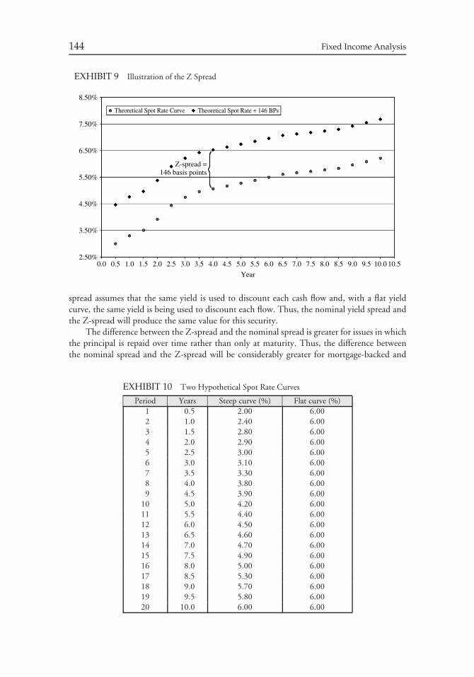
144 Fixed Income Analysis
EXHIBIT 9 Illustration of the Z Spread
8.50%
7.50%
6.50%
5.50%
4.50%
3.50%
2.50%0.0 0.5 1.0 1.5 2.0 2.5 3.0 3.5 4.0 4.5 5.0 5.5 6.0 6.5 7.0 7.5 8.0 8.5 9.0 9.5 10.0 10.5
Year
Theoretical Spot Rate + 146 BPsTheoretical Spot Rate Curve
Z-spread =146 basis points
spread assumes that the same yield is used to discount each cash flow and, with a flat yieldcurve, the same yield is being used to discount each flow. Thus, the nominal yield spread andthe Z-spread will produce the same value for this security.
The difference between the Z-spread and the nominal spread is greater for issues in whichthe principal is repaid over time rather than only at maturity. Thus, the difference betweenthe nominal spread and the Z-spread will be considerably greater for mortgage-backed and
EXHIBIT 10 Two Hypothetical Spot Rate Curves
Period Years Steep curve (%) Flat curve (%)1 0.5 2.00 6.002 1.0 2.40 6.003 1.5 2.80 6.004 2.0 2.90 6.005 2.5 3.00 6.006 3.0 3.10 6.007 3.5 3.30 6.008 4.0 3.80 6.009 4.5 3.90 6.00
10 5.0 4.20 6.0011 5.5 4.40 6.0012 6.0 4.50 6.0013 6.5 4.60 6.0014 7.0 4.70 6.0015 7.5 4.90 6.0016 8.0 5.00 6.0017 8.5 5.30 6.0018 9.0 5.70 6.0019 9.5 5.80 6.0020 10.0 6.00 6.00
Chapter 6 Yield Measures, Spot Rates, and Forward Rates 145
asset-backed securities in a steep yield curve environment. We can see this intuitively if wethink in terms of a 10-year zero-coupon bond and a 10-year amortizing security with equalsemiannual cash flows (that includes interest and principal payment). The Z-spread for thezero-coupon bond will not be affected by the shape of the term structure but the amortizingsecurity will be.
b. Z-Spread Relative to Any Benchmark In the same way that a Z-spread relative to aTreasury spot rate curve can be calculated, a Z-spread to any benchmark spot rate curve canbe calculated. To illustrate, suppose that a hypothetical non-Treasury security with a couponrate of 8% and a 10-year maturity is trading at $105.5423. Assume that the benchmark spotrate curve for this issuer is the one given in Exhibit 10 of the previous chapter. The Z-spreadrelative to that issuer’s benchmark spot rate curve is the spread that must be added to thespot rates shown in the next-to-last column of that exhibit that will make the present valueof the cash flows equal to the market price. In our illustration, the Z-spread relative to thisbenchmark is 40 basis points.
What does the Z-spread mean when the benchmark is not the Treasury spot rate curve(i.e., default-free spot rate curve)? When the Treasury spot rate curve is the benchmark, we saidthat the Z-spread for a non-Treasury issue embodies credit risk, liquidity risk, and any optionrisk. When the benchmark is the spot rate curve for the issuer, the Z-spread is measuring thespread attributable to the liquidity risk of the issue and any option risk.
Thus, when a Z-spread is cited, it must be cited relative to some benchmark spot ratecurve. This is necessary because it indicates the credit and sector risks that are being consideredwhen the Z-spread was calculated. While Z-spreads are typically calculated using Treasurysecurities as the benchmark interest rates, this need not be the case. Vendors of analyticalsystems commonly allow the user to select a benchmark spot rate curve. Moreover, in non-U.S.markets, Treasury securities are typically not the benchmark. The key point is that an investorshould always ask what benchmark was used to compute the Z-spread.
2. Option-Adjusted Spread The Z-spread seeks to measure the spread over a spot ratecurve thus overcoming the first problem of the nominal spread that we cited earlier. Now let’slook at the second shortcoming—failure to take future interest rate volatility into accountwhich could change the cash flows for bonds with embedded options.
a. Valuation Models What investors seek to do is to buy undervalued securities (securitieswhose value is greater than their price). Before they can do this though, they need to knowwhat the security is worth (i.e., a fair price to pay). A valuation model is designed to provideprecisely this. If a model determines the fair price of a share of common stock is $36 and themarket price is currently $24, then the stock is considered to be undervalued. If a bond isselling for less than its fair value, then it too is considered undervalued.
A valuation model need not stop here, however. Market participants find it moreconvenient to think about yield spread than about price differences. A valuation model cantake this difference between the fair price and the market price and convert it into a yieldspread measure. Instead of asking, ‘‘How much is this security undervalued?’’, the model canask, ‘‘How much return will I earn in exchange for taking on these risks?’’
The option-adjusted spread (OAS) was developed as a way of doing just this: taking thedollar difference between the fair price and market price and converting it into a yield spreadmeasure. Thus, the OAS is used to reconcile the fair price (or value) to the market price byfinding a return (spread) that will equate the two (using a trial and error procedure). This is
146 Fixed Income Analysis
somewhat similar to what we did earlier when calculating yield to maturity, yield to call, etc.,only in this case, we are calculating a spread (measured in basis points) rather than a percentagerate of return as we did then.
The OAS is model dependent. That is, the OAS computed depends on the valuation modelused. In particular, OAS models differ considerably in how they forecast interest rate changes,leading to variations in the level of OAS. What are two of these key modeling differences?
• Interest rate volatility is a critical assumption. Specifically, the higher the interest ratevolatility assumed, the lower the OAS. In comparing the OAS of dealer firms, it isimportant to check on the volatility assumption made.
• The OAS is a spread, but what is it a ‘‘spread’’ over? The OAS is a spread over the Treasuryspot rate curve or the issuer’s benchmark used in the analysis. In the model, the spot ratecurve is actually the result of a series of assumptions that allow for changes in interest rates.Again, different models yield different results.
Why is the spread referred to as ‘‘option adjusted’’? Because the security’s embeddedoption can change the cash flows; the value of the security should take this change of cashflow into account. Note that the Z-spread doesn’t do this—it ignores the fact that interestrate changes can affect the cash flows. In essence, it assumes that interest rate volatility is zero.This is why the Z-spread is also referred to as the zero-volatility OAS.
b. Option Cost The implied cost of the option embedded in any security can be obtainedby calculating the difference between the OAS at the assumed interest rate or yield volatilityand the Z-spread. That is, since the Z-spread is just the sum of the OAS and option cost, i.e.,
Z-spread = OAS + option cost
it follows that:
option cost = Z-spread − OAS
The reason that the option cost is measured in this way is as follows. In an environmentin which interest rates are assumed not to change, the investor would earn the Z-spread. Whenfuture interest rates are uncertain, the spread is different because of the embedded option(s);the OAS reflects the spread after adjusting for this option. Therefore, the option cost is thedifference between the spread that would be earned in a static interest rate environment (theZ-spread, or equivalently, the zero-volatility OAS) and the spread after adjusting for the option(the OAS).
For callable bonds and most mortgage-backed and asset-backed securities, the option costis positive. This is because the issuer’s ability to alter the cash flows will result in an OAS that isless than the Z-spread. In the case of a putable bond, the OAS is greater than the Z-spread so thatthe option cost is negative. This occurs because of the investor’s ability to alter the cash flows.
In general, when the option cost is positive, this means that the investor has sold anoption to the issuer or borrower. This is true for callable bonds and most mortgage-backedand asset-backed securities. A negative value for the option cost means that the investor haspurchased an option from the issuer or borrower. A putable bond is an example of this negativeoption cost. There are certain securities in the mortgage-backed securities market that alsohave an option cost that is negative.

Chapter 6 Yield Measures, Spot Rates, and Forward Rates 147
c. Highlighting the Pitfalls of the Nominal Spread We can use the concepts presentedin this chapter to highlight the pitfalls of the nominal spread. First, we can recast therelationship between the option cost, Z-spread, and OAS as follows:
Z-spread = OAS + option cost
Next, recall that the nominal spread and the Z-spread may not diverge significantly.Suppose that the nominal spread is approximately equal to the Z-spread. Then, we cansubstitute nominal spread for Z-spread in the previous relationship giving:
nominal spread ≈ OAS + option cost
This relationship tells us that a high nominal spread could be hiding a high option cost.The option cost represents the portion of the spread that the investor has given to the issuer orborrower. Thus, while the nominal spread for a security that can be called or prepaid mightbe, say 200 basis points, the option cost may be 190 and the OAS only 10 basis points. But,an investor is only compensated for the OAS. An investor that relies on the nominal spreadmay not be adequately compensated for taking on the option risk associated with a securitywith an embedded option.
3. Summary of Spread Measures We have just described three spread measures:
• nominal spread• zero-volatility spread• option-adjusted spread
To understand different spread measures we ask two questions:
1. What is the benchmark for computing the spread? That is, what is the spread measuredrelative to?
2. What is the spread measuring?
The table below provides a summary showing for each of the three spread measures thebenchmark and the risks for which the spread is compensating.
Spread measure Benchmark Reflects compensation for:Nominal Treasury yield curve Credit risk, option risk, liquidity riskZero-volatility Treasury spot rate curve Credit risk, option risk, liquidity riskOption-adjusted Treasury spot rate curve Credit risk, liquidity risk
V. FORWARD RATES
We have seen how a default-free theoretical spot rate curve can be extrapolated fromthe Treasury yield curve. Additional information useful to market participants can beextrapolated from the default-free theoretical spot rate curve: forward rates. Under certainassumptions described later, these rates can be viewed as the market’s consensus of futureinterest rates.
148 Fixed Income Analysis
Examples of forward rates that can be calculated from the default-free theoretical spotrate curve are the:
• 6-month forward rate six months from now• 6-month forward rate three years from now• 1-year forward rate one year from now• 3-year forward rate two years from now• 5-year forward rates three years from now
Since the forward rates are implicitly extrapolated from the default-free theoretical spotrate curve, these rates are sometimes referred to as implied forward rates. We begin byshowing how to compute the 6-month forward rates. Then we explain how to compute anyforward rate.
While we continue to use the Treasury yield curve in our illustrations, as noted earlier,a LIBOR spot rate curve can also be constructed using the bootstrapping methodology andforward rates for LIBOR can be obtained in the same manner as described below.
A. Deriving 6-Month Forward Rates
To illustrate the process of extrapolating 6-month forward rates, we will use the yield curveand corresponding spot rate curve from Exhibit 4. We will use a very simple arbitrage principleas we did earlier in this chapter to derive the spot rates. Specifically, if two investments havethe same cash flows and have the same risk, they should have the same value.
Consider an investor who has a 1-year investment horizon and is faced with the followingtwo alternatives:
• buy a 1-year Treasury bill, or• buy a 6-month Treasury bill and, when it matures in six months, buy another 6-month
Treasury bill.
The investor will be indifferent toward the two alternatives if they produce the samereturn over the 1-year investment horizon. The investor knows the spot rate on the 6-monthTreasury bill and the 1-year Treasury bill. However, he does not know what yield will beon a 6-month Treasury bill purchased six months from now. That is, he does not know the6-month forward rate six months from now. Given the spot rates for the 6-month Treasurybill and the 1-year Treasury bill, the forward rate on a 6-month Treasury bill is the rate thatequalizes the dollar return between the two alternatives.
To see how that rate can be determined, suppose that an investor purchased a 6-monthTreasury bill for $X . At the end of six months, the value of this investment would be:
X (1 + z1)
where z1 is one-half the bond-equivalent yield (BEY) of the theoretical 6-month spot rate.Let f represent one-half the forward rate (expressed as a BEY) on a 6-month Treasury bill
available six months from now. If the investor were to rollover his investment by purchasingthat bill at that time, then the future dollars available at the end of one year from the Xinvestment would be:
X (1 + z1)(1 + f )

Chapter 6 Yield Measures, Spot Rates, and Forward Rates 149
EXHIBIT 11 Graphical Depiction of the Six-Month Forward Rate Six Months from Now
Today 6-months 1-year
1 + z1
(1 + z2)2
1 + f
Now consider the alternative of investing in a 1-year Treasury bill. If we let z2 representone-half the BEY of the theoretical 1-year spot rate, then the future dollars available at the endof one year from the X investment would be:
X (1 + z2)2
The reason that the squared term appears is that the amount invested is being compoundedfor two periods. (Recall that each period is six months.)
The two choices are depicted in Exhibit 11. Now we are prepared to analyze the investor’schoices and what this says about forward rates. The investor will be indifferent toward thetwo alternatives confronting him if he makes the same dollar investment ($X ) and receives thesame future dollars from both alternatives at the end of one year. That is, the investor will beindifferent if:
X (1 + z1)(1 + f ) = X (1 + z2)2
Solving for f , we get:
f = (1 + z2)2
(1 + z1)− 1
Doubling f gives the BEY for the 6-month forward rate six months from now.We can illustrate the use of this formula with the theoretical spot rates shown in Exhibit
4. From that exhibit, we know that:
6-month bill spot rate = 0.030, therefore z1 = 0.0150
1-year bill spot rate = 0.033, therefore z2 = 0.0165
Substituting into the formula, we have:
f = (1.0165)2
(1.0150)− 1 = 0.0180 = 1.8%
Therefore, the 6-month forward rate six months from now is 3.6% (1.8% × 2) BEY.Let’s confirm our results. If X is invested in the 6-month Treasury bill at 1.5% and
the proceeds then reinvested for six months at the 6-month forward rate of 1.8%, the totalproceeds from this alternative would be:
X (1.015)(1.018) = 1.03327 X

150 Fixed Income Analysis
Investment of X in the 1-year Treasury bill at one-half the 1-year rate, 1.0165%, wouldproduce the following proceeds at the end of one year:
X (1.0165)2 = 1.03327 X
Both alternatives have the same payoff if the 6-month Treasury bill yield six months fromnow is 1.8% (3.6% on a BEY). This means that, if an investor is guaranteed a 1.8% yield(3.6% BEY) on a 6-month Treasury bill six months from now, he will be indifferent towardthe two alternatives.
The same line of reasoning can be used to obtain the 6-month forward rate beginning atany time period in the future. For example, the following can be determined:
• the 6-month forward rate three years from now• the 6-month forward rate five years from now
The notation that we use to indicate 6-month forward rates is 1fm where the subscript1 indicates a 1-period (6-month) rate and the subscript m indicates the period beginningm periods from now. When m is equal to zero, this means the current rate. Thus, the first6-month forward rate is simply the current 6-month spot rate. That is, 1f0 = z1.
The general formula for determining a 6-month forward rate is:
1fm = (1 + zm+1)m+1
(1 + zm)m− 1
For example, suppose that the 6-month forward rate four years (eight 6-month periods)from now is sought. In terms of our notation, m is 8 and we seek 1f8. The formula is then:
1f8 = (1 + z9)9
(1 + z8)8− 1
From Exhibit 4, since the 4-year spot rate is 5.065% and the 4.5-year spot rate is 5.1701%,z8 is 2.5325% and z9 is 2.58505%. Then,
1f8 = (1.0258505)9
(1.025325)8− 1 = 3.0064%
Doubling this rate gives a 6-month forward rate four years from now of 6.01%Exhibit 12 shows all of the 6-month forward rates for the Treasury yield curve shown
in Exhibit 4. The forward rates reported in Exhibit 12 are the annualized rates on a bond-equivalent basis. In Exhibit 13, the short-term forward rates are plotted along with the Treasurypar yield curve and theoretical spot rate curve. The graph of the short-term forward ratesis called the short-term forward-rate curve. Notice that the short-term forward rate curvelies above the other two curves. This will always be the case if the par yield curve is upwardsloping. If the par yield curve is downward sloping, the short-term forward rate curve will bethe lowest curve. Notice the unusual shape for the short-term forward rate curve. There is amathematical reason for this shape. In practice, analysts will use statistical techniques to createa smooth short-term forward rate curve.
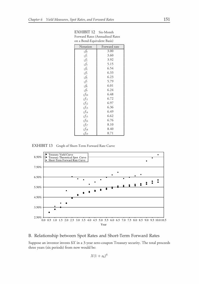
Chapter 6 Yield Measures, Spot Rates, and Forward Rates 151
EXHIBIT 12 Six-MonthForward Rates (Annualized Rateson a Bond-Equivalent Basis)
Notation Forward rate1f0 3.001f1 3.601f2 3.921f3 5.151f4 6.541f5 6.331f6 6.231f7 5.791f8 6.011f9 6.24
1f10 6.481f11 6.721f12 6.971f13 6.361f14 6.491f15 6.621f16 6.761f17 8.101f18 8.401f19 8.71
EXHIBIT 13 Graph of Short-Term Forward Rate Curve
7.50%
8.50%
6.50%
5.50%
4.50%
3.50%
2.50%0.0 0.5 1.0 1.5 2.0 2.5 3.0 3.5 4.0 4.5 5.0 5.5 6.0 6.5 7.0 7.5 8.0 8.5 9.0 9.5 10.0 10.5
Year
Treasury Yield CurveTreasury Theoretical Spot CurveShort-Term Forward Rate Curve
B. Relationship between Spot Rates and Short-Term Forward Rates
Suppose an investor invests $X in a 3-year zero-coupon Treasury security. The total proceedsthree years (six periods) from now would be:
X (1 + z6)6
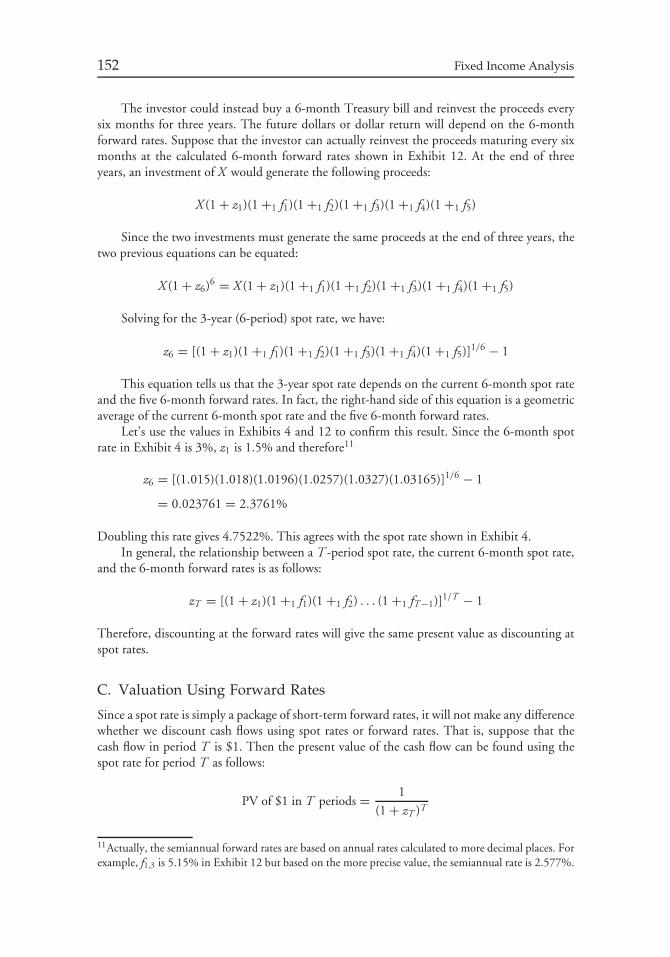
152 Fixed Income Analysis
The investor could instead buy a 6-month Treasury bill and reinvest the proceeds everysix months for three years. The future dollars or dollar return will depend on the 6-monthforward rates. Suppose that the investor can actually reinvest the proceeds maturing every sixmonths at the calculated 6-month forward rates shown in Exhibit 12. At the end of threeyears, an investment of X would generate the following proceeds:
X (1 + z1)(1 +1 f1)(1 +1 f2)(1 +1 f3)(1 +1 f4)(1 +1 f5)
Since the two investments must generate the same proceeds at the end of three years, thetwo previous equations can be equated:
X (1 + z6)6 = X (1 + z1)(1 +1 f1)(1 +1 f2)(1 +1 f3)(1 +1 f4)(1 +1 f5)
Solving for the 3-year (6-period) spot rate, we have:
z6 = [(1 + z1)(1 +1 f1)(1 +1 f2)(1 +1 f3)(1 +1 f4)(1 +1 f5)]1/6 − 1
This equation tells us that the 3-year spot rate depends on the current 6-month spot rateand the five 6-month forward rates. In fact, the right-hand side of this equation is a geometricaverage of the current 6-month spot rate and the five 6-month forward rates.
Let’s use the values in Exhibits 4 and 12 to confirm this result. Since the 6-month spotrate in Exhibit 4 is 3%, z1 is 1.5% and therefore11
z6 = [(1.015)(1.018)(1.0196)(1.0257)(1.0327)(1.03165)]1/6 − 1
= 0.023761 = 2.3761%
Doubling this rate gives 4.7522%. This agrees with the spot rate shown in Exhibit 4.In general, the relationship between a T -period spot rate, the current 6-month spot rate,
and the 6-month forward rates is as follows:
zT = [(1 + z1)(1 +1 f1)(1 +1 f2) . . . (1 +1 fT−1)]1/T − 1
Therefore, discounting at the forward rates will give the same present value as discounting atspot rates.
C. Valuation Using Forward Rates
Since a spot rate is simply a package of short-term forward rates, it will not make any differencewhether we discount cash flows using spot rates or forward rates. That is, suppose that thecash flow in period T is $1. Then the present value of the cash flow can be found using thespot rate for period T as follows:
PV of $1 in T periods = 1
(1 + zT )T
11Actually, the semiannual forward rates are based on annual rates calculated to more decimal places. Forexample, f1,3 is 5.15% in Exhibit 12 but based on the more precise value, the semiannual rate is 2.577%.

Chapter 6 Yield Measures, Spot Rates, and Forward Rates 153
Alternatively, since we know that
zT = [(1 + z1)(1 +1 f1)(1 +1 f2) · · · (1 +1 fT−1)]1/T − 1
then, adding 1 to both sides of the equation,
(1 + zT ) = [(1 + z1)(1 +1 f1)(1 +1 f2) · · · (1 +1 fT−1)]1/T
Raising both sides of the equation to the T -th power we get:
(1 + zT )T = (1 + z1)(1 +1 f1)(1 +1 f2) · · · (1 +1 fT−1)
Substituting the right-hand side of the above equation into the present value formula we get:
PV of $1 in T periods = 1
(1 + z1)(1 +1 f1(1 +1 f2 . . . (1 +1 fT−1)
In practice, the present value of $1 in T periods is called the forward discount factor forperiod T .
For example, consider the forward rates shown in Exhibit 12. The forward discount ratefor period 4 is found as follows:
z1 = 3%/2 = 1.5% 1f1 = 3.6%/2 = 1.8%1f2 = 3.92%/2 = 1.958% 1f3 = 5.15%/2 = 2.577%
forward discount factor of $1 in 4 periods = $1
(1.015)(1.018)(1.01958)(1.02577)
= 0.925369
To see that this is the same present value that would be obtained using the spot rates,note from Exhibit 4 that the 2-year spot rate is 3.9164%. Using that spot rate, we find:
z4 = 3.9164%/2 = 1.9582%
PV of $1 in 4 periods = $1
(1.019582)4= 0.925361
The answer is the same as the forward discount factor (the slight difference is due to rounding).Exhibit 14 shows the computation of the forward discount factor for each period based
on the forward rates in Exhibit 12. Let’s show how both the forward rates and the spot ratescan be used to value a 2-year 6% coupon Treasury bond. The present value for each cash flowis found as follows using spot rates:
cash flow for period t(1 + zt )t
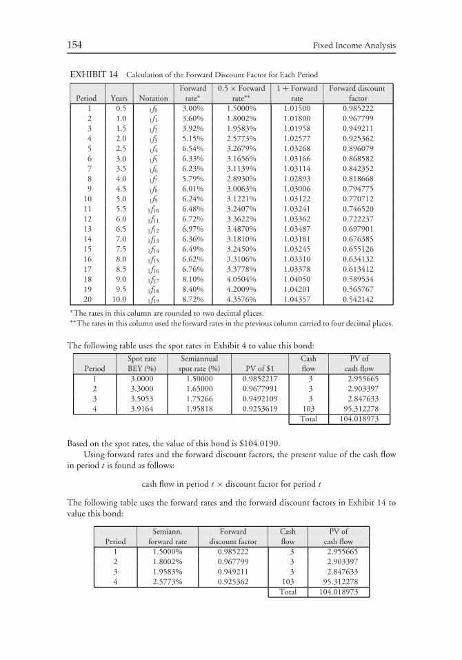
154 Fixed Income Analysis
EXHIBIT 14 Calculation of the Forward Discount Factor for Each Period
Forward 0.5 × Forward 1 + Forward Forward discountPeriod Years Notation rate∗ rate∗∗ rate factor
1 0.5 1f0 3.00% 1.5000% 1.01500 0.9852222 1.0 1f1 3.60% 1.8002% 1.01800 0.9677993 1.5 1f2 3.92% 1.9583% 1.01958 0.9492114 2.0 1f3 5.15% 2.5773% 1.02577 0.9253625 2.5 1f4 6.54% 3.2679% 1.03268 0.8960796 3.0 1f5 6.33% 3.1656% 1.03166 0.8685827 3.5 1f6 6.23% 3.1139% 1.03114 0.8423528 4.0 1f7 5.79% 2.8930% 1.02893 0.8186689 4.5 1f8 6.01% 3.0063% 1.03006 0.794775
10 5.0 1f9 6.24% 3.1221% 1.03122 0.77071211 5.5 1f10 6.48% 3.2407% 1.03241 0.74652012 6.0 1f11 6.72% 3.3622% 1.03362 0.72223713 6.5 1f12 6.97% 3.4870% 1.03487 0.69790114 7.0 1f13 6.36% 3.1810% 1.03181 0.67638515 7.5 1f14 6.49% 3.2450% 1.03245 0.65512616 8.0 1f15 6.62% 3.3106% 1.03310 0.63413217 8.5 1f16 6.76% 3.3778% 1.03378 0.61341218 9.0 1f17 8.10% 4.0504% 1.04050 0.58953419 9.5 1f18 8.40% 4.2009% 1.04201 0.56576720 10.0 1f19 8.72% 4.3576% 1.04357 0.542142
∗The rates in this column are rounded to two decimal places.∗∗The rates in this column used the forward rates in the previous column carried to four decimal places.
The following table uses the spot rates in Exhibit 4 to value this bond:Spot rate Semiannual Cash PV of
Period BEY (%) spot rate (%) PV of $1 flow cash flow1 3.0000 1.50000 0.9852217 3 2.9556652 3.3000 1.65000 0.9677991 3 2.9033973 3.5053 1.75266 0.9492109 3 2.8476334 3.9164 1.95818 0.9253619 103 95.312278
Total 104.018973
Based on the spot rates, the value of this bond is $104.0190.Using forward rates and the forward discount factors, the present value of the cash flow
in period t is found as follows:
cash flow in period t × discount factor for period t
The following table uses the forward rates and the forward discount factors in Exhibit 14 tovalue this bond:
Semiann. Forward Cash PV ofPeriod forward rate discount factor flow cash flow
1 1.5000% 0.985222 3 2.9556652 1.8002% 0.967799 3 2.9033973 1.9583% 0.949211 3 2.8476334 2.5773% 0.925362 103 95.312278
Total 104.018973
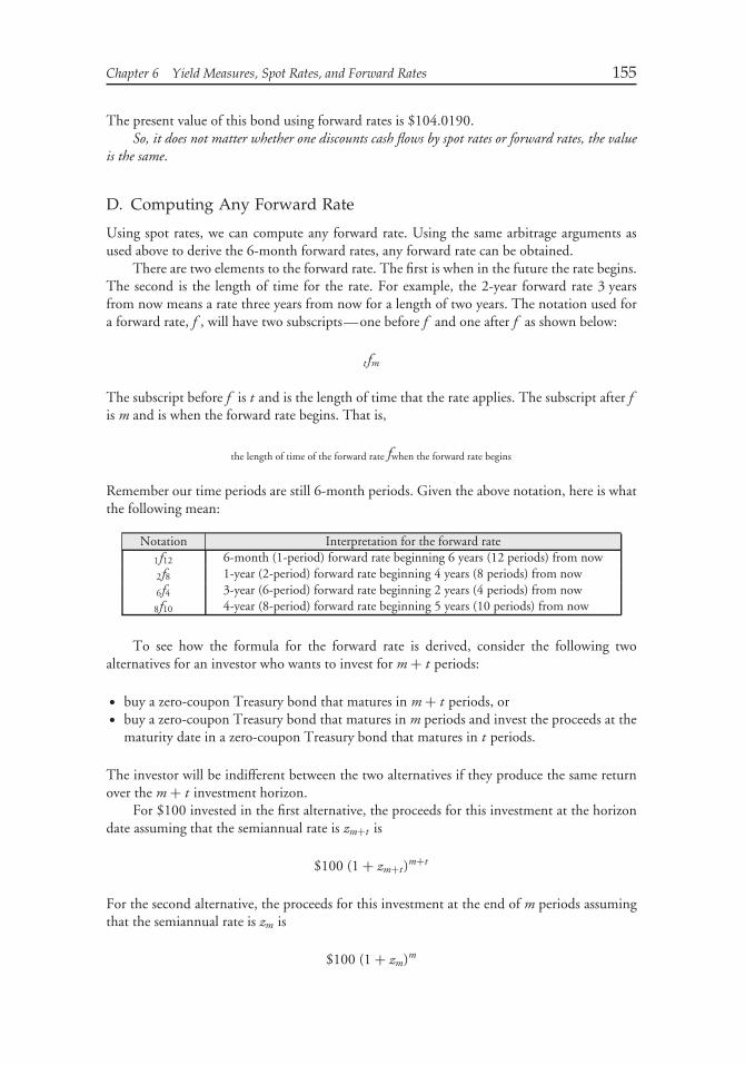
Chapter 6 Yield Measures, Spot Rates, and Forward Rates 155
The present value of this bond using forward rates is $104.0190.So, it does not matter whether one discounts cash flows by spot rates or forward rates, the value
is the same.
D. Computing Any Forward Rate
Using spot rates, we can compute any forward rate. Using the same arbitrage arguments asused above to derive the 6-month forward rates, any forward rate can be obtained.
There are two elements to the forward rate. The first is when in the future the rate begins.The second is the length of time for the rate. For example, the 2-year forward rate 3 yearsfrom now means a rate three years from now for a length of two years. The notation used fora forward rate, f , will have two subscripts—one before f and one after f as shown below:
t fm
The subscript before f is t and is the length of time that the rate applies. The subscript after fis m and is when the forward rate begins. That is,
the length of time of the forward rate fwhen the forward rate begins
Remember our time periods are still 6-month periods. Given the above notation, here is whatthe following mean:
Notation Interpretation for the forward rate1f12 6-month (1-period) forward rate beginning 6 years (12 periods) from now2f8 1-year (2-period) forward rate beginning 4 years (8 periods) from now6f4 3-year (6-period) forward rate beginning 2 years (4 periods) from now
8f10 4-year (8-period) forward rate beginning 5 years (10 periods) from now
To see how the formula for the forward rate is derived, consider the following twoalternatives for an investor who wants to invest for m + t periods:
• buy a zero-coupon Treasury bond that matures in m + t periods, or• buy a zero-coupon Treasury bond that matures in m periods and invest the proceeds at the
maturity date in a zero-coupon Treasury bond that matures in t periods.
The investor will be indifferent between the two alternatives if they produce the same returnover the m + t investment horizon.
For $100 invested in the first alternative, the proceeds for this investment at the horizondate assuming that the semiannual rate is zm+t is
$100 (1 + zm+t)m+t
For the second alternative, the proceeds for this investment at the end of m periods assumingthat the semiannual rate is zm is
$100 (1 + zm)m

156 Fixed Income Analysis
When the proceeds are received in m periods, they are reinvested at the forward rate, t fm,producing a value for the investment at the end of m + t periods of
$100 (1 + zm)m(1 +t fm)t
For the investor to be indifferent to the two alternatives, the following relationship must hold:
$100 (1 + zm+t)m+t = $100 (1 + zm)m(1 +t fm)t
Solving for t fm we get:
t fm =[
(1 + zm+t )m+t
(1 + zm)m
]1/t
− 1
Notice that if t is equal to 1, the formula reduces to the 1-period (6-month) forward rate.To illustrate, for the spot rates shown in Exhibit 4, suppose that an investor wants to
know the 2-year forward rate three years from now. In terms of the notation, t is equal to 4and m is equal to 6. Substituting for t and m into the equation for the forward rate we have:
4f6 =[
(1 + z10)10−
(1 + z6)6
]1/4
− 1
This means that the following two spot rates are needed: z6 (the 3-year spot rate) and z10 (the5-year spot rate). From Exhibit 4 we know
z6(the 3-year spot rate) = 4.752%/2 = 0.02376
z10(the 5-year spot rate) = 5.2772%/2 = 0.026386
then
4f6 =[
(1.026386)10−
(1.02376)6
]1/4
− 1 = 0.030338
Therefore, 4f6 is equal to 3.0338% and doubling this rate gives 6.0675% the forward rate ona bond-equivalent basis.
We can verify this result. Investing $100 for 10 periods at the spot rate of 2.6386% willproduce the following value:
$100 (1.026386)10 = $129.7499
Investing $100 for 6 periods at 2.376% and reinvesting the proceeds for 4 periods at theforward rate of 3.030338% gives the same value:
$100 (1.02376)6(1.030338)4 = $129.75012
CHAPTER 7INTRODUCTION TO THE
MEASUREMENT OFINTEREST RATE RISK
I. INTRODUCTION
In Chapter 2, we discussed the interest rate risk associated with investing in bonds. We knowthat the value of a bond moves in the opposite direction to a change in interest rates. If interestrates increase, the price of a bond will decrease. For a short bond position, a loss is generatedif interest rates fall. However, a manager wants to know more than simply when a positiongenerates a loss. To control interest rate risk, a manager must be able to quantify that result.
What is the key to measuring the interest rate risk? It is the accuracy in estimating thevalue of the position after an adverse interest rate change. A valuation model determines thevalue of a position after an adverse interest rate move. Consequently, if a reliable valuationmodel is not used, there is no way to properly measure interest rate risk exposure.
There are two approaches to measuring interest rate risk—the full valuation approachand the duration/convexity approach.
II. THE FULL VALUATION APPROACH
The most obvious way to measure the interest rate risk exposure of a bond position or aportfolio is to re-value it when interest rates change. The analysis is performed for differentscenarios with respect to interest rate changes. For example, a manager may want to measurethe interest rate exposure to a 50 basis point, 100 basis point, and 200 basis point instantaneouschange in interest rates. This approach requires the re-valuation of a bond or bond portfoliofor a given interest rate change scenario and is referred to as the full valuation approach.It is sometimes referred to as scenario analysis because it involves assessing the exposure tointerest rate change scenarios.
To illustrate this approach, suppose that a manager has a $10 million par value positionin a 9% coupon 20-year bond. The bond is option-free. The current price is 134.6722 fora yield (i.e., yield to maturity) of 6%. The market value of the position is $13,467,220(134.6722% × $10 million). Since the manager owns the bond, she is concerned with a risein yield since this will decrease the market value of the position. To assess the exposure to arise in market yields, the manager decides to look at how the value of the bond will changeif yields change instantaneously for the following three scenarios: (1) 50 basis point increase,
157
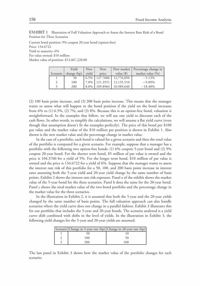
158 Fixed Income Analysis
EXHIBIT 1 Illustration of Full Valuation Approach to Assess the Interest Rate Risk of a BondPosition for Three Scenarios
Current bond position: 9% coupon 20-year bond (option-free)Price: 134.6722Yield to maturity: 6%Par value owned: $10 millionMarket value of position: $13,467,220.00
Yield New New New market Percentage change inScenario change (bp) yield price value ($) market value (%)
1 50 6.5% 127.7606 12,776,050 −5.13%2 100 7.0% 121.3551 12,135,510 −9.89%3 200 8.0% 109.8964 10,989,640 −18.40%
(2) 100 basis point increase, and (3) 200 basis point increase. This means that the managerwants to assess what will happen to the bond position if the yield on the bond increasesfrom 6% to (1) 6.5%, (2) 7%, and (3) 8%. Because this is an option-free bond, valuation isstraightforward. In the examples that follow, we will use one yield to discount each of thecash flows. In other words, to simplify the calculations, we will assume a flat yield curve (eventhough that assumption doesn’t fit the examples perfectly). The price of this bond per $100par value and the market value of the $10 million par position is shown in Exhibit 1. Alsoshown is the new market value and the percentage change in market value.
In the case of a portfolio, each bond is valued for a given scenario and then the total valueof the portfolio is computed for a given scenario. For example, suppose that a manager has aportfolio with the following two option-free bonds: (1) 6% coupon 5-year bond and (2) 9%coupon 20-year bond. For the shorter term bond, $5 million of par value is owned and theprice is 104.3760 for a yield of 5%. For the longer term bond, $10 million of par value isowned and the price is 134.6722 for a yield of 6%. Suppose that the manager wants to assessthe interest rate risk of this portfolio for a 50, 100, and 200 basis point increase in interestrates assuming both the 5-year yield and 20-year yield change by the same number of basispoints. Exhibit 2 shows the interest rate risk exposure. Panel a of the exhibit shows the marketvalue of the 5-year bond for the three scenarios. Panel b does the same for the 20-year bond.Panel c shows the total market value of the two-bond portfolio and the percentage change inthe market value for the three scenarios.
In the illustration in Exhibit 2, it is assumed that both the 5-year and the 20-year yieldschanged by the same number of basis points. The full valuation approach can also handlescenarios where the yield curve does not change in a parallel fashion. Exhibit 3 illustrates thisfor our portfolio that includes the 5-year and 20-year bonds. The scenario analyzed is a yieldcurve shift combined with shifts in the level of yields. In the illustration in Exhibit 3, thefollowing yield changes for the 5-year and 20-year yields are assumed:
Scenario Change in 5-year rate (bp) Change in 20-year rate (bp)1 50 102 100 503 200 100
The last panel in Exhibit 3 shows how the market value of the portfolio changes for eachscenario.
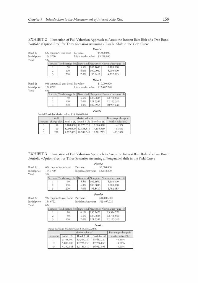
Chapter 7 Introduction to the Measurement of Interest Rate Risk 159
EXHIBIT 2 Illustration of Full Valuation Approach to Assess the Interest Rate Risk of a Two BondPortfolio (Option-Free) for Three Scenarios Assuming a Parallel Shift in the Yield Curve
Panel aBond 1: 6% coupon 5-year bond Par value: $5,000,000Initial price: 104.3760 Initial market value: $5,218,800Yield: 5%
Scenario Yield change (bp) New yield New price New market value ($)1 50 5.5% 102.1600 5,108,0002 100 6.0% 100.0000 5,000,0003 200 7.0% 95.8417 4,792,085
Panel bBond 2: 9% coupon 20-year bond Par value: $10,000,000Initial price: 134.6722 Initial market value: $13,467,220Yield: 6%
Scenario Yield change (bp) New yield New price New market value ($)1 50 6.5% 127.7605 12,776,0502 100 7.0% 121.3551 12,135,5103 200 8.0% 109.8964 10,989,640
Panel cInitial Portfolio Market value: $18,686,020.00
Yield Market value of Percentage change inScenario change (bp) Bond 1 ($) Bond 2 ($) Portfolio ($) market value (%)
1 50 5,108,000 12,776,050 17,884,020 −4.29%2 100 5,000,000 12,135,510 17,135,510 −8.30%3 200 4,792,085 10,989,640 15,781,725 −15.54%
EXHIBIT 3 Illustration of Full Valuation Approach to Assess the Interest Rate Risk of a Two BondPortfolio (Option-Free) for Three Scenarios Assuming a Nonparallel Shift in the Yield Curve
Panel aBond 1: 6% coupon 5-year bond Par value: $5,000,000Initial price: 104.3760 Initial market value: $5,218,800Yield: 5%
Scenario Yield change (bp) New yield New price New market value ($)1 50 5.5% 102.1600 5,108,0002 100 6.0% 100.0000 5,000,0003 200 7.0% 95.8417 4,792,085
Panel bBond 2: 9% coupon 20-year bond Par value: $10,000,000Initial price: 134.6722 Initial market value: $13,467,220Yield: 6%
Scenario Yield change (bp) New yield New price New market value ($)1 10 6.1% 133.2472 13,324,7202 50 6.5% 127.7605 12,776,0503 100 7.0% 121.3551 12,135,510
Panel cInitial Portfolio Market value: $18,686,020.00
Market value of Percentage change inScenario Bond 1 ($) Bond 2 ($) Portfolio ($) market value (%)
1 5,108,000 13,324,720 18,432,720 −1.36%2 5,000,000 12,776,050 17,776,050 −4.87%3 4,792,085 12,135,510 16,927,595 −9.41%
160 Fixed Income Analysis
The full valuation approach seems straightforward. If one has a good valuation model,assessing how the value of a portfolio or individual bond will change for different scenarios forparallel and nonparallel yield curve shifts measures the interest rate risk of a portfolio.
A common question that often arises when using the full valuation approach is whichscenarios should be evaluated to assess interest rate risk exposure. For some regulated entities,there are specified scenarios established by regulators. For example, it is common for regulatorsof depository institutions to require entities to determine the impact on the value of theirbond portfolio for a 100, 200, and 300 basis point instantaneous change in interest rates (upand down). (Regulators tend to refer to this as ‘‘simulating’’ interest rate scenarios rather thanscenario analysis.) Risk managers and highly leveraged investors such as hedge funds tend tolook at extreme scenarios to assess exposure to interest rate changes. This practice is referredto as stress testing.
Of course, in assessing how changes in the yield curve can affect the exposure of aportfolio, there are an infinite number of scenarios that can be evaluated. The state-of-the-arttechnology involves using a complex statistical procedure1 to determine a likely set of yieldcurve shift scenarios from historical data.
It seems like the chapter should end right here. We can use the full valuation approachto assess the exposure of a bond or portfolio to interest rate changes to evaluate any scenario,assuming—and this must be repeated continuously— that the manager has a good valuationmodel to estimate what the price of the bonds will be in each interest rate scenario. However,we are not stopping here. In fact, the balance of this chapter is considerably longer than thissection. Why? The reason is that the full valuation process can be very time consuming. Thisis particularly true if the portfolio has a large number of bonds, even if a minority of thosebonds are complex (i.e., have embedded options). While the full valuation approach is therecommended method, managers want one simple measure that they can use to get an idea ofhow bond prices will change if rates change in a parallel fashion, rather than having to revaluean entire portfolio. In Chapter 2, such a measure was introduced—duration. We will discussthis measure as well as a supplementary measure (convexity) in Sections IV and V, respectively.To build a foundation to understand the limitations of these measures, we describe the basicprice volatility characteristics of bonds in Section III. The fact that there are limitations ofusing one or two measures to describe the interest rate exposure of a position or portfolioshould not be surprising. These measures provide a starting point for assessing interest rate risk.
III. PRICE VOLATILITY CHARACTERISTICSOF BONDS
In Chapter 2, we described the characteristics of a bond that affect its price volatility:(1) maturity, (2) coupon rate, and (3) presence of embedded options. We also explained howthe level of yields affects price volatility. In this section, we will take a closer look at the pricevolatility of bonds.
A. Price Volatility Characteristics of Option-Free Bonds
Let’s begin by focusing on option-free bonds (i.e., bonds that do not have embedded options).A fundamental characteristic of an option-free bond is that the price of the bond changes in
1The procedure used is principal component analysis.
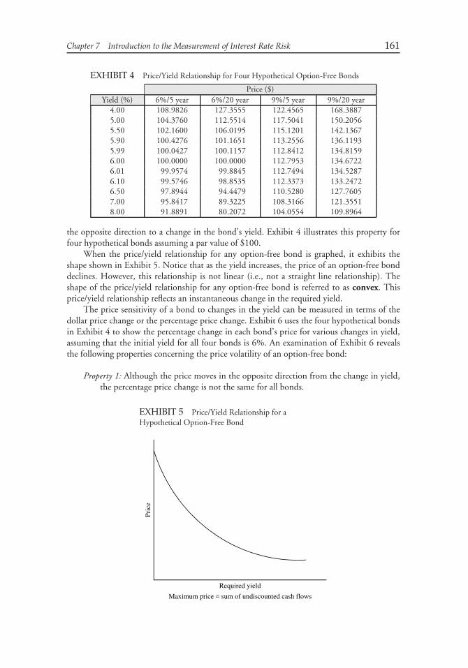
Chapter 7 Introduction to the Measurement of Interest Rate Risk 161
EXHIBIT 4 Price/Yield Relationship for Four Hypothetical Option-Free Bonds
Price ($)Yield (%) 6%/5 year 6%/20 year 9%/5 year 9%/20 year
4.00 108.9826 127.3555 122.4565 168.38875.00 104.3760 112.5514 117.5041 150.20565.50 102.1600 106.0195 115.1201 142.13675.90 100.4276 101.1651 113.2556 136.11935.99 100.0427 100.1157 112.8412 134.81596.00 100.0000 100.0000 112.7953 134.67226.01 99.9574 99.8845 112.7494 134.52876.10 99.5746 98.8535 112.3373 133.24726.50 97.8944 94.4479 110.5280 127.76057.00 95.8417 89.3225 108.3166 121.35518.00 91.8891 80.2072 104.0554 109.8964
the opposite direction to a change in the bond’s yield. Exhibit 4 illustrates this property forfour hypothetical bonds assuming a par value of $100.
When the price/yield relationship for any option-free bond is graphed, it exhibits theshape shown in Exhibit 5. Notice that as the yield increases, the price of an option-free bonddeclines. However, this relationship is not linear (i.e., not a straight line relationship). Theshape of the price/yield relationship for any option-free bond is referred to as convex. Thisprice/yield relationship reflects an instantaneous change in the required yield.
The price sensitivity of a bond to changes in the yield can be measured in terms of thedollar price change or the percentage price change. Exhibit 6 uses the four hypothetical bondsin Exhibit 4 to show the percentage change in each bond’s price for various changes in yield,assuming that the initial yield for all four bonds is 6%. An examination of Exhibit 6 revealsthe following properties concerning the price volatility of an option-free bond:
Property 1: Although the price moves in the opposite direction from the change in yield,the percentage price change is not the same for all bonds.
EXHIBIT 5 Price/Yield Relationship for aHypothetical Option-Free Bond
Pric
e
Maximum price = sum of undiscounted cash flows
Required yield
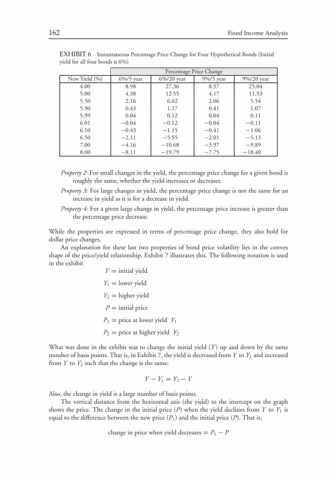
162 Fixed Income Analysis
EXHIBIT 6 Instantaneous Percentage Price Change for Four Hypothetical Bonds (Initialyield for all four bonds is 6%)
Percentage Price ChangeNew Yield (%) 6%/5 year 6%/20 year 9%/5 year 9%/20 year
4.00 8.98 27.36 8.57 25.045.00 4.38 12.55 4.17 11.535.50 2.16 6.02 2.06 5.545.90 0.43 1.17 0.41 1.075.99 0.04 0.12 0.04 0.116.01 −0.04 −0.12 −0.04 −0.116.10 −0.43 −1.15 −0.41 −1.066.50 −2.11 −5.55 −2.01 −5.137.00 −4.16 −10.68 −3.97 −9.898.00 −8.11 −19.79 −7.75 −18.40
Property 2: For small changes in the yield, the percentage price change for a given bond isroughly the same, whether the yield increases or decreases.
Property 3: For large changes in yield, the percentage price change is not the same for anincrease in yield as it is for a decrease in yield.
Property 4: For a given large change in yield, the percentage price increase is greater thanthe percentage price decrease.
While the properties are expressed in terms of percentage price change, they also hold fordollar price changes.
An explanation for these last two properties of bond price volatility lies in the convexshape of the price/yield relationship. Exhibit 7 illustrates this. The following notation is usedin the exhibit
Y = initial yield
Y1 = lower yield
Y2 = higher yield
P = initial price
P1 = price at lower yield Y1
P2 = price at higher yield Y2
What was done in the exhibit was to change the initial yield (Y ) up and down by the samenumber of basis points. That is, in Exhibit 7, the yield is decreased from Y to Y1 and increasedfrom Y to Y2 such that the change is the same:
Y − Y1 = Y2 − Y
Also, the change in yield is a large number of basis points.The vertical distance from the horizontal axis (the yield) to the intercept on the graph
shows the price. The change in the initial price (P) when the yield declines from Y to Y1 isequal to the difference between the new price (P1) and the initial price (P). That is,
change in price when yield decreases = P1 − P
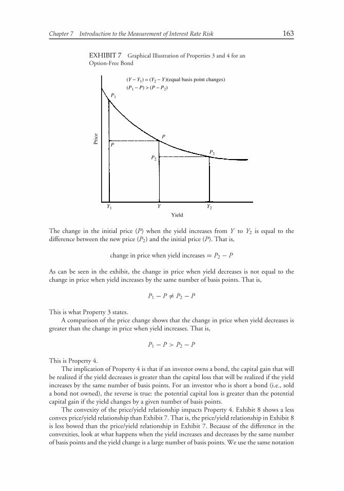
Chapter 7 Introduction to the Measurement of Interest Rate Risk 163
EXHIBIT 7 Graphical Illustration of Properties 3 and 4 for anOption-Free Bond
Pric
eP1
Y1 Y2Y
Yield
P2P2
P
P
(Y − Y1) = (Y2 − Y )(equal basis point changes)
(P1 − P) > (P − P2)
The change in the initial price (P) when the yield increases from Y to Y2 is equal to thedifference between the new price (P2) and the initial price (P). That is,
change in price when yield increases = P2 − P
As can be seen in the exhibit, the change in price when yield decreases is not equal to thechange in price when yield increases by the same number of basis points. That is,
P1 − P �= P2 − P
This is what Property 3 states.A comparison of the price change shows that the change in price when yield decreases is
greater than the change in price when yield increases. That is,
P1 − P > P2 − P
This is Property 4.The implication of Property 4 is that if an investor owns a bond, the capital gain that will
be realized if the yield decreases is greater than the capital loss that will be realized if the yieldincreases by the same number of basis points. For an investor who is short a bond (i.e., solda bond not owned), the reverse is true: the potential capital loss is greater than the potentialcapital gain if the yield changes by a given number of basis points.
The convexity of the price/yield relationship impacts Property 4. Exhibit 8 shows a lessconvex price/yield relationship than Exhibit 7. That is, the price/yield relationship in Exhibit 8is less bowed than the price/yield relationship in Exhibit 7. Because of the difference in theconvexities, look at what happens when the yield increases and decreases by the same numberof basis points and the yield change is a large number of basis points. We use the same notation
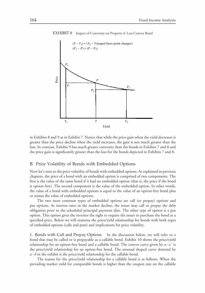
164 Fixed Income Analysis
EXHIBIT 8 Impact of Convexity on Property 4: Less Convex Bond
Pric
e
P1
Y1 Y2Y
Yield
P2P2
P
P
(Y − Y1) = (Y2 − Y )(equal basis point changes)
(P1 − P) > (P − P2)
in Exhibits 8 and 9 as in Exhibit 7. Notice that while the price gain when the yield decreases isgreater than the price decline when the yield increases, the gain is not much greater than theloss. In contrast, Exhibit 9 has much greater convexity than the bonds in Exhibits 7 and 8 andthe price gain is significantly greater than the loss for the bonds depicted in Exhibits 7 and 8.
B. Price Volatility of Bonds with Embedded Options
Now let’s turn to the price volatility of bonds with embedded options. As explained in previouschapters, the price of a bond with an embedded option is comprised of two components. Thefirst is the value of the same bond if it had no embedded option (that is, the price if the bondis option free). The second component is the value of the embedded option. In other words,the value of a bond with embedded options is equal to the value of an option-free bond plusor minus the value of embedded options.
The two most common types of embedded options are call (or prepay) options andput options. As interest rates in the market decline, the issuer may call or prepay the debtobligation prior to the scheduled principal payment date. The other type of option is a putoption. This option gives the investor the right to require the issuer to purchase the bond at aspecified price. Below we will examine the price/yield relationship for bonds with both typesof embedded options (calls and puts) and implications for price volatility.
1. Bonds with Call and Prepay Options In the discussion below, we will refer to abond that may be called or is prepayable as a callable bond. Exhibit 10 shows the price/yieldrelationship for an option-free bond and a callable bond. The convex curve given by a–a ′ isthe price/yield relationship for an option-free bond. The unusual shaped curve denoted bya–b in the exhibit is the price/yield relationship for the callable bond.
The reason for the price/yield relationship for a callable bond is as follows. When theprevailing market yield for comparable bonds is higher than the coupon rate on the callable
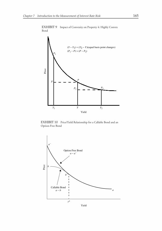
Chapter 7 Introduction to the Measurement of Interest Rate Risk 165
EXHIBIT 9 Impact of Convexity on Property 4: Highly ConvexBond
Pric
e
P1
Y1 Y2Y
Yield
P2P2
PP
(Y − Y1) = (Y2 − Y )(equal basis point changes)
(P1 − P) > (P − P2)
EXHIBIT 10 Price/Yield Relationship for a Callable Bond and anOption-Free Bond
Option-Free Bonda − a´
Callable Bonda − b a
a´
y*
Pric
e
Yield
b
b´

166 Fixed Income Analysis
bond, it is unlikely that the issuer will call the issue. For example, if the coupon rate on abond is 7% and the prevailing market yield on comparable bonds is 12%, it is highly unlikelythat the issuer will call a 7% coupon bond so that it can issue a 12% coupon bond. Since thebond is unlikely to be called, the callable bond will have a similar price/yield relationship toan otherwise comparable option-free bond. Consequently, the callable bond will be valued asif it is an option-free bond. However, since there is still some value to the call option,2 thebond won’t trade exactly like an option-free bond.
As yields in the market decline, the concern is that the issuer will call the bond. The issuerwon’t necessarily exercise the call option as soon as the market yield drops below the couponrate. Yet, the value of the embedded call option increases as yields approach the coupon ratefrom higher yield levels. For example, if the coupon rate on a bond is 7% and the marketyield declines to 7.5%, the issuer will most likely not call the issue. However, market yieldsare now at a level at which the investor is concerned that the issue may eventually be calledif market yields decline further. Cast in terms of the value of the embedded call option, thatoption becomes more valuable to the issuer and therefore it reduces the price relative to anotherwise comparable option-free bond.3 In Exhibit 10, the value of the embedded call optionat a given yield can be measured by the difference between the price of an option-free bond(the price shown on the curve a–a ′) and the price on the curve a–b. Notice that at low yieldlevels (below y∗ on the horizontal axis), the value of the embedded call option is high.
Using the information in Exhibit 10, let’s compare the price volatility of a callable bondto that of an option-free bond. Exhibit 11 focuses on the portion of the price/yield relationshipfor the callable bond where the two curves in Exhibit 10 depart (segment b′ –b in Exhibit 10).We know from our earlier discussion that for a large change in yield, the price of an option-freebond increases by more than it decreases (Property 4 above). Is that what happens for a callablebond in the region of the price/yield relationship shown in Exhibit 11? No, it is not. In fact,as can be seen in the exhibit, the opposite is true! That is, for a given large change in yield, theprice appreciation is less than the price decline.
This very important characteristic of a callable bond—that its price appreciation is lessthan its price decline when rates change by a large number of basis points—is referred toas negative convexity.4 But notice from Exhibit 10 that callable bonds don’t exhibit thischaracteristic at every yield level. When yields are high (relative to the issue’s coupon rate),the bond exhibits the same price/yield relationship as an option-free bond; therefore at highyield levels it also has the characteristic that the gain is greater than the loss. Because marketparticipants have referred to the shape of the price/yield relationship shown in Exhibit 11 asnegative convexity, market participants refer to the relationship for an option-free bond aspositive convexity. Consequently, a callable bond exhibits negative convexity at low yieldlevels and positive convexity at high yield levels. This is depicted in Exhibit 12.
As can be seen from the exhibits, when a bond exhibits negative convexity, the bondcompresses in price as rates decline. That is, at a certain yield level there is very little priceappreciation when rates decline. When a bond enters this region, the bond is said to exhibit‘‘price compression.’’
2This is because there is still some chance that interest rates will decline in the future and the issue willbe called.3For readers who are already familiar with option theory, this characteristic can be restated as follows:When the coupon rate for the issue is below the market yield, the embedded call option is said to be‘‘out-of-the-money.’’ When the coupon rate for the issue is above the market yield, the embedded calloption is said to be ‘‘in-the-money.’’4Mathematicians refer to this shape as being ‘‘concave.’’
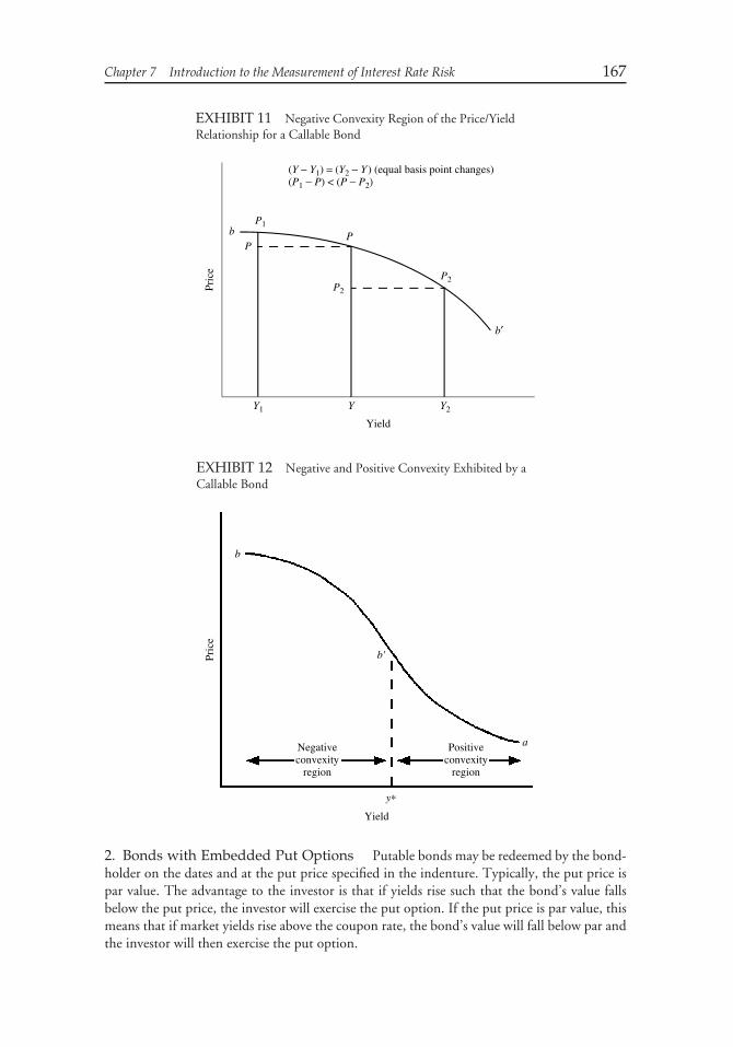
Chapter 7 Introduction to the Measurement of Interest Rate Risk 167
EXHIBIT 11 Negative Convexity Region of the Price/YieldRelationship for a Callable Bond
Pric
e
Yield
Y2Y1 Y
b′
b P
P2
P1
P
P2
(Y − Y1) = (Y2 − Y ) (equal basis point changes)(P1 − P) < (P − P2)
EXHIBIT 12 Negative and Positive Convexity Exhibited by aCallable Bond
Negativeconvexity
region
Positiveconvexity
region
Pric
e
b
a
b'
y∗
Yield
2. Bonds with Embedded Put Options Putable bonds may be redeemed by the bond-holder on the dates and at the put price specified in the indenture. Typically, the put price ispar value. The advantage to the investor is that if yields rise such that the bond’s value fallsbelow the put price, the investor will exercise the put option. If the put price is par value, thismeans that if market yields rise above the coupon rate, the bond’s value will fall below par andthe investor will then exercise the put option.
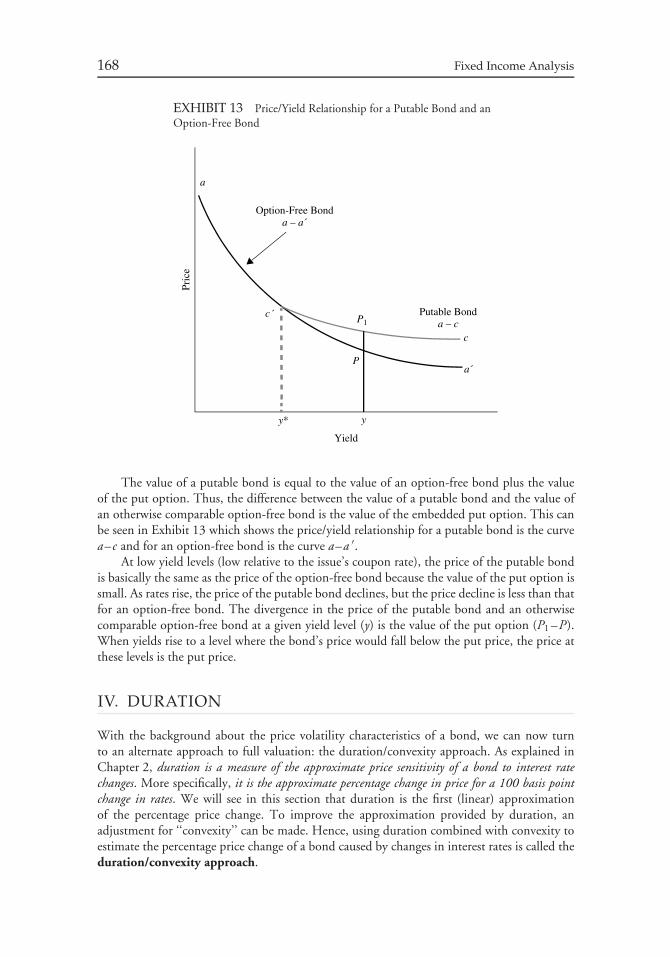
168 Fixed Income Analysis
EXHIBIT 13 Price/Yield Relationship for a Putable Bond and anOption-Free Bond
Option-Free Bonda – a´
a
y*
Pric
e
Yield
c
Putable Bonda – c
a´
c´ P1
P
y
The value of a putable bond is equal to the value of an option-free bond plus the valueof the put option. Thus, the difference between the value of a putable bond and the value ofan otherwise comparable option-free bond is the value of the embedded put option. This canbe seen in Exhibit 13 which shows the price/yield relationship for a putable bond is the curvea–c and for an option-free bond is the curve a–a ′.
At low yield levels (low relative to the issue’s coupon rate), the price of the putable bondis basically the same as the price of the option-free bond because the value of the put option issmall. As rates rise, the price of the putable bond declines, but the price decline is less than thatfor an option-free bond. The divergence in the price of the putable bond and an otherwisecomparable option-free bond at a given yield level (y) is the value of the put option (P1 –P).When yields rise to a level where the bond’s price would fall below the put price, the price atthese levels is the put price.
IV. DURATION
With the background about the price volatility characteristics of a bond, we can now turnto an alternate approach to full valuation: the duration/convexity approach. As explained inChapter 2, duration is a measure of the approximate price sensitivity of a bond to interest ratechanges. More specifically, it is the approximate percentage change in price for a 100 basis pointchange in rates. We will see in this section that duration is the first (linear) approximationof the percentage price change. To improve the approximation provided by duration, anadjustment for ‘‘convexity’’ can be made. Hence, using duration combined with convexity toestimate the percentage price change of a bond caused by changes in interest rates is called theduration/convexity approach.
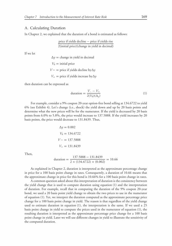
Chapter 7 Introduction to the Measurement of Interest Rate Risk 169
A. Calculating Duration
In Chapter 2, we explained that the duration of a bond is estimated as follows:
price if yields decline − price if yields rise
2(initial price)(change in yield in decimal)
If we let�y = change in yield in decimal
V0 = initial price
V − = price if yields decline by�y
V+ = price if yields increase by�y
then duration can be expressed as
duration = V− − V+2(V0)(�y)
(1)
For example, consider a 9% coupon 20-year option-free bond selling at 134.6722 to yield6% (see Exhibit 4). Let’s change (i.e., shock) the yield down and up by 20 basis points anddetermine what the new prices will be for the numerator. If the yield is decreased by 20 basispoints from 6.0% to 5.8%, the price would increase to 137.5888. If the yield increases by 20basis points, the price would decrease to 131.8439. Thus,
�y = 0.002
V0 = 134.6722
V − = 137.5888
V+ = 131.8439
Then,
duration = 137.5888 − 131.8439
2 × (134.6722) × (0.002)= 10.66
As explained in Chapter 2, duration is interpreted as the approximate percentage changein price for a 100 basis point change in rates. Consequently, a duration of 10.66 means thatthe approximate change in price for this bond is 10.66% for a 100 basis point change in rates.
A common question asked about this interpretation of duration is the consistency betweenthe yield change that is used to compute duration using equation (1) and the interpretationof duration. For example, recall that in computing the duration of the 9% coupon 20-yearbond, we used a 20 basis point yield change to obtain the two prices to use in the numeratorof equation (1). Yet, we interpret the duration computed as the approximate percentage pricechange for a 100 basis point change in yield. The reason is that regardless of the yield changeused to estimate duration in equation (1), the interpretation is the same. If we used a 25basis point change in yield to compute the prices used in the numerator of equation (1), theresulting duration is interpreted as the approximate percentage price change for a 100 basispoint change in yield. Later we will use different changes in yield to illustrate the sensitivity ofthe computed duration.
170 Fixed Income Analysis
B. Approximating the Percentage Price Change Using Duration
In Chapter 2, we explained how to approximate the percentage price change for a given changein yield and a given duration. Here we will express the process using the following formula:
approximate percentage price change = −duration × �y∗ × 100 (2)
where �y∗ is the yield change (in decimal) for which the estimated percentage price change issought.5 The reason for the negative sign on the right-hand side of equation (2) is due to theinverse relationship between price change and yield change (e.g., as yields increase, bond pricesdecrease). The following two examples illustrate how to use duration to estimate a bond’sprice change.
Example #1: small change in basis point yield. For example, consider the 9% 20-year bondtrading at 134.6722 whose duration we just showed is 10.66. The approximate percentageprice change for a 10 basis point increase in yield (i.e., �y∗ = +0.001) is:
approximate percentage price change = −10.66 × (+0.001)×100 = −1.066%
How good is this approximation? The actual percentage price change is −1.06% (asshown in Exhibit 6 when yield increases to 6.10%). Duration, in this case, did an excellentjob in estimating the percentage price change.
We would come to the same conclusion if we used duration to estimate the percentageprice change if the yield declined by 10 basis points (i.e., �y = −0.001). In this case, theapproximate percentage price change would be +1.066% (i.e., the direction of the estimatedprice change is the reverse but the magnitude of the change is the same). Exhibit 6 shows thatthe actual percentage price change is +1.07%.
In terms of estimating the new price, let’s see how duration performed. The initial price is134.6722. For a 10 basis point increase in yield, duration estimates that the price will declineby 1.066%. Thus, the price will decline to 133.2366 (found by multiplying 134.6722 by oneminus 0.01066). The actual price from Exhibit 4 if the yield increases by 10 basis points is133.2472. Thus, the price estimated using duration is close to the actual price.
For a 10 basis point decrease in yield, the actual price from Exhibit 4 is 136.1193 and theestimated price using duration is 136.1078 (a price increase of 1.066%). Consequently, thenew price estimated by duration is close to the actual price for a 10 basis point change in yield.
Example #2: large change in basis point yield. Let’s look at how well duration does inestimating the percentage price change if the yield increases by 200 basis points instead of 10basis points. In this case, �y is equal to +0.02. Substituting into equation (2), we have
approximate percentage price change = −10.66 × (+0.02)×100 = −21.32%
5The difference between �y in the duration formula given by equation (1) and �y∗ in equation (2) toget the approximate percentage change is as follows. In the duration formula, the �y is used to estimateduration and, as explained later, for reasonably small changes in yield the resulting value for duration willbe the same. We refer to this change as the ‘‘rate shock.’’ Given the duration, the next step is to estimatethe percentage price change for any change in yield. The �y∗ in equation (2) is the specific change inyield for which the approximate percentage price change is sought.
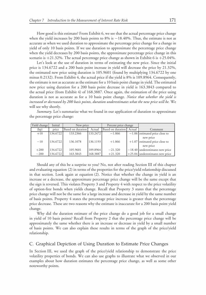
Chapter 7 Introduction to the Measurement of Interest Rate Risk 171
How good is this estimate? From Exhibit 6, we see that the actual percentage price changewhen the yield increases by 200 basis points to 8% is −18.40%. Thus, the estimate is not asaccurate as when we used duration to approximate the percentage price change for a change inyield of only 10 basis points. If we use duration to approximate the percentage price changewhen the yield decreases by 200 basis points, the approximate percentage price change in thisscenario is +21.32%. The actual percentage price change as shown in Exhibit 6 is +25.04%.
Let’s look at the use of duration in terms of estimating the new price. Since the initialprice is 134.6722 and a 200 basis point increase in yield will decrease the price by 21.32%,the estimated new price using duration is 105.9601 (found by multiplying 134.6722 by oneminus 0.2132). From Exhibit 4, the actual price if the yield is 8% is 109.8964. Consequently,the estimate is not as accurate as the estimate for a 10 basis point change in yield. The estimatednew price using duration for a 200 basis point decrease in yield is 163.3843 compared tothe actual price (from Exhibit 4) of 168.3887. Once again, the estimation of the price usingduration is not as accurate as for a 10 basis point change. Notice that whether the yield isincreased or decreased by 200 basis points, duration underestimates what the new price will be. Wewill see why shortly.
Summary. Let’s summarize what we found in our application of duration to approximatethe percentage price change:
Yield change Initial New price Percent price change(bp) price Based on duration Actual Based on duration Actual Comment+10 134.6722 133.2366 133.2472 −1.066 −1.06 estimated price close to
new price−10 134.6722 136.1078 136.1193 +1.066 +1.07 estimated price close to
new price+200 134.6722 105.9601 109.8964 −21.320 −18.40 underestimates new price−200 134.6722 163.3843 168.3887 +21.320 +25.04 underestimates new price
Should any of this be a surprise to you? No, not after reading Section III of this chapterand evaluating equation (2) in terms of the properties for the price/yield relationship discussedin that section. Look again at equation (2). Notice that whether the change in yield is anincrease or a decrease, the approximate percentage price change will be the same except thatthe sign is reversed. This violates Property 3 and Property 4 with respect to the price volatilityof option-free bonds when yields change. Recall that Property 3 states that the percentageprice change will not be the same for a large increase and decrease in yield by the same numberof basis points. Property 4 states the percentage price increase is greater than the percentageprice decrease. These are two reasons why the estimate is inaccurate for a 200 basis point yieldchange.
Why did the duration estimate of the price change do a good job for a small changein yield of 10 basis points? Recall from Property 2 that the percentage price change will beapproximately the same whether there is an increase or decrease in yield by a small numberof basis points. We can also explain these results in terms of the graph of the price/yieldrelationship.
C. Graphical Depiction of Using Duration to Estimate Price Changes
In Section III, we used the graph of the price/yield relationship to demonstrate the pricevolatility properties of bonds. We can also use graphs to illustrate what we observed in ourexamples about how duration estimates the percentage price change, as well as some othernoteworthy points.
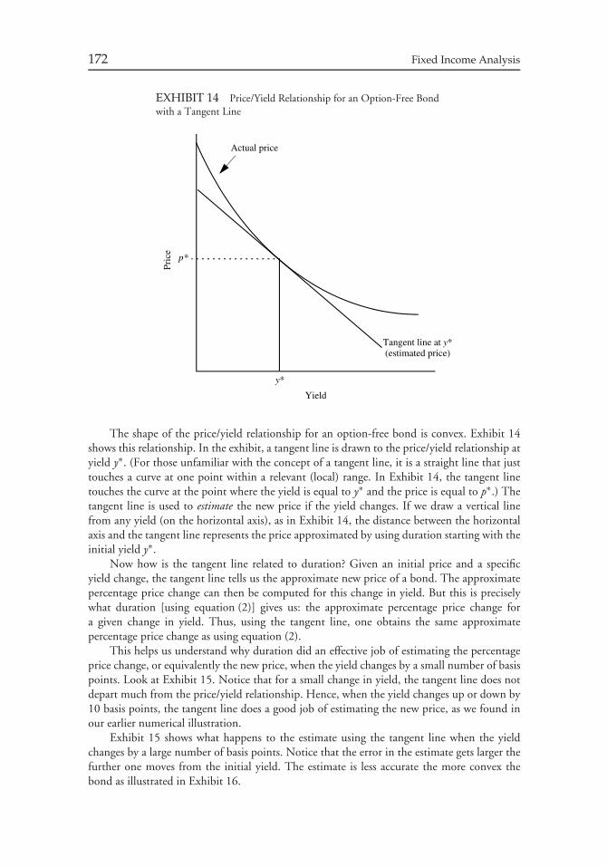
172 Fixed Income Analysis
EXHIBIT 14 Price/Yield Relationship for an Option-Free Bondwith a Tangent Line
Pric
e
Yield
Actual price
Tangent line at y*(estimated price)
p*
y*
The shape of the price/yield relationship for an option-free bond is convex. Exhibit 14shows this relationship. In the exhibit, a tangent line is drawn to the price/yield relationship atyield y∗. (For those unfamiliar with the concept of a tangent line, it is a straight line that justtouches a curve at one point within a relevant (local) range. In Exhibit 14, the tangent linetouches the curve at the point where the yield is equal to y∗ and the price is equal to p∗.) Thetangent line is used to estimate the new price if the yield changes. If we draw a vertical linefrom any yield (on the horizontal axis), as in Exhibit 14, the distance between the horizontalaxis and the tangent line represents the price approximated by using duration starting with theinitial yield y∗.
Now how is the tangent line related to duration? Given an initial price and a specificyield change, the tangent line tells us the approximate new price of a bond. The approximatepercentage price change can then be computed for this change in yield. But this is preciselywhat duration [using equation (2)] gives us: the approximate percentage price change fora given change in yield. Thus, using the tangent line, one obtains the same approximatepercentage price change as using equation (2).
This helps us understand why duration did an effective job of estimating the percentageprice change, or equivalently the new price, when the yield changes by a small number of basispoints. Look at Exhibit 15. Notice that for a small change in yield, the tangent line does notdepart much from the price/yield relationship. Hence, when the yield changes up or down by10 basis points, the tangent line does a good job of estimating the new price, as we found inour earlier numerical illustration.
Exhibit 15 shows what happens to the estimate using the tangent line when the yieldchanges by a large number of basis points. Notice that the error in the estimate gets larger thefurther one moves from the initial yield. The estimate is less accurate the more convex thebond as illustrated in Exhibit 16.
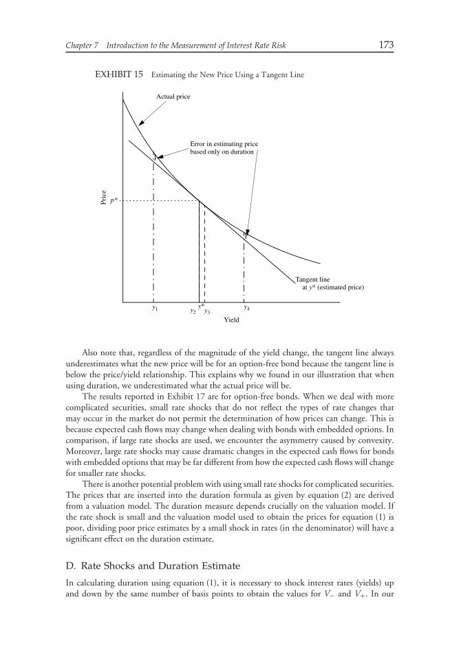
Chapter 7 Introduction to the Measurement of Interest Rate Risk 173
EXHIBIT 15 Estimating the New Price Using a Tangent Line
}
Pric
e
Yield
Actual price
Error in estimating pricebased only on duration
Tangent lineat y* (estimated price)
p*
y1 y2y*
y3y4
}
Also note that, regardless of the magnitude of the yield change, the tangent line alwaysunderestimates what the new price will be for an option-free bond because the tangent line isbelow the price/yield relationship. This explains why we found in our illustration that whenusing duration, we underestimated what the actual price will be.
The results reported in Exhibit 17 are for option-free bonds. When we deal with morecomplicated securities, small rate shocks that do not reflect the types of rate changes thatmay occur in the market do not permit the determination of how prices can change. This isbecause expected cash flows may change when dealing with bonds with embedded options. Incomparison, if large rate shocks are used, we encounter the asymmetry caused by convexity.Moreover, large rate shocks may cause dramatic changes in the expected cash flows for bondswith embedded options that may be far different from how the expected cash flows will changefor smaller rate shocks.
There is another potential problem with using small rate shocks for complicated securities.The prices that are inserted into the duration formula as given by equation (2) are derivedfrom a valuation model. The duration measure depends crucially on the valuation model. Ifthe rate shock is small and the valuation model used to obtain the prices for equation (1) ispoor, dividing poor price estimates by a small shock in rates (in the denominator) will have asignificant effect on the duration estimate.
D. Rate Shocks and Duration Estimate
In calculating duration using equation (1), it is necessary to shock interest rates (yields) upand down by the same number of basis points to obtain the values for V− and V+. In our
174 Fixed Income Analysis
EXHIBIT 16 Estimating the New Price for a Large Yield Change for Bonds withDifferent Convexities
Pric
e
Yield
Tangent lineat y* (estimated price)
p*
y*
Actual pricefor bond A
Actual pricefor bond B
Bond B has greater convexity than bond A.Price estimate better for bond A than bond B.
EXHIBIT 17 Duration Estimates for Different Rate Shocks
Assumption: Initial yield is 6%Bond 1 bp 10 bps 20 bps 50 bps 100 bps 150 bps 200 bps
6% 5 year 4.27 4.27 4.27 4.27 4.27 4.27 4.276% 20 year 11.56 11.56 11.56 11.57 11.61 11.69 11.799% 5 year 4.07 4.07 4.07 4.07 4.07 4.08 4.089% 20 year 10.66 10.66 10.66 10.67 10.71 10.77 10.86
illustration, 20 basis points was arbitrarily selected. But how large should the shock be? Thatis, how many basis points should be used to shock the rate?
In Exhibit 17, the duration estimates for our four hypothetical bonds using equation (1) forrate shocks of 1 basis point to 200 basis points are reported. The duration estimates for the two5-year bonds are not affected by the size of the shock. The two 5-year bonds are less convex thanthe two 20-year bonds. But even for the two 20-year bonds, for the size of the shocks reportedin Exhibit 17, the duration estimates are not materially affected by the greater convexity.
What is done in practice by dealers and vendors of analytical systems? Each systemdeveloper uses rate shocks that they have found to be realistic based on historical rate changes.
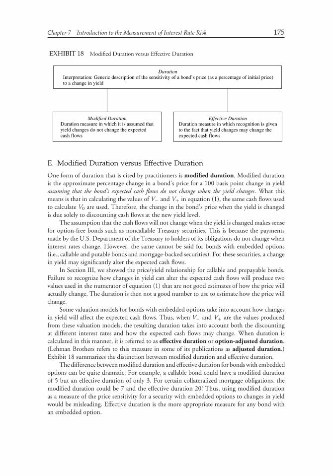
Chapter 7 Introduction to the Measurement of Interest Rate Risk 175
EXHIBIT 18 Modified Duration versus Effective Duration
DurationInterpretation: Generic description of the sensitivity of a bond’s price (as a percentage of initial price)to a change in yield
Modified DurationDuration measure in which it is assumed thatyield changes do not change the expectedcash flows
Effective DurationDuration measure in which recognition is givento the fact that yield changes may change theexpected cash flows
E. Modified Duration versus Effective Duration
One form of duration that is cited by practitioners is modified duration. Modified durationis the approximate percentage change in a bond’s price for a 100 basis point change in yieldassuming that the bond’s expected cash flows do not change when the yield changes. What thismeans is that in calculating the values of V− and V+ in equation (1), the same cash flows usedto calculate V0 are used. Therefore, the change in the bond’s price when the yield is changedis due solely to discounting cash flows at the new yield level.
The assumption that the cash flows will not change when the yield is changed makes sensefor option-free bonds such as noncallable Treasury securities. This is because the paymentsmade by the U.S. Department of the Treasury to holders of its obligations do not change wheninterest rates change. However, the same cannot be said for bonds with embedded options(i.e., callable and putable bonds and mortgage-backed securities). For these securities, a changein yield may significantly alter the expected cash flows.
In Section III, we showed the price/yield relationship for callable and prepayable bonds.Failure to recognize how changes in yield can alter the expected cash flows will produce twovalues used in the numerator of equation (1) that are not good estimates of how the price willactually change. The duration is then not a good number to use to estimate how the price willchange.
Some valuation models for bonds with embedded options take into account how changesin yield will affect the expected cash flows. Thus, when V− and V+ are the values producedfrom these valuation models, the resulting duration takes into account both the discountingat different interest rates and how the expected cash flows may change. When duration iscalculated in this manner, it is referred to as effective duration or option-adjusted duration.(Lehman Brothers refers to this measure in some of its publications as adjusted duration.)Exhibit 18 summarizes the distinction between modified duration and effective duration.
The difference between modified duration and effective duration for bonds with embeddedoptions can be quite dramatic. For example, a callable bond could have a modified durationof 5 but an effective duration of only 3. For certain collateralized mortgage obligations, themodified duration could be 7 and the effective duration 20! Thus, using modified durationas a measure of the price sensitivity for a security with embedded options to changes in yieldwould be misleading. Effective duration is the more appropriate measure for any bond withan embedded option.

176 Fixed Income Analysis
F. Macaulay Duration and Modified Duration
It is worth comparing the relationship between modified duration to the another durationmeasure, Macaulay duration. Modified duration can be written as:6
1
(1 + yield/k)
[1 × PVCF1 + 2 × PVCF2 . . . + n × PVCFn
k × Price
](3)
wherek = number of periods, or payments, per year (e.g., k = 2
for semiannual-pay bonds and k = 12 for monthly-pay bonds)n = number of periods until maturity (i.e., number of years to maturity times k)
yield = yield to maturity of the bondPVCFt = present value of the cash flow in period t discounted at the yield to maturity
where t = 1, 2, . . . , n
We know that duration tells us the approximate percentage price change for a bond if theyield changes.
The expression in the brackets of the modified duration formula given by equation (3) isa measure formulated in 1938 by Frederick Macaulay.7 This measure is popularly referred toas Macaulay duration. Thus, modified duration is commonly expressed as:
Modified duration = Macaulay duration
(1 + yield/k)
The general formulation for duration as given by equation (1) provides a short-cutprocedure for determining a bond’s modified duration. Because it is easier to calculate themodified duration using the short-cut procedure, most vendors of analytical software will useequation (1) rather than equation (3) to reduce computation time.
However, modified duration is a flawed measure of a bond’s price sensitivity to interest ratechanges for a bond with embedded options and therefore so is Macaulay duration. The durationformula given by equation (3) misleads the user because it masks the fact that changes inthe expected cash flows must be recognized for bonds with embedded options. Althoughequation (3) will give the same estimate of percent price change for an option-free bond asequation (1), equation (1) is still better because it acknowledges cash flows and thus value canchange due to yield changes.
G. Interpretations of Duration
Throughout this book, the definition provided for duration is: the approximate percentageprice change for a 100 basis point change in rates. That definition is the most relevant for howa manager or investor uses duration. In fact, if you understand this definition, you can easilycalculate the change in a bond’s value.
For example, suppose we want to know the approximate percentage change in pricefor a 50 basis point change in yield for our hypothetical 9% coupon 20-year bond sellingfor 134.6722. Since the duration is 10.66, a 100 basis point change in yield would changethe price by about 10.66%. For a 50 basis point change in yield, the price will change by
6More specifically, this is the formula for the modified duration of a bond on a coupon anniversary date.7Frederick Macaulay, Some Theoretical Problems Suggested by the Movement of Interest Rates, Bond Yields,and Stock Prices in the U.S. Since 1856 (New York: National Bureau of Economic Research, 1938).

Chapter 7 Introduction to the Measurement of Interest Rate Risk 177
approximately 5.33% (= 10.66%/2). So, if the yield increases by 50 basis points, the pricewill decrease by about 5.33% from 134.6722 to 127.4942.
Now let’s look at some other duration definitions or interpretations that appear inpublications and are cited by managers in discussions with their clients.
1. Duration Is the ‘‘First Derivative’’ Sometimes a market participant will refer toduration as the ‘‘first derivative of the price/yield function’’ or simply the ‘‘first derivative.’’Wow! Sounds impressive. First, ‘‘derivative’’ here has nothing to do with ‘‘derivative instru-ments’’ (i.e., futures, swaps, options, etc.). A derivative as used in this context is obtainedby differentiating a mathematical function using calculus. There are first derivatives, secondderivatives, and so on. When market participants say that duration is the first derivative, hereis what they mean. The first derivative calculates the slope of a line—in this case, the slopeof the tangent line in Exhibit 14. If it were possible to write a mathematical equation for abond in closed form, the first derivative would be the result of differentiating that equationthe first time. Even if you don’t know how to do the process of differentiation to get thefirst derivative, it sounds like you are really smart since it suggests you understand calculus!While it is a correct interpretation of duration, it is an interpretation that in no way helps usunderstand what the interest rate risk is of a bond. That is, it is an operationally meaninglessinterpretation.
Why is it an operationally meaningless interpretation? Go back to the $10 million bondposition with a duration of 6. Suppose a client is concerned with the exposure of the bond tochanges in interest rates. Now, tell that client the duration is 6 and that it is the first derivativeof the price function for that bond. What have you told the client? Not much. In contrast,tell that client that the duration is 6 and that duration is the approximate price sensitivityof a bond to a 100 basis point change in rates and you have told the client more relevantinformation with respect the bond’s interest rate risk.
2. Duration Is Some Measure of Time When the concept of duration was originallyintroduced by Macaulay in 1938, he used it as a gauge of the time that the bond wasoutstanding. More specifically, Macaulay defined duration as the weighted average of the timeto each coupon and principal payment of a bond. Subsequently, duration has too often beenthought of in temporal terms, i.e., years. This is most unfortunate for two reasons.
First, in terms of dimensions, there is nothing wrong with expressing duration in terms ofyears because that is the proper dimension of this value. But the proper interpretation is thatduration is the price volatility of a zero-coupon bond with that number of years to maturity.So, when a manager says a bond has a duration of 4 years, it is not useful to think of thismeasure in terms of time, but that the bond has the price sensitivity to rate changes of a 4-yearzero-coupon bond.
Second, thinking of duration in terms of years makes it difficult for managers and theirclients to understand the duration of some complex securities. Here are a few examples. Fora mortgage-backed security that is an interest-only security (i.e., receives coupons but notprincipal repayment) the duration is negative. What does a negative number, say, −4 mean?In terms of our interpretation as a percentage price change, it means that when rates changeby 100 basis points, the price of the bond changes by about 4% but the change is in the samedirection as the change in rates.
As a second example, consider an inverse floater created in the collateralized mortgageobligation (CMO) market. The underlying collateral for such a security might be loans with 25years to final maturity. However, an inverse floater can have a duration that easily exceeds 25.

178 Fixed Income Analysis
This does not make sense to a manager or client who uses a measure of time as a definition forduration.
As a final example, consider derivative instruments, such as an option that expires in oneyear. Suppose that it is reported that its duration is 60. What does that mean? To someonewho interprets duration in terms of time, does that mean 60 years, 60 days, 60 seconds? Itdoesn’t mean any of these. It simply means that the option tends to have the price sensitivityto rate changes of a 60-year zero-coupon bond.
3. Forget First Derivatives and Temporal Definitions The bottom line is that oneshould not care if it is technically correct to think of duration in terms of years (volatility of azero-coupon bond) or in terms of first derivatives. There are even some who interpret durationin terms of the ‘‘half life’’ of a security.8 Subject to the limitations that we will describe aswe proceed in this book, duration is the measure of a security’s price sensitivity to changes inyield. We will fine tune this definition as we move along.
Users of this interest rate risk measure are interested in what it tells them about the pricesensitivity of a bond (or a portfolio) to changes in interest rates. Duration provides the investorwith a feel for the dollar price exposure or the percentage price exposure to potential interestrate changes. Try the following definitions on a client who has a portfolio with a duration of4 and see which one the client finds most useful for understanding the interest rate risk of theportfolio when rates change:
Definition 1: The duration of 4 for your portfolio indicates that the portfolio’s value willchange by approximately 4% if rates change by 100 basis points.
Definition 2: The duration of 4 for your portfolio is the first derivative of the pricefunction for the bonds in the portfolio.
Definition 3: The duration of 4 for your portfolio is the weighted average number of yearsto receive the present value of the portfolio’s cash flows.
Definition 1 is clearly preferable. It would be ridiculous to expect clients to understand thelast two definitions better than the first.
Moreover, interpreting duration in terms of a measure of price sensitivity to interest ratechanges allows a manager to make comparisons between bonds regarding their interest raterisk under certain assumptions.
H. Portfolio Duration
A portfolio’s duration can be obtained by calculating the weighted average of the durationof the bonds in the portfolio. The weight is the proportion of the portfolio that a securitycomprises. Mathematically, a portfolio’s duration can be calculated as follows:
w1D1 + w2D2 + w3D3 + . . . + wK DKwhere
wi = market value of bond i/market value of the portfolioDi = duration of bond iK = number of bonds in the portfolio
8‘‘Half-life’’ is the time required for an element to be reduced to half its initial value.
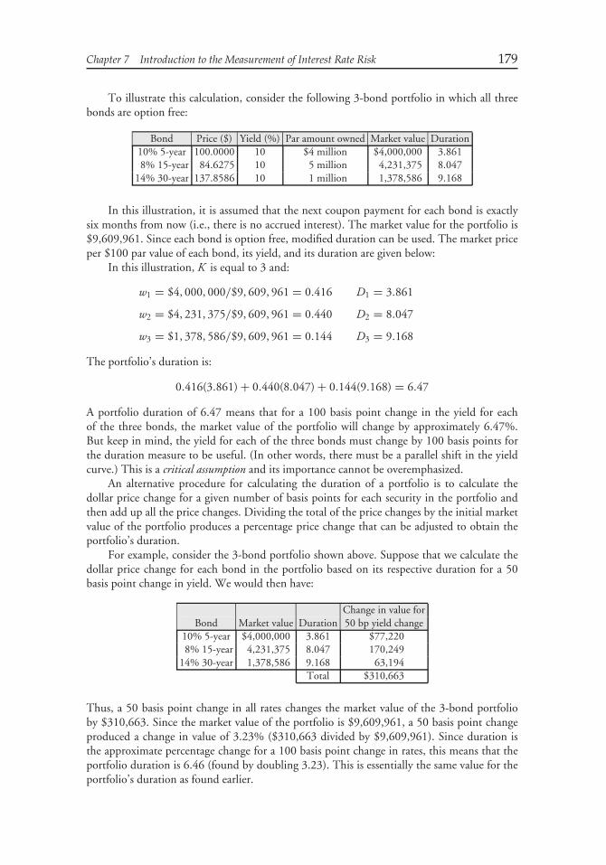
Chapter 7 Introduction to the Measurement of Interest Rate Risk 179
To illustrate this calculation, consider the following 3-bond portfolio in which all threebonds are option free:
Bond Price ($) Yield (%) Par amount owned Market value Duration10% 5-year 100.0000 10 $4 million $4,000,000 3.8618% 15-year 84.6275 10 5 million 4,231,375 8.047
14% 30-year 137.8586 10 1 million 1,378,586 9.168
In this illustration, it is assumed that the next coupon payment for each bond is exactlysix months from now (i.e., there is no accrued interest). The market value for the portfolio is$9,609,961. Since each bond is option free, modified duration can be used. The market priceper $100 par value of each bond, its yield, and its duration are given below:
In this illustration, K is equal to 3 and:
w1 = $4, 000, 000/$9, 609, 961 = 0.416 D1 = 3.861
w2 = $4, 231, 375/$9, 609, 961 = 0.440 D2 = 8.047
w3 = $1, 378, 586/$9, 609, 961 = 0.144 D3 = 9.168
The portfolio’s duration is:
0.416(3.861) + 0.440(8.047) + 0.144(9.168) = 6.47
A portfolio duration of 6.47 means that for a 100 basis point change in the yield for eachof the three bonds, the market value of the portfolio will change by approximately 6.47%.But keep in mind, the yield for each of the three bonds must change by 100 basis points forthe duration measure to be useful. (In other words, there must be a parallel shift in the yieldcurve.) This is a critical assumption and its importance cannot be overemphasized.
An alternative procedure for calculating the duration of a portfolio is to calculate thedollar price change for a given number of basis points for each security in the portfolio andthen add up all the price changes. Dividing the total of the price changes by the initial marketvalue of the portfolio produces a percentage price change that can be adjusted to obtain theportfolio’s duration.
For example, consider the 3-bond portfolio shown above. Suppose that we calculate thedollar price change for each bond in the portfolio based on its respective duration for a 50basis point change in yield. We would then have:
Change in value forBond Market value Duration 50 bp yield change
10% 5-year $4,000,000 3.861 $77,2208% 15-year 4,231,375 8.047 170,249
14% 30-year 1,378,586 9.168 63,194Total $310,663
Thus, a 50 basis point change in all rates changes the market value of the 3-bond portfolioby $310,663. Since the market value of the portfolio is $9,609,961, a 50 basis point changeproduced a change in value of 3.23% ($310,663 divided by $9,609,961). Since duration isthe approximate percentage change for a 100 basis point change in rates, this means that theportfolio duration is 6.46 (found by doubling 3.23). This is essentially the same value for theportfolio’s duration as found earlier.
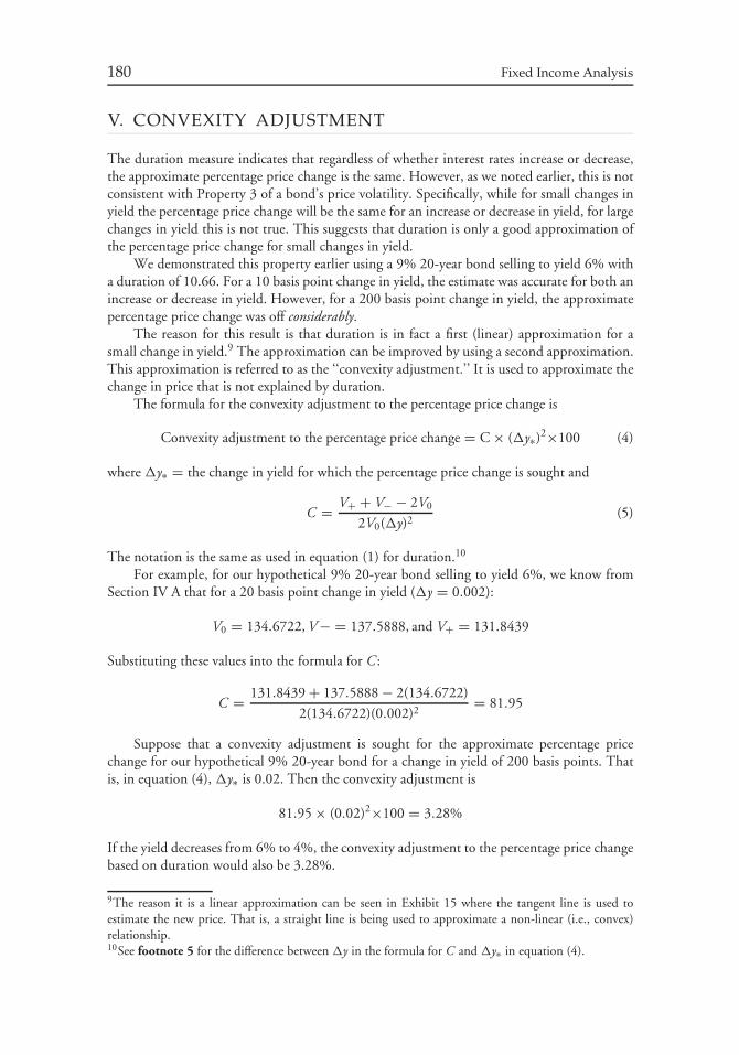
180 Fixed Income Analysis
V. CONVEXITY ADJUSTMENT
The duration measure indicates that regardless of whether interest rates increase or decrease,the approximate percentage price change is the same. However, as we noted earlier, this is notconsistent with Property 3 of a bond’s price volatility. Specifically, while for small changes inyield the percentage price change will be the same for an increase or decrease in yield, for largechanges in yield this is not true. This suggests that duration is only a good approximation ofthe percentage price change for small changes in yield.
We demonstrated this property earlier using a 9% 20-year bond selling to yield 6% witha duration of 10.66. For a 10 basis point change in yield, the estimate was accurate for both anincrease or decrease in yield. However, for a 200 basis point change in yield, the approximatepercentage price change was off considerably.
The reason for this result is that duration is in fact a first (linear) approximation for asmall change in yield.9 The approximation can be improved by using a second approximation.This approximation is referred to as the ‘‘convexity adjustment.’’ It is used to approximate thechange in price that is not explained by duration.
The formula for the convexity adjustment to the percentage price change is
Convexity adjustment to the percentage price change = C × (�y∗)2×100 (4)
where �y∗ = the change in yield for which the percentage price change is sought and
C = V+ + V− − 2V0
2V0(�y)2(5)
The notation is the same as used in equation (1) for duration.10
For example, for our hypothetical 9% 20-year bond selling to yield 6%, we know fromSection IV A that for a 20 basis point change in yield (�y = 0.002):
V0 = 134.6722, V − = 137.5888, and V+ = 131.8439
Substituting these values into the formula for C :
C = 131.8439 + 137.5888 − 2(134.6722)
2(134.6722)(0.002)2= 81.95
Suppose that a convexity adjustment is sought for the approximate percentage pricechange for our hypothetical 9% 20-year bond for a change in yield of 200 basis points. Thatis, in equation (4), �y∗ is 0.02. Then the convexity adjustment is
81.95 × (0.02)2×100 = 3.28%
If the yield decreases from 6% to 4%, the convexity adjustment to the percentage price changebased on duration would also be 3.28%.
9The reason it is a linear approximation can be seen in Exhibit 15 where the tangent line is used toestimate the new price. That is, a straight line is being used to approximate a non-linear (i.e., convex)relationship.10See footnote 5 for the difference between �y in the formula for C and �y∗ in equation (4).
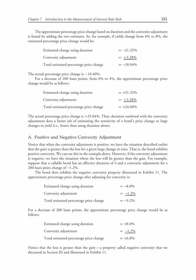
Chapter 7 Introduction to the Measurement of Interest Rate Risk 181
The approximate percentage price change based on duration and the convexity adjustmentis found by adding the two estimates. So, for example, if yields change from 6% to 8%, theestimated percentage price change would be:
Estimated change using duration = −21.32%
Convexity adjustment = +3.28%
Total estimated percentage price change = −18.04%
The actual percentage price change is −18.40%.For a decrease of 200 basis points, from 6% to 4%, the approximate percentage price
change would be as follows:
Estimated change using duration = +21.32%
Convexity adjustment = +3.28%
Total estimated percentage price change = +24.60%
The actual percentage price change is +25.04%. Thus, duration combined with the convexityadjustment does a better job of estimating the sensitivity of a bond’s price change to largechanges in yield (i.e., better than using duration alone).
A. Positive and Negative Convexity Adjustment
Notice that when the convexity adjustment is positive, we have the situation described earlierthat the gain is greater than the loss for a given large change in rates. That is, the bond exhibitspositive convexity. We can see this in the example above. However, if the convexity adjustmentis negative, we have the situation where the loss will be greater than the gain. For example,suppose that a callable bond has an effective duration of 4 and a convexity adjustment for a200 basis point change of −1.2%.
The bond then exhibits the negative convexity property illustrated in Exhibit 11. Theapproximate percentage price change after adjusting for convexity is:
Estimated change using duration = −8.0%
Convexity adjustment = −1.2%
Total estimated percentage price change = −9.2%
For a decrease of 200 basis points, the approximate percentage price change would be asfollows:
Estimated change using duration = +8.0%
Convexity adjustment = −1.2%
Total estimated percentage price change = +6.8%
Notice that the loss is greater than the gain—a property called negative convexity that wediscussed in Section III and illustrated in Exhibit 11.
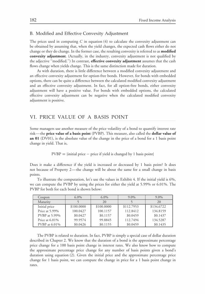
182 Fixed Income Analysis
B. Modified and Effective Convexity Adjustment
The prices used in computing C in equation (4) to calculate the convexity adjustment canbe obtained by assuming that, when the yield changes, the expected cash flows either do notchange or they do change. In the former case, the resulting convexity is referred to as modifiedconvexity adjustment. (Actually, in the industry, convexity adjustment is not qualified bythe adjective ‘‘modified.’’) In contrast, effective convexity adjustment assumes that the cashflows change when yields change. This is the same distinction made for duration.
As with duration, there is little difference between a modified convexity adjustment andan effective convexity adjustment for option-free bonds. However, for bonds with embeddedoptions, there can be quite a difference between the calculated modified convexity adjustmentand an effective convexity adjustment. In fact, for all option-free bonds, either convexityadjustment will have a positive value. For bonds with embedded options, the calculatedeffective convexity adjustment can be negative when the calculated modified convexityadjustment is positive.
VI. PRICE VALUE OF A BASIS POINT
Some managers use another measure of the price volatility of a bond to quantify interest raterisk—the price value of a basis point (PVBP). This measure, also called the dollar value ofan 01 (DV01), is the absolute value of the change in the price of a bond for a 1 basis pointchange in yield. That is,
PVBP = |initial price − price if yield is changed by 1 basis point|
Does it make a difference if the yield is increased or decreased by 1 basis point? It doesnot because of Property 2—the change will be about the same for a small change in basispoints.
To illustrate the computation, let’s use the values in Exhibit 4. If the initial yield is 6%,we can compute the PVBP by using the prices for either the yield at 5.99% or 6.01%. ThePVBP for both for each bond is shown below:
Coupon 6.0% 6.0% 9.0% 9.0%Maturity 5 20 5 20Initial price $100.0000 $100.0000 $112.7953 $134.6722Price at 5.99% 100.0427 100.1157 112.8412 134.8159PVBP at 5.99% $0.0427 $0.1157 $0.0459 $0.1437Price at 6.01% 99.9574 99.8845 112.7494 134.5287PVBP at 6.01% $0.0426 $0.1155 $0.0459 $0.1435
The PVBP is related to duration. In fact, PVBP is simply a special case of dollar durationdescribed in Chapter 2. We know that the duration of a bond is the approximate percentageprice change for a 100 basis point change in interest rates. We also know how to computethe approximate percentage price change for any number of basis points given a bond’sduration using equation (2). Given the initial price and the approximate percentage pricechange for 1 basis point, we can compute the change in price for a 1 basis point change inrates.
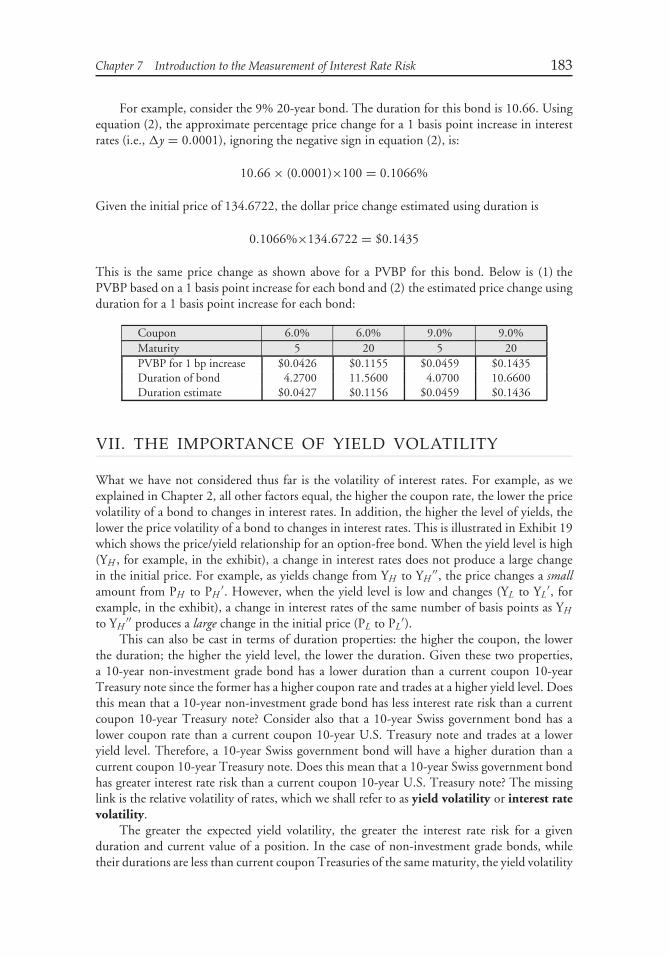
Chapter 7 Introduction to the Measurement of Interest Rate Risk 183
For example, consider the 9% 20-year bond. The duration for this bond is 10.66. Usingequation (2), the approximate percentage price change for a 1 basis point increase in interestrates (i.e., �y = 0.0001), ignoring the negative sign in equation (2), is:
10.66 × (0.0001)×100 = 0.1066%
Given the initial price of 134.6722, the dollar price change estimated using duration is
0.1066%×134.6722 = $0.1435
This is the same price change as shown above for a PVBP for this bond. Below is (1) thePVBP based on a 1 basis point increase for each bond and (2) the estimated price change usingduration for a 1 basis point increase for each bond:
Coupon 6.0% 6.0% 9.0% 9.0%Maturity 5 20 5 20PVBP for 1 bp increase $0.0426 $0.1155 $0.0459 $0.1435Duration of bond 4.2700 11.5600 4.0700 10.6600Duration estimate $0.0427 $0.1156 $0.0459 $0.1436
VII. THE IMPORTANCE OF YIELD VOLATILITY
What we have not considered thus far is the volatility of interest rates. For example, as weexplained in Chapter 2, all other factors equal, the higher the coupon rate, the lower the pricevolatility of a bond to changes in interest rates. In addition, the higher the level of yields, thelower the price volatility of a bond to changes in interest rates. This is illustrated in Exhibit 19which shows the price/yield relationship for an option-free bond. When the yield level is high(YH , for example, in the exhibit), a change in interest rates does not produce a large changein the initial price. For example, as yields change from YH to YH
′′, the price changes a smallamount from PH to PH
′. However, when the yield level is low and changes (YL to YL′, for
example, in the exhibit), a change in interest rates of the same number of basis points as YH
to YH′′ produces a large change in the initial price (PL to PL
′).This can also be cast in terms of duration properties: the higher the coupon, the lower
the duration; the higher the yield level, the lower the duration. Given these two properties,a 10-year non-investment grade bond has a lower duration than a current coupon 10-yearTreasury note since the former has a higher coupon rate and trades at a higher yield level. Doesthis mean that a 10-year non-investment grade bond has less interest rate risk than a currentcoupon 10-year Treasury note? Consider also that a 10-year Swiss government bond has alower coupon rate than a current coupon 10-year U.S. Treasury note and trades at a loweryield level. Therefore, a 10-year Swiss government bond will have a higher duration than acurrent coupon 10-year Treasury note. Does this mean that a 10-year Swiss government bondhas greater interest rate risk than a current coupon 10-year U.S. Treasury note? The missinglink is the relative volatility of rates, which we shall refer to as yield volatility or interest ratevolatility.
The greater the expected yield volatility, the greater the interest rate risk for a givenduration and current value of a position. In the case of non-investment grade bonds, whiletheir durations are less than current coupon Treasuries of the same maturity, the yield volatility
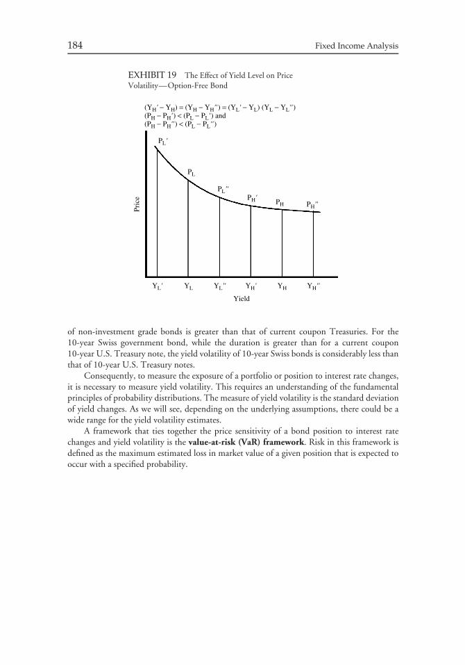
184 Fixed Income Analysis
EXHIBIT 19 The Effect of Yield Level on PriceVolatility—Option-Free Bond
(YH' − YH) = (YH − YH'' ) = (YL' − YL) (YL − YL'' )(PH − PH' ) < (PL − PL' ) and(PH − PH'' ) < (PL − PL'' )
Pric
ePL'
YL' YL YL'' YH' YH YH''
PL''PH'
PH''PH
PL
Yield
of non-investment grade bonds is greater than that of current coupon Treasuries. For the10-year Swiss government bond, while the duration is greater than for a current coupon10-year U.S. Treasury note, the yield volatility of 10-year Swiss bonds is considerably less thanthat of 10-year U.S. Treasury notes.
Consequently, to measure the exposure of a portfolio or position to interest rate changes,it is necessary to measure yield volatility. This requires an understanding of the fundamentalprinciples of probability distributions. The measure of yield volatility is the standard deviationof yield changes. As we will see, depending on the underlying assumptions, there could be awide range for the yield volatility estimates.
A framework that ties together the price sensitivity of a bond position to interest ratechanges and yield volatility is the value-at-risk (VaR) framework. Risk in this framework isdefined as the maximum estimated loss in market value of a given position that is expected tooccur with a specified probability.
CHAPTER 8TERM STRUCTURE AND
VOLATILITY OF INTERESTRATES
I. INTRODUCTION
Market participants pay close attention to yields on Treasury securities. An analysis ofthese yields is critical because they are used to derive interest rates which are used to valuesecurities. Also, they are benchmarks used to establish the minimum yields that investorswant when investing in a non-Treasury security. We distinguish between the on-the-run(i.e., the most recently auctioned Treasury securities) Treasury yield curve and the termstructure of interest rates. The on-the-run Treasury yield curve shows the relationship betweenthe yield for on-the-run Treasury issues and maturity. The term structure of interest ratesis the relationship between the theoretical yield on zero-coupon Treasury securities andmaturity. The yield on a zero-coupon Treasury security is called the Treasury spot rate.The term structure of interest rates is thus the relationship between Treasury spot ratesand maturity. The importance of this distinction between the Treasury yield curve andthe Treasury spot rate curve is that it is the latter that is used to value fixed-incomesecurities.
In Chapter 6 we demonstrated how to derive the Treasury spot rate curve from theon-the-run Treasury issues using the method of bootstrapping and then how to obtain anarbitrage-free value for an option-free bond. In this chapter we will describe other methods toderive the Treasury spot rates. In addition, we explained that another benchmark that is beingused by practitioners to value securities is the swap curve. We discuss the swap curve in thischapter.
In Chapter 4, the theories of the term structure of interest rates were explained. Each ofthese theories seeks to explain the shape of the yield curve. Then, in Chapter 6, the concept offorward rates was explained. In this chapter, we explain the role that forward rates play in thetheories of the term structure of interest rates. In addition, we critically evaluate one of thesetheories, the pure expectations theory, because of the economic interpretation of forward ratesbased on this theory.
We also mentioned the role of interest rate volatility or yield volatility in valuing securitiesand in measuring interest rate exposure of a bond. In the analytical chapters we will continueto see the importance of this measure. Specifically, we will see the role of interest rate volatilityin valuing bonds with embedded options, valuing mortgage-backed and certain asset-backed
185
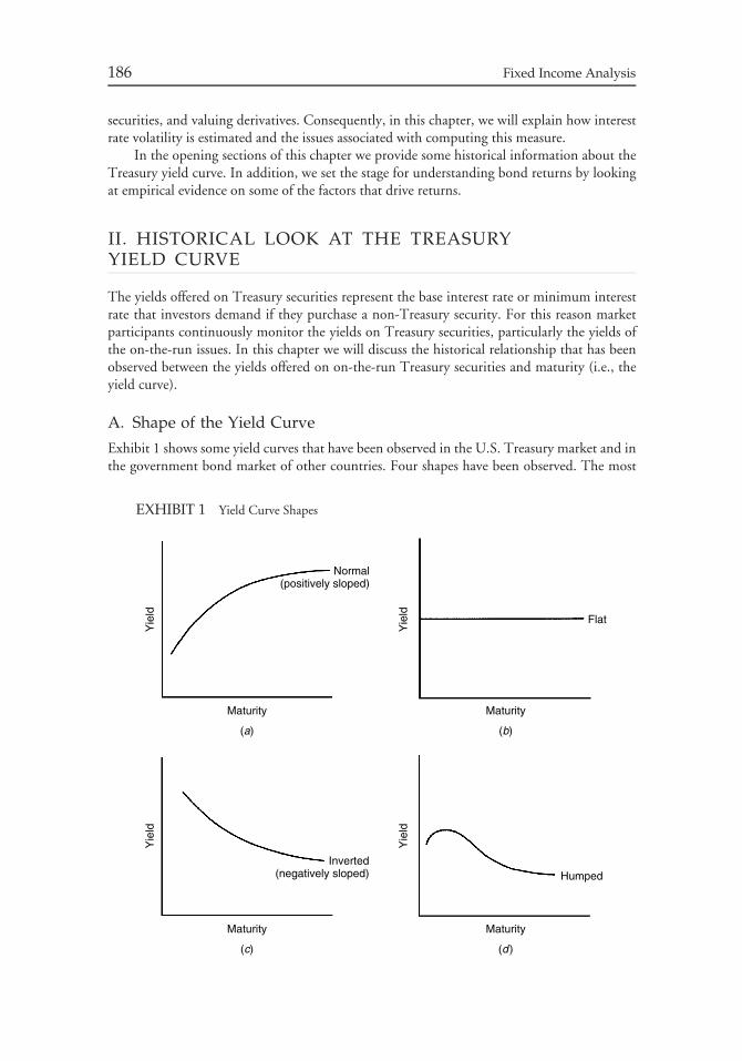
186 Fixed Income Analysis
securities, and valuing derivatives. Consequently, in this chapter, we will explain how interestrate volatility is estimated and the issues associated with computing this measure.
In the opening sections of this chapter we provide some historical information about theTreasury yield curve. In addition, we set the stage for understanding bond returns by lookingat empirical evidence on some of the factors that drive returns.
II. HISTORICAL LOOK AT THE TREASURYYIELD CURVE
The yields offered on Treasury securities represent the base interest rate or minimum interestrate that investors demand if they purchase a non-Treasury security. For this reason marketparticipants continuously monitor the yields on Treasury securities, particularly the yields ofthe on-the-run issues. In this chapter we will discuss the historical relationship that has beenobserved between the yields offered on on-the-run Treasury securities and maturity (i.e., theyield curve).
A. Shape of the Yield Curve
Exhibit 1 shows some yield curves that have been observed in the U.S. Treasury market and inthe government bond market of other countries. Four shapes have been observed. The most
EXHIBIT 1 Yield Curve Shapes
Maturity
Yie
ld
Yie
ldY
ield
Yie
ld
Normal(positively sloped)
Inverted(negatively sloped)
Flat
Humped
(a)
Maturity
(c)
Maturity
(b)
Maturity
(d)
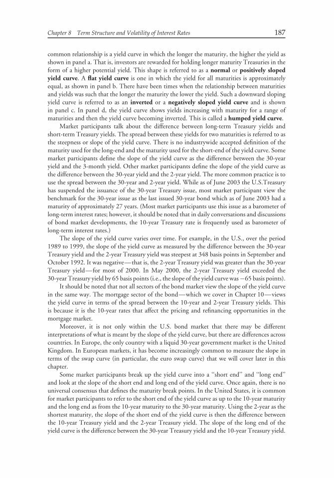
Chapter 8 Term Structure and Volatility of Interest Rates 187
common relationship is a yield curve in which the longer the maturity, the higher the yield asshown in panel a. That is, investors are rewarded for holding longer maturity Treasuries in theform of a higher potential yield. This shape is referred to as a normal or positively slopedyield curve. A flat yield curve is one in which the yield for all maturities is approximatelyequal, as shown in panel b. There have been times when the relationship between maturitiesand yields was such that the longer the maturity the lower the yield. Such a downward slopingyield curve is referred to as an inverted or a negatively sloped yield curve and is shownin panel c. In panel d, the yield curve shows yields increasing with maturity for a range ofmaturities and then the yield curve becoming inverted. This is called a humped yield curve.
Market participants talk about the difference between long-term Treasury yields andshort-term Treasury yields. The spread between these yields for two maturities is referred to asthe steepness or slope of the yield curve. There is no industrywide accepted definition of thematurity used for the long-end and the maturity used for the short-end of the yield curve. Somemarket participants define the slope of the yield curve as the difference between the 30-yearyield and the 3-month yield. Other market participants define the slope of the yield curve asthe difference between the 30-year yield and the 2-year yield. The more common practice is touse the spread between the 30-year and 2-year yield. While as of June 2003 the U.S.Treasuryhas suspended the issuance of the 30-year Treasury issue, most market participant view thebenchmark for the 30-year issue as the last issued 30-year bond which as of June 2003 had amaturity of approximately 27 years. (Most market participants use this issue as a barometer oflong-term interest rates; however, it should be noted that in daily conversations and discussionsof bond market developments, the 10-year Treasury rate is frequently used as barometer oflong-term interest rates.)
The slope of the yield curve varies over time. For example, in the U.S., over the period1989 to 1999, the slope of the yield curve as measured by the difference between the 30-yearTreasury yield and the 2-year Treasury yield was steepest at 348 basis points in September andOctober 1992. It was negative—that is, the 2-year Treasury yield was greater than the 30-yearTreasury yield—for most of 2000. In May 2000, the 2-year Treasury yield exceeded the30-year Treasury yield by 65 basis points (i.e., the slope of the yield curve was −65 basis points).
It should be noted that not all sectors of the bond market view the slope of the yield curvein the same way. The mortgage sector of the bond—which we cover in Chapter 10—viewsthe yield curve in terms of the spread between the 10-year and 2-year Treasury yields. Thisis because it is the 10-year rates that affect the pricing and refinancing opportunities in themortgage market.
Moreover, it is not only within the U.S. bond market that there may be differentinterpretations of what is meant by the slope of the yield curve, but there are differences acrosscountries. In Europe, the only country with a liquid 30-year government market is the UnitedKingdom. In European markets, it has become increasingly common to measure the slope interms of the swap curve (in particular, the euro swap curve) that we will cover later in thischapter.
Some market participants break up the yield curve into a ‘‘short end’’ and ‘‘long end’’and look at the slope of the short end and long end of the yield curve. Once again, there is nouniversal consensus that defines the maturity break points. In the United States, it is commonfor market participants to refer to the short end of the yield curve as up to the 10-year maturityand the long end as from the 10-year maturity to the 30-year maturity. Using the 2-year as theshortest maturity, the slope of the short end of the yield curve is then the difference betweenthe 10-year Treasury yield and the 2-year Treasury yield. The slope of the long end of theyield curve is the difference between the 30-year Treasury yield and the 10-year Treasury yield.
188 Fixed Income Analysis
Historically, the long end of the yield curve has been flatter than the short-end of the yieldcurve. For example, in October 1992 when the slope of the yield curve was the greatest at 348basis points, the slope of the long end of the yield curve was only 95 basis points.
Market participants often decompose the yield curve into three maturity sectors: short,intermediate, and long. Again, there is no consensus as to what the maturity break points areand those break points can differ by sector and by country. In the United States, a commonbreakdown has the 1–5 year sector as the short end (ignoring maturities less than 1 year), the5–10 year sector as the intermediate end, and greater than 10-year maturities as the long end.1
In Continental Europe where there is little issuance of bonds with a maturity greater than 10years, the long end of the yield sector is the 10-year sector.
B. Yield Curve Shifts
A shift in the yield curve refers to the relative change in the yield for each Treasury maturity.A parallel shift in the yield curve refers to a shift in which the change in the yield forall maturities is the same. A nonparallel shift in the yield curve means that the yield fordifferent maturities does not change by the same number of basis points. Both of these shiftsare graphically portrayed in Exhibit 2.
Historically, two types of nonparallel yield curve shifts have been observed: (1) a twistin the slope of the yield curve and (2) a change in the humpedness or curvature of the yieldcurve. A twist in the slope of the yield curve refers to a flattening or steepening of the yieldcurve. A flattening of the yield curve means that the slope of the yield curve (i.e., the spreadbetween the yield on a long-term and short-term Treasury) has decreased; a steepening of theyield curve means that the slope of the yield curve has increased. This is depicted in panel bof Exhibit 2.
The other type of nonparallel shift is a change in the curvature or humpedness of theyield curve. This type of shift involves the movement of yields at the short maturity and longmaturity sectors of the yield curve relative to the movement of yields in the intermediatematurity sector of the yield curve. Such nonparallel shifts in the yield curve that changeits curvature are referred to as butterfly shifts. The name comes from viewing the threematurity sectors (short, intermediate, and long) as three parts of a butterfly. Specifically, theintermediate maturity sector is viewed as the body of the butterfly and the short maturity andlong maturity sectors are viewed as the wings of the butterfly.
A positive butterfly means that the yield curve becomes less humped (i.e., has lesscurvature). This means that if yields increase, for example, the yields in the short maturity andlong maturity sectors increase more than the yields in the intermediate maturity sector. If yieldsdecrease, the yields in the short and long maturity sectors decrease less than the intermediatematurity sector. A negative butterfly means the yield curve becomes more humped (i.e., hasmore curvature). So, if yields increase, for example, yields in the intermediate maturity sectorwill increase more than yields in the short maturity and long maturity sectors. If, instead,yields decrease, a negative butterfly occurs when yields in the intermediate maturity sectordecrease less than the short maturity and long maturity sectors. Butterfly shifts are depicted inpanel c of Exhibit 2.
1Index constructors such as Lehman Brothers when constructing maturity sector indexes define ‘‘short-term sector’’ as up to three years, the ‘‘intermediate sector’’ as maturities greater than three years but lessthan 10 years (note the overlap with the short-term sector), and the ‘‘long-term sector’’ as greater than10 years.
Chapter 8 Term Structure and Volatility of Interest Rates 189
EXHIBIT 2 Types of Yield Curve Shifts
(a) Parallel shifts
Upward parallel shift
Yield
Maturity
(b) Nonparallel shifts: Twists (steepening and flattening)
(c) Nonparallel shifts: Butterfly shifts (positive and negative)
Initial curveDownward parallel shift
Flattening of curveInitial curve
Steepening of curveInitial curve
Initial curveInitial curve
Negative butterfly shift
Positive butterfly shift
Yield
Maturity
Yield
Maturity
Yield
Maturity
Yield
Maturity
Historically, these three types of shifts in the yield curve have not been found to beindependent. The two most common types of shifts have been (1) a downward shift in theyield curve combined with a steepening of the yield curve and (2) an upward shift in theyield curve combined with a flattening of the yield curve. Positive butterfly shifts tend to beassociated with an upward shift in yields and negative butterfly shifts with a downward shift inyields. Another way to state this is that yields in the short-tem sector tend to be more volatilethan yields in the long-term sector.
III. TREASURY RETURNS RESULTING FROMYIELD CURVE MOVEMENTS
As we discussed in Chapter 6, a yield measure is a promised return if certain assumptionsare satisfied; but total return (return from coupons and price change) is a more appropriatemeasure of the potential return from investing in a Treasury security. The total return for a
190 Fixed Income Analysis
short investment horizon depends critically on how interest rates change, reflected by how theyield curve changes.
There have been several published and unpublished studies of how changes in the shapeof the yield curve affect the total return on Treasury securities. The first such study by tworesearchers at Goldman Sachs (Robert Litterman and José Scheinkman) was published in1991.2 The results reported in more recent studies support the findings of the Litterman-Scheinkman study so we will just discuss their findings. Litterman and Scheinkman found thatthree factors explained historical returns for zero-coupon Treasury securities for all maturities.The first factor was changes in the level of rates, the second factor was changes in the slope ofthe yield curve, and the third factor was changes in the curvature of the yield curve.
Litterman and Scheinkman employed regression analysis to determine the relativecontribution of these three factors in explaining the returns on zero-coupon Treasury securitiesof different maturities. They determined the importance of each factor by its coefficient ofdetermination, popularly referred to as the ‘‘R2.’’ In general, the R2 measures the percentageof the variance in the dependent variable (i.e., the total return on the zero-coupon Treasurysecurity in their study) explained by the independent variables (i.e., the three factors).3 Forexample, an R2 of 0.8 means that 80% of the variation of the return on a zero-coupon Treasurysecurity is explained by the three factors. Therefore, 20% of the variation of the return is notexplained by these three factors. The R2 will have a value between 0% and 100%. In theLitterman-Scheinkman study, the R2 was very high for all maturities, meaning that the threefactors had a very strong explanatory power.
The first factor, representing changes in the level of rates, holding all other factors constant(in particular, yield curve slope), had the greatest explanatory power for all the maturities,averaging about 90%. The implication is that the most important factor that a manager of aTreasury portfolio should control for is exposure to changes in the level of interest rates. Forthis reason it is important to have a way to measure or quantify this risk. Duration is in factthe measure used to quantify exposure to a parallel shift in the yield curve.
The second factor, changes in the yield curve slope, was the second largest contributingfactor. The average relative contribution for all maturities was 8.5%. Thus, changes in theyield curve slope was, on average, about one tenth as significant as changes in the level of rates.While the relative contribution was only 8.5%, this can still have a significant impact on thereturn for a Treasury portfolio and a portfolio manager must control for this risk. We brieflyexplained in Chapter 2 how a manager can do this using key rate duration and will discussthis further in this chapter.
The third factor, changes in the curvature of the yield curve, contributed relatively littleto explaining historical returns for Treasury zero-coupon securities.
IV. CONSTRUCTING THE THEORETICAL SPOTRATE CURVE FOR TREASURIES
Our focus thus far has been on the shape of the Treasury yield curve. In fact, often thefinancial press in its discussion of interest rates focuses on the Treasury yield curve. However,
2Robert Litterman and José Scheinkman, ‘‘Common Factors Affecting Bond Returns,’’ Journal of FixedIncome (June 1991), pp. 54–61.3For a further explanation of the coefficient of determination, see Richard A. DeFusco, DennisW. McLeavey, Jerald E. Pinto, and David E. Runkle, Quantitative Methods for Investment Analysis(Charlottesville, VA: Association for Investment Management and Research, 2002), pp. 388–390.
Chapter 8 Term Structure and Volatility of Interest Rates 191
as explained in Chapter 5, it is the default-free spot rate curve as represented by the Treasuryspot rate curve that is used in valuing fixed-income securities. But how does one obtainthe default-free spot rate curve? This curve can be constructed from the yields on Treasurysecurities. The Treasury issues that are candidates for inclusion are:
1. Treasury coupon strips2. on-the-run Treasury issues3. on-the-run Treasury issues and selected off-the-run Treasury issues4. all Treasury coupon securities and bills
Once the securities that are to be included in the construction of the theoretical spotrate curve are selected, the methodology for constructing the curve must be determined. Themethodology depends on the securities included. If Treasury coupon strips are used, theprocedure is simple since the observed yields are the spot rates. If the on-the-run Treasuryissues with or without selected off-the-run Treasury issues are used, then the methodology ofbootstrapping is used.
Using an estimated Treasury par yield curve, bootstrapping is a repetitive techniquewhereby the yields prior to some maturity, same m, are used to obtain the spot rate for yearm. For example, suppose that the yields on the par yield curve are denoted by y1,...,yT wherethe subscripts denote the time periods. Then the yield for the first period, y1, is the spot ratefor the first period. Let the first period spot rate be denoted as s1. Then y2 and s1 can be usedto derive s2 using arbitrage arguments. Next, y3, s1, and s2 are used to derive s3 using arbitragearguments. The process continues until all the spot rates are derived, s1,..., sm.
In selecting the universe of securities used to construct a default-free spot rate curve,one wants to make sure that the yields are not biased by any of the following: (1) default,(2) embedded options, (3) liquidity, and (4) pricing errors. To deal with default, U.S. Treasurysecurities are used. Issues with embedded options are avoided because the market yield reflectsthe value of the embedded options. In the U.S. Treasury market, there are only a few callablebonds so this is not an issue. In other countries, however, there are callable and putablegovernment bonds. Liquidity varies by issue. There are U.S. Treasury issues that have lessliquidity than bonds with a similar maturity. In fact, there are some issues that have extremelyhigh liquidity because they are used by dealers in repurchase agreements. Finally, in somecountries the trading of certain government bonds issues is limited, resulting in estimatedprices that may not reflect the true price.
Given the theoretical spot rate for each maturity, there are various statistical techniquesthat are used to create a continuous spot rate curve. A discussion of these statistical techniquesis a specialist topic.
A. Treasury Coupon Strips
It would seem simplest to use the observed yield on Treasury coupon strips to constructan actual spot rate curve because there are three problems with using the observed rates onTreasury strips. First, the liquidity of the strips market is not as great as that of the Treasurycoupon market. Thus, the observed rates on strips reflect a premium for liquidity.
Second, the tax treatment of strips is different from that of Treasury coupon securities.Specifically, the accrued interest on strips is taxed even though no cash is received by theinvestor. Thus, they are negative cash flow securities to taxable entities, and, as a result, theiryield reflects this tax disadvantage.
192 Fixed Income Analysis
Finally, there are maturity sectors where non-U.S. investors find it advantageous to tradeoff yield for tax advantages associated with a strip. Specifically, certain foreign tax authoritiesallow their citizens to treat the difference between the maturity value and the purchase price asa capital gain and tax this gain at a favorable tax rate. Some will grant this favorable treatmentonly when the strip is created from the principal rather than the coupon. For this reason,those who use Treasury strips to represent theoretical spot rates restrict the issues included tocoupon strips.
B. On-the-Run Treasury Issues
The on-the-run Treasury issues are the most recently auctioned issues of a given maturity. Inthe U.S., these issues include the 1-month, 3-month, and 6-month Treasury bills, and the2-year, 5-year, and 10-year Treasury notes. Treasury bills are zero-coupon instruments; thenotes are coupon securities.4
There is an observed yield for each of the on-the-run issues. For the coupon issues, theseyields are not the yields used in the analysis when the issue is not trading at par. Instead, foreach on-the-run coupon issue, the estimated yield necessary to make the issue trade at par isused. The resulting on-the-run yield curve is called the par coupon curve. The reason forusing securities with a price of par is to eliminate the effect of the tax treatment for securitiesselling at a discount or premium. The differential tax treatment distorts the yield.
C. On-the-Run Treasury Issues and Selected Off-the-Run TreasuryIssues
One of the problems with using just the on-the-run issues is the large gap between maturities,particularly after five years. To mitigate this problem, some dealers and vendors use selectedoff-the-run Treasury issues. Typically, the issues used are the 20-year issue and 25-year issue.5
Given the par coupon curve including any off-the-run selected issues, a linear interpolationmethod is used to fill in the gaps for the other maturities. The bootstrapping method is thenused to construct the theoretical spot rate curve.
D. All Treasury Coupon Securities and Bills
Using only on-the-run issues and a few off-the-run issues fails to recognize the informationembodied in Treasury prices that are not included in the analysis. Thus, some marketparticipants argue that it is more appropriate to use all outstanding Treasury coupon securitiesand bills to construct the theoretical spot rate curve. Moreover, a common practice is to filterthe Treasury securities universe to eliminate securities that are on special (trading at a loweryield than their true yield) in the repo market.6
4At one time, the Department of the Treasury issued 3-year notes, 7-year notes, 15-year bonds, 20-yearbonds, and 30-year bonds.5See, for example, Philip H. Galdi and Shenglin Lu, Analyzing Risk and Relative Value of Corporate andGovernment Securities, Merrill Lynch & Co., Global Securities Research & Economics Group, FixedIncome Analytics, 1997, p. 11.6There must also be an adjustment for what is known as the ‘‘specials effect.’’ This has to do with asecurity trading at a lower yield than its true yield because of its value in the repurchase agreementmarket. As explained, in a repurchase agreement, a security is used as collateral for a loan. If the security

Chapter 8 Term Structure and Volatility of Interest Rates 193
When all coupon securities and bills are used, methodologies more complex thanbootstrapping must be employed to construct the theoretical spot rate curve since there may bemore than one yield for each maturity. There are various methodologies for fitting a curve tothe points when all the Treasury securities are used. The methodologies make an adjustmentfor the effect of taxes.7 A discussion of the various methodologies is a specialist topic.
V. THE SWAP CURVE (LIBOR CURVE)
In the United States it is common to use the Treasury spot rate curve for purposes ofvaluation. In other countries, either a government spot rate curve is used (if a liquid marketfor the securities exists) or the swap curve is used (or as explained shortly, the LIBOR curve).LIBOR is the London interbank offered rate and is the interest rate which major internationalbanks offer each other on Eurodollar certificates of deposit (CD) with given maturities. Thematurities range from overnight to five years. So, references to ‘‘3-month LIBOR’’ indicatethe interest rate that major international banks are offering to pay to other such banks on aCD that matures in three months. A swap curve can be constructed that is unique to a countrywhere there is a swap market for converting fixed cash flows to floating cash flows in thatcountry’s currency.
A. Elements of a Swap and a Swap Curve
To discuss a swap curve, we need the basics of a generic (also called a ‘‘plain vanilla’’ interestrate) swap. In a generic interest rate swap two parties are exchanging cash flows based on anotional amount where (1) one party is paying fixed cash flows and receiving floating cashflows and (2) the other party is paying floating cash flows and receiving fixed cash flows. Itis called a ‘‘swap’’ because the two parties are ‘‘swapping’’ payments: (1) one party is payinga floating rate and receiving a fixed rate and (2) the other party is paying a fixed rate andreceiving a floating rate. While the swap is described in terms of a ‘‘rate,’’ the amount theparties exchange is expressed in terms of a currency and determined by using the notionalamount as explained below.
For example, suppose the swap specifies that (1) one party is to pay a fixed rate of 6%,(2) the notional amount is $100 million, (3) the payments are to be quarterly, and (4) theterm of the swap is 7 years. The fixed rate of 6% is called the swap rate, or equivalently, theswap fixed rate. The swap rate of 6% multiplied by the notional amount of $100 milliongives the amount of the annual payment, $6 million. If the payment is to be made quarterly,the amount paid each quarter is $1.5 million ($6 million/4) and this amount is paid everyquarter for the next 7 years.8
is one that is in demand by dealers, referred to as ‘‘hot collateral’’ or ‘‘collateral on special,’’ then theborrowing rate is lower if that security is used as collateral. As a result of this favorable feature, a securitywill offer a lower yield in the market if it is on special so that the investor can finance that securitycheaply. As a result, the use of the yield of a security on special will result in a biased yield estimate. The10-year on-the-run U.S. Treasury issue is typically on special.7See, Oldrich A. Vasicek and H. Gifford Fong, ‘‘Term Structure Modeling Using Exponential Splines,’’Journal of Finance (May 1982), pp. 339–358.8Actually we will see in Chapter 14 that the payments are slightly different each quarter because theamount of the quarterly payment depends on the actual number of days in the quarter.
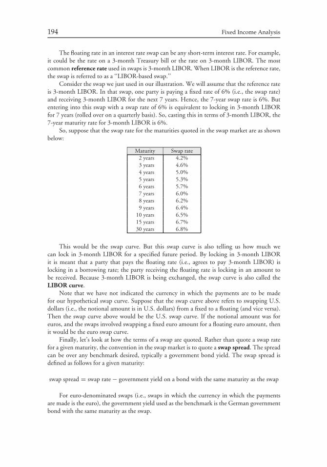
194 Fixed Income Analysis
The floating rate in an interest rate swap can be any short-term interest rate. For example,it could be the rate on a 3-month Treasury bill or the rate on 3-month LIBOR. The mostcommon reference rate used in swaps is 3-month LIBOR. When LIBOR is the reference rate,the swap is referred to as a ‘‘LIBOR-based swap.’’
Consider the swap we just used in our illustration. We will assume that the reference rateis 3-month LIBOR. In that swap, one party is paying a fixed rate of 6% (i.e., the swap rate)and receiving 3-month LIBOR for the next 7 years. Hence, the 7-year swap rate is 6%. Butentering into this swap with a swap rate of 6% is equivalent to locking in 3-month LIBORfor 7 years (rolled over on a quarterly basis). So, casting this in terms of 3-month LIBOR, the7-year maturity rate for 3-month LIBOR is 6%.
So, suppose that the swap rate for the maturities quoted in the swap market are as shownbelow:
Maturity Swap rate2 years 4.2%3 years 4.6%4 years 5.0%5 years 5.3%6 years 5.7%7 years 6.0%8 years 6.2%9 years 6.4%
10 years 6.5%15 years 6.7%30 years 6.8%
This would be the swap curve. But this swap curve is also telling us how much wecan lock in 3-month LIBOR for a specified future period. By locking in 3-month LIBORit is meant that a party that pays the floating rate (i.e., agrees to pay 3-month LIBOR) islocking in a borrowing rate; the party receiving the floating rate is locking in an amount tobe received. Because 3-month LIBOR is being exchanged, the swap curve is also called theLIBOR curve.
Note that we have not indicated the currency in which the payments are to be madefor our hypothetical swap curve. Suppose that the swap curve above refers to swapping U.S.dollars (i.e., the notional amount is in U.S. dollars) from a fixed to a floating (and vice versa).Then the swap curve above would be the U.S. swap curve. If the notional amount was foreuros, and the swaps involved swapping a fixed euro amount for a floating euro amount, thenit would be the euro swap curve.
Finally, let’s look at how the terms of a swap are quoted. Rather than quote a swap ratefor a given maturity, the convention in the swap market is to quote a swap spread. The spreadcan be over any benchmark desired, typically a government bond yield. The swap spread isdefined as follows for a given maturity:
swap spread = swap rate − government yield on a bond with the same maturity as the swap
For euro-denominated swaps (i.e., swaps in which the currency in which the paymentsare made is the euro), the government yield used as the benchmark is the German governmentbond with the same maturity as the swap.
Chapter 8 Term Structure and Volatility of Interest Rates 195
For example, consider our hypothetical 7-year swap. Suppose that the currency of theswap payments is in U.S. dollars and the estimated 7-year U.S. Treasury yield is 5.4%. Thensince the swap rate is 6%, the swap spread is:
swap spread = 6% − 5.4% = 0.6% = 60 basis points.
Suppose, instead, the swap was denominated in euros and the swap rate is 6%. Alsosuppose that the estimated 7-year German government bond yield is 5%. Then the swapspread would be quoted as 100 basis points (6%–5%).
Effectively the swap spread reflects the risk of the counterparty to the swap failing tosatisfy its obligation. Consequently, it primarily reflects credit risk. Since the counterparty inswaps are typically bank-related entities, the swap spread is a rough indicator of the credit riskof the banking sector. Therefore, the swap rate curve is not a default-free curve. Instead, it isan inter-bank or AA rated curve.
Notice that the swap rate is compared to a government bond yield to determine the swapspread. Why would one want to use a swap curve if a government bond yield curve is available?We answer that question next.
B. Reasons for Increased Use of Swap Curve
Investors and issuers use the swap market for hedging and arbitrage purposes, and the swapcurve as a benchmark for evaluating performance of fixed income securities and the pricingof fixed income securities. Since the swap curve is effectively the LIBOR curve and investorsborrow based on LIBOR, the swap curve is more useful to funded investors than a governmentyield curve.
The increased application of the swap curve for these activities is due to its advantages overusing the government bond yield curve as a benchmark. Before identifying these advantages,it is important to understand that the drawback of the swap curve relative to the governmentbond yield curve could be poorer liquidity. In such instances, the swap rates would reflect aliquidity premium. Fortunately, liquidity is not an issue in many countries as the swap markethas become highly liquid, with narrow bid-ask spreads for a wide range of swap maturities. Insome countries swaps may offer better liquidity than that country’s government bond market.
The advantages of the swap curve over a government bond yield curve are:9
1. There is almost no government regulation of the swap market. The lack of governmentregulation makes swap rates across different markets more comparable. In somecountries, there are some sovereign issues that offer various tax benefits to investors and,as a result, for global investors it makes comparative analysis of government rates acrosscountries difficult because some market yields do not reflect their true yield.
2. The supply of swaps depends only on the number of counterparties that are seekingor are willing to enter into a swap transaction at any given time. Since there is nounderlying government bond, there can be no effect of market technical factors10 thatmay result in the yield for a government bond issue being less than its true yield.
9See Uri Ron, ‘‘A Practical Guide to Swap Curve Construction,’’ Chapter 6 in Frank J. Fabozzi (ed.),Interest Rate, Term Structure, and Valuation Modeling (NY: John Wiley & Sons, 2002).10For example, a government bond issue being on ‘‘special’’ in the repurchase agreement market.
196 Fixed Income Analysis
3. Comparisons across countries of government yield curves is difficult because of thedifferences in sovereign credit risk. In contrast, the credit risk as reflected in theswaps curve are similar and make comparisons across countries more meaningful thangovernment yield curves. Sovereign risk is not present in the swap curve because, asnoted earlier, the swap curve is viewed as an inter-bank yield curve or AA yield curve.
4. There are more maturity points available to construct a swap curve than a governmentbond yield curve. More specifically, what is quoted in the swap market are swap rates for2, 3, 4, 5, 6, 7, 8, 9, 10, 15, and 30 year maturities. Thus, in the swap market there are10 market interest rates with a maturity of 2 years and greater. In contrast, in the U.S.Treasury market, for example, there are only three market interest rates for on-the-runTreasuries with a maturity of 2 years or greater (2, 5, and 10 years) and one of the rates,the 10-year rate, may not be a good benchmark because it is often on special in the repomarket. Moreover, because the U.S. Treasury has ceased the issuance of 30-year bonds,there is no 30-year yield available.
C. Constructing the LIBOR Spot Rate Curve
In the valuation of fixed income securities, it is not the Treasury yield curve that is used as thebasis for determining the appropriate discount rate for computing the present value of cashflows but the Treasury spot rates. The Treasury spot rates are derived from the Treasury yieldcurve using the bootstrapping process.
Similarly, it is not the swap curve that is used for discounting cash flows when the swapcurve is the benchmark but the spot rates. The spot rates are derived from the swap curve inexactly the same way—using the bootstrapping methodology. The resulting spot rate curveis called the LIBOR spot rate curve. Moreover, a forward rate curve can be derived fromthe spot rate curve. The same thing is done in the swap market. The forward rate curvethat is derived is called the LIBOR forward rate curve. Consequently, if we understand themechanics of moving from the yield curve to the spot rate curve to the forward rate curve inthe Treasury market, there is no reason to repeat an explanation of that process here for theswap market; that is, it is the same methodology, just different yields are used.11
VI. EXPECTATIONS THEORIES OF THE TERMSTRUCTURE OF INTEREST RATES
So far we have described the different types of curves that analysts and portfolio managersfocus on. The key curve is the spot rate curve because it is the spot rates that are used to value
11The question is what yields are used to construct the swap rate curve. Practitioners use yields fromtwo related markets: the Eurodollar CD futures contract and the swap market. We will not review theEurodollar CD futures contract here. It is discussed in Chapter 14. For now, the only important fact tonote about this contract is that it provides a means for locking in 3-month LIBOR in the future. In fact,it provides a means for doing so for an extended time into the future.
Practitioners. use the Eurodollar CD futures rate up to four years to get 3-month LIBOR for everyquarter. While there are Eurodollar CD futures contracts that settle further out than four years, fortechnical reasons (having to do with the convexity of the contract) analysts use only the first four years.(In fact, this actually varies from practitioner to practitioner. Some will use the Eurodollar CD futuresfrom two years up to four years.) For maturities after four years, the swap rates are used to get 3-monthLIBOR. As noted above, there is a swap rate for maturities for each year to year 10, and then swap ratesfor 15 years and 30 years.
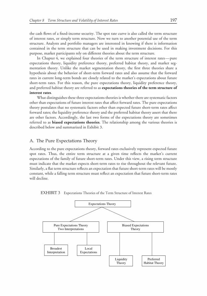
Chapter 8 Term Structure and Volatility of Interest Rates 197
the cash flows of a fixed-income security. The spot rate curve is also called the term structureof interest rates, or simply term structure. Now we turn to another potential use of the termstructure. Analysts and portfolio managers are interested in knowing if there is informationcontained in the term structure that can be used in making investment decisions. For thispurpose, market participants rely on different theories about the term structure.
In Chapter 4, we explained four theories of the term structure of interest rates—pureexpectations theory, liquidity preference theory, preferred habitat theory, and market seg-mentation theory. Unlike the market segmentation theory, the first three theories share ahypothesis about the behavior of short-term forward rates and also assume that the forwardrates in current long-term bonds are closely related to the market’s expectations about futureshort-term rates. For this reason, the pure expectations theory, liquidity preference theory,and preferred habitat theory are referred to as expectations theories of the term structure ofinterest rates.
What distinguishes these three expectations theories is whether there are systematic factorsother than expectations of future interest rates that affect forward rates. The pure expectationstheory postulates that no systematic factors other than expected future short-term rates affectforward rates; the liquidity preference theory and the preferred habitat theory assert that thereare other factors. Accordingly, the last two forms of the expectations theory are sometimesreferred to as biased expectations theories. The relationship among the various theories isdescribed below and summarized in Exhibit 3.
A. The Pure Expectations Theory
According to the pure expectations theory, forward rates exclusively represent expected futurespot rates. Thus, the entire term structure at a given time reflects the market’s currentexpectations of the family of future short-term rates. Under this view, a rising term structuremust indicate that the market expects short-term rates to rise throughout the relevant future.Similarly, a flat term structure reflects an expectation that future short-term rates will be mostlyconstant, while a falling term structure must reflect an expectation that future short-term rateswill decline.
EXHIBIT 3 Expectations Theories of the Term Structure of Interest Rates
Expectations Theory
Pure Expectations TheoryTwo Interpretations
Biased ExpectationsTheory
BroadestInterpretation
LocalExpectations
LiquidityTheory
PreferredHabitat Theory

198 Fixed Income Analysis
1. Drawbacks of the Theory The pure expectations theory suffers from one shortcom-ing, which, qualitatively, is quite serious. It neglects the risks inherent in investing in bonds.If forward rates were perfect predictors of future interest rates, then the future prices of bondswould be known with certainty. The return over any investment period would be certain andindependent of the maturity of the instrument acquired. However, with the uncertainty aboutfuture interest rates and, therefore, about future prices of bonds, these instruments becomerisky investments in the sense that the return over some investment horizon is unknown.
There are two risks that cause uncertainty about the return over some investment horizon.The first is the uncertainty about the price of the bond at the end of the investment horizon.For example, an investor who plans to invest for five years might consider the following threeinvestment alternatives:
Alternative 1: Invest in a 5-year zero-coupon bond and hold it for five years.
Alternative 2: Invest in a 12-year zero-coupon bond and sell it at the end of five years.
Alternative 3: Invest in a 30-year zero-coupon bond and sell it at the end of five years.
The return that will be realized in Alternatives 2 and 3 is not known because the price of eachof these bonds at the end of five years is unknown. In the case of the 12-year bond, the pricewill depend on the yield on 7-year bonds five years from now; and the price of the 30-yearbond will depend on the yield on 25-year bonds five years from now. Since forward ratesimplied in the current term structure for a 7-year bond five years from now and a 25-year bondfive years from now are not perfect predictors of the actual future rates, there is uncertaintyabout the price for both bonds five years from now. Thus, there is interest rate risk; that is, theprice of the bond may be lower than currently expected at the end of the investment horizondue to an increase in interest rates. As explained earlier, an important feature of interest raterisk is that it increases with the length of the bond’s maturity.
The second risk involves the uncertainty about the rate at which the proceeds from abond that matures prior to the end of the investment horizon can be reinvested until thematurity date, that is, reinvestment risk. For example, an investor who plans to invest for fiveyears might consider the following three alternative investments:
Alternative 1: Invest in a 5-year zero-coupon bond and hold it for five years.
Alternative 2: Invest in a 6-month zero-coupon instrument and, when it matures, reinvestthe proceeds in 6-month zero-coupon instruments over the entire 5-year investmenthorizon.
Alternative 3: Invest in a 2-year zero-coupon bond and, when it matures, reinvest the proceedsin a 3-year zero-coupon bond.
The risk for Alternatives 2 and 3 is that the return over the 5-year investment horizon isunknown because rates at which the proceeds can be reinvested until the end of the investmenthorizon are unknown.
2. Interpretations of the Theory There are several interpretations of the pure expec-tations theory that have been put forth by economists. These interpretations are not exact
Chapter 8 Term Structure and Volatility of Interest Rates 199
equivalents nor are they consistent with each other, in large part because they offer differenttreatments of the two risks associated with realizing a return that we have just explained.12
a. Broadest Interpretation The broadest interpretation of the pure expectations theorysuggests that investors expect the return for any investment horizon to be the same, regardlessof the maturity strategy selected.13 For example, consider an investor who has a 5-yearinvestment horizon. According to this theory, it makes no difference if a 5-year, 12-year, or30-year bond is purchased and held for five years since the investor expects the return fromall three bonds to be the same over the 5-year investment horizon. A major criticism of thisvery broad interpretation of the theory is that, because of price risk associated with investingin bonds with a maturity greater than the investment horizon, the expected returns from thesethree very different investments should differ in significant ways.14
b. Local Expectations Form of the Pure Expectations Theory A second interpretation,referred to as the local expectations form of the pure expectations theory, suggests that thereturn will be the same over a short-term investment horizon starting today. For example, ifan investor has a 6-month investment horizon, buying a 1-year, 5-year or 10-year bond willproduce the same 6-month return.
To illustrate this, we will use the hypothetical yield curve shown in Exhibit 4. InChapter 6, we used the yield curve in Exhibit 4 to show how to compute spot rates andforward rates. Exhibit 5 shows all the 6-month forward rates. We will focus on the 1-year,5-year, and 10-year issues.
Our objective is to look at what happens to the total return over a 6-month investmenthorizon for the 1-year, 5-year, and 10-year issues if all the 6-month forward rates are realized.Look first at panel a in Exhibit 6. This shows the total return for the 1-year issue. At the endof 6 months, this issue is a 6-month issue. The 6-month forward rate is 3.6%. This meansthat if the forward rate is realized, the 6-month yield 6 months from now will be 3.6%. Givena 6-month issue that must offer a yield of 3.6% (the 6-month forward rate), the price of thisissue will decline from 100 (today) to 99.85265 six months from now. The price must declinebecause if the 6-month forward rate is realized 6 months from now, the yield increases from3.3% to 3.6%. The total dollars realized over the 6 months are coupon interest adjusted forthe decline in the price. The total return for the 6 months is 3%.
What the local expectations theory asserts is that over the 6-month investment horizoneven the 5-year and the 10-year issues will generate a total return of 3% if forward rates arerealized. Panels b and c show this to be the case. We need only explain the computationfor one of the two issues. Let’s use the 5-year issue. The 6-month forward rates are shownin the third column of panel b. Now we apply a few principles discussed in Chapter 6. Wedemonstrated that to value a security each cash flow should be discounted at the spot rate withthe same maturity. We also demonstrated that 6-month forward rates can be used to value thecash flows of a security and that the results will be identical using the forward rates to value asecurity. For example, consider the cash flow in period 3 for the 5-year issue. The cash flow is$2.60. The 6-month forward rates are 3.6%, 3.92%, and 5.15%. These are annual rates. So,
12These formulations are summarized by John Cox, Jonathan Ingersoll, Jr., and Stephen Ross, ‘‘ARe-examination of Traditional Hypotheses About the Term Structure of Interest Rates,’’ Journal ofFinance (September 1981), pp. 769–799.13F. Lutz, ‘‘The Structure of Interest Rates,’’ Quarterly Journal of Economics (1940–41), pp. 36–63.14Cox, Ingersoll, and Ross, pp. 774–775.
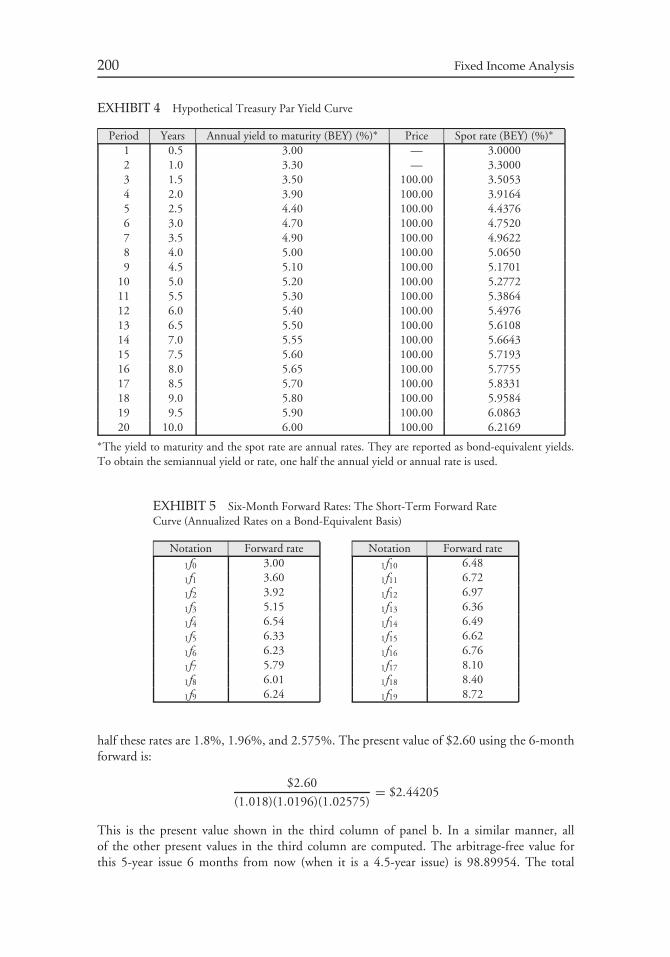
200 Fixed Income Analysis
EXHIBIT 4 Hypothetical Treasury Par Yield Curve
Period Years Annual yield to maturity (BEY) (%)∗ Price Spot rate (BEY) (%)∗1 0.5 3.00 — 3.00002 1.0 3.30 — 3.30003 1.5 3.50 100.00 3.50534 2.0 3.90 100.00 3.91645 2.5 4.40 100.00 4.43766 3.0 4.70 100.00 4.75207 3.5 4.90 100.00 4.96228 4.0 5.00 100.00 5.06509 4.5 5.10 100.00 5.1701
10 5.0 5.20 100.00 5.277211 5.5 5.30 100.00 5.386412 6.0 5.40 100.00 5.497613 6.5 5.50 100.00 5.610814 7.0 5.55 100.00 5.664315 7.5 5.60 100.00 5.719316 8.0 5.65 100.00 5.775517 8.5 5.70 100.00 5.833118 9.0 5.80 100.00 5.958419 9.5 5.90 100.00 6.086320 10.0 6.00 100.00 6.2169
∗The yield to maturity and the spot rate are annual rates. They are reported as bond-equivalent yields.To obtain the semiannual yield or rate, one half the annual yield or annual rate is used.
EXHIBIT 5 Six-Month Forward Rates: The Short-Term Forward RateCurve (Annualized Rates on a Bond-Equivalent Basis)
Notation Forward rate Notation Forward rate1f0 3.00 1f10 6.481f1 3.60 1f11 6.721f2 3.92 1f12 6.971f3 5.15 1f13 6.361f4 6.54 1f14 6.491f5 6.33 1f15 6.621f6 6.23 1f16 6.761f7 5.79 1f17 8.101f8 6.01 1f18 8.401f9 6.24 1f19 8.72
half these rates are 1.8%, 1.96%, and 2.575%. The present value of $2.60 using the 6-monthforward is:
$2.60
(1.018)(1.0196)(1.02575)= $2.44205
This is the present value shown in the third column of panel b. In a similar manner, allof the other present values in the third column are computed. The arbitrage-free value forthis 5-year issue 6 months from now (when it is a 4.5-year issue) is 98.89954. The total
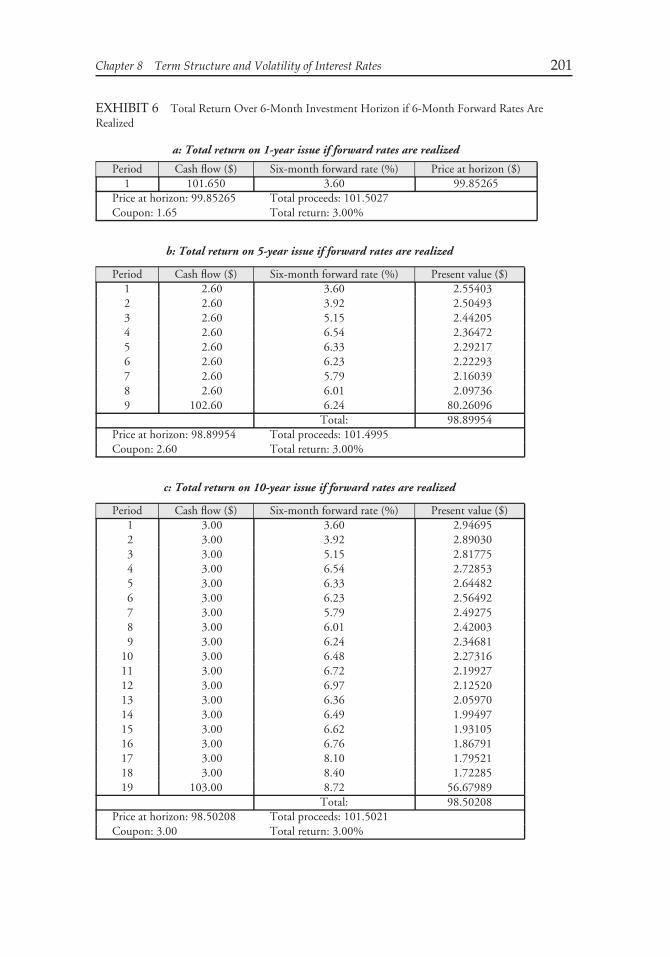
Chapter 8 Term Structure and Volatility of Interest Rates 201
EXHIBIT 6 Total Return Over 6-Month Investment Horizon if 6-Month Forward Rates AreRealized
a: Total return on 1-year issue if forward rates are realized
Period Cash flow ($) Six-month forward rate (%) Price at horizon ($)1 101.650 3.60 99.85265
Price at horizon: 99.85265 Total proceeds: 101.5027Coupon: 1.65 Total return: 3.00%
b: Total return on 5-year issue if forward rates are realized
Period Cash flow ($) Six-month forward rate (%) Present value ($)1 2.60 3.60 2.554032 2.60 3.92 2.504933 2.60 5.15 2.442054 2.60 6.54 2.364725 2.60 6.33 2.292176 2.60 6.23 2.222937 2.60 5.79 2.160398 2.60 6.01 2.097369 102.60 6.24 80.26096
Total: 98.89954Price at horizon: 98.89954 Total proceeds: 101.4995Coupon: 2.60 Total return: 3.00%
c: Total return on 10-year issue if forward rates are realized
Period Cash flow ($) Six-month forward rate (%) Present value ($)1 3.00 3.60 2.946952 3.00 3.92 2.890303 3.00 5.15 2.817754 3.00 6.54 2.728535 3.00 6.33 2.644826 3.00 6.23 2.564927 3.00 5.79 2.492758 3.00 6.01 2.420039 3.00 6.24 2.34681
10 3.00 6.48 2.2731611 3.00 6.72 2.1992712 3.00 6.97 2.1252013 3.00 6.36 2.0597014 3.00 6.49 1.9949715 3.00 6.62 1.9310516 3.00 6.76 1.8679117 3.00 8.10 1.7952118 3.00 8.40 1.7228519 103.00 8.72 56.67989
Total: 98.50208Price at horizon: 98.50208 Total proceeds: 101.5021Coupon: 3.00 Total return: 3.00%
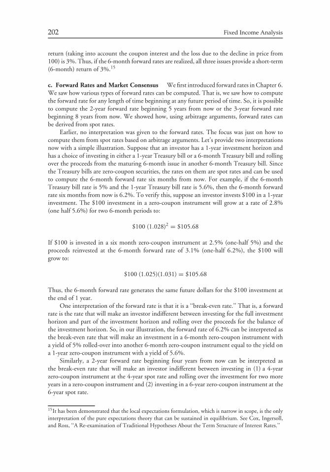
202 Fixed Income Analysis
return (taking into account the coupon interest and the loss due to the decline in price from100) is 3%. Thus, if the 6-month forward rates are realized, all three issues provide a short-term(6-month) return of 3%.15
c. Forward Rates and Market Consensus We first introduced forward rates in Chapter 6.We saw how various types of forward rates can be computed. That is, we saw how to computethe forward rate for any length of time beginning at any future period of time. So, it is possibleto compute the 2-year forward rate beginning 5 years from now or the 3-year forward ratebeginning 8 years from now. We showed how, using arbitrage arguments, forward rates canbe derived from spot rates.
Earlier, no interpretation was given to the forward rates. The focus was just on how tocompute them from spot rates based on arbitrage arguments. Let’s provide two interpretationsnow with a simple illustration. Suppose that an investor has a 1-year investment horizon andhas a choice of investing in either a 1-year Treasury bill or a 6-month Treasury bill and rollingover the proceeds from the maturing 6-month issue in another 6-month Treasury bill. Sincethe Treasury bills are zero-coupon securities, the rates on them are spot rates and can be usedto compute the 6-month forward rate six months from now. For example, if the 6-monthTreasury bill rate is 5% and the 1-year Treasury bill rate is 5.6%, then the 6-month forwardrate six months from now is 6.2%. To verify this, suppose an investor invests $100 in a 1-yearinvestment. The $100 investment in a zero-coupon instrument will grow at a rate of 2.8%(one half 5.6%) for two 6-month periods to:
$100 (1.028)2 = $105.68
If $100 is invested in a six month zero-coupon instrument at 2.5% (one-half 5%) and theproceeds reinvested at the 6-month forward rate of 3.1% (one-half 6.2%), the $100 willgrow to:
$100 (1.025)(1.031) = $105.68
Thus, the 6-month forward rate generates the same future dollars for the $100 investment atthe end of 1 year.
One interpretation of the forward rate is that it is a ‘‘break-even rate.’’ That is, a forwardrate is the rate that will make an investor indifferent between investing for the full investmenthorizon and part of the investment horizon and rolling over the proceeds for the balance ofthe investment horizon. So, in our illustration, the forward rate of 6.2% can be interpreted asthe break-even rate that will make an investment in a 6-month zero-coupon instrument witha yield of 5% rolled-over into another 6-month zero-coupon instrument equal to the yield ona 1-year zero-coupon instrument with a yield of 5.6%.
Similarly, a 2-year forward rate beginning four years from now can be interpreted asthe break-even rate that will make an investor indifferent between investing in (1) a 4-yearzero-coupon instrument at the 4-year spot rate and rolling over the investment for two moreyears in a zero-coupon instrument and (2) investing in a 6-year zero-coupon instrument at the6-year spot rate.
15It has been demonstrated that the local expectations formulation, which is narrow in scope, is the onlyinterpretation of the pure expectations theory that can be sustained in equilibrium. See Cox, Ingersoll,and Ross, ‘‘A Re-examination of Traditional Hypotheses About the Term Structure of Interest Rates.’’
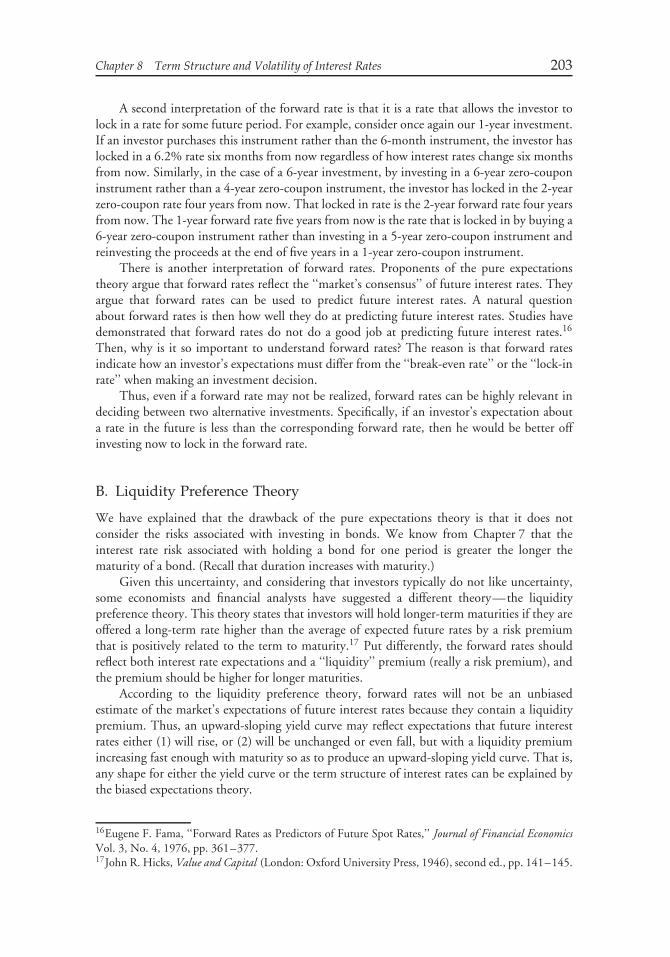
Chapter 8 Term Structure and Volatility of Interest Rates 203
A second interpretation of the forward rate is that it is a rate that allows the investor tolock in a rate for some future period. For example, consider once again our 1-year investment.If an investor purchases this instrument rather than the 6-month instrument, the investor haslocked in a 6.2% rate six months from now regardless of how interest rates change six monthsfrom now. Similarly, in the case of a 6-year investment, by investing in a 6-year zero-couponinstrument rather than a 4-year zero-coupon instrument, the investor has locked in the 2-yearzero-coupon rate four years from now. That locked in rate is the 2-year forward rate four yearsfrom now. The 1-year forward rate five years from now is the rate that is locked in by buying a6-year zero-coupon instrument rather than investing in a 5-year zero-coupon instrument andreinvesting the proceeds at the end of five years in a 1-year zero-coupon instrument.
There is another interpretation of forward rates. Proponents of the pure expectationstheory argue that forward rates reflect the ‘‘market’s consensus’’ of future interest rates. Theyargue that forward rates can be used to predict future interest rates. A natural questionabout forward rates is then how well they do at predicting future interest rates. Studies havedemonstrated that forward rates do not do a good job at predicting future interest rates.16
Then, why is it so important to understand forward rates? The reason is that forward ratesindicate how an investor’s expectations must differ from the ‘‘break-even rate’’ or the ‘‘lock-inrate’’ when making an investment decision.
Thus, even if a forward rate may not be realized, forward rates can be highly relevant indeciding between two alternative investments. Specifically, if an investor’s expectation abouta rate in the future is less than the corresponding forward rate, then he would be better offinvesting now to lock in the forward rate.
B. Liquidity Preference Theory
We have explained that the drawback of the pure expectations theory is that it does notconsider the risks associated with investing in bonds. We know from Chapter 7 that theinterest rate risk associated with holding a bond for one period is greater the longer thematurity of a bond. (Recall that duration increases with maturity.)
Given this uncertainty, and considering that investors typically do not like uncertainty,some economists and financial analysts have suggested a different theory—the liquiditypreference theory. This theory states that investors will hold longer-term maturities if they areoffered a long-term rate higher than the average of expected future rates by a risk premiumthat is positively related to the term to maturity.17 Put differently, the forward rates shouldreflect both interest rate expectations and a ‘‘liquidity’’ premium (really a risk premium), andthe premium should be higher for longer maturities.
According to the liquidity preference theory, forward rates will not be an unbiasedestimate of the market’s expectations of future interest rates because they contain a liquiditypremium. Thus, an upward-sloping yield curve may reflect expectations that future interestrates either (1) will rise, or (2) will be unchanged or even fall, but with a liquidity premiumincreasing fast enough with maturity so as to produce an upward-sloping yield curve. That is,any shape for either the yield curve or the term structure of interest rates can be explained bythe biased expectations theory.
16Eugene F. Fama, ‘‘Forward Rates as Predictors of Future Spot Rates,’’ Journal of Financial EconomicsVol. 3, No. 4, 1976, pp. 361–377.17John R. Hicks, Value and Capital (London: Oxford University Press, 1946), second ed., pp. 141–145.
204 Fixed Income Analysis
C. The Preferred Habitat Theory
Another theory, known as the preferred habitat theory, also adopts the view that the termstructure reflects the expectation of the future path of interest rates as well as a risk premium.However, the preferred habitat theory rejects the assertion that the risk premium must riseuniformly with maturity.18 Proponents of the preferred habitat theory say that the latterconclusion could be accepted if all investors intend to liquidate their investment at the shortestpossible date while all borrowers are anxious to borrow long. This assumption can be rejectedsince institutions have holding periods dictated by the nature of their liabilities.
The preferred habitat theory asserts that if there is an imbalance between the supplyand demand for funds within a given maturity range, investors and borrowers will not bereluctant to shift their investing and financing activities out of their preferred maturity sectorto take advantage of any imbalance. However, to do so, investors must be induced by a yieldpremium in order to accept the risks associated with shifting funds out of their preferredsector. Similarly, borrowers can only be induced to raise funds in a maturity sector other thantheir preferred sector by a sufficient cost savings to compensate for the corresponding fundingrisk.
Thus, this theory proposes that the shape of the yield curve is determined by bothexpectations of future interest rates and a risk premium, positive or negative, to induce marketparticipants to shift out of their preferred habitat. Clearly, according to this theory, yieldcurves that slope up, down, or flat are all possible.
VII. MEASURING YIELD CURVE RISK
We now know how to construct the term structure of interest rates and the potentialinformation content contained in the term structure that can be used for making investmentdecisions under different theories of the term structure. Next we look at how to measureexposure of a portfolio or position to a change in the term structure. This risk is referred to asyield curve risk.
Yield curve risk can be measured by changing the spot rate for a particular key maturityand determining the sensitivity of a security or portfolio to this change holding the spot ratefor the other key maturities constant. The sensitivity of the change in value to a particularchange in spot rate is called rate duration. There is a rate duration for every point on the spotrate curve. Consequently, there is not one rate duration, but a vector of durations representingeach maturity on the spot rate curve. The total change in value if all rates change by the samenumber of basis points is simply the effective duration of a security or portfolio to a parallelshift in rates. Recall that effective duration measures the exposure of a security or portfolio toa parallel shift in the term structure, taking into account any embedded options.
This rate duration approach was first suggested by Donald Chambers and WillardCarleton in 198819 who called it ‘‘duration vectors.’’ Robert Reitano suggested a similar
18Franco Modigliani and Richard Sutch, ‘‘Innovations in Interest Rate Policy,’’ American EconomicReview (May 1966), pp. 178–197.19Donald Chambers and Willard Carleton, ‘‘A Generalized Approach to Duration,’’ Research inFinance 7(1988).
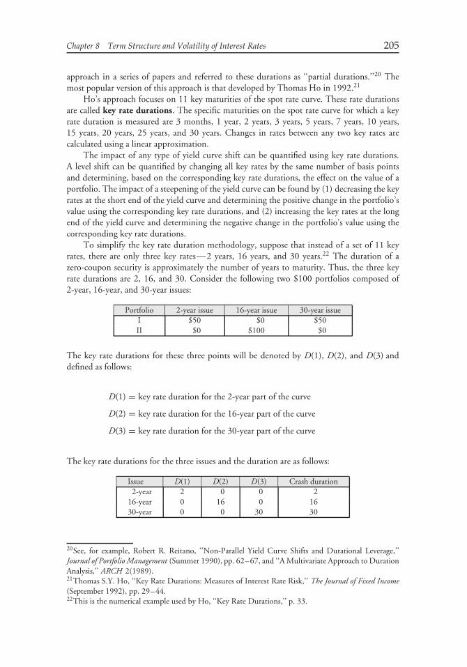
Chapter 8 Term Structure and Volatility of Interest Rates 205
approach in a series of papers and referred to these durations as ‘‘partial durations.’’20 Themost popular version of this approach is that developed by Thomas Ho in 1992.21
Ho’s approach focuses on 11 key maturities of the spot rate curve. These rate durationsare called key rate durations. The specific maturities on the spot rate curve for which a keyrate duration is measured are 3 months, 1 year, 2 years, 3 years, 5 years, 7 years, 10 years,15 years, 20 years, 25 years, and 30 years. Changes in rates between any two key rates arecalculated using a linear approximation.
The impact of any type of yield curve shift can be quantified using key rate durations.A level shift can be quantified by changing all key rates by the same number of basis pointsand determining, based on the corresponding key rate durations, the effect on the value of aportfolio. The impact of a steepening of the yield curve can be found by (1) decreasing the keyrates at the short end of the yield curve and determining the positive change in the portfolio’svalue using the corresponding key rate durations, and (2) increasing the key rates at the longend of the yield curve and determining the negative change in the portfolio’s value using thecorresponding key rate durations.
To simplify the key rate duration methodology, suppose that instead of a set of 11 keyrates, there are only three key rates—2 years, 16 years, and 30 years.22 The duration of azero-coupon security is approximately the number of years to maturity. Thus, the three keyrate durations are 2, 16, and 30. Consider the following two $100 portfolios composed of2-year, 16-year, and 30-year issues:
Portfolio 2-year issue 16-year issue 30-year issueI $50 $0 $50II $0 $100 $0
The key rate durations for these three points will be denoted by D(1), D(2), and D(3) anddefined as follows:
D(1) = key rate duration for the 2-year part of the curve
D(2) = key rate duration for the 16-year part of the curve
D(3) = key rate duration for the 30-year part of the curve
The key rate durations for the three issues and the duration are as follows:
Issue D(1) D(2) D(3) Crash duration2-year 2 0 0 2
16-year 0 16 0 1630-year 0 0 30 30
20See, for example, Robert R. Reitano, ‘‘Non-Parallel Yield Curve Shifts and Durational Leverage,’’Journal of Portfolio Management (Summer 1990), pp. 62–67, and ‘‘A Multivariate Approach to DurationAnalysis,’’ ARCH 2(1989).21Thomas S.Y. Ho, ‘‘Key Rate Durations: Measures of Interest Rate Risk,’’ The Journal of Fixed Income(September 1992), pp. 29–44.22This is the numerical example used by Ho, ‘‘Key Rate Durations,’’ p. 33.
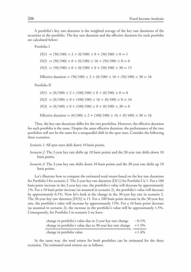
206 Fixed Income Analysis
A portfolio’s key rate duration is the weighted average of the key rate durations of thesecurities in the portfolio. The key rate duration and the effective duration for each portfolioare calculated below:
Portfolio I
D(1) = (50/100) × 2 + (0/100) × 0 + (50/100) × 0 = 1
D(2) = (50/100) × 0 + (0/100) × 16 + (50/100) × 0 = 0
D(3) = (50/100) × 0 + (0/100) × 0 + (50/100) × 30 = 15
Effective duration = (50/100) × 2 + (0/100) × 16 + (50/100) × 30 = 16
Portfolio II
D(1) = (0/100) × 2 + (100/100) × 0 + (0/100) × 0 = 0
D(2) = (0/100) × 0 + (100/100) × 16 + (0/100) × 0 = 16
D(3) = (0/100) × 0 + (100/100) × 0 + (0/100) × 30 = 0
Effective duration = (0/100) × 2 + (100/100) × 16 + (0/100) × 30 = 16
Thus, the key rate durations differ for the two portfolios. However, the effective durationfor each portfolio is the same. Despite the same effective duration, the performance of the twoportfolios will not be the same for a nonparallel shift in the spot rates. Consider the followingthree scenarios:
Scenario 1: All spot rates shift down 10 basis points.
Scenario 2: The 2-year key rate shifts up 10 basis points and the 30-year rate shifts down 10basis points.
Scenario 3: The 2-year key rate shifts down 10 basis points and the 30-year rate shifts up 10basis points.
Let’s illustrate how to compute the estimated total return based on the key rate durationsfor Portfolio I for scenario 2. The 2-year key rate duration [D(1)] for Portfolio I is 1. For a 100basis point increase in the 2-year key rate, the portfolio’s value will decrease by approximately1%. For a 10 basis point increase (as assumed in scenario 2), the portfolio’s value will decreaseby approximately 0.1%. Now let’s look at the change in the 30-year key rate in scenario 2.The 30-year key rate duration [D(3)] is 15. For a 100 basis point decrease in the 30-year keyrate, the portfolio’s value will increase by approximately 15%. For a 10 basis point decrease(as assumed in scenario 2), the increase in the portfolio’s value will be approximately 1.5%.Consequently, for Portfolio I in scenario 2 we have:
change in portfolio’s value due to 2-year key rate change −0.1%change in portfolio’s value due to 30-year key rate change +1.5%
change in portfolio value +1.4%
In the same way, the total return for both portfolios can be estimated for the threescenarios. The estimated total returns are as follows:
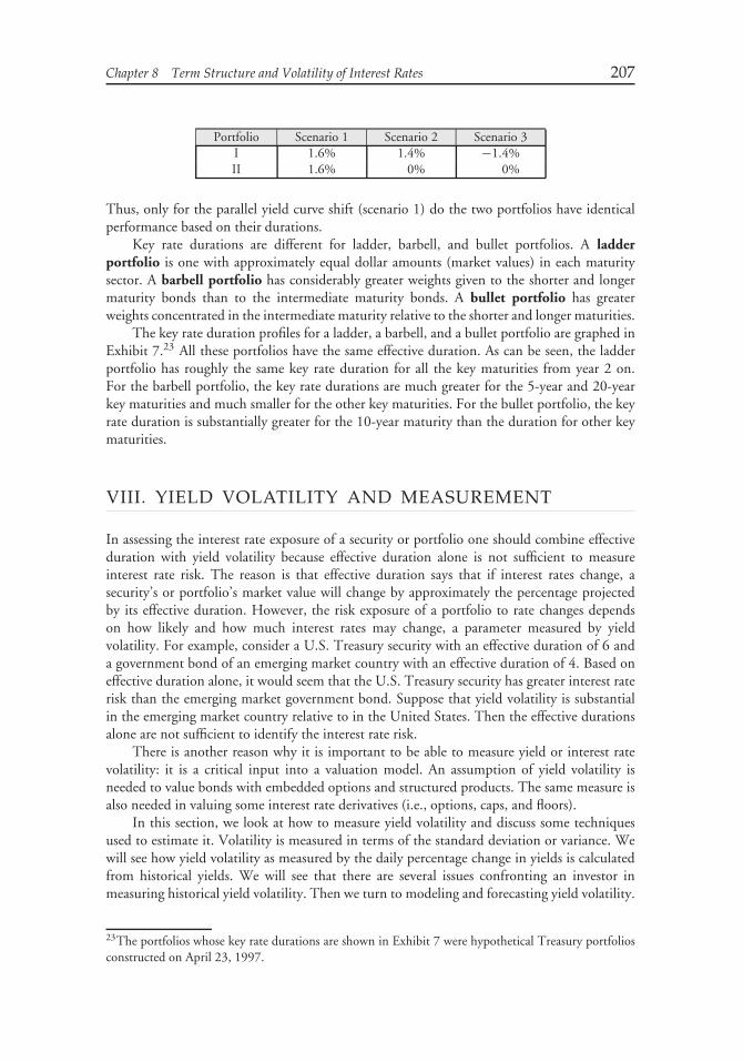
Chapter 8 Term Structure and Volatility of Interest Rates 207
Portfolio Scenario 1 Scenario 2 Scenario 3I 1.6% 1.4% −1.4%II 1.6% 0% 0%
Thus, only for the parallel yield curve shift (scenario 1) do the two portfolios have identicalperformance based on their durations.
Key rate durations are different for ladder, barbell, and bullet portfolios. A ladderportfolio is one with approximately equal dollar amounts (market values) in each maturitysector. A barbell portfolio has considerably greater weights given to the shorter and longermaturity bonds than to the intermediate maturity bonds. A bullet portfolio has greaterweights concentrated in the intermediate maturity relative to the shorter and longer maturities.
The key rate duration profiles for a ladder, a barbell, and a bullet portfolio are graphed inExhibit 7.23 All these portfolios have the same effective duration. As can be seen, the ladderportfolio has roughly the same key rate duration for all the key maturities from year 2 on.For the barbell portfolio, the key rate durations are much greater for the 5-year and 20-yearkey maturities and much smaller for the other key maturities. For the bullet portfolio, the keyrate duration is substantially greater for the 10-year maturity than the duration for other keymaturities.
VIII. YIELD VOLATILITY AND MEASUREMENT
In assessing the interest rate exposure of a security or portfolio one should combine effectiveduration with yield volatility because effective duration alone is not sufficient to measureinterest rate risk. The reason is that effective duration says that if interest rates change, asecurity’s or portfolio’s market value will change by approximately the percentage projectedby its effective duration. However, the risk exposure of a portfolio to rate changes dependson how likely and how much interest rates may change, a parameter measured by yieldvolatility. For example, consider a U.S. Treasury security with an effective duration of 6 anda government bond of an emerging market country with an effective duration of 4. Based oneffective duration alone, it would seem that the U.S. Treasury security has greater interest raterisk than the emerging market government bond. Suppose that yield volatility is substantialin the emerging market country relative to in the United States. Then the effective durationsalone are not sufficient to identify the interest rate risk.
There is another reason why it is important to be able to measure yield or interest ratevolatility: it is a critical input into a valuation model. An assumption of yield volatility isneeded to value bonds with embedded options and structured products. The same measure isalso needed in valuing some interest rate derivatives (i.e., options, caps, and floors).
In this section, we look at how to measure yield volatility and discuss some techniquesused to estimate it. Volatility is measured in terms of the standard deviation or variance. Wewill see how yield volatility as measured by the daily percentage change in yields is calculatedfrom historical yields. We will see that there are several issues confronting an investor inmeasuring historical yield volatility. Then we turn to modeling and forecasting yield volatility.
23The portfolios whose key rate durations are shown in Exhibit 7 were hypothetical Treasury portfoliosconstructed on April 23, 1997.
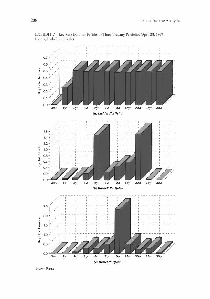
208 Fixed Income Analysis
EXHIBIT 7 Key Rate Duration Profile for Three Treasury Portfolios (April 23, 1997):Ladder, Barbell, and Bullet
(a) Ladder Portfolio
0.7
Key
Rat
e D
urat
ion
Key
Rat
e D
urat
ion
0.6
0.5
0.4
0.3
0.2
0.1
1.6
1.4
1.2
1.0
0.8
0.6
0.4
0.2
0.0
Key
Rat
e D
urat
ion
0.0
2.5
2.0
1.5
1.0
0.5
0.03mo 1yr 2yr 3yr 5yr 7yr 10yr 15yr 20yr 25yr 30yr
(b) Barbell Portfolio
3mo 1yr 2yr 3yr 5yr 7yr 10yr 15yr 20yr 25yr 30yr
(c) Bullet Portfolio
3mo 1yr 2yr 3yr 5yr 7yr 10yr 15yr 20yr 25yr 30yr
Source: Barra
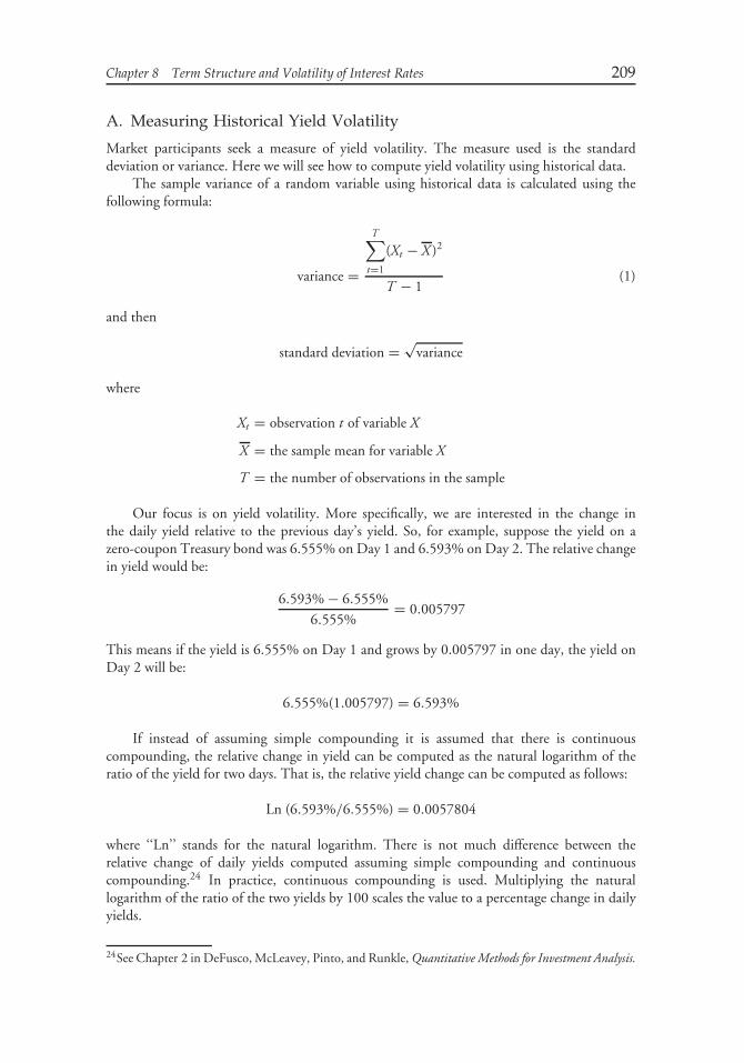
Chapter 8 Term Structure and Volatility of Interest Rates 209
A. Measuring Historical Yield Volatility
Market participants seek a measure of yield volatility. The measure used is the standarddeviation or variance. Here we will see how to compute yield volatility using historical data.
The sample variance of a random variable using historical data is calculated using thefollowing formula:
variance =
T∑t=1
(Xt − X )2
T − 1(1)
and then
standard deviation = √variance
where
Xt = observation t of variable X
X = the sample mean for variable X
T = the number of observations in the sample
Our focus is on yield volatility. More specifically, we are interested in the change inthe daily yield relative to the previous day’s yield. So, for example, suppose the yield on azero-coupon Treasury bond was 6.555% on Day 1 and 6.593% on Day 2. The relative changein yield would be:
6.593% − 6.555%
6.555%= 0.005797
This means if the yield is 6.555% on Day 1 and grows by 0.005797 in one day, the yield onDay 2 will be:
6.555%(1.005797) = 6.593%
If instead of assuming simple compounding it is assumed that there is continuouscompounding, the relative change in yield can be computed as the natural logarithm of theratio of the yield for two days. That is, the relative yield change can be computed as follows:
Ln (6.593%/6.555%) = 0.0057804
where ‘‘Ln’’ stands for the natural logarithm. There is not much difference between therelative change of daily yields computed assuming simple compounding and continuouscompounding.24 In practice, continuous compounding is used. Multiplying the naturallogarithm of the ratio of the two yields by 100 scales the value to a percentage change in dailyyields.
24See Chapter 2 in DeFusco, McLeavey, Pinto, and Runkle, Quantitative Methods for Investment Analysis.

210 Fixed Income Analysis
Therefore, letting yt be the yield on day t and yt−1 be the yield on day t−1, the percentagechange in yield, Xt , is found as follows:
Xt = 100[Ln(yt/yt−1)]
In our example, yt is 6.593% and yt−1 is 6.555%. Therefore,
Xt = 100[Ln(6.593/6.555)] = 0.57804%
To illustrate how to calculate a daily standard deviation from historical data, consider thedata in Exhibit 8 which show the yield on a Treasury zero for 26 consecutive days. From the26 observations, 25 days of percentage yield changes are calculated in Column (3). Column(4) shows the square of the deviations of the observations from the mean. The bottom ofExhibit 8 shows the calculation of the daily mean for 25 yield changes, the variance, and thestandard deviation. The daily standard deviation is 0.6360%.
The daily standard deviation will vary depending on the 25 days selected. It is importantto understand that the daily standard deviation is dependent on the period selected, a pointwe return to later in this chapter.
1. Determining the Number of Observations In our illustration, we used 25 obser-vations for the daily percentage change in yield. The appropriate number of observationsdepends on the situation at hand. For example, traders concerned with overnight positionsmight use the 10 most recent trading days (i.e., two weeks). A bond portfolio manager whois concerned with longer term volatility might use 25 trading days (about one month). Theselection of the number of observations can have a significant effect on the calculated dailystandard deviation.
2. Annualizing the Standard Deviation The daily standard deviation can be annual-ized by multiplying it by the square root of the number of days in a year.25 That is,
daily standard deviation ×√
number of days in a year
Market practice varies with respect to the number of days in the year that should be used inthe annualizing formula above. Some investors and traders use the number of days in the year,365 days, to annualize the daily standard deviation. Some investors and traders use only either250 days or 260 days to annualize. The latter is simply the number of trading days in a yearbased on five trading days per week for 52 weeks. The former reduces the number of tradingdays of 260 for 10 non-trading holidays.
Thus, in calculating an annual standard deviation, the investor must decide on:
1. the number of daily observations to use2. the number of days in the year to use to annualize the daily standard deviation.
25For any probability distribution, it is important to assess whether the value of a random variable inone period is affected by the value that the random variable took on in a prior period. Casting this interms of yield changes, it is important to know whether the yield today is affected by the yield in aprior period. The term serial correlation is used to describe the correlation between the yield in differentperiods. Annualizing the daily yield by multiplying the daily standard deviation by the square root of thenumber of days in a year assumes that serial correlation is not significant.
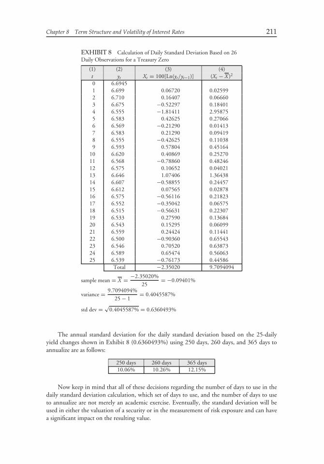
Chapter 8 Term Structure and Volatility of Interest Rates 211
EXHIBIT 8 Calculation of Daily Standard Deviation Based on 26Daily Observations for a Treasury Zero
(1) (2) (3) (4)t yt Xt = 100[Ln(yt/yt−1)] (Xt − X )2
0 6.69451 6.699 0.06720 0.025992 6.710 0.16407 0.066603 6.675 −0.52297 0.184014 6.555 −1.81411 2.958755 6.583 0.42625 0.270666 6.569 −0.21290 0.014137 6.583 0.21290 0.094198 6.555 −0.42625 0.110389 6.593 0.57804 0.45164
10 6.620 0.40869 0.2527011 6.568 −0.78860 0.4824612 6.575 0.10652 0.0402113 6.646 1.07406 1.3643814 6.607 −0.58855 0.2445715 6.612 0.07565 0.0287816 6.575 −0.56116 0.2182317 6.552 −0.35042 0.0657518 6.515 −0.56631 0.2230719 6.533 0.27590 0.1368420 6.543 0.15295 0.0609921 6.559 0.24424 0.1144122 6.500 −0.90360 0.6554323 6.546 0.70520 0.6387324 6.589 0.65474 0.5606325 6.539 −0.76173 0.44586
Total −2.35020 9.7094094
sample mean = X = −2.35020%
25= −0.09401%
variance = 9.7094094%
25 − 1= 0.4045587%
std dev = √0.4045587% = 0.6360493%
The annual standard deviation for the daily standard deviation based on the 25-dailyyield changes shown in Exhibit 8 (0.6360493%) using 250 days, 260 days, and 365 days toannualize are as follows:
250 days 260 days 365 days10.06% 10.26% 12.15%
Now keep in mind that all of these decisions regarding the number of days to use in thedaily standard deviation calculation, which set of days to use, and the number of days to useto annualize are not merely an academic exercise. Eventually, the standard deviation will beused in either the valuation of a security or in the measurement of risk exposure and can havea significant impact on the resulting value.
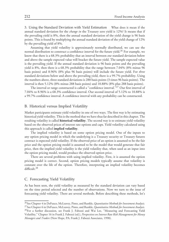
212 Fixed Income Analysis
3. Using the Standard Deviation with Yield Estimation What does it mean if theannual standard deviation for the change in the Treasury zero yield is 12%? It means that ifthe prevailing yield is 8%, then the annual standard deviation of the yield change is 96 basispoints. This is found by multiplying the annual standard deviation of the yield change of 12%by the prevailing yield of 8%.
Assuming that yield volatility is approximately normally distributed, we can use thenormal distribution to construct a confidence interval for the future yield.26 For example, weknow that there is a 68.3% probability that an interval between one standard deviation belowand above the sample expected value will bracket the future yield. The sample expected valueis the prevailing yield. If the annual standard deviation is 96 basis points and the prevailingyield is 8%, then there is a 68.3% probability that the range between 7.04% (8% minus 96basis points) and 8.96% (8% plus 96 basis points) will include the future yield. For threestandard deviations below and above the prevailing yield, there is a 99.7% probability. Usingthe numbers above, three standard deviations is 288 basis points (3 times 96 basis points). Theinterval is then 5.12% (8% minus 288 basis points) and 10.88% (8% plus 288 basis points).
The interval or range constructed is called a ‘‘confidence interval.’’27 Our first interval of7.04% to 8.96% is a 68.3% confidence interval. Our second interval of 5.12% to 10.88% isa 99.7% confidence interval. A confidence interval with any probability can be constructed.
B. Historical versus Implied Volatility
Market participants estimate yield volatility in one of two ways. The first way is by estimatinghistorical yield volatility. This is the method that we have thus far described in this chapter. Theresulting volatility is called historical volatility. The second way is to estimate yield volatilitybased on the observed prices of interest rate options and caps. Yield volatility calculated usingthis approach is called implied volatility.
The implied volatility is based on some option pricing model. One of the inputs toany option pricing model in which the underlying is a Treasury security or Treasury futurescontract is expected yield volatility. If the observed price of an option is assumed to be the fairprice and the option pricing model is assumed to be the model that would generate that fairprice, then the implied yield volatility is the yield volatility that, when used as an input intothe option pricing model, would produce the observed option price.
There are several problems with using implied volatility. First, it is assumed the optionpricing model is correct. Second, option pricing models typically assume that volatility isconstant over the life of the option. Therefore, interpreting an implied volatility becomesdifficult.28
C. Forecasting Yield Volatility
As has been seen, the yield volatility as measured by the standard deviation can vary basedon the time period selected and the number of observations. Now we turn to the issue offorecasting yield volatility. There are several methods. Before describing these methods, let’s
26See Chapter 4 in DeFusco, McLeavey, Pinto, and Runkle, Quantitative Methods for Investment Analysis.27See Chapter 6 in DeFusco, McLeavey, Pinto, and Runkle, Quantitative Methods for Investment Analysis.28For a further discussion, see Frank J. Fabozzi and Wai Lee, ‘‘Measuring and Forecasting YieldVolatility,’’ Chapter 16 in Frank J. Fabozzi (ed.), Perspectives on Interest Rate Risk Management for MoneyManagers and Traders (New Hope, PA: Frank J. Fabozzi Associates, 1998).
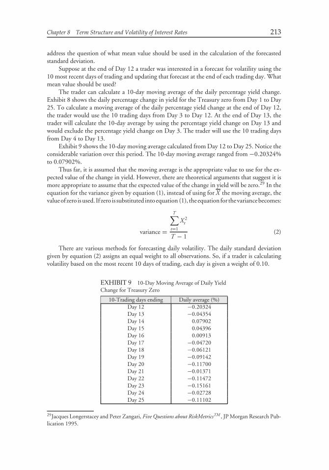
Chapter 8 Term Structure and Volatility of Interest Rates 213
address the question of what mean value should be used in the calculation of the forecastedstandard deviation.
Suppose at the end of Day 12 a trader was interested in a forecast for volatility using the10 most recent days of trading and updating that forecast at the end of each trading day. Whatmean value should be used?
The trader can calculate a 10-day moving average of the daily percentage yield change.Exhibit 8 shows the daily percentage change in yield for the Treasury zero from Day 1 to Day25. To calculate a moving average of the daily percentage yield change at the end of Day 12,the trader would use the 10 trading days from Day 3 to Day 12. At the end of Day 13, thetrader will calculate the 10-day average by using the percentage yield change on Day 13 andwould exclude the percentage yield change on Day 3. The trader will use the 10 trading daysfrom Day 4 to Day 13.
Exhibit 9 shows the 10-day moving average calculated from Day 12 to Day 25. Notice theconsiderable variation over this period. The 10-day moving average ranged from −0.20324%to 0.07902%.
Thus far, it is assumed that the moving average is the appropriate value to use for the ex-pected value of the change in yield. However, there are theoretical arguments that suggest it ismore appropriate to assume that the expected value of the change in yield will be zero.29 In theequation for the variance given by equation (1), instead of using for X the moving average, thevalueof zero isused. If zero is substituted intoequation (1), theequation for thevariancebecomes:
variance =
T∑t=1
X 2t
T − 1(2)
There are various methods for forecasting daily volatility. The daily standard deviationgiven by equation (2) assigns an equal weight to all observations. So, if a trader is calculatingvolatility based on the most recent 10 days of trading, each day is given a weight of 0.10.
EXHIBIT 9 10-Day Moving Average of Daily YieldChange for Treasury Zero
10-Trading days ending Daily average (%)Day 12 −0.20324Day 13 −0.04354Day 14 0.07902Day 15 0.04396Day 16 0.00913Day 17 −0.04720Day 18 −0.06121Day 19 −0.09142Day 20 −0.11700Day 21 −0.01371Day 22 −0.11472Day 23 −0.15161Day 24 −0.02728Day 25 −0.11102
29Jacques Longerstacey and Peter Zangari, Five Questions about RiskMetricsTM , JP Morgan Research Pub-lication 1995.
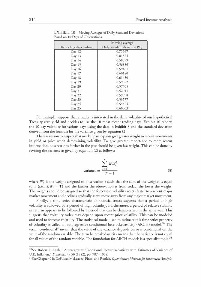
214 Fixed Income Analysis
EXHIBIT 10 Moving Averages of Daily Standard DeviationsBased on 10 Days of Observations
Moving average10-Trading days ending Daily standard deviation (%)
Day 12 0.75667Day 13 0.81874Day 14 0.58579Day 15 0.56886Day 16 0.59461Day 17 0.60180Day 18 0.61450Day 19 0.59072Day 20 0.57705Day 21 0.52011Day 22 0.59998Day 23 0.53577Day 24 0.54424Day 25 0.60003
For example, suppose that a trader is interested in the daily volatility of our hypotheticalTreasury zero yield and decides to use the 10 most recent trading days. Exhibit 10 reportsthe 10-day volatility for various days using the data in Exhibit 8 and the standard deviationderived from the formula for the variance given by equation (2).
There is reason to suspect that market participants give greater weight to recent movementsin yield or price when determining volatility. To give greater importance to more recentinformation, observations farther in the past should be given less weight. This can be done byrevising the variance as given by equation (2) as follows:
variance =
T∑t=1
WtX 2t
T − 1(3)
where Wt is the weight assigned to observation t such that the sum of the weights is equalto T (i.e., �Wt = T) and the farther the observation is from today, the lower the weight.The weights should be assigned so that the forecasted volatility reacts faster to a recent majormarket movement and declines gradually as we move away from any major market movement.
Finally, a time series characteristic of financial assets suggests that a period of highvolatility is followed by a period of high volatility. Furthermore, a period of relative stabilityin returns appears to be followed by a period that can be characterized in the same way. Thissuggests that volatility today may depend upon recent prior volatility. This can be modeledand used to forecast volatility. The statistical model used to estimate this time series propertyof volatility is called an autoregressive conditional heteroskedasticity (ARCH) model.30 Theterm ‘‘conditional’’ means that the value of the variance depends on or is conditional on thevalue of the random variable. The term heteroskedasticity means that the variance is not equalfor all values of the random variable. The foundation for ARCH models is a specialist topic.31
30See Robert F. Engle, ‘‘Autoregressive Conditional Heteroskedasticity with Estimates of Variance ofU.K. Inflation,’’ Econometrica 50 (1982), pp. 987–1008.31See Chapter 9 in DeFusco, McLeavey, Pinto, and Runkle, Quantitative Methods for Investment Analysis.
CHAPTER 9VALUING BONDS WITH
EMBEDDED OPTIONS
I. INTRODUCTION
The presence of an embedded option in a bond structure makes the valuation of such bondscomplicated. In this chapter, we present a model to value bonds that have one or moreembedded options and where the value of the embedded options depends on future interestrates. Examples of such embedded options are call and put provisions and caps (i.e., maximuminterest rate) in floating-rate securities. While there are several models that have been proposedto value bonds with embedded options, our focus will be on models that provide an ‘‘arbitrage-free value’’ for a security. At the end of this chapter, we will discuss the valuation of convertiblebonds. The complexity here is that these bonds are typically callable and may be putable.Thus, the valuation of convertible bonds must take into account not only embedded optionsthat depend on future interest rates (i.e., the call and the put options) but also the future pricemovement of the common stock (i.e., the call option on the common stock).
In order to understand how to value a bond with an embedded option, there are severalfundamental concepts that must be reviewed. We will do this in Sections II, III, IV, and V. InSection II, the key elements involved in developing a bond valuation model are explained. InSection III, an overview of the bond valuation process is provided. Since the valuation of bondsrequires benchmark interest rates, the various benchmarks are described in Section IV. In thissection we also explain how to interpret spread measures relative to a particular benchmark.In Section V, the valuation of an option-free bond is reviewed using a numerical illustration.We first introduced the concepts described in this section in Chapter 5. The bond used inthe illustration in this section to show how to value an option-free bond is then used in theremainder of the chapter to show how to value that bond if there is one or more embeddedoptions.
II. ELEMENTS OF A BOND VALUATION MODEL
The valuation process begins with determining benchmark interest rates. As will be explainedlater in this section, there are three potential markets where benchmark interest rates can beobtained:
• the Treasury market• a sector of the bond market• the market for the issuer’s securities
215
216 Fixed Income Analysis
An arbitrage-free value for an option-free bond is obtained by first generating the spotrates (or forward rates). When used to discount cash flows, the spot rates are the rates thatwould produce a model value equal to the observed market price for each on-the-run securityin the benchmark. For example, if the Treasury market is the benchmark, an arbitrage-freemodel would produce a value for each on-the-run Treasury issue that is equal to its observedmarket price. In the Treasury market, the on-the-run issues are the most recently auctionedissues. (Note that all such securities issued by the U.S. Department of the Treasury are optionfree.) If the market used to establish the benchmark is a sector of the bond market or themarket for the issuer’s securities, the on-the-run issues are estimates of what the market pricewould be if newly issued option-free securities with different maturities are sold.
In deriving the interest rates that should be used to value a bond with an embeddedoption, the same principle must be maintained. No matter how complex the valuation model,when each on-the-run issue for a benchmark security is valued using the model, the valueproduced should be equal to the on-the-run issue’s market price. The on-the-run issues for agiven benchmark are assumed to be fairly priced.1
The first complication in building a model to value bonds with embedded options isthat the future cash flows will depend on what happens to interest rates in the future. Thismeans that future interest rates must be considered. This is incorporated into a valuationmodel by considering how interest rates can change based on some assumed interest ratevolatility. In the previous chapter, we explained what interest rate volatility is and how itis estimated. Given the assumed interest rate volatility, an interest rate ‘‘tree’’ representingpossible future interest rates consistent with the volatility assumption can be constructed. It isfrom the interest rate tree that two important elements in the valuation process are obtained.First, the interest rates on the tree are used to generate the cash flows taking into account theembedded option. Second, the interest rates on the tree are used to compute the present valueof the cash flows.
For a given interest rate volatility, there are several interest rate models that have beenused in practice to construct an interest rate tree. An interest rate model is a probabilisticdescription of how interest rates can change over the life of the bond. An interest rate modeldoes this by making an assumption about the relationship between the level of short-terminterest rates and the interest rate volatility as measured by the standard deviation. A discussionof the various interest rate models that have been suggested in the finance literature and thatare used by practitioners in developing valuation models is beyond the scope of this chapter.2
What is important to understand is that the interest rate models commonly used are based onhow short-term interest rates can evolve (i.e., change) over time. Consequently, these interestrate models are referred to as one-factor models, where ‘‘factor’’ means only one interest rateis being modeled over time. More complex models would consider how more than one interestrate changes over time. For example, an interest rate model can specify how the short-terminterest rate and the long-term interest rate can change over time. Such a model is called atwo-factor model.
Given an interest rate model and an interest rate volatility assumption, it can be assumedthat interest rates can realize one of two possible rates in the next period. A valuation model
1Market participants also refer to this characteristic of a model as one that ‘‘calibrates to the market.’’2An excellent source for further explanation of many of these models is Gerald W. Buetow Jr. and JamesSochacki, Term Structure Models Using Binomial Trees: Demystifying the Process (Charlottesville, VA:Association of Investment Management and Research, 2000).
Chapter 9 Valuing Bonds with Embedded Options 217
that makes this assumption in creating an interest rate tree is called a binomial model. Thereare valuation models that assume that interest rates can take on three possible rates in the nextperiod and these models are called trinomial models. There are even more complex modelsthat assume in creating an interest rate tree that more than three possible rates in the nextperiod can be realized. These models that assume discrete change in interest rates are referredto as ‘‘discrete-time option pricing models.’’ It makes sense that option valuation technology isemployed to value a bond with an embedded option because the valuation requires an estimateof what the value of the embedded option is worth. However, a discussion of the underlyingtheory of discrete-time pricing models in general and the binomial model in particular arebeyond the scope of this chapter.3
As we will see later in this chapter, when a discrete-time option pricing model isportrayed in graph form, it shows the different paths that interest rates can take. The graphicalpresentation looks like a lattice.4 Hence, discrete-time option pricing models are sometimesreferred to as ‘‘lattice models.’’ Since the pattern of the interest rate paths also look like thebranches of a tree, the graphical presentation is referred to as an interest rate tree.
Regardless of the assumption about how many possible rates can be realized in the nextperiod, the interest rate tree generated must produce a value for the securities in the benchmarkthat is equal to their observed market price—that is, it must produce an arbitrage-free value.Consequently, if the Treasury market is used for the benchmark interest rates, the interestrate tree generated must produce a value for each on-the-run Treasury issue that is equalto its observed market price. Moreover, the intuition and the methodology for using theinterest rate tree (i.e., the backward induction methodology described later) are the same.Once an interest rate tree is generated that (1) is consistent with both the interest rate volatilityassumption and the interest rate model and (2) generates the observed market price for thesecurities in the benchmark, the next step is to use the interest rate tree to value a bondwith an embedded option. The complexity here is that a set of rules must be introducedto determine, for any period, when the embedded option will be exercised. For a callablebond, these rules are called the ‘‘call rules.’’ The rules vary from model builder to modelbuilder.
While the building of a model to value bonds with embedded options is more complexthan building a model to value option-free bonds, the basic principles are the same. In the caseof valuing an option-free bond, the model that is built is simply a set of spot rates that are usedto value cash flows. The spot rates will produce an arbitrage-free value. For a model to value abond with embedded options, the interest rate tree is used to value future cash flows and theinterest rate tree is combined with the call rules to generate the future cash flows. Again, theinterest rate tree will produce an arbitrage-free value.
Let’s move from theory to practice. Only a few practitioners will develop their ownmodel to value bonds with embedded options. Instead, it is typical for a portfolio manageror analyst to use a model developed by either a dealer firm or a vendor of analytical systems.A fair question is then: Why bother covering a valuation model that is readily available froma third-party? The answer is that a valuation model should not be a black box to portfoliomanagers and analysts. The models in practice share all of the principles described in this chapter,
3For a discussion of the binomial model and the underlying theory, see Chapter 4 in Don M. Chance,Analysis of Derivatives for the CFA Program (Charlottesville, VA: Association for Investment Managementand Research, 2003).4A lattice is an arrangement of points in a regular periodic pattern.
218 Fixed Income Analysis
but differ with respect to certain assumptions that can produce quite different values. The reasonsfor these differences in valuation must be understood. Moreover, third-party models give theuser a choice of changing the assumptions. A user who has not ‘‘walked through’’ a valuationmodel has no appreciation of the significance of these assumptions and therefore how to assessthe impact of these assumptions on the value produced by the model. Earlier, we discussed‘‘modeling risk.’’ This is the risk that the underlying assumptions of a model may be incorrect.Understanding a valuation model permits the user to effectively determine the significance ofan assumption.
As an example of the importance of understanding the assumptions of a model, considerinterest rate volatility. Suppose that the market price of a bond is $89. Suppose further thata valuation model produces a value for a bond with an embedded option of $90 based on a12% interest rate volatility assumption. Then, according to the valuation model, this bond ischeap by one point. However, suppose that the same model produces a value of $87 if a 15%volatility is assumed. This tells the portfolio manager or analyst that the bond is two pointsrich. Which is correct? The answer clearly depends on what the investor believes interest ratevolatility will be in the future.
In this chapter, we will use the binomial model to demonstrate all of the issues andassumptions associated with valuing a bond with embedded options. This model is available onBloomberg, as well as from other commercial vendors and several dealer firms.5 We show howto create an interest rate tree (more specifically, a binomial interest rate tree) given a volatilityassumption and how the interest rate tree can be used to value an option-free bond. Giventhe interest rate tree, we then show how to value several types of bonds with an embeddedoption—a callable bond, a putable bond, a step-up note, and a floating-rate note with a cap.We postpone until Chapter 12 an explanation of why the binomial model is not used to valuemortgage-backed and asset-backed securities. The binomial model is used to value options,caps, and floors as will be explained in Chapter 14.
Once again, it must be emphasized that while the binomial model is used in this chapterto demonstrate how to value bonds with embedded options, other models that allow for morethan one interest rate in the next period all follow the same principles—they begin withon-the-run yields, they produce an interest rate tree that generates an arbitrage-free value, andthey depend on assumptions regarding the volatility of interest rates and rules for when anembedded option will be exercised.
III. OVERVIEW OF THE BOND VALUATIONPROCESS
In this section we review the bond valuation process and the key concepts that were introducedearlier. This will help us tie together the concepts that have already been covered and how theyrelate to the valuation of bonds with embedded options.
Regardless if a bond has an embedded option, we explained that the following can bedone:
5The model described in this chapter was first presented in Andrew J. Kalotay, George O. Williams, andFrank J. Fabozzi, ‘‘A Model for the Valuation of Bonds and Embedded Options,’’ Financial AnalystsJournal (May–June 1993), pp. 35–46.
Chapter 9 Valuing Bonds with Embedded Options 219
1. Given a required yield to maturity, we can compute the value of a bond. For example,if the required yield to maturity of a 9-year, 8% coupon bond that pays interestsemiannually is 7%, its price is 106.59.
2. Given the observed market price of a bond we can calculate its yield to maturity. Forexample, if the price of a 5-year, 6% coupon bond that pays interest semiannually is93.84, its yield to maturity is 7.5%.
3. Given the yield to maturity, a yield spread can be computed. For example, if the yieldto maturity for a 5-year, 6% coupon bond that pays interest semiannually is 7.5% andits yield is compared to a benchmark yield of 6.5%, then the yield spread is 100 basispoints (7.5% minus 6.5%). We referred to the yield spread as the nominal spread.
The problem with using a single interest rate when computing the value of a bond (as in(1) above) or in computing a yield to maturity (as in (2) above) is that it fails to recognize thateach cash flow is unique and warrants its own discount rate. Failure to discount each cash flowat an appropriate interest unique to when that cash flow is expected to be received results inan arbitrage opportunity as described in Chapter 8.
It is at this point in the valuation process that the notion of theoretical spot rates areintroduced to overcome the problem associated with using a single interest rate. The spotrates are the appropriate rates to use to discount cash flows. There is a theoretical spot ratethat can be obtained for each maturity. The procedure for computing the spot rate curve(i.e., the spot rate for each maturity) was explained and discussed further in the previouschapter.
Using the spot rate curve, one obtains the bond price. However, how is the spot ratecurve used to compute the yield to maturity? Actually, there is no equivalent concept to a yieldto maturity in this case. Rather, there is a yield spread measure that is used to overcome theproblem of a single interest rate. This measure is the zero-volatility spread that was explainedin Chapter 4. The zero-volatility spread, also called the Z-spread and the static spread, is thespread that when added to all of the spot rates will make the present value of the bond’s cashflow equal to the bond’s market price.
At this point, we have not introduced any notion of how to handle bonds with embeddedoptions. We have simply dealt with the problem of using a single interest rate for discountingcash flows. But there is still a critical issue that must be resolved. When a bond has anembedded option, a portion of the yield, and therefore a portion of the spread, is attributableto the embedded option. When valuing a bond with an embedded option, it is necessary toadjust the spread for the value of the embedded option. The measure that does this is called theoption-adjusted spread (OAS). We mentioned this measure in Chapter 4 but did not provideany details. In this chapter, we show of how this spread measure is computed for bonds withembedded options.
A. The Benchmark Interest Rates and Relative Value Analysis
Yield spread measures are used in assessing the relative value of securities. Relative valueanalysis involves identifying securities that can potentially enhance return relative to abenchmark. Relative value analysis can be used to identify securities as being overpriced(‘‘rich’’), underpriced (‘‘cheap’’), or fairly priced. A portfolio manager can use relative valueanalysis in ranking issues within a sector or sub-sector of the bond market or different issuesof a specific issuer.
220 Fixed Income Analysis
Two questions that need to be asked in order to understand spread measures wereidentified:
1. What is the benchmark for computing the spread? That is, what is the spread measuredrelative to?
2. What is the spread measuring?
As explained, the different spread measures begin with benchmark interest rates. Thebenchmark interest rates can be one of the following:
• the Treasury market• a specific bond sector with a given credit rating• a specific issuer
A specific bond sector with a given credit rating, for example, would include single-A ratedcorporate bonds or double-A rated banks. The LIBOR curve discussed in the previous chapteris an example, since it is viewed by the market as an inter-bank or AA rated benchmark.
Moreover, the benchmark interest rates can be based on either
• an estimated yield curve• an estimated spot rate curve
A yield curve shows the relationship between yield and maturity for coupon bonds; a spot ratecurve shows the relationship between spot rates and maturity.
Consequently, there are six potential benchmark interest rates as summarized below:
Specific bond sectorwith a given
Treasury market credit rating Specific issuerYield curve Treasury yield curve Sector yield curve Issuer yield curveSpot rate curve Treasury spot rate curve Sector spot rate curve Issuer spot rate curve
We illustrated and explained further in Chapter 8 how the Treasury spot rate curve canbe constructed from the Treasury yield curve. Rather than start with yields in the Treasurymarket as the benchmark interest rates, an estimated on-the-run yield curve for a bond sectorwith a given credit rating or a specific issuer can be obtained. To obtain a sector with a givencredit rating or a specific issuer’s on-the-run yield curve, an appropriate credit spread is addedto each on-the-run Treasury issue. The credit spread need not be constant for all maturities.For example, as explained in Chapter 5, the credit spread may increase with maturity. Giventhe on-the-run yield curve, the theoretical spot rates for the bond sector with a given creditrating or issuer can be constructed using the same methodology to construct the Treasury spotrates given the Treasury yield curve.
B. Interpretation of Spread Measures
Given the alternative benchmark interest rates, in this section we will see how to interpretthe three spread measures that were described nominal spread, zero-volatility spread, andoption-adjusted spread.
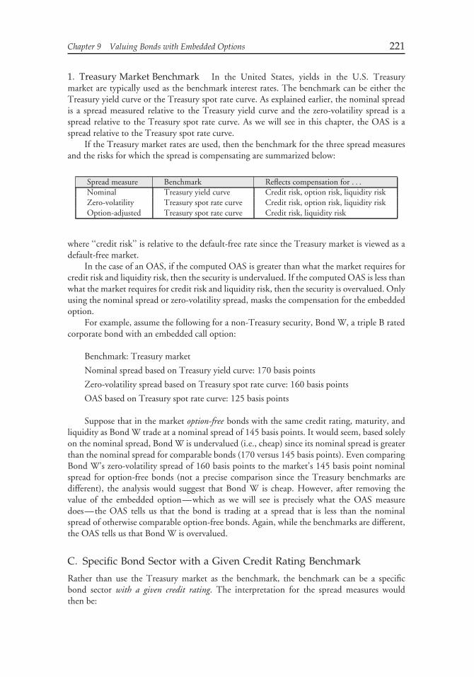
Chapter 9 Valuing Bonds with Embedded Options 221
1. Treasury Market Benchmark In the United States, yields in the U.S. Treasurymarket are typically used as the benchmark interest rates. The benchmark can be either theTreasury yield curve or the Treasury spot rate curve. As explained earlier, the nominal spreadis a spread measured relative to the Treasury yield curve and the zero-volatility spread is aspread relative to the Treasury spot rate curve. As we will see in this chapter, the OAS is aspread relative to the Treasury spot rate curve.
If the Treasury market rates are used, then the benchmark for the three spread measuresand the risks for which the spread is compensating are summarized below:
Spread measure Benchmark Reflects compensation for . . .
Nominal Treasury yield curve Credit risk, option risk, liquidity riskZero-volatility Treasury spot rate curve Credit risk, option risk, liquidity riskOption-adjusted Treasury spot rate curve Credit risk, liquidity risk
where ‘‘credit risk’’ is relative to the default-free rate since the Treasury market is viewed as adefault-free market.
In the case of an OAS, if the computed OAS is greater than what the market requires forcredit risk and liquidity risk, then the security is undervalued. If the computed OAS is less thanwhat the market requires for credit risk and liquidity risk, then the security is overvalued. Onlyusing the nominal spread or zero-volatility spread, masks the compensation for the embeddedoption.
For example, assume the following for a non-Treasury security, Bond W, a triple B ratedcorporate bond with an embedded call option:
Benchmark: Treasury market
Nominal spread based on Treasury yield curve: 170 basis points
Zero-volatility spread based on Treasury spot rate curve: 160 basis points
OAS based on Treasury spot rate curve: 125 basis points
Suppose that in the market option-free bonds with the same credit rating, maturity, andliquidity as Bond W trade at a nominal spread of 145 basis points. It would seem, based solelyon the nominal spread, Bond W is undervalued (i.e., cheap) since its nominal spread is greaterthan the nominal spread for comparable bonds (170 versus 145 basis points). Even comparingBond W’s zero-volatility spread of 160 basis points to the market’s 145 basis point nominalspread for option-free bonds (not a precise comparison since the Treasury benchmarks aredifferent), the analysis would suggest that Bond W is cheap. However, after removing thevalue of the embedded option—which as we will see is precisely what the OAS measuredoes—the OAS tells us that the bond is trading at a spread that is less than the nominalspread of otherwise comparable option-free bonds. Again, while the benchmarks are different,the OAS tells us that Bond W is overvalued.
C. Specific Bond Sector with a Given Credit Rating Benchmark
Rather than use the Treasury market as the benchmark, the benchmark can be a specificbond sector with a given credit rating. The interpretation for the spread measures wouldthen be:
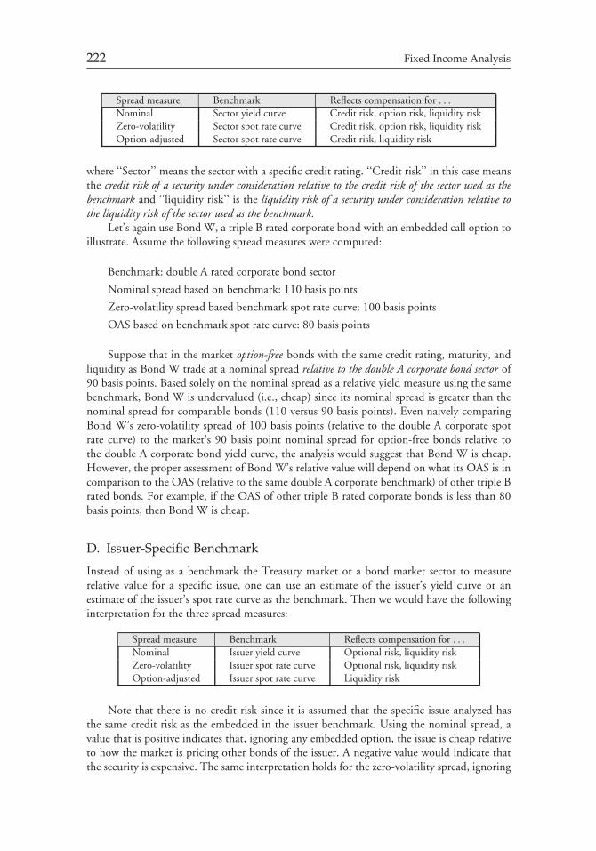
222 Fixed Income Analysis
Spread measure Benchmark Reflects compensation for . . .
Nominal Sector yield curve Credit risk, option risk, liquidity riskZero-volatility Sector spot rate curve Credit risk, option risk, liquidity riskOption-adjusted Sector spot rate curve Credit risk, liquidity risk
where ‘‘Sector’’ means the sector with a specific credit rating. ‘‘Credit risk’’ in this case meansthe credit risk of a security under consideration relative to the credit risk of the sector used as thebenchmark and ‘‘liquidity risk’’ is the liquidity risk of a security under consideration relative tothe liquidity risk of the sector used as the benchmark.
Let’s again use Bond W, a triple B rated corporate bond with an embedded call option toillustrate. Assume the following spread measures were computed:
Benchmark: double A rated corporate bond sector
Nominal spread based on benchmark: 110 basis points
Zero-volatility spread based benchmark spot rate curve: 100 basis points
OAS based on benchmark spot rate curve: 80 basis points
Suppose that in the market option-free bonds with the same credit rating, maturity, andliquidity as Bond W trade at a nominal spread relative to the double A corporate bond sector of90 basis points. Based solely on the nominal spread as a relative yield measure using the samebenchmark, Bond W is undervalued (i.e., cheap) since its nominal spread is greater than thenominal spread for comparable bonds (110 versus 90 basis points). Even naively comparingBond W’s zero-volatility spread of 100 basis points (relative to the double A corporate spotrate curve) to the market’s 90 basis point nominal spread for option-free bonds relative tothe double A corporate bond yield curve, the analysis would suggest that Bond W is cheap.However, the proper assessment of Bond W’s relative value will depend on what its OAS is incomparison to the OAS (relative to the same double A corporate benchmark) of other triple Brated bonds. For example, if the OAS of other triple B rated corporate bonds is less than 80basis points, then Bond W is cheap.
D. Issuer-Specific Benchmark
Instead of using as a benchmark the Treasury market or a bond market sector to measurerelative value for a specific issue, one can use an estimate of the issuer’s yield curve or anestimate of the issuer’s spot rate curve as the benchmark. Then we would have the followinginterpretation for the three spread measures:
Spread measure Benchmark Reflects compensation for . . .
Nominal Issuer yield curve Optional risk, liquidity riskZero-volatility Issuer spot rate curve Optional risk, liquidity riskOption-adjusted Issuer spot rate curve Liquidity risk
Note that there is no credit risk since it is assumed that the specific issue analyzed hasthe same credit risk as the embedded in the issuer benchmark. Using the nominal spread, avalue that is positive indicates that, ignoring any embedded option, the issue is cheap relativeto how the market is pricing other bonds of the issuer. A negative value would indicate thatthe security is expensive. The same interpretation holds for the zero-volatility spread, ignoring
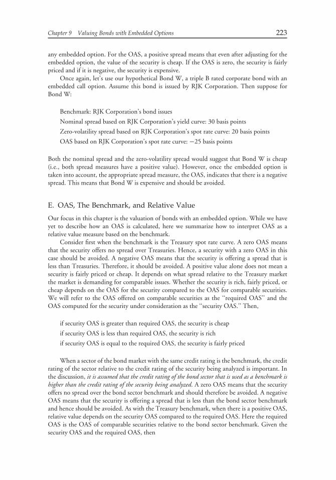
Chapter 9 Valuing Bonds with Embedded Options 223
any embedded option. For the OAS, a positive spread means that even after adjusting for theembedded option, the value of the security is cheap. If the OAS is zero, the security is fairlypriced and if it is negative, the security is expensive.
Once again, let’s use our hypothetical Bond W, a triple B rated corporate bond with anembedded call option. Assume this bond is issued by RJK Corporation. Then suppose forBond W:
Benchmark: RJK Corporation’s bond issues
Nominal spread based on RJK Corporation’s yield curve: 30 basis points
Zero-volatility spread based on RJK Corporation’s spot rate curve: 20 basis points
OAS based on RJK Corporation’s spot rate curve: −25 basis points
Both the nominal spread and the zero-volatility spread would suggest that Bond W is cheap(i.e., both spread measures have a positive value). However, once the embedded option istaken into account, the appropriate spread measure, the OAS, indicates that there is a negativespread. This means that Bond W is expensive and should be avoided.
E. OAS, The Benchmark, and Relative Value
Our focus in this chapter is the valuation of bonds with an embedded option. While we haveyet to describe how an OAS is calculated, here we summarize how to interpret OAS as arelative value measure based on the benchmark.
Consider first when the benchmark is the Treasury spot rate curve. A zero OAS meansthat the security offers no spread over Treasuries. Hence, a security with a zero OAS in thiscase should be avoided. A negative OAS means that the security is offering a spread that isless than Treasuries. Therefore, it should be avoided. A positive value alone does not mean asecurity is fairly priced or cheap. It depends on what spread relative to the Treasury marketthe market is demanding for comparable issues. Whether the security is rich, fairly priced, orcheap depends on the OAS for the security compared to the OAS for comparable securities.We will refer to the OAS offered on comparable securities as the ‘‘required OAS’’ and theOAS computed for the security under consideration as the ‘‘security OAS.’’ Then,
if security OAS is greater than required OAS, the security is cheap
if security OAS is less than required OAS, the security is rich
if security OAS is equal to the required OAS, the security is fairly priced
When a sector of the bond market with the same credit rating is the benchmark, the creditrating of the sector relative to the credit rating of the security being analyzed is important. Inthe discussion, it is assumed that the credit rating of the bond sector that is used as a benchmark ishigher than the credit rating of the security being analyzed. A zero OAS means that the securityoffers no spread over the bond sector benchmark and should therefore be avoided. A negativeOAS means that the security is offering a spread that is less than the bond sector benchmarkand hence should be avoided. As with the Treasury benchmark, when there is a positive OAS,relative value depends on the security OAS compared to the required OAS. Here the requiredOAS is the OAS of comparable securities relative to the bond sector benchmark. Given thesecurity OAS and the required OAS, then

224 Fixed Income Analysis
if security OAS is greater than required OAS, the security is cheap
if security OAS is less than required OAS, the security is rich
if security OAS is equal to the required OAS, the security is fairly priced
The terms ‘‘rich,’’ ‘‘cheap,’’ and ‘‘fairly priced’’ are only relative to the benchmark. Ifan investor is a funded investor who is assessing a security relative to his or her borrowingcosts, then a different set of rules exists. For example, suppose that the bond sector used as thebenchmark is the LIBOR spot rate curve. Also assume that the funding cost for the investor isa spread of 40 basis points over LIBOR. Then the decision to invest in the security dependson whether the OAS exceeds the 40 basis point spread by a sufficient amount to compensatefor the credit risk.
Finally, let’s look at relative valuation when the issuer’s spot rate curve is the benchmark.If a particular security by the issuer is fairly priced, its OAS should be equal to zero. Thus,unlike when the Treasury benchmark or bond sector benchmark are used, a zero OAS is fairlyvalued security. A positive OAS means that the security is trading cheap relative to other
EXHIBIT 1 Relationship Between the Benchmark, OAS, and Relative Value
Benchmark Negative OAS Zero OAS Positive OASTreasury market Overpriced (rich)
securityOverpriced (rich)security
Comparison must bemade between securityOAS and OAS ofcomparable securities(required OAS):if security OAS >
required OAS, securityis cheapif security OAS <
required OAS, securityis richif security OAS =required OAS, securityis fairly priced
Bond sector with agiven credit rating(assumes credit ratinghigher than securitybeing analyzed )
Overpriced (rich)security (assumescredit rating higherthan security beinganalyzed )
Overpriced (rich)security (assumescredit rating higherthan security beinganalyzed )
Comparison must bemade between securityOAS and OAS ofcomparable securities(required OAS):if security OAS >
required OAS, securityis cheapif security OAS <
required OAS, securityis richif security OAS =required OAS, securityis fairly priced
Issuer’s ownsecurities
Overpriced (rich)security
Fairly valued Underpriced (cheap)security
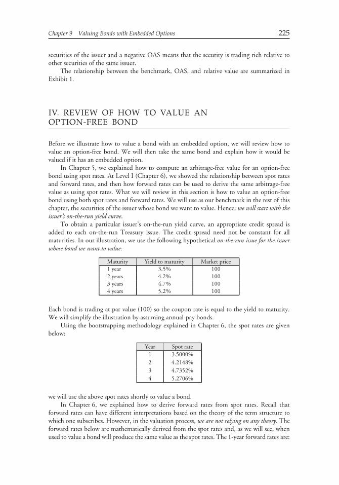
Chapter 9 Valuing Bonds with Embedded Options 225
securities of the issuer and a negative OAS means that the security is trading rich relative toother securities of the same issuer.
The relationship between the benchmark, OAS, and relative value are summarized inExhibit 1.
IV. REVIEW OF HOW TO VALUE ANOPTION-FREE BOND
Before we illustrate how to value a bond with an embedded option, we will review how tovalue an option-free bond. We will then take the same bond and explain how it would bevalued if it has an embedded option.
In Chapter 5, we explained how to compute an arbitrage-free value for an option-freebond using spot rates. At Level I (Chapter 6), we showed the relationship between spot ratesand forward rates, and then how forward rates can be used to derive the same arbitrage-freevalue as using spot rates. What we will review in this section is how to value an option-freebond using both spot rates and forward rates. We will use as our benchmark in the rest of thischapter, the securities of the issuer whose bond we want to value. Hence, we will start with theissuer’s on-the-run yield curve.
To obtain a particular issuer’s on-the-run yield curve, an appropriate credit spread isadded to each on-the-run Treasury issue. The credit spread need not be constant for allmaturities. In our illustration, we use the following hypothetical on-the-run issue for the issuerwhose bond we want to value:
Maturity Yield to maturity Market price1 year 3.5% 1002 years 4.2% 1003 years 4.7% 1004 years 5.2% 100
Each bond is trading at par value (100) so the coupon rate is equal to the yield to maturity.We will simplify the illustration by assuming annual-pay bonds.
Using the bootstrapping methodology explained in Chapter 6, the spot rates are givenbelow:
Year Spot rate1 3.5000%2 4.2148%3 4.7352%4 5.2706%
we will use the above spot rates shortly to value a bond.In Chapter 6, we explained how to derive forward rates from spot rates. Recall that
forward rates can have different interpretations based on the theory of the term structure towhich one subscribes. However, in the valuation process, we are not relying on any theory. Theforward rates below are mathematically derived from the spot rates and, as we will see, whenused to value a bond will produce the same value as the spot rates. The 1-year forward rates are:
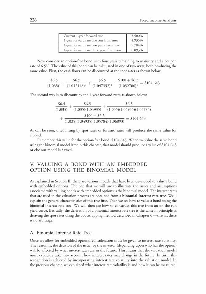
226 Fixed Income Analysis
Current 1-year forward rate 3.500%1-year forward rate one year from now 4.935%1-year forward rate two years from now 5.784%1-year forward rate three years from now 6.893%
Now consider an option-free bond with four years remaining to maturity and a couponrate of 6.5%. The value of this bond can be calculated in one of two ways, both producing thesame value. First, the cash flows can be discounted at the spot rates as shown below:
$6.5
(1.035)1+ $6.5
(1.042148)2+ $6.5
(1.047352)3+ $100 + $6.5
(1.052706)4= $104.643
The second way is to discount by the 1-year forward rates as shown below:
$6.5
(1.035)+ $6.5
(1.035)(1.04935)+ $6.5
(1.035)(1.04935)(1.05784)
+ $100 + $6.5
(1.035)(1.04935)(1.05784)(1.06893)= $104.643
As can be seen, discounting by spot rates or forward rates will produce the same value fora bond.
Remember this value for the option-free bond, $104.643. When we value the same bondusing the binomial model later in this chapter, that model should produce a value of $104.643or else our model is flawed.
V. VALUING A BOND WITH AN EMBEDDEDOPTION USING THE BINOMIAL MODEL
As explained in Section II, there are various models that have been developed to value a bondwith embedded options. The one that we will use to illustrate the issues and assumptionsassociated with valuing bonds with embedded options is the binomial model. The interest ratesthat are used in the valuation process are obtained from a binomial interest rate tree. We’llexplain the general characteristics of this tree first. Then we see how to value a bond using thebinomial interest rate tree. We will then see how to construct this tree from an on-the-runyield curve. Basically, the derivation of a binomial interest rate tree is the same in principle asderiving the spot rates using the bootstrapping method described in Chapter 6—that is, thereis no arbitrage.
A. Binomial Interest Rate Tree
Once we allow for embedded options, consideration must be given to interest rate volatility.The reason is, the decision of the issuer or the investor (depending upon who has the option)will be affected by what interest rates are in the future. This means that the valuation modelmust explicitly take into account how interest rates may change in the future. In turn, thisrecognition is achieved by incorporating interest rate volatility into the valuation model. Inthe previous chapter, we explained what interest rate volatility is and how it can be measured.
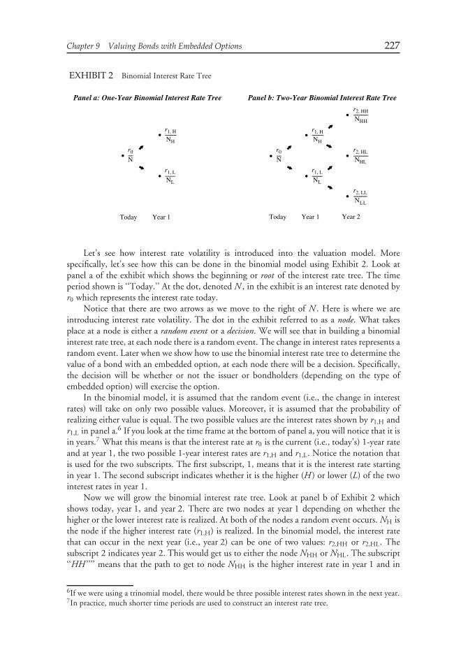
Chapter 9 Valuing Bonds with Embedded Options 227
EXHIBIT 2 Binomial Interest Rate Tree
r2, HH
NHH-------------
r1, H
NH----------
r1, H
NH----------
r0
N----
r0
N----
r2, HL
NHL-------------
r1, L
NL---------
r1, L
NL---------
r2, LL
NLL------------
•
•
• • •
•
•
•
•
Panel a: One-Year Binomial Interest Rate Tree Panel b: Two-Year Binomial Interest Rate Tree
Today Year 1 Year 1 Year 2Today
Let’s see how interest rate volatility is introduced into the valuation model. Morespecifically, let’s see how this can be done in the binomial model using Exhibit 2. Look atpanel a of the exhibit which shows the beginning or root of the interest rate tree. The timeperiod shown is ‘‘Today.’’ At the dot, denoted N , in the exhibit is an interest rate denoted byr0 which represents the interest rate today.
Notice that there are two arrows as we move to the right of N . Here is where we areintroducing interest rate volatility. The dot in the exhibit referred to as a node. What takesplace at a node is either a random event or a decision. We will see that in building a binomialinterest rate tree, at each node there is a random event. The change in interest rates represents arandom event. Later when we show how to use the binomial interest rate tree to determine thevalue of a bond with an embedded option, at each node there will be a decision. Specifically,the decision will be whether or not the issuer or bondholders (depending on the type ofembedded option) will exercise the option.
In the binomial model, it is assumed that the random event (i.e., the change in interestrates) will take on only two possible values. Moreover, it is assumed that the probability ofrealizing either value is equal. The two possible values are the interest rates shown by r1,H andr1,L in panel a.6 If you look at the time frame at the bottom of panel a, you will notice that it isin years.7 What this means is that the interest rate at r0 is the current (i.e., today’s) 1-year rateand at year 1, the two possible 1-year interest rates are r1,H and r1,L. Notice the notation thatis used for the two subscripts. The first subscript, 1, means that it is the interest rate startingin year 1. The second subscript indicates whether it is the higher (H ) or lower (L) of the twointerest rates in year 1.
Now we will grow the binomial interest rate tree. Look at panel b of Exhibit 2 whichshows today, year 1, and year 2. There are two nodes at year 1 depending on whether thehigher or the lower interest rate is realized. At both of the nodes a random event occurs. NH isthe node if the higher interest rate (r1,H) is realized. In the binomial model, the interest ratethat can occur in the next year (i.e., year 2) can be one of two values: r2,HH or r2,HL. Thesubscript 2 indicates year 2. This would get us to either the node NHH or NHL. The subscript‘‘HH ’’’’ means that the path to get to node NHH is the higher interest rate in year 1 and in
6If we were using a trinomial model, there would be three possible interest rates shown in the next year.7In practice, much shorter time periods are used to construct an interest rate tree.
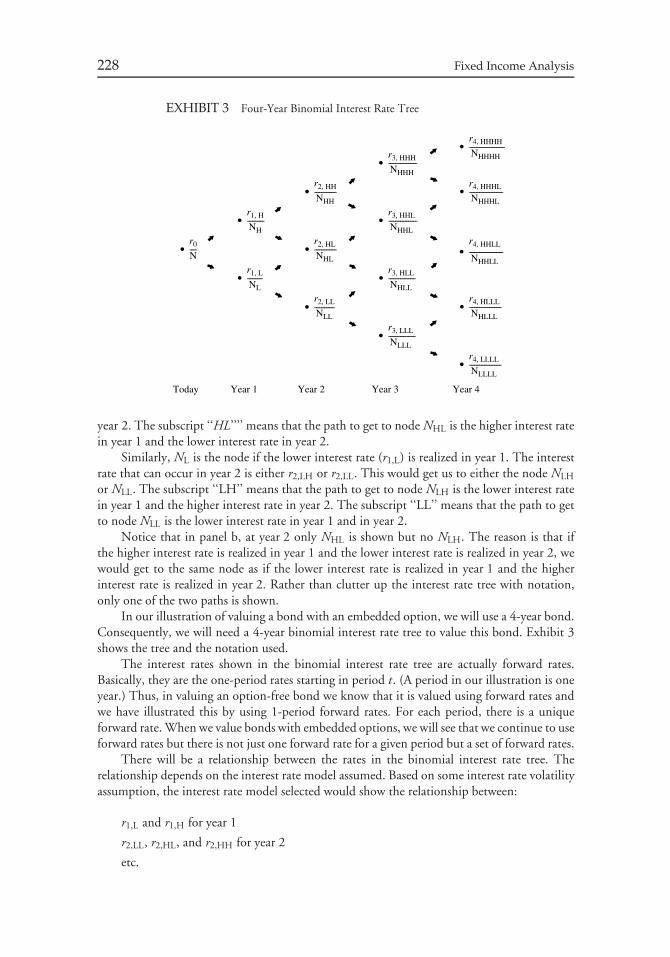
228 Fixed Income Analysis
EXHIBIT 3 Four-Year Binomial Interest Rate Tree
Today Year 1 Year 2 Year 3 Year 4
r4, HHHH
NHHHH---------------------
r3, HHH
NHHH-----------------
r2, HH
NHH-------------
r4, HHHL
NHHHL--------------------
r1, H
NH----------
r3, HHL
NHHL-----------------
r0
N----
r2, HL
NHL-------------
r4, HHLL
NHHLL--------------------
r1, L
NL---------
r3, HLL
NHLL----------------
r2, LL
NLL------------
r4, HLLL
NHLLL-------------------
r3, LLL
NLLL----------------
r4, LLLL
NLLLL-------------------
•
•
•
•
•
•
•
•
•
•
•
•
•
•
•
year 2. The subscript ‘‘HL’’’’ means that the path to get to node NHL is the higher interest ratein year 1 and the lower interest rate in year 2.
Similarly, NL is the node if the lower interest rate (r1,L) is realized in year 1. The interestrate that can occur in year 2 is either r2,LH or r2,LL. This would get us to either the node NLH
or NLL. The subscript ‘‘LH’’ means that the path to get to node NLH is the lower interest ratein year 1 and the higher interest rate in year 2. The subscript ‘‘LL’’ means that the path to getto node NLL is the lower interest rate in year 1 and in year 2.
Notice that in panel b, at year 2 only NHL is shown but no NLH. The reason is that ifthe higher interest rate is realized in year 1 and the lower interest rate is realized in year 2, wewould get to the same node as if the lower interest rate is realized in year 1 and the higherinterest rate is realized in year 2. Rather than clutter up the interest rate tree with notation,only one of the two paths is shown.
In our illustration of valuing a bond with an embedded option, we will use a 4-year bond.Consequently, we will need a 4-year binomial interest rate tree to value this bond. Exhibit 3shows the tree and the notation used.
The interest rates shown in the binomial interest rate tree are actually forward rates.Basically, they are the one-period rates starting in period t. (A period in our illustration is oneyear.) Thus, in valuing an option-free bond we know that it is valued using forward rates andwe have illustrated this by using 1-period forward rates. For each period, there is a uniqueforward rate. When we value bonds with embedded options, we will see that we continue to useforward rates but there is not just one forward rate for a given period but a set of forward rates.
There will be a relationship between the rates in the binomial interest rate tree. Therelationship depends on the interest rate model assumed. Based on some interest rate volatilityassumption, the interest rate model selected would show the relationship between:
r1,L and r1,H for year 1
r2,LL, r2,HL, and r2,HH for year 2
etc.
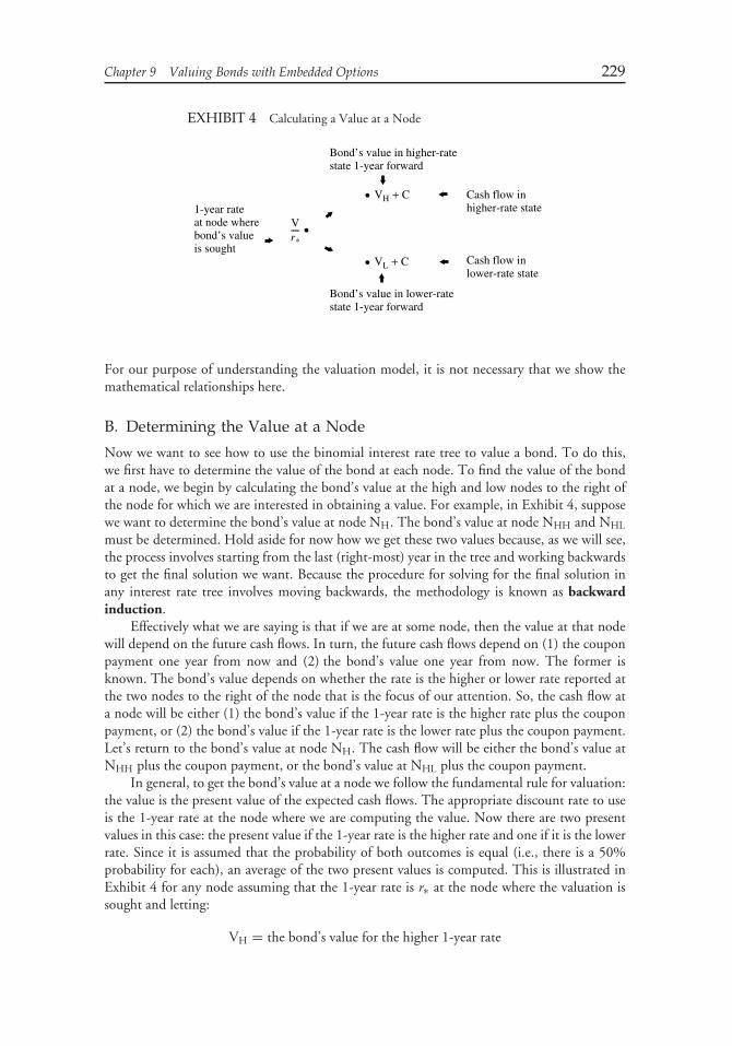
Chapter 9 Valuing Bonds with Embedded Options 229
EXHIBIT 4 Calculating a Value at a Node
1-year rateat node wherebond’s valueis sought
Cash flow inhigher-rate state
Cash flow inlower-rate state
Bond’s value in lower-ratestate 1-year forward
Bond’s value in higher-ratestate 1-year forward
VH C+
Vr*----
VL C+
•
•
•
For our purpose of understanding the valuation model, it is not necessary that we show themathematical relationships here.
B. Determining the Value at a Node
Now we want to see how to use the binomial interest rate tree to value a bond. To do this,we first have to determine the value of the bond at each node. To find the value of the bondat a node, we begin by calculating the bond’s value at the high and low nodes to the right ofthe node for which we are interested in obtaining a value. For example, in Exhibit 4, supposewe want to determine the bond’s value at node NH. The bond’s value at node NHH and NHL
must be determined. Hold aside for now how we get these two values because, as we will see,the process involves starting from the last (right-most) year in the tree and working backwardsto get the final solution we want. Because the procedure for solving for the final solution inany interest rate tree involves moving backwards, the methodology is known as backwardinduction.
Effectively what we are saying is that if we are at some node, then the value at that nodewill depend on the future cash flows. In turn, the future cash flows depend on (1) the couponpayment one year from now and (2) the bond’s value one year from now. The former isknown. The bond’s value depends on whether the rate is the higher or lower rate reported atthe two nodes to the right of the node that is the focus of our attention. So, the cash flow ata node will be either (1) the bond’s value if the 1-year rate is the higher rate plus the couponpayment, or (2) the bond’s value if the 1-year rate is the lower rate plus the coupon payment.Let’s return to the bond’s value at node NH. The cash flow will be either the bond’s value atNHH plus the coupon payment, or the bond’s value at NHL plus the coupon payment.
In general, to get the bond’s value at a node we follow the fundamental rule for valuation:the value is the present value of the expected cash flows. The appropriate discount rate to useis the 1-year rate at the node where we are computing the value. Now there are two presentvalues in this case: the present value if the 1-year rate is the higher rate and one if it is the lowerrate. Since it is assumed that the probability of both outcomes is equal (i.e., there is a 50%probability for each), an average of the two present values is computed. This is illustrated inExhibit 4 for any node assuming that the 1-year rate is r∗ at the node where the valuation issought and letting:
VH = the bond’s value for the higher 1-year rate
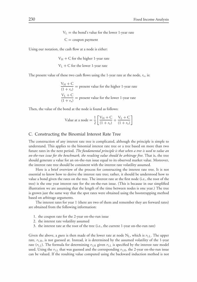
230 Fixed Income Analysis
VL = the bond’s value for the lower 1-year rate
C = coupon payment
Using our notation, the cash flow at a node is either:
VH + C for the higher 1-year rate
VL + C for the lower 1-year rate
The present value of these two cash flows using the 1-year rate at the node, r∗, is:
VH + C
(1 + r∗)= present value for the higher 1-year rate
VL + C
(1 + r∗)= present value for the lower 1-year rate
Then, the value of the bond at the node is found as follows:
Value at a node = 1
2
[VH + C
(1 + r∗)+ VL + C
(1 + r∗)
]
C. Constructing the Binomial Interest Rate Tree
The construction of any interest rate tree is complicated, although the principle is simple tounderstand. This applies to the binomial interest rate tree or a tree based on more than twofuture rates in the next period. The fundamental principle is that when a tree is used to value anon-the-run issue for the benchmark, the resulting value should be arbitrage free. That is, the treeshould generate a value for an on-the-run issue equal to its observed market value. Moreover,the interest rate tree should be consistent with the interest rate volatility assumed.
Here is a brief overview of the process for constructing the interest rate tree. It is notessential to know how to derive the interest rate tree; rather, it should be understood how tovalue a bond given the rates on the tree. The interest rate at the first node (i.e., the root of thetree) is the one year interest rate for the on-the-run issue. (This is because in our simplifiedillustration we are assuming that the length of the time between nodes is one year.) The treeis grown just the same way that the spot rates were obtained using the bootstrapping methodbased on arbitrage arguments.
The interest rates for year 1 (there are two of them and remember they are forward rates)are obtained from the following information:
1. the coupon rate for the 2-year on-the-run issue2. the interest rate volatility assumed3. the interest rate at the root of the tree (i.e., the current 1-year on-the-run rate)
Given the above, a guess is then made of the lower rate at node NL, which is r1,L. The upperrate, r1,H, is not guessed at. Instead, it is determined by the assumed volatility of the 1-yearrate (r1,L). The formula for determining r1,H given r1,L is specified by the interest rate modelused. Using the r1,L that was guessed and the corresponding r1,H, the 2-year on-the-run issuecan be valued. If the resulting value computed using the backward induction method is not
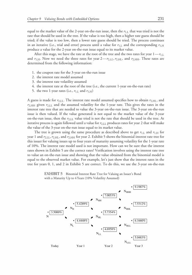
Chapter 9 Valuing Bonds with Embedded Options 231
equal to the market value of the 2-year on-the-run issue, then the r1,L that was tried is not therate that should be used in the tree. If the value is too high, then a higher rate guess should betried; if the value is too low, then a lower rate guess should be tried. The process continuesin an iterative (i.e., trial and error) process until a value for r1,L and the corresponding r1,H
produce a value for the 2-year on-the-run issue equal to its market value.After this stage, we have the rate at the root of the tree and the two rates for year 1—r1,L
and r1,H. Now we need the three rates for year 2—r2,LL, r2,HL, and r2,HH. These rates aredetermined from the following information:
1. the coupon rate for the 3-year on-the-run issue2. the interest rate model assumed3. the interest rate volatility assumed4. the interest rate at the root of the tree (i.e., the current 1-year on-the-run rate)5. the two 1-year rates (i.e., r1,L and r1,H)
A guess is made for r2,LL. The interest rate model assumed specifies how to obtain r2,HL, andr2,HH given r2,LL and the assumed volatility for the 1-year rate. This gives the rates in theinterest rate tree that are needed to value the 3-year on-the-run issue. The 3-year on-the-runissue is then valued. If the value generated is not equal to the market value of the 3-yearon-the-run issue, then the r2,LL value tried is not the rate that should be used in the tree. Atiterative process is again followed until a value for r2,LL produces rates for year 2 that will makethe value of the 3-year on-the-run issue equal to its market value.
The tree is grown using the same procedure as described above to get r1,L and r1,H foryear 1 and r2,LL, r2,HL, and r2,HH for year 2. Exhibit 5 shows the binomial interest rate tree forthis issuer for valuing issues up to four years of maturity assuming volatility for the 1-year rateof 10%. The interest rate model used is not important. How can we be sure that the interestrates shown in Exhibit 5 are the correct rates? Verification involves using the interest rate treeto value an on-the-run issue and showing that the value obtained from the binomial model isequal to the observed market value. For example, let’s just show that the interest rates in thetree for years 0, 1, and 2 in Exhibit 5 are correct. To do this, we use the 3-year on-the-run
EXHIBIT 5 Binomial Interest Rate Tree for Valuing an Issuer’s Bondwith a Maturity Up to 4 Years (10% Volatility Assumed)
• 9.1987%NHHH
• 7.0053%NHH
• 5.4289% • 7.5312%NH NHHL
• 3.5000% • 5.7354%N NHL
• 4.4448% • 6.1660%NL NHLL
• 4.6958%NLL
• 5.0483%NLLL
Today Year 1 Year 2 Year 3
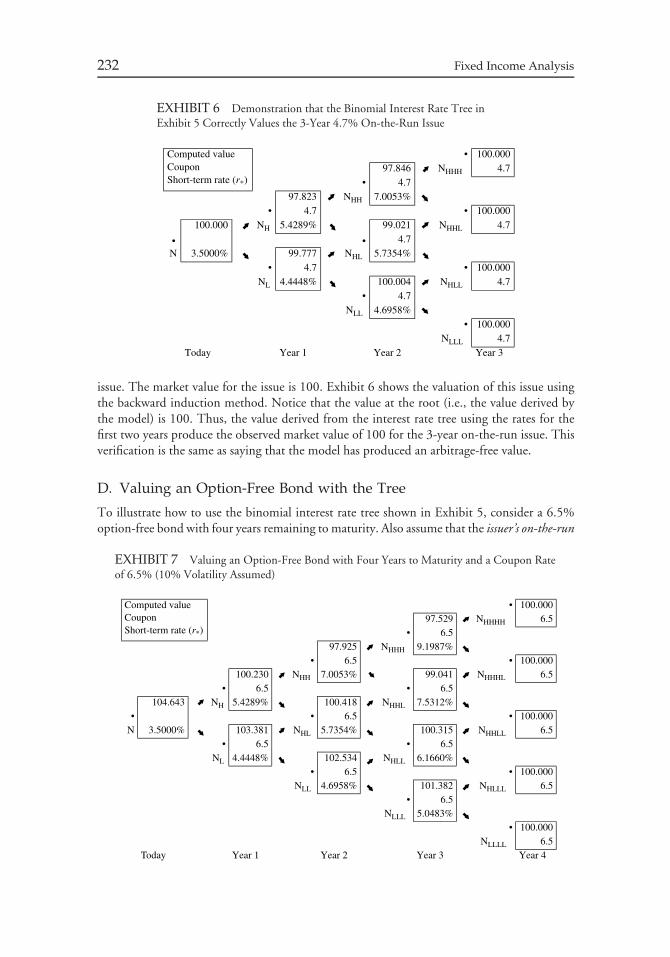
232 Fixed Income Analysis
EXHIBIT 6 Demonstration that the Binomial Interest Rate Tree inExhibit 5 Correctly Values the 3-Year 4.7% On-the-Run Issue
Computed valueCouponShort-term rate (r*)
• 100.00097.846 NHHH 4.7
• 4.797.823 NHH 7.0053%
•
••
4.7 • 100.000100.000 NH 5.4289% 99.021 NHHL 4.7
4.7N 3.5000% 99.777 NHL 5.7354%
• 4.7 • 100.000NL 4.4448% 100.004 NHLL 4.7
• 4.7NLL 4.6958%
• 100.000NLLL 4.7
Today Year 1 Year 2 Year 3
issue. The market value for the issue is 100. Exhibit 6 shows the valuation of this issue usingthe backward induction method. Notice that the value at the root (i.e., the value derived bythe model) is 100. Thus, the value derived from the interest rate tree using the rates for thefirst two years produce the observed market value of 100 for the 3-year on-the-run issue. Thisverification is the same as saying that the model has produced an arbitrage-free value.
D. Valuing an Option-Free Bond with the Tree
To illustrate how to use the binomial interest rate tree shown in Exhibit 5, consider a 6.5%option-free bond with four years remaining to maturity. Also assume that the issuer’s on-the-run
EXHIBIT 7 Valuing an Option-Free Bond with Four Years to Maturity and a Coupon Rateof 6.5% (10% Volatility Assumed)
Computed valueCouponShort-term rate (r*)
• 100.00097.529 NHHHH 6.5
•97.925 NHHH 9.1987%
• 6.5 • 100.000100.230 NHH 7.0053% 99.041 NHHHL 6.5
• 6.5
6.5
• 6.5
6.5
104.643 NH 5.4289% 100.418 NHHL 7.5312%• • 6.5 • 100.000
N 3.5000% 103.381 NHL 5.7354% 100.315 NHHLL 6.5• • 6.5
6.5
NL 4.4448% 102.534 NHLL 6.1660%• 6.5 • 100.000
NLL 4.6958% 101.382 NHLLL 6.5•
NLLL 5.0483%• 100.000
NLLLL 6.5Today Year 1 Year 2 Year 3 Year 4
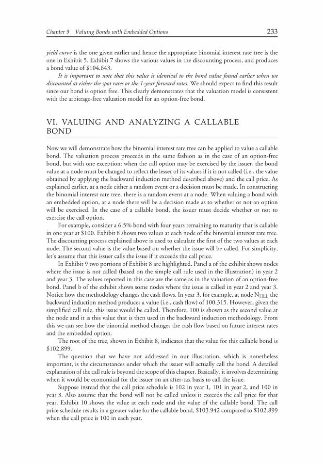
Chapter 9 Valuing Bonds with Embedded Options 233
yield curve is the one given earlier and hence the appropriate binomial interest rate tree is theone in Exhibit 5. Exhibit 7 shows the various values in the discounting process, and producesa bond value of $104.643.
It is important to note that this value is identical to the bond value found earlier when wediscounted at either the spot rates or the 1-year forward rates. We should expect to find this resultsince our bond is option free. This clearly demonstrates that the valuation model is consistentwith the arbitrage-free valuation model for an option-free bond.
VI. VALUING AND ANALYZING A CALLABLEBOND
Now we will demonstrate how the binomial interest rate tree can be applied to value a callablebond. The valuation process proceeds in the same fashion as in the case of an option-freebond, but with one exception: when the call option may be exercised by the issuer, the bondvalue at a node must be changed to reflect the lesser of its values if it is not called (i.e., the valueobtained by applying the backward induction method described above) and the call price. Asexplained earlier, at a node either a random event or a decision must be made. In constructingthe binomial interest rate tree, there is a random event at a node. When valuing a bond withan embedded option, at a node there will be a decision made as to whether or not an optionwill be exercised. In the case of a callable bond, the issuer must decide whether or not toexercise the call option.
For example, consider a 6.5% bond with four years remaining to maturity that is callablein one year at $100. Exhibit 8 shows two values at each node of the binomial interest rate tree.The discounting process explained above is used to calculate the first of the two values at eachnode. The second value is the value based on whether the issue will be called. For simplicity,let’s assume that this issuer calls the issue if it exceeds the call price.
In Exhibit 9 two portions of Exhibit 8 are highlighted. Panel a of the exhibit shows nodeswhere the issue is not called (based on the simple call rule used in the illustration) in year 2and year 3. The values reported in this case are the same as in the valuation of an option-freebond. Panel b of the exhibit shows some nodes where the issue is called in year 2 and year 3.Notice how the methodology changes the cash flows. In year 3, for example, at node NHLL thebackward induction method produces a value (i.e., cash flow) of 100.315. However, given thesimplified call rule, this issue would be called. Therefore, 100 is shown as the second value atthe node and it is this value that is then used in the backward induction methodology. Fromthis we can see how the binomial method changes the cash flow based on future interest ratesand the embedded option.
The root of the tree, shown in Exhibit 8, indicates that the value for this callable bond is$102.899.
The question that we have not addressed in our illustration, which is nonethelessimportant, is the circumstances under which the issuer will actually call the bond. A detailedexplanation of the call rule is beyond the scope of this chapter. Basically, it involves determiningwhen it would be economical for the issuer on an after-tax basis to call the issue.
Suppose instead that the call price schedule is 102 in year 1, 101 in year 2, and 100 inyear 3. Also assume that the bond will not be called unless it exceeds the call price for thatyear. Exhibit 10 shows the value at each node and the value of the callable bond. The callprice schedule results in a greater value for the callable bond, $103.942 compared to $102.899when the call price is 100 in each year.
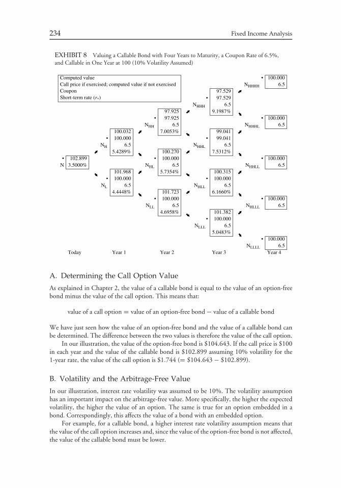
234 Fixed Income Analysis
EXHIBIT 8 Valuing a Callable Bond with Four Years to Maturity, a Coupon Rate of 6.5%,and Callable in One Year at 100 (10% Volatility Assumed)
Computed valueCall price if exercised; computed value if not exercisedCouponShort-term rate (r*)
• 100.000NHHHH 6.5
97.529• 97.529
NHHH 6.597.925 9.1987%
• 97.925 • 100.000NHH 6.5 NHHHL 6.5
100.032 7.0053% 99.041• 100.000 • 99.041
NH 6.5 NHHL 6.55.4289% 100.270 7.5312%
• 102.899 • 100.000 • 100.000N 3.5000% NHL 6.5 NHHLL 6.5
101.968 5.7354% 100.315• 100.000 • 100.000
NL 6.5 NHLL 6.54.4448% 101.723 6.1660%
• 100.000 • 100.000NLL 6.5 NHLLL 6.5
4.6958% 101.382• 100.000
NLLL 6.55.0483%
• 100.000NLLLL 6.5
Today Year 1 Year 2 Year 3 Year 4
A. Determining the Call Option Value
As explained in Chapter 2, the value of a callable bond is equal to the value of an option-freebond minus the value of the call option. This means that:
value of a call option = value of an option-free bond − value of a callable bond
We have just seen how the value of an option-free bond and the value of a callable bond canbe determined. The difference between the two values is therefore the value of the call option.
In our illustration, the value of the option-free bond is $104.643. If the call price is $100in each year and the value of the callable bond is $102.899 assuming 10% volatility for the1-year rate, the value of the call option is $1.744 (= $104.643 − $102.899).
B. Volatility and the Arbitrage-Free Value
In our illustration, interest rate volatility was assumed to be 10%. The volatility assumptionhas an important impact on the arbitrage-free value. More specifically, the higher the expectedvolatility, the higher the value of an option. The same is true for an option embedded in abond. Correspondingly, this affects the value of a bond with an embedded option.
For example, for a callable bond, a higher interest rate volatility assumption means thatthe value of the call option increases and, since the value of the option-free bond is not affected,the value of the callable bond must be lower.
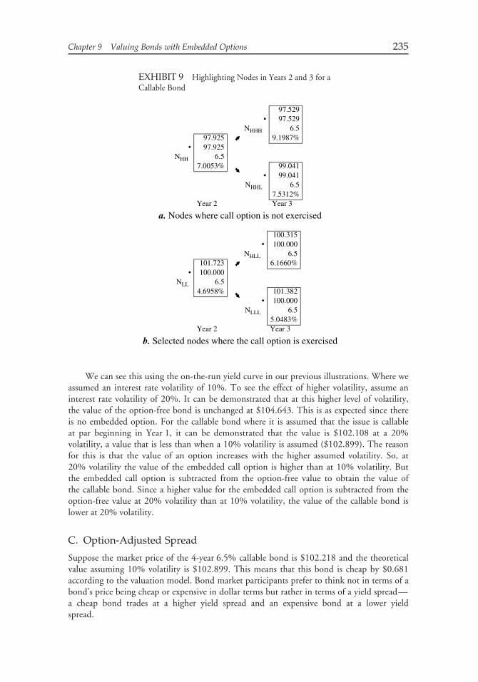
Chapter 9 Valuing Bonds with Embedded Options 235
EXHIBIT 9 Highlighting Nodes in Years 2 and 3 for aCallable Bond
a. Nodes where call option is not exercised
b. Selected nodes where the call option is exercised
97.529• 97.529
NHHH 6.597.925 9.1987%
• 97.925NHH 6.5
7.0053% 99.041• 99.041
NHHL 6.57.5312%
Year 2 Year 3
100.315• 100.000
NHLL 6.5101.723 6.1660%
• 100.000NLL 6.5
4.6958% 101.382• 100.000
NLLL 6.55.0483%
Year 2 Year 3
We can see this using the on-the-run yield curve in our previous illustrations. Where weassumed an interest rate volatility of 10%. To see the effect of higher volatility, assume aninterest rate volatility of 20%. It can be demonstrated that at this higher level of volatility,the value of the option-free bond is unchanged at $104.643. This is as expected since thereis no embedded option. For the callable bond where it is assumed that the issue is callableat par beginning in Year 1, it can be demonstrated that the value is $102.108 at a 20%volatility, a value that is less than when a 10% volatility is assumed ($102.899). The reasonfor this is that the value of an option increases with the higher assumed volatility. So, at20% volatility the value of the embedded call option is higher than at 10% volatility. Butthe embedded call option is subtracted from the option-free value to obtain the value ofthe callable bond. Since a higher value for the embedded call option is subtracted from theoption-free value at 20% volatility than at 10% volatility, the value of the callable bond islower at 20% volatility.
C. Option-Adjusted Spread
Suppose the market price of the 4-year 6.5% callable bond is $102.218 and the theoreticalvalue assuming 10% volatility is $102.899. This means that this bond is cheap by $0.681according to the valuation model. Bond market participants prefer to think not in terms of abond’s price being cheap or expensive in dollar terms but rather in terms of a yield spread—a cheap bond trades at a higher yield spread and an expensive bond at a lower yieldspread.
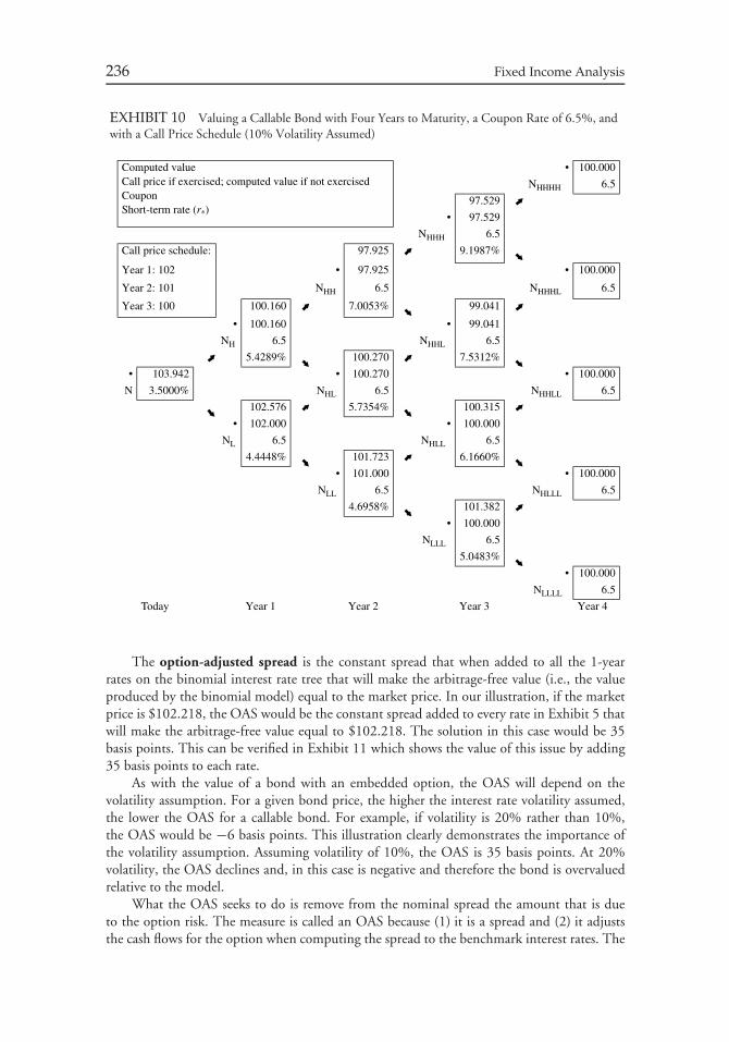
236 Fixed Income Analysis
EXHIBIT 10 Valuing a Callable Bond with Four Years to Maturity, a Coupon Rate of 6.5%, andwith a Call Price Schedule (10% Volatility Assumed)
Computed valueCall price if exercised; computed value if not exercisedCouponShort-term rate (r*)
• 100.000
NHHHH 6.5
97.529
• 97.529
NHHH 6.5
Call price schedule: 97.925 9.1987%
Year 1: 102 • 97.925 • 100.000
Year 2: 101 NHH 6.5 NHHHL 6.5
Year 3: 100 100.160 7.0053% 99.041
• 100.160 • 99.041
NH 6.5 NHHL 6.5
5.4289% 100.270 7.5312%
• 103.942 • 100.270 • 100.000
N 3.5000% NHL 6.5 NHHLL 6.5
102.576 5.7354% 100.315
• 102.000 • 100.000
NL 6.5 NHLL 6.5
4.4448% 101.723 6.1660%
• 101.000 • 100.000
NLL 6.5 NHLLL 6.5
4.6958% 101.382
• 100.000
NLLL 6.5
5.0483%
• 100.000
NLLLL 6.5
Today Year 1 Year 2 Year 3 Year 4
The option-adjusted spread is the constant spread that when added to all the 1-yearrates on the binomial interest rate tree that will make the arbitrage-free value (i.e., the valueproduced by the binomial model) equal to the market price. In our illustration, if the marketprice is $102.218, the OAS would be the constant spread added to every rate in Exhibit 5 thatwill make the arbitrage-free value equal to $102.218. The solution in this case would be 35basis points. This can be verified in Exhibit 11 which shows the value of this issue by adding35 basis points to each rate.
As with the value of a bond with an embedded option, the OAS will depend on thevolatility assumption. For a given bond price, the higher the interest rate volatility assumed,the lower the OAS for a callable bond. For example, if volatility is 20% rather than 10%,the OAS would be −6 basis points. This illustration clearly demonstrates the importance ofthe volatility assumption. Assuming volatility of 10%, the OAS is 35 basis points. At 20%volatility, the OAS declines and, in this case is negative and therefore the bond is overvaluedrelative to the model.
What the OAS seeks to do is remove from the nominal spread the amount that is dueto the option risk. The measure is called an OAS because (1) it is a spread and (2) it adjuststhe cash flows for the option when computing the spread to the benchmark interest rates. The
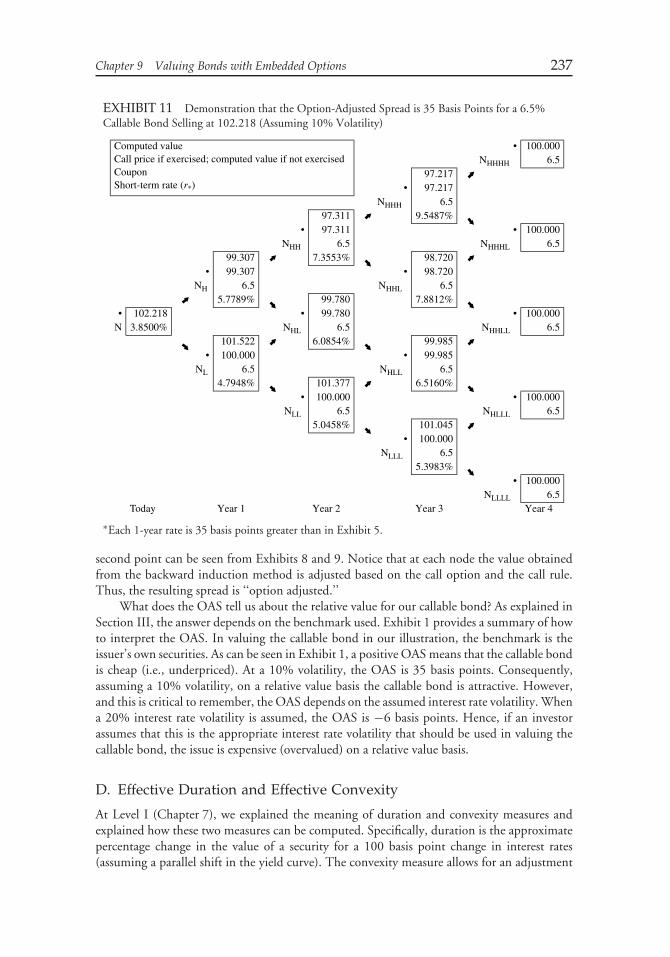
Chapter 9 Valuing Bonds with Embedded Options 237
EXHIBIT 11 Demonstration that the Option-Adjusted Spread is 35 Basis Points for a 6.5%Callable Bond Selling at 102.218 (Assuming 10% Volatility)
Computed valueCall price if exercised; computed value if not exercisedCouponShort-term rate (r*)
• 100.000NHHHH 6.5
97.217• 97.217
NHHH 6.597.311 9.5487%
• 97.311 • 100.000NHH 6.5 NHHHL 6.5
99.307 7.3553% 98.720• 99.307 • 98.720
NH 6.5 NHHL 6.55.7789% 99.780 7.8812%
• 102.218 • 99.780 • 100.000N 3.8500% NHL 6.5 NHHLL 6.5
101.522 6.0854% 99.985• 100.000 • 99.985
NL 6.5 NHLL 6.54.7948% 101.377 6.5160%
• 100.000 • 100.000NLL 6.5 NHLLL 6.5
5.0458% 101.045• 100.000
NLLL 6.55.3983%
• 100.000NLLLL 6.5
Today Year 1 Year 2 Year 3 Year 4
∗Each 1-year rate is 35 basis points greater than in Exhibit 5.
second point can be seen from Exhibits 8 and 9. Notice that at each node the value obtainedfrom the backward induction method is adjusted based on the call option and the call rule.Thus, the resulting spread is ‘‘option adjusted.’’
What does the OAS tell us about the relative value for our callable bond? As explained inSection III, the answer depends on the benchmark used. Exhibit 1 provides a summary of howto interpret the OAS. In valuing the callable bond in our illustration, the benchmark is theissuer’s own securities. As can be seen in Exhibit 1, a positive OAS means that the callable bondis cheap (i.e., underpriced). At a 10% volatility, the OAS is 35 basis points. Consequently,assuming a 10% volatility, on a relative value basis the callable bond is attractive. However,and this is critical to remember, the OAS depends on the assumed interest rate volatility. Whena 20% interest rate volatility is assumed, the OAS is −6 basis points. Hence, if an investorassumes that this is the appropriate interest rate volatility that should be used in valuing thecallable bond, the issue is expensive (overvalued) on a relative value basis.
D. Effective Duration and Effective Convexity
At Level I (Chapter 7), we explained the meaning of duration and convexity measures andexplained how these two measures can be computed. Specifically, duration is the approximatepercentage change in the value of a security for a 100 basis point change in interest rates(assuming a parallel shift in the yield curve). The convexity measure allows for an adjustment
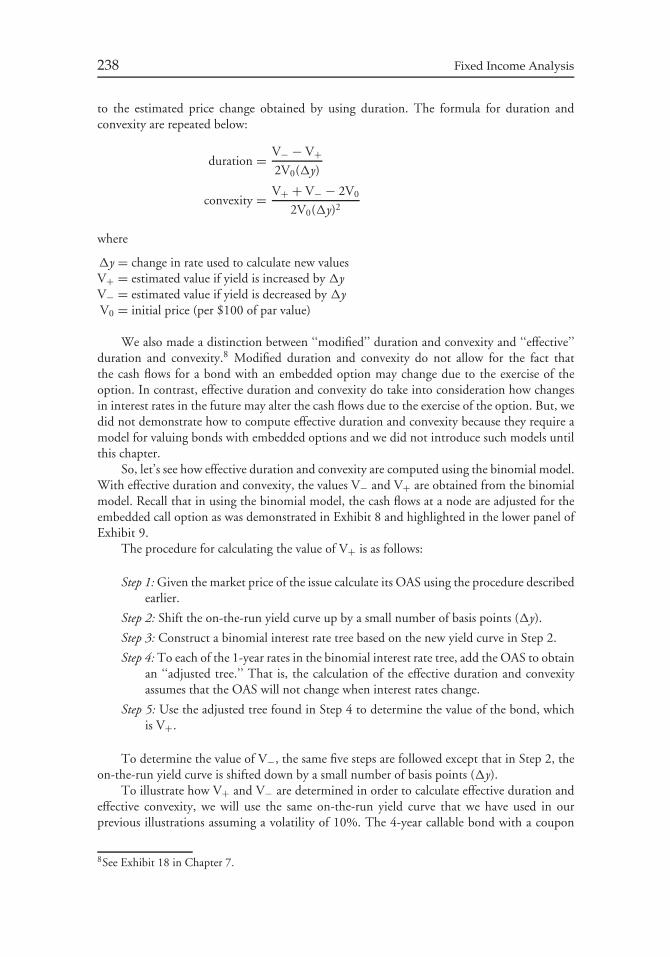
238 Fixed Income Analysis
to the estimated price change obtained by using duration. The formula for duration andconvexity are repeated below:
duration = V− − V+2V0(�y)
convexity = V+ + V− − 2V0
2V0(�y)2
where
�y = change in rate used to calculate new valuesV+ = estimated value if yield is increased by �yV− = estimated value if yield is decreased by �yV0 = initial price (per $100 of par value)
We also made a distinction between ‘‘modified’’ duration and convexity and ‘‘effective’’duration and convexity.8 Modified duration and convexity do not allow for the fact thatthe cash flows for a bond with an embedded option may change due to the exercise of theoption. In contrast, effective duration and convexity do take into consideration how changesin interest rates in the future may alter the cash flows due to the exercise of the option. But, wedid not demonstrate how to compute effective duration and convexity because they require amodel for valuing bonds with embedded options and we did not introduce such models untilthis chapter.
So, let’s see how effective duration and convexity are computed using the binomial model.With effective duration and convexity, the values V− and V+ are obtained from the binomialmodel. Recall that in using the binomial model, the cash flows at a node are adjusted for theembedded call option as was demonstrated in Exhibit 8 and highlighted in the lower panel ofExhibit 9.
The procedure for calculating the value of V+ is as follows:
Step 1: Given the market price of the issue calculate its OAS using the procedure describedearlier.
Step 2: Shift the on-the-run yield curve up by a small number of basis points (�y).
Step 3: Construct a binomial interest rate tree based on the new yield curve in Step 2.
Step 4: To each of the 1-year rates in the binomial interest rate tree, add the OAS to obtainan ‘‘adjusted tree.’’ That is, the calculation of the effective duration and convexityassumes that the OAS will not change when interest rates change.
Step 5: Use the adjusted tree found in Step 4 to determine the value of the bond, whichis V+.
To determine the value of V−, the same five steps are followed except that in Step 2, theon-the-run yield curve is shifted down by a small number of basis points (�y).
To illustrate how V+ and V− are determined in order to calculate effective duration andeffective convexity, we will use the same on-the-run yield curve that we have used in ourprevious illustrations assuming a volatility of 10%. The 4-year callable bond with a coupon
8See Exhibit 18 in Chapter 7.
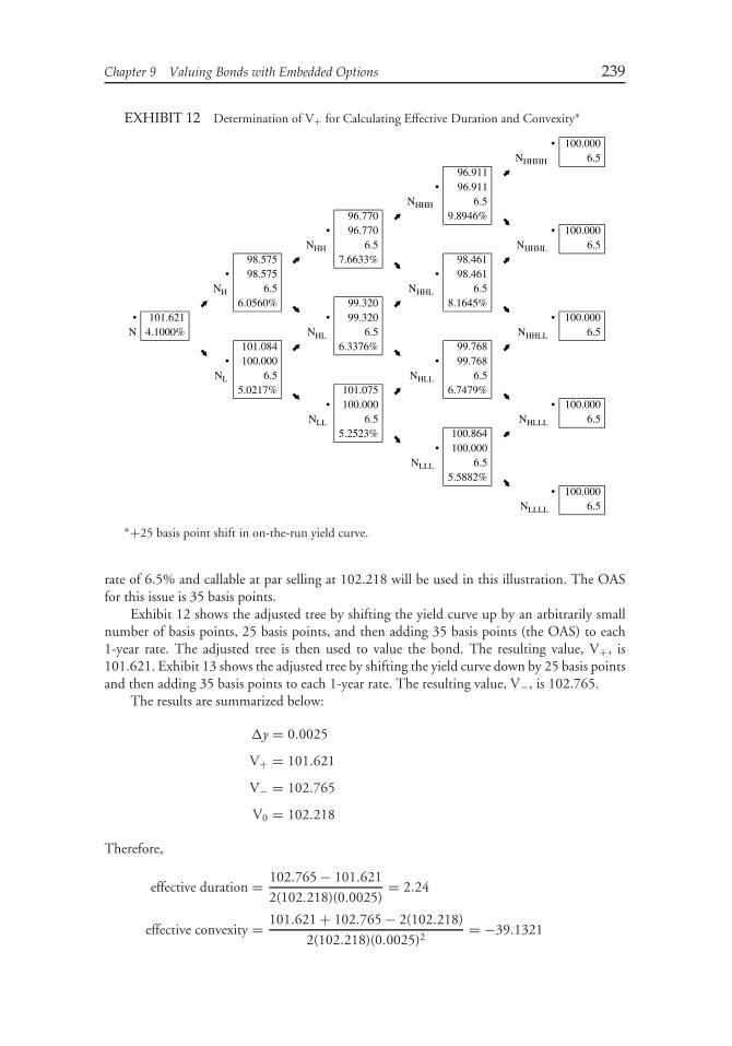
Chapter 9 Valuing Bonds with Embedded Options 239
EXHIBIT 12 Determination of V+ for Calculating Effective Duration and Convexity∗
• 100.000NHHHH 6.5
96.911• 96.911
NHHH 6.596.770 9.8946%
• 96.770 • 100.000NHH 6.5 NHHHL 6.5
98.575 7.6633% 98.461• 98.575 • 98.461
NH 6.5 NHHL 6.56.0560% 99.320 8.1645%
• 101.621 • 99.320 • 100.000N 4.1000% NHL 6.5 NHHLL 6.5
101.084 6.3376% 99.768• 100.000 • 99.768
NL 6.5 NHLL 6.55.0217% 101.075 6.7479%
• 100.000 • 100.000NLL 6.5 NHLLL 6.5
5.2523% 100.864• 100.000
NLLL 6.55.5882%
• 100.000NLLLL 6.5
∗+25 basis point shift in on-the-run yield curve.
rate of 6.5% and callable at par selling at 102.218 will be used in this illustration. The OASfor this issue is 35 basis points.
Exhibit 12 shows the adjusted tree by shifting the yield curve up by an arbitrarily smallnumber of basis points, 25 basis points, and then adding 35 basis points (the OAS) to each1-year rate. The adjusted tree is then used to value the bond. The resulting value, V+, is101.621. Exhibit 13 shows the adjusted tree by shifting the yield curve down by 25 basis pointsand then adding 35 basis points to each 1-year rate. The resulting value, V−, is 102.765.
The results are summarized below:
�y = 0.0025
V+ = 101.621
V− = 102.765
V0 = 102.218
Therefore,
effective duration = 102.765 − 101.621
2(102.218)(0.0025)= 2.24
effective convexity = 101.621 + 102.765 − 2(102.218)
2(102.218)(0.0025)2= −39.1321
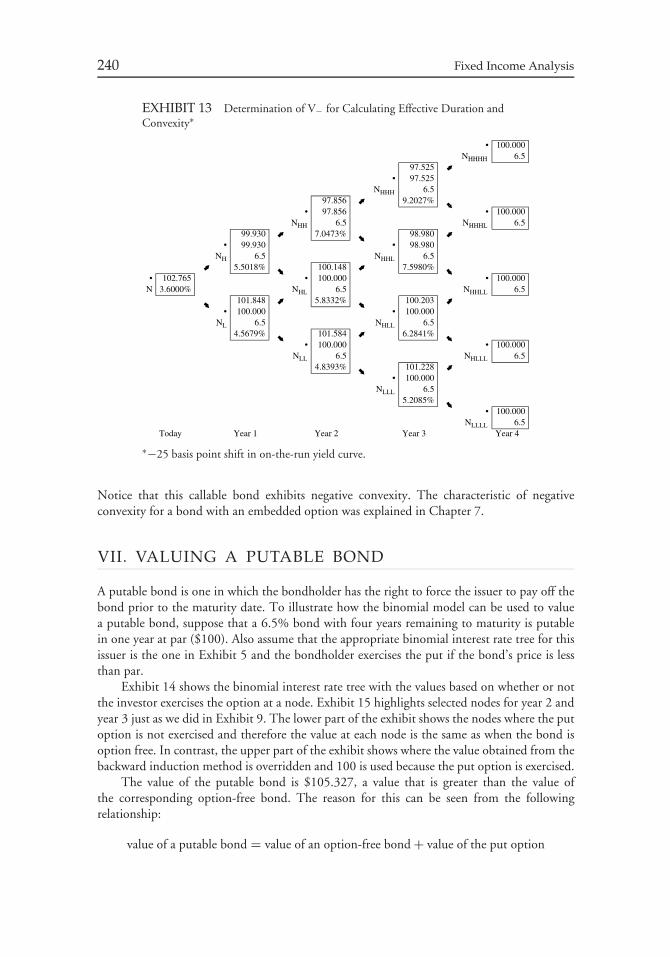
240 Fixed Income Analysis
EXHIBIT 13 Determination of V− for Calculating Effective Duration andConvexity∗
• 100.000NHHHH 6.5
97.525• 97.525
NHHH 6.597.856 9.2027%
• 97.856 • 100.000NHH 6.5 NHHHL 6.5
99.930 7.0473% 98.980• 99.930 • 98.980
NH 6.5 NHHL 6.55.5018% 100.148 7.5980%
• 102.765 • 100.000 • 100.000N 3.6000% NHL 6.5 NHHLL 6.5
101.848 5.8332% 100.203• 100.000 • 100.000
NL 6.5 NHLL 6.54.5679% 101.584 6.2841%
• 100.000 • 100.000NLL 6.5 NHLLL 6.5
4.8393% 101.228• 100.000
NLLL 6.55.2085%
• 100.000NLLLL 6.5
Today Year 1 Year 2 Year 3 Year 4
∗−25 basis point shift in on-the-run yield curve.
Notice that this callable bond exhibits negative convexity. The characteristic of negativeconvexity for a bond with an embedded option was explained in Chapter 7.
VII. VALUING A PUTABLE BOND
A putable bond is one in which the bondholder has the right to force the issuer to pay off thebond prior to the maturity date. To illustrate how the binomial model can be used to valuea putable bond, suppose that a 6.5% bond with four years remaining to maturity is putablein one year at par ($100). Also assume that the appropriate binomial interest rate tree for thisissuer is the one in Exhibit 5 and the bondholder exercises the put if the bond’s price is lessthan par.
Exhibit 14 shows the binomial interest rate tree with the values based on whether or notthe investor exercises the option at a node. Exhibit 15 highlights selected nodes for year 2 andyear 3 just as we did in Exhibit 9. The lower part of the exhibit shows the nodes where the putoption is not exercised and therefore the value at each node is the same as when the bond isoption free. In contrast, the upper part of the exhibit shows where the value obtained from thebackward induction method is overridden and 100 is used because the put option is exercised.
The value of the putable bond is $105.327, a value that is greater than the value ofthe corresponding option-free bond. The reason for this can be seen from the followingrelationship:
value of a putable bond = value of an option-free bond + value of the put option
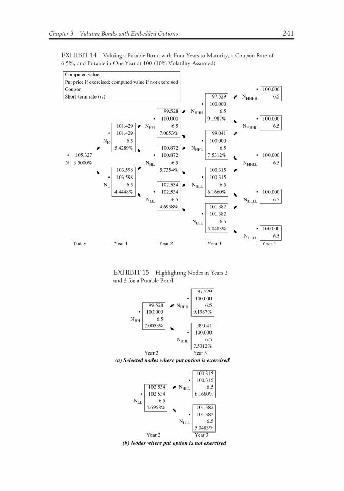
Chapter 9 Valuing Bonds with Embedded Options 241
EXHIBIT 14 Valuing a Putable Bond with Four Years to Maturity, a Coupon Rate of6.5%, and Putable in One Year at 100 (10% Volatility Assumed)
Computed value
Put price if exercised; computed value if not exercised
Coupon • 100.000
Short-term rate (r*) 97.529 NHHHH 6.5
• 100.000
99.528 NHHH 6.5
• 100.000 9.1987% • 100.000
101.429 NHH 6.5 NHHHL 6.5
• 101.429 7.0053% 99.041
NH 6.5 • 100.000
5.4289% 100.872 NHHL 6.5
• 105.327 • 100.872 7.5312% • 100.000
N 3.5000% NHL 6.5 NHHLL 6.5
103.598 5.7354% 100.315
• 103.598 • 100.315
NL 6.5 102.534 NHLL 6.5
4.4448% • 102.534 6.1660% • 100.000
NLL 6.5 NHLLL 6.5
4.6958% 101.382
• 101.382
NLLL 6.5
5.0483% • 100.000
NLLLL 6.5
Today Year 1 Year 2 Year 3 Year 4
EXHIBIT 15 Highlighting Nodes in Years 2and 3 for a Putable Bond
97.529• 100.000
99.528 NHHH 6.5• 100.000 9.1987%
NHH 6.57.0053% 99.041
• 100.000NHHL 6.5
7.5312%Year 2 Year 3
(a) Selected nodes where put option is exercised
(b) Nodes where put option is not exercised
100.315• 100.315
102.534 NHLL 6.5• 102.534 6.1660%
NLL 6.54.6958% 101.382
• 101.382NLLL 6.5
5.0483%Year 2 Year 3
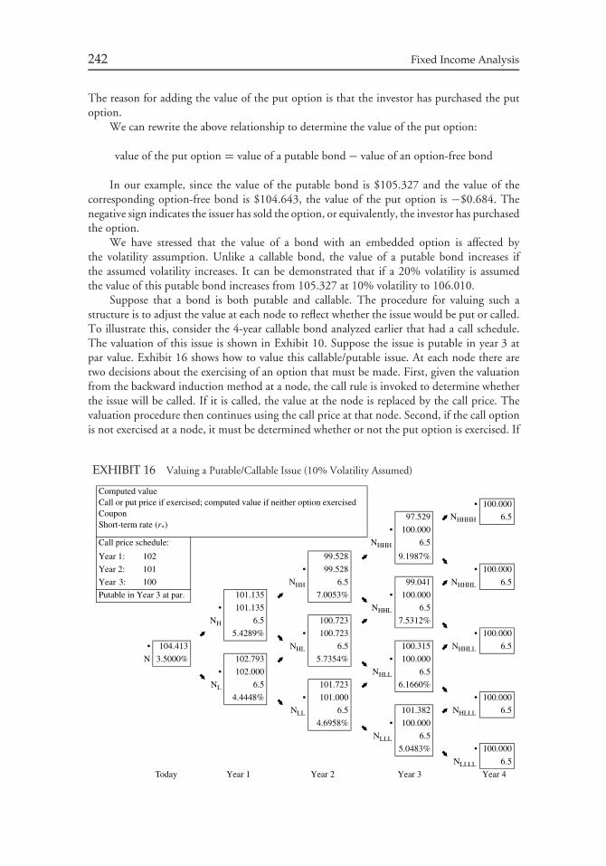
242 Fixed Income Analysis
The reason for adding the value of the put option is that the investor has purchased the putoption.
We can rewrite the above relationship to determine the value of the put option:
value of the put option = value of a putable bond − value of an option-free bond
In our example, since the value of the putable bond is $105.327 and the value of thecorresponding option-free bond is $104.643, the value of the put option is −$0.684. Thenegative sign indicates the issuer has sold the option, or equivalently, the investor has purchasedthe option.
We have stressed that the value of a bond with an embedded option is affected bythe volatility assumption. Unlike a callable bond, the value of a putable bond increases ifthe assumed volatility increases. It can be demonstrated that if a 20% volatility is assumedthe value of this putable bond increases from 105.327 at 10% volatility to 106.010.
Suppose that a bond is both putable and callable. The procedure for valuing such astructure is to adjust the value at each node to reflect whether the issue would be put or called.To illustrate this, consider the 4-year callable bond analyzed earlier that had a call schedule.The valuation of this issue is shown in Exhibit 10. Suppose the issue is putable in year 3 atpar value. Exhibit 16 shows how to value this callable/putable issue. At each node there aretwo decisions about the exercising of an option that must be made. First, given the valuationfrom the backward induction method at a node, the call rule is invoked to determine whetherthe issue will be called. If it is called, the value at the node is replaced by the call price. Thevaluation procedure then continues using the call price at that node. Second, if the call optionis not exercised at a node, it must be determined whether or not the put option is exercised. If
EXHIBIT 16 Valuing a Putable/Callable Issue (10% Volatility Assumed)
Computed valueCall or put price if exercised; computed value if neither option exercisedCouponShort-term rate (r*)
• 100.000
97.529 NHHHH 6.5
• 100.000
Call price schedule: NHHH 6.5
Year 1: 102 99.528 9.1987%
Year 2: 101 • 99.528 • 100.000
Year 3: 100 NHH 6.5 99.041 NHHHL 6.5
Putable in Year 3 at par. 101.135 7.0053% • 100.000
• 101.135 NHHL 6.5
NH 6.5 100.723 7.5312%
5.4289% • 100.723 • 100.000
• 104.413 NHL 6.5 100.315 NHHLL 6.5
N 3.5000% 102.793 5.7354% • 100.000
• 102.000 NHLL 6.5
NL 6.5 101.723 6.1660%
4.4448% • 101.000 • 100.000
NLL 6.5 101.382 NHLLL 6.5
4.6958% • 100.000
NLLL 6.5
5.0483% • 100.000
NLLLL 6.5
Today Year 1 Year 2 Year 3 Year 4
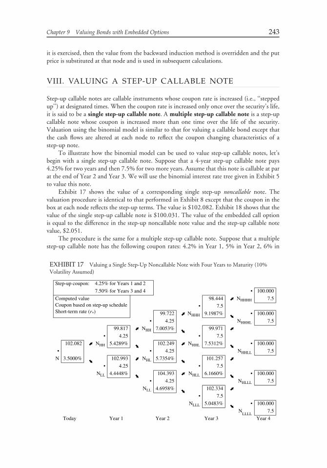
Chapter 9 Valuing Bonds with Embedded Options 243
it is exercised, then the value from the backward induction method is overridden and the putprice is substituted at that node and is used in subsequent calculations.
VIII. VALUING A STEP-UP CALLABLE NOTE
Step-up callable notes are callable instruments whose coupon rate is increased (i.e., ‘‘steppedup’’) at designated times. When the coupon rate is increased only once over the security’s life,it is said to be a single step-up callable note. A multiple step-up callable note is a step-upcallable note whose coupon is increased more than one time over the life of the security.Valuation using the binomial model is similar to that for valuing a callable bond except thatthe cash flows are altered at each node to reflect the coupon changing characteristics of astep-up note.
To illustrate how the binomial model can be used to value step-up callable notes, let’sbegin with a single step-up callable note. Suppose that a 4-year step-up callable note pays4.25% for two years and then 7.5% for two more years. Assume that this note is callable at parat the end of Year 2 and Year 3. We will use the binomial interest rate tree given in Exhibit 5to value this note.
Exhibit 17 shows the value of a corresponding single step-up noncallable note. Thevaluation procedure is identical to that performed in Exhibit 8 except that the coupon in thebox at each node reflects the step-up terms. The value is $102.082. Exhibit 18 shows that thevalue of the single step-up callable note is $100.031. The value of the embedded call optionis equal to the difference in the step-up noncallable note value and the step-up callable notevalue, $2.051.
The procedure is the same for a multiple step-up callable note. Suppose that a multiplestep-up callable note has the following coupon rates: 4.2% in Year 1, 5% in Year 2, 6% in
EXHIBIT 17 Valuing a Single Step-Up Noncallable Note with Four Years to Maturity (10%Volatility Assumed)
Step-up coupon: 4.25% for Years 1 and 2
7.50% for Years 3 and 4 • 100.000
Computed valueCoupon based on step-up scheduleShort-term rate (r*)
98.444 NHHHH 7.5
• 7.5
99.722 NHHH 9.1987% • 100.000
• 4.25 NHHHL 7.5
99.817 NHH 7.0053% 99.971
• 4.25 • 7.5
102.082 NHH 5.4289% 102.249 NHHL 7.5312% • 100.000
• • 4.25 NHHLL 7.5
N 3.5000% 102.993 NHL 5.7354% 101.257
• 4.25 • 7.5
NLL 4.4448% 104.393 NHLL 6.1660% • 100.000
• 4.25 NHLLL 7.5
NLL 4.6958% 102.334
• 7.5
NLLL 5.0483% • 100.000
NLLLL
7.5
Today Year 1 Year 2 Year 3 Year 4
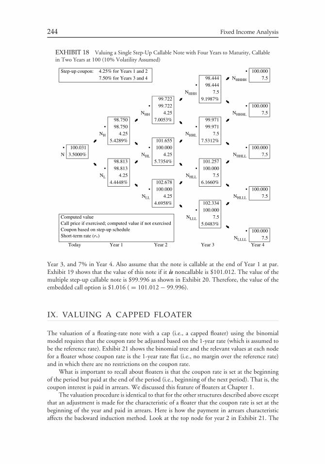
244 Fixed Income Analysis
EXHIBIT 18 Valuing a Single Step-Up Callable Note with Four Years to Maturity, Callablein Two Years at 100 (10% Volatility Assumed)
Step-up coupon: 4.25% for Years 1 and 2 • 100.0007.50% for Years 3 and 4 98.444 NHHHH 7.5
• 98.444NHHH 7.5
99.722 9.1987%• 99.722 • 100.000
NHH 4.25 NHHHL 7.598.750 7.0053% 99.971
• 98.750 • 99.971NH 4.25 NHHL 7.5
5.4289% 101.655 7.5312%• 100.031 • 100.000 • 100.000
N 3.5000% NHL 4.25 NHHLL 7.598.813 5.7354% 101.257
• 98.813 • 100.000NL 4.25 NHLL 7.5
4.4448% 102.678 6.1660%• 100.000 • 100.000
NLL 4.25 NHLLL 7.54.6958% 102.334
• 100.000Computed valueCall price if exercised; computed value if not exercisedCoupon based on step-up scheduleShort-term rate (r*)
NLLL 7.55.0483%
• 100.000NLLLL 7.5
Today Year 1 Year 2 Year 3 Year 4
Year 3, and 7% in Year 4. Also assume that the note is callable at the end of Year 1 at par.Exhibit 19 shows that the value of this note if it is noncallable is $101.012. The value of themultiple step-up callable note is $99.996 as shown in Exhibit 20. Therefore, the value of theembedded call option is $1.016 ( = 101.012 − 99.996).
IX. VALUING A CAPPED FLOATER
The valuation of a floating-rate note with a cap (i.e., a capped floater) using the binomialmodel requires that the coupon rate be adjusted based on the 1-year rate (which is assumed tobe the reference rate). Exhibit 21 shows the binomial tree and the relevant values at each nodefor a floater whose coupon rate is the 1-year rate flat (i.e., no margin over the reference rate)and in which there are no restrictions on the coupon rate.
What is important to recall about floaters is that the coupon rate is set at the beginningof the period but paid at the end of the period (i.e., beginning of the next period). That is, thecoupon interest is paid in arrears. We discussed this feature of floaters at Chapter 1.
The valuation procedure is identical to that for the other structures described above exceptthat an adjustment is made for the characteristic of a floater that the coupon rate is set at thebeginning of the year and paid in arrears. Here is how the payment in arrears characteristicaffects the backward induction method. Look at the top node for year 2 in Exhibit 21. The
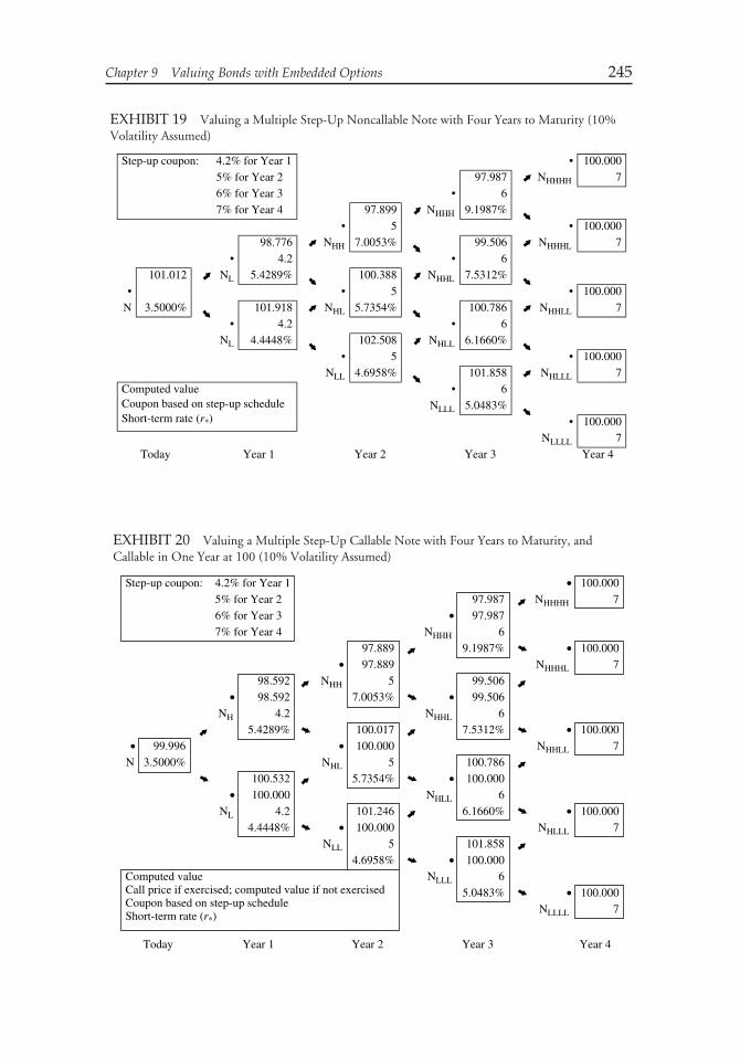
Chapter 9 Valuing Bonds with Embedded Options 245
EXHIBIT 19 Valuing a Multiple Step-Up Noncallable Note with Four Years to Maturity (10%Volatility Assumed)
Step-up coupon: 4.2% for Year 1 • 100.0005% for Year 2 97.987 NHHHH 76% for Year 3 • 67% for Year 4 97.899 NHHH 9.1987%
• 5 • 100.00098.776 NHH 7.0053% 99.506 NHHHL 7
• 4.2
4.2
• 6101.012 NL 5.4289% 100.388 NHHL 7.5312%
• • 5 • 100.000N 3.5000% 101.918 NHL 5.7354% 100.786 NHHLL 7
• •
•
6NL 4.4448% 102.508 NHLL 6.1660%
• 5 • 100.000NLL 4.6958% 101.858 NHLLL 7
Computed valueCoupon based on step-up scheduleShort-term rate (r*)
6NLLL 5.0483%
• 100.000NLLLL 7
Today Year 1 Year 2 Year 3 Year 4
EXHIBIT 20 Valuing a Multiple Step-Up Callable Note with Four Years to Maturity, andCallable in One Year at 100 (10% Volatility Assumed)
Step-up coupon: 4.2% for Year 1 • 100.0005% for Year 2 97.987 NHHHH 76% for Year 3 • 97.9877% for Year 4 NHHH 6
97.889 9.1987% • 100.000• 97.889 NHHHL 7
98.592 NHH 5 99.506• 98.592 7.0053% • 99.506
NH 4.2 NHHL 65.4289% 100.017 7.5312% • 100.000
• 99.996 • 100.000 NHHLL 7N 3.5000% NHL 5 100.786
100.532 5.7354% • 100.000• 100.000 NHLL 6
NL 4.2 101.246 6.1660% • 100.0004.4448% • 100.000 NHLLL 7
NLL 5 101.8584.6958% • 100.000
Computed valueCall price if exercised; computed value if not exercisedCoupon based on step-up scheduleShort-term rate (r*)
NLLL 65.0483% • 100.000
NLLLL 7
Today Year 1 Year 2 Year 3 Year 4
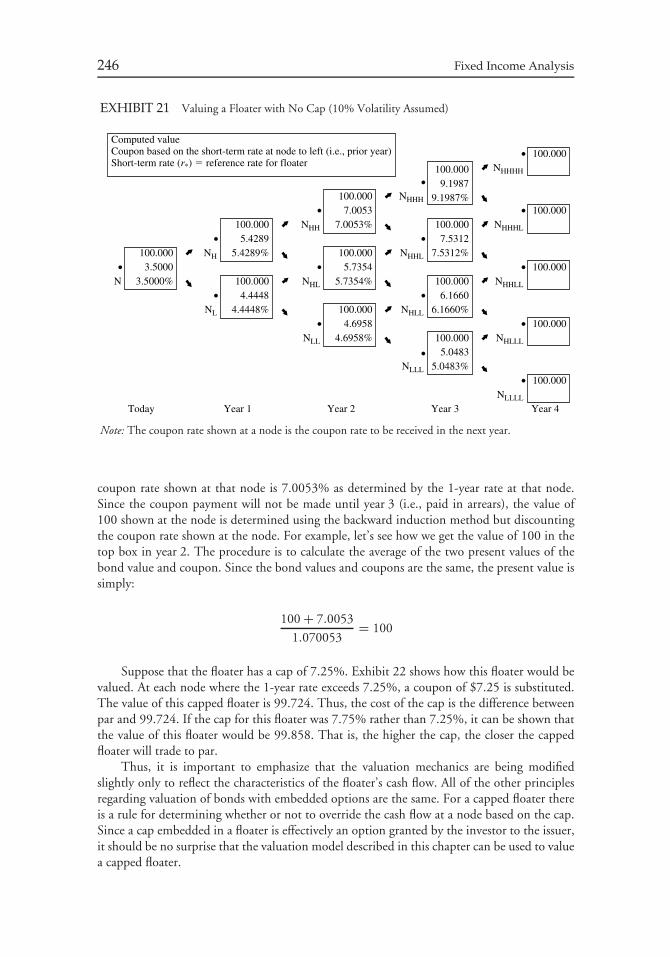
246 Fixed Income Analysis
EXHIBIT 21 Valuing a Floater with No Cap (10% Volatility Assumed)
Computed valueCoupon based on the short-term rate at node to left (i.e., prior year)Short-term rate (r*) � reference rate for floater
• 100.000
100.000 NHHHH
9.1987100.000 NHHH 9.1987%
• 7.0053 • 100.000100.000 NHH 7.0053% 100.000 NHHHL
• 5.4289 •
•
7.5312100.000 NH 5.4289% 100.000 NHHL 7.5312%
• 3.5000 • 5.7354 • 100.000N 3.5000% 100.000 NHL 5.7354% 100.000 NHHLL
• 4.4448 •
•
6.1660NL 4.4448% 100.000 NHLL 6.1660%
• 4.6958 • 100.000NLL 4.6958% 100.000 NHLLL
5.0483NLLL 5.0483%
• 100.000NLLLL
Today Year 1 Year 2 Year 3 Year 4
Note: The coupon rate shown at a node is the coupon rate to be received in the next year.
coupon rate shown at that node is 7.0053% as determined by the 1-year rate at that node.Since the coupon payment will not be made until year 3 (i.e., paid in arrears), the value of100 shown at the node is determined using the backward induction method but discountingthe coupon rate shown at the node. For example, let’s see how we get the value of 100 in thetop box in year 2. The procedure is to calculate the average of the two present values of thebond value and coupon. Since the bond values and coupons are the same, the present value issimply:
100 + 7.0053
1.070053= 100
Suppose that the floater has a cap of 7.25%. Exhibit 22 shows how this floater would bevalued. At each node where the 1-year rate exceeds 7.25%, a coupon of $7.25 is substituted.The value of this capped floater is 99.724. Thus, the cost of the cap is the difference betweenpar and 99.724. If the cap for this floater was 7.75% rather than 7.25%, it can be shown thatthe value of this floater would be 99.858. That is, the higher the cap, the closer the cappedfloater will trade to par.
Thus, it is important to emphasize that the valuation mechanics are being modifiedslightly only to reflect the characteristics of the floater’s cash flow. All of the other principlesregarding valuation of bonds with embedded options are the same. For a capped floater thereis a rule for determining whether or not to override the cash flow at a node based on the cap.Since a cap embedded in a floater is effectively an option granted by the investor to the issuer,it should be no surprise that the valuation model described in this chapter can be used to valuea capped floater.
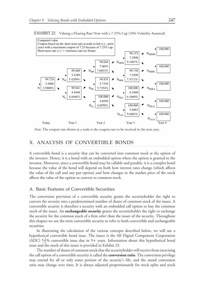
Chapter 9 Valuing Bonds with Embedded Options 247
EXHIBIT 22 Valuing a Floating Rate Note with a 7.25% Cap (10% Volatility Assumed)
Computed valueCoupon based on the short-term rate at node to left (i.e., prioryear) with a maximum coupon of 7.25 because of 7.25% capShort-term rate (r*) � reference rate for floater
• 100.00098.215 NHHHH
7.2500
99.044 NHHH 9.1987%
• 7.0053 • 100.000
99.488 NHH 7.0053% 99.738 NHHHL
•
•
5.4289 •
•
•
•
7.250099.724 NH 5.4289% 99.876 NHHL 7.5312%
• 3.5000 • 5.7354 • 100.000
N 3.5000% 99.941 NHL 5.7354% 100.000 NHHLL
4.4448 6.1660
NL 4.4448% 100.000 NHLL 6.1660%
• 4.6958 • 100.000NLL 4.6958% 100.000 NHLLL
5.0483NLLL 5.0483% • 100.000
NLLLL
Today Year 1 Year 2 Year 3 Year 4
Note: The coupon rate shown at a node is the coupon rate to be received in the next year.
X. ANALYSIS OF CONVERTIBLE BONDS
A convertible bond is a security that can be converted into common stock at the option ofthe investor. Hence, it is a bond with an embedded option where the option is granted to theinvestor. Moreover, since a convertible bond may be callable and putable, it is a complex bondbecause the value of the bond will depend on both how interest rates change (which affectsthe value of the call and any put option) and how changes in the market price of the stockaffects the value of the option to convert to common stock.
A. Basic Features of Convertible Securities
The conversion provision of a convertible security grants the securityholder the right toconvert the security into a predetermined number of shares of common stock of the issuer. Aconvertible security is therefore a security with an embedded call option to buy the commonstock of the issuer. An exchangeable security grants the securityholder the right to exchangethe security for the common stock of a firm other than the issuer of the security. Throughoutthis chapter we use the term convertible security to refer to both convertible and exchangeablesecurities.
In illustrating the calculation of the various concepts described below, we will use ahypothetical convertible bond issue. The issuer is the All Digital Component Corporation(ADC) 5 3
4 % convertible issue due in 9+ years. Information about this hypothetical bondissue and the stock of this issuer is provided in Exhibit 23.
The number of shares of common stock that the securityholder will receive from exercisingthe call option of a convertible security is called the conversion ratio. The conversion privilegemay extend for all or only some portion of the security’s life, and the stated conversionratio may change over time. It is always adjusted proportionately for stock splits and stock
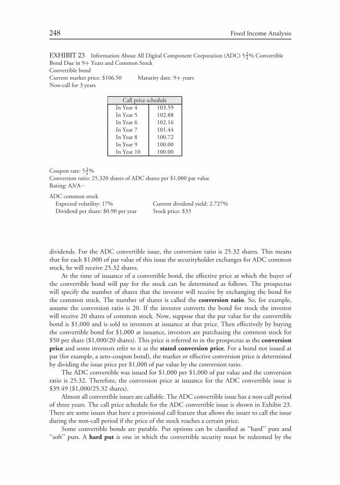
248 Fixed Income Analysis
EXHIBIT 23 Information About All Digital Component Corporation (ADC) 5 34 % Convertible
Bond Due in 9+ Years and Common StockConvertible bondCurrent market price: $106.50 Maturity date: 9+ yearsNon-call for 3 years
Call price scheduleIn Year 4 103.59In Year 5 102.88In Year 6 102.16In Year 7 101.44In Year 8 100.72In Year 9 100.00In Year 10 100.00
Coupon rate: 5 34 %
Conversion ratio: 25.320 shares of ADC shares per $1,000 par valueRating: A3/A−ADC common stock
Expected volatility: 17% Current dividend yield: 2.727%Dividend per share: $0.90 per year Stock price: $33
dividends. For the ADC convertible issue, the conversion ratio is 25.32 shares. This meansthat for each $1,000 of par value of this issue the securityholder exchanges for ADC commonstock, he will receive 25.32 shares.
At the time of issuance of a convertible bond, the effective price at which the buyer ofthe convertible bond will pay for the stock can be determined as follows. The prospectuswill specify the number of shares that the investor will receive by exchanging the bond forthe common stock. The number of shares is called the conversion ratio. So, for example,assume the conversion ratio is 20. If the investor converts the bond for stock the investorwill receive 20 shares of common stock. Now, suppose that the par value for the convertiblebond is $1,000 and is sold to investors at issuance at that price. Then effectively by buyingthe convertible bond for $1,000 at issuance, investors are purchasing the common stock for$50 per share ($1,000/20 shares). This price is referred to in the prospectus as the conversionprice and some investors refer to it as the stated conversion price. For a bond not issued atpar (for example, a zero-coupon bond), the market or effective conversion price is determinedby dividing the issue price per $1,000 of par value by the conversion ratio.
The ADC convertible was issued for $1,000 per $1,000 of par value and the conversionratio is 25.32. Therefore, the conversion price at issuance for the ADC convertible issue is$39.49 ($1,000/25.32 shares).
Almost all convertible issues are callable. The ADC convertible issue has a non-call periodof three years. The call price schedule for the ADC convertible issue is shown in Exhibit 23.There are some issues that have a provisional call feature that allows the issuer to call the issueduring the non-call period if the price of the stock reaches a certain price.
Some convertible bonds are putable. Put options can be classified as ‘‘hard’’ puts and‘‘soft’’ puts. A hard put is one in which the convertible security must be redeemed by the
Chapter 9 Valuing Bonds with Embedded Options 249
issuer for cash. In the case of a soft put, while the investor has the option to exercise the put,the issuer may select how the payment will be made. The issuer may redeem the convertiblesecurity for cash, common stock, subordinated notes, or a combination of the three.
B. Traditional Analysis of Convertible Securities
Traditional analysis of convertible bonds relies on measures that do not attempt to directlyvalue the embedded call, put, or common stock options. We present and illustrate thesemeasures below and later discuss an option-based approach to valuation of convertible bonds.
1. Minimum Value of a Convertible Security The conversion value or parity valueof a convertible security is the value of the security if it is converted immediately.9 That is,
conversion value = market price of common stock × conversion ratio
The minimum price of a convertible security is the greater of10
1. Its conversion value, or2. Its value as a security without the conversion option—that is, based on the convertible
security’s cash flows if not converted (i.e., a plain vanilla security). This value is called itsstraight value or investment value. The straight value is found by using the valuationmodel described earlier in this chapter because almost all issues are callable.
If the convertible security does not sell for the greater of these two values, arbitrage profitscould be realized. For example, suppose the conversion value is greater than the straight value,and the security trades at its straight value. An investor can buy the convertible security at thestraight value and immediately convert it. By doing so, the investor realizes a gain equal to thedifference between the conversion value and the straight value. Suppose, instead, the straightvalue is greater than the conversion value, and the security trades at its conversion value. Bybuying the convertible at the conversion value, the investor will realize a higher yield than acomparable straight security.
Consider the ADC convertible issue. Suppose that the straight value of the bond is $98.19per $100 of par value. Since the market price per share of common stock is $33, the conversionvalue per $1,000 of par value is:
conversion value = $33 × 25.32 = $835.56
Consequently, the conversion value is 83.556% of par value. Per $100 of par value theconversion value is $83.556. Since the straight value is $98.19 and the conversion value is$83.556, the minimum value for the ADC convertible has to be $98.19.
9Technically, the standard textbook definition of conversion value given here is theoretically incorrectbecause as bondholders convert, the price of the stock will decline. The theoretically correct definition forthe conversion value is that it is the product of the conversion ratio and the stock price after conversion.10If the conversion value is the greater of the two values, it is possible for the convertible bond totrade below the conversion value. This can occur for the following reasons: (1) there are restrictionsthat prevent the investor from converting, (2) the underlying stock is illiquid, and (3) an anticipatedforced conversion will result in loss of accrued interest of a high coupon issue. See, Mihir Bhattacharya,‘‘Convertible Securities and Their Valuation,’’ Chapter 51 in Frank J. Fabozzi (ed.), The Handbook ofFixed Income Securities: Sixth Edition (New York: McGraw Hill, 2001), p. 1128.
250 Fixed Income Analysis
2. Market Conversion Price The price that an investor effectively pays for the commonstock if the convertible bond is purchased and then converted into the common stock is calledthe market conversion price or conversion parity price. It is found as follows:
market conversion price = market price of convertible security
conversion ratio
The market conversion price is a useful benchmark because once the actual market priceof the stock rises above the market conversion price, any further stock price increase is certainto increase the value of the convertible bond by at least the same percentage. Therefore, themarket conversion price can be viewed as a break-even price.
An investor who purchases a convertible bond rather than the underlying stock, effectivelypays a premium over the current market price of the stock. This premium per share is equalto the difference between the market conversion price and the current market price of thecommon stock. That is,
market conversion premium per share = market conversion price − current market price
The market conversion premium per share is usually expressed as a percentage of the currentmarket price as follows:
market conversion premium ratio = market conversion premium per share
market price of common stock
Why would someone be willing to pay a premium to buy the stock? Recall that theminimum price of a convertible security is the greater of its conversion value or its straight value.Thus, as the common stock price declines, the price of the convertible bond will not fall belowits straight value. The straight value therefore acts as a floor for the convertible security’s price.However, it is a moving floor as the straight value will change with changes in interest rates.
Viewed in this context, the market conversion premium per share can be seen as theprice of a call option. As will be explained in Chapter 13, the buyer of a call option limitsthe downside risk to the option price. In the case of a convertible bond, for a premium,the securityholder limits the downside risk to the straight value of the bond. The differencebetween the buyer of a call option and the buyer of a convertible bond is that the formerknows precisely the dollar amount of the downside risk, while the latter knows only that themost that can be lost is the difference between the convertible bond’s price and the straightvalue. The straight value at some future date, however, is unknown; the value will change asmarket interest rates change or if the issuer’s credit quality changes.
The calculation of the market conversion price, market conversion premium per share,and market conversion premium ratio for the ADC convertible issue is shown below:
market conversion price = $1, 065
25.32= $42.06
Thus, if the investor purchased the convertible and then converted it to common stock, theeffective price that the investor paid per share is $42.06.
market conversion premium per share = $42.06 − $33 = $9.06
Chapter 9 Valuing Bonds with Embedded Options 251
The investor is effectively paying a premium per share of $9.06 by buying the convertiblerather than buying the stock for $33.
market conversion premium ratio = $9.06
$33= 0.275 = 27.5%
The premium per share of $9.06 means that the investor is paying 27.5% above the marketprice of $33 by buying the convertible.
3. Current Income of Convertible Bond versus Common Stock As an offset to themarket conversion premium per share, investing in the convertible bond rather than buyingthe stock directly, generally means that the investor realizes higher current income fromthe coupon interest from a convertible bond than would be received from common stockdividends based on the number of shares equal to the conversion ratio. Analysts evaluatinga convertible bond typically compute the time it takes to recover the premium per share bycomputing the premium payback period (which is also known as the break-even time). Thisis computed as follows:
premium payback period = market conversion premium per share
favorable income differential per share
where the favorable income differential per share is equal to the following:
coupon interest − (conversion ratio × common stock dividend per share)
conversion ratio
The numerator of the formula is the difference between the coupon interest for the issue andthe dividends that would be received if the investor converted the issue into common stock.Since the investor would receive the number of shares specified by the conversion ratio, thenmultiplying the conversion ratio by the dividend per share of common stock gives the totaldividends that would be received if the investor converted. Dividing the difference betweenthe coupon interest and the total dividends that would be received if the issue is converted bythe conversion ratio gives the favorable income differential on a per share basis by owning theconvertible rather than the common stock or changes in the dividend over the period.
Notice that the premium payback period does not take into account the time value ofmoney or changes in the dividend over the period.
For the ADC convertible issue, the market conversion premium per share is $9.06. Thefavorable income differential per share is found as follows:
coupon interest from bond = 0.0575 × $1, 000 = $57.50
conversion ratio × dividend per share = 25.32 × $0.90 = $22.79
Therefore,
favorable income differential per share = $57.50 − $22.79
25.32= $1.37
and
premium payback period = $9.06
$1.37= 6.6 years
252 Fixed Income Analysis
Without considering the time value of money, the investor would recover the marketconversion premium per share assuming unchanged dividends in about 6.6 years.
4. Downside Risk with a Convertible Bond Unfortunately, investors usually use thestraight value as a measure of the downside risk of a convertible security, because it is assumedthat the price of the convertible cannot fall below this value. Thus, some investors view thestraight value as the floor for the price of the convertible bond. The downside risk is measuredas a percentage of the straight value and computed as follows:
premium over straight value = market price of convertible bond
straight value− 1
The higher the premium over straight value, all other factors constant, the less attractive theconvertible bond.
Despite its use in practice, this measure of downside risk is flawed because the straightvalue (the floor) changes as interest rates change. If interest rates rise (fall), the straight valuefalls (rises) making the floor fall (rise). Therefore, the downside risk changes as interest rateschange.
For the ADC convertible issue, since the market price of the convertible issue is 106.5and the straight value is 98.19, the premium over straight value is
premium over straight value = $106.50
$98.19− 1 = 0.085 = 8.5%
5. The Upside Potential of a Convertible Security The evaluation of the upsidepotential of a convertible security depends on the prospects for the underlying commonstock. Thus, the techniques for analyzing common stocks discussed in books on equity analysisshould be employed.
C. Investment Characteristics of a Convertible Security
The investment characteristics of a convertible bond depend on the common stock price. Ifthe price is low, so that the straight value is considerably higher than the conversion value, thesecurity will trade much like a straight security. The convertible security in such instances isreferred to as a fixed income equivalent or a busted convertible.
When the price of the stock is such that the conversion value is considerably higher thanthe straight value, then the convertible security will trade as if it were an equity instrument;in this case it is said to be a common stock equivalent. In such cases, the market conversionpremium per share will be small.
Between these two cases, fixed income equivalent and common stock equivalent, theconvertible security trades as a hybrid security, having the characteristics of both a fixedincome security and a common stock instrument.
D. An Option-Based Valuation Approach
In our discussion of convertible bonds, we did not address the following questions:
1. What is a fair value for the conversion premium per share?2. How do we handle convertible bonds with call and/or put options?3. How does a change in interest rates affect the stock price?

Chapter 9 Valuing Bonds with Embedded Options 253
Consider first a noncallable/nonputable convertible bond. The investor who purchasesthis security would be effectively entering into two separate transactions: (1) buying anoncallable/nonputable straight security and (2) buying a call option (or warrant) on thestock, where the number of shares that can be purchased with the call option is equal to theconversion ratio.
The question is: What is the fair value for the call option? The fair value depends on thefactors to be discussed in Chapter 14 that affect the price of a call option. While the discussionin that chapter will focus on options where the underlying is a fixed income instrument,the principles apply also to options on common stock. One key factor is the expected pricevolatility of the stock: the higher the expected price volatility, the greater the value of the calloption. The theoretical value of a call option can be valued using the Black-Scholes optionpricing model. This model will be discussed in Chapter 14 and is explained in more detail ininvestment textbooks. As a first approximation to the value of a convertible bond, the formulawould be:
convertible security value = straight value + value of the call option on the stock
The value of the call option is added to the straight value because the investor has purchased acall option on the stock.
Now let’s add in a common feature of a convertible bond: the issuer’s right to call theissue. Therefore, the value of a convertible bond that is callable is equal to:
convertible bond value = straight value + value of the call option on the stock
− value of the call option on the bond
Consequently, the analysis of convertible bonds must take into account the value of the issuer’sright to call. This depends, in turn, on (1) future interest rate volatility and (2) economicfactors that determine whether or not it is optimal for the issuer to call the security. TheBlack-Scholes option pricing model cannot handle this situation.
Let’s add one more wrinkle. Suppose that the callable convertible bond is also putable.Then the value of such a convertible would be equal to:
convertible bond value = straight value + value of the call option on the stock
− value of the call option on the bond
+ value of the put option on the bond
To link interest rates and stock prices together (the third question we raise above),statistical analysis of historical movements of these two variables must be estimated andincorporated into the model.
Valuation models based on an option pricing approach have been suggested by severalresearchers.11 These models can generally be classified as one-factor or multi-factor models.By ‘‘factor’’ we mean the stochastic (i.e., random) variables that are assumed to drive the
11See, for example: Michael Brennan and Eduardo Schwartz, ‘‘Convertible Bonds: Valuation andOptimal Strategies for Call and Conversion,’’ Journal of Finance (December 1977), pp. 1699–1715;Jonathan Ingersoll, ‘‘A Contingent-Claims Valuation of Convertible Securities,’’ Journal of FinancialEconomics (May 1977), pp. 289–322; Michael Brennan and Eduardo Schwartz, ‘‘Analyzing Convertible
254 Fixed Income Analysis
value of a convertible or bond. The obvious candidates for factors are the price movementof the underlying common stock and the movement of interest rates. According to MihirBhattacharya and Yu Zhu, the most widely used convertible valuation model has beenthe one-factor model and the factor is the price movement of the underlying commonstock.12
E. The Risk/Return Profile of a Convertible Security
Let’s use the ADC convertible issue and the valuation model to look at the risk/return profileby investing in a convertible issue or the underlying common stock.
Suppose an investor is considering the purchase of either the common stock of ADCor the convertible issue. The stock can be purchased in the market for $33. By buying theconvertible bond, the investor is effectively purchasing the stock for $42.06 (the marketconversion price per share). Exhibit 24 shows the total return for both alternatives one yearlater assuming (1) the stock price does not change, (2) it changes by ±10%, and (3) it changesby ±25%. The convertible’s theoretical value is based on some valuation model not discussedhere.
If the ADC’s stock price is unchanged, the stock position will underperform the convertibleposition despite the fact that a premium was paid to purchase the stock by acquiring theconvertible issue. The reason is that even though the convertible’s theoretical value decreased,the income from coupon more than compensates for the capital loss. In the two scenarioswhere the price of ADC stock declines, the convertible position outperforms the stock positionbecause the straight value provides a floor for the convertible.
EXHIBIT 24 Comparison of 1-Year Return for ADC Stock and Convertible Issue for AssumedChanges in Stock Price
Beginning of horizon: October 7, 1993End of horizon: October 7, 1994Price of ADC stock on October 7, 1993: $33.00Assumed volatililty of ADC stock return: 17%
Stock price GSX stock Convertible’s Convertible’schange (%) return (%) theoretical value return (%)
−25 −22.27 100.47 −0.26−10 −7.27 102.96 2.08
0 2.73 105.27 4.2410 12.73 108.12 6.9225 27.73 113.74 12.20
Bonds,’’ Journal of Financial and Quantitative Analysis (November 1980), pp. 907–929; and, GeorgeConstantinides, ‘‘Warrant Exercise and Bond Conversion in Competitive Markets,’’ Journal of FinancialEconomics (September 1984), pp. 371–398.12Mihir Bhattacharya and Yu Zhu, ‘‘Valuation and Analysis of Convertible Securities,’’ Chapter 42 inFrank J. Fabozzi (ed.), The Handbook of Fixed Income Securities: Fifth Edition (Chicago: Irwin ProfessionalPublishing, 1997).

Chapter 9 Valuing Bonds with Embedded Options 255
One of the critical assumptions in this analysis is that the straight value does not changeexcept for the passage of time. If interest rates rise, the straight value will decline. Even ifinterest rates do not rise, the perceived creditworthiness of the issuer may deteriorate, causinginvestors to demand a higher yield. The illustration clearly demonstrates that there are benefitsand drawbacks of investing in convertible securities. The disadvantage is the upside potentialgive-up because a premium per share must be paid. An advantage is the reduction in downsiderisk (as determined by the straight value).
Keep in mind that the major reason for the acquisition of the convertible bond is thepotential price appreciation due to the increase in the price of the stock. An analysis of thegrowth prospects of the issuer’s earnings and stock price is beyond the scope of this book butis described in all books on equity analysis.
CHAPTER 10MORTGAGE-BACKED
SECTOR OF THE BONDMARKET
I. INTRODUCTION
In this chapter and the next we will discuss securities backed by a pool of loans orreceivables—mortgage-backed securities and asset-backed securities. We described thesesecurities briefly in Chapter 3. The mortgage-backed securities sector, simply referred to as themortgage sector of the bond market, includes securities backed by a pool of mortgage loans.There are securities backed by residential mortgage loans, referred to as residential mortgage-backed securities, and securities backed by commercial loans, referred to as commercialmortgage-backed securities.
In the United States, the securities backed by residential mortgage loans are dividedinto two sectors: (1) those issued by federal agencies (one federally related institution andtwo government sponsored enterprises) and (2) those issued by private entities. The formersecurities are called agency mortgage-backed securities and the latter nonagency mortgage-backed securities.
Securities backed by loans other than traditional residential mortgage loans or commercialmortgage loans and backed by receivables are referred to as asset-backed securities. Thereis a long and growing list of loans and receivables that have been used as collateral for thesesecurities. Together, mortgage-backed securities and asset-backed securities are referred to asstructured financial products.
It is important to understand the classification of these sectors in terms of bond marketindexes. A popular bond market index, the Lehman Aggregate Bond Index, has a sectorthat it refers to as the ‘‘mortgage passthrough sector.’’ Within the ‘‘mortgage passthroughsector,’’ Lehman Brothers includes only agency mortgage-backed securities that are mortgagepassthrough securities. To understand why it is essential to understand this sector, consider thatthe ‘‘mortgage passthrough sector’’ represents more than one third of the Lehman AggregateBond Index. It is the largest sector in the bond market index. The commercial mortgage-backedsecurities sector represents about 2% of the bond market index. The mortgage sector of theLehman Aggregate Bond Index includes the mortgage passthrough sector and the commercialmortgage-backed securities.
In this chapter, our focus will be on the mortgage sector. Although many countrieshave developed a mortgage-backed securities sector, our focus in this chapter is the U.S.mortgage sector because of its size and it important role in U.S. bond market indexes.
256
Chapter 10 Mortgage-Backed Sector of the Bond Market 257
Credit risk does not exist for agency mortgage-backed securities issued by a federally relatedinstitution and is viewed as minimal for securities issued by government sponsored enterprises.The significant risk is prepayment risk and there are ways to redistribute prepayment riskamong the different bond classes created. Historically, it is important to note that the agencymortgage-backed securities market developed first. The technology developed for creatingagency mortgage-backed security was then transferred to the securitization of other types ofloans and receivables. In transferring the technology to create securities that expose investors tocredit risk, mechanisms had to be developed to create securities that could receive investmentgrade credit ratings sought by the issuer. In the next chapter, we will discuss these mechanisms.We postpone a discussion of how to value and estimate the interest rate risk of bothmortgage-backed and asset-backed securities until Chapter 12.
Outside the United States, market participants treat asset-backed securities more gener-ically. Specifically, asset-backed securities include mortgage-backed securities as a subsector.While that is actually the proper way to classify these securities, it was not the conventionadopted in the United States. In the next chapter, the development of the asset-backedsecurities (including mortgage-backed securities) outside the United States will be covered.
Residential mortgage-backed securities include: (1) mortgage passthrough securities,(2) collateralized mortgage obligations, and (3) stripped mortgage-backed securities. The lattertwo mortgage-backed securities are referred to as derivative mortgage-backed securitiesbecause they are created from mortgage passthrough securities.
II. RESIDENTIAL MORTGAGE LOANS
A mortgage is a loan secured by the collateral of some specified real estate property whichobliges the borrower to make a predetermined series of payments. The mortgage gives thelender the right to ‘‘foreclose’’ on the loan if the borrower defaults and to seize the property inorder to ensure that the debt is paid off. The interest rate on the mortgage loan is called themortgage rate or contract rate. Our focus in this section is on residential mortgage loans.
When the lender makes the loan based on the credit of the borrower and on the collateralfor the mortgage, the mortgage is said to be a conventional mortgage. The lender may requirethat the borrower obtain mortgage insurance to guarantee the fulfillment of the borrower’sobligations. Some borrowers can qualify for mortgage insurance which is guaranteed by oneof three U.S. government agencies: the Federal Housing Administration (FHA), the Veteran’sAdministration (VA), and the Rural Housing Service (RHS). There are also private mortgageinsurers. The cost of mortgage insurance is paid by the borrower in the form of a highermortgage rate.
There are many types of mortgage designs used throughout the world. A mortgagedesign is a specification of the interest rate, term of the mortgage, and the manner inwhich the borrowed funds are repaid. In the United States, the alternative mortgage designsinclude (1) fixed rate, level-payment fully amortized mortgages, (2) adjustable-rate mortgages,(3) balloon mortgages, (4) growing equity mortgages, (5) reverse mortgages, and (6) tieredpayment mortgages. Other countries have developed mortgage designs unique to their housingfinance market. Some of these mortgage designs relate the mortgage payment to the country’srate of inflation. Below we will look at the most common mortgage design in the UnitedStates—the fixed-rate, level-payment, fully amortized mortgage. All of the principles we needto know regarding the risks associated with investing in mortgage-backed securities and thedifficulties associated with their valuation can be understood by just looking at this mortgagedesign.
258 Fixed Income Analysis
A. Fixed-Rate, Level-Payment, Fully Amortized Mortgage
A fixed-rate, level-payment, fully amortized mortgage has the following features:
• the mortgage rate is fixed for the life of the mortgage loan• the dollar amount of each monthly payment is the same for the life of the mortgage loan
(i.e., there is a ‘‘level payment’’)• when the last scheduled monthly mortgage payment is made the remaining mortgage
balance is zero (i.e., the loan is fully amortized).
The monthly mortgage payments include principal repayment and interest. The frequencyof payment is typically monthly. Each monthly mortgage payment for this mortgage design isdue on the first of each month and consists of:
1. interest of 112 of the fixed annual interest rate times the amount of the outstanding
mortgage balance at the beginning of the previous month, and2. a repayment of a portion of the outstanding mortgage balance (principal).
The difference between the monthly mortgage payment and the portion of the paymentthat represents interest equals the amount that is applied to reduce the outstanding mortgagebalance. The monthly mortgage payment is designed so that after the last scheduled monthlymortgage payment is made, the amount of the outstanding mortgage balance is zero (i.e., themortgage is fully repaid).
To illustrate this mortgage design, consider a 30-year (360-month), $100,000 mortgagewith an 8.125% mortgage rate. The monthly mortgage payment would be $742.50. Exhibit 1shows for selected months how each monthly mortgage payment is divided between interestand scheduled principal repayment. At the beginning of month 1, the mortgage balance is$100,000, the amount of the original loan. The mortgage payment for month 1 includesinterest on the $100,000 borrowed for the month. Since the interest rate is 8.125%, themonthly interest rate is 0.0067708 (0.08125 divided by 12). Interest for month 1 is therefore$677.08 ($100,000 times 0.0067708). The $65.41 difference between the monthly mortgagepayment of $742.50 and the interest of $677.08 is the portion of the monthly mortgagepayment that represents the scheduled principal repayment. It is also referred to as thescheduled amortization and we shall use the terms scheduled principal repayment andscheduled amortization interchangeably throughout this chapter. This $65.41 in month 1reduces the mortgage balance.
The mortgage balance at the end of month 1 (beginning of month 2) is then $99,934.59($100,000 minus $65.41). The interest for the second monthly mortgage payment is $676.64,the monthly interest rate (0.0067708) times the mortgage balance at the beginning of month2 ($99,934.59). The difference between the $742.50 monthly mortgage payment and the$676.64 interest is $65.86, representing the amount of the mortgage balance paid off withthat monthly mortgage payment. Notice that the mortgage payment in month 360—the finalpayment—is sufficient to pay off the remaining mortgage balance.
As Exhibit 1 clearly shows, the portion of the monthly mortgage payment applied to interestdeclines each month and the portion applied to principal repayment increases. The reason forthis is that as the mortgage balance is reduced with each monthly mortgage payment, theinterest on the mortgage balance declines. Since the monthly mortgage payment is a fixeddollar amount, an increasingly larger portion of the monthly payment is applied to reduce themortgage balance outstanding in each subsequent month.
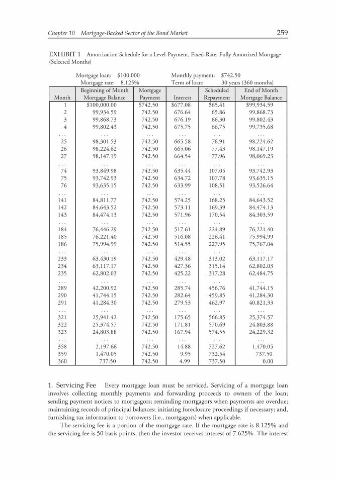
Chapter 10 Mortgage-Backed Sector of the Bond Market 259
EXHIBIT 1 Amortization Schedule for a Level-Payment, Fixed-Rate, Fully Amortized Mortgage(Selected Months)
Mortgage loan: $100,000 Monthly payment: $742.50Mortgage rate: 8.125% Term of loan: 30 years (360 months)Beginning of Month Mortgage Scheduled End of Month
Month Mortgage Balance Payment Interest Repayment Mortgage Balance1 $100,000.00 $742.50 $677.08 $65.41 $99,934.592 99,934.59 742.50 676.64 65.86 99,868.733 99,868.73 742.50 676.19 66.30 99,802.434 99,802.43 742.50 675.75 66.75 99,735.68
. . . . . . . . . . . . . . . . . .
25 98,301.53 742.50 665.58 76.91 98,224.6226 98,224.62 742.50 665.06 77.43 98,147.1927 98,147.19 742.50 664.54 77.96 98,069.23. . . . . . . . . . . . . . . . . .
74 93,849.98 742.50 635.44 107.05 93,742.9375 93,742.93 742.50 634.72 107.78 93,635.1576 93,635.15 742.50 633.99 108.51 93,526.64. . . . . . . . . . . . . . . . . .
141 84,811.77 742.50 574.25 168.25 84,643.52142 84,643.52 742.50 573.11 169.39 84,474.13143 84,474.13 742.50 571.96 170.54 84,303.59. . . . . . . . . . . . . . . . . .
184 76,446.29 742.50 517.61 224.89 76,221.40185 76,221.40 742.50 516.08 226.41 75,994.99186 75,994.99 742.50 514.55 227.95 75,767.04. . . . . . . . . . . . . . . . . .
233 63,430.19 742.50 429.48 313.02 63,117.17234 63,117.17 742.50 427.36 315.14 62,802.03235 62,802.03 742.50 425.22 317.28 62,484.75. . . . . . . . . . . . . . . . . .
289 42,200.92 742.50 285.74 456.76 41,744.15290 41,744.15 742.50 282.64 459.85 41,284.30291 41,284.30 742.50 279.53 462.97 40,821.33. . . . . . . . . . . . . . . . . .
321 25,941.42 742.50 175.65 566.85 25,374.57322 25,374.57 742.50 171.81 570.69 24,803.88323 24,803.88 742.50 167.94 574.55 24,229.32. . . . . . . . . . . . . . . . . .
358 2,197.66 742.50 14.88 727.62 1,470.05359 1,470.05 742.50 9.95 732.54 737.50360 737.50 742.50 4.99 737.50 0.00
1. Servicing Fee Every mortgage loan must be serviced. Servicing of a mortgage loaninvolves collecting monthly payments and forwarding proceeds to owners of the loan;sending payment notices to mortgagors; reminding mortgagors when payments are overdue;maintaining records of principal balances; initiating foreclosure proceedings if necessary; and,furnishing tax information to borrowers (i.e., mortgagors) when applicable.
The servicing fee is a portion of the mortgage rate. If the mortgage rate is 8.125% andthe servicing fee is 50 basis points, then the investor receives interest of 7.625%. The interest
260 Fixed Income Analysis
rate that the investor receives is said to be the net interest or net coupon. The servicing fee iscommonly called the servicing spread.
The dollar amount of the servicing fee declines over time as the mortgage amortizes. Thisis true for not only the mortgage design that we have just described, but for all mortgagedesigns.
2. Prepayments and Cash Flow Uncertainty Our illustration of the cash flow from alevel-payment, fixed-rate, fully amortized mortgage assumes that the homeowner does not payoff any portion of the mortgage balance prior to the scheduled due date. But homeowners canpay off all or part of their mortgage balance prior to the maturity date. A payment made inexcess of the monthly mortgage payment is called a prepayment. The prepayment could beto pay off the entire outstanding balance or a partial paydown of the mortgage balance. Whena prepayment is not for the entire outstanding balance it is called a curtailment.
The effect of prepayments is that the amount and timing of the cash flow from a mortgageloan are not known with certainty. This risk is referred to as prepayment risk. For example,all that the lender in a $100,000, 8.125% 30-year mortgage knows is that as long as the loanis outstanding and the borrower does not default, interest will be received and the principalwill be repaid at the scheduled date each month; then at the end of the 30 years, the investorwould have received $100,000 in principal payments. What the investor does not know—theuncertainty—is for how long the loan will be outstanding, and therefore what the timing ofthe principal payments will be. This is true for all mortgage loans, not just the level-payment,fixed-rate, fully amortized mortgage. Factors affecting prepayments will be discussed later inthis chapter.
Most mortgages have no prepayment penalty. The outstanding loan balance can be repaidat par. However, there are mortgages with prepayment penalties. The purpose of the penaltyis to deter prepayment when interest rates decline. A prepayment penalty mortgage has thefollowing structure. There is a period of time over which if the loan is prepaid in full or inexcess of a certain amount of the outstanding balance, there is a prepayment penalty. Thisperiod is referred to as the lockout period or penalty period. During the penalty period, theborrower may prepay up to a specified amount of the outstanding balance without a penalty.Over that specified amount, the penalty is set in terms of the number of months of interestthat must be paid.
III. MORTGAGE PASSTHROUGH SECURITIES
A mortgage passthrough security is a security created when one or more holders of mortgagesform a collection (pool) of mortgages and sell shares or participation certificates in the pool. Apool may consist of several thousand or only a few mortgages. When a mortgage is included ina pool of mortgages that is used as collateral for a mortgage passthrough security, the mortgageis said to be securitized.
A. Cash Flow Characteristics
The cash flow of a mortgage passthrough security depends on the cash flow of the underlyingpool of mortgages. As we explained in the previous section, the cash flow consists of monthlymortgage payments representing interest, the scheduled repayment of principal, and anyprepayments.
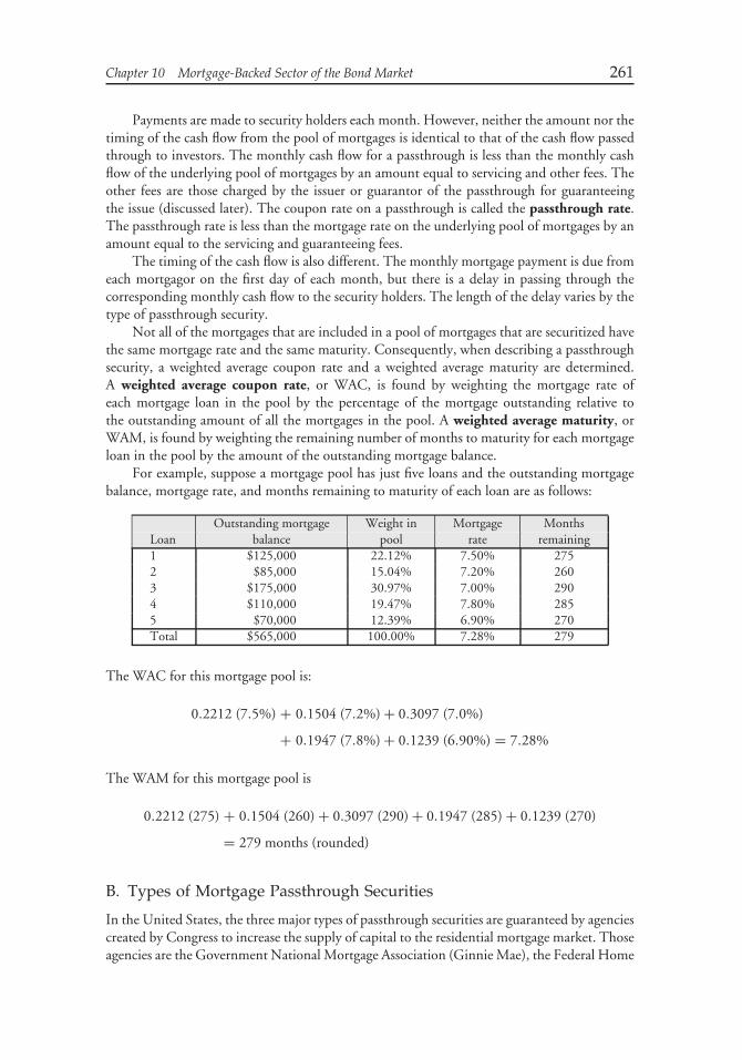
Chapter 10 Mortgage-Backed Sector of the Bond Market 261
Payments are made to security holders each month. However, neither the amount nor thetiming of the cash flow from the pool of mortgages is identical to that of the cash flow passedthrough to investors. The monthly cash flow for a passthrough is less than the monthly cashflow of the underlying pool of mortgages by an amount equal to servicing and other fees. Theother fees are those charged by the issuer or guarantor of the passthrough for guaranteeingthe issue (discussed later). The coupon rate on a passthrough is called the passthrough rate.The passthrough rate is less than the mortgage rate on the underlying pool of mortgages by anamount equal to the servicing and guaranteeing fees.
The timing of the cash flow is also different. The monthly mortgage payment is due fromeach mortgagor on the first day of each month, but there is a delay in passing through thecorresponding monthly cash flow to the security holders. The length of the delay varies by thetype of passthrough security.
Not all of the mortgages that are included in a pool of mortgages that are securitized havethe same mortgage rate and the same maturity. Consequently, when describing a passthroughsecurity, a weighted average coupon rate and a weighted average maturity are determined.A weighted average coupon rate, or WAC, is found by weighting the mortgage rate ofeach mortgage loan in the pool by the percentage of the mortgage outstanding relative tothe outstanding amount of all the mortgages in the pool. A weighted average maturity, orWAM, is found by weighting the remaining number of months to maturity for each mortgageloan in the pool by the amount of the outstanding mortgage balance.
For example, suppose a mortgage pool has just five loans and the outstanding mortgagebalance, mortgage rate, and months remaining to maturity of each loan are as follows:
Outstanding mortgage Weight in Mortgage MonthsLoan balance pool rate remaining1 $125,000 22.12% 7.50% 2752 $85,000 15.04% 7.20% 2603 $175,000 30.97% 7.00% 2904 $110,000 19.47% 7.80% 2855 $70,000 12.39% 6.90% 270Total $565,000 100.00% 7.28% 279
The WAC for this mortgage pool is:
0.2212 (7.5%) + 0.1504 (7.2%) + 0.3097 (7.0%)
+ 0.1947 (7.8%) + 0.1239 (6.90%) = 7.28%
The WAM for this mortgage pool is
0.2212 (275) + 0.1504 (260) + 0.3097 (290) + 0.1947 (285) + 0.1239 (270)
= 279 months (rounded)
B. Types of Mortgage Passthrough Securities
In the United States, the three major types of passthrough securities are guaranteed by agenciescreated by Congress to increase the supply of capital to the residential mortgage market. Thoseagencies are the Government National Mortgage Association (Ginnie Mae), the Federal Home
262 Fixed Income Analysis
Loan Mortgage Corporation (Freddie Mac), and the Federal National Mortgage Association(Fannie Mae).
While Freddie Mac and Fannie Mae are commonly referred to as ‘‘agencies’’ of the U.S.government, both are corporate instrumentalities of the U.S. government. That is, they aregovernment sponsored enterprises; therefore, their guarantee does not carry the full faith andcredit of the U.S. government. In contrast, Ginnie Mae is a federally related institution; it ispart of the Department of Housing and Urban Development. As such, its guarantee carriesthe full faith and credit of the U.S. government. The passthrough securities issued by FannieMae and Freddie Mac are called conventional passthrough securities. However, in this bookwe shall refer to those passthrough securities issued by all three entities (Ginnie Mae, FannieMae, and Freddie Mac) as agency passthrough securities. It should be noted, however, thatmarket participants do reserve the term ‘‘agency passthrough securities’’ for those issued onlyby Ginnie Mae.1
In order for a loan to be included in a pool of loans backing an agency security, it mustmeet specified underwriting standards. These standards set forth the maximum size of theloan, the loan documentation required, the maximum loan-to-value ratio, and whether or notinsurance is required. If a loan satisfies the underwriting standards for inclusion as collateralfor an agency mortgage-backed security, it is called a conforming mortgage. If a loan fails tosatisfy the underwriting standards, it is called a nonconforming mortgage.
Nonconforming mortgages used as collateral for mortgage passthrough securities areprivately issued. These securities are called nonagency mortgage passthrough securities andare issued by thrifts, commercial banks, and private conduits. Private conduits may purchasenonconforming mortgages, pool them, and then sell passthrough securities whose collateral isthe underlying pool of nonconforming mortgages. Nonagency passthrough securities are ratedby the nationally recognized statistical rating organizations. These securities are supported bycredit enhancements so that they can obtain an investment grade rating. We shall describethese securities in the next chapter.
C. Trading and Settlement Procedures
Agency passthrough securities are identified by a pool prefix and pool number provided by theagency. The prefix indicates the type of passthrough. There are specific rules established by theBond Market Association for the trading and settlement of mortgage-backed securities. Manytrades occur while a pool is still unspecified, and therefore no pool information is knownat the time of the trade. This kind of trade is known as a TBA trade (to-be-announcedtrade). In a TBA trade the two parties agree on the agency type, the agency program, thecoupon rate, the face value, the price, and the settlement date. The actual pools of mortgageloans underlying the agency passthrough are not specified in a TBA trade. However, thisinformation is provided by the seller to the buyer before delivery. There are trades where morespecific requirements are established for the securities to be delivered. An example is a Freddie
1The name of the passthrough issued by Ginnie Mae and Fannie Mae is a Mortgage-Backed Security orMBS. So, when a market participant refers to a Ginnie Mae MBS or Fannie Mae MBS, what is meantis a passthrough issued by these two entities. The name of the passthrough issued by Freddie Mac is aParticipation Certificate or PC. So, when a market participant refers to a Freddie Mac PC, what is meant isa passthrough issued by Freddie Mac. Every agency has different ‘‘programs’’ under which passthroughsare issued with different types of mortgage pools (e.g., 30-year fixed-rate mortgages, 15-year fixed-ratemortgages, adjustable-rate mortgages). We will not review the different programs here.
Chapter 10 Mortgage-Backed Sector of the Bond Market 263
Mac with a coupon rate of 8.5% and a WAC between 9.0% and 9.2%. There are also specifiedpool trades wherein the actual pool numbers to be delivered are specified.
Passthrough prices are quoted in the same manner as U.S. Treasury coupon securities. Aquote of 94-05 means 94 and 5 32nds of par value, or 94.15625% of par value. The price thatthe buyer pays the seller is the agreed upon sale price plus accrued interest. Given the par value,the dollar price (excluding accrued interest) is affected by the amount of the pool mortgagebalance outstanding. The pool factor indicates the percentage of the initial mortgage balancestill outstanding. So, a pool factor of 90 means that 90% of the original mortgage pool balanceis outstanding. The pool factor is reported by the agency each month.
The dollar price paid for just the principal is found as follows given the agreed upon price,par value, and the month’s pool factor provided by the agency:
price × par value × pool factor
For example, if the parties agree to a price of 92 for $1 million par value for a passthroughwith a pool factor of 0.85, then the dollar price paid by the buyer in addition to accruedinterest is:
0.92 × $1, 000, 000 × 0.85 = $782, 000
The buyer does not know what he will get unless he specifies a pool number. Thereare many seasoned issues of the same agency with the same coupon rate outstanding ata given point in time. For example, in early 2000 there were more than 30,000 pools of30-year Ginnie Mae MBSs outstanding with a coupon rate of 9%. One passthrough maybe backed by a pool of mortgage loans in which all the properties are located in California,while another may be backed by a pool of mortgage loans in which all the properties are inMinnesota. Yet another may be backed by a pool of mortgage loans in which the propertiesare from several regions of the country. So which pool are dealers referring to when they talkabout Ginnie Mae 9s? They are not referring to any specific pool but instead to a genericsecurity, despite the fact that the prepayment characteristics of passthroughs with underlyingpools from different parts of the country are different. Thus, the projected prepayment ratesfor passthroughs reported by dealer firms (discussed later) are for generic passthroughs. Aparticular pool purchased may have a materially different prepayment rate from the generic.Moreover, when an investor purchases a passthrough without specifying a pool number, theseller has the option to deliver the worst-paying pools as long as the pools delivered satisfygood delivery requirements.
D. Measuring the Prepayment Rate
A prepayment is any payment toward the repayment of principal that is in excess of thescheduled principal payment. In describing prepayments, market participants refer to the pre-payment rate or prepayment speed. In this section we will see how the historical prepaymentrate is computed for a month. We then look at how to annualize a monthly prepayment rateand then explain the convention in the residential mortgage market for describing a pattern ofprepayment rates over the life of a mortgage pool.
There are three points to keep in mind in the discussion in this section. First, we will lookat how the actual or historical prepayment rate of a mortgage pool is calculated. Second, wewill see later how in projecting the cash flow of a mortgage pool, an investor uses the same
264 Fixed Income Analysis
prepayment measures to project prepayments given a prepayment rate. The third point is thatwe are just describing the mechanics of calculating prepayment measures. The difficult taskof projecting the prepayment rate is not discussed here. In fact, this task is beyond the scopeof this chapter. However, the factors that investors use in prepayment models (i.e., statisticalmodels used to project prepayments) will be described in Section III F.
1. Single Monthly Mortality Rate Given the amount of the prepayment for a monthand the amount that was available to prepay that month, a monthly prepayment rate canbe computed. The amount available to prepay in a month is not the outstanding mortgagebalance of the pool in the previous month. The reason is that there will be scheduled principalpayments for the month and therefore by definition this amount cannot be prepaid. Thus, theamount available to prepay in a given month, say month t, is the beginning mortgage balancein month t reduced by the scheduled principal payment in month t.
The ratio of the prepayment in a month and the amount available to prepay that monthis called the single monthly mortality rate2 or simply SMM. That is, the SMM for month tis computed as follows
SMMt = prepayment in month tbeginning mortgage balance for month t− scheduled principal payment in month t
Let’s illustrate the calculation of the SMM. Assume the following:
beginning mortgage balance in month 33 = $358, 326, 766
scheduled principal payment in month 33 = $297, 825
prepayment in month 33 = $1, 841, 347
The SMM for month 33 is therefore:
SMM33 = $1, 841, 347
$358, 326, 766 − $297, 825= 0.005143 = 0.5143%
The SMM33 of 0.5143% is interpreted as follows: In month 33, 0.5143% of theoutstanding mortgage balance available to prepay in month 33 prepaid.
Let’s make sure we understand the two ways in which the SMM can be used. First, giventhe prepayment for a month for a mortgage pool, an investor can calculate the SMM as wejust did in our illustration to determine the SMM for month 33. Second given an assumedSMM, an investor will use it to project the prepayment for a month. The prepayment for amonth will then be used to determine the cash flow of a mortgage pool for the month. We’llsee this later in this section when we illustrate how to calculate the cash flow for a passthroughsecurity. For now, it is important to understand that given an assumed SMM for month t, theprepayment for month t is found as follows:
prepayment for month t = SMM × (beginning mortgage balance for month t
− scheduled principal payment for month t) (1)
2It may seem strange that the term ‘‘mortality’’ is used to describe this prepayment measure. This termreflects the influence of actuaries who in the early years of the development of the mortgage marketmigrated to dealer firms to assist in valuing mortgage-backed securities. Actuaries viewed the prepaymentof a mortgage loan as the ‘‘death’’ of a mortgage.
Chapter 10 Mortgage-Backed Sector of the Bond Market 265
For example, suppose that an investor owns a passthrough security in which the remainingmortgage balance at the beginning of some month is $290 million and the scheduled principalpayment for that month is $3 million. The investor believes that the SMM next month willbe 0.5143%. Then the projected prepayment for the month is:
0.005143 × ($290, 000, 000 − $3, 000, 000) = $1, 476, 041
2. Conditional Prepayment Rate Market participants prefer to talk about prepaymentrates on an annual basis rather than a monthly basis. This is handled by annualizing the SMM.The annualized SMM is called the conditional prepayment rate or CPR.3 Given the SMMfor a given month, the CPR can be demonstrated to be:4
CPR = 1 − (1 − SMM)12 (2)
For example, suppose that the SMM is 0.005143. Then the CPR is
CPR = 1 − (1 − 0.005143)12
= 1 − (0.994857)12 = 0.06 = 6%
A CPR of 6% means that, ignoring scheduled principal payments, approximately 6% of theoutstanding mortgage balance at the beginning of the year will be prepaid by the end of the year.
Given a CPR, the corresponding SMM can be computed by solving equation (2) for theSMM:
SMM = 1 − (1 − CPR)1/12 (3)
To illustrate equation (3), suppose that the CPR is 6%, then the SMM is
SMM = 1 − (1 − 0.06)1/12 = 0.005143 = 0.5143%
3. PSA Prepayment Benchmark An SMM is the prepayment rate for a month. A CPRis a prepayment rate for a year. Market participants describe prepayment rates (historical/actualprepayment rates and those used for projecting future prepayments) in terms of a prepaymentpattern or benchmark over the life of a mortgage pool. In the early 1980s, the Public SecuritiesAssociation (PSA), later renamed the Bond Market Association, undertook a study to lookat the pattern of prepayments over the life of a typical mortgage pool. Based on the study,the PSA established a prepayment benchmark which is referred to as the PSA prepaymentbenchmark. Although sometimes referred to as a ‘‘prepayment model,’’ it is a convention andnot a model to predict prepayments.
The PSA prepayment benchmark is expressed as a monthly series of CPRs. The PSAbenchmark assumes that prepayment rates are low for newly originated mortgages and thenwill speed up as the mortgages become seasoned. The PSA benchmark assumes the followingprepayment rates for 30-year mortgages: (1) a CPR of 0.2% for the first month, increased by
3It is referred to as a ‘‘conditional’’ prepayment rate because the prepayments in one year depend upon(i.e., are conditional upon) the amount available to prepay in the previous year. Sometimes marketparticipants refer to the CPR as the ‘‘constant’’ prepayment rate.4The derivation of the CPR for a given SMM is beyond the scope of this chapter. The proof is providedin Lakhbir S. Hayre and Cyrus Mohebbi, ‘‘Mortgage Mathematics,’’ in Frank J. Fabozzi (ed.), Handbookof Mortgage-Backed Securities: Fifth Edition (New York, NY: McGraw-Hill, 2001), pp. 844–845.
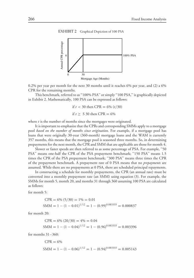
266 Fixed Income Analysis
EXHIBIT 2 Graphical Depiction of 100 PSA
100% PSA
Mortgage Age (Months)
Ann
ual C
PR p
erce
ntag
e
0 30
6
0.2% per year per month for the next 30 months until it reaches 6% per year, and (2) a 6%CPR for the remaining months.
This benchmark, referred to as ‘‘100% PSA’’ or simply ‘‘100 PSA,’’ is graphically depictedin Exhibit 2. Mathematically, 100 PSA can be expressed as follows:
if t < 30 then CPR = 6% (t/30)
if t ≥ S 30 then CPR = 6%
where t is the number of months since the mortgages were originated.It is important to emphasize that the CPRs and corresponding SMMs apply to a mortgage
pool based on the number of months since origination. For example, if a mortgage pool hasloans that were originally 30-year (360-month) mortgage loans and the WAM is currently357 months, this means that the mortgage pool is seasoned three months. So, in determiningprepayments for the next month, the CPR and SMM that are applicable are those for month 4.
Slower or faster speeds are then referred to as some percentage of PSA. For example, ‘‘50PSA’’ means one-half the CPR of the PSA prepayment benchmark; ‘‘150 PSA’’ means 1.5times the CPR of the PSA prepayment benchmark; ‘‘300 PSA’’ means three times the CPRof the prepayment benchmark. A prepayment rate of 0 PSA means that no prepayments areassumed. While there are no prepayments at 0 PSA, there are scheduled principal repayments.
In constructing a schedule for monthly prepayments, the CPR (an annual rate) must beconverted into a monthly prepayment rate (an SMM) using equation (3). For example, theSMMs for month 5, month 20, and months 31 through 360 assuming 100 PSA are calculatedas follows:
for month 5:
CPR = 6% (5/30) = 1% = 0.01
SMM = 1 − (1 − 0.01)1/12 = 1 − (0.99)0.083333 = 0.000837
for month 20:
CPR = 6% (20/30) = 4% = 0.04
SMM = 1 − (1 − 0.04)1/12 = 1 − (0.96)0.083333 = 0.003396
for months 31–360:
CPR = 6%
SMM = 1 − (1 − 0.06)1/12 = 1 − (0.94)0.083333 = 0.005143
Chapter 10 Mortgage-Backed Sector of the Bond Market 267
What if the PSA were 165 instead? The SMMs for month 5, month 20, and months 31through 360 assuming 165 PSA are computed as follows:
for month 5:
CPR = 6% (5/30) = 1% = 0.01
165 PSA = 1.65(0.01) = 0.0165
SMM = 1 − (1 − 0.0165)1/12 = 1 − (0.9835)0.08333 = 0.001386
for month 20:
CPR = 6% (20/30) = 4% = 0.04
165 PSA = 1.65 (0.04) = 0.066
SMM = 1 − (1 − 0.066)1/12 = 1 − (0.934)0.08333 = 0.005674
for months 31–360:
CPR = 6%
165 PSA = 1.65 (0.06) = 0.099
SMM = 1 − (1 − 0.099)1/12 = 1 − (0.901)0.08333 = 0.008650
Notice that the SMM assuming 165 PSA is not just 1.65 times the SMM assuming 100 PSA.It is the CPR that is a multiple of the CPR assuming 100 PSA.
4. Illustration of Monthly Cash Flow Construction As our first step in valuing ahypothetical passthrough given a PSA assumption, we must construct a monthly cash flow.For the purpose of this illustration, the underlying mortgages for this hypothetical passthroughare assumed to be fixed-rate, level-payment, fully amortized mortgages with a weighted averagecoupon (WAC) rate of 8.125%. It will be assumed that the passthrough rate is 7.5% with aweighted average maturity (WAM) of 357 months.
Exhibit 3 shows the cash flow for selected months assuming 100 PSA. The cash flow is bro-ken down into three components: (1) interest (based on the passthrough rate), (2) the scheduledprincipal repayment (i.e., scheduled amortization), and (3) prepayments based on 100 PSA.
Let’s walk through Exhibit 3 column by column.
Column 1: This is the number of months from now when the cash flow will be received.
Column 2: This is the number of months of seasoning. Since the WAM for this mortgagepool is 357 months, this means that the loans are seasoned an average of 3 months(360 months − 357 months) now.
Column 3: This column gives the outstanding mortgage balance at the beginning of themonth. It is equal to the outstanding balance at the beginning of the previous monthreduced by the total principal payment in the previous month.
Column 4: This column shows the SMM based on the number of months the loans areseasoned—the number of months shown in Column (2). For example, for the firstmonth shown in the exhibit, the loans are seasoned three months going into thatmonth. Therefore, the CPR used is the CPR that corresponds to four months. Fromthe PSA benchmark, the CPR is 0.8% (4 times 0.2%). The corresponding SMM is
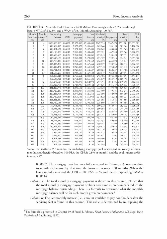
268 Fixed Income Analysis
EXHIBIT 3 Monthly Cash Flow for a $400 Million Passthrough with a 7.5% PassthroughRate, a WAC of 8.125%, and a WAM of 357 Months Assuming 100 PSA
Months Months Outstanding Mortgage Net Scheduled Total Cashfrom now seasoned* balance SMM payment interest principal Prepayment principal flow
(1) (2) (3) (4) (5) (6) (7) (8) (9) (10)1 4 $400,000,000 0.00067 $2,975,868 $2,500,000 $267,535 $267,470 $535,005 $3,035,0052 5 399,464,995 0.00084 2,973,877 2,496,656 269,166 334,198 603,364 3,100,0203 6 398,861,631 0.00101 2,971,387 2,492,885 270,762 400,800 671,562 3,164,4474 7 398,190,069 0.00117 2,968,399 2,488,688 272,321 467,243 739,564 3,228,2525 8 397,450,505 0.00134 2,964,914 2,484,066 273,843 533,493 807,335 3,291,4016 9 396,643,170 0.00151 2,960,931 2,479,020 275,327 599,514 874,841 3,353,8607 10 395,768,329 0.00168 2,956,453 2,473,552 276,772 665,273 942,045 3,415,5978 11 394,826,284 0.00185 2,951,480 2,467,664 278,177 730,736 1,008,913 3,476,5779 12 393,817,371 0.00202 2,946,013 2,461,359 279,542 795,869 1,075,410 3,536,769
10 13 392,741,961 0.00219 2,940,056 2,454,637 280,865 860,637 1,141,502 3,596,14011 14 391,600,459 0.00236 2,933,608 2,447,503 282,147 925,008 1,207,155 3,654,65827 30 364,808,016 0.00514 2,766,461 2,280,050 296,406 1,874,688 2,171,094 4,451,14428 31 362,636,921 0.00514 2,752,233 2,266,481 296,879 1,863,519 2,160,398 4,426,87929 32 360,476,523 0.00514 2,738,078 2,252,978 297,351 1,852,406 2,149,758 4,402,73630 33 358,326,766 0.00514 2,723,996 2,239,542 297,825 1,841,347 2,139,173 4,378,715
100 103 231,249,776 0.00514 1,898,682 1,445,311 332,928 1,187,608 1,520,537 2,965,848101 104 229,729,239 0.00514 1,888,917 1,435,808 333,459 1,179,785 1,513,244 2,949,052102 105 228,215,995 0.00514 1,879,202 1,426,350 333,990 1,172,000 1,505,990 2,932,340103 106 226,710,004 0.00514 1,869,538 1,416,938 334,522 1,164,252 1,498,774 2,915,712104 107 225,211,230 0.00514 1,859,923 1,407,570 335,055 1,156,541 1,491,596 2,899,166105 108 223,719,634 0.00514 1,850,357 1,398,248 335,589 1,148,867 1,484,456 2,882,703200 203 109,791,339 0.00514 1,133,751 686,196 390,372 562,651 953,023 1,639,219201 204 108,838,316 0.00514 1,127,920 680,239 390,994 557,746 948,740 1,628,980202 205 107,889,576 0.00514 1,122,119 674,310 391,617 552,863 944,480 1,618,790203 206 106,945,096 0.00514 1,116,348 668,407 392,241 548,003 940,243 1,608,650300 303 32,383,611 0.00514 676,991 202,398 457,727 164,195 621,923 824,320301 304 31,761,689 0.00514 673,510 198,511 458,457 160,993 619,449 817,960302 305 31,142,239 0.00514 670,046 194,639 459,187 157,803 616,990 811,629303 306 30,525,249 0.00514 666,600 190,783 459,918 154,626 614,545 805,328352 355 3,034,311 0.00514 517,770 18,964 497,226 13,048 510,274 529,238353 356 2,524,037 0.00514 515,107 15,775 498,018 10,420 508,437 524,213354 357 2,015,600 0.00514 512,458 12,597 498,811 7,801 506,612 519,209355 358 1,508,988 0.00514 509,823 9,431 499,606 5,191 504,797 514,228356 359 1,004,191 0.00514 507,201 6,276 500,401 2,591 502,992 509,269357 360 501,199 0.00514 504,592 3,132 501,199 0 501,199 504,331
∗Since the WAM is 357 months, the underlying mortgage pool is seasoned an average of threemonths, and therefore based on 100 PSA, the CPR is 0.8% in month 1 and the pool seasons at 6%in month 27.
0.00067. The mortgage pool becomes fully seasoned in Column (1) correspondingto month 27 because by that time the loans are seasoned 30 months. When theloans are fully seasoned the CPR at 100 PSA is 6% and the corresponding SMM is0.00514.
Column 5: The total monthly mortgage payment is shown in this column. Notice thatthe total monthly mortgage payment declines over time as prepayments reduce themortgage balance outstanding. There is a formula to determine what the monthlymortgage balance will be for each month given prepayments.5
Column 6: The net monthly interest (i.e., amount available to pay bondholders after theservicing fee) is found in this column. This value is determined by multiplying the
5The formula is presented in Chapter 19 of Frank J. Fabozzi, Fixed Income Mathematics (Chicago: IrwinProfessional Publishing, 1997).
Chapter 10 Mortgage-Backed Sector of the Bond Market 269
outstanding mortgage balance at the beginning of the month by the passthrough rateof 7.5% and then dividing by 12.
Column 7: This column gives the scheduled principal repayment (i.e., scheduled amor-tization). This is the difference between the total monthly mortgage payment [theamount shown in Column (5)] and the gross coupon interest for the month. Thegross coupon interest is found by multiplying 8.125% by the outstanding mortgagebalance at the beginning of the month and then dividing by 12.
Column 8: The prepayment for the month is reported in this column. The prepaymentis found by using equation (1). For example, in month 100, the beginning mortgagebalance is $231,249,776, the scheduled principal payment is $332,928, and theSMM at 100 PSA is 0.00514301 (only 0.00514 is shown in the exhibit to savespace), so the prepayment is:
0.00514301 × ($231, 249, 776 − $332, 928) = $1, 187, 608
Column 9: The total principal payment, which is the sum of columns (7) and (8), isshown in this column.
Column 10: The projected monthly cash flow for this passthrough is shown in this lastcolumn. The monthly cash flow is the sum of the interest paid [Column (6)] and thetotal principal payments for the month [Column (9)].
Let’s look at what happens to the cash flows for this passthrough if a different PSAassumption is made. Suppose that instead of 100 PSA, 165 PSA is assumed. Prepaymentsare assumed to be faster. Exhibit 4 shows the cash flow for this passthrough based on 165PSA. Notice that the cash flows are greater in the early years compared to Exhibit 3 becauseprepayments are higher. The cash flows in later years are less for 165 PSA compared to 100PSA because of the higher prepayments in the earlier years.
E. Average Life
It is standard practice in the bond market to refer to the maturity of a bond. If a bond maturesin five years, it is referred to as a ‘‘5-year bond.’’ However, the typical bond repays principalonly once: at the maturity date. Bonds with this characteristic are referred to as ‘‘bullet bonds.’’We know that the maturity of a bond affects its interest rate risk. More specifically, for a givencoupon rate, the greater the maturity the greater the interest rate risk.
For a mortgage-backed security, we know that the principal repayments (scheduledpayments and prepayments) are made over the life of the security. While a mortgage-backedhas a ‘‘legal maturity,’’ which is the date when the last scheduled principal payment is due,the legal maturity does not tell us much about the characteristic of the security as its pertainsto interest rate risk. For example, it is incorrect to think of a 30-year corporate bond anda mortgage-backed security with a 30-year legal maturity with the same coupon rate asbeing equivalent in terms of interest rate risk. Of course, duration can be computed forboth the corporate bond and the mortgage-backed security. (We will see how this is donefor a mortgage-backed security in Chapter 12.) Instead of duration, another measure widelyused by market participants is the weighted average life or simply average life. This is theconvention-based average time to receipt of principal payments (scheduled principal paymentsand projected prepayments).

270 Fixed Income Analysis
EXHIBIT 4 Monthly Cash Flow for a $400 Million Passthrough with a 7.5% Passthrough Rate, aWAC of 8.125%, and a WAM of 357 Months Assuming 165 PSA
Months Outstanding Mortgage Net Scheduled Total CashMonth seasoned* Balance SMM payment interest principal prepayment principal flow
(1) (2) (3) (4) (5) (6) (7) (8) (9) (10)1 4 $400,000,000 0.00111 $2,975,868 $2,500,000 $267,535 $442,389 $709,923 $3,209,9232 5 399,290,077 0.00139 2,972,575 2,495,563 269,048 552,847 821,896 3,317,4593 6 398,468,181 0.00167 2,968,456 2,490,426 270,495 663,065 933,560 3,423,9864 7 397,534,621 0.00195 2,963,513 2,484,591 271,873 772,949 1,044,822 3,529,4135 8 396,489,799 0.00223 2,957,747 2,478,061 273,181 882,405 1,155,586 3,633,6476 9 395,334,213 0.00251 2,951,160 2,470,839 274,418 991,341 1,265,759 3,736,5987 10 394,068,454 0.00279 2,943,755 2,462,928 275,583 1,099,664 1,375,246 3,838,1748 11 392,693,208 0.00308 2,935,534 2,454,333 276,674 1,207,280 1,483,954 3,938,2879 12 391,209,254 0.00336 2,926,503 2,445,058 277,690 1,314,099 1,591,789 4,036,847
10 13 389,617,464 0.00365 2,916,666 2,435,109 278,631 1,420,029 1,698,659 4,133,76911 14 387,918,805 0.00393 2,906,028 2,424,493 279,494 1,524,979 1,804,473 4,228,96527 30 347,334,116 0.00865 2,633,950 2,170,838 282,209 3,001,955 3,284,164 5,455,00228 31 344,049,952 0.00865 2,611,167 2,150,312 281,662 2,973,553 3,255,215 5,405,52729 32 340,794,737 0.00865 2,588,581 2,129,967 281,116 2,945,400 3,226,516 5,356,48330 33 337,568,221 0.00865 2,566,190 2,109,801 280,572 2,917,496 3,198,067 5,307,869
100 103 170,142,350 0.00865 1,396,958 1,063,390 244,953 1,469,591 1,714,544 2,777,933101 104 168,427,806 0.00865 1,384,875 1,052,674 244,478 1,454,765 1,699,243 2,751,916102 105 166,728,563 0.00865 1,372,896 1,042,054 244,004 1,440,071 1,684,075 2,726,128103 106 165,044,489 0.00865 1,361,020 1,031,528 243,531 1,425,508 1,669,039 2,700,567104 107 163,375,450 0.00865 1,349,248 1,021,097 243,060 1,411,075 1,654,134 2,675,231105 108 161,721,315 0.00865 1,337,577 1,010,758 242,589 1,396,771 1,639,359 2,650,118200 203 56,746,664 0.00865 585,990 354,667 201,767 489,106 690,874 1,045,540201 204 56,055,790 0.00865 580,921 350,349 201,377 483,134 684,510 1,034,859202 205 55,371,280 0.00865 575,896 346,070 200,986 477,216 678,202 1,024,273203 206 54,693,077 0.00865 570,915 341,832 200,597 471,353 671,950 1,013,782300 303 11,758,141 0.00865 245,808 73,488 166,196 100,269 266,465 339,953301 304 11,491,677 0.00865 243,682 71,823 165,874 97,967 263,841 335,664302 305 11,227,836 0.00865 241,574 70,174 165,552 95,687 261,240 331,414303 306 10,966,596 0.00865 239,485 68,541 165,232 93,430 258,662 327,203352 355 916,910 0.00865 156,460 5,731 150,252 6,631 156,883 162,614353 356 760,027 0.00865 155,107 4,750 149,961 5,277 155,238 159,988354 357 604,789 0.00865 153,765 3,780 149,670 3,937 153,607 157,387355 358 451,182 0.00865 152,435 2,820 149,380 2,611 151,991 154,811356 359 299,191 0.00865 151,117 1,870 149,091 1,298 150,389 152,259357 360 148,802 0.00865 149,809 930 148,802 0 148,802 149,732
∗Since the WAM is 357 months, the underlying mortgage pool is seasoned an average of three months,and therefore based on 165 PSA, the CPR is 0.8% × 1.65 in month 1 and the pool seasons at 6% × 1.65in month 27.
Mathematically, the average life is expressed as follows:
Average life =T∑
t=1
t × Projected principal received at time t12 × Total principal
where T is the number of months.The average life of a passthrough depends on the prepayment assumption. To see this,
the average life is shown below for different prepayment speeds for the pass-through we usedto illustrate the cash flow for 100 PSA and 165 PSA in Exhibits 3 and 4:
PSA speed 50 100 165 200 300 400 500 600 700Average life (years) 15.11 11.66 8.76 7.68 5.63 4.44 3.68 3.16 2.78
Chapter 10 Mortgage-Backed Sector of the Bond Market 271
F. Factors Affecting Prepayment Behavior
The factors that affect prepayment behavior are:
1. prevailing mortgage rate2. housing turnover3. characteristics of the underlying residential mortgage loans
The current mortgage rate affects prepayments. The spread between the prevailingmortgage rate in the market and the rate paid by the homeowner affects the incentiveto refinance. Moreover, the path of mortgage rates since the loan was originated affectsprepayments through a phenomenon referred to as refinancing burnout. Both the spread andpath of mortgage rates affect prepayments that are the product of refinancing.
By far, the single most important factor affecting prepayments because of refinancingis the current level of mortgage rates relative to the borrower’s contract rate. The greaterthe difference between the two, the greater the incentive to refinance the mortgage loan.For refinancing to make economic sense, the interest savings must be greater than the costsassociated with refinancing the mortgage. These costs include legal expenses, origination fees,title insurance, and the value of the time associated with obtaining another mortgage loan.Some of these costs will vary proportionately with the amount to be financed. Other costssuch as the application fee and legal expenses are typically fixed.
Historically it had been observed that mortgage rates had to decline by between 250 and350 basis points below the contract rate in order to make it worthwhile for borrowers torefinance. However, the creativity of mortgage originators in designing mortgage loans suchthat the refinancing costs are folded into the amount borrowed has changed the view thatmortgage rates must drop dramatically below the contract rate to make refinancing economic.Moreover, mortgage originators now do an effective job of advertising to make homeownerscognizant of the economic benefits of refinancing.
The historical pattern of prepayments and economic theory suggests that it is not only thelevel of mortgage rates that affects prepayment behavior but also the path that mortgage ratestake to get to the current level. To illustrate why, suppose the underlying contract rate for apool of mortgage loans is 11% and that three years after origination, the prevailing mortgagerate declines to 8%. Let’s consider two possible paths of the mortgage rate in getting to the8% level. In the first path, the mortgage rate declines to 8% at the end of the first year, thenrises to 13% at the end of the second year, and then falls to 8% at the end of the third year. Inthe second path, the mortgage rate rises to 12% at the end of the first year, continues its riseto 13% at the end of the second year, and then falls to 8% at the end of the third year.
If the mortgage rate follows the first path, those who can benefit from refinancing willmore than likely take advantage of this opportunity when the mortgage rate drops to 8%in the first year. When the mortgage rate drops again to 8% at the end of the third year,the likelihood is that prepayments because of refinancing will not surge; those who want tobenefit by taking advantage of the refinancing opportunity will have done so already when themortgage rate declined for the first time. This is the prepayment behavior referred to as therefinancing burnout (or simply, burnout) phenomenon. In contrast, the expected prepaymentbehavior when the mortgage rate follows the second path is quite different. Prepayment ratesare expected to be low in the first two years. When the mortgage rate declines to 8% in thethird year, refinancing activity and therefore prepayments are expected to surge. Consequently,the burnout phenomenon is related to the path of mortgage rates.
272 Fixed Income Analysis
There is another way in which the prevailing mortgage rate affects prepayments: throughits effect on the affordability of housing and housing turnover. The level of mortgage ratesaffects housing turnover to the extent that a lower rate increases the affordability of homes.However, even without lower interest rates, there is a normal amount of housing turnover.This is attribute to economic growth. The link is as follows: a growing economy results ina rise in personal income and in opportunities for worker migration; this increases familymobility and as a result increases housing turnover. The opposite holds for a weak economy.
Two characteristics of the underlying residential mortgage loans that affect prepaymentsare the amount of seasoning and the geographical location of the underlying properties.Seasoning refers to the aging of the mortgage loans. Empirical evidence suggests thatprepayment rates are low after the loan is originated and increase after the loan is somewhatseasoned. Then prepayment rates tend to level off, in which case the loans are referred to as fullyseasoned. This is the underlying theory for the PSA prepayment benchmark discussed earlierin this chapter. In some regions of the country the prepayment behavior tends to be faster thanthe average national prepayment rate, while other regions exhibit slower prepayment rates.This is caused by differences in local economies that affect housing turnover.
G. Contraction Risk and Extension Risk
An investor who owns passthrough securities does not know what the cash flow will be becausethat depends on actual prepayments. As we noted earlier, this risk is called prepayment risk.
To understand the significance of prepayment risk, suppose an investor buys a 9% couponpassthrough security at a time when mortgage rates are 10%. Let’s consider what will happento prepayments if mortgage rates decline to, say, 6%. There will be two adverse consequences.First, a basic property of fixed income securities is that the price of an option-free bond willrise. But in the case of a passthrough security, the rise in price will not be as large as that of anoption-free bond because a fall in interest rates will give the borrower an incentive to prepaythe loan and refinance the debt at a lower rate. This results in the same adverse consequencefaced by holders of callable bonds. As in the case of those instruments, the upside pricepotential of a passthrough security is compressed because of prepayments. (This is the negativeconvexity characteristic explained in Chapter 7.) The second adverse consequence is that thecash flow must be reinvested at a lower rate. Basically, the faster prepayments resulting froma decline in interest rates causes the passthrough to shorten in terms of the timing of its cashflows. Another way of saying this is that ‘‘shortening’’ results in a decline in the average life.Consequently, the two adverse consequences from a decline in interest rates for a passthroughsecurity are referred to as contraction risk.
Now let’s look at what happens if mortgage rates rise to 15%. The price of the passthrough,like the price of any bond, will decline. But again it will decline more because the higher rateswill tend to slow down the rate of prepayment, in effect increasing the amount invested atthe coupon rate, which is lower than the market rate. Prepayments will slow down, becausehomeowners will not refinance or partially prepay their mortgages when mortgage rates arehigher than the contract rate of 10%. Of course this is just the time when investors wantprepayments to speed up so that they can reinvest the prepayments at the higher marketinterest rate. Basically, the slower prepayments associated with a rise in interest rates thatcauses these adverse consequences are due to the passthrough lengthening in terms of thetiming of its cash flows. Another way of saying this is that ‘‘lengthening’’ results in an increasein the average life. Consequently, the adverse consequence from a rise in interest rates for apassthrough security is referred to as extension risk.
Chapter 10 Mortgage-Backed Sector of the Bond Market 273
Therefore, prepayment risk encompasses contraction risk and extension risk. Prepaymentrisk makes passthrough securities unattractive for certain financial institutions to hold froman asset/liability management perspective. Some institutional investors are concerned withextension risk and others with contraction risk when they purchase a passthrough security.This applies even for assets supporting specific types of insurance contracts. Is it possible toalter the cash flow of a passthrough so as to reduce the contraction risk or extension riskfor institutional investors? This can be done, as we shall see, when we describe collateralizedmortgage obligations.
IV. COLLATERALIZED MORTGAGEOBLIGATIONS
As we noted, there is prepayment risk associated with investing in a mortgage passthroughsecurity. Some institutional investors are concerned with extension risk and others withcontraction risk. This problem can be mitigated by redirecting the cash flows of mortgage-related products (passthrough securities or a pool of loans) to different bond classes, calledtranches,6 so as to create securities that have different exposure to prepayment risk and thereforedifferent risk/return patterns than the mortgage-related product from which they are created.
When the cash flows of mortgage-related products are redistributed to different bondclasses, the resulting securities are called collateralized mortgage obligations (CMO). Themortgage-related products from which the cash flows are obtained are referred to as thecollateral. Since the typical mortgage-related product used in a CMO is a pool of passthroughsecurities, sometimes market participants will use the terms ‘‘collateral’’ and ‘‘passthroughsecurities’’ interchangeably. The creation of a CMO cannot eliminate prepayment risk; it canonly distribute the various forms of this risk among different classes of bondholders. The CMO’smajor financial innovation is that the securities created more closely satisfy the asset/liabilityneeds of institutional investors, thereby broadening the appeal of mortgage-backed products.
There is a wide range of CMO structures.7 We review the major ones below.
A. Sequential-Pay Tranches
The first CMO was structured so that each class of bond would be retired sequentially. Suchstructures are referred to as sequential-pay CMOs. The rule for the monthly distribution of theprincipal payments (scheduled principal plus prepayments) to the tranches would be as follows:
• Distribute all principal payments to Tranche 1 until the principal balance for Tranche 1 iszero. After Tranche 1 is paid off,
6‘‘Tranche’’ is from an old French word meaning ‘‘slice.’’ In the case of a collateralized mortgageobligation it refers to a ‘‘slice of the cash flows.’’7The issuer of a CMO wants to be sure that the trust created to pass through the interest and principalpayments is not treated as a taxable entity. A provision of the Tax Reform Act of 1986, called the RealEstate Mortgage Investment Conduit (REMIC), specifies the requirements that an issuer must fulfill sothat the legal entity created to issue a CMO is not taxable. Most CMOs today are created as REMICs.While it is common to hear market participants refer to a CMO as a REMIC, not all CMOs areREMICs.
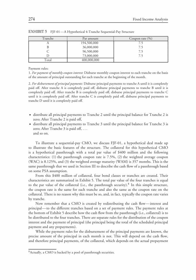
274 Fixed Income Analysis
EXHIBIT 5 FJF-01—A Hypothetical 4-Tranche Sequential-Pay Structure
Tranche Par amount Coupon rate (%)A 194,500,000 7.5B 36,000,000 7.5C 96,500,000 7.5D 73,000,000 7.5
Total 400,000,000
Payment rules:1. For payment of monthly coupon interest: Disburse monthly coupon interest to each tranche on the basisof the amount of principal outstanding for each tranche at the beginning of the month.
2. For disbursement of principal payments: Disburse principal payments to tranche A until it is completelypaid off. After tranche A is completely paid off, disburse principal payments to tranche B until it iscompletely paid off. After tranche B is completely paid off, disburse principal payments to tranche Cuntil it is completely paid off. After tranche C is completely paid off, disburse principal payments totranche D until it is completely paid off.
• distribute all principal payments to Tranche 2 until the principal balance for Tranche 2 iszero; After Tranche 2 is paid off,
• distribute all principal payments to Tranche 3 until the principal balance for Tranche 3 iszero; After Tranche 3 is paid off, . . .
and so on.
To illustrate a sequential-pay CMO, we discuss FJF-01, a hypothetical deal made upto illustrate the basic features of the structure. The collateral for this hypothetical CMOis a hypothetical passthrough with a total par value of $400 million and the followingcharacteristics: (1) the passthrough coupon rate is 7.5%, (2) the weighted average coupon(WAC) is 8.125%, and (3) the weighted average maturity (WAM) is 357 months. This is thesame passthrough that we used in Section III to describe the cash flow of a passthrough basedon some PSA assumption.
From this $400 million of collateral, four bond classes or tranches are created. Theircharacteristics are summarized in Exhibit 5. The total par value of the four tranches is equalto the par value of the collateral (i.e., the passthrough security).8 In this simple structure,the coupon rate is the same for each tranche and also the same as the coupon rate on thecollateral. There is no reason why this must be so, and, in fact, typically the coupon rate variesby tranche.
Now remember that a CMO is created by redistributing the cash flow—interest andprincipal—to the different tranches based on a set of payment rules. The payment rules atthe bottom of Exhibit 5 describe how the cash flow from the passthrough (i.e., collateral) is tobe distributed to the four tranches. There are separate rules for the distribution of the couponinterest and the payment of principal (the principal being the total of the scheduled principalpayment and any prepayments).
While the payment rules for the disbursement of the principal payments are known, theprecise amount of the principal in each month is not. This will depend on the cash flow,and therefore principal payments, of the collateral, which depends on the actual prepayment
8Actually, a CMO is backed by a pool of passthrough securities.
Chapter 10 Mortgage-Backed Sector of the Bond Market 275
rate of the collateral. An assumed PSA speed allows the cash flow to be projected. Exhibit 6shows the cash flow (interest, scheduled principal repayment, and prepayments) assuming 165PSA. Assuming that the collateral does prepay at 165 PSA, the cash flow available to all fourtranches of FJF-01 will be precisely the cash flow shown in Exhibit 6.
To demonstrate how the payment rules for FJF-01 work, Exhibit 6 shows the cashflow for selected months assuming the collateral prepays at 165 PSA. For each tranche, theexhibit shows: (1) the balance at the end of the month, (2) the principal paid down (scheduledprincipal repayment plus prepayments), and (3) interest. In month 1, the cash flow for thecollateral consists of a principal payment of $709,923 and an interest payment of $2.5 million(0.075 times $400 million divided by 12). The interest payment is distributed to the fourtranches based on the amount of the par value outstanding. So, for example, tranche A receives$1,215,625 (0.075 times $194,500,000 divided by 12) of the $2.5 million. The principal,however, is all distributed to tranche A. Therefore, the cash flow for tranche A in month 1is $1,925,548. The principal balance at the end of month 1 for tranche A is $193,790,076(the original principal balance of $194,500,000 less the principal payment of $709,923). Noprincipal payment is distributed to the three other tranches because there is still a principalbalance outstanding for tranche A. This will be true for months 2 through 80. The cashflow for tranche A for each month is found by adding the amounts shown in the ‘‘Principal’’and ‘‘Interest’’ columns. So, for tranche A, the cash flow in month 8 is $1,483,954 plus$1,169,958, or $2,653,912. The cash flow from months 82 on is zero based on 165 PSA.
After month 81, the principal balance will be zero for tranche A. For the collateral, thecash flow in month 81 is $3,318,521, consisting of a principal payment of $2,032,197 andinterest of $1,286,325. At the beginning of month 81 (end of month 80), the principal balancefor tranche A is $311,926. Therefore, $311,926 of the $2,032,196 of the principal paymentfrom the collateral will be disbursed to tranche A. After this payment is made, no additionalprincipal payments are made to this tranche as the principal balance is zero. The remainingprincipal payment from the collateral, $1,720,271, is distributed to tranche B. Based on anassumed prepayment speed of 165 PSA, tranche B then begins receiving principal paymentsin month 81. The cash flow for tranche B for each month is found by adding the amountsshown in the ‘‘Principal’’ and ‘‘Interest’’ columns. For months 1 though 80, the cash flow isjust the interest. There is no cash flow after month 100 for tranche B.
Exhibit 6 shows that tranche B is fully paid off by month 100, when tranche C begins toreceive principal payments. Tranche C is not fully paid off until month 178, at which timetranche D begins receiving the remaining principal payments. The maturity (i.e., the timeuntil the principal is fully paid off) for these four tranches assuming 165 PSA would be 81months for tranche A, 100 months for tranche B, 178 months for tranche C, and 357 monthsfor tranche D. The cash flow for each month for tranches C and D is found by adding theprincipal and the interest for the month.
The principal pay down window or principal window for a tranche is the time periodbetween the beginning and the ending of the principal payments to that tranche. So, forexample, for tranche A, the principal pay down window would be month 1 to month 81assuming 165 PSA. For tranche B it is from month 81 to month 100.9 In confirmation oftrades involving CMOs, the principal pay down window is specified in terms of the initial
9The window is also specified in terms of the length of the time from the beginning of the principal paydown window to the end of the principal pay down window. For tranche A, the window would be statedas 81 months, for tranche B 20 months.
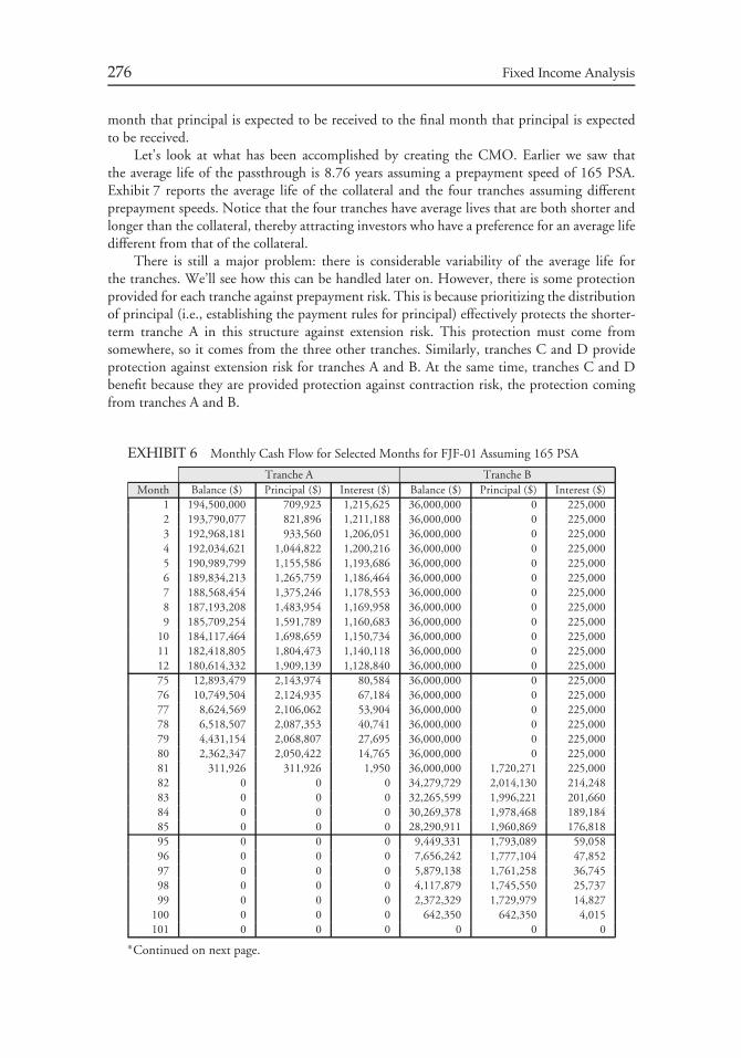
276 Fixed Income Analysis
month that principal is expected to be received to the final month that principal is expectedto be received.
Let’s look at what has been accomplished by creating the CMO. Earlier we saw thatthe average life of the passthrough is 8.76 years assuming a prepayment speed of 165 PSA.Exhibit 7 reports the average life of the collateral and the four tranches assuming differentprepayment speeds. Notice that the four tranches have average lives that are both shorter andlonger than the collateral, thereby attracting investors who have a preference for an average lifedifferent from that of the collateral.
There is still a major problem: there is considerable variability of the average life forthe tranches. We’ll see how this can be handled later on. However, there is some protectionprovided for each tranche against prepayment risk. This is because prioritizing the distributionof principal (i.e., establishing the payment rules for principal) effectively protects the shorter-term tranche A in this structure against extension risk. This protection must come fromsomewhere, so it comes from the three other tranches. Similarly, tranches C and D provideprotection against extension risk for tranches A and B. At the same time, tranches C and Dbenefit because they are provided protection against contraction risk, the protection comingfrom tranches A and B.
EXHIBIT 6 Monthly Cash Flow for Selected Months for FJF-01 Assuming 165 PSA
Tranche A Tranche BMonth Balance ($) Principal ($) Interest ($) Balance ($) Principal ($) Interest ($)
1 194,500,000 709,923 1,215,625 36,000,000 0 225,0002 193,790,077 821,896 1,211,188 36,000,000 0 225,0003 192,968,181 933,560 1,206,051 36,000,000 0 225,0004 192,034,621 1,044,822 1,200,216 36,000,000 0 225,0005 190,989,799 1,155,586 1,193,686 36,000,000 0 225,0006 189,834,213 1,265,759 1,186,464 36,000,000 0 225,0007 188,568,454 1,375,246 1,178,553 36,000,000 0 225,0008 187,193,208 1,483,954 1,169,958 36,000,000 0 225,0009 185,709,254 1,591,789 1,160,683 36,000,000 0 225,000
10 184,117,464 1,698,659 1,150,734 36,000,000 0 225,00011 182,418,805 1,804,473 1,140,118 36,000,000 0 225,00012 180,614,332 1,909,139 1,128,840 36,000,000 0 225,00075 12,893,479 2,143,974 80,584 36,000,000 0 225,00076 10,749,504 2,124,935 67,184 36,000,000 0 225,00077 8,624,569 2,106,062 53,904 36,000,000 0 225,00078 6,518,507 2,087,353 40,741 36,000,000 0 225,00079 4,431,154 2,068,807 27,695 36,000,000 0 225,00080 2,362,347 2,050,422 14,765 36,000,000 0 225,00081 311,926 311,926 1,950 36,000,000 1,720,271 225,00082 0 0 0 34,279,729 2,014,130 214,24883 0 0 0 32,265,599 1,996,221 201,66084 0 0 0 30,269,378 1,978,468 189,18485 0 0 0 28,290,911 1,960,869 176,81895 0 0 0 9,449,331 1,793,089 59,05896 0 0 0 7,656,242 1,777,104 47,85297 0 0 0 5,879,138 1,761,258 36,74598 0 0 0 4,117,879 1,745,550 25,73799 0 0 0 2,372,329 1,729,979 14,827
100 0 0 0 642,350 642,350 4,015101 0 0 0 0 0 0
∗Continued on next page.
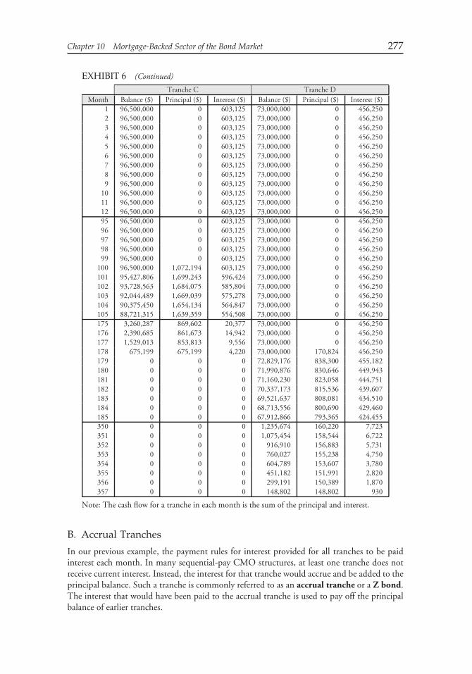
Chapter 10 Mortgage-Backed Sector of the Bond Market 277
EXHIBIT 6 (Continued)
Tranche C Tranche DMonth Balance ($) Principal ($) Interest ($) Balance ($) Principal ($) Interest ($)
1 96,500,000 0 603,125 73,000,000 0 456,2502 96,500,000 0 603,125 73,000,000 0 456,2503 96,500,000 0 603,125 73,000,000 0 456,2504 96,500,000 0 603,125 73,000,000 0 456,2505 96,500,000 0 603,125 73,000,000 0 456,2506 96,500,000 0 603,125 73,000,000 0 456,2507 96,500,000 0 603,125 73,000,000 0 456,2508 96,500,000 0 603,125 73,000,000 0 456,2509 96,500,000 0 603,125 73,000,000 0 456,250
10 96,500,000 0 603,125 73,000,000 0 456,25011 96,500,000 0 603,125 73,000,000 0 456,25012 96,500,000 0 603,125 73,000,000 0 456,25095 96,500,000 0 603,125 73,000,000 0 456,25096 96,500,000 0 603,125 73,000,000 0 456,25097 96,500,000 0 603,125 73,000,000 0 456,25098 96,500,000 0 603,125 73,000,000 0 456,25099 96,500,000 0 603,125 73,000,000 0 456,250
100 96,500,000 1,072,194 603,125 73,000,000 0 456,250101 95,427,806 1,699,243 596,424 73,000,000 0 456,250102 93,728,563 1,684,075 585,804 73,000,000 0 456,250103 92,044,489 1,669,039 575,278 73,000,000 0 456,250104 90,375,450 1,654,134 564,847 73,000,000 0 456,250105 88,721,315 1,639,359 554,508 73,000,000 0 456,250175 3,260,287 869,602 20,377 73,000,000 0 456,250176 2,390,685 861,673 14,942 73,000,000 0 456,250177 1,529,013 853,813 9,556 73,000,000 0 456,250178 675,199 675,199 4,220 73,000,000 170,824 456,250179 0 0 0 72,829,176 838,300 455,182180 0 0 0 71,990,876 830,646 449,943181 0 0 0 71,160,230 823,058 444,751182 0 0 0 70,337,173 815,536 439,607183 0 0 0 69,521,637 808,081 434,510184 0 0 0 68,713,556 800,690 429,460185 0 0 0 67,912,866 793,365 424,455350 0 0 0 1,235,674 160,220 7,723351 0 0 0 1,075,454 158,544 6,722352 0 0 0 916,910 156,883 5,731353 0 0 0 760,027 155,238 4,750354 0 0 0 604,789 153,607 3,780355 0 0 0 451,182 151,991 2,820356 0 0 0 299,191 150,389 1,870357 0 0 0 148,802 148,802 930
Note: The cash flow for a tranche in each month is the sum of the principal and interest.
B. Accrual Tranches
In our previous example, the payment rules for interest provided for all tranches to be paidinterest each month. In many sequential-pay CMO structures, at least one tranche does notreceive current interest. Instead, the interest for that tranche would accrue and be added to theprincipal balance. Such a tranche is commonly referred to as an accrual tranche or a Z bond.The interest that would have been paid to the accrual tranche is used to pay off the principalbalance of earlier tranches.
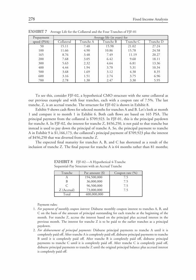
278 Fixed Income Analysis
EXHIBIT 7 Average Life for the Collateral and the Four Tranches of FJF-01
Prepayment Average life (in years) forspeed (PSA) Collateral Tranche A Tranche B Tranche C Tranche D
50 15.11 7.48 15.98 21.02 27.24100 11.66 4.90 10.86 15.78 24.58165 8.76 3.48 7.49 11.19 20.27200 7.68 3.05 6.42 9.60 18.11300 5.63 2.32 4.64 6.81 13.36400 4.44 1.94 3.70 5.31 10.34500 3.68 1.69 3.12 4.38 8.35600 3.16 1.51 2.74 3.75 6.96700 2.78 1.38 2.47 3.30 5.95
To see this, consider FJF-02, a hypothetical CMO structure with the same collateral asour previous example and with four tranches, each with a coupon rate of 7.5%. The lasttranche, Z, is an accrual tranche. The structure for FJF-02 is shown in Exhibit 8.
Exhibit 9 shows cash flows for selected months for tranches A and B. Let’s look at month1 and compare it to month 1 in Exhibit 6. Both cash flows are based on 165 PSA. Theprincipal payment from the collateral is $709,923. In FJF-01, this is the principal paydownfor tranche A. In FJF-02, the interest for tranche Z, $456,250, is not paid to that tranche butinstead is used to pay down the principal of tranche A. So, the principal payment to trancheA in Exhibit 9 is $1,166,173, the collateral’s principal payment of $709,923 plus the interestof $456,250 that was diverted from tranche Z.
The expected final maturity for tranches A, B, and C has shortened as a result of theinclusion of tranche Z. The final payout for tranche A is 64 months rather than 81 months;
EXHIBIT 8 FJF-02—A Hypothetical 4-TrancheSequential-Pay Structure with an Accrual Tranche
Tranche Par amount ($) Coupon rate (%)A 194,500,000 7.5B 36,000,000 7.5C 96,500,000 7.5
Z (Accrual) 73,000,000 7.5Total 400,000,000
Payment rules:1. For payment of monthly coupon interest: Disburse monthly coupon interest to tranches A, B, and
C on the basis of the amount of principal outstanding for each tranche at the beginning of themonth. For tranche Z, accrue the interest based on the principal plus accrued interest in theprevious month. The interest for tranche Z is to be paid to the earlier tranches as a principalpaydown.
2. For disbursement of principal payments: Disburse principal payments to tranche A until it iscompletely paid off. After tranche A is completely paid off, disburse principal payments to trancheB until it is completely paid off. After tranche B is completely paid off, disburse principalpayments to tranche C until it is completely paid off. After tranche C is completely paid off,disburse principal payments to tranche Z until the original principal balance plus accrued interestis completely paid off.
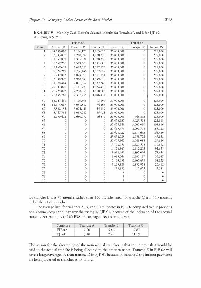
Chapter 10 Mortgage-Backed Sector of the Bond Market 279
EXHIBIT 9 Monthly Cash Flow for Selected Months for Tranches A and B for FJF-02Assuming 165 PSA
Tranche A Tranche BMonth Balance ($) Principal ($) Interest ($) Balance ($) Principal ($) Interest ($)
1 194,500,000 1,166,173 1,215,625 36,000,000 0 225,0002 193,333,827 1,280,997 1,208,336 36,000,000 0 225,0003 192,052,829 1,395,531 1,200,330 36,000,000 0 225,0004 190,657,298 1,509,680 1,191,608 36,000,000 0 225,0005 189,147,619 1,623,350 1,182,173 36,000,000 0 225,0006 187,524,269 1,736,446 1,172,027 36,000,000 0 225,0007 185,787,823 1,848,875 1,161,174 36,000,000 0 225,0008 183,938,947 1,960,543 1,149,618 36,000,000 0 225,0009 181,978,404 2,071,357 1,137,365 36,000,000 0 225,000
10 179,907,047 2,181,225 1,124,419 36,000,000 0 225,00011 177,725,822 2,290,054 1,110,786 36,000,000 0 225,00012 175,435,768 2,397,755 1,096,474 36,000,000 0 225,000
60 15,023,406 3,109,398 93,896 36,000,000 0 225,00061 11,914,007 3,091,812 74,463 36,000,000 0 225,00062 8,822,195 3,074,441 55,139 36,000,000 0 225,00063 5,747,754 3,057,282 35,923 36,000,000 0 225,00064 2,690,472 2,690,472 16,815 36,000,000 349,863 225,00065 0 0 0 35,650,137 3,023,598 222,81366 0 0 0 32,626,540 3,007,069 203,91667 0 0 0 29,619,470 2,990,748 185,12268 0 0 0 26,628,722 2,974,633 166,43069 0 0 0 23,654,089 2,958,722 147,83870 0 0 0 20,695,367 2,943,014 129,34671 0 0 0 17,752,353 2,927,508 110,95272 0 0 0 14,824,845 2,912,203 92,65573 0 0 0 11,912,642 2,897,096 74,45474 0 0 0 9,015,546 2,882,187 56,34775 0 0 0 6,133,358 2,867,475 38,33376 0 0 0 3,265,883 2,852,958 20,41277 0 0 0 412,925 412,925 2,58178 0 0 0 0 0 079 0 0 0 0 0 080 0 0 0 0 0 0
for tranche B it is 77 months rather than 100 months; and, for tranche C it is 113 monthsrather than 178 months.
The average lives for tranches A, B, and C are shorter in FJF-02 compared to our previousnon-accrual, sequential-pay tranche example, FJF-01, because of the inclusion of the accrualtranche. For example, at 165 PSA, the average lives are as follows:
Structure Tranche A Tranche B Tranche CFJF-02 2.90 5.86 7.87FJF-01 3.48 7.49 11.19
The reason for the shortening of the non-accrual tranches is that the interest that would bepaid to the accrual tranche is being allocated to the other tranches. Tranche Z in FJF-02 willhave a longer average life than tranche D in FJF-01 because in tranche Z the interest paymentsare being diverted to tranches A, B, and C.

280 Fixed Income Analysis
EXHIBIT 10 FJF-03—A Hypothetical 5-Tranche Sequential-PayStructure with Floater, Inverse Floater, and Accrual Bond Tranches
Tranche Par amount ($) Coupon rate (%)A 194,500,000 7.50B 36,000,000 7.50FL 72,375,000 1-month LIBOR + 0.50IFL 24,125,000 28.5 − 3 × (1-month LIBOR)
Z (Accrual) 73,000,000 7.50Total 400,000,000
Payment rules:1. For Payment of monthly coupon interest: Disburse monthly coupon interest to tranches A, B, FL,
and IFL on the basis of the amount of principal outstanding at the beginning of the month.For tranche Z, accrue the interest based on the principal plus accrued interest in the previousmonth. The interest for tranche Z is to be paid to the earlier tranches as a principal paydown. Themaximum coupon rate for FL is 10%; the minimum coupon rate for IFL is 0%.
2. For disbursement of principal payments: Disburse principal payments to tranche A until it iscompletely paid off. After tranche A is completely paid off, disburse principal payments to trancheB until it is completely paid off. After tranche B is completely paid off, disburse principalpayments to tranches FL and IFL until they are completely paid off. The principal paymentsbetween tranches FL and IFL should be made in the following way: 75% to tranche FL and 25%to tranche IFL. After tranches FL and IFI are completely paid off, disburse principal payments totranche Z until the original principal balance plus accrued interest are completely paid off.
Thus, shorter-term tranches and a longer-term tranche are created by including anaccrual tranche in FJF-02 compared to FJF-01. The accrual tranche has appeal to investorswho are concerned with reinvestment risk. Since there are no coupon payments to reinvest,reinvestment risk is eliminated until all the other tranches are paid off.
C. Floating-Rate Tranches
The tranches described thus far have a fixed rate. There is a demand for tranches that havea floating rate. The problem is that the collateral pays a fixed rate and therefore it wouldbe difficult to create a tranche with a floating rate. However, a floating-rate tranche canbe created. This is done by creating from any fixed-rate tranche a floater and an inversefloater combination. We will illustrate the creation of a floating-rate tranche and an inversefloating-rate tranche using the hypothetical CMO structure—the 4-tranche sequential-paystructure with an accrual tranche (FJF-02).10 We can select any of the tranches from whichto create a floating-rate and inverse floating-rate tranche. In fact, we can create these twosecurities for more than one of the four tranches or for only a portion of one tranche.
In this case, we create a floater and an inverse floater from tranche C. A floater could havebeen created from any of the other tranches. The par value for this tranche is $96.5 million,and we create two tranches that have a combined par value of $96.5 million. We refer to thisCMO structure with a floater and an inverse floater as FJF-03. It has five tranches, designatedA, B, FL, IFL, and Z, where FL is the floating-rate tranche and IFL is the inverse floating-ratetranche. Exhibit 10 describes FJF-03. Any reference rate can be used to create a floater and the
10The same principle for creating a floating-rate tranche and inverse-floating rate tranche could havebeen accomplished using the 4-tranche sequential-pay structure without an accrual tranche (FJF-01).
Chapter 10 Mortgage-Backed Sector of the Bond Market 281
corresponding inverse floater. The reference rate for setting the coupon rate for FL and IFL inFJF-03 is 1-month LIBOR.
The amount of the par value of the floating-rate tranche will be some portion of the$96.5 million. There are an infinite number of ways to slice up the $96.5 million between thefloater and inverse floater, and final partitioning will be driven by the demands of investors.In the FJF-03 structure, we made the floater from $72,375,000 or 75% of the $96.5 million.The coupon formula for the floater is 1-month LIBOR plus 50 basis points. So, for example,if LIBOR is 3.75% at the reset date, the coupon rate on the floater is 3.75% + 0.5%, or4.25%. There is a cap on the coupon rate for the floater (discussed later).
Unlike a floating-rate note in the corporate bond market whose principal is unchangedover the life of the instrument, the floater’s principal balance declines over time as principalpayments are made. The principal payments to the floater are determined by the principalpayments from the tranche from which the floater is created. In our CMO structure, this istranche C.
Since the floater’s par value is $72,375,000 of the $96.5 million, the balance is parvalue for the inverse floater. Assuming that 1-month LIBOR is the reference rate, the couponformula for the inverse floater takes the following form:
K − L × (1-month LIBOR)
where K and L are constants whose interpretation will be explained shortly.In FJF-03, K is set at 28.50% and L at 3. Thus, if 1-month LIBOR is 3.75%, the coupon
rate for the month is:
28.50% − 3 × (3.75%) = 17.25%
K is the cap or maximum coupon rate for the inverse floater. In FJF-03, the cap forthe inverse floater is 28.50%. The determination of the inverse floater’s cap rate is based on(1) the amount of interest that would have been paid to the tranche from which the floaterand the inverse floater were created, tranche C in our hypothetical deal, and (2) the couponrate for the floater if 1-month LIBOR is zero.
We will explain the determination of K by example. Let’s see how the 28.5% for theinverse floater is determined. The total interest to be paid to tranche C if it was not split intothe floater and the inverse floater is the principal of $96,500,000 times 7.5%, or $7,237,500.The maximum interest for the inverse floater occurs if 1-month LIBOR is zero. In that case,the coupon rate for the floater is
1-month LIBOR + 0.5% = 0.5%
Since the floater receives 0.5% on its principal of $72,375,000, the floater’s interest is$361,875. The remainder of the interest of $7,237,500 from tranche C goes to the inversefloater. That is, the inverse floater’s interest is $6,875,625 (= $7, 237, 500 − $361, 875).Since the inverse floater’s principal is $24,125,000, the cap rate for the inverse floater is
$6, 875, 625
$24, 125, 000= 28.5%
In general, the formula for the cap rate on the inverse floater, K , is
K = inverse floater interest when reference rate for floater is zero
principal for inverse floater

282 Fixed Income Analysis
The L or multiple in the coupon formula to determine the coupon rate for the inversefloater is called the leverage. The higher the leverage, the more the inverse floater’s coupon ratechanges for a given change in 1-month LIBOR. For example, a coupon leverage of 3 meansthat a 1-basis point change in 1-month LIBOR will change the coupon rate on the inversefloater by 3 basis points.
As in the case of the floater, the principal paydown of an inverse floater will be aproportionate amount of the principal paydown of tranche C.
Because 1-month LIBOR is always positive, the coupon rate paid to the floater cannot benegative. If there are no restrictions placed on the coupon rate for the inverse floater, however,it is possible for its coupon rate to be negative. To prevent this, a floor, or minimum, is placedon the coupon rate. In most structures, the floor is set at zero. Once a floor is set for the inversefloater, a cap or ceiling is imposed on the floater.
In FJF-03, a floor of zero is set for the inverse floater. The floor results in a cap ormaximum coupon rate for the floater of 10%. This is determined as follows. If the floor for theinverse floater is zero, this means that the inverse floater receives no interest. All of the interestthat would have been paid to tranche C, $7,237,500, would then be paid to the floater. Sincethe floater’s principal is $72,375,000, the cap rate on the floater is $7,237,500/$72,375,000,or 10%.
In general, the cap rate for the floater assuming a floor of zero for inverse floater is determinedas follows:
cap rate for floater = collateral tranche interest
principal for floater
The cap for the floater and the inverse floater, the floor for the inverse floater, the leverage,and the floater’s spread are not determined independently. Any cap or floor imposed on thecoupon rate for the floater and the inverse floater must be selected so that the weighted averagecoupon rate does not exceed the collateral tranche’s coupon rate.
D. Structured Interest-Only Tranches
CMO structures can be created so that a tranche receives only interest. Interest only (IO)tranches in a CMO structure are commonly referred to as structured IOs to distinguish themfrom IO mortgage strips that we will describe later in this chapter. The basic principle increating a structured IO is to set the coupon rate below the collateral’s coupon rate so thatexcess interest can be generated. It is the excess interest that is used to create one or morestructured IOs.
Let’s look at how a structured IO is created using an illustration. Thus far, we used a simpleCMO structure in which all the tranches have the same coupon rate (7.5%) and that couponrate is the same as the collateral. A structured IO is created from a CMO structure where thecoupon rate for at least one tranche is different from the collateral’s coupon rate. This is seenin FJF-04 shown in Exhibit 11. In this structure, notice that the coupon interest rate for eachtranche is less than the coupon interest rate for the collateral. That means that there is excessinterest from the collateral that is not being paid to all the tranches. At one time, all of that excessinterest not paid to the tranches was paid to a bond class called a ‘‘residual.’’ Eventually (dueto changes in the tax law that do not concern us here), structurers of CMO began allocatingthe excess interest to the tranche that receives only interest. This is tranche IO in FJF-04.
Notice that for this structure the par amount for the IO tranche is shown as $52,566,667and the coupon rate is 7.5%. Since this is an IO tranche there is no par amount. The amountshown is the amount upon which the interest payments will be determined, not the amount
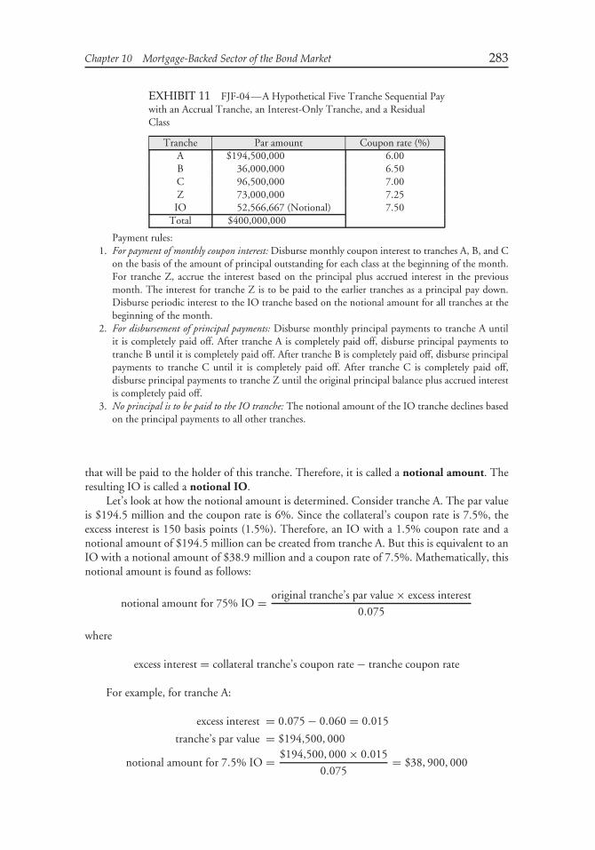
Chapter 10 Mortgage-Backed Sector of the Bond Market 283
EXHIBIT 11 FJF-04—A Hypothetical Five Tranche Sequential Paywith an Accrual Tranche, an Interest-Only Tranche, and a ResidualClass
Tranche Par amount Coupon rate (%)A $194,500,000 6.00B 36,000,000 6.50C 96,500,000 7.00Z 73,000,000 7.25IO 52,566,667 (Notional) 7.50
Total $400,000,000
Payment rules:1. For payment of monthly coupon interest: Disburse monthly coupon interest to tranches A, B, and C
on the basis of the amount of principal outstanding for each class at the beginning of the month.For tranche Z, accrue the interest based on the principal plus accrued interest in the previousmonth. The interest for tranche Z is to be paid to the earlier tranches as a principal pay down.Disburse periodic interest to the IO tranche based on the notional amount for all tranches at thebeginning of the month.
2. For disbursement of principal payments: Disburse monthly principal payments to tranche A untilit is completely paid off. After tranche A is completely paid off, disburse principal payments totranche B until it is completely paid off. After tranche B is completely paid off, disburse principalpayments to tranche C until it is completely paid off. After tranche C is completely paid off,disburse principal payments to tranche Z until the original principal balance plus accrued interestis completely paid off.
3. No principal is to be paid to the IO tranche: The notional amount of the IO tranche declines basedon the principal payments to all other tranches.
that will be paid to the holder of this tranche. Therefore, it is called a notional amount. Theresulting IO is called a notional IO.
Let’s look at how the notional amount is determined. Consider tranche A. The par valueis $194.5 million and the coupon rate is 6%. Since the collateral’s coupon rate is 7.5%, theexcess interest is 150 basis points (1.5%). Therefore, an IO with a 1.5% coupon rate and anotional amount of $194.5 million can be created from tranche A. But this is equivalent to anIO with a notional amount of $38.9 million and a coupon rate of 7.5%. Mathematically, thisnotional amount is found as follows:
notional amount for 75% IO = original tranche’s par value × excess interest
0.075
where
excess interest = collateral tranche’s coupon rate − tranche coupon rate
For example, for tranche A:
excess interest = 0.075 − 0.060 = 0.015
tranche’s par value = $194,500, 000
notional amount for 7.5% IO = $194,500, 000 × 0.015
0.075= $38, 900, 000
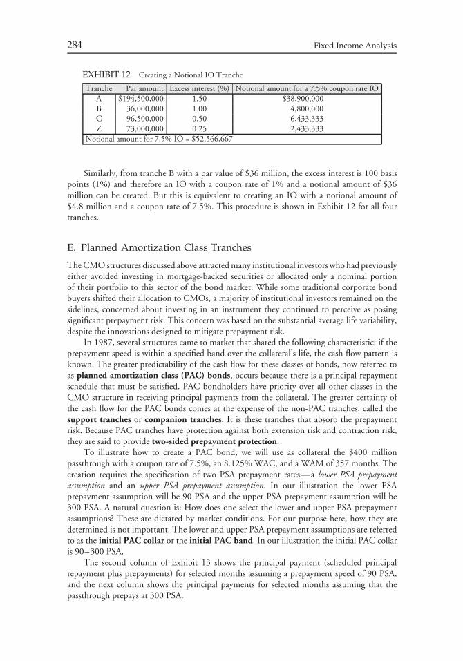
284 Fixed Income Analysis
EXHIBIT 12 Creating a Notional IO Tranche
Tranche Par amount Excess interest (%) Notional amount for a 7.5% coupon rate IOA $194,500,000 1.50 $38,900,000B 36,000,000 1.00 4,800,000C 96,500,000 0.50 6,433,333Z 73,000,000 0.25 2,433,333
Notional amount for 7.5% IO = $52,566,667
Similarly, from tranche B with a par value of $36 million, the excess interest is 100 basispoints (1%) and therefore an IO with a coupon rate of 1% and a notional amount of $36million can be created. But this is equivalent to creating an IO with a notional amount of$4.8 million and a coupon rate of 7.5%. This procedure is shown in Exhibit 12 for all fourtranches.
E. Planned Amortization Class Tranches
The CMO structures discussed above attracted many institutional investors who had previouslyeither avoided investing in mortgage-backed securities or allocated only a nominal portionof their portfolio to this sector of the bond market. While some traditional corporate bondbuyers shifted their allocation to CMOs, a majority of institutional investors remained on thesidelines, concerned about investing in an instrument they continued to perceive as posingsignificant prepayment risk. This concern was based on the substantial average life variability,despite the innovations designed to mitigate prepayment risk.
In 1987, several structures came to market that shared the following characteristic: if theprepayment speed is within a specified band over the collateral’s life, the cash flow pattern isknown. The greater predictability of the cash flow for these classes of bonds, now referred toas planned amortization class (PAC) bonds, occurs because there is a principal repaymentschedule that must be satisfied. PAC bondholders have priority over all other classes in theCMO structure in receiving principal payments from the collateral. The greater certainty ofthe cash flow for the PAC bonds comes at the expense of the non-PAC tranches, called thesupport tranches or companion tranches. It is these tranches that absorb the prepaymentrisk. Because PAC tranches have protection against both extension risk and contraction risk,they are said to provide two-sided prepayment protection.
To illustrate how to create a PAC bond, we will use as collateral the $400 millionpassthrough with a coupon rate of 7.5%, an 8.125% WAC, and a WAM of 357 months. Thecreation requires the specification of two PSA prepayment rates—a lower PSA prepaymentassumption and an upper PSA prepayment assumption. In our illustration the lower PSAprepayment assumption will be 90 PSA and the upper PSA prepayment assumption will be300 PSA. A natural question is: How does one select the lower and upper PSA prepaymentassumptions? These are dictated by market conditions. For our purpose here, how they aredetermined is not important. The lower and upper PSA prepayment assumptions are referredto as the initial PAC collar or the initial PAC band. In our illustration the initial PAC collaris 90–300 PSA.
The second column of Exhibit 13 shows the principal payment (scheduled principalrepayment plus prepayments) for selected months assuming a prepayment speed of 90 PSA,and the next column shows the principal payments for selected months assuming that thepassthrough prepays at 300 PSA.
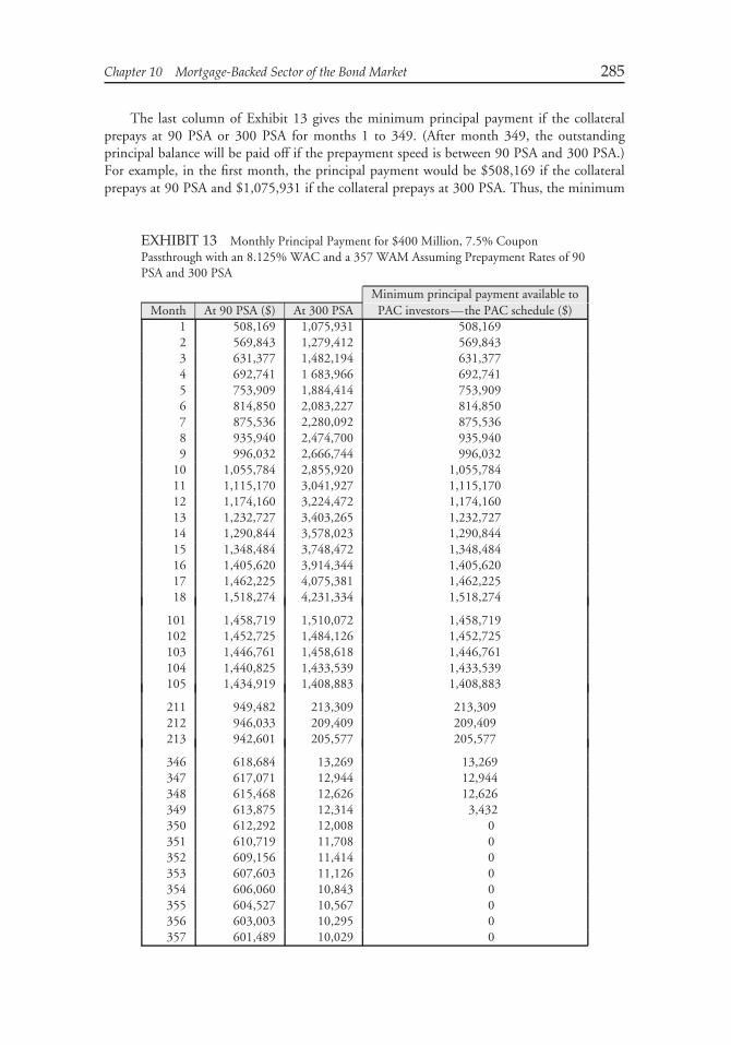
Chapter 10 Mortgage-Backed Sector of the Bond Market 285
The last column of Exhibit 13 gives the minimum principal payment if the collateralprepays at 90 PSA or 300 PSA for months 1 to 349. (After month 349, the outstandingprincipal balance will be paid off if the prepayment speed is between 90 PSA and 300 PSA.)For example, in the first month, the principal payment would be $508,169 if the collateralprepays at 90 PSA and $1,075,931 if the collateral prepays at 300 PSA. Thus, the minimum
EXHIBIT 13 Monthly Principal Payment for $400 Million, 7.5% CouponPassthrough with an 8.125% WAC and a 357 WAM Assuming Prepayment Rates of 90PSA and 300 PSA
Minimum principal payment available toMonth At 90 PSA ($) At 300 PSA PAC investors—the PAC schedule ($)
1 508,169 1,075,931 508,1692 569,843 1,279,412 569,8433 631,377 1,482,194 631,3774 692,741 1 683,966 692,7415 753,909 1,884,414 753,9096 814,850 2,083,227 814,8507 875,536 2,280,092 875,5368 935,940 2,474,700 935,9409 996,032 2,666,744 996,032
10 1,055,784 2,855,920 1,055,78411 1,115,170 3,041,927 1,115,17012 1,174,160 3,224,472 1,174,16013 1,232,727 3,403,265 1,232,72714 1,290,844 3,578,023 1,290,84415 1,348,484 3,748,472 1,348,48416 1,405,620 3,914,344 1,405,62017 1,462,225 4,075,381 1,462,22518 1,518,274 4,231,334 1,518,274
101 1,458,719 1,510,072 1,458,719102 1,452,725 1,484,126 1,452,725103 1,446,761 1,458,618 1,446,761104 1,440,825 1,433,539 1,433,539105 1,434,919 1,408,883 1,408,883
211 949,482 213,309 213,309212 946,033 209,409 209,409213 942,601 205,577 205,577
346 618,684 13,269 13,269347 617,071 12,944 12,944348 615,468 12,626 12,626349 613,875 12,314 3,432350 612,292 12,008 0351 610,719 11,708 0352 609,156 11,414 0353 607,603 11,126 0354 606,060 10,843 0355 604,527 10,567 0356 603,003 10,295 0357 601,489 10,029 0
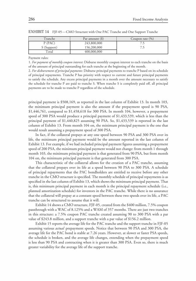
286 Fixed Income Analysis
EXHIBIT 14 FJF-05—CMO Structure with One PAC Tranche and One Support Tranche
Tranche Par amount ($) Coupon rate (%)P (PAC) 243,800,000 7.5
S (Support) 156,200,000 7.5Total 400,000,000
Payment rules:1. For payment of monthly coupon interest: Disburse monthly coupon interest to each tranche on the basisof the amount of principal outstanding for each tranche at the beginning of the month.2. For disbursement of principal payments: Disburse principal payments to tranche P based on its scheduleof principal repayments. Tranche P has priority with respect to current and future principal paymentsto satisfy the schedule. Any excess principal payments in a month over the amount necessary to satisfythe schedule for tranche P are paid to tranche S. When tranche S is completely paid off, all principalpayments are to be made to tranche P regardless of the schedule.
principal payment is $508,169, as reported in the last column of Exhibit 13. In month 103,the minimum principal payment is also the amount if the prepayment speed is 90 PSA,$1,446,761, compared to $1,458,618 for 300 PSA. In month 104, however, a prepaymentspeed of 300 PSA would produce a principal payment of $1,433,539, which is less than theprincipal payment of $1,440,825 assuming 90 PSA. So, $1,433,539 is reported in the lastcolumn of Exhibit 13. From month 104 on, the minimum principal payment is the one thatwould result assuming a prepayment speed of 300 PSA.
In fact, if the collateral prepays at any one speed between 90 PSA and 300 PSA over itslife, the minimum principal payment would be the amount reported in the last column ofExhibit 13. For example, if we had included principal payment figures assuming a prepaymentspeed of 200 PSA, the minimum principal payment would not change: from month 1 throughmonth 103, the minimum principal payment is that generated from 90 PSA, but from month104 on, the minimum principal payment is that generated from 300 PSA.
This characteristic of the collateral allows for the creation of a PAC tranche, assumingthat the collateral prepays over its life at a speed between 90 PSA to 300 PSA. A scheduleof principal repayments that the PAC bondholders are entitled to receive before any othertranche in the CMO structure is specified. The monthly schedule of principal repayments is asspecified in the last column of Exhibit 13, which shows the minimum principal payment. Thatis, this minimum principal payment in each month is the principal repayment schedule (i.e.,planned amortization schedule) for investors in the PAC tranche. While there is no assurancethat the collateral will prepay at a constant speed between these two speeds over its life, a PACtranche can be structured to assume that it will.
Exhibit 14 shows a CMO structure, FJF-05, created from the $400 million, 7.5% couponpassthrough with a WAC of 8.125% and a WAM of 357 months. There are just two tranchesin this structure: a 7.5% coupon PAC tranche created assuming 90 to 300 PSA with a parvalue of $243.8 million, and a support tranche with a par value of $156.2 million.
Exhibit 15 reports the average life for the PAC tranche and the support tranche in FJF-05assuming various actual prepayment speeds. Notice that between 90 PSA and 300 PSA, theaverage life for the PAC bond is stable at 7.26 years. However, at slower or faster PSA speeds,the schedule is broken, and the average life changes, extending when the prepayment speedis less than 90 PSA and contracting when it is greater than 300 PSA. Even so, there is muchgreater variability for the average life of the support tranche.
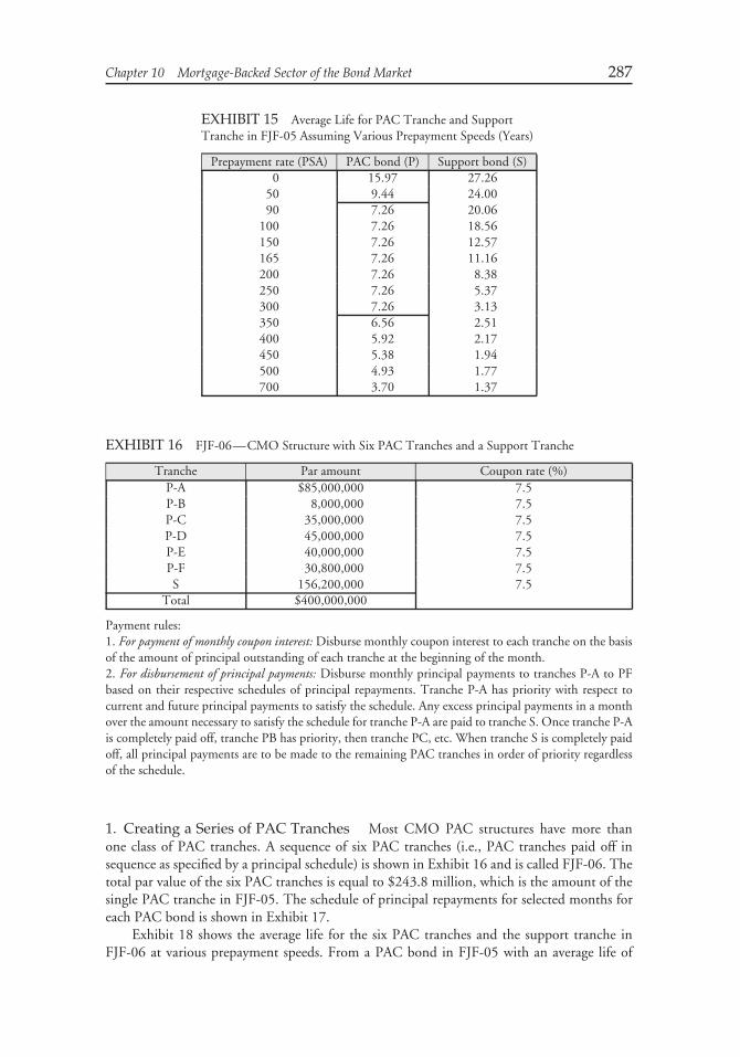
Chapter 10 Mortgage-Backed Sector of the Bond Market 287
EXHIBIT 15 Average Life for PAC Tranche and SupportTranche in FJF-05 Assuming Various Prepayment Speeds (Years)
Prepayment rate (PSA) PAC bond (P) Support bond (S)0 15.97 27.26
50 9.44 24.0090 7.26 20.06
100 7.26 18.56150 7.26 12.57165 7.26 11.16200 7.26 8.38250 7.26 5.37300 7.26 3.13350 6.56 2.51400 5.92 2.17450 5.38 1.94500 4.93 1.77700 3.70 1.37
EXHIBIT 16 FJF-06—CMO Structure with Six PAC Tranches and a Support Tranche
Tranche Par amount Coupon rate (%)P-A $85,000,000 7.5P-B 8,000,000 7.5P-C 35,000,000 7.5P-D 45,000,000 7.5P-E 40,000,000 7.5P-F 30,800,000 7.5S 156,200,000 7.5
Total $400,000,000
Payment rules:1. For payment of monthly coupon interest: Disburse monthly coupon interest to each tranche on the basisof the amount of principal outstanding of each tranche at the beginning of the month.2. For disbursement of principal payments: Disburse monthly principal payments to tranches P-A to PFbased on their respective schedules of principal repayments. Tranche P-A has priority with respect tocurrent and future principal payments to satisfy the schedule. Any excess principal payments in a monthover the amount necessary to satisfy the schedule for tranche P-A are paid to tranche S. Once tranche P-Ais completely paid off, tranche PB has priority, then tranche PC, etc. When tranche S is completely paidoff, all principal payments are to be made to the remaining PAC tranches in order of priority regardlessof the schedule.
1. Creating a Series of PAC Tranches Most CMO PAC structures have more thanone class of PAC tranches. A sequence of six PAC tranches (i.e., PAC tranches paid off insequence as specified by a principal schedule) is shown in Exhibit 16 and is called FJF-06. Thetotal par value of the six PAC tranches is equal to $243.8 million, which is the amount of thesingle PAC tranche in FJF-05. The schedule of principal repayments for selected months foreach PAC bond is shown in Exhibit 17.
Exhibit 18 shows the average life for the six PAC tranches and the support tranche inFJF-06 at various prepayment speeds. From a PAC bond in FJF-05 with an average life of
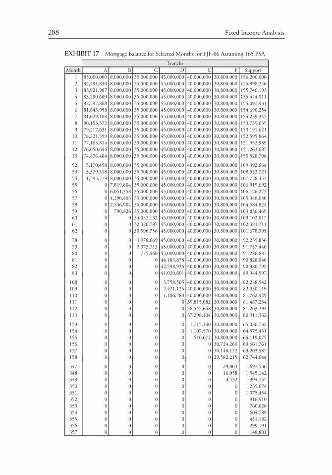
288 Fixed Income Analysis
EXHIBIT 17 Mortgage Balance for Selected Months for FJF-06 Assuming 165 PSA
TrancheMonth A B C D E F Support
1 85,000,000 8,000,000 35,000,000 45,000,000 40,000,000 30,800,000 156,200,0002 84,491,830 8,000,000 35,000,000 45,000,000 40,000,000 30,800,000 155,998,2463 83,921,987 8,000,000 35,000,000 45,000,000 40,000,000 30,800,000 155,746,1934 83,290,609 8,000,000 35,000,000 45,000,000 40,000,000 30,800,000 155,444,0115 82,597,868 8,000,000 35,000,000 45,000,000 40,000,000 30,800,000 155,091,9316 81,843,958 8,000,000 35,000,000 45,000,000 40,000,000 30,800,000 154,690,2547 81,029,108 8,000,000 35,000,000 45,000,000 40,000,000 30,800,000 154,239,3458 80,153,572 8,000,000 35,000,000 45,000,000 40,000,000 30,800,000 153,739,6359 79,217,631 8,000,000 35,000,000 45,000,000 40,000,000 30,800,000 153,191,621
10 78,221,599 8,000,000 35,000,000 45,000,000 40,000,000 30,800,000 152,595,86411 77,165,814 8,000,000 35,000,000 45,000,000 40,000,000 30,800,000 151,952,98912 76,050,644 8,000,000 35,000,000 45,000,000 40,000,000 30,800,000 151,263,68713 74,876,484 8,000,000 35,000,000 45,000,000 40,000,000 30,800,000 150,528,708
52 5,170,458 8,000,000 35,000,000 45,000,000 40,000,000 30,800,000 109,392,66453 3,379,318 8,000,000 35,000,000 45,000,000 40,000,000 30,800,000 108,552,72154 1,595,779 8,000,000 35,000,000 45,000,000 40,000,000 30,800,000 107,728,45355 0 7,819,804 35,000,000 45,000,000 40,000,000 30,800,000 106,919,69256 0 6,051,358 35,000,000 45,000,000 40,000,000 30,800,000 106,126,27557 0 4,290,403 35,000,000 45,000,000 40,000,000 30,800,000 105,348,04058 0 2,536,904 35,000,000 45,000,000 40,000,000 30,800,000 104,584,82459 0 790,826 35,000,000 45,000,000 40,000,000 30,800,000 103,836,46960 0 0 34,052,132 45,000,000 40,000,000 30,800,000 103,102,81761 0 0 32,320,787 45,000,000 40,000,000 30,800,000 102,383,71162 0 0 30,596,756 45,000,000 40,000,000 30,800,000 101,678,995
78 0 0 3,978,669 45,000,000 40,000,000 30,800,000 92,239,83679 0 0 2,373,713 45,000,000 40,000,000 30,800,000 91,757,44080 0 0 775,460 45,000,000 40,000,000 30,800,000 91,286,88781 0 0 0 44,183,878 40,000,000 30,800,000 90,828,04682 0 0 0 42,598,936 40,000,000 30,800,000 90,380,79283 0 0 0 41,020,601 40,000,000 30,800,000 89,944,997
108 0 0 0 3,758,505 40,000,000 30,800,000 82,288,542109 0 0 0 2,421,125 40,000,000 30,800,000 82,030,119110 0 0 0 1,106,780 40,000,000 30,800,000 81,762,929111 0 0 0 0 39,815,082 30,800,000 81,487,234112 0 0 0 0 38,545,648 30,800,000 81,203,294113 0 0 0 0 37,298,104 30,800,000 80,911,362
153 0 0 0 0 1,715,140 30,800,000 65,030,732154 0 0 0 0 1,107,570 30,800,000 64,575,431155 0 0 0 0 510,672 30,800,000 64,119,075156 0 0 0 0 0 30,724,266 63,661,761157 0 0 0 0 0 30,148,172 63,203,587158 0 0 0 0 0 29,582,215 62,744,644
347 0 0 0 0 0 29,003 1,697,536348 0 0 0 0 0 16,058 1,545,142349 0 0 0 0 0 3,432 1,394,152350 0 0 0 0 0 0 1,235,674351 0 0 0 0 0 0 1,075,454352 0 0 0 0 0 0 916,910353 0 0 0 0 0 0 760,026354 0 0 0 0 0 0 604,789355 0 0 0 0 0 0 451,182356 0 0 0 0 0 0 299,191357 0 0 0 0 0 0 148,801
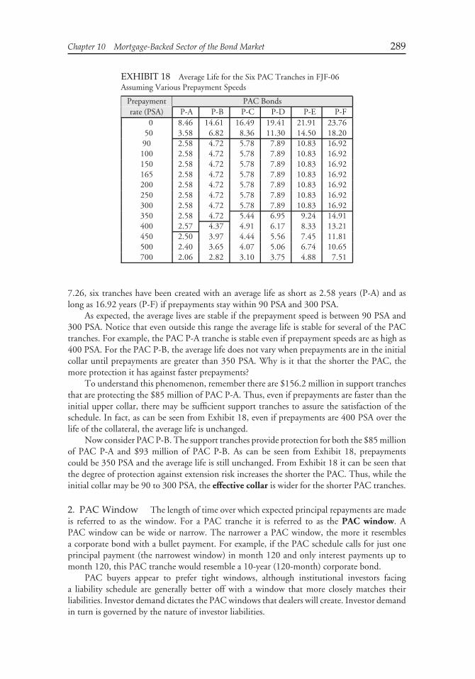
Chapter 10 Mortgage-Backed Sector of the Bond Market 289
EXHIBIT 18 Average Life for the Six PAC Tranches in FJF-06Assuming Various Prepayment Speeds
Prepayment PAC Bondsrate (PSA) P-A P-B P-C P-D P-E P-F
0 8.46 14.61 16.49 19.41 21.91 23.7650 3.58 6.82 8.36 11.30 14.50 18.2090 2.58 4.72 5.78 7.89 10.83 16.92100 2.58 4.72 5.78 7.89 10.83 16.92150 2.58 4.72 5.78 7.89 10.83 16.92165 2.58 4.72 5.78 7.89 10.83 16.92200 2.58 4.72 5.78 7.89 10.83 16.92250 2.58 4.72 5.78 7.89 10.83 16.92300 2.58 4.72 5.78 7.89 10.83 16.92350 2.58 4.72 5.44 6.95 9.24 14.91400 2.57 4.37 4.91 6.17 8.33 13.21450 2.50 3.97 4.44 5.56 7.45 11.81500 2.40 3.65 4.07 5.06 6.74 10.65700 2.06 2.82 3.10 3.75 4.88 7.51
7.26, six tranches have been created with an average life as short as 2.58 years (P-A) and aslong as 16.92 years (P-F) if prepayments stay within 90 PSA and 300 PSA.
As expected, the average lives are stable if the prepayment speed is between 90 PSA and300 PSA. Notice that even outside this range the average life is stable for several of the PACtranches. For example, the PAC P-A tranche is stable even if prepayment speeds are as high as400 PSA. For the PAC P-B, the average life does not vary when prepayments are in the initialcollar until prepayments are greater than 350 PSA. Why is it that the shorter the PAC, themore protection it has against faster prepayments?
To understand this phenomenon, remember there are $156.2 million in support tranchesthat are protecting the $85 million of PAC P-A. Thus, even if prepayments are faster than theinitial upper collar, there may be sufficient support tranches to assure the satisfaction of theschedule. In fact, as can be seen from Exhibit 18, even if prepayments are 400 PSA over thelife of the collateral, the average life is unchanged.
Now consider PAC P-B. The support tranches provide protection for both the $85 millionof PAC P-A and $93 million of PAC P-B. As can be seen from Exhibit 18, prepaymentscould be 350 PSA and the average life is still unchanged. From Exhibit 18 it can be seen thatthe degree of protection against extension risk increases the shorter the PAC. Thus, while theinitial collar may be 90 to 300 PSA, the effective collar is wider for the shorter PAC tranches.
2. PAC Window The length of time over which expected principal repayments are madeis referred to as the window. For a PAC tranche it is referred to as the PAC window. APAC window can be wide or narrow. The narrower a PAC window, the more it resemblesa corporate bond with a bullet payment. For example, if the PAC schedule calls for just oneprincipal payment (the narrowest window) in month 120 and only interest payments up tomonth 120, this PAC tranche would resemble a 10-year (120-month) corporate bond.
PAC buyers appear to prefer tight windows, although institutional investors facinga liability schedule are generally better off with a window that more closely matches theirliabilities. Investor demand dictates the PAC windows that dealers will create. Investor demandin turn is governed by the nature of investor liabilities.
290 Fixed Income Analysis
3. Effective Collars and Actual Prepayments The creation of a mortgage-backedsecurity cannot make prepayment risk disappear. This is true for both a passthrough and aCMO. Thus, the reduction in prepayment risk (both extension risk and contraction risk) thata PAC offers investors must come from somewhere.
Where does the prepayment protection come from? It comes from the support tranches.It is the support tranches that defer principal payments to the PAC tranches if the collateralprepayments are slow; support tranches do not receive any principal until the PAC tranchesreceive the scheduled principal repayment. This reduces the risk that the PAC tranches willextend. Similarly, it is the support tranches that absorb any principal payments in excess ofthe scheduled principal payments that are made. This reduces the contraction risk of the PACtranches. Thus, the key to the prepayment protection offered by a PAC tranche is the amountof support tranches outstanding. If the support tranches are paid off quickly because of faster-than-expected prepayments, then there is no longer any protection for the PAC tranches. In fact,in FJF-06, if the support tranche is paid off, the structure effectively becomes a sequential-pay CMO.
The support tranches can be thought of as bodyguards for the PAC bondholders. Whenthe bullets fly—i.e., prepayments occur—it is the bodyguards that get killed off first. Thebodyguards are there to absorb the bullets. Once all the bodyguards are killed off (i.e., thesupport tranches paid off with faster-than-expected prepayments), the PAC tranches mustfend for themselves: they are exposed to all the bullets. A PAC tranche in which all the supporttranches have been paid off is called a busted PAC or broken PAC.
With the bodyguard metaphor for the support tranches in mind, let’s consider twoquestions asked by investors in PAC tranches:
1. Will the schedule of principal repayments be satisfied if prepayments are faster than theinitial upper collar?
2. Will the schedule of principal repayments be satisfied as long as prepayments stay withinthe initial collar?
a. Actual Prepayments Greater than the Initial Upper Collar Let’s address the firstquestion. The initial upper collar for FJF-06 is 300 PSA. Suppose that actual prepay-ments are 500 PSA for seven consecutive months. Will this disrupt the schedule of principalrepayments? The answer is: It depends!
There are two pieces of information we will need to answer this question. First, whendoes the 500 PSA occur? Second, what has been the actual prepayment experience up to thetime that prepayments are 500 PSA? For example, suppose six years from now is when theprepayments reach 500 PSA, and also suppose that for the past six years the actual prepaymentspeed has been 90 PSA every month. What this means is that there are more bodyguards (i.e.,support tranches) around than were expected when the PAC was structured at the initial collar.In establishing the schedule of principal repayments, it is assumed that the bodyguards wouldbe killed off at 300 PSA. (Recall that 300 PSA is the upper collar prepayment assumptionused in creating FJF-06.) But the actual prepayment experience results in them being killedoff at only 90 PSA. Thus, six years from now when the 500 PSA is assumed to occur, there aremore bodyguards than expected. In turn, a 500 PSA for seven consecutive months may haveno effect on the ability of the schedule of principal repayments to be met.
In contrast, suppose that the actual prepayment experience for the first six years is 300PSA (the upper collar of the initial PAC collar). In this case, there are no extra bodyguards
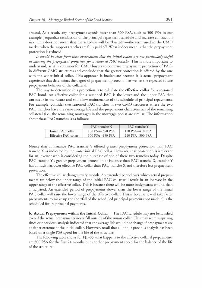
Chapter 10 Mortgage-Backed Sector of the Bond Market 291
around. As a result, any prepayment speeds faster than 300 PSA, such as 500 PSA in ourexample, jeopardize satisfaction of the principal repayment schedule and increase contractionrisk. This does not mean that the schedule will be ‘‘busted’’—the term used in the CMOmarket when the support tranches are fully paid off. What it does mean is that the prepaymentprotection is reduced.
It should be clear from these observations that the initial collars are not particularly usefulin assessing the prepayment protection for a seasoned PAC tranche. This is most important tounderstand, as it is common for CMO buyers to compare prepayment protection of PACsin different CMO structures and conclude that the greater protection is offered by the onewith the wider initial collar. This approach is inadequate because it is actual prepaymentexperience that determines the degree of prepayment protection, as well as the expected futureprepayment behavior of the collateral.
The way to determine this protection is to calculate the effective collar for a seasonedPAC bond. An effective collar for a seasoned PAC is the lower and the upper PSA thatcan occur in the future and still allow maintenance of the schedule of principal repayments.For example, consider two seasoned PAC tranches in two CMO structures where the twoPAC tranches have the same average life and the prepayment characteristics of the remainingcollateral (i.e., the remaining mortgages in the mortgage pools) are similar. The informationabout these PAC tranches is as follows:
PAC tranche X PAC tranche YInitial PAC collar 180 PSA–350 PSA 170 PSA–410 PSAEffective PAC collar 160 PSA–450 PSA 240 PSA–300 PSA
Notice that at issuance PAC tranche Y offered greater prepayment protection than PACtranche X as indicated by the wider initial PAC collar. However, that protection is irrelevantfor an investor who is considering the purchase of one of these two tranches today. DespitePAC tranche Y’s greater prepayment protection at issuance than PAC tranche X, tranche Yhas a much narrower effective PAC collar than PAC tranche X and therefore less prepaymentprotection.
The effective collar changes every month. An extended period over which actual prepay-ments are below the upper range of the initial PAC collar will result in an increase in theupper range of the effective collar. This is because there will be more bodyguards around thananticipated. An extended period of prepayments slower than the lower range of the initialPAC collar will raise the lower range of the effective collar. This is because it will take fasterprepayments to make up the shortfall of the scheduled principal payments not made plus thescheduled future principal payments.
b. Actual Prepayments within the Initial Collar The PAC schedule may not be satisfiedeven if the actual prepayments never fall outside of the initial collar. This may seem surprisingsince our previous analysis indicated that the average life would not change if prepayments areat either extreme of the initial collar. However, recall that all of our previous analysis has beenbased on a single PSA speed for the life of the structure.
The following table shows for FJF-05 what happens to the effective collar if prepaymentsare 300 PSA for the first 24 months but another prepayment speed for the balance of the lifeof the structure:
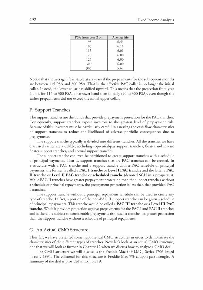
292 Fixed Income Analysis
PSA from year 2 on Average life95 6.43
105 6.11115 6.01120 6.00125 6.00300 6.00305 5.62
Notice that the average life is stable at six years if the prepayments for the subsequent monthsare between 115 PSA and 300 PSA. That is, the effective PAC collar is no longer the initialcollar. Instead, the lower collar has shifted upward. This means that the protection from year2 on is for 115 to 300 PSA, a narrower band than initially (90 to 300 PSA), even though theearlier prepayments did not exceed the initial upper collar.
F. Support Tranches
The support tranches are the bonds that provide prepayment protection for the PAC tranches.Consequently, support tranches expose investors to the greatest level of prepayment risk.Because of this, investors must be particularly careful in assessing the cash flow characteristicsof support tranches to reduce the likelihood of adverse portfolio consequences due toprepayments.
The support tranche typically is divided into different tranches. All the tranches we havediscussed earlier are available, including sequential-pay support tranches, floater and inversefloater support tranches, and accrual support tranches.
The support tranche can even be partitioned to create support tranches with a scheduleof principal payments. That is, support tranches that are PAC tranches can be created. Ina structure with a PAC tranche and a support tranche with a PAC schedule of principalpayments, the former is called a PAC I tranche or Level I PAC tranche and the latter a PACII tranche or Level II PAC tranche or scheduled tranche (denoted SCH in a prospectus).While PAC II tranches have greater prepayment protection than the support tranches withouta schedule of principal repayments, the prepayment protection is less than that provided PACI tranches.
The support tranche without a principal repayment schedule can be used to create anytype of tranche. In fact, a portion of the non-PAC II support tranche can be given a scheduleof principal repayments. This tranche would be called a PAC III tranche or a Level III PACtranche. While it provides protection against prepayments for the PAC I and PAC II tranchesand is therefore subject to considerable prepayment risk, such a tranche has greater protectionthan the support tranche without a schedule of principal repayments.
G. An Actual CMO Structure
Thus far, we have presented some hypothetical CMO structures in order to demonstrate thecharacteristics of the different types of tranches. Now let’s look at an actual CMO structure,one that we will look at further in Chapter 12 when we discuss how to analyze a CMO deal.
The CMO structure we will discuss is the Freddie Mac (FHLMC) Series 1706 issuedin early 1994. The collateral for this structure is Freddie Mac 7% coupon passthroughs. Asummary of the deal is provided in Exhibit 19.
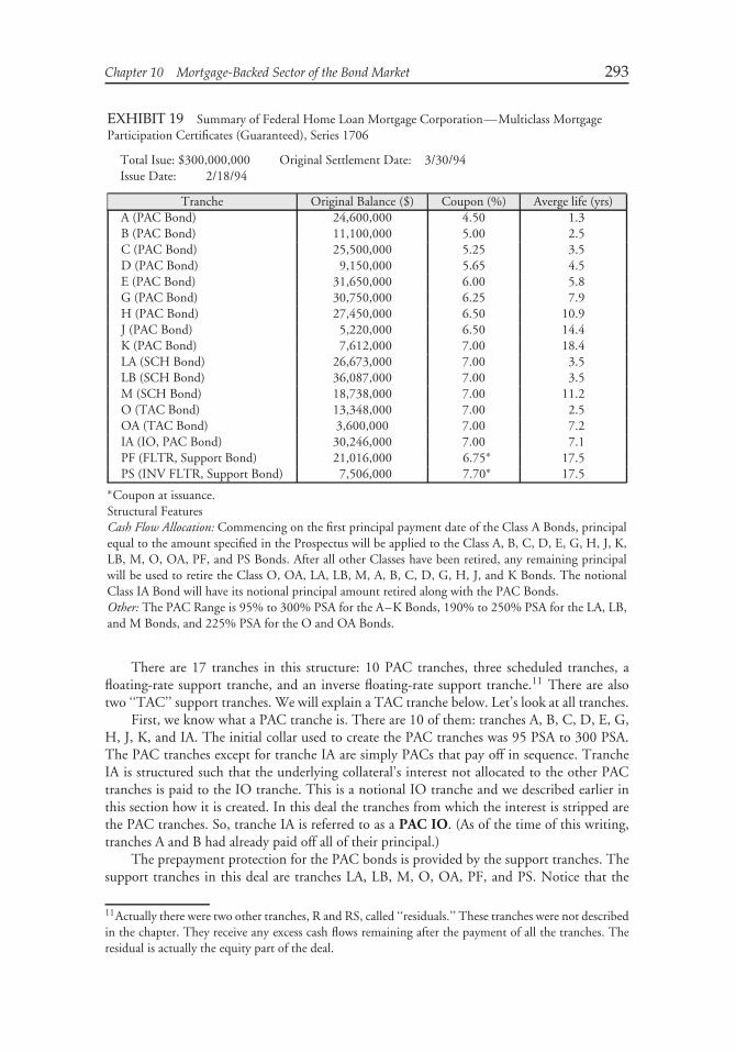
Chapter 10 Mortgage-Backed Sector of the Bond Market 293
EXHIBIT 19 Summary of Federal Home Loan Mortgage Corporation—Multiclass MortgageParticipation Certificates (Guaranteed), Series 1706
Total Isue: $300,000,000 Original Settlement Date: 3/30/94Issue Date: 2/18/94
Tranche Original Balance ($) Coupon (%) Averge life (yrs)A (PAC Bond) 24,600,000 4.50 1.3B (PAC Bond) 11,100,000 5.00 2.5C (PAC Bond) 25,500,000 5.25 3.5D (PAC Bond) 9,150,000 5.65 4.5E (PAC Bond) 31,650,000 6.00 5.8G (PAC Bond) 30,750,000 6.25 7.9H (PAC Bond) 27,450,000 6.50 10.9J (PAC Bond) 5,220,000 6.50 14.4K (PAC Bond) 7,612,000 7.00 18.4LA (SCH Bond) 26,673,000 7.00 3.5LB (SCH Bond) 36,087,000 7.00 3.5M (SCH Bond) 18,738,000 7.00 11.2O (TAC Bond) 13,348,000 7.00 2.5OA (TAC Bond) 3,600,000 7.00 7.2IA (IO, PAC Bond) 30,246,000 7.00 7.1PF (FLTR, Support Bond) 21,016,000 6.75∗ 17.5PS (INV FLTR, Support Bond) 7,506,000 7.70∗ 17.5
∗Coupon at issuance.Structural FeaturesCash Flow Allocation: Commencing on the first principal payment date of the Class A Bonds, principalequal to the amount specified in the Prospectus will be applied to the Class A, B, C, D, E, G, H, J, K,LB, M, O, OA, PF, and PS Bonds. After all other Classes have been retired, any remaining principalwill be used to retire the Class O, OA, LA, LB, M, A, B, C, D, G, H, J, and K Bonds. The notionalClass IA Bond will have its notional principal amount retired along with the PAC Bonds.Other: The PAC Range is 95% to 300% PSA for the A–K Bonds, 190% to 250% PSA for the LA, LB,and M Bonds, and 225% PSA for the O and OA Bonds.
There are 17 tranches in this structure: 10 PAC tranches, three scheduled tranches, afloating-rate support tranche, and an inverse floating-rate support tranche.11 There are alsotwo ‘‘TAC’’ support tranches. We will explain a TAC tranche below. Let’s look at all tranches.
First, we know what a PAC tranche is. There are 10 of them: tranches A, B, C, D, E, G,H, J, K, and IA. The initial collar used to create the PAC tranches was 95 PSA to 300 PSA.The PAC tranches except for tranche IA are simply PACs that pay off in sequence. TrancheIA is structured such that the underlying collateral’s interest not allocated to the other PACtranches is paid to the IO tranche. This is a notional IO tranche and we described earlier inthis section how it is created. In this deal the tranches from which the interest is stripped arethe PAC tranches. So, tranche IA is referred to as a PAC IO. (As of the time of this writing,tranches A and B had already paid off all of their principal.)
The prepayment protection for the PAC bonds is provided by the support tranches. Thesupport tranches in this deal are tranches LA, LB, M, O, OA, PF, and PS. Notice that the
11Actually there were two other tranches, R and RS, called ‘‘residuals.’’ These tranches were not describedin the chapter. They receive any excess cash flows remaining after the payment of all the tranches. Theresidual is actually the equity part of the deal.
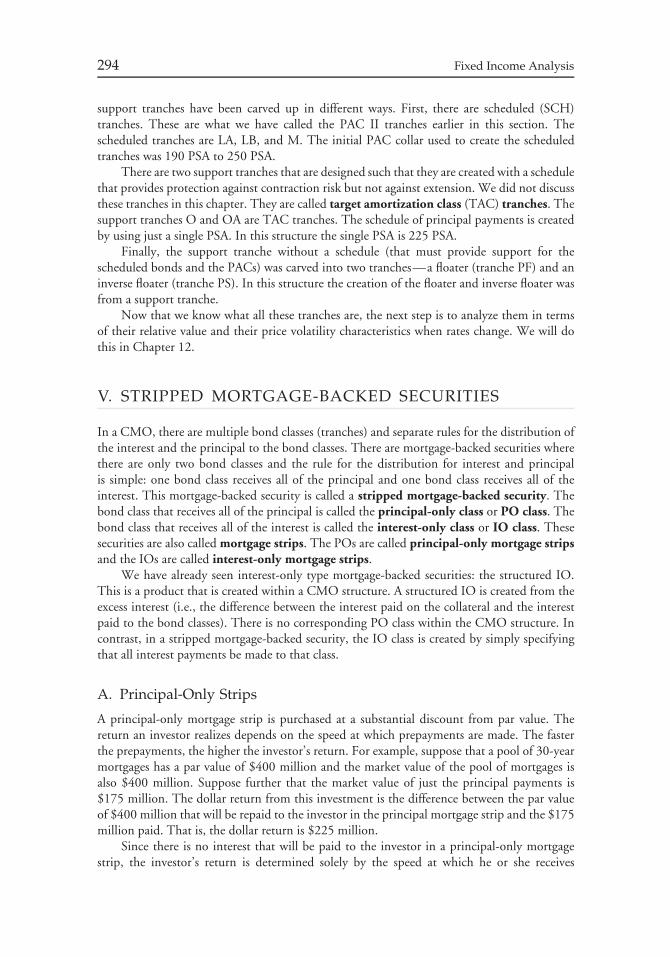
294 Fixed Income Analysis
support tranches have been carved up in different ways. First, there are scheduled (SCH)tranches. These are what we have called the PAC II tranches earlier in this section. Thescheduled tranches are LA, LB, and M. The initial PAC collar used to create the scheduledtranches was 190 PSA to 250 PSA.
There are two support tranches that are designed such that they are created with a schedulethat provides protection against contraction risk but not against extension. We did not discussthese tranches in this chapter. They are called target amortization class (TAC) tranches. Thesupport tranches O and OA are TAC tranches. The schedule of principal payments is createdby using just a single PSA. In this structure the single PSA is 225 PSA.
Finally, the support tranche without a schedule (that must provide support for thescheduled bonds and the PACs) was carved into two tranches—a floater (tranche PF) and aninverse floater (tranche PS). In this structure the creation of the floater and inverse floater wasfrom a support tranche.
Now that we know what all these tranches are, the next step is to analyze them in termsof their relative value and their price volatility characteristics when rates change. We will dothis in Chapter 12.
V. STRIPPED MORTGAGE-BACKED SECURITIES
In a CMO, there are multiple bond classes (tranches) and separate rules for the distribution ofthe interest and the principal to the bond classes. There are mortgage-backed securities wherethere are only two bond classes and the rule for the distribution for interest and principalis simple: one bond class receives all of the principal and one bond class receives all of theinterest. This mortgage-backed security is called a stripped mortgage-backed security. Thebond class that receives all of the principal is called the principal-only class or PO class. Thebond class that receives all of the interest is called the interest-only class or IO class. Thesesecurities are also called mortgage strips. The POs are called principal-only mortgage stripsand the IOs are called interest-only mortgage strips.
We have already seen interest-only type mortgage-backed securities: the structured IO.This is a product that is created within a CMO structure. A structured IO is created from theexcess interest (i.e., the difference between the interest paid on the collateral and the interestpaid to the bond classes). There is no corresponding PO class within the CMO structure. Incontrast, in a stripped mortgage-backed security, the IO class is created by simply specifyingthat all interest payments be made to that class.
A. Principal-Only Strips
A principal-only mortgage strip is purchased at a substantial discount from par value. Thereturn an investor realizes depends on the speed at which prepayments are made. The fasterthe prepayments, the higher the investor’s return. For example, suppose that a pool of 30-yearmortgages has a par value of $400 million and the market value of the pool of mortgages isalso $400 million. Suppose further that the market value of just the principal payments is$175 million. The dollar return from this investment is the difference between the par valueof $400 million that will be repaid to the investor in the principal mortgage strip and the $175million paid. That is, the dollar return is $225 million.
Since there is no interest that will be paid to the investor in a principal-only mortgagestrip, the investor’s return is determined solely by the speed at which he or she receives
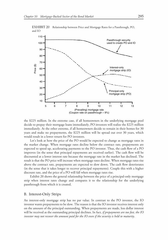
Chapter 10 Mortgage-Backed Sector of the Bond Market 295
EXHIBIT 20 Relationship between Price and Mortgage Rates for a Passthrough, PO,and IO
Passthrough securityused to create PO and IO
Interest-onlymortgage strip (IO)
Principal-onlymortgage strip (PO)
(Prevailing) mortgage rate(Coupon rate on passthrough = 9%)
110
100
90
80
70
60
Pric
e ($
)
50
40
30
20
10
5 6 7 8 9 10 11 12 13
the $225 million. In the extreme case, if all homeowners in the underlying mortgage pooldecide to prepay their mortgage loans immediately, PO investors will realize the $225 millionimmediately. At the other extreme, if all homeowners decide to remain in their homes for 30years and make no prepayments, the $225 million will be spread out over 30 years, whichwould result in a lower return for PO investors.
Let’s look at how the price of the PO would be expected to change as mortgage rates inthe market change. When mortgage rates decline below the contract rate, prepayments areexpected to speed up, accelerating payments to the PO investor. Thus, the cash flow of a POimproves (in the sense that principal repayments are received earlier). The cash flow will bediscounted at a lower interest rate because the mortgage rate in the market has declined. Theresult is that the PO price will increase when mortgage rates decline. When mortgage rates riseabove the contract rate, prepayments are expected to slow down. The cash flow deteriorates(in the sense that it takes longer to recover principal repayments). Couple this with a higherdiscount rate, and the price of a PO will fall when mortgage rates rise.
Exhibit 20 shows the general relationship between the price of a principal-only mortgagestrip when interest rates change and compares it to the relationship for the underlyingpassthrough from which it is created.
B. Interest-Only Strips
An interest-only mortgage strip has no par value. In contrast to the PO investor, the IOinvestor wants prepayments to be slow. The reason is that the IO investor receives interest onlyon the amount of the principal outstanding. When prepayments are made, less dollar interestwill be received as the outstanding principal declines. In fact, if prepayments are too fast, the IOinvestor may not recover the amount paid for the IO even if the security is held to maturity.
296 Fixed Income Analysis
Let’s look at the expected price response of an IO to changes in mortgage rates. Ifmortgage rates decline below the contract rate, prepayments are expected to accelerate. Thiswould result in a deterioration of the expected cash flow for an IO. While the cash flow willbe discounted at a lower rate, the net effect typically is a decline in the price of an IO. Ifmortgage rates rise above the contract rate, the expected cash flow improves, but the cash flowis discounted at a higher interest rate. The net effect may be either a rise or fall for the IO.
Thus, we see an interesting characteristic of an IO: its price tends to move in the samedirection as the change in mortgage rates (1) when mortgage rates fall below the contract rateand (2) for some range of mortgage rates above the contract rate. Both POs and IOs exhibitsubstantial price volatility when mortgage rates change. The greater price volatility of the IOand PO compared to the passthrough from which they were created is due to the fact thatthe combined price volatility of the IO and PO must be equal to the price volatility of thepassthrough.
Exhibit 20 shows the general relationship between the price of an interest-only mortgagestrip when interest rates change and compares it to the relationship for the correspondingprincipal-only mortgage strip and underlying passthrough from which it is created.
An average life for a PO can be calculated based on some prepayment assumption.However, an IO receives no principal payments, so technically an average life cannot becomputed. Instead, for an IO a cash flow average life is computed, using the projectedinterest payments in the average life formula instead of principal.
C. Trading and Settlement Procedures
The trading and settlement procedures for stripped mortgage-backed securities are similarto those set by the Public Securities Association for agency passthroughs described inSection III C. IOs and POs are extreme premium and discount securities and consequentlyare very sensitive to prepayments, which are driven by the specific characteristics (weightedaverage coupon, weighted average maturity, geographic concentration, average loan size) ofthe underlying loans. Therefore, almost all secondary trades in IOs and POs are on a specifiedpool basis rather than on a TBA basis.
All IOs and POs are given a trust number. For instance, Fannie Mae Trust 1 is a IO/POtrust backed by specific pools of Fannie Mae 9% mortgages. Fannie Mae Trust 2 is backed byFannie Mae 10% mortgages. Fannie Mae Trust 23 is another IO/PO trust backed by FannieMae 10% mortgages. Therefore, a portfolio manager must specify which trust he or she isbuying.
The total proceeds of a PO trade are calculated the same way as with a passthrough tradeexcept that there is no accrued interest. The market trades IOs based on notional principal.The proceeds include the price on the notional amount and the accrued interest.
VI. NONAGENCY RESIDENTIALMORTGAGE-BACKED SECURITIES
In the previous sections we looked at agency mortgage-backed securities in which theunderlying mortgages are 1- to 4-single family residential mortgages. The mortgage-backedsecurities market includes other types of securities. These securities are called nonagencymortgage-backed securities (referred to as nonagency securities hereafter).
Chapter 10 Mortgage-Backed Sector of the Bond Market 297
The underlying mortgage loans for nonagency securities can be for any type of real estateproperty. There are securities backed by 1- to 4-single family residential mortgages with a firstlien (i.e., the lender has a first priority or first claim) on the mortgaged property. There arenonagency securities backed by other types of single family residential loans. These includehome equity loan-backed securities and manufactured housing-loan backed securities. Ourfocus in this section is on nonagency securities in which the underlying loans are first-lienmortgages for 1- to 4-single-family residential properties.
As with an agency mortgage-backed security, the servicer is responsible for the collectionof interest and principal. The servicer also handles delinquencies and foreclosures. Typically,there will be a master servicer and subservicers. The servicer plays a key role. In fact, inassessing the credit risk of a nonagency security, rating companies look carefully at the qualityof the servicers.
A. Underlying Mortgage Loans
The underlying loans for agency securities are those that conform to the underwriting standardsof the agency issuing or guaranteeing the issue. That is, only conforming loans are included inpools that are collateral for an agency mortgage-backed security. The three main underwritingstandards deal with
1. the maximum loan-to-value ratio2. the maximum payment-to-income ratio3. the maximum loan amount
The loan-to-value ratio (LTV) is the ratio of the amount of the loan to the market valueor appraised value of the property. The lower the LTV, the greater the protection afforded thelender. For example, an LTV of 0.90 means that if the lender has to repossess the property andsell it, the lender must realize at least 90% of the market value in order to recover the amountlent. An LTV of 0.80 means that the lender only has to sell the property for 80% of its marketvalue in order to recover the amount lent.12 Empirical studies of residential mortgage loanshave found that the LTV is a key determinant of whether a borrower will default: the higherthe LTV, the greater the likelihood of default.
As mentioned earlier in this chapter, a nonconforming mortgage loan is one that does notconform to the underwriting standards established by any of the agencies. Typically, the loansfor a nonagency security are nonconforming mortgage loans that fail to qualify for inclusionbecause the amount of the loan exceeds the limit established by the agencies. Such loansare referred to as jumbo loans. Jumbo loans do not necessarily have greater credit risk thanconforming mortgages.
Loans that fail to qualify because of the first two underwriting standards expose thelender to greater credit risk than conforming loans. There are specialized lenders who providemortgage loans to individuals who fail to qualify for a conforming loan because of theircredit history. These specialized lenders classify borrowers by credit quality. Borrowers areclassified as A borrowers, B borrowers, C borrowers, and D borrowers. A borrowers are thosethat are viewed as having the best credit record. Such borrowers are referred to as primeborrowers. Borrowers rated below A are viewed as subprime borrowers. However, there isno industry-wide classification system for prime and subprime borrowers.
12This ignores the costs of repossession and selling the property.
298 Fixed Income Analysis
B. Differences Between Agency and Nonagency Securities
Nonagency securities can be either passthroughs or CMOs. In the agency market, CMOs arecreated from pools of passthrough securities. In the nonagency market, CMOs are createdfrom unsecuritized mortgage loans. Since a mortgage loan not securitized as a passthrough iscalled a whole loan, nonagency CMOs are commonly referred to as whole-loan CMOs.
The major difference between agency and nonagency securities has to do with guarantees.With a nonagency security there is no explicit or implicit government guarantee of paymentof interest and principal as there is with an agency security. The absence of any such guaranteemeans that the investor in a nonagency security is exposed to credit risk. The nationallyrecognized statistical rating organizations rate nonagency securities.
Because of the credit risk, all nonagency securities are credit enhanced. By creditenhancement it means that additional support against defaults must be obtained. The amountof credit enhancement needed is determined relative to a specific rating desired for a securityrating agency. There are two general types of credit enhancement mechanisms: external andinternal. We describe each of these types of credit enhancement in the next chapter where wecover asset-backed securities.
VII. COMMERCIAL MORTGAGE-BACKEDSECURITIES
Commercial mortgage-backed securities (CMBSs) are backed by a pool of commercialmortgage loans on income-producing property—multifamily properties (i.e., apartmentbuildings), office buildings, industrial properties (including warehouses), shopping centers,hotels, and health care facilities (i.e., senior housing care facilities). The basic building block ofthe CMBS transaction is a commercial loan that was originated either to finance a commercialpurchase or to refinance a prior mortgage obligation.
There are two types of CMBS deal structures that have been of primary interest tobond investors: (1) multiproperty single borrower and (2) multiproperty conduit. Conduitsare commercial-lending entities that are established for the sole purpose of generating collateralto securitize.
CMBS have been issued outside the United States. The dominant issues have been U.K.based (more than 80% in 2000) with the primary property types being retail and officeproperties. Starting in 2001, there was dramatic increase in the number of CMBS deals issuedby German banks. An increasing number of deals include multi-country properties. The firstpan-European securitization was Pan European Industrial Properties in 2001.13
A. Credit Risk
Unlike residential mortgage loans where the lender relies on the ability of the borrower torepay and has recourse to the borrower if the payment terms are not satisfied, commercialmortgage loans are nonrecourse loans. This means that the lender can only look to theincome-producing property backing the loan for interest and principal repayment. If there is
13Christopher Flanagan and Edward Reardon, European Structures Products: 2001 Review and 2002Outlook, Global Structured Finance Research, J.P. Morgan Securities Inc. (January 11, 2002), pp.12–13.
Chapter 10 Mortgage-Backed Sector of the Bond Market 299
a default, the lender looks to the proceeds from the sale of the property for repayment and hasno recourse to the borrower for any unpaid balance. The lender must view each property as astand-alone business and evaluate each property using measures that have been found usefulin assessing credit risk.
While fundamental principles of assessing credit risk apply to all property types, traditionalapproaches to assessing the credit risk of the collateral differs between CMBS and nonagencymortgage-backed securities and real estate-backed securities that fall into the asset-backedsecurities sector described in Chapter 11 (those backed by home equity loans and manufacturedhousing loans). For mortgage-backed securities and asset backed securities in which thecollateral is residential property, typically the loans are lumped into buckets based on certainloan characteristics and then assumptions regarding default rates are made regarding eachbucket. In contrast, for commercial mortgage loans, the unique economic characteristics ofeach income-producing property in a pool backing a CMBS require that credit analysis beperformed on a loan-by-loan basis not only at the time of issuance, but monitored on anongoing basis.
Regardless of the type of commercial property, the two measures that have been found tobe key indicators of the potential credit performance is the debt-to-service coverage ratio andthe loan-to-value ratio.
The debt-to-service coverage ratio (DSC) is the ratio of the property’s net operatingincome (NOI) divided by the debt service. The NOI is defined as the rental income reducedby cash operating expenses (adjusted for a replacement reserve). A ratio greater than 1 meansthat the cash flow from the property is sufficient to cover debt servicing. The higher the ratio,the more likely that the borrower will be able to meet debt servicing from the property’s cashflow.
For all properties backing a CMBS deal, a weighted average DSC ratio is computed. Ananalysis of the credit quality of an issue will also look at the dispersion of the DSC ratios forthe underlying loans. For example, one might look at the percentage of a deal with a DSCratio below a certain value.
As explained in Section VI.A, in computing the LTV, the figure used for ‘‘value’’ in theratio is either market value or appraised value. In valuing commercial property, it is typicallythe appraised value. There can be considerable variation in the estimates of the property’sappraised value. Thus, analysts tend to be skeptical about estimates of appraised value and theresulting LTVs reported for properties.
B. Basic CMBS Structure
As with any structured finance transaction, a rating agency will determine the necessary levelof credit enhancement to achieve a desired rating level. For example, if certain DSC and LTVratios are needed, and these ratios cannot be met at the loan level, then ‘‘subordination’’ isused to achieve these levels. By subordination it is meant that there will be bond classes inthe structure whose claims on the cash flow of the collateral are subordinated to that of otherbond classes in the structure.
The rating agencies will require that the CMBS transaction be retired sequentially,with the highest-rated bonds paying off first. Therefore, any return of principal caused byamortization, prepayment, or default will be used to repay the highest-rated tranche.
Interest on principal outstanding will be paid to all tranches. In the event of a delinquencyresulting in insufficient cash to make all scheduled payments, the transaction’s servicer willadvance both principal and interest. Advancing will continue from the servicer for as long asthese amounts are deemed recoverable.

300 Fixed Income Analysis
Losses arising from loan defaults will be charged against the principal balance of thelowest-rated CMBS tranche outstanding. The total loss charged will include the amountpreviously advanced as well as the actual loss incurred in the sale of the loan’s underlyingproperty.
1. Call Protection A critical investment feature that distinguishes residential MBS andcommercial MBS is the call protection afforded an investor. An investor in a residential MBSis exposed to considerable prepayment risk because the borrower has the right to prepay a loan,in whole or in part, before the scheduled principal repayment date. Typically, the borrowerdoes not pay any penalty for prepayment. When we discussed CMOs, we saw how certaintypes of tranches (e.g., sequential-pay and PAC tranches) can be purchased by an investor toreduce prepayment risk.
With CMBS, there is considerable call protection afforded investors. In fact, it is thisprotection that results in CMBS trading in the market more like corporate bonds thanresidential MBS. This call protection comes in two forms: (1) call protection at the loan leveland (2) call protection at the structure level. We discuss both below.
a. Protection at the Loan Level At the commercial loan level, call protection can take thefollowing forms:
1. prepayment lockout2. defeasance3. prepayment penalty points4. yield maintenance charges
A prepayment lockout is a contractual agreement that prohibits any prepayments duringa specified period of time, called the lockout period. The lockout period at issuance canbe from 2 to 5 years. After the lockout period, call protection comes in the form of eitherprepayment penalty points or yield maintenance charges. Prepayment lockout and defeasanceare the strongest forms of prepayment protection.
With defeasance, rather than loan prepayment, the borrower provides sufficient fundsfor the servicer to invest in a portfolio of Treasury securities that replicates the cash flowsthat would exist in the absence of prepayments. Unlike the other call protection provisionsdiscussed next, there is no distribution made to the bondholders when the defeasance takesplace. So, since there are no penalties, there is no issue as to how any penalties paid by theborrower are to be distributed amongst the bondholders in a CMBS structure. Moreover, thesubstitution of the cash flow of a Treasury portfolio for that of the borrower improves thecredit quality of the CMBS deal.
Prepayment penalty points are predetermined penalties that must be paid by theborrower if the borrower wishes to refinance. (A point is equal to 1% of the outstanding loanbalance.) For example, 5-4-3-2-1 is a common prepayment penalty point structure. That is, ifthe borrower wishes to prepay during the first year, the borrower must pay a 5% penalty for atotal of $105 rather than $100 (which is the norm in the residential market). Likewise, duringthe second year, a 4% penalty would apply, and so on.
When there are prepayment penalty points, there are rules for distributing the penaltyamong the tranches. Prepayment penalty points are not common in new CMBS structures.Instead, the next form of call protection discussed, yield maintenance charges, is morecommonly used.
Chapter 10 Mortgage-Backed Sector of the Bond Market 301
Yield maintenance charge, in its simplest terms, is designed to make the lender indifferentas to the timing of prepayments. The yield maintenance charge, also called the make-wholecharge, makes it uneconomical to refinance solely to get a lower mortgage rate. While thereare several methods used in practice for calculating the yield maintenance charge, the keyprinciple is to make the lender whole. However, when a commercial loan is included as partof a CMBS deal, there must be an allocation of the yield maintenance charge amongst thetranches. Several methods are used in practice for distributing the yield maintenance chargeand, depending on the method specified in a deal, not all tranches may be made whole.
b. Structural Protection The other type of call protection available in CMBS transactionsis structural. Because the CMBS bond structures are sequential-pay (by rating), the AA-ratedtranche cannot pay down until the AAA is completely retired, and the AA-rated bonds mustbe paid off before the A-rated bonds, and so on. However, principal losses due to defaults areimpacted from the bottom of the structure upward.
2. Balloon Maturity Provisions Many commercial loans backing CMBS transactionsare balloon loans that require substantial principal payment at the end of the term of the loan.If the borrower fails to make the balloon payment, the borrower is in default. The lender mayextend the loan, and in so doing may modify the original loan terms. During the workoutperiod for the loan, a higher interest rate will be charged, called the default interest rate.
The risk that a borrower will not be able to make the balloon payment because eitherthe borrower cannot arrange for refinancing at the balloon payment date or cannot sell theproperty to generate sufficient funds to pay off the balloon balance is called balloon risk.Since the term of the loan will be extended by the lender during the workout period, balloonrisk is a type of ‘‘extension risk.’’ This is the same risk that we referred to earlier in describingresidential mortgage-backed securities.
Although many investors like the ‘‘bullet bond-like’’ pay down of the balloon maturities,it does present difficulties from a structural standpoint. That is, if the deal is structured tocompletely pay down on a specified date, an event of default will occur if any delays occur.However, how such delays impact CMBS investors is dependent on the bond type (premium,par, or discount) and whether the servicer will advance to a particular tranche after the balloondefault.
Another concern for CMBS investors in multitranche transactions is the fact that all loansmust be refinanced to pay off the most senior bondholders. Therefore, the balloon risk of themost senior tranche (i.e., AAA) may be equivalent to that of the most junior tranche (i.e., B).
CHAPTER 11ASSET-BACKED SECTOROF THE BOND MARKET
I. INTRODUCTION
As an alternative to the issuance of a bond, a corporation can issue a security backed by loansor receivables. Debt instruments that have as their collateral loans or receivables are referredto as asset-backed securities. The transaction in which asset-backed securities are created isreferred to as a securitization.
While the major issuers of asset-backed securities are corporations, municipal governmentsuse this form of financing rather than issuing municipal bonds and several European centralgovernments use this form of financing. In the United States, the first type of asset-backedsecurity (ABS) was the residential mortgage loan. We discussed the resulting securities, referredto as mortgage-backed securities, in the previous chapter. Securities backed by other typesof assets (consumer and business loans and receivables) have been issued throughout theworld. The largest sectors of the asset-backed securities market in the United States aresecurities backed by credit card receivables, auto loans, home equity loans, manufacturedhousing loans, student loans, Small Business Administration loans, corporate loans, and bonds(corporate, emerging market, and structured financial products). Since home equity loans andmanufactured housing loans are backed by real estate property, the securities backed by themare referred to as real estate-backed asset-backed securities. Other asset-backed securitiesinclude securities backed by home improvement loans, health care receivables, agriculturalequipment loans, equipment leases, music royalty receivables, movie royalty receivables, andmunicipal parking ticket receivables. Collectively, these products are called credit-sensitivestructured products.
In this chapter, we will discuss the securitization process, the basic features of asecuritization transaction, and the major asset types that have been securitized. In the lastsection of this chapter, we look at collateralized debt obligations. While this product hastraditionally been classified as part of the ABS market, we will see how the structure of thisproduct differs from that of a typical securitization.
There are two topics not covered in this chapter. The first is the valuation of an ABS.This topic is covered in Chapter 12. Second, the factors considered by rating agencies in ratingan ABS transaction are not covered here but are covered in Chapter 15. In that chapter wealso compare the factors considered by rating agencies in rating an asset-backed security and acorporate bond.
302
Chapter 11 Asset-Backed Sector of the Bond Market 303
II. THE SECURITIZATION PROCESSAND FEATURES OF ABS
The issuance of an asset-backed security is more complicated than the issuance of a corporatebond. In this section, we will describe the securitization process and the parties to asecuritization. We will do so using a hypothetical securitization.
A. The Basic Securitization Transaction
Quality Home Theaters Inc. (QHT) manufacturers high-end equipment for home theaters.The cost of one of QHT’s home theaters ranges from $20,000 to $200,000. Some of itssales are for cash, but the bulk of its sales are by installment sales contracts. Effectively, aninstallment sales contract is a loan to the buyer of the home theater who agrees to repay QHTover a specified period of time. For simplicity we will assume that the loans are typically forfour years. The collateral for the loan is the home theater purchased by the borrower. The loanspecifies an interest rate that the buyer pays.
The credit department of QHT makes the decision as to whether or not to extend creditto a customer. That is, the credit department will request a credit loan application form becompleted by a customer and based on criteria established by QHT will decide on whetherto extend a loan. The criteria for extending credit are referred to as underwriting standards.Because QHT is extending the loan, it is referred to as the originator of the loan. Moreover,QHT may have a department that is responsible for servicing the loan. Servicing involvescollecting payments from borrowers, notifying borrowers who may be delinquent, and, whennecessary, recovering and disposing of the collateral (i.e., home theater equipment in ourillustration) if the borrower does not make loan repayments by a specified time. While theservicer of the loans need not be the originator of the loans, in our illustration we are assumingthat QHT will be the servicer.
Now let’s see how these loans can be used in a securitization. We will assume that QHThas $100 million of installment sales contracts. This amount is shown on QHT’s balancesheet as an asset. We will further assume that QHT wants to raise $100 million. Rather thanissuing corporate bonds for $100 million, QHT’s treasurer decides to raise the funds via asecuritization. To do so, QHT will set up a legal entity referred to as a special purpose vehicle(SPV). In our discussion of asset-backed securities we described the critical role of this legalentity; its role will become clearer in our illustration. In our illustration, the SPV that is set upis called Homeview Asset Trust (HAT). QHT will then sell to HAT $100 million of the loans.QHT will receive from HAT $100 million in cash, the amount it wanted to raise. But wheredoes HAT get $100 million? It obtains those funds by selling securities that are backed by the$100 million of loans. These securities are the asset-backed securities we referred to earlier andwe will discuss these further in Section II.C.
In the prospectus, HAT (the SPV) would be referred to as either the ‘‘issuer’’ or the‘‘trust.’’ QHT, the seller of the collateral to HAT, would be referred to as the ‘‘seller.’’ Theprospectus might then state: ‘‘The securities represent obligations of the issuer only and donot represent obligations of or interests in Quality Home Theaters Inc. or any of its affiliates.’’
The transaction is diagramed in panel a of Exhibit 1. In panel b, the parties to thetransaction are summarized.
The payments that are received from the collateral are distributed to pay servicingfees, other administrative fees, and principal and interest to the security holders. The legaldocuments in a securitization (prospectus or private placement memorandum) will set forth
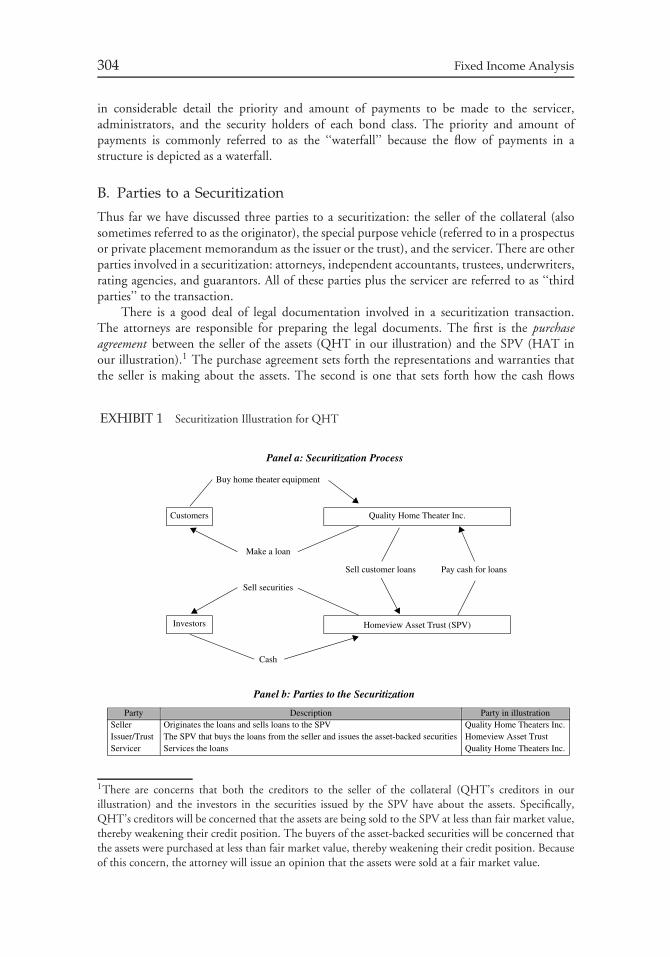
304 Fixed Income Analysis
in considerable detail the priority and amount of payments to be made to the servicer,administrators, and the security holders of each bond class. The priority and amount ofpayments is commonly referred to as the ‘‘waterfall’’ because the flow of payments in astructure is depicted as a waterfall.
B. Parties to a Securitization
Thus far we have discussed three parties to a securitization: the seller of the collateral (alsosometimes referred to as the originator), the special purpose vehicle (referred to in a prospectusor private placement memorandum as the issuer or the trust), and the servicer. There are otherparties involved in a securitization: attorneys, independent accountants, trustees, underwriters,rating agencies, and guarantors. All of these parties plus the servicer are referred to as ‘‘thirdparties’’ to the transaction.
There is a good deal of legal documentation involved in a securitization transaction.The attorneys are responsible for preparing the legal documents. The first is the purchaseagreement between the seller of the assets (QHT in our illustration) and the SPV (HAT inour illustration).1 The purchase agreement sets forth the representations and warranties thatthe seller is making about the assets. The second is one that sets forth how the cash flows
EXHIBIT 1 Securitization Illustration for QHT
Panel a: Securitization Process
Panel b: Parties to the Securitization
Buy home theater equipment
Customers Quality Home Theater Inc.
Make a loan
Sell customer loans Pay cash for loans
Sell securities
Investors Homeview Asset Trust (SPV)
Cash
Party Description Party in illustrationSeller Originates the loans and sells loans to the SPV Quality Home Theaters Inc.Issuer/Trust The SPV that buys the loans from the seller and issues the asset-backed securities Homeview Asset TrustServicer Services the loans Quality Home Theaters Inc.
1There are concerns that both the creditors to the seller of the collateral (QHT’s creditors in ourillustration) and the investors in the securities issued by the SPV have about the assets. Specifically,QHT’s creditors will be concerned that the assets are being sold to the SPV at less than fair market value,thereby weakening their credit position. The buyers of the asset-backed securities will be concerned thatthe assets were purchased at less than fair market value, thereby weakening their credit position. Becauseof this concern, the attorney will issue an opinion that the assets were sold at a fair market value.
Chapter 11 Asset-Backed Sector of the Bond Market 305
are divided among the bond classes (i.e., the structure’s waterfall). Finally, the attorneys createthe servicing agreement between the entity engaged to service the assets (in our illustrationQHT retained the servicing of the loans) and the SPV.
An independent accounting firm will verify the accuracy of all numerical informationplaced in either the prospectus or private placement memorandum.2 The result of this taskresults in a comfort letter for a securitization.
The trustee or trustee agent is the entity that safeguards the assets after they have beenplaced in the trust, receives the payments due to the bond holders, and provides periodicinformation to the bond holders. The information is provided in the form of remittance reportsthat may be issued monthly, quarterly or whenever agreed to by the terms of the prospectusor the private placement memorandum.
The underwriters and rating agencies perform the same function in a securitization asthey do in a standard corporate bond offering. The rating agencies make an assessment of thecollateral and the proposed structure to determine the amount of credit enhancement requiredto achieve a target credit rating for each bond class.
Finally, a securitization may have an entity that guarantees part of the obligationsissued by the SPV. These entities are called guarantors and we will discuss their role in asecuritization later.
C. Bonds Issued
Now let’s take a closer look at the securities issued, what we refer to as the asset-backedsecurities.
A simple transaction can involve the sale of just one bond class with a par value of $100million in our illustration. We will call this Bond Class A. Suppose HAT issues 100,000certificates for Bond Class A with a par value of $1,000 per certificate. Then, each certificateholder would be entitled to 1/100,000 of the payment from the collateral after payment offees and expenses. Each payment made by the borrowers (i.e., the buyers of the home theaterequipment) consists of principal repayment and interest.
A structure can be more complicated. For example, there can be rules for distribution ofprincipal and interest other than on a pro rata basis to different bond classes. As an example,suppose HAT issues Bond Classes A1, A2, A3, and A4 whose total par value is $100 millionas follows:
Bond class Par value (million)A1 $40A2 30A3 20A4 10Total $100
As with a collateralized mortgage obligation (CMO) structure described in the previouschapter, there are different rules for the distribution of principal and interest to these four
2The way this is accomplished is that a copy of the transaction’s payment structure, underlying collateral,average life, and yield are supplied to the accountants for verification. In turn, the accountants reverseengineer the deal according to the deal’s payment rules (i.e., the waterfall). Following the rules and usingthe same collateral that will actually generate the cash flows for the transaction, the accountants reproducethe yield and average life tables that are put into the prospectus or private placement memorandum.
306 Fixed Income Analysis
bond classes or tranches. A simple structure would be a sequential-pay one. As explained in theprevious chapter, in a basic sequential-pay structure, each bond class receives periodic interest.However, the principal is repaid as follows: all principal received from the collateral is paidfirst to Bond Class A1 until it is fully paid off its $40 million par value. After Bond Class A1is paid off, all principal received from the collateral is paid to Bond Class A2 until it is fullypaid off. All principal payments from the collateral are then paid to Bond Class A3 until it isfully paid off and then all principal payments are made to Bond Class A4.
The reason for the creation of the structure just described, as explained in the previouschapter, is to redistribute the prepayment risk among different bond classes. Prepayment riskis the uncertainty about the cash flow due to prepayments. This risk can be decomposed intocontraction risk (i.e., the undesired shortening in the average life of a security) or extensionrisk (i.e., the undesired lengthening in the average life of a security). The creation of thesebond classes is referred to as prepayment tranching or time tranching.
Now let’s look at a more common structure in a transaction. As will be explained later,there are structures where there is more than one bond class and the bond classes differ as tohow they will share any losses resulting from defaults of the borrowers. In such a structure,the bond classes are classified as senior bond classes and subordinate bond classes. Thisstructure is called a senior-subordinate structure. Losses are realized by the subordinate bondclasses before there are any losses realized by the senior bond classes. For example, suppose thatHAT issued $90 million par value of Bond Class A, the senior bond class, and $10 millionpar value of Bond Class B, the subordinate bond class. So the structure is as follows:
Bond class Par value (million)A (senior) $90B (subordinate) 10Total $100
In this structure, as long as there are no defaults by the borrower greater than $10 million,then Bond Class A will be repaid fully its $90 million.
The purpose of this structure is to redistribute the credit risk associated with the collateral.This is referred to as credit tranching. As explained later, the senior-subordinate structure isa form of credit enhancement for a transaction.
There is no reason why only one subordinate bond class is created. Suppose that HATissued the following structure
Bond class Par value (million)A (senior) $90B (subordinate) 7C (subordinate) 3Total $100
In this structure, Bond Class A is the senior bond class while both Bond Classes B and C aresubordinate bond classes from the perspective of Bond Class A. The rules for the distributionof losses would be as follows. All losses on the collateral are absorbed by Bond Class C beforeany losses are realized by Bond Classes A or B. Consequently, if the losses on the collateral donot exceed $3 million, no losses will be realized by Bond Classes A and B. If the losses exceed$3 million, Bond Class B absorbs the loss up to $7 million (its par value). As an example,if the total loss on the collateral is $8 million, Bond Class C losses its entire par value ($3million) and Bond Class B realizes a loss of $5 million of its $7 million par value. Bond Class
Chapter 11 Asset-Backed Sector of the Bond Market 307
A does not realize any loss in this scenario. It should be clear that Bond Class A only realizesa loss if the loss from the collateral exceeds $10 million. The bond class that must absorb thelosses first is referred to as the first loss piece. In our hypothetical structure, Bond Class C isthe first loss piece.
Now we will add just one more twist to the structure. Often in larger transactions,the senior bond class will be carved into different bond classes in order to redistribute theprepayment risk. For example, HAT might issue the following structure:
Bond class Par value (million)A1 (senior) $35A2 (senior) 28A3 (senior) 15A4 (senior) 12B (subordinate) 7C (subordinate) 3Total $100
In this structure there is both prepayment tranching for the senior bond class (creation ofBond Classes A1, A2, A3, and A4) and credit tranching (creation of the senior bond classesand the two subordinate bond classes, Bond Classes B and C).
As explained in the previous chapter, a bond class in a securitization is also referred to asa ‘‘tranche.’’ Consequently, throughout this chapter the terms ‘‘bond class’’ and ‘‘tranche’’ areused interchangeably.
D. General Classification of Collateral and Transaction Structure
Later in this chapter, we will describe some of the major assets that have been securitized.In general, the collateral can be classified as either amortizing or non-amortizing assets.Amortizing assets are loans in which the borrower’s periodic payment consists of scheduledprincipal and interest payments over the life of the loan. The schedule for the repayment ofthe principal is called an amortization schedule. The standard residential mortgage loan fallsinto this category. Auto loans and certain types of home equity loans (specifically, closed-endhome equity loans discussed later in this chapter) are amortizing assets. Any excess paymentover the scheduled principal payment is called a prepayment. Prepayments can be made topay off the entire balance or a partial prepayment, called a curtailment.
In contrast to amortizing assets, non-amortizing assets require only minimum periodicpayments with no scheduled principal repayment. If that payment is less than the intereston the outstanding loan balance, the shortfall is added to the outstanding loan balance. Ifthe periodic payment is greater than the interest on the outstanding loan balance, then thedifference is applied to the reduction of the outstanding loan balance. Since there is noschedule of principal payments (i.e., no amortization schedule) for a non-amortizing asset,the concept of a prepayment does not apply. A credit card receivable is an example of anon-amortizing asset.
The type of collateral—amortizing or non-amortizing—has an impact on the structureof the transaction. Typically, when amortizing assets are securitized, there is no change in thecomposition of the collateral over the life of the securities except for loans that have beenremoved due to defaults and full principal repayment due to prepayments or full amortization.For example, if at the time of issuance the collateral for an ABS consists of 3,000 four-yearamortizing loans, then the same 3,000 loans will be in the collateral six months from now
308 Fixed Income Analysis
assuming no defaults and no prepayments. If, however, during the first six months, 200 of theloans prepay and 100 have defaulted, then the collateral at the end of six months will consistof 2,700 loans (3,000 – 200 – 100). Of course, the remaining principal of the 2,700 loanswill decline because of scheduled principal repayments and any partial prepayments. All of theprincipal repayments from the collateral will be distributed to the security holders.
In contrast, for an ABS transaction backed by non-amortizing assets, the composition ofthe collateral changes. The funds available to pay the security holders are principal repaymentsand interest. The interest is distributed to the security holders. However, the principalrepayments can be either (1) paid out to security holders or (2) reinvested by purchasingadditional loans. What will happen to the principal repayments depends on the time since thetransaction was originated. For a certain amount of time after issuance, all principal repaymentsare reinvested in additional loans. The period of time for which principal repayments arereinvested rather than paid out to the security holders is called the lockout period or revolvingperiod. At the end of the lockout period, principal repayments are distributed to the securityholders. The period when the principal repayments are not reinvested is called the principalamortization period. Notice that unlike the typical transaction that is backed by amortizingassets, the collateral backed by non-amortizing assets changes over time. A structure in whichthe principal repayments are reinvested in new loans is called a revolving structure.
While the receivables in a revolving structure may not be prepaid, all the bonds issuedby the trust may be retired early if certain events occur. That is, during the lockout period,the trustee is required to use principal repayments to retire the securities rather than reinvestprincipal in new collateral if certain events occur. The most common trigger is the poorperformance of the collateral. This provision that specifies the redirection of the principalrepayments during the lockout period to retire the securities is referred to as the earlyamortization provision or rapid amortization provision.
Not all transactions that are revolving structures are backed by non-amortizing assets.There are some transactions in which the collateral consists of amortizing assets but during alockout period, the principal repayments are reinvested in additional loans. For example, thereare transactions in the European market in which the collateral consists of residential mortgageloans but during the lockout period principal repayments are used to acquire additionalresidential mortgage loans.
E. Collateral Cash Flow
For an amortizing asset, projection of the cash flows requires projecting prepayments. Onefactor that may affect prepayments is the prevailing level of interest rates relative to the interestrate on the loan. In projecting prepayments it is critical to determine the extent to whichborrowers take advantage of a decline in interest rates below the loan rate in order to refinancethe loan.
As with nonagency mortgage-backed securities, described in the previous chapter, mod-eling defaults for the collateral is critical in estimating the cash flows of an asset-backedsecurity. Proceeds that are recovered in the event of a default of a loan prior to the scheduledprincipal repayment date of an amortizing asset represent a prepayment and are referred toas an involuntary prepayment. Projecting prepayments for amortizing assets requires anassumption about the default rate and the recovery rate. For a non-amortizing asset, while theconcept of a prepayment does not exist, a projection of defaults is still necessary to projecthow much will be recovered and when.
The analysis of prepayments can be performed on a pool level or a loan level. In pool-levelanalysis it is assumed that all loans comprising the collateral are identical. For an amortizing
Chapter 11 Asset-Backed Sector of the Bond Market 309
asset, the amortization schedule is based on the gross weighted average coupon (GWAC) andweighted average maturity (WAM) for that single loan. We explained in the previous chapterwhat the WAC and WAM of a pool of mortgage loans is and illustrated how it is computed.In this chapter, we refer to the WAC as gross WAC. Pool-level analysis is appropriate wherethe underlying loans are homogeneous. Loan-level analysis involves amortizing each loan (orgroup of homogeneous loans).
The expected final maturity of an asset-backed security is the maturity date based onexpected prepayments at the time of pricing of a deal. The legal final maturity can be two ormore years after the expected final maturity. The average life, or weighted average life, wasexplained in the previous chapter.
Also explained in the previous chapter is a tranche’s principal window which refers tothe time period over which the principal is expected to be paid to the bondholders. A principalwindow can be wide or narrow. When there is only one principal payment that is scheduledto be made to a bondholder, the bond is referred to as having a bullet maturity. Due toprepayments, an asset-backed security that is expected to have a bullet maturity may have anactual maturity that differs from that specified in the prospectus. Hence, asset-backed securitiesbonds that have an expected payment of only one principal are said to have a soft bullet.
F. Credit Enhancements
All asset-backed securities are credit enhanced. That means that support is provided for one ormore of the bondholders in the structure. Credit enhancement levels are determined relativeto a specific rating desired by the issuer for a security by each rating agency. Specifically, aninvestor in a triple A rated security expects to have ‘‘minimal’’ (virtually no) chance of losingany principal due to defaults. For example, a rating agency may require credit enhancementequal to four times expected losses to obtain a triple A rating or three times expected lossesto obtain a double A rating. The amount of credit enhancement necessary depends on ratingagency requirements.
There are two general types of credit enhancement structures: external and internal. Wedescribe each type below.
1. External Credit Enhancements In an ABS, there are two principal parties: the issuerand the security holder. The issuer in our hypothetical securitization is HAT. If another entityis introduced into the structure to guarantee any payments to the security holders, that entityis referred to as a ‘‘third party.’’
The most common third party in a securitization is a monoline insurance company (alsoreferred to as a monoline insurer). A monoline insurance company is an insurance companywhose business is restricted to providing guarantees for financial products such as municipalsecurities and asset-backed securities.3 When a securitization has external credit enhancementthat is provided by a monoline insurer, the securities are said to be ‘‘wrapped.’’ The insuranceworks as follows. The monoline insurer agrees to make timely payment of interest and principalup to a specified amount should the issuer fail to make the payment. Unlike municipal bondinsurance which guarantees the entire principal amount, the guarantee in a securitization is
3The major monoline insurance companies in the United States are Capital Markets AssuranceCorporation (CapMAC), Financial Security Assurance Inc. (FSA), Financial Guaranty InsuranceCorporation (FGIC), and Municipal Bond Investors Assurance Corporation (MBIA).
310 Fixed Income Analysis
only for a percentage of the par value at origination. For example, a $100 million securitizationmay have only $5 million guaranteed by the monoline insurer.
Two less common forms of external credit enhancement are a letter of credit from a bankand a guarantee by the seller of the assets (i.e., the entity that sold the assets to the SPV—QHTin our hypothetical illustration).4 The reason why these two forms of credit enhancementare less commonly used is because of the ‘‘weak link approach’’ employed by rating agencieswhen they rate securitizations. According to this approach, when rating a proposed structure,the credit quality of a security is only as good as the weakest link in its credit enhancementregardless of the quality of underlying assets. Consequently, if an issuer seeks a triple A ratingfor one of the bond classes in the structure, it would be unlikely to be awarded such a rating ifthe external credit enhancer has a rating that is less than triple A. Since few corporations andbanks that issue letters of credit have a sufficiently high rating themselves to achieve the ratingthat may be sought in a securitization, these two forms of external credit enhancement are notas common as insurance.
There is credit risk in a securitization when there is a third-party guarantee because thedowngrading of the third party could result in the downgrading of the securities in a structure.
2. Internal Credit Enhancements Internal credit enhancements come in more com-plicated forms than external credit enhancements. The most common forms of internal creditenhancement are reserve funds, overcollateralization, and senior/subordinate structures.
a. Reserve Funds Reserve funds come in two forms:
• cash reserve funds• excess spread accounts
Cash reserve funds are straight deposits of cash generated from issuance proceeds. In thiscase, part of the underwriting profits from the deal are deposited into a fund which typicallyinvests in money market instruments. Cash reserve funds are typically used in conjunctionwith external credit enhancements.
Excess spread accounts involve the allocation of excess spread or cash into a separatereserve account after paying out the net coupon, servicing fee, and all other expenses on amonthly basis. The excess spread is a design feature of the structure. For example, suppose that:
1. gross weighted average coupon (gross WAC) is 8.00%—this is the interest rate paid bythe borrowers
2. servicing and other fees are 0.25%3. net weighted average coupon (net WAC) is 7.25%—this is the rate that is paid to all
the tranches in the structure
So, for this hypothetical deal, 8.00% is available to make payments to the tranches, tocover servicing fees, and to cover other fees. Of that amount, 0.25% is paid for servicingand other fees and 7.25% is paid to the tranches. This means that only 7.50% must be paidout, leaving 0.50% (8.00% − 7.50%). This 0.50% or 50 basis points is called the excessspread. This amount is placed in a reserve account—the excess servicing account—and itwill gradually increase and can be used to pay for possible future losses.
4As noted earlier, the seller is not a party to the transaction once the assets are sold to the SPV who thenissues the securities. Hence, if the seller provides a guarantee, it is viewed as a third-party guarantee.
Chapter 11 Asset-Backed Sector of the Bond Market 311
b. Overcollateralization Overcollateralization in a structure refers to a situation in whichthe value of the collateral exceeds the amount of the par value of the outstanding securitiesissued by the SPV. For example, if $100 million par value of securities are issued and atissuance the collateral has a market value of $105, there is $5 million in overcollateralization.Over time, the amount of overcollateralization changes due to (1) defaults, (2) amortization,and (3) prepayments. For example, suppose that two years after issuance, the par value of thesecurities outstanding is $90 million and the value of the collateral at the time is $93 million.As a result, the overcollateralization is $3 million ($93 million – $90 million).
Overcollateralization represents a form of internal credit enhancement because it can beused to absorb losses. For example, if the liability of the structure (i.e., par value of all the bondclasses) is $100 million and the collateral’s value is $105 million, then the first $5 million oflosses will not result in a loss to any of the bond classes in the structure.
c. Senior-Subordinate Structure Earlier in this section we explained a senior-subordinatestructure in describing the bonds that can be issued in a securitization. We explained thatthere are senior bond classes and subordinate bond classes. The subordinate bond classes arealso referred to as junior bond classes or non-senior bond classes.
As explained earlier, the creation of a senior-subordinate structure is done to providecredit tranching. More specifically, the senior-subordinate structure is a form of internal creditenhancement because the subordinate bond classes provide credit support for the senior bondclasses. To understand why, the hypothetical HAT structure with one subordinate bond classthat was described earlier is reproduced below:
Bond class Par value (million)A (senior) $90B (subordinate) 10Total $100
The senior bond class, A, is credit enhanced because the first $10 million in losses is absorbedby the subordinate bond class, B. Consequently, if defaults do not exceed $10 million, thenthe senior bond will receive the entire par value of $90 million.
Note that one subordinate bond class can provide credit enhancement for anothersubordinate bond class. To see this, consider the hypothetical HAT structure with twosubordinate bond classes presented earlier:
Bond class Par value (million)A (senior) $90B (subordinate) 7C (subordinate) 3Total $100
Bond Class C, the first loss piece, provides credit enhancement for not only the senior bondclass, but also the subordinate bond class B.
The basic concern in the senior-subordinate structure is that while the subordinate bondclasses provide a certain level of credit protection for the senior bond class at the closing of thedeal, the level of protection changes over time due to prepayments. Faster prepayments canremove the desired credit protection. Thus, the objective after the deal closes is to distributeany prepayments such that the credit protection for the senior bond class does not deteriorateover time.
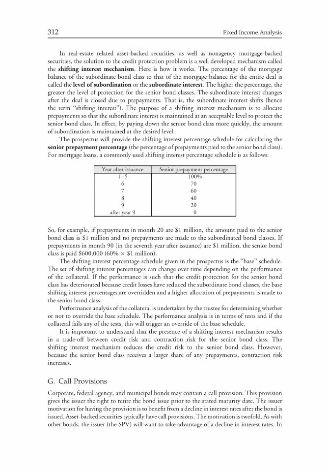
312 Fixed Income Analysis
In real-estate related asset-backed securities, as well as nonagency mortgage-backedsecurities, the solution to the credit protection problem is a well developed mechanism calledthe shifting interest mechanism. Here is how it works. The percentage of the mortgagebalance of the subordinate bond class to that of the mortgage balance for the entire deal iscalled the level of subordination or the subordinate interest. The higher the percentage, thegreater the level of protection for the senior bond classes. The subordinate interest changesafter the deal is closed due to prepayments. That is, the subordinate interest shifts (hencethe term ‘‘shifting interest’’). The purpose of a shifting interest mechanism is to allocateprepayments so that the subordinate interest is maintained at an acceptable level to protect thesenior bond class. In effect, by paying down the senior bond class more quickly, the amountof subordination is maintained at the desired level.
The prospectus will provide the shifting interest percentage schedule for calculating thesenior prepayment percentage (the percentage of prepayments paid to the senior bond class).For mortgage loans, a commonly used shifting interest percentage schedule is as follows:
Year after issuance Senior prepayment percentage1–5 100%
6 707 608 409 20
after year 9 0
So, for example, if prepayments in month 20 are $1 million, the amount paid to the seniorbond class is $1 million and no prepayments are made to the subordinated bond classes. Ifprepayments in month 90 (in the seventh year after issuance) are $1 million, the senior bondclass is paid $600,000 (60% × $1 million).
The shifting interest percentage schedule given in the prospectus is the ‘‘base’’ schedule.The set of shifting interest percentages can change over time depending on the performanceof the collateral. If the performance is such that the credit protection for the senior bondclass has deteriorated because credit losses have reduced the subordinate bond classes, the baseshifting interest percentages are overridden and a higher allocation of prepayments is made tothe senior bond class.
Performance analysis of the collateral is undertaken by the trustee for determining whetheror not to override the base schedule. The performance analysis is in terms of tests and if thecollateral fails any of the tests, this will trigger an override of the base schedule.
It is important to understand that the presence of a shifting interest mechanism resultsin a trade-off between credit risk and contraction risk for the senior bond class. Theshifting interest mechanism reduces the credit risk to the senior bond class. However,because the senior bond class receives a larger share of any prepayments, contraction riskincreases.
G. Call Provisions
Corporate, federal agency, and municipal bonds may contain a call provision. This provisiongives the issuer the right to retire the bond issue prior to the stated maturity date. The issuermotivation for having the provision is to benefit from a decline in interest rates after the bond isissued. Asset-backed securities typically have call provisions. The motivation is twofold. As withother bonds, the issuer (the SPV) will want to take advantage of a decline in interest rates. In
Chapter 11 Asset-Backed Sector of the Bond Market 313
addition, to reduce administrative fees, the trustee may want to call in the issue because the parvalue of a bond class is small and it is more cost effective to payoff the one or more bond classes.
Typically, for a corporate, federal agency, and municipal bond the trigger event for a callprovision is that a specified amount of time has passed.5 In the case of asset-backed securities,it is not simply the passage of time whereby the trustee is permitted to exercise any calloption. There are trigger events for exercising the call option based on the amount of the issueoutstanding.
There are two call provisions where the trigger that grants the trustee to call in the issueis based on a date being reached: (1) call on or after specified date and (2) auction call. A callon or after specified date operates just like a standard call provision for corporate, federalagency, and municipal securities: once a specified date is reached, the trustee has the option tocall all the outstanding bonds. In an auction call, at a certain date a call will be exercised ifan auction results in the outstanding collateral being sold at a price greater than its par value.The premium over par value received from the auctioned collateral is retained by the trusteeand is eventually distributed to the seller of the assets.
Provisions that allow the trustee to call an issue or a tranche based on the par valueoutstanding are referred to as optional clean-up call provisions. Two examples are (1) percentof collateral call and (2) percent of bond call. In a percent of collateral call, the outstandingbonds can be called at par value if the outstanding collateral’s balance falls below a predeterminedpercent of the original collateral’s balance. This is the most common type of clean-up callprovision for amortizing assets and the predetermined level is typically 10%. For example,suppose that the value for the collateral is $100 million. If there is a percent of collateral callprovision with a trigger of 10%, then the trustee can call the entire issue if the value of the callis $10 million or less. In a percent of bond call, the outstanding bonds can be called at parvalue if the outstanding bond’s par value relative to the original par value of bonds issued fallsbelow a specified amount.
There is a call option that combines two triggers based on the amount outstanding and date.In a latter of percent or date call, the outstanding bonds can be called if either (1) the collat-eral’s outstanding balance reaches a predetermined level before the specified call date or (2) thecall date has been reached even if the collateral outstanding is above the predetermined level.
In addition to the above call provisions which permit the trustee to call the bonds, theremay be an insurer call. Such a call permits the insurer to call the bonds if the collateral’scumulative loss history reaches a predetermined level.
III. HOME EQUITY LOANS
A home equity loan (HEL) is a loan backed by residential property. At one time, the loan wastypically a second lien on property that was already pledged to secure a first lien. In some cases,the lien was a third lien. In recent years, the character of a home equity loan has changed.Today, a home equity loan is often a first lien on property where the borrower has either animpaired credit history and/or the payment-to-income ratio is too high for the loan to qualify asa conforming loan for securitization by Ginnie Mae, Fannie Mae, or Freddie Mac. Typically,the borrower used a home equity loan to consolidate consumer debt using the current homeas collateral rather than to obtain funds to purchase a new home.
5As explained earlier, the calling of a portion of the issue is permitted to satisfy any sinking fundrequirement.
314 Fixed Income Analysis
Home equity loans can be either closed end or open end. A closed-end HEL is structuredthe same way as a fully amortizing residential mortgage loan. That is, it has a fixed maturityand the payments are structured to fully amortize the loan by the maturity date. With anopen-end HEL, the homeowner is given a credit line and can write checks or use a creditcard for up to the amount of the credit line. The amount of the credit line depends onthe amount of the equity the borrower has in the property. Because home equity loansecuritizations are predominately closed-end HELs, our focus in this section is securitiesbacked by them.
There are both fixed-rate and variable-rate closed-end HELs. Typically, variable-rate loanshave a reference rate of 6-month LIBOR and have periodic caps and lifetime caps. (A periodiccap limits the change in the mortgage rate from the previous time the mortgage rate wasreset; a lifetime cap sets a maximum that the mortgage rate can ever be for the loan.) Thecash flow of a pool of closed-end HELs is comprised of interest, regularly scheduled principalrepayments, and prepayments, just as with mortgage-backed securities. Thus, it is necessary tohave a prepayment model and a default model to forecast cash flows. The prepayment speedis measured in terms of a conditional prepayment rate (CPR).
A. Prepayments
As explained in the previous chapter, in the agency MBS market the PSA prepaymentbenchmark is used as the base case prepayment assumption in the prospectus. This benchmarkassumes that the conditional prepayment rate (CPR) begins at 0.2% in the first month andincreases linearly for 30 months to 6% CPR. From month 36 to the last month that thesecurity is expected to be outstanding, the CPR is assumed to be constant at 6%. At the timethat the prepayment speed is assumed to be constant, the security is said to be seasoned. Forthe PSA benchmark, a security is assumed to be seasoned in month 36. When the prepaymentspeed is depicted graphically, the linear increase in the CPR from month 1 to the monthwhen the security is assumed to be seasoned is called the prepayment ramp. For the PSAbenchmark, the prepayment ramp begins at month 1 and extends to month 30. Speeds that areassumed to be faster or slower than the PSA prepayment benchmark are quoted as a multipleof the base case prepayment speed.
There are differences in the prepayment behavior for home equity loans and agency MBS.Wall Street firms involved in the underwriting and market making of securities backed byHELs have developed prepayment models for these deals. Several firms have found that thekey difference between the prepayment behavior of HELs and agency residential mortgages isthe important role played by the credit characteristics of the borrower.6
Borrower characteristics and the amount of seasoning (i.e., how long the loans havebeen outstanding) must be kept in mind when trying to assess prepayments for a particulardeal. In the prospectus of a HEL, a base case prepayment assumption is made. Rather thanuse the PSA prepayment benchmark as the base case prepayment speed, issuer’s now use abase case prepayment benchmark that is specific to that issuer. The benchmark prepaymentspeed in the prospectus is called the prospectus prepayment curve or PPC. As with the PSAbenchmark, faster or slower prepayments speeds are a quoted as a multiple of the PPC. Havingan issuer-specific prepayment benchmark is preferred to a generic benchmark such as the PSA
6Dale Westhoff and Mark Feldman, ‘‘Prepayment Modeling and Valuation of Home Equity LoanSecurities,’’ Chapter 18 in Frank J. Fabozzi, Chuck Ramsey, and Michael Marz (eds.), The Handbook ofNonagency Mortgage-Backed Securities: Second Edition (New Hope, PA: Frank J. Fabozzi Associates, 2000).
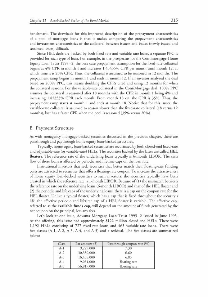
Chapter 11 Asset-Backed Sector of the Bond Market 315
benchmark. The drawback for this improved description of the prepayment characteristicsof a pool of mortgage loans is that it makes comparing the prepayment characteristicsand investment characteristics of the collateral between issuers and issues (newly issued andseasoned issues) difficult.
Since HEL deals are backed by both fixed-rate and variable-rate loans, a separate PPC isprovided for each type of loan. For example, in the prospectus for the Contimortgage HomeEquity Loan Trust 1998–2, the base case prepayment assumption for the fixed-rate collateralbegins at 4% CPR in month 1 and increases 1.45455% CPR per month until month 12, atwhich time it is 20% CPR. Thus, the collateral is assumed to be seasoned in 12 months. Theprepayment ramp begins in month 1 and ends in month 12. If an investor analyzed the dealbased on 200% PPC, this means doubling the CPRs cited and using 12 months for whenthe collateral seasons. For the variable-rate collateral in the ContiMortgage deal, 100% PPCassumes the collateral is seasoned after 18 months with the CPR in month 1 being 4% andincreasing 1.82353% CPR each month. From month 18 on, the CPR is 35%. Thus, theprepayment ramp starts at month 1 and ends at month 18. Notice that for this issuer, thevariable-rate collateral is assumed to season slower than the fixed-rate collateral (18 versus 12months), but has a faster CPR when the pool is seasoned (35% versus 20%).
B. Payment Structure
As with nonagency mortgage-backed securities discussed in the previous chapter, there arepassthrough and paythrough home equity loan-backed structures.
Typically, home equity loan-backed securities are securitized by both closed-end fixed-rateand adjustable-rate (or variable-rate) HELs. The securities backed by the latter are called HELfloaters. The reference rate of the underlying loans typically is 6-month LIBOR. The cashflow of these loans is affected by periodic and lifetime caps on the loan rate.
Institutional investors that seek securities that better match their floating-rate fundingcosts are attracted to securities that offer a floating-rate coupon. To increase the attractivenessof home equity loan-backed securities to such investors, the securities typically have beencreated in which the reference rate is 1-month LIBOR. Because of (1) the mismatch betweenthe reference rate on the underlying loans (6-month LIBOR) and that of the HEL floater and(2) the periodic and life caps of the underlying loans, there is a cap on the coupon rate for theHEL floater. Unlike a typical floater, which has a cap that is fixed throughout the security’slife, the effective periodic and lifetime cap of a HEL floater is variable. The effective cap,referred to as the available funds cap, will depend on the amount of funds generated by thenet coupon on the principal, less any fees.
Let’s look at one issue, Advanta Mortgage Loan Trust 1995–2 issued in June 1995.At the offering, this issue had approximately $122 million closed-end HELs. There were1,192 HELs consisting of 727 fixed-rate loans and 465 variable-rate loans. There werefive classes (A-1, A-2, A-3, A-4, and A-5) and a residual. The five classes are summarizedbelow:
Class Par amount ($) Passthrough coupon rate (%)A-1 9,229,000 7.30A-2 30,330,000 6.60A-3 16,455,000 6.85A-4 9,081,000 floating rateA-5 56,917,000 floating rate
316 Fixed Income Analysis
The collateral is divided into group I and group II. The 727 fixed-rate loans are includedin group I and support Classes A-1, A-2, A-3, and A-4 certificates. The 465 variable-rate loansare in group II and support Class A-5.
Tranches have been structured in home equity loan deals so as to give some senior tranchesgreater prepayment protection than other senior tranches. The two types of structures that dothis are the non-accelerating senior tranche and the planned amortization class tranche.
1. Non-Accelerating Senior Tranches A non-accelerating senior tranche (NAStranche) receives principal payments according to a schedule. The schedule is not a dol-lar amount. Rather, it is a principal schedule that shows for a given month the share of prorata principal that must be distributed to the NAS tranche. A typical principal schedule for aNAS tranche is as follows:7
Months Share of pro rata principal1 through 36 0%37 through 60 45%61 through 72 80%73 through 84 100%After month 84 300%
The average life for the NAS tranche is stable for a large range of prepayments becausefor the first three years all prepayments are made to the other senior tranches. This reduces therisk of the NAS tranche contracting (i.e., shortening) due to fast prepayments. After month84, 300% of its pro rata share is paid to the NAS tranche thereby reducing its extension risk.
The average life stability over a wide range of prepayments is illustrated in Exhibit 2. Thedeal analyzed is the ContiMortgage Home Equity Loan Trust 1997–2.8 Class A-9 is the NAStranche. The analysis was performed on Bloomberg shortly after the deal was issued using theissue’s PPC. As can be seen, the average life is fairly stable between 75% to 200% PPC. Infact, the difference in the average life between 75% PPC and 200% PPC is slightly greaterthan 1 year.
In contrast, Exhibit 2 also shows the average life over the same prepayment scenarios for anon-NAS sequential-pay tranche in the same deal—Class A-7. Notice the substantial averagelife variability. While the average life difference between 75% and 200% PPC for the NAStranche is just over 1 year, it is more than 9 years for the non-NAS tranche. Of course, thenon-NAS in the same deal will be less stable than a regular sequential tranche because thenon-NAS gets a greater share of principal than it would otherwise.
2. Planned Amortization Class Tranche In our discussion of collateralized mortgageobligations issued by the agencies in the previous chapter we explained how a plannedamortization class tranche can be created. These tranches are also created in HEL structures.Unlike agency CMO PAC tranches that are backed by fixed-rate loans, the collateral for HELdeals is both fixed rate and adjustable rate.
An example of a HEL PAC tranche in a HEL-backed deal is tranche A-6 in ContiMortgage1998–2. We described the PPC for this deal in Section III.A.1 above. There is a separate PAC
7Charles Schorin, Steven Weinreich, and Oliver Hsiang, ‘‘Home Equity Loan Transaction Structures,’’Chapter 6 in Frank J. Fabozzi, Chuck Ramsey, and Michael Marz, Handbook of Nonagency Mortgage-Backed Securities: Second Edition (New Hope, PA: Frank J. Fabozzi Associates, 2000).8This illustration is from Schorin, Weinreich, and Hsiang, ‘‘Home Equity Loan Transaction Structures.’’
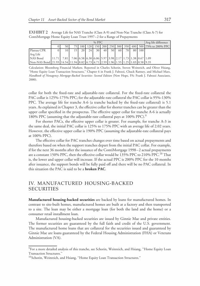
Chapter 11 Asset-Backed Sector of the Bond Market 317
EXHIBIT 2 Average Life for NAS Tranche (Class A-9) and Non-Nas Tranche (Class A-7) forContiMortgage Home Equity Loan Trust 1997–2 for a Range of Prepayments
% PPC Avg life difference0 50 75 100 120 150 200 250 300 350 400 500 75% to 200% PPC
Plateau CPR 0 10 15 20 24 30 40 50 60 70 80 100Avg LifeNAS Bond 11.71 7.81 7.06 6.58 6.30 6.06 5.97 3.98 2.17 1.73 1.38 0.67 1.09Non-NAS Bond 21.93 14.54 11.94 8.82 6.73 4.71 2.59 1.96 1.55 1.25 1.03 0.58 9.35
Calculation: Bloomberg Financial Markets. Reported in Charles Schorin, Steven Weinreich, and Oliver Hsiang,‘‘Home Equity Loan Transaction Structures,’’ Chapter 6 in Frank J. Fabozzi, Chuck Ramsey, and Michael Marz,Handbook of Nonagency Mortgage-Backed Securities: Second Edition (New Hope, PA: Frank J. Fabozzi Associates,2000).
collar for both the fixed-rate and adjustable-rate collateral. For the fixed-rate collateral thePAC collar is 125%-175% PPC; for the adjustable-rate collateral the PAC collar is 95%-130%PPC. The average life for tranche A-6 (a tranche backed by the fixed-rate collateral) is 5.1years. As explained in Chapter 3, the effective collar for shorter tranches can be greater than theupper collar specified in the prospectus. The effective upper collar for tranche A-6 is actually180% PPC (assuming that the adjustable-rate collateral pays at 100% PPC).9
For shorter PACs, the effective upper collar is greater. For example, for tranche A-3 inthe same deal, the initial PAC collar is 125% to 175% PPC with an average life of 2.02 years.However, the effective upper collar is 190% PPC (assuming the adjustable-rate collateral paysat 100% PPC).
The effective collar for PAC tranches changes over time based on actual prepayments andtherefore based on when the support tranches depart from the initial PAC collar. For example,if for the next 36 months after the issuance of the ContiMortgage 1998–2 actual prepaymentsare a constant 150% PPC, then the effective collar would be 135% PPC to 210% PPC.10 Thatis, the lower and upper collar will increase. If the actual PPC is 200% PPC for the 10 monthsafter issuance, the support bonds will be fully paid off and there will be no PAC collateral. Inthis situation the PAC is said to be a broken PAC.
IV. MANUFACTURED HOUSING-BACKEDSECURITIES
Manufactured housing-backed securities are backed by loans for manufactured homes. Incontrast to site-built homes, manufactured homes are built at a factory and then transportedto a site. The loan may be either a mortgage loan (for both the land and the home) or aconsumer retail installment loan.
Manufactured housing-backed securities are issued by Ginnie Mae and private entities.The former securities are guaranteed by the full faith and credit of the U.S. government.The manufactured home loans that are collateral for the securities issued and guaranteed byGinnie Mae are loans guaranteed by the Federal Housing Administration (FHA) or VeteransAdministration (VA).
9For a more detailed analysis of this tranche, see Schorin, Weinreich, and Hsiang, ‘‘Home Equity LoanTransaction Structures.’’10Schorin, Weinreich, and Hsiang, ‘‘Home Equity Loan Transaction Structures.’’

318 Fixed Income Analysis
Loans not backed by the FHA or VA are called conventional loans. Manufacturedhousing-backed securities that are backed by such loans are called conventional manufacturedhousing-backed securities. These securities are issued by private entities.
The typical loan for a manufactured home is 15 to 20 years. The loan repayment isstructured to fully amortize the amount borrowed. Therefore, as with residential mortgageloans and HELs, the cash flow consists of net interest, regularly scheduled principal, andprepayments. However, prepayments are more stable for manufactured housing-backedsecurities because they are not sensitive to refinancing.
There are several reasons for this. First, the loan balances are typically small so that thereis no significant dollar savings from refinancing. Second, the rate of depreciation of mobilehomes may be such that in the earlier years depreciation is greater than the amount of the loanpaid off. This makes it difficult to refinance the loan. Finally, typically borrowers are of lowercredit quality and therefore find it difficult to obtain funds to refinance.
As with residential mortgage loans and HELs, prepayments on manufactured housing-backed securities are measured in terms of CPR and each issue contains a PPC.
The payment structure is the same as with nonagency mortgage-backed securities andhome equity loan-backed securities.
V. RESIDENTIAL MBS OUTSIDE THE UNITEDSTATES
Throughout the world where the market for securitized assets has developed, the largest sectoris the residential mortgage-backed sector. It is not possible to provide a discussion of theresidential mortgage-backed securities market in every country. Instead, to provide a flavor forthis market sector and the similarities with the U.S. nonagency mortgage-backed securitiesmarket, we will discuss just the market in the United Kingdom and Australia.
A. U.K. Residential Mortgage-Backed Securities
In Europe, the country in which there has been the largest amount of issuance of asset-backed securities is the United Kingdom.11 The largest component of that market is theresidential mortgage-backed security market which includes ‘‘prime’’ residential mortgage-backed securities and ‘‘nonconforming’’ residential mortgage-backed securities. In the U.S.mortgage market, a nonconforming mortgage loan is one that does not meet the underwritingstandards of Ginnie Mae, Fannie Mae, or Freddie Mac. However, this does not mean thatthe loan has greater credit risk. In contrast, in the U.K. mortgage market, nonconformingmortgage loans are made to borrowers that are viewed as having greater credit risk–those thatdo not have a credit history and those with a history of failing to meet their obligations.
11Information about the U.K. residential mortgage-backed securities market draws from the followingsources: Phil Adams, ‘‘UK Residential Mortgage-Backed Securities,’’ and ‘‘UK Non-ConformingResidential Mortgage-Backed Securities,’’ in Building Blocks, Asset-Backed Securities Research, BarclaysCapital, January 2001; Christopher Flanagan and Edward Reardon, European Structured Products: 2001Review and 2002 Outlook, Global Structured Finance Research, J.P. Morgan Securities Inc., January11, 2002; and, ‘‘UK Mortgages–MBS Products for U.S. Investors,’’ Mortgage Strategist, UBS Warburg,February 27, 2001, pp. 15–21.
Chapter 11 Asset-Backed Sector of the Bond Market 319
The standard mortgage loan is a variable rate, fully amortizing loan. Typically, the termof the loan is 25 years. As in the U.S. mortgage market, borrowers seeking a loan with a highloan-to-value ratio are required to obtain mortgage insurance, called a ‘‘mortgage indemnityguarantee’’ (MIG).
The deals are more akin to the nonagency market since there is no guarantee by a federallyrelated agency or a government sponsored enterprise as in the United States. Thus, there iscredit enhancement as explained below.
Because the underlying mortgage loans are floating rate, the securities issued are floatingrate (typically, LIBOR is the reference rate). The cash flow depends on the timing of theprincipal payments. The deals are typically set up as a sequential-pay structure. For example,consider the Granite Mortgage 00–2 transaction, a typical structure in the United Kingdom.12
The mortgage pool consists of prime mortgages. There are four bond classes. The two class Atranches, Class A-1 and Class A-2, are rated AAA. One is a dollar denominated tranche andthe other a pound sterling tranche. Class B is rated single A and tranche C is rated triple BBB.The sequence of principal payments is as follows: Class A-1 and Class A-2 are paid off on apro rata basis, then Class B is paid off, and then Class C is paid off.
The issuer has the option to call the outstanding notes under the following circumstances:
• A withholding tax is imposed on the interest payments to noteholders• a clean up call (if the mortgage pool falls to 10% or less of the original pool amount)• on a specified date (called the ‘‘step up date’’) or dates in the future
For example, for the Granite Mortgage 00–02 transaction, the step up date is September2007. The issuer is likely to call the issue because the coupon rate on the notes increases atthat time. In this deal, as with most, the margin over LIBOR doubles.
Credit enhancement can consist of excess spread, reserve fund, and subordination. Forthe Granite Mortgage 00–2, there was subordination: Class B and C tranches for the twoClass A tranche and Class C tranche for the Class B tranche. The reserve was fully funded atthe time of issuance and the excess spread was used to build up the reserve fund. In addition,there is a ‘‘principal shortfall provision.’’ This provision requires that if the realized losses fora period are such that the excess reserve for that period is not sufficient to cover the losses, asexcess spread becomes available in future periods they are used to cover these losses. Also thereare performance triggers that under certain conditions will provide further credit protection tothe senior bonds by modifying the payment of principal. When the underlying mortgage poolconsists of nonconforming mortgage loans, additional protections are provided for investors.
Since prepayments will reduce the average life of the senior notes in a transaction, typicaldeals have provision that permit the purchase of substitute mortgages if the prepayment rateexceeds a certain rate. For example, in the Granite Mortgage 00–02 deal, this rate is 20% perannum.
B. Australian Mortgage-Backed Securities
In Australia, lending is dominated by mortgage banks, the larger ones being ANZ, Com-monwealth Bank of Australia, National Australia Bank, Westpac, and St. George Bank.13
12For a more detailed discussion of this structure, see Adams, ‘‘UK Residential Mortgage-BackedSecurities,’’ pp. 31–37.13Information about the Australian residential mortgage-backed securities market draws from thefollowing sources: Phil Adams, ‘‘Australian Residential Mortgage-Backed Securities,’’ in Building Blocks;
320 Fixed Income Analysis
Non-mortgage bank competitors who have entered the market have used securitization as afinancing vehicle. The majority of the properties are concentrated in New South Wales, par-ticularly the city of Sydney. Rating agencies have found that the risk of default is considerablyless than in the U.S. and the U.K.
Loan maturities are typically between 20 and 30 years. As in the United States, there is awide range of mortgage designs with respect to interest rates. There are fixed-rate, variable-rate(both capped and uncapped), and rates tied to a benchmark.
There is mortgage insurance for loans to protect lenders, called ‘‘lenders mortgageinsurance’’ (LMI). Loans typically have LMI covering 20% to 100% of the loan. Thecompanies that provide this insurance are private corporations.14 When mortgages loans thatdo not have LMI are securitized, typically the issuer will purchase insurance for those loans.
LMI is important for securitized transactions since it is the first layer of credit enhancementin a deal structure. The rating agencies recognize this in rating the tranches in a structure. Theamount that a rating agency will count toward credit enhancement for LMI depends on therating agency’s assessment of the mortgage insurance company.
When securitized, the tranches have a floating rate. There is an initial revolvingperiod—which means that no principal payments are made to the tranche holders butinstead reinvested in new collateral. As with the U.K. Granite Mortgage 00–02 deal, theissuer has the right to call the issue if there is an imposition of a withholding tax on noteholders’ interest payments, after a certain date, or if the balance falls below a certain level(typically, 10%).
Australian mortgage-backed securities have tranches that are U.S. dollar denominated andsome that are denominated in Euros.15 These global deals typically have two or three AAAsenior tranches and one AA or AA− junior tranche.
For credit enhancement, there is excess spread (which in most deals is typically small),subordination, and, as noted earlier, LMI. To illustrate this, consider the Interstar MillenniumSeries 2000-3E Trust—a typical Australian MBS transaction. There are two tranches: a seniortranche (Class A) that was rated AAA and a subordinated tranche (Class B) that was AA−.The protection afforded the senior tranche is the subordinated tranche, LMI (all the propertieswere covered up to 100% and were insured by all five major mortgage insurance companies),and the excess spread.
VI. AUTO LOAN-BACKED SECURITIES
Auto loan-backed securities represents one of the oldest and most familiar sectors of theasset-backed securities market. Auto loan-backed securities are issued by:
1. the financial subsidiaries of auto manufacturers
Karen Weaver, Eugene Xu, Nicholas Bakalar, and Trudy Weibel, ‘‘Mortgage-Backed Securities inAustralia,’’ Chapter 41 in The Handbook of Mortgage-Backed Securities: Fifth Edition (New York, NY:McGraw Hill, 2001); and, ‘‘Australian Value Down Under,’’ Mortgage Strategist, UBS Warburg, February6, 2001, pp. 14–22.14The five major ones are Royal and Sun Alliance Lenders Mortgage Insurance Limited, CGU LendersMortgage Insurance Corporation Ltd., PMI mortgage insurance limited, GE Mortgage InsuranceProperty Ltd., and GE Mortgage Insurance Corporation.15The foreign exchange risk for these deals is typically hedged using various types of swaps (fixed/floating,floating/floating, and currency swaps).
Chapter 11 Asset-Backed Sector of the Bond Market 321
2. commercial banks3. independent finance companies and small financial institutions specializing in auto loans
Historically, auto loan-backed securities have represented between 18% to 25% of theasset-backed securities market. The auto loan market is tiered based on the credit quality ofthe borrowers. ‘‘Prime auto loans’’ are of fundamentally high credit quality and originated bythe financial subsidiaries of major auto manufacturers. The loans are of high credit quality forthe following reasons. First, they are a secured form of lending. Second, they begin to repayprincipal immediately through amortization. Third, they are short-term in nature. Finally,for the most part, major issuers of auto loans have tended to follow reasonably prudentunderwriting standards.
Unlike the sub-prime mortgage industry, there is less consistency on what actuallyconstitutes various categories of prime and sub-prime auto loans. Moody’s assumes the primemarket is composed of issuers typically having cumulative losses of less than 3%; near-primeissuers have cumulative losses of 3–7%; and sub-prime issuers have losses exceeding 7%.
The auto sector was a small part of the European asset-backed securities market in 2002,about 5% of total securitization. There are two reasons for this. First, there is lower per capitacar ownership in Europe. Second, there is considerable variance of tax and regulations dealingwith borrower privacy rules in Europe thereby making securitization difficult.16 Auto dealshave been done in Italy, the U.K., Germany, Portugal, and Belgium.
A. Cash Flow and Prepayments
The cash flow for auto loan-backed securities consists of regularly scheduled monthlyloan payments (interest and scheduled principal repayments) and any prepayments. Forsecurities backed by auto loans, prepayments result from (1) sales and trade-ins requiringfull payoff of the loan, (2) repossession and subsequent resale of the automobile, (3) loss ordestruction of the vehicle, (4) payoff of the loan with cash to save on the interest cost, and(5) refinancing of the loan at a lower interest cost.
Prepayments due to repossession and subsequent resale are sensitive to the economic cycle.In recessionary economic periods, prepayments due to this factor increase. While refinancingsmay be a major reason for prepayments of mortgage loans, they are of minor importance forautomobile loans. Moreover, the interest rates for the automobile loans underlying some dealsare substantially below market rates since they are offered by manufacturers as part of a salespromotion.
B. Measuring Prepayments
For most asset-backed securities where there are prepayments, prepayments are measuredin term of the conditional prepayment rate, CPR. As explained in the previous chapter,monthly prepayments are quoted in terms of the single monthly mortality (SMM) rate. Theconvention for calculating and reporting prepayment rates for auto-loan backed securities isdifferent. Prepayments for auto loan-backed securities are measured in terms of the absolute
16Flanagan and Reardon, European Structures Products: 2001 Review and 2002 Outlook, p. 9.
322 Fixed Income Analysis
prepayment speed, denoted by ABS.17 The ABS is the monthly prepayment expressed as apercentage of the original collateral amount. As explained in the previous chapter, the SMM(monthly CPR) expresses prepayments based on the prior month’s balance.
There is a mathematical relationship between the SMM and the ABS measures. LettingM denote the number of months after loan origination, the SMM rate can be calculated fromthe ABS rate using the following formula:
SMM = ABS
1 − [ABS × (M − 1)]
where the ABS and SMM rates are expressed in decimal form.For example, if the ABS rate is 1.5% (i.e., 0.015) at month 14 after origination, then the
SMM rate is 1.86%, as shown below:
SMM = 0.015
1 − [0.015 × (14 − 1)]= 0.0186 = 1.86%
The ABS rate can be calculated from the SMM rate using the following formula:
ABS = SMM
1 + [SMM × (M − 1)]
For example, if the SMM rate at month 9 after origination is 1.3%, then the ABS rate is:
ABS = 0.013
1 + [0.013 × (9 − 1)]= 0.0118 = 1.18%
Historically, when measured in terms of SMM rate, auto loans have experienced SMMsthat increase as the loans season.
VII. STUDENT LOAN-BACKED SECURITIES
Student loans are made to cover college cost (undergraduate, graduate, and professionalprograms such as medical and law school) and tuition for a wide range of vocational andtrade schools. Securities backed by student loans, popularly referred to as SLABS (student loanasset-backed securities), have similar structural features as the other asset-backed securities wediscussed above.
The student loans that have been most commonly securitized are those that are madeunder the Federal Family Education Loan Program (FFELP). Under this program, the
17The only reason for the use of ABS rather than SMM/CPR in this sector is historical. Auto-loanbacked securities (which were popularly referred to at one time as CARS (Certificates of AutomobileReceivables)) were the first non-mortgage assets to be developed in the market. (The first non-mortgageasset-backed security was actually backed by computer lease receivables.) The major dealer in this marketat the time, First Boston (now Credit Suisse First Boston) elected to use ABS for measuring prepayments.You may wonder how one obtains ‘‘ABS’’ from ‘‘absolute prepayment rate.’’ Again, it is historical. Whenthe market first started, the ABS measure probably meant ‘‘asset-backed security’’ but over time to avoidconfusion evolved to absolute prepayment rate.
Chapter 11 Asset-Backed Sector of the Bond Market 323
government makes loans to students via private lenders. The decision by private lenders toextend a loan to a student is not based on the applicant’s ability to repay the loan. If a defaultof a loan occurs and the loan has been properly serviced, then the government will guaranteeup to 98% of the principal plus accrued interest.18
Loans that are not part of a government guarantee program are called alternative loans.These loans are basically consumer loans and the lender’s decision to extend an alternativeloan will be based on the ability of the applicant to repay the loan. Alternative loans have beensecuritized.
A. Issuers
Congress created Fannie Mae and Freddie Mac to provide liquidity in the mortgage marketby allowing these government sponsored enterprises to buy mortgage loans in the secondarymarket. Congress created the Student Loan Marketing Association (nicknamed ‘‘Sallie Mae’’)as a government sponsored enterprise to purchase student loans in the secondary marketand to securitize pools of student loans. Since its first issuance in 1995, Sallie Mae isnow the major issuer of SLABS and its issues are viewed as the benchmark issues.19
Other entities that issue SLABS are either traditional corporate entities (e.g., the MoneyStore and PNC Bank) or non-profit organizations (Michigan Higher Education LoanAuthority and the California Educational Facilities Authority). The SLABS of the lattertypically are issued as tax-exempt securities and therefore trade in the municipal market. Inrecent years, several not-for-profit entities have changed their charter and applied for ‘‘forprofit’’ treatment.
B. Cash Flow
Let’s first look at the cash flow for the student loans themselves. There are different types ofstudent loans under the FFELP including subsidized and unsubsidized Stafford loans, ParentalLoans for Undergraduate Students (PLUS), and Supplemental Loans to Students (SLS). Theseloans involve three periods with respect to the borrower’s payments—deferment period, graceperiod, and loan repayment period. Typically, student loans work as follows. While a studentis in school, no payments are made by the student on the loan. This is the deferment period.Upon leaving school, the student is extended a grace period of usually six months when nopayments on the loan must be made. After this period, payments are made on the loan by theborrower.
Student loans are floating-rate loans, exclusively indexed to the 3-month Treasury billrate. As a result, some issuers of SLABs issue securities whose coupon rate is indexed to the3-month Treasury bill rate. However, a large percentage of SLABS issued are indexed toLIBOR floaters.20
Prepayments typically occur due to defaults or loan consolidation. Even if there is noloss of principal faced by the investor when defaults occur, the investor is still exposed to
18Actually, depending on the origination date, the guarantee can be up to 100%.19In 1997 Sallie Mae began the process of unwinding its status as a GSE; until this multi-year process iscompleted, all debt issued by Sallie Mae under its GSE status will be ‘‘grandfathered’’ as GSE debt untilmaturity.20This creates a mismatch between the collateral and the securities. Issuers have dealt with this byhedging with the risk by using derivative instruments such as interest rate swaps (floating-to-floating rateswaps described in Chapter 14) or interest rate caps (described in Chapter 14).
324 Fixed Income Analysis
contraction risk. This is the risk that the investor must reinvest the proceeds at a lower spreadand in the case of a bond purchased at a premium, the premium will be lost. Studies haveshown student loan prepayments are insensitive to the level of interest rates. Consolidations ofa loan occur when the student who has loans over several years combines them into a singleloan. The proceeds from the consolidation are distributed to the original lender and, in turn,distributed to the bondholders.
VIII. SBA LOAN-BACKED SECURITIES
The Small Business Administration (SBA) is an agency of the U.S. government empowered toguarantee loans made by approved SBA lenders to qualified borrowers. The loans are backedby the full faith and credit of the government. Most SBA loans are variable-rate loans wherethe reference rate is the prime rate. The rate on the loan is reset monthly on the first ofthe month or quarterly on the first of January, April, July, and October. SBA regulationsspecify the maximum coupon allowable in the secondary market. Newly originated loans havematurities between 5 and 25 years.
The Small Business Secondary Market Improvement Act passed in 1984 permitted thepooling of SBA loans. When pooled, the underlying loans must have similar terms andfeatures. The maturities typically used for pooling loans are 7, 10, 15, 20, and 25 years. Loanswithout caps are not pooled with loans that have caps.
Most variable-rate SBA loans make monthly payments consisting of interest and principalrepayment. The amount of the monthly payment for an individual loan is determined asfollows. Given the coupon formula of the prime rate plus the loan’s quoted margin, the interestrate is determined for each loan. Given the interest rate, a level payment amortization scheduleis determined. It is this level payment that is paid for the next month until the coupon rateis reset.
The monthly cash flow that the investor in an SBA-backed security receives consists of
• the coupon interest based on the coupon rate set for the period• the scheduled principal repayment (i.e., scheduled amortization)• prepayments
Prepayments for SBA-backed securities are measured in terms of CPR. Voluntaryprepayments can be made by the borrower without any penalty. There are several fac-tors contributing to the prepayment speed of a pool of SBA loans. A factor affectingprepayments is the maturity date of the loan. It has been found that the fastest speedson SBA loans and pools occur for shorter maturities.21 The purpose of the loan alsoaffects prepayments. There are loans for working capital purposes and loans to financereal estate construction or acquisition. It has been observed that SBA pools with maturi-ties of 10 years or less made for working capital purposes tend to prepay at the fastestspeed. In contrast, loans backed by real estate that are long maturities tend to prepay at aslow speed.
21Donna Faulk, ‘‘SBA Loan-Backed Securities,’’ Chapter 10 in Asset-Backed Securities.
Chapter 11 Asset-Backed Sector of the Bond Market 325
IX. CREDIT CARD RECEIVABLE-BACKEDSECURITIES
When a purchase is made on a credit card, the issuer of the credit card (the lender) extendscredit to the cardholder (the borrower). Credit cards are issued by banks (e.g., Visa andMasterCard), retailers (e.g., Sears and Target Corporation), and travel and entertainmentcompanies (e.g., American Express). At the time of purchase, the cardholder is agreeing torepay the amount borrowed (i.e., the cost of the item purchased) plus any applicable financecharges. The amount that the cardholder has agreed to pay the issuer of the credit card is areceivable from the perspective of the issuer of the credit card. Credit card receivables are usedas collateral for the issuance of an asset-backed security.
A. Cash Flow
For a pool of credit card receivables, the cash flow consists of finance charges collected, fees,and principal. Finance charges collected represent the periodic interest the credit card borroweris charged based on the unpaid balance after the grace period. Fees include late payment feesand any annual membership fees.
Interest to security holders is paid periodically (e.g, monthly, quarterly, or semiannually).The interest rate may be fixed or floating—roughly half of the securities are floaters. Thefloating rate is uncapped.
A credit card receivable-backed security is a nonamortizing security. For a specifiedperiod of time, the lockout period or revolving period, the principal payments made by creditcard borrowers comprising the pool are retained by the trustee and reinvested in additionalreceivables to maintain the size of the pool. The lockout period can vary from 18 months to10 years. So, during the lockout period, the cash flow that is paid out to security holders isbased on finance charges collected and fees. After the lockout period, the principal is no longerreinvested but paid to investors, the principal-amortization period and the various types ofstructures are described next.
B. Payment Structure
There are three different amortization structures that have been used in credit card receivable-backed security deals: (1) passthrough structure, (2) controlled-amortization structure, and(3) bullet-payment structure. The latter two are the more common. One source reports that80% of the deals are bullet structures and the balance are controlled amortization structures.22
In a passthrough structure, the principal cash flows from the credit card accounts arepaid to the security holders on a pro rata basis. In a controlled-amortization structure, ascheduled principal amount is established, similar to the principal window for a PAC bond.The scheduled principal amount is sufficiently low so that the obligation can be satisfiedeven under certain stress scenarios, where cash flow is decreased due to defaults or slowerrepayment by borrowers. The security holder is paid the lesser of the scheduled principalamount and the pro rata amount. In a bullet-payment structure, the security holder receivesthe entire amount in one distribution. Since there is no assurance that the entire amount canbe paid in one lump sum, the procedure is for the trustee to place principal monthly into an
22Thompson, ‘‘MBNA Tests the Waters.’’
326 Fixed Income Analysis
account that generates sufficient interest to make periodic interest payments and accumulatethe principal to be repaid. These deposits are made in the months shortly before the scheduledbullet payment. This type of structure is also often called a soft bullet because the maturityis technically not guaranteed, but is almost always satisfied. The time period over which theprincipal is accumulated is called the accumulation period.
C. Performance of the Portfolio of Receivables
There are several concepts that must be understood in order to assess the performance of theportfolio of receivables and the ability of the issuer to meet its interest obligation and repayprincipal as scheduled.
We begin with the concept of the gross portfolio yield. This yield includes financecharges collected and fees. Charge-offs represent the accounts charged off as uncollectible.Net portfolio yield is equal to gross portfolio yield minus charge-offs. The net portfolio yieldis important because it is from this yield that the bondholders will be paid. So, for example,if the average yield (WAC) that must be paid to the various tranches in the structure is 5%and the net portfolio yield for the month is only 4.5%, there is the risk that the bondholderobligations will not be satisfied.
Delinquencies are the percentages of receivables that are past due for a specified numberof months, usually 30, 60, and 90 days. They are considered an indicator of potential futurecharge-offs.
The monthly payment rate (MPR) expresses the monthly payment (which includesfinance charges, fees, and any principal repayment) of a credit card receivable portfolio as apercentage of credit card debt outstanding in the previous month. For example, suppose a$500 million credit card receivable portfolio in January realized $50 million of payments inFebruary. The MPR would then be 10% ($50 million divided by $500 million).
There are two reasons why the MPR is important. First, if the MPR reaches an extremelylow level, there is a chance that there will be extension risk with respect to the principalpayments on the bonds. Second, if the MPR is very low, then there is a chance that there willnot be sufficient cash flows to pay off principal. This is one of the events that could triggerearly amortization of the principal (described below).
At issuance, portfolio yield, charge-offs, delinquency, and MPR information are providedin the prospectus. Information about portfolio performance is then available from Bloomberg,the rating agencies, and dealers.
D. Early Amortization Triggers
There are provisions in credit card receivable-backed securities that require early amortizationof the principal if certain events occur. Such provisions, which as mentioned earlier in thischapter are referred to as early amortization or rapid amortization provisions, are included tosafeguard the credit quality of the issue. The only way that the principal cash flows can bealtered is by the triggering of the early amortization provision.
Typically, early amortization allows for the rapid return of principal in the event thatthe 3-month average excess spread earned on the receivables falls to zero or less. When earlyamortization occurs, the credit card tranches are retired sequentially (i.e., first the AAA bondthen the AA rated bond, etc.). This is accomplished by paying the principal payments made bythe credit card borrowers to the investors instead of using them to purchase more receivables.The length of time until the return of principal is largely a function of the monthly payment
Chapter 11 Asset-Backed Sector of the Bond Market 327
rate. For example, suppose that a AAA tranche is 82% of the overall deal. If the monthlypayment rate is 11% then the AAA tranche would return principal over a 7.5-month period(82%/11%). An 18% monthly payment rate would return principal over a 4.5-month period(82%/18%).
X. COLLATERALIZED DEBT OBLIGATIONS
A collateralized debt obligation (CDO) is a security backed by a diversified pool of one ormore of the following types of debt obligations:
• U.S. domestic high-yield corporate bonds• structured financial products (i.e., mortgage-backed and asset-backed securities)• emerging market bonds• bank loans• special situation loans and distressed debt
When the underlying pool of debt obligations are bond-type instruments (high-yieldcorporate, structured financial products, and emerging market bonds), a CDO is referred toas a collateralized bond obligation (CBO). When the underlying pool of debt obligationsare bank loans, a CDO is referred to as a collateralized loan obligation (CLO).
A. Structure of a CDO
In a CDO structure, there is an asset manager responsible for managing the portfolio ofdebt obligations. There are restrictions imposed (i.e., restrictive covenants) as to what theasset manager may do and certain tests that must be satisfied for the tranches in the CDOto maintain the credit rating assigned at the time of issuance and determine how and whentranches are repaid principal.
The funds to purchase the underlying assets (i.e., the bonds and loans) are obtained fromthe issuance of debt obligations (i.e., tranches) and include one or more senior tranches, one ormore mezzanine tranches, and a subordinate/equity tranche. There will be a rating sought forall but the subordinate/equity tranche. For the senior tranches, at least an A rating is typicallysought. For the mezzanine tranches, a rating of BBB but no less than B is sought. As explainedbelow, since the subordinate/equity tranche receives the residual cash flow, no rating is soughtfor this tranche.
The ability of the asset manager to make the interest payments to the tranches andpayoff the tranches as they mature depends on the performance of the underlying assets. Theproceeds to meet the obligations to the CDO tranches (interest and principal repayment) cancome from (1) coupon interest payments of the underlying assets, (2) maturing assets in theunderlying pool, and (3) sale of assets in the underlying pool.
In a typical structure, one or more of the tranches is a floating-rate security. Withthe exception of deals backed by bank loans which pay a floating rate, the asset managerinvests in fixed-rate bonds. Now that presents a problem—paying tranche investors a floatingrate and investing in assets with a fixed rate. To deal with this problem, the asset manageruses derivative instruments to be able to convert fixed-rate payments from the assets intofloating-rate payments. In particular, interest rate swaps are used. This derivative instrumentallows a market participant to swap fixed-rate payments for floating-rate payments or vice
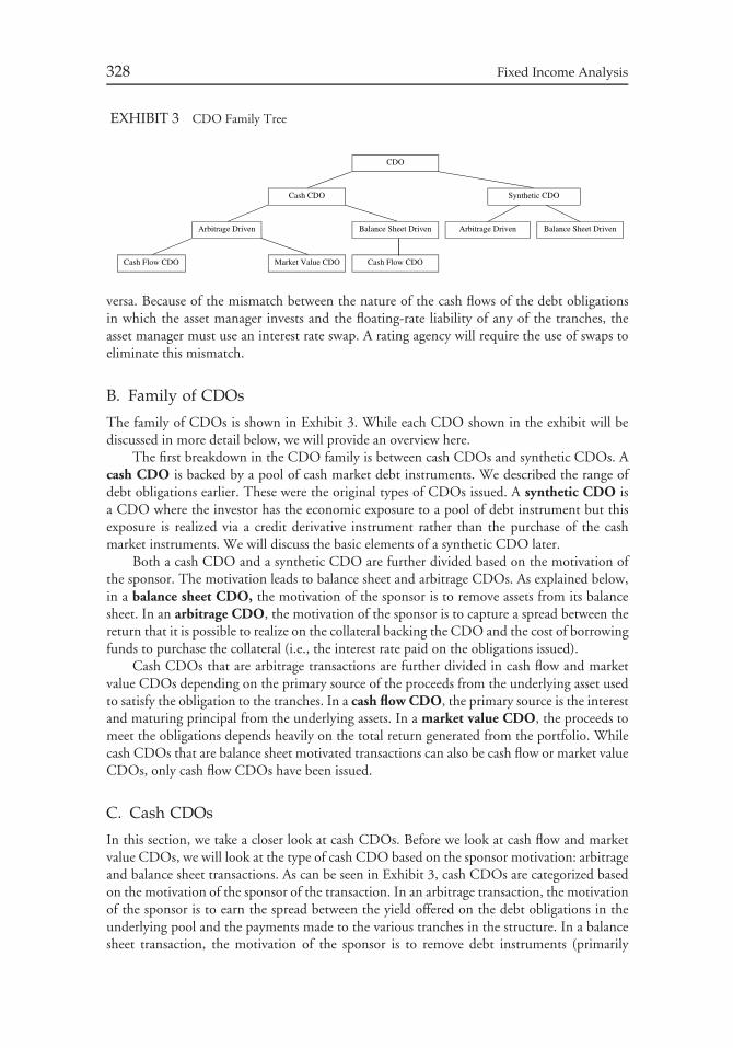
328 Fixed Income Analysis
EXHIBIT 3 CDO Family Tree
CDO
Cash CDO Synthetic CDO
Arbitrage Driven Balance Sheet Driven Arbitrage Driven Balance Sheet Driven
Cash Flow CDO Market Value CDO Cash Flow CDO
versa. Because of the mismatch between the nature of the cash flows of the debt obligationsin which the asset manager invests and the floating-rate liability of any of the tranches, theasset manager must use an interest rate swap. A rating agency will require the use of swaps toeliminate this mismatch.
B. Family of CDOs
The family of CDOs is shown in Exhibit 3. While each CDO shown in the exhibit will bediscussed in more detail below, we will provide an overview here.
The first breakdown in the CDO family is between cash CDOs and synthetic CDOs. Acash CDO is backed by a pool of cash market debt instruments. We described the range ofdebt obligations earlier. These were the original types of CDOs issued. A synthetic CDO isa CDO where the investor has the economic exposure to a pool of debt instrument but thisexposure is realized via a credit derivative instrument rather than the purchase of the cashmarket instruments. We will discuss the basic elements of a synthetic CDO later.
Both a cash CDO and a synthetic CDO are further divided based on the motivation ofthe sponsor. The motivation leads to balance sheet and arbitrage CDOs. As explained below,in a balance sheet CDO, the motivation of the sponsor is to remove assets from its balancesheet. In an arbitrage CDO, the motivation of the sponsor is to capture a spread between thereturn that it is possible to realize on the collateral backing the CDO and the cost of borrowingfunds to purchase the collateral (i.e., the interest rate paid on the obligations issued).
Cash CDOs that are arbitrage transactions are further divided in cash flow and marketvalue CDOs depending on the primary source of the proceeds from the underlying asset usedto satisfy the obligation to the tranches. In a cash flow CDO, the primary source is the interestand maturing principal from the underlying assets. In a market value CDO, the proceeds tomeet the obligations depends heavily on the total return generated from the portfolio. Whilecash CDOs that are balance sheet motivated transactions can also be cash flow or market valueCDOs, only cash flow CDOs have been issued.
C. Cash CDOs
In this section, we take a closer look at cash CDOs. Before we look at cash flow and marketvalue CDOs, we will look at the type of cash CDO based on the sponsor motivation: arbitrageand balance sheet transactions. As can be seen in Exhibit 3, cash CDOs are categorized basedon the motivation of the sponsor of the transaction. In an arbitrage transaction, the motivationof the sponsor is to earn the spread between the yield offered on the debt obligations in theunderlying pool and the payments made to the various tranches in the structure. In a balancesheet transaction, the motivation of the sponsor is to remove debt instruments (primarily

Chapter 11 Asset-Backed Sector of the Bond Market 329
loans) from its balance sheet. Sponsors of balance sheet transactions are typically financialinstitutions such as banks seeking to reduce their capital requirements by removing loansdue to their higher risk-based capital requirements. Our focus in this section is on arbitragetransactions because such transactions are the largest part of the cash CDO sector.
1. Cash CDO Arbitrage Transactions The key as to whether or not it is economic tocreate an arbitrage CDO is whether or not a structure can be created that offers a competitivereturn for the subordinate/equity tranche.
To understand how the subordinate/equity tranche generates cash flows, consider thefollowing basic $100 million CDO structure with the coupon rate to be offered at the time ofissuance as shown below:
Tranche Par Value Coupon rateSenior $80,000,000 LIBOR + 70 basis pointsMezzanine 10,000,000 10-year Treasury rate plus 200 basis pointsSubordinate/Equity 10,000,000
Suppose that the collateral consists of bonds that all mature in 10 years and the couponrate for every bond is the 10-year Treasury rate plus 400 basis points. The asset manager entersinto an interest rate swap agreement with another party with a notional amount of $80 millionin which it agrees to do the following:
• pay a fixed rate each year equal to the 10-year Treasury rate plus 100 basis points• receive LIBOR
The interest rate agreement is simply an agreement to periodically exchange interestpayments. The payments are benchmarked off of a notional amount. This amount is notexchanged between the two parties. Rather it is used simply to determine the dollar interestpayment of each party. This is all we need to know about an interest rate swap in order tounderstand the economics of an arbitrage transaction. Keep in mind, the goal is to show howthe subordinate/equity tranche can be expected to generate a return.
Let’s assume that the 10-year Treasury rate at the time the CDO is issued is 7%. Now wecan walk through the cash flows for each year. Look first at the collateral. The collateral willpay interest each year (assuming no defaults) equal to the 10-year Treasury rate of 7% plus400 basis points. So the interest will be:
Interest from collateral: 11% × $100,000,000 = $11,000,000
Now let’s determine the interest that must be paid to the senior and mezzanine tranches.For the senior tranche, the interest payment will be:
Interest to senior tranche: $80,000,000 × (LIBOR + 70 bp)
The coupon rate for the mezzanine tranche is 7% plus 200 basis points. So, the coupon rate is9% and the interest is:
Interest to mezzanine tranche: 9% × $10,000,000 = $900, 000
330 Fixed Income Analysis
Finally, let’s look at the interest rate swap. In this agreement, the asset manager is agreeingto pay some party (we’ll call this party the ‘‘swap counterparty’’) each year 7% (the 10-yearTreasury rate) plus 100 basis points, or 8%. But 8% of what? As explained above, in an interestrate swap payments are based on a notional amount. In our illustration, the notional amountis $80 million. The reason the asset manager selected the $80 million was because this is theamount of principal for the senior tranche which receives a floating rate. So, the asset managerpays to the swap counterparty:
Interest to swap counterparty: 8% × $80,000,000 = $6,400,000
The interest payment received from the swap counterparty is LIBOR based on a notionalamount of $80 million. That is,
Interest from swap counterparty: $80,000,000 × LIBOR
Now we can put this all together. Let’s look at the interest coming into the CDO:
Interest from collateral . . . . . . . . . . . . . . . . . . . . $11,000,000Interest from swap counterparty . . . . . . . . . . . . $80,000,000 × LIBORTotal interest received . . . . . . . . . . . . . . . . . . . . $11,000,000 + $80,000,000 × LIBOR
The interest to be paid out to the senior and mezzanine tranches and to the swapcounterparty include:
Interest to senior tranche . . . . . . . . . . . . . . . . $80,000,000 × (LIBOR + 70 bp)Interest to mezzanine tranche . . . . . . . . . . . . $900,000Interest to swap counterparty . . . . . . . . . . . . $6,400,000Total interest paid . . . . . . . . . . . . . . . . . . . . . $7,300,000 + $80,000,000 × (LIBOR + 70 bp)
Netting the interest payments coming in and going out we have:
Total interest received . . . . . . . . . . . . . $11,000,000 + $80,000,000 × LIBORTotal interest paid . . . . . . . . . . . . . $ 7,300,000 + $80,000,000 × (LIBOR + 70 bp)Net interest . . . . . . . . . . . . . . . . . . . . . . $ 3,700,000 - $80,000,000 × (70 bp)
Since 70 bp times $80 million is $560,000, the net interest remaining is $3,140,000 (=$3,700,000 − $560,000). From this amount any fees (including the asset management fee)must be paid. The balance is then the amount available to pay the subordinate/equity tranche.Suppose that these fees are $634,000. Then the cash flow available to the subordinate/equitytranche for the year is $2.5 million. Since the tranche has a par value of $10 million and isassumed to be sold at par, this means that the annual return is 25%.
Obviously, some simplifying assumptions have been made. For example, it is assumedthat there are no defaults. It is assumed that all of the issues purchased by the asset managerare noncallable and therefore the coupon rate would not decline because issues are called.Moreover, as explained below, after some period the asset manager must begin repayingprincipal to the senior and mezzanine tranches. Consequently, the interest rate swap mustbe structured to take this into account since the entire amount of the senior tranche is notoutstanding for the life of the collateral. Despite the simplifying assumptions, the illustrationdoes demonstrate the basic economics of an arbitrage transaction, the need for the use of aninterest rate swap, and how the subordinate/equity tranche will realize a return.
Chapter 11 Asset-Backed Sector of the Bond Market 331
2. Cash Flow CDO Structure In a cash flow CDO, the objective of the asset manageris to generate cash flow (primarily from interest earned and proceeds from bonds that havematured, have been called, or have amortized) to repay investors in the senior and mezzaninetranches. Because the cash flows from the structure are designed to accomplish the objective foreach tranche, restrictions are imposed on the asset managers. The conditions for disposing ofissues held are specified and are usually driven by credit risk considerations. Also, in assemblingthe portfolio, the asset manager must meet certain requirements set forth by the rating agencyor agencies that rate the deal.
There are three relevant periods. The first is the ramp up period. This is the period thatfollows the closing date of the transaction where the manager begins investing the proceedsfrom the sale of the debt obligations issued. This period is usually less than one year. Thereinvestment period or revolving period is where principal proceeds are reinvested and is usuallyfor five or more years. In the final period, the portfolio assets are sold and the debt holders arepaid off as described below.
a. Distribution of Income Income is derived from interest income from the underlyingassets and capital appreciation. The income is then used as follows. Payments are first made tothe trustee and administrators and then to the asset manager.23 Once these fees are paid, thenthe senior tranches are paid their interest. At this point, before any other payments are made,there are certain tests that must be passed.
These tests are called coverage tests and will be discussed later. If the coverage tests arepassed then interest is paid to the mezzanine tranches. Once the mezzanine tranches are paid,interest is paid to the subordinate/equity tranche.
In contrast, if the coverage tests are not passed then there are payments that are made so asto protect the senior tranches. The remaining income after paying the fees and senior trancheinterest is used to redeem the senior tranches (i.e., pay off principal) until the coverage testsare brought into compliance. If the senior tranches are paid off fully because the coverage testsare not brought into compliance, then any remaining income is used to redeem the mezzaninetranches. Any remaining income is then used to redeem the subordinate/equity tranche.
b. Distribution of Principal Cash Flow The principal cash flow is distributed as followsafter the payment of the fees to the trustees, administrators, and asset manager. If there is ashortfall in interest paid to the senior tranches, principal proceeds are used to make up theshortfall. Assuming that the coverage tests are satisfied, during the reinvestment period theprincipal is reinvested. After the reinvestment period or if the coverage tests are failed, theprincipal cash flow is used to pay down the senior tranches until the coverage tests are satisfied.If all the senior tranches are paid down, then the mezzanine tranches are paid off and then thesubordinate/equity tranche is paid off.
c. Restrictions on Management The asset manager in both a cash flow CDO and a marketvalue CDO (discussed next) actively manage the portfolio. The difference is in the degreeof active management. In a cash flow CDO, the asset manager initially structures and thenrebalances the portfolio so that interest from the pool of assets plus repaid principal is sufficientto meet the obligations of the tranches. In contrast, the asset manager in a market value CDOseeks to generate trading profits to satisfy a portion of the obligations to the tranches.
23There are other management fees that are usually made based on performance. But these payments aremade after payments to the mezzanine tranches.
332 Fixed Income Analysis
The asset manager for both types of CDOs must monitor the collateral to ensure thatcertain tests imposed by the rating agencies are being met. For cash flow CDOs there are twotypes of tests: quality tests and coverage tests.
In rating a transaction, the rating agencies are concerned with the diversity of the assets.There are tests that relate to the diversity of the assets. These tests are called quality tests. Anasset manager may not undertake a trade that will result in the violation of any of the qualitytests. Quality tests include (1) a minimum asset diversity score,24 (2) a minimum weightedaverage rating, and (3) maturity restrictions.
There are tests to ensure that the performance of the collateral is sufficient to makepayments to the various tranches. These tests are called coverage tests. There are two typesof quality tests: par value tests and interest coverage ratio. Recall that if the coverage tests areviolated, then income from the collateral is diverted to pay down the senior tranches.
3. Market Value CDO As with a cash flow CDO, in a market value CDO there are debttranches and a subordinate/equity tranche. However, because in a market value CDO theasset manager must sell assets in the underlying pool in order to generate proceeds for interestand repayment of maturing tranches, there is a careful monitoring of the assets and their pricevolatility. This is done by the frequent marking to market of the assets.
Because a market value CDO relies on the activities of the asset manager to generatecapital appreciation and enhanced return to meet the obligations of the tranches in thestructure, greater flexibility is granted to the asset manager with respect to some activitiescompared to a cash flow CDO. For example, while in a cash flow CDO the capital structureis fixed, in a market value CDO the asset manager is permitted to utilize additional leverageafter the closing of the transaction.
D. Synthetic CDOs
A synthetic CDO is so named because the CDO does not actually own the underlying assetson which it has risk exposure. That is, in a synthetic CDO the CDO debt holders absorb theeconomic risks, but not the legal ownership, of a pool of assets.
1. Key Elements of a Synthetic CDO In a synthetic CDO there is credit risk exposureto a portfolio of assets, call the reference asset. The reference asset serves as the basis for acontingent payment as will be explained later. The reference asset can be a bond market indexsuch as a high-yield bond index or a mortgage index. Or, the reference asset can be a portfolioof corporate loans that is owned by a bank.
The credit risk associated with the reference asset is divided into two sections: (1) seniorsection and (2) junior section. In a typical synthetic CDO structure, the senior section is about90% and the junior section is about 10%. (We’ll see what we mean by 90% and 10% shortly.)The losses that are realized from the reference are first realized by the junior section up to anotional amount and then after that full loss is realized, the senior section begins realizinglosses.
For example, let’s suppose that the reference asset is a high-yield corporate bond index. Anamount of credit risk exposure in terms of market value must be determined. Suppose that itis $500 million. The $500 million is referred to as the notional amount. Suppose further that
24Rating agencies have developed measures that quantify the diversity of a portfolio. These measures arereferred to as ‘‘diversity scores.’’
Chapter 11 Asset-Backed Sector of the Bond Market 333
the credit risk associated with the $500 million credit exposure is divided into a $450 millionsenior section and $50 million junior section. The $450 million is the notional amount forthe senior section and the $50 million is the notional amount for the junior section. The first$50 million of loss to the reference asset due to a credit event (explained later) is absorbed bythe junior section. Only after the junior section absorbs the first $50 million in loss will thesenior section realize any loss.
You may wonder why we refer to senior and junior ‘‘sections’’ rather than senior andjunior ‘‘note holders.’’ The reason is that in a synthetic CDO structure, no debt obligations areissued to fund the senior section. However, for the junior section, debt obligations are issued.In our illustration, $50 million of junior notes are issued. They are issued in the same way asin a cash CDO structure. That is, there is typically several tranches of junior notes issued bythe special purpose vehicle (SPV). There will be the most senior tranche of the junior notesand there will be the subordinate/equity tranche.
The proceeds received from the issuance of the junior notes are then invested by theasset manager. However, the investments are restricted to high quality debt instruments. Thisincludes government securities, federal agency debentures, and corporate, mortgage-backed,and asset-backed securities rated triple A.
Now we introduce the key to a synthetic CDO—a credit derivative instrument. Aninterest rate derivative is used by an investor to protect against interest rate risk. (We actuallyillustrated the use of one type of interest rate derivative, an interest rate swap, earlier whenwe demonstrated the economics of an arbitrage CDO transaction.) A credit derivative, as thename indicates, is used to protect against credit risk. The type of credit derivative used in asynthetic CDO is a credit default swap. Here we discuss the essential elements of a creditdefault swap, just enough to understand its role in a synthetic CDO.
A credit default swap is conceptually similar to an insurance policy. There is a ‘‘protectionbuyer’’ who purchases protection against credit risk on the reference asset. In a syntheticCDO, the insurance buyer is the asset manager. The protection buyer (the asset manager ina synthetic CDO) pays a periodic fee (like an insurance premium) and receives, in return,payment from the protection seller in the event of a ‘‘credit event’’ affecting any asset includedin the reference asset. Who is the seller of the protection seller? It is the SPV on behalf of thejunior note holders.
As with an interest rate swap, a credit default swap has a notional amount. The notionalamount will be equal to the senior section, $450 million in our example.
Let’s clarify this by continuing with our earlier illustration and look at the return to thejunior note holder in the structure. The junior note holders are getting payments that comefrom two sources:
(1) the income from the high quality securities purchased with the funds from the issuanceof the junior debt obligations and
(2) the insurance premium (premium from the credit default swap) paid by the assetmanager to the SPV
Effectively, the junior note holders are receiving the return on a portfolio of high-qualityassets subsidized by the insurance premium (i.e., the payment from the credit default swap).However, this ignores the obligation of the junior note holders with respect to the creditdefault swap. If there is a credit event (discussed below) that requires the junior note holdersto make a payment to the protection buyer, then this reduces the return to the junior noteholders. As noted earlier, the effect on a particular tranche of the junior section depends on its
334 Fixed Income Analysis
priority. That is, the subordinate/equity tranche is affected first before the most senior trancheand the other tranches superior to the subordinate/equity tranche is affected.
So what becomes critical for the junior note holders’ return is when it must make apayment. In credit derivatives, a payoff by the protection seller occurs when there is a creditevent. Credit events are defined in the credit derivative documentation. On a debt instrumenta credit event generally includes: bankruptcy, failure to pay when due, cross default/crossacceleration, repudiation, and restructuring. This credit event applies to any of the assetswithin the reference asset. For example, if a high-yield corporate bond index is the referenceasset and Company X is in the index, a credit event with respect to Company X results in apayment to the protection buyer. If a designated portfolio of bank loans to corporations isthe reference asset and Corporation Y’s loan is included, then a credit event with respect toCorporation Y results in a payment to the protection buyer.
How much must be paid by the protection seller (the junior tranches in our illustration)to the protection buyer (the asset manager)? Should a credit event occur, there is an intentthat the protection buyer be made whole: The protection buyer should be paid the differencebetween par and the ‘‘fair value’’ of the securities. How this is determined is set forth in thecredit derivative agreement.
What is the motivation for the creation of synthetic CDOs? There exist two types:synthetic balance sheet CDOs and synthetic arbitrage CDOs. In the case of a synthetic balancesheet CDO, by embedding a credit default swap within a CDO structure, a bank can shedthe credit risk of a portfolio of bank loans without having to notify any borrowers that theyare selling the loans to another party, a requirement in some countries. No consent is neededfrom borrowers to transfer the credit risk of the loans, as is effectively done in a credit defaultswap. This is the reason synthetic balance sheet CDOs were initially set up to accommodateEuropean bank balance sheet deals.
For a synthetic arbitrage CDO, there are several economic advantages of using a syntheticCDO structure rather than a cash CDO structure. First, it is not necessary to obtain fundingfor the senior section, thus making it easier to do a CDO transaction.25 Second, the ramp-upperiod is shorter than for a cash CDO structure since only the high-quality assets need beassembled, not all of the assets contained in the reference asset. Finally, there are opportunitiesin the market to be able to effectively acquire the assets included in the reference asset via acredit default swap at a cheaper cost than buying the assets directly.26 It because of these threeadvantages that issuance of synthetic CDO structures has increased dramatically since 2001and is expected to continue to increase relative to cash CDO structures.
25It is for this reason that a nonsynthetic CDO structure is referred to as a ‘‘cash’’ CDO structure becausecash is required to be raised to purchase all the collateral assets.26For a more detailed discussion of these advantages and how it impacts the economics of a CDO, seeChapter 8 in Laurie S. Goodman and Frank J. Fabozzi, Collateralized Debt Obligations: Structures andAnalysis (New York, NY: John Wiley & Sons, 2002).
CHAPTER 12VALUING
MORTGAGE-BACKED ANDASSET-BACKED SECURITIES
I. INTRODUCTION
In the two previous chapters, we looked at mortgage-backed and asset-backed securities. Ourfocus was on understanding the risks associated with investing in these securities, how theyare created (i.e., how they are structured), and why the products are created. Specifically,in the case of agency mortgage-backed securities we saw how prepayment risk can beredistributed among different tranches to create securities with a prepayment risk profile thatis different from the underlying pool of mortgages. For asset-backed securities and nonagencymortgage-backed security, we saw how to create tranches with different degrees of creditrisk.
What we did not discuss in describing these securities is how to value them and howto quantify their exposure to interest rate risk. That is, we know, for example, that asupport tranche in a CMO structure has greater prepayment risk than a planned amortizationclass (PAC) tranche. However, how do we determine whether or not the price at which asupport tranche is offered in the market adequately compensates for the greater prepaymentrisk? In this chapter, we will describe and then apply a methodology for valuing mortgage-backed securities and some types of asset-backed securities—Monte Carlo simulation. Aswe stressed in Chapter 9, a byproduct of a valuation model is the option-adjusted spread.We will see how the option-adjusted spread for a mortgage-backed or an asset-backedsecurity is computed and applied. From a valuation model the effective duration and effectiveconvexity of any security can be computed. We will explain how to compute effectiveduration and effective convexity using the Monte Carlo simulation model. However, in thecase of mortgage-backed securities, there have been several alternative measures of durationused by practitioners. These measures will be identified along with their advantages anddisadvantages.
Admittedly, the majority of this chapter is devoted to the valuation of mortgage-backedsecurities and by extension to all real estate-related asset-backed securities. They are the mostdifficult asset-backed products to value and to quantify in terms of interest rate exposure. Atthe end of this chapter, we provide a framework for determining which analytical measuresdiscussed in this chapter are appropriate for valuing any asset-backed security. In fact, theprinciples apply to all fixed income products.
335
336 Fixed Income Analysis
II. CASH FLOW YIELD ANALYSIS
Let’s begin with the traditional analysis of mortgage-backed and asset-backed securities—cashflow yield analysis. As explained in Chapter 6, the yield on any financial instrument is theinterest rate that makes the present value of the expected cash flow equal to its market priceplus accrued interest. When applied to mortgage-backed and asset-backed securities, this yieldis called a cash flow yield. The problem in calculating the cash flow yield of a mortgage-backed and asset-backed securities is that the cash flow is unknown because of prepayments.Consequently, to determine a cash flow yield, some assumption about the prepayment ratemust be made. And, in the case of all but agency mortgage-backed securities, an assumptionabout default rates and recovery rates must be made.
The cash flow for mortgage-backed and asset-backed securities is typically monthly. Theconvention is to compare the yield on mortgage-backed and asset-backed securities to that ofa Treasury coupon security by calculating the security’s bond-equivalent yield. As explained inChapter 6, the bond-equivalent yield for a Treasury coupon security is found by doubling thesemiannual yield to maturity. However, it is incorrect to do this for a mortgage-backed or anasset-backed security because the investor has the opportunity to generate greater reinvestmentincome by reinvesting the more frequent (i.e., monthly) cash flows. The market conventionis to calculate a yield so as to make it comparable to the yield to maturity on a bond-equivalentbasis. The formula for annualizing the monthly cash flow yield for a monthly-pay product istherefore:
bond-equivalent yield = 2[(1 + iM )6 − 1]
where iM is the monthly interest rate that will equate the present value of the projectedmonthly cash flow equal to the market price (plus accrued interest) of the security.
To illustrate the calculation of the bond-equivalent yield, suppose that the monthly yieldis 0.6%. That is, iM is 0.006. Then
bond-equivalent yield = 2[(1.006)6 − 1] = 0.0731 = 7.31%
A. Limitations of Cash Flow Yield Measure
All yield measures suffer from problems that limit their use in assessing a security’s potentialreturn. The yield to maturity has two major shortcomings as a measure of a bond’s potentialreturn. To realize the stated yield to maturity, the investor must:
1. reinvest the coupon payments at a rate equal to the yield to maturity, and2. hold the bond to the maturity date
As explained in Chapter 6, the reinvestment of the coupon payments is critical and forlong-term bonds can be as much as 80% of the bond’s return. Reinvestment risk is the risk ofhaving to reinvest the interest payments at less than the computed yield. Interest rate risk isthe risk associated with having to sell the security before its maturity date at a price less thanthe purchase price.
These shortcomings are equally applicable to the cash flow yield measure:
1. the projected cash flows are assumed to be reinvested at the cash flow yield, and
Chapter 12 Valuing Mortgage-Backed and Asset-Backed Securities 337
2. the mortgage-backed or asset-backed security is assumed to be held until the final payoutbased on some prepayment assumption.
The importance of reinvestment risk, the risk that the cash flow will have to be reinvestedat a rate less than the cash flow yield, is particularly important for many mortgage-backed andasset-backed securities because payments are monthly and both interest and principal mustbe reinvested. Moreover, an additional assumption is that the projected cash flow is actuallyrealized. If the prepayment, default, and recovery experience is different from that assumed,the cash flow yield will not be realized.
B. Nominal Spread
Given the computed cash flow yield and the average life for a mortgage-backed or asset-backedsecurity based on some prepayment, default, and recovery assumption, the next step is tocompare the yield to the yield for a comparable Treasury security. ‘‘Comparable’’ is typicallydefined as a Treasury security with the same maturity as the security’s average life. Thedifference between the cash flow yield and the yield on a comparable Treasury security is calledthe nominal spread.
Unfortunately, it is the nominal spread that some managers will use as a measure ofrelative value. However, this spread masks the fact that a portion of the nominal spreadis compensation for accepting prepayment risk. For example, CMO support tranches havebeen offered at large nominal spreads. However, the nominal spread embodies the substantialprepayment risk associated with support tranches. The manager who buys solely on thebasis of nominal spread fails to determine whether or not that nominal spread offeredadequate compensation given the substantial prepayment risk faced by the holder of a supporttranche.
Instead of nominal spread, managers need a measure that indicates the potential compen-sation after adjusting for prepayment risk. This measure is called the option-adjusted spread.We discussed this measure in Chapter 9 where we covered the valuation of corporate andagency bonds with embedded options. Before discussing this measure for structured products,we describe another spread measure commonly quoted for structured products called thezero-volatility spread, a measure described in Chapter 9.
III. ZERO-VOLATILITY SPREAD
As explained earlier, the proper procedure to compare any security to a U.S. Treasury securityis to compare it to a portfolio of Treasury securities that have the same cash flow. The valueof the security is then equal to the present value of all of the cash flows. The security’s value,assuming the cash flows are default-free, will equal the present value of the replicating portfolioof Treasury securities. In turn, these cash flows are valued at the Treasury spot rates.
The zero-volatility spread is a measure of the spread that the investor would realize overthe entire Treasury spot rate curve if the mortgage-backed or asset-backed security is held tomaturity. It is not a spread off one point on the Treasury yield curve, as is the nominal spread.The zero-volatility spread (also called the Z-spread and the static spread) is the spread that willmake the present value of the cash flows from the mortgage-backed or asset-backed securitywhen discounted at the Treasury spot rate plus the spread equal to the price of the security.

338 Fixed Income Analysis
A trial-and-error procedure (or search algorithm) is required to determine the zero-volatilityspread. We illustrated this in Chapter 6.1
Also as explained at Level I, in general, the shorter the maturity or average life of astructured product, the less the zero-volatility spread will differ from the nominal spread. Themagnitude of the difference between the nominal spread and the zero-volatility spread alsodepends on the shape of the yield curve. The steeper the yield curve, the greater the difference.
One of the objectives of this chapter is to explain when it is appropriate to use theZ-spread instead of the OAS. What will be seen is that if a structured product has an optionand the borrower tends to take advantage of that option when interest rates decline, then theOAS should be used. If the borrower has an option but tends not to take advantage of it wheninterest rates decline, then the Z-spread should be used.
IV. MONTE CARLO SIMULATION MODELAND OAS
In Chapter 9, we discussed one model that is used to value callable agency debentures andcorporate bonds, the binomial model. This valuation model accommodates securities in whichthe decision to exercise a call option is not dependent on how interest rates evolved over time.That is, the decision of an issuer to call a bond will depend on the level of the rate at which theissue can be refunded relative to the issue’s coupon rate, and not the path interest rates tookto get to that rate. In contrast, there are fixed income securities and derivative instruments forwhich the periodic cash flows are ‘‘interest rate path-dependent.’’ This means that the cashflow received in one period is determined not only by the current interest rate level, but alsoby the path that interest rates took to get to the current level.
For example, in the case of passthrough securities, prepayments are interest rate path-dependent because this month’s prepayment rate depends on whether there have been prioropportunities to refinance since the underlying mortgages were originated. This phenomenonis referred to as ‘‘prepayment burnout.’’ Pools of passthroughs are used as collateral for thecreation of CMOs. Consequently, there are typically two sources of path dependency in aCMO tranche’s cash flows. First, the collateral prepayments are path-dependent as discussedabove. Second, the cash flows to be received in the current month by a CMO tranche dependon the outstanding balances of the other tranches in the deal. Thus, we need the history ofprepayments to calculate these balances.
Conceptually, the valuation of agency passthroughs using the Monte Carlo model issimple. In practice, however, it is very complex. The simulation involves generating a setof cash flows based on simulated future mortgage refinancing rates, which in turn implysimulated prepayment rates.
Valuation modeling for agency CMOs is similar to valuation modeling for passthroughs,although the difficulties are amplified because the issuer has distributed both the prepaymentrisk and the interest rate risk into different tranches. The sensitivity of the passthroughscomprising the collateral to these two risks is not transmitted equally to every tranche. Someof the tranches wind up more sensitive to prepayment risk and interest rate risk than thecollateral, while some of them are much less sensitive.
The objective is to figure out how the value of the collateral gets transmitted to thetranches in a deal. More specifically, the objective is to find out where the value goes and
1Most common spreadsheet programs offer this type of algorithm.
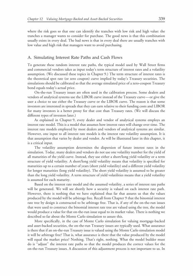
Chapter 12 Valuing Mortgage-Backed and Asset-Backed Securities 339
where the risk goes so that one can identify the tranches with low risk and high value: thetranches a manager wants to consider for purchase. The good news is that this combinationusually exists in every deal. The bad news is that in every deal there are usually tranches withlow value and high risk that managers want to avoid purchasing.
A. Simulating Interest Rate Paths and Cash Flows
To generate these random interest rate paths, the typical model used by Wall Street firmsand commercial vendors takes as input today’s term structure of interest rates and a volatilityassumption. (We discussed these topics in Chapter 9.) The term structure of interest rates isthe theoretical spot rate (or zero coupon) curve implied by today’s Treasury securities. Thesimulations should be calibrated so that the average simulated price of a zero-coupon Treasurybond equals today’s actual price.
On-the-run Treasury issues are often used in the calibration process. Some dealers andvendors of analytical systems use the LIBOR curve instead of the Treasury curve—or give theuser a choice to use either the Treasury curve or the LIBOR curve. The reason is that someinvestors are interested in spreads that they can earn relative to their funding costs and LIBORfor many investors is a better proxy for that cost than Treasury rates. (We will discuss thedifferent types of investors later.)
As explained in Chapter 9, every dealer and vendor of analytical systems employs aninterest rate model. This is a model that assumes how interest rates will change over time. Theinterest rate models employed by most dealers and vendors of analytical systems are similar.However, one input to all interest rate models is the interest rate volatility assumption. It isthat assumption that varies by dealer and vendor. As will be illustrated later in this chapter, itis a critical input.
The volatility assumption determines the dispersion of future interest rates in thesimulation. Today, many dealers and vendors do not use one volatility number for the yield ofall maturities of the yield curve. Instead, they use either a short/long yield volatility or a termstructure of yield volatility. A short/long yield volatility means that volatility is specified formaturities up to a certain number of years (short yield volatility) and a different yield volatilityfor longer maturities (long yield volatility). The short yield volatility is assumed to be greaterthan the long yield volatility. A term structure of yield volatilities means that a yield volatilityis assumed for each maturity.
Based on the interest rate model and the assumed volatility, a series of interest rate pathswill be generated. We will see shortly how a security is valued on each interest rate path.However, there is nothing that we have explained thus far that assures us that the valuesproduced by the model will be arbitrage free. Recall from Chapter 9 that the binomial interestrate tree by design is constructed to be arbitrage free. That is, if any of the on-the-run issuesthat were used to construct the binomial interest rate tree are valued using the tree, the modelwould produce a value for that on-the-run issue equal to its market value. There is nothing wedescribed so far about the Monte Carlo simulation to assure this.
More specifically, in the case of Monte Carlo simulation for valuing mortgage-backedand asset-backed securities, the on-the-run Treasury issues are typically used. What assuranceis there that if an on-the-run Treasury issue is valued using the Monte Carlo simulation modelit will be arbitrage free? That is, what assurance is there that the value produced by the modelwill equal the market price? Nothing. That’s right, nothing. What the model builder mustdo is ‘‘adjust’’ the interest rate paths so that the model produces the correct values for theon-the-run Treasury issues. A discussion of this adjustment process is not important to us. In

340 Fixed Income Analysis
fact, there are very few published sources that describe how this is done. The key point hereis that no such adjustment is necessary in a binomial model for valuing corporate and agencybonds with embedded options because the tree is built to be arbitrage free. In the case of theMonte Carlo simulation model, the builder must make an arbitrary adjustment to the interestrate paths to get the model to be arbitrage free.
The simulation works by generating many scenarios of future interest rate paths. As justexplained, the ‘‘raw’’ interest rate paths that are simulated must be ‘‘adjusted’’ so as to make themodel generate arbitrage-free values for whatever benchmark interest rates are used—typically,the on-the-run Treasury issues. So, in the remainder of this chapter, when we refer to interest ratepaths it is understood that it is the ‘‘adjusted’’ interest rate paths where ‘‘adjusted’’ means that eachinterest rate path is adjusted so that the model will produce arbitrage-free values.
In each month of the scenario (i.e., path), a monthly interest rate and a mortgagerefinancing rate are generated. The monthly interest rates are used to discount the projectedcash flows in the scenario. The mortgage refinancing rate is needed to determine the cash flowsbecause it represents the opportunity cost the borrower (i.e., mortgagor) is facing at that time.
If the refinancing rates are high relative to the borrower’s original coupon rate (i.e., therate on the borrower’s loan), the borrower will have less incentive to refinance, or even adisincentive (i.e., the homeowner will avoid moving in order to avoid refinancing). If therefinancing rate is low relative to the borrower’s original coupon rate, the borrower has anincentive to refinance.
Prepayments are projected by feeding the refinancing rate and loan characteristics intoa prepayment model. Given the projected prepayments, the cash flows along an interest ratepath can be determined.
To make this more concrete, consider a newly issued mortgage passthrough securitywith a maturity of 360 months. Exhibit 1 shows N ‘‘adjusted’’ simulated interest rate pathscenarios—adjusted to be arbitrage free. Each scenario consists of a path of 360 simulated1-month future interest rates. (The number of paths generated is based on a well knownprinciple in simulation which will not be discussed here.) So, our first assumption that wemake to get Exhibit 1 is the volatility of interest rates.
Exhibit 2 shows the paths of simulated mortgage refinancing rates corresponding to thescenarios shown in Exhibit 1. In going from Exhibit 1 to Exhibit 2, an assumption must bemade about the relationship between the Treasury rates and refinancing rates. The assumptionis that there is a constant spread relationship between the rate that the borrower will use todetermine whether or not to refinance (i.e., the refinancing rate) and the 1-month interestrates shown in Exhibit 1. For example, for 30-year mortgage loans, model builders use the10-year Treasury rate as a proxy for the refinancing rate.
Given the mortgage refinancing rates, the cash flows on each interest rate path can begenerated. For agency mortgage-backed securities, this requires a prepayment model. For asset-backed securities and nonagency mortgage-backed securities, this requires both a prepaymentmodel and a model of defaults and recoveries. So, our next assumption is that the output ofthese models (prepayments, defaults, and recoveries) are correct. The resulting cash flows aredepicted in Exhibit 3.
B. Calculating the Present Value for an Interest Rate Path
Given the cash flows on an interest rate path, the path’s present value can be calculated. Thediscount rate for determining the present value is the simulated spot rate for each month onthe interest rate path plus an appropriate spread. The spot rate on a path can be determined
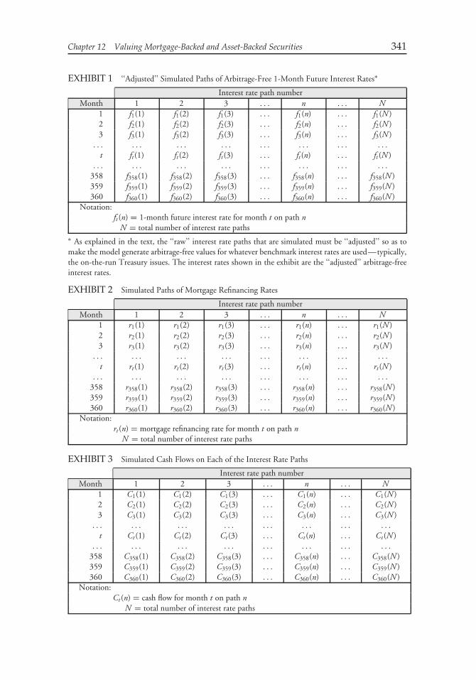
Chapter 12 Valuing Mortgage-Backed and Asset-Backed Securities 341
EXHIBIT 1 ‘‘Adjusted’’ Simulated Paths of Arbitrage-Free 1-Month Future Interest Rates∗
Interest rate path numberMonth 1 2 3 . . . n . . . N
1 f1(1) f1(2) f1(3) . . . f1(n) . . . f1(N )2 f2(1) f2(2) f2(3) . . . f2(n) . . . f2(N )3 f3(1) f3(2) f3(3) . . . f3(n) . . . f3(N )
. . . . . . . . . . . . . . . . . . . . . . . .
t ft (1) ft (2) ft (3) . . . ft (n) . . . ft (N ). . . . . . . . . . . . . . . . . . . . . . . .
358 f358(1) f358(2) f358(3) . . . f358(n) . . . f358(N )359 f359(1) f359(2) f359(3) . . . f359(n) . . . f359(N )360 f360(1) f360(2) f360(3) . . . f360(n) . . . f360(N )
Notation:ft (n) = 1-month future interest rate for month t on path n
N = total number of interest rate paths∗ As explained in the text, the ‘‘raw’’ interest rate paths that are simulated must be ‘‘adjusted’’ so as tomake the model generate arbitrage-free values for whatever benchmark interest rates are used—typically,the on-the-run Treasury issues. The interest rates shown in the exhibit are the ‘‘adjusted’’ arbitrage-freeinterest rates.
EXHIBIT 2 Simulated Paths of Mortgage Refinancing Rates
Interest rate path numberMonth 1 2 3 . . . n . . . N
1 r1(1) r1(2) r1(3) . . . r1(n) . . . r1(N )2 r2(1) r2(2) r2(3) . . . r2(n) . . . r2(N )3 r3(1) r3(2) r3(3) . . . r3(n) . . . r3(N )
. . . . . . . . . . . . . . . . . . . . . . . .
t rt (1) rt (2) rt (3) . . . rt (n) . . . rt (N ). . . . . . . . . . . . . . . . . . . . . . . .
358 r358(1) r358(2) r358(3) . . . r358(n) . . . r358(N )359 r359(1) r359(2) r359(3) . . . r359(n) . . . r359(N )360 r360(1) r360(2) r360(3) . . . r360(n) . . . r360(N )
Notation:rt (n) = mortgage refinancing rate for month t on path n
N = total number of interest rate paths
EXHIBIT 3 Simulated Cash Flows on Each of the Interest Rate Paths
Interest rate path numberMonth 1 2 3 . . . n . . . N
1 C1(1) C1(2) C1(3) . . . C1(n) . . . C1(N )2 C2(1) C2(2) C2(3) . . . C2(n) . . . C2(N )3 C3(1) C3(2) C3(3) . . . C3(n) . . . C3(N )
. . . . . . . . . . . . . . . . . . . . . . . .
t Ct (1) Ct (2) Ct (3) . . . Ct (n) . . . Ct (N ). . . . . . . . . . . . . . . . . . . . . . . .
358 C358(1) C358(2) C358(3) . . . C358(n) . . . C358(N )359 C359(1) C359(2) C359(3) . . . C359(n) . . . C359(N )360 C360(1) C360(2) C360(3) . . . C360(n) . . . C360(N )
Notation:Ct (n) = cash flow for month t on path n
N = total number of interest rate paths

342 Fixed Income Analysis
from the simulated future monthly rates. The relationship that holds between the simulatedspot rate for month T on path n and the simulated future 1-month rates is:
zT (n) = {[1 + f1(n)][1 + f2(n)] · · · [1 + fT (n)]}1/T − 1
where
zT (n) = simulated spot rate for monthT on path nft (n) = simulated future 1-month rate for monthton path n
In Chapter 6 we explained the relationship between spot rates and forward rates.Consequently, the interest rate path for the simulated future 1-month rates can be
converted to the interest rate path for the simulated monthly spot rates as shown in Exhibit 4.Therefore, the present value of the cash flows for month T on interest rate path n discountedat the simulated spot rate for month T plus some spread is:
PV[CT (n)] = CT (n)
[1 + zT (n) + K ]T
where
PV[CT (n)] = present value of cash flows for month T on path nCT (n) = cash flow for month T on path nzT (n) = spot rate for month T on path nK = spread
The spread, K , reflects the risks that the investor feels are associated with realizing the cashflows.
The present value for path n is the sum of the present value of the cash flows for eachmonth on path n. That is,
PV[Path(n)] = PV[C1(n)] + PV[C2(n)] + · · · + PV[C360(n)]
where PV[Path(n)] is the present value of interest rate path n.
C. Determining the Theoretical Value
The present value of a given interest rate path can be thought of as the theoretical value of apassthrough if that path was actually realized. The theoretical value of the passthrough can bedetermined by calculating the average of the theoretical values of all the interest rate paths.That is, the theoretical value is equal to
theoretical value = PV[Path(1)] + PV[Path(2)] + . . . + PV[Path(N )]
N
where N is the number of interest rate paths. The theoretical value derived from the aboveequation is based on some spread, K . It follows the usual practice of discounting cash flows atspot rates plus a spread—in this case the spread is K .
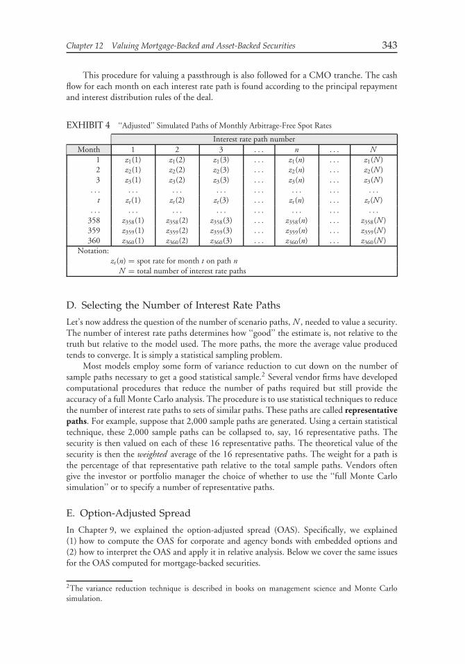
Chapter 12 Valuing Mortgage-Backed and Asset-Backed Securities 343
This procedure for valuing a passthrough is also followed for a CMO tranche. The cashflow for each month on each interest rate path is found according to the principal repaymentand interest distribution rules of the deal.
EXHIBIT 4 ‘‘Adjusted’’ Simulated Paths of Monthly Arbitrage-Free Spot Rates
Interest rate path numberMonth 1 2 3 . . . n . . . N
1 z1(1) z1(2) z1(3) . . . z1(n) . . . z1(N )2 z2(1) z2(2) z2(3) . . . z2(n) . . . z2(N )3 z3(1) z3(2) z3(3) . . . z3(n) . . . z3(N )
. . . . . . . . . . . . . . . . . . . . . . . .
t zt (1) zt (2) zt (3) . . . zt (n) . . . zt (N ). . . . . . . . . . . . . . . . . . . . . . . .
358 z358(1) z358(2) z358(3) . . . z358(n) . . . z358(N )359 z359(1) z359(2) z359(3) . . . z359(n) . . . z359(N )360 z360(1) z360(2) z360(3) . . . z360(n) . . . z360(N )
Notation:zt (n) = spot rate for month t on path n
N = total number of interest rate paths
D. Selecting the Number of Interest Rate Paths
Let’s now address the question of the number of scenario paths, N , needed to value a security.The number of interest rate paths determines how ‘‘good’’ the estimate is, not relative to thetruth but relative to the model used. The more paths, the more the average value producedtends to converge. It is simply a statistical sampling problem.
Most models employ some form of variance reduction to cut down on the number ofsample paths necessary to get a good statistical sample.2 Several vendor firms have developedcomputational procedures that reduce the number of paths required but still provide theaccuracy of a full Monte Carlo analysis. The procedure is to use statistical techniques to reducethe number of interest rate paths to sets of similar paths. These paths are called representativepaths. For example, suppose that 2,000 sample paths are generated. Using a certain statisticaltechnique, these 2,000 sample paths can be collapsed to, say, 16 representative paths. Thesecurity is then valued on each of these 16 representative paths. The theoretical value of thesecurity is then the weighted average of the 16 representative paths. The weight for a path isthe percentage of that representative path relative to the total sample paths. Vendors oftengive the investor or portfolio manager the choice of whether to use the ‘‘full Monte Carlosimulation’’ or to specify a number of representative paths.
E. Option-Adjusted Spread
In Chapter 9, we explained the option-adjusted spread (OAS). Specifically, we explained(1) how to compute the OAS for corporate and agency bonds with embedded options and(2) how to interpret the OAS and apply it in relative analysis. Below we cover the same issuesfor the OAS computed for mortgage-backed securities.
2The variance reduction technique is described in books on management science and Monte Carlosimulation.

344 Fixed Income Analysis
1. Computing the OAS In the Monte Carlo model, the OAS is the spread that whenadded to all the spot rates on all interest rate paths will make the average present value of thepaths equal to the observed market price (plus accrued interest). Mathematically, OAS is thevalue for K (the spread) that will satisfy the following condition:
PV[Path(1)] + PV[Path(2)] + . . . + PV[Path(N )]
N= market price
where N is the number of interest rate paths. The left-hand side of the above equation looksidentical to that of the equation for the theoretical value. The difference is that the objectiveis to determine what spread, K , will make the model produce a theoretical value equal to themarket price.
The procedure for determining the OAS is straightforward and involves the same searchalgorithm explained for the zero-volatility spread. The next question, then, is how to interpretthe OAS. Basically, the OAS is used to reconcile value with market price. On the right-handside of the previous equation is the market’s statement: the price of a structured product. Theaverage present value over all the paths on the left-hand side of the equation is the model’soutput, which we refer to as the theoretical value.
2. Interpreting the OAS and Relative Value Application What an investor or aportfolio manager seeks to do is to buy a mortgage-backed security where value is greater thanprice. By using a valuation model such as the Monte Carlo model, a portfolio manager couldestimate the value of a security, which at this point would be sufficient in determining whetherto buy a security. That is, the portfolio manager can say that this security is 1 point cheap or2 points cheap, and so on. The model does not stop here. Instead, it converts the divergencebetween price and value into some type of spread measure since most market participants findit more convenient to think about spreads than price differences.
The OAS was developed as a measure of the spread that can be used to convert dollardifferences between value and price. As we explained in Chapter 9, in the binomial model aspread is measured relative to the benchmark interest rates used to generate the interest ratetree and which is therefore used to make the tree arbitrage free. The same is true in the caseof the Monte Carlo simulation model. The spread is measured relative to the benchmarkinterest rates that were used to generate the interest rate paths and to adjust the interest ratepaths to make them arbitrage free. Typically, for a mortgage-backed security the benchmarkinterest rates are the on-the-run Treasury rates. The OAS is then measuring the average spreadover the Treasury spot rate curve, not the Treasury yield as explained in Chapter 9. It is anaverage spread since the OAS is found by averaging over the interest rate paths for the possibleTreasury spot rate curves. Of course, if the LIBOR curve is used, the OAS is the spread overthat curve.
This spread measure is superior to the nominal spread which gives no recognition tothe prepayment risk. As explained in Chapter 9, the OAS is ‘‘option adjusted’’ becausethe cash flows on the interest rate paths are adjusted for the option of the borrowers toprepay. While we may understand the mechanics of how to compute the OAS and whyit is appropriate to use the OAS rather than the nominal spread or Z-spread, the questionis what does the spread represent? In Chapter 9, a discussion of what compensation theOAS reflects for corporate and agency bonds with embedded options was presented. Thecompensation is for a combination of credit risk and liquidity risk. The compensationdepends on the benchmark interest rates used in the analysis. For example, consider theuse of Treasury interest rates and more specifically the Treasury spot rate curve since this is
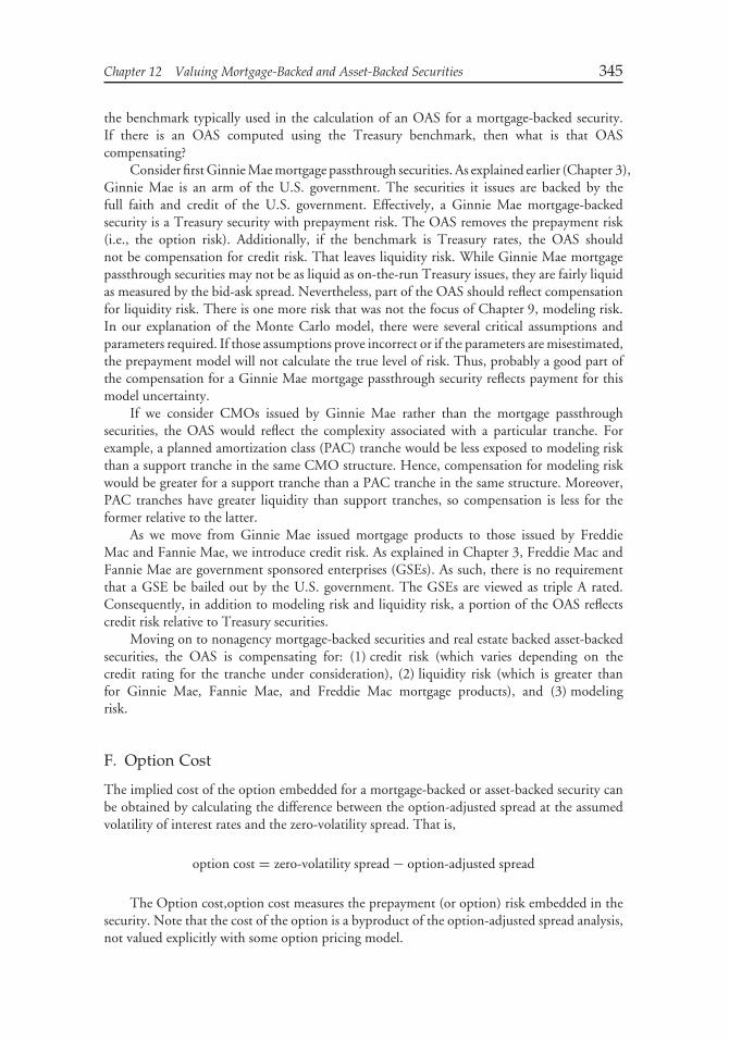
Chapter 12 Valuing Mortgage-Backed and Asset-Backed Securities 345
the benchmark typically used in the calculation of an OAS for a mortgage-backed security.If there is an OAS computed using the Treasury benchmark, then what is that OAScompensating?
Consider first Ginnie Mae mortgage passthrough securities. As explained earlier (Chapter 3),Ginnie Mae is an arm of the U.S. government. The securities it issues are backed by thefull faith and credit of the U.S. government. Effectively, a Ginnie Mae mortgage-backedsecurity is a Treasury security with prepayment risk. The OAS removes the prepayment risk(i.e., the option risk). Additionally, if the benchmark is Treasury rates, the OAS shouldnot be compensation for credit risk. That leaves liquidity risk. While Ginnie Mae mortgagepassthrough securities may not be as liquid as on-the-run Treasury issues, they are fairly liquidas measured by the bid-ask spread. Nevertheless, part of the OAS should reflect compensationfor liquidity risk. There is one more risk that was not the focus of Chapter 9, modeling risk.In our explanation of the Monte Carlo model, there were several critical assumptions andparameters required. If those assumptions prove incorrect or if the parameters are misestimated,the prepayment model will not calculate the true level of risk. Thus, probably a good part ofthe compensation for a Ginnie Mae mortgage passthrough security reflects payment for thismodel uncertainty.
If we consider CMOs issued by Ginnie Mae rather than the mortgage passthroughsecurities, the OAS would reflect the complexity associated with a particular tranche. Forexample, a planned amortization class (PAC) tranche would be less exposed to modeling riskthan a support tranche in the same CMO structure. Hence, compensation for modeling riskwould be greater for a support tranche than a PAC tranche in the same structure. Moreover,PAC tranches have greater liquidity than support tranches, so compensation is less for theformer relative to the latter.
As we move from Ginnie Mae issued mortgage products to those issued by FreddieMac and Fannie Mae, we introduce credit risk. As explained in Chapter 3, Freddie Mac andFannie Mae are government sponsored enterprises (GSEs). As such, there is no requirementthat a GSE be bailed out by the U.S. government. The GSEs are viewed as triple A rated.Consequently, in addition to modeling risk and liquidity risk, a portion of the OAS reflectscredit risk relative to Treasury securities.
Moving on to nonagency mortgage-backed securities and real estate backed asset-backedsecurities, the OAS is compensating for: (1) credit risk (which varies depending on thecredit rating for the tranche under consideration), (2) liquidity risk (which is greater thanfor Ginnie Mae, Fannie Mae, and Freddie Mac mortgage products), and (3) modelingrisk.
F. Option Cost
The implied cost of the option embedded for a mortgage-backed or asset-backed security canbe obtained by calculating the difference between the option-adjusted spread at the assumedvolatility of interest rates and the zero-volatility spread. That is,
option cost = zero-volatility spread − option-adjusted spread
The Option cost,option cost measures the prepayment (or option) risk embedded in thesecurity. Note that the cost of the option is a byproduct of the option-adjusted spread analysis,not valued explicitly with some option pricing model.
346 Fixed Income Analysis
G. Illustrations
We will use two deals to show how CMOs can be analyzed using the Monte Carlo model/OASprocedure discussed above—a simple structure and a PAC/support structure.3
1. Simple Structure The simple structure analyzed is Freddie Mac (FHLMC) 1915. Itis a simple sequential-pay CMO bond structure. The structure includes eight tranches, A, B,C, D, E, F, G, and S. The focus of our analysis is on tranches A, B, and C. All three trancheswere priced at a premium.
The top panel of Exhibit 5 shows the OAS, the option cost, and effective duration4 forthe collateral and the three tranches in the CMO structure. However, tranche A had thesmallest effective duration and tranche C had the largest effective duration. The OAS for thecollateral is 51 basis points. Since the option cost is 67 basis points, the zero-volatility spreadis 118 basis points (51 basis points plus 67 basis points).
At the time this analysis was performed, March 10, 1998, the Treasury yield curve wasnot steep. We explained that when the yield curve is relatively flat the zero-volatility spreadwill not differ significantly from the nominal spread. Thus, for the three tranches shown inExhibit 5, the zero-volatility spread is 83 basis points for A, 115 basis points for B, and 116basis points for C.
Notice that the tranches did not share the OAS equally. The same is true for the optioncost. Both the Z-spread and the option cost increase as the effective duration increases.Whether or not any of these tranches were attractive investments requires a comparison toother tranches in the market with the same effective duration. While not presented here, allthree tranches offered an OAS similar to other sequential-pay tranches with the same effectiveduration available in the market. On a relative basis (i.e., relative to the other tranches analyzedin the deal), the only tranche where there appears to be a bit of a bargain is tranche C. Aportfolio manager contemplating the purchase of this last cash flow tranche can see that Coffers a higher OAS than B and appears to bear less of the risk (i.e., has lower option cost),as measured by the option cost. The problem portfolio managers may face is that they mightnot be able to go out as long on the yield curve as tranche C because of effective duration,maturity, and average life constraints relative to their liabilities, for example.
Now let’s look at modeling risk. Examination of the sensitivity of the tranches to changesin prepayments and interest rate volatility will help us to understand the interaction of thetranches in the structure and who is bearing the risk. How the deal behaves under variousscenarios should reinforce and be consistent with the valuation (i.e., a tranche may look‘‘cheap’’ for a reason).
We begin with prepayments. Specifically, we keep the same interest rate paths as thoseused to get the OAS in the base case (the top panel of Exhibit 5), but reduce the prepaymentrate on each interest rate path to 80% of the projected rate. As can be seen in the second panelof Exhibit 5, slowing down prepayments increases the OAS and price for the collateral. Theexhibit reports two results of the sensitivity analysis. First, it indicates the change in the OAS.Second, it indicates the change in the price, holding the OAS constant at the base case.
3These illustrations are from Frank J. Fabozzi, Scott F. Richard, and David S. Horowitz, ‘‘Valuationof CMOs,’’ Chapter 6 in Frank J. Fabozzi (ed.), Advances in the Valuation and Management ofMortgage-Backed Securities (New Hope, PA: Frank J. Fabozzi Associates, 1998).4We will explain how to compute the effective duration using the Monte Carlo methodology inSection V. A.
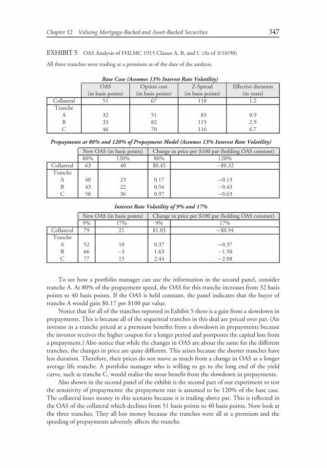
Chapter 12 Valuing Mortgage-Backed and Asset-Backed Securities 347
EXHIBIT 5 OAS Analysis of FHLMC 1915 Classes A, B, and C (As of 3/10/98)
All three tranches were trading at a premium as of the date of the analysis.
Base Case (Assumes 13% Interest Rate Volatility)OAS Option cost Z-Spread Effective duration
(in basis points) (in basis points) (in basis points) (in years)Collateral 51 67 118 1.2Tranche
A 32 51 83 0.9B 33 82 115 2.9C 46 70 116 6.7
Prepayments at 80% and 120% of Prepayment Model (Assumes 13% Interest Rate Volatility)
New OAS (in basis points) Change in price per $100 par (holding OAS constant)80% 120% 80% 120%
Collateral 63 40 $0.45 −$0.32Tranche
A 40 23 0.17 −0.13B 43 22 0.54 −0.43C 58 36 0.97 −0.63
Interest Rate Volatility of 9% and 17%
New OAS (in basis points) Change in price per $100 par (holding OAS constant)9% 17% 9% 17%
Collateral 79 21 $1.03 −$0.94Tranche
A 52 10 0.37 −0.37B 66 −3 1.63 −1.50C 77 15 2.44 −2.08
To see how a portfolio manager can use the information in the second panel, considertranche A. At 80% of the prepayment speed, the OAS for this tranche increases from 32 basispoints to 40 basis points. If the OAS is held constant, the panel indicates that the buyer oftranche A would gain $0.17 per $100 par value.
Notice that for all of the tranches reported in Exhibit 5 there is a gain from a slowdown inprepayments. This is because all of the sequential tranches in this deal are priced over par. (Aninvestor in a tranche priced at a premium benefits from a slowdown in prepayments becausethe investor receives the higher coupon for a longer period and postpones the capital loss froma prepayment.) Also notice that while the changes in OAS are about the same for the differenttranches, the changes in price are quite different. This arises because the shorter tranches haveless duration. Therefore, their prices do not move as much from a change in OAS as a longeraverage life tranche. A portfolio manager who is willing to go to the long end of the yieldcurve, such as tranche C, would realize the most benefit from the slowdown in prepayments.
Also shown in the second panel of the exhibit is the second part of our experiment to testthe sensitivity of prepayments: the prepayment rate is assumed to be 120% of the base case.The collateral loses money in this scenario because it is trading above par. This is reflected inthe OAS of the collateral which declines from 51 basis points to 40 basis points. Now look atthe three tranches. They all lost money because the tranches were all at a premium and thespeeding of prepayments adversely affects the tranche.
348 Fixed Income Analysis
Before looking at the last panel that shows the effect of a change in interest rate volatilityon the OAS, let’s review the relationship between expected interest rate volatility and thevalue of a mortgage-backed security. Recall that the investor in a mortgage-backed securityhas sold an option to homeowners (borrowers). Thus, the investor is short an option. Aswill be explained in Chapter 14, the value of an option depends on expected interest ratevolatility. When expected interest rate volatility decreases, the value of the option embeddedin a mortgage-backed security decreases and therefore the value of a mortgage-backed securityincreases. The opposite is true when expected interest rate volatility increases—the value ofthe embedded option increases and the value of a mortgage-backed security decreases.
Now let’s look at the sensitivity to the interest rate volatility assumption, 13% in the basecase. Two experiments are performed: reducing the volatility assumption to 9% and increasingit to 17%. These results are reported in the third panel of Exhibit 5.
Reducing the volatility to 9% increases the dollar price of the collateral by $1.03 andincreases the OAS from 51 in the base case to 79 basis points. However, this $1.03 increasein the price of the collateral is not equally distributed among the three tranches. Most of theincrease in value is realized by the longer tranches. The OAS gain for each of the tranchesfollows more or less the effective durations of those tranches. This makes sense, because thelonger the duration, the greater the risk, and when volatility declines, the reward is greater forthe accepted risk. At the higher level of assumed interest rate volatility of 17%, the collateralis severely affected. The longer the duration, the greater the loss. These results for a decreaseand an increase in interest rate volatility are consistent with what we explained earlier.
Using the Monte Carlo simulation/OAS analysis, a fair conclusion that can be madeabout this simple structure is: what you see is what you get. The only surprise in this structureis the lower option cost in tranche C. In general, however, a portfolio manager willing toextend duration gets paid for that risk in this structure.
2. PAC/Support Tranche Structure Now let’s look at how to apply the methodologyto a more complicated CMO structure, FHLMC Series 1706. The collateral (i.e., pool ofpassthroughs) for this structure is Freddie Mac 7s (7% coupon rate). A partial summary of thedeal is provided in Exhibit 6. That is, only the tranches we will be discussing in this sectionare shown in the exhibit.5
While this deal looks complicated, it is relatively simple compared to many deals that havebeen issued. Nonetheless, it brings out all the key points about application of OAS analysis,specifically, the fact that most deals include cheap bonds, expensive bonds, and fairly pricedbonds. The OAS analysis helps identify how a tranche shouldbeclassified.Amoreproper analysiswould compare the OAS for each tranche to a similar duration tranche available in the market.
All of the tranches in Exhibit 6 were discussed in Chapter 10. At issuance, there were10 PAC tranches, three scheduled tranches, a floating-rate support tranche, and an inversefloating-rate support. Recall that the ‘‘scheduled tranches’’ are support tranches with a schedule,referred to in Chapter 10 as ‘‘PAC II tranches.’’
The first two PAC tranches in the deal, tranche A and tranche B, were paid off at thetime of the analysis. The other PAC tranches were still available at the time of the analysis.The prepayment protection for the PAC tranches is provided by the support tranches. Thesupport tranches in this deal that are shown in Exhibit 6 are tranches LA, LB, and M. Therewere other support tranches not shown in Exhibit 6. LA is the shortest average life supporttranche (a scheduled (SCH) bond).
5This deal was described in Chapter 10.
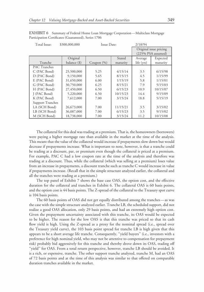
Chapter 12 Valuing Mortgage-Backed and Asset-Backed Securities 349
EXHIBIT 6 Summary of Federal Home Loan Mortgage Corporation—Multiclass MortgageParticipation Certificates (Guaranteed), Series 1706
Total Issue: $300,000,000 Issue Date: 2/18/94Original issue pricing(225% PSA assumed)
Original Stated Average ExpectedTranche balance ($) Coupon (%) maturity life (yrs) maturity
PAC TranchesC (PAC Bond) 25,500,000 5.25 4/15/14 3.5 6/15/98D (PAC Bond) 9,150,000 5.65 8/15/15 4.5 1/15/99E (PAC Bond) 31,650,000 6.00 1/15/19 5.8 1/15/01G (PAC Bond) 30,750,000 6.25 8/15/21 7.9 5/15/03H (PAC Bond) 27,450,000 6.50 6/15/23 10.9 10/15/07J (PAC Bond) 5,220,000 6.50 10/15/23 14.4 9/15/09K (PAC Bond) 7,612,000 7.00 3/15/24 18.8 5/15/19Support TranchesLA (SCH Bond) 26,673,000 7.00 11/15/21 3.5 3/15/02LB (SCH Bond) 36,087,000 7.00 6/15/23 3.5 9/15/02M (SCH Bond) 18,738,000 7.00 3/15/24 11.2 10/15/08
The collateral for this deal was trading at a premium. That is, the homeowners (borrowers)were paying a higher mortgage rate than available in the market at the time of the analysis.This meant that the value of the collateral would increase if prepayments slow down but woulddecrease if prepayments increase. What is important to note, however, is that a tranche couldbe trading at a discount, par, or premium even though the collateral is priced at a premium.For example, PAC C had a low coupon rate at the time of the analysis and therefore wastrading at a discount. Thus, while the collateral (which was selling at a premium) loses valuefrom an increase in prepayments, a discount tranche such as tranche C would increase in valueif prepayments increase. (Recall that in the simple structure analyzed earlier, the collateral andall the tranches were trading at a premium.)
The top panel of Exhibit 7 shows the base case OAS, the option cost, and the effectiveduration for the collateral and tranches in Exhibit 6. The collateral OAS is 60 basis points,and the option cost is 44 basis points. The Z-spread of the collateral to the Treasury spot curveis 104 basis points.
The 60 basis points of OAS did not get equally distributed among the tranches—as wasthe case with the simple structure analyzed earlier. Tranche LB, the scheduled support, did notrealize a good OAS allocation, only 29 basis points, and had an extremely high option cost.Given the prepayment uncertainty associated with this tranche, its OAS would be expectedto be higher. The reason for the low OAS is that this tranche was priced so that its cashflow yield is high. Using the Z-spread as a proxy for the nominal spread (i.e., spread overthe Treasury yield curve), the 103 basis point spread for tranche LB is high given that thisappears to be a short average life tranche. Consequently, ‘‘yield buyers’’ (i.e., investors with apreference for high nominal yield, who may not be attentive to compensation for prepaymentrisk) probably bid aggressively for this tranche and thereby drove down its OAS, trading off‘‘yield’’ for OAS. From a total return perspective, however, tranche LB should be avoided. Itis a rich, or expensive, tranche. The other support tranche analyzed, tranche M, had an OASof 72 basis points and at the time of this analysis was similar to that offered on comparableduration tranches available in the market.
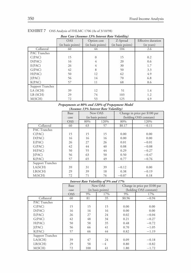
350 Fixed Income Analysis
EXHIBIT 7 OAS Analysis of FHLMC 1706 (As of 3/10/98)
Base Case (Assumes 13% Interest Rate Volatility)OAS Option cost Z-Spread Effective duration
(in basis points) (in basis points) (in basis points) (in years)Collateral 60 44 104 2.6
PAC TranchesC(PAC) 15 0 15 0.2D(PAC) 16 4 20 0.6E(PAC) 26 4 30 1.7G(PAC) 42 8 50 3.3H(PAC) 50 12 62 4.9J(PAC) 56 14 70 6.8K(PAC) 57 11 68 8.6Support TranchesLA (SCH) 39 12 51 1.4LB (SCH) 29 74 103 1.2M(SCH) 72 53 125 4.9
Prepayments at 80% and 120% of Prepayment Model(Assumes 13% Interest Rate Volatility)
Base New OAS Change in price per $100 parcase (in basis points) (holding OAS constant)OAS 80% 120% 80% 120%
Collateral 60 63 57 $0.17 −0.11PAC TranchesC(PAC) 15 15 15 0.00 0.00D(PAC) 16 16 16 0.00 0.00E(PAC) 26 27 26 0.01 −0.01G(PAC) 42 44 40 0.08 −0.08H(PAC) 50 55 44 0.29 −0.27J(PAC) 56 63 50 0.50 −0.47K(PAC) 57 65 49 0.77 −0.76Support TranchesLA(SCH) 39 31 39 −0.12 0.00LB(SCH) 29 39 18 0.38 −0.19M(SCH) 72 71 76 −0.07 0.18
Interest Rate Volatility of 9% and 17%Base New OAS Change in price per $100 parcase (in basis points) (holding OAS constant)OAS 9% 17% 9% 17%
Collateral 60 81 35 $0.96 −0.94PAC TranchesC(PAC) 15 15 15 0.00 0.00D(PAC) 16 16 16 0.00 0.00E(PAC) 26 27 24 0.02 −0.04G(PAC) 42 48 34 0.21 −0.27H(PAC) 50 58 35 0.48 −0.72J(PAC) 56 66 41 0.70 −1.05K(PAC) 57 66 44 0.82 −1.19Support TranchesLA(SCH) 39 47 24 0.09 −0.18LB(SCH) 29 58 −4 0.80 −0.82M(SCH) 72 100 41 1.80 −1.72
Chapter 12 Valuing Mortgage-Backed and Asset-Backed Securities 351
The analysis reported in the top panel of Exhibit 7 help us identify where the cheaptranches are in the deal. The long average life and effective duration tranches in the deal arethe PAC tranches G, H, J, and K. These tranches have high OAS relative to the other tranchesand low option cost. They appear to be the cheap tranches in the deal. These PAC trancheshad well protected cash flows and exhibited positive convexity (i.e., these tranches lose less inan adverse scenario than they gain in a positive scenario).
The next two panels in Exhibit 7 show the sensitivity of the OAS and the price (holdingOAS constant at the base case) to changes in the prepayment speed (80% and 120% of thebase case) and to changes in volatility (9% and 17%). This analysis shows that the changein the prepayment speed does not affect the collateral significantly, while the change in theOAS (holding the price constant) and price (holding OAS constant) for each tranche can besignificant.
Tranches C and D at the time of the analysis were priced at a discount with short averagelives. The OAS and price of these two tranches were not affected by a slowing down or aspeeding up of the prepayment model. Tranche H was a premium tranche with a medium-termaverage life at the time of the analysis. Because tranche H was trading at a premium, it benefitsfrom a slowing in prepayments, as the bondholder will receive the coupon for a longer time.Faster prepayments represent an adverse scenario. The PAC tranches are quite well-protected.The longer average life PACs will actually benefit from a reduced prepayment rate because theywill be earning the higher coupon interest longer. So, on an OAS basis, the earlier conclusionthat the long PACs were allocated a good part of the deal’s value holds up under our first stresstest (i.e., changing prepayments).
The sensitivity of the collateral and the tranches to changes in volatility are shown in thethird panel of Exhibit 7. A lower volatility increases the value of the collateral, while a highervolatility reduces its value (This is consistent with our option cost equation in Section IV.E.)The long average life PACs continue to be fairly well-protected, whether the volatility is loweror higher. In the two volatility scenarios they continue to get a good OAS on a relative valuebasis, although not as much as in the base case if volatility is higher (but the OAS still lookslike a reasonable value in this scenario). This reinforces the earlier conclusion concerning theinvestment merit of the long PACs in this deal. Note, however, that PAC tranches H, J, andK are more sensitive to the volatility assumption than tranches C, D, E, and G and thereforethe investor is accepting greater volatility risk (i.e., the risk that volatility will change) withtranches H, J, and K relative to tranches C, D, E, and G.
V. MEASURING INTEREST RATE RISK
As explained in Chapter 9, duration and convexity can be used to estimate the interest rateexposure to parallel shifts in the yield curve (i.e., a measure of level risk). In this sectionwe will discuss duration measures for mortgage-backed securities. There are several durationmeasures that are used in practice. Two researchers who have done extensive work in measuringduration, Lakhbir Hayre and Hubert Chang, conclude that ‘‘No single duration measure willconsistently work well for mortgage securities.’’6 To that conclusion should be added thatthere are some measures that do not work at all.
6Lakhbir Hayre and Hubert Chang, ‘‘Effective and Empirical Duration of Mortgage Securities,’’ TheJournal of Fixed Income (March 1997), pp. 17–33.

352 Fixed Income Analysis
A. Duration Measures
Duration is a measure of the price sensitivity to changes in interest rates. We have seen howto compute the duration of a security by shocking rates up and down and determining howthe price of the security changes. Duration is then computed as follows:
duration = V− − V+2V0(�y)
where
�y = change in rate used to calculate new values (i.e., the interest rate shock)V+ = estimated value if yield is increased by�yV− = estimated value if yield is decreased by�yV0 = initial price (per $100 of par value)
For bonds with embedded options such as mortgage-backed securities, the appropriatemeasure is effective duration and to capture the negative convexity of a bond with an embeddedoption, effective convexity should be computed. We will see how to calculate the effectiveduration for a mortgage-backed security using the Monte Carlo simulation model. Then wewill see how the assumptions of the model impact the duration estimate. Dealers and vendorsuse other measures of duration that will be described later.
1. Effective Duration To calculate effective duration, the value of the security must beestimated when rates are shocked up and down a given number of basis points. In terms of theMonte Carlo model, the yield curve used (either the Treasury yield curve or LIBOR curve)is shocked up and down and the new curve is used to generate the values to be used in theeffective duration and effective convexity formulas. This is analogous to the process we usedto compute effective duration and effective convexity using the binomial model in Chapter 9.
In generating the prices when rates are shocked up and down, there is an assumptionthat the relationships assumed in generating the initial price do not change when rates areshocked up and down. Specifically, the yield volatility is assumed to be unchanged to derivethe new interest rate paths for a given shock (i.e., the new Exhibit 1), the spread between themortgage rate and the 10-year Treasury rate is assumed to be unchanged in constructing thenew Exhibit 2 from the newly constructed Exhibit 1, and the OAS is assumed to be constant.The constancy of the OAS comes into play because when discounting the new cash flows (i.e.,the cash flows in the new Exhibit 3), the current OAS that was computed is assumed to be thesame and is added to the new rates in the new Exhibit 1.
We’ll use an illustration by Lakhbir Hayre and Hubert Chang to explain the calculationof effective duration for a mortgage-backed security, a FNMA 7.5% TBA passthrough on May1, 1996.7 On that day, the base mortgage rate was 7.64%. The price of the issue at the timewas 98.781 (i.e., 98-25). The OAS was 65 basis points. Based on a shock of 25 basis points,the estimated prices holding the OAS constant at 65 basis points were as follows:
V− = 99.949 for a decrease in the yield curve of 25 basis pointsV+ = 97.542 for an increase in the yield curve of 25 basis points
7Hayre and Chang, ‘‘Effective and Empirical Duration of Mortgage Securities.’’

Chapter 12 Valuing Mortgage-Backed and Asset-Backed Securities 353
The effective duration based on a �y of 0.0025 is then
99.949 − 97.542
2 × 98.781 × 0.0025= 4.87
There are differences in the effective durations for a given mortgage-backed securityreported by dealers and vendors of analytical systems. Several practitioners have explained andillustrated why there are differences in effective duration estimates reported by dealers andvendors. The differences result from, among others:8
1. differences in the amount of the rate shock used2. differences in prepayment models3. differences in option-adjusted spread4. differences in the relationship between short-term interest rates and refinancing rates
Earlier, we discussed the first reason. As explained, the rate shock is the amount interestrates are increased and decreased to obtain the two values that are inserted into the effectiveduration formula. If the change is too large, there is the problem with picking up the effect ofconvexity.
Prepayment models differ across dealers and vendors. Some dealer models consistentlyforecast slower prepayments relative to other dealer models and others the reverse.
The effective duration is dependent on the OAS computed. Recall that the calculation ofthe OAS is a byproduct of the Monte Carlo model. Therefore, the computed value for theOAS depends on all of the assumptions in the Monte Carlo model. Specifically, it depends onthe yield volatility assumed and the prepayment model employed. Dealers and vendors makedifferent assumptions regarding yield volatility and use proprietary prepayment models. Thesecan result in differences in OAS. Since the OAS is added to the new simulated short-term ratesto compute the new values for V− and V+, a different OAS will result in different effectivedurations.
Finally, recall that in explaining the Monte Carlo simulation model that we stated that inmoving from Exhibit 1 (the simulated short-term rates) to Exhibit 2 (the refinancing rates),an assumption must be made about the relationship between short-term rates and the 10-yearTreasury rate (i.e., the rate used as a proxy for refinancing). Differences in models about howlarge the spread between these rates will be affects the value of a mortgage-backed security andtherefore the values used in the duration equation when rates are shocked.
2. Other Duration Measures There have been other measures proposed for estimatingthe duration of a mortgage-backed security. These measures include cash flow duration,coupon curve duration, and empirical duration. The first two duration measures are formsof effective duration in that they do recognize that the values that should be used in theduration formula should take into account how the cash flows may change due to changesin prepayments when interest rates change. In contrast, empirical duration is a duration thatis computed statistically using observed market prices. Below we describe how each of theseduration measures is calculated, as well as the advantages and limitations of each.
8Sam Choi, ‘‘Effective Durations for Mortgage-Backed Securities: Recipes for Improvement,’’ TheJournal of Fixed Income (March 1996), pp. 24–30; and, Hayre and Chang, ‘‘Effective and EmpiricalDuration of Mortgage Securities.’’
354 Fixed Income Analysis
a. Cash Flow Duration Recall from the general duration formula that there are two valuesthat must be substituted into the numerator of the formula—the value if rates are decreased(V−) and the value if rates are increased (V+). With effective duration, these two valuesconsider how changes in interest rates change the cash flow due to prepayments. This is donethrough the Monte Carlo simulation by allowing for the cash flows to change on the interestrate paths.
For cash flow duration, there is recognition that the cash flow can change but the analysisto obtain the cash flow is done following a static methodology. Specifically, the cash flowduration is calculated as follows:
Step 1: Calculate the cash flow based on some prepayment assumption.
Step 2: From the cash flow in Step 1 and the market price (V0), compute the cash flowyield.
Step 3: Increase the cash flow yield by �y and from a prepayment model determine thenew prepayment rate at that higher cash flow yield. Typically, the prepayment ratewill be lower than in Step 1 because of the higher yield level.
Step 4: Using the lower prepayment rate in Step 3 determine the cash flow and then valuethe cash flow using the higher cash flow yield as the discount rate. This gives thevalue (V+).
Step 5: Decrease the cash flow yield by �y and from a prepayment model determine thenew prepayment rate at that lower cash flow yield. Typically, the prepayment ratewill be higher than in Step 1 because of the lower yield level.
Step 6: Using the higher prepayment rate in Step 5 determine the cash flow and thenvalue the cash flow using the lower cash flow yield as the discount rate. This givesthe value (V−).
From the change in basis points (�y), the values for V+ and V− found in Steps 4 and 6, andthe initial value V0, the duration can be computed.
We can use the hypothetical CMO structure in Chapter 10 to illustrate how to calculatecash flow duration. Specifically, in FJF-2, there were four tranches, A, B, C, and Z. Let’s focuson tranche C. Suppose that the price for this tranche is 100.2813. Then the cash flow durationis computed as follows:
Step 1: Suppose that the assumed prepayment rate for this tranche is 165 PSA.
Step 2: Based on the assumed prepayment rate of 165 PSA and the price of 100.2813, itcan be demonstrated that the cash flow yield is 7%.
Step 3: Suppose that the cash flow yield is increased (i.e., shocked) by 25 basis points (from7% to 7.25%) and suppose that some prepayment model projects a prepayment rateof 150 PSA. (Note that this is a slower prepayment rate than at 7%.)
Step 4: Based on 150 PSA, a new cash flow can be generated. The cash flow is thendiscounted at 7.25% (the new cash flow yield). It can be demonstrated that the valueof this tranche based on these assumptions would be 98.3438. This is the value V+.
Step 5: Suppose that the cash flow yield is decreased (i.e., shocked) by 25 basis points (from7% to 6.75%) and suppose that some prepayment model projects a prepayment rateof 200 PSA. (Note that this is a faster prepayment rate than at 7%.)
Chapter 12 Valuing Mortgage-Backed and Asset-Backed Securities 355
Step 6: Based on 200 PSA, the new cash flow can be generated. The cash flow is thendiscounted at 6.75% (the new cash flow yield). It can be demonstrated that the valueof this tranche based on these assumptions would be 101.9063. This is the value V−.
Now we have the following information:
V0 = 100.2813V+ = 98.3438V− = 101.9063�y = 0.0025
Then using the general form of duration, we obtain:
duration = 101.9063 − 98.3438
2(100.2813)(0.0025)= 7.11
What type of duration measure is the cash flow duration—effective duration or modifiedduration? Technically, it is a form of effective duration because notice that in Steps 3 and 5when the rate is changed, the cash flow is allowed to change. However, as has been stressedthroughout, the valuation model that is used to get the new values to substitute into theduration formula is critical. The valuation model in the case of the cash flow duration isbased on the naive assumption that there is a single prepayment rate over the life of themortgage-backed security for any given interest rate shock. This is in contrast to the valuesproduced by the Monte Carlo simulation model that does more sophisticated analyses of howthe cash flow can change when interest rates change.
Why bother discussing the cash flow duration if it is an inferior form of effective duration?The reason is that it is a commonly cited duration measure and practitioners should be awareof how it is computed. Likewise, we did discuss in detail yield calculations despite theirlimitations.
An interesting question is how does this form of duration compare to modified duration.Recall from Chapter 7 and Chapter 9 that modified duration does not assume that cash flowswill change when rates are shocked. That is, in the steps discussed above to obtain cash flowduration, in Steps 3 and 5 it is assumed that the prepayment rate is the same as in Step 1.
To illustrate this, we’ll once again use tranche C in FJF-2. In Step 3, the prepayment rateassumed is still 165 PSA despite the fact that rates are assumed to increase. That is, the cashflow is not assumed to change. Based on a cash flow yield of 7.25% and a prepayment rateof 165 PSA, the value of this tranche would decline to 98.4063. When the cash flow yieldis assumed to decline to 6.75%, the prepayment rate is still assumed to be 165 PSA and thevalue of this tranche would be 102.1875. Then to calculate the modified duration we know:
V0 = 100.2813
V+ = 98.4063
V− = 102.1875
�y = 0.0025
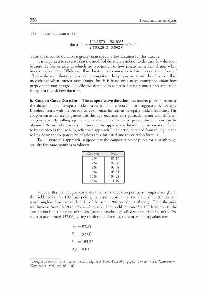
356 Fixed Income Analysis
The modified duration is then:
duration = 102.1875 − 98.4063
2(100.2813)(0.0025)= 7.54
Thus, the modified duration is greater than the cash flow duration for this tranche.It is important to reiterate that the modified duration is inferior to the cash flow duration
because the former gives absolutely no recognition to how prepayments may change wheninterest rates change. While cash flow duration is commonly cited in practice, it is a form ofeffective duration that does give some recognition that prepayments and therefore cash flowmay change when interest rates change, but it is based on a naive assumption about howprepayments may change. The effective duration as computed using Monte Carlo simulationis superior to cash flow duration.
b. Coupon Curve Duration The coupon curve duration uses market prices to estimatethe duration of a mortgage-backed security. This approach, first suggested by DouglasBreeden,9 starts with the coupon curve of prices for similar mortgage-backed securities. Thecoupon curve represents generic passthrough securities of a particular issuer with differentcoupon rates. By rolling up and down the coupon curve of prices, the duration can beobtained. Because of the way it is estimated, this approach to duration estimation was referredto by Breeden as the ‘‘roll-up, roll-down approach.’’ The prices obtained from rolling up androlling down the coupon curve of prices are substituted into the duration formula.
To illustrate this approach, suppose that the coupon curve of prices for a passthroughsecurity for some month is as follows:
Coupon Price6% 85.197% 92.068% 98.389% 103.34
10% 107.2811% 111.19
Suppose that the coupon curve duration for the 8% coupon passthrough is sought. Ifthe yield declines by 100 basis points, the assumption is that the price of the 8% couponpassthrough will increase to the price of the current 9% coupon passthrough. Thus, the pricewill increase from 98.38 to 103.34. Similarly, if the yield increases by 100 basis points, theassumption is that the price of the 8% coupon passthrough will decline to the price of the 7%coupon passthrough (92.06). Using the duration formula, the corresponding values are:
V0 = 98.38
V+ = 92.06
V− = 103.34
�y = 0.01
9Douglas Breeden, ‘‘Risk, Return, and Hedging of Fixed-Rate Mortgages,’’ The Journal of Fixed Income(September 1991), pp. 85–107.
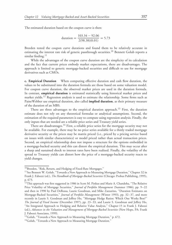
Chapter 12 Valuing Mortgage-Backed and Asset-Backed Securities 357
The estimated duration based on the coupon curve is then:
duration = 103.34 − 92.06
2(98.38)(0.01)= 5.73
Breeden tested the coupon curve durations and found them to be relatively accurate inestimating the interest rate risk of generic passthrough securities.10 Bennett Golub reports asimilar finding.11
While the advantages of the coupon curve duration are the simplicity of its calculationand the fact that current prices embody market expectations, there are disadvantages. Theapproach is limited to generic mortgage-backed securities and difficult to use for mortgagederivatives such as CMOs.
c. Empirical Duration When computing effective duration and cash flow duration, thevalues to be substituted into the duration formula are those based on some valuation model.For coupon curve duration, the observed market prices are used in the duration formula.In contrast, empirical duration is estimated statistically using historical market prices andmarket yields.12 Regression analysis is used to estimate the relationship. Some firms such asPaineWebber use empirical duration, also called implied duration, as their primary measureof the duration of an MBS.
There are three advantages to the empirical duration approach.13 First, the durationestimate does not rely on any theoretical formulas or analytical assumptions. Second, theestimation of the required parameters is easy to compute using regression analysis. Finally, theonly inputs that are needed are a reliable price series and Treasury yield series.
There are disadvantages.14 First, a reliable price series for the mortgage security may notbe available. For example, there may be no price series available for a thinly traded mortgagederivative security or the prices may be matrix priced (i.e., priced by a pricing service basedon issues with similar characteristics) or model priced rather than actual transaction prices.Second, an empirical relationship does not impose a structure for the options embedded ina mortgage-backed security and this can distort the empirical duration. This may occur aftera sharp and sustained shock to interest rates have been realized. Finally, the volatility of thespread to Treasury yields can distort how the price of a mortgage-backed security reacts toyield changes.
10Breeden, ‘‘Risk, Return, and Hedging of Fixed-Rate Mortgages.’’11See Bennett W. Golub, ‘‘Towards a New Approach to Measuring Mortgage Duration,’’ Chapter 32 inFrank J. Fabozzi (ed.), The Handbook of Mortgage-Backed Securities (Chicago: Probus Publishing, 1995),p. 673.12This approach was first suggested in 1986 in Scott M. Pinkus and Marie A. Chandoha, ‘‘The RelativePrice Volatility of Mortgage Securities,’’ Journal of Portfolio Management (Summer 1986), pp. 9–22and then in 1990 by Paul DeRossa, Laurie Goodman, and Mike Zazzarino, ‘‘Duration Estimates onMortgage-Backed Securities,’’ Journal of Portfolio Management (Winter 1993), pp. 32–37, and morerecently in Laurie S. Goodman and Jeffrey Ho, ‘‘Mortgage Hedge Ratios: Which One Works Best?’’The Journal of Fixed Income (December 1997), pp. 23–33, and Laurie S. Goodman and Jeffrey Ho,‘‘An Integrated Approach to Hedging and Relative Value Analysis,’’ Chapter 15 in Frank J. Fabozzi(ed.), Advances in the Valuation and Management of Mortgage-Backed Securities (New Hope, PA: FrankJ. Fabozzi Associates, 1999).13Golub, ‘‘Towards a New Approach to Measuring Mortgage Duration,’’ p. 672.14Golub, ‘‘Towards a New Approach to Measuring Mortgage Duration.’’
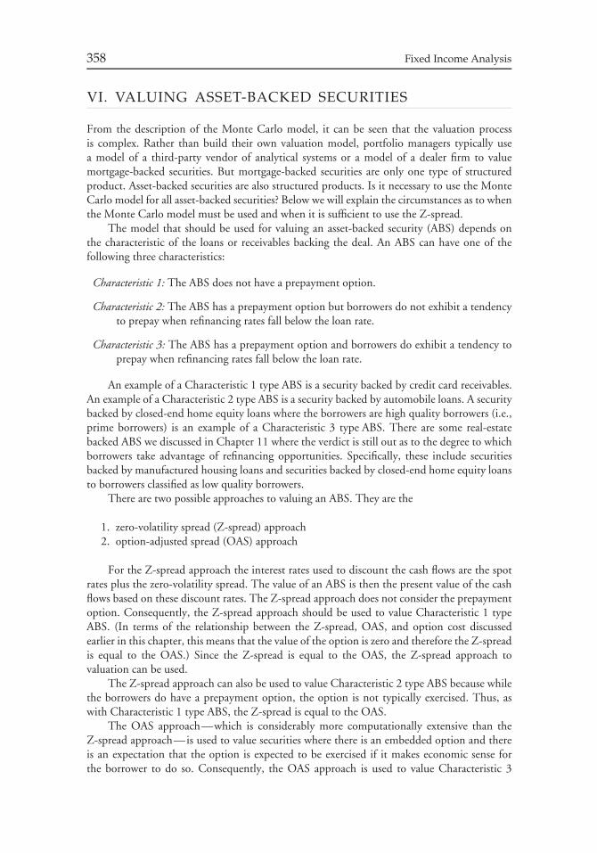
358 Fixed Income Analysis
VI. VALUING ASSET-BACKED SECURITIES
From the description of the Monte Carlo model, it can be seen that the valuation processis complex. Rather than build their own valuation model, portfolio managers typically usea model of a third-party vendor of analytical systems or a model of a dealer firm to valuemortgage-backed securities. But mortgage-backed securities are only one type of structuredproduct. Asset-backed securities are also structured products. Is it necessary to use the MonteCarlo model for all asset-backed securities? Below we will explain the circumstances as to whenthe Monte Carlo model must be used and when it is sufficient to use the Z-spread.
The model that should be used for valuing an asset-backed security (ABS) depends onthe characteristic of the loans or receivables backing the deal. An ABS can have one of thefollowing three characteristics:
Characteristic 1: The ABS does not have a prepayment option.
Characteristic 2: The ABS has a prepayment option but borrowers do not exhibit a tendencyto prepay when refinancing rates fall below the loan rate.
Characteristic 3: The ABS has a prepayment option and borrowers do exhibit a tendency toprepay when refinancing rates fall below the loan rate.
An example of a Characteristic 1 type ABS is a security backed by credit card receivables.An example of a Characteristic 2 type ABS is a security backed by automobile loans. A securitybacked by closed-end home equity loans where the borrowers are high quality borrowers (i.e.,prime borrowers) is an example of a Characteristic 3 type ABS. There are some real-estatebacked ABS we discussed in Chapter 11 where the verdict is still out as to the degree to whichborrowers take advantage of refinancing opportunities. Specifically, these include securitiesbacked by manufactured housing loans and securities backed by closed-end home equity loansto borrowers classified as low quality borrowers.
There are two possible approaches to valuing an ABS. They are the
1. zero-volatility spread (Z-spread) approach2. option-adjusted spread (OAS) approach
For the Z-spread approach the interest rates used to discount the cash flows are the spotrates plus the zero-volatility spread. The value of an ABS is then the present value of the cashflows based on these discount rates. The Z-spread approach does not consider the prepaymentoption. Consequently, the Z-spread approach should be used to value Characteristic 1 typeABS. (In terms of the relationship between the Z-spread, OAS, and option cost discussedearlier in this chapter, this means that the value of the option is zero and therefore the Z-spreadis equal to the OAS.) Since the Z-spread is equal to the OAS, the Z-spread approach tovaluation can be used.
The Z-spread approach can also be used to value Characteristic 2 type ABS because whilethe borrowers do have a prepayment option, the option is not typically exercised. Thus, aswith Characteristic 1 type ABS, the Z-spread is equal to the OAS.
The OAS approach—which is considerably more computationally extensive than theZ-spread approach—is used to value securities where there is an embedded option and thereis an expectation that the option is expected to be exercised if it makes economic sense forthe borrower to do so. Consequently, the OAS approach is used to value Characteristic 3

Chapter 12 Valuing Mortgage-Backed and Asset-Backed Securities 359
type ABS. The choice is then whether to use the binomial model (or a comparable model)or the Monte Carlo simulation model. Since typically the cash flow for an ABS with aprepayment option is interest rate path dependent—as with a mortgage-backed security—theMonte Carlo simulation model is used.
VII. VALUING ANY SECURITY
We conclude this chapter with a summary of the approaches to valuing any fixed incomesecurity using the two approaches that we discussed in the previous section—the Z-spreadapproach and the OAS approach.
Below we match the valuation approach with the type of security.
1. For an option-free bond the correct approach is the Z-spread approach.2. For a bond with an embedded option where the cash flow is not interest rate path dependent
(such as a callable corporate or agency debenture bond or a putable bond) the correctapproach is the OAS approach. Since the backward induction method can be used forsuch bonds, the binomial model or its equivalent should be used.
3. For a bond with an embedded option where the cash flow is interest rate path dependent(such as a mortgage-backed security or certain real estate-backed ABS) the correctapproach is the OAS approach. However, because of the interest rate path dependencyof the cash flow, the Monte Carlo simulation model should be used.
CHAPTER 13INTEREST RATE
DERIVATIVE INSTRUMENTS
I. INTRODUCTION
In this chapter we turn our attention to financial contracts that are popularly referred to asinterest rate derivative instruments because they derive their value from some cash marketinstrument or reference interest rate. These instruments include futures, forwards, options,swaps, caps, and floors. In this chapter we will discuss the basic features of these instrumentsand in the next we will see how they are valued.
Why would a portfolio manager be motivated to use interest rate derivatives rather thanthe corresponding cash market instruments. There are three principal reasons for doing thiswhen there is a well-developed interest rate derivatives market for a particular cash marketinstrument. First, typically it costs less to execute a transaction or a strategy in the interest ratederivatives market in order to alter the interest rate risk exposure of a portfolio than to makethe adjustment in the corresponding cash market. Second, portfolio adjustments typicallycan be accomplished faster in the interest rate derivatives market than in the correspondingcash market. Finally, interest rate derivative may be able to absorb a greater dollar transactionamount without an adverse effect on the price of the derivative instrument compared to theprice effect on the cash market instrument; that is, the interest rate derivative may be moreliquid than the cash market. To summarize: There are three potential advantages that motivatethe use of interest rate derivatives: cost, speed, and liquidity.
II. INTEREST RATE FUTURES
A futures contract is an agreement that requires a party to the agreement either to buy or sellsomething at a designated future date at a predetermined price. Futures contracts are productscreated by exchanges. Futures contracts based on a financial instrument or a financial indexare known as financial futures. Financial futures can be classified as (1) stock index futures,(2) interest rate futures, and (3) currency futures. Our focus in this chapter is on interestrate futures.
A. Mechanics of Futures Trading
A futures contract is an agreement between a buyer (seller) and an established exchange orits clearinghouse in which the buyer (seller) agrees to take (make) delivery of something (theunderlying) at a specified price at the end of a designated period of time. The price at which
360
Chapter 13 Interest Rate Derivative Instruments 361
the parties agree to transact in the future is called the futures price. The designated date atwhich the parties must transact is called the settlement date or delivery date.
1. Liquidating a Position Most financial futures contracts have settlement dates in themonths of March, June, September, and December. This means that at a predetermined timein the contract settlement month the contract stops trading, and a price is determined by theexchange for settlement of the contract. The contract with the closest settlement date is calledthe nearby futures contract. The next futures contract is the one that settles just after thenearby futures contract. The contract farthest away in time from settlement is called the mostdistant futures contract.
A party to a futures contract has two choices on liquidation of the position. First, theposition can be liquidated prior to the settlement date. For this purpose, the party must takean offsetting position in the same contract. For the buyer of a futures contract, this meansselling the same number of the identical futures contracts; for the seller of a futures contract,this means buying the same number of identical futures contracts.
The alternative is to wait until the settlement date. At that time the party purchasing afutures contract accepts delivery of the underlying at the agreed-upon price; the party thatsells a futures contract liquidates the position by delivering the underlying at the agreed-uponprice. For some interest rate futures contracts, settlement is made in cash only. Such contractsare referred to as cash settlement contracts.
2. The Role of the Clearinghouse Associated with every futures exchange is a clearing-house, which performs several functions. One of these functions is to guarantee that the twoparties to the transaction will perform.
When an investor takes a position in the futures market, the clearinghouse takes theopposite position and agrees to satisfy the terms set forth in the contract. Because of theclearinghouse, the investor need not worry about the financial strength and integrity ofthe party taking the opposite side of the contract. After initial execution of an order, therelationship between the two parties ends. The clearinghouse interposes itself as the buyer forevery sale and the seller for every purchase. Thus investors are free to liquidate their positionswithout involving the other party in the original contract, and without worrying that the otherparty may default. This is the reason that we define a futures contract as an agreement betweena party and a clearinghouse associated with an exchange. Besides its guarantee function, theclearinghouse makes it simple for parties to a futures contract to unwind their positions priorto the settlement date.
3. Margin Requirements When a position is first taken in a futures contract, theinvestor must deposit a minimum dollar amount per contract as specified by the exchange.This amount is called initial margin and is required as deposit for the contract. The initialmargin may be in the form of an interest-bearing security such as a Treasury bill. As theprice of the futures contract fluctuates, the value of the margin account changes. Markingto market means effectively replacing the initiation price with a current settlement price.The contract thus has a new settlement price. At the end of each trading day, the exchangedetermines the current settlement price for the futures contract. This price is used to markto market the investor’s position, so that any gain or loss from the position is reflectedin the margin account.1
1For a further discussion of margin requirements and illustrations of how the margin accountchanges as the futures price changes, see Don M. Chance, Analysis of Derivatives for the CFA

362 Fixed Income Analysis
Maintenance margin is the minimum level (specified by the exchange) to which themargin account may fall to as a result of an unfavorable price movement before the investoris required to deposit additional margin. The additional margin deposited is called variationmargin, and it is an amount necessary to bring the account back to its initial margin level.This amount is determined from the process of marking the position to market. Unlike initialmargin, variation margin must be in cash, not interest-bearing instruments. Any excess marginin the account may be withdrawn by the investor. If a party to a futures contract who isrequired to deposit variation margin fails to do so within 24 hours, the futures position isclosed out.
Although there are initial and maintenance margin requirements for buying securities onmargin, the concept of margin differs for securities and futures. When securities are acquiredon margin, the difference between the price of the security and the initial margin is borrowedfrom the broker. The security purchased serves as collateral for the loan, and the investor paysinterest. For futures contracts, the initial margin, in effect, serves as ‘‘good faith’’ money, anindication that the investor will satisfy the obligation of the contract.
B. Forward Contracts
A forward contract, just like a futures contract, is an agreement for the future delivery ofsomething at a specified price at the end of a designated period of time. Futures contractsare standardized agreements as to the delivery date (or month) and quality of the deliverable,and are traded on organized exchanges. A forward contract differs in that it is usually non-standardized (that is, the terms of each contract are negotiated individually between buyer andseller), there is no clearinghouse, and secondary markets are often non-existent or extremelythin. Unlike a futures contract, which is an exchange-traded product, a forward contract is anover-the-counter instrument.
Futures contracts are marked to market at the end of each trading day. Consequently,futures contracts are subject to interim cash flows as additional margin may be required inthe case of adverse price movements, or as cash is withdrawn in the case of favorable pricemovements. A forward contract may or may not be marked to market, depending on the wishesof the two parties. For a forward contract that is not marked to market, there are no interimcash flow effects because no additional margin is required.
Finally, the parties in a forward contract are exposed to credit risk because either partymay default on its obligation. This risk is called counterparty risk. This risk is minimal in thecase of futures contracts because the clearinghouse associated with the exchange guarantees theother side of the transaction. In the case of a forward contract, both parties face counterpartyrisk. Thus, there exists bilateral counterparty risk.
Other than these differences, most of what we say about futures contracts applies equallyto forward contracts.
C. Risk and Return Characteristics of Futures Contracts
When an investor takes a position in the market by buying a futures contract, the investor issaid to be in along position or to belong futures. The buyer of the futures contract is also
Program (Charlottesville, VA: Association for Investment Management and Research, 2003), pp.86–91.
Chapter 13 Interest Rate Derivative Instruments 363
referred to as the ‘‘long.’’ If, instead, the investor’s opening position is the sale of a futurescontract, the investor is said to be in a short position or to be short futures. The seller of thefutures contract is also referred to as the ‘‘short.’’ The buyer of a futures contract will realizea profit if the futures price increases; the seller of a futures contract will realize a profit if thefutures price decreases.
When a position is taken in a futures contract, the party need not put up the entireamount of the investment. Instead, only initial margin must be put up. Consequently, aninvestor can effectively create a leveraged position by using futures. At first, the leverageavailable in the futures market may suggest that the market benefits only those who wantto speculate on price movements. This is not true. As we shall see, futures markets canbe used to control interest rate risk. Without the effective leverage possible in futurestransactions, the cost of reducing price risk using futures would be too high for many marketparticipants.
D. Exchange-Traded Interest Rate Futures Contracts
Interest rate futures contracts can be classified by the maturity of their underlying security.Short-term interest rate futures contracts have an underlying security that matures in lessthan one year. Examples of these are futures contracts in which the underlying is a 3-month Treasury bill and a 3-month Eurodollar certificate of deposit. The maturity of theunderlying security of long-term futures contracts exceeds one year. Examples of these arefutures contracts in which the underlying is a Treasury coupon security, a 10-year agencynote, and a municipal bond index. Our focus will be on futures contracts in which theunderlying is a Treasury coupon security (a Treasury bond or a Treasury note). Thesecontracts are the most widely used by managers of bond portfolios and we begin with thespecifications of the Treasury bond futures contract. We will also discuss the agency notefutures contracts.
There are futures contracts on non-U.S. government securities traded throughout theworld. Many of them are modeled after the U.S. Treasury futures contracts and consequently,the concepts discussed below apply directly to those futures contracts.
1. Treasury Bond Futures The Treasury bond futures contract is traded on the ChicagoBoard of Trade (CBOT). The underlying instrument for a Treasury bond futures contractis $100,000 par value of a hypothetical 20-year coupon bond. The coupon rate on thehypothetical bond is called the notional coupon.
The futures price is quoted in terms of par being 100. Quotes are in 32nds of 1%.Thus a quote for a Treasury bond futures contract of 97–16 means 97 and 16/32 or 97.50.So, if a buyer and seller agree on a futures price of 97–16, this means that the buyer agreesto accept delivery of the hypothetical underlying Treasury bond and pay 97.50% of parvalue and the seller agrees to accept 97.50% of par value. Since the par value is $100,000,the futures price that the buyer and seller agree to for this hypothetical Treasury bond is$97,500.
The minimum price fluctuation for the Treasury bond futures contract is 1/32 of 1%,which is referred to as ‘‘a 32nd.’’ The dollar value of a 32nd for $100,000 par value (the parvalue for the underlying Treasury bond) is $31.25. Thus, the minimum price fluctuation is$31.25 for this contract.
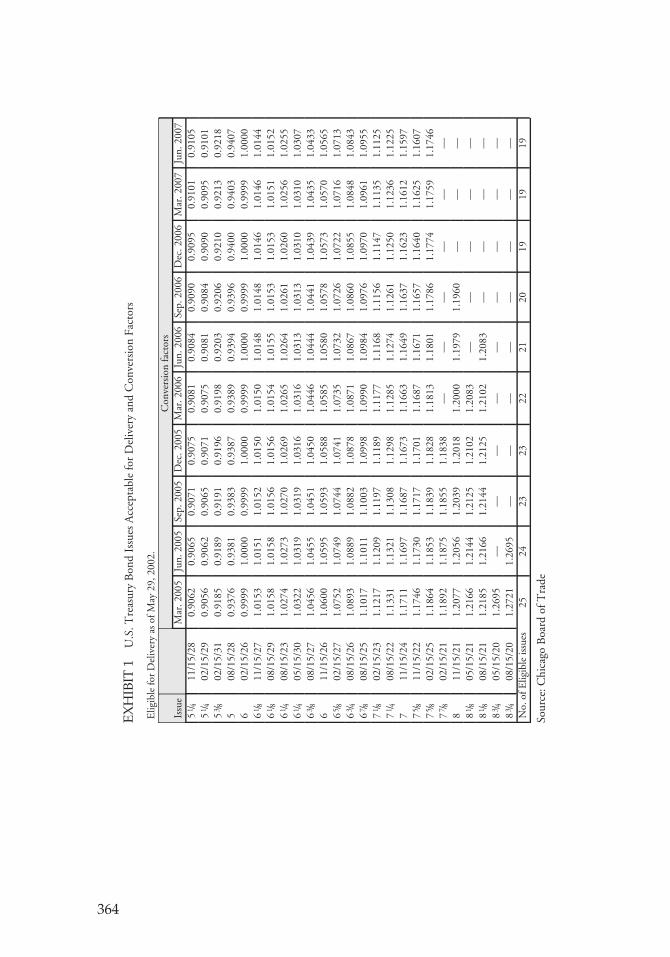
EX
HIB
IT1
U.S
.Tre
asur
yB
ond
Issu
esA
ccep
tabl
efo
rD
eliv
ery
and
Con
vers
ion
Fact
ors
Elig
ible
for
Del
iver
yas
ofM
ay29
,200
2.C
onve
rsio
nfa
ctor
sIs
sue
Mar
.200
5Ju
n.20
05Se
p.20
05D
ec.2
005
Mar
.200
6Ju
n.20
06Se
p.20
06D
ec.2
006
Mar
.200
7Ju
n.20
075
1 / 411
/15/
280.
9062
0.90
650.
9071
0.90
750.
9081
0.90
840.
9090
0.90
950.
9101
0.91
055
1 / 402
/15/
290.
9056
0.90
620.
9065
0.90
710.
9075
0.90
810.
9084
0.90
900.
9095
0.91
015
3 / 802
/15/
310.
9185
0.91
890.
9191
0.91
960.
9198
0.92
030.
9206
0.92
100.
9213
0.92
185
08/1
5/28
0.93
760.
9381
0.93
830.
9387
0.93
890.
9394
0.93
960.
9400
0.94
030.
9407
602
/15/
260.
9999
1.00
000.
9999
1.00
000.
9999
1.00
000.
9999
1.00
000.
9999
1.00
006
1 / 811
/15/
271.
0153
1.01
511.
0152
1.01
501.
0150
1.01
481.
0148
1.01
461.
0146
1.01
446
1 / 808
/15/
291.
0158
1.01
581.
0156
1.01
561.
0154
1.01
551.
0153
1.01
531.
0151
1.01
526
1 / 408
/15/
231.
0274
1.02
731.
0270
1.02
691.
0265
1.02
641.
0261
1.02
601.
0256
1.02
556
1 / 405
/15/
301.
0322
1.03
191.
0319
1.03
161.
0316
1.03
131.
0313
1.03
101.
0310
1.03
076
3 / 808
/15/
271.
0456
1.04
551.
0451
1.04
501.
0446
1.04
441.
0441
1.04
391.
0435
1.04
336
11/1
5/26
1.06
001.
0595
1.05
931.
0588
1.05
851.
0580
1.05
781.
0573
1.05
701.
0565
65 / 8
02/1
5/27
1.07
521.
0749
1.07
441.
0741
1.07
351.
0732
1.07
261.
0722
1.07
161.
0713
63 / 4
08/1
5/26
1.08
931.
0889
1.08
821.
0878
1.08
711.
0867
1.08
601.
0855
1.08
481.
0843
67 / 8
08/1
5/25
1.10
171.
1011
1.10
031.
0998
1.09
901.
0984
1.09
761.
0970
1.09
611.
0955
71 / 8
02/1
5/23
1.12
171.
1209
1.11
971.
1189
1.11
771.
1168
1.11
561.
1147
1.11
351.
1125
71 / 4
08/1
5/22
1.13
311.
1321
1.13
081.
1298
1.12
851.
1274
1.12
611.
1250
1.12
361.
1225
711
/15/
241.
1711
1.16
971.
1687
1.16
731.
1663
1.16
491.
1637
1.16
231.
1612
1.15
977
5 / 811
/15/
221.
1746
1.17
301.
1717
1.17
011.
1687
1.16
711.
1657
1.16
401.
1625
1.16
077
5 / 802
/15/
251.
1864
1.18
531.
1839
1.18
281.
1813
1.18
011.
1786
1.17
741.
1759
1.17
467
7 / 802
/15/
211.
1892
1.18
751.
1855
1.18
38—
——
——
—8
11/1
5/21
1.20
771.
2056
1.20
391.
2018
1.20
001.
1979
1.19
60—
——
81 / 8
05/1
5/21
1.21
661.
2144
1.21
251.
2102
1.20
83—
——
——
81 / 8
08/1
5/21
1.21
851.
2166
1.21
441.
2125
1.21
021.
2083
——
——
83 / 4
05/1
5/20
1.26
95—
——
——
——
——
83 / 4
08/1
5/20
1.27
211.
2695
——
——
——
——
No.
ofE
ligib
leis
sues
2524
2323
2221
2019
1919
Sour
ce:C
hica
goB
oard
ofT
rade
364
Chapter 13 Interest Rate Derivative Instruments 365
We have been referring to the underlying as a hypothetical Treasury bond. The seller of aTreasury bond futures contract who decides to make delivery rather than liquidate the positionby buying back the contract prior to the settlement date must deliver some Treasury bondissue. But what Treasury bond issue? The CBOT allows the seller to deliver one of severalTreasury bonds that the CBOT designates as acceptable for delivery. The specific issues thatthe seller may deliver are published by the CBOT for all contracts by settlement date. TheCBOT makes its determination of the Treasury bond issues that are acceptable for deliveryfrom all outstanding Treasury bond issues that have at least 15 years to maturity from the dateof delivery.
Exhibit 1 shows the Treasury bond issues that the seller could have selected to deliver tothe buyer of the CBOT Treasury bond futures contract as of May 29, 2002. Should the U.S.Department of the Treasury issue any Treasury bonds that meet the CBOT criteria for eligibledelivery, those issues would be added to the list. Notice that for the Treasury bond futurescontract settling (i.e., maturing) in March 2005, notice that there are 25 eligible issues. Forcontracts settling after March 2005, there are fewer than 25 eligible issues due to the shortermaturity of each previous eligible issue that results in a maturity of less than 15 years.
Although the underlying Treasury bond for this contract is a hypothetical issue andtherefore cannot itself be delivered into the futures contract, the contract is not a cashsettlement contract. The only way to close out a Treasury bond futures contract is toeither initiate an offsetting futures position, or to deliver a Treasury bond issue satisfyingthe above-mentioned criteria into the futures contract.
a. Conversion Factors The delivery process for the Treasury bond futures contract makesthe contract interesting. At the settlement date, the seller of a futures contract (the short) isnow required to deliver to the buyer (the long) $100,000 par value of a 6% 20-year Treasurybond. Since no such bond exists, the seller must choose from one of the acceptable deliverableTreasury bonds that the CBOT has specified. Suppose the seller is entitled to deliver $100,000of a 5% 20-year Treasury bond to settle the futures contract. The value of this bond is lessthan the value of a 6% 20-year bond. If the seller delivers the 5% 20-year bond, this wouldbe unfair to the buyer of the futures contract who contracted to receive $100,000 of a 6%20-year Treasury bond. Alternatively, suppose the seller delivers $100,000 of a 7% 20-yearTreasury bond. The value of a 7% 20-year Treasury bond is greater than that of a 6% 20-yearbond, so this would be a disadvantage to the seller.
How can this problem be resolved? To make delivery equitable to both parties, the CBOThas introduced conversion factors for adjusting the price of each Treasury issue that can bedelivered to satisfy the Treasury bond futures contract. The conversion factor is determinedby the CBOT before a contract with a specific settlement date begins trading.2 The adjustedprice is found by multiplying the conversion factor by the futures price. The adjusted price iscalled the converted price.
Exhibit 1 shows conversion factors as of May 29, 2002. The conversion factors are shownby contract settlement date. Note that the conversion factor depends not only on the issuedelivered but also on the settlement date of the contract. For example, look at the first issue inExhibit 1, the 51/4% coupon bond maturing 11/15/28. For the Treasury bond futures contractsettling (i.e., maturing) in March 2005, the conversion factor is 0.9062. For the December2005 contract, the conversion factor is 0.9075.
2The conversion factor is based on the price that a deliverable bond would sell for at the beginning ofthe delivery month if it were to yield 6%.
366 Fixed Income Analysis
The price that the buyer must pay the seller when a Treasury bond is delivered is calledthe invoice price. The invoice price is the futures settlement price plus accrued interest.However, as just noted, the seller can deliver one of several acceptable Treasury issues andto make delivery fair to both parties, the invoice price must be adjusted based on the actualTreasury issue delivered. It is the conversion factors that are used to adjust the invoice price.The invoice price is:
invoice price = contract size × futures settlement price × conversion factor
+ accrued interest
Suppose the Treasury March 2006 futures contract settles at 105–16 and that the issuedelivered is the 8% of 11/15/21. The futures contract settlement price of 105–16 means105.5% of par value or 1.055 times par value. As indicated in Exhibit 1, the conversion factorfor this issue for the March 2006 contract is 1.2000. Since the contract size is $100,000, theinvoice price the buyer pays the seller is:
$100, 000 × 1.055 × 1.2000 + accrued interest = $126, 600 + accrued interest
b. Cheapest-to-Deliver Issue As can be seen in Exhibit 1, there can be more than oneissue that is permitted to be delivered to satisfy a futures contract. In fact, for the March 2005contract, there are 25 deliverable or eligible bond issues. It is the short that has the optionof selecting which one of the deliverable bond issues if he decides to deliver.3 The decisionof which one of the bond issues a short will elect to deliver is not made arbitrarily. There isan economic analysis that a short will undertake in order to determine the best bond issueto deliver. In fact, as we will see, all of the elements that go into the economic analysis willbe the same for all participants in the market who are either electing to deliver or who areanticipating delivery of one of the eligible bond issues. In this section, how the best bond issueto deliver is determined will be explained.
The economic analysis is not complicated. The basic principle is as follows. Suppose thatan investor enters into the following two transactions simultaneously:
1. buys one of the deliverable bond issues today with borrowed money and2. sells a futures contract
The two positions (i.e., the long position in the deliverable bond issue purchased and theshort position in the futures contract) will be held to the delivery date. At the delivery date,the bond issue purchased will be used to satisfy the short’s obligation to deliver an eligiblebond issue. The simultaneous transactions above and the delivery of the acceptable bond issuepurchased to satisfy the short position in the futures contract is called a cash and carry trade.We will discuss this in more detail in the next chapter where the importance of selecting thebest bond issue to deliver for the pricing of a futures contract is explained.
Let’s look at the economics of this cash and carry trade. The investor (who by virtue ofthe fact that he sold a futures contract is the short), has synthetically created a short-terminvestment vehicle. The reason is that the investor has purchased a bond issue (one of the
3Remember that the short can always unwind his position by buying the same futures contract beforethe settlement date.

Chapter 13 Interest Rate Derivative Instruments 367
deliverable bond issues) and at the delivery date delivers that bond issue and receives thefutures price. So, the investor knows the cost of buying the bond issue and knows how muchwill be received from the investment. The amount received is the coupon interest until thedelivery date, any reinvestment income from reinvesting coupon payments, and the futuresprice at the delivery date. (Remember that the futures price at the delivery date for a givendeliverable bond issue will be its converted price.) Thus, the investor can calculate the rate ofreturn that will be earned on the investment. In the futures market, this rate of return is calledthe implied repo rate.
An implied repo rate can be calculated for every deliverable bond issue. For example,suppose that there are N deliverable bond issues that can be delivered to satisfy a bond futurescontract. Market participants who want to know either the best issue to deliver or what issue islikely to be delivered will calculate an implied repo rate for all N eligible bond issues. Whichwould be the best issue to deliver by a short? Since the implied repo rate is the rate of returnon an investment, the best bond issue is the one that has the highest implied repo rate (i.e.,the highest rate of return). The bond issue with the highest implied repo rate is called thecheapest-to-deliver issue.
Now that we understand the economic principle for determining the best bond issue todeliver (i.e., the cheapest-to-deliver issue), let’s look more closely at how one calculates theimplied repo rate for each deliverable bond issue. This rate is computed using the followinginformation for a given deliverable bond issue:
1. the price plus accrued interest at which the Treasury issue could be purchased2. the converted price plus the accrued interest that will be received upon delivery of that
Treasury bond issue to satisfy the short futures position3. the coupon payments that will be received between today and the date the issue is
delivered to satisfy the futures contract.4. the reinvestment income that will be realized on the coupon payments between the time
the interim coupon payment is received and the date that the issue is delivered to satisfythe Treasury bond futures contract.
The first three elements are known. The last element will depend on the reinvestment ratethat can be earned. While the reinvestment rate is unknown, typically this is a small part ofthe rate of return and not much is lost by assuming that the implied repo rate can be predictedwith certainty.
The general formula for the implied repo rate is as follows:
implied repo rate = dollar return
cost of the investment× 360
days1
where days1 is equal to the number of days until settlement of the futures contract. Below wewill explain the other components in the formula for the implied repo rate.
Let’s begin with the dollar return. The dollar return for an issue is the difference betweenthe proceeds received and the cost of the investment. The proceeds received are equal to theproceeds received at the settlement date of the futures contract and any interim coupon paymentplus interest from reinvesting the interim coupon payment. The proceeds received at the settle-ment date include the converted price (i.e., futures settlement price multiplied by the conversionfactor for the issue) and the accrued interest received from delivery of the issue. That is,
368 Fixed Income Analysis
proceeds received = converted price + accrued interest received + interim coupon payment
+ interest from reinvesting the interim coupon payment
As noted earlier, all of the elements are known except the interest from reinvesting theinterim coupon payment. This amount is estimated by assuming that the coupon paymentcan be reinvested at the term repo rate. Later, we describe the repo market and the term reporate. The term repo rate is not only a borrowing rate for an investor who wants to borrowin the repo market but also the rate at which an investor can invest proceeds on a short-termbasis. For how long is the reinvestment of the interim coupon payment? It is the number ofdays from when the interim coupon payment is received and the actual delivery date to satisfythe futures contract. The reinvestment income is then computed as follows:
interest from reinvesting the interim coupon payment
= interim coupon × term repo rate × (days2/360)
where
days2 = number of days between when the interim coupon payment is received and
the actual delivery date of the futures contract
The reason for dividing days2 by 360 is that the ratio represents the number of days theinterim coupon is reinvested as a percentage of the number of days in a year as measured inthe money market.
The cost of the investment is the amount paid to purchase the issue. This cost is equal tothe purchase price plus accrued interest paid. That is,
cost of the investment = purchase price + accrued interest paid
Thus, the dollar return for the numerator of the formula for the implied repo rate isequal to
dollar return = proceeds received − cost of the investment
The dollar return is then divided by the cost of the investment.4
So, now we know how to compute the numerator and the denominator in the formulafor the implied repo rate. The second ratio in the formula for the implied repo rate simplyinvolves annualizing the return using a convention in the money market for the number ofdays. (Recall that in the money market the convention is to use a 360 day year.) Since theinvestment resulting from the cash and carry trade is a synthetic money market instrument,360 days are used.
Let’s compute the implied repo rate for a hypothetical issue that may be delivered tosatisfy a hypothetical Treasury bond futures contract. Assume the following for the deliverableissue and the futures contract:
4Actually, the cost of the investment should be adjusted because the amount that the investor ties up inthe investment is reduced if there is an interim coupon payment. We will ignore this adjustment here.
Chapter 13 Interest Rate Derivative Instruments 369
Futures contract
futures price = 96
days to futures delivery date (days1) = 82 days
Deliverable issue
price of issue = 107accrued interest paid = 3.8904coupon rate = 10%days remaining before interim coupon paid = 40 daysinterim coupon = $5number of days between when the interim coupon payment is received and
the actual delivery date of the futures contract (days2) = 42conversion factor = 1.1111accrued interest received at futures settlement date = 1.1507
Other information:
42-day term repo rate = 3.8%
Let’s begin with the proceeds received. We need to compute the converted price and theinterest from reinvesting the interim coupon payment. The converted price is:
converted price = futures price × conversion factor
= 96 × 1.1111 = 106.6656
The interest from reinvesting the interim coupon payment depends on the term repo rate.The term repo rate is assumed to be 3.8%. Therefore,
interest from reinvesting the interim coupon payment = $5 × 0.038 ×(
42
360
)
= 0.0222
To summarize:
converted price = 106.6656accrued interest received at futures settlement date = 1.1507interim coupon payment = 5.0000interest from reinvesting the interim coupon payment = 0.0222proceeds received = 112.8385
The cost of the investment is the purchase price for the issue plus the accrued interestpaid, as shown below:
cost of the investment = 107 + 3.8904 = 110.8904
370 Fixed Income Analysis
EXHIBIT 2 Delivery Options Granted to the Short (Seller) of a CBOT Treasury Bond FuturesContract
Delivery option DescriptionQuality or swap option Choice of which acceptable Treasury issue to deliverTiming option Choice of when in delivery month to deliverWild card option Choice to deliver after the closing price of the futures contract
is determined
The implied repo rate is then:
implied repo rate = 112.8385 − 110.8904
110.8904× 360
82= 0.0771 = 7.71%
Once the implied repo rate is calculated for each deliverable issue, the cheapest-to-deliverissue will be the one that has the highest implied repo rate (i.e., the issue that gives themaximum return in a cash-and-carry trade). As explained in the next chapter, this issue playsa key role in the pricing of a Treasury bond futures contract.
While an eligible bond issue may be the cheapest to deliver today, changes in factorsmay cause some other eligible bond issue to be the cheapest to deliver at a future date. Asensitivity analysis can be performed to determine how a change in yield affects the cheapestto deliver.
c. Other Delivery Options In addition to the choice of which acceptable Treasury issueto deliver—sometimes referred to as the quality option or swap option—the short has atleast two more options granted under CBOT delivery guidelines. The short is permitted todecide when in the delivery month delivery actually will take place. This is called the timingoption. The other option is the right of the short to give notice of intent to deliver up to 8:00p.m. Chicago time after the closing of the exchange (3:15 p.m. Chicago time) on the datewhen the futures settlement price has been fixed. This option is referred to as the wild cardoption. The quality option, the timing option, and the wild card option (in sum referred toas the delivery options), mean that the long position can never be sure which Treasury bondwill be delivered or when it will be delivered. These three delivery options are summarized inExhibit 2.
d. Delivery Procedure For a short who wants to deliver, the delivery procedure involvesthree days. The first day is the position day. On this day, the short notifies the CBOT that itintends to deliver. The short has until 8:00 p.m. central standard time to do so. The second dayis the notice day. On this day, the short specifies which particular issue will be delivered. Theshort has until 2:00 p.m. central standard time to make this declaration. (On the last possiblenotice day in the delivery month, the short has until 3:00 p.m.) The CBOT then selects thelong to whom delivery will be made. This is the long position that has been outstanding forthe greatest period of time. The long is then notified by 4:00 p.m. that delivery will be made.The third day is the delivery day. By 10:00 a.m. on this day the short must have in its accountthe Treasury issue that it specified on the notice day and by 1:00 p.m. must deliver that bondto the long that was assigned by the CBOT to accept delivery. The long pays the short theinvoice price upon receipt of the bond.
Chapter 13 Interest Rate Derivative Instruments 371
2. Treasury Note Futures The three Treasury note futures contracts are 10-year, 5-year,and 2-year note contracts. All three contracts are modeled after the Treasury bond futurescontract and are traded on the CBOT.
The underlying instrument for the 10-year Treasury note futures contract is $100,000par value of a hypothetical 10-year, 6% Treasury note. Several acceptable Treasury issues maybe delivered by the short. An issue is acceptable if the maturity is not less than 6.5 years andnot greater than 10 years from the first day of the delivery month. Delivery options are grantedto the short position.
For the 5-year Treasury note futures contract, the underlying is $100,000 par valueof a 6% notional coupon U.S. Treasury note that satisfies the following conditions: (1) anoriginal maturity of not more than 5 years and 3 months, (2) a remaining maturity nogreater than 5 years and 3 months, and (3) a remaining maturity not less than 4 years and 2months.
The underlying for the 2-year Treasury note futures contract is $200,000 par value of a6% notional coupon U.S. Treasury note with a remaining maturity of not more than 2 yearsand not less than 1 year and 9 months. Moreover, the original maturity of the note deliveredto satisfy the 2-year futures cannot be more than 5 years and 3 months.
3. Agency Note Futures Contract In 2000, the CBOT and the Chicago MercantileExchange (CME) began trading in futures contracts in which the underlying is a Fannie Mae orFreddie Mac agency debenture security. (Agency debentures are explained in Chapter 3.) Theunderlying for the CBOT 10-year agency note futures contract is a Fannie Mae benchmarknote or Freddie Mac reference note having a par value of $100,000 and a notional coupon of6%. The 10-year agency note futures contract of the CME is similar to that of the CBOT,but has a notional coupon of 6.5% instead of 6%.
As with the Treasury futures contract, more than one issue is deliverable for both theCBOT and CME agency note futures contract. The contract delivery months are March, June,September, and December. As with the Treasury futures contract a conversion factor appliesto each eligible issue for each contract settlement date. Because many issues are deliverable,one issue is the cheapest-to-deliver issue. This issue is found in exactly the same way as withthe Treasury futures contract.
III. INTEREST RATE OPTIONS
An option is a contract in which the writer of the option grants the buyer of the option theright, but not the obligation, to purchase from or sell to the writer something at a specifiedprice within a specified period of time (or at a specified date). The writer, also referred to asthe seller, grants this right to the buyer in exchange for a certain sum of money, called theoption price or option premium. The price at which the underlying for the contract may bebought or sold is called the exercise price or strike price. The date after which an option isvoid is called the expiration date. Our focus is on options where the ‘‘something’’ underlyingthe option is an interest rate instrument or an interest rate.
When an option grants the buyer the right to purchase the designated instrument fromthe writer (seller), it is referred to as a call option, or call. When the option buyer has theright to sell the designated instrument to the writer, the option is called a put option, or put.

372 Fixed Income Analysis
An option is also categorized according to when the option buyer may exercise the option.There are options that may be exercised at any time up to and including the expiration date.Such an option is referred to as an American option. There are options that may be exercisedonly at the expiration date. An option with this feature is called a European option. Anoption that can be exercised prior to maturity but only on designated dates is called a modifiedAmerican, Bermuda, or Atlantic option.
A. Risk and Return Characteristics of Options
The maximum amount that an option buyer can lose is the option price. The maximum profitthat the option writer can realize is the option price at the time of sale. The option buyer hassubstantial upside return potential, while the option writer has substantial downside risk.
It is assumed in this chapter that the reader has an understanding of the basic positionsthat can be created with options. These positions include:
1. long call position (buying a call option)2. short call position (selling a call option)3. long put position (buying a put option)4. short put position (selling a put option)
Exhibit 3 shows the payoff profile for these four option positions assuming that each optionposition is held to the expiration date and not exercised early.
B. Differences Between Options and Futures Contracts
Unlike a futures contract, one party to an option contract is not obligated to transact.Specifically, the option buyer has the right, but not the obligation, to transact. The optionwriter does have the obligation to perform. In the case of a futures contract, both buyer andseller are obligated to perform. Of course, a futures buyer does not pay the seller to accept theobligation, while an option buyer pays the option seller an option price.
Consequently, the risk/reward characteristics of the two contracts are also different. In thecase of a futures contract, the buyer of the contract realizes a dollar-for-dollar gain whenthe price of the futures contract increases and suffers a dollar-for-dollar loss when the price ofthe futures contract drops. The opposite occurs for the seller of a futures contract. Optionsdo not provide this symmetric risk/reward relationship. The most that the buyer of an optioncan lose is the option price. While the buyer of an option retains all the potential benefits,the gain is always reduced by the amount of the option price. The maximum profit that thewriter may realize is the option price; this is compensation for accepting substantial downsiderisk.
Both parties to a futures contract are required to post margin. There are no marginrequirements for the buyer of an option once the option price has been paid in full. Becausethe option price is the maximum amount that the investor can lose, no matter how adverse theprice movement of the underlying, there is no need for margin. Because the writer of an optionhas agreed to accept all of the risk (and none of the reward) of the position in the underlying,the writer is generally required to put up the option price received as margin. In addition, asprice changes occur that adversely affect the writer’s position, the writer is required to depositadditional margin (with some exceptions) as the position is marked to market.
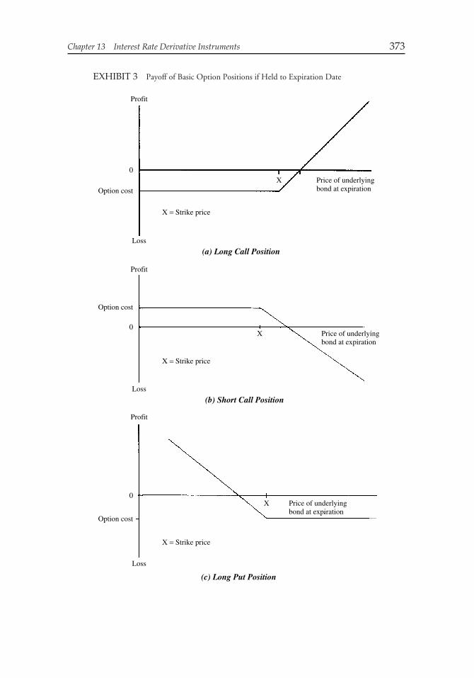
Chapter 13 Interest Rate Derivative Instruments 373
EXHIBIT 3 Payoff of Basic Option Positions if Held to Expiration Date
(a) Long Call Position
(b) Short Call Position
(c) Long Put Position
Profit
Option cost
X
X = Strike price
Price of underlyingbond at expiration
Loss
0
Option cost
0
Profit
Option cost
X
X = Strike price
X = Strike price
Price of underlyingbond at expiration
X Price of underlyingbond at expiration
Loss
Profit
Loss
0
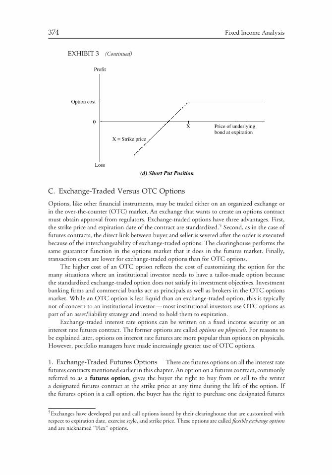
374 Fixed Income Analysis
EXHIBIT 3 (Continued)
(d) Short Put Position
Profit
Option cost
X
X = Strike price
Price of underlyingbond at expiration
Loss
0
C. Exchange-Traded Versus OTC Options
Options, like other financial instruments, may be traded either on an organized exchange orin the over-the-counter (OTC) market. An exchange that wants to create an options contractmust obtain approval from regulators. Exchange-traded options have three advantages. First,the strike price and expiration date of the contract are standardized.5 Second, as in the case offutures contracts, the direct link between buyer and seller is severed after the order is executedbecause of the interchangeability of exchange-traded options. The clearinghouse performs thesame guarantor function in the options market that it does in the futures market. Finally,transaction costs are lower for exchange-traded options than for OTC options.
The higher cost of an OTC option reflects the cost of customizing the option for themany situations where an institutional investor needs to have a tailor-made option becausethe standardized exchange-traded option does not satisfy its investment objectives. Investmentbanking firms and commercial banks act as principals as well as brokers in the OTC optionsmarket. While an OTC option is less liquid than an exchange-traded option, this is typicallynot of concern to an institutional investor—most institutional investors use OTC options aspart of an asset/liability strategy and intend to hold them to expiration.
Exchange-traded interest rate options can be written on a fixed income security or aninterest rate futures contract. The former options are called options on physicals. For reasons tobe explained later, options on interest rate futures are more popular than options on physicals.However, portfolio managers have made increasingly greater use of OTC options.
1. Exchange-Traded Futures Options There are futures options on all the interest ratefutures contracts mentioned earlier in this chapter. An option on a futures contract, commonlyreferred to as a futures option, gives the buyer the right to buy from or sell to the writera designated futures contract at the strike price at any time during the life of the option. Ifthe futures option is a call option, the buyer has the right to purchase one designated futures
5Exchanges have developed put and call options issued by their clearinghouse that are customized withrespect to expiration date, exercise style, and strike price. These options are called flexible exchange optionsand are nicknamed ‘‘Flex’’ options.
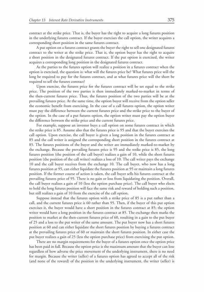
Chapter 13 Interest Rate Derivative Instruments 375
contract at the strike price. That is, the buyer has the right to acquire a long futures positionin the underlying futures contract. If the buyer exercises the call option, the writer acquires acorresponding short position in the same futures contract.
A put option on a futures contract grants the buyer the right to sell one designated futurescontract to the writer at the strike price. That is, the option buyer has the right to acquirea short position in the designated futures contract. If the put option is exercised, the writeracquires a corresponding long position in the designated futures contract.
As the parties to the futures option will realize a position in a futures contract when theoption is exercised, the question is: what will the futures price be? What futures price will thelong be required to pay for the futures contract, and at what futures price will the short berequired to sell the futures contract?
Upon exercise, the futures price for the futures contract will be set equal to the strikeprice. The position of the two parties is then immediately marked-to-market in terms ofthe then-current futures price. Thus, the futures position of the two parties will be at theprevailing futures price. At the same time, the option buyer will receive from the option sellerthe economic benefit from exercising. In the case of a call futures option, the option writermust pay the difference between the current futures price and the strike price to the buyer ofthe option. In the case of a put futures option, the option writer must pay the option buyerthe difference between the strike price and the current futures price.
For example, suppose an investor buys a call option on some futures contract in whichthe strike price is 85. Assume also that the futures price is 95 and that the buyer exercises thecall option. Upon exercise, the call buyer is given a long position in the futures contract at85 and the call writer is assigned the corresponding short position in the futures contract at85. The futures positions of the buyer and the writer are immediately marked-to-market bythe exchange. Because the prevailing futures price is 95 and the strike price is 85, the longfutures position (the position of the call buyer) realizes a gain of 10, while the short futuresposition (the position of the call writer) realizes a loss of 10. The call writer pays the exchange10 and the call buyer receives from the exchange 10. The call buyer, who now has a longfutures position at 95, can either liquidate the futures position at 95 or maintain a long futuresposition. If the former course of action is taken, the call buyer sells his futures contract at theprevailing futures price of 95. There is no gain or loss from liquidating the position. Overall,the call buyer realizes a gain of 10 (less the option purchase price). The call buyer who electsto hold the long futures position will face the same risk and reward of holding such a position,but still realizes a gain of 10 from the exercise of the call option.
Suppose instead that the futures option with a strike price of 85 is a put rather than acall, and the current futures price is 60 rather than 95. Then, if the buyer of this put optionexercises it, the buyer would have a short position in the futures contract at 85; the optionwriter would have a long position in the futures contract at 85. The exchange then marks theposition to market at the then-current futures price of 60, resulting in a gain to the put buyerof 25 and a loss to the put writer of the same amount. The put buyer now has a short futuresposition at 60 and can either liquidate the short futures position by buying a futures contractat the prevailing futures price of 60 or maintain the short futures position. In either case theput buyer realizes a gain of 25 (less the option purchase price) from exercising the put option.
There are no margin requirements for the buyer of a futures option once the option pricehas been paid in full. Because the option price is the maximum amount that the buyer can loseregardless of how adverse the price movement of the underlying instrument, there is no needfor margin. Because the writer (seller) of a futures option has agreed to accept all of the risk(and none of the reward) of the position in the underlying instrument, the writer (seller) is
376 Fixed Income Analysis
required to deposit not only the margin required on the interest rate futures contract positionbut also (with certain exceptions) the option price that is received from writing the option.
The price of a futures option is quoted in 64ths of 1% of par value. For example, a priceof 24 means 24/64 of 1% of par value. Since the par value of a Treasury bond futures contractis $100,000, an option price of 24 means: [(24/64)/100]× $100,000 = $375. In general, theprice of a futures option quoted at Q is equal to:
Option price =[
Q/64
100
]× $100, 000
There are three reasons that futures options have largely supplanted options on fixed incomesecurities as the options vehicle of choice for institutional investors who want to use exchange-traded options. First, unlike options on fixed income securities, options on Treasury couponfutures do not require payments for accrued interest to be made. Consequently, when afutures option is exercised, the call buyer and the put writer need not compensate the otherparty for accrued interest. Second, futures options are believed to be ‘‘cleaner’’ instrumentsbecause of the reduced likelihood of delivery squeezes. Market participants who must deliveran instrument are concerned that at the time of delivery the instrument to be delivered willbe in short supply, resulting in a higher price to acquire the instrument. As the deliverablesupply of futures contracts is infinite for futures options currently traded, there is no concernabout a delivery squeeze. Finally, in order to price any option, it is imperative to know at alltimes the price of the underlying instrument. In the bond market, current prices are not aseasily available as price information on the futures contract. The reason is that as bonds tradein the OTC market there is no single reporting system with recent price information. Thus,an investor who wanted to purchase an option on a Treasury bond would have to call severaldealer firms to obtain a price. In contrast, futures contracts are traded on an exchange and, asa result, price information is reported.
2. Over-the-Counter Options Institutional investors who want to purchase an optionon a specific Treasury security or a Ginnie Mae passthrough security can do so on an over-the-counter basis. There are government and mortgage-backed securities dealers who makea market in options on specific securities. OTC options, also called dealer options, usuallyare purchased by institutional investors who want to hedge the risk associated with a specificsecurity. For example, a thrift may be interested in hedging its position in a specific mortgagepassthrough security. Typically, the maturity of the option coincides with the time periodover which the buyer of the option wants to hedge, so the buyer is not concerned with theoption’s liquidity.
In the absence of a clearinghouse the parties to any over-the-counter contract are exposedto counterparty risk.6 In the case of forward contracts where both parties are obligated toperform, both parties face counterparty risk. In contrast, in the case of an option, once theoption buyer pays the option price, it has satisfied its obligation. It is only the seller that mustperform if the option is exercised. Thus, the option buyer is exposed to counterparty risk—therisk that the option seller will fail to perform.
6There are well-established institutional arrangements for mitigating counterparty risk in not onlyOTC options but also the other OTC derivatives described in this chapter (swaps, caps, and floors).These arrangement include limiting exposure to a specific counterparty, marking to market positions,collateralizing trades, and netting arrangement. For a discussion of these arrangements, see Chance,Analysis of Derivatives for the CFA Program, pp. 595–598.
Chapter 13 Interest Rate Derivative Instruments 377
OTC options can be customized in any manner sought by an institutional investor.Basically, if a dealer can reasonably hedge the risk associated with the opposite side of theoption sought, it will create the option desired by a customer. OTC options are not limitedto European or American type. Dealers also create modified American (Bermuda or Atlantic)type options.
IV. INTEREST RATE SWAPS
In an interest rate swap, two parties agree to exchange periodic interest payments. Thedollar amount of the interest payments exchanged is based on some predetermined dollarprincipal, which is called the notional principal or notional amount. The dollar amounteach counterparty pays to the other is the agreed-upon periodic interest rate times thenotional principal. The only dollars that are exchanged between the parties are the interestpayments, not the notional principal. In the most common type of swap, one party agreesto pay the other party fixed interest payments at designated dates for the life of thecontract. This party is referred to as the fixed-rate payer. The fixed rate that the fixed-rate payer must make is called the swap rate. The other party, who agrees to makeinterest rate payments that float with some reference rate, is referred to as the fixed-ratereceiver.
The reference rates that have been used for the floating rate in an interest rate swap arethose on various money market instruments: Treasury bills, the London interbank offeredrate, commercial paper, bankers acceptances, certificates of deposit, the federal funds rate, andthe prime rate. The most common is the London interbank offered rate (LIBOR). LIBORis the rate at which prime banks offer to pay on Eurodollar deposits available to other primebanks for a given maturity. Basically, it is viewed as the global cost of bank borrowing. Thereis not just one rate but a rate for different maturities. For example, there is a 1-month LIBOR,3-month LIBOR, 6-month LIBOR, etc.
To illustrate an interest rate swap, suppose that for the next five years party X agrees topay party Y 6% per year (the swap rate), while party Y agrees to pay party X 6-month LIBOR(the reference rate). Party X is the fixed-rate payer, while party Y is the fixed-rate receiver.Assume that the notional principal is $50 million, and that payments are exchanged every sixmonths for the next five years. This means that every six months, party X (the fixed-rate payer)will pay party Y $1.5 million (6% times $50 million divided by 2).7 The amount that partyY (the fixed-rate receiver) will pay party X will be 6-month LIBOR times $50 million dividedby 2. If 6-month LIBOR is 5% at the beginning of the 6-month period, party Y will payparty X $1.25 million (5% times $50 million divided by 2). Mechanically, the floating-rate isdetermined at the beginning of a period and paid in arrears—that is, it is paid at the end ofthe period. The two payments are actually netted out so that $0.25 million will be paid fromparty X to party Y. Note that we divide by two because one-half year’s interest is being paid.This is illustrated in panel a of Exhibit 4.
The convention that has evolved for quoting a swap rate is that a dealer sets the floatingrate equal to the reference rate and then quotes the fixed rate that will apply. The fixed rateis the swap rate and reflects a ‘‘spread’’ above the Treasury yield curve with the same term tomaturity as the swap. This spread is called the swap spread.
7In the next chapter we will fine tune our calculation to take into consideration day count conventionswhen computing swap payments.
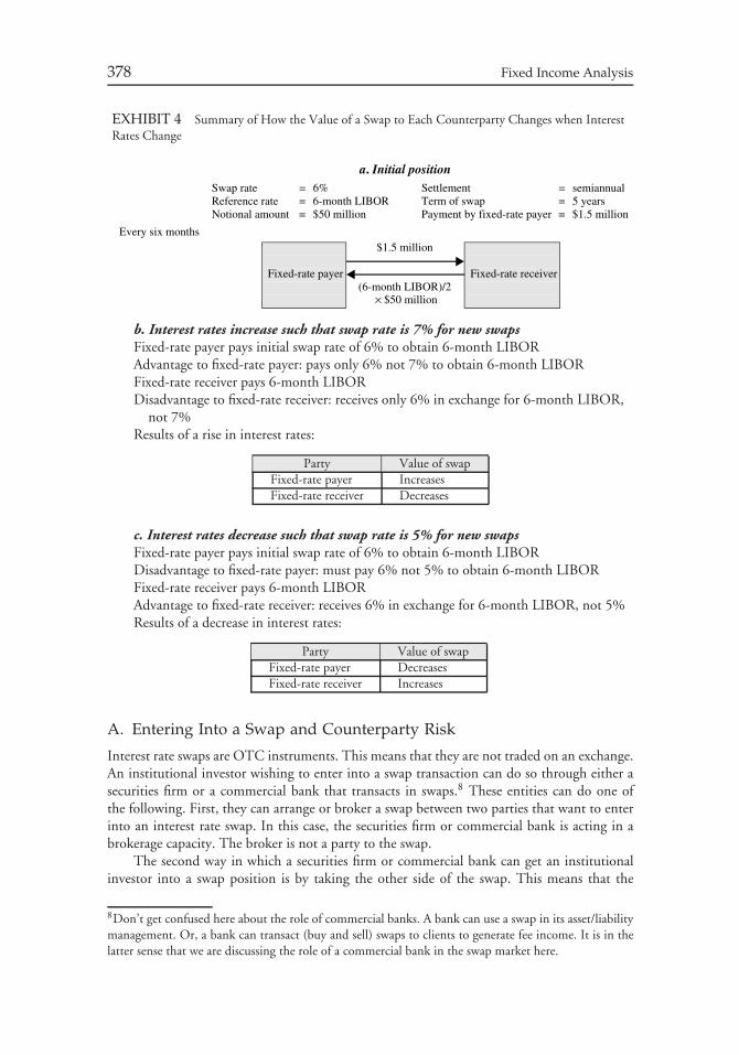
378 Fixed Income Analysis
EXHIBIT 4 Summary of How the Value of a Swap to Each Counterparty Changes when InterestRates Change
a. Initial position
Every six months
Swap rate = 6% Settlement = semiannualReference rate = 6-month LIBOR Term of swap = 5 yearsNotional amount = $50 million Payment by fixed-rate payer = $1.5 million
$1.5 million
Fixed-rate payer Fixed-rate receiver(6-month LIBOR)/2
× $50 million
b. Interest rates increase such that swap rate is 7% for new swapsFixed-rate payer pays initial swap rate of 6% to obtain 6-month LIBORAdvantage to fixed-rate payer: pays only 6% not 7% to obtain 6-month LIBORFixed-rate receiver pays 6-month LIBORDisadvantage to fixed-rate receiver: receives only 6% in exchange for 6-month LIBOR,
not 7%Results of a rise in interest rates:
Party Value of swapFixed-rate payer IncreasesFixed-rate receiver Decreases
c. Interest rates decrease such that swap rate is 5% for new swapsFixed-rate payer pays initial swap rate of 6% to obtain 6-month LIBORDisadvantage to fixed-rate payer: must pay 6% not 5% to obtain 6-month LIBORFixed-rate receiver pays 6-month LIBORAdvantage to fixed-rate receiver: receives 6% in exchange for 6-month LIBOR, not 5%Results of a decrease in interest rates:
Party Value of swapFixed-rate payer DecreasesFixed-rate receiver Increases
A. Entering Into a Swap and Counterparty Risk
Interest rate swaps are OTC instruments. This means that they are not traded on an exchange.An institutional investor wishing to enter into a swap transaction can do so through either asecurities firm or a commercial bank that transacts in swaps.8 These entities can do one ofthe following. First, they can arrange or broker a swap between two parties that want to enterinto an interest rate swap. In this case, the securities firm or commercial bank is acting in abrokerage capacity. The broker is not a party to the swap.
The second way in which a securities firm or commercial bank can get an institutionalinvestor into a swap position is by taking the other side of the swap. This means that the
8Don’t get confused here about the role of commercial banks. A bank can use a swap in its asset/liabilitymanagement. Or, a bank can transact (buy and sell) swaps to clients to generate fee income. It is in thelatter sense that we are discussing the role of a commercial bank in the swap market here.
Chapter 13 Interest Rate Derivative Instruments 379
securities firm or the commercial bank is a dealer rather than a broker in the transaction.Acting as a dealer, the securities firm or the commercial bank must hedge its swap positionin the same way that it hedges its position in other securities that it holds. Also it meansthat the dealer (which we refer to as a swap dealer) is the counterparty to the transaction.If an institutional investor entered into a swap with a swap dealer, the institutional investorwill look to the swap dealer to satisfy the obligations of the swap; similarly, that sameswap dealer looks to the institutional investor to fulfill its obligations as set forth in theswap.
The risk that the two parties take on when they enter into a swap is that the other partywill fail to fulfill its obligations as set forth in the swap agreement. That is, each party facesdefault risk and therefore there is bilateral counterparty risk.
B. Risk/Return Characteristics of an Interest Rate Swap
The value of an interest rate swap will fluctuate with market interest rates. As interest ratesrise, the fixed-rate payer is receiving a higher 6-month LIBOR (in our illustration). He wouldneed to pay more for a new swap. Let’s consider our hypothetical swap. Suppose that interestrates change immediately after parties X and Y enter into the swap. Panel a in Exhibit 4 showsthe transaction. First, consider what would happen if the market demanded that in any 5-yearswap the fixed-rate payer must pay 7% in order to receive 6-month LIBOR. If party X (thefixed-rate payer) wants to sell its position to party A, then party A will benefit by having to payonly 6% (the original swap rate agreed upon) rather than 7% (the current swap rate) to receive6-month LIBOR. Party X will want compensation for this benefit. Consequently, the valueof party X’s position has increased. Thus, if interest rates increase, the fixed-rate payer willrealize a profit and the fixed-rate receiver will realize a loss. Panel b in Exhibit 4 summarizesthe results of a rise in interest rates.
Next, consider what would happen if interest rates decline to, say, 5%. Now a 5-year swapwould require a new fixed-rate payer to pay 5% rather than 6% to receive 6-month LIBOR.If party X wants to sell its position to party B, the latter would demand compensation to takeover the position. In other words, if interest rates decline, the fixed-rate payer will realize a loss,while the fixed-rate receiver will realize a profit. Panel c in Exhibit 4 summarizes the results ofa decline in interest rates
While we know in what direction the change in the value of a swap will be for thecounterparties when interest rates change, the question is how much will the value of the swapchange. We show how to compute the change in the value of a swap in the next chapter.
C. Interpreting a Swap Position
There are two ways that a swap position can be interpreted: (1) a package of forward (futures)contracts and (2) a package of cash flows from buying and selling cash market instruments.
1. Package of Forward (Futures) Contracts Contrast the position of the counterpar-ties in an interest rate swap summarized above to the position of the long and short interestrate futures (forward) contract. The long futures position gains if interest rates declineand loses if interest rates rise—this is similar to the risk/return profile for a floating-ratepayer. The risk/return profile for a fixed-rate payer is similar to that of the short futuresposition: a gain if interest rates increase and a loss if interest rates decrease. By taking acloser look at the interest rate swap we can understand why the risk/return relationships aresimilar.
380 Fixed Income Analysis
Consider party X’s position in our previous swap illustration. Party X has agreedto pay 6% and receive 6-month LIBOR. More specifically, assuming a $50 millionnotional principal, X has agreed to buy a commodity called ‘‘6-month LIBOR’’ for$1.5 million. This is effectively a 6-month forward contract where X agrees to pay$1.5 million in exchange for delivery of 6-month LIBOR. If interest rates increase to7%, the price of that commodity (6-month LIBOR) is higher, resulting in a gain forthe fixed-rate payer, who is effectively long a 6-month forward contract on 6-monthLIBOR. The floating-rate payer is effectively short a 6-month forward contract on 6-monthLIBOR. There is therefore an implicit forward contract corresponding to each exchangedate.
Now we can see why there is a similarity between the risk/return relationship for aninterest rate swap and a forward contract. If interest rates increase to, say, 7%, the priceof that commodity (6-month LIBOR) increases to $1.75 million (7% times $50 milliondivided by 2). The long forward position (the fixed-rate payer) gains, and the short forwardposition (the floating-rate payer) loses. If interest rates decline to, say, 5%, the price of ourcommodity decreases to $1.25 million (5% times $50 million divided by 2). The short forwardposition (the floating-rate payer) gains, and the long forward position (the fixed-rate payer)loses.
Consequently, interest rate swaps can be viewed as a package of more basic interest ratederivatives, such as forwards.9 The pricing of an interest rate swap will then depend on theprice of a package of forward contracts with the same settlement dates in which the underlyingfor the forward contract is the same reference rate. We will make use of this principle in thenext chapter when we explain how to value swaps.
While an interest rate swap may be nothing more than a package of forward con-tracts, it is not a redundant contract for several reasons. First, maturities for forward orfutures contracts do not extend out as far as those of an interest rate swap; an inter-est rate swap with a term of 15 years or longer can be obtained. Second, an interestrate swap is a more transactionally efficient instrument. By this we mean that in onetransaction an entity can effectively establish a payoff equivalent to a package of forwardcontracts. The forward contracts would each have to be negotiated separately. Third, theinterest rate swap market has grown in liquidity since its introduction in 1981; interestrate swaps now provide more liquidity than forward contracts, particularly long-dated(i.e., long-term) forward contracts.
2. Package of Cash Market Instruments To understand why a swap can also be inter-preted as a package of cash market instruments, consider an investor who enters into thetransaction below:
• buy $50 million par of a 5-year floating-rate bond that pays 6-month LIBOR every sixmonths
• finance the purchase by borrowing $50 million for five years on terms requiring a 6%annual interest rate payable every six months
9More specifically, an interest rate swap is equivalent to a package of forward rate agreements. Aforward rate agreement (FRA) is the over-the-counter equivalent of the exchange-traded futures contractson short-term rates. Typically, the short-term rate is LIBOR. The elements of an FRA are the contractrate, reference rate, settlement rate, notional amount, and settlement date.
Chapter 13 Interest Rate Derivative Instruments 381
As a result of this transaction, the investor
• receives a floating rate every six months for the next five years• pays a fixed rate every six months for the next five years
The cash flows for this transaction are set forth in Exhibit 5. The second column of theexhibit shows the cash flow from purchasing the 5-year floating-rate bond. There is a $50million cash outlay and then ten cash inflows. The amount of the cash inflows is uncertainbecause they depend on future LIBOR. The next column shows the cash flow from borrowing$50 million on a fixed-rate basis. The last column shows the net cash flow from the entiretransaction. As the last column indicates, there is no initial cash flow (no cash inflow or cashoutlay). In all ten 6-month periods, the net position results in a cash inflow of LIBOR anda cash outlay of $1.5 million. This net position, however, is identical to the position of afixed-rate payer/floating-rate receiver.
It can be seen from the net cash flow in Exhibit 5 that a fixed-rate payer has a cash marketposition that is equivalent to a long position in a floating-rate bond and a short position in afixed-rate bond—the short position being the equivalent of borrowing by issuing a fixed-ratebond.
What about the position of a floating-rate payer? It can be easily demonstrated that theposition of a floating-rate payer is equivalent to purchasing a fixed-rate bond and financingthat purchase at a floating rate, where the floating rate is the reference rate for the swap. Thatis, the position of a floating-rate payer is equivalent to a long position in a fixed-rate bond anda short position in a floating-rate bond.
D. Describing the Counterparties to a Swap Agreement
The terminology used to describe the position of a party in the swap markets combines cashmarket jargon and futures market jargon, given that a swap position can be interpreted as aposition in a package of cash market instruments or a package of futures/forward positions.As we have said, the counterparty to an interest rate swap is either a fixed-rate payer orfloating-rate payer.
Exhibit 6 lists how the counterparties to an interest rate swap agreement are described.10
To understand why the fixed-rate payer is viewed as ‘‘short the bond market,’’ and thefloating-rate payer is viewed as ‘‘long the bond market,’’ consider what happens when interestrates change. Those who borrow on a fixed-rate basis will benefit if interest rates rise becausethey have locked in a lower interest rate. But those who have a short bond position will alsobenefit if interest rates rise. Thus, a fixed-rate payer can be said to be short the bond market.A floating-rate payer benefits if interest rates fall. A long position in a bond also benefits ifinterest rates fall, so terminology describing a floating-rate payer as long the bond market isnot surprising. From our discussion of the interpretation of a swap as a package of cash marketinstruments, describing a swap in terms of the sensitivities of long and short cash positionsfollows naturally.11
10Robert F. Kopprasch, John Macfarlane, Daniel R. Ross, and Janet Showers, ‘‘The Interest Rate SwapMarket: Yield Mathematics, Terminology, and Conventions,’’ Chapter 58 in Frank J. Fabozzi and IrvingM. Pollack (eds.), The Handbook of Fixed Income Securities (Homewood, IL: Dow Jones-Irwin, 1987).11It is common for market participants to refer to one leg of a swap as the ‘‘funding leg’’ and the other asthe ‘‘asset leg.’’ This jargon is the result of the interpretation of a swap as a leveraged position in the asset.
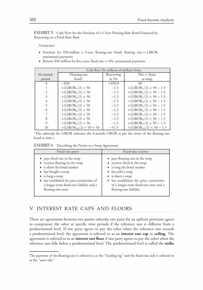
382 Fixed Income Analysis
EXHIBIT 5 Cash Flow for the Purchase of a 5-Year Floating-Rate Bond Financed byBorrowing on a Fixed-Rate Basis
Transaction:
• Purchase for $50 million a 5-year floating-rate bond: floating rate = LIBOR,semiannual payments
• Borrow $50 million for five years: fixed rate = 6%, semiannual payments
Cash flow (In millions of dollars) from:Six month Floating-rate Borrowing Net = Same
period bond∗ at 5% as swap0 −$50 +$50.0 $01 +(LIBOR1/2) × 50 −1.5 +(LIBOR1/2) × 50 − 1.52 +(LIBOR2/2) × 50 −1.5 +(LIBOR2/2) × 50 − 1.53 +(LIBOR3/2) × 50 −1.5 +(LIBOR3/2) × 50 − 1.54 +(LIBOR4/2) × 50 −1.5 +(LIBOR4/2) × 50 − 1.55 +(LIBOR5/2) × 50 −1.5 +(LIBOR5/2) × 50 − 1.56 +(LIBOR6/2) × 50 −1.5 +(LIBOR6/2) × 50 − 1.57 +(LIBOR7/2) × 50 −1.5 +(LIBOR7/2) × 50 − 1.58 +(LIBOR8/2) × 50 −1.5 +(LIBOR8/2) × 50 − 1.59 +(LIBOR9/2) × 50 −1.5 +(LIBOR9/2) × 50 − 1.510 +(LIBOR10/2) × 50 + 50 −51.5 +(LIBOR10/2) × 50 − 1.5
∗The subscript for LIBOR indicates the 6-month LIBOR as per the terms of the floating-ratebond at time t.
EXHIBIT 6 Describing the Parties to a Swap Agreement
Fixed-rate payer Fixed-rate receiver
• pays fixed rate in the swap• receives floating in the swap• is short the bond market• has bought a swap• is long a swap• has established the price sensitivities of
a longer-term fixed-rate liability and afloating-rate asset
• pays floating rate in the swap• receives fixed in the swap• is long the bond market• has sold a swap• is short a swap• has established the price sensitivities
of a longer-term fixed-rate asset and afloating-rate liability
V. INTEREST RATE CAPS AND FLOORS
There are agreements between two parties whereby one party for an upfront premium agreesto compensate the other at specific time periods if the reference rate is different from apredetermined level. If one party agrees to pay the other when the reference rate exceedsa predetermined level, the agreement is referred to as an interest rate cap or ceiling. Theagreement is referred to as an interest rate floor if one party agrees to pay the other when thereference rate falls below a predetermined level. The predetermined level is called the strike
The payment of the floating-rate is referred to as the ‘‘funding leg’’ and the fixed-rate side is referred toas the ‘‘asset side.’’

Chapter 13 Interest Rate Derivative Instruments 383
rate. The strike rate for a cap is called the cap rate; the strike rate for a floor is called the floorrate.
The terms of a cap and floor agreement include:
1. the reference rate2. the strike rate (cap rate or floor rate) that sets the ceiling or floor3. the length of the agreement4. the frequency of settlement5. the notional principal
For example, suppose that C buys an interest rate cap from D with the following terms:
1. the reference rate is 3-month LIBOR.2. the strike rate is 6%.3. the agreement is for four years.4. settlement is every three months.5. the notional principal is $20 million.
Under this agreement, every three months for the next four years, D will pay C whenever3-month LIBOR exceeds 6% at a settlement date. The payment will equal the dollar value ofthe difference between 3-month LIBOR and 6% times the notional principal divided by 4.For example, if three months from now 3-month LIBOR on a settlement date is 8%, thenD will pay C 2% (8% minus 6%) times $20 million divided by 4, or $100,000. If 3-monthLIBOR is 6% or less, D does not have to pay anything to C.
In the case of an interest rate floor, assume the same terms as the interest rate cap we justillustrated. In this case, if 3-month LIBOR is 8%, C receives nothing from D, but if 3-monthLIBOR is less than 6%, D compensates C for the difference. For example, if 3-month LIBORis 5%, D will pay C $50,000 (6% minus 5% times $20 million divided by 4).12
A. Risk/Return Characteristics
In an interest rate agreement, the buyer pays an upfront fee which represents the maximumamount that the buyer can lose and the maximum amount that the seller (writer) cangain. The only party that is required to perform is the seller of the interest rate agreement.The buyer of an interest rate cap benefits if the reference rate rises above the strike ratebecause the seller must compensate the buyer. The buyer of an interest rate floor benefitsif the reference rate falls below the strike rate, because the seller must compensate thebuyer.
The seller of an interest rate cap or floor does not face counterparty risk once the buyerpays the fee. In contrast, the buyer faces counterparty risk. Thus, as with options, there isunilateral counterparty risk.
12Interest rate caps and floors can be combined to create an interest rate collar. This is done by buyingan interest rate cap and selling an interest rate floor. The purchase of the cap sets a maximum rate; thesale of the floor sets a minimum rate. The range between the maximum and minimum rate is called thecollar.

384 Fixed Income Analysis
B. Interpretation of a Cap and Floor Position
In an interest rate cap and floor, the buyer pays an upfront fee, which represents the maximumamount that the buyer can lose and the maximum amount that the seller of the agreement cangain. The only party that is required to perform is the seller of the interest rate agreement. Thebuyer of an interest rate cap benefits if the reference rate rises above the strike rate because theseller must compensate the buyer. The buyer of an interest rate floor benefits if the referencerate falls below the strike rate because the seller must compensate the buyer.
How can we better understand interest rate caps and interest rate floors? In essence thesecontracts are equivalent to a package of interest rate options at different time periods. As witha swap, a complex contract can be seen to be a package of basic contracts—options in thecase of caps and floors. Each of the interest rate options comprising a cap are called caplets;similarly, each of the interest rate options comprising a floor are called floorlets.
The question is what type of package of options is a cap and a floor. Note the followingvery carefully! It depends on whether the underlying is a rate or a fixed-income instrument.If the underlying is considered a fixed-income instrument, its value changes inversely withinterest rates. Therefore:
• for a call option on a fixed-income instrument:
(1) interest rates increase → fixed-income instrument’s price decreases→ call option value decreasesand
(2) interest rates decrease → fixed-income instrument’s price increases→ call option value increases
• for a put option on a fixed-income instrument
(1) interest rates increase → fixed-income instrument’s price decreases→ put option value increasesand
(2) interest rates decrease → fixed-income instrument’s price increases→ put option value decreases
To summarize the situation for call and put options on a fixed-income instrument:
When interest ratesValue of: increase decreaselong call decrease increaseshort call increase decreaselong put increase decreaseshort put decrease increase
For a cap and floor, the situation is as follows
When interest ratesValue of: increase decrease
short cap decrease increaselong cap increase decreaseshort floor increase decreaselong floor decrease increase
Chapter 13 Interest Rate Derivative Instruments 385
Therefore, buying a cap (long cap) is equivalent to buying a package of puts on afixed-income instrument and buying a floor (long floor) is equivalent to buying a package ofcalls on a fixed-income instrument.
Caps and floors can also be seen as packages of options on interest rates. In the over-the-counter market one can purchase an option on an interest rate. These options work as followsin terms of their payoff. There is a strike rate. For a call option on an interest rate, there is apayoff if the reference rate is greater than the strike rate. This means that when interest ratesincrease, the call option’s value increases and when interest rates decrease, the call option’svalue decreases. As can be seen from the payoff for a cap and a floor summarized above, this isthe payoff of a long cap. Consequently, a cap is equivalent to a package of call options on aninterest rate. For a put option on an interest rate, there is a payoff when the reference rate isless than the strike rate. When interest rates increase, the value of the put option on an interestrate decreases, as does the value of a long floor position (see the summary above); when interestrates decrease, the value of the put on an interest rate increases, as does the value of a longfloor position (again, see the summary above). Thus, a floor is equivalent to a package of putoptions on an interest rate.
When market participants talk about the equivalency of caps and floors in terms of putand call options, they must specify the underlying. For example, a long cap is equivalent toa package of call options on interest rates or a package of put options on a fixed-incomeinstrument.
C. Creation of an Interest Rate Collar
Interest rate caps and floors can be combined by borrowers to create an interest rate collar.This is done by buying an interest rate cap and selling an interest rate floor. The purchase ofthe cap sets a maximum interest rate that a borrower would have to pay if the reference raterises. The sale of a floor sets the minimum interest rate that a borrower can benefit from ifthe reference rate declines. Therefore, there is a range for the interest rate that the borrowermust pay if the reference rate changes. The net premium that a borrower who wants to createa collar must pay is the difference between the premium paid to purchase the cap and thepremium received to sell the floor.
For example, consider the following collar created by a borrower: a cap purchased with astrike rate of 7% and a floor sold with a strike rate of 4%. If the reference rate exceeds 7%,the borrower receives a payment; if the reference rate is less than 4%, the borrower makes apayment. Thus, the borrower’s cost will have a range from 4% to 7%. Note, however, that theborrower’s effective interest cost is adjusted by the net premium that the borrower must pay.
CHAPTER 14VALUATION OF INTEREST
RATE DERIVATIVEINSTRUMENTS
I. INTRODUCTION
In the previous chapter, we described interest rate derivative instruments—futures, forwards,options, swaps, caps, and floors. In this chapter, we focus on the valuation of these instruments.Later, we will see how they can be used by portfolio managers to control interest rate risk.
II. INTEREST RATE FUTURES CONTRACTS
In this section we will use an illustration to show how a futures contract is valued. Supposethat a 20-year, $100 par value bond with a coupon rate of 8% is selling at par and that the nextcoupon payment is six months from now. Also suppose that this bond is the deliverable for afutures contract that settles in three months. If the current 3-month interest rate at which fundscan be loaned or borrowed is 4% per year, what should be the price of this futures contract?
Suppose the price of the futures contract is 105. Consider the following strategy:
Sell the futures contract that settles in three months at $105.
Borrow $100 for three months at 4% per year.
With the borrowed funds, purchase the underlying bond for the futures contract.
This strategy is shown in Exhibit 1.Notice that, ignoring initial margin and other transaction costs, there is no cash outlay
for this strategy because the borrowed funds are used to purchase the bond. Three monthsfrom now, the following must be done:
Deliver the purchased bond to settle the futures contract.
Repay the loan.
When the bond is delivered to settle the futures contract three months from now, the amountreceived is the futures price of $105 plus the accrued interest. Since the coupon rate is8% for the bond delivered and the bond is held for three months, the accrued interest is
386
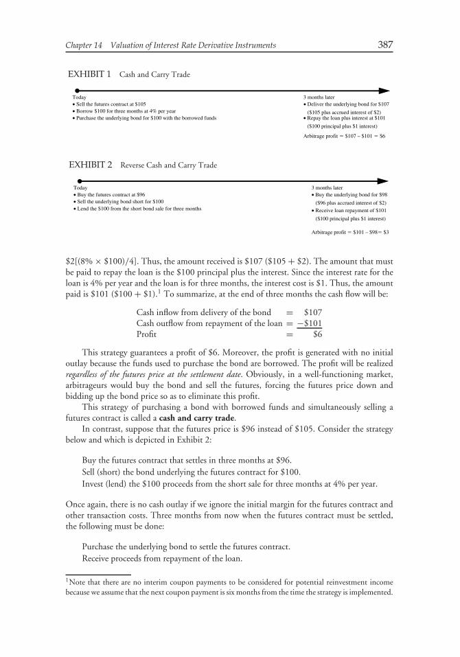
Chapter 14 Valuation of Interest Rate Derivative Instruments 387
EXHIBIT 1 Cash and Carry Trade
Today 3 months later• Sell the futures contract at $105 • Deliver the underlying bond for $107
($105 plus accrued interest of $2)• Borrow $100 for three months at 4% per year • Purchase the underlying bond for $100 with the borrowed funds • Repay the loan plus interest at $101
($100 principal plus $1 interest)
Arbitrage profit � $107 – $101 � $6
EXHIBIT 2 Reverse Cash and Carry Trade
Today 3 months later• Buy the futures contract at $96 Buy the underlying bond for $98
($96 plus accrued interest of $2)• Sell the underlying bond short for $100 • Lend the $100 from the short bond sale for three months Receive loan repayment of $101
($100 principal plus $1 interest)
Arbitrage profit � $101 – $98� $3
•
•
$2[(8% × $100)/4]. Thus, the amount received is $107 ($105 + $2). The amount that mustbe paid to repay the loan is the $100 principal plus the interest. Since the interest rate for theloan is 4% per year and the loan is for three months, the interest cost is $1. Thus, the amountpaid is $101 ($100 + $1).1 To summarize, at the end of three months the cash flow will be:
Cash inflow from delivery of the bond = $107Cash outflow from repayment of the loan = −$101Profit = $6
This strategy guarantees a profit of $6. Moreover, the profit is generated with no initialoutlay because the funds used to purchase the bond are borrowed. The profit will be realizedregardless of the futures price at the settlement date. Obviously, in a well-functioning market,arbitrageurs would buy the bond and sell the futures, forcing the futures price down andbidding up the bond price so as to eliminate this profit.
This strategy of purchasing a bond with borrowed funds and simultaneously selling afutures contract is called a cash and carry trade.
In contrast, suppose that the futures price is $96 instead of $105. Consider the strategybelow and which is depicted in Exhibit 2:
Buy the futures contract that settles in three months at $96.Sell (short) the bond underlying the futures contract for $100.Invest (lend) the $100 proceeds from the short sale for three months at 4% per year.
Once again, there is no cash outlay if we ignore the initial margin for the futures contract andother transaction costs. Three months from now when the futures contract must be settled,the following must be done:
Purchase the underlying bond to settle the futures contract.Receive proceeds from repayment of the loan.
1Note that there are no interim coupon payments to be considered for potential reinvestment incomebecause we assume that the next coupon payment is six months from the time the strategy is implemented.
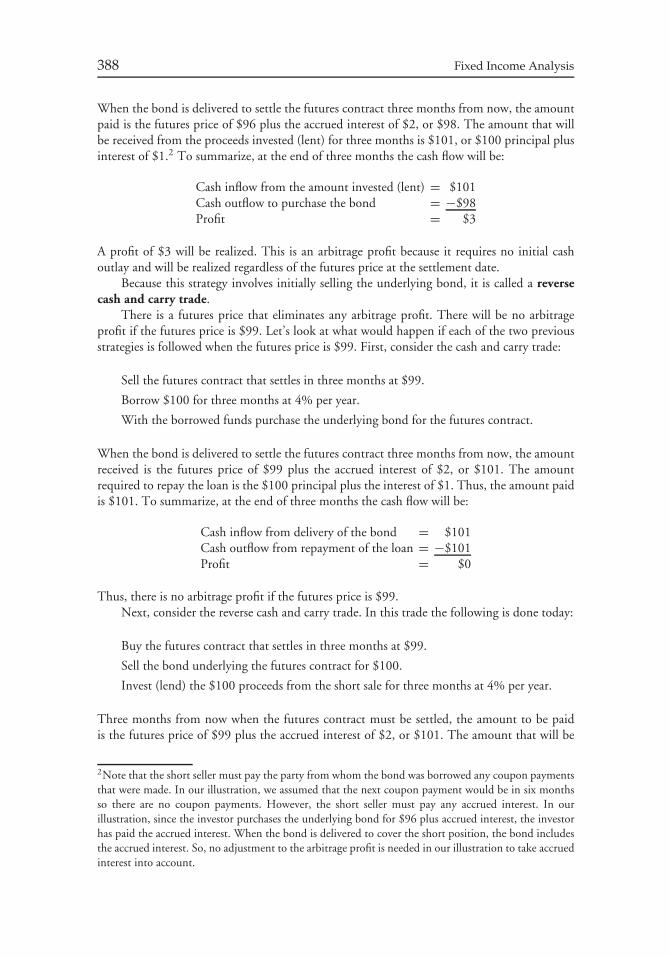
388 Fixed Income Analysis
When the bond is delivered to settle the futures contract three months from now, the amountpaid is the futures price of $96 plus the accrued interest of $2, or $98. The amount that willbe received from the proceeds invested (lent) for three months is $101, or $100 principal plusinterest of $1.2 To summarize, at the end of three months the cash flow will be:
Cash inflow from the amount invested (lent) = $101Cash outflow to purchase the bond = −$98Profit = $3
A profit of $3 will be realized. This is an arbitrage profit because it requires no initial cashoutlay and will be realized regardless of the futures price at the settlement date.
Because this strategy involves initially selling the underlying bond, it is called a reversecash and carry trade.
There is a futures price that eliminates any arbitrage profit. There will be no arbitrageprofit if the futures price is $99. Let’s look at what would happen if each of the two previousstrategies is followed when the futures price is $99. First, consider the cash and carry trade:
Sell the futures contract that settles in three months at $99.
Borrow $100 for three months at 4% per year.
With the borrowed funds purchase the underlying bond for the futures contract.
When the bond is delivered to settle the futures contract three months from now, the amountreceived is the futures price of $99 plus the accrued interest of $2, or $101. The amountrequired to repay the loan is the $100 principal plus the interest of $1. Thus, the amount paidis $101. To summarize, at the end of three months the cash flow will be:
Cash inflow from delivery of the bond = $101Cash outflow from repayment of the loan = −$101Profit = $0
Thus, there is no arbitrage profit if the futures price is $99.Next, consider the reverse cash and carry trade. In this trade the following is done today:
Buy the futures contract that settles in three months at $99.
Sell the bond underlying the futures contract for $100.
Invest (lend) the $100 proceeds from the short sale for three months at 4% per year.
Three months from now when the futures contract must be settled, the amount to be paidis the futures price of $99 plus the accrued interest of $2, or $101. The amount that will be
2Note that the short seller must pay the party from whom the bond was borrowed any coupon paymentsthat were made. In our illustration, we assumed that the next coupon payment would be in six monthsso there are no coupon payments. However, the short seller must pay any accrued interest. In ourillustration, since the investor purchases the underlying bond for $96 plus accrued interest, the investorhas paid the accrued interest. When the bond is delivered to cover the short position, the bond includesthe accrued interest. So, no adjustment to the arbitrage profit is needed in our illustration to take accruedinterest into account.

Chapter 14 Valuation of Interest Rate Derivative Instruments 389
received from the proceeds of the three month loan is $101, $100 plus interest of $1. At theend of three months the cash flow will be:
Cash inflow from the amount invested (lent) = $101Cash outflow to purchase the bond = −$101Profit = $0
Thus, neither strategy results in a profit or loss. Hence, the futures price of $99 is the equilibriumor theoretical price, because any higher or lower futures price will permit arbitrage profits.
A. Theoretical Futures Price Based on Arbitrage Model
Considering the arbitrage arguments (based on the cash and carry trade) just presented, thetheoretical futures price can be determined from the following information:
1. The price of the underlying bond in the cash market. (In our example, the price of thebond is $100.)
2. The coupon rate on the bond. (In our example, the coupon rate is 8% per year.)3. The interest rate for borrowing and lending until the settlement date. The borrowing
and lending rate is referred to as the financing rate. (In our example, the financing rateis 4% per year.)
We will let
r = financing rate (in decimal)c = current yield, or annual dollar coupon divided by the cash market price (in decimal)P = cash market priceF = futures pricet = time, in years, to the futures delivery date
Given an assumption of no interim cash flows and no transaction costs, the equationbelow gives the theoretical futures price that produces a zero profit (i.e., no arbitrage profit)using either the cash and carry trade or the reverse cash and carry trade:
F = P + Pt (r − c) (1)
Let’s apply equation (1) to our previous example in which
r = 0.04 c = 0.08 P = 100 t = 0.25
Then the theoretical futures price is
F = 100 + 100 × 0.25 × (0.04 − 0.08) = 100 − 1 = 99
This agrees with the theoretical futures price we derived earlier.It is important to note that c is the current yield, found by dividing the coupon interest
payment by the cash market price. In our illustration above, since the cash market price of thebond is 100, the coupon rate is equal to the current yield. If the cash market price is not thepar value, the coupon rate is not equal to the current yield.
The theoretical futures price may be at a premium to the cash market price (higher thanthe cash market price) or at a discount from the cash market price (lower than the cash
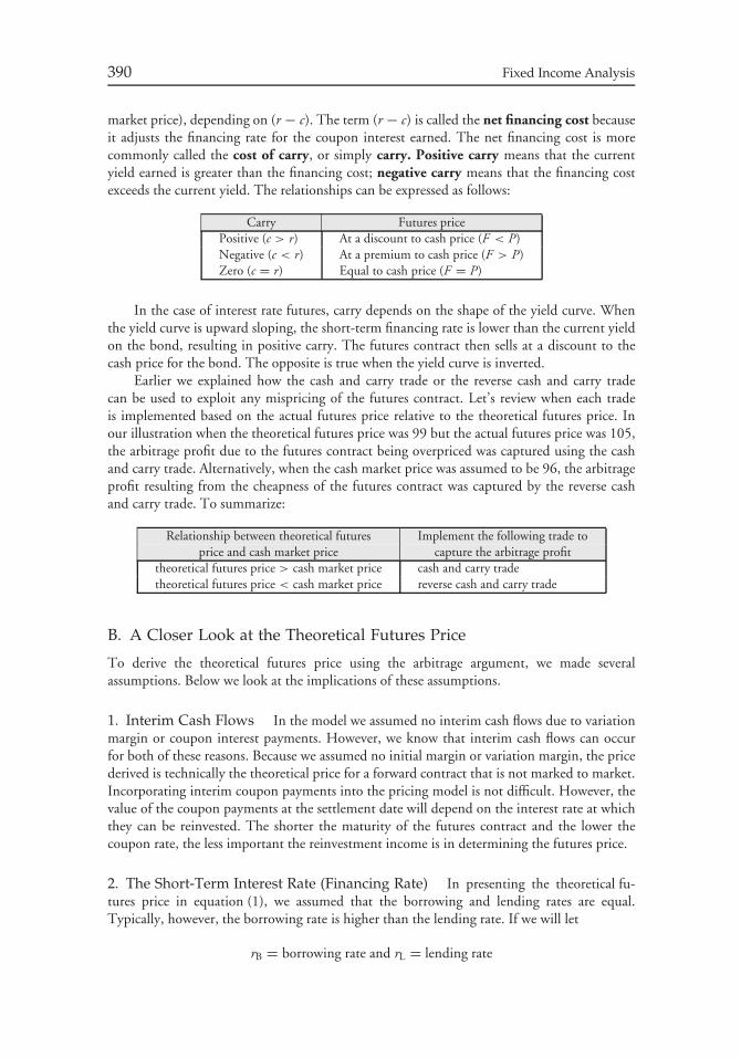
390 Fixed Income Analysis
market price), depending on (r − c). The term (r − c) is called the net financing cost becauseit adjusts the financing rate for the coupon interest earned. The net financing cost is morecommonly called the cost of carry, or simply carry. Positive carry means that the currentyield earned is greater than the financing cost; negative carry means that the financing costexceeds the current yield. The relationships can be expressed as follows:
Carry Futures pricePositive (c > r) At a discount to cash price (F < P)Negative (c < r) At a premium to cash price (F > P)Zero (c = r) Equal to cash price (F = P)
In the case of interest rate futures, carry depends on the shape of the yield curve. Whenthe yield curve is upward sloping, the short-term financing rate is lower than the current yieldon the bond, resulting in positive carry. The futures contract then sells at a discount to thecash price for the bond. The opposite is true when the yield curve is inverted.
Earlier we explained how the cash and carry trade or the reverse cash and carry tradecan be used to exploit any mispricing of the futures contract. Let’s review when each tradeis implemented based on the actual futures price relative to the theoretical futures price. Inour illustration when the theoretical futures price was 99 but the actual futures price was 105,the arbitrage profit due to the futures contract being overpriced was captured using the cashand carry trade. Alternatively, when the cash market price was assumed to be 96, the arbitrageprofit resulting from the cheapness of the futures contract was captured by the reverse cashand carry trade. To summarize:
Relationship between theoretical futures Implement the following trade toprice and cash market price capture the arbitrage profit
theoretical futures price > cash market price cash and carry tradetheoretical futures price < cash market price reverse cash and carry trade
B. A Closer Look at the Theoretical Futures Price
To derive the theoretical futures price using the arbitrage argument, we made severalassumptions. Below we look at the implications of these assumptions.
1. Interim Cash Flows In the model we assumed no interim cash flows due to variationmargin or coupon interest payments. However, we know that interim cash flows can occurfor both of these reasons. Because we assumed no initial margin or variation margin, the pricederived is technically the theoretical price for a forward contract that is not marked to market.Incorporating interim coupon payments into the pricing model is not difficult. However, thevalue of the coupon payments at the settlement date will depend on the interest rate at whichthey can be reinvested. The shorter the maturity of the futures contract and the lower thecoupon rate, the less important the reinvestment income is in determining the futures price.
2. The Short-Term Interest Rate (Financing Rate) In presenting the theoretical fu-tures price in equation (1), we assumed that the borrowing and lending rates are equal.Typically, however, the borrowing rate is higher than the lending rate. If we will let
rB = borrowing rate and rL = lending rate
Chapter 14 Valuation of Interest Rate Derivative Instruments 391
and continue with our assumption of no interim cash flows and no transaction costs, then thefutures price that would produce no cash and carry arbitrage profit is
F = P + Pt (rB − c) (2)
and the futures price that would produce no reverse cash and carry arbitrage profit is
F = P + Pt (rL − c) (3)
Equations (2) and (3) together provide boundaries for the theoretical futures price.Equation (2) provides the upper boundary and equation (3) the lower boundary. For example,assume that the borrowing rate is 4% per year, while the lending rate is 3.2% per year. Thenusing equation (2) and the previous example, the upper boundary is
F (upper boundary) = 100 + 100 × 0.25 × (0.04 − 0.08) = 99
The lower boundary, using equation (3), is
F (lower boundary) = 100 + 100 × 0.25 × (0.032 − 0.08) = 98.8
In calculating these boundaries, we assume no transaction costs are involved in taking theposition. In actuality, the transaction costs of entering into and closing the cash position aswell as the round-trip transaction costs for the futures contract must be considered becausethese transaction costs affect the boundaries for the futures contract.
3. Deliverable Bond Is Not Known The arbitrage arguments used to derive equa-tion (1) assumed that only one instrument is deliverable. But as explained in the previouschapter, the futures contracts on Treasury bonds and Treasury notes are designed to allow theshort the choice of delivering any one of a number of deliverable issues (the quality or swapoption3). Because there may be more than one deliverable, market participants track the priceof each deliverable bond and determine which bond is the cheapest to deliver. The futuresprice will then trade in relation to the cheapest-to-deliver issue.
There is the risk that while an issue may be the cheapest to deliver at the time a positionin the futures contract is taken, it may not be the cheapest to deliver after that time. A changein the cheapest-to-deliver can dramatically alter the futures price. What are the implications ofthe quality (swap) option on the futures price? Because the swap option is an option grantedby the long to the short, the long will want to pay less for the futures contract than indicatedby equation (1). Therefore, as a result of the quality option, the theoretical futures price asgiven by equation (1) must be adjusted as follows:
F = P + Pt (r − c) − value of quality option (4)
Market participants have employed theoretical models to estimate the fair value of thequality option. A discussion of these models is beyond the scope of this chapter.
3As explained in the previous chapter, this is the option granted to the short in the futures contract toselect from among the eligible issues the one to deliver.
392 Fixed Income Analysis
4. Delivery Date Is Not Known In the pricing model based on arbitrage arguments, aknown delivery date is assumed. For Treasury bond and note futures contracts, the short hasa timing option and a wild card option, so the long does not know when the security will bedelivered. The effect of the timing and wild card options4 on the theoretical futures price isthe same as with the quality option. These delivery options result in a theoretical futures pricethat is lower than the one suggested by equation (1), as shown below:
F = P + P (r − c) − value of quality option − value of timing option
− value of wildcard option (5)
or alternatively,F = P + P (r − c) − delivery options (6)
Market participants attempt to value the delivery options in order to apply equation (6).A discussion of these models is a specialist topic.
5. Putting It Altogether To summarize, there is not one theoretical futures price thatwould eliminate any arbitrage profit, but a range for the theoretical futures prices based onborrowing and lending rates. Consequently, the futures price can fluctuate within this rangeand there will be no arbitrage profit. Once recognition is given to the delivery options grantedto the short in the futures contract, the theoretical futures price is lower. Specifically, it isreduced by the value of the delivery options. This means that the lower boundary for thetheoretical futures price shifts down by an amount equal to the value of the delivery optionsand the upper boundary for the theoretical futures price shifts down by the same amount.
III. INTEREST RATE SWAPS
In an interest rate swap, the counterparties agree to exchange periodic interest payments. Thedollar amount of the interest payments exchanged is based on the notional principal. In themost common type of swap, there is a fixed-rate payer and a fixed-rate receiver. The conventionfor quoting swap rates is that a swap dealer sets the floating rate equal to the reference rate(i.e., the interest rate used to determine the floating-rate in a swap) and then quotes the fixedrate that will apply.
A. Computing the Payments for a Swap
In the previous chapter on interest rate derivative instruments, we described the basic featuresof an interest rate swap using rough calculations for the payments and explained how theparties to a swap either gain or lose when interest rates change. For valuation, however. we needmore details. To value a swap it is necessary to determine the present value of the fixed-ratepayments and the present value of the floating-rate payments. The difference between these
4As explained in the previous chapter, the timing option is the option granted to the short to select thedelivery date in the delivery month. The wild card option is the option granted to the short to give noticeof intent to deliver after the closing of the exchange on the date when the futures settlement price hasbeen fixed.
Chapter 14 Valuation of Interest Rate Derivative Instruments 393
two present values is the value of a swap. As will be explained below, whether the valueis positive (i.e., an asset) or negative (i.e., a liability) depends on whether the party is thefixed-rate payer or the fixed-rate receiver.
We are interested in how the swap rate is determined at the inception of the swap. At theinception of the swap, the terms of the swap are such that the present value of the floating-ratepayments is equal to the present value of the fixed-rate payments. At inception the value ofthe swap is equal to zero. This is the fundamental principle in determining the swap rate (i.e.,the fixed rate that the fixed-rate payer will pay).
Here is a roadmap of the presentation. First we will look at how to compute thefloating-rate payments. We will see how the future values of the reference rate are determinedto obtain the floating rate for the period. From the future values of the reference rate we willthen see how to compute the floating-rate payments, taking into account the number of daysin the payment period. Next we will see how to calculate the fixed-rate payments given theswap rate. Before we look at how to calculate the value of a swap, we will see how to calculatethe swap rate. This will require an explanation of how the present value of any cash flow inan interest rate swap is computed. Given the floating-rate payments and the present value ofthe floating-rate payments, the swap rate can be determined by using the principle that theswap rate is the fixed rate that makes the present value of the fixed-rate payments equal to thepresent value of the floating-rate payments. Finally, we will see how the value of a swap isdetermined after the inception of a swap.
1. Calculating the Floating-Rate Payments For the first floating-rate payment, theamount is known because the floating-rate is known at the beginning of the period eventhough it is paid at the end of the period (i.e., payment is made in arrears). For all subsequentpayments, the floating-rate payment depends on the value of the reference rate when thefloating rate is determined. To illustrate the issues associated with calculating the floating-ratepayment, we assume that:
• swap starts today, January 1 of year 1• the floating-rate payments are made quarterly based on ‘‘actual/360’’ (‘‘actual’’ means the
actual number of days in the quarter)• the reference rate is 3-month LIBOR (London interbank offered rate)• the notional amount of the swap is $100 million• the term of the swap is three years
The quarterly floating-rate payments are based on an ‘‘actual/360’’ day count convention.This convention means that we assume 360 days in a year and that, in computing the interestfor the quarter, the actual number of days in the quarter is used. The floating-rate payment isset at the beginning of the quarter but paid at the end of the quarter—that is, the floating-ratepayments are made in arrears.
Suppose that today 3-month LIBOR is 4.05%. Let’s look at what the fixed-rate payer willreceive on March 31 of year 1—the date when the first quarterly swap payment is made. Thereis no uncertainty about what the floating-rate payment will be. In general, the floating-ratepayment is determined as follows:
notional amount × (3-month LIBOR) × no. of days in period
360
394 Fixed Income Analysis
In our illustration, assuming a non-leap year, the number of days from January 1 of year 1 toMarch 31 of year 1 (the first quarter) is 90. If 3-month LIBOR is 4.05%, then the fixed-ratepayer will receive a floating-rate payment on March 31 of year 1 equal to:
$100, 000, 000 × 0.0405 × 90
360= $1,012,500
Now the difficulty is in determining the floating-rate payments after the first quarterlypayment. While the first quarterly payment is known, the next 11 are not. However, there isa way to hedge the next 11 floating-rate payments by using a futures contract. The futurescontract equivalent to the future floating-rate payments in a swap whose reference rate is3-month LIBOR is the Eurodollar CD futures contract. In effect then, the remaining swappayments are equivalent to a package of futures contracts. We will digress to discuss thiscontract.
a. The Eurodollar CD Futures Contract As explained in the previous chapter, a swapposition can be interpreted as a package of forward/futures contracts or a package of cash flowsfrom buying and selling cash market instruments. It is the former interpretation that will beused as the basis for valuing a swap.
Eurodollar certificates of deposit (CDs) are denominated in dollars but represent theliabilities of banks outside the United States. The contracts are traded on both the InternationalMonetary Market of the Chicago Mercantile Exchange and the London International FinancialFutures Exchange. The rate paid on Eurodollar CDs is LIBOR.
The 3-month Eurodollar CD is the underlying instrument for the Eurodollar CD futurescontract. The contract is for $1 million of face value and is traded on an index price basis.The index price basis is equal to 100 minus the product of the annualized LIBOR futures ratein decimal and 100. For example, a Eurodollar CD futures price of 94.00 means a 3-monthLIBOR futures rate of 6% [100 minus (0.06 × 100)].
The Eurodollar CD futures contract is a cash settlement contract. That is, the partiessettle in cash for the value of a Eurodollar CD based on LIBOR at the settlement date.
The Eurodollar CD futures contract allows the buyer of the contract to lock in the rate on3-month LIBOR today for a future 3-month period. For example, suppose that on February 1in Year 1 an investor purchases a Eurodollar CD futures contract that settles in March of Year1. Assume that the LIBOR futures rate for this contract is 5%. This means that the investorhas agreed to invest in a 3-month Eurodollar CD that pays a rate of 5%. Specifically, theinvestor has locked in a 3-month rate of 5% beginning March of Year 1. If on February 1 ofYear 1 this investor purchased a contract that settles in September of Year 2 and the LIBORfutures rate is 5.4%, the investor has locked in the rate on a 3-month investment beginningSeptember of Year 2.
The seller of a Eurodollar CD futures contract is agreeing to lend funds for three monthsat some future date at the LIBOR futures rate. For example, suppose that on February 1 ofYear 1 a bank sells a Eurodollar CD futures contract that settles in March of Year 1 andthe LIBOR futures rate is 5%. The bank locks in a borrowing rate of 5% for three monthsbeginning in March of Year 1. If the settlement date is September of Year 2 and the LIBORfutures rate is 5.4%, the bank is locking in a borrowing rate of 5.4% for the 3-month periodbeginning September of Year 2.
The key point here is that the Eurodollar CD futures contract allows a participant in thefinancial market to lock in a 3-month rate on an investment or a 3-month borrowing rate.The 3-month period begins in the month that the contract settles.
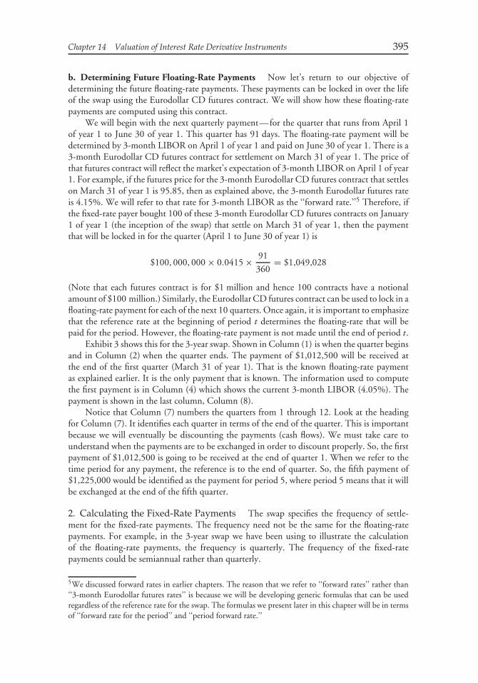
Chapter 14 Valuation of Interest Rate Derivative Instruments 395
b. Determining Future Floating-Rate Payments Now let’s return to our objective ofdetermining the future floating-rate payments. These payments can be locked in over the lifeof the swap using the Eurodollar CD futures contract. We will show how these floating-ratepayments are computed using this contract.
We will begin with the next quarterly payment—for the quarter that runs from April 1of year 1 to June 30 of year 1. This quarter has 91 days. The floating-rate payment will bedetermined by 3-month LIBOR on April 1 of year 1 and paid on June 30 of year 1. There is a3-month Eurodollar CD futures contract for settlement on March 31 of year 1. The price ofthat futures contract will reflect the market’s expectation of 3-month LIBOR on April 1 of year1. For example, if the futures price for the 3-month Eurodollar CD futures contract that settleson March 31 of year 1 is 95.85, then as explained above, the 3-month Eurodollar futures rateis 4.15%. We will refer to that rate for 3-month LIBOR as the ‘‘forward rate.’’5 Therefore, ifthe fixed-rate payer bought 100 of these 3-month Eurodollar CD futures contracts on January1 of year 1 (the inception of the swap) that settle on March 31 of year 1, then the paymentthat will be locked in for the quarter (April 1 to June 30 of year 1) is
$100, 000, 000 × 0.0415 × 91
360= $1,049,028
(Note that each futures contract is for $1 million and hence 100 contracts have a notionalamount of $100 million.) Similarly, the Eurodollar CD futures contract can be used to lock in afloating-rate payment for each of the next 10 quarters. Once again, it is important to emphasizethat the reference rate at the beginning of period t determines the floating-rate that will bepaid for the period. However, the floating-rate payment is not made until the end of period t.
Exhibit 3 shows this for the 3-year swap. Shown in Column (1) is when the quarter beginsand in Column (2) when the quarter ends. The payment of $1,012,500 will be received atthe end of the first quarter (March 31 of year 1). That is the known floating-rate paymentas explained earlier. It is the only payment that is known. The information used to computethe first payment is in Column (4) which shows the current 3-month LIBOR (4.05%). Thepayment is shown in the last column, Column (8).
Notice that Column (7) numbers the quarters from 1 through 12. Look at the headingfor Column (7). It identifies each quarter in terms of the end of the quarter. This is importantbecause we will eventually be discounting the payments (cash flows). We must take care tounderstand when the payments are to be exchanged in order to discount properly. So, the firstpayment of $1,012,500 is going to be received at the end of quarter 1. When we refer to thetime period for any payment, the reference is to the end of quarter. So, the fifth payment of$1,225,000 would be identified as the payment for period 5, where period 5 means that it willbe exchanged at the end of the fifth quarter.
2. Calculating the Fixed-Rate Payments The swap specifies the frequency of settle-ment for the fixed-rate payments. The frequency need not be the same for the floating-ratepayments. For example, in the 3-year swap we have been using to illustrate the calculationof the floating-rate payments, the frequency is quarterly. The frequency of the fixed-ratepayments could be semiannual rather than quarterly.
5We discussed forward rates in earlier chapters. The reason that we refer to ‘‘forward rates’’ rather than‘‘3-month Eurodollar futures rates’’ is because we will be developing generic formulas that can be usedregardless of the reference rate for the swap. The formulas we present later in this chapter will be in termsof ‘‘forward rate for the period’’ and ‘‘period forward rate.’’
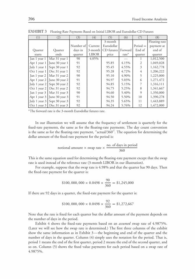
396 Fixed Income Analysis
EXHIBIT 3 Floating-Rate Payments Based on Initial LIBOR and Eurodollar CD Futures
(1) (2) (3) (4) (5) (6) (7) (8)3-month Floating-rate
Number of Current Eurodollar Period = payment atQuarter Quarter days in 3-month CD futures Forward End of end of
starts ends quarter LIBOR price rate∗ quarter quarterJan 1 year 1 Mar 31 year 1 90 4.05% — 1 1,012,500Apr 1 year 1 June 30 year 1 91 95.85 4.15% 2 1,049,028July 1 year 1 Sept 30 year 1 92 95.45 4.55% 3 1,162,778Oct 1 year 1 Dec 31 year 1 92 95.28 4.72% 4 1,206,222Jan 1 year 2 Mar 31 year 2 90 95.10 4.90% 5 1,225,000Apr 1 year 2 June 30 year 2 91 94.97 5.03% 6 1,271,472July 1 year 2 Sept 30 year 2 92 94.85 5.15% 7 1,316,111Oct 1 year 2 Dec 31 year 2 92 94.75 5.25% 8 1,341,667Jan 1 year 3 Mar 31 year 3 90 94.60 5.40% 9 1,350,000Apr 1 year 3 June 30 year 3 91 94.50 5.50% 10 1,390,278July 1 year 3 Sept 30 year 3 92 94.35 5.65% 11 1,443,889Oct 1 year 3 Dec 31 year 3 92 94.24 5.76% 12 1,472,000
∗The forward rate is the 3-month Eurodollar futures rate.
In our illustration we will assume that the frequency of settlement is quarterly for thefixed-rate payments, the same as for the floating-rate payments. The day count conventionis the same as for the floating-rate payment, ‘‘actual/360’’. The equation for determining thedollar amount of the fixed-rate payment for the period is:
notional amount × swap rate × no. of days in period
360
This is the same equation used for determining the floating-rate payment except that the swaprate is used instead of the reference rate (3-month LIBOR in our illustration).
For example, suppose that the swap rate is 4.98% and that the quarter has 90 days. Thenthe fixed-rate payment for the quarter is:
$100, 000, 000 × 0.0498 × 90
360= $1,245,000
If there are 92 days in a quarter, the fixed-rate payment for the quarter is:
$100, 000, 000 × 0.0498 × 92
360= $1,272,667
Note that the rate is fixed for each quarter but the dollar amount of the payment depends onthe number of days in the period.
Exhibit 4 shows the fixed-rate payments based on an assumed swap rate of 4.9875%.(Later we will see how the swap rate is determined.) The first three columns of the exhibitshow the same information as in Exhibit 3—the beginning and end of the quarter and thenumber of days in the quarter. Column (4) simply uses the notation for the period. That is,period 1 means the end of the first quarter, period 2 means the end of the second quarter, andso on. Column (5) shows the fixed value payments for each period based on a swap rate of4.9875%.
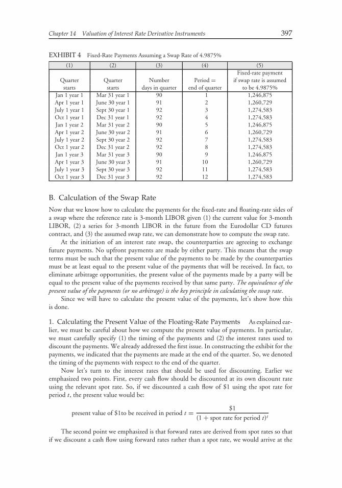
Chapter 14 Valuation of Interest Rate Derivative Instruments 397
EXHIBIT 4 Fixed-Rate Payments Assuming a Swap Rate of 4.9875%
(1) (2) (3) (4) (5)Fixed-rate payment
Quarter Quarter Number Period = if swap rate is assumedstarts starts days in quarter end of quarter to be 4.9875%
Jan 1 year 1 Mar 31 year 1 90 1 1,246,875Apr 1 year 1 June 30 year 1 91 2 1,260,729July 1 year 1 Sept 30 year 1 92 3 1,274,583Oct 1 year 1 Dec 31 year 1 92 4 1,274,583Jan 1 year 2 Mar 31 year 2 90 5 1,246,875Apr 1 year 2 June 30 year 2 91 6 1,260,729July 1 year 2 Sept 30 year 2 92 7 1,274,583Oct 1 year 2 Dec 31 year 2 92 8 1,274,583Jan 1 year 3 Mar 31 year 3 90 9 1,246,875Apr 1 year 3 June 30 year 3 91 10 1,260,729July 1 year 3 Sept 30 year 3 92 11 1,274,583Oct 1 year 3 Dec 31 year 3 92 12 1,274,583
B. Calculation of the Swap Rate
Now that we know how to calculate the payments for the fixed-rate and floating-rate sides ofa swap where the reference rate is 3-month LIBOR given (1) the current value for 3-monthLIBOR, (2) a series for 3-month LIBOR in the future from the Eurodollar CD futurescontract, and (3) the assumed swap rate, we can demonstrate how to compute the swap rate.
At the initiation of an interest rate swap, the counterparties are agreeing to exchangefuture payments. No upfront payments are made by either party. This means that the swapterms must be such that the present value of the payments to be made by the counterpartiesmust be at least equal to the present value of the payments that will be received. In fact, toeliminate arbitrage opportunities, the present value of the payments made by a party will beequal to the present value of the payments received by that same party. The equivalence of thepresent value of the payments (or no arbitrage) is the key principle in calculating the swap rate.
Since we will have to calculate the present value of the payments, let’s show how thisis done.
1. Calculating the Present Value of the Floating-Rate Payments As explained ear-lier, we must be careful about how we compute the present value of payments. In particular,we must carefully specify (1) the timing of the payments and (2) the interest rates used todiscount the payments. We already addressed the first issue. In constructing the exhibit for thepayments, we indicated that the payments are made at the end of the quarter. So, we denotedthe timing of the payments with respect to the end of the quarter.
Now let’s turn to the interest rates that should be used for discounting. Earlier weemphasized two points. First, every cash flow should be discounted at its own discount rateusing the relevant spot rate. So, if we discounted a cash flow of $1 using the spot rate forperiod t, the present value would be:
present value of $1to be received in period t = $1
(1 + spot rate for period t)t
The second point we emphasized is that forward rates are derived from spot rates so thatif we discount a cash flow using forward rates rather than a spot rate, we would arrive at the

398 Fixed Income Analysis
same value. That is, the present value of $1 to be received in period t can be rewritten as:
present value of $1 to be received in period t =$1
(1+ forward rate for period 1)(1+ forward rate for period 2) ···(1+ forward rate for period t)
We will refer to the present value of $1 to be received in period t as the forward discountfactor. In our calculations involving swaps, we will compute the forward discount factor for aperiod using the forward rates. These are the same forward rates that are used to compute thefloating-rate payments—those obtained from the Eurodollar CD futures contract. We mustmake just one more adjustment. We must adjust the forward rates used in the formula for thenumber of days in the period (i.e., the quarter in our illustrations) in the same way that wemade this adjustment to compute the payments. Specifically, the forward rate for a period,which we will refer to as the period forward rate, is computed using the following equation:
period forward rate = annual forward rate ×(
days in period
360
)
For example, look at Exhibit 3. The annual forward rate for period 4 is 4.72%. Theperiod forward rate for period 4 is:
period forward rate = 4.72% ×(
92
360
)= 1.2062%
Column (5) in Exhibit 5 shows the annual forward rate for each of the 12 periods (reproducedfrom Exhibit 3) and Column (6) shows the period forward rate for each of the 12 periods.Note that the period forward rate for period 1 is 90/360 4.05%, which is 90/360 of the knownrate for 3-month LIBOR.
EXHIBIT 5 Calculating the Forward Discount Factor
(1) (2) (3) (4) (5) (6) (7)Number of Period = Period Forward
Quarter Quarter days in end of Forward forward discountstarts ends quarter quarter rate rate factor
Jan 1 year 1 Mar 31 year 1 90 1 4.05% 1.0125% 0.98997649Apr 1 year 1 June 30 year 1 91 2 4.15% 1.0490% 0.97969917July 1 year 1 Sept 30 year 1 92 3 4.55% 1.1628% 0.96843839Oct 1 year 1 Dec 31 year 1 92 4 4.72% 1.2062% 0.95689609Jan 1 year 2 Mar 31 year 2 90 5 4.90% 1.2250% 0.94531597Apr 1 year 2 June 30 year 2 91 6 5.03% 1.2715% 0.93344745July 1 year 2 Sept 30 year 2 92 7 5.15% 1.3161% 0.92132183Oct 1 year 2 Dec 31 year 2 92 8 5.25% 1.3417% 0.90912441Jan 1 year 3 Mar 31 year 3 90 9 5.40% 1.3500% 0.89701471Apr 1 year 3 June 30 year 3 91 10 5.50% 1.3903% 0.88471472July 1 year 3 Sept 30 year 3 92 11 5.65% 1.4439% 0.87212224Oct 1 year 3 Dec 31 year 3 92 12 5.76% 1.4720% 0.85947083
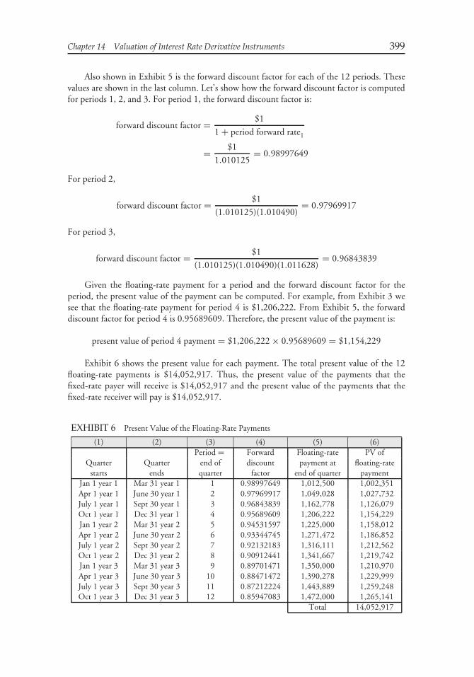
Chapter 14 Valuation of Interest Rate Derivative Instruments 399
Also shown in Exhibit 5 is the forward discount factor for each of the 12 periods. Thesevalues are shown in the last column. Let’s show how the forward discount factor is computedfor periods 1, 2, and 3. For period 1, the forward discount factor is:
forward discount factor = $1
1 + period forward rate1
= $1
1.010125= 0.98997649
For period 2,
forward discount factor = $1
(1.010125)(1.010490)= 0.97969917
For period 3,
forward discount factor = $1
(1.010125)(1.010490)(1.011628)= 0.96843839
Given the floating-rate payment for a period and the forward discount factor for theperiod, the present value of the payment can be computed. For example, from Exhibit 3 wesee that the floating-rate payment for period 4 is $1,206,222. From Exhibit 5, the forwarddiscount factor for period 4 is 0.95689609. Therefore, the present value of the payment is:
present value of period 4 payment = $1,206,222 × 0.95689609 = $1,154,229
Exhibit 6 shows the present value for each payment. The total present value of the 12floating-rate payments is $14,052,917. Thus, the present value of the payments that thefixed-rate payer will receive is $14,052,917 and the present value of the payments that thefixed-rate receiver will pay is $14,052,917.
EXHIBIT 6 Present Value of the Floating-Rate Payments
(1) (2) (3) (4) (5) (6)Period = Forward Floating-rate PV of
Quarter Quarter end of discount payment at floating-ratestarts ends quarter factor end of quarter payment
Jan 1 year 1 Mar 31 year 1 1 0.98997649 1,012,500 1,002,351Apr 1 year 1 June 30 year 1 2 0.97969917 1,049,028 1,027,732July 1 year 1 Sept 30 year 1 3 0.96843839 1,162,778 1,126,079Oct 1 year 1 Dec 31 year 1 4 0.95689609 1,206,222 1,154,229Jan 1 year 2 Mar 31 year 2 5 0.94531597 1,225,000 1,158,012Apr 1 year 2 June 30 year 2 6 0.93344745 1,271,472 1,186,852July 1 year 2 Sept 30 year 2 7 0.92132183 1,316,111 1,212,562Oct 1 year 2 Dec 31 year 2 8 0.90912441 1,341,667 1,219,742Jan 1 year 3 Mar 31 year 3 9 0.89701471 1,350,000 1,210,970Apr 1 year 3 June 30 year 3 10 0.88471472 1,390,278 1,229,999July 1 year 3 Sept 30 year 3 11 0.87212224 1,443,889 1,259,248Oct 1 year 3 Dec 31 year 3 12 0.85947083 1,472,000 1,265,141
Total 14,052,917
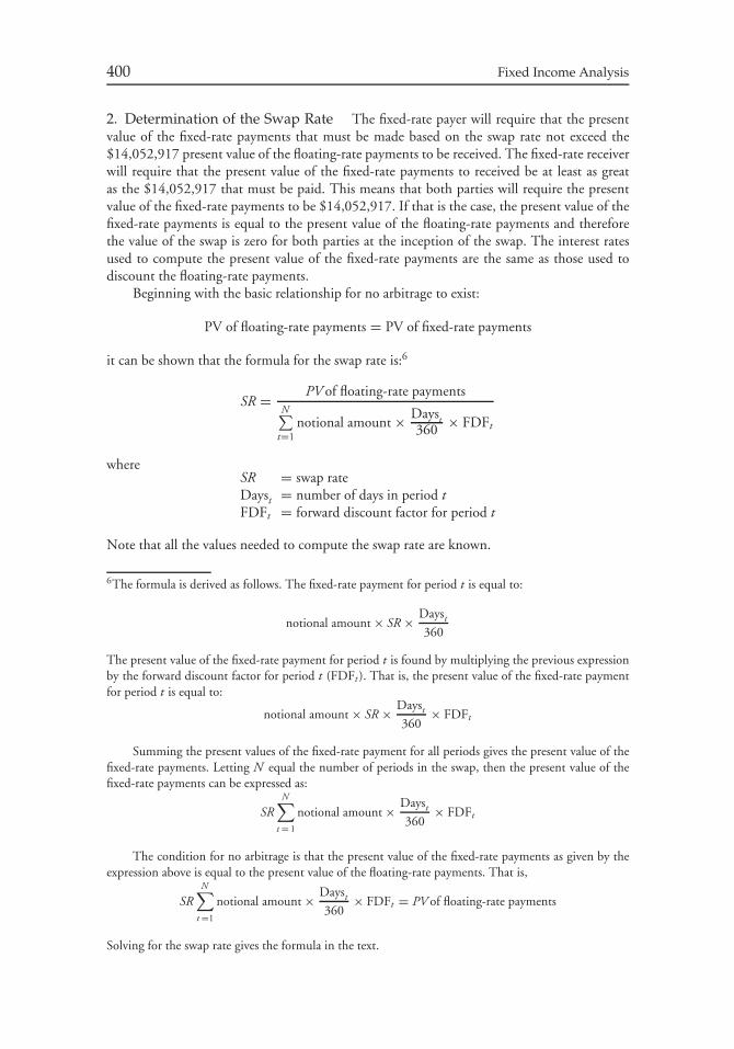
400 Fixed Income Analysis
2. Determination of the Swap Rate The fixed-rate payer will require that the presentvalue of the fixed-rate payments that must be made based on the swap rate not exceed the$14,052,917 present value of the floating-rate payments to be received. The fixed-rate receiverwill require that the present value of the fixed-rate payments to received be at least as greatas the $14,052,917 that must be paid. This means that both parties will require the presentvalue of the fixed-rate payments to be $14,052,917. If that is the case, the present value of thefixed-rate payments is equal to the present value of the floating-rate payments and thereforethe value of the swap is zero for both parties at the inception of the swap. The interest ratesused to compute the present value of the fixed-rate payments are the same as those used todiscount the floating-rate payments.
Beginning with the basic relationship for no arbitrage to exist:
PV of floating-rate payments = PV of fixed-rate payments
it can be shown that the formula for the swap rate is:6
SR = PV of floating-rate paymentsN∑
t=1notional amount × Dayst
360 × FDFt
whereSR = swap rateDayst = number of days in period tFDFt = forward discount factor for period t
Note that all the values needed to compute the swap rate are known.
6The formula is derived as follows. The fixed-rate payment for period t is equal to:
notional amount × SR × Dayst
360
The present value of the fixed-rate payment for period t is found by multiplying the previous expressionby the forward discount factor for period t (FDFt ). That is, the present value of the fixed-rate paymentfor period t is equal to:
notional amount × SR × Dayst
360× FDFt
Summing the present values of the fixed-rate payment for all periods gives the present value of thefixed-rate payments. Letting N equal the number of periods in the swap, then the present value of thefixed-rate payments can be expressed as:
SRN∑
t = 1
notional amount × Dayst
360× FDFt
The condition for no arbitrage is that the present value of the fixed-rate payments as given by theexpression above is equal to the present value of the floating-rate payments. That is,
SRN∑
t =1
notional amount × Dayst
360× FDFt = PV of floating-rate payments
Solving for the swap rate gives the formula in the text.
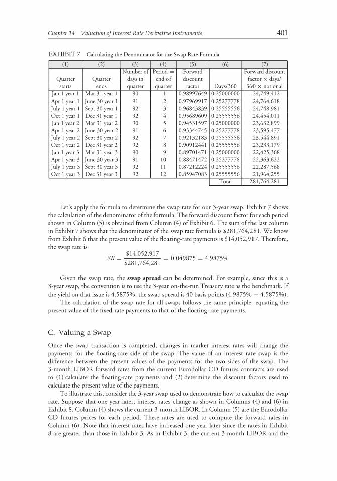
Chapter 14 Valuation of Interest Rate Derivative Instruments 401
EXHIBIT 7 Calculating the Denominator for the Swap Rate Formula
(1) (2) (3) (4) (5) (6) (7)Number of Period = Forward Forward discount
Quarter Quarter days in end of discount factor × days/starts ends quarter quarter factor Days/360 360 × notional
Jan 1 year 1 Mar 31 year 1 90 1 0.98997649 0.25000000 24,749,412Apr 1 year 1 June 30 year 1 91 2 0.97969917 0.25277778 24,764,618July 1 year 1 Sept 30 year 1 92 3 0.96843839 0.25555556 24,748,981Oct 1 year 1 Dec 31 year 1 92 4 0.95689609 0.25555556 24,454,011Jan 1 year 2 Mar 31 year 2 90 5 0.94531597 0.25000000 23,632,899Apr 1 year 2 June 30 year 2 91 6 0.93344745 0.25277778 23,595,477July 1 year 2 Sept 30 year 2 92 7 0.92132183 0.25555556 23,544,891Oct 1 year 2 Dec 31 year 2 92 8 0.90912441 0.25555556 23,233,179Jan 1 year 3 Mar 31 year 3 90 9 0.89701471 0.25000000 22,425,368Apr 1 year 3 June 30 year 3 91 10 0.88471472 0.25277778 22,363,622July 1 year 3 Sept 30 year 3 92 11 0.87212224 0.25555556 22,287,568Oct 1 year 3 Dec 31 year 3 92 12 0.85947083 0.25555556 21,964,255
Total 281,764,281
Let’s apply the formula to determine the swap rate for our 3-year swap. Exhibit 7 showsthe calculation of the denominator of the formula. The forward discount factor for each periodshown in Column (5) is obtained from Column (4) of Exhibit 6. The sum of the last columnin Exhibit 7 shows that the denominator of the swap rate formula is $281,764,281. We knowfrom Exhibit 6 that the present value of the floating-rate payments is $14,052,917. Therefore,the swap rate is
SR = $14,052,917
$281,764,281= 0.049875 = 4.9875%
Given the swap rate, the swap spread can be determined. For example, since this is a3-year swap, the convention is to use the 3-year on-the-run Treasury rate as the benchmark. Ifthe yield on that issue is 4.5875%, the swap spread is 40 basis points (4.9875% − 4.5875%).
The calculation of the swap rate for all swaps follows the same principle: equating thepresent value of the fixed-rate payments to that of the floating-rate payments.
C. Valuing a Swap
Once the swap transaction is completed, changes in market interest rates will change thepayments for the floating-rate side of the swap. The value of an interest rate swap is thedifference between the present values of the payments for the two sides of the swap. The3-month LIBOR forward rates from the current Eurodollar CD futures contracts are usedto (1) calculate the floating-rate payments and (2) determine the discount factors used tocalculate the present value of the payments.
To illustrate this, consider the 3-year swap used to demonstrate how to calculate the swaprate. Suppose that one year later, interest rates change as shown in Columns (4) and (6) inExhibit 8. Column (4) shows the current 3-month LIBOR. In Column (5) are the EurodollarCD futures prices for each period. These rates are used to compute the forward rates inColumn (6). Note that interest rates have increased one year later since the rates in Exhibit8 are greater than those in Exhibit 3. As in Exhibit 3, the current 3-month LIBOR and the
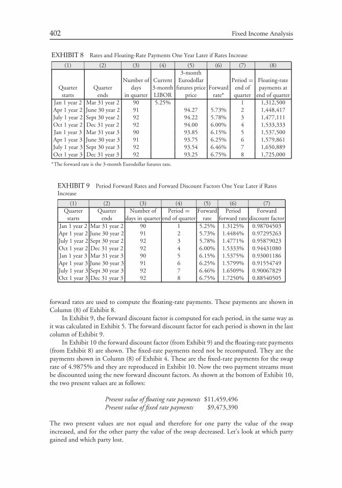
402 Fixed Income Analysis
EXHIBIT 8 Rates and Floating-Rate Payments One Year Later if Rates Increase
(1) (2) (3) (4) (5) (6) (7) (8)3-month
Number of Current Eurodollar Period = Floating-rateQuarter Quarter days 3-month futures price Forward end of payments at
starts ends in quarter LIBOR price rate* quarter end of quarterJan 1 year 2 Mar 31 year 2 90 5.25% 1 1,312,500Apr 1 year 2 June 30 year 2 91 94.27 5.73% 2 1,448,417July 1 year 2 Sept 30 year 2 92 94.22 5.78% 3 1,477,111Oct 1 year 2 Dec 31 year 2 92 94.00 6.00% 4 1,533,333Jan 1 year 3 Mar 31 year 3 90 93.85 6.15% 5 1,537,500Apr 1 year 3 June 30 year 3 91 93.75 6.25% 6 1,579,861July 1 year 3 Sept 30 year 3 92 93.54 6.46% 7 1,650,889Oct 1 year 3 Dec 31 year 3 92 93.25 6.75% 8 1,725,000
∗The forward rate is the 3-month Eurodollar futures rate.
EXHIBIT 9 Period Forward Rates and Forward Discount Factors One Year Later if RatesIncrease
(1) (2) (3) (4) (5) (6) (7)Quarter Quarter Number of Period = Forward Period Forward
starts ends days in quarter end of quarter rate forward rate discount factorJan 1 year 2 Mar 31 year 2 90 1 5.25% 1.3125% 0.98704503Apr 1 year 2 June 30 year 2 91 2 5.73% 1.4484% 0.97295263July 1 year 2 Sept 30 year 2 92 3 5.78% 1.4771% 0.95879023Oct 1 year 2 Dec 31 year 2 92 4 6.00% 1.5333% 0.94431080Jan 1 year 3 Mar 31 year 3 90 5 6.15% 1.5375% 0.93001186Apr 1 year 3 June 30 year 3 91 6 6.25% 1.5799% 0.91554749July 1 year 3 Sept 30 year 3 92 7 6.46% 1.6509% 0.90067829Oct 1 year 3 Dec 31 year 3 92 8 6.75% 1.7250% 0.88540505
forward rates are used to compute the floating-rate payments. These payments are shown inColumn (8) of Exhibit 8.
In Exhibit 9, the forward discount factor is computed for each period, in the same way asit was calculated in Exhibit 5. The forward discount factor for each period is shown in the lastcolumn of Exhibit 9.
In Exhibit 10 the forward discount factor (from Exhibit 9) and the floating-rate payments(from Exhibit 8) are shown. The fixed-rate payments need not be recomputed. They are thepayments shown in Column (8) of Exhibit 4. These are the fixed-rate payments for the swaprate of 4.9875% and they are reproduced in Exhibit 10. Now the two payment streams mustbe discounted using the new forward discount factors. As shown at the bottom of Exhibit 10,the two present values are as follows:
Present value of floating rate payments $11,459,496Present value of fixed rate payments $9,473,390
The two present values are not equal and therefore for one party the value of the swapincreased, and for the other party the value of the swap decreased. Let’s look at which partygained and which party lost.
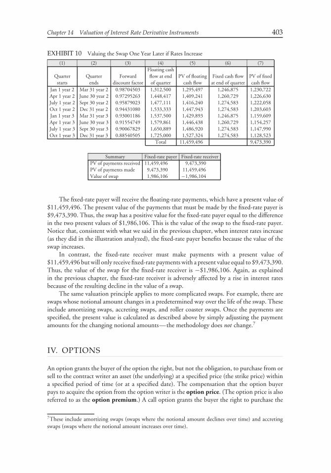
Chapter 14 Valuation of Interest Rate Derivative Instruments 403
EXHIBIT 10 Valuing the Swap One Year Later if Rates Increase
(1) (2) (3) (4) (5) (6) (7)Floating cash
Quarter Quarter Forward flow at end PV of floating Fixed cash flow PV of fixedstarts ends discount factor of quarter cash flow at end of quarter cash flow
Jan 1 year 2 Mar 31 year 2 0.98704503 1,312,500 1,295,497 1,246,875 1,230,722Apr 1 year 2 June 30 year 2 0.97295263 1,448,417 1,409,241 1,260,729 1,226,630July 1 year 2 Sept 30 year 2 0.95879023 1,477,111 1,416,240 1,274,583 1,222,058Oct 1 year 2 Dec 31 year 2 0.94431080 1,533,333 1,447,943 1,274,583 1,203,603Jan 1 year 3 Mar 31 year 3 0.93001186 1,537,500 1,429,893 1,246,875 1,159,609Apr 1 year 3 June 30 year 3 0.91554749 1,579,861 1,446,438 1,260,729 1,154,257July 1 year 3 Sept 30 year 3 0.90067829 1,650,889 1,486,920 1,274,583 1,147,990Oct 1 year 3 Dec 31 year 3 0.88540505 1,725,000 1,527,324 1,274,583 1,128,523
Total 11,459,496 9,473,390
Summary Fixed-rate payer Fixed-rate receiverPV of payments received 11,459,496 9,473,390PV of payments made 9,473,390 11,459,496Value of swap 1,986,106 −1,986,104
The fixed-rate payer will receive the floating-rate payments, which have a present value of$11,459,496. The present value of the payments that must be made by the fixed-rate payer is$9,473,390. Thus, the swap has a positive value for the fixed-rate payer equal to the differencein the two present values of $1,986,106. This is the value of the swap to the fixed-rate payer.Notice that, consistent with what we said in the previous chapter, when interest rates increase(as they did in the illustration analyzed), the fixed-rate payer benefits because the value of theswap increases.
In contrast, the fixed-rate receiver must make payments with a present value of$11,459,496 but will only receive fixed-rate payments with a present value equal to $9,473,390.Thus, the value of the swap for the fixed-rate receiver is −$1,986,106. Again, as explainedin the previous chapter, the fixed-rate receiver is adversely affected by a rise in interest ratesbecause of the resulting decline in the value of a swap.
The same valuation principle applies to more complicated swaps. For example, there areswaps whose notional amount changes in a predetermined way over the life of the swap. Theseinclude amortizing swaps, accreting swaps, and roller coaster swaps. Once the payments arespecified, the present value is calculated as described above by simply adjusting the paymentamounts for the changing notional amounts—the methodology does not change.7
IV. OPTIONS
An option grants the buyer of the option the right, but not the obligation, to purchase from orsell to the contract writer an asset (the underlying) at a specified price (the strike price) withina specified period of time (or at a specified date). The compensation that the option buyerpays to acquire the option from the option writer is the option price. (The option price is alsoreferred to as the option premium.) A call option grants the buyer the right to purchase the
7These include amortizing swaps (swaps where the notional amount declines over time) and accretingswaps (swaps where the notional amount increases over time).
404 Fixed Income Analysis
underlying from the writer (seller); a put option gives the buyer the right to sell the underlyingto the writer. An American option allows the buyer to exercise the option at any time up toand including the expiration date. A European option allows the buyer to exercise the optiononly on the expiration date.
The maximum amount that an option buyer can lose is the option price. The maximumprofit that the option writer can realize is the option price. The option buyer has substantialupside return potential, while the option writer has substantial downside risk.
A. Components of the Option Price
The option price can be decomposed into two parts: the intrinsic value and the time value.We describe each below.
1. Intrinsic Value The option value is a reflection of the option’s intrinsic value and itstime value. The intrinsic value of an option is its economic value if it is exercised immediately.If no positive economic value would result from exercising the option immediately, then theintrinsic value is zero.
For a call option, the intrinsic value is positive if the current market price of the underlyingsecurity is greater than the strike price. The intrinsic value is then the difference between thecurrent market price of the underlying security and the strike price. If the strike price of a calloption is greater than or equal to the current market price of the security, the intrinsic value iszero. For example, if the strike price for a call option is $100 and the current market price ofthe security is $105, the intrinsic value is $5. That is, an option buyer exercising the optionand simultaneously selling the underlying security would realize $105 from the sale of thesecurity, which would be covered by acquiring the security from the option writer for $100,thereby netting a $5 gain.
When an option has intrinsic value, it is said to be in the money. When the strike priceof a call option exceeds the current price of the security, the call option is said to be out of themoney; it has no intrinsic value. An option for which the strike price is equal to the currentprice of the security is said to be at the money. Both at-the-money and out-of-the-moneyoptions have an intrinsic value of zero because they are not profitable to exercise.
For a put option, the intrinsic value is equal to the amount by which the current price ofthe security is below the strike price. For example, if the strike price of a put option is $100and the current price of the security is $92, the intrinsic value is $8. The owner of the putoption who simultaneously buys the underlying security and exercises the put will net $8 sinceby exercising the option the security will be sold to the writer for $100, while the security ispurchased in the market for $92. The intrinsic value is zero if the strike price is less than orequal to the current market price.
Our put option with a strike price of $100 would be: (1) in the money when the security’sprice is less than $100, (2) out of the money when the security’s price exceeds $100, and (3) atthe money when the security’s price is equal to $100.
The relationships above are summarized in Exhibit 11.
2. Time Value The time value of an option is the amount by which the option priceexceeds its intrinsic value. The option buyer hopes that at some time up to the expirationdate, changes in the market price of the underlying security will increase the value of the rightsconveyed by the option. For this prospect, the option buyer is willing to pay a premium abovethe intrinsic value.
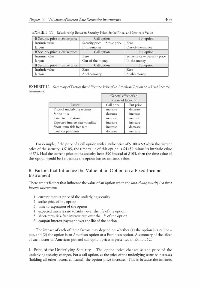
Chapter 14 Valuation of Interest Rate Derivative Instruments 405
EXHIBIT 11 Relationship Between Security Price, Strike Price, and Intrinsic Value
If Security price > Strike price Call option Put optionIntrinsic value Security price − Strike price ZeroJargon In-the-money Out-of-the-moneyIf Security price < Strike price Call option Put optionIntrinsic value Zero Strike price − Security priceJargon Out-of-the-money In-the-moneyIf Security price = Strike price Call option Put optionIntrinsic value Zero ZeroJargon At-the-money At-the-money
EXHIBIT 12 Summary of Factors that Affect the Price of an American Option on a Fixed IncomeInstrument
General effect of anincrease of factor on:
Factor Call price Put pricePrice of underlying security increase decreaseStrike price decrease increaseTime to expiration increase increaseExpected interest rate volatility increase increaseShort-term risk-free rate increase decreaseCoupon payments decrease increase
For example, if the price of a call option with a strike price of $100 is $9 when the currentprice of the security is $105, the time value of this option is $4 ($9 minus its intrinsic valueof $5). Had the current price of the security been $90 instead of $105, then the time value ofthis option would be $9 because the option has no intrinsic value.
B. Factors that Influence the Value of an Option on a Fixed IncomeInstrument
There are six factors that influence the value of an option when the underlying security is a fixedincome instrument:
1. current market price of the underlying security2. strike price of the option3. time to expiration of the option4. expected interest rate volatility over the life of the option5. short-term risk-free interest rate over the life of the option6. coupon interest payment over the life of the option
The impact of each of these factors may depend on whether (1) the option is a call or aput, and (2) the option is an American option or a European option. A summary of the effectof each factor on American put and call option prices is presented in Exhibit 12.
1. Price of the Underlying Security The option price changes as the price of theunderlying security changes. For a call option, as the price of the underlying security increases(holding all other factors constant), the option price increases. This is because the intrinsic

406 Fixed Income Analysis
value of a call option increases when the price of the underlying security increases. Theopposite holds for a put option: as the price of the underlying security increases, the price ofa put option decreases. This is because the intrinsic value of a put option decreases when theprice of the underlying security increases.
2. Strike Price All other factors equal, the lower the strike price, the higher the price of acall option. For put options, the higher the strike price, the higher the option price.
3. Time to Expiration of the Option An option is a ‘‘wasting asset.’’ That is, after theexpiration date passes the option has no value. Holding all other factors equal, the longerthe time to expiration of the option, the greater the option price. As the time to expirationdecreases, less time remains for the underlying security’s price to rise (for a call buyer) or to fall(for a put buyer)—to compensate the option buyer for any time value paid—and, therefore,the probability of a favorable price movement decreases. Consequently, for American options,as the time remaining until expiration decreases, the option price approaches its intrinsic value.
4. Expected Interest Rate Volatility Over the Life of the Option All other factorsequal, the greater the expected interest rate volatility or yield volatility, the more an investorwould be willing to pay for the option, and the more an option writer would demand forit. This is because the greater the volatility, the greater the probability that the price of theunderlying security will move in favor of the option buyer at some time before expiration. Theprocedure for estimating interest rate volatility is explained in Chapter 8.
5. Short-Term Risk-Free Rate Over the Life of the Option Buying the underlyingsecurity ties up one’s money. Buying an option on the dollar amount of the underlyingsecurity makes available for investment the difference between the security price and theoption price at the risk-free rate. All other factors constant, the higher the short-term risk-freerate, the greater the cost of buying the underlying security and carrying it to the expiration dateof the call option. Hence, the higher the short-term risk-free rate, the more attractive the calloption is relative to the direct purchase of the underlying security. As a result, the higher theshort-term risk-free rate, the greater the price of a call option. In the case of a put option, thealternative to buying a put is shorting the security. When the security is shorted, the proceedsreceived can be invested at the short-term risk-free rate. When the short-term risk-free rateincreases, this makes it more attractive to short the security relative to buying a put option.Consequently, the value of a put option declines when the short-term risk-free rate increases.
6. Coupon Payments Over the Life of the Option Coupon interest payments on theunderlying security tend to decrease the price of a call option because they make it moreattractive to hold the underlying security than to hold the option. That is, the owner of thesecurity receives the coupon payments but the buyer of the call option does not. The higherthe coupon payment received by the owner of the security, the more attractive it is to ownthe security and the less attractive it is to own the call option. So, the value of a call optiondeclines the higher the coupon payment.
The opposite is true for the put option. Coupon interest payments on the underlyingsecurity tend to increase the price of a put option. The buyer of a put option compares theposition to a short position in the security. When shorting the security, the coupon paymentmust be paid by the short seller. So, the higher the coupon payment the less attractive it is toshort the security and the more attractive it is to buy the put option. As a result, the value of aput option increases the higher the coupon payment.

Chapter 14 Valuation of Interest Rate Derivative Instruments 407
C. Factors that Influence the Value of a Futures Option
There are five factors that influence the value of an option in which the underlying is a futurescontract:
1. current futures price2. strike price of the option3. time to expiration of the option4. expected interest rate volatility over the life of the option5. short-term risk-free rate over the life of the option
These are the same factors that affect the value of an option on a fixed income instrument.Notice that the coupon payment is not a factor since the underlying is a futures contract.
D. Pricing Models for Options and Options on Futures
At any time, the intrinsic value of an option can be determined. The question is, what is anapproximate time value for an option? To answer this question, option pricing models havebeen developed. Two models used to value options on a fixed income instrument are theBlack-Scholes model and the arbitrage-free binomial model. For options on futures, the mostcommon model is the Black model, a version of the Black-Scholes model. We will discussthe two common models for options on fixed income instruments before discussing the Blackmodel for options on futures for fixed income instruments.
1. The Black-Scholes Model The most common model for the pricing of options is theBlack-Scholes option pricing model. Although this model was developed for options on stocks,it has been applied to options on bonds as well. Such applications are fraught with problems.We will discuss the model for stocks first and then discuss the limitations of applying themodel to bonds.
The model was developed for valuing European style call options on a non-dividend-paying common stock.8 To derive the option pricing model based on arbitrage arguments,
8The Black-Scholes option pricing formula is:
C = SN (d1) − Xe−rtN (d2)
where
d1 = ln(S/X )+(r+0.5s2)ts√
t
d2 = d1 − s√
tln = natural logarithmC = call option priceS = current stock priceX = strike pricer = short-term risk-free interest ratee = 2.718 (natural antilog of 1)t = time remaining to the expiration date(measured as a fraction of a year)s = standard deviation of the stock returns
N (.) = the cumulative probability density. The value for N(.) is obtained from a normaldistribution function.

408 Fixed Income Analysis
certain assumptions are imposed. There have been a good number of extensions of theBlack-Scholes option pricing that have been formulated by relaxing the assumptions. Whilethe model was developed for common stock, it has been applied to value options on fixedincome instruments. With the exception of the coupon payment, the factors that we explainedearlier that determine the value of an option of a fixed income instrument are included in theBlack-Scholes formula. As we will see, because of the assumptions imposed the Black-Scholesoption pricing model does not necessarily produce reasonable values for options on bonds.
The option price derived from the Black-Scholes option pricing model is ‘‘fair’’ in thesense that if any other price existed, it would be possible to earn riskless arbitrage profits bytaking an offsetting position in the underlying stock. If the price of the call option in themarket is higher than that derived from the Black-Scholes option pricing model, an investorcould sell the call option and buy a certain number of shares in the underlying stock. If thereverse is true and the market price of the call option is less than the ‘‘fair’’ price derived fromthe model, the investor could buy the call option and sell short a certain number of sharesin the underlying stock. This process of hedging by taking a position in the underlying stockallows the investor to lock in the riskless arbitrage profit. The number of shares necessary tohedge the position changes as the factors that affect the option price change, so the hedgedposition must be changed constantly.
To understand the limitations of applying the model to bonds, let’s look at the valuesthat would be derived in a couple of examples. We know that there are coupon-paying bondsand zero-coupon bonds. In our illustration we will use a zero-coupon bond. The reason is thatthe original Black-Scholes model was for common stock that did not pay a dividend and soa zero-coupon bond would be the equivalent type of instrument. Specifically, we will look athow the Black-Scholes option pricing model would value a zero-coupon bond with three yearsto maturity assuming the following:
Strike price = $88.00
Time remaining to expiration = 2 years
Current bond price = $83.96 (assuming for simplicity annual compounding)
Expected return volatility = standard deviation = 10%
Risk-free rate = 6%
The Black-Scholes formula gives a value of $ 8.116.9 There is no reason to suspect that thisestimated value is incorrect. However, let’s change the problem slightly. Instead of a strike
9The value is derived as follows. The current price of $83.96 is the present value of the maturity valueof $100 discounted at 6% (assuming a flat yield curve). We know
S = 83.96 X = 88.00 t = 2 s = 0.10 r = 0.06
Substituting these values into the formula in the previous footnote:
d1 = ln(83.96/88) + (0.06 + 0.5(0.10)2)2
0.10√
2= 0.5869
d2 = 0.5869 − 0.10√
2 = 0.4455
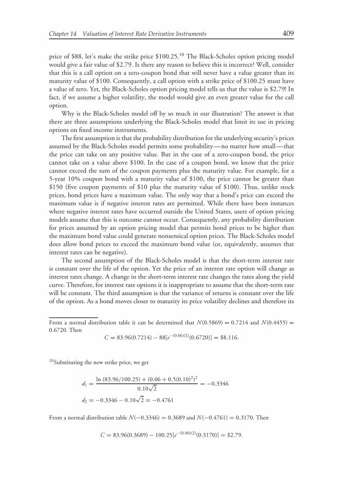
Chapter 14 Valuation of Interest Rate Derivative Instruments 409
price of $88, let’s make the strike price $100.25.10 The Black-Scholes option pricing modelwould give a fair value of $2.79. Is there any reason to believe this is incorrect? Well, considerthat this is a call option on a zero-coupon bond that will never have a value greater than itsmaturity value of $100. Consequently, a call option with a strike price of $100.25 must havea value of zero. Yet, the Black-Scholes option pricing model tells us that the value is $2.79! Infact, if we assume a higher volatility, the model would give an even greater value for the calloption.
Why is the Black-Scholes model off by so much in our illustration? The answer is thatthere are three assumptions underlying the Black-Scholes model that limit its use in pricingoptions on fixed income instruments.
The first assumption is that the probability distribution for the underlying security’s pricesassumed by the Black-Scholes model permits some probability—no matter how small—thatthe price can take on any positive value. But in the case of a zero-coupon bond, the pricecannot take on a value above $100. In the case of a coupon bond, we know that the pricecannot exceed the sum of the coupon payments plus the maturity value. For example, for a5-year 10% coupon bond with a maturity value of $100, the price cannot be greater than$150 (five coupon payments of $10 plus the maturity value of $100). Thus, unlike stockprices, bond prices have a maximum value. The only way that a bond’s price can exceed themaximum value is if negative interest rates are permitted. While there have been instanceswhere negative interest rates have occurred outside the United States, users of option pricingmodels assume that this is outcome cannot occur. Consequently, any probability distributionfor prices assumed by an option pricing model that permits bond prices to be higher thanthe maximum bond value could generate nonsensical option prices. The Black-Scholes modeldoes allow bond prices to exceed the maximum bond value (or, equivalently, assumes thatinterest rates can be negative).
The second assumption of the Black-Scholes model is that the short-term interest rateis constant over the life of the option. Yet the price of an interest rate option will change asinterest rates change. A change in the short-term interest rate changes the rates along the yieldcurve. Therefore, for interest rate options it is inappropriate to assume that the short-term ratewill be constant. The third assumption is that the variance of returns is constant over the lifeof the option. As a bond moves closer to maturity its price volatility declines and therefore its
From a normal distribution table it can be determined that N (0.5869) = 0.7214 and N (0.4455) =0.6720. Then
C = 83.96(0.7214) − 88[e−(0.06)(2)(0.6720)] = $8.116.
10Substituting the new strike price, we get
d1 = ln (83.96/100.25) + (0.06 + 0.5(0.10)2)2
0.10√
2= −0.3346
d2 = −0.3346 − 0.10√
2 = −0.4761
From a normal distribution table N (−0.3346) = 0.3689 and N (−0.4761) = 0.3170. Then
C = 83.96(0.3689) − 100.25[e−(0.06)(2)(0.3170)] = $2.79.
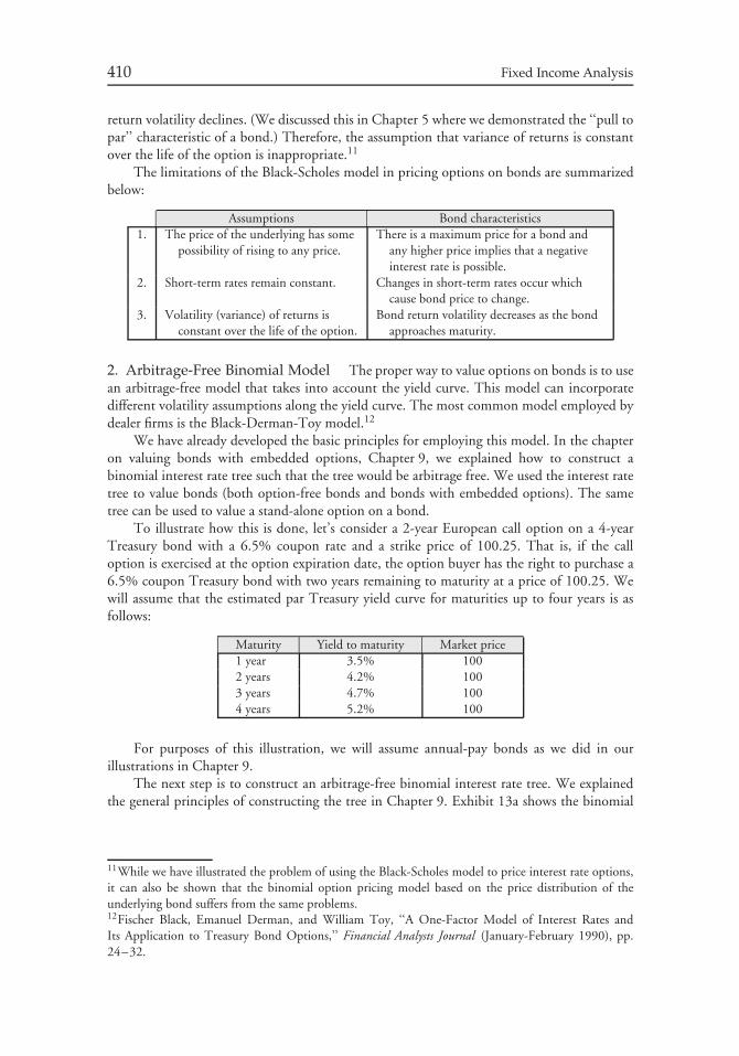
410 Fixed Income Analysis
return volatility declines. (We discussed this in Chapter 5 where we demonstrated the ‘‘pull topar’’ characteristic of a bond.) Therefore, the assumption that variance of returns is constantover the life of the option is inappropriate.11
The limitations of the Black-Scholes model in pricing options on bonds are summarizedbelow:
Assumptions Bond characteristics1. The price of the underlying has some
possibility of rising to any price.There is a maximum price for a bond and
any higher price implies that a negativeinterest rate is possible.
2. Short-term rates remain constant. Changes in short-term rates occur whichcause bond price to change.
3. Volatility (variance) of returns isconstant over the life of the option.
Bond return volatility decreases as the bondapproaches maturity.
2. Arbitrage-Free Binomial Model The proper way to value options on bonds is to usean arbitrage-free model that takes into account the yield curve. This model can incorporatedifferent volatility assumptions along the yield curve. The most common model employed bydealer firms is the Black-Derman-Toy model.12
We have already developed the basic principles for employing this model. In the chapteron valuing bonds with embedded options, Chapter 9, we explained how to construct abinomial interest rate tree such that the tree would be arbitrage free. We used the interest ratetree to value bonds (both option-free bonds and bonds with embedded options). The sametree can be used to value a stand-alone option on a bond.
To illustrate how this is done, let’s consider a 2-year European call option on a 4-yearTreasury bond with a 6.5% coupon rate and a strike price of 100.25. That is, if the calloption is exercised at the option expiration date, the option buyer has the right to purchase a6.5% coupon Treasury bond with two years remaining to maturity at a price of 100.25. Wewill assume that the estimated par Treasury yield curve for maturities up to four years is asfollows:
Maturity Yield to maturity Market price1 year 3.5% 1002 years 4.2% 1003 years 4.7% 1004 years 5.2% 100
For purposes of this illustration, we will assume annual-pay bonds as we did in ourillustrations in Chapter 9.
The next step is to construct an arbitrage-free binomial interest rate tree. We explainedthe general principles of constructing the tree in Chapter 9. Exhibit 13a shows the binomial
11While we have illustrated the problem of using the Black-Scholes model to price interest rate options,it can also be shown that the binomial option pricing model based on the price distribution of theunderlying bond suffers from the same problems.12Fischer Black, Emanuel Derman, and William Toy, ‘‘A One-Factor Model of Interest Rates andIts Application to Treasury Bond Options,’’ Financial Analysts Journal (January-February 1990), pp.24–32.
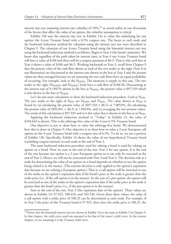
Chapter 14 Valuation of Interest Rate Derivative Instruments 411
interest rate tree assuming interest rate volatility of 10%;13 as noted earlier in our discussionof the factors that affect the value of an option, the volatility assumption is critical.
Exhibit 13b uses the interest rate tree in Exhibit 13a to value the underlying for ouroption: the 4-year Treasury bond with a 6.5% coupon rate. The boxes at each node andthe backward induction method for valuation using the interest rate tree were described inChapter 9. The valuation of our 4-year Treasury bond using the binomial interest rate treeusing the backward induction method is as follows. Begin in Year 4 (the bond’s maturity). Weknow that regardless of the path taken by interest rates, at Year 4 our 4-year Treasury bondwill have a value of $100 and there will be a coupon payment of $6.5. That is why each box atYear 4 shows a value of $100 and $6.5. Working backwards to Year 3, recall from Chapter 9that the present value of the cash flow shown at each of the two nodes to the right (Year 4 inour illustration) are discounted at the interest rate shown in the box at Year 3 and the presentvalues are then averaged because we are assuming the two cash flows have an equal probabilityof occurring. For example, look at the NHHH. The situation is simple in this case. The twonodes to the right (NHHHH and NHHHL) both have a cash flow of $106.50. Discounting atthe interest rate of 9.1987% shown in the box at NHHH, the present value is $97.529 whichis also shown in the box at NHHH.
Let’s do one more calculation to show the backward induction procedure. Look at NHH.The two nodes to the right of NHH are NHHH and NHHL. The value shown at NHH isfound by (a) calculating the present value of ($97.529 + $6.5) at 7.0053%, (b) calculatingthe present value of ($99.041 + $6.5) at 7.0053%, and (c) averaging the two present values.The result of this calculation is $97.925 and it is this value that is shown in the box at at NHH.
Applying the backward induction method to ‘‘Today’’ in Exhibit 13, the value of$104.643 is shown. This is the arbitrage-free value of the 4-year 6.5% Treasury bond.
Our objective is not to show how to value the arbitrage-free bond. We demonstratedhow this in done in Chapter 9. Our objective is to show how to value a 2-year European calloption on the 4-year Treasury bond with a coupon rate of 6.5%. To do so, we use a portionof Exhibit 13b. Specifically, Exhibit 14 shows the value of our hypothetical Treasury bond(excluding coupon interest) at each node at the end of Year 2.
The same backward induction procedure used for valuing a bond is used for valuing anoption on a bond. Now we start at the end of the tree, Year 2 for our option. It is the endof the tree because our option is a 2-year European option so it can only be exercised at theend of Year 2. Hence, we will not be concerned with Year 3 and Year 4. The decision rule at anode for determining the value of an option on a bond depends on whether or not the optionbeing valued is in the money. (The exercise decision is only applied at the option’s expirationdate because we are valuing a European option.) That is, a call option will be exercised at oneof the nodes at the option’s expiration date if the bond’s price at the node is greater than thestrike price (i.e., if the call option is in the money). In the case of a put option, the option willbe exercised at one of the nodes at the option’s expiration date if the strike price at the node isgreater than the bond’s price (i.e., if the put option is in the money).
Start at the end of the tree, Year 2 (the expiration date of the option). Three values areshown in Exhibit 14: 97.925, 100.418, and 102.534. Given these three values, the value ofa call option with a strike price of 100.25 can be determined at each node. For example, ifin Year 2 the price of this Treasury bond is 97.925, then since the strike price is 100.25, the
13Notice that the binomial interest rate tree shown in Exhibit 13a is the same as Exhibit 5 in Chapter 9.In that chapter, the yield curve used was assumed to be that of the issuer’s yield curve. In the currentchapter, we are assuming it is the Treasury yield curve.
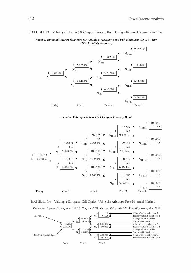
412 Fixed Income Analysis
EXHIBIT 13 Valuing a 4-Year 6.5% Coupon Treasury Bond Using a Binomial Interest Rate Tree
Panel b: Valuing a 4-Year 6.5% Coupon Treasury Bond
Panel a: Binomial Interest Rate Tree for Valuihg a Treasury Bond with a Maturity Up to 4 Years(10% Volatility Assumed)
• 100.00097.529 NHHHH 6.5
• 6.597.925 NHHH 9.1987%
• 6.5 • 100.000100.230 NHH 7.0053% 99.041 NHHHL 6.5
• 6.5 • 6.5
NH5.4289% 100.418 NHHL 7.5312%
• 104.643 • 6.5 • 100.000N 3.5000% 103.381 NHL 5.7354% 100.315 NHHLL 6.5
• 6.5 • 6.5NL 4.4448% 102.534 NHLL 6.1660%
• 6.5 • 100.000NLL 4.6958% 101.382 NHLLL 6.5
• 6.5NLLL 5.0483% • 100.000
NLLLL 6.5Today Year 1 Year 2 Year 3 Year 4
• 9.1987%
NHHH• 7.0053%
NHH• 5.4289% • 7.5312%
NHNHHL
• 3.5000% • 5.7354%N NHL
• 4.4448% • 6.1660%NL NHLL
• 4.6958%NLL
• 5.0483%NLLL
Today Year 1 Year 2 Year 3
EXHIBIT 14 Valuing a European Call Option Using the Arbitrage-Free Binomial Method
• 0 Value of call at end of year 2Call value NHH 97.925 Treasury value at end of year 2
• 0.079871 Average PV of call value
NH5.4289% Rate from binomial tree
• 0.6056 • 0.168414 Value of call at end of year 2N 3.5000% NHL 100.418 Treasury value at end of year 2
• 1.173785 Average PV of call valueNL 4.4448% Rate from binomial tree
Rate from binomial tree • 2.283501 Value of call at end of year 2NLL 102.534 Treasury value at end of year 2
Today Year 1 Year 2
Expiration: 2 years; Strike price: 100.25; Coupon: 6.5%; Current Price: 104.643: Volatility assumption:10 %
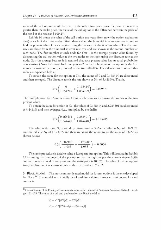
Chapter 14 Valuation of Interest Rate Derivative Instruments 413
value of the call option would be zero. In the other two cases, since the price in Year 2 isgreater than the strike price, the value of the call option is the difference between the price ofthe bond at the node and 100.25.
Exhibit 14 shows the value of the call option two years from now (the option expirationdate) at each of the three nodes. Given these values, the binomial interest rate tree is used tofind the present value of the call option using the backward induction procedure. The discountrates are those from the binomial interest rate tree and are shown as the second number ateach node. The first number at each node for Year 1 is the average present value found bydiscounting the call option value at the two nodes to the right using the discount rate at thenode. (It is the average because it is assumed that each present value has an equal probabilityof occurring.) Now let’s move back one year to ‘‘Today.’’ The value of the option is the firstnumber shown at the root (i.e., Today) of the tree, $0.6056. The calculations to obtain thisvalue are explained below.
To obtain the value for the option at NH, the values of 0 and 0.168414 are discountedand then averaged. The discount rate is the rate shown at NH of 5.4289%. That is,
0.5
(0
1.054289+ 0.168414
1.054289
)= 0.079871
The multiplication by 0.5 in the above formula is because we are taking the average of the twopresent values.
To obtain the value for option at NL, the values of 0.168414 and 2.283501 are discountedat 4.4448% and then averaged (i.e., multiplied by one half):
0.5
(0.168414
1.044448+ 2.283501
1.044448
)= 1.173785
The value at the root, N, is found by discounting at 3.5% the value at NH of 0.079871and the value at NL of 1.173785 and then averaging the values to get the value of 0.6056 asshown below:
0.5
(0.079871
1.035+ 1.173785
1.035
)= 0.6056
The same procedure is used to value a European put option. This is illustrated in Exhibit15 assuming that the buyer of the put option has the right to put the current 4-year 6.5%coupon Treasury bond in two years and the strike price is 100.25. The value of the put optiontwo years from now is shown at each of the three nodes in Year 2.
3. Black Model The most commonly used model for futures options is the one developedby Black.14 The model was initially developed for valuing European options on forwardcontracts.
14Fischer Black, ‘‘The Pricing of Commodity Contracts,’’ Journal of Financial Economics (March 1976),pp. 161-179. The value of a call and put based on the Black model is:
C = e−rt [FN (d1) − XN (d2)]
P = e−rt [XN (−d2) − FN (−d1)]
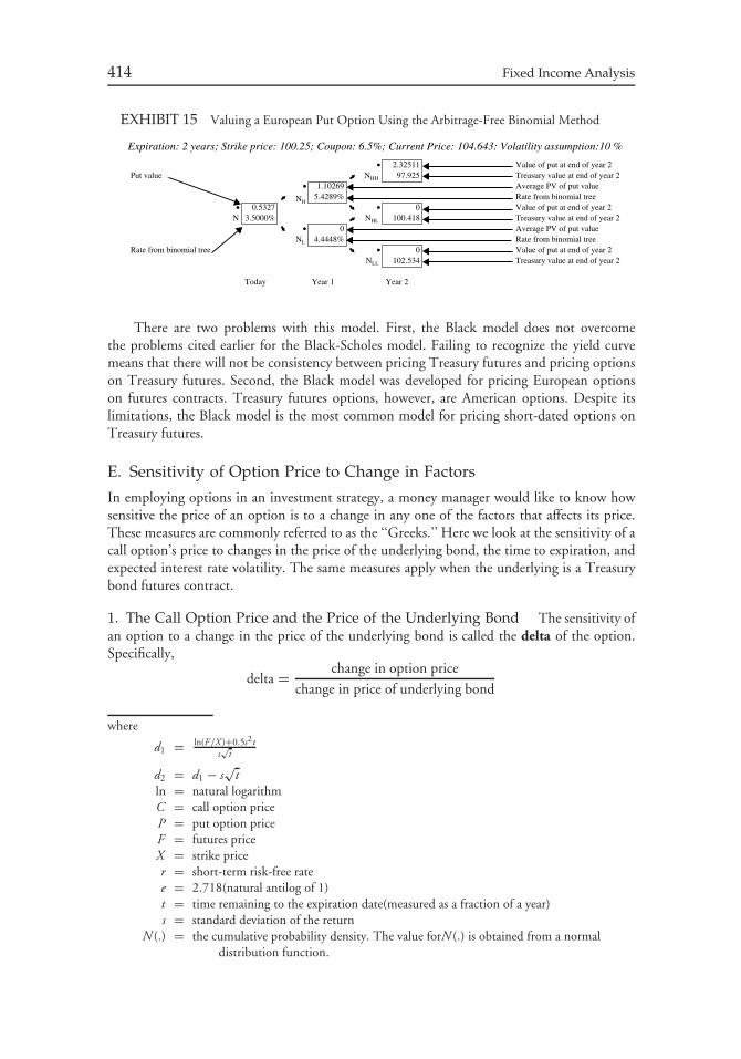
414 Fixed Income Analysis
EXHIBIT 15 Valuing a European Put Option Using the Arbitrage-Free Binomial Method
• 2.32511 Value of put at end of year 2Put value NHH 97.925 Treasury value at end of year 2
• 1.10269 Average PV of put value
NH5.4289% Rate from binomial tree
• 0.5327 • 0 Value of put at end of year 2N 3.5000% NHL 100.418 Treasury value at end of year 2
• 0 Average PV of put valueNL 4.4448% Rate from binomial tree
Rate from binomial tree • 0 Value of put at end of year 2NLL 102.534 Treasury value at end of year 2
Today Year 1 Year 2
Expiration: 2 years; Strike price: 100.25; Coupon: 6.5%; Current Price: 104.643: Volatility assumption:10 %
There are two problems with this model. First, the Black model does not overcomethe problems cited earlier for the Black-Scholes model. Failing to recognize the yield curvemeans that there will not be consistency between pricing Treasury futures and pricing optionson Treasury futures. Second, the Black model was developed for pricing European optionson futures contracts. Treasury futures options, however, are American options. Despite itslimitations, the Black model is the most common model for pricing short-dated options onTreasury futures.
E. Sensitivity of Option Price to Change in Factors
In employing options in an investment strategy, a money manager would like to know howsensitive the price of an option is to a change in any one of the factors that affects its price.These measures are commonly referred to as the ‘‘Greeks.’’ Here we look at the sensitivity of acall option’s price to changes in the price of the underlying bond, the time to expiration, andexpected interest rate volatility. The same measures apply when the underlying is a Treasurybond futures contract.
1. The Call Option Price and the Price of the Underlying Bond The sensitivity ofan option to a change in the price of the underlying bond is called the delta of the option.Specifically,
delta = change in option price
change in price of underlying bond
where
d1 = ln(F/X )+0.5s2ts√
t
d2 = d1 − s√
tln = natural logarithmC = call option priceP = put option priceF = futures priceX = strike pricer = short-term risk-free ratee = 2.718(natural antilog of 1)t = time remaining to the expiration date(measured as a fraction of a year)s = standard deviation of the return
N (.) = the cumulative probability density. The value forN (.) is obtained from a normaldistribution function.
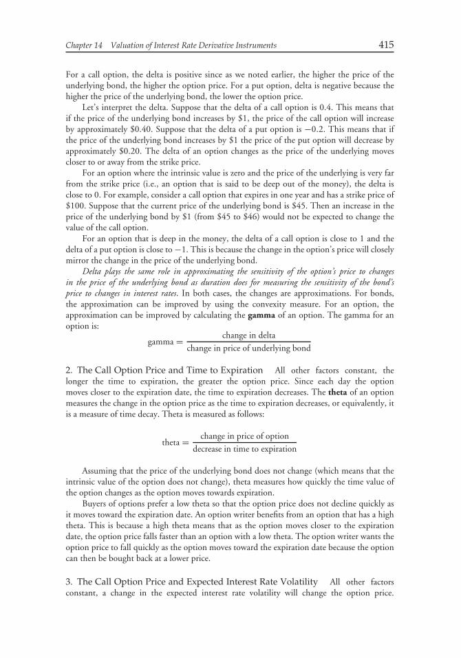
Chapter 14 Valuation of Interest Rate Derivative Instruments 415
For a call option, the delta is positive since as we noted earlier, the higher the price of theunderlying bond, the higher the option price. For a put option, delta is negative because thehigher the price of the underlying bond, the lower the option price.
Let’s interpret the delta. Suppose that the delta of a call option is 0.4. This means thatif the price of the underlying bond increases by $1, the price of the call option will increaseby approximately $0.40. Suppose that the delta of a put option is −0.2. This means that ifthe price of the underlying bond increases by $1 the price of the put option will decrease byapproximately $0.20. The delta of an option changes as the price of the underlying movescloser to or away from the strike price.
For an option where the intrinsic value is zero and the price of the underlying is very farfrom the strike price (i.e., an option that is said to be deep out of the money), the delta isclose to 0. For example, consider a call option that expires in one year and has a strike price of$100. Suppose that the current price of the underlying bond is $45. Then an increase in theprice of the underlying bond by $1 (from $45 to $46) would not be expected to change thevalue of the call option.
For an option that is deep in the money, the delta of a call option is close to 1 and thedelta of a put option is close to −1. This is because the change in the option’s price will closelymirror the change in the price of the underlying bond.
Delta plays the same role in approximating the sensitivity of the option’s price to changesin the price of the underlying bond as duration does for measuring the sensitivity of the bond’sprice to changes in interest rates. In both cases, the changes are approximations. For bonds,the approximation can be improved by using the convexity measure. For an option, theapproximation can be improved by calculating the gamma of an option. The gamma for anoption is:
gamma = change in delta
change in price of underlying bond
2. The Call Option Price and Time to Expiration All other factors constant, thelonger the time to expiration, the greater the option price. Since each day the optionmoves closer to the expiration date, the time to expiration decreases. The theta of an optionmeasures the change in the option price as the time to expiration decreases, or equivalently, itis a measure of time decay. Theta is measured as follows:
theta = change in price of option
decrease in time to expiration
Assuming that the price of the underlying bond does not change (which means that theintrinsic value of the option does not change), theta measures how quickly the time value ofthe option changes as the option moves towards expiration.
Buyers of options prefer a low theta so that the option price does not decline quickly asit moves toward the expiration date. An option writer benefits from an option that has a hightheta. This is because a high theta means that as the option moves closer to the expirationdate, the option price falls faster than an option with a low theta. The option writer wants theoption price to fall quickly as the option moves toward the expiration date because the optioncan then be bought back at a lower price.
3. The Call Option Price and Expected Interest Rate Volatility All other factorsconstant, a change in the expected interest rate volatility will change the option price.

416 Fixed Income Analysis
The kappa of an option measures the change in the price of the option for a 1% change inexpected interest rate volatility. (An option’s kappa is also referred to as its vega.) That is,
kappa = change in option price
1% change in expected interest rate volatility
The kappa of an option is positive because, as explained earlier, the option price increaseswhen expected interest rate volatility increases.
V. CAPS AND FLOORS
In applying the backward induction methodology to valuing caps and floors, the decisionto exercise at a node will depend on whether or not the cap or the floor is in the money.Remember that a cap and a floor are nothing more than a package or strip of options. Morespecifically, they are a strip of European options on interest rates. Thus, to value a cap, thevalue of each period’s cap, called a caplet, is found and the values of all the caplets are thensummed. The same can be done for a floor.
To illustrate how this is done, we will use the binomial tree given in Exhibit 13a. Wewill simplify the analysis by ignoring the difference in the timing of the payments for caps andfloors. Specifically, the settlement payment for caps and floors is in arrears. Allowing for thatwould require complicating the presentation and revising the binomial tree.15 Consider first a5.2% 3-year cap with a notional amount of $10 million. The reference rate is the 1-year ratein the binomial tree. The payoff for the cap is annual.
Exhibits 16a, 16b, and 16c show how this cap is valued by valuing the three caplets. Thevalue for the caplet for any year, say Year X, is found as follows. First, calculate the payoff inYear X at each node as either:16
1. zero if the 1-year rate at the node is less than or equal to 5.2%, or2. the notional principal amount of $10 million times the difference between the l-year
rate at the node and 5.2% if the 1-year rate at the node is greater than 5.2%.
Then, the backward induction method is used to determine the value of the Year X caplet.For example, consider the Year 3 caplet. At the top node in Year 3 of Exhibit 16c, the
1-year rate is 9.1987%. Since the 1-year rate at this node exceeds 5.2%, the payoff in Year 3 is:
$10, 000, 000 × (0.091987 − 0.052) = $399,870
Let’s show how the values shown at the nodes NHH, NH, and the root of the tree, N,are determined. For node NHH we look at the value for the cap at the two nodes to its right,NHHH and NHHL. The backward induction method involves discounting the values at these
15Profeesor Donald Smith of Boston University provides a framework for the adjustment. A presentationusing his framework is provided in Chapter 28 of Frank J. Fabozzi, Bond Markets, Analysis, and Strategies(Upper Saddle River, NJ: Pearson Prentice Hall, 2006).16Mathematically, the decision at a node is expressed as follows:
$10, 000, 000 × Maximum[(Rate at node − 5.2%), 0]
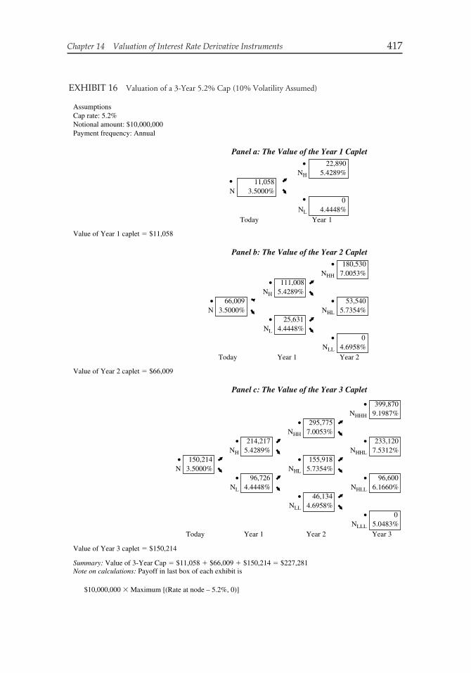
Chapter 14 Valuation of Interest Rate Derivative Instruments 417
EXHIBIT 16 Valuation of a 3-Year 5.2% Cap (10% Volatility Assumed)
AssumptionsCap rate: 5.2%Notional amount: $10,000,000Payment frequency: Annual
Panel a: The Value of the Year 1 Caplet
Value of Year 1 caplet � $11,058
Panel b: The Value of the Year 2 Caplet
Value of Year 2 caplet � $66,009
Panel c: The Value of the Year 3 Caplet
22,890NH 5.4289%
11,058N 3.5000%
0NL 4.4448%
Today Year 1
• 180,530NHH 7.0053%
• 111,008NH 5.4289%
• 66,009 • 53,540N 3.5000% NHL 5.7354%
• 25,631NL 4.4448%
• 0NLL 4.6958%
Today Year 1 Year 2
• 399,870NHHH 9.1987%
• 295,775NHH 7.0053%
• 214,217 • 233,120NH 5.4289% NHHL 7.5312%
• 150,214 • 155,918N 3.5000% NHL 5.7354%
• 96,726 • 96,600NL 4.4448% NHLL 6.1660%
• 46,134NLL 4.6958%
• 0NLLL 5.0483%
Today Year 1 Year 2 Year 3
•
•
•
Value of Year 3 caplet � $150,214
Summary: Value of 3-Year Cap � $11,058 � $66,009 � $150,214 � $227,281Note on calculations: Payoff in last box of each exhibit is
$10,000,000 � Maximum [(Rate at node – 5.2%, 0)]
418 Fixed Income Analysis
nodes, $399,870 and $233,120, by the interest rate from the binomial tree at node NHH,7.0053%, and computing the average present value. That is,
Value at NHH = [$399,870/(1.070053) + $233,120/(1.070053)]/2 = $295,775
This is the value reported at NHH.Now let’s see how the value at node NH is determined. Using the backward induction
method, the values at nodes NHH and NHL are discounted at the interest rate from thebinomial tree at node NH, 5.4289%, and then the present value is averaged. That is,
Value at NH = [$295,775/(1.054289) + $155,918/(1.054289)]/2 = $214,217
This is the value reported at NH.Finally, we get the value at the root, node N, which is the value of the Year 3 caplet
found by discounting the value at NH and NL by 3.5% (the interest rate at node N) and thenaveraging the two present values. Doing so gives:
Value at N = [$214,217/(1.035) + $96,726/(1.035)]/2 = $150,214
This is the value reported at N.Following the same procedure, the value of the Year 2 caplet is found to be $66,009 and
the value of the Year 1 caplet is $11,058. The value of the cap is then the sum of the values ofthe three caplets. That is,
value of cap = value of Year 1 caplet + value of Year 2 caplet + value of Year 3 caplet
Thus, the value of the cap is $227,281, found by adding $11,058, $66,009, and $150,214.Similarly, an interest rate floor can be valued. Exhibit 17 shows how for a 4.8% 3-year
floor with a notional amount of $10 million. Again, the reference rate is the 1-year rate in thebinomial tree and the payoff for the floor is annual. The value for the floor for any year, calleda floorlet, say Year X, is found as follows. First, calculate the payoff in Year X at each node aseither17
1. zero if the 1-year rate at the node is greater than or equal to 4.8%, or2. the notional amount of $10 million times the difference between 4.8% and the 1-year
rate at the node if the 1-year rate at the node is less than 4.8%.
Let’s see how the value of the Year 2 floorlet is determined using the backward inductionmethod. Specifically, we will see how to compute the values at nodes NLL, NL., and N (theroot of the tree and the value of the Year 2 floorlet). Look first at NLL. Since the rate of4.6958% is less than the floor rate of 4.8%, there is a payoff equal to
$10, 000, 000 × (0.048 − 0.046958) = $10,420
17Mathematically, the decision to exercise at a node is expressed as follows:
$10, 000, 000 × Maximum [(4.8% − Rate at node), 0]
Chapter 14 Valuation of Interest Rate Derivative Instruments 419
EXHIBIT 17 Valuation of a 3-Year 4.8% Floor (10% Volatility Assumed)
AssumptionsFloor rate: 4.8%Notional amount: $10,000,000Payment frequency: Annual
Panel a: The Value of the Year 1 Floorlet
Value of Year 1 floorlet � $17,159
Panel b: The Value of the Year 2 Floorlet
Value of Year 2 floorlet � $2,410
Value of Year 3 floorlet � $0
Panel c: The Value of the Year 3 Floorlet
0NH 5.4289%
17,159N 3.5000%
35,520NL 4.4448%
Today Year 1
• 0NHH 7.0053%
• 0NH 5.4289%
• 2,410 • 0N 3.5000% NHL 5.7354%
• 4,988NL 4.4448%
• 10,420NLL 4.6958%
Today Year 1 Year 2
• 0NHHH 9.1987%
• 00
NHH 7.0053%• 0
0• 0
NH 5.4289% NHHL 7.5312%• 0 • 0
0
N 3.5000% NHL 5.7354%• 0
0• 0
NL 4.4448% NHLL 6.1660%• 0
0
NLL 4.6958%• 0
NLLL 5.0483%Today Year 1 Year 2 Year 3
•
•
•
Summary: Value of 3-Year Floor � $17,159 � $2,410 � $0 � $19,569Note on calculations: Payoff in last box of each exhibit is
$10,000,000 � Maximum[ (4.8% – Rate at node), 0 ]

420 Fixed Income Analysis
This is the value shown at node NLL. Now we use the backward induction method tocompute the value at NL. We use the values at NLL and NHL to get the value at NL. The twovalues are discounted at 4.4448% (the interest rate at node NL) and then averaged. That is,
Value at NL = [0/(1.044448) + $10,420/(1.044448)]/2 = $4,988
This is the value reported at NL.Finally, we compute the value for the Year 2 floorlet by discounting the values at NH and
NL at 3.5% and then averaging, as shown below:
Value at N = [0/(1.035) + $4,988/(1.035)]/2 = $2,410
This is the value shown at the root of the tree and is the value of the Year 2 floorlet.Adding the Year 1 floorlet, Year 2 floorlet, and Year 3 floorlet shown in Exhibit 17 gives
the value of the 3-year floor: $17,159 + $2, 410 + $0 = $19,569.
CHAPTER 15GENERAL PRINCIPLES OF
CREDIT ANALYSIS
I. INTRODUCTION
The credit risk of a bond includes:
1. the risk that the issuer will default on its obligation and2. the risk that the bond’s value will decline and/or the bond’s price performance will
be worse than that of other bonds against which the investor is compared becauseeither (a) the market requires a higher spread due to a perceived increase in the riskthat the issuer will default or (b) companies that assign ratings to bonds will lower abond’s rating.
The first risk is referred to as default risk. The second risk is labeled based on the reasonfor the adverse or inferior performance. The risk attributable to an increase in the spread, ormore specifically the credit spread, is referred to as credit spread risk; the risk attributable toa lowering of the credit rating (i.e., a downgrading) is referred to as downgrade risk.1
Credit analysis of any entity—a corporation, a municipality, or a sovereign govern-ment—involves the analysis of a multitude of quantitative and qualitative factors over thepast, present, and future. There are four general approaches to gauging credit risk:
• credit ratings• traditional credit analysis• credit scoring models• credit risk models
In this chapter, we discuss each approach. Our primary focus is on the credit analysis ofcorporate bonds.
II. CREDIT RATINGS
A credit rating is a formal opinion given by a specialized company of the default risk faced byinvesting in a particular issue of debt securities. The specialized companies that provide credit
1These types of credit risk were discussed in detail earlier.
421
422 Fixed Income Analysis
ratings are referred to as ‘‘rating agencies.’’ The three nationally recognized rating agencies inthe United States are Moody’s Investors Service, Standard & Poor’s Corporation, and FitchRatings. The symbols used by these rating agencies and a summary description of each ratingis provided in Chapter 2.
A. Rating Process, Surveillance, and Review
The rating process begins when a rating agency receives a formal request from an entityplanning to issue a bond in which it seeks a rating for the bond issue (i.e., an ‘‘issue specificcredit rating’’). The cost associated with obtaining a credit rating is paid by the entity makingthe request for a rating. The request for a rating is made because without one, it would bedifficult for the entity to issue a bond. The rating assigned applies to the specific bond to beissued, not to the entity requesting the rating. A rating agency may also be requested to providea rating for a company that has no public debt outstanding (i.e., an ‘‘issuer credit rating’’).This is done for companies that are parties in derivative transactions, such as swaps, so thatmarket participants can assess counterparty risk.2
Once a credit rating is assigned to a corporate debt obligation, a rating agency monitors thecredit quality of the issuer and can reassign a different credit rating to its bonds. An ‘‘upgrade’’occurs when there is an improvement in the credit quality of an issue; a ‘‘downgrade’’ occurswhen there is a deterioration in the credit quality of an issue. As noted earlier, downgrade riskis the risk that an issue will be downgraded.
Typically, before an issue’s rating is changed, the rating agency will announce in advancethat it is reviewing the issue with the potential for upgrade or downgrade. The issue in suchcases is said to be on ‘‘rating watch’’ or ‘‘credit watch.’’ In the announcement, the rating agencywill state the direction of the potential change in rating—upgrade or downgrade. Typically, adecision will be made within three months.
In addition, rating agencies will issue rating outlooks. A rating outlook is a projectionof whether an issue in the long term (from six months to two years) is likely to be upgraded,downgraded, or maintain its current rating. Rating agencies designate a rating outlook aseither positive (i.e., likely to be upgraded), negative (i.e., likely to be downgraded), or stable(i.e., likely to be no change in the rating).
B. Gauging Default Risk and Downgrade Risk
The information available to investors from rating agencies about credit risk are: (1) ratings,(2) rating watches or credit watches, and (3) rating outlooks. Moreover, periodic studies bythe rating agencies provide information to investors about credit risk. Below we describe howthe information provided by rating agencies can be used to gauge two forms of credit risk:default risk and downgrade risk.
For long-term debt obligations, a credit rating is a forward-looking assessment of (1) theprobability of default and (2) the relative magnitude of the loss should a default occur. Forshort-term debt obligations (i.e., obligations with initial maturities of one year or less), acredit rating is a forward-looking assessment of the probability of default. Consequently, creditratings are the rating agencies assessment of the default risk associated with a bond issue.
Periodic studies by rating agencies provide information about two aspects of defaultrisk—default rates and default loss rates. First, rating agencies study and make available to
2Counterparty risk is the risk that a party to a financial transaction will default on its obligation.
Chapter 15 General Principles of Credit Analysis 423
investors the percentage of bonds of a given rating at the beginning of a period that havedefaulted at the end of the period. This percentage is referred to as the default rate.3 Forexample, a rating agency might report that the one-year default rate for triple B rated bonds is1.8%. These studies have shown that the lower the credit rating, the higher the default rate.Rating agency studies also show default loss rates by rating and other characteristics of theissue (e.g., level of seniority and industry). A default loss rate is a measure of the magnitudeof the potential of the loss should a default occur.4
A study by Moody’s found that for a corporate bond, its ratings combined with its ratingwatches and rating outlook status provide a better gauge for default risk than using the ratingsalone.5 The authors of the study looked at one-year and three-year default rates from 1996through 2003 for senior unsecured rated bonds and within each rating by rating watch (watchupgrade and watch downgrade) and rating outlook status (positive, stable, and negative). Theone-year default rate results for three selected ratings are shown below:
Rating Watch up Positive Stable Negative Watch downBaa3 NA 0.20% 0.60% 1.25% 2.26%B1 NA 0.98% 2.53% 5.07% 12.03%Caa1 3.7% 3.82% 8.43% 14.93% 42.21%
Notice that as one moves from left to right for a given credit rating in the above tablethat the default rate increases. Look at the Caa1 rating. For issues that were on ratingwatch for a potential upgrade at the beginning of the period, 3.7% defaulted in oneyear. However, for those on rating watch for a potential downgrade at the beginningof the period, 42.21% defaulted in one year. This suggests that rating watches containuseful information in gauging default risk. Look at the rating outlook status for Caa1.Issues that had a negative rating outlook at the beginning of the year had a one-yeardefault rate that was almost four times greater than issues that had a positive ratingoutlook.
Moody’s makes the following suggestion as to how an analyst can combine the informationcontained in rating watches and outlook rating status to adjust the senior unsecured rating ofa corporate bond:
For issues on: Suggestion:downgrade watch reduce current rating by two rating notches6
upgrade watch increase current rating by two rating notchesnegative outlook reduce current rating by one rating notchstable outlook keep current ratingpositive outlook increase current rating by one rating notch
Of course, portfolio managers may elect to develop their own system for adjusting thecurrent rating of a bond based on their assessment of the findings of the study by Moody’s.
3There are several ways that default rates can be measured. These are described in Chapter 3.4The default loss rate is described in Chapter 3.5David T. Hamilton and Richard Cantor, Rating Transitions and Defaults Conditional on Watchlist,Outlook and Rating History, Moody’s Investors Service, February 2004.6A rating ‘‘notch’’ is a rating based on the modified rating (i.e., in the case of Moody’s with the ‘‘1’’,‘‘2’’, and ‘‘3’’ modifiers). For example, if an issue is rated Baa2, then a reduction of one rating notchwould be a rating of Baa3. A reduction of two rating notches would be a rating of Ba1.
424 Fixed Income Analysis
What is essential, however, is that in assessing the default risk when using credit ratings,portfolio managers should take into consideration rating watches and rating outlook status.
While the discussion above has focused on default risk, other studies by rating agenciesalso provide information. In Chapter 2, the rating transition matrix published periodically bythe rating agencies was explained. A rating transition table shows the percentage of issues ofeach rating at the beginning of a period that was downgraded or upgraded by the end of thetime period. Consequently, by looking at the percentage of downgrades for a given rating, anestimate can be obtained of the probability of a downgrade and this can serve as a measure ofdowngrade risk.7
III. TRADITIONAL CREDIT ANALYSIS
In traditional credit analysis, the analyst considers the four C’s of credit:
• capacity• collateral• covenants• character
Capacity is the ability of an issuer to repay its obligations. Collateral is looked at notonly in the traditional sense of assets pledged to secure the debt, but also to the quality andvalue of those unpledged assets controlled by the issuer. In both senses the collateral is capableof supplying additional aid, comfort, and support to the debt and the debtholder. Assets formthe basis for the generation of cash flow which services the debt in good times as well as bad.Covenants are the terms and conditions of the lending agreement. They lay down restrictionson how management operates the company and conducts its financial affairs. Covenantscan restrict management’s discretion. A default or violation of any covenant may providea meaningful early warning alarm enabling investors to take positive and corrective actionbefore the situation deteriorates further. Covenants have value as they play an important partin minimizing risk to creditors. They help prevent the transfer of wealth from debt holdersto equity holders. Character of management is the foundation of sound credit. This includesthe ethical reputation as well as the business qualifications and operating record of the boardof directors, management, and executives responsible for the use of the borrowed funds andrepayment of those funds.
A. Analysis of the Capacity to Pay
A corporation will generate the funds to service its debt from its cash flow. The cash flow isgenerated from revenues and reduced by the costs of operations. Therefore, in assessing theability of an issuer to pay, an analysis of the financial statements as discussed later in thischapter is undertaken. In addition to management quality, the factors examined by analysts atMoody’s are:8
7An illustration of a rating transition matrix and the calculation of the probability of downgrade wereprovided.8‘‘Industrial Company Rating Methodology,’’ Moody’s Investors Services: Global Credit Research (July1998), p. 3.
Chapter 15 General Principles of Credit Analysis 425
1. industry trends2. the regulatory environment3. basic operating and competitive position4. financial position and sources of liquidity5. company structure (including structural subordination and priority of claim)6. parent company support agreements7. special event risk
In considering industry trends, analysts look at the vulnerability of the company toeconomic cycles, the barriers to entry, and the exposure of the company to technologicalchanges. For firms in regulated industries, proposed changes in regulations must be analyzedto assess their impact on future cash flows. At the company level, diversification of the productline and the cost structure are examined in assessing the basic operating position of the firm.
In addition to the measures described later in this chapter for assessing a company’sfinancial position over the past three to five years, an analyst must look at the capacity of a firmto obtain additional financing and back-up credit facilities. There are various forms of back-upcredit facilities. The strongest forms of back-up credit facilities are those that are contractuallybinding and do not include provisions that permit the lender to refuse to provide funds. Anexample of such a provision is one that allows the bank to refuse funding if the bank feels thatthe borrower’s financial condition or operating position has deteriorated significantly. (Such aprovision is called a material adverse change clause.) Non-contractual facilities such as linesof credit that make it easy for a bank to refuse funding should be of concern to the analyst.The analyst must also examine the quality of the bank providing the back-up facility.
Analysts should also assess whether the company can use securitization as a funding sourcefor generating liquidity. Asset securitization involves using a pool of loans or receivables as col-lateral for a security. The decision of whether to securitize assets to borrow or use traditionalborrowing sources is done on the basis of cost. However, if traditional sources dry up when a com-pany faces a liquidity crisis, securitization may provide the needed liquidity. An analyst shouldinvestigate the extent to which management has considered securitization as a funding source.
Other sources of liquidity for a company may be third-party guarantees, the most commonbeing a contractual agreement with its parent company. When such a financial guaranteeexists, the analyst must undertake a credit analysis of the parent company.
In the analysis of an issuer’s ability to pay, the analyst will analyze the issuer’s financialstatements (income statement, balance sheet, and statement of cash flows), project futurefinancial statements based on certain assumptions, and compute various measures. Thesemeasures include traditional ratio measures and cash flow measures. Below we review thesemeasures and explain how an additional analysis of cash flows provides a better early warningalarm of potential financial difficulties than traditional ratios.
1. Traditional Ratios Traditional ratios to evaluate the ability of an issuer to meet itsobligations include:
• profitability ratios• debt and coverage ratios
a. Profitability Ratios Equity analysts focus on the earnings of a firm, particularly theearnings per share. While a holder of the debt obligation of a firm does not have the opportunityto share in the economic growth of the firm, this does not mean that a credit analyst should
426 Fixed Income Analysis
ignore a firm’s profitability. It is from revenues that a firm will continue to grow in order togenerate cash flow to meet obligations.
Profitability ratios are utilized to explore the underlying causes of a change in the company’searnings. They show the combined effects of liquidity and asset and debt management on theprofitability of the firm. These ratios break earnings per share into its basic determinants forpurposes of assessing the factors underlying the profitability of the firm. They help to assess theadequacy of historical profits, and to project future profitability through better understandingof its underlying causes.
Standards for a given ratio will vary according to operating characteristics of the companybeing analyzed and general business conditions; such standards cannot be stated as fixed andimmutable. It is assumed that the analyst has made all adjustments deemed necessary to reflectcomparable and true earning power of the corporation before calculating the ratios discussedbelow. It is important to stress that ratios are utilized to raise significant questions requiringfurther analysis, not to provide answers.
Equity analysts use the DuPont formula (explained in textbooks on equity analysis) toassess the determinants of a company’s earnings per share. The profitability ratios analyzed toassess earnings per share are:
• return on stockholders’ equity• return on total assets• profit margin• asset turnover
Each of these measures and their limitations are explained in textbooks on financial statementanalysis and equity analysis so they will not be repeated here.
b. Debt and Coverage Analysis There are three sets of ratios that are used by creditanalysts as indicators to assess the ability of a firm to satisfy its debt obligations:
• short-term solvency ratios• capitalization (or financial leverage) ratios• coverage ratios
i. Short-Term Solvency Ratios Short-term solvency ratios are used to judge the adequacy ofliquid assets for meeting short-term obligations as they come due. A complete analysis of theadequacy of working capital for meeting current liabilities as they come due and assessingmanagement’s efficiency in using working capital would require a thorough analysis of cashflows and forecasts of fund flows in future periods that will be discussed in the next section.However, ratios provide a crude but useful assessment of working capital. The following tworatios are calculated to assess the adequacy of working capital for a firm:
• the current ratio• the acid-test ratio
The current ratio is calculated by dividing current assets by current liabilities:
current ratio = current assets
current liabilities
Chapter 15 General Principles of Credit Analysis 427
The current ratio indicates the company’s coverage of current liabilities by current assets.For example, if the ratio were 2:1, the firm could realize only half of the values stated in thebalance sheet in liquidating current assets and still have adequate funds to pay all currentliabilities.
A general standard for this ratio (such as 2:1) is not useful. Such a standard fails torecognize that an appropriate current ratio is a function of the nature of a company’s businessand would vary with differing operating cycles of different businesses. The operating cycle ofa company is the duration from the time cash is invested in goods and services to the time thatinvestment produces cash.9
A current asset is one that is expected to be converted into cash in the ordinary operatingcycle of a business. Inventory, therefore, is a current asset. In a tobacco or liquor manufacturingcompany, inventory may be as much as 80% to 90% of current assets. However, for a liquorcompany that inventory may have to age four years or more before it can be converted into asalable asset. Such a company typically would require a much higher current ratio than averageto have adequate liquidity to meet current liabilities maturing in one year. For a public utilitycompany where there is no inventory or receivables collection problem, a current ratio of 1.1or 1.2 to 1 has proved satisfactory. Industry averages are published by organizations such asDun & Bradstreet and Robert Morris Associates. While industry averages have their faults,they are preferable to general standards that do not recognize operating differences amongclasses of companies.
The current ratio has a major weakness as an analytical tool. It ignores the compositionof current assets, which may be as important as their relationship with current liabilities.Therefore, current ratio analysis must be supplemented by other working capital ratios.
Since the problem in meeting current liabilities may rest on slowness or even inability toconvert inventories into cash to meet current obligations, the acid-test ratio (also called thequick ratio) is recommended. This is the ratio of current assets minus inventories to currentliabilities; that is:
acid-test ratio = current assets − inventories
current liabilities
This ratio does assume that receivables are of good quality and will be converted into cash overthe next year.
ii. Capitalization Ratios Credit analysts also calculate capitalization ratios to determinethe extent to which the corporation is using financial leverage. These ratios, also calledfinancial leverage ratios, can be interpreted only in the context of the stability of industry andcompany earnings and cash flow. The assumption is that the greater the stability of industryand company earnings and cash flow, the more the company is able to accept the risk associatedwith financial leverage, and the higher the allowable ratio of debt to total capitalization (thetotal dollar amount of all long-term sources of funds in the balance sheet).
9For example, a firm that produces and sells goods has an operating cycle comprising of four phases:(1) purchase of raw material and produce goods, investing in inventory; (2) sell goods, generating sales,which may or may not be for cash; (3) extend credit, creating accounts receivable; and, (4) collectaccounts receivable, generating cash. The four phases make up the cycle of cash use and generation. Theoperating cycle would be somewhat different for companies that produce services rather than goods, butthe idea is the same—the operating cycle is the length of time it takes to generate cash through theinvestment of cash.
428 Fixed Income Analysis
There are many variations to be found within the industry to calculate capitalizationratios. Two such ratios are shown below:
long-term debt to capitalization = long-term debt
long-term debt + shareholders’equity including minority interest
total debt to capitalization
= current liabilities + long-term debt
long-term debt + current liabilities + shareholders’ equityincluding minority interest
where shareholders’ equity includes preferred stock.For both ratios, the higher the ratio, the greater the financial leverage. The value used
to measure debt in both ratios is book value. It is useful to calculate stockholders’ equityat market as well as at book value for the purpose of determining these ratios. A marketcalculation for common equity may indicate considerably more or less financial leverage thana book calculation.
Commercial rating companies and most Wall Street analysts rely heavily upon thelong-term debt to capitalization ratio, and this is often provided in research reports sent outto clients. While this ratio can be useful, it should be noted that in recent years, given theuncertain interest rate environment, many corporations have taken to financing a good dealof their business with short-term debt. Indeed, an imaginative treasurer with a keen insightinto money market activities can earn as much for a company as a plant manager, simply byswitching debt from long term to short term and vice versa, at the right time.
Other considerations in using the long-term debt to capitalization ratio involves leasedassets. Many corporations rent buildings and equipment under long-term lease contracts.Required rental payments are contractual obligations similar to bond coupon and repaymentobligations. However, assets acquired through leasing (i.e., those leases classified as operatingleases) may not be capitalized and shown in the balance sheet. Two companies, therefore,might work with the same amount of fixed assets and produce the same profits before interestor rental payments, but the one leasing a high proportion of its productive equipment couldshow significantly lower financial leverage.
iii. Coverage Tests Coverage ratios are used to test the adequacy of cash flows generatedthrough earnings for purposes of meeting debt and lease obligations. The four most commonlyused coverage ratios are:
• EBIT interest coverage ratio• EBITDA interest coverage ratio• funds from operations/total debt ratio• free operating cash flow/total debt ratio
EBIT stands for ‘‘earnings before interest and taxes.’’ The EBIT interest coverage ratiois simply EBIT divided by the annual interest expense. (Interest expense includes ‘‘capitalizedinterest.’’ This is effectively interest expense imputed for capitalized assets, the most importantof which is leased assets.) Interest expense is tax deductible and, therefore, all earnings beforetaxes are available for paying such charges. Also, the interest should be added back to determinethe amount available to meet annual interest expenses.
Chapter 15 General Principles of Credit Analysis 429
EBITDA stands for ‘‘earnings before interest, taxes, depreciation, and amortization.’’ TheEBITDA interest coverage ratio is simply the ratio of EBITDA divided by the annual interestexpense.
The last two ratios listed above indicate the amount of funds from operations relative tothe amount of total debt. The funds from operations includes net income plus the following:depreciation, amortization, deferred income taxes, and other noncash items. The definition offree operating cash flows varies by rating agency. In the next section we describe one variantof free operating cash flow.
Suggested standards for coverage ratios are based on experience and empirical studiesrelating the incidence of defaults over a number of years to such ratios. Different standards areneeded for a highly cyclical company than for a stable company. In the case study presentedin the appendix to this chapter, benchmark ratios (as measured in terms of median ratios)by credit rating are presented for the coverage ratios described above, as well as for thecapitalization ratios.
2. Cash Flow Analysis Will the ratios just described be sufficient to help an analystidentify companies that may encounter financial difficulties? Consider the study by Largayand Stickney who analyzed the financial statements of W.T. Grant during the 1966–1974period preceding its bankruptcy in 1975 and ultimate liquidation.10 They noted that financialindicators such as profitability ratios, turnover ratios, and liquidity ratios showed some downtrends, but provided no definite clues to the company’s impending bankruptcy. A studyof cash flows from operations, however, revealed that company operations were causing anincreasing drain on cash, rather than providing cash.11 This necessitated an increased use ofexternal financing, the required interest payments on which exacerbated the cash flow drain.Cash flow analysis clearly was a valuable tool in this case since W.T. Grant had been running anegative cash flow from operations for years. Yet none of the traditional ratios discussed abovetake into account the cash flow from operations.
The need to look at cash flow is emphasized by Standard & Poor’s:
Cash flow analysis is the single most critical aspect of all credit rating decisions. It takes onadded importance for speculative-grade issuers. While companies with investment-graderatings generally have ready access to external cash to cover temporary shortfalls, junk-bondissuers lack this degree of flexibility and have fewer alternatives to internally generatedcash for servicing debt.12
S&P also notes that: ‘‘Discussions about cash flow often suffer from lack of uniformdefinition of terms.’’13 Below we describe how S&P’s terminology with respect to four cashflow concepts: operating cash flow, free operating cash flow, discretionary cash flow, andprefinancing cash flow. In addition, we discuss the various ratios employing these cash flowmeasures.
10J.A. Largay III and C.P. Stickney, ‘‘Cash Flows, Ratio Analysis and the W.T. Grant CompanyBankruptcy,’’ Financial Analysts Journal (July-August 1980), pp. 51-54.11For the period investigated, a statement of changes of financial position (on a working capital basis)was required prior to 1988.12Standard & Poor’s, Corporate Ratings Criteria, undated, p. 26.13Corporate Ratings Criteria, p. 27.
430 Fixed Income Analysis
a. Cash Flow Measures Prior to the adoption of the statement of cash flows in 1987, theinformation regarding a firm’s cash flows was quite limited. The statement of cash flows is asummary over a period of time of a firm’s cash flows from operating, investing, and financingactivities. The firm’s statement of cash flows lists separately its
• cash flows from operating activities• cash flows from investing• cash flow financing activities
Typically the corresponding cash flows are referred to as:14
• Cash provided by operating activities• Cash provided by/(used for) investing activities• Cash used for financing activities
‘‘Cash provided by operating activities’’ is also referred to as ‘‘cash flow from operations.’’By analyzing these individual statement of cash flows, creditors can examine such aspects
of the business as:
• The source of financing for business operations, whether through internally generatedfunds or external sources of funds.
• The ability of the company to meet debt obligations (interest and principal payments).• The ability of the company to finance expansion through cash flow from its operating
activities.• The ability of the company to pay dividends to shareholders.• The flexibility the business has in financing its operations.
A firm that generates cash flows only by selling off its assets (obtaining cash flows frominvesting) or by issuing more securities (obtaining cash flows from financing) cannot keep thatup for very long. For future prosperity and the ability to meet its obligations, the firm mustbe able to generate cash flows from its operations.
Analysts have reformatted the information from the firm’s income statement and statementof cash flows to obtain what they view as a better description of the company’s activities. S&Pbegins with what it refers to as funds from operations. The funds from operations is definedas net income adjusted for depreciation and other noncash debits and credits. Then from thefunds from operation, the following cash flow measures are computed:15
Funds from operationsDecrease (increase) in noncash current assetsIncrease (decrease) in nondebt current liabilities
Operating cash flowDecrease by capital expenditures
14Some firms use different labels. For example, Microsoft refers to these cash flows as: Net cash fromoperations, Net cash used for financing, and Net cash used for investing.15Corporate Ratings Criteria, p. 27.
Chapter 15 General Principles of Credit Analysis 431
Free operating cash flowDecrease by cash dividends
Discretionary cash flowDecrease by acquisitionsIncrease by asset disposalsNet other sources (uses) of cash
Prefinancing cash flow
Operating cash flow is therefore funds from operations reduced by changes in theinvestment in working capital (current assets less current liabilities). Subtracting capitalexpenditures gives what S&P defines as free operating cash flow. It is this cash flow measurethat can be used to pay dividends and make acquisitions.16 Reducing free operating cashflow by cash dividends gives discretionary cash flow. Adjusting discretionary cash flow formanagerial discretionary decisions for acquisition of other companies, the disposal of assets(e.g., lines of business or subsidiaries), and others sources or uses of cash gives prefinancingcash flow. As stated by S&P, prefinancing cash flow ‘‘represents the extent to which companycash flow from all internal sources have been sufficient to cover all internal needs.’’17
b. Cash Flow Ratios S&P uses the following cash flow ratios (based on its cash flowdefinitions described above) in analyzing a company in addition to the measures describedearlier for coverage ratios:
Funds from operations
Total debt (adjusted for off-balance sheet liabilities)
Free operating cash flow + Interest
InterestFree operating cash flow + Interest
Interest + Annual principal repayment obligation
(the above ratio is referred to as the ‘‘debt service coverage ratio’’)
Total debt
Discretionary cash flow
16One of the most popular measures of cash flow in equity analysis is the ‘‘free cash flow.’’ This cash flowmeasure is defined as ‘‘the cash flow available to the company’s suppliers of capital after all operatingexpenses (including taxes) have been paid and necessary investments in working capital (e.g., inventory)and fixed capital (e.g., equipment) have been made.’’ (See, John D. Stowe, Thomas R. Robinson,Jerald E. Pinto, and Dennis W. McLeavey, Analysis of Equity Investments: Valuation (Charlottesville,VA: Association for Investment Management and Research, 2002), p. 115.) Analysts will make differentadjustments to the statement of cash flows to obtain the free cash flow depending on the accountinginformation that is available. The procedure for calculating free cash flow starting with net incomeor statement of cash flows is explained in Stowe, Robinson, Pinto, and McLeavey, Analysis of EquityInvestments: Valuation, pp. 119–124.17Corporate Ratings Criteria, p. 27.
432 Fixed Income Analysis
(the above ratio is called the ‘‘debt payback period’’)
Funds from operations
Capital spending requirements
The particular cash flow ratios that S&P focuses on depends on the type of companybeing analyzed. According to S&P:
Where long-term viability is more assured (i.e., higher in the rating spectrum) therecan be greater emphasis on the level of funds from operations and its relation to totaldebt burden. These measures clearly differentiate between levels of protection over time.Focusing on debt service coverage and free cash flow becomes more critical in the analysisof a weaker company. Speculative-grade issuers typically face near-term vulnerabilities,which are better measured by free cash flow ratios.18
B. Analysis of Collateral
A corporate debt obligation can be secured or unsecured. In our discussion of creditor rightsin a bankruptcy, we explained that in the case of a liquidation, proceeds from a bankruptcyare distributed to creditors based on the absolute priority rule. However, in the case of areorganization, the absolute priority rule rarely holds. That is, an unsecured creditor mayreceive distributions for the entire amount of his or her claim and common stockholders mayreceive something, while a secured creditor may receive only a portion of its claim. The reasonis that a reorganization requires approval of all the parties. Consequently, secured creditorsare willing to negotiate with both unsecured creditors and stockholders in order to obtainapproval of the plan of reorganization.
The question is then, what does a secured position mean in the case of a reorganization ifthe absolute priority rule is not followed in a reorganization? The claim position of a securedcreditor is important in terms of the negotiation process. However, because absolute priorityis not followed and the final distribution in a reorganization depends on the bargaining abilityof the parties, some analysts place less emphasis on collateral compared to the other factorsdiscussed earlier and covenants discussed next.
We discussed the various types of collateral used for a corporate debt issue and features thatanalysts should be cognizant of in looking at an investor’s secured position. Other importantfeatures are covered in our discussion of covenants below.
C. Analysis of Covenants
Covenants deal with limitations and restrictions on the borrower’s activities. Some covenantsare common to all indentures, such as
• to pay interest, principal, and premium, if any, on a timely basis• to pay all taxes and other claims when due unless contested in good faith• to maintain all properties used and useful in the borrower’s business in good condition and
working order• to submit periodic certificates to the trustee stating whether the debtor is in compliance
with the loan agreement
18Corporate Ratings Criteria, p. 27.
Chapter 15 General Principles of Credit Analysis 433
These covenants are called affirmative covenants since they call upon the debtor to makepromises to do certain things.
Negative covenants are those which require the borrower not to take certain actions.There are an infinite variety of restrictions that can be placed on borrowers, depending onthe type of debt issue, the economics of the industry and the nature of the business, and thelenders’ desires. Some of the more common restrictive covenants include various limitationson the company’s ability to incur debt, since unrestricted borrowing can lead a companyand its debtholders to ruin. Thus, debt restrictions may include limits on the absolute dollaramount of debt that may be outstanding or may require a ratio test—for example, debt maybe limited to no more than 60% of total capitalization or that it cannot exceed a certainpercentage of net tangible assets.
There may be an interest or fixed charge coverage test. The two common tests are:
• maintenance test: This test requires the borrower’s ratio of earnings available for interestor fixed charges to be at least a certain minimum figure on each required reporting date(such as quarterly or annually) for a certain preceding period.
• debt incurrence test: only comes into play when the company wishes to do additionalborrowing. In order to take on additional debt, the required interest or fixed charge coveragefigure adjusted for the new debt must be at a certain minimum level for the required periodprior to the financing. Debt incurrence tests are generally considered less stringent thanmaintenance provisions.
There could also be cash flow tests (or cash flow requirements) and working capitalmaintenance provisions.
Some indentures may prohibit subsidiaries from borrowing from all other companiesexcept the parent. Indentures often classify subsidiaries as restricted or unrestricted. Restrictedsubsidiaries are those considered to be consolidated for financial test purposes; unrestrictedsubsidiaries (often foreign and certain special-purpose companies) are those excluded fromthe covenants governing the parent. Often, subsidiaries are classified as unrestricted in orderto allow them to finance themselves through outside sources of funds.
Limitations on dividend payments and stock repurchases may be included in indentures.Often, cash dividend payments will be limited to a certain percentage of net income earnedafter a specific date (often the issuance date of the debt, called the ‘‘peg date’’) plus a fixedamount. Sometimes the dividend formula might allow the inclusion of the net proceeds fromthe sale of common stock sold after the peg date. In other cases, the dividend restriction mightbe so worded as to prohibit the declaration and payment of cash dividends if tangible networth (or other measures, such as consolidated quick assets) declines below a certain amount.
D. Character of a Corporation
Character analysis involves the analysis of the quality of management. In discussing thefactors it considers in assigning a credit rating, Moody’s Investors Service notes the followingregarding the quality of management:19
Although difficult to quantify, management quality is one of the most important factorssupporting an issuer’s credit strength. When the unexpected occurs, it is a management’sability to react appropriately that will sustain the company’s performance.
19‘‘Industrial Company Rating Methodology,’’ p. 6.
434 Fixed Income Analysis
In assessing management quality, the analysts at Moody’s, for example, try to understandthe business strategies and policies formulated by management. Following are factors that areconsidered: (1) strategic direction, (2) financial philosophy, (3) conservatism, (4) track record,(5) succession planning, and (6) control systems.
In recent years, focus has been on the corporate governance of the firm and the role ofthe board of directors.
1. Corporate Governance The bylaws are the rules of governance for the corporation.The bylaws define the rights and obligations of officers, members of the board of directors,and shareholders. In most large corporations, it is not possible for each owner to participatein monitoring of the management of the business. Therefore, the owners of a corporationelect a board of directors to represent them in the major business decisions and to monitorthe activities of the corporation’s management. The board of directors, in turn, appoints andoversees the officers of the corporation. Directors who are also employees of the corporationare called inside directors; those who have no other position within the corporation areoutside directors or independent directors.
It is the board of directors that decides whether to hire, retain, or dismiss the chiefexecutive officer, to establish the compensation system for senior management, and to ensurethat the proper internal corporate control systems are in place to monitor management.Generally it is believed that the greater the proportion of outside directors, the greater theboard independence from the management of the company. The proportion of outsidedirectors on corporate boards varies significantly.
Recently, there have been a number of scandals and allegations regarding the financialinformation that is being reported to shareholders and the market. Financial results reportedin the income statements and balance sheets of some companies indicated much betterperformance than the true performance or much better financial condition than actual.20
Along with these financial reporting issues, the independence of the auditors and the role offinancial analysts have been brought to the forefront.
The eagerness of managers to present favorable results to shareholders and the marketappears to be a major factor in several of the scandals. Personal enrichment at the expense ofshareholders seems to explain some of the scandals. Whatever the motivation, chief executiveofficers (CEOs), chief financial officers (CFOs), and board members are being held directlyaccountable for financial disclosures. For example, in 2002, the U.S. Securities and ExchangeCommission ordered sworn statements attesting to the accuracy of financial statements. Thefirst deadline for such statements resulted in several companies restating financial results.
The accounting scandals are creating an awareness of the importance of corporategovernance, the importance of the independence of the public accounting auditing function,the role of financial analysts, and the responsibilities of CEOs and CFOs.
2. Agency Problem Corporate financial theory helps us understand how the abuses thatdiminish shareholder value arise and the potential for mitigating the abuse. In a publicly tradedcompany, typically the managers of a corporation are not the major owners. The managersmake decisions for owners. Thus, the managers act as agents. An agent is a person who actsfor—and exerts powers on behalf of—another person or group of persons. The person (or
20Examples include Xerox, which was forced to restate earnings for several years because it had inflatedpre-tax profits by $1.4 billion, Enron, which is accused of inflating earnings and hiding substantial debt,and Worldcom, which failed to properly account for $3.8 billion of expenses.
Chapter 15 General Principles of Credit Analysis 435
group of persons) the agent represents is referred to as the principal. The relationship betweenthe agent and his or her principal is an agency relationship. There is an agency relationshipbetween the managers and the shareholders of corporations.21
In an agency relationship, the agent is charged with the responsibility of acting forthe principal. As a result, it is possible that the agent may not act in the best interestof the principal, but instead act in his or her own self-interest. This is because the agenthas his or her own objective of maximizing personal wealth. In a large corporation, forexample, the managers may enjoy many fringe benefits, such as golf club memberships, accessto private jets, and company cars. These benefits (also called perquisites, or ‘‘perks’’) maybe useful in conducting business and may help attract or retain management personnel,but there is room for abuse. The abuse of perquisites imposes costs on the firm—andultimately on the owners of the firm. There is also a possibility that managers who feelsecure in their positions may not bother to expend their best efforts toward the business.Finally, there is the possibility that managers will act in their own self-interest, rather thanin the interest of the shareholders when those interests clash. For example, managementmay fight the acquisition of their firm by some other firm even if the acquisition wouldbenefit shareholders. This is because in most takeovers, the management of the acquiredfirm generally lose their jobs. Consequently, a manager’s self-interest may be placed aheadof those of shareholders who may be offered an attractive price for their stock in theacquisition.
There are costs involved with any effort to minimize the potential for conflict betweenthe principal’s interest and the agent’s interest. Such costs are called agency costs, and theyare of three types: monitoring costs, bonding costs, and residual loss.
Monitoring costs are costs incurred by the principal to monitor or limit the actions ofthe agent. In a corporation, shareholders may require managers to periodically report on theiractivities via audited accounting statements, which are sent to shareholders. The accountants’fees and the management time lost in preparing such statements are monitoring costs. Anotherexample is the implicit cost incurred when shareholders limit the decision-making power ofmanagers. By doing so, the owners may miss profitable investment opportunities; the foregoneprofit is a monitoring cost.
The board of directors of corporation has a fiduciary duty to shareholders; that is, thelegal responsibility to make decisions (or to see that decisions are made) that are in the bestinterests of shareholders. Part of that responsibility is to ensure that managerial decisions arealso in the best interests of the shareholders. Therefore, at least part of the cost of havingdirectors is a monitoring cost.
Bonding costs are incurred by agents to assure principals that they will act in theprincipal’s best interest. The name comes from the agent’s promise or bond to take certainactions. A manager may enter into a contract that requires him or her to stay on with the firmeven though another company acquires it; an implicit cost is then incurred by the manager,who foregoes other employment opportunities. Even when monitoring and bonding devicesare used, there may be some divergence between the interests of principals and those ofagents. The resulting cost, called the residual loss, is the implicit cost that results because theprincipal’s and the agent’s interests cannot be perfectly aligned even when monitoring andbonding costs are incurred.
21The seminal paper on the agency-principal relationship in corporate finance is Michael Jensenand William Meckling, ‘‘Theory and the Firm: Managerial Behavior, Agency Costs and OwnershipStructure,’’ Journal of Financial Economics (October 1976), pp. 305-360.
436 Fixed Income Analysis
3. Stakeholders and Corporate Governance When managers of a corporation assessa potential investment in a new product, they examine the risks and the potential benefits andcosts. Similarly, managers assess current investments for the same purpose; if benefits do notcontinue to outweigh costs, they will not continue to invest in the product but will shift theirinvestment elsewhere. This is consistent with the goal of shareholder wealth maximization andwith the allocative efficiency of the market economy.
Discontinuing investment in an unprofitable business may mean closing down plants,laying off workers, and, perhaps destroying an entire town that depends on the business forincome. So decisions to invest or disinvest may affect great numbers of people. All but thesmallest business firms are linked in some way to groups of persons who are dependent toa degree on the business. These groups may include suppliers, customers, the communityitself, and nearby businesses, as well as employees and shareholders. The various groups ofpersons that depend on a firm are referred to as its stakeholders; they all have some stake inthe outcomes of the firm. For example, if the Boeing Company lays off workers or increasesproduction, the effects are felt by Seattle and the surrounding communities.
Can a firm maximize the wealth of shareholders and stakeholders at the same time?Probably. If a firm invests in the production of goods and services that meet the demandof consumers in such a way that benefits exceed costs, then the firm will be allocating theresources of the community efficiently, employing assets in their most productive use. If laterthe firm must disinvest—perhaps close a plant—it has a responsibility to assist employeesand other stakeholders who are affected. Failure to do so could tarnish its reputation, erodeits ability to attract new stakeholder groups to new investments, and ultimately act to thedetriment of shareholders.
The effects of a firm’s actions on others are referred to as externalities. Pollution isan important example. Suppose the manufacture of a product creates air pollution. If thepolluting firm acts to reduce this pollution, it incurs a cost that either increases the price of itsproduct or decreases profit and the market value of its stock. If competitors do not likewiseincur costs to reduce their pollution, the firm is at a disadvantage and may be driven out ofbusiness through competitive pressure.
The firm may try to use its efforts at pollution control to enhance its reputation in thehope that this will lead to a sales increase large enough to make up for the cost of reducingpollution. This is a market solution: the market places a value on the pollution control andrewards the firm (or an industry) for it. If society really believes that pollution is bad and thatpollution control is good, the interests of owners and society can be aligned.
It is more likely, however, that pollution control costs will be viewed as reducing owners’wealth. Then firms must be forced to reduce pollution through laws or government regulations.But such laws and regulations also come with a cost—the cost of enforcement. Again, if thebenefits of mandatory pollution control outweigh the cost of government action, society isbetter off. In such a case, if the government requires all firms to reduce pollution, then pollutioncontrol costs simply become one of the conditions under which owner wealth-maximizingdecisions are to be made.
4. Mitigating the Agency Problem: Standard and Codes of Best Practices forCorporate Governance Let’s focus on just shareholders and the agency problem as itrelates to shareholders. There are three ways that shareholders can reduce the likelihood thatmanagement will act in its self interest. First, the compensation of the manager can be tiedto the price performance of the firm. Second, managers can be granted a significant equityinterest in the company. While an interesting solution, in practice most CEOs and boards
Chapter 15 General Principles of Credit Analysis 437
have an extremely small equity interest in their firms. For example, a study of 1,000 of thelargest U.S. corporations found that the median holdings of CEOs was less than 0.2% of theoutstanding equity.22
Finally, the firm’s internal corporate control systems can provide a means for effectivelymonitoring the performance and decision-making behavior of management. The timelyremoval of the CEO by the board of directors who believe that a CEO’s performance is notin the best interest of the shareholders is one example of how an internal corporate controlsystem can work. In general, there are several key elements of an internal corporate controlsystem that are necessary for the effective monitoring of management. It is the breakdownof the internal control corporate control systems that lead to corporate difficulties and thedestruction of shareholder wealth.
Because of the important role placed by the board of directors, the structure andcomposition of the board is critical for effective corporate governance. The key is to removethe influence of the CEO on board members. This can be done in several ways. First, whilethere is no optimal board size, the more members the less likely the influence of the CEO. Withmore board members, a larger number of committees can be formed to deal with importantmatters of the firm. At a minimum, there should be an auditing committee, a nominatingcommittee (for board members), and a compensation committee. Second, the composition ofthe committee should have a majority of independent directors and the committees shouldinclude only independent directors. Third, the nominating committee should develop soundcriteria for the selection of potential directors and the retention of current board members.The nominating committee should use the services of recruiting agencies to identify potentialindependent board members rather than rely on the CEO or management to put forth a slateof candidates. Fourth, the sole chairman of the board of directors should not be the CEO.This practice allows the CEO to exert too much influence over board members and set agendaitems at board meetings. A compromise position is having the chair of the board being jointlyheld by the CEO and an independent board member.
The standards and codes of best practice for effective corporate governance are evolving.Unlike securities laws or regulatory requirements (such as exchange listing requirements) whichset forth rules that affect corporate governance, standards and codes of best practice go beyondthe applicable securities law of the country and are adopted voluntarily by a corporation. Theexpectation is that the adoption of best practice for corporate governance is a signal to investorsabout the character of management. The standards of best practice that have become widelyaccepted as a benchmark are those set forth by the Organisation of Economic Cooperationand Development (OECD) in 1999. The OECD Principles of Corporate Governance cover:
• the basic rights of shareholders• equitable treatment of shareholders• the role of stakeholders• disclosure and transparency• the role of the board of directors.
Other entities that have established standards and codes for corporate governance arethe Commonwealth Association for Corporate Governance, the International Corporate
22Michael Jensen, ‘‘The Modern Industrial Revolution, Exist, and the Failure of Internal ControlSystems,’’ in Donald H. Chew, Jr. (ed.), The New Corporate Finance: Second Edition (New York, NY:McGraw-Hill, 1999).
438 Fixed Income Analysis
Governance Network, and the Business Roundtable. Countries have established their owncode and standards using the OECD principles.23
A survey of more than 200 institutional investors throughout the world conductedbetween April and May 2002 by McKinsey & Company found that investors ‘‘put corporategovernance on a par with financial indicators when evaluating investment decisions.’’24 Theinvestors surveyed indicated that they were prepared to pay a premium for the stock ofcompanies that they felt exhibited high governance standards.
5. Corporate Governance and Bond Ratings Empirically, there have been severalstudies that have investigated the impact of corporate governance on stockholder returns.25
Our interest in this chapter is the relationship between corporate governance and bond ratings(and hence bond yields). A study by Bhojraj and Sengupta investigates this relationship usinga large sample of 1,001 industrial bonds for the period 1991–1996.26
They note that a firm’s likelihood of default can be decomposed into two risks, informationrisk and agency risk. Information risk is the risk that the available information for evaluatingdefault risk is not credible. There are two studies that support the position that corporategovernance mechanisms reduce information risk. Beasley found that the greater the proportionof a board composed of outsiders, the lower the probability of financial statement fraud.27
Sengupta found that the higher the quality of corporate disclosure, the high the bondrating.28 Agency risk is the risk that management will make decisions in its own self interest,thereby reducing firm value. There is mixed evidence on how the different types of corporategovernance mechanism affect equity returns.
Bhojraj and Sengupta argue that if corporate governance mechanisms reduce agency riskand information risk, the result is that strong corporate governance should be associatedwith superior bond ratings and therefore lower yields. They find that companies that havegreater institutional ownership and stronger outside control of the board benefitted fromlower bond yields and higher ratings on their new bond issues. Bhojraj and Senguptaconclude that their findings ‘‘are consistent with the view that institutional owners andoutside directors play an active role in reducing management opportunism and promotingfirm value.’’
They also investigate the effect of governance mechanisms on lower rated corporatebonds. Bhojraj and Sengupta argue that the monitoring role of governance mechanismswould be more important when dealing with such bonds because traditional measures for
23The World Bank updates country progress on corporate governance on its web site: www.worldbank.org/html/fpd/privatesector/cg/codes.htm.24McKinsey & Company’s Global Investor Opinion Survey, May 2002.25For a review of the impact of various corporate governance mechanism on shareholder returns, aswell as the experiences and perspective of the California Public Employee Pension Fund (CalPERS),see Chapter 22 in Mark J.P. Anson, Handbook of Alternative Assets (Hoboken, NJ: John Wiley &Sons, 2002).26Sanjeev Bhojraj and Partha Sengupta, ‘‘Effect of Corporate Governance on Bond Ratings and Yields:The Role of Institutional Investors and Outside Directors,’’ Journal of Business, Vol. 76, No. 3 (2003),pp. 455–476.27M. Beasley, ‘‘An Empirical Analysis of the Relation Between the Board of Director Composition andFinancial Statement Fraud,’’ Accounting Review (October 1996), pp. 443–465.28Partha Sengupta, ‘‘Corporate Disclosure Quality and the Cost of Debt,’’ Accounting Review (October1998), pp. 459–474.
Chapter 15 General Principles of Credit Analysis 439
assessing default risk described earlier in this chapter (profitability ratios, debt and coverageratios, and cash flow measures) may not be informative about future prospects for satisfyingdebt obligations. Their results are consistent with a greater role for corporate governancemechanisms in reducing default risk for corporations that issue lower rated bonds.
6. Corporate Governance Ratings Several firms have developed services that assesscorporate governance. One type of service provides confidential assessment of the relativestrength of a firm’s corporate governance practices. The customer for this service is acorporation seeking external evaluations of its current practice. The second is a service thatrates (or scores) the corporate governance mechanisms of companies. Generally, these ratingsare made public at the option of the company requesting an evaluation. The motivation fordeveloping a corporate governance rating is described by one of the firms that provides thisservice, Governance Metrics International (GMI), as follows:
Why are we undertaking this challenge? Our premise is simple: companies that focuson corporate governance and transparency will, over time, generate superior returns andeconomic performance and lower their cost of capital. The opposite is also true: companiesweak in corporate governance and transparency represent increased investment risks andresult in a higher cost of capital. Our hope is that GMI research and ratings will helpdiligent investors and corporations focus on governance on an ongoing basis, identifycompanies and particular items that need improvement and, just as important, recognisecompanies that are clearly trying to set the best example with a positive rating.29
Firms that provide corporate governance ratings for companies fall into two categories.The first are those that provide ratings for companies within a country. Examples of countrieswhere firms have produced or plan to produce corporate governance ratings are Australia,Brazil, Greece, India, Malaysia, Philippines, Russia, South Korea, and Thailand.30 The secondcategory includes firms that rate across country borders. Examples of firms that fall into thiscategory are Standard & Poor’s, Governance Metrics International, The Corporate Library,and Deminor. We discuss each below.
Standard & Poor’s produces a Corporate Governance Score which, at the option ofthe company, may be disclosed to the public. The score or rating is based on a reviewof both publicly available information, interviews with senior management and directors,and confidential information that S&P may have available from its credit rating of thecorporation’s debt.
S&P believes that its Corporate Governance Score helps companies in the following ways:
• Benchmark their current governance practices against global best practices• Communicate both the substance and form of their governance practices to investors,
insurers, creditors, customers, regulators, employees, and other stakeholders• Enhance the investor relations process when used as part of a program designed to highlight
governance effectiveness to both potential and current investors, thus differentiating thecompany from its competitors31
29Howard Sherman, ‘‘Corporate Governance Ratings,’’ Corporate Governance (January 2004), p. 6.30Sherman, ‘‘Corporate Governance Ratings,’’ p. 5.31Standard & Poor’s, Corporate Governance Evaluations & Scores, undated, p. 2.
440 Fixed Income Analysis
The score is based on four key elements evaluated by S&P:32
1. Ownership structure and external influences• Transparency of ownership structure• Concentration and influence of ownership and external stakeholders
2. Shareholder rights and stakeholder relations• Shareholder meeting and voting procedures• Ownership rights and takeover defenses• Stakeholder relations
3. Transparency, disclosure and audit• Content of public disclosure• Timing of and access to public disclosure• Audit process
4. Board structure and effectiveness• Board structure and independence• Role and effectiveness of the board• Director and senior executive compensation
Based on the S&P’s analysis of the four key elements listed above, its assessment of thecompany’s corporate governance practices and policies and how its policies serve shareholdersand other stakeholders is reflected in the Corporate Governance Score. The score ranges from10 (the highest score) to 1 (the lowest score).
Governance Metrics International (GMI) provides two types of ratings. The first is whatGMI refers to as a its ‘‘basic’’ rating; the information for this rating is based on publiclyavailable information (regulatory filings, company websites, and news services); no fee ischarged to a company receiving a basic rating. The second is a fee-based ‘‘comprehensive’’rating obtained from interviews with outside directors and senior management. The sevencategories analyzed by GMI are shareholder rights, compensation policies, accountability ofthe board, financial disclosure, market for control, shareholder base, and corporate reputation.There are more than 600 metrics that are used in generating the rating. GMI’s scoring modelcalculates a value between 1 (l lowest score) and 10 (highest score). The scores are relative tothe other companies that are included in the universe researched by GMI. The ratings providedinclude a global rating (which allows a comparison to all the companies in the universe), ahome market rating (which allows a comparison to all of the companies in the home countryor region), and corresponding ratings for each of the seven categories analyzed by GMI.
The Corporate Library (TCL) has a rating service it calls ‘‘Board Effectiveness Rating.’’Rather than using best practice standards or codes in developing its corporate governanceindicators, ratings are based on what this firm believes are ‘‘proven dynamics indicatorsof interest to shareholders and investors.’’33 The indicators include compensation, outsidedirector shareholdings, board structure and make-up, accounting and audit oversight, andboard decision-making. The focus is on ‘‘which boards are most likely to enhance and preserveshareholder value, and which boards might actually increase investor risk.’’34 The ratings are
32Corporate Governance Evaluations & Scores, p. 2.33http://www.thecorporatelibrary.net/products/ratings2003.html.34Indicators that best practice might suggest such as a split chairman of the board/CEO role or a leadindependent director are not considered by TCL because the firm does not believe they are significantin improving board effectiveness.
Chapter 15 General Principles of Credit Analysis 441
expressed on a scale ranging from A (highest effectiveness) to F (lowest effectiveness). TCLdoes not intend for its ratings to be used on a stand alone basis. Rather, the ratings are intendedto improve current investment research methods employed by investors.
Finally, Deminor focuses on corporate governance ratings for Western European firms.The rating is based on 300 corporate governance indicators obtained from public and non-public information provided by the company being rated, as well as on interviews with membersof the board of directors and executive committee. The ratings are based on standards that areinternationally recognized such as the OECD Principles of Corporate Governance. The fourcategories analyzed are (1) rights and duties of shareholders, (2) commitment to shareholdervalue, (3) disclosure on corporate governance, and (4) board structure and functioning. Theratings range from 1 (lowest) to 10 (highest). There is an overall rating and a rating for eachof the four categories.
E. Special Considerations for High-Yield Corporate Bonds
The discussion thus far has focused on credit analysis for any issuer regardless of credit rating.There are some unique factors that should be considered in the analysis of high-yield bonds.We will discuss the following:
• analysis of debt structure• analysis of corporate structure• analysis of covenants
In addition, we will discuss the reasons why an equity analysis approach to high-yield bondissuers is being used.
1. Analysis of Debt Structure In January 1990, the Association for Investment Man-agement and Research held a conference on high-yield bonds. One of the presenters at theconference was William Cornish, then President of Duff & Phelps Credit Rating Company.35
In his presentation he identified a unique factor in the credit analysis of high-yield issuers—thecharacteristics of the types of debt obligations comprising a high-yield issuer’s debt structure.36
Cornish explained why it was necessary for an analyst to examine a high-yield issuer’sdebt structure. At the time of his presentation, new types of bonds were being introduced intothe high-yield market such as deferred coupon bonds. He noted that the typical debt structureof a high-yield issuer includes:
• bank debt• brokers loans or ‘‘bridge loans’’• reset notes• senior debt• senior subordinated debt• subordinated debt (payment in kind bonds)
35Duff & Phelps was acquired by Fitch.36William A. Cornish, ‘‘Unique Factors in the Credit Analysis of High-Yield Bonds,’’ in Frank K. Reilly(ed.), High-Yield Bonds: Analysis and Risk Assessment (Charlottesville, VA: Association for InvestmentManagement and Research, 1990).

442 Fixed Income Analysis
Cornish then went on to explain the importance of understanding the characteristics of thediverse debt obligations that are included in a typical high-yield debt structure.
Consider first bank loans. While investment-grade issuers also have bank debt in theircapital structure, high-yield issuers rely to a greater extent on this form of debt because of alack of alternative financing sources. Banks loans have three key characteristics. First, holdersof bank debt have a priority over other debt holders on the firm’s assets. Second, bank debt istypically short-term (usually it is not greater than two years). Finally, the rate on bank debtfloats with the level of interest rates.
There are three implications of these characteristics of bank debt for the analysis of thecredit worthiness of high-yield issuers. First, because the cost of this source of debt financing isaffected by changes in short-term interest rates, the analyst must incorporate changing interestrate scenarios into cash flow projections. A rise in short-term interest rates can impose severecash flow problems for an issuer heavily financed by bank debt.
Second, because the debt is short term, bank debt must be repaid in the near future. Thechallenge that the analyst faces is determining where the funds will be obtained to pay offmaturing bank debt. There are three sources available:
1. repayment from operating cash flow2. refinancing3. sale of assets
Typically, it is a combination of the above three sources that a high-yield issuer will use. Theimplication is that the analyst must carefully examine the timing and amount of maturingbank debt and consider the sources for repayment.
If the repayment is to come from operations, the projections of cash flow from operationsbecome even more critical than for a high-grade issuer which can rely on a wider range offunding sources such as commercial paper. When refinancing is the source of funds for loanrepayment, there is the issue discussed earlier that future conditions in the financial marketmust be incorporated into the analyst’s projections in order to assess future funding costs.
If the source of the loan repayment is the sale of assets, the analyst must consider whichassets will be sold and how the sale of such assets will impact future cash flow from operations.If key assets must be sold to pay off maturing bank debt, management is adversely impactingthe ability to repay other debt in the future from cash flow from operations. In leveragedbuyouts, the new management will have a specific plan for the disposal of certain assets inorder to pay off bank debt and other debt or related payments. One credit analyst, Jane TrippHowe, suggests that the analyst ask the following questions regarding asset sales:37
Can the company meet its cash obligations if the sale of assets is delayed?How liquid are the assets that are scheduled for sale?Are the appraised values for these assets accurate?
Banks will not provide short-term funds where there are insufficient assets to cover a loanin the case of liquidation. If short-term to intermediate-term funds are needed, a high-yieldissuer will turn to broker loans (or bridge loans) and/or reset notes. Earlier (Chapter 1), wecovered reset notes. A reset note is a security where the coupon rate is reset periodically such
37Jane Tripp Howe, ‘‘Credit Considerations in Evaluating High-Yield Bonds,’’ Chapter 21 in Frank J.Fabozzi (ed.), Handbook of Fixed Income Securities (Burr Ridge, IL: Irwin Professional Publishing, 1997),p. 408.
Chapter 15 General Principles of Credit Analysis 443
that the security price will trade at some specified premium above par value. The presence ofreset notes in the debt structure is of particular concern to the analyst for two reasons. First,there is the need to analyze the impact of future interest rates and spreads to assess the impactof higher borrowing costs. Second, to avoid a higher reset rate when interest rates rise due torising interest rates in general and/or because of a higher spread demanded by the market forthe particular issuer, the issuer may seek to dispose of assets. Again the assets sold may have anadverse impact on future cash flow from operations.
While there are typically longer term bonds referred to as ‘‘senior bonds’’ in a high-yieldissuer’s debt structure, the term ‘‘senior bonds’’ is misleading in the presence of bank loans.Moreover, there are deferred coupon bonds. One such bond structure is a zero-coupon bond.Deferred coupon bonds permit the issuer to postpone interest payment to some future year.As a result, the interest burden is placed on future cash flow to meet the interest obligations.Because of this burden, the presence of deferred coupon bonds may impair the ability ofthe issuer to improve its credit quality in future periods. Moreover, if senior bonds havedeferred coupon payments, the subordinated bonds will be adversely affected over time as theamount of senior bonds increases over time relative to the amount of subordinated bonds. Forexample, one type of deferred coupon bond that was commonly issued at one time was thepayment-in-kind (PIK) bond. With this bond structure, a high-yield issuer has the option toeither pay interest in cash or pay the equivalent of interest with another bond with the samecoupon rate. If the issuer does not have the ability to pay the interest in cash, payment withanother bond will increase future interest expense and thereby adversely impact the issuer’sfuture cash flow. If the PIK bonds are senior bonds, subordinated bonds are adversely affectedover time as more senior bonds are added to the capital structure and future interest expenseis increased further.
2. Analysis of Corporate Structure High-yield issuers usually have a holding companystructure. The assets to pay creditors of the holding company will come from the operatingsubsidiaries. Cornish explains why it is critical to analyze the corporate structure for a high-yieldissuer. Specifically, the analyst must understand the corporate structure in order to assess howcash will be passed between subsidiaries and the parent company and among the subsidiaries.The corporate structure may be so complex that the payment structure can be confusing.
Cornish provides an illustration of this. At the time of his presentation (January 1990),Farley Inc. had the following debt structure: senior subordinated debt, subordinated notes,and junior subordinated debt. The question raised by Cornish was where Farley Inc. was goingto obtain cash flow to make payments to its creditors. One possibility was to obtain fundsfrom its operating subsidiaries. At the time, Farley Inc. had three operating subsidiaries: Fruitof the Loom, Acme Boot, and West Point Pepperell. An examination of the debt structureof Fruit of the Loom (20% owned by Farley Inc.) indicated that there was bank debt andno intercompany loans were permitted. While there were restrictions on dividend payments,none were being paid at the time. An examination of the Acme Boot (100% owned by FarleyInc.) showed that there was bank debt and while there were restrictions but no prohibitionson intercompany loans, Farley Inc. had in fact put cash into this operating subsidiary. Finally,West Point Pepperell (95% owned by Farley Inc.) had bridge loans that restricted asset salesand dividend payments. Moreover, any payments that could be made to Farley Inc. from WestPoint Pepperell had to be such that they would not violate West Point Pepperell’s financialratio requirements imposed by its bridge loan. The key point of the illustration is that ananalyst evaluating the ability of Farley Inc. to meet its obligations to creditors would haveto look very closely at the three operating subsidiaries. Just looking at financial ratios for the

444 Fixed Income Analysis
entire holding company structure would not be adequate. At the time, it was not likely thatthe three operating subsidiaries would be able to make any contribution to assist the parentcompany in paying off its creditors.
3. Analysis of Covenants While an analyst should of course consider covenants whenevaluating any bond issue (investment grade or high yield), it is particularly important for theanalysis of high-yield issuers. The importance of understanding covenants was summarized byone high-yield portfolio manager, Robert Levine, as follows:38
Covenants provide insight into a company’s strategy. As part of the credit process, onemust read covenants within the context of the corporate strategy. It is not sufficient to hirea lawyer to review the covenants because a lawyer might miss the critical factors necessaryto make the appropriate decision. Also, loopholes in covenants often provide clues aboutthe intentions of management teams.
4. Equity Analysis Approach Historically, the return on high-yield bonds has beengreater than that of high-grade corporate bonds but less than that of common stocks. Therisk (as measured in terms of the standard deviation of returns) has been greater than the riskof high-grade bonds but less than that of common stock. Moreover, high-yield bond returnshave been found to be more highly correlated to equity returns than to investment grade bondreturns. This is why, for example, managers hedging high-yield bond portfolios have foundthat a combination of stock index futures contracts and Treasury futures contracts has offereda better hedging alternative than just hedging with Treasury bond futures.39
Consequently, some portfolio managers strongly believe that high-yield bond analysisshould be viewed from an equity analyst’s perspective. As Stephen Esser notes:40
Using an equity approach, or at least considering the hybrid nature of high-yield debt, caneither validate or contradict the results of traditional credit analysis, causing the analystto dig further.
He further states:41
For those who work with investing in high-yield bonds, whether issued by public orprivate companies, dynamic, equity-oriented analysis is invaluable. If analysts thinkabout whether they would want to buy a particular high-yield company’s stock and whatwill happen to the future equity value of that company, they have a useful approachbecause, as equity values go up, so does the equity cushion beneath the company’s debt. Allelse being equal, the bonds then become better credits and should go up in value relativeto competing bond investments.
We will not review the equity analysis framework here. But, there has been strong sentimentgrowing in the investment community that an equity analysis approach will provide a betterframework for high-yield bond analysis than a traditional credit approach.
38Robert Levine, ‘‘Unique Factors in Managing High-Yield Bond Portfolios,’’ in High-Yield Bonds,p. 35.39Kenneth S. Choie, ‘‘How to Hedge a High-Yield Bond Portfolio,’’ Chapter 13 in Frank J. Fabozzi(ed.), The New High-Yield Debt Market (New York, NY: HarperBusiness, 1990).40Stephen F. Esser, ‘‘High-Yield Bond Analysis: The Equity Perspective,’’ in Ashwinpaul C. Sondhi(ed.), Credit Analysis of Nontraditional Debt Securities (Charlottesville, VA: Association for InvestmentManagement and Research, 1995), p. 47.41Esser, ‘‘High-Yield Bond Analysis: The Equity Perspective,’’ p. 54.
Chapter 15 General Principles of Credit Analysis 445
F. Credit Analysis of Non-Corporate Bonds
In this section we will look at the key factors analyzed in assessing the credit of the followingnon-corporate bonds:
• asset-backed securities and non-agency mortgage-backed securities• municipal bonds• sovereign bonds
1. Asset-Backed Securities and Non-Agency Mortgage-Backed Securities Asset-backed securities and non-agency mortgage-backed securities expose investors to credit risk.The three nationally recognized statistical rating organizations rate asset-backed securities.We begin with the factors considered by rating agencies in assigning ratings to asset-backedsecurities. Then we will discuss how the agencies differ with respect to rating asset-backedsecurities versus corporate bonds.
a. Factors Considered by Rating Agencies In analyzing credit risk, the rating companiesfocus on: (1) credit quality of the collateral, (2) quality of the seller/servicer, (3) cash flowstress and payment structure, and (4) legal structure.42 We discuss each below.
i. Credit Quality of the Collateral Analysis of the credit quality of the collateral depends onthe asset type. The rating companies will look at the underlying borrower’s ability to pay andthe borrower’s equity in the asset. The latter will be a key determinant as to whether theunderlying borrower will default or sell the asset and pay off a loan. The rating companies willlook at the experience of the originators of the underlying loans and will assess whether theloans underlying a specific transaction have the same characteristics as the experience reportedby the issuer.
The concentration of loans is examined. The underlying principle of asset securitizationis that the large number of borrowers in a pool will reduce the credit risk via diversification.If there are a few borrowers in the pool that are significant in size relative to the entirepool balance, this diversification benefit can be lost, resulting in a higher level of defaultrisk. This risk is called concentration risk. In such instances, rating companies will setconcentration limits on the amount or percentage of receivables from any one borrower. If theconcentration limit at issuance is exceeded, the issue will receive a lower credit rating than ifthe concentration limit was not exceeded. If after issuance the concentration limit is exceeded,the issue may be downgraded.
Based on its analysis of the collateral and other factors described below, a ratingcompany will determine the amount of credit enhancement necessary for an issue to receivea particular rating. Credit enhancement levels are determined relative to a specific ratingdesired for a security and can be either internal or external. External credit enhancement canbe either insurance, corporate guarantees, letters of credit, or cash collateral reserves. Internalcredit enhancements include reserve funds, overcollateralization, and senior/subordinatedstructures.
42Suzanne Michaud, ‘‘A Rating Agency Perspective on Asset-Backed Securities,’’ Chapter 16 in AnandK. Bhattacharya and Frank J. Fabozzi (eds.), Asset-Backed Securities (New Hope, PA: Frank J. FabozziAssociates, 1997).
446 Fixed Income Analysis
ii. Quality of the Seller/Servicer All loans must be serviced. Servicing involves collectingpayments from borrowers, notifying borrowers who may be delinquent, and, when necessary,recovering and disposing of the collateral if the borrower does not make loan repayments by aspecified time. These responsibilities are fulfilled by a third-party to an asset-backed securitiestransaction called a servicer. The servicer may be the originator of the loans used as thecollateral.
In addition to the administration of the loan portfolio as just described, the serviceris responsible for distributing the proceeds collected from the borrowers to the differentbondholders according to the payment priorities. Where there are floating-rate securities inthe transaction, the servicer will determine the interest rate for the period. The servicer mayalso be responsible for advancing payments when there are delinquencies in payments (thatare likely to be collected in the future) resulting in a temporary shortfall in the payments thatmust be made to the bondholders.
The role of the servicer is critical in a securitization transaction. Therefore, ratingagencies look at the ability of a servicer to perform its duties before assigning a ratingto the bonds in a transaction. For example, the following factors are reviewed whenevaluating servicers: servicing history, experience, underwriting standard for loan originations,servicing capabilities, human resources, financial condition, and growth/competition/businessenvironment.
As explained in the chapter on asset-backed securities, the issuer is the special purposevehicle or trust. There are no employees. The trust simply has loans and receivables. Theservicer therefore plays an important role in assuring that the payments are made to thebondholders. Shortly we will see how the characteristics of the servicer affect the way in whichan issue is evaluated in terms of credit quality in comparison to the rating of a corporate bondissue.
iii. Cash Flow Stress and Payment Structure As explained in the chapter on asset-backedsecurities, the waterfall describes how the cash flow (i.e., interest and principal payments) fromthe collateral will be distributed to pay trustee fees, servicing fees, other administrative fees, andinterest and principal to the bondholders in the structure. In determining a rating for bondclass, the process begins with an analysis of the cash flow from the collateral under differentassumptions about losses and delinquencies and economic scenarios established by the ratingagency. (That is, the rating agencies perform a scenario analysis.) Then in each scenario, thecash flow is distributed to all bond classes in accordance with the structure’s waterfall. Once adetermination of what loss to the different bond’s in the structure can occur, a rating can beassigned.
iv. Legal Structure A corporation using structured financing seeks a rating on the secu-rities it issues that is higher than its own corporate bond rating. If that is not pos-sible, the corporation seeking funds would be better off simply issuing a corporatebond.
As explained in the discussion on securitization in Chapter 11, the corporation seek-ing funds will sell collateral to a special purpose vehicle (SPV). The corporation sellingthe collateral to the SPV is called the ‘‘seller.’’ It is the SPV that issues the securitiesand is therefore referred to as the ‘‘issuer.’’ The SPV is used so that the collateral isno longer an asset of the corporation that sold it and therefore available to the seller’screditors. The key in a securitization is to protect the buyers of the asset-backed secu-rities issued by the SPV from having a bankruptcy judge redirect the collateral to the
Chapter 15 General Principles of Credit Analysis 447
creditors of the selling corporation. Consequently, the rating agencies examine the legalstructure and the underlying legal documents to assure that this will not happen in abankruptcy.43
b. Corporate Bond versus Asset-Backed Securities Credit Analysis Let’s look at howthe rating of an asset-backed security differs from that of a corporate bond issue. Tounderstand the difference, it is important to appreciate how the cash flow that must begenerated differs for a corporate bond issue and a securitization transaction from which theasset-backed securities are created.
In a corporate bond issue, management through its operations must undertake thenecessary activities that will produce revenues and collect revenues. Management will incurcosts in creating products and services. These costs include management compensation,employee salaries, the costs of raw materials, and financial costs. Consequently, in evaluatingthe credit risk of a corporate bond issue, an analyst will examine the factors discussed earlierin this chapter regarding the corporation’s capacity to pay and the corporation’s character.
In contrast, in a securitization transaction, there are assets (loans or receivables) that areto be collected and distributed to bondholders (i.e., investors in the asset-backed securities).There are no operating or business risks such as the competitive environment or existence ofcontrol systems that are needed to assess the cash flow. What is important is the quality of thecollateral in generating the cash flow needed to make interest and principal payments. Theassurance of cash flow based on different scenarios regarding defaults and delinquencies thatthe rating agencies will review. The rating agencies will review the likelihood of the cash flowbased on different scenarios regarding defaults and delinquencies. The greater predictability ofthe cash flow in a securitization transaction that will be distributed to each bond class issuedue to the absence of operational risks that distinguishes it from a corporate bond issue. It isthe greater predictability of the cash flow in an asset-backed security transaction due to theabsence of operational risks that distinguishes it from a corporate bond issue.
In a ‘‘true’’ securitization transaction, the role of the servicer is to simply collect thecash flow. There is no active management with respect to the collateral as is the case of themanagement necessary to operate a corporation to generate cash flow to pay bondholders.Standard & Poor’s defines a ‘‘true securitization’’ as follows:
In a true securitization, repayment is not dependent on the ability of the servicer toreplenish the pool with new collateral or to perform more than routine administrativefunctions.44
There are securitization transactions where the role of the servicer is more than admin-istrative. Where the role of the servicer is more than administrative, Standard & Poor’s, forexample, refers to such transactions as hybrid transactions. This is because such transactionshave elements of an asset-backed security transaction and a corporation performing a service.According to Standard & Poor’s:
In a hybrid transaction, the role of the servicer is akin to that of a business manager. Thehybrid servicer performs not only administrative duties, as in a true securitization, butalso . . . [other] services that are needed to generate cash flow for debt service.45
43In the chapter on asset-backed securities, the role of the attorneys in a transaction was described.44Standard & Poor’s, ‘‘Rating Hybrid Securitizations,’’ Structured Finance (October 1999), p. 2.45‘‘Rating Hybrid Securitizations,’’ p. 3.

448 Fixed Income Analysis
Moreover, Standard & Poor’s notes that:
Unlike a true securitization, where the servicer is a fungible entity replaceable with few,if any, consequences to the transaction, bondholders depend on the expertise of the hybridservicer for repayment. . . . Not coincidentally, these are the same attributes that form thebasis of a corporate rating of the hybrid servicer. They also explain the rating linkagebetween the securitization and its hybrid servicer.46
Standard & Poor’s provides an illustration of the distinction between a true asset-backedsecuritization transaction and one requiring a more active role for the servicer.47 Consider arailcar company that has several hundred leases and the leases are with a pool of diversifiedhighly rated companies. Suppose that each lease is for 10 years and it is the responsibility of thecustomers—not the railcar company—to perform the necessary maintenance on the leasedrailcars. If there is an asset-backed security transaction backed by these leases and the term ofthe transaction is 10 years, then the role of the servicer is minimal. Since the leases are for 10years and the securities issued are for 10 years, the servicer is just collecting the lease paymentsand distributing them to the holders of the securities. In such a transaction, it is possible forthis issue to obtain a high investment-grade rating as a true asset-backed security transaction.
Suppose we change the assumptions as follows. The securities issued are for 25 years,not 10 years. Also assume that the railcar company, not the customers, is responsible for theservicing. Now the role of the servicer changes. The servicer will be responsible for findingnew companies to release the railcars to when the original leases terminate in 10 years. This isnecessary because the securities issued have a maturity of 25 years but the original leases onlycover payments to securityholders for the first 10 years. It is the releasing of the railcars that isrequired for the last 15 years. The servicer under this new set of assumptions is also responsiblefor the maintenance of the railcars leased. Thus, the servicer must be capable of maintainingthe railcars or have on-going arrangements with one or more companies that have the abilityto perform such maintenance.
How do rating agencies evaluate hybrid transactions? These transactions will be rated bothin terms of a standard methodology for rating an asset-backed security transaction and usinga ‘‘quasi-corporate approach’’ (in the words of Standard & Poor’s) which involves an analysisof the servicer. The relative weight of the evaluations in assigning a rating to an asset-backedsecurity transaction will depend on the involvement of the servicer. The more important therole of the servicer, the more weight will be assigned to the quasi-corporate approach analysis.
2. Municipal Bonds Earlier we discussed municipal bonds available in the UnitedStates—tax-backed debt and revenue bonds. However, municipal governments in othercountries are making greater use of bonds with similar structures to raise funds. Below wediscuss the factors that should be considered in assessing the credit risk of an issue.
a. Tax-Backed Debt In assessing the credit risk of tax-backed debt, there are four basiccategories that should be considered. The first category includes information on the issuer’sdebt structure to determine the overall debt burden.48 The second category relates to the
46‘‘Rating Hybrid Securitizations,’’ p. 3.47‘‘Rating Hybrid Securitizations,’’ p. 3.48For municipalities, the debt burden usually is composed of the debt per capita as well as the debt aspercentages of real estate valuations and personal incomes.
Chapter 15 General Principles of Credit Analysis 449
issuer’s ability and political discipline to maintain sound budgetary policy. The focus ofattention here usually is on the issuer’s general operating funds and whether it has maintainedat least balanced budgets over three to five years. The third category involves determining thespecific local taxes and intergovernmental revenues available to the issuer, as well as obtaininghistorical information both on tax collection rates, which are important when looking atproperty tax levies, and on the dependence of local budgets on specific revenue sources. Thefinal category of information necessary to the credit analysis is an assessment of the issuer’soverall socioeconomic environment. The determinations that have to be made here includetrends of local employment distribution and composition, population growth, real estateproperty valuation, and personal income, among other economic factors.
b. Revenue Bonds Revenue bonds are issued for either project or enterprise financingswhere the bond issuers pledge to the bondholders the revenues generated by the operatingprojects financed, or for general public-purpose financings in which the issuers pledge to thebondholders the tax and revenue resources that were previously part of the general fund.
While there are numerous security structures for revenue bonds, the underlying principlein assessing an issuer’s credit worthiness is whether the project being financed will generatesufficient cash flows to satisfy the obligations due bondholders. Consequently, the analysis ofrevenue bonds is similar to the analysis of corporate bonds.
In assessing the credit risk of revenue bonds, the trust indenture and legal opinionshould provide legal comfort in the following bond-security areas: (1) the limits of thebasic security, (2) the flow-of-funds structure, (3) the rate, or user-charge, covenant, (4) thepriority-of-revenue claims, (5) the additional-bonds tests, and (6) other relevant covenants.
i. Limits of the Basic Security The trust indenture and legal opinion should explain thenature of the revenues for the bonds and how they realistically may be limited by federal,state, and local laws and procedures. The importance of this is that while most revenue bondsare structured and appear to be supported by identifiable revenue streams, those revenuessometimes can be negatively affected directly by other levels of government.
ii. Flow of Funds Structure for Revenue Bonds For a revenue bond, the revenue of the enter-prise is pledged to service the debt of the issue. The details of how revenue received by theenterprise will be disbursed are set forth in the trust indenture. Typically, the flow of fundsfor a revenue bond is as follows. First, all revenues from the enterprise are put into a revenuefund. It is from the revenue fund that disbursements for expenses are made to the followingfunds: operation and maintenance fund, sinking fund, debt service reserve fund, renewaland replacement fund, reserve maintenance fund, and surplus fund.
There are structures in which it is legally permissible for others to tap the revenues of theenterprise prior to the disbursement set forth in the flow of funds structure just described. Forexample, it is possible that the revenue bond could be structured such that the revenue is firstapplied to the general obligation of the municipality that has issued the bond.
Operations of the enterprise have priority over the servicing of the issue’s debt, and cashneeded to operate and maintain the enterprise is deposited from the revenue fund into theoperation and maintenance fund. The pledge of revenue to the bondholders is a net revenuepledge, ‘‘net’’ meaning after operation expenses, so cash required to service the debt is depositednext into the sinking fund. Disbursements are then made to bondholders as specified in thetrust indenture. Any remaining cash is then distributed to the reserve funds.
The purpose of the debt service reserve fund is to accumulate cash to cover any shortfall offuture revenue to service the issue’s debt. The specific amount that must be deposited is stated
450 Fixed Income Analysis
in the trust indenture. The function of the renewal and replacement fund is to accumulatecash for regularly scheduled major repairs and equipment replacement. The function of thereserve maintenance fund is to accumulate cash for extraordinary maintenance or replacementcosts that might arise. Finally, if any cash remains after disbursement for operations, debtservicing, and reserves, it is deposited in the surplus fund. The entity issuing the bond can usethe cash in this fund in any way it deems appropriate.
iii. Rate, or User-Charge, Covenants There are various restrictive covenants included in thetrust indenture for a revenue bond to protect the bondholders. A rate covenant (or usercharge covenant) dictates how charges will be set on the product or service sold by theenterprise. The covenant could specify that the minimum charges be set so as to satisfy bothexpenses and debt servicing, or to yield a higher rate to provide for a certain amount of reserves.
iv. Priority-of-Revenue Claims The legal opinion as summarized in the official statementshould clearly indicate whether or not others can legally tap the revenue of the issuer evenbefore they start passing through the issuer’s flow-of-funds structure.
v. Additional-Bonds Test An additional-bonds test covenant indicates whether additionalbonds with the same lien (i.e., claim against property) may be issued. If additional bonds withthe same lien may be issued, the conditions that must first be satisfied are specified. Othercovenants specify that the facility may not be sold, the amount of insurance to be maintained,requirements for recordkeeping and for the auditing of the enterprise’s financial statements byan independent accounting firm, and requirements for maintaining the facilities in good order.
vi. Other Relevant Covenants There are other relevant covenants for the bondholder’sprotection that the trust indenture and legal opinion should cover. These usually includepledges by the issuer of the bonds to have insurance on the project, to have accounting recordsof the issuer annually audited by an outside certified public accountant, to have outsideengineers annually review the condition of the facility, and to keep the facility operating forthe life of the bonds.
c. Corporate Versus Municipal Bond Credit Analysis The credit analysis of municipalbonds involves the same factors and quantitative measures as in corporate credit analysis. Fortax-backed debt, the analysis of the character of the public officials is the same as that ofthe analysis of the character of management for a corporate bond. The analysis of the abilityto pay in the case of tax-backed debt involves looking at the ability of the issuing entity togenerate taxes and fees. As a corporate analyst would look at the composition of the revenuesand profits by product line for a corporation, the municipal analyst will look at employment,industry, and real estate valuation trends needed to generate taxes and fees.
The credit analysis of municipal revenue bonds is identical to that of a corporate bondanalysis. Effectively, the enterprise issuing a municipal revenue bond must generate cash flowfrom operations to satisfy the bond payments. For example, here are the types of questionsthat a municipal analyst evaluating a toll road, bridge, or tunnel revenue bond would ask. Asyou read these questions you will see that they are the same types of questions that a corporateanalyst would ask in evaluating a corporate issuer if it could issue a bond for a toll road, bridge,or tunnel.49
49Sylvan G. Feldstein and Frank J. Fabozzi, The Dow Jones-Irwin Guide to Municipal Bonds (Homewood,IL: Dow Jones-Irwin, 1987), p. 72.
Chapter 15 General Principles of Credit Analysis 451
1. What is the traffic history and how sensitive is the demand to the toll charged?Equivalently, does the toll road, bridge, or tunnel provide a vital transportationlink or does it face competition from interstate highways, toll-free bridges, or masstransportation?
2. How well is the facility maintained? Has the issuer established a maintenance reservefund at a reasonable level to use for such repair work as road resurfacing and bridgepainting?
3. What is the history of labor-management relations, and can public employee strikessubstantially reduce toll collections?
The covenants that are unique to a municipal revenue bond and impact the credit analysisare the rate covenants and the priority-of-revenue covenants. The former dictates how the usercharges will be set to meet the bond obligations. Also, just as in the case of a bond issue of aregulated corporate entity, restrictions on pricing must be recognized. In a municipal revenuebond the analyst must determine whether changes in the user charge require approval of othergovernmental entities such as the governor or state legislature. Priority-of-revenue covenantsspecify if other parties can legally tap the revenue of the enterprise before the revenue can bepassed through to bondholders.
3. Sovereign Bonds The debt of other national governments is rated by nationallyrecognized statistical rating organizations. These ratings are referred to as sovereign ratings.Standard & Poor’s and Moody’s rate sovereign debt. We will first look at the factors consideredby rating agencies in assigning sovereign ratings and then look at a structured approach thatan analyst familiar with corporate credit analysis can use in assessing sovereign credits.
The categories used by S&P in deriving their ratings are listed in Exhibit 1. The twogeneral categories are economic risk and political risk. The former category represents S&P’sassessment of the ability of a government to satisfy its obligations. Both quantitative andqualitative analyses are used in assessing economic risk. Political risk is an assessment of thewillingness of a government to satisfy its obligations. A government may have the ability topay, but many be unwilling to pay. Political risk is assessed based on qualitative analysis of theeconomic and political factors that influence a government’s economic policies.
There are two ratings assigned to each national government. One is a local currencydebt rating and the other is a foreign currency debt rating. The reason for distinguishingbetween the two types of debt is that historically, the default frequency differs by thecurrency denomination of the debt. Specifically, defaults have been greater on foreign currencydenominated debt.50
The reason for the difference in default rates for local currency debt and foreign currencydebt is that if a government is willing to raise taxes and control its domestic financial system,it can generate sufficient local currency to meet its local currency debt obligation. This isnot the case with foreign currency denominated debt. A national government must purchaseforeign currency to meet a debt obligation in that foreign currency and therefore has lesscontrol with respect to its exchange rate. Thus, a significant depreciation of the local currencyrelative to a foreign currency in which a debt obligation is denominated will impair a nationalgovernment’s ability to satisfy a foreign currency obligation.
50David T. Beers and Marie Cavanaugh, ‘‘Sovereign Ratings: A Primer,’’ Chapter 6 in Frank J. Fabozziand Alberto Franco (eds.), Handbook of Emerging Fixed Income & Currency Markets (New Hope, PA:Frank J. Fabozzi Associates, 1997).
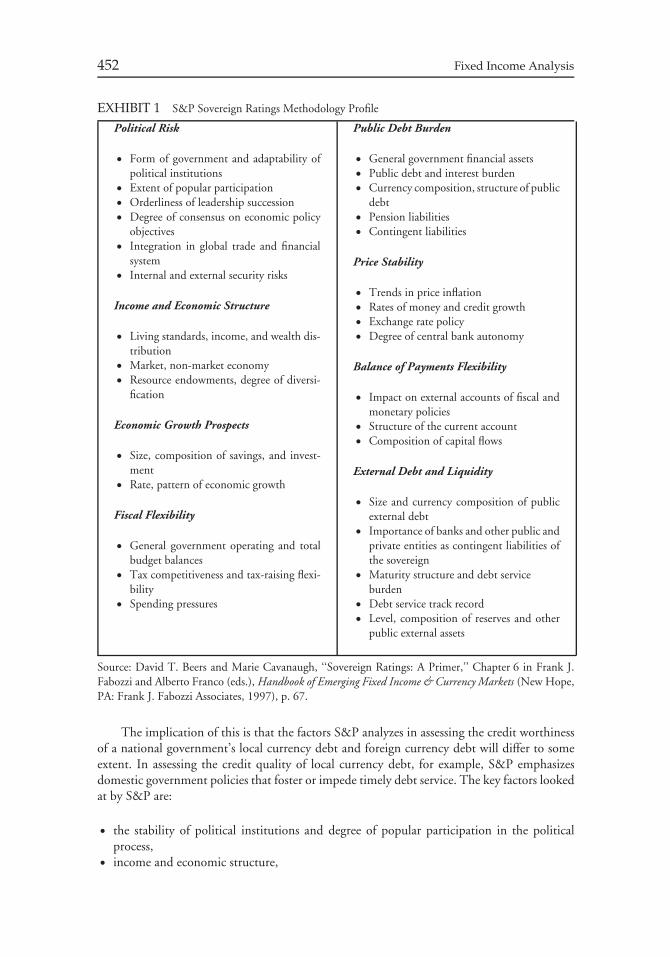
452 Fixed Income Analysis
EXHIBIT 1 S&P Sovereign Ratings Methodology Profile
Political Risk
• Form of government and adaptability ofpolitical institutions
• Extent of popular participation• Orderliness of leadership succession• Degree of consensus on economic policy
objectives• Integration in global trade and financial
system• Internal and external security risks
Income and Economic Structure
• Living standards, income, and wealth dis-tribution
• Market, non-market economy• Resource endowments, degree of diversi-
fication
Economic Growth Prospects
• Size, composition of savings, and invest-ment
• Rate, pattern of economic growth
Fiscal Flexibility
• General government operating and totalbudget balances
• Tax competitiveness and tax-raising flexi-bility
• Spending pressures
Public Debt Burden
• General government financial assets• Public debt and interest burden• Currency composition, structure of public
debt• Pension liabilities• Contingent liabilities
Price Stability
• Trends in price inflation• Rates of money and credit growth• Exchange rate policy• Degree of central bank autonomy
Balance of Payments Flexibility
• Impact on external accounts of fiscal andmonetary policies
• Structure of the current account• Composition of capital flows
External Debt and Liquidity
• Size and currency composition of publicexternal debt
• Importance of banks and other public andprivate entities as contingent liabilities ofthe sovereign
• Maturity structure and debt serviceburden
• Debt service track record• Level, composition of reserves and other
public external assets
Source: David T. Beers and Marie Cavanaugh, ‘‘Sovereign Ratings: A Primer,’’ Chapter 6 in Frank J.Fabozzi and Alberto Franco (eds.), Handbook of Emerging Fixed Income & Currency Markets (New Hope,PA: Frank J. Fabozzi Associates, 1997), p. 67.
The implication of this is that the factors S&P analyzes in assessing the credit worthinessof a national government’s local currency debt and foreign currency debt will differ to someextent. In assessing the credit quality of local currency debt, for example, S&P emphasizesdomestic government policies that foster or impede timely debt service. The key factors lookedat by S&P are:
• the stability of political institutions and degree of popular participation in the politicalprocess,
• income and economic structure,
Chapter 15 General Principles of Credit Analysis 453
• fiscal policy and budgetary flexibility,• monetary policy and inflation pressures, and• public debt burden and debt service track record.51
For foreign currency debt, credit analysis by S&P focuses on the interaction of domesticand foreign government policies. S&P analyzes a country’s balance of payments and thestructure of its external balance sheet. The area of analysis with respect to its external balancesheet are the net public debt, total net external debt, and net external liabilities.
IV. CREDIT SCORING MODELS
The previous section described the traditional ratios and other measures that credit analystsuse in assessing default risk. Several researchers have used these measures as input to assessthe default risk of issuers using the statistical technique of multiple discriminant analysis(MDA). This statistical technique is primarily a classification technique that is helpful indistinguishing between or among groups of objects and in identifying the characteristics ofobjects responsible for their inclusion in one or another group. One of the chief advantagesof MDA is that it permits a simultaneous consideration of a large number of characteristicsand does not restrict the investigator to a sequential evaluation of each individual attribute.For example, MDA permits a credit analyst studying ratings of corporate bonds to examine,at one time, the total and joint impact on ratings of multiple financial ratios, financialmeasures, and qualitative factors. Thus, the analyst is freed from the cumbersome and possiblymisleading task of looking at each characteristic in isolation from the others. MDA seeks toform groups that are internally as similar as possibly but that are as different from one anotheras possible.
From the above description of MDA it can be seen why it has been applied to problemsof why bonds get the ratings they do and what variables seem best able to account for abond’s rating. Moreover, MDA has been used as a predictor of bankruptcy. While the stepsinvolved in MDA for predicting bond ratings and corporate bankruptcies are a specialist topic,we will discuss the results of the work by Edward Altman, the primary innovator of MDAfor predicting corporate bankruptcy.52 The models of Altman and others involved in thisarea are updated periodically. Our purpose here is only to show what an MDA model lookslike.
In one of Altman’s earlier models, referred to as the ‘‘Z-score model,’’ he found that thefollowing MDA could be used to predict corporate bankruptcy:53
Z = 1.2 X1 + 1.4 X2 + 3.3 X3 + 0.6 X4 + 1.0 X5
51Beers and Cavanaugh, ‘‘Sovereign Credit Ratings: A Primer,’’ p. 68.52See Chapters 8 and 9 in Edward I. Altman, Corporate Financial Distress and Bankruptcy: A CompleteGuide to Predicting and Avoiding Distress and Profiting from Bankruptcy (Hoboken, NJ: John Wiley &Sons, 1993). For discussion of MDA applied to predicting municipal bond ratings, see Michael G. Ferriand Frank J. Fabozzi, ‘‘Statistical Techniques for Predicting the Credit Worthiness of Municipal Bonds,’’Chapter 44 in Frank J. Fabozzi, Sylvan G. Feldstein, Irving M. Pollack, and Frank G. Zarb (eds.), TheMunicipal Bond Handbook: Volume I (Homewood, IL: Dow-Jones Irwin 1983).53Edward I. Altman, ‘‘Financial Bankruptcies, Discriminant Analysis and the Prediction of CorporateBankruptcy,’’ Journal of Finance (September 1968), pp. 589–699.
454 Fixed Income Analysis
where
X1 = Working capital/Total assets (in decimal)X2 = Retained earnings/Total assets (in decimal)X3 = Earnings before interest and taxes/Total assets (in decimal)X4 = Market value of equity/Total liabilities (in decimal)X5 = Sales/Total assets (number of times)Z = Z-score
Given the value of the five variables for a given firm, a Z-score is computed. It is theZ-score that is used to classify firms with respect to whether or not there is potentially aserious credit problem that would lead to bankruptcy. Specifically, Altman found that Z-scoresless than 1.81 indicated a firm with serious credit problems while a Z-score in excess of 3.0indicated a healthy firm.
Subsequently, Altman and his colleagues revised the Z-score model based on more recentdata. The resulting model, referred to as the ‘‘Zeta model,’’ found that the following sevenvariables were important in predicting corporate bankruptcies and were highly correlated withbond ratings:54
• Earnings before interest and taxes (EBIT)/Total assets• Standard error of estimate of EBIT/Total assets (normalized) for 10 years• EBIT/Interest charges• Retained earnings/Total assets• Current assets/Current liabilities• Five-year average market value of equity/Total capitalization• Total tangible assets, normalized
While credit scoring models have been found to be helpful to analysts and bond portfoliomanagers, they do have limitations as a replacement for human judgment in credit analysis.Marty Fridson, for example, provides the following sage advice about using MDA models:
. . . quantitative models tend to classify as troubled credits not only most of the companiesthat eventually default, but also many that do not default. Often, firms that fall intofinancial peril bring in new management and are revitalized without ever failingin their debt service. If faced with a huge capital loss on the bonds of a financiallydistressed company, an institutional investor might wish to assess the probability of aturnaround—an inherently difficult-to-quantify prospect—instead of selling purely onthe basis of a default model.55
Fridson then goes on to explain that credit analyst must bear in mind that ‘‘companiescan default for reasons that a model based on reported financial data cannot pick up’’ andprovides several actual examples of companies that filed for bankruptcy for such reasons.
54Edward I. Altman, Robert G. Haldeman, and Paul Narayann, ‘‘Zeta Analysis: A New Model toIdentify Bankruptcy Risk of Corporations,’’ Journal of Banking and Finance (June 1977), pp. 29-54.55Martin S. Fridson, Financial Statement Analysis: A Practitioner’s Guide, Second Edition (Hoboken, NJ:John Wiley & Sons, 1995), p. 195.
Chapter 15 General Principles of Credit Analysis 455
V. CREDIT RISK MODELS
Historically, credit risk modeling has focused on credit ratings, default rates, and traditionalcredit analysis. In recent years, models for assessing credit risk to value corporate bonds havebeen introduced. The models can be divided into two groups: structural models and reducedform models. In this section we briefly describe these models.
A. Structural Models
Structural models are credit risk models developed on the basis of option pricing theorypresented by Fisher Black and Mryon Scholes56 and Robert Merton.57 The basic idea,common to all structural-type models, is that a company defaults on its debt if the value ofthe assets of the company falls below a certain default point. For this reason, these models arealso known as ‘‘firm-value models.’’58 In these models it has been demonstrated that defaultcan be modeled as an option to the stockholders granted by the bondholders and, as a result,an analyst can apply the same principles used for option pricing to the valuation of riskycorporate securities.59
The use of the option pricing theory set forth by Black-Scholes-Merton (BSM) provides asignificant improvement over traditional methods for valuing default risky bonds. Subsequentto the work of BSM, there have been many extensions on both a theoretical and practical level.The BSM framework has been used by a number of credit software/consulting companies,including Moody’s KMV Corporation and JP Morgan’s Credit Metrics (co-developed withReuters). Both systems use the BSM approach to model defaults and obtain the probabilityof default. (Moody’s KMV refers to this probability as the ‘‘expected default frequency.’’) Tomake the BSM model operational, model developers define default occurring when the equityprice falls below a certain barrier. This simplification is due to the fact that equity prices aremuch more available than asset values of the company.
B. Reduced Form Models
In structural models, the default process of a corporation is driven by the value of its assets.Since the value of any option depends on the volatility of the underlying (the volatility ofthe asset value in structural models), the probability of default is explicitly linked to theexpected volatility of a corporation’s asset value. Thus, in structural models both the defaultprocess and recovery rates should a bankruptcy occur depend on the corporation’s structuralcharacteristics.
56Fischer Black and Myron Scholes, ‘‘The Pricing of Options and Corporate Liabilities,’’ Journal ofPolitical Economy (May-June 1973), pp. 637–654.57Robert Merton, ‘‘Theory of Rational Option Pricing,’’ Bell Journal of Economics and Management(Spring 1973), pp. 141–183, and ‘‘On the Pricing of Corporate Debt: The Risk Structure of InterestRates,’’ Journal of Finance, Vol. 29, No. 2 (1974), pp. 449–470.58For a more detailed discussion of these models, see Chapter 8 in Mark J.P. Anson, Frank J. Fabozzi,Moorad Choudhry, and Ren Raw Chen, Credit Derivatives: Instruments, Applications, and Pricing(Hoboken, NJ: John Wiley & Sons, 2004).59For the underlying theory and an illustration, see Don M. Chance, Analysis of Derivatives for theCFA Program (Charlottesville, VA: Association for Investment Management and Research, 2003), pp.588-591.
456 Fixed Income Analysis
In contrast, reduced form models do not look ‘‘inside the firm,’’ but instead modeldirectly the probability of default or downgrade.60 That is, the default process and the recoveryprocess are (1) modeled independently of the corporation’s structural features and (2) areindependent of each other.
The two most popular reduced form models are the Jarrow and Turnbull model61 andthe Duffie and Singleton model.62 The statistical tools for modeling the default process andthe recovery process are a specialized topic.63
APPENDIX:CASE STUDY: BERGEN BRUNSWIG CORPORATION
The purpose of this case is to illustrate how the analysis of financial statements based ontraditional ratios discussed in this chapter can be used to identify a corporate issuer that mightbe downgraded. The corporation used in the illustration is Bergen Brunswig Corporation.
I. BACKGROUND INFORMATION
Bergen Brunswig Corporation is a supply channel management company that providespharmaceuticals, medical-surgical supplies, and specialty products. The company also providesinformation management solutions and outsourcing services, as well as develops disease-specifictreatment protocols and pharmaco-economic initiatives to assist in the reduction of healthcare costs.
The original corporate bond rating was BBB+. On December 17, 1999, S&P loweredthe company’s rating to BBB− citing ‘‘disappointing results at the company’s two recentlyacquired businesses, PharMerica and Statlander.’’ PharMerica, an institutional pharmacy,suffered from changes in Medicare reimbursement policies which reduced hospital patientoccupancy and the use of high-margin drugs.
On February 2, 2000, S&P decided to downgrade the company’s corporate rating againto BB. S&P’s rationale was ‘‘deteriorating conditions in the company’s core drug distributionbusiness as well as continued losses at Statlander, a specialty drug distributor acquired in1999.’’
60The name ‘‘reduced form’’ was first given by Darrell Duffie to differentiate these models from thestructural form models of the Black-Scholes-Merton type.61Robert Jarrow and Stuart Turnbull, ‘‘Pricing Derivatives on Financial Securities Subject to DefaultRisk,’’ Journal of Finance, Vol. 50, No. 1 (1995), pp. 53–86.62Darrell Duffie and Kenneth Singleton, ‘‘Modeling Term Structures of Defaultable Bonds,’’ Review ofFinancial Studies, Vol. 12 (1999), pp. 687-720.63For a further discussion of reduced form models, see Chapter 9 in Anson, Fabozzi, Choudhry, andChen, Credit Derivatives: Instruments, Applications, and Pricing ; Darrell Duffie and Kenneth J. Singleton,Credit Risk: Pricing Measurement, and Management (Princeton, NJ: Princeton University Press, 2003), orSrichander Ramaswamy, Managing Credit Risk in Corporate Bond Portfolios (Hoboken, NJ: John Wiley& Sons, 2003).
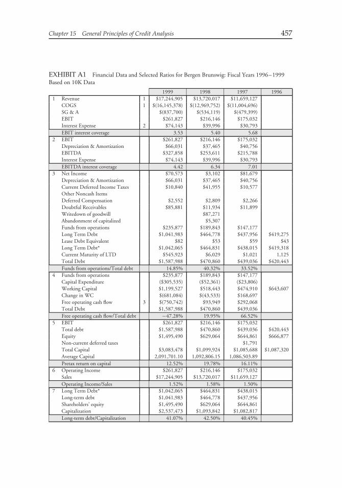
Chapter 15 General Principles of Credit Analysis 457
EXHIBIT A1 Financial Data and Selected Ratios for Bergen Brunswig: Fiscal Years 1996–1999Based on 10K Data
1999 1998 1997 19961 Revenue 1 $17,244,905 $13,720,017 $11,659,127
COGS 1 $(16,145,378) $(12,969,752) $(11,004,696)SG & A $(837,700) $(534,119) $(479,399)EBIT $261,827 $216,146 $175,032Interest Expense 2 $74,143 $39,996 $30,793EBIT interest coverage 3.53 5.40 5.68
2 EBIT $261,827 $216,146 $175,032Depreciation & Amortization $66,031 $37,465 $40,756EBITDA $327,858 $253,611 $215,788Interest Expense $74,143 $39,996 $30,793EBITDA interest coverage 4.42 6.34 7.01
3 Net Income $70,573 $3,102 $81,679Depreciation & Amortization $66,031 $37,465 $40,756Current Deferred Income Taxes $10,840 $41,955 $10,577Other Noncash ItemsDeferred Compensation $2,552 $2,809 $2,266Doubtful Receivables $85,881 $11,934 $11,899Writedown of goodwill $87,271Abandonment of capitalized $5,307Funds from operations $235,877 $189,843 $147,177Long Term Debt $1,041,983 $464,778 $437,956 $419,275Lease Debt Equivalent $82 $53 $59 $43Long Term Debt* $1,042,065 $464,831 $438,015 $419,318Current Maturity of LTD $545,923 $6,029 $1,021 1,125Total Debt $1,587,988 $470,860 $439,036 $420,443Funds from operations/Total debt 14.85% 40.32% 33.52%
4 Funds from operations $235,877 $189,843 $147,177Capital Expenditure ($305,535) ($52,361) ($23,806)Working Capital $1,199,527 $518,443 $474,910 $643,607Change in WC $(681,084) $(43,533) $168,697Free operating cash flow 3 $(750,742) $93,949 $292,068Total Debt $1,587,988 $470,860 $439,036Free operating cash flow/Total debt −47.28% 19.95% 66.52%
5 EBIT $261,827 $216,146 $175,032Total debt $1,587,988 $470,860 $439,036 $420,443Equity $1,495,490 $629,064 $644,861 $666,877Non-current deferred taxes $1,791Total Capital $3,083,478 $1,099,924 $1,085,688 $1,087,320Average Capital 2,091,701.10 1,092,806.15 1,086,503.89Pretax return on capital 12.52% 19.78% 16.11%
6 Operating Income $261,827 $216,146 $175,032Sales $17,244,905 $13,720,017 $11,659,127Operating Income/Sales 1.52% 1.58% 1.50%
7 Long Term Debt* $1,042,065 $464,831 $438,015Long-term debt $1,041,983 $464,778 $437,956Shareholders’ equity $1,495,490 $629,064 $644,861Capitalization $2,537,473 $1,093,842 $1,082,817Long-term debt/Capitalization 41.07% 42.50% 40.45%
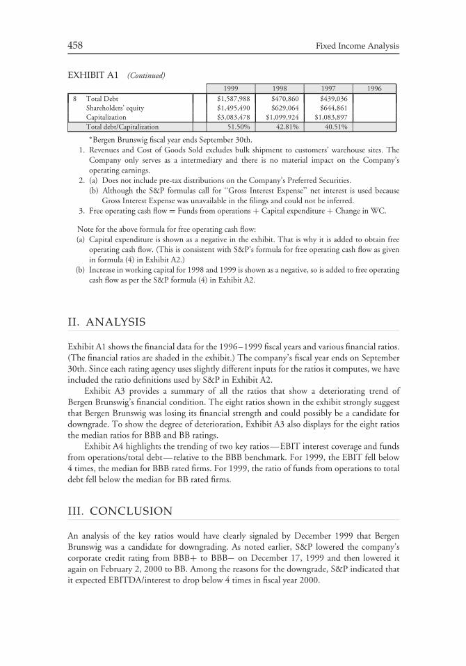
458 Fixed Income Analysis
EXHIBIT A1 (Continued)
1999 1998 1997 19968 Total Debt $1,587,988 $470,860 $439,036
Shareholders’ equity $1,495,490 $629,064 $644,861Capitalization $3,083,478 $1,099,924 $1,083,897Total debt/Capitalization 51.50% 42.81% 40.51%∗Bergen Brunswig fiscal year ends September 30th.
1. Revenues and Cost of Goods Sold excludes bulk shipment to customers’ warehouse sites. TheCompany only serves as a intermediary and there is no material impact on the Company’soperating earnings.
2. (a) Does not include pre-tax distributions on the Company’s Preferred Securities.(b) Although the S&P formulas call for ‘‘Gross Interest Expense’’ net interest is used because
Gross Interest Expense was unavailable in the filings and could not be inferred.3. Free operating cash flow = Funds from operations + Capital expenditure + Change in WC.
Note for the above formula for free operating cash flow:(a) Capital expenditure is shown as a negative in the exhibit. That is why it is added to obtain free
operating cash flow. (This is consistent with S&P’s formula for free operating cash flow as givenin formula (4) in Exhibit A2.)
(b) Increase in working capital for 1998 and 1999 is shown as a negative, so is added to free operatingcash flow as per the S&P formula (4) in Exhibit A2.
II. ANALYSIS
Exhibit A1 shows the financial data for the 1996–1999 fiscal years and various financial ratios.(The financial ratios are shaded in the exhibit.) The company’s fiscal year ends on September30th. Since each rating agency uses slightly different inputs for the ratios it computes, we haveincluded the ratio definitions used by S&P in Exhibit A2.
Exhibit A3 provides a summary of all the ratios that show a deteriorating trend ofBergen Brunswig’s financial condition. The eight ratios shown in the exhibit strongly suggestthat Bergen Brunswig was losing its financial strength and could possibly be a candidate fordowngrade. To show the degree of deterioration, Exhibit A3 also displays for the eight ratiosthe median ratios for BBB and BB ratings.
Exhibit A4 highlights the trending of two key ratios—EBIT interest coverage and fundsfrom operations/total debt—relative to the BBB benchmark. For 1999, the EBIT fell below4 times, the median for BBB rated firms. For 1999, the ratio of funds from operations to totaldebt fell below the median for BB rated firms.
III. CONCLUSION
An analysis of the key ratios would have clearly signaled by December 1999 that BergenBrunswig was a candidate for downgrading. As noted earlier, S&P lowered the company’scorporate credit rating from BBB+ to BBB− on December 17, 1999 and then lowered itagain on February 2, 2000 to BB. Among the reasons for the downgrade, S&P indicated thatit expected EBITDA/interest to drop below 4 times in fiscal year 2000.

EX
HIB
ITA
2S&
P’s
Form
ulas
for
Key
Rat
ios
1.E
BIT
inte
rest
cove
rage
=E
arni
ngs
from
cont
inui
ngop
erat
ions
∗∗be
fore
inte
rest
and
taxe
sG
ross
inte
rest
incu
rred
befo
resu
btra
ctin
g(1
)ca
pita
lized
inte
rest
and
(2)
inte
rest
inco
me
2.E
BIT
DA
inte
rest
cove
rage
=E
arni
ngs
from
cont
inui
ngop
erat
ions
∗∗be
fore
inte
rest
and
taxe
s,de
prec
iati
on,a
ndam
orti
zati
onG
ross
inte
rest
incu
rred
befo
resu
btra
ctin
g(1
)ca
pita
lized
inte
rest
and
(2)
inte
rest
inco
me
3.Fu
nds
from
oper
atio
ns/t
otal
debt
=N
etin
com
efr
omco
ntin
uing
oper
atio
nspl
usde
prec
iati
on,
amor
tiza
tion
,def
erre
din
com
eta
xes,
and
othe
rno
ncas
hit
ems
Long
-ter
mde
bt∗ pl
uscu
rren
tmat
urit
ies,
com
mer
cial
pape
r,an
dot
her
shor
t-te
rmbo
rrow
ings
4.Fr
eeop
erat
ing
cash
flow
/tot
alde
bt=
Fund
sfr
omop
erat
ions
min
usca
pita
lexp
endi
ture
s,m
inus
(plu
s)th
ein
crea
se(d
ecre
ase)
inw
orki
ngca
pita
l(ex
clud
ing
chan
ges
inca
sh)
Long
-ter
mde
bt∗ pl
uscu
rren
tmat
urit
ies,
com
mer
cial
pape
r,an
dot
her
shor
t-te
rmbo
rrow
ings
5.Pr
etax
retu
rnon
capi
tal=
EB
ITA
vera
geof
begi
nnin
gof
year
and
end
ofye
arca
pita
l,in
clud
ing
shor
t-te
rmde
bt,c
urre
ntm
atur
itie
s,lo
ng-t
erm
debt
∗ ,no
n-cu
rren
tdef
erre
dta
xes,
and
equi
ty
6.O
pera
ting
inco
me/
sale
s=
Sale
sm
inus
cost
ofgo
ods
man
ufac
ture
d(b
efor
ede
prec
iati
onan
dam
orti
zati
on),
selli
ng,g
ener
alan
dad
min
istr
ativ
e,an
dre
sear
chan
dde
velo
pmen
tcos
tsSa
les
7.Lo
ng-t
erm
debt
/cap
ital
izat
ion
=Lo
ng-t
erm
debt
∗lo
ng-t
erm
debt
+sh
areh
olde
rs’e
quit
y(i
nclu
ding
pref
erre
dst
ock)
plus
min
orit
yin
tere
st
8.T
otal
debt
/cap
ital
izat
ion
=Lo
ng-t
erm
debt
∗pl
uscu
rren
tmat
urit
ies,
com
mer
cial
pape
r,an
dot
her
shor
t-te
rmbo
rrow
ings
Long
-ter
mde
bt∗
plus
curr
entm
atur
itie
s,co
mm
erci
alpa
per,
and
othe
rsh
ort-
term
borr
owin
gs+s
hare
hold
ers’
equi
ty(i
nclu
ding
pref
erre
dst
ock)
plus
min
orit
yin
tere
st∗ I
nclu
ding
amou
ntfo
rop
erat
ing
leas
ede
bteq
uiva
lent
∗∗In
clud
ing
inte
rest
inco
me
and
equi
tyea
rnin
gs;e
xclu
ding
nonr
ecur
ring
item
s.
459
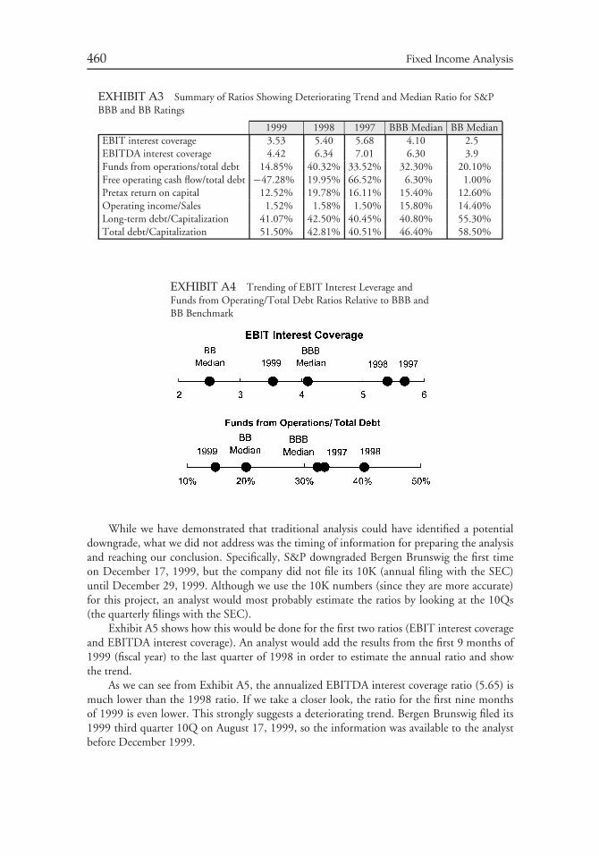
460 Fixed Income Analysis
EXHIBIT A3 Summary of Ratios Showing Deteriorating Trend and Median Ratio for S&PBBB and BB Ratings
1999 1998 1997 BBB Median BB MedianEBIT interest coverage 3.53 5.40 5.68 4.10 2.5EBITDA interest coverage 4.42 6.34 7.01 6.30 3.9Funds from operations/total debt 14.85% 40.32% 33.52% 32.30% 20.10%Free operating cash flow/total debt −47.28% 19.95% 66.52% 6.30% 1.00%Pretax return on capital 12.52% 19.78% 16.11% 15.40% 12.60%Operating income/Sales 1.52% 1.58% 1.50% 15.80% 14.40%Long-term debt/Capitalization 41.07% 42.50% 40.45% 40.80% 55.30%Total debt/Capitalization 51.50% 42.81% 40.51% 46.40% 58.50%
EXHIBIT A4 Trending of EBIT Interest Leverage andFunds from Operating/Total Debt Ratios Relative to BBB andBB Benchmark
While we have demonstrated that traditional analysis could have identified a potentialdowngrade, what we did not address was the timing of information for preparing the analysisand reaching our conclusion. Specifically, S&P downgraded Bergen Brunswig the first timeon December 17, 1999, but the company did not file its 10K (annual filing with the SEC)until December 29, 1999. Although we use the 10K numbers (since they are more accurate)for this project, an analyst would most probably estimate the ratios by looking at the 10Qs(the quarterly filings with the SEC).
Exhibit A5 shows how this would be done for the first two ratios (EBIT interest coverageand EBITDA interest coverage). An analyst would add the results from the first 9 months of1999 (fiscal year) to the last quarter of 1998 in order to estimate the annual ratio and showthe trend.
As we can see from Exhibit A5, the annualized EBITDA interest coverage ratio (5.65) ismuch lower than the 1998 ratio. If we take a closer look, the ratio for the first nine monthsof 1999 is even lower. This strongly suggests a deteriorating trend. Bergen Brunswig filed its1999 third quarter 10Q on August 17, 1999, so the information was available to the analystbefore December 1999.
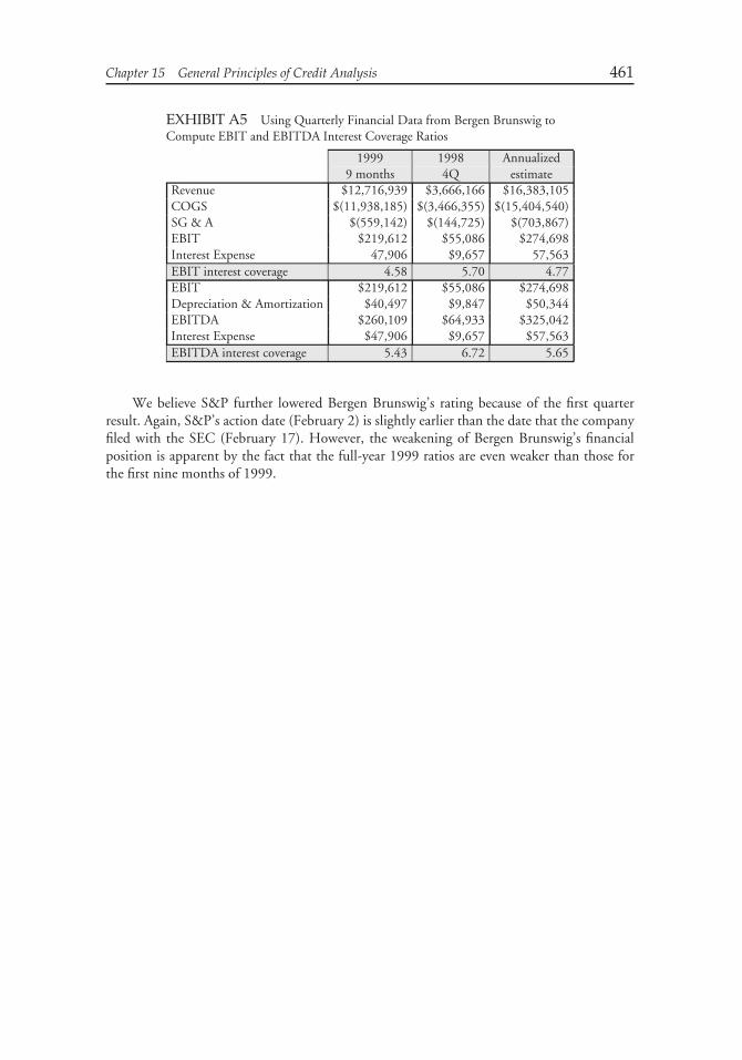
Chapter 15 General Principles of Credit Analysis 461
EXHIBIT A5 Using Quarterly Financial Data from Bergen Brunswig toCompute EBIT and EBITDA Interest Coverage Ratios
1999 1998 Annualized9 months 4Q estimate
Revenue $12,716,939 $3,666,166 $16,383,105COGS $(11,938,185) $(3,466,355) $(15,404,540)SG & A $(559,142) $(144,725) $(703,867)EBIT $219,612 $55,086 $274,698Interest Expense 47,906 $9,657 57,563EBIT interest coverage 4.58 5.70 4.77EBIT $219,612 $55,086 $274,698Depreciation & Amortization $40,497 $9,847 $50,344EBITDA $260,109 $64,933 $325,042Interest Expense $47,906 $9,657 $57,563EBITDA interest coverage 5.43 6.72 5.65
We believe S&P further lowered Bergen Brunswig’s rating because of the first quarterresult. Again, S&P’s action date (February 2) is slightly earlier than the date that the companyfiled with the SEC (February 17). However, the weakening of Bergen Brunswig’s financialposition is apparent by the fact that the full-year 1999 ratios are even weaker than those forthe first nine months of 1999.
CHAPTER 16INTRODUCTION TO BOND
PORTFOLIO MANAGEMENT
I. INTRODUCTION
The products of the fixed-income market, the risks associated with investing in fixed-incomesecurities, and the fundamentals of valuation and interest rate risk measurement were covered.In depth coverage of the valuation of fixed-income securities with embedded options, featuresof structured products (mortgage-backed securities and asset-backed securities), and theprinciples of credit analysis were covered. Now, we will put all these tools together todemonstrate how to construct portfolios in such a way as to increase the likelihood of meetingan investment objective.
In this chapter, we set forth the framework for the investment management process.Regardless of the asset class being managed (i.e., stocks, bonds, or real estate), the investmentmanagement process follows the same integrated activities. John Maginn and Donald Tuttledefine these activities as follows:
1. An investor’s objectives, preferences, and constraints are identified and specified todevelop explicit investment policies;
2. Strategies are developed and implemented through the choice of optimal combinationsof financial and real assets in the marketplace;
3. Market conditions, relative asset values, and the investor’s circumstances are moni-tored; and
4. Portfolio adjustments are made as appropriate to reflect significant change in any or allof the relevant variables.1
In this chapter, we will use the Maginn-Tuttle framework to describe the investmentmanagement process for fixed-income portfolios. We refer to these four activities in theinvestment management process as:
1. setting the investment objectives2. developing and implementing a portfolio strategy
1John L. Maginn and Donald L. Tuttle, ‘‘The Portfolio Management Process and Its Dynamics,’’Chapter 1 in John L. Maginn and Donald L. Tuttle (editors), Managing Investment Portfolios: A DynamicProcess (New York: Warren, Gorham & Lamont, sponsored by the Institute of Chartered FinancialAnalysts, Second Edition, 1990), pp. 1–3 and 1–5.
462
Chapter 16 Introduction to Bond Portfolio Management 463
3. monitoring the portfolio4. adjusting the portfolio
A discussion of the investment management process provides a context in which to appreciatethe significance of the chapters to follow in this book. Our focus, of course, is on themanagement of fixed-income portfolios.
II. SETTING INVESTMENT OBJECTIVESFOR FIXED-INCOME INVESTORS
The investment objectives of a fixed-income investor are often specified in terms of returnand risk. The investment objectives should be expressed quantitatively in terms of somebenchmark. The benchmark varies by the type of investor.
In general, we can divide fixed-income investors into two categories based on thecharacteristic of the benchmark. The first category of investor specifies the benchmark in termsof the investor’s liability structure. The investment objective is to generate a cash flow fromthe fixed-income portfolio that, at a minimum, satisfies the liability structure. The secondcategory of fixed-income investor specifies the benchmark as a particular bond market index.The investment objective may be to match the performance of the bond market index aftermanagement fees, or to outperform the bond market index after management fees by at leasta predetermined number of basis points. Below we discuss each category of investor further interms of its investment objectives.
A. Return Objectives
An investor identifies the benchmark to the portfolio manager. The manager may be employedby the investor or may be an external manager. Once the investment objective is specifiedin terms of a benchmark, the performance of a manager will be evaluated relative tothat benchmark. It is important to note that, even if a manager is successful in terms ofoutperforming the benchmark, the client may not realize its investment objective. This canoccur if the client does not correctly specify a benchmark to reflect its investment needs from arisk, return, and cash flow perspective. A good example is a defined benefit pension fund thatspecifies the investment objective in terms of a particular bond market index when, in fact,a more appropriate benchmark would be the liability structure of the fund. If the manageroutperforms the benchmark, then the manager is successful. However, if sufficient cash flowis not generated to satisfy the pension liabilities, then the failure lies not with the manager butwith the client’s inability to properly specify an appropriate benchmark.
1. Liabilities as the Investment Objective In general, investors who specify the bench-mark in terms of a liability structure that must be satisfied fall into two categories. The firstcategory consists of investors who borrow funds and then invest those funds. Here, theobjective is to earn a return on the funds borrowed that is greater than the cost of borrowing.The difference between the return on the funds invested and the cost of borrowing is calledthe spread. These investors are referred to as funded investors.
Depository institutions (banks, savings and loan associations, and credit unions) are clearlyfunded investors. Insurance companies have a wide range of products. For some products,the insurance company is a funded investor. For example, an insurance company that issues
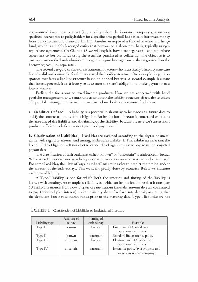
464 Fixed Income Analysis
a guaranteed investment contract (i.e., a policy where the insurance company guarantees aspecified interest rate to policyholders for a specific time period) has basically borrowed moneyfrom policyholders and created a liability. Another example of a funded investor is a hedgefund, which is a highly leveraged entity that borrows on a short-term basis, typically using arepurchase agreement. (In Chapter 18 we will explain how a manager can use a repurchaseagreement to borrow funds using the securities purchased as collateral.) The objective is toearn a return on the funds obtained through the repurchase agreement that is greater than theborrowing cost (i.e., repo rate).
The second category consists of institutional investors who must satisfy a liability structurebut who did not borrow the funds that created the liability structure. One example is a pensionsponsor that faces a liability structure based on defined benefits. A second example is a statethat invests proceeds from a lottery so as to meet the state’s obligation to make payments to alottery winner.
Earlier, the focus was on fixed-income products. Now we are concerned with bondportfolio management, so we must understand how the liability structure affects the selectionof a portfolio strategy. In this section we take a closer look at the nature of liabilities.
a. Liabilities Defined A liability is a potential cash outlay to be made at a future date tosatisfy the contractual terms of an obligation. An institutional investor is concerned with boththe amount of the liability and the timing of the liability, because the investor’s assets mustproduce sufficient cash flow to meet promised payments.
b. Classification of Liabilities Liabilities are classified according to the degree of uncer-tainty with regard to amount and timing, as shown in Exhibit 1. This exhibit assumes that theholder of the obligation will not elect to cancel the obligation prior to any actual or projectedpayout date.
The classification of cash outlays as either ‘‘known’’ or ‘‘uncertain’’ is undoubtedly broad.When we refer to a cash outlay as being uncertain, we do not mean that it cannot be predicted.For some liabilities, the ‘‘law of large numbers’’ makes it easier to predict the timing and/orthe amount of the cash outlays. This work is typically done by actuaries. Below we illustrateeach type of liability.
A Type-I liability is one for which both the amount and timing of the liability isknown with certainty. An example is a liability for which an institution knows that it must pay$8 million six months from now. Depository institutions know the amount they are committedto pay (principal plus interest) on the maturity date of a fixed-rate deposit, assuming thatthe depositor does not withdraw funds prior to the maturity date. Type-l liabilities are not
EXHIBIT 1 Classification of Liabilities of Institutional Investors
Amount of Timing ofLiability type outlay cash outlay ExampleType I known known Fixed-rate CD issued by a
depository institutionType II known uncertain Standard life insurance policyType III uncertain known Floating-rate CD issued by a
depository institutionType IV uncertain uncertain Insurance policy by a property and
casualty insurance company
Chapter 16 Introduction to Bond Portfolio Management 465
limited to depository institutions. A guaranteed investment contract is an example of this typeof liability that is created by a life insurance company.
A Type-II liability is one for which the amount of the cash outlay is known, but thetiming of the cash outlay is uncertain. The most obvious example of a Type-II liability is atypical life insurance policy. There are many types of life insurance policies, but the most basicprovides that, for an annual premium, a life insurance company agrees to make a specifieddollar payment to policy beneficiaries upon the death of the insured. Naturally, the timing ofthe insured’s death is uncertain.
A Type-III liability is one for which the timing of the cash outlay is known, but theamount is uncertain. An example is, a 2-year floating-rate certificate of deposit issued by adepository institution, with an interest rate that is reset quarterly based on a particular marketinterest rate.
For a Type-IV liability, there is uncertainty as to both the amount and the timing ofthe cash outlay. Numerous insurance products and pension obligations are in this category.Probably the most obvious examples are automobile and home insurance policies issued byproperty and casualty insurance companies. When, and if, a payment will be made to thepolicyholder is uncertain. Whenever an insured asset is damaged, the amount of the paymentthat must be made is uncertain.
The liabilities of pension plans can also be Type-IV liabilities. For defined benefit plans,retirement benefits depend on the participant’s income for a specified number of years beforeretirement and the total number of years the participant worked. This affects the amount of thecash outlay. The timing of the cash outlay depends on whether the employee remains withthe sponsoring plan until retirement and when the employee elects to retire. Moreover, boththe amount and the timing depend on how the employee elects to have payments made—over the employee’s lifetime or those of the employee and spouse.
2. Bond Market Index as the Investment Objective When there are no liabilitiesthat must be met, the investment objective is often to either match or outperform a designatedbond market index. It is important to note that some clients that have a liability structurechoose to specify that the manager manage against a bond market index. This is particularlytrue of pension sponsors. The expectation of the plan sponsor is that the performance of thebond market index selected will generate sufficient cash flow to satisfy the liability structure.
In selecting a benchmark, there are several characteristics a client should consider so thatthe benchmark can serve as an effective tool for evaluating a portfolio manager. According toBailey, Richards, and Tierney, the basic characteristics of any useful benchmark are:2
• Unambiguous: The names and weights of the securities included in the benchmark areclearly identifiable.
• Investable: The client has the option to simply buy-and-hold the benchmark rather thanhave funds actively managed.
• Measurable: The benchmark’s return can be calculated on a reasonably frequent basis byeither the manager, client, or some third party.
• Appropriate: The benchmark is consistent with the manager’s investment style.
2Jeffrey V. Bailey, Thomas M. Richards, and David E. Tierney, ‘‘Benchmark Portfolios and the Man-ager/Plan Sponsor Relationship,’’ in Frank J. Fabozzi (ed.), Current Topics in Investment Management(New York, NY: Harper & Row Publishers, 1990), p. 70.
466 Fixed Income Analysis
• Reflective of current investment opinions: The manager has current investment knowledgeof the securities included in the benchmark and the way they are categorized within thebenchmark.3
• Specified in advance: The benchmark is constructed before the beginning of the period forwhich the manager is evaluated.
The investable characteristic of a benchmark is critical. A benchmark represents thereturn to a passive investment strategy. The establishment of a benchmark means that activemanagement decisions made by a portfolio manager can be judged. For example, Bailey,Richards, and Tierney note that it is common for consultants and plan sponsors to use as abenchmark the median performance of a group of portfolio managers for the same asset class.Such a benchmark is not investable.
It is essential for a manager to understand the composition and risk profile of a bondmarket index. Here we review the composition of various bond market indexes. These indexesare classified as broad-based U.S. bond market indexes, specialized U.S. bond market indexes,and global and international bond market indexes. In Chapter 17, we explain the risk profileof a bond market index because the risk profile of a portfolio relative to that of the benchmarkbond market index determines relative performance.
a. Broad-Based U.S. Bond Market Indexes The three broad-based U.S. bond marketindexes most commonly used by institutional investors are the Lehman Brothers U.S.Aggregate Index, the Salomon Smith Barney (SSB) Broad Investment-Grade Bond Index(BIG), and the Merrill Lynch Domestic Market Index. There are more than 5,500 issues ineach index. One study found that the correlation of annual returns between the broad-basedbond market indexes is around 98%.4
The three broad-based U.S. bond market indexes are computed daily and are ‘‘market-value weighted.’’ This means that, for each issue, the ratio of the market value of an issuerelative to the market value of all issues in the index is used as the weight for the issue inall calculations. The securities in the SSB BIG index are all trader priced. For the two otherindexes, the securities are either trader priced or model priced. Each index handles intra-monthcash flows that must be reinvested in a different way. For the SSB BIG index, these cash flowsare assumed to be reinvested at the 1-month Treasury bill rate, while for the Merrill Lynchindex, they are assumed to be reinvested in the specific issue. The Lehman index assumes noreinvestment of intra-month cash flows.
Each index is broken into sectors. The Lehman index, for example, is divided intothe following six sectors: (1) Treasury sector, (2) agency sector, (3) mortgage passthroughsector, (4) commercial mortgage-backed securities sector, (5) asset-backed securities sector,and (6) credit sector. Exhibit 2 shows the percentage composition of the index as of September8, 2003.
The agency sector includes agency debentures, but not mortgage-backed or asset-backedsecurities issued by federal agencies. The mortgage passthrough sector includes agencypassthrough securities—Ginnie Mae, Fannie Mae, and Freddie Mac passthrough securities.Recall that the mortgage passthrough securities issued by Ginnie Mae are referred to as
3For example, for an equity benchmark, categorization might be value, growth, capitalization in termsof size. For a bond benchmark it might be the major sectors of the bond index.4Frank K. Reilly and David J. Wright, ‘‘Bond Indexes,’’ Chapter 7 in Frank J. Fabozzi (ed.), TheHandbook of Fixed Income Securities (New York: McGraw-Hill, 2000).
Chapter 16 Introduction to Bond Portfolio Management 467
EXHIBIT 2 Percentage Composition of Lehman Brothers U.S. AggregateIndex as of September 8, 2003
Sector Percent of market valueTreasury 21.94%Agency 11.96Mortgage Passthroughs 34.40Commercial Mortgage-Backed Securities 2.55Accept-Backed Securities 1.89Credit 27.27Total 100.00%
Source: Global Relative Value, Lehman Brothers, Fixed Income Research, Septem-ber 8, 2003.
agency passthroughs and those issued by Fannie Mae and Freddie Mac are called conventionalpassthroughs. However, we shall simply refer to all mortgage passthroughs of these threeentities as agency passthroughs. Agency collateralized mortgage obligations and agency strippedmortgage-backed securities are not included in the index. These mortgage derivatives productsare not included because inclusion would result in double counting since they are created fromagency passthroughs.
In constructing the index for the mortgage sector, for example, the Lehman index groupsmore than 800,000 individual mortgage pools with fixed-rate coupons into generic aggregates.These generic aggregates are defined in terms of agency (i.e., Ginnie Mae, Fannie Mae,and Freddie Mac), program type (i.e., 30-year, 15-year, balloon mortgages, etc.), couponrate for the passthrough, and the year the passthrough was originated (i.e., vintage). For anissue to be included, it must have a minimum of $100 million outstanding and a minimumweighted average maturity of one year. Agency passthroughs backed by pools of adjustable-ratemortgages are not included in the mortgage index. (We discuss the composition of this sectorin the next chapter.)
The credit sector in the Lehman Brothers index includes corporate issues. In the othertwo U.S. broad-based bond market indexes, this sector is referred to as the corporate sector.
b. Specialized U.S. Bond Market Indexes The specialized U.S. bond market indexesfocus on one sector or sub-sector of the bond market. Indexes on sectors of the market arepublished by the same three firms that produce the broad-based U.S. bond market indexes.Nonbrokerage firms have created specialized indexes for sectors. For example, Ryan Labsproduces a Treasury index. Since none of the broad-based U.S. bond market indexes includenoninvestment-grade or high-yield issues, indexes for this sector have been created by the threefirms that have created the broad-based indexes and the firms CS First Boston and DonaldsonLufkin and Jenrette. The number of issues included in each high-yield index varies from indexto index. The types of issues permitted (e.g., convertible, floating-rate, payment-in-kind) alsovary. The index creators treat interim income and default issues differently.
c. Global and International Bond Market Indexes The growth in non-U.S. bond invest-ing has resulted in the proliferation of international bond market indexes. Three types ofindexes that include non-U.S. bonds are available. The first is an index that includes bothU.S. and non-U.S. bonds. Such indexes are referred to as global bond indexes or worldbond indexes. The second type includes only non-U.S. bonds and is commonly referred to

468 Fixed Income Analysis
as international bond indexes or ex-U.S. bond indexes. Finally, there are specialized bondindexes for particular non-U.S. bond sectors. Indexes can be reported on a hedged currencybasis and/or an unhedged currency basis.
There are two types of global bond indexes. The first type restricts each country sectorto government bonds. For example, the Merrill Lynch Government Bond Index includes thegovernment sectors of the following countries:
Europe-EMU: Austria, Belgium, Finland, France, Germany, Ireland, Italy, Netherlands,Portugal, and Spain
Europe-Non-EMU: Denmark, Sweden, Switzerland, and U.K.
North America: Canada and U.S.
Japan & Asia/Pacific: Australia, Japan, and New Zealand
Other similar indexes are the Salomon World Government Bond Index and the J.P. MorganGlobal Bond Index.
An example of a global bond index that includes government and non-governmentsectors is the Lehman Brothers Global Index (which Lehman also refers to as its ‘‘Core PlusPlus’’ Portfolio). The index is divided into a U.S. dollar sector and a nondollar sector. TheU.S. dollar sector includes all the sectors within the Lehman Brothers U.S. Aggregate Indexplus high-yield bonds and dollar-denominated emerging market bonds. The nondollar sectorincludes the following countries: France, Germany, Italy, Spain, Sweden, and the UnitedKingdom. An index such as the Lehman Brothers Global Index is an appropriate benchmarkfor a manager who is permitted to invest in both U.S. and non-U.S. bonds.
An international bond index is an appropriate benchmark for a manager who invests onlyin non-U.S. bonds. There are two types of non-U.S. indexes. The first is an index that includesgovernment and nongovernment sectors. Other indexes include just the government sectorof an international bond index. For example, the Salomon Non-U.S. Government Index is abyproduct of the Salomon World Government Bond Index.
The third type of non-U.S. bond index is a specialized bond index. Examples of suchindexes published by two investment banking firms are:
Lehman Brothers Merrill LynchEurodollar Index Pan European Broad Market IndexEmerging Markets Index EMU Broad Market IndexPan-European Aggregate Index European Currencies High Yield IndexPan-European High-Yield Index Emerging Europe IndexEuro-Aggregate Index
B. Risks
The inability to satisfy an investment objective is called performance risk. Let’s look at therisks associated with strategies for institutional investors managing funds against a bond marketindex and those managing funds against a liability structure. A more detailed discussion onquantifying performance risk appears in Chapter 17.
Chapter 16 Introduction to Bond Portfolio Management 469
1. Risks Associated with Managing Relative to a Bond Market Index Earlier, therisks associated with investing in individual bonds were discussed. These risks are reviewedin the next chapter, and we also expand our discussion to include risks associated with aportfolio and a benchmark index. We shall refer to the bond market index as the ‘‘benchmarkindex.’’ It is essential that a manager understand the risk profile of a benchmark index. Theportfolio’s relative performance is determined by the differences between the risk profile of thebenchmark index and the risk profile of the portfolio.
It is essential that we describe the risk profile of a portfolio and a benchmark index,and that we are able to quantify that risk profile. We will see in the next chapter that thereare several measures to quantify a portfolio’s risk. One measure that allows the manager toincorporate all of the major risks associated with a portfolio relative to a benchmark index istracking error. (We postpone discussion of this important measure until the next chapter.)For now, it is important when constructing a portfolio to be able to predict how well theperformance of the portfolio will track the future performance of a benchmark index. Thelarger the tracking error the greater the likelihood that the portfolio’s performance will differfrom the performance of the benchmark index.
2. Risks Associated with Managing Against a Liability Structure Some institu-tional investors want their managers to construct portfolios to meet a liability structure.A liability structure can be a single future liability or multiple liabilities. The risk associatedwith managing portfolios when the benchmark is liabilities is that the managed portfoliomight not generate sufficient cash flow to satisfy the liability structure. Managing relative to aliability structure is popularly referred to as asset-liability management. (Our focus here ison managing the assets to satisfy the liability structure, not in managing liabilities.)
As is the case for assets, there are risks associated with liabilities. Here are three examplesthat should give you a feel for some of these risks. We will see more examples—and moredetails—in other chapters.
a. Call Risk for Liabilities Consider a liability that can be terminated by the holder at hisoption. The simplest case is a certificate of deposit specifying that the depositor can withdrawfunds prior to the maturity date, but must pay a penalty to do so. If, due to a rise in interestrates, one or more depositors terminate CDs prior to the maturity date, then the depositoryinstitution will have to fund itself with new deposits (or borrow in the market) at a higherrate. But, if the depository institution previously invested in a fixed-rate asset paying less thanthe new borrowing rate, the depository institution realizes a negative spread. This risk is verymuch like call risk but in this case, the depository institution is concerned with the prematurewithdrawal of funds when interest rates rise, not when rates fall.
b. Cap Risk Funded investors might invest in a floating-rate bond. Typically, the floaterhas a cap (i.e., a maximum interest rate). To fund the investment in the floater, the investormight borrow funds on a short-term basis. There is no cap on the borrowing cost. Thus, ifrates rise above the cap specified for the floater and there is no cap on the liabilities, then, atsome point the funding cost will exceed the rate earned on the floater. This risk is called caprisk.
c. Interest Rate Risk Let’s look at the interest rate risk for an institution as a whole. Theeconomic surplus of an entity is the difference between the market value of its assets and the

470 Fixed Income Analysis
market value of its liabilities. That is,
economic surplus = market value of assets − market value of liabilities
While the concept that assets have a market value may not seem unusual, one might ask:What is the market value of liabilities? This value is simply the present value of the liabilities,where the liabilities are discounted at an appropriate interest rate. A rise in interest rates willtherefore decrease the present value or market value of the liabilities; a decrease in interest rateswill increase the present value or market value of liabilities. Thus, the economic surplus canbe expressed as:
economic surplus = market value of assets − present value of liabilities
For example, consider an institution that has a portfolio comprised of only bonds andliabilities. Let’s look at what happens to the economic surplus if interest rates rise. This willcause the bonds to decline in value; but it will also cause the liabilities to decline in value.Since both the assets and liabilities decline, the economic surplus can either increase, decrease,or remain unchanged. The net effect depends on the relative interest-rate sensitivity of theassets and the liabilities.
We can define the duration of liabilities as the responsiveness of the value of the liabilitiesto a 100 basis point change in interest rates. We define the dollar duration of assets and theliabilities in terms of a 100 basis point change in interest rates per $100 present value. If thedollar duration of the assets is less than the dollar duration of the liabilities, the economicsurplus will decrease if interest rates fall. For example, suppose that the current market valueof the asset portfolio is equal to $100 million and the present value of liabilities is $90 million.Then the economic surplus is $10 million. Suppose that the duration of the assets is 3 and theduration of the liabilities is 5. This means that the dollar duration per 100 basis point changein interest rates for the assets per $100 of market value is $3 and the dollar duration of theliabilities per $100 present value is $5.
Consider the following two scenarios. In the first scenario, interest rates decline by 100basis points. Because the dollar duration of the assets is $3, the market value of the assetswill increase by approximately $3 million to $103 million. The present value of the liabilitieswill also increase. Since the dollar duration of the liabilities is $5, the present value of theliabilities will increase by approximately $4.5 million to $94.5 million. Thus, the economicsurplus decreases from $10 million to $8.5 million as a result of a decline in interest rates.
In the second scenario, assume that interest rates rise by 100 basis points. Because thedollar duration of the assets is $3, the market value of the assets will decrease by approximately$3 million to $97 million. The value of the liabilities will also decrease. Since the dollarduration of the liabilities is $5, the present value of the liabilities will decrease by $4.5 millionto $85.5 million. The economic surplus therefore increases to $11.5 million from $10 millionas a result of the rise in interest rates.
Notice that if we looked only at the interest rate risk of the bond portfolio for thisinstitution, our concern is that the assets increase in value if interest rates fall. The interest raterisk for the assets alone derives from a possible increase in interest rates. However, when weanalyze the change in interest rates, considering both assets and liabilities, we see that a declinein interest rates is the source of the interest rate risk to this institution because it reduces theeconomic surplus.
This example is particularly important for corporate pension sponsors since financialaccounting rules specify that assets and liabilities must be marked-to-market (FASB 87).
Chapter 16 Introduction to Bond Portfolio Management 471
Moreover, the accounting rules require that, if the surplus becomes negative, then the deficitmust be reported as a liability on the corporate sponsor’s balance sheet.
While our focus has been on the duration of assets, recall that duration is only a firstapproximation of the sensitivity of an asset or a liability to a change in rates. In analyzingthe interest rate sensitivity of assets relative to liabilities, the convexity of both must alsobe considered. Recall that assets can have negative convexity. This means that, even if theduration of the assets and liabilities is matched, a portfolio of assets with negative convexitywill not increase by as much as the liabilities when interest rates decline. This would result ina decline in the economic surplus. Consequently, to determine the true impact on the valueof the economic surplus, the convexity of the assets and the liabilities must be considered.
C. Constraints
Clients impose constraints on managers. Examples of constraints a client might impose are amaximum allocation of funds to particular issuer or industry, a minimum acceptable creditrating for issues eligible for purchase, the minimum and maximum duration for the portfolio,whether leverage is permitted, whether shorting is permitted, and limitations on the use ofderivative instruments (i.e., futures, options, swaps, caps, and floors).
The constraints imposed should be realistic and consistent with the investment objective.For example, suppose an insurance company issues a 5-year guaranteed investment contract(GIC) with a rate guaranteed 200 basis points over the on-the-run 5-year Treasury issue whichhas a yield of 6%. The investment objective is then to earn 8% plus a spread for the riskthe insurance company incurs. However, if the constraints imposed on the manager requireinvestment only in AAA rated securities and maturities that do not exceed five years, then itwill be extremely difficult for the manager to meet the investment objective without excessivelytrading the portfolio to try to generate short-run returns.
In addition to client-imposed constraints, regulators of state-regulated institutions such asinsurance companies (both life and property and casualty companies) may restrict the amountof funds allocated to certain major asset classes. Even the amount allocated within a major assetclass may be restricted, depending on the characteristics of the particular asset. Managers ofpension funds must comply with ERISA requirements. In the case of investment companies,restrictions on asset allocation are set forth in the prospectus and may be changed only withapproval of the fund’s board of directors.
Tax implications must also be considered. For example, life insurance companies enjoycertain tax advantages that make investing in tax-exempt municipal securities generallyunappealing. Because pension funds too are exempt from taxes, they are not interested intax-exempt municipal securities.
III. DEVELOPING AND IMPLEMENTING APORTFOLIO STRATEGY
The second activity in the investment management process is developing and implementinga portfolio strategy. The strategy must be consistent with the investment objective and allconstraints. This activity can be divided into the following tasks:
• writing an investment policy• selecting the type of investment strategy
472 Fixed Income Analysis
• formulating the inputs for portfolio construction• constructing the portfolio
We discuss each of these activities in the following pages.
A. Writing an Investment Policy
The investment policy is a document that links the investor’s investment objectives and thetypes of strategies that the manager (internal and external) may employ in seeking to reachthose objectives. The investment policy should specify the permissible risks and the manner inwhich performance risk is measured.
Typically, the investment policy is developed by the investor in conjunction with a consul-tant. Given the investment policy, investment guidelines are established for individual managershired by the investor. For example, if the investment objective is to outperform an aggregatebond index, a different manager might be hired to manage each sector of the index. While at theinvestor level the investment objective may be to outperform the bond index, the investmentobjective of each manager hired would be to outperform a specific sector of the index.
The investment guidelines established for each manager are developed in conjunctionwith the investor, the investor’s consultant, and the individual manager. The investmentguidelines must be consistent with both the investment policy and the investment philosophyof the manager being retained. The investment guidelines should also define how managerswho are engaged will be evaluated.
B. Selecting the Type of Investment Strategy
In the broadest terms, portfolio strategies can be classified as either active strategies or passivestrategies. (A finer breakdown of this classification is provided in Chapter 18.) Essential toall active bond portfolio strategies is the specification of expectations about the factors thatinfluence the performance of an asset class. The risk factors that have historically driven thereturn on bond portfolios were reviewed, and more detail is provided in the next chapter. Inthe case of active bond management, this may involve forecasts of interest rates, changes inthe term structure of interest rates, interest rate volatility, or yield spreads. Active portfoliostrategies involving non-base currency bonds require forecasts of exchange rates as well as localmarket interest rates.
Passive strategies require minimal expectational input. One popular type of passivestrategy is indexing, whose objective is to replicate the performance of a designated bondmarket index. While indexing has been employed extensively in the management of equityportfolios, indexing of bond portfolios is a relatively new practice. Indexing is covered moreextensively in Chapter 18.
Several bond portfolio strategies classified as structured portfolio strategies have beencommonly used. A structured portfolio strategy involves designing a portfolio so as to achievethe same performance as a designated benchmark. Such strategies are frequently followed whentrying to satisfy liabilities. Immunization is a strategy designed to generate funds to satisfy asingle liability regardless of the course of future interest rates. When the designated benchmarkinvolves satisfying multiple future liabilities regardless of how interest rates change, strategiessuch as immunization and cash flow matching (or dedication) are being used. These strategieswill be covered in Chapter 19.
Chapter 16 Introduction to Bond Portfolio Management 473
1. Strategy Selection and Risk Strategy selection begins with a comprehensive analysisof the risk profile of the benchmark index. For that reason, in Chapter 17, we cover not onlythe various risk characteristics that make up the risk profile of a benchmark index but wealso show how these risks can be quantified. Once we understand the risk characteristics of abenchmark index, we can differentiate between the two general types of investing—passiveversus active management.
The most common form of passive strategy is bond indexing. In a bond indexing strategy,a portfolio is created to mirror the risk profile of the benchmark index. Typically, it is difficultto replicate the benchmark index precisely, at minimal cost, for the reasons explained inChapter 18. As a result, the tracking error for an indexed portfolio should be small.
In active management the manager creates a portfolio that departs from the riskcharacteristics of the benchmark index. The types of departure determine the differencesbetween the risk characteristics of the actively managed portfolio and the benchmark index.The manager makes a decision about the relative risks he wants to accept, compared to thebenchmark, based on his expectations. Here tracking error relative to an indexing strategy isexpected to be large.
Active management can be differentiated in terms of the ‘‘degree’’ of departure from therisk profile of the benchmark index. Some managers create portfolios with a risk profile thatdiffers in a small way from the benchmark index. Such a management strategy is referredto as ‘‘enhanced indexing.’’ The problem is that ‘‘in a small way’’ is difficult to quantify,so knowing where enhanced indexing ends and active management begins is subjective.(Enhanced indexing is covered in Chapter 18.)
2. Role of Derivatives in Investment Strategies Regardless of whether an active ora passive strategy is selected, a manager must decide whether to employ derivatives inimplementing a strategy. Derivatives include futures, forwards, swaps, options, caps, andfloors. Of course, the use of derivatives and restrictions on their use are established by theclient and/or regulators.
Derivative instruments can be used to control the interest rate risk of a portfolio. Theadvantages of using derivative instruments rather than cash market instruments are explainedin Chapter 22. Bond portfolio strategies employing derivatives to control interest rate risk arealso explained in Chapter 22.
C. Formulating the Inputs for Portfolio Construction
Formulating the inputs for portfolio construction in an active portfolio strategy requirestwo tasks. The first is a forecast by the manager of the inputs that are expected to impactthe performance of a security and a portfolio. For many strategies this involves forecastingchanges in interest rates, changes in interest rate volatility, changes in credit spreads, and, forinternational bond portfolios, changes in exchange rates. A discussion of forecasting models isbeyond the scope of this book.
The second task is to extrapolate from market data the market’s ‘‘expectations.’’ Recallthat a manager’s view is always relative to what is ‘‘priced’’ into the market. We illustratedthis when we introduced forward rates. To illustrate the essential point, we can use a simpleexample of a manager who has a 1-year investment horizon and is deciding between thefollowing two alternatives:
• buy a 1-year Treasury bill
474 Fixed Income Analysis
• buy a 6-month Treasury bill, and, when it matures in six months, buy another 6-monthTreasury bill
The alternative selected by the manager is not based solely on the manager’s forecastof the 6-month Treasury bill rate six months from now. Rather, it is based on that forecastrelative to the 6-month rate that is ‘‘priced’’ into the 1-year Treasury bill rate. For example,suppose that the 6-month Treasury bill rate is 3.0% (on a bond-equivalent basis) and the1-year Treasury bill rate is 3.3% (on a bond-equivalent basis).5 Earlier, it was shown thatthe 6-month interest rate six months from now that would make the manager indifferent toinvesting in either alternative is 3.6%.6 This 3.6% interest rate is sometimes referred to as the‘‘breakeven rate,’’ or more commonly the ‘‘forward rate.’’ The manager would be indifferentbetween the two alternatives if her forecast is that the 6-month rate six months from now willbe 3.6%. The manager would prefer the 1-year Treasury bill if her forecast is that the 6-monthrate six months from now will be less than 3.6%. The manager would prefer the 6-monthTreasury bill if her forecast is that the 6-month rate six months from now will be greater than3.6%.
As explained in the discussion of forward rates, it is common to refer to forward rates asthe market’s consensus of future rates; however, from the manager’s perspective it is irrelevantwhether the rate is truly a ‘‘consensus’’ value. The manager is only concerned with her view offuture rates relative to the rates built into today’s prices. Consequently, forward rates can beviewed as ‘‘hedgeable rates.’’ That is, if a manager purchases the 1-year Treasury bill, she ishedging the 6-month Treasury bill rate six months from now. By doing so, the manager haslocked in a 6-month Treasury bill rate six months from now of 3.6%.
Forward rates are just one example of the way in which a portfolio manager can usemarket information. We will see other examples in some of the chapters that follow.
D. Constructing the Portfolio
Given the manager’s forecasts and market-derived information, the manager then assemblesthe portfolio with specific issues. In active bond portfolio management, asset selection involvesidentifying opportunities to enhance return relative to the benchmark. In doing so, themanager determines the relative value of the securities that are candidates for purchase in theportfolio and candidates for sale from the portfolio.
5This is the same example used at earlier. Bond-equivalent basis is computed by doubling the semiannualyield.6To see this, suppose $100,000 is invested in each alternative. For the 1-year Treasury bill alternative,the manager earns 1.65% (one half the 1-year rate of 3.3%) each 6-month period for two periods (i.e.,one year). The total dollars at the end of one year will be:
$100, 000 (1.0165)2 = $103, 327
For the 6-month Treasury bill alternative, the manager invests $100,000 for six months at 1.5% (onehalf the annual rate) and then reinvests the proceeds for another six months at 1.8% (one half the 3.6%rate). The total dollars at the end of one year will be
$100, 000 (1.015)(1.018) = $103, 327.
Thus, both alternatives provide the same future value.
Chapter 16 Introduction to Bond Portfolio Management 475
According to Jack Malvey, in the bond market the term ‘‘relative value’’ refers to ‘‘theranking of fixed-income investments by sectors, structures, issuers, and issues in terms oftheir expected performance during some future interval.’’7 The various methodologies forperforming relative value analysis are explained in Chapters 18 and 20.
IV. MONITORING THE PORTFOLIO
Once the portfolio has been constructed, it must be monitored. Monitoring involves twoactivities. The first is to assess whether there have been changes in the market that mightsuggest that any of the key inputs used in constructing the portfolio may not be realized. Thesecond task is to monitor the performance of the portfolio.
Monitoring the performance of a portfolio involves two phases. The first is performancemeasurement. This involves the calculation of the return realized by a manager over a specifiedtime interval (the evaluation period). Given a performance measurement over some evaluationperiod, the second task is performance evaluation. This task is concerned with two issues. Thefirst issue is to determine whether the manager added value by outperforming the establishedbenchmark. The second issue is to determine how the manager achieved the observed return.The decomposition of the performance results to explain why those results were achieved iscalled return attribution analysis. Performance evaluation is described in Chapter 18.
V. ADJUSTING THE PORTFOLIO
Investment management is an ongoing process. The activities involved in monitoring theportfolio indicate whether adjustments need be made to the portfolio. By monitoringdevelopments in the capital market, a manager determines whether to revise the inputs usedin the portfolio construction process. Based on the new inputs, a manager then constructs anew portfolio. In constructing the new portfolio, the cost of trading issues currently in theportfolio is evaluated. These costs include transaction costs and any adverse tax or regulatoryconsequences.
Performance measurement indicates how well the manager is performing relative tothe investment objectives. Performance is used by the client in deciding whether to retaina manager. However, a client must understand that the time horizon must be adequateto assess the performance of the manager and the strategy selected by the manager. Forexample, if analysis of the first quarter for a newly hired active manager indicates that he hasunderperformed the benchmark by 30 basis points, this may not be sufficient time for a fairevaluation. Instead, suppose that a new manager is hired and given cash to invest using a bondindexing strategy. If the same 30 basis point underperformance is observed for this manager, aquarter may be adequate time to assess the manager’s ability to index a portfolio. In fact, evenif the manager of an indexed portfolio outperforms the benchmark by 30 basis points, this maybe sufficient evidence to question the manager’s ability. An indexing strategy should not havea 30 basis point underperformance or outperformance even for a newly retained manager.
7Chapter 20 in this book.
CHAPTER 17MEASURING
A PORTFOLIO’S RISKPROFILE
I. INTRODUCTION
Earlier, we described the risks associated with individual bonds. These risks include:
• Interest rate risk• Call and prepayment risk• Yield curve risk• Reinvestment risk• Credit risk• Liquidity risk• Exchange-rate risk• Volatility risk• Inflation or purchasing power risk• Event risk
It is assumed that the reader is familiar with these risks.Our focus is on bond portfolio strategies. In this chapter we explain how to measure
a portfolio’s risk profile. Because we focus on bond portfolio strategies, our interest is onperformance relative to a bond market index. We refer to the bond market index as thebenchmark index. So the process of managing funds relative to a benchmark index requires thata manager thoroughly understand the portfolio’s risk profile relative to that of the benchmarkindex. The difference between the risk profile of the portfolio and the benchmark index resultsin performance differences. The best way to construct and control the risk profile of a portfoliorelative to a benchmark index is to quantify all of the important risks. It is important tounderstand that a trade can reduce one type of risk while simultaneously increasing another.
II. REVIEW OF STANDARD DEVIATION ANDDOWNSIDE RISK MEASURES
The risk associated with an investment can be defined in terms of a well-known statisticalmeasure, the variance, or its conceptual equivalent, the standard deviation (the square root of
476
Chapter 17 Measuring a Portfolio’s Risk Profile 477
the variance). Professor Harry Markowitz was the first to show how to measure the risk of aportfolio when the risks of individual assets are correlated, and how to use that informationto build efficient portfolios.1 The concepts developed by Professor Markowitz, which arenow referred to as modern portfolio theory, are covered in more detail elsewhere.2 The focusbelow is on highlighting the application and limitations of the concepts to bond portfoliomanagement.
A. Standard Deviation
In portfolio management, we are interested in the variability of the returns of a portfolio. Thestandard deviation and the variance are measures of the variability of returns. The larger thestandard deviation or the variance, the greater the variability of the returns. The calculation ofthis variability begins with historical returns. The return for each time period is an observationor data point. The average return is calculated from the historical returns. The variance ofreturns is found by first computing the deviation of each observed return from the averagereturns and then squaring each deviation. The sum of these squared deviations divided by thenumber of observations minus one is the variance.
One of the problems with using the variance as a measure of dispersion is that the varianceis in terms of squared units of observed returns. Consequently, the square root of the variance,which is called the standard deviation, is used as a more understandable measure of the degreeof dispersion.
There are some important qualifications to be aware of when using the standard deviationas a risk measure. In many applications of probability theory, it is assumed that the underlyingprobability distribution is a normal distribution. Exhibit 1(a) shows the graph of a normalprobability distribution. The average value is also called the expected value. The normaldistribution has the following properties:
1. The distribution is symmetric around the expected value. That is, the probability ofobtaining a value less than the expected value is 50%. The probability of obtaining avalue greater than the expected value is also 50%.
2. The probability that an actual outcome will be within a range from one standarddeviation below the expected value to one standard deviation above the expected valueis 68.3%.
3. The probability that an actual outcome will be within a range from two standarddeviations below the expected value to two standard deviations above the expected valueis 95.5%.
4. The probability that an actual outcome will be within a range from three standarddeviations below the expected value to three standard deviations above the expectedvalue is 99.7%.
For a normal distribution, the expected value and the standard deviation are all theinformation needed to make statements about the probabilities of realizing certain outcomes.In order to apply the normal distribution to make statements about probabilities, it is necessary
1Harry M. Markowitz, ‘‘Portfolio Selection,’’ Journal of Finance (March 1952), pp. 71–91.2Many of the concepts are covered in Richard A. DeFusco, Dennis W. McLeavey, Jerald E. Pinto,and David E. Runkle, Quantitative Methods for Investment Analysis (Charlottesville, VA: Association forInvestment Management and Research, 2001).
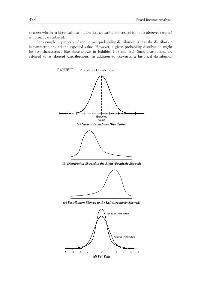
478 Fixed Income Analysis
to assess whether a historical distribution (i.e., a distribution created from the observed returns)is normally distributed.
For example, a property of the normal probability distribution is that the distributionis symmetric around the expected value. However, a given probability distribution mightbe best characterized like those shown in Exhibits 1(b) and 1(c). Such distributions arereferred to as skewed distributions. In addition to skewness, a historical distribution
EXHIBIT 1 Probability Distributions
(a) Normal Probability Distribution
(b) Distribution Skewed to the Right (Positively Skewed)
(c) Distribution Skewed to the Left (negatively Skewed)
(d) Fat Tails
ExpectedValue
Fat Tails Distribution
Normal Distribution
-5 -4 -3 -2 -1 0 1 2 3 4 5
Chapter 17 Measuring a Portfolio’s Risk Profile 479
may have more outliers (i.e., observations in the ‘‘tails’’) than the normal distribution predicts.Distributions with this characteristic are said to have fat tails. This is depicted in Exhibit1(d). Notice that, if a distribution does indeed have fat tails but it is assumed to be normallydistributed, then the probability of an actual value in a tail is assumed to be less than the trueprobability.3
In order to determine whether a historical distribution can be characterized as a normaldistribution, the following two questions must be addressed:
1. Do the data fit the values predicted by the normal distribution?2. Are the returns observed today independent of the returns of the prior periods?
Most introductory courses in statistics explain how to test whether historical data can becharacterized by a normal distribution and whether historical returns are serially correlated.These tests are beyond the scope of this chapter.4
Let’s look at the evidence on bond returns. For bonds, there is a lower limit on theloss. For Treasury securities, the limit depends on how high interest rates can rise. SinceTreasury rates have never exceeded 15%, this places a lower bound on negative returns fromholding a bond. There is a maximum return. Assuming that negative interest rates are notpossible, the maximum price for a bond is the undiscounted value of the cash flows (i.e., thesum of the interest payments and maturity value). In turn, this determines the maximumreturn. On balance, government bond return distributions are negatively skewed. Studies byJP Morgan RiskMetrics suggest that this occurs for government bonds. Moreover, governmentbond returns exhibit fat tails.5
Another issue in using a normal distribution is the independence of observations. Castingthis in terms of returns, it is important to know whether the return that might be realizedtoday is affected by the return that was realized in a prior period. The term serial correlation isused to describe the correlation between returns in different periods. Studies by JP Morgan’sRiskMetrics suggest that there is a small positive serial correlation for government bondreturns.6
B. Downside Risk Measures
Now you understand why the standard deviation is used as a measure of risk and thelimitations in using standard deviation as a measure of risk for a distribution that is notnormally distributed or symmetric.
Other measures of risk focus on only that portion of an investment’s return distributionthat is below a specified level. These measures of risk are referred to as downside risk measures.For downside risk measures, the portfolio manager defines the target return, and returns lessthan the target return represent adverse consequences. In the case of the standard deviation,the target return is the expected value. However, in practice, this need not be the case. Forexample, in managing money against a benchmark index, the target return might be X basis
3For a further discussion of skewed distributions, see Chapter 3 in DeFusco, McLeavey, Pinto, andRunkle, Quantitative Methods for Investment Analysis, pp. 138–144.4Tests for serial correlation are explained and illustrated in Chapter 9 of DeFusco, McLeavey, Pinto, andRunkle, Quantitative Methods for Investment Analysis, pp. 450–453.5RiskMetricsTM —Technical Document, JP Morgan, May 26, 1995, New York p. 48.6RiskMetricsTM —Technical Document, p. 48.
480 Fixed Income Analysis
points over the return of the benchmark index. Outcomes that are less than the return of thebenchmark index plus X basis points represent downside risk. In managing money againstliabilities, the target return might be the rate guaranteed on liabilities plus a spread of S basispoints. Returns with an outcome less than the rate guaranteed on liabilities plus S basis pointsthen represent downside risk.
The three more popular downside risk measures are:
• target semivariance• shortfall probability• value at risk.
1. Target Semivariance The target semivariance is a measure of the dispersion of theoutcomes below the target return. A special case of the target semivariance arises when thetarget return is the expected value. The resulting measure is called the semivariance.
While theoretically the semivariance is superior to the variance (standard deviation) as arisk measure, it is not used in bond portfolio management to any significant extent. RonaldKahn gave the following reasons why semivariance (which he defines as downside risk) is notused:7
First, its definition is not as unambiguous as standard deviation or variance, norare its statistical properties as well known, so it isn’t an ideal choice for a universal riskdefinition. We need a definition which managers, plan sponsors, and beneficiaries can alluse.
Second, it is computationally challenging for large portfolio construction problems.In fact, while we can aggregate individual bond standard deviations into a portfoliostandard deviation, for other measures of risk we must rely much more on historicalextrapolation of portfolio return patterns.
Third, to the extent that investment returns are reasonably symmetric, most definitionsof downside risk are simply proportional to standard deviation or variance and so containno additional information. To the extent that investment returns may not be symmetric,there are problems forecasting downside risk. Return asymmetries are not stable over time,and so are very difficult to forecast. Realized downside risk may not be a good forecast offuture downside risk. Moreover, we estimate downside risk with only half the data, losingstatistical accuracy.
In Section IIC we review how individual bond standard deviations of return are combinedto determine a bond portfolio’s standard deviation. In addition, we address the problem ofusing historical return patterns for individual bonds.
2. Shortfall Risk Shortfall risk is the probability that an outcome will have a value lessthan the target return.8 From a historical distribution of returns, shortfall risk is the ratio ofthe number of observations below the target return to the total number of observations. Oneproblem with this risk measure is that the magnitude of the losses below the target return isignored.
7Ronald N. Kahn, ‘‘Fixed Income Risk,’’ Chapter 1 in Frank J. Fabozzi (ed.), Managing Fixed IncomePortfolios (New Hope, PA: Frank J. Fabozzi Associates, 1997), pp. 2–3.8For a further discussion of the measures of shortfall risk discussed here, see DeFusco, McLeavey, Pinto,and Runkle, Quantitative Methods for Investment Analysis, pp. 253–256.
Chapter 17 Measuring a Portfolio’s Risk Profile 481
When the target return is zero, shortfall risk is commonly called the risk of loss. It iscalculated from historical data by dividing the number of observations with a return less thanzero by the total number of observations.
Ronald Kahn notes that the use of shortfall risk leads to the same problems identifiedearlier for target semivariance, namely, ‘‘ambiguity, poor statistical understanding, difficultyof forecasting.’’9
3. Value at Risk To calculate shortfall risk, the portfolio manager specifies a target returnand then computes the percentage of observed returns that are less than the target return.A related approach to risk measurement requires that the portfolio manager specify a targetprobability; the return will not fall below a yet-to-be determined value the percentage of timerepresented by the target probability.
For example, suppose that the portfolio manager specifies a target probability of 95%.The portfolio manager then determines the return such that the area in the left tail of theprobability distribution has a 5% probability. The target return computed is called the valueat risk (VaR).10
C. Portfolio Variance
One of the advantages of using the standard deviation or variance as a measure of risk is theability to compute portfolio risk from the risk of each individual bond in the portfolio. Theexpected value for a portfolio is the weighted average of the expected values of the individualbonds in the portfolio. The weight assigned to each bond is the market value of the bond asa percentage of the market value of the portfolio. No surprises here. However, the varianceof a portfolio is not simply a weighted average of the variances of the bonds comprising theportfolio. A basic principle of modern portfolio theory is that the variance of a portfolioof assets depends not only on the variance of each asset, but also on their covariances orcorrelations.11
If the standard deviation is used as the measure of risk, the variance of each bond andthe covariance for each pair of bonds must be estimated in order to be able to compute theportfolio’s standard deviation. Let’s look at two major problems with this approach. After wediscuss these problems, we will see how to resolve these issues.
The first problem with this approach is that the number of required estimated inputsincreases dramatically as the number of bonds in the portfolio or the number of bondsconsidered for inclusion in the portfolio increases. For example, consider a manager who wantsto construct a portfolio for which there are 5,000 bonds that are candidates for inclusion. (Ifthis number sounds large, consider that the broad-based bond market indexes are comprisedof far more than 5,000 bonds.) Then the number of variances and covariances that must beestimated is 12,502,500.12
9Kahn, ‘‘Fixed Income Risk,’’ p. 3.10For a further discussion of value at risk, see Chapter 9 in Don M. Chance, Analysis of Derivatives forthe CFA Program (Charlottesville, VA: Association for Investment Management and Research, 2003),pp. 576–578.11The calculation of the portfolio variance is described in Chapter 11 of DeFusco, McLeavey, Pinto, andRunkle, Quantitative Methods for Investment Analysis.12The formula for determining the number of variances and covariances is found as follows:[Number of bonds × (Number of bonds + 1)]/2.
482 Fixed Income Analysis
The second problem is that, whether it is 55 variances and covariances for a 10-bondportfolio or 12,502,500 for a 5,000-bond portfolio, these values must all be estimated. Wheredoes the portfolio manager obtain these values? The answer is that they must be estimatedfrom historical data. While equity portfolio managers have the luxury of working with a longtime series of returns on stocks, bond portfolio managers often do not have good sources ofhistorical bond data. In addition, even with time series data on the return for a particularbond, a portfolio manager must question what these returns mean. The reason is that thecharacteristics of a bond change over time.
For example, consider a 10-year Treasury note issued 8 years ago for which quarterlyreturns have been calculated. The first quarterly return is the return on a 10-year Treasury note.However, the second quarterly return is the return on a 9.75-year Treasury note. The thirdquarterly return is the return on a 9.5-year Treasury note, and so on. If the original 10-yearTreasury note is in the current portfolio and the manager wants to estimate the standarddeviation for that security, the historical standard deviation is not meaningful. Since it waspurchased 8 years ago, this security is now a 2-year Treasury note and does not share the returnvolatility characteristics of the earlier maturities. Not only does the changing time to maturityaffect the historical data and render it of limited use, but some securities’ characteristics changedramatically over time because of call/prepayment provisions. For example, we discussedmortgage-backed securities. CMO support bonds have average lives that change dramaticallydue to prepayments, which affects the historical return pattern.
Now, if we couple the problem of a large number of required estimates and the lack ofrelevant data, we see another major problem. Consider a 100-bond portfolio. There are 5,050inputs to be estimated. Suppose that just 10% of the inputs are misestimated because of a lackof good historical or meaningful data. This means that there are 505 misestimated numberswhich could have a material impact on the estimated portfolio standard deviation.
III. TRACKING ERROR
The measures described in Section II quantify risk exposure in terms of the variability relativeto the average value or in the case of downside risk measures, relative to some target return.Consequently, such measures are useful in managing a portfolio compared to liabilities or atarget return objective.
When a manager’s benchmark is a bond market index, performance relative to thatbenchmark index is important. A manager who realizes a −1% annual return when thebenchmark index returns −3% has performed well. So, it is important that such a managerunderstand the risk of a portfolio relative to the risk of the benchmark index. The measureused for this purpose is tracking error.
A. Measuring Tracking Error
Tracking error measures the dispersion between a portfolio’s returns and the returns of abenchmark index. Historical observations are used to compute the potential future trackingerror of a portfolio relative to the selected benchmark index. Specifically, the observation usedin calculating tracking error is the active return, which is defined as:
active return = portfolio’s return − benchmark index’s return
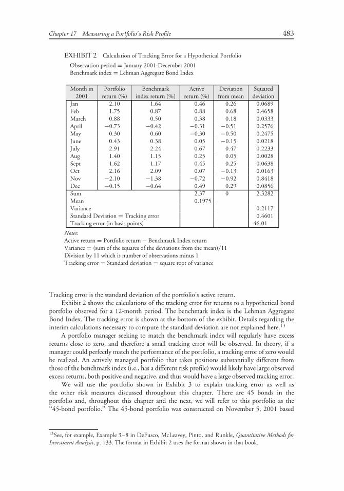
Chapter 17 Measuring a Portfolio’s Risk Profile 483
EXHIBIT 2 Calculation of Tracking Error for a Hypothetical Portfolio
Observation period = January 2001-December 2001Benchmark index = Lehman Aggregate Bond Index
Month in Portfolio Benchmark Active Deviation Squared2001 return (%) index return (%) return (%) from mean deviation
Jan 2.10 1.64 0.46 0.26 0.0689Feb 1.75 0.87 0.88 0.68 0.4658March 0.88 0.50 0.38 0.18 0.0333April −0.73 −0.42 −0.31 −0.51 0.2576May 0.30 0.60 −0.30 −0.50 0.2475June 0.43 0.38 0.05 −0.15 0.0218July 2.91 2.24 0.67 0.47 0.2233Aug 1.40 1.15 0.25 0.05 0.0028Sept 1.62 1.17 0.45 0.25 0.0638Oct 2.16 2.09 0.07 −0.13 0.0163Nov −2.10 −1.38 −0.72 −0.92 0.8418Dec −0.15 −0.64 0.49 0.29 0.0856Sum 2.37 0 2.3282Mean 0.1975Variance 0.2117Standard Deviation = Tracking error 0.4601Tracking error (in basis points) 46.01
Notes:Active return = Portfolio return − Benchmark Index returnVariance = (sum of the squares of the deviations from the mean)/11Division by 11 which is number of observations minus 1Tracking error = Standard deviation = square root of variance
Tracking error is the standard deviation of the portfolio’s active return.Exhibit 2 shows the calculations of the tracking error for returns to a hypothetical bond
portfolio observed for a 12-month period. The benchmark index is the Lehman AggregateBond Index. The tracking error is shown at the bottom of the exhibit. Details regarding theinterim calculations necessary to compute the standard deviation are not explained here.13
A portfolio manager seeking to match the benchmark index will regularly have excessreturns close to zero, and therefore a small tracking error will be observed. In theory, if amanager could perfectly match the performance of the portfolio, a tracking error of zero wouldbe realized. An actively managed portfolio that takes positions substantially different fromthose of the benchmark index (i.e., has a different risk profile) would likely have large observedexcess returns, both positive and negative, and thus would have a large observed tracking error.
We will use the portfolio shown in Exhibit 3 to explain tracking error as well asthe other risk measures discussed throughout this chapter. There are 45 bonds in theportfolio and, throughout this chapter and the next, we will refer to this portfolio as the‘‘45-bond portfolio.’’ The 45-bond portfolio was constructed on November 5, 2001 based
13See, for example, Example 3–8 in DeFusco, McLeavey, Pinto, and Runkle, Quantitative Methods forInvestment Analysis, p. 133. The format in Exhibit 2 uses the format shown in that book.
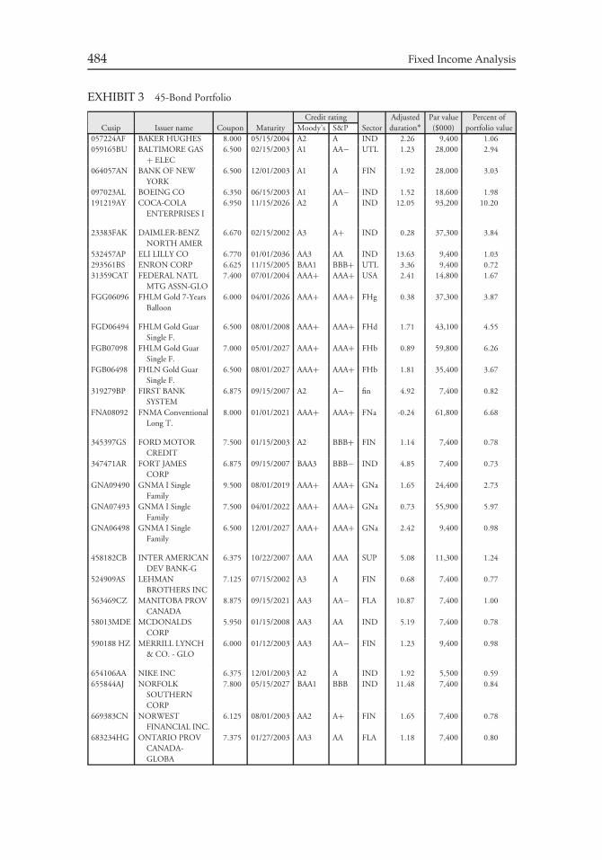
484 Fixed Income Analysis
EXHIBIT 3 45-Bond Portfolio
Credit rating Adjusted Par value Percent ofCusip Issuer name Coupon Maturity Moody’s S&P Sector duration∗ ($000) portfolio value
057224AF BAKER HUGHES 8.000 05/15/2004 A2 A IND 2.26 9,400 1.06059165BU BALTIMORE GAS
+ ELEC6.500 02/15/2003 A1 AA− UTL 1.23 28,000 2.94
064057AN BANK OF NEWYORK
6.500 12/01/2003 A1 A FIN 1.92 28,000 3.03
097023AL BOEING CO 6.350 06/15/2003 A1 AA− IND 1.52 18,600 1.98191219AY COCA-COLA
ENTERPRISES I6.950 11/15/2026 A2 A IND 12.05 93,200 10.20
23383FAK DAIMLER-BENZNORTH AMER
6.670 02/15/2002 A3 A+ IND 0.28 37,300 3.84
532457AP ELI LILLY CO 6.770 01/01/2036 AA3 AA IND 13.63 9,400 1.03293561BS ENRON CORP 6.625 11/15/2005 BAA1 BBB+ UTL 3.36 9,400 0.7231359CAT FEDERAL NATL
MTG ASSN-GLO7.400 07/01/2004 AAA+ AAA+ USA 2.41 14,800 1.67
FGG06096 FHLM Gold 7-YearsBalloon
6.000 04/01/2026 AAA+ AAA+ FHg 0.38 37,300 3.87
FGD06494 FHLM Gold GuarSingle F.
6.500 08/01/2008 AAA+ AAA+ FHd 1.71 43,100 4.55
FGB07098 FHLM Gold GuarSingle F.
7.000 05/01/2027 AAA+ AAA+ FHb 0.89 59,800 6.26
FGB06498 FHLN Gold GuarSingle F.
6.500 08/01/2027 AAA+ AAA+ FHb 1.81 35,400 3.67
319279BP FIRST BANKSYSTEM
6.875 09/15/2007 A2 A− fin 4.92 7,400 0.82
FNA08092 FNMA ConventionalLong T.
8.000 01/01/2021 AAA+ AAA+ FNa -0.24 61,800 6.68
345397GS FORD MOTORCREDIT
7.500 01/15/2003 A2 BBB+ FIN 1.14 7,400 0.78
347471AR FORT JAMESCORP
6.875 09/15/2007 BAA3 BBB− IND 4.85 7,400 0.73
GNA09490 GNMA I SingleFamily
9.500 08/01/2019 AAA+ AAA+ GNa 1.65 24,400 2.73
GNA07493 GNMA I SingleFamily
7.500 04/01/2022 AAA+ AAA+ GNa 0.73 55,900 5.97
GNA06498 GNMA I SingleFamily
6.500 12/01/2027 AAA+ AAA+ GNa 2.42 9,400 0.98
458182CB INTER AMERICANDEV BANK-G
6.375 10/22/2007 AAA AAA SUP 5.08 11,300 1.24
524909AS LEHMANBROTHERS INC
7.125 07/15/2002 A3 A FIN 0.68 7,400 0.77
563469CZ MANITOBA PROVCANADA
8.875 09/15/2021 AA3 AA− FLA 10.87 7,400 1.00
58013MDE MCDONALDSCORP
5.950 01/15/2008 AA3 AA IND 5.19 7,400 0.78
590188 HZ MERRILL LYNCH& CO. - GLO
6.000 01/12/2003 AA3 AA− FIN 1.23 9,400 0.98
654106AA NIKE INC 6.375 12/01/2003 A2 A IND 1.92 5,500 0.59655844AJ NORFOLK
SOUTHERNCORP
7.800 05/15/2027 BAA1 BBB IND 11.48 7,400 0.84
669383CN NORWESTFINANCIAL INC.
6.125 08/01/2003 AA2 A+ FIN 1.65 7,400 0.78
683234HG ONTARIO PROVCANADA-GLOBA
7.375 01/27/2003 AA3 AA FLA 1.18 7,400 0.80
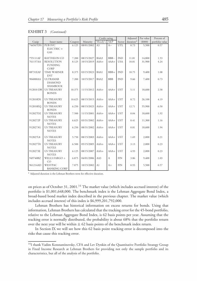
Chapter 17 Measuring a Portfolio’s Risk Profile 485
EXHIBIT 3 (Continued)
Credit rating Adjusted Par value Percent ofCusip Issuer name Coupon Maturity Moody’s S&P Sector duration∗ ($000) portfolio value
744567DN PUB SVCELECTRIC +GAS
6.125 08/01/2002 A3 A− UTL 0.73 5,500 0.57
755111AF RAYTHEON CO 7.200 08/15/2027 BAA3 BBB− IND 11.81 14,800 1.53761157AA RESOLUTION
FUNDINGCORP
8.125 10/15/2019 AAA+ AAA+ USA 10.81 31,900 4.24
88731EAF TIME WARNERENT
8.375 03/15/2023 BAA1 BBB+ IND 10.75 9,400 1.08
904000AA ULTRAMARDIAMONDSHAMROCK
7.200 10/15/2017 BAA2 BBB IND 9.66 7,400 0.73
912810 DB US TREASURYBONDS
10.375 11/15/2012 AAA+ AAA+ UST 5.11 18,600 2.58
912810DS US TREASURYBONDS
10.625 08/15/2015 AAA+ AAA+ UST 8.72 26,100 4.19
912810EQ US TREASURYBONDS
6.250 08/15/2023 AAA+ AAA+ UST 12.71 55,900 6.50
912827D2 US TREASURYNOTES
7.500 11/15/2001 AAA+ AAA+ UST 0.04 18,600 1.92
9128272P US TREASURYNOTES
6.625 03/31/2002 AAA+ AAA+ UST 0.41 11,300 1.16
9128273G US TREASURYNOTES
6.250 08/31/2002 AAA+ AAA+ UST 0.81 18,600 1.94
912827L8 US TREASURYNOTES
5.750 08/15/2003 AAA+ AAA+ UST 1.69 2,000 0.21
912827T8 US TREASURYNOTES
6.500 05/15/2005 AAA+ AAA+ UST 3.13 2,000 0.23
9128273E US TREASURYNOTES
6.125 08/15/2007 AAA+ AAA+ UST 4.93 2,000 0.23
949740BZ WELLS FARGO +CO
6.875 04/01/2006 AA3 A FIN 3.86 9,400 1.03
961214AD WESTPACBANKING CORP
7.875 10/15/2002 A1 A+ FIN 0.93 5,500 0.57
∗ Adjusted duration is the Lehman Brothers term for effective duration.
on prices as of October 31, 2001.14 The market value (which includes accrued interest) of theportfolio is $1,001,648,000. The benchmark index is the Lehman Aggregate Bond Index, abroad-based bond market index described in the previous chapter. The market value (whichincludes accrued interest) of this index is $6,999,201,792,000.
Lehman Brothers has historical information on excess returns for bonds. Using thatinformation, Lehman Brothers has calculated that the tracking error for the 45-bond portfolio,relative to the Lehman Aggregate Bond Index, is 62 basis points per year. Assuming that thetracking error is normally distributed, the probability is about 68% that the portfolio returnover the next year will be within ± 62 basis points of the benchmark index return.
In Section IX we will see how this 62 basis point tracking error is decomposed into therisks that cause this tracking error.
14I thank Vadim Konstantinovsky, CFA and Lev Dynkin of the Quantitative Portfolio Strategy Groupin Fixed Income Research at Lehman Brothers for providing not only the sample portfolio and itscharacteristics, but all of the analysis of the portfolio.
486 Fixed Income Analysis
B. Actual Versus Predicted Tracking Error
In Exhibit 2, the tracking error calculation is based on the active returns realized. However, theperformance shown is the result of the portfolio manager’s decisions during those 12 monthswith respect to portfolio positioning issues such as duration, sector allocations, and creditstructure. Hence, we can call the tracking error calculated from these trailing active returnsa backward-looking tracking error. It is also called the ex post tracking error and actualtracking error. We will use the term actual tracking error in this chapter and the next.
One problem with the use of actual tracking error is that it does not reflect the effect ofthe portfolio manager’s current decisions on the future active returns and hence the trackingerror that may be realized in the future. If, for example, the manager significantly changesthe portfolio’s effective duration or sector allocations today, then the actual tracking errorcalculated using data from prior periods would not accurately reflect the current portfoliorisks. That is, the actual tracking error will have little predictive value and can be misleadingregarding portfolio risks.
The portfolio manager needs a forward looking estimate of tracking error to accuratelyreflect future portfolio risk. In practice, this is accomplished by using the services of acommercial vendor that has a model, called a multi-factor risk model, that has identifiedand defined the risks associated with a benchmark index. Such a model is described inSection X. Statistical analysis of historical return data for the bonds in the benchmark indexis used to obtain the risk factors and to quantify the risks. (This involves the use of variancesand correlations/covariances.) Using the manager’s current portfolio holdings, the portfolio’scurrent exposure to the various risk factors can be calculated and compared to the benchmark’sexposures to the risk factors. Using the differential factor exposures and the risks of the factors,a forward looking tracking error for the portfolio can be computed. This tracking error isalso referred to as ex ante tracking error or predicted tracking error. We will use the termpredicted tracking error in this chapter and the next.
There is no guarantee that the predicted tracking error at the start of, say, a year wouldexactly match the actual tracking error calculated at the end of the year. There are two reasonsfor this. The first is that, as the year progresses and changes are made to the portfolio, thepredicted tracking error changes to reflect the new exposures. The second is that the accuracy ofthe predicted tracking error depends on stability in the variances and correlations/covariancesused in the analysis. These problems notwithstanding, the average of predicted tracking errorsobtained at different times during the year will be reasonably close to the actual tracking errorsobserved at the end of the year.
Both calculations of tracking error have their use. The predicted tracking error is usefulin risk control and portfolio construction. The manager can immediately see the likely effecton tracking error of any intended change in the portfolio. Thus, the portfolio manager cando a what-if analysis for various portfolio strategies and eliminate those that would resultin tracking errors beyond his tolerance for risk. The actual tracking error can be useful forassessing performance as discussed in the next chapter.
When actual tracking error is reported, the following supplementary information isoften provided: average return difference (i.e., average of the active returns), the maximumactive return difference (i.e., the highest of the active returns), and the minimum activereturn difference (i.e., the lowest of the active returns). It should be noted that some marketparticipants refer to the active return for a given observation period as tracking error.15
15The author uses this term. See also DeFusco, McLeavey, Pinto, and Runkle, Quantitative Methods forInvestment Analysis, p. 236 and the glossary to the book, p. 657.

Chapter 17 Measuring a Portfolio’s Risk Profile 487
IV. MEASURING A PORTFOLIO’S INTERESTRATE RISK
A portfolio’s duration is used to measure the portfolio’s exposure to changes in the levelof interest rates under the assumption of a parallel shift in the yield curve. For a portfolio,duration is the approximate percentage change in market value for a 100 basis point change ininterest rates, assuming a parallel shift in the yield curve. So, a portfolio duration of 4 meansthat the portfolio’s market value will change by approximately 4% for a 100 basis point changein the interest rate for all maturities. Earlier, we explained how to compute the duration forindividual securities.
Three different duration measures are used to quantify a bond’s or a portfolio’s exposureto a parallel shift in the yield curve—modified duration, Macaulay duration, and effectiveduration. As explained, modified duration assumes that, when interest rates change, thecash flows do not change. This is a limitation when measuring the exposure of bonds withembedded options (e.g., callable bonds, mortgage-backed securities, and some asset-backedsecurities) to changes in interest rates. Macaulay duration is related to modified duration andsuffers from the same failure to consider changes in cash flows when interest rates change. Incontrast, effective duration takes these changes in cash flows into account and thus, is theappropriate measure for bonds with embedded options. Effective duration is also referred toas option-adjusted duration.
The calculation of a portfolio’s duration begins with the calculation of the duration foreach of the individual bonds comprising the portfolio. This calculation requires the use of avaluation model. Duration is found by shocking (i.e., changing) interest rates and computingthe new value of the bond will be. Consequently, the duration measure is only as good as thevaluation model. We explained how the effective duration of a bond with an embedded optionis computed using the binomial model and also explained mortgage-backed and asset-backedsecurities.
For the 45-bond portfolio, the duration of each issue is shown in the column labeled‘‘adjusted duration.’’ Lehman Brothers uses this term instead of effective duration or option-adjusted duration. It is important to understand that the measure used by Lehman Brotherstakes into consideration the impact of changes in interest rates on the cash flows of a security.Here we see a clear example of the differences in the terminology used by major bond marketparticipants.
A. Portfolio Duration
A portfolio’s duration can be obtained by calculating the weighted average of the durationsof the bonds in the portfolio. The weight for a bond is the proportion of the market valueof a portfolio represented by a security. Mathematically, a portfolio’s duration is calculated asfollows:
w1D1 + w2D2 + w3D3 + . . . + wK DK
where
wi = market value of bond i/market value of the portfolioDi = duration of bond iK = number of bonds in the portfolio
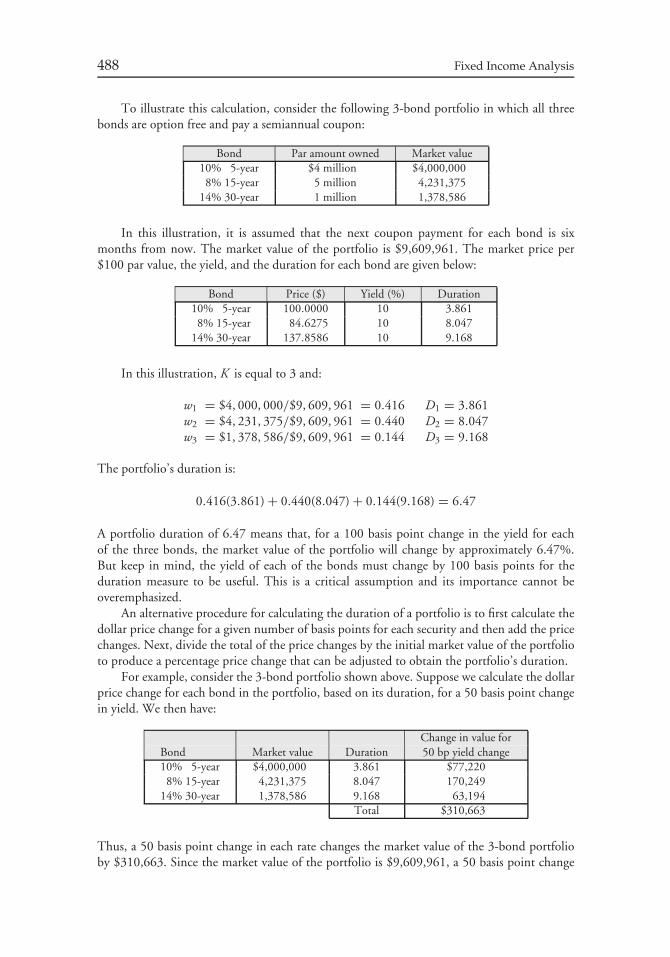
488 Fixed Income Analysis
To illustrate this calculation, consider the following 3-bond portfolio in which all threebonds are option free and pay a semiannual coupon:
Bond Par amount owned Market value10% 5-year $4 million $4,000,000
8% 15-year 5 million 4,231,37514% 30-year 1 million 1,378,586
In this illustration, it is assumed that the next coupon payment for each bond is sixmonths from now. The market value of the portfolio is $9,609,961. The market price per$100 par value, the yield, and the duration for each bond are given below:
Bond Price ($) Yield (%) Duration10% 5-year 100.0000 10 3.8618% 15-year 84.6275 10 8.047
14% 30-year 137.8586 10 9.168
In this illustration, K is equal to 3 and:
w1 = $4, 000, 000/$9, 609, 961 = 0.416 D1 = 3.861w2 = $4, 231, 375/$9, 609, 961 = 0.440 D2 = 8.047w3 = $1, 378, 586/$9, 609, 961 = 0.144 D3 = 9.168
The portfolio’s duration is:
0.416(3.861) + 0.440(8.047) + 0.144(9.168) = 6.47
A portfolio duration of 6.47 means that, for a 100 basis point change in the yield for eachof the three bonds, the market value of the portfolio will change by approximately 6.47%.But keep in mind, the yield of each of the bonds must change by 100 basis points for theduration measure to be useful. This is a critical assumption and its importance cannot beoveremphasized.
An alternative procedure for calculating the duration of a portfolio is to first calculate thedollar price change for a given number of basis points for each security and then add the pricechanges. Next, divide the total of the price changes by the initial market value of the portfolioto produce a percentage price change that can be adjusted to obtain the portfolio’s duration.
For example, consider the 3-bond portfolio shown above. Suppose we calculate the dollarprice change for each bond in the portfolio, based on its duration, for a 50 basis point changein yield. We then have:
Change in value forBond Market value Duration 50 bp yield change10% 5-year $4,000,000 3.861 $77,220
8% 15-year 4,231,375 8.047 170,24914% 30-year 1,378,586 9.168 63,194
Total $310,663
Thus, a 50 basis point change in each rate changes the market value of the 3-bond portfolioby $310,663. Since the market value of the portfolio is $9,609,961, a 50 basis point change
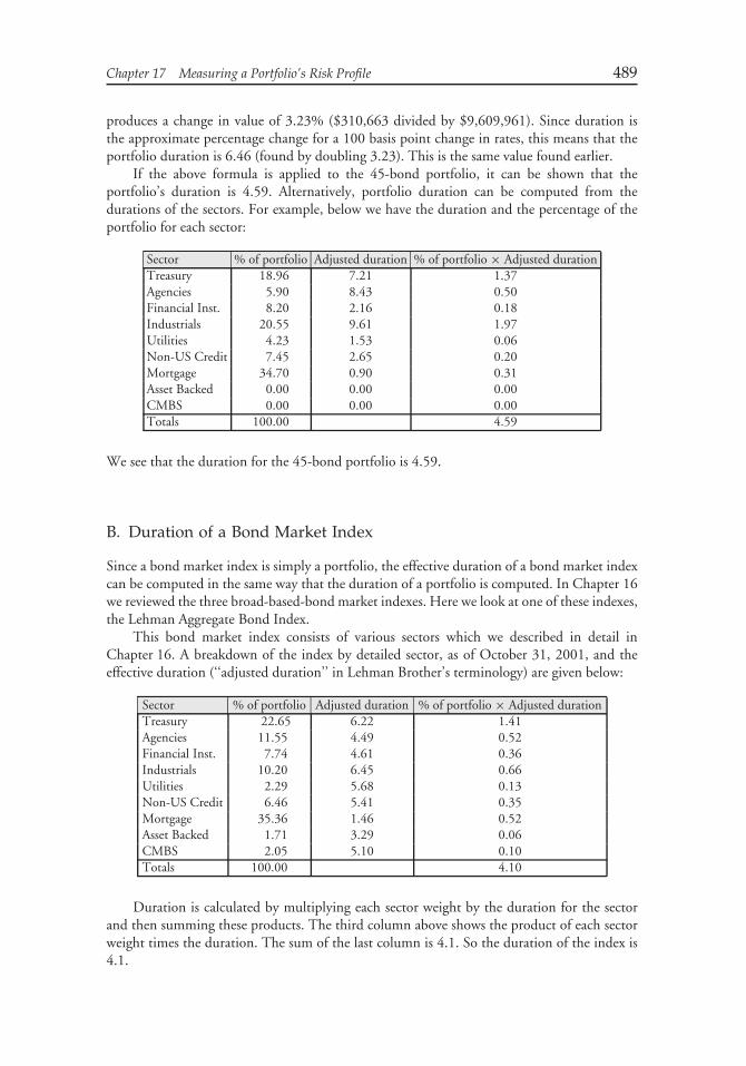
Chapter 17 Measuring a Portfolio’s Risk Profile 489
produces a change in value of 3.23% ($310,663 divided by $9,609,961). Since duration isthe approximate percentage change for a 100 basis point change in rates, this means that theportfolio duration is 6.46 (found by doubling 3.23). This is the same value found earlier.
If the above formula is applied to the 45-bond portfolio, it can be shown that theportfolio’s duration is 4.59. Alternatively, portfolio duration can be computed from thedurations of the sectors. For example, below we have the duration and the percentage of theportfolio for each sector:
Sector % of portfolio Adjusted duration % of portfolio × Adjusted durationTreasury 18.96 7.21 1.37Agencies 5.90 8.43 0.50Financial Inst. 8.20 2.16 0.18Industrials 20.55 9.61 1.97Utilities 4.23 1.53 0.06Non-US Credit 7.45 2.65 0.20Mortgage 34.70 0.90 0.31Asset Backed 0.00 0.00 0.00CMBS 0.00 0.00 0.00Totals 100.00 4.59
We see that the duration for the 45-bond portfolio is 4.59.
B. Duration of a Bond Market Index
Since a bond market index is simply a portfolio, the effective duration of a bond market indexcan be computed in the same way that the duration of a portfolio is computed. In Chapter 16we reviewed the three broad-based-bond market indexes. Here we look at one of these indexes,the Lehman Aggregate Bond Index.
This bond market index consists of various sectors which we described in detail inChapter 16. A breakdown of the index by detailed sector, as of October 31, 2001, and theeffective duration (‘‘adjusted duration’’ in Lehman Brother’s terminology) are given below:
Sector % of portfolio Adjusted duration % of portfolio × Adjusted durationTreasury 22.65 6.22 1.41Agencies 11.55 4.49 0.52Financial Inst. 7.74 4.61 0.36Industrials 10.20 6.45 0.66Utilities 2.29 5.68 0.13Non-US Credit 6.46 5.41 0.35Mortgage 35.36 1.46 0.52Asset Backed 1.71 3.29 0.06CMBS 2.05 5.10 0.10Totals 100.00 4.10
Duration is calculated by multiplying each sector weight by the duration for the sectorand then summing these products. The third column above shows the product of each sectorweight times the duration. The sum of the last column is 4.1. So the duration of the index is4.1.
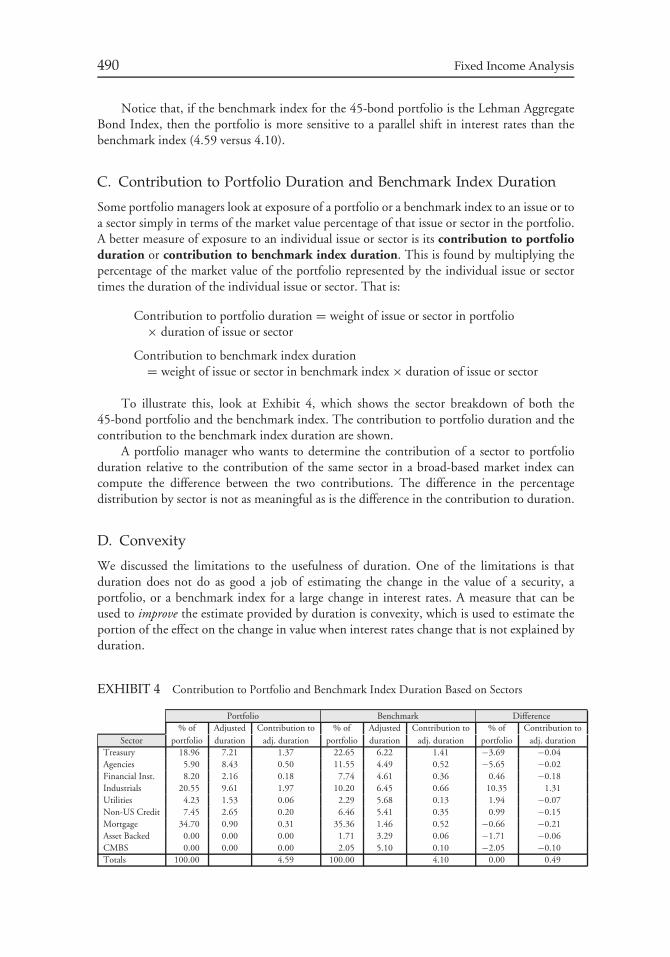
490 Fixed Income Analysis
Notice that, if the benchmark index for the 45-bond portfolio is the Lehman AggregateBond Index, then the portfolio is more sensitive to a parallel shift in interest rates than thebenchmark index (4.59 versus 4.10).
C. Contribution to Portfolio Duration and Benchmark Index Duration
Some portfolio managers look at exposure of a portfolio or a benchmark index to an issue or toa sector simply in terms of the market value percentage of that issue or sector in the portfolio.A better measure of exposure to an individual issue or sector is its contribution to portfolioduration or contribution to benchmark index duration. This is found by multiplying thepercentage of the market value of the portfolio represented by the individual issue or sectortimes the duration of the individual issue or sector. That is:
Contribution to portfolio duration = weight of issue or sector in portfolio× duration of issue or sector
Contribution to benchmark index duration= weight of issue or sector in benchmark index × duration of issue or sector
To illustrate this, look at Exhibit 4, which shows the sector breakdown of both the45-bond portfolio and the benchmark index. The contribution to portfolio duration and thecontribution to the benchmark index duration are shown.
A portfolio manager who wants to determine the contribution of a sector to portfolioduration relative to the contribution of the same sector in a broad-based market index cancompute the difference between the two contributions. The difference in the percentagedistribution by sector is not as meaningful as is the difference in the contribution to duration.
D. Convexity
We discussed the limitations to the usefulness of duration. One of the limitations is thatduration does not do as good a job of estimating the change in the value of a security, aportfolio, or a benchmark index for a large change in interest rates. A measure that can beused to improve the estimate provided by duration is convexity, which is used to estimate theportion of the effect on the change in value when interest rates change that is not explained byduration.
EXHIBIT 4 Contribution to Portfolio and Benchmark Index Duration Based on Sectors
Portfolio Benchmark Difference% of Adjusted Contribution to % of Adjusted Contribution to % of Contribution to
Sector portfolio duration adj. duration portfolio duration adj. duration portfolio adj. durationTreasury 18.96 7.21 1.37 22.65 6.22 1.41 −3.69 −0.04Agencies 5.90 8.43 0.50 11.55 4.49 0.52 −5.65 −0.02Financial Inst. 8.20 2.16 0.18 7.74 4.61 0.36 0.46 −0.18Industrials 20.55 9.61 1.97 10.20 6.45 0.66 10.35 1.31Utilities 4.23 1.53 0.06 2.29 5.68 0.13 1.94 −0.07Non-US Credit 7.45 2.65 0.20 6.46 5.41 0.35 0.99 −0.15Mortgage 34.70 0.90 0.31 35.36 1.46 0.52 −0.66 −0.21Asset Backed 0.00 0.00 0.00 1.71 3.29 0.06 −1.71 −0.06CMBS 0.00 0.00 0.00 2.05 5.10 0.10 −2.05 −0.10Totals 100.00 4.59 100.00 4.10 0.00 0.49
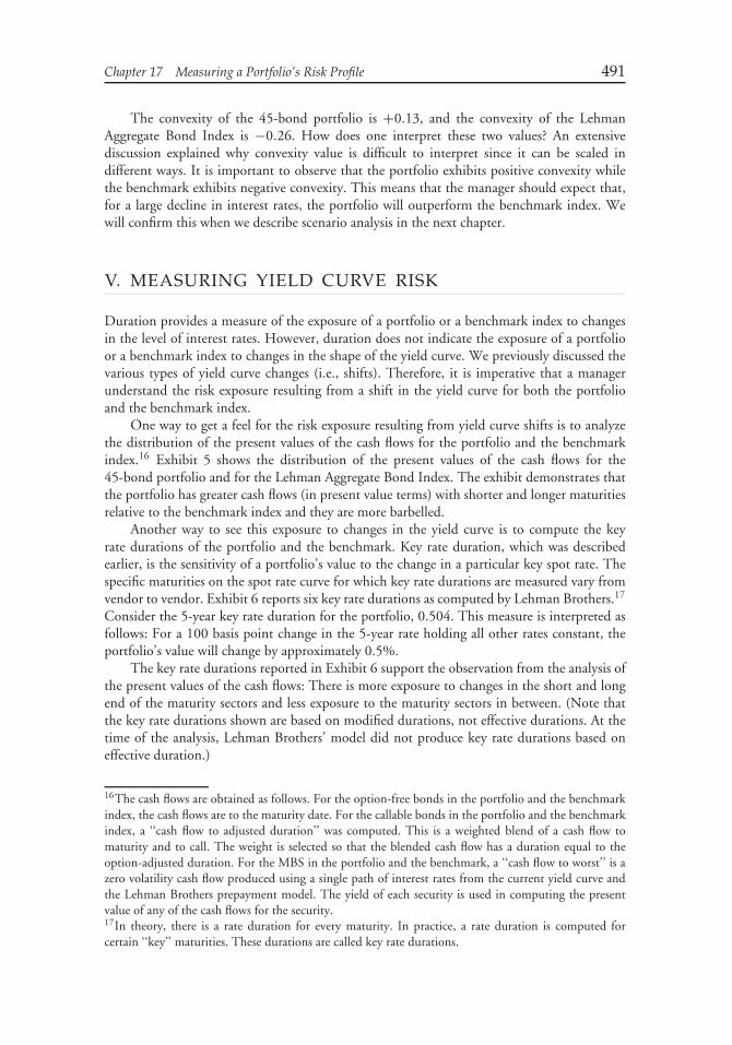
Chapter 17 Measuring a Portfolio’s Risk Profile 491
The convexity of the 45-bond portfolio is +0.13, and the convexity of the LehmanAggregate Bond Index is −0.26. How does one interpret these two values? An extensivediscussion explained why convexity value is difficult to interpret since it can be scaled indifferent ways. It is important to observe that the portfolio exhibits positive convexity whilethe benchmark exhibits negative convexity. This means that the manager should expect that,for a large decline in interest rates, the portfolio will outperform the benchmark index. Wewill confirm this when we describe scenario analysis in the next chapter.
V. MEASURING YIELD CURVE RISK
Duration provides a measure of the exposure of a portfolio or a benchmark index to changesin the level of interest rates. However, duration does not indicate the exposure of a portfolioor a benchmark index to changes in the shape of the yield curve. We previously discussed thevarious types of yield curve changes (i.e., shifts). Therefore, it is imperative that a managerunderstand the risk exposure resulting from a shift in the yield curve for both the portfolioand the benchmark index.
One way to get a feel for the risk exposure resulting from yield curve shifts is to analyzethe distribution of the present values of the cash flows for the portfolio and the benchmarkindex.16 Exhibit 5 shows the distribution of the present values of the cash flows for the45-bond portfolio and for the Lehman Aggregate Bond Index. The exhibit demonstrates thatthe portfolio has greater cash flows (in present value terms) with shorter and longer maturitiesrelative to the benchmark index and they are more barbelled.
Another way to see this exposure to changes in the yield curve is to compute the keyrate durations of the portfolio and the benchmark. Key rate duration, which was describedearlier, is the sensitivity of a portfolio’s value to the change in a particular key spot rate. Thespecific maturities on the spot rate curve for which key rate durations are measured vary fromvendor to vendor. Exhibit 6 reports six key rate durations as computed by Lehman Brothers.17
Consider the 5-year key rate duration for the portfolio, 0.504. This measure is interpreted asfollows: For a 100 basis point change in the 5-year rate holding all other rates constant, theportfolio’s value will change by approximately 0.5%.
The key rate durations reported in Exhibit 6 support the observation from the analysis ofthe present values of the cash flows: There is more exposure to changes in the short and longend of the maturity sectors and less exposure to the maturity sectors in between. (Note thatthe key rate durations shown are based on modified durations, not effective durations. At thetime of the analysis, Lehman Brothers’ model did not produce key rate durations based oneffective duration.)
16The cash flows are obtained as follows. For the option-free bonds in the portfolio and the benchmarkindex, the cash flows are to the maturity date. For the callable bonds in the portfolio and the benchmarkindex, a ‘‘cash flow to adjusted duration’’ was computed. This is a weighted blend of a cash flow tomaturity and to call. The weight is selected so that the blended cash flow has a duration equal to theoption-adjusted duration. For the MBS in the portfolio and the benchmark, a ‘‘cash flow to worst’’ is azero volatility cash flow produced using a single path of interest rates from the current yield curve andthe Lehman Brothers prepayment model. The yield of each security is used in computing the presentvalue of any of the cash flows for the security.17In theory, there is a rate duration for every maturity. In practice, a rate duration is computed forcertain ‘‘key’’ maturities. These durations are called key rate durations.
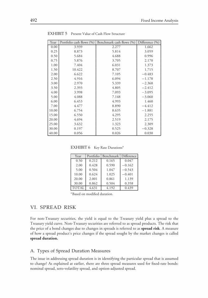
492 Fixed Income Analysis
EXHIBIT 5 Present Value of Cash Flow Structure
Year Portfolio cash flows (%) Benchmark cash flows (%) Difference (%)0.00 3.939 2.277 1.6620.25 8.873 5.814 3.0590.50 5.684 4.688 0.9960.75 5.876 3.705 2.1701.00 7.404 6.031 1.3731.50 10.422 8.707 1.7152.00 6.622 7.105 −0.4832.50 4.916 6.094 −1.1783.00 2.970 5.339 −2.3683.50 2.393 4.805 −2.4124.00 3.998 7.093 −3.0955.00 4.088 7.148 −3.0606.00 6.453 4.993 1.4607.00 4.477 8.890 −4.412
10.00 6.754 8.635 −1.88115.00 6.550 4.295 2.25520.00 4.694 2.519 2.17525.00 3.632 1.323 2.30930.00 0.197 0.525 −0.32840.00 0.056 0.026 0.030
EXHIBIT 6 Key Rate Durations∗
Year Portfolio Benchmark Difference0.50 0.212 0.165 0.0472.00 0.428 0.590 −0.1625.00 0.504 1.047 −0.543
10.00 0.624 1.025 −0.40120.00 2.001 0.861 1.13930.00 0.862 0.504 0.358
TOTAL 4.631 4.192 0.439∗Based on modified duration.
VI. SPREAD RISK
For non-Treasury securities, the yield is equal to the Treasury yield plus a spread to theTreasury yield curve. Non-Treasury securities are referred to as spread products. The risk thatthe price of a bond changes due to changes in spreads is referred to as spread risk. A measureof how a spread product’s price changes if the spread sought by the market changes is calledspread duration.
A. Types of Spread Duration Measures
The issue in addressing spread duration is in identifying the particular spread that is assumedto change? As explained at earlier, there are three spread measures used for fixed-rate bonds:nominal spread, zero-volatility spread, and option-adjusted spread.
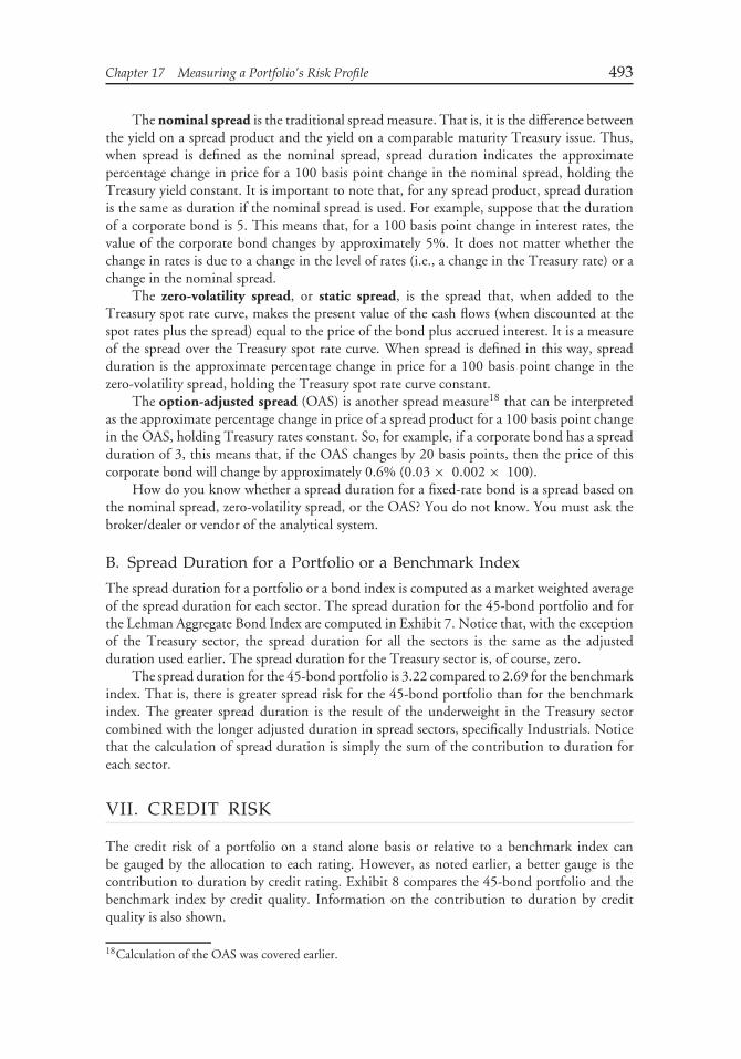
Chapter 17 Measuring a Portfolio’s Risk Profile 493
The nominal spread is the traditional spread measure. That is, it is the difference betweenthe yield on a spread product and the yield on a comparable maturity Treasury issue. Thus,when spread is defined as the nominal spread, spread duration indicates the approximatepercentage change in price for a 100 basis point change in the nominal spread, holding theTreasury yield constant. It is important to note that, for any spread product, spread durationis the same as duration if the nominal spread is used. For example, suppose that the durationof a corporate bond is 5. This means that, for a 100 basis point change in interest rates, thevalue of the corporate bond changes by approximately 5%. It does not matter whether thechange in rates is due to a change in the level of rates (i.e., a change in the Treasury rate) or achange in the nominal spread.
The zero-volatility spread, or static spread, is the spread that, when added to theTreasury spot rate curve, makes the present value of the cash flows (when discounted at thespot rates plus the spread) equal to the price of the bond plus accrued interest. It is a measureof the spread over the Treasury spot rate curve. When spread is defined in this way, spreadduration is the approximate percentage change in price for a 100 basis point change in thezero-volatility spread, holding the Treasury spot rate curve constant.
The option-adjusted spread (OAS) is another spread measure18 that can be interpretedas the approximate percentage change in price of a spread product for a 100 basis point changein the OAS, holding Treasury rates constant. So, for example, if a corporate bond has a spreadduration of 3, this means that, if the OAS changes by 20 basis points, then the price of thiscorporate bond will change by approximately 0.6% (0.03 × 0.002 × 100).
How do you know whether a spread duration for a fixed-rate bond is a spread based onthe nominal spread, zero-volatility spread, or the OAS? You do not know. You must ask thebroker/dealer or vendor of the analytical system.
B. Spread Duration for a Portfolio or a Benchmark Index
The spread duration for a portfolio or a bond index is computed as a market weighted averageof the spread duration for each sector. The spread duration for the 45-bond portfolio and forthe Lehman Aggregate Bond Index are computed in Exhibit 7. Notice that, with the exceptionof the Treasury sector, the spread duration for all the sectors is the same as the adjustedduration used earlier. The spread duration for the Treasury sector is, of course, zero.
The spread duration for the 45-bond portfolio is 3.22 compared to 2.69 for the benchmarkindex. That is, there is greater spread risk for the 45-bond portfolio than for the benchmarkindex. The greater spread duration is the result of the underweight in the Treasury sectorcombined with the longer adjusted duration in spread sectors, specifically Industrials. Noticethat the calculation of spread duration is simply the sum of the contribution to duration foreach sector.
VII. CREDIT RISK
The credit risk of a portfolio on a stand alone basis or relative to a benchmark index canbe gauged by the allocation to each rating. However, as noted earlier, a better gauge is thecontribution to duration by credit rating. Exhibit 8 compares the 45-bond portfolio and thebenchmark index by credit quality. Information on the contribution to duration by creditquality is also shown.
18Calculation of the OAS was covered earlier.
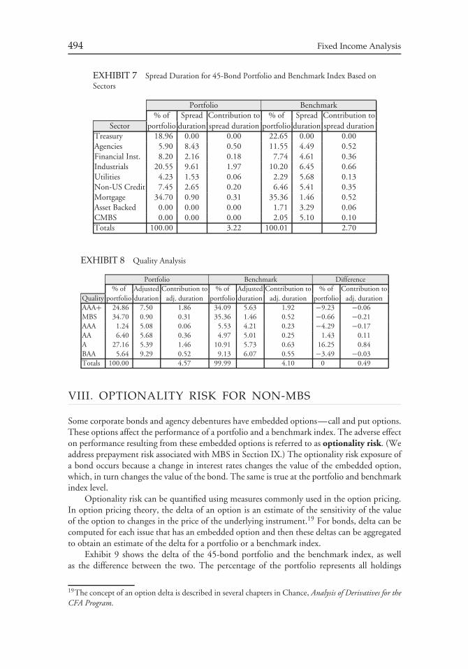
494 Fixed Income Analysis
EXHIBIT 7 Spread Duration for 45-Bond Portfolio and Benchmark Index Based onSectors
Portfolio Benchmark% of Spread Contribution to % of Spread Contribution to
Sector portfolio duration spread duration portfolio duration spread durationTreasury 18.96 0.00 0.00 22.65 0.00 0.00Agencies 5.90 8.43 0.50 11.55 4.49 0.52Financial Inst. 8.20 2.16 0.18 7.74 4.61 0.36Industrials 20.55 9.61 1.97 10.20 6.45 0.66Utilities 4.23 1.53 0.06 2.29 5.68 0.13Non-US Credit 7.45 2.65 0.20 6.46 5.41 0.35Mortgage 34.70 0.90 0.31 35.36 1.46 0.52Asset Backed 0.00 0.00 0.00 1.71 3.29 0.06CMBS 0.00 0.00 0.00 2.05 5.10 0.10Totals 100.00 3.22 100.01 2.70
EXHIBIT 8 Quality Analysis
Portfolio Benchmark Difference% of Adjusted Contribution to % of Adjusted Contribution to % of Contribution to
Quality portfolio duration adj. duration portfolio duration adj. duration portfolio adj. durationAAA+ 24.86 7.50 1.86 34.09 5.63 1.92 −9.23 −0.06MBS 34.70 0.90 0.31 35.36 1.46 0.52 −0.66 −0.21AAA 1.24 5.08 0.06 5.53 4.21 0.23 −4.29 −0.17AA 6.40 5.68 0.36 4.97 5.01 0.25 1.43 0.11A 27.16 5.39 1.46 10.91 5.73 0.63 16.25 0.84BAA 5.64 9.29 0.52 9.13 6.07 0.55 −3.49 −0.03Totals 100.00 4.57 99.99 4.10 0 0.49
VIII. OPTIONALITY RISK FOR NON-MBS
Some corporate bonds and agency debentures have embedded options—call and put options.These options affect the performance of a portfolio and a benchmark index. The adverse effecton performance resulting from these embedded options is referred to as optionality risk. (Weaddress prepayment risk associated with MBS in Section IX.) The optionality risk exposure ofa bond occurs because a change in interest rates changes the value of the embedded option,which, in turn changes the value of the bond. The same is true at the portfolio and benchmarkindex level.
Optionality risk can be quantified using measures commonly used in the option pricing.In option pricing theory, the delta of an option is an estimate of the sensitivity of the valueof the option to changes in the price of the underlying instrument.19 For bonds, delta can becomputed for each issue that has an embedded option and then these deltas can be aggregatedto obtain an estimate of the delta for a portfolio or a benchmark index.
Exhibit 9 shows the delta of the 45-bond portfolio and the benchmark index, as wellas the difference between the two. The percentage of the portfolio represents all holdings
19The concept of an option delta is described in several chapters in Chance, Analysis of Derivatives for theCFA Program.
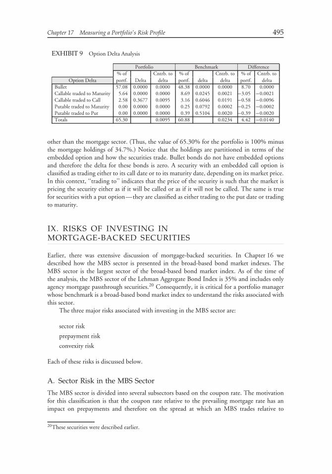
Chapter 17 Measuring a Portfolio’s Risk Profile 495
EXHIBIT 9 Option Delta Analysis
Portfolio Benchmark Difference% of Cntrb. to % of Cntrb. to % of Cntrb. to
Option Delta portf. Delta delta portf. delta delta portf. deltaBullet 57.08 0.0000 0.0000 48.38 0.0000 0.0000 8.70 0.0000Callable traded to Maturity 5.64 0.0000 0.0000 8.69 0.0245 0.0021 −3.05 −0.0021Callable traded to Call 2.58 0.3677 0.0095 3.16 0.6046 0.0191 −0.58 −0.0096Putable traded to Maturity 0.00 0.0000 0.0000 0.25 0.0792 0.0002 −0.25 −0.0002Putable traded to Put 0.00 0.0000 0.0000 0.39 0.5104 0.0020 −0.39 −0.0020Totals 65.30 0.0095 60.88 0.0234 4.42 −0.0140
other than the mortgage sector. (Thus, the value of 65.30% for the portfolio is 100% minusthe mortgage holdings of 34.7%.) Notice that the holdings are partitioned in terms of theembedded option and how the securities trade. Bullet bonds do not have embedded optionsand therefore the delta for these bonds is zero. A security with an embedded call option isclassified as trading either to its call date or to its maturity date, depending on its market price.In this context, ‘‘trading to’’ indicates that the price of the security is such that the market ispricing the security either as if it will be called or as if it will not be called. The same is truefor securities with a put option—they are classified as either trading to the put date or tradingto maturity.
IX. RISKS OF INVESTING INMORTGAGE-BACKED SECURITIES
Earlier, there was extensive discussion of mortgage-backed securities. In Chapter 16 wedescribed how the MBS sector is presented in the broad-based bond market indexes. TheMBS sector is the largest sector of the broad-based bond market index. As of the time ofthe analysis, the MBS sector of the Lehman Aggregate Bond Index is 35% and includes onlyagency mortgage passthrough securities.20 Consequently, it is critical for a portfolio managerwhose benchmark is a broad-based bond market index to understand the risks associated withthis sector.
The three major risks associated with investing in the MBS sector are:
sector risk
prepayment risk
convexity risk
Each of these risks is discussed below.
A. Sector Risk in the MBS Sector
The MBS sector is divided into several subsectors based on the coupon rate. The motivationfor this classification is that the coupon rate relative to the prevailing mortgage rate has animpact on prepayments and therefore on the spread at which an MBS trades relative to
20These securities were described earlier.
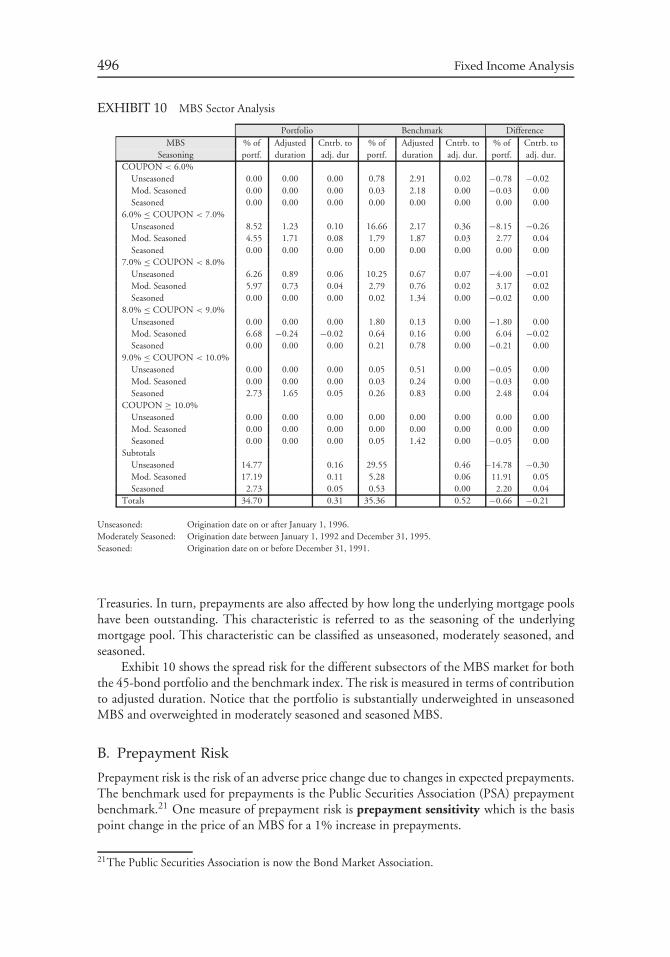
496 Fixed Income Analysis
EXHIBIT 10 MBS Sector Analysis
Portfolio Benchmark DifferenceMBS % of Adjusted Cntrb. to % of Adjusted Cntrb. to % of Cntrb. to
Seasoning portf. duration adj. dur portf. duration adj. dur. portf. adj. dur.COUPON < 6.0%
Unseasoned 0.00 0.00 0.00 0.78 2.91 0.02 −0.78 −0.02Mod. Seasoned 0.00 0.00 0.00 0.03 2.18 0.00 −0.03 0.00Seasoned 0.00 0.00 0.00 0.00 0.00 0.00 0.00 0.00
6.0% ≤ COUPON < 7.0%Unseasoned 8.52 1.23 0.10 16.66 2.17 0.36 −8.15 −0.26Mod. Seasoned 4.55 1.71 0.08 1.79 1.87 0.03 2.77 0.04Seasoned 0.00 0.00 0.00 0.00 0.00 0.00 0.00 0.00
7.0% ≤ COUPON < 8.0%Unseasoned 6.26 0.89 0.06 10.25 0.67 0.07 −4.00 −0.01Mod. Seasoned 5.97 0.73 0.04 2.79 0.76 0.02 3.17 0.02Seasoned 0.00 0.00 0.00 0.02 1.34 0.00 −0.02 0.00
8.0% ≤ COUPON < 9.0%Unseasoned 0.00 0.00 0.00 1.80 0.13 0.00 −1.80 0.00Mod. Seasoned 6.68 −0.24 −0.02 0.64 0.16 0.00 6.04 −0.02Seasoned 0.00 0.00 0.00 0.21 0.78 0.00 −0.21 0.00
9.0% ≤ COUPON < 10.0%Unseasoned 0.00 0.00 0.00 0.05 0.51 0.00 −0.05 0.00Mod. Seasoned 0.00 0.00 0.00 0.03 0.24 0.00 −0.03 0.00Seasoned 2.73 1.65 0.05 0.26 0.83 0.00 2.48 0.04
COUPON ≥ 10.0%Unseasoned 0.00 0.00 0.00 0.00 0.00 0.00 0.00 0.00Mod. Seasoned 0.00 0.00 0.00 0.00 0.00 0.00 0.00 0.00Seasoned 0.00 0.00 0.00 0.05 1.42 0.00 −0.05 0.00
SubtotalsUnseasoned 14.77 0.16 29.55 0.46 −14.78 −0.30Mod. Seasoned 17.19 0.11 5.28 0.06 11.91 0.05Seasoned 2.73 0.05 0.53 0.00 2.20 0.04
Totals 34.70 0.31 35.36 0.52 −0.66 −0.21
Unseasoned: Origination date on or after January 1, 1996.Moderately Seasoned: Origination date between January 1, 1992 and December 31, 1995.Seasoned: Origination date on or before December 31, 1991.
Treasuries. In turn, prepayments are also affected by how long the underlying mortgage poolshave been outstanding. This characteristic is referred to as the seasoning of the underlyingmortgage pool. This characteristic can be classified as unseasoned, moderately seasoned, andseasoned.
Exhibit 10 shows the spread risk for the different subsectors of the MBS market for boththe 45-bond portfolio and the benchmark index. The risk is measured in terms of contributionto adjusted duration. Notice that the portfolio is substantially underweighted in unseasonedMBS and overweighted in moderately seasoned and seasoned MBS.
B. Prepayment Risk
Prepayment risk is the risk of an adverse price change due to changes in expected prepayments.The benchmark used for prepayments is the Public Securities Association (PSA) prepaymentbenchmark.21 One measure of prepayment risk is prepayment sensitivity which is the basispoint change in the price of an MBS for a 1% increase in prepayments.
21The Public Securities Association is now the Bond Market Association.
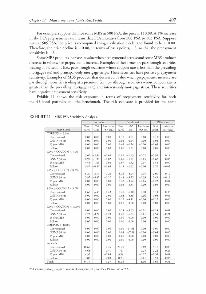
Chapter 17 Measuring a Portfolio’s Risk Profile 497
For example, suppose that, for some MBS at 500 PSA, the price is 110.08. A 1% increasein the PSA prepayment rate means that PSA increases from 500 PSA to 505 PSA. Supposethat, at 505 PSA, the price is recomputed using a valuation model and found to be 110.00.Therefore, the price decline is −0.08, in terms of basis points, −8, so that the prepaymentsensitivity is −8.
Some MBS products increase in value when prepayments increase and some MBS productsdecrease in value when prepayments increase. Examples of the former are passthrough securitiestrading at a discount (i.e., passthrough securities whose coupon rate is less than the prevailingmortgage rate) and principal-only mortgage strips. These securities have positive prepaymentsensitivity. Examples of MBS products that decrease in value when prepayments increase arepassthrough securities trading at a premium (i.e., passthrough securities whose coupon rate isgreater than the prevailing mortgage rate) and interest-only mortgage strips. These securitieshave negative prepayment sensitivity.
Exhibit 11 shows the risk exposure in terms of prepayment sensitivity for boththe 45-bond portfolio and the benchmark. The risk exposure is provided for the same
EXHIBIT 11 MBS PSA Sensitivity Analysis
Portfolio Benchmark Difference% of PSA Cntrb. to % of PSA Cntrb. to % of Cntrb. to
MBS Sector portf. sens PSA sens portf. sens PSA sens portf. PSA sensCOUPON < 6.0%
Conventional 0.00 0.00 0.00 0.10 0.01 0.00 −0.10 −0.00GNMA 30 yrs 0.00 0.00 0.00 0.02 0.44 0.00 −0.02 −0.0015 year MBS 0.00 0.00 0.00 0.63 −0.74 −0.00 −0.63 0.00Balloon 0.00 0.00 0.00 0.05 −1.21 −0.00 −0.05 0.00
6.0% ≤ COUPON < 7.0%Conventional 3.67 −2.33 −0.09 11.66 −1.93 −0.22 −7.99 0.14GNMA 30 yrs 0.98 −1.98 −0.02 2.65 −1.71 −0.05 −1.67 0.0315 year MBS 4.55 −1.69 −0.08 3.97 −1.82 −0.07 0.58 −0.00Balloon 3.87 −0.87 −0.03 0.18 −1.92 −0.00 3.70 −0.03
7.0% ≤ COUPON < 8.0%Conventional 6.26 −3.70 −0.23 8.32 −4.24 −0.35 −2.06 0.12GNMA 30 yrs 5.97 −4.47 −0.27 3.48 −3.75 −0.13 2.49 −0.1415 year MBS 0.00 0.00 0.00 1.22 −3.24 −0.04 −1.22 0.04Balloon 0.00 0.00 0.00 0.05 −3.31 −0.00 −0.05 0.00
8.0% ≤ COUPON < 9.0%Conventional 6.68 −6.45 −0.43 1.48 −6.48 −0.10 5.19 −0.33GNMA 30 yrs 0.00 0.00 0.00 1.05 −5.56 −0.06 −1.05 0.0615 year MBS 0.00 0.00 0.00 0.12 −4.11 −0.00 −0.12 0.00Balloon 0.00 0.00 0.00 0.00 0.00 0.00 0.00 0.00
9.0% ≤ COUPON < 10.0%Conventional 0.00 0.00 0.00 0.14 −9.05 −0.01 −0.14 0.01GNMA 30 yrs 2.73 −8.27 −0.23 0.20 −6.54 −0.01 2.54 −0.2115 year MBS 0.00 0.00 0.00 0.00 0.00 0.00 0.00 0.00Balloon 0.00 0.00 0.00 0.00 0.00 0.00 0.00 0.00
COUPON ≥ 10.0%Conventional 0.00 0.00 0.00 0.01 −11.01 −0.00 −0.01 0.00GNMA 30 yrs 0.00 0.00 0.00 0.04 −7.88 −0.00 −0.04 0.0015 year MBS 0.00 0.00 0.00 0.00 0.00 0.00 0.00 0.00Balloon 0.00 0.00 0.00 0.00 0.00 0.00 0.00 0.00
SubtotalsConventional 16.60 −0.75 21.71 −0.69 −5.11 −0.06GNMA 30 yrs 9.68 −0.51 7.44 −0.25 2.24 −0.2615 year MBS 4.55 −0.08 5.94 −0.12 −1.39 0.04Balloon 3.87 −0.03 0.28 −0.01 3.59 −0.03
Totals 34.70 −1.37 35.36 −1.06 −0.66 −0.31
PSA sensitivity: change in price (in units of basis points of price) for a 1% increase in PSA.
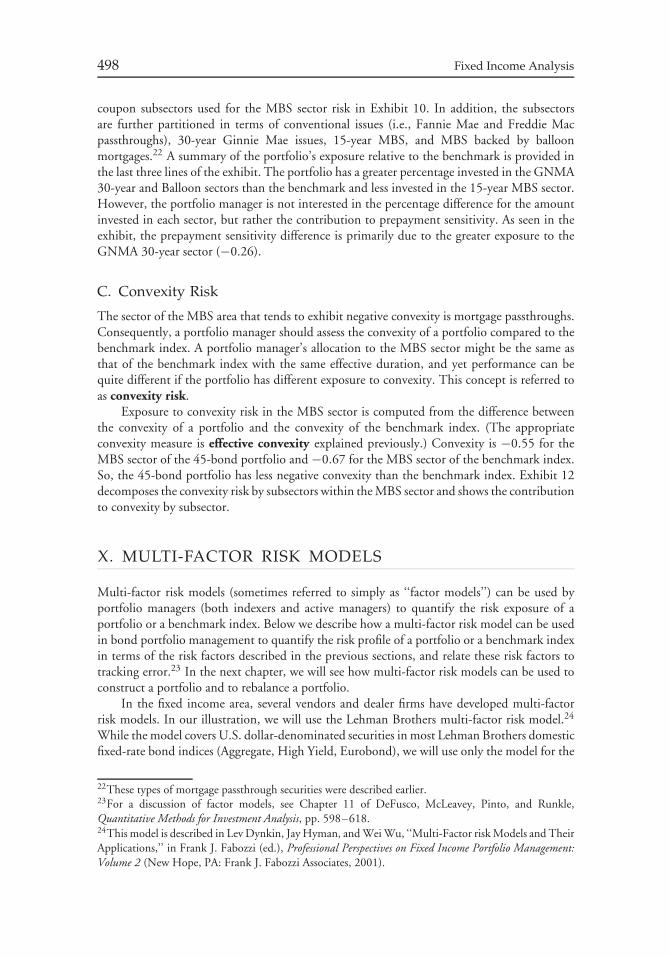
498 Fixed Income Analysis
coupon subsectors used for the MBS sector risk in Exhibit 10. In addition, the subsectorsare further partitioned in terms of conventional issues (i.e., Fannie Mae and Freddie Macpassthroughs), 30-year Ginnie Mae issues, 15-year MBS, and MBS backed by balloonmortgages.22 A summary of the portfolio’s exposure relative to the benchmark is provided inthe last three lines of the exhibit. The portfolio has a greater percentage invested in the GNMA30-year and Balloon sectors than the benchmark and less invested in the 15-year MBS sector.However, the portfolio manager is not interested in the percentage difference for the amountinvested in each sector, but rather the contribution to prepayment sensitivity. As seen in theexhibit, the prepayment sensitivity difference is primarily due to the greater exposure to theGNMA 30-year sector (−0.26).
C. Convexity Risk
The sector of the MBS area that tends to exhibit negative convexity is mortgage passthroughs.Consequently, a portfolio manager should assess the convexity of a portfolio compared to thebenchmark index. A portfolio manager’s allocation to the MBS sector might be the same asthat of the benchmark index with the same effective duration, and yet performance can bequite different if the portfolio has different exposure to convexity. This concept is referred toas convexity risk.
Exposure to convexity risk in the MBS sector is computed from the difference betweenthe convexity of a portfolio and the convexity of the benchmark index. (The appropriateconvexity measure is effective convexity explained previously.) Convexity is −0.55 for theMBS sector of the 45-bond portfolio and −0.67 for the MBS sector of the benchmark index.So, the 45-bond portfolio has less negative convexity than the benchmark index. Exhibit 12decomposes the convexity risk by subsectors within the MBS sector and shows the contributionto convexity by subsector.
X. MULTI-FACTOR RISK MODELS
Multi-factor risk models (sometimes referred to simply as ‘‘factor models’’) can be used byportfolio managers (both indexers and active managers) to quantify the risk exposure of aportfolio or a benchmark index. Below we describe how a multi-factor risk model can be usedin bond portfolio management to quantify the risk profile of a portfolio or a benchmark indexin terms of the risk factors described in the previous sections, and relate these risk factors totracking error.23 In the next chapter, we will see how multi-factor risk models can be used toconstruct a portfolio and to rebalance a portfolio.
In the fixed income area, several vendors and dealer firms have developed multi-factorrisk models. In our illustration, we will use the Lehman Brothers multi-factor risk model.24
While the model covers U.S. dollar-denominated securities in most Lehman Brothers domesticfixed-rate bond indices (Aggregate, High Yield, Eurobond), we will use only the model for the
22These types of mortgage passthrough securities were described earlier.23For a discussion of factor models, see Chapter 11 of DeFusco, McLeavey, Pinto, and Runkle,Quantitative Methods for Investment Analysis, pp. 598–618.24This model is described in Lev Dynkin, Jay Hyman, and Wei Wu, ‘‘Multi-Factor risk Models and TheirApplications,’’ in Frank J. Fabozzi (ed.), Professional Perspectives on Fixed Income Portfolio Management:Volume 2 (New Hope, PA: Frank J. Fabozzi Associates, 2001).
Chapter 17 Measuring a Portfolio’s Risk Profile 499
EXHIBIT 12 MBS Convexity Analysis
Portfolio Benchmark Difference% of Contrb. to % of Contrb. to % of Contrb. to
MBS Sector portf. Convexity conv. portf. Convexity conv. portf. conv.COUPON < 6.0%
Conventional 0.00 0.00 0.00 0.10 −1.56 −0.00 −0.10 0.00GNMA 30 yrs 0.00 0.00 0.00 0.02 −1.22 −0.00 −0.02 0.0015 year MBS 0.00 0.00 0.00 0.63 −1.36 −0.01 −0.63 0.01Balloon 0.00 0.00 0.00 0.05 −1.75 −0.00 −0.05 0.00
6.0% ≤ COUPON < 7.0%Conventional 3.67 −2.30 −0.08 11.66 −2.41 −0.28 −7.99 0.20GNMA 30 yrs 0.98 −2.99 −0.03 2.65 −2.95 −0.08 −1.67 0.0515 year MBS 4.55 −0.81 −0.04 3.97 −1.53 −0.06 0.58 0.02Balloon 3.87 −0.75 −0.03 0.18 −1.45 −0.00 3.70 −0.03
7.0% ≤ COUPON < 8.0%Conventional 6.26 −1.76 −0.11 8.32 −1.47 −0.12 −2.06 0.01GNMA 30 yrs 5.97 −1.96 −0.12 3.48 −2.29 −0.08 2.49 −0.0415 year MBS 0.00 0.00 0.00 1.22 −1.02 −0.01 −1.22 0.01Balloon 0.00 0.00 0.00 0.05 −0.78 −0.00 −0.05 0.00
8.0% ≤ COUPON < 9.0%Conventional 6.68 −1.99 −0.13 1.48 −0.80 −0.01 5.19 −0.12GNMA 30 yrs 0.00 0.00 0.00 1.05 −0.85 −0.01 −1.05 0.0115 year MBS 0.00 0.00 0.00 0.12 −0.55 −0.00 −0.12 0.00Balloon 0.00 0.00 0.00 0.00 0.00 0.00 0.00 0.00
9.0% ≤ COUPON < 10.0%Conventional 0.00 0.00 0.00 0.14 −0.81 −0.00 −0.14 0.00GNMA 30 yrs 2.73 −0.24 −0.01 0.20 −0.60 −0.00 2.54 −0.0115 year MBS 0.00 0.00 0.00 0.00 0.00 0.00 0.00 0.00Balloon 0.00 0.00 0.00 0.00 0.00 0.00 0.00 0.00
COUPON ≥ 10.0%Conventional 0.00 0.00 0.00 0.01 −0.54 −0.00 −0.01 0.00GNMA 30 yrs 0.00 0.00 0.00 0.04 −0.24 −0.00 −0.04 0.0015 year MBS 0.00 0.00 0.00 0.00 0.00 0.00 0.00 0.00Balloon 0.00 0.00 0.00 0.00 0.00 0.00 0.00 0.00
SubtotalsConventional 16.60 −0.33 21.71 −0.42 −5.11 0.09GNMA 30 yrs 9.68 −0.15 7.44 −0.17 2.24 0.0215 year MBS 4.55 −0.04 5.94 −0.08 −1.39 0.05Balloon 3.87 −0.03 0.28 −0.00 3.59 −0.03
Totals 34.70 −0.55 35.36 −0.67 −0.66 0.13
Lehman Aggregate Bond Index. The historical data needed to estimate the model are updatedmonthly by Lehman Brothers. The portfolio we will analyze is the 45-bond portfolio that hasbeen used throughout this chapter.
Much like other commercially available or dealer proprietary multi-factor risk models,the Lehman Brothers model focuses on predicted tracking error. Specifically, tracking erroris defined as one standard deviation of the difference between the 45-bond portfolio andbenchmark annualized returns. For the 45-bond portfolio, the predicted tracking error is 62basis points per year.
A. Systematic and Non-Systematic Risks
The multi-factor risk model seeks to identify the specific risks that contribute to the predictedtracking error. All of the risks are measured in terms of predicted tracking error. The analysisbegins with a decomposition of the risks into two general categories— systematic risk andnon-systematic risk. The latter is the risk that remains after removing systematic risk and, is alsoreferred to as residual risk. For the portfolio, the following was determined:
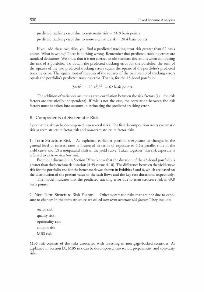
500 Fixed Income Analysis
predicted tracking error due to systematic risk = 54.8 basis points
predicted tracking error due to non-systematic risk = 28.4 basis points
If you add these two risks, you find a predicted tracking error risk greater than 62 basispoints. What is wrong? There is nothing wrong. Remember that predicted tracking errors arestandard deviations. We know that it is not correct to add standard deviations when computingthe risk of a portfolio. To obtain the predicted tracking error for the portfolio, the sum ofthe squares of the two predicted tracking errors equals the square of the portfolio’s predictedtracking error. The square root of the sum of the squares of the two predicted tracking errorsequals the portfolio’s predicted tracking error. That is, for the 45-bond portfolio:
[54.82 + 28.42]0.5 = 62 basis points.
The addition of variances assumes a zero correlation between the risk factors (i.e., the riskfactors are statistically independent). If this is not the case, the correlation between the riskfactors must be taken into account in estimating the predicted tracking error.
B. Components of Systematic Risk
Systematic risk can be decomposed into several risks. The first decomposition treats systematicrisk as term structure factor risk and non-term structure factor risks.
1. Term Structure Risk As explained earlier, a portfolio’s exposure to changes in thegeneral level of interest rates is measured in terms of exposure to (1) a parallel shift in theyield curve and (2) a nonparallel shift in the yield curve. Taken together, this risk exposure isreferred to as term structure risk.
From our discussion in Section IV we know that the duration of the 45-bond portfolio isgreater than the benchmark duration (4.59 versus 4.10). The difference between the yield curverisk for the portfolio and for the benchmark was shown in Exhibits 5 and 6, which are based onthe distribution of the present value of the cash flows and the key rate durations, respectively.
The model indicates that the predicted tracking error due to term structure risk is 49.8basis points.
2. Non-Term Structure Risk Factors Other systematic risks that are not due to expo-sure to changes in the term structure are called non-term structure risk factors. They include:
sector risk
quality risk
optionality risk
coupon risk
MBS risk
MBS risk consists of the risks associated with investing in mortgage-backed securities. Asexplained in Section IX, MBS risk can be decomposed into sector, prepayment, and convexityrisks.
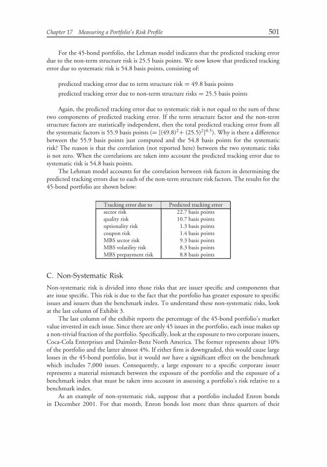
Chapter 17 Measuring a Portfolio’s Risk Profile 501
For the 45-bond portfolio, the Lehman model indicates that the predicted tracking errordue to the non-term structure risk is 25.5 basis points. We now know that predicted trackingerror due to systematic risk is 54.8 basis points, consisting of:
predicted tracking error due to term structure risk = 49.8 basis points
predicted tracking error due to non-term structure risks = 25.5 basis points
Again, the predicted tracking error due to systematic risk is not equal to the sum of thesetwo components of predicted tracking error. If the term structure factor and the non-termstructure factors are statistically independent, then the total predicted tracking error from allthe systematic factors is 55.9 basis points (= [(49.8)2+ (25.5)2]0.5). Why is there a differencebetween the 55.9 basis points just computed and the 54.8 basis points for the systematicrisk? The reason is that the correlation (not reported here) between the two systematic risksis not zero. When the correlations are taken into account the predicted tracking error due tosystematic risk is 54.8 basis points.
The Lehman model accounts for the correlation between risk factors in determining thepredicted tracking errors due to each of the non-term structure risk factors. The results for the45-bond portfolio are shown below:
Tracking error due to Predicted tracking errorsector risk 22.7 basis pointsquality risk 10.7 basis pointsoptionality risk 1.3 basis pointscoupon risk 1.4 basis pointsMBS sector risk 9.3 basis pointsMBS volatility risk 8.3 basis pointsMBS prepayment risk 8.8 basis points
C. Non-Systematic Risk
Non-systematic risk is divided into those risks that are issuer specific and components thatare issue specific. This risk is due to the fact that the portfolio has greater exposure to specificissues and issuers than the benchmark index. To understand these non-systematic risks, lookat the last column of Exhibit 3.
The last column of the exhibit reports the percentage of the 45-bond portfolio’s marketvalue invested in each issue. Since there are only 45 issues in the portfolio, each issue makes upa non-trivial fraction of the portfolio. Specifically, look at the exposure to two corporate issuers,Coca-Cola Enterprises and Daimler-Benz North America. The former represents about 10%of the portfolio and the latter almost 4%. If either firm is downgraded, this would cause largelosses in the 45-bond portfolio, but it would not have a significant effect on the benchmarkwhich includes 7,000 issues. Consequently, a large exposure to a specific corporate issuerrepresents a material mismatch between the exposure of the portfolio and the exposure of abenchmark index that must be taken into account in assessing a portfolio’s risk relative to abenchmark index.
As an example of non-systematic risk, suppose that a portfolio included Enron bondsin December 2001. For that month, Enron bonds lost more than three quarters of their

502 Fixed Income Analysis
value. The weighting of the bonds in the Merrill Lynch High Grade Index was 0.2%. Ifthese bonds represent 1.6% of the portfolio, this would have resulted in a 100 basis pointunderperformance relative to the index at a time when sectors such as Consumer Cyclicals,Media, Telecom, and Technology outperformed the index by more than 200 basis points.25
25Phil Galdi, Mark Anderson, and Arjun Kondamani, U.S. High Grade Bond Index, Merrill Lynch(December 5, 2001).
CHAPTER 18MANAGING FUNDS
AGAINST A BOND MARKETINDEX
I. INTRODUCTION
The benchmark for a manager can be either a bond market index or liabilities. In this chapter,we provide an overview of strategies for managing funds against a bond market index. Werestrict our discussion to domestic bond markets, specifically the U.S. bond market, in theillustrations in this chapter. In Chapter 20, we cover global bond investing. In Chapter 19, wediscuss strategies for managing funds when the benchmark is one or more liabilities.
II. DEGREES OF ACTIVE MANAGEMENT
In the previous chapter we discussed the risk factors associated with a bond portfolio anda bond market index. One can classify bond portfolio strategies in terms of the degree towhich a manager constructs a portfolio with a risk profile that differs from the risk profile ofthe benchmark index. Kenneth Volpert of the Vanguard Group has classified bond portfoliostrategies as follows:1
1. pure bond index matching2. enhanced indexing/matching risk factors3. enhanced indexing/minor risk factor mismatches4. active management/larger risk factor mismatches5. unrestricted active management
We discuss each of these strategies below.
1Kenneth E. Volpert, ‘‘Managing Indexed and Enhanced Indexed Bond Portfolios,’’ Chapter 3 in FrankJ. Fabozzi (ed.), Fixed Income Readings for the Chartered Financial Analyst Program: First Edition (NewHope, PA: Frank J. Fabozzi Associates, 2000). Volpert uses the term ‘‘active management/full-blownactive’’ instead of ‘‘unrestricted active management.’’ I have changed the classification based on thesuggestion of David Zahn, CFA, of Citigroup Asset Management.
503
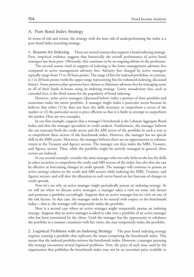
504 Fixed Income Analysis
A. Pure Bond Index Strategy
In terms of risk and return, the strategy with the least risk of underperforming the index is apure bond index matching strategy.
1. Reasons for Indexing There are several reasons that support a bond indexing strategy.First, empirical evidence suggests that historically the overall performance of active bondmanagers has been poor. Obviously, this continues to be an ongoing debate in the profession.
The second reason cited in support of indexing is the lower management advisory feescompared to active management advisory fees. Advisory fees charged by active managerstypically range from 15 to 50 basis points. The range of fees for indexed portfolios, in contrast,is 1 to 20 basis points (with the upper range representing fees for enhanced indexing, discussedbelow). Some pension plan sponsors have chosen to eliminate advisory fees by managing someor all of their funds in-house using an indexing strategy. Lower nonadvisory fees, such ascustodial fees, is the third reason for the popularity of bond indexing.
However, some active managers (discussed below) index a portion of their portfolio andsometimes index the entire portfolio. A manager might index a particular sector because hebelieves that either (1) he does not have the skills necessary to outperform a sector of themarket or (2) the particular sector is price efficient so that it is futile to attempt to outperformthe market. Here are two examples.
In our first example, suppose that a manager’s benchmark is the Lehman Aggregate BondIndex and that the manager specializes in credit analysis. Furthermore, the manager believesshe can structure both the credit sector and the ABS sector of the portfolio in such a way asto outperform these sectors of the benchmark index. However, the manager has no specialskill in the MBS sector. Moreover, the manager believes there are no opportunities to enhancereturn in the Treasury and Agency sectors. The manager can then index the MBS, Treasury,and Agency sectors. Thus, while the portfolio might be actively managed in general, threesectors are indexed.
In our second example, consider the same manager who not only believes she has the skillsto select securities to outperform the credit and ABS sectors of the index, but also that she canbe effective in forecasting changes in credit spreads. The manager will continue to pursue anactive strategy relative to the credit and ABS sectors while indexing the MBS, Treasury, andAgency sectors, and will alter the allocation to each sector based on her forecasts of changes incredit spreads.
Now let’s see why an active manager might periodically pursue an indexing strategy. Aswe will see when we discuss active strategies, a manager takes a view on some risk factorsand positions a portfolio accordingly. Suppose that an active manager has no view on any ofthe risk factors. In that case, the manager seeks to be neutral with respect to the benchmarkindex—that is, the manager will temporarily index the portfolio.
Here is a second case where an active manager might temporarily pursue an indexingstrategy. Suppose that an active manager is asked to take over a portfolio of an active managerwho has been terminated by the client. Until the manager has the opportunity to rebalancethe portfolio in a manner consistent with her views, she may temporarily index the portfolio.
2. Logistical Problems with an Indexing Strategy The pure bond indexing strategyrequires creating a portfolio that replicates the issues comprising the benchmark index. Thismeans that the indexed portfolio mirrors the benchmark index. However, a manager pursuingthis strategy encounters several logistical problems. First, the price of each issue used by theorganization that publishes the benchmark index may not be an execution price available to
Chapter 18 Managing Funds against a Bond Market Index 505
the manager. In fact, these prices might be materially different from the prices offered bydealers. In addition, the prices used by organizations reporting index values are based on bidprices. However, the prices the manager pays when constructing or rebalancing the portfolioare dealer ask prices. Thus there is a bias between the performance of the benchmark indexand the indexed portfolio equal to the bid-ask spread.
Furthermore, there are logistical problems unique to certain sectors of the bond market.Consider first the corporate bond market. There are more than 4,000 issues in the corporatebond sector of a broad-based bond market index. Because many of these issues are illiquid,not only might the prices be unreliable, but many of the issues may not even be available.Next, consider the mortgage sector. There are over 800,000 agency passthrough issues. Asexplained in Chapter 16, the organizations that publish indexes aggregate these issues intoa few hundred generic issues. The manager is then faced with the difficult task of findingpassthrough securities with risk/return profiles that are the same as those of the hypotheticalgeneric issues.
Finally, as explained in Section IV, total return depends on the reinvestment rate availableon interim cash flows received prior to month end. If the organization publishing thebenchmark index regularly overestimates the reinvestment rate, then the indexed portfoliomight underperform the benchmark index.
3. Rebalancing an Indexing Portfolio Once an indexed portfolio is constructed, theportfolio must then be rebalanced as the composition and the characteristics of the target indexchange. For example, over time the duration of an index and the indexed portfolio changes,making rebalancing necessary to bring the portfolio’s duration in line with the duration ofthe index. Transaction costs arise when rebalancing a portfolio. The manager will seek arebalancing strategy that minimizes transaction costs. The multi-factor risk model describedlater in this chapter can be used to rebalance an indexed portfolio at minimum cost.
B. Enhanced Indexing/Matching Risk Factors
An enhanced indexing strategy can be used to construct a portfolio that matches the primaryrisk factors without acquiring each issue in the index. This is a common strategy used by smallerfunds because of the difficulties in acquiring all of the issues comprising the index. Generallyspeaking, the smaller the number of issues used to replicate the benchmark index, the lowerthe transaction costs but the greater the difficulties in matching the risk factors. In contrast,the more issues purchased to replicate the benchmark index, the greater the transaction costs,but the lower the risk due to the mismatch of risk factors between the indexed portfolio andthe benchmark index.
In the spectrum of strategies defined by Volpert, this strategy is called an ‘‘enhancedstrategy,’’ although some investors refer to this as simply an indexing strategy. Two commonlyused techniques to construct a portfolio that replicates an index are:
1. cell matching (stratified sampling)2. tracking error minimization using a multi-factor risk model
Both techniques assume that the performance of an individual bond depends on a numberof systematic factors that affect the performance of all bonds and on an unsystematic factorunique to the individual issue or issuers.

506 Fixed Income Analysis
1. Cell Matching With the cell matching technique (also called the stratified samplingtechnique), the index is divided into cells representing the risk factors. The objective is thento select from all of the issues in the index one or more issues in each cell to represent thatentire cell. The total dollar amount purchased of the issues from each cell will be based ona criterion such as the percentage of the index’s total market value that the cell represents.For example, if W % of the market value of the index is comprised of double-A corporatebonds, then W % of the market value of the indexed portfolio should be composed of doubleA corporate bond issues. A better approach would be to base selection on the contribution toduration, a measure explained in the previous chapter.
The number of cells the indexer uses depends on the dollar amount of the portfolio to beindexed. In indexing a portfolio of less than $50 million, for example, a large number of cellswould require the purchase of odd lots of issues. This increases the cost of buying the issuesto represent a cell, and thus would increase the likelihood of underperforming the benchmarkindex. Reducing the number of cells to overcome this problem increases predicted trackingerror because the risk profile of the indexed portfolio might differ materially from that of theindex.
2. Tracking Error Minimization Using a Multi-Factor Risk Model In the previ-ous chapter we discussed multi-factor risk models. Specifically, our focus was on usingsuch models to quantify the risk profile of a portfolio or a benchmark index, and describingthe risk factors in the model. We used a Lehman model in our illustrations. As mentioned inthe previous chapter, a multi-factor risk model can also be used to construct a portfolio with apredicted tracking error acceptable to a manager pursuing an enhanced indexing strategy thatmatches the risk factors.
C. Enhanced Indexing/Minor Risk Factor Mismatches
Another enhanced strategy is based on constructing a portfolio with minor deviations fromthe risk factors that affect the performance of the index. For example, such a strategy might beused to create a portfolio with a slight overweighting of issues or sectors that are relative values.This strategy matches the duration of the portfolio with the duration of the benchmark index.That is, there are no duration bets in this strategy, as is the case with the pure index matchstrategy and the enhanced index with matching risk strategy.
D. Active Management/Larger Risk Factor Mismatches
Active bond strategies attempt to outperform the market by constructing a portfolio that hasa greater index mismatch than is the case for enhanced indexing. The decision to pursue anactive strategy or to recommend that a client direct a manager to pursue an active strategymust be based on the belief that there is some gain to be derived from such costly efforts;in order for a gain to exist, pricing inefficiencies must exist. The particular strategy chosendepends on the reasons that price inefficiencies exist.
Volpert identifies two types of active strategies. In the more conservative of these strategies,the manager creates larger mismatches, in terms of risk factors, relative to the benchmarkindex. This includes minor duration mismatches. Typically, there is a limit to the degree ofduration mismatch. For example, the manager might be constrained to within ±1 of the
Chapter 18 Managing Funds against a Bond Market Index 507
duration of the index.2 So, if the duration of the index is 4, the manager may construct aportfolio with duration between 3 and 5. To take advantage of anticipated reshaping of theyield curve, the manager might create a portfolio such that there are significant differences incash flow distribution between the benchmark index and the portfolio. As another example, ifthe manager believes that, within the corporate sector, A rated issues will outperform AA ratedissues, the manager might overweight the A rated issues and underweight AA rated issues.
The manager can choose to invest a small percentage of the portfolio in one or moresectors that are not in the bond market index. For example, the portfolio might have a smallallocation to nonagency mortgage-backed securities. If the index includes only investment-grade products, the manager can allocate some portion of the portfolio, if permitted byinvestment guidelines, to non-investment-grade products.
Most active managers fall into this category of active management rather than theunrestricted active management category described below.
E. Unrestricted Active Management
In the case of unrestricted active management, the manager is permitted to make a significantduration bet without any constraint. The portfolio can have a duration of zero (i.e., investedall in cash) or, using leverage, the portfolio can have a duration that is a large multiple of theduration of the benchmark index. The manager can choose not to invest in one or more of themajor sectors of the broad-based bond market indexes. The manager can make a significantallocation to sectors not included in the index.
We will discuss various strategies used in active bond portfolio management in the nextsection.
III. STRATEGIES
Active portfolio strategies seek to generate additional return after adjusting for risk. Thisadditional return is popularly referred to as alpha. We shall refer to these strategies as valueadded strategies, which can be classified as strategic strategies and tactical strategies.
Strategic strategies, sometimes referred to as top down value added strategies, includethe following:
1. interest rate expectations strategies2. yield curve strategies3. inter- and intra-sector allocation strategies
Tactical strategies, sometimes referred to as relative value strategies, are short-termtrading strategies. They include:
1. strategies based on rich/cheap analysis2. yield curve trading strategies3. return enhancing strategies employing futures and options
2Actually, some might say that the manager may be constrained to be within ‘‘±1 year’’ of the durationof the index. However, as emphasized earlier, characterizing duration in temporal terms (i.e., years)should be avoided.
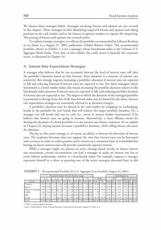
508 Fixed Income Analysis
We discuss these strategies below. Strategies involving futures and options are not coveredin this chapter. These strategies involve identifying mispriced futures and options and takingpositions in the cash market and in the futures or options markets to capture the mispricing.The pricing of futures and options was covered earlier.
To explain strategic strategies, we will use the portfolio recommended by Lehman Brothersto its clients in a August 27, 2001 publication (Global Relative Value). The recommendedportfolio, shown in Exhibit 1, is for a manager whose benchmark index is the Lehman U.S.Aggregate Bond Index. Note that, in this exhibit, the credit sector is basically the corporatesector, as discussed in Chapter 16.
A. Interest Rate Expectations Strategies
A manager who believes that he can accurately forecast the level of interest rates will alterthe portfolio’s duration based on that forecast. Since duration is a measure of interest ratesensitivity, this strategy requires increasing a portfolio’s duration if interest rates are expectedto fall and reducing duration if interest rates are expected to rise. For those managers whosebenchmark is a bond market index, this means increasing the portfolio duration relative to thebenchmark index duration if interest rates are expected to fall, and reducing portfolio durationif interest rates are expected to rise. The degree to which the duration of the managed portfoliois permitted to diverge from that of the benchmark index may be limited by the client. Interestrate expectations strategies are commonly referred to as duration strategies.
A portfolio’s duration may be altered in the cash market by swapping (or exchanging)bonds in the portfolio for new bonds that will achieve the target portfolio duration. Or, amanager can sell bonds and stay in cash (i.e., invest in money market instruments) if hebelieves that interest rates are going to increase. Alternatively, a more efficient means foraltering the duration of a bond portfolio is to use interest rate futures contracts. As we explainin Chapter 22, buying futures increases a portfolio’s duration, while selling futures decreasesthe duration.
The key to this active strategy is, of course, an ability to forecast the direction of interestrates. The academic literature does not support the view that interest rates can be forecastedwith accuracy in order to realize positive active returns on a consistent basis. It is doubtful thatbetting on future interest rates will provide consistently superior returns.
While a manager might not pursue an active strategy based strictly on future interestrate movements, certain circumstances can lead a manager to make an interest rate bet tocover inferior performance relative to a benchmark index. For example, suppose a managerrepresents himself to a client as pursuing one of the active strategies discussed later in this
EXHIBIT 1 Recommended Portfolio for U.S. Aggregate Core Portfolio (August 24, 2001)
Percent of market value by duration range Contribution to0–2 2–4 4–7 7–9 9+ Total OAD∗ Spread duration
Sector Index Rec Index Rec Index Rec Index Rec Index Rec Index Rec Index Rec Diff Index Rec DiffTreasury 5.53 2.01 5.12 3.64 4.80 0.00 0.78 3.22 7.20 4.19 23.44 13.05 1.40 0.99 −0.41 0.00 0.00 0.00Agency 3.09 0.00 3.53 5.74 2.56 3.44 0.65 1.61 1.42 0.92 11.25 11.71 0.50 0.55 0.05 0.50 0.56 0.06Mtg.Pass-throughs 6.81 5.54 19.79 22.78 8.22 8.49 0.00 0.00 0.00 0.00 34.82 36.81 1.04 1.22 0.18 1.16 1.32 0.16CMBS 0.03 0.00 0.37 0.27 1.53 1.87 0.03 0.00 0.00 0.00 1.95 2.14 0.10 0.12 0.02 0.10 0.12 0.02ABS 0.53 3.19 0.69 2.33 0.48 0.00 0.06 0.00 0.00 0.00 1.75 5.51 0.06 0.12 0.07 0.06 0.12 0.07Credit 3.01 3.17 7.77 10.35 9.37 9.98 2.28 3.16 4.35 4.11 26.78 30.78 1.46 1.62 0.16 1.46 1.61 0.15Total 19.00 13.91 37.27 45.11 26.96 23.78 3.81 7.99 12.97 9.22 100.00 100.00 4.56 4.63 0.07 3.28 3.73 0.45
∗OAD = option-adjusted durationSource: Global Relative Value, Lehman Brothers, Fixed Income Research, August 27, 2001, p. 2.
Chapter 18 Managing Funds against a Bond Market Index 509
chapter. Suppose further that the manager is evaluated over a 1-year investment horizon, andthat, three months before the end of the investment horizon, the manager’s performance issignificantly below the client-specified benchmark index. If the manager believes the accountwill be lost due to the underperformance, the manager has an incentive to bet on interest ratemovements. If the manager is correct, the account will be saved, while an incorrect bet willresult in further underperforming the index. In this case, the account will probably be lostregardless of the extent of the underperformance. A client can prevent this type of gaming byimposing constraints on the extent to which the portfolio’s duration can diverge from that ofthe index. Also, in the performance evaluation stage of the investment management process,described later in this chapter, decomposing the portfolio’s return into the risk factors thatgenerate the return highlights the extent to which a portfolio’s return is attributable to changesin the level of interest rates.
Exhibit 1 shows the option-adjusted duration for the Lehman Brothers Aggregate Indexand for the recommended portfolio. In this case, Lehman Brothers uses the term ‘‘option-adjusted duration’’ rather than effective duration, which in other reports, the term ‘‘adjustedduration’’ is used. Exhibit 1 shows that the recommended duration for a U.S. aggregateportfolio is 4.63, compared to 4.56 for the index. That is, the recommended portfolioduration is 102% of the index duration and therefore the portfolio has slightly greaterexposure to changes in interest rates.
B. Yield Curve Strategies
As explained previously, the yield curve for U.S. Treasury securities shows the relationshipbetween maturity and yield. The shape of the yield curve changes over time. A shift in theyield curve refers to a change in the yield of each Treasury maturity. A parallel shift in the yieldcurve refers to a shift in which the change in yield is the same for all maturities. A nonparallelshift in the yield curve means that the yield change is not the same number of basis points foreach maturity.
Top down yield curve strategies involve positioning a portfolio to capitalize on expectedchanges in the shape of the Treasury yield curve. There are three yield curve strategies: (1) abullet strategy, (2) a barbell strategy, and (3) a ladder strategy. In a bullet strategy, the portfoliois constructed so that the maturities of the bonds in the portfolio are highly concentrated at onepoint on the yield curve. In a barbell strategy, the maturities of the bonds in the portfolio areconcentrated at two extreme maturities. In practice, when managers refer to a barbell strategy,they are referring to a comparison with a bullet strategy. For example, a bullet strategy mightbe to create a portfolio with maturities concentrated around 10 years, while a correspondingbarbell strategy might be a portfolio with 5-year and 20-year maturities. In a ladder strategy,the portfolio has approximately equal amounts of each maturity. So, for example, a portfoliomight have equal amounts of bonds with one year to maturity, two years to maturity, etc.
Each of these strategies results in different performance when the yield curve shifts. Theactual performance depends on both the type and magnitude of the shift. Thus, no generalstatements can be made about the optimal yield curve strategy. This conclusion will bedemonstrated in Section IV.
When a yield curve strategy is applied by a manager whose benchmark index is a broad-based bond market index, a mismatch of maturities relative to the benchmark index exists inone or more of the bond sectors. Some managers use duration buckets rather than maturity,as a measure of the mismatch. For example, in Exhibit 1, the index and the recommendedportfolio are grouped into five duration ranges: 0–2, 2–4, 4–7, 7–9, and 9+. Notice that the
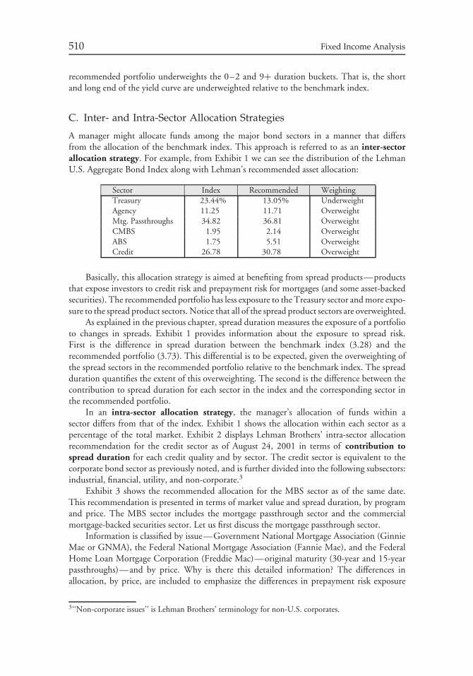
510 Fixed Income Analysis
recommended portfolio underweights the 0–2 and 9+ duration buckets. That is, the shortand long end of the yield curve are underweighted relative to the benchmark index.
C. Inter- and Intra-Sector Allocation Strategies
A manager might allocate funds among the major bond sectors in a manner that differsfrom the allocation of the benchmark index. This approach is referred to as an inter-sectorallocation strategy. For example, from Exhibit 1 we can see the distribution of the LehmanU.S. Aggregate Bond Index along with Lehman’s recommended asset allocation:
Sector Index Recommended WeightingTreasury 23.44% 13.05% UnderweightAgency 11.25 11.71 OverweightMtg. Passthroughs 34.82 36.81 OverweightCMBS 1.95 2.14 OverweightABS 1.75 5.51 OverweightCredit 26.78 30.78 Overweight
Basically, this allocation strategy is aimed at benefiting from spread products—productsthat expose investors to credit risk and prepayment risk for mortgages (and some asset-backedsecurities). The recommended portfolio has less exposure to the Treasury sector and more expo-sure to the spread product sectors. Notice that all of the spread product sectors are overweighted.
As explained in the previous chapter, spread duration measures the exposure of a portfolioto changes in spreads. Exhibit 1 provides information about the exposure to spread risk.First is the difference in spread duration between the benchmark index (3.28) and therecommended portfolio (3.73). This differential is to be expected, given the overweighting ofthe spread sectors in the recommended portfolio relative to the benchmark index. The spreadduration quantifies the extent of this overweighting. The second is the difference between thecontribution to spread duration for each sector in the index and the corresponding sector inthe recommended portfolio.
In an intra-sector allocation strategy, the manager’s allocation of funds within asector differs from that of the index. Exhibit 1 shows the allocation within each sector as apercentage of the total market. Exhibit 2 displays Lehman Brothers’ intra-sector allocationrecommendation for the credit sector as of August 24, 2001 in terms of contribution tospread duration for each credit quality and by sector. The credit sector is equivalent to thecorporate bond sector as previously noted, and is further divided into the following subsectors:industrial, financial, utility, and non-corporate.3
Exhibit 3 shows the recommended allocation for the MBS sector as of the same date.This recommendation is presented in terms of market value and spread duration, by programand price. The MBS sector includes the mortgage passthrough sector and the commercialmortgage-backed securities sector. Let us first discuss the mortgage passthrough sector.
Information is classified by issue—Government National Mortgage Association (GinnieMae or GNMA), the Federal National Mortgage Association (Fannie Mae), and the FederalHome Loan Mortgage Corporation (Freddie Mac)—original maturity (30-year and 15-yearpassthroughs)—and by price. Why is there this detailed information? The differences inallocation, by price, are included to emphasize the differences in prepayment risk exposure
3‘‘Non-corporate issues’’ is Lehman Brothers’ terminology for non-U.S. corporates.
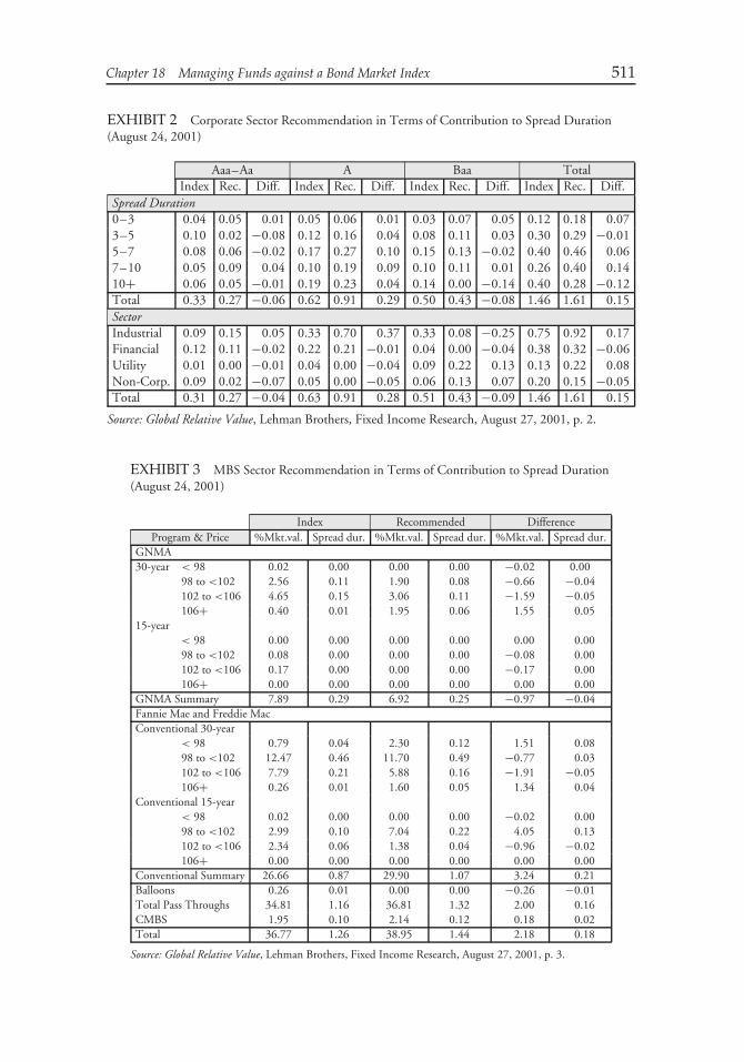
Chapter 18 Managing Funds against a Bond Market Index 511
EXHIBIT 2 Corporate Sector Recommendation in Terms of Contribution to Spread Duration(August 24, 2001)
Aaa–Aa A Baa TotalIndex Rec. Diff. Index Rec. Diff. Index Rec. Diff. Index Rec. Diff.
Spread Duration0–3 0.04 0.05 0.01 0.05 0.06 0.01 0.03 0.07 0.05 0.12 0.18 0.073–5 0.10 0.02 −0.08 0.12 0.16 0.04 0.08 0.11 0.03 0.30 0.29 −0.015–7 0.08 0.06 −0.02 0.17 0.27 0.10 0.15 0.13 −0.02 0.40 0.46 0.067–10 0.05 0.09 0.04 0.10 0.19 0.09 0.10 0.11 0.01 0.26 0.40 0.1410+ 0.06 0.05 −0.01 0.19 0.23 0.04 0.14 0.00 −0.14 0.40 0.28 −0.12Total 0.33 0.27 −0.06 0.62 0.91 0.29 0.50 0.43 −0.08 1.46 1.61 0.15SectorIndustrial 0.09 0.15 0.05 0.33 0.70 0.37 0.33 0.08 −0.25 0.75 0.92 0.17Financial 0.12 0.11 −0.02 0.22 0.21 −0.01 0.04 0.00 −0.04 0.38 0.32 −0.06Utility 0.01 0.00 −0.01 0.04 0.00 −0.04 0.09 0.22 0.13 0.13 0.22 0.08Non-Corp. 0.09 0.02 −0.07 0.05 0.00 −0.05 0.06 0.13 0.07 0.20 0.15 −0.05Total 0.31 0.27 −0.04 0.63 0.91 0.28 0.51 0.43 −0.09 1.46 1.61 0.15
Source: Global Relative Value, Lehman Brothers, Fixed Income Research, August 27, 2001, p. 2.
EXHIBIT 3 MBS Sector Recommendation in Terms of Contribution to Spread Duration(August 24, 2001)
Index Recommended DifferenceProgram & Price %Mkt.val. Spread dur. %Mkt.val. Spread dur. %Mkt.val. Spread dur.
GNMA30-year < 98 0.02 0.00 0.00 0.00 −0.02 0.00
98 to <102 2.56 0.11 1.90 0.08 −0.66 −0.04102 to <106 4.65 0.15 3.06 0.11 −1.59 −0.05106+ 0.40 0.01 1.95 0.06 1.55 0.05
15-year< 98 0.00 0.00 0.00 0.00 0.00 0.0098 to <102 0.08 0.00 0.00 0.00 −0.08 0.00102 to <106 0.17 0.00 0.00 0.00 −0.17 0.00106+ 0.00 0.00 0.00 0.00 0.00 0.00
GNMA Summary 7.89 0.29 6.92 0.25 −0.97 −0.04Fannie Mae and Freddie MacConventional 30-year
< 98 0.79 0.04 2.30 0.12 1.51 0.0898 to <102 12.47 0.46 11.70 0.49 −0.77 0.03102 to <106 7.79 0.21 5.88 0.16 −1.91 −0.05106+ 0.26 0.01 1.60 0.05 1.34 0.04
Conventional 15-year< 98 0.02 0.00 0.00 0.00 −0.02 0.0098 to <102 2.99 0.10 7.04 0.22 4.05 0.13102 to <106 2.34 0.06 1.38 0.04 −0.96 −0.02106+ 0.00 0.00 0.00 0.00 0.00 0.00
Conventional Summary 26.66 0.87 29.90 1.07 3.24 0.21Balloons 0.26 0.01 0.00 0.00 −0.26 −0.01Total Pass Throughs 34.81 1.16 36.81 1.32 2.00 0.16CMBS 1.95 0.10 2.14 0.12 0.18 0.02Total 36.77 1.26 38.95 1.44 2.18 0.18
Source: Global Relative Value, Lehman Brothers, Fixed Income Research, August 27, 2001, p. 3.
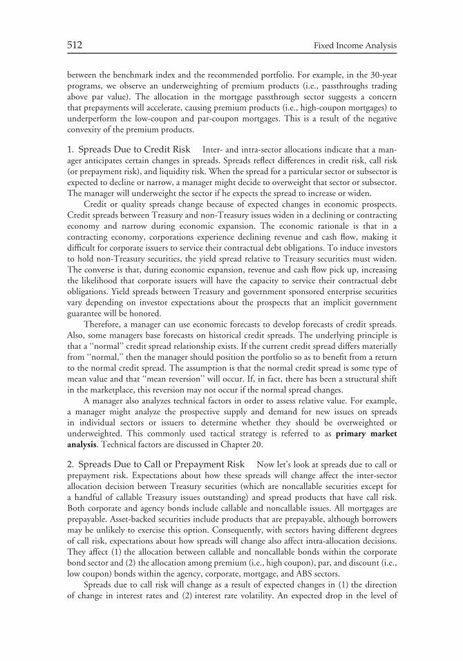
512 Fixed Income Analysis
between the benchmark index and the recommended portfolio. For example, in the 30-yearprograms, we observe an underweighting of premium products (i.e., passthroughs tradingabove par value). The allocation in the mortgage passthrough sector suggests a concernthat prepayments will accelerate, causing premium products (i.e., high-coupon mortgages) tounderperform the low-coupon and par-coupon mortgages. This is a result of the negativeconvexity of the premium products.
1. Spreads Due to Credit Risk Inter- and intra-sector allocations indicate that a man-ager anticipates certain changes in spreads. Spreads reflect differences in credit risk, call risk(or prepayment risk), and liquidity risk. When the spread for a particular sector or subsector isexpected to decline or narrow, a manager might decide to overweight that sector or subsector.The manager will underweight the sector if he expects the spread to increase or widen.
Credit or quality spreads change because of expected changes in economic prospects.Credit spreads between Treasury and non-Treasury issues widen in a declining or contractingeconomy and narrow during economic expansion. The economic rationale is that in acontracting economy, corporations experience declining revenue and cash flow, making itdifficult for corporate issuers to service their contractual debt obligations. To induce investorsto hold non-Treasury securities, the yield spread relative to Treasury securities must widen.The converse is that, during economic expansion, revenue and cash flow pick up, increasingthe likelihood that corporate issuers will have the capacity to service their contractual debtobligations. Yield spreads between Treasury and government sponsored enterprise securitiesvary depending on investor expectations about the prospects that an implicit governmentguarantee will be honored.
Therefore, a manager can use economic forecasts to develop forecasts of credit spreads.Also, some managers base forecasts on historical credit spreads. The underlying principle isthat a ‘‘normal’’ credit spread relationship exists. If the current credit spread differs materiallyfrom ‘‘normal,’’ then the manager should position the portfolio so as to benefit from a returnto the normal credit spread. The assumption is that the normal credit spread is some type ofmean value and that ‘‘mean reversion’’ will occur. If, in fact, there has been a structural shiftin the marketplace, this reversion may not occur if the normal spread changes.
A manager also analyzes technical factors in order to assess relative value. For example,a manager might analyze the prospective supply and demand for new issues on spreadsin individual sectors or issuers to determine whether they should be overweighted orunderweighted. This commonly used tactical strategy is referred to as primary marketanalysis. Technical factors are discussed in Chapter 20.
2. Spreads Due to Call or Prepayment Risk Now let’s look at spreads due to call orprepayment risk. Expectations about how these spreads will change affect the inter-sectorallocation decision between Treasury securities (which are noncallable securities except fora handful of callable Treasury issues outstanding) and spread products that have call risk.Both corporate and agency bonds include callable and noncallable issues. All mortgages areprepayable. Asset-backed securities include products that are prepayable, although borrowersmay be unlikely to exercise this option. Consequently, with sectors having different degreesof call risk, expectations about how spreads will change also affect intra-allocation decisions.They affect (1) the allocation between callable and noncallable bonds within the corporatebond sector and (2) the allocation among premium (i.e., high coupon), par, and discount (i.e.,low coupon) bonds within the agency, corporate, mortgage, and ABS sectors.
Spreads due to call risk will change as a result of expected changes in (1) the directionof change in interest rates and (2) interest rate volatility. An expected drop in the level of
Chapter 18 Managing Funds against a Bond Market Index 513
interest rates will widen the spread between callable bonds and noncallable bonds as prospectsincrease that the issuer will exercise the call option. The spread narrows if interest rates areexpected to rise. An increase in interest rate volatility increases the value of the embedded calloption, and thereby increases the spread between (1) callable bonds and noncallable bonds and(2) premium and discount bonds. Trades that are motivated by the manager’s anticipation ofbetter performance resulting from the embedded options of individual issues or sectors arereferred to as structure trades. Such trades are discussed in Chapter 20.
D. Individual Security Selection Strategies
Once the manager makes the allocation to a sector or subsector, he must then select the specificissues. A manager does not typically invest in all issues within a sector or subsector. Instead,depending on the size of the portfolio, the manager selects a representative number of issues.
At this stage, a manager makes an intra-sector allocation decision to the specific issues.The manager might believe that some securities within a subsector are mispriced and willtherefore outperform other issues within the same sector over the time horizon. Managerspursue several different active strategies in order to identify mispriced securities. The mostcommon strategy identifies an issue as undervalued because either (1) its yield is higher thanthat of comparably rated issues or (2) its yield is expected to decline (and price thereforerise) because the manager’s credit analysis leads the manager to believe that an issue will beupgraded by the rating agency before the issue is put on credit watch/rating watch for anupgrade or a positive rating outlook is assigned by a rating agency.
Once a portfolio is constructed, a manager might undertake a swap of one bond foranother that is similar in terms of coupon, maturity, and credit quality, but offers a higheryield. This is a substitution swap, and it depends on capital market imperfections. Suchsituations sometimes exist due to temporary market imbalances and the fragmented nature ofthe non-Treasury bond market. The risk the manager faces in making a substitution swap isthat the bond purchased is not identical to the bond for which it is exchanged. Moreover,bonds typically have similar, but not identical, maturity and coupon, which might result indifferences in convexity.
An active strategy used in the mortgage-backed securities market is to identify mispricedindividual issues of passthroughs, CMO classes, or stripped MBS, given an assumed prepaymentrate. In the case of CMOs and stripped MBS, this strategy involves investing in a non-indexproduct—that is, a product not included in the benchmark index.
It is critical when evaluating any potential swaps to assess the impact of the swap on therisk exposure of the portfolio. We will see how a bond swap can be assessed when we discussmultifactor risk models in Section V. Also, we will see how a manager can use a multi-factorrisk model to incorporate a security selection strategy in constructing a portfolio.
IV. SCENARIO ANALYSIS FOR ASSESSINGPOTENTIAL PERFORMANCE
An active manager needs a tool for assessing the potential performance of:
1. a trading strategy,2. a portfolio, and3. a portfolio relative to a benchmark index.
514 Fixed Income Analysis
In this section, we will explain how scenario analysis can be used to assess potentialperformance.
A. Assessing Trades
A trade is evaluated in terms of its potential performance. When comparing possible trades, ora trade of a security with a current position, the relative performance of the alternatives mustbe assessed, where performance means the expected total return over the investment horizon.The total return is comprised of three sources:
1. the coupon payments2. the change in the value of the bond3. income from reinvestment of coupon payments and principal repayment (in the case of
amortizing securities) from the time of receipt to the end of the investment horizon.
For example, suppose that an investor purchases a security for $90 and expects a returnover a 1-year investment horizon from the three sources equal to $6. Then the expected totalrate of return is 6.7%(= $6/$90).
When a trade involves borrowing, the interest cost of the borrowed funds is deductedfrom the dollar return from these three sources. (In Section VII we will discuss how fundscan be borrowed in the bond market via a repurchase agreement.) The dollar return,adjusted for the financial cost, is then related to the dollar amount invested. For example,suppose the investor purchased the $90 security by borrowing $80 and investing $10 ofhis own funds (i.e., the investor’s equity). Suppose also that the cost of the borrowedfunds is 5%, or $4. Then the dollar return, after adjusting for the financing cost, is $2($6 − $4). The total rate of return is 20% ($2 return divided by the investor’s equity of$10).
1. Computing the Total Return The total return takes into account all three potentialsources of dollar return over the investor’s investment horizon. It is the rate of return thatwill grow the amount invested (i.e., price plus accrued interest) to the projected total dollarreturn at the investment horizon.4 The calculation of the total return requires that the investorspecify:
• the investment horizon• the reinvestment rate• the price of the bond at the investment horizon.
A graphical depiction of the total return calculation is presented in Exhibit 4. Moreformally, the steps for computing total return are as follows:
Step 1: Compute the total coupon payments plus the reinvestment income based on anexpected reinvestment rate. If coupon payments are semiannual, the reinvestment rateis one-half the annual interest rate that the investor assumes can be earned on thereinvestment of coupon interest payments.5
4The total return is also referred to as the horizon return.5An investor can use multiple reinvestment rates for cash flows from the bond over the investmenthorizon.
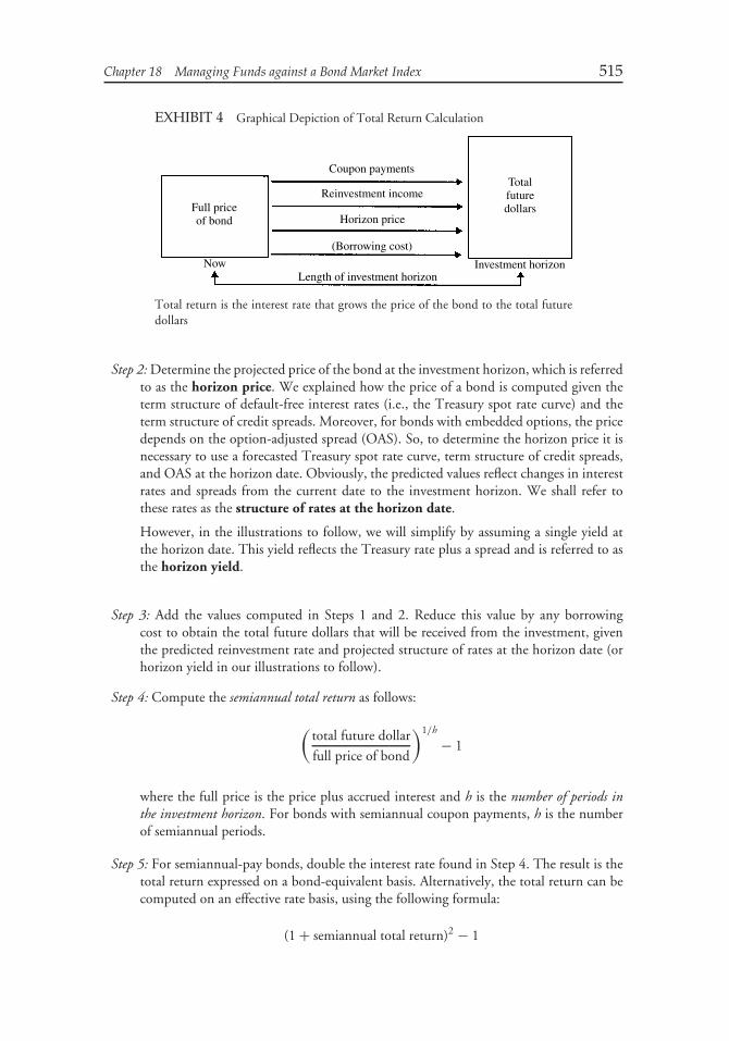
Chapter 18 Managing Funds against a Bond Market Index 515
EXHIBIT 4 Graphical Depiction of Total Return Calculation
Coupon payments
Reinvestment income
Horizon price
(Borrowing cost)
Length of investment horizonInvestment horizon
Full priceof bond
Now
Totalfuturedollars
Total return is the interest rate that grows the price of the bond to the total futuredollars
Step 2: Determine the projected price of the bond at the investment horizon, which is referredto as the horizon price. We explained how the price of a bond is computed given theterm structure of default-free interest rates (i.e., the Treasury spot rate curve) and theterm structure of credit spreads. Moreover, for bonds with embedded options, the pricedepends on the option-adjusted spread (OAS). So, to determine the horizon price it isnecessary to use a forecasted Treasury spot rate curve, term structure of credit spreads,and OAS at the horizon date. Obviously, the predicted values reflect changes in interestrates and spreads from the current date to the investment horizon. We shall refer tothese rates as the structure of rates at the horizon date.
However, in the illustrations to follow, we will simplify by assuming a single yield atthe horizon date. This yield reflects the Treasury rate plus a spread and is referred to asthe horizon yield.
Step 3: Add the values computed in Steps 1 and 2. Reduce this value by any borrowingcost to obtain the total future dollars that will be received from the investment, giventhe predicted reinvestment rate and projected structure of rates at the horizon date (orhorizon yield in our illustrations to follow).
Step 4: Compute the semiannual total return as follows:
(total future dollar
full price of bond
)1/h
− 1
where the full price is the price plus accrued interest and h is the number of periods inthe investment horizon. For bonds with semiannual coupon payments, h is the numberof semiannual periods.
Step 5: For semiannual-pay bonds, double the interest rate found in Step 4. The result is thetotal return expressed on a bond-equivalent basis. Alternatively, the total return can becomputed on an effective rate basis, using the following formula:
(1 + semiannual total return)2 − 1
516 Fixed Income Analysis
Whether the total return is calculated on a bond-equivalent basis or an effective rate basisdepends on the situation. If the total return is compared to a benchmark index whose rate ofreturn is calculated on a bond-equivalent basis, then the total return should be calculated inthe same way. However, if the bond is used to satisfy liabilities with rates calculated on aneffective basis, then the total return should be calculated on an effective rate basis.
To illustrate the computation of total return, suppose that an investor with a 1-yearinvestment horizon is considering the purchase of a 20-year 6% corporate bond. The issue isselling for $86.4365 at a yield of 7.3%, and will be purchased for cash (i.e., no funds will beborrowed). Assume that the yield curve is flat and the projected yield for a 20-year Treasuryissue is 6.5%. This means that the yield spread over the projected Treasury issue is 80 basispoints. The investor expects that:
1. he can reinvest the coupon payments at 6%2. the Treasury yield curve will shift down by 25 basis points and remain flat at the end of
1 year, so that the yield for the 19-year Treasury issue is 6.25% (6.5% minus 25 basispoints)
3. the yield spread to the 19-year Treasury issue is unchanged at 80 basis points, so thehorizon yield is 7.05% (6.25% plus 80 basis points)
The calculations are shown below.
Step 1: Compute the total coupon payments plus reinvestment income using an annualreinvestment rate of 6%, or 3% every six months. The semiannual coupon payment is$3. The future value of an annuity formula can be used for this calculation or, becausethe investment horizon is only one year, the future value can be computed as follows:
First coupon payment reinvested for six months = $3 (1.03) = $3.09Second coupon payment = $3.00Total = $6.09
Step 2: The horizon price is determined as follows. The price of this bond when discountedat a flat 7.05% yield is $89.0992.
Step 3: Adding the amounts in Steps 1 and 2 gives the total future dollars of $95.1892.
Step 4: Compute the following (h is 2 in our illustration):
($95.1892
$86.4365
)1/2
− 1 = 4.94%
Step 5: The total return on a bond-equivalent basis and on an effective rate basis are:
2 × 4.94% = 9.88% (BEY)
(1 + 0.0494)2 − 1 = 10.13% (effective rate basis)
Chapter 18 Managing Funds against a Bond Market Index 517
a. OAS-Total Return A valuation model can be used to incorporate the option-adjustedspread (OAS) into the calculation of the horizon price. The manager must specify the changeshe expects in the OAS at the investment horizon. The horizon price can be ‘‘backed out’’ ofa valuation model. This technique can be extended to the total return framework by makingassumptions about the required variables at the horizon date.
Assumptions about the OAS at the investment horizon reflect the expectations of theportfolio manager. It is common to assume that the OAS at the horizon date will be the sameas the OAS at the time of purchase. A total return calculated under this assumption is referredto as a constant-OAS total return. Alternatively, managers take positions that reflect theirviews on how the OAS will change. The total return framework can be used to assess thesensitivity of the performance of a bond with an embedded option to changes in the OAS.
b. Total Return for a Mortgage-Backed and Asset-Backed Security In calculating thetotal return for mortgage-backed and asset-backed securities, the total future dollars depend on(1) the projected principal repayment (scheduled repayment plus projected prepayments) and(2) the interest earned on reinvestment of projected interest payments and principal payments.To compute the total future dollars, a prepayment rate over the investment horizon must beprojected.
The monthly total return for a mortgage-backed security or an asset-backed security withmonthly payments is computed as follows:
monthly total return =(
total future dollars
full price
) 1
number of months in horizon − 1
The monthly total return can be annualized on a bond-equivalent yield basis as follows:
bond-equivalent annual return = 2[(1 + monthly total return)6 − 1]
Recall from our discussion that we calculate the bond-equivalent yield for a monthly paysecurity by first computing the effective 6-month yield and then doubling the effective 6-monthyield. This is the calculation indicated by the bond-equivalent annual return formula above.
So, for example, if the monthly total return for a monthly pay mortgage-backed securityor asset-backed security is 0.7%, the bond-equivalent annual return is
2[(1 + 0.007)6 − 1] = 0.0855 = 8.55%
Or, the effective annual return can be computed as follows:
effective annual return = (1 + monthly total return)12 − 1
The effective annual return is computed by compounding the monthly return. For the previousexample, the effective annual return is:
(1 + 0.007)12 − 1 = 0.0873 = 8.73%
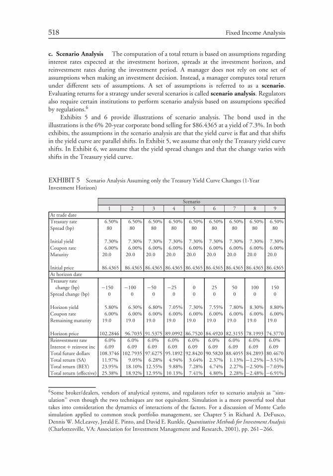
518 Fixed Income Analysis
c. Scenario Analysis The computation of a total return is based on assumptions regardinginterest rates expected at the investment horizon, spreads at the investment horizon, andreinvestment rates during the investment period. A manager does not rely on one set ofassumptions when making an investment decision. Instead, a manager computes total returnunder different sets of assumptions. A set of assumptions is referred to as a scenario.Evaluating returns for a strategy under several scenarios is called scenario analysis. Regulatorsalso require certain institutions to perform scenario analysis based on assumptions specifiedby regulations.6
Exhibits 5 and 6 provide illustrations of scenario analysis. The bond used in theillustrations is the 6% 20-year corporate bond selling for $86.4365 at a yield of 7.3%. In bothexhibits, the assumptions in the scenario analysis are that the yield curve is flat and that shiftsin the yield curve are parallel shifts. In Exhibit 5, we assume that only the Treasury yield curveshifts. In Exhibit 6, we assume that the yield spread changes and that the change varies withshifts in the Treasury yield curve.
EXHIBIT 5 Scenario Analysis Assuming only the Treasury Yield Curve Changes (1-YearInvestment Horizon)
Scenario1 2 3 4 5 6 7 8 9
At trade dateTreasury rate 6.50% 6.50% 6.50% 6.50% 6.50% 6.50% 6.50% 6.50% 6.50%Spread (bp) 80 80 80 80 80 80 80 80 80
Initial yield 7.30% 7.30% 7.30% 7.30% 7.30% 7.30% 7.30% 7.30% 7.30%Coupon rate 6.00% 6.00% 6.00% 6.00% 6.00% 6.00% 6.00% 6.00% 6.00%Maturity 20.0 20.0 20.0 20.0 20.0 20.0 20.0 20.0 20.0
Initial price 86.4365 86.4365 86.4365 86.4365 86.4365 86.4365 86.4365 86.4365 86.4365At horizon dateTreasury rate
change (bp) −150 −100 −50 −25 0 25 50 100 150Spread change (bp) 0 0 0 0 0 0 0 0 0
Horizon yield 5.80% 6.30% 6.80% 7.05% 7.30% 7.55% 7.80% 8.30% 8.80%Coupon rate 6.00% 6.00% 6.00% 6.00% 6.00% 6.00% 6.00% 6.00% 6.00%Remaining maturity 19.0 19.0 19.0 19.0 19.0 19.0 19.0 19.0 19.0
Horizon price 102.2846 96.7035 91.5375 89.0992 86.7520 84.4920 82.3155 78.1993 74.3770Reinvestment rate 6.0% 6.0% 6.0% 6.0% 6.0% 6.0% 6.0% 6.0% 6.0%Interest + reinvest inc 6.09 6.09 6.09 6.09 6.09 6.09 6.09 6.09 6.09Total future dollars 108.3746 102.7935 97.6275 95.1892 92.8420 90.5820 88.4055 84.2893 80.4670Total return (SA) 11.97% 9.05% 6.28% 4.94% 3.64% 2.37% 1.13% −1.25% −3.51%Total return (BEY) 23.95% 18.10% 12.55% 9.88% 7.28% 4.74% 2.27% −2.50% −7.03%Total return (effective) 25.38% 18.92% 12.95% 10.13% 7.41% 4.80% 2.28% −2.48% −6.91%
6Some broker/dealers, vendors of analytical systems, and regulators refer to scenario analysis as ‘‘sim-ulation’’ even though the two techniques are not equivalent. Simulation is a more powerful tool thattakes into consideration the dynamics of interactions of the factors. For a discussion of Monte Carlosimulation applied to common stock portfolio management, see Chapter 5 in Richard A. DeFusco,Dennis W. McLeavey, Jerald E. Pinto, and David E. Runkle, Quantitative Methods for Investment Analysis(Charlottesville, VA: Association for Investment Management and Research, 2001), pp. 261–266.
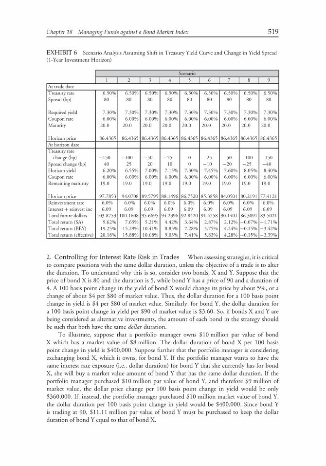
Chapter 18 Managing Funds against a Bond Market Index 519
EXHIBIT 6 Scenario Analysis Assuming Shift in Treasury Yield Curve and Change in Yield Spread(1-Year Investment Horizon)
Scenario1 2 3 4 5 6 7 8 9
At trade dateTreasury rate 6.50% 6.50% 6.50% 6.50% 6.50% 6.50% 6.50% 6.50% 6.50%Spread (bp) 80 80 80 80 80 80 80 80 80
Required yield 7.30% 7.30% 7.30% 7.30% 7.30% 7.30% 7.30% 7.30% 7.30%Coupon rate 6.00% 6.00% 6.00% 6.00% 6.00% 6.00% 6.00% 6.00% 6.00%Maturity 20.0 20.0 20.0 20.0 20.0 20.0 20.0 20.0 20.0
Horizon price 86.4365 86.4365 86.4365 86.4365 86.4365 86.4365 86.4365 86.4365 86.4365At horizon dateTreasury rate
change (bp) −150 −100 −50 −25 0 25 50 100 150Spread change (bp) 40 25 20 10 0 −10 −20 −25 −40Horizon yield 6.20% 6.55% 7.00% 7.15% 7.30% 7.45% 7.60% 8.05% 8.40%Coupon rate 6.00% 6.00% 6.00% 6.00% 6.00% 6.00% 6.00% 6.00% 6.00%Remaining maturity 19.0 19.0 19.0 19.0 19.0 19.0 19.0 19.0 19.0
Horizon price 97.7853 94.0708 89.5795 88.1496 86.7520 85.3858 84.0501 80.2191 77.4121Reinvestment rate 6.0% 6.0% 6.0% 6.0% 6.0% 6.0% 6.0% 6.0% 6.0%Interest + reinvest inc 6.09 6.09 6.09 6.09 6.09 6.09 6.09 6.09 6.09Total future dollars 103.8753 100.1608 95.6695 94.2396 92.8420 91.4758 90.1401 86.3091 83.5021Total return (SA) 9.62% 7.65% 5.21% 4.42% 3.64% 2.87% 2.12% −0.07% −1.71%Total return (BEY) 19.25% 15.29% 10.41% 8.83% 7.28% 5.75% 4.24% −0.15% −3.42%Total return (effective) 20.18% 15.88% 10.68% 9.03% 7.41% 5.83% 4.28% −0.15% −3.39%
2. Controlling for Interest Rate Risk in Trades When assessing strategies, it is criticalto compare positions with the same dollar duration, unless the objective of a trade is to alterthe duration. To understand why this is so, consider two bonds, X and Y. Suppose that theprice of bond X is 80 and the duration is 5, while bond Y has a price of 90 and a duration of4. A 100 basis point change in the yield of bond X would change its price by about 5%, or achange of about $4 per $80 of market value. Thus, the dollar duration for a 100 basis pointchange in yield is $4 per $80 of market value. Similarly, for bond Y, the dollar duration fora 100 basis point change in yield per $90 of market value is $3.60. So, if bonds X and Y arebeing considered as alternative investments, the amount of each bond in the strategy shouldbe such that both have the same dollar duration.
To illustrate, suppose that a portfolio manager owns $10 million par value of bondX which has a market value of $8 million. The dollar duration of bond X per 100 basispoint change in yield is $400,000. Suppose further that the portfolio manager is consideringexchanging bond X, which it owns, for bond Y. If the portfolio manager wants to have thesame interest rate exposure (i.e., dollar duration) for bond Y that she currently has for bondX, she will buy a market value amount of bond Y that has the same dollar duration. If theportfolio manager purchased $10 million par value of bond Y, and therefore $9 million ofmarket value, the dollar price change per 100 basis point change in yield would be only$360,000. If, instead, the portfolio manager purchased $10 million market value of bond Y,the dollar duration per 100 basis point change in yield would be $400,000. Since bond Yis trading at 90, $11.11 million par value of bond Y must be purchased to keep the dollarduration of bond Y equal to that of bond X.
520 Fixed Income Analysis
Mathematically, the market value of bond Y that is required in order to have the samedollar duration (per 100 basis point change in rates) as bond X is:
market value of bond Y = dollar duration of bond X
duration of bond Y/100
The par value of bond Y that must be purchased to obtain the same dollar duration as bondX is:
par value of bond Y = market value of bond Y
price of bond Y per $1 of par value
Using our previous illustration to demonstrate how to use these formulas, we know that:
dollar duration of bond X = $400, 000
duration of bond Y = 4
market value of bond Y = $400, 000
4/100= $10, 000, 000
This means that $10 million market value of bond Y has the same dollar duration as the$8 million market value position in bond X. The amount of par value of bond Y that must bepurchased, given its price of 90, or 0.90 per $1 of par value, is:
par value of bond Y = $10, 000, 000
0.90= $11.11 million
Failure to adjust a trade to account for an expected change in yield spread, keeping thedollar duration constant, leads to the result that the outcome of the trade will be affected bythe expected change in the yield spread and the change in the yield level. Thus, a managerwould be taking a conscious yield spread view and possibly an undesired view on the level ofinterest rates.
Also note that equating the dollar durations of two positions only means that they will beequal for small changes in rates because of the convexity of a bond.
3. Assessing the Portfolio There is no shortage of trading strategies suggested by bonddealer firms or in the popular press. Investment management firms have developed proprietarytrading strategies. All of these strategies are based on a set of expectations about the bondmarket over the investment horizon. Furthermore, these strategies all involve risk. A tradingstrategy might involve borrowing in the repo market and/or shorting bonds. Some managersand dealers incorrectly use the term ‘‘arbitrage’’ to refer to these trading strategies they tout tocustomers. In fact, such strategies incur risk, even though the proponent of the strategy mightperceive the risk to be small.
The potential performance of any trading strategy can be quantified using total returnanalysis. More specifically, scenario analysis is used to determine the total return under differentassumptions about what might occur over the investment horizon. Scenario analysis identifiesthe range of possible outcomes and therefore provides the manager with a feel for the riskassociated with a trade.
In this section, we use a basic illustration illustrate how a trade can be evaluated. Webegin with three Treasury securities—A, B, and C. Information about each of these three
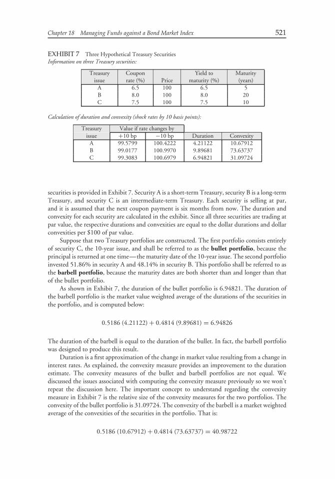
Chapter 18 Managing Funds against a Bond Market Index 521
EXHIBIT 7 Three Hypothetical Treasury SecuritiesInformation on three Treasury securities:
Treasury Coupon Yield to Maturityissue rate (%) Price maturity (%) (years)
A 6.5 100 6.5 5B 8.0 100 8.0 20C 7.5 100 7.5 10
Calculation of duration and convexity (shock rates by 10 basis points):
Treasury Value if rate changes byissue +10 bp −10 bp Duration Convexity
A 99.5799 100.4222 4.21122 10.67912B 99.0177 100.9970 9.89681 73.63737C 99.3083 100.6979 6.94821 31.09724
securities is provided in Exhibit 7. Security A is a short-term Treasury, security B is a long-termTreasury, and security C is an intermediate-term Treasury. Each security is selling at par,and it is assumed that the next coupon payment is six months from now. The duration andconvexity for each security are calculated in the exhibit. Since all three securities are trading atpar value, the respective durations and convexities are equal to the dollar durations and dollarconvexities per $100 of par value.
Suppose that two Treasury portfolios are constructed. The first portfolio consists entirelyof security C, the 10-year issue, and shall be referred to as the bullet portfolio, because theprincipal is returned at one time—the maturity date of the 10-year issue. The second portfolioinvested 51.86% in security A and 48.14% in security B. This portfolio shall be referred to asthe barbell portfolio, because the maturity dates are both shorter than and longer than thatof the bullet portfolio.
As shown in Exhibit 7, the duration of the bullet portfolio is 6.94821. The duration ofthe barbell portfolio is the market value weighted average of the durations of the securities inthe portfolio, and is computed below:
0.5186 (4.21122) + 0.4814 (9.89681) = 6.94826
The duration of the barbell is equal to the duration of the bullet. In fact, the barbell portfoliowas designed to produce this result.
Duration is a first approximation of the change in market value resulting from a change ininterest rates. As explained, the convexity measure provides an improvement to the durationestimate. The convexity measures of the bullet and barbell portfolios are not equal. Wediscussed the issues associated with computing the convexity measure previously so we won’trepeat the discussion here. The important concept to understand regarding the convexitymeasure in Exhibit 7 is the relative size of the convexity measures for the two portfolios. Theconvexity of the bullet portfolio is 31.09724. The convexity of the barbell is a market weightedaverage of the convexities of the securities in the portfolio. That is:
0.5186 (10.67912) + 0.4814 (73.63737) = 40.98722
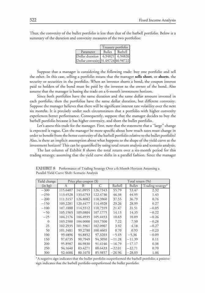
522 Fixed Income Analysis
Thus, the convexity of the bullet portfolio is less than that of the barbell portfolio. Below is asummary of the duration and convexity measures of the two portfolios:
Treasury portfolioParameter Bullet Barbell
Dollar duration 6.94821 6.94826Dollar convexity 31.09724 40.98722
Suppose that a manager is considering the following trade: buy one portfolio and sellthe other. In this case, selling a portfolio means that the manager sells short, or shorts, thesecurity or securities in the portfolio. When an investor shorts a bond, the coupon interestpaid to holders of the bond must be paid by the investor to the owner of the bond. Alsoassume that the manager is basing the trade on a 6-month investment horizon.
Since both portfolios have the same duration and the same dollar amount invested ineach portfolio, then the portfolios have the same dollar duration, but different convexity.Suppose the manager believes that there will be significant interest rate volatility over the nextsix months. It is precisely under such circumstances that a portfolio with higher convexityexperiences better performance. Consequently, suppose that the manager decides to buy thebarbell portfolio because it has higher convexity, and short the bullet portfolio.
Let’s assess this trade for the manager. First, note that the statement that a ‘‘large’’ changeis expected is vague. Can the manager be more specific about how much rates must change inorder to benefit from the better convexity of the barbell portfolio relative to the bullet portfolio?Also, is there an implicit assumption about what happens to the shape of the yield curve at theinvestment horizon? This can be quantified by using total return analysis and scenario analysis.
The last column of Exhibit 8 shows the total return over a six-month period for thistrading strategy, assuming that the yield curve shifts in a parallel fashion. Since the manager
EXHIBIT 8 Performance of Trading Strategy Over a 6-Month Horizon Assuming aParallel Yield Curve Shift: Scenario Analysis
Yield change Price plus coupon ($) Total return (%)(in bp) A B C Barbell Bullet Trading strategy∗
−300 115.6407 141.0955 126.7343 55.79 53.47 2.32−250 113.4528 133.6753 122.4736 46.38 44.95 1.43−200 111.3157 126.8082 118.3960 37.55 36.79 0.76−150 109.2281 120.4477 114.4928 29.26 28.99 0.27−100 107.1888 114.5512 110.7559 21.47 21.51 −0.05−50 105.1965 109.0804 107.1775 14.13 14.35 −0.22−25 104.2176 106.4935 105.4453 10.63 10.89 −0.26
0 103.2500 104.0000 103.7500 7.22 7.50 −0.2825 102.2935 101.5961 102.0907 3.92 4.18 −0.2750 101.3481 99.2780 100.4665 0.70 0.93 −0.23
100 99.4896 94.8852 97.3203 −5.45 −5.36 −0.09150 97.6735 90.7949 94.3050 −11.28 −11.39 0.11200 95.8987 86.9830 91.4146 −16.79 −17.17 0.38250 94.1640 83.4271 88.6433 −22.01 −22.71 0.70300 92.4686 80.1070 85.9857 −26.96 −28.03 1.06
∗A negative sign indicates that the bullet portfolio outperformed the barbell portfolio; a positivesign indicates that the barbell portfolio outperformed the bullet portfolio.
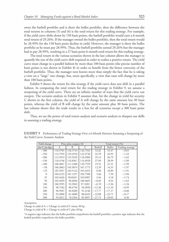
Chapter 18 Managing Funds against a Bond Market Index 523
owns the barbell portfolio and is short the bullet portfolio, then the difference between thetotal returns in columns (5) and (6) is the total return for this trading strategy. For example,if the yield curve shifts down by 150 basis points, the barbell portfolio would earn a 6-monthtotal return of 29.26%. If the manager owned the bullet portfolio, then the total return wouldbe 28.99% for the 150 basis point decline in yield. However, the manager is short the bulletportfolio so he must pay 28.99%. Thus, the barbell portfolio earned 29.26% but the managerhad to pay 28.99%, resulting in a 27 basis point 6-month total return for this trading strategy.
The total return in the various scenarios shown in the last column allows the manager toquantify the size of the yield curve shift required in order to realize a positive return. The yieldcurve must change in a parallel fashion by more than 100 basis points (the precise number ofbasis points is not shown in Exhibit 8) in order to benefit from the better convexity of thebarbell portfolio. Thus, the manager now knows more than simply the fact that he is takinga view on a ‘‘large’’ rate change, but, more specifically, a view that rates will change by morethan 100 basis points.
Exhibit 9 shows the return for this strategy if the yield curve does not shift in a parallelfashion. In computing the total return for the trading strategy in Exhibit 9, we assume asteepening of the yield curve. There are an infinite number of ways that the yield curve cansteepen. The scenario analysis in Exhibit 9 assumes that, for the change in yield for securityC shown in the first column, the yield of A will change by the same amount less 30 basispoints, whereas the yield of B will change by the same amount plus 30 basis points. Thelast column shows that the trade results in a loss for all scenarios except a 300 basis pointshift.
Thus, we see the power of total return analysis and scenario analysis to sharpen our skillsin assessing a trading strategy.
EXHIBIT 9 Performance of Trading Strategy Over a 6-Month Horizon Assuming a Steepening ofthe Yield Curve: Scenario Analysis
Yield change Price plus coupon ($) Total return (%)for C (in bp) A B C Barbell Bullet Trading strategy∗
−300 116.9785 136.5743 126.7343 52.82 53.47 −0.65−250 114.7594 129.4918 122.4736 43.70 44.95 −1.24−200 112.5919 122.9339 118.3960 35.14 36.79 −1.65−150 110.4748 116.8567 114.4928 27.09 28.99 −1.89−100 108.4067 111.2200 110.7559 19.52 21.51 −1.99−50 106.3863 105.9874 107.1775 12.39 14.35 −1.97−25 105.3937 103.5122 105.4453 8.98 10.89 −1.91
0 104.4125 101.1257 103.7500 5.66 7.50 −1.8425 103.4426 98.8243 102.0907 2.44 4.18 −1.7450 102.4839 96.6046 100.4665 −0.69 0.93 −1.63
100 100.5995 92.3963 97.3203 −6.70 −5.36 −1.34150 98.7582 88.4758 94.3050 −12.38 −11.39 −0.99200 96.9587 84.8200 91.4146 −17.77 −17.17 −0.60250 95.2000 81.4080 88.6433 −22.88 −22.71 −0.17300 93.4812 78.2204 85.9857 −27.73 −28.03 0.30
Assumptions:Change in yield of A = Change in yield of C minus 30 bp.Change in yield of B = Change in yield of C plus 30 bp.∗A negative sign indicates that the bullet portfolio outperforms the barbell portfolio; a positive sign indicates that thebarbell portfolio outperforms the bullet portfolio.
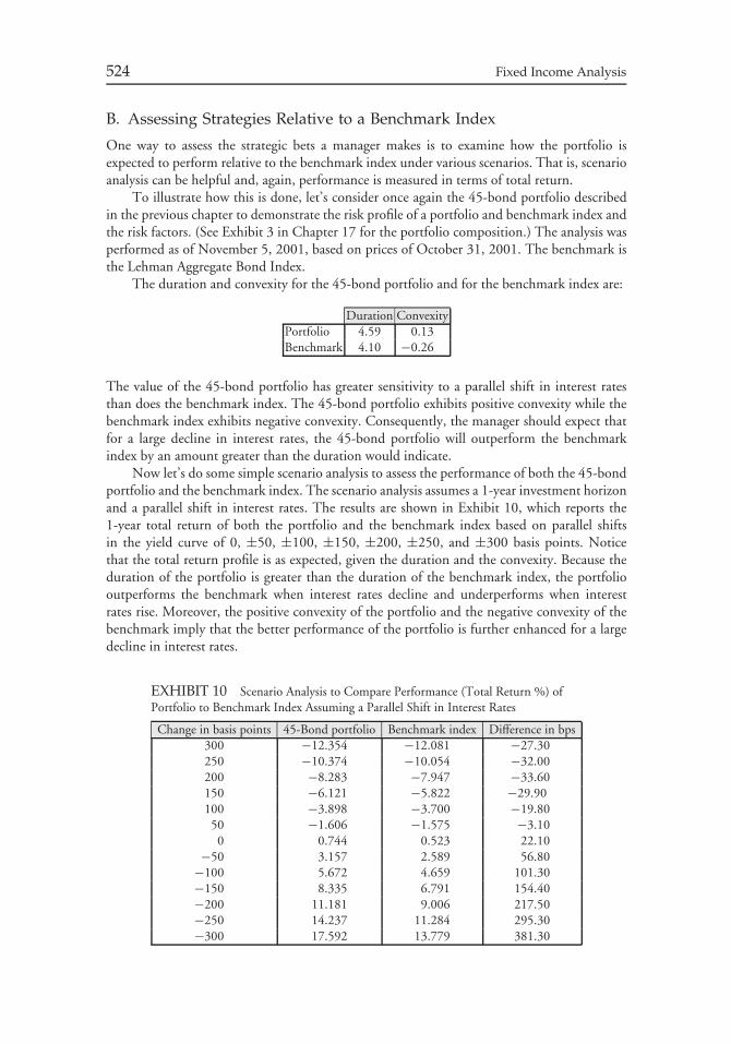
524 Fixed Income Analysis
B. Assessing Strategies Relative to a Benchmark Index
One way to assess the strategic bets a manager makes is to examine how the portfolio isexpected to perform relative to the benchmark index under various scenarios. That is, scenarioanalysis can be helpful and, again, performance is measured in terms of total return.
To illustrate how this is done, let’s consider once again the 45-bond portfolio describedin the previous chapter to demonstrate the risk profile of a portfolio and benchmark index andthe risk factors. (See Exhibit 3 in Chapter 17 for the portfolio composition.) The analysis wasperformed as of November 5, 2001, based on prices of October 31, 2001. The benchmark isthe Lehman Aggregate Bond Index.
The duration and convexity for the 45-bond portfolio and for the benchmark index are:
Duration ConvexityPortfolio 4.59 0.13Benchmark 4.10 −0.26
The value of the 45-bond portfolio has greater sensitivity to a parallel shift in interest ratesthan does the benchmark index. The 45-bond portfolio exhibits positive convexity while thebenchmark index exhibits negative convexity. Consequently, the manager should expect thatfor a large decline in interest rates, the 45-bond portfolio will outperform the benchmarkindex by an amount greater than the duration would indicate.
Now let’s do some simple scenario analysis to assess the performance of both the 45-bondportfolio and the benchmark index. The scenario analysis assumes a 1-year investment horizonand a parallel shift in interest rates. The results are shown in Exhibit 10, which reports the1-year total return of both the portfolio and the benchmark index based on parallel shiftsin the yield curve of 0, ±50, ±100, ±150, ±200, ±250, and ±300 basis points. Noticethat the total return profile is as expected, given the duration and the convexity. Because theduration of the portfolio is greater than the duration of the benchmark index, the portfoliooutperforms the benchmark when interest rates decline and underperforms when interestrates rise. Moreover, the positive convexity of the portfolio and the negative convexity of thebenchmark imply that the better performance of the portfolio is further enhanced for a largedecline in interest rates.
EXHIBIT 10 Scenario Analysis to Compare Performance (Total Return %) ofPortfolio to Benchmark Index Assuming a Parallel Shift in Interest Rates
Change in basis points 45-Bond portfolio Benchmark index Difference in bps300 −12.354 −12.081 −27.30250 −10.374 −10.054 −32.00200 −8.283 −7.947 −33.60150 −6.121 −5.822 −29.90100 −3.898 −3.700 −19.80
50 −1.606 −1.575 −3.100 0.744 0.523 22.10
−50 3.157 2.589 56.80−100 5.672 4.659 101.30−150 8.335 6.791 154.40−200 11.181 9.006 217.50−250 14.237 11.284 295.30−300 17.592 13.779 381.30
Chapter 18 Managing Funds against a Bond Market Index 525
The scenario analysis framework in Exhibit 10 is useful for giving the portfolio managera feel for the relationship between the performance of the portfolio relative to the benchmarkindex. However, this analysis considers only one risk: interest rate risk. In addition, the analysisof interest rate risk is limited to a parallel shift in the yield curve so that a nonparallel shiftis not considered. Of course, a portfolio manager can ‘‘play’’ with different yield curve shiftsto assess the impact on the portfolio and benchmark index. In fact, some portfolio managersseek to identify ‘‘realistic yield curve shifts’’ and analyze a portfolio based on these shifts. Thesimple scenario analysis of Exhibit 10 also ignores changes in spreads for spread products.Again, one can attempt to assess the performance assuming different changes in spreads.However, a more insightful methodology for quantifying the risk exposure of a portfoliorelative to a benchmark index was discussed in the previous chapter—a multi-factor riskmodel.
V. USING MULTI-FACTOR RISK MODELS INPORTFOLIO CONSTRUCTION
In the previous chapter we explained how multi-factor risk models can be used to quantifythe risk exposure of a portfolio. But a multi-factor risk model is also an invaluable tool forconstructing a portfolio, where the term ‘‘constructing a portfolio’’ means either the initialconstruction or the rebalancing of a portfolio.
In constructing a portfolio using the multi-factor risk model, an optimizer is used. Thepurpose of an optimizer is to obtain the optimal value for an objective function subjectto constraints. Optimizers use mathematical programming, but a discussion of the types ofmathematical programming and the algorithms used to solve mathematical programmingproblems is beyond the scope of this chapter. It is important to understand that, if aportfolio manager specifies an objective, the optimizer or mathematical programming modelwill compute the optimal solution. We will give two illustrations to see how this is done. Inour illustrations, we will use the 45-bond portfolio and continue to use the Lehman U.S.Aggregate Bond Index as the benchmark index.
A. Rebalancing to Construct a More Passive Portfolio
In the previous chapter, we saw that the predicted tracking error for the 45-bond portfolio is62 basis points per year. Suppose that the portfolio manager wants to reduce the predictedtracking error significantly. That is, the manager wants to rebalance the portfolio in such amanner that its risk exposure is much closer to that of the benchmark index. Depending onthe extent to which the manager reduces the predicted tracking error, the manager shifts fromactively managing a portfolio to an approach that more closely resembles enhanced indexing.The goal is to rebalance the portfolio in a cost efficient manner. Here is where the optimizercomes in.
An optimizer can be used to identify trades that reduce tracking error in a cost efficientway. Specifically, the objective specified for the optimizer is to minimize tracking error, theconstraint is to keep the turnover of the portfolio to a minimum. The optimizer begins with auniverse of market prices for acceptable securities. The acceptable securities are those permittedby the investment guidelines. The optimizer is designed to select a trade that identifies a 1-for-1bond swap with the greatest reduction in tracking error per unit of each bond purchased.
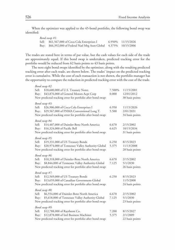
526 Fixed Income Analysis
When the optimizer was applied to the 45-bond portfolio, the following bond swap wasidentified:
Bond swap #1:Sell: $61,567,000 of Coca-Cola Enterprises I 6.950% 11/15/2026Buy: $66,392,000 of Federal Natl Mtg Assn-Global 4.375% 10/15/2006
The trades are stated here in terms of par value, but the cash values for each side of the tradeare approximately equal. If this bond swap is undertaken, predicted tracking error for theportfolio would be reduced from 62 basis points to 43 basis points.
The next eight bond swaps identified by the optimizer, along with the resulting predictedtracking error after each trade, are shown below. The trades’ impact on the predicted trackingerror is cumulative. While the cost of each transaction is not shown, the portfolio manager hasthe opportunity to compare the reduction in predicted tracking error with the cost of the trade.
Bond swap #2:Sell: $18,600,000 of U.S. Treasury Notes 7.500% 11/15/2001Buy: $43,876,000 of General Motors Acpt Corp 0.000 12/01/2012New predicted tracking error for portfolio after bond swap: 38 basis points
Bond swap #3:Sell: $26,906,000 of Coca-Cola Enterprises I 6.950 11/15/2026Buy: $29,567,000 of FNMA Conventional Long T. 5.500 2/01/2031New predicted tracking error for portfolio after bond swap: 34 basis points
Bond swap #4:Sell: $14,407,000 of Daimler-Benz North America 6.670 2/15/2002Buy: $16,324,000 of Pacific Bell 6.625 10/15/2034New predicted tracking error for portfolio after bond swap: 31 basis points
Bond swap #5:Sell: $19,331,000 of US Treasury Bonds 6.250 8/15/2023Buy: $20,974,000 of Tennessee Valley Authority-Global 5.375 11/13/2008New predicted tracking error for portfolio after bond swap: 28 basis points
Bond swap #6:Sell: $10,318,000 of Daimler-Benz North America 6.670 2/15/2002Buy: $8,844,000 of Tennessee Valley Authority-Global 7.125 5/1/2030New predicted tracking error for portfolio after bond swap: 26 basis points
Bond swap #7:Sell: $12,569,000 of US Treasury Bonds 6.250 8/15/2023Buy: $13,659,000 of Canadian Government-Global 11/5/2008New predicted tracking error for portfolio after bond swap: 24 basis points
Bond swap #8:Sell: $6,554,000 of Daimler-Benz North America 6.670 2/15/2002Buy: $5,618,000 of Tennessee Valley Authority-Global 7.125 5/1/2030New predicted tracking error for portfolio after bond swap: 23 basis points
Bond swap #9:Sell: $12,788,000 of Raytheon Co. 7.200 8/15/2027Buy: $12,878,000 of Intl Business Machines 5.375 2/1/2009New predicted tracking error for portfolio after bond swap: 22 basis points
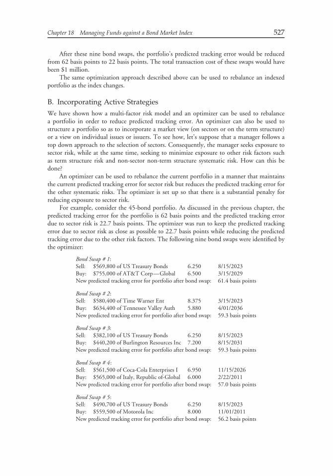
Chapter 18 Managing Funds against a Bond Market Index 527
After these nine bond swaps, the portfolio’s predicted tracking error would be reducedfrom 62 basis points to 22 basis points. The total transaction cost of these swaps would havebeen $1 million.
The same optimization approach described above can be used to rebalance an indexedportfolio as the index changes.
B. Incorporating Active Strategies
We have shown how a multi-factor risk model and an optimizer can be used to rebalancea portfolio in order to reduce predicted tracking error. An optimizer can also be used tostructure a portfolio so as to incorporate a market view (on sectors or on the term structure)or a view on individual issues or issuers. To see how, let’s suppose that a manager follows atop down approach to the selection of sectors. Consequently, the manager seeks exposure tosector risk, while at the same time, seeking to minimize exposure to other risk factors suchas term structure risk and non-sector non-term structure systematic risk. How can this bedone?
An optimizer can be used to rebalance the current portfolio in a manner that maintainsthe current predicted tracking error for sector risk but reduces the predicted tracking error forthe other systematic risks. The optimizer is set up so that there is a substantial penalty forreducing exposure to sector risk.
For example, consider the 45-bond portfolio. As discussed in the previous chapter, thepredicted tracking error for the portfolio is 62 basis points and the predicted tracking errordue to sector risk is 22.7 basis points. The optimizer was run to keep the predicted trackingerror due to sector risk as close as possible to 22.7 basis points while reducing the predictedtracking error due to the other risk factors. The following nine bond swaps were identified bythe optimizer:
Bond Swap # 1:Sell: $569,800 of US Treasury Bonds 6.250 8/15/2023Buy: $755,000 of AT&T Corp—Global 6.500 3/15/2029New predicted tracking error for portfolio after bond swap: 61.4 basis points
Bond Swap # 2:Sell: $580,400 of Time Warner Ent 8.375 3/15/2023Buy: $634,400 of Tennessee Valley Auth 5.880 4/01/2036New predicted tracking error for portfolio after bond swap: 59.3 basis points
Bond Swap # 3:Sell: $382,100 of US Treasury Bonds 6.250 8/15/2023Buy: $440,200 of Burlington Resources Inc 7.200 8/15/2031New predicted tracking error for portfolio after bond swap: 59.3 basis points
Bond Swap # 4:Sell: $561,500 of Coca-Cola Enterprises I 6.950 11/15/2026Buy: $565,000 of Italy, Republic of-Global 6.000 2/22/2011New predicted tracking error for portfolio after bond swap: 57.0 basis points
Bond Swap # 5:Sell: $490,700 of US Treasury Bonds 6.250 8/15/2023Buy: $559,500 of Motorola Inc 8.000 11/01/2011New predicted tracking error for portfolio after bond swap: 56.2 basis points
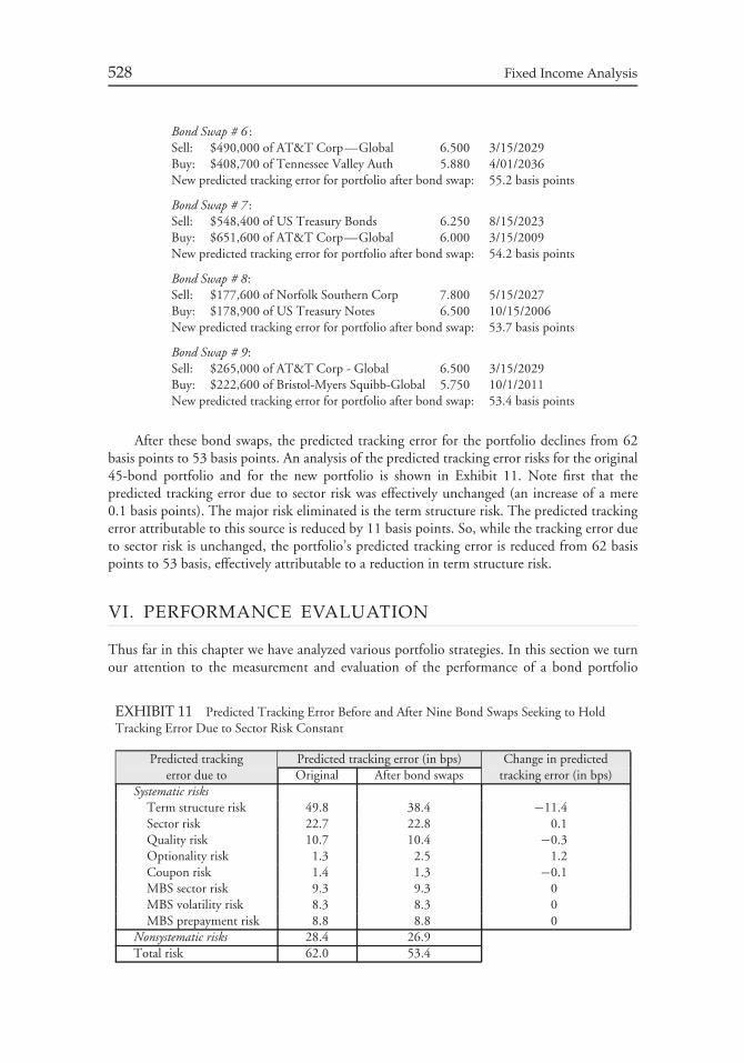
528 Fixed Income Analysis
Bond Swap # 6 :Sell: $490,000 of AT&T Corp—Global 6.500 3/15/2029Buy: $408,700 of Tennessee Valley Auth 5.880 4/01/2036New predicted tracking error for portfolio after bond swap: 55.2 basis points
Bond Swap # 7 :Sell: $548,400 of US Treasury Bonds 6.250 8/15/2023Buy: $651,600 of AT&T Corp—Global 6.000 3/15/2009New predicted tracking error for portfolio after bond swap: 54.2 basis points
Bond Swap # 8:Sell: $177,600 of Norfolk Southern Corp 7.800 5/15/2027Buy: $178,900 of US Treasury Notes 6.500 10/15/2006New predicted tracking error for portfolio after bond swap: 53.7 basis points
Bond Swap # 9:Sell: $265,000 of AT&T Corp - Global 6.500 3/15/2029Buy: $222,600 of Bristol-Myers Squibb-Global 5.750 10/1/2011New predicted tracking error for portfolio after bond swap: 53.4 basis points
After these bond swaps, the predicted tracking error for the portfolio declines from 62basis points to 53 basis points. An analysis of the predicted tracking error risks for the original45-bond portfolio and for the new portfolio is shown in Exhibit 11. Note first that thepredicted tracking error due to sector risk was effectively unchanged (an increase of a mere0.1 basis points). The major risk eliminated is the term structure risk. The predicted trackingerror attributable to this source is reduced by 11 basis points. So, while the tracking error dueto sector risk is unchanged, the portfolio’s predicted tracking error is reduced from 62 basispoints to 53 basis, effectively attributable to a reduction in term structure risk.
VI. PERFORMANCE EVALUATION
Thus far in this chapter we have analyzed various portfolio strategies. In this section we turnour attention to the measurement and evaluation of the performance of a bond portfolio
EXHIBIT 11 Predicted Tracking Error Before and After Nine Bond Swaps Seeking to HoldTracking Error Due to Sector Risk Constant
Predicted tracking Predicted tracking error (in bps) Change in predictederror due to Original After bond swaps tracking error (in bps)
Systematic risksTerm structure risk 49.8 38.4 −11.4Sector risk 22.7 22.8 0.1Quality risk 10.7 10.4 −0.3Optionality risk 1.3 2.5 1.2Coupon risk 1.4 1.3 −0.1MBS sector risk 9.3 9.3 0MBS volatility risk 8.3 8.3 0MBS prepayment risk 8.8 8.8 0
Nonsystematic risks 28.4 26.9Total risk 62.0 53.4
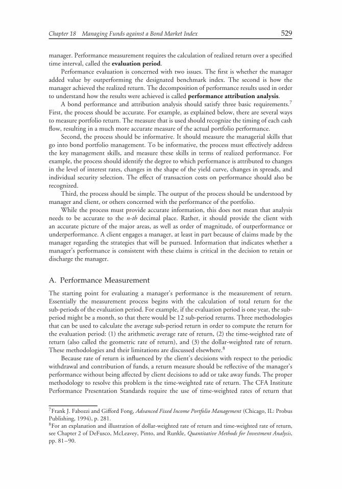
Chapter 18 Managing Funds against a Bond Market Index 529
manager. Performance measurement requires the calculation of realized return over a specifiedtime interval, called the evaluation period.
Performance evaluation is concerned with two issues. The first is whether the manageradded value by outperforming the designated benchmark index. The second is how themanager achieved the realized return. The decomposition of performance results used in orderto understand how the results were achieved is called performance attribution analysis.
A bond performance and attribution analysis should satisfy three basic requirements.7
First, the process should be accurate. For example, as explained below, there are several waysto measure portfolio return. The measure that is used should recognize the timing of each cashflow, resulting in a much more accurate measure of the actual portfolio performance.
Second, the process should be informative. It should measure the managerial skills thatgo into bond portfolio management. To be informative, the process must effectively addressthe key management skills, and measure these skills in terms of realized performance. Forexample, the process should identify the degree to which performance is attributed to changesin the level of interest rates, changes in the shape of the yield curve, changes in spreads, andindividual security selection. The effect of transaction costs on performance should also berecognized.
Third, the process should be simple. The output of the process should be understood bymanager and client, or others concerned with the performance of the portfolio.
While the process must provide accurate information, this does not mean that analysisneeds to be accurate to the n-th decimal place. Rather, it should provide the client withan accurate picture of the major areas, as well as order of magnitude, of outperformance orunderperformance. A client engages a manager, at least in part because of claims made by themanager regarding the strategies that will be pursued. Information that indicates whether amanager’s performance is consistent with these claims is critical in the decision to retain ordischarge the manager.
A. Performance Measurement
The starting point for evaluating a manager’s performance is the measurement of return.Essentially the measurement process begins with the calculation of total return for thesub-periods of the evaluation period. For example, if the evaluation period is one year, the sub-period might be a month, so that there would be 12 sub-period returns. Three methodologiesthat can be used to calculate the average sub-period return in order to compute the return forthe evaluation period: (1) the arithmetic average rate of return, (2) the time-weighted rate ofreturn (also called the geometric rate of return), and (3) the dollar-weighted rate of return.These methodologies and their limitations are discussed elsewhere.8
Because rate of return is influenced by the client’s decisions with respect to the periodicwithdrawal and contribution of funds, a return measure should be reflective of the manager’sperformance without being affected by client decisions to add or take away funds. The propermethodology to resolve this problem is the time-weighted rate of return. The CFA InstitutePerformance Presentation Standards require the use of time-weighted rates of return that
7Frank J. Fabozzi and Gifford Fong, Advanced Fixed Income Portfolio Management (Chicago, IL: ProbusPublishing, 1994), p. 281.8For an explanation and illustration of dollar-weighted rate of return and time-weighted rate of return,see Chapter 2 of DeFusco, McLeavey, Pinto, and Runkle, Quantitative Methods for Investment Analysis,pp. 81–90.
530 Fixed Income Analysis
adjust for cash flows (i.e., contributions and withdrawals). Time-weighted rates of return thatadjust for daily-weighted cash flows must be used for periods beginning January 1, 2005 andlater.
B. Single-Index Performance Evaluation Measures
In the 1960s, several single-index measures were used to evaluate the relative performance ofportfolio managers. The three measures are referred to as the Treynor measure, the Sharpemeasure, and the Jensen measure. All three measures assume that there is a linear relationshipbetween the portfolio’s return and the return on the benchmark index.9 These measures didnot indicate how or why a portfolio manager outperformed or underperformed a benchmarkindex.
In early studies of portfolio manager performance, these measures were used primarily toevaluate the performance of equity mutual fund managers. However, these measures are lessuseful today because of the subsequent development of the performance attribution modelsdiscussed next.
C. Performance Attribution Analysis
Single-index performance evaluation measures do not explain how a manager achieved aparticular observed return. The reason a client must have the answer to this question is thata manager may tell a client that he plans to pursue an active strategy. The client would thenexpect that any superior return achieved by the manager results from this active strategy. Buthow can the client be certain?
For example, suppose a manager who solicits funds from a client claims that he canachieve superior performance by selecting underpriced bonds. Suppose also that this managergenerates a superior return compared to the client-designated bond index. The client shouldnot necessarily be satisfied with this performance until the return realized by the manageris decomposed into the components that generated the return. A client may find that thesuperior performance is due to the manager’s timing of the market (i.e., modifying portfolioduration in anticipation of interest rate movements) rather than due to selecting underpricedbonds. In such an instance, the manager may have outperformed the benchmark index, butnot by following the strategy that the manager stated that he intended to pursue.
Performance attribution analysis seeks to identify and quantify the active managementdecisions that contributed to the performance of a portfolio. The performance of a portfoliocan be decomposed in terms of the risk factors discussed in Chapter 17.
Several commercial vendors have developed models for performance attribution analysis.The analysis is performed relative to a benchmark index. We will illustrate performanceattribution models using the system developed by Global Advanced Technology (G.A.T.).10
This model decomposes a portfolio’s total return into the following factors: (1) static return,(2) interest sensitive return, (3) spread change return, and (4) trading return. The differencebetween the total return and the sum of the four factors is called the residual (error). Each ofthe return factors can be further decomposed as described below.
9These measures are described in Frank K. Reilly and Keith C. Brown, Investment Analysis and PortfolioManagement (South-Western College Publishing, 2002), pp. 1109–1117.10The illustration is provided by Frank Jones and Leonard Peltzman of Guardian Life. A model developedby another vendor is presented in one of the end of chapter questions.
Chapter 18 Managing Funds against a Bond Market Index 531
The static return is the portion of a portfolio’s total return that is attributable to ‘‘rollingdown the yield curve.’’ That is, the static return is the portion of the return that would beearned assuming a static (meaning zero volatility) world, in which the yield curve evolvesto its implied forward curve. The static return is further decomposed into two components:(1) risk-free return and (2) accrual of OAS return. The risk-free return is based on theassumption that the portfolio consists of only Treasury strips. The risk-free return is thencalculated based on the rolling down of the yield curve. The accrual of OAS return is alsocalculated from rolling down the yield curve, but, unlike the risk-free return, it is based oninvesting in spread products.
The interest sensitive return is that portion of a portfolio’s return attributable to changesin the level, slope, and shape of the yield curve. In turn, this return is decomposed into twocomponents: (1) effective duration return and (2) convexity return. Key rate durations can beused to measure sensitivity to changes in the shape of the yield curve. The effective durationreturn is the sum of the returns attributable to the key rate durations. The convexity returnis the return due to change in the portfolio’s duration over the evaluation period.
The spread change return is the portion of a portfolio’s return that is due to changes inboth (1) bond sector spreads and (2) individual security richness/cheapness. The portion ofthe spread return attributable to changes in the sector’s OAS is called the delta OAS returnand the spread return due to a widening or tightening of a specific issue’s spread is called thedelta rich/cheap return.
The portion of a portfolio’s total return that is attributable to changes in the compositionof the portfolio is called the trading return. The trading return identifies the manager’s valueadded from changes in the composition of the portfolio, as opposed to a simple buy-and-holdstrategy.
In the illustration, a performance attribution analysis is performed on a portfolio ofcorporate securities. We will refer to this portfolio as Portfolio A. The evaluation period isSeptember 1996, a month when the yield curve shifted downward. The shift was almost aparallel shift. The effective duration of Portfolio A was 7.09. The effective duration of thebenchmark index, the Merrill Lynch Corporate Index, was 5.76. Thus, Portfolio A had ahigher duration than did the benchmark index.
Exhibit 12 presents the results of the performance attribution analysis for the portfolio andfor the individual sectors. The second column provides information about the manager’s sectorviews (i.e., underweighting or overweighting). The third column shows how the allocationpaid off for each sector.
Because the yield curve shifted downward in an almost parallel fashion, Portfolio A wouldbe expected to outperform the benchmark index because of the portfolio’s higher duration.This is captured in the interest sensitive return, the fifth column of Exhibit 12. This indicatesthat, holding all other factors constant, the outperformance would have been 37.9 basis points.Portfolio A did not outperform by that much because the spread change return which was−18.5 basis points. The static return and the trading return were minimal.
Exhibit 13 provides a summary of the analysis. The return on Portfolio A was 2.187%and the return on the benchmark index was 1.954%, so that Portfolio A outperformed theindex by 23 bps in September 1996.
VII. LEVERAGING STRATEGIES
A manager may be permitted to use leverage as part of a trade or trading strategy. Leveragemeans that funds are borrowed to purchase some of the securities involved in the strategy.
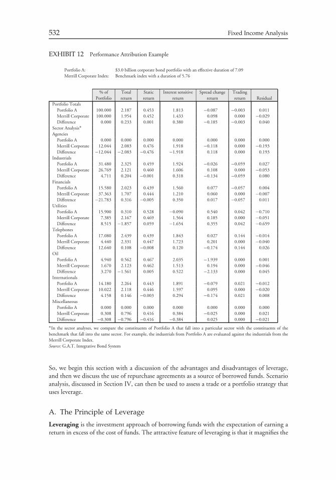
532 Fixed Income Analysis
EXHIBIT 12 Performance Attribution Example
Portfolio A: $3.0 billion corporate bond portfolio with an effective duration of 7.09Merrill Corporate Index: Benchmark index with a duration of 5.76
% of Total Static Interest sensitive Spread change TradingPortfolio return return return return return Residual
Portfolio TotalsPortfolio A 100.000 2.187 0.453 1.813 −0.087 −0.003 0.011Merrill Corporate 100.000 1.954 0.452 1.433 0.098 0.000 −0.029Difference 0.000 0.233 0.001 0.380 −0.185 −0.003 0.040
Sector Analysis∗Agencies
Portfolio A 0.000 0.000 0.000 0.000 0.000 0.000 0.000Merrill Corporate 12.044 2.083 0.476 1.918 −0.118 0.000 −0.193Difference −12.044 −2.083 −0.476 −1.918 0.118 0.000 0.193
IndustrialsPortfolio A 31.480 2.325 0.459 1.924 −0.026 −0.059 0.027Merrill Corporate 26.769 2.121 0.460 1.606 0.108 0.000 −0.053Difference 4.711 0.204 −0.001 0.318 −0.134 −0.059 0.080
FinancialsPortfolio A 15.580 2.023 0.439 1.560 0.077 −0.057 0.004Merrill Corporate 37.363 1.707 0.444 1.210 0.060 0.000 −0.007Difference −21.783 0.316 −0.005 0.350 0.017 −0.057 0.011
UtilitiesPortfolio A 15.900 0.310 0.528 −0.090 0.540 0.042 −0.710Merrill Corporate 7.385 2.167 0.469 1.564 0.185 0.000 −0.051Difference 8.515 −1.857 0.059 −1.654 0.355 0.042 −0.659
TelephonesPortfolio A 17.080 2.439 0.439 1.843 0.027 0.144 −0.014Merrill Corporate 4.440 2.331 0.447 1.723 0.201 0.000 −0.040Difference 12.640 0.108 −0.008 0.120 −0.174 0.144 0.026
OilPortfolio A 4.940 0.562 0.467 2.035 −1.939 0.000 0.001Merrill Corporate 1.670 2.123 0.462 1.513 0.194 0.000 −0.046Difference 3.270 −1.561 0.005 0.522 −2.133 0.000 0.045
InternationalsPortfolio A 14.180 2.264 0.443 1.891 −0.079 0.021 −0.012Merrill Corporate 10.022 2.118 0.446 1.597 0.095 0.000 −0.020Difference 4.158 0.146 −0.003 0.294 −0.174 0.021 0.008
MiscellaneousPortfolio A 0.000 0.000 0.000 0.000 0.000 0.000 0.000Merrill Corporate 0.308 0.796 0.416 0.384 −0.025 0.000 0.021Difference −0.308 −0.796 −0.416 −0.384 0.025 0.000 −0.021
∗In the sector analyses, we compare the constituents of Portfolio A that fall into a particular sector with the constituents of thebenchmark that fall into the same sector. For example, the industrials from Portfolio A are evaluated against the industrials from theMerrill Corporate Index.Source: G.A.T. Integrative Bond System
So, we begin this section with a discussion of the advantages and disadvantages of leverage,and then we discuss the use of repurchase agreements as a source of borrowed funds. Scenarioanalysis, discussed in Section IV, can then be used to assess a trade or a portfolio strategy thatuses leverage.
A. The Principle of Leverage
Leveraging is the investment approach of borrowing funds with the expectation of earning areturn in excess of the cost of funds. The attractive feature of leveraging is that it magnifies the
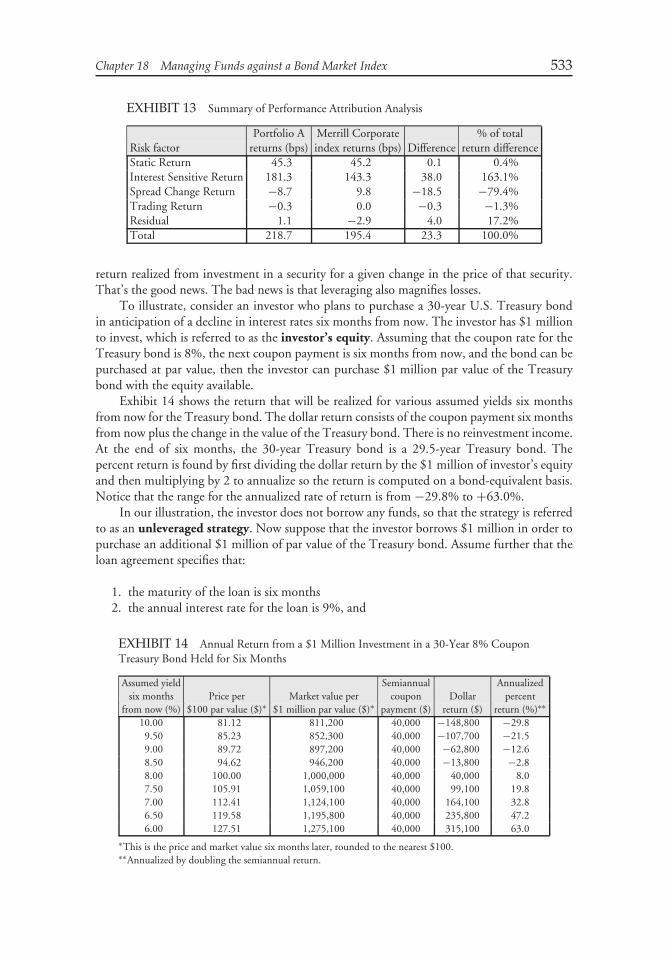
Chapter 18 Managing Funds against a Bond Market Index 533
EXHIBIT 13 Summary of Performance Attribution Analysis
Portfolio A Merrill Corporate % of totalRisk factor returns (bps) index returns (bps) Difference return differenceStatic Return 45.3 45.2 0.1 0.4%Interest Sensitive Return 181.3 143.3 38.0 163.1%Spread Change Return −8.7 9.8 −18.5 −79.4%Trading Return −0.3 0.0 −0.3 −1.3%Residual 1.1 −2.9 4.0 17.2%Total 218.7 195.4 23.3 100.0%
return realized from investment in a security for a given change in the price of that security.That’s the good news. The bad news is that leveraging also magnifies losses.
To illustrate, consider an investor who plans to purchase a 30-year U.S. Treasury bondin anticipation of a decline in interest rates six months from now. The investor has $1 millionto invest, which is referred to as the investor’s equity. Assuming that the coupon rate for theTreasury bond is 8%, the next coupon payment is six months from now, and the bond can bepurchased at par value, then the investor can purchase $1 million par value of the Treasurybond with the equity available.
Exhibit 14 shows the return that will be realized for various assumed yields six monthsfrom now for the Treasury bond. The dollar return consists of the coupon payment six monthsfrom now plus the change in the value of the Treasury bond. There is no reinvestment income.At the end of six months, the 30-year Treasury bond is a 29.5-year Treasury bond. Thepercent return is found by first dividing the dollar return by the $1 million of investor’s equityand then multiplying by 2 to annualize so the return is computed on a bond-equivalent basis.Notice that the range for the annualized rate of return is from −29.8% to +63.0%.
In our illustration, the investor does not borrow any funds, so that the strategy is referredto as an unleveraged strategy. Now suppose that the investor borrows $1 million in order topurchase an additional $1 million of par value of the Treasury bond. Assume further that theloan agreement specifies that:
1. the maturity of the loan is six months2. the annual interest rate for the loan is 9%, and
EXHIBIT 14 Annual Return from a $1 Million Investment in a 30-Year 8% CouponTreasury Bond Held for Six Months
Assumed yield Semiannual Annualizedsix months Price per Market value per coupon Dollar percent
from now (%) $100 par value ($)∗ $1 million par value ($)∗ payment ($) return ($) return (%)∗∗
10.00 81.12 811,200 40,000 −148,800 −29.89.50 85.23 852,300 40,000 −107,700 −21.59.00 89.72 897,200 40,000 −62,800 −12.68.50 94.62 946,200 40,000 −13,800 −2.88.00 100.00 1,000,000 40,000 40,000 8.07.50 105.91 1,059,100 40,000 99,100 19.87.00 112.41 1,124,100 40,000 164,100 32.86.50 119.58 1,195,800 40,000 235,800 47.26.00 127.51 1,275,100 40,000 315,100 63.0
∗This is the price and market value six months later, rounded to the nearest $100.∗∗Annualized by doubling the semiannual return.
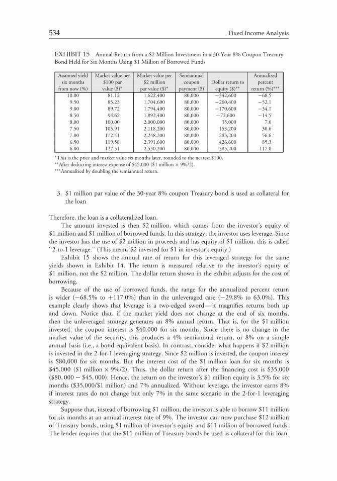
534 Fixed Income Analysis
EXHIBIT 15 Annual Return from a $2 Million Investment in a 30-Year 8% Coupon TreasuryBond Held for Six Months Using $1 Million of Borrowed Funds
Assumed yield Market value per Market value per Semiannual Annualizedsix months $100 par $2 million coupon Dollar return to percent
from now (%) value ($)∗ par value ($)∗ payment ($) equity ($)∗∗ return (%)∗∗∗
10.00 81.12 1,622,400 80,000 −342,600 −68.59.50 85.23 1,704,600 80,000 −260,400 −52.19.00 89.72 1,794,400 80,000 −170,600 −34.18.50 94.62 1,892,400 80,000 −72,600 −14.58.00 100.00 2,000,000 80,000 35,000 7.07.50 105.91 2,118,200 80,000 153,200 30.67.00 112.41 2,248,200 80,000 283,200 56.66.50 119.58 2,391,600 80,000 426,600 85.36.00 127.51 2,550,200 80,000 585,200 117.0
∗This is the price and market value six months later, rounded to the nearest $100.∗∗After deducting interest expense of $45,000 ($1 million × 9%/2).∗∗∗Annualized by doubling the semiannual return.
3. $1 million par value of the 30-year 8% coupon Treasury bond is used as collateral forthe loan
Therefore, the loan is a collateralized loan.The amount invested is then $2 million, which comes from the investor’s equity of
$1 million and $1 million of borrowed funds. In this strategy, the investor uses leverage. Sincethe investor has the use of $2 million in proceeds and has equity of $1 million, this is called‘‘2-to-1 leverage.’’ (This means $2 invested for $1 in investor’s equity.)
Exhibit 15 shows the annual rate of return for this leveraged strategy for the sameyields shown in Exhibit 14. The return is measured relative to the investor’s equity of$1 million, not the $2 million. The dollar return shown in the exhibit adjusts for the cost ofborrowing.
Because of the use of borrowed funds, the range for the annualized percent returnis wider (−68.5% to +117.0%) than in the unleveraged case (−29.8% to 63.0%). Thisexample clearly shows that leverage is a two-edged sword—it magnifies returns both upand down. Notice that, if the market yield does not change at the end of six months,then the unleveraged strategy generates an 8% annual return. That is, for the $1 millioninvested, the coupon interest is $40,000 for six months. Since there is no change in themarket value of the security, this produces a 4% semiannual return, or 8% on a simpleannual basis (i.e., a bond-equivalent basis). In contrast, consider what happens if $2 millionis invested in the 2-for-1 leveraging strategy. Since $2 million is invested, the coupon interestis $80,000 for six months. But the interest cost of the $1 million loan for six months is$45,000 ($1 million × 9%/2). Thus, the dollar return after the financing cost is $35,000($80, 000 − $45, 000). Hence, the return on the investor’s $1 million equity is 3.5% for sixmonths ($35,000/$1 million) and 7% annualized. Without leverage, the investor earns 8%if interest rates do not change but only 7% in the same scenario in the 2-for-1 leveragingstrategy.
Suppose that, instead of borrowing $1 million, the investor is able to borrow $11 millionfor six months at an annual interest rate of 9%. The investor can now purchase $12 millionof Treasury bonds, using $1 million of investor’s equity and $11 million of borrowed funds.The lender requires that the $11 million of Treasury bonds be used as collateral for this loan.
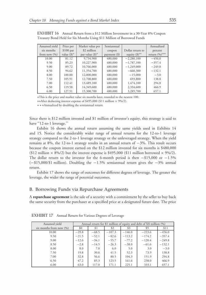
Chapter 18 Managing Funds against a Bond Market Index 535
EXHIBIT 16 Annual Return from a $12 Million Investment in a 30-Year 8% CouponTreasury Bond Held for Six Months Using $11 Million of Borrowed Funds
Assumed yield Price per Market value per Semiannual Annualizedsix months $100 par $2 million coupon Dollar return to percent
from now (%) value ($)∗ par value ($)∗ payment ($) equity ($)∗∗ return (%)∗∗∗
10.00 81.12 9,734,900 480,000 −2,280,100 −456.09.50 85.23 10,227,900 480,000 −1,787,100 −357.49.00 89.72 10,766,000 480,000 −1,249,000 −249.88.50 94.62 11,354,700 480,000 −660,300 −132.18.00 100.00 12,000,000 480,000 −15,000 −3.07.50 105.91 12,708,800 480,000 693,800 138.87.00 112.41 13,489,100 480,000 1,474,100 294.86.50 119.58 14,349,600 480,000 2,334,600 466.96.00 127.51 15,300,700 480,000 3,285,700 657.1
∗This is the price and market value six months later, rounded to the nearest 100.∗∗After deducting interest expense of $495,000 ($11 million × 9%/2).∗ ∗ ∗Annualized by doubling the semiannual return.
Since there is $12 million invested and $1 million of investor’s equity, this strategy is said tohave ‘‘12-to-1 leverage.’’
Exhibit 16 shows the annual return assuming the same yields used in Exhibits 14and 15. Notice the considerably wider range of annual returns for the 12-to-1 leveragestrategy compared to the 2-to-1 leverage strategy or the unleveraged strategy. When the yieldremains at 8%, the 12-to-1 strategy results in an annual return of −3%. This result occursbecause the coupon interest earned on the $12 million invested for six months is $480,000($12 million × 8%/2) but the interest expense is $495,000 ($11 million borrowed × 9%/2).The dollar return to the investor for the 6-month period is then −$15,000 or −1.5%(−$15,000/$1 million). Doubling the −1.5% semiannual return gives the −3% annualreturn.
Exhibit 17 shows the range of outcomes for different degrees of leverage. The greater theleverage, the wider the range of potential outcomes.
B. Borrowing Funds via Repurchase Agreements
A repurchase agreement is the sale of a security with a commitment by the seller to buy backthe same security from the purchaser at a specified price at a designated future date. The price
EXHIBIT 17 Annual Return for Various Degrees of Leverage
Assumed yield Annual return for $1 million of equity and debt of X$ million (%)six months from now (%) $0 $1 $2 $3 $5 $11
10.00 −29.8 −68.5 −107.3 −146.0 −223.6 −456.09.50 −21.5 −52.1 −82.6 −113.2 −174.2 −357.49.00 −12.6 −34.1 −55.7 −77.2 −120.4 −249.88.50 −2.8 −14.5 −26.3 −38.0 −61.6 −132.18.00 8.0 7.0 6.0 5.0 3.0 −3.07.50 19.8 30.6 41.5 52.3 73.9 138.87.00 32.8 56.6 80.5 104.3 151.9 294.86.50 47.2 85.3 123.5 161.6 238.0 466.96.00 63.0 117.0 171.1 225.1 333.1 657.1
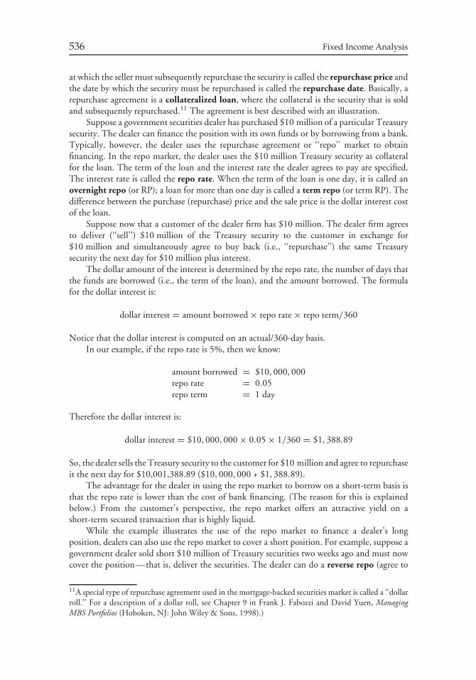
536 Fixed Income Analysis
at which the seller must subsequently repurchase the security is called the repurchase price andthe date by which the security must be repurchased is called the repurchase date. Basically, arepurchase agreement is a collateralized loan, where the collateral is the security that is soldand subsequently repurchased.11 The agreement is best described with an illustration.
Suppose a government securities dealer has purchased $10 million of a particular Treasurysecurity. The dealer can finance the position with its own funds or by borrowing from a bank.Typically, however, the dealer uses the repurchase agreement or ‘‘repo’’ market to obtainfinancing. In the repo market, the dealer uses the $10 million Treasury security as collateralfor the loan. The term of the loan and the interest rate the dealer agrees to pay are specified.The interest rate is called the repo rate. When the term of the loan is one day, it is called anovernight repo (or RP); a loan for more than one day is called a term repo (or term RP). Thedifference between the purchase (repurchase) price and the sale price is the dollar interest costof the loan.
Suppose now that a customer of the dealer firm has $10 million. The dealer firm agreesto deliver (‘‘sell’’) $10 million of the Treasury security to the customer in exchange for$10 million and simultaneously agree to buy back (i.e., ‘‘repurchase’’) the same Treasurysecurity the next day for $10 million plus interest.
The dollar amount of the interest is determined by the repo rate, the number of days thatthe funds are borrowed (i.e., the term of the loan), and the amount borrowed. The formulafor the dollar interest is:
dollar interest = amount borrowed × repo rate × repo term/360
Notice that the dollar interest is computed on an actual/360-day basis.In our example, if the repo rate is 5%, then we know:
amount borrowed = $10, 000, 000repo rate = 0.05repo term = 1 day
Therefore the dollar interest is:
dollar interest = $10, 000, 000 × 0.05 × 1/360 = $1, 388.89
So, the dealer sells the Treasury security to the customer for $10 million and agree to repurchaseit the next day for $10,001,388.89 ($10, 000, 000 + $1, 388.89).
The advantage for the dealer in using the repo market to borrow on a short-term basis isthat the repo rate is lower than the cost of bank financing. (The reason for this is explainedbelow.) From the customer’s perspective, the repo market offers an attractive yield on ashort-term secured transaction that is highly liquid.
While the example illustrates the use of the repo market to finance a dealer’s longposition, dealers can also use the repo market to cover a short position. For example, suppose agovernment dealer sold short $10 million of Treasury securities two weeks ago and must nowcover the position—that is, deliver the securities. The dealer can do a reverse repo (agree to
11A special type of repurchase agreement used in the mortgage-backed securities market is called a ‘‘dollarroll.’’ For a description of a dollar roll, see Chapter 9 in Frank J. Fabozzi and David Yuen, ManagingMBS Portfolios (Hoboken, NJ: John Wiley & Sons, 1998).)
Chapter 18 Managing Funds against a Bond Market Index 537
buy the securities and then sell them back). Of course, the dealer eventually would have to buythe Treasury security in the market in order to cover the short position. In this case, the dealeractually makes a collateralized loan to the customer. The customer (or other dealer) then usesthe funds obtained from the collateralized loan to create leverage.
1. Industry Jargon A good deal of industry jargon is used to describe repo transactions.In order to understand the terminology, remember that one party lends money and accepts asecurity as collateral for the loan; the other party borrows money and provides collateral in theform of a security.
We discuss the following terminology below:
1. ‘‘repo’’ versus ‘‘reverse repo’’2. ‘‘reversing out a security’’ and ‘‘reversing in a security’’3. ‘‘selling collateral’’ and ‘‘buying collateral’’
First, if a party loans a security and receives cash, then, from this party’s perspective, thetransaction is called a ‘‘repo.’’ If a party loans cash and receives a security as collateral, this is a‘‘reverse repo’’ transaction from this party’s perspective.
When someone lends a security (i.e., uses a security as collateral) in order to receive cash(i.e., borrow money), that party is said to be ‘‘reversing out’’ a security. A party that lendsmoney with a security as collateral is said to be ‘‘reversing in’’ a security.
Finally, the expressions ‘‘selling collateral’’ and ‘‘buying collateral’’ are used to describe aparty financing a security with a repo on the one hand, and lending on the basis of collateral,on the other.
To summarize, the following expressions are used for the transaction:
Borrower of funds Lender of fundsrepo reverse reporeversing out a security reversing in a securityselling collateral buying collateral
Rather than using industry jargon, investment guidelines should be clear as to what amanager is permitted to do. For example, a client may have no objections to its portfoliomanager using a repo as a short-term investment—that is, the portfolio manager may lendfunds on a short-term basis. The investment guidelines will set forth how the loan arrangementshould be structured to protect against credit risk. We’ll discuss this below. However, if aclient does not want a money manager to use the repo agreement as a vehicle for borrowingfunds (thereby, creating leverage), it should state so.
2. Margin and Marking to Market Despite the fact that high-quality collateral under-lies a repo transaction, both parties to the transaction are exposed to credit risk. Why doescredit risk exist in a repo transaction? Consider our initial example of the dealer who uses$10 million of government securities as collateral for a loan. If the dealer cannot repurchasethe government securities, the customer keeps the collateral; if interest rates on governmentsecurities increase subsequent to the repo transaction, however, the market value of thegovernment securities declines, and the customer then owns securities with a market value lessthan the amount of the loan. If the market value of the security rises instead, the dealer willbe concerned with the return of the collateral, which then has a market value greater than theamount of the loan.
538 Fixed Income Analysis
Repos should be carefully structured to reduce credit risk exposure. The amount lentshould be less than the market value of the security used as collateral, thereby providing thelender with cushion should the market value of the security decline. The amount by whichthe market value of the security used as collateral exceeds the value of the loan is called repomargin or simply margin. Margin is also referred to as the ‘‘haircut.’’ Repo margin is generallybetween 1% and 3%, but can be 10% or more for borrowers of lower credit worthiness and/orwhen less liquid or more price sensitive securities are used as collateral.
For example, consider the dealer who needs to borrow $10 million to finance the purchaseof a Treasury security. Suppose that the repo margin is 2%. Then for a Treasury security witha market value of $10 million, only 98% of that amount, $9.8 million, will be lent. That is,the dealer will agree to deliver (sell) $10 million of the Treasury security to the customer for$9.8 million and agree to repurchase the $10 million of the Treasury security the next day for$9.8 million plus the dollar interest. The dollar interest for this overnight repo, assuming arepo rate of 5%, is:
dollar interest = $9, 800, 000 × 0.05 × 1/360 = $1, 361.11
Note that the dollar interest is based on $9.8 million (the amount actually lent by thecustomer), not $10 million as in our earlier example.
Another practice used to limit credit risk is to mark the collateral to market on a regularbasis. Marking a position to market means recording the value of a position at its marketvalue. When the market value changes by a certain percentage, the repo position is adjustedaccordingly. The decline in market value below a specified amount results in a margin deficit.In such cases, the borrower of funds typically has the option to resolve the margin deficit eitherby providing additional cash or by transferring additional acceptable securities to the lender.When the market value rises above the amount required, excess margin will result. When thisoccurs, the lender of funds has the option to give cash to the borrower equal to the amount ofthe excess margin or to transfer purchased securities to the borrower.
3. Delivery and Credit Risk One concern of the parties to a repo is delivery of thecollateral to the lender. The most obvious procedure is for the borrower to deliver the collateralto the lender or to the lender’s clearing agent. In such instances, the collateral is said to be‘‘delivered out.’’ At the end of the repo term, the lender returns the collateral to the borrowerin exchange for the principal and interest payment. This procedure may be expensive though,particularly for short-term repos, because of costs associated with delivering the collateral. Thecost of delivery would be factored into the repo rate. The lender’s risk in terms of takingpossession of the collateral derives from the fact that the borrower might sell the security, orgo under so that the lender has nothing to liquidate, or use the same security as collateral for arepo with another party.
As an alternative to delivering out the collateral, the lender might agree to allow theborrower to hold the security in a segregated customer account. Of course, in this arrangement,the lender still faces the risk that the borrower might use the collateral fraudulently by offeringit as collateral for another repo transaction. If the borrower holds the collateral, then thetransaction is called a hold-in-custody repo (HIC repo). Despite the credit risk associatedwith a HIC repo, this arrangement is sometimes used in transactions when the collateral isdifficult to deliver or when the transaction amount is small and the lender is comfortable withthe reputation of the borrower.
Another arrangement is for the borrower to deliver the collateral to the lender’s custodialaccount at the borrower’s clearing bank. The custodian then has possession of the collateral
Chapter 18 Managing Funds against a Bond Market Index 539
on behalf of the lender. This practice reduces the cost of delivery because it requires only atransfer within the borrower’s clearing bank. If, for example, a dealer enters into an overnightrepo with Customer A, the collateral is transferred back to the dealer the next day. The dealercan then enter into a repo with Customer B for, say, five days without having to redeliver thecollateral. The clearing bank simply establishes a custodian account for Customer B and holdsthe collateral in that account. This specialized type of arrangement is called a tri-party repo.Tri-party repos account for about half of all repo arrangements.
The third party bank is responsible for marking the collateral to market and reportingthese values each day to the two parties. Also, if the borrower wishes to substitute collateral(i.e., change the specific Treasury securities collateralizing the loan), the third-party agentverifies that the collateral satisfies the requirements set forth in the repo agreement.
4. Determinants of the Repo Rate The repo rate varies from transaction to transactiondepending on a variety of factors, including:
• quality of collateral• term of the repo• delivery requirement• availability of collateral• prevailing federal funds rate
The higher the credit quality and liquidity of the collateral, the lower the repo rate. Therepo rate varies with the term of the repo agreement. This is basically the very short-term endof the yield curve. The maturity of the security used as collateral for the repo does not affectthe repo rate. If delivery of the collateral to the lender is required, the repo rate is lower.
The more difficult it is to obtain the collateral, the lower the repo rate. To understandwhy this is so, remember that the borrower (or equivalently the seller of the collateral) has asecurity that lenders of cash want. Such collateral is referred to as hot collateral or specialcollateral (or just as ‘‘on special’’). Collateral that does not have this characteristic is referredto as general collateral. The party that needs the hot collateral will be willing to lend at alower rate in order to obtain the collateral.
While these factors determine the repo rate on a particular transaction, the federal fundsrate determines the general level of repo rates in the United States. Banks borrow funds fromeach other via the federal funds market. The interest rate charged on such borrowing is calledthe federal funds rate (or ‘‘fed funds’’). The repo rate is generally lower than the federal fundsrate because a repo is a form of collateralized borrowing, while a federal funds transaction isunsecured borrowing.
C. Computing Duration for a Leveraged Portfolio
When a manager borrows to leverage a portfolio, the following procedure should be usedto compute the portfolio’s duration. The portfolio is then composed of the assets and theliabilities. The change in the portfolio value that includes borrowed funds is equal to:
dollar price change of all the bonds when rates change− dollar price change of the liabilities when rates change
total change in the portfolio value when rates change
540 Fixed Income Analysis
Dividing the total change in the portfolio value by the initial value of the portfolio andadjusting for the basis point change in rates equals the duration of the portfolio. If theliabilities are short term, then the duration of the liability is low.
To illustrate these calculations, consider the following three-bond portfolio, with durationand change in value for a 50-basis point change as shown:
Market Change in value forBond value Duration 50 bp yield change
10% 5-year $4,000,000 3.861 $77,2208% 15-year 4,231,375 8.047 170,249
14% 30-year 1,378,586 9.168 63,194Portfolio $9,609,961 6.470 $310,663
Note that this is the portfolio used in Chapter 17 to illustrate the duration calculationfor an unlevered portfolio. Suppose that $2 million was borrowed to buy the securities in theportfolio, so that the amount of the client’s funds invested (i.e., the equity) is $7,609,961.The client is interested in how the rate changes affect the equity investment. Suppose furtherthat the funds are borrowed using a 3-month repurchase agreement so that the duration ofthe liabilities is close to zero and the dollar change in the value of the liabilities for a 50 basispoint change in rates is close to zero. Then the change in the value of the portfolio for a 50basis point change in rates is computed as follows:
dollar price change of the bonds = $310, 663− dollar price change of the liabilities = 0
total change in portfolio value = $310, 663
Thus, the percentage change in the portfolio’s value for a 50 basis point change in ratesis 4.08% ($310,663 divided by $7,609,961), so the portfolio’s duration is 8.16. The higherduration that results from the $2 million short-term reverse repo borrowing (8.16 versus 6.47)is due to the leveraging of the portfolio.
CHAPTER 19PORTFOLIO
IMMUNIZATION ANDCASH FLOW MATCHING
I. INTRODUCTION
In this chapter we will explain strategies for managing bond portfolios to satisfy predeterminedliabilities. The two strategies we will discuss are immunization and cash flow matching.Immunization is a hybrid strategy having elements of both active and passive strategies. It isused to minimize reinvestment risk over a specified investment horizon. Immunization canbe employed to structure a portfolio designed to fund a single liability or multiple liabilities.Cash flow matching is used to construct a portfolio that will fund a schedule of liabilitiesfrom a portfolio’s cash flows, with the portfolio’s value diminishing to zero after payment ofthe last liability.
II. IMMUNIZATION STRATEGY FOR A SINGLELIABILITY
Classical immunization can be defined as the process by which a bond portfolio is createdto have an assured return for a specific time horizon irrespective of interest rate changes.1
The fundamental principle underlying immunization is to structure a portfolio that balancesthe change in the value of the portfolio at the end of the investment horizon with the returnfrom the reinvestment of portfolio cash flows (both coupon and principal payments). Thatis, immunization offsets interest rate risk and reinvestment risk. The general principle ofimmunization is summarized in Exhibit 1.
To accomplish this balancing requires controlling portfolio duration. By setting theportfolio duration equal to the desired portfolio time horizon, positive and negative incrementalreturn sources offset one another. This is a necessary condition for effectively immunizedportfolios.
1The classical theory of immunization is set forth in F.M. Reddington, ‘‘Review of the Principles of LifeInsurance Valuations,’’ Journal of the Institute of Actuaries, 1952; and Lawrence Fisher and Roman Weil,‘‘Coping with Risk of Interest Rate Fluctuations: Returns to Bondholders from Naive and OptimalStrategies,’’ Journal of Business (October 1971), pp. 408–431.
541
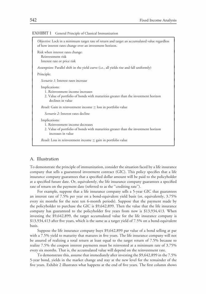
542 Fixed Income Analysis
EXHIBIT 1 General Principle of Classical Immunization
Objective: Lock in a minimum target rate of return and target an accumulated value regardlessof how interest rates change over an investment horizon.
Risk when interest rates change:Reinvestment riskInterest rate or price risk
Assumption: Parallel shift in the yield curve (i.e., all yields rise and fall uniformly)
Principle:
Scenario 1: Interest rates increase
Implications:1. Reinvestment income increases2. Value of portfolio of bonds with maturities greater than the investment horizon
declines in value
Result: Gain in reinvestment income ≥ loss in portfolio value
Scenario 2: Interest rates decline
Implications:1. Reinvestment income decreases2. Value of portfolio of bonds with maturities greater than the investment horizon
increases in value
Result: Loss in reinvestment income ≤ gain in portfolio value
A. Illustration
To demonstrate the principle of immunization, consider the situation faced by a life insurancecompany that sells a guaranteed investment contract (GIC). This policy specifies that a lifeinsurance company guarantees that a specified dollar amount will be paid to the policyholderat a specified future date. Or, equivalently, the life insurance company guarantees a specifiedrate of return on the payment date (referred to as the ‘‘crediting rate’’).
For example, suppose that a life insurance company sells a 5-year GIC that guaranteesan interest rate of 7.5% per year on a bond-equivalent yield basis (or, equivalently, 3.75%every six months for the next ten 6-month periods). Suppose that the payment made bythe policyholder to purchase the GIC is $9,642,899. Then the value that the life insurancecompany has guaranteed to the policyholder five years from now is $13,934,413. Wheninvesting the $9,642,899, the target accumulated value for the life insurance company is$13,934,413 after five years, which is the same as a target yield of 7.5% on a bond-equivalentbasis.
Suppose the life insurance company buys $9,642,899 par value of a bond selling at parwith a 7.5% yield to maturity that matures in five years. The life insurance company will notbe assured of realizing a total return at least equal to the target return of 7.5% because torealize 7.5% the coupon interest payments must be reinvested at a minimum rate of 3.75%every six months. That is, the accumulated value will depend on the reinvestment rate.
To demonstrate this, assume that immediately after investing the $9,642,899 in the 7.5%5-year bond, yields in the market change and stay at the new level for the remainder of thefive years. Exhibit 2 illustrates what happens at the end of five years. The first column shows
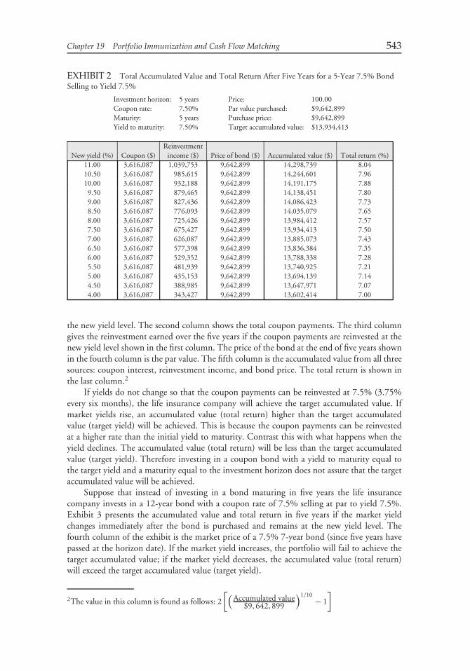
Chapter 19 Portfolio Immunization and Cash Flow Matching 543
EXHIBIT 2 Total Accumulated Value and Total Return After Five Years for a 5-Year 7.5% BondSelling to Yield 7.5%
Investment horizon: 5 years Price: 100.00Coupon rate: 7.50% Par value purchased: $9,642,899Maturity: 5 years Purchase price: $9,642,899Yield to maturity: 7.50% Target accumulated value: $13,934,413
ReinvestmentNew yield (%) Coupon ($) income ($) Price of bond ($) Accumulated value ($) Total return (%)
11.00 3,616,087 1,039,753 9,642,899 14,298,739 8.0410.50 3,616,087 985,615 9,642,899 14,244,601 7.9610.00 3,616,087 932,188 9,642,899 14,191,175 7.889.50 3,616,087 879,465 9,642,899 14,138,451 7.809.00 3,616,087 827,436 9,642,899 14,086,423 7.738.50 3,616,087 776,093 9,642,899 14,035,079 7.658.00 3,616,087 725,426 9,642,899 13,984,412 7.577.50 3,616,087 675,427 9,642,899 13,934,413 7.507.00 3,616,087 626,087 9,642,899 13,885,073 7.436.50 3,616,087 577,398 9,642,899 13,836,384 7.356.00 3,616,087 529,352 9,642,899 13,788,338 7.285.50 3,616,087 481,939 9,642,899 13,740,925 7.215.00 3,616,087 435,153 9,642,899 13,694,139 7.144.50 3,616,087 388,985 9,642,899 13,647,971 7.074.00 3,616,087 343,427 9,642,899 13,602,414 7.00
the new yield level. The second column shows the total coupon payments. The third columngives the reinvestment earned over the five years if the coupon payments are reinvested at thenew yield level shown in the first column. The price of the bond at the end of five years shownin the fourth column is the par value. The fifth column is the accumulated value from all threesources: coupon interest, reinvestment income, and bond price. The total return is shown inthe last column.2
If yields do not change so that the coupon payments can be reinvested at 7.5% (3.75%every six months), the life insurance company will achieve the target accumulated value. Ifmarket yields rise, an accumulated value (total return) higher than the target accumulatedvalue (target yield) will be achieved. This is because the coupon payments can be reinvestedat a higher rate than the initial yield to maturity. Contrast this with what happens when theyield declines. The accumulated value (total return) will be less than the target accumulatedvalue (target yield). Therefore investing in a coupon bond with a yield to maturity equal tothe target yield and a maturity equal to the investment horizon does not assure that the targetaccumulated value will be achieved.
Suppose that instead of investing in a bond maturing in five years the life insurancecompany invests in a 12-year bond with a coupon rate of 7.5% selling at par to yield 7.5%.Exhibit 3 presents the accumulated value and total return in five years if the market yieldchanges immediately after the bond is purchased and remains at the new yield level. Thefourth column of the exhibit is the market price of a 7.5% 7-year bond (since five years havepassed at the horizon date). If the market yield increases, the portfolio will fail to achieve thetarget accumulated value; if the market yield decreases, the accumulated value (total return)will exceed the target accumulated value (target yield).
2The value in this column is found as follows: 2
[(Accumulated value
$9, 642, 899
)1/10 − 1
]
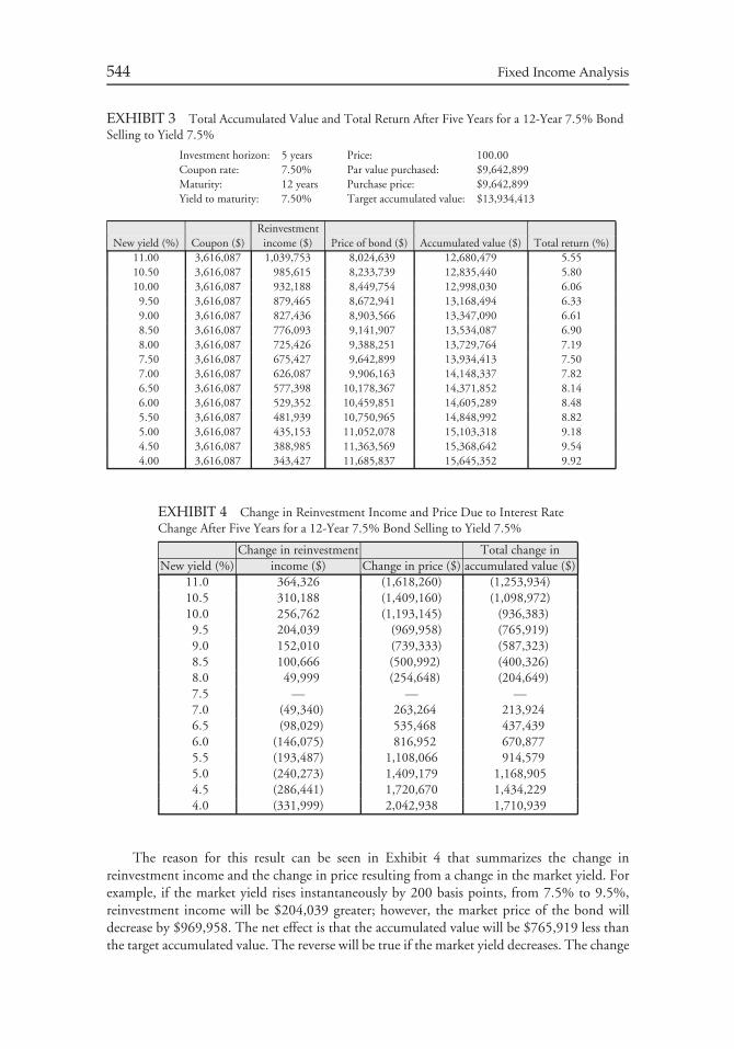
544 Fixed Income Analysis
EXHIBIT 3 Total Accumulated Value and Total Return After Five Years for a 12-Year 7.5% BondSelling to Yield 7.5%
Investment horizon: 5 years Price: 100.00Coupon rate: 7.50% Par value purchased: $9,642,899Maturity: 12 years Purchase price: $9,642,899Yield to maturity: 7.50% Target accumulated value: $13,934,413
ReinvestmentNew yield (%) Coupon ($) income ($) Price of bond ($) Accumulated value ($) Total return (%)
11.00 3,616,087 1,039,753 8,024,639 12,680,479 5.5510.50 3,616,087 985,615 8,233,739 12,835,440 5.8010.00 3,616,087 932,188 8,449,754 12,998,030 6.06
9.50 3,616,087 879,465 8,672,941 13,168,494 6.339.00 3,616,087 827,436 8,903,566 13,347,090 6.618.50 3,616,087 776,093 9,141,907 13,534,087 6.908.00 3,616,087 725,426 9,388,251 13,729,764 7.197.50 3,616,087 675,427 9,642,899 13,934,413 7.507.00 3,616,087 626,087 9,906,163 14,148,337 7.826.50 3,616,087 577,398 10,178,367 14,371,852 8.146.00 3,616,087 529,352 10,459,851 14,605,289 8.485.50 3,616,087 481,939 10,750,965 14,848,992 8.825.00 3,616,087 435,153 11,052,078 15,103,318 9.184.50 3,616,087 388,985 11,363,569 15,368,642 9.544.00 3,616,087 343,427 11,685,837 15,645,352 9.92
EXHIBIT 4 Change in Reinvestment Income and Price Due to Interest RateChange After Five Years for a 12-Year 7.5% Bond Selling to Yield 7.5%
Change in reinvestment Total change inNew yield (%) income ($) Change in price ($) accumulated value ($)
11.0 364,326 (1,618,260) (1,253,934)10.5 310,188 (1,409,160) (1,098,972)10.0 256,762 (1,193,145) (936,383)9.5 204,039 (969,958) (765,919)9.0 152,010 (739,333) (587,323)8.5 100,666 (500,992) (400,326)8.0 49,999 (254,648) (204,649)7.5 — — —7.0 (49,340) 263,264 213,9246.5 (98,029) 535,468 437,4396.0 (146,075) 816,952 670,8775.5 (193,487) 1,108,066 914,5795.0 (240,273) 1,409,179 1,168,9054.5 (286,441) 1,720,670 1,434,2294.0 (331,999) 2,042,938 1,710,939
The reason for this result can be seen in Exhibit 4 that summarizes the change inreinvestment income and the change in price resulting from a change in the market yield. Forexample, if the market yield rises instantaneously by 200 basis points, from 7.5% to 9.5%,reinvestment income will be $204,039 greater; however, the market price of the bond willdecrease by $969,958. The net effect is that the accumulated value will be $765,919 less thanthe target accumulated value. The reverse will be true if the market yield decreases. The change
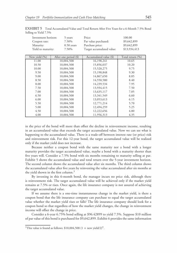
Chapter 19 Portfolio Immunization and Cash Flow Matching 545
EXHIBIT 5 Total Accumulated Value and Total Return After Five Years for a 6-Month 7.5% BondSelling to Yield 7.5%
Investment horizon: 5 years Price: 100.00Coupon rate: 7.50% Par value purchased: $9,642,899Maturity: 0.50 years Purchase price: $9,642,899Yield to maturity: 7.50% Target accumulated value: $13,934,413
New yield (%) After one period ($) Accumulated value ($) Total return (%)11.00 10,004,508 16,198,241 10.6510.50 10,004,508 15,856,037 10.2010.00 10,004,508 15,520,275 9.75
9.50 10,004,508 15,190,848 9.309.00 10,004,508 14,867,650 8.858.50 10,004,508 14,550,580 8.408.00 10,004,508 14,239,534 7.957.50 10,004,508 13,934,415 7.507.00 10,004,508 13,635,117 7.056.50 10,004,508 13,341,549 6.606.00 10,004,508 13,053,613 6.155.50 10,004,508 12,771,214 5.705.00 10,004,508 12,494,259 5.254.50 10,004,508 12,222,656 4.804.00 10,004,508 11,956,313 4.35
in the price of the bond will more than offset the decline in reinvestment income, resultingin an accumulated value that exceeds the target accumulated value. Now we can see what ishappening to the accumulated value. There is a trade-off between interest rate (or price) riskand reinvestment risk. For this 12-year bond, the target accumulated value will be realizedonly if the market yield does not increase.
Because neither a coupon bond with the same maturity nor a bond with a longermaturity provides the target accumulated value, maybe a bond with a maturity shorter thanfive years will. Consider a 7.5% bond with six months remaining to maturity selling at par.Exhibit 5 shows the accumulated value and total return over the 5-year investment horizon.The second column shows the accumulated value after six months. The third column showsthe accumulated value after five years by reinvesting the value accumulated after six months atthe yield shown in the first column.3
By investing in this 6-month bond, the manager incurs no price risk, although thereis reinvestment risk. The target accumulated value will be achieved only if the market yieldremains at 7.5% or rises. Once again, the life insurance company is not assured of achievingthe target accumulated value.
If we assume there is a one-time instantaneous change in the market yield, is there acoupon bond that the life insurance company can purchase to equal the target accumulatedvalue whether the market yield rises or falls? The life insurance company should look for acoupon bond so that regardless of how the market yield changes, the change in reinvestmentincome will offset the change in price.
Consider a 6-year 6.75% bond selling at $96.42899 to yield 7.5%. Suppose $10 millionof par value of this bond is purchased for $9,642,899. Exhibit 6 provides the same information
3This value is found as follows: $10,004,508 (1 + new yield/2)9.
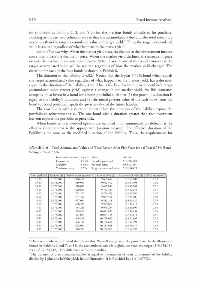
546 Fixed Income Analysis
for this bond as Exhibits 2, 3, and 5 do for the previous bonds considered for purchase.Looking at the last two columns, we see that the accumulated value and the total return arenever less than the target accumulated value and target yield.4 Thus, the target accumulatedvalue is assured regardless of what happens to the market yield.
Exhibit 7 shows why. When the market yield rises, the change in the reinvestment incomemore than offsets the decline in price. When the market yield declines, the increase in priceexceeds the decline in reinvestment income. What characteristic of this bond assures that thetarget accumulated value will be realized regardless of how the market yield changes? Theduration for each of the four bonds is shown in Exhibit 8.
The duration of the liability is 4.82.5 Notice that the 6-year 6.75% bond which equalsthe target accumulated value regardless of what happens to the market yield, has a durationequal to the duration of the liability, 4.82. This is the key. To immunize a portfolio’s targetaccumulated value (target yield) against a change in the market yield, the life insurancecompany must invest in a bond (or a bond portfolio) such that (1) the portfolio’s duration isequal to the liability’s duration, and (2) the initial present value of the cash flows from thebond (or bond portfolio) equals the present value of the future liability.
The two bonds with a duration shorter than the duration of the liability expose theportfolio to reinvestment risk. The one bond with a duration greater than the investmenthorizon exposes the portfolio to price risk.
When bonds with embedded options are included in an immunized portfolio, it is theeffective duration that is the appropriate duration measure. The effective duration of theliability is the same as the modified duration of the liability. Thus, the requirements for
EXHIBIT 6 Total Accumulated Value and Total Return After Five Years for a 6-Year 6.75% BondSelling to Yield 7.5%
Investment horizon: 5 years Price: 100.00Coupon rate: 6.75% Par value purchased: $10,000,000Maturity: 6 years Purchase price: $9,642,899Yield to maturity: 7.5% Target accumulated value: $13,934,413
New yield (%) Coupon ($) Reinvestment income ($) Price of bond ($) Accumulated value ($) Total return (%)11.00 3,375,000 970,432 9,607,657 13,953,089 7.5310.50 3,375,000 919,903 9,652,592 13,947,495 7.5210.00 3,375,000 870,039 9,697,846 13,942,885 7.519.50 3,375,000 820,831 9,743,423 13,939,253 7.519.00 3,375,000 772,271 9,789,325 13,936,596 7.508.50 3,375,000 724,350 9,835,556 13,934,906 7.508.00 3,375,000 677,061 9,882,119 13,934,180 7.507.50 3,375,000 630,395 9,929,017 13,934,413 7.507.00 3,375,000 584,345 9,976,254 13,935,599 7.506.50 3,375,000 538,902 10,023,832 13,937,734 7.506.00 3,375,000 494,059 10,071,755 13,940,814 7.515.50 3,375,000 449,808 10,120,027 13,944,835 7.525.00 3,375,000 406,141 10,168,650 13,949,791 7.524.50 3,375,000 363,051 10,217,628 13,955,679 7.534.00 3,375,000 320,531 10,266,965 13,962,495 7.54
4There is a mathematical proof that shows this. We will not present the proof here. In the illustrationshown in Exhibits 6 and 7, at 8% the accumulated value is slightly less than the target ($13,934,180versus $13,934,413). This difference is due to rounding.5The duration of a zero-coupon liability is equal to the number of years to maturity of the liabilitydivided by 1 plus one-half the yield. In our illustration, it is 5 divided by (1 + 0.075/2).
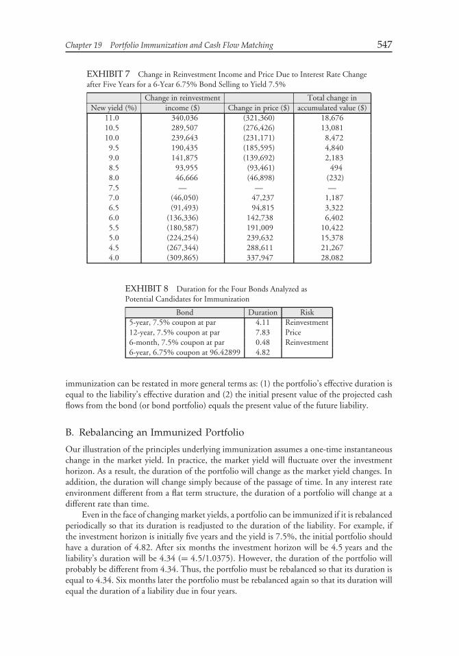
Chapter 19 Portfolio Immunization and Cash Flow Matching 547
EXHIBIT 7 Change in Reinvestment Income and Price Due to Interest Rate Changeafter Five Years for a 6-Year 6.75% Bond Selling to Yield 7.5%
Change in reinvestment Total change inNew yield (%) income ($) Change in price ($) accumulated value ($)
11.0 340,036 (321,360) 18,67610.5 289,507 (276,426) 13,08110.0 239,643 (231,171) 8,472
9.5 190,435 (185,595) 4,8409.0 141,875 (139,692) 2,1838.5 93,955 (93,461) 4948.0 46,666 (46,898) (232)7.5 — — —7.0 (46,050) 47,237 1,1876.5 (91,493) 94,815 3,3226.0 (136,336) 142,738 6,4025.5 (180,587) 191,009 10,4225.0 (224,254) 239,632 15,3784.5 (267,344) 288,611 21,2674.0 (309,865) 337,947 28,082
EXHIBIT 8 Duration for the Four Bonds Analyzed asPotential Candidates for Immunization
Bond Duration Risk5-year, 7.5% coupon at par 4.11 Reinvestment12-year, 7.5% coupon at par 7.83 Price6-month, 7.5% coupon at par 0.48 Reinvestment6-year, 6.75% coupon at 96.42899 4.82
immunization can be restated in more general terms as: (1) the portfolio’s effective duration isequal to the liability’s effective duration and (2) the initial present value of the projected cashflows from the bond (or bond portfolio) equals the present value of the future liability.
B. Rebalancing an Immunized Portfolio
Our illustration of the principles underlying immunization assumes a one-time instantaneouschange in the market yield. In practice, the market yield will fluctuate over the investmenthorizon. As a result, the duration of the portfolio will change as the market yield changes. Inaddition, the duration will change simply because of the passage of time. In any interest rateenvironment different from a flat term structure, the duration of a portfolio will change at adifferent rate than time.
Even in the face of changing market yields, a portfolio can be immunized if it is rebalancedperiodically so that its duration is readjusted to the duration of the liability. For example, ifthe investment horizon is initially five years and the yield is 7.5%, the initial portfolio shouldhave a duration of 4.82. After six months the investment horizon will be 4.5 years and theliability’s duration will be 4.34 (= 4.5/1.0375). However, the duration of the portfolio willprobably be different from 4.34. Thus, the portfolio must be rebalanced so that its duration isequal to 4.34. Six months later the portfolio must be rebalanced again so that its duration willequal the duration of a liability due in four years.
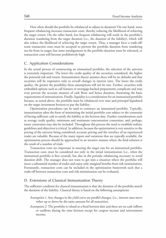
548 Fixed Income Analysis
How often should the portfolio be rebalanced to adjust its duration? On one hand, morefrequent rebalancing increases transaction costs, thereby reducing the likelihood of achievingthe target return. On the other hand, less frequent rebalancing will result in the portfolio’sduration wandering from the target duration (i.e., the duration of the liability), which willalso reduce the likelihood of achieving the target return. Thus, a manager faces a trade-off:some transaction costs must be accepted to prevent the portfolio duration from wanderingtoo far from its target; but some misalignment in the portfolio duration must be tolerated, ortransaction costs will become prohibitively high.
C. Application Considerations
In the actual process of constructing an immunized portfolio, the selection of the universeis extremely important. The lower the credit quality of the securities considered, the higherthe potential risk and return. Immunization theory assumes there will be no defaults and thatsecurities will be responsive only to overall changes in interest rates. The lower the creditquality, the greater the possibility these assumptions will not be met. Further, securities withembedded options such as call features or mortgage-backed prepayments complicate and mayeven prevent the accurate measure of cash flows and hence duration, frustrating the basicrequirements of immunization. Finally, liquidity is a consideration for an immunized portfoliobecause, as noted above, the portfolio must be rebalanced over time and principal liquidatedon the target investment horizon to pay the liability.
Optimization procedures can be used to construct an immunized portfolio. Typically,immunization takes the form of minimizing the initial portfolio cost subject to the constraintof having sufficient cash to satisfy the liability at the horizon date. Further considerations suchas average credit quality, minimum and maximum concentration constraints, and, perhaps,issuer constraints may also be included. Throughout this process the need to establish realisticguidelines and objectives is critical. In addition, because the optimization is very sensitive to thepricing of the universe being considered, accurate pricing and the interface of an experiencedtrader are valuable. Because of the many inputs and variations that are typically available, theoptimization process should be approached in an iterative manner where the final solution isthe result of a number of trials.
Transaction costs are important in meeting the target rate for an immunized portfolio.Transaction costs must be considered not only in the initial immunization (i.e., when theimmunized portfolio is first created), but also in the periodic rebalancing necessary to avoidduration drift. The manager does not want to get into a situation where the portfolio willincur a substantial number of trades and enjoy only marginal benefits from risk minimization.Fortunately, transaction costs can be included in the optimization framework such that atrade-off between transaction costs and risk minimization can be evaluated.
D. Extensions of Classical Immunization Theory
The sufficient condition for classical immunization is that the duration of the portfolio matchthe duration of the liability. Classical theory is based on the following assumptions:
Assumption 1. Any changes in the yield curve are parallel changes, (i.e., interest rates moveeither up or down by the same amount for all maturities).
Assumption 2. The portfolio is valued at a fixed horizon date and there are no cash inflowsor outflows during the time horizon except for coupon income and reinvestmentincome.
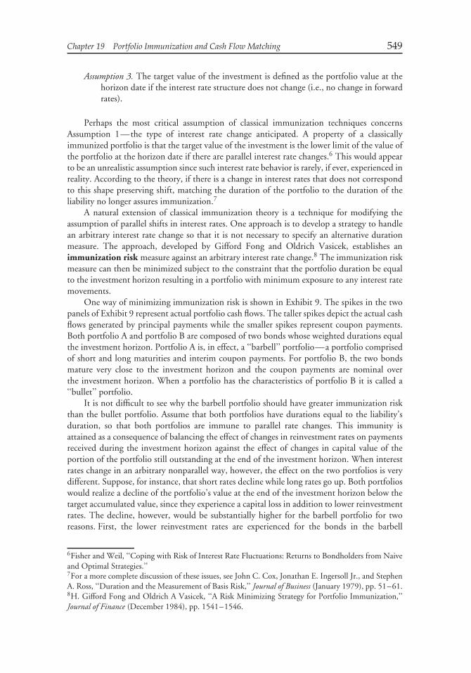
Chapter 19 Portfolio Immunization and Cash Flow Matching 549
Assumption 3. The target value of the investment is defined as the portfolio value at thehorizon date if the interest rate structure does not change (i.e., no change in forwardrates).
Perhaps the most critical assumption of classical immunization techniques concernsAssumption 1—the type of interest rate change anticipated. A property of a classicallyimmunized portfolio is that the target value of the investment is the lower limit of the value ofthe portfolio at the horizon date if there are parallel interest rate changes.6 This would appearto be an unrealistic assumption since such interest rate behavior is rarely, if ever, experienced inreality. According to the theory, if there is a change in interest rates that does not correspondto this shape preserving shift, matching the duration of the portfolio to the duration of theliability no longer assures immunization.7
A natural extension of classical immunization theory is a technique for modifying theassumption of parallel shifts in interest rates. One approach is to develop a strategy to handlean arbitrary interest rate change so that it is not necessary to specify an alternative durationmeasure. The approach, developed by Gifford Fong and Oldrich Vasicek, establishes animmunization risk measure against an arbitrary interest rate change.8 The immunization riskmeasure can then be minimized subject to the constraint that the portfolio duration be equalto the investment horizon resulting in a portfolio with minimum exposure to any interest ratemovements.
One way of minimizing immunization risk is shown in Exhibit 9. The spikes in the twopanels of Exhibit 9 represent actual portfolio cash flows. The taller spikes depict the actual cashflows generated by principal payments while the smaller spikes represent coupon payments.Both portfolio A and portfolio B are composed of two bonds whose weighted durations equalthe investment horizon. Portfolio A is, in effect, a ‘‘barbell’’ portfolio—a portfolio comprisedof short and long maturities and interim coupon payments. For portfolio B, the two bondsmature very close to the investment horizon and the coupon payments are nominal overthe investment horizon. When a portfolio has the characteristics of portfolio B it is called a‘‘bullet’’ portfolio.
It is not difficult to see why the barbell portfolio should have greater immunization riskthan the bullet portfolio. Assume that both portfolios have durations equal to the liability’sduration, so that both portfolios are immune to parallel rate changes. This immunity isattained as a consequence of balancing the effect of changes in reinvestment rates on paymentsreceived during the investment horizon against the effect of changes in capital value of theportion of the portfolio still outstanding at the end of the investment horizon. When interestrates change in an arbitrary nonparallel way, however, the effect on the two portfolios is verydifferent. Suppose, for instance, that short rates decline while long rates go up. Both portfolioswould realize a decline of the portfolio’s value at the end of the investment horizon below thetarget accumulated value, since they experience a capital loss in addition to lower reinvestmentrates. The decline, however, would be substantially higher for the barbell portfolio for tworeasons. First, the lower reinvestment rates are experienced for the bonds in the barbell
6Fisher and Weil, ‘‘Coping with Risk of Interest Rate Fluctuations: Returns to Bondholders from Naiveand Optimal Strategies.’’7For a more complete discussion of these issues, see John C. Cox, Jonathan E. Ingersoll Jr., and StephenA. Ross, ‘‘Duration and the Measurement of Basis Risk,’’ Journal of Business (January 1979), pp. 51–61.8H. Gifford Fong and Oldrich A Vasicek, ‘‘A Risk Minimizing Strategy for Portfolio Immunization,’’Journal of Finance (December 1984), pp. 1541–1546.
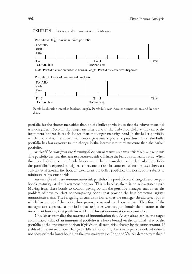
550 Fixed Income Analysis
EXHIBIT 9 Illustration of Immunization Risk Measure
Portfolio A: High-risk immunized portfolio:
Portfolio B: Low-risk immunized portfolio:
Portfoliocashflow
Portfoliocashflow
T = 0Current date
Note: Portfolio duration matches horizon length. Portfolio’s cash flow dispersed.
T = H TimeHorizon date
T = 0Current date
T = H TimeHorizon date
Portfolio duration matches horizon length. Portfolio’s cash flow concentrated around horizondates.
portfolio for the shorter maturities than on the bullet portfolio, so that the reinvestment riskis much greater. Second, the longer maturity bond in the barbell portfolio at the end of theinvestment horizon is much longer than the longer maturity bond in the bullet portfolio,which means that the same rate increase generates a greater capital loss. Thus, the bulletportfolio has less exposure to the change in the interest rate term structure than the barbellportfolio.
It should be clear from the foregoing discussion that immunization risk is reinvestment risk.The portfolio that has the least reinvestment risk will have the least immunization risk. Whenthere is a high dispersion of cash flows around the horizon date, as in the barbell portfolio,the portfolio is exposed to higher reinvestment risk. In contrast, when the cash flows areconcentrated around the horizon date, as in the bullet portfolio, the portfolio is subject tominimum reinvestment risk.
An example of a zero immunization risk portfolio is a portfolio consisting of zero-couponbonds maturing at the investment horizon. This is because there is no reinvestment risk.Moving from these bonds to coupon-paying bonds, the portfolio manager encounters theproblem of how to select coupon-paying bonds that provide the best protection againstimmunization risk. The foregoing discussion indicates that the manager should select bondswhich have most of their cash flow payments around the horizon date. Therefore, if themanager can construct a portfolio that replicates zero-coupon bonds that mature at theinvestment horizon, that portfolio will be the lowest immunization risk portfolio.
Now let us formalize the measure of immunization risk. As explained earlier, the targetaccumulated value of an immunized portfolio is a lower bound on the terminal value of theportfolio at the investment horizon if yields on all maturities change by the same amount. Ifyields of different maturities change by different amounts, then the target accumulated value isnot necessarily the lower bound on the investment value. Fong and Vasicek demonstrate that if
Chapter 19 Portfolio Immunization and Cash Flow Matching 551
the yield curve changes in any arbitrary way, the relative change in the portfolio value dependson the product of two terms.9 The first term depends solely on the structure of the investmentportfolio while the second term is a function of interest rate movement only. The second termcharacterizes the nature of the yield curve shift. Since this shift can be arbitrary, this term isan uncertain quantity and therefore outside of the control of the manager. However, the firstterm is under the control of the manager since it depends solely on the composition of theportfolio. This first term is thus a measure of risk for immunized portfolios and defined asfollows:
Immunization risk measure = PVCF1(1 − H )2 + PVCF2(2 − H )2 + . . . + PVCFn(n − H )2
Initial investment value
where
PVCFt = present value of the cash flow in period t discounted at the prevailing yieldH = length of the investment horizonn = time to receipt of the last portfolio cash flow
The immunization risk measure agrees with the intuitive interpretation of risk discussedearlier. For portfolio A in Exhibit 9, the barbell portfolio, the portfolio payments are widelydispersed in time and the immunization risk measure would be high. The portfolio paymentsoccur close to the investment horizon for portfolio B in Exhibit 9, the bullet portfolio, so thatthe immunization risk measure is low.
Given the measure of immunization risk that is to be minimized and the constraint thatthe duration of the portfolio equals the duration of the liability as well as any other applicableinvestment constraints, the optimal immunized portfolio can be found using optimizationmodels.10
III. CONTINGENT IMMUNIZATION
Contingent immunization consists of identifying both the available immunization target rateand a lower safety net level return with which a client would be minimally satisfied or is aminimum required rate of return.11 The manager can continue to pursue an active strategyuntil an adverse investment experience drives the then available potential return—combinedactive return (from actual past experience) and immunized return (from expected futureexperience)—down to the safety net level; at such time the manager would be obligated tocompletely immunize the portfolio and lock in the safety net level return. As long as thissafety net return is not violated, the manager can continue to actively manage the portfolio.Once the immunization mode is activated because the safety net return is violated, themanager can no longer return to the active mode unless the contingent immunization plan isabandoned.
9Fong and Vasicek, ‘‘A Risk Minimizing Strategy for Portfolio Immunization.’’10More specifically, linear programming can be employed because the risk measure is linear in theportfolio payments.11Martin L. Leibowitz and Alfred Weinberger, ‘‘Contingent Immunization—Part I: Risk ControlProcedures,’’ Financial Analysts Journal (November-December 1982), pp. 17–31.
552 Fixed Income Analysis
A. Key Considerations
The key considerations in implementing a contingent immunization strategy are:
1. establishing well defined immunized initial and ongoing available target returns2. identifying a suitable and immunizable safety net3. implementing an effective monitoring procedure to ensure that the safety net return is
not violated
B. An Illustration
To illustrate the basic principles of the contingent immunization strategy suppose a plansponsor is willing to accept a 6% return over a 5-year investment horizon at a time whenthe possible immunized rate of return is 7.5%. The 6% rate of return is called the safety net(or minimum target or floor) return. The difference between the possible immunized rate of7.5% and the safety net return is called the cushion spread or excess achievable return. Itis this cushion spread of 150 basis points in our example that offers the manager latitude inpursuing an active strategy. The greater the cushion spread the more scope the manager hasfor an active management policy.
Assuming an initial portfolio of $100 million, the required terminal asset value when thesafety net return is 6% is $134.39 million. The general formula for the required terminal valueassuming semiannual compounding is:
Required terminal value = I (1 + s/2)2H
where
I = initial portfolio values = safety net rateH = number of years in the investment horizon
In our example, the initial portfolio value is $100 million, s is 6%, and H is five years.Therefore, the required terminal value is:
$100 million(1.03)10 = $134.39 million
Since the current available return is assumed to be 7.5%, the assets required at theinception of the plan in order to generate the required terminal value of $134.39 million are$93 million. This is found as follows assuming semiannual compounding. The required assetsat any given point in time, t, necessary to achieve the required terminal value are:
Required assets at time t = Required terminal value
(1 + it)2(H−t)
where
it = the immunized semiannual yield available at time t
The other variables were defined earlier.
Chapter 19 Portfolio Immunization and Cash Flow Matching 553
Since in our example the required terminal value is $134.39 million and the market yieldthat can be realized if the immunization mode is activated is 7.5%, the required assets are:
$134.39 million
(1.0375)10= $93 million
Consequently, the safety cushion of 150 basis points translates into an initial dollar safetymargin of $7 million ($100 million − $93 million).
Now suppose that the portfolio manager invested the initial $100 million in a portfolioof 30-year par bonds with a coupon of 7.5%. Let’s look at what happens if there is a changein the yield level immediately following the purchase of these bonds.
First assume the yield level decreases to 5.6% from 7.5%. The value of the portfolio of30-year bonds would increase to $127.46 million. However, the asset value required to achievethe required terminal value if the portfolio is immunized at a 5.6% rate is $102 million. Thisis found by using the previous formula. The required terminal value is $134.39 million andthe market yield for immunizing (following the yield change) is 5.6%, therefore:
$134.39 million
(1.028)10= $101.96 million
The amount by which the $127.46 million exceeds the required asset value (i.e., the dollarsafety margin) in this case is $25.5 million ($127.46 million − $101.96 million). This amountis $18.46 million greater than the initial dollar safety margin of $7 million and therefore allowsthe manager more freedom to pursue active management.
Suppose instead of a decline in the yield level the immediate change is an increase in theyield level to 8.6%. At that yield level the portfolio of 30-year bonds would decline in valueto $88.23 million. The required asset value to achieve the terminal value of $134.39 millionis $88.21 million. Consequently, an immediate rise in the yield by 110 basis points to 8.6%will decrease the dollar safety margin to zero. At this yield level the immunization modewould be triggered with an immunization target rate of 8.6% to ensure that the requiredterminal value will be realized. If this were not followed, further adverse movements of interestrates would jeopardize the required terminal value for the portfolio of $134.39 million.The yield level at which the immunization mode becomes necessary is called the triggerpoint.
C. Controlling and Monitoring the Strategy
For purposes of monitoring a contingent immunization plan, it is useful to recast the dollarsafety margin in terms of the potential return. This return, also called the return achievablewith an immunization strategy, measures the yield that would be realized if, at any givenpoint in time, the current value of the portfolio is immunized at the prevailing marketyield.
Since duration approximates the price sensitivity of a portfolio to changes in marketyields, trigger yields can be computed for portfolios of different durations so that the managerwould know how much leeway there is for a given risk position with respect to an adversemovement in the market yield; that is, how much of an adverse movement in the marketyield can be tolerated before the immunization mode must be activated. However, when usingduration to compute trigger points it is important to remember the limitation of duration—itassumes a small parallel shift in the yield curve. In practice, the specific rate movements need
554 Fixed Income Analysis
to be monitored because the skewness of any particular movement should be expected tochange the portfolio’s trigger point.
The key to a contingent immunization plan is the ability to control and monitor theperformance of the portfolio over time so that the manager knows how much leeway he hasto actively manage the portfolio, and when the portfolio should be immunized in order toachieve the minimum target return.
An accurate immunization target is critical in determining not only the basis for the initialproblem set-up (e.g., the safety net return will usually be a certain basis point difference fromthe target over a specified time period), but also in determining what immunization levels areavailable over the investment horizon. A safety net return too close to the initial target returnmakes triggering the immunization process highly likely, while too low a safety net defeats thepurpose of the process since the very low satisfactory minimum return would probably nevertrigger immunization. Finally, without an adequate monitoring procedure, the benefits of thestrategy may be lost because of the inability to know when action is appropriate.
In spite of good control and monitoring procedures, attainment of the minimum targetreturn may not be realized due to factors beyond the control of the manager. There aretwo reasons for this.12 The first is that there is the possibility of a rapid adverse largemovement in market yields that the manager does not have enough time to shift from anactive to an immunization strategy at the rate needed to achieve the minimum target return.Frequent jumps of market yields of several hundred basis points would hinder the effectiveimplementation of a contingent immunization strategy. The second reason why the minimumtarget return may not be attained is that, if the immunization strategy is implemented, thereis no guarantee that the immunized rate will be achieved even if the portfolio is reconstructedat the required rate.
IV. IMMUNIZATION FOR MULTIPLELIABILITIES
Immunization with respect to a single investment horizon is applicable to situations wherethe objective of the investment is to preserve the value of the investment at the horizon date.This may be the case when a single given liability is payable at the horizon date or a targetinvestment value is to be attained at that date. More often, however, investment funds paya number of liabilities and no single horizon corresponds to the schedule of liabilities (i.e.,multiple liabilities). Examples of such liabilities are pension fund payments, insurance policyannuity payments, and contractual payments under a structured settlement in a legal case.
Two strategies can be employed in seeking to satisfy these liabilities. The first is anextension of the single-period immunization strategy discussed earlier. The second is a cashflow matching strategy. We discuss the immunization strategy first.
A portfolio is said to be immunized with respect to a given liability stream if there areenough funds to pay all of the liabilities when due even if interest rates change by a parallelshift. However having the portfolio duration match the liabilities duration is not sufficient forimmunizing multiple liabilities.13
12Martin L. Leibowitz and Alfred Weinberger, ‘‘Contingent Immunization—Part II: Problem Areas,’’Financial Analysts Journal (January-February 1983).13G.O. Bierwag, George G. Kaufman, and Alden Toevs, ‘‘Immunization for Multiple Planning Periods,’’unpublished paper, Center for Capital Market Research, University of Oregon, October 1979.
Chapter 19 Portfolio Immunization and Cash Flow Matching 555
A. Conditions for Immunizing Multiple Liabilities
The necessary and sufficient conditions to assure multiple liability immunization in the caseof parallel rate shifts are as follows:14
• The first condition is that the present value of the assets must equal the present value of theliabilities.
• The second condition is that the (composite) portfolio duration must equal the (composite)liabilities duration.
The composite liabilities duration is a weighted average, found as follows:
(1)PVL1 + (2)PVL2 + . . . + (m)PVLm
Total present value of liabilities
where
PVLt = present value of the liability occurring at time tm = time of the last liability payment
• The third condition is that the distribution of durations of individual assets in the portfoliomust have a wider range than the distribution of the liabilities.
An implication of the second condition is that if there are liabilities beyond 30 years, it isnot necessary to have a duration for the portfolio that is 30 years in order to immunize theentire liability stream. The condition requires the manager construct a portfolio so the portfolioduration matches the weighted average of the liability durations. This is important becausein any reasonable interest rate environment it is unlikely that a portfolio of investment-gradecoupon bonds can be constructed with a duration in excess of 15 years. However, in a corporatepension fund situation, the liability stream is typically a diminishing amount liability stream.That is, liabilities in the earlier years are the greatest and liabilities further out toward the30-year end are generally lower. By taking a weighted average duration of the liabilities, themanager can usually construct the portfolio duration at something that is more manageable,say, 8 or 9.
The third condition requires that when selecting securities to be included in a portfolio,the manager not only has to keep track of matching assets and liabilities duration, but alsomust track the specified distribution of portfolio assets.
The three conditions for multiple liability immunization assure immunity against parallelrate shifts only. In a series of articles, Reitano has explored the limitations of the parallel shiftassumption.15 He has also developed models that generalize the immunization of multipleliabilities to arbitrary yield curve shifts. His research makes it clear that classical multiple-period
14H. Gifford Fong and Oldrich A Vasicek, ‘‘A Risk Minimizing Strategy for Portfolio Immunization,’’Journal of Finance (December 1984), pp. 1541–1546.15Robert R. Reitano, ‘‘A Multivariate Approach to Immunization Theory,’’ Actuarial Research ClearingHouse, Vol. 2 (1990), and ‘‘Multivariate Immunization Theory,’’ Transactions of the Society of Actuaries,Vol. XLIII, 1991. For a detailed illustration of the relationship between the underlying yield curve shiftand immunization, see Robert R. Reitano, ‘‘Non-Parallel Yield Curve Shifts and Immunization,’’ Journalof Portfolio Management (Spring 1992), pp. 36–43.
556 Fixed Income Analysis
immunization can disguise the risks associated with nonparallel yield curve shifts and that amodel that protects against one type of yield curve shift may introduce reinvestment and pricerisk to other interest rate shifts.
B. Acceptable Universe of Securities and the Cost of Immunizing
When discussing the actual process to construct a single-period immunization strategy, severalfactors affecting portfolio return were reviewed. Effectively, the greater the credit risk themanager is willing to accept, the higher the potential yield that can be locked in whenimmunizing a single liability. Equivalently, the higher the potential yield, the lower the costof immunizing a single-period liability (i.e., the lower the present value of the liability).
The situation is the same when seeking to immunize multiple liabilities. However, aportfolio manager does not think in terms of a single ‘‘yield’’ that can be locked in viaimmunization since there are multiple liabilities. Instead, a portfolio manager thinks in termsof the cost of creating the initial immunized portfolio. Again, the greater the credit risk that theportfolio manager/client is willing to accept, the lower the cost of the immunized portfolio. Infact, it is not simply credit risk where the portfolio manager can pick up additional potentialyield. If a portfolio manager/client is willing to accept call risk or prepayment risk, for example,there is potential to create a lower cost immunized portfolio.
C. Immunizing Defined Benefit Obligations
Sponsors of defined benefit plans represent the major potential users of the multiple liabilityimmunization strategy.16 As just explained, a plan sponsor will work with a portfolio managerin deciding the universe of securities that are permitted in the immunized portfolio. In turn,this depends on the degree of risk the plan sponsor is willing to accept.
A special case of immunization for multiple liabilities is when the plan sponsor wantsto immunize the surplus of the defined benefit plan against an adverse movement in interestrates. Recall that surplus is the difference between the present value of the plan assets and thepresent value of the liabilities. When interest rates change, this will affect the value of the planassets and the plan liabilities. To determine the value of the liabilities of a defined benefit plana suitable interest rate or interest rates must be employed. Let’s look at this issue of valuingliabilities.
First, it should be clear that the liabilities should not be discounted at a single interest ratefor the same reason that it is inappropriate to discount cash inflows for an asset using a singleinterest rate. Each liability is unique in terms of when it is paid in the future and thereforerequires its own interest rate–the spot rate. There is no controversy in the finance literatureabout the use of spot rates for discounting liabilities. Where there is a controversy is the spotrates that should be used.
Historically, in determining the value of liabilities actuaries would somehow figure outwhat single interest rate they believe that a plan sponsor could earn on plan assets. That singleinterest rate would then be used to determine the present value of the plan liabilities. Notonly is the valuation of liabilities using a single interest rate wrong, but the interest rate wassubjectively determined (i.e., it was not market determined). This approach to determiningthe value of plan liabilities is unacceptable.
16In a defined benefit plan, the projected benefit payments estimated by an actuary represent the legalobligation of the plan sponsor.
Chapter 19 Portfolio Immunization and Cash Flow Matching 557
There are two yield curves that have been proposed for valuing liabilities based on marketyields and multiple interest rates: (1) the Treasury spot rate curve and (2) the Treasury yieldcurve plus a spread. In the United States, this issue is unresolved as of year-end 2003. Advocatesof the Treasury spot rate curve approach to valuing liabilities argue that liabilities should bereported for financial reporting purposes based on how much it would cost the plan sponsor topay them off today by buying a portfolio of zero-coupon Treasuries.17 That is, if a corporatesponsor of a defined benefit pension plan became bankrupt and the liabilities had to be paidoff, this would be the cost to pay off those liabilities without any risk that they would not besatisfied.
Those who advocate a spread over the Treasury yield curve—an approach that has beenadvocated by the U.S. Department of the Treasury—argue that it is reasonable to expect areturn could be earned on plan assets greater than that offered on Treasury securities in thelong run. More specifically, an investment-grade rated corporate bond index yield curve ismentioned as the appropriate interest rates at which to discount liabilities. There are at leastthree problems with this approach. First, the yields are for coupon-bearing instruments andtherefore are not spot rates. Second, using a corporate bond index yield curve means thatas corporate credit spreads in the market increase (assuming Treasury yields do not declineto offset this), the value of plan liabilities will decrease. This does not make economic sense.Third, there is credit risk and therefore no assurance that the liabilities will be satisfied.18
V. CASH FLOW MATCHING FOR MULTIPLELIABILITIES
Cash flow matching is an alternative to immunizing portfolio to match liabilities. It isan intuitively appealing strategy because the manager need only select securities to matchliabilities.
Cash flow matching can be described intuitively as follows. A bond is selected with amaturity that matches the last liability. The amount invested in this bond is such that theprincipal plus final coupon payment is equal to the last liability. The remaining elements ofthe liability stream are then reduced by the coupon payments on this bond, and another bondis chosen for the next to last liability, adjusted for any coupon payments of the first bondselected. Going backward in time, this sequence is continued until all liabilities have beenmatched by payments on the securities selected for the portfolio. Exhibit 10 provides a simpleillustration of this process for a 5-year liability stream. Linear programming techniques can beemployed to construct a least-cost cash flow matching portfolio from an acceptable universeof bonds.
A. Cash Flow Matching Versus Multiple Liability Immunization
In the special case where all of the liability flows were perfectly matched by the asset flowsof the portfolio, the resulting portfolio would have no reinvestment risk and, therefore, no
17Ronald Ryan and Frank J. Fabozzi, ‘‘Rethinking Pension Liabilities and Asset Allocation,’’ Journal ofPortfolio Management (Summer 2002), pp. 7–15.18Moreover, as of the end of 2003, the corporate bond index yield curves that had been advocated are notgood proxies for corporate bond market yields. For a more detailed discussion of the problems with thisapproach, see Ronald Ryan and Frank J. Fabozzi, ‘‘Pension Fund Crisis Revealed,’’ Journal of Investing(Fall 2003), pp. 43–48.
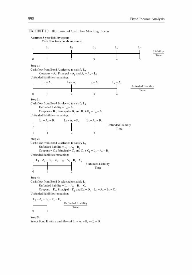
558 Fixed Income Analysis
EXHIBIT 10 Illustration of Cash Flow Matching Process
Assume: 5-year liability streamCash flow from bonds are annual.
Step 1:Cash flow from Bond A selected to satisfy L5
Step 1:Cash flow from Bond B selected to satisfy L4
Unfunded liabilities remaining:
Unfunded liabilities remaining:Coupons = Ac; Principal = Ap and Ac + Ap = L5
Coupons = Bc; Principal = Bp and Bc + Bp = L4 − Ac
Unfunded liability = L4 − Ac
Step 3:Cash flow from Bond C selected to satisfy L3
Unfunded liabilities remaining:Coupons = Cc; Principal = Cp and Cc + Cp = L3 − Ac − Bc
Unfunded liability = L3 − Ac − Bc
Step 4:Cash flow from Bond D selected to satisfy L2
Step 5:Select Bond E with a cash flow of L1 − Ac − Bc − Cc − Dc
Unfunded liabilities remaining:Coupons = Dc; Principal = Dp and Dc + Dp = L2 − Ac − Bc − Cc
Unfunded liability = L4 − Ac − Bc − Cc
L1
0 1 2 3 4
0 1 2 3
0 1 2
0 1
0 1
2
3
4
5
L2 L3 L4 L5
LiabilityTime
L1 − Ac L2 − Ac L3 − Ac L4 − Ac
Unfunded LiabilityTime
Unfunded LiabilityTime
Unfunded LiabilityTime
Unfunded LiabilityTime
L1 − Ac − Bc L2 − Ac − Bc L3 − Ac − Bc
L1 − Ac − Bc − Cc
L1 − Ac − Bc − Cc − Dc
L2 − Ac − Bc − Cc
Chapter 19 Portfolio Immunization and Cash Flow Matching 559
immunization or cash flow matching risk. However, given typical liability schedules andbonds available for cash flow matching, perfect matching is unlikely. Under such conditions,a minimum immunization risk approach would, at worst, be equal to cash flow matching andwould probably be better, because an immunization strategy is less costly to fund liabilities.This is due to two factors.
First, a relatively conservative rate of return assumption for short-term cash, which mayoccasionally be substantial, must be made throughout the life of the plan in cash flow matching,whereas an immunized portfolio is essentially fully invested at the remaining horizon duration.Second, funds from a cash flow matched portfolio must be available when each liability is dueand, because of the difficulty in perfect matching, usually before. An immunized portfolioneed only have sufficient value on the date of each liability because funding is achieved bya rebalancing of the portfolio. Because the reinvestment assumption for excess cash for cashflow matching is for many years into the future, a conservative assumption is appropriate.
Thus, even with the sophisticated linear programming techniques used in cash flowmatching, in most cases it will be more costly than immunization. However, cash flow matchingis easier to understand than multiple liability immunization, and this has occasionally led toits selection as the strategy for meeting liabilities (i.e., called dedicated portfolio strategies).
B. Extensions of Basic Cash Flow Matching
In the basic cash flow matching technique described above, only asset cash flows occurringprior to a liability date can be used to satisfy the liability. The technique can be extended tohandle situations in which cash flows occurring both before and after the liability date can beused to meet a liability.
A popular variation of multiple liability immunization and cash flow matching to fundliabilities is one that combines the two strategies. This strategy, referred to as combinationmatching or horizon matching, creates a portfolio that is duration-matched with the addedconstraint that it be cash matched in the first few years, usually five years. The advantage ofcombination matching over multiple liability immunization is that liquidity needs are providedfor in the initial cash flow matched period. Also, most of the positive slope or inversion of ayield curve tends to take place in the first few years. Cash flow matching the initial portion ofthe liability stream reduces the risk associated with nonparallel shifts of the yield curve. Thedisadvantage of combination matching over multiple liability immunization is that the cost isgreater.
CHAPTER 20RELATIVE-VALUE
METHODOLOGIES FORGLOBAL CREDIT BOND
PORTFOLIOMANAGEMENT∗
I. INTRODUCTION
Corporate bonds are the second oldest and, for most asset managers, the most demandingand fascinating subset of the global debt capital markets. The label, ‘‘corporate,’’ understatesthe scope of this burgeoning asset class. As commonly traded and administered within thecontext of an overall debt portfolio, the ‘‘corporate asset class’’ actually encompasses muchmore than pure corporate entities. Instead of the title, ‘‘corporate asset class,’’ this segmentof the global bond market really should be classified as the ‘‘credit asset class,’’ includingany nonagency mortgage-backed securities (MBS), commercial mortgage-backed securities(CMBS), asset-backed securities (ABS). Sovereigns and government-controlled entities withforeign currency debt issues thought to have more credit risk than the national governmentshould also be included. In keeping with conventional practice in the fixed-income markethowever, the application of the term ‘‘credit asset class’’ in this chapter will pertain only tocorporate bonds, sovereigns, and government-controlled entities.
From six continents, thousands of organizations (corporations, government agencies,projects and structured pools of debt securities) with different credit ‘‘stories’’ have sold debt tosustain their operations and to finance their expansion. These borrowers use dozens of differenttypes of debt instruments (first mortgage bonds, debentures, equipment trust certificates,subordinated debentures, medium-term notes, floating rate notes, private placements, preferredstock) and in multiple currencies (dollars, yen, euros, Swiss francs, pounds) from maturitiesranging from one year to even a thousand years. Sometimes these debt structures carryembedded options, which may allow for full or partial redemption prior to maturity at theoption of either the borrower or the investor. Sometimes, the coupon payment floats withshort-term interest rates or resets to a higher rate after a fixed interval or a credit rating change.
∗This chapter is authored by Jack Malvey, CFA.
560
Relative-Value Methodologies for Global Credit Bond Portfolio Management 561
Investors buy credit assets because of the presumption of higher long-term returns despitethe assumption of credit risk. Except near and during recessions, credit products usuallyoutperform U.S. Treasury securities and other higher-quality ‘‘spread sectors’’ like U.S. agencysecurities, mortgage-backed securities, and asset-backed securities. In the 30-year period sincethe beginning of the Lehman indices (1973 through 2002), investment-grade credit outper-formed U.S. Treasuries by 30 basis points (bp) per year on average (9.42% versus 9.12%).1 Asusual, an average masks the true daily, weekly, monthly, and annual volatility of credit assetsrelative performance. Looking at the rolling 5-year excess returns of U.S. investment-gradecredit from 1926 through early 2003 in Exhibit 1, one can observe extended periods of gen-erous and disappointing returns for credit assets. Perhaps more meaningful, an examinationof volatility-adjusted (Sharpe ratio) excess returns over Treasuries over a rolling 5-year periodshown in Exhibit 2 further underscores the oscillations in relative credit performance.
Global credit portfolio management presents a complex challenge. Each day, hundreds ofcredit portfolio managers face thousands of choices in the primary (new issue) and secondarymarkets. In addition to tracking primary and secondary flows, investors have to keep tabson ever-varying issuer fundamentals, creditworthiness, acquisitions, earnings, ratings, etc. Thetask of global credit portfolio management is to process all of this rapidly changing informationabout the credit markets (issuers, issues, dealers, and competing managers) and to constructthe portfolio with the best return for a given risk tolerance. This discipline combines thequalitative tools of equity analysis with the quantitative precision of fixed-income analysis.This chapter provides a brief guide to methodologies that may help portfolio managers meetthis formidable challenge.
II. CREDIT RELATIVE-VALUE ANALYSIS
Credit portfolio management represents a major subset of the multi-asset global portfoliomanagement process illustrated in Exhibit 3. After setting the currency allocation (in this case,dollars were selected for illustration convenience) and distribution among fixed-income assetclasses, bond managers are still left with a lengthy list of questions to construct an optimalcredit portfolio. Some examples are:
• Should U.S. investors add U.S. dollar-denominated bonds of non-U.S. issuers?• Should central banks add high-quality euro-denominated corporate bonds to their reserve
holdings?• Should LIBOR-funded London-based portfolio managers buy fixed-rate U.S. industrial
paper and swap into floating-rate notes?• Should Japanese mutual funds own euro-denominated telecommunications debt, swapped
back into dollars or yen using currency swaps?• Should U.S. insurers buy perpetual floaters (i.e., floaters without a maturity date) issued
by British banks and swap back into fixed-rate coupons in dollars using a currency/interestrate swap?
• When should investors reduce their allocation to the credit sector and increase allocationto governments, pursue a ‘‘strategic upgrade trade’’ (sell Baa/BBBs and buy higher-ratedAa/AA credit debt), rotate from industrials into utilities, switch from consumer cyclicals to
1Based on absolute returns of key Lehman indices from 1973.
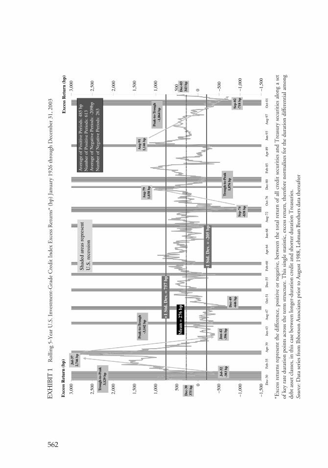
EX
HIB
IT1
Rol
ling
5-Y
ear
U.S
.Inv
estm
ent-
Gra
deC
redi
tIn
dex
Exc
ess
Ret
urns
*(b
p)Ja
nuar
y19
26th
roug
hD
ecem
ber
31,2
003
Exc
ess
Ret
urn
(bp)
Shad
ed a
reas
rep
rese
ntU
.S. r
eces
sion
Ave
rage
of
Posi
tive
Peri
ods:
485
bp
Num
ber
of P
ositi
ve P
erio
ds: 6
13
Num
ber
of N
egat
ive
Peri
ods:
263
Ave
rage
of
Neg
ativ
e Pe
riod
s: -
209b
p
Jul-
372,
746
bp
Tro
ugh-
to-P
eak
3,12
9 bp
Pea
k-to
-Tro
ugh
-3,1
42 b
p
Mea
n =
276
bp
+1 S
td. D
ev. =
757
bp
-1 S
td. D
ev. =
-20
5 bp
Dec
-30
375
bp
Jul-
32-3
83 b
pJu
n-42
-396
bp
Dec
-49
-646
bp
Sep-
74-8
38 b
p
Sep-
02-7
18 b
p
Aug
-79
1,03
8 bp
Aug
-91
1,14
6 bp
Pea
k-to
-Tro
ugh
-1,8
64 b
p
Dec
-03
343
bp
Exc
ess
Ret
urn
(bp)
Tro
ugh-
to-P
eak
1,87
6 bp
Feb-
35D
ec-3
0A
pr-3
9Ju
n-43
Aug
-47
Oct
-51
Dec
-55
Feb-
60A
pr-6
4Ju
n-68
Aug
-72
Oct
-76
Dec
-80
Feb-
85A
pr-8
9Ju
n-93
Aug
-97
Oct
-01
3,00
03,
000
2,50
0
2,00
0
1,50
0
1,00
0
500
0 −500
−1,0
00
−1,5
00
2,50
0
2,00
0
1,50
0
1,00
0
500
−500
−1,0
00
−1,5
000
∗ Exc
ess
retu
rns
repr
esen
tth
edi
ffere
nce,
posi
tive
orne
gati
ve,b
etw
een
the
tota
lret
urn
ofal
lcre
dit
secu
riti
esan
dT
reas
ury
secu
riti
esal
ong
ase
tof
key
rate
dura
tion
poin
tsac
ross
the
term
stru
ctur
e.T
his
sing
lest
atis
tic,
exce
ssre
turn
,the
refo
reno
rmal
izes
for
the
dura
tion
diffe
rent
iala
mon
gde
btas
set
clas
ses,
inth
isca
sebe
twee
nlo
nger
-dur
atio
ncr
edit
and
shor
ter
dura
tion
Tre
asur
ies.
Sour
ce:D
ata
seri
esfr
omIb
bots
onA
ssoc
iate
spr
ior
toA
ugus
t198
8,Le
hman
Bro
ther
sda
tath
erea
fter
562
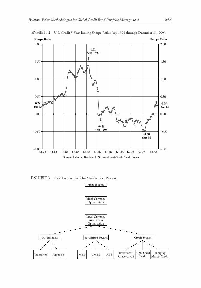
Relative-Value Methodologies for Global Credit Bond Portfolio Management 563
EXHIBIT 2 U.S. Credit 5-Year Rolling Sharpe Ratio: July 1993 through December 31, 2003
Source: Lehman Brothers U.S. Investment-Grade Credit Index
Sharpe Ratio Sharpe Ratio
2.00
1.50
1.00
0.50
0.26Jul-93
1.61Sept-1997
-0.50Sep-02
-0.18Oct-1998
0.25Dec-03
0.00
−1.00
−0.50
2.00
1.50
1.00
0.50
0.00
−1.00
−0.50
Jul-93 Jul-94 Jul-95 Jul-96 Jul-97 Jul-98 Jul-99 Jul-00 Jul-01 Jul-02 Jul-03
EXHIBIT 3 Fixed Income Portfolio Management Process
Fixed Income
Multi-CurrencyOptimization
Local CurrencyAsset Class
Optimization
Securitized SectorsGovernments
Treasuries Agencies MBS CMBS ABSInvestment-Grade Credit
High-YoeldCredit
Emerging-Market Credit
Credit Sectors
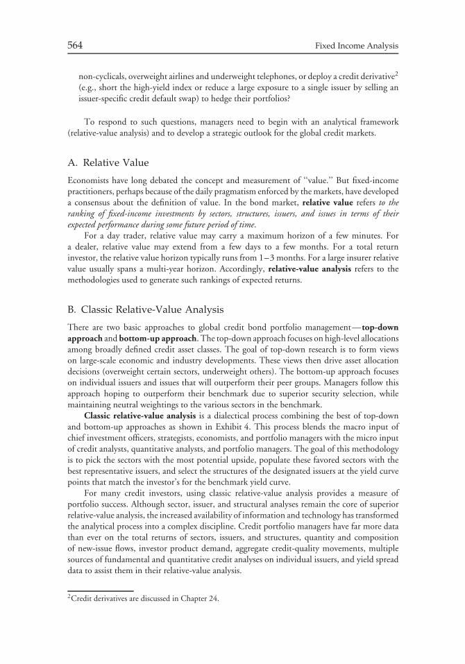
564 Fixed Income Analysis
non-cyclicals, overweight airlines and underweight telephones, or deploy a credit derivative2
(e.g., short the high-yield index or reduce a large exposure to a single issuer by selling anissuer-specific credit default swap) to hedge their portfolios?
To respond to such questions, managers need to begin with an analytical framework(relative-value analysis) and to develop a strategic outlook for the global credit markets.
A. Relative Value
Economists have long debated the concept and measurement of ‘‘value.’’ But fixed-incomepractitioners, perhaps because of the daily pragmatism enforced by the markets, have developeda consensus about the definition of value. In the bond market, relative value refers to theranking of fixed-income investments by sectors, structures, issuers, and issues in terms of theirexpected performance during some future period of time.
For a day trader, relative value may carry a maximum horizon of a few minutes. Fora dealer, relative value may extend from a few days to a few months. For a total returninvestor, the relative value horizon typically runs from 1–3 months. For a large insurer relativevalue usually spans a multi-year horizon. Accordingly, relative-value analysis refers to themethodologies used to generate such rankings of expected returns.
B. Classic Relative-Value Analysis
There are two basic approaches to global credit bond portfolio management—top-downapproach and bottom-up approach. The top-down approach focuses on high-level allocationsamong broadly defined credit asset classes. The goal of top-down research is to form viewson large-scale economic and industry developments. These views then drive asset allocationdecisions (overweight certain sectors, underweight others). The bottom-up approach focuseson individual issuers and issues that will outperform their peer groups. Managers follow thisapproach hoping to outperform their benchmark due to superior security selection, whilemaintaining neutral weightings to the various sectors in the benchmark.
Classic relative-value analysis is a dialectical process combining the best of top-downand bottom-up approaches as shown in Exhibit 4. This process blends the macro input ofchief investment officers, strategists, economists, and portfolio managers with the micro inputof credit analysts, quantitative analysts, and portfolio managers. The goal of this methodologyis to pick the sectors with the most potential upside, populate these favored sectors with thebest representative issuers, and select the structures of the designated issuers at the yield curvepoints that match the investor’s for the benchmark yield curve.
For many credit investors, using classic relative-value analysis provides a measure ofportfolio success. Although sector, issuer, and structural analyses remain the core of superiorrelative-value analysis, the increased availability of information and technology has transformedthe analytical process into a complex discipline. Credit portfolio managers have far more datathan ever on the total returns of sectors, issuers, and structures, quantity and compositionof new-issue flows, investor product demand, aggregate credit-quality movements, multiplesources of fundamental and quantitative credit analyses on individual issuers, and yield spreaddata to assist them in their relative-value analysis.
2Credit derivatives are discussed in Chapter 24.
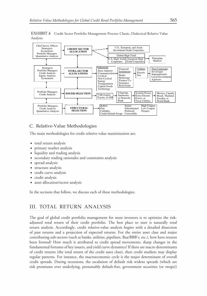
Relative-Value Methodologies for Global Credit Bond Portfolio Management 565
EXHIBIT 4 Credit Sector Portfolio Management Process: Classic, Dialectical Relative ValueAnalysis
Chief Invest. OfficerStrategistsEconomists
Portfolio ManagersQuantitative Analysis
StrategistsPortfolio Managers
Credit AnalysisEquity Analysis
Economists
Portfolio ManagersCredit Analysis
Portfolio ManagersCredit Analysis
Quantitative Analysis
CREDIT SECTORALLOCATION
INTRA-SECTORALLOCATIONS
ISSUER SELECTION
STRUCTURALSELECTION
U.S., European, and AsianInvestment-Grade Corporates
Global High YieldU.S. High Yield
CorporatesEuropean High
Yield CorporatesEmergingMarkets
IndustrialsBasic IndustryCommunicationsCyclicalNon-CyclicalEnergyTransportationCapital GoodsTechnology
Volkswagen,Toyota, or GM
BulletsPutsCallablesCredit Default Swaps
SeniorSubordinatedPreferredConvertible
High CouponLow CouponFloaters
FinancialInstitutionsBanksBrokerageFinance Co.InsuranceReal Estate
Utilities
ElectricGas
Non-CorporatesSovereignsSupranationalsLocal GovernmentAgencies
Citigroup,Sumitomo,or DeutscheBank
Scottish Power,Korea ElectricPower, orTexas Utilities
Mexico, Canada,Brazil, Thailand,Sweden, orWorld Bank
C. Relative-Value Methodologies
The main methodologies for credit relative-value maximization are:
• total return analysis• primary market analysis• liquidity and trading analysis• secondary trading rationales and constraints analysis• spread analysis• structure analysis• credit curve analysis• credit analysis• asset allocation/sector analysis
In the sections that follow, we discuss each of these methodologies.
III. TOTAL RETURN ANALYSIS
The goal of global credit portfolio management for most investors is to optimize the risk-adjusted total return of their credit portfolio. The best place to start is naturally totalreturn analysis. Accordingly, credit relative-value analysis begins with a detailed dissectionof past returns and a projection of expected returns. For the entire asset class and majorcontributing sub-sectors (such as banks, utilities, pipelines, Baa/BBB’s, etc.), how have returnsbeen formed? How much is attributed to credit spread movements, sharp changes in thefundamental fortunes of key issuers, and yield curve dynamics? If there are macro determinantsof credit returns (the total return of the credit asset class), then credit markets may displayregular patterns. For instance, the macroeconomic cycle is the major determinant of overallcredit spreads. During recessions, the escalation of default risk widens spreads (which arerisk premiums over underlying, presumably default-free, government securities (or swaps))
566 Fixed Income Analysis
and reduces credit returns relative to Treasuries. Conversely, economic prosperity reducesbankruptcies and enhances overall credit fundamentals of most issuers. Economic prosperityusually leads to tighter credit spreads and boosts credit returns relative to Treasuries. For briefintervals, noncyclical technical factors can offset fundamentals. For example, the inversionof the U.S. Treasury yield curve in 2000 actually led to wider credit spreads and creditunderperformance despite solid global economic growth and corporate profitability.
Thanks to the development of total return indices for credit debt (databases of prices,spreads, issuer, and structure composition), analyses of monthly, annual, and multi-year totalreturns have uncovered numerous patterns (i.e., large issue versus small issue performancevariation, seasonality, election-cycle effects, and government benchmark auction effects) in theglobal credit market. Admittedly, these patterns do not always re-occur. But an awareness andunderstanding of these total-return patterns are essential to optimizing portfolio performance.
IV. PRIMARY MARKET ANALYSIS
The analysis of primary markets centers on new issue supply and demand. Supply is often amisunderstood factor in tactical relative-value analysis. Prospective new supply induces manytraders, analysts, and investors to advocate a defensive stance toward the overall corporatemarket as well as toward individual sectors and issuers. Yet the premise, ‘‘supply will hurtspreads,’’ which may apply to an individual issuer, does not generally hold up for the entirecredit market. Credit spreads are determined by many factors; supply, although important,represents one of many determinants. During most years, increases in issuance (most notablyduring the first quarter of each year) are associated with market-spread contraction and strongrelative returns for credit debt. In contrast, sharp supply declines are accompanied frequentlyby spread expansion and a major fall in both relative and absolute returns for credit securities.For example, this counter-intuitive effect was most noticeable during the August-October1998 interval when new issuance nearly disappeared in the face of the substantial increase incredit spreads. (This period is referred to as the ‘‘Great Spread-Sector Crash.’’)
In the investment-grade credit market, heavy supply often compresses spreads and boostrelative returns for credit assets as new primary valuations validate and enhance secondaryvaluations. When primary origination declines sharply, secondary traders lose reinforcementfrom the primary market and tend to reduce their bid spreads. Contrary to the normal supply-price relationship, relative credit returns often perform best during periods of heavy supply.For example, 2001 will be recalled for both the then all-time record for new credit originationas well as the best relative performance for U.S. credit securities in nearly two decades.
A. The Effect of Market-Structure Dynamics
Given their immediate focus on the deals of the day and week, portfolio managers oftenoverlook short-term and long-term market-structure dynamics in making portfolio decisions.Because the pace of change in market structure is often gradual, market dynamics have lesseffect on short-term tactical investment decision-making than on long-term strategy.
The composition of the global credit bond market has shifted markedly since the early1980s. Medium-term notes (MTN) dominate issuance in the front end of the credit yield curve.Structured notes and swap products have heralded the introduction of derivative instrumentsinto the mainstream of the credit market. The high-yield corporate sector has become anaccepted asset class. Global origination has become more popular for U.S. governmentagencies, supranationals (e.g., The World Bank), sovereigns, and large corporate borrowers.
Relative-Value Methodologies for Global Credit Bond Portfolio Management 567
Although the ascent of derivatives and high-yield instruments stands out during the1990s, the true globalization of the credit market was the most important development. Therapid development of the Eurobond market since 1975, the introduction of many non-U.S.issuers into the dollar markets during the 1990s, and the birth of the euro on January 1, 1999,have led to the proliferation of truly transnational credit portfolios.
These long-term structural changes in the composition of the global credit asset class arisedue to the desire of issuers to minimize funding costs under different yield curve and yieldspread, as well as the needs of both active and asset/liability bond managers to satisfy their riskand return objectives. Portfolio managers will adapt their portfolios either in anticipation ofor in reaction to these structural changes across the global credit markets.
B. The Effect of Product Structure
Partially offsetting this proliferation of issuers since the mid-1990s, the global credit markethas become structurally more homogeneous. Specifically, bullet and intermediate-maturitystructures have come to dominate the credit market. A bullet maturity means that the issueis not callable, putable, or sinkable prior to its scheduled final maturity. The trend towardbullet securities does not pertain to the high-yield market, where callables remain the structureof choice. With the hope of credit-quality improvement, many high-yield issuers expect torefinance prior to maturity at lower rates.
There are three strategic portfolio implications for this structural evolution. First, thedominance of bullet structures translates into scarcity value for structures with embeddedcall and put features. That is, credit securities with embedded options have become rareand therefore demand a premium price. Typically, this premium (price) is not capturedby option-valuation models. Yet, this ‘‘scarcity value’’ should be considered by managers inrelative-value analysis of credit bonds.
Second, bonds with maturities beyond 20 years are a small share of outstanding creditdebt. This shift reduced the effective duration of the credit asset class and cut aggregatesensitivity to interest-rate risk. For asset/liability managers with long time horizons, this shiftof the maturity distribution suggests a rise in the value of long credit debt and helps to explainthe warm reception afforded, initially at least, to most new offerings of issues with 100-yearmaturities in the early and mid-1990s.
Third, the use of credit derivatives has skyrocketed since the early 1990s. The rapidmaturation of the credit derivative market will lead investors and issuers to develop newstrategies to match desired exposures to credit sectors, issuers, and structures.
V. LIQUIDITY AND TRADING ANALYSIS
Short-term and long-term liquidity needs influence portfolio management decisions. Citinglower expected liquidity, some investors are reluctant to purchase certain types of issues such assmall-sized issues (less than $1.0 billion), private placements, MTNs, and non-local corporateissuers. Other investors gladly exchange a potential liquidity disadvantage for incrementalyield. For investment-grade issuers, these liquidity concerns often are exaggerated.
As explained earlier, the liquidity of credit debt changes over time. Specifically, liquidityvaries with the economic cycle, credit cycle, shape of the yield curve, supply, and the season.As in all markets, unknown shocks, like a surprise wave of defaults, can reduce credit debtliquidity as investors become unwilling to purchase new issues at any spread and dealersbecome reluctant to position secondary issues except at very wide spreads. In reality, these
568 Fixed Income Analysis
transitory bouts of illiquidity mask an underlying trend toward heightened liquidity acrossthe global credit asset class. With a gentle push from regulators, the global credit asset class iswell along in converting from its historic ‘‘over-the-counter’’ domain to a fully transparent,equity/U.S. Treasury style marketplace. In the late 1990s, new technology led to creatingECNs (electronic communication networks), essentially electronic trading exchanges. In turn,credit bid/ask spreads generally have trended lower for very large, well-known corporate issues.This powerful twin combination of technological innovation and competition promises therapid development of an even more liquid and efficient global credit market during the early21st Century.
VI. SECONDARY TRADE RATIONALES
Capital market expectations constantly change. Recessions may arrive sooner rather than later.The yield curve may steepen rather than flatten. The auto and paper cycles may be movingdown from their peaks. Higher oil and natural gas prices may benefit the credit quality of theenergy sector. An industrial may have announced a large debt-financed acquisition, earningan immediate ratings rebuke from the rating agencies. A major bank may plan to repurchase15% of its outstanding common stock (great for shareholders but leading to higher financialleverage for debtholders). In response to such daily information flows, portfolio managersamend their holdings. To understand trading flows and the real dynamics of the credit market,investors should consider the most common rationales of whether to trade and not to trade.
A. Popular Reasons for Trading
There are dozens of rationales to execute secondary trades when pursuing portfolio optimiza-tion. Several of the most popular are discussed below. The framework for assessing secondarytrades is the total return framework explained in Chapter 18.
1. Yield/Spread Pickup Trades Yield/spread pickup trades represent the most com-mon secondary transactions across all sectors of the global credit market. Historically, atleast half of all secondary swaps reflect investor intentions to add additional yield within theduration and credit-quality constraints of a portfolio. If 5-year, Baa1/BBB General Motorspaper trades at 150 bp, 10 bp more than 5-year, Baa1/BBB–Ford Motor, some investors willdetermine the rating differential irrelevant and purchase General Motors bond and sell theFord Motor (an issue swap) for a spread gain of 10 bp per annum.
This ‘‘yield-first psychology’’ reflects the institutional yield need of long-term asset/liabilitymanagers. Despite the passage of more than three decades, this investor bias toward yield maxi-mization also may be a methodological relic left over from the era prior to the introduction andmarket acceptance of total-return indices in the early-1970s. The limitations of yield measuresas an indicator of potential performance were explained and the total return framework wasdemonstrated to be a superior framework for assessing potential performance for a trade.
2. Credit-Upside Trades Credit-upside trades take place when the debt asset managerexpects an upgrade in an issuer’s credit quality that is not already reflected in the currentmarket yield spread. In the illustration of the General Motors and Ford Motor trade describedabove, some investors may swap based on their view of potential credit-quality improvementfor General Motors. Obviously, such trades rely on the credit analysis skills of the investmentmanagement team. Moreover, the manager must be able to identify a potential upgrade before
Relative-Value Methodologies for Global Credit Bond Portfolio Management 569
the market, otherwise the spread for the upgrade candidate will already exhibit the benefits ofa credit upgrade.
Credit-upside trades are particularly popular in the crossover sector—securities withratings between Ba2/BB and Baa3/BBB- by two major rating agencies. In this case, theportfolio manager is expressing an expectation that an issue of the highest speculative graderating (Ba1/BB+) has sufficiently positive credit fundamentals to be upgraded to investmentgrade (i.e., Baa3/BBB-). If this upgrade occurs, not only would the issue’s spread narrowbased on the credit improvement (with an accompanying increase in total return, all elseequal), but the issue also would benefit from improved liquidity, as managers prohibited frombuying high-yield bonds could then purchase that issue. Further, the manager would expectan improvement in the portfolio’s overall risk profile.
3. Credit-Defense Trades Credit-defense trades become more popular as geopoliticaland economic uncertainty increase. Secular sector changes often generate uncertainties andinduce defensive positioning by investors. In anticipating greater competition, in the mid-1990s some investors reduced their portfolio exposures to sectors like electric utilities andtelecommunications. As some Asian currencies and equities swooned in mid-1997, manyportfolio managers cut their allocation to the Asian debt market. Unfortunately becauseof yield-maximization needs and a general reluctance to realize losses by some institutions(i.e., insurers), many investors reacted more slowly to credit-defensive positioning. But aftera record number of ‘‘fallen angels’’ in 2002, which included such major credit bellwetherissuers as WorldCom, investors became more quick to jettison potential problem creditsfrom their portfolios. Ironically once a credit is downgraded by the rating agencies, internalportfolio guidelines often dictate security liquidation immediately after the loss of single-A orinvestment-grade status. This is usually the worst possible time to sell a security and maximizeslosses incurred by the portfolio.
4. New Issue Swaps New-issue swaps contribute to secondary turnover. Because ofperceived superior liquidity, many portfolio managers prefer to rotate their portfolios graduallyinto more current and usually larger sized on-the-run issues. This disposition, reinforced bythe usually superior market behavior of newer issues in the U.S. Treasury market (i.e., theon-the-run issues), has become a self-fulfilling prophecy for many credit issues. In addition,some managers use new issue swaps to add exposure to a new issuer or a new structure.
5. Sector-Rotation Trades Sector-rotation trades, within credit and among fixed-income asset classes, have become more popular since the early 1990s. In this strategy, the man-ager shifts the portfolio from a sector or industry that is expected to underperform to a sector orindustry which is believed will outperform on a total return basis. With the likely developmentof enhanced liquidity and lower trading transaction costs across the global bond market in theearly 21st Century, sector-rotation trades should become more prevalent in the credit asset class.
Such intra-asset class trading already has played a major role in differentiating performanceamong credit portfolio managers. For example, as soon as the Fed launched its preemptivestrike against inflation in February 1994, some investors correctly exchanged fixed-rate corpo-rates for floating-rate corporates. In 1995, the specter of U.S. economic weakness promptedsome investors in high-yield corporates to rotate from consumer-cyclical sectors like autos andretailing into consumer non-cyclical sectors like food, beverage, and healthcare. Anticipatingslower U.S. economic growth in 1998 induced a defensive tilt by some portfolio managersaway from other cyclical groups like paper and energy. The resurrection of Asian and European
570 Fixed Income Analysis
economic growth in 1999 stimulated increased portfolio interest in cyclicals, financial institu-tions, and energy debt. Credit portfolio managers could have avoided a great deal of portfolioperformance disappointment in 2002 by underweighting utilities and many industrial sectors.
6. Curve Adjustment Trades Yield curve-adjustment trades, or simply, curve-adjustment trades are taken to reposition a portfolio’s duration. For most credit investors,their portfolio duration is typically within a range from 20% below to 20% above the durationof the benchmark index. If credit investors could have predicted U.S., euro, and yen yieldcurve movements perfectly in 2002, then they would have increased their credit portfolioduration at the beginning of 2002 in anticipation of a decrease in interest rates. Althoughmost fixed-income investors prefer to alter the duration of their aggregate portfolios in themore-liquid Treasury market, strategic portfolio duration tilts also can be implemented in thecredit market.
This is also done with respect to anticipated changes in the credit term structure or creditcurve. For example, if a portfolio manager believes credit spreads will tighten (either overallor in a particular sector), with rates in general remaining relatively stable, they might shift theportfolio’s exposure to longer spread duration issues in that sector.
7. Structure Trades Structure trades involve swaps into structures (e.g., callable struc-tures, bullet structures, and putable structures) that are expected to have better performancegiven expected movements in volatility and the shape of the yield curve. Here are someexamples of how different structures performed in certain periods in the 1990s.
• During the second quarter of 1995, the rapid descent of the U.S. yield curve contributedto underperformance of high-coupon callable structures because of their negative convexityproperty.
• When the yield curve stabilized during the third quarter of 1995, investors were morewilling to purchase high-quality callable bonds versus high-quality bullet structures to earnan extra 35 bp of spread.
• The sharp downward rotation of the U.S. yield curve during the second half of 1997 con-tributed to poor relative performance by putable structures. The yield investors had sacrificedfor protection against higher interest rates instead constrained total return as rates fell.
• The plunge in U.S. interest rates and escalation of yield-curve volatility during the secondhalf of 1998 again restrained the performance of callable structures compared to bulletstructures.
• The upward rebound in U.S. interest rates and the fall in interest-rate volatility during 1999contributed to the relative outperformance of callable structures versus bullet structures.
These results follow from the price/yield properties of the different structures that wereexplained previously. Structural analysis is also discussed in Section VIII of this chapter.
8. Cash Flow Reinvestment Cash flow reinvestment forces investors into the sec-ondary market on a regular basis. During 2003, the sum of all coupon, maturity, and partialredemptions (via tenders, sinking funds, and other issuer prepayments) equaled approximately100% of all new gross issuance across the dollar bond market. Before the allocation of anynet new investment in the bond market, investors had sufficient cash flow reinvestment toabsorb nearly all new bond supply. Some portfolio cash inflows occur during interludes inthe primary market or the composition of recent primary supply may not be compatible
Relative-Value Methodologies for Global Credit Bond Portfolio Management 571
with portfolio objectives. In these periods, credit portfolio managers must shop the secondarymarket for investment opportunities to remain fully invested or temporarily replicate thecorporate index by using financial futures. Portfolio managers who incorporate analysis of cashflow reinvestment into their valuation of the credit market can position their portfolios to takeadvantage of this cash flow reinvestment effect on spreads.
B. Trading Constraints
Portfolio managers also should review their main rationales for not trading. Some of the bestinvestment decisions are not to trade. Conversely, some of the worst investment decisionsemanate from stale views based on dated and anachronistic constraints (e.g., avoid investingin bonds rated below Aa/AA). The best portfolio managers retain very open minds, constantlyself-critiquing both their successful and unsuccessful methodologies.
1. Portfolio Constraints Collectively, portfolio constraints are the single biggest contrib-utor to the persistence of market inefficiency across the global credit market. Here are someexamples:
• Because many asset managers are limited to holding securities with investment-graderatings, they are forced to sell immediately the debt of issuers who are downgraded tospeculative-gradings (Ba1/BB+ and below). In turn, this selling at the time of downgradeprovides an opportunity for investors with more flexible constraints to buy such newlydowngraded securities at a temporary discount (provided, of course, that the issuer’screditworthiness stabilizes after downgrade).
• Some U.S. state employee pension funds cannot purchase credit securities with ratingsbelow A3/A—due to administrative and legislative guidelines.
• Some U.S. pension funds also have limitations on their ownership of MTNs and non-U.S.corporate issues.
• Regulators have limited U.S. insurance companies investment in high-yield corporates.• Many European investors are restricted to issues rated at least single-A and sometimes
Aa3/AA—and above, created originally in annual-pay Eurobond form.• Many investors are confined to their local currency market—yen, sterling, euro, U.S.
dollar. Often, the same issuer, like Ford, will trade at different spreads across differentgeographic markets.
• Globally, many commercial banks must operate exclusively in the floating-rate realm: allfixed-rate securities, unless converted into floating-rate cash flows via an interest rate swap,are prohibited.
2. ‘‘Story’’ Disagreement ‘‘Story’’ disagreement can work to the advantage or disad-vantage of a portfolio manager. Traders, salespersons, sell-side analysts and strategists, andbuy-side credit research have dozens of potential trade rationales that supposedly will benefitportfolio performance. The proponents of a secondary trade may make a persuasive argument,but the portfolio manager may be unwilling to accept the ‘‘shortfall risk’’3 if the investmentrecommendation does not provide its expected return. For example in early 1998, analystsand investors alike were divided equally on short-term prospects for better valuations of
3Shortfall risk is explained in Chapter 17. Shortfall risk is the probability that the outcome will have avalue less than the target return.
572 Fixed Income Analysis
Asian sovereign debt. After a very disappointing 1997 for Asian debt performance, Asiaenthusiasts had little chance to persuade pessimists to buy Asian debt at the beginning of1998. Technically, such lack of consensus in the credit market signals an investment withgreat outperformance potential. Indeed, most Asian debt issues recorded exceptional outper-formance over the full course of 1998 and 1999. After a difficult 2002, the same ‘‘reboundeffect’’ was observed in electric utilities during 2003. Of course, ‘‘story’’ disagreement can alsowork in the other direction. For example, Enron was long viewed as a very solid credit beforeits sudden bankruptcy in late 2001. An asset manager wedded to this long-term view mighthave been reluctant to act on the emergence of less favorable information about Enron in thesummer of 2001.
3. Buy-and-Hold Although many long-term asset/liability managers claim to havebecome more total return focused in the 1990s, accounting constraints (cannot sell posi-tions at a loss compared with book cost or take too extravagant a gain compared with bookcost) often limit the ability of these investors to trade. Effectively, these investors (mainlyinsurers) remain traditional ‘‘buy-and-hold’’ investors. Some active bond managers have con-verged to quasi-‘‘buy-and-hold’’ investment programs at the behest of consultants to curbportfolio turnover. In the aftermath of the ‘‘Asian Contagion’’ in 1997–1998, this dispositiontoward lower trading turnover was reinforced by the temporary reduction in market liquidityprovided by more wary bond dealers. As shown in 2000–2002, however, a buy-and-holdstrategy can gravely damage the performance of a credit portfolio. At the first signs of credittrouble for an issuer, many credit portfolios would have improved returns by reducing theirexposure to a deteriorating credit.
4. Seasonality Secondary trading slows at month ends, more so at quarter ends, and themost at the conclusion of calendar years. Dealers often prefer to reduce their balance sheets atfiscal year-end (November 30, December 31, or March 31 (Japan)). Also, portfolio managerstake time to mark their portfolios, prepare reports for their clients, and chart strategy for thenext investment period. During these intervals, even the most compelling secondary offeringscan languish.
VII. SPREAD ANALYSIS
By custom, some segments of the high-yield and emerging (EMG) debt markets still prefer tomeasure value by bond price or bond yield rather than spread. But for the rest of the globalcredit market, nominal spread (the yield difference between corporate and government bondsof similar maturities) has been the basic unit of both price and relative-value analysis for morethan two centuries.
A. Alternative Spread Measures
Many U.S. practitioners prefer to value investment-grade credit securities in terms of option-adjusted spreads (OAS) so they can be more easily compared to the volatility (‘‘vol’’) sectors(mortgage-backed securities and U.S. agencies).4 But given the rapid reduction of credit
4These sectors are referred to as ‘‘vol’’ sectors because the value of the securities depends on expectedinterest rate volatility. These ‘‘vol’’ securities have embedded call options and the value of the options,and hence the value of the securities, depends on expected interest rate volatility.
Relative-Value Methodologies for Global Credit Bond Portfolio Management 573
structures with embedded options since 1990 (see structural discussion above), the use of OASin primary and secondary pricing has diminished within the investment-grade credit assetclass. Moreover, the standard one-factor binomial models5 do not account for credit spreadvolatility. Given the exclusion of default risk in OAS option-valuation models, OAS valuationhas seen only limited extension into the higher-risk markets of the quasi-equity, high-yieldcorporate, and EMG-debt asset classes.
Starting in Europe during the early 1990s and gaining momentum during the late 1990s,interest rate swap spreads have emerged as the common denominator to measure relative valueacross fixed- and floating-rate note credit structures. The U.S. investment-grade and high-yieldmarkets eventually may switch to swap spreads to be consistent with Europe and Asia.
Other U.S. credit spread calculations have been proposed, most notably using the U.S.agency benchmark curve. These proposals emanate from the assumption of a persistent U.S.budgetary surplus and significant liquidation of outstanding U.S. Treasury securities duringthe first decade of the 21st Century. As again demonstrated by 2002, history teaches that thesebudget assumptions may unfortunately prove to be faulty. Although some practitioners maychoose to derive credit-agency spreads for analytical purposes, this practice will be unlikely tobecome standard market convention.
Credit-default swap spreads have emerged as the latest valuation tool during the greatstresses in the credit markets of 2000–2002. Most likely, credit-default swap spreads will beused as a companion valuation reference to nomial spreads, OAS, and swap spreads. Themarket, therefore, has an ability to price any credit instrument using multiple spread references.These include the spread measures discussed earlier—nominal spread, static or zero-volatilityspread, OAS, credit-swap spreads (or simply swap spreads), and credit default spreads. Thespread measures used the Treasury yield curve or Treasury spot rate curve as the benchmark.Given the potential that swap spreads will become the new benchmark, these same measurescan be performed relative to swaps rather than relative to U.S. Treasuries. However, usingswap rates as a benchmark has been delayed by the decoupling of traditional credit spreads(credit yield minus government yield) from swap spreads over 2000–2002. Effectively, creditrisk during a global recession and its aftermath superseded the countervailing influence ofstrong technical factors like lower and steeper yield curves which affected the interest rate swapmarket differently.
B. Closer Look at Swap Spreads
Swap spreads became a popular valuation yardstick for credit debt in Europe during the 1990s.This practice was enhanced by the unique nature of the European credit asset class. Unlike itsAmerican counterpart, the European credit market has been consistently homogeneous. Mostissuance was of high quality (rated Aa3/AA–and above) and intermediate maturity (10 yearsand less). Consequently, swap spreads are a good proxy for credit spreads in such a uniformmarket. Most issuers were financial institutions, natural swappers between fixed-rate andfloating-rate obligations. And European credit investors, often residing in financial institutionslike commercial banks, have been much more willing to use the swap methodology to capturevalue discrepancies between the fixed- and floating-rate markets.
Structurally, the Asian credit market more closely resembles the European than the U.S.credit market. As a result, the use of swap spreads as a valuation benchmark also becamecommon in Asia.
5The model is referred to as a one-factor model because only the short-term rate is the factor used toconstruct the tree.
574 Fixed Income Analysis
The investment-grade segment of the U.S. credit market may well be headed towardan embrace of swap spreads. The U.S. MBS, CMBS, agency, and ABS sectors (accountingfor about 55% of the U.S. fixed-income market) made the transition to swap spreads as avaluation benchmark during the second half of the 1990s. Classical nominal credit spreadsderived directly from the U.S. Treasury yield curve were distorted by the special effects ofU.S. fiscal surpluses and buybacks of U.S. Treasury securities in 2000 and 2001. Accordingly,many market practitioners envision a convergence to a single global spread standard derivedfrom swap spreads.
Here is an illustration of how a bond manager can use the interest rate swap spreadframework. Suppose that a hypothetical Ford Motor Credit 71/2x’s of 2008 traded at a bidprice (i.e., the price at which a dealer is willing to buy the issue) of 113 bp over the 5-year U.S.Treasury yield of 6.43%. This equates to a yield-to-maturity of 7.56% (6.43% + 113 bp).On that date, 5-year swap spreads were 83 bp (to the 5-year U.S. Treasury). Recall that swapsare quoted where the fixed-rate payer pays the yield on a Treasury with a maturity equal to theinitial term of the swap plus the swap spread. The fixed-rate payer receives LIBOR flat—thatis, no increment over LIBOR. So, if the bond manager invests in the Ford Motor Credit issueand simultaneously enters into this 5-year swap, the following would result:
Receive from Ford Motor Credit (6.43% + 113 bp) 7.56%−Pay on swap (6.43% + 83 bp) 7.26%+ Receive from swap LIBORNet LIBOR + 30 bp
Thus, a bond manager could exchange this Ford Motor Credit bond’s fixed coupon flow forLIBOR + 30 bp. On the trade date, LIBOR was 6.24%, so that the asset swapper wouldearn 6.54% (= 6.24% + 30 bp) until the first reset date of the swap. A total return managerwould want to take advantage of this swap by paying fixed and receiving floating if he expectsinterest rates to increase in the future.
The swaps framework allows managers (as well as issuers) to more easily compare securitiesacross fixed-rate and floating-rate markets. The extension of the swap spread framework maybe less relevant for speculative-grade securities, where default risk becomes more important. Incontrast to professional money managers, individual investors are not comfortable using bondvaluation couched in terms of swap spreads. The traditional nominal spread framework iswell understood by individual investors, has the advantages of long-term market convention,and works well across the entire credit-quality spectrum from Aaa’s to B’s. However, thisnominal spread framework does not work very well for investors and issuers when comparingthe relative attractiveness between the fixed-rate and floating-rate markets.
C. Spread Tools
Investors should also understand how best to evaluate spread levels in their decision-making.Spread valuation includes mean-reversion analysis, quality-spread analysis, and percent yieldspread analysis.
1. Mean-Reversion Analysis The most common technique for analyzing spreads amongindividual securities and across industry sectors is mean-reversion analysis. The ‘‘mean’’ isthe average value of some variable over a defined interval (usually one economic cycle for thecredit market). The term ‘‘mean reversion’’ refers to the tendency for some variable’s value torevert (i.e., move towards) its average value. Mean-reversion analysis is a form of relative-value
Relative-Value Methodologies for Global Credit Bond Portfolio Management 575
analysis based on the assumption that the spread between two sectors or two issuers will revertback to its historical average. This would lead investors to buy a sector or issuer identifiedas ‘‘cheap’’ because historically the spread has been tighter and will eventually revert back tothat tighter spread. Also, this would lead investors to sell a sector or issuer identified as ‘‘rich’’because the spread has been wider and is expected to widen in the future.
Mean-reversion analysis involves the use of statistical analysis to assess whether the currentdeviation from the mean spread is significant. For example, suppose the mean spread foran issuer is 80 basis points over the past six months and the standard deviation is 12 basispoints. Suppose that the current spread of the issuer is 98 basis points. The spread is 18 basispoints over the mean spread or equivalently 1.5 standard deviations above the mean spread.The manager can use that information to determine whether or not the spread deviation issufficient to purchase the issue. The same type of analysis can be used to rank a group ofissuers in a sector.
Mean-reversion analysis can be instructive as well as misleading. The mean is highlydependent on the interval selected. There is no market consensus on the appropriate intervaland ‘‘persistence’’ frequents the credit market meaning cheap securities, mainly a function ofcredit uncertainty, often tend to become cheaper. Rich securities, usually high-quality issues,tend to remain rich.
2. Quality-Spread Analysis Quality-spread analysis examines the spread differentialsbetween low and high-quality credits. For example, portfolio managers would be welladvised to consider the ‘‘credit upgrade trade’’ discussed in Section VI when quality-spreadscollapse to cyclical troughs. The incremental yield advantage of lower-quality products maynot compensate investors for lower-quality spread expansion under deteriorating economicconditions. Alternatively, credit portfolio managers have long profited from overweightinglower-quality debt at the outset of an upward turn in the economic cycle.
3. Percent Yield Spread Analysis Dating from the early 20th Century, percent yieldspread analysis (the ratio of credit yields to government yields for similar duration securities)is another popular technical tool used by some investors. This methodology has seriousdrawbacks that undermine its usefulness. Percent yield spread is more a derivative than anexplanatory or predictive variable. The usual expansion of credit percent yield spreads duringlow-rate periods like 1997, 1998, and 2002 overstates the risk as well as the comparativeattractiveness of credit debt. And the typical contraction of credit percent yield spreads duringupward shifts of the benchmark yield curve does not necessarily signal an imminent bout ofunderperformance for the credit asset class. Effectively, the absolute level of the underlyingbenchmark yield is merely a single factor among many factors (demand, supply, profitability,defaults, etc.) that determine the relative value of the credit asset class. These other factors canoffset or reinforce any insights derived from percent yield spread analysis.
VIII. STRUCTURAL ANALYSIS
As explained earlier in this chapter, there are bullet, callable, putable, and sinking fundstructures. Structural analysis is simply analyzing the performance of the different structuresdiscussed throughout this chapter. While evaluating bond structures was extremely importantin the 1980s, it became less influential in credit bond market since the mid-1990s for severalreasons. First, the European credit bond market almost exclusively features intermediate
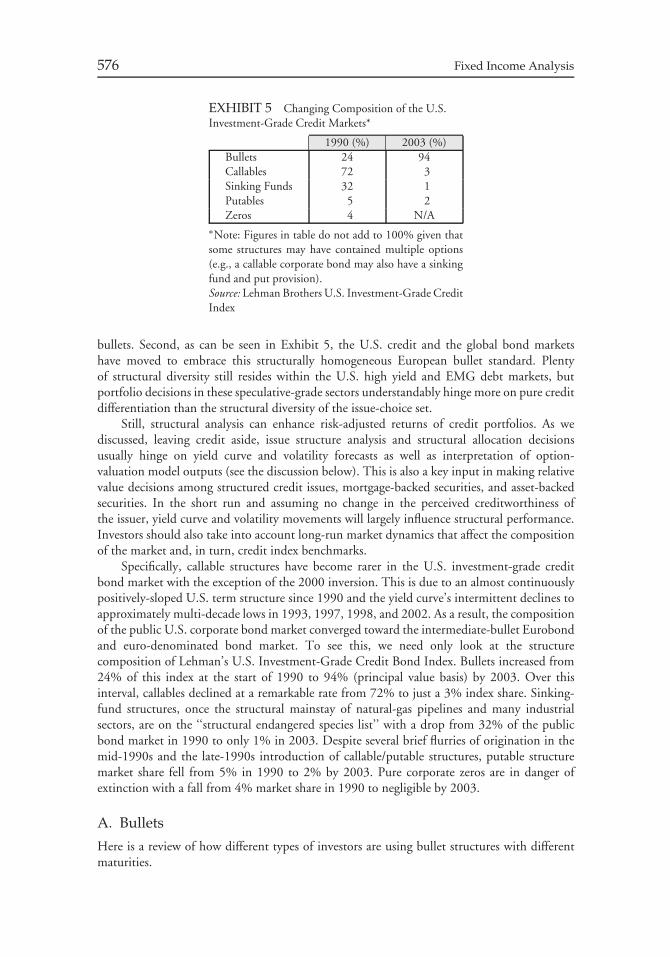
576 Fixed Income Analysis
EXHIBIT 5 Changing Composition of the U.S.Investment-Grade Credit Markets*
1990 (%) 2003 (%)Bullets 24 94Callables 72 3Sinking Funds 32 1Putables 5 2Zeros 4 N/A
∗Note: Figures in table do not add to 100% given thatsome structures may have contained multiple options(e.g., a callable corporate bond may also have a sinkingfund and put provision).Source: Lehman Brothers U.S. Investment-Grade CreditIndex
bullets. Second, as can be seen in Exhibit 5, the U.S. credit and the global bond marketshave moved to embrace this structurally homogeneous European bullet standard. Plentyof structural diversity still resides within the U.S. high yield and EMG debt markets, butportfolio decisions in these speculative-grade sectors understandably hinge more on pure creditdifferentiation than the structural diversity of the issue-choice set.
Still, structural analysis can enhance risk-adjusted returns of credit portfolios. As wediscussed, leaving credit aside, issue structure analysis and structural allocation decisionsusually hinge on yield curve and volatility forecasts as well as interpretation of option-valuation model outputs (see the discussion below). This is also a key input in making relativevalue decisions among structured credit issues, mortgage-backed securities, and asset-backedsecurities. In the short run and assuming no change in the perceived creditworthiness ofthe issuer, yield curve and volatility movements will largely influence structural performance.Investors should also take into account long-run market dynamics that affect the compositionof the market and, in turn, credit index benchmarks.
Specifically, callable structures have become rarer in the U.S. investment-grade creditbond market with the exception of the 2000 inversion. This is due to an almost continuouslypositively-sloped U.S. term structure since 1990 and the yield curve’s intermittent declines toapproximately multi-decade lows in 1993, 1997, 1998, and 2002. As a result, the compositionof the public U.S. corporate bond market converged toward the intermediate-bullet Eurobondand euro-denominated bond market. To see this, we need only look at the structurecomposition of Lehman’s U.S. Investment-Grade Credit Bond Index. Bullets increased from24% of this index at the start of 1990 to 94% (principal value basis) by 2003. Over thisinterval, callables declined at a remarkable rate from 72% to just a 3% index share. Sinking-fund structures, once the structural mainstay of natural-gas pipelines and many industrialsectors, are on the ‘‘structural endangered species list’’ with a drop from 32% of the publicbond market in 1990 to only 1% in 2003. Despite several brief flurries of origination in themid-1990s and the late-1990s introduction of callable/putable structures, putable structuremarket share fell from 5% in 1990 to 2% by 2003. Pure corporate zeros are in danger ofextinction with a fall from 4% market share in 1990 to negligible by 2003.
A. Bullets
Here is a review of how different types of investors are using bullet structures with differentmaturities.
Relative-Value Methodologies for Global Credit Bond Portfolio Management 577
Front-end bullets (i.e., bullet structures with 1- to 5-year maturities) have great appealfor investors who pursue a ‘‘barbell strategy.’’ A barbell strategy was described in which boththe short and long end of the barbell are U.S. Treasury securities. There are ‘‘barbellers’’ whouse credit securities at the front or short-end of the curve and Treasuries at the long-end ofthe yield curve. There are non-U.S. institutions who convert short bullets into floating-rateproducts by using interest rate swaps. The transactions are referred to as ‘‘asset swaps,’’ andthe investors who employ this transaction are referred to as ‘‘asset swappers.’’
Intermediate credit bullets (5- to 12-year maturities), especially the 10-year maturitysector, have become the most popular segment of the U.S. and European investment-gradeand high-yield credit markets. Fifteen-year maturities, benchmarked off the 10-year bellwetherTreasury, are comparatively rare and have been favored by banks that occasionally use themfor certain types of swaps. Because new 15-year structures take five years to descend along apositively sloped yield curve to their underlying 10-year bellwether, 15-year maturities holdless appeal for many investors in search of return through price appreciation emanating frombenchmark rolldown. In contrast, rare 20-year structures have been favored by many investors.Spreads for these structures are benched off the 30-year Treasury. With a positively slopedyield curve, the 20-year structure provides higher yield than a 10-year or 15-year security andless vulnerability (lower duration) than a 30-year security.
The 30-year maturity is the most popular form of long-dated security in the globalcredit market. In 1992, 1993, late 1995, and 1997, there was a minor rush to issue 50-year(half-Centuries) and 100-year (Centuries) securities in the U.S. credit bond market. These1onger-dated securities provide investors with extra positive convexity for only a modestincrease in effective (or modified-adjusted) duration.6 In the wake of the ‘‘Asian Contagion’’and especially the ‘‘Great Spread-Sector Crash’’ of August 1998, the cyclical increases in riskaversion and liquidity premiums greatly reduced both issuer and investor interest in theseultra-long maturities.
B. Callables
Typically after a 5-year or 10-year wait (longer for some rare issues), credit structures arecallable at the option of the issuer at any time. Call prices usually are set at a premium abovepar (par + the initial coupon) and decline linearly on an annual basis to par by 5–10 yearsprior to final scheduled maturity. The ability to refinance debt in a potentially lower-interestrate environment is extremely valuable to issuers. Conversely, the risk of earlier-than-expectedretirement of an above-current market coupon is bothersome to investors.
In issuing callables, issuers pay investors an annual spread premium (about 20 bp to 40bp for high-quality issuers) for being long (from an issuer’s perspective) the call option. Likeall security valuations, this call premium varies through time with capital market conditions.Given the higher chance of exercise, this call option becomes much more expensive during lowrate and high volatility periods. Since 1990, this call premium has ranged from approximately15 bp to 50 bp for investment-grade issuers. Callables significantly underperform bulletswhen interest rates decline because of their negative convexity. When the bond market rallies,callable structures do not fully participate given the upper boundary imposed by call prices.Conversely, callable structures outperform bullets in bear bond markets as the probability ofearly call diminishes.
6Recall that the longer the maturity, the greater the convexity.

578 Fixed Income Analysis
C. Sinking Funds
A sinking fund structure allows an issuer to execute a series of partial calls (annually orsemiannually) prior to maturity. Issuers also usually have an option to retire an additionalportion of the issue on the sinking fund date, typically ranging from 1 to 2 times the mandatorysinking fund obligation. Historically, especially during the early 1980s, total return investorsfavored the collection of sinking fund structures at sub-par prices. These discounted sinkingfunds retained price upside during interest rate rallies (provided the indicated bond priceremained below par), and, given the issuers’ requirement to retire at least annually someportion of the issue at par, the price of these sinking fund structures did not fall as muchcompared to callables and bullets when interest rates rose. It should be noted that astuteissuers with strong liability management skills can sometimes satisfy such annual sinking fundobligations in whole or in part through prior open market purchases at prices below par.Nonetheless, this annual sinking fund purchase obligation by issuers does limit bond pricedepreciation during periods of rising rates.
D. Putables
Conventional put structures are simpler than callables. Yet in trading circles, put bondvaluations often are the subject of debate. American-option callables grant issuers the rightto call an issue at any time at the designated call price after expiration of the non-callableor non-redemption period. Put bonds typically provide investors with a one-time, one-dateput option (European option) to demand full repayment at par. Less frequently, put bondsinclude a second or third put option date. A very limited number of put issues afford investorsthe privilege to put such structures back to the issuers at par in the case of rating downgrades(typically to below investment-grade status).
Thanks to falling interest rates, issuers shied away from new put structures as the 1990sprogressed. Rather than incur the risk of refunding the put bond in 5 or 10 years at a highercost, many issuers would prefer to pay an extra 10 bp to 20 bp in order to issue a longer-termliability.
Put structures provide investors with a partial defense against sharp increases in interestrates. Assuming that the issuer still has the capability to meet its sudden obligation, putstructures triggered by a credit event enable investors to escape from a deteriorating credit.Perhaps because of its comparative scarcity, the performance and valuation of put structureshave been a challenge for many portfolio managers. Unlike callable structures, put prices havenot conformed to expectations formed in a general volatility-valuation framework. Specifically,as explained, the implied yield volatility of an option can be computed from the option’s priceand a valuation model. In the case of a putable bond, the implied volatility can be obtainedusing a valuation model such as the binomial model. The implied volatility should be thesame for both puts and calls, all factors constant. Yet, for putable structures, implied volatilityhas ranged between 4%–9% since 1990, well below the 10%-20% volatility range associatedwith callable structures for the same time period. This divergence in implied volatility betweencallables (high) and putables (low) suggests that asset managers, often driven by a desire toboost portfolio yield, underpay issuers for the right to put a debt security back to the issuerunder specified circumstances. In other words, the typical put bond should trade at a loweryield in the market than is commonly the case.
Unless put origination increases sharply, allowing for greater liquidity and the creationof more standardized trading conventions for this rarer structural issue, this asymmetry inimplied volatility between putable and corporate structures will persist. Meanwhile, this
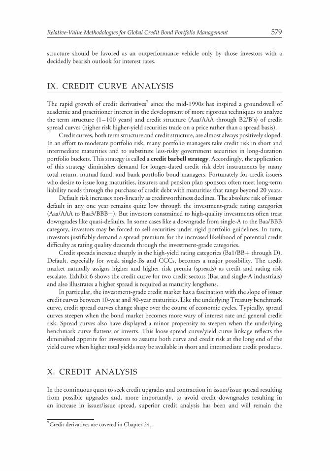
Relative-Value Methodologies for Global Credit Bond Portfolio Management 579
structure should be favored as an outperformance vehicle only by those investors with adecidedly bearish outlook for interest rates.
IX. CREDIT CURVE ANALYSIS
The rapid growth of credit derivatives7 since the mid-1990s has inspired a groundswell ofacademic and practitioner interest in the development of more rigorous techniques to analyzethe term structure (1–100 years) and credit structure (Aaa/AAA through B2/B’s) of creditspread curves (higher risk higher-yield securities trade on a price rather than a spread basis).
Credit curves, both term structure and credit structure, are almost always positively sloped.In an effort to moderate portfolio risk, many portfolio managers take credit risk in short andintermediate maturities and to substitute less-risky government securities in long-durationportfolio buckets. This strategy is called a credit barbell strategy. Accordingly, the applicationof this strategy diminishes demand for longer-dated credit risk debt instruments by manytotal return, mutual fund, and bank portfolio bond managers. Fortunately for credit issuerswho desire to issue long maturities, insurers and pension plan sponsors often meet long-termliability needs through the purchase of credit debt with maturities that range beyond 20 years.
Default risk increases non-linearly as creditworthiness declines. The absolute risk of issuerdefault in any one year remains quite low through the investment-grade rating categories(Aaa/AAA to Baa3/BBB−). But investors constrained to high-quality investments often treatdowngrades like quasi-defaults. In some cases like a downgrade from single-A to the Baa/BBBcategory, investors may be forced to sell securities under rigid portfolio guidelines. In turn,investors justifiably demand a spread premium for the increased likelihood of potential creditdifficulty as rating quality descends through the investment-grade categories.
Credit spreads increase sharply in the high-yield rating categories (Ba1/BB+ through D).Default, especially for weak single-Bs and CCCs, becomes a major possibility. The creditmarket naturally assigns higher and higher risk premia (spreads) as credit and rating riskescalate. Exhibit 6 shows the credit curve for two credit sectors (Baa and single-A industrials)and also illustrates a higher spread is required as maturity lengthens.
In particular, the investment-grade credit market has a fascination with the slope of issuercredit curves between 10-year and 30-year maturities. Like the underlying Treasury benchmarkcurve, credit spread curves change shape over the course of economic cycles. Typically, spreadcurves steepen when the bond market becomes more wary of interest rate and general creditrisk. Spread curves also have displayed a minor propensity to steepen when the underlyingbenchmark curve flattens or inverts. This loose spread curve/yield curve linkage reflects thediminished appetite for investors to assume both curve and credit risk at the long end of theyield curve when higher total yields may be available in short and intermediate credit products.
X. CREDIT ANALYSIS
In the continuous quest to seek credit upgrades and contraction in issuer/issue spread resultingfrom possible upgrades and, more importantly, to avoid credit downgrades resulting inan increase in issuer/issue spread, superior credit analysis has been and will remain the
7Credit derivatives are covered in Chapter 24.
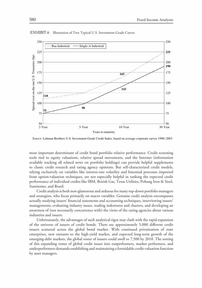
580 Fixed Income Analysis
EXHIBIT 6 Illustration of Two Typical U.S. Investment-Grade Curves
Source: Lehman Brothers U.S. Investment-Grade Credit Index, based on average corporate curves 1990–2003
250Baa Industrial Single-A Industrial
225
200
175
150
Spre
ad o
ver
on-t
he-r
un U
.S. T
reas
urie
s (b
p)
125
100
7575
110
165
143
98
502-Year 5-Year
Years to maturity
10-Year 30-Year
250
225
200190
175
150
125
100
75
50
most important determinant of credit bond portfolio relative performance. Credit screeningtools tied to equity valuations, relative spread movements, and the Internet (informationavailable tracking all related news on portfolio holdings) can provide helpful supplementsto classic credit research and rating agency opinions. But self-characterized credit models,relying exclusively on variables like interest-rate volatility and binomial processes importedfrom option-valuation techniques, are not especially helpful in ranking the expected creditperformance of individual credits like IBM, British Gas, Texas Utilities, Pohang Iron & Steel,Sumitomo, and Brazil.
Credit analysis is both non-glamorous and arduous for many top-down portfolio managersand strategists, who focus primarily on macro variables. Genuine credit analysis encompassesactually studying issuers’ financial statements and accounting techniques, interviewing issuers’managements, evaluating industry issues, reading indentures and charters, and developing anawareness of (not necessarily concurrence with) the views of the rating agencies about variousindustries and issuers.
Unfortunately, the advantages of such analytical rigor may clash with the rapid expansionof the universe of issuers of credit bonds. There are approximately 5,000 different creditissuers scattered across the global bond market. With continued privatization of stateenterprises, new entrants to the high-yield market, and expected long-term growth of theemerging-debt markets, the global roster of issuers could swell to 7,500 by 2010. The sortingof this expanding roster of global credit issues into outperformers, market performers, andunderperformers demands establishing and maintaining a formidable credit-valuation functionby asset managers.
Relative-Value Methodologies for Global Credit Bond Portfolio Management 581
XI. ASSET ALLOCATION/SECTOR ROTATION
Sector rotation strategies have long played a key role in equity portfolio management. In thecredit bond market, ‘‘macro’’ sector rotations among industrials, utilities, financial institutions,sovereigns, and supranationals also have a long history. During the last quarter of the 20thCentury, there were major variations in investor sentiment toward these major credit sectors.Utilities endured market wariness about heavy supply and nuclear exposure in the early-to-mid1980s. U.S. and European financial institutions coped with investor concern about assetquality in the late 1980s and early 1990s. Similar investor skittishness affected demand forAsian financial institution debt in the late 1990s. Industrials embodied severe ‘‘event risk’’ inthe mid-to-late 1980s, recession vulnerability during 1990–1992, a return of event risk inthe late 1990s amid a general boom in corporate mergers and acquisitions, and a devastatingseries of accounting and corporate governance blows during 2001–2002. Sovereigns wereexposed to periodic market reservations about the implications of independence for Quebec,political risk for various countries (i.e., Russia), the effects of the ‘‘Asian Contagion’’ during1997–1998, and outright defaults like Argentina (2001).
In contrast, ‘‘micro’’ sector rotation strategies have a briefer history in the creditmarket. A detailed risk/return breakdown (i.e., average return and standard deviation) of themain credit sub-sectors (i.e., banks, brokerage, energy, electrics, media, railroads, sovereigns,supranationals, technology) was not available from credit index providers until 1993 in theUnited States and until 1999 in Europe. Beginning in the mid-1990s, these ‘‘micro’’ sectorrotation strategies in the credit asset class have become much more influential as portfoliomanagers gain a greater understanding of the relationships among intra-credit sectors fromthese statistics.
Exhibit 7 illustrates the main factors bearing on sector rotation and issuer selectionstrategies. For example, an actual or perceived change in rating agency philosophy toward asector and a revision in profitability expectations for a particular industry represent just two ofmany factors that can influence relative sectoral performance.
EXHIBIT 7 Some Outperformance Methodologies
Economic ExpectationsGDPInterest RatesExchange Rates
Credit-Quality FundamentalsEarnings/Cash Flow GrowthFinancial LeverageRating Agency Philosophy
TechnicalsMarker Risk Premiums (spreads)Origination ExpectationsDealer PositioningInvestor Demand
Structural FactorsIssuer IndustriesAsset Management IndustryInvestment Banking IndustryAcademic Developments
Portfolio CharacteristicsLiquidityAvailabilityDurationConvexitySenior vs. Junior Obligations
Seasonality: Quarter Ends, “First” &“Fourth Quarter Effects”
Geographic Extensions
Credit-Quality Constraint Relaxatior1
Asset Swaps
Credit Barbells
Sector Rotation
Issuer Selection
Issue &Structural Selection
PortfolioEnhancements
Current Coupon Rotations
Treasury Auction Effects
Political Cycles
Futures
Credit Derivatives

582 Fixed Income Analysis
Common tactics to hopefully enhance credit portfolio performance are also highlightedin Exhibit 7. In particular, seasonality deserves comment. The annual rotation toward riskaversion in the bond market during the second half of most years contributes to a ‘‘fourth-quarter effect’’—that is, there is underperformance of lower-rated credits, B’s in high-yield andBaa’s in investment-grade, compared to higher-rated credits. A fresh spurt of market optimismgreets nearly every New Year. Lower-rated credit outperforms higher-quality credit—thisis referred to as the ‘‘first-quarter effect.’’ This pattern suggests a very simple and popularportfolio strategy: underweight low-quality credits and possibly even credit products altogetheruntil the mid-third quarter of each year and then move to overweight lower-quality creditsand all credit product in the fourth quarter of each year.
CHAPTER 21INTERNATIONAL BOND
PORTFOLIOMANAGEMENT∗
I. INTRODUCTION
Management of an international bond portfolio poses more varied challenges than managementof a domestic bond portfolio. Differing time zones, local market structures, settlement andcustodial issues, and currency management all complicate the fundamental decisions facingevery fixed income manager in determining how the portfolio should be positioned withrespect to duration, sector, and yield curve.
In Chapter 16, the fundamental steps in the investment management process wereexplained. These steps include:
1. setting investment objectives2. developing and implementing a portfolio strategy3. monitoring the portfolio4. adjusting the portfolio
The added complexities of cross-border investing magnify the importance of a well defined,disciplined, investment process. This chapter is organized to address these challenges for steps1, 2, and 4.
To provide a broad overview of the many aspects of international fixed income investingin one chapter implies that many topics do not receive the depth of discussion they deserve. Forexample, the topic of currency management is extensive and we provide only the fundamentalprinciples here. However, the same principles involved with currency management applyequally to international equity portfolio management.
While many of the examples and illustrations in this chapter apply to internationalinvesting from the perspective of a U.S. manager investing in bond markets outside of theUnited States, it is important to keep in mind that the principles apply to any cross-bordermanager investing outside of his or her domestic bond market. The same issues faced by U.S.managers regarding currency management apply to managers throughout the world when theyinvest in bonds in which the cash flows are not denominated in their local currency.
∗This chapter is authored by Christopher B. Steward, CFA, J. Hank Lynch, CFA, and Frank J. Fabozzi,
PhD, CFA, CPA.
583
584 Fixed Income Analysis
II. INVESTMENT OBJECTIVES AND POLICYSTATEMENTS
Most investors are attracted to global bonds as an asset class because of their historically higherreturns than U.S. bonds. Others are drawn to global bonds because of their diversificationvalue in reducing overall portfolio risk.1 An investor’s rationale for investing in internationalbonds is central to developing appropriate return objectives and risk tolerances for a portfolio.
Broadly speaking, investor specifications include:
1. return objectives2. risk tolerances
Each of these investment objectives has implications for the management of an internationalbond portfolio and should be reflected in the investment policy statement.
Global bonds are usually a small part of an overall portfolio added for both return anddiversification. The strategic asset allocation for the portfolio is made up of benchmarks thatboth define the asset class and provide a performance target that each investment managerstrives to outperform. Return objectives are often expressed in terms of the benchmark return,e.g., benchmark return plus 100 basis points over a market cycle. The return objectives and risktolerances will indicate not only the most appropriate benchmark, but also the most suitableinvestment management style. Investors who are primarily concerned with diversification maywish to place tight limits on the size of positions taken away from the benchmark to ensurediversification is not weakened. A total-return oriented investor might be far less concernedwith diversification and focused on absolute return rather than on benchmark relative return.
Investment policy statements should be flexible enough to allow the portfolio managersufficient latitude for active management while keeping the portfolio close enough to thebenchmark to ensure that the portfolio remains diversified. The policy statements shouldaddress allowable investments including:
1. the countries in the investment universe, including emerging markets2. allowable instruments, including mortgages, corporate bonds, asset-backed securities,
and inflation-adjusted bonds3. minimum credit ratings4. the currency benchmark position and risk limits5. the use of derivatives such as forwards, futures, options, swaps, and structured notes
The time horizon for investment performance is also important. A short-term timehorizon, such as a calendar quarter, may encourage more short-term trading which could
1Some investors were concerned that the diversification benefits of global bond investing would besubstantially diminished by the commencement of European Monetary Union (EMU) in 1999. But,in fact, the economies of continental Europe were already very closely tied together before EMU withmost European central banks following the interest rate policies of the German Bundesbank for severalyears before the move to a single currency. Thus, the impact on diversification of a global bond portfoliocaused by EMU has been a small one. EMU, however, has created a much more robust credit market inEurope as issuers and investors, no longer confined to their home markets, have access to a larger, moreliquid pan-European bond market. Corporate bond issuance has increased sharply in Europe, and seemslikely to continue, building toward a broader range of credits and instruments similar to those availablein the U.S. bond market. This was discussed in Chapter 20.

Chapter 21 International Bond Portfolio Management 585
diminish the natural diversification benefit from international bonds as an asset class. Investorswho emphasize the risk reduction, or diversification aspect of international bond investing,should have a longer time horizon of perhaps three to five years. As differences betweeneconomic cycles can be prolonged, this provides enough time for a full economic cycle to addany diversification benefit.
A. Benchmark Selection
Benchmark selection for an international bond portfolio has many ramifications and shouldbe done carefully. As is the case when choosing an international equity benchmark index,the choice of a pure capitalization (market value) weighted index may create a benchmarkthat exposes the investor to a disproportionate share in the Japanese2 market relative to theinvestor’s liabilities or diversification preferences.3 While international equity indices chosenfor benchmarks are most often quoted in the investor’s local currency (i.e., unhedged),international bond benchmarks may be hedged, unhedged, or partially hedged depending onthe investor’s objectives. The choice of a hedged, unhedged, or partially hedged benchmarkwill likely alter the risk and return profile of the investment portfolio and should reflect therationale for investing in international bonds.
B. Available Benchmarks
Benchmarks can be selected from one, or a combination of the many existing bond indices:
• global (all countries, including home country)• international (ex-home country)• government-only• multi-sector or broad (including corporates and mortgages)• currency-hedged• G7 only• maturity constrained, e.g., 1–3 year, 3–5 year, 7–10 year• emerging markets
Alternatively, a customized index or ‘‘normal’’ portfolio can be created.The most frequently used fixed-income benchmarks are the Citigroup World Govern-
ment Bond Index (WGBI) and the Lehman Global Aggregate. As discussed above, thebenchmark often provides both the return objective and the measure of portfolio risk.
C. Benchmark Currency Position
Currency management is a matter of much debate in the academic literature. Investinginternationally naturally generates foreign currency exposures. These currency exposures canbe managed either passively or actively, although most global bond managers utilize activemanagement to some degree.
Many managers are attracted to active currency management because of the large gainsthat can be attained through correctly anticipating currency movements. As currency returns
2The Japanese bond market has historically offered lower yields than most other bond markets.3While in the equity market where growth in a company’s market capitalization generally indicatesfinancial strength, a company or country that issues a large amount of debt (especially relative to itsequity in the case of a company or gross national product in the case of a country) may find itself in amore precarious financial position.
586 Fixed Income Analysis
are much more volatile than bond market returns, even modest positions in currencies canresult in significant tracking error (see Chapter 17). Traditionally, the bond manager hashandled currency exposures assuming the same fundamental economic factors (identifiedlater in this chapter) influence currency levels. However, many managers are hiring foreignexchange specialists because bonds and currencies can behave quite differently in reaction tothe same stimulus. Both the risks and opportunities posed by currency movements suggestthat some specialization in currency is warranted and that a joint optimization of the bond andcurrency decision provides better risk-adjusted returns.4 Research has also shown that activemanagement by currency specialists can consistently add to returns.
The first task is to determine the neutral or strategic foreign currency exposure appropriatefor the investment objectives. Most of the academic research on currency hedging for U.S.dollar-based investors suggests that a partially hedged benchmark offers superior risk-adjustedreturns as compared with either a fully hedged or unhedged benchmark.5 This research hasled some to recommend a 50% hedged benchmark for either a passively managed currencystrategy, or as a good initial hedged position for an active currency manager. Once thebenchmark has been selected, a suitable currency hedge position needs to be determined.For example, a U.S. dollar-based fixed income manager whose primary goal is risk reductionmight adopt a hedged or mostly hedged benchmark which has historically shown greaterdiversification benefit from international bonds. Despite a higher correlation with the U.S.bond market than unhedged international bonds, hedged international bonds offer better riskreduction due to a lower standard deviation of bond returns than an only U.S. bond marketportfolio.6 In addition, this lesser volatility of hedged international bonds results in morepredictable returns. Conversely, an investor who has a total return objective, and a greater risktolerance, would be more likely to adopt an unhedged, or mostly unhedged benchmark, andallow more latitude for active currency management.
From the perspective of a U.S. investor, Exhibit 1 shows that for the 18-year period1985–2002 the currency component of investing in unhedged international bonds accountedfor much of the total return volatility. The international bond index used is the CitigroupWGBI excluding the United States (denoted by ‘‘non-U.S. WGBI’’). Investing in internationalbonds on a hedged basis reduced the return in most periods, but also substantially reduced thereturn volatility. As can be seen in Exhibit 1, over the 18-year history of the WGBI, hedgedinternational bonds returned less than unhedged international bonds and even lagged the U.S.component of the WGBI slightly. However, the volatility of the hedged non-U.S. WGBI wasone third that of the unhedged index, and three quarters that of the U.S. component.
To compare returns on a risk-adjusted basis we can use the Sharpe ratio.7 Despite thehigher return of the unhedged non-U.S. WGBI, its risk-adjusted return was lower than thehedged index and the U.S. bond component alone for the 1985 through 2002 period.
4See Philippe Jorion, ‘‘Mean/Variance Analysis of Currency Overlays,’’ Financial Analysts Journal(May/June 1994), pp. 48–56. Jorion argues that currency overlays, although they can add value, areinferior to an integrated approach to currency management.5See Gary L. Gastineau, ‘‘The Currency Hedging Decision: A Search for Synthesis in Asset Allocation,’’Financial Analysts Journal (May-June 1995), pp. 8–17 for a broad overview of the currency hedgingdebate. For a full discussion of the benefits of utilizing a partially hedged benchmark, see the currencydiscussion in Steve Gorman, The International Equity Commitment (Charlottesville, VA: AIMR 1998).6Recall from modern portfolio theory the important role of correlation in determining the benefits fromdiversification.7The Sharpe ratio measures returns in excess of the risk-free rate, per unit of standard deviation.
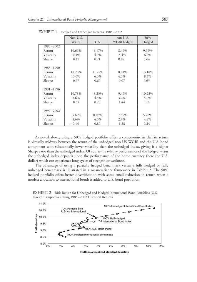
Chapter 21 International Bond Portfolio Management 587
EXHIBIT 1 Hedged and Unhedged Returns: 1985–2002
Non-U.S. non-U.S. 50%WGBI U.S. WGBI hedged Hedged
1985–2002Return 10.66% 9.17% 8.49% 9.69%Volatility 10.4% 4.9% 3.4% 6.2%Sharpe 0.47 0.71 0.82 0.64
1985–1990Return 18.23% 11.27% 8.01% 13.18%Volatility 13.6% 6.0% 4.3% 8.4%Sharpe 0.77 0.60 0.07 0.65
1991–1996Return 10.78% 8.23% 9.49% 10.23%Volatility 8.6% 4.3% 3.2% 5.0%Sharpe 0.69 0.78 1.44 1.09
1997–2002Return 3.46% 8.05% 7.97% 5.78%Volatility 8.6% 4.3% 2.4% 4.8%Sharpe −0.14 0.80 1.38 0.24
As noted above, using a 50% hedged portfolio offers a compromise in that its returnis virtually midway between the return of the unhedged non-US WGBI and the U.S. bondcomponent with substantially lower volatility than the unhedged index, giving it a higherSharpe ratio than the unhedged index. Of course the relative performance of the hedged versusthe unhedged index depends upon the performance of the home currency (here the U.S.dollar) which can experience long cycles of strength or weakness.
The advantage of using a partially hedged benchmark versus a fully hedged or fullyunhedged benchmark is illustrated in a mean-variance framework in Exhibit 2. The 50%hedged portfolio offers better diversification with some small reduction in return when amodest allocation to international bonds is added to U.S. bond portfolios.
EXHIBIT 2 Risk-Return for Unhedged and Hedged International Bond Portfolios (U.S.Investor Perspective) Using 1985–2002 Historical Returns
Po
rtfo
lio r
etu
rn
Portfolio annualized standard deviation
10% Portfolio ShiftU.S. vs. International
100% Unhedged International Bond Index
100% Hedged International Bond Index
100% U.S. Bond Index
International Bond Index100% Half-Hedged
2% 3% 4% 5% 6% 7% 8% 9% 10% 11%
11.0%
10.5%
10.0%
9.5%
9.0%
8.5%
8.0%
588 Fixed Income Analysis
D. Risk Limits
Many investment guidelines will include explicit risk limits on bond and currency positions aswell as duration and credit risk. Exposure limits can be either expressed as absolute percentages,or weights relative to a benchmark. Increasingly, tracking error limits have also been used toset risk limits in investment guidelines.
Bond markets can be divided into four trading blocs:
1. dollar bloc (the U.S., Canada, Australia, and New Zealand)2. European bloc3. Japan4. emerging markets
The European bloc is subdivided into two groups:
1. euro zone market bloc which has a common currency (Germany, France, Holland,Belgium, Luxembourg, Austria, Italy, Spain, Finland, Portugal, and Greece)
2. non-euro zone market bloc (Norway, Denmark, and Sweden)
The United Kingdom often trades more on its own, influenced by both the euro zone and theU.S., as well as its own economic fundamentals.
The trading bloc construct is useful because each bloc has a benchmark market thatgreatly influences price movements in the other markets. Investors are often focused more onthe spread level of, say, Denmark to Germany, than the absolute level of yields in Denmark.(Since the beginning of the European Monetary Union (EMU) in 1999, the euro zone bondmarkets have traded in a much tighter range.)
Limits on investment in countries outside the benchmark should also be specified at theoutset. Despite the pitfalls of using duration to measure interest rate risk across countries, risklimits on duration are nonetheless useful and should be established. Typically, the range ofallowable exposures is wider for bond exposures than currency exposures.
Credit risk limits, usually a minimum weighted average credit rating from the major creditrating agencies, and limits on the absolute amount of low or non-investment grade credits,should also be included. Apart from default risk, the illiquidity of lower rated securities mayhamper a manager’s ability to alter exposures as desired. In the past, due to the lack of a liquidcorporate bond market in many countries, and the relative illiquidity of Eurobonds comparedto domestic government bond markets, most credit risk in international bond portfolioswas concentrated in U.S. and emerging market bonds. However, this difference in liquiditybetween U.S. corporate bonds and those in other countries has diminished significantly inrecent years due to strong growth in the European corporate bond market since EuropeanMonetary Union.
III. DEVELOPING A PORTFOLIO STRATEGY
Once the investment policy statement is established, the portfolio manager needs to developa portfolio strategy appropriate to the investor’s objectives and risk tolerances. Just as inmany other areas of investment management, portfolio managers often subscribe to differentmanagement styles, or investment disciplines.
Since the performance of most portfolio managers is judged against a benchmark return,managers are constantly seeking opportunities to outperform a benchmark. There are anumber of means by which portfolio managers can add to returns; however, the bulk of excess
Chapter 21 International Bond Portfolio Management 589
returns relative to the benchmark comes from broad bond market and currency allocationdecisions. A disciplined investment approach, based upon fundamental economic factors ormarket indicators of value, facilitates the market and currency selection process. Because of thehistorical high volatility of currency returns, the approach to currency management should bea primary concern.
A. Styles of International Bond Portfolio Management
The challenges faced by international fixed income managers are different from those facingdomestic fixed income managers. First, the international fixed income portfolio manager mustoperate in the U.S. bond market plus 10 to 20 other markets, each with their own marketdynamics. Second, changes in interest rates generally affect different sectors of the U.S. bondmarket in much the same way (with the exception of mortgage-backed securities), althoughthe magnitude of the changes may vary. Like the equity market, where it is not unusual to havesome industries or market sectors move in opposite directions, international bond marketsmay also move in different directions depending upon economic conditions and investor risktolerances.
International bond managers also utilize one or more different management styles. Thesecan be divided into four general categories:
1. the experienced trader2. the fundamentalist3. the black box4. the chartist
We discuss each management style below.
1. The Experienced Trader The experienced trader uses his or her experience andintuition to identify market opportunities. The experienced trader tends to be an active trader,trying to anticipate the next market shift by international fixed income and hedge fundmanagers. The basis for these trades is derived from estimates of competitors’ positions andrisk tolerances bolstered by observation of market price movements and flow information.The experienced trader is often a contrarian, looking to profit from situations where manyinvestors may be forced to stop themselves out of losing positions.
2. The Fundamentalist The fundamental style rests upon a belief that bonds andcurrencies trade according to the economic cycle. Sector rotation within corporate bonds alsowill be affected by the economic cycle as different sectors perform relatively better at differentpoints in the cycle. Some of these managers believe that the economic cycle is forecastable, andrely mostly upon economic analysis and forecasts in selecting bond markets and currencies.These managers tend to have less portfolio turnover as the economic fundamentals havelittle impact on short-term price movements. ‘‘Bottom-up’’ security selection in corporatebonds could also be characterized as a fundamentalist approach even though it rests uponissuer-specific fundamental analysis rather than broad economic fundamentals.
3. The Black Box The black box approach is used by quantitative managers who believethat computer models can identify market relationships that people cannot. These models canrely exclusively on economic data, price data, or some combination of the two. Quantitativemanagers believe using computer models can create a more disciplined investment approach
590 Fixed Income Analysis
which, because of other managers’ emotional attachment to positions, their lack of tradingdisciplines, or their inability to process more than a few variables simultaneously, will providesuperior investment results.
4. The Chartist Some investors called chartists or technicians may rely primarily ontechnical analysis to determine which assets to buy or sell.8 Chartists will look at daily, weekly,and monthly charts to try to ascertain the strength of market trends, or to identify potentialturning points in markets. Trend-following approaches, such as moving averages, aim toallow the portfolio manager to exploit market momentum. Counter-trend approaches, suchas relative strength indices and oscillators try to identify when recent price trends are likely toreverse.
5. Combining Styles Very few international bond portfolio managers rely on only one ofthese management styles, but instead use some combination of each. Investment managers thatrely on forecasts of the economic cycle to drive their investment process will from time to timetake positions contrary to their medium-term strategy to take advantage of temporary underor overvaluation of markets identified by technical analysis, or estimates of market positions.Even ‘‘quant shops’’ that rely heavily on computer models for driving investment decisionswill sometimes look to other management styles to add incremental returns. Regardless of themanager’s investment style, investment decisions must be consistent with the investor’s returnobjectives and risk tolerances, and within the investment guidelines.
International bond portfolio managers would do well to maintain a disciplined approachto buy and sell decisions. This would require each allocation away from the benchmark to havea specified price target (or more often yield spread or exchange rate level), and stated underlyingrationale. Depending upon the management style, the size of the position should reflect thestrength of the investor’s conviction or model’s signal. As long as the investment rationale thatsupported the initial decision remained unchanged, the position would be held, or potentiallyincreased, if the market moves in the opposite direction. Each trade should be designedwith consideration for the relevant bond yield or exchange rate’s behavior through time. Forexample, an exchange rate that exhibits a tendency to trend will require a different buy andsell discipline than one that tends to consistently revert back to an average exchange rate.
B. Sources of Excess Return
The baseline for any international bond portfolio is the benchmark. However, in order to earnreturns in excess of the benchmark, after management fees, the portfolio manager must findways to augment returns. These excess returns can be generated through a combination of fivebroad strategies:
1. currency selection2. duration management/yield curve plays3. bond market selection4. sector/credit/security selection5. investing in markets outside the benchmark (if permitted)
Each of these strategies can add to returns; however, currency and bond market selectionsgenerally provide the lion’s share of returns. We discuss each of these sources of excess returnon the following page.
8Technical analysis is covered in equity management textbooks.
Chapter 21 International Bond Portfolio Management 591
1. Currency Selection Most investment guidelines will allow for some active manage-ment of currency exposures. The attraction of active currency management is strong becausepotential gains are so large. The spread between the top and bottom performing bond marketsin local currency terms is 13% on average. When currency movements are added to the localcurrency bond market returns, the average spread between the best and worst performingmarkets more than doubles to 28%. Thus, international bond portfolio managers may signifi-cantly enhance returns by overweighting the better performing bond markets and currenciesin the index.
However, as the volatility of currency returns is generally higher than that of bond marketreturns, the incremental returns gained from currency exposures must be evaluated relativeto the additional risk incurred. For an active currency management strategy to consistentlyprovide superior risk-adjusted performance, a currency forecasting method is required that canpredict future spot rates (i.e., future exchange rates) better than forward foreign exchange rates(i.e., rates that can be locked in today using the market for forward contracts). As shown later,forward foreign exchange rates are not forecasts of future spot foreign exchange rates, but aredetermined by short-term interest rate differentials between currencies.
Academic studies have shown that several strategies have been successful in generatingconsistent profits through active currency management. The fact that forward foreign exchangerates are poor predictors of future spot exchange rates is well established. Historically, discountcurrencies (i.e., those with higher interest rates than the investor’s local currency) havedepreciated less than the amount implied by the forward rates, providing superior returns fromholding unhedged positions in currencies with higher interest rates. Overweighting currencieswith high real interest rates versus those with lower real interest rates has also been shown toprovide incremental returns.9
In addition, some currency movements are not a random walk, but exhibit serialcorrelation (i.e., currency movements have a tendency to trend).10 In a market thattends to trend, simple technical trading rules may provide opportunities for incrementalcurrency returns.11 These findings in several academic studies demonstrate that excess cur-rency returns can be generated consistently, providing a powerful incentive for active currencymanagement.
2. Duration Management Although closely aligned with the bond market selectiondecision, duration management can also enhance returns. Bullet versus barbell strategies ina curve steepening or flattening environment within a particular country’s bond market canenhance yield and total return.12 In addition to these strategies that are also available tomanagers investing in their domestic bond market, the international fixed income portfoliomanager has the option of shifting duration between markets while leaving the portfolio’soverall duration unchanged.
9See Gastineau, ‘‘The Currency Hedging Decision,’’ pp. 13–14.10One suggestion as to why currency markets trend is that central banks attempt to smooth foreignexchange rate movements through intervention. Thus, because central bank participation in the foreignexchange market is not motivated by profit, their actions keep the market from being truly efficient.See Robert D. Arnott and Tan K. Pham, ‘‘Tactical Currency Allocation,’’ Financial Analysts Journal,(May/June 1993) pp. 47–52.11See Richard M. Levich and Lee R. Thomas, ‘‘The Merits of Active Currency Risk Management:Evidence from International Bond Portfolios,’’ Financial Analysts Journal, (September/October 1993)pp. 63–70.12See Chapter 18 for a discussion of this strategy and how it is analyzed.
592 Fixed Income Analysis
Duration management has become easier in international markets in recent years. Manycountries have concentrated their debt in fewer, more liquid, bond issues. Official strip markets(which separate government bond cash flows into individual interest and principal payments)now exist in at least nine countries. Interest rate futures, available in most markets, offer aliquid and low-cost vehicle for changing duration or market exposure quickly. The interestrate swaps market, used extensively by large institutional investors, is generally very liquidacross international bond markets. Following European Monetary Union, the swap curve,rather than individual country yield curves, has increasingly been used as a reference for somemarkets. Increasingly, countries have set up professional debt management offices that areindependent from both central banks and finance ministries. These debt management officeshave become significant users of derivatives themselves to minimize borrowing costs, alter thematurity structure or currency composition of outstanding debt, and to promote liquidity intheir domestic market.13
3. Bond Market Selection Excess returns over the benchmark index from overweightingthe best performing bond markets can be extremely large. As we saw above, the annual localcurrency return differential between the best and worst performing developed bond marketshas been 13% on average, providing significant opportunity for generating excess returns. Theprocess for making the bond market selection decision is discussed further in Section III C.
4. Sector/Credit/Security Selection The corporate bond market experienced signifi-cant growth in many countries, especially in Europe following European Monetary Union.According to data collected by Merrill Lynch on the size and structure of the world bondmarket, government bonds account for 55% of the $30 trillion market for developed countrybonds. Corporate bonds account for 25% of the bond market, and about 20% excluding theUnited States. Some global bond indices include only government bonds, but others, like theLehman Global Aggregate and the Citigroup Global Broad Investment Grade Indices, includeother instruments including corporate bonds and mortgages.
5. Investing in Markets Outside the Index If allowed by investment guidelines, allo-cating assets to markets outside the index can significantly enhance returns without dramaticallyaltering the risk profile of the portfolio. Here are two examples. First, Finland was one of thebest performing bond markets during 1995, but, because of its small size, was not included inthe Citigroup World Government Bond Index (WGBI) until June 1996. Second, investing inemerging markets debt as represented by the JP Morgan EMBI + Index would have boostedreturns substantially in 1999 and 2000 when it outperformed all developed bond markets ona local currency or U.S. dollar basis.14
The process for selecting an out-of-index market is similar to that followed by an activemanager for a domestic bond portfolio manager when deciding whether or not to construct aportfolio with allocations different from the benchmark index and whether or not to investoutside the index. The manager will assess the potential performance on a total return basis ofthe markets outside of the index relative to that of the markets to be underweighted in orderto allocate funds to out-of-index markets. An international bond portfolio manager, however,
13See ‘‘OECD Public Debt Markets: Trends and Recent Structural Changes’’ OECD 2002.14The JP Morgan EMBI + Index is comprised of mostly U.S. dollar-denominated sovereign debt issuedby emerging market countries. Therefore, credit risk, and to a lesser extent interest rate risk, are thepredominate risks associated with the index. For a U.S. investor, currency risk is virtually zero.
Chapter 21 International Bond Portfolio Management 593
must also take into account the affect of currency movements and hedging decision of aninvestment outside or within the index.
As we saw above, exposure to emerging markets can significantly add to returns. Forexample, a portfolio composed of 80% exposure to the Citigroup Non-U.S. GovernmentBond Index and 20% exposure to the J.P. Morgan EMBI+ Index from 1994 through 2002would have added 120 basis points to the return of the international index and reducedthe standard deviation of returns by 12%. A 20% allocation to emerging markets in aninternational bond portfolio that was half-hedged against foreign exchange rate changes wouldhave increased returns by 223 basis points while decreasing the standard deviation of returnsby 37%.
C. A Fundamental-Based Approach to Investing
The portfolio strategy is often composed of
1. a medium-term strategic allocation and2. a shorter-term tactical allocation
The strategic allocation is composed of positions held for one to three months, or longerdesigned to take advantage of longer-term economic trends. A fundamental-based approachis used to develop the portfolio’s strategic allocation. The investment style used in thefundamental-based approach is, of course, the fundamental style, but can also be combinedwith a quantitative or black box style to forecast relevant strategic factors. The tacticalallocation generally relies on technical analysis or flow information to identify shifts in marketprices that are likely to occur within a few days to several weeks. Tactical allocations are oftencontrarian in nature, driven by expectations of a reversal in a recent price trend.15 Of course,the experienced trader, black box, and chartist investment styles most often use technicalanalysis combinations in their tactical allocation decisions.
The strategic decision of which bond markets and currencies to overweight usually beginswith an economic outlook and bond and currency forecasts in each of the markets consideredfor investment. The long-run economic cycle is closely correlated with changes in bond yields,and trends in both the economic cycle and bond yields tend to persist for a year or longer. Themillions of dollars spent each year by money management firms, banks, and brokerage housesin forecasting economic trends is testimony to the potential returns that can be achieved bycorrectly forecasting economic growth or turning points in the economic cycle.
Forecasting interest rates, however, is extremely difficult. Academic literature generallyholds that interest rate forecasts are unable to generate consistent risk-adjusted excess returns.This is partly because market prices can deviate substantially over the short term from thelevel consistent with the economic fundamentals. Economic fundamentals impact bond andcurrency prices over the medium to long term. Also, the volatile nature of certain economicdata series may result in exaggerated market reactions to individual data releases that maybe different from the actual trend in the economy. These deviations may persist for severalmonths until either the initial figure is revised, or several subsequent data releases reveal theerror in the initial interpretation.
15However, tactical allocations can also be momentum following, especially if a breakout of a technicalrange appears likely. Again, such technical strategies are discussed in investment management textbooks.

594 Fixed Income Analysis
The creation of an independent economic outlook can be useful in several ways. First, itcan help identify when market interpretations of the economic data are too extreme, or addvalue through correctly anticipating economic shifts not reflected in the market consensus.Second, as it is often not absolute changes in interest rates, but changes in interest rates relativeto other markets that determine the margin of performance in international fixed incomeinvesting, an independent economic outlook does not require accurate growth forecasts foreach individual market, but only economic growth differentials to be able to add value.Whether the portfolio will invest in U.S. bonds or not, the large influence of the U.S. dollarand the Treasury market on foreign markets underlines the importance of an independentoutlook on the U.S. economy.
Thus, the economic outlook forms the foundation for bonds and currencies strategicallocation. An economic outlook for each country should be constructed to assist in rankingthe relative attractiveness of markets. However, even though economic fundamentals in aparticular country may be extremely bond supportive, bond prices may be too high to makeit an attractive investment. Likewise, bonds are sometimes excessively cheap in countries withpoor economic fundamentals, yet may still provide an attractive investment opportunity.Thus, the economic outlook must be compared with either consensus economic forecasts, orsome market value measure to identify attractive investment opportunities.
The strategic allocation decision regarding which markets to overweight or underweightrelative to the benchmark is thus a complex interaction of expected returns derived fromassessing economic trends, and technical and value factors. Each set of variables is defined andexplored below, beginning with the fundamental factors used to create the economic outlook.
1. Fundamental Economic Factors The seven main fundamental economic factors are:
1. cyclical economic indicators2. inflation3. monetary policy4. fiscal policy5. debt6. balance of payments7. politics
Each factor needs to be evaluated against market expectations to determine its likely impact onbond prices and currency rates. Each of these factors is covered in considerable detail in bookson macroeconomics and international economics. Some of these factors were also discussed inthe context of the factors rating agencies consider when assigning credit ratings to sovereignissuers.
2. Value and Technical Indicators Identifying trends in economic fundamentals canhelp identify attractive investment opportunities in markets, but some yardstick to measurerelative value is needed. Determining relative value is highly subjective. Three relativelyobjective value measures—real yields, technical analysis, and market sentiment surveys—arediscussed below.
a. Real Yields A real yield is the inflation-adjusted rate of return demanded by the marketfor holding long-term fixed income securities. Real yields can quickly erode from sustainedinflation. Real yields are impacted by a variety of factors including supply and demand for

Chapter 21 International Bond Portfolio Management 595
capital as well as inflation expectations. Real yields are nominal bond yields minus expectedinflation; however, expected inflation is often difficult to quantify. Some countries, includingthe United States, have inflation-indexed bonds that pay a real rate of interest above theinflation rate.16 These bonds not only provide investors with protection against a surge ininflation but also offer a means of gauging investor inflation expectations.17
Nominal bond yields deflated by current inflation, although not a precise measure of themarket’s real interest rate premium, are easily measurable and can still provide some usefulinsight into bond valuation. Real yields can be compared across markets or against theirlong-run averages, such as 5 or 10 years, in each market. The usefulness of real yields as ameasure of relative value has diminished as global inflation rates have converged to very lowlevels.
b. Technicals Technical analysis can be as simple as drawing a trend line on a chart or ascomplicated as calculating the target of the third impulse wave of an Elliott wave analysis. Inaddition to valuing bonds and currencies, technical analysis can be used to value everythingfrom stocks, to gold, to pork bellies. What all technical analysis has in common is that it triesto predict future prices solely from examining past price movements. Most technical analysismodels fall into one of two camps: trend following or counter trend. The former try to identifytrends that should persist for some period of time, and the latter attempt to predict whena recent trend is likely to change. We will not discuss these models here because they aretypically described in investment management textbooks.
c. Market Sentiment Market sentiment can be used as a contra-indicator of value in thefollowing way. A heavy overweight of a particular country’s bond market implies that fewermanagers are likely to add to that market, and more managers, at least eventually, are likelyto sell. Market sentiment can be estimated by investor sentiment surveys, or by estimates ofinvestment flows.
Historic trends, as well as the overall levels, should be taken into account when assessingmarket sentiment. For example, an indication that managers are underweighting Japanesebonds might lead some to conclude that Japanese bonds are due for a rally even thoughinternational fixed income managers have consistently underweighted the Japanese market, inpart due to its low nominal yields. Sentiment surveys, however, may not capture all marketparticipants such as retail investors, who can also move markets.
IV. PORTFOLIO CONSTRUCTION
Translating the strategic outlook into a portfolio allocation requires a framework for assessingexpected returns against incremental portfolio risk. The following discussion on sourcesof return illustrates how returns can be separated into three components: excess returnson bonds, excess returns on currencies, and the short-term risk-free interest rate. This
16Inflation-indexed bonds were explained earlier.17Nominal yield to maturity is composed of a real yield and an inflation expectations component (Yieldto Maturity = Real Yield to Maturity + Expected Inflation to Maturity). In these markets the nominalgovernment bond yield and the real yield offered by inflation-indexed debt of the same maturity can beused to calculate the expected inflation rate to the maturity, sometimes called the breakeven inflationrate.
596 Fixed Income Analysis
component methodology can assist identifying where market prices are most out of line withthe economic outlook and whether bond market currency exposures should be hedged or leftunhedged.
A. Components of ReturnTo explain the total return components of an international bond portfolio,18 we will use thefollowing notation. We will let ‘‘home currency’’ mean the currency of the manager. So, fora U.S. manager it is U.S. dollars. For a Japanese portfolio manager it is yen. In the notation,the subscript ‘‘H ’’ will denote home currency.
We will let ‘‘local currency’’ be the currency of the country where the manager hasinvested and use the subscript ‘‘L’’ to denote the local currency. So, to a U.S. portfoliomanager, yen would be the local currency for bonds purchased in the Japanese bond marketand denominated in yen, while for a Japanese portfolio manager, U.S. dollars would be thelocal currency for bonds purchased in the U.S. and denominated in U.S. dollars.
The expected total return of an unhedged international bond portfolio in terms of thehome currency depends on three factors:
1. the weight of each country’s bonds in the overall portfolio2. the expected bond market return for each country in local currency3. the expected exchange rate percentage change between the home currency and the local
currency
Mathematically, the expected total return of an unhedged bond portfolio in terms of thehome currency can be expressed as follows:19
total expected portfolio return in manager’s home currency
= W1 × (r1 + eH ,1) + W2 × (r2 + eH ,2) + · · · + WN × (rN + eH ,N ) (1)
where
N = number of countries whose bonds are in the portfolio
Wi = weight of country i’s bonds in the portfolio (i = 1, 2, . . . , N )
ri = expected bond return for country i in local currency (i = 1, 2, . . . , N )
eH ,i = expected percentage change of the home currency with country i’s local currency
We will refer to eH ,i as the currency return.The expected portfolio return as given by equation (1) is changed to the extent the
manager alters exposure to each country’s exchange rate. A common instrument used to alterexposure to exchange rates is a currency forward contract. So, let’s look at these contractsand how they are priced. This will lead us to an important relationship that we will use in thebalance of this chapter, called interest rate parity.
18The structure of this discussion is taken from Brian D. Singer and Denis S. Karnosky, The GeneralFramework for Global Investment Management and Performance Attribution (Charlottesville, VA: TheResearch Foundation of the Institute of Chartered Financial Analysts, 1994). The notation used isconsistent with that of the authors.19The relationship in equation (1) is approximate because bond market and currency returns of aforeign investment is more accurately expressed as the compounded gain of the two components:(1 + ri) × (1 + e$, i) − 1.
Chapter 21 International Bond Portfolio Management 597
1. Currency Forward Contracts and Their Pricing A forward contract is an agree-ment where one party agrees to buy ‘‘something,’’ and another party agrees to sell that same‘‘something’’ at a designated date in the future. Forward contracts are used extensively forcurrency hedging.
Most currency forward contracts have a maturity of less than one year. For longer-datedforward contracts, the bid-ask spread increases; that is, the size of the bid-ask spread for a givencontract increases with the length of the time to contract settlement. Consequently, currencyforward contracts become less attractive for hedging long-dated foreign exchange exposure.Other instruments, such as currency swaps,20 can be used for hedging.
A manager can use currency forward contracts to lock in an exchange rate at the futuredelivery date. In exchange for locking in a foreign exchange rate, the manager forgoes theopportunity to benefit from any advantageous foreign exchange rate movement but eliminatesdownside risk.
Earlier, the relationship between spot prices and forward prices was demonstrated.Arbitrage arguments can also be used to derive the relationship for currency forward contracts.Consider a U.S. manager with a 1-year investment horizon who has two choices:
Alternative 1: Deposit $100,000 in a U.S. bank that pays 6% compounded annually forone year.
Alternative 2: Deposit the U.S. dollar equivalent of $100,000 in some country outside theU.S. where the bank pays 5% compounded annually for one year. We will refer tothis country as country i.
Which is the best alternative? It will be the alternative that produces the largest numberof U.S. dollars one year from now. Ignoring U.S. and country i’s taxes on interest income orany other taxes, we need to know two things in order to determine the best alternative:
• the spot exchange rate between U.S. dollars and country i’s local currency
and
• the spot exchange rate one year from now between U.S. dollars and country i’s localcurrency
The first is known; the second is not. However, we can determine the spot exchange rate oneyear from now between U.S. dollars and country i’s local currency that will make the U.S.manager indifferent between the two investment alternatives.
For alternative 1: The amount of U.S. dollars available one year from now would be$106,000 ($100,000 times 1.06).
For alternative 2: Assume that the spot rate is $0.6757 per one local currency unit.Denoting the local currency units by ‘‘LC,’’ and ignoring the bid/ask spread,$100,000 can be exchanged for LC 147,995 ($100,000 divided by 0.6757). Theamount of local currency units available at the end of one year would be LC 155,395(LC 147,995 times 1.05).
20For an explanation of currency swaps, see Chapter 5 in Don M. Chance, Analysis of Derivatives for theCFA Program (Charlottesville, VA: Association for Investment Management and Research, 2003).
598 Fixed Income Analysis
The number of U.S. dollars that the LC 155,395 can be exchanged for depends onthe exchange rate one year from now. Let F denote the exchange rate between these twocurrencies one year from now. Specifically, F will denote the number of U.S. dollars that canbe exchanged for one unit of the local currency one year from now and is called the forwardexchange rate. Thus, the number of U.S. dollars at the end of one year from the secondalternative is:
amount of U.S. dollars one year from now = LC 155, 395 × F
The investor will be indifferent between the two alternatives if the number of U.S. dollarsis $106,000, equal to the dollars resulting from alternative 1. That is,
$106, 000 = LC 155, 395 × F , or F = $106, 000/LC 155, 395
Solving, we find that F is equal to $0.6821. Since the spot rate is $0.6757 and the forwardexchange rate (F ) is $0.6821, then the implied appreciation for the local currency versus theU.S. dollar is 0.95% [($0.6821/$0.6757) −1]. When there is an implied appreciation, it iscalled a forward exchange rate premium (or simply forward premium). If, instead, therehad been an implied depreciation, it would be referred to as a forward exchange rate discount(or simply forward discount).
Thus, if one year from now the spot exchange rate is $0.6821 per one local currency unit,then the two alternatives will produce the same number of U.S. dollars.21 If the local currencyhas appreciated by more than 0.95%, i.e., one local currency unit can be exchanged for morethan $0.6821, then there will be more than $106,000 at the end of one year. An exchange rateof $0.6910 per one local currency unit, for example, would produce $107,378 (LC 155,395times $0.6910). The opposite is also true if one local currency unit can be exchanged for lessthan $0.6821. For example, if the future exchange rate is $0.6790, there will be $105,513(LC 155,395 times $0.6790).
Now suppose that a dealer quotes a 1-year forward exchange rate between the twocurrencies. The 1-year forward exchange rate fixes today the exchange rate one year fromnow. Thus, if the 1-year forward exchange rate quoted is $0.6821 per one local currency unit,investing in the bank in country i will provide no arbitrage opportunity for the U.S. investor.If the 1-year forward rate quoted is more than $0.6821 per one local currency unit, the U.S.manager can earn an arbitrage profit by selling the local currency forward (and buying U.S.dollars forward for the local currency). In this example, assume the borrowing and lendingrates within each country are equal.
To understand this arbitrage opportunity, consider how a portfolio manager could takeadvantage of a mispricing in the market.22 Under the conditions in the above example, assumethat the bid for a 1-year forward contract in local currency is quoted $0.6910 per local currencyunit. The portfolio manager could generate an arbitrage profit by using the following strategy:
Strategy: Borrow $100,000 for one year at the U.S. rate of 6% compounded annually andenter into a forward contract agreeing to deliver LC 155,395 one year from now at$0.6910 per local currency.
21The forward rate can also be derived by looking at the alternatives from the perspective of a portfoliomanager in country i.22A portfolio manager in any country, not just one located in one of the countries whose currency ismispriced, could take advantage of this arbitrage opportunity.
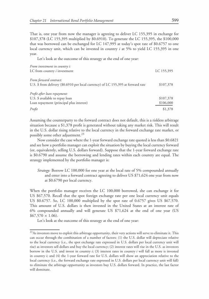
Chapter 21 International Bond Portfolio Management 599
That is, one year from now the manager is agreeing to deliver LC 155,395 in exchange for$107,378 (LC 155,395 multiplied by $0.6910). To generate the LC 155,395, the $100,000that was borrowed can be exchanged for LC 147,995 at today’s spot rate of $0.6757 to onelocal currency unit, which can be invested in country i at 5% to yield LC 155,395 in oneyear.
Let’s look at the outcome of this strategy at the end of one year:
From investment in country i:LC from country i investment LC 155,395
From forward contract:U.S. $ from delivery ($0.6910 per local currency) of LC 155,395 at forward rate $107,378
Profit after loan repayment:U.S. $ available to repay loan $107,378Loan repayment (principal plus interest) $106,000
Profit $1,378
Assuming the counterparty to the forward contract does not default, this is a riskless arbitragesituation because a $1,378 profit is generated without taking any market risk. This will resultin the U.S. dollar rising relative to the local currency in the forward exchange rate market, orpossibly some other adjustment.23
Now consider the case where the 1-year forward exchange rate quoted is less than $0.6821and see how a portfolio manager can exploit the situation by buying the local currency forward(or, equivalently, selling U.S. dollars forward). Suppose that the 1-year forward exchange rateis $0.6790 and assume the borrowing and lending rates within each country are equal. Thestrategy implemented by the portfolio manager is:
Strategy: Borrow LC 100,000 for one year at the local rate of 5% compounded annuallyand enter into a forward contract agreeing to deliver US $71,624 one year from nowat $0.6790 per local currency.
When the portfolio manager receives the LC 100,000 borrowed, she can exchange it forUS $67,570. Recall that the spot foreign exchange rate per one local currency unit equalsUS $0.6757. So, LC 100,000 multiplied by the spot rate of 0.6757 gives US $67,570.This amount of U.S. dollars is then invested in the United States at an interest rate of6% compounded annually and will generate US $71,624 at the end of one year (US$67,570 × 1.06).
Let’s look at the outcome of this strategy at the end of one year:
23As investors move to exploit this arbitrage opportunity, their very actions will serve to eliminate it. Thiscan occur through the combination of a number of factors: (1) the U.S. dollar will depreciate relativeto the local currency (i.e., the spot exchange rate expressed in U.S. dollars per local currency unit willrise) as investors sell dollars and buy the local currency; (2) interest rates will rise in the U.S. as investorsborrow in the U.S. and invest in country i; (3) interest rates in country i will fall as more is investedin country i; and (4) the 1-year forward rate for U.S. dollars will show an appreciation relative to thelocal currency (i.e., the forward exchange rate expressed in U.S. dollars per local currency unit will fall)to eliminate the arbitrage opportunity as investors buy U.S. dollars forward. In practice, the last factorwill dominate.
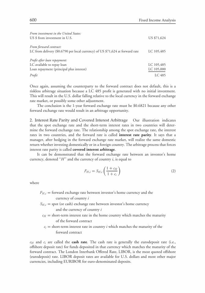
600 Fixed Income Analysis
From investment in the United States:US $ from investment in U.S. US $71,624
From forward contract:LC from delivery ($0.6790 per local currency) of US $71,624 at forward rate LC 105,485
Profit after loan repayment:LC available to repay loan LC 105,485Loan repayment (principal plus interest) LC 105,000
Profit LC 485
Once again, assuming the counterparty to the forward contract does not default, this is ariskless arbitrage situation because a LC 485 profit is generated with no initial investment.This will result in the U.S. dollar falling relative to the local currency in the forward exchangerate market, or possibly some other adjustment.
The conclusion is the 1-year forward exchange rate must be $0.6821 because any otherforward exchange rate would result in an arbitrage opportunity.
2. Interest Rate Parity and Covered Interest Arbitrage Our illustration indicatesthat the spot exchange rate and the short-term interest rates in two countries will deter-mine the forward exchange rate. The relationship among the spot exchange rate, the interestrates in two countries, and the forward rate is called interest rate parity. It says that amanager, after hedging in the forward exchange rate market, will realize the same domesticreturn whether investing domestically or in a foreign country. The arbitrage process that forcesinterest rate parity is called covered interest arbitrage.
It can be demonstrated that the forward exchange rate between an investor’s homecurrency, denoted ‘‘H ’’ and the currency of country i, is equal to
FH ,i = SH ,i
(1 + cH
1 + ci
)(2)
where
FH ,i = forward exchange rate between investor’s home currency and thecurrency of country i
SH ,i = spot (or cash) exchange rate between investor’s home currency
and the currency of country icH = short-term interest rate in the home country which matches the maturity
of the forward contractci = short-term interest rate in country i which matches the maturity of the
forward contract
cH and ci are called the cash rate. The cash rate is generally the eurodeposit rate (i.e.,offshore deposit rate) for funds deposited in that currency which matches the maturity of theforward contract. The London Interbank Offered Rate, LIBOR, is the most quoted offshore(eurodeposit) rate. LIBOR deposit rates are available for U.S. dollars and most other majorcurrencies, including EURIBOR for euro-denominated deposits.
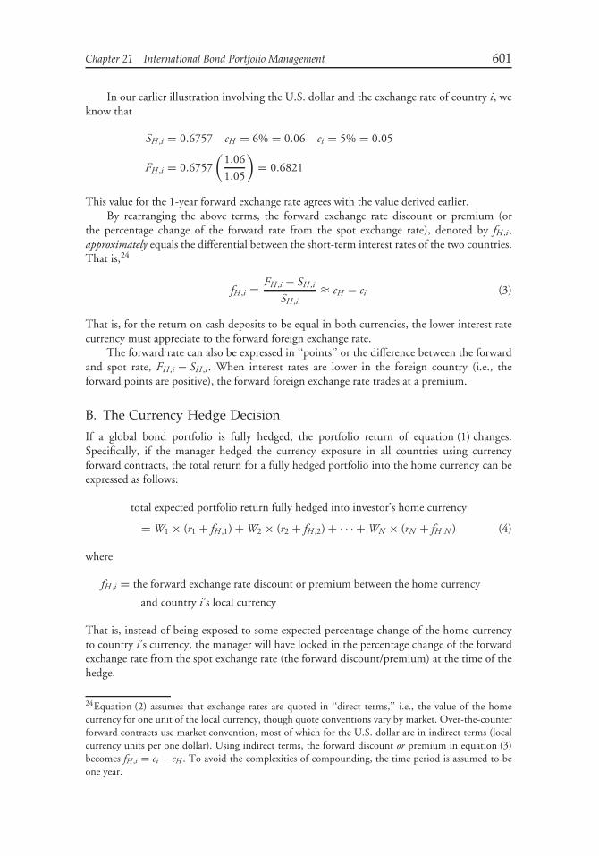
Chapter 21 International Bond Portfolio Management 601
In our earlier illustration involving the U.S. dollar and the exchange rate of country i, weknow that
SH ,i = 0.6757 cH = 6% = 0.06 ci = 5% = 0.05
FH ,i = 0.6757
(1.06
1.05
)= 0.6821
This value for the 1-year forward exchange rate agrees with the value derived earlier.By rearranging the above terms, the forward exchange rate discount or premium (or
the percentage change of the forward rate from the spot exchange rate), denoted by fH ,i,approximately equals the differential between the short-term interest rates of the two countries.That is,24
fH ,i = FH ,i − SH ,i
SH ,i≈ cH − ci (3)
That is, for the return on cash deposits to be equal in both currencies, the lower interest ratecurrency must appreciate to the forward foreign exchange rate.
The forward rate can also be expressed in ‘‘points’’ or the difference between the forwardand spot rate, FH ,i − SH ,i . When interest rates are lower in the foreign country (i.e., theforward points are positive), the forward foreign exchange rate trades at a premium.
B. The Currency Hedge Decision
If a global bond portfolio is fully hedged, the portfolio return of equation (1) changes.Specifically, if the manager hedged the currency exposure in all countries using currencyforward contracts, the total return for a fully hedged portfolio into the home currency can beexpressed as follows:
total expected portfolio return fully hedged into investor’s home currency
= W1 × (r1 + fH ,1) + W2 × (r2 + fH ,2) + · · · + WN × (rN + fH ,N ) (4)
where
fH ,i = the forward exchange rate discount or premium between the home currency
and country i’s local currency
That is, instead of being exposed to some expected percentage change of the home currencyto country i’s currency, the manager will have locked in the percentage change of the forwardexchange rate from the spot exchange rate (the forward discount/premium) at the time of thehedge.
24Equation (2) assumes that exchange rates are quoted in ‘‘direct terms,’’ i.e., the value of the homecurrency for one unit of the local currency, though quote conventions vary by market. Over-the-counterforward contracts use market convention, most of which for the U.S. dollar are in indirect terms (localcurrency units per one dollar). Using indirect terms, the forward discount or premium in equation (3)becomes fH ,i = ci − cH . To avoid the complexities of compounding, the time period is assumed to beone year.
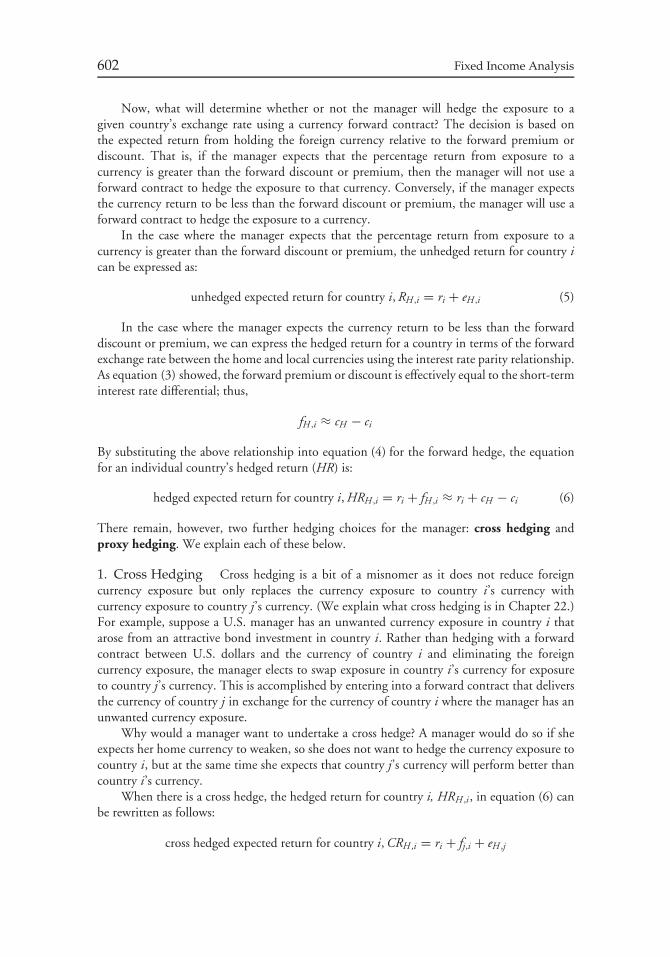
602 Fixed Income Analysis
Now, what will determine whether or not the manager will hedge the exposure to agiven country’s exchange rate using a currency forward contract? The decision is based onthe expected return from holding the foreign currency relative to the forward premium ordiscount. That is, if the manager expects that the percentage return from exposure to acurrency is greater than the forward discount or premium, then the manager will not use aforward contract to hedge the exposure to that currency. Conversely, if the manager expectsthe currency return to be less than the forward discount or premium, the manager will use aforward contract to hedge the exposure to a currency.
In the case where the manager expects that the percentage return from exposure to acurrency is greater than the forward discount or premium, the unhedged return for country ican be expressed as:
unhedged expected return for country i, RH ,i = ri + eH ,i (5)
In the case where the manager expects the currency return to be less than the forwarddiscount or premium, we can express the hedged return for a country in terms of the forwardexchange rate between the home and local currencies using the interest rate parity relationship.As equation (3) showed, the forward premium or discount is effectively equal to the short-terminterest rate differential; thus,
fH ,i ≈ cH − ci
By substituting the above relationship into equation (4) for the forward hedge, the equationfor an individual country’s hedged return (HR) is:
hedged expected return for country i, HRH ,i = ri + fH ,i ≈ ri + cH − ci (6)
There remain, however, two further hedging choices for the manager: cross hedging andproxy hedging. We explain each of these below.
1. Cross Hedging Cross hedging is a bit of a misnomer as it does not reduce foreigncurrency exposure but only replaces the currency exposure to country i’s currency withcurrency exposure to country j’s currency. (We explain what cross hedging is in Chapter 22.)For example, suppose a U.S. manager has an unwanted currency exposure in country i thatarose from an attractive bond investment in country i. Rather than hedging with a forwardcontract between U.S. dollars and the currency of country i and eliminating the foreigncurrency exposure, the manager elects to swap exposure in country i’s currency for exposureto country j’s currency. This is accomplished by entering into a forward contract that deliversthe currency of country j in exchange for the currency of country i where the manager has anunwanted currency exposure.
Why would a manager want to undertake a cross hedge? A manager would do so if sheexpects her home currency to weaken, so she does not want to hedge the currency exposure tocountry i, but at the same time she expects that country j’s currency will perform better thancountry i’s currency.
When there is a cross hedge, the hedged return for country i, HRH ,i , in equation (6) canbe rewritten as follows:
cross hedged expected return for country i, CRH ,i = ri + fj,i + eH ,j
Chapter 21 International Bond Portfolio Management 603
where fj,i is the forward discount or premium between country j and country i. The aboveexpression says that the cross hedged return for country i depends on (1) the expected bondreturn for country i, (2) the currency return locked in by the cross hedge between country jand country i, and (3) the currency return between the home currency and country j.
We can rewrite the above equation in terms of short-term interest rates as given by interestrate parity. That is, for fj,i we substitute cj − ci . Doing so and rearranging terms gives:
cross hedged expected return for country i, CRH ,i ≈ (ri − ci) + (cj + eH ,j) (7)
Equation (7) says that the cross hedged expected return for country i depends on (1) thedifferential between country i’s bond return and country i’s short-term interest rate plus(2) the short-term interest rate in country j, and (3) the currency return between the homecurrency and currency j.
2. Proxy Hedging Proxy hedging keeps the currency exposure in country i, but createsa hedge by establishing a short position in country j’s currency. Why would a manager wantto undertake a proxy hedge? This strategy would normally be considered only where thecurrencies of country i and country j are highly correlated, and the hedge costs in countryj are lower than in country i. A proxy hedge can also represent a bullish view on the homecurrency, with a more negative view on country j’s currency than country i’s currency.
When there is a proxy hedge, the hedged return for country i, HRH ,i , in equation (6) canbe rewritten as follows:
proxy hedged expected return for country i, PRH ,i = ri + eH ,i + fH ,j − eH ,j
where fH ,j is the forward discount or premium between the home country and country j.Notice that in the above equation, there is still the exposure to the exchange rate between
the home currency and currency i. The proxy hedge comes into play by the shorting of thecurrency return between the home currency and currency j.
Based on interest rate parity we can replace fH ,j with the difference in short-term interestrates, cH − cj , to get
proxy hedged expected return for country i, PRH ,i ≈ ri + eH ,i + cH − cj − eH ,j
This is equivalent to
proxy hedged expected return for country i,
PRH ,i ≈ (ri − ci) + (ci + eH ,i) + [(cH − cj) − eH ,j] (8)
Equation (8) states the expected return for country i using proxy hedging depends on
1. the differential between the bond return for country i and the short-term interest ratefor country i
2. the short-term interest rate for country i adjusted for the currency return for country irelative to the home currency
3. the differential in the short-term interest rates between the home currency and countryj adjusted for the short currency position in country j.
604 Fixed Income Analysis
3. Recasting Relationships in Terms of Short-Term Interest Rates When we sub-stituted short-term interest rate differentials for the forward premia or discounts above, itbecomes apparent from equations (6), (7), and (8) that the difference in return between hedg-ing, cross hedging, and proxy hedging is entirely due to differences in short-term interest ratesand currency exposure.25 This is also true for the unhedged return for a country as given byequation (5). This can be seen by simply rewriting equation (5) as follows:
unhedged expected return for country i, RH ,i = (ri − ci) + (ci + eH ,i)
The unhedged expected return is thus equal to (1) the differential between the bond return incountry i and the short-term interest rate in country i and (2) the short-term interest rate incountry i adjusted for the currency return.
These equations show how integral the short-term interest rate differential is to the cur-rency hedge decision. This means that (1) the short-term interest rate differential should relateto the currency decision and (2) bond market returns should be an excess return, calculatedless the local short-term interest rate. This can be made explicit by adding and subtracting thehome currency short-term interest rate to the four return relationships—unhedged, hedged,cross hedged, and proxy hedged. (The derivations are provided in the appendix to this chapter.)By doing so, this allows the forward premium (fH ,i = cH − ci) to be inserted into the currencyterm giving:
unhedged expected return for country i, RH ,i = cH + (ri − ci) + (eH ,i − fH ,i) (9)
hedged expected return for country i, HRH ,i = cH + (ri − ci) (10)
cross hedged expected return for country i,
CRH ,i = cH + (ri − ci) + (eH ,j − fH ,j) (11)
proxy hedged expected return for country i,
PRH ,i = cH + (ri − ci) + [(eH ,i − eH ,j) − fj,i] (12)
From equations (9) through (12), we see the return for each strategy can be divided into threedistinct return components:
Component 1: the short-term interest rate for the home currency: (cH )
Component 2: the excess bond return of country i over the short-term interest rate ofcountry i: (ri − ci)
Component 3: the excess currency return, either unhedged, cross-hedged, or proxy hedged
The first two components, cH and (ri − ci), are the same for each strategy. The excess currencyreturn (the third component) becomes the currency return in excess of the forward premium(or discount) and becomes the basis for the decision of currency hedging. (We will illustratethis below.) The bond decision is purely a matter of selecting the markets which offer the bestexpected excess return (ri − ci) and the bond and currency allocation decisions are entirelyindependent. In a sense, the hedged expected return can be considered the base expected returnas it is a component of the unhedged, cross hedged, and proxy hedged expected returns. Thus,
25The derivation of the relationships presented in this section are provided in the appendix to thischapter.
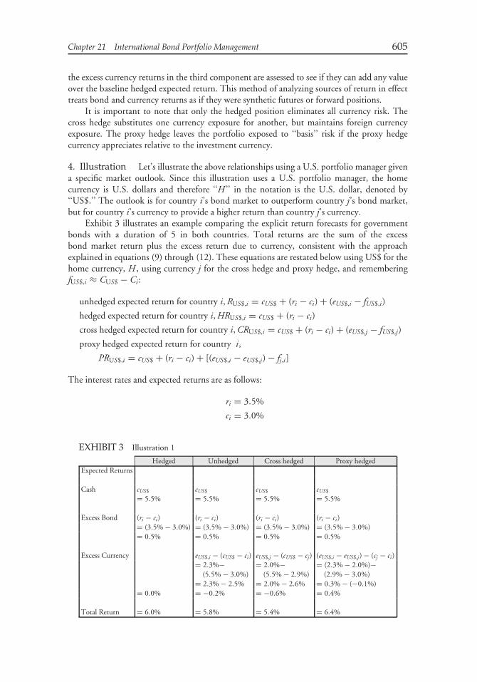
Chapter 21 International Bond Portfolio Management 605
the excess currency returns in the third component are assessed to see if they can add any valueover the baseline hedged expected return. This method of analyzing sources of return in effecttreats bond and currency returns as if they were synthetic futures or forward positions.
It is important to note that only the hedged position eliminates all currency risk. Thecross hedge substitutes one currency exposure for another, but maintains foreign currencyexposure. The proxy hedge leaves the portfolio exposed to ‘‘basis’’ risk if the proxy hedgecurrency appreciates relative to the investment currency.
4. Illustration Let’s illustrate the above relationships using a U.S. portfolio manager givena specific market outlook. Since this illustration uses a U.S. portfolio manager, the homecurrency is U.S. dollars and therefore ‘‘H ’’ in the notation is the U.S. dollar, denoted by‘‘US$.’’ The outlook is for country i’s bond market to outperform country j’s bond market,but for country i’s currency to provide a higher return than country j’s currency.
Exhibit 3 illustrates an example comparing the explicit return forecasts for governmentbonds with a duration of 5 in both countries. Total returns are the sum of the excessbond market return plus the excess return due to currency, consistent with the approachexplained in equations (9) through (12). These equations are restated below using US$ for thehome currency, H , using currency j for the cross hedge and proxy hedge, and rememberingfUS$,i ≈ CUS$ − Ci:
unhedged expected return for country i, RUS$,i = cUS$ + (ri − ci) + (eUS$,i − fUS$,i)
hedged expected return for country i, HRUS$,i = cUS$ + (ri − ci)
cross hedged expected return for country i, CRUS$,i = cUS$ + (ri − ci) + (eUS$,j − fUS$,j)
proxy hedged expected return for country i,
PRUS$,i = cUS$ + (ri − ci) + [(eUS$,i − eUS$,j) − fj,i]
The interest rates and expected returns are as follows:
ri = 3.5%
ci = 3.0%
EXHIBIT 3 Illustration 1
Hedged Unhedged Cross hedged Proxy hedgedExpected Returns
Cash cUS$ cUS$ cUS$ cUS$
= 5.5% = 5.5% = 5.5% = 5.5%
Excess Bond (ri − ci) (ri − ci) (ri − ci) (ri − ci)= (3.5% − 3.0%) = (3.5% − 3.0%) = (3.5% − 3.0%) = (3.5% − 3.0%)= 0.5% = 0.5% = 0.5% = 0.5%
Excess Currency eUS$,i − (cUS$ − ci) eUS$,j − (cUS$ − cj) (eUS$,i − eUS$,j) − (cj − ci)= 2.3%− = 2.0%− = (2.3% − 2.0%)−
(5.5% − 3.0%) (5.5% − 2.9%) (2.9% − 3.0%)= 2.3% − 2.5% = 2.0% − 2.6% = 0.3% − (−0.1%)
= 0.0% = −0.2% = −0.6% = 0.4%
Total Return = 6.0% = 5.8% = 5.4% = 6.4%
606 Fixed Income Analysis
eUS$,i = 2.3%
cj = 2.9%
eUS$,j = 2.0%
cUS$ = 5.5%
As mentioned earlier, the first two components of the above equations, the U.S. cash rateand the expected excess bond return in country i, are identical in all four equations, and equalto the expected hedged bond return. Thus, we can begin with the hedged bond return andcompare the excess currency returns (the third component of the equations) of the unhedged,cross hedged, and proxy hedged strategies. The hedged bond return is
cUS$ + (ri − ci) or 5.5% + (3.5% − 3.0%) = 6.0%.
Let’s look at this component for the unhedged strategy. From the first equation:
excess currency return for unhedged strategy for country i = (eUS$,i − fUS$,i)
or equivalently, since from interest rate parity fUS$,i = cUS$ − ci, we can rewrite the expres-sion as
excess currency return for unhedged strategy for country i = eUS$,i − (cUS$ − ci)
Thus, the performance relative to the hedged currency strategy depends on whether theexpected currency appreciation is greater than the short-term interest rate differential [i.e.,eUS$,i > (cUS$ − ci)] or less than the interest rate differential [i.e., eUS$,i < (cUS$ − ci)]. In theformer case, the unhedged strategy is expected to outperform the hedged strategy.
Turning to our illustration, the expected return on currency i of 2.3% is less than theshort-term interest rate differential of 2.5% over the 1-year horizon (5.5% in the U.S. versus3.0% in country i). Stated another way, the expected excess currency return componentto a U.S. dollar-based investor from an unhedged bond holding in currency i is −0.2%.Consequently, the position would offer a higher return when hedged back into U.S. dollars.
Now consider a cross hedging strategy. Cross hedging allows the portfolio manager tocreate a currency exposure that can vary substantially from the underlying bond marketexposure. A cross hedge replaces one foreign currency exposure with another that usually hasa higher expected return. The excess currency component from the cross hedge strategy is:
excess currency return for cross hedged strategy for country i = (eUS$,j − fUS$,j)
or equivalently, since from interest rate parity fUS$,j ≈ cUS$ − cj , we can rewrite the expres-sion as
excess currency return for cross hedged strategy for country i = eUS$,j − (cUS$ − cj)
Compared to a hedged strategy, a cross hedge is attractive if the short-term interest rate of thecountry used for the cross hedge plus the expected return in the cross currency is greater thanthe U.S. dollar short-term interest rate. If the U.S. dollar short-term interest rate is greater thanthe sum of these two terms, a cross hedged strategy is less attractive than a hedged strategy.
In the illustration, the short-term interest rate differential of 2.6% between the U.S. andcountry j (cUS$ − cj) is greater than the 2.0% expected appreciation of the currency of countryj versus the U.S. (eUS$,j). In this case, the expected excess currency return for the cross hedge
Chapter 21 International Bond Portfolio Management 607
strategy for country i using country j (i.e., eUS$,j − (cUS$ − cj)) is −0.6%. The expected returnfrom cross hedging is 5.4%, so a cross hedge with country j will not be used because theexpected return is less than the unhedged position and a straight hedge of currency i.
Finally, let’s look at the proxy hedging strategy. From the return of the proxy hedgedstrategy we know that
excess currency return for proxy hedged strategy for country i = [(eUS$,i − eUS$,j) − fj,i]
or equivalently, since from interest rate parity fj,i ≈ cj − ci , we can rewrite the expression as
excess currency return for proxy hedged strategy for country i = [(eUS$,i − eUS$,j) − (cj − ci)]
To interpret the above equation, let’s understand the currency position of the U.S. investor.The investor is long currency i. Consequently, the investor benefits if currency i appreciatesbut is hurt if currency i depreciates. In a proxy hedge, the investor is still long currency ibut the investor is also short currency j. Since the investor is short currency j, the investoris adversely affected if currency j appreciates, but benefits if currency j depreciates relative tocurrency i.
In our illustration, both currency i and currency j are expected to appreciate relative tothe U.S. dollar. The relative currency appreciation between currency i and currency j is whatis important according to the equation. If the appreciation for currency i—which the investoris long—is greater than the appreciation for currency j —which the investor is short—aninvestor will benefit from a proxy hedge. In our illustration, country i’s expected appreciationis 2.3% while country j’s is only 2.0%. Thus, there will be an expected currency return fromthis proxy hedging strategy of 30 basis points. This is what the first bracketed term in theexcess currency return equation above says.
Just looking at the expected currency return from a proxy hedging strategy, however, isnot sufficient. The above equation shows the expected currency return for the proxy hedgingstrategy must be adjusted to determine the excess currency return for the proxy hedgingstrategy. The adjustment is obtained by subtracting the short-term interest rate differential incountries j and i from the expected currency return from proxy hedging. If that differential isless than the expected currency return from proxy hedging, then proxy hedging is attractive.If it is greater than the expected currency return from proxy hedging, then proxy hedging isunattractive.
In our illustration, the proxy hedging strategy is attractive because the short-term interestrate differential between country j and country i is −10 basis points, which is less than the30 basis point currency return for the proxy hedging strategy. The excess return from theproxy hedging strategy is then 30 basis points minus the −10 basis point short-term interestrate differential. So, the excess return from the proxy hedging strategy in our illustration is 40basis points. The proxy hedged expected return is 6.4%, which is greater than the three otheralternatives—unhedged, hedge with currency i, and cross hedge with currency j.
In Exhibit 4 we have changed the example in Exhibit 3 by altering one number. In thisillustration, the expected appreciation for currency j is now 3.2% rather than 2.0%. Thus,the expected appreciation for currency j is greater than for currency i. The expected currencyreturn for the proxy hedging strategy is then −90 basis points (2.3% − 3.2%). After adjustingfor the short-term interest differential of −10 basis points, the excess currency return usingcountry j in a proxy hedge is −80 basis points. Consequently, the proxy hedge return of 5.2%is unattractive, as it is less than the three other alternatives analyzed. In this illustration, thecross hedge presents the best choice based on the expected returns.
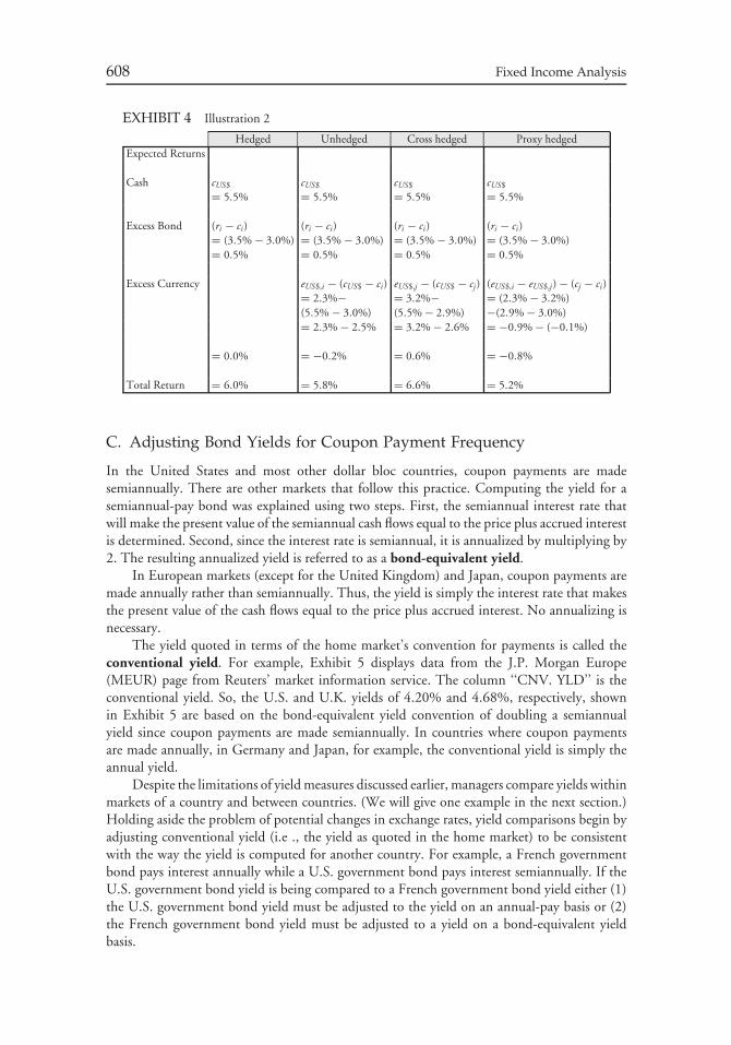
608 Fixed Income Analysis
EXHIBIT 4 Illustration 2
Hedged Unhedged Cross hedged Proxy hedgedExpected Returns
Cash cUS$ cUS$ cUS$ cUS$
= 5.5% = 5.5% = 5.5% = 5.5%
Excess Bond (ri − ci) (ri − ci) (ri − ci) (ri − ci)= (3.5% − 3.0%) = (3.5% − 3.0%) = (3.5% − 3.0%) = (3.5% − 3.0%)= 0.5% = 0.5% = 0.5% = 0.5%
Excess Currency eUS$,i − (cUS$ − ci) eUS$,j − (cUS$ − cj) (eUS$,i − eUS$,j) − (cj − ci)= 2.3%− = 3.2%− = (2.3% − 3.2%)(5.5% − 3.0%) (5.5% − 2.9%) −(2.9% − 3.0%)= 2.3% − 2.5% = 3.2% − 2.6% = −0.9% − (−0.1%)
= 0.0% = −0.2% = 0.6% = −0.8%
Total Return = 6.0% = 5.8% = 6.6% = 5.2%
C. Adjusting Bond Yields for Coupon Payment Frequency
In the United States and most other dollar bloc countries, coupon payments are madesemiannually. There are other markets that follow this practice. Computing the yield for asemiannual-pay bond was explained using two steps. First, the semiannual interest rate thatwill make the present value of the semiannual cash flows equal to the price plus accrued interestis determined. Second, since the interest rate is semiannual, it is annualized by multiplying by2. The resulting annualized yield is referred to as a bond-equivalent yield.
In European markets (except for the United Kingdom) and Japan, coupon payments aremade annually rather than semiannually. Thus, the yield is simply the interest rate that makesthe present value of the cash flows equal to the price plus accrued interest. No annualizing isnecessary.
The yield quoted in terms of the home market’s convention for payments is called theconventional yield. For example, Exhibit 5 displays data from the J.P. Morgan Europe(MEUR) page from Reuters’ market information service. The column ‘‘CNV. YLD’’ is theconventional yield. So, the U.S. and U.K. yields of 4.20% and 4.68%, respectively, shownin Exhibit 5 are based on the bond-equivalent yield convention of doubling a semiannualyield since coupon payments are made semiannually. In countries where coupon paymentsare made annually, in Germany and Japan, for example, the conventional yield is simply theannual yield.
Despite the limitations of yield measures discussed earlier, managers compare yields withinmarkets of a country and between countries. (We will give one example in the next section.)Holding aside the problem of potential changes in exchange rates, yield comparisons begin byadjusting conventional yield (i.e ., the yield as quoted in the home market) to be consistentwith the way the yield is computed for another country. For example, a French governmentbond pays interest annually while a U.S. government bond pays interest semiannually. If theU.S. government bond yield is being compared to a French government bond yield either (1)the U.S. government bond yield must be adjusted to the yield on an annual-pay basis or (2)the French government bond yield must be adjusted to a yield on a bond-equivalent yieldbasis.
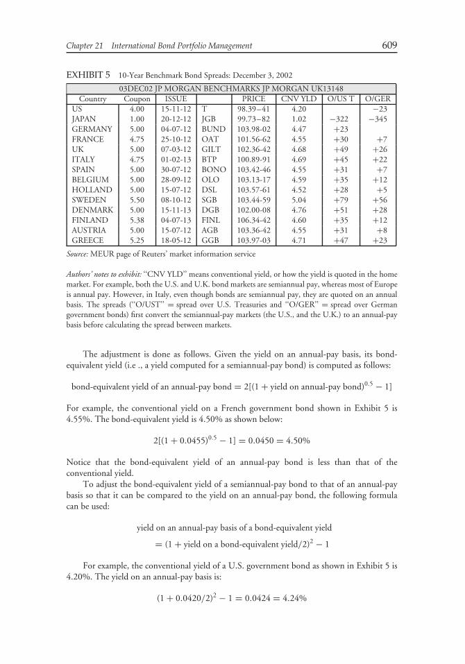
Chapter 21 International Bond Portfolio Management 609
EXHIBIT 5 10-Year Benchmark Bond Spreads: December 3, 2002
03DEC02 JP MORGAN BENCHMARKS JP MORGAN UK13148Country Coupon ISSUE PRICE CNV YLD O/US T O/GER
US 4.00 15-11-12 T 98.39–41 4.20 −23JAPAN 1.00 20-12-12 JGB 99.73–82 1.02 −322 −345GERMANY 5.00 04-07-12 BUND 103.98-02 4.47 +23FRANCE 4.75 25-10-12 OAT 101.56-62 4.55 +30 +7UK 5.00 07-03-12 GILT 102.36-42 4.68 +49 +26ITALY 4.75 01-02-13 BTP 100.89-91 4.69 +45 +22SPAIN 5.00 30-07-12 BONO 103.42-46 4.55 +31 +7BELGIUM 5.00 28-09-12 OLO 103.13-17 4.59 +35 +12HOLLAND 5.00 15-07-12 DSL 103.57-61 4.52 +28 +5SWEDEN 5.50 08-10-12 SGB 103.44-59 5.04 +79 +56DENMARK 5.00 15-11-13 DGB 102.00-08 4.76 +51 +28FINLAND 5.38 04-07-13 FINL 106.34-42 4.60 +35 +12AUSTRIA 5.00 15-07-12 AGB 103.36-42 4.55 +31 +8GREECE 5.25 18-05-12 GGB 103.97-03 4.71 +47 +23
Source: MEUR page of Reuters’ market information service
Authors’ notes to exhibit: ‘‘CNV YLD’’ means conventional yield, or how the yield is quoted in the homemarket. For example, both the U.S. and U.K. bond markets are semiannual pay, whereas most of Europeis annual pay. However, in Italy, even though bonds are semiannual pay, they are quoted on an annualbasis. The spreads (‘‘O/UST’’ = spread over U.S. Treasuries and ‘‘O/GER’’ = spread over Germangovernment bonds) first convert the semiannual-pay markets (the U.S., and the U.K.) to an annual-paybasis before calculating the spread between markets.
The adjustment is done as follows. Given the yield on an annual-pay basis, its bond-equivalent yield (i.e ., a yield computed for a semiannual-pay bond) is computed as follows:
bond-equivalent yield of an annual-pay bond = 2[(1 + yield on annual-pay bond)0.5 − 1]
For example, the conventional yield on a French government bond shown in Exhibit 5 is4.55%. The bond-equivalent yield is 4.50% as shown below:
2[(1 + 0.0455)0.5 − 1] = 0.0450 = 4.50%
Notice that the bond-equivalent yield of an annual-pay bond is less than that of theconventional yield.
To adjust the bond-equivalent yield of a semiannual-pay bond to that of an annual-paybasis so that it can be compared to the yield on an annual-pay bond, the following formulacan be used:
yield on an annual-pay basis of a bond-equivalent yield
= (1 + yield on a bond-equivalent yield/2)2 − 1
For example, the conventional yield of a U.S. government bond as shown in Exhibit 5 is4.20%. The yield on an annual-pay basis is:
(1 + 0.0420/2)2 − 1 = 0.0424 = 4.24%
610 Fixed Income Analysis
Notice that the yield on an annual-pay basis will be greater than the conventional yield.Yield spreads are typically computed between a country’s yield and that of a benchmark.
As explained, the U.S. government bond market and the German government bond marketare the two most common benchmarks used. The next-to-the-last column in Exhibit 5, labeled‘‘O/US T,’’ shows the spread between a country’s yield and the U.S. Treasury yield. Noticethat for the French government bond, the spread is shown as +30 basis points. This spreadis obtained by subtracting the French government bond of 4.54% (the conventional yieldreported in Exhibit 5) from the adjusted U.S. government bond yield of 4.24% (as computedabove).
The last column in Exhibit 5, labeled ‘‘O/GER,’’ shows the spread between a country’syield and the German government bond yield. For example, when the spread of the Frenchgovernment bond yield over the German government bond yield is computed, since bothmarkets pay coupon interest annually, the spread is simply the difference in their conventionalyields. Since the yield on the French government bond is 4.55% and the yield on a Germangovernment bond is 4.47%, the spread is 8 basis points. (Exhibit 5 shows a 7 basis pointspread. The difference is due to rounding.)
D. Forward Rates and Breakeven Analysis
As explained earlier, there are various methods of evaluating relative value in international bondmarkets. Before these can be translated into a market allocation, a manager must compare theirstrategic outlook to that which is already priced into the market. This can be accomplished byeither converting the economic outlook into point forecasts for bond and currency levels, orlooking at the forward rates implied by current market conditions and comparing them withthe economic outlook.
Bond and currency breakeven rates, the rate which make two investments produceidentical total returns, are usually calculated versus a benchmark market return over a specifictime horizon. A large yield spread between two markets implies a larger ‘‘cushion’’ (therequired spread widening to equate total returns in both markets, or the breakeven rate) overthe investment time horizon.
Comparing of forward interest rates can be instrumental in identifying where differencesbetween the strategic outlook and market prices may present investment opportunities. Asexplained previously, forward interest rates use the shape of the yield curve to calculate impliedforward bond rates and allow a quick comparison of what is required, in terms of yield shiftsin each market, to provide a return equal to the short-term risk-free rate (a zero excess return).This would correspond to a bond excess return of zero in equations (9) through (12), or(ri − ci) = 0. Forward interest rates represent a breakeven rate, not across markets, but withinmarkets. The strategic bond allocation can then be derived by increasing exposure to marketswhere the expected bond return over the short-term interest rate is most positive—that is,where the expected bond yield is furthest below the forward yield. Forward rate calculators arealso available on systems such as Bloomberg as illustrated in Exhibit 6.
The forward foreign exchange rate represents a breakeven rate between hedged andunhedged currency returns as previously shown in the components of return analysis. In termsof equations (9), (11), and (12), currency excess return is zero when the percentage change inthe currency equals the forward premium or discount. As forward foreign exchange rates aredetermined by short-term interest rate differentials, they can be estimated from the interestrates on deposits, specifically, Eurodeposit rates as in equations (2) and (3), which can be easilyobtained from market data services such as Bloomberg and Reuters.
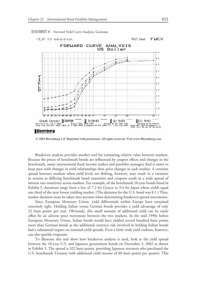
Chapter 21 International Bond Portfolio Management 611
EXHIBIT 6 Forward Yield Curve Analysis: Germany
2004 Bloomberg L.P. Reprinted with permission. All rights reserved. Visit www.Bloomberg.com.
Breakeven analysis provides another tool for estimating relative value between markets.Because the prices of benchmark bonds are influenced by coupon effects and changes in thebenchmark, many international fixed income traders and portfolio managers find it easier tokeep pace with changes in yield relationships than price changes in each market. A constantspread between markets when yield levels are shifting, however, may result in a variationin returns as differing benchmark bond maturities and coupons result in a wide spread ofinterest rate sensitivity across markets. For example, of the benchmark 10-year bonds listed inExhibit 5, durations range from a low of 7.2 for Greece to 9.4 for Japan where yields equalone third of the next lowest yielding market. (The duration for the U.S. bond was 8.1.) Thus,market duration must be taken into account when determining breakeven spread movements.
Since European Monetary Union, yield differentials within Europe have remainedextremely tight. Holding Italian versus German bonds provides a yield advantage of only22 basis points per year. Obviously, this small amount of additional yield can be easilyoffset by an adverse price movement between the two markets. In the mid 1990s beforeEuropean Monetary Union, Italian bonds would have yielded several hundred basis pointsmore than German bonds as the additional currency risk involved in holding Italian bondshad a substantial impact on nominal yield spreads. Even a fairly wide yield cushion, however,can also quickly evaporate.
To illustrate this and show how breakeven analysis is used, look at the yield spreadbetween the 10-year U.S. and Japanese government bonds on December 3, 2002 as shownin Exhibit 5. The spread is 322 basis points, providing Japanese investors who purchased theU.S. benchmark Treasury with additional yield income of 80 basis points per quarter. This
612 Fixed Income Analysis
additional yield advantage can be eliminated by the spread widening substantially less than the80 basis points. The widening can occur in one of the following two ways:
• yields in Japan can decrease, resulting in price appreciation of the Japanese governmentbond
• yields in the United States can increase, resulting in a price decline of the U.S. Treasurybond
Of course, a combination of the two can also occur. To quantify the amount of spreadwidening that would erase the yield advantage from investing in a higher yielding market, weneed to conduct a breakeven analysis.
It is important to note this breakeven analysis is not a total return analysis; it applies onlyto bond returns in local currency and ignores currency movements. This breakeven analysis iseffective in comparing bond markets that share a common currency, as within the euro zone;however, currency must be taken into account when applying breakeven analysis to marketswith different currencies. The additional yield advantage in the example above is erased ifthe U.S. dollar depreciates by more than 0.80% during the quarter. Below, we illustrate howa hedged breakeven analysis can be calculated using hedged returns, or simply the forwardforeign exchange premium or discount between the two currencies.
We know that the duration of the Japanese bond is 9.4.26 This means that for a 100 basispoint change in yield the approximate percentage price change for the Japanese bond will be9.4%. For a 50 basis point change in yield, the percentage price change for the Japanese bondwill change by approximately 4.7%. We can generalize this as follows:
change in price = 9.4 × change in yield
If we let W denote the spread widening, we can rewrite the above equation as:
change in price = 9.4 × W
We want to determine the amount of yield movement in Japan that would exactly offset theyield advantage of 0.80% from investing in U.S. bonds. Thus, we need to calculate whatdecline in Japanese bond yields would generate exactly 0.80% in price appreciation to makethe Japanese investor indifferent between the two investments (ignoring any potential currencymovements). Thus, the equation becomes
0.80% = 9.4 × W
Solving for W ,
W = 0.80%/9.4 = 0.085% = 8.5 basis points
Therefore, a spread widening of 8.5 basis points due to a decline in the yield in Japan wouldnegate the additional yield from buying the U.S. Treasury issue. In other words, a change in
26This is the modified duration for the issue. Since the Japanese bond and the U.S. bonds are option-free,the modified duration is close to the effective duration. Duration is only a first approximation of theapproximate change in value when interest rates change. By only considering duration, the analysis aboveignores the impact of convexity on returns.
Chapter 21 International Bond Portfolio Management 613
yields of only 8.5 basis points is needed in this case to delete the 3-month yield advantage of80 basis points.
We refer to this yield spread change as the breakeven spread movement. Note that thebreakeven spread movement must (1) be related to an investment horizon and (2) utilize thehigher of the two countries’ modified durations. Using the highest modified duration providesthe minimum spread movement that would offset the additional yield from investing in ahigher yielding market. So, in our example, the 3-month breakeven spread movement dueto Japanese yields is 8.5 basis points, meaning that it is the spread movement due to a dropin Japanese rates by 8.5 basis points that would eliminate the 3-month additional yield frominvesting in U.S. Treasury bonds. The breakeven spread movement using the 8.1 duration inthe U.S. would be 9.9 basis points (0.8/8.1 = 9.9); a difference of only 1.4 basis points.
The breakeven spread movement described above completely ignores the affect of currencymovements on returns. It also ignores the implied appreciation or depreciation of the currencyreflected in the forward premium or discount. If we subscribe to the methodology discussedearlier in the chapter of attributing cash returns to the currency decision, and measuring bondmarket returns as the local return minus the cash rate, the results of the breakeven spreadmovement analysis on a hedged basis may be quite different. We can easily calculate thehedged breakeven spread movement by adding in the forward foreign exchange discount orpremium. At the time of this breakeven analysis, 3-month interest rates were 0.0675% inJapan and 1.425% in the United States. With this information we can obtain the embeddedforward rate using equation (3); that is,
f¥,$ ≈ c¥ − c$ = (0.0675% − 1.425%)/4 = −0.34%
The expected hedged return over the 3-month period, assuming no change in rates, is thesum of the nominal spread differential (0.80%) and the forward premium (−0.34%), or0.46%. Thus, the breakeven spread movement on a hedged basis is a mere 5 basis points(0.46% = 9.4 × W ) instead of the 8.5 basis points of potential widening calculated on a localcurrency basis. Consequently, a Japanese investor would have to expect either that spreadswould not widen by more than 5 basis points or believe that the dollar would depreciate versusthe yen by less than the embedded forward rate to make the trade attractive. Because currencyhedge costs (i.e., the forward premium or discount) are determined by short-term interestrates, the breakeven spread movement on a hedged basis will always be smaller when hedginga currency with higher short-term interest rates.
Alternatively, we could use equation (10) to calculate the expected hedged return to ayen-based investor over a 3-month period and compare it to the return on a Japanese 10-yearbond over the same period. In order to do so, it is first necessary to adjust the U.S. governmentbond yield (which is quoted on a bond-equivalent yield basis) to an annual-pay yield basisbecause the Japanese yield is based on an annual basis. Earlier we showed that the conventionalyield of 4.20% for the U.S. government bond as reported in Exhibit 5 is 4.24% on anannual-pay basis. Assuming no change in rates, the expected hedged return is:
[(r$ − c$) + c¥]/4 = [(4.24% − 1.43%) + 0.07%]/4 = [2.88%]/4 = 0.72%
and the expected Japanese bond return is (1.02%/4, or 0.26%). Thus, the expected return ona hedged basis is 0.44%, which is close to the 0.46% in the first answer that we calculated.
614 Fixed Income Analysis
E. Security Selection
Once the bond market allocation decisions have been made and the optimal duration and yieldcurve profile selected for each market, the overall portfolio structure needs to be constructedthrough the purchase or sale of individual securities. Many international bond investors preferto trade only benchmark issues since they are more liquid than other similar maturity bonds.This can sometimes lead to a ‘‘dip’’ in the yield curve as investors prefer a certain issue ormaturity sector. The same phenomenon can result from a squeeze of certain issues in therepo market, or short-term demand imbalances for bonds deliverable into short bond futurespositions.
Taxation issues also need to be taken into account when selecting individual bonds forpurchase. For example, several markets have tax systems that encourage investors to hold lowercoupon bonds, hence certain bonds will tend to trade rich or cheap to the curve depending ontheir coupon. In markets that impose withholding taxes on coupon payments, internationalfixed income portfolio managers often minimize their tax liability by replacing a bond that isnear its coupon date with another bond of similar maturity. Market anomalies can also arisefrom differing tax treatment within markets. For example, Italian Eurobonds issued before1988 are exempt of withholding tax for Italian investors, hence they tend to trade at a loweryield than similar maturity bonds issued after 1988.
APPENDIX
The purpose of this appendix is to show how equations (9), (10), (11), and (12) in the chapterwere derived. All equation numbers refer to equations in this chapter.
Unhedged expected return:To derive the unhedged expected return given by equation (9), we begin with equation (5):
unhedged expected return for country i, RH ,i = ri + eH ,i
adding and subtracting ci on the right-hand side of the equation we get:
RH ,i = ri − ci + ci + eH ,i
We know that fH ,i = cH − ci, so ci = cH − fH ,i. Substituting for the second ci in the aboveequation and rearranging terms we have
RH ,i = cH + (ri − ci) + (eH ,i − fH ,i)
The above equation is equation (9), which states that the unhedged expected return forcountry i is equal to the short-term interest rate for the home country, the excess bond returnof country i, and the unhedged excess currency return of country i’s currency. The excesscurrency return is the currency return in country i relative to the home country less theshort-term interest rate differential between the home country and country i.
Hedged expected return:The hedged expected bond return for country i, equation (6), is derived by adding a
currency hedge (−eH ,i + cH − ci) to the unhedged return, equation (5). By doing so we get:
hedged expected return for country i, HRH ,i = ri + eH ,i − eH ,i + cH − ci
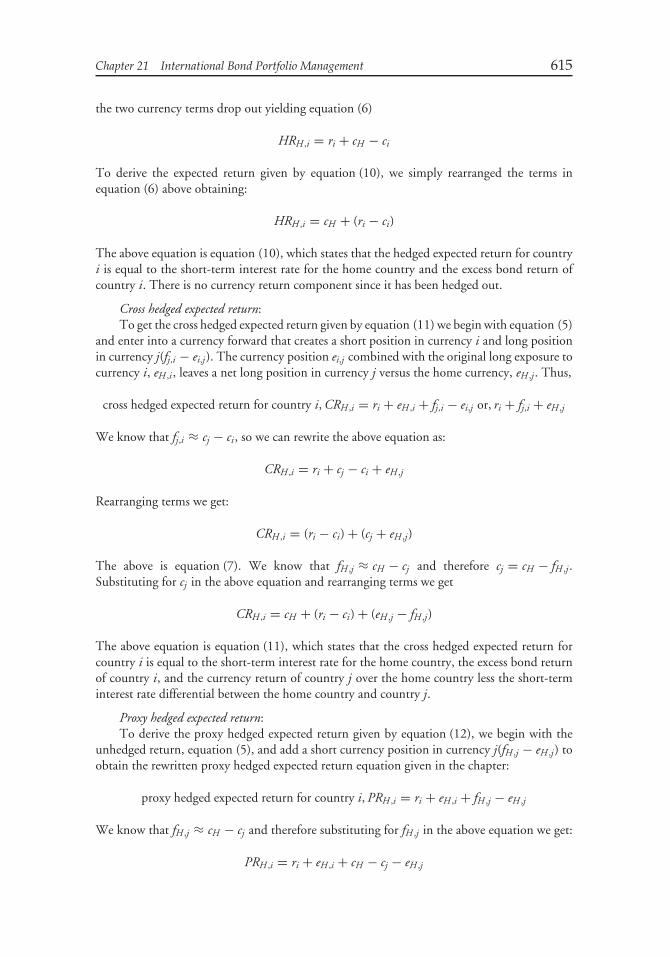
Chapter 21 International Bond Portfolio Management 615
the two currency terms drop out yielding equation (6)
HRH ,i = ri + cH − ci
To derive the expected return given by equation (10), we simply rearranged the terms inequation (6) above obtaining:
HRH ,i = cH + (ri − ci)
The above equation is equation (10), which states that the hedged expected return for countryi is equal to the short-term interest rate for the home country and the excess bond return ofcountry i. There is no currency return component since it has been hedged out.
Cross hedged expected return:To get the cross hedged expected return given by equation (11) we begin with equation (5)
and enter into a currency forward that creates a short position in currency i and long positionin currency j(fj,i − ei,j). The currency position ei,j combined with the original long exposure tocurrency i, eH ,i , leaves a net long position in currency j versus the home currency, eH ,j . Thus,
cross hedged expected return for country i, CRH ,i = ri + eH ,i + fj,i − ei,j or, ri + fj,i + eH ,j
We know that fj,i ≈ cj − ci, so we can rewrite the above equation as:
CRH ,i = ri + cj − ci + eH ,j
Rearranging terms we get:
CRH ,i = (ri − ci) + (cj + eH ,j)
The above is equation (7). We know that fH ,j ≈ cH − cj and therefore cj = cH − fH ,j .Substituting for cj in the above equation and rearranging terms we get
CRH ,i = cH + (ri − ci) + (eH ,j − fH ,j)
The above equation is equation (11), which states that the cross hedged expected return forcountry i is equal to the short-term interest rate for the home country, the excess bond returnof country i, and the currency return of country j over the home country less the short-terminterest rate differential between the home country and country j.
Proxy hedged expected return:To derive the proxy hedged expected return given by equation (12), we begin with the
unhedged return, equation (5), and add a short currency position in currency j(fH ,j − eH ,j) toobtain the rewritten proxy hedged expected return equation given in the chapter:
proxy hedged expected return for country i, PRH ,i = ri + eH ,i + fH ,j − eH ,j
We know that fH ,j ≈ cH − cj and therefore substituting for fH ,j in the above equation we get:
PRH ,i = ri + eH ,i + cH − cj − eH ,j
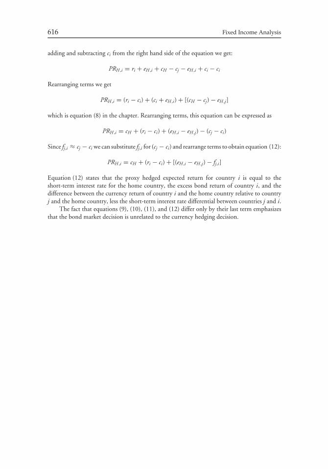
616 Fixed Income Analysis
adding and subtracting ci from the right hand side of the equation we get:
PRH ,i = ri + eH ,i + cH − cj − eH ,i + ci − ci
Rearranging terms we get
PRH ,i = (ri − ci) + (ci + eH ,i) + [(cH − cj) − eH ,j]
which is equation (8) in the chapter. Rearranging terms, this equation can be expressed as
PRH ,i = cH + (ri − ci) + (eH ,i − eH ,j) − (cj − ci)
Since fj,i ≈ cj − ci we can substitute fj,i for (cj − ci) and rearrange terms to obtain equation (12):
PRH ,i = cH + (ri − ci) + [(eH ,i − eH ,j) − fj,i]
Equation (12) states that the proxy hedged expected return for country i is equal to theshort-term interest rate for the home country, the excess bond return of country i, and thedifference between the currency return of country i and the home country relative to countryj and the home country, less the short-term interest rate differential between countries j and i.
The fact that equations (9), (10), (11), and (12) differ only by their last term emphasizesthat the bond market decision is unrelated to the currency hedging decision.
CHAPTER 22CONTROLLING INTEREST
RATE RISK WITHDERIVATIVES∗
I. INTRODUCTION
Previously, the features and characteristics of interest rate futures and swaps were explained.In addition, at Level II, the valuation of these derivative instruments was explained. In thischapter, our focus is on using derivatives to control the interest rate risk of a portfolio. Otheruses for derivatives include speculating on interest rate movements and speculating on changesin interest rate volatility. These strategies are similar to those employed in the equity marketand are not covered in this book.
II. CONTROLLING INTEREST RATE RISK WITHFUTURES
The price of an interest rate futures contract moves in the opposite direction from the changein interest rates: when rates rise, the futures price falls; when rates fall, the futures pricerises. Buying a futures contract increases a portfolio’s exposure to a rate change. That is, theportfolio’s duration increases. Selling a futures contract decreases a portfolio’s exposure toa rate change. Equivalently, selling a futures contract that reduces the portfolio’s duration.Consequently, buying and selling futures can be used to alter the duration of a portfolio.
While managers can alter the duration of their portfolios with cash market instruments(buying or selling Treasury securities), using interest rate futures has the following fouradvantages:
Advantage 1: Transaction costs for trading futures are lower than trading in the cashmarket.
Advantage 2: Margin requirements are lower for futures than for Treasury securities; usingfutures thus permits greater leverage.
Advantage 3: It is easier to sell short in the futures market than in the cash market.
∗This chapter is authored by Frank J. Fabozzi, PhD, CFA, CPA, Shrikant Ramamurthy, and Mark Pitts,
PhD.
617
618 Fixed Income Analysis
Advantage 4: Futures can be used to construct a portfolio with a longer duration than isavailable using cash market securities.
To appreciate the last advantage, suppose that in a certain interest rate environment apension fund manager must structure a portfolio to have a duration of 15 to accomplish aparticular investment objective. Bonds with such a long duration may not be available. Bybuying the appropriate number and kind of interest rate futures contracts, a pension fundmanager can increase the portfolio’s duration to the target level of 15.
A. General Principles of Interest Rate Risk Control
The general principle in controlling interest rate risk with futures is to combine the dollarexposure of the current portfolio and the dollar exposure of a futures position so that the totaldollar exposure is equal to the target dollar exposure. This means that the manager must beable to accurately measure the dollar exposure of both the current portfolio and the futurescontract employed to alter the risk profile.
There are two commonly used measures for approximating the change in the dollar valueof a bond or bond portfolio resulting from changes in interest rates: price value of a basis point(PVBP) and duration. PVBP is the dollar price change resulting from a one-basis-point changein yield. Duration is the approximate percentage change in price for a 100-basis-point change inrates. (Given the percentage price change, the dollar price change for a given change in interestrates can be computed.) There are two measures of duration: modified and effective. Effectiveduration is the appropriate measure for bonds with embedded options. In this chapter whenwe refer to duration, we mean effective duration. Moreover, since the manager is interested indollar price exposure, the effective dollar duration should be used. For a one basis point changein rates, PVBP is equal to the effective dollar duration for a one-basis-point change in rates.
As emphasized in earlier chapters, a good valuation model is needed to estimate the effectivedollar duration. The valuation model is used to determine the new values for the bonds inthe portfolio if rates change. Consequently, the starting point in controlling interest rate riskis the development of a reliable valuation model. A reliable valuation model is also needed tovalue the derivative contracts that the manager wants to use to control interest rate exposure.
Suppose that a manager seeks a target duration for the portfolio based on eitherexpectations of interest rates or client-specified exposure. Given the target duration, a targetdollar duration for a small basis point change in interest rates can be computed. For a 50basis point change in interest rates the target dollar duration can be found by multiplying thetarget duration by the dollar value of the portfolio and then dividing by 200. (We divide by 2because we are dealing with one half of a 100 basis point change.) For example, suppose thatthe manager of a $500 million portfolio wants a target duration of 6. That is, the managerseeks a 3% change in the value of the portfolio for a 50 basis point change in rates (assuminga parallel shift in rates of all maturities). Multiplying the target duration of 6 by $500 millionand dividing by 200 gives a target dollar duration of $15 million.
The manager must then determine the dollar duration of the current portfolio. Thecurrent dollar duration for a 50 basis point change in interest rates is calculated by multiplyingthe current duration by the dollar value of the portfolio and dividing by 200. For our $500million portfolio, suppose that the current duration is 4. The current dollar duration is then$10 million (4 times $500 million divided by 200).
The target dollar duration is then compared to the current dollar duration; the differenceis the dollar exposure that must be provided by a position in the futures contract. If the
Controlling Interest Rate Risk with Derivatives 619
target dollar duration exceeds the current dollar duration, a futures position must increase thedollar exposure by the difference. To increase the dollar exposure, an appropriate number offutures contracts must be purchased. If the target dollar duration is less than the current dollarduration, an appropriate number of futures contracts must be sold. That is,
If target dollar duration − current dollar duration > 0, buy futures
If target dollar duration − current dollar duration < 0, sell futures
Once a futures position is taken, the portfolio’s dollar duration is equal to the sumof the current dollar duration without futures plus the dollar duration of the futuresposition. That is,
portfolio’s dollar duration = current dollar duration without futures
+ dollar duration of futures position
The objective is to control the portfolio’s interest rate risk by establishing a futuresposition such that the portfolio’s dollar duration is equal to the target dollar duration. Thus,
portfolio’s dollar duration = target dollar duration
Or, equivalently,
target dollar duration = current dollar duration without futures
+ dollar duration of futures position (1)
Over time, as interest rates change, the portfolio’s dollar duration will move away from thetarget dollar duration. The manager can alter the futures position to adjust the portfolio’sdollar duration back to the target dollar duration.
Our focus above is on duration. However, duration measures price sensitivity to changesin interest rates assuming a parallel shift in the yield curve. For bond portfolios, nonparallelshifts in the yield curve should be taken into account. The same is true for individual mortgage-backed securities because, as explained in the next chapter, these securities are sensitive tochanges in the yield curve. In the next chapter, a framework will be presented that shows howto hedge both a change in the level of interest rates and a change in the shape of the yield curve.
1. Determining the Number of Contracts Each futures contract calls for delivery ofa specified par value of the underlying instrument. When interest rates change, the marketvalue of the underlying instrument changes, and therefore the value of the futures contractchanges. The amount of change in the futures dollar value must be estimated. This amount iscalled the dollar duration per futures contract. For example, assume the price of an interestrate futures contract is 70 and that the underlying interest rate instrument has a par value of$100,000. Thus, the futures delivery price is $70,000 (0.70 times $100,000). Suppose that achange in interest rates of 100 basis points results in a futures price change of about 3% percontract. Then the dollar duration per futures contract is $2,100 (0.03 times $70,000).
The dollar duration of a futures position is then the number of futures contracts multipliedby the dollar duration per futures contract. That is,
dollar duration of futures position = number of futures contracts
× dollar duration per futures contract (2)

620 Fixed Income Analysis
How many futures contracts are needed to obtain the target dollar duration? Substitutingequation (2) into equation (1), we get
number of futures contracts × dollar duration per futures contract
= target dollar duration − current dollar duration without futures (3)
Solving for the number of futures contracts we have:
number of futures contracts
= target dollar duration − current dollar duration without futures
dollar duration per futures contract(4)
Equation (4) gives the approximate number of futures contracts needed to adjust theportfolio’s dollar duration to the target dollar duration. A positive number means that futurescontracts must be purchased; a negative number means that futures contracts must be sold.Notice that if the target dollar duration is greater than the current dollar duration withoutfutures, the numerator is positive and futures contracts are purchased. If the target dollarduration is less than the current dollar duration without futures, the numerator is negativeand futures contracts are sold.
2. Dollar Duration for a Futures Position Now we discuss how to measure the dollarduration of a bond futures position. Keep in mind that the goal is to measure the sensitivityof the bond futures value to a change in rates.
Given a valuation model, the general methodology for computing the dollar duration of afutures position for a given change in interest rates is straightforward. The procedure is used forcomputing the dollar duration of any cash market instrument—shock (change) interest ratesup and down by the same number of basis points and compute the average dollar price change.
An adjustment is needed for the Treasury bond and note futures contracts. As explained,the pricing of the futures contract depends on the cheapest-to-deliver (CTD) issue.1 Thecalculation of the dollar duration of a Treasury bond or note futures contract requirescomputing the effect of a change in interest rates on the price of the CTD issue, which in turndetermines the change in the futures price. The dollar duration of a Treasury bond and notefutures contract is determined as follows:
dollar duration of futures contract = dollar duration of the CTD issue
× dollar duration of futures contract
dollar duration of the CTD issue
Recall that a conversion factor is specified for each issue that is acceptable for delivery underthe futures contract. For each deliverable issue, the product of the futures price and theconversion factor is the adjusted futures price for the issue. This adjusted price is called theconverted price. Relating this to the equation above, the second term is approximately equalto the reciprocal of the conversion factor of the cheapest-to-deliver issue. Thus, we can write:
dollar duration of futures contract = dollar duration of the CTD issue
conversion factor for the CTD issue
1The cheapest-to-deliver issue is the one issue from among all those that are eligible for delivery on acontract that has the highest return in a cash and carry trade. This return is called the implied repo rate.
Controlling Interest Rate Risk with Derivatives 621
B. Hedging with Interest Rate Futures
Hedging with futures calls for taking a futures position as a temporary substitute fortransactions to be made in the cash market at a later date. If cash and futures prices areperfectly positively correlated, any loss realized by the hedger from one position (whether cashor futures) will be exactly offset by a profit on the other position. Hedging is a special caseof controlling interest rate risk. In a hedge, the manager seeks a target duration or target dollarduration of zero.
A short hedge (or sell hedge) is used to protect against a decline in the cash price ofa bond. To execute a short hedge, futures contracts are sold. By establishing a short hedge,the manager has fixed the future cash price and transferred the price risk of ownership to thebuyer of the futures contract. To understand why a short hedge might be executed, supposethat a pension fund manager knows that bonds must be liquidated in 40 days to make a $5million payment to beneficiaries. If interest rates rise during the 40-day period, more bondswill have to be liquidated at a lower price than today to realize $5 million. To guard againstthis possibility, the manager can lock in a selling price by selling bonds in the futures market.2
A long hedge (or buy hedge) is undertaken to protect against an increase in the cashprice of a bond. In a long hedge, the manager buys a futures contract to lock in a purchaseprice. A pension fund manager might use a long hedge when substantial cash contributionsare expected and the manager is concerned that interest rates will fall. Also, a money managerwho knows that bonds are maturing in the near future and expects that interest rates will fallbefore receipt can employ a long hedge to lock in a rate for the proceeds to be reinvested.
In bond portfolio management, typically the bond or portfolio to be hedged is notidentical to the bond underlying the futures contract. This type of hedging is referred to ascross hedging.
The hedging process can be broken down into four steps:
Step 1: Determining the appropriate hedging instrument.
Step 2: Determining the target for the hedge.
Step 3: Determining the position to be taken in the hedging instrument.
Step 4: Monitoring and evaluating the hedge.
We discuss each step below.
1. Determining the Appropriate Hedging Instrument A primary factor in deter-mining which futures contract will provide the best hedge is the correlation between the priceon the futures contract and the interest rate that creates the underlying risk that the managerseeks to eliminate. For example, a long-term corporate bond portfolio can be better hedgedwith Treasury bond futures than with Treasury bill futures because long-term corporate bondrates are more highly correlated with Treasury bond futures than Treasury bill futures. Usingthe correct delivery month is also important. A manager trying to lock in a rate or price forSeptember will use September futures contracts because they will give the highest degree ofcorrelation.
2When hedging more than just the level of interest rates (e.g., hedging changes in the slope also), morethan one hedging instrument is used. One of the hedging instruments could require a long position eventhough the instrument to be hedged is a long position.
622 Fixed Income Analysis
Correlation is not, however, the only consideration if the hedging program is of significantsize. If, for example, a manager wants to hedge $600 million of a cash position in a distantdelivery month, liquidity becomes an important consideration. In such a case, it might benecessary for the manager to spread the hedge across two or more different contracts.
While our focus in this chapter is on hedging changes in the level of interest rates, whenmore than one type of change in the yield curve is to be hedged, then more than one hedginginstrument must be used. For example, hedging a mortgage security is covered in the nextchapter. As explained in the next chapter, because of the characteristic of mortgage securities,hedging both a change in the level and slope of the yield curve would be more effective. In suchcases, two hedging instruments are used. One can also hedge the level, slope, and curvaturechanges of the yield curve. In that case, three hedging instruments are used.
2. Determining the Target for the Hedge Having determined the correct contractand the correct delivery months, the manager should then determine what is expected from thehedge—that is, what rate will, on average, be locked in by the hedge. This is the target rateor target price. If this target rate is too high (if hedging a future sale) or too low (if hedginga future purchase), hedging may not be the right strategy for dealing with the unwanted risk.Determining what is expected (calculating the target rate or price for a hedge) is not alwayssimple. We’ll see how a manager should approach this problem for both simple and complexhedges.
a. Risk and Expected Return in a Hedge When a manager enters into a hedge, theobjective is to ‘‘lock in’’ a rate for the sale or purchase of a security. However, there is muchdisagreement about which rate or price a manager should expect to lock in when futures areused to hedge. Here are the two views:
View 1: The manager can, on average, lock in the rate at which the futures contracts arebought or sold.
View 2: The manager can, on average, lock in the current spot rate for the security (i.e.,current rate in the cash market).
Reality usually lies somewhere between these two views. However, as the following casesillustrate, each view is appropriate for certain situations.
b. The Target for Hedges Held to Delivery Hedges that are held until the futures deliv-ery date provide an example of a hedge that locks in the futures rate (i.e., the first view). Thefutures rate is the interest rate corresponding to the futures delivery price of the deliverableinstrument. The complication in the case of using Treasury bond futures and Treasury notefutures to hedge the value of intermediate- and long-term bonds, is that because of the deliveryoptions the manager does not know for sure when delivery will take place or which bond willbe delivered. This is because of the delivery options granted to the short.3
To illustrate how a Treasury bond futures contract held to the delivery date locks inthe futures rate, assume for the sake of simplicity that the manager knows which Treasurybond will be delivered and that delivery will take place on the last day of the delivery month.Suppose that for delivery on the September 1999 futures contract, the conversion factor for adeliverable Treasury issue—the 11 1
4 % of 2/15/15—is 1.283, implying that the investor who
3These delivery options were explained earlier.
Controlling Interest Rate Risk with Derivatives 623
delivers this issue would receive from the buyer 1.283 times the futures settlement price plusaccrued interest. An important principle to remember is that at delivery, the spot price andthe futures price times the conversion factor must converge. Convergence refers to the factthat at delivery there can be no discrepancy between the spot price and futures price for agiven security. If convergence does not take place, arbitrageurs would buy at the lower priceand sell at the higher price and earn risk-free profits. Accordingly, a manager could lock in aSeptember 1999 sale price for this issue by selling Treasury bond futures contracts equal to1.283 times the par value of the bonds. For example, $100 million face value of this issuewould be hedged by selling $128.3 million face value of bond futures (1,283 contracts).
The sale price that the manager locks in would be 1.283 times the futures price. This isthe converted price. Thus, if the futures price is 113 when the hedge is set, the manager locksin a sale price of 144.979 (113 times 1.283) for September 1999 delivery, regardless of whererates are in September 1999. Exhibit 1 shows the cash flows for various final prices for thisissue and illustrates how cash flows on the futures contracts offset gains or losses relative to thetarget price of 144.979.
Let’s look at each of the columns in Exhibit 1 and explain the computations for oneof the scenarios—that is, for one actual sale price for the 11 1
4 % of 2/15/15 Treasury issue.Consider the first actual sale price of 140. By convergence, at the delivery date the final futuresprice shown in Column (2) must equal the Treasury bond’s actual sale price adjusted by theconversion factor. Thus, the final futures price in Column (2) of Exhibit 1 is computed asfollows:
final futures price = Treasury bonds actual sale price
conversion factor
Since the conversion factor is 1.283 for the 11 14 % of 2/15/15 Treasury issue, for the first
actual sale price of 140, the final futures price is
final futures price = 140
1.283= 109.1193
Column (3) shows the market value of the Treasury bonds. This is found by dividing theactual sale price in Column (1) by 100 to obtain the actual sale price per $1 of par value andthen multiplying by the $100 million par value. That is,
market value of Treasury bonds = (actual sale price/100) × $100, 000, 000
For the actual sale price of 140, the value in Column (3) is
market value of Treasury bonds = (140/100) × $100, 000, 000 = $140, 000, 000
Column (4) shows the value of the futures position at the delivery date. This value iscomputed by first dividing the futures price shown in Column (2) by 100 to obtain thefutures price per $1 of par value. Then this value is multiplied by the par value per contract of$100,000 and further multiplied by the number of futures contracts. That is,
value of futures position = (final futures price/100) × $100, 000
× number of futures contracts
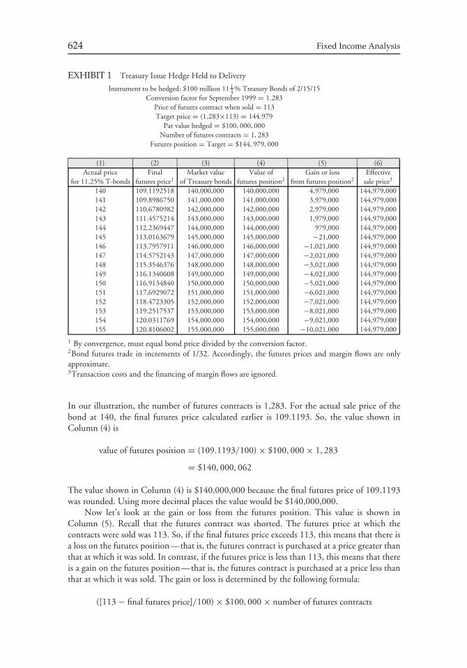
624 Fixed Income Analysis
EXHIBIT 1 Treasury Issue Hedge Held to Delivery
Instrument to be hedged: $100 million 11 14 % Treasury Bonds of 2/15/15
Conversion factor for September 1999 = 1.283Price of futures contract when sold = 113Target price = (1.283×113) = 144.979
Par value hedged = $100, 000, 000Number of futures contracts = 1, 283
Futures position = Target = $144, 979, 000
(1) (2) (3) (4) (5) (6)Actual price Final Market value Value of Gain or loss Effective
for 11.25% T-bonds futures price1 of Treasury bonds futures position2 from futures position2 sale price3
140 109.1192518 140,000,000 140,000,000 4,979,000 144,979,000141 109.8986750 141,000,000 141,000,000 3,979,000 144,979,000142 110.6780982 142,000,000 142,000,000 2,979,000 144,979,000143 111.4575214 143,000,000 143,000,000 1,979,000 144,979,000144 112.2369447 144,000,000 144,000,000 979,000 144,979,000145 113.0163679 145,000,000 145,000,000 −21,000 144,979,000146 113.7957911 146,000,000 146,000,000 −1,021,000 144,979,000147 114.5752143 147,000,000 147,000,000 −2,021,000 144,979,000148 115.3546376 148,000,000 148,000,000 −3,021,000 144,979,000149 116.1340608 149,000,000 149,000,000 −4,021,000 144,979,000150 116.9134840 150,000,000 150,000,000 −5,021,000 144,979,000151 117.6929072 151,000,000 151,000,000 −6,021,000 144,979,000152 118.4723305 152,000,000 152,000,000 −7,021,000 144,979,000153 119.2517537 153,000,000 153,000,000 −8,021,000 144,979,000154 120.0311769 154,000,000 154,000,000 −9,021,000 144,979,000155 120.8106002 155,000,000 155,000,000 −10,021,000 144,979,000
1 By convergence, must equal bond price divided by the conversion factor.2Bond futures trade in increments of 1/32. Accordingly, the futures prices and margin flows are onlyapproximate.3Transaction costs and the financing of margin flows are ignored.
In our illustration, the number of futures contracts is 1,283. For the actual sale price of thebond at 140, the final futures price calculated earlier is 109.1193. So, the value shown inColumn (4) is
value of futures position = (109.1193/100) × $100, 000 × 1, 283
= $140, 000, 062
The value shown in Column (4) is $140,000,000 because the final futures price of 109.1193was rounded. Using more decimal places the value would be $140,000,000.
Now let’s look at the gain or loss from the futures position. This value is shown inColumn (5). Recall that the futures contract was shorted. The futures price at which thecontracts were sold was 113. So, if the final futures price exceeds 113, this means that there isa loss on the futures position—that is, the futures contract is purchased at a price greater thanthat at which it was sold. In contrast, if the futures price is less than 113, this means that thereis a gain on the futures position—that is, the futures contract is purchased at a price less thanthat at which it was sold. The gain or loss is determined by the following formula:
([113 − final futures price]/100) × $100, 000 × number of futures contracts
Controlling Interest Rate Risk with Derivatives 625
In our illustration, for a final futures price of 109.1193 and 1,283 futures contracts, we have
([113 − 109.1193]/100) × $100, 000 × 1, 283 = $4, 978, 938.1
The value shown in Column (5) is $4,979,000 because that is the more precise value usingmore decimal places for the final futures price than shown in Exhibit 1. The value is positiveindicating a gain in the futures position. Note that for all the final futures prices above 113 inExhibit 1, there is a negative value which means that there is a loss on the futures position.
Finally, Column (6) shows the effective sale price for the Treasury bond. This value iscomputed as follows:
effective sale price for Treasury bond = actual sale price of Treasury bond
+ gain or loss on futures position
which is the sum of the numbers in each of the rows of Columns (3) and (5). For the actualsale price of $140 million, the gain is $4,979,000. Therefore the effective sale price for theTreasury bond is
$140, 000, 000 + $4, 979, 000 = $144, 979, 000
Note that this is the target price for the Treasury bond. In fact, it can be seen from Column(6) of Exhibit 1 that the effective sale price for all the actual sale prices for the Treasury bondis the target price. However, the target price is determined by the futures price, so the targetprice may be higher or lower than the cash (spot) market price when the hedge is set.
When we admit the possibility that bonds other than the issue used in our illustrationcan be delivered, and that it might be advantageous to do so, the situation becomes somewhatmore involved. In this more realistic case, the manager may decide not to deliver this issue, butif she does decide to deliver it, the manager is still assured of receiving an effective sale price ofapproximately 144.979. If the manager does not deliver this issue, it would be because anotherissue can be delivered more cheaply, and thus the manager does better than the targeted price.
In summary, if a manager establishes a futures hedge that is held until delivery, themanager can be assured of receiving an effective price dictated by the futures rate (not the spotrate) on the day the hedge is set.
c. The Target for Hedges with Short Holding Periods When a manager must lift(remove) a hedge prior to the delivery date, the effective rate that is obtained is morelikely to approximate the current spot rate than the futures rate and this likelihood increasesthe shorter the term of the hedge. The critical difference between this hedge and the hedgeheld to the delivery date is that convergence will generally not take place by the terminationdate of the hedge.
To illustrate why a manager should expect the hedge to lock in the spot rate rather thanthe futures rate for very short-lived hedges, let’s return to the simplified example used earlierto illustrate a hedge maintained to the delivery date. It is assumed that this issue is the onlydeliverable instrument for the Treasury bond futures contract. Suppose that the hedge is setthree months before the delivery date and the manager plans to lift the hedge one day later. Itis much more likely that the spot price of the bond will move parallel to the converted futuresprice (that is, the futures price times the conversion factor), than that the spot price and theconverted futures price will converge by the time the hedge is lifted.
626 Fixed Income Analysis
A 1-day hedge is, admittedly, an extreme example. Other than underwriters, dealers, andtraders who reallocate assets very frequently, few money managers are interested in such ashort horizon. The very short-term hedge does, however, illustrate a very important point:when hedging, a manager should not expect to lock in the futures rate (or price) just by hedgingwith futures contracts. The futures rate is locked in only if the hedge is held until delivery, atwhich point convergence must take place. If the hedge is held for only one day, the managershould expect to lock in the 1-day forward rate,4 which will very nearly equal the spot rate.Generally hedges are held for more than one day, but not necessarily to delivery.
d. How the Basis Affects the Target Rate for a Hedge The proper target for a hedgethat is to be lifted prior to the delivery date depends on the basis. The basis is simply thedifference between the spot (cash) price of a security and its futures price; that is:
basis = spot price − futures price
In the bond market, a problem arises when trying to make practical use of the conceptof the basis. The quoted futures price does not equal the price that one receives at delivery.For the Treasury bond and note futures contracts, the actual futures price equals the quotedfutures price times the appropriate conversion factor. Consequently, to be useful, the basisin the bond market should be defined using actual futures delivery prices rather than quotedfutures prices. Thus, the price basis for bonds should be redefined as:
price basis = spot price − futures delivery price
For hedging purposes it is also frequently useful to define the basis in terms of interestrates rather than prices. The rate basis is defined as:
rate basis = spot rate − futures rate
where spot rate refers to the current rate on the instrument to be hedged and the futures rateis the interest rate corresponding to the futures delivery price of the deliverable instrument.
The rate basis is helpful in explaining why the two views of hedging described earlier areexpected to lock in such different rates. To see this, we first define the target rate basis. Thisis defined as the expected rate basis on the day the hedge is lifted. That is,
target rate basis = spot rate on date hedge is lifted − futures rate on date hedge is lifted
The target rate for the hedge is equal to
target rate for hedge = futures rate + target rate basis
Substituting for target rate basis in the above equation
target rate for hedge = futures rate + spot rate on date hedge is lifted
− futures rate on date hedge is lifted
4Forward rates were covered earlier.
Controlling Interest Rate Risk with Derivatives 627
Consider first a hedge lifted on the delivery date. On the delivery date, the spot rate andthe futures rate will be the same by convergence. Thus, the target rate basis if the hedge isexpected to be removed on the delivery date is zero. Substituting zero for the target rate basisin the equation above we have the following:
target rate for hedge = futures rate
That is, if the hedge is held to the delivery date, the target rate for the hedge is equal to thefutures rate.
Now consider if a hedge is lifted prior to the delivery date. Let’s consider the case wherethe hedge is removed the next day. One would not expect the basis to change very much inone day. Assume that the basis does not change. Then,
spot rate on date hedge is lifted = spot rate when hedge was placed
futures rate on date hedge is lifted = futures rate when hedge was placed
The spot rate when the hedge was placed is simply the spot rate and the futures rate when thehedge was placed is simply the futures rate. So, we can write
target rate basis = spot rate − futures rate
and substituting the right-hand side of the equation into the target rate for hedge
target rate for hedge = futures rate + (spot rate − futures rate)or
target rate for hedge = spot rate
Thus, we see that when hedging for one day (and assuming the basis does not change in thatone day), the manager is locking in the spot rate (i.e., the current rate).
If projecting the basis in terms of price rather than rate is easier (as is often the case forintermediate- and long-term futures), it is easier to work with the target price basis instead ofthe target rate basis. The target price basis is the projected price basis for the day the hedge isto be lifted. For a deliverable security, the target for the hedge then becomes
target price for hedge = futures delivery price + target price basis
The idea of a target price or rate basis explains why a hedge held until the delivery datelocks in a price, and other hedges do not. The examples have shown that this is true. For thehedge held to delivery, there is no uncertainty surrounding the target basis; by convergence,the basis on the day the hedge is lifted will be zero. For the short-lived hedge, the basis willprobably approximate the current basis when the hedge is lifted, but its actual value is notknown in advance. For hedges longer than one day but ending prior to the futures deliverydate, there can be considerable basis risk because the basis on the day the hedge is lifted canend up being anywhere within a wide range. Thus, the uncertainty surrounding the outcomeof a hedge is directly related to the uncertainty surrounding the basis on the day the hedge islifted (i.e., the uncertainty surrounding the target basis).
The uncertainty about the value of the basis at the time the hedge is removed is calledbasis risk. For a given investment horizon, hedging substitutes basis risk for price risk. Thus, one
628 Fixed Income Analysis
trades the uncertainty of the price of the hedged security for the uncertainty of the basis. Amanager would be willing to substitute basis risk for price risk if the manager expects thatbasis risk is less than price risk. Consequently, when hedges do not produce the desired results,it is common to place the blame on basis risk. However, basis risk is the real culprit only ifthe target for the hedge is properly defined. Basis risk should refer only to the unexpectedor unpredictable part of the relationship between cash and futures prices. The fact that thisrelationship changes over time does not in itself imply that there is basis risk.
Basis risk, properly defined, refers only to the uncertainty associated with the target ratebasis or target price basis. Accordingly, it is imperative that the target basis be properly definedif one is to correctly assess the risk and expected return in a hedge.
3. Determining the Position to Be Taken The final step that must be determinedbefore the hedge is set is the number of futures contracts needed for the hedge. This iscalled the hedge ratio. Usually the hedge ratio is expressed in terms of relative par amounts.Accordingly, a hedge ratio of 1.20 means that for every $1 million par value of securities tobe hedged, one needs $1.2 million par value of futures contracts to offset the risk. In ourdiscussion, the values are defined so that the hedge ratio is the number of futures contracts.
Earlier, we defined a cross hedge in the futures market as a hedge in which the security tobe hedged is not deliverable on the futures contract used in the hedge. (A bond that does notmeet the specific criteria for delivery to satisfy a particular futures contract is referred to as anondeliverable bond.) For example, a manager who wants to hedge the sale price of long-termcorporate bonds might hedge with the Treasury bond futures contract, but since non-Treasurybonds cannot be delivered in satisfaction of the contract, the hedge would be considered across hedge. A manager might also want to hedge a rate that is of the same quality as the ratespecified in one of the contracts, but that has a different maturity. For example, it might benecessary to cross hedge a Treasury bond, note, or bill with a maturity that does not qualify fordelivery on any futures contract. Thus, when the security to be hedged differs from the futurescontract specification in terms of either quality or maturity, one is led to the cross hedge.
Conceptually, cross hedging is somewhat more complicated than hedging deliverablesecurities, because it involves two relationships. First, there is the relationship between thecheapest-to-deliver (CTD) issue and the futures contract. Second, there is the relationshipbetween the security to be hedged and the CTD issue. Practical considerations may at timeslead a manager to shortcut this two-step relationship and focus directly on the relationshipbetween the security to be hedged and the futures contract, thus ignoring the CTD issuealtogether. However, in so doing, a manager runs the risk of miscalculating the target rate andthe risk in the hedge. Furthermore, if the hedge does not perform as expected, the shortcutmakes it difficult to tell why the hedge did not work out as expected.
The key to minimizing risk in a cross hedge is to choose the right number of futurescontracts. This depends on the relative dollar duration of the bond to be hedged and thedollar duration of the futures position. Equation (4) indicated the number of futures contractsrequired to achieve a particular target dollar duration. The objective in hedging is to make thetarget dollar duration equal to zero. Substituting zero for target dollar duration in equation (4)we obtain:
number of futures contracts = current dollar duration without futures
dollar duration per futures contract(5)
To calculate the dollar duration of a bond, the manager must know the precise point intime that the dollar duration is to be calculated (because price volatility generally declines as abond matures) as well as the price or yield at which to calculate dollar duration (because higher
Controlling Interest Rate Risk with Derivatives 629
yields generally reduce dollar duration for a given yield change). The relevant point in the lifeof the bond for calculating price volatility is the point at which the hedge will be lifted. Dollarduration at any other point in time is essentially irrelevant because the goal is to lock in a price orrate only on that particular day. Similarly, the relevant yield at which to calculate dollar durationinitially is the target yield. Consequently, the numerator of equation (5) is the dollar duration onthe date the hedge is expected to be lifted. The yield that can be used on this date in order todetermine the dollar duration is the forward rate.
Let’s look at how we apply equation (5) when using the Treasury bond futures contractto hedge. The number of futures contracts will be affected by the dollar duration of the CTDissue. We can modify equation (5) as follows:
number of futures contracts
= − current dollar duration without futures
dollar duration of the CTD issue× dollar duration of the CTD issue
dollar duration per futures contract(6)
As noted earlier, the conversion ratio for the CTD issue is a good approximation of the secondratio. Thus, equation (6) can be rewritten as
number of futures contracts
= − current dollar duration without futures
dollar duration of the CTD issue× conversion factor for the CTD issue (7)
a. An Illustration An example for a single bond shows why dollar duration weighting leadsto the correct number of contracts for a hedge. The hedge illustrated is a cross hedge. Supposethat on 6/24/99, a manager owned $10 million par value of a 6.25% Fannie Mae (FNMA)option-free bond maturing on 5/15/29 selling at 88.39 to yield 7.20%. The manager wants tosell September 1999 Treasury bond futures to hedge a future sale of the FNMA bond. At thetime, the price of the September Treasury bond futures contract was 113. The CTD issue wasthe 11.25% of 2/15/15 issue that was trading at 146.19 to yield 6.50%. The conversion factorfor the CTD issue was 1.283. To simplify, assume that the yield spread between the FNMAbond and the CTD issue remains at 0.70% (i.e., 70 basis points) and that the anticipated saledate is the last business day in September 1999.
The target price for hedging the CTD issue would be 144.979 (113 × 1.283), and thetarget yield would be 6.56% (the yield at a price of 144.979). Since the yield on the FNMAbond is assumed to stay at 0.70% above the yield on the CTD issue, the target yield forthe FNMA bond would be 7.26%. The corresponding price for the FNMA bond for thistarget yield is 87.76. At these target levels, the dollar durations for a 50 basis point change inrates for the CTD issue and the FNMA bond per $100 of par value are $6.255 and $5.453,respectively. As indicated earlier, all these calculations are made using a settlement date equalto the anticipated sale date, in this case the end of September 1999. The dollar duration for a50 basis point change in rates for $10 million par value of the FNMA bond is then $545,300([$10 million/100] × $5.453). Per $100,000 par value for the CTD issue, the dollar durationper futures contract is $6,255 ([$100,000/100] × $6.255).
Thus, we knowcurrent dollar duration without futures = dollar duration of the FNMA bond = $545, 300
dollar duration of the CTD issue = $6, 255conversion factor for CTD issue = 1.283
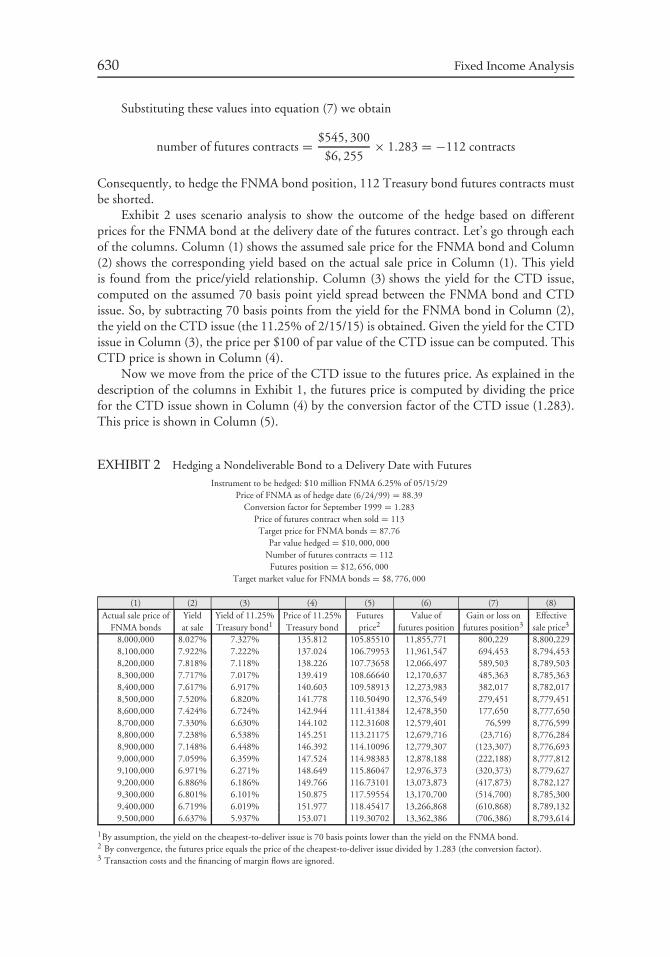
630 Fixed Income Analysis
Substituting these values into equation (7) we obtain
number of futures contracts = $545, 300
$6, 255× 1.283 = −112 contracts
Consequently, to hedge the FNMA bond position, 112 Treasury bond futures contracts mustbe shorted.
Exhibit 2 uses scenario analysis to show the outcome of the hedge based on differentprices for the FNMA bond at the delivery date of the futures contract. Let’s go through eachof the columns. Column (1) shows the assumed sale price for the FNMA bond and Column(2) shows the corresponding yield based on the actual sale price in Column (1). This yieldis found from the price/yield relationship. Column (3) shows the yield for the CTD issue,computed on the assumed 70 basis point yield spread between the FNMA bond and CTDissue. So, by subtracting 70 basis points from the yield for the FNMA bond in Column (2),the yield on the CTD issue (the 11.25% of 2/15/15) is obtained. Given the yield for the CTDissue in Column (3), the price per $100 of par value of the CTD issue can be computed. ThisCTD price is shown in Column (4).
Now we move from the price of the CTD issue to the futures price. As explained in thedescription of the columns in Exhibit 1, the futures price is computed by dividing the pricefor the CTD issue shown in Column (4) by the conversion factor of the CTD issue (1.283).This price is shown in Column (5).
EXHIBIT 2 Hedging a Nondeliverable Bond to a Delivery Date with Futures
Instrument to be hedged: $10 million FNMA 6.25% of 05/15/29Price of FNMA as of hedge date (6/24/99) = 88.39
Conversion factor for September 1999 = 1.283Price of futures contract when sold = 113Target price for FNMA bonds = 87.76
Par value hedged = $10, 000, 000Number of futures contracts = 112Futures position = $12, 656, 000
Target market value for FNMA bonds = $8, 776, 000
(1) (2) (3) (4) (5) (6) (7) (8)Actual sale price of Yield Yield of 11.25% Price of 11.25% Futures Value of Gain or loss on Effective
FNMA bonds at sale Treasury bond1 Treasury bond price2 futures position futures position3 sale price3
8,000,000 8.027% 7.327% 135.812 105.85510 11,855,771 800,229 8,800,2298,100,000 7.922% 7.222% 137.024 106.79953 11,961,547 694,453 8,794,4538,200,000 7.818% 7.118% 138.226 107.73658 12,066,497 589,503 8,789,5038,300,000 7.717% 7.017% 139.419 108.66640 12,170,637 485,363 8,785,3638,400,000 7.617% 6.917% 140.603 109.58913 12,273,983 382,017 8,782,0178,500,000 7.520% 6.820% 141.778 110.50490 12,376,549 279,451 8,779,4518,600,000 7.424% 6.724% 142.944 111.41384 12,478,350 177,650 8,777,6508,700,000 7.330% 6.630% 144.102 112.31608 12,579,401 76,599 8,776,5998,800,000 7.238% 6.538% 145.251 113.21175 12,679,716 (23,716) 8,776,2848,900,000 7.148% 6.448% 146.392 114.10096 12,779,307 (123,307) 8,776,6939,000,000 7.059% 6.359% 147.524 114.98383 12,878,188 (222,188) 8,777,8129,100,000 6.971% 6.271% 148.649 115.86047 12,976,373 (320,373) 8,779,6279,200,000 6.886% 6.186% 149.766 116.73101 13,073,873 (417,873) 8,782,1279,300,000 6.801% 6.101% 150.875 117.59554 13,170,700 (514,700) 8,785,3009,400,000 6.719% 6.019% 151.977 118.45417 13,266,868 (610,868) 8,789,1329,500,000 6.637% 5.937% 153.071 119.30702 13,362,386 (706,386) 8,793,614
1By assumption, the yield on the cheapest-to-deliver issue is 70 basis points lower than the yield on the FNMA bond.2 By convergence, the futures price equals the price of the cheapest-to-deliver issue divided by 1.283 (the conversion factor).3 Transaction costs and the financing of margin flows are ignored.

Controlling Interest Rate Risk with Derivatives 631
The value of the futures position is found in the same way as in Exhibit 1. First the futuresprice per $1 of par value is computed by dividing the futures price by 100. Then this value ismultiplied by $100,000 (the par value for the contract) and the number of futures contracts.That is,
value of futures position = (futures price/100) × $100, 000 × number of futures contracts
The values in Column (6) are derived using this formula. Using the first sale price forthe FNMA of $8 million as an example, the corresponding futures price in Column (5) is105.8551. Since the number of futures contracts sold is 112, the value of the futures position is
value of futures position = (105.8551/100) × $100, 000 × 112 = $11, 855, 711
Now let’s calculate the gain or loss on the futures position shown in Column (7). Notethat the negative values in Column (7) for all futures prices above 113 mean there is a loss onthe futures position. Since the futures price at which the contracts are sold at the inception ofthe hedge is 113, the gain or loss on the futures position is found as follows:
([113 − final futures price]/100) × $100, 000 × number of futures contracts
For example, for the first scenario in Exhibit 2, the futures price is 105.8551 and 112 futurescontract were sold. Therefore,
([113 − 105.8551]/100) × $100, 000 × 112 = $800, 229
There is a gain from the futures position because the futures price is less than 113. Note thatfor all the final futures prices above 113 in Exhibit 2, there is a negative value which meansthat there is a loss on the futures position. For all futures prices below 113, there is a gain.
Finally, Column (8) shows the effective sale price for the FNMA bond. This value isfound as follows:
effective sale price for FNMA bond = actual sale price of FNMA bond
+ gain or loss on futures position
For the actual sale price of $8 million, the gain is $800,229. Therefore the effective sale pricefor the FNMA bond is
$8, 000, 000 + $800, 229 = $8, 800, 229
Looking at Column (8) of Exhibit 2 we see that if the simplifying assumptions hold, a futureshedge using the recommended number of futures contracts (112) very nearly locks in thetarget price for $10 million par value of the FNMA bonds.
b. Refining for Changing Yield Spread Another refinement in the hedging strategy isusually necessary when hedging nondeliverable securities. This refinement concerns theassumption about the relative yield spread between the CTD issue and the bond to be hedged.In the prior discussion, we assumed that the yield spread was constant over time. Yield spreads,however, are not constant over time. They vary with the maturity of the instruments inquestion and the level of rates, as well as with many unpredictable and nonsystematic factors.

632 Fixed Income Analysis
Regression analysis allows the manager to capture the relationship between yield levelsand yield spreads and use it to advantage. For hedging purposes, the variables are the yieldon the bond to be hedged and the yield on the CTD issue. The regression equation takes theform:
yield on bond to be hedged = a + b × yield on CTD issue + error (8)
The regression procedure provides an estimate of b, which is the expected relative yield changein the two bonds. This parameter b is called the yield beta. Our example that used constantspreads implicitly assumes that the yield beta, b, equals l.0 and a equals 0.70 (because 0.70 isthe assumed spread).
For the two issues in question, the FNMA bond and the CTD issue, suppose the estimatedyield beta is 1.05. Thus, yields on the FNMA issue are expected to move 5% more than yieldson the Treasury issue. To calculate the number of futures contracts correctly, this fact mustbe taken into account; thus, the number of futures contracts derived in our earlier example ismultiplied by the factor 1.05. Consequently, instead of shorting 112 Treasury bond futurescontracts to hedge $10 million of the FNMA bond, the investor would short 118 (roundedup) contracts.
To incorporate the impact of a yield beta, the formula for the number of futures contractsis revised as follows:
number of futures contracts = − current dollar duration without futures
dollar duration of the CTD issue
× conversion factor for the CTD issue × yield beta (9)
The effect of a change in the CTD issue and the yield spread can be assessed beforethe hedge is implemented. An exhibit similar to Exhibit 2 can be constructed under a widerange of assumptions. For example, at different yield levels at the date the hedge is to be lifted(the second column in Exhibit 2), a different yield spread may be appropriate and a differentacceptable issue will be the CTD issue. The manager can determine what this will do to theoutcome of the hedge.
4. Monitoring and Evaluating the Hedge After a target is determined and a hedge isset, there are two remaining tasks. The hedge must be monitored during its life and evaluatedafter it is over. While hedges must be monitored, overactive management of a hedge posesmore of a threat to most hedges than does inactive management. The reason for this is thatthe manager usually will not receive enough new information during the life of the hedge tojustify a change in the hedging strategy. For example, it is not advisable to readjust the hedgeratio every day in response to new data and a possible corresponding change in the estimatedvalue of the yield beta.
There are, however, exceptions to this general rule. As rates change, dollar durationchanges. Consequently, the hedge ratio may change slightly. In other cases, there may besound economic reasons to believe that the yield beta has changed. While there are exceptions,the best approach is usually to let a hedge run its course using the original hedge ratio withonly slight adjustments.
A hedge can normally be evaluated only after it has been lifted. Evaluation involves, first,an assessment of how closely the hedge locked in the target rate—that is, how much errorthere was in the hedge. To provide a meaningful interpretation of the error, the manager
Controlling Interest Rate Risk with Derivatives 633
should calculate how far from the target the sale (or purchase) would have been, had therebeen no hedge at all. One good reason for evaluating a completed hedge is to ascertain thesources of error in the hedge in the hope that the manager will gain insights that can be usedto advantage in subsequent hedges. A manager will find that there are three major sources ofhedging errors:
1. The dollar duration for the hedged instrument was incorrect.2. The projected value of the basis at the date the hedge is removed can be in error.3. The parameters estimated from the regression (a and b) can be inaccurate.
Let’s discuss the first two sources of hedging error. The third source is self-explanatory.Recall from the calculation of duration that interest rates are changed up and down by a smallnumber of basis points and the security is revalued. The two recalculated values are used in thenumerator of the duration formula. The first source of error listed above recognizes that theinstrument to be hedged may be a complex instrument (i.e., one with embedded options) andthat the valuation model does not do a good job of valuing the security when interest rateschange.
The second major source of errors in a hedge—an inaccurate projected value of thebasis—is a more difficult problem. Unfortunately, there are no satisfactory easy modelslike regression analysis that can be applied to the basis. Simple models of the basis violatecertain equilibrium relationships for bonds that should not be violated. On the other hand,theoretically rigorous models are very unintuitive and usually solvable only by complexnumerical methods. Modeling the basis is undoubtedly one of the most important anddifficult problems that managers face when seeking to hedge.
III. CONTROLLING INTEREST RATE RISK WITHSWAPS
An interest rate swap is equivalent to a package of forward/futures contracts. Consequently,swaps can be used for controlling interest rate risk and hedging as we discussed earlier withfutures.
A. Hedging Interest Rate Risk
The following illustration demonstrates how an interest rate swap can be used to hedge interestrate risk by altering the cash flow characteristics of an entity so as to better match the cash flowcharacteristics of assets and liabilities. In our illustration we will use two hypothetical financialinstitutions—a commercial bank and a life insurance company.
Suppose a bank has a portfolio consisting of 4-year commercial loans with a fixed interestrate. The principal value of the portfolio is $100 million, and the interest rate on every loan inthe portfolio is 11%. The loans are interest-only loans; interest is paid semiannually, and theprincipal is paid at the end of four years. That is, assuming no default on the loans, the cashflow from the loan portfolio is $5.5 million every six months for the next four years and $100million at the end of four years. To fund its loan portfolio, assume that the bank can borrowat 6-month LIBOR for the next four years.
The risk that the bank faces is that 6-month LIBOR will be 11% or greater. To understandwhy, remember that the bank is earning 11% annually on its commercial loan portfolio. If
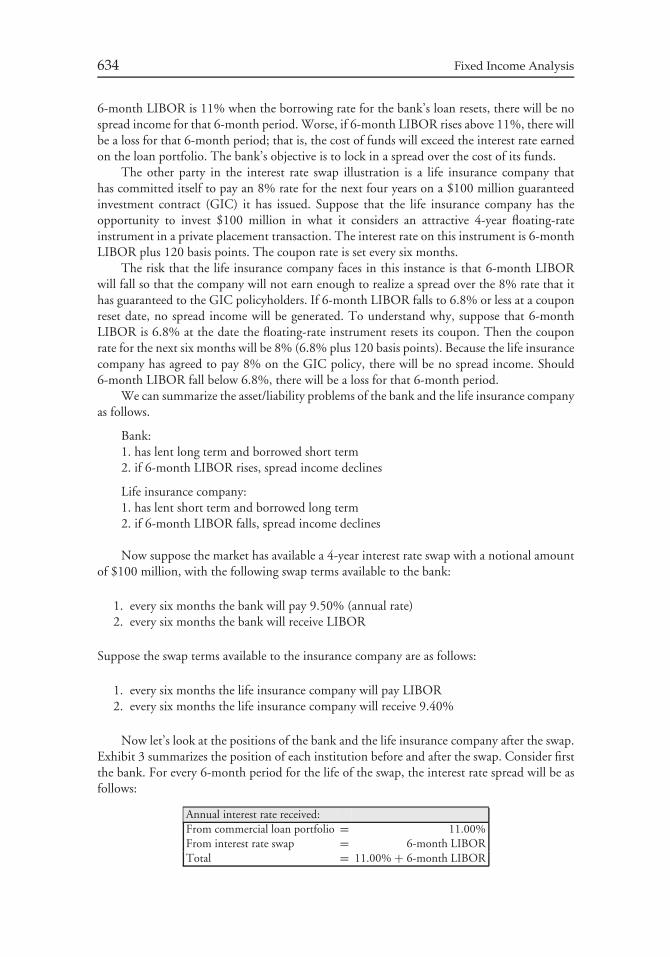
634 Fixed Income Analysis
6-month LIBOR is 11% when the borrowing rate for the bank’s loan resets, there will be nospread income for that 6-month period. Worse, if 6-month LIBOR rises above 11%, there willbe a loss for that 6-month period; that is, the cost of funds will exceed the interest rate earnedon the loan portfolio. The bank’s objective is to lock in a spread over the cost of its funds.
The other party in the interest rate swap illustration is a life insurance company thathas committed itself to pay an 8% rate for the next four years on a $100 million guaranteedinvestment contract (GIC) it has issued. Suppose that the life insurance company has theopportunity to invest $100 million in what it considers an attractive 4-year floating-rateinstrument in a private placement transaction. The interest rate on this instrument is 6-monthLIBOR plus 120 basis points. The coupon rate is set every six months.
The risk that the life insurance company faces in this instance is that 6-month LIBORwill fall so that the company will not earn enough to realize a spread over the 8% rate that ithas guaranteed to the GIC policyholders. If 6-month LIBOR falls to 6.8% or less at a couponreset date, no spread income will be generated. To understand why, suppose that 6-monthLIBOR is 6.8% at the date the floating-rate instrument resets its coupon. Then the couponrate for the next six months will be 8% (6.8% plus 120 basis points). Because the life insurancecompany has agreed to pay 8% on the GIC policy, there will be no spread income. Should6-month LIBOR fall below 6.8%, there will be a loss for that 6-month period.
We can summarize the asset/liability problems of the bank and the life insurance companyas follows.
Bank:1. has lent long term and borrowed short term2. if 6-month LIBOR rises, spread income declines
Life insurance company:1. has lent short term and borrowed long term2. if 6-month LIBOR falls, spread income declines
Now suppose the market has available a 4-year interest rate swap with a notional amountof $100 million, with the following swap terms available to the bank:
1. every six months the bank will pay 9.50% (annual rate)2. every six months the bank will receive LIBOR
Suppose the swap terms available to the insurance company are as follows:
1. every six months the life insurance company will pay LIBOR2. every six months the life insurance company will receive 9.40%
Now let’s look at the positions of the bank and the life insurance company after the swap.Exhibit 3 summarizes the position of each institution before and after the swap. Consider firstthe bank. For every 6-month period for the life of the swap, the interest rate spread will be asfollows:
Annual interest rate received:From commercial loan portfolio = 11.00%From interest rate swap = 6-month LIBORTotal = 11.00% + 6-month LIBOR
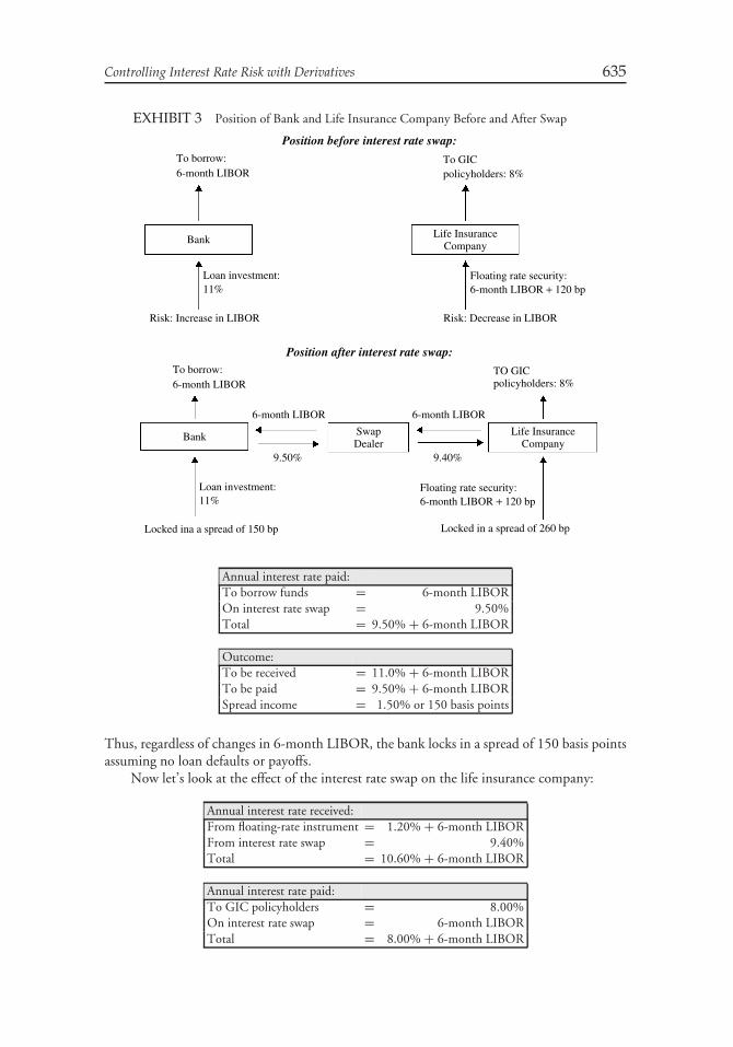
Controlling Interest Rate Risk with Derivatives 635
EXHIBIT 3 Position of Bank and Life Insurance Company Before and After Swap
Position before interest rate swap:
Position after interest rate swap:
To borrow:6-month LIBOR
To GICpolicyholders: 8%
Floating rate security:6-month LIBOR + 120 bp
Floating rate security:6-month LIBOR + 120 bp
To borrow:6-month LIBOR
6-month LIBOR
9.50%
6-month LIBOR
9.40%
Bank Life InsuranceCompany
Risk: Increase in LIBOR Risk: Decrease in LIBOR
Locked ina a spread of 150 bp Locked in a spread of 260 bp
Loan investment:11%
Loan investment:11%
Bank SwapDealer
Life InsuranceCompany
TO GICpolicyholders: 8%
Annual interest rate paid:To borrow funds = 6-month LIBOROn interest rate swap = 9.50%Total = 9.50% + 6-month LIBOR
Outcome:To be received = 11.0% + 6-month LIBORTo be paid = 9.50% + 6-month LIBORSpread income = 1.50% or 150 basis points
Thus, regardless of changes in 6-month LIBOR, the bank locks in a spread of 150 basis pointsassuming no loan defaults or payoffs.
Now let’s look at the effect of the interest rate swap on the life insurance company:
Annual interest rate received:From floating-rate instrument = 1.20% + 6-month LIBORFrom interest rate swap = 9.40%Total = 10.60% + 6-month LIBOR
Annual interest rate paid:To GIC policyholders = 8.00%On interest rate swap = 6-month LIBORTotal = 8.00% + 6-month LIBOR
636 Fixed Income Analysis
Outcome:To be received = 10.60% + 6-month LIBORTo be paid = 8.00% + 6-month LIBORSpread income = 2.60% or 260 basis points
Regardless of what happens to 6-month LIBOR, the life insurance company locks in a spreadof 260 basis points assuming the issuer of the floating-rate instrument does not default.
The interest rate swap has allowed each party to accomplish its asset/liability objectiveof locking in a spread.5 It permits the two financial institutions to alter the cash flowcharacteristics of its assets: from fixed to floating in the case of the bank, and from floating tofixed in the case of the life insurance company.
B. Dollar Duration of a Swap
Effectively, a position in an interest rate swap is a leveraged position. This agrees withthe economic interpretations of an interest rate swap explained earlier. We know thatfutures/forwards are leveraged instruments. In the case of a package of cash instruments, it is aleveraged position involving either buying a fixed-rate bond and financing it on a floating-ratebasis (i.e., fixed-rate receiver position) or buying a floating-rate bond on a fixed-rate basis (i.e.,fixed-rate payer position). So, we would expect that the dollar duration of a swap is a multipleof the bond that effectively underlies the swap.
To see how to calculate the dollar duration, let’s work with the second economicinterpretation of a swap—a package of cash flows from buying and selling cash marketinstruments. From the perspective of the fixed-rate receiver, the position can be viewed asfollows:
long a fixed-rate bond + short a floating-rate bond
The fixed-rate bond is a bond with a coupon rate equal to the swap rate, a maturity equal tothe term of the swap, and a par value equal to the notional amount of the swap.
This means that the dollar duration of an interest rate swap from the perspective of afixed-rate receiver is the difference between the dollar durations of the two bond positions thatcomprise the swap. That is,
dollar duration of a swap for a fixed-rate receiver
= dollar duration of a fixed-rate bond − dollar duration of a floating-rate bond
Most of the swap’s interest rate sensitivity results from the dollar duration of the fixed-ratebond since the dollar duration of the floating-rate bond will be small. The dollar duration ofa floating-rate bond is smaller the closer the swap is to its reset date. If the dollar duration ofthe floating-rate bond is close to zero then:
dollar duration of a swap for a fixed-rate receiver ≈ dollar duration of a fixed-rate bond
5Whether the size of the spread is adequate is not an issue to us in this illustration.

Controlling Interest Rate Risk with Derivatives 637
Thus, adding an interest rate swap to a portfolio in which the manager pays a floating-rateand receives a fixed-rate increases the dollar duration of the portfolio by roughly the dollar durationof the underlying fixed-rate bond. This is because it effectively involves buying a fixed-rate bondon a leveraged basis.
We can use the cash market instrument economic interpretation to compute the dollarduration of a swap for the fixed-rate payer. The dollar duration is:
dollar duration of a swap for a fixed-rate payer
= dollar duration of a floating-rate bond − dollar duration of a fixed-rate bond
Again, assuming that the dollar duration of the floater is small, we have
dollar duration of a swap for a fixed-rate payer ≈ −dollar duration of a fixed-rate bond
Consequently, a manager who adds to a portfolio a swap involving paying fixed and receivingfloating decreases the dollar duration of the portfolio by an amount roughly equal to the dollarduration of the fixed-rate bond.
The dollar duration of a portfolio that includes a swap is:
dollar duration of assets − dollar duration of liabilities + dollar duration of a swap position
Let’s look at our bank/life insurance illustration in terms of duration mismatch. The bankhas a larger duration for its assets (the fixed-rate loans) than the duration for its liabilities (theshort-term funds it borrows). Effectively, the position of the bank is as follows:
bank′s dollar duration = dollar duration of assets − dollar duration of liabilities > 0
The bank entered into an interest rate swap in which it pays fixed and receives floating. Thedollar duration of that swap position is negative, so adding the swap position moves the bank’sdollar duration position closer to zero and, therefore, reduces interest rate risk.
For the life insurance company, the duration of the liabilities is long while the durationof the floating-rate assets is short. That is,
life insurance company′s dollar duration = dollar duration of assets
− dollar duration of liabilities < 0
The life insurance company entered into an interest rate swap in which it pays floating andreceives fixed. This swap position has a positive duration. By adding it to a portfolio it movesthe duration closer to zero, thereby reducing interest rate risk.
IV. HEDGING WITH OPTIONS
Hedging strategies using options involve taking a position in an option and a position inthe underlying bond in such a way that changes in the value of one position will offset anyunfavorable price (interest rate) movement in the other position. We begin with the basichedging strategies using options. Then we illustrate these basic strategies using futures options
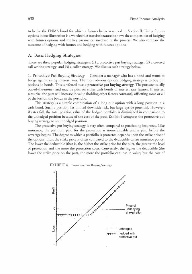
638 Fixed Income Analysis
to hedge the FNMA bond for which a futures hedge was used in Section II. Using futuresoptions in our illustration is a worthwhile exercise because it shows the complexities of hedgingwith futures options and the key parameters involved in the process. We also compare theoutcome of hedging with futures and hedging with futures options.
A. Basic Hedging Strategies
There are three popular hedging strategies: (1) a protective put buying strategy, (2) a coveredcall writing strategy, and (3) a collar strategy. We discuss each strategy below.
1. Protective Put Buying Strategy Consider a manager who has a bond and wants tohedge against rising interest rates. The most obvious options hedging strategy is to buy putoptions on bonds. This is referred to as a protective put buying strategy. The puts are usuallyout-of-the-money and may be puts on either cash bonds or interest rate futures. If interestrates rise, the puts will increase in value (holding other factors constant), offsetting some or allof the loss on the bonds in the portfolio.
This strategy is a simple combination of a long put option with a long position in acash bond. Such a position has limited downside risk, but large upside potential. However,if rates fall, the total position value of the hedged portfolio is diminished in comparison tothe unhedged position because of the cost of the puts. Exhibit 4 compares the protective putbuying strategy to an unhedged position.
The protective put buying strategy is very often compared to purchasing insurance. Likeinsurance, the premium paid for the protection is nonrefundable and is paid before thecoverage begins. The degree to which a portfolio is protected depends upon the strike price ofthe options; thus, the strike price is often compared to the deductible on an insurance policy.The lower the deductible (that is, the higher the strike price for the put), the greater the levelof protection and the more the protection costs. Conversely, the higher the deductible (thelower the strike price on the put), the more the portfolio can lose in value; but the cost of
EXHIBIT 4 Protective Put Buying Strategy
Price ofunderlyingat expiration
Pro
fitLo
ss
0
+
−
unhedged
hedged withprotective put
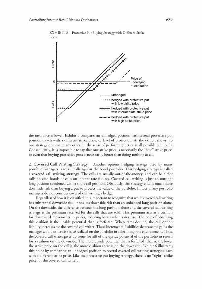
Controlling Interest Rate Risk with Derivatives 639
EXHIBIT 5 Protective Put Buying Strategy with Different StrikePrices
Price ofunderlyingat expiration
Pro
fitLo
ss
0
+
−
unhedged
hedged with protective putwith low strike price
hedged with protective putwith intermediate strike price
hedged with protective putwith high strike price
the insurance is lower. Exhibit 5 compares an unhedged position with several protective putpositions, each with a different strike price, or level of protection. As the exhibit shows, noone strategy dominates any other, in the sense of performing better at all possible rate levels.Consequently, it is impossible to say that one strike price is necessarily the ‘‘best’’ strike price,or even that buying protective puts is necessarily better than doing nothing at all.
2. Covered Call Writing Strategy Another options hedging strategy used by manyportfolio managers is to sell calls against the bond portfolio. This hedging strategy is calleda covered call writing strategy. The calls are usually out-of-the-money, and can be eithercalls on cash bonds or calls on interest rate futures. Covered call writing is just an outrightlong position combined with a short call position. Obviously, this strategy entails much moredownside risk than buying a put to protect the value of the portfolio. In fact, many portfoliomanagers do not consider covered call writing a hedge.
Regardless of how it is classified, it is important to recognize that while covered call writinghas substantial downside risk, it has less downside risk than an unhedged long position alone.On the downside, the difference between the long position alone and the covered call writingstrategy is the premium received for the calls that are sold. This premium acts as a cushionfor downward movements in prices, reducing losses when rates rise. The cost of obtainingthis cushion is the upside potential that is forfeited. When rates decline, the call optionliability increases for the covered call writer. These incremental liabilities decrease the gains themanager would otherwise have realized on the portfolio in a declining rate environment. Thus,the covered call writer gives up some (or all) of the upside potential of the portfolio in returnfor a cushion on the downside. The more upside potential that is forfeited (that is, the lowerthe strike price on the calls), the more cushion there is on the downside. Exhibit 6 illustratesthis point by comparing an unhedged position to several covered call writing strategies, eachwith a different strike price. Like the protective put buying strategy, there is no ‘‘right’’ strikeprice for the covered call writer.
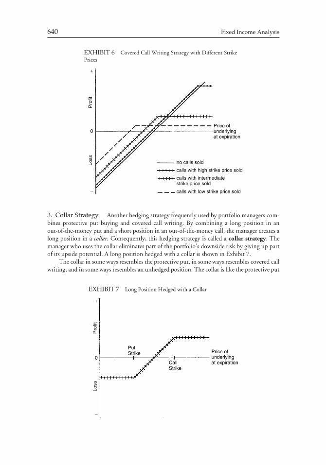
640 Fixed Income Analysis
EXHIBIT 6 Covered Call Writing Strategy with Different StrikePrices
Price ofunderlyingat expiration
Pro
fitLo
ss
0
+
−
no calls sold
calls with high strike price sold
calls with intermediatestrike price sold
calls with low strike price sold
3. Collar Strategy Another hedging strategy frequently used by portfolio managers com-bines protective put buying and covered call writing. By combining a long position in anout-of-the-money put and a short position in an out-of-the-money call, the manager creates along position in a collar. Consequently, this hedging strategy is called a collar strategy. Themanager who uses the collar eliminates part of the portfolio’s downside risk by giving up partof its upside potential. A long position hedged with a collar is shown in Exhibit 7.
The collar in some ways resembles the protective put, in some ways resembles covered callwriting, and in some ways resembles an unhedged position. The collar is like the protective put
EXHIBIT 7 Long Position Hedged with a Collar
Price ofunderlyingat expirationCall
Strike
PutStrike
Pro
fitLo
ss
0
+
−
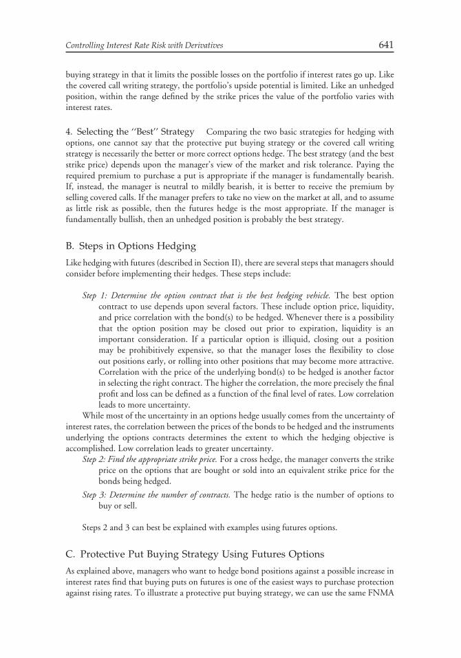
Controlling Interest Rate Risk with Derivatives 641
buying strategy in that it limits the possible losses on the portfolio if interest rates go up. Likethe covered call writing strategy, the portfolio’s upside potential is limited. Like an unhedgedposition, within the range defined by the strike prices the value of the portfolio varies withinterest rates.
4. Selecting the ‘‘Best’’ Strategy Comparing the two basic strategies for hedging withoptions, one cannot say that the protective put buying strategy or the covered call writingstrategy is necessarily the better or more correct options hedge. The best strategy (and the beststrike price) depends upon the manager’s view of the market and risk tolerance. Paying therequired premium to purchase a put is appropriate if the manager is fundamentally bearish.If, instead, the manager is neutral to mildly bearish, it is better to receive the premium byselling covered calls. If the manager prefers to take no view on the market at all, and to assumeas little risk as possible, then the futures hedge is the most appropriate. If the manager isfundamentally bullish, then an unhedged position is probably the best strategy.
B. Steps in Options Hedging
Like hedging with futures (described in Section II), there are several steps that managers shouldconsider before implementing their hedges. These steps include:
Step 1: Determine the option contract that is the best hedging vehicle. The best optioncontract to use depends upon several factors. These include option price, liquidity,and price correlation with the bond(s) to be hedged. Whenever there is a possibilitythat the option position may be closed out prior to expiration, liquidity is animportant consideration. If a particular option is illiquid, closing out a positionmay be prohibitively expensive, so that the manager loses the flexibility to closeout positions early, or rolling into other positions that may become more attractive.Correlation with the price of the underlying bond(s) to be hedged is another factorin selecting the right contract. The higher the correlation, the more precisely the finalprofit and loss can be defined as a function of the final level of rates. Low correlationleads to more uncertainty.
While most of the uncertainty in an options hedge usually comes from the uncertainty ofinterest rates, the correlation between the prices of the bonds to be hedged and the instrumentsunderlying the options contracts determines the extent to which the hedging objective isaccomplished. Low correlation leads to greater uncertainty.
Step 2: Find the appropriate strike price. For a cross hedge, the manager converts the strikeprice on the options that are bought or sold into an equivalent strike price for thebonds being hedged.
Step 3: Determine the number of contracts. The hedge ratio is the number of options tobuy or sell.
Steps 2 and 3 can best be explained with examples using futures options.
C. Protective Put Buying Strategy Using Futures Options
As explained above, managers who want to hedge bond positions against a possible increase ininterest rates find that buying puts on futures is one of the easiest ways to purchase protectionagainst rising rates. To illustrate a protective put buying strategy, we can use the same FNMA
642 Fixed Income Analysis
bond that we used to demonstrate how to hedge with Treasury bond futures.6 In that example,a manager held $10 million par value of a 6.25% FNMA bond maturing 5/15/29 and usedSeptember 1999 Treasury bond futures to lock in a sale price for those bonds on the futuresdelivery date. Now we want to show how the manager could use futures options instead offutures to protect against rising rates.
On 6/24/99 the FNMA bond was selling for 88.39 to yield 7.20% and the CTD issue’syield was 6.50%. For simplicity, it is assumed that the yield spread between the FNMA bondand the CTD issue remains at 70 basis points.
1. Selecting the Strike Price In our illustration, selecting the strike price means deter-mining the minimum price that the manager wants to establish for the FNMA bonds. Inour illustration we will assume that the minimum acceptable price (before the cost of the putoptions) is 84.453. This is equivalent to saying that the manager wants to establish a strikeprice for a put on the hedged bonds of 84.453. But, the manager is not buying a put onthe FNMA bond. He is buying a put on a Treasury bond futures contract. Therefore, themanager must determine the strike price for a put on a Treasury bond futures contract that isequivalent to a strike price of 84.453 for the FNMA bond.
This can be done with the help of Exhibit 8. Notice that all the boxes are numbered andwe shall refer to these numbered boxes as we illustrate the process. We begin at Box 1 of theexhibit. In our illustration, the portfolio manager set the strike price at 84.453 for the FNMAbond. Now we can calculate, given its coupon rate of 6.25%, its maturity, and the price of84.453 (the strike price desired), that its yield is 7.573%. That is, setting a strike price of84.453 for the FNMA bond is equivalent to setting a strike yield (or equivalently a maximumyield) of 7.573% in Box 2.
Now let’s move to Box 3—the yield of the cheapest-to-deliver issue. To move fromBox 2 to Box 3 we use the assumption that the spread between the FNMA bond and thecheapest-to-deliver issue is a constant 70 basis points. Since the strike yield for the FNMAbond is 7.573%, subtracting 70 basis points gives 6.873% as the strike yield (or maximumyield) for the cheapest-to-deliver issue.
We again use the price/yield relationship to move from Box 3 to Box 4. The cheapest-to-deliver issue was the 11.25% of 2/15/15 issue. Given the maturity, the coupon rate, and thestrike yield of 6.873%, the price is computed to be 141.136. This is the value that would goin Box 4.
Now for the final value we need—the strike price for the Treasury bond futures contract.We know that the converted price for any issue eligible for delivery on the bond futurescontract is:
converted price = futures price × conversion factor
6Futures options on Treasury bonds are more commonly used by institutional investors. The mechanicsof futures options are as follows. If a put option is exercised, the option buyer receives a short positionin the underlying futures contract and the option writer receives the corresponding long position. Thefutures price for both positions is the strike price for the put option. The exchange then marks thepositions to market and the futures price for both positions is then the current futures price. If a calloption is exercised, the option buyer receives a long position in the underlying futures contract and theoption writer receives the corresponding short position. The futures price for both positions is the strikeprice for the call option. The exchange then marks the positions to market and the futures price for bothpositions is then the current futures price.
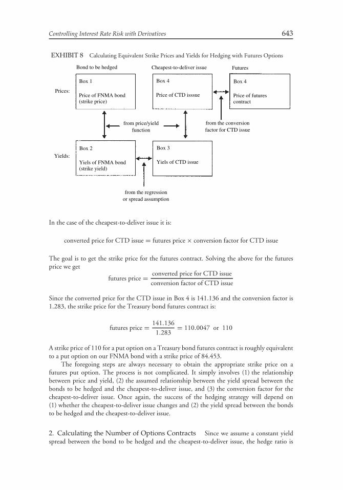
Controlling Interest Rate Risk with Derivatives 643
EXHIBIT 8 Calculating Equivalent Strike Prices and Yields for Hedging with Futures Options
Bond to be hedged
Prices:
Yields:
Box 1
Price of FNMA bond(strike price)
from price/yieldfunction
from the conversionfactor for CTD issue
from the regressionor spread assumption
Box 2
Yiels of FNMA bond(strike yield)
Box 3
Yiels of CTD issue
Box 4
Price of CTD isssue
Box 4
Price of futurescontract
Cheapest-to-deliver issue Futures
In the case of the cheapest-to-deliver issue it is:
converted price for CTD issue = futures price × conversion factor for CTD issue
The goal is to get the strike price for the futures contract. Solving the above for the futuresprice we get
futures price = converted price for CTD issue
conversion factor of CTD issue
Since the converted price for the CTD issue in Box 4 is 141.136 and the conversion factor is1.283, the strike price for the Treasury bond futures contract is:
futures price = 141.136
1.283= 110.0047 or 110
A strike price of 110 for a put option on a Treasury bond futures contract is roughly equivalentto a put option on our FNMA bond with a strike price of 84.453.
The foregoing steps are always necessary to obtain the appropriate strike price on afutures put option. The process is not complicated. It simply involves (1) the relationshipbetween price and yield, (2) the assumed relationship between the yield spread between thebonds to be hedged and the cheapest-to-deliver issue, and (3) the conversion factor for thecheapest-to-deliver issue. Once again, the success of the hedging strategy will depend on(1) whether the cheapest-to-deliver issue changes and (2) the yield spread between the bondsto be hedged and the cheapest-to-deliver issue.
2. Calculating the Number of Options Contracts Since we assume a constant yieldspread between the bond to be hedged and the cheapest-to-deliver issue, the hedge ratio is
644 Fixed Income Analysis
determined using the following equation, which is similar to equation (7):
number of options contracts = current dollar duration without options
dollar duration of the CTD issue
× conversion factor for CTD issue
The current duration refers to the duration at the time the hedge is placed. Recall that thedollar durations are calculated as of the date that the hedge is expected to be removed usingthe target yield for the bond to be hedged. For the protective put buying strategy, we willassume that the hedge will be removed on the expiration date of the option (assumed to be theend of September 1999). To obtain the current dollar duration for the bond, the target yieldis the 7.573% strike yield of the FNMA bond. The current dollar duration for the FNMAbond as of the end of September 1999 for a 50 basis point change in rates and for a targetyield of 7.573% would produce a value of $512,320. This value differs from the current dollarduration used to compute the number of contracts when hedging with futures. That value was$545,300 because it was based on a target yield of 7.26%.
The dollar duration for the CTD issue is based on a different target price (i.e., theminimum price) than in the hedging strategy with futures. The target price in the futureshedging strategy was 113 and the dollar duration of the CTD issue was $6,255. For theprotective put buying strategy, since the strike price of the futures option is 110 (the targetprice in this strategy), it can be shown that the dollar duration for the CTD issue for a 50 basispoint change in rates is $6,021.
Therefore, we know that for a 50 basis point change in rates:
current dollar duration without options = $512, 320
dollar duration for the CTD issue = $6, 021
Substituting these values and the conversion factor for the CTD issue of 1.283 into theformula for the number of options contracts, we find that:
number of options contracts = $512, 320
$6, 021× 1.283 = 109 put options
Thus, to hedge the FNMA bond position with put options on Treasury bond futures, 109 putoptions must be purchased.
3. Outcome of the Hedge To create a table for the protective put hedge, we can usedata from Exhibit 2. Exhibit 9 shows the scenario analysis for the protective put buyingstrategy. The first five columns are the same as in Exhibit 2. For the put option hedge, Column(6) shows that the value of the put position at expiration equals zero if the futures price isgreater than or equal to the strike price of 110. If the futures price is below 110, then theoptions expire in the money and:
value of put option position = ([110 − futures price]/100) × $100, 000
× number of put options
For example, for the first scenario in Exhibit 9, the corresponding futures price is 105.8551and the value of the put options is
([110 − futures price]/100) × $100, 000 × 109 = $451, 794
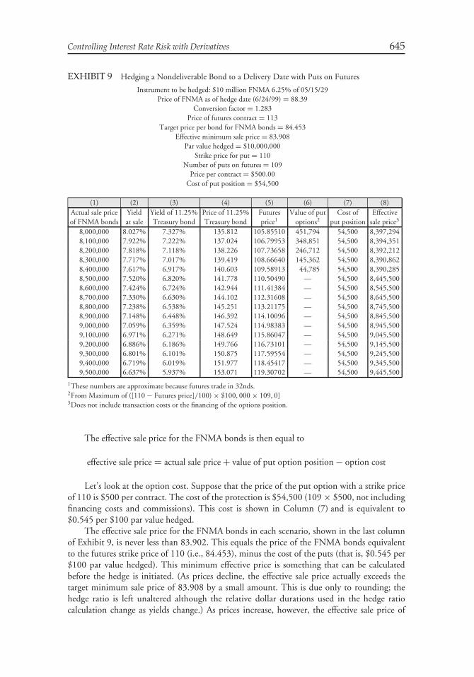
Controlling Interest Rate Risk with Derivatives 645
EXHIBIT 9 Hedging a Nondeliverable Bond to a Delivery Date with Puts on Futures
Instrument to be hedged: $10 million FNMA 6.25% of 05/15/29Price of FNMA as of hedge date (6/24/99) = 88.39
Conversion factor = 1.283Price of futures contract = 113
Target price per bond for FNMA bonds = 84.453Effective minimum sale price = 83.908
Par value hedged = $10,000,000Strike price for put = 110
Number of puts on futures = 109Price per contract = $500.00
Cost of put position = $54,500
(1) (2) (3) (4) (5) (6) (7) (8)Actual sale price Yield Yield of 11.25% Price of 11.25% Futures Value of put Cost of Effectiveof FNMA bonds at sale Treasury bond Treasury bond price1 options2 put position sale price3
8,000,000 8.027% 7.327% 135.812 105.85510 451,794 54,500 8,397,2948,100,000 7.922% 7.222% 137.024 106.79953 348,851 54,500 8,394,3518,200,000 7.818% 7.118% 138.226 107.73658 246,712 54,500 8,392,2128,300,000 7.717% 7.017% 139.419 108.66640 145,362 54,500 8,390,8628,400,000 7.617% 6.917% 140.603 109.58913 44,785 54,500 8,390,2858,500,000 7.520% 6.820% 141.778 110.50490 — 54,500 8,445,5008,600,000 7.424% 6.724% 142.944 111.41384 — 54,500 8,545,5008,700,000 7.330% 6.630% 144.102 112.31608 — 54,500 8,645,5008,800,000 7.238% 6.538% 145.251 113.21175 — 54,500 8,745,5008,900,000 7.148% 6.448% 146.392 114.10096 — 54,500 8,845,5009,000,000 7.059% 6.359% 147.524 114.98383 — 54,500 8,945,5009,100,000 6.971% 6.271% 148.649 115.86047 — 54,500 9,045,5009,200,000 6.886% 6.186% 149.766 116.73101 — 54,500 9,145,5009,300,000 6.801% 6.101% 150.875 117.59554 — 54,500 9,245,5009,400,000 6.719% 6.019% 151.977 118.45417 — 54,500 9,345,5009,500,000 6.637% 5.937% 153.071 119.30702 — 54,500 9,445,500
1These numbers are approximate because futures trade in 32nds.2From Maximum of ([110 − Futures price]/100) × $100, 000 × 109, 0]3Does not include transaction costs or the financing of the options position.
The effective sale price for the FNMA bonds is then equal to
effective sale price = actual sale price + value of put option position − option cost
Let’s look at the option cost. Suppose that the price of the put option with a strike priceof 110 is $500 per contract. The cost of the protection is $54,500 (109 × $500, not includingfinancing costs and commissions). This cost is shown in Column (7) and is equivalent to$0.545 per $100 par value hedged.
The effective sale price for the FNMA bonds in each scenario, shown in the last columnof Exhibit 9, is never less than 83.902. This equals the price of the FNMA bonds equivalentto the futures strike price of 110 (i.e., 84.453), minus the cost of the puts (that is, $0.545 per$100 par value hedged). This minimum effective price is something that can be calculatedbefore the hedge is initiated. (As prices decline, the effective sale price actually exceeds thetarget minimum sale price of 83.908 by a small amount. This is due only to rounding; thehedge ratio is left unaltered although the relative dollar durations used in the hedge ratiocalculation change as yields change.) As prices increase, however, the effective sale price of
646 Fixed Income Analysis
the hedged bonds increases as well; unlike the futures hedge shown in Exhibit 2, the optionshedge protects the investor if rates rise, but allows the investor to profit if rates fall.
D. Covered Call Writing Strategy with Futures OptionsUnlike the protective put buying strategy, the purpose of covered call writing is not to protecta portfolio against rising rates. The covered call writer, believing that the market will nottrade much higher or much lower than its present level, sells out-of-the-money calls against anexisting bond portfolio. The sale of the calls brings in premium income that provides partialprotection in case rates increase. The premium received does not, of course, provide the kindof protection that a long put position provides, but it does provide some additional incomethat can be used to offset declining prices. If, instead, rates fall, portfolio appreciation is limitedbecause the short call position constitutes a liability for the seller, and this liability increases asrates decline. Consequently, there is limited upside price potential for the covered call writer.Of course, this is not a concern if prices are essentially going nowhere; the added income fromthe sale of call options is obtained without sacrificing any gains.
To see how covered call writing with futures options works for the bond used in theprotective put example, we construct a table much as we did before. We assume in thisillustration that a sale of a call option with a strike price of 117 is selected by the manager.7
As in the futures hedging and protective buying strategies it is assumed that the hedged bondwill remain at a 70 basis point spread over the CTD issue. We also assume that the price ofeach call option is $500.
Working backwards from box 5 in Exhibit 8, a strike price for the futures option of 117would be equivalent to the following at the expiration date of the call option:
target price for CTD issue = 117 × 1.283 = 150.111(value at box 4)
target yield for CTD issue = 6.16% (from price/yield relationship, box 3)
target yield for FNMA bond = 6.86% (from 70 bp spread assumption, box 2)
target price for FNMA bond = 92.3104 (from price/yield relationship, box 1)
Given the above information, the current dollar duration for the FNMA bond and thedollar duration of the CTD issue can be computed. The information above represents valuesas of the expiration date of the call option. It can be shown that the dollar durations based ona 50 basis point change in rates are:
current dollar duration without options = $592, 031
dollar duration for the CTD issue = $6, 573
Substituting these values and the conversion factor for the CTD issue of 1.283 into theformula for the number of options contracts, we find:
number of options contracts = $592, 031
$6, 573× 1.283 = 115.6 (rounded to 116)
The proceeds received from the sale of 116 call options are $58,000 (116 calls × $500) andproceeds per $100 of par value hedged are $0.580.
7Note that this is based on the risk-return profile the manager is willing to accept. It is not derivedanalytically in this illustration.
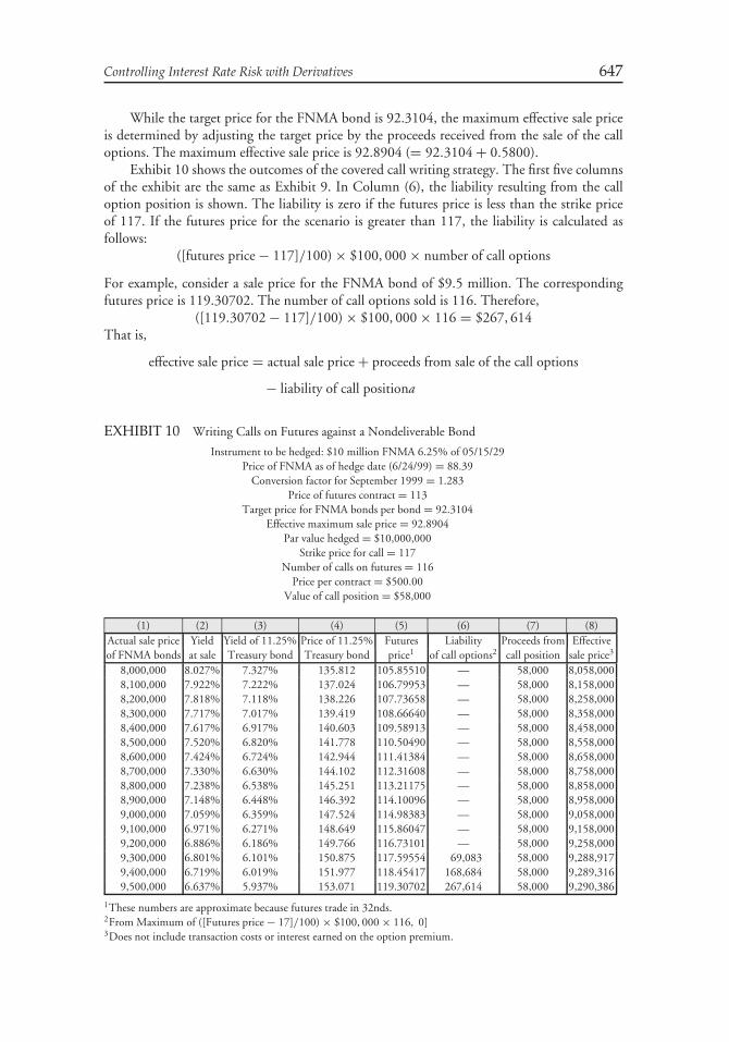
Controlling Interest Rate Risk with Derivatives 647
While the target price for the FNMA bond is 92.3104, the maximum effective sale priceis determined by adjusting the target price by the proceeds received from the sale of the calloptions. The maximum effective sale price is 92.8904 (= 92.3104 + 0.5800).
Exhibit 10 shows the outcomes of the covered call writing strategy. The first five columnsof the exhibit are the same as Exhibit 9. In Column (6), the liability resulting from the calloption position is shown. The liability is zero if the futures price is less than the strike priceof 117. If the futures price for the scenario is greater than 117, the liability is calculated asfollows:
([futures price − 117]/100) × $100, 000 × number of call options
For example, consider a sale price for the FNMA bond of $9.5 million. The correspondingfutures price is 119.30702. The number of call options sold is 116. Therefore,
([119.30702 − 117]/100) × $100, 000 × 116 = $267, 614That is,
effective sale price = actual sale price + proceeds from sale of the call options
− liability of call positiona
EXHIBIT 10 Writing Calls on Futures against a Nondeliverable Bond
Instrument to be hedged: $10 million FNMA 6.25% of 05/15/29Price of FNMA as of hedge date (6/24/99) = 88.39
Conversion factor for September 1999 = 1.283Price of futures contract = 113
Target price for FNMA bonds per bond = 92.3104Effective maximum sale price = 92.8904
Par value hedged = $10,000,000Strike price for call = 117
Number of calls on futures = 116Price per contract = $500.00
Value of call position = $58,000
(1) (2) (3) (4) (5) (6) (7) (8)Actual sale price Yield Yield of 11.25% Price of 11.25% Futures Liability Proceeds from Effectiveof FNMA bonds at sale Treasury bond Treasury bond price1 of call options2 call position sale price3
8,000,000 8.027% 7.327% 135.812 105.85510 — 58,000 8,058,0008,100,000 7.922% 7.222% 137.024 106.79953 — 58,000 8,158,0008,200,000 7.818% 7.118% 138.226 107.73658 — 58,000 8,258,0008,300,000 7.717% 7.017% 139.419 108.66640 — 58,000 8,358,0008,400,000 7.617% 6.917% 140.603 109.58913 — 58,000 8,458,0008,500,000 7.520% 6.820% 141.778 110.50490 — 58,000 8,558,0008,600,000 7.424% 6.724% 142.944 111.41384 — 58,000 8,658,0008,700,000 7.330% 6.630% 144.102 112.31608 — 58,000 8,758,0008,800,000 7.238% 6.538% 145.251 113.21175 — 58,000 8,858,0008,900,000 7.148% 6.448% 146.392 114.10096 — 58,000 8,958,0009,000,000 7.059% 6.359% 147.524 114.98383 — 58,000 9,058,0009,100,000 6.971% 6.271% 148.649 115.86047 — 58,000 9,158,0009,200,000 6.886% 6.186% 149.766 116.73101 — 58,000 9,258,0009,300,000 6.801% 6.101% 150.875 117.59554 69,083 58,000 9,288,9179,400,000 6.719% 6.019% 151.977 118.45417 168,684 58,000 9,289,3169,500,000 6.637% 5.937% 153.071 119.30702 267,614 58,000 9,290,386
1These numbers are approximate because futures trade in 32nds.2From Maximum of ([Futures price − 17]/100) × $100, 000 × 116, 0]3Does not include transaction costs or interest earned on the option premium.
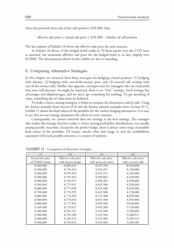
648 Fixed Income Analysis
Since the proceeds from sale of the call options is $58,000, then
effective sale price = actual sale price + $58, 000 − liability of call position
The last column of Exhibit 10 shows the effective sale price for each scenario.As Exhibit 10 shows, if the hedged bond trades at 70 basis points over the CTD issue
as assumed, the maximum effective sale price for the hedged bond is, in fact, slightly over92.8904. The discrepancies shown in the exhibit are due to rounding.
E. Comparing Alternative Strategies
In this chapter we reviewed three basic strategies for hedging a bond position: (1) hedgingwith futures, (2) hedging with out-of-the-money puts, and (3) covered call writing without-of-the-money calls. Similar, but opposite, strategies exist for managers who are concernedthat rates will decrease. As might be expected, there is no ‘‘best’’ strategy. Each strategy hasadvantages and disadvantages, and we never get something for nothing. To get anything ofvalue, something else of value must be forfeited.
To make a choice among strategies, it helps to compare the alternatives side by side. Usingthe futures example from Section II B and the futures options examples from Section IV C,Exhibit 11 shows the final values of the portfolio for the various hedging alternatives. It is easyto see that no one strategy dominates the others in every scenario.
Consequently, we cannot conclude that one strategy is the best strategy. The managerwho makes the strategy decision makes a choice among probability distributions, not usuallyamong specific outcomes. Except for the perfect hedge, there is always some range of possiblefinal values of the portfolio. Of course, exactly what that range is, and the probabilitiesassociated with each possible outcome, is a matter of opinion.
EXHIBIT 11 Comparison of Alternative Strategies
(1) (2) (3) (4)Actual sale price Effective sale price Effective sale price Effective sale priceof FNMA bonds with futures hedge with protective puts with covered calls
8,000,000 8,800,229 8,397,294 8,058,0008,100,000 8,794,453 8,394,351 8,158,0008,200,000 8,789,503 8,392,212 8,258,0008,300,000 8,785,363 8,390,862 8,358,0008,400,000 8,782,017 8,390,285 8,458,0008,500,000 8,779,451 8,445,500 8,558,0008,600,000 8,777,650 8,545,500 8,658,0008,700,000 8,776,599 8,645,500 8,758,0008,800,000 8,776,284 8,745,500 8,858,0008,900,000 8,776,693 8,845,500 8,958,0009,000,000 8,777,812 8,945,500 9,058,0009,100,000 8,779,627 9,045,500 9,158,0009,200,000 8,782,127 9,145,500 9,258,0009,300,000 8,785,300 9,245,500 9,288,9179,400,000 8,789,132 9,345,500 9,289,3169,500,000 8,793,614 9,445,500 9,290,386
Controlling Interest Rate Risk with Derivatives 649
F. Hedging with Options on Cash Instruments
Hedging a position with options on cash bonds is relatively straightforward. Most strategies,including the purchase of protective puts, covered call writing, and buying collars, areessentially the same whether futures options or options on physicals are used. As explained,an option on a physical is an option on a bond. In our illustrations we used options onfutures because they are the more actively traded types of futures contracts and therefore thecontracts used in hedging. While there are mechanical differences in the way the two typesof option contracts are traded, the basic economics of the hedging strategies are virtuallyidentical.
Using options on physicals frequently eliminates much of the basis risk associated with afutures options hedge. For example, a manager of Treasury bonds or notes can usually buy orsell options on the exact security held in the portfolio. Using options on futures, rather thanoptions on Treasury bonds, introduces additional elements of uncertainty.
Given the illustration presented above, and given that the risk-return profile of options onphysicals and options on futures are essentially identical, additional illustrations for options onphysicals are unnecessary. The only important differences are the calculations of the hedge ratioand the equivalent strike price. To derive the hedge ratio, we always resort to an expressionof relative dollar durations. Thus, assuming a constant spread, the hedge ratio for options onphysicals is:
current dollar duration without options
dollar duration of underlying for option
If a relationship is estimated between the yield on the bonds to be hedged and theinstrument underlying the option, the appropriate hedge ratio is:
current dollar duration without options
dollar duration of underlying for option× yield beta
Unlike futures options, there is only one deliverable, so there is no conversion factor.When cross hedging with options on physicals, the procedure for finding the equivalent strikeprice on the bonds to be hedged is similar. Given the strike price of the option, the strike yield isdetermined using the price/yield relationship for the instrument underlying the option. Thengiven the projected relationship between the yield on the instrument underlying the optionand the yield on the bonds to be hedged, an equivalent strike yield is derived for the bonds tobe hedged. Finally, using the yield-to-price formula for the bonds to be hedged, the equivalentstrike price for the bonds to be hedged can be found.
V. USING CAPS AND FLOORS
Interest rate caps can be used in liability management to create a cap for funding costs.Combining a cap and a floor creates a collar for funding costs. Floors can be used by buyers offloating-rate instruments to set a floor on the periodic interest earned. To reduce the cost of afloor, a manager can sell a cap. By doing so, the manager limits the upside on the coupon rateof a floating-rate instrument should rates rise, thereby creating a collar for the coupon rate.
To see how interest rate caps and floors can be used for asset/liability management,consider the problems faced by the commercial bank and the life insurance company discussedin Section III A. Recall that the bank’s objective is to lock in a spread over its cost of funds.

650 Fixed Income Analysis
Yet because the bank borrows short term, its cost of funds is uncertain. The bank may be ableto purchase a cap, however, so that the cap rate plus the cost of purchasing the cap is less thanthe rate it is earning on its fixed-rate commercial loans. If short-term rates decline, the bankdoes not benefit from the cap, but its cost of funds declines. The cap therefore allows thebank to impose a ceiling on its cost of funds while retaining the opportunity to benefit from adecline in rates.
The bank can reduce the cost of purchasing the cap by selling a floor. In this case, thebank agrees to pay the buyer of the floor if the reference rate falls below the strike rate. Thebank receives a fee for selling the floor, but it has sold off its opportunity to benefit from adecline in rates below the strike rate. By buying a cap and selling a floor, the bank has createda predetermined range for its cost of funds (i.e., a collar).
Recall the problem of the life insurance company that guarantees an 8% rate on a GIC forfour years and is considering the purchase of a floating-rate instrument in a private placementtransaction. The risk the company faces is that interest rates will fall so that it will not earnenough to realize the 8% guaranteed rate plus a spread. The life insurance company may be ableto purchase a floor to set a lower bound on its investment return, yet retain the opportunityto benefit should rates increase. To reduce the cost of purchasing the floor, the life insurancecompany can sell an interest rate cap. By doing so, however, it forfeits the opportunity tobenefit from an increase in the reference rate above the strike rate of the cap.
CHAPTER 23HEDGING MORTGAGE
SECURITIES TO CAPTURERELATIVE VALUE∗
I. INTRODUCTION
Because of the spread offered on residential agency mortgage-backed securities, they oftenoutperform government securities with the same interest rate risk and therefore they can be usedto generate enhanced returns relative to a benchmark when the yield advantage of mortgagesecurities is attractive. However, to execute this strategy successfully, the prepayment riskof mortgage securities must be managed carefully. In this chapter, we will see how this isdone. Specifically, we will see how to ‘‘hedge’’ the interest rate risk associated with a fixedrate mortgage security in order to capture the spread over Treasuries.1 Note that we use theterms mortgage-backed securities and mortgage securities interchangeably in this chapter. Asexplained earlier, the most basic form of mortgage-backed security is the mortgage passthroughsecurity. Securities that are created from mortgage passthrough securities include collateralizedmortgage obligations and mortgage strips (interest-only and principal-only securities).
II. THE PROBLEM
To illustrate the problem faced by a portfolio manager who believes that the spread offeredon a mortgage security, is attractive and wants to hedge that spread, look at Exhibit 1. Theexhibit shows the relationship between price and yield for a mortgage passthrough security.The yield for a mortgage security is the cash flow yield.2 The price-yield relationship exhibitsboth positive and negative convexity. At yield levels above y*, the mortgage security exhibitspositive convexity; at yield levels below y*, the mortgage security exhibits negative convexity.
∗This chapter is authored by Kennath B. Dunn, PhD, Roberto M. Sella and Frank J. Fabozzi, PhD,
CFA, CPA.1In European countries where mortgage-backed securities are issued, the coupon rate is typically afloating rate.2The cash flow yield is the interest rate (properly annualized) that makes the present value of theprojected cash flows from a mortgage-backed security equal to its price.
651
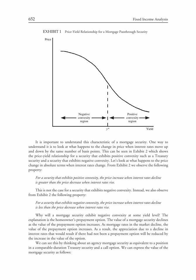
652 Fixed Income Analysis
EXHIBIT 1 Price-Yield Relationship for a Mortgage Passthrough Security
Negativeconvexity
region
Positiveconvexity
region
Yieldy*
Price
It is important to understand this characteristic of a mortgage security. One way tounderstand it is to look at what happens to the change in price when interest rates move upand down by the same number of basis points. This can be seen in Exhibit 2 which showsthe price-yield relationship for a security that exhibits positive convexity such as a Treasurysecurity and a security that exhibits negative convexity. Let’s look at what happens to the pricechange in absolute terms when interest rates change. From Exhibit 2 we observe the followingproperty:
For a security that exhibits positive convexity, the price increase when interest rates declineis greater than the price decrease when interest rates rise.
This is not the case for a security that exhibits negative convexity. Instead, we also observefrom Exhibit 2 the following property:
For a security that exhibits negative convexity, the price increase when interest rates declineis less than the price decrease when interest rates rise.
Why will a mortgage security exhibit negative convexity at some yield level? Theexplanation is the homeowner’s prepayment option. The value of a mortgage security declinesas the value of the prepayment option increases. As mortgage rates in the market decline, thevalue of the prepayment option increases. As a result, the appreciation due to a decline ininterest rates that would result if there had not been a prepayment option will be reduced bythe increase in the value of the option.
We can see this by thinking about an agency mortgage security as equivalent to a positionin a comparable-duration Treasury security and a call option. We can express the value of themortgage security as follows:
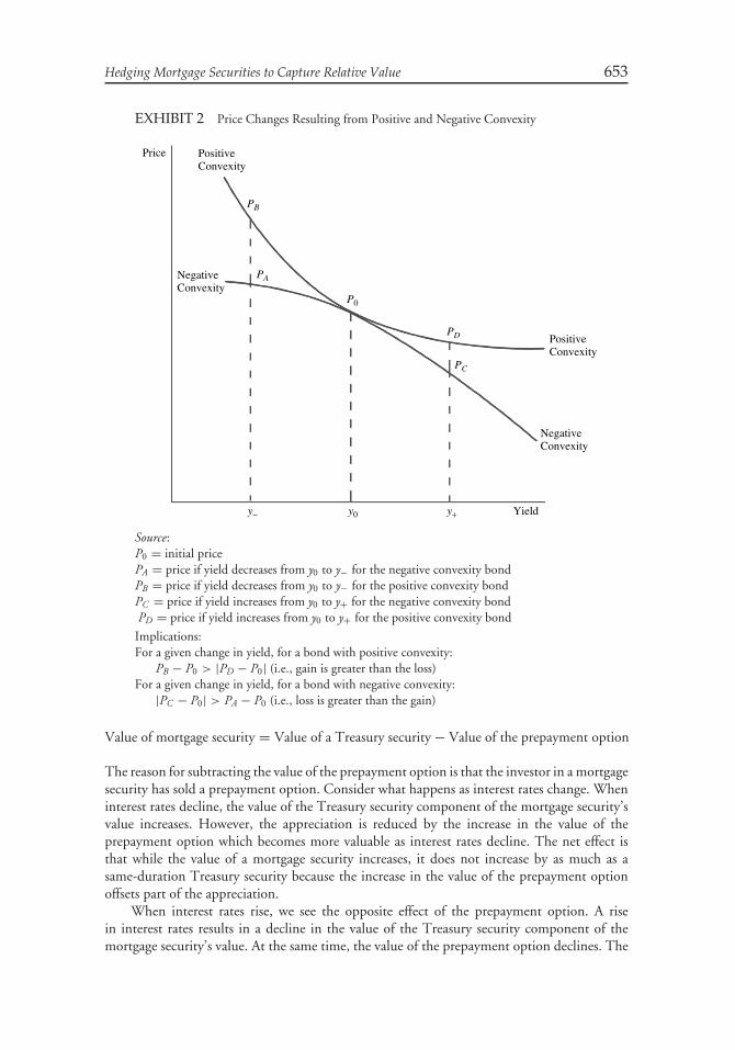
Hedging Mortgage Securities to Capture Relative Value 653
EXHIBIT 2 Price Changes Resulting from Positive and Negative Convexity
PositiveConvexity
NegativeConvexity
Price
PB
PA
P0
PD
PC
PositiveConvexity
NegativeConvexity
Yieldy− y+y0
Source:P0 = initial pricePA = price if yield decreases from y0 to y− for the negative convexity bondPB = price if yield decreases from y0 to y− for the positive convexity bondPC = price if yield increases from y0 to y+ for the negative convexity bondPD = price if yield increases from y0 to y+ for the positive convexity bond
Implications:For a given change in yield, for a bond with positive convexity:
PB − P0 > |PD − P0| (i.e., gain is greater than the loss)For a given change in yield, for a bond with negative convexity:
|PC − P0| > PA − P0 (i.e., loss is greater than the gain)
Value of mortgage security = Value of a Treasury security − Value of the prepayment option
The reason for subtracting the value of the prepayment option is that the investor in a mortgagesecurity has sold a prepayment option. Consider what happens as interest rates change. Wheninterest rates decline, the value of the Treasury security component of the mortgage security’svalue increases. However, the appreciation is reduced by the increase in the value of theprepayment option which becomes more valuable as interest rates decline. The net effect isthat while the value of a mortgage security increases, it does not increase by as much as asame-duration Treasury security because the increase in the value of the prepayment optionoffsets part of the appreciation.
When interest rates rise, we see the opposite effect of the prepayment option. A risein interest rates results in a decline in the value of the Treasury security component of themortgage security’s value. At the same time, the value of the prepayment option declines. The
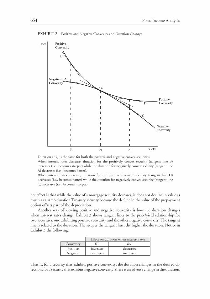
654 Fixed Income Analysis
EXHIBIT 3 Positive and Negative Convexity and Duration Changes
Price PositiveConvexity
NegativeConvexity
B
A
P0
DPositiveConvexity
NegativeConvexity
Yieldy+y− y0
C
Duration at y0 is the same for both the positive and negative convex securities.When interest rates decrease, duration for the positively convex security (tangent line B)increases (i.e., becomes steeper) while the duration for negatively convex security (tangent lineA) decreases (i.e., becomes flatter).When interest rates increase, duration for the positively convex security (tangent line D)decreases (i.e., becomes flatter) while the duration for negatively convex security (tangent lineC) increases (i.e., becomes steeper).
net effect is that while the value of a mortgage security deceases, it does not decline in value asmuch as a same-duration Treasury security because the decline in the value of the prepaymentoption offsets part of the depreciation.
Another way of viewing positive and negative convexity is how the duration changeswhen interest rates change. Exhibit 3 shows tangent lines to the price/yield relationship fortwo securities, one exhibiting positive convexity and the other negative convexity. The tangentline is related to the duration. The steeper the tangent line, the higher the duration. Notice inExhibit 3 the following:
Effect on duration when interest ratesConvexity fall risePositive increases decreasesNegative decreases increases
That is, for a security that exhibits positive convexity, the duration changes in the desired di-rection; for a security that exhibits negative convexity, there is an adverse change in the duration.
Hedging Mortgage Securities to Capture Relative Value 655
While a mortgage security can exhibit both positive and negative convexity, a Treasurysecurity exhibits only positive convexity. Look at the problem of hedging the interest raterisk associated with a mortgage security by either shorting Treasury securities or sellingTreasury futures (i.e., hedging an instrument that has the potential for negative convexitywith an instrument that only exhibits positive convexity). As explained in Chapter 22, thehedging principle is that the change in the value of the mortgage security position for agiven basis point change in interest rates will be offset by the change in the value of theTreasury position for the same basis point change in interest rates. When interest rates decline,prepayments cause the value of a mortgage security to increase less in value than that of aTreasury position with the same initial duration. Thus, when interest rates decline, simplymatching the dollar duration of the Treasury position with the dollar duration of the mortgagesecurity will not provide an appropriate hedge when the mortgage security exhibits negativeconvexity.
For this reason, many investors consider mortgages to be market-directional investmentsthat should be avoided when one expects interest rates to decline.3 Fortunately, when properlymanaged, mortgage securities are not market-directional investments. Proper managementbegins with separating mortgage valuation decisions from decisions concerning the appropriateinterest-rate sensitivity of the portfolio. In turn, this separation of the value decision fromthe duration decision hinges critically on proper hedging. Without proper hedging to offsetthe changes in the duration of mortgage securities caused by interest rate movements, theportfolio’s duration would drift adversely from its target duration. In other words, the portfoliowould be shorter than desired when interest rates decline and longer than desired when interestrates rise.
III. MORTGAGE SECURITY RISKS
Proper hedging requires understanding the principal risks associated with investing in mortgagesecurities. There are five principal risks: spread, interest-rate, prepayment, volatility, and modelrisk.4 The yield of a mortgage security—the cumulative reward for bearing all five of theserisks—has two components: the yield on equal interest-rate risk Treasury securities plus aspread. This spread is itself the sum of the option cost, which is the expected cost of bearingprepayment risk, and the option-adjusted spread (OAS), which is the risk premium for bearingthe remaining risks, including model risk.
A. Spread Risk
A portfolio manager would want to invest in mortgage securities when their spreads versusTreasuries are large enough to compensate for the risk surrounding the homeowner’s prepay-ment option. Because the OAS can be thought of as the risk premium for holding mortgagesecurities, a portfolio manager does not seek to hedge spread risk. If a portfolio manager hedgesagainst spread widening, she also gives up the benefit from spread narrowing. Instead, a
3This perception is exacerbated by the common practice of comparing the returns of the mortgage indexwith the returns of the government and corporate indices without adjusting for differences in duration.Because the mortgage index typically has less duration than either the corporate or government index, itgenerally has better relative performance when interest rates rise than when interest rates fall.4Model risk was discussed earlier.
656 Fixed Income Analysis
portfolio manager seeks to capture the OAS over time by increasing the allocation to mortgagesecurities when yield spreads are wide and reducing exposure to mortgage securities when yieldspreads are narrow.
To calculate the OAS for any mortgage security, a prepayment model is employed thatassigns an expected prepayment rate every month—implying an expected cash flow—fora given interest rate path. These expected cash flows are discounted at U.S. Treasury spotrates to obtain their present value. This process is repeated for a large number of interestrate paths. Finally, the average present value of the cash flows across all paths is calculated.Typically, the average present value across all paths is not equal to the price of the security.However, we can search for a unique ‘‘spread’’ (in basis points) that, when added to the U.S.Treasury spot rates, equates the average present value to the price of the security. This spreadis the OAS.
Historical comparisons are of only limited use for making judgments about currentOAS levels relative to the past, because option-adjusted spreads depend on their underlyingprepayment models. As a model changes, so does the OAS for a given mortgage security.There are periods where prepayment models change significantly, making comparisons tohistorical OASs tenuous. A portfolio manager should augment OAS analysis with other toolsto help identify periods when spreads on mortgage securities are attractive, attempting to avoidperiods when spread widening will erase the yield advantage over Treasuries with the sameinterest rate risk. The risk that the OAS may change, or spread risk, is managed by investingheavily in mortgage securities only when the initial OAS is large.
B. Interest Rate Risk
The interest rate risk of a mortgage security corresponds to the interest rate risk of comparableTreasury securities (i.e., a Treasury security with the same duration). This risk can be hedgeddirectly by selling a package of Treasury notes or Treasury note futures. Once a portfoliomanager has hedged the interest rate risk of a mortgage security, what can the manager earn?Recall that by hedging interest rate risk, a manager synthetically creates a Treasury bill andtherefore earns the return on a Treasury bill. But what still remains after the interest rate riskis removed is the spread risk which, as just explained, is not hedged away. So, the portfoliomanager after hedging interest rate risk can earn the Treasury bill return plus a spread overTreasuries. However, a portfolio manager cannot capture all of this spread because some of itis needed to cover the value of the homeowner’s prepayment option. After netting the valueof the option, the portfolio manager earns the Treasury bill rate plus the potential to capturethe OAS.
1. Yield Curve Risk Duration and convexity are measures of interest rate risk for ‘‘level’’changes in interest rates. That is, if all Treasury rates shifted up or down by the same numberof basis points, these measures do a good job of approximating the exposure of a securityor a portfolio to a rate change. However, yield curves do not change in a parallel fashion.Consequently, portfolios with the same duration can perform quite differently when the yieldcurve shifts in a nonparallel fashion. Yield curve risk is the exposure of a portfolio or a securityto a nonparallel change in the yield curve shape.
One approach to quantifying yield curve risk for a security or a portfolio is to computehow changes in a specific spot rate, holding all other spot rates constant, affect the value of asecurity or a portfolio. The sensitivity of the change in value of a security or a portfolio to a
Hedging Mortgage Securities to Capture Relative Value 657
particular spot rate change is called rate duration.5 In theory, there is a rate duration for everypoint on the yield curve. Consequently, there is not one rate duration, but a profile of ratedurations representing each maturity on the yield curve. The total change in value if all rateschange by the same number of basis points is simply the duration of a security or portfolio toa change in the level of rates. That is, it is the duration measure for level risk (i.e., a parallelshift in the yield curve).
Vendors of analytical system do not provide a rate duration for every point on the yieldcurve. Instead, they focus on key maturities of the spot rate curve. These rate durations arecalled key rate durations.
The impact of any type of yield curve shift can be quantified using key rate durations.A level shift can be quantified by changing all key rates by the same number of basis pointsand computing, based on the corresponding key rate durations, the affect on the value of aportfolio. The impact of a steepening of the yield curve can be found by (1) decreasing thekey rates at the short end of the yield curve and determining the change in the portfolio valueusing the corresponding key rate durations, and (2) increasing the key rates at the long end ofthe yield curve and determining the change in the portfolio value using the corresponding keyrate durations.
The value of an option-free bond with a bullet maturity payment (i.e., entire principaldue at the maturity date) is sensitive to changes in the level of interest rates but not as sensitiveto changes in the shape of the yield curve. This is because for an option-free bond whose cashflow consists of periodic coupon payments but only one principal payment (at maturity), thechange of rates along the spot rate curve will not have a significant impact on its value. Incontrast, while the value of a portfolio of option-free bonds is, of course, sensitive to changesin the level of interest rates, it is much more sensitive to changes in the shape of the yield curvethan individual option-free bonds.
In the case of mortgage securities, the value of both an individual mortgage security and aportfolio of mortgage securities will be sensitive to changes in the shape of the yield curve, aswell as changes in the level of interest rates. This is because a mortgage security is an amortizingsecurity with a prepayment option. Consequently, the pattern of the expected cash flows foran individual mortgage security can be materially affected by the shape of the yield curve. Tosee this, look at Exhibit 4 which shows the key rate durations for a Ginnie Mae 30-year 10%passthrough, the current coupon passthrough at the time the graph was prepared. Exhibit5 shows the key rate duration profile for a principal-only (PO) and an interest-only (IO)mortgage strip created from the Ginnie Mae passthrough whose key rate durations are shownin Exhibit 4.
From Exhibit 4 it can be seen that the passthrough exhibits a bell-shaped curve with thepeak of the curve between 5 and 15 years. Adding up the key rate durations from 5 to 15 years(i.e., the 5-year, 7-year, 10-year, and 15-year key rate durations) indicates that of the totalinterest rate exposure, about 70% is within this maturity range. That is, the effective durationalone masks the fact that the interest rate exposure for this passthrough is concentrated in the5-year to 15-year maturity range.
A PO will have a high positive duration. From the key rate duration profile for thePO shown in Exhibit 5 it can be seen that the key rate durations are negative up to year7. Thereafter, the key rate durations are positive and have a high value. While the total riskexposure (i.e., effective duration) may be positive, there is exposure to yield curve risk. Forexample, the key rate durations suggest that if the long end of the yield curve is unchanged,
5Rate duration was discussed previously.
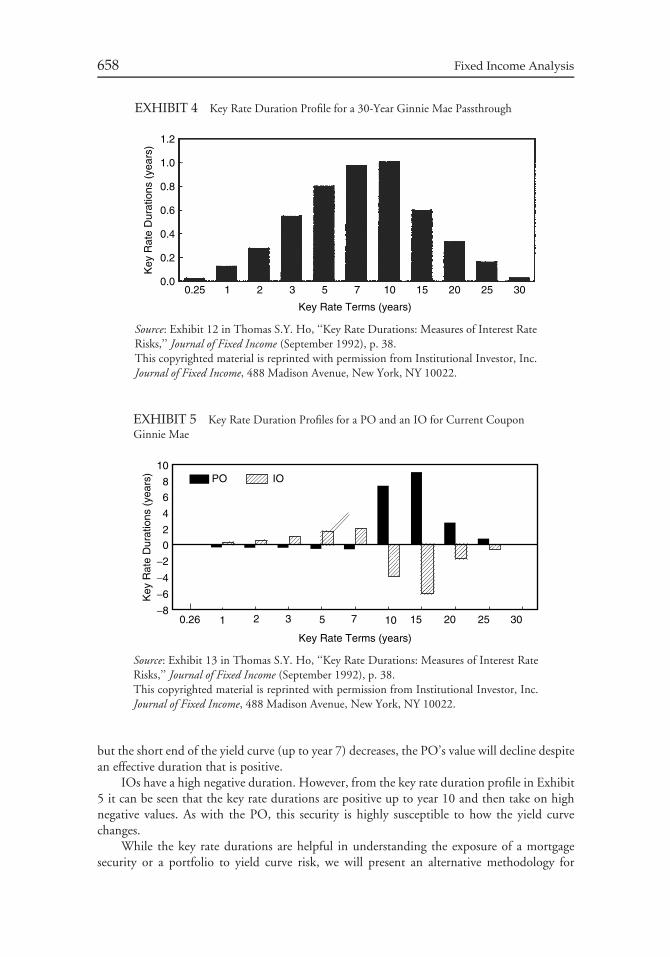
658 Fixed Income Analysis
EXHIBIT 4 Key Rate Duration Profile for a 30-Year Ginnie Mae Passthrough
1.2
1.0
0.8
0.6
0.4
0.2
0.0
Key
Rat
e D
urat
ions
(ye
ars)
Key Rate Terms (years)
0.25 1 2 3 5 7 10 15 20 25 30
Source: Exhibit 12 in Thomas S.Y. Ho, ‘‘Key Rate Durations: Measures of Interest RateRisks,’’ Journal of Fixed Income (September 1992), p. 38.This copyrighted material is reprinted with permission from Institutional Investor, Inc.Journal of Fixed Income, 488 Madison Avenue, New York, NY 10022.
EXHIBIT 5 Key Rate Duration Profiles for a PO and an IO for Current CouponGinnie Mae
Key Rate Terms (years)
Key
Rat
e D
urat
ions
(ye
ars)
0.26 1 2 3 5 7 10 15 20 25 30−8
−6
−4
−2
0
2
4
6
8
10PO IO
Source: Exhibit 13 in Thomas S.Y. Ho, ‘‘Key Rate Durations: Measures of Interest RateRisks,’’ Journal of Fixed Income (September 1992), p. 38.This copyrighted material is reprinted with permission from Institutional Investor, Inc.Journal of Fixed Income, 488 Madison Avenue, New York, NY 10022.
but the short end of the yield curve (up to year 7) decreases, the PO’s value will decline despitean effective duration that is positive.
IOs have a high negative duration. However, from the key rate duration profile in Exhibit5 it can be seen that the key rate durations are positive up to year 10 and then take on highnegative values. As with the PO, this security is highly susceptible to how the yield curvechanges.
While the key rate durations are helpful in understanding the exposure of a mortgagesecurity or a portfolio to yield curve risk, we will present an alternative methodology for
Hedging Mortgage Securities to Capture Relative Value 659
assessing the yield curve risk of a mortgage security when we discuss the hedging methodologyin Section V.
C. Prepayment Risk
When interest rates decline, homeowners have an economic incentive to prepay their existingmortgages by refinancing at a lower rate. As demonstrated earlier, because of the prepaymentoption the duration of mortgage securities varies in an undesirable way as interest rates change:extending as rates rise and shortening as rates fall. Therefore, the percentage increase in priceof a mortgage security for successive 25 basis point declines in yield, for example, becomessmaller and smaller. Conversely, the percentage decline in price becomes greater as interestrates rise. Termed negative convexity, this effect can be significant—particularly for mortgagesecurities that concentrate prepayment risk such as interest-only strips.
When interest rates change we must offset the resultant change in mortgage durations inorder to keep the overall interest rate risk of the portfolio at its desired target. Neglecting to doso would leave the portfolio with less interest rate risk than desired after interest rates declineand more risk than desired after rates increase. A portfolio manager should adjust for changesin durations of mortgage securities—or equivalently, manage negative convexity—either bybuying options or by hedging dynamically.
Hedging dynamically requires lengthening duration—buying futures—after rates havedeclined, and shortening duration—selling futures—after rates have risen.6 Whether aportfolio manager employs this ‘‘buy high/sell low’’ dynamic strategy, or buys options, theportfolio’s performance is bearing the cost associated with managing negative convexity byforegoing part of the spread over Treasuries.
D. Volatility Risk
An investment characteristic of an option is that its value increases with expected volatility.7
In the case of an interest rate option, the pertinent volatility is interest rate volatility. Theprepayment option granted to a homeowner is an interest rate option and therefore thehomeowner’s prepayment option becomes more valuable when future interest rate volatility isexpected to be high than when it is expected to be low. Because the OAS adjusts to compensatethe investor for selling the prepayment option to the homeowner, OAS tends to widen whenexpected volatility increases and narrow when expected volatility declines.
A portfolio manager can manage volatility risk by buying options or by hedgingdynamically. The selection depends on the following:
• When the volatility implied in option prices is high and the portfolio manager believes thatfuture realized volatility will be lower than implied volatility, he should hedge dynamically.
• When implied volatility is low and the portfolio manager believes that actual futurevolatility will be higher than implied volatility, he should hedge by purchasing options.
Because it has been our experience that implied volatilities have tended to exceed subsequentrealized volatility, we have generally hedged dynamically to a greater extent than we havehedged through the use of options.
6How the buying and selling of futures affects duration is explained in Chapter 22.7This was explained earlier.
660 Fixed Income Analysis
E. Model Risk
Mortgage prepayment models generate cash flows for a given set of interest rate paths. Butwhat happens when the models are wrong? In the rally of 1993, premium mortgages prepaidat much faster rates than predicted by most prepayment models in use at that time. Investorswho had purchased interest-only strips (IOs) backed by premium mortgages, and had reliedon the prepayment predictions of those models, sustained losses. It is important to note thatprior to the rally, the OAS on IOs seemed attractive on a historical basis. However, themodel OAS assumed a conditional prepayment rate (CPR) of 40% for premium mortgages;the actual CPR for premium mortgages was as high as 60%, causing the realized OAS to benegative.
Current models calibrate to historical experience. Although a portfolio manager does notknow the magnitude of model error going forward, he can measure sensitivity to model errorby increasing the prepayment rate assumed by the model for mortgage securities that arehurt by faster-than-expected prepayments and decreasing the prepayment rate assumed by themodel for mortgage securities that are hurt by slower-than-expected prepayments.
Over time it has become cheaper to refinance mortgages as technological improvementshave reduced the costs associated with refinancing. We expect this type of prepaymentinnovation to continue in the years ahead. Models calibrated to past behavior will understatethe impact of innovation. Therefore, when evaluating mortgage securities that are vulnerable tothis type of risk, a portfolio manager should carefully consider the likelihood and the effect ofprepayment innovation in determining the size of a portfolio’s mortgage securities. Althougha portfolio manager cannot hedge model risk explicitly, he can measure it and manage it bykeeping a portfolio’s exposure to this risk in line with that of the broad-based bond marketindices.
IV. HOW INTEREST RATES CHANGE OVERTIME
While key rate duration is a useful measure for identifying the exposure of a portfolio todifferent potential shifts in the yield curve, it is difficult to employ this approach to yield curverisk in hedging a portfolio. An alternative approach is to investigate how yield curves havechanged historically and incorporate typical yield curve change scenarios into the hedgingprocess. This approach has been used by several firms that specialize in the management ofmortgage-backed securities.8
Empirically, studies have found that yield curve changes are not parallel. Rather, whenthe level of interest rates changes, studies have found that short-term rates move more thanlonger-term rates. Some firms develop their own proprietary models that decompose historicalmovements in the rate changes of Treasury strips with different maturities in order to analyzetypical or likely rate movements. The statistical technique used to decompose rate movementsis principal components analysis.
8For example, the approach is used by Morgan Stanley as discussed in this chapter and by Smith BreedenAssociates (see Michael P. Schumacher, Daniel C. Dektar, and Frank J. Fabozzi, ‘‘Yield Curve Riskof CMO Bonds,’’ Chapter 15 in Frank J. Fabozzi (ed.), CMO Portfolio Management (New Hope, PA:Frank J. Fabozzi Associates, 1994).
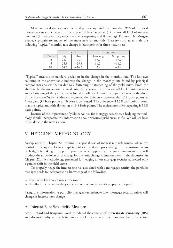
Hedging Mortgage Securities to Capture Relative Value 661
Most empirical studies, published and proprietary, find that more than 95% of historicalmovements in rate changes can be explained by changes in (1) the overall level of interestrates and (2) twists in the yield curve (i.e., steepening and flattening). For example, MorganStanley’s proprietary model of the movement of monthly Treasury strip rates finds thefollowing ‘‘typical’’ monthly rate change in basis points for three maturities:
Level Change fromYears Up Down Flattening Steepening
2 23.0 −23.0 17.2 −17.25 25.8 −25.8 11.2 −11.2
10 24.3 −24.3 3.4 −3.4
‘‘Typical’’ means one standard deviation in the change in the monthly rate. The last twocolumns in the above table indicate the change in the monthly rate found by principalcomponents analysis that is due to a flattening or steepening of the yield curve. From theabove table, the impact on the yield curve for a typical rise in the overall level of interest ratesand a flattening of the yield curve is found as follows. To find the typical change in the slopeof the 10-year–2-year yield-curve segment, the difference between the 17.2 basis points at2-year, and 3.4 basis points at 10 years is computed. The difference of 13.8 basis points meansthat the typical monthly flattening is 13.8 basis points. The typical monthly steepening is 13.8basis points.
Because of the importance of yield curve risk for mortgage securities, a hedging method-ology should incorporate this information about historical yield curve shifts. We will see howthis is done in the next section.
V. HEDGING METHODOLOGY
As explained in Chapter 22, hedging is a special case of interest rate risk control where theportfolio manager seeks to completely offset the dollar price change in the instrument tobe hedged by taking an opposite position in an appropriate hedging instrument that willproduce the same dollar price change for the same change in interest rates. In the discussion inChapter 22, the methodology presented for hedging a non-mortgage security addressed onlya parallel shift in the yield curve.
To properly hedge the interest rate risk associated with a mortgage security, the portfoliomanager needs to incorporate his knowledge of the following:
• how the yield curve changes over time• the effect of changes in the yield curve on the homeowner’s prepayment option
Using this information, a portfolio manager can estimate how mortgage security prices willchange as interest rates change.
A. Interest Rate Sensitivity Measure
Scott Richard and Benjamin Gord introduced the concept of interest-rate sensitivity (IRS)and discussed why it is a better measure of interest rate risk than modified or effective
662 Fixed Income Analysis
duration.9 IRS measures a security’s or a portfolio’s percentage price change in response to ashift in the yield curve.
Since two factors (the ‘‘level’’ and ‘‘twist’’ factors discussed in the previous section) haveaccounted for most of the changes in the yield curve, two Treasury notes (typically the 2-yearand 10-year) can hedge virtually all of the interest rate risk in mortgage securities. Since twohedging instruments are used, the hedge is referred to as a two-bond hedge.
To create the two-bond hedge, we begin by expressing a particular mortgage securityin terms of an ‘‘equivalent position’’ in U.S. Treasuries or ‘‘equivalent position’’ in Treasuryfutures contracts.10 We identify this equivalent position by picking a package of 2-yearand 10-year Treasuries that—on average—has the same price performance as the mortgagesecurity to be hedged under the assumed ‘‘level’’ and ‘‘twist’’ yield curve scenarios. Forhedging purposes, the direction of the change—up or down in the case of the ‘‘level’’ factor,flattening or steepening in the case of the ‘‘twist’’ factor—is not known. (In calculating howthe price will change in response to changes in the two factors, it is assumed that the OAS isconstant.)
In this way, the portfolio manager can calculate the unique quantities of 2-year and10-year Treasury notes or futures that will simultaneously hedge the mortgage security’s priceresponse to both ‘‘level’’ and ‘‘twist’’ scenarios. This combination is the appropriate two-bondhedge for typical yield curve shifts and therefore defines the interest rate sensitivity of themortgage security in terms of 2-year and 10-year Treasury notes or futures.
B. Computing the Two-Bond Hedge
The steps to compute the two-bond hedge are as follows:
Step 1: For an assumed shift in the level of the yield curve, compute the following:
• price of the mortgage security for an assumed increase in the level of interest rates• price for the mortgage security for an assumed decrease in the level of interest rates• price of the 2-year Treasury note (or futures) for an assumed increase in the level
of interest rates• price of the 2-year Treasury note (or futures) for an assumed decrease in the level
of interest rates• price of the 10-year Treasury note (or futures) for an assumed increase in the level
of interest rates• price of the 10-year Treasury note (or futures) for an assumed decrease in the level
of interest rates
Step 2: From the prices found in Step 1, calculate the price change for the mortgagesecurity, 2-year Treasury note (or futures), and 10-year Treasury note (or futures)for the assumed shift in the level of interest rates. There will be two prices changesfor each of the mortgage security, 2-year hedging instrument, and 10-year hedginginstrument.
9Scott F. Richard and Benjamin J. Gord, ‘‘Measuring and Managing Interest-Rate Risk,’’ Chapter 7 inFrank J. Fabozzi (ed.), Perspectives on Interest Rate Risk Management for Money Managers and Traders(New Hope, PA: Frank J. Fabozzi Associates, 1998).10Treasury futures contracts were discussed at earlier.

Hedging Mortgage Securities to Capture Relative Value 663
Step 3: Calculate the average price change for the mortgage security and the two hedginginstruments for the assumed shift in the level of interest rates assuming that the twoscenarios (i.e., increase and decrease) are equally likely to occur. The average pricechange will be denoted as follows:
MBS priceL = average price change for the mortgage security for a level shift
2-H priceL = average price change for the 2-year Treasury hedging instrument
for a level shift
10-H priceL = average price change for the 10-year Treasury hedging instrument
for a level shift
Step 4: For an assumed twist (flattening and steepening) of the yield curve, compute thefollowing:
• price of the mortgage security for an assumed flattening of the yield curve• price of the mortgage security for an assumed steepening of the yield curve• price of 2-year Treasury note (or futures) for an assumed flattening of the yield
curve• price of 2-year Treasury note (or futures) for an assumed steepening of the yield
curve• price of 10-year Treasury note (or futures) for an assumed flattening of the yield
curve• price of 10-year Treasury note (or futures) for an assumed steepening of the yield
curve
Step 5: From the prices found in Step 4, calculate the price change for the mortgagesecurity, 2-year Treasury note (or futures), and 10-year Treasury note (or futures) forthe assumed twist in the yield curve. There will be two prices changes for each of themortgage security, 2-year hedging instrument, and 10-year hedging instrument.
Step 6: Calculate the average price change for the mortgage security and the two hedginginstruments for the assumed twist in the yield curve assuming that the two scenarios(i.e., flattening and steepening) are equally likely to occur. The average price changewill be denoted as follows:
MBS priceT = average price change for the mortgage security for a twist in the
yield curve
2-H priceT = average price change for the 2-year Treasury hedging instrument
for a twist in the yield curve
10-H priceT = average price change for the 10-year Treasury hedging instrument
for a twist in the yield curve
664 Fixed Income Analysis
Step 7: Compute the change in value of the two-bond hedge portfolio for a change in thelevel of the yield curve. This is done as follows. Let
H2 = amount of the 2-year hedging instrument per $1 of market value of the
mortgage security
H10 = amount of the 10-year hedging instrument per $1 of market value of the
mortgage security
Our objective is to find the appropriate values for H2 and H10 that will produce the samechange in value for the two-bond hedge as the change in the price of the mortgage securitythat the portfolio manager seeks to hedge.
The change in value of the two-bond hedge for a change in the level of the yield curve is:
H2 × (2-HpriceL) + H10 × (10-H priceL)
Step 8: Determine the change in value of the two-bond hedge portfolio for a twist in theyield curve. This value is
H2 × (2-HpriceT ) + H10 × (10-H priceT )
Step 9: Determine the set of equations that equates the change in the value of the two-bondhedge to the change in the price of the mortgage security. To be more precise, wewant the change in the value produced by the two-bond hedge to be in the oppositedirection to the change in the price of the mortgage security. Using our notation, thetwo equations are:
Level: H2 × (2-H priceL) + H10 × (10-H priceL) = −MBS priceL
Twist: H2 × (2-H priceT ) + H10 × (10-H priceT ) = −MBS priceT
Step 10: Solve the simultaneous equations in Step 9 for the values of H2 and H10. Noticethat for the two equations, all of the values are known except for H2 and H10. Thus,there are two equations and two unknowns.
In Step 9, a negative value for H2 or H10 represents a short position and a positive valuefor H2 or H10 represents a long position.
C. Illustrations of the Two-Bond Hedge
To illustrate the steps to compute the two-bond hedge, we will examine at two different dates:February 12, 2003 and March 4, 1997. Illustration 1 shows a combination of a long positionand a short position in two hedging instruments to hedge the long position in a passthroughsecurity. Illustration 2 involves a short position in two hedging instruments in order to hedgea long position in a passthrough security.
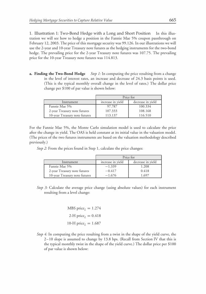
Hedging Mortgage Securities to Capture Relative Value 665
1. Illustration 1: Two-Bond Hedge with a Long and Short Position In this illus-tration we will see how to hedge a position in the Fannie Mae 5% coupon passthrough onFebruary 12, 2003. The price of this mortgage security was 99.126. In our illustrations we willuse the 2-year and 10-year Treasury note futures as the hedging instruments for the two-bondhedge. The prevailing price for the 2-year Treasury note futures was 107.75. The prevailingprice for the 10-year Treasury note futures was 114.813.
a. Finding the Two-Bond Hedge Step 1: In computing the price resulting from a changein the level of interest rates, an increase and decrease of 24.3 basis points is used.(This is the typical monthly overall change in the level of rates.) The dollar pricechange per $100 of par value is shown below:
Price forInstrument increase in yield decrease in yield
Fannie Mae 5% 97.787 100.3342-year Treasury note futures 107.333 108.16810-year Treasury note futures 113.137 116.510
For the Fannie Mae 5%, the Monte Carlo simulation model is used to calculate the priceafter the change in yield. The OAS is held constant at its initial value in the valuation model.(The prices of the two futures instruments are based on the valuation methodology describedpreviously.)
Step 2: From the prices found in Step 1, calculate the price changes:
Price forInstrument increase in yield decrease in yield
Fannie Mae 5% −1.339 1.2082-year Treasury note futures −0.417 0.41810-year Treasury note futures −1.676 1.697
Step 3: Calculate the average price change (using absolute values) for each instrumentresulting from a level change:
MBS priceL = 1.274
2-H priceL = 0.418
10-H priceL = 1.687
Step 4: In computing the price resulting from a twist in the shape of the yield curve, the2–10 slope is assumed to change by 13.8 bps. (Recall from Section IV that this isthe typical monthly twist in the shape of the yield curve.) The dollar price per $100of par value is shown below:
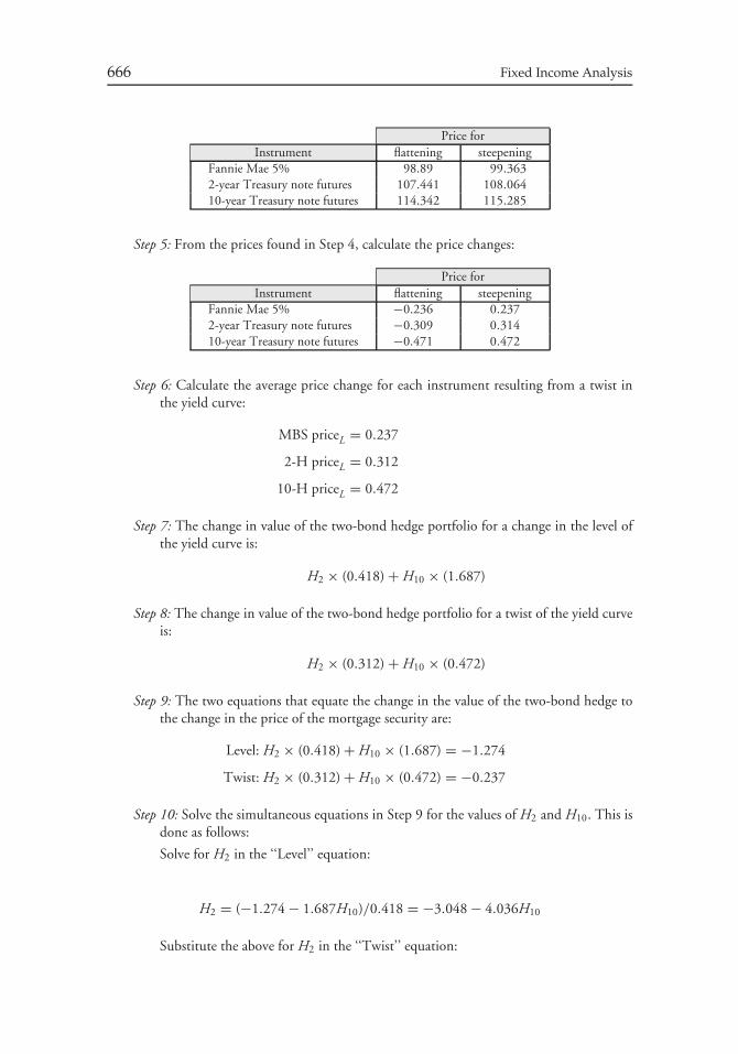
666 Fixed Income Analysis
Price forInstrument flattening steepening
Fannie Mae 5% 98.89 99.3632-year Treasury note futures 107.441 108.06410-year Treasury note futures 114.342 115.285
Step 5: From the prices found in Step 4, calculate the price changes:
Price forInstrument flattening steepening
Fannie Mae 5% −0.236 0.2372-year Treasury note futures −0.309 0.31410-year Treasury note futures −0.471 0.472
Step 6: Calculate the average price change for each instrument resulting from a twist inthe yield curve:
MBS priceL = 0.237
2-H priceL = 0.312
10-H priceL = 0.472
Step 7: The change in value of the two-bond hedge portfolio for a change in the level ofthe yield curve is:
H2 × (0.418) + H10 × (1.687)
Step 8: The change in value of the two-bond hedge portfolio for a twist of the yield curveis:
H2 × (0.312) + H10 × (0.472)
Step 9: The two equations that equate the change in the value of the two-bond hedge tothe change in the price of the mortgage security are:
Level: H2 × (0.418) + H10 × (1.687) = −1.274
Twist: H2 × (0.312) + H10 × (0.472) = −0.237
Step 10: Solve the simultaneous equations in Step 9 for the values of H2 and H10. This isdone as follows:
Solve for H2 in the ‘‘Level’’ equation:
H2 = (−1.274 − 1.687H10)/0.418 = −3.048 − 4.036H10
Substitute the above for H2 in the ‘‘Twist’’ equation:
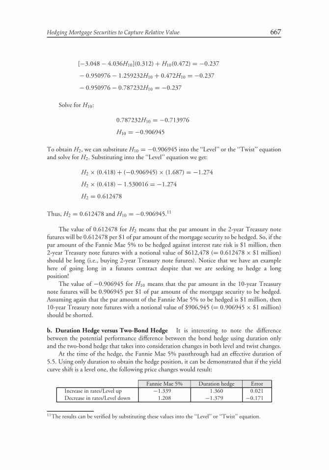
Hedging Mortgage Securities to Capture Relative Value 667
[−3.048 − 4.036H10](0.312) + H10(0.472) = −0.237
− 0.950976 − 1.259232H10 + 0.472H10 = −0.237
− 0.950976 − 0.787232H10 = −0.237
Solve for H10:
0.787232H10 = −0.713976
H10 = −0.906945
To obtain H2, we can substitute H10 = −0.906945 into the ‘‘Level’’ or the ‘‘Twist’’ equationand solve for H2. Substituting into the ‘‘Level’’ equation we get:
H2 × (0.418) + (−0.906945) × (1.687) = −1.274
H2 × (0.418) − 1.530016 = −1.274
H2 = 0.612478
Thus, H2 = 0.612478 and H10 = −0.906945.11
The value of 0.612478 for H2 means that the par amount in the 2-year Treasury notefutures will be 0.612478 per $1 of par amount of the mortgage security to be hedged. So, if thepar amount of the Fannie Mae 5% to be hedged against interest rate risk is $1 million, then2-year Treasury note futures with a notional value of $612,478 (= 0.612478 × $1 million)should be long (i.e., buying 2-year Treasury note futures). Notice that we have an examplehere of going long in a futures contract despite that we are seeking to hedge a longposition!
The value of −0.906945 for H10 means that the par amount in the 10-year Treasurynote futures will be 0.906945 per $1 of par amount of the mortgage security to be hedged.Assuming again that the par amount of the Fannie Mae 5% to be hedged is $1 million, then10-year Treasury note futures with a notional value of $906,945 (= 0.906945 × $1 million)should be shorted.
b. Duration Hedge versus Two-Bond Hedge It is interesting to note the differencebetween the potential performance difference between the bond hedge using duration onlyand the two-bond hedge that takes into consideration changes in both level and twist changes.
At the time of the hedge, the Fannie Mae 5% passthrough had an effective duration of5.5. Using only duration to obtain the hedge position, it can be demonstrated that if the yieldcurve shift is a level one, the following price changes would result:
Fannie Mae 5% Duration hedge ErrorIncrease in rates/Level up −1.339 1.360 0.021Decrease in rates/Level down 1.208 −1.379 −0.171
11The results can be verified by substituting these values into the ‘‘Level’’ or ‘‘Twist’’ equation.
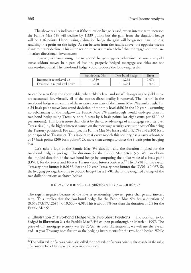
668 Fixed Income Analysis
The above results indicate that if the duration hedge is used, when interest rates increase,the Fannie Mae 5% will decline by 1.339 points but the gain from the duration hedgewill be 1.36 points. Hence, using a duration hedge the gain will be greater than the loss,resulting in a profit on the hedge. As can be seen from the results above, the opposite occursif interest rates decline. This is the reason there is a market belief that mortgage securities are‘‘market-directional’’ investments.
However, evidence using the two-bond hedge suggests otherwise: because the yieldcurve seldom moves in a parallel fashion, properly hedged mortgage securities are notmarket-directional. The two-bond hedge would produce the following results:
Fannie Mae 5% Two-bond hedge ErrorIncrease in rates/Level up −1.339 1.263 −0.076Decrease in rates/Level down 1.208 −1.284 −0.076
As can be seen from the above table, when ‘‘likely level and twist’’ changes in the yield curveare accounted for, virtually all of the market-directionality is removed. The ‘‘error’’ in thetwo-bond hedge is a measure of the negative convexity of the Fannie Mae 5% passthrough. Fora 24 basis point move (one stand deviation of monthly level shift) in the 10-year—assumingno rebalancing of the hedge—the Fannie Mae 5% passthrough would underperform itstwo-bond hedge using Treasury note futures by 8 basis points (or eight cents per $100 ofpar amount). This loss is more than offset by the carry advantage of a mortgage security overTreasuries (i.e., the higher interest earned on the mortgage security versus the cost of financingthe Treasury positions). For example, the Fannie Mae 5% has a yield of 5.17% and a 200 basispoint spread to Treasuries. This implies that every month this security has a carry advantageof 17 basis points (200 basis points/12), more than enough to offset the 8 basis point hedgingloss.
Let’s take a look at the Fannie Mae 5% duration and the duration implied for thetwo-bond hedging package. The duration for the Fannie Mae 5% is 5.5. We can obtainthe implied duration of the two-bond hedge by computing the dollar value of a basis point(DV01) for the 2-year and 10-year Treasury note futures contracts.12 The DV01 for the 2-yearTreasury note futures is 0.0186. For the 10-year Treasury note futures the DV01 is 0.067. Sothe hedging package (i.e., the two-bond hedge) has a DV01 that is the weighted average of thetwo dollar durations as shown below:
0.612478 × 0.0186 + (−0.906945) × 0.067 = −0.049373
The sign is negative because of the inverse relationship between price change and interestrates. This implies that the two-bond hedge for the Fannie Mae 5% has a duration of(0.049373/99.126) ) × 10,000 = 4.98. This is about 9% less than the duration of 5.5 for theFannie Mae 5%.
2. Illustration 2: Two-Bond Hedge with Two Short Positions The position to behedged in Illustration 2 is the Freddie Mac 7.5% coupon passthrough on March 4, 1997. Theprice of this mortgage security was 99 25/32. As with Illustration 1, we will use the 2-yearand 10-year Treasury note futures as the hedging instruments for the two-bond hedge. While
12The dollar value of a basis point, also called the price value of a basis point, is the change in the valueof a position for a 1 basis point change in interest rates.

Hedging Mortgage Securities to Capture Relative Value 669
in Illustration 1 a long position was required in the 2-year Treasury note futures and a shortposition in the 10-year Treasury note futures, we will see that a short position is required inboth hedging instruments in Illustration 2.
We will not go through all the steps but just provide the following basic information sothat the positions in the hedging instruments can be computed:
�MBS priceL = 1.22 �2-H priceL = 0.62 �10-H priceL = 1.69
�MBS priceT = 0.25 �2-H priceT = 0.01 �10-H priceT = 0.55
Based on the above information, we can complete Steps 7 through 10 as shown below:
Step 7: The change in value of the two-bond hedge portfolio for a change in the level ofthe yield curve is found as follows:
H2 × (0.62) + H10 × (1.69)
Step 8: The change in value of the two-bond hedge portfolio for a twist of the yield curveis found as follows:
H2 × (0.01) + H10 × (0.55)
Step 9: The two equations that equate the change in the value of the two-bond hedge tothe change in the price of the mortgage security are:
Level: H2 × (0.62) + H10 × (1.69) = −1.22
Twist: H2 × (0.01) + H10 × (0.55) = −0.25
Step 10: Solve the simultaneous equations in Step 9 for the values of H2 and H10. This isdone as follows:
Solve for H2 in the ‘‘Level’’ equation:
H2 = −1.22 − 1.69 H10
0.62= −1.967742 − 2.725806 H10
Substitute the above for H2 in the ‘‘Twist’’ equation:
[−1.967742 − 2.725806 H10](0.01) + H10(0.55) = −0.25
− 0.019677 − 0.027258 H10 + 0.55 H10 = −0.25
− 0.019677 + 0.522742 H10 = −0.25
Solve for H10:
0.522742 H10 = −0.230323
H10 = −0.440605
670 Fixed Income Analysis
To obtain H2, we can substitute H10 = − 0.440605 into the ‘‘Level’’ or the ‘‘Twist’’equation and solve for H2. Substituting into the ‘‘Level’’ equation we get:
H2 × (0.62) + (−0.440605) × (1.69) = −1.22
H2 × (0.62) − 0.744622 = −1.22
H2 = −0.766739
Thus, H2 = −0.766739 and H10 = −0.440605.
These values indicate that a short position will be taken in both the 2-year and 10-yearTreasury note futures. The value of 0.766739 for H2 means that the par amount in the 2-yearTreasury note futures will be 0.766739 per $1 of par amount of the mortgage security tobe hedged. So, if the par amount of the Freddie Mac 7.5% to be hedged against interestrate risk is $1 million, then 2-year Treasury note futures with a par amount of $766,739(= 0.766739 × $1 million) should be shorted. Similarly, the value of 0.440605 for H10
means that the par amount in the 10-year Treasury note futures will be 0.440605 per $1 ofmarket value of the mortgage security to be hedged.
Once again we see the value of using the two-bond hedge rather than using a durationhedge. At the time of the hedge, the Freddie Mac 7.5% passthrough had an effective durationof 4.4. Using only duration to obtain the hedge position, it can be demonstrated that if theyield curve shift is a parallel one, the following price changes would result:
Freddie Mae 75% Duration hedge ErrorIncrease in rates/Level up −1.27 1.36 +0.09Decrease in rates/Level down 1.18 −1.34 −0.16
As in Illustration 1, using a duration hedge the gain will be greater than the loss, resultingin a profit on the hedge and suggesting that mortgage securities are ‘‘market-directional’’investments. However, for the two-bond hedge we would find the following:
Freddie Mae 75% Two-bond hedge ErrorIncrease in rates/Level up −1.27 1.25 −0.02Decrease in rates/Level down 1.18 −1.20 −0.02
As can be seen from the above table, when typical changes in the yield curve are accountedfor, virtually all of the market-directionality is removed.
D. Underlying Assumptions
Now that the underlying principles and mechanics for hedging the interest rate risk ofa mortgage security have been covered, let’s look at the underlying assumptions for thetwo-bond hedge. They are:
• the yield curve shifts used in constructing the two-bond hedge are reasonable• the prepayment model used does a good job of estimating how the cash flows will change
when the yield curve changes• assumptions underlying the Monte Carlo simulation model are realized (e.g., the interest
rate volatility assumption)
Hedging Mortgage Securities to Capture Relative Value 671
• the average price change is a good approximation of how the mortgage security’s price willchange for a small movement in interest rates
This last assumption may be unacceptable for certain types of mortgage securities as explainedin the next section.
VI. HEDGING CUSPY-COUPON MORTGAGESECURITIES
In many cases, the ‘‘average’’ price change is a good approximation of how a mortgage security’sprice will change for a small movement in interest rates. This can be seen by the tangent linelabeled ‘‘Current Coupon’’ in Exhibit 6. However, some mortgage securities are very sensitiveto small movements in interest rates. For example, a mortgage security whose coupon is 100basis points higher than the current coupon could be prepaid slowly if rates rise by 25 basispoints but prepaid very quickly if rates fall by 25 basis points. Small changes in interest rateshave large effects on prepayments for such securities and hence on their prices.
A mortgage security with this characteristic is referred to as a ‘‘cuspy-coupon’’ mortgagesecurity. For such mortgage securities, averaging the price changes is not a good measure ofhow prices will change. In other words, the tangent line (labeled ‘‘Cuspy Coupon’’ in Exhibit6) is not a good proxy for the price/yield curve. At times, cuspy-coupon mortgage securitiesoffer attractive risk-adjusted expected returns; however, they have more negative convexitythan current-coupon mortgages.
Hedging cuspy-coupon mortgage securities only with Treasury notes or futures contractsmay leave the investor exposed to more negative convexity than is desired. The negativeconvexity feature, as has been mentioned, is the result of the option that the mortgage securityinvestor has granted to homeowners to prepay. That is, the investor has effectively sold anoption to homeowners. To hedge the sale of an option (i.e., a short position in an option),an investor can buy an option. Thus, a portfolio manager can extend the two-bond hedgeby buying interest rate options to offset some or all of a cuspy-coupon mortgage security’snegative convexity.
We will use a Freddie Mac 8.5% passthrough, a cuspy-coupon mortgage security inFebruary 1997, to illustrate how the two-bond hedging methodology is extended to includeoptions. The price of the Freddie Mac 8.5% passthrough was 103.50.
Without going through the mechanics of how to construct the two-bond hedge, panel ain Exhibit 7 shows (1) the change in the price for the mortgage security and (2) the changein the value of the two-bond hedge for changes in the level and twist in the yield curve. Thelast column in panel a of the exhibit shows the error for the two-bond hedge. The error is dueto the negative convexity characteristic of the Freddie Mac 8.5% passthrough (cuspy-couponmortgage security).
Because the prepayment option of the Freddie Mac 8.5s is closer to the refinancingthreshold than that of the Freddie Mac 7.5s at the time of the analysis, the two-bond hedgeerror is greater: −0.05 for the 8.5s versus −0.02 for the 7.5s. Buying calls and puts eliminatesthis drift. Specifically, we added the purchase of the following two option positions per $100of the Freddie Mac 8.5s to be hedged:
• $18 6-month call option on a 10-year Treasury note with a strike price of 99.5• $17 6-month put option on a 10-year Treasury note with a strike price of 95
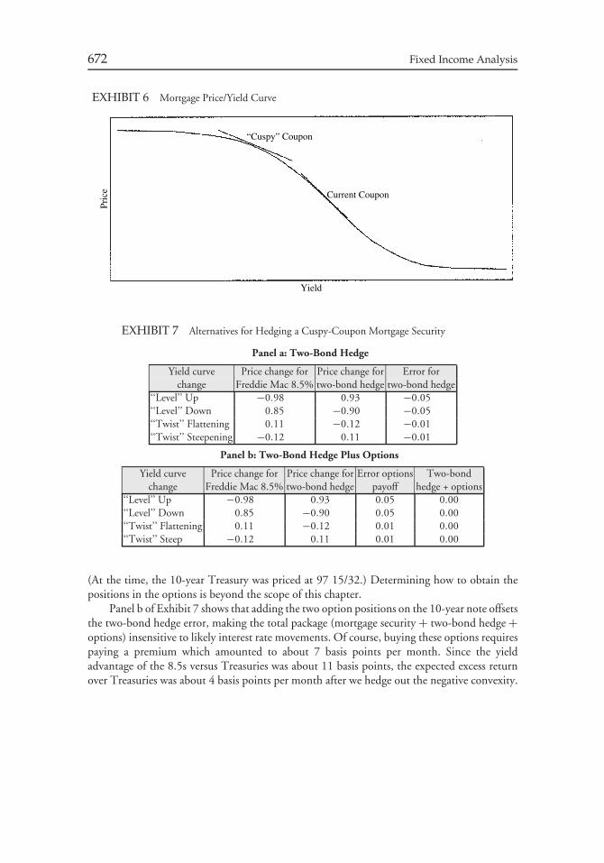
672 Fixed Income Analysis
EXHIBIT 6 Mortgage Price/Yield Curve
“Cuspy” Coupon
Current Coupon
Yield
Pric
e
EXHIBIT 7 Alternatives for Hedging a Cuspy-Coupon Mortgage Security
Panel a: Two-Bond Hedge
Yield curve Price change for Price change for Error forchange Freddie Mac 8.5% two-bond hedge two-bond hedge
‘‘Level’’ Up −0.98 0.93 −0.05‘‘Level’’ Down 0.85 −0.90 −0.05‘‘Twist’’ Flattening 0.11 −0.12 −0.01‘‘Twist’’ Steepening −0.12 0.11 −0.01
Panel b: Two-Bond Hedge Plus Options
Yield curve Price change for Price change for Error options Two-bondchange Freddie Mac 8.5% two-bond hedge payoff hedge + options
‘‘Level’’ Up −0.98 0.93 0.05 0.00‘‘Level’’ Down 0.85 −0.90 0.05 0.00‘‘Twist’’ Flattening 0.11 −0.12 0.01 0.00‘‘Twist’’ Steep −0.12 0.11 0.01 0.00
(At the time, the 10-year Treasury was priced at 97 15/32.) Determining how to obtain thepositions in the options is beyond the scope of this chapter.
Panel b of Exhibit 7 shows that adding the two option positions on the 10-year note offsetsthe two-bond hedge error, making the total package (mortgage security + two-bond hedge +options) insensitive to likely interest rate movements. Of course, buying these options requirespaying a premium which amounted to about 7 basis points per month. Since the yieldadvantage of the 8.5s versus Treasuries was about 11 basis points, the expected excess returnover Treasuries was about 4 basis points per month after we hedge out the negative convexity.
CHAPTER 24CREDIT DERIVATIVES IN
BOND PORTFOLIOMANAGEMENT∗
I. INTRODUCTION
Derivatives are financial instruments designed to efficiently transfer some form of risk betweentwo parties. Derivatives can be classified based on the type of risk that is being transferred.In the fixed-income market, derivatives include interest rate derivatives which transfer interestrate risk and credit derivatives which transfer credit risk. With credit derivatives, a portfoliomanager can either acquire or reduce credit risk exposure. Many managers have portfoliosthat are highly sensitive to changes in the spread between riskless and risky assets and creditderivatives are an efficient way to manage this exposure. Conversely, other managers may usecredit derivatives to target specific exposures as a way to enhance portfolio returns. In eachcase, the ability to transfer credit risk and return provides a tool for portfolio managers toimprove performance.
Credit derivatives can be classified as follows:
• total return swaps• credit default products• credit spread options
Credit derivative products used in structured credit products include synthetic collateral-ized debt obligations and credit-linked notes. In this chapter we will review each typeof credit derivative describing their structure and how they can be used by portfoliomanagers. After reviewing credit derivatives, we will explain synthetic credit debt obliga-tions.
We begin this chapter with a short discussion about the participants in the creditderivatives market and why credit risk is important.
∗This chapter is authored by Mark J.P. Anson, PhD, CFA, CDA, Esq., and Frank J. Fabozzi, PhD,
CFA, CPA.
673
674 Fixed Income Analysis
II. MARKET PARTICIPANTS
According to the British Bankers Association (BBA), the dominant center for the globalcredit derivatives market is London, which is well ahead of New York and Asia.1 The creditderivatives market consists of three groups of players:2
• end-buyers of protection• end-sellers of protection• intermediaries
End-buyers of protection are entities that seek to hedge credit risk taken in other partsof their business. The predominate entity in this group is commercial banks for their loanportfolio. However, there are also insurance companies, pension funds, and mutual funds whoseek protection for credits held in their portfolio. End-sellers of protection are entities thatseek to diversify their current portfolio and can do so more efficiently with credit derivatives.An entity that provides protection is seeking exposure to a specific credit or a basket of credits.
Intermediaries include investment banking arms of commercial banks and securitieshouses. Their key role in the credit derivatives market is to provide liquidity to end-users. Theytrade for their own account looking for arbitrage opportunities and other profitable oppor-tunities. In addition, some intermediaries will assemble, using credit derivatives, structuredproducts which, in turn, they may or may not manage.
III. WHY CREDIT RISK IS IMPORTANT
A fixed-income instrument represents a basket of risks. There is (1) interest rate risk (asmeasured by duration and convexity), (2) call risk, and (3) credit risk. Credit risk includes therisk of defaults, downgrades, and widening credit spreads. The total return from a fixed-incomeinstrument is the compensation for assuming all of these risks. Depending upon the ratingon the underlying debt instrument, the return from credit risk can be a significant part of abond’s total return.
A. Types of Credit Risk
Credit risk may affect a portfolio in three ways: default risk, credit spread risk, and downgraderisk. Each can have a detrimental impact on the value of a fixed-income portfolio.
1. Default Risk Default risk is the risk that the issuer will default on its obligations. Thedefault rate on credit risky bonds can be quite high. For example, estimates of the averagedefault rates for high-yield bonds in the United States range from 3.17% to 6.25%.3 However,default rates increase significantly during periods of economic malaise. For example, duringthe recession of 2001, the default rate for high-yield bonds was 10.2%. All told, there were
1British Bankers Association, Credit Derivatives Report 2002.2David Rule, ‘‘The Credit Derivatives Market: Its Development and Possible Implications for FinancialStability,’’ Financial Stability Review (June 2001), pp. 117–140.3Edward Altman, ‘‘Measuring Corporate Bond Mortality and Performance,’’ The Journal of Finance(June 1991), pp. 909-922; and Gabriella Petrucci, ‘‘High-Yield Review—First-Half 1997,’’ SalomonBrothers Corporate Bond Research (August 1997).
Credit Derivatives in Bond Portfolio Management 675
a total of $106 billion of corporate bond defaults in 2001.4 The greatest default rate in theUnited States for all corporate bonds (high yield and investment grade) was 9.2% during theGreat Depression in the 1930s.5
There is default risk associated with investing in the foreign currency debt of anothernation compared to an investor’s home country. Most investors consider the sovereign debtof the G-7 countries (the largest industrialized nations in the world: The United States, theUnited Kingdom, France German, Italy, Canada, and Japan) to be default free. The reason isthat these countries have significant internal resources and borrowing capacity to support theprompt payment of their outstanding debt.
Instead, sovereign debt default risk is associated mainly with emerging economies. Anemerging economy relies on two forms of cash flows to finance its government programs andto pay its debt obligations: taxes and revenues from state-owned enterprises. Taxes can comefrom personal income taxes, corporate taxes, import duties, and other excise taxes. State-ownedenterprises can be oil companies, telephone companies, national airlines and railroads, andother manufacturing enterprises. In times of economic turmoil such as a recession, cashflows from state-owned enterprises decline along with the general malaise of the economy.Additionally, tax revenues decline as corporations earn less profits, as unemployment rises, andas personal incomes decline. Lastly, with a declining foreign currency value, imports decline,reducing revenue from import taxes.
The possibility of default is a significant risk for portfolio managers, and one thatcan be effectively hedged by shifting the credit exposure to another party. Credit derivativestherefore appeal to portfolio managers who invest in corporate bonds—particularly, high-yieldcorporate bonds—and sovereign bonds.
2. Credit Spread Risk Credit spread risk is the risk that the interest rate spread for arisky bond over a riskless bond will increase after the risky bond has been purchased. Forinstance, in the United States, U.S Treasury securities are generally considered to be withoutcredit risk (default free). Therefore, corporate bonds, agency debentures, and the debt offoreign governments are typically priced at a spread to comparable U.S. Treasury securities.Should this spread widen after purchase of the credit risky bond, the value of the bond woulddecline. Credit spreads can widen based on macroeconomic events in the domestic or globalfinancial markets.
As an example, in October of 1997, a rapid decline in Asian stock markets spilled overinto the U.S. stock markets, causing a significant decline in financial stocks. The turbulencein the financial markets, both domestically and worldwide, resulted in a flight to safety ofinvestment capital. In other words, investors sought safer havens for their investment capitalin order to avoid further losses and volatility. This flight to safety resulted in a significantincrease in credit spreads of corporate bonds to U.S. Treasuries. For instance, on June 30,1997, corporate bonds rated BB by Standard & Poor’s were trading at an average spread overU.S. Treasuries of 215 basis points.6 However, by October 31, 1997, this spread had increasedto 319 basis points. For a $1,000 market value BB-rated corporate bond with a duration of 5,this resulted in a loss of value of about $52.50 per bond.
4See ‘‘Default and Recovery Rates of Corporate Bond Issuers,’’ Moody’s Investors Services, February2002.5Moody’s Investor Service Global Credit Research, Special Comment, ‘‘Historical Default Rates ofCorporate Bond Issuers, 1920–1999,’’ January 2000.6‘‘Financial Firms Lose $8 Billion so Far,’’ The Wall Street Journal (September 3, 1998), p. A2.
676 Fixed Income Analysis
An estimate of this credit spread risk is spread duration, a measure discussed earlier. Forcredit-risky bonds, spread duration is the approximate percentage change in the bond’s pricefor a 100 basis point increase in the credit spread (holding the Treasury rate constant). Forexample, a spread duration of 3 means that for a 100 basis point increase in the credit spread,the bond’s price will decline by approximately 3%. The spread duration for a portfolio is foundby computing a market weighted average of the spread duration for each bond. The same istrue for a bond market index. Note, however, that the spread duration reported for a bondmarket index is not the same as the spread duration for estimating the credit spread risk of anindex. For example, on April 25, 2003, the spread duration reported for the Lehman BrothersAggregate Bond Index was 2.99. However, the spread duration for the index is computed byLehman Brothers based on all non-Treasury securities. Some of these sectors offer a spreadto Treasuries that reflects more than just credit risk. For example, the mortgage sector in theindex offers a spread due to prepayment risk. The same is true for some sub-sectors withinthe ABS sector. Lehman Brothers does have a Credit Sector for the index. For that sector, thespread duration reflects the exposure to credit spreads in general. It was 1.49 on April 25, 2003and is interpreted as follows: If credit spreads increase by 100 basis points, the approximatedecline in the value of the index will be 1.49%.
3. Downgrade Risk Downgrade risk occurs when a nationally recognized statisticalrating organization such Standard & Poor’s, Moody’s Investors Services, or Fitch Ratingsreduces its outstanding credit rating for an issuer based on an evaluation of that issuer’s currentearning power versus its capacity to pay its fixed income obligations as they become due.7
The rating agencies construct credit transition matrices. These matrices can be used toforecast the probabilities of credit upgrades or downgrades for a particular class of rated bonds.For example, a transition matrix might forecast the probability (on average) of a company rated‘‘single A’’ being upgraded to ‘‘double A’’ to be 2%. Conversely, a transition matrix mightforecast the probability of a company rated ‘‘single A’’ being downgraded to ‘‘triple B’’ to be 5%.
B. Reasons for Selling Credit Protection
Credit risk is not all one-sided. A market participant may be willing to be a seller of creditprotection. This can be done in one of two ways. First, a market participant can sell contingentor insurance-type protection. That is, if the market participant believes that credit performancewill be such that it will be unnecessary to make an insurance payment to a counterparty (i.e.,the party buying credit protection), then the market participant earns the insurance premiumreceived. Second, a market participant may want to take the opposite view of a credit protectionbuyer and in fact benefit from an improvement in a credit. This is done by selling protection.
There are at least three reasons why a portfolio manager may be willing to assume thecredit risk of an underlying asset or issuer. First, there are credit upgrades as well as downgrades.A factor affecting credit rating upgrades is a strong stock market which encourages publicofferings of stock by credit risky companies. Often, a large portion of these equity financingsare used to reduce outstanding costly debt, resulting in improved balance sheets and creditratings for the issuers.
A second reason why a portfolio manager may be willing to sell credit protection is thatthere is an expectation of other credit events which have a positive effect on credit riskybonds. Mergers and acquisitions, for instance, have been historically a frequent occurrencein the high-yield corporate bond market. Even though a credit risky issuer may have a low
7For a discussion of the factors considered by rating agencies, see Chapter 15.
Credit Derivatives in Bond Portfolio Management 677
debt rating, it may have valuable technology worth acquiring. High-yield corporate bondissuers tend to be small to mid-cap companies with viable products but nascent cash flows.Consequently, they make attractive takeover candidates for financially mature companies.
The third reason is that with a growing economy, banks may be willing to provide termloans to high-yield companies at more attractive rates than the bond market. Consequently, ithas been advantageous for credit risky companies to redeem their high-yield bonds and replacean outstanding bond issue with a lower cost term loan. The resulting premium for redemptionof high-yield bonds is a positive credit event which enhances portfolio returns.
IV. TOTAL RETURN SWAP
A total return swap in the fixed-income market is a swap in which one party makes periodicfloating payments to a counterparty in exchange for the total return realized on an individualreference obligation or a basket of reference obligations. A total return payment includesall cash flows that flow from the reference obligations as well as any capital appreciation ordepreciation. The party that agrees to make the floating payments and receive the total returnis referred to as the total return receiver; the party that agrees to receive the floating paymentsand pay the total return is referred to as the total return payer. When the reference obligationis a sector of a bond index, it is called a total return index swap.
Notice that in a total return swap, the total return receiver is exposed to both credit riskand interest rate risk. For example, the credit risk spread can decline (resulting in a favorableprice movement for the reference obligation), but this gain can be offset by a rise in the levelof interest rates.
A portfolio manager typically uses a total return swap to increase credit exposure. Atotal return swap transfers all of the economic exposure of a reference obligation or referenceobligations to the total return receiver. In return for accepting this exposure, the total returnreceiver makes a floating payment to the total return payer.
A. Illustration of a Total Return Swap
Consider a portfolio manager who believes that the fortunes of XYZ Mobile Corporation willimprove over the next year, and that the company’s credit spread relative to U.S. Treasurysecurities will decline. The company has issued a 10-year bond at par with a coupon rate of8.5% and therefore the yield is 8.5%. Suppose at the time of issuance, the 10-year Treasuryyield is 5.5%. This means that the credit spread is 300 basis points and the portfolio managerbelieves it will decrease over the year to less than this amount.
The portfolio manager can express this view by entering into a total return swap thatmatures in one year as a total return receiver with the reference obligation being the 10-year,8.5% XYZ Mobile Corporate bond issue. Suppose (1) the swap calls for an exchange ofpayments semiannually and (2) the terms of the swap are such that the total return receiverpays the 6-month Treasury rate plus 140 basis points in order to receive the total return onthe reference obligation. The notional amount for the contract is $10 million.
Assume that over the one year, the following occurs:
• the 6-month Treasury rate is 4.6% initially• the 6-month Treasury rate for computing the second semiannual payment is 5.6%• at the end of one year the 9-year Treasury rate is 7%• at the end of one year the credit spread for the reference obligation is 200 basis points
678 Fixed Income Analysis
First let’s look at the payments that must be made by the portfolio manager. The firstsemi-annual swap payment made by the portfolio manager is 3% (4.6% plus 140 basis pointsdivided by two) multiplied by the $10 million notional amount. The second swap paymentmade is 3.5% (5.6% plus 140 basis points divided by two) multiplied by the $10 millionnotional amount. Thus,
First swap payment paid : $10 million × 3% = $300, 000Second swap payment paid : $10 million × 3.5% = $350, 000Total payments = $650, 000
The payments that will be received by the portfolio manager are the two coupon paymentsplus the change in the value of the reference obligation. There will be two coupon payments.Since the coupon rate is 8.5%, the amount received for the coupon payments is $850,000.
Finally, the change in the value of the reference obligation must be determined. At theend of one year, the reference obligation has a maturity of 9 years. Since the 9-year Treasuryrate is assumed to be 7% and the credit spread is assumed to decline from 300 basis points to200 basis points, the reference obligation will sell to yield 9%. The price of an 8.5%, 9-yearbond selling to yield 9% is 96.96. Since the par value is $10 million, the price is $9,696,000.The capital loss is therefore $304,000. The payment to the total return receiver is then:
Coupon payment = $850, 000Capital loss = $304, 000Swap payment = $546, 000
Netting the swap payment made and the swap payment received, the portfolio manager mustmake a payment of $104,000.
Notice that even though the portfolio manager’s expectations were realized (i.e., a declinein the credit spread), the portfolio manager had to make a net outlay. This illustration high-lights one of the disadvantages of a total return swap: the return to the investor is dependent onboth credit risk (declining or increasing credit spreads) and market risk (declining or increasingmarket rates). Two types of market interest rate risk can affect the price of a fixed-incomeinstrument. Credit independent market risk is the risk that the general level of interest rateswill change over the term of the swap. This type of risk has nothing to do with the creditdeterioration of a reference obligation. Credit dependent market interest rate risk is the riskthat the discount rate applied to the value of an asset will changed based on either perceivedor actual default risk.
In the illustration, the reference obligation was adversely affected by credit independentmarket interest rate risk, but positively rewarded for accepting credit dependent market interestrate risk. To remedy this problem, a total return receiver can customize the total return swaptransaction. For example, the portfolio manager could negotiate to receive the coupon incomeon the reference obligation plus any change in value due to changes in the credit spread.Now the portfolio manager has expressed a view exclusively of credit risk; credit independentmarket risk does not affect the swap outcome. In this case, in addition to the coupon income,the portfolio manager would receive the difference between the present value of the referenceobligation at a current spread of 200 basis points and the present value of the referenceobligation at a credit spread of 300 basis points.
Credit Derivatives in Bond Portfolio Management 679
B. Benefits of Total Return Swaps
There are several benefits in using a total return swap as opposed to purchasing referenceobligations themselves. First, the total return receiver does not have to finance the purchase ofthe reference obligations. Instead, it pays a fee to the total return payer in return for receivingthe total return on the reference obligations.
Second, the total return receiver can achieve the same economic exposure to a diversifiedbasket of assets in one swap transaction that would otherwise take several cash markettransactions to achieve. In this way a total return swap is much more efficient means fortransacting than the cash market.
Finally, an investor who wants to short the corporate bond of one or more issuers will find itdifficult to do so in the corporate bond market. An investor can do so efficiently by using a totalreturn swap. In this case the investor will pay the total return and receive a floating payment.
V. CREDIT DEFAULT PRODUCTS
Credit default products fall into two categories:
• credit default swap• credit default options on a credit-risky asset
By far, the most popular type of credit derivative is the credit default swap. An annual survey ofthe BBA finds that credit default swaps account for almost half of the credit derivatives market.Not only is this form of credit derivative the most commonly used stand-alone product, but itis also used extensively in structured credit products.
A. Credit Default Swaps
A credit default swap is probably the simplest form of credit risk transference among all creditderivatives. Credit default swaps are used to shift credit exposure to a credit protection seller.Their primary purpose is to hedge the credit exposure to a particular asset or issuer. In thissense, credit default swaps operate much like a standby letter of credit or insurance policy.
While credit default swaps are customized transactions, there has been standardizationof contract terms and provisions for certain types of credit default swaps. Swaps are usuallydocumented under a standard set of forms published by the International Swap and DerivativesAssociation (ISDA).
In a credit default swap, the documentation will identify the reference entity and thereference obligation. The reference entity is the issuer of the debt instrument. It could be acorporation or a sovereign government. The reference obligation is the particular issue forwhich the credit protection is being sought. For example, one of the most liquid referenceentities traded in the credit default swap market is Ford Motor Credit Company. The referenceobligation would be a specific Ford Motor Credit Company bond issue.
A credit default swap in which there is only one reference obligation is called a single-name credit default swap. When there is a portfolio of reference obligations (e.g., a high-yieldcorporate bond portfolio), it is referred to as a basket default swap. For a credit default swapindex the underlying is a standardized basket of reference entities. The most actively tradedcredit default swap index is the North American Investment Grade Index. The index consistsof 125 corporate names.
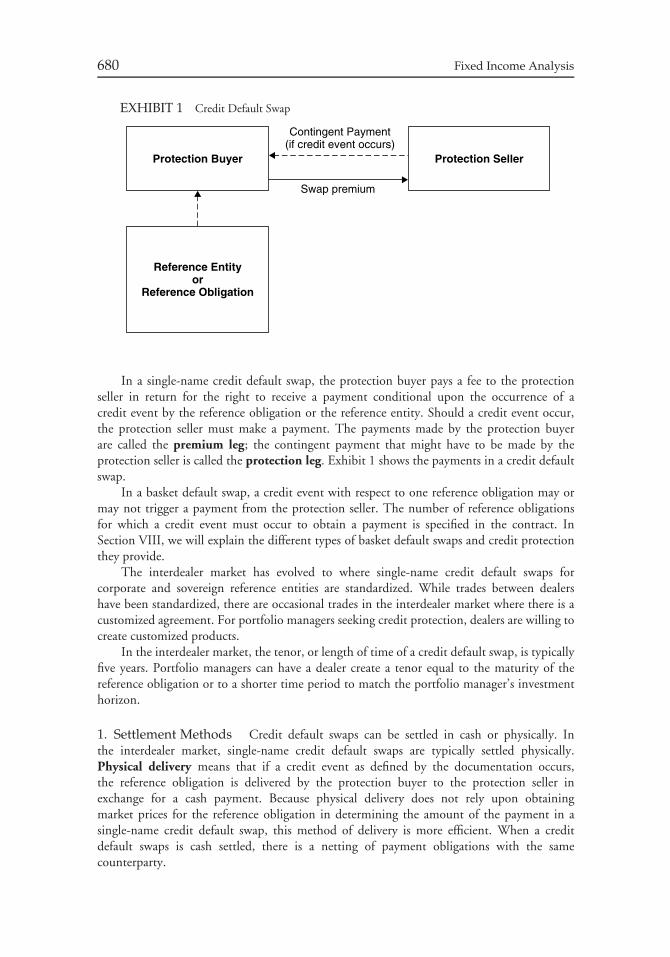
680 Fixed Income Analysis
EXHIBIT 1 Credit Default Swap
Protection Buyer
Reference Entityor
Reference Obligation
Protection Seller
Contingent Payment(if credit event occurs)
Swap premium
In a single-name credit default swap, the protection buyer pays a fee to the protectionseller in return for the right to receive a payment conditional upon the occurrence of acredit event by the reference obligation or the reference entity. Should a credit event occur,the protection seller must make a payment. The payments made by the protection buyerare called the premium leg; the contingent payment that might have to be made by theprotection seller is called the protection leg. Exhibit 1 shows the payments in a credit defaultswap.
In a basket default swap, a credit event with respect to one reference obligation may ormay not trigger a payment from the protection seller. The number of reference obligationsfor which a credit event must occur to obtain a payment is specified in the contract. InSection VIII, we will explain the different types of basket default swaps and credit protectionthey provide.
The interdealer market has evolved to where single-name credit default swaps forcorporate and sovereign reference entities are standardized. While trades between dealershave been standardized, there are occasional trades in the interdealer market where there is acustomized agreement. For portfolio managers seeking credit protection, dealers are willing tocreate customized products.
In the interdealer market, the tenor, or length of time of a credit default swap, is typicallyfive years. Portfolio managers can have a dealer create a tenor equal to the maturity of thereference obligation or to a shorter time period to match the portfolio manager’s investmenthorizon.
1. Settlement Methods Credit default swaps can be settled in cash or physically. Inthe interdealer market, single-name credit default swaps are typically settled physically.Physical delivery means that if a credit event as defined by the documentation occurs,the reference obligation is delivered by the protection buyer to the protection seller inexchange for a cash payment. Because physical delivery does not rely upon obtainingmarket prices for the reference obligation in determining the amount of the payment in asingle-name credit default swap, this method of delivery is more efficient. When a creditdefault swaps is cash settled, there is a netting of payment obligations with the samecounterparty.
Credit Derivatives in Bond Portfolio Management 681
If no credit event has occurred by the maturity of the swap, both sides terminate the swapagreement and no further obligations are incurred.
2. Determination of the Payment Obligation The methods used to determine theamount of the payment obligation of the protection seller under the swap agreement can varygreatly. For instance, a credit default swap can specify at the contract date the exact amountof payment that will be made by the protection seller should a credit event occur. Conversely,the credit default swap can be structured so that the amount of the swap payment by the selleris determined after the credit event. Under these circumstances, the amount payable by theprotection seller is determined based upon the observed prices of similar debt obligations ofthe reference entity in the market. Finally, the swap can be documented much like a credit putoption (discussed later) where the amount to be paid by the protection seller is an establishedstrike price less the current market value of the reference obligation.
The cash payment by the credit protection seller if a credit event occurs may be apredetermined fixed amount or it may be determined by the decline in value of the referenceasset. In the interdealer market, the standard single-name credit default swap when thereference obligation is a corporate bond or a sovereign bond is fixed based on a notionalamount. When the cash payment is based on the amount of asset value deterioration, thisamount is typically determined by a poll of several dealers.
In a typical credit default swap, the protection buyer pays for the protection premium overseveral settlement dates rather than upfront. A standard credit default swap in the interdealermarket specifies quarterly payments.
3. Credit Event Definitions The most important section of the documentation for acredit default swap is what the parties to the contract agree constitutes a credit event for acredit default payment. Definitions for credit events are provided by the ISDA. First publishedin 1999, there have been periodic updates and revisions of these definitions.
The 1999 ISDA Credit Derivatives Definitions (referred to as the ‘‘1999 Definitions’’)provides a list of eight credit events:
1. bankruptcy2. credit event upon merger3. cross acceleration4. cross default5. downgrade6. failure to pay7. repudiation/moratorium8. restructuring
These eight events attempt to capture every type of situation that could cause the credit qualityof the reference entity to deteriorate, or cause the value of the reference obligation to decline.
Bankruptcy is defined as a variety of acts that are associated with bankruptcy orinsolvency laws. Failure to pay results when a reference entity fails to make one or morerequired payments when due. When a reference entity breaches a covenant, it has defaultedon its obligation.
When a default occurs, the obligation becomes due and payable prior to the scheduled duedate had the reference entity not defaulted. This is referred to as an obligation acceleration.A reference entity may disaffirm or challenge the validity of its obligation. This is a credit
682 Fixed Income Analysis
event that is covered by repudiation/moratorium. In the U.S. credit default swap market,obligation acceleration and repudiation/moratorium were dropped as standard credit events inNovember 2002. In April 2003, these two credit events were dropped in the standard creditdefault swap in the European market.
A restructuring occurs when the terms of the obligation are altered so as to make the newterms less attractive to the debt holder than the original terms. The terms that can be changedwould typically include, but are not limited to, one or more of the following: (1) a reduction inthe interest rate, (2) a reduction in the principal, (3) a rescheduling of the principal repaymentschedule (e.g., lengthening the maturity of the obligation) or postponement of an interestpayment, or (4) a change in the level of seniority of the obligation in the reference entity’sdebt structure.
Restructuring is the most controversial credit event that may be included in a creditdefault swap. The reason why it is so controversial is easy to understand. A protection buyerbenefits from the inclusion of a restructuring as a credit event and feels that eliminatingrestructuring as a credit event will erode its credit protection. The protection seller, in contrast,would prefer not to include restructuring since even routine modifications of obligations thatoccur in lending arrangements would trigger a payout to the protection buyer.
Moreover, if the reference obligation is a loan and the protection buyer is the lender, thereis a dual benefit for the protection buyer to restructure a loan. The first benefit it that theprotection buyer receives a payment from the protection seller. Second, the accommodatingrestructuring fosters a relationship between the lender (who is the protection buyer) and itscustomer (the corporate entity that is the obligor of the reference obligation).
Because of this problem, the Restructuring Supplement to the 1999 ISDA Credit DerivativesDefinitions (the Supplement Definition) issued in April 2001 provided a modified definitionfor restructuring. The modified definition includes a provision for the limitation on referenceobligations in connection with restructuring of loans made by the protection buyer to theborrower that is the obligor of the reference obligation.8
Consequently, in the credit default swap market, until 2003, the parties to a trade hadthe following three choices for restructuring:
1. no restructuring2. restructured based on the 1999 Definition for restructuring, referred to as ‘‘old
restructuring’’ or ‘‘full restructuring’’3. restructuring as defined by the Restructuring Supplement Definition, referred to as
‘‘modified restructuring.’’
Modified restructuring is typically used in North America while old restructuring is used inEurope. When the reference entity is a sovereign, restructuring is often old restructuring.
Whether restructuring is included and, if it is included, whether it is old restructuringor modified restructuring, affects the swap premium. Specifically, all other factors constant, itis more expensive if restructuring is included. Moreover, old restructuring results in a largerswap premium than modified restructuring.
8This provision requires the following in order to qualify for a restructuring: (1) there must be four ormore holders of the reference obligation and (2) there must be a consent to the restructuring of thereference obligation by a supermajority (66 2/3%). In addition, the supplement limits the maturity ofreference obligations that are physically deliverable when restructuring results in a payout triggered bythe protection buyer.
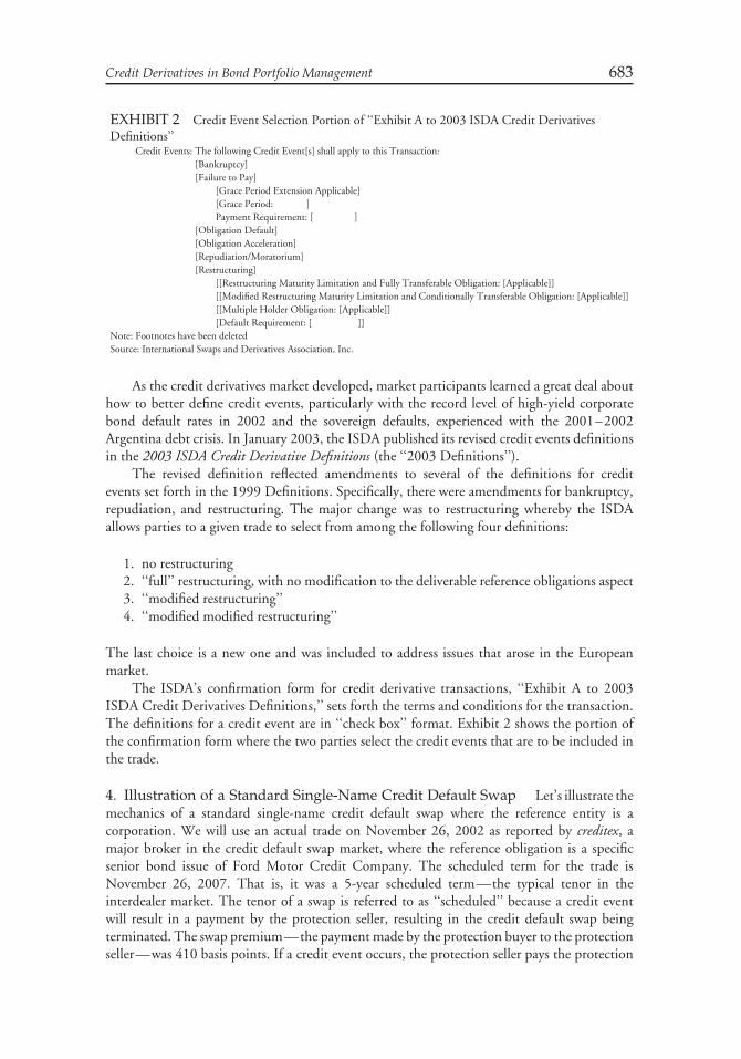
Credit Derivatives in Bond Portfolio Management 683
EXHIBIT 2 Credit Event Selection Portion of ‘‘Exhibit A to 2003 ISDA Credit DerivativesDefinitions’’
Credit Events: The following Credit Event[s] shall apply to this Transaction:[Bankruptcy][Failure to Pay]
[Grace Period Extension Applicable][Grace Period: ]Payment Requirement: [ ]
[Obligation Default][Obligation Acceleration][Repudiation/Moratorium][Restructuring]
[[Restructuring Maturity Limitation and Fully Transferable Obligation: [Applicable]][[Modified Restructuring Maturity Limitation and Conditionally Transferable Obligation: [Applicable]][[Multiple Holder Obligation: [Applicable]][Default Requirement: [ ]]
Note: Footnotes have been deletedSource: International Swaps and Derivatives Association, Inc.
As the credit derivatives market developed, market participants learned a great deal abouthow to better define credit events, particularly with the record level of high-yield corporatebond default rates in 2002 and the sovereign defaults, experienced with the 2001–2002Argentina debt crisis. In January 2003, the ISDA published its revised credit events definitionsin the 2003 ISDA Credit Derivative Definitions (the ‘‘2003 Definitions’’).
The revised definition reflected amendments to several of the definitions for creditevents set forth in the 1999 Definitions. Specifically, there were amendments for bankruptcy,repudiation, and restructuring. The major change was to restructuring whereby the ISDAallows parties to a given trade to select from among the following four definitions:
1. no restructuring2. ‘‘full’’ restructuring, with no modification to the deliverable reference obligations aspect3. ‘‘modified restructuring’’4. ‘‘modified modified restructuring’’
The last choice is a new one and was included to address issues that arose in the Europeanmarket.
The ISDA’s confirmation form for credit derivative transactions, ‘‘Exhibit A to 2003ISDA Credit Derivatives Definitions,’’ sets forth the terms and conditions for the transaction.The definitions for a credit event are in ‘‘check box’’ format. Exhibit 2 shows the portion ofthe confirmation form where the two parties select the credit events that are to be included inthe trade.
4. Illustration of a Standard Single-Name Credit Default Swap Let’s illustrate themechanics of a standard single-name credit default swap where the reference entity is acorporation. We will use an actual trade on November 26, 2002 as reported by creditex, amajor broker in the credit default swap market, where the reference obligation is a specificsenior bond issue of Ford Motor Credit Company. The scheduled term for the trade isNovember 26, 2007. That is, it was a 5-year scheduled term—the typical tenor in theinterdealer market. The tenor of a swap is referred to as ‘‘scheduled’’ because a credit eventwill result in a payment by the protection seller, resulting in the credit default swap beingterminated. The swap premium—the payment made by the protection buyer to the protectionseller—was 410 basis points. If a credit event occurs, the protection seller pays the protection
684 Fixed Income Analysis
buyer the notional amount of the contract. In our illustration, we will assume that the notionalamount is $10 million.
The notional amount is not the par value of the reference obligation. For example,suppose that a bond issue is trading at 80 (par value being 100). If a portfolio manager owns$12.5 million par value of the bond issue and wants to protect the current market value of$10 million (= 80% of $12.5 million), then the portfolio manager will want a $10 millionnotional amount. If a credit event occurs, the portfolio manager will deliver the $12.5 millionpar value of the bond and receive a cash payment of $10 million.
The standard contract for a single-name credit default swap in the interdealer market callsfor a quarterly payment of the swap premium. The quarterly payment is determined usingone of the day count conventions in the bond market. A day count convention indicates thenumber of days in the month and the number of days in a year that will be used to determinehow to prorate the swap premium to a quarter. The possible day count conventions are(1) actual/actual, (2) actual/360, and (3) 30/360. The day count convention used in the U.S.government bond market is actual/actual, while the convention used in the corporate bondmarket is 30/360. The day count convention used for credit default swaps is actual/360. Thisis the same convention used in the interest rate swap market. A day convention of actual/360means that to determine the payment in a quarter, the actual number of days in the quarterare used and 360 days are assumed for the year. Consequently, the
quarterly swap premium payment
= notional amount × swap premium (in decimal) × actual number of days in quarter
360
For example, if the notional amount is $10 million and there are 92 actual days ina quarter, then if the swap rate is 410 basis points (0.0410), the quarterly swap premiumpayment made by the protection buyer would be:
$10, 000, 000 × 0.0410 × 92
360= $104, 777.80
In the absence of a credit event occurring in any quarter, the protection buyer willcontinue to make a quarterly swap premium payment. If a credit event occurs, the protectionseller pays the protection buyer the notional amount, $10 million in our illustration, andreceives from the protection buyer the Ford Motor Credit Company senior bonds (i.e., thereference obligation).
5. Market Terminology Newcomers to the credit default swap market sometimes getconfused regarding market terminology. The first potential source of confusion arises becausemarket participants attempt to relate a position in the derivative market to a position in thecash market. The second potential source has to do with the use of the term ‘‘swap’’ to describethe transaction when the payment is contingent on the a credit event occurring.
a. Cash versus Credit Default Swap Market Terminology Participants in derivativesmarkets find it helpful to compare their exposure (long or short) in the derivative mar-ket to that of an exposure in the cash market. Sometimes the relationship is straightforward.For example, as explained in Chapter 22, a long position in a Treasury bond futures contractis equivalent to a long position in the Treasury bond market; a short position in a Treasury
Credit Derivatives in Bond Portfolio Management 685
bond futures contract is equivalent to a short position in the Treasury bond market. In othercases, the relationship is not straightforward. For example, in a generic interest rate swap, thefixed-rate payer is said to be ‘‘short the bond market’’ and the fixed-rate receiver is said to be‘‘long the bond market.’’ This is because for the fixed-rate payer, the value of an interest rateswap increases when interest rates increase. A position in the cash market whereby the valueof the position increases when interest rates increase is a short bond position. Similarly, forthe fixed-rate receiver, the value of an interest swap increases when interest rates decrease andtherefore is equivalent to being long a bond.
The terminology of the position of the parties in a credit default swap can be confusing.To ‘‘go long’’ an instrument generally is to purchase it. In the cash market, going long abond means one is buying a bond and so receiving the coupon payments; the bond buyer hastherefore taken on credit risk exposure to the issuer. In a credit default swap, going long is tobuy the swap, but the buyer is purchasing protection and therefore paying the swap premium;the buyer has no credit exposure on the reference entity and has in effect ‘‘gone short’’ onthe reference obligation (the equivalent of shorting a bond in the cash market and payingcoupons). So buying a credit default swap (buying protection) is frequently referred to in thecredit derivatives market as ‘‘shorting’’ the reference obligation.
b. Swap versus Option Nomenclature The protection seller has literally ‘‘insured’’ theprotection buyer against any credit losses on the reference obligation. While the term ‘‘swap’’is used to describe this credit derivative, it should be clear that it has an option-type payoff.That is, it does not have the characteristics of the typical swap found in the derivatives market.For example, in a plain vanilla or generic interest rate swap, two parties swap paymentsperiodically. One of the counterparties pays a fixed rate (called the ‘‘swap rate’’) and the otherparty pays a floating rate. The payments are made by both parties over the term of the swapagreement. Moreover, the payments are not contingent on some event and the occurrenceof any event does not terminate the swap agreement. This is not a characteristic of a creditdefault swap.
The question is then: Why is the transaction referred to as a swap? The reason has todue with the way one characterizes an option. There are two attributes for characterizing aderivative as an option. The first attribute is that there is an asymmetric payoff. The secondattribute involves the price performance feature. While a credit default swap does have anasymmetric payoff, its price performance is like that of a swap rather than an option. Theprice performance of an option depends on the price of the underlying. When a credit-riskybond is the underlying, it is the credit spread that affects the price of the bond. So the priceperformance mechanism for an option is as follows: changes in the credit spread affect theprice of the underlying bond which, in turn, changes the price of the option. In the case of acredit default swap, the change in the credit spread directly affects the price of the transactionrather than through its effect on the reference obligation (i.e., underlying bond). This is acharacteristic of a swap such as an interest rate swap where the price of a swap depends directlyon interest rates. It is for this reason that a credit default swap is referred to as a swap.
B. Default Options on a Credit Risky Asset
A default option on a credit risky asset is another form of credit default product. Theseoptions have not been nearly as popular as credit default swaps. Consequently, we will onlyprovide a brief review of them.
In a binary credit option the option seller will pay out a fixed sum if and when a defaultevent occurs with respect to a reference obligation or reference entity. Therefore, a binary
686 Fixed Income Analysis
option represents two states of the world: default or no default. It is the clearest example ofcredit protection. At maturity of the option, if the reference obligation or reference entity hasdefaulted, the option holder receives a predetermined payout. If there is no default at maturityof the option, the option buyer receives nothing.
A binary credit option could also be triggered by a rating downgrade.We’ll illustrate abinary credit option (both a put and a call) based on a credit rating. Consider the situationwhere a portfolio manager holds an investment-grade bond but is concerned that the creditrating for the issuer will be lowered and that the bond will decline in value. The portfoliomanager can purchase a binary credit put option which allows putting the bond back to theoption seller at the bond’s par value if the bond issuer is downgraded below investment grade.
As an example, assume that the portfolio manager purchased at par $1 million of CompanyW bonds, currently rated AA. The portfolio manager purchases a put option where he can sellthe bonds at par value to the put option seller should the credit rating for Company W fallbelow investment grade (below BBB). The payoff to this binary put option can be described as:
payout =
$1, 000, 000 − market value of the bonds, if the credit rating ofCompany W falls below a BBB ratingor$0 if the credit rating of Company W remains investment grade
(1)
Equation (1) is called a binary credit option because of its ‘‘either or’’ payout structure.Either Company W’s credit rating is below investment grade or it is not. Therefore, theportfolio manager receives a payout on the credit put option only in one state of the world:Company W is downgraded to below investment grade; otherwise, the portfolio managerreceives nothing.
Let’s now consider a binary credit call option. Suppose that instead of purchasing abinary credit put option on the par value of the bonds to protect her investment, the portfoliomanager purchases a series of call options that provide her with additional income shouldCompany W be downgraded. In other words, whenever Company W is downgraded, theportfolio manager gets to call for a payment that will compensate her for the greater credit riskassociated with her bond holdings. This is like receiving additional coupon income to reflectthe higher credit risk associated with Company W’s bonds.
Consider the example where the portfolio manager gets to call for an additional 25 basispoints of income should Company W be downgraded one credit rating, 50 basis points ofincome should Company W be downgraded two steps, and so forth. The pay out to this creditcall option may be described as:
payout =
$2,500 if the credit rating of Company W declines by one credit rating;or$5, 000 if the credit rating of Company W declines by two credit rating;or$0 if the credit rating of Company W is not downgraded.
(2)
where $2, 500 = 0.25% × $1, 000, 000
and $5, 000 = 0.50% × $1, 000, 000
Equation (2) is different from equation 1 in that the payout to the binary credit call option isnot a function of the bonds’ market value.

Credit Derivatives in Bond Portfolio Management 687
VI. CREDIT SPREAD PRODUCTS
The third category of credit derivatives is credit spread products which include:
• credit spread options• credit spread forward
We describe each below. However, it should be noted that the market for credit spread optionshas not developed as rapidly as market participants had anticipated.
A. Credit Spread Options
A credit spread option is an option whose value/payoff depends on the change in creditspreads for a reference obligation. It is critical in discussion of credit spread options to definewhat the underlying is. The underlying can be:
• a reference obligation with a fixed credit spread• the level of the credit spread for a reference obligation
1. Underlying is a Reference Obligation with a Fixed Credit Spread When theunderlying is a reference obligation with a fixed credit spread, then a credit spread option isdefined as follows:
Credit spread put option: An option that grants the option buyer the right, but not theobligation, to sell a reference obligation at a price that is determined by a strike creditspread over a referenced benchmark at the exercise date.
Credit spread call option: An option that grants the option buyer the right, but notthe obligation, to buy a reference obligation at a price that is determined by a strikecredit spread over a referenced benchmark at the exercise date.
A credit spread option can have any exercise style: only at the exercise date (European), atany time prior to the exercise date (American), or only on specified dates by the exercise date(Bermudean).
The price for the reference obligation (i.e., the credit-risky bond) is determined byspecifying a strike credit spread over the referenced benchmark, typically a default-freegovernment security. For example, suppose that the reference obligation is an 8% 10-yearcredit-risky bond selling to yield 8%. The price of this bond is 100. Suppose further that thereferenced benchmark is a same maturity U.S. Treasury bond that is selling to yield 6%. Thenthe current credit spread is 200 basis points. Assume that a strike credit spread of 300 basispoints is specified and that the option expires in six months. At the end of six months, supposethat the 9.5-year Treasury rate is 6.5%. Since the strike credit spread is 300 basis points, thenthe yield used to compute the strike price for the reference obligation is 9.5% (the Treasuryrate of 6.5% plus the strike credit spread of 300 basis points). The price of a 9.5-year 8%coupon bond selling to yield 9.5% is $90.75 per $100 par value.
The payoff at the expiration date would then depend on the market price for the referenceobligation. For example, suppose that at the end of six months, the reference obligation istrading at 82.59. This is a yield of 11% and therefore a credit spread of a 450 basis pointsover the 9.5-year Treasury yield of 6.5%. For a credit spread put option, the buyer can sell the

688 Fixed Income Analysis
reference obligation (selling at 82.59) for the strike price of 90.75. The payoff from exercisingis 8.16. This payoff is reduced by the cost of the option. For a credit spread call option, thebuyer will not exercise the option and will allow it to expire worthless. There is a loss equal tothe cost of the option.
There is one problem with using a credit spread option in which the underlying is areference obligation with a fixed credit spread. The payoff is dependent upon the value of thereference obligation’s price, which is affected by both the change in the level of the interestrates (as measured by the referenced benchmark) and the change in the credit spread. Forexample, suppose in our illustration that the 9.5-year Treasury at the exercise date is 4.5%(instead of 6.5%) and the credit spread increases to 450 basis points. This means that thereference obligation is trading at 9% (4.5% plus 450 basis points). Since it is an 8% couponbond with 9.5-years to maturity selling at 9%, the price is 93.70. In this case, the credit spreadput option would have a payoff of $965 because the price of the reference obligation is 93.70and the strike price is 103.35. Thus, there was no protection against credit spread risk becauseinterest rates for the referenced benchmark fell enough to offset the increase in the creditspread.
Notice the following payoff from the perspective of the owner of the option before takinginto account the option cost when the underlying for the a credit spread option is the referenceobligation with a fixed credit spread:
Type of option Positive payoff if at expirationPut credit spread at expiration > strike credit spreadCall credit spread at expiration < strike credit spread
Consequently, to protect against credit spread risk, an investor can buy a credit spread putoption where the underlying is a reference obligation with a fixed credit spread.
2. Underlying is a Credit Spread on a Reference Obligation When the underlyingfor a credit spread option is the credit spread for a reference obligation over a referencedbenchmark, then the payoff of a call and a put option if exercised are as follows:
Credit spread call option:
payoff = (credit spread at exercise − strike credit spread) × notional amount × risk factor
Credit spread put option:
payoff = (strike credit spread − credit spread at exercise) × notional amount × risk factor
where the strike credit spread (in decimal form) is fixed at the outset of the option; the creditspread at exercise (in decimal form) is the credit spread over a referenced benchmark at theexercise date; and, the risk factor is based on the interest rate sensitivity of the debt instrument.
Notice that when the underlying for the credit spread option is the credit spread for areference obligation over a referenced benchmark, a credit spread call option is used to protectagainst an increase in the credit spread. In contrast, when the underlying for the credit spreadoption is the reference obligation, a credit spread put option is used to protect against anincrease in the credit spread.
The risk factor is determined by the sensitivity of the reference obligation to changesin the credit spread. The risk factor can be computed in one of several ways. One way is tocompute the percentage change in the price of the reference obligation to a 100 basis point
Credit Derivatives in Bond Portfolio Management 689
change in interest rates. Since the percentage price change will differ depending on whether weare looking at an increase or decrease in the credit spread, the change used will be dictated bythe circumstances. For example, if the option involved a credit spread widening, an increasein interest rates is used to determine the price decline. Once the percentage change in priceis determined for a 100 basis point change in rates, then it is divided by 100 to get theapproximate percentage price change for a 1 basis point change in rates. That is,
approximate percentage price change per 1 bp change in rates
= percentage price change for a 100 basis point change in rates
100
To scale the risk factor in terms of how the credit spread at expiration and the strike creditspread are defined, the following calculation is performed:
risk factor = percentage price change for a 1 basis point change in rates × 10, 000
By including the risk factor, this form of credit spread option overcomes the problemwe identified with the credit spread option in which the underlying is a reference obligation:the payoff depends on both changes in the level of interest rates (the yield on the referencedbenchmark) and the credit spread. Instead, it is only dependent upon the change in the creditspread. Therefore, fluctuations in the level of the referenced benchmark’s interest rate will notaffect the value of the options.
To illustrate a credit spread call option, consider the BB rated, 7.75 Niagara MohawkPower bond due in 2008. In September 1998, this bond was trading at a price of $104.77with a yield to maturity around 7.08%. The risk factor is determined using the percentagechange in price for a 100 basis point increase in interest rates.9 For the Niagara Mohawk bond,there would be a percentage price change of 6.65% for a 100 basis point increase in rates. So,for each 1 basis point increase in the credit spread, there would be approximately a 0.0665%price change. The risk factor is then:
0.000665 × 10, 000 = 6.65
At the time that this bond was offering a yield of 7.08%, the 10-year Treasury note was yieldingabout 5.3% for a credit spread of 178 basis points. At the time this was a very narrow spreadconsidering Niagara Mohawk Power’s BB credit rating. Perhaps the market was implying thatthe credit risk of Niagara Mohawk was closer to BBB than BB.
Alternatively, it could be that the market overvalued the bond. If a portfolio managerbelieved that the bond was overvalued, the portfolio manager could purchase a credit spreadoption struck at 178 basis points. This is the same as the portfolio manager expressing aview that the price of the reference obligation is inflated at the prevailing credit spread, andexpecting the credit spread to widen out to more normal levels.
Suppose that the manager believes that the credit spread for this bond will increase to250 basis points in one year. The portfolio manager can purchase a $20 million notionalat-the-money call option on the credit spread between the debt of Niagara Mohawk Power
9An increase in interest rates is used because we are looking at the price sensitivity to an increase in thecredit spread.
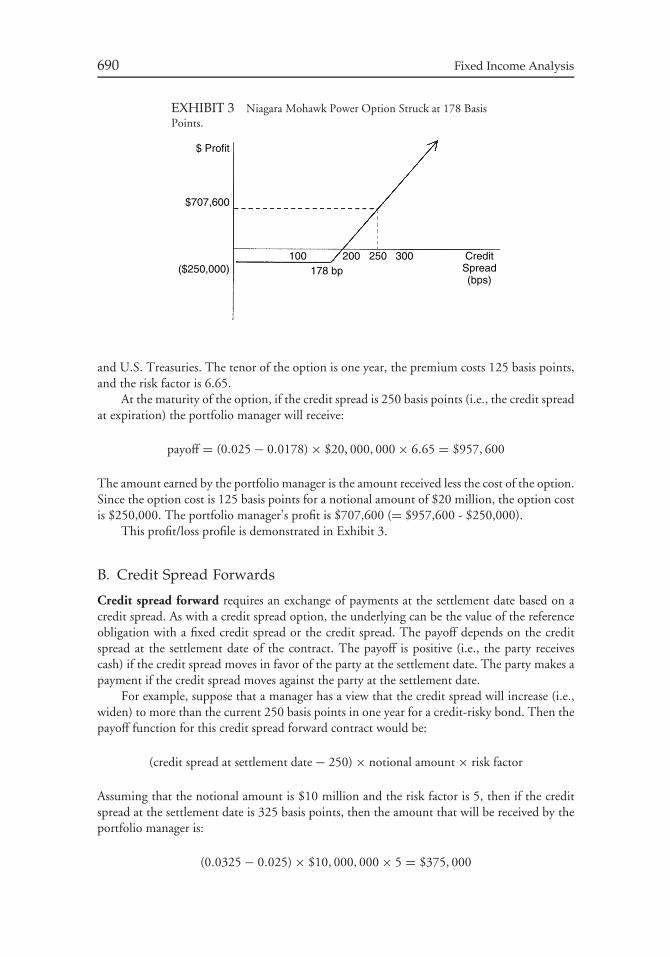
690 Fixed Income Analysis
EXHIBIT 3 Niagara Mohawk Power Option Struck at 178 BasisPoints.
$ Profit
$707,600
($250,000)100
178 bp200 250 300 Credit
Spread(bps)
and U.S. Treasuries. The tenor of the option is one year, the premium costs 125 basis points,and the risk factor is 6.65.
At the maturity of the option, if the credit spread is 250 basis points (i.e., the credit spreadat expiration) the portfolio manager will receive:
payoff = (0.025 − 0.0178) × $20, 000, 000 × 6.65 = $957, 600
The amount earned by the portfolio manager is the amount received less the cost of the option.Since the option cost is 125 basis points for a notional amount of $20 million, the option costis $250,000. The portfolio manager’s profit is $707,600 (= $957,600 - $250,000).
This profit/loss profile is demonstrated in Exhibit 3.
B. Credit Spread Forwards
Credit spread forward requires an exchange of payments at the settlement date based on acredit spread. As with a credit spread option, the underlying can be the value of the referenceobligation with a fixed credit spread or the credit spread. The payoff depends on the creditspread at the settlement date of the contract. The payoff is positive (i.e., the party receivescash) if the credit spread moves in favor of the party at the settlement date. The party makes apayment if the credit spread moves against the party at the settlement date.
For example, suppose that a manager has a view that the credit spread will increase (i.e.,widen) to more than the current 250 basis points in one year for a credit-risky bond. Then thepayoff function for this credit spread forward contract would be:
(credit spread at settlement date − 250) × notional amount × risk factor
Assuming that the notional amount is $10 million and the risk factor is 5, then if the creditspread at the settlement date is 325 basis points, then the amount that will be received by theportfolio manager is:
(0.0325 − 0.025) × $10, 000, 000 × 5 = $375, 000
Credit Derivatives in Bond Portfolio Management 691
Instead, suppose that the credit spread at the settlement date decreased to 190 basispoints, then the portfolio manager would have to payout $300,000 as shown below:
(0.019 − 0.025) × $10, 000, 000 × 5 = −$300, 000
In general, if a portfolio manager takes a position in a credit spread forward to benefitfrom an increase in the credit spread, then the payoff would be as follows:
(credit spread at settlement date − contracted credit spread) × notional amount × risk factor
For a portfolio manager taking a position that the credit spread will decrease, the payoff is:
(contracted credit spread − credit spread at settlement date) × notional amount × risk factor
VII. SYNTHETIC COLLATERALIZED DEBTOBLIGATIONS
Credit derivatives are used to create debt instruments with structures whose payoffs are linkedto, or derived from, the credit characteristics of a reference obligation or entity or a basket ofreference obligations or entities. These products are called structured credit products. Wewill focus on one of these products: synthetic collateralized debt obligations.
Previously, collateralized debt obligations were explained. A collateralized debt obligation(CDO) is backed by a diversified pool of one or more of the following types of debt obligations:investment-grade corporate bonds, high-yield corporate bonds, emerging market bonds, bankloans, asset-backed securities, residential and commercial mortgage-backed securities, and realestate investment trusts. In a CDO structure, there is a collateral manager responsible formanaging the collateral assets. The funds to purchase the collateral assets are obtained fromthe issuance of bonds. Typically, there are senior bonds and mezzanine bonds. There is also asubordinate/equity tranche.
A CDO is classified as either a cash CDO or a synthetic CDO. In a cash CDO thecollateral manager purchases the collateral assets. It was the cash CDO that was discussed. Ourfocus in this section is on synthetic CDOs, the fastest growing sector of the CDO market. Asynthetic CDO is so named because the collateral manager does not actually own the pool ofassets on which it has the credit risk exposure. Stated differently, a synthetic CDO absorbsthe credit risk, but not the legal ownership, of its reference credit exposures. A basket creditdefault swap is typically employed to allow institutions to transfer the credit risk, but not thelegal ownership, of underlying assets.
The basic structure of a synthetic CDO is as follows. As with a cash CDO, there areliabilities issued. The proceeds received from the bonds sold are invested by the collateralmanager in assets with low risk. At the same time, the collateral manager enters into a basketcredit default swap with a counterparty in which it will provide credit protection (i.e., thecollateral manager is a protection seller) for the reference obligations that have credit riskexposure. Because it is selling credit protection, the collateral manager will receive the creditdefault swap premium.
On the other side of the basket credit default swap is a protection buyer who will bepaying the swap premium to the collateral manager. This entity will be a financial institutionseeking to shed the credit risk of assets that it owns and are the reference obligations forthe credit default swap. If a credit event does not occur, the return realized by the collateral
692 Fixed Income Analysis
manager that will be available to meet the payment to the CDO bondholders is the return onthe collateral consisting of low risk assets plus the credit default swap premium. If a credit eventoccurs for any of the reference obligations, the collateral manager must make a payment to thecounterparty. This reduces the return available to meet the payments to CDO bondholders.
Recently, a new form of synthetic CDO was traded: Standard tranches of credit defaultswap indices.10
VIII. BASKET DEFAULT SWAPS
Because of the growing importance of the synthetic CDO market and the role of basketdefault swaps in these structures and other types of credit structured products that may becreated in the market, in this section we will take a closer look at the different types of basketdefault swaps. In a basket default swap, there is more than one reference entity. Typically, in abasket default swap, there are three to five reference entities. There are different types of basketdefault swaps. They are classified as follows:
• N th-to-default swaps• Subordinate basket default swaps• Senior basket default swaps
In this section we describe each type.
A. N th-to-Default Swaps
In an N th-to-default swap, the protection seller makes a payment to the protection buyeronly after there has been a default for the N th reference entity and no payment for default ofthe first (N − 1) reference entities. Once there is a payout for the N th reference entity, thecredit default swap terminates. That is, if the other reference entities that have not defaultedsubsequently do default, the protection seller does not make any payout.
For example, suppose that there are five reference entities. In a first-to-default basketswap, a payout is triggered after there is a default for only one of the reference entities. Thereare no other payouts made by the protection seller even if the other four reference entitiessubsequently have a credit event. If a payout is triggered only after there is a second defaultfrom among the reference entities, the swap is referred to as a second-to-default basket swap.So, if there is only one reference entity for which there is a default over the tenor of the swap,the protection seller does not make any payment. If there is a default for a second referenceentity while the swap is in effect, there is a payout by the protection seller and the swapterminates. The protection seller does not make any payment for a default that may occur forthe three remaining reference entities.
B. Subordinate and Senior Basket Credit Default Swaps
In a subordinate basket default swap there is (1) a maximum payout for each defaultedreference entity and (2) a maximum aggregate payout over the tenor of the swap for the basketof reference entities. For example, assume there are five reference entities and that (1) themaximum payout is $10 million for a reference entity and (2) the maximum aggregate payout
10See Chapter 15 in Douglas J. Lucas, Laurie S. Goodman, and Frank J. Fabozzi, Collateralized DebtObligations: Structures and Analysis, Second Edition (Hoboken, NJ: John Wiley & Sons, 2006).
Credit Derivatives in Bond Portfolio Management 693
is $15 million. Also assume that defaults result in the following losses over the tenor of theswap:
Loss resulting from default of first reference entity = $6 million
Loss result from default of second reference entity = $10 million
Loss result from default of third reference entity = $16 million
Loss result from default of fourth reference entity = $12 million
Loss result from default of fifth reference entity = $15 million
When there is a default for the first reference entity, there is a $6 million payout. Theremaining amount that can be paid out on any subsequent defaults for the other four referenceentities is $9 million. When there is a default for the second reference entity of $10 million,only $9 million will be paid out. At that point, the swap terminates.
In a senior basket default swap there is a maximum payout for each reference entity,but the payout is not triggered until after a specified dollar loss threshold is reached. Toillustrate, again assume there are five reference entities and the maximum payout for anindividual reference entity is $10 million. Also assume that there is no payout until the first$40 million of default losses (the threshold). Using the hypothetical losses above, the payoutby the protection seller would be as follows. The losses for the first three defaults is $32million. However, because of the maximum loss for a reference entity, only $10 million of the$16 million loss is applied to the $40 million threshold. Consequently, after the third default,$26 million ($6 million + $10 million + $10 million) is applied toward the threshold. Whenthe fourth reference entity defaults, only $10 million is applied to the $40 million threshold.At this point, $36 million is applied to the $40 million threshold. When the fifth referenceentity defaults in our illustration, only $10 million is relevant since the maximum payout fora reference entity is $10 million. The first $4 million of the $10 million is applied to cover thethreshold. Thus, there is a $6 million payout by the protection seller.
C. Comparison of Riskiness of Different Default Swaps11
Let’s compare the riskiness of each type of default swap from the perspective of the protectionseller. This will also help reinforce an understanding of the different types of swaps. We willassume that for the basket default swaps there are the same five reference entities. Four creditdefault swaps, ranked by highest to lowest risk for the reasons to be explained, are:
1. Subordinate basket default swap: he maximum for each reference entity is $10 millionwith a maximum aggregate payout of $10 million.
2. First-to-default swap: he maximum payout is $10 million for the first reference entity todefault.
3. Fifth-to-default swap: he maximum payout for the fifth reference entity to default is $10million.
4. Senior basket default swap: here is a maximum payout for each reference entity of $10million, but there is no payout until a threshold of $40 million is reached.
11The illustration and discussion in this section draws from ‘‘Nth to Default Swaps and Notes: All AboutDefault Correlation,’’ CDO Insight (May 30, 2003) UBS Warburg.

694 Fixed Income Analysis
All but the senior basket default swap will definitely require the protection seller to makea payout by the time the fifth loss reference entity defaults (subject to the maximum payouton the loss for the individual reference entities). Consequently, the senior basket default swapexposes the protection seller to the least risk.
Now let’s look at the relative risk of the other three default swaps with a $10 millionmaximum payout: subordinate basket default swap, first-to-default swap, and fifth-to-defaultswap. Consider first the subordinate basket swap versus first-to-default swap. Suppose thatthe loss for the first reference entity to default is $8 million. In the first-to-default swap thepayout required by the protection seller is $8 million and then the swap terminates (i.e., thereare no further payouts that must be made by the protection seller). For the subordinate basketswap, after the payout of $8 million of the first reference entity to default, the swap doesnot terminate. Instead, the protection seller is still exposed to $2 million for any default lossresulting from the other four reference entities. Consequently, the subordinate basket defaultswap has greater risk than the first-to-default swap.
Finally, the first-to-default has greater risk for the protection seller than the fifth-to-defaultswap because the protection seller must make a payout on the first reference entity to default.

ABOUT THECFA PROGRAM
The Chartered Financial Analyst designation (CFA) is a globally recognized standardof excellence for measuring the competence and integrity of investment professionals. Toearn the CFA charter, candidates must successfully pass through the CFA Program, a globalgraduate-level self-study program that combines a broad curriculum with professional conductrequirements as preparation for a wide range of investment specialties.
Anchored by a practice-based curriculum, the CFA Program is focused on the knowledgeidentified by professionals as essential to the investment decision-making process. This bodyof knowledge maintains current relevance through a regular, extensive survey of practicingCFA charterholders across the globe. The curriculum covers 10 general topic areas rangingfrom equity and fixed-income analysis to portfolio management to corporate finance, all witha heavy emphasis on the application of ethics in professional practice. Known for its rigor andbreadth, the CFA Program curriculum highlights principles common to every market so thatprofessionals who earn the CFA designation have a thoroughly global investment perspectiveand a profound understanding of the global marketplace.
www.cfainstitute.org
695

ABOUT THE AUTHOR
Frank J. Fabozzi, PhD, CFA, CPA, is the Frederick Frank Adjunct Professor of Finance atYale University’s School of Management and a consultant in the fixed income and derivativesarea. He is a Fellow of the International Center for Finance at Yale University. From 1986to 1992, he was a visiting professor of finance at MIT’s Sloan School of Management. He ison the board of directors of the BlackRock complex of funds and the Guardian Life family offunds.
Dr. Fabozzi has edited and authored many acclaimed books. Three of his books areco-authored with the late Professor Franco Modigliani, recipient of the 1985 Nobel MemorialPrize in Economic Science. He is co-editor of The Theory and Practice of Investment Managementwith Dr. Harry Markowitz, co-recipient of the 1990 Nobel Memorial Prize in EconomicScience.
He is the editor of the Journal of Portfolio Management and an associate editor of TheJournal of Fixed Income, The Journal of Structured Finance, and Risk Letters.
In 1994, Dr. Fabozzi received an honorary doctorate of Humane Letters from NovaSoutheastern University. In November 2002, he was inducted into the Fixed Income AnalystsSociety Hall of Fame. The Hall of Fame was established in 1995 to recognize the lifetimeachievements of outstanding practitioners in the advancement of the analysis of fixed-incomesecurities and portfolios.
In 2003, he was appointed to Princeton University’s Advisory Council for the Departmentof Operations Research and Financial Engineering. Dr. Fabozzi is the Honorary Advisor tothe Chinese Asset Securitization website (www.chinasecuritization.com) whose mission is ‘‘Topromote the theoretical and application research of asset securitization, enhance the inceptionand growth of the securitization market and to provide technical support to securitizationpractices in China.’’
Dr. Fabozzi earned a doctorate in economics from the Graduate Center of the CityUniversity of New York in 1972 and a BA and MA in economics from the City College ofNew York in 1970.
697


ABOUT THECONTRIBUTORS
Mark J. P. Anson, PhD, CFA, CPA, Esq.Mark Anson is the Chief Investment Officer for the California Public Employees’ RetirementSystem (CalPERS). He has complete responsibility for all asset classes in which CalPERSinvests. Dr. Anson earned his law degree from the Northwestern University School of Lawin Chicago where he graduated as the Executive/Production Editor of the Law Review, andhis PhD and Masters in Finance from the Columbia University Graduate School of Businessin New York City where he graduated with honors as Beta Gamma Sigma. Dr. Anson is amember of the New York and Illinois State Bar Associations. He has also earned the CharteredFinancial Analyst, Chartered Alternative Investment Analyst, Certified Public Accountant,Certified Management Accountant, and Certified Internal Auditor designations. Dr. Ansonhas authored books on credit derivatives, alternative assets, and tax and accounting issues forderivatives, as well as authoring more than 70 articles in professional journals.
Kenneth B. Dunn, PhDKenneth B. Dunn has served as the dean of the Tepper School of Business at CarnegieMellon University since July 2002. This appointment followed a 16-year career managingfixed-income portfolios as managing director of Morgan Stanley Investment Management,co-director of the U.S. Core Fixed Income Team and Morgan Stanley’s Mortgage Team, anda partner of the investment firm of Miller Anderson & Sherrerd (acquired by Morgan Stanleyin 1996). Prior to his position with Miller Anderson, Dr. Dunn was a tenured professor offinance and economics at Carnegie Mellon. He received the school’s Excellence in TeachingAward in 1982 and served as the Leslie Wong Distinguished Professor (a visiting position)at the University of British Columbia in 1986. He produced pioneering research regardingthe application of option-based approaches to the analysis and valuation of mortgages, whichhas been published in leading finance journals. Dr. Dunn is currently an associate editor ofthe Journal of Fixed Income. He earned a doctorate in industrial administration from PurdueUniversity in 1979 and his master’s and bachelor’s degrees in business administration fromOhio State University in 1976 and 1974, respectively.
Frank J. Fabozzi, PhD, CFA, CPAFrank J. Fabozzi, PhD, CFA, CPA, is the Frederick Frank Adjunct Professor of Finance atYale University’s School of Management and a consultant in the fixed income and derivativesarea. He is a Fellow of the International Center for Finance at Yale University. From 1986to 1992, he was a visiting professor of finance at MIT’s Sloan School of Management. Heis on the board of directors of the BlackRock complex of funds and the Guardian Life
699

700 About the Contributors
family of funds. He is the editor of the Journal of Portfolio Management and an associateeditor of The Journal of Fixed Income, The Journal of Structured Finance, and Risk Letters. InNovember 2002, he was inducted into the Fixed Income Analysts Society Hall of Fame. Dr.Fabozzi earned a doctorate in economics from the Graduate Center of the City Universityof New York in 1972 and a BA and MA in economics from the City College of New Yorkin 1970.
J. Hank Lynch, CFAHank Lynch is Managing Director and Global Head of Currency Options at State StreetGlobal Markets. He was previously Managing Director and Senior Options Trader in ForeignExchange at Fleet National Bank where he was a market-maker in currency options forthe bank’s global customer base and applied a proactive portfolio approach toward the risk-management and positioning of the bank’s currency derivatives portfolio. Prior to joiningFleet, he was a vice president at Scudder, Stevens and Clark, where he served on the firm’sglobal bond management team with a focus on portfolio allocation and quantitative strategy.While at Scudder, Mr. Lynch also worked in quantitative bond research where he wasresponsible for yield curve strategy, relative value analysis, and analysis of structured notes.He holds a BA from Amherst College and earned the designation of Chartered FinancialAnalyst.
Jack Malvey, CFAJack Malvey is a Managing Director and the Chief Global Fixed-Income Strategist at LehmanBrothers, with responsibility as well for Lehman’s widely followed weekly Global RelativeValue publication, Global Family of Indices, and Quantitative Portfolio Strategy teams. Priorto joining Lehman Brothers as Corporate Bond Strategist in 1992, Mr. Malvey was Directorof Corporate Bond Research at Kidder Peabody and an analyst at Moody’s Investor Service.A holder of the Chartered Financial Analyst designation, Mr. Malvey is a former president ofthe Fixed Income Analysts Society and, in November 2003, was inducted into the Society’sHall of Fame. Mr. Malvey has lectured at the Georgetown, Wharton, Columbia, Polytechnic,and Yale graduate business schools. For the past 12 consecutive years, he has been a first-teambond strategist in Institutional Investor’s annual fixed-income research survey. In 1993, 1994,1995, 1996, and 1997, Mr. Malvey was elected to Institutional Investor’s first team forcorporate bond strategy. After moving from corporate strategist to general strategist, Mr.Malvey was selected to Institutional Investor’s first team for general fixed-income strategy in1997, 1998, 1999, 2000, 2001, 2002, and 2003. Mr. Malvey received an AB in economicsfrom Georgetown University and did graduate work in economics at the New School forSocial Research in New York.
Mark Pitts, PhDMark Pitts is a Principal at White Oak Capital Management in New Jersey. Prior to formingWhite Oak Capital Management, Dr. Pitts was a Senior Vice President at Lehman Brothers.At that firm he created and traded interest rate swap products and also served as the Directorof the Quantitative Strategies Group in the firm’s Futures Division. He has served on theeditorial board of the Journal of Portfolio Management and was an associate editor of Advancesin Futures and Options Research. Papers by Dr. Pitts have been published in leading academic

About the Contributors 701
and practitioner journals, and he is the co-author of Interest Rate Futures and Options (ProbusPublishing, 1990). He has a doctorate in economics from Duke University.
Shrikant RamamurthyShrikant Ramamurthy is a Senior Vice President and Co-Head, Agency Group, at GreenwichCapital. Prior to that, he was a Senior Vice-President and Director of Fixed-Income Research atPrudential Securities Incorporated where he was responsible for taxable fixed-income strategyand quantitative research. He has published in the areas of hedging, asset/liability management,interest-rate swaps, futures and options, and OAS modeling. Mr. Ramamurthy has a BA fromEarlham College and an MBA from Duke University.
Roberto M. SellaRoberto M. Sella is a Managing Director at Morgan Stanley where he is the Co-Head of U.S.Fixed Income Investments and a member of the Mortgage and Core Plus Fixed Income teams.Prior to joining the firm, he was a consultant for the Organization for Economic Cooperationand Development in Paris. He previously worked at the Federal Reserve Board. Mr. Sellareceived a BS, Phi Beta Kappa, from the University of Wisconsin in Economics and an MBAin Finance from the Wharton School of the University of Pennsylvania.
Christopher B. Steward, CFAChristopher B. Steward is a Vice President and portfolio advisor at Wellington ManagementCompany, LLP where he works with portfolio managers as well as the firm’s macroanalystsand asset allocation strategists and is responsible for articulating investment strategy acrossdifferent asset classes to Wellington’s clients and prospects. Mr. Steward’s prior positionsinclude serving as a portfolio advisor to global fixed income and global asset allocation clientsat Putnam Investments, and serving as a research analyst and portfolio manager within theglobal bond group at Scudder, Stevens and Clark. Mr. Steward also spent 5 years at the FederalReserve Bank of New York as a senior market analyst. He holds an MA in economics fromCambridge University and a BA from Vassar College. Mr. Steward earned the designationof Chartered Financial Analyst, and was an adjunct professor at the Graduate School ofInternational Economics and Finance at Brandeis University. He has also published otherpieces on international bond investing including two chapters in Perspectives on InternationalFixed Income Investing published by John Wiley & Sons.

Index
Page numbers followed by an e indicate exhibits.Page numbers followed by an n indicate notes.
45-bond portfolio, 484e–485e
AAbsolute prepayment speed, 321–322Absolute priority rule, 57Absolute yield spread, 82ABSs. See Asset-backed securitiesAccelerated sinking fund provision, 13Accrual tranches (Z bond), 277–280Accrued interest (AI), 8, 107, 366
computation, 108Accumulation period, 326Acid-test ratio, 426, 427Active management. See Unrestricted active
managementdegrees, 503–507mismatches, 506–507
Active return, 482Active strategies, 472
incorporation, 527–528Actual prepayments. See Effective collar;
Initial collarcomparison. See Initial upper collar
Actual tracking error, 486predicted tracking error, contrast,
486Additional-bonds test covenant, 450Ad hoc auction system, 40Adjusted duration. See Effective durationAffirmative covenants, 2, 58, 433After-tax yield, 88–89Agency
bonds. See Government agency bondscosts, 435
problem, 434–435mitigation, 436–438
relationship, 435risk, 428
Agency CMOs, valuation modeling, 338Agency MBSs (agency securities), 46, 256.
See also U.S. agency MBSsnonagency securities, contrast, 297–298
Agency passthrough securities, 262, 467trading/settlement procedures, 262–263
Agent, 434–435AI. See Accrued interestAlternative loans, 323Alternative spread measures, 572–573American option, 372
callables, 578price. See Fixed income instrument
Amortization, 46period. See Principal amortization periodprovision. See Early amortizationschedule, 307. See also Level-payment,
fixed-rate, fully amortized mortgageAmortizing assets, 307Amortizing securities, 8Annual-pay bonds
BEY, 609comparison. See Semiannual bonds
Annuity payment, 105Appropriation-backed obligations, 54Arbitrage CDO, 328Arbitrage-free binomial model, 410–413
usage, 414eArbitrage-free one-month future interest
rates, adjusted simulated paths, 341e
703
704 Index
Arbitrage-free valuationapproach, 110–117
comparison. See U.S. Treasurysecurities
relationship. See Reconstitution;Stripping
Arbitrage-free value, 111calculation. See Non-Treasury securitiesdetermination. See U.S. Treasuryrelationship. See Volatility
Arbitrage modelusage. See Theoretical futures price
Arbitrage transaction, 70Asian Contagion, 572Asset allocation/sector rotation,
581–582Asset-backed securities (ABSs), 1, 67–69,
256analysis, 445–448credit analysis, contrast. See Corporate
bondsfeatures, 303–313illustrations, 346–351legal structure, 446–447payment structure, 446prepayment option, 358securitization process, 303–313simple structure, 346–348total return, 517valuation, 335, 358–359
Asset-liability management, 469Assets, sale, 442At-the-money option, 404Auction call, 313Auction process, 71Audits, 440Australia, MBSs, 319–320Auto loan-backed securities,
320–322cash flow/prepayments, 321
Available funds cap, 315Average life. See Cash flow; Collateral;
Non-accelerating senior tranches;Planned amortization class tranche;Support tranche; Tranches; Weightedaverage life
Average price change, 663calculation, 665–666
BBackward induction, 229, 411Backward-looking tracking error, 486Balance sheet
CDO, 328transaction, 70
Balloon maturity, 12provisions, 301
Balloon risk, 301Bank debt, 441Bankers acceptances, 66–67Bank loans, 1Bank obligations, 65–67Bankruptcy, 56–57, 681. See also
Involuntary bankruptcy; Voluntarybankruptcy
Barbell portfolio, 207, 208e, 521, 549Basic option positions, payoff, 373e–374eBasis, 626
point, 5nprice value. See Price value of basispoint
risk, 627–628Basket default swap, 679, 692–694BBA. See British Bank Association; British
Bankers AssociationBenchmark. See Issuer-specific benchmark
availability, 587bond spreads, 609echaracteristics, 465–466currency position, 585–587index, 480, 524e
duration, 490, 490estrategies, assessment, 524–525
interest rates, 220erelative value analysis, relationship,219–220
relationship. See Option-adjusted spreadselection, 585Z-spread, relationship, 145
Benchmark Bonds, 45Benchmark Notes, 45Benchmark spot rate curve (benchmark
zero-coupon rate curve), 117usage. See Non-Treasury securities
Bergen Brunswig Corporationanalysis, 458background information, 456–458
Index 705
case study, 456conclusion, 458–461EBIT interest coverage, 460financial data/ratios, 457e–458emedian ratio, 460quarterly financial data, 461ratios, summary, 460S&P’s ratio formula, 459
Beta. See YieldBEY. See Bond-equivalent yieldBiased expectations theory, 80, 197Bid-ask spread. See Broker/dealer bid-ask
spreads; MarketBilateral counterparty risk, 362Binary credit option, 685–686Binomial interest rate tree, 226–229. See also
Bondsconstruction, 230–232illustration, 227e, 228eusage, 412e. See also Option-free bonds
Binomial model, 117, 217. See alsoArbitrage-free binomial model
usage. See BondsBlack box approach, 589–590Black-Derman-Toy model, 410Black model, 413–414Black-Scholes Model, 407–410
problem, 409Black-Scholes option pricing, formulation,
408Bond-equivalent basis, 122
annualized rates, 151eBond-equivalent yield (BEY), 121,
130–131, 608convention, 122determination, 148–150
Bondholdersembedded options, granting, 14rights, 56–57
Bonding costs, 435Bond market. See Domestic bond market;
Eurobond market; External bondmarket; Foreign bond market; Internalbond market; International bondmarket; National bond market;Offshore bond market
asset-backed sector, 302going short/long, 381
mortgage-backed sector, 256sectors, 37–39
overview, 38eselection, 592
Bond market index. See Broad-based U.S.bond market indexes; Internationalbond market; Specialized U.S. bondmarket indexes
duration, 489–490funds management, 503investment objective, 465–468strategies, 507–513
Bond portfolio. See 45-bond portfoliomanagement, credit derivatives (usage),
673performance evaluation, 528–531spread duration, 494e
Bond portfolio management, 462Bonds, 1. See also Planned amortization class;
Reference bonds; U.S. Treasurybreakeven rates, 610call
options, inclusion, 164–167percent, 313
comparison. See Semiannual bondsconvexity, 165e
reduction, 164eyield change, price estimation, 174e
credit analysis. See Non-corporate bondsdollar duration, 520embedded options, inclusion
price volatility, 164–168valuation, 215valuation, binomial model usage,226–233
embedded put options (inclusion),167–168
excess returns, 595Lehman Brothers historicalinformation, 485
features, impact. See Interest rate riskinstantaneous percentage price change,
162instruments, overview, 37investment, risks, 17issuance, 305–307issue. See Currently callable bond issuepar value, 520
706 Index
Bonds, (contd.)payment provisions, 8–13position, interest rate risk assessment (full
valuation approach), 158e, 159eprepay options, inclusion, 164–167price
time, impact, 103evolatility characteristics, 160–168
primary market, 70–73purchase, funds (borrowing), 15–16rating symbols/summary description, 30ereinvestment income, total dollar return
(percentage), 127erisk, introduction, 17secondary market, 70–73sectors
credit rating benchmark, 221–222overview, 37
structure/effectiveness, 440swaps, usage, 528etraded flat, 8value, change (maturity movement),
101–102Bond valuation
coupon payment complication, 106–109model, elements, 215–218process, 218–225
Bons du Trésor á Taux Fixe et á IntérétAnnuel (BTANs), 43
Bootstrapping, 135–140Borrower, 1Bottom-up approach, 564Bought deal process, 71Brady bonds, 44Breakeven analysis, 610–613Breakeven spread movement, 613Break-even time. See Premium payback
periodBridge loans, 441British Bank Association (BBA), 92British Bankers Association (BBA), 673Broad-based U.S. bond market indexes,
466–467Broken PAC. See Busted PACBroker/dealer bid-ask spreads, 32eBrokers loans, 441BTANs. See Bons du Trésor á Taux Fixe et á
Intérét Annuel
BTPs. See Buoni del Tresoro PoliennaliBullet maturity, 8, 309, 567Bullet-payment structure, 325Bullet portfolio, 207, 208e, 521Bullets, 576–577Bundesobligationen (Bobls), 43Buoni del Tresoro Poliennali (BTPs), 43Busted convertible. See Fixed income
equivalentBusted PAC (broken PAC), 290, 317Butterfly. See Negative butterfly; Positive
butterflyshifts, 188. See also Yield curve
Buy-and-hold, 572Buy hedge, 621
CCall, 371. See also Deferred call
date. See First call date; First par call dateoption, 371, 384e
price, 415–416purchase, 375value, determination, 234
protection, 300–301provision, 8–12, 312–313. See also
Optional clean-up call provisionrisk, 26–27schedule, 10
Callable Benchmark Notes, 45Callable bond, 9
analysis, 233–240negative/positive convexity, 167enode, highlighting, 235eOAS, demonstration, 237eprice/yield relationship, 165e
negative convexity region, 167evaluation, 233–240
maturity/coupon rate, inclusion, 234e,236e
Callable Reference Notes, 45Callables, 577Call price, 9–11. See also Single call price
call schedule, basis, 10make-whole provision, basis, 11
Cap, 6position, interpretation, 383–385rate, 382risk, 21, 469
Index 707
Capacity, 424Capacity to pay, analysis. See Payment
capacityCapital gain/loss, 120Capitalization ratios, 426, 427–428Caplets, 384, 416
value, 417eCapped floater, valuation, 244–247Caps
usage, 416–420, 649–650valuation, 417e
Carry. See Cost of carryCash/carry trade, 387. See also Reverse
cash/carry tradeCash CDOs, 328–332, 691
arbitrage transactions, 329–330Cash flow, 97. See also Discretionary cash
flow; Free operating cash flow; Interimcash flows; Operating cash flow;Prefinancing cash flow; Securities
analysis, 429–432average life, 296calculation, 354CDO, 328
management restrictions, 331–332structure, 331–332
characteristics, 260–261discounting. See Expected cash flows
interest rate, usage, 98distribution. See Principal cash flowduration, 353–356estimation, 97–98measures, 430–431present value, 139ratios, 431–432reinvestment, 570–571requirements, 433simulation, 339–340statement, 430stress, 446structure, present value, 492etests, 433timing, 99uncertainty. See Prepaymentusage, 381valuation. See Semiannual cash flows
Cash flow matching, 541, 557. See alsoMultiple liabilities
application considerations, 548extensions, 559multiple liability immunization, contrast,
557–559process, illustration, 558e
Cash flow yield, 130–131, 336analysis, 336–337limitations, 131measure, limitations, 336–337
Cash instruments, hedging (options usage),649
Cash market instruments, package, 380–381Cash rate, 600Cash reserve funds, 311Cash settlement contracts, 361Cash terminology, credit default swap
market terminology (contrast),684–685
CBOs. See Collateralized bond obligationsCBOT. See Chicago Board of TradeCDOs. See Collateralized debt obligationsCell matching, 505, 506
technique, 506Certificates of deposit (CDs), 65. See also
Eurodollar CD; Negotiable CDsCertificati di Credito del Tresoro (CCTs), 43Certificati di Tresoro a Zero Coupon
(CTZs), 43Certificati di Tresoro con Opzione (CTOs),
43Character, 424Character, capacity, collateral, covenants, 57,
424Character analysis, 58Charge-offs, 326Chartists, 590Cheapest-to-deliver (CTD) issue, 366–370,
620converted price, 643dollar duration, 629relationship, 628relative yield spread, 631–632
Chicago Board of Trade (CBOT), 363Treasury bond futures contract,
365delivery option, granting, 370e
Citigroup Non-U.S. Government BondIndex, 593
708 Index
Citigroup World Government Bond Index(WGBI), 585, 592. See also Non-U.S.WGBI
Classical immunization, 541principle, 542theory, extensions, 548–551
Classic relative value analysis, 564Clean price (price), 8, 107
computation, 108Clearinghouse, role, 361Closed-end HEL, 314CMO. See Collateralized mortgage
obligationCollar strategy, 640–641Collateral, 57, 424. See also General
collateral; Hot collateral; Specialcollateral
analysis, 432average life, 278ecall, percent, 313cash flow, 308–309credit quality, 445dollar price, increase, 348structure, classification, 307–308trust bonds, 59
Collateralized bond obligations (CBOs), 70,327
Collateralized debt obligations (CDOs),69–70, 327–334. See also CashCDOs; Synthetic CDOs
family, 328tree, 328e
structure, 327–328Collateralized loan, 15, 534, 536Collateralized loan obligations (CLOs), 70,
327Collateralized mortgage obligation (CMO),
51–52, 273–294creation, 52estructure, 280–282, 292–294
tranches, inclusion, 286e, 287eusage, 354
Combination matching, 559Commercial MBSs, 256, 298–301
structure, 299–301Commercial paper, 64–65. See also
Dealer-placed commercial paperratings, 65e
Commodity Credit Corporation, 44Common stock
current income, contrast. See Convertiblebond
equivalent, 252Companion tranches. See Support trancheCompany
operating cycle, 427structure, 425
Concentration risk, 445Conditional prepayment rate (CPR),
265–267, 321, 660Conforming loans, 50Conforming mortgage, 262Constant-OAS total return, 517Contingent immunization, 551–554
considerations, 552illustration, 552–553strategy, control/monitoring,
553–554Contraction risk, 272–273Contract rate. See MortgageContracts, number (determination),
619–620Controlled-amortization structure, 325Conventional loans, 318Conventional manufactured housing-backed
securities, 318Conventional mortgage, 257Conventional passthrough securities, 262,
467Conventional yield, 608Convergence, 623Conversion
factors, 365–366parity price. See Marketprice, 248. See also Market; Stated
conversion priceprivilege, 13ratio, 247, 248value (parity value), 249
Converted price, 365, 620, 623Convertible bond, 13
analysis, 247–255current income, common stock current
income (contrast), 251–252downside risk, 252value, 253

Index 709
Convertible securitiesfeatures, 247–249investment characteristics, 252minimumvalue, 249risk/return profile, 254–255traditional analysis, 249–252value, 253
Convex curve, 100Convexity. See Negative convexity; Positive
convexityadjustment, 180–182. See also Effective
convexityimpact, 164e, 165ereturn, 531risk, 498usage, 490–491
Corporate bankruptcy, predicting, 453Corporate bonds, 58–61
ABS credit analysis, contrast, 447–448considerations. See High-yield corporate
bondscredit analysis, municipal bond credit
analysis (contrast), 450–451credit spreads, 85e
Corporate debt securities, 56–67overview, 56e
Corporate governance, 434best practices, standard/codes, 436–438bond ratings, relationship, 438–439ratings, 439–441relationship. See Stakeholders
Corporate sector, credit spreads, 85eCorporate structure, analysis, 441, 443–444Corporate takeovers/restructurings, 35Corporation
character, 433–441information, example, 248e, 254eliquidation, 57reorganization, 57
Cost of carry (carry), 390. See also Negativecarry; Positive carry
Cost of the investment. See InvestmentCounterparties, 92
changes, 378edescription. See Swapsrisk, 362. See also Bilateral counterparty
riskentering, 378–379
Coupon, 4bonds. See Deferred coupon bonds
yield to call, 129ecurve duration, 353, 356–357formula, 5
range, 7interest, 123
payments, 119. See also Optionspassthrough, 356
monthly principal payment, 285epayment, 514
complication. See Bond valuationreinvestment income, 124
rate, 4–8discount rate/par value price,relationship, 100–101
impact, 19stripping, 42estrips, 42. See also U.S. TreasuryTreasury
bond, 412e, 534e, 535ecash flows, 139
Coupon payment frequency, bond yields(adjustment), 608–610
Covenants, 2, 57, 424. See also Affirmativecovenants; Negative covenants; Ratecovenants; User-charge covenants
analysis, 432–433discussion, 441, 444
Coverage ratios, 426, 428Coverage tests, 332, 428–429Covered call writing strategy, 639–640
futures options, inclusion, 646–648strike prices, inclusion, 640
Covered interest arbitrage, 600CPR. See Conditional prepayment rateCredit
analysis, 424–453, 579–580analysis, principles, 421barbell strategy, 579enhancement, 59–60, 309–312. See also
External credit enhancements; Internalcredit enhancements; NonagencyMBSs
mechanisms, 69event, 333–334
definitions, 681–683selection portions, 683e

710 Index
Credit (contd.)four Cs, 57protection, selling, 676–677rating, 29, 421–424
assignation, factors, 57–58scoring models, 453–454spread, increase, 579tranching, 306
Credit card receivable-backed securities,325–327
cash flow, 325payment structure, 325–326
Credit curve analysis, 579Credit default
products, 679–686swap, 333, 573, 679–684
illustration, 680eCredit-defense trades, 569Creditor. See LenderCredit-quality improvement, 567Credit relative-value analysis, 561–565Credit risk, 28–31, 39, 298–299. See also
Portfolioimportance, 674–677models, 455–456reduced form models, 455–456structural models, 455types, 674–676usage, 538–539
Credit sector portfolio management process,565e
Credit-sensitive structured products, 302Credit spread, 29, 84–86. See also Corporate
bonds; Corporate sectorcall option, 687, 690eforwards, 690–691non-Treasury securities, valuation,
115–117options, 687–690products, 687–691put option, 687risk, 28–29, 421
defining, 675–676term structure, 117
Credit-swap spreads, 573Credit-upside trades, 568–569Cross hedged expected return, 615Cross hedging, 602–603, 621
CTD. See Cheapest-to-deliverCTOs. See Certificati di Tresoro con
OpzioneCTZs. See Certificati di Tresoro a Zero
CouponCurrency
breakeven rates, 610debt rating. See Foreign currency debt
rating; Local currency debt ratingdenomination, 13excess returns, 595forward contract, 596
pricing, 597–600hedge decision, 601–608
illustration, 605–608movements, 591return, 596
volatility, 591risk, 33–34selection, 591
Current asset, 427current liability ratio, 454
Current dollar duration, futures (absence),619
Current issue. See On-the-run issueCurrently callable bond issue, 11Current ratio, 426Current yield, 120–121Curtailment, 48, 307Curve adjustment trades, 570Cushion spread, 552Cuspy-coupon mortgage securities, hedging,
671–672alternatives, 672e
DDaily standard deviation
calculation, 211emoving averages, 214e
Date call. See Latter of percent callDay count conventions, 108–109Dealer-placed commercial paper, 65Dealer-to-customer systems, 73Debenture, 45. See also U.S. agency
debentures/discount notesbonds, 59. See also Subordinated
debenture bondsDebt and coverage analysis, 426–429
Index 711
Debt and coverage ratios, 425Debt incurrence test, 433Debt obligations, public credit enhancement
program support, 54–55Debt securities
introduction, 1–2valuation, introduction, 97
Debt service reserve fund, 449Debt structure, analysis, 441–443Debt-to-service coverage (DSC) ratio, 299Dedicated portfolio strategies, 559Default loss rate, 423Default options, 685
credit risky asset, 685–686Default rate, 28, 60–61, 423Default risk, 28, 421
defining, 674–675gauging, 422–424
Default swaps, riskiness (comparison),693–694
Defeasance, 300Deferment period, 323Deferred call, 9Deferred coupon bonds, 5Defined benefit obligations, immunization,
556–557Deleveraged floaters, 63Delinquencies, 326Deliverable bond, knowledge (absence), 391Deliverable issue, 369Delivery
date, 361, 370knowledge, absence, 392
options, 370procedure, 370risk, 538–539
Delta. See Optionsanalysis. See Option delta analysisOAS return, 531rich/cheap return, 531
Derivative MBSs, 257Derivatives, usage. See Interest rate riskDirectly placed paper, 65Directors. See Independent directors; Inside
directors; Outside directorsDirty price, 8, 107Discount. See Trading at a discount
margin, 132–133
calculation. See Floating-rate securitiesmovement, 103erate, 99
relationship. See Couponusage. See Valuation
Discounted value, 99Discount notes, 45. See also U.S. agency
debentures/discount notesDiscretionary cash flow, 431Distinctly speculative grade, meaning, 29Diversification
benefits, 584preferences, 585
Dollar bloc, 588Dollar default rate, 61Dollar-denominated issue, 13. See also
Nondollar-denominated issueDollar duration, 22Dollar duration per futures contract, 619Dollar interest, 536–538Dollar price change, approximating, 22Dollar return, 367–368. See also Total dollar
returnDollar value of 01 (DV01), 182, 668Domestic bond market, 37Doubled-barreled in security, 54Downgrade, 30
risk, 29–31, 421gauging, 422–424occurrence, 676
Downside risk. See Convertible bondmeasures, 479–481
review, 476–482DSC. See Debt-to-service coverageDual-currency issue, 13Dual-indexed floaters, 63Duration, 22, 76, 168–179. See also Dollar
duration; Effective duration; Portfolio;Rate duration
approximation, 521–522calculation, 169comparison. See Macaulay durationcontrast. See Modified durationestimate, 173–175first derivative, 177hedge, two-bond hedge (contrast),
667–668interpretation, 176–178

712 Index
Duration, (contd.)management, 591–592measures, 352–357
proposal, 353–357type, 355
time measure, 177–178usage. See Percentage price change; Price
Duration/convexity approach, 168DV01. See Dollar value of 01
EEarly amortization
provision (rapid amortization period),308
triggers, 326–327Earnings before interest and taxes (EBIT)
interest charges ratio, 454interest coverage ratio, 428–429total assets ratio, 454
Earnings before interest taxes depreciationand amortization (EBITDA) interestcoverage ratio, 429
Earnings test, 59EBIT. See Earnings before interest and taxesEBITDA. See Earnings before interest taxes
depreciation and amortizationECNs. See Electronic communication
networksEconomic surplus, 469–470Effective collar, 289
actual prepayments, 290–292calculation, 291
Effective convexity, 237–240, 498adjustment, 182calculation
V+ determination, 239eV– determination, 240e
Effective duration (option-adjusted duration// adjusted duration), 175, 237–240,352–353
basis, 353calculation
V+ determination, 239eV− determination, 240e
contrast, 487. See also Modified durationreturn, 531
Electronic communication networks(ECNs), 568
Embedded options, 14–15granting. See Bondholders; Issuersimpact, 19–20inclusion, 86–87
price volatility. See Bondsunderstanding, importance, 15
EMG-debt asset classes, 573Empirical duration, 353, 357End-buyers of protection. See ProtectionEnd-sellers of protection. See ProtectionEnhanced indexing
factors, 505–506mismatches, 506
Equity analysis approach, 444Equivalent strike prices, calculation, 643eEscrowed-to-maturity bonds, 56Eurobond market, 38Eurodollar CD, 66
futures contract, 394European bloc, division, 588European Monetary Union, 592
yield differentials, impact, 611European option, 372European put option, valuation, 414eEvaluation period, 529Event risk, 35–36Ex ante tracking error, 486Excess achievable return, 552Excess bond return, 604Excess currency return, 604Excess margin, 538Excess return, sources, 590–593Excess spread, 310
accounts, 310Exchangeable bond, 13Exchangeable security, 247Exchange rate, 33–34
risk, 34Exchange systems, 73Exchange-traded interest rate futures
contracts, 363–371Exchange-traded options, OTC options
(contrast), 374–377Exercise price, 371Expectations theories. See Interest ratesExpected cash flows, discounting,
98–102Expected final maturity, 309
Index 713
Expected interest rate volatility, 415–416.See also Options
Expected price volatility, 34Expected total return, 514Expected value, 477Expected volatility, 34Experienced trader, 589Expiration date, 371Ex post tracking error, 486Extension risk, 272–273External bond market, 38–49External credit enhancements, 69External influences, 440Externalities, 436Ex-U.S. bond indexes, 468
FFace value, 3Failure to pay, occurrence, 681Fallen angels, 569Farmers Housing Administration, 44Fat tails, 479FDIC. See Federal Deposit Insurance
CorporationFederal agency securities, 44Federal Agricultural Mortgage Corporation,
44Federal Deposit Insurance Corporation
(FDIC), 65Federal Family Education Loan Program
(FFELP), 322Federal Farm Credit System, 44Federal funds rate, 539Federal Home Loan Bank System, 44Federal Home Loan Mortgage Corporation
(FHLMC), 441915 Classes A/B/C, OAS analysis, 347emulticlass mortgage participation
certificates, summary, 349OAS analysis, 350summary, 293e
Federally related institutions, 44Federal National Mortgage Association
(FNMA), 44TBA passthrough, 352
Federal National Mortgage Association(FNMA) bond, 629, 632
effective sale price, 645
establish, 642hedging, 638position, hedging, 630sale, 631strike price, inclusion, 643strike yield, 644
FFELP. See Federal Family Education LoanProgram
FHLMC. See Federal Home Loan MortgageCorporation
Fifth-to-default swap, 693Final futures price, 623Financial futures, 360Financial leverage, 426Financing rate, 389. See also Short-term
interest rateFirst and general mortgage bonds, 59First call date, 9First derivatives, 178First loss piece, 307First mortgage and collateral trusts, 59First mortgage bonds, 59First par call date, 10First refunding mortgage bonds, 59First-to-default basket swap, 692First-to-default swap, 693Fitch Ratings, 29Five-tranche sequential-pay structure, 280e
accrual tranche, inclusion, 283eFixed income equivalent (busted
convertible), 252Fixed income instrument
American option price, 405eoption value, factors, 405–406
Fixed-income investorsconstraints, 471risks, 468–471
Fixed-income investors, investmentobjectives (setting), 463–471
Fixed income portfolio management process,563e
Fixed-principal Treasury securities,40–41
Fixed-rate level-payment fully amortizedmortgage, 258–260
Fixed-rate payer, 92, 377Fixed-rate payments
determination, 395–397
714 Index
Fixed-rate payments (contd.)present value, 402swap rate assumption, 397e
Fixed-rate receiver, 92, 377FJF-01, monthly cash flow, 276e, 277eFJF-02, monthly cash flow, 279eFJF-03, 280eFJF-04, 283eFJF-05, 286eFJF-06, 287e, 288e, 289eFlat yield curve, 77, 187Floater, no cap inclusion (valuation), 246eFloating-rate bond, purchase (cash flow),
382eFloating-rate note, valuation, 247eFloating-rate payments, 402e
calculation, 393–397LIBOR/Eurodollar CD futures, basis,
396epresent value
calculation, 397–399equations, 400
Floating-rate securities, 5–7discount margin, calculation, 134einterest rate risk, 20–21spread/margin measures, 131–133
Floating-rate tranches, 280–282. See alsoInverse floating-rate tranches
Floorlets, 384calculation, 418value, 419e
Floors, 6calculation, 416–420position, interpretation, 383–385rate, 382usage, 649–650value, 419e
FNMA. See Federal National MortgageAssociation
Foreign bond market, 37Foreign currency debt rating, 39
assignation, 451Forward contracts, 362
counterparty, default assumption, 599package, 379–380
Forward discount, 598Forward discount factor, 153, 398, 402e
calculation, 154e, 398e
computation, 155–156usage, 154e
Forward exchange rate, 598discount, 598premium, 598
Forward foreign exchange rate,representation, 610
Forward premium, 598Forward rates, 119, 147–156, 200e. See also
Implied forward ratesagreements, 380ncurve. See London Interbank Offered
Rate; Short-term forward rate curvederivation, 148–151graphical depiction, 149eillustration, 151einterpretation, 155emarket consensus, relationship, 202–203usage, 610–613. See also Valuation
Four-tranche sequential-pay structure, 274eaccrual tranche, inclusion, 278e
France, OAT yield curve, 91eFree operating cash flow, 431Front-end bullets, 577Full price, 8, 107
computation, 107–108Full valuation approach. See Interest rate riskFundamental economic factors, 594Fundamentalist, 589Fundamental style, 589Funded investors, 463Funds, borrowing. See Bonds
industry jargon, 537repurchase agreements, usage, 535–539
Funds from operation, 430–432Funds management. See Bond market indexFuture dollars. See Total future dollarsFuture floating-rate payments,
determination, 395–397Futures
option, 374–375usage, 407–414value, factors, 407
position, dollar duration, 619price, 361trading, mechanics, 360–362
Futures contract, 360. See also EurodollarCD; Exchange-traded interest rate
Index 715
futures contracts; Most distant futurescontract; Nearby futures contract
contrast. See Optionsdollar duration, 620number, 628, 629package, 379–380risk/return characteristics, 363
GGamma. See OptionsGeneral and refunding mortgage bonds, 59General collateral, 539General obligation debt, 54General obligation municipal bonds, yield
ratio, 88eGeneral redemption prices, 12General Services Administration, 44Generic aggregates, 467Germany
Bund yield curve, 90edaily swap spreads, 96eforward yield curve analysis, 611swap spread curves, 96e
GIC. See Guaranteed investment contractGilt-edged stocks, 43Global bonds, 39, 45
indexes, 467market indexes, 467–468
Global credit bond portfolio management,relative-value methodologies, 560
GMI. See Governance Metrics InternationalGovernance Metrics International (GMI),
439, 440Government agency bonds, 44–52Government bond yield curve, swap curve
advantages, 195–196Government National Mortgage Association
(GNMA), 44mortgage passthrough securities, 345passthrough, key rate duration profile,
658eyield spreads/OAS, 87e
Government securities, distributionmethods, 39–44
Government-sponsored enterprises (GSEs),44
Grace period, 323Gross portfolio yield, 326
Gross WAC (GWAC), 309Guaranteed investment contract (GIC), 634
HHard put, 248–249Hedged expected return, usage, 614–615Hedged international bond portfolios,
risk-return, 587eHedged returns, 587eHedges
held for delivery, target, 622–625monitoring/evaluation, 632–633outcomes, 644–646ratio, 628risk/expected return, 622
Hedge targetdetermination, 622–628rate, 627
basis, impact, 626–628short holding period, 625–626
Hedgingfutures, usage, 621instrument, determination, 621–622methodology, 661–671options, usage, 637–649strategies, 638–641
alternatives, 648alternatives, comparison, 648e
HELs. See Home equity loansHIC. See Hold-in-custodyHigh grade, meaning, 29High quality grade, meaning, 29High yield bonds (junk bonds), 30High-yield corporate bonds, considerations,
441–444High-yield issuers, 443Historical volatility, implied volatility
(contrast), 212Historical yield volatility, measurement,
209–212Hold-in-custody (HIC) repo, 538–539Home currency, short-term interest rate,
604Home equity loans (HELs), 313–317. See
also Closed-end HEL; Open-end HELfloaters, 315payment structure, 315–317prepayments, 314–315

716 Index
Horizondate, rates (structure), 515matching, 559price, 515return, 514nyield, 515
Hot collateral, 539Housing turnover, 272Humped yield curve, 187Hybrid security, 252Hybrid transactions, 447
IIANs. See Index amortizing notesImmunization, 541
cost, 556risk, 549
measure, illustration, 550estrategy. See Single liability
return, achievement, 553Immunized portfolio, rebalancing, 547–548Implied duration, 357Implied forward rates, 148Implied repo rate, 367Implied volatility, contrast. See Historical
volatilityIncome, distribution, 331Indentures, 2Independent directors, 434Index amortizing notes (IANs), 64Indexing, 472
factors. See Enhanced indexingportfolio, rebalancing, 505reasons, 504strategies, logistical problems, 504–505
Individual security selection strategies, 513Industry trends, 425Inflation-adjusted bonds, 584Inflation-adjusted principal, 41Inflation-indexed Treasury securities, 41–42Inflation-linked bonds (inflation-indexed
bonds), 6Inflation-protection securities, 75Inflation risk, 34Information risk, 438Initial collar, actual prepayments, 291–292Initial margin, 361Initial PAC collar (initial PAC band), 284
Initial upper collar, actual prepayments(comparison), 290–291
Inside directors, 434Instantaneous percentage price change. See
BondsInstitutional investors, liabilities
(classification), 464eInsured bonds, 55Insurer call, 313Interest. See Accrued interest
income, taxability, 87–89Interest-only (IO). See Notional IO; Planned
amortization class; Structuredinterest-only tranches
class, 294key rate duration profiles, 658emortgage strips, 294, 657strips, 295–296
Interest rate pathsnumber, selection, 343present value, calculation, 340–342simulated cash flows, 341esimulation, 339–340
Interest rate risk, 17–22, 126, 469–471. Seealso Floating-rate securities; Mortgagesecurities
assessment, full valuation approach. SeeBonds
bond features, impact, 19–20control. See Trades
derivatives, usage, 617futures, usage, 617–633principles, 618–620swaps, usage, 633–637
full valuation approach, 157–160hedging, 633–636
assumptions, 670–671measurement, 21–22, 351–357. See also
Portfoliointroduction, 157
percentage price change, approximation,21–22
Interest rates. See Non-U.S. interest rates;Short-term interest rate
caps/floors, 382–385risk/return characteristics, 383
ceiling, 382change, 544e, 547e, 660–661

Index 717
collar, creation, 385decrease, 378ederivative instruments, 360
valuation, 386determination, 74–75expectations strategies, 508–509floor, 382futures, 360–371
contracts, 386–392. See alsoExchange-traded interest rate futurescontracts
position, determination, 628–632illustration, 605eincrease, 377model, 216options, 371–377parity, 596, 600prices, changes (inverse relationship
reasons), 18–19returns, hedging (usage), 621–633term structure, 82, 185
expectations theories, 196–204, 197etheories, 79–81
tree, 217. See also Binomial interest ratetree
volatility, 185, 347e, 350eInterest rate sensitivity (IRS), 661
measure, 661–662Interest rate swaps, 377–382
examination, 392–403position, 635risk/return characteristics, 379role, 93–94swap spread, relationship, 92–93
Interest rate volatility, 183Interest sensitive return, 531Interim cash flows, 390Interim coupon payment, 369Intermarket sector spreads, 83–84Intermediaries, 674Intermediate credit bullets, 577Intermediate whole-year maturities,
on-the-run yield, 136Internal bond market, 37–38Internal credit enhancements, 69,
310–312Internal rate of return (IRR), 121International bond indexes, 468
International bond market, 38indexes, 467–468
International bond portfolio management,583
appendix, 614–616investment objectives, 583–588policy statements, 583–588risk limits, 587–588styles, 589–590
combination, 590International Swap and Derivatives
Association (ISDA), 679Credit Derivative Definitions, 683
Inter-sector allocation strategies, 510–513In-the-money option, 404Intramarket spreads, 83–84Intra-sector allocation strategies, 510–513Intrinsic value, 404. See also Options
relationship. See SecuritiesInverse floaters (reverse floaters), 6Inverse floating-rate tranches, 280Inverted yield curve (negatively sloped yield
curve), 77Investment
annual return, 533e, 534ecost, 367–368fundamentalist-based approach, 593–595horizon, 514
duration, equality, 549total return, 201e
opinion, reflection, 466performance, time horizon, 584policy, writing, 472strategy
derivatives, role, 473selection/risk, 472–473type, selection, 472–473
value. See Straight valueInvestment-grade bonds, 29. See also
Noninvestment-grade bondsInvestors
equity, 533specifications, 584
Invoice price, 366Involuntary bankruptcy, 57Involuntary prepayment, 308IO. See Interest-onlyIRR. See Internal rate of return
718 Index
IRS. See Interest rate sensitivityISDA. See International Swap and
Derivatives AssociationIssuance tests, 59Issuers. See Non-U.S. sovereign bond issuers;
Securitybond valuation, binomial interest rate
tree, 231edefault rate, 61embedded options, granting, 14on-the-run yield curve, 84
Issuer-specific benchmark, 222–223
JJapan
government Bund yield curve, 90eswap spread curves, 96e
Japanese bond return, 613Japanese government securities (JGBs), 43J.P. Morgan EMBI, 592J.P. Morgan EMBI+ Index, 593J.P. Morgan Europe (MEUR), 608Junk bonds. See High yield bonds
KKappa, calculation, 416Key rate duration, 26, 205–207, 492e
LLadder portfolio, 207, 208eLarger risk factor mismatches, 506–507Latter of percent call (date call), 313Legal final maturity, 309Lehman Brothers
Aggregate Bond Index, 491historical information. See BondsU.S. Aggregate Index, percentage
composition, 467eLehman Global Aggregate, 585, 592Lender (creditor), 1Lenders mortgage insurance (LMI), 320Letters of credit (LOCs), 60Level-payment fixed-rate fully amortized
mortgage, amortization schedule, 48e,259e
Leveragedegrees, annual return, 535principle, 532–535
Leveraged portfolio, duration(computation), 539–540
Leveraging, 532–533strategies, 531–540
Liabilitiesamount, 464call risk, 469classification, 464–465. See also
Institutional investorsdefining, 464ratio. See Current assetsstructure, management risks, 469–471timing, 464
LIBOR. See London Interbank Offered RateLimited tax general obligation debt, 54Linkers, 43Liquidation. See CorporationLiquidity, 87
trading analysis, relationship,567–568
Liquidity preference theory, 80, 203Liquidity risk, 32–33
changes, 33LMI. See Lenders mortgage insuranceLoan level, protection, 300–301Loan-level analysis, 309Loan-to-value (LTV) ratio, 297Local currency debt rating, 39
assignation, 451Lockout period (revolving period),
308LOCs. See Letters of creditLondon Interbank Offered Rate (LIBOR),
66, 92calculations, 281–282changes, 635curve. See Swap curveexistence, 377forward rate curve, 196increase, 634LIBOR-funded London-based portfolio
managers, 561payment values, 93–94spot rate curve, construction, 196
Long futures, 363Long hedge, 621Long position, 363
hedging, collar (usage), 640e
Index 719
Long-term debt to capitalization ratio,428
Lower medium grade, meaning, 29LTV. See Loan-to-value
MMacaulay duration, 487
modified duration, comparison, 176Maintenance margin, 362Maintenance test, 433Make-whole charge, 300–301Make-whole premium provision, 11Make-whole provision, basis. See Call priceMake-whole redemption price, 11Manufactured housing-backed securities,
317–318Margin, 538. See also Discount; Initial
margin; Maintenance margin; Quotedmargin; Simple margin; Variationmargin
buying, 15–16arrangement, 15
deficit, 538marking to market, 537–538requirements, 361–362
Maritime Administration, 44Marked-to-market, 32Market
bid-ask spread, 32convention, 336conversion price (conversion parity price),
250–251expectations, 473investments, 592–593participants, 673–674sentiment, 595
Market-directional investments, 668Market segmentation theory, 81Market-structure dynamics, effect, 566–567Market value CDO, 328, 332Market value of equity, 454Marking positions to market, 32–33Marking to market. See MarginMatching risk factors, 505–506Material adverse change clause, 425Maturity, 2–3. See also Balloon maturity;
Bullet maturity; Term to maturitydate, 2
impact, 19value, 3
present value, 105MBSs. See Mortgage-backed securitiesMDA. See Multiple discriminant analysisMean-reversion analysis, 574–575Medium-term notes (MTNs), 45, 62–64.
See also Structured MTNsdominance, 566ownership, 571primary market, 62–63
MEUR. See J.P. Morgan EuropeMIG. See Mortgage indemnity guaranteeMinor risk factor mismatches, 506Modeling risk, 15, 118Model risk, 660Modified American option, 372Modified Atlantic option, 372Modified Bermuda option, 372Modified convexity adjustment, 182Modified duration, 487
comparison. See Macaulay durationeffective duration, contrast, 175, 175e
Monitoring costs, 435Monte Carlo simulation model, 117
OAS, relationship, 338–351Monthly arbitrage-free spot rates, adjusted
simulated paths, 343eMonthly payment rate (MPR), 326Moody’s Investors Service, Inc., 29, 423Moral obligations bonds, 54Mortgage, 257. See also Securitized mortgage
balance, 288ebonds. See First mortgage bondsdebt, 59designs, 257loans, 46–48, 297
example, 49eprice/yield curve, 672erate (contract rate), 46, 257refinancing rates, simulated paths, 341esector, 256
Mortgage-backed securities (MBSs), 1. Seealso Agency MBSs; Australia;Commercial MBSs; Nonagency MBSs;Residential MBSs; U.S. agency MBSs
convexity analysis, 499illustrations, 346–351
720 Index
Mortgage-backed securities (MBSs), (contd.)investment, risks, 495–498OAS, computation, 343–345PSA sensitivity analysis, 497esector
analysis, 496esector risk, 495–496
simple structure, 346–348total return, 517valuation, 335
Mortgage indemnity guarantee (MIG), 319Mortgage passthrough securities, 49–50
price-yield relationship, 652etypes, 261–262
Mortgage securitieshedging, 651interest rate risk, 656–659problem, 651–655risks, 655–660value, 653
Most distant futures contract, 361Moving averages. See Daily standard
deviation; U.S. TreasuryMPR. See Monthly payment rateMTNs. See Medium-term notesMulti-factor risk models, 498–502
usage, 505, 506. See PortfolioMultiple discriminant analysis (MDA), 453Multiple liabilities
cash flow matching, 557–559immunization, 554–557
conditions, 555–556contrast. See Cash flow matching
Multiple step-up noncallable note, valuation,245e
Multiple step-up note, 4Municipal bonds, 53, 448–451
credit analysis, contrast. See Corporatebonds
tax-backed debt, 448–449yield ratio. See General obligation
municipal bondsMunicipal securities, 53
NNAS tranches. See Non-accelerating senior
tranchesNational bond market, 37
Nearby futures contract, 361Negative butterfly, 188Negative carry, 390Negative convexity, 166
adjustment, 181duration changes, 654eprice changes, 653e
Negative covenants, 2, 58, 433Negatively sloped yield curve. See Inverted
yield curveNegative pledge clause, 60Negotiable CDs, 65–66Net financing cost, 390Net interest, 47Net operating income (NOI), 299Net portfolio yield, 326New issues swaps, 569Node, highlighting. See Callable bond;
Putable bondNode, value
calculation, 229edetermination, 229–230
NOI. See Net operating incomeNominal rate, 4Nominal spreads, 87, 141, 337, 493
disadvantages, highlighting, 147divergence. See Zero-volatility spreadillustration, 142e
Non-accelerating senior tranches (NAStranches), 316
average life, 317Non-agency MBSs, 445–448
legal structure, 446–447payment structure, 446
Nonagency MBSs (nonagency securities),256, 296–298
contrast. See Agency MBSscredit enhancement, 298
Nonagency mortgage passthrough securities,262
Noncallable/nonrefundable (terms),confusion, 11
Nonconforming mortgage, 262Non-corporate bonds, credit analysis,
445–453Nondeliverable bond, 628
delivery date, hedging, 630e, 645efutures, call writing, 647e

Index 721
Nondollar-denominated issue, 13Noninvestment-grade bonds (speculative
bonds), 29–30Non-MBSs, optionality risk, 494–495Nonrecourse loans, 298Non-systematic risks, 499–500
components, 501–502Non-term structure risk factors, 500–501Non-Treasury securities
arbitrage-free value calculation,benchmark spot rate curve (usage),118e
valuation. See Credit spreadyields, 82–86
Non-U.S. interest rates, 90–92Non-U.S. residential MBSs, 318–320Non-U.S. sovereign bond issuers, 43–44Non-U.S. WGBI, 586Normal distribution, 477Normal yield curve (positively sloped yield
curve), 77, 187Notes. See Reference notes; Step-up notes;
U.S. Treasury notesNotice day, 370Notional coupon, 363Notional IO, 283
tranche, creation, 284eNotional principal (notional amount), 92,
193, 283, 377Nth-to-default swaps, 692
OOAS. See Option-adjusted spreadObligation acceleration, 681–682Obligation Assimilable du Trésor (OATS),
43Obligation debt. See Limited tax obligation
debt; Unlimited tax obligation debtObservations, number (determination),
210OECD. See Organization of Economic
Cooperation and DevelopmentOffshore bond market, 38Off-the-run Treasury issues, 192One-factor models, 216One-year rating transition matrix, example,
31eOn-the-run issue (current issue), 40
On-the-run Treasury issues, 192yield/maturity, relationship, 77e
On-the-run yield curve. See IssuersOpen-end HEL, 314Operating cash flow, 430
repayment, 442Operating cycle. See CompanyOperation and maintenance fund, 449Option-adjusted duration, 487. See also
Effective durationOption-adjusted spread (OAS), 145–147,
235–237, 337. See also GovernmentNational Mortgage Association;Zero-volatility OAS
approach, 358basis points, 349benchmark/relative value, relationship,
223–225, 224ecomputation, 344–345. See also
Mortgage-backed securitiesdemonstration. See Callable bondexplanation, 493interpretation, 344–345OAS-total return, 517relationship. See Monte Carlo simulation
modelreturn, accrual, 531risk premium, 655terms, 572–573
Optional clean-up call provision, 313Optionality risk, 494. See also Non-MBSsOption-based valuation approach, 252–254Option cost, 146–147, 345
increase, 346Option delta analysis, 495Option-free bonds
price/discount rate relationship, 100eprice volatility characteristics, 160–164price/yield relationship, 161e, 165e,
168eproperties, graphical illustration, 163etangent line (inclusion), price/yield
relationship, 172evaluation
binomial interest rate tree, usage,232–233
maturity/coupon rate, 232eprocess, 225–226
722 Index
Options, 371, 403–416contracts, number, 644
calculation, 643–644coupon interest payment, 405coupon payments, 406delta, 414expected interest rate volatility, 406futures contracts, contrast, 372–374gamma, 415hedging, steps, 641intrinsic value, 404positions, payoff. See Basic option
positionspremium, 371, 403price, 371, 376, 403
components, 404–405sensitivity, 414–416
pricing models, 407–414risk/return characteristics, 372short-term risk-free interest rates,
405short-term risk-free rate, 406strike price, 405time to expiration, 405, 406time value, 404–405value, 413
Organization of Economic Cooperation andDevelopment (OECD), 437
Originator, 303Out-of-the-money option, 404Outperformance methodologies, 581eOutside directors, 434Overcollateralization, 311Overnight repo, 16, 536Over-the-counter (OTC) options, 376–377
contrast. See Exchange-traded optionsOwnership structure, 440
PPAC. See Planned amortization classPaineWebber, empirical duration (usage),
357Parallel yield curve shift, assumption,
522ePar bond, movement, 103ePar call problem, 12Parental Loans for Undergraduate Students
(PLUS), 323
Parent company support agreements,425
Parity value. See ConversionPar value, 3–4, 263, 543
relative price, relationship. See CouponPar yield curve. See U.S. TreasuryPassive portfolio, construction (rebalancing),
525–527Passive strategies, 472Passthrough
monthly cash flow, 268e, 270eprice/mortgage rates, relationship, 295erate, 261structure, 325
Passthrough security. See Agencypassthrough securities; Conventionalpassthrough securities; Mortgagepassthrough securities
creation, 50ePayment
capacity, analysis, 424–432obligation, determination, 681structure. See Asset-backed securities;
Non-agency MBSsPercentage price change. See Interest rate risk
approximation, duration (usage),170–171
Percent of bond call. See BondsPercent of collateral call. See CollateralPercent yield spread analysis, 575Performance
attribution analysis, 529impact, 530–531summary, 533e
attribution example, 532eevaluation, 475. See also Bondsmeasurement, 475. See also Returnrisk, 468
Period forward rate, 398, 402ePersonal property, 59Physical delivery, 680Planned amortization class (PAC). See
Busted PACbonds, 284collar/band. See Initial PAC collarIO, 293level I/II/III tranches, 292PAC II tranches, 348

Index 723
structure, 348–351tranche, 52, 284–292, 316–317
average life, 287e, 289eseries, creation, 287–289
Planned amortization class (PAC) window,289
PLUS. See Parental Loans for UndergraduateStudents
PO. See Principal-onlyPool factor, 263Pool-level analysis, 308–309Portfolio. See Barbell portfolio; Bullet
portfolio; Ladder portfolioadjustment, 475assessment, 520–523constraints, 571construction, 474, 595–614
inputs, formulation, 473–474multi-factor risk models, usage,525–528
credit risk, 493–494dollar duration, 619duration, 178–179, 487–489
contribution, 490, 490eimmunization, 541
application considerations, 548interest rate risk, measurement, 487–491monitoring, 475risk profile, measurement, 476strategy
development, 471–474, 588–595implementation, 471–474
variance, 481–482yield. See Gross portfolio yield; Net
portfolio yieldincrease, 578
Positionday, 370liquidation, 361
Positive butterfly, 188Positive carry, 390Positive convexity, 166
adjustment, 181duration changes, 654eprice changes, 653e
Positively sloped yield curve. See Normalyield curve
PO strips. See Principal-only strips
Potential performance (assessment), scenarioanalysis (usage), 513–525
PPC. See Prospectus prepayment curvePredicted tracking error, 486
contrast. See Actual tracking errorPreferred habitat theory, 81, 204Preferred stock, 1Prefinancing cash flow, 431Premium. See Trading at a premium
leg, 680movement, 103e
Premium payback period (break-even time),251
Prepayment, 12, 48. See also Home equityloans; Involuntary prepayment
behavior, factors, 271–272cash flow uncertainty, 260curve. See Prospectus prepayment curvelockout, 300measurement, 321–322model, 350eoptions, 12penalty points, 300projection, 340protection. See Two-sided prepayment
protectionramp, 314rate/speed, 130. See also Conditional
prepayment ratemeasurement, 263–269
risk, 26–27, 48, 496–498, 659sensitivity, 496tranching (time tranching), 306
Prerefunded bonds, 55–56Prerefunded municipal bonds, 55Present value, 99. See also Cash flow;
Maturitycalculation. See Floating-rate payments;
Interest rate pathsproperties, 99–100
Present value of cash flow (PVCF),551
Present value of liabilities (PVL),555
Price. See Clean price; Dirty price; Full pricechanges (estimation), duration (usage),
171–173compression, 27
724 Index
Price. See Clean price; Dirty price; Full price(contd.)
estimation, tangent line (usage), 173evolatility. See Bonds
yield level, impact, 184ePrice value of basis point (PVBP), 182–183,
618Price-yield relationship, 651Primary market. See Bonds
analysis, 512impact, 566–567
Prime borrowers, 297. See also Subprimeborrowers
Prime grade, meaning, 29Principal, 435Principal amortization period, 308Principal cash flow, distribution, 331Principal-only (PO)
class, 294key rate duration profiles, 658emortgage strips, 294, 657strips, 294–295
Principal pay down window (principalwindow), 275–276
Principal payment. See Scheduled principalpayment
distribution, 273Principal strips, 42Principal value, 3Principal window, 309Priority-of-revenue claims, 450Private Export Funding Corporation,
44Probability distribution, 478e
properties, 477Proceeds received, 367Product structure, effect, 567Profitability ratios, 425–426Pro rata basis, 9Prospectus prepayment curve (PPC),
314–315Protection
end-buyers, 674end-sellers, 674leg, 680
Protective put buying strategy, 638–639futures options, usage, 641–646strike prices, inclusion, 539e
Proxy hedged expected return, 603usage, 615–616
Proxy hedged strategy, excess currency, 607Proxy hedging, 602, 603PSA. See Public Securities AssociationPublic credit enhancement programs,
support. See Debt obligationsPublic Securities Association (PSA)
graphical depiction, 266eprepayment benchmark, 265–267, 496speed, 275
Purchasing power risk, 34Pure bond index strategy, 504–505Pure expectations theory, 79–80, 197–203
drawbacks, 198interpretations, 198–203local expectations form, 199–202
Put, 371option, 371, 384eprice, 13provision, 13
Putable bondnodes, highlighting, 241eprice/yield relationship, 168evaluation, 240–243
maturity/coupon rate, inclusion, 241ePutable/callable issue, valuation, 242ePutables, 578–579PVBP. See Price value of basis pointPVCF. See Present value of cash flowPVL. See Present value of liabilities
QQuality analysis, 494eQuality option, 370Quality spread, 84Quality-spread analysis, 575Quality tests, 332Quarterly swap premium payment, 684Quick ratio, 427Quoted margin, 5
RRange notes, 64Rapid amortization provision. See Early
amortizationRate basis, 626Rate covenants, 450
Index 725
Rate duration, 26, 204. See also Key rateduration
Rate shocks, 173–175duration estimates, 174e
Ratingagencies, 29
factors, 445–447outlook, 422process, 422
Rating transition matrix, 31example. See One-year rating transition
matrixRatios, 425–432. See also Debt and coverage
ratios; Profitability ratiosReal estate ABSs, 302Real property, 59Real return bonds, 43Real yield, 594–595Receivables, portfolio (performance), 326Reconstitution, arbitrage-free valuation
(relationship), 114–115Recovery rate, 28, 60–62Redemption
price, 9–11. See also Make-wholeredemption price
contrast. See Regular redemption pricesvalue, 3
Reduced form models, 455–456. See alsoCredit risk
Reference asset, 332Reference bonds, 45Reference entity, 679Reference notes, 45. See also Callable
Reference NotesReference obligation
credit spread, 688–690Reference obligation, 679Reference rate, 194, 393Refinancing, 442
burnout, 271incentive, 271
Refunding provision, 9–12Regular auction cycle/multiple-price
method, 39Regular auction cycle/single-price method,
39Regular redemption prices, special
redemption prices (contrast), 12
Regulatory environment, 425Regulatory risk, 36Reinvestment income, 120, 543e
change, 544e, 547etotal dollar return, percentage. See Bonds
Reinvestment rate, 514Reinvestment risk, 27–28, 126
factors, 126–127Relative value, 564. See also Securities
analysis, 564. See also Classic relative valueanalysis
relationship. See Benchmarkapplication, interpretation, 344–345assessment. See Securitiescapture, 651
problem, 651–655methodologies, 564–565relationship. See Option-adjusted spreadstrategies, 507
Relative yield spread, 82Renewal and replacement fund, 449Reorganization. See LiquidationRepo margin, 538Repo rate, 16, 536
determinants, 539Repudiation/moratorium, 682Repurchase
agreement, 16date, 536price, 16, 536
Reserve funds, 310Reserve maintenance fund, 449Reset notes, 441Residential MBSs, 256. See also Non-U.S.
residential MBSs; United KingdomResidential mortgage loans, 257–260Residual error, 530Residual loss, 435Restricted subsidiaries, 433Restructuring, 682Return
achievement. See Immunizationattribution analysis, 475components, 596–601objectives, 463–468performance measurement, 529–530sources, 119–120variance, 477
726 Index
Revenue bonds, 53, 55basic security , limits, 449flow of funds structure, 449–450issuance, 449
Revenue fund, 449Reverse cash/carry trade, 387e, 388Reverse floaters. See Inverse floatersRevolving period. See Lockout periodRevolving structure, 308Risk factor, 688–689Risk-free return, 531RiskMetrics (J.P. Morgan), 479R-squared (R2), 190Rural Electrification Administration, 44Rural Telephone Bank, 44
SSafety net level return, 551SBA. See Small Business AdministrationScarcity value, 567Scenario analysis, 157
illustration, 518e, 519eperformance, comparison, 524eusage, 518–519. See also Potential
performanceScheduled amortization, 258Scheduled principal payment, 46Scheduled tranche, 292Seasonality, 572Seasoned security, 314Seasoning, 272Secondary market. See BondsSecondary trade rationales, 568–572Second-to-default basket swap, 692Sector/credit/security selection, 592Sector rotation. See Asset allocation/sector
rotationSector-rotation trades, 569Secured debt, 59–60Securities. See Amortizing securities; Federal
agency securities; Floating-ratesecurities; Seasoned security; U.S.Treasury; Variable-rate securities
cash flows, 97issuer, 1market price, 405price, strike price/intrinsic value
(relationship), 405e
private placement, 71–72relative value, 474
assessment, 219risk. See U.S. Treasuryselection, 614
strategies. See Individual securityselection strategies
universe, acceptance, 556valuation, 359
Securitization, 302illustration, 304eparties, 304–305transaction, 303–304
Securitized mortgage, 49, 260Seller, 371
quality, 446Sell hedge, 621Selling short, 522Semiannual bonds, annual-pay bonds
(comparison), 127–128Semiannual cash flows, valuation, 104–106Semiannual coupon payment, 105Semiannual-pay bonds, 515Semiannual total return, computation, 515Semi-government bonds, 44–52Semivariance, 480. See also Target
semivarianceSenior basket credit default swaps, 692–693Senior basket default swaps, 693Senior debts, 441Senior prepayment percentage, 312Senior subordinated debt, 441Senior-subordinate structure, 306, 311–312Senior tranches. See Non-accelerating senior
tranchesSeparate Trading of Registered Interest and
Principal Securities (STRIPS), 42. Seealso Treasury STRIPs
Sequential-pay CMOs, 273Sequential-pay tranches, 273–277Servicer, quality, 446Servicing, 303
fee, 259–260Settlement
date, 361methods, 680–681
Shareholder rights, 440Shifting interest mechanism, 312

Index 727
Shortfall risk, 480–481Short futures, 363Short hedge, 621Short position, 363Short-term forward rates
curve, 150, 200egraph, 151e
relationship. See Spot rateShort-term interest rate (financing rate),
390–391increase, 613relationships, recasting, 604–605
Short-term risk-free interest rates, 595. Seealso Options
Short-term solvency ratios, 426–427Short-term trading strategies, 507Simple margin, 132Single call price, call date (irrelevance), 9–10Single-index performance evaluation
measures, 530Single liability, immunization strategy,
541–551illustration, 542–547
Single monthly mortgage (SMM) rate,264–265, 321
Single-name credit default swap, 679illustration, 683–684
Single step-up noncallable note, valuation,243e, 244e
Single step-up note, 4Sinking fund, 449, 578
provision, 8, 12–13. See also Acceleratedsinking fund provision
requirement, 12Skewed distributions, 478SLABS. See Student loan-backed securitiesSLS. See Supplemental Loans to StudentsSmall Business Administration (SBA), 44
loan-backed securities, 324SMM. See Single monthly mortgageSoft bullet, 309, 326Soft put, 249Sovereign bonds, 39–44
reference, 451Sovereign ratings, 39Sovereign risk, 36Special bond structures, 55–56Special collateral, 539
Special event risk, 425Specialized U.S. bond market indexes, 467Special purpose vehicle (SPV) (special
purpose corporation), 68–69, 303Special redemption price, contrast. See
Regular redemption pricesSpeculative bonds. See Noninvestment-grade
bondsSpeculative grade, meaning, 29Spot exchange rate, 597Spot rate, 82, 119. See also Theoretical spot
rates; U.S. Treasurycurve. See Benchmark spot rate curve
construction. See London InterbankOffered Rate
yield spread measure, relationship,140–147
hypothetical curves, 144eshift, 206short-term forward rates, relationship,
151–152usage, 154e
Spread, 463. See also Yield spreadanalysis, 572–575call risk, impact, 512–513change return, 531credit risk, impact, 512measures
interpretation, 220–221summary, 147
prepayment risk, impact, 512–513products, 82risk, 492–493, 655–656sectors, 82tools, 574–575widening, 612
Spread duration. See Bond portfoliocontribution, 510
corporate sector recommendation,511e
MBS sector recommendation, 511emeasures, types, 492–493
Spread for life, 132SPV. See Special purpose vehicleStakeholders, 436
corporate governance, relationship,436
relations, 440

728 Index
Standard deviation, 477–479annualizing, 210–211calculation. See Daily standard deviationmeasures, review, 476–482usage, yield estimation (usage), 212
Standard & Poor’s Corporation, 29analysis, 429Governance Metrics/Score, 439observations, 448sovereign ratings methodology profile,
452eStated conversion price, 248State/local governments, entities,
53–56Statement of cash flows. See Cash flowStatic return, 531Static spread, 142, 337
explanation, 493Step-up callable note, valuation, 243–244Step-up notes, 4–5. See also Multiple
step-up note; Single step-up noteStory disagreement, 571–572Straight value (investment value), 249Strategic allocation, 593Strategic strategies, 507Stratified sampling, 505, 506
technique, 506Stress testing, 160Strike price, 371, 406. See also Federal
National Mortgage Association bondrelationship. See Securitiesselection, 642–643
Strike rate, 382Stripped MBSs, 294–296
trading/settlement procedures, 296Stripping, arbitrage-free valuation
(relationship), 113–114STRIPS. See Separate Trading of Registered
Interest and Principal SecuritiesStructural analysis, 575–579Structural models. See Credit riskStructural protection, 301Structured credit products, 691Structured financial products, 256Structured interest-only tranches (structured
IOs), 282–284Structured MTNs, 63–64Structured portfolio strategies, 472
Structure trades, 513involvement, 570
Student loan-backed securities (SLABS),322–324
cash flow, 323–324issuers, 323
Student Loan Marketing Association, 44Subordinate basket default swaps, 693Subordinate credit default swaps, 692–693Subordinated debenture bonds, 59Subordinated debt, 441Subordinate interest, 312Subordination, level, 312Subprime borrowers, 297Subsidiaries. See Restricted subsidiaries;
Unrestricted subsidiariesSubstitution swap, 513Supplemental Loans to Students (SLS), 323Support tranche (companion tranche), 52,
284, 292average life, 287estructure, 348–351
Supranation, l38Surplus fund, 449Surveillance, 422Swap curve (LIBOR curve), 193–196
advantages. See Government bond yieldcurve
elements, 183–185usage increase, reasons, 195–196
Swap rate, 92, 377calculation, 397–401determination, 400–401formula, denominator (calculation), 401e
Swapsagreement, counterparty description,
381–382counterparty, 330dealer, 379dollar duration, 636–637elements, 193–195entering, 378–379fixed rate, 193initiation, 393nomenclature, option nomenclature
(contrast), 685notional amount, 393option, 370
Index 729
payment, computation, 392–397position, interpretation, 379–381term, 393valuation, 378e, 403e
calculation, 401–403Swap spreads, 92–96, 194, 377, 401
credit spreads, trailing correlation, 95ecurve, 96. See also Germany; Japan;
United Kingdom; United Statesdeterminants, 95–96examination, 573–574relationship. See Interest rate swaps
Synthetic CDOs, 328, 332–334, 691–692elements, 332–334
Systematic risks, 499–500components, 500–501
TTactical allocation, 593Tactical strategies, 507Tangent line
inclusion. See Option-free bondsusage. See Price
Target amortization class (TAC) tranches,293–294
Target dollar duration, 618–619Target duration, 618Target price, 622
basis, 627Target rate, 622Target rate basis, 626Target return, 479Target semivariance, 480Taxable-equivalent yield, 88–89Tax-backed debt, 53–55. See also Municipal
bondsissues. See U.S. municipal securities
marketTax-equivalent yield, 89Tax-exempt securities, 53TBA trade. See To-be-announced tradeTCL. See The Corporate LibraryTechnical analysis, 595Technical factors, 89Technical indicators, 594–595Technicals, 595Temporal definitions, impact, 178Tennessee Valley Authority (TVA), 44
Terminal value, 552Term repo, 16, 536
rate, 368Term structure risk, 500Term to maturity, 2The Corporate Library (TCL), 440–441Then-current futures price, 375Theoretical futures price
arbitrage model, usage, 389–390examination, 390–392
Theoretical spot rates, 135–147construction. See U.S. Treasurycurve, 140
Treasury yield curve, relationship,141e
Theoretical value, determination,342–343
Theta, calculation, 415Third-party guarantee, 60TIIS. See Treasury Inflation Indexed
SecuritiesTime tranching. See PrepaymentTime value, 404–405. See also OptionsTiming option, 370TIPS. See Treasury Inflation Protection
SecuritiesTo-be-announced (TBA) trade, 262Top-down approach, 564Top down value added strategies, 507Total accumulated value, 543e–546eTotal debt to capitalization ratio, 428Total dollar return, 122
receiving, 125Total future dollars, 122
receiving, 125Total return, 543e–546e. See also
Investment horizonanalysis, 565–566calculation, graphical depiction, 515ecomputation, 514–519
illustration, 516index swap, 677payer, 677receiver, 677swap, 677–679
benefits, 679illustration, 677–678
Total-return oriented investor, 584
730 Index
Total tangible assets, 454Tracking error, 469, 482–486
calculation, 483econtrast. See Actual tracking errormeasurement, 482–485minimization, 505, 506prediction, 528e
Traded flat. See BondsTraders, experience. See Experienced traderTrades
assessment, 514–523interest rate risk, control, 519–520
Tradingconstraints, 571–572reasons, 568–571return, 531strategy, performance, 522e, 523e
Trading at a discount, 4Trading at a premium, 4Tranches, 51. See also Non-accelerating
senior tranches; Planned amortizationclass; Scheduled tranche; Supporttranche
average life, 278C/D, 351creation. See Notional IOmonthly cash flow, 279eusage, 355
Transaction structure, classification,307–308
Transition matrix, example. See One-yearrating transition matrix
Transparency disclosure, 440Treasury Inflation Indexed Securities (TIIS),
41Treasury Inflation Protection Securities
(TIPS), 6, 41, 76Treasury securities. See Fixed-principal
Treasury securities; Inflation-indexedTreasury securities; U.S. Treasurysecurities
creation. See Zero-coupon Treasurysecurities
Treasury STRIPs, 42–43Trigger point, 553Trinomial models, 217
Trustee (trustee agent), 305TVA. See Tennessee Valley AuthorityTwo-bond hedge, 662
computation, 662–664contrast. See Durationfinding, 665–667illustrations, 664–671long position, inclusion, 665–668short position, inclusion, 665–668
illustration, 668–670Two-factor models, 216Two-sided prepayment protection,
284Type-III liability, 465Type-II liability, 465Type-I liability, 464–465Type-IV liability, 465
UUnderlying, delivery, 361Underlying bond
call option price, 414–415price, 414–415
Underwriting standards, 303Unhedged expected return, 602, 604
usage, 614Unhedged international bond portfolios,
risk-return, 587eUnhedged returns, 587eUnhedged strategy, excess currency return,
606United Kingdom (UK)
gilt yield curve, 91eresidential MBSs, 318–319swap spread curves, 96e
United States (US)daily swap spreads, 96eswap spread curves, 96e
Unleveraged strategy, 533Unlimited tax obligation debt, 54Unrestricted active management, 507Unrestricted subsidiaries, 433Unsecured debt, 59–60Upgrade, 30Upper medium grade, meaning, 29Upward sloping yield curve, 77
Index 731
U.S. agency debentures/discount notes,45–46
U.S. agency MBSs, 46–52U.S. aggregate core portfolio, portfolio
recommendation, 508eU.S. bond market indexes. See Broad-based
U.S. bond market indexes;Specialized U.S. bond marketindexes
U.S. credit rolling Sharpe Ratio, 563eU.S. federal agency securities, overview,
45eU.S. investment-grade credit index excess
returns, 562eU.S. investment-grade credit markets,
composition (change), 576eU.S. investment-grade curves, illustration,
580eU.S. investors, perspective, 586U.S. municipal securities market, tax-backed
debt issues, 53eU.S. Treasury
arbitrage-free value, determination, 112e,113e
bills, 75yield, 133–135
coupon securities/bills, 192–193coupon strips, 191–192debt instruments, overview, 40eequivalent position, 662hypothetical yields, 137eissue hedge held to delivery, 624eissues. See Off-the-run Treasury issues;
On-the-run Treasury issuesmarket benchmark, 221notes, 41, 75
futures, 371par yield curve, 138e, 200eportfolios, key rate duration profile,
208eprice, discount rate valuation, 115e,
116erates, 75–82returns, yield curve movements (impact),
189–190securities, 521e
spot rate, 82, 111usage. See Valuationusage reason, 113–115
stripping, arbitrage profit, 116estrips, 81–82theoretical spot rate, construction,
190–193yield curve, 77–81
changes, 518e, 519eexamination, 186–189illustration, 78e
Zero, daily yield change (moving average),213e
U.S. Treasury bonds, 41, 75futures, 363–370issues, delivery/conversion factors
(acceptance), 364emarket value, 623valuation, 412e
U.S. Treasury securities, 40–43cash flows, 110erisks, 76–77stripping, 81valuation, traditional
approach/arbitrage-free approach(comparison), 111e
User-charge covenants, 450
VValuation
approach. See Arbitrage-free valuationapproach
forward rates, usage, 152–155models, 117–118, 145–146multiple discount rates, usage,
102–104principles, 97–109traditional approach, 109–110
comparison. See U.S. Treasurysecurities
Treasury spot rates, usage, 112–113valuationValue added strategies, 507Value-at-Risk (VaR), 481
framework, 184Value indicators, 594–595
732 Index
Variable-rate securities, 5Variance, 477. See also ReturnVariation margin, 362Vega, calculation, 416Volatility. See Yield volatility
arbitrage-free value, relationship,234–235
assumption, 339contrast. See Historical volatilityreduction, 348risk, 34–35, 659sectors, 572
Voluntary bankruptcy, 57
WWAC. See Weighted average couponWAM. See Weighted average maturityWashington Metropolitan Area Transit
Authority, 44Weighted average coupon (WAC) rate, 261,
267, 274Weighted average life (average life),
269–270, 309Weighted average maturity (WAM), 261,
267, 274, 309WGBI. See Citigroup World Government
Bond IndexWhole-loan CMOs, 297Wild card option, 370Working capital maintenance provisions,
433World bond indexes, 467Writer, 371W.T. Grant, financial statements,
429
YYield. See After-tax yield; Cash flow yield;
Current yield; Non-Treasurysecurities; Taxable-equivalent yield
beta, 632curve-adjustment trades, 570estimation, usage. See Standard deviationmaintenance charge, 300maturity, relationship. See On-the-run
Treasury issuesmeasures, 119
limitations, 608
ratio, 83traditional measures, 120–135
Yield curve, 3, 23. See also Flat yieldcurve; Humped yield curve; Invertedyield curve; Normal yield curve;Upward sloping yield curve; U.S.Treasury
butterfly shift, 189eflattening, 188movements, impact. See U.S. Treasurynonparallel shift, 25e, 26e, 188, 189eparallel shift, 25e, 188, 189erisk, 23–26, 656–659
composition, example, 24emeasurement, 204–207,491–492
shape, 186–188illustration, 186e
shifts, 188–189impact, 657types, 189e
slope, twist, 188steepening, 188
assumption, 523estrategies, 509–510twists, 189e
Yield level, impact, 20Yield spread, 29. See also Absolute yield
spread; Government NationalMortgage Association; Relative yieldspread
change, refinement, 631–632measures, relationship. See Spot rateunderstanding, 74
Yield/spread pickup trades, 568Yield to call, 128–129Yield to first par call, 128Yield to maturity, 121–128
measure, limitations, 122–126Yield to next call, 128Yield to put, 129–130Yield to refunding, 128Yield to worst, 130Yield volatility
forecasting, 212–214importance, 183–184measurement, 207–214. See also
Historical yield volatility

Index 733
ZZ bond. See Accrual tranchesZero-coupon bonds, 4
valuation, 106Zero-coupon Treasury securities, creation,
42eZero-volatility OAS, 146Zero-volatility spread (Z-spread),
141–145, 337–338approach, 358
determination, 143eexplanation, 493illustration, 144eincrease, 346nominal spread, divergence,
143–145relationship. See Benchmark
Zeta model, 454