Empirical Bayes fitting of semiparametric random effects models

to large data sets

Michael L. Pennell1,2,∗ and David B. Dunson2

1Department of Biostatistics, University of North Carolina at Chapel Hill

2Biostatistics Branch, National Institute of Environmental Health Sciences, MD A3-03, P.O.

Box 12233, Research Triangle Park, NC 27709

*email: pennell@niehs.nih.gov

For large data sets, it can be difficult or impossible to fit models with random effects

using standard algorithms due to convergence or memory problems. In addition, it would

be advantageous to use the abundant information to relax assumptions, such as normality

of random effects. Motivated by maternal smoking and childhood growth data from the

Collaborative Perinatal Project (CPP), we propose a two-stage clustering procedure for large

longitudinal data sets. In the first stage, we use a multivariate clustering method to identify

G << N groups of subjects whose data have no scientifically important differences, as defined

by subject matter experts. Then, in Stage 2, group-specific random effects are assumed

to come from an unknown distribution, which is assigned a Dirichlet process prior (DPP),

further clustering the groups from Stage 1. Using simulation studies, we demonstrate that

both the clusters and population means generated by our method are accurate. In some cases,

our method performs as well as Dirichlet process mixture models fit to N subjects and can

decrease computation time by days. In applying the approach to the CPP data, we provide

the first random effects analysis of the smoking data. We find evidence that current and

past maternal smoking is associated with a lower birth weight and a higher rate of childhood

growth. We also find heterogeneity in the smoking effect across the study population.

1

Key Words: Cluster analysis; Dirichlet process; Empirical Bayes; Longitudinal data; Mixed

effects model; Prior elicitation

1. Introduction

When multilevel data are compiled from a large study, multiple centers, or lengthy followups,

the number of observations can become massive. In these situations, it can be difficult to fit

random effect models (Laird and Ware 1982) using standard frequentist (e.g., Wolfinger et

al. 1994) and Bayesian (e.g., Zeger and Karim 1991) methods due to convergence or memory

problems. These difficulties are illustrated by data collected in the Collaborative Perinatal

Project (CPP), a prospective epidemiologic study of pregnant women and their children in

the U.S. from 1959-1974. Recently, Chen et al. (2005) examined the relationship between

maternal smoking habits and childhood obesity within N = 34, 866 children in the CPP using

generalized estimating equations, or GEE (Liang and Zeger 1986). Although GEE allowed the

authors to perform inferences on population mean effects, it would have also been interesting

to assess how smoking varied in its effect across the children. In addition, a random effects

model would have relaxed assumptions on missingness by requiring only missing at random

(MAR) instead of missing completely at random (MCAR). Unfortunately, investigators were

unable to fit random effects models to the CPP data using frequentist or Bayesian methods

due, in part, to the large sample size. For example, SAS PROC MIXED (SAS 2002) failed to

converge.

When a data set is large, as in the CPP, it would also be advantageous to use the abundant

information to relax assumptions of models, such as normality of random effects. Bayesian

nonparametric or semiparametric methods are attractive in these settings since the random

effect distribution can be assigned a prior which reflects a priori knowledge about the shape

or location. A common Bayesian semiparametric method for hierarchical models is to assign

a Dirichlet process prior (DPP) to the random effect distribution (see, for example, West et

2

al. 1994, Bush and MacEachern 1996, Mukhopadhyay and Gelfand 1997, and Kleinman and

Ibrahim 1998), which reduces the number of random effects to a set of K ≤ N unique values.

Each of these K clusters represent subjects with common latent traits which may include

interesting genetic or environmental factors worthy of future study. Despite the promise

of the DPP, K increases rapidly with N which can lead to a scientifically implausible and

computationally impractical number of clusters when N is very large.

Unfortunately, few authors have considered adapting the computational methods for the

DPP to handle large data sets. Recently, Blei and Jordan (2005) proposed a variational

inference method for Dirichlet process mixtures (DPM). Although this method can substan-

tially reduce computation time, especially for large N , the approach relies on replacing the

true posterior density with a lower bound having unknown accuracy. As described in Chopin

(2002) and Ridgeway and Madigan (2003), particle filtering methods can make Markov Chain

Monte Carlo (MCMC) feasible in massive databases. In this paper, we consider an alternate

approach which involves scaling-down the size of the data prior to performing MCMC. Exist-

ing methods for data squashing include methods which fit models to both real and generated

data, also known as pseudo-data, which are representative of the complete data. For ex-

ample, DuMouchel et al. (1999) and Madigan et al. (2002) construct pseudo-data using

a moment matching and likelihood-based approach, respectively, while Owen (2003) uses a

random sample of the complete data.

Motivated by the CPP data, we propose a data squashing procedure for fitting semi-

parametric random effects models to large, longitudinal data sets. Our method consists of

two stages. First, a multivariate clustering procedure is used to identify G << N groups

of scientifically indistinguishable subjects, meaning that differences between subjects in each

group are so small that they would not be considered significant by an expert of the subject

matter. In the second stage, we use a DPP to model the G cluster means, further clustering

the groups from the first stage. By applying the DPP to the cluster means instead of the

3

complete data, we reduce both the computation time and the number of latent classes. In

addition, our use of expert opinion improves the scientific justification of clustering. For dis-

cussion of the importance of expert elicitation, refer to Kadane and Wolfson (1998), Meyer

and Booker (2001), and Garthwaite et al. (2005).

In Section 2, we discuss the CPP data and previous results. In Section 3, we propose the

method. Section 4 contains a series of simulation examples, Section 5 applies the approach

to the CPP data, and Section 6 discusses the results.

2. Maternal Smoking and Childhood Growth Data

As described by Broman (1984), the Collaborative Perinatal Project (CPP) was a large

prospective study of pregnancy and childhood development. The study consisted of 55, 043

pregnant mothers enrolled at 12 study centers in the U.S. between 1959 to 1965 and included

measurements obtained from children starting at birth and concluding at age 8. The inves-

tigators targeted 20 different outcomes in the study including the presence of mental and

communicative disorders in the children and physical growth.

The CPP measured smoking during pregnancy and child height and weight at followup

visits. Chen et al. (2005) used the measurements at birth and at years 1, 3, 4, 7, and 8

to determine the effects of maternal smoking on childhood growth amongst 34,866 children

(17,348 boys and 17,518 girls). Categories of smoking exposure included (1) never smoked,

(2) ex-smokers, and (3) currently smoking based on questionnaire data at registration or

subsequent prenatal visits. Being unable to implement random effects models due to the

large sample size, the authors used GEE to demonstrate that mothers who smoked during

pregnancy had infants with lower birth weight, but by age 8, these children had a greater risk

of being overweight.

As mentioned in Section 1, mixed effects models have several advantages including their

ability to assess heterogeneity across subjects and relaxed assumptions on missingness. In

4

exploratory analyses of the data, we found that the heavier children at age 4 were more likely

to miss followups at ages 7 and 8. Thus, the MCAR assumption of GEE may be violated. In

this paper, we wish to address these concerns by fitting a random effects model to the CPP

data. We focus on the effects of smoking on weight in females to illustrate the approach as

Chen et al. found the largest effect in this group.

3. Methods

3.1 General Motivation

For i = 1, . . . , N , let yi = (yi1, . . . , yini)′ denote a set of ni longitudinal measurements

on subject i. Letting Xi = (xi1, . . . ,xip) denote a set of predictors, we focus on the linear

random effects model

[yi |bi,Xi

]∼ N

(Xibi, τ

−1Ini

), (1)

where Iniis an ni × ni identify matrix and bi = (bi1, . . . , bip)

′ ∼ H, an unknown distribution

with mean β and covariance V.

As N becomes very large and both ni and p remain modest, many subjects have essentially

identical values with yi ≈ yj and Xi ≈ Xj for many different pairs i, j. Outcomes, such as

weight, that are treated as continuous are often truncated or rounded when recorded, limiting

the number of unique values in the data. In addition, values which are so close that a subject

matter expert would consider them scientifically indistinguishable can be grouped together

without loss of important information. Under these circumstances, the data are adequately

summarized by values for G << N clusters. For an observation i in cluster g let

ygi = yg + εgi

Xgi = Xg + ∆gi bgi = bg + φgi (2)

where yg, Xg, and bg are the cluster-specific means of the response, predictors, and random

effects, εgi and φgi are random variables, and ∆gi is a matrix of constants. When the G

5

clusters adequately represent the heterogeneity in the data, the observed values of εgi, φgi,

and ∆gi are all approximately zero. Thus, β = E(bi) can be reasonably estimated by

β =1

N

N∑i=1

bi =1

N

G∑g=1

∑i∈g

(bg + φgi) ≈1

N

G∑g=1

mgbg = β, (3)

where mg is the number of subjects in cluster g.

Instead of fitting models to all N subjects, we propose an alternative approach in which

we fit our model to the pseudo-sample, (y∗1,X

∗1), . . . , (y

∗G,X∗

G), where (y∗g,X

∗g) represents the

typical subject in cluster g (i.e., y∗g = yg and X∗

g = Xg). In Section 3.2, we recommend a

strategy for initial clustering of the N subjects in G groups. In Section 3.3, we propose a

flexible Stage 2 clustering procedure which uses a DPP to avoid restrictions on H. Section

3.4 describes the MCMC algorithm and in Section 3.5 we discuss our approach to inference.

3.2 Stage 1 Clustering

We propose a stratified methodology to generate the first stage clusters. Although related

to the data-sphere method used by DuMouchel et al. (1999), our procedure is geared to

the random effects problem and incorporates knowledge of subject matter experts. Subject-

specific data are first divided into q strata based on categorical predictors. For example, if

there are two categorical predictors, one dichotomous and one with three levels, q should

equal 6. Within each stratum, we wish to develop clusters of scientifically indistinguishable

subjects based on the values of the continuous variables, i.e., the longitudinal responses and

continuous predictors. For subject i in stratum j, we denote the values of these variables

as wji = (wji1, . . . , wjipji)′. For ease in exposition, we will temporarily assume that pji = pj

for i = 1, . . . ,Mj, where pj is the number of continuous variables for each subject subject

in stratum j and Mj is the stratum frequency. Prior to clustering, we transform wji to

zji = (zji1, . . . , zjipj)′, where

zjik =(wjik − wjk)

swjk

,

6

and wjk and swjkdenote the mean and standard deviation, respectively, of the kth continuous

variable in stratum j.

Let the z-scores in stratum j be divided into Gj clusters whose location in pj-space are

represented by a set of data points or seeds, cj1, . . . , cjGj, where cjl = (cjl1, . . . , cjlpj

)′ and

cjlk is the average value of the kth standardized variable in cluster l. We assume that both

the number of clusters and locations are unknown a priori, but through expert elicitation, we

define a threshold r such that

d(zji, cjl) =

√√√√ pj∑k=1

(zjik − cjlk)2 ≤ r (4)

for subject j, i in cluster j, l. Thus, in a cluster of scientifically indistinguishable subjects, r

is the elicited maximum distance between the data of a single subject and the cluster seed,

or the maximum radius of a cluster.

To elicit r, we recommend performing a set of exploratory cluster analyses and presenting

the results to one or more subject matter experts. These analyses may be performed using a

set of historical data, or alternatively, one stratum of the current data. In the latter method,

the data used to elicit r will also be used in the second stage of the analysis, thus creating a

sort of an empirical Bayes approach. In our analysis of the CPP data, we treated the data on

male children of never smokers as our historical data, and we used it to choose an appropriate

r for the female subjects. In our exploratory analyses, we used a range of r values to cluster

the longitudinal weight of males with complete data (i.e., with followups at ages 0, 1, 3, 4,

7, and 8). Following each analysis, we plotted the growth curves from subjects in the cluster

with largest radius (see Figure 1). Using these plots, we asked a panel of experts on body

weight research to tell us which clusters (each indexed by a radius, r) contain curves with

potentially significant differences. In our example, 3 out of 4 panel members agreed that when

r ≤ 2.14, the growth curves in each cluster were not significantly different. Thus, r = 2.14 was

the obvious choice for the CPP. In other applications where there is substantial disagreement

7

across the experts, the average elicited value could be used instead. Our method for choosing

r is similar to the use of opinion pools to combine probability distributions elicited by several

experts; for a recent example see Cooke and Goossens (2000).

[Figure 1 about here.]

Once we have specified r, we apply the following three-step methodology to cluster the

continuous data in stratum j:

Step 1. Initialize cluster seeds.

Initialize Gj at 1 and let c(0)j1 = zj1. For i = 2, . . . ,Mj, if d∗ji = minl d(zji, c

(0)jl ) > r, then

increment Gj by 1 and define a new seed, c(0)jGj

= zji.

Step 2. Iteratively update the seeds. Initialize an index variable, t, at 1 and perform

the following steps:

2.1 For i = 1, . . . ,Mj, if d∗ji ≤ r assign zji to the cluster with the closest seed.

2.2 For l = 1 . . . , Gj compute

c(t)jl =

1

mjl

∑i∈j,l

zji,

where mjl is the number of subjects currently in cluster j, l. Let 0 ≤ ν < 1 denote

a pre-specified convergence criterion such that changes in the cluster seeds less

than or equal to ν · d∗j0 are permissible, where d∗j0 denotes the minimum distance

between the initial seeds. If maxl d(c(t)jl , c

(t−1)jl ) > ν · d∗j0, then increment t by 1 and

repeat Steps 2.1 and 2.2, otherwise proceed to Step 3.

Step 3. Construct final clusters.

3.1 Repeat Step 2.1 using c(t)j1 , . . . , c

(t)jGj

.

3.2 For all i : d∗ji > r, assign zji to its own cluster and update the value of Gj accord-

ingly.

8

Step 1 of our method is related to the leader algorithm (Hartigan 1974), while Step 2 can

be thought of as a form of k-means clustering (MacQueen 1967) since the cluster seeds are

the means of the observations assigned to each cluster when the algorithm is iterated until

complete convergence (i.e., ν = 0). A proof of convergence of our algorithm is provided

in Appendix A. After completing Steps 1-3 for j = 1, . . . , q, we compute the means of the

untransformed variables in each cluster, wjl =∑

i∈(j,l) wji. As mentioned in Section 3.1,

these data (plus the values of any categorical predictors) will constitute our G =∑q

j=1 Gj

pseudo-subjects.

The above method is attractive for many large data sets since it leads to the quick formu-

lation of first stage clusters chosen to have minimal scientifically-important distances between

them. By choosing r based on expert elicitation, we induce a prior on the clustering process.

Our initialization method then uses this prior to identify the most important separations in

the data. Another attractive feature of our method is that all three steps may be implemented

using PROC FASTCLUS (SAS, version 9) and sample code is available upon request from

the authors.

In many longitudinal studies, including the CPP, pji 6= pji′ for several pairs (j, i), (j, i′)

due to missing followups. A simple solution is to stratify by missingness, but sometimes the

number of patterns may be too numerous to make this feasible. For instance, there are 58

different missingness patterns in the CPP data. Thus, to resolve this problem, we recommend

stratifying by the most common patterns and assigning the remaining subjects to the stratum

for which they have the least number of missing variables. In each of these strata, the initial

cluster seeds are chosen using subjects with complete data. Then, in Steps 2 and 3, subjects

with missing observations are assigned to clusters based on adjusted distances,

dadj(zji, cjl) =

√pj

pji

∑(zjik − cjlk)2, (5)

where the sum is taken over the pji nonmissing variables for subject i in cluster j. As before,

9

these subjects may still be assigned to their own cluster if d∗ji > r in Step 3, and thus, we do

not ignore any important outliers.

3.3 Dirichlet process clustering

In the remaining sections of this paper, we will drop the stratum index from the Stage

1 clusters and refer to the pseudo-data as (y∗1,X

∗1), . . . , (y

∗G,X∗

G). For pseudo-subject g =

1, . . . , G, we assume

[y∗g |X∗

g,b∗g, τ ] ∼ N(X∗

gb∗g, τ

−1In∗g)

b∗g ∼ H H ∼ DP(αH0), (6)

where n∗g is the number of measurements on pseudo-subject g, H0 is a known distribution,

and α is a precision parameter. In all the examples we will consider, H0 = N(µ, D).

Marginalizing over the DPP for H, the sequence of random effects, b∗1, . . . ,b

∗G, follows a

Polya urn scheme (Blackwell and MacQueen 1973), i.e.,

b∗k|b∗

1, . . . ,b∗k−1

{= b∗

j with probability 1α+k−1

∼ H0 with probability αα+k−1

,(7)

for j < k and k = 2, . . . , G. Thus, under the DPP, the random effects are clustered into

K ≤ G different groups whose random effects are θ1, . . . ,θK , where θl ∼ H0 for l = 1, . . . , K

(MacEachern 1994).

Let S1,i ∈ {1, . . . , G} and S2,i ∈ {1, . . . , K} index the stage 1 and 2 clusters of subject i,

respectively. Given the frequencies of our Stage 1 clusters, m1, . . . ,mG, the probability that

two, randomly selected subjects are in the same Stage 1 cluster is

Pi,i′ = Pr(S1,i = S1,i′) =G∑

g=1

(mg

2

)(N2

) , (8)

which follows from the multivariate hypergeometric distribution. Also, under the DPP, the

probability that two pseudo-subjects are grouped together is 1/(α + 1) (Antoniak 1974).

Therefore, a priori,

Pr(S2,i = S2,i′) = Pi,i′ +1− Pi,i′

α + 1≥ 1

α + 1. (9)

10

Thus, our method increases the prior probability that two subjects are clustered together,

relative to a DPP applied to N subjects. As a result, our prior favors a smaller, but more

scientifically justified, number of clusters.

3.4 Posterior Computation

Conditional on the other random effects, the prior for b∗g is the mixture distribution

[b∗g|θ,n(g), α] ∼

(α

α + G− 1

)H0 +

(1

α + G− 1

) K∑k=1

n(g)k δθk

, (10)

where θ = (θ′1, . . . ,θ

′k)

′, n(g) = (n(g)1 , . . . , n

(g)K )′, n

(g)k is the number of pseudo-subjects (other

than g) with common random effect value θk, and δθkdenotes a degenerate distribution at

θk. After incorporating the likelihood for pseudo-subject g, f(y∗g|b∗

g), the full conditional

posterior distribution of each b∗g can be derived as

[b∗g|y∗

g, α,θ,n(g)] ∼ qg0Hg0 +K∑

k=1

qgkδθk, (11)

where

qgk =

{c · α · h(y∗

g) k = 0,

c · n(g)k · f(y∗

g|θk) k > 0,

Hg0 is a normal distribution with mean µg = Ug(D−1µ + τX∗′

g y∗g) and covariance matrix

Ug = (D−1 + τX∗′g X∗

g)−1,

h(y∗g) =

(τ

2π

)n∗g2

|D|−1/2|Ug|1/2 · exp

{− 1

2

(τy∗′

g y∗g + µ′D−1µ− µ′

gU−1g µg

)},

and c is a normalization constant.

Although Gibbs sampling could proceed by sampling directly from (11) for g = 1, . . . , G,

we propose a more efficient updating algorithm which parallels methods described by MacEach-

ern (1994) and West et al. (1994):

1. For g = 1, . . . , G, sample a random variable, Sg ∈ {0, 1, . . . , K}, which equals k with

probability qgk. When Sg = 0, sample b∗g from Hg0 and increment K by one; for

Sg = k > 0 set b∗g = θk.

11

2. For k = 1, . . . , K update θk from its full conditional posterior, which is N(µθk,Rk), where

µθk= Rk(D

−1µ + τ∑

g:Sg=k

X∗′g y∗

g), Rk = (D−1 + τ∑

g:Sg=k

X∗′g X∗

g)−1. (12)

Note that updating θk changes the value of b∗g for all g such that Sg = k.

The MCMC methodology thus proceeds by iterating between Steps 1 and 2 for a large number

of iterations and discarding a burn-in period to allow convergence. Note that if the DPP were

applied to N random effects, instead of G, the algorithm would iterate very slowly for large

samples and computation may be infeasible. In addition, the large matrices needed to needed

to update values for N subjects can cause memory problems in certain software, such as

Matlab. This latter difficulty prevented us from applying the DPP to each subject in the

CPP data.

To reduce the sensitivity of the Stage 2 clustering to subjectively chosen hyperparameters,

we recommend placing hyperpriors on µ, D, τ , and α. For our models, we use the priors

π(µ) = N(µ0,Σ0), π(D−1) = W(d0,D0) π(τ) = Ga(ντ0, ν)

which results in the following full conditional posteriors:

π(µ|θ,D) = N

(Σµ(Σ−1

0 µ0 + D−1K∑

k=1

θk),Σµ

)

π(D−1|θ, µ) = W

(d0 + K,D0 +

K∑k=1

(θk − µ)(θk − µ)′)

π(τ |e∗1, . . . , e∗G) = Ga

(ντ0 +

n∗

2, ν +

1

2

G∑g=1

e∗′

g e∗g

), (13)

where W(·) is the Wishart density, Ga(·) is the gamma density, Σµ = (Σ−10 + KD−1)−1,

n∗ =∑G

g=1 n∗g, and e∗g = (y∗

g −X∗gb

∗g). We also use a Ga(a,b) prior for α, which results in a

full conditional posterior which is a mixture of two gamma distributions,

π(α|z, K) = πzGa

(a + K, b− log(z)

)+ (1− πz)Ga

(a + K − 1, b− log(z)

), (14)

12

where

πz

(1− πz)=

(a + K − 1)

G(b− log(z)

)and π(z|α, K) = Be(α + 1, G), where Be(·) is the beta density (West, 1992). Our updating

algorithm is then modified to add the following steps:

3-5. Sample µ from π(µ|·), D−1 from π(D−1|·), and τ from π(τ |·).

6-7. Sample z from π(z|α, K) and then sample α from π(α|z, K).

3.5 Methods for Inference

In Section 3.1, we demonstrated that population-average effects, β, can be estimated by

a weighed mean of b1, . . . ,bG. Although the DPP is applied to cluster means, b∗1, . . . ,b

∗G are

computed based on one pseudo-subject and, as a result,

Cov

(1

N

∑g=1

mgb∗g

)= V,

instead of V/N , the covariance of β. However, given β, a transformation can be made,

bg = m−1/2g b∗

g + (1−m−1/2g )β,

which preserves the mean for b∗g, but changes the covariance to V/mg so that

Cov

(1

N

∑g=1

mgbg

)=

1

NV.

Based on the above results, we make a similar, posterior transformation of b∗1, . . . ,b

∗G,

which ensures that the variance of the population effects is reflective of the cluster size.

Following convergence, let b∗(t)g denote the value of b∗

g observed at iteration t, t = 1, . . . , T .

Prior to calculating the population mean, we replace b∗(t)g with

b(t)

g = m−1/2g b∗(t)

g + (1−m−1/2g )b∗

g, (15)

where b∗g =

∑Tt=1 b∗(t)

g /T . Note that for large T , Cov(b∗g) approaches 0 and, thus, we do not

(significantly) inflate the variances of bg by estimating the posterior mean. In the special case

13

where mg=1, we simply have b(t)

g = b∗(t)g , and as the first stage cluster sizes grow, we shrink

back towards the mean of the samples. By doing shrinkage within the first stage clusters

instead of across the clusters, we do not obscure or mask non-normal features in the random

effect distribution.

Now that we have corrected our estimates of the cluster-specific means, population effects

can be estimated at each iteration of the MCMC as

β(t)

(∗) =1

N

G∑g=1

mgb(t)

g . (16)

Thus, linear combinations of β(∗) can be used to test hypotheses about the average effects of

the predictors, similar to what is done with fixed effects in mixed models.

Inferences about heterogeneity can be based on the posterior clustering of the random ef-

fects. As in Bigelow and Dunson (2005), the Dirichlet process clustering can be summarized

by post-processing the results from the MCMC using a hierarchical clustering procedure such

as single linkage, which is also known as nearest-neighbors (Sneath 1957). In this paper, we

define a new set of Stage 2 clusters k = 1, . . . , K∗ where for each pseudo-subject g in cluster k,

there exists some other pseudo-subject g∗ such that Pr(Sg = Sg∗) ≥ p∗, where, as in Section

3.4, Sg indicates the cluster membership of pseudo-subject g under the Dirichlet process. To

ensure adequate separation between our clusters, we choose p∗ = 0.5 in our analyses. This

clustering procedure can be implemented using the linkage and cluster functions in MAT-

LAB (version 6). As seen in our analysis of the CPP data, the cluster-specific longitudinal

trajectories and the proportion of subjects per cluster are useful in identifying outliers in the

data.

4. Simulation Studies

We applied the approach to three simulated data examples. In each case, the true model

for yi given bi was yi ∼ N(Xibi, I6) where Xi = (xi0,xi1,xi2) with xi0 = 16, xi1 = ui · 16,

14

ui ∈ {0, 1}, and xi2 = (0, 1, 3, 4, 7, 8)′/8 for i = 1, . . . , N . The predictor xi2 can be thought of

as the age at followup for subject i and ui as an exposure indicator, where∑N

i=1 ui = N/2 in

Cases 1-3.

4.1 Case 1: Latent Class Data

In the first case, we simulated a single data set of size N = 2000 using the discrete

distribution

bi =

θ1 = (2.26, 0.46, 20.35)′ with probability 0.0792θ2 = (3.14, 1.34, 22.76)′ 0.2969θ3 = (3.30, 1.50, 23.20)′ 0.3065θ4 = (3.46, 1.66, 23.64)′ 0.2969θ5 = (4.77, 2.97, 27.23)′ 0.0205,

which has mean β = (3.25, 1.45, 23.06)′. We will refer to all i : bi = θj as Class j.

We applied our approach for r = 2.14 (elicited value), r = 1.66, and r = 0 (complete data).

Diffuse priors were chosen for µ and τ with µ0 = (15, 0, 0)′, Σ0 = 100 ·I3, τ0 = 1, and ν = 0.1.

The prior for D was centered on the identity matrix, with d0 = 3. We also let α ∼ Ga(a, 1)

where we let a = 0.25 for r = 2.14 and r = 1.66, but chose a = 0.1 for the complete data

to induce a similar prior for K across G. The MCMC was run for 25,000 iterations in each

analysis with the first 5,000 iterations discarded as a burn-in and with every 10th sample

collected to thin the chain. To speed up computation, we sampled each Sg conditional on the

random effect values at the previous iteration.

Table 1 provides estimates of K and the population effects from our MCMC. Both the

number of clusters and the values of the regression parameters are similar across r. In addition,

the elicited r reduced computation time by approximately 19 hours, relative to complete data,

which demonstrates the efficiency of our method.

[Table 1 about here.]

After post-processing the results of our MCMC using nearest neighbor clustering, we

obtained 4 Stage 2 clusters. One cluster consisted of an outlier from Class 2 but, as seen in

15

Table 3, the remaining clusters demonstrate good agreement with the subjects’ true clusters:

one cluster consists of mostly Class 1 subjects, another is primarily comprised of subjects from

Classes 2-4, while the third only contains subjects from Class 3. Thus, under the elicited r,

our method effectively separated the extreme outliers (Class 5) from the rest of the data

and, although less successful, was able to isolate most of the moderate outliers (Class 1). In

addition, the parameter estimates within each cluster, β(∗1), β(∗2), and β(∗3), are comparable

to the true values within Classes 1, 2-4, and 5, respectively. Under r = 1.66 and r = 0,

the parameter estimates of the three largest clusters were similar to those listed in Table

2. However, the number of singleton clusters increased as r decreased. This exemplifies the

importance of the expert elicitation as the value of r will significantly impact the number of

outliers in Stage 2.

[Table 2 about here.]

4.2 Cases 2-3: Continuous Random Effects

In Case 2, bi ∼ N(β, diag(ω)

), where β = (3.3, 1.5, 23.2)′ and ω = (0.4, 0.4, 3)′, while in

Case 3

bi ∼ 0.65 · N(β1, diag(ω1)

)+ 0.35 · N

(β2, diag(ω2)

),

where β1 = (2.9, 1.1, 22.2)′, β2 = (4, 2.25, 25)′, ω1 = (0.075, 0.1, 1)′, and ω2 = (0.175, 0.2, 2)′.

Since computation was more intensive than in Case 1, we reduced our sample sizes to 1000

in each study. The Stage 1 clustering and MCMC proceeded as in Case 1, but with different

priors for α; in Case 2, a = 1 for r > 0, while in Case 3, a = 3 for r = 2.14 and a = 2 for

r = 1.66. In both cases, a = 0.5 when r = 0.

Under normal random effects, the parameter estimates under r = 2.14 were virtually

identical to those provided by a random effects model fit to the complete data (see Table 3).

However, when the random effects came from a mixture of normals, it appears as if r = 2.14

underestimates the variability in the population, resulting in population effects which are

16

slightly biased. Note that in simulating data from a mixture of normals, we do not account

for the expert opinion that there are no important differences within each cluster. Hence,

these results demonstrate the robustness of our method to r. Also, even for a sample size of

1,000 choosing r = 2.14 instead of r = 0 reduced computation time from approximately 1.5

days to less than an hour and the computational gain will increase with sample size.

[Table 3 about here.]

5. Analysis of the CPP Data

5.1 Methods

We now return to the CPP data discussed in Section 2. In our analysis, we considered

modelling the longitudinal weight of girls by age and exposure category: child of never smoker

(N1 = 6, 684), ex-smoker (N2 = 1, 849), or current smoker (N3 = 8, 985). In Stage 1, we

stratified by exposure and the four most common missingness patterns: no missing data,

missing followup at year 8, missing followups at years 3 and 8, and lost to followup following

year 1. Within each stratum, we clustered under r = 2.14(pj/6)1/2 where pj is the number

of followups under the missingness pattern in stratum j. Note that the correction, (pj/6)1/2,

is the reciprocal of the correction used in (5). These Stage 1 analyses generated G = 526

clusters across the 12 strata.

In Stage 2, we modelled the weight of pseudo-subject g using an intercept, x∗g0, indicators

of smoking exposure (x∗g1 for ex-smokers and x∗

g2 for current smokers), mean age at each

followup (x∗g3), and ex-smoker by age (x∗

g4) and current smoker by age (x∗g5) interactions. Age

was centered around the mean value amongst the pseudo-subjects (3.16) and was assumed to

have a linear effect due to the relatively few ages at which measurements were collected.

We used the same priors for τ , µ, and D as in the simulations and assigned a Ga(0.5,1)

to α to express an a priori belief in few second stage clusters. We ran our MCMC for 45,000

iterations following a burn-in of 10,000, otherwise implementing as in Section 4.

17

5.2 Results

As in Chen et al. (2005), our estimated population effects suggest that a mother’s smoking

habits during pregnancy had a significant impact on the growth of female children. As seen

in Table 4, the 95% credible intervals for the smoking-age interactions (β4 and β5) obtained

using our method (denoted G-DPP) exclude 0, suggesting that the effects of smoking on

child weight increased with age. To describe the smoking effect, we provide estimates of the

ex-smoker and current smoker effects at birth (νE0 and νC0) and age 8 (νE8 and νC8). At

birth, the children of ex-smokers and current smokers were leaner than the children of never

smokers, with the decrease being highly significant, Pr(νC0 < 0) and Pr(νE0 < 0) > 0.99,

but similar across the two groups, Pr(νC0 < νE0)=0.668. However, at age 8, children in

both exposure groups were significantly heavier, Pr(νC0 > 0) and Pr(νE0 > 0) > 0.999, with

the increase in weight being greater in the children of ex-smokers, Pr(νE0 > νC0) = 0.997.

It is likely that some or most of the ex-smoker effect is due to confounding as Chen et al.

found that adjustment for covariates such as center and pre-pregnancy weight resulted in an

insignificant ex-smoker effect. However, the authors found that a current smoker effect did

persist following adjustment for confounders.

Table 4 also presents smoking effect estimates obtained using GEE as in Chen et al.’s

(2005) covariate adjusted models. Although the GEE estimates suggest a significant effect

of smoking on child weight, there is no significant ex-smoker by age interaction (p = 0.141).

It is not surprising that GEE provides a flatter slope for the ex-smoker effect since, under

the assumption of MCAR, it does not allow a child’s observed weight to be related to her

missingness pattern, which, as discussed in Section 2, appears to be the case in the CPP.

Another common method for large data sets is to fit a model to a random sub-sample of

the data. Thus, we compared our population effect estimates to those obtained from fitting a

semiparametric random effects model to two random samples of size 1752 (denoted RS1-DPP

and RS2-DPP in Table 4). In each case, the ex-smoker effects had wide credible intervals

18

and were insignificant. However, the results for the current smoker effects were not consistent

across the random samples; in one sample the effect increased with age, while in the other

sample, the effect was insignificant. These results demonstrate two key weaknesses of fitting

a model to a random sample: a loss of power to detect an effect of a rare exposure and,

since the method is sensitive to outliers in the data, dependence on the sample chosen. Our

method does not suffer from either weakness since we preserve all scientifically important

differences in Stage 1 and, by weighting our population effects by cluster size, we ensure that

our estimates are reflective of the complete data. The two-stage methodology is also more

computationally efficient; in this example it took approximately 30 more hours to complete

the MCMC for RS1- and RS2-DPP.

[Table 4 about here.]

Figure 2 summarizes the Dirichlet process clustering of the pseudo-subjects in Stage 2.

Although the posterior mean and 95% credible interval for K were 10.2 (6, 17), the clustering

probabilities, i.e. Pr(Sg = Sg∗), indicate that many of these Stage 2 clusters are not well sep-

arated. However, we could identify outliers in the data when we post-processed the Dirichlet

process clustering. We found that 15,740 subjects belong to a sub-population with “normal”

traits, labelled “(1)” in Figure 2, and that 40 subjects (20 non-smokers, 2 ex-smokers, and 18

current smokers) belong to a small outlier cluster, labelled “(2).” The children in Cluster 2

are substantially heavier than the normal subjects and have steeper growth curves: Cluster 2

subjects averaged 3.5 kg at birth and 53 kg at age 8, while normal subjects averaged 3.1 kg at

birth and 26.1 kg at age 8. The remaining 1,738 subjects in the CPP data were represented

by pseudo-subjects who were not grouped with another pseudo-subject in at least half of

the iterations. Although some of these subjects appear to be outliers with unusual growth

patterns, most (1,722) were lost to follow-up following birth or year 1 and the DPP could not

accurately classify them due to their limited data. Had we not stratified by missingness in

19

Stage 1, it is likely that many of these subjects would be grouped with the normal subjects.

However, we discourage this practice as it increases the amount of imputation in the Stage 1

clusters.

[Figure 2 about here.]

Figure 3 provides the posterior mean of the ex-smoker and current smoker effects within

the normal sub-population and Cluster 2 as well as the mean effect values for the remaining

pseudo-subjects. As expected, the posterior means for normal subjects are similar to the

population estimates. Other subjects have larger effect values. In particular, the average

ex-smoker effect in Cluster 2 is 7.8 kg at age 7 and the average current smoker effect is 2.7 kg

at age 8. In addition to exhibiting unusual growth, the children in Cluster 2 also had mothers

who were, on average, 17.2 kg heavier prior to pregnancy than the mothers of normal children.

This is an important result as Chen et al. (2005) found that pre-pregnancy weight is one of

the strongest confounders of the association between smoking and child growth.

[Figure 3 about here.]

6. Conclusion

We have proposed a two-stage clustering procedure for fitting Bayesian semiparametric ran-

dom effects models to large data sets. Our method uses expert elicitation to generate a smaller,

biologically meaningful, pseudo-sample of data that summarize the important differences in

the complete data. Then, by applying the DPP to these data, we substantially decrease the

computational burden and generate scientifically interesting clusters in the posterior. Simu-

lation studies have shown that our method can detect true trends in the data under discrete

and continuous random effects, though there may be a small bias for multimodal, continuous

distributions.

20

In applying our method to the CPP data, we have provided the first random effects

analysis of the smoking data. Although our overall conclusions on the effect of maternal

smoking during pregnancy are similar to those in Chen et al. (2005), we have also shown

that their GEE methodology may have underestimated the effects of smoking on child weight.

Our semiparametric method also allows inferences on heterogeneity in the smoking effects as

well as the identification of clusters of subjects with large regression coefficients. Some of

these outliers could be explained by confounders that were omitted from our model, such as

maternal weight. Others likely reflect data entry or recording errors, and thus, an attractive

feature of our approach is that inferences on subjects in the larger clusters are not sensitive

to these outliers.

Although our method was motivated by a specific example, it can easily be extended to

handle data with a slightly different form, or studies with different analysis objectives. For

example, in studies where models are constructed for predictive purposes, one can use the

pseudo-subjects to predict the random effects of future subjects. This methodology should

work well for large data sets where the probability of a future outlier, dissimilar from previous

outliers, is low. In some prospective epidemiology studies, there may be interest in fitting a

model with many covariates, as was the case in Chen et al.’s analysis of the CPP. In these

settings, it may be necessary to modify our first stage clustering to improve efficiency; for

example, the clustering could be stratified based on propensity scores (Rosenbaum and Rubin,

1983) rather than across each covariate level. Finally, it would be interesting to modify our

method to handle data with a large number of measurements on each subject, as in menstrual

diary data (e.g., Harlow et al., 2000).

ACKNOWLEDGMENTS

We thank Aimin Chen and Matthew Longnecker, NIEHS, for providing the data used in

our example and our panel of subject matter experts, Walter Rogan, MD, Allen Wilcox,

21

MD, NIEHS and Robert McMurray, Department of Exercise Physiology, Diane Holditch-

Davis, School of Nursing, UNC-Chapel Hill. This research was supported by the Intramural

Research Program of the NIH and NIEHS.

APPENDIX A: Proof of convergence of the Stage 1 clustering algorithm.

In Step 2 of our Stage 1 clustering algorithm we wish to minimize the modified squared error,

Qj(zj, cj) =∑Mj

i=1 Qji(zji, cj), where zj = (z′j1, . . . , z′jMj

)′, cj = (c′j1, . . . , c′jGj

)′, and

Qji(zji, cj) =

{(d∗ji)

2 d∗ji ≤ rr2 d∗ji > r.

Thus, the proof of convergence of the algorithm involves showing two conditions: 1.) changing

the cluster assignment of a subject does not increase the modified square error, Qj(zj, cj),

denoted Qj hereafter 2.) updating the seed of a cluster does not increase Qj.

1. Let Qji denote contribution of subject j, i to Qj prior to cluster assignment and Q∗ji

denote its value afterward. At iteration t, if subject j, i is:

a.) moved from cluster j, l to cluster j, l′ then

Q∗ji = d2(zji, c

(t−1)jl′ ) < d2(zji, c

(t−1)jl ) = Qji.

b.) assigned to cluster j, l′ after not being assigned to a cluster at iteration t− 1 then

Q∗ji = d2(zji, c

(t−1)jl′ ) ≤ r2 = Qji.

c.) not assigned to a cluster after being in cluster l at iteration t− 1 then

Q∗ji = r2 ≤ d2(zji, c

(t−1)jl ) = Qji.

In each case, changing the cluster assignment of j, i does not increase its contribution

to Qj, thus demonstrating that Condition 1 holds.

22

2. Following the (t)th iteration of Step 2.1, the contribution of cluster j, l to Qj is

Q∗jl =

∑i∈jl

pj∑k=1

(zjik − c(t−1)jlk )2

=∑i∈jl

pj∑k=1

(zjik + c(t)jlk − c

(t)jlk − c

(t−1)jlk )2

=∑i∈jl

pj∑k=1

(zjik − c(t)jlk)

2 + mjl

pj∑k=1

(c(t)jlk − c

(t−1)jlk )2 + 2

∑i∈jl

pj∑k=1

(zjik − c(t)jlk)(c

(t)jlk − c

(t−1)jlk )

=∑i∈jl

pj∑k=1

(zjik − c(t)jlk)

2 + mjl

pj∑k=1

(c(t)jlk − c

(t−1)jlk )2

≥∑i∈jl

pj∑k=1

(zjik − c(t)jlk)

2 = Qjl,

where Qjl is the contribution of cluster j, l to Qj following Step 2.2. This demonstrates

that updating the seed of a cluster does not increase its contribution to Qj, thereby com-

pleting the proof of convergence. Similar arguments can be used to prove convergence

of k-means clustering under squared-error loss (MacQueen 1967).

REFERENCES

Antoniak, C.E. (1974), “Mixtures of Dirichlet processes with applications to nonparametric

problems,” Annals of Statistics, 2, 1152-1174.

Bigelow, J.L. and Dunson, D.B. (2005), “Semiparametric classification in hierarchical func-

tional analysis,” ISDS Discussion Paper 2005-18, Duke University.

Blackwell, D. and MacQueen, J.B. (1973), “Ferguson distributions via Polya urn schemes,”

The Annals of Statistics, 1, 353-355.

Blei, D.M. and Jordan, M.I. (2005), “Variational inference for Dirichlet process mixtures,”

Bayesian Analysis, 1, 1-23.

23

Broman, S. (1984), “The collaborative perinatal project: an overview,” in Handbook of

Longitudinal Research, eds. S.A. Medrick, M. Harway, and K.M. Finello, New York:

Praeger, pp. 185-215.

Bush, C.A. and MacEachern, S.N. (1996), “A semi-parametric Bayesian model for random-

ized block designs,” Biometrika 83, 175-185.

Chen, A., Pennell, M.L., Klebanoff, M.A., Rogan, W.J., and Longnecker, M.P. (2005),

“Maternal smoking during pregnancy in relation to child overweight: follow-up to age

8 years,” in press, International Journal of Epidemiology.

Chopin, N. (2002), “A sequential particle filter method for static models,” Biometrika, 89,

539-551.

Cooke, R.M. and Goossens, L.H.J. (2000) “Procedures guide for structured expert judgement

in accident consequence modelling,” Radiation Protection Dosimetry, 90, 303-309.

DuMouchel, W., Volinsky, C., Johnson, T., Cortes, C., and Pregibon, D. (1999), “Squashing

flat files flatter,” in Proceedings of the Fifth ACM Conference on Knowledge Discovery

and Data Mining, pp. 6-15.

Garthwaite, P.H., Kadane, J.B., O’Hagan, A. (2005), “Statistical methods for eliciting prob-

ability distributions,” Journal of the American Statistical Association, 100, 680-700.

Harlow, S.D., Lin, X., and Ho, M.J. (2000), “Analysis of menstrual diary data across the

reproductive life span: applicability of the bipartite model approach and the importance

of within-woman variance,” Journal of Clinical Epidemiology, 53, 722-733.

Hartigan, J.A. (1975), Clustering Algorithms, New York: John Wiley & Sons, Inc., pp.

74-78.

24

Kadane, J.B. and Wolfson, L.J. (1998), “Experiences in elicitation,” The Statistician, 47,

3-19.

Kleinman, K.P. and Ibrahim, J.G. (1998), “A semiparametric Bayesian approach to the

random effects model,” Biometrics 54, 921-938.

Laird, N.M and Ware, J.H. (1982), “Random-effects models for longitudinal data,” Biomet-

rics, 38, 963-974.

Liang, K.Y. and Zeger, S.L. (1986), “Longitudinal data analysis using generalized linear

models,” Biometrika, 73, 13-22.

MacEachern, S.N. (1994), “Estimating normal means with a conjugate style Dirichlet process

prior,” Communications in Statistics - Simulation and Computation, 23, 727-741.

MacQueen, J.B. (1967), “Some methods for classification and analysis of multivariate ob-

servations,” in Proceedings of the Fifth Berkeley Symposium on Mathematical Statistics

and Probability, pp. 281-297.

Madigan, D., Raghavan, N., DuMouchel, W., Nason, M., Posse, C., and Ridgeway, G. (2002),

“Likelihood-based data squashing: a modeling approach to instance construction,” Data

Mining and Knowledge Discovery, 6, 173-190.

Meyer, M.A. and Booker, J.M. (2001), Eliciting and Analyzing Expert Judgment: A Practical

Guide, Philadelphia: ASA/Society of Industrial and Applied Mathematics.

Mukhopadhyay, S. and Gelfand, A.E. (1997) “Dirichlet process mixed generalized linear

models,” Journal of the American Statistical Association, 92, 633-639.

Owen, A. (2003), “Data squashing by empirical likelihood,” Data Mining and Knowledge

Discovery, 7, 101-113.

25

Ridgeway, G. and Madigan, D. (2003), “A sequential Monte Carlo Method for Bayesian

analysis of massive datasets,” Data Mining and Knowledge Discovery, 7, 301-319.

Rosenbaum, P.R. and Rubin, D.B. (1983), “The central role of the propensity score in

observational studies for causal effects,” Biometrika, 70, 41-55.

SAS Institute Inc. (2002), SAS/STAT User’s Guide, Version 9, Cary, NC: SAS Institute,

Inc.

Sneath, P.H.A. (1957), “The application of computers to taxonomy,” Journal of General

Microbiology, 17, 201-226.

West, M., Muller, P., and Escobar, M.D. (1994), “Hierarchical priors and mixture models

with application in regression and density estimation,” in Aspects of Uncertainty: A

Tribute to D.V. Lindley, eds. A. Smith and P. Freeman, New York: Wiley, pp. 363-386.

Wolfinger, R, Tobias, R., and Sall, J. (1994), “Computing Gaussian likelihoods and their

derivatives for generalized linear mixed models,” SIAM Journal on Scientific Comput-

ing, 15, 1294-1310.

Zeger, S.L. and Karim, M.R. (1991), “Generalized linear models with random effects; a

Gibbs sampling approach,” Journal of the American Statistical Association, 86, 79-86.

26

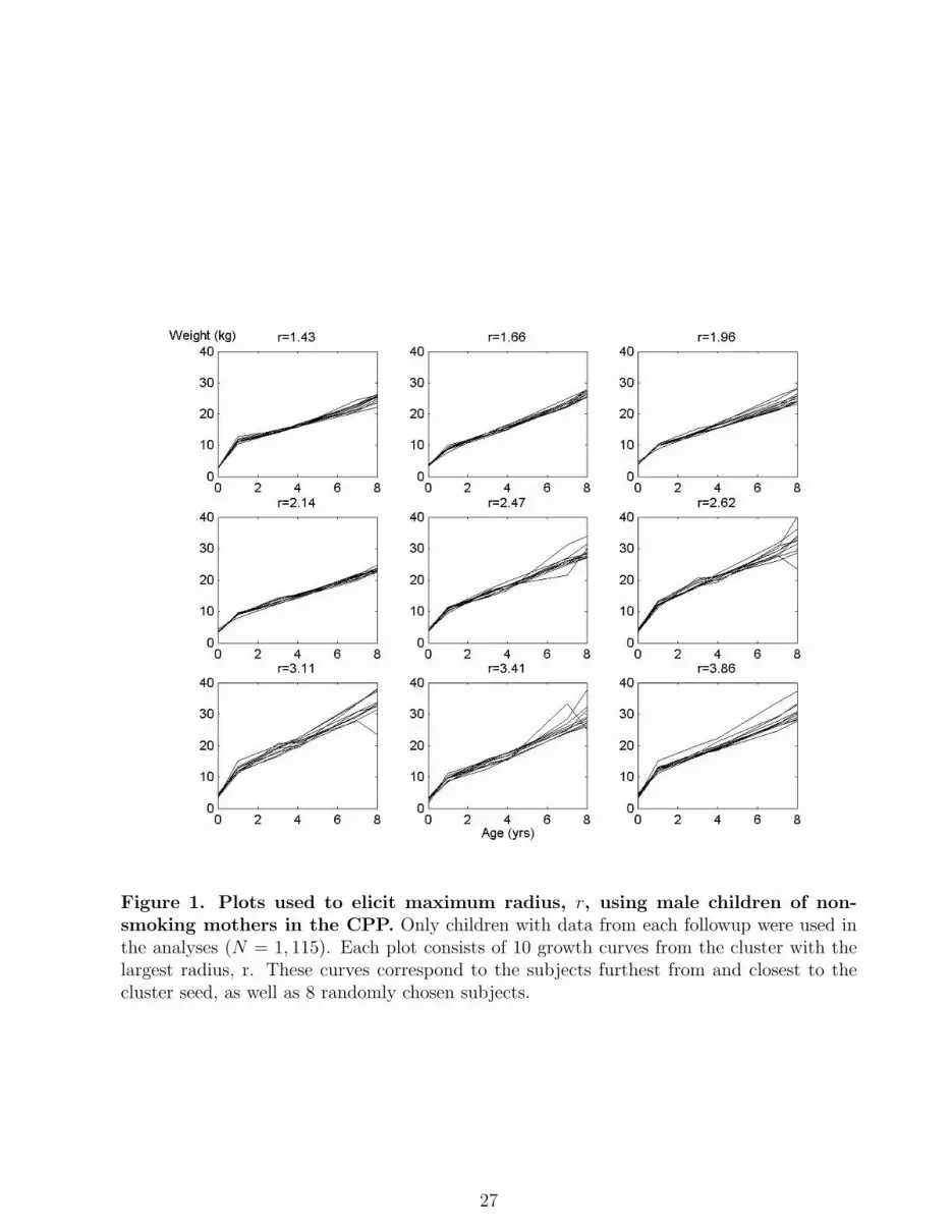
Figure 1. Plots used to elicit maximum radius, r, using male children of non-smoking mothers in the CPP. Only children with data from each followup were used inthe analyses (N = 1, 115). Each plot consists of 10 growth curves from the cluster with thelargest radius, r. These curves correspond to the subjects furthest from and closest to thecluster seed, as well as 8 randomly chosen subjects.

27

Figure 2. Dirichlet process clustering of CPP data. The order of the pseudo-subjectscorresponds to the order of the singleton clusters in a dendrogram generated in Matlab (version6). This dendrogram summarized nearest-neighbors clustering of the pseudo subjects using1-Pr(Sg = Sg∗) as the distance measure. The arrows denote subjects in the normal sub-population “(1)” (pseudo-subjects 1-425 in the figure). Cluster 2 (labelled “(2)”) containspseudo-subjects 430-453, while the remaining pseudo-subjects were not clustered with anotherpseudo-subject in at least half of the iterations.

28

Figure 3. Mean smoking effects in the CPP data. Clusters 1 and 2 correspond to thegroups of pseudo-subjects denoted in Figure 1. The solid, unlabelled lines correspond to theremaining pseudo-subjects. Effect estimates were computed up to the last followup of theexposed subjects. Estimates for unexposed pseudo-subjects are omitted.

29

Table 1. Means and 95% credible intervals for K and β(∗) from Case 1 of our simulations. Thetrue values of the population effects were β = (3.25, 1.45, 23.06)′.

r G K β(∗)0 β(∗)1 β(∗)2

2.14 93 7.06 3.21 1.47 23.03(4, 14) (3.18, 3.25) (1.42, 1,52) (22.98, 23.07)

1.66 215 8.2 3.25 1.44 23.03(4, 18) (3.22, 3.29) (1.39, 1.49) (22.98, 23.08)

0 2000 8.3 3.25 1.45 23.02(4, 15) (3.21, 3.29) (1.40, 1.49) (22.97, 23.07)

30

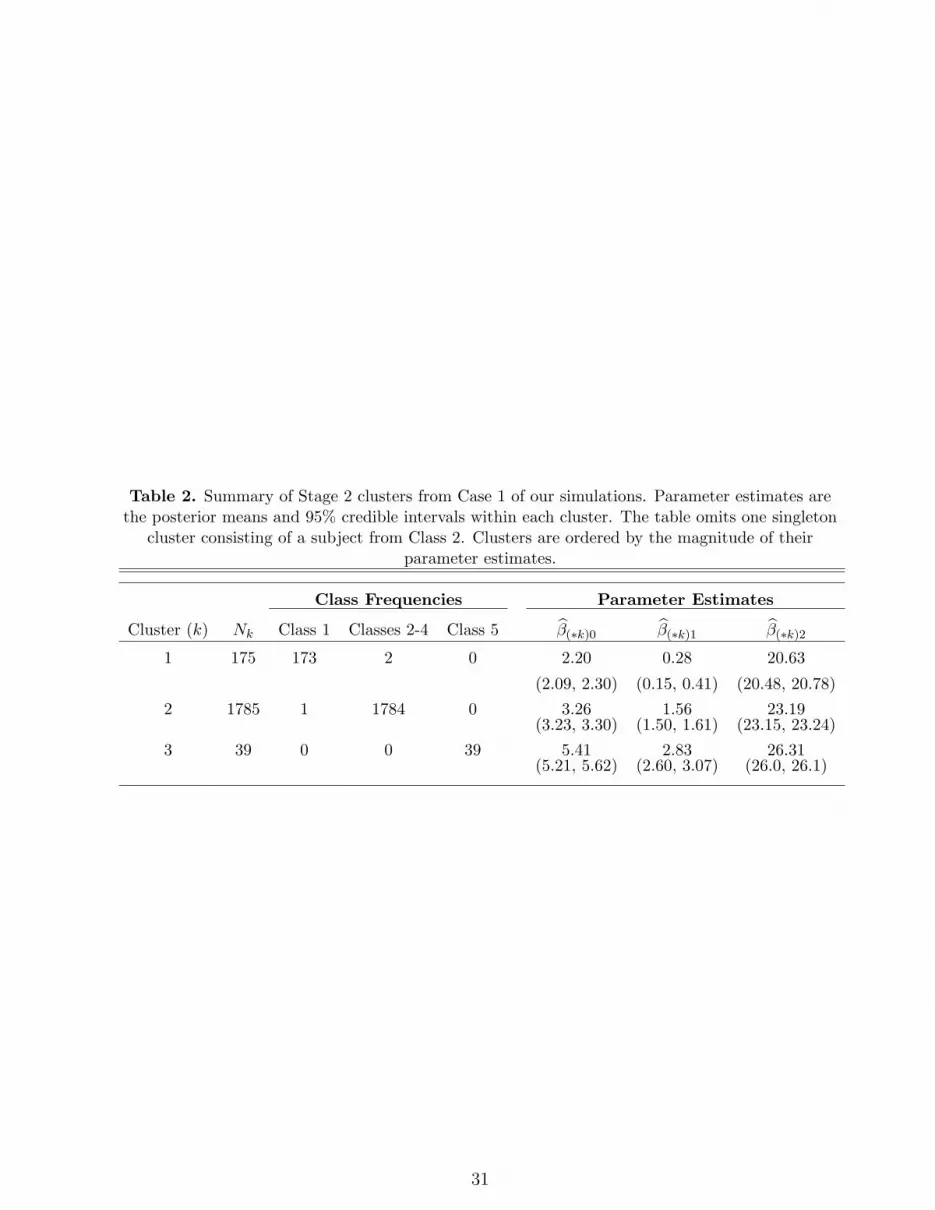
Table 2. Summary of Stage 2 clusters from Case 1 of our simulations. Parameter estimates arethe posterior means and 95% credible intervals within each cluster. The table omits one singleton

cluster consisting of a subject from Class 2. Clusters are ordered by the magnitude of theirparameter estimates.

Class Frequencies Parameter Estimates

Cluster (k) Nk Class 1 Classes 2-4 Class 5 β(∗k)0 β(∗k)1 β(∗k)2

1 175 173 2 0 2.20 0.28 20.63

(2.09, 2.30) (0.15, 0.41) (20.48, 20.78)2 1785 1 1784 0 3.26 1.56 23.19

(3.23, 3.30) (1.50, 1.61) (23.15, 23.24)3 39 0 0 39 5.41 2.83 26.31

(5.21, 5.62) (2.60, 3.07) (26.0, 26.1)

31

Table 3. Means and 95% credible intervals for K, and β(∗) from Cases 2 and 3 of our simulations.The true values of the population effects were approximately β = (3.3, 1.5, 23.2)′ in each case.

Case 2

r G K β(∗)0 β(∗)1 β(∗)2

2.14 81 54.5 3.33 1.48 23.21(44, 65) (3.26, 3.40) (1.34, 1.61) (23.14, 23.27)

1.66 163 94 3.36 1.44 23.19(76.5, 111) (3.29, 3.42) (1.32, 1.57) (23.12, 23.26)

0 1000 492.3 3.34 1.49 23.21(439.5, 541) (3.28, 3.41) (1.38, 1.60) (23.15, 23.29)

Case 32.14 48 31.6 3.23 1.71 23.27

(23, 40) (3.17, 3.28) (1.57, 1.85) (23.21, 23.33)1.66 101 55.0 3.30 1.45 23.32

(41, 69) (3.24, 3.36) (1.32, 1.59) (23.26, 23.39)0 1000 301.1 3.28 1.53 23.30

(238.5, 357.5) (3.22, 3.35) (1.42, 1.64) (23.23, 23.37)

32

Table 4. Population effects of smoking in CPP analysis. The DPP estimates listed aremeans and 95% credible intervals; 95% confidence intervals are listed for the GEE results.

Ex-smoker effects Current smoker effects

Method β4 ηE0 ηE8 β5 ηC0 ηC8

G-DPP 0.11 -0.08 0.82 0.07 -0.10 0.45(0.08, 0.14) (-0.15, -0.02) (0.61, 1.02) (0.05, 0.09) (-0.15, -0.05) (0.29,0.60)

GEE 0.03 -0.004 0.40 0.05 -0.14 0.27(-0.01, 0.06) (-0.11, 0.10) (0.23, 0.58) (0.03, 0.07) (-0.17, -0.11) (0.09, 0.44)

RS1-DPP -0.08 0.16 -0.45 0.07 -0.14 0.39(-0.17, 0.03) (-0.07, 0.31) (-1.14, 0.36) (-0.001, 0.15) (-0.27, -0.01) (-0.11, 1.00)

RS2-DPP -0.09 0.12 -0.60 -0.01 -0.13 -0.21(-0.18, 0.01) (-0.12, 0.35) (-1.27, 0.14) (-0.07, 0.06) (-0.26, 0.01) (-0.66, 0.29)

33