Embed Size (px)
Citation preview

07-Ch01-N51893 [21:49 2008/10/29] Temam & Tribbia: Computational Methods for the Atmosphere and the Oceans Page: 3 1–120
Finite-Volume Methods in Meteorology
Bennert MachenhauerDanish Meteorological Institute, Lyngbyvej 100, DK-2100 Copenhagen, DENMARK
Eigil KaasUniversity of Copenhagen, Juliane Maries Vej 30, DK-2100 Copenhagen, DENMARK
Peter Hjort LauritzenNational Center for Atmospheric Research, Boulder, Colorado, P.O. Box 3000, Boulder,CO 80307-3000, USA
AbstractRecent developments in finite-volume methods provide the basis for new dynam-
ical cores that conserve exactly integral invariants, globally as well as locally, and,especially, for the design of exact mass conserving tracer transport models. The newtechnologies are reviewed and the perspectives for the future are discussed.
1. Introduction
Finite-volume (FV) methods are numerical methods where the fundamental prognosticvariable considered is an integrated quantity over a certain finite-control volume. Thus,instead of grid-point values, finite elements or spectral components, cell-integrated meanvalues are considered. In meteorology, FV methods are, therefore, frequently referred toas cell-integrated methods. Some FV methods include additional prognostic variablesto enhance the numerical accuracy. These variables can be higher order moments orpoint/face values between the control volumes.
In meteorological applications, so far, the control volumes adopted have generallybeen the conventional grid cells used in most operational prediction models: i.e., quasi-horizontal regular grid cells in cartesian coordinates on map projections of the sphere orregular grid cells in spherical latitude-longitude coordinates. These grid cells are referred
Computational Methods for the Atmosphere and the Oceans Copyright © 2009 Elsevier B.V.Special Volume (Roger M. Temam and Joseph J. Tribbia, Guest Editors) of All rights reservedHANDBOOK OF NUMERICAL ANALYSIS, VOL. XIV ISSN 1570-8659P.G. Ciarlet (Editor) DOI 10.1016/S1570-8659(08)00201-9
3

07-Ch01-N51893 [21:49 2008/10/29] Temam & Tribbia: Computational Methods for the Atmosphere and the Oceans Page: 4 1–120
4 B. Machenhauer et al.
to as the Eulerian grid cells. In the cell-integrated methods, these are complemented byLagrangian control volumes, which move with the air flow, usually in a quasi-Lagrangiansense, i.e., departing from or arriving at Eulerian grid cells.
Exceptions to the basis of conventional Eulerian grid cells are new operationalmodels based on grids, which are almost uniform on the sphere. Examples are theMassachusetts Institute of Technology general circulation model (Adcroft, Campin,Hill and Marshall [2004]) which is based on the conformal expanded sphericalcube, but still has orthogonal coordinates and quadri laterally shaped grid cells, and theGerman NWP model (Majewski, Liermann, Prohl, Ritter, Buchhold, Hanisch,Paul, Wergen and Baumgardner [2002]) that is based on a non-orthogonalicosahedral-hexagonal grid on the sphere. For the sake of simplicity, we shall not gointo details with these new grids, which currently is a very active research topic. Thesame limitation applies to nonuniform grids, such as the one introduced by Li and Chang(1996). Thus we shall consider only FV methods in conventional grids.
The FV or cell-integrated methods are well suited for the numerical simulation ofconservation laws. Before the implementation of FV methods in meteorological mod-eling, only conservative spatial discretization schemes were developed and used (e.g.,Arakawa [2000],Arakawa and Lamb [1981], Burridge and Hasler [1977], Machen-hauer [1979], Simmons and Burridge [1981]). With these schemes, just the globallyintegrated discretized time derivative of the invariant quantity in question was zero.Time truncation errors could still cause nonconservation globally. With the introductionof the FV method, the possibility of a conservative full space-time discretization becamepossible (e.g., Machenhauer [1994]). Previously, just global conservation was consid-ered of importance, whereas with the FV methods, local conservation is considered evenmore important (e.g., Machenhauer and Olk [1997]). Conservation laws for mass,total energy, angular momentum, and entropy constitute the fundamental laws for thedynamics and thermodynamics of the atmosphere. Also, potential vorticity is considereda fundamental invariant which should be conserved in an adiabatic friction-free flow. Ingeneral, a discretized cell-integrated prognostic equation for a conservative quantity isobtained by integrating the differential flux form of the conservation law in question inspace over an Eulerian grid cell and in time over the time-step!t. The space integrationresults in an equation stating that the time rate of change of the total quantity in thegrid cell is equal to the sum of fluxes through the cell boundaries. The time integrationdetermines the fluxes through the cell boundaries during the time-step. These fluxes areexact if the integration is performed along exact trajectories ending at the boundariesof the regular Eulerian grid cell (also called the arrival cell) at time t +!t and orig-inating from the boundaries of an irregular so-called Lagrangian cell (also called thedeparture cell) at time t. With such an exact integration, the integral of the conservativequantity over the arrival cell at time t +!t is equal to the integral over the departurecell at time t, plus changes due to sources and sinks, if any. We shall mainly concentrateon conservation of mass, which is the simplest conservation law, as it has no sourcesor sinks if precipitation and diffusion of mass is neglected. For this conservation law,called the continuity equation, we shall derive the exact prognostic equation (Eq. (1.8)in Section 1.1). Since exact integrations along exact trajectories will be assumed inthe derivation, and since no further approximations are being made, this equation is

07-Ch01-N51893 [21:49 2008/10/29] Temam & Tribbia: Computational Methods for the Atmosphere and the Oceans Page: 5 1–120
Finite-Volume Methods in Meteorology 5
referred to as the exact discretized cell-integrated continuity equation. It implies exactconservation of mass during a time step, both global conservation, i.e., conservation ofthe total mass in the entire integration area and local conservation, i.e., conservation ofthe mass in each individual departure cell. During the derivation of the exact discretizedcell-integrated continuity equation, it will be demonstrated that there is equivalencebetween traditional flux-form FV approaches and newer semi-Lagrangian FV methods.In both formulations, one attempts to approximate the same equation.
The general exact discretized cell-integrated continuity equation describes conserva-tion of mass of “moist air,” which is the atmospheric air including all its constituents.Corresponding exact continuity equations for the different constituents in the moist air,for example, water vapor or any chemical constituent, are obtained by simply replacingthe density of moist air " with the density "q = q" of the constituent in question, whereq is its specific concentration1. In meteorological models, the solution to the continuityequation for moist air is of special importance. The solution determines the flow of airmass, which determines the pressure distribution and thus the dynamics of weather sys-tems, especially the development and decay of weather systems. Spurious mass sourcesdue to local nonconservation of mass might thus influence the simulation of weathersystems (Machenhauer and Olk [1997]). The solution determines the flow of all con-stituents in the moist air since they are transported with the air and thus share trajectorieswith the air. This is important especially in chemical models as spurious changes in theratios between linearly correlated (in space) concentrations of reacting chemical con-stituents are avoided (Lin and Rood [1996]). Thus, in meteorological models, a “correct”simulation of the atmospheric dynamics and all kinds of interactions among constituentsdepends heavily on the accuracy of the numerical solutions to the continuity equations.
In Section 2, the different mass conserving schemes that have been developed formeteorological applications in two dimensions (2Ds) are described in detail. In the dif-ferent schemes, different approximations are made in the determination of the trajectoriesand in the integration along the trajectories over the time-step or in the integration overthe departure cell. The approximate schemes presented in Section 2 will be comparedwith the exact solution. It will be shown that all the different schemes conserve massglobally, simply because they are all constructed so that the mass that leaves a certainface of an Eulerian arrival cell during a time-step is exactly gained in the neighboringcell with which the cell face is shared. This, of course, does not guarantee a high level ofaccuracy as the global conservation may be obtained even with rather inaccurate localfluxes. However, the accuracy with which the local mass conservation is approximatedis a real measure of the accuracy of the local transports of the moist air and its con-stituents. Section 2 will mainly focus on relatively new schemes, most of which arebased on (semi-) Lagrangian approaches. For completeness, a short introduction to themore traditional flux-form schemes is presented as well.
Section 3 provides an overview over the general applicability of FV techniquesin meteorology. This section is initiated with an example of a complete set of FV
1The specific concentration of a constituent is the ratio between the mass of the constituent and the mass ofthe moist air it is mixed into.

07-Ch01-N51893 [21:49 2008/10/29] Temam & Tribbia: Computational Methods for the Atmosphere and the Oceans Page: 6 1–120
6 B. Machenhauer et al.
prognostic equations that conserve mass, entropy, total energy, and angular momen-tum in an adiabatic and friction-free atmosphere. Furthermore, Section 3 provides twoexamples of pioneering mass conserving hydrostatic dynamical cores in sphericalgeometry, which are based on FV techniques. By a dynamical core, we mean a computercode for the numerical integration of the system of meteorological equations governingthe dynamics of the atmosphere. Roughly speaking, the dynamical core approximatesthe solution to the meteorological equations on resolved scales, while parameterizationsrepresent subgrid-scale processes and other processes not included in the dynamical core(Thuburn [2006]). However, in tests of dynamical cores, one includes those dissipa-tion terms, which are needed for smooth and stable integrations. Furthermore, Section 3includes a discussion of a few remaining issues, such as the so-called mass-wind incon-sistency in in-line and off-line FV tracer transport applications, and possibilities ofextensions to non-hydrostatic models are briefly discussed. Finally, Section 4 includesa brief summary of the main issues presented in this chapter.
1.1. The exact cell-integrated continuity equation
In this section, an “exact” discretized cell-integrated continuity equation is derived.This is introduced as a pre-requisite and reference for the approximate 2D and three-dimensional (3D) FV schemes to be presented in Sections 2 and 3, respectively. It isexact in the sense explained above. It is derived from assumed exact integrals alongassumed exact trajectories, which are determined from given exact 3D fields of densityand velocity during a time interval !t from t to t +!t. No further assumptions aremade, apart from a simplifying one of no vertical shear of the horizontal velocity in eachdiscrete model layer.
Define Eulerian grid cells as the arrival cell indicated to the right in Fig. 1.1 in acartesian coordinate system (x, y, h) so that the grid length along the x-axis is !x, thegrid spacing along the y-axis is !y, and h is a terrain following height-based verticalcoordinate defined as h = z ! zs, where z is the height above mean sea level and zs
is the height of the surface of the Earth. Surfaces with h equal to a constant hk+1/2separate the grid-cell layers in the vertical. The “!” in the index refers to the Lorenzvertical staggering of the variables (Lorenz [1960]). The “half-levels” are located inbetween “full-levels” hk = 1/2 (hk+! + hk!!) with integer index k, where point valuesof mass and velocity variables traditionally have been located. Thus, the height differencebetween the bottom and the top of the Eulerian grid cell centered at level k, which isconsidered in Fig. 1.1, is !k h = hk+! ! hk!!.
To derive the FV version of the continuity equation, we need to integrate along exacttrajectories ending at the boundaries of the arrival cell at time t +!t and originating fromthe boundaries of the corresponding departure cell at time t. In Fig. 1.1, the departurecell is shown as the irregular cell to the left. Only four of the trajectories are shown inthe figure. The exact velocity fields, supposed to be given during the whole time interval!t from t to t +!t, determine a trajectory ending at any of the points inside or at theboundaries of the arrival cell. We now define an additional auxiliary vertical coordinate# for a particle: a Lagrangian vertical coordinate (Starr [1945]), which per definitionis constant along its 3D trajectory. We choose the Lagrangian coordinate # of a particle,

07-Ch01-N51893 [21:49 2008/10/29] Temam & Tribbia: Computational Methods for the Atmosphere and the Oceans Page: 7 1–120
Finite-Volume Methods in Meteorology 7
h
y
x
C1 D C
BDA
A
B1A1
!A
D1
Fig. 1.1 Conceptual sketch showing a cell that is moving with the flow in a Lagrangian model layer duringa time-step !t. To the left is shown the cell at time t (the so-called departure cell). The horizontal velocity"V within the model layer is assumed independent of height so that the cell walls, which initially at time t arevertical, remain vertical. The cell ends up at time t +!t as the horizontally regular Eulerian grid cell (theso-called arrival cell) shown in the vertical column to the right. Just four trajectories are shown. The projections
on a horizontal plane are shown in more detail in Fig. 1.2. (See also color insert).
that is moving with the 3D flow during the time-step, to be equal to its h value in orat the boundary of the arrival cell. Thus, the trajectories constitute a vertical coordinatesystem, which is defined only in the time interval from t to t +!t. Obviously, in thiscoordinate system, the vertical velocity of a particle is zero:
# = d#dt
= 0. (1.1)
Here, a simplifying assumption is made, namely that the horizontal wind "V is independentof height within the Lagrangian model layer, i.e., the layer enclosing all the trajectorieswhich are ending inside or at the boundary of the arrival cell. Thus, as indicated inFig. 1.1, vertical columns that move with the horizontal wind in the layer will remainvertical. Mathematically, it implies a simplifying separation of the vertical and horizontalintegrations to be performed in the layer. A column may, of course, still change itsthickness $kh due to horizontal convergence or divergence. The trajectories in Fig. 1.2,which are ending at the corners of the arrival cell, originate from the corner of thedeparture cell. For simplicity of the sketch, it is assumed that the horizontal velocityfield is such that the trajectories and lines between neighboring corners in the departurecell are straight, i.e., the vertical faces of the departure cell in Fig. 1.1 are plane. Note thatsince trajectories ending at the boundaries of the arrival cells are shared by neighboringcells, it follows that the departure cells, as does the arrival cells, fill out the entireintegration domain without any cracks in between.

07-Ch01-N51893 [21:49 2008/10/29] Temam & Tribbia: Computational Methods for the Atmosphere and the Oceans Page: 8 1–120
8 B. Machenhauer et al.
!ADA
A1
B1
C1D1
BA
DC
Fig. 1.2 Horizontal projections of the arrival cell (A, B, C, D) at time t +!t with area !A and the corre-sponding upstream departure cell (A1, B1, C1, D1) at time t with area $A. This figure corresponds to a view
from above at the departure and arrival cells in Fig. 1.1.
The differential flux form of the continuity equation in the #-coordinate systembecomes
%"
%t= !## · " "V ! %"#
%#, (1.2)
where " is the density of moist air and "V is the horizontal velocity. To obtain the conti-nuity equation for a regular vertical column, integrate Eq. (1.2) vertically over theLagrangian model layer. The result is
%"k $kh
%t= !## · "k $kh "Vk, (1.3)
where Eq. (1.1) has been used and " is the vertical mean density:
"k = 1$kh
!
$kh
" dz.
To obtain the cell-integrated continuity equation, integrate Eq. (1.3) horizontally overthe area of the arrival grid cell. After application of the Gauss’s divergence theorem,we get
!A%""k $kh
#
%t= !
4$
i=1
"<""k $kh
# "Vk > · "n !l#i, (1.4)
where !A = !x!y is the horizontal area of the grid cell and
""k $kh
#= 1!A
!!
!x!y
""k $kh
#dxdy (1.5)
is the horizontal mean value of "k $kh in the Eulerian grid cell. In Eq. (1.4), "ni is a unitvector normal to the ith face of the cell pointing outward, and !li is the length of the

07-Ch01-N51893 [21:49 2008/10/29] Temam & Tribbia: Computational Methods for the Atmosphere and the Oceans Page: 9 1–120
Finite-Volume Methods in Meteorology 9
face equal to either !x or !y.""k
#i, ($kh)i, and ( "Vk)i are instantaneous values at the
cell face i, and the angle brackets represent averages in the x- or y-direction over the cellfaces. The next step is to integrate over the time-step !t, between t and t +!t, whichresults in
!A"""k $kh
#+ !""k $kh
##= !!t
4$
i=1
"<""k $kh
# "Vk > · "n !l#i
(1.6)
Here, the plus-sign in superscript indicates the updated value and the double bar refersto the time average over !t. Each term on the right-hand side of Eq. (1.6) representsthe mass transported through one of the four Eulerian cell faces into the cell duringthe time-step. Each term involves integrals over the cell face in question and over thetime-step. The integral in time over the time-step may be performed in space along thetrajectories terminating on the Eulerian cell face in question, cell face AB for instance(see Fig. 1.2). Thus, this term in Eq. (1.6) is computed as a surface integral of
""k $kh
#
over the area between the Eulerian cell face AB, the two backward trajectories, AA1and BB1 originating from the two end points of the Eulerian cell face and the respectiveface of the departure cell A1B1. That is, the mass inflow through the southern (or lower)face in Fig. 1.2 is equal to the integral of
"" $kh
#over the area marked A1ABB1 in the
figure. Writing this integral as%%
A1B1BA
"k $kh dx dy, Eq. (1.6) may be rewritten as
""k $kh
#+!A =
!!
ABCD
""k $kh
#dx dy +
!!
A1B1BA
""k $kh
#dx dy
+!!
A1ADD1
""k $kh
#dx dy +
!!
D1DCC1
""k $kh
#dx dy !
!!
B1BCC1
""k $kh
#dx dy
=!!
A1B1C1D1
""k $kh
#dx dy. (1.7)
Here, the mass inflows through the remaining three cell faces are included in the secondline by similar integrals. The first term on the right-hand side is
!A""k $kh
#=!!
ABCD
""k $kh
#dx dy,
i.e., the original mass in the Eulerian grid cell at time t. Thus, as illustrated in Fig. 1.2,the sum of the first four terms on the right-hand side of Eq. (1.7), representing theoriginal mass in the Eulerian grid cell, the inflow through the southern, the western,and the northern cell face is compensated partly by the outflow through the eastern cellface, represented by the fifth negative term in Eq. (1.7). The result is the integral on thesecond right-hand side of Eq. (1.7) that represents the mass in the Lagrangian departure

07-Ch01-N51893 [21:49 2008/10/29] Temam & Tribbia: Computational Methods for the Atmosphere and the Oceans Page: 10 1–120
10 B. Machenhauer et al.
cell A1B1C1D1. Denoting the departure cell area as $A (Fig. 1.2), the result may bewritten as
!!
A1B1C1D1
""k $kh
#dx dy = "k $kh $A,
and we obtain finally
""k !kh
#+!A =
""k $kh
#$A. (1.8)
This is a prognostic equation predicting the mass in the arrival area at t +!t,""k $kh
#+!A, from the mass in the departure area at time t,
""k $kh
#$A. Note that
no information is needed between t and t +!t and recall that in the arrival area (exactlyin the center of the area) the Lagrangian model layer coincide with the Eulerian cell so that$kh = !kh. Thus, the right-hand side of Eq. (1.8) can be determined by an integrationof""k $kh
#over the departure area and Eq. (1.8) becomes
""k
#+ = 1!kh !A
!!
A1B1C1D1
""k $kh
#dx dy = 1
!kV
!!!
$kV
"k dx dy dz, (1.9)
or""k
#+!kV =
!!!
$kV
"k dx dy dz. (1.10)
""k
#+!kV is the updated mass in the Eulerian arrival grid cell at time t +!t. According
to Eq. (1.10) it is equal to the mass in the upstream departure cell at time t. Thus, the exactdiscrete cell-integrated continuity equation (Eq. (1.8)) is simply a cell-integrated analogto the well-known grid-point semi-Lagrangian continuity equation (Robert [1969, 1981,1982]) that presently is used in most operational meteorological models. Contrary to thegrid-point version, the cell-integrated equation is inherently mass conservative. It fulfillsexactly our definition of a locally mass conserving scheme as the updated mass in anEulerian arrival grid cell is exactly the mass in the upstream departure cell. It is easilyshown by a summation of Eq. (1.8) over the entire integration domain, with assumedperiodic lateral boundary conditions, that it also implies global mass conservation. Theanalogy to the grid-point semi-Lagrangian continuity equation shows that an alternativeway to derive Eq. (1.8) would be to set up the mass conservation law directly for FV on aLagrangian form and then integrate that form over!t. The mass in a FV $kV consideredat time t is
M$kV =!!!
$kV
"k dx dy dz. (1.11)

07-Ch01-N51893 [21:49 2008/10/29] Temam & Tribbia: Computational Methods for the Atmosphere and the Oceans Page: 11 1–120
Finite-Volume Methods in Meteorology 11
The mass conservation law for this FV, which is supposed to move with the flow withoutany mass flux through its boundaries, is
d M$kV
dt= 0. (1.12)
When integrated in time from t to t +!t, Eq. (1.12) gives Eq. (1.8), which as shownabove leads to Eq. (1.10). The reason for presenting the more complicated derivationstarting from the Eulerian flux form of the mass conservation law (1.2) is that somenumerical FV schemes, the so-called f lux-form schemes, are based on the flux form(1.2), whereas others, the so-called Lagrangian schemes, are based on the Lagrangianform (1.12). The purpose of the present derivation was to show that in the case of exacttrajectories and exact mass integrals over the relevant volumes, the flux-form Eq. (1.2)is equivalent to the Lagrangian form (1.12). When, as it is usually the case, a flux-formscheme becomes different from a Lagrangian scheme, it is due to different approxima-tions to the trajectories defining the departure volume and different approximations to theupstream mass integrals. A measure of accuracy for both types of schemes should there-fore be how close they are to the ideal “exact” scheme. That is, how close the approximatedeparture volume is to the real, exact one and how close the exact mass integral overthe exact departure volume is to the approximate mass integral over the approximatedeparture volume. In other words, how accurate the local mass conservation is.
1.2. Longtime step schemes and combinations with semi-implicit time-stepping
The reason for the recent renewed interest in FV methods in meteorological model-ing was the observation of a significant lack of global mass conservation in numericalmodels using the grid-point version of the semi-Lagrangian scheme unless an unphys-ical so-called mass-fixer, which restores the total mass globally after each time step, isused. There is an arbitrariness in the way these mass-fixing algorithms repeatedly restoreglobal mass conservation without ensuring any local mass conservation, i.e., without ful-filling a continuity equation for the mass that is transported locally between the Euleriangrid cells of the model each time-step (Machenhauer and Olk [1997]). Without such amass-fix, a significant drift in the global mass was observed (Bates, Higgins and Moor-thi [1995]), and even with a mass-fixer, it seems likely that significant local errors aredeveloped (Machenhauer and Olk [1997]). Nevertheless, the reason for the popularityof the grid-point semi-Lagrangian schemes has been its almost unconditional absolutestability, which in practice eliminates the advective Courant-Fredrichs-Levy (CFL) time-step restriction. This property is utilized in most operational meteorological models incombination with a semi-implicit treatment of the gravity wave terms in the primitiveequations, which eliminates the fast wave CFL time-step restriction. Then, in principle,the length of the time-steps in a combined semi-implicit semi-Lagrangian model can bechosen solely based on accuracy considerations. This is extremely important in meteo-rological models where any gain by an increased time-step can be utilized to increase therealism of parameterized physical processes and/or the spatial resolution of the model

07-Ch01-N51893 [21:49 2008/10/29] Temam & Tribbia: Computational Methods for the Atmosphere and the Oceans Page: 12 1–120
12 B. Machenhauer et al.
grid. According to general operational experience, such improvements have practicallyalways led to an increase in accuracy. As should be expected from the experiencewith the grid-point semi-Lagrangian schemes, the recently developed cell-integratedsemi-Lagrangian schemes are also (almost) unconditionally stable (Lauritzen [2007]),eliminating in practice the advective CFL time-step restriction. It has furthermorerecently been shown that fast waves in cell-integrated semi-Lagrangian models canbe stabilized by a combination with a semi-implicit time extrapolation scheme. This hasbeen demonstrated by Machenhauer and Olk [1997] for a simple one-dimensional(1D) mass and momentum or mass and total energy conserving model and Lauritzen,Kaas and Machenhauer [2006] for shallow water models and by Lauritzen, Kaas,Machenhauer and Lindberg [2008] for a complete 3D mass conserving model. Analternative method, which has been used in finite difference grid-point models to stabi-lize the fast waves, is the so-called split-explicit time-stepping. However, this possibilitywas abandoned by Machenhauer and Olk [1997] for FV models because when split-ting the system of continuous equations into an advective part, which should use largetime-steps, and an adjustment gravity wave part, which should use short time-steps, itwas found that neither of the sub systems were conserving momentum or total energy.Consequently, these invariants for the full system could not be conserved exactly in anyFV version.
As mentioned above, Section 3 describes two mass conserving quasi-hydrostaticdynamical cores, both combined with comprehensive physical parameterization pack-ages. One of these dynamical cores described in Lauritzen, Kaas, Machenhauer andLindberg [2008] is a semi-implicit version using large time steps for all variables, whilethe other one described in Lin [2004] and Collins, Rasch, Boville, Hack, Mccaa,Williamson, Kiehl, Briegleb, Bitz, Lin, Zhang and Dai [2004] uses an explicittime-stepping scheme. The latter model uses explicit, relatively small time-steps for thedynamical core but large time-steps for the transport of all tracer species (including watervapor) and for physical parameterizations.
2. Transport schemes in one and two dimensions
In meteorological models, a FV method for the continuity is based on the exact cell-integrated continuity equation and obviously it should be approximated as accurately aspossible.As discussed in Section 1, the vertical and horizontal problems can be separatedin a consistent way considering Lagrangian cells moving with vertical walls along threedimensional trajectories. Consequently, only horizontal integrals of vertically integratedmass distributions are needed in the solution of the continuity equation. So in case ofa flux-form Eulerian scheme, the fluxes through the four cell faces can be determinedby horizontal integrals (as described in connection with Eq. (1.6)), and for the departurecell-integrated semi-lagrangian (DCISL) scheme, direct integrations over the horizontaldeparture area approximating the true departure area can be performed (as indicated inEq. (1.8)). Hence, by using this approach, one can directly apply 2D FV schemes forthe 3D problem. Alternatively, flux-form schemes may be extended to 3Ds by includingvertical advection through the top and bottom surfaces of Eulerian grid cells. Similarly,

07-Ch01-N51893 [21:49 2008/10/29] Temam & Tribbia: Computational Methods for the Atmosphere and the Oceans Page: 13 1–120
Finite-Volume Methods in Meteorology 13
the 3D DCISL scheme would perform a 3D integral over the Lagrangian departure cell.However, following these fully 3D approaches would become very complicated if oneaims at a numerically efficient and mass conserving integration.
Because of the general applicability of 2D solutions to the continuity equation, thissection, beside basic 1D formulations, is devoted to the fully 2D schemes. Compared withthe large number of mass conserving transport schemes published in the general fluiddynamical literature, there are many fewer schemes that have been used or are applicablein real meteorological applications on the sphere. Here, we mostly concentrate on thesubset that is potentially applicable in a wide range of atmospheric models. Therefore,descriptions of the vast majority of the hundreds of transport schemes developed incomputational fluid dynamics in general are excluded. For a more general review of FVmethods, see e.g., Leveque [2002] and Eumard, Gallouët and Herbin [2000].
Before discussing the different FV schemes used in the atmospheric sciences, it isimportant to realize which properties a transport scheme ideally should possess. Anoverview of these properties is provided in Section 2.1. The FV schemes presented inthis overview use sub grid representations at time t in order to make the forecast attime t +!t. The most frequently used sub grid representations and associated filtersensuring some of the properties listed in Section 2.1 are introduced in Section 2.2.This is followed, in Section 2.3, by an overview of the different types of FV methodsapplied in 2D problems. Section 2.4 briefly describes some – mostly recent – local massconservation fixers for semi-Lagrangian models which can be considered closely relatedto FV semi-Lagrangian schemes. Aiming at enhanced accuracy, Section 2.5 discussesthe possibilities to include extra prognostic variables in addition to the cell-mean values.The so-called flux-limiter methods have been popular approaches to maintain attractiveshape-preserving properties. A brief introduction to these methodologies, which arecomplementary to the filtering methods mentioned in Section 2.2, is given in Section 2.6.Finally, Section 2.7 provides some concluding remarks on the basic FV transport schemesin 1 and 2Ds.
2.1. Desirable properties
The equation subject to the toughest requirements is probably the continuity equation fortracers such as moisture, the spatial distribution of which includes sharp gradients. Raschand Williamson [1990] have defined seven desirable properties for transport schemes:accuracy, stability, computational efficiency, transportivity, locality, conservation, andshape-preservation. In addition to the seven desirable properties defined by Rasch andWilliamson [1990], even more desirable properties have emerged in the literature, e.g.,consistency, compatibility, and preservation of constancy. The perfect scheme wouldhave all the desirable properties listed above under all conditions but, in practice, nosingle method is advantageous under all conditions.
2.1.1. AccuracyThe high-accuracy property is, of course, the primary aim for any numerical method, andall the desirable properties listed above, apart from the efficiency requirement, are part ofthe overall accuracy. Note that for a flow with shocks or sharp gradients, the formal order

07-Ch01-N51893 [21:49 2008/10/29] Temam & Tribbia: Computational Methods for the Atmosphere and the Oceans Page: 14 1–120
14 B. Machenhauer et al.
of accuracy in terms of Taylor series expansions does not necessarily guarantee a highlevel of accuracy. Part of the accuracy is also the rate of convergence of the numericalalgorithm.
Widely used measures of accuracy in the meteorological community for idealized testcases are the standard error measures l1, l2, and l$ (e.g., Williamson, Drake, Hack,Jakob, Swarztrauber, [1992]):
l1 = I (|& ! &E|)I (|&E|) , (2.1)
l2 =&I'(& ! &E)2()1/2
&I'(&E)2()1/2 , and (2.2)
l$ = max [|& ! &E|]max [|&E|] , (2.3)
where I(·) denotes the integral over the entire domain, & is the numerical solution, and&E is the exact solution if it exists. In case an exact solution does not exist, &E is a high-resolution reference solution. l1 and l2 are the measures for the global “distance” between& and &E, and l$ is the normalized maximum deviation of & from &E over the entiredomain. In addition to these error measures, the normalized maximum and minimumvalues of & are also used to indicate errors related to overshooting and undershooting.
To evaluate the accuracy of new schemes, several idealized advection test cases havebeen formulated. The interscheme comparison, however, is often made difficult by thefact that different authors use different test cases and/or different error measures. Thetest problems can be divided into two categories. Firstly, translational passive advectiontests where distributions are transported by prescribed non-divergent winds that, ideally,translate the initial distribution without distorting it; these test cases involve the entiredomain. Secondly, deformational test cases which focus on part of the domain such asan initial distribution being deformed by a vortex. Recently, Nair and Jablonowski[2007] combined these two types of test cases into one.
Probably, the most commonly used idealized test case in the meteorological literatureis the solid body rotation of a cosine cone and/or a slotted cylinder. In cartesian geometry,the test case is described in, e.g., Zalesak [1979] and Bermejo and Staniforth [1992],and the spherical version is test case 1 of the suite of test cases by Williamson, Drake,Hack, Jakob and Swarztrauber [1992]. The analytic solution to this problem is simplythe translation of the initial distribution along a circle in cartesian geometry and a greatcircle in the spherical case. It is an important part of accuracy that the advection schemescan transport distributions across the singularities of the numerical grids without distor-tion and imposing severe time-step limitations. Drake, Hack, Jakob, Swarztrauberand Williamson [1992] suggested that the cosine bell is transported along the equatorand across the poles with a slight offset to avoid any symmetry. Note, however, thataway from the poles, advection along these great circles is almost along coordinateaxis for conventional latitude-longitude grids that, in general, favor the advectionscheme.

07-Ch01-N51893 [21:49 2008/10/29] Temam & Tribbia: Computational Methods for the Atmosphere and the Oceans Page: 15 1–120
Finite-Volume Methods in Meteorology 15
Passive advection of scalars using the solid body rotation test case only addresses theability of the scheme to translate a distribution without distorting it. Other commonlyused test cases are based on a deformational flow, for example the swirling shear flow testin cartesian geometry considered by Durran [1999, Section 5.7.4], which is specified interms of a periodically reversing time-dependent velocity field. Hence, after one period,the exact solution is the initial distribution. It could, however, be speculated that someerrors introduced during the first half period are cancelled when the wind field reverses.Other deformational flow test cases, to which the exact solution is known throughoutthe time of integration, are defined in Smolarkiewicz [1982] (analytical solution isgiven in Côté, Staniforth and Pudykjewicz [1987]) and Armengaud and Hourdin[1999]. The idealized cyclogenesis problem described by Doswell [1984], to which theanalytic solution is known, has been used for scalar-advection tests by several authors.For example, the non-smooth deformational flow vortex defined on a tangent plane(e.g., Rancic [1992], Hólm [1995], Côté, Nair and Staniforth [1999a]). A versionwas formulated for the sphere by Nair, Scroggs and Semazzi [2002] and Nair andMachenhauer [2002]. It is a smooth deformational flow test case that consists oftwo symmetric vortices, one over each pole. This test case has been combined with atranslational wind field in Nair and Jablonowski [2007] to form a test case (where theanalytical solution is known) that simultaneously challenges schemes with respect todeformation and translation.
2.1.2. StabilityThe stability property ensures that the solution does not “blow up” during the time ofintegration. Usually, the stability of Eulerian methods is governed by the CFL condition,which in 1D is given by
max****u!t
!x
**** % 1, (2.4)
where u is the velocity and!x the grid interval. Hence, a fluid parcel may not travel morethan one grid interval during one time-step. This overly restrictive time-step limitationis usually alleviated in semi-Lagrangian methods and can be replaced by the less severeLipschitz convergence criterion
****%u
%x
****!t < 1, (2.5)
(Benoit, Pudykiewicz and Staniforth [1985]; Kuo and Williams [1990]), whichguarantees that parcel trajectories do not cross during one time-step and ensures theconvergence of the trajectory algorithm (a multi dimensional extension of Eq. (2.5) isgiven in Benoit, Pudykiewicz and Staniforth [1985]). Hence, in semi-Lagrangianmodels, the time-step can be chosen for accuracy and not for stability because of thelenient stability condition.
For global models based on a conventional latitude-longitude grid, the efficiency andstability of the advection schemes are often challenged by the convergence of the meridi-ans near the poles, and special care must be taken in the vicinity of the poles.Alternatively,

07-Ch01-N51893 [21:49 2008/10/29] Temam & Tribbia: Computational Methods for the Atmosphere and the Oceans Page: 16 1–120
16 B. Machenhauer et al.
the problem can be tackled by using other types of grids that do not have these singulari-ties or at least reduce the effect of them, for example, the icosahedral-hexagonal grid usedoperationally by the German Weather Service (e.g., Arakawa, Mintz and Sadourny[1968], Williamson [1968], Thuburn [1997], Majewski, Liermann, Prohl, Ritter,Buchhold, Hanisch, Paul,Wergen and Baumgardner [2002]), and the cubed sphereapproach originally introduced by Sadourny [1972] which, after having remained dor-mant for many years, has become a very active research topic (e.g., Iacono, Paolucciand Ronchi [1996], Mesinger and Rancic, Purser [1996], McGregor [1996], Iskan-drani, Taylor and Tribbia [1997], Loft, Nair and Thomas [2005]). These grids aremore isotropic than conventional latitude-longitude grids, i.e., all cells have nearly thesame size, contrarily to latitude-longitude grids, where the areas decrease as aspectratios increase toward the poles (this effect can, however, be alleviated by using aGaussian-reduced grid in which the number of longitudes decrease toward the poles).
2.1.3. Computational efficiencyComputing resources are limited and, given the complexity of geophysical fluiddynamics, the algorithms should be computationally efficient in order to allow for high-resolution runs and/or a large number of prognostic variables. Efficiency is, however,hard to measure objectively. One measure for the efficiency of an algorithm is the numberof elementary mathematical operations or the total number of floating-point operationsper second (FLOPS) used by the algorithm. The advantage of counting FLOPS is thatit can be done without using a computer and is, therefore, a machine-independent mea-sure. But the number of FLOPS only captures one of several dimensions of the efficiencyissue. The actual program execution involves subscripting, memory traffic and count-less other overheads. In addition, different computer architectures favor different kindsof algorithms and compilers optimize code differently. Measuring efficiency in termsof the execution time on a specific platform can be misleading for a user on anothercomputer platform. Weather prediction and climate models are often executed on mas-sively parallel distributed memory computers where the efficiency is partly determinedby the amount of communication between the nodes. This becomes increasingly impor-tant if the resolution is held fixed while the number of distributed memory processorsis increased. Hence, the parallel programmer is concerned about algorithms being local,thus minimizing the need for communication between the nodes. Nevertheless, a veryimportant measure of efficiency is probably the level of simplicity of the algorithm.
Since models include an increasing number of tracers, an important aspect of theefficiency is how much of the transport algorithm can be reused for additional tracers.Obviously, if the entire transport algorithm must be repeated for each additional tracer,such an algorithm would not be attractive in modern transport models that include hun-dreds of tracers. In semi-Lagrangian models, for example, the computation of trajectoriesneed only be computed once and can be reused for all tracers (e.g., Dukowicz andBaumgardner [2000]).
Thus, the computational cost of a given model depends not only on the number ofFLOPS involved in the production of say one model day; it depends also to a high degreeon the computer architecture on which the model is run. The optimization of a givenmodel intended for operational application on a given platform is often an extensive

07-Ch01-N51893 [21:49 2008/10/29] Temam & Tribbia: Computational Methods for the Atmosphere and the Oceans Page: 17 1–120
Finite-Volume Methods in Meteorology 17
and complicated work for an experienced programmer, and the result will vary with theingenuity of the programmer. The new algorithms presented here are often developed onan experimental basis by scientists who are not specialized programmers, and therefore,they are usually far from an optimized code suited for operational applications. It is,therefore, not fair to uncritically compare the computational cost of such new FV algo-rithms with traditional well-optimized algorithms. For this reason, information on thecomputational costs of the new algorithms are most often not available in the literature.When they are available, they should be considered with the reservations stated here andshould only be considered as possible maximum computational costs, which most likelycould be reduced for operational applications.
It should be noted that it could be misleading to compare computational efficiencyand accuracy of two algorithms at the same spatial and temporal resolution. A schememight be computationally inefficient at a given resolution compared to other schemesbut have an accuracy that other schemes would need a much finer resolution in orderto achieve (the opposite situation is, of course, also possible). In other words, ideallyone should consider the ratio between computational cost and accuracy when comparingnumerical schemes. That would enable one to select the scheme where one pays as littleas possible computationally for the highest level of accuracy.
2.1.4. Transportivity and localityThe transportive and local property guarantee that information is transported with thecharacteristics and that only adjacent grid values affect the forecast at a given point. ForFV schemes, one aspect of the local property is the degree of local mass-conservationthat we define as follows. Since the mass enclosed in an area moving with the flow isconserved in the absence of sources and sinks, the degree to which the effective departurearea of the numerical scheme coincides with the exact departure area is a measure for thelocal mass conservation of a given scheme. Another aspect of local mass conservationis the degree to which the reconstruction of the subgrid-scale distribution is local. Forexample, near sharp gradients, it is important that the gradient is not weakened during theprocess of reconstructing the subgrid-scale distribution, i.e., the reconstruction shouldbe local.
2.1.5. Shape-preservationThe shape of a distribution undergoing pure advection should ideally be preserved inthe numerical solution. For general velocity fields, the shape of the distribution maybe altered in the form of new extrema. In such situations, the numerical scheme shouldreproduce only the physical extrema without creating spurious numerical extrema. Thesespurious numerical extrema especially cause problems in situations where the advectionscheme produces negative mixing ratios (or concentrations) or when the values areabove the maximum possible. Negative mixing ratios or mixing ratios above a physicalthreshold value are unphysical and would most likely cause a breakdown in physicalparameterizations. If a numerical scheme inherently prevents negative undershoots inmixing ratios (or concentrations), it is termed positive-definite (or positivity preserving),if it preserves gradients, then the scheme is monotone, and if artificial oscillations areprevented, it is termed nonoscillatory.All these properties are, of course, interrelated and,

07-Ch01-N51893 [21:49 2008/10/29] Temam & Tribbia: Computational Methods for the Atmosphere and the Oceans Page: 18 1–120
18 B. Machenhauer et al.
constitutes together the shape-preservation property. The very popular spectral methodsare well known for producing “wiggles” (also known as Gibb’s phenomena) near sharpgradients and are, therefore, a typical example of a monotonicity-violating and oscillatorynumerical method.
2.1.6. ConservationIdeally, all global integral invariants of the corresponding continuous problem shouldbe conserved for any kind of flow. For long simulations, the conservation propertiesbecome increasingly important as numerical sources, and sinks can degrade the accuracyand alter global balance budgets significantly over time. Hence, for climate models, theFV methods are very attractive given their inherent conservation properties. However,a numerical model can only maintain a small number of analogous invariant propertiesconstant, and some choice must be made as to which conserved quantities are to beconserved in the numerical model. For a comprehensive discussion of this issue, seeThuburn [2006]. Probably, the most important property to conserve for a continuityequation is the first moment, i.e., mass.
2.1.7. ConsistencyThe consistency property is less frequently discussed in the literature. Notable exceptionsare Jöckel, Von Kuhlmann, Lawrence, Steil, Brenninkmeijer, Crutzen, Raschand Eaton [2001] and Byun [1999]. This property concerns the coupling betweenthe continuity equation for air as a whole and for individual tracer constituents. Inthe continuous case, the flux-form continuity equation for a constituent with specificconcentration q,
%
%t(q") + # ·
""vq"#
= 0 (2.6)
degenerates to
%
%t(") + # ·
""v"#
= 0 (2.7)
for q = 1. This should ideally be the case numerically as well. If the two equations aresolved using the same numerical method, on the same grid and using the same time-step, the consistency is guaranteed. However, in reality, in practical applications of FVtransport schemes, the settings are often inconsistent in this sense. This is definitely thecase in offline tracer transport models. The consistency property, or rather the lack of it(referred to as the mass-wind inconsistency), will be discussed in detail in Section 3.
2.1.8. CompatibilityThe compatibility property was defined by Schär and Smolarkiewicz [1996] forEulerian schemes, and the definition is here extended also to include semi-Lagrangianschemes. As the consistency property, it concerns the relationship between continuityequations. Equations (2.6) and (2.7) imply
dq
dt= 0, (2.8)

07-Ch01-N51893 [21:49 2008/10/29] Temam & Tribbia: Computational Methods for the Atmosphere and the Oceans Page: 19 1–120
Finite-Volume Methods in Meteorology 19
which states that the constituent mixing ratio is conserved along the characteristics of theflow. Compatible transport is when the discretization of Eq. (2.6) is consistent with theadvective form (Eq. (2.8)) so that the predicted mixing ratio qn+1, which in a flux-formsetting is recovered from (q")n+1, is limited by the mixing ratios in the Eulerian cellsfrom which the mass departs. The compatibility property is graphically illustrated inFig. 2.1.
2.1.9. Preservation of constancyAnother desirable property is the ability of the scheme to preserve a constant tracer fieldfor a non-divergent flow. For traditional semi-Lagrangian methods based on Eq. (2.8),a constant distribution is trivially conserved since the divergence of the velocity fielddoes not appear in the prognostic equation (for a review of traditional semi-Lagrangianmethods, see, e.g., Staniforth and Coté [1991]). In fact, for any velocity field, thetraditional semi-Lagrangian method preserves a constant mixing ratio. For FV methodswhere the divergence appears explicitly since tracer mass, and not mixing ratio, is theprognostic variable, it is not automatic that a constant field is preserved for a nondivergentvelocity field. Non-conservation of constant fields may cause error problems and eveninstability, see Section 3.3.2.
2.1.10. Preservation of linear correlations between constituentsAnother desirable property identified by Lin and Rood [1996] is that a numerical schemeshould ideally preserve tracer correlations since correlations carry fundamental infor-mation on atmospheric transport. This is particularly important in chemical atmosphericmodels where the relative concentrations of constituents are crucial for the speed and
21
43
Fig. 2.1 A graphical illustration of the compatibility property. The arrows show the trajectories for the cellvertices. The shaded area is the departure cell that, after one time-step, ends up at the regular grid as depicted
by the arrows. A finite-volume scheme predicts the change in total mass in the Eulerian cell (q")n+1, which
is the mass enclosed in the departure cell (shaded area). Since the mixing ratios are preserved along parceltrajectories, the mixing ratio in the arrival cell q n+1 should be within the range of the mixing ratios at thedeparture points. For the situation depicted on the figure, the compatibility condition is min
"q n
1 , q n2 , q n
3 , q n4#
%q n+1 % max
"q n
1 , q n2 , q n
3 , q n4#, where qi denotes the average mixing ratio in the cell numbered i, i = 1.4, on
the figure.

07-Ch01-N51893 [21:49 2008/10/29] Temam & Tribbia: Computational Methods for the Atmosphere and the Oceans Page: 20 1–120
20 B. Machenhauer et al.
balances of chemical reactions. It is possible to construct transport schemes that maintainspatially constant linear correlations between tracers exactly, see, e.g., Lin and Rood[1996].
2.2. Subgrid-cell distributions of the prognostic variables
In all FV schemes presented here – flux based as well as Lagrangian types – it is necessaryto determine the subgrid-cell distribution from the surrounding cell averages in order tomake accurate estimates of the fluxes through the Eulerian cell walls or mass enclosedin the upstream departure cell. Therefore, 1 and 2D reconstructions are discussed beforethe actual schemes are introduced.
2.2.1. 1D subgrid-cell reconstructionsSeveral 1D methods for reconstructing the subgrid distribution have been published in theliterature. The simplest subgrid representation is a piecewise constant function followed,in complexity, by a piecewise linear representation (Van Leer [1974]). Both methodsare computationally cheap, optionally monotonic, and positive-definite (the piecewiseconstant method is shape-preserving by default) but, on the other hand, excessivelydamping and therefore not suited for long runs at coarser resolutions. To reduce thedissipation to a tolerable level, the subgrid-cell representation must be polynomials of atleast second degree. Requirements of computational efficiency put an upper limit to theorder of the polynomials used, which explains why the predominant choice is secondorder.
Let the walls of the ith cell be located at xi and xi+1 and denote the cell width!xi =xi+1 ! xi. The coefficients of the subgrid-cell reconstruction polynomials are determinedby imposing constraints. Apart from the basic requirement of mass conservation withineach grid cell, the choice of constraints is not trivial. Probably the simplest parabolic fitis obtained by requiring that the polynomial
pi(x) = (a0)i + (a1)i x + (a2)i x2, x & [xi, xi+1] (2.9)
not only conserves mass in the ith grid cell
xi+1!
xi
pi(x)dx = !xi&i, & = ", "q (2.10)
but also in the two adjacent cells:
xi+2!
xi+1
pi(x)dx = !xi+1&i+1, (2.11)
xi!
xi!1
pi(x)dx = !xi!1&i!1, (2.12)

07-Ch01-N51893 [21:49 2008/10/29] Temam & Tribbia: Computational Methods for the Atmosphere and the Oceans Page: 21 1–120
Finite-Volume Methods in Meteorology 21
(Laprise and Plante [1995]). By substituting Eq. (2.9) into Eqs. (2.10), (2.11), and(2.12) and by evaluating the analytic integrals, a linear system results that can easily besolved for the three unknown coefficients (a0)i, (a1)i, and (a2)i (Laprise and Plante[1995]). When performing this operation for all cells, a global piecewise-parabolic repre-sentation is obtained. The method is only locally of second order since it is not necessarilycontinuous across cell borders. This method is referred to as the piecewise parabolicmethod 1 (PPM1).
An alternative way of constructing the parabolas, which ensures a globally continuousdistribution if no filters are applied, is the piecewise-parabolic method ofWoodward andColella [1984] (hereafter referred to as PPM2). PPM2 has been reviewed in the con-text of meteorological modeling in Carpenter, Droegemeier, Hane and Woodward[1990]. Instead of requiring that pi(x) conserves mass in adjacent cells, the constraintis that the polynomial equals prescribed west and east cell-edge values, pW
i = pi(xi)
and pEi = pi(xi+1), respectively, at the cell edges. pE
i is computed with a cubic polyno-mial fit (see Woodward and Colella [1984] for details). For an equidistant grid, theresult is
pWi = 7
12
"&i!1 + &i
#! 1
12
"&i+1 + &i!2
#, (2.13)
(for a nonequidistant grid, see Colella and Woodward [1984]). The east cell-bordervalue, pE
i , is simply an index shift of the formula for pWi
pEi = pW
i+1. (2.14)
It is convenient to use the cell average, &i, and pWi and pE
i to define the ith parabola,instead of using (a0)i, (a1)i, and (a2)i. The equivalent formula for pi(x) is given by
pi
"#x#
= &i +"$px#i#x +
"px
6#i
+112
!"#x#2,, (2.15)
where ($px)i is the mean slope
"$px#i= pE
i ! pWi , (2.16)
"px
6
#i
is the “curvature”
"px
6#i= 6&i ! 3
"pW
i + pEi
#, (2.17)
and #x is the nondimensional position defined by
#x = x ! xi
!xi! 1
2. (2.18)

07-Ch01-N51893 [21:49 2008/10/29] Temam & Tribbia: Computational Methods for the Atmosphere and the Oceans Page: 22 1–120
22 B. Machenhauer et al.
PPM2 uniquely defines the parabolas and Eq. (2.15) guarantees that the global subgriddistribution is continuous across cell borders. Zerroukat, Wood and Staniforth[2002] found in passive advection tests that using the PPM2 for the subgrid-cell recon-structions (where the parabolas were continuous across cell borders) results in moreaccurate solutions compared with PPM1 (in which the distribution is not necessarilycontinuous across cell borders).
Instead of using the PPM1 or PPM2, Zerroukat, Wood and Staniforth [2002]derived a piecewise cubic method for the reconstruction of the subgrid-cell distribu-tions. PPM2 is a special case of the piecewise cubic method. Of course, any kind ofreconstruction that is mass conserving can be used, e.g., rational functions as used in thetransport scheme of Xiao, Yabe, Peng and Kobayashi [2002] and the parabolic splinemethod (PSM) recently developed by Zerroukat, Wood and Staniforth [2006]. Inidealized advection tests, Zerroukat, Wood and Staniforth [2007] found that usingthe PSM for the subgrid-scale reconstructions in their scheme generally leads to moreaccurate results than when using PPM2. This is despite the fact that, in terms of operationcount, PSM is 60% more efficient than PPM2. However, at present, the most widespreadsubgrid-cell reconstruction method is PPM2.
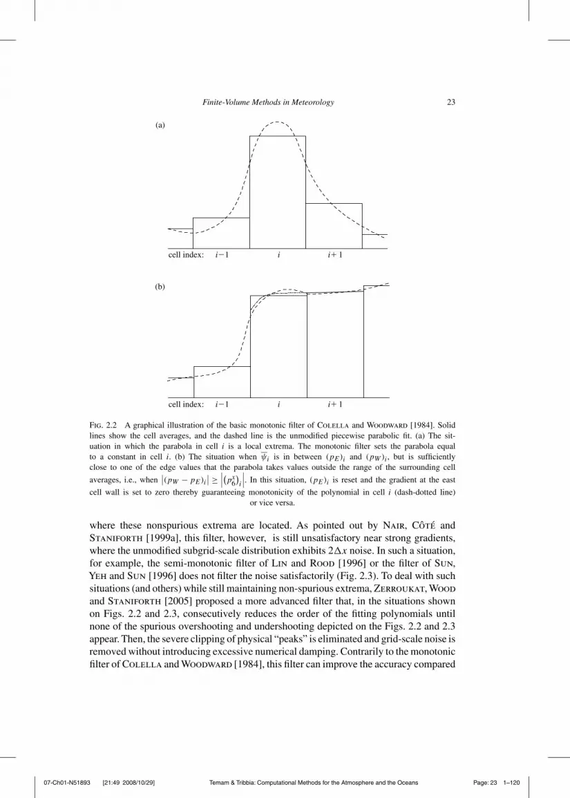
Without further constraining the coefficients of the parabolas, it is not guaranteedthat the subgrid-scale reconstruction preserves monotonicity or positive definiteness(Godunov [1959]). A simple monotonic filter was proposed by Colella and Wood-ward [1984], and is explained in Fig. 2.2. For local extrema, the filter is similar tothe quasi-monotonic filter by Bermejo and Staniforth [1992] for traditional semi-Lagrangian advection schemes, i.e., the subgrid-scale distribution is reduced to a constantwhen there is a local extrema in the cell averages (Fig. 2.2a). This severe clipping can sig-nificantly reduce the accuracy as idealized advection tests have shown (compare CISL-Nwith CISL-M and CCS-N with CCS-M in Table 2.1). Clearly, one would like to retainthe higher order polynomial in the situation depicted in Fig. 2.2a while not altering thetreatment of the situation in Fig. 2.2b.
Lin and Rood [1996] modified the Colella and Woodward [1984] monotonic filterso that the monotonic filter only applies to undershooting and does not interfere with anyof the overshooting (referred to as semi-monotonic filter). The semi-monotonic filter canfurther be modified so that it only prevents negative undershooting, whereby it becomesa positive-definite filter. Since these filters avoid the severe clipping of overshoots, theapplication of these filters shows a dramatic increase in accuracy in idealized advectiontests compared with the monotonic filter described in the previous paragraph (CISL-Pand CCS-P in Table 2.1). Other filters with more relaxed constraints, but which arecomputationally more efficient, can be found in Lin [2004]. However, all these filtersare still not fully satisfactory since they do not interfere with all types of spurious under-shooting and overshooting.
As mentioned, the filter should not interfere with local extrema as the one in Fig. 2.2abut still apply the monotonic filter in the situation depicted on Fig. 2.2b (similarly forundershooting). That is what the filter of Sun, Yeh, Sun and Sun [1996] for traditionalsemi-Lagrangian schemes is designed to do. Through a series of logical statements, thefilter detects local extrema and does not alter the high-order subgrid-scale reconstruction
07-Ch01-N51893 [21:49 2008/10/29] Temam & Tribbia: Computational Methods for the Atmosphere and the Oceans Page: 23 1–120
Finite-Volume Methods in Meteorology 23
i1 1i21cell index: i
(a)
(b)
i1 1i21cell index: i
Fig. 2.2 A graphical illustration of the basic monotonic filter of Colella and Woodward [1984]. Solidlines show the cell averages, and the dashed line is the unmodified piecewise parabolic fit. (a) The sit-uation in which the parabola in cell i is a local extrema. The monotonic filter sets the parabola equalto a constant in cell i. (b) The situation when &i is in between (pE)i and (pW)i, but is sufficientlyclose to one of the edge values that the parabola takes values outside the range of the surrounding cell
averages, i.e., when**(pW ! pE)i
** '***"px
6#i
***. In this situation, (pE)i is reset and the gradient at the east
cell wall is set to zero thereby guaranteeing monotonicity of the polynomial in cell i (dash-dotted line)or vice versa.
where these nonspurious extrema are located. As pointed out by Nair, Côté andStaniforth [1999a], this filter, however, is still unsatisfactory near strong gradients,where the unmodified subgrid-scale distribution exhibits 2!x noise. In such a situation,for example, the semi-monotonic filter of Lin and Rood [1996] or the filter of Sun,Yeh and Sun [1996] does not filter the noise satisfactorily (Fig. 2.3). To deal with suchsituations (and others) while still maintaining non-spurious extrema, Zerroukat, Woodand Staniforth [2005] proposed a more advanced filter that, in the situations shownon Figs. 2.2 and 2.3, consecutively reduces the order of the fitting polynomials untilnone of the spurious overshooting and undershooting depicted on the Figs. 2.2 and 2.3appear. Then, the severe clipping of physical “peaks” is eliminated and grid-scale noise isremoved without introducing excessive numerical damping. Contrarily to the monotonicfilter of Colella and Woodward [1984], this filter can improve the accuracy compared

07-Ch01-N51893 [21:49 2008/10/29] Temam & Tribbia: Computational Methods for the Atmosphere and the Oceans Page: 24 1–120
24 B. Machenhauer et al.
Table 2.1Error norms for the schemes of Zerroukat, Wood and Staniforth [2005] (SLICE), Nair andMachenhauer [2002] (CISL), and Nair, Scroggs and Semazzi [2002] (CCS) for test case 1 in Williamson,Drake, Hack, Jakob and Swarztrauber [1992]. ' is the angle between the axis of solid body rotation andthe polar axis of the spherical coordinate system. Hence ' = 0 is solid body rotation along the equator and' = (/2 advection across the poles. The error measures for ' = (/3 are from Lauritzen, Kaas and Machen-hauer [2006]. “N” denotes no filter, “M” the monotonic filter, and “P” the positive-definite filter used in therespective schemes. Note that the monotonic filter and subgrid-scale reconstructions in SLICE are different
from the other schemes (see text for details)
' = 0 ' = (/2 ' = (/3
Schemes l1 l2 l$ l1 l2 l$ l1 l2 l$
SLICE-N 0.046 0.029 0.022 0.079 0.049 0.042 — — —SLICE-M 0.038 0.024 0.017 0.058 0.040 0.037 — — —CISL-N 0.052 0.035 0.032 0.063 0.046 0.048 0.075 0.051 0.083CISL-P 0.025 0.025 0.031 0.059 0.045 0.048 0.043 0.082 0.076CISL-M 0.094 0.091 0.108 0.084 0.084 0.109 0.077 0.089 0.18CCS-N — — — 0.054 0.042 0.065 0.051 0.039 0.076CCS-P 0.036 0.034 0.042 0.051 0.041 0.065 0.033 0.034 0.077CCS-M — — — 0.076 0.082 0.129 0.070 0.086 0.186
i1 1i21cell index: i
Fig. 2.3 A situation in which the unmodified subgrid-cell reconstruction exhibits strong Gibbs phenom-ena. The semimonotonic filter of Lin and Rood [1996] would set the polynomials in cell i ! 1 andi + 1 equal to the cell average, but would not modify the polynomial in cell i that, in this situation, is a
spurious overshoot.
to the unfiltered high-order solution (see Semi-Lagrangian inherently conserving andefficient (SLICE)-N and SLICE-M in Table 2.1). A similar filter has also been developedfor the PSM (Zerroukat, Wood and Staniforth [2006]).
2.2.2. 2D subgrid-cell reconstructionsAs for the 1D case, 2D linear reconstructions exist (e.g., Dukowicz and Baumgardner[2000] and Scroggs and Semazzi [1995]), but, in general, they introduce too muchnumerical damping for meteorological applications. The PPM in 1D can be directly

07-Ch01-N51893 [21:49 2008/10/29] Temam & Tribbia: Computational Methods for the Atmosphere and the Oceans Page: 25 1–120
Finite-Volume Methods in Meteorology 25
extended to 2Ds as done by Rancic [1992], i.e., in terms of a fully 2D subgrid-cellreconstruction
pi,j (x, y) = (a1)i,j + (a2)i,j x + (a3)i,j x2 + (a4)i,j y + (a5)i,j y2 + (a6)i,j xy
+ (a7)i,j xy2 + (a8)i,j x2y + (a9)i,j x2y2, (x, y) & [xi, xi+1] ('yj, yj+1
(.
(2.19)
This fully biparabolic fit involves the computation of nine coefficients, so nine constraintsare needed to determine the coefficient values.Apart from the conservation of mass withineach cell
!!
!Ai,j
pi,j(x, y)dxdy = &i,j!Ai,j, (2.20)
the other eight constraints chosen by Rancic were formulated in terms of the four cornervalues of pi,j(x, y) and the average of pi,j(x, y) along the four cell walls. The cornerpoint scalar values were computed by fitting 2D third-order polynomials using the 16 cellaverages surrounding the corner point in question. The average along the cell walls wascomputed using & along a line perpendicular to the cell wall in question. For additionaldetails, see Rancic [1992].
The computational cost of the approach taken by Rancic can be reduced significantlyby using a quasi-biparabolic subgrid-cell representation. Contrarily to fully biparabolicfits, the quasi-biparabolic representation does not include the “diagonal” terms and sim-ply consists of the sum of two 1D parabolas, one in each coordinate direction. Using theform (Eq. (2.15)) for the parabolas, the quasi-biparabolic subgrid-cell representation isgiven by
pi
"#x, #y
#= &i,j +
"$px#i,j#x +
"px
6#i,j
+112
!"#x#2,
+"$py#i,j#y
+"p
y6
#i,j
+112
!"#y#2,, (2.21)
where ($px)i,j ,"px
6
#i,j
, ($py)i,j , and"p
y6
#i,j
are the coefficients of the parabolic func-tions in each coordinate direction (Machenhauer and Olk [1998]). This representationreduces the computational cost of the subgrid-cell reconstruction significantly but, ofcourse, does not include variation along the diagonals of the cells.
By using 1D filters that prevent undershoot and overshoot to the parabolas in eachcoordinate direction, monotonicity-violating behavior can be reduced but not strictlyeliminated in 2Ds. In case of negative values at the cell boundaries of both unfiltered1D parabolic representations, even larger negative values may be present in one ormore of the cell corners when the 1D representations are added. The monotone andpositive-definite filters eliminate only the negative values at the boundaries and notthe possible negative corner values. As a result, small negative values can appear evenafter the application of a monotonic filter (e.g., Lin and Rood [1996] and Nair andMachenhauer [2002]). To eliminate these negative values an additional filter must beapplied.

07-Ch01-N51893 [21:49 2008/10/29] Temam & Tribbia: Computational Methods for the Atmosphere and the Oceans Page: 26 1–120
26 B. Machenhauer et al.
2.3. Different schemes in 2Ds
As mentioned above, different approaches can be used to estimate the integral over thedeparture cell. These can be divided into two main categories:
• Semi-Lagrangian schemes in which the integral over the departure cell is approxi-mated explicitly. These schemes to be described in Section 2.3.1 are referred to asDCISL schemes. DCISL schemes come in two types: fully 2D schemes and cascadeschemes in which the approximation of the upstream integral is divided into twosteps where each substep applies 1D methods.
• Flux-based schemes in which the fluxes through the Eulerian arrival cell walls areapproximated. These schemes are described in Section 2.3.2. As for the DCISLschemes, there are two types of conceptually different schemes of this category:schemes based on a sequential operator splitting (often referred to as time-splitting)and schemes based on direct estimation of the 2D fluxes.
It is important to note, as was also pointed out in the introduction, that DCISL andflux-based FV schemes are conceptually equivalent since they both estimate the massin the departure cell. However, as will be illustrated, this is, in practice, done in quitedifferent ways.
The following overview of these two categories will mainly focus on recent devel-opments in DCISL schemes since these have not yet been introduced in textbooks orgeneral overview articles. For these schemes, a stability analysis is performed. Fur-thermore, the level of local mass conservation, i.e., the accuracy of the approximationto the exact departure area in different DCISL schemes and one flux-based method, isinvestigated.
2.3.1. DCISL schemesThe semi-Lagrangian scheme can either be based on backward or forward trajectories(or equivalently downstream and upstream trajectories), i.e., by considering parcels arriv-ing or departing from a regular grid, respectively. The majority of semi-Lagrangianschemes are based on backward trajectories because it is usually simpler to interpo-late/remap from a regular to a distorted mesh. However, forward trajectory cascadeschemes and the downstream version of the schemes in Laprise and Plante [1995]are exceptions to this. The deformed grid resulting from tracking the parcels movingwith the flow is referred to as the Lagrangian grid, while the stationary and regular gridis referred to as the Eulerian grid. The curve resulting from tracking a latitude mov-ing with the flow is referred to as a Lagrangian latitude. Similarly for a Lagrangianlongitude.
The choice of trajectory algorithm is crucial for the accuracy of DCISL schemes.Traditional semi-Lagrangian schemes employ backward trajectories that are computedwith an implicit iterative algorithm also known as the second-order implicit midpointmethod (see, e.g., Côté and Staniforth [1991]). This trajectory algorithm does notinclude the acceleration. Several schemes that include estimates of the acceleration in thetrajectory computations have been proposed (e.g., Hortal [2002], Mcgregor [1993],Lauritzen, Kaas and Machenhauer [2006] – see Section 3).

07-Ch01-N51893 [21:49 2008/10/29] Temam & Tribbia: Computational Methods for the Atmosphere and the Oceans Page: 27 1–120
Finite-Volume Methods in Meteorology 27
Using backward trajectories, the 2D discretization of Eq. (1.8) leads to the CISLscheme
&+!A = &$A, & = ", "q, (2.22)
where
& = 1$A
!!
$A
& (x, y) dA(2.23)
is the integral mean value of & (x, y) over the irregular departure cell area $A, and&
+is the mean value of &+ (x, y) over the regular arrival cell area !A (see Fig. 2.4).
The approximation of the integral on the right-hand side of Eq. (2.22) employs twosteps: firstly, defining the geometry of the departure cell that involves the computation ofparcel trajectories; secondly, performing the remapping, i.e., computing the integral overthe departure cell using some reconstruction of the subgrid distribution at the previoustime-step. The geometrical definition of the departure cell and the complexity of thesubgrid-scale distribution are crucial for the efficiency and accuracy of the scheme.
For realistic flows and for time-steps obeying the Lipschitz criterion (see Section 2.1),the upstream cells deform into simply connected but non-rectangular and possibly locallyconcave geometric patterns. The question is how to integrate & (x, y) efficiently oversuch a complex area.
2.3.1.1. Fully 2D DCISL schemes In 1D, there is very little ambiguity on how toapproximate the upstream cell, but in 2Ds, it is much more complicated and severalapproaches have been suggested in the literature. In Fig. 2.5, the arrival and departurecells in cartesian geometry for three different DCISL schemes are shown.
Rancic [1992] defines the departure cell as a quadrilateral by tracking backward thecell vertices A, B, C, and D and connecting them with straight lines (Fig. 2.5(a)). The
DA
!A
Fig. 2.4 The regular arrival cell with area !A and the irregular departure cell (shaded area) with area $Ain the continuous case for a generic upstream DCISL scheme. Using the figure of speech in Laprise andPlante [1995], the departure–arrival cell relationship is conceptually equivalent to throwing a fishing netupstream to fetch the mass enclosed into a area that will, after one time-step, end up at the regular mesh.The arrows are the parcel trajectories from the departure points (open circles), which arrive at the regular cell
vertices (filled circles).

07-Ch01-N51893 [21:49 2008/10/29] Temam & Tribbia: Computational Methods for the Atmosphere and the Oceans Page: 28 1–120
28 B. Machenhauer et al.
(a)
(c)
(b)
Fig. 2.5 The departure cell (shaded area) when using the scheme of (a) Rancic [1992], (b) Machenhauerand Olk [1998] scheme, and (c) the cascade scheme of Nair, Scroggs and Semazzi [2002]. The filledcircles are the departure points, and open circles the midpoints between the departure points, and aster-isks are the intermediate grid points which are used to define the intermediate cells in the cascade scheme
(crosshatched area).
vertices are not necessarily aligned with the coordinate axis, which leads to some algo-rithmic complexity for the evaluation of the upstream integral. The integral over thedeparture area is, in the situation depicted in Fig. 2.5a, decomposed into four subintegrals,i.e., the integral over the areas defined by the overlap between the departure cell and theEulerian cells. Thus, one has to perform analytic integrals over many possible cases ofshapes of subdomains, which makes the computer code rather cumbersome. In addition,the subgrid-scale distribution used by Rancic was a piecewise-biparabolic representationwhich, being fully 2D, is quite expensive to compute in itself. The combination of thecomplex geometry of the departure cell and the fully 2D subgrid-cell representation makesthe scheme approximately 2.5 times less efficient than the traditional semi-Lagrangianadvection scheme using bicubic Lagrange interpolation (Rancic [1992]). This, and thefact that the scheme has not been extended to spherical geometry, has hindered the schemefor widespread use in the meteorological community.
In order to speed up the remapping process, Machenhauer and Olk [1998] sim-plified both the geometry of the departure cell and the subgrid-scale distribution.The departure cell is defined as a polygon with sides parallel to the coordinate axis(Fig. 2.5(b)). The sides parallel to the x-axis are at the y-values of the departure points,and the sides parallel to the y-axis pass through E, F, G, and H, located halfway betweenthe departure points. Hence, the area of the departure cell is identical to the area of theRancic [1992] scheme. Since the sides of the departure cell are parallel to the coor-dinate axis, the evaluation of the upstream integral is greatly simplified. By using the

07-Ch01-N51893 [21:49 2008/10/29] Temam & Tribbia: Computational Methods for the Atmosphere and the Oceans Page: 29 1–120
Finite-Volume Methods in Meteorology 29
pseudobiparabolic subgrid-scale distribution (see Eq. (2.21)) and accumulated parabola-coefficients along latitudes (see Nair and Machenhauer [2002] for details), the integralover the departure cell can be computed much more efficiently compared to the approachtaken by Rancic [1992]. For advection in cartesian geometry, Nair and Machen-hauer [2002] reported a 10% overhead with this scheme compared with the traditionalsemi-Lagrangian scheme.
Note that the departure areas in Fig. 2.5 completely cover the entire integration areawithout overlaps or cracks, which is crucial to an upstream DCISL scheme, otherwisethe total mass is not conserved. For a downwind cell-integrated scheme using forwardtrajectories, it is, however, not necessary that the arrival cells span the entire domainof integration in order to have global mass conservation. Using the figure of speech ofLaprise and Plante [1995], a downstream cell-integrated scheme is equivalent to throw-ing dust contained in little buckets (regular departure cells) into the wind and watching itlater fall into bins (regular Eulerian cells). Contrary to upstream DCISL schemes, whereone integrates over a particular departure cell, a downstream cell-integrated schemekeeps track of the contribution to each regular Eulerian cell from the irregular arrivalcells. As long as all the mass in each arrival cell is redistributed with a mass conser-vative method, mass is conserved even if the neighboring arrival cells overlap. This istaken advantage of in the scheme of Laprise and Plante [1995], which probably usesthe simplest cell geometry of all the schemes presented here. The arrival cell is defined asa rectangle where the edges have the same orientation as the regular cells (see Fig. 2.6).This is achieved by tracing the traverse motion of cell edges and not the cell vertices.Hereby, the arrival cell retains the orthogonality and orientation of the regular departurecell. Note, however, that only two cells share edges, while, if cell vertices are tracked,
Departure level
x
y
y
x
Arrival level
Fig. 2.6 A graphical illustration of the downstream version of the cell-integrated schemes of Laprise andPlante [1995]. The filled circles are the departure points that are at the edge centers of the regular departurecell. The arrows connect the departure points with the respective arrival points (unfilled circles). The dashedrectangle is the arrival cell which edges have the same orientation as the departure cell. In a downstreamcell-integrated scheme, the amount of mass that arrives at a regular Eulerian cell is computed, i.e., the integralover the area (shaded area at the departure level) that arrives at the intersection between the regular Euleriancell and the arrival cell (shaded area at the arrival level). Similarly for the remaining intersections with
Eulerian cells.

07-Ch01-N51893 [21:49 2008/10/29] Temam & Tribbia: Computational Methods for the Atmosphere and the Oceans Page: 30 1–120
30 B. Machenhauer et al.
cell vertices are shared by four cells. Consequently, one must compute twice as manytrajectories compared to a downstream scheme tracking cell vertices.
The actual integral in the downstream scheme of Laprise and Plante [1995] isnot performed at the arrival level since that would require the reconstruction of thesubgrid-scale distributions from irregular and overlapping arrival cell averages. Theintegral is performed at the departure level over the part of the departure cell that, afterone time-step, “falls” into a particular regular Eulerian cell (see Fig. 2.6). The intersectionbetween the arrival cell and a particular Eulerian cell is always a rectangular region withsides parallel to the coordinate axis, which simplifies the integration process significantly.Consequently, the downstream scheme of Laprise and Plante [1995] is approximatelytwice as fast as the Rancic [1992] scheme, even though both schemes use fully 2Dsubgrid-scale reconstructions. The schemes of Laprise and Plante [1995] and Rancic[1992] have not been extended to spherical geometry.
2.3.1.2. Cascade DCISL schemes Using the so-called cascade method, originallydeveloped for non-conservative interpolation by Purser and Leslie [1991], the 2Dupstream integral can also be approximated by splitting it into two 1D steps. The basicidea is to track backward (forward) the Eulerian grid and then apply 1D integrals,firstly along the Eulerian (Lagrangian) longitudes or latitudes and secondly along theLagrangian (Eulerian) latitudes or longitudes (see Fig. 2.7). To obtain inherent mass con-servation, the interpolation in the original cascade interpolation method must be replacedwith the PPM (Colella and Woodward [1984]) or some other mass-conservativeremapping method. Contrary to fully 2D DCISL schemes, the cascade approach isequally suited for downstream and upstream trajectories, or equivalently, the 1D remap-ping methods are equally suited for remapping from a distorted as from a regular 1Dgrid. However, to facilitate the comparison with fully 2D DCISL schemes, we assumeupstream trajectories in the discussion of the cascade schemes, although some of theschemes initially were formulated for downstream trajectories.
The cascade method can be divided into three steps. Firstly, given the departurepoints, the application of 1D remappings is prepared by computing an intermediate grid.It is crucial to the cascade technique that the intermediate grid is well defined, i.e., thatthere should not be multiple intersections between Lagrangian latitudes (longitudes) andEulerian longitudes (latitudes) (see, e.g., Fig. 1 in Nair, Côté and Staniforth [1999a]).Therefore, in spherical coordinates, it cannot be applied very near the poles. Secondly,a 1D remapping of mass from the regular Eulerian cells to the intermediate grid cells isperformed. Thirdly, the mass on the intermediate grid is remapped to the departure cells.
We start out by considering the conservative cascade DCISL scheme of Nair,Scroggs and Semazzi [2002]. In this scheme, the departure cells are defined as poly-gons with sides parallel to the coordinate axis as in the Machenhauer and Olk [1998]scheme. In each 1D cascade step, the PPM2 is used. Compared to the Machenhauerand Olk [1998] scheme, the departure cell geometry is defined somewhat differently(see Fig. 2.5(c)). Two of the sides parallel to the y-axis, x = x(E) and x = x(G), aredefined as in the Machenhauer and Olk [1998] scheme, and the remaining two sidesparallel to the y-axis are at the Eulerian longitude x = xi. The sides parallel to thex-axis are determined from the intermediate Lagrangian grid points I, J, K, L, M, and

07-Ch01-N51893 [21:49 2008/10/29] Temam & Tribbia: Computational Methods for the Atmosphere and the Oceans Page: 31 1–120
Finite-Volume Methods in Meteorology 31
Fig. 2.7 Graphical illustration of the cascade interpolation method introduced by Purser and Leslie [1991].Solid lines are the regular Eulerian grid and the dashed lines are the Lagrangian grid. Here we consider anupstream scheme, hence, the Lagrangian grid end up at the Eulerian grid when moving with the flow over onetime-step. The intermediate grid is defined by the crossings between the Eulerian longitudes and the Lagrangianlatitudes (unfilled circles). The nonconservative cascade interpolation method proceeds as follows. Performa 1D interpolation from the Eulerian grid to the intermediate grid, i.e., interpolate along Eulerian longitudesfrom the filled circles to the unfilled circles. Hereafter interpolate from the intermediate grid to the Lagrangiangrid, i.e., from the unfilled circles to the asterisks. Ideally one should interpolate along the curved Lagrangianlatitude, but in the original cascade interpolation scheme of Purser and Leslie [1991], the x-coordinate is usedas the position variable for interpolation along the Lagrangian latitude, which corresponds to approximating
the Lagrangian latitude with line segments parallel to the x-axis.
N defined as y = ! [y(I ) + y(J )] , y = ! [y(K) + y(L)] , y = ! [y(L) + y(M)], andy = ! [y(I ) + y(N )], respectively. The y-values of the intermediate points are deter-mined by cubic Lagrange interpolation between the y-values of four adjacent departurepoints along the Lagrangian latitude (dashed line in Fig. 2.5(c)). The Lagrange weightsfor computing the intersections can be efficiently evaluated using the algorithm outlinedin the Appendix in Purser and Leslie [1991]. The upstream integral is computed bya remapping in the north-south direction from the Eulerian cells to the intermediatecells (crosshatched rectangular regions on Fig. 2.5(c)), followed by a remapping alongthe Lagrangian latitudes from the intermediate cells to the departure cells. Hence, thefirst remapping is along the Eulerian longitude passing through the Eulerian cell centers.Since the second remapping uses the x-coordinate as the independent variable, it is alongline segments parallel to the x-axis. Without any a priori knowledge of the flow, thereis no argument for not reversing the order of the directional sweeps, i.e., first to remapalong the Eulerian latitude and then along the Lagrangian longitude. As discussed insome detail in Lauritzen [2007], the order of the directional sweeps is not symmetric,and hence there is a directional bias built into the cascade approach. However, in neither

07-Ch01-N51893 [21:49 2008/10/29] Temam & Tribbia: Computational Methods for the Atmosphere and the Oceans Page: 32 1–120
32 B. Machenhauer et al.
of the cascade schemes presented here has this been reported to be a problem. A symmet-ric version of the cascade scheme can easily be constructed, for example, by alternatingbetween the sweep directions, i.e., by using Lagrangian longitudes and Eulerian latitudesat even time-steps and Lagrangian latitudes and Eulerian longitudes at odd time-steps.
Since the two remappings are 1D and that the intermediate grid can be efficientlycomputed, the Nair, Scroggs and Semazzi [2002] scheme is more than twice as efficientas the fully 2D scheme of Machenhauer and Olk [1998]. Cascade methods are equallysuited for upstream and downstream trajectories. For example, the Nair, Scroggs andSemazzi [2002] scheme formulated for backward trajectories has also been extended toforward trajectories in Nair, Scroggs and Semazzi [2003].
On equidistant cartesian grids, the conservative cascade scheme developed by Nair,Scroggs and Semazzi [2002] is very similar to the one of Rancic [1995], althoughthe way they are presented in the respective articles is very different. Rancic [1995]formulated his scheme without explicit reference to areas by assigning mass to nodes ormass-points. The scheme is identical to the Purser and Leslie [1991] cascade interpola-tion but with the two 1D Lagrange interpolation sweeps replaced with PPM2. AlthoughRancic did not make explicit reference to areas in his formulation, the scheme can,however, be interpreted in terms of areas: in each 1D sweep, the mass nodes representthe mass enclosed in cells with walls located midway between the mass nodes, andthe remapping is along line segments which are parallel to the coordinate axis. Hence,by formulating Rancic scheme for upstream trajectories, the only differences betweenthe Nair, Scroggs and Semazzi [2002] and Rancic scheme are the choice of pointsfor which the trajectories are computed and the order of the 1D sweeps. Where Nair,Scroggs and Semazzi [2002] track cell vertices as they are transported by the flow,Rancic used cell centers; and where Nair, Scroggs and Semazzi [2002] remaps firstalong Eulerian longitudes, the upstream version of Rancic’s scheme remaps along theEulerian latitudes first. Hence, in principle, these schemes are identical and only differ-ing in implementation details when considering a cartesian equidistant grid. However,it is not clear if Rancic’s scheme can be extended to non-equidistant grids, and hence ithas not been extended to spherical geometry, whereas the Nair, Scroggs and Semazzi[2002] scheme has been extended to spherical geometry using two different approaches(Nair, Scroggs and Semazzi [2002] and Nair [2004]).
In the cascade schemes discussed so far, the second sweep is along Lagrangian lati-tudes (longitudes) that are defined by line segments parallel to the x-axis (y-axis). In thecontinuous case, the Lagrangian latitude (longitude) is a curve, and one should ideallyremap mass along such a curve. Zerroukat, Wood and Staniforth [2002] refinedthe approaches described so far by performing the second sweep along a continuouspiecewise linear line that more accurately represents the curved Lagrangian latitude(longitude). The scheme is called the SLICE scheme and is described next.
The remapping procedure used in SLICE is graphically illustrated on Fig. 2.8. Asin the scheme of Machenhauer and Olk [1998] and the cascade scheme of Nair,Scroggs and Semazzi [2002], the cell vertices are tracked backward. The correspondingdeparture points are connected with straight lines to define Lagrangian longitudes andlatitudes. Regular intermediate cells are defined by the intersections between theLagrangian longitudes and the Eulerian latitudes that pass through the center of the

07-Ch01-N51893 [21:49 2008/10/29] Temam & Tribbia: Computational Methods for the Atmosphere and the Oceans Page: 33 1–120
Finite-Volume Methods in Meteorology 33
Fig. 2.8 Agraphical illustration of the remappings in the Semi-Lagrangian inherently conserving and efficientscheme. The filled circles are the departure points corresponding to the cell vertices. The dotted (dashed) linesare the Lagrangian latitudes defined by connecting the departure points which arrive along the same latitudewith straight line segments. The shaded areas are the intermediate areas that are defined by the crossingsbetween the Lagrangian longitudes and the Eulerian latitudes passing through the center of the Eulerian cells(thin lines). The crossings are marked with asterisk. First the mass is remapped from the Eulerian cells to theintermediate cells. The dash-dotted line is the line along which the cumulative distance function is defined,
and is used for the second remapping.
cells. Similarly to the Nair, Scroggs and Semazzi [2002] scheme, the cell averagesare mapped from the Eulerian cells to the regular intermediate cells defined by theintersections (see shaded area in Fig. 2.8). As mentioned in the previous paragraph, theremapping from the intermediate cells to the departure cells is quite different from theNair, Scroggs and Semazzi [2002] scheme. The second remapping is performed alongthe Lagrangian longitude that is defined by a continuous piecewise linear line (dash-dotline in Fig. 2.8). A cumulative distance function along the Lagrangian longitude is usedto define the Eulerian and Lagrangian north-south cell walls for the second remapping(see Zerroukat, Wood and Staniforth [2002] for details). Hereby the independentcoordinate for the second sweep is defined along continuous piecewise linear lines that,in principle, are more accurate than line segments parallel to the coordinate axis. How-ever, the intermediate cells have walls parallel to the coordinate axis (east-west wallsof shaded on Fig. 2.8). Hence the mass used in the second sweep is only approxi-mately along the piecewise linear Lagrangian longitude (dashed lines on Fig. 2.8). Forthe 1D remappings, SLICE applies a piecewise cubic method (Zerroukat, Wood andStaniforth [2002]) or the PSM (Zerroukat, Wood and Staniforth [2007]).

07-Ch01-N51893 [21:49 2008/10/29] Temam & Tribbia: Computational Methods for the Atmosphere and the Oceans Page: 34 1–120
34 B. Machenhauer et al.
A great potential of cascade schemes is that they may be extended to 3Ds withoutexcessive computational cost and algorithmic complexity. For example, 3D Lagrangianinterpolation requires O
"o3# operations, where o is the formal order of accuracy of the
interpolator, while cascade schemes require O(o) operations (e.g., Purser and Leslie[1991]). Cascade schemes retain their simplicity in higher dimensions, whereas fullyhigher dimensional DCISL schemes increase rapidly in complexity as the number ofdimensions is increased. Cascade interpolation has not only been applied in semi-Lagrangian advection schemes but have also been used for remapping state variablesbetween the regular latitude-longitude grid and the cubed-sphere grid in a conservativeand monotone manner (Lauritzen and Nair [2007]).
In some situations, the cascade DCISL schemes get a more accurate subgrid-scalerepresentation compared to the fully 2D DCISL scheme of Machenhauer and Olk[1998]. The latter scheme uses a 2D reconstruction that does not include variation alongthe diagonals of the cells. In the cascade schemes, the second sweep is along Lagrangianlatitudes (longitudes). Hence, in situations in which the Lagrangian latitudes (longi-tudes) are sloping toward north-east or north-west and significant variation is alongthese Lagrangian latitudes (longitudes), the cascade schemes get some of the diagonalvariation that is eliminated by the subgrid-scale reconstructions used in Machenhauerand Olk [1998]. This is clearly demonstrated when comparing the error measures for thesolid body advection for the flow orientation parameter ' = (/3 in Table 2.1 (see CCSand CISL). In this situation, the distribution is far away from the poles and the transportis nearly along celldiagonals.
2.3.1.3. Degree of local mass conservation To understand to which extent the differentDCISL schemes are local, a test case using an analytic flow field involving translation,rotation, and divergence has been constructed. We define the degree of mass “locality” ofthe schemes as their ability to approximate the domain of the exact upstream departurecell over which the mass is integrated. Note that the domain of dependence is largerthan the upstream departure cell area. The domain of dependence is the area from whichinformation is needed to construct the subgrid-cell representations in the Eulerian cellsoverlapped by the departure cell.
The analytic wind field is given by
u(x, y) = u0 + D0x ! R0y,
v(x, y) = v0 + D0y + R0x,
(2.24)
where (u0, v0) = 54 ms ( (cos(10)), sin(10))), D0 = !0.0023 /s, and R0 = 0.0029 /s.
The time-step used for the test is !t = 120 s and the grid-point spacing is !x = !y =5000 m. These values have been estimated from typical forecast values near strongbaroclinic developments obtained with the operational 5 ( 5 km high-resolution limited-area model (HIRLAM) forecasting system run at the Danish Meteorological Institute.However, the HIRLAM D0 and R0 values have been multiplied by a factor 10 in order tovisualize the effect of divergence and rotation. The “exact” trajectories and departure cellare shown on Fig. 2.9 (“exact” refers to a 18-digit precise computation of the departure

07-Ch01-N51893 [21:49 2008/10/29] Temam & Tribbia: Computational Methods for the Atmosphere and the Oceans Page: 35 1–120
Finite-Volume Methods in Meteorology 35
0.5
1
0.5
0
20.5
21
1.51 2 2.5 3
Fig. 2.9 ‘Exact’ departure cell and backward trajectories (curved lines) for the analytic velocity field con-sisting of a translational, divergent, and rotational part. The unfilled circles are the departure points computedwith the trajectory algorithm of Lauritzen, Kaas and Machenhauer [2006]. The values on the x- and
y-axis are in units of 5000 m.
points using a Fehlberg fourth–fifth order Runge-Kutta method). Three error measuresare used to measure the degree of local mass conservation:
• The area of the departure cell normalized by the exact departure cell area.• The area located outside the exact departure cell normalized by the exact departure
area.• The area located inside the exact departure cell normalized by the exact departure
area.
Figure 2.10 shows the departure cells of the different DCISL schemes and the exactdeparture cell for the parameters listed above. For this flow field, the departure cell isa polygon with straight-line walls, and hence the departure area of scheme of Rancic[1992] is exact if exact trajectories are used.
In Table 2.2, the error measures for the degree of local mass conservation are shownfor three different DCISL schemes. The trajectory algorithm of Lauritzen, Kaas andMachenhauer [2006] has been used for the computation of the departure points.The deviation from unity of the first error measure (column 1 in Table 2.2) for theMachenhauer and Olk [1998] scheme is due to the fact that the departure points arenot exact. Had the trajectories been exact, the Machenhauer and Olk [1998] schemewould have had the first error measure equal to one. With respect to the first error measure,all DCISL schemes are equally accurate for this particular test case. The cascade schemesare more local than the fully 2D scheme of Machenhauer and Olk [1998] in termsof the two remaining error measures. Hence, there is less of the departure cell locatedoutside the exact departure cell and less of the exact departure area that is not includedin the schemes departure area. Of the two cascade schemes, the SLICE scheme is mostaccurate for this particular flow case. Note that the order of the 1D sweeps is reversedin the SLICE scheme compared to the Nair, Scroggs and Semazzi [2002] scheme.

07-Ch01-N51893 [21:49 2008/10/29] Temam & Tribbia: Computational Methods for the Atmosphere and the Oceans Page: 36 1–120
36 B. Machenhauer et al.
(b)
(c) (d)
(a)
Fig. 2.10 The departure cells (dark area) when using the scheme of (a) Rancic [1992], (b) Machenhauerand Olk [1998], (c) the cascade scheme of Nair, Scroggs and Semazzi [2002] and (d) the cascade schemeof Zerroukat, Wood and Staniforth [2002] for the idealized test case for assessing the degree of localmass-conservation. The departure areas are based on the departure points computed with the trajectory scheme
of Lauritzen, Kaas and Machenhauer [2006]. The grey lines are the “exact” departure cell walls.
Table 2.2Error measures for the degree of local mass conservation for the schemes of Machenhauer andOlk [1998] (CISL), Nair, Scroggs and Semazzi [2002] (CCS), and Zerroukat, Wood and
Staniforth [2005] (SLICE) for the analytic flow field described in Section 2
Scheme Departure area/(exact (Area outside exact Area mising inside exactdeparture area) departure area)/(exact departure area)/(exact
departure area) departure area)
CISL 1.0009 0.1124 0.1124CCS 1.0009 0.0813 0.0805SLICE 1.0009 0.0778 0.0769
It is important to note that the above example does by no means substitute a generalanalysis including a statistically large number of departure cells in realistic flows. There-fore, one should not use the analysis to draw general conclusions on the relative accuracyof the three DCISL schemes. For instance, part of the advantage of the Nair, Scroggsand Semazzi [2002] scheme over the Machenhauer and Olk [1998] scheme is, in thecase shown, due to the fact that the flow is convergent. Consequently, the departure cell

07-Ch01-N51893 [21:49 2008/10/29] Temam & Tribbia: Computational Methods for the Atmosphere and the Oceans Page: 37 1–120
Finite-Volume Methods in Meteorology 37
consists of three rectangles, so there are two “jumps” in the north and south walls, respec-tively. The Machenhauer and Olk [1998] scheme only has one “jump” in the north andsouth wall. For a divergent flow field, this advantage would no longer appear. Similarly,the direction of the cascade sweeps influences the degree of local mass conservation.
In Section 2.3.2.1, the “locality” of the flux-based scheme of Lin and Rood [1996]is assessed on the present test case. The results in Fig. 2.11 show the actual areas ofinformation needed to obtain a forecast using that transport scheme and the wind fieldin Eq. (2.24). It can be seen in this case that the effective departure area is substantiallymore spread out than those of the DCISL schemes in Fig. 2.10.
2.3.1.4. Stability analysis Although the PPM is a widely used numerical method, therehas not been performed a Von Neumann stability analysis of that method, as far the
P
L
O
(a)
(c) (d)
K GJ F
1/2
1/2 21/2
21/2
1
C N B
HI E
D M A (b) P"
L"
O"
K" G" F"
C"N B"
HI" E"
D M" A"
21
Fig. 2.11 A graphical illustration of the Lin and Rood [1996] scheme for the idealized test case for assessingthe degree of local mass conservation. The arrival cell is the north-eastern most regular grid cell in all plots. Thecapital letters on (a) and (b) refer to the vertices located south-west of the letter in question except for J’ and N’that refer to the vertice to the south-east of the letter in question. The notation ABCD will refer to the average
value in the cell with vertices atA, B, C, and D. (a) and (c) illustrate XC
-!.&
n + &AY
/0, where&AY (yellow
area) is computed using an advective operator. (a) Following the conceptual illustration of Leonard, Lock and
Macvean [1996], XC
-!.&
n + &AY
/0is given by !
"DCOP + HGKL
#! !
"ABNM + EFJI
#. (c) shows
the cell averages with weight one (dark blue), half (light blue), minus one (red), and minus half (light red), for the
contribution from XC . (b) Similarly for YC , we get that YC
-!.&
n + &AX
/0= !
.BF *G*C + N *J *K*O*
/!
!.AE*H *D + M*I *L*P *
/and the green area is &AX. (d) shows the final forecast with the same coloring
as in (c). The red rectangle is the exact departure area. (See also color insert).

07-Ch01-N51893 [21:49 2008/10/29] Temam & Tribbia: Computational Methods for the Atmosphere and the Oceans Page: 38 1–120
38 B. Machenhauer et al.
authors are aware. Rather the stability of the schemes has been demonstrated numerically.Here, a stability analysis of the PPM2 in 1 and 2Ds using DCISL schemes is given andis further detailed in Lauritzen [2007].
First, consider the 1D situation in which all the DCISL schemes are identical. Thestability analysis and the notation used here are similar to that used in the stability analysisof traditional grid-point semi-Lagrangian schemes presented in Bates and Mcdonald[1982]. If we assume a constant flow u (without loss of generality assume u positive),then the west cell wall of cell i, located at xi = i!x, departs from
(xi)+ = xi ! u!t. (2.25)
Similarly for the right cell wall. Let integer p be such that (xi)+ is located in between(i ! p ! 1)!x and (i ! p)!x, and define
' = u!t
!x! p. (2.26)
For a constant flow and if a piecewise constant subgrid-cell distribution is used, then theforecast is given by
&+i = (1 ! ')&i!p + '&i!p!1, (2.27)
which is identical to the traditional semi-Lagrangian grid-point scheme using linearLagrange interpolation under the assumption that the grid-point values represent cellaverages. Assume a solution in the form
&i = &0)n exp.ikx/, (2.28)
where ) is the complex amplification factor, &0 is the initial amplitude, k is the wavenumber, and i is the imaginary unit. Since a cell-integrated scheme is based on cellaverages,
&i =(i+1)!x!
i!x
&0)n exp.ikx/
dx (2.29)
must be evaluated and the resulting expression substituted into Eq. (2.28). It may easilybe shown that the squared modulus of the amplification factor can be written as
|)|2 = 1 ! 2'(1 ! ')(1 ! cos k!x). (2.30)
This is the same result as would have been obtained for a traditional semi-Lagrangiangrid-point scheme using linear Lagrange interpolation (see, e.g., Bates and Mcdonald[1982]). For all resolvable wavelengths, the scheme is stable |)|2 % 1 as long as 0 %' % 1. By definition, ' is within that range, and hence the 1D DCISL scheme using apiecewise constant subgrid-scale reconstruction is unconditionally stable.

07-Ch01-N51893 [21:49 2008/10/29] Temam & Tribbia: Computational Methods for the Atmosphere and the Oceans Page: 39 1–120
Finite-Volume Methods in Meteorology 39
Using the PPM2 for the subgrid-scale distribution with no filters and assuming aconstant wind field, the forecast can be written as
&+i = 1
12'2(1 ! ')&i!p!3 ! 1
12'(1 + 7')(1 ! ')&i!p!2
! 13'.
4'2 ! 5'! 2/&i!p!1 ! 1
3(1 ! ')
.4'2 ! 3'! 3
/&i!p
! 112'(1 ! ')(8 ! 7')&i!p+1 + 1
12'(1 ! ')2 &i!p+2. (2.31)
By performing a Von Neuman stability analysis, it may be shown, after some algebra,that the squared modulus of the amplification factor can be written as
|)|2 = 1 + 29'2.
4'2 ! 4'! 7/
(1 ! ')2 ! 89'2.
4'2 ! 4'! 5/(1 ! ')2 cos k!x
+ 19'2.
50'2 ! 50'! 39/(1 ! ')2 cos2 k!x
! 29'2.
19'2 ! 19'! 7/(1 ! ')2 cos3 k!x
+ 19'2.
14'2 ! 14'! 1/(1 ! ')2 cos4 k!x + 2
9'3(1 ! ')3 cos5 k!x.
(2.32)
Since DCISL schemes approximate the integral over the departure area explicitly, theamplification factors in Eq. (2.31) and Eq. (2.32) are not a function of p. Figure 2.12shows |)|2 for the four shortest wavelengths for the DCISL scheme using piecewise con-stant subgrid-cell reconstructions and PPM2, and for comparison, the squared modulusof the amplification factor for the traditional semi-Lagrangian scheme using cubic inter-polation. Apart from the 2!x-wave, the higher order subgrid-cell reconstruction leadsto a much less damping scheme compared with the lowest order scheme (as expected).The shortest resolvable wave (2!x-wave) is, however, severely damped with the DCISLscheme based on PPM2, which might explain why schemes based on PPM2 do not exhibitexcessive noise problems near sharp gradients even without applying filters. It can bedemonstrated numerically that the scheme is unconditionally stable for all wavelengthswhen 0 % ' % 1 (which is satisfied by definition).
The above analysis is directly extended to 2Ds. Assume a constant flow field (u, v)
where the velocity components are positive, let p and q be integers such that the south-west vertice of cell (i, j) is located in the Eulerian cell with indices (i ! p ! 1, j ! r ! 1)
(see Fig. 7 in Bates and Mcdonald [1982]), ' is defined in Eq. (2.26) and
* = v!t
!y! r. (2.33)
Here, only the fully 2D schemes of Machenhauer and Olk [1998] and the cascadescheme of Nair, Scroggs and Semazzi [2002] are considered. Note, however, that fora constant flow field the cascade scheme of Nair, Scroggs and Semazzi [2002] and

07-Ch01-N51893 [21:49 2008/10/29] Temam & Tribbia: Computational Methods for the Atmosphere and the Oceans Page: 40 1–120
40 B. Machenhauer et al.
0.
.0
.8
1.0
.5
.25
.75
1.0
.5
.75
1.0
.25 .5 .75 1.0
0. .25 .5 .75 1.0 0. .25 .5 .75 1.0
0.
.7
.8
.9
1.0
.25 .5 .75 1.0
L 5 5*dx
L 5 2*dx L 5 3*dx
L 5 4*dx
Fig. 2.12 Squared modulus of the amplification factor as a function of ' for the (a) 2!x, (b) 3!x, (c) 4!x,and (d) 5!x waves. Red and green lines are for the DCISL scheme using PPM2 and piecewise constantsubgrid-cell representation, respectively. For comparison, the squared modulus of the amplification factor forthe traditional semi-Lagrangian scheme based on cubic Lagrange interpolation (blue line) is shown as well.
(See also color insert).
Zerroukat, Wood and Staniforth [2002] are identical, apart from the order of thepolynomial used for the subgrid-scale reconstructions. When using piecewise constantsubgrid-scale reconstructions, the explicit forecast formula for all DCISL schemes isgiven by
&+i,j = (1 ! ')(1 ! *)&i!p,j!r + '(1 ! *)&i!p!1,j!r
+ *(1 ! ')&i!p,j!r!1 + '*&i!p!1,j!r!1. (2.34)
Again, the formula is equivalent to the forecast for the traditional semi-Lagrangianscheme using bilinear Lagrange interpolation under the assumption that grid-point valuesrepresent cell averages (see, e.g., Bates and Mcdonald [1982]). Assuming a solutionin the form
&i,j = &0)n exp-i (kx + ly)
0, (2.35)
where k and l are the components of the wave number vector, then the mean value ofthe solution over cell (i, j) is given by
&i,j =(j+1)!y!
j!y
12
3
(i+1)!x!
i!x
&0)n exp-i (kx + ly)
0dx
45
6 dy. (2.36)

07-Ch01-N51893 [21:49 2008/10/29] Temam & Tribbia: Computational Methods for the Atmosphere and the Oceans Page: 41 1–120
Finite-Volume Methods in Meteorology 41
Substituting Eq. (2.36) into Eq. (2.34), the complex amplification factor can be written as
) =7
1 ! '-1 ! exp
.!ik!x
/08 71 ! *
-1 ! exp
.!il!y
/08exp-!i (p!x + r!y)
0.
(2.37)
It may be easily verified that |)|2 % 1 for 0 % ' % 1 and 0 % * % 1, hence the 2Dscheme using piecewise constant subgrid-cell reconstructions is unconditionally stable.
For the higher order schemes, Maple software has been used to compute the explicitforecast formulas and for performing the stability analysis. The explicit formula for theforecast when using the scheme of Machenhauer and Olk [1998] and Nair, Scroggsand Semazzi [2002] can be written as a weighted sum
&+i,j =
3$
h=!2
3$
g=!2
Ch,g(',*)&ni!p!1+h,j!r!1+g (2.38)
The coefficients are listed in Tables 2.3 and 2.4 for the Machenhauer and Olk [1998]and Nair, Scroggs and Semazzi [2002] schemes, respectively. The formula for thesquared modulus of the amplification factor resulting from the Von Neumann stabilityanalysis is too lengthy to display here. Instead, plots of |)|2 for selected wave numbers areshown (see Fig. 2.13). See Lauritzen [2007] for further details. The cascade schemeof Nair, Scroggs and Semazzi [2002] is slightly more damping than the fully 2Dscheme of Machenhauer and Olk [1998] for the shortest resolvable traverse wave(Fig. 2.12(a)), and the situation is vice versa for the next shortest resolvable traversewave (Fig. 2.12(b)) as well as longer wavelengths. It has been verified numerically thatthe squared modulus of the amplification factor is less than or equal to unity for 0 % ' % 1and 0 % * % 1, i.e., the 2D DCISL schemes are unconditionally stable and less diffusivecompared to a traditional semi-Lagrangian scheme based on bi cubic interpolation.
2.3.1.5. Extension of DCISL schemes to spherical geometry The singularities on thesphere are one of the main challenges for transport schemes formulated on conventionallatitude-longitude grids, and most algorithms require a certain amount of “engineering”to tackle the pole problem, which often reduces the efficiency and simplicity of the algo-rithms. As already mentioned, the number of schemes developed in cartesian geometryis significantly larger than the number of schemes formulated for spherical geometry.For the DCISL schemes discussed here, only the scheme of Machenhauer and Olk[1998], Nair, Scroggs and Semazzi [2002], and Zerroukat, Wood and Staniforth[2002] have been extended to the sphere.
In cartesian geometry, the most accurate approximation to a departure cell, giventhe departure points, is the polygon resulting from connecting the departure points withstraight lines. Similarly, in spherical geometry, the cells defined by connecting the depar-ture points with great circle arcs seem as the optimal choice. But as in cartesian geometry,integrating along the optimal curves leads to complicated and computationally expen-sive algorithms. Therefore, as in the cartesian case, the area approximation must besimplified.

07-Ch01-N51893 [21:49 2008/10/29] Temam & Tribbia: Computational Methods for the Atmosphere and the Oceans Page: 42 1–120
42 B. Machenhauer et al.
Tab
le2.
3T
heco
effic
ient
sC
h,g
wri
tten
in“m
atri
x”fo
rmat
for
the
expl
icit
fore
cast
form
ula
inca
seof
aco
nsta
ntw
ind
field
whe
nus
ing
the
sche
me
ofM
ach
enh
auer
and
Olk
[199
8](s
eeE
q.(2
.38)
).T
hein
dex
his
inth
efir
stco
lum
nan
dth
ese
cond
inde
xg
isin
the
first
row
h,g
!2!1
01
23
!20
01 12'
2 *(1
!')
1 12'
2 (1
!')(
1!*)
00
!10
0!
1 12'*(1
!')(
1+
7')
!1 12'(1
!')(
(1!*)(
1+
7')
00
01 12'*
2 (1
!*)
!1 12'*(1
!*)(
( 1+
7*)
!1 3'*(
. 4'2
!5'
+4*
2!
5*!
1/!
1 3'
( 1!*)(
. 4'2
!5'
+4*
2!
3*!
2/!
1 12'*(
( 1!*)( 8
!7*
)
1 12'*
( 1!*)2
11 12*
2( 1
!')( 1
!*)
!1 12*
( 1!*)(
( 1!')( 1
+7*
)
!1 3*
( 1!')(
. 4'2
!3'
+4*
2!
5*!
2/!
1 3( 1
!')( 1
!*)(
. 4'2
!3'
+4*
2!
3*!
3/!
1 12*
( 1!')(
( 1!*)( 8
!7*
)
1 12*
( 1!')( 1
!*)2
20
0!
1 12'*
( 1!')( 8
!7'
)!
1 12'
( 1!')(
( 1!*)( 8
!7'
)0
0
30
01 12'*
( 1!')2
1 12'
( 1!')2
( 1!*)
00

07-Ch01-N51893 [21:49 2008/10/29] Temam & Tribbia: Computational Methods for the Atmosphere and the Oceans Page: 43 1–120
Finite-Volume Methods in Meteorology 43T
able
2.4
The
coef
ficie
ntsC
h,g
wri
tten
in“m
atri
x”fo
rmat
fort
heex
plic
itfo
reca
stfo
rmul
ain
case
ofa
cons
tant
win
dfie
ldw
hen
usin
gth
esc
hem
eof
Nai
r,Sc
rogg
san
dSe
maz
zi[2
002]
(see
Eq.
(2.3
8)).
The
inde
xh
isin
the
first
colu
mn
and
the
seco
ndin
dex
gis
inth
efir
stro
w.
!2!1
01
23
!21 14
4'
2 *2 (
1!')(
(1!*)
!1 14
4'
2 *(1
!')(
(1!*)( 1
+7*
)
!1 36'
2 *(1
!')(
. 4*2
!5*
!2/
!1 36'
2 (1
!')(
1!*)(
. 4*2
!3*
!3/
!1 14
4'
2 *(1
!')(
(1!*)( 8
!7*
)
1 144'
2 *(1
!')(
(1!*)2
!1!
1 144'*
2 (1
!')(
(1!*)(
1+
7')
1 144'*(1
!')(
(1!*)(
1+
7')(
( 1+
7*)
1 36'*(1
!')(
(1+
7')(
. 4*2
!5*
!2/
1 36'(1
!')(
(1!*)(
1+
7')(
. 4*2
!3*
!3/
1 144'*(1
!')(
(1!*)( 8
!7*
)(
(1+
7')
!1 14
4'*(1
!')(
(1!*)2 (
1+
7')
0!
1 36'*
2 (1
!*)(
. 4'2
!5'
!2/
1 36'*(1
!*)(
. 4'2
!5'
!2/
(( 1
+7*
)
1 9'*(
. 4'2
!5'
!2/
(. 4*
2!
5*!
2/
1 9'(1
!*)(
. 4'2
!5'
!2/
(. 4*
2!
3*!
3/
1 36'*(1
!*)(
. 4'2
!5'
!2/
(( 8
!7*
)
!1 36'*(1
!*)2 (
. 4'2
!5'
!2/
1
!1 36*
2 (1
!')(
(1!*)(
. 4'2
!3'
!3/
1 36*(1
!')(
1!*)(
( 1+
7*)(
. 4'2
!3'
!3/
1 9*(1
!')(
. 4'2
!3'
!3/
(. 4*
2!
5*!
2/
1 9(1
!')(
1!*)(
. 4'2
!3'
!3/
(. 4*
2!
3*!
3/
1 36*(1
!')(
1!*)(
. 4'2
!3'
!3/
(( 8
!7*
)
!1 36*(1
!')(
(1!*)2 (
. 4'2
!3'
!3/
!2!1
01
23
!21 14
4'
2 *2 (
1!')(
(1!*)
!1 14
4'
2 *(1
!')(
(1!*)( 1
+7*
)
!1 36'
2 *(1
!')(
. 4*2
!5*
!2/
!1 36'
2 (1
!')(
1!*)(
. 4*2
!3*
!3/
!1 14
4'
2 *(1
!')(
(1!*)( 8
!7*
)
1 144'
2 *(1
!')(
(1!*)2

07-Ch01-N51893 [21:49 2008/10/29] Temam & Tribbia: Computational Methods for the Atmosphere and the Oceans Page: 44 1–120
44 B. Machenhauer et al.
(k,1) 5 (2*pi/3)*(dx,dy)1
0.8
0.6
0.4
0.2
00 0.2 0.4 0.6##
$
0.8 1
(k,1) 5 (pi/2)*(dx,dy)1
0.8
0.6
0.4
0.2
00 0.2 0.4 0.6
$
0.8 1(a) (b)
Fig. 2.13 Squared modulus of the amplification factor as a function of (',*) for (a)"Lx, Ly
#= 2 (!x,!y)
and (b)"Lx, Ly
#= 3 (!x,!y), where Lx is the wavelength in the x-direction and similarly for Ly . Black
contours are for the scheme of Machenhauer and Olk [1998] and grey contours the scheme of Nair, Scroggsand Semazzi [2002]. The contour-interval is 0.1 and contours start at 0.9 at the corners and decrease toward
the center of the plot. The two schemes show similar damping properties.
The Machenhauer and Olk [1998] scheme is extended to spherical geometry byusing the µ-grid originally introduced by Machenhauer and Olk [1996] (Nair andMachenhauer [2002]). The µ-grid is a latitude-longitude grid in which the latitude +is replaced by µ = sin(+) (see Fig. 2.14). This transformation is area preserving, and theµ-grid is essentially a cartesian grid where the latitude grid lines are no longer equidis-tant. The departure cells are defined as quadrilaterals on the (,, µ)-plane exactly as incartesian geometry, i.e., the cell walls that in cartesian geometry were parallel to x andy isolines are parallel to the longitudes and latitudes on the µ-grid, respectively. Hence,away from the poles, this transformation is invariant in the sense that the correspond-ing upstream integrals and departure cells take exactly the same form as in cartesiangeometry. Since the algorithm is formally equivalent on the µ-grid, only minor modifi-cations of the algorithm in cartesian geometry are needed away from the poles. In thevicinity of the poles, however, approximating the cells with straight-line walls on theµ-grid is a poor approximation of the cells on the spherical latitude-longitude grid (see,e.g., Fig. 4c in Nair and Machenhauer [2002]). Especially the exact north and southwalls are deviating significantly from linearity on the (,, µ)-grid, and hence some “engi-neering” is needed. Local tangent planes at the poles are introduced for more accuratecell-approximations. The areas in which the tangent planes are used are referred to asthe polar caps. Ideally, the integration should be performed along straight lines on thetangent planes. Instead, more latitudes are introduced in the polar caps, and the coordi-nates of the cell vertices on the tangent plane are transformed into (,, µ)-coordinates,and thereafter, the integrals are performed along straight lines in the (,, µ) plane. In theLagrangian belt containing the pole point (referred to as the singular belt), the algorithmbreaks down since the Lagrangian cell containing the Eulerian pole is not well defined(see Fig. 2.14). The total mass inside the singular belt can, however, be computed and isdistributed among the cells in a mass conservative way using a regular semi-Lagrangian

07-Ch01-N51893 [21:49 2008/10/29] Temam & Tribbia: Computational Methods for the Atmosphere and the Oceans Page: 45 1–120
Finite-Volume Methods in Meteorology 45
!i12
%j23
%j51
%j21
%j22
%j23
%j24
%j24
%j22
%j21
!i11
!i23 !i22 !i21 !i12!i21 !i13 !i14!i
!i21
!i23
!i22
Polar steoreographic plane
!i13
!i14
!i
(!, %) - plane
Fig. 2.14 A graphical illustration of the polar cap treatment in the scheme of Nair and Machenhauer[2002]. The upper plot shows the polar stereographic projection of the Eulerian cells (bounded by the dashedlines which are the , and µ isolines), and the singular belt (shaded region). The singular belt is the set ofdeparture cells bounded by two consecutive Lagrangian latitudes that contain the Eulerian pole point (filledcircle). On the lower plot, the Eulerian cells and the singular belt are plotted on the (,, µ)-plane. Note that thepole point (filled circle on upper plot) is the line µj = 1 on the lower plot. The filled square is the Lagrangian
pole point.

07-Ch01-N51893 [21:49 2008/10/29] Temam & Tribbia: Computational Methods for the Atmosphere and the Oceans Page: 46 1–120
46 B. Machenhauer et al.
method. The method computes the densities at the approximate departure cell centersusing a quasi-bicubic interpolation. These values are used as weights for distributing thetotal mass in the singular belt among the cells, i.e., the point value of the density at agiven departure cell center, normalized by the sum of all the departure cell point values,determines the fraction of the total mass which the cell in question is attributed (see Nairand Machenhauer [2002] for additional details).
The cascade scheme of Nair, Scroggs and Semazzi [2002] has been extendedto the sphere using the µ grid as well but with two different treatments of the polarcap. The first method used cascade interpolation throughout the spherical domain exceptfor the Lagrangian belts over the Eulerian poles, but the scheme was limited by themeridional Courant number, which must be less than unity in the version presented inNair, Scroggs and Semazzi [2002]. Later, the scheme was adapted to large meridionalCourant numbers by using the cascade approach away from the polar caps and by usingthe fully 2D scheme of Nair and Machenhauer [2002] over the polar caps (Nair[2004]).
Away from the poles, the extension of the cascade remapping method from cartesiangeometry to the µ-grid is straightforward. The computation of the intermediate grid,or equivalently, the crossings of the Lagrangian latitudes and Eulerian longitudes arecomputed using cubic Lagrange interpolation on the µ-grid. The mass is transferred tothe intermediate grid and from there to the Lagrangian grid, exactly as in the cartesiancase, but simply on the µ-grid. Since the meridional Courant number is less than unity,the only problematic zone with ill-defined cells (singular belt) is made up by the cellsnorth of the first Lagrangian latitude that ends up at the first Eulerian latitude circle afterone time-step (similarly for the Southern hemisphere). As in the case of the Nair andMachenhauer [2002] scheme, the total mass in the singular belt can be computed andthe total mass can be redistributed to the individual cells as explained above. Contraryto the Nair and Machenhauer [2002] scheme, the cascade scheme does not use high-resolution polar belts. Only the singular belts are treated differently from the rest of thedomain.
For general applications, this restriction on the meridional Courant number is a severelimitation. Nair [2004] suggested the use of the efficient cascade method of Nair,Scroggs and Semazzi [2002] away from the poles and the polar cap treatment of Nairand Machenhauer [2002] in the zones where the cascade method would break down(north of the Lagrangian latitude closest to the Lagrangian pole point and similarly forthe Southern hemisphere). Hereby the severe meridional Courant number restriction isalleviated.
The SLICE scheme is extended to spherical geometry by using a regular latitude-longitude grid (Zerroukat, Wood and Staniforth [2004]). The intermediate grid iscomputed in spherical coordinates by using the great circle approach of Nair, Côtéand Staniforth [1999b] (for details see Section 2b in this reference), which is moreefficient though less accurate than the cubic Lagrange interpolation on the µ-grid usedin Nair, Cote and Staniforth [2002]. The cascade method breaks down when notall Lagrangian longitudes intersect an Eulerian latitude. Consequently, there are someintermediate cells that are ill defined, i.e., the intermediate cell walls are not both well

07-Ch01-N51893 [21:49 2008/10/29] Temam & Tribbia: Computational Methods for the Atmosphere and the Oceans Page: 47 1–120
Finite-Volume Methods in Meteorology 47
defined. Consider the situation in which the western intermediate cell wall exists but notthe eastern one, while the east cell wall of intermediate cell (i + 1, j) is well defined.After the first cascade sweep, the total mass between the west wall of intermediate cell(i, j) and the east wall of intermediate cell (i + 1, j) is known. The total mass is splitin two and allocated to the nearest Lagrangian mass centers used in the second cascadesweep. This is not accurate but the redistribution is mass conservative. Some of the lostaccuracy is recovered with a “post fix” procedure similar to the singular belt treatmentin Nair and Machenhauer [2002]. Here, however, the mass in the entire polar cap isredistributed mass-conservatively using Lagrange weights.
For solid body rotation over the poles, the error measures shown in Table 2.1 donot indicate a superior method for treating the pole problem. Even though SLICE usesa subgrid-reconstruction that, under the assumption that no filters are invoked, is oneorder of magnitude higher than PPM2 used in the scheme of Nair and Machenhauer[2002] and Nair, Scroggs and Semazzi [2002], SLICE is not superior with respect toerror measures l1 and l2. This also suggests that the polar treatment reduces the accuracyof the scheme.
2.3.2. Flux-based FV schemes in 2DsUp to the beginning of the 1990s, when Rancic [1992] presented the first semi-Lagrangian DCISL scheme, all FV schemes used in meteorology were flux-based innature.2 In flux-based schemes, the prognostic equation for the volume-specific scalar&is obtained as a sum of estimates of inward and outward fluxes in the Eulerian grid cell.Generally assuming an Eulerian grid cell to be a polygon with L faces, the differentialFV prognostic equation (1.6) for the total “mass” for this particular cell can be writtenas follows:
&n+1
!A = &n!A +
$L
l=1mL
l , (2.39)
where & is the cell average “density,” n is the time step index,!A is the area, and mLl is
the total inward mass flux integrated over a time step for face l. mLl is defined negative if
the net flow through face l is outward and positive for inward fluxes. The conservationis ensured if mL
l is unique for face l, i.e., the mass that leaves a cell through face l isexactly gained in the neighboring cells sharing face l.
As pointed out by Hirsch [1990], FV schemes of the type in Eq. (2.39) were intro-duced by Godunov [1959], and they were first used in meteorological applicationsby Crowley [1968]. Since then, the schemes have gradually evolved with increasingsophistication, and they have been used extensively in recent decades in both meteorol-ogy and oceanography. We will not go into great detail regarding the entire historicaldevelopment of flux-based FV methods and their application on the sphere. Instead thefocus is on some aspects that are important for understanding the methodology and howit has evolved into the most modern schemes.
To introduce the basic ideas behind flux-based FV schemes, consider at first thecontinuity equation in 1D, x, without any source terms. Define the flux convergence
2The process of integrating over the departure cell, or equivalently, the remapping or rezoning of massbetween two grids, was, however, studied already in the 1970’s (e.g., Hirt, Amsden and Cook [1974]).

07-Ch01-N51893 [21:49 2008/10/29] Temam & Tribbia: Computational Methods for the Atmosphere and the Oceans Page: 48 1–120
48 B. Machenhauer et al.
operator
XC
.u,!t,!x;& n
/='Fn
w + Fne
(/!x (2.40)
for a given Eulerian cell with extension!x. Indices w and e indicate the left (“western”)and right (“eastern”) cell boundary, and F is the time-integrated mass flux related to theflow speed u, i.e., F corresponds to the flux “m” in the multidimensional case (Eq. (2.39)).Since the total fluxes depend on the flow speed, the time-step !t, and !x, this is alsothe case for XC. Implicitly XC also depends on the Eulerian cell averages since theyare used for the reconstruction of the subgrid-cell distributions. For schemes where alsohigher order moments or cell face values are prognostic variables (e.g., Prather [1986],Xiao and Yabe [2002]), the subgrid-cell representation also depends on these momentsor values. In the limit as!t and!x approach zero, the operator XC divided by!t is theFV approximation to the term !%(u&)/%x. Expressed in terms of the flux convergenceoperator, the 1D version of Eq. (2.39) becomes
&n+1i = &
ni + XiC(&
n) (2.41)
for the Eulerian grid cell i, omitting the obvious dependence on u,!t, and !x forbrevity. The operatorXC redistributes mass between the Eulerian grid cells. By definition,application of the XC operator does not change the total mass in the integration domainsince the left-flux of cell i always cancels the right-flux of cell i ! 1 (Fi!1e = !Fiw ). Inall FV schemes, the fluxes are obtained as integrals – or as approximations to integrals –of the total mass in the length interval being “swept though” the face within the time-step!t. This leads to the following “general” equation for XC:
XC
.&
n/
= 1!x
9! xw
xw!u+w!t
&ndx !! xe
xe!u+e!t
&ndx
:
;= 1!x
[Fw + Fe]<
, (2.42)
where u+w is the effective advection speed for the area (interval) ‘swept though’ the left
face within the time-step from n!t to (n + 1)!t. Similarly u+e is for the right face. Note,
that the integrant& n in (2.42) in each grid cell (i) is an analytic function of x determinedas a constant, the cell mean value &
ni , plus a subgrid-scale deviation from this mean
value. The deviation inside grid cell (i) is determined by &ni and cell mean values of
surrounding cells, in the case of a parabolic representation, of two cells on each side.As mentioned in Section 2.2, the accuracy of FV schemes will depend on how accuratethe fluxes are estimated. Assuming exact effective advective speeds, the accuracy ofthe scheme will therefore depend only on the order of the & subcell representation. Tomaintain mass conservation, obviously u+
i!1e must equal u+iw for any pair (i ! 1, i) of grid
cells. For flux-based transport schemes, the advective speed used to estimate the massflux Fn
l is the flow speed at the spatial location of face l. Ideally this flow speed shouldbe a time mean value over !t. In practice it is evaluated as a local forecast or a simple

07-Ch01-N51893 [21:49 2008/10/29] Temam & Tribbia: Computational Methods for the Atmosphere and the Oceans Page: 49 1–120
Finite-Volume Methods in Meteorology 49
extrapolation valid at time (n + !)!t. For a 1D flow with no spatial variations andwhere Eq. (2.42) is used to determine XC, Eq. (2.41) becomes identical to a 1D DCISLscheme. The reader is referred to Section 1 for a general description of the analogybetween DCISL and flux-based schemes. One of the main differences between the flux-based FV schemes and the DCISL schemes is that the departure points is identified fromtrajectories (i.e., characteristics) estimated iteratively in both time and space to betterinclude the effect of spatial as well as temporal variations in the flow. A similar accurateestimation of the true departure area is generally not part of the flux-based schemes.
The generalization of the 1D FV schemes to 2Ds can be done in two fundamentallydifferent ways: via a more or less direct estimation of the 2D-fluxes – to be describedbelow in Section 2.3.2.3 – or via operator splitting. In the operator splitting methodSection 2.3.2.1 – the transport problem is split into a combination of operators in eachof the two coordinate directions.
2.3.2.1. Operator splitting Consider for simplicity only cartesian x-y coordinates. Inthis case, the individual conservative flux convergence operators are in the x-direction(Eq. (2.40)) and in the y-direction,
YC
.v,!t,!y;&n
/='Gn
s + Gnn
(/!y, (2.43)
where v is the spatially varying speed in the y-direction, !y is the grid extension in they-direction while s and n denote the lower (“southern”) and upper (“northern”) face ofthe grid cell. G denotes the fluxes related solely to the translations in the y-direction.
A simple-minded operator splitting is where the fluxes in each direction are treatedindependently as simultaneous 1D fluxes:
&n+1i,j = &
ni,j + Xi,jC
.&
n/
+ Yi,jC
.&
n/, (2.44)
where i and j is the spatial index in the x- and y-direction, respectively. This scheme isinherently mass-conserving, and as noted by Leonard, Lock and Macvean [1996], itis also stable when the flux is calculated using a first-order – or so-called donor cell –method. However, as shown by Leith [1965], a scheme of a type in Eq. (2.44) is unstablewhen second-order polynomials are used for the subgrid-cell representation in Eq. (2.42)and in the corresponding expression for flux convergence in the y-direction,
YC
.&
n/
= 1!y
9! ys
ys!v+s!t
&ndy !! yn
yn!v+n!t
&ndy
:
;= 1!y
[Gs + Gn]<
, (2.45)
where v+ is the effective advection speed in the y-direction.It is not surprising that the simple-minded update becomes unstable: the effective
departure area being split into two separate areas in the upstream x and y directions. Whatis needed to achieve stability is a sequential flux splitting instead of the simultaneous flux

07-Ch01-N51893 [21:49 2008/10/29] Temam & Tribbia: Computational Methods for the Atmosphere and the Oceans Page: 50 1–120
50 B. Machenhauer et al.
splitting in (2.44). This means that the transport problem is first solved in one coordinatedirection and the resulting field is subsequently transported in the transverse coordinatedirection. Thereby the transport through a certain cell wall is determined from both thevelocity parallel to the cell wall, by the first transport step, and from the velocity normalto the cell wall, by the second transport step. As a result an unbroken and more realisticdeparture area is obtained. Inspired by the notation in Leonard, Lock and Macvean[1996], consider first the intermediate transport problem in the x-direction (omitting forsimplicity the grid cell indexing):
&CX = &n + XC
.&
n/. (2.46)
By definition, the total mass is conserved after this intermediate forecast. The subsequentsecond update step in the y-direction becomes
&n+1CXY = &CX + YC
"&CX
#, (2.47)
or equivalently (by inserting Eq. (2.46) into Eq. (2.47)):
&n+1CXY = &
n + XC
.&
n/
+ YC
"&CX
#. (2.48)
Here the argument &CX to the YC operator is obtained as integrals of the subgrid-cellrepresentation in the y-direction of the&CX field. Since only conservative operators havebeen applied, the total mass is unchanged.
The algorithm in Eq. (2.48) introduces a directional bias. Therefore, in practicalapplications, it has been common procedure to alternate between the directional splittingin (2.48) and the opposite sequential splitting:
&n+1CYX = &
n + YC
.&
n/
+ XC
"&CY
#(2.49)
with
&CY = &n + YC
.&
n/. (2.50)
The operator split schemes in Eq. (2.48)/Eq. (2.49) are also referred to as time-splitschemes. Alternatively, instead of alternating Eq. (2.48) and Eq. (2.49), one can, ofcourse, combine the operators and define a spatially symmetric conservative scheme as
&n+1 = !
.&
n+1CXY + &
n+1CYX
/
= &n + XC
-!.&
n + &CY
/0+ YC
-!.&
n + &CX
/0. (2.51)
Schemes of the general type Eq. (2.48)/Eq. (2.49)/Eq. (2.51) have been presentedin several papers, e.g., Tremback, Powell, Cotton and Pielke [1987], Bott [1989,1992].

07-Ch01-N51893 [21:49 2008/10/29] Temam & Tribbia: Computational Methods for the Atmosphere and the Oceans Page: 51 1–120
Finite-Volume Methods in Meteorology 51
There is a fundamental time split error – often referred to as lumpiness – associ-ated with schemes of this type. This splitting error is a consequence of the fact that aconstant &-field is generally not conserved with these schemes as it should in a spa-tially but divergence free flow (i.e. a flow with %u/%x = !%v/%y ,= 0). This lake ofconstancy conservation of the scheme (2.46)–(2.47) arises because &CX in (2.47) isa result of not only an advection but also a deformation in the x-coordinate direc-tion. This is illustrated in Fig. 2.15 for the operator splitting scheme in Eqs. (2.46)and (2.47). The original constant density &0 is indicated by the level of shading inthe left two columns in the left panel (grid cells with x-index, i ! 1 and i ! 2). Theeffect of the operation (Eq. (2.46)), i.e., &CX, is shown for the cells with x-indexi (only) as the level of shading. The effective deformation in the x-direction for thearrival cell marked i, j is a convergence !D0 leading to increased values with darkershading. Around the arrival cell i, j ! 2, no deformation takes place in the x-directionand the shading is therefore unchanged. Finally, in the arrival cell i, j ! 3 defor-mation (i.e. divergence) is leading to a decreased value and consequently a lightershading. The horizontal dotted lines in the right panel indicate the limits of the sub-sequent transport in the y-direction through the “southern” and “northern” walls,respectively, of cell i, j. Since the y-extension of this area is less than one (i.e., diver-gence D0). However, since the air that is transported into the arrival cell i, j comesfrom a place with density less than &0 the final forecasted value &
n+1CYX (not shown)
in cell i, j will end up being less than the original value &0 which it should haveretained.
The operator splitting error problem leads to serious error growth for transport bydeformational flows. Petschek and Libersky [1975] showed that a kind of numericalinstability is associated with the time-splitting. In simulations of highly compressiblefluids, the splitting error seems to be of less importance (e.g., Woodward and Colella[1984], Carpenter, Droegemeier, Hane and Woodward [1990], Colella [1990]).However, in most geophysical applications, the splitting error must be explicitly dealtwith to obtain sufficiently accurate simulations.
Leonard, Lock and Macvean [1996] and Lin and Rood [1996], independently,introduced essentially the same technique to eliminate the splitting error. The followingderivation leads to the same expressions as those originally presented by these authors.Here, however, the focus is on the motivation behind the basic idea: ensuring the con-tribution from flow deformations to the final forecasted value are excluded in the initialtransports parallel to the cell faces. The first ingredient is to define those contributionsto Xc - !!t %
"u&#/%x and Yc - !!t %
"v&#/%y that are related to flow deformations
in each direction (TDx - !!t &%u/%x and TDy - !!t &%v/%y) and those related toadvection (TAx - !!t u%&/%x and TAy - !!t v%&/%y). For given conservative fluxconvergences, one can at first define either the deformation or the advection contributionsand then determine the other pair using the following relationships:
XC
.&
n/
= TAx + TDx,
YC
.&
n/
= TAy + TDy.
(2.52)

07-Ch01-N51893 [21:49 2008/10/29] Temam & Tribbia: Computational Methods for the Atmosphere and the Oceans Page: 52 1–120
52 B. Machenhauer et al.
The advective updates are defined in terms of TAx and TAy:
&AX = &n + TAx,
&AY = &n + TAy.
(2.53)
Lin [2004] defined initially deformations by the following centered approximations(here expressed in cartesian coordinates):
TDx = !!t&n u+
e ! u+w
!x,
TDy = !!t&n u+
n ! u+s
!y.
(2.54)
The associated advective contributions to the forecasts are then defined from theconservative flux-form operators as follows:
TAx = XC ! TDx, (2.55)
TAy = YC ! TDy, (2.56)
respectively. The terms TAx and TAy are referred to as “advective” since they areapproximations to !!tu%&
n/%x and !!tv%&
n/%y, respectively.
When initially advective contributions are defined, e.g., as in Lin and Rood [1996],one will typically define them as:
TAx = &AX ! &n = 1
!x
! xe!u+!t
xw!u+!t&ndx ! &
n - !!tu+ %&n
%x,
TAy = &AY ! &n = 1
!y
! yn!v+!t
ys!v+!t&ndy ! &
n - !!tv+ %&n
%y,
(2.57)
where u+ = 1/2(u+w + u+
e ) and v+ = 1/2(v+n + v+
s ). In this case,
TDx = XC ! TAx
= 1!x
9! xw
xw!u+w!t
&ndx !! xe
xe!u+e!t
&ndx
:
+ &n ! 1
!x
! xe!u+!t
xw!u+!t& ndx
= 1!x
9! xw
xw!u+w!t
&ndx +! xe
xw
&ndx +! xe!u+
e!t
xe
&ndx
:
! 1!x
! xe!u+!t
xw!u+!t&ndx
= 1!x
9! xe!u+e!t
xw!u+w!t
&ndx !! xe!u+!t
xw!u+!t&ndx
:
- !!t&n u+e ! u+
w
!x(2.58)
with a similar expression for TDy.

07-Ch01-N51893 [21:49 2008/10/29] Temam & Tribbia: Computational Methods for the Atmosphere and the Oceans Page: 53 1–120
Finite-Volume Methods in Meteorology 53
Once the advective update in the x-direction &AX has been calculated from (2.53)and (2.57), one can consider a provisional conservative transport of this update in they-direction:
&CYAX = &AX + YC
"&AX
#. (2.59)
Note that generally!!
totaldomain
&CYAXdxdy =!!
totaldomain
&AXdxdy ,=!!
totaldomain
&ndxdy, (2.60)
where the last integral represents the total mass. To achieve mass conservation, we needto re-add the TDx field:
&n+1YX = &CYAX + TDx
= &AX + YC
"&AX
#+ TDx
= &CX + YC
"&AX
#
= &n + XC
.&
n/
+ YC
"&AX
#.
(2.61)
Like the (2.48) forecast the (2.61) forecast is conservative since it only includes conserva-tive operators. However, the difference is that the field&AX, which is finally transportedin the north-south direction into the i, j-cell, has been advected but not deformed. With&n . &0 in (2.61) it is easily verified that
&n+1YX = &0
;1 !!t
+!u
!x+ !v
!y
,<= &0 if
+!u
!x+ !v
!y
,. 0.
Here !u = ue ! un and !v = vn ! vs. Thus, a constant is exactly conserved if thediscretized divergence
-!u!x + !v
!y
0. 0.
As for Eq. (2.48), a directional bias is introduced by Eq. (2.61). This can be compen-sated by averaging the update &YX in Eq. (2.61) with the equivalent update &XY in theopposite direction leading to the symmetric expression:
&n+1 = !
"&YX + &XY
#
= &n + XC
-!.&
n + &AY
/0+ YC
-!.&
n + &AX
/0.
(2.62)
An alternative and slightly cheaper approach than Eq. (2.62) is to alternate between&YX
and &XY in each second time-step.Considering the forecast in Eq. (2.61) as an example, it is noteworthy to observe
that the contributions to the divergence term !!t&(!u/!x +!v/!y) are determinedfrom field values at different locations for each of the two directions. It is obvious thata contribution comes from YC(&AX) at a location upstream in the y-direction, and due

07-Ch01-N51893 [21:49 2008/10/29] Temam & Tribbia: Computational Methods for the Atmosphere and the Oceans Page: 54 1–120
54 B. Machenhauer et al.
&x
&y
(i, j 21)
(i, j 22)
(i, j 23) (i, j 23)
!xi,j
!yi, j
(i, j ) (i, j )
(i, j 21)
(i, j 22)
Fig. 2.15 Schematic illustration of the mass conservative but not constancy conserving time splitting inEqs. (2.46)/(2.47) for a nondivergent flow. The left panel illustrates the intermediate forecast of &CX forthe ith column of grid cells. The upstream departure areas $x = !x +!t
"u+e ! u+
w
#arriving in the ith
column are indicated with dashed lines. The shading in column i indicates the level of flow deformation(! ($x !!x) / (!t!x)) related to the flow in the x-direction only, with dark shading indicating strong “con-vergence” and light shading “divergence.” The right panel illustrates the final forecast (Eq. (2.47)) of &n+1
CXY
for grid cell (i, j). Here, the upstream departure area $yi,j = !y +!t.v+i,je ! v
+i,jw
/is illustrated with dotted
lines. The shading in the right panel is identical to that in the left, i.e., the final forecast in (i, j) is not indicatedwith shading. It is obvious, however, that it would be lighter than the original shading in the two grid columnsj ! 1 and j ! 2. Thus, the scheme is not constancy conserving. Note that since flow is nondivergent, we have
D - !"$xi,j !!x
#/ (!t!x) !
"$yi,j !!y
#/ (!t!y) = 0.
to the definition of YC (&AX) the ultimate origin of this contribution is upstream in boththe y- and x-directions as it should be according to the “exact solution”. Contrary to this,the term TDx gives a contribution to the divergence term that is based on field valuesat a different location: if TDx is chosen as the primary definition and the definition inEq. (2.54) is used, it is based on the value &
nat the location of the arrival Eulerian cell,
and if TAx is chosen as the primary definition and (2.58) apply, it is based on the value&
nat a location !tu+ upstream in the x-direction. Similar arguments apply to &XY ,
and therefore the forecast in Eq. (2.62) includes some (small) contributions from the &n
field either at the location of the Eulerian arrival cell (when TDx and TDy are chosen asprimary definition) or upstream in each of the two directions (when TAx and TAy areprimaries). Fig. 2.11 shows the actual departure area for a forecast using the transportschemes by Lin and Rood [1996] and the wind field in Eq. (2.24). It can be seen that forthis particular case, there is a considerable spread out of the departure area relative to theDCISLschemes in Fig. 2.10.Acareful inspection of Fig. 2.11 shows that the net departurearea is displaced systematically towards “south-east” as compared to the “exact departurearea”. This is related to curvature of the trajectories in Fig. 2.9.As for the DCISL schemesthe shift of mass inside grid cells, due to calculated sub-grid-scale deviations from thecell average value &
nin cells crossed by the boundary of the departure area, may result
in a larger or a smaller effective departure area from which mass is contributed to &n+1
,

07-Ch01-N51893 [21:49 2008/10/29] Temam & Tribbia: Computational Methods for the Atmosphere and the Oceans Page: 55 1–120
Finite-Volume Methods in Meteorology 55
compared to the departure area shown in Fig. 2.11. However, in any case the global massis conserved and the sub-grid-scale distributions serve to reduce any artificial damping.
The approaches by Leonard, Lock and Macvean [1996] and Lin and Rood [1996]to eliminate the operator – or time – splitting error may have been inspired by the earliertechniques introduced by Bott [1993] and Easter [1993]. Bott [1993] applied fluxlimiters (see Section 2.6) to obtain monotonicity-preserving transport, but otherwise, thebasic idea is the same as explained above. One fundamental difference is, however, thatthe Bott [1993] scheme does not permit time-steps exceeding the CFL criterion suchas the schemes by Leonard, Lock and Macvean [1996] and Lin and Rood [1996].
Easter [1993] introduced an alternative way of eliminating the splitting error in theoriginal positive-definite scheme by Bott [1989]. His approach is equivalent to that byLeonard, Lock and Macvean [1996] and Lin and Rood [1996]: the 1D conservativetransport in the first direction of the operator splitting will generally change the fluiddensity due to fluid deformations and due to pure advection. For tracer mixing ratio,only pure advection along tracer gradients can change the value. By eliminating thedeformational part, one can isolate mixing ratio transport and subsequently during thetransport in the second direction include the deformational contribution in a consistentway: the estimated total deformation in each of the two directions for a given cell isbased on the local flow around this cell.
Schemes of the type presented above have been quite popular in recent years (e.g.,Rasch and Lawrence [1998], Lin [2004]) and have and will be been implementedinto atmospheric models ranging from meso-scale models (e.g., Skamarock, Klemp,Dudhia, Gill, Barker,Wang and Powers [2007]) to general circulation models GCMs(e.g., Adcroft, Campin, Hill and Marshall [2004]. Note, however, that by far mostapplications have been offline, i.e., passive advection of tracers in models using a differentscheme for the solution of the continuity equation in the dynamical core. For such models,the need for special attention in relation to the mass-wind inconsistency problem – seeSection 3 – is often even more important than in the online models mentioned here.
As shown by Lin and Rood [1996], the flux-based schemes derived above will nor-mally lead to conservation of linear correlations between the mixing ratios qa and qb
of two tracers a and b, i.e., if qnb = 'qn
a + * then qn+1b = 'qn+1
a + * where ' and* are constants. This is because the flux convergences and transports of the types ofEqs. (2.42), (2.45), and (2.54) satisfy the general linear relationships:
Z (& + *) = Z (&) + Z (*) ,
Z ('&) = 'Z (&). (2.63)
The above relationships will in general also apply to DCISL schemes based on, e.g., thePPM method.
The conservation of linear relationships between different tracers is an attractivefeature in, e.g., chemical modeling because it prevents artificial chemical reactions in ide-alized situations where the mixing ratio within a domain of one tracer can be expressed asa linear function of another. Note, however, that for schemes where the upstream subgrid-cell representation is forced positive-definite or monotonic, Eq. (2.63) is generally notfulfilled. It should also be mentioned that no such thing as linear relationships exist

07-Ch01-N51893 [21:49 2008/10/29] Temam & Tribbia: Computational Methods for the Atmosphere and the Oceans Page: 56 1–120
56 B. Machenhauer et al.
between tracers in nature. Generally, the flux-based schemes (and the DCISL schemes)do, therefore, not conserve the local relative concentrations or mixing ratios betweentwo tracers. In particular, this is the case in regions where one tracer has a reasonablysmooth behavior while the other is dominated by a sharp variation of the spatial gradient.
In practice, the mixing ratio for a tracer is used as prognostic variable in many flux-based schemes. Hourdin and Armengaud [1999] used a scheme quite similar to thatby Lin and Rood [1996], where a few requirements on the spatial behavior of themixing ratio were sufficient to ensure both monotonicity and positive definiteness. Gen-erally, schemes based on mixing ratio should conserve a constant mixing ratio, althoughenforcement of positive definiteness and monotonicity in such schemes may deterioratecorrelations between mixing ratios. Note that schemes based solely on mixing ratio willgenerally not conserve the total mass of the tracer unless care is taken to conserve totalmass of the air in a consistent way. If flux-limiters (see Section 2.6) or a priori con-straints on the subcell representation are applied solely to mixing ratios, one will losemass conservation unless special additional constraints are imposed. In meteorologicalmodels the atmospheric air contain more or less water vapour so specific concentration(see definition page 3) is used instead of mixing ratio, defined relative to dry air.
2.3.2.2. Stability of operator-split, flux-based schemes The operator-split, flux-basedschemes have often been subject to a CFL criterion (i.e., !t < !x/u+) in 1D. One canidentify two main reasons for this:
• The upstream subgrid-cell representation needed to estimate the face fluxes wasdefined locally from the grid cells neighboring the target Eulerian cell. This meansthat longer time steps led to extrapolation (and not aggregation) of informationand hence the CFL criterion. It was not considered to apply “semi-Lagrangian”thinking.
• Some schemes are quite heavily hooked up on localized flux limiters. This makesit difficult to generalize into far upstream constraints. Examples are the otherwisepopular and accurate schemes by Bott [1989, 1992, 1993].
As pointed out by Leonard [1994], there are, however, no immediate scientific rea-sons to limit the integration domain to the neighboring grid cells for schemes wherethe face fluxes are based on pure upstream integrals of “mass”.3 If the subgrid-cellinformation is defined everywhere without extrapolation, the face fluxes consist of inter-polation/aggregation of information and they will be stable as shown in the 1D PPMcase for the DCISL schemes (Section 2.3.1.4).
The stability of low-order versions of 2D flux-based semi-Lagrangian schemes wascursorily investigated by Lin and Rood [1996].4 Later, Lauritzen [2007] made adetailed stability analysis of both higher and lower order versions of the Lin and Rood
3However, depending on the machine architecture and the actual scheme it may in some case be moreefficient to require that characteristics depart from the immediate neighbouring cells because then there is noneed for searching.
4Note that equations (A.5) and (B.1) in Lin and Rood [1996] are missing some terms, but that the correctformulas have the same generic form. See the Appendix in Lauritzen [2007].

07-Ch01-N51893 [21:49 2008/10/29] Temam & Tribbia: Computational Methods for the Atmosphere and the Oceans Page: 57 1–120
Finite-Volume Methods in Meteorology 57
[1996] class of schemes as well as a conceptual analysis to explain the results. The Linand Rood [1996] class of schemes is given by Eq. (2.62), and the different schemes inthe class are formed by varying the order of the 1D operators that are applied. The flux-form operators applied to the terms in the square brackets in Eq. (2.62) are referred to asouter operators, whereas the operators used for&AX and&AY are referred to as the inneroperators. When the inner and outer operators differ, Lauritzen [2007] showed in alinear Von Neumann stability analysis that increased damping (or weak instability) mayresult, but this spurious damping disappears when the operators are identical (similarlyfor phase errors). This is due to the fact that for Courant numbers larger than unitythere can be contributions to the forecast not originating from the Lagrangian departurearea as they physically should. If the operators are identical and under the assumptionsapplied in a Von Neumann stability analysis, the Lin and Rood [1996] scheme becomesformally identical to the Nair, Scroggs and Semazzi [2002] and Zerroukat, Woodand Staniforth [2002] schemes, and therefore only includes information from thedeparture cell. For more details, see Lauritzen [2007].
2.3.2.3. Explicit estimation of the 2D fluxes Most flux-based schemes have used thetechnique of time- or operator splitting described in Section 2.3.2.1, and the approachhas proven to be very efficient and economic. There will, however, always be a slightinconsistency since the splitting prevents integration of the exact departure area. Toreduce these problems, several papers (e.g., Dukowicz and Ramshaw [1979], Smo-larkiewicz [1984], Bell, Dawson and Shubin [1988], Colella [1990], Dukowiczand Kodis [1987], Smolarkiewicz and Grabowski [1990], Rasch [1994], Leonard[1994], Hólm [1995], Dukowicz and Baumgardner [2000]) have investigated the pos-sibility of constructing fully 2D flux-based schemes. In these schemes, one aims directlyat an estimate of the transport in the “cross-directions”, which was taken care of by thesequential approach in the operator split methods.
The fully 2D flux-based schemes are similar to fully 2D DCISL schemes since they –more or less directly – are based on estimates of integrals over upstream areas to obtainthe mass interactions with all the neighboring grid cells. One example is the scheme byHólm [1995] in cartesian geometry, which for a given grid cell is based on four uniquefluxes in the x-direction, the y-direction, and the two cross-directions (see Fig. 2.16).
The scheme proposed by Rasch [1994] appears to be somewhat different. This schemeis based on an upwind biased stencil of points that are used to define an upstream spatialinterpolation of the same type as that in semi-Lagrangian models.5 However, makinguse of certain symmetry rules in the upstream polynomials, this interpolation can beformulated in the traditional flux form (Eq. (2.39)) for a given Eulerian grid cell. Inother words, constraints on the polynomial coefficients ensure that the implied fluxesare unique for each face.
Contrary to the operator-split flux-form FV schemes, it is complicated to circumventthe CFLcriterion for fully 2D flux-based schemes. Referring to the discussion in Section 1on the analogies between flux-form and DCISL schemes, a fully 2D semi-Lagrangianflux-form scheme would in fact be the same as a DCISL scheme.
5Note, however, that the scheme by Rasch [1994] is Eulerian and therefore subject to a CFL criterion.

07-Ch01-N51893 [21:49 2008/10/29] Temam & Tribbia: Computational Methods for the Atmosphere and the Oceans Page: 58 1–120
58 B. Machenhauer et al.
(i, j)
Fig. 2.16 Schematic illustration of the four unique fluxes needed in fully 2D flux-based finite-volumeschemes.
2.4. Locally mass conserving semi-Lagrangian grid point methods
Recently, a few locally mass conserving upstream or downstream interpolating semi-Lagrangian grid point schemes have been proposed in the literature. Mass conservationhas been achieved via local modifications of the polynomial interpolations in such a waythat the total mass is always conserved. Effectively the prognostic grid point variable insuch schemes is the average density in Eulerian grid cells, and therefore these schemescan be considered special types of semi-Lagrangian FV schemes.
We have already – in Section 2.3.1.1 – mentioned the scheme by Laprise and Plante[1995] where a downstream semi-Lagrangian scheme was modified along these lines.The scheme by Rasch [1994] – although Eulerian – is an example of an upstream massconserving scheme based on modifications of the polynomial coefficients. More recently,Kaas [2008], Cotter, Frank, Reich [2007] and Reich [2007] have proposed upstreamand downstream grid point semi-Lagrangian schemes which are locally mass conserv-ing. The basic idea is to modify the upstream or downstream polynomial interpolationcoefficients.
For an upstream traditional semi-Lagrangian scheme – following Kaas [2008] –these coefficients can be considered area (or volume in the 3D case) weights transferringinformation from Eulerian grid points to the different irregularly spaced neighboringsemi-Lagrangian departure points. The original weights in this remapping are modi-fied by that fraction, which ensures that the sum of the weights given off by a givenEulerian grid point to all the surrounding departure points is equal to the unique area(volume) represented by this grid point. Hereby a local mass conservation is achievedwhen the prognostic variable is density. The forecasted densities (in the arrival Euleriangrid points), including the effects of divergence, are equal to the modified upstream inter-polated values divided by the unique area (volume) represented by the arrival Euleriangrid point.

07-Ch01-N51893 [21:49 2008/10/29] Temam & Tribbia: Computational Methods for the Atmosphere and the Oceans Page: 59 1–120
Finite-Volume Methods in Meteorology 59
For downstream schemes as in Cotter, Frank, Reich [2007] and Reich [2007],the procedure is opposite and somewhat more tricky since it is the distribution weightsthat are modified. Also Reich [2007] discusses the possibility of introducing modifiedupstream semi-Lagrangian weights.
The domain of dependence of locally mass conserving semi-Lagrangian schemesis comparable to that in pure DCISL schemes and depends on the actual polynomialaccuracy used for the upstream interpolations/subgrid-cell representations. However, thedegree of local mass conservation is higher in the DCISL schemes since the departurecell area is close to the true departure area, while in the locally mass conserving semi-Lagrangian schemes, mass is extracted from grid cells in a larger domain.
2.5. Additional prognostic variables
To improve the subgrid-cell representation needed to estimate the mass fluxes, one mayintroduce additional prognostic variables. Van Leer [1977] (scheme IV) and Prather[1986] used traditional second-order polynomials to represent the spatial distributionand used both gradients and curvatures as additional prognostic variables to define thesepolynomials. This allowed for the formulation of a formally very accurate schemethat conserved second-order moments. Note, however, the arguments by Thuburn[2006] that it is not desirable to conserve second moments since one can only conservethe resolved part. Furthermore, the Prather [1986] scheme is very computationallydemanding both in terms of CPU and memory requirements. Therefore, it has not beenpopular in “real” applications.
More recently, schemes have been introduced (e.g., Xiao and Yabe [2002]), wherenot only the cell mean values but also the values and gradients at the cell interfacesare prognostic variables. These additional prognostic variables have the same role asthe moments introduced by Prather [1986]: the reduction of the loss of information(damping) associated with the spatial remappings that are fundamental to all FV schemes.The proposed new schemes are highly accurate as the scheme by Prather [1986], but atsignificantly reduced computational cost, particularly in terms of CPU usage. The schemehas been further improved and generalized to 2 and 3Ds using directional splitting (Xiao,Yabe, Peng and Kobayashi [2002], Peng, Xiao, Ohfuchi and Fuchigami [2005]). Todescribe the basics behind the new so-called conservative semi-Lagrangian schemesbased on rational functions (CSLR) schemes, consider transport in 1D and assume thatwe know the cell mean value & and the “west” and “east” interface values, &w and&e. From this information, one has three degrees of freedom to construct the subgrid-cell representation at a given time step n. One possible choice of functions could ofcourse be the PPM. However, Xiao, Yabe, Peng and Kobayashi [2002] found thatrational functions with second-order polynomials gave better results at less numericalcost. However, the rational functions used have a built-in singularity that causes problemsunless special care is taken. In the CSLR scheme, this singularity can appear when a localmaximum or minimum is transported. According to Xiao, Yabe, Peng and Kobayashi[2002], the problem can be dealt with by introducing a small machine-dependent constantthat prevents division by zero at the singularity. In the 2D case, the update of the &values is performed as standard flux-form integrals, Eqs. (2.42) and (2.45), of the rational

07-Ch01-N51893 [21:49 2008/10/29] Temam & Tribbia: Computational Methods for the Atmosphere and the Oceans Page: 60 1–120
60 B. Machenhauer et al.
functions.The cell interface values are updated using standard semi-Lagrangian upstreaminterpolation based on the rational functions followed by the relevant change related tothe divergence of the flow. The new schemes are stable and efficient, but, of course, theywill be more memory demanding since an additional prognostic variable is introduced.It is anticipated that the basic idea behind the CSLR schemes is so powerful that it willbe adopted in many future integration schemes used in atmospheric models.
We see no fundamental problems in applying the powerful technique of including cellinterface values as additional prognostic values in fully 2D and cascade DCISL schemesalthough the authors are not aware of any specific attempts along this direction.
2.6. Flux limiters
FV schemes based on polynomial unfiltered subcell representations do not, in general,fulfill requirements such as positive definiteness and monotonicity. In particular, numer-ical oscillations often develop near discontinuities or large variability in gradients. InSection 2.2.1, it was described how it is possible to introduce different filters or con-straints on the subgrid-cell representations to reduce or eliminate these problems. In mostcases – with the filter by Zerroukat, Wood and Staniforth [2005] as an exception –the applications of such filters tend to reduce the accuracy of the schemes because ofthe implied clippings and smoothings of the subcell scale polynomials. We can denotethese filters a priori filters because they are introduced before the estimation of fluxesor the upstream cell integrations. It is, however, also possible to introduce a posterioricorrections – often referred to as flux limiters – of the fluxes to ensure fulfillment of thedesired properties. This type of flux corrected transport (FCT) filters was introduced byBoris and Book [1973] and by Zalezak [1979]. The basic idea behind the classicalFCT is to perform a local mixing of the fluxes obtained from a high-order scheme (whichis accurate but violate the desired properties) with fluxes from a low-order highly dif-fusive scheme (which fulfill the properties), e.g., a simple so-called upstream scheme.The procedure is – for each cell interface – to modify the local fluxes of the diffusivescheme as much as possible toward the fluxes in the high-order scheme without exceed-ing the magnitude of this flux and without creating new local maxima or minima in theneighboring cells; i.e., the local fluxes are changed differently at all interfaces underthe constraint that the change in neighboring cell values do not lead to changed sign ofgradients in the neighboring interfaces.
Several different types of flux limiter approaches have been presented in the literatureto obtain positive definiteness, e.g., Bott [1989], or monotonicity, e.g., Smolarkiewiczand Grabowski [1990], Bott [1992], Rasch [1994], Hólm [1995], Xue [2000]. Forsome schemes, such as the schemes by Bott [1989], Bott [1992], the flux limiters areinherent parts of the basic flux calculations. Hólm [1995] was the first to apply fluxlimiters directly to the fluxes in fully 2D flux-based schemes.
Although one can argue that the specific flux limiters used will be somewhat arbitraryfrom a physical point of view, such filters can improve the performance of transportschemes significantly at a reasonable cost although there are some logical statements and“max/min” functions involved in the algorithms. As mentioned above, limiters enforcingpositive definiteness will generally not ensure conservation of mixing ratios between

07-Ch01-N51893 [21:49 2008/10/29] Temam & Tribbia: Computational Methods for the Atmosphere and the Oceans Page: 61 1–120
Finite-Volume Methods in Meteorology 61
different tracers. Furthermore, when flux limiters are applied in operator-split schemespermitting long time-steps, the flux limiters cannot guarantee strict multidimensionalshape conservation in flows with strong deformation (Leonard, Lock and Macvean[1996]). An exception is the limiter of Skamarock [2006].
2.7. Concluding remarks
Two fundamentally different FV methods in 2Ds are being used in meteorology: DCISLschemes and the flux-based methods. In DCISL schemes, the forecast for a given Eule-rian cell is based on an integral over an isolated area approximating the exact upstreamdeparture area. This means that DCISL schemes are quite direct approximations to theexact forecast that is an integral of the exact subgrid representation over the exact depar-ture area. In flux-based methods, the forecast is obtained as the net flux of mass througheach of the faces of the Eulerian cell. For each face of the cell, this flux is shared with aneighboring Eulerian cell and it is determined as an integral over the area swept throughthe actual face during one time-step. Although less direct than DCISL schemes, the flux-based methods also approximate an integral over the exact departure area. Therefore,the two methods are equivalent and the accuracy of both will depend on the order ofthe subgrid representation being integrated and the effective approximation to the “true”departure cell.
For DCISL as well as flux-based schemes, the operations related to two directionscan be separated or split. For DCISL schemes, this is referred to as cascade integration,and for the flux-based schemes, it is termed operator- or time-splitting. The advantage ofthe splitting is that only 1D subgrid representations and integrations are required whichmakes these schemes considerably more efficient.
Although the flux-based schemes are generally quite accurate and conserve mass (orany integral invariant) locally, higher order subgrid representations, i.e., high accuracy,will generally violate conservation of shape, i.e., the schemes become nonmonotonicor nonpositive-definite. A number of constraints to reduce or eliminate such problemscan be applied to the subgrid representations entering the upstream integrals. It is alsopossible to apply a posteriori corrections (e.g., so-called flux limiters) to the forecast thatreduce or eliminate these problems.
DCISL schemes are by construction semi-Lagrangian and not subject to any advectiveCFL criterion that limits the maximum possible time-step apart from the requirement ofthe departure cells being well defined. In contrast to this, many traditional flux-basedschemes are formulated to allow only transport over a maximum distance of one grid cellwithin one time-step, i.e., the Courant number must be less than unity to obtain stability.For operator-split flux-form schemes, it is, however, possible to extend the integrationdomain thereby avoiding the CFL criterion.
In the original time-split flux-form schemes, the lake of conservation of constantdensity fields in non-divergent (but deforming) flow, caused a splitting error, the so-callednudging error, The introduction of combined advective-conservastive flux-form schemescircumvented this problem. In realistic case studies with DCISL schemes no error like theflux-form nudging error has been reported, although the DCISL schemes do not conserveexactly a constant field in non-divergent flow. Such constancy conservation will be

07-Ch01-N51893 [21:49 2008/10/29] Temam & Tribbia: Computational Methods for the Atmosphere and the Oceans Page: 62 1–120
62 B. Machenhauer et al.
obtained in upstream DCISL schemes only if the departure area $A is exactly equal to thearrival area!A, or in other words if the discretized Lagrangian divergence D = %A!!A
!t!A isexactly zero. This should be the case in any reasonably smooth divergence free flow if thedetermination of the departure area was exact. In praxis the departure area is determinedonly approximately. In present schemes it is dependent on the accuracy of the backwardtrajectories from the corner points of the arrival area and the strait line approximationto the exact connections between the departure corner points. Laprise and Plante[1995] found in an idealized solid body rotation experiment an accumulated relativeerror (%A !!A)/!A over 10 time steps of up to 1%. It seems reasonably to assumethat this number will be reduced substantially with a trajectory computation like that usedby Lauritzen, Lindberg, Kaas and Machenhauer [2008], that takes accelerationsinto account. This should be investigated further. Furthermore in realistic flows it must beexpected that accumulation of errors will occur less frequent and cancellation of errorswill reduce the problem, if any.
For the schemes considered here, the exact departure area in deforming flows is betterrepresented and integrated over in the DCISLschemes than in flux-based schemes. There-fore, with respect to the schemes for effective approximation to the departure area, onemay conclude that DCISL schemes are generally more accurate than flux-based schemes.
One may anticipate that further developments of FV methods will include introduc-tion of additional prognostic values and gradients at the cell interfaces as was recentlyproposed.
3. FV models
As stated previously, FV methods are well suited for the numerical simulation of conser-vation laws. This is demonstrated in Section 3.1 where a complete set of FV prognosticequations, that conserve exactly mass, entropy, total energy, and angular momentumin an adiabatic, friction-free and quasi-hydrostatic atmosphere, is derived. A numericalmodel based on this set of FV conservation laws, a so-called complete set of conserva-tion laws (CSCL) model, remains to be realized. However, assuming forcing terms andEulerian vertical discretization as in an existing operational primitive equation model, itis shown how such a prognostic system may be set up. The advection of all invariants issupposed to be calculated by an explicit, absolutely stable DCISL time-stepping schemeborrowed from Lauritzen, Kaas, Machenhauer and Lindberg [2008]. Here, in eachtime-step, mass and other invariants are transported conservatively along Lagrangian sur-faces determined as in Lauritzen, Kaas, Machenhauer and Lindberg [2008] by 3D,so-called hybrid trajectories that are horizontally upstream (determined from the hori-zontal wind field) and vertically downstream (determined indirectly by the condition ofhydrostatic balance).
In Sections 3.2 and 3.3, respectively, two recently developed quasi-hydrostaticdynamical cores in spherical coordinates are described, namely, the global NCAR-FFSL(National Center for Atmospheric Research – Flux Form Semi-Lagrangian) dynami-cal core (Collins, Rasch, Boville, Hack, Mccaa, Williamson, Kiehl, Briegleb,Bitz, Lin, Zhang and Dai [2004]) and the limited area HIRLAM-DCISL dynamicalcore (Lauritzen, Kaas, Machenhauer and Lindberg [2008]). They are pioneering

07-Ch01-N51893 [21:49 2008/10/29] Temam & Tribbia: Computational Methods for the Atmosphere and the Oceans Page: 63 1–120
Finite-Volume Methods in Meteorology 63
examples of the two different types of FV dynamical cores developed in the meteoro-logical modeling community. The former is based on the flux-form (Eq. (1.2)) and thelatter on the Lagrangian form (Eq. (1.8)) of the continuity equation. These dynamicalcore examples of FV dynamical cores developed recently in the meteorological model-ing community. In both dynamical cores, the continuity equation is solved by absolutelystable FV advection methods, which ensure exact mass conservation. In the HIRLAMDCISL, the remaining primitive equations are solved with finite-difference methods thatdo not ensure exact conservation of additional integral invariants. In the NCAR-FFSL,additionally potential temperature and absolute potential vorticity are conserved foradiabatic friction-free flow. In the HIRLAM-DCISL dynamical core, the DCISL advec-tion scheme is combined with a semi-implicit time-stepping, thereby allowing largetime-steps for all variables at the expense of solutions to elliptic Helmholtz equationseach time-step (Robert [1969, 1981, 1982]). In the NCAR-flux-form semi-Lagrangian(FFSL) dynamical core, an explicit flux-based advection scheme is used, which meansthat shorter time-steps must be used for the dynamical variables, while advection oftracers (including water vapor) and physical parameterization can be predicted withlong time-steps. Both dynamical cores have been coupled with comprehensive physicalparameterization packages. In Section 3.4, the properties of the dynamical cores arediscussed.
The main part of this section is dealing almost exclusively with complete quasi-hydrostatic atmospheric models. However, relevant aspects of online and off-lineapplications are taken up in Section 3.5, and finally in Section 3.6, possibilities ofextensions to nonhydrostatic models are briefly discussed.
3.1. A complete set of FV conservation laws for a quasi-hydrostatic atmosphere
As shown by Machenhauer [1994], an explicit FV general circulation model, whichconserves exactly a maximum number of fundamental integral invariants, may be formu-lated. Let it as above be called a CSCL model. In this section, the prognostic equationsare derived and a possible explicit time-stepping procedure is presented. Finally, thefeasibility of such a model is discussed.
3.1.1. The continuous primitive equationsConsider the continuous equations, the so-called primitive equations, for a generalpressure-based terrain-following vertical coordinate - (p, ps) as formulated, for exam-ple, for the European Center for Medium Weather Research (ECMWF) integratedforecast system (IFS) model (Simmons and Burridge [1981]) and the HIRLAM(Källén [1996]) operational atmospheric models. The prognostic equations are:the quasi-horizontal momentum equation
d "Vdt
= !#. ! '#p ! f "k ( "V + "P "V + "K "V , (3.1)
the thermodynamic equation
cpdT
dt= '/ + (PT + KT )cp, (3.2)

07-Ch01-N51893 [21:49 2008/10/29] Temam & Tribbia: Computational Methods for the Atmosphere and the Oceans Page: 64 1–120
64 B. Machenhauer et al.
the continuity equation for moist air
ddt
;%p
%-
<+ %p
%-# · "V + %p
%-
%-
%-= 0, (3.3)
and the moisture equation
dqv
dt= Pqv + Kqv, (3.4)
which in combination with Eq. (3.3) may be written as
ddt
;qv%p
%-
<+;
qv%p
%-
<# · "V +
;qv%p
%-
<%-
%-= %p
%-
"Pqv + Kqv
#. (3.5)
The hybrid vertical coordinate - (p, ps), introduced by Simmons and Burridge [1981],is a monotonic function of pressure p and surface pressure ps such that
-(0, ps) = 0 and -(ps, ps) = 1.
Here t is time, "V is the horizontal wind vector, qv is the specific humidity, # is thehorizontal gradient operator along --surfaces, . is the geopotential, "k is the verticalupward unit vector, f is the Coriolis parameter (f = 20 sin 1, where 0 is the angularvelocity of the Earth and 1 is the latitude), / is the p-coordinate vertical velocity (/ =dp/dt), ' is the specific volume, and " is the density of moist air determined by the idealgas equation
' = 1"
= RdTv
p. (3.6)
Rd is the gas constant for dry air and Tv is the virtual temperature defined byTv = T
-1 +
.1!22
/qv
0, where T is the absolute temperature, 2 = Rd/Rv, and Rv is
the gas constant for water vapor. cp is the specific heat of moist air defined bycp = cpd(1 + ($! 1) qv), where $ = cpv/cpd , cpv and cpd are the specific heat of watervapor and dry air, respectively. The geopotential ., which appears in Eq. (3.1), is definedby the diagnostic hydrostatic equation:
%.
%-= RdTv
% ln p
%-. (3.7)
The P-forcing terms in Eqs. (3.1), (3.2), and (3.4) represent the contributions of theparameterized physical processes while the k-forcing terms represent the parameterizedhorizontal diffusion. The P-terms may be specified as for the ECMWF model:
"P "V = !g
;%p
%-
<!1 %"J "V%-
, (3.8)
cPPT = QR + QL + QD ! g
;%p
%-
<!1 +%JS
%-! cpdT ($! 1)
%Jqv
%-
,, (3.9)
Pq = Sqv ! g
;%p
%-
<!1 %Jqv
%-, (3.10)

07-Ch01-N51893 [21:49 2008/10/29] Temam & Tribbia: Computational Methods for the Atmosphere and the Oceans Page: 65 1–120
Finite-Volume Methods in Meteorology 65
where "J "V , JS , and Jqv represent net parameterized vertical fluxes of momentum, drystatic energy cpdT + ., and moisture. QR, QL, and QD represent heating due, respec-tively, to radiation, internal phase changes, and internal dissipation of kinetic energyassociated with the "P "v-term. Sqv denotes the rate of change of qv due to rain and snow-fall. Comprehensive physical forcing packages have been developed for the calculationof the P- and k-terms in operational primitive equation models as the IFS and HIRLAM.Assuming that such a package is available, it is convenient to express the forcing of theCSCL model in terms of P- and k-terms.
3.1.2. Vertical discretizationIn the formulation of the FV CSCL model, it is convenient to make use of the traditionalEulerian hybrid sigma-pressure vertical discretization which is used widely, e.g., in theECMWF and the HIRLAM models. This means that the model atmosphere is dividedinto NLEV layers which are defined by the pressures at the interfaces between them (the“half levels”):
pk+1/2 = Ak+1/2 + Bk+1/2ps (3.11)
for 0 % k % NLEV. The pressure thickness of the model layers is denoted as !kp =pk+1/2 ! pk!1/2. The coefficients Ak+1/2 and Bk+1/2 are constants whose valuescompletely define the vertical - coordinate.
The finite difference analog, to the hydrostatic Eq. (3.7) for the geopotential thicknessof a single layer and for the air mass from surface and up to a half level, is given by
.k+1/2 ! .k!1/2 = !Rd(Tv)k (! ln p)k , (3.12)
.k+1/2 = .s + Rd
NLEV$
l=k+1
(Tv)l (! ln p)l , (3.13)
respectively, where
(! ln p)k = ln;
pk+1/2
pk!1/2
<. (3.14)
To obtain the geopotential at a full level, the almost universal approach of Simmons andBurridge [1981] is used:
.k = .k+1/2 + 'kR(Tv)k , (3.15)
where
'k =
12
3
ln 2 k = 1
1 ! pk!1/2
!kp(! ln p)k k = 2, .., NLEV
45
6 . (3.16)

07-Ch01-N51893 [21:49 2008/10/29] Temam & Tribbia: Computational Methods for the Atmosphere and the Oceans Page: 66 1–120
66 B. Machenhauer et al.
Following Lauritzen, Kaas, Machenhauer and Lindberg [2008], the “full level”pressures pk are computed with
pk = pk+1/2 exp(!'k) . (3.17)
Away from the upper boundary, pk/= 1
2
"pk+1/2 + pk!1/2
#. The various FV conservation
laws may be derived directly from the primitive equations listed above (as was done inMachenhauer [1994]). However, the more straightforward procedure used in Section 1to derive the mass conservation law (Eq. (1.12)) will be used here.
3.1.3. Conservation of mass of moist airThe mass in a FV $V with vertical walls, horizontal cross-section $A, and thickness$z = z1 ! z2 (see Fig. 3.1) is
M$V =!!
$A
;! z1
z2
" dz
<dxdy. (3.18)
Utilizing the hydrostatic balance dp = !g" dz, the inner integral may be written as! z1
z2
" dz = 1g
! p2
p1
dp = 1g
(p2 ! p1) = 1g$p
z 5 ` p 5 0&A
!A
Ak 2 1/2 Bk 2 1/25 1pk2 1/22n 11 p
S2n11
Ak11/2 Bk 11/25 1pk11/22n11 p
S
2n 1 1
p15 pn11k21/2
p15 pn 1 1k 1 1/2
^2
^2
p25 p2nk11/2
p15 p2nk21/2
&x &y
z1
z2
z1
z2
z 5 zs
p5 p2n 1 1s
Fig. 3.1 Cell of moist air with vertical walls extending from the height z1 at pressurep1 to the heightz2 at pressure p2, situated in the left column at time t = n!t and in the right column at time t +!t =(n + 1)!t. During a time step, we suppose the cell is moving in an air flow without vertical shear so thatits vertical walls remain vertical. Generally, its horizontal cross-section area $A, its thickness $z = z1 ! z2,and the corresponding pressure difference $p = p2 ! p1 are changing with time during the time-step. Attime t the cell is enclosed in model layer k, i.e., p1 = pn
k!1/2 = Ak!1/2 + Bk!1/2 pns and p2 = pn
k+1/2 =Ak+1/2 + Bk+1/2 pn
s , and at t +!t, the cell arrives in the regular grid column (the column to the right) withcross-section area !A = !x!y in a layer, which generally do not coincide with a model layer ((p1, p2) ,=.
pnk!1/2, p n
k+1/2
/).

07-Ch01-N51893 [21:49 2008/10/29] Temam & Tribbia: Computational Methods for the Atmosphere and the Oceans Page: 67 1–120
Finite-Volume Methods in Meteorology 67
so that Eq. (3.18) becomes
M$V = 1g
!!
$A
$pdxdy = 1g$p $A (3.19)
This FV is supposed to move with the flow with vertical walls and without any flux ofmass through its boundaries. Thus, the condition for mass conservation is
dM$V
dt= 1
g
ddt
"$p $A
#= 0 (3.20)
This is similar to Eq. (1.12) except that here the hydrostatic approximation has beenapplied.
3.1.3.1. 3D trajectories In Section 1.1, a traditional FV Lagrangian approach wasapplied with an integration of Eq. (1.12) in time along (exact) 3D upstream trajecto-ries, starting at time t from the irregular departure cell and ending at t +!t at theregular arrival cell (an Eulerian grid cell with area !A and vertical height difference!kh = hk+1/2 ! hk!1/2). This resulted in the prognostic Eq. (1.8) that was rewrittenfinally as Eq. (1.10). A prediction based on Eq. (1.10) would require a 3D integrationover the irregular departure FV that would be very complicated and thus inefficientto do in practice. An even more serious objection against using Eq. (1.10) in practiceis that it would require the construction of 3D trajectories that would require a pri-ori known vertical velocities. In a quasi-hydrostatic atmosphere, however, the verticalvelocity is a diagnostic quantity, which is determined by the diabatic heating and theinstantaneous horizontal flow of mass and heat (Richardson [1922]). In pressure coor-dinates, which is more relevant here, it is even simpler; the pressure vertical velocity/ = dp/dt is diagnostically determined by the continuity equation from just the instan-taneous horizontal flow of mass. Thus, the vertical displacements of mass during a timestep!t must be determined as those displacements that ensure re-establishment of hydro-static equilibrium after the given horizontal displacements of mass. Such considerationsled Machenhauer and Olk [1997] to suggest a change in the traditional Lagrangianapproach used in Section 1.1. They suggested construction and use of combined back-ward horizontal and forward vertical trajectories as indicated in Fig. 3.1. This ideaof introducing quasi-horizontal Lagrangian trajectories and associated hydrostaticallydetermined vertical velocities was concretized by Lauritzen, Kaas, Machenhauerand Lindberg [2008] in the HIRLAM-DCISL (Section 3.2) as described in the follow-ing. They called the combined backward horizontal and forward vertical trajectorieshybrid trajectories. Also Lin and Rood [1998, 2004] introduced a so-called “floatingLagrangian control volume vertical coordinate” determined from hydrostatic balance,which in its essence is similar to the Lagrangian trajectories introduced by Machen-hauer and Olk [1997], although the vertical displacements and thereby the verticalvelocity in their scheme are defined from upstream trajectories determined by horizontalwinds at the faces of the arrival Eulerian cell only and not from upstream winds as inDCISL.
The DCISL hybrid trajectories depart at t = n!t from the corner points of the irreg-ular area $kAn (the departure cell in the left column in Fig. 3.1) with a vertical extent

07-Ch01-N51893 [21:49 2008/10/29] Temam & Tribbia: Computational Methods for the Atmosphere and the Oceans Page: 68 1–120
68 B. Machenhauer et al.
equal to that of a model layer, i.e., with an averaged pressure difference between itstop and bottom equal to !kp
n $ = pnk+1/2 ! pn
k!1/2$ = 1
$A
%%
$A
!kpn dxdy, the hori-
zontal mean of !kpn over the irregular departure area $kAn. Note that (x)
$denotes
a horizontal mean over an irregular departure cell area $kAn, whereas (x) denotes ahorizontal mean value over a regular arrival cell area !A. The area-averaged full levelpressure pn
k
$in the departure area is determined from pn
k+1/2$
and pnk!1/2
$analogously to
Eq. (3.17). The pressure at the trajectory starting point is interpolated from the pnk values
in the surrounding grid cells. The trajectories are ending at time t +!t = (n + 1)!t
at the corner points of an arrival cell with horizontal area !A located in a regulargrid column (the right column in the figure) and in a layer with pressure thickness
$kpn+1 =
.pk+1/2
/ n+1!.pk!1/2
/ n+1. The full level pressure in the arrival cell is
pn+1k =
.pk+1/2
/ n+1exp.!' n+1
k
/; and the pressure at the trajectory end point is inter-
polated from the pn+1k values in the surrounding grid cells. In general, $kp
n+1does not
coincide with an Eulerian model layer (as also indicated in the figure).The Lagrangian FV is supposed to move along the hybrid trajectories so that an
integration of Eq. (3.20) from t = n!t to t +!t = (n + 1)!t results in the prognosticequation
$kpn+1
!A = !kpn $$kA
n, (3.21)
where the n and n + 1 superscripts refer to the time levels.As indicated in Fig. 3.2, NLEV-1 FVs arrive at time t +!t in the same grid column
in addition to cell k considered above. These FVs originate from all the other modellayers, one FV on top of the other. Here, it is assumed that a FV originating from modellevel k ends up in the arrival column also as number k from the top (without mixingwith the one above and the one below). It is described below how the right-hand side ofEq. (3.21) can be estimated for each of the layers. Once the right-hand sides are known
for each of the NLEV layers, $kpn+1
can be computed from Eq. (3.21) for each level k,
and finally pn+1k!1/2 can be determined by summing up the hydrostatic weight of all the
cells above:
pn+1k!1/2 =
k!1$
l=1
$kpn+1
. (3.22)
Hereby the vertical displacement from pnk!1/2 to p
n+1k!1/2 is determined in a hydrostatically
fully consistent way (see Eq. (3.34) below).Summing up the hydrostatic weight of all the NLEV cells yields the surface pressure
pn+1s =
NLEV$
l=1
$kpn+1
, (3.23)

07-Ch01-N51893 [21:49 2008/10/29] Temam & Tribbia: Computational Methods for the Atmosphere and the Oceans Page: 69 1–120
Finite-Volume Methods in Meteorology 69
p 5 0
pns
21
pns
Fig. 3.2 Schematic illustration of the departure and arrival cells which make up the deformed column on theleft and the regular column on the right, respectively. The cells move with vertical walls, and the horizontalextension is a polygon. In this figure, the polygon is as in the 2D DCISL scheme of Nair and Machenhauer[2002] but the general idea applies to all DCISL schemes. The filled and unfilled circles indicate the center ofmass of the departure and arrival cells, respectively. Note that the vertical levels in the arrival column p n+1
k+1/2
are the ones implied by the advection scheme and not the model levels, pn+1k+1/2, based on the hydrostatically
determined surface pressure, pn+1s , and the predefined coefficients (Eq. (3.11)).
from which the pressure at the interfaces between the Eulerian model layers can bedetermined:
pn+1k!1/2 = Ak!1/2 + Bk!1/2 pn+1
s . (3.24)
Now Eq. (3.23) we return to the determination of the right-hand side of Eq. (3.21),!kp
n $$Ank . This is an iterative process where each iteration involves two steps: (I)
at first the area $Ank is determined by constructing hybrid trajectories from the corner
points in the irregular departure cell to the corner points of the regular arrival cell. Thesides in $An
k are defined as the straight lines connecting the corner points. (II) Then,
!kpn $ = pn
k+1/2 ! pnk!1/2
$ = 1$A
%%
$A
!kpn dxdy, the horizontal mean of !kp
n over
the irregular departure area $Ank is computed. Steps I and II are iterated.
3.1.3.2. Trajectory algorithm (I) Several trajectory algorithms have been developed(see Section 2.3); here we choose the hybrid trajectory scheme developed by Lauritzen,Kaas, Machenhauer and Lindberg [2008], which is used in the HIRLAM-DCISLdynamical core to be described in Section 3.2.
Since the FV is assumed to move with horizontal winds and vertical walls, the problemis 2D. Thus, we need to consider only the projection of the trajectories on a horizontalplane. The horizontal position vectors for the departure point, the arrival point, and the

07-Ch01-N51893 [21:49 2008/10/29] Temam & Tribbia: Computational Methods for the Atmosphere and the Oceans Page: 70 1–120
70 B. Machenhauer et al.
trajectory midpoint are denoted "rn+ , "rn+1, and "rn+1/2
+/2 , respectively. The arrival point isdefined as
"rn+1 = "rn+ +
."C1" "Vn
+#+ "C2
."Vn+1
//. (3.25)
For notational clarity, the level number (k) has been suppressed. The trajectory consistsof two parts:
(i) "C1" "Vn
+#
= "rn+1/2+/2 ! "rn
+ is the vector from the departure point to the trajectory mid-
point. It depends on "Vn+ , the horizontal velocity at the departure point at time
t = n!t. "C1" "Vn
+#
is determined by one or more terms in a Taylor series expansionabout the departure point:
"C1 = !t
2"Vn+ +
N!1$
3=1
1(3 + 1)!
;!t
2
<3+1=
d3 "Vdt4
>n
+, (3.26)
where N is the order of the expansion.
(ii) "C2
."Vn+1
/= "rn+1 ! "rn+1/2
+/2 is the vector from the trajectory midpoint to the arrival
point. It depends on "Vn+1, a horizontal velocity at the arrival point extrapolated in
time to t +!t = (n + 1)!t. The time extrapolation, defined by "Vn+1 = 2 "Vn !"Vn!1. "C2
."Vn+1
/, is determined by one or more terms in a Taylor series expansion
about the arrival point:
"C2 = !t
2"Vn+1 !
N!1$
3=1
1(3 + 1)!
;!!t
2
<3+1=
d3 "Vdt4
>n+1
. (3.27)
In the HIRLAM-CISLdynamical core, the first two terms in the Taylor series are included
(N = 2), and thus, estimates of the accelerationd "Vdt
are taken into account. The accelera-
tion is approximated withd "Vdt
- "V · # "V (Mcgregor [1993]). It follows from Eq. (3.25)
that the departure point is given by
"rn+ = "rn+1 !
."C1" "Vn
+#+ "C2
."Vn+1
//. (3.28)
3.1.3.3. Upstream integral (II) An “upstream integration”
!kpn $ = pn
k+1/2 ! pnk!1/2
$ = 1$A
!!
$A
!kpn dxdy (3.29)
determines the horizontal mean of !kpn over the irregular departure area $kAn. It may
be estimated by one of the DCISL methods described in Section 2. In HIRLAM-DCISL

07-Ch01-N51893 [21:49 2008/10/29] Temam & Tribbia: Computational Methods for the Atmosphere and the Oceans Page: 71 1–120
Finite-Volume Methods in Meteorology 71
(Lauritzen, Kaas, Machenhauer and Lindberg [2008]), two alternative methods areavailable, the method of Nair and Machenhauer [2002] and that of Nair, Scroggsand Semazzi [2002]. For each of the model layers, all the departure areas $kAn coverthe entire integration domain without overlaps or cracks. Consequently, it follows fromEq. (3.21) that mass is conserved both locally and globally.
3.1.3.4. Iteration In order to determine the departure point from Eq. (3.28), we needto iterate steps I and II (Sections 3.1.3.2 and 3.1.3.3) since, to start with, the pressure atthe end point of the trajectory (at a corner of the regular arrival cell) is not known, andalso the horizontal positions of the start point of the trajectory (the corner point of thedeparture cell) are unknown. Generally, for each grid cell, only the trajectory ending atthe south-western corner point needs to be determined since adjacent cells share vertices.
The first guess (iteration number v = 1)
1. The winds in model layer k are extrapolated in time to time level n + 1 andinterpolated to the arrival point, the south-western corner of a grid cell. The
result is."Vn+1
k
/
SW. It is used to determine a first guess "C2-value:
."C2
/1
k.
2. A first guess "C1-value ("C1)1k is determined using the time level n winds "V
n
k ,interpolated also to the arrival point.
3. Thus, the first-guess departure point""rn+#1 is determined from Eq. (3.28) using
the first guess C’s:""rn+#1="rn+1 !
;."C1
/1
k+.
"C2
/1
k
<.
Iterations
1. The upstream integral is made using the departure points""rn+#3 and an
updated (4 + 1)th guess pressure.p
n+1k!1/2
/3+1is determined using
Eqs. (3.21) and (3.22). Corresponding full level pressures"pk
#3+1 =.pk+1/2 exp(!'k)
/3+1are computed and an interpolation of these to the
south-western corner point gives"pk
#3+1SW
.
2. Vertical interpolation of.
"C2
/3k
is made to this pressure."
pk
#3+1SW
/giving
."C2
/3+1
k.
3. Interpolate.
"C1
/3k
to a preliminary point""rn+#3+1prel.
= "r n+1 !;.
"C1
/3k
+.
"C2
/3+1
k
<giving
."C1
/3+1
k.
4. Determine the (3 + 2)th iteration location of the departure point""rn+#3+1k
="rn+1 !
;."C1
/3+1
k+.
"C2
/3+1
k
<.
5. If repeat steps 1 to 4.

07-Ch01-N51893 [21:49 2008/10/29] Temam & Tribbia: Computational Methods for the Atmosphere and the Oceans Page: 72 1–120
72 B. Machenhauer et al.
Note that this departure point algorithm does not require 3D interpolation. Only 1 and2D interpolations are used.
3.1.3.5. Values needed for the prediction of other invariants To be used for the pre-diction of other invariants, the following values are stored each time-step for every gridcell:
Horizontal position of the final departure corner points, determined fromSection 3.1.3.4:
"rn+ = "rn+1 !
."C1" "Vn
+#+ "C2
."Vn+1
//. (3.30)
These determine the areas $kAn of the departure cells.
Full level pressure"pn
k
#$+ averaged over the departure area $kAn, determined from
Eqs. (3.16) and (3.17):
"pn
k
#$+ = pn
k+1/2 exp"!' n
k
#$, (3.31)
where
' nk =
1?2
?3
ln 2 k = 1
1 ! pnk!1/2
!kpn ln
;pn
k+1/2pn
k!1/2
<k = 2, .., NLEV
4?5
?6. (3.32)
Mean pressure at the top of arrival cells, determined from Eq. (3.22):
pn+1k!1/2 =
k!1$
l=1
$kpn+1
. (3.33)
They determine together with Eq. (3.31) a mean value of the vertical pressure velocity/ = dp/dt of the cell, moving along the trajectories:
(/k)n+1/2+/2 = 1
!t
;p
n+1k !
"pn
k
#$+
<. (3.34)
This may be used for parameterizations.The mean surface pressure is determined from Eq. (3.23):
pn+1s =
NLEV$
l=1
$kpn+1
, (3.35)
which determine the pressure at the top of the Eulerian cells (3.24):
pn+1k!1/2 = Ak!1/2 + Bk!1/2 pn+1
s . (3.36)

07-Ch01-N51893 [21:49 2008/10/29] Temam & Tribbia: Computational Methods for the Atmosphere and the Oceans Page: 73 1–120
Finite-Volume Methods in Meteorology 73
3.1.4. Conservation of mass of passive tracersThe mass of a passive tracer with specific concentration qi in a FV $V with vertical walls,horizontal cross-section $A, and thickness $z = z1 ! z2 (see Fig. 3.1) is
Mqi$V =!!
$A
;! z1
z2
qi" dz
<dxdy. (3.37)
Utilizing again the hydrostatic balance dp = !g" dz, the inner integral may bewritten as
! z1
z2
qi" dz = 1g
! p2
p1
qidp = 1g
5qi (p2 ! p1) = 1
g
5qi$p,
where 5qi is the pressure averaged specific concentration. Hereby, Eq. (3.37) becomes
Mqi$V = 1g
!!
$A
5qi$pdxdy = 1
g
5qi$p $A. (3.38)
The FV mass conservation law for this passive tracer, which is supposed to move withthe flow, with vertical walls, and without any flux of mass through its boundaries, is then
dMqi$V
dt= 1
g
ddt
.5qi$p $A
/= 0. (3.39)
The FV is supposed to move along the hybrid trajectories determined for the continuityequation so that an integration of Eq. (3.39) from t = n!t to t +!t = (n + 1)!t resultsin the prognostic equation
.5q$
i
/ n+1
k$kp
n+1!A =
.5q!
i
/ n
k!kp
n$
$Ank , (3.40)
where 5x$ and 5
x! denote vertical mean values over $kp and !kp, respectively. Here andin the following, we make the discretization assumption: the horizontal mean over thearrival area of a product is equal to the product of the horizontal mean values of thefactors.
3.1.5. Conservation of mass of water vaporApart from forcing terms, the derivation of the discretized prognostic equation for watervapor is identical to the above for passive tracers. The mass of water vapor with specifichumidity qv in a FV $V with vertical walls, horizontal cross-section $A, and pressurethickness $p is
Mqv$V = 1g
!!
$A
5qv$pdxdy = 1
g
5qv$p $A. (3.41)

07-Ch01-N51893 [21:49 2008/10/29] Temam & Tribbia: Computational Methods for the Atmosphere and the Oceans Page: 74 1–120
74 B. Machenhauer et al.
The FV mass conservation law for water vapor is then
ddt
.5qv$p $A
/=.5
Pqv + 5
Kqv
/$p $A, (3.42)
and the discretized prediction equation becomes
.5q$
v
/n+1
k$kp
n+1!A =
.5q!
v
/n
k!kp
n$
$Ank
+!t
;5
P!
qv+ 5
K!
qv
< n+1/2
k
$kpn+1/2
$n+1/2
$An+1/2k
(3.43)
For simplicity, here and in the following, an instantaneous forcing is assumed to workon the FV at time t +!t/2 when it is at the midpoint of the trajectory. Of course, itshould ideally be averaged along the trajectory. In reality, it might be convenient to treatthe forcing as in an existing semi-Lagrangian model. Thus, in the current HIRLAM-DCISL, for instance, the physics are added at time level n + 1 at the arrival cell asin HIRLAM.
3.1.6. Conservation of total energyThe total energy E is the sum of the internal energy Ei, the potential energy Ep, and thekinetic energy Ek.The internal energy
Ei =! z1
z2
cvT " dz = 1/g! p2
p1
cvT dp. (3.44)
The potential energy
Ep =! z1
z2
gz " dz =! p2
p1
z dp
= z2p2 ! z1p1 !! z2
z1
p dz
= z2p2 ! z1p1 + 1/g! p2
p1
RT dp, (3.45)
where integration by parts as well as the equation of state p = "RT has been used.The “total potential” energy is then
Ei + Ep = z2p2 ! z1p1 + 1/g! p2
p1
(cv + R)T dp
= 1/g($(. p) +! p2
p1
cpT dp), (3.46)

07-Ch01-N51893 [21:49 2008/10/29] Temam & Tribbia: Computational Methods for the Atmosphere and the Oceans Page: 75 1–120
Finite-Volume Methods in Meteorology 75
where $(. p) = . 2p2 ! .1 p1 with . = gz and, in addition, the relation cp = R + cv
has been used. Here, respectively, cp, cv, and R are the specific heat capacity at constantpressure, the specific heat capacity at constant volume, and the individual gas constants,all for moist air.
The kinetic energy is defined as
Ek = 1/(2g)
! p2
p1
.u2 + v2
/dp. (3.47)
Hence, the total energy becomes
E = Ei + Ep + Ek = 1/g($(. p) +! p2
p1
cpT dp + 1/2! p2
p1
.u2 + v2
/dp).
(3.48)
Introducing vertical mean values and including the level index k, Eq. (3.48) may bewritten as
E = 1/g($k(. p) +.5cp
5
T/
k$kp + (!)
.5u2
k + 5v2k
/$kp), (3.49)
where we have assumed that 5cpT = 5cp
5
T and 5u2 = 5
u5u and similarly for the northward
component v. This is consistent with assuming that the variables are independent ofpressure in the layer.
The total energy of a FV $V with vertical walls and horizontal cross-section $A andthickness $z = z2 ! z1 (see Fig. 3.1) is then E$A, where ( ) = 1
$A
%%$A ( ) dxdy. Finally,
we can construct the FV total energy conservation law:
d"E$A
#
dt=!!!
$V
" "V ·" "P "V + "K "V
#+ cp (PT + KT )
#dp dx dy, (3.50)
where the right-hand side follows from a derivation directly from the primitive equations(see Machenhauer [1994])
The FV is supposed to move along the hybrid trajectories determined from the conti-nuity equation so that an integration of Eq. (3.50) from t = n!t to t +!t = (n + 1)!t
results in the prognostic equation
$k
..p/ n+1
+;;
5c$
p
5
T$
k
<+ 1/2
;.5u$
k
/2+.5v$
k
/2<$kp
< n+1
!A
= !k
".p# n +
;;5c!
p
5
T!
k
<+ 1/2
;.5u!
k
/2+.5v!
k
/2<!kp
< n$
$Ank
+!t
=5
"V ·=5
"P!
"V +5
"K!
"V
>
+5c!
p
;5
P!
T + 5
K!
T
<> n+1/2
$kpn+1/2
$n+1/2
$An+1/2k .
(3.51)

07-Ch01-N51893 [21:49 2008/10/29] Temam & Tribbia: Computational Methods for the Atmosphere and the Oceans Page: 76 1–120
76 B. Machenhauer et al.
3.1.7. Conservation of entropyThe specific entropy is S = cp ln +, where + is the potential temperature defined by+ = T (p/p0)
R/cp and p0 = 1000 hPa. Note that here R and cp are for moist air andnot, as usual, for dry air. The total entropy of a FV $V with vertical walls and horizontalcross-section $A and thickness $p = p2 ! p1 (see Fig. 3.1) is then
S$V = 1g
!!!
$V
cp ln + dp dx dy. (3.52)
Introducing vertical and horizontal mean values and at the same time including the levelnumber k, Eq. (3.52) may be written as
S$V = 1g
.5cp ln
5
+/
k$kp $Ak, (3.53)
from which we get the FV entropy conservation law:
dS$V
dt=!!!
$V
;cp (PT + KT )
T+&"
cpv ! cpd
#ln T
+ (Rv ! Rd) ln(p/p0))"
Pqv + Kqv
#<dp dx dy, (3.54)
where again the right-hand side follows from a derivation directly from the primitiveequations (see Machenhauer [1994]).
The FV is supposed to move along the hybrid trajectories determined for the continuityequation so that an integration of Eq. (3.54) from t = n!t to t +!t = (n + 1)!t resultsin the prediction equation
;5c$
p ln5
+$< n+1
k
$kpn+1
!A =;5c!
p ln5
+!<n
k
!kpn
$
$Ank
+!t
=5c!p
.5P!T +
5K!
T
/
5T
+7.
5c!pv !5
c!pd
/ln
5
T! +.5
R!v ! Rd
/ln (pk/p0)
8
(.5
P!qv+ 5
K!qv
// n+1/2$kpn+1/2
$n+1/2
$An+1/2k .
(3.55)
Here, a further “discretization assumption” is made: the mean value of ln x over thearrival area is set equal to the logarithm of the mean value.
3.1.8. Conservation of angular momentumThe absolute angular momentum per unit mass of air is
m = (0a cos1 + u)a cos1 (3.56)

07-Ch01-N51893 [21:49 2008/10/29] Temam & Tribbia: Computational Methods for the Atmosphere and the Oceans Page: 77 1–120
Finite-Volume Methods in Meteorology 77
or
m = 0a2 cos2 1 + ua cos1, (3.57)
where u is the eastward component of velocity, a is the radius of the Earth (for simplicityand as usual assumed constant), and 1 is the latitude.
The absolute angular momentum of the mass in a FV $V with vertical walls andhorizontal cross-section $A and thickness $p = p1 ! p2 (see Fig. 3.1) is then
m$V = 1g
!!
$A
! p2
p1
(0a cos1 + u)a cos1 dp dx dy. (3.58)
Introducing vertical and horizontal mean values and at the same time adding the levelnumber k, Eq. (3.58) may be written as
m$V = 1g
"5mk $kp $Ak
#= 1
g
" "0a2 cos2 1k + 5
uka cos1k
#$kp $Ak
#(3.59)
So, the absolute angular momentum conservation law becomes
d(m$V )
dt= 1
g
!!
$A
p2!
p1
;!;%.
%,+ RdTv
%
%,(ln p)
<+ (Pu + Ku)a cos1
<dp dx dy.
(3.60)
The FV is supposed to move along the hybrid trajectories determined for the continuityequation so that an integration of Eq. (3.60) from t = n!t to t +!t = (n + 1)!t resultsin the prognostic equation;0a2 cos2 1 +
.5u$
k
/n+1a cos1
<$kp
n+1!kA
=;0a2 cos2 1 +
.5u!
k
/n
a cos1<!kp
n
$
$Ank
+!t
@
!=%5
.!
%,+ Rd
5
T!v%
%,
.ln 5
p!/>
+.5
P!u + 5
K!u
/A
a cos1 $kp
$n+1/2
$An+1/2k .
(3.61)
3.1.9. Choice of invariantsAs mentioned by Thuburn [2006], the continuous adiabatic frictionless equations havean infinite number of invariants. In CSCL, we have chosen to fulfill those conservationlaws which are fundamental for the dynamics and thermodynamics of the atmosphere,namely the basic conservation laws from which the primitive equations are derived. Itshould be mentioned that other invariants might substitute for some of those selectedabove. One obvious example is to replace the conservation of angular momentum byconservation of Ertel potential vorticity. In this case, we would still have a complete setof prognostic equations. An advantage of using angular momentum is that it leads to adirect separation of the u and v contributions to kinetic energy.

07-Ch01-N51893 [21:49 2008/10/29] Temam & Tribbia: Computational Methods for the Atmosphere and the Oceans Page: 78 1–120
78 B. Machenhauer et al.
3.1.10. Explicit integration procedureTogether with the diagnostic hydrostatic equation (Eq. (3.13)), the discretized FV ver-sions of the conservation laws for (1) mass of moist air (Eq. (3.21)), (2) mass of passivetracers (Eq. (3.40)), (3) mass of water vapor (Eq. (3.43)), (4) total energy (Eq. (3.51)),(5) entropy (Eq. (3.55)), and (6) angular momentum (Eq. (3.61)) constitute a completeprognostic system equivalent to the primitive equations. Initially, the following quantitiesshould be given: Eulerian grid cell area averaged surface pressure ps for each vertical
grid column, grid cell averaged values of temperature5
T!
k , specific humidity.5q!
v
/
k,
specific concentration of passive tracers.5q!
i
/
k, and eastward and northward horizontal
velocity components, 5u!
k and5v!
k . These would be the history carrying variables. Explicittime-stepping with such a system would be relatively easy. At first the continuity equa-tion (Eq. (3.21)) is solved as described in Section 3.1.3. The outcome, summarized inSection 3.2.1, is the grid cell averaged surface pressure pn+1
s . In addition, the hybridtrajectories needed for the transport of all the other invariants and diagnostic values of/ (which might be needed in the physical parameterization package) are determined.Next step is to solve the continuity equations for water vapor (Eq. (3.43)) and pas-
sive tracers (Eq. (3.40)) giving the updated cell averaged prognostic variables.5q$
v
/ n+1
k
and.5q$
i
/n+1
k. The cell averaged values, $kp,
.5q$
v
/n+1
k, and
.5q$
i
/n+1
k, over the Lagrangian
cells, which originally are transported into a vertical Eulerian column, must be remapped
into the Eulerian cells, giving !kp,.5q!
v
/n+1
k, and
.5q!
i
/n+1
k. Next, the conservation law
for entropy (Eq. (3.55)) is solved giving (after some algebra) the updated cell averaged
prognostic variables5
T$
k. Again, the cell-averaged Lagrangian values5
T$
k of the cells must
be remapped into the Eulerian cells giving5
T!
k . Next, the conservation law of angularmomentum (Eq. (3.61)) is solved giving (after some algebra) the updated cell averaged
prognostic variables 5u$
k. Again, they must be remapped into the Eulerian cells giving 5u!
k .Finally, the conservation law of total energy (Eq. (3.51)) is solved giving (after some
algebra and vertical remapping) the updated cell averaged prognostic variables 5v!
k .
3.1.11. Feasibility of a CSCL modelTo the author’s knowledge, a dynamical core that includes FV versions of all the con-servation laws considered here has not yet been realized in spite of the “fact” that (asmentioned in the introduction) it may be expected that a simultaneous exact conserva-tion of all the fundamental physical invariants valid for the atmosphere will result ina particular fast convergence to any “true” solution. The reason for not realizing sucha system seems to be difficulties with the application of any of the popular fast-wave-stabilizing techniques, i.e., the semi-implicit or the split-explicit technique, which wouldeliminate fast wave CFL restrictions on the time-step. Machenhauer and Olk [1997]succeeded in the construction of two 1D shallow water semi-implicit semi-Lagrangiandynamical cores, one that conserves mass and total energy and another that conserves

07-Ch01-N51893 [21:49 2008/10/29] Temam & Tribbia: Computational Methods for the Atmosphere and the Oceans Page: 79 1–120
Finite-Volume Methods in Meteorology 79
mass and angular moment (see Section 3.2.2). A 1D shallow water system has just twoprognostic variables. Therefore, just two invariants can be conserved exactly. In bothcases, the fast wave CFL restriction on the time-step was eliminated and large time stepscould be used. However, it seems difficult to extend this to 2 and 3Ds (see Section 3.2.3).Another possibility would be the application of the split-explicit technique. However, asalready noted in Section 1, this possibility was abandoned by Machenhauer and Olk[1997] for FV models because when splitting the system of continuous equations intoan advective part (which should use large time steps) and an adjustment gravity wavepart (which should use short time steps), it was found that neither of the sub systemswas conserving momentum or total energy. Consequently, it seems unlikely that theseinvariants could be conserved exactly for the full system in any FV version. In the twoexamples of dynamical cores with FV techniques, which are described in the followingtwo sections, the continuity equations are solved with the FV technique so that mass isconserved exactly. In the NCAR-FFSL also potential temperature is conserved for adi-abatic and friction-free flow. In the HIRLAM-DCISL, a semi-implicit time-stepping isimplemented, thereby allowing large time-steps for all variables at the expense of solu-tions to elliptic Helmholtz equations. This has been feasible because just the continuityequation is solved with the FV technique, while the other primitive equations are keptin their original form, i.e., Eq. (3.1) with u and v and Eq. (3.2) with T as prognosticvariables. Furthermore, a special “predictor-corrector” approach (see Section 3.2.3.2)has been used successfully in the semi-implicit continuity equation. In the other sys-tem, the NCAR-FFSL, an explicit time-stepping scheme, is used. Consequently, shortertime-steps have to be used for the dynamical core. Tracers (including water vapor) andphysical parameterization can, however, be updated with long time-steps. Such a time-stepping procedure would, of course, be possible also in a CSCL model, which then,most likely, would be comparable to the NCAR-FFSL in efficiency.
3.2. The HIRLAM-DCISL with a departure cell-integrated semi-implicitsemi-Lagrangian dynamical core
The HIRLAM-DCISL, described in details by Lauritzen, Kaas, Machenhauer andLindberg [2008], is a pioneering example of a FV model based on the Lagrangianform of the continuity equation (Eq. (1.8)). The continuity equations for moist air, watervapor, cloud water, and miscellaneous passive tracers are updated each time-step usinga DCISL FV scheme while the remaining prognostic equations are in finite differenceform and solved using a traditional upstream semi-Lagrangian scheme. It has been devel-oped from the HIRLAM system, (Källén [1996] and Undén et al. [2002]). The newHIRLAM-DCISL uses the same horizontal C-grid (Arakawa and Lamb [1977]) and ver-tical Lorenz [1960] staggering of variables as the HIRLAM model (see Section 3.1.2).Also the lateral boundary relaxation scheme is the same. HIRLAM-DCISL is the firstmodel that combines a FV semi-Lagrangian integration scheme with a semi-implicittreatment of gravity wave terms. Thus, this semi-implicit version is absolutely stable aslong as the trajectories do not cross (Lipschitz criterion), which in practice means thatit runs stably with relatively long time-steps, similar to those used by HIRLAM, andstill sufficiently small compared to the time scale of weather system developments. In
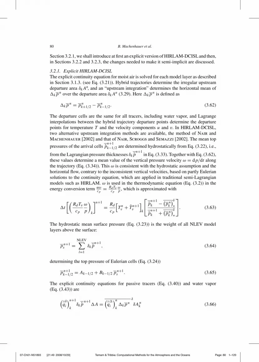
07-Ch01-N51893 [21:49 2008/10/29] Temam & Tribbia: Computational Methods for the Atmosphere and the Oceans Page: 80 1–120
80 B. Machenhauer et al.
Section 3.2.1, we shall introduce at first an explicit version of HIRLAM-DCISL and then,in Sections 3.2.2 and 3.2.3, the changes needed to make it semi-implicit are discussed.
3.2.1. Explicit HIRLAM-DCISLThe explicit continuity equation for moist air is solved for each model layer as describedin Section 3.1.3. (see Eq. (3.21)). Hybrid trajectories determine the irregular upstreamdeparture area $kAn, and an “upstream integration” determines the horizontal mean of!kp
n over the departure area $kAn (3.29). Here !kpn is defined as
!kpn = pn
k+1/2 ! pnk!1/2. (3.62)
The departure cells are the same for all tracers, including water vapor, and Lagrangeinterpolations between the hybrid trajectory departure points determine the departurepoints for temperature T and the velocity components u and v. In HIRLAM-DCISL,two alternative upstream integration methods are available, the method of Nair andMachenhauer [2002] and that of Nair, Scroggs and Semazzi [2002]. The mean top
pressures of the arrival cells pn+1k!1/2 are determined hydrostatically from Eq. (3.22), i.e.,
from the Lagrangian pressure thicknesses $kpn+1
in Eq. (3.33). Together with Eq. (3.62),these values determine a mean value of the vertical pressure velocity / = dp/dt alongthe trajectory (Eq. (3.34)). This / is consistent with the hydrostatic assumption and thehorizontal flow, contrary to the inconsistent vertical velocities, based on partly Euleriansolutions to the continuity equation, which are applied in traditional semi-Lagrangianmodels such as HIRLAM. / is used in the thermodynamic equation (Eq. (3.2)) in theenergy conversion term '/
cp= RdTv
cp
/p , which is approximated with
!t
+;RdTv
cp
/
p
<
k
,n+1
= Rd
cp
-T n
v + T n+1v
0
k
B
C pn+1k !
"pn
k
#$+
pn+1k +
"pn
k
#$+
D
E. (3.63)
The hydrostatic mean surface pressure (Eq. (3.23)) is the weight of all NLEV modellayers above the surface:
pn+1s =
NLEV$
l=1
$kpn+1
, (3.64)
determining the top pressure of Eulerian cells (Eq. (3.24))
pn+1k!1/2 = Ak!1/2 + Bk!1/2 pn+1
s . (3.65)
The explicit continuity equations for passive tracers (Eq. (3.40)) and water vapor(Eq. (3.43)) are
.5q$
i
/n+1
k$kp
n+1!A =
.5q!
i
/n
k!kp
n$
$Ank (3.66)

07-Ch01-N51893 [21:49 2008/10/29] Temam & Tribbia: Computational Methods for the Atmosphere and the Oceans Page: 81 1–120
Finite-Volume Methods in Meteorology 81
and
.5q$
v
/n+1
k$kp
n+1!A =
.5q!
v
/n
k!kp
n$
$Ank
+!t
;5
P!
qv+ 5
K!
qv
<n+1/2
k
$kpn+1/2
$n+1/2
$An+1/2k , (3.67)
respectively, determine updated specific concentrations,.5q$
i
/n+1
kand
.5q$
v
/n+1
k, in
Lagrangian arrival cells"$V = $p!V
#from
.5q!
i
/n
kand
.5q!
v
/n
kplus Eq. (3.62). Finally,
the updated specific concentrations,.5q!
i
/n+1
kand
.5q!
v
/n+1
k, in the Eulerian cells
(!V = !p!A) are determined from.5q$
i
/n+1
kand
.5q$
v
/n+1
kby 1D vertical remappings.
The discretized explicit momentum and thermodynamic equations are straightforwardgrid-point semi-Lagrangian and finite difference approximations to Eqs. (3.1) and (3.2),respectively (see Källén [1996] and Undén et al. [2002]), except that in the thermo-dynamic equation the consistent energy conversion term is approximated consistentlywith (3.63). Regarding the addition of the physics in Eq. (3.67): since DMI-HIRLAMadds the physics at the arrival level (no averaging along the trajectory), that procedurewas also adopted in HIRLAM-DCISL. Of course, it should ideally be done as indicatedin Eq. (3.67).
3.2.2. 1D semi-implicit CSCL shallow water modelsMachenhauer and Olk [1997] made a preliminary study, in which a successful imple-mentation of a semi-implicit scheme was made in two different cell-integrated versionsof the simple 1D shallow water model. One version conserves mass and momentumand another version conserves mass and total energy. The momentum and continuityequations for the 1D shallow water model are, respectively,
du
dt+ g
%h
%x= 0 and (3.68)
dh
dt+ h
%u
%x= 0, (3.69)
where u is velocity (constant with height), h height (of the fluid surface), and x distance.Aperiodic domain is assumed 0 % x % L. The implementation of a semi-implicit schemein the cell-integrated model versions will be compared with the traditional approach ina traditional finite difference grid-point model based on Eqs. (3.68) and (3.69). Thetraditional explicit semi-Lagrangian prediction equations are
un+1exp = un ! !tg
!x($(h))n+1/2, (3.70)

07-Ch01-N51893 [21:49 2008/10/29] Temam & Tribbia: Computational Methods for the Atmosphere and the Oceans Page: 82 1–120
82 B. Machenhauer et al.
hn+1exp = hn ! !t
!x(h$u)n+1/2, (3.71)
where $ indicates a finite difference operator. Like in HIRLAM, we choose a second-order centered finite difference. A semi-implicit system corresponding to this system isobtained simply by averaging (n+1)!t and n!t values of the pressure gradient term andthe linear part of the divergence term (H$u) along the trajectories instead of taking themat (n+1/2)!t at the midpoint of the trajectory as in Eqs. (3.70) and (3.71). The resultingequations may be written as
un+1 = un+1exp ! !tg
2!x
-$hn+1 + $hn ! 2($(h))n+1/2
0, (3.72)
hn+1 = hn+1exp ! !tH
2!x
-$un+1 + $un ! 2($(u))n+1/2
0. (3.73)
We note that a linear version of Eqs. (3.70) and (3.71), linearized around a state at restwith a mean fluid height H , has gravity wave solutions. These solutions are characterizedby purely divergent velocity fields. The height field and the divergence field in thesesolutions oscillate with a frequency v - 2(/
0gH driven by an oscillating pressure
gradient force !g%h/%x and divergence !H%u/%x, respectively. This explains intuitivelywhy the implicit system, obtained by averaging these terms, can be expected to havestable gravity wave solutions. The system (Eqs. (3.72) and (3.73)) is absolutely stable(as long as the trajectories do not cross).
We may write the system as
un+1 = q1 ! !tg
2!x$hn+1, (3.74)
hn+1 = q2 ! !tH
2!x$un+1. (3.75)
In q1 and q2, the terms which do not depend on values at (n+1)!t have been collected.Applying the $ operator on Eq. (3.75) and substituting in Eq. (3.74) gives
un+1 ! gH!t2
4!x2 $2un+1 = q1 ! g!t
2!x$q2. (3.76)
This is an elliptic equation which can be solved to give un+1 and then (3.75) can be usedto determine hn+1.
The fact that the elliptic equation is with constant coefficients, a so-called Helmholtzequation, means that it is relatively easy and fast to solve. In operational semi-implicitmulti-level models as HIRLAM, a series of elliptic equations must be solved. Thisreduces the advantage of large time-steps. It is therefore important that the elliptic equa-tions in any new implementation of the semi-implicit scheme are kept as simple andfast to solve as possible. The strategy of Machenhauer and Olk [1997] for the present

07-Ch01-N51893 [21:49 2008/10/29] Temam & Tribbia: Computational Methods for the Atmosphere and the Oceans Page: 83 1–120
Finite-Volume Methods in Meteorology 83
models and later that of Lauritzen, Kaas, Machenhauer, Lindberg, [2006, 2008]for the HIRLAM-DCISL has been to do the semi-implicit implementation in the FVmodel in such a way that the resulting elliptic equation becomes similar to that of thetraditional model it replaces.
Now let us derive the FV models corresponding to Eqs. (3.70) and (3.71). The mass,momentum, and total energy in a volume of length $x are, respectively,
M$x = "
! x+$x
x
=! h
0zdz
>
dx = "h $x, (3.77)
m$x = "
! x+$x
x
=
u
! h
0dz
>
dx = "uh $x, and (3.78)
E = "
! x+$x
x
! h
0(gz + (1/2)(u2))dzdx = (1/2)"
.gh2 + hu2
/$x, (3.79)
where " is a constant density (mass per unit length). Then the conservation laws formass, momentum, and total energy are
ddt
"h$x#
= 0, (3.80)
ddt
"uh$x
#= !g$x
%
%x
;12h2<
= !g
2$.h2/, and (3.81)
ddt
..gh2 + hu2
/$x/
= !g$x%
%x
;12h2u
<= !g
2$.h2u/, (3.82)
respectively, and after integration over a time-step from t = n!t to t +!t = (n + 1)!t,we get the corresponding discretized conservation laws
hn+1!x = h
n$x, (3.83)
uhn+1
!x = uhn$x ! g
!t
2$.h2/n+1/2
, and (3.84)
.gh2 + hu2
/n+1!x =
.gh2 + hu2
/n$x ! g
!t
2$.h2u/n+1/2
(3.85)
A summation over all grid cells of each of these equations and application of the periodicboundary condition show that mass, momentum, and total energy are globally conserved.
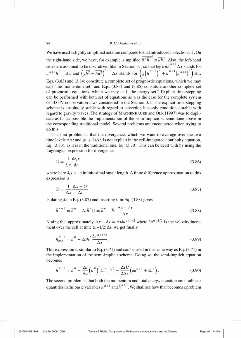
07-Ch01-N51893 [21:49 2008/10/29] Temam & Tribbia: Computational Methods for the Atmosphere and the Oceans Page: 84 1–120
84 B. Machenhauer et al.
We have used a slightly simplified notation compared to that introduced in Section 3.1. On
the right-hand side, we have, for example, simplified unhn$
to uhn. Also, the left-hand
sides are assumed to be discretized like in Section 3.1 so that here uhn+1
!x stands for
un+1hn+1
!x and.gh2 + hu2
/n+1!x stands for
;g.h
n+1/2
+ hn+1"
un+1#2<!x.
Eqs. (3.83) and (3.84) constitute a complete set of prognostic equations, which we maycall “the momentum set” and Eqs. (3.83) and (3.85) constitute another complete setof prognostic equations, which we may call “the energy set.” Explicit time-steppingcan be performed with both set of equations as was the case for the complete systemof 3D FV conservation laws considered in the Section 3.1. The explicit time-steppingscheme is absolutely stable with regard to advection but only conditional stable withregard to gravity waves. The strategy of Machenhauer and Olk [1997] was to dupli-cate as far as possible the implementation of the semi-implicit scheme done above inthe corresponding traditional model. Several problems are encountered when trying todo this.
The first problem is that the divergence, which we want to average over the twotime levels n!t and (n + 1)!t, is not explicit in the cell-integrated continuity equation,Eq. (3.83), as it is in the traditional one, Eq. (3.70). This can be dealt with by using theLagrangian expression for divergence.
D = 1$ix
d$ixdt
(3.86)
where here $ix is an infinitesimal small length. A finite difference approximation to thisexpression is
D = 1!x
!x ! $x
!t. (3.87)
Isolating $x in Eq. (3.87) and inserting it in Eq. (3.83) gives
hn+1 = h
n !!thnD = h
n ! hn!x ! $x
!x. (3.88)
Noting that approximately !x ! $x = !t$un+1/2 where $un+1/2 is the velocity incre-ment over the cell at time (n+1/2)!t, we get finally
hn+1exp = h
n !!thn $un+1/2
!x. (3.89)
This expression is similar to Eq. (3.71) and can be used in the same way as Eq. (3.71) inthe implementation of the semi-implicit scheme. Doing so, the semi-implicit equationbecomes
hn+1 = h
n ! !t
!x
.h
n/*$un+1/2 ! !tH
2!x
.$un+1 + $un
/. (3.90)
The second problem is that both the momentum and total energy equation are nonlinearquantities in the basic variables un+1 and h
n+1. We shall see how that becomes a problem

07-Ch01-N51893 [21:49 2008/10/29] Temam & Tribbia: Computational Methods for the Atmosphere and the Oceans Page: 85 1–120
Finite-Volume Methods in Meteorology 85
and how Machenhauer and Olk [1997] dealt with it. The explicit momentum equation(Eq. (3.84)) may be written as
uhn+1exp !x = uh
n!x !!t
.UH + (uh)*
n/$un+1/2 ! g
!t
2$.h*2 + 2h*H
/n+1/2,
(3.91)
where we have used (uh)n = (uh)*
n + UH and $x = !x !!t$un+1/2.The correspond-ing semi-implicit equation becomes
uhn+1 = uh
n!x ! !t
!x(uh)*
n$un+1/2 ! g
!t
2!x$.h*2/ n+1/2
! !tH
2!x
..U.$un+1 + $un
/+ g.$hn+1 + $hn
///. (3.92)
The two semi-implicit equations (Eqs. (3.90) and (3.92)) may now be written in the form
hn+1 = h
n+1exp ! !tH
!x
.$un+1 + $un ! 2$un+1/2
/(3.93)
and
(uh)n+1 = (uh)
n+1exp ! !tH
!x
.U.$un+1 + $un ! 2$un+1/2
/+ g.$hn+1 + $hn ! 2$hn+1/2
//.
(3.94)
As for the explicit momentum system (Eqs. (3.83) and (3.84)), a summation over all gridcells of each of these equations and application of the periodic boundary condition showthat also the semi-implicit system conserves mass and momentum globally. This followsfrom the fact that the sum of the semi-implicit corrections to the explicit updated valuesis zero.
To proceed as for the traditional system in Eqs. (3.72) and (3.73), (uh)n+1 in Eq. (3.94)must be linearized. At first it is expanded as
(uh)n+1 =""
U + u*#"H + h*##n+1 = UH +"u*#n+1
H +"h*#n+1
U +"u*h*#n+1
.
(3.95)
In order to make it linear in"u*#n+1 and
"h*#n+1, we approximate
"u*h*#n+1 with
"u*h*#n
getting
(uh)n+1 /= UH + u*n+1H + h*n+1U +"u*h*#n . (3.96)
When Eq. (3.96) is inserted in Eq. (3.94), it becomes (after using Eq. (3.93) and somealgebra)
u*n+1 = 1H
;(uh)n+1
exp ! Uhn+1exp !
"u*h*#n ! !tg
!x
.$hn+1 + $hn ! 2$hn+1/2
/<! U.
(3.97)

07-Ch01-N51893 [21:49 2008/10/29] Temam & Tribbia: Computational Methods for the Atmosphere and the Oceans Page: 86 1–120
86 B. Machenhauer et al.
This equation is in the same form as the traditional velocity equation (Eq. (3.72)). So,using it together with Eq. (3.93), we can establish a system, similar to the traditionalsystem (Eqs. (3.74) and (3.75)):
u*n+1 = q1 ! !tg
2!x$hn+1, (3.98)
hn+1 = q2 ! !tH
2!x$un+1, (3.99)
where terms not depending on values at time level (n+1)!t are collected in q1 and q2,respectively. Applying the operator $ (.) on Eq. (3.99) and substituting in Eq. (3.98), aHelmholtz equation like Eq. (3.76) is obtained:
u*n+1 ! gH!t2
4!x2 $2un+1 = q1 ! g!t
2!x$q2. (3.100)
The solution to this equation determines u*n+1 and Eq. (3.101) determines hn+1,which may then be used to determine the semi-implicit correction terms in Eqs. (3.93)and (3.94).
Machenhauer and Olk [1997] derived a similar semi-implicit model for the cell-integrated energy system. As for the momentum system, a summation over all grid cellsof each of these equations and application of the periodic boundary condition showedthat the semi-implicit corrections to the explicit updated values become zero so that alsothe semi-implicit energy system conserves mass and total energy globally.
In this case, the question is if the prognostic variable in Eq. (3.76), the total energygh2 + hu2, can be linearized as we did with the momentum. To show that, we first expandit and then approximate nonlinear terms in perturbations with their values at time n!t.
gh2n+1 + hu2
n+1 = gh2 + hu2n+1
= g(H + h*)2 + (H + h*) (U + u*)2n+1
= 2HUu* n+1 + (UU + 2gH) h* n+1 +"gh*2 + Hu*2 + 2Uh*u* + h*u*2#n
+gH2 + HU2.
(3.101)
Apparently, one gets something that might work as it did for the momentum equation.The main question is if the coefficient 2HU in front of u* n+1
is sufficiently large. Ofcourse, it will not work if U = 0, i.e., if the mean zonal flow is zero. In a realistic flow,however, both H and U are relatively large compared to the perturbations u* n+1
. In testruns with such a flow, the resulting semi-implicit energy system did work satisfactorily,even with a time-step 50 times larger than the CFL maximum.
However, for the full multilevel CSCL system considered in Section 3.1, a corres-ponding linearization of the total energy E = 1/g($k(. p) + (
5cp
5
T )k$kp + 1/2

07-Ch01-N51893 [21:49 2008/10/29] Temam & Tribbia: Computational Methods for the Atmosphere and the Oceans Page: 87 1–120
Finite-Volume Methods in Meteorology 87
"5u2
k + 5v2k
#$kp), defined in Eq. (3.48), cannot be expected to work. Therefore, the present
approach cannot be expected to lead to a semi-implicit system that works satisfactory.The reason is that, in the full CSCL system, the explicit angular momentum equationdetermines the zonal velocity u and the explicit energy equation determines the merid-ional velocity v. Thus, the question is how big the coefficient in front of v* will be in alinearized expression for E. It is easily seen that the term in question is
"!kp
ref V#v
*k,
where we have used $kp ="!kp
ref + $kp#
and vk = V + v*k. Thus, the question is
whether the coefficient"!kp
ref V#
is large enough. Generally, the answer is no as atime independent V in most places will be close to zero. Thus, most likely the approachof Machenhauer and Olk [1997] cannot be extended to the full CSCL system – atleast not in a system including the total energy conservation law. An efficient full semi-implicit CSCL system may be possible and may be developed, eventually. However, itwill require the invention of a new way to transform the explicit system to a semi-implicitsystem. The classical approach, described above, goes back to Robert [1969]. It wasdeveloped for a system consisting of the momentum equations (or the vorticity and thedivergence equations), the continuity equation, and the thermodynamic equation. A newapproach, if possible, should be based directly on modifications of the explicit CSCLsystem.
3.2.3. The semi-implicit version of HIRLAM-DCISLAs a consequence of the conclusions in the last paragraph of the preceding section,Lauritzen, Kaas, Machenhauer and Lindberg [2006, 2008] decided to develop asemi-implicit version of the HIRLAM model in which u and v are kept as prognosticvariables, and just the continuity equation is implemented in FV form. In this case, nolinearization of the prognostic variables is needed. In the present section, we presentthe derivation of a semi-implicit system of prognostic equations based on the systemof explicit equations in Section 3.2.1. The derivation is described in more details inLauritzen, Kaas, Machenhauer and Lindberg [2006, 2008]. Here we concentrateon deviations from the traditional derivation procedure used, e.g., for HIRLAM. Thetraditional procedure for deriving the elliptic equations associated with the baroclinicHIRLAM model is for the central parts the same as for the 1D shallow water modelsconsidered in Section 3.2.2.
First, the explicit system is made semi-implicit by time averaging certain right-handside terms in the discretized primitive equations between time levels n!t and (n + 1)!t.
These linearized terms are:
1. the linearized pressure gradient force in the momentum equation (Eq. (3.1)), i.e.,!#Gk, which depends on temperature and surface pressure
2. two linearized divergence terms: (1) one in the FV continuity equation (Eq. (3.21))and (2) one in the energy conversion term '/ in the thermodynamic equation
(Eq. (3.2)), i.e., ! Rdcpd
.T
pk+1/2
/ref kFl=1
(!lp)ref Dn+1/2l in Eq. (3.120).
Secondly, the formula for the surface pressure and temperatures at time level (n + 1) fromthe semi-implicit continuity and thermodynamic equations, respectively, are inserted in

07-Ch01-N51893 [21:49 2008/10/29] Temam & Tribbia: Computational Methods for the Atmosphere and the Oceans Page: 88 1–120
88 B. Machenhauer et al.
the formula for the linearized pressure gradient force, !#Gk, in the momentum equa-tions. Finally, the divergence operator, # · ( ), is applied to the momentum equationresulting in a set of coupled elliptic equations with updated divergence as an indepen-dent variable. The vertically coupled equations are separated into a set of verticallydecoupled shallow water Helmholtz equations via diagonalization. The final solution tothe elliptic system determines the semi-implicit corrections to the explicit solutions forall the prognostic variables.
3.2.3.1. The linearized pressure gradient force The explicit semi-Lagrangian momen-tum equation at model level k is
."Vn+1k
/
exp! "Vn
k
!t= !#.k ! Rd(Tv)k# ln pk ! f "k ( "Vk +
" "P "V + "K "V#k.
(3.102)
The pressure gradient force
"Fk = !#.k ! Rd(Tv)k
pk#pk = !#
G
H.s + Rd
NLEV$
l=k+1
(Tv)l(! ln p)l + Rd'k(Tv)k
I
J
! Rd(Tv)k # ln pk (3.103)
is linearized as in HIRLAM:
!#Gk = !#
G
H.s + Rd
NLEV$
l=k+1
(Tv)l"! ln pref
#l+ Rd'
refk (Tv)k
I
J! RdTref
prefs
#ps,
(3.104)
where T ref and prefs are constant reference temperature and constant surface pressure,
respectively."! ln pref
#k
and 'refk are defined by Eqs. (3.14) and (3.16) with the “half-
level” pressures obtained from Eq. (3.11) by choosing ps = prefs .
After temporal averaging of !#Gk, the semi-implicit momentum equation may bewritten as in HIRLAM:
+"V + !t
2#G ! f0"k ( "V
,n+1
k
=""R "V
#k, (3.105)
where""R "V
#k
represents explicit terms. In the traditional HIRLAM derivation of theelliptic system, a substitution in the linearized pressure gradient force, !#Gn+1
k , of theupdated surface pressure from the continuity equation and the updated temperaturesfrom the thermodynamic equations is performed. Thereby the linearized geopotential,Gn+1
k , is expressed in terms of the divergence, Dn+1k . The HIRLAM-DCISL derivation
proceeds similarly. Here, just those parts involving the FV continuity equation will bedealt with. These are the parts which deviate from the traditional derivation.

07-Ch01-N51893 [21:49 2008/10/29] Temam & Tribbia: Computational Methods for the Atmosphere and the Oceans Page: 89 1–120
Finite-Volume Methods in Meteorology 89
3.2.3.2. The semi-implicit DCISL continuity equations The discretization of theexplicit continuity equation for moist air was discussed in Section 3.2.1. The deriva-tion of the semi-implicit continuity equation considered here is a direct extension of thederivation for the 1D shallow water models in Section 3.2.2. Defining the discretizedLagrangian divergence,
Dn+1/2k = 1
!A
!A ! $Ank
!t= 1!t
;1 ! $An
k
!A
<(3.106)
and substituting $kAn
!A from the explicit continuity equation (Eq. (3.21)) in the form
"$kp#n+1
exp = !kpn $A
nk
!A, (3.107)
it may be written as
"$kp#n+1
exp = !kpn !!t!kp
nD n+1/2k
= !kpn !!t
.!kp
n/*
Dn+1/2k !!t(!kp)ref D n+1/2
k . (3.108)
Treating the linear term as a temporal average, the (“ideal”) semi-implicit continuityequation results
$kpn+1 =
"$kp# n+1
exp ! !t
2(!kp)ref
.Dn+1
k
."V n+1k
/+ Dn
k
" "Vnk
#! 2Dn+1/2
k
/
(3.109)
or
$kpn+1 =
"$kp# n+1
exp ! !t
2(!kp)ref
.Dn+1
k
."Vn+1k
/! Dn+1
k
."Vn+1
k
//, (3.110)
where Dn+1k
."Vn+1
k
/is defined as the Lagrangian divergence for the last part of the hybrid
trajectory
Dn+1k
."Vn+1
k
/= 1!A
!A ! $An+1/2k
!t/2(3.111)
and Dnk
" "Vnk
#is defined as the Lagrangian divergence for the first part of the hybrid
trajectory
Dnk
" "Vnk
#= 1!A
$An+1/2k ! $An
k
!t/2, (3.112)
(see Fig. 3.3). Thus,
Dnk
" "Vnk
#+ Dn+1
k
."Vn+1
k
/= 2Dn+1/2
k . (3.113)

07-Ch01-N51893 [21:49 2008/10/29] Temam & Tribbia: Computational Methods for the Atmosphere and the Oceans Page: 90 1–120
90 B. Machenhauer et al.
Fig. 3.3 Illustrating the different areas in Eqs. (3.113) and (3.114): $Ank (red), the departure area at time
n!t, $An+1/2k (green), the “mid-way” area at time (n + 1/2)!t, and $An+1
k (blue), the arrival area at time(n + 1)!t. (See also color insert).
This was used to derive Eq. (3.110) from Eq. (3.109). Note that corresponding toEq. (3.112), Dn+1
k
."Vn+1k
/is defined as
Dn+1k
."Vn+1k
/= 1!A
$An+1/2k ! $An+1
k
!t/2= 1!A
$An+3/2k ! $A
n+1/2k
!t, (3.114)
where the last expression is centered about time level n + 1.In order to proceed with the derivation of the semi-implicit system, the Lagrangian
divergence (Eq. (3.114)) should be expressed as a function of the velocity components.In 1D, it was straightforward (see Eq. (3.89)), but in 2Ds, it is complicated althoughnot impossible. However, Lauritzen, Kaas and Machenhauer [2006], Lauritzen,Kaas, Machenhauer and Lindberg [2008], found that the resulting elliptic equationswould be much more complicated than the elliptic equations associated with the tradi-tional HIRLAM system, and therefore, it would be more time consuming to solve. Thiswould significantly reduce the efficiency of the semi-implicit model version. There-fore, they decided to use instead a predictor-corrector approach, which results in ellipticequations in the same form as in HIRLAM. The predictor-corrector approach applied toEq. (3.110) gives finally the semi-implicit continuity equation for moist air:
$kpn+1 =
"$kp#n+1
exp ! !t
2(!kp)ref
.Dn+1
k
."Vn+1k
/! D
."Vn+1
k
//
+ !t
2(!kp)ref
'Dn
k
" "Vnk
#! Dn
k
" "Vnk
#($+$An
k
!A, (3.115)

07-Ch01-N51893 [21:49 2008/10/29] Temam & Tribbia: Computational Methods for the Atmosphere and the Oceans Page: 91 1–120
Finite-Volume Methods in Meteorology 91
where the discretized Eulerian divergence Dn+1k
."Vn+1k
/is defined in the C-grid in
spherical coordinates as
Dnk
" "Vnk
#= 1
a cos1
9$,u
nk
!,+ $1
"vnk cos1
#
!1
:
= $,unk
!x+ 1
cos1$1"vnk cos1
#
!y,
(3.116)
, is the longitude, 1 is the latitude, !x = a cos1!,, and !y = a!1.By replacing Dn+1
k ( "Vn+1k ) in Eq. (3.110) with the discretized Eulerian divergence
Dn+1k ( "Vn+1
k ), as done in Eq. (3.115), an elliptic equation in the same form as in thetraditional HIRLAM system results. However, if just this replacement was done, thescheme would be inconsistent since Dn+1
k
."Vn+1k
/is different from Dn+1
k
."Vn+1k
/(in
fact small-scale noise would develop and it would result in an instability). There-fore, a correction term is added, the last term in Eq. (3.115), which corrects forthe error introduced in the first term of Eq. (3.115). The correction term is equalto the error Dn+1
k
."Vn+1k
/! Dn+1
k
."Vn+1k
/introduced at time level n + 1, but it is
computed in the subsequent time-step when Dnk
" "Vnk
#is known. (The current Dn
k
" "Vnk
#
is then equal to Dn+1k
."Vn+1k
/from the previous time step.) Note that the bar over
the last term in Eq. (3.115) indicates a spatial average over the departure area $Ank ,
i.e., the same departure area as the one used to calculate"$kp#n+1
exp . In practice,!t2 (!kp)ref
'Dn
k
" "Vnk
#! Dn
k
" "Vnk
#(can be added to the term !kp
n as the first oper-ation in each time-step. This means that only one upstream integration is needed toevaluate the first and the last term on the right-hand side of Eq. (3.115). The correctionterm is necessary because the discretized Eulerian divergence Dn+1
k
."Vn+1k
/, defined in
Eq. (3.116), corresponds to a discretized Lagrangian divergence (see Fig. 3.4a), whichis different from Dn+1
k
."Vn+1k
/, defined in Eq. (3.114). This difference is illustrated in
Fig. 3.4.As demonstrated in Section 3.1.3.3, the explicit continuity equation (Eq. (3.21)) con-
serves mass both locally and globally. Since the correction terms in Eq. (3.115), whichcorrect the explicit prediction, consist of linear divergence terms, integration over theentire integration area become zero if the Lagrangian and the Eulerian divergence bothare zero at the boundaries or if the integration area is global. Consequently, with theseassumptions fulfilled, the semi-implicit continuity equation also conserves global mass.It is the impression from preliminary tests that the semi-implicit correction terms gen-erally are small compared to the explicit local mass changes, so it is our impression thatthe local mass conservation is only slightly modified by the semi-implicit corrections.
The explicit continuity equation for a passive tracer was derived in Section 3.1.4. Theresult was Eq. (3.40) which may be written as
;"5q$i#n+1k
$kpn+1<
exp=;.
5q!
i
/n
k!kp
n
<$
+
"$An
k
#
!A.

07-Ch01-N51893 [21:49 2008/10/29] Temam & Tribbia: Computational Methods for the Atmosphere and the Oceans Page: 92 1–120
92 B. Machenhauer et al.
(a)
(b)
Fig. 3.4 Panel A: Illustrating the Lagrangian divergence Dnk
" "Vnk
#= 1
!A
$An+1k !!A
!t , which corresponds tothe Eulerian divergence (Eq. (3.116)). The periphery of a regular departure area, !A, is marked red and theperiphery around its arrival area, $An+1
k , is marked blue. Additional departure and arrival areas for three neigh-
bor cells are shown. Note that the areas $An+1k do not cover the whole domain; there are cracks between them.
Panel B: Illustrating the Lagrangian divergence Dnk
" "Vnk
#= 1
!A
$An+1/2k !$An!1/2
k!t , where the departure area
$An!1/2k is marked red and the arrival area $An+1/2
k is marked blue. Obviously, Dnk
" "Vnk
#is generally different
fromDnk
" "Vnk
#in A. In both panels: Black arrows are velocity components in the C-grid. (See also color insert).

07-Ch01-N51893 [21:49 2008/10/29] Temam & Tribbia: Computational Methods for the Atmosphere and the Oceans Page: 93 1–120
Finite-Volume Methods in Meteorology 93
The variable on the left-hand side is the weight of the cell-integrated tracer mass per unithorizontal area (see Section 3.1.4). For a nonpassive tracer, source and sink terms shouldbe added on the right-hand side of the equation. In a semi-implicit model, semi-implicitcorrection terms must be added to the explicit predicted tracer weights in order to makethem consistent with the predicted moist air weights. The corrected semi-implicit tracer
prediction equation must be identical to that for moist air (Eq. (3.115)) for.5qi
/n
k. 1.
This means that the semi-implicit tracer continuity equation must be
"5q$i#n+1k
$pn+1k =
=.5q$
i
/n+1
k$kp
n+1>
exp
! !t
2
..5q!
i
/
k!kp
/ ref.Dn+1
k
."Vn+1k
/! D
."Vn+1
k
//
+ !t
2
..5q!
i
/
k!kp
/ref 'Dn
k
" "Vnk
#! Dn
k
" "Vnk
#($+$An
k
!A.
3.2.3.3. The semi-implicit energy conversion term Also a dependence on divergencein the thermodynamic equation (Eq. (3.2)) needs to be temporally averaged in the semi-implicit model. Specifically, it is the energy converting term '/
cp= RdTv
cp
/p , approximated
in the explicit model with Eq. (3.63), which is divergence dependent. To isolate thisdependence /k
n+1/2, given by Eq. (3.34), is expanded as follows:
[/k]n+1/2exp = 1
!t
;p
n+1k !
"pn
k
#$+
<= 1!t
=
exp.!'n+1
k
/ k$
l=1
$lpn+1 !
"pn
k
#$+
>
,
(3.117)
where Eqs. (3.17) and (3.22) have been used. When then $lpn+1
is substituted fromEq. (3.108), the result is
[/k]n+1/2exp = 1
!t
=
exp.!'n+1
k
/ k$
l=1
.!lp
n !!t!lpnDn+1/2
l
/!"pn
k
#$+
>
= 1!t
=
exp.!'n+1
k
/ k$
l=1
!lpn !
"pn
k
#$+
>
! exp.!'n+1
k
/ k$
l=1
!lpnDn+1/2
l .
(3.118)
Thus, the explicit energy converting term may be written as
+;RdTv/
cpp
<
k
,n+1
exp

07-Ch01-N51893 [21:49 2008/10/29] Temam & Tribbia: Computational Methods for the Atmosphere and the Oceans Page: 94 1–120
94 B. Machenhauer et al.
= Rd(Tv)n+1/2k"
cp
#n+1/2k
pn+1/2k
[/k]n+1/2exp = Rd (Tv)
n+1/2k"
cp
#n+1/2k
exp.!'n+1/2
k
/p
n+1/2k+1/2
[/k]n+1/2exp
= Rd(Tv)n+1/2k"
cp
#n+1/2k
exp.!'n+1/2
k
/p
n+1/2k+1/2
1!t
=
exp.!'n+1
k
/ k$
l=1
!lpn !
"pn
k
#$+
>
!Rd(Tv)
n+1/2k exp
.!'n+1
k
/
"cp
#n+1/2k
exp.!'n+1/2
k
/p
n+1/2k+1/2
k$
l=1
!lpnDn+1/2
l , (3.119)
where again Eqs. (3.17) and (3.22) have been used. When the last term is linearizedabout a reference temperature T ref and a reference surface pressure p
refs , the result is
+;RdTv/
cpp
<
k
,n+1
exp
= Rd (Tv)n+1/2k"
cp
#n+1/2k
exp.!'n+1/2
k
/p
n+1/2k+1/2
1!t
=
exp.!'n+1
k
/ k$
l=1
!lpn !
"pn
k
#$+
>
!k$
l=1
G
KHRd (Tv)
n+1/2k exp
.!'n+1
k
/
"cp
#n+1/2k
exp.!'n+1/2
k
/p
n+1/2k+1/2
!lp
nI
LJ
*
Dn+1/2l
! Rd
cpd
;T
pk+1/2
<ref k$
l=1
(!lp)ref Dn+1/2l . (3.120)
Treating the linear term as a temporal average, we finally get the (“ideal”) semi-implicitenergy conversion term;
RdTv/
cpp
<n+1
k
=+;
RdTv/
cpp
<
k
,n+1
exp
! Rd
cpd
;T
pk+1/2
<ref k$
l=1
(!lp)ref.Dn+1
l
."Vn+1l
/+ Dn
l
" "Vnk
#! 2Dn+1/2
l
/
(3.121)
or;
RdTv/
cpp
<n+1
k
=+;
RdTv/
cpp
<
k
,n+1
exp
! Rd
cpd
;T
pk+1/2
<ref k$
l=1
(!lp)ref.Dn+1
l
."Vn+1k
/! D
."Vn+1
l
//,
(3.122)

07-Ch01-N51893 [21:49 2008/10/29] Temam & Tribbia: Computational Methods for the Atmosphere and the Oceans Page: 95 1–120
Finite-Volume Methods in Meteorology 95
where again D."Vn+1
l
/is defined by Eq. (3.111).
In order to obtain the same uncomplicated elliptic equations as in HIRLAM, thepredictor-corrector approach is again utilized. This changes Eq. (3.122) to
;RdTv/
cpp
<n+1
k
=+;
RdTv/
cpp
<
k
,n+1
exp
! Rd
cpd
;T
pk+1/2
<ref9
k$
l=1
(!lp)ref.Dn+1
l
."Vn+1l
/! D
."Vn+1
l
//
!k$
l=1
(!lp)ref'Dn
l
" "Vnk
#! Dn
l
" "Vnk
#($+$An
l
!A
:
. (3.123)
3.3. The NCAR-FFSL dynamical core
This section describes main features of the FV dynamical core, included in the NCARCommunity Atmospheric Model (CAM 3.0) description, Collins, Rasch, Boville,Hack, Mccaa, Williamson, Kiehl, Briegleb, Bitz, Lin, Zhang and Dai [2004],Chapter 3.3. It is the pioneering example of a meteorological FV model based on theflux form (Eq. (1.2)) of the continuity equation. It was initially developed and used at theNASA Data Assimilation Office for data assimilation, numerical weather prediction, andclimate simulations. The dynamical core is quasi-hydrostatic, global, and formulated fortraditional latitude-longitude coordinates.
3.3.1. The 3D transport schemeThe quasi-horizontal transport of air mass, tracer mass, and potential temperature isbased on a 2D FV FFSL scheme developed by Lin and Rood [1996] and Lin and Rood[1997]. This Eulerian scheme of the operator splitting or time splitting type, describedin Section 2.3.2, is among the most modern flux-based FV schemes. For the sake of thefollowing description of the dynamical core, it is convenient to rewrite the predictionequation, Eq. (2.52), with the notations of Lin and Rood [1997].
At first, the following standard finite difference $ and average ( ) operators are defined
$6q = q
;6 + !6
2
<! q
;6 ! !6
2
<,
q6 = 12
+q
;6 + !6
2
<+ q
;6 ! !6
2
<,.
(3.124)
The conservation law for a density-like variable Q is
%Q
%t+ # ·
"Q "V
#= 0. (3.125)

07-Ch01-N51893 [21:49 2008/10/29] Temam & Tribbia: Computational Methods for the Atmosphere and the Oceans Page: 96 1–120
96 B. Machenhauer et al.
As explained in Section 2.3.2, the FFSL scheme involves the application of 1D fluxconvergence operators and advective operators, successively applied along the two hor-izontal coordinate directions, in such a way that the scheme becomes both conservativeand constancy preserving.
The 1D flux convergence operators F and G are defined as
F"u+,!7; Qn
#= ! !7
a!, cos1$,'X"u+,!7; Qn
#(,
G"v+,!7; Qn
#= ! !7
a!1 cos1$1'cos1Y
"v+,!7; Qn
#(.
(3.126)
F and G updates Q for one time-step in the zonal (,) and meridional (1) directions,respectively. Here, X and Y, the time-averaged fluxes of Q in the zonal (,) and meridional(1) directions, respectively, are defined as
X"u+,!7; Qn
# /= 1!7
! t+!7
tuQ dt ! hot /= u+"Qn
#+,,
Y"v+,!7; Qn
# /= 1!7
! t+!7
tvQ dt ! hot /= v+"Qn
#+1,
(3.127)
where u+ and v+ are predicted time-centered velocity components at t +!7/2 in C-gridpositions at the east and south face of the cell, respectively. (Qn)+, is determined by anupstream integral
"Qn#+,
= 1a cos1!,
! u+!7
0Qna cos1d,, (3.128)
with a corresponding expression for (Qn)+1.Thus, to approximate the time-averaged fluxes across the cell faces the time-centered
winds, u+ and v+, and the cell averaged field, Qn, at time level n are required. Fur-thermore, for modeling cross-stream advection in the zonal and meridional directions,respectively, the advective flux operators f and g are introduced. They are defined inCollins, Rasch, Boville, Hack, Mccaa, Williamson, Kiehl, Briegleb, Bitz, Lin,Zhang and Dai [2004] in terms of the corresponding F and G operators. Here, f isdefined as
f"u+,!7; Qn
#= F
"u+,!7; Qn
#+ !7
a!, cos1$,u
+, (3.129)
with a corresponding definition for g. With these definitions, the following prognosticequation (corresponding to Eq. (2.52)) results
Qn+1 = Qn + F
+u+,!7; Qn + 1
2g"v+,!7; Qn
#,
+ G
+v+,!7; Qn + 1
2f"u+,!7; Qn
#,(3.130)

07-Ch01-N51893 [21:49 2008/10/29] Temam & Tribbia: Computational Methods for the Atmosphere and the Oceans Page: 97 1–120
Finite-Volume Methods in Meteorology 97
or
Qn+1 = Qn + F'u+,!7; Q1
(+ G
'v+,!7; Q,
(, (3.131)
where
Q1 = Qn + 12g"v+,!7; Qn
#and Q, = Qn + 1
2f"u+,!7; Qn
#. (3.132)
As in the HIRLAM-DCISL, the fluxes are assumed to be along 3D trajectories; however,here the trajectories are line-segment parallel to the coordinate axes. The final verticaldisplacements after each time-step are determined so that hydrostatic balance is main-tained. A Lagrangian vertical coordinate #, is introduced (see Section 3.1.3.1), whichper definition is constant along the 3D trajectories. The quasi-horizontal flow along suchcoordinate surfaces is 2D and relative to the coordinate surfaces, where the verticalvelocity is zero as expressed in Eq. (1.1). The governing Eulerian equations, presentedbelow in Section 3.3.2, are therefore without vertical advection terms.
In the present setup, the Eulerian vertical discretization defining the vertical extendof the Eulerian grid cells is similar to the hybrid sigma-pressure discretization (Simmonsand Burridge [1981]) described in Section 3.1.2, except that here the top of the modelatmosphere is at a constant pressurep$. Thus, the pressure at a --model-surface ispn
k+1/2 = p$ + Ak+1/2 + Bk+1/2pns and the vertical “pressure thickness” of an Eulerian
grid cell is $kpn = !kA +!kB pns . As illustrated in Fig. 3.1, the transport of air during
a time-step, ending up in an Eulerian grid column, is effectuated by a Lagrangian cell,with initial pressure thickness $kpn = pn
k+1/2 ! pnk!1/2. The Lagrangian cell is moving
with the 3D flow and is ending up with a pressure thickness $kpn = pnk+1/2 ! pn
k!1/2.
Its pressure (pn+1k+1/2) is determined hydrostatically from the weight of the cells arriving
above in the same Eulerian grid column. The scheme is globally conservative; however,it is less locally conservative than the DCISLschemes. Thus, as illustrated in Fig. 2.15(d),the FFSL scheme uses information from an area that is somewhat dispersed comparedto the exact departure area.
3.3.2. The governing equationsNeglecting physical forcing terms, the governing continuous quasi-hydrostatic equationsin spherical latitude-longitude coordinates are:
The hydrostatic balance equation on the form
$kp = !g"$kz, (3.133)
which shows that the variable in the continuity equation, $kp, is the weight per unithorizontal area in the layer of air with thickness $kz.
The continuity equation or in other words the conservation law for mass is written as
%
%t$kp + 1
a cos1
+%
%,(uk$kp) + %
%1(vk$kp cos1)
,= 0. (3.134)

07-Ch01-N51893 [21:49 2008/10/29] Temam & Tribbia: Computational Methods for the Atmosphere and the Oceans Page: 98 1–120
98 B. Machenhauer et al.
Similarly, the mass conservation law for tracer species (including water vapor) is
%
%t
"(qi)k $kp
#+ 1
a cos1
+%
%,
"uk(qi)k $kp
#+ %
%1
"vk (qi)k $kp cos1
#,= 0.
(3.135)
The thermodynamic equation or the conservation law for potential temperature is
%
%t(+k$kp) + 1
a cos1
+%
%,(uk+k$kp) + %
%1(vk+k$kp cos1)
,= 0, (3.136)
where +k = (Tv)k" pk
1000 hPa
# Rdcpd is the (virtual) potential temperature.
The momentum equations are used on the so-called “vector invariant form:”
%
%tuk = -kvk ! 1
a cos1
+%
%,((ekin)k + .k ! 4Dk) + 1
"
%pk
%,
,, (3.137)
%
%tvk = !-kuk ! 1
a
+%
%1((ekin)k + .k ! 4Dk) + 1
"
%pk
%1
,, (3.138)
where Dk is the divergence, defined as in Eq. (3.146), 4 is the coefficient for an optionaldivergence damping, and the absolute vorticity -k is
-k = 20 sin 1 + 1a cos1
+%vk
%,! %(uk cos1)
%1
,. (3.139)
Here,0 is the angular velocity of the earth. Finally, the kinetic energy (ekin)k is definedas
(ekin)k = 12
.(uk)
2 + (vk)2/
. (3.140)
3.3.3. Time-steppingIn the model, the dynamics and the NCAR CAM physics are time-split as in HIRLAM inthe sense that all prognostic variables are updated sequentially, at first by the dynamicsand then by the physics. The time-stepping is fully explicit with subcycling over smalltime-steps, !7 = !t/m, within the 2D dynamics. The number of subcycles needed tostabilize the fast gravity waves is m. To avoid excessive small time-steps due to theconvergence of the meridians near the poles, a polar Fourier filter, which filters outthe shortest zonal waves, is applied to u+ and v+ and certain tendency terms in theprognostic equations. The transport for tracers, however, can take a much larger time-step !t equal to the interval between the physics updates. In the present setup, thecells are transported along the Lagrangian surfaces during the long tracer time-steps,starting initially at the beginning of the first small time-step as a model layer with“pressure thickness”!kp
n = !kA +!kB pns , without any remapping of the variables
to the Eulerian model levels. So during these m short time-steps, the transport is fullyLagrangian. Only at the end of each tracer time-step, a remapping takes place. This isdone to avoid excessive smoothing caused by too frequent vertical remapping after eachsmall time-step.

07-Ch01-N51893 [21:49 2008/10/29] Temam & Tribbia: Computational Methods for the Atmosphere and the Oceans Page: 99 1–120
Finite-Volume Methods in Meteorology 99
3.3.3.1. Conservative predictions The prognostic variables, the cell averaged values$kp, (qi)k , +k, uk, and vk, are updated by the use of the prognostic equations (Eqs. (3.134)– (3.138)), but only the Eqs. (3.134)–(3.136) for the density-related variables are inthe proper flux-form (Eq. (3.125)) and are integrated directly by the FFSL predictionequation (Eq. (3.130)). Thus, the dynamical core conserves exactly mass of air, tracermass, including water vapor (apart from evaporation and condensation), and potentialtemperature (in adiabatic friction free flow). The integration of the momentum equations,(Eqs. (3.137) and (3.138)) is discussed in Section 3.3.3.2.
At the start of time-step n (time n!7), the prognostic variables, $kp, (qi)k , +k, uk, andvk, are given in the D-grid as indicated in Fig. 3.5. In addition, the advective winds u+
and v+are needed for the update of $kp, (qi)k, and +k. So at first, these are updated to time(n+1/2)!7on the C-grid using the momentum prediction equation (Eq. (3.144)). Whenthey are available, Eqs. (3.134)–(3.136) can be advanced one time-step using the FFSLprediction form (Eq. (3.130)). u+ and v+ are not history carrying variables. They areoverwritten after being used. When the continuity equation has been solved, the updated
pressure thickness of each Lagrangian layer,"$kp#n+1
, determines the pressure of theLagrangian surfaces by summing up the hydrostatic weight of all the cells above:
pn+1k!1/2 = p$ +
k!1$
l=1
$lpn+1
. (3.141)
Summing up the hydrostatic weight of all the NLEV Lagrangian layers yields the surfacepressure:
pn+1s = p$ +
NLEV$
l=1
$lpn+1
. (3.142)
This is needed for determination of the pressure at the interfaces between the Eulerianmodel layers:
pn+1k!1/2 = p$ + Ak!1/2 + Bk!1/2 pn+1
s , (3.143)
ekin
ekinekin
ekin
v*
uk
v*
uk
u*
vk
u*
vk
!k p (qi )k'k
Fig. 3.5 Schematic stencil of the location of variables in finite volume schemes for the Arakawa C- (indicatedwith superscript *) and D-grids.

07-Ch01-N51893 [21:49 2008/10/29] Temam & Tribbia: Computational Methods for the Atmosphere and the Oceans Page: 100 1–120
100 B. Machenhauer et al.
which are needed for the physical parameterization and the vertical remapping of theprognostic variables. The density-like prognostic variables are given after each large
time-step, !t, as mean values over the Lagrangian layers, $kpn+1
. To be used for phys-ical parameterization, they must be remapped on the Eulerian model layers !kp
n+1
(determined from Eq. (3.143)).
3.3.3.2. Integration of the momentum equation Inspired by the papers of Sadourny[1972] and Arakawa and Lamb [1981], a discretization of the momentum equationshas been achieved that results in conservation of the absolute vorticity. Since also massand potential energy are conserved and all three invariants are consistently transported,it might be expected that approximately the same will be the case for potential vorticity.
The resulting prognostic equations are
un+1 = un +!7
MY"v+,!7; -,
#! 1
a cos1!,$,[(ekin)
+ ! 4D+] + 5
P,
N,
vn+1 = vn !!7
MX"u+,!7; -1
#! 1
a!1$1 [(ekin)
+ ! 4D+] + 5
P1
N,
(3.144)
where (ekin)+, the upstream-biased kinetic energy (defined in the four corners of the
D-grid (Fig. 3.5)), is formulated as
(ekin)+ = 1
2
7X"u+1,!7; un
#‘ + Y
.v+,,!7; vn
/8(3.145)
and
D+ = 1a cos1
9$,u
n+1
!,+ $1
"cos1 vn+1#
!1
:
. (3.146)
The FV mean pressure gradient terms5
P, and5
P1 in Eq. (3.144) are computed by themethod presented in Lin [1997], which eliminates a long-standing problem in terrain-following coordinates, i.e., the inaccuracy caused by different truncation errors in thetwo terms that the pressure gradient force traditionally are split into.
The velocity components uk and vk are given after each large time at Lagrangianlevels, pk. Like the remaining prognostic variables, they need to be remapped to Eulerianlevels. An accurate and conservative remapping procedure has been developed. Thecurrent remapping version, described in detail in Collins, Rasch, Boville, Hack,Mccaa, Williamson, Kiehl, Briegleb, Bitz, Lin, Zhang and Dai [2004], conservesexactly mass, momentum, and total energy.
3.4. Properties of the dynamical cores
3.4.1. Conservation propertiesWith proper boundary conditions, the HIRLAM-DCISL dynamical core conservesexactly global mass of moist air and tracers, including water vapor, liquid water, and

07-Ch01-N51893 [21:49 2008/10/29] Temam & Tribbia: Computational Methods for the Atmosphere and the Oceans Page: 101 1–120
Finite-Volume Methods in Meteorology 101
solid water, if included (apart from evaporation and condensation).Also the NCAR-FFSLdynamical core conserves exactly these global masses. However, in addition, it conservesglobally potential temperature (in adiabatic friction-free flow) and absolute vorticity (inadiabatic friction-free flow). Thus, the NCAR-FFSL dynamical core comes closer thanthe HIRLAM-DCISL to the ideal CSCL model considered in Section 3.1. However, aswe have seen in the idealized tests presented in Section 2, the local conservation is moreaccurate in the HIRLAM-DCISL transport schemes than in the NCAR-FFSL scheme(compare Figs. 2.10(b) and 2.10(c) with Fig. 2.11(d)). Although the vertical remappingis designed to conserve the total energy, it is not globally conserved in NCAR-FFSL. Thehorizontal discretization and the use of a “diffusive” transport scheme with monotonicityconstraint tend to decrease the kinetic energy and thereby the total energy. Whether thisis realistic is difficult to assess. A total energy “fixer” is applied to effectively add theloss in kinetic energy due to “diffusion” back to the model as total potential energy sothat the total energy is globally conserved. However, even without the fixer, the loss isfound to be very small, less than 2 W/m2 with a 2-degree resolution and it is found todecrease with increasing resolution. It is stated in Collins, Rasch, Boville, Hack,Mccaa, Williamson, Kiehl, Briegleb, Bitz, Lin, Zhang and Dai [2004] that in thefuture it may considered to use the total energy as a transported prognostic so that thetotal energy could be automatically conserved. In the HIRLAM-DCISL dynamical core,no total energy “fixer” is applied.
3.4.2. FV Lagrangian pressure gradient forceAs mentioned above, a particular feature of the NCAR-FFSL model is the Eulerianexpression for the FV mean pressure-gradient force (Lin [1997]), which is used inthe model. It eliminates a long-standing problem: the inaccuracy caused by differenttruncation errors in the two terms that the pressure gradient force traditionally is splitinto in terrain-following coordinates. A similar finite volume Lagrangian expression forthe mean pressure gradient force along the trajectories during a time-step is suggested byLauritzen, Kaas, Machenhauer and Lindberg [2008]. It may be used in any DCISLmodel. It has not yet been implemented in HIRLAM-DCISL; however, it is expectedthat it may lead to increased accuracy, even though the linearized pressure gradientforce (Eq. (3.104)), used to derive the semi-implicit correction terms, is based on thetwo-term expression of the pressure gradient force. The proposed Lagrangian meanpressure gradient force PGF!s* along the sloping trajectory!s*is easily computed from
the pressure of the arrival cell, at the end of the trajectory,.p
n+1k
/
expand the pressure
of the departure cell, at the start of the trajectory,"pn
k
#$+. Note that these are the same
pressures that are used to define / in Eq. (3.117). The proposed expression is
PGF!s* =+;
! 1"
%p
%s*
<
k
,n+1/2
exp= ! 1
"
.p
n+1k
/
exp!"pn
k
#$+
!s*
= ! 1
"
.p
n+1k
/
exp!"pn
k
#$+
!scos(8). (3.147)

07-Ch01-N51893 [21:49 2008/10/29] Temam & Tribbia: Computational Methods for the Atmosphere and the Oceans Page: 102 1–120
102 B. Machenhauer et al.
" is an approximation of the mean density along the trajectory. !s is the horizontaldistance between the midpoints of the departure and the arrival cells, and !s* is thecorresponding distance along the sloping trajectory. cos (8) = !s
!s* defines the slope ofthe trajectory. In order to determine the horizontal component of the pressure gradientforce PGFh, the vertical component PGFv, which is balanced by gravity g, must besubtracted:
PGFh =O
(PGF!s*)2 ! g2. (3.148)
3.4.3. Tests of performanceThuburn [2006] has made an attempt to estimate the relative importance of differentconservation laws. It is argued that satisfactory model performance requires spurioussources of a conservable quantity to be much weaker than any true physical sources; forseveral conservable quantities, the magnitudes of the physical sources are estimated inorder to provide benchmarks against which any spurious sources may be measured. Amodel with weak spurious sources of a conservable quantity compared with the physicalsources may in practice produce as accurate forecasts, especially long simulations, as amodel which conserves the quantity exactly if the spurious sources are not systematic.However, even if the spurious sources are weak but the spurious sources are systematic,long simulations may be very inaccurate. Of course, if possible, the spurious sourcesshould be estimated relative to the physical sources, but that may be very difficult andit is not enough; it is also necessary to know if the spurious sources are systematic. So,in practice, as when other potential model improvements are considered, it is necessaryto carry out a series of real cases that is validated against observations in competitionwith any model it is supposed to substitute. To the authors’ knowledge, such a seriesof real case tests have not yet been carried out for any of the two FV dynamical coresconsidered here.
3.4.4. Idealized baroclinic wave testHowever, both have been preliminary tested in the idealized baroclinic wave test case ofJablonowski and Williamson [2006a], in the following called JW06a (a more detailedtechnical note Jablonowski and Williamson [2006b] is available). These tests have, aswe shall see, confirmed that both dynamical cores work properly, producing in generalas realistic baroclinic developments as present day’s nonconservative state-of-the-artdynamical cores. It would have been of considerable interest to validate the importanceof the mass conservation property of the FV dynamical cores considered here in real casetracer transport simulations. There seems to be no doubt that this property is essentialfor tracer transport however to the authors’ knowledge, it has not yet been verified.
The idealized baroclinic wave test case of JW06a consists of an analytic steady-statezonal solution to the global primitive equations. The steady-state is unstable so that anoverlaid perturbation in global reference integrations triggers the development of anidealized baroclinic wave in the northern hemisphere. By day 4, a well-defined wavetrain is established, and by days 7–9, a significant deepening of the highs and lows takesplace before a breakdown by days 20–30 leads to a full circulation in both hemispheres.
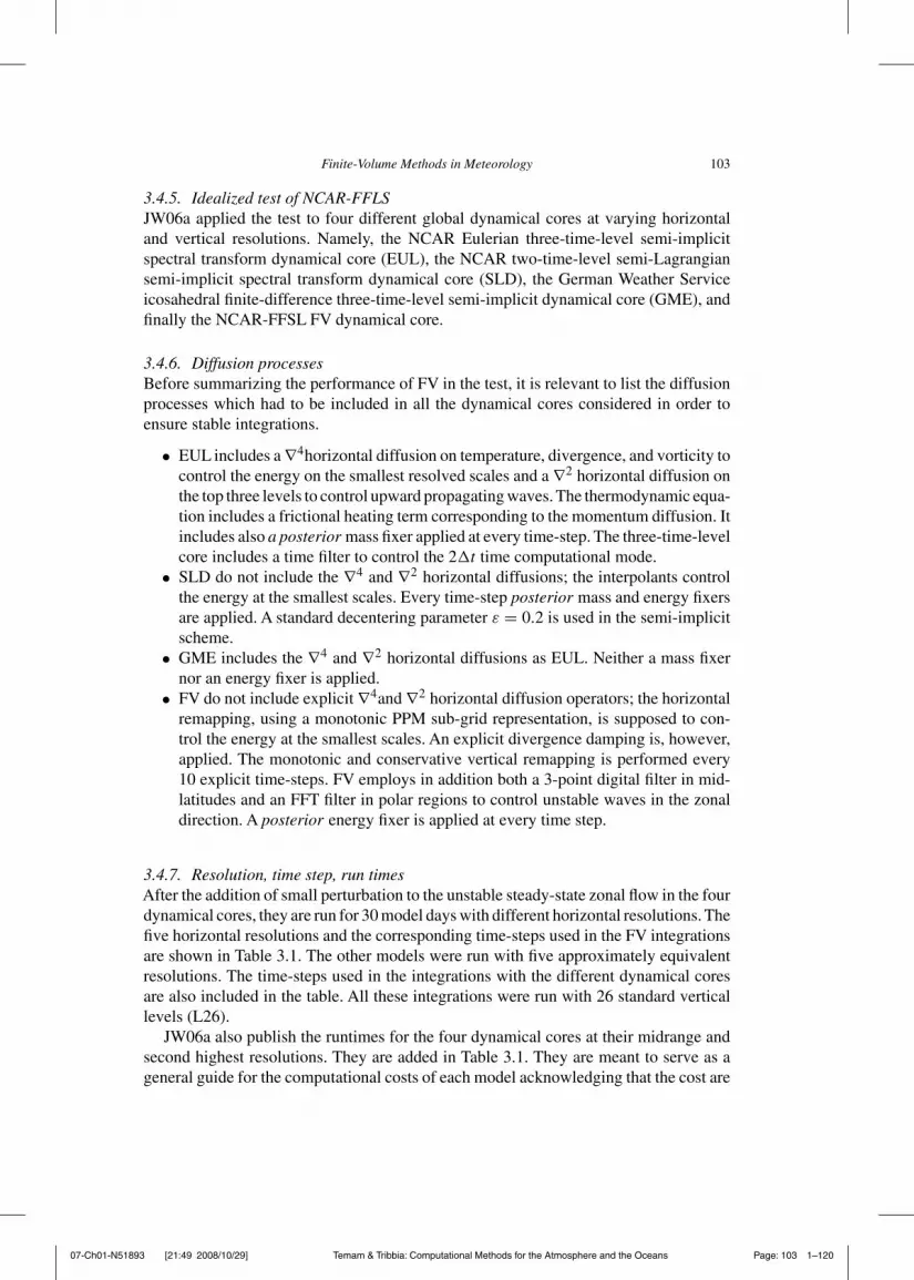
07-Ch01-N51893 [21:49 2008/10/29] Temam & Tribbia: Computational Methods for the Atmosphere and the Oceans Page: 103 1–120
Finite-Volume Methods in Meteorology 103
3.4.5. Idealized test of NCAR-FFLSJW06a applied the test to four different global dynamical cores at varying horizontaland vertical resolutions. Namely, the NCAR Eulerian three-time-level semi-implicitspectral transform dynamical core (EUL), the NCAR two-time-level semi-Lagrangiansemi-implicit spectral transform dynamical core (SLD), the German Weather Serviceicosahedral finite-difference three-time-level semi-implicit dynamical core (GME), andfinally the NCAR-FFSL FV dynamical core.
3.4.6. Diffusion processesBefore summarizing the performance of FV in the test, it is relevant to list the diffusionprocesses which had to be included in all the dynamical cores considered in order toensure stable integrations.
• EUL includes a #4horizontal diffusion on temperature, divergence, and vorticity tocontrol the energy on the smallest resolved scales and a #2 horizontal diffusion onthe top three levels to control upward propagating waves. The thermodynamic equa-tion includes a frictional heating term corresponding to the momentum diffusion. Itincludes also a posterior mass fixer applied at every time-step. The three-time-levelcore includes a time filter to control the 2!t time computational mode.
• SLD do not include the #4 and #2 horizontal diffusions; the interpolants controlthe energy at the smallest scales. Every time-step posterior mass and energy fixersare applied. A standard decentering parameter 2 = 0.2 is used in the semi-implicitscheme.
• GME includes the #4 and #2 horizontal diffusions as EUL. Neither a mass fixernor an energy fixer is applied.
• FV do not include explicit #4and #2 horizontal diffusion operators; the horizontalremapping, using a monotonic PPM sub-grid representation, is supposed to con-trol the energy at the smallest scales. An explicit divergence damping is, however,applied. The monotonic and conservative vertical remapping is performed every10 explicit time-steps. FV employs in addition both a 3-point digital filter in mid-latitudes and an FFT filter in polar regions to control unstable waves in the zonaldirection. A posterior energy fixer is applied at every time step.
3.4.7. Resolution, time step, run timesAfter the addition of small perturbation to the unstable steady-state zonal flow in the fourdynamical cores, they are run for 30 model days with different horizontal resolutions. Thefive horizontal resolutions and the corresponding time-steps used in the FV integrationsare shown in Table 3.1. The other models were run with five approximately equivalentresolutions. The time-steps used in the integrations with the different dynamical coresare also included in the table. All these integrations were run with 26 standard verticallevels (L26).
JW06a also publish the runtimes for the four dynamical cores at their midrange andsecond highest resolutions. They are added in Table 3.1. They are meant to serve as ageneral guide for the computational costs of each model acknowledging that the cost are

07-Ch01-N51893 [21:49 2008/10/29] Temam & Tribbia: Computational Methods for the Atmosphere and the Oceans Page: 104 1–120
104 B. Machenhauer et al.
Table 3.1Horizontal resolutions (FV), time-step !t (s) and wall clock time WT (s)
for one model day
Resolution EUL SLD GME FV(FV) !t/WT !t/WT !t/WT !7(= !t/10)/WT
!1 (!,
4) ( 5) 2400 7200 1600 7202) ( 2.5) 1200 3600 800 3601) ( 1.25) 600/44 1800/24 400/48 180/66
0.5) ( 0.625) 300/483 900/271 200/325 90/6250.25) ( 0.3125) 150 450 100 45
hardware-dependent and vary with the ingenuity of the programmer. The runtime datarepresent the wall clock time (WT) needed to complete one model day on a 32-processernode of an IBM (International Business Machines) Power 4 architecture when using apure message passing interface parallelization approach. Identical compiler optimizationflags were used for all models. No efforts was made to optimize the numerical schemes orto configure the models in their optimal setup, such as selecting an optimal time-step orswitching from quadratic to a linear truncation technique in case of SLD. The dynamicalcores represent the standard versions in CAM3 (The NCAR Community AtmosphericModel system, version3) and GME.
The FV model is seen to be the most expensive in computational costs. Thus, theconservative property is achieved on the expense of efficiency.At the medium resolution,it is 2.75 times more expensive than the semi-Lagrangian semi-implicit SLD dynamicalcore. However, it is also more expensive than the two Eulerian semi-implicit dynamicalcores at medium resolution: 50% more expensive than EUL and 38% more expensivethan GME. At the second highest resolution, it is still the most expensive dynamicalcore. Its WT has increased by a factor 9.5, whereas those of EUL and SLD increased bya factor of 11.0 and 11.3, respectively. However, GME increased much less, by a factorof only 6.8. So at this resolution, FV is 92% more expensive than GME. The advantageof EUL on the other hand has been reduced, but FV is still 29% more expensive thanEUL.
It should be noted that here FV is compared with operational dynamical cores thathave been carefully optimized. It must be noted furthermore that with massive parallelcomputers with a high number of nodes, expected to be more common in the future, theFV explicit code is supposed to gain in relative efficiency due to better parallelizationthan Eulerian as well as semi-Lagrangian semi-implicit codes with elliptic solvers thatinvolve more data exchange between nodes.
3.4.8. Results of the global simulationsAs already mentioned, the JW06a tests indicated that the synoptic performance of the FV(or NCAR-FFSL) dynamical core generally is satisfactory. It is producing as realisticidealized baroclinic developments as the state-of-the-art dynamical cores it is com-pared with. All four dynamical cores compared are found to converge toward a common

07-Ch01-N51893 [21:49 2008/10/29] Temam & Tribbia: Computational Methods for the Atmosphere and the Oceans Page: 105 1–120
Finite-Volume Methods in Meteorology 105
solution. Thus, the second-highest and highest resolution FV L26 surface pressure solu-tions at day 9 are visually almost indistinguishable (see Fig. 6 in JW06a). Up to day10, differences between the solutions from different dynamical cores can only be seenat the smallest scales that are most influenced by the diffusive characteristics of thenumerical schemes, summarized above. An example is the closed cells in the low-pressure center of the surface pressure fields at day 9 (Fig. 7 in JW06a) of the EULand GME solutions. They are slightly deeper than those from the FV dynamical core.Such small-scale differences are seen more clearly in the 850 hPa relative vorticity fields(shown in Fig. 8 in JW06a). At day 7, the high-resolution FV dynamical core exhibitsa slightly weaker vorticity pattern in comparison with EUL, SLD, and GME at highresolutions. According to JW06a, the slightly weaker vorticity fields are caused by thefrequent remappings with monotonicity constraint for every short dynamic time-step inthe FV dynamical core. This constraint adds nonlinear intrinsic diffusion in the regionswhere the monotonicity principle is locally violated. Note that JW06a has shown that theslightly more diffusive solution of the FV dynamical core can be matched very closelyby EUL and SLD when increasing their diffusive coefficients. So there is no doubt thatthe excessive smoothing in FV is caused by the intrinsic diffusion caused by the frequentremappings at the end of every short dynamic time-step. Since the vertical remap-pings are performed only every 10 dynamic time-step, their smoothing effects are lesspronounced.
The small-scale differences between the solutions of the different dynamical corewere interpreted as an uncertainty of their individual estimates of the true referencesolution. JW06a defined the uncertainty as the maximum root mean square deviation l2between a highest and a second highest horizontal resolution surface pressure simulationamong all model versions (see JW06a for details). The uncertainty is increasing withthe number of days simulated, becoming more and more large scale, until saturationbetween day 25 and 30, when the l2 difference is as big as the l2 difference between tworandomly picked global surface pressure fields. Using this uncertainty measure, JW06afound that both two highest resolutions of the FV, the SLD and the EUL dynamical cores,converge within the estimated uncertainty to the true solution, whereas only the highestresolution of the GME dynamical core was found to converge.
3.4.9. Idealized test of HIRLAM-DCISLAlso the HIRLAM-DCISL dynamical core has been tested with the Jablonowski-Williamson test case. As it would be difficult to extend the limited area of theHIRLAM-DCISL dynamical core to a global domain, its domain was made as globalas possible and an effort was made to minimize the effects of its boundaries. The activedomain was extended meridionally to 80°S – 80°N and zonally to 80°W – 280°E, withoutchanging the zero divergence boundary condition, used in the elliptic system solver, toa periodic boundary condition at the zonal boundaries. The zonal extension was chosenso that the initial perturbation, centered at (20°E, 40°N), which triggers a main waveis separated (by exactly 100°) from the western domain boundary where the boundaryscheme initially trigger a weak boundary wave. Both waves develop into wave trainswhich become less and less separated, although they move with approximately the samespeed toward the east. The usual HIRLAM boundary relaxation scheme is applied in a 6)

07-Ch01-N51893 [21:49 2008/10/29] Temam & Tribbia: Computational Methods for the Atmosphere and the Oceans Page: 106 1–120
106 B. Machenhauer et al.
wide zone along the boundary inside the active domain. Within this zone, the updatedprognostic variables are relaxed toward the initial values with a weight that decreasefrom 1 at the boundary to zero approximately 6) inside it. To accommodate the DCISLupstream integrations, there is also a halo zone around the active domain in which theprognostic variables are held fixed at the initial values. In order to facilitate a com-parison with the global FV dynamical core reference solution, the boundary wave waseffectively eliminated from both the HIRLAM-DCISL and the HIRLAM solutions. Thiswas done by utilizing that a completely similar boundary wave is created in simulationswithout an initial perturbation. The simulations with the boundary wave removed werethen compared with the global reference solution. This was done only up to day 8 afterwhich the main wave reached the eastern boundary zone.
3.4.10. Resolution, time-step and runtimesTwo horizontal resolutions were used. The lower resolution, corresponding to the middleglobal resolution (see Table 3.1), is!1 (!, = 1.15) ( 1.45) and the higher resolution,corresponding to the second highest global resolution, is!1 (!, = 0.59) ( 0.74). Inthe vertical, 27 levels are placed as in JW06b but with one more level at the top of themodel atmosphere to accommodate the zero top pressure of HIRLAM. Like the globalSLD dynamical core, the time-steps used for the two horizontal resolutions were 30 and15 minutes, respectively. On a single NEC SX6 processor using ad hoc coding withalmost no optimization, the lowest resolution HIRLAM-DCISL dynamical core isapproximately twice as expensive as the corresponding highly optimized referenceHIRLAM dynamical core. There is no doubt, however, that the efficiency of theHIRLAM-DCISL dynamical core can be increased considerably by a dedicatedoptimization.
3.4.11. Diffusion processes• HIRLAM use decentering with a decentering parameter 2 = 0.1. The nonlinear
terms in continuity equation, the thermodynamic equation, and the momentumequations are needed at time level n + 1/2. As they are potential sources ofinstability, they are extrapolated from filtered values at time level n ! 1 as fol-lows: &n+1/2 = (3&n ! &n!1
f )/2, where & is any of the nonlinear terms and
&n!1f = &n!1 + 2N[&n ! 2&n!1 + &n!2
f ] with 2N = 0.1. At the end of each time-step, all prognostic variable, except liquid water, are diffused using an approximateimplicit #4 horizontal diffusion with the diffusion coefficient K = 3.5 ( 1014 for!x = 0.5) and !t = 300 s (see p. 12–13 in Undén 2002). The coefficients arescaled for resolution so that the e-folding time of the 2!x wave is the same regard-less of resolution (McDonald, 1998). There has been no attempt to tune the diffusioncoefficient for the present idealized dry adiabatic simulations. The horizontal diffu-sion was increased at the uppermost 4 model layers. In addition, the horizontal andvertical interpolations, using cubic Lagrange interpolation, are supposed to controlthe energy at the smallest scales. No mass and energy fixers are applied.
• HIRLAM-DCISL does not use decentering and filtering of the nonlinear terms, butit was necessary to retain a weak implicit #6 horizontal diffusion on T , u, and v. Thehorizontal diffusion was increased at the uppermost 4 model layers. In addition,the horizontal and vertical remapping and interpolations, using, respectively, a

07-Ch01-N51893 [21:49 2008/10/29] Temam & Tribbia: Computational Methods for the Atmosphere and the Oceans Page: 107 1–120
Finite-Volume Methods in Meteorology 107
positive-definite PPM subgrid representation and cubic Lagrange interpolation, aresupposed to control the energy at the smallest scales. No energy fixer is applied
3.4.12. Results of simulationsFor both resolutions of HIRLAM and HIRLAM-DCISL, the l2 difference betweenthe simulation and the simulation of the global highest resolution FV dynamical core(!1 (!, = 0.25) ( 0.3125)) was computed. The results showed that up to day 8 boththe highest resolution (!1 (!, = 0.59) ( 0.74)) simulation of HIRLAM and the high-est resolution simulation of HIRLAM-DCISLhad converted within the uncertainty of thereference solution. For the lower resolution simulations, the simulation of the HIRLAM-DCISL version had not converted, whereas that of the HIRLAM version had; so the FVversion needs higher resolution than the grid-point version for the same level of accuracy(Fig. 3(a) in Lauritzen, Kaas, Machenhauer and Lindberg [2008]). The explanationseems, as for the global FV dynamical core, to be too heavy smoothing due to the repeatedremappings and interpolations. Regarding phase error, the HIRLAM-DCISL simula-tion is slightly better than the HIRLAM simulation. When using the cascade schemeof Nair, Scroggs and Semazzi [2002] instead of the fully 2D CISL scheme of Nairand Machenhauer [2002], the accuracy in terms of the l2 difference is not altered(Fig. 3(b) in Lauritzen, Kaas, Machenhauer and Lindberg [2008]). An importantresult of the idealized baroclinic wave tests is that the consistent Lagrangian discretiza-tion of the energy conversion term, introduced in Section 3.2.1, is seen clearly to bebetter with both a smaller l2 difference and a smaller phase error, than when using thetraditional Eulerian discretization (Fig. 3(b) in Lauritzen, Kaas, Machenhauer andLindberg [2008]).
HIRLAM-DCISL has also been coupled with the HIRLAM physics package andinitial test runs from the initial conditions of a strongly developing extratropical stormhave been performed. The mass conserving version ran stably and produced simulationsthat were quite similar to the reference HIRLAM simulations, except again for slightlymore smoothing in the DCISL version. Also for the full-physics run, the Lagrangiandiscretization of the energy conversion term leads to a more accurate simulation thanthe traditional discretization. The results of these tests are mentioned in Lauritzen,Kaas, Machenhauer and Lindberg [2008]. In this paper also a possible cure for theslightly excessive smoothing is suggested, although it was not tested in practice. It issuggested to keep the Lagrangian cells in the Lagrangian model layers for a numberof consecutive large semi-implicit time-steps before performing the vertical remappingand interpolation to the Eulerian model layers and levels, just as it is done in the NCAR-FFSL over 10 consecutive small time-steps. In HIRLAM-DCISL, an additional verticalremapping and interpolation must be performed after each of the long semi-implicittime-steps as it is needed for the physical parameterization. Thus, it will not affect thecomputational efficiency.
3.5. Online and offline applications – The problem of mass-wind inconsistency
An obvious application of FV models such as the NCAR-FFSL and the HIRLAM-DCISLis tracer transport since tracer-mass conservation is important. These quasi-hydrostaticFV models use a pressure-based vertical coordinate and the prognostic variable for tracer

07-Ch01-N51893 [21:49 2008/10/29] Temam & Tribbia: Computational Methods for the Atmosphere and the Oceans Page: 108 1–120
108 B. Machenhauer et al.
mass is the cell averaged value 5q!
i !p, where p is the horizontal mean pressure over
the area !A of an Eulerian grid cell and !p is the pressure thickness of the cell. 5q!
i is
the Eulerian cell average specific concentration6 of the tracer in question. Thus, 5q!
i !p
is the weight of tracer mass in the cell per unit horizontal area.7 At each time-step, theFV model solves at first the continuity equation for air mass. The input to the continuityequation for air mass is the horizontal wind field which together with the hydrostaticbalance determines the 3D trajectories along which the air is transported. The output isthe updated values of!p. Hereafter, the continuity equation for each specific tracer mass
is solved, using the same trajectories, giving the updated values of5q!
i !p. Thus, both thepredicted air mass and the predicted tracer mass fields are consistent with the “driving”horizontal velocity field. If, the specific concentration qi is needed (e.g., for a compability
check as illustrated in Fig. 2.1) 5q!
i !p must be divided by !p. In a model setup wherethe tracer continuity equation is an integrated part of the dynamical core, this can be
done without loss of mass because 5q!
i !p and!p are internally consistent, i.e., they areboth computed by the same mass conserving transport and remapping operations.
Often a FV transport scheme is imported into a GCM, which dynamical coredoes not conserve the mass of air locally. For example, in the Eulerian ECHAM5(ECmwf/HAMburg, version 5) model, where the vertically integrated mass variableis log ps the continuity equation for air is solved using the spectral transform method.This model is neither globally nor locally mass conserving, while the tracer transportis performed using the inherently mass-conserving advection scheme of Lin and Rood[1996]. This set up is called an online coupling. Here, the FV transport scheme is solvedon the same grid as used by the GCM and the horizontal GCM winds "VGCM needed bythe transport scheme are provided by the GCM at every GCM time-step. A problem ofsuch an online coupling is that the GCM predicts its own air mass field !pGCM , whichis generally different from the !p predicted from the GCM wind field by the mass con-servative tracer transport scheme with qi = 1 (see Fig. 3.6). This is a manifestation ofthe so-called mass-wind inconsistency discussed in detail by Jöckel, Von Kuhlmann,Lawrence, Steil, Brenninkmeijer, Crutzen, Rasch and Eaton [2001].
The consequences of the mass-wind inconsistency in long online coupled simula-tions can be severe. Jöckel, Von Kuhlmann, Lawrence, Steil, Brenninkmeijer,Crutzen, Rasch and Eaton [2001] ran a low-resolution FV transport scheme onlinecoupled to a nonmass conserving GCM. For passive tracers initialized at different loca-tions in the atmosphere, the variations in the total mass were up to 70% in a one-yearsimulation. The amount of artificially (spuriously) created and destroyed mass due tothe mass-wind inconsistency is strongly dependent on the vertical gradient of the tracer.Since tracer gradients are usually steepest around the tropopause the problem is large inthe tropopause region.
6The specific tracer concentration qi is the ratio between the mass of the tracer mtand the mass of the moistair it is mixed into mv.
75q!i !p = mt
mv
5"vg!z = mt
mv
mv!A!z g!z = g mt
!A = the weight of tracer mass per unit horizontal area.

07-Ch01-N51893 [21:49 2008/10/29] Temam & Tribbia: Computational Methods for the Atmosphere and the Oceans Page: 109 1–120
Finite-Volume Methods in Meteorology 109
ps(t 5 (n 1 1)*dt)
finite–volumetransport scheme(q 51)
offline data ordynamical corein online model
p
t 5 n*dt t 5 (n 1 1)*dt t 5 (n 1 1)*dt
ps(t 5 n*dt)
ps(t 5 (n 1 1)*dt)
offline data ordynamical corein online model
Fig. 3.6 Graphical illustration of the mass-wind inconsistency. The figure shows the location of pressurelevels at the beginning of a time-step t = n!t (left), after one time-step t = (n + 1)!t using a FV transportscheme (middle) and given by offline data or predicted by the continuity equation of the dynamical core (right),respectively. If the vertical levels implied by the transport scheme and the dynamical core or offline data do notcoincide, an inconsistency between the mass and wind fields exists and affects the mass of the tracer advection.
If the wind and pressure data driving a FV transport model are not given at every time-step and may be specified on another grid than used in the FV transport model (typicallyan archived meteorological data-set such as ECMWF reanalysis (REA), ERA40, orthe National Centers for Environmental Prediction (NCEP)/NCAR REA) so that bothinterpolation in time and space is needed, then the coupling is called offline. This istypically the situation in a chemical transport model. (It should be noted that this doesnot apply to the NCAR-FFSL model although this model for the tracer transport uses alarge time-step that is equal to an integer number m of the small time-steps, which areused for determining the air mass transport. This is because the fluxes used in the tracertransport during a large time-step is obtained by accumulating fluxes over the m smalltime-steps.) In an offline setting, assimilated analysis or REAdata is often provided to theFV transport scheme. Both the driving horizontal wind field VREA and the correspondingmass field !pREA must be spatially and temporally interpolated to accommodate thegrid and time-step used by the transport scheme. In such a situation, the consistencybetween the mass and wind fields cannot be achieved unless a posteriori consistencycorrection methods are applied to the offline data. This inconsistency with respect to theECMWF analyses is discussed in Trenberth [1991].
One can attempt to restore the mass conservation by altering the specific tracer concen-trations a posteriori. Jöckel, Von Kuhlmann, Lawrence, Steil, Brenninkmeijer,

07-Ch01-N51893 [21:49 2008/10/29] Temam & Tribbia: Computational Methods for the Atmosphere and the Oceans Page: 110 1–120
110 B. Machenhauer et al.
Crutzen, Rasch and Eaton [2001] investigated the effects of various a posteriorimass-fixing algorithms. But all these fixers have severe disadvantages such as violationof shape preservation or introduction of non physical transport components.
Instead of altering the specific tracer concentrations a posteriori, one can as welladjust the horizontal velocity field such that the tracer advection equation is consistentwith the mass field, i.e., the winds are corrected so that the vertical integrated divergenceof mass matches the surface pressure tendency of the meteorological data (for detailssee Prather, Mcelroy, Wofsy, Russel and Rind [1987]; Rotman, Tannahill, Kin-nison, Connell, Bergmann, Proctor, Rodriguez, Lin, Rood, Prather, Rasch,Considine, Ramaroson and Kawa [2001]; Cameron-Smith, Connell and Prather[2002])8. This type of restoration algorithm is referred to as a pressure fixer. Contraryto the algorithms described in the preceding paragraph, it ensures that constant specificconcentrations and mass conservation are retained with this pressure fixer. However,the approach is not completely satisfactory either since “true” wind data are enforcedto provide mass-wind consistency. Introduction of a pressure fixer in a semi-LagrangianFV model would be somewhat different from that used by Eulerian type FV models sincedivergence is defined directly by the trajectories. Therefore modifications of trajectoriesare needed in such models to achieve an analogy to the traditional pressure fixer.
The pressure fixer method can be used to indicate the severity of the mass-wind incon-sistency problem, i.e., by running a model with and without a pressure fixer and assumingthat the pressure fixer does not have a significant effect on the wind field. Horowitz,Walters, Mauzerall, Emmons, Rasch, Granier, Tie, Lamarque, Schultz, Tyn-dall, Orlando and Brasseuret [2003] have run the global Model of Ozone Researchversion 2 (MOZART-2) with and without a pressure fixer. Near the tropopause (wherethe vertical gradient of the ozone specific concentration is large) the difference betweenthe two runs was approximately 187 Tg/yr. Assuming that the pressure fixer is perfect,it can be estimated that a spurious source of ozone of 187 Tg/yr is caused by the mass-wind inconsistency problem which is not a negligible amount. For example, the spurioussource of ozone is similar in magnitude to the estimated amount of influx of ozone peryear to the troposphere from the stratosphere. This is, of course, only an indication ofthe magnitude of the problem. In order to estimate the systematic spurious sources andsinks a fully consistent model must be run. But the estimates provided by Horowitz,Walters, Mauzerall, Emmons, Rasch, Granier, Tie, Lamarque, Schultz, Tyn-dall, Orlando and Brasseuret [2003] suggest that the mass-wind inconsistency canintroduce significant errors.
As discussed above, the problem of performing accurate offline or online tracertransport in a model using a pressure-based vertical coordinate is not limited to theuse of an accurate FV tracer transport scheme, but it is also a question of mass-windconsistency. That is consistency between on one hand the mass field !p determined bythe FV transport scheme and the driving wind field and on the other hand the associatedmass field !pREA or !pGCM . In offline applications using existing REA data, thereis little choice but to use some kind of correction method. However, it is hoped that
8Alternatively one may adjust the surface pressure field instead of the horizontal velocity field to achieveconsistency (P. Jöckel personal communication).

07-Ch01-N51893 [21:49 2008/10/29] Temam & Tribbia: Computational Methods for the Atmosphere and the Oceans Page: 111 1–120
Finite-Volume Methods in Meteorology 111
in the future analysis data set with a better inherent mass conservation, produced bymass conserving data-assimilation models, may become available. In an online trans-port coupling, the consistency can be guaranteed only if the same numerical method isused for the continuity equation of the driving model as for the tracer transport. Thatis the case if a consistent FV model like the NCAR-FFSL or the HIRHAM-DCISLis used. The problem is that the majority of the GCM models available are based onnonlocally conservative schemes for the air mass continuity equation (e.g., traditionalsemi-Lagrangian models such as the IFS at ECMWF, the HIRLAM, and the Max-PlanckInstitute model (ECHAM)). The problem is, as described above, that the changes neededto convert a non-conserving model to a locally mass conserving one, like the change ofHIRLAM to the HIRLAM-DCISL, are rather extensive. All discretizations in the modelas a whole must be carefully rethought in order to obtain inherent local mass conserva-tion. It involves changes to almost all parts of the model and all the prognostic equationsand not only changes to the continuity equations. However, it is necessary in order toguarantee consistency and thereby accurate tracer transport.
3.6. Extensions to nonhydrostatic models
In the quasi-hydrostatic FV dynamical cores considered in Sections 3.1–3.5, the con-tinuity equation was solved in so-called Lagrangian (#) vertical coordinates, with, perdefinition, # = constant along 3D trajectories. That is, all transport during a time-stepwas assumed to be effectuated by Lagrangian finite control volumes moving with the3D flow, usually in a semi-Lagrangian sense, starting or ending as Eulerian grid cells.The advantage is that in such Lagrangian coordinates, the vertical velocity is zero asexpressed in Eq. (1.1), so the transport problem becomes 2D. However, the verticalcomponents of the 3D trajectories still need to be determined. In the quasi-hydrostaticmodels considered so far, this is done hydrostatically, i.e., the vertical displacementof the Lagrangian control-volume during a time-step was determined by requiring thatthe arrival cell is in hydrostatic balance. Of course, this approach cannot be used in anonhydrostatic model, but instead the vertical displacement can be determined directlyfrom the vertical velocity, which in a nonhydrostatic model is an independent prognosticvariable. Realizing this one can formulate a DCISL solution to the continuity equationalso for the nonhydrostatic case.
We may start from the continuity equation on the form (Eq. (1.8)), which was derivedwithout assuming hydrostatic balance. Using the notations in Section 1.1 Eq. (1.8) is
"" $kh
#+!A =
"" $kh
#$kA. (3.149)
This is a prognostic equation when"" $kh
#is known in the departure area at time t. Unlike
what we did in the “exact” case, we now set the height of the Lagrangian surfaces #k!1/2and #k+1/2 equal to the Eulerian surfaces hk!1/2 and hk+1/2, respectively, in the departurearea so that here $kh = !kh. Thus, Eq. (3.149) becomes
"" $kh
#+!A = !kh
""#$kA, (3.150)

07-Ch01-N51893 [21:49 2008/10/29] Temam & Tribbia: Computational Methods for the Atmosphere and the Oceans Page: 112 1–120
112 B. Machenhauer et al.
Now in the nonhydrostatic case, we utilize the prognostic variable w, the vertical velocity,to determine $kh. So it is a known constant in Eq. (3.150). Therefore, it may be written as
""#+$kh!A = !kh
""#$kA, (3.151)
or
""#+ = !kh
$kh!A
!!
$kA
" dx dy. (3.152)
""#+$kh!A is the updated mass in the arrival grid cell at time t +!t. According to
Eq. (3.152), it is equal to the mass in the upstream departure cell at time t, which can becomputed simply as a 2D integral over the departure area of the vertical mean densityin the Eulerian model layer considered.
This demonstrates that FV methods of the DCISL type, like the one used in HIRLAM-DCISL, can be used also for nonhydrostatic models. It also means that the Lagrangian(#) vertical coordinate approach can be used in nonhydrostatic Eulerian flux-type FVmodels, just as the corresponding quasi-hydrostatic approach was used in the NCAR-FFSL dynamical core.
Of course, alternatively, a nonhydrostatic model may be based on a traditional 3Doperator-split flux-form method, with fluxes entering an Eulerian grid cell at both hori-zontal and vertical faces. However, it becomes rather complicated if one uses the mostaccurate schemes of the symmetric FFSL type. Thus, Leonard, Lock and Macvean[1996] presents a symmetric 3D scheme. Using a notation similar to that used inSection 2.3.2, it becomes
&n+1 =&
n + XC
M *16
-.&
n + &AY + &AYZ
/+.&
n + &AZ + &AZY
/0N
+ YC
M *16
-.&
n + &AZ + &AZX
/+.&
n + &AX + &AXZ
/0N
+ ZC
M *16
-.&
n + &AX + &AXY
/+.&
n + &AY + &AYX
/0N, (3.153)
where, for example,
&AYZ = &AZ
"&AY
#= &AY + ZA
"&AY
#. (3.154)
Such schemes have been used extensively; a recent example is the MIT-GCM (Adcroft,Campin, Hill and Marshall [2004]).
4. Summary
Recent developments in FV methods have provided the basis for new meteorologicaldynamical cores that conserve integral invariants exactly, globally as well as locally. Inparticular, these new FV methods have been the basis for design of exact mass conserving

07-Ch01-N51893 [21:49 2008/10/29] Temam & Tribbia: Computational Methods for the Atmosphere and the Oceans Page: 113 1–120
Finite-Volume Methods in Meteorology 113
tracer transport models. The new technologies are reviewed and the perspectives for thefuture are discussed.
During about two decades, the traditional semi-implicit and semi-Lagrangian spectralor grid-point dynamical cores have been dominating worldwide in meteorological modelsapplied for weather prediction and climate simulations. They are efficient and otherwiseaccurate but lack exact mass conservation, which is considered a serious drawback forthe hydrometeorological variables as well as an increasing number of chemical variablesincluded in the models. In Section 3, we presented two recently developed pioneeringmeteorological dynamical cores which potentially solve these problems. These are thesemi-implicit cell-integrated semi-Lagrangian limited area dynamical core HIRLAM-DCISL and the global flux-form NCAR-FFSL dynamical core. Each of them extendsnewly developed 2D FV semi-Lagrangian schemes, described among others in Section 2,to 3D utilizing a common newly developed Lagrangian time-stepping technique buildingon horizontally upstream and vertically downstream time-steps. Values of certain quan-tities integrated horizontally over an upstream departure area in an Eulerian model layerare assumed to be transported with vertical walls along 3D trajectories into a Lagrangianlayer in a column of Eulerian grid cells. The vertical coordinates of this Lagrangian layerare then determined hydrostatically. As a result, the quantities in question are conservedexactly globally and with high, slightly different accuracy, also locally in both dynam-ical cores. Idealized tests presented in Section 2 showed that the local conservation isslightly more accurate in the HIRLAM-DCISL transport schemes than in the NCAR-FFSL scheme. With proper boundary conditions, the HIRLAM-DCISL dynamical coreconserves the global mass of moist air and tracers exactly, including water vapor, liquidwater, and solid water, if included (apart from evaporation and condensation). Also theNCAR-FFSL dynamical core conserves exactly these masses. In addition, it conserves,except for time truncation errors, potential temperature and absolute vorticity (in adia-batic friction-free flow). Thus, the NCAR-FFSL dynamical core comes closer than theHIRLAM-DCISL to the ideal CSCL model considered in Section 3.1. Both FV dynam-ical cores have been tested and compared with nonconservative dynamical cores in anidealized baroclinic wave test. All dynamical cores considered were found to convergetoward a common solution. However, in their present formulation, the FV dynamicalcores needed higher resolution than the nonconservative dynamical cores they were com-pared with for the same level of accuracy. The explanation seems to be a slight smoothingdue to the repeated remappings and interpolations. As a possible cure to HIRLAM-DCISL, it is suggested to keep the vertical Lagrangian cells for a number of consecutivelarge semi-implicit time-steps before performing the vertical remapping to the Eulerianmodel layers. The idealized as well as other tests with HIRLAM DCISL showed that aconsistent Lagrangian discretization of the energy conversion term in the thermodynamicequation leads to a more accurate simulation than the traditional discretization. A furtherincrease in accuracy is expected from a corresponding Lagrangian discretization of thehorizontal pressure gradient term in the momentum equation. The idealized intercom-parison tests showed that among the dynamical cores the FV ones are the most expensivein computational costs. Thus, the conservative property is achieved at the expense ofefficiency. There is no doubt, however, that the efficiency of the present experimen-tal ad hoc coded FV dynamical cores can be increased considerably by a dedicatedoptimization.

07-Ch01-N51893 [21:49 2008/10/29] Temam & Tribbia: Computational Methods for the Atmosphere and the Oceans Page: 114 1–120
114 B. Machenhauer et al.
An obvious application of FV models such as the NCAR-FFSL and the HIRLAM-DCISL is tracer transport since tracer-mass conservation is essential. As described inSection 3.5, a FV transport scheme has often been imported into a GCM with a dynamicalcore that does not conserve mass locally. A problem of such an online coupling is thatit leads to the so-called mass-wind inconsistency, which in long simulations can lead tosevere errors with large amounts of artificially (spuriously) created or destroyed tracermass. The only way to avoid completely such errors is to use a complete FV model withexactly the same locally mass conserving algorithms for all tracers and for the moist air.
To facilitate a wider application, the limited area HIRLAM-DCISL may be extendedto a global domain. This may be done by using the extension of the horizontal FVschemes used in this dynamical core that have already been developed in sphericallatitude-longitude coordinates. Another possibility which may be relevant also for theNCAR-FFSL is to change to a new grid, as the icosahedral-hexagonal grid, which isalmost uniform on the sphere. Finally, the possibility of an extension to nonhydrostaticdynamical cores is discussed in Section 3.6.The same extension, as used in the hydrostaticdynamical cores, of the available 2D FV semi-Lagrangian schemes to 3Ds may be usedin nonhydrostatic dynamical cores. That is, utilizing horizontally upstream and verticallydownstream time-stepping. The only difference is that the vertical displacement of theLagrangian cells must be determined directly by predicted vertical velocities and notfrom hydrostatic balance.
5. Acknowledgments
The authors wish to express their gratitude to Dr. Ramachandran D. Nair and Dr. PhilRasch for helpful suggestions and useful discussions on parts of Section 2. Thanks toDr. Patrick Jöckel and Rune Graversen for their comments on the ‘mass-wind incon-sistency’ section. The third author is grateful to NCAR’s Advanced Study Program andClimate Modeling Section for providing necessary support for this research.

07-Ch01-N51893 [21:49 2008/10/29] Temam & Tribbia: Computational Methods for the Atmosphere and the Oceans Page: 115 1–120
References
Adcroft, A., Campin, J-M., Hill, C., Marshall, J. (2004). Implementation of an atmosphere-ocean generalcirculation model on the expanded spherical cube. Mon. Wea. Rev. 132 (12), 2845–2863.
Arakawa, A. (2000). A personal perspective on the early years of general circulation modeling at UCLA. In:Randall, D.A. (ed.), General Circulation Model Development. Past, Present, and Future (Academic Press),pp. 1–65.
Arakawa, A., Lamb, V. (1977). Computational design and the basic dynamical processes of the UCLA generalcirculation model. Methods Comput. Phys. 17, 173–265.
Arakawa, A., Lamb, V. (1981). A potential enstrophy and energy conserving scheme for the shallow waterequations. Mon. wea. Rev. 109, 18–36.
Bates, J.R., Mcdonald, A. (1982). Multiply-upstream, semi-Lagrangian advective schemes: analysis andapplication to a multi-level primitive equation model. Mon. Wea. Rev. 110 (12), 1831–1842.
Bell, J.B., Dawson, C.N., Shubin, G.N. (1988). An unsplit, higher order Godunov method for scalarconservation laws in multiple dimensions. J. Comput. Phys. 74, 1–24.
Bermejo, R. Staniforth, A. (1992). The conversion of semi-Lagrangian advection schemes to quasi-monotone schemes. Mon. Wea. Rev. 120 (11), 2622–2632.
Boris, J.P., Book, D.L. (1973). Flux corrected transport. I. SHASTA: a fluid transport algorithm that works.J. Comput. Phys. 11, 38–69.
Bott, A. (1989). A positive definite advection scheme obtained by nonlinear renormalization of the advectivefluxes. Mon. Wea. Rev. 117 (5), 1006–1016.
Bott, A. (1992). Monotone flux limitation in the area-preserving flux-form advection algorithm. Mon. Wea.Rev. 120 (11), 2592–2602.
Bott, A. (1993). The monotone area-preserving flux-form advection algorithm: reducing the time-splittingerror in two-dimensional flow fields. Mon. Wea. Rev. 121 (9), 2637–2641.
Burridge, D.M., Hasler, J. (1977). A model for medium range forecasting. Adiabatic formulation. ECMWFTech. Rep. 4, Reading, United Kingdom, pp. 46.
Byun, B.W. (1999). Dynamically consistent formulations in meteorological and air quality models formultiscale atmospheric studies, Part II: mass conservation issues. J. Atmos. Sci. 56 (21), 3808–3820.
Cameron-Smith, P., Connell, P., Prather, M. (2002). Pressure fixers: conserving mass in chemical transportmodels by adjusting the winds. Available at 2002; http://eed.llnl.gov/pfix/.
Carpenter, J.R., Droegemeier, K.K., Woodward, P.R., Hane, C.E. (1990). Application of the piecewiseparabolic method (PPM) to meteorological modeling. Mon. Wea. Rev. 118 (3), 586–612.
Colella, P. (1990). Multidimensional upwind methods for hyperbolic conservation laws. J. Comput. Phys.87, 171–200.
Colella, P., Woodward, P.R. (1984). Piecewise parabolic method for gas-dynamical simulations. J. Comput.Phys. 54, 174–201.
Collins, W.D., Rasch, P.J., Boville, B.A., Hack, J.J., Mccaa, J.R., Williamson, D.L., Kiehl, J.T.,Briegleb, B., Bitz, C., Lin, S.-J., Zhang, M., Dai, Y. (2004). Description of the NCAR CommunityAtmosphere Model (CAM3). Technical Report, NCAR/TN- 464+STR, National Center for AtmosphericResearch, Boulder, Colorado 80307-3000, pp. 226.
Cotter, C.J., Frank, J., Reich, S. (2007). The remapped particle-mesh semi-Lagrangian advection scheme.Q. J. R. Meteorol. Soc. 133, 251–260.
Crowley, W.P. (1968). Numerical advection experiments. Mon. Wea. Rev. 96 (1), 1–11.
115

07-Ch01-N51893 [21:49 2008/10/29] Temam & Tribbia: Computational Methods for the Atmosphere and the Oceans Page: 116 1–120
116 B. Machenhauer et al.
Doswell III, C.A. (1984). A kinematic analysis of frontogenesis associated with a nondivergent vortex.J. Atmos. Sci. 41 (7), 1242–1248.
Dukowicz, J.K., Baumgardner, J.R. (2000). Incremental remapping as a transport/advection algorithm.J. Comput. Phys. 160, 318–335.
Dukowicz, J.K., Kodis, J.W. (1987). Accurate conservative remapping (rezoning) for arbitrary Lagrangian-Eulerian computations. SIAM J. Sci. Stat. Comput. 8, 305–321.
Dukowicz, J.K., Ramshaw, J.D. (1979). Tensor viscosity method for convection in numerical fluid dynamics.J. Comput. Phys. 32, 71–79.
Durran, D.R. (1999). Numerical Methods for Wave Equations in Geophysical Fluid Dynamics (Springer-Verlag), pp. 465.
Easter, R.E. (1993). Two modified versions of Bott’s positive-definite numerical advection scheme. Mon.Wea. Rev. 121 (1), 297–304.
Eumard, R., Gallouët, T., Herbin, R. (2000). Finite volume methods. In: Ciarlet, P.G., Lions, J.L. (eds.),Handbook of Numerical Analysis, vol. VII (Elsevier Science B.V.), pp. 715–1020.
Godunov, S.K. (1959). Finite difference method for numerical computation of discontinous solution of theequations of fluid dynamics. Math. Sb. 47, 271, translated from Russian by I. Bohachevsky.
Hirsch, C. (1990). Numerical Computation of Internal and External Flows, vol. 2, Wiley Series in NumericalMethods (John Wiley and Sons), pp. 714.
Hirt, C.W., Amsden, A.A., Cook, J.L. (1974). An arbitrary Lagrangian-Eulerian computing method for allflow speeds. J. Comput. Phys. 14, 227.
Hólm, E.V. (1995). A fully two-dimensional, nonoscillatory advection scheme for momentum and scalartransport equations. Mon. Wea. Rev. 123 (2), 536–552.
Horowitz, L.W., Walters, S., Mauzerall, D.L., Emmons, L.K., Rasch, P.J., Granier, C., Tie, X.,Lamarque, J., Schultz, M.G., Tyndall, G.S., Orlando, J.J., Brasseuret, G.P. (2003). A global sim-ulation of tropospheric ozone and related tracers: description and evaluation of MOZART, version 2.J. Geophys. Res. 108 (D24), 4784.
Hortal, M. (2002). The development and testing of a new two-time-level semi-Lagrangian scheme (SETTLS)in the ECMWF forecast model. Q. J. R. Meteorol. Soc. 128, 1671–1687.
Hourdin, F., Armengaud, A. (1999). The use of finite-volume methods for atmospheric advection of tracespecies. Part I: test of various formulation in a general circulation model. Mon. Wea. Rev. 127 (5), 822–837.
Jablonowski, C. and Williamson, D.L. (2006a). A baroclinic instability test case for atmospheric modeldynamical cores. Q. J. R. Meteorol. Soc. 132, 2943–2975.
Jablonowski, C. and Williamson, D.L. (2006b). A baroclinic wave test case for dynamical cores ofgeneral circulation models: Model intercomparisons. NCAR Technical Note, NCAR/TN-469+STR,Boulder CO, pp. 89.
Jöckel, P., Von Kuhlmann, R., Lawrence, M.G., Steil, B., Brenninkmeijer, C.A.M., Crutzen, P.J.,Rasch, P.J., Eaton, B. (2001). On a fundamental problem in implementing flux-form advection schemesfor tracer transport in 3-dimensional general circulation and chemistry transport models. Q. J. R. Meteorol.Soc. 127, 1035–1052.
Kaas, E. (2008). A simple and efficient locally mass conserving semi-Lagrangian transport scheme. Tellus A,in press.
Källén, E. (1996). HIRLAM documentation manual, System 2.5.Available from SMHI, Norrköping, Sweden.Kuo, H., Williams, R.T. (1990). Semi-Lagrangian solutions to the inviscid burgers equation. Mon. Wea. Rev.
118 (6), 1278–1288.Laprise, L.P.R., Plante, A. (1995). A class of semi-Lagrangian integrated-mass (SLIM) numerical transport
algorithms. Mon. Wea. Rev. 123 (2), 553–565.Lauritzen, P.H. (2007). A stability analysis of finite-volume advection schemes permitting long time steps.
Mon. Wea. Rev. 135 (7), 2658–2673.Lauritzen, P.H., Kaas, E., Machenhauer, B. (2006). A mass-conservative semi-implicit, semi-Lagrangian
limited-area shallow water model on the sphere. Mon. Wea. Rev. 134 (4), 1196–1212.Lauritzen, P.H., Kaas, E., Machenhauer, B., Lindberg, K. (2008). A mass-conservative version of the
semi-implicit semi-Lagrangian HIRLAM. Q. J. R. Meteorol. Soc., 134 (635), 1583–1595.Lauritzen, P.H., Nair, R.D. (2008). Monotone and conservative cascade remapping between spherical grids
(CaRS): regular latitude-longitude and cubed-sphere grids. Mon. Wea. Rev., 136 (4), 1416–1432.

07-Ch01-N51893 [21:49 2008/10/29] Temam & Tribbia: Computational Methods for the Atmosphere and the Oceans Page: 117 1–120
References 117
Leith, C.E. (1965). Numerical simulation of the earth’s atmosphere. Methods Comput. Phys. 4, 1–28.Leonard, B.P. (1994). Note on the von Neumann stability of explicit one-dimensional advection schemes.
Comp. Meth. Appl. Mech. Ens. 118, 29–46.Leonard, B.P., Lock, A.P., Macvean, M.K. (1996). Conservative explicit unrestricted time step multidimen-
sional constancy-preserving advection schemes. Mon. Wea. Rev. 124 (11), 2588–2606.Leslie, M.L., Purser, R.J. (1995). Three-dimensional mass-conserving semi-Lagrangian scheme employing
forward trajectories. Mon. Wea. Rev. 123 (8), 2551–2566.Leveque, R.J. (2002). Finite Volume Methods for Hyperbolic Problems (Cambridge University Press).Li, Y., Chang, J.S. (1996). A mass-conservative, positive-definite, and efficient Eulerian advection scheme in
spherical geometry and on a non-uniform grid system. J. Appl. Meteorol. 35, 1897–1913.Lin, S.-J. (1997). A finite-volume integration method for computing pressure gradient forces in general vertical
coordinates. Q. J. R. Meteorol. Soc. 123, 1749–1762.Lin, S.-J. (2004). A “Vertically Lagrangian” finite-volume dynamical core for global models. Mon. Wea. Rev.
132 (10), 2293–2307.Lin, S.-J., Rood, R.B. (1996). Multidimensional flux-form semi-Lagrangian transport schemes. Mon. Wea.
Rev. 124 (9), 2064–2070.Lin, S.-J., Rood, R.B. (1997). An explicit flux-form semi-Lagrangian shallow water model on the sphere. Q. J.
R. Meteorol. Soc. 123, 2477–2498.Lin, S.-J., Rood, R.B. (1998). A flux-form semi-Lagrangian general circulation model with a Lagrangian
control-volume vertical coordinate. In: Proc. The Rossby-100 Symp. (University of Stockholm, Stockholm,Sweden), pp. 220–222.
Lorenz, E.N. (1960). Energy and numerical weather prediction. Tellus 12, 364–373.Machenhauer, B. (1979). The spectral method. In: Kasahara, A. (ed.), Numerical Methods Used in Atmo-
spheric Models, vol. 2. GARP Publications Series No.17 (WMO and IGSU, Geneva, Switzerland),pp. 121–275.
Machenhauer, B. (1994). A Note on a Mass-, Energy- and Entropy Conserving Semi-Lagrangian andExplicit Integration Scheme for the Primitive Equations. MPI Workshop on Semi-Lagrangian Methods,Hamburg 8-9 Oct. 1992. 146 (Max Planck Institute for Meteorology Tech. Rep, Hamburg, Germany),pp. 73–102.
Machenhauer, B., Olk, M. (1996). On the development of a cell-integrated semi-Lagrangian shallowwater model on the sphere. ECMWF Workshop on semi-Lagrangian methods, 6-8 November, WorkshopProceedings, pp. 213–228.
Machenhauer, B., Olk, M. (1997). The implementation of the semi-implicit scheme in cell-integratedsemi-Lagrangian models. Atmos. Ocean. 35, 103–126.
Machenhauer, B., Olk, M. (1998). Design of a semi-implicit cell-integrated semi-Lagrangian model. MaxPlanck Institute for Meteorology Tech. Rep., 265, Hamburg, Germany, pp. 76–85.
Majewski, D., Liermann, D., Prohl, P., Ritter, B., Buchhold, M., Hanisch, T., Paul, G., Wergen, W.,Baumgardner, J. (2002). The operational global icosahedral-hexagonal gridpoint model GME: descriptionand high-resolution tests. Mon. Wea. Rev. 130 (2), 319–338.
McDonald A. (1998). Default horizontal diffusion coefficients in HIRLAM-4.1. HIRLAM NewsletterNo. 31, electronic version available at http://hirlam.knmi.nl/.
Mcgregor, J.L. (1993). Economical determination of departure points for semi-Lagrangian models. Mon.Wea. Rev. 121 (1), 221–230.
Mcgregor, J.L. (1996). Semi-Lagrangian advection on a conformal cubic grid. Mon. Wea. Rev. 124 (6),1311–1322.
Moorthi, S., Higgins, R.W., Bates, J.R. (1995). A global multilevel atmospheric model using a vec-tor semi-Lagrangian finite-difference scheme. Part II: version with physics. Mon. Wea. Rev. 123 (5),1523–1541.
Nair, R.D., Côté, J., Staniforth, A. (1999a). Monotonic cascade interpolation for semi-Lagrangianadvection. Q. J. R. Meteorol. Soc. 125, 197–212.
Nair, R.D., Côté, J., Staniforth, A. (1999b). Cascade interpolation for semi-Lagrangian advection over thesphere. Q. J. R. Meteorol. Soc. 125, 1445–1468.
Nair, R.D., Thomas, S.J., Loft, R.D. (2005). A discontinuous galerkin transport scheme on the cubed sphere.Mon. Wea. Rev. 133 (4), 814–828.

07-Ch01-N51893 [21:49 2008/10/29] Temam & Tribbia: Computational Methods for the Atmosphere and the Oceans Page: 118 1–120
118 B. Machenhauer et al.
Nair, R.D. (2004). Extension of a conservative cascade scheme on the sphere to large courant numbers. Mon.Wea. Rev. 132 (1), 390–395.
Nair, R.D., Jablonowski, C. (2007). Moving vortices on the sphere: a test-case for horizontal advectionproblems. Mon. Wea. Rev., to appear.
Nair, R.D., Scroggs, J.S., Semazzi, F.H.M. (2003). A forward-trajectory global semi-Lagrangian transportscheme. J. Comput. Phys. 190, 275–294.
Nair, R.D., Scroggs, J.S., Semazzi, F.H.M. (2002). Efficient conservative global transport schemes forclimate and atmospheric chemistry models. Mon. Wea. Rev. 130 (8), 2059–2073.
Nair, R.D., Machenhauer, B. (2002). The mass-conservative cell-integrated semi-Lagrangian advectionscheme on the sphere. Mon. Wea. Rev. 130 (3), 649–667.
Peng, X., Xiao, F., Ohfuchi, W., Fuchigami, H. (2005). Conservative semi-Lagrangian transport on a sphereand the impact on vapor advection in an atmospheric general circulation model. Mon. Wea. Rev. 133 (3),504–520.
Petschek, A.G., Libersky, L.D. (1975). Stability, accuracy, and improvement of Crowley advection schemes.Mon. Wea. Rev. 103 (12), 1104–1109.
Prather, M., Mcelroy, M., Wofsy, S., Russel, G., Rind, D. (1987). Chemistry of the global troposphere:fluorocarbons as tracers of air motion. J. Geophys. Res. 92 (D6), 6579–6613.
Prather, M.J. (1986). Numerical advection by conservation of second order moments. J. Geophys. Res. 91,6671–6681.
Pudykiewicz, J., Benoit, R., Staniforth, A. (1985). Preliminary results from a partial LRTAP model basedon an existing meteorological forecast model. Atmos. Ocean. 22, 283–308.
Purser, R.J., Leslie, L.M. (1991). An efficient interpolation procedure for high-order three-dimensionalsemi-Lagrangian models. Mon. Wea. Rev. 119 (10), 2492–2498.
Rancic, M. (1992). Semi-Lagrangian piecewise biparabolic scheme for two-dimensional horizontal advectionof a passive scalar. Mon. Wea. Rev. 120 (7), 1394–1406.
Rancic, M. (1995).An efficient, conservative, monotone remapping for semi-Lagrangian transport algorithms.Mon. Wea. Rev. 123 (4), 1213–1217.
Rancic, M.R., Purser, J., Mesinger, F. (1996). A global-shallow water model using an expanded sphericalcube. Q. J. R. Meteorol. Soc. 122, 959–982.
Rasch, P.J. (1994). Conservative shape-preserving two-dimensional transport on a spherical reduced grid.Mon. Wea. Rev. 122 (6), 1337–1350.
Rasch, P.J., Lawrence, M. (1998). Recent development in transport models at NCAR. In: Mchenhauer, B.(ed.), MPI Workshop on Conservative Transport Schemes Hamburg 2-3 June 1997. 265, pp. 65–75, (MaxPlanck Institute for Meteorology Tech. Rep, Hamburg, Germany).
Rasch, P.J., Williamson, D.L. (1990). Computational aspects of moisture transport in global models of theatmosphere. Q. J. R. Meteorol. Soc. 116, 1071–1090.
Reich, S. (2007). An explicit and conservative remapping strategy for semi-Lagrangian advection. Atmos. Sci.Let., in press.
Richardson, L.F. (1922). Weather Prediction by Numerical Process (Cambridge University Press).Robert, A.J. (1969). The integration of a spectral model of the atmosphere by the implicit method. In:
Proc. WMO/IUGG Symp. on Numerical Weather Prediction (Japan Meteorological Agency, Tokyo, Japan),pp. VII-19–VII-24.
Robert, A. (1981) A stable numerical integration scheme for the primitive meteorological equations. Atmos.Ocean. 19, 35–46.
Robert, A. (1982). A semi-Lagrangian and semi-implicit numerical integration scheme for the primitivemeteorological equations. J. Meteorol. Soc. Jpn. 60, 319–325.
Ronchi, C., Iacono, R., Paolucci, P.S. (1996). The “cubed sphere”: A new method for the solution of partialdifferential equations in spherical geometry. J. Comput. Phys. 124, 93–114.
Rotman, D.A., Tannahill, J.R., Kinnison, D.E., Connell, P.S., Bergmann, D., Proctor, D., Rodriguez,J.M., Lin, S.J., Rood, R.B., Prather, M.J., Rasch, P.J., Considine, D.B., Ramaroson, R., Kawa, S.R.(2001). Global modeling initiative assessment model: model description, integration, and testing of thetransport shell. J. Geophys. Res. 106 (D2), 1669–1692.
Sadourny, R., Arakawa, A., Mintz,Y. (1968). Integration of the non-divergent barotropic vorticity equationwith an icosahedral-hexagonal grid for the sphere. Mon. Wea. Rev. 96 (6), 351–356.

07-Ch01-N51893 [21:49 2008/10/29] Temam & Tribbia: Computational Methods for the Atmosphere and the Oceans Page: 119 1–120
References 119
Sadourny, R. (1972). Conservative finite-difference approximations of the primitive equations on quasi-uniform spherical grids. Mon. Wea. Rev. 100 (2), 136–144.
Schär, C., Smolarkiewicz, P.K. (1996). A synchronous and iterative flux-correction formalism for coupledtransport. J. Comput. Phys. 128, 101–120.
Scroggs, J.S., Semazzi, F.H.M. (1995). A conservative semi-Lagrangian method for multidimensional fluiddynamics applications. Numer. Methods Partial Differ. Equ. 11, 445–452.
Simmons, A.J., Burridge, D.M. (1981). An energy and angular-momentum conserving vertical finite-difference scheme and hybrid vertical coordinates. Mon. Wea. Rev. 109 (4), 758–766.
Skamarock, W.C. (2006). Positive-definite and monotonic limiters for unrestricted-time-step transportschemes. Mon. Wea. Rev. 134 (8), 2241–2250.
Skamarock, W.C., Klemp, J.B., Dudhia, J., Gill, D.O., Barker, D.M., Wang, W., Powers, J.G. (2007). Adescription of the advanced research WRF Version 2. NCAR Tech Note, NCAR/TN–468+STR, Jun. 2005,Upd. Jan. 2007.
Smolarkiewicz, P.K. (1982). The multi-dimensional Crowley advection transport algorithm with smallimplicit diffusion. Mon. Wea. Rev. 110 (12), 1968–1983.
Smolarkiewicz, P.K. (1984). A fully multidimensional positive definite advection transport algorithm withsmall implicit diffusion. J. Comput. Phys. 54, 325–362.
Smolarkiewicz, P.K., Pudykiewicz, J.A. (1992). A class of semi-Lagrangian approximations for fluids.J. Atmos. Sci. 49 (22), 2082–2096.
Smolarkiewicz, P.K., Grabowski, W.W. (1990). The multidimensional positive definite advection transportalgorithm: non oscillatory option. J. Comput. Phys. 86, 355–375.
Staniforth, A., Côté, J. (1991). Semi-Lagrangian integration schemes for atmospheric models—a review.Mon. Wea. Rev. 119 (9), 2206–2223.
Staniforth, A., Coté, J., Pudykjewicz, J. (1987). Comments on “Swolarkiewicz’s Deformational Flow.”Mon. Wea. Rev. 115 (4), 894–900.
Starr, V.P. (1945). A quasi-Lagrangian system of hydrodynamical equations. J. Atmos. Sci. 2 (4), 227–237.Sun, W.Y., Yeh, K.S., Sun, R.Y. (1996). A simple semi-Lagrangian scheme for advection equations. Q. J. R.
Meteorol. Soc. 122, 1211–1226.Taylor, M., Tribbia, J., Iskandrani, M. (1997). The spectral element method for the shallow water equations
on the sphere. J. Comput. Phys. 130, 92–108.Thuburn, J. (1997). A PV-based shallow-water model on a hexagonal-icosahedral grid. Mon. Wea. Rev. 125
(9), 2328–2347.Thuburn, J. (2006). Some conservation issues for dynamical cores of NWP and climate models. J. Comput.
Phys., in press.Tremback, C.J., Powell, J., Cotton, W.R., Pielke, R.A. (1987). The forward in time upstream advection
scheme: extension to higher orders. Mon. Wea. Rev. 115 (2), 540–555.Trenberth, K.E. (1991). Climate diagnostics from global analyses: conservation of mass in ECMWF analyses.
J. Clim. 4 (7), 707–722.Per Undén, Laura Rontu, Heikki Järvinen, Peter Lynch, Javier Calvo, Gerard Cats, Joan Cuxart,
Kalle Eerola, Carl Fortelius, Jose Antonio Garcia-Moya, Colin Jones, Geert Lenderlink,Aidan McDonald, Ray McGrath, Beatriz Navascues, Niels Woetman Nielsen, Viel Øde-gaard, Ernesto Rodriguez, Markku Rummukainen, Rein Rõõm, Kai Sattler, Bent HansenSass, Hannu Savijärvi, Ben Wichers Schreur, Robert Sigg, Han The, Aleksander Tijm (2002).Hirlam-5 scientific documentation. SMHI Hirlam-5 Project Tech. Rep., pp. 146 [Available online athttp://www-hirlam.knmi.nl.].
Van Leer, B. (1974). Towards the ultimate conservative difference scheme. II. Monotonicity and conservationcombined in a second-order scheme. J. Comput. Phys. 14, 361–370.
Van Leer, B. (1977). Towards the ultimate conservative difference scheme. Part IV: a new approach tonumerical convection. J. Comput. Phys. 23, 276–299.
Williamson, D.L. (1968). Integration of the barotropic vorticity equation on a spherical geodesic grid. Tellus20, 642–653.
Williamson, D.L., Drake, J.B., Hack, J.J., Jakob, R., Swarztrauber, R.N. (1992). A standard test set fornumerical approximations to the shallow water equations in spherical geometry. J. Comput. Phys. 102,211–224.

07-Ch01-N51893 [21:49 2008/10/29] Temam & Tribbia: Computational Methods for the Atmosphere and the Oceans Page: 120 1–120
120 B. Machenhauer et al.
Wooward, P.R., Colella, P. (1984). The numerical simulation of two-dimensional fluid flow with strongshocks. J. Comput. Phys. 54, 115–173.
Xue, M. (2000). High-order monotonic numerical diffusion and smoothing. Mon. Wea. Rev. 128, 2853–2864.Xiao, F., Yabe, T., Peng, X., Kobayashi, H. (2002). Conservative and oscillation-less atmospheric transport
schemes based on rational functions. J. Geophys. Res. 107 (D22), 4609, doi: 10.1029/2001JD001532.Xiao, F.,Yabe, T. (2001). Completely conservative and oscillation-less semi-Lagrangian schemes for advection
transport. J. Comput. Phys. 170, 498–522.Yabe, T., Ishikawa, T., Wang, P.Y., Aoki, T., Kodota,Y., Ikeda, F. (1991). A universal solver for hyperbolic-
equations by cubic-polynomial interpolation. II. Two- and three-dimensional solvers. Comput. Phys.Commun. 66, 233–242.
Zalesak, S.T. (1979). Fully multidimensional flux-corrected transport algorithm for fluids. J. Comput. Phys.31, 335–362.
Zerroukat, M., Wood, N., Staniforth, A. (2002). SLICE: a semi-Lagrangian inherently conservative andefficient scheme for transport problems. Q. J. R. Meteorol. Soc. 128 (586), 2801–2820.
Zerroukat, M., Wood, N., Staniforth, A. (2004). SLICE-S: A semi-Lagrangian inherently conserving andefficient scheme for transport problems on the sphere. Q. J. R. Meteorol. Soc. 130 (602), 2649–2664.
Zerroukat, M., Wood, N., Staniforth, A. (2005). A monotonic and positive-definite filter for a semi-Lagrangian inherently conserving and efficient (SLICE). Q. J. R. Meteorol. Soc. 131 (611), 2923–2936.
Zerroukat, M., Wood, N., Staniforth, A. (2006). The parabolic spline method (PSM) for conservativetransport. Int. J. Numer. Methods Fluids 11, 1297–1318.
Zerroukat, M., Wood, N., Staniforth, A. (2007). Application of the parabolic spline method (PSM) toa multi-dimensional conservative semi-Lagrangian transport scheme (SLICE). J. Comput. Phys. 225 (1),935–948.


