Finite element modeling of multi-pass welding and shaped metal deposition processes

Computer Methods in Applied Mechanics and Engineering 199 (2010) 2343–2359

Contents lists available at ScienceDirect

Computer Methods in Applied Mechanics and Engineering

j ourna l homepage: www.e lsev ie r.com/ locate /cma

Finite element modeling of multi-pass welding and shaped metaldeposition processes

Michele Chiumenti a,⁎, Miguel Cervera a, Alessandro Salmi b, Carlos Agelet de Saracibar a,Narges Dialami a, Kazumi Matsui c

a International Center for Numerical Methods in Engineering (CIMNE), Universidad Politécnica de Cataluña, UPC, Modulo C1, Campus Norte, C/ Gran Capitán s/n 08034 Barcelona, Spainb Politecnico di Torino, Department of Production Systems and Business Economics (DISPEA), Corso Duca degli Abruzzi 24 - 10129 Torino, Italyc Yokohama National University, Graduate School of Environment and Information Science, Tokiwadai 79-7, Yokohama, Japan

⁎ Corresponding author.URL's:URL: [email protected], http://www.cim

0045-7825/$ – see front matter © 2010 Elsevier B.V. Aldoi:10.1016/j.cma.2010.02.018

a b s t r a c t
a r t i c l e i n f o
Article history:Received 17 July 2009Received in revised form 25 February 2010Accepted 26 February 2010Available online 14 April 2010

Keywords:Shaped metal deposition processMulti-pass weldingHot-crackingThermo-mechanical analysisFinite element method

This paper describes the formulation adopted for the numerical simulation of the shaped metal depositionprocess (SMD) and the experimental work carried out at ITP Industry to calibrate and validate the proposedmodel. The SMD process is a novel manufacturing technology, similar to the multi-pass welding used forbuilding features such as lugs andflanges on fabricated components (see Fig. 1a and b). A fully coupled thermo-mechanical solution is adopted including phase-change phenomena defined in terms of both latent heatrelease and shrinkage effects. Temperature evolution as well as residual stresses and distortions, due to thesuccessive welding layers deposited, are accurately simulated coupling the heat transfer and the mechanicalanalysis. The material behavior is characterized by a thermo-elasto-viscoplastic constitutive model coupledwith ametallurgical model. Nickel super-alloy 718 is the targetmaterial of thiswork. Both heat convection andheat radiationmodels are introduced to dissipate heat through the boundaries of the component. An in-housecoupled FE software is used to deal with the numerical simulation and an ad-hoc activation methodology isformulated to simulate the deposition of the different layers of filler material. Difficulties and simplifyinghypotheses are discussed. Thermo-mechanical results are presented in terms of both temperature evolutionand distortions, and compared with the experimental data obtained at the SMD laboratory of ITP.

ne.com (M. Chiumenti).

l rights reserved.

© 2010 Elsevier B.V. All rights reserved.

1. Introduction

Automotive, aeronautical and naval industries use different kinds ofwelding technologieswhen assembling or joining structural components.

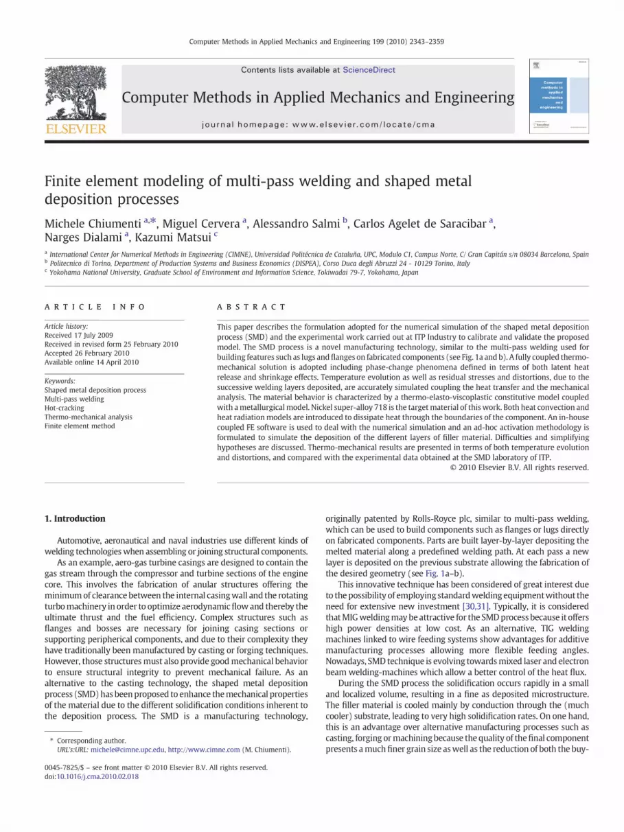
As an example, aero-gas turbine casings are designed to contain thegas stream through the compressor and turbine sections of the enginecore. This involves the fabrication of anular structures offering theminimumof clearance between the internal casingwall and the rotatingturbomachinery in order to optimize aerodynamicflowand thereby theultimate thrust and the fuel efficiency. Complex structures such asflanges and bosses are necessary for joining casing sections orsupporting peripherical components, and due to their complexity theyhave traditionally been manufactured by casting or forging techniques.However, those structuresmust also provide goodmechanical behaviorto ensure structural integrity to prevent mechanical failure. As analternative to the casting technology, the shaped metal depositionprocess (SMD)has beenproposed to enhance themechanical propertiesof the material due to the different solidification conditions inherent tothe deposition process. The SMD is a manufacturing technology,

originally patented by Rolls-Royce plc, similar to multi-pass welding,which can be used to build components such as flanges or lugs directlyon fabricated components. Parts are built layer-by-layer depositing themelted material along a predefined welding path. At each pass a newlayer is deposited on the previous substrate allowing the fabrication ofthe desired geometry (see Fig. 1a–b).

This innovative technique has been considered of great interest dueto thepossibility of employing standardweldingequipmentwithout theneed for extensive new investment [30,31]. Typically, it is consideredthatMIGweldingmaybeattractive for the SMDprocess because it offershigh power densities at low cost. As an alternative, TIG weldingmachines linked to wire feeding systems show advantages for additivemanufacturing processes allowing more flexible feeding angles.Nowadays, SMD technique is evolving towardsmixed laser and electronbeam welding-machines which allow a better control of the heat flux.

During the SMD process the solidification occurs rapidly in a smalland localized volume, resulting in a fine as deposited microstructure.The filler material is cooled mainly by conduction through the (muchcooler) substrate, leading to very high solidification rates. On one hand,this is an advantage over alternative manufacturing processes such ascasting, forging ormachiningbecause the quality of thefinal componentpresents amuchfiner grain size aswell as the reduction of both the buy-

[email protected]

http://www.cimne.com

http://dx.doi.org/10.1016/j.cma.2010.02.018

http://www.sciencedirect.com/science/journal/00457825

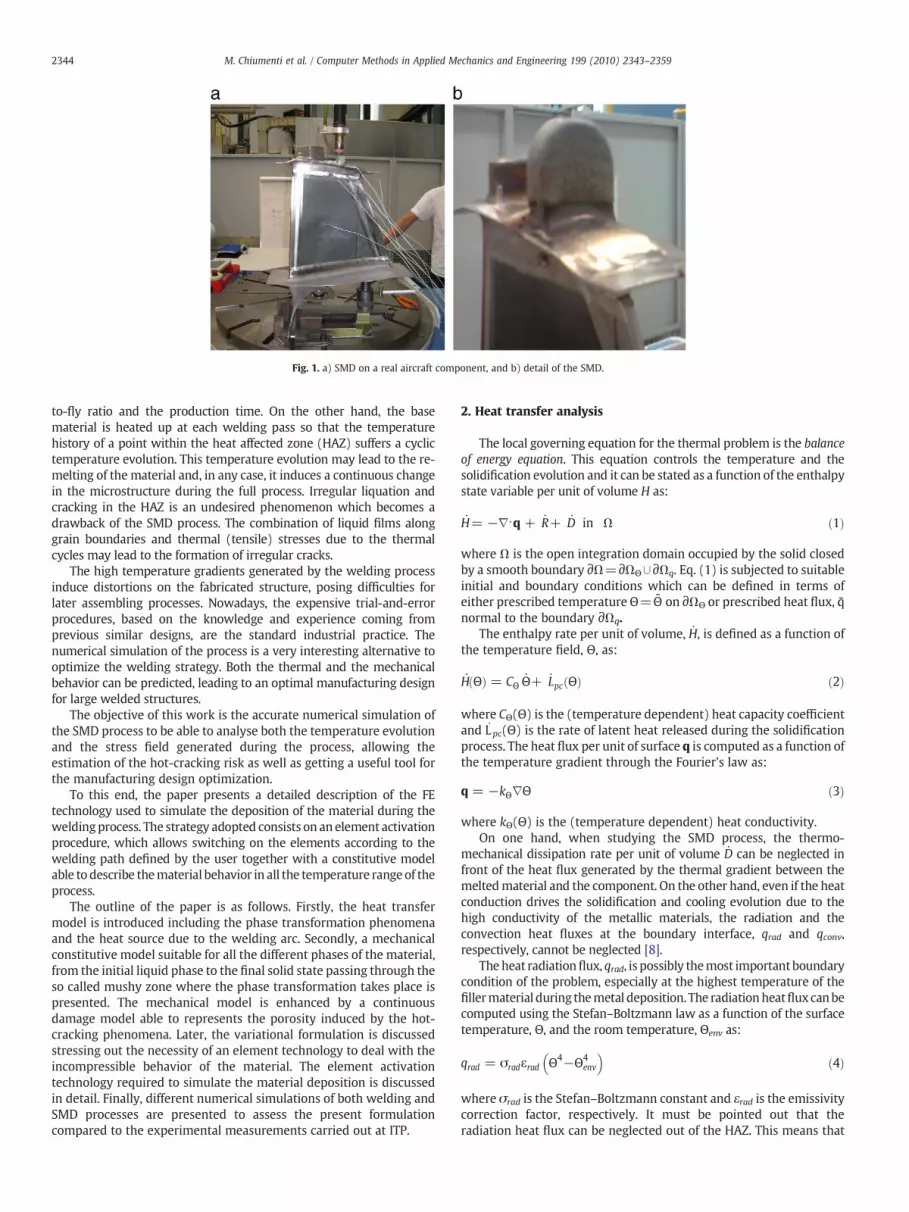
Fig. 1. a) SMD on a real aircraft component, and b) detail of the SMD.

2344 M. Chiumenti et al. / Computer Methods in Applied Mechanics and Engineering 199 (2010) 2343–2359

to-fly ratio and the production time. On the other hand, the basematerial is heated up at each welding pass so that the temperaturehistory of a point within the heat affected zone (HAZ) suffers a cyclictemperature evolution. This temperature evolution may lead to the re-melting of the material and, in any case, it induces a continuous changein the microstructure during the full process. Irregular liquation andcracking in the HAZ is an undesired phenomenon which becomes adrawback of the SMD process. The combination of liquid films alonggrain boundaries and thermal (tensile) stresses due to the thermalcycles may lead to the formation of irregular cracks.

The high temperature gradients generated by the welding processinduce distortions on the fabricated structure, posing difficulties forlater assembling processes. Nowadays, the expensive trial-and-errorprocedures, based on the knowledge and experience coming fromprevious similar designs, are the standard industrial practice. Thenumerical simulation of the process is a very interesting alternative tooptimize the welding strategy. Both the thermal and the mechanicalbehavior can be predicted, leading to an optimal manufacturing designfor large welded structures.

The objective of this work is the accurate numerical simulation ofthe SMD process to be able to analyse both the temperature evolutionand the stress field generated during the process, allowing theestimation of the hot-cracking risk as well as getting a useful tool forthe manufacturing design optimization.

To this end, the paper presents a detailed description of the FEtechnology used to simulate the deposition of the material during theweldingprocess. The strategy adopted consists on an element activationprocedure, which allows switching on the elements according to thewelding path defined by the user together with a constitutive modelable to describe thematerial behavior in all the temperature range of theprocess.

The outline of the paper is as follows. Firstly, the heat transfermodel is introduced including the phase transformation phenomenaand the heat source due to the welding arc. Secondly, a mechanicalconstitutive model suitable for all the different phases of the material,from the initial liquid phase to the final solid state passing through theso called mushy zone where the phase transformation takes place ispresented. The mechanical model is enhanced by a continuousdamage model able to represents the porosity induced by the hot-cracking phenomena. Later, the variational formulation is discussedstressing out the necessity of an element technology to deal with theincompressible behavior of the material. The element activationtechnology required to simulate the material deposition is discussedin detail. Finally, different numerical simulations of both welding andSMD processes are presented to assess the present formulationcompared to the experimental measurements carried out at ITP.

2. Heat transfer analysis

The local governing equation for the thermal problem is the balanceof energy equation. This equation controls the temperature and thesolidification evolution and it can be stated as a function of the enthalpystate variable per unit of volume H as:

H= −∇⋅q + R+ D in Ω ð1Þ

where Ω is the open integration domain occupied by the solid closedby a smooth boundary ∂Ω=∂ΩΘ∪∂Ωq. Eq. (1) is subjected to suitableinitial and boundary conditions which can be defined in terms ofeither prescribed temperature Θ= Θ on ∂ΩΘ or prescribed heat flux, q normal to the boundary ∂Ωq.

The enthalpy rate per unit of volume, H, is defined as a function ofthe temperature field, Θ, as:

H Θð Þ = CΘ Θ+ Lpc Θð Þ ð2Þ

where CΘ(Θ) is the (temperature dependent) heat capacity coefficientand L pc(Θ) is the rate of latent heat released during the solidificationprocess. The heat flux per unit of surface q is computed as a function ofthe temperature gradient through the Fourier's law as:

q = −kΘ∇Θ ð3Þ

where kΘ(Θ) is the (temperature dependent) heat conductivity.On one hand, when studying the SMD process, the thermo-

mechanical dissipation rate per unit of volume D can be neglected infront of the heat flux generated by the thermal gradient between themeltedmaterial and the component. On the other hand, even if the heatconduction drives the solidification and cooling evolution due to thehigh conductivity of the metallic materials, the radiation and theconvection heat fluxes at the boundary interface, qrad and qconv,respectively, cannot be neglected [8].

The heat radiationflux, qrad, is possibly themost important boundarycondition of the problem, especially at the highest temperature of thefillermaterial during themetal deposition. The radiationheatfluxcanbecomputed using the Stefan–Boltzmann law as a function of the surfacetemperature, Θ, and the room temperature, Θenv as:

qrad = σradεrad Θ4−Θ4env

� �ð4Þ

where σrad is the Stefan–Boltzmann constant and εrad is the emissivitycorrection factor, respectively. It must be pointed out that theradiation heat flux can be neglected out of the HAZ. This means that

Fig. 2. Phase diagram for Nickel alloy-718.

2345M. Chiumenti et al. / Computer Methods in Applied Mechanics and Engineering 199 (2010) 2343–2359

its global effect can be accounted for by modifying the efficiencyparameter of the heat source without loss of accuracy in the simulation.

The heat dissipated by convection, qconv, can be estimated usingthe Newton's law, as:

qconv = hconv Θ−Θenvð Þ ð5Þ

where hconv(Θ) is the convection heat transfer coefficient.

3. The phase change transformation

The solidification of the feeding material, once deposited, isdescribed by a liquid-to-solid phase change transformation. The rateof latent heat released during this solidification process can bedescribed using the following latent heat function:

Lpc Θð Þ = Lpc f˙L Θð Þ ð6Þ

where Lpc is the total amount of latent heat released/absorbed duringthe phase-change, fL(Θ)=1− fS(Θ) is the liquid fraction function andfS(Θ) is the solid fraction.

The referencematerial in thiswork is the nickel super-alloy 718. Thismaterial is one of thenickel-base alloys frequently used in the aerospaceindustry, particularly for turbine components, having a combination ofhigh strength at moderate temperatures and a good creep and fatigueresistance. Furthermore thematerial is outstanding regarding oxidationand corrosion resistance features making it well suited for service inextreme environments. In practice, nickel-base alloys have an excellentperformance regarding weldability, particularly for gas-tungsten arc(GTA), plasma-arc or electron-beam welding. This alloy is common ingas turbine blades, lugs, bosses, and combustors, aswell as turbochargerrotors and seals, high temperature fasteners, chemical processing andpressure vessels, heat exchanger tubing, steam generators in nuclearpressurized water reactors and race car exhaust systems.

The solidificationmicrostructure of nickel super-alloy 718 initiatesat the liquidus temperature (1360 °C) by a primary L→γ dendriticreaction, in which the interdendritic liquid is enriched in Nb and C.This reaction is followed by a eutectic type L→γ+MC(NbC, TiC)reaction, which reduces the C content in the interdendritic liquid.These types of carbides frequently solidify intergranularly during longaging times and stress conditions [13]. Finally, at lower values of C/Nbratios, a second eutectic type L→γ+Laves occurs reducing the Nbcontent. At very high cooling rates, the small amount of γ+MCcarbides can be ignored so that the solidification can be represented asa binary eutectic γ/Laves phases [14] as presented in Fig. 2.

Denoting C0 as the nominal alloy composition (Nb) and CL, CS as theinstantaneous liquidus and solidus compositions, respectively, then itis possible to write:

fS CS + fL CL = C0 ð7Þ

and differentiating:

CL−CSð ÞdfS = fS dCS + fL dCL ð8Þ

It is reasonable to assume no solid state diffusion (fSdCS=0) duringthe solidification, especially at the very high cooling rates induced bythe welding (SMD) process, no dendritic branching, and that thethermodynamic equilibrium is maintained at the moving solid/liquidinterface. This given, the alloying element concentration profilebetween the cell core and the interdendritic region can be describedby the Scheil's rule by integrating the above equation:

CL = C0 1−fSð Þ k−1ð Þ ð9Þ

where k=Cs/CL is the partition coefficient, that is, the ratio betweenthe composition of the solid and the composition of the liquid at

equilibrium. As a further hypothesis, it is possible to considerk=const, that is not significantly different from the beginning untilthe end of the solidification, leading to:

CL Θð Þ = C0ΘF−ΘΘF−ΘL

� �; CS Θð Þ = C0

ΘF−ΘΘF−ΘS

� �ð10Þ

where ΘF is the fusion temperature.As a result, it is possible to study the solidification process (Scheil's

rule hypothesis) using the following expression for the solid fractionfunction:

fS Θð Þ = 1− ΘF−ΘΘF−ΘL

� � 1k−1

� �ð11Þ

Observe that fS(ΘL)=0 but fS ΘSð Þ = 1− 1=kð Þ1

k−1

� �≠1 meaning

that there exists an instantaneous solidification of the eutecticconstituent at Θ=ΘS (see Fig. 4). Numerically, this is linearlyregularized within the temperature range ΘS≤Θ≤ΘS+ΔΘ, so that:

fS Θð Þ = 1− ΘF−ΘΘF−ΘL

� � 1k−1

� �for ΘS + ΔΘ≤Θ≤ΘL

fS Θð Þ = 1−fS ΘS + ΔΘð Þ½ �⋅ ΘS−ΘΔΘ

� �+ 1 for ΘS≤Θ≤ΘS + ΔΘ

:

8>>>><>>>>:

ð12Þ

4. The heat source

The source term, Ṙ, which appears in Eq. (1), is one of the keypoints when studying the SMD process. In the literature it is possibleto find different models to represent the welding heat source withdifferent degrees of sophistication.

A first level of complexity, the mathematical model proposed byRosenthal [9] considers a moving heat flux on a 3D geometry. It ispossible to choose a more accurate characterization of the energy inputdefining a Gaussian power distribution for a circular welding pool aspresented by Pavelec et al. in [10]. The double ellipsoidal power densitydistribution presented in [11] by Goldak et al. is the most sophisticatedmodel currently proposed.

There exist technical difficulties from the numerical point of view toadopt such a detailed power distribution. The mesh density generallyused to discretize both the SMDmaterial and the metal sheet below, isnot fine enough to define a complex welding pool shape or a non-uniform heat source. This is only done if the simulation of the weldingpool is the objective itself. If the global structuremust be considered, the

Fig. 3. Scheil's rule and lever rule to describe the solidification evolution.


size of heat source is of the same dimension than the element sizegenerally used for a thermo-mechanical analysis. Therefore, when theglobal model must be taken into account, the resulting mesh density isusually too coarse to represent the actual shape of the heat source [12].

It is important to remark that when the filler material is used in thewelding process, a large percentage of the energy dispensed by thewelding arc is used to melt that material and it is only partiallytransmitted to the base. Experimentally, it can be also observed thatafter melting, the filler material forms a welding pool, which covers thebase material. Due to the over-heating induced by the welding arc, thebase material is also partially melted and the heat convection processgenerated in the welding pool mixes the two materials. Hence, twophasesmay be distinguished: firstly, the filler material dispensed by thefeeding system is heated-up to the melting point and deposited on thebasematerial; later, thewelding pool is further heated,melting the basematerial too.

It can be noted that the numerical model could set the temperatureat the welding pool as the initial temperature of the depositedmaterial.Unfortunately, it is really complex to get an accurate experimental valuefor this temperature because any temperaturemeasurement is distortedby the heat flux of the gas close to the welding arc: approximately10.000 °C. The only accurate input data is the power of the welding arc,which controls the amount of energy introduced into the system.

The welding arc power is defined by the arc voltage, V and thewelding current, I, as:

P= η·VI ð13Þ

where η is the welding efficiency.Hence, when a filler material is used in the welding process, the

definition of a uniform volume heat source seems to be a convenientsolution to heat up the material to be deposited along the weldingpath. Note that this heat source is applied just to the volume depositedwithin the current time step (filler material) and is moving accordingto the metal deposition procedure. Therefore, the simulation strategy,based on finite element discretization, must combine the searchingtechnique used to find out the elements below the welding arctogether with the definition of an impulse thermal loading (the appliedheat source) at each time-increment of the simulation.

The power density, Ṙ, is computed as:

R=P

VMDð14Þ

where VMD is the volume of the SMD layer deposited during thecurrent time-step. In a numerical simulation, this volume depends onthe FE discretization, leading to an approximation error which

increases when coarse meshes are adopted. As an alternative, thevolume of the filler material melted by the feeding system during thesame time-step, Vfeed, is a more convenient choice to be used as areference volume when computing the power density:

R=P

Vfeed=

η·VIVfeed

: ð15Þ

A final feature, to be taken into account, is the thermal expansionthat the material experiences when its temperature increases from theroom temperature to the melting temperature. During the process, thisexpansion is experimented by the wire when it passes through thewelding arc. Later on, the material is deposited and its temperaturedecreases provoking a thermal contraction of the material. In thenumerical model the activated elements are not free to expand duringthe heating phase because their nodes are shared with the layers of thematerial below it. To avoid the generation of spurious thermal stresses,the initial temperature of the elements to be activated is set to themelting (liquid) temperature, ΘL, so that any temperature incrementabove this value does not induce any thermal deformation (see fulldetails in the next section). Consequently, Eq. (15) should be correctedto remove the energy rate which corresponds to the adiabatic tem-perature increment from the room to the melting temperature, that is

Rmelt = CΘ ΘL−Θref

� �=Δt: ð16Þ

For the actual values of the material parameters and the standardsetting of the welding arc, yields Ṙmelt≈2.5% Ṙ, which is negligible ifcompared to the power density of the welding arc.

5. Mechanical analysis

The mechanical problem is governed by the balance of momentumequation. The local form, for the quasi-static problem, can be stated as:find the displacement field, u, for given (prescribed) body forces f,such that:

∇·σ + f = 0 in Ω ð17Þ

where ∇⋅(⋅) is the divergence operator and σ=σ(u) denotes theCauchy stress tensor. Additionally, suitable Dirichlet and Neumannconditions must be supplied on the boundary ∂Ω=∂Ωu∪∂Ωt. In thefollowing, we will assume these in the form of prescribed displace-ments u=ū on ∂Ωu and prescribed tractions t on ∂Ωt.

The stress tensor σ is split into its hydrostatic (pressure) anddeviatoric parts, p = 1

3 tr σð Þ and s=dev(σ), respectively, asσ=p⋅ I+s. This is a very convenient choice to deal with the incompressibilitybehavior, which is a characteristic of the liquid phase or, moregenerally, when the deformations are mainly deviatoric as for theclassical elasto-visco-plastic model defined for a metallic alloy in thefollowing section.

This given, the local form of the continuum mechanical problemcan be stated as: find the displacement field, u, and the pressure field,p(defined as an independent variable of the problem), such that:

∇·s uð Þ + ∇p + f = 0

∇·u−eΘ− pK

= 0in Ω

8<: ð18Þ

where eΘ is the thermal deformationwhich is defined in thenext sectionaccording to the constitutive equation. Note that this mixed u/pformulation of the mechanical problem is equivalent to Eq. (17) and itis valid for both the compressible and incompressible cases. Inparticular, when the material is liquid, no thermal deformation is


allowed (eΘ=0) and the bulk modulus (also referred to as compress-ibility modulus) K→∞ so that Eq. (18)-b enforces the volumetricconstraint as:

∇·u = 0 in Ω: ð19Þ

In the following section it will be detailed the constitutive law forthe stress tensorσ (in terms of p and s, respectively) suitable in all thetemperature range of the process.

6. Mechanical constitutive laws

The mechanical model chosen to simulate the constitutive behaviorof thematerial is based onprevious developments in thefield of coupledthermo-mechanical analysis for casting processes [6–8]. In both castingand welding processes the temperature range varies from roomtemperature to very high temperatures above the melting point. As aconsequence, the material response should vary from an elasto-plasticbehavior when the material is at room temperature to a pure viscousbehavior above themelting point. This evolution can be simulated witha thermo-elasto-visco-plastic constitutive model, which includes bothisotropic hardening and thermal softening. The definition of tempera-ture dependent material properties (the elastic limit among them)allows a gradual contraction of the von Mises yield-surface as thetemperature increases. When the temperature is close to the meltingpoint, the viscous behavior becomes more and more predominant, theelastic limit gradually reduces, vanishing when liquidus temperature isreached. As a result, a purely viscous (Norton-Hoff) model is recoveredwhen liquid-likebehaviormustbe simulated.Hence, the transition fromthe solid phase to the liquid-like behavior is driven by the temperaturedependency of the material properties and can be forced during thephase change transformation according to the solid fraction function.

6.1. Solid state (ΘbΘS)

The material behavior in all the temperature range below thesolidus temperature is characterized by a thermo-elasto-visco-plasticconstitutive model. The total strain tensor is the driven variable of themechanical problem computed in terms of the displacement field as:ε=∇S(u). The constitutive model can be written as:

p = K ∇·u−εΘ� �

s = 2Gdev ε−εvp�

(ð20Þ

where G(Θ) is the (temperature dependent) shear modulus and K(Θ)is the (temperature dependent) bulk modulus which controls thematerial compressibility.

The thermal deformation (a volumetric term), εΘ, is computedadding the thermal shrinkage characteristic of the change of phase,εpc, to the thermal contraction during the cooling process from thesolidus to room temperature, εcool(Θ), as follows:

εΘ Θð Þ = εcool Θð Þ + εpc ð21Þ

where εpc and εcool(Θ) are computed as:

εpc =ΔVpc

V0=

ρS−ρLρS

εcool Θð Þ = 3 α Θð Þ Θ−Θref

� �−α Θ0ð Þ Θ0−Θref

� �h i8>><>>: ð22Þ

where α(Θ) is the (temperature dependent) thermal expansioncoefficient while ρS=ρ(ΘS) and ρL=ρ(ΘL) are the material density atsolidus and liquidus temperature, respectively. The equation used tocompute εpc can be deduced from the principle of mass conservation

introducing the volume shrinkage, ΔVpc, induced by the change ofdensity during the solidification.

The constitutive model considers a temperature dependent J2-yield-surface Φvp(s, q, Θ) defined as:

Φvp s; q;Θð Þ = ∥s∥−R q;Θð Þ≤0 ð23Þ

where R(q, Θ) is the (temperature dependent) yield-surface radiusdefined as:

R q;Θð Þ =ffiffiffi23

rσ0 Θð Þ−q½ �: ð24Þ

The visco-plastic strain tensor (purely deviatoric term), εvp, togetherwith the evolution laws for the isotropic strain-hardening variable ξ, arederived from the principle of maximum plastic dissipation as [17]:

εvp

= γvp ∂Φvp s; q;Θð Þ∂s = γvpn

ξ= γvp ∂Φvp s; q;Θð Þ∂q = γvp

ffiffiffi23

rð25Þ

where n = s∥s∥ and γvp = ⟨Φ

vp s; q;Θð Þη ⟩ are the normal to the yield

surface and the visco-plastic multiplier, respectively, when a rate-dependent evolution law is assumed.

The stress-like variable, q, conjugate to the isotropic strain-hardening variable ξ, is computed as:

q = − σ∞−σ0½ � 1− exp δξð Þ½ �−Hξ ð26Þ

where H and δ are the coefficients which control the linear and theexponential isotropic hardening laws, respectively. σ∞=σ∞(Θ) andσ0=σ0(Θ) are the (temperature dependent) saturation and initialflow stress (elastic limit) parameters, respectively [15].

6.2. Mushy state (ΘSbΘbΘL)

In this temperature range the material transforms from liquid tosolid or vice-versa. The material behavior can be controlled using thesolid fraction function: in the limit case, when fS(ΘS)=1, the modelshould return to the thermo-elasto-visco-plastic model proposed forthe solid phase. On the other hand, when fS(ΘL)=0 the purely viscousbehavior is expected. This transition can be achieved modifying theequations that characterize the solid phase model as follows [6,7]. Theconstitutive model can be written as:

p = K ∇·u−εΘ� �

s = 2 G dev ε−εvp�

8><>: ð27Þ

where K Θð Þ = K Θð ÞfS Θð Þ is a modified bulk modulus which controls the

material compressibility. On one hand, when fS(ΘL)=0 no thermaldeformations are allowed and the incompressible behavior is recovered,as ∇⋅u=0. On the other hand, G Θð Þ = G Θð Þ

fS Θð Þ is a modified shear

modulus, which leads, in the limit case, to a rigid-viscoplastic behaviorfor the liquid-like state.

The thermal deformation, εΘ, is computed considering theevolution the thermal shrinkage during the change of phase, εpc(Θ) as:

εΘ Θð Þ = εpc Θð Þ = ρ Θð Þ−ρLρS

ð28Þ


where ρ(Θ) is the (temperaturedependent) density. Observe thatwhenΘ=ΘL the thermal deformation vanishes.

Finally, the model introduces a J2-yield-surface where the (temper-ature dependent) yield-surface radius R(q,Θ) vanishes according to thesolid fraction evolution, as:

R q;Θð Þ = fS Θð Þffiffiffi23

rσ0 Θð Þ−q½ � ð29Þ

This is the generalization of Eq. (24) which enforces a rigid-viscoplastic behavior when the material is liquid while restoring thestandard elasto-viscoplastic model when the material solidifies.

6.3. Liquid-like state (ΘNΘL)

In this case, the material behavior is characterized by a purelyviscous (Norton-Hoff) model which can be written as:

∇·u = 0s = η εvp

�ð30Þ

According to this model, the deviatoric part of the stress tensor iscomputed as a function of the visco-plastic strain-rate and the(temperature dependent) viscosity parameter, η(Θ). Eq. (30)-acorresponds to Eq. (20)-a when the material is liquid (K→∞, andeΘ=0). Observe that no volumetric deformations are allowed abovethe liquidus temperature (the material is incompressible) so thatEq. (30)-a represents the continuity equation for mass conservation.Finally, as neither thermal deformations exist nor elastic strains candevelop (G→∞), the viscoplastic strain rate corresponds to the totalstrain rate and the deviatoric part of the stress tensor is computed as:

s = η ε ð31Þ

7. Hot cracking

Intergranular liquation and cracking in the weld heat affected zone(HAZ) is a phenomenon encountered in several alloy systems. Thecombination of liquid films along grain boundaries and thermal tensilestresses induced by the thermal deformations during the thermal cyclesof the SMD process may lead to the formation of irregular cracks.

In the nickel super-alloy 718 the formation of liquid films has beenattributed to the liquation of MC-carbides and Laves phase. When thealloy is rapidly heated to a temperature above the binary eutectictemperature, theremaybe insufficient time for the complete dissolutionof the Laves phase and a liquid film is generated to later re-solidify inaccordance with the phase diagram requirements. If tensile stressesdevelop the risk of cracking is high [23].

The prediction of the hot cracking phenomena is a very challengingtask from the computational point of view [24]. In fact, it is very difficultto correlate the evolution of the metallurgy with the macro-phenom-enological model presented in the previous section. The metallurgicalscale ismuchsmaller than themacro scalewhere the FEmesh is defined.The level of definition of the FEmesh usually adopted for the numericalsimulation of the SMD process is insufficient to consider such complexmaterial behavior and the time scale which should be used to study themicrostructure kinetics is incompatible with the one used in anindustrial simulation. Both temperature gradients, and phase changeevolution can be captured only in terms of thermal shrinkage and latentheat release and in many cases the non-linearity induced by suchphenomena should require a much finer mesh and time-steppingselection too.

In thiswork analternative approach is adopted. Themodel proposedis based on macroscopic quantities such as strains, stresses andtemperature fields (see [12]) which are the natural output of thethermo-mechanical simulation of the SMD process. The proposed

methodology consists of computing a damage induced porosity in themushy zone according to the solid fraction evolution in the temperaturerange ΘE≤Θ≤ΘS, that is, between the eutectic temperature, ΘE (whenthe Laves solidify at the end of the segregation process) and the solidtemperature, ΘS (when the matrix solidifies). Within this temperaturerange, the macroscopic model proposed for the mushy phase behaviormust account for the shrinkage of the material induced by the phasechange. This thermal deformation is volumetric and conventionalmodels such as the one proposed in the previous section do not accountfor plastic volumetric change because it assumes a von Mises visco-plastic (deviatoric) behavior.

To overcome this, the constitutivemodel is enhancedwith a damageinduced porosity behavior including the effects of the drastic volumechanges of the phase transformation shrinkage.

A vonMises based visco-plastic model does not pose any restrictionto the hydrostatic stress (pressure) limit neither for compression nor fortensile stresses [27]. The objective of the hot-cracking model is toprevent from an excessive (tensile) stress level when the material, stillpartially liquid, contracts (shrinkage) but all the surrounding phase hassolidified.

The present work makes use of a continuum damage model tocharacterize the porosity formation. In particular, a damage index (hotcracking risk indicator), d, is introduced as one scalar internal variableleading to a simple constitutive model which, nevertheless, is able toreproduce the overall non-linear behavior including stiffness degrada-tion and hot tearing phenomena. The constitutive equation used tocompute the pressure field, within the temperature range ΘE≤Θ≤ΘS,results in:

p = 1−dð Þ K ∇·u−εpc�

= 1−dð Þp ð32Þ

where, p=K(▽∙u−εpc), is the effective pressure, that is, the value ofthe pressure for the undamaged state of the material [28].

The damage criterion, Φ, is introduced as:

Φ p; rð Þ = p−r≤0: ð33Þ

Variable r is an internal stress-like variable,which can be interpretedas the current damage threshold, in the sense that its value controls thesize of the (monotonically) expanding damage surface: ṙ≥0. The initialvalue of the damage threshold is r0=p0, where p0 is the pressurethreshold for the undamaged material.

Theevolutionof thedamagebounding surface, for loading, unloadingand reloading conditions, is controlled by the Kuhn-Tucker relations:

r≥0

Φ p; rð Þ≤0

rΦ p; rð Þ = 0

→

Loading :

r≥0 Φ p; rð Þ = 0

Unloading and reloading : r= 0 Φ p; rð Þ≤0:

8>>><>>>:

ð34Þ

The consistency condition, ṙΦ(p, r)=0, together with Eq. (32) isused to obtain an explicit definition of the current value of the damagethreshold in the form [29]:

r = max r0;max p–ð Þf g ð35Þ

This given, if the pN r, the damage threshold is updated to r=p andthe damage index d=d(r) is updated accordingly as:

d rð Þ = r−r0r

: ð36Þ

Observe that the damage variable is only allowed to monotonicallyincrease ḋ≥0 and it can vary within the range 0≤d≤1: hence d=1means 100% hot-cracking risk.


8. Variational formulation

The solution of the coupled thermo-mechanical problem consistsof enforcing the weak forms of either the balance of energy equationor the balance of momentum equation. This means integrating bothEqs. (1) and (18) over the domainΩ together with the correspondingDirichlet and Neumann boundaries conditions on ∂Ω.

Consequently, the weak form associated to the energy balanceequation, which solves the thermal problem, takes the followingexpression [6,7]:

δϑ; CΘ Θ+ Lpc� �

+ ∇ δϑð Þ; kΘ∇Θð Þ = δϑ; R� �

+ δϑ; qrad + qconvð Þ∂Ω ∀δϑ

ð37Þ

where δϑ are the test functions associated to the temperature field, Θ,while (⋅, ⋅) denotes the inner product in L2(Ω).

It is important to remark that the SMD process induces extremelyhigh temperature gradients along the welding path in the heat-affected zone. From the numerical point-of-view such temperaturegradients can provoke unrealistic temperature overshots and under-shots especially if coarse meshes and large time-steps are used. In thiswork, the problem has been avoided adopting a nodal (Lobatto)integration rule, which stabilizes the solution introducing a smallnumerical diffusivity into the heat conduction problem [6,7].

The weak form of the balance of momentum equation can bestated as:

δv; ∇·sð Þ + ∇· δvð Þ; pð Þ = δv; fð Þ + δv; t–� �

∂Ωt

∀δv

δq; ∇·uð Þ− δq; eΘ� �

− δq;pK

� �= 0 ∀δq

8><>: ð38Þ

where δv and δq are the variations of the displacement and pressurefield, respectively.

Observe that both the J2-plasticity (solid model) and the purelyviscous behavior (liquid model) generate only deviatoric deforma-tions (isochoric response) leading to possible locking problems.Recent works of the authors in the field of incompressibility in solidmechanics [16–19] show the necessity of an ad-hoc finite elementtechnology. The mixed variational formulation proposed, uses lineardisplacements and pressure interpolations, leading to robust trian-gular or tetrahedral elements suitable for large-scale computation ofconstrained media problems. The orthogonal sub-grid scale approach[20,21] is assumed as an attractive alternative to circumvent theBabuska-Brezzi stability condition [22]. When meshing with hexahe-dral elements, the B-bar method or the equivalent Q1/P0 elementtechnology is an alternative formulation to deal with this problem.

9. Time integration of the coupled problem

The numerical solution of the coupled thermo-mechanical prob-lem (Eqs. (37) and (38)) involves the transformation of an infinitedimensional transient system into a sequence of discrete non-linearalgebraic problems. This can be achieved by means of a Galerkin finiteelement projection and a time-marching scheme for the advancementof the primary nodal variables, displacements, pressure and tempera-tures, together with a return mapping algorithm to update of theinternal variables.

With regard to the time stepping scheme different strategies arepossible, but they can be grouped in two categories: simultaneous(monolithic) solution and staggered (block-iterative or fractional-step) time-stepping algorithms.

In this work a staggered solution has been chosen. A productformula algorithm has been introduced leading to a time-integrationscheme in which the two sub-problems (thermal andmechanical) aresolved sequentially, within the framework of classical fractional stepmethods [6,7]. As a result, the original coupled problem is split intotwo smaller and typically symmetric partitions allowing the use ofany integration technique originally developed for the uncoupled sub-problems.

The final result is an accurate, efficient and robust numericalstrategy, which allows the numerical simulation of large coupledthermo-mechanical problems such as the multi-pass welding and theSMD processes.

10. FE modeling of the SMD process

The shaped metal deposition (SMD) process is a weldingtechnology in which the filler material is melted and depositedlayer-by-layer. From the numerical point of view, the simulation ofthe SMD process requires an ad-hoc finite element activationtechnology able to reproduce the deposition of the melted materialalong the welding path. In the literature two different approacheshave been used to simulate the multi-pass welding, referred to asquiet elements and born-dead elements techniques [1–5].

The first approach considers that all the elements of the meshdefining the successive welding layers, whichwill be deposited duringthe process simulation, are included into the initial computationalmodel. These elements are made passive (quiet) by setting materialproperties which do not affect the rest of the model (penalization).Very low values for both the stiffness and heat conductivity areconsidered until the welding layer is used. Later on, according to themetal deposition process, the elements can be activated, meaning thattheir real thermo-physical properties are re-established. There aredifferent drawbacks to be taken into account: firstly, the simulationprocess is performed assembling all the elements and solving the fullsystem of equations leading to a very high computational cost.Secondly, the penalization of the material properties of the passiveelements induces an ill-conditioning of the solutionmatrixwhichmaycause numerical problems for its solution such as a reduction of theconvergence ratio of iterative solvers. Finally, fictitious strains andtemperature gradients in the quiet elements are accumulated andthey will be transformed into spurious stresses and heat fluxes whenthese elements are activated. On the other hand, the implementationis straightforward.

The simulation strategy adopted in this work to deal with the SMDprocess consists of an ad-hoc activation process based on the so calledborn-dead elements technique. This activation strategy classifies theelements defined in the original finite element mesh into: active,inactive and activated elements. The active elements (e.g. the meshwhich define the base material) are computed and assembled into theglobal matrix. On the other hand, the inactive elements, such as theentire discretized domain where the welding path is defined, are notassumed as part of the model: they have been generated but do notplay any role in the computational model. At each time-step a numberof elements (activated elements) are switched on according to thedeposition of the filler material along the welding-path defined by theuser. Only active and activated elements are assembled into thesolution model.

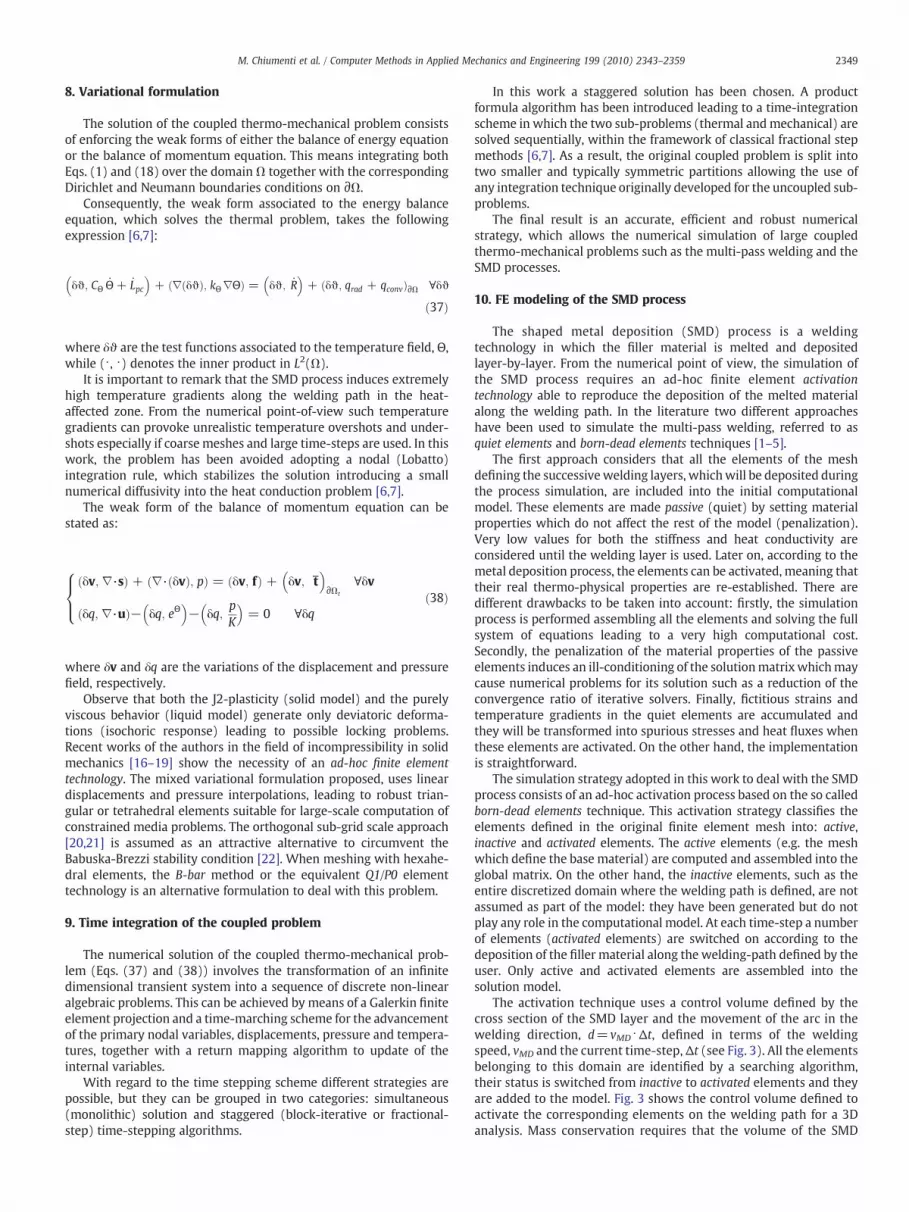
The activation technique uses a control volume defined by thecross section of the SMD layer and the movement of the arc in thewelding direction, d=vMD ⋅Δt, defined in terms of the weldingspeed, vMD and the current time-step, Δt (see Fig. 3). All the elementsbelonging to this domain are identified by a searching algorithm,their status is switched from inactive to activated elements and theyare added to the model. Fig. 3 shows the control volume defined toactivate the corresponding elements on the welding path for a 3Danalysis. Mass conservation requires that the volume of the SMD

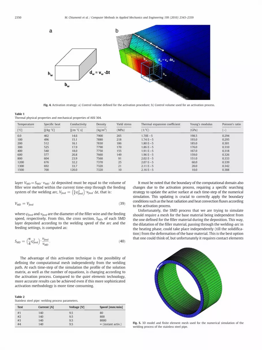
Fig. 4. Activation strategy: a) Control volume defined for the activation procedure; b) Control volume used for an activation process.

Table 1Thermal physical properties and mechanical properties of AISI 304.

Temperature Specific heat Conductivity Density Yield stress Thermal expansion coefficient Young's modulus Poisson's ratio

[°C] [J/kg °C] [J/m °C s] (kg/m3) (MPa) (1/°C) (GPa) (–)

0.0 462 14.6 7900 265 1.70E−5 198.5 0.294100 496 15.1 7880 218 1.74 E−5 193.0 0.295200 512 16.1 7830 186 1.80 E−5 185.0 0.301300 525 17.9 7790 170 1.86 E−5 176.0 0.310400 540 18.0 7750 155 1.91 E−5 167.0 0.318600 577 20.8 7660 149 1.96 E−5 159.0 0.326800 604 23.9 7560 91 2.02 E−5 151.0 0.3331200 676 32.2 7370 25 2.07 E−5 60.0 0.3391300 692 33.7 7320 21 2.11 E−5 20.0 0.3421500 700 120.0 7320 10 2.16 E−5 10.0 0.388


layer VMD=SMD ⋅vMD ⋅Δt deposited must be equal to the volume offiller wire melted within the current time-step through the feedingsystem of the welding arc, Vfeed = π

4φ2feed

� �⋅vfeed⋅Δt, that is:

VMD = Vfeed ð39Þ

where φfeed and vfeed are the diameter of the filler wire and the feedingspeed, respectively. From this, the cross section, SMD, of each SMDlayer deposited according to the welding speed of the arc and thefeeding settings, is computed as:

SMD =π4φ2feed

� �⋅vfeedvMD

: ð40Þ

The advantage of this activation technique is the possibility ofdefining the computational mesh independently from the weldingpath. At each time-step of the simulation the profile of the solutionmatrix, as well as the number of equations, is changing according tothe activation process. Compared to the quiet elements technology,more accurate results can be achieved even if this more sophisticatedactivation methodology is more time consuming.

Table 2Stainless steel pipe: welding process parameters.

Test Current [A] Voltage [V] Speed [mm/min]

#1 140 9.5 80#2 140 9.5 800#3 140 9.5 8000#4 140 9.5 ∞ (instant activ.)

It must be noted that the boundary of the computational domain alsochanges due to the activation process, requiring a specific searchingstrategy to update the active surface at each time-step of the numericalsimulation. This updating is crucial to correctly apply the boundaryconditions suchas theheat radiationandheat convectionfluxes accordingto the activation process.

Unfortunately, the SMD process that we are trying to simulateshould require a mesh for the base material being independent fromthe one defined for the filler material during the deposition. This way,the dilatation of the filler material, passing through the welding-arc inthe heating phase, could take place independently (till the solidifica-tion) from the deformation of the basematerial. This is the best optionthat one could think of, but unfortunately it requires contact elements

Fig. 5. 3D model and finite element mesh used for the numerical simulation of thewelding process of the stainless steel pipe.

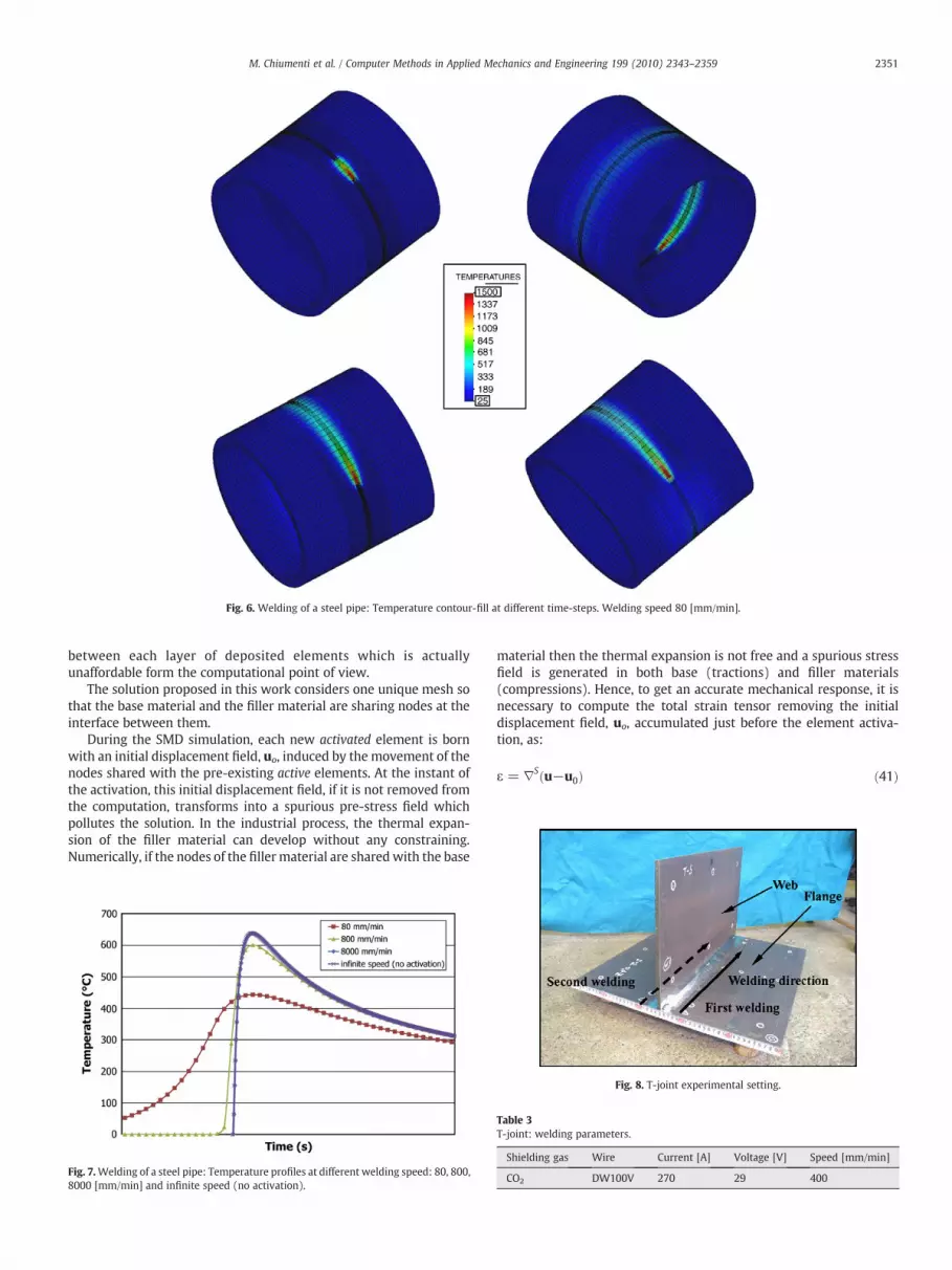
Fig. 6. Welding of a steel pipe: Temperature contour-fill at different time-steps. Welding speed 80 [mm/min].


between each layer of deposited elements which is actuallyunaffordable form the computational point of view.

The solution proposed in this work considers one unique mesh sothat the base material and the filler material are sharing nodes at theinterface between them.

During the SMD simulation, each new activated element is bornwith an initial displacement field, uo, induced by the movement of thenodes shared with the pre-existing active elements. At the instant ofthe activation, this initial displacement field, if it is not removed fromthe computation, transforms into a spurious pre-stress field whichpollutes the solution. In the industrial process, the thermal expan-sion of the filler material can develop without any constraining.Numerically, if the nodes of the filler material are sharedwith the base

Fig. 7.Welding of a steel pipe: Temperature profiles at different welding speed: 80, 800,8000 [mm/min] and infinite speed (no activation).

material then the thermal expansion is not free and a spurious stressfield is generated in both base (tractions) and filler materials(compressions). Hence, to get an accurate mechanical response, it isnecessary to compute the total strain tensor removing the initialdisplacement field, uo, accumulated just before the element activa-tion, as:

ε = ∇S u−u0ð Þ ð41Þ

Fig. 8. T-joint experimental setting.

Table 3T-joint: welding parameters.

Shielding gas Wire Current [A] Voltage [V] Speed [mm/min]

CO2 DW100V 270 29 400

Table 4T-joint: thermal and mechanical temperature-dependent properties.

Fig. 9. T-joint welding: 3D model and FE mesh for the T-joint simulation.

Fig. 10. T-joint welding: temperature field in a cross section using: a) Clo


11. Numerical simulations

11.1. Welding process for a stainless steel pipe

The aim of this first simulation is to assess the accuracy of themodel implemented with special regard to the element activationtechnology proposed. The welding data, the process parameters, aswell as the material characterization have been obtained from theexperimental setting described in [25]. A Gas Tungsten Arc Welding(GTAW) process is used in the experiments. This welding technologyconsists of an electric arc between a non-consumable tungstenelectrode and the work-piece. The filler metal used is an AISI304stainless steel wire. Argon gas is used to prevent oxidation in the weldzone. The work-piece consists of an AISI304 stainless steel pipe withan outer diameter of 114.5 [mm], 6 [mm] thick and 100 [mm] long.

The thermo-physical properties used to characterize both thestainless steel pipe and the filler material are shown in Table 1.Different analyses have been performed considering the same energyinput but different welding speeds (see Table 2). The efficiency of thewelding arc has been set to 70%.

For symmetry reasons, a 3Dmodel of one half of the pipe to be jointedas well as half of the filler material deposited has been considered for

se (Lobatto) integration rule; and b) Open (Gauss) integration rule.

Fig. 11. T-joint welding: temperature evolution at two different locations.

Fig. 13. T-joint welding: Temperature comparison with the experimental result.


the numerical simulation model. A finite element mesh with 10.880hexahedrical elements and 14.000 nodes (see Fig. 5) has been used.

The first simulation has been carried out considering an instan-taneous activation of all the elements which correspond to the fillermaterial. This hypothesis is equivalent to an infinite welding speed.Moreover, three analyses have been performed using the activationtechnology proposed in this work, assuming different weldingspeeds: 80, 800 and 8000 [mm/min], respectively. Fig. 6 shows thetemperature contour-fill at different time-steps of the simulation for awelding speed of 80 [mm/min].

Fig. 7 shows the resulting temperature evolution curves at thesame location of the thermo-couple for each welding speedconsidered. It is important to remark that the curve obtained for8000 [mm/min] exactly matches the one obtained considering aninfinite welding speed. This means that the activation technologyproposed is able to introduce into the model exactly the same energyinput which correspond to an instantaneous activation where all theelements belonging to the filler material are active from the beginningof the simulation and the corresponding energy input assigned.

This test proves that at lower welding speed, it is really necessaryto adopt a numerical strategy to simulate the metal deposition step-by-step. The Péclet number Pe = hv

α , can be used to decide when it ismandatory to consider the activation strategy. The Péclet number is adimensionless quantity that compares thermal advection (for SMDcase v is the welding speed and h is the characteristic length of theproblem, e.g. the thickness of the pipe) with respect to thermaldiffusivity, α=kΘ/CΘ (where kΘ is the thermal conductivity and CΘ the

Fig. 12. T-joint welding: locations of the thermo-couples.

heat capacity). Substituting the corresponding data it is possible toconclude that for:

• PeN50. The activation strategy is not necessary: instantaneousactivation process gives an accurate response;

• 6bPeb50. In this range the instantaneous activation process showsan error lower than 15%.

• Peb6. It is necessary to model the SMD including the elementactivation process according to the welding speed.

11.2. Double-pass welding for a T-joint

The second FE simulation proposed, consists of a fully coupledthermo-mechanical analysis showing the accuracy of the numericalmodel proposed in terms of both thermal and mechanical model.

The process consists of a fillet-welded T-joint where two weldingpasses, one at each side, are performed to join the flange to the web.

Fig. 14. T-joint welding : a) Deformed shape of the T-joint; b) Vertical deflections at 6different locations of the transversal section along the flange: comparison betweennumerical and experimental results.

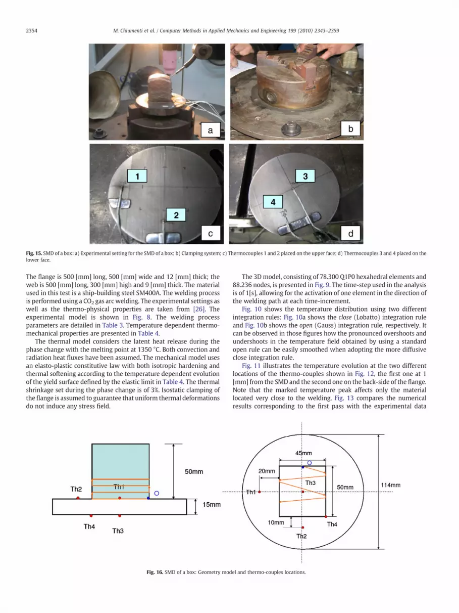
Fig. 15. SMD of a box: a) Experimental setting for the SMD of a box; b) Clamping system; c) Thermocouples 1 and 2 placed on the upper face; d) Thermocouples 3 and 4 placed on thelower face.


The flange is 500 [mm] long, 500 [mm] wide and 12 [mm] thick; theweb is 500 [mm] long, 300 [mm] high and 9 [mm] thick. The materialused in this test is a ship-building steel SM400A. The welding processis performed using a CO2 gas arc welding. The experimental settings aswell as the thermo-physical properties are taken from [26]. Theexperimental model is shown in Fig. 8. The welding processparameters are detailed in Table 3. Temperature dependent thermo-mechanical properties are presented in Table 4.

The thermal model considers the latent heat release during thephase change with the melting point at 1350 °C. Both convection andradiation heat fluxes have been assumed. The mechanical model usesan elasto-plastic constitutive law with both isotropic hardening andthermal softening according to the temperature dependent evolutionof the yield surface defined by the elastic limit in Table 4. The thermalshrinkage set during the phase change is of 3%. Isostatic clamping ofthe flange is assumed to guarantee that uniform thermal deformationsdo not induce any stress field.

Fig. 16. SMD of a box: Geometry mod

The 3Dmodel, consisting of 78.300 Q1P0 hexahedral elements and88.236 nodes, is presented in Fig. 9. The time-step used in the analysisis of 1[s], allowing for the activation of one element in the direction ofthe welding path at each time-increment.

Fig. 10 shows the temperature distribution using two differentintegration rules: Fig. 10a shows the close (Lobatto) integration ruleand Fig. 10b shows the open (Gauss) integration rule, respectively. Itcan be observed in those figures how the pronounced overshoots andundershoots in the temperature field obtained by using a standardopen rule can be easily smoothed when adopting the more diffusiveclose integration rule.

Fig. 11 illustrates the temperature evolution at the two differentlocations of the thermo-couples shown in Fig. 12, the first one at 1[mm] from the SMD and the second one on the back-side of the flange.Note that the marked temperature peak affects only the materiallocated very close to the welding. Fig. 13 compares the numericalresults corresponding to the first pass with the experimental data

el and thermo-couples locations.

Fig. 17. SMD of a box: a) FE mesh used in the analysis; b) Temperature contour-fill at the end of the SMD process.


available in [26]. The agreement is remarkably good. Fig. 12 shows anasymptotic value for the temperature field for both the numerical andthe experimental results. This is just because the cooling phase in thesimulation should be much longer to let the temperature decrease tothe room value. Unfortunately, the cooling phase is governed by theenvironment heat transfer coefficient which is a quite smallparameter. As a result the heat evacuated through the boundaries isnot enough to cool down the T-join as fast as expected.

The accuracy of themechanical analysis is assessed by comparing theangular distortionsof theflangewith theexperimentalmeasures. Fig. 14ashows the distorted shape of the T-joint obtained with the FE analysis.This shape is not symmetric due to the different plastic deformation fieldinduced by the temperature field. Fig. 14b shows the comparisonbetween the vertical deflections at 6 different locations of the transversalsection along the flange. The agreement is very good also in this case.

Fig. 18. Temperature dependent material

11.3. Shaped metal deposition of a box

Tovalidate andcalibrate thenumericalmodel presentedwhenaSMDprocess is considered, a large number of experimental tests have beencarried out at ITP Industry (Industria de Turbo Propulsores, SA, Spain).

A Gas Tungsten Arc Welding (GTAW) is used to melt the fillermaterial. The experimental setting is shown in Fig. 15a. Both the basematerial and the filler material (wire) is nickel super-alloy 718. Theclamping system used to retain the plate has been designed toguarantee that uniform thermal distortions can develop withoutinducing any stress fields (see Fig. 15b).The temperature evolution isrecorded by four thermocouples as shown in Fig. 15c and d.

The geometrical modeling consists of two different parts: the baseplate and the metal deposition material, which is activated accordingto the givenwelding path (see Fig. 16). The base plate has a cylindrical

properties for nickel super-alloy 718.

Fig. 20. SMD of a box: Hot cracking risk indicator.

Fig. 19. SMD of a box: Comparison between numerical and experimental results at the 4thermocouples locations.


shape 15 [mm] high and with a diameter of 114[mm] while the SMDarea is defined by a rectangular shape 45 [mm] long and 50 [mm]widewhich will grow according to the SMD process up to the final height of50 [mm].

A finite elementmesh for the 3Dmodel consists of 6.114 hexahedralelements and 6.496 nodes (see Fig. 17a). The analysis considers 10 time-steps for each layer activated, that is, 400 time-steps.

The material properties used for this analysis are confidential. Thematerial behavior modeled is nickel super-alloy 718 in all thetemperature range varying from room to the melting temperature.

Fig. 21. 10-Layers SMD test: a) Experimental setting

Fig. 18 shows the temperature dependency of some of the mostcharacteristic material properties within the temperature rangeconsidered in this simulation. The thermal model considers a latentheat release during the phase change with the melting point at1335 °C. Both convection and radiation heat fluxes have been takeninto account in this analysis.

Fig. 17b shows the temperature contour-fill at the end of thedeposition, just before the cooling phase.

The comparison between numerical and experimental results ispresented in Fig. 19 where it is possible to appreciate the goodagreement achieved, assessing the accuracy of the numerical modelproposed.

Fig. 20 shows the hot cracking risk indicator computed accordingto the damage model proposed in this work.

11.4. 10 layer SMD process

The second SMD test case is intended to assess the accuracy ofproposedmethodwhen a fully coupled thermo-mechanical analysis isapplied to predict both the temperature evolution and the distortionof the structure.

The experimental setting is shown in Fig. 21a: it consists of arectangular base plate 275 [mm] long, 100 [mm] wide and 12 [mm]thick. The SMD process consists of 2 pre-heating passes (no feed-ing material is used) followed by the deposition of 10 layers ofmaterial.

An isostatic clamping of the base plate is assumed to avoid anystress concentration induced by the thermal deformation of the plate(see Fig. 21b).

The material used is nickel super-alloy 718. The welding arc andwelding efficiency are set out as in the previous case.

The finite element model consists of 54.862 Q1/P0 hexahedralelements and 34,012 nodes (Fig. 22b).

Fig. 23b–d compares the temperature evolution at the differentthermocouple locations as shown in Fig. 23a.

Fig. 24 shows the Z-displacement field achieved by the analysisafter the cooling phase. The comparison between experiment andnumerical results for a transversal and a longitudinal section arepresented in Figs. 25 and 26, respectively [10]. It is possible to observehow numerical results underestimate the deflection. One possiblereason is the kinematic adopted. Most probably when using a large-strain formulation the results will look better but on the other handthis formulation is too expensive from the computational point ofview when running industrial cases.

Finally, Fig. 27 compares the residual stress field at three differentlocations of the strain-gauges. Hole drilling method has been used toobtain the residual stresses at the different locations. J2 von Mises

for the 10 layers SMD test; b) Clamping system.

Fig. 22. 10-Layers SMD test: a) Cross section for the 10-layers SMD process; b) FE mesh used for the numerical simulation of the 10-layers SMD process.


stress indicator has been chosen to check the full stress tensorbehavior. Fig. 27 shows a 10% as average error between theexperimental and the numerical results.

An overall good accuracy of the numerical model proposed can beobserved.

12. Conclusions

This work presents the strategy adopted for the numericalsimulation of the SMD processes. A coupled thermo-mechanicalframework for the solution of both the energy and momentumbalance equations is presented. The appropriate definition of theenergy input is discussed when a filler material is used in the welding

Fig. 23. 10-Layers SMD test: a) Thermocouples location; b) Comparison between numericad) Thermocouples 2 and 6.

process. A smooth transition model able to describe the materialbehavior when the material transforms from liquid (purely viscous)to solid (elasto-plastic) has been presented as an original contributionof this work. Later on, a damage induced porosity model has beenintroduced to put a limitation to the tensile volumetric strength of thematerial leading to a hot cracking risk index depending on the phasechange shrinkage during the solidification process. The activationprocedure to simulate the SMD process along the welding path is alsodiscussed and validated. Later, a number of SMD tests-cases have beencarried out at ITP industry. It has been possible to register both thetemperature evolution during the full process and the residualstresses after cooling. Distortions have been also measured to becompared with the results achieved by the numerical model. The

l and experimental results for thermocouples 1 and 4; c) Thermocouples 3 and 5; and

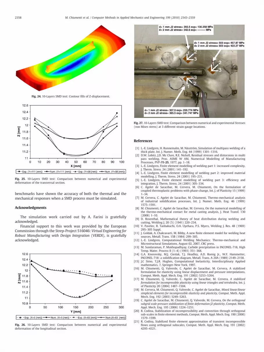
Fig. 25. 10-Layers SMD test: Comparison between numerical and experimentaldeformation of the transversal section.

Fig. 27. 10-Layers SMD test: Comparison between numerical and experimental Stresses(von Mises stress) at 3 different strain-gauge locations.

Fig. 24. 10-Layers SMD test: Contour fills of Z-displacement.


benchmarks have shown the accuracy of both the thermal and themechanical responses when a SMD process must be simulated.

Acknowledgments

The simulation work carried out by A. Farini is gratefullyacknowledged.

Financial support to this work was provided by the EuropeanCommission through the Strep-Project 516046: Virtual Engineering forRobust Manufacturing with Design Integration (VERDI), is gratefullyacknowledged.

Fig. 26. 10-Layers SMD test: Comparison between numerical and experimentaldeformation of the longitudinal section.

References

[1] L.-E. Lindgren, H. Runnemalm, M. Näsström, Simulation of multipass welding of athick plate, Int. J. Numer. Meth. Eng. 44 (1999) 1301–1316.

[2] D.W. Lobitz, J.D. Mc Clure, R.E. Nickell, Residual stresses and distorsions in multipass welding, Proc. ASME W AM, Numerical Modelling of ManufacturingProcesses, PVP-PB-25, 1977, pp. 1–18.

[3] L.-E. Lindgren, Finite element modelling of welding part 1: increased complexity,J. Therm. Stress. 24 (2001) 141–192.

[4] L.-E. Lindgren, Finite element modelling of welding part 2: improved materialmodelling, J. Therm. Stress. 24 (2001) 195–231.

[5] L.-E. Lindgren, Finite element modelling of welding part 3: efficiency andintegration, J. Therm. Stress. 24 (2001) 305–334.

[6] C. Agelet de Saracibar, M. Cervera, M. Chiumenti, On the formulation ofcoupled thermoplastic problems with phase-change, Int. J. of Plasticity 15 (1999)1–34.

[7] M. Cervera, C. Agelet de Saracibar, M. Chiumenti, Thermo-mechanical analysisof industrial solidification processes, Int. J. Numer. Meth. Eng. 46 (1999)1575–1591.

[8] M. Chiumenti, C. Agelet de Saracibar, M. Cervera, On the numerical modelling ofthe thermo-mechanical contact for metal casting analysis, J. Heat Transf. 130(2008) 1–10.

[9] D. Rosenthal, Mathematical theory of heat distribution during welding andcutting, Welding J. 20 (5) (1941) 220–234.

[10] V. Pavelec, R. Tanbakuchi, O.A. Uyehara, P.S. Myers, Welding J. Res. 48 (1969)295–305 Suppl.

[11] J. Goldak, A. Chakravarti, M. Bibby, A new finite element model for welding heatsources, Metall. Trans. 15B (1984) 299–305.

[12] L.-E. Lindgren, Computational Welding Mechanics: Thermo-mechanical andMicrostructural Simulations, August 02, 2007, CRC press.

[13] M. Sundaraman, P. Mukhopadhyay, Carbide precipitation in INCONEL-718, HighTemp. Mater. Process II (1–4) (1993) 351–368.

[14] G.A. Knorovsky, M.J. Cieslak, T.J. Headley, A.D. Romig Jr., W.F. Hammetter,INCONEL-718: a solidification diagram, Metall. Trans. A 20A (1989) 2149–2158.

[15] J.C Simo, T.J.R. Hughes, Computational Inelasticity, Interdisciplinary Appliedmathematics, 7, Springer-New York, 1997.

[16] M. Chiumenti, Q. Valverde, C. Agelet de Saracibar, M. Cervera, A stabilizedformulation for elasticity using linear displacement and pressure interpolations,Comput. Meth. Appl. Mech. Eng. 191 (2002) 5253–5264.

[17] M. Chiumenti, Q. Valverde, C. Agelet de Saracibar, M. Cervera, A stabilizedformulation for incompressible plasticity using linear triangles and tetrahedra, Int. J.of Plasticity 20 (2004) 1487–1504.

[18] M. Cervera, M. Chiumenti, Q. Valverde, C. Agelet de Saracibar, Mixed linear/linearsimplicial elements for incompressible elasticity and plasticity, Comput. Meth. Appl.Mech. Eng. 192 (2003) 5249–5263.

[19] C. Agelet de Saracibar, M. Chiumenti, Q. Valverde, M. Cervera, On the orthogonalsubgrid scale pressure stabilization of finite deformation J2 plasticity, Comput. Meth.Appl. Mech. Eng. 195 (2006) 1224–1251.

[20] R. Codina, Stabilization of incompressibility and convection through orthogonalsub-scales in finite element methods, Comput. Meth. Appl. Mech. Eng. 190 (2000)1579–1599.

[21] R. Codina, Stabilized finite element approximation of transient incompressibleflows using orthogonal subscales, Comput. Meth. Appl. Mech. Eng. 191 (2002)4295–4321.


[22] F. Brezzi, M. Fortin, Mixed and Hybrid Finite Element Methods, Spinger, New York,1991.

[23] B. Radhakrishnan, R.G. Thompson, A phase diagram approach to study liquationcracking in alloy 718, Metall. Trans. A 22A (1991) 887–902.

[24] O. Hunzinker, D. Dye, S.M. Roberts, R.C. Reed, A coupled approach for theprediction of solidification cracking during the welding of superalloys, Proc. Conf.on Numerical Analysis of Weldability, Graz-Seggau, Austria, 1999.

[25] D. Deng, H. Murakawa, Numerical simulation of temperature field and residualstress in multi-pass welds in stainless steel pipe and comparison withexperimental measurements, Comput. Mater. Sci. 37 (2006) 269–277.

[26] D. Deng, H. Murakawa, W. Liang, Numerical simulation of welding distortion inlarge structures, Comput. Meth. Appl. Mech. Eng. 196 (2007) 4613–4627.

[27] M.G. Pokorny, C.A. Monroe, C. Beckermann, L. Bichler, C. Ravindran, Prediction ofhot tear formation in a magnesium alloy permanent mold casting, Int. J.Metalcasting 2 (2008) 41–53.

[28] J. Lemaitre, J.L. Chaboche, Aspects phénoménologiques de la ruptureparendommagement, J. Méc. Appl. 2 (1978) 317–365 (in French).

[29] J.C. Simó, J.W. Ju, Strain- and stress-based continuum damage models — I:formulation, Int. J. Solids Struct. 23 (1987) 821–840.

[30] D. Clarka, M.R. Bacheb, M.T. Whittaker, Shaped metal deposition of a nickel alloyfor aero engine applications, J.Mater. Process. Technol. 203 (1–3) (2008) 439–448.

[31] B. Baufelda, O. Van der Biesta, R. Gault, Additive manufacturing of Ti–6Al–4Vcomponents by shaped metal deposition: Microstructure and mechanicalproperties, Materials and Design. Article in press, Accepted 16 November 2009.

Documents

Finite element modeling of multi-pass welding and shaped metal deposition processes