Embed Size (px)
Citation preview
HAL Id: tel-02115942https://tel.archives-ouvertes.fr/tel-02115942
Submitted on 30 Apr 2019
HAL is a multi-disciplinary open accessarchive for the deposit and dissemination of sci-entific research documents, whether they are pub-lished or not. The documents may come fromteaching and research institutions in France orabroad, or from public or private research centers.
L’archive ouverte pluridisciplinaire HAL, estdestinée au dépôt et à la diffusion de documentsscientifiques de niveau recherche, publiés ou non,émanant des établissements d’enseignement et derecherche français ou étrangers, des laboratoirespublics ou privés.
Financialization and its Implications on theDetermination of Exchange Rates of Emerging Market
EconomiesRaquel Almeida Ramos
To cite this version:Raquel Almeida Ramos. Financialization and its Implications on the Determination of ExchangeRates of Emerging Market Economies. Economics and Finance. Université Sorbonne Paris Cité;Universidade estadual de Campinas (Brésil), 2016. English. �NNT : 2016USPCD056�. �tel-02115942�
Univesite Sorbonne Paris Cite
Univesite Paris 13
“U.F.R des Sciences Economiques et
de Gestion”
Universidade Estadual de
Campinas
“Instituto de Economia”
THESIS
in order to become
PhD from Univesites Paris 13 & from Unicamp
academic field: economics
publicly defended by
Raquel Almeida Ramos
on December 2, 2016
Title
Financialization and its Implications on the Determination of
Exchange Rates of Emerging Market Economies
Thesis Advisors Daniela Magalhaes Prates
Dany Lang
Dominique Plihon
Defense Committee Annina Kaltenbrunner
Antonio Carlos Macedo e Silva
Barbara Fritz
Bruno De Conti
Marc Lavoie, President
Library Number | | | | | | | | | |
Univesite Sorbonne Paris Cite
Univesite Paris 13
“U.F.R des Sciences Economiques et
de Gestion”
Universidade Estadual de
Campinas
“Instituto de Economia”
THESE
pour obtenir le grade de
Docteur de l’Univesites Paris 13 & de l’Unicamp
discipline: Sciences Economiques
presentee et soutenue publiquement par
Raquel Almeida Ramos
le 2 decembre 2016
Titre
La financiarisation et ses consequences dans la determination
du taux de change des pays emergents
Directeurs de these Daniela Magalhaes Prates
Dany Lang
Dominique Plihon
Jury Annina Kaltenbrunner
Antonio Carlos Macedo e Silva
Barbara Fritz
Bruno De Conti
Marc Lavoie, President
Numero attribue par la bibliotheque | | | | | | | | | |

Univesite Sorbonne Paris Cite
Univesite Paris 13
“U.F.R des Sciences Economiques et
de Gestion”
Universidade Estadual de
Campinas
“Instituto de Economia”
TESE
para obtencao do tıtulo de
Doutora da Univesite Paris 13 & da Unicamp
disciplina: Ciencias Economicas
apresentada e defendida publicamente por
Raquel Almeida Ramos
dia 2 de dezembro de 2016
Tıtulo
A financeirizacao e suas implicacoes para a determinacao da taxa de
cambio das economias emergentes
Orientadores Daniela Magalhaes Prates
Dany Lang
Dominique Plihon
Banca Annina Kaltenbrunner
Antonio Carlos Macedo e Silva
Barbara Fritz
Bruno De Conti
Marc Lavoie, Presidente
Numero da biblioteca | | | | | | | | | |
Abstract
This thesis investigates the impacts of financialization on exchange rates of emerging market
economies (EMEs). With financialization, finance follows a patrimonial and increasingly
speculative logic at the international level, reflecting innovations of products and practices
such as FX derivatives and carry trading by money managers. Through their portfolio
allocation decisions, these portfolio investors bridge markets and currencies across the globe,
their decisions being key to exchange rate determination. Simultaneously, some EMEs have
been facing high exchange rate volatility, especially in moments of turbulence in international
financial markets.
The thesis seeks to answer whether these dynamics are associated with financialization
and why they are stronger in some EMEs. Specifically, it raises the hypothesis that the use
of an EME’s assets and currency in those innovative strategies increases emerging currencies’
fragility to money managers’ decisions, thus to conditions of financial markets worldwide.
To test this hypothesis an indicator of financialized integration is suggested and compared
to countries’ exchange-rate features.
Results demonstrate a strong association of financialization with higher exchange rate
volatility, more frequent extreme depreciations, closer association with international financial
conditions, and high correlation with other emerging currencies. Apart from scrutinizing
emerging currencies’ special dynamics and their reasons, the thesis suggests a Minskyan
open-economy framework that details the underlying mechanisms and forms of modeling key
elements to explain exchange rate dynamics in the SFC framework.
Resume
Cette these etudie les impacts de la financiarisation sur le taux de change des pays
emergents. La financiarisation entraine la finance vers une logique patrimoniale et plus
speculative au niveau international comme l’indique l’utilisation de produits et pratiques
innovantes par les gestionnaires de portefeuille internationaux. Parallelement, on constate
une volatilite elevee des taux de change dans certains pays emergents, notamment lors de
turbulences sur les marches financiers internationaux.
La these analyse la relation entre la financiarisation et cette dynamique du taux de
change et pourquoi le taux de change est plus volatile dans certainas pays. La these emet
l’hypothese que l’inclusion d’actifs des pays emergents et de leur monnaie dans les strategies
innovantes de gestion de portefeuille soumet leurs taux de change aux decisions des money
managers et les rend dependant aux variations des marches financiers mondiaux. Pour tester
cette hypothese, la these propose l’utilisation d’un indicateur d’integration financiarisee et
le compare aux caracteristiques de chaque taux de change.
Les resultats demontrent une forte relation entre le niveau de financiarisation de l’integration
d’un pays et la volatilite de son taux de change, la frequence des depreciations extremes, la
correlation avec les conditions financieres internationales ainsi qu’avec d’autres monnaies
emergentes. La these propose une analyse dans une approche Minskyenne d’economie ou-
verte qui detaille les mecanismes sous-jacents a ces resultats et des modelisations des elements
importants pour la determination du taux de change dans un cadre SFC.
Resumo
A tese estuda o impacto da financeirizacao nas taxas de cambio das economias emergentes
(EMEs). Com a financeirizacao, as financas, no nıvel internacional, seguem uma logica parti-
monial onde a especulacao tem espaco cada vez maior, como reflexo de inovacoes de produtos
e praticas como derivativos cambiais e carry trading por parte dos money managers. Atraves
de suas escolhas de alocacao de portfolio, esses investidores de portfolio conectam mercados
e moedas ao redor do globo, o que faz de suas decisees elementos-chave da determinacao
da taxa de cambio. Ao mesmo tempo, algumas economias emergentes tem se deparado
com uma alta volatilidade cambial, especialmente em momentos de turbulencia em mercados
financeiros internacionais.
Essas dinamicas cambiais seriam associadas ao processo de financeirizacao? Por qual
motivo elas seriam mais importantes em algumas economias do que em outras? Essas sao
algumas das questoes as quais essa tese busca responder. Especificamente, a tese sugere a
hipotese de que o uso de ativos e de moedas dessas economias nas atividades inovadoras
mencionadas torna as taxas de cambio das mesmas vulneraveis as decisoes dos money man-
agers – e assim as condicoes de mercados financeiros ao redor do mundo. Para testar essa
hipotese, um indicador de integracao financerizada e proposto e comparado as caracterısticas
das taxas de cambio do paıs em questao.
Os resultados demonstram uma forte associacao da financeirizacao com uma volatilidade
cambial mais elevada, uma relacao mais proxima com as condicoes dos mercados financeiros
globais e uma maior correlacao com outras moedas de economias emergentes. Alem de ex-
aminar as dinamicas especıficas as moedas emergentes e suas razoes de forma empırica, a
tese sugere um arcabouco Minskyano de economia aberta que detalha os mecanismos subja-
centes aos resultados encontrados e formas de modelar elementos-chave para a compreensao
da dinamica cambial em modelos de consistencia de fluxos e estoques (SFC).
iv
Keywords Exchange Rates; Financialization; Emerging Market Economies; Financial Inte-gration; Minsky; Stock-Flow Consistent Models
Mots-cles Taux de change; Financiarisation; Pays emergents; Integration financiere inter-nationale; Minsky; Modeles stock flux coherents
Palavras-chave Taxas de cambio; Financeirizacao; Economias emergentes; Integracao fi-nanceira internacional; Minsky; Modelos de consistencia de fluxos e estoques
v
This thesis was written at
Centre d’Economie de Paris Nord
(UMR CNRS 7234-CEPN)
Universite Paris 13
99 avenue Jean-Baptiste Clement
93430 Villetaneuse
France
+33 1 49 40 32 55 / 01 49 40 35 27
https://cepn.univ-paris13.fr
Instituto de Economia
Universidade Estadual de Campinas
R. Pitagoras, 353
Cidade Universitaria
13083-857 Campinas, SP
Bresil
+ 55 19 3521 5707
http://www.eco.unicamp.br

Para Heloisa, Lucy, e Ondina.
Acknowledgements
I would like to express my deepest gratitude to my husband, Max, whose endless support
and encouragement throughout these years were key in accomplishing this project. A special
thanks to my son, Andre, for making the thesis period a delight.
I am deeply grateful to my thesis supervisors, Daniela Magalhaes Prates, Dany Lang,
and Dominique Plihon for their guidance, mentoring and knowledge which deeply enhanced
this thesis. It was an honor and great privilege to have you as advisors.
I further extent my thanks to the different professors who helped me with enlightening
discussions on different subjects studied in the thesis, specially Bruno De Conti, Philip
Arestis, Jan Priewe, Eric Tymoigne, Jan Kregel and Pedro Rossi. Thanks Marc Lavoie,
Genaro Zezza, Antoine Godin and Federico Bassi for the SFC and ABM courses. I am
thankful to the Ecole doctorale Erasme and the CFDIP for the multidisciplinary workshops
organized.
I also take this opportunity to express my appreciation for the incentives of Sebastian
Dullien, Jan Priewe, Rathin Roy and Frederico Gonzaga Jayme Jr, who were key in prior
moments in my academic carrier.
I must thanks my friends at Paris 13 and Unicamp for the cheerful days, specially
Louison, Serge, Joao, Federico, Luıs, Idir, Leonard and Jamel.
Finally, I would like to acknowledge with gratitude the support and love of my parents,
Heloisa and Luıs Otavio, and of Luıs Felipe, Henrique, Sofia, Carlos and Sandra.
Contents
List of Figures xii
List of Tables xiv
List of Abbreviations xvi
1 Introduction 11.1 Motivation . . . . . . . . . . . . . . . . . . . . . . . . . . . . . . . . . . . . . 2
1.1.1 Exchange Rate’s Relevance . . . . . . . . . . . . . . . . . . . . . . . . 21.1.2 Emerging Currencies: a Constant Upheaval . . . . . . . . . . . . . . . 21.1.3 Policy Makers’ Concerns . . . . . . . . . . . . . . . . . . . . . . . . . . 51.1.4 The Exchange-Rate Literature . . . . . . . . . . . . . . . . . . . . . . 6
1.2 The Purpose of the Study, Theoretical Framework and Methodology . . . . . 81.3 The Structure of the Thesis . . . . . . . . . . . . . . . . . . . . . . . . . . . . 10
2 Financialization and its Potential Impact on Emerging Currencies 162.1 The Rise of Financialization . . . . . . . . . . . . . . . . . . . . . . . . . . . . 20
2.1.1 Concluding Remarks . . . . . . . . . . . . . . . . . . . . . . . . . . . . 262.2 The Three Developments That Characterize Financialization . . . . . . . . . 26
2.2.1 Increasing Importance of Finance at the International Level . . . . . . 282.2.2 Transformations of Finance . . . . . . . . . . . . . . . . . . . . . . . . 312.2.3 The Changing Relationship Between Finance and Other Sectors . . . 43
2.3 Potential Impacts of Financialization on Exchange Rates . . . . . . . . . . . . 462.3.1 The Financialization Literature on Exchange Rates . . . . . . . . . . . 462.3.2 Studying Money Managers’ Balance-Sheets . . . . . . . . . . . . . . . 48
2.4 Conclusions . . . . . . . . . . . . . . . . . . . . . . . . . . . . . . . . . . . . . 49
3 Exchange Rate Theories for Times of Financialization 523.1 Exchange Rate Determination . . . . . . . . . . . . . . . . . . . . . . . . . . . 53
3.1.1 Theories From Before the Collapse of the Bretton Woods System . . . 553.1.2 First-Generation Models . . . . . . . . . . . . . . . . . . . . . . . . . . 623.1.3 Second-Generation Models . . . . . . . . . . . . . . . . . . . . . . . . 673.1.4 Third-Generation Models . . . . . . . . . . . . . . . . . . . . . . . . . 703.1.5 Fourth-Generation Models . . . . . . . . . . . . . . . . . . . . . . . . . 713.1.6 Fifth-Generation Models . . . . . . . . . . . . . . . . . . . . . . . . . . 753.1.7 Concluding Remarks . . . . . . . . . . . . . . . . . . . . . . . . . . . 77
3.2 Exchange-Rate Crisis Theories . . . . . . . . . . . . . . . . . . . . . . . . . . 79
viii
Contents ix
3.2.1 First-Generation Models . . . . . . . . . . . . . . . . . . . . . . . . . . 803.2.2 Second-Generation Models . . . . . . . . . . . . . . . . . . . . . . . . 813.2.3 Third-Generation Models . . . . . . . . . . . . . . . . . . . . . . . . . 843.2.4 Concluding Remarks . . . . . . . . . . . . . . . . . . . . . . . . . . . . 88
3.3 Heterodox Views . . . . . . . . . . . . . . . . . . . . . . . . . . . . . . . . . . 893.3.1 The Evolving Financial Convention . . . . . . . . . . . . . . . . . . . 903.3.2 Foreign Exchange as a ‘Trending Market’ . . . . . . . . . . . . . . . . 923.3.3 Foreign Investor’s ‘Mental Model’ . . . . . . . . . . . . . . . . . . . . . 963.3.4 Emerging Currencies’ Specificities and Dynamics . . . . . . . . . . . . 1043.3.5 Exchange-rate dynamics in SFC Models . . . . . . . . . . . . . . . . . 1173.3.6 Adding post-Keynesian Features to SFC Portfolio Equations . . . . . 1263.3.7 Concluding Remarks . . . . . . . . . . . . . . . . . . . . . . . . . . . . 135
3.4 Conclusions . . . . . . . . . . . . . . . . . . . . . . . . . . . . . . . . . . . . . 137
4 Emerging Countries’ Foreign Liabilities and Vulnerabilities 1394.1 Who are the Emerging Market Economies? . . . . . . . . . . . . . . . . . . . 142
4.1.1 Operationally Defining Emerging Market Economies . . . . . . . . . . 1424.1.2 General Features of Emerging Market Economies . . . . . . . . . . . . 143
4.2 Emerging Market Economies’ Foreign Liabilities: an Overview . . . . . . . . . 1474.2.1 Main Data Used . . . . . . . . . . . . . . . . . . . . . . . . . . . . . . 1484.2.2 Emerging Market Economies’ Foreign Liabilities . . . . . . . . . . . . 1494.2.3 The Most Important Increases of Foreign Liabilities: BRICs . . . . . . 1524.2.4 Different Types of Liabilities in Different Countries . . . . . . . . . . . 154
4.3 The Volatility of the Different Types of Liabilities . . . . . . . . . . . . . . . 1564.3.1 On the Measure of Volatility of a Time-Series . . . . . . . . . . . . . . 159
4.4 The Evolution of the Stock of Foreign Liabilities . . . . . . . . . . . . . . . . 1604.4.1 Equities’ Special Pattern . . . . . . . . . . . . . . . . . . . . . . . . . 1604.4.2 The Pattern of FDI Liabilities . . . . . . . . . . . . . . . . . . . . . . 1644.4.3 The Pattern of Debt Liabilities . . . . . . . . . . . . . . . . . . . . . . 165
4.5 The Similarity of the Pattern of Liabilities: a PCA Analysis . . . . . . . . . . 1664.5.1 Theoretical Considerations . . . . . . . . . . . . . . . . . . . . . . . . 1664.5.2 The Results . . . . . . . . . . . . . . . . . . . . . . . . . . . . . . . . . 167
4.6 Stock Prices and Exchange Rate Dynamics . . . . . . . . . . . . . . . . . . . 1694.6.1 Theoretical Considerations . . . . . . . . . . . . . . . . . . . . . . . . 1714.6.2 The Model . . . . . . . . . . . . . . . . . . . . . . . . . . . . . . . . . 1754.6.3 Comparing the Results With the Empirical Literature . . . . . . . . . 1804.6.4 The determination of impact from stock exchange to exchange rates . 181
4.7 Conclusions . . . . . . . . . . . . . . . . . . . . . . . . . . . . . . . . . . . . . 1844.8 Appendix . . . . . . . . . . . . . . . . . . . . . . . . . . . . . . . . . . . . . . 186
5 The Concept of Financialized Integration 1985.1 Measuring Financial Integration . . . . . . . . . . . . . . . . . . . . . . . . . . 201
5.1.1 De Facto Measures of Integration . . . . . . . . . . . . . . . . . . . . . 2035.2 From Financial to Financialized Integration . . . . . . . . . . . . . . . . . . . 207
5.2.1 The Weight of Reserves . . . . . . . . . . . . . . . . . . . . . . . . . . 2075.2.2 Liabilities . . . . . . . . . . . . . . . . . . . . . . . . . . . . . . . . . . 2115.2.3 The Assets-to-Liabilities Ratio . . . . . . . . . . . . . . . . . . . . . . 2115.2.4 Absolute Financial Integration . . . . . . . . . . . . . . . . . . . . . . 214
Contents x
5.2.5 Financial Integration Relative to GDP . . . . . . . . . . . . . . . . . . 2145.2.6 Financial-to-Trade Integration . . . . . . . . . . . . . . . . . . . . . . 2165.2.7 Concluding Remarks . . . . . . . . . . . . . . . . . . . . . . . . . . . . 219
5.3 Increasing Importance of FX Transactions . . . . . . . . . . . . . . . . . . . . 2205.3.1 Total FX Market . . . . . . . . . . . . . . . . . . . . . . . . . . . . . . 2215.3.2 FX Markets Relative to the Productive Economy . . . . . . . . . . . . 2235.3.3 Spot and Derivatives Markets . . . . . . . . . . . . . . . . . . . . . . . 2265.3.4 Concluding Remarks . . . . . . . . . . . . . . . . . . . . . . . . . . . . 230
5.4 Measuring Financialized Integration . . . . . . . . . . . . . . . . . . . . . . . 2305.5 Characterizing Financial Integration: a Principal Components Analysis . . . 2335.6 Conclusions . . . . . . . . . . . . . . . . . . . . . . . . . . . . . . . . . . . . . 2405.7 Appendix I: List of Countries for Figure 5.7 . . . . . . . . . . . . . . . . . . . 2445.8 Appendix II: Additional Statistics and Figures . . . . . . . . . . . . . . . . . 245
6 Emerging Countries’ Exchange Rate Dynamics 2556.1 The Expected Impacts of Integration . . . . . . . . . . . . . . . . . . . . . . 2606.2 Exchange Rate Volatility . . . . . . . . . . . . . . . . . . . . . . . . . . . . . . 264
6.2.1 Measuring Volatility: the Standard Deviation . . . . . . . . . . . . . . 2656.2.2 Measuring Volatility: Frequency of Extreme Exchange Rate Changes . 2746.2.3 Concluding Remarks . . . . . . . . . . . . . . . . . . . . . . . . . . . . 289
6.3 Influence From International Liquidity Cycles . . . . . . . . . . . . . . . . . . 2906.3.1 International Liquidity Cycles and Capital Flows to EMEs . . . . . . 2906.3.2 Liquidity Preference and the VIX Index . . . . . . . . . . . . . . . . . 2926.3.3 The VIX and Capital Flows . . . . . . . . . . . . . . . . . . . . . . . . 2956.3.4 The VIX Index and Emerging Currencies . . . . . . . . . . . . . . . . 2976.3.5 The VIX Index, Stock Exchange, and Exchange Rates . . . . . . . . . 3036.3.6 Concluding Remarks . . . . . . . . . . . . . . . . . . . . . . . . . . . . 307
6.4 Comovement and Correlation of Different Currencies . . . . . . . . . . . . . . 3096.4.1 Comovement of Currencies . . . . . . . . . . . . . . . . . . . . . . . . 3106.4.2 Correlation of Currencies . . . . . . . . . . . . . . . . . . . . . . . . . 3136.4.3 Concluding Remarks . . . . . . . . . . . . . . . . . . . . . . . . . . . . 314
6.5 Other Important Elements in Explaining Emerging Currencies . . . . . . . . 3166.5.1 Exchange Rate Regimes and Monetary Policy Frameworks . . . . . . . 3186.5.2 Other Elements . . . . . . . . . . . . . . . . . . . . . . . . . . . . . . . 318
6.6 Conclusions . . . . . . . . . . . . . . . . . . . . . . . . . . . . . . . . . . . . . 3266.7 Appendix I: Information on Interest Rate Differential . . . . . . . . . . . . . . 3346.8 Appendix II: Information on Exchange Rate Regimes . . . . . . . . . . . . . . 3356.9 Appendix III: Other Data . . . . . . . . . . . . . . . . . . . . . . . . . . . . . 339
7 The Fragility of Emerging Currencies: a Minskyan Analysis 3527.1 The Financial Instability Hypothesis . . . . . . . . . . . . . . . . . . . . . . . 354
7.1.1 Minsky’s Framework Applied to an International Context . . . . . . . 3577.2 Emerging Currencies’ Fragility . . . . . . . . . . . . . . . . . . . . . . . . . . 364
7.2.1 The Economic Units: Money Managers . . . . . . . . . . . . . . . . . 3647.2.2 Exchange Rates and Margins of Safety . . . . . . . . . . . . . . . . . . 3667.2.3 Self-Feeding Interactions, Tranquility and the Build-up of Fragility . . 3677.2.4 The end of the Boom Phase: Fragility and Exchange Rate Turbulence 3767.2.5 Policy Responses and Implications . . . . . . . . . . . . . . . . . . . . 378
Contents xi
7.3 Conclusions . . . . . . . . . . . . . . . . . . . . . . . . . . . . . . . . . . . . . 384
8 Conclusions 3898.1 Financialization and EMEs’ Integration . . . . . . . . . . . . . . . . . . . . . 3908.2 Integration and Emerging Currencies’ Dynamics . . . . . . . . . . . . . . . . 3928.3 Policy Implications . . . . . . . . . . . . . . . . . . . . . . . . . . . . . . . . . 397
Bibliography 400
List of Figures
1.1 Emerging Currencies, 2000 to 2013 . . . . . . . . . . . . . . . . . . . . . . . . 4
2.1 Global Network of Cross-Border Equity Holdings and Liabilities Issued . . . . 31
3.1 Harvey’s ‘Augmented Mental Model’ . . . . . . . . . . . . . . . . . . . . . . . 100
4.1 Cross-Border Equity Holdings . . . . . . . . . . . . . . . . . . . . . . . . . . . 1404.2 EMEs’ GDP and Foreign Trade . . . . . . . . . . . . . . . . . . . . . . . . . . 1444.3 Capital Account Openness and Financial Integration . . . . . . . . . . . . . . 1454.4 EMEs’ Foreign Exchange Market: Size and Derivatives-to-Spot Ratio . . . . . 1474.5 EMEs’ Stock Market Capitalization . . . . . . . . . . . . . . . . . . . . . . . 1484.6 Change in Stocks of Foreign Liabilities . . . . . . . . . . . . . . . . . . . . . . 1514.7 Average Increase in Stocks . . . . . . . . . . . . . . . . . . . . . . . . . . . . . 1534.8 Weight of Equity, Debt and FDI . . . . . . . . . . . . . . . . . . . . . . . . . 1554.9 Stocks of Foreign Assets in EMEs: Equities . . . . . . . . . . . . . . . . . . . 1614.10 Stocks of Foreign Assets in EMEs: FDI, 1990-2011 . . . . . . . . . . . . . . . 1644.11 Stocks of Foreign Assets in EMEs: Debt, 1990-2011 . . . . . . . . . . . . . . . 1654.12 Equity Liabilities Over Stock Market Capitalization . . . . . . . . . . . . . . 1704.13 Stock Exchange and Exchange Rates . . . . . . . . . . . . . . . . . . . . . . . 1714.14 Stocks-Exchange-Rate Interaction: Capital Account Openness and Trade . . 1824.15 Stocks-Exchange-Rate Interaction: Equities Share and Stock Market . . . . . 1844.16 The Weight of Reserves, Assets and Liabilities . . . . . . . . . . . . . . . . . 1954.17 Equity Shares on Total Liabilities and Stock Market Capitalization . . . . . . 197
5.1 Openness and Integration of EMEs . . . . . . . . . . . . . . . . . . . . . . . . 2045.2 Financial Integration: Absolute and Relative Measures . . . . . . . . . . . . . 2065.3 Assets and Liabilities . . . . . . . . . . . . . . . . . . . . . . . . . . . . . . . . 2105.4 Assets-to-Liabilities Ratio . . . . . . . . . . . . . . . . . . . . . . . . . . . . . 2125.5 Assets-to-Liabilities Ratio: Different Instruments . . . . . . . . . . . . . . . . 2135.6 Assets Plus Liabilities . . . . . . . . . . . . . . . . . . . . . . . . . . . . . . . 2155.7 Assets Plus Liabilities Over GDP: Long-Term Development . . . . . . . . . . 2165.8 Assets Plus Liabilities Over GDP: Two Points in Time . . . . . . . . . . . . . 2175.9 Assets Plus Liabilities Over Exports . . . . . . . . . . . . . . . . . . . . . . . 2185.10 Foreign Exchange Market . . . . . . . . . . . . . . . . . . . . . . . . . . . . . 2225.11 Foreign Exchange Market Over GDP . . . . . . . . . . . . . . . . . . . . . . . 2245.12 Foreign Exchange Markets Over Trade . . . . . . . . . . . . . . . . . . . . . . 2255.13 Daily Exchange Rate Transactions . . . . . . . . . . . . . . . . . . . . . . . . 2275.14 Total Foreign Exchange Contracts . . . . . . . . . . . . . . . . . . . . . . . . 228
xii
List of Figures xiii
5.15 Derivatives-to-Spot Ratios . . . . . . . . . . . . . . . . . . . . . . . . . . . . . 2295.16 Financialization Level: Five Indicators . . . . . . . . . . . . . . . . . . . . . . 2335.17 Country Scores on the Four Principal Components on the Four Principal Com-
ponents . . . . . . . . . . . . . . . . . . . . . . . . . . . . . . . . . . . . . . . 2375.18 Country Scores on the Four Principal Components: EMEs . . . . . . . . . . . 2385.19 Loadings on PC1 and PC3: Advanced and EMEs . . . . . . . . . . . . . . . . 2475.20 Loadings on PC2 and PC3: Advanced and EMEs . . . . . . . . . . . . . . . . 2485.21 Loadings on PC2 and PC4: Advanced and EMEs . . . . . . . . . . . . . . . . 2495.22 Loadings on PC3 and PC4: Advanced and EMEs . . . . . . . . . . . . . . . . 2505.23 Loadings on PC1 and PC3: EMEs . . . . . . . . . . . . . . . . . . . . . . . . 2515.24 Loadings on PC2 and PC3: EMEs . . . . . . . . . . . . . . . . . . . . . . . . 2525.25 Loadings on PC2 and PC4: EMEs . . . . . . . . . . . . . . . . . . . . . . . . 2535.26 Loadings on PC3 and PC4: EMEs . . . . . . . . . . . . . . . . . . . . . . . . 254
6.1 Emerging currencies’ exchange rates, 2000-2013 . . . . . . . . . . . . . . . . . 2566.2 Volatility of Emerging Currencies . . . . . . . . . . . . . . . . . . . . . . . . . 2666.3 Exchange Rate Volatility and Financial-to-Trade Integration . . . . . . . . . 2696.4 Exchange Rate Volatility and Financialized Integration . . . . . . . . . . . . . 2716.5 Histogram of Emerging Currencies’ Changes . . . . . . . . . . . . . . . . . . . 2776.6 Frequency of Exchange Rate Change . . . . . . . . . . . . . . . . . . . . . . . 2816.7 Frequency of Exchange Rate Depreciation . . . . . . . . . . . . . . . . . . . . 2826.8 Index of Frequency of Extreme Change and Depreciation . . . . . . . . . . . 2836.9 Frequency of Extreme Depreciation and Standard Deviation . . . . . . . . . . 2846.10 Frequency of Extreme Depreciation and Financialized Integration . . . . . . . 2866.11 Frequency of Extreme Depreciation and Financial-to-Trade Integration . . . . 2886.12 Liquidity Preference: VIX and VSTOXX . . . . . . . . . . . . . . . . . . . . 2946.13 Capital Flows to Emerging Countries . . . . . . . . . . . . . . . . . . . . . . . 2966.14 The VIX Index and Emerging Currencies . . . . . . . . . . . . . . . . . . . . 2986.15 The VIX Index and Financialized Integration . . . . . . . . . . . . . . . . . . 3016.16 EMEs’ Stock Exchange indices . . . . . . . . . . . . . . . . . . . . . . . . . . 3046.17 EMEs’ Stock Exchange indices and the VIX . . . . . . . . . . . . . . . . . . . 3056.18 EMEs’ Stock Exchange and the VIX indices, Correlation . . . . . . . . . . . . 3066.19 Stock Exchange, the VIX indices and Financialized Integration . . . . . . . . 3086.20 Exchange Rate Comovement . . . . . . . . . . . . . . . . . . . . . . . . . . . 3136.21 Exchange-Rate Features and Monetary and Exchange-Rate Regimes . . . . . 3196.22 Exchange Rate Volatility and Explanatory Variables . . . . . . . . . . . . . . 3216.23 Frequency of Extreme Depreciation and Explanatory Variables . . . . . . . . 3246.24 Correlation with the VIX and Explanatory Variables . . . . . . . . . . . . . . 3286.25 Interest Rate Differential . . . . . . . . . . . . . . . . . . . . . . . . . . . . . . 3346.26 Interest Rates and Interest Rate Differential . . . . . . . . . . . . . . . . . . . 3356.27 Financial-to-Trade and Financialized Integration . . . . . . . . . . . . . . . . 3396.28 Emerging Currencies’ Daily Changes . . . . . . . . . . . . . . . . . . . . . . . 3416.29 Volatility: Standard Deviation and Index of Non-Stability . . . . . . . . . . . 3426.30 Capital Account Openness . . . . . . . . . . . . . . . . . . . . . . . . . . . . . 350
7.1 EMBI+, Selected EMEs . . . . . . . . . . . . . . . . . . . . . . . . . . . . . . 3737.2 Foreign Equity Liabilities and Stock Exchanges . . . . . . . . . . . . . . . . . 3747.3 Foreign Portfolio Liabilities and Exchange Rates . . . . . . . . . . . . . . . . 375
List of Tables
3.1 Exchange Rate Puzzles . . . . . . . . . . . . . . . . . . . . . . . . . . . . . . . 543.2 Harvey’s ‘Mental Model’: Three Layers . . . . . . . . . . . . . . . . . . . . . 983.3 Modeling Exchange-Rate Expectations . . . . . . . . . . . . . . . . . . . . . . 123
4.1 Exchange Rate, Monetary Regimes, and Interest Rate Differential . . . . . . 1464.2 Weight of Different Types of Liabilities, 2011 . . . . . . . . . . . . . . . . . . 1504.3 Volatility of the Stocks of Foreign Liabilities . . . . . . . . . . . . . . . . . . . 1584.4 PCA Stock of Liabilities: Individual Series . . . . . . . . . . . . . . . . . . . . 1684.5 Results of the VAR Model (1/2) . . . . . . . . . . . . . . . . . . . . . . . . . 1784.6 Results of the VAR Model (2/2) . . . . . . . . . . . . . . . . . . . . . . . . . 1794.7 Stock Exchange and Exchange Rates: Granger Causality Test . . . . . . . . . 1804.9 Change in and Variability of the Stock of Foreign Liabilities . . . . . . . . . . 1864.10 Cross-Country Average, Yearly Variation of Stocks: Different Instruments . . 193
5.1 Indicators of Financialization . . . . . . . . . . . . . . . . . . . . . . . . . . . 2325.2 PCA Variables . . . . . . . . . . . . . . . . . . . . . . . . . . . . . . . . . . . 2345.3 Principal Components and Eigenvalues . . . . . . . . . . . . . . . . . . . . . . 2345.4 Component Loadings . . . . . . . . . . . . . . . . . . . . . . . . . . . . . . . . 2355.5 Total FX Markets, Advanced Economies . . . . . . . . . . . . . . . . . . . . . 2455.6 Total FX Markets, EMEs . . . . . . . . . . . . . . . . . . . . . . . . . . . . . 2455.7 Country Scores . . . . . . . . . . . . . . . . . . . . . . . . . . . . . . . . . . . 246
6.1 Distribution of Daily Exchange Rate Percent Changes . . . . . . . . . . . . . 2786.2 Integration and Volatility: Correlation Coefficients . . . . . . . . . . . . . . . 2876.3 Correlation Exchange Rate & VIX . . . . . . . . . . . . . . . . . . . . . . . . 2996.4 Integration and International Influence: Correlation Coefficients . . . . . . . . 3026.5 EMEs’ Stock indices and VIX: Correlation Coefficients . . . . . . . . . . . . . 3076.6 PCA: Exchange Rate Changes . . . . . . . . . . . . . . . . . . . . . . . . . . 3106.7 Emerging Currencies With Relevant “out of the Region” Correlation . . . . . 3146.8 EMEs’ Exchange Rate and other Characteristics . . . . . . . . . . . . . . . . 3176.9 Standard Deviation and Explanatory Factors: Correlation . . . . . . . . . . 3226.10 Extreme Depreciations and Explanatory Factors: Correlation . . . . . . . . . 3266.11 Correlation With the VIX and Explanatory Factors: Correlation . . . . . . . 3276.12 EMEs’ Exchange Rate Arrangements . . . . . . . . . . . . . . . . . . . . . . . 3386.13 Details on Countries Currencies and Stock Exchange indices . . . . . . . . . . 3406.14 Vulnerability and Fragility . . . . . . . . . . . . . . . . . . . . . . . . . . . . . 3436.15 Exchange Rate Volatility: Summary . . . . . . . . . . . . . . . . . . . . . . . 3446.16 PCA: Exchange Rate Changes, 2000 to 2003 . . . . . . . . . . . . . . . . . . . 345
xiv
List of Tables xv
6.17 PCA: Exchange Rate Changes, 2003 to Aug, 2008 . . . . . . . . . . . . . . . 3466.18 PCA: Exchange Rate Changes, Aug, 2008 to 2013 . . . . . . . . . . . . . . . 3476.19 Correlation of Emerging Currencies (1/2) . . . . . . . . . . . . . . . . . . . . 3486.20 Correlation of Emerging Currencies (2/2) . . . . . . . . . . . . . . . . . . . . 3496.21 Regression Coefficients: Explaining Exchange Rate Patterns . . . . . . . . . 351

List of Abbreviations
List of Countries
ARG ArgentinaBRA BrazilCHL ChileCHN ChinaCOL ColombiaCZE Czech RepublicHKG Hong KongHUN HungaryIDN IndonesiaIND IndiaKOR KoreaMEX MexicoMYS MalaysiaPER PeruPHL PhilippinesPOL PolandRUS RussiaSGP SingaporeTHA ThailandTUR TurkeyTWN TaiwanZAF South Africa
List of Currencies
ARS Argentine pesoBRL Brazilian realCLP Chilean peso
xvi
Abbreviations Abbreviations xvii
CNY Chinese yuanCOP Colombian pesoCZK Czech korunaHKD Hong Kong dollarHUF Hungarian forintIDR Indonesian rupiahINR Indian rupeeKRW South Korean wonMXN Mexican pesoMYR Malaysian ringgitPEN Peruvian nuevo solPHP Philippine pesoPLN Polish zlotyRUB Russian rubleSGD Singapore dollarTHB Thai bahtTRY New Turkish liraTWD New Taiwan dollarZAR South African rand
Chapter 1
Introduction
This thesis investigates the impacts of financialization on the dynamics of exchange rates in
emerging market economies (EMEs) – the developing countries that are most integrated to
the international financial system. From a focus on the international level, financialization
is defined as the patrimonial and increasingly speculative logic of finance at the international
level. With financialization, the role of finance at the international level is decoupled from
functions related to the productive economy, as financing production or trade. Instead,
finance follows an increasingly speculative logic, manifested by innovations of usages and
products.
The implications of these developments in EMEs exchange rates (hereafter emerging
currencies) vary according to the extent of the use of these countries’ assets and currencies
in the different strategies of money managers – the portfolio investors funded in advanced
countries; they are small in numbers and manage the major amounts of liquidity available
in these economies, having a great impact on markets. As it will be demonstrated in the
thesis, financialization-related developments are revealed in the characteristics of emerging
countries’ integration, which are associated with an specific exchange rate pattern, marked
by fragility for being vulnerable to the international financial conditions.
1
Introduction 2
1.1 Motivation
1.1.1 Exchange Rate’s Relevance
This thesis is focused on nominal exchange rates, the relative price of two currencies. From
the post-Keynesian (PK) perspective of the thesis (see page 8), the relevance of nominal
exchange rates derive from direct impacts and indirect ones through the real exchange rate.
First, turbulent exchange rates can be a shock to entrepreneurs’ animal spirits for increasing
uncertainty thus discouraging trade, investment and growth. This is key in the PK frame-
work given the understanding of uncertainty as fundamental (see page 34), thus the role of
expectations. Secondly, nominal exchange rates determine real exchange rates, the relative
price of goods in two countries: the latter are the former adjusted for inflation.
The real exchange rate is a key relative price. Pervading an economy in several forms,
its effects on growth through trade and investments enjoy better empirical support. Real
exchange-rate ‘undervaluation’ positively impacts growth as it favors trade and investment
in tradable sectors, relaxes the foreign exchange constraint on growth, and promotes resource
reallocation from the non-tradable to the tradable sector, a locus of learning-by-doing ex-
ternalities and technological spillovers. ‘Overvaluation’ has the opposite effect. Exchange
rate volatility also negatively impacts growth for discouraging trade and investment (Cottani
et al. (1990); Dollar (1992); Eichengreen (2007); Ibarra (2010); Missio et al. (2015); Rapetti
et al. (2012); Rapetti (2013); Razmi et al. (2009); Rodrik (2008)).
1.1.2 Emerging Currencies: a Constant Upheaval
A new expansionary phase of the international liquidity cycle, with its consequent capi-
tal flows to EMEs, started in 2003, only a few years after the implementation of floating
exchange-rate regimes in several EMEs in the late 1990s1 (Prates, 2015). Since then, ex-
change rates of EMEs have been ‘a constant upheaval’. Moreover, the adoption of these
regimes did not bring about monetary policy autonomy. Accordingly, EMEs authorities’
policy trilemma is reduced to a dilemma, namely, absence of monetary policy autonomy
1Exchange-rate regimes since the 2000s are presented in Chapter Six, Table 6.12.
Introduction 3
with capital account convertibility independently of the exchange rate regime2 (Flassbeck
(2001); Rey (2015)).
From 2003 to the outbreak of the Global Financial Crisis (GFC) with the collapse of
the investment bank Lehman Brothers in September 2008, many emerging currencies faced
strong appreciation trends. The Brazilian real ended the period with an appreciation of 49%,
the Czech koruna, 44%, the Polish zloty, 38%, the Colombian peso, 28%. On average, there
was a 17% appreciation of emerging currencies3. Note that these estimations include the
year prior to the collapse of the Lehman Brothers, when EMEs’ assets continued booming
despite numerous signs of crisis in the US and Europe (there had been ‘illiquidity waves’
in the US, U.S. house prices had declined sharply, capital flows among advanced countries
had retrenched). This context was marked by a debate on whether emerging economies
would have decoupled from advanced countries’ outlook (Brunnermeier (2008); Dooley and
Hutchison (2009); Frank and Hesse (2009); Gorton (2008); Milesi-Ferretti and Tille (2011)).
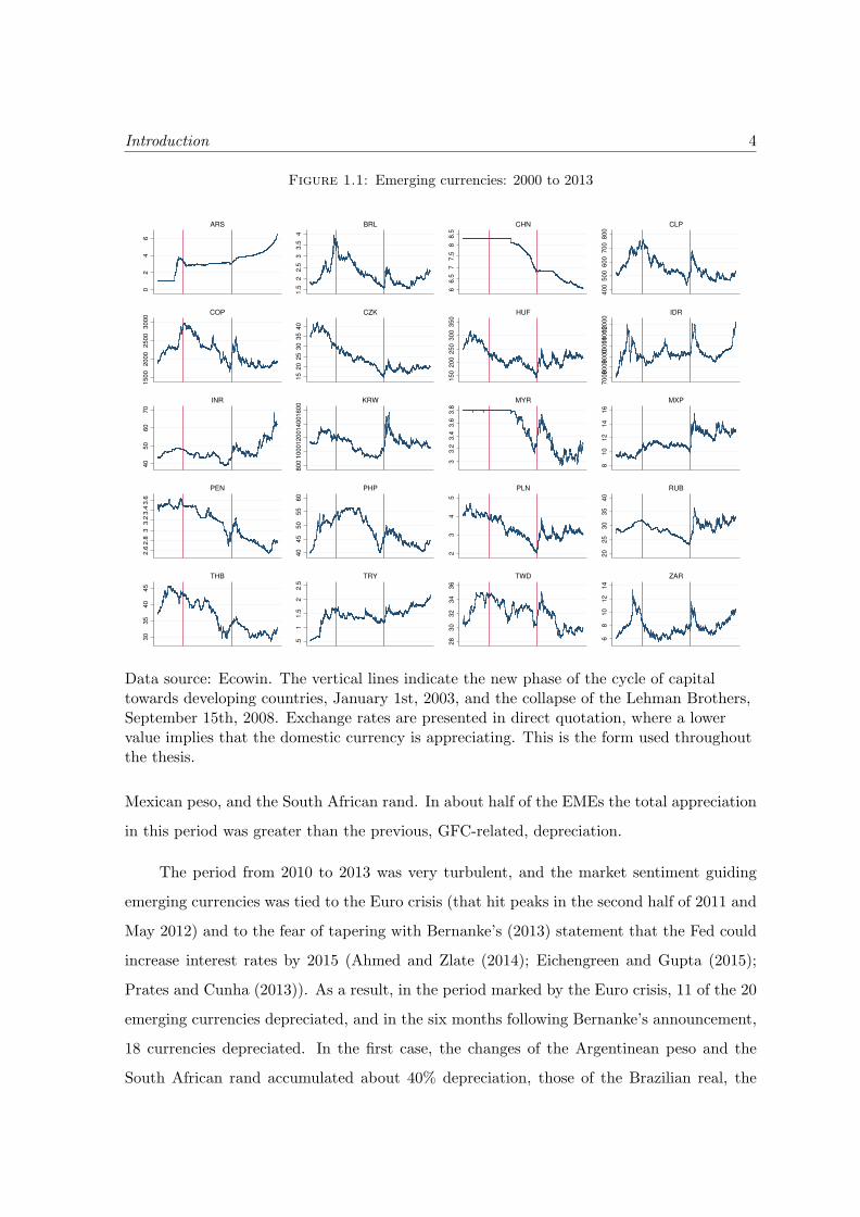
The path followed by emerging currencies since the year 2000 is shown in Figure 1.1. The
collapse of Lehman Brothers was an immediate and immense shock on emerging currencies as
investors across the globe liquidated their holdings abroad (Milesi-Ferretti and Tille (2011);
Frank and Hesse (2009)). In many EMEs, the vast exchange rate appreciation since 2003
disappeared within a few weeks. Specifically, daily depreciations peaks as high as 6.2% were
seen in the South African rand, and as high as 5% in the Polish zloty, the Brazilian real, the
Colombian peso and the Chilean peso.
However, these major depreciation shocks were relatively short-lived4. In a context that
combined a more favorable growth outlook in EMEs than in advanced countries (the ‘two-
speed recovery’), as well as massive policies of quantitative easing (QE) including historically
low interest rates in advanced countries, capital flew back to EMEs and their exchange rates
went through major appreciations in the following year (Bernanke (2010); Brunnermeier
(2008); Fawley and Neely (2013)). In this period, appreciation hit daily peaks of more than
4% in the Colombian peso and the Polish zloty, and more than 3% in the Brazilian real, the
2This contrasts with the argument of the ‘impossible trinity’, according o which capital account convert-ibility and flexible exchange rate regimes result in monetary policy autonomy.
3This considers the group as a whole, including countries who follow both floating and non-floating regimes.4For instance, in the case of the Brazilian real it lasted 18 weeks.
Introduction 4
Figure 1.1: Emerging currencies: 2000 to 2013
02
46
ARS
1.5
22
.53
3.5
4
BRL
66
.57
7.5
88
.5
CHN
40
05
00
60
07
00
80
0
CLP
15
00
20
00
25
00
30
00
COP
15
20
25
30
35
40
CZK
15
02
00
25
03
00
35
0
HUF
70
008
00
090
0010
00
01
10
00
12
00
0
IDR
40
50
60
70
INR
80
01
00
01
20
01
40
01
60
0
KRW
33
.23
.43
.63
.8
MYR
81
01
21
41
6
MXP
2.6
2.8
33
.23
.43
.6
PEN
40
45
50
55
60
PHP
23
45
PLN
20
25
30
35
40
RUB
30
35
40
45
THB
.51
1.5
22
.5
TRY
28
30
32
34
36
TWD
68
10
12
14
ZAR
Data source: Ecowin. The vertical lines indicate the new phase of the cycle of capitaltowards developing countries, January 1st, 2003, and the collapse of the Lehman Brothers,September 15th, 2008. Exchange rates are presented in direct quotation, where a lowervalue implies that the domestic currency is appreciating. This is the form used throughoutthe thesis.
Mexican peso, and the South African rand. In about half of the EMEs the total appreciation
in this period was greater than the previous, GFC-related, depreciation.
The period from 2010 to 2013 was very turbulent, and the market sentiment guiding
emerging currencies was tied to the Euro crisis (that hit peaks in the second half of 2011 and
May 2012) and to the fear of tapering with Bernanke’s (2013) statement that the Fed could
increase interest rates by 2015 (Ahmed and Zlate (2014); Eichengreen and Gupta (2015);
Prates and Cunha (2013)). As a result, in the period marked by the Euro crisis, 11 of the 20
emerging currencies depreciated, and in the six months following Bernanke’s announcement,
18 currencies depreciated. In the first case, the changes of the Argentinean peso and the
South African rand accumulated about 40% depreciation, those of the Brazilian real, the
Introduction 5
Turkish lira, and the Indian rupee, about 25-30%. In the six months that followed, marked
by the fear of tapering, the Argentinean peso depreciated almost 60%, the Russian ruble,
35%, and the Indonesian rupiah, the Turkish lira, and the Chilean peso depreciated about
15-20%.
The significance of external financial conditions in determining the turbulence of emerg-
ing currencies since 2003 is unambiguous. In terms of daily exchange rate depreciation, EMEs
were much more impacted by these developments than the advanced economies themselves:
Although the US and the Europe were the locus of the crisis, from 2003 to 2013 the daily
changes of the U.S. dollar/euro pair were limited to 3%5.
The manifest turbulence of emerging currencies, in addition of being a problem per se
might indicate their determination by the conditions of international financial markets, what
is also of concern since it demonstrates that these countries’ exchange-rate levels are not
coherent with their underlying economy. The striking similarity of these currencies’ path is
an evidence in this sense. These dynamics indicate the fragility of emerging currencies to
the conditions prevailing in international financial markets.
1.1.3 Policy Makers’ Concerns
The repeated cases of turbulence in the aftermath of the GFC have not gone unnoticed
by EMEs’ policy makers. On the contrary, countries’ authorities expressed concern over
the impacts of the international context on their currencies to the IMF (Roy and Ramos,
2012) and the two public manifestations of concern by Brazilian authorities became broadly
known – over the ‘currency war’ (in the context of broad implementation of capital controls
in 2010) and over the ‘monetary tsunami’ caused by the QE policies in 2012. In light of
the turbulence emanating from the international context, several countries also decided to
accumulate reserves of international assets6, and to impose capital account management
policies.
5A comparison between the distribution of exchange returns of emerging currencies and the U.S. dollar/eurois provided in Chapter Six.
6The rise of reserves is studied in Chapter Five, Section 5.2.1. The policy of accumulating reserves isstudied in Chapter Seven, Section 7.2.5.2.
Introduction 6
The accumulation of reserves started only a few years after the late-1990s crises (whose
roots were said to partially rely on the inadequacy of reserves, provoking a change of the
related policy recommendations). Reserves were relatively not used during the GFC, a
choice that underscores both how treasured they are by policy makers, and the latter’s
relative contentment with the GFC exchange-rate depreciation after a period marked by
appreciation and the fear of these authorities of losing their investment grade (Aizenman
and Lee (2007); Aizenman and Hutchison (2012); Garcia and Soto (2004); Feldstein (1999);
Fischer (2001); Prates (2015); Rodrik and Velasco (1999)).
Another policy response was the capital account management or regulation. Specially
in the form of residency-based taxes in the wake of the return of capital flows to EMEs
after the GFC. Not only spot, but also derivatives markets were subject to new regulation,
evincing the impact of pressures coming from these markets. At that moment, there was a
major debate over the use of capital controls, including a review of IMF’s position on the
subject7(Ahmed and Zlate (2014); ECLAC (2011); Forbes et al. (2011); Ocampo (2012);
Prates and Fritz (2016)).
1.1.4 The Exchange-Rate Literature
Mainstream exchange-rate theories are marked by a dichotomy between studies related to
exchange-rate determination and others focused on crisis. This very construction of two
separate bodies of literature reveals the incapacity of the first strand for accounting for
sharp exchange rate movements – that are frequent in EMEs. This literature is indeed
focused on long-term dynamics where the exchange rate is a market-clearing price. Whether
the exchange rate will be found at its PPP-predicted value after five years of ‘misalignment’
is irrelevant: It does not provide us with any information on the causes of the turbulence
seen in those years that likely affected entrepreneurs’ animal spirits.
Because it is focused on fixed exchange rates, most of the dynamics are not present in
mainstream crisis literature, and, in these models, internal disequilibrium play an important
7This subject is covered in Chapter Seven. For studies published inside the IMF that present a change intheir view, see Blanchard et al. (2012); Claessens et al. (2010); Ostry et al. (2010); Ostry et al. (2011). For anassessment of the new IMF policy see Fritz and Prates (2014). For a review of the extent of the considerationof the Fund’s new position on their policy recommendations to developing countries, see Roy and Ramos(2012).
Introduction 7
role, but it was clearly absent in recent emerging currencies’ crises. On the contrary, in more
recent episodes, capital flew to the countries in crisis (Kohler, 2010) – which can be seen as
a no-safe-heaven puzzle, as it is the opposite of what is expected by the usual safe-heaven
effect.
Heterodox theories explain that puzzle and have more to add to our understanding
of emerging currencies for considering that crises are inherent to these currencies’ dynam-
ics. Their patterns emerge from their subordinated place in the hierarchical financial and
monetary systems that reflects their inability to perform the functions of money in the inter-
national scenario (as it will be seen in Chapter Three). Specifically, two main characteristics
of emerging currencies explain why they are massively sold in case of turbulence. First,
they are not used as reserve of value, and during crisis, the preference for the most liquid
currency increases. Second, they are not used as denominator of financial liabilities, that
are needed when crises emerge and financial obligations must be met (Andrade and Prates
(2013); Kaltenbrunner (2015); Prates (2005a)).
These explanations are in line with the evidence of fragility of some emerging currencies
to the developments of the international financial markets just discussed, but they do not
explain why they occurred in some emerging currencies but not in others. They also do not
explain why this pattern happens to some emerging currencies but not to currencies of other
developing countries that also do not exercise the functions of money in the international
sphere. This is the gap in the knowledge that the thesis aims at enlightening. As seen
from the brief description of events, exchange rate fragility seems to be concentrated in a
few currencies only. Why were the Brazilian real and the Turkish lira frequently mentioned
among the most turbulent, but not the Korean won or the Peruvian nuevo sol?
Emerging countries are different from other developing countries for being highly in-
tegrated to financial markets. Is it the different magnitude of integration among emerging
countries that explains the occurrence of turbulence or would it be associated to a different
type of integration?
Introduction 8
1.2 The Purpose of the Study, Theoretical Framework and
Methodology
The thesis aims at contributing to the exchange-rate literature with the study of why some
emerging currencies are more marked by fragility to international conditions than others.
Specifically, it suggests different indicators that characterize exchange-rate dynamics – ex-
change rate volatility, frequency of extreme depreciations, co-movement with international
financial scenario and with other emerging currencies – and studies the implications of fi-
nancialization in determining these features as revealed from the characteristics of EMEs’
financial integration.
With financialization, the logic of finance at the international level is associated with
capital gains related to the patrimonial decisions of money managers, and the focus on ex-
change rate returns is a marked feature of its innovations, as observed from the innovations of
products (such as FX derivatives) and usages (such as carry trade or currency trading). The
analyses assume that the extent of the use of a country’s assets or currency in these strategies
is revealed from the characteristics of its financial integration. Based on this assumption, the
thesis suggests an indicator that characterizes integration with regards to financialization and
studies how the level of financialization of countries’ integration is associated with exchange
rate fragility.
The thesis follows a post-Keynesian framework. As opposed to the orthodox instru-
mentalism, this framework insists on the importance of the ‘realisticness’ of theories for un-
derstanding the phenomena under study. ‘Realisticness’ refers to whether a representation is
about reality or observables8, while ‘unrealisticness’ defines the oversimplified, implausible,
practically irrelevant (Lang and Setterfield (2006); Lavoie (2014)).
Post-Keynesians value ‘realisticness’ and “believe it is better to develop a model which
emphasizes the special characteristics of the economic world in which we live than to contin-
ually refine and polish a beautifully precise, but irrelevant model” (Davidson, 1984, as cited
8According to Maki (1989, p. 196, as cited by Hodge (2008)): “A representation can be said to be realisticif it is about reality (i.e. it refers factually) or about observables (i.e. it refers observationally) or aboutessentials (i.e. it refers essentially), or if it represents what it refers to, or if it is true of what it represent”.
Introduction 9
by Lavoie (2014)). Orthodox frameworks, on the contrary, value a model’s ability to provide
precise predictions more than the truth of its assumptions9.
For valuing realisticness, the thesis underscores the need to understand the structure
formed by the rise of money managers as well as the fact that their decisions (key for exchange
rates) are constrained by balance-sheet considerations. The focus on balance-sheets is a key
feature of Stock Flow Consistent models (used in Chapter Three) and of Minsky’s analyses
(used in Chapter Seven).
Analyses of balance-sheets of private institutions and the acknowledgment that they
are not confined within a country’s boarders have also been an increasing feature of studies
published by the Bank of International Settlements (Avdjiev et al. (2015); Disyatat (2011);
Shin (2016)). Their authors are not associated with post-Keynesian economics, nor with
other heterodox schools of thought, but they share a taste for realisticness.
As a reflection of the concern over realisticness, in-depth analyses of the potential effect
of financialization on exchange rates at a theoretical level is the methodology used to test this
hypothesis, followed by a detailed empirical assessment of the manifestations of financializa-
tion in financial integration (as a whole and in the characteristics of countries’ integration),
and in the exchange-rate dynamics. Most of the analyses start in 2003, the year that marked
the beginning of a new expansionary phase of capital flows to developing countries (Prates,
2015) and when most EMEs had already opted for floating exchange rate regimes.
From the empirical analyses of the manifestations of financialization, an index is built to
proxy how financialized a country’s integration is. It was then compared to the occurrence
of the exchange-rate features of concern. To characterize integration and exchange-rate
dynamics, the thesis uses graphical analyses, descriptive statistics, correlation coefficients,
principal component analyses and a VAR model.
These analyses are done for the 20 EMEs. As mentioned, EMEs are theoretically defined
as the most most financially integrated developing countries. As money managers are the
9This assumption is very clear in Friedman (1953b, p. 8-9, italics in the original): “the only relevant testof the validity of a hypothesis is comparison of its predictions with experience. The hypothesis is rejected ifits predictions are contradicted”. See Maki (2003) for a critical assessment of Friedman’s (1953b) article andthe argument that Friedman deemed the ‘unrealisticness’ of the assumptions not only irrelevant, but also avirtue.
Introduction 10
ones who decide which countries will be integrated, the thesis proposes a financial-markets
oriented operational definition of EMEs based on which countries the financial community
saw as ‘emerging’ during the analyzed period (Bibow (2009); Chesnais (1997)).
Major Finding The thesis concludes that a group of emerging currencies is characterized
by higher exchange rate volatility, more frequent extreme depreciations than the euro/U.S.
dollar pair, closer association with international financial conditions, and high correlation
with other emerging currencies. The intensity of these features can be explained by the level
of financialization of these economies’ financial integration. Financialized integration is more
strongly associated with the concerned features than measures of absolute integration or of
the weight of financial integration vis-a-vis trade integration, demonstrating the influence of
the characteristics of the FX market. Other findings are highlighted in the Thesis Structure
Section.
Relevance The thesis’ findings raise serious policy concerns: for having its assets used
in money managers’ innovative strategies, emerging currencies have been presenting higher
volatility and frequently passing through major depreciations. For impacting uncertainty and
animal spirits and real exchange rates, such exchange rate behavior has negative implications
in terms of trade, investment and growth.
The thesis’ findings call the attention of regulators to the need of avoiding this develop-
ment to continue, thus decreasing the vulnerability of emerging economies to international
developments and fostering a more stable context that favors these economies’ capital and
human development. The theoretical relevance of the findings are presented in the thesis’
conclusions, and their policy implications, in Chapter Seven.
1.3 The Structure of the Thesis
The thesis is divided in six chapters, apart from this introduction (Chapter One) and the
Conclusions (Chapter Eight). The first two are focused on the two bodies of literature the
thesis discusses the most: financialization and exchange rates. They are followed by three
Introduction 11
empirical chapters. The last chapter provides a framework that explains the transmission
channels mentioned in the theoretical chapters and that results in the exchange-rate dynamics
seen in the empirical part.
Chapter Two The chapter reviews the literature on the changes of capitalism known as
financialization. Its broad tenets are grouped into three main types of developments: i) the
increasing importance of finance at the international level with the decoupling from its earlier
functions and logic; ii) the changes within the financial system, including the sophistication
of finance through major innovations of products and usages; and iii) the changing relation-
ship between finance and other economic sectors. The chapter argues that, in the concerned
countries, financialization might have changed exchange rate determination not only through
the increasing weight of finance internationally, but also from its patrimonial and strength-
ened speculative logic, in line with its innovation of products (such as FX derivatives) and
usages (such as carry trading). With financialization, capitalism saw the rise of money man-
agers, whose assets and liabilities are located in different markets and labeled in different
currencies. The result is an international financial system characterized by a network of
different countries’ markets, interconnected through money managers’ balance-sheets. The
chapter argues that exchange-rate dynamics must be analyzed as a result of the dynamics of
this broad network, i.e. through money managers’ decisions, specifically their balance-sheet
constraints.
Chapter Three The chapter analyzes exchange-rate theories on exchange-rate determi-
nation and crisis, both from mainstream and heterodox perspectives, including analysis that
have a broader focus and that are specific to emerging currencies. The chapter concludes
that mainstream models have been gradually taking financialization-related features into ac-
count, but without relaxing the idea of exchange rates as a market-clearing price, which is
not coherent with the pattern of capital flows (and thus exchange-rate dynamics) in times of
financialization. The chapter also points to a dichotomy inside the mainstream exchange rate
theories: a set of analyses has emerged to explain exchange rate crisis episodes without much
reference to the existing literature on exchange rate determination. Given the frequency of
Introduction 12
turbulence and crisis, this dichotomy reveals the failure of the first set of models to explain
exchange-rate dynamics.
Heterodox approaches, on the other hand, provide many insights on the characteristics
of FX markets, on investors’ decision-making processes and on the specific dynamics of
financial flows to EMEs due to the attributes of these countries’ currencies. In an attempt
to approximate financialization and exchange-rate debates, and to resemble the discussion
of heterodox authors on exchange rates through different approaches, the chapter suggests
ways to model their main insights on a Stock Flow Consistent framework. The use of the
SFC approach echoes the need of considering exchange rates as the result of the decisions of
money managers, and their balance-sheet constraints discussed in Chapter Two.
Chapter Four Given the importance of money managers’ decisions and the idea of EMEs’
assets being interconnected through money manager’s balance sheets, Chapter Four analyzes
the stock of foreign liabilities of EMEs. It discusses the changing international insertion
of EMEs and their associated vulnerabilities with a focus on the implications related to
the increasing weight of equities among foreign portfolio investment. It contributes to the
literature that studies this trend by highlighting other features of equity, going beyond the
discussion of equity’s higher volatility. One of the findings is the manifest co-movement of
equity liabilities across EMEs, that hints to the relevance of the international scenario in
their determination. Due to its price variability, equities are a privileged locus of capital
gains, making them attractive to money managers given their increasingly speculative focus.
Equities could therefore be not only more volatile, but a type of investment that is more subject
to contagion. The chapter also demonstrates that stock markets have an impact on exchange
rates in most EMEs. As a consequence, its turbulence is directly transmitted to exchange
rates. The interaction between stock prices and exchange rates is also strengthened by the
participation of foreign investors, that increase the liquidity of equity markets.
Chapter Five Most of the changes of exchange rate determination due to financialization
are related to the greater magnitude and evolving logic of ‘finance at the international level’
(the first two phenomena of financialization as argued in Chapter Two). Chapter Five studies
the different characteristics of financial integration. On a more general level, the chapter
Introduction 13
presents evidence of the decoupling of FX transactions not only from the productive economy
(as measured by GDP or trade), but also from the economy’s financial integration. This
dissociation is found among advanced countries and EMEs. With this evidence, the chapter
contributes to the validation of the financialization thesis and argues for the importance of
analyzing the implications of financial integration not only through its magnitude, but also
from its characteristics.
In this sense, and in line with the analyses of Chapter Two that pointed to the potential
implications of the innovative trading strategies on exchange rates, the chapter analyzes how
EMEs’ assets and currencies are traded as revealed by the characteristics of their integration.
After identifying the five most relevant indicators, the chapter proposes a composite index of
how financialized the integration of these economies is.
Through the analyses of the different characteristics of integration, the chapter argues
that emerging countries’ insertion in the IFS is characterized by an asymmetrical type of
demand for their assets. While the demand for EMEs’ assets is marked by speculative
motives, part of the demand for advanced country’s assets is marked by the stability and
stabilizing features of emerging countries’ policies of accumulating reserves. Finally, the
chapter also suggests ways of identifying carry trading currencies based on different ratios
involving their foreign liabilities and FX markets vis-a-vis their economy’s GDP and trade.
Chapter Six The features of emerging currencies and their relationship with the types
of integration are the focus of Chapter Six. Exchange rate volatility is a major feature
of concern. Its analysis go beyond the use of the standard deviation (that is deemed a
partial proxy of volatility and is subject to biases when applied to exchange rates), including
analyses of the frequency of extreme exchange rate changes – the latter have proven to
be better for characterizing emerging currencies and are more coherent with the theoretical
debate (as argued in Chapter Three). The chapter presents a clear differentiation of emerging
currencies features from the euro/U.S. dollar pair : exchange rate returns vary significantly
across the 20 EMEs, but the most volatile emerging currencies have more frequent extreme
changes than the euro/U.S. dollar pair, and most emerging currencies have more frequent
modest deviations.
Introduction 14
Two other characteristics analyzed in Chapter Six are the correlation of emerging cur-
rencies with the conditions of international financial markets (as proxied by the VIX index)
and the co-movement of emerging currencies among themselves. As shown in the chapter,
the four characteristics are associated : the group of emerging currencies to present the high-
est volatility, the highest frequency of extreme depreciations, the highest correlation with
the VIX, and correlation with a higher number of emerging currencies is very similar. This
result is evidence of the importance of the international financial conditions in determining
the volatility of emerging currencies.
Apart from the characterization of emerging currencies dynamics vis-a-vis advanced
countries and among EMEs, the second group of findings of Chapter Six concern the reasons
behind these features. The occurrence of these features are compared against the level
of financialization of the countries integration, as measured in Chapter Five. The chapter
concludes that the type of integration is strongly associated with the aforementioned exchange-
rate features and that this index can better explain exchange-rate features than absolute and
relative measures of financial integration. These results underscore the need of analyzing the
impacts of integration not only from its magnitude, but also from its characteristics (as also
revealed from the analyses of Chapter Five).
Chapter Seven The chapter presents a Minskyan account of the dynamics leading to the
exchange rate patterns found in Chapter Six. The contributions of the chapter are around
two main axis. The first is related to the utilization of Minsky’s framework: it identifies its
main elements and suggest how to transpose them not only to an international context, but
also to a case where the main decisions are related to assets, not liabilities – in this case,
money managers’ international portfolio allocation. The second is related to exchange-rate
theory: through an empirical analysis of how emerging currencies’ fragility was built in the
2000s, the framework proposed details the transmission mechanisms.
In the open economy context, the exchange rate is the additional element of uncertainty
that differentiates hedge from speculative and Ponzi units. This allows emphasis on the role
of currency mismatch of balance sheets and differentiating investing in assets labeled in a
currency from an EME (as Ponzi) or from an advanced country (as speculative) in line with
Chapters’ Six findings on the higher volatility of emerging currencies.
Introduction 15
The main point of the model is on the build-up of fragility with the appreciation of
the emerging currency, that is based on self-feeding mechanisms (appreciation leads to an
expectation of further appreciation, higher demand, and further appreciation). As argued
in the chapter, this self-feeding mechanism is stronger in a group of EMEs and in times of
financialization. It is stronger because of the small size of their markets relative to the capital
received and because of the increasing focus on exchange rate returns – that might be even
more important for the money managers who invest in the EMEs for their higher exchange
rate variability.
With the self-feeding mechanisms, emerging currencies dynamics are best described as
a ‘deviation amplifying system’, backed by money managers’ decisions. When the system is
fragile, any ‘not-unusual’ event might trigger a crisis. In times of financialization, given the
interconnection of markets across the world through money managers’ balance-sheets, the
source of shocks are enlarged. When hit, EMEs’ assets are sold, in an asset/exchange-rate
deflation spiral.
The Minskyan model accurately depicts the pattern of emerging currencies since the
implementation of floating exchange rate regimes: fluctuation in cycles according to the inter-
national financial scenario. As argued in the chapter, an exchange rate determination based
on amplifying deviations that reverses in the advent of an external shock is however markedly
different than the view of exchange rates as equilibrium-seeking system with market-clearing
properties. Policy alternatives to hinder the self-feeding cycle to emerge are discussed: capital
inflow controls, reserves of foreign assets and derivatives management techniques.
Chapter 2
Financialization and its Potential
Impact on Emerging Currencies
The thesis discusses whether the determination of exchange rates in emerging market economies
(EMEs) could be influenced by the developments that have been characterizing capitalism.
A large number of authors name these developments financialization. However, it is a rather
elusive term, that has been used to indicate a large set of characteristics. Although they indi-
cate different phenomena, most definitions have a common point: the increasing importance
of finance, fitting the broad definition proposed by Epstein (2005, p. 3): “financialization
means the increasing role of financial motives, financial markets, financial actors and financial
institutions in the operation of the domestic and international economies.”
Specifically, the term financialization has been used to designate the following changes:
i) the increasing importance of finance at the international level with the decou-
pling from its earlier functions and logic;
ii) the changes within the financial system, with the increasing importance of
markets, the evolution of banks, and the sophistication of finance through inno-
vations of products and usages; and
iii) the changing relationship between finance and other economic sectors, with
the increasing importance of the first and its associated class group, the rentiers.
16
Chapter II. Financialization 17
Capitalism changes have also been studied by authors who suggested different names
for its current phase, including Money Manager capitalism (Minsky, 1986), Patrimonial
capitalism (Aglietta, 1999), Finance-led growth regime (Boyer, 2000), Financialized growth
regime (Chesnais, 2001), Shareholder capitalism1 (Plihon, 2003), and Finance-dominated
accumulation regime (Stockhammer, 2008).
When studying the current phase of capitalism, some of these authors have also analyzed
prior phases. With an institutionalist perspective, these works analyze the different “types”
of capitalism of a specific country and its impact on economic growth. This introduction
briefly presents two of these categorizations: the French Regulation school one, and the one
done by Minsky2.
The regulation modes from the French Regulation school According to the French
Regulation school, different regulation modes are observed inside the capitalist system (that is
a production mode) based on the different combination of: the monetary constraints (financial
and monetary policies); the wage-setting rules; the industries’ organization; the form of
integration of the economy to the international regime; and its governmental form (Boyer,
2004).
The current regulation mode found in advanced countries is financial (“Capitalisme
Financier”). It has succeeded Fordism, that ruled from the 1950s to the 1970s and was
marked, in advanced countries, by higher stability based on the different configuration of
the above mentioned institutions. For instance, wage-setting during Fordism was done in a
common agreement between unions and management, according to productivity gains, which
fastly grew, given Taylorism and the scientific organization of work, and enhanced demand.
Demand was also boosted by active fiscal and monetary policies, social protection,
and low interest rates (that had, as objective, financing productive capital through banking
financing) (Plihon, 2003)3.
1For Plihon (2003, p. 41), the main characteristics of “Capitalisme actionnarial” are: a new distribution ofwealth inside companies; the key role of stock-markets and its institutional investors; the predominance of theshareholder logic leading to new forms of companies’ governance; the new financial behavior of non-financialcompanies; and the loss of autonomy of economic policies in face of financial markets.
2Chavance et al. (2007) also cite the “New Institutional economics” of Douglas North, that would havethe same object of study.
3For a review of the French Regulation school, also see Chavance et al. (2007) and Amable (2005).
Chapter II. Financialization 18
Minsky’s four stages of capitalism Analyses of the different phases of capitalism (in
this case, the U.S. economy) also interested Minsky. His interest in these changes is not
dissociated from his financial fragility hypothesis. On the contrary, Minsky’s interest in
these “main evolutionary changes” (Minsky, 1990, p. 33) might even be seen as the source
of the hypothesis, as he saw in these changes the explanation for the behavior of firms and
the increase of financial fragility (as in Minsky (1986)4).
Minsky’s characterization is divided into four phases: Commercial, Finance, Managerial,
and Money Manager capitalism. The stages are distinguished “by differences between trade
and industry; the capital intensity as measured by production; and the balance of economic
power between merchants and managers on one side and financing institutions and financial
market operators on the other” (Minsky, 1990, p. 27). With respect to finance, these stages
are “related to what is financed and who does the proximate financing”, representing “the
structure of the relations among business, households and finance”. Although these stages
are understood as consecutive, the last one representing the current period, they can also
coexist in an advanced capitalist economy (Minsky, 1992, p. 107).
During Commercial capitalism, funding involved “goods that are being traded or pro-
cessed”, but not durable capital assets used in production. This phase is associated with
merchants and has as a main financial instrument a bill of exchange or other instruments
that relate credits to specific commodities5. The geographic location of the business creation
was very important in this period, as those transactions were based upon the knowledge of
home bankers about local merchants and distant bankers.
Finance capitalism emerged with the industrial revolution and the requirement of fi-
nancing expensive and durable capital assets. The period saw the emergence of corporations
and of investment bankers as the main institutions in the funding markets. They act as
4The association between the financial instability hypothesis and the four phases of capitalism is very clearin Minsky (1986, p. 24), where the author begins with a description of the changes in the United States to,based on this historical-analysis, present the financial instability hypothesis. In the book, for instance, theprocess of debt-deflation of the 1930s is presented as a moment when margins of safety were increased, movingthe economy to a more robust situation.
5An important legacy of this stage is the hierarchy of contingent commitments: the banker issues aguarantee of payment that is often reinforced by another financial institution – an acceptance house. Anotherinteresting point of Minsky’s analysis of this period is the endogeneity of money supply: contracts createcredit, which is later destroyed as the contract is fulfilled.
Chapter II. Financialization 19
brokers when facilitating trade in existing issues, and as dealers when underwriting new is-
sues. The 1929 crash saw the end of investment bankers as the dominant institution. In the
following stage, Managerial capitalism, government had an important role in adequating ag-
gregate demand and profits through “variations in government deficits [that] offset the effect
of variations in private investment upon aggregate profits” (Minsky, 1992, p. 110). As gov-
ernment’s deficits allowed the internal cash flows of firms to finance their own investments,
firms were more independent from investment bankers and managers were independent from
stockholders. “The result was management autonomy, which (...) enabled firms to take
long-run views: the short-term bottom line was not the binding constraint upon investment
decisions” (p. 110). Corporate management had the freedom to pursue “long range objec-
tives, be ‘sociably’ responsible, enjoy the easy life of a monopolist, and build conglomerate
organization” (p. 31). Firms, rather than bankers, were the central institution in the private
economy.
In the public sphere, Managerial capitalism saw a “revolution of government interven-
tion” marked by the combination of Big Government and Big Bank, a Central Bank that
intervenes and act as lender-of-last-resort (Minsky, 1990, p. 23). Big government’s deficits
were related to the rising welfare state, including the state’s support to old-age pension, which
was supplemented with private pensions. A second important element is broad Central Bank
intervention “that prevented a collapse in dollar asset values” and “depression induced dis-
savings” (Minsky, 1990, p. 30-32). From the working of Big Government and Big Bank,
Managerial capitalism “did not exhibit the serious recessions and depressions of Finance
capitalism”. This evolution is essential in understanding the transition to Money Manager
capitalism. The government revolution of this period decreased the downside vulnerability
of firms’ profits (which became much lower than in a small government capitalist economy)
(Minsky, 1986). The margins of safety of firms, that reflected earlier experience, were then
deemed excessive; and the new reality allowed firms to change liability structures to accom-
modate higher indebtedness levels (Minsky, 1992, p. 111). When business, financiers and
portfolio managers saw the financial impact of these changes and realized the obsolescence
of the regulatory arrangements, put into place prior to World War II, they were “remarkably
fecund in developing new instruments, institutions and usages”6 (Minsky, 1990, p. 22-23).
6Also key for these innovations is the development of communication and computing capabilities. Minskycites the rise of exotic instruments and activities such as program trading and portfolio insurance as the
Chapter II. Financialization 20
During Managerial capitalism, financial innovation (of instruments and usages) emerged in
a typical profit-seeking behavior of the different economic units.
The structure of the chapter Apart from this introduction, the chapter is divided as
follows. Section 2.1 presents the developments of the last three decades that allowed the
emergence of financialization. Section 2.2 discusses the different developments that have been
referred to as financialization. Section 2.3 discusses the potential impacts of financialization
in terms of exchange-rate determination. Section 2.4 presents the chapters’ conclusions.
2.1 The Developments Leading to the Rise of Financialization
The emergence of financialization is rooted in a large set of developments. First and most
importantly, liberalization policies have a role in allowing financial integration and innova-
tion. Second, the combined changes of monetary policies and socio-demographic evolution
also played a role in creating the liquidity that circulates in the enlarged financial sphere.
Finally, financialization must be understood in light of prior developments of financial deep-
ening, technological improvements and globalization. Each of these developments will be
detailed next.
Liberalization policies Deregulation and liberalization policies7 begun in the 1960s in
the US and in France, with the interest equalization tax and the deregulation of banking
lending rates, respectively. In the UK, the repeal of foreign exchange (FX) controls in late
1970s is seen as the important mark of liberalization policies (Goldstein and Mussa, 1993),
but the lack of government intervention on the rising eurodollar market in the 1960s is also
results of trading activities of money managers (Minsky, 1990, p. 9). Minsky also worked on securitization,as in Minsky (1990, p. 22-23).
7Some authors use deregulation and liberalization as synonyms. Bourguinat (1992) differentiate dereg-ulation from other types of liberalization policies. For Goldstein and Mussa (1993) deregulation is a typeof liberalization policy. Freitas (1997a, as cited in Prates (2002)) agrees, and adds that deregulation meansthe elimination of restrictions to the working of markets and the decrease of government integration, whileliberalization is a historic process.
Chapter II. Financialization 21
a crucial moment – though not a policy, it is a choice of non-intervention that follow the
direction of the liberalization policies8 (Prates, 2002).
Liberalization policies are important for allowing finance to overpass not only the bar-
riers between different countries’ markets, but also the internal barriers between different
national financial markets9 (Bourguinat, 1992). Remarkable events in this sense are the
softening of the Glass Steagall Act’s restrictions10 in the US since the 1950s (Cintra, 1998)
and the Big Bang of 1986 in the UK, which respectively “removed” the barriers between
commercial and investment banks, and between jobbers and brokers (Bourguinat, 1992).
Moreover, the competitive pressures unleashed by the eurodollar market encouraged
the imposition of liberalization policies (or the choices for non-intervention) among advanced
countries. As put by Helleiner (1996):
When these two states [US and UK] supported growth of the Euro market in
the 1960s and then liberalized and deregulated their financial markets in the
1970s and 1980s, foreign financial centers increasingly witnessed their business
and capital migrating to these more attractive markets. To compete effectively
for this mobile financial business and capital, they were forced to follow the lead of
Britain and the United States by liberalizing and deregulating their own financial
systems. This ‘competitive deregulation’ in finance was a central reason for the
8Following the terms used by Strange (1986) and Helleiner (1994, as cited in Prates (2002)), it is interestingto note that the political influence also manifests through non-actions (or negative decisions) of governments.Actions (or positive decisions) and non-actions (or negative decisions) refer, respectively, to the countries’interventions to influence markets through regulation of financial incentive, and the choices of non-interventionin markets. Apart from the U.K. non-intervention in the rising eurodollar market, another important exampleof non-action (or negative decision) is the U.S. unilateral rupture of the Breton Wood’s agreements (Prates,2002).
9This aspect was highlighted by Bourguinat (1992), which instead of talking about liberalization, uses theterm “decloisonement”, which could be understood as unification or possibility to communicate. “Decloi-sonement”, “disintermediation”, and “deregulation” are the 3D rules of Bourguinat (1992) on the policiesleading to financial globalization. Also see Chesnais (1997), Plihon (1997), and Plihon (2003). However, it isimportant to note that there is a debate on whether direct finance is indeed a form of desintermediation, oranother form of finance, as banks are still involved in these transactions. This will be discussed next.
10The Glass Steagall Act was only repealed in 1999, but since the 1950s its application has been softened.Cintra (1998) mentions some important acts in this direction. The Bank Holding Company Act of 1956 allowedthe formation of bank holding companies that offered services that banks were not allowed to (this was animportant step in the creation of the full-service banking, or the financial supermarkets, that characterize theU.S. banking system). Banks also created legally distinct companies, through which they avoided the legalrestrictions that separated commercial and investment banking operations. Later, investment banking evenmerged with banks, in contradiction to the Glass Steagall’s legislation. Moreover, since 1987, the Board ofthe Federal Reserve has allowed banks to trade some types of securities under certain restrictions.
Chapter II. Financialization 22
flurry of liberalization activity throughout the advanced industrial world in the
1980s. (p. 12)
Shifting the analysis to developing countries, it was only with the implementation of the
Washington Consensus policies of domestic and international liberalization in the 1990s that
these countries’ integration to the central economies’ development was allowed (Epstein and
Power, 2003). International organizations are thus key for developing countries’ integration
given the IMF’s and the World Bank’s pressure for the implementation of the Washington
Consensus policies. More broadly, the IMF also has a role in pushing for capital account
liberalization in its Articles of Agreement (see Eichengreen et al. (1998)). The United States
has also participated in pushing liberalization policies in its multilateral accords (Guttmann,
2008), and, indirectly, through its influence in the IMF’s and the World Bank’s decisions.
It should also be mentioned that part of the aspects related to financialization were
ideologically backed by economic theories. Palley (2007) and Stockhammer (2010) cite the
arguments of Arrow and Debreu (1954) that the expansion of financial markets enhances
economic efficiency; Friedman’s (1953) case that speculation is stabilizing; Brainard and
Tobin’s (1977) ‘q’ ratio that would have helped improve the optimistic view about financial
markets by suggesting a simple and clear way of signaling where opportunities exist and where
capital lacks (apart from linking the real and the financial sectors); and, finally, Jensen and
Meckling’s (1976) agency approach that envisages the solution to the corporate governance
problem as one of aligning the interest of managers with those of financial market participants
(this approach promotes a legal view whereby the sole purpose of corporations is to maximize
shareholder returns in the confines of the law)11.
Monetary policies Policies that created incentives for the formation of liquid capital
searching for investment opportunities were also important, as the change in the monetary
regime in the US in the 1970s. With this monetary shock, real interest rates had achieved
11See Palley (2007) and Stockhammer (2010) for their references.
Chapter II. Financialization 23
their highest level since the 1929 crisis, favoring the rise of liquidity (Aglietta (1999); Dumenil
and Levy (2003); and Plihon and Ponssard (2002))12.
This change in the monetary regime reveals the rise of the focus on price stability13,
instead of the prior one of supporting fiscal policy in the pursuit of economic growth (Plihon,
2003, p. 41) and full employment (Stockhammer, 2009)14. With the rise of the monetarist
tenet, the growth- and employment-related goals were expected to be achieved with the
attainment of price stability (Plihon, 2003). With regards to advanced countries, this new
focus was a public and official agreement, sealed in the G515 meeting in Tokyo in 1979. It
begun in 1979 in the US, spread to other advanced countries (Plihon, 2003, p. 41-43), and
is now evident in the increasing use of inflation targeting (Epstein and Power, 2003)16. It is
also the rule among EMEs, where the vast majority of countries follow an inflation targeting
regime. The high interest rates of that time favored the creation of liquidity.
Liquidity availability The existence of a pool of liquidity available, or a reserve of fi-
nancial means (Bourguinat, 1992) is crucial for financialization. This liquidity increased
considerably with the emergence of the eurodollar market in the middle 1960s. The mar-
ket emerged for enabling agents to circumvent regulations, such as U.S. control on capital
outflows and interest-rate ceilings, and from the non-repatriated and non-reinvested profits
of American international companies. It grew fast, more than doubling from 1950 to 1960,
12Aglietta (1999) discusses the new monetary regime and Dumenil and Levy (2003) argue that this led toa major change in the power relations between creditors and debtors, with gains to the former. This changewas certainly important in creating liquidity at that time, but the balance in power relations is different nowthat the interest rate level clearly changed, being currently at very low levels in advanced countries. In fact,European companies have recently even taken loans at negative rates (“Societe payee pour s’endetter”, 2016)
13It should be highlighted that the rise of interest rates also reveal open economy concerns – as the importantcapital outflows in the US in the late-1970s.
14Other important policies aimed at controlling inflation were those that concerned limiting wage increases,such as the desindexation of wages from price index in France (Plihon, 2003, p. 43).
15In this context, the “G5” was composed of six countries: France, the Federal Republic of Germany, Italy,Japan, the United Kingdom, and the United States.
16The GFC triggered interesting reassessments of prior policies, including monetary concerns. Inside theIMF, it was argued that monetary policies can no longer be only focused on one goal, inflation, as price stabilitywould not ensure growth (Blanchard et al., 2010) - also see the discussion in Chapter Six, page 262. Indeed,EMEs and advanced countries have recently been opting for lower interest rates than the values suggested bythe Taylor rule (Hofmann and Bogdanova, 2012). Whether this is a real shift of focus of monetary policies,with inflation fighting losing its importance, is yet to be confirmed when inflation rates will be above theirunusual low levels in advanced countries. As it will be seen in Chapter Four, from the 20 EMEs, only four(Argentina, China, Malaysia and Russia) do not follow an inflation targeting regime.
Chapter II. Financialization 24
and is known for the notorious damages it caused17. The exchange-rate crisis of the pound,
the spectacular withdraws of the dollar (in 1968, 1971 and 1973) that put an end to the
system of fixed exchange rates, and the two oil-price shocks are examples (Chesnais (1997);
Guttmann (2008)).
The creation of liquidity is also related to a combination of socio-demographic changes
with the change of the monetary regime in advanced countries, where fecundity rates de-
crease, live expectancy increases, and post-war baby boomers retired (Plihon and Pon-
ssard, 2002)18. These developments triggered an increase of savings aiming at retirement
(Le Cacheux and Touze, 2003) and of the demand for financial assets (Aglietta, 1999). In
the mid 1970s liquidity also increased due to the stumble of production and the high returns
of the circulation sphere (also due to its high productivity) that caused a shift of capital from
production to the circulation sphere (Lapavitsas, 2009)19.
Looking at more recent developments, the availability of liquidity might also be rooted
in the increasing inequality, or the concentration of personal wealth. For instance, Goda et al.
(2014) argue that inequality increased asset demand from the rich, which enabled poor and
middle-income households to accumulate increasing amounts of debt in the United States
and in Europe. Inequality also has a role in the supply of financial products. Goda and
Lysandrou (2014) argue that the emergence of financial instruments as CDOs (collateralised
debt obligations) on a mass scale before the GFC is rooted in the availability of demand for
these products, and the pressure on the American banks to create them. Both demand and
supply side being rooted in the increasing unequal distribution of income and wealth20.
In this context, the type of investment also changed, with securities and equities taking
an increased part of savings (Plihon and Ponssard (2002); Plihon (2003, p. 36)21). In general,
17Chesnais (1997) considers this market, in itself, as a phase of financial globalization, not a developmentleading to it, highlighting its importance.
18For Aglietta (1999), liquidity availability and the aging population are the very reasons behind the glob-alization of finance. Liquidity and pensions are so important for financialization, that Minsky (1990, p. 35)saw the increase of private supplementary pensions as a condition for the continuity of the growth of MoneyManager capitalism.
19The idea of a shift of capital from production to the circulation sphere is is also present in the works ofCrotty (1990), Epstein (2005), and Pollin (2007).
20The importance of wealthy citizens in the availability of liquidity is also mentioned by UNCTAD (2007,p. 15), when arguing that the current huge amounts of capital flows depend on the “access to massive poolsof capital from pension funds or wealthy citizens”.
21Plihon (2003) presents the weight of the different types of investment of French households in 1990 and2007.
Chapter II. Financialization 25
wealth holding increasingly took the form of “ownership of liabilities of managed funds”
instead of a portfolio of shares of liabilities of firms. The assignment of the management of
private pensions and wealth to “fund arrangements” (“mutual, pension and trust funds”) is
at the core of the development of money managers (Minsky, 1990, p. 4, 9, italics added).
Financial deepening It is also important to acknowledge that financialization has been
enabled by the increasing importance of finance as a sector in an economy. Indeed, the
first references to the term financialization are associated with the debate that followed
McKinnon’s (1973) and Shaw’s (1973) arguments in favor of financial development. The term
“financialization of savings” is used, for example, as a reference to “financial deepening”,
or the development of a country’s financial system (Serieux, 2008). With this meaning,
financialization is proxied by the banking system’s assets or deposits as a part of GDP
(Haseeb and Makdisi, 1982). The connotation of financial deepening is however no longer
representative of the financialization debate, that characterizes finance in a more complex
way. Financial deepening is however an important step in the developments leading to
financialization, as it would probably not occur in under-developed financial systems.
Technological progress The advances in information technology (IT) and in communi-
cations were undoubtedly important for allowing the globalization of finance (Plihon and
Ponssard, 2002) by reducing the ‘natural’ barriers to international financial transactions
through its dramatic improvements and reductions in costs (Blecker, 2005)22.
Globalization Financialization followed globalization of production and trade, that makes
the earlier (and ongoing) process of multilateral trade liberalization an important driver
of financialization (Blecker, 2005). Arguing that international financial transactions and
the rise of instruments to hedge against exchange-rate fluctuations are requirements of the
globalization of production, some authors see financialization as part of the globalization
of production (see Stockhammer (2010)). Despite the importance of these aspects in a
first moment, financialization should not be understood as simply a part of globalization of
production. On the contrary, finance and the international financial system have decoupled
22Also Minsky (1995, p. 25) mentions the importance of technologies in enabling financial integration.
Chapter II. Financialization 26
from their earlier functions, starting to follow their own logic (Plihon and Ponssard, 2002)
and having only an indirect link with financing trade and investment (Chesnais, 1997), as it
will be discussed in Section 2.2.
2.1.1 Concluding Remarks
To conclude, it is important emphasize the centrality of governments and money managers in
the process of financialization. Financialization is not a natural phenomenon, it was enabled
by policy-makers choices of liberalization policies and/or non-intervention in markets and
by money managers’ decisions to innovate. As put by Minsky (1990), money managers saw
profit opportunities from government choices and how to profit from them. Money managers
innovated when developing the different financial products, and, in terms of usages, by
investing or being funded in another market. They have a crucial role on financial integration,
as they are the ones who define which country (and market) will be integrated to international
financial markets (Chesnais, 1997).
Developments related to IT, financial deepening, monetary changes and the creation of
liquidity only have a secondary role in encouraging financialization. It should also be noted
that these developments were also motivated by financialization – in a classical egg-and-
chicken causality.
2.2 The Three Developments That Characterize Financializa-
tion
As already mentioned, the term financialization has been used to describe several develop-
ments that have been changing the face of capitalism. This section discusses these different
transformations according to the three groups mentioned in the introduction, i.e. the in-
creasing importance of finance at the international level; the transformations of finance; and
the changing relationship between finance and other economic sectors.
Chapter II. Financialization 27
Before analyzing these phenomena, it is interesting to differentiate this categorization
from others found in the related literature. Stockhammer (2004) characterizes financializa-
tion by developments that include the globalization of financial markets, the shareholder
revolution, and the rise of incomes from financial investment. Compared to what is proposed
in this chapter, the first development is common to both classifications, and the latter two
are tied to the changing relationship between finance and the other sectors.
Although not directly referring to characteristics of financialization, but to “financial
innovations” behind financial crises, Boyer et al. (2004) presents a similar list: deregulation,
globalization and sophistication of new (financial) instruments. While the first is seen in this
chapter as a development that allowed financialization to occur, globalization is similar to
the increased weight of finance internationally, and sophistication is the same as the changes
that occurred within finance. We could therefore argue that from the three phenomena
used to describe financialization here, the changing (power) relation between finance and the
other sectors would be the only one not directly related to crises – which indicates the close
relationship between financialization and crisis.
Financial globalization It is also important to mention the use of the term financial
globalization23. Definitions of financial globalization refer to the important integration of
different countries’ markets. For instance, Bibow (2009, p. 7) defines it as “the integration
of national financial systems through rising cross-border financial flows and asset holdings”
and Arestis et al. (2005, p. 507) define it as “the integration of financial markets of all
countries of the world into one”.
Some references however also include aspects related to financial deregulation or liber-
alization, as Chesnais et al. (1996, p. 10-11), who add the elimination of internal barriers
among different segments of financial markets and the interpenetration of national monetary
and financial markets to the definition of financial globalization. That is also the approach
of Bresser-Pereira (2010, p. 506), who defines financial globalization as “the liberalization of
financial markets and a major increase in financial flows around the world”.
23There are two most important terms in the French literature, “globalisation financiere” and “mondialisa-tion du capital”. Chesnais (1997) does not use globalization, but “mondialisation”, what is close to financialglobalization is the “mondialisation” of capital in the financial sphere (“mondialisation du capital dans lasphere financiere”). The term financialization is more common in more recent and in Anglophone papers.
Chapter II. Financialization 28
However, theoretical discussions are facilitated by differentiating two aspects, integra-
tion and what led to integration, into terms. Such a differentiation emphasizing the causalities
involved is clear in Arestis et al. (2005, p. 507-508), who state that “financial liberalization
provides a necessary, but not a sufficient, condition for financial globalization.” This chapter
follows this approach: Financial globalization refers to the integration of different national fi-
nancial systems. Financialization is a broader phenomenon. The emergence of both financial
globalization and financialization depends on financial deregulation and liberalization.
2.2.1 Increasing Importance of Finance at the International Level
The increasing importance of finance internationally, with its decoupling from its earlier
functions, is the first of the three financialization aspects. Financialization is related to
financial globalization and integration, but the idea that this integration is of a different
logic, no longer determined by its prior function, is keen to financialization. As a result of
this concern, both integration (as proxied by capital flows or by the stock of foreign assets and
liabilities)24, and FX transactions (that would normally be associated to it), are analyzed.
The growth of finance at an international or open-economy level has been broadly
detected and much attention is given to the rapid pace in which this process occurred.
Part of the proxies used are based on absolute values. Examining financial integration,
Chesnais (1997) mentions that the ownership of foreign assets in portfolios of U.S. funds
rose significantly – from 0.7% in 1980 to 5.7% in 1993. Analyzing FX transactions, Chesnais
(1997) and Epstein (2005) demonstrate their rapid growth – in the US, UK and Japan they
have six-folded from 1986 to 1992 and, in total, they have almost four-folded from 1989 to
2004. The rapid increase of FX transactions continued in the 2000s. As analyzed in Chapter
Five, total transactions four-folded from 2001 to 2013, the ones relative to EMEs’ currencies
(hereafter emerging currencies) having grown two times faster than those relative to advanced
countries’ currencies25.
To better understand these absolute increases, a discussion on the growth of finance
internationally in relative terms – relative to what it was supposed to be considering its
24Chapter Five discusses these two proxies of de facto financial integration.25The developments of the FX markets and the level of integration are discussed in Chapter Five, respec-
tively on Sections 5.3 and 5.2. A summary of these figures is presented in Table 5.1, page 232.
Chapter II. Financialization 29
prior function of financing production and trade – is required. The most common proxies
used are relative to GDP or trade. Analyzing integration, Baker et al. (1998, p. 10) shows
that the value of funds raised on international financial markets, as a percentage of world
exports, rose from 0.5% in 1950 to over 20% in 1996 in OECD26 countries.
Plihon (2010) discusses the increasing weight of financial flows on France’s balance of
payment (from 28.8% in 1980 to 92.8% in 2005) and relative to its GDP (from 14% to 448%
in the same period). The author also compares this dynamic with that of current account
transactions, that not only lost its relative space in the balance of payments, but were stable
in percentage of GDP (around 35%). This comparison sheds light on the growing decoupling
between financial motives and flows related to the productive economy.
The decoupling of financial integration from GDP and trade has continued to grow
rapidly since the 2000s: seen through foreign assets and liabilities, financial integration in-
creased 50% more than GDP and 40% more than trade integration among advanced countries
from 2001 to 2011. Among EMEs, integration grew on average 40% more than GDP and
as fast as trade. In 2011, financial integration was more than four times greater than GDP
among advanced countries and almost as great among EMEs.
Finance has also continuously gained importance internationally when FX transactions
are analyzed. FX transactions with advanced countries’ currencies grew two times faster
than GDP and trade from 2001 to 2013. Among emerging currencies, the decoupling of FX
transactions from GDP and trade was even greater. It grew 158% more than GDP and 136%
more than trade. Note that the growth of FX transactions relative to GDP and trade was
greater than the growth of financial integration relative to GDP and trade.
The major magnitude of finance at the international level relative to GDP or trade
underlines that the function of the international financial system is no longer to assure
the financing of the international trade and of the balance of payments (Chesnais et al.,
1996). Instead, it has only indirect links with these functions, following its own logic (Plihon
and Ponssard, 2002). The logic of today’s international financial market is determined by
speculative motives, that gained force with the sophistication of finance – as discussed in
the following section. The mentioned decoupling of FX transactions not only from GDP and
26OCED stands for Organization for Economic Co-operation and Development.
Chapter II. Financialization 30
trade, but also from financial integration is evidence of the changing features of integration
and finance, and its new logic.
Some features of financial integration must be mentioned before discussing innovations
of finance. Financialization is characterized both by a unity of time and place, given that the
world is connected through modern communication networks in a non-stop market (Bour-
guinat (1992); Plihon (1997)), as well as by the fact that money managers across the globe
have the same investment possibilities. It is also characterized by the limited ability of gov-
ernments to intervene against major attacks and currency crises, as the events cited in page
24 (Chesnais, 1997).
The evidence of the rise of finance at the international level shows the evolution of the
location of assets and funding of economic units. As Minsky (1990, p. 36) put it, “managed
money capitalism is international in both the funds and the assets in the funds.” As the
integration among different countries’ markets increase, the same portfolio becomes available
to every investor (“as money managers capitalism grows in importance the same portfolio
options will become available to all wealth holders regardless of their national ‘base”’ (Minsky,
1988)). The result is an interconnection of balance-sheets that is reflected in important
capital flows and foreign exchange contracts. The global economy is no longer characterized
by individual economies, but “as a closed system of capitalist systems” (Wolfson, 2002).
A very interesting picture of countries in this network with regards to equity holdings
can be seen in Figure 2.1 taken from Haldane (2011), where the nodes represent different
countries and the arrows represent the gross external equity assets and liabilities27. Although
this is shown for countries, the units responsible for the interconnections are the money
managers.
The limited ability of government intervention is often alluded to in the literature and
is of main importance to understand the consequences and the risks associated with finan-
cialization. It should not, however, be understood as an argument that governments have a
small role to play when crises occur; as argued in the last section, governments are responsi-
ble for policy choices that allow financialization to occur in the first place and they have the
27Figure 2.1 is further debated in Chapter Three, where it is presented for different years since 1980. It ishowever replicated here for reader’s convenience.
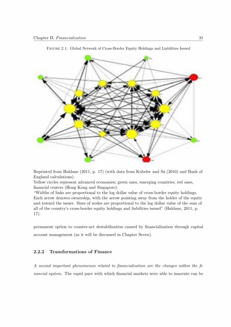
Chapter II. Financialization 31
Figure 2.1: Global Network of Cross-Border Equity Holdings and Liabilities Issued
Reprinted from Haldane (2011, p. 17) (with data from Kubelec and Sa (2010) and Bank ofEngland calculations).Yellow circles represent advanced economies; green ones, emerging countries; red ones,financial centers (Hong Kong and Singapore).“Widths of links are proportional to the log dollar value of cross-border equity holdings.Each arrow denotes ownership, with the arrow pointing away from the holder of the equityand toward the issuer. Sizes of nodes are proportional to the log dollar value of the sum ofall of the country’s cross-border equity holdings and liabilities issued” (Haldane, 2011, p.17).
permanent option to counter-act destabilization caused by financialization through capital
account management (as it will be discussed in Chapter Seven).
2.2.2 Transformations of Finance
A second important phenomenon related to financialization are the changes within the fi-
nancial system. The rapid pace with which financial markets were able to innovate can be
Chapter II. Financialization 32
explained by the profit prospects of these innovations as well as by their own characteris-
tics. On the profit-making possibilities they provide, Lapavitsas (2009) stresses the different
degree of productivity offered by these changes:
Finance might have become neither more efficient nor more productive in terms
of intermediation per worker, but it has became capable of operations that were
previously completely impossible (...) Not least, finance has become technically
capable of dealing with huge numbers of individual borrowers. (p. 110)
Regarding the characteristics of financial innovations, it is interesting to note that unlike
industrial innovations, financial innovations are simply contractual arrangements, and are
more easily implemented and more readily copied for being devoid of protection by intellectual
property rights, resulting in much shorter life cycles (Guttmann, 2008).
The changes of finance analyzed in this section are: the increasing importance of mar-
kets, the evolution of banking, and the sophistication of its financial products and usages.
2.2.2.1 The increasing importance of markets and the evolution of banking
The role of banks in credit intermediation changed with the emergence of securities. The
development of securities is rooted in the bad solvency-ratios of U.S. banks due to devel-
oping countries-debt crises, in the beginning of the 1980s. Securities came as a solution
to allow banks to put risky debtors off balance-sheets and to make themselves intermedi-
ates only, passing these risks to other institutions. Debt was then fractionated into smaller
pieces and constantly renewed; as a result, investors have longer debt maturities and banks
intermediation is limited to cases of insufficient liquidity in markets (Bourguinat, 1992).
Observing the increasing role of markets, Aglietta (1999) argued that the financial
system would have shifted from being “banking-based” to “market-based”. Despite the
enlarged role of markets, the financial system is still mainly based on banks, that also have
access to markets – characterizing what is called a market-based banking system28. In fact,
28The idea of a system based on markets, as opposed to a system based on banks would stem from Allen’s(1999, as cited by Plihon (2003)) observation of the differences between the German/French and the Anglo-saxon systems: while the first two countries’ systems were based on bank intermediation and private infor-mation, the latter is characterized by the central role of financial markets as a source of funding and thequality-level of public information (Plihon, 2003).
Chapter II. Financialization 33
the evolution of banks has resulted in a blurry frontier between bank and market-financing.
For instance, banks acquire and issue equities in markets, creating a “market intermediation”
(Plihon, 1995). Minsky (1990) had also stressed the shifting importance of banking credit to
credit in the form of securities and to the blurriness of the frontier between banks and direct
markets, highlighting the role of banks as fund managers.
Indeed, fund management is a current function of banks along with commercial banking,
investment banking, private wealth management, and insurance. With these new functions,
banks evolved to financial institutions called “do-it-all” groups, “financial supermarket”, or
“full-service” banks. In these new structures, capital markets are used as a source of income
along with the traditional functions of commercial banks (Prates and Farhi, 2015). These
changes in interaction between banks and markets and the high degree of concentration in
the provision of banking services have occurred around the globe (Pastr (2007); Plihon et al.
(2006)).
Risk management techniques have also gone through important changes: While banking
institutions used to do private evaluations based upon the specific knowledge of each debtor,
financial markets use statistical data to infer probability distributions of risk characteristics
(Aglietta and Breton, 2001), a kind of risk evaluation that has been included in bank’s
techniques. This practice has been referred to as the logic of “originate and distribute” its
loans to other financial institutions instead of the old “originate and hold” (Brunnermeier,
2008). By doing so, banks have become less cautious about their lending practices as risk is
passed to other agents and they do not gain with the return of carrying the operation, but
from its fees (Kregel, 2008)29.
Among the risks brought by the new structure, Aglietta (1999) stresses the features
of market- vis-a-vis banking liquidity. In a bank, liquidity is totally and permanently held
because deposits are assured and the bank has access to the ultimate liquidity out of the
market, the central bank. Market liquidity, on the other hand, is a collective “imaginary” of
participants, not an objective reality, as it is relative to the equilibrium between the diverse
expectations of buyers and sellers. In case of doubt about the prevailing collective opinion,
29Lapavitsas (2009, p. 110) highlights other changes within finance, such as changes in the internal or-ganization of financial institutions, speed of transactions, feasibility of financial engineering, links betweenfinancial markets, and pricing techniques.
Chapter II. Financialization 34
liquidity deteriorates abruptly, causing a major shift in prices, and instability. This constant
risk of losing capital might also oblige market participants to speculate on the future evolution
of the assets’ prices, that depends on the behavior of other market participants. Speculation
is thus a necessity of the functioning of financial markets, making financial fragility inherent
to the dynamics of markets30.
In the Post-keynesian framework, this dependency on the expectation about collective
opinion comes from the very fact that prices change according to the demand, which itself
can change abruptly, following participants’ expectations. A fundamental issue of financial
asset markets is that their high volatility makes participants aware of the high risk, trig-
gering a feeling of necessity to be among the “first to move”, generating a herd behavior
that then feeds back into volatility. This problem is intrinsic to financial markets due to
(Knightian) fundamental uncertainty, that refers to situations in which “at least some es-
sential information about future events cannot be known at the moment of decision because
this information does not exist and cannot be inferred from any existing data set” (Dequech,
1999, p. 415-416), as “the future is yet to be created” (Dequech, 2000, p. 41).
The key role of money managers in the dynamics of markets is an important feature
to note. Their great impact in prices derive from the fact that they are a limited number
of agents, who hold significant amounts of capital, and tend to make similar decisions (as
they are guided by the same assets’ ratings and tend to simulate important indeces) (Plihon
and Ponssard, 2002). Moreover, aware of their impact on prices, other investors also follow
money managers. For instance, a better rating might drive important financial flows to a
country not only by flows from money managers who follow a rating-based rule, but also
from flows of investors that expected the former to do so. Finally, institutional investors’
decisions are also important simply for the presence of herd behavior (they have an impact
on markets, and the first variation will be followed by trend-following investors, as it will be
discussed in Chapter Three).
The trend towards market-based finance has been reinforced by financial innovations as
derivatives that reduced different types of risks associated with finance (Guttmann, 2008)
30Aglietta (1999) also stresses that markets are procyclical and prone to crises. But it should be noted thatbanks are also procyclical institutions, increasing lending in times of higher economic growth and choosingindustries according to their specific growth outlooks.
Chapter II. Financialization 35
and by allowing investors to decide which types of risk they want to assume and to what
degree (Aglietta and Breton, 2001)31. The unbundling of risks associated with different
investment vehicles have, for instance, facilitated the growth of private capital flows that led
to the East Asia crises in the late-1990s (Dodd, 2002, p. 447). The following section presents
some of these innovations that characterize the level of sophistication of finance in times of
financialization.
2.2.2.2 The sophistication of finance
In other phases of capitalism (as in Minsky’s Finance capitalism) finance also played a central
role in the economy, but its current sophistication (seen by the innovations of products and
usages) reveals a decoupling from its earlier role of financing production. Minsky and Aglietta
defended the changing role of financial markets across different phases of capitalism. While
finance currently focuses on a “quick turn of the speculator, upon trading profits”, its earlier
focus was upon the capital development of the economy (Minsky, 1992, p. 111), or in serving
capital accumulation (Aglietta, 1999).
Indeed, it seems hard to defend that the sophistication of finance is strictly tied to
prior functions of finance related to capital development, and not to its new patrimonial
logic where speculation matters and relies on sophisticated products. As put by Guttmann
(2008):
[Finance-led capitalism] has given priority to fictitious capital whose new con-
duits, such as derivatives or asset-backed securities, are several layers removed
from any real economic activity of value creation. In that realm the key objective
is to trade paper assets profitably for capital gains, an activity best described as
speculation. (para. 23, italics added)
Guttmann (2008) is probably referencing Kaldor’s (1939) definition of speculation;
where speculation is related to trading with the objective of profiting from change in the
price of a good. In Kaldor’s words:
31According to Dodd (2005), the use of derivatives, in general, dates back: it can be traced to some centuriesor even to Aristotle’s period.
Chapter II. Financialization 36
Speculation [...] may be defined by the purchase (or sell) of goods with a view to
re-sale (re-purchase) at a later date, where the motive behind such action is the
expectation of a change in the relevant prices relatively to the ruling prices and
not a gain accruing to their use. (p. 1)32
This thesis uses Kaldor’s definition as reference.
Innovations of products The rise of financial innovations reveals the changing function
of finance. Indeed, speculation gained amplitude with the development or the broad use of
sophisticated products as futures, options, forwards, or swaps. These are excellent tools of
speculation due to the leveraging possibilities they offer that make risk-taking cheaper and
more available (Dodd (2005), Farhi (1999), and Guttmann (2008)). As reminded by Prates
and Fritz (2016):
One important characteristic of financial derivatives as a whole is their high
degree of leverage, to the extent that they require only a margin requirement or
the payment of a premium to be carried out. This specific feature, in turn, makes
FX derivatives a privileged instrument for currency speculation and profiting from
interest rate differentials. (p. 187)
Apart from favoring speculation, derivatives add pressure on spot markets through
arbitrage. Indeed, they are considered an extra conduit of spot exchange-rate determination:
as the pricing of forward exchange rate is given by the spot rate plus a cost of carrying
the asset33 (the interest rate) any change in one of the markets translates into a change in
32Farhi (1999) questions Kaldor’s definition, arguing that acting according to expectations about changingprices is not only a characteristic of speculators, but also common to today’s hedgers and arbitrageurs giventhe high volatility of financial markets. Farhi thus suggests a concise definition of speculation as liquidpositions (sold or bought) in a spot or derivatives market that is not hedged by an opposite position in thederivatives or spot market of the same asset. This definition of speculation characterizes one of the fouraspects of speculative operations raised by Miotti and Plihon (2001): i) they implicate risk-taking, meaningtaking position on interest rates, asset prices, or the exchange rate; ii) they are motivated by expectations ofcapital gains associated with expectations of increasing price of assets; iii) they are “pure” or “dry”, meaningthat they are self-sufficient and that they do not have a direct counterpart in the economy’s real side (in linewith Farhi (1999)); iv) they happen, most of the time, with lent money as speculators aim to leverage theirposition.
33If both the spot prices and the interest rate do not change and the forward price increases, marketparticipants will see an opportunity for arbitrage and buy the asset on the spot and sell it on the derivativesmarkets. The more liquid the derivatives markets are, the more intense this connection between the threevariables will be (Farhi, 1999).
Chapter II. Financialization 37
the other34. When derivatives markets are insignificant in comparison to spot markets, the
influence goes from the spot to the derivatives market. But when derivatives markets gain
in weight, the rates in the two markets constantly influence one another (Farhi, 1999). More
than being a determinant of the spot rate, derivatives markets can also increase its volatility
for being more volatile and subject to changing expectations.
Dodd (2005) also mentions other risks: “derivatives can be used to ‘outflank’ laws and
regulations; they can distort the price discovery process; they can be used to manipulate
accounting rules. In short, while they have their benefits, they can also facilitate many
‘unproductive’ and ‘inefficient’ activities”35.
The intensification of business cycles is a different risk associated with financial inno-
vations. Following Schumpeter, Minsky (1990) saw any evolution and innovation as driven
by a change in prospective profits. Accordingly, the importance of innovation comes from its
ability to change profit prospects and to change behaviors, which results in a pro-cyclicality:
innovations allow for more financing to occur, facilitating investment and leading to economic
growth; an increase in risk aversion, however, induces a desire to unwind debt financing. As
Minsky (1990) concluded: “boom associated with financial innovations is likely to carry the
seeds of its own destruction: the fruit of these seeds being a wave of bankruptcies that can
lead to a debt deflation process.” Brunnermeier (2008) specifically discusses the creation of
credit booms in the wake of the GFC. Instead of yielding in a more stable system, as risks
are transferred to those who are able to support them, financial innovation led to an un-
precedented credit expansion that helped feed the boom in housing prices in the US (before
the Global Financial Crisis (GFC)).
Indeed, the consequences of speculation in terms of stability are well known. Differently
from Friedman’s view of stabilizing speculation on FX markets36, speculation led to notorious
crises (in advanced and developing countries, discussed in Chapter Three, Section 3.2) and
34Note that it is a simple arbitrage operation that does not involve any expectation about future exchangerates. It is an arbitrage on the covered interest rate parity (discussed in the next chapter, in Section 3.1.1.3)(Rossi, 2014). Fernandes (2008) argues that in the case of the Brazilian real, whose future market is muchmore liquid than the spot one, the causality runs from the future to the spot rate.
35See Prates and Fritz (2016) on the use of derivatives in circumventing capital controls in Brazil after theGFC.
36The concept of stabilizing speculation emerged from Friedman’s defense of flexible exchange rate regimes:“Despite the prevailing opinion to the contrary, I am very dubious that in fact speculation in foreign exchangewould be destabilizing. Evidence from the earlier experiences of fluctuation in Switzerland, Tangiers, andelsewhere seems to suggest that, in general, speculation is stabilizing rather than the reverse, though the
Chapter II. Financialization 38
is the root of the trending pattern of exchange rates (discussed in Chapter Three, Section
3.3.2).
As Plihon and Ponssard (2002) remind us, speculation becomes an issue when its logic
becomes the determinant, as financial flows prevail over others which are more connected
to the economic reality of a country. The magnitude of FX derivatives markets might raise
concerns over the weight of speculation in these markets. Among both EMEs and advanced
countries, there were, in 2013, two times more derivatives than spot contracts. In Brazil and
Turkey, there were three times more derivatives contracts than spot ones37.
More recently, financial innovation also count with high frequency trading and dark
pools (Prates and Farhi, 2016, p. 10)38. With a combination of the two, investors can
trade according to algorithms, benefiting from privileges such as greater or faster access
to information in a completely opaque environment – without making their orders public.
There are many risks associated with these two instruments, two of them being a very rapid
collapse in prices (the ‘Flash Crashes’39) and the determination of market prices at the will
of few large international banks – the most notorious one being the manipulation of the Libor
(Prates and Farhi, 2016).
Apart from innovation of products, the high level of sophistication of finance in times
of financialization is also revealed by the innovation of usages. Carry trading operations
and the financialization of commodities and currencies are two examples discussed in what
follows.
Commodity and currency financialization A specific financial innovation that is of
special interest for this thesis is the creation of asset classes from other assets, or the finan-
cialization of these assets; the financialization of commodities and currencies are important
examples.
evidence has not yet been analyzed in sufficient detail to establish this conclusion with any evidence” (Friedman,1953a, p. 175, italics added).
37The weight of derivatives markets is discussed in Chapter Five, Section 5.3.3.38High frequency trading is a “class of electronic trading featured by high-speed connections and the use of
complex algorithms” (p. 3), while dark pools are “equity-trading systems that do not publicly display orders”(p. 14).
39Prates and Farhi (2016, p. 10) define Flash Crash as “a very rapid, deep, and volatile movement insecurity prices occurring within an extremely short time.” There have also been flash rallies of prices.
Chapter II. Financialization 39
Commodities’ financialization refers to the observation that commodities are traded as
an asset class. UNCTAD (2009) has shown that the price dynamics of commodities has
changed since the early 2000s: “these markets follow more the logic of financial markets
than that of a typical goods market” (UNCTAD, 2015, p. 24)40. Also important for the
financialization thesis is the fact that this change of dynamic was associated with a sizable
increase of portfolio investors’ position on these markets, as revealed by the sizable volumes
of exchange-traded derivatives – 20 to 30 times larger than physical production (UNCTAD,
2012).
Tang and Xiong (2010) argue that the financialization of commodities begun in the early
2000s: After the collapse of equity markets in 2001 and the “widely publicized discovery of
a small negative correlation between commodity returns and stock returns”, commodities
were promoted as an interesting asset for reducing portfolio risk. The use of these different
commodities as a part of a common portfolio diversification strategy has however resulted
in higher volatility, higher correlation between their prices and increasing sensitiveness to
international market conditions (Kyle and Xiong (2001); UNCTAD (2009)).
The higher correlation between asset markets is explained by contagion: the need of
liquidity in a market calls for withdraws in another (Aglietta, 1999), as the strategy of
financial investors is determined by their “own needs” that are related to financial markets
in general (UNCTAD, 2009, p. 23)41.
Another important type of financialization of assets is the emergence of the financial-
ization of currencies, the consideration of a currency as an asset class per se, with the expec-
tation of incurring gains from the changes in their values (Kaltenbrunner, 2011). Analyzing
the trade of the Brazilian real as an asset, Kaltenbrunner (2011) concluded that this process
resulted in large exchange rate swings and in a higher vulnerability to international market
conditions.
40Apart of the effect of the macroeconomic conditions of the international economic scenario, it is importantto mention the changes related to the productive economy that also explain the steady rise of commodityprices in that period, as the high growth rate of China, and supply shocks that affect the production of someagriculture commodities (Prates, 2007).
41Kyle and Xiong (2001) also analyze contagion as the result of a need of liquidity in a market that leadtraders to liquidate position in other markets. They call it a wealth effect.
Chapter II. Financialization 40
Currency trading is in fact a different process than trading an asset denominated in that
currency, due to money’s special attributes of the denominator of contractual obligations and
the medium with which these are met42 (Kaltenbrunner, 2011). This specific feature of money
will have important implications on the currency dynamics, as it will be discussed in the next
chapter.
Carry trading Another important form of speculation is carry trade. Different definitions
of carry trade range from “borrowing in low-interest currencies to fund deposits in high-
interest currencies” to “any financial transaction that increases one’s high-yielding assets
relative to one’s low-yielding assets, even when no foreign exchange transaction is involved,
such as when a household uses low-interest-bearing short-term deposits to purchase long-
term bonds” (Gagnon and Chaboud, 2007, p. 2-3). However, the latter definitions are too
broad in describing any attempt to maximize portfolio’s returns43.
Gagnon and Chaboud (2007) make the debate on carry trade more precise by differenti-
ating carry trade in two types, depending on whether they are done in spot or in derivatives
markets. The canonical carry trade involves borrowing in a currency of lower interest rate
(the funding currency) and investing in a high-interest-paying currency (the investment or
target currency), while the derivatives carry trade, involves being sold in the funding currency
and bought in the investment currency, “particularly through currency futures and forward
contracts” (p. 10-11)44. Derivatives carry trading is thus a type of currency financialization.
An important aspect of the definition of canonical carry trading is that it specifies that the
operation is based on borrowing (UNCTAD, 2007).
Carry trading is also a specific type of investment for not being hedged – which is essential
in characterizing its objective of gaining with the exchange rate change. This is featured, for
instance, in the definition of Burnside et al. (2006, p. 5): carry trading “involves borrowing
42The consideration of currencies as an asset class can be tracked back to Keynes’ General Theory mainlythrough the liquidity preference theory which, when applied to an international context, explains the demandfor different currencies based on its return and liquidity features (Kaltenbrunner, 2011).
43An example of broad definition of carry trade is Frankel’s (2008): “a useful, still broader definition of thecarry trade would cover any investment strategy that involved shifting out of low-interest-rate assets and intoanything else – emerging market debt, equities, real estate, commodities, and the like”. This might howevernot help the debate on carry trade for describing a large range of operations.
44Gagnon and Chaboud (2007) shows that the two strategies have the same results, precisely because theuncovered interest parity (UIP) does not hold (Prates, 2015). See Section 3.1.1.2 (page 57) for more on theUIP.
Chapter II. Financialization 41
low-interest-rate currencies and lending high-interest-rate currencies, without hedging the
exchange rate risk”45.
Carry trade is difficult to tract in data (Heath et al., 2007), making it difficult to indicate
when these operations started. Its use might be found in the early-20th Century46, but it
certainly gained importance by the end of the century, when it funded the bubbles leading
to the Asian crisis. It is also in the late 1990s that Burnside et al. (2006) first find evidence
of the consequences of carry trade operations in the yen (a major funding currency)47. It
would also be in the late 1990s that economists (and international institutions, such as the
BIS) begun paying more attention to carry trade, and in the 2000s they begun being referred
to in the literature as “famous carry trade”. It was also by the end of the 20th Century
that the definition of carry trade started centering on investments that involve two different
currencies, as revealed by the use of the term currency carry trade (Rossi, 2016).
The importance of carry trading continued throughout the 2000s. Galati and Melvin
(2004) cite it as a major reason for the surge seen in FX markets from 2001 to 2004 – when
they were favored by the low interest rates of advanced countries since the early 21st century
(Prates, 2015).
Focus on exchange rate returns Both canonical and derivatives carry trade are a type
of currency financialization. This is clear in derivatives carry trade where the return is the
exchange rate return. However exchange rate returns are also a feature of canonical carry
trading: as it is not a hedged operation, part of its returns stem from the exchange rate
change (also see Equation 3.24 and the discussion in Chapter Three, Section 3.1.6.1).
The focus on exchange rate return can only exist with flexible exchange rate regimes,
being a clearly a dated phenomenon: after the collapse of the Bretton Woods Institutions;
and in EMEs, since the late-1990s. It is also revealed from foreign portfolio investment in
45It should however be noted that although carry trading does not involve hedging, the existence of liquidderivatives markets of the currencies involved facilitate their operation for enabling the “derivatives carrytrade”.
46Eichengreen (2008, as cited in Rossi (2016)) states that: “It had of course been the same carry trade thatcontributed to the unstable equilibrium of the late 1920s, as investors funded themselves at 3 per cent in NewYork and Paris in order to lend to Germany at 6 or 8 per cent.”
47The start date of the empirical analysis of Burnside et al. (2006) is not clear, but it seems to be 1990.
Chapter II. Financialization 42
assets labeled in domestic currencies, as equities, that is increasingly used by foreign investors
in EMEs (Kaltenbrunner and Painceira, 2014), and by the rise of FX derivatives.
Seen from Kaldor’s (1939) definition of speculation, the profit from exchange rate return
is an speculative activity, as it is a type of capital gain inferred with the asset. The mentioned
innovations of usage and products thus indicate a rise of the speculative logic of finance
internationally, what is distinguished from a logic of financing trade and production and
simply from a patrimonial logic (it could be a patrimonial logic with a higher focus on
speculation).
Kaltenbrunner and Painceira (2014) argue that the focus on exchange rate returns is
behind the ‘new forms of vulnerabilities’ of developing and emerging countries. In Chapter
Seven it will be argued that due to the high variability of a group of emerging currencies
(presented in Chapter Six), EMEs might attract money managers who are even more focused
on exchange rate returns, and aware of exchange rate changes, than others, meaning a bias
towards speculative behavior.
Interactions The changes of finance interact with the increasing importance of finance
at the international level. The qualitative changes which finance has passed through have
certainly impelled the increase of finance at the international level. Derivatives allowed
investors to hedge risks related to a large set of assets, reducing the uncertainties related
to the volatility of main economic indicators that could hinder cross-national operations
(Farhi, 1999). It also made risk-taking cheaper, thus more available, due to the leveraging
possibilities offered (Dodd, 2005). In general, by allowing investors to decide which types of
risk they wish to assume and to what degree (Aglietta and Breton (2001)), derivatives favor
both hedged cross-border investments and currency financialization.
Innovations also played a role for increasing the supply of financial assets, and thus,
of investment possibilities. For instance, with securitization, assets are freed from national
boundaries, allowing money managers to act internationally (Minsky, 1987, as cited in Wray
(2009))
Chapter II. Financialization 43
2.2.3 The Changing Relationship Between Finance and Other Economic
Sectors
The third aspect of financialization is the transformation of the interaction between finance
and other domestic sectors. It has different nuances, such as the placement of capital or
profit-making in the financial rather than in the production sphere (Lapavitsas, 2009)48, the
focus on share-holder value, and the rise of the rentiers.
Profit-making in the financial sphere The evolution of profit-making forms is the fo-
cus of Krippner (2005, p. 173), who defines financialization as a “pattern of accumulation
in which profit making occurs increasingly through financial channels rather than through
trade and commodity production”. This development is also seen among non-financial firms.
Epstein and Power (2003) highlight the increasing importance of profits from financial trans-
actions in non-financial companies and Stockhammer (2004, p. 719) defines financialization
as “the increased activity of non-financial businesses on financial markets”, measuring it by
the corresponding income streams.
Share-holder orientation Another main manifestation of this evolving relationship be-
tween finance and the other sectors of the economy is the increasing focus on share-holder
value inside companies. An important part of the recent research on financialization stud-
ies this issue. Stockhammer (2004) even sees the study of corporate governance and labor
relations as the first area of debate around financialization.
The increasing focus on shareholder value cannot be dissociated from the increasing use
of equities as a form of funding (as mentioned in Section 2.2.1). As shown by Plihon (2003,
p. 46), the share of equity funding increased from 2.8% of external funding in 1980 to 42.6%
in 2008 among French companies. Accordingly, banking financing decreased.
Companies have undertaken changes to maximize shareholder value by adopting sophis-
ticated techniques of financial engineering and by the following practices: i) the broad use
48An example of proxy for financialization from a focus on this third aspect is the ratio of financial assets asa percentage of tangible assets, which moved from about 40% in the mid-1980s to over 100% in the beginningof the 1990s in the US (Orhangazi, 2008).
Chapter II. Financialization 44
of mergers and acquisitions; ii) a greater focus on their core activities; iii) the re-engineering
of production chains; and iv) downsizing through stock buyback (Plihon, 2003, p. 58-60).
The main point of the literature is to identify whether the focus on shareholders’ interests
and the consequent distribution of profits is done at the expense of reinvestment, which
would be detrimental to growth49. This development is known in the literature as a change
in management strategies from “retain and invest” profits to “downsize and distribute” them
(Lazonick and O’sullivan, 2000).
This short-termism of management would have decreased “managements’ animal spirits
with respect to real investment in capital stock and long-run growth of the firm” and the
draining of internal means of finance increased dividend payments and share buybacks in
order to boost stock prices and thus shareholder value. Two channels that would have
negative effects on growth (Hein, 2011, p. 2).
Minsky (1990) had a similar point: The changes in the control of firms triggered the de-
crease of financial independence of corporate management and its consequent short-termism.
In his words: “the capitalism of money managers emphasizes cash flows in the near term
to support stock prices and heavily indebted liability structures”. While the capital devel-
opment of the economy “has taken a back seat to the quest for short-run total returns” (p.
34-35).
Indeed, Stockhammer (2004) argues that financialization has contributed to the slow-
down in accumulation of capital goods since the Golden Age in France, the USA and the UK,
as management adopted the preferences of rentiers in the process of institutional changes of
financialization50.
Although the main focus of the literature is on reinvestment and capital accumulation,
financialization could also have negative impacts on growth through a decreased potential
to innovate and by worsening distribution. Minsky (1990) calls attention to the former: as
liabilities’ structures pledge a major part of cash flows, venture capital might be enough for
funding smaller innovative efforts, but not the financial investment required by capital needs
49For an example of the working of “financialized” firms and the potential consequences of growth on aStock Flow Consistent model, see Reyes and Mazier (2014).
50Stockhammer (2004) does not find evidence of such a process in Germany. For an analysis of the impactof financialization on growth through a SFC analysis see Do Nascimento and Macedo e Silva (2016)).
Chapter II. Financialization 45
of advanced technology. The author sees it as a decreasing importance of managers vis-a-vis
stockholders. Regarding effects on distribution, Epstein and Power (2003) argue that the
increase of rentiers’ share of national income has not occurred without losses of non-financial
institutions and that this increase has happened at the expense of the labor’s share. Indeed,
as shown by Plihon (2003, p. 44), the wage share as a percentage of GDP has decreased
7 percentage points from the 1970s average to the average of 2001-2008 in Europe. If the
profits’ from the rentiers were redistributed, a boom in stock markets and in consumption
could occur (Boyer, 2000).
The rise of the rentiers Another important feature of financialization is the rise of ren-
tiers: “wealthy people who get most of their incomes from owning financial assets, rather
than working or from owning productive assets (factories, natural resources)” (Epstein and
Power, 2003, p. 229)51. The rise of the rentiers cannot be dissociated from the other as-
pects of financialization. Rentiers have especially benefited from: i) financial innovations
of products and usages and their enlarged profit possibilities; and ii) the prioritization of
paying shareholders. These two features are also a consequence of the increasing power of
this particular class group. The spiral is clear: with increased economic power, rentiers
gained political power, that enabled them to push for policies they have greatly benefited
from, increasing their power even more (Epstein and Power (2003); Lapavitsas (2009); Palley
(2007)).
Perhaps rentiers’ interconectedness with the other aspects of financialization is what
has made them so unanmbiguously significant in the financialization literature. Epstein and
Power (2003) and Stockhammer (2004) use rentiers’ remuneration as indicators of finan-
cialization52. The definition of financial globalization proposed by Chesnais (1997) has an
important focus on rentiers: financial globalization is a new age ruled by a financial capital
of “rentier character”. The increasing remuneration of rentiers is one of three characteristics
51See Epstein and Power (2003) for the definitions of rentiers by Keynes and Kalecki.52Epstein and Power (2003) define rentiers’ income as profits earned by firms engaged primarily in financial
intermediation plus interest income realized by all non-financial non-government resident units, i.e. the restof the private economy. When data is available, capital gains on financial assets is added. In Stockhammer(2004), income is calculated as interest and dividend income of the non-financial business sector divided byits value added.
Chapter II. Financialization 46
of financialization cited by Hein (2011) and the sizable remuneration of savings is a feature
of Aglietta’s (1999) Patrimonial capitalism.
2.3 Potential Impacts of Financialization on Exchange Rates
This section discusses the potential impacts of financialization on exchange-rate determi-
nation. It first presents the main points raised by the financialization literature on how it
would affect exchange rates and its implications on the global economy. It later suggests an
alternative way of analyzing the potential implications of financialization on exchange-rate
determination.
2.3.1 The Financialization Literature on Exchange Rates
The financialization literature mostly focuses on its impacts on growth. The literature’s
concerns over exchange-rates are mostly focused on the consequences of the higher weight of
financial flows and of the speculation associated to the changes of finance.
As mentioned in Section 2.2.1, with the increasing importance of finance at the inter-
national level, the amounts traded on the financial account increased considerably. Hudson
(2008) stressed that this development could shift the dynamics, determining the exchange
rate to the capital account. Similarly, Eatwell and Taylor (2001) stated that “for industri-
alized countries at least, the trade account makes up such a tiny fraction of total external
transactions that it cannot possibly play a central role in determining the exchange rate”. As
Minsky (1990) puts it, as a consequence, exchange rates would depend on portfolio choices
rather than upon trade imbalances.
Apart from the impacts of greater magnitude of the financial account, its different
dynamics must also be considered. The first characteristic of the financial account is its
greater volatility, which has different roots. Carvalho (2008) has highlighted the implications
of the fact that the financial account reflects trading of assets, that take the form of stocks
– differently from the current account, where goods are traded, in flows. As described by
the author, the trade of stocks can have more important and rapid implications, because,
Chapter II. Financialization 47
in response to an event, an entire stock of a given asset might be put for sale, substantially
increasing the values involved.
Differently from assets markets, transactions in goods markets are decided in advance53,
with no room for increase in uncertainty or panic at the time of the actual (payment) trans-
action or change to commitments already made (for contractual reasons and because a seller
has financial commitments with the production of those goods). Assets markets, on the
other hand, are characterized by a very different timing, given that an important part of this
market’s investors has as objective and raison d’etre, to profit by immediately reacting to
changes in the economic or political scene. As a result, repricing under stress happens faster
in assets than in goods markets, indicating that substantial changes in prices (or volatility)
are more frequent in the capital account than in the current account (Carvalho, 2008)54.
The pace of liquidity changes also differs: The trade of assets is subject to extreme
movements and features which are traditionally studied with reference to financial markets,
as intrinsic instability, proneness to crisis and to being subject to contagion. As financial
flows become (quantitatively) more important, financial markets’ features are transposed
to FX markets. Bibow (2009), for instance, argues that FX markets are characterized by
asset-market play of Keynes’ beauty contest type55 due to the uncertainty about the sup-
posed fundamentals determining exchange rates: FX market volatility would be inherent to
volatility in financial markets more generally, and to the fickleness of private capital flows
in particular. Eatwell and Taylor (2001) also highlight the role of investors’ expectations
and conventions in determining exchange rates. Apart from these considerations from the
financialization literature, post-Keynesian analyses of exchange-rate determination also call
53For a few goods, as some commodities, the derivatives price might face higher volatility, but this is nottranslated into higher volatility in the time the flows are being decided.
54Note that the financialization of commodities makes this differentiation between asset and goods marketsless clear: commodities markets, supposed to be goods markets, can also be characterized by important shareof speculators.
55Beauty contest type of expectation refers to building forecasts according to what you expect others’forecast to be, not necessarily according to your own views. It is common in financial markets given potentialgains from trading according to what the market will do; or, gains from anticipating the market. It was firstdiscussed by Keynes (1936). Also see the comparison with Orlean’s type of auto-referential expectations,on Chapter Three, page 90. A consequence of having participants trading according to what they thinkothers will do is “trending” and volatility, as “every” participant will be trading in the same direction. On“trending”, see the work of Schulmeister, especially on the effects of trend-following technical trading systemsin Chapter Three, page 94.
Chapter II. Financialization 48
attention to the role of expectations and conventions, as it will be discussed in the next
chapter.
Implications of the different type of exchange-rate determination The financializa-
tion literature also mentions the implications of this different type of exchange-rate determi-
nation. With regards to domestic economies, the fact that a currency follows an externally
determined dynamic might implicate in loss of policy autonomy, demanding a concern of
monetary policy over the exchange rates, instead of domestic objectives, even in a floating
exchange rate regime (Flassbeck, 2001). The speculative determination of exchange rates
also raises issues for international economics, because trade liberalization policies are based
on the purchasing power parity hypothesis, whose persistent violation can be a reason for
the trade imbalances (Blecker (2005)56; Stockhammer (2010)). These imbalances are also
widened by carry trading operations, that, as argued by Flassbeck and La Marca (2007, p. 1-
2), would result in “a pattern of real appreciation for deficit economies and real depreciation
for surplus economies”.
2.3.2 Studying Money Managers’ Balance-Sheets
The understanding of the exchange-rate determination that emerges with financialization
might be enhanced by focusing the analyses on the structure formed by this phenomenon,
instead of studying the patterns of capital flows, that are a result of this structure.
With the rise of money managers and the possibilities of investing in different country
markets brought by financial liberalization, the international economy is characterized by
an important network connected through money managers’ balance-sheets. In other words,
with financialization, assets and liabilities of money managers’ balance-sheets are placed in
different countries and labeled in different currencies, tying different country markets and
exchange rates, together.
In this context, exchange rates of countries which are part of this network are subject to
money managers’ investment decisions, and thus vulnerable to changes in funding countries
and in different markets where money managers have assets. This explains why, when assets
56Blecker (2005) also mentions the increasing correlation of business cycles.
Chapter II. Financialization 49
become part of money managers’ portfolio diversification strategies, their prices become
more volatile, more subject to international influence, and correlated with prices of other
assets used in the same strategy, as shown by the analyses of commodities and currency
financialization.
The second aspect of financialization, i.e. the changes of finance, also have implications
on exchange rates. The innovations of product as FX derivatives, as mentioned, favor specu-
lation and are an extra conduit of exchange-rate determination, increasing volatility (for the
reasons pointed in page 36). With the innovations of usage and its related focus on exchange
rate returns, emerging currencies volatility is also increased from the more speculative be-
havior of money mangers. Financial innovations also indirectly impact exchange rates by
favoring the integration of different countries to this network of money managers’ balance-
sheet, through the innovations of products and usages (as discussed in Section 2.2.2.2).
Emerging countries are supposed to suffer these consequences for having sophisticated
FX markets and being, by definition, integrated to international financial systems. This
process would have begun when they decided to adopt liberalization policies in the late-
1990s and increased considerably in the early-2000s (as it will be discussed in Chapter Five).
2.4 Conclusions
Capitalism is not a stable system, and understanding its developments is key to understand
exchange rate dynamics. Featured from the perspective of the three groups of financialization-
related developments presented in this chapter, and with a focus on the international level,
financialization is defined as the patrimonial and increasingly speculative logic of finance at
the international level. With financialization, the role of finance at the international level
is decoupled from functions related to the productive economy, as financing production or
trade. Instead, it follows an increasingly speculative logic, manifested by innovations of
usages and products.
Despite the broad range of subjects covered by the financialization literature, exchange-
rate implications are not so often brought about and the analyses of emerging currencies
are rare. As seen in the literature review, financialization would impact exchange rates for
Chapter II. Financialization 50
shifting its determination to the capital account and so yielding in exchange rates behave
as asset prices. Exchange rates would be subject to expectation changes and crisis and
contagion occur often.
Interesting points come from the studies of the financialization of commodities and cur-
rencies: assets used by money managers in portfolio diversification can be more volatile and
more closely linked to international financial conditions for being used as portfolio diversifi-
cation strategies of financial investors that have operations in other markets. These analyses
highlight the need to understand the structure formed with the rise of financialization: differ-
ent countries’ markets are interconnected through money managers’ balance-sheets, as their
assets and liabilities are located in different markets and labeled in different currencies.
With the inclusion of EMEs’ assets in this network, these countries’ currencies are po-
tentially more volatile, more closely associated to the conditions of international financial
markets, and their currencies would move in an increasingly similar path. In other words,
emerging currencies would be vulnerable to international markets’ conditions due to their
insertion in the financialized international financial system. Fragility could thus be a char-
acteristic of emerging currencies in times of financialization, that instead of being based on
trade imbalances, are based on money managers’ decisions.
The extent of the consideration of these financialization-related developments by the
exchange-rate literature is the subject of Chapter Three. In order to be coherent with these
developments and to their potential mechanisms of impact on exchange rates, interesting
features of exchange rate theories are: i) a patrimonial approach, given the centrality of
money managers and their decisions; ii) to count with a sophisticated financial market and
speculative practices; iii) the consideration of the constraints of these institutions, and thus of
the transmission channels of contagion from a market to another. In addition to that, Chapter
Three suggests ways of including main insights from exchange-rate theories on these three
points on a Stock Flow Consistent model, providing a framework that associates exchange-
rate theories to this chapter’s debate.
Given the importance of the increasing financial integration to exchange rate-determi-
nation, the main features of EMEs’ integration are studied in Chapter Four. It is focused on
the changes of the characteristics of EMEs’ integration from the 1990s to the 2000s and on
Chapter II. Financialization 51
vulnerabilities related to the different types of foreign liabilities. The chapter also analyzes
how the function of EMEs in this network of money managers’ balance-sheets differs from
that of advanced countries.
In subsequent chapters, the hypothesis of different exchange rate-determination among
EMEs due to financialization is tested in two steps. Chapter Five presents an index of the type
of integration of EMEs, aiming at measuring the level of impact from the financialization
process in their integration. In accordance with this chapter’s claim that exchange-rate
determination depend on EMEs’ integration to money manager’s balance-sheets and on the
change of this integration, a more financialized integration is one where financial integration is
relatively important and takes place though sophisticated FX markets. Chapter Six analyzes
whether a financialized integration is associated with the presence of the mentioned features
of fragile exchange rates – i.e. higher exchange rate volatility, and higher correlation with
international financial markets’ conditions and with other emerging currencies.
Given the focus on the determination of exchange rates based on EMEs’ insertion in
this international network of markets connected by money managers’ balance-sheets, the
interaction of their behavior with EMEs’ exchange rates is the focus of Chapter Seven.
Following Minsky’s analysis of increasing fragility, the chapter provides a model that details
the evolution of money managers’ choices through an exchange-rate cycle. It explains how
their decisions lead to the mentioned exchange rate features (analyzed in Chapter Six).
Chapter 3
Exchange Rate Theories for Times
of Financialization
As discussed in Chapter Two, capitalism has undergone significant changes since the 1980s,
which is expected to change how exchange rates are determined. This chapter reviews ex-
change rate theories in light of the recent context of financialization with the aim of high-
lighting whether its developments have been considered by these studies. Financialization is
marked by the centrality of money managers and their decisions; financial flows are of great
magnitude, and follow a patrimonial and increasingly speculative logic, as a reflect of innova-
tions of products, such as FX derivatives, and practices, such as carry trading and currency
financialization more broadly, by money managers. These portfolio investors funded in ad-
vanced countries are small in numbers and manage the major amounts of liquidity available
in these economies, having a great impact on markets. Through their international portfolio
allocation decisions, these portfolio investors tie together markets and currencies across the
globe, their decisions being key to exchange rates of EMEs – that will henceforth be referred
to as emerging currencies. The appropriate exchange rate model should take this context
into account and account for exchange rate crisis or sudden depreciations – as those seen in
emerging currencies since the 2000s, specifically with the Global Financial Crisis (GFC) and
the Euro crisis mentioned in the Introduction Chapter.
52
Chapter III. Exchange Rate Theories 53
Given these objectives, the chapter presents the different models proposed by both
mainstream and heterodox approaches, discussing their appropriateness to analyze emerging
currencies. The mainstream models of exchange rate determination are presented according
to their schools of thought, following Prates (2015), who divide them in six generations. As
the author argues, the evolution of mainstream models especially after the collapse of the
Bretton Woods system is closely tied to the empirical failures of prior models – the most
well-known, Meese and Rogoff (1983), argues that a random walk could outperform exchange
rate models in explaining short-run exchange-rate developments. An important mark of these
subsequent failures is the emergence of exchange rate puzzles throughout the literature, as
presented in Table 3.11.
It will be discussed that financialization-related aspects are better accounted for by
the heterodox literature. However, this is based on different approaches. With the aim of
facilitating the dialogue between them, the chapter presents how to model their insights
through a common framework, the Stock Flow Consistent (SFC) approach.
The structure of the chapter The remainder of the chapter is organized as following.
Section 3.1 looks at mainstream theories of exchange-rate determination. Section 3.2 presents
mainstream theories of exchange-rate crisis. Section 3.3 presents the exchange rate theories
based on heterodox approaches. Conclusions follow.
3.1 Exchange Rate Determination
This section discusses the mainstream theoretical models of exchange rate determination. It
first presents the models that emerged before the collapse of the BrettonWoods System. Even
if created in a very different scenario, many aspects remain present in most recent mainstream
models. The models of the post-Bretton Woods era emerged in a context marked by floating
exchange rate regimes and, specially the most recent, in the period of capitalism characterized
1Table 3.1 presents six main puzzles: five proposed by De Grauwe and Grimaldi (2006a) and the sixthsuggested by Prates (2015). Obstfeld and Rogoff (2001, p. 372-373) present six major puzzles on open macroe-conomics. Two of them concern exchange rates: the Purchasing-Power-Parity Puzzle and the Exchange-RateDisconnect Puzzle, that refers to the disconnection between exchange rates and “virtually any macroeconomicaggregates” (similarly to what we here call the first puzzle). The authors present potential elements to solvesuch puzzles: trade costs and “elements of monopoly and sticky nominal prices for goods and/or labor”.
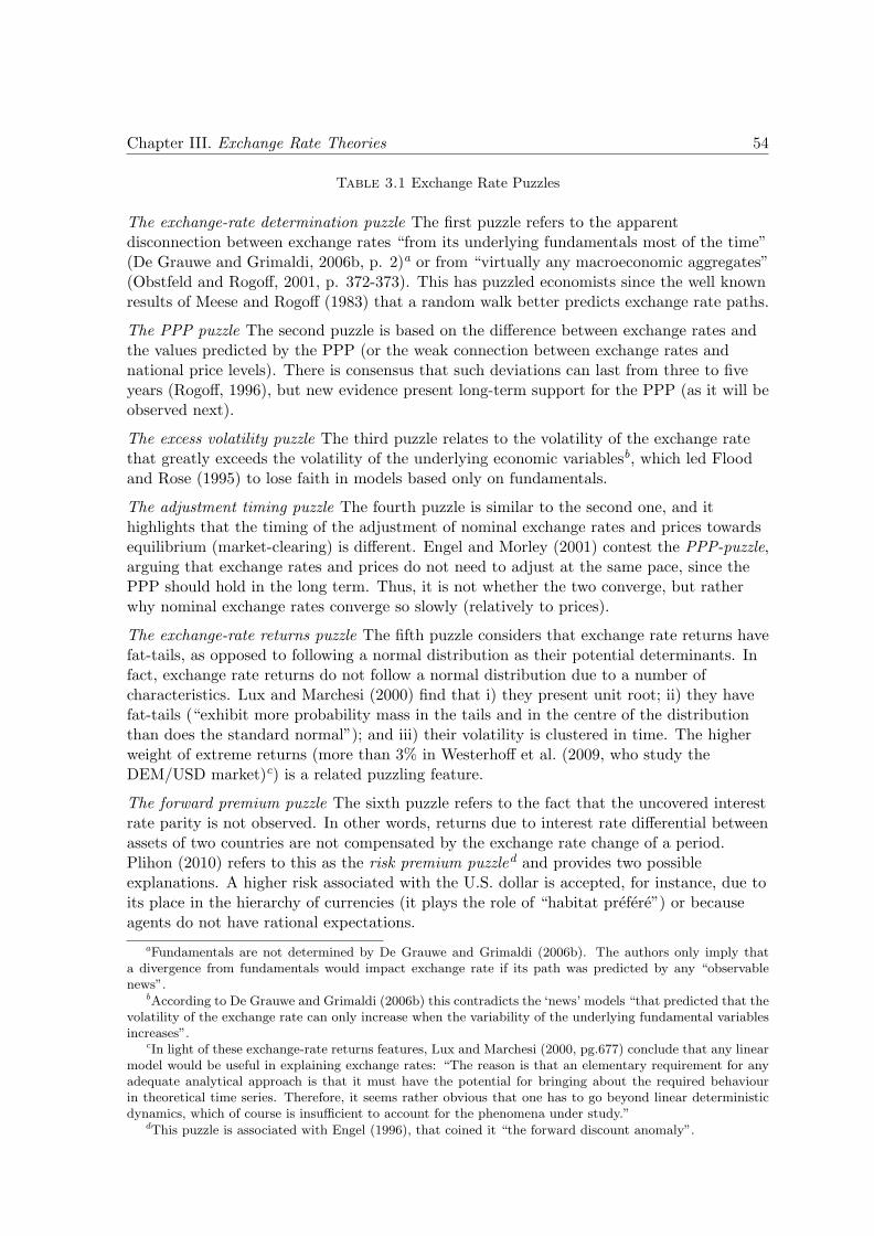
Chapter III. Exchange Rate Theories 54
Table 3.1 Exchange Rate Puzzles
The exchange-rate determination puzzle The first puzzle refers to the apparentdisconnection between exchange rates “from its underlying fundamentals most of the time”(De Grauwe and Grimaldi, 2006b, p. 2)a or from “virtually any macroeconomic aggregates”(Obstfeld and Rogoff, 2001, p. 372-373). This has puzzled economists since the well knownresults of Meese and Rogoff (1983) that a random walk better predicts exchange rate paths.
The PPP puzzle The second puzzle is based on the difference between exchange rates andthe values predicted by the PPP (or the weak connection between exchange rates andnational price levels). There is consensus that such deviations can last from three to fiveyears (Rogoff, 1996), but new evidence present long-term support for the PPP (as it will beobserved next).
The excess volatility puzzle The third puzzle relates to the volatility of the exchange ratethat greatly exceeds the volatility of the underlying economic variablesb, which led Floodand Rose (1995) to lose faith in models based only on fundamentals.
The adjustment timing puzzle The fourth puzzle is similar to the second one, and ithighlights that the timing of the adjustment of nominal exchange rates and prices towardsequilibrium (market-clearing) is different. Engel and Morley (2001) contest the PPP-puzzle,arguing that exchange rates and prices do not need to adjust at the same pace, since thePPP should hold in the long term. Thus, it is not whether the two converge, but ratherwhy nominal exchange rates converge so slowly (relatively to prices).
The exchange-rate returns puzzle The fifth puzzle considers that exchange rate returns havefat-tails, as opposed to following a normal distribution as their potential determinants. Infact, exchange rate returns do not follow a normal distribution due to a number ofcharacteristics. Lux and Marchesi (2000) find that i) they present unit root; ii) they havefat-tails (“exhibit more probability mass in the tails and in the centre of the distributionthan does the standard normal”); and iii) their volatility is clustered in time. The higherweight of extreme returns (more than 3% in Westerhoff et al. (2009, who study theDEM/USD market)c) is a related puzzling feature.
The forward premium puzzle The sixth puzzle refers to the fact that the uncovered interestrate parity is not observed. In other words, returns due to interest rate differential betweenassets of two countries are not compensated by the exchange rate change of a period.Plihon (2010) refers to this as the risk premium puzzled and provides two possibleexplanations. A higher risk associated with the U.S. dollar is accepted, for instance, due toits place in the hierarchy of currencies (it plays the role of “habitat prefere”) or becauseagents do not have rational expectations.
aFundamentals are not determined by De Grauwe and Grimaldi (2006b). The authors only imply thata divergence from fundamentals would impact exchange rate if its path was predicted by any “observablenews”.
bAccording to De Grauwe and Grimaldi (2006b) this contradicts the ‘news’ models “that predicted that thevolatility of the exchange rate can only increase when the variability of the underlying fundamental variablesincreases”.
cIn light of these exchange-rate returns features, Lux and Marchesi (2000, pg.677) conclude that any linearmodel would be useful in explaining exchange rates: “The reason is that an elementary requirement for anyadequate analytical approach is that it must have the potential for bringing about the required behaviourin theoretical time series. Therefore, it seems rather obvious that one has to go beyond linear deterministicdynamics, which of course is insufficient to account for the phenomena under study.”
dThis puzzle is associated with Engel (1996), that coined it “the forward discount anomaly”.
Chapter III. Exchange Rate Theories 55
by financialization – particularly of sophisticated foreign exchange (FX) markets2 (discussed
in Chapter Two).
3.1.1 Theories From Before the Collapse of the Bretton Woods System
3.1.1.1 Purchasing power parity
The Purchasing Power Parity (PPP) is a main reference in exchange rate theories. In the
formalization of Cassel (1916), it meant that the exchange rate would change according to
the relative price changes in two countries. The PPP has both absolute and relative forms.
In the absolute form, the exchange rate (E ) represents the prices prevailing in a country (P)
relative to that of a foreign country (P* ), as in Equation 3.13:
E =P
P ∗(3.1)
Its relative form implies that the exchange rate changes (e) are determined by the
changes of domestic prices (p) relative to changes of international prices (p* ), as in Equation
3.2:
e = p− p∗ (3.2)
Although broadly known and used, the PPP has relevant limitations. First, it supposes
the verification of the law of one price (goods would have one unique price in different places),
that cannot be achieved given that i) international economic integration is not perfect; ii)
2As discussed in Chapter Two, finance saw important transformations, with innovations in the senseof products and of usages. What characterizes sophisticated FX markets are the broad use of products asderivatives, and activities including carry trade and currency financialization more broadly (see the discussionthat begins on page 35). The operational definition of a sophisticated market is used in Chapter Five: a marketthat has an important ratio of future-to-spot FX contracts.
3In this quotation, the exchange rate (E) is the value of one unit of foreign currency in the domesticcurrency; a higher rate (E) corresponds to a depreciation of the domestic currency. This type of quotation,known as direct quotation, is the one used throughout this thesis. In French it is called cotation a l’incertain,in opposition to the cotation au certain. In Portuguese it is called cotacao direta, as opposed to cotacao
indireta.
Chapter III. Exchange Rate Theories 56
goods are not perfect substitutes as agents do not have the same preferences in different places
and companies differentiate their products’ prices in different markets4 (Plihon, 2010).
Secondly, on the empirical front, the validity of the PPP is questionable, resulting
in the presented purchasing power puzzle (Rogoff, 1996). However, recent works that use
other econometric techniques, have found long term convergence between exchange rates
and values predicted by the PPP. In other words, as the exchange rate and relative prices
are co-integrated, the real exchange rate would tend to equilibrium (market-clearing5) in the
long run (See MacDonald (1995) and Taylor (2009b)). Based on this, Taylor and Taylor
(2004) state that we currently see the emergence of “some degree of confidence in long-run
PPP”.
Trade costs are a broadly accepted solution to the PPP puzzle, as they “include trans-
port costs but also tariffs, non-tariff barriers, and possibly other broader factors that impede
trade” (Obstfeld and Rogoff, 2001, p. 372-373). Note, however, that this argument still does
not solve the problems related to the law of one price.
An intriguing theoretical consideration on the long-run convergence of the PPP is dis-
cussed by Priewe (2014, p. 17): if divergence leads to desindustialization and to change in
production structure, how can the prices of the new economy be compared to those prevailing
before the deviation from PPP? In the author’s word: “In this case the statistical approx-
imation to the PPP after correction of the exchange rate is an illusion” – the goods whose
prices would have to be the same in different countries, “are no longer produced or are only
4Isard (1977, p. 4-5) compare domestic (US) and foreign prices of manufactured goods and concludes:“The denial of the law of one price in this context – at the most diaggregated product level for which pricedata can be readily. matched – provides a strong presumption that it is impossible to assemble availabledata into aggregate price indeces which can be expected to obey the law of one price (except, perhaps, whenproduct coverage is restricted to primary commodities). Obversely, the notion that aggregate indeces of exportor tradable-goods prices will exhibit purchasing power parity – i.e., that the relative home-currency prices ofdifferent countries will stay in line with exchange rates – cannot validly lean on the law of one price”. Alsosee Dornbusch (1985) for a review on the law of one price.
5In mainstream works equilibrium is used in the market-clearing sense, or to indicate a situation where“quantity demanded exactly equals the quantity supplied” (Davidson, 2011, p. 204). Equilibrium, on theother hand, is a state “where no forces are at work to alter the position of the economy as long as the specifiedconditions remained unchanged” (p. 203). The concept of equilibrium was brought from physics to economicsby Marshal, and meant “a balancing of endogenous forces so that the body under study is at rest” (Rotheim,2003, p. 23). Market-clearing is a sufficient, but not necessary condition for equilibrium.
Chapter III. Exchange Rate Theories 57
produced to minor extent in one or more countries. The production structure then adapts
to the distorted exchange rate, instead of the exchange rate adapting to production”6.
Drine and Rault (2004) make a similar argument when analyzing why evidence is less
favorable to PPP among developing countries, mentioning the role of productivity shocks as
one of the reasons for this result. In line with the Balassa (1964)-Samuelson (1964) effect,
increasing productivity leads to long term appreciation of exchange rates and thus deviations
from the PPP7.
3.1.1.2 Uncovered interest rate parity
With the uncovered interest rate parity (UIP), Keynes emphasized that the exchange rate
cannot respond only to developments related to the goods market and shifted the focus
towards assets markets. According to the UIP, the expected return of fixed-income assets
of two different countries is the same when measured in one currency. In other words, the
expected return of a foreign asset (i∗e) should be the same as the return of the domestic asset
(ie) plus the exchange rate change in a given period (Eet+1 − Et) – as shown by Equations
3.3 and 3.4:
i∗e = ie + Et+1 − Et (3.3)
i∗e = ie + e (3.4)
Shifting the focus towards exchange rate determination and expected future exchange
rates (Eet+1), an alternative and common representation of UIP is shown in Equation 3.5
(following Lavoie (2014, p. 479)):
6It is interesting to note that arguing for the path-dependency of exchange rates, is the same as arguing forthe existence of exchange-rate hysteresis, because exchange rates do not come back to their previous trajectoryafter a shock. Lang and De Peretti (2009, p. 447) defines a hysteretic process as characterized for having aremanence and selective memory: “Remanence occurs when the application of a shock of the same extent asan initial shock, but in the opposite direction, does not bring the system back to its initial position”; in aselective memory, “only the nondominated extreme values of the shocks remain”.
7Regardless of theoretical limitations and the relative empirical failure, the current practical relevance ofthe PPP should be noted. It has became an essential tool in global macroeconomic statistics, due to its wideuse in international comparison of macro aggregates by international institutions such as the IMF, the WorldBank or the OECD.
Chapter III. Exchange Rate Theories 58
i∗e − ie = Eet+1 − Et (3.5)
The UIP depends on significant hypothesis of perfect arbitrage (implying no transaction
costs nor restrictions to capital account transactions) and perfect substitution of assets of
different countries, in terms of both risks and liquidity (Prates, 2015, p. 24).
Despite its restrictive assumptions and statistical failure, the UIP is widely used by
mainstream economists in the post-Bretton Woods period. According to Burnside et al.
(2006), the “UIP is a central feature of virtually all linearized general-equilibrium open-
economy models”. These models either ignore the “statistical failure” of the UIP, or try to
account for it by introducing a “risk premium shock” in the model.
It is also used by some heterodox authors. Taylor (2009a, p. 333) uses UIP for believing
that the “exchange rate must evolve over time subject to rules based on expectations about
its future”, and the UIP is the best option to take expectations into account8. Its use is
defended even if it “does not reliably fit the data”. For Lavoie (2014, p. 480), this choice
reflects an “instrumentalist philosophy (...) according to which it is better to be precisely
wrong than vaguely right”.
From a theoretical point of view, the advent of the UIP has shifted focus to capital
account considerations – essential for an exchange rate analysis in times of financialization.
It also considers exchange-rate expectations, which later was neglected by most mainstream
models. It is a simple model that has a restrictive hypothesis and does not account for
trade-related dynamics, but it is an important shift to capital account considerations that is
only revived in portfolio models (analyzed in Section 3.1.2.3) where the hypothesis of perfect
substitute assets is relaxed.
3.1.1.3 Covered interest parity
If we consider that the forward exchange rate (F ) is a proxy for the expected future exchange
rate (Eet+1), the difference between the forward and the current rate is equal to the interest
8Taylor (2009a, p. 333) adds that “n a world of shifting and perhaps unstable expectations, no simpledynamic theory is likely to emerge.”
Chapter III. Exchange Rate Theories 59
rate differential (as shown in Equation 3.6):
i∗e − ie = F − Et (3.6)
In this case, the forward rate is said to be “an unbiased and efficient predictor of the spot
rate prevailing in the future” (Moosa, 2004, p. 366). However, this can only be realized in
the presence of unbiased expectations (Lavoie, 2014)9.
The empirical evidence supports the CIP10. But CIP holds because it is “a definition
rather than an equilibrium relationship” (Harvey, 2009, p. 21). Lavoie (2000, p. 172) posits
that “the forward exchange rate is not an expectational variable, but rather the result of a
simple arithmetic operation”: “Banks set the forward rate by adding the interest differential
to the spot exchange rate”.
The CIP is a rare example of consideration of derivatives markets – along with the ones
analyzed in Section 3.1.5 – but because it is a definition rather than an analytical framework
it does not add to our understanding of exchange-rate expectations.
3.1.1.4 The Keynesian Models: Elasticities, Absorption, Mundell-Fleming
In the 1940s and 1950s, mainstream economists were challenged by the need to develop an
open macroeconomic model that took into account the impacts of exchange rate and foreign
income in determining domestic income (Prates, 2015).
Elasticities The elasticity approach presented the effect of an exchange-rate depreciation
on the current account. Given that prices were determined by constant monetary incomes,
9The parity between the forward rate and the realized future exchange rate (F = Et+1) is known as theforward market unbiasedness hypothesis or the unbiased efficient hypothesis (UEH) (Lavoie, 2014). Notethat when both UIP and PPP hold, there is real interest rate parity (RIRP). This relationship suggests thatexpected adjustments in the real exchange rate are represented by expected real interest rates. Lavoie (2014,p. 478) argues that if the RIRP holds, then central banks are not able “to set real interest rates as it wishes fordomestic reasons (...) and are forced to set the real interest rate in line with interest rates that prevail in thebiggest economies.” Lavoie (2014, p. 478) sees this relationship as “the crucial relation in mainstream open-economy macroeconomics”, and Smithin (2002, p. 224) says that it “transfers the doctrine of the ‘naturalrate of interest’ to the international setting.”
10It should be noted that Shin (2016) argues that the CIP has not hold in turbulent periods, such as in theonset of the Global Financial Crisis and the Euro are crisis of 2011-12 and that it has also not hold recently,although we are living a calm period. Moreover, the deviation from the CIP would be increasing. The authorargues that it is related to the strong dollar and the consequent tighter credit condition.
Chapter III. Exchange Rate Theories 60
it assumed that nominal and real changes were equivalent11. As highlighted by Krueger
(1983), it allowed for an analysis based on the opposite direction as that of the elasticity
approach: the impact of macroeconomic variables as trade balance and domestic income on
the exchange rate.
Absorption Polak (1957) and Alexander (1952) criticized this approach as it did not allow
interaction from foreign trade to domestic income given the hypothesis of constant nominal
income. The authors highlighted these effects, especially the importance of change in domes-
tic absorption12 on the trade balance13, developing what became known as the absorption
approach. This approach concludes that an exchange-rate depreciation has only a transitory
impact and is thus ineffective in enhancing trade balance, while restrictive monetary poli-
cies, by decreasing domestic absorption, would solve current account issues. As highlighted
by Prates (2015), IMF external adjustment policies were based on this approach, however,
Prates (2015) argues that an exchange-rate depreciation does not necessarily has a positive
impact on the trade balance but can reduce domestic income, as resource reallocation does
not take place immediately. On the theoretical front, the absorption approach has abandoned
analyses of the consequences of an exchange-rate change.
Meade’s (1951) model combines the elasticity and the absorption approaches: an exchange-
rate depreciation improves trade balance, but to a lesser extent than in the elasticity ap-
proach, as its effects on a country’s absorption are taken into account. Because it emerged
in the early Bretton-Woods era, some of the model’s features differ from today’s reality: the
exchange rate is considered fixed or exogenous and capital account dynamics are not taken
into account (reflecting the lesser importance of capital flows in the period). In light of this,
Taylor (2004) considers these models obsolete14.
11Prates (2015) reminds us that this approach is based on a Marshalian framework: as the exchange rateis the price that equals supply and demand for foreign exchange, it analyzes the impact of a change in thisrelative price on quantities and the stability of the equilibrium.
12The total absorption is the sum of consumption, investment, government expenditure and imports.13As reminded by Prates (2015), although these models have also been called current account models (as
by (Krueger, 1983)), they focus only on the trade of goods, and overlook services.14According to Taylor (2004), an interesting exchange rate fundamental emerges from a similar model: the
traded/non-traded goods price ratio, where a decrease can be interpreted as an overvaluation (referring tothe works of Salter (1959) and Swan (1960)).
Chapter III. Exchange Rate Theories 61
Mundell-Fleming The Mundell (1963)-Fleming (1962) model incorporates, to the keyne-
sian models just presented, the monetary market, capital flows and the possibility of flexible
exchange rates15. Mundell’s (1963) conclusions differs from Meade’s (1951): While the latter
argues that a policy conflict exists between the domestic (full employment) and the exter-
nal (balance-of-payments) equilibrium, the former argues that in the context of free capital
movements this trade-off would not take place, with neither floating nor fixed exchange-rates.
In fact, appropriate fiscal and monetary policies would allow both objectives to be achieved.
In terms of exchange rate determination, Mundell (1963) incorporates a very simplified
form of UIP, where the domestic (i) and foreign (i* ) interest rates are equal (as in Equation
3.7): implying risk-neutral investors with static expectations about the exchange rate –
the expected rate (Eet+1) equals the current one (Et+1) in Equation 3.5. Indeed, this is
a simplified form - as put by Krugman (2001a), “nobody believes in static expectations
about e”. Consider equations 3.7 to 3.9 as a simplified form of the Mundell-Fleming model
(Krugman, 2001a). Equation 3.8 presents the determination of aggregate demand from both
domestic demand (that depends on income, Y, and interest rates (i)), and net exports (NX )
(that, in turn, depends on the real exchange rate (eP ∗/P ) and income (Y )). Equation 3.9
illustrates money demand.
i = i∗ (3.7)
Y = D(Y, i) +NX(eP ∗/P, Y ) (3.8)
M
P= L(Y, i) (3.9)
In the Mundell-Fleming model with floating exchange rates, this is the variable that
adjusts excess supply and demand in FX markets. Capital account dynamics are extremely
simplified: assets are perfect substitutes and expectations are static. The only dynamic taken
into account is capital inflows (outflows) when interest rate increases (decreases). Although
an important step in understanding exchange rates at the time, this is a simple model, with
restrictive assumptions.
15See Mundell (2001) for the history of the IS-LM-BP model.
Chapter III. Exchange Rate Theories 62
The keynesian models are also called balance of payment or flow models, as exchange
rate determination arises from the current and the capital accounts of the balance of pay-
ments, that are “flow magnitudes” (MacDonald, 2007, p. 7). This is a clear distinction from
the focus on stocks characteristic of the monetarist and and portfolio models, presented next.
3.1.2 First-Generation Models
The first generation models emerged in the context of flexible exchange rates, with the
collapse of the Bretton Woods System. These models shift the focus of exchange rate deter-
mination from flows to monetary or financial stocks.
3.1.2.1 Monetarist Model
The monetarist criticism of the keynesian models shifted the focus of exchange rate determi-
nation through (mostly) trade-related flows to monetary policy. They can be considered “a
monetary approach to the balance of payments” (Taylor, 2004, p. 211). The models start
from the traditional equation of the money market equilibrium, given by the equality of the
stock of money supply and money demand (M s = Md). As usual in monetarist models,
money supply is exogenous, determined by the Central Bank (Ms), and money demand de-
pends on price level (P ), real income level (Y ) and rate of interest (i). The stock of money
(M) can thus be given by Equation 3.10 and 3.11, for domestic and foreign (∗) variables,
respectively (Plihon, 2010):
M = P × L(Y, i) (3.10)
M∗ = P ∗ × L(Y ∗, i∗) (3.11)
Given the use of PPP (shown in Equation 3.1), the exchange rate (E) depends on prices,
resulting, in the monetarist view, on exchange rates that depend on the evolution of domestic
and foreign money demands, income and interest rates (as in Equation 3.12):
Chapter III. Exchange Rate Theories 63
E =M
M∗×
L(Y ∗, i∗)
L(Y, i)(3.12)
Therefore, in the monetarist view, the exchange rate is determined by a country’s central
bank policies and by the behavior of money-holders vis-a-vis these determinants in the other
country. In the words of Kouri (1976, p. 1), the behavior of exchange rate, the “relative
price of monies”, can be explained by “the supplies of various monies and other financial
assets, as well as the behaviour of demands for these assets”16. The model thus concludes
that the central bank can control any potential exchange rate disequilibrium with monetary
policies17 (which is in line with monetarist models more generally, where the real sphere can
be controlled by monetary policies).
According to Plihon (2010), this result was key in providing support the superiority of
the floating exchange rate regime, which was the aim of the studies.
It is worth mentioning that these models lead to the conclusion that an increase of
domestic revenue lead to an appreciation of the domestic currency, contradicting the findings
of the keynesian models, discussed in Section 3.1.1.4 (Plihon, 2010). In fact, combined with
a stable stock of money, the higher money demand can only occur when domestic prices are
lower ; and as the PPP holds, a decrease in domestic prices corresponds to an appreciation.
The fact that the variables used to explain exchange rates and the exchange rate in
itself have very different features – the former is stable, while the latter can be volatile – is
a main issue of monetarist models. Though the issue is not exclusive to monetarist models,
it is worse in them, and originated the excess-volatility puzzle. The monetarist models also
receive both PPP-related criticism, as well as criticism related to different financial assets
being considered perfect substitutes. Nevertheless, from a PK perspective, it is the very
concept of monetary policy based on authorities’ changes of money supply and of money as
an exogenous variable, that make monetarist models an inadequate framework for exchange
rate analysis, not only for EMEs or for a context marked by financialization, but in general.
16Mussa (1976, p. 229) summarizes the dynamics involved: “When the demand for a particular moneyrises relative to the supply of that money, either the domestic credit component of the money supply mustbe expanded, or the exchange rate must appreciate, or the official settlements balance must go into surplus,or some combination of the three.”
17The impact of change in money supply (M) on the exchange rate (E) is clear on Equation 3.12.
Chapter III. Exchange Rate Theories 64
In retrospect, it must be highlighted that monetarist analyses associate stocks (as the
money stock) and flows (as the revenue) variables, leading the way to portfolio-models (Pli-
hon, 2010) and to patrimonial approaches that followed (which, in turn, are key to times of
financialization and to the crucial role of international portfolio allocation).
3.1.2.2 Overshooting models (Dornbusch)
Dornbusch’s (1976) overshooting models is an important monetarist approach focused on
explaining exchange rate volatility. It assumes that capital markets’ dynamics reflect the
UIP, but that the PPP is the long-term determinant of exchange rates. The exchange rate
volatility analyzed by the model refers to the deviation from the PPP when UIP dynamics
take place. It results from the different adjustment timings of assets’ and goods’ markets, the
first being immediate and the latter fixed (in the short run). In the case of a loose monetary
policy, for instance, the adjustment of the monetary market, being immediate, leads to an
interest rate decrease. Given that, in the short-term, the FX market is dominated by capital
flows which are determined by the UIP, the lower interest rate leads to an expectation of
exchange rate depreciation. The name of the model stems from the contrast between the
immediate adjustment of both the assets’ and the goods’ markets. In fact, the adjustment
in the latter will only occur with the exchange rate depreciation, the enhancement of the
trade balance, resulting in an exchange rate appreciation, back to the PPP-predicted value.
Before this occurrence, markets caused overshooting of the exchange rate (Plihon, 2010).
It should be highlighted that Dornbusch’s overshooting model implies adaptive expec-
tations: agents action in building the overshooting does not takes into account any consid-
eration that they know that the depreciation will only be temporary – or that the overshoot
would later be canceled out.
Although Dornbusch (1976) advances the analysis of exchange rate volatility, since it is
the first model to focus on this analysis and to to combine financial and real factors (Plihon,
2010), it must be highlighted that it explains a very specific volatility. It is similar to what
is studied as PPP-deviation, a change that is canceled after a relatively long period18. It
is therefore not the same as weekly or daily volatility from FX markets. The model must
18As mentioned in Section 3.1.1.1, PPP deviations prevail for 3 to 5 years.
Chapter III. Exchange Rate Theories 65
be acknowledged for stressing the need to explain volatility and to indicate negative aspects
inherent to flexible exchange rates, but, in light of the most recent models (mainstream and
heterodox), it falls far from explaining the volatility phenomenon in all its complexity.
3.1.2.3 Portfolio models
Portfolio Models are inspired by the financial market analyses of Markowitz (1968) and Tobin
(1965). In these models the exchange rate is a result of the portfolio allocation among mon-
etary and financial assets of different risk and returns. They therefore reveal a patrimonial
approach to exchange rates (Plihon, 2010). McKinnon (1966), Branson (1974) and Kouri
(1976) are influential references for these models.
In simple one country models, portfolio equations are written as in Equations 3.13 to
3.16, where a country’s wealth (W ) is allocated among domestic assets (B), foreign assets
(B∗) in local currency units (B∗ × E), and the money stock (M). Domestic agents cannot
hold foreign currency19. Portfolio allocation depends on interest rates paid by domestic (i)
and foreign (i∗) assets, adjusted for their respective risks (r, r∗) (Plihon, 2010)20.
M = a(i, i∗, r, r∗)W (3.13)
B = b(i, i∗, r, r∗)W (3.14)
E ×B∗ = c(i, i∗, r, r∗)W (3.15)
W = M +B + E ×B∗ (3.16)
19This hypothesis is done in both the monetary and portfolio models, but is relaxed in the monetary modelswith currency substitution where agents can only hold domestic currency as in Miles (1978) and McKinnon(1982). By allowing agents to hold currencies from different countries, these models achieved two importantresults: i) the volatility of flexible exchange rates and ii) the importance of changes on relative costs related toholding currencies when determining exchange rates. The result highlights a serious issue: the interdependenceof monetary policies in different countries (Plihon, 2010).
20The direction of the impact of the risk and return variables on the demand for assets or money is thestandard: demand for money (Equation 3.13) is negatively impacted by the return of domestic or foreigninterest rates and positively impacted by their risks; demand for domestic assets (Equation 3.14) is positivelyimpacted by their return or by the risk of foreign assets and negatively impacted by its own risks or the returnof foreign assets; symmetrically, the demand for foreign assets (Equation 3.14) is positively impacted by itsown return or by the risk of domestic assets, and negatively impacted by its own risk or by the return ofdomestic assets.
Chapter III. Exchange Rate Theories 66
Given the budgetary constraint presented in Equation 3.16, the sum of the coefficients
a, b and c must equal 1, leading to a reduced form of the model in Equation 3.17 and the
exchange rate determination in Equation 3.19:
E ×B∗ = (1− a− b)W (3.17)
E ×B∗ = f(i, i∗, r, r∗)W (3.18)
E = f(i, i∗, r, r∗)W
B∗(3.19)
In portfolio models, the exchange rate results from the relative risk and return of do-
mestic vis-a-vis foreign assets and money demand: an interest rate hike increases demand
for domestic financial assets, triggering an exchange rate appreciation (E decreases). Note
that this result is the opposite of the monetary models used until then.
Because they are difficult to estimate, portfolio models are often presented in simplified
forms21. However, some models may include a large set of determinants, such as equities and
its rate of return, real capital stock, savings, real investments and its profit rates, exports,
imports, and taxes (as in Branson (1974, p. 30)).
Portfolio models present the most suitable features for analyzing the dynamics of EMEs’
currencies out of all mainstream models analyzed in this chapter. As mentioned, the fact
that financial assets are not perfect substitutes is central in dealing with current exchange
rate issues in general (Blanchard et al., 2005), particularly in analysis involving emerging
countries’ assets due to the specificities of their currencies – to be discussed in Section 3.3.4.
In addition, portfolio models put emphasis on the importance of stocks in determining the
exchange rate, a patrimonial approach that is key given financialization22. This treatment
of stocks is also important for two reasons: i) the magnitude of the stock of financial assets
that might be converted in another currency at any moment is not comparable to the size
of the current account flows, and ii) these two would also differ on the adjustment timing,
being much faster in assets markets than in goods markets (Plihon, 2010) (more on capital
account adjustment will be seen in the conclusions).
21See Melitz and Owen (1983) for a discussion on the simplifications in exchange rate modeling.22Branson (1974) specifically considers the effects stemming from “stock-shifts” and “continuing-flow”.
Chapter III. Exchange Rate Theories 67
3.1.3 Second-Generation Models (New-Classical)
The exchange rate models grouped into the second generation consider rational expecta-
tions when determining exchange rates, and are, therefore, part of the New-Classical School
(Prates, 2015).
3.1.3.1 Efficient market models
As the name indicates, expectations in these models were modeled according to Fama’s
(1970) efficient market hypothesis: under the assumption that the future can be reduced to
probabilistic events and that agents’ decisions reflect their rational expectations based on
available information, the price of an asset constitutes the best indicator of its intrinsical
value, reflecting all information available in a given moment. Thus, exchange rates in period
t would reflect all information available in t.
Two major assumptions are implied. First, arbitrage are perfect: assets are perfect
substitutes and the UIP (Equation 3.4) holds. It means that higher returns in country A than
in country B could only hold if agents expect the currency of country A to depreciate until
the maturity of the asset by the same amount of the interest rate differential. A deviation
from the values predicted by this equation, in turn, would reflect agents’ perception of these
assets as riskier (and not as substitutes), which calls for a risk-premium (Plihon, 2010).
The second implicit hypothesis is that agents have rational expectations: they use all of
available information, know the “real” determinants of exchange rates, and, as a consequence,
do not make persistent forecast errors23. With such unlikely hypotheses, these models have
not directly enhanced our understanding of exchange rates. They have, however, triggered
critiques that were further developed into interesting insights.
With rational expectations, the UIP states that the exchange rate change between
period t and t+n (Eet+n −Et) equals the interest rate differential (it − i∗t ) plus an error term
(ut):
23This means that their errors have a mathematical average of zero: Et+n − Et = (Ee
t+n − Et)|It−1 + ut
and E(ut) = 0.
Chapter III. Exchange Rate Theories 68
Et+n − Et = it − i∗t + ut (3.20)
The empirical tests of the efficient market view thus test if, in Equation 3.21, a can be
said to be statistically equal to zero, b equal to 1, and if the errors terms (ut) are independent
(Plihon, 2010). If this is the case, there is no possibility of higher returns by investing in
a foreign country and the exchange rate is determined only by the expectation errors of
investors which are only temporary (Prates, 2015).
Et+n − Et = a+ b(it − i∗t ) + ut (3.21)
As expected, these assumptions were rejected by most econometric tests (see MacDonald
(2007)), which supports the existence of a risk premium – leading to the emergence of the
risk-premium puzzle. Two main explanations for the “puzzle” emerged: a reason for asking
for a risk premium might indeed exist, or agents’ expectations were not rational. There are
two main reasons for the risk-premium: the instability of a currency (Giovannini and Jorion,
1989) or the position of the currency on the hierarchical international monetary market
(Frankel and Froot, 1985) – a hypothesis developed in details by the heterodox literature
featured in Section 3.3.4. The rejection of the efficient market hypothesis could also indicate
that agents are not rational. This hypothesis was further developed by the authors who later
created models composed of heterogeneous traders with bounded rationality (discussed in
Section 3.1.5).
These studies criticize the efficient market hypothesis that prices always reflect funda-
mental values by arguing that this is not compatible with fast changing prices. As put by
Westerhoff et al. (2009),
The efficient market hypothesis states that prices always reflect their fundamental
values. Hence, price changes are due to unexpected fundamental shocks. Clearly,
if we observe an exchange rate movement by five percent, then this should cor-
respond to a five percent shock in the fundamentals. Given also the fact that
exchange rates change on a second-to-second basis, it is difficult to imagine where
all these fundamental shocks should come from. (p. 2)
Chapter III. Exchange Rate Theories 69
These models were criticized when the main features of exchange-rate return distribu-
tion (the fifth puzzle) were brought to attention, as the features they reproduced were only
partially coherent with what was empirically observed: though they were non-stationary,
they were also not simultaneously volatile, random, and with clustered volatility (Lux and
Marchesi, 2000). However, these criticisms came later, and the efficient market view of
exchange rates profited from relative success at the time (Prates, 2015)24.
Despite the fact that exchange rate behavior created in the models only partially fits
reality, the main problem with the efficient market view of exchange rates remains its unre-
alistic hypotheses of an intrinsic value, of rational expectations, of the UIP, and of different
country assets as perfect substitutes. Though it allowed for the emergence of interesting
discussions over the reasons behind country risk-premiums, it cannot explain exchange-rate
dynamics.
3.1.3.2 Rational speculative bubbles
Other important New-Classical models are the rational speculative bubbles, that aimed at
explaining markets’ development in the 1980s, addressing the puzzle on the exchange rate
determination. According to these models, the exchange rate (E) deviates from its equilib-
rium (meaning market-clearing) value (E∗) due to speculative bubbles (B) (as in Equation
3.22) without relaxing the hypothesis of rational agents and efficient markets: if rumors lead
agents to expect an exchange-rate appreciation, their trading creates appreciation, and a
bubble. At some point their expectations would change and destroy the bubble, but the fact
that expectations were correct (because they were self-fulfilling) is in line with the efficient
market hypothesis: that the markets had correctly anticipated the appreciation25.
E = E∗ +B (3.22)
24Prates (2015) highlight the potential reasons behind this success: i) they proposed to solve the firstexchange rate puzzle, namely the exchange rate determination puzzle, or why exchange rate behavior wasa random walk; ii) the role of expectations could not be further denied with financial globalization iii) thenew-classical school’s rational expectation hypothesis was the mainstream at the time.
25Plihon (2010) stresses that markets cannot be efficient given that not all information was taken intoaccount – in the case of the 1980s, agents overlooked the increasing twin (budgetary and external) deficits inthe US (showed by Krugman (1985)). Had it been analyzed, the expectation of appreciation would not havebeen built.
Chapter III. Exchange Rate Theories 70
The use of the rational bubbles hypothesis to exchange rate analyses relies on the same
assumptions of other efficient market views: efficient markets and rational agents.
3.1.4 Third-Generation Models (New Keynesians)
3.1.4.1 New open macroeconomics
The third generation models maintain the hypothesis of rational expectations, but allow
rigidities to take place resulting in exchange rates that do not follow fundamentals. These
are dynamic models, with maximization of utility and representative agents. They can
therefore be called New-Keynesian (Prates, 2015)26. They claim to be an alternative to the
Mundell-Fleming models (Lane, 2001) – reflecting their closer methodological ties to the
eynesian models that emerged before the collapse of the Bretton Woods system than to the
Monetarists (Section 3.1.2.1) and the New Classical (Section 3.1.3) models that followed.
Lane (2001) presents the redux exchange rate model of Obstfeld and Rogoff (1995),
considered to be the one that initiated this research program27. The model makes the relevant
hypothesis already discussed on the law of one price and the PPP. It is a two country model
with farmers and no capital. It involves the utility functions of farmers that include leisure
and the disutility of work effort. Farmers have access to riskfree international bond markets
where interest rates are constant. Agents make “optimal choices of consumption, money
holding, labor supply” and set their “optimal output price.”
Once the steady state of the model is calculated, the authors examine the impact of an
increase in money supply (also known as Dornbusch’s shock) on welfare. The result is: shock
has output effects, and while farmers of one country work more, home and foreign welfare
are raised by the same amount, as “the extra revenue is exactly canceled out by the increase
in work effort” (Lane, 2001, p. 239).
Lane (2001, p. 240) states the superiority of this framework: “The surprising result that
both countries gain equally from an unexpected domestic monetary expansion illustrates the
26 New Open Macroeconomics is defined by Lane (2001, pg.1) as a “new workhorse model for open-economymacroeconomic analysis” that has, as a unifying feature “the introduction of nominal rigidities and marketimperfections into a dynamic general equilibrium model with well-specified microfoundations.”
27Also see Obstfeld and Rogoff (2000) and Obstfeld (2002).
Chapter III. Exchange Rate Theories 71
utility-based evaluation offers a non-trivial advantage over traditional ad-hoc loss functions”,
but acknowledges that the results are highly sensitive to “the precise denomination of price
stickiness, the specification of preferences and financial market structure” and concludes that,
for these reasons, they should not be used for policy recommendations28.
The inappropriateness of these models for exchange-rate dynamics is not due to the
sensitiveness of results, but to the unrealistic characteristics they feature on both assumptions
– no capital, the law of one price and PPP – and on results – an increase of domestic money
supply triggers a fall of the world’s real interest rate. Therefore, the inclusion of rigidities has
not yielded any further gains on the understanding of exchange-rate dynamics than what the
keynesian models had provided. If the latter were said to lack capital account considerations
(except for Mundell Fleming), New Keynesian models with no capital (such as Lane’s (2001))
are certainly not able to tackle the issue.
3.1.5 Fourth-Generation Models (Micro-Structure)
According to Prates (2015) the fourth generation label groups exchange rate models that
have abandoned the hypothesis of a representative agent, but are still orthodox for assuming
ergodicity – which allows for the use of stochastic models. In these models, the focus is on
the micro-structure of FX markets and their participants.
The shift of focus from the mainstream to the microstructure of FX markets is closely
tied to the failure of all prior models, that were focused on the role of macro aggregates, and
their inadequacy to solve exchange rate puzzles. This is clear in Flood and Rose’s (1995)
analysis. After presenting what became known as the excess volatility puzzle, Flood and
Rose (1995, p. 22-23) conclude that “future research should shy away from macroeconomic
fundamentals, and concentrate on more microeconomic detail” (p. 21). Krugman and Miller
(1993) introduced stop-loss traders into a model of FX markets, arguing that the microeco-
nomic focus may well provide a future rationalization for the phenomenon of regime-varying
volatility.
28“For this reason, any policy recommendations emanating from this literature must be highly qualified.This is an issue of some concern, since the new open economy macroeconomics will be of only limited interestin policy circles unless researchers converge on a ‘preferred’ specification that is buttressed by extensivesupporting empirical evidence. For all that, the many unanswered questions that remain should ensure thatthis burgeoning field is likely to grow yet further in the coming years” (Lane, 2001, p. 262).
Chapter III. Exchange Rate Theories 72
There are two main types of Micro-Structure models: one focused on the flow of buy-
ing and selling orders in FX markets (such as Evans and Lyons (1999)) and the other on
explaining the behavior of these markets’ agents by taking insights from behavior economics
(most of which followed De Grauwe and Grimaldi (2006a)). They are presented below.
3.1.5.1 Order flow models
The “order flows models” greatly differ from previously proposed models. Instead of fo-
cusing on variables that could directly determine exchange rates (such as money supply on
monetary models) or on variables that affect agents’ decisions and thus the exchange rates
(such as interest rates on portfolio models), order flow models use either orders themselves
in their analyses, or the flow of orders of buying or selling foreign exchange29. Methodolog-
ically speaking, these models present themselves as alternative to the macro-based models
that empirically failed, and superior to previously presented alternatives: rational bubbles
and irrational agents (Evans and Lyons, 1999)30. The framework admits analyses of future
markets, as done by Klitgaard and Weir (2004) – however, this it still incomplete, because
it does not include the interactions between spot and future markets (Prates, 2015).
Order flow models are successful empirically. Evans and Lyons (2005, p. 1) provide a
micro-based model and compare it to both “a standard macro model” and a random walk.
Its forecast power is far superior to that of other models (Evans and Lyons, 2005). Their
model explains exchange rates from flow of orders and interest rates – an odd combination
of the orders themselves and one of their potential determinants (interest rates).
Despite their empirical success, these models have a major limitation: as they do not
explain what determines flows, they cannot explain what the determinants of exchange rates
29In the words of Evans and Lyons (1999, p. 2): “Order flow is a measure of buying/selling pressure. It isthe net of buyer-initiated orders and seller-initiated orders. In a dealer market such as spot foreign exchange,it is the dealers who absorb this order flow, and they are compensated for doing so.”
30As put by Evans and Lyons (1999, p. 1): “If determinants are not macro fundamentals like interest rates,money supplies, and trade balances, then what are they? Two alternatives have attracted attention. Thefirst is that exchange rate determinants include extraneous variables. These extraneous variables are typicallymodeled as rational speculative bubbles (...) A second alternative to macro fundamentals is irrationality. (...)On a priori grounds, many economists find this second alternative unappealing. Even if one is sympatheticto the presence of irrationality, there is a wide gulf between its presence and accounting for exchange ratesempirically. Until it can produce an empirical account, this too will remain an unconvincing alternative.”
Chapter III. Exchange Rate Theories 73
are. In other words, if we consider that orders are not simply exogenous, it is their determi-
nants that are of interest, and not the orders themselves (Williamson, 2009). In Evans and
Lyons (1999), this paradox is clear. The authors claim their study “produces R2 statistics
above 50 percent” and concludes that for the DM/USD spot market “1 billion of net dollar
purchases increases the DM price of a dollar by about 1 pfennig” – a conclusion that does
not add to our understanding of exchange rates determination. They might however prove
interesting for central bankers in fine tuning their interventions. The direction of causality,
from price to quantities or vice versa, is also an interesting question. Gradojevic et al. (2008,
p. 1, italics added) argues that “financial order flow appears to contemporaneously drive the
CAD/USD while commercial order flow seems to contemporaneously respond to exchange
rate movements”.
An interesting part of the order/flow approach could be the study of how orders are
determined (already suggested rather early by Evans and Lyons (1999)). Gradojevic et al.
(2008, p. 20), for instance, analyzes the impact of economic announcements on order flow
concluding that: “Several types of U.S. economic announcements housing starts, leading
indicators, PPI, CPI and trade balance influence order flow to a statistically significant
degree”. However, is it an order flow model? Or does it study the importance of news on ex-
change rate as others that focus on the role of unexpected announcements31 on fundamentals
or “macro surprises”?32
If order flows models have limited contributions to our understanding of exchange rate
determination, on the methodological front, it is interesting to see that it is a mainstream
model that significantly diverges from its peers by completely shifting the focus away from
real variables and long-run relations (Harvey, 2009).
3.1.5.2 Behavior economics and heterogeneous agents
The second body of literature that examines the microstructure of FX markets is the one de-
veloped from insights of behavior economics, more specifically, from the behavioral heuristic
31According to the efficient market view of exchange rates, unexpected announcements would cause adeviation as it is not part of the informational set available when decisions were taken.
32The author compares his own work to others that study announcements, such as Christie-David andChaudhry (2001) and Han et al. (1999).
Chapter III. Exchange Rate Theories 74
approach of Kahneman and Tversky (2000)33. Three heuristic principles that influence how
a person makes decisions are relevant from this literature: availability, representativeness,
and anchoring.
Availability refers to agents according more weight to most recent events. Represen-
tativeness relates to agents’ search for causality between two events (especially if they are
similar), when both could be the result of a random event. Anchoring relates to how people
form expectations about future events: by anchoring any future revision of expectations on
the first estimation.
By including these considerations on agents decision-making process (specially on their
trading strategies), behavior finance relax the hypothesis of rational expectations. Instead
agents would have “bounded rationality”34, a feature that would arise from empirical ob-
servation of real traders (Westerhoff et al., 2009). Heterogenous-agents models claim to be
different from the order-flows models that assume bounded rationality35.
De Grauwe and Grimaldi (2006a) suggest a market composed of two types of agents
according to their exchange-rate forecasting rule: chartist and fundamentalist traders. Fun-
damentalists always trade expecting exchange rate to go back to its fundamental value –
which, in turn, is determined by a stochastic process. Chartists, on the other hand, expect
the future change in the exchange rate to be the same as the latest one36. This behavior
would be related to an anchoring heuristic (Lavoie and Daigle, 2011) according to which
agents’ new forecast is based on their latest one. The market would, therefore, be com-
posed of stabilizing (fundamentalist) and destabilizing (chartist) trader behavior. Ex-post,
traders analyze the result of their operations and choose a new strategy. Thus, the amount of
33For an overview of their findings in a non-academic text, see Kahneman (2011).34According to Dequech (2001, p. 912-913), bounded rationality is usually used to denote the type of
rationality that people resort to “when the environment in which they operate is too complex relative to theirlimited mental abilities”; due to bounded rationality, “the decision maker adopts a ‘satisficing’ rather thanan optimizing strategy”. See also Dequech (2001) for an assessment on the notion of bounded rationalitygiven fundamental uncertainty. Put by the author, “Simon’s theory [of bounded rationality] assumes, evenif implicitly, that an objectively defined optimal solution exists ex ante, although people may not be able toidentify it. This assumption is incompatible with fundamental uncertainty, as unimagined and unimaginablenew states may occur in the future, either through the intended or through the unintended consequences ofpeople’s actions.”
35See Westerhoff et al. (2009) for criticisms done by these analyses on the efficient market hypothesis.36Note that the chartist behavior is coherent with only part of the trading rules seen in FX markets, notably
the trend-following rules. Section 3.3 will discuss the works of Schulmeister and Harvey that analyze differenttraders’ behaviors.
Chapter III. Exchange Rate Theories 75
chartists and fundamentalists is constantly changing. The model result in multiple equilibria
and path dependence (Priewe, 2014)37.
On the empirical front, models with heterogenous agents were able to respond to the
exchange-rate return puzzle. For instance, Lux and Marchesi (2000, p. 675) (a multi-agent
framework of speculative activity) can predict the statistical phenomenon of exchange rate
returns (“unit roots in levels together with heteroscedasticity and leptokurtosis”).
Although models based on heterogenous agents and behavior finance seem to have
broadened the mainstream literature for relaxing the rationality assumption, there is a dis-
cussion on whether their agents are really far from the traditional rational model (see Fryd-
man (2008), as cited in Kaltenbrunner (2011)). Instead, these models would still adhere to
rational expectations and to an ergodic world where the exchange rate is a market-clearing
price that has a fundamental value that agents know. A second criticism is that they seem
to be constructed for spot exchange rates of advanced countries, although they do not make
any reference to the institutional context they aim at explaining38 (Kaltenbrunner, 2011).
3.1.6 Fifth-Generation Models
3.1.6.1 Carry trade
The exchange rate models grouped as fifth-generation models aim at answering the forward
premium puzzle. The question involved is how carry trade operations could be profitable
and how the uncovered interest rate parity could hold, simultaneously. As seen in Section
3.1.1.2, the UIP states that an investment in fixed income in different countries should be the
same when measured in one currency (as in Equation 3.4, reprinted below), or that interest
rate differential should equal the exchange rate change, as in Equation 3.23:
i∗e = ie + e (3.4)
i∗e − ie = e (3.23)
37See Kaltenbrunner (2011) for a review of the behavior view on exchange rates.38Also in Kaltenbrunner (2011), see the review of another strand of the literature that maintains the
assumption that agents are fully rational, but acknowledges that they might not have full knowledge of theunderlying structure of the economy, the imperfect knowledge economics.
Chapter III. Exchange Rate Theories 76
A carry trade, on the other hand, is an investment strategy based on borrowing in a low
interest rate currency and investing in a higher interest rate currency (as seen in Chapter
Two). Therefore, it is a bet that “the exchange rate will not change so as to offset the interest
rate differential” (Galati and Melvin, 2004, p. 69). It is represented by Equation 3.24. If
i∗ is the interest rate of the target currency and i is the (lower) return paid by the funding
currency, a successful carry trade operation is one where the interest rate differential is big
enough to accommodate a possible depreciation of the target currency (↑ e).
i∗ − i > e (3.24)
The very existence of carry trade operations (that is widely documented, as seen in Chapter
Two) is therefore an evidence that the UIP does not hold39. Brunnermeier et al. (2008)
argues that the UIP does not hold due to transaction costs: “the presence of transactions
costs and price pressure limits the size of the bets that agents choose to place on these
strategies”. This argument also features models of the third, fourth and fifth generations
(transaction costs are seen as market imperfections). However, transaction costs tend to
be small in large financial operations. The authors also argue that, while there is evidence
that UIP does not hold, the amount of money that can be made from this “failure seems
relatively small”. This contradicts the estimations done by UNCTAD (2007) and the Galati
and Melvin’s (2004) argument that carry trade is the reason behind the major surge in FX
markets.
The fourth and fifth generations of models reflect the need to account for features
that are manifestly important for exchange rates – especially volatility. While they do not
account for all of the financialization-related characteristics, they add features that improve
the characterization of speculation, better reflecting the current FX markets. Specifically the
modeling of carry trade reflects international markets in the early 21st century. However,
the analyses of these fourth and fifth generation models are based on restrictive hypotheses
39The yields of “currency speculation” would also not be due to country risks. As put by Burnside et al.(2006, p. 23): “in this paper we document that implementable currency-speculation strategies generate verylarge Sharpe ratios and that their payoffs are uncorrelated with standard risk factors”. Note that Sharperatios are broadly used in financial markets to estimate the excess amount of returns that would have beendue to a potentially different risk level. For examples of carry trade models, see Burnside et al. (2006) ondeveloped-country currencies and its references Bansal (2000) and Lustig (2007) for analyses that includeemerging markets.
Chapter III. Exchange Rate Theories 77
of homogeneous agents and rational expectations (Prates, 2015). They are able to reproduce
exchange-rate features as volatility, but the use of unrealistic assumptions hinder these models
from explaining how these feature emerge. Therefore, they offer no insight on exchange rate
determination.
3.1.7 Concluding Remarks
As discussed in this section, mainstream models have gradually relaxed some assumptions,
such as to consider different countries’ assets as perfect substitutes (relaxed in portfolio
models), to have static expectations (relaxed on behavioral models), and have tried to move
away from rational expectations by adding imperfections (New-open economy models) or by
considering only bounded rationality (behavior finance). This development might indicate
an awareness that these models’ empirical failures rely on their unrealistic and restrictive
assumptions.
In portfolio models they are presented most completely as the hypothesis of international
assets as perfect substitutes is relaxed. Later, behavioral models presented a complex account
of how expectations are formed in FX markets by relaxing the hypothesis of representative
agents. Most recently, derivatives markets were also included in some models. At first sight,
it could be concluded that these models are appropriate to the context of financialization:
capital flows are considered, and so are their drivers, the expectations of participants and the
sophistication of FX markets. However, these models are not able to account for the very
dynamics of capital flows, that unlike trade flows, do not have, in exchange rates, a force
pushing to equilibrium.
In a world with only trade flows, the exchange rate favors a movement of convergence
(since Cassel (1916)): higher inflows lead to an appreciation of the domestic currency, rising
the prices of its products, and, consequently, increasing their demand. Therefore, the ex-
change rate balances trade flows. However, the dynamics of financial flows are not the same.
As a country receives more flows and its exchange rate appreciates, this appreciation increases
foreign investors’ total return with the country’s assets, an incentive for further inflows. This
is stronger in the flows to equity markets, where higher inflows increase total returns not only
with the exchange rate appreciation, but also by pushing up stock prices (these dynamics
Chapter III. Exchange Rate Theories 78
are studied in Chapter Seven). Therefore, the exchange rate can be a destabilizing force for
capital flows.
This specific dynamic of capital flows is not considered by the mainstream literature that
has remained grounded to the (trade-related) view of exchange rates as a market-clearing
price. The assumption is closely tied to that of rational agents. Even in behavioral models
where agents are not considered rational, fundamentalist participants trade knowing the
equilibrium (market-clearing) price and expecting the exchange rate to converge to this price
at some point.
By considering the exchange rate as a market-clearing price, the mainstream models
cannot account for the role of capital flows. Although their drivers and some of the charac-
teristics of traders and of FX markets are considered, the resulting dynamics are not realistic,
because the very exchange rate dynamic it aims at elucidating is taken as given in the as-
sumptions. This preconception of the exchange rate as a market-clearing variable and the
fact that these model “begins with the conclusions” is seen by Harvey (2001, p. 13) as the
“greatest obstacle to understanding currency price determination”.
In conclusion, although the most recent models consider some features for analyzing
exchange rate analyses in times of financialization, the fact that the exchange rate is ex-
ante assumed to clear markets and to converge to equilibrium and market-clearing, reflects
a non-consideration of the very characteristics of capital flows – and these characteristics
are intensified with financialization. Lacking realistic assumptions, most of these models
cannot explain exchange rate determination (as seen by their empirical failure) and those
that apply the empirical features do so without explaining the forces behind the exchange
rate determination.
The assumption of exchange rates as a market-clearing price has also been rejected for
other arguments. Weeks (2012, p. 2) stresses that the notion of equilibrium exchange-rate
is based on general equilibrium and its hypothesis (full employment and instantaneously
adjusting prices under perfect competition). However, if “one does not accept the analytical
validity of Walrasian outcomes, the ‘equilibrium exchange rate’ and a ‘distorted exchange
Chapter III. Exchange Rate Theories 79
rate’ are irrelevant.”40. Taylor (2004, p. 210) also has an insightful remark: how could the
exchange rate simultaneously clear two markets (capital and current accounts) that “have
their own separate determinants?” (this will be further developed in Section 3.3.5).
Apart from the fundamentals, the models analyzed are also flawed because they are
presented as general truths, valid for any country, regardless of their institutional settings.
This is not as strong in the exchange rate crisis models (presented in the next section), in
which induction plays a larger role, for they are built based on the observation of specific
events. It is however in heterodox approaches (presented in Section 3.3) that interesting
insights from context-specific analyses are provided.
3.2 Exchange-Rate Crisis Theories
A different strand of exchange rate theory is dedicated to crises. These models emerged
in the 1980s after speculative attacks against the U.S. dollar, and continued with the crisis
of the European Monetary System (EMS) of the early 1990s, and the different crises that
affected some EMEs in the late 1990s and early 2000s. Since then, EMEs have been opting for
(de jure) floating regimes, but the detachment from fixed regimes has not put an end to the
exchange rate turbulence. Although of smaller magnitude and with different implications, the
major exchange rate changes observed in some of these countries should be treated as crisis41.
Could these models enlighten our understanding of emerging currencies behavior during the
Global Financial Crisis and the Euro crisis even though they were built for fixed exchange
rate regimes? This section reviews the main models proposed guided by this question.
40It is worth highlighting that regardless of accepting the assumptions of an equilibrium exchange rate,one can still analyze whether an exchange rate level is appropriate or not. Such analyses also concern realexchange rates, but instead of assuming equilibrium in the market-clearing sense, they focus on estimatingwhat we could call “development-oriented” exchange rates. Similarly as the mainstream estimations of realexchange rates, these are also not far from the policy stance: they are frequent in developing countries wherethe central bank intervenes in FX markets and where there is a question on the appropriate exchange ratelevel, or on what the central bank should target. Bresser-Pereira (2008, p. 1) discusses an industrial exchangerate, “the one that make viable efficient tradable industries” given the importance of the manufacturingindustry for development (as seen during the twentieth century). In Frenkel and Rapetti’s (2014) discussion,the call for a stable and competitive exchange rate derives from the importance of high-productivity (thatare largely tradable) activities for development and of the role of the exchange rate on trade. Weeks (2012)also estimates a real exchange rate with a focus on trade-induced development as seen by his measures onlyincluding trade-related concerns: “purchasing power parity, trade weighted, export competitiveness, importcompetitiveness, and the ratio of tradables to non-tradables”.
41The frequency and magnitudes of these exchange rate crises are presented in Chapter Six. Their impli-cations in policy making is discussed in the Introduction.
Chapter III. Exchange Rate Theories 80
If the recent theories of exchange rate determination emerged in close dialogue with
empirical works that questioned the validity of precedent theories, crisis’ analyses tracked
these events always considering an added element relevant to the new crisis that had not
been considered by prior models. As put by Eichengreen et al. (1994), each wave of crises
elicit a new style of model. Or, from another point of view, every model is one crisis too late
Plihon (2010)42.
There is consensus in dividing the literature in three generations of models : Eichengreen
et al. (1994) introduced the “first generation” and “second generation” labels and Krugman
(2001a) refers to the models dealing with the 1990s crises in Asia as “third generation”. This
is the categorization used in this section.
3.2.1 First-Generation Models: Speculative Attacks
The canonical model of the first generation is Krugman (1979)43, whose motivation are
the attacks against the U.S. dollar in the late 1970s44. In the following models, country
fundamentals – fiscal and monetary policies – and central bank’s reserves play a crucial
role. As Krugman (1979) highlights, with a growing current account deficit and worsening
fundamentals a country’s reserves level become inadequate to maintain the exchange rate
peg. The situation is unbearable: “at some point” there will be a sudden speculative attack
eliminating the last of the reserves, demanding an exchange rate devaluation to restore
equilibrium. In Krugman’s (1979) words: “When the government is no longer able to defend
a fixed parity because of the constraints on its actions, there is a ‘crisis’ in the balance of
payments” (p. 311). The author also considers that the government might find extra reserves
(from gold or a loan), regain the market’s confidence, and postpone the speculative attack,
but the attack will take place - it is a model of a unique equilibrium.
Methodologically, Krugman (1979) is a simple model with one good and two assets
(domestic and foreign money). Most of the model is taken from Kouri (1976). It has
42Given that economists have been too late, it is important to discuss the next crisis model. To myknowledge, there has been no study on models focused on the GFC as a coherent body of literature, indicatingcommon points of this crisis. For a discussion on what could be the fourth generation model, that was donebefore the GFC, see Krugman (2001a).
43Another important first-generation model is Flood and Garber (1984).44Krugman (2001a, p. 1) specifically indicates that his motivations in the 1970s were “the speculative
attacks that brought down the Bretton Woods system in 1971 and the Smithsonian system in 1973.”
Chapter III. Exchange Rate Theories 81
restrictive assumptions, such as perfect foresight. It is a balance-of-payment-crisis model
with only a current account45. This sheds light in the focus of current account dynamics of
this “balance of payment” model. The restrictiveness of the hypothesis is acknowledged by
Krugman, who, however, does not see it as a limitation to the analysis: “The model involves
many special assumptions, and no claims are made for its realism. But it should become
clear later that the main points of the analysis would go through in a variety of models”
(Krugman, 1979, p. 313).
Thus, it is a model of a balance-of-payments “problem” that, due to a speculative attack
become a balance-of-payment “crisis” that obliges an exchange-rate adjustment. Ultimately,
the government is responsible for the crisis, that followed their “inappropriate domestic
policies” (Obstfeld, 1986, p. 72)46. It is interesting to highlight that the label of “balance-of-
payments crises” was later substituted by the “first-generation crises” label. Along with this
change, the models began to be more frequently associated to fiscal disequilibrium rather
than to external deficits (the balance-of-payment problem). Such shift might be due to the
lack of external disequilibrium in (most of the) future cases of crisis.
3.2.2 Second-Generation Models: Self-Fulfilling Speculative Attacks
If the first generation models analyzes whether a fixed exchange rate suffers an speculative
attack if policies are deemed as unappropriated, those of the second generation are known
for alerting that such attacks can occur in a simple, self-fulfilling way, even in the absence of
(fiscal and monetary) problems evoked by first-generation models.
Such arguments are first found in models by Obstfeld (1986) and Flood and Garber
(1987), but most of this generation’s models emerged in the aftermath of the European
monetary system crisis, that occurred a few years later, in 1992/93. Indeed, the first and
second generations’ labels emerged with Eichengreen et al. (1994)47, almost a decade after
the first two models. The authors differentiate them, respectively, by the “early contributions
45See Prates (2005b) for a critical analysis of the different hypothesis). There is also no capital account.46As put by Obstfeld (1996, p. 1039, italics added), in these models “a fixed exchange rate contains
inflationary pressures which ultimately explode in a sudden balance-of-payments crisis that frees the currencyto depreciate.”
47Before the consensus on the generation categorization, the first generation models were referred to as“balance-of-payments literature” (Obstfeld, 1986, p. 72), “classical theories of rational speculative attack”(Obstfeld, 1996, p. 1039), or simply speculative attacks model (Jeanne, 1996)
Chapter III. Exchange Rate Theories 82
to the speculative attack literature” and the “models of self-fulfilling speculative attacks and
multiple equilibria in foreign exchange markets” (p. 1-2), arguing that the latter provide an
alternative interpretation that better fits the EMS crises48. As a result, the second-generation
label is found as a reference for every model that studies the possibility of self-fulfilling crisis,
and also as a specific reference to the models that examine the EMS crises49.
The models that later became known as second-generation models differ from earlier
ones for considering the possibility of speculative attacks that are simply self-fulfilling, not
based on bad fundamentals (Jeanne, 1996). It is exactly for not relying on problems with
fundamentals that these models are relevant to the context of the SME crises – that took
place in countries that did not exhibit any sign of problem50; in other words, their success
is based on the suggestion that “even sustainable currency pegs may be attacked and even
broken” (Obstfeld, 1996, p. 1038).
Obstfeld’s early model Obstfeld (1986) compares balance-of-payment crisis with bank
runs (in the style of Diamond and Dybvig (1983)), where the result involves “self-fulfilling
expectations because banks fail if, and only if, there is a run” (p. 70). Unlike bank runs,
balance-of-payment crisis need not be self-ratifying. Instead, they are dependent on expec-
tations relating to authorities’ responses. The model, therefore, does not imply that crises
are necessarily self-fulfilling; they are only potentially self-fulfilling, effectively taking place
only if there is an expectation of change of government policies51. In this model, the risk of
48To be precise, Eichengreen et al. (1994, p. 2) write that they are better fits than the first-generationmodels, but they do not necessarily fit the event.
49Indeed, Obstfeld (1986) is mentioned as a a second-generation model by most of the authors surveyed inthis chapter. Prates (2005b) precises that this model (together with Velasco (1987, as citet in Prates (2005b)),is an intermediary model that planted the seeds of the second-generation models – a label she uses as referenceto the models that followed the EMS. Jeanne (1996) uses a different categorization, differentiating models ofspeculative attacks due to bad fundamentals, as Krugman (1979), or self-fulfilling, as Obstfeld (1986); andmodels that put emphasis on the dynamics that emerge from the fact that a monetary union has irrevocableescape clauses or not, as Obstfeld (1997) and Obstfeld (1996). The latter have more of an institutional focus,differently than Obstfeld (1994) that focuses on government policies.
50Krugman (2001a, p. 5) argues that there were no inappropriate policies “in any of the countries involved”.More specifically, Eichengreen et al. (1994, p. 3-4) cites references to two strands of the literature, one thatemphasizes the “unsustainable policy stances of weak-currency countries” and another that argues that “forseveral countries concerned, the evidence of lax policies is far from compelling.”
51Krugman (2001a, p. 6) argues that there is a discussion on whether the second-generation crisis are self-fulfilling or not: “There is a question about whether second-generation models necessarily imply that crises areself-fulfilling, or for that matter whether self-fulfilling crises can occur for first-generation reasons. However,the general thrust of the second-generation models is toward the idea that crises may occur suddenly insituations where no crisis seemed inevitable.” In Obstfeld (1986, p. 79) the fact that they are only potentiallyself-fulfilling is clear: “Balance-of-payment crisis, unlike bank runs, need not be self-ratifying. The stability
Chapter III. Exchange Rate Theories 83
a self-fulfilling crisis is eliminated if the central bank implements a policy “which implies an
exchange rate appreciation” (Eichengreen et al., 1996, p. 11). It is therefore a model with
more than one equilibria: with and without crisis, dependent on the government’s response,
while in Krugman (1979) the speculative attack results in a unique equilibrium, crisis.
Post-EMS-crises models The crises of the EMS raised questions about the power of the
models of speculative attacks a la Krugman (1979) to explain the fact that sound currencies
could also suffer attacks (Jeanne, 1996). Indeed, the fact that (at least some of) these
currencies were sound generated a common assessment of these crises as unexpected. In
these exercises of explaining the EMS crises, the models have broadened the understanding
of fundamentals, from exclusively focusing on fiscal and monetary policies, to including a
large set of circumstances that might affect the stability of an exchange rate peg - because,
as put by Flood and Marion (1998, p. 1), “the governments’ commitments with a fixed
exchange rate is constrained by other policy goals”. In this sense, these models incorporate
as fundamentals variables that might impact expectations about future monetary policies,
such as unemployment rates, monetary policies in other countries that are part of the same
exchange rate system (Jeanne, 1996), public deficit, and banking system situation (Prates,
2005b).
The diversity of variables considered reflect these models’ focus on the expectations
regarding the governments’ response. Indeed, following Obstfeld (1994), these models em-
phasized facts that determine a government’s decision to abandon or not a peg, given that
the speculative anticipations depend on the expectations relating to government’s responses.
Note that, since Obstfeld (1986), it is the expectation about government policies that create
the multiple equilibria (crisis or not), and differentiate these models from those of the first-
generation. As highlighted by Prates (2005b), a major contribution of Obstfeld (1986) in
relation to first-generation models is indeed the consideration of agents’ expectations about
government policies (as opposed to the absence of expectations of the first models).
of a peg-regime hinges on the anticipated response of the authorities.” But as Krugman puts it, the focus ofreviews of this model is that crisis can be self-fulfilling, differently than in the first-generation models.
Chapter III. Exchange Rate Theories 84
Insights from the second-generation models As these are models of fixed exchange
rates, expectations are focused on the government’s decision as they define the future ex-
change rate path. Of relevance for investors and, thus, of ultimate importance, is the an-
ticipated exchange rate path. As highlighted by Jeanne (1996, p. 158), these are actually
models of contagion of expectations : If there is no problem with a currency, it can suffer an
attack only if agents expected an attack to occur. This is also relevant for floating regimes
because even with no peg to defend, agents will “attack” if they believe that the value of
a currency will change. The expectations of FX market participants is deeply analyzed by
heterodox authors, such as Harvey, and the specific role of the expected future exchange
rate path for emerging currencies is discussed by Andrade and Prates (2013) (as presented
in Section 3.3).
Jeanne (1996) highlights the point that these models suggest an interesting circularity
between market expectations and economic policy: The credibility of a rate depends on the
government’s determination to defend it, which, in turn, depends on the rate itself – if it is not
convincing (for instance, very overvalued) it imposes important costs on the government to
defend the rate and, thus, it is less likely to be carried on. Such circularity is also observed in
cases of flexible exchange rate regimes. When a government intervenes in a sizable exchange
rate change, it signalizes to the market that this movement might not continue, which may
hinder (or attenuate) a speculative attack by raising doubts about the future exchange rate
path. This is indeed a potential impact of capital controls52.
3.2.3 Third-Generation Models: The Balance-Sheet View
The Asian crisis in the late 1990s led to the evolvement of the mainstream literature (Prates,
2005b). Indeed, the episodes could not be explained by the incompatibility of monetary
and fiscal policies and external position (as in the first-generation models), nor were they
marked by inappropriate policies in a larger sense that would raise expectations of change
of governmental policies (as in the second-generation models). In addition, these currency
crises were characterized by the collapse of both the exchange-rate system and the domestic
52Capital controls, including the expectation channel are discussed in Chapter Seven. Ramos (2010) arguesthat this channel was effective in capital controls imposed by Brazil in 2009 as the expectations of futureexchange rate change of domestic financial market participants changed with the announcement of the policy.
Chapter III. Exchange Rate Theories 85
banking systems (Prates, 2005b), and the depreciation of the nominal exchange rate became
“more a symptom than a fundamental aspect of these crises” (Krugman, 2001a, p. 8).
Accordingly, third-generation models are not limited to exchange-rate crisis, but aim at
indicating a broader dynamic of financial instability (Plihon, 2010), especially by analyzing
the characteristics of these countries banking or financial systems53.
Third-generation models are varied, the first two generation labels aggregating more
coherent models (Krugman, 2001a). While some focus on moral hazard, others emphasize
the role of panic and runs (similarly as bank runs) in financial markets. There are others
that combine both aspects (Prates, 2005b)54.
Krugman (2001b) is an example of considerations of both government inappropriate
actions and the behavior of external participants. His analysis claims that due to poor
regulation of financial intermediaries, there is moral hazard and overpricing of risky assets,
leading in only an apparently better financial condition of the intermediaries. Although these
government-led distortions are the focus of his analysis, Krugman also mentions that foreign
institutional investors and their herding behavior have some explanatory role to play55.
Over-investment fueled by external credit is also the subject of Kaminsky and Reinhart
(1999) who argue that these crises were associated with the banking crisis that takes place
when an economy enters a recession after a period of boom fueled by credit, capital inflows,
53In this sense, Dornbusch (2001) distinguishes two types of models: the old style crisis, related to macroe-conomic disequilibrium and real exchange rate distortions, and new style balance sheet crisis, related to thevulnerabilities of the banking system. Similarly, Krugman (2001a), underscores the fragility of the bankingsystem and of financial markets’ imperfections.Krugman (2001a) concludes that the third-generation modelspresent “the balance-sheet view”. It is important to highlight the author’s critique that some models mighthave overseen the real side. To cope with this, the author presents a model that includes the balance-sheet con-siderations to a simple Mundell-Fleming model (discussed in Section 3.1.1.4). By accounting for the impactsof balance-sheet constrained firms on investment and aggregate demand, the model presents an alternativeexplanation for crisis: “Something – it could be anything – causes a sudden large currency depreciation; thisdepreciation creates havoc with balance sheets; and the economy plunges into the crisis equilibrium.” Thismodel is however different from the others for focusing on the effects of a currency depreciation, withoutlooking at what causes the exchange rate crisis.
54Given these differences, Prates (2005b) divides the third-generation models into three groups. The firstassociates the Asian crisis with moral hazard that would have emerged from government guarantees. Inthese models the problem thus arises from inappropriate public policies, as in the first-generation models.The second group focus on the panic in financial markets and self-fulfilling expectations of foreign investors.Analysis of the third group of models would include considerations on both moral hazard and panic asSchneider and Tornell (2004, as cited in Prates (2005b)).
55As Krugman (2001b, p. 325) puts: “Finally, it is clearly wrong to blame all of the overinvestment andovervaluation of assets in Asia on domestic financial intermediaries. After all, private individuals - and foreigninstitutional investors - did buy stocks and even real estate in all the economies now in crisis. This suggeststhat other kinds of market failure, notably “herding” by investors, still have some explanatory role to play.”
Chapter III. Exchange Rate Theories 86
and an overvalued currency. The problems in the banking sector would typically precede a
currency crisis that, in turn, deepens the banking crisis, creating a vicious spiral.
These are examples of a group of third-generation models that, similarly to the ones from
the first generation, recognize the roots of the crises in the government and its guarantees to
the residents’ liabilities. These would result in distortions to markets’ workings, triggering an
unsustainable inflow of capital in a context of insufficient regulation and banking supervision
(Prates, 2005b),
However, there are also third-generation models whose main point in explaining those
crises is on the dynamics concerning foreign investors, as in Chang and Velasco (2001). This
model applies Diamond and Dybvig’s (1983) bank run model to the open economy context
of the Asian crisis, in a mix of a run from domestic agents and panic of foreign investors56.
As Chang and Velasco (2001) argue, an illiquid position57 of domestic banks make them
vulnerable to movements of panic of foreign investors (through withdraws or halt of debt
rollover). This vulnerability might transform into a crisis or not, depending whether there
are coordination failures. As in the second-generation models, these models have therefore
more than one equilibrium possibility: crisis or not. In order to avoid this result, the authors
conclude that governments should negotiate debt rollovers or reprogrammings. Moreover,
this should ideally be coupled with “prudent macro policies, privatization, and other investor-
friendly signals” (Chang and Velasco, 2001, p. 504).
Models of financial fragility Third generation models are also seen as models of financial
fragility more broadly: Krugman (2001a, p. 2) sees these works as in the spirit of Bernanke
and Gertler’s (1989) “financial fragility” closed-economies models58, where fragility arises
from the fact that funding costs are pro-cyclical, depending on the borrowers’ balance-sheet
56The focus on the international sphere is so important that Chang and Velasco (2001, p. 491) even concludethat “financial liberalization may increase financial fragility and the incidence of crises even though it is exante welfare-enhancing”.
57Chang and Velasco (2001, p. 490) define illiquidity as “a situation in which the financial system’s potentialshort-term obligations exceed the liquidation value of its assets”.
58As Krugman (2001a, p. 2) puts it: “third-generation currency crisis models are actually not very specificto currency crises: the mechanisms for speculative attack and self-fulfilling pessimism that these modelsidentify, while they do make room for an Asian-style crisis in which capital flight leads to plunging currenciesthat validate the initial loss of confidence, also allow with small modification for other types of financial crisis.In particular, some third-generation crisis models are very close in spirit to the closed-economy “financialfragility” models of Bernanke and Gertler (1989).”

Chapter III. Exchange Rate Theories 87
(and net worth)59. It is a model in which most of the operations take place in the supply
side of the economy (Fazzari et al., 2008)60. Also Chang and Velasco’s (2001) model is a
transposition of Diamond and Dybvig’s (1983) domestic model of financial fragility to the
open economy level.
The Minskyan closed-economy model of financial fragility has also been translated to
the open economy environment to explain the Asian crisis – as Arestis and Glickman (2002)
and Wolfson (2002), presented in Chapter Seven. These are obviously very different from the
others in many respects, especially because they focus on the demand side and for concluding
that fragility is endogenously built61.
This transposition of closed-economies models to the open-economy context in both
mainstream and heterodox schools bespeak the impossibility of analyzing turbulence in fi-
nancial markets as limited to a closed-economy context.
Insights from third-generation models The third wave of crisis models raises relevant
points as to the vulnerability of countries to international investors that fueled a boom
(Kaminsky and Reinhart, 1999), partially in a herd behavior (Krugman, 2001b), and that
later stop debt rollover or withdraw (Chang and Velasco, 2001). However, these dynamics
of the international financial system are not always considered the main cause of crises, and
when that is the case, they derive from the government (whose policies are either distorted
and create moral hazard, or lead to market distortions as coordination failures). Thus,
because they attribute the crises to governments’ decisions, these models are of little help in
explaining the recent emerging currencies’ crises, that were triggered by the GFC and the
Euro crisis, which, surely, are not connected to EMEs’ policies or market distortions.
59“Business upturns improve net worth, lower agency costs, and increase investment, which amplifies theupturn; and vice-versa for downturns” (Bernanke and Gertler, 1989, p. 1).
60As a new Keynesian model, “output deviates from its ‘natural rate’ as the result of nominal rigidity, andfaster adjustments of wages and prices stabilize the system” (Fazzari et al., 2008, p. 2).
61The Minskyan framework differs greatly from the mainstream third-generation models. On the method-ological front, it should be added that in Minskyan models “macroeconomic fluctuations are endogenous anddisplay a true cyclical pattern with identifiable dynamic processes that cause turning points”. They differfrom New classical macroeconomic models for not relying on stochastic shocks and from New Keynesian mod-els for focusing on the demand-, not the supply-, side of the economy (Fazzari et al., 2008, p. 2). A mainresult of the Minskyan models is that fragility is endogenous to the capitalist system and will be at higher orlower levels depending on the behavior of economic agents that interact with this system. When fragility isat high levels, the economy is susceptible to entering in a debt-deflation crisis if it is hit by any ‘not-unusual’
surprise.
Chapter III. Exchange Rate Theories 88
3.2.4 Concluding Remarks
Governments play a role in a crisis in all of the three generations of exchange-rate crisis
models. In the first and the second generations, unappropriated policies (reflected in the
fundamentals) lead to crises. In addition to that, in second generation models, governments
fail to create the expectation that would ensure the stability of the peg. In the third-
generation models, governments are also co-responsible for crises, due to the policies and
distortions they create. In an analysis of crises of fixed-exchange rates, the government is
expected to have a more important role than in crises of floating regimes. Still, there are
features of interest for analyzing recent emerging-currency crises.
The most interesting feature of these models is the role of the financial market par-
ticipants’ expectations: the fact that there is contagion of expectations, and that they are
influenced by government’s decisions – all features of second-generation models. Also inter-
esting, is the consideration of financial fragility in an open economy level, rather than its
being limited to the domestic sphere. Third-generation models are a step in this direction.
In fact, though EMEs were not at the center of the GFC and the Euro crisis, their
currencies still depreciated sharply (Kohler, 2010). To be precise, this depreciation was
not even a “symptom” (in Krugman’s (2001b) words) of domestic financial markets, but a
reflection of the problems of a foreign financial market. Therefore, in order to account for
these crises, it should be considered that a currency might also fall into crisis from issues
taking place in another country’s “domestic” market.
Boyer et al. (2004) argued that with liberalization and financial globalization financial
instability now results from systemic interactions between different asset markets62. As dis-
cussed in Chapter Two, different countries’ assets markets are indeed connected through
money managers’ portfolio decisions. The funding conditions, related to where money man-
agers’ liabilities are, also have an impact on markets used to allocate the respective assets.
In this sense, the network of money managers’ balance-sheets can explain the contagion of a
market to another, and of a currency to another because the exchange-rate, reflecting these
62 Krugman (2001a, p. 2) also mentioned the interconnection of asset markets in explaining crises aspotential characteristic of fourth generation models: “(...) a fourth-generation crisis model may not be acurrency crisis model at all; it may be a more general financial crisis model in which other asset prices playthe starring role.”
Chapter III. Exchange Rate Theories 89
patrimonial changes, is always affected. In other words, “domestic” financial markets are
tied to each other globally, and when one market is affected the exchange rate necessarily
feels the shock.
EMEs and advanced countries are tied together, but the effects are not the same in the
two groups of countries63 given the asymmetry of the international financial and monetary
market64: the U.S. dollar market is too big for the USD/EUR or the EUR/GBP pair to
be affected from a crisis in Brazil and changes in the USD/BRL transactions. Crises in the
USD/BRL market will however affect any currency pair involving the BRL. Chapter Seven
suggests an open economy Minskyan model to study the dynamics of floating emerging
currencies where money managers play the central role.
In conclusion, the striking point from the review of the mainstream exchange-rate de-
termination and crisis theories is the clear distinction between the two. The latter literature
is a completely independent body of literature that neither references nor is mentioned in
the former. There is, for instance, no mention of investors’ beliefs on government policies or
of financial fragility in the models analyzed in Section 3.1. Crises are also not explained with
Dornbusch’s overshooting model, nor as a development led by chartists. There is no such
dichotomy in the heterodox literature, that will be analyzed next (nor in the model presented
in Chapter Seven), in which most theories developed to explain exchange rate developments
also account for crises.
3.3 Heterodox Contributions to Exchange Rates
As seen in Section 3.1, the mainstream literature is composed of several models that highlight
the importance of different variables in determining exchange rates. These variables are
referred to as the exchange rate fundamentals, or the drivers that result in exchange rates as
63Countries smaller than EMEs are not considered here for not being sufficiently inserted in the internationalfinancial markets (see the theoretical definition of EMEs in the Introduction, page 10 and see the operationaldefinition in Chapter Four, page 142.
64This is discussed in the next section, page 105.
Chapter III. Exchange Rate Theories 90
the clearing price of foreign exchange65. Despite the discussion on whether fundamentals are
“the” exchange rate drivers or not, and whether the exchange rate is a market-clearing price,
the consideration of fundamentals inside financial circles, guiding investors’ decisions, can
make them the de facto drivers. For this reason, fundamentals also have a role to play inside
the heterodox literature, that places investors in the center of its exchange rate approach. In
this literature, however, fundamentals are mostly seen as a convention, a value, or a set of
variables, that result from the social context.
Orlean presents a deep analysis of conventions in asset markets66. Specifically, the au-
thor highlights the fact that markets are guided by financial conventions that evolve through
time. His analysis is presented in what follows. It is then followed by three meaningful
heterodox contributions: i) the specific dynamics seen in FX markets by Schulmeister (in
Section 3.3.2); ii) the functioning of investors ‘mental model’ by Harvey (in Section 3.3.3);
and iii) the specificities of emerging currencies mostly by Andrade, Prates and Kaltenbrunner
(in Section 3.3.4). Finally, the section discusses the use of SFC models as a framework to
exchange rate analyses proposing ways to include some of exchange-rate features discussed
by the PK literature in this framework (in Section 3.3.5).
3.3.1 The Evolving Financial Convention
Fundamentals as a convention based on Keynes’ analysis of the beauty contest, Orlean
proposes an alternative to the concept of rationality ofthe efficient market hypothesis: agents
would be ‘auto-referentially rational’. These are strategic investors, that trade according to
65The concept of fundamentals is very elusive in the mainstream literature, being at best, defined byexamples such as inflation, money supply, foreign trade, interest rate differential, output, and income (Harvey,2001, p. 10) – variables that might be seen as reference to PPP, UIP, the monetarist-, portfolio-, and thekeynesian models. Fundamentals are also the very “set of variables guaranteeing the efficient operation of theforeign currency market” (Harvey, 2001, p. 4). To consider that drivers are also the variables making marketsefficient, is seen by Harvey (2001) as an indication of the benign approach to markets of mainstream authors.
66Note that most of Orlean’s work was carried to analyze stock markets. But given the focus on the decisionof investors and their importance in determining exchange rates, stock markets and FX markets are simple,specific cases of financial markets, with similar dynamics. The most striking difference is that stock pricesare closely tied to investors’ expectations, while in FX markets, there are also trade flows and other tradingthat takes place independently of investors expectations about future price.
Chapter III. Exchange Rate Theories 91
what they think others think – the convention of the market – and not according to their
personal believes about the trend (Orlean, 1999, p. 89)67.
Conventions are to the ‘auto-referential’ approach as fundamentals are to the main-
stream works, but instead of yielding in an objective fundamental value, that is unique and
derives from the rarity of the asset, it results in a subjective fundamental value, that depends
on the workings of the group itself. Assuming that everybody believes in the convention, to
predict the opinion of the others is the same as to predict the result of a model. The model
is determined by the conventional rules, that organize private expectations Orlean (1999).
The financial convention and its crisis Orlean’s analyses of financial markets are fo-
cused on the ‘financial convention’, or the socially accepted, prevailing quantitative model
used to estimate the expected value (Orlean, 1999, p. 88). The dominant financial convention
evolves, and so do the variables used in the estimations (Orlean, 2004, p. 264).
Moreover, the fact that a prevailing model exists does not hinder the constitution of
different individual expectations. This diversity includes two extra categories of agents: the
‘skeptical fundamentalists’ that trade values allowed by the conventional model, but that are
marginal (their estimations being very closely related to the news); and the ‘contrarians’,
who take positions that are contrary to the conventional one (Orlean, 1999, p. 88-92).
In light of the existence of these other agents, the keynesian convention of continuity
becomes only transitory because it would be constantly tested. The stability of the convention
will depend on how legitimate it is and, in order to establish itself lastingly, it must display
its adequacy to the economy it wants to explain (Orlean, 2004, p. 264).
A convention falls into crisis when a significant deviation from the conventionally es-
timated value and the observed one emerges, or when these deviations happen too often
(Orlean, 2004, p. 264-265). In the period of the ‘convention of continuity’, conventions are
validated by the fact that agents trade according to this convention and, by doing so, they
67The analysis of Orlean differs from Keynes’ beauty contest because Orlean wants to highlight that theconvention evolves. For Orlean (1999, p. 87), Keynes convention involves continuity and stability. He quotesKeynes (1936): “The essence of this convention though it does not, of course, work out quite so simply liesin assuming that the existing state of affairs will continue indefinitely, except in so far as we have specificreasons to expect a change.”
Chapter III. Exchange Rate Theories 92
ensure liquidity to the market (Orlean, 1999, p. 128). But when a convention falls into cri-
sis, liquidity dries up, causing moments of crisis and panic until another convention appears
(Orlean, 1999, p. 61)68.
Applied to exchange rates, Orlean’s analysis suggests that when investors expect an
exchange rate appreciation for following a financial convention that highlights the importance
of the variable x (whose trend indicates an appreciation), and the exchange rate depreciates
(for being also influenced by variable y that moved in the other direction), the convention falls
into crisis: x can no longer explain exchange rates. With the crisis, investors are no longer
capable of building forecasts, and will prefer holding more liquid assets, drying liquidity from
the market.
Orlean’s ‘auto-referential’ approach has great significance for the study of expectation
formation and exchange rates. First, for shifting the focus of convention from the forecast
to the financial model used to build the forecast, it indicates how the convention is built:
from the academic and financial sector’s models. Secondly, for emphasizing that conventions
evolve, are not eternal, it opens up the space for different exchange rate determination
processes in different periods or places.
Fundamentals do play a role in exchange rate determination as they are the variables
that investors consider, but according to the different conventions, they will pay attention
to different fundamentals. The role of a fundamental is therefore not static. And with no
permanent causal relation between fundamentals and the exchange rate, models based on
fundamentals are not empirically successful.
3.3.2 Foreign Exchange as a ‘Trending Market’
Schulmeister has been analyzing exchange rate patterns and developing theoretical expla-
nations for them since the 1980s. He has an inductive approach, “primarily based on in-
formation stemming from markets participants and from empirical investigations into their
68It is interesting to highlight that these dynamics refer to the change in the convention, not the reverse ofthe asset’s price trend. What can be inferred from Orlean’s work is that the convention can be robust to atrend reversal if it is caused by a reversal of the indicators considered by the convention. In this case, wheninputted in the dominant conventional model, indicators will reveal a reversal of the asset price, resulting inno deviation from the forecasted value to the observed one.
Chapter III. Exchange Rate Theories 93
trading practices” (Schulmeister, 2009, p. 309). Schulmeister (1988, p. 1), analyzed short-
and medium-term movements of the DM/USD market from 1973 to 1988, with what he
called an “exploratory approach”. By observing that these patterns were exploited by tech-
nical trading, the author examined the importance of technical analysis for “the formation of
expectations and consequently for the determination of exchange rates”69. One of the main
results from his first studies was that the exchange rate does not simply follow a random
walk, as inferred from Meese and Rogoff (1983). Instead, “a systematic pattern in the process
of exchange rate determination” exists (Schulmeister, 1987, p. 1, italics added)70.
Schulmeister (2009, p. 309) presents a synthetic overview of his findings, that he names
“a hypothetical picture of expectations formation, trading behaviour and price dynamics.”
The findings begin with the observation that exchange rates fluctuate around underlying up-
or downward trends – a phenomenon he calls “trending”, that repeats itself across different
time scales. Long-term trends result from the accumulation of short-term runs in different
directions (for instance, in a bull market, upward trends lasted longer than the counter-
movements, the downward trends). The determination of the short-term trend is partially
autonomous, reflecting the micro-structure of the market, and partially influenced by the
“expectational bias”, whose determinants are mostly related to the macroeconomy, but also
associated with agents’ behavior.
How are the short-term trends built? Schulmeister’s answer is threefold: what triggers
the trend, the mechanisms through which they continue, and how they end. Trends are set
off by news, particularly ones concerning “relevant fundamentals” (p. 311). The consequent
direction of trade indicated by the news is defined by the market’s convention in line with
69Technical trading is indeed very important in the work of Schulmeister, which he justifies with evidenceof the major importance of technical analysis today. Analyzing survey studies, Schulmeister (2008, p. 317)concludes that: “Technical analysis is widely used in the currency markets. Surveys conducted among marketparticipants over the past 20 years document the following. First, roughly 90% of market participants basetheir trading at least in part on technical analysis. Second, between 30% and 40% of professionals use technicalanalysis as their most important trading technique. Third, the importance of technical analysis has increasedmore strongly over the 1990s than other trading practices like the orientation on fundamentals or on customerorders.” The author provides a list of references for survey studies.
70As argued by Prates (2015), the evolution of exchange rate theories after the collapse of the Brettonwoods institutions is driven by the empirical failure of prior theories. The most famous of these studies (andthe first) is Meese and Rogoff (1983), who claim that a random walk could better predict the exchange ratebehavior than prior models. Schulmeister’s work is however very important for dialog with this literature,claiming that, empirically, the exchange rate does not follow a random walk either, but rather a trending,systematic pattern. See Schulmeister (2009, p. 328) on a comparison between a real exchange rate path (theUSD/Euro pair from 1999 to 2005) and the path predicted by a random walk. Among other differences, thereal path presented marked trending, or “fluctuations around underlying trends”.
Chapter III. Exchange Rate Theories 94
the keynesian concept of the beauty contest (Keynes, 1936): traders will either buy or sell
an specific asset according to what they think other traders will do. Expectations concern
only the direction: Traders will not define, for instance, the total impact of the news on the
dollar/pound rate, but only assess whether it will cause an appreciation or a depreciation.
After the initial trigger, the exchange rate dynamic is determined by the workings of
the trend-following technical trading systems – models that generate signals to buy or sell
exclusively based on analysis of previous price changes. Schulmeister (2009, p. 312) refers to
two models: the “trend-following models generate signals according to the current trend”;
and the “contrarians” “produce sell (buy) signals when prices are still rising (falling), but at
a declining speed”. Some models generate signals more rapidly than others: based on high
frequency data, “fast models” act first. The “slow models”, on the other hand, are based on
hourly or daily data, and therefore require more time to accumulate the observations needed
to generate a buy- or sell signal.
Schulmeister (2009) summarized the dynamics building the trend in the following way:
Subsequent to an initial upward (downward) price movement triggered by news
follows a “cascade” of buy (sell) signals stemming from trend-following technical
trading systems. At first the most price-sensitive models based on high frequency
data (“fast models”) produce signals, at last the “slow models” based on hourly or
daily data. The execution of the trading signals in turn strengthens and lengthens
the price movement. As a consequence, this feedback-mechanism will transform
the news-induced price change into a trend. (p. 311)
Apart from the workings of technical trading, the trend is also continued though the trading
of amateurs that follow that of professional traders.
How does a trend end? Schulmeister (2009, p. 312) does not – and probably cannot
– straightly answer this question. However, he discusses the fact that “the longer an asset
price trend lasts the greater becomes the probability that it ends”. This phenomenon could
be explained by three reasons: i) the decline in the number of traders getting into the
bandwagon (in a herd behavior), ii) the higher incentive for cashing-in profits and iii) the
increasing amount of “contrarian” traders that will consider the asset overbought or oversold
Chapter III. Exchange Rate Theories 95
and open a position speculating on the reversal of the trend. These reasons explain why an
asset price always alternate trends, not following one infinitely.
As mentioned, medium-term trends are formed by short-run trends in one direction
that last longer than counter-movements. It is in the explanation of why that is so that
Schulmeister (2009) includes the considerations that approximate his approach to those that
look into expectations. As argued, there is always an “expectational bias” in favor or against
an asset that reflects the market’s mood – bullish or bearish (p. 312). A change in the
market’s mood is said to be determined according to psychological, economic or social factors.
The most important economic factor is the extent of the under- or overvaluation of an
asset71. In the author’s words: “The longer an overshooting process lasts and the more an
asset is therefore over(under)valued, the weaker becomes the “bullishness” (“bearishness”)”
and the higher number of agents will change their expectations and trading behavior72.
Among emotional factors, the author mentions “manic” and “depressive” phases (re-
spectively when prices rise or fall strongly) and herd effects. Recommendations from analysts
and rating agencies are important to confirm if a boom is sound73.
Schulmeister (2009, p. 312) also analyzes “recognition and reaction bias”: “News in line
with the prevailing expectational bias get higher recognition and reaction than news which
contradict the “market mood”.” As a result, traders invest more if the news are in line with
the direction determined by the market mood, intensifying the trend.
The inductive analyses of Schulmeister resulted in an important picture of the FX
market. These analyses are important in Harvey’s work – probably because it looks at
exchange rates “as they are”, which is an important difference from mainstream analyses
(Harvey, 2001, p. 13). To summarize, for Schulmeister (2009, p. 313), exchange rates
therefore alternate upward (manic) and downward (depressive) trends, that will last longer
if they are in line with the “market mood” (expectational bias). Fundamentals play an
71Although the author refers to exchange rate misalignment, he does not agree with the view of the exchangerate as an equilibrium, market-clearing price.
72Schulmeister (2009, p. 312) argues that the impact of the real under- or overvaluation of the exchange ratein an economy can change the expectational bias, as this would “strengthen the expectation of a “correction”,i.e., a depreciation of the respective currency”.
73An interesting note from Schulmeister (2009): as agencies strengthen the market mood when it is soundand recommend not to panic or not to sell in other circumstances, they leave an optimistic bias in the longrun.
Chapter III. Exchange Rate Theories 96
important role. Firstly, when the short-term trend is triggered, the fundamentals determine
in which direction the news will push trading. Secondly, they determine whether the exchange
rate is misaligned or not, determining the “expectational bias”. The exchange rate will thus
be a sequence of ups and downs, according to short-term movements that are highly due
to technical trading, and that have the fundamental value as a “center of gravity” or an
“attractor” (p. 332), because they determine agents’ trading.
Although Schulmeister does not detail his understanding of fundamental values, he
argues that they do not serve as equilibrium in the market-clearing sense of the mainstream
school and that the exchange rate does not present any tendency of convergence towards
the fundamental value (p. 332). From the description of the market dynamics, it can
be inferred that the concept of fundamentals in Schulmeister’s work is similar to that of
Orlean: a subjective value determined by the convention ruling in financial markets. Indeed,
fundamentals have a role in defining how agents interpret the news (and thus buy or sell and
asset) and on how they interpret an asset’s value (as over- or undervalued) (p. 310-312).
Moreover, the author’s mentioning of the “most relevant fundamentals” (p. 310) indicate
that he refers to a set of variables that are subject to evolve. Harvey’s analysis is in line with
this argument.
3.3.3 Foreign Investor’s ‘Mental Model’
Harvey’s analyses derive from a criticism on the view of the exchange rate as a market clear-
ing price in mainstream models, an aspect that would derive from the great role played by
trade-flows in mainstream approaches (presumably in the long run)74. However, such con-
sideration is not coherent with the reality of large and developed economies where portfolio
flows dominate (Harvey, 2009, p. 54), and that call for the need to understand how portfolio
investors form their expectations. In the author’s words: “portfolio capital flows dominate
the market and that within that context market participants forecasts of future currency
price movements are the prime movers of foreign exchange rates” (p. 54).
74As put by Harvey (2009, p. 64), “There is no reason to expect exchange rates to move in a way thatrestores balanced trade. That exchange rates do just that is a central theme in almost every Neoclassicaltheory”. Note however that, as shown in Section 3.1 financial flows have been considered by mainstreamauthors since the collapse of the Bretton Woods institutions with the monetarist models.
Chapter III. Exchange Rate Theories 97
Harvey’s analysis of expectation formation is based on concepts taken from Keynes and
from behavior economics (the heuristics). Based on these principles, agents’ decision-making
process is influenced by forecast-construction biases (or an “unreasonable influence of some
factor”(Harvey, 2009, p. 44)). Given these biases, to Harvey, the foreign currency market is
characterized by volatility, bandwagons, and agents that employ technical analysis, trading
limits and engage in periodic profit taking (cash-in).
Keynesian concepts, heuristics, and forecast-construction biases Harvey (2009,
p. 50) indicates five keynesian insights on asset markets that enhance our understanding
of why forecast-biases are built. Given fundamental uncertainty, available information has
an undue weight in agents’ forecasts. For the same reason, there will be low confidence in
asset markets, resulting in opinions and forecasts that change rapidly. Convention makes
participants take the current valuation of an asset by a market as the correct price. Making
quick returns is necessary. And, notably, it is due to animal spirits that agents are able to
act despite their ignorance face to fundamental uncertainty.
Apart from these keynesian insights, three heuristics and two biases taken from behavior
economics are used to explain forecast-construction biases. According to the availability
principle, the more available something is in our memory (“either through imagination or
recalling past instances”) the more frequent or likely that event is deemed to be. The impact
of availability on what Harvey (2009) called forecast-construction biases is evident:
The inherent problem is, however, that there are many things that can make
something more available in memory without making it more frequent or likely.
An instance may be more easily accessed, for example, simply because it was
dramatic, more recent, or falls into the decision maker’s area of interest. (p. 47)
As a result, agents overrate the importance of dramatic events, which is a bias on their
exchange rate forecast. The representativeness principle is related to the calculation of the
probability that event A is a result of event B. The more one event resembles the other, the
more people will think that this causal relation exists. The impact of the representativeness
principle is also great: people will constantly look for explanations about exchange rate
movements, whether they can discern it or not. In the anchoring principle, people will make
Chapter III. Exchange Rate Theories 98
new forecasts always having a prior one as reference. As a result, agents will put undue
weight on their first forecast, regardless of how it was done.
The forecast-construction bias is also a response to two other problems related to
probability-calculation: wishful-thinking, according to which agents believe that outcomes
that are more beneficial to them are more likely to occur; and ii) framing, which is how
people see and describe events, because in Harvey’s (1998) words, “a likelihood is an opin-
ion, not an objective value. Opinion is based not only on the information available to the
decision-maker, but also on the framing of that information” (p. 54).
The consequence is the forecast-construction bias in expectation-formation. As put by
Harvey (2009):
agents will place undue emphasis on dramatic and more recent events, ignore
basic statistical principles, anchor to early estimates, have a tendency to expect
events that favor them, and tend to ignore evidence that does not fit their pre-
conceptions. (p. 47)
These forecast-construction biases and their consequences come into play when agents are
forming their expectations and trading – presented as “the agents’ mental model”.
Agents’ ‘mental model’ Harvey proposes a detailed analysis of the agents’ ‘mental
model’, based in three layers: the reasons why agents need foreign currency, the base factors
that they believe influence these reasons, and the indicators they might use in building ex-
pectations concerning changes in these factors. These are presented in Table 3.2. Though
the model is shown as diagrams, it will be presented in the form of equations to more easily
compare it with the literature. Also refer to Figure 3.1 that presents the ‘augmented mental
model’, which concerns the dynamics that occur up to the exchange rate forecast.
Table 3.2 Harvey’s ‘Mental Model’: Three Layers
Three Reasons Four Base Factors Several Indicators
Net exports, FDI, and Prices, GDP growth, Trade account,portfolio investment interest rates, and liquidity unemployment, etc
Chapter III. Exchange Rate Theories 99
The exchange rate expectation (Ee) is determined relative to the “three reasons to
purchase foreign currency”(Harvey, 2009, p. 83): expected net exports ((X−M)e), expected
net direct foreign investments (FDIe), and expected net portfolio foreign investment (PIe –
in equation 3.2575).
Ee = f((X −M)e, FDIe, P Ie) (3.25)
These three reasons depend on four other variables, that Harvey (2009) calls base
factors: the expected price differential between the domestic and the foreign (* ) country
((P −P ∗)e), the expected relative “macroeconomic growth and stability” ((y−y∗)e), the ex-
pected relative interest rates76 ((i− i∗)e), and expected liquidity77 (le). These are presented
in Equations 3.26, 3.27, and 3.2878.
(X −M)e = f((P − P ∗)e, (y − y∗)e) (3.26)
FDIe = f((P − P ∗)e, (y − y∗)e) (3.27)
PIe = f((y − y∗)e, (i− i∗)e, le) (3.28)
Finally, Harvey suggests some of the indicators that impact base factors. These in-
dicators are especially important for forming forecasts when the base factors are not often
published. For instance, trade balances are published monthly, but GDP rates are not re-
ported as frequently. In this case, unemployment can be an important indicator for future
economic growth. Two other important indicators in the post-Bretton Woods era are interest
and inflation rates.
Indicators are expected to evolve with time as “the structure of the mental model is
75Exchange rates are given in the form of the amount of foreign currency needed to buy an unit of the localcurrency, where an increase means a depreciation of the domestic currency. Therefore, all the three variableshave positive impacts on agents’ forecast of exchange rates.
76The author does not mention whether these are real or nominal interest rates, but they are probablynominal rates, since prices are not considered as determinants of portfolio investment. The variable used foreconomic growth (y), on the other hand, seems to be in real terms given that earlier in the book Harvey hadused Py to refer to nominal growth.
77It is not specified whether liquidity is related to the asset or the currency in which it is labeled, or both.78The impacts of (P − P ∗)e and (y − y∗)e on (X − M)e are negative. The impacts of (P − P ∗)e and
(y− y∗)e on FDIe are, respectively, negative and positive. The impacts of (y− y∗)e, (i− i∗)e, and le on PIe
are positive. See Harvey (2009, p. 83-84) for details on these causalities.
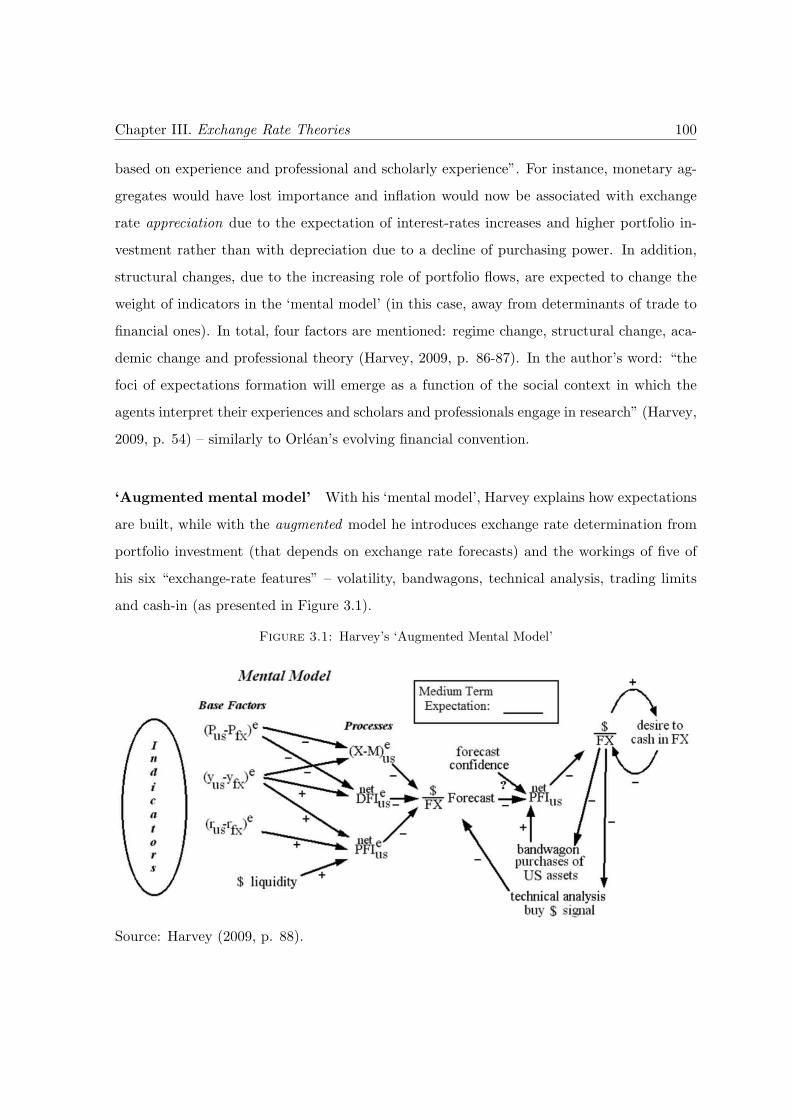
Chapter III. Exchange Rate Theories 100
based on experience and professional and scholarly experience”. For instance, monetary ag-
gregates would have lost importance and inflation would now be associated with exchange
rate appreciation due to the expectation of interest-rates increases and higher portfolio in-
vestment rather than with depreciation due to a decline of purchasing power. In addition,
structural changes, due to the increasing role of portfolio flows, are expected to change the
weight of indicators in the ‘mental model’ (in this case, away from determinants of trade to
financial ones). In total, four factors are mentioned: regime change, structural change, aca-
demic change and professional theory (Harvey, 2009, p. 86-87). In the author’s word: “the
foci of expectations formation will emerge as a function of the social context in which the
agents interpret their experiences and scholars and professionals engage in research” (Harvey,
2009, p. 54) – similarly to Orlean’s evolving financial convention.
‘Augmented mental model’ With his ‘mental model’, Harvey explains how expectations
are built, while with the augmented model he introduces exchange rate determination from
portfolio investment (that depends on exchange rate forecasts) and the workings of five of
his six “exchange-rate features” – volatility, bandwagons, technical analysis, trading limits
and cash-in (as presented in Figure 3.1).
Figure 3.1: Harvey’s ‘Augmented Mental Model’
Source: Harvey (2009, p. 88).
Chapter III. Exchange Rate Theories 101
Technical analysis’ dynamics based on Schulmeister’s work: a sign that follows an ex-
change rate change has an impact on the forecasts and thus in portfolio flows79. With the
bandwagon effect, an exchange rate change makes agents increase their net portfolio invest-
ments, adding pressure to the currency. Trading limits are not presented in the diagram, but
can be thought as a ceiling to both technical analysis and the bandwagon purchases.
While technical analysis and bandwagon purchases are self-feeding cycles, cash-in acts
against the trend. It is however said to be just white noise over the trend, having no effect
over longer time horizons.
A fourth important element is confidence, that affects different interactions inside the
model80: the more confident the participant is, the stronger the response of these mechanisms
will be81. Finally, Harvey considers the medium-term expectations as “attractors”, or “a
sort of lens through which agents filter inputs” (as in Schulmeister (1987) and Schulmeister
(1988))82. These expectations guide how agents see an event: the significance of events that
would lead to an exchange rate change in line with the medium-term expectations (be it
bullish, bearish or neutral) is magnified. Also confidence is positively affected in the case of
an event that is in line with the medium-term expectation.
Harvey’s (2009) words well summarize these interactions that determine exchange rates:
In sum, the three feedback loops – cash in, bandwagon effects, and technical anal-
ysis – are key to behavior. It is because of them that, in general, currency markets
tend to move under their own momentum (due to bandwagon and technical anal-
ysis), interrupted by brief reversals caused by cash in. Cash in causes a zigzag
pattern; if bandwagon and technical analysis have imparted a particular direc-
tion to the market, the zigzag occurs around that vector. As market participants
work with their ‘mental model’ to interpret the impact of events (base factors and
79In Schulmeister, the sign has a direct impact on trading.80Although, according to Harvey’s text confidence seems to affect any kind of expectation formation, in the
illustration, it is placed as to affect expected net portfolio investment.81 Schulmeister does not directly mention concerns over confidence, but indirectly he mentions that rat-
ing agencies’ communications “strengthen the market mood” when they “confirm that an ongoing boom isfundamentally sound”, Schulmeister (2009, p. 4+), which is very close to increasing confidence on a forecast.
82Note that this is consistent with survey analysis, that argues that there is an important skew towardstechnical analysis at short horizons, that reverses as the length of the considered horizon is increased.
Chapter III. Exchange Rate Theories 102
indicators) on the processes (thus generating their short-term and medium-term
forecasts), so the zigzagging vector may be turned in new directions (p. 89).
3.3.3.1 Concluding remarks
Similarly to Orlean’s and Schulmeister’s analyses, Harvey concludes that the exchange rate
is determined by social context that, in turn, in longer time horizons, is determined by
fundamentals, and that they are relevant “because portfolio investors have decided that
there should be [such associations]” (Harvey, 2009, p. 64). While for Orlean decisions are
based on financial conventions, Harvey’s ‘mental model’ details the indicators considered
by investors in forming their expectations – presenting what, in the terms of Orlean, could
be seen as our current financial convention. These details are interesting because they are
specifically focused on the forecast of currencies, while Orlean’s analysis is directed at assets
markets in general.
A more complete picture emerges with the inclusion of FX markets’ features (partially
proposed by Schulmeister) in Harvey’s ‘augmented mental model’. FX features complement
the financial convention and the description of the indicators for explaining how the manifest
zigzag pattern of exchange rates are built.
The definition of the turning points is of major importance. Harvey (implicitly) suggests
two explanations of how these are built. The first is cash-in operations (Harvey, 2009, p.
89), and the other (that focuses on a longer time-horizon) is the difference from agents’
interpretation and the actual rate:
These [bandwagon effects] can continue unabated until current events (as inter-
preted by market participants) accumulate against the trend. If the discrepancy
between the level to which a currency price has risen due to bandwagons and the
interpretation of events is large enough then agents confidence can be shattered
and panic and collapse can result. (p. 66, italics added)
Note the similarity with Orlean: the fact that participants are no longer able to explain a
trend leads to a crisis, putting an end to the movement.
Chapter III. Exchange Rate Theories 103
Harvey and Orlean’s explanation of turning points seem more appropriate for defining
the turning points of up-trends, as the lack of liquidity and crisis are associated with sells
and not with purchases of the asset. An alternative is to think of turning points of downturn
trend as coming from investors buying an asset for perceiving its price as excessively low –
what maintains the general idea of the divergence of investors’ perception and the actual
rate.
As in portfolio models (discussed in Section 3.1.2.3), portfolio flows play an important
role in Harvey’s model. Their determination is surely much more complex in the latter, where
exchange-rate expectations are not only included, but deeply discussed and seen in parallel
to the specific features of today’s FX markets – and assumptions are realistic. Portfolio
models, however, include features that are absent from Harvey’s model. First, they are
based on portfolio allocation strategies that involve investing in one country or another,
underscoring that the decision involves several alternative investments. Harvey partially
considers the importance of other country’s features in its model as base factors are always
considered in relative terms (as expected relative macroeconomic growth and stability, (y −
y∗)e). However, this is only marginal, and what could be the central issue, the other country’s
expected exchange rate change (ee) is not taken into account. In a two-country model, this
would not be important as the depreciation of one is the appreciation of the other. But
portfolio allocation involves more than two countries and when considering an advanced and
an emerging currency, the expected change in the emerging currency might be seen with
respect to the advanced country, but the advanced currencies forecasts would probably be
estimated with respect to another advanced currency.
Another important point is that, differently to portfolio models, stocks and changes in
stocks play no role in Harvey’s model. Portfolio flows are considered, but these flows do
not accumulate somewhere indicating the potential impact of an investors withdraw from a
market – which indicates the great difference between the potential impact of financial and
trade-related flows (see Carvalho (2009)). Such consideration enhances our understanding of
exchange rate volatility – a feature that manifests not only as the zigzagging behavior nicely
explained by Schulmeister and Harvey, but also as sudden depreciations. In this case, the
consideration of stocks is central for understanding the vulnerability brought by portfolio
flows (as it will be seen in Section 3.3.5, they are considered by SFC models).
Chapter III. Exchange Rate Theories 104
In fact, neither Schulmeister’s nor Harvey’s models can better explain usual volatility
of FX markets than exchange rate crises like the ones faced by emerging currencies since the
2000s. These heterodox models include features as herd behavior, but they do not explain
what would have triggered the major depreciations seen in these currencies nor why they
are recurrent in some countries. The analyses of emerging currencies presented in the next
section shed light in these questions.
Finally, a remark on the absence of impact from other types of flows on the exchange
rate in Harvey’s analysis. Foreign trade and FDI are included in the model as reasons for
trading in foreign exchange markets, but their role is limited to affecting agents’ exchange
rate forecast, not having a direct impact on the exchange rate. This inclusion would enhance
realisticness and is of especial importance for countries that can experience a shock of terms
of trade (as due to commodity prices).
3.3.4 Emerging Currencies’ Specificities and Dynamics
Of special interest for this thesis are the analyses of the specificities of emerging currencies.
These are heterodox works, and as the ones presented earlier in this section, they disagree
with the view of exchange rates as a market-clearing price. They agree with the role of
expectations in driving exchange rates and with the view that expectations are anchored in
social conventions given the weight of fundamental uncertainty. As in other heterodox works,
expectations impact exchange rates through investors’ decisions on financial investments, but
these decisions are now conditioned by a currency’s liquidity premium associated with the
place it occupies on the hierarchical international monetary and financial system (IMFS).
These works are based on structuralists concepts of hierarchy and asymmetries that
differentiate the center from the periphery. Institutions play a central role and the analy-
ses are based on the context and dynamics of the post-Bretton Woods era. The broader
center-periphery literature analyzes different types of asymmetries, but the most relevant
for exchange-rate dynamics are financial and monetary asymmetries83. The asymmetries
83Described by Andrade and Prates (2013), Prebisch’s (1949 e 1981, as cited in Andrade and Prates (2013))work focused on three main types of asymmetries between the center and the periphery: the technical/pro-ductive, the macroeconomic, and the financial. The literature emphasized the following asymmetries: thecreation and dissemination of technical progress; national innovation systems as the institutional structure
Chapter III. Exchange Rate Theories 105
of the IMFS are briefly presented in the following section, followed by an analysis of the
exchange-rate per se.
3.3.4.1 Asymmetries of the international monetary and financial system (IMFS)
The international monetary system (IMS) has undergone significant changes in the 20th
Century. There were periods of fixed and floating exchange rates, of capital controls and
free mobility, and while the Gold-Standard had the pound sterling as key-currency, this lost
its space to the U.S. dollar at the emergence of the Bretton-Woods system84. It is from
historical analysis of its development that authors argue that the IMS is asymmetrical85,
that a currency’s position determines its country’s policy autonomy (as Carneiro’s (1999)),
the dynamics of the capital flows it receives, and thus its exchange rate’s main features (as
Prates (2002)).
There is consensus that the central86 place of the IMS in the post-Bretton Woods system
is occupied by the U.S. dollar87, followed by currencies of other central economies, with
peripheral currencies coming next. But the exact explanations of these layers might diverge.
Carneiro (1999) argue that the U.S. dollar was at its center for being the system’s reserve-
currency, while the other two layers were divided between convertible and non-convertible
currencies, but no further development on the concept of convertibility is presented88.
leading to technical progress; productive structures; the income-distribution and job creation profiles; thedegree of autonomy of the political economy; and the financial and monetary asymmetries.
84Note that the period between the two World Wars also has important implications for exchange rateanalysis, for being a period of exchange rate flexibility.
85De Paula et al. (2016) mention that the hierarchical feature of the IMS and its resulting asymmetrieswere already pointed out by Keynes in the Treatise on Money and in his preparatory works for the BrettonWoods Conference (Keynes, 1930, 1944, as cited by De Paula et al. (2016).
86The idea of centrality is a direct reference to the center-periphery framework that results in a repre-sentation of currencies based on circles. Another representation is the currencies pyramid, where the mostimportant currency occupies the highest position (see Cohen (1998) for the concept of the currencies’ pyra-mid).
87Indeed, the IMFS that emerged after the collapse of the Bretton Woods institutions is labeled by Prates(2002) as the one based on a “flexible, financial and fiduciary dollar” as the very definition of a IFMS is based,among other features, on the presence of a key-currency and the dynamics that it imposes. In the currentIFMS the U.S. dollar is the key and the ‘reserve’ currency, the one that better incorporates the idea of reserveof value.
88Carneiro (1999) analyzes how interest rates of different countries are set in the context of financial glob-alization, arguing that the interest rate of the reserve currency would work as a floor for the other countries,whose interest rates would increase according to the distance to the center of the system).
Chapter III. Exchange Rate Theories 106
The reasons behind these three layers that differentiate currencies is examined by Prates
(2002)89:
The concept of convertibility is based on the acceptance of national currencies
as means of payment, unity of account and contract denomination, and store of
value in the international monetary system. In other words, a national currency
is completely convertible if capable of performing, in the international context,
the three functions of money90. (p. 148)
The U.S. dollar is the only currency “to fully perform the three functions”, as it is the currency
mostly used “in monetary (means of change) and financial (unit of contract denomination)
transactions, as well as the most liquid and safe asset and therefore the most desired by agents
as receptacle of uncertainty”, and thus, it is at the system’s center. Other currencies from
central countries occupy second place in this hierarchy as they are also used to denominate
contracts internationally (unit of account) and are relatively demanded as store of value.
Currencies from peripheral countries occupy the third place, as they do not exercise any of
the three functions internationally (they are not de facto convertible) (Prates, 2002, p. 148).
De Conti (2011, p. 46), following Prates’ (2002) three-functions definition, argues for
the increasing importance of the euro as store of value and unit of account and suggests an
specific layer for the currency, resulting in an IMS with four layers91.
Apart from monetary asymmetry, the positioning of countries in the international fi-
nancial system (IFS) is also important for Andrade and Prates (2013) in determining the
liquidity premium of a currency. The hierarchy of the IFS is related to the different mag-
nitudes of capital flows to different countries, those directed at emerging countries being
marginal in comparison to total flows92.
Although marginal, these flows exercise important pressures on countries’ foreign ex-
change markets due to the smaller size of their economies. Haldane (2011) uses the “Big
89Note that this definition involved a de facto understanding of convertibility, that differs from de jure
convertibility that is associated with the legal possibility of converting a currency into another.90Author’s translation from Portuguese.91De Conti (2011, p. 46) also argues for the relative heterogeneity of peripheral currencies, as some are used
regionally; but given its still marginal importance, all peripheral currencies are taken as a unique group. Also,on IMS’ current configuration, see De Conti and Prates (2014) that analyze the current IMS configurationbased on data on the specific usages of money that are associated with each of its three functions.
92See Prates (2015) on how the financial and monetary hierarchies reinforce themselves.
Chapter III. Exchange Rate Theories 107
Fish Small Content” metaphor to illustrate this issue: “The Big Fish here are the large
capital-exporting, advanced countries. The Small Ponds are the relatively modest financial
markets of capital-importing emerging countries.” The numbers on the size of the ‘fish’ and
the ‘pond’ are impressive93:
For example, a fall of 0.1 in the weighted home bias index for advanced countries
in 2007 relative to 2006 would have equated to a portfolio reallocation to foreign
markets of around $4.5 trillion. That is a big fish. To give some context, the
market capitalisation of all G20 emerging market countries in 2007 was $6.8
trillion. That is a smallish pond. (p. 5)
3.3.4.2 Store of value or unit of account? Assets or liabilities?
While some authors follow Prates’ (2002) definition of a currency’s ability to exercise the
three functions of money in the international context, others seem to focus exclusively on the
store of value function. Kaltenbrunner (2015) cites the German monetary keynesians (GMK)
school’s94 analyses as example. As argued, the school suggests that a currency’s position,
and thus its liquidity premium, results from its ability to store wealth. The leading currency
would be the one at the highest position in the hierarchy, with the greatest ability to store
value, followed by intermediate currencies (from other developed countries), and, finally, by
developing and emerging countries that have “unstable currencies with a poor reputation
concerning their ability to act as a stable store of value” (Kaltenbrunner, 2015, p. 432-433).
In the dynamics described by Andrade and Prates (2013, p. 410) the store of value
function also seems particularly important: they refer, for instance, to the incapability of
93Haldane (2011) uses the ‘Big Fish Small Pond’ metaphor to refer to the very different magnitudes ofinternational portfolios and emerging countries markets:
Haldane (2011, p. 15) also presents the importance of gross portfolio equity inflows relative to laggedmarket capitalization for G20 emerging markets in different years, which was about 4% in 2010. The ratio ofthe foreign liabilities in the form of equities over market capitalization might however be a more interestingmeasure for comparing two stock -values. As presented in Chapter Four, this ratio achieved levels of 45% inHungary and 42% in Mexico in the 2000-2011 period.
94See Kaltenbrunner (2015) for the GMK references.
Chapter III. Exchange Rate Theories 108
these currencies to be “a receptacle of uncertainty on a global scale” in moments when
investors have “a clear preference for money and its closer substitutes” (p. 402)95.
Kaltenbrunner (2015) argues for the importance of shifting the (GMK’s) focus on the
store of value function, focusing instead on the currency’s ability to settle financial obligations
internationally (p. 428), as it determines its ability to be used as a means of meeting
outstanding obligations97 (p. 436).
This shift of focus from the assets’ (store of value) to the liabilities’ side (denominate
financial obligations) would be an insight taken from Minsky (1975). Specifically, it is based
on Minsky’s argument that for debtors, “it is convenient to hold liquid assets in the currency
in which your debts are denominated”. It is also based on the understanding of the concept of
liquidity in the international context as the ability to convert assets into “the currency with
which positions in these assets have been funded”, given that in closed economies, liquidity is
associated with the ability to convert an asset at any time, without loss of value, into money,
which is “the mean of account and denominator of contractual obligations” (Kaltenbrunner,
2015, p. 436).
Though the store of value function is still important, to Kaltenbrunner (2015), the
liquidity premium paid by a currency (and thus its position in the IMS) is ultimately deter-
mined by a currency’s ability to act as international medium of contractual settlement that,
in turn, defines its ability to act as store of value98. In this sense, Kaltenbrunner (2015)
proposes a causal relation between two of the three functions of money that, according to
95When discussing periods of uncertainty, Andrade and Prates (2013) refer to the search for the most liquidassets with the idea of saving value for investment in a future moment96: “liquidity is strongly valued in timesof higher uncertainty regarding the future, justifying an increased demand for money as an asset, or for itsclose substitutes, so as to structure a portfolio that is as liquid as possible, while one waits for more auspiciouscircumstances in which one can hold less liquid assets that may, however, generate higher overall returns. (...)Given the logic of capitalist accumulation and the ubiquitous existence of uncertainty, in particular situationsthere will be a clear preference for money and its closer substitutes, since they are the liquid assets parexcellence, and the postponement of real investment plans” (Andrade and Prates, 2013, p. 402).
97The role of the dollar as the currency in which the banking system runs is also highlighted by somemainstream authors. Its importance, however, is rooted on the role of the dollar in international trade (whichis the same as arguing that inside the unit of account function, the denomination of trade contracts has ledto the denomination of financial obligations). As put by Shin (2016, p. 6): “The consequence of the dollar’sinternational role in transactions is that the global banking system runs on dollars”.
98“It is important to note that in the Minskyan framework presented here a currency’s ability to act asinternational store of value remains a crucial element of its international liquidity premium. It is, however, itsinability to act as international medium of contractual settlement that undermines this function in the firstplace” (Kaltenbrunner, 2015, p. 437).
Chapter III. Exchange Rate Theories 109
Prates (2002), would jointly determine a country’s position in the IMS99. The causal relation
would be from the non-use as denominator of financial contracts to the non-use as store of
value: with the inability to denominate financial contracts, a country would have foreign de-
nominated liabilities, demanding investors to sell domestic currency to buy the funding one
when external obligations must be met (p. 436), resulting in a latent depreciation pressure
and risk of sudden and sharp exchange rate depreciations. It is due to this dynamic that
a currency’s ability to act as store of value and media of contractual settlement would be
undermined, and thus its international liquidity premia (Kaltenbrunner, 2015, p. 440).
It should be highlighted that the unit of account function can manifest in different
forms. While the usages cited by De Conti and Prates (2014)100 reflect a focus on the ability
of a currency to be used in price setting, Kaltenbrunner (2015) suggests the specific use
of a currency as denomination of financial contracts. The ability to denominate contracts
mentioned by Prates (2002) had a focus on the country’s capacity to issue debt in its own
currency101, which reflects the objective of explaining the late-1990s crises where the public
sphere and debt played prominent roles. Kaltenbrunner (2015), on the other hand, focuses
on international investors and on any type of external liability (not only debt), reflecting a
higher influence of the GFC dynamics, in which the liabilities of emerging countries were
more varied (as it will be seen in Chapter Four).
In the last two decades, the analyses of the specificities of emerging currencies and
its tendency to crisis have therefore pointed to different aspects featured in different crisis
episodes. The (lack of) store of value function is central to dynamics concerning the assets’
side of foreign investors and their choices for maintaining the value of their assets. The func-
tion of denomination of financial contracts comes into play in the liabilities’ dynamics and
the implications of having to meet financial obligations. Both are important and cannot be
dissociated. As seen in Chapter Two, the different markets, and thus countries, are intercon-
nected by money managers’ balance-sheets. Minsky’s analysis, discussed in Chapter Seven,
is different from others for pointing exactly to this interconnection of balance-sheets (and
99See De Conti and Prates (2014) for arguments on the opposite causality.100De Conti and Prates (2014) follow Cohen (1971, as cited in De Conti and Prates (2014)) on the specific
usages.101Note that the presence of original sin (a country’s ability to issue debt in its own currency) is, itself, a
dimension of the de facto convertibility of a currency.
Chapter III. Exchange Rate Theories 110
the associated fragility that derives from it). Andrade and Prates (2013) and Kaltenbrun-
ner (2015), respectively, focus on the assets’ and liabilities’ sides, and are therefore, highly
complementary.
3.3.4.3 The use of Keynes’ equation on an assets’ own rate of interest
The different positions in the international monetary and financial system (IMFS) would
thus be translated in different levels of liquidity premium: the highest for the U.S. dollar, the
lowest for the emerging currencies. The analysis of the implications of this different attribute
of emerging currencies is facilitated by the use of Keynes’ equation on an asset’s own rate of
interest. With this equation, Keynes (1936) indicated that in a monetary production economy
an asset’s own interest rate (or “total expected returns”, ra) is determined by four main
attributes102: its expected appreciation (a), its quasi-rent (q, or yield), its carrying costs103
(c) and its liquidity premium (l, a power of disposal that confers a potential convenience or
security) (Andrade and Prates, 2013, p. 402) – see Equation 3.29:
r = a+ q − c+ l (3.29)
The equation was developed by Keynes to estimate the return of domestic economy assets
(including money) being built for same currency assets. However, it has been translated to
the context of currencies based on the view of a domestic currency as an “international asset
class” (Kaltenbrunner, 2011, p. 90)104 or, because “currencies are held as a portfolio capital
asset” (Andrade and Prates, 2013, p. 404).
The analysis of the implications of the specificities related to the hierarchic nature of
the IMFS on a currency’s return can therefore be done through its liquidity premium, l, that
is lower for emerging currencies than for those of central countries.
102The characteristics of a monetary production economy will be discussed in Chapter Seven.103Capital controls (Andrade and Prates, 2013) and transaction costs, that could be reduced with higher
liquidity (Prates, 2015, p. 401-402) are examples of carrying costs. Alternatively, it could be seen as thedegree of financial openness of a country (De Paula et al., 2016).104Kaltenbrunner (2015, p. 428) cites several authors that have used some of the variables in this equation
in exchange-rate analysis, while Kaltenbrunner (2011), Andrade and Prates (2013), and Kaltenbrunner (2015)are cited as examples of uses of all elements present in Keynes’ equation. While it is not clear whether thefirst group of references focus specifically on emerging-currencies dynamics, this is the case of the latter threepapers.
Chapter III. Exchange Rate Theories 111
Andrade and Prates (2013) focus on the impact of a country’s features in defining capital
flow dynamics. Given that l is structurally low, capital flows would mostly be attracted by the
other features – a, q, or c). These changes are analyzed in light of the liquidity preference
scenario, which is therefore seen as the major determinant of capital flows. For instance,
capital will be directed to emerging countries:
in situations marked by an excess of international liquidity and a higher appetite
for risk, or eagerness to bet against the uncertain future (lower liquidity prefer-
ence), when, normally, conventions (and expectations) about the future trajectory
of the economy are more optimistic, and interest rates in core countries are lower.
(p. 401)
In these moments, there will be an increase of the feature a that compensates for the low l,
resulting in capital flows.
Conversely, when uncertainty and liquidity preference are high, these countries will face
capital outflows: In moments of “reversal of the cycle, of monetary/fiscal policy changes in
the center or of increase in the liquidity preference”, these countries are the “first victims of
the global investors” (Andrade and Prates, 2013, p. 410) due to the lower l and consequent
incapability of being “a receptable of uncertainty on a global scale”105.
In Andrade and Prates (2013), although the narrative sometimes refers to the features in
relative terms, the equation is presented in absolute terms (which might reflect the authors’
intent to analyze the desirability of a currency, and not exchange rates (De Paula, Fritz and
Prates, 2016)). For exchange rate analyses, however, relative returns are key (as done in
traditional portfolio models, discussed in Section 3.1.2.3, and in SFC models, discussed in
Section 3.3.5). The explicit consideration of a currency’s returns in relative forms is done by
Kaltenbrunner (2015) and De Paula et al. (2016)106.
105Andrade and Prates (2013, p. 411) also use the equation to discuss a possible governmental interference:in case of capital outflows and need of stabilizing the currency, policy rate might be raised (thus managingboth q and a) and financial openness can be deepened through a decrease of capital controls (a decrease ofc).106In Kaltenbrunner (2011) the importance of relative terms is also seen, as it considers that the assets’
return should be equal “to the return offered by the currency with the highest liquidity premium, i.e. themoney of the system”.
Chapter III. Exchange Rate Theories 112
In De Paula et al. (2016), the consideration of relative terms is presented in the form
of Equation 3.30107. The emphasis is put on the alternatives that emerging countries have
to compensate for the low liquidity of their currencies (l < l∗, where ∗ denotes a central
currency):
to compensate for the lower liquidity premium, those currencies have to offer a
higher q, which is a policy variable in order to try to achieve a higher a (currency
appreciation), creating conditions which are attractive for international investors,
and/or to reduce c, i.e. the obstacles for capital inflows (or capital outflows), with
the withdrawal of capital account regulation. (p. 8)
l∗ − l = (a+ q − c)− (a∗ + q∗ − c∗) (3.30)
Assuming that expected rates of return (r) throughout the world will be driven toward
equality108 and given that there is a “world reserve currency”, Kaltenbrunner (2015, p. 431)
presents the following equations (3.31 and 3.32), where (∗) denotes the equivalent for the
world reserve currency. The expected appreciation (a) is considered with regards to the
world’s money, and it assumes that carrying costs (c) are negligible for short-term financial
instruments109:
r = a+ (q − c) + l = (q∗ − c∗) + l∗ (3.31)
(q − q∗) + a = (l∗ − l) (3.32)
Equation 3.32 is presented by Kaltenbrunner (2015) as a representation of a reason
behind the structurally higher interest rates of some emerging countries:
107De Paula et al. (2016) actually use the subscript n and s as reference to northern and southern (orperipheral emerging) countries. The reference to a central currency instead of a northern currency is done tofacilitate a comparison with Kaltenbrunner (2015).108Kaltenbrunner (2015) does not detail the convergence mechanism. If the higher return of a country (q)
leads to higher capital inflows, the resulting exchange rate appreciation might lead to an expectation of furtherappreciation (an increase of a) and thus an increase of returns, diverging r further, instead of converging.This mechanism of divergence is in line with Kaltenbrunner and Painceira (2009), with the bandwagon effectsof Schulmeister and Harvey, and with the model that will be proposed in Chapter Seven. The hypothesis ofconvergence also assumes that the policy rate is not used as an instrument of inflation control, while mostemerging countries follow inflation targeting regimes (as it will be seen in Chapter Four).109Equation 3.31 does not consider that the return of world’s reserve currency (r∗) includes an expectation of
exchange rate change (a∗). In a two country model, the appreciation of a currency should be the depreciationof the other, in the terms of the equations, a = −a∗, that could demand the exclusion of a∗ from Equation 3.32if a∗ were considered in Equation 3.31. Kaltenbrunner’s choice might have been based on the considerationof the equations not as a two-country model, or on the fact that the relevant a∗ is not estimated with regardsto the emerging currency.
Chapter III. Exchange Rate Theories 113
(...) similar to Keyness understanding of interest rate determination in the closed
economy, a currency’s yield differential (q − q∗) has to compensate for its lower
liquidity premium relative to that of the leading currency (l∗ − l) if demand for
it is to be maintained”110. (p. 433)
Emerging currencies would therefore be marked by “latent depreciation pressures and
risks of sudden and sharp exchange rate depreciations” that are exogenous to domestic con-
ditions – in moments when “investors have to sell these currencies (and acquire the funding
currency) to meet their contractual obligations” (Kaltenbrunner, 2015, p. 440).
Volatility or extreme depreciations? And the role of the international scenario
Andrade and Prates’ (2013) and Kaltenbrunner’s (2015) analyses therefore argue that emerg-
ing countries’ currencies are vulnerable to moments of crisis internationally either for being
unable to store value (Andrade and Prates, 2013) or for not being used in contractual obli-
gations (Kaltenbrunner, 2015). The consequent major depreciations would occur in specific
moments of turbulence internationally, such as in moments of “reversal of the cycle, of mon-
etary/fiscal policy changes in the center or of increase in the liquidity preference” when
“investors [...] reassess their investment decisions” (Andrade and Prates, 2013, p. 410),
or “moments of market turmoil” (Kaltenbrunner, 2015, p. 442), or change in international
“funding” (p. 439), or “liquidity conditions” (p. 440).
Therefore, it can be asserted that the authors’ arguments do not refer to the higher
volatility of emerging currencies in general, but to the important depreciations in specific
moments. As it will be shown later in the thesis, such argument would be coherent with
empirical findings for some emerging currencies since the 2000s111. This type of volatility is
different from that analyzed by Schulmeister and Harvey (depicted as zigzags) that emerge
from technical trading, bandwagon and herd behavior. Some emerging countries that count
with deep and sophisticated foreign exchange markets, are also subject to this type of volatility,
110Note that this implies stable expectations about exchange rate developments (a), either of appreciationor depreciation, but it does not necessarily imply stability, (a = 0).111Chapter Six presents findings about the volatility of some emerging countries (specifically those that have
a more “financialized integration”, a concept suggested and discussed in Chapter Five).Specifically, the comparison of these emerging countries exchange rates with the Euro/Dollar rate, shows
that while the former suffer from more frequent extreme depreciations, the latter presents a higher standarddeviation from its trend.

Chapter III. Exchange Rate Theories 114
but the analysis presented in this section points to what could be an additional source of
volatility: one that emanates from external shocks due to the specificities of their currencies
and its use in international portfolio allocation.
In addition, the definition of the exchange rate cycles seen in emerging currencies
might be different than those of advanced countries’ currencies. Based on an analysis of
the Deutsche mark, the euro and the dollar, Schulmeister argues that long-term cycles are
the result of short-term cycles, with the trend being determined by whether the short-term
‘up’ trend is longer than its ‘down’ trend, combined with the way investors saw fundamen-
tals (the role of their medium-term expectations). On the other hand, the internal dynamics
of the foreign exchange market in emerging currencies are dominated by prevailing condi-
tions in international financial markets, resulting in cycles whose length is dependent on the
frequency of turmoils in those markets.
These analyses therefore suggest emerging currencies’ vulnerability to changes in the
international scenario. The idea of emerging currencies being vulnerable to money managers’
decisions will be developed in Chapter Seven.
An important explanatory power The explanatory power of the analyses based on
the asymmetry of liquidity premia among currencies is considerable. It can account for
the appreciation of the Japanese yen after the Fukushima accident in 2011 when Japanese
insurance firms and carry-trade investors repatriated their investments (“What is happening
to the Japanese yen?”, 2011). At that moment, capital flew to Japan because of the financial
obligations of insurance firms. As a consequence, knowing that and expecting the yen to
appreciate with this inflow of capital, carry-trade investors repatriated their investments to
gain with the exchange-rate change. The role of the denomination of financial obligations
also explains the GFC-related flows – when investment currencies depreciated sharply, and
the funding currencies appreciated, unrelated to their countries’ conditions (Kohler, 2010)112.
With the Euro crisis, depreciation of emerging currencies are better explained by the non-use
of emerging currencies as store of value, as it was more of a crisis of uncertainty than a need
of covering losses as the GFC.
112See Brunnermeier (2008), Hesse et al. (2008), and Milesi-Ferretti and Tille (2011) for a description of the2007/2008 events and see Tridico (2012) for a review of competing explanations of the crisis.
Chapter III. Exchange Rate Theories 115
Irrespective of the reason, if the high liquidity premium is due to the denomination of
financial obligations or to the store of value function, liquidity premium asymmetries can
also explain why the United States has received so much foreign private-sector investment
even with very low interest rates since the GFC. Indeed, Forbes (2010) finds that:
Foreigners have earned substantially lower returns on their U.S. investments over
the past five years than U.S. investors have earned abroad, even after removing the
effects of exchange rate movements and official sector investments. This return
differential against foreigners even exists within individual asset classes (equities,
foreign direct investment, and to a lesser extent, bonds) and even after making
rough adjustments for risk. (p. 2)
From this framework, the high flows to the United States even with very low interest rates
(q∗ < q) and ”high risk” is no puzzle: they derive from its currency’s exceptional place in
the international monetary system (and consequent high liquidity premium, l∗ > l). This
suggests the superiority of the keynesian framework when compared to traditional portfolio
models – what derives from their account for the liquidity premium and the fact that it is a
more complete concept than risk.
3.3.4.4 Including liquidity preference in the equation
Emerging currencies’ l-feature is therefore structurally low to both Andrade and Prates
(2013) and Kaltenbrunner (2015). Although l is structurally defined, its impact on a curren-
cies’ return might change if there is a change in how agents value this feature: in moments
of change in liquidity preference. To account for such possibility in the keynesian-equation,
a weight (β) can be included on how “preferred” the liquidity attribute is, as in Equation
3.33 and 3.34 that are receptively related to assets denominated in emerging currency (r)
and one denominated in the currency of a central economy (r∗), or in Equation 3.35:
r = a+ (q − c) + βl (3.33)
r∗ = a∗ + (q∗ − c∗) + βl∗ (3.34)
r − r∗ = (a+ q − c)− (a∗ + q∗ − c∗) + β(l − l∗) (3.35)
Chapter III. Exchange Rate Theories 116
Given that l∗ is higher than l, (l − l∗) has a negative effect on the return differential
(r− r∗). An increase in liquidity preference (↑ β) increases the negative impact of (l− l∗) on
the return differential (r∗ − r). The consequence is an outflow of capital from the emerging
to the central economy, what is in line with the dynamics suggested by Biancareli (2011).
The analysis based on a system of two equations is an option for analyzing exchange
rates – “the relation between domestic and foreign money, (...) a manifestation of these
differential returns” (Kaltenbrunner, 2015, p. 431) – without assuming the convergence of
returns. But the liquidity preference coefficient can also be added to the framework proposed
by Kaltenbrunner (2015), as in Equation 3.36:
(q − q∗) + a = β(l∗ − l) (3.36)
Equation 3.36 shows that an increase of liquidity preference (β) increases the yield differential
(q− q∗) needed to maintain the stability of capital flows (given no change in expectations, a,
nor in liquidity premia, l and l∗). In other words, in moments of higher liquidity preference,
emerging countries would have to increase its policy rate to maintain capital flows. This is
a clear representation of the lack of autonomy of monetary policies in emerging countries.
3.3.4.5 Additional remarks on the use of Keynes’ equation
The use of Keynes’ equation on an asset’s own rate of interest is a very important step on
elucidating the dynamics of emerging currencies for including the significant liquidity feature
in the exchange-rate discussion. Having included liquidity concerns, this framework dialogues
with the risk-return founding dilemma of portfolio equations. It is however an heterodox
alternative, where uncertainty is not reduced to calculable risk (as r in Equation 3.15)113.
On the contrary, it is a subjective variable, allowing the consideration of expectations and
conventions.
While Andrade and Prates (2013) focus on the desirability of a currency, Kaltenbrun-
ner (2015) highlights that such desirability gains on meaning when seen in relation to the
attributes of a ‘competing’ currency, which is an important step in exchange-rate analyses.
113The discussion on the concepts of risk and liquidity preference is done in Chapter Five.
Chapter III. Exchange Rate Theories 117
Still, synthetic and detailed formalization have both positive and negative features. On the
one hand, the schematic (a + q − c) versus (l) dilemma in Andrade and Prates (2013) and
the (q − q∗ + a) versus (l∗ − l) dilemma in Kaltenbrunner (2015) allow for rich discussions
on the role of international dynamics in emerging countries’ exchange rates.
On the other hand, the synthetic form might be unable to account for crucial dynamics.
For instance, the analysis based on the currency’s return (q) as policy rate is restrictive,
given the different dynamics related to equity returns114. On a general level, it should be
noted that due to not having fixed returns, equities’ liabilities are more subject to changes in
expectations, increasing “speculative” behavior. But the most significant and specific point
is that equities can trigger a self-fulfilling spiral forming bubbles and leading to diverging
returns in two markets: as an increase in inflows to stock markets increases its returns,
it leads to expectations of exchange rate appreciation and higher returns, leading to more
inflows. This is specially important in light of the increasing weight of equities as a form of
foreign liabilities in emerging countries (as it will be discussed in Chapter Four).
Another consequence of the very synthetic character of Keynes’ equation is the side-
by-side consideration of monetary and non-pecuniary variables: l is considered in the same
way as monetary variables (a, q, c), as an additional and independent form of return despite
its nonpecuniary characteristics (Andrade and Prates, 2013, p. 402). It is therefore a non-
pecuniary variable that determines returns115. However, having the liquidity feature be a
determinant of demand could be more precise, with liquidity and return jointly determining
demand. This is suggested in the following session.
3.3.5 Exchange-rate dynamics in SFC Models
SFC models are similar to portfolio models presented in Section 3.1.2.3 in that both are
inspired by Brainard and Tobin’s (1968) method (Godley and Lavoie, 2007, p. 15)116.
114The variable q should account not only for the public bonds or equities, but also other assets. I want toemphasize, however, the specific dynamics related to equities.115Note that this inconsistency is not eliminated with the inclusion of the liquidity-preference feature (β) in
Equations 3.33, 3.34 and 3.36.116Dos Santos (2006) enumerates four features presented by Tobin in his Nobel lecture as features that
distinguish his work, that also apply to SFC modeling: the tracking of stocks and precision regarding time;the several assets and rates of return; the modeling of financial and monetary operations; the budget constraintand the adding-up constraint.
Chapter III. Exchange Rate Theories 118
SFC models are built from different sectors’ (such as households, firms, the government)
stock-flows norms with the aim of describing the most important economic relations in an
economy117. It is based on accounting and behavior equations, the latter being those that de-
termine the causality among the model’s variables, thus its assumptions – or how the models
are ‘closed’118. It is in the behavior equations that heterodox and traditional portfolio models
differ: while the latter are labeled neo-classical-Keynesian, SFC models are “essentially post-
Keynesian or heterodox” (Godley and Lavoie, 2007, p. 15)119. SFC models are expected to
be more realistic than the standard portfolio models, as the search for realisticness is a char-
acteristic of the school (as opposed to the mainstream’s instrumentalism (Lavoie, 2014)120).
For instance, some models have as ‘closures’ Central Banks that set interest rates, instead of
attempting to target money supply or securities’ supply121 (Godley and Lavoie, 2003, p. 3).
Indeed, it is one of the most prominent type of modeling in the Post Keynesian tradition122.
Macedo e Silva and Dos Santos (2011, p. 105) argue that institutionally rich SFC models
are “the ideal tool for rigorous post-Keynesian analyses of the medium run” given its ‘period
by period balance sheet dynamics and throughout description of the short-period behavior
of agents. SFC framework is thus “crucial to the consolidation of the broad post-Keynesian
research programme”.
117A synthetic description of Godley and Lavoie’s (2007) open-economy model by Lavoie and Daigle (2011, p.438) provides a good idea of how comprehensive SFC models can be: “The key features specific to this modelare the ability of agents to trade for foreign assets, the dependence of international trade on both domestic andforeign output as well as relative prices, and the endogeneity of prices. The model features a large number ofendogenous variables. Import prices, export prices, domestic sales deflators, GDP deflators and the exchangerate are all endogenous variables. So are real quantities such as exports, imports, output, consumption,domestic sales, and disposable income. Other endogenous variables include taxes, interest payments, thesupply of money, holdings of foreign and domestic bills, household wealth, and of course the governmentdeficit and the government debt. Standard balance of payment measures, such as the trade balance, thecurrent account balance, the capital account balance and the value of foreign reserves are endogenous aswell. Still, simplifying assumptions needed to be made to keep the model under 100 equations. There is nodomestic or foreign investment in fixed or working capital. As a consequence, the model, when it converges,tends toward a stationary state. Also there is no wage inflation, no commercial banking, and as pointed outalready, the treatment of exchange rate expectations is more than rudimentary.”118Taylor provides a good definition of a model ‘closure’: “Formally, prescribing a closure boils down to
stating which variables are endogenous or exogenous in an equation system largely based upon macroeconomicaccounting identities, and figuring out how they influence one another” (Taylor, 1991, as cited in Dos Santos(2006)).119See Dos Santos (2006) for a comparison between SFC modeling and mainstream macroeconomics.120See the discussion in the Introduction Chapter.121Godley and Lavoie (2003, p. 3) reminds us that this assumption (or ’closure’) is not unique to Post-
keynesians. In fact, it is also common to ‘New consensus’ models, as they are found among central bankpractitioners and some New Keynesians.122Path-dependence models, the neo-kaleckian and Minskyan models of income distribution and growth are
other important types of economic modeling in the Post Keynesian tradition (Asensio et al., 2011).
Chapter III. Exchange Rate Theories 119
Lavoie and Daigle (2011) also highlight the importance of the consideration of time as
historical-time, a key feature for post-Keynesian analyses:
“A major difference between standard open-economy portfolio models and stock-
flow consistent models however is that while the former establish timeless equi-
libria, the latter track stocks of assets and flow variables through time, in a
sequential manner.” (p. 244)
For exhibiting historical time, SFC models are also used to study issues of path-dependence
or hysteresis (as done by Lavoie and Daigle (2011) for exchange rates).
A very praised characteristic of SFC models is that it has “no black holes”, as “all
stocks are the result of cumulated flows plus capital appreciation” (Godley and Lavoie, 2005,
p. 3). This feature has theoretical and technical advantages – in addition to allowing the
construction of applied models to study specific conditions and run economic scenarios123
(Dos Santos and Zezza, 2008). On the theoretical front, as reminded by Dos Santos (2005,
p. 718), the absence of black holes with all economic sectors tied together make SFC mod-
els a perfect framework for analyses of monetary economics, which, in Minsky’s words, is
characterized by “the set of interrelated balance sheets among the various units”, so that
“one way every economic unit can be characterized is by its portfolio: the set of tangible and
financial assets it owns and the financial liabilities on which it owes” (Minsky, 1975, as cited
in Dos Santos (2005))124.
123SFC models have indeed been built with different goals. In Dos Santos and Zezza’s (2008) review, theaim of the different models are as diverse as: “(i) checking the logical consistency of incomplete models; (ii)extending the approach to deal with open economy issues; (iii) discussing the theoretical compatibility of SFCmodels with the views of important authors who phrased their views in literary form; (iv) producing appliedmodels which can be used to study actual economies; and (v) exploring the properties of models with differentfinancial architectures and supply specifications” (p. 471).124It is interesting to note that the analysis of balance-sheets and the liabilities of a countries’ sectors also
appears to be gaining importance in mainstream circles. The ‘risk-channel’ Shin (2016)) and the ‘bank lendingchannel’ (Disyatat, 2011) are evidence of great concern with the global banking dynamics and its spillovers onother economies. Indeed, several works from the Bank of International Settlements seem to go in this direction.Shin (2016) criticizes traditional international economy models for their belief on the three-coincidences “wherethe GDP area, decision-making unit and currency area are one and the same. [...] Textbooks therefore startwith the assumption that each GDP area has its own currency and the use of that currency is largely confinedto that economic area. The Mundell-Fleming model is a classic example of the triple coincidence, but evenin sophisticated macroeconomic models, the triple coincidence is rarely questioned. Currency appreciation ordepreciation then acts on the economy through changes in net exports” (see Avdjiev et al. (2015)). Althoughnot posited this way, his reasoning based on these criticisms put light on the liabilities’ dynamics. Basedon the triple coincidence, pre-GFC US deficits would lead to a dollar depreciation, but instead, U.S. dollarappreciated sharply. In the author’s view, the reason for this appreciation is found on a sector’s balance-sheet:it is associated with “a deleveraging of financial market participants outside the United States that had usedshort-term dollar funding to invest in risky long-term dollar assets, with the European banks mentioned above
Chapter III. Exchange Rate Theories 120
On the technical side, the no-black-hole constraint, together with the fact that it is a
complete model, allows for a detailed examination of economic models proposed by other
theoretical approaches and thus, an assessment of its dynamics and of the validity of their
conclusions. As argued by Taylor (2009a, p. 2) SFC macro modeling helps to “remove many
degrees of freedom from possible configurations of patterns of payments at the macro level,
making tractable the task of constructing theories to “close” the accounts into complete
models”. Differently from literary analyses, in the SFC approach the concerned dynamics
are forced to interact with all other variables of the economic system, requiring an explicit
recognition of such “system-wide constraints”, as well as of the potential limitations of the
analyses (Dos Santos, 2006, p. 564).
In this sense, Godley (2012) argues that SFC is an interesting framework for allowing
more detailed and precise discussions than the narrative method. Indeed it highlights dis-
agreement in areas where further studies are needed, and is useful in comparing dynamics
that might differ from one place to another, through a change in the equations or in the
‘closures’ of the models. However, it must be noted that the level of details of the discussion
might be constrained by the difficulty of running very complex SFC models and of keeping
track of their causalities125.
Therefore, SFC models have great potential for exchange-rate analyses. By allowing a
simultaneous treatment of flows and stocks, and of real and financial variables, both portfolio
(stocks) adjustments and trade flows have potential to impact exchange rates (which is
especially important in times of financialization, where portfolio adjustments across different
global financial assets are of major relevance)126.
Moreover, the SFC constraints can be added to an Agent-Based model (ABM) result-
ing in a (AB-SFC)127 model that has heterogeneous agents, with micro-macro interactions.
being the most prominent example. As the crisis erupted, these financial institutions found themselves shortthe dollar and overleveraged, and sought to reduce their dollar liabilities, bidding up the value of the dollarin the process.” (Shin, 2016, p. 13-14).125Godley (2012) argues that one of the intents of the SFC approach is to “supplement the narrative method
used perforce by Keynes and his followers before the computer age”.126Note that this feature was already present in some mainstream portfolio models such as Branson’s (1974).127The ABM provides a bottom up framework where the economy results from agents’ decision – relaxing the
representative agents’ hypothesis. It combines a microeconomic approach with the macroeconomic strictness(Clevenot and Heron, 2014).
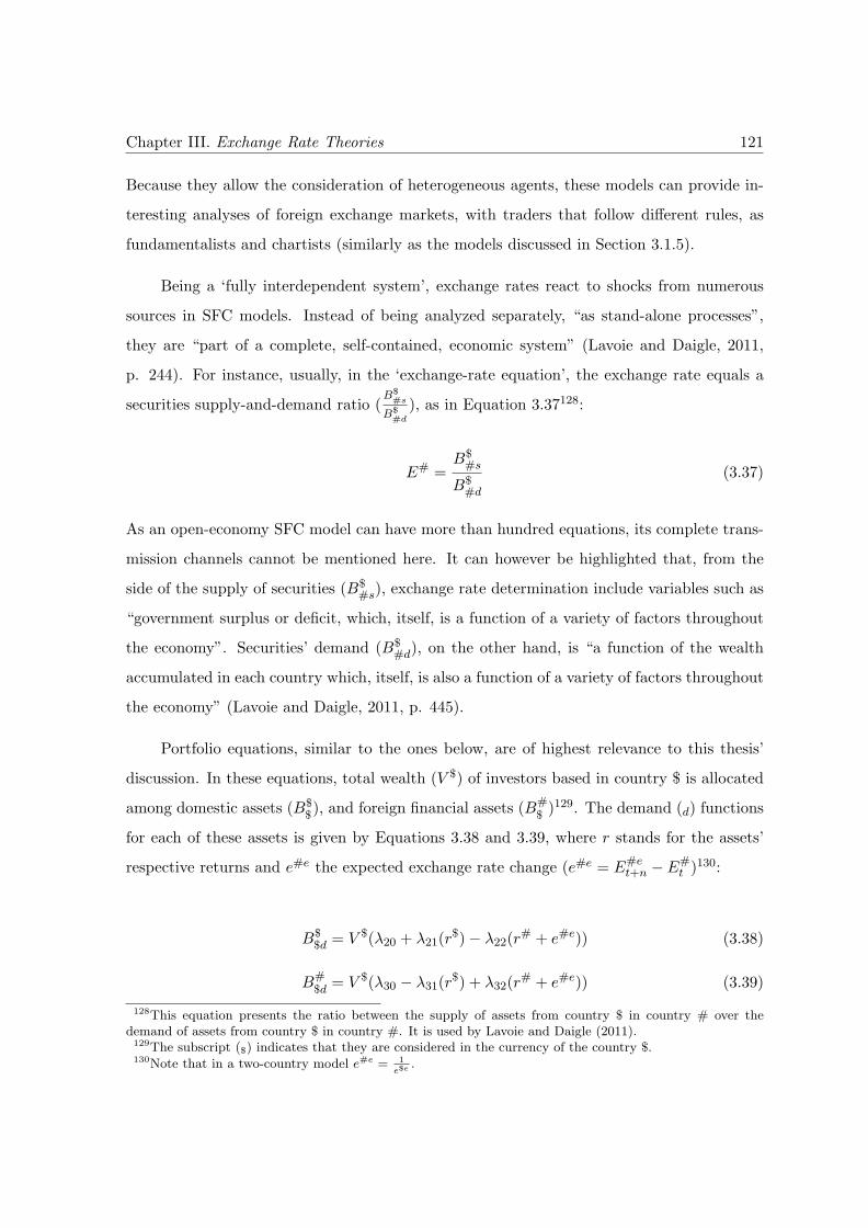
Chapter III. Exchange Rate Theories 121
Because they allow the consideration of heterogeneous agents, these models can provide in-
teresting analyses of foreign exchange markets, with traders that follow different rules, as
fundamentalists and chartists (similarly as the models discussed in Section 3.1.5).
Being a ‘fully interdependent system’, exchange rates react to shocks from numerous
sources in SFC models. Instead of being analyzed separately, “as stand-alone processes”,
they are “part of a complete, self-contained, economic system” (Lavoie and Daigle, 2011,
p. 244). For instance, usually, in the ‘exchange-rate equation’, the exchange rate equals a
securities supply-and-demand ratio (B$
#s
B$#d
), as in Equation 3.37128:
E# =B$
#s
B$#d
(3.37)
As an open-economy SFC model can have more than hundred equations, its complete trans-
mission channels cannot be mentioned here. It can however be highlighted that, from the
side of the supply of securities (B$#s), exchange rate determination include variables such as
“government surplus or deficit, which, itself, is a function of a variety of factors throughout
the economy”. Securities’ demand (B$#d), on the other hand, is “a function of the wealth
accumulated in each country which, itself, is also a function of a variety of factors throughout
the economy” (Lavoie and Daigle, 2011, p. 445).
Portfolio equations, similar to the ones below, are of highest relevance to this thesis’
discussion. In these equations, total wealth (V $) of investors based in country $ is allocated
among domestic assets (B$$), and foreign financial assets (B#
$)129. The demand (d) functions
for each of these assets is given by Equations 3.38 and 3.39, where r stands for the assets’
respective returns and e#e the expected exchange rate change (e#e = E#et+n − E#
t )130:
B$$d = V $(λ20 + λ21(r
$)− λ22(r# + e#e)) (3.38)
B#$d
= V $(λ30 − λ31(r$) + λ32(r
# + e#e)) (3.39)
128This equation presents the ratio between the supply of assets from country $ in country # over thedemand of assets from country $ in country #. It is used by Lavoie and Daigle (2011).129The subscript ($) indicates that they are considered in the currency of the country $.130Note that in a two-country model e#e = 1
e$e.
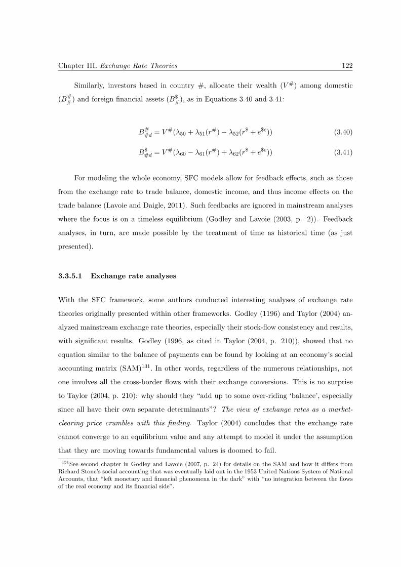
Chapter III. Exchange Rate Theories 122
Similarly, investors based in country #, allocate their wealth (V #) among domestic
(B##) and foreign financial assets (B$
#), as in Equations 3.40 and 3.41:
B##d = V #(λ50 + λ51(r
#)− λ52(r$ + e$e)) (3.40)
B$#d = V #(λ60 − λ61(r
#) + λ62(r$ + e$e)) (3.41)
For modeling the whole economy, SFC models allow for feedback effects, such as those
from the exchange rate to trade balance, domestic income, and thus income effects on the
trade balance (Lavoie and Daigle, 2011). Such feedbacks are ignored in mainstream analyses
where the focus is on a timeless equilibrium (Godley and Lavoie (2003, p. 2)). Feedback
analyses, in turn, are made possible by the treatment of time as historical time (as just
presented).
3.3.5.1 Exchange rate analyses
With the SFC framework, some authors conducted interesting analyses of exchange rate
theories originally presented within other frameworks. Godley (1196) and Taylor (2004) an-
alyzed mainstream exchange rate theories, especially their stock-flow consistency and results,
with significant results. Godley (1996, as cited in Taylor (2004, p. 210)), showed that no
equation similar to the balance of payments can be found by looking at an economy’s social
accounting matrix (SAM)131. In other words, regardless of the numerous relationships, not
one involves all the cross-border flows with their exchange conversions. This is no surprise
to Taylor (2004, p. 210): why should they “add up to some over-riding ‘balance’, especially
since all have their own separate determinants”? The view of exchange rates as a market-
clearing price crumbles with this finding. Taylor (2004) concludes that the exchange rate
cannot converge to an equilibrium value and any attempt to model it under the assumption
that they are moving towards fundamental values is doomed to fail.
131See second chapter in Godley and Lavoie (2007, p. 24) for details on the SAM and how it differs fromRichard Stone’s social accounting that was eventually laid out in the 1953 United Nations System of NationalAccounts, that “left monetary and financial phenomena in the dark” with “no integration between the flowsof the real economy and its financial side”.
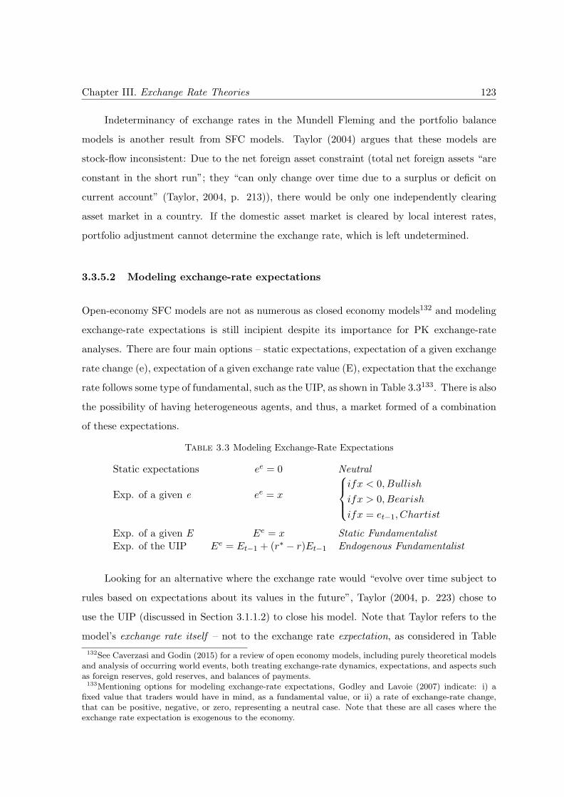
Chapter III. Exchange Rate Theories 123
Indeterminancy of exchange rates in the Mundell Fleming and the portfolio balance
models is another result from SFC models. Taylor (2004) argues that these models are
stock-flow inconsistent: Due to the net foreign asset constraint (total net foreign assets “are
constant in the short run”; they “can only change over time due to a surplus or deficit on
current account” (Taylor, 2004, p. 213)), there would be only one independently clearing
asset market in a country. If the domestic asset market is cleared by local interest rates,
portfolio adjustment cannot determine the exchange rate, which is left undetermined.
3.3.5.2 Modeling exchange-rate expectations
Open-economy SFC models are not as numerous as closed economy models132 and modeling
exchange-rate expectations is still incipient despite its importance for PK exchange-rate
analyses. There are four main options – static expectations, expectation of a given exchange
rate change (e), expectation of a given exchange rate value (E), expectation that the exchange
rate follows some type of fundamental, such as the UIP, as shown in Table 3.3133. There is also
the possibility of having heterogeneous agents, and thus, a market formed of a combination
of these expectations.
Table 3.3 Modeling Exchange-Rate Expectations
Static expectations ee = 0 Neutral
Exp. of a given e ee = x
ifx < 0, Bullish
ifx > 0, Bearish
ifx = et−1, Chartist
Exp. of a given E Ee = x Static FundamentalistExp. of the UIP Ee = Et−1 + (r∗ − r)Et−1 Endogenous Fundamentalist
Looking for an alternative where the exchange rate would “evolve over time subject to
rules based on expectations about its values in the future”, Taylor (2004, p. 223) chose to
use the UIP (discussed in Section 3.1.1.2) to close his model. Note that Taylor refers to the
model’s exchange rate itself – not to the exchange rate expectation, as considered in Table
132See Caverzasi and Godin (2015) for a review of open economy models, including purely theoretical modelsand analysis of occurring world events, both treating exchange-rate dynamics, expectations, and aspects suchas foreign reserves, gold reserves, and balances of payments.133Mentioning options for modeling exchange-rate expectations, Godley and Lavoie (2007) indicate: i) a
fixed value that traders would have in mind, as a fundamental value, or ii) a rate of exchange-rate change,that can be positive, negative, or zero, representing a neutral case. Note that these are all cases where theexchange rate expectation is exogenous to the economy.
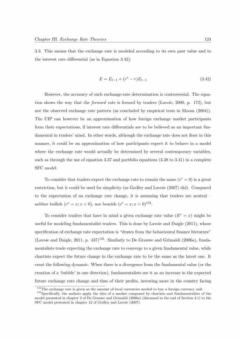
Chapter III. Exchange Rate Theories 124
3.3. This means that the exchange rate is modeled according to its own past value and to
the interest rate differential (as in Equation 3.42):
E = Et−1 + (r∗ − r)Et−1 (3.42)
However, the accuracy of such exchange-rate determination is controversial. The equa-
tion shows the way that the forward rate is formed by traders (Lavoie, 2000, p. 172), but
not the observed exchange rate pattern (as concluded by empirical tests in Moosa (2004)).
The UIP can however be an approximation of how foreign exchange market participants
form their expectations, if interest rate differentials are to be believed as an important fun-
damental in traders’ mind. In other words, although the exchange rate does not float in this
manner, it could be an approximation of how participants expect it to behave in a model
where the exchange rate would actually be determined by several contemporary variables,
such as through the use of equation 3.37 and portfolio equations (3.38 to 3.41) in a complete
SFC model.
To consider that traders expect the exchange rate to remain the same (ee = 0) is a great
restriction, but it could be used for simplicity (as Godley and Lavoie (2007) did). Compared
to the expectation of an exchange rate change, it is assuming that traders are neutral –
neither bullish (ee = x;x < 0), nor bearish (ee = x;x > 0)134.
To consider traders that have in mind a given exchange rate value (Ee = x) might be
useful for modeling fundamentalist traders. This is done by Lavoie and Daigle (2011), whose
specification of exchange rate expectation is “drawn from the behavioural finance literature”
(Lavoie and Daigle, 2011, p. 437)135. Similarly to De Grauwe and Grimaldi (2006a), funda-
mentalists trade expecting the exchange rate to converge to a given fundamental value, while
chartists expect the future change in the exchange rate to be the same as the latest one. It
creat the following dynamic. When there is a divergence from the fundamental value (or the
creation of a ‘bubble’ in one direction), fundamentalists see it as an increase in the expected
future exchange rate change and thus of their profits, investing more in the country facing
134The exchange rate is given as the amount of local currencies needed to buy a foreign currency unit.135Specifically, the authors apply the idea of a market composed by chartists and fundamentalists of the
model presented in chapter 2 of De Grauwe and Grimaldi (2006a) (discussed in the end of Section 3.1) to theSFC model presented in chapter 12 of Godley and Lavoie (2007).
Chapter III. Exchange Rate Theories 125
the exchange rate depreciation. This happens up to the point when the trend is reverted.
At this moment, chartists change the direction of their trading, bringing the exchange rate
back to its fundamental value. From this moment on, a ‘bubble’ is created in the opposite
direction and the mechanism repeats itself. Therefore, the model yields in exchange rates
cycles around an exogenously defined fundamental value.
Static vs. endogenous fundamentalist behavior The idea of a foreign market partici-
pant that trades knowing the fundamental value of the exchange rate is subject to criticisms
related to the very existence of fundamental values and of efficient market models. How-
ever a fundamentalist trader may simply be a participant that knows what (part of) the
other participants think about future exchange-rate value, coherently with Orlean’s concept
of an ‘auto-referential’ market. By expecting the exchange rate to be at a given level, these
participants make their forecasts according to the current financial convention. As put by
Orlean, to be ‘auto-referentially’ rational is the same as to estimate the result of a model.
Similarly to the mainstream fundamental, their forecast is an external value that does not
depend on their own opinion, but on the market’s. In both Lavoie and Daigle (2011) and
De Grauwe and Grimaldi (2006a), the forecast is an external value (a given value, and a
stochastic process, respectively). In this sense, in both cases the modeling of the exchange
rate forecast through a ‘fundamentalist trader’ does not necessarily imply the assumption of
the exchange rate as a market clearing price.
Additionally, to consider that participants trade expecting the exchange rate to converge
to a (supposedly) market-clearing price (in accordance with the result of mainstream models)
is not the same as to assume that such price exists. Indeed, such consideration is realistic, if
it is agreed that real world traders believe in market-clearing exchange rates. This is in line
with the argument that the exchange rate converges to ‘fundamentals’ because traders make
them behave in this way.
The simplification done by Lavoie and Daigle (2011) is not based on the assumption of
fundamentalist traders, but on the fact that the given fundamental value is static and does not
evolve with the economy. The use of a stochastic variable as exchange rate expectation has the
same drawbacks: they are not associated with the economy’s condition. In the different PK
analyses discussed in this section, expectations are allowed to change: in Orlean’s analysis,
Chapter III. Exchange Rate Theories 126
the financial convention evolves; in Schulmeister and Harvey, expectations “react” either to
events, or to base factors and indicators, respectively. Static expectations in a context of
important exchange-rate fluctuation are also not in line with the representativeness principle.
Instead, traders would look for reasons for these fluctuations and adapt their expectations
accordingly.
Modeling such floating fundamentalist expectations is not easy, but can be enabled
by tying economic variables already estimated by the model to the exchange rate forecast,
creating endogenous fundamentalist behavior – as in the fourth option of Table 3.3.
In conclusion, in light of this section’s theoretical discussion, an SFC model in the line
of Lavoie and Daigle’s (2011) could be made more complex by including a series of features:
the behavior of chartists could account for different types of model, as cash-in or contrarian
traders, and participants could praise different currencies differently. Providing a framework
to which details can be added and opening space for questioning how to model endogenous
(and thus floating) fundamental values is a step forward in heterodox exchange rate modeling.
This question will be dealt with in the next section, that also suggests ways to model the
features that emerged from PK exchange-rate analyses to an SFC model.
3.3.6 Adding post-Keynesian Features to SFC Portfolio Equations
This section has presented heterodox views on exchange rate determination, that emerged
from different approaches: Schulmeister’s work is inductive, based on empirical analysis of
the foreign exchange markets; both him and Harvey consider psychological insights into
their analysis; analyses of the specificities of emerging currencies are based on historical and
institutional analyses of the evolution of the international monetary and financial system; and
SFC models are based on transactions matrix that aim to put down in equations domestic
or open-economy dynamics in a detailed fashion. The main insights and shortcomings of the
different approaches have been analyzed throughout the section. The following analysis aims
at suggesting ways to use the different insights brought by these analyses in a SFC model,
specifically on its portfolio equations, the locus of most of the discussions presented.
Chapter III. Exchange Rate Theories 127
The intention of discussing how these features could be added to a SFC model is to
provide a common basis for theoretical discussion on exchange rate determination. If added
to an empirical model (which is probably not an easy task) it might also be used to explain
specific past exchange rate patterns136. This discussion may also be relevant to the SFC
literature in general, for adding realism (or realisticness137) to the treatment of exchange
rates in models that focus on different matters. Indeed, assumptions are simplifications, and
“to avoid to avoid cluttering a model with insignificant details” is needed (Lavoie, 2014, p.
13).
The choice of SFC framework derives from the following advantages. First, portfolio
equations allow adding considerations on the specificities of two (or more) currencies. This
can be done within the framework of the keynesian equation (as seen in the last section),
but it implies considering liquidity as a determinant of returns, while in SFC models they
determine demand, which is more specific. Harvey’s ‘mental model’, On the other hand, does
not allow such considerations for being based on one single currency.
Second, in an SFC model financial and real interactions are considered. This is an
advantage over Harvey’s ‘mental model’, for instance, that is a partial model where only
portfolio investment is considered as a factor adding supply or demand to the foreign exchange
market. Third, the stock and flow coherence can be added to an agent-based model (an AB-
SFC model), allowing for heterogeneous agents and a greater details of agents’ decisions.
In this way, the investor is at the center of the model, perfectly matching the theoretical
background of the rise of financialization and the importance of money managers. Note that
this is also a feature of Harvey’s ‘mental model’, but not the heterogeneity of agents. Fourth,
in an SFC model the interaction between flows and stocks can be taken into account while
none of the PK models discussed consider stocks.
Fifth, due to the flexibility of the SFC model, features that have not yet been discussed
or institutional changes can be accommodated. These features are not only restricted to
portfolio changes, but can also come from other sectors (as a policy of reserve accumulation
or capital control). While different features and complex analysis can also be done by using
136It is worth noting that there is no intention to use such a model for exchange rate forecast: the exchangerate is the result of social interactions that cannot be foreseen (whether investors will focus on one fundamentalor another is unknowable) and that depend on responses to unpredictable events.137See the discussion on realisticness, as opposed to instrumentalism, in the Introduction Chapter.
Chapter III. Exchange Rate Theories 128
literary analysis, they are more explicit when the SFC framework is used, as it demands a
high level of precision over assumptions. Finally, the SFC framework allows the simulation
of changes in economic variables, presenting its impacts through the economy.
How the different features of PK exchange-rate analyses can be added to the portfolio
equations of SFC models will be discussed next. The equations 3.38, 3.39, 3.40, and 3.41 are
replicated here for the reader’s convenience. This analysis assumes that country $ is a central
country issuing a currency that occupies a higher place in the IMFS, and that country # is
an EME whose currency occupies a peripheral position.
B$$d = V $(λ20 + λ21(r
$)− λ22(r# + e#e)) (3.38)
B#$d
= V $(λ30 − λ31(r$) + λ32(r
# + e#e)) (3.39)
B##d = V #(λ50 + λ51(r
#)− λ52(r$ + e$e)) (3.40)
B$#d = V #(λ60 − λ61(r
#) + λ62(r$ + e$e)) (3.41)
Liquidity-premium asymmetry and country bias The dynamics created by Lavoie
and Daigle (2011) include country-bias: investors’ preference for its own country assets138.
Liquidity-premium asymmetry is a different phenomenon: as central currencies offer a higher
liquidity premium, investors prefer investments in a central, rather than in a peripheral
currency, regardless of their country of origin.
Country-bias can be translated in higher demand for its own country’s assets (B$$d
> B#$d
and B##d > B$
#d) even if the return differential would not predict this (for instance, if
138Forbes (2010, p. 11) explains home-bias as a puzzle that cannot be explained by portfolio models:“standard portfolio theory shows that if investors care only about the mean and variance of the real returnof their invested wealth, if markets are efficient, and the cross-border barriers to investment are small, theninvestors should hold the world market portfolio of stocks. An extensive literature on home bias, however,shows that investors deviate substantially from this prediction and tend to hold a larger share of domesticassets in their portfolios.” Based on Kaltenbrunner (2015) one could argue that country-bias derives from thefact that investors’ liabilities are held in their own country’s currency. The framework presented in ChapterSeven is consistent with that and suggests that these biases derive from the additional element of uncertaintythat affects any foreign investment: the unknown exchange-rate development.
Chapter III. Exchange Rate Theories 129
r$ = r# + e#e139). Country-bias could be added through the constants in the determination
of demand for assets denominated in its own currency: λ20 > λ30 and λ50 > λ60140.
Different liquidity premiums, in turn, result in a bias in favor of central currencies from
investors in the two countries even if central and emerging countries offer the same total
expected returns: B$$d
> B#$d
and B##d < B$
#d even if r# = r$ + e$e.
With regards to the behavior of the central country’s investors, both liquidity-premium
asymmetry and county-bias result in biases towards their own country’s assets, which can be
modeled by considering λ20 > λ30 orλ20
λ30> 1141. Accordingly, the simultaneous consideration
of the two biases could be done by increasing the difference between λ20 and λ30, or by
increasing λ20
λ30above 1.
However, with regards to the demand of the emerging-country investor, the two features
act in opposite directions: the country-bias favors emerging assets and the liquidity-premium
asymmetry favors the asset from the central economy. In terms of the coefficients, these
considerations favor, respectively, λ50 and λ60. If the two features are considered equally
important, λ50
λ60= 1. Most likely, country bias is more important142 and thus λ50
λ60> 1.
Therefore, λ20
λ30> 1 and λ50
λ60> 1. Since the two biases are working in the same direction
in the case of foreign investor’s demand, and in opposite directions in the case of emerging
country’s investors, it can be concluded that λ20
λ30> λ50
λ60. Distinguishing the lambdas in two is
an option to deal with the two features (country bias, cb, and liquidity-premium asymmetry,
lpm), separately:
λi0 = λcbi0 + λlpm
i0 (3.43)
In this case, the higher liquidity premium of central currencies are translated into λlpm20 >
λlpm50 and λlpm
60 > λlpm30 . The country bias, on the other hand, leads to λcb
20 > λcb30 and λcb
50 > λcb60.
139Note that this dynamic must emerge independently from issues of liquidity premium and liquidity pref-erence.140Also see how Lavoie and Daigle (2011, p. 444) calibrate their coefficients for allowing the emergence of
country-bias.141For simplicity, the discussion focuses only in the constants (λi0), but the coefficients λi1 and λi2 could
also be adjusted.142A way to test it would be to compare an emerging country’s foreign assets position net of central bank
reserves with its country equity and bond markets capitalization net of foreign liabilities.
Chapter III. Exchange Rate Theories 130
Liquidity preference Given that the different level of liquidity premium are accounted
for, liquidity preference concerns are the most important feature to add to analyze the
impacts of the changes of the international financial scenario in emerging currencies. As
liquidity preference varies, there is a change on how investors value the liquidity premium
of a currency. Its coefficient (λlpfi0 ), must therefore be considered next to liquidity premium
(λlpmi0 ) in Equation 3.44143:
λlpi0 = λlpm
i0 × λlpfi0 (3.44)
λlpfi0 is mostly stable. It increases in time of turbulence (↑ λlpf
i0 ), leading to a shift of demand
from emerging (↓ B#$d, ↓ B#
#d) to central economy’s assets (↑ B$$d, ↑ B$
#d), from both types
of investors. Such a change in liquidity preference can be analyzed as a shock on λlpfi0 , or, in
an AB-SFC model, an exogenous series could be used (in the same way that the exchange
rate fundamental is modeled in De Grauwe and Grimaldi (2006a)). In the latter case, the
series could be modeled to resemble the VIX index, which is currently used as a proxy for
uncertainty and thus liquidity preference in the literature (as it will be seen in Chapter
Five)144.
Liquidity and liquidity preference The SFC framework allows the analysis of not only
changes in liquidity preference (λlpfi0 ), but also of liquidity itself, that can be seen as the
hike of wealth in the center or in the periphery (V $ and V #, respectively). While liquidity
preference acts by shifting demand from assets in one country to another, changes in liquidity
change the total demand for assets. Liquidity increase is an important development that led
to the rise of financialization (as discussed in Chapter Two) and it is of major relevance to
the integration of emerging countries’ assets in the international financial system.
Exchange-rate expectations As briefly discussed in Section 3.3.5 and in Table 3.3, there
are different ways to model exchange-rate expectations (Eie). Fundamentalists (f ) have a
143Note that this is the same of considering β next to l as in Equations 3.33 to 3.36144As shown in Chapter Five, the behavior of the VIX in the 2000s has been characterized by more or less
long stability, of levels close to 20, with peaks that are usually as high as 40, having achieved the 80-levelwith the GFC. A purely stochastic process would therefore not be the most welcomed. The optimum wouldbe a series that has major hikes that slowly fade.
Chapter III. Exchange Rate Theories 131
fixed exchange rate (x) in mind, shown in Equation 3.45. (In a two-country model, E$ef = x
and E#ef = 1/x)145.
Eief = x (3.45)
As discussed in Section 3.3.5, such fundamentalist behavior is static and not in line with
PK analyses. An option for modeling an endogenous fundamentalist behavior is to think of
what traders see as fundamental exchange rates. If traders believe that the exchange rate
follows the UIP, their behavior could be modeled as in Equation 3.46: A hike of interest
rates in the emerging country (↑ r#) is expected to lead to an appreciation of the country’s
currency (↓ E#; E#efUIP < E#
t−1):
E#efUIP = E#
t−1 + (r$ − r#)E#t−1 (3.46)
A PPP-fundamentalist trader could use price differentials in their forecast (as in Equa-
tion 3.47, that follows from Equation 3.2): Higher prices in the emerging country (↑ p#) are
associated with a loss of competitiveness internationally and an exchange rate depreciation
(↑ E#; E#efPPP > E#
t−1)146:
E#efPPP = E#
t−1 + (p# − p$)E#t−1 (3.47)
In complete models as the one presented in the Chapter 12 of Godley and Lavoie (2007),
a more specific behavior might be modeled, as a participant that trades according to changes
on the trade balance instead of the PPP. In Equation 3.48, a higher trade balance (↑ X# −
IM#147) is expected to lead to an appreciation of the local currency (↓ E#; E#eftrade < E#
t−1).
E#eftrade = E#
t−1 − γ(X# − IM#)E#t−1 (3.48)
145In all equations where past exchange rate change is a factor in determining future exchange rates, theoption to consider Et−1 − Et−2 instead of Et − Et−1 is based on a concern over the simultaneous definitionsand the problems that can arise when running a SFC model.146Note that this implies a case with zero inflation. Similarly, p could denote inflation, and a rise of inflation
in emerging countries above the one of central countries would have the same effect.147This follows the notations and the variables’ definitions of chapter 12 of Godley and Lavoie (2007).
Chapter III. Exchange Rate Theories 132
This expectation formation could be made more complex to better represent the impact
of changes in indicators in the exchange rate forecast, as described by Harvey in its ‘mental
model’ (presented in Section 3.3.3 and in Figure 3.1) by adding other concerns, as in Equation
3.49148. Heterogeneous agents with different focus on each of these variables can also be
considered by adjusting their respective γ, ǫ, and θ.
E#efindic = E#
t−1 − E#t−1[γ(X
# − IM#) + ǫ(y# − y$) + θ(r# − r$)] (3.49)
Chartists (c), on the other hand, do not look at economic variables, just at the exchange
rate itself, expecting the last exchange rate change to repeat in the future, as in Equations
3.50 or 3.51:
eiec = eit−1 (3.50)
Eiec = Ei
t−1 +Ei
t−1 − Eit−2
Eit−2
(3.51)
More complex chartist behavior, based on Schulmeister’s fast and slow technical systems,
could also be added. When forming their expectation, slow chartists (cslow) look for a longer
average change of exchange rates than fast chartists (cfast); as shown in Equations 3.53 and
3.52, where m > n:
Eiecfast = Ei
t−1 +Ei
t−1 − Eit−n
Eit−n
(3.52)
Eiecslow = Ei
t−1 +Ei
t−1 − Eit−m
Eit−m
(3.53)
Cash-in Cash-in can be included through a limit in the profits accumulated with an asset.
Its modeling asks for the addition of a variable that counts the stock of profits of a given
amount of periods and a rule that the agent sells an asset when its stock of profits achieves a
148The causalities are the ones considered by Harvey. Higher trade is expected to lead to an appreciation(or ↑ (X# − IM#), ↓ E#). Higher growth would lead to more portfolio investment and FDI (although lesstrade), and is thus expected to lead to an exchange rate appreciation (or ↑ (y# − y$), ↓ E#.). Higher interestrate differential is expected to have the same impact, ↑ (r# − r$), ↓ E#
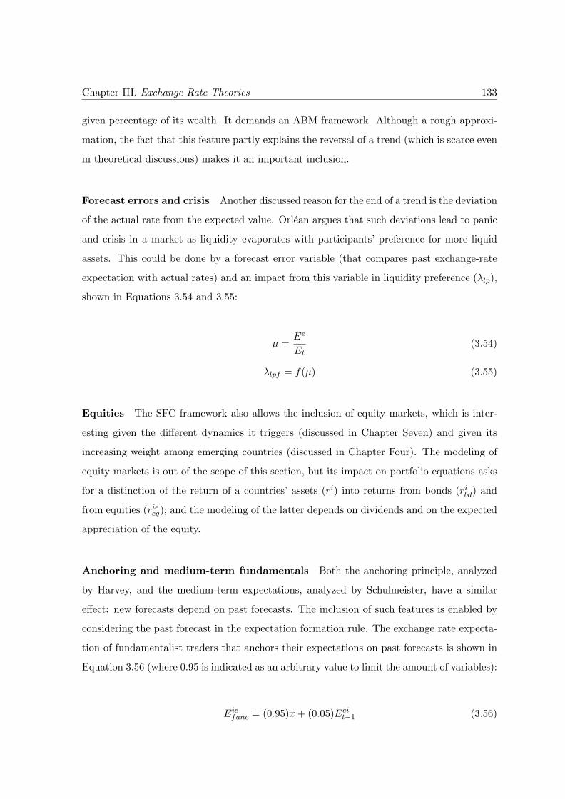
Chapter III. Exchange Rate Theories 133
given percentage of its wealth. It demands an ABM framework. Although a rough approxi-
mation, the fact that this feature partly explains the reversal of a trend (which is scarce even
in theoretical discussions) makes it an important inclusion.
Forecast errors and crisis Another discussed reason for the end of a trend is the deviation
of the actual rate from the expected value. Orlean argues that such deviations lead to panic
and crisis in a market as liquidity evaporates with participants’ preference for more liquid
assets. This could be done by a forecast error variable (that compares past exchange-rate
expectation with actual rates) and an impact from this variable in liquidity preference (λlp),
shown in Equations 3.54 and 3.55:
µ =Ee
Et
(3.54)
λlpf = f(µ) (3.55)
Equities The SFC framework also allows the inclusion of equity markets, which is inter-
esting given the different dynamics it triggers (discussed in Chapter Seven) and given its
increasing weight among emerging countries (discussed in Chapter Four). The modeling of
equity markets is out of the scope of this section, but its impact on portfolio equations asks
for a distinction of the return of a countries’ assets (ri) into returns from bonds (ribd) and
from equities (rieeq); and the modeling of the latter depends on dividends and on the expected
appreciation of the equity.
Anchoring and medium-term fundamentals Both the anchoring principle, analyzed
by Harvey, and the medium-term expectations, analyzed by Schulmeister, have a similar
effect: new forecasts depend on past forecasts. The inclusion of such features is enabled by
considering the past forecast in the expectation formation rule. The exchange rate expecta-
tion of fundamentalist traders that anchors their expectations on past forecasts is shown in
Equation 3.56 (where 0.95 is indicated as an arbitrary value to limit the amount of variables):
Eiefanc = (0.95)x+ (0.05)Eei
t−1 (3.56)
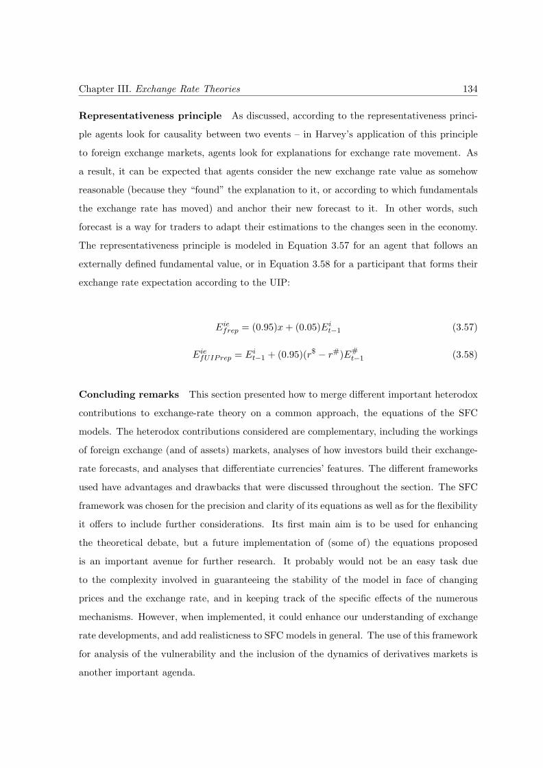
Chapter III. Exchange Rate Theories 134
Representativeness principle As discussed, according to the representativeness princi-
ple agents look for causality between two events – in Harvey’s application of this principle
to foreign exchange markets, agents look for explanations for exchange rate movement. As
a result, it can be expected that agents consider the new exchange rate value as somehow
reasonable (because they “found” the explanation to it, or according to which fundamentals
the exchange rate has moved) and anchor their new forecast to it. In other words, such
forecast is a way for traders to adapt their estimations to the changes seen in the economy.
The representativeness principle is modeled in Equation 3.57 for an agent that follows an
externally defined fundamental value, or in Equation 3.58 for a participant that forms their
exchange rate expectation according to the UIP:
Eiefrep = (0.95)x+ (0.05)Ei
t−1 (3.57)
EiefUIPrep = Ei
t−1 + (0.95)(r$ − r#)E#t−1 (3.58)
Concluding remarks This section presented how to merge different important heterodox
contributions to exchange-rate theory on a common approach, the equations of the SFC
models. The heterodox contributions considered are complementary, including the workings
of foreign exchange (and of assets) markets, analyses of how investors build their exchange-
rate forecasts, and analyses that differentiate currencies’ features. The different frameworks
used have advantages and drawbacks that were discussed throughout the section. The SFC
framework was chosen for the precision and clarity of its equations as well as for the flexibility
it offers to include further considerations. Its first main aim is to be used for enhancing
the theoretical debate, but a future implementation of (some of) the equations proposed
is an important avenue for further research. It probably would not be an easy task due
to the complexity involved in guaranteeing the stability of the model in face of changing
prices and the exchange rate, and in keeping track of the specific effects of the numerous
mechanisms. However, when implemented, it could enhance our understanding of exchange
rate developments, and add realisticness to SFC models in general. The use of this framework
for analysis of the vulnerability and the inclusion of the dynamics of derivatives markets is
another important agenda.
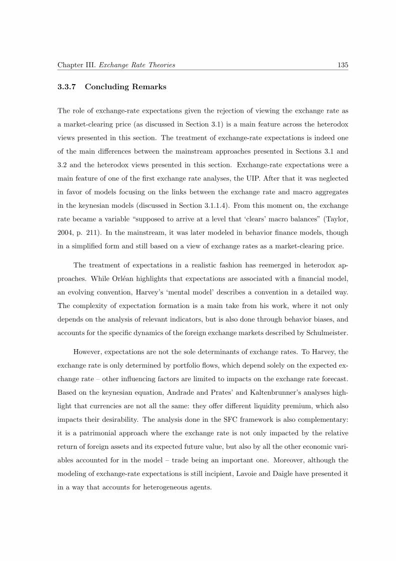
Chapter III. Exchange Rate Theories 135
3.3.7 Concluding Remarks
The role of exchange-rate expectations given the rejection of viewing the exchange rate as
a market-clearing price (as discussed in Section 3.1) is a main feature across the heterodox
views presented in this section. The treatment of exchange-rate expectations is indeed one
of the main differences between the mainstream approaches presented in Sections 3.1 and
3.2 and the heterodox views presented in this section. Exchange-rate expectations were a
main feature of one of the first exchange rate analyses, the UIP. After that it was neglected
in favor of models focusing on the links between the exchange rate and macro aggregates
in the keynesian models (discussed in Section 3.1.1.4). From this moment on, the exchange
rate became a variable “supposed to arrive at a level that ‘clears’ macro balances” (Taylor,
2004, p. 211). In the mainstream, it was later modeled in behavior finance models, though
in a simplified form and still based on a view of exchange rates as a market-clearing price.
The treatment of expectations in a realistic fashion has reemerged in heterodox ap-
proaches. While Orlean highlights that expectations are associated with a financial model,
an evolving convention, Harvey’s ‘mental model’ describes a convention in a detailed way.
The complexity of expectation formation is a main take from his work, where it not only
depends on the analysis of relevant indicators, but is also done through behavior biases, and
accounts for the specific dynamics of the foreign exchange markets described by Schulmeister.
However, expectations are not the sole determinants of exchange rates. To Harvey, the
exchange rate is only determined by portfolio flows, which depend solely on the expected ex-
change rate – other influencing factors are limited to impacts on the exchange rate forecast.
Based on the keynesian equation, Andrade and Prates’ and Kaltenbrunner’s analyses high-
light that currencies are not all the same: they offer different liquidity premium, which also
impacts their desirability. The analysis done in the SFC framework is also complementary:
it is a patrimonial approach where the exchange rate is not only impacted by the relative
return of foreign assets and its expected future value, but also by all the other economic vari-
ables accounted for in the model – trade being an important one. Moreover, although the
modeling of exchange-rate expectations is still incipient, Lavoie and Daigle have presented it
in a way that accounts for heterogeneous agents.
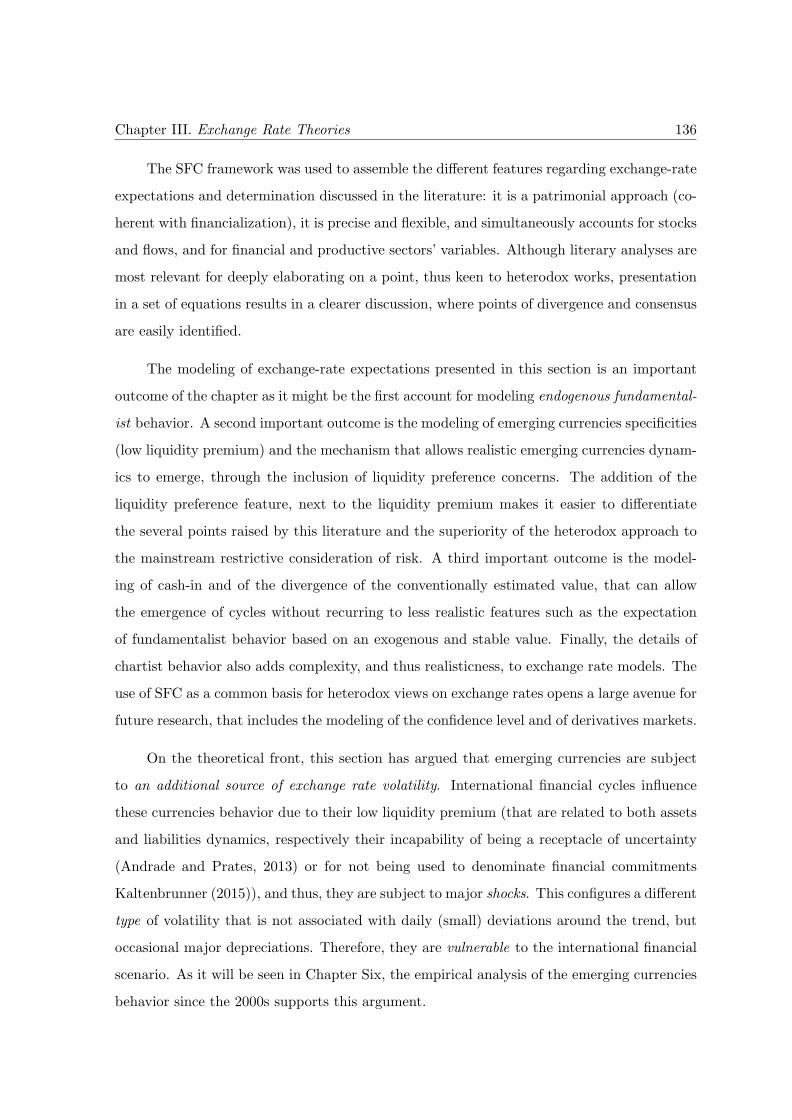
Chapter III. Exchange Rate Theories 136
The SFC framework was used to assemble the different features regarding exchange-rate
expectations and determination discussed in the literature: it is a patrimonial approach (co-
herent with financialization), it is precise and flexible, and simultaneously accounts for stocks
and flows, and for financial and productive sectors’ variables. Although literary analyses are
most relevant for deeply elaborating on a point, thus keen to heterodox works, presentation
in a set of equations results in a clearer discussion, where points of divergence and consensus
are easily identified.
The modeling of exchange-rate expectations presented in this section is an important
outcome of the chapter as it might be the first account for modeling endogenous fundamental-
ist behavior. A second important outcome is the modeling of emerging currencies specificities
(low liquidity premium) and the mechanism that allows realistic emerging currencies dynam-
ics to emerge, through the inclusion of liquidity preference concerns. The addition of the
liquidity preference feature, next to the liquidity premium makes it easier to differentiate
the several points raised by this literature and the superiority of the heterodox approach to
the mainstream restrictive consideration of risk. A third important outcome is the model-
ing of cash-in and of the divergence of the conventionally estimated value, that can allow
the emergence of cycles without recurring to less realistic features such as the expectation
of fundamentalist behavior based on an exogenous and stable value. Finally, the details of
chartist behavior also adds complexity, and thus realisticness, to exchange rate models. The
use of SFC as a common basis for heterodox views on exchange rates opens a large avenue for
future research, that includes the modeling of the confidence level and of derivatives markets.
On the theoretical front, this section has argued that emerging currencies are subject
to an additional source of exchange rate volatility. International financial cycles influence
these currencies behavior due to their low liquidity premium (that are related to both assets
and liabilities dynamics, respectively their incapability of being a receptacle of uncertainty
(Andrade and Prates, 2013) or for not being used to denominate financial commitments
Kaltenbrunner (2015)), and thus, they are subject to major shocks. This configures a different
type of volatility that is not associated with daily (small) deviations around the trend, but
occasional major depreciations. Therefore, they are vulnerable to the international financial
scenario. As it will be seen in Chapter Six, the empirical analysis of the emerging currencies
behavior since the 2000s supports this argument.
Chapter III. Exchange Rate Theories 137
3.4 Conclusions
The thesis aims at enlightening the behavior of emerging currencies in times of financial-
ization. As seen in Chapter Two, the current phase of capitalism is characterized by the
centrality of money managers and their portfolio decisions: financial flows are of great rele-
vance, financial markets are sophisticated (with great derivatives markets, where leveraging
allows speculating large amounts), there is a high amount of liquidity in central economies
that are allocated worldwide according to the decisions of a few investors. Are these fea-
tures accounted for by exchange rate theories? As discussed in this chapter, among the
mainstream theories, the patrimonial approach of portfolio models is coherent with the fi-
nancialization context. Additionally, the inclusion of exchange-rate expectations in models
with heterogeneous agents should be recognized. However, both approaches are based on
assumptions of the exchange rate as a market-clearing price. As argued in this chapter, this
is inconsistent with the very dynamics of financial flows in a context of floating exchange
rate and financialization, where exchange rate returns are key for attracting financial flows,
determining a self-feeding interaction that, instead of leading to equilibrium, is a ‘deviation
amplifying system’. This is strengthened in the case of equity investment, as also the asset
price will pass through the interaction. This dynamic, that will be presented in Chapter
Seven, is the opposite of the mainstream idea of exchange rates that tend to equilibrium and
clear markets. Note that this dynamic is the opposite to the dynamics related to trade flows,
where the exchange rate is a converging force: higher exports put appreciation pressure that
discourage exports.
Given the post-Keynesian perspective, the realisticness of theories, specifically with
regards to the financialization-related features, is key for understanding exchange rates. The
failure of most mainstream models might result from their lack of realisticness. As the section
has shown, there is however a search for more realistic features among mainstream approach
when they explicitly attempt to answer the exchange-rate puzzles, and thus enhance the
explanation power of models – these include heterogeneous agents and derivatives markets;
also the third-generation crisis models, that are case specific analyses, are a noteworthy step
in this direction.
Chapter III. Exchange Rate Theories 138
On the other hand, heterodox models are based on realistic assumptions, emerging
from analyses of the workings of foreign-exchange markets and of the configuration of the
international monetary and financial system. For this reason, they result in insights that
enhance our understanding of exchange rate behavior. While mainstream analyses deem
short-term exchange rate behavior as irrational, concentrating on long-term trends, short-
term fluctuations impact the economy in general (as discussed in the Introduction) and their
understanding is crucial for policy concerns. For the same reason, the understanding of
crisis is also crucial. In this point, once more, the heterodox approach proves superior as
most of the theories discussed account for both exchange rate determination and crisis –
differently from the mainstream where these are divided in two bodies of literature. This
very dichotomy in the mainstream literature is an evidence of the failure of its models to
explain exchange rate developments. The ability of heterodox studies to explain exchange
rates in its complexity – in both tranquil and turbulent periods – is even more relevant for
analyses of emerging currencies, where crises are frequent.
From the literature review on the specificities of emerging currencies, this chapter has
argued that the inclusion of EMEs’ assets in money managers’ portfolios results in impor-
tant shocks when there is a change in the international financial scenario and in their close
association to it. In other words, emerging currencies become more fragile to changes in the
international scenario. These hypotheses will be tested in Chapter Six.
Chapter Seven will analyze the dynamics behind this phenomenon, based on the Min-
skyan framework of analyzing the evolution of agents’ behavior throughout the economic cycle
and how that creates a fragile system. It differs from the literature analyzed in this chap-
ter by centering on money-managers’ decisions, their evolution and the creation of fragility,
although a currency’s features and behavioral biases are considered in the analysis.
Chapter 4
Emerging Countries’ Changing
Foreign Liabilities and
Vulnerabilities
As discussed in Chapter Two, the 1990s was a period of important changes in developing
countries due to the broad implementation of policies of capital account liberalization in the
wake of what became known as the ‘Washington Consensus’ policies1. If financial globaliza-
tion started in the 1970s and consolidated among advanced countries in the 1980s, it was in
the 1990s that some developing countries became part of this process, and, as argued in Chap-
ter Two, became part of a network determined by money managers’ balance-sheets2. Figure
4.1, taken from Haldane (2011, p. 17), illustrates the changing participation of emerging
countries’ equity assets3: showing a marginal presence before the 1990s, and the subsequent
integration of several EMEs as part of a very complex network in the 2000s.
In fact, there was a massive increase of flows to developing countries in the 1990s,
building important stocks of foreign liabilities following domestic reforms and the decrease
1See Williamson (1990).2See Akyuz and Cornford (2002, p. 10) for the change in capital flows to developing and emerging countries
in the period, with regards to the countries GNP, type of flow and geographical area.3Emerging markets in this work are represented by Argentina, Brazil, Mexico, China, India and Korea
(Kubelec and Sa, 2010, p. 35).
139
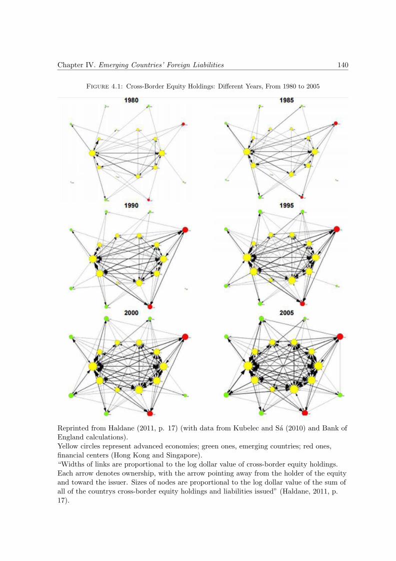
Chapter IV. Emerging Countries’ Foreign Liabilities 140
Figure 4.1: Cross-Border Equity Holdings: Different Years, From 1980 to 2005
Reprinted from Haldane (2011, p. 17) (with data from Kubelec and Sa (2010) and Bank ofEngland calculations).Yellow circles represent advanced economies; green ones, emerging countries; red ones,financial centers (Hong Kong and Singapore).“Widths of links are proportional to the log dollar value of cross-border equity holdings.Each arrow denotes ownership, with the arrow pointing away from the holder of the equityand toward the issuer. Sizes of nodes are proportional to the log dollar value of the sum ofall of the countrys cross-border equity holdings and liabilities issued” (Haldane, 2011, p.17).
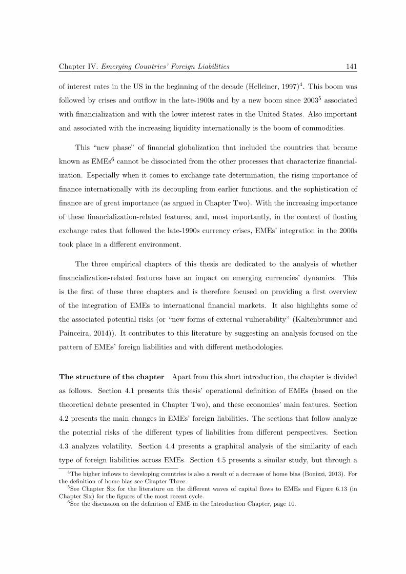
Chapter IV. Emerging Countries’ Foreign Liabilities 141
of interest rates in the US in the beginning of the decade (Helleiner, 1997)4. This boom was
followed by crises and outflow in the late-1900s and by a new boom since 20035 associated
with financialization and with the lower interest rates in the United States. Also important
and associated with the increasing liquidity internationally is the boom of commodities.
This “new phase” of financial globalization that included the countries that became
known as EMEs6 cannot be dissociated from the other processes that characterize financial-
ization. Especially when it comes to exchange rate determination, the rising importance of
finance internationally with its decoupling from earlier functions, and the sophistication of
finance are of great importance (as argued in Chapter Two). With the increasing importance
of these financialization-related features, and, most importantly, in the context of floating
exchange rates that followed the late-1990s currency crises, EMEs’ integration in the 2000s
took place in a different environment.
The three empirical chapters of this thesis are dedicated to the analysis of whether
financialization-related features have an impact on emerging currencies’ dynamics. This
is the first of these three chapters and is therefore focused on providing a first overview
of the integration of EMEs to international financial markets. It also highlights some of
the associated potential risks (or “new forms of external vulnerability” (Kaltenbrunner and
Painceira, 2014)). It contributes to this literature by suggesting an analysis focused on the
pattern of EMEs’ foreign liabilities and with different methodologies.
The structure of the chapter Apart from this short introduction, the chapter is divided
as follows. Section 4.1 presents this thesis’ operational definition of EMEs (based on the
theoretical debate presented in Chapter Two), and these economies’ main features. Section
4.2 presents the main changes in EMEs’ foreign liabilities. The sections that follow analyze
the potential risks of the different types of liabilities from different perspectives. Section
4.3 analyzes volatility. Section 4.4 presents a graphical analysis of the similarity of each
type of foreign liabilities across EMEs. Section 4.5 presents a similar study, but through a
4The higher inflows to developing countries is also a result of a decrease of home bias (Bonizzi, 2013). Forthe definition of home bias see Chapter Three.
5See Chapter Six for the literature on the different waves of capital flows to EMEs and Figure 6.13 (inChapter Six) for the figures of the most recent cycle.
6See the discussion on the definition of EME in the Introduction Chapter, page 10.
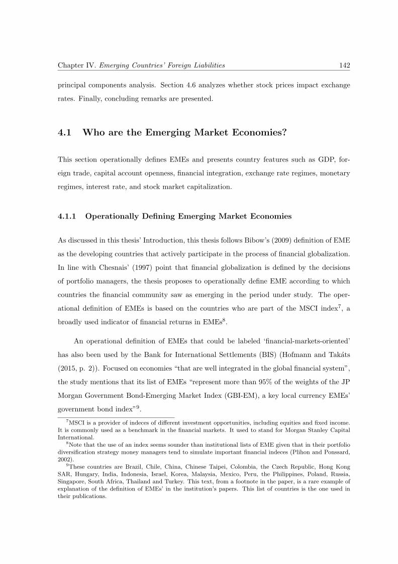
Chapter IV. Emerging Countries’ Foreign Liabilities 142
principal components analysis. Section 4.6 analyzes whether stock prices impact exchange
rates. Finally, concluding remarks are presented.
4.1 Who are the Emerging Market Economies?
This section operationally defines EMEs and presents country features such as GDP, for-
eign trade, capital account openness, financial integration, exchange rate regimes, monetary
regimes, interest rate, and stock market capitalization.
4.1.1 Operationally Defining Emerging Market Economies
As discussed in this thesis’ Introduction, this thesis follows Bibow’s (2009) definition of EME
as the developing countries that actively participate in the process of financial globalization.
In line with Chesnais’ (1997) point that financial globalization is defined by the decisions
of portfolio managers, the thesis proposes to operationally define EME according to which
countries the financial community saw as emerging in the period under study. The oper-
ational definition of EMEs is based on the countries who are part of the MSCI index7, a
broadly used indicator of financial returns in EMEs8.
An operational definition of EMEs that could be labeled ‘financial-markets-oriented’
has also been used by the Bank for International Settlements (BIS) (Hofmann and Takats
(2015, p. 2)). Focused on economies “that are well integrated in the global financial system”,
the study mentions that its list of EMEs “represent more than 95% of the weights of the JP
Morgan Government Bond-Emerging Market Index (GBI-EM), a key local currency EMEs’
government bond index”9.
7MSCI is a provider of indeces of different investment opportunities, including equities and fixed income.It is commonly used as a benchmark in the financial markets. It used to stand for Morgan Stanley CapitalInternational.
8Note that the use of an index seems sounder than institutional lists of EME given that in their portfoliodiversification strategy money managers tend to simulate important financial indeces (Plihon and Ponssard,2002).
9These countries are Brazil, Chile, China, Chinese Taipei, Colombia, the Czech Republic, Hong KongSAR, Hungary, India, Indonesia, Israel, Korea, Malaysia, Mexico, Peru, the Philippines, Poland, Russia,Singapore, South Africa, Thailand and Turkey. This text, from a footnote in the paper, is a rare example ofexplanation of the definition of EMEs’ in the institution’s papers. This list of countries is the one used intheir publications.
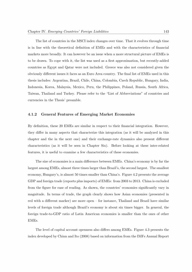
Chapter IV. Emerging Countries’ Foreign Liabilities 143
The list of countries in the MSCI index changes over time. That it evolves through time
is in line with the theoretical definition of EMEs and with the characteristics of financial
markets more broadly. It can however be an issue when a more structural picture of EMEs is
to be drawn. To cope with it, the list was used as a first approximation, but recently-added
countries as Egypt and Qatar were not included. Greece was also not considered given the
obviously different issues it faces as an Euro Area country. The final list of EMEs used in this
thesis includes: Argentina, Brazil, Chile, China, Colombia, Czech Republic, Hungary, India,
Indonesia, Korea, Malaysia, Mexico, Peru, the Philippines, Poland, Russia, South Africa,
Taiwan, Thailand and Turkey. Please refer to the “List of Abbreviations” of countries and
currencies in the Thesis’ preamble.
4.1.2 General Features of Emerging Market Economies
By definition, these 20 EMEs are similar in respect to their financial integration. However,
they differ in many aspects that characterize this integration (as it will be analyzed in this
chapter and the in the next one) and their exchange-rate dynamics also present different
characteristics (as it will be seen in Chapter Six). Before looking at these inter-related
features, it is useful to examine a few characteristics of these economies.
The size of economies is a main difference between EMEs. China’s economy is by far the
largest among EMEs, almost three times larger than Brazil’s, the second largest. The smallest
economy, Hungary’s, is almost 50 times smaller than China’s. Figure 4.2 presents the average
GDP and foreign trade (exports plus imports) of EMEs: from 2003 to 2013. China is excluded
from the figure for ease of reading. As shown, the countries’ economies significantly vary in
magnitude. In terms of trade, the graph clearly shows how Asian economies (presented in
red with a different marker) are more open – for instance, Thailand and Brazil have similar
levels of foreign trade although Brazil’s economy is about six times bigger. In general, the
foreign trade-to-GDP ratio of Latin American economies is smaller than the ones of other
EMEs.
The level of capital account openness also differs among EMEs. Figure 4.3 presents the
index developed by Chinn and Ito (2008) based on information from the IMFs Annual Report
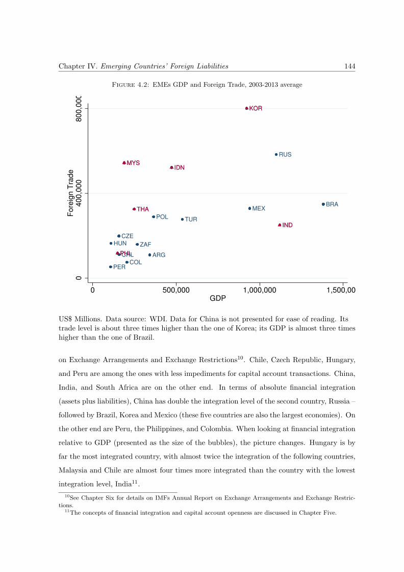
Chapter IV. Emerging Countries’ Foreign Liabilities 144
Figure 4.2: EMEs GDP and Foreign Trade, 2003-2013 average
ARG
BRA
CHL
COL
CZE
HUN
IDN
IND
KOR
MEX
MYS
PER
PHL
POL
RUS
THA
TUR
ZAF
IDN
IND
KOR
MYS
PHL
THA
04
00
,00
08
00
,00
0F
ore
ign
Tra
de
0 500,000 1,000,000 1,500,00GDP
US$ Millions. Data source: WDI. Data for China is not presented for ease of reading. Itstrade level is about three times higher than the one of Korea; its GDP is almost three timeshigher than the one of Brazil.
on Exchange Arrangements and Exchange Restrictions10. Chile, Czech Republic, Hungary,
and Peru are among the ones with less impediments for capital account transactions. China,
India, and South Africa are on the other end. In terms of absolute financial integration
(assets plus liabilities), China has double the integration level of the second country, Russia –
followed by Brazil, Korea and Mexico (these five countries are also the largest economies). On
the other end are Peru, the Philippines, and Colombia. When looking at financial integration
relative to GDP (presented as the size of the bubbles), the picture changes. Hungary is by
far the most integrated country, with almost twice the integration of the following countries,
Malaysia and Chile are almost four times more integrated than the country with the lowest
integration level, India11.
10See Chapter Six for details on IMFs Annual Report on Exchange Arrangements and Exchange Restric-tions.
11The concepts of financial integration and capital account openness are discussed in Chapter Five.
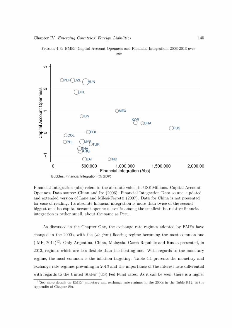
Chapter IV. Emerging Countries’ Foreign Liabilities 145
Figure 4.3: EMEs’ Capital Account Openness and Financial Integration, 2003-2013 aver-age
ARG
BRA
CHL
COL
CZE HUN
IND
IDN
MYS
MEX
PER
PHL
POLRUS
ZAF
THA
TUR
KOR
−1
01
23
Ca
pita
l A
cco
un
t O
pe
nn
ess
0 500,000 1,000,000 1,500,000 2,000,00Financial Integration (Abs)
Bubbles: Financial Integration (% GDP)
Financial Integration (abs) refers to the absolute value, in US$ Millions. Capital AccountOpenness Data source: Chinn and Ito (2006). Financial Integration Data source: updatedand extended version of Lane and Milesi-Ferretti (2007). Data for China is not presentedfor ease of reading. Its absolute financial integration is more than twice of the secondbiggest one; its capital account openness level is among the smallest; its relative financialintegration is rather small, about the same as Peru.
As discussed in the Chapter One, the exchange rate regimes adopted by EMEs have
changed in the 2000s, with the (de jure) floating regime becoming the most common one
(IMF, 2014)12. Only Argentina, China, Malaysia, Czech Republic and Russia presented, in
2013, regimes which are less flexible than the floating one. With regards to the monetary
regime, the most common is the inflation targeting. Table 4.1 presents the monetary and
exchange rate regimes prevailing in 2013 and the importance of the interest rate differential
with regards to the United States’ (US) Fed Fund rates. As it can be seen, there is a higher
12See more details on EMEs’ monetary and exchange rate regimes in the 2000s in the Table 6.12, in theAppendix of Chapter Six.
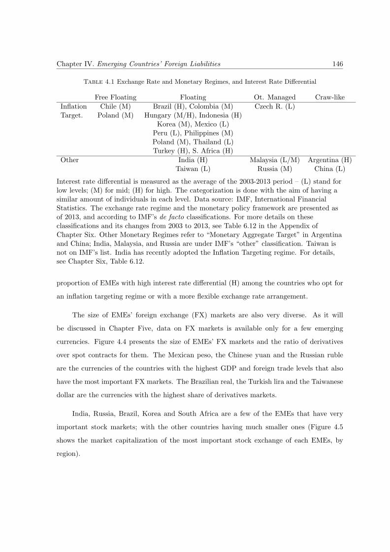
Chapter IV. Emerging Countries’ Foreign Liabilities 146
Table 4.1 Exchange Rate and Monetary Regimes, and Interest Rate Differential
Free Floating Floating Ot. Managed Craw-like
Inflation Chile (M) Brazil (H), Colombia (M) Czech R. (L)Target. Poland (M) Hungary (M/H), Indonesia (H)
Korea (M), Mexico (L)Peru (L), Philippines (M)Poland (M), Thailand (L)Turkey (H), S. Africa (H)
Other India (H) Malaysia (L/M) Argentina (H)Taiwan (L) Russia (M) China (L)
Interest rate differential is measured as the average of the 2003-2013 period – (L) stand forlow levels; (M) for mid; (H) for high. The categorization is done with the aim of having asimilar amount of individuals in each level. Data source: IMF, International FinancialStatistics. The exchange rate regime and the monetary policy framework are presented asof 2013, and according to IMF’s de facto classifications. For more details on theseclassifications and its changes from 2003 to 2013, see Table 6.12 in the Appendix ofChapter Six. Other Monetary Regimes refer to “Monetary Aggregate Target” in Argentinaand China; India, Malaysia, and Russia are under IMF’s “other” classification. Taiwan isnot on IMF’s list. India has recently adopted the Inflation Targeting regime. For details,see Chapter Six, Table 6.12.
proportion of EMEs with high interest rate differential (H) among the countries who opt for
an inflation targeting regime or with a more flexible exchange rate arrangement.
The size of EMEs’ foreign exchange (FX) markets are also very diverse. As it will
be discussed in Chapter Five, data on FX markets is available only for a few emerging
currencies. Figure 4.4 presents the size of EMEs’ FX markets and the ratio of derivatives
over spot contracts for them. The Mexican peso, the Chinese yuan and the Russian ruble
are the currencies of the countries with the highest GDP and foreign trade levels that also
have the most important FX markets. The Brazilian real, the Turkish lira and the Taiwanese
dollar are the currencies with the highest share of derivatives markets.
India, Russia, Brazil, Korea and South Africa are a few of the EMEs that have very
important stock markets; with the other countries having much smaller ones (Figure 4.5
shows the market capitalization of the most important stock exchange of each EMEs, by
region).
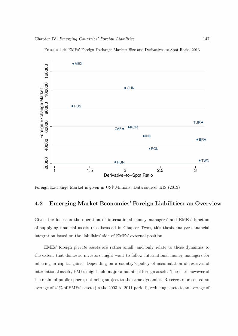
Chapter IV. Emerging Countries’ Foreign Liabilities 147
Figure 4.4: EMEs’ Foreign Exchange Market: Size and Derivatives-to-Spot Ratio, 2013
BRA
CHN
HUN
IND
KOR
MEX
POL
RUS
TWN
TUR
ZAF
20
00
04
00
00
60
00
08
00
00
10
00
00
12
00
00
Fo
reig
n E
xch
an
ge
Ma
rke
t
1 1.5 2 2.5 3Derivative−to−Spot Ratio
Foreign Exchange Market is given in US$ Millions. Data source: BIS (2013)
4.2 Emerging Market Economies’ Foreign Liabilities: an Overview
Given the focus on the operation of international money managers’ and EMEs’ function
of supplying financial assets (as discussed in Chapter Two), this thesis analyzes financial
integration based on the liabilities’ side of EMEs’ external position.
EMEs’ foreign private assets are rather small, and only relate to these dynamics to
the extent that domestic investors might want to follow international money managers for
inferring in capital gains. Depending on a country’s policy of accumulation of reserves of
international assets, EMEs might hold major amounts of foreign assets. These are however of
the realm of public sphere, not being subject to the same dynamics. Reserves represented an
average of 41% of EMEs’ assets (in the 2003-to-2011 period), reducing assets to an average of
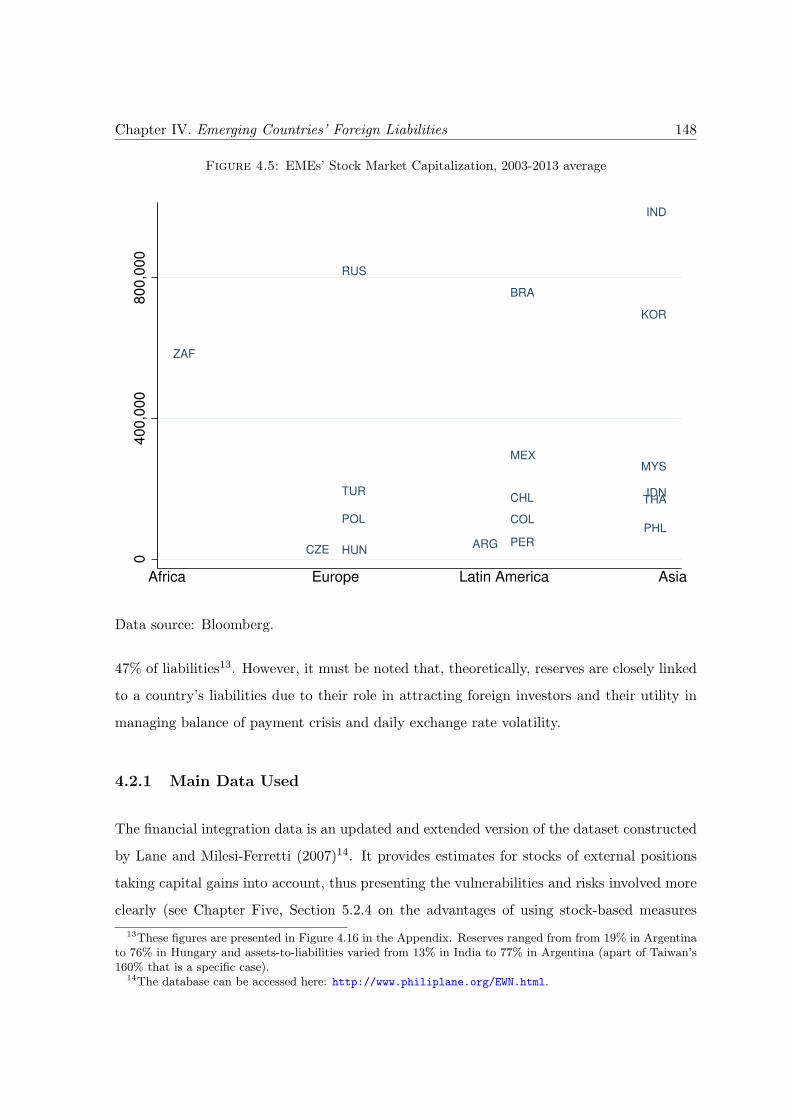
Chapter IV. Emerging Countries’ Foreign Liabilities 148
Figure 4.5: EMEs’ Stock Market Capitalization, 2003-2013 average
IND
IDN
KOR
MYS
PHL
THA
ZAF
BRA
CHL
COL
MEX
PERARGHUN
POL
RUS
TUR
CZE
04
00
,00
08
00
,00
0
Africa Europe Latin America Asia
Data source: Bloomberg.
47% of liabilities13. However, it must be noted that, theoretically, reserves are closely linked
to a country’s liabilities due to their role in attracting foreign investors and their utility in
managing balance of payment crisis and daily exchange rate volatility.
4.2.1 Main Data Used
The financial integration data is an updated and extended version of the dataset constructed
by Lane and Milesi-Ferretti (2007)14. It provides estimates for stocks of external positions
taking capital gains into account, thus presenting the vulnerabilities and risks involved more
clearly (see Chapter Five, Section 5.2.4 on the advantages of using stock-based measures
13These figures are presented in Figure 4.16 in the Appendix. Reserves ranged from from 19% in Argentinato 76% in Hungary and assets-to-liabilities varied from 13% in India to 77% in Argentina (apart of Taiwan’s160% that is a specific case).
14The database can be accessed here: http://www.philiplane.org/EWN.html.
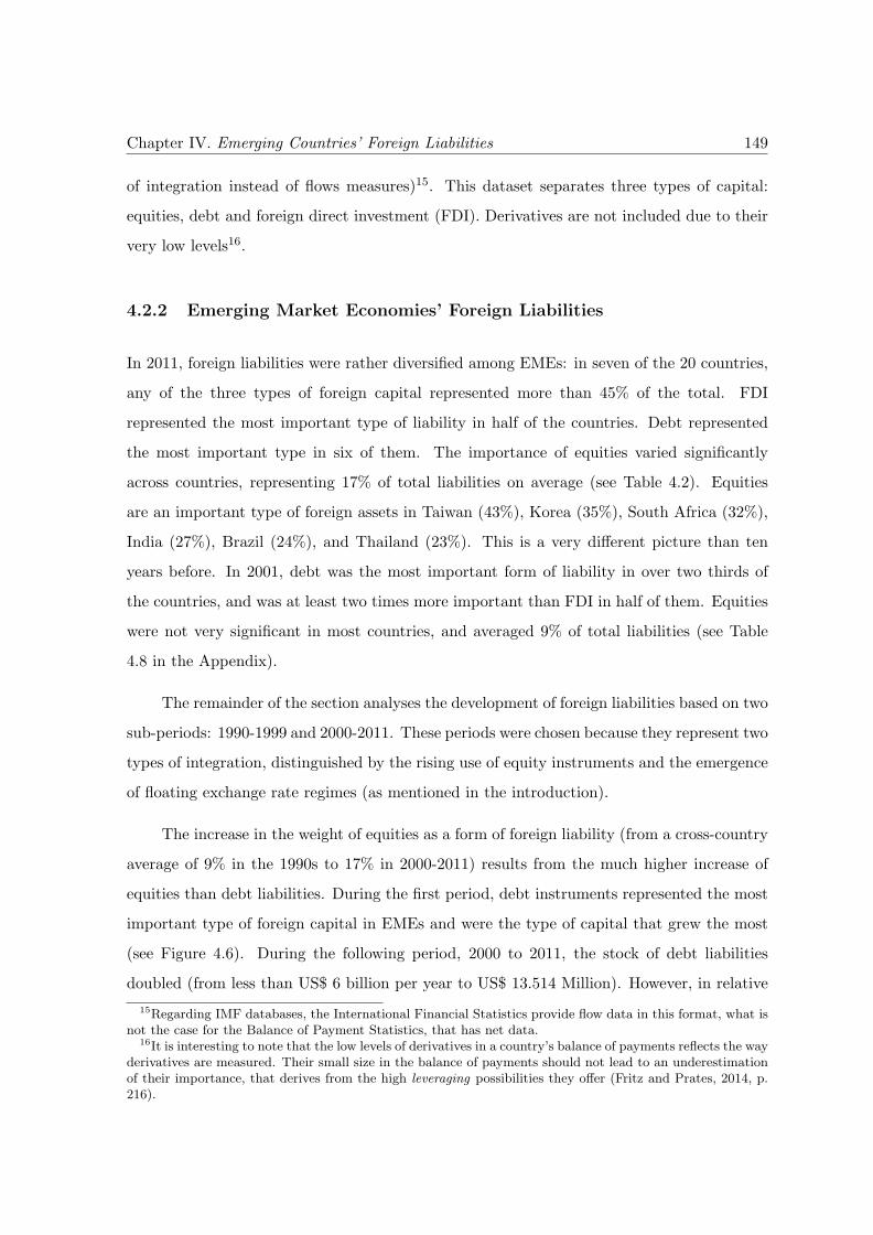
Chapter IV. Emerging Countries’ Foreign Liabilities 149
of integration instead of flows measures)15. This dataset separates three types of capital:
equities, debt and foreign direct investment (FDI). Derivatives are not included due to their
very low levels16.
4.2.2 Emerging Market Economies’ Foreign Liabilities
In 2011, foreign liabilities were rather diversified among EMEs: in seven of the 20 countries,
any of the three types of foreign capital represented more than 45% of the total. FDI
represented the most important type of liability in half of the countries. Debt represented
the most important type in six of them. The importance of equities varied significantly
across countries, representing 17% of total liabilities on average (see Table 4.2). Equities
are an important type of foreign assets in Taiwan (43%), Korea (35%), South Africa (32%),
India (27%), Brazil (24%), and Thailand (23%). This is a very different picture than ten
years before. In 2001, debt was the most important form of liability in over two thirds of
the countries, and was at least two times more important than FDI in half of them. Equities
were not very significant in most countries, and averaged 9% of total liabilities (see Table
4.8 in the Appendix).
The remainder of the section analyses the development of foreign liabilities based on two
sub-periods: 1990-1999 and 2000-2011. These periods were chosen because they represent two
types of integration, distinguished by the rising use of equity instruments and the emergence
of floating exchange rate regimes (as mentioned in the introduction).
The increase in the weight of equities as a form of foreign liability (from a cross-country
average of 9% in the 1990s to 17% in 2000-2011) results from the much higher increase of
equities than debt liabilities. During the first period, debt instruments represented the most
important type of foreign capital in EMEs and were the type of capital that grew the most
(see Figure 4.6). During the following period, 2000 to 2011, the stock of debt liabilities
doubled (from less than US$ 6 billion per year to US$ 13.514 Million). However, in relative
15Regarding IMF databases, the International Financial Statistics provide flow data in this format, what isnot the case for the Balance of Payment Statistics, that has net data.
16It is interesting to note that the low levels of derivatives in a country’s balance of payments reflects the wayderivatives are measured. Their small size in the balance of payments should not lead to an underestimationof their importance, that derives from the high leveraging possibilities they offer (Fritz and Prates, 2014, p.216).
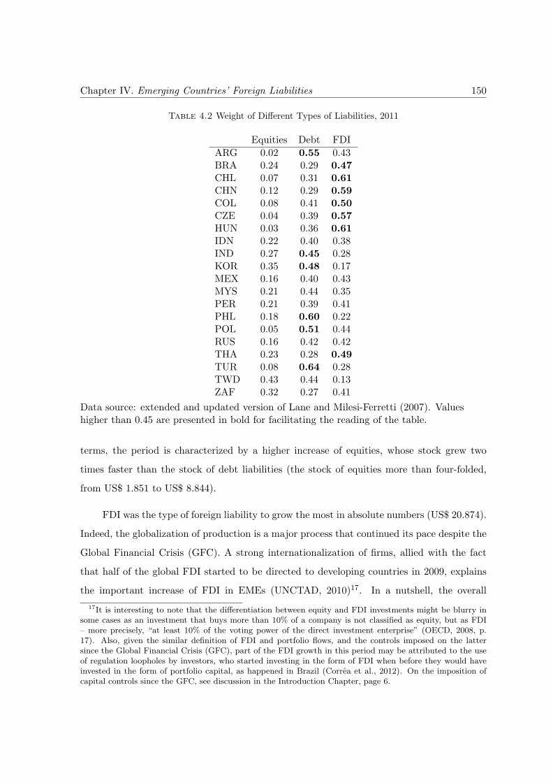
Chapter IV. Emerging Countries’ Foreign Liabilities 150
Table 4.2 Weight of Different Types of Liabilities, 2011
Equities Debt FDI
ARG 0.02 0.55 0.43BRA 0.24 0.29 0.47CHL 0.07 0.31 0.61CHN 0.12 0.29 0.59COL 0.08 0.41 0.50CZE 0.04 0.39 0.57HUN 0.03 0.36 0.61IDN 0.22 0.40 0.38IND 0.27 0.45 0.28KOR 0.35 0.48 0.17MEX 0.16 0.40 0.43MYS 0.21 0.44 0.35PER 0.21 0.39 0.41PHL 0.18 0.60 0.22POL 0.05 0.51 0.44RUS 0.16 0.42 0.42THA 0.23 0.28 0.49TUR 0.08 0.64 0.28TWD 0.43 0.44 0.13ZAF 0.32 0.27 0.41
Data source: extended and updated version of Lane and Milesi-Ferretti (2007). Valueshigher than 0.45 are presented in bold for facilitating the reading of the table.
terms, the period is characterized by a higher increase of equities, whose stock grew two
times faster than the stock of debt liabilities (the stock of equities more than four-folded,
from US$ 1.851 to US$ 8.844).
FDI was the type of foreign liability to grow the most in absolute numbers (US$ 20.874).
Indeed, the globalization of production is a major process that continued its pace despite the
Global Financial Crisis (GFC). A strong internationalization of firms, allied with the fact
that half of the global FDI started to be directed to developing countries in 2009, explains
the important increase of FDI in EMEs (UNCTAD, 2010)17. In a nutshell, the overall
17It is interesting to note that the differentiation between equity and FDI investments might be blurry insome cases as an investment that buys more than 10% of a company is not classified as equity, but as FDI– more precisely, “at least 10% of the voting power of the direct investment enterprise” (OECD, 2008, p.17). Also, given the similar definition of FDI and portfolio flows, and the controls imposed on the lattersince the Global Financial Crisis (GFC), part of the FDI growth in this period may be attributed to the useof regulation loopholes by investors, who started investing in the form of FDI when before they would haveinvested in the form of portfolio capital, as happened in Brazil (Correa et al., 2012). On the imposition ofcapital controls since the GFC, see discussion in the Introduction Chapter, page 6.
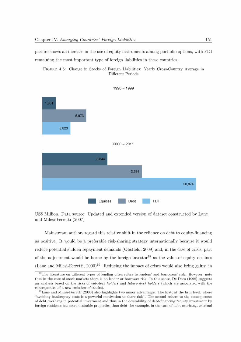
Chapter IV. Emerging Countries’ Foreign Liabilities 151
picture shows an increase in the use of equity instruments among portfolio options, with FDI
remaining the most important type of foreign liabilities in these countries.
Figure 4.6: Change in Stocks of Foreign Liabilities: Yearly Cross-Country Average inDifferent Periods
3,823
5,973
1,851
1990 − 1999
20,874
13,514
8,844
2000 − 2011
Equities Debt FDI
US$ Million. Data source: Updated and extended version of dataset constructed by Laneand Milesi-Ferretti (2007)
Mainstream authors regard this relative shift in the reliance on debt to equity-financing
as positive. It would be a preferable risk-sharing strategy internationally because it would
reduce potential sudden repayment demands (Obstfeld, 2009) and, in the case of crisis, part
of the adjustment would be borne by the foreign investor18 as the value of equity declines
(Lane and Milesi-Ferretti, 2000)19. Reducing the impact of crises would also bring gains: in
18The literature on different types of lending often refers to lenders’ and borrowers’ risk. However, notethat in the case of stock markets there is no lender or borrower risk. In this sense, De Deos (1998) suggestsan analysis based on the risks of old-stock holders and future-stock holders (which are associated with theconsequences of a new emission of stocks).
19Lane and Milesi-Ferretti (2000) also highlights two minor advantages. The first, at the firm level, where“avoiding bankruptcy costs is a powerful motivation to share risk”. The second relates to the consequencesof debt overhang in potential investment and thus in the desirability of debt-financing:“equity investment byforeign residents has more desirable properties than debt for example, in the case of debt overhang, external
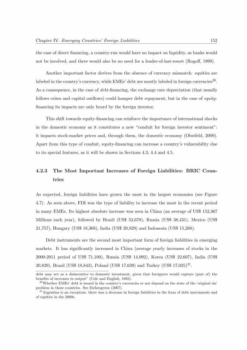
Chapter IV. Emerging Countries’ Foreign Liabilities 152
the case of direct financing, a country-run would have no impact on liquidity, as banks would
not be involved, and there would also be no need for a lender-of-last-resort (Rogoff, 1999).
Another important factor derives from the absence of currency mismatch: equities are
labeled in the country’s currency, while EMEs’ debt are mostly labeled in foreign currencies20.
As a consequence, in the case of debt-financing, the exchange rate depreciation (that usually
follows crises and capital outflows) could hamper debt repayment, but in the case of equity-
financing its impacts are only beard by the foreign investor.
This shift towards equity-financing can reinforce the importance of international shocks
in the domestic economy as it constitutes a new “conduit for foreign investor sentiment”:
it impacts stock-market prices and, through them, the domestic economy (Obstfeld, 2009).
Apart from this type of conduit, equity-financing can increase a country’s vulnerability due
to its special features, as it will be shown in Sections 4.3, 4.4 and 4.5.
4.2.3 The Most Important Increases of Foreign Liabilities: BRIC Coun-
tries
As expected, foreign liabilities have grown the most in the largest economies (see Figure
4.7). As seen above, FDI was the type of liability to increase the most in the recent period
in many EMEs. Its highest absolute increase was seen in China (an average of US$ 152,367
Millions each year), followed by Brazil (US$ 52,678), Russia (US$ 38,431), Mexico (US$
21,757), Hungary (US$ 18,368), India (US$ 20,829) and Indonesia (US$ 15,268).
Debt instruments are the second most important form of foreign liabilities in emerging
markets. It has significantly increased in China (average yearly increases of stocks in the
2000-2011 period of US$ 71,100), Russia (US$ 14,992), Korea (US$ 22,607), India (US$
20,829), Brazil (US$ 18,843), Poland (US$ 17,639) and Turkey (US$ 17,025)21.
debt may act as a disincentive to domestic investment, given that foreigners would capture (part of) thebenefits of increases in output” (Cole and English, 1992).
20Whether EMEs’ debt is issued in the country’s currencies or not depend on the state of the ‘original sin’problem in these countries. See Eichengreen (2007).
21Argentina is an exception: there was a decrease in foreign liabilities in the form of debt instruments andof equities in the 2000s.
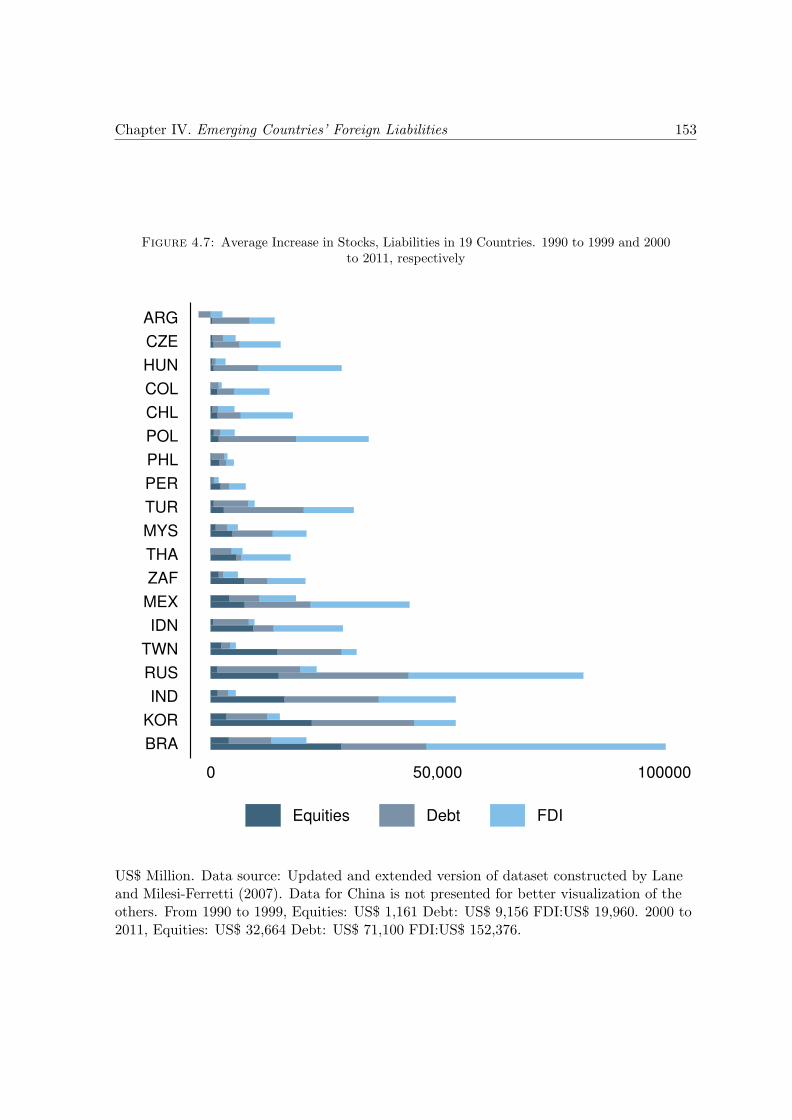
Chapter IV. Emerging Countries’ Foreign Liabilities 153
Figure 4.7: Average Increase in Stocks, Liabilities in 19 Countries. 1990 to 1999 and 2000to 2011, respectively
0 50,000 100000
BRA
KOR
IND
RUS
TWN
IDN
MEX
ZAF
THA
MYS
TUR
PER
PHL
POL
CHL
COL
HUN
CZE
ARG
Equities Debt FDI
US$ Million. Data source: Updated and extended version of dataset constructed by Laneand Milesi-Ferretti (2007). Data for China is not presented for better visualization of theothers. From 1990 to 1999, Equities: US$ 1,161 Debt: US$ 9,156 FDI:US$ 19,960. 2000 to2011, Equities: US$ 32,664 Debt: US$ 71,100 FDI:US$ 152,376.
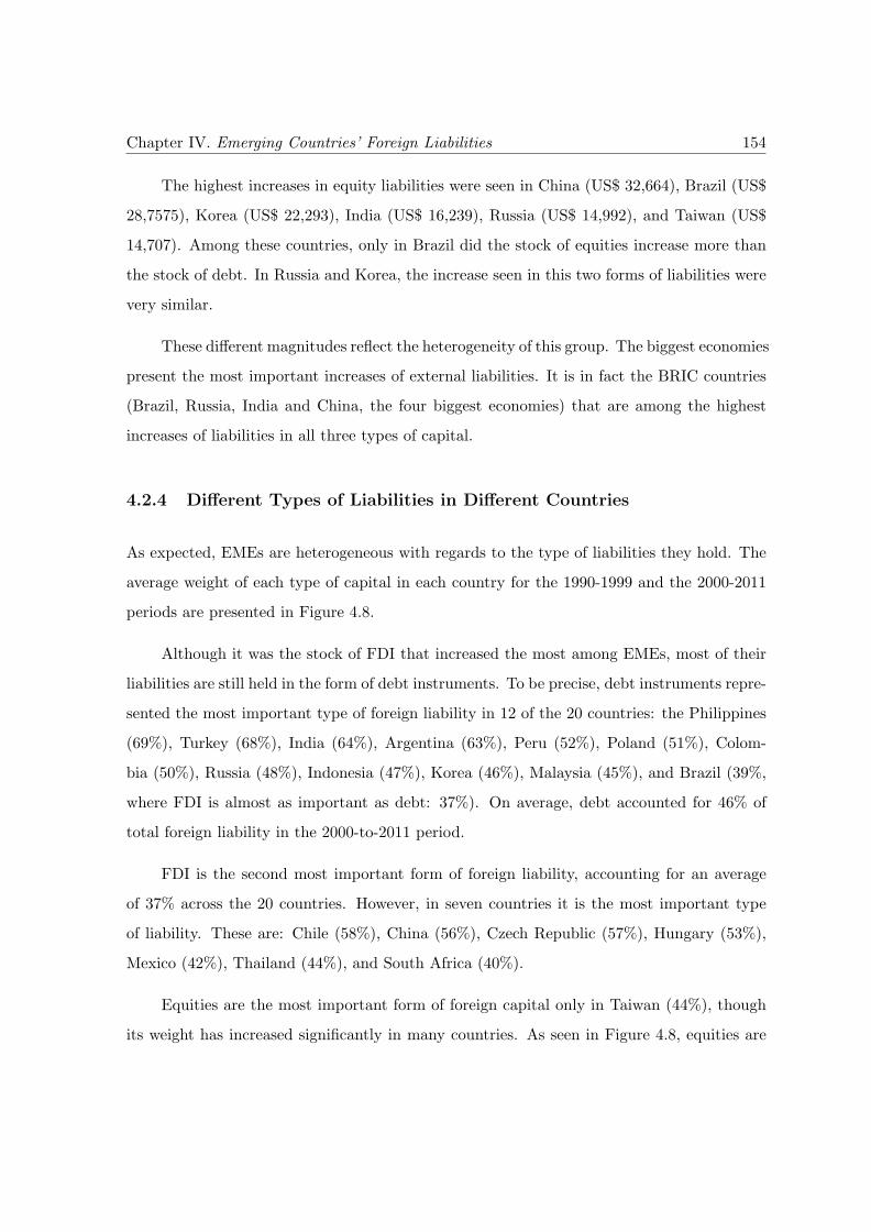
Chapter IV. Emerging Countries’ Foreign Liabilities 154
The highest increases in equity liabilities were seen in China (US$ 32,664), Brazil (US$
28,7575), Korea (US$ 22,293), India (US$ 16,239), Russia (US$ 14,992), and Taiwan (US$
14,707). Among these countries, only in Brazil did the stock of equities increase more than
the stock of debt. In Russia and Korea, the increase seen in this two forms of liabilities were
very similar.
These different magnitudes reflect the heterogeneity of this group. The biggest economies
present the most important increases of external liabilities. It is in fact the BRIC countries
(Brazil, Russia, India and China, the four biggest economies) that are among the highest
increases of liabilities in all three types of capital.
4.2.4 Different Types of Liabilities in Different Countries
As expected, EMEs are heterogeneous with regards to the type of liabilities they hold. The
average weight of each type of capital in each country for the 1990-1999 and the 2000-2011
periods are presented in Figure 4.8.
Although it was the stock of FDI that increased the most among EMEs, most of their
liabilities are still held in the form of debt instruments. To be precise, debt instruments repre-
sented the most important type of foreign liability in 12 of the 20 countries: the Philippines
(69%), Turkey (68%), India (64%), Argentina (63%), Peru (52%), Poland (51%), Colom-
bia (50%), Russia (48%), Indonesia (47%), Korea (46%), Malaysia (45%), and Brazil (39%,
where FDI is almost as important as debt: 37%). On average, debt accounted for 46% of
total foreign liability in the 2000-to-2011 period.
FDI is the second most important form of foreign liability, accounting for an average
of 37% across the 20 countries. However, in seven countries it is the most important type
of liability. These are: Chile (58%), China (56%), Czech Republic (57%), Hungary (53%),
Mexico (42%), Thailand (44%), and South Africa (40%).
Equities are the most important form of foreign capital only in Taiwan (44%), though
its weight has increased significantly in many countries. As seen in Figure 4.8, equities are
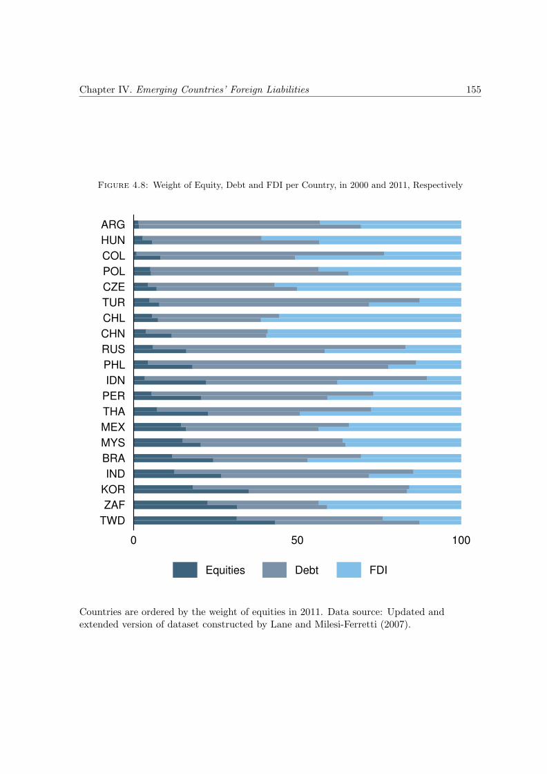
Chapter IV. Emerging Countries’ Foreign Liabilities 155
Figure 4.8: Weight of Equity, Debt and FDI per Country, in 2000 and 2011, Respectively
0 50 100
TWD
ZAF
KOR
IND
BRA
MYS
MEX
THA
PER
IDN
PHL
RUS
CHN
CHL
TUR
CZE
POL
COL
HUN
ARG
Equities Debt FDI
Countries are ordered by the weight of equities in 2011. Data source: Updated andextended version of dataset constructed by Lane and Milesi-Ferretti (2007).
Chapter IV. Emerging Countries’ Foreign Liabilities 156
specially important in Korea (where it account for 35% of total liabilities), South Africa
(33%), India (32%), Brazil (23%), and Malaysia (20%)22.
In the following section the volatility of the three types of liabilities will be analyzed,
indicating the fragility of the different types of integration among EMEs.
4.3 The Volatility of the Different Types of Liabilities
As seen above, there was an important change in the type of foreign liabilities across EMEs,
with equities growing in importance among portfolio inflows. In order to study the potential
implications of this shift, and of the type of integration of different countries, this subsection
looks at the volatility of the different types of capital: FDI, debt and equities. Although
technically FDI and equities do not differ greatly (see Footnote 17), portfolio flows are broadly
seen as most volatile, and FDI as most stable. This difference should however not be taken
for granted: Claessens et al. (1995) and Kregel (1996) have long argued that foreign direct
investment can be as volatile as the other types of flows. But others, as Chuhan et al.
(1996), Sarno and Taylor (1999), and Moguillansky (2002, p. 57) have reached the opposite
conclusion23. An interesting point raised by Sula and Willett (2009) is that volatility during
inflow periods might not be a good predictor of the size of reversals during crises. From this
perspective, the authors analyze the reversibility of the different types of flow and conclude
that FDI is the least reversible and portfolio and loans are equally reversible.
The stock of foreign liabilities increased substantially in EMEs since the year 2003 – as
Section 4.4 will show. The analysis starts in this point for this reason and to avoid including
periods of extreme volatility in some countries due to the late-1990s and early-2000s crises.
The yearly change of stocks of the three types of foreign liabilities is seen in Table 4.9 in the
Appendix. These values show that the series of equities seem to be the most volatile: there
are significant changes in values and alternates periods of increase and periods of decrease
of stocks. Table 4.10 (in the Appendix) provides the year-by-year cross-country average.
22The countries where equities grew considerably are very similar: India (25 p.p.), Taiwan (25 p.p.), Korea(24 p.p), Russia (15 p.p.), Brazil (15 p.p), South Africa (14 p.p.), Indonesia (12 p.p.), Peru (11 p.p.), andChina (10 p.p).
23There might also be specific factors related to the origins of the crisis. In the Asian crisis, for instance,bank loans were said to be the most important type of outflow (Willett et al., 2001).
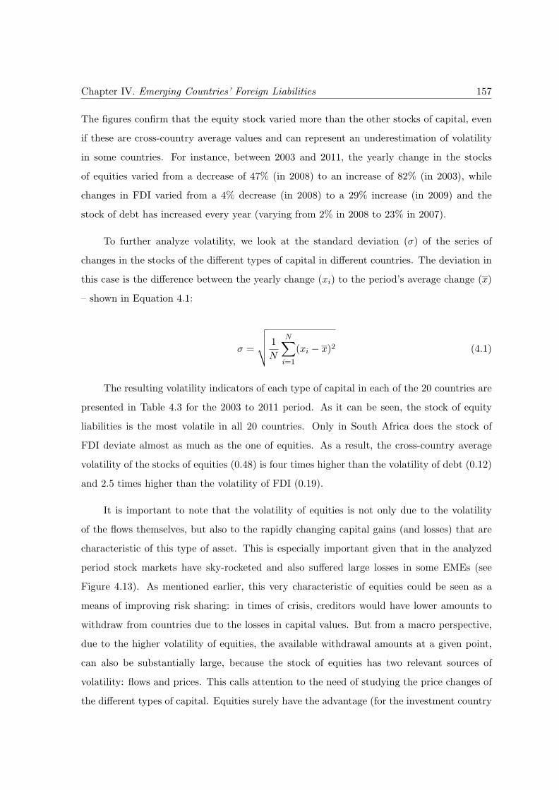
Chapter IV. Emerging Countries’ Foreign Liabilities 157
The figures confirm that the equity stock varied more than the other stocks of capital, even
if these are cross-country average values and can represent an underestimation of volatility
in some countries. For instance, between 2003 and 2011, the yearly change in the stocks
of equities varied from a decrease of 47% (in 2008) to an increase of 82% (in 2003), while
changes in FDI varied from a 4% decrease (in 2008) to a 29% increase (in 2009) and the
stock of debt has increased every year (varying from 2% in 2008 to 23% in 2007).
To further analyze volatility, we look at the standard deviation (σ) of the series of
changes in the stocks of the different types of capital in different countries. The deviation in
this case is the difference between the yearly change (xi) to the period’s average change (x)
– shown in Equation 4.1:
σ =
√
√
√
√
1
N
N∑
i=1
(xi − x)2 (4.1)
The resulting volatility indicators of each type of capital in each of the 20 countries are
presented in Table 4.3 for the 2003 to 2011 period. As it can be seen, the stock of equity
liabilities is the most volatile in all 20 countries. Only in South Africa does the stock of
FDI deviate almost as much as the one of equities. As a result, the cross-country average
volatility of the stocks of equities (0.48) is four times higher than the volatility of debt (0.12)
and 2.5 times higher than the volatility of FDI (0.19).
It is important to note that the volatility of equities is not only due to the volatility
of the flows themselves, but also to the rapidly changing capital gains (and losses) that are
characteristic of this type of asset. This is especially important given that in the analyzed
period stock markets have sky-rocketed and also suffered large losses in some EMEs (see
Figure 4.13). As mentioned earlier, this very characteristic of equities could be seen as a
means of improving risk sharing: in times of crisis, creditors would have lower amounts to
withdraw from countries due to the losses in capital values. But from a macro perspective,
due to the higher volatility of equities, the available withdrawal amounts at a given point,
can also be substantially large, because the stock of equities has two relevant sources of
volatility: flows and prices. This calls attention to the need of studying the price changes of
the different types of capital. Equities surely have the advantage (for the investment country
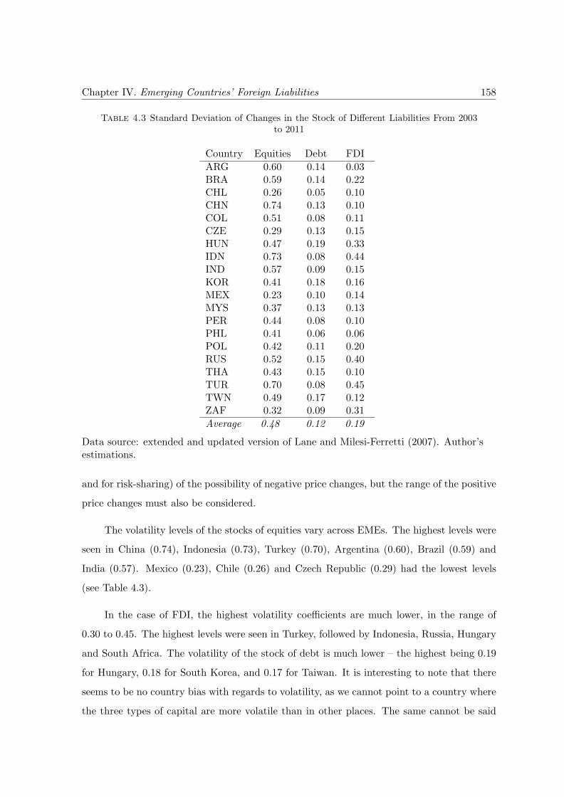
Chapter IV. Emerging Countries’ Foreign Liabilities 158
Table 4.3 Standard Deviation of Changes in the Stock of Different Liabilities From 2003to 2011
Country Equities Debt FDI
ARG 0.60 0.14 0.03BRA 0.59 0.14 0.22CHL 0.26 0.05 0.10CHN 0.74 0.13 0.10COL 0.51 0.08 0.11CZE 0.29 0.13 0.15HUN 0.47 0.19 0.33IDN 0.73 0.08 0.44IND 0.57 0.09 0.15KOR 0.41 0.18 0.16MEX 0.23 0.10 0.14MYS 0.37 0.13 0.13PER 0.44 0.08 0.10PHL 0.41 0.06 0.06POL 0.42 0.11 0.20RUS 0.52 0.15 0.40THA 0.43 0.15 0.10TUR 0.70 0.08 0.45TWN 0.49 0.17 0.12ZAF 0.32 0.09 0.31
Average 0.48 0.12 0.19
Data source: extended and updated version of Lane and Milesi-Ferretti (2007). Author’sestimations.
and for risk-sharing) of the possibility of negative price changes, but the range of the positive
price changes must also be considered.
The volatility levels of the stocks of equities vary across EMEs. The highest levels were
seen in China (0.74), Indonesia (0.73), Turkey (0.70), Argentina (0.60), Brazil (0.59) and
India (0.57). Mexico (0.23), Chile (0.26) and Czech Republic (0.29) had the lowest levels
(see Table 4.3).
In the case of FDI, the highest volatility coefficients are much lower, in the range of
0.30 to 0.45. The highest levels were seen in Turkey, followed by Indonesia, Russia, Hungary
and South Africa. The volatility of the stock of debt is much lower – the highest being 0.19
for Hungary, 0.18 for South Korea, and 0.17 for Taiwan. It is interesting to note that there
seems to be no country bias with regards to volatility, as we cannot point to a country where
the three types of capital are more volatile than in other places. The same cannot be said
Chapter IV. Emerging Countries’ Foreign Liabilities 159
about types of capital, as the lowest volatility of the stock of equities, for instance, is higher
than the highest volatility of the stock of debt.
The volatility of the stock of foreign liabilities in the form of equities was also the highest
among the three types of capital when analyzing a longer period, from 1970 to 2011 and in
every one of the three sub-periods (1970-1989, 1990-1999 and 2000-2011). From 1970 to
1989, the volatility of equities was four times higher than that of debt and FDI; from 1980
to 1990 this ratio increased to 43 times in relation to FDI and 180 times in relation to debt;
it was in the most recent period (from 2000 to 2011) that the volatility of equities was the
closest to that of FDI (two times higher) and debt (less than four times higher). The higher
volatility level of equities in earlier periods might be a consequence of the very low values of
the stocks of equities, making any “small” absolute change be an important deviation.
4.3.1 On the Measure of Volatility of a Time-Series
Although equities clearly presented higher volatility than the other types of foreign liabilities,
estimating it through the standard deviation results in an underestimation of volatility levels.
The standard deviation cannot differentiate the volatility of a series that is only growing
at x% from another that alternates increases and decreases of x%, as is the case of a series of
equities, because it is based on absolute values, where the impact of a positive or a negative
change is the same.
An option to this underestimation problem could be to look at the standard deviation
of the stocks themselves, instead of their changes. However, such measure would also under-
estimate the variance of the equity series that for alternating increases and decreases of the
stock have values that are closer to each other than the values of debt that for having only
increased have larger ranges. In other words, the series of equities has values which are closer
to their averages than the series of debt, resulting in deviations from the average which are
less significant.
Another alternative could be to look at the coefficient of variation (cv) of the series of
changes in stocks, therefore considering the standard deviation (σ) relative to the mean (x)
of the series – as in Equation 4.2:
Chapter IV. Emerging Countries’ Foreign Liabilities 160
cv =σ
x(4.2)
This option was also rejected. Given that the original values (xi), and thus their average
(x), represent changes and variability, the higher the average change in stocks (x), the lower
the (cv), which is the opposite of what one understands of volatility: that its estimator must
increase with an increase of the deviation (x).
4.4 The Evolution of the Stock of Foreign Liabilities
Continuing the analysis of the vulnerabilities associated with each type of capital, this section
discusses the path followed by the three types of foreign capital since the 2000s. Figures 4.9,
4.10, and 4.11, show the evolution of the stock of foreign capital of equities, FDI, and debt,
respectively.
4.4.1 Equities’ Special Pattern
The recent evolution of the stock of equities present a very similar pattern, forming a N-
or M-line across several countries (See Figure 4.9). This striking similarity is unique to the
stock of equities, not occurring in the cases of FDI nor debt – with the interesting exceptions
of FDI in the cases of Russia and Turkey.
The increase in the stock of equities from the mid-2000s was impressive in most coun-
tries24. In the first years of the 2000s (the aftermath the late-1990s crises that affected many
EMEs), the stocks of foreign equity liability still decreased in most countries. From 2003
onward the situation reversed. This was the expansionary stage of the new cycle of capital
24A notable exception is Argentina, where the stock of equities was already at very high levels in the 1990s.To a smaller extend Malaysia, Mexico and Thailand also present different cases. Moreover, it must be notedthat in percentage terms the average increase was higher in the early 1990s due to the very small values beforethis decade.
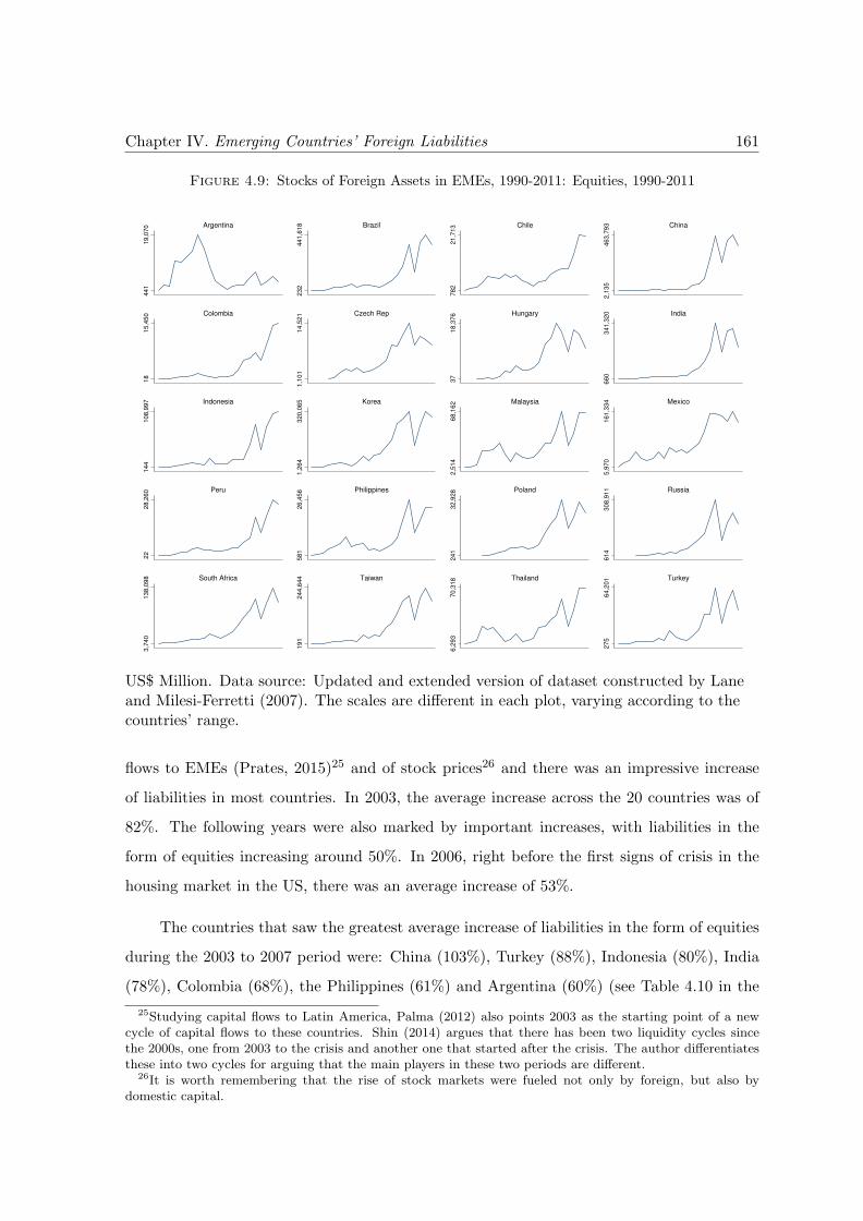
Chapter IV. Emerging Countries’ Foreign Liabilities 161
Figure 4.9: Stocks of Foreign Assets in EMEs, 1990-2011: Equities, 1990-2011
44
11
9,0
70 Argentina
23
24
41
,61
8 Brazil
78
22
1,7
13 Chile
2,1
35
46
3,7
93 China
18
15
,45
0 Colombia
1,1
01
14
,52
1 Czech Rep
37
18
,37
6 Hungary
66
03
41
,32
0 India
14
41
08
,99
7 Indonesia
1,2
64
32
0,0
65 Korea
2,5
14
68
,16
2 Malaysia
5,9
70
16
1,3
34 Mexico
22
28
,26
0 Peru
58
12
6,4
56 Philippines
24
13
2,9
28 Poland
61
43
08
,91
1 Russia
3,7
40
13
8,0
98 South Africa
19
12
44
,64
4 Taiwan
6,2
93
70
,31
8 Thailand
27
56
4,2
01 Turkey
US$ Million. Data source: Updated and extended version of dataset constructed by Laneand Milesi-Ferretti (2007). The scales are different in each plot, varying according to thecountries’ range.
flows to EMEs (Prates, 2015)25 and of stock prices26 and there was an impressive increase
of liabilities in most countries. In 2003, the average increase across the 20 countries was of
82%. The following years were also marked by important increases, with liabilities in the
form of equities increasing around 50%. In 2006, right before the first signs of crisis in the
housing market in the US, there was an average increase of 53%.
The countries that saw the greatest average increase of liabilities in the form of equities
during the 2003 to 2007 period were: China (103%), Turkey (88%), Indonesia (80%), India
(78%), Colombia (68%), the Philippines (61%) and Argentina (60%) (see Table 4.10 in the
25Studying capital flows to Latin America, Palma (2012) also points 2003 as the starting point of a newcycle of capital flows to these countries. Shin (2014) argues that there has been two liquidity cycles sincethe 2000s, one from 2003 to the crisis and another one that started after the crisis. The author differentiatesthese into two cycles for arguing that the main players in these two periods are different.
26It is worth remembering that the rise of stock markets were fueled not only by foreign, but also bydomestic capital.
Chapter IV. Emerging Countries’ Foreign Liabilities 162
Appendix). Specifically looking at the period just before the crisis (2006 and 2007), the stock
of equities achieved an increase of 132% in Indonesia, 119% in China, 79% in India, 77% in
the Philippines 73% in Peru, 71% in Brazil, 67% in Argentina, and 62% Russia. Among the
European EMEs, Czech Republic, Hungary, and Poland (and to a smaller extent Turkey)
the growth rate from these years was not impressive. In fact, in these countries the stock of
equities had already been substantially increasing since the mid-2000s, in the wake of their
integration to the European Union. It is interesting to note that in the countries where the
stocks of equities grew the most in pre-crisis periods presented the most volatile stock of
equity liabilities.
Following the collapse of the Lehman Brothers and the repatriation of capital to ad-
vanced economies with the consequent fall of stock prices in EMEs, the stock of equity
liabilities decreased considerably in 2008 – an average of 47% across the 20 countries. The
most impacted were Russia (73%), Turkey (64%), Argentina (63%), Korea (61%), Brazil
(59%), Malaysia (59%), Indonesia (57%), Thailand (55%), India (51%) and Taiwan (50%).
The falls are represented by the first inflection point of the N- or M-like lines in the plots of
Figure 4.9.
In 2009, the great recession in advanced countries and the relatively quick recovery of
EMEs (characterizing the situation known as ‘double-speed recovery’) resulted in inflows of
capital to these countries and the stocks of equities increased significantly, reaching a cross-
country average of 72%. With this increase, by the end of 2009, the stock of equities achieved
end-2007 levels – indicated by the third inflection point of the N- or M-like lines in the plots.
More precisely, 2009 level in some countries was even higher than in 2007. These are: Brazil,
Indonesia, Peru, South Africa, Taiwan and Thailand.
The years of 2010 and 2011 were characterized by uncertainties related to the Euro
crisis. In 2010 the stock of equities still presented an increase (of 31%, on average), but
in 2011 it decreased (16%). The post-crisis increases were the greatest in Brazil (85%),
Indonesia (79%), Russia (71%), Colombia (68%), Turkey (67%), Thailand (65%), and Korea
(62%). As expected, the group of countries that faced the highest decreases in liabilities is
very similar to the one that faced the highest increases some years before, given that the
countries where liabilities increased the most are the ones with the highest potential for
Chapter IV. Emerging Countries’ Foreign Liabilities 163
a decrease. This is important to be highlighted because it it indicates the importance of
external (push) factors because in determining capital flows and thus foreign liabilities (a
subject that will be discussed in Chapter Six).
The fact that the stock of equity liabilities followed a specific N- or M-pattern calls
attention to two important aspects. First, the similarity across several countries sheds light
on the importance of push factors in their determination. They could only reflect pull factors
if all these countries’ domestic conditions were similar and had evolved in the same manner,
but, as shown by Kaltenbrunner and Painceira (2014), who study six of these EMEs, their
fundamentals were markedly different at this moment.
Secondly, this pattern is similar to the evolution of uncertainty in international financial
markets, as proxied by the VIX index – presented in Figure 6.12 (in Chapter Six)27. As shown
from its path and from the academic discussion presented in Chapter Six, the VIX suggests
that the 2000s were marked by low level of uncertainty from the dot-com bubble to the GFC,
when it hit a historical peak. The period after the GFC was marked by much smaller but
frequent peaks of uncertainty (related to crisis in Europe). This similarity of the inflection
points of the two series indicates a close association between the stock of equity liabilities in
EMEs and the international financial markets28.
Moreover, the fact that it is only the stock of equities and not the stocks of debt or
FDI that presents a similar pattern across EMEs is in line with the aforementioned “double
volatility” characteristic of the equities’ liabilities. The “double volatility” could explain why
the stock of equities is more sensitive to international financial markets, as exposed in this
section: international shocks affect not only its flows, but also its prices.
27By measuring the expected volatility implied in different S&P 500 index options, the VIX is a broadlyused indicator of uncertainty and stress in financial markets in general. Values lower than 20 are commonlyconsidered as less stressful periods and values higher than 30 are associated with crisis. This index is furtherdiscussed in Chapter Six.
28Unfortunately an econometric measure of the relationship between the VIX and the countries’ equityliabilities is hindered. The data on liabilities is published yearly while the VIX’s daily, and an yearly averageof the VIX would lose much of its information. For instance, the average of the VIX 2008 values is probablynot representative of the uncertainty of that year given that the hike of the VIX was (as they always are)very short-lived.
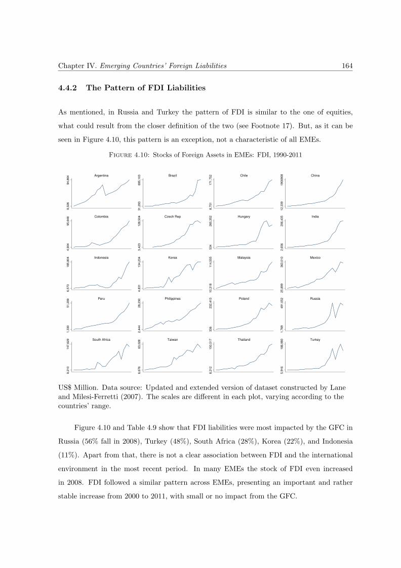
Chapter IV. Emerging Countries’ Foreign Liabilities 164
4.4.2 The Pattern of FDI Liabilities
As mentioned, in Russia and Turkey the pattern of FDI is similar to the one of equities,
what could result from the closer definition of the two (see Footnote 17). But, as it can be
seen in Figure 4.10, this pattern is an exception, not a characteristic of all EMEs.
Figure 4.10: Stocks of Foreign Assets in EMEs: FDI, 1990-2011
9,3
26
94
,86
4 Argentina
31
,29
36
95
,10
3 Brazil
8,7
51
17
1,7
52 Chile
12
,33
91
90
69
08 China
4,9
04
95
,64
8 Colombia
3,4
23
12
8,5
04 Czech Rep
53
42
65
,35
2 Hungary
2,6
56
20
6,4
35 India
6,5
73
18
5,8
04 Indonesia
4,8
31
13
4,2
34 Korea
10
,31
81
14
,55
5 Malaysia
25
,89
93
63
,01
0 Mexico
1,3
30
51
,20
9 Peru
2,4
44
28
,23
0 Philippines
33
62
32
,41
3 Poland
1,7
69
49
1,0
52 Russia
9,2
10
14
7,6
29 South Africa
6,6
76
63
,02
8 Taiwan
8,2
12
15
0,5
17 Thailand
5,9
16
18
6,9
80 Turkey
US$ Million. Data source: Updated and extended version of dataset constructed by Laneand Milesi-Ferretti (2007). The scales are different in each plot, varying according to thecountries’ range.
Figure 4.10 and Table 4.9 show that FDI liabilities were most impacted by the GFC in
Russia (56% fall in 2008), Turkey (48%), South Africa (28%), Korea (22%), and Indonesia
(11%). Apart from that, there is not a clear association between FDI and the international
environment in the most recent period. In many EMEs the stock of FDI even increased
in 2008. FDI followed a similar pattern across EMEs, presenting an important and rather
stable increase from 2000 to 2011, with small or no impact from the GFC.
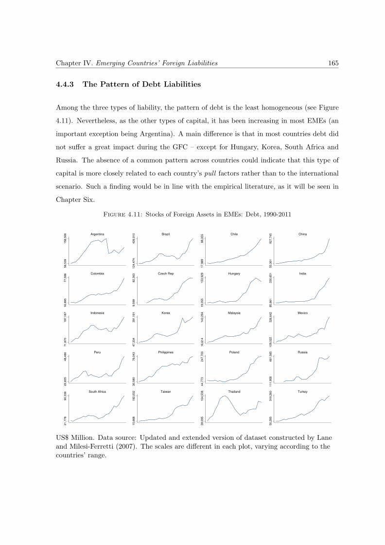
Chapter IV. Emerging Countries’ Foreign Liabilities 165
4.4.3 The Pattern of Debt Liabilities
Among the three types of liability, the pattern of debt is the least homogeneous (see Figure
4.11). Nevertheless, as the other types of capital, it has been increasing in most EMEs (an
important exception being Argentina). A main difference is that in most countries debt did
not suffer a great impact during the GFC – except for Hungary, Korea, South Africa and
Russia. The absence of a common pattern across countries could indicate that this type of
capital is more closely related to each country’s pull factors rather than to the international
scenario. Such a finding would be in line with the empirical literature, as it will be seen in
Chapter Six.
Figure 4.11: Stocks of Foreign Assets in EMEs: Debt, 1990-2011
58
,53
91
58
,50
6 Argentina
12
4,4
74
42
6,0
10 Brazil
17
,98
98
8,3
55 Chile
55
,30
19
27
,74
5 China
16
,89
57
7,5
86 Colombia
9,5
99
82
,36
3 Czech Rep
19
,05
51
53
,92
9 Hungary8
5,6
61
33
0,6
51 India
71
,87
01
97
,18
7 Indonesia
47
,33
43
91
,19
1 Korea
16
,61
41
43
,29
4 Malaysia
10
9,0
22
32
6,6
42 Mexico
22
,83
54
8,4
80 Peru
30
,58
07
6,0
43 Philippines
44
,77
32
47
,70
0 Poland
11
1,9
58
46
1,5
85 Russia
21
,77
89
0,3
39 South Africa
15
,66
81
92
,03
2 Taiwan
28
,09
51
04
,53
8 Thailand
50
,28
53
19
,26
0 Turkey
US$ Million. Data source: Updated and extended version of dataset constructed by Laneand Milesi-Ferretti (2007). The scales are different in each plot, varying according to thecountries’ range.
Chapter IV. Emerging Countries’ Foreign Liabilities 166
4.5 The Similarity of the Pattern of Liabilities: a Principal
Components Analysis
In order to further analyze whether the pattern of liabilities is becoming increasingly similar
across EMEs – as indicated by the graphical analyses for the case of equities – this section
looks at the comovement of stocks of different types of capital across EMEs in different
periods through a principal components analysis (PCA).
4.5.1 Theoretical Considerations
PCA is a mathematical technique that reduces the dimensions of a dataset into a series of
principal components – that, in turn, explain as much of the variance of the original series
as possible. As straightly put by Edison and Reinhart (2001), the number of components
resulting from the PCA indicates the extent of the variance of the original data series. In
their words:
The higher the degree of co-movement that exists among the original series, the
fewer the number of principal components that will be needed to explain a large
portion of the variance of the original series. In the case where the original series
were identical (perfectly collinear), the first principal component would explain
100 percent of the variation of the original series. Alternatively, if all the series
are orthogonal to one another, it would take as many principal components as
there are series to explain all of the variance in the original series. (p. 23)
The simplicity of the meaning of PCA has made it useful in a variety of cases. It is used
by Edison and Reinhart (2001) to assess comovement between stock exchanges and exchange
rates in EMEs. The authors conduct estimations of comovement for a control period and for
a period when capital controls are imposed, testing whether the comovement decreases with
the imposition of capital controls, and, therefore, its success. Comovement was also the focus
of Calvo and Reinhart (1996), who studied contagion of crisis between different countries,
with an increase in comovement being evidence of contagion.
Chapter IV. Emerging Countries’ Foreign Liabilities 167
Studying the impact of factors on productivity, Loko and Diouf (2009) used PCA to
understand how a few selected factors are related to others before adding them to an econo-
metric exercise. Another interesting application is the one of Chinn and Ito (2008), that used
PCA to build a financial openness indicator, composed from different data series, allowing
the use of one unique series instead of a set of series in their study.
Miotti and Plihon (2001) used factor analysis, a similar technique to PCA, to analyze
the different behavior of Argentinean banks before the late-1990s crisis. The analysis resulted
in axis that were related to a more or less speculative behavior (built from indicators that
were related or not to speculation) against which banks are located. The result is a typology
of banks according to their speculative behavior that is then compared to the list of banks
that default in 1998.
4.5.2 The Results
In this chapter, PCA is used to study whether the stock of foreign liabilities of a type of
capital has been recently following a similar pattern across EMEs – as argued from the
graphical analyses to the case of equities. The analysis is done based on the amount of
components whose Eigenvalues29 is greater than one30.
The results are presented in Table 4.4. They indicate a higher comovement of the
countries’ series of equities in the most recent period: while three components were needed
to explain 90% of the variance of the evolution of the stock in different countries for the
1990s period, for the 2000s, two components explained more than that percentage. Seen
from another angle, for the series of the 1990s, the first component could explain 52%, while
for the 2000s, the component explained 85%31.
The same exercise was done for the stock of external liabilities in the form of FDI
and debt instruments. They suggest that the pattern of the stocks of these two types of
29As neatly put by Kolenikov and Angeles (2004, p. 8) “the eigenvalues are the variances of the correspond-ing linear combinations. Then the linear combination that corresponds to the largest eigenvalue is the onethat has the greatest variance”, in other words, the one that explains the greatest variance from the originaldataset, or the one that explains the most of it
30This rule for choosing the amount of “relevant” components is known as the Kaiser rule.31A comparison with the 1970s and 1980s is not possible due to lack of data for several countries in this
period.
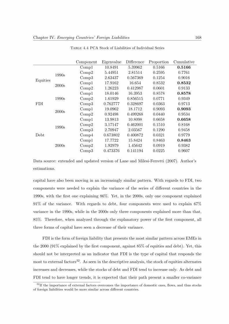
Chapter IV. Emerging Countries’ Foreign Liabilities 168
Table 4.4 PCA Stock of Liabilities of Individual Series
Component Eigenvalue Difference Proportion Cumulative
Equities1990s
Comp1 10.8491 5.39962 0.5166 0.5166Comp2 5.44951 2.81514 0.2595 0.7761Comp3 2.63437 0.567369 0.1254 0.9016
2000sComp1 17.9162 16.654 0.8532 0.8532Comp2 1.26223 0.412987 0.0601 0.9133
FDI1990s
Comp1 18.0146 16.3953 0.8578 0.8578Comp2 1.61929 0.856515 0.0771 0.9349Comp3 0.762777 0.328697 0.0363 0.9713
2000sComp1 19.0962 18.1712 0.9093 0.9093Comp2 0.92498 0.499268 0.0440 0.9534
Debt
1990s
Comp1 13.9813 10.8098 0.6658 0.6658Comp2 3.17147 0.462001 0.1510 0.8168Comp3 2.70947 2.03567 0.1290 0.9458Comp4 0.673802 0.400872 0.0321 0.9779
2000sComp1 17.7722 15.8424 0.8463 0.8463Comp2 1.92979 1.45642 0.0919 0.9382Comp3 0.473376 0.141194 0.0225 0.9607
Data source: extended and updated version of Lane and Milesi-Ferretti (2007). Author’s
estimations.
capital have also been moving in an increasingly similar pattern. With regards to FDI, two
components were needed to explain the variance of the series of different countries in the
1990s, with the first one explaining 86%. Yet, in the 2000s, only one component explained
91% of the variance. With regards to debt, four components were used to explain 67%
variance in the 1990s, while in the 2000s only three components explained more than that,
85%. Therefore, when analyzed through the explanatory power of the first component, all
three forms of capital have seen a decrease of their variance.
FDI is the form of foreign liability that presents the most similar pattern across EMEs in
the 2000 (91% explained by the first component, against 85% of equities and debt). Yet, this
should not be interpreted as an indicator that FDI is the type of capital that responds the
most to external factors32. As seen in the descriptive analysis, the stock of equities alternates
increases and decreases, while the stocks of debt and FDI tend to increase only. As debt and
FDI tend to have longer trends, it is expected that their path present a smaller co-variance
32If the importance of external factors overcomes the importance of domestic ones, flows, and thus stocksof foreign liabilities would be more similar across different countries.
Chapter IV. Emerging Countries’ Foreign Liabilities 169
across countries. The stock of equities saw the greatest increase in the explanatory power
of its first component from the 1990s to the 2000s, which could indicate evidence of the
increasing use of equities as an instrument of portfolio diversification. Moreover, the overall
result of increasing comovement of all three types of stocks of liabilities might be an evidence
of the higher importance of external (push) factors in their determination, along with these
countries’ higher integration to international financial markets.
In summary, the PCA analysis confirmed that the stock of equities is now more similar
across EMEs, but not that this similarity is higher than that other types of capital, which
might be due to its different characteristics.
4.6 Stock Prices and Exchange Rate Dynamics
This section further discusses the potential impacts of equity-financing by adding considera-
tions on the interactions between equity markets and exchange rates. It is expected that the
rise of equity-financing and the rise of foreign investors in EMEs’ domestic stock exchanges
lead to a growth of these markets, making such an interaction more important33. Indeed,
by comparing the stock of foreign liabilities held in the form of equities to EMEs’ stock
market capitalization, the importance of foreign investment in these markets is evident. The
highest average share in the 2003-2011 period was 45% in Hungary and 42% in Mexico. But
it also varied significantly, starting with Chile’s 6% – see Figure 4.12 for the average ratio
and Figure 4.17 in the Appendix for the behavior of the two series in the period.
Following the same approach used in the thesis, this section first presents the two
series before going into a more precise empirical analysis. Figure 4.13 presents EMEs’ stock
exchange indeces, plotted against the countries’ exchange rates (USD per local currency)
from 2000 to 2013.
Figure 4.13 indicates that the relationship between stock exchange and exchange rates
is not the same across EMEs. In some countries or in certain periods the two seem to move in
tandem, while in others, they go in opposite directions. The case of Brazil from 2003 to the
33In a similar exercise, Haldane (2011) compares gross portfolio equity flows to emerging markets and theMSCI index in 2010, which seem to be strongly correlated.
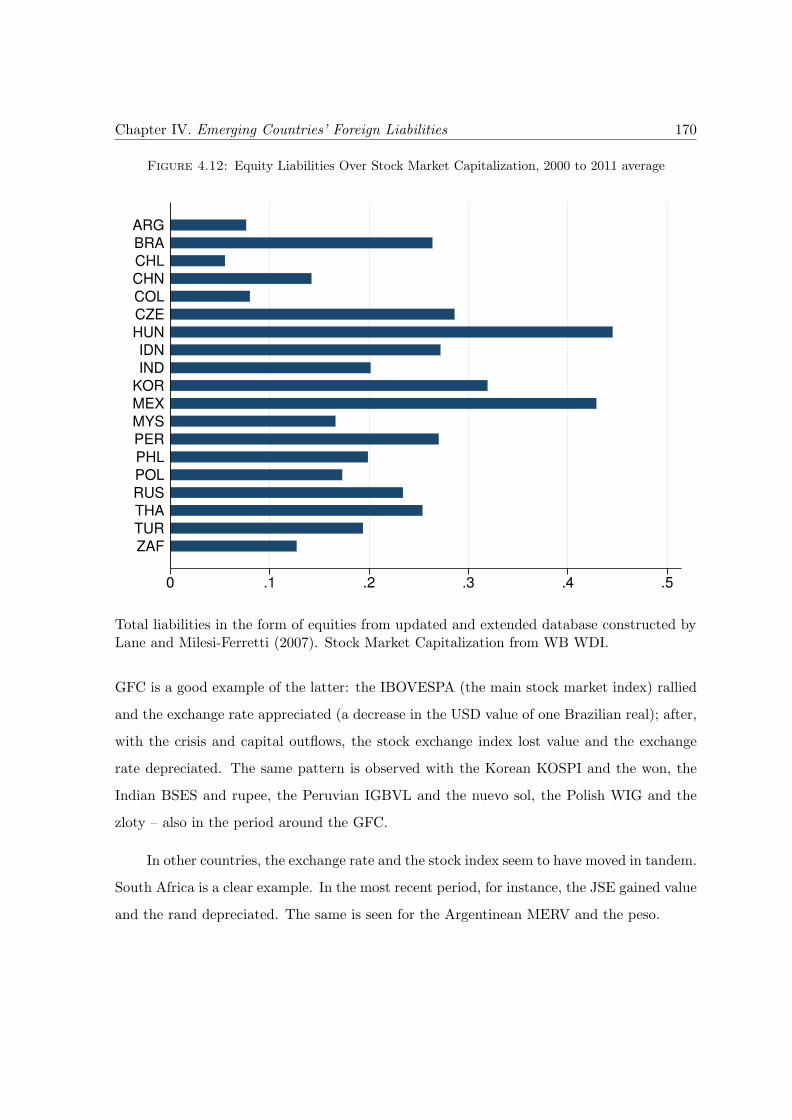
Chapter IV. Emerging Countries’ Foreign Liabilities 170
Figure 4.12: Equity Liabilities Over Stock Market Capitalization, 2000 to 2011 average
0 .1 .2 .3 .4 .5
ZAF
TUR
THA
RUS
POL
PHL
PER
MYS
MEX
KOR
IND
IDN
HUN
CZE
COL
CHN
CHL
BRA
ARG
Total liabilities in the form of equities from updated and extended database constructed byLane and Milesi-Ferretti (2007). Stock Market Capitalization from WB WDI.
GFC is a good example of the latter: the IBOVESPA (the main stock market index) rallied
and the exchange rate appreciated (a decrease in the USD value of one Brazilian real); after,
with the crisis and capital outflows, the stock exchange index lost value and the exchange
rate depreciated. The same pattern is observed with the Korean KOSPI and the won, the
Indian BSES and rupee, the Peruvian IGBVL and the nuevo sol, the Polish WIG and the
zloty – also in the period around the GFC.
In other countries, the exchange rate and the stock index seem to have moved in tandem.
South Africa is a clear example. In the most recent period, for instance, the JSE gained value
and the rand depreciated. The same is seen for the Argentinean MERV and the peso.
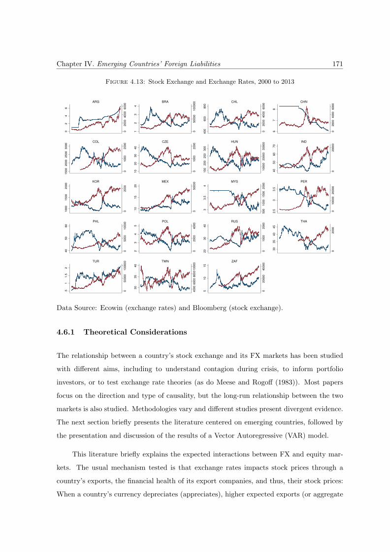
Chapter IV. Emerging Countries’ Foreign Liabilities 171
Figure 4.13: Stock Exchange and Exchange Rates, 2000 to 2013
02
00
04
00
06
00
0
02
46
ARG
05
00
00
10
00
00
12
34
BRA
02
00
04
00
06
00
0
40
06
00
80
0
CHL
02
00
04
00
06
00
0
67
8
CHN
01
00
02
00
0
15
00
20
00
25
00
30
00
COL
01
00
02
00
0
10
20
30
40
CZE
10
00
02
00
00
30
00
0
15
02
00
25
03
00
HUN
02
00
00
40
50
60
70
IND
02
00
0
10
00
15
00
20
00
KOR
05
00
00
10
15
20
MEX
50
01
00
01
50
02
00
0
33
.54
MYS
01
00
00
20
00
0
2.5
33
.5
PER
05
00
01
00
00
40
50
60
PHL
02
00
04
00
0
23
45
POL
01
00
02
00
0
20
30
40
RUS
02
00
0
30
35
40
45
THA
05
00
00
10
00
00
.51
1.5
2
TUR
40
00
60
00
80
00
10
00
0
30
35
40
TWN0
20
00
04
00
00
51
01
5
ZAF
Data Source: Ecowin (exchange rates) and Bloomberg (stock exchange).
4.6.1 Theoretical Considerations
The relationship between a country’s stock exchange and its FX markets has been studied
with different aims, including to understand contagion during crisis, to inform portfolio
investors, or to test exchange rate theories (as do Meese and Rogoff (1983)). Most papers
focus on the direction and type of causality, but the long-run relationship between the two
markets is also studied. Methodologies vary and different studies present divergent evidence.
The next section briefly presents the literature centered on emerging countries, followed by
the presentation and discussion of the results of a Vector Autoregressive (VAR) model.
This literature briefly explains the expected interactions between FX and equity mar-
kets. The usual mechanism tested is that exchange rates impacts stock prices through a
country’s exports, the financial health of its export companies, and thus, their stock prices:
When a country’s currency depreciates (appreciates), higher expected exports (or aggregate
Chapter IV. Emerging Countries’ Foreign Liabilities 172
demand) improves (deteriorates) export companies future cash flows leading to a hike (de-
crease) of their stock prices. The causality is thus from exchange rates to stock prices and
the impact is positive (if the exchange rate is given as the dollar price of a local currency
unit). This is known as the ‘traditional channel’34.
The opposite causality, that a currency depreciation leads to lower stock prices, has
also been defended. Yang and Doong (2004) argue that in an economy with a significant
import sector, currency depreciation could cause inflation, which, in turn, might exert a direct
dampening effect on the stock market and an indirect one because foreign investors would be
discouraged to invest in the country. However this causality might only take place in specific
cases: in fact, if inflation is contemporaneous to economic growth, the stock exchange is more
likely to present a positive rather than a negative performance.
The impact on the other direction, from stock prices to exchange rates, is said to take
place through two channels, the ‘wealth effects’ and the ‘portfolio channel’ (as in Chkili and
Nguyen (2014), Granger et al. (2000), Phylaktis and Ravazzolo (2005), Pan et al. (2007),
and Yang and Doong (2004)). The first is based on the portfolio approach to exchange
rate determination (seen in Chapter Three, Section 3.1.2.3)35, according to which, changes
in investors demand for domestic and foreign financial assets determine the exchange rate.
This is known as the ‘portfolio channel’.
The impact from stock markets on exchange rates could also take place through ‘wealth
effects’: According to the monetarist view of exchange rate determination (seen in Chapter
Three, Section 3.1.2.1)36, a change in stock prices affect wealth and the demand for money,
causing effects on the exchange rate. Given the restrictive hypothesis of the monetarist view
and its empirical failure, this channel might not be deemed as relevant, so the portfolio
channel is more realistic.
34Some further details on this literature. Chkili and Nguyen (2014) argue that the impact of an exchangerate change in a firm’s performance, and thus, on the stock exchange could have been reduced with theadvance of hedging strategies, as they reduce firms’ sensitiveness to exchange rate fluctuations. As a result,this transmission channel would become less significant. Pan et al. (2007) refer to it as the ‘goods markethypothesis’, that they associate with Dornbusch and Fischer (1980). It is however slightly different from thedynamics just presented: instead of thinking about a change in the firms’ expected revenues, it is focused onthe actual increase of exports.
35Precisely, the usual references for portfolio models in this literature are Branson (1981), Dornbusch andFischer (1980), and Frankel et al. (1987).
36Precisely, the usual references for monetary models in this literature is Gavin (1989), that argues that animportant rise of stock markets can lead to a monetary expansion and exchange rate appreciation
Chapter IV. Emerging Countries’ Foreign Liabilities 173
These two effects, from exchange rates to stock prices and the opposite, are not self
excluding and cases where the two are in place are known as cases of bi-directional causality.
When the transmission mechanisms in place are the ‘traditional’ and the ‘portfolio’ channels,
one will attenuate the other, and the final result will depend on which one is stronger (Granger
et al., 2000).
A few relevant points should be highlighted from these transmission mechanisms. First,
the impact of stock prices on exchange rates is based on the assumption that markets are
efficient and its prices perfectly reflect future economic conditions. In the words of Yang
and Doong (2004, p. 1034) “stock prices incorporate present and expected economic activity
as measured by industrial production, real economic growth, employment rate or corporate
profits (see Fama, 1981; Geske and Roll, 1983)”37. It must be said that this hypothesis is
controversial, at best.
Secondly, different transmission mechanisms might occur, but their timing might be
different. It is important that the data frequency be chosen to reflect the hypothesis to
be tested and that the two expected transmission mechanisms have the same timing. The
impact from stock exchanges on exchange rates of the ‘portfolio channel’, for instance, is
instantaneous. However, the impact of exchange rates on stock exchanges through inflation,
takes a longer period to occur. This is also valid for the impact of exchange rate depreciation
on actual net exports and thus, on stock prices (the ‘traditional channel’): this would take
a long time to take place and the first impact could even be of the opposite direction as in
the J-curve38.
Finally, a general remark. The pre-determination of transmission mechanisms supposed
to work across different countries oversees the countries’ specificities and the institutions in
place. Take, for instance, the claimed negative impact of a currency depreciation on stock
prices due to inflation. If an inflation targeting regime is in place, an inflationary depreciation
might be followed by an interest rate rise, capital inflows and exchange rate appreciation,
37See Yang and Doong (2004) for references.38The J-curve is famous in international-economics analyses for denoting the path of the current account
that would follow a depreciation of the domestic currency: with the rising price of imported goods, the firsteffect will be a worsen, that will later give place to a hike as exports increase and imports decrease – suggestinga behavior in the format of the letter J. See McCombie (1993) for a more complex analysis on the expectedimpact of a depreciation.
Chapter IV. Emerging Countries’ Foreign Liabilities 174
ruling out the first impact. The interest rate rise might also be expected to have a negative
effect on aggregate demand, and thus, on the stock markets.
Which event will predominate depends on a country’s institutions and on the “rel-
ative strength of the various competing events” (Phylaktis and Ravazzolo (2005)), which
may also vary with time. Thus, the importance of understanding countries’ transmission
mechanisms39.
4.6.1.1 Methodology
These studies use different techniques to empirically analyze the relationship between stock
and foreign-exchange markets. Meese and Rogoff (1983) and Pan et al. (2007) use VAR
models and the latter add a test for Granger causality. Phylaktis and Ravazzolo (2005) ran
the Granger causality test on a cointegration model. In this case, the cointegration model
was chosen for enabling tests on the level of the variables, which is rarely done as they are
not stationary40. Chkili and Nguyen (2014) apply a Markov-Switching EGARCH model
that allows differentiating this relationship during normal and turbulent periods. Another
interesting methodology is the Multivariate EGARCH model used by Yang and Doong (2004)
that has the advantage of considering not only price, but also asymmetric volatility spillovers
between the two markets.
An interesting methodological point is the one raised by Phylaktis and Ravazzolo (2005):
the models that include stock and foreign exchange markets “could be incomplete systems
because of the omission of an important variable”, in their case, the influence of world
markets. To handle this issue, the authors include the U.S. stock market in their model.
The inclusion is justified by the hypothetical channels tested: a rise in U.S. stocks, occurring
in tandem with higher economic growth, leads to higher imports that, in the four Asian
countries studied, means more exports and, thus, enhances the financial condition of local
39This is also acknowledged by Pan et al. (2007) who states that “the linkages could vary across economieswith respect to exchange rate regimes, the trade size, the degree of capital control, and the size of equitymarket” – even if authors only superficially do this type of analysis.
40Although this was a choice on the part of the authors, arguing that economic theory does not precludethe relationship in terms of levels, they recognize that the variations of these series seem to be imbibed ofmore economic sense.
Chapter IV. Emerging Countries’ Foreign Liabilities 175
companies and rises local stock markets41. Such inclusion of a third element is however only
justified by the importance of exports for the four economies under analysis. Given that this
chapter deals with very different emerging economies, a similar procedure cannot be justified.
Still on the methodological front, two other ways of looking at the link between these
two markets should be mentioned. The first specifically analyses the impact of stock market
news on exchange rates, as done by Koulakiotis et al. (2015). The second analyses the
transmission of the volatility from one market to the other. In so doing, Ho and Huang
(2015) conclude that volatility could be transmitted between stock index and exchange rate
even when there is no evidence of an impact on prices.
4.6.2 The Model
To model the short-run dynamic relationships between stock prices and exchange rates among
EMEs the following VAR model is used:
SEt = ci + αii,1SEt−1 + ....+ αii,kSEt−k + βji,1ERt−1 + ...+ βji,kERt−k + ei,t (4.3)
ERt = cj + βjj,1ERt−1 + ...+ βjj,kERt−k + αij,1SEt−1 + ...+ αij,kSEt−k + ej,t (4.4)
Where SEt is the stock exchange return in period t, ERt is the exchange rate change in
period t, αii, αij , βjj and βji are the coefficients of the impact from one market to the other
or on itself (i for stock exchanges and j for exchange rate), ci,j are the intercepts, and ei,j
are the error terms. k represent the number of lags, that vary from country to country.
4.6.2.1 The hypothesis
The main objective with the model is to test whether the exchange rate suffers impacts
from the stock markets. An indication in this direction is given if we cannot reject the null
hypothesis that the lagged (k) coefficients αij,1 to αij,k in Equation 4.4 are different from
zero, and if in the Granger causality test we cannot reject the hypothesis that stock returns
41The link between these events and the exchange rate is expected to be necessarily positive or negative,given the occurrence of impacts in two opposing directions.
Chapter IV. Emerging Countries’ Foreign Liabilities 176
Granger cause exchange rates. This impact would be in accordance with the transmission
channel proposed if the coefficients are negative.
Similarly, the impact from the exchange rate change on stocks is given by the impossi-
bility of rejection that one of the (k) coefficients βji,1 to βji,k is different from zero, and by a
result that does not allow us to reject that exchange rates Granger cause stock returns. We
expect negative coefficients.
There are two hypothesis behind the case of bi-directional causality among EMEs. The
first is that rising (decreasing) stock prices attract more (less) foreign investors, thus lead-
ing to exchange rate appreciation (depreciation). This channel has the same effect as the
aforementioned “portfolio approach”. The second interaction is that an exchange rate appre-
ciation (depreciation), by increasing (decreasing) foreign investors’ expected total returns,
attracts (discourages) foreign investors. As they partially invest in stocks, there will be a
rise (fall) of stock prices. Combined, these two mechanisms form a self-fulfilling spiral that
can be either of a constantly appreciating exchange rate and booming stock exchange or the
opposite, which is characteristic of country-runs. Kaltenbrunner and Painceira (2009) raises
this point in the case of Brazil, and this mechanisms is further studied in Chapter Seven.
4.6.2.2 The specifications and tests
The two sets of series used – exchange rate change and stock exchange return were tested
for non-stationarity, what was rejected at the 1% significance level for all 19 countries42.
The Akaike (AIC) criteria was used to choose the number of lags. If the resulting model
presented autocorrelated residuals43, the number of lags was chosen according to a different
test (HQIC, SBIC, or FPE). If the problem persisted, another number of lags was chosen
(up to four lags). Turkey is the only country for which the model’s residuals presented
autocorrelation with any number of lags between one and four. Running the model with
more than four lags was not an option due to the number of observations needed.
In order to examine the dynamics of the system and better analyze the results, Granger
causality tests were performed.
42The results are not included here, but can be requested to the author.43Such a concern over residual tests was also present in the choice of Yang and Doong (2004) over its
optimal lag length.
Chapter IV. Emerging Countries’ Foreign Liabilities 177
4.6.2.3 The results
The estimated coefficients are presented in Tables 4.5 and 4.6. The first part of the table,
“Stock Exchange”, lists the statistics when lagged stock returns (αii,k) and lagged exchange
rate changes (βji,k) are regressed on stock price returns. The statistics of the reverse-order
regressions are reported in the second part, “Exchange Rate”, where βjj,k is the lagged
exchange rate and αij,k the lagged stock exchange. The results from the Granger causality
tests are presented in Table 4.7.
The results of the VAR model and of the Granger causality test suggest that there are
important interactions between foreign exchange and stock markets among EMEs, specially
from exchange rates to stock exchanges. A bi-directional causality between stock returns
and exchange rates is found in half of the EMEs: Brazil, Hungary, India, Korea, Peru,
South Africa, Russia, Taiwan, and Thailand. In seven other countries there is a causality
from exchange rates to stock returns: Chile, Colombia, Malaysia, Mexico, the Philippines,
Poland, and Turkey, but not an impact from stock prices to exchange rates. Finally, there
are only three countries where there seems to be no cross-market impact: Argentina, China,
and Czech Republic. Note that Argentina and China did not follow a floating regime in the
period44.
In countries where foreign exchange market Granger causes stock markets, the impact
was almost always (except Colombia) in the sense of a depreciation (appreciation) of the
country’s exchange rate leading to a drop (increase) of stock returns45. The result is coherent
with the hypothesis that an exchange rate appreciation is seen by foreign investors as a rise
of expected total returns, leading to higher purchases of the country’s stocks and thus a rise
of stock prices.
The impacts of stock returns on exchange rates are found to be negative in Brazil, India,
Korea, Peru, Taiwan and Thailand, meaning that when the stock returns increase (decrease),
the exchange rate appreciates (depreciates). This could support the portfolio determination
44However, Malaysia and Russia (to a lesser extent) have had non-floating regimes and for these countriesimpacts from at least one market to the other were found (see Table 6.12, on Exchange Rate Arrangementsin Chapter Six).
45Recall that the exchange-rate series used in the Chapter are of the U.S. dollar price of one local currencyunit, where a depreciation means an increase of value).
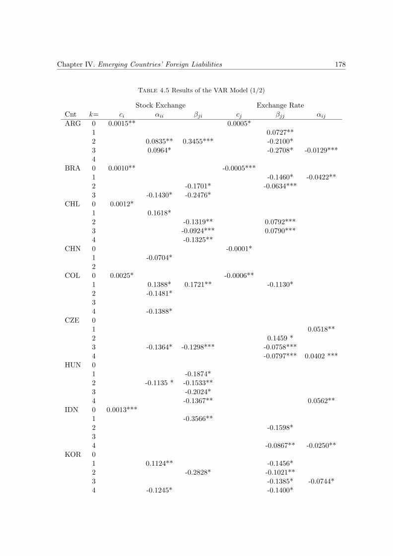
Chapter IV. Emerging Countries’ Foreign Liabilities 178
Table 4.5 Results of the VAR Model (1/2)
Stock Exchange Exchange RateCnt k= ci αii βji cj βjj αij
ARG 0 0.0015** 0.0005*1 0.0727**2 0.0835** 0.3455*** -0.2100*3 0.0964* -0.2708* -0.0129***4
BRA 0 0.0010** -0.0005***1 -0.1460* -0.0422**2 -0.1701* -0.0634***3 -0.1430* -0.2476*
CHL 0 0.0012*1 0.1618*2 -0.1319** 0.0792***3 -0.0924*** 0.0790***4 -0.1325**
CHN 0 -0.0001*1 -0.0704*2
COL 0 0.0025* -0.0006**1 0.1388* 0.1721** -0.1130*2 -0.1481*34 -0.1388*
CZE 01 0.0518**2 0.1459 *3 -0.1364* -0.1298*** -0.0758***4 -0.0797*** 0.0402 ***
HUN 01 -0.1874*2 -0.1135 * -0.1533**3 -0.2024*4 -0.1367** 0.0562**
IDN 0 0.0013***1 -0.3566**2 -0.1598*34 -0.0867** -0.0250**
KOR 01 0.1124** -0.1456*2 -0.2828* -0.1021**3 -0.1385* -0.0744*4 -0.1245* -0.1400*
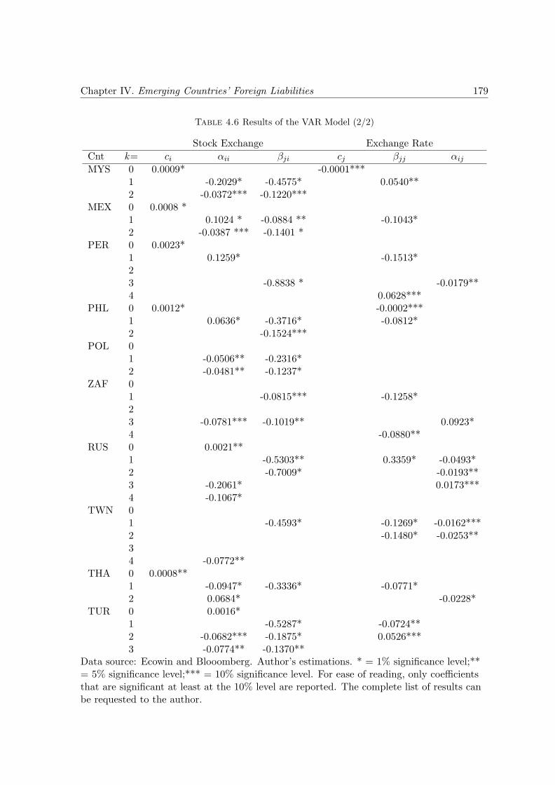
Chapter IV. Emerging Countries’ Foreign Liabilities 179
Table 4.6 Results of the VAR Model (2/2)
Stock Exchange Exchange Rate
Cnt k= ci αii βji cj βjj αij
MYS 0 0.0009* -0.0001***1 -0.2029* -0.4575* 0.0540**2 -0.0372*** -0.1220***
MEX 0 0.0008 *1 0.1024 * -0.0884 ** -0.1043*2 -0.0387 *** -0.1401 *
PER 0 0.0023*1 0.1259* -0.1513*23 -0.8838 * -0.0179**4 0.0628***
PHL 0 0.0012* -0.0002***1 0.0636* -0.3716* -0.0812*2 -0.1524***
POL 01 -0.0506** -0.2316*2 -0.0481** -0.1237*
ZAF 01 -0.0815*** -0.1258*23 -0.0781*** -0.1019** 0.0923*4 -0.0880**
RUS 0 0.0021**1 -0.5303** 0.3359* -0.0493*2 -0.7009* -0.0193**3 -0.2061* 0.0173***4 -0.1067*
TWN 01 -0.4593* -0.1269* -0.0162***2 -0.1480* -0.0253**34 -0.0772**
THA 0 0.0008**1 -0.0947* -0.3336* -0.0771*2 0.0684* -0.0228*
TUR 0 0.0016*1 -0.5287* -0.0724**2 -0.0682*** -0.1875* 0.0526***3 -0.0774** -0.1370**
Data source: Ecowin and Blooomberg. Author’s estimations. * = 1% significance level;**= 5% significance level;*** = 10% significance level. For ease of reading, only coefficientsthat are significant at least at the 10% level are reported. The complete list of results canbe requested to the author.
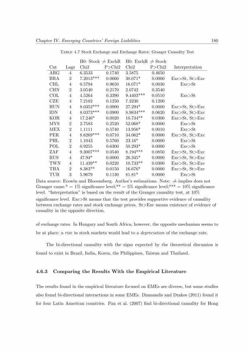
Chapter IV. Emerging Countries’ Foreign Liabilities 180
Table 4.7 Stock Exchange and Exchange Rates: Granger Causality Test
H0: Stock 6→ ExchR H0: ExchR 6→ StockCnt Lags Chi2 P>Chi2 Chi2 P>Chi2 Interpretation
ARG 4 6.3533 0.1740 3.5875 0.4650BRA 3 7.2013*** 0.0660 30.071* 0.0000 Exc>St, St>ExcCHL 4 0.5794 0.9650 16.071* 0.0030 Exc>StCHN 2 3.0540 0.2170 2.0742 0.3540COL 4 4.5264 0.3390 9.4403*** 0.0510 Exc>StCZE 4 7.2102 0.1250 7.3230 0.1200HUN 4 8.0352*** 0.0900 27.294* 0.0000 Exc>St, St>ExcIDN 4 8.0373*** 0.0900 8.9834*** 0.0620 Exc>St, St>ExcKOR 4 17.246* 0.0020 10.734** 0.0300 Exc>St, St>ExcMYS 2 2.7583 0.2520 52.068* 0.0000 Exc>StMEX 2 1.1111 0.5740 13.956* 0.0010 Exc>StPER 4 8.6269*** 0.0710 34.062* 0.0000 Exc>St, St>ExcPHL 2 1.1043 0.5760 23.16* 0.0000 Exc>StPOL 2 0.9255 0.6300 50.293* 0.0000 Exc>StZAF 4 9.3007*** 0.0540 8.194*** 0.0850 Exc>St, St>ExcRUS 4 47.94* 0.0000 26.345* 0.0000 Exc>St, St>ExcTWN 4 11.439** 0.0220 10.733** 0.0300 Exc>St, St>ExcTHA 2 8.383** 0.0150 16.676* 0.0000 Exc>St, St>ExcTUR 3 5.9679 0.1130 81.81* 0.0000 Exc>St
Data source: Ecowin and Blooomberg. Author’s estimations. Note: 6→ implies does notGranger cause.* = 1% significance level;** = 5% significance level;*** = 10% significancelevel. “Interpretation” is based on the result of the Granger causality test, at 10%
significance level. Exc>St means that the test provides supportive evidence of causalitybetween exchange rates and stock exchange prices. St>Exc means existence of evidence ofcausality in the opposite direction.
of exchange rates. In Hungary and South Africa, however, the opposite mechanism seems to
be at place: a rise in stock markets would lead to a depreciation of the exchange rate.
The bi-directional causality with the signs expected by the theoretical discussion is
found to exist in Brazil, India, Korea, the Philippines, Taiwan and Thailand.
4.6.3 Comparing the Results With the Empirical Literature
The results found in the empirical literature focused on EMEs are diverse, but some studies
also found bi-directional interactions in some EMEs. Diamandis and Drakos (2011) found it
for four Latin American countries. Pan et al. (2007) find bi-directional causality for Hong
Chapter IV. Emerging Countries’ Foreign Liabilities 181
Kong only. Granger et al. (2000) find bi-directional causality for nine countries46, but for a
different period (1986 to 1997) and with a different type of impact of stock returns in foreign
exchange markets: a currency depreciation leads to a hike in stocks. However, as the period
analyzed by the authors vary from the one analyzed in this thesis, comparisons cannot be
made given the significant difference in the importance of stocks markets.
Causality from stock exchange to foreign exchange was found by Chkili and Nguyen
(2014) for Brazil, India and Russia and by Chkili et al. (2011) for Hong Kong, Singapore,
Malaysia and Mexico. Chkili and Nguyen (2014) found it for China (using weekly data).
Pan et al. (2007) found that stock returns are significant predictors of exchange rate
movements for Korea, Singapore, and Taiwan (as in our exercise) but not in Malaysia or
Thailand (as do we). Moreover, their study concludes that exchange rates respond to stock
price movements only in Japan, Malaysia, and Thailand (with the same sign as in our study).
There is, however, an issue with comparability: their study uses data from 1988 to 1998,
when equity markets in these countries were of a very different order47.
4.6.4 The determination of impact from stock exchange to exchange rates
This section has brought up a different potential source of vulnerability that arises from
the shift towards equity-financing: an impact from stock markets to exchange rates. The
model has shown that this impact occurs in half of EMEs, namely Brazil, Hungary, India,
Korea, Peru, South Africa, Russia, Taiwan and Thailand. What could be the determinants
of whether an impact from stock exchanges to exchange rates exist? Pan et al. (2007)
indicate a few possibilities: exchange rate regimes, trade size, degree of capital control, and
size of equity markets. In economies with less capital account restrictions the exchange rate
would be more responsive to stock exchanges; high values of trade could make it respond
more to trade than to financial flows (as the ones related to the stock markets); important
equity markets are expected to generate more of such flows and thus increase its impact on
46Hong Kong, Indonesia, Japan, South Korea, Malaysia, the Philippines, Singapore, Thailand, and Taiwan.47No comparison is made with studies that use monthly data, such as Phylaktis and Ravazzolo (2005),
and Abdalla and Murinde (1997), due to the significant change in the hypothesis revealed by the differentperiodicity.

Chapter IV. Emerging Countries’ Foreign Liabilities 182
the exchange rate; exchange rate regimes that provide no flexibility obviously decrease the
potential response of exchange rates to stock prices.
To analyze the potential relationships, Figure 4.14 presents the capital account openness
data (based on Chinn and Ito (2008)) and the trade levels of different EMEs. Figure 4.15
presents a country’s stock market (presented in Section 4.1) and the share of equities on its
total foreign liabilities (presented in Section 4.2). Countries where the stock exchange has
an impact on the exchange rates are shown with round blue markers, the others with red
triangles.
Figure 4.14: Stock-Prices-Exchange-Rate Interaction: Capital Account Openness andTrade
BRA
HUN
IND
KOR
PER
RUS
ZAF
THA
ARG CHL
COL
CZE
MYS
MEX
PHL
POLTUR
02
00
,00
04
00
,00
06
00
,00
08
00
,00
0T
rad
e
−1 0 1 2 3Capital Account Openness
Foreign Trade: Exports plus Imports over GDP: US$ Millions. Data source: WB WDI.2003-2013 average. Capital Account Openness Data source: Chinn and Ito (2006). Data forChina is not presented for ease of reading. Its trade level is about three times higher thanthe one of Korea; its capital account openness index is among the smallest.
In Figure 4.14, we observe that capital account openness and trade are not good predic-
tors of the stock-price-exchange-rates interaction. Countries that have very little restrictions
Chapter IV. Emerging Countries’ Foreign Liabilities 183
to capital account transactions, as as Chile and Czech Republic, do not present such inter-
action, while places with the most significant restrictions, as is the case of South Africa and
Indonesia, do. Also the effect of trade is not as expected.
Figure 4.15, shows that the magnitude of a country’s stock market (also presented in
Section 4.1) and the share of equities on its total foreign liabilities (discussed in Section
4.2) seem to be better predictors of whether a change in stock prices will have an effect on
exchange rates. In the countries with the most important stock markets the stocks-prices-
exchange-rate-interaction was found – with the exception of China, that does not have a
floating exchange rate. The share of the stock of equities on total foreign liabilities is also
important: the interaction exists in half of the countries with the highest shares, with the
sole exception of Mexico (Malaysia does not have a flexible exchange rate regime48); and
among the countries with the lowest shares the interaction is only found in Hungary and
Peru.
Regardless of their relatively small stock markets and share of equities in foreign liabil-
ities, the presence of Hungary and Peru among the countries where the interaction is found,
can be explained by the high presence of foreign investors in the two countries’ stock markets
(seen in Figure 4.12), their very low trade, or the smaller magnitudes of their economies (as
shown in Figure 4.2).
In a nutshell, apart from the evident role of the exchange rate regime, the magnitude
of the domestic equity market and of the importance of equities in the total stock hold
by foreigners in the country seem to have determined whether an EME’ exchange rate has
responded to a change in stock prices in the last decade. The importance of trade plays a
secondary role and capital account openness does not seem to have an effect on the presence
or lack thereof of such interaction49.
48See more details on EMEs’ exchange rate regimes in the Appendix of Chapter Six, Table 6.12.49Analyses on the volatility of the different stock markets and its relationship with the country’s charac-
teristics were conducted, but the two do not seem to be closely related. The most volatile stock markets arethe smallest ones: the Philippines, Argentina, Peru and Colombia.
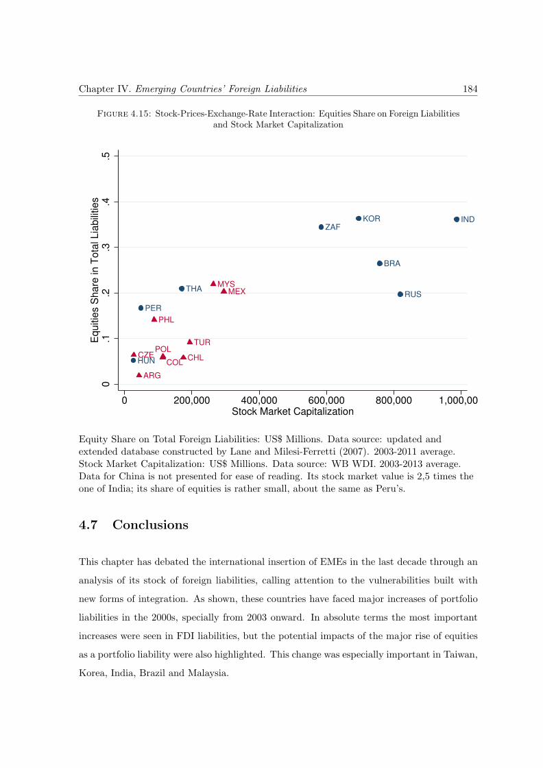
Chapter IV. Emerging Countries’ Foreign Liabilities 184
Figure 4.15: Stock-Prices-Exchange-Rate Interaction: Equities Share on Foreign Liabilitiesand Stock Market Capitalization
BRA
HUN
INDKOR
PER
RUS
ZAF
THA
ARG
CHLCZE
MYSMEX
PHL
TURPOL
COL
0.1
.2.3
.4.5
Eq
uitie
s S
ha
re in
To
tal L
iab
ilitie
s
0 200,000 400,000 600,000 800,000 1,000,00Stock Market Capitalization
Equity Share on Total Foreign Liabilities: US$ Millions. Data source: updated andextended database constructed by Lane and Milesi-Ferretti (2007). 2003-2011 average.Stock Market Capitalization: US$ Millions. Data source: WB WDI. 2003-2013 average.Data for China is not presented for ease of reading. Its stock market value is 2,5 times theone of India; its share of equities is rather small, about the same as Peru’s.
4.7 Conclusions
This chapter has debated the international insertion of EMEs in the last decade through an
analysis of its stock of foreign liabilities, calling attention to the vulnerabilities built with
new forms of integration. As shown, these countries have faced major increases of portfolio
liabilities in the 2000s, specially from 2003 onward. In absolute terms the most important
increases were seen in FDI liabilities, but the potential impacts of the major rise of equities
as a portfolio liability were also highlighted. This change was especially important in Taiwan,
Korea, India, Brazil and Malaysia.
Chapter IV. Emerging Countries’ Foreign Liabilities 185
Regardless of different sizes of the economies, different fundamentals and different types
of flows that are attracted, in almost all EMEs the stock of equities presented a N- or M-like
path. Moreover, in addition to being strikingly similar across EMEs, their pattern seems
to follow conditions of global financial markets. This common pattern indicates the high
importance of international conditions (push factors) in the determination of this type of
liability, which, in turn, adds an extra source of vulnerability: it is subject not only to
domestic, but also to international shocks – in funding countries and in others that are also
used in a portfolio diversification strategy. In other words, equities might be an important
source of contagion of turbulence from other markets. The higher importance of equity-
financing also has the effect of significantly increasing the volumes traded in EMEs’ stock
exchanges, increasing the impact of these markets on the country’s exchange rates50. An
analysis based on the PCA was however unable to point to a higher comovement of equities
than other types of foreign liabilities, which might result from the different pattern of the
series.
The vulnerability related to equity financing also include the self-feeding interactions it
can trigger: higher demand for equities increase its price, attracting more investors, pushing
prices further. In addition of being negative per se, this spiral can also be transposed to an
spiral of exchange rates. This will be analyzed in Chapter Seven.
The risk-sharing advantages of equity-financing must therefore be seen in light of the
related risks: Equities are importantly influenced by push factors, being an important locus
of transmission of contagion from other countries (as reflected in its higher volatility). A
higher share of equity liabilities and a higher stock market might add exchange rate volatility
for establishing an impact from stock markets to exchange rates – that is an impact from
a volatile market. Equities self-feeding mechanisms can be transposed to exchange rates,
creating an exchange rate spiral.
This chapter has looked at the overall changes in EMEs’ integration. The next chapter
will present a typology of financial integration among EMEs pointing to the differences in
the integration of each country, especially focusing on financialization-related features. These
three chapters have the objective of presenting a macro picture of EMEs’ external insertion
50The preponderance of push factors in the determination of capital flows (this chapter is focused on stocks)to equity instruments has been broadly identified in the literature, as will be seen in Chapter Six.
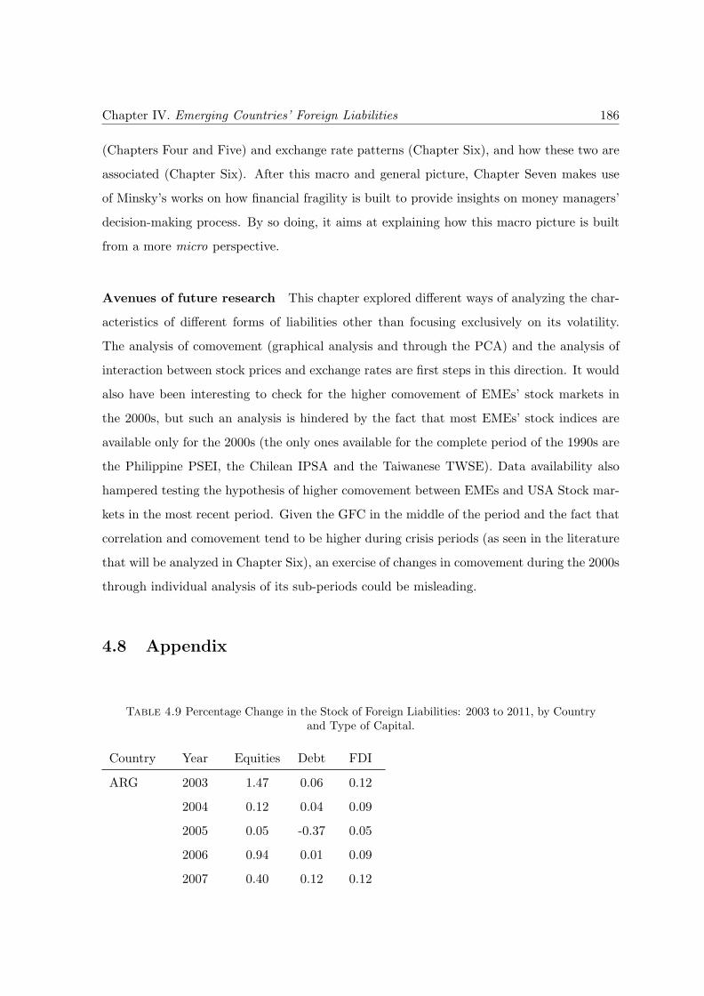
Chapter IV. Emerging Countries’ Foreign Liabilities 186
(Chapters Four and Five) and exchange rate patterns (Chapter Six), and how these two are
associated (Chapter Six). After this macro and general picture, Chapter Seven makes use
of Minsky’s works on how financial fragility is built to provide insights on money managers’
decision-making process. By so doing, it aims at explaining how this macro picture is built
from a more micro perspective.
Avenues of future research This chapter explored different ways of analyzing the char-
acteristics of different forms of liabilities other than focusing exclusively on its volatility.
The analysis of comovement (graphical analysis and through the PCA) and the analysis of
interaction between stock prices and exchange rates are first steps in this direction. It would
also have been interesting to check for the higher comovement of EMEs’ stock markets in
the 2000s, but such an analysis is hindered by the fact that most EMEs’ stock indices are
available only for the 2000s (the only ones available for the complete period of the 1990s are
the Philippine PSEI, the Chilean IPSA and the Taiwanese TWSE). Data availability also
hampered testing the hypothesis of higher comovement between EMEs and USA Stock mar-
kets in the most recent period. Given the GFC in the middle of the period and the fact that
correlation and comovement tend to be higher during crisis periods (as seen in the literature
that will be analyzed in Chapter Six), an exercise of changes in comovement during the 2000s
through individual analysis of its sub-periods could be misleading.
4.8 Appendix
Table 4.9 Percentage Change in the Stock of Foreign Liabilities: 2003 to 2011, by Countryand Type of Capital.
Country Year Equities Debt FDI
ARG 2003 1.47 0.06 0.12
2004 0.12 0.04 0.09
2005 0.05 -0.37 0.05
2006 0.94 0.01 0.09
2007 0.40 0.12 0.12
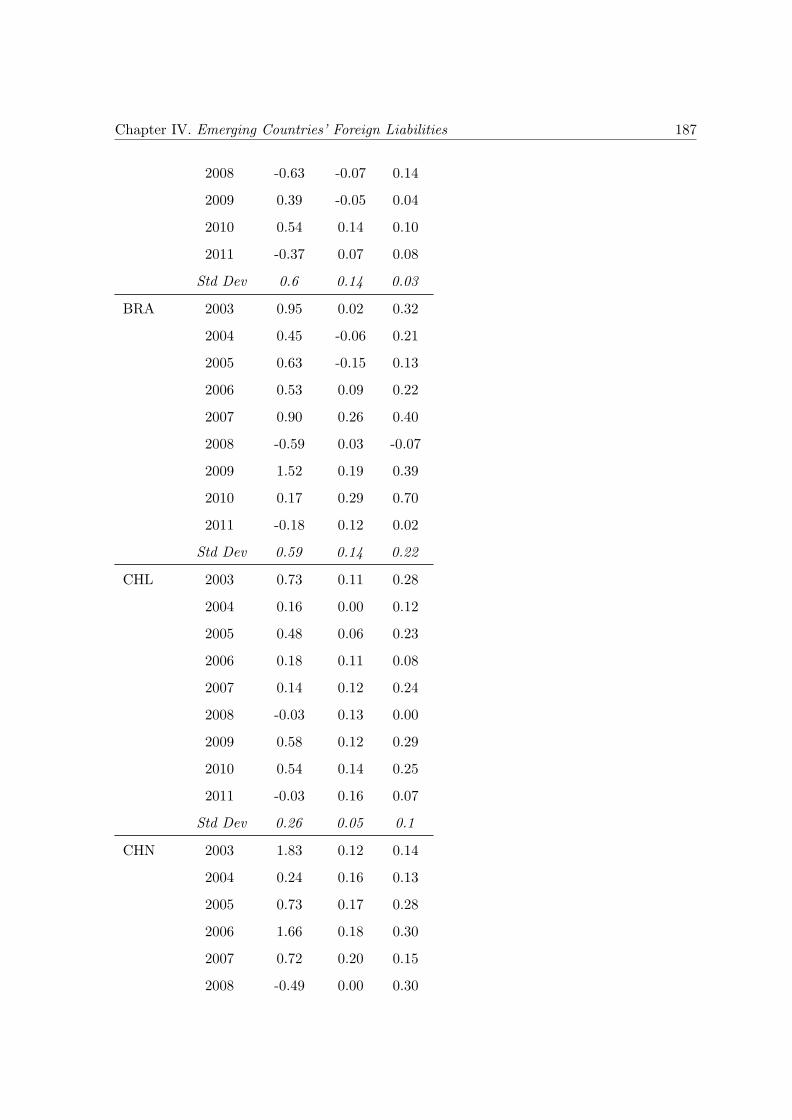
Chapter IV. Emerging Countries’ Foreign Liabilities 187
2008 -0.63 -0.07 0.14
2009 0.39 -0.05 0.04
2010 0.54 0.14 0.10
2011 -0.37 0.07 0.08
Std Dev 0.6 0.14 0.03
BRA 2003 0.95 0.02 0.32
2004 0.45 -0.06 0.21
2005 0.63 -0.15 0.13
2006 0.53 0.09 0.22
2007 0.90 0.26 0.40
2008 -0.59 0.03 -0.07
2009 1.52 0.19 0.39
2010 0.17 0.29 0.70
2011 -0.18 0.12 0.02
Std Dev 0.59 0.14 0.22
CHL 2003 0.73 0.11 0.28
2004 0.16 0.00 0.12
2005 0.48 0.06 0.23
2006 0.18 0.11 0.08
2007 0.14 0.12 0.24
2008 -0.03 0.13 0.00
2009 0.58 0.12 0.29
2010 0.54 0.14 0.25
2011 -0.03 0.16 0.07
Std Dev 0.26 0.05 0.1
CHN 2003 1.83 0.12 0.14
2004 0.24 0.16 0.13
2005 0.73 0.17 0.28
2006 1.66 0.18 0.30
2007 0.72 0.20 0.15
2008 -0.49 0.00 0.30

Chapter IV. Emerging Countries’ Foreign Liabilities 188
2009 0.80 0.15 0.44
2010 0.10 0.43 0.19
2011 -0.19 0.42 0.22
Std Dev 0.74 0.13 0.1
COL 2003 0.49 0.02 0.14
2004 1.44 0.05 0.21
2005 1.08 -0.02 0.49
2006 0.10 0.05 0.23
2007 0.27 0.13 0.25
2008 -0.29 0.01 0.19
2009 0.78 0.15 0.12
2010 0.57 0.22 0.10
2011 0.06 0.18 0.16
Std Dev 0.51 0.08 0.11
CZE 2003 0.29 0.32 0.17
2004 0.70 0.32 0.26
2005 -0.04 0.03 0.06
2006 0.29 0.25 0.32
2007 0.26 0.34 0.41
2008 -0.36 0.09 0.01
2009 0.23 0.07 0.11
2010 -0.07 0.07 0.02
2011 -0.12 -0.01 -0.06
Std Dev 0.29 0.13 0.15
HUN 2003 0.48 0.41 0.34
2004 1.03 0.48 0.27
2005 0.16 0.05 -0.01
2006 0.40 0.32 0.96
2007 -0.17 0.33 0.63
2008 -0.41 0.10 0.31
2009 0.78 0.09 0.04
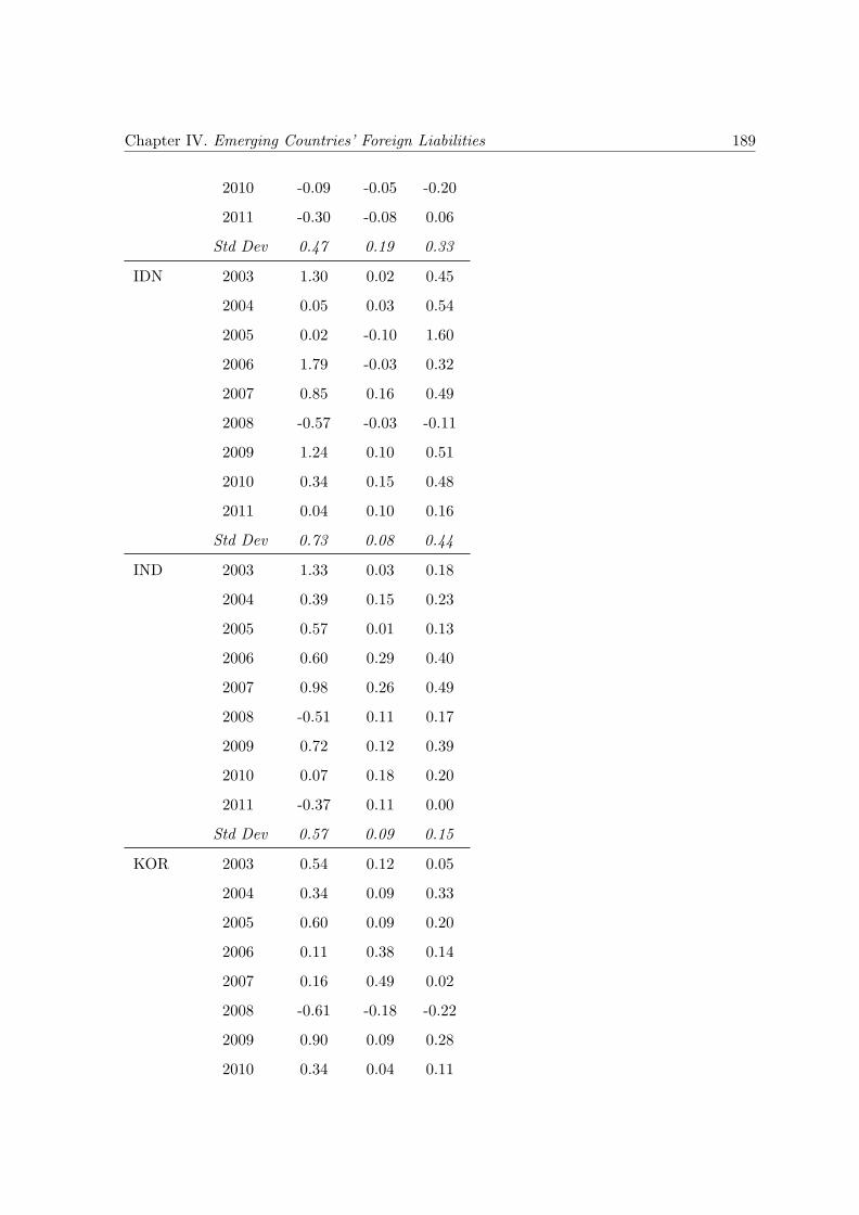
Chapter IV. Emerging Countries’ Foreign Liabilities 189
2010 -0.09 -0.05 -0.20
2011 -0.30 -0.08 0.06
Std Dev 0.47 0.19 0.33
IDN 2003 1.30 0.02 0.45
2004 0.05 0.03 0.54
2005 0.02 -0.10 1.60
2006 1.79 -0.03 0.32
2007 0.85 0.16 0.49
2008 -0.57 -0.03 -0.11
2009 1.24 0.10 0.51
2010 0.34 0.15 0.48
2011 0.04 0.10 0.16
Std Dev 0.73 0.08 0.44
IND 2003 1.33 0.03 0.18
2004 0.39 0.15 0.23
2005 0.57 0.01 0.13
2006 0.60 0.29 0.40
2007 0.98 0.26 0.49
2008 -0.51 0.11 0.17
2009 0.72 0.12 0.39
2010 0.07 0.18 0.20
2011 -0.37 0.11 0.00
Std Dev 0.57 0.09 0.15
KOR 2003 0.54 0.12 0.05
2004 0.34 0.09 0.33
2005 0.60 0.09 0.20
2006 0.11 0.38 0.14
2007 0.16 0.49 0.02
2008 -0.61 -0.18 -0.22
2009 0.90 0.09 0.28
2010 0.34 0.04 0.11
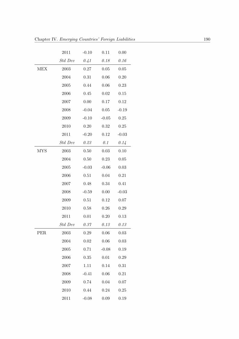
Chapter IV. Emerging Countries’ Foreign Liabilities 190
2011 -0.10 0.11 0.00
Std Dev 0.41 0.18 0.16
MEX 2003 0.27 0.05 0.05
2004 0.31 0.06 0.20
2005 0.44 0.06 0.23
2006 0.45 0.02 0.15
2007 0.00 0.17 0.12
2008 -0.04 0.05 -0.19
2009 -0.10 -0.05 0.25
2010 0.20 0.32 0.25
2011 -0.20 0.12 -0.03
Std Dev 0.23 0.1 0.14
MYS 2003 0.50 0.03 0.10
2004 0.50 0.23 0.05
2005 -0.03 -0.06 0.03
2006 0.51 0.04 0.21
2007 0.48 0.34 0.41
2008 -0.59 0.00 -0.03
2009 0.51 0.12 0.07
2010 0.58 0.26 0.29
2011 0.01 0.20 0.13
Std Dev 0.37 0.13 0.13
PER 2003 0.29 0.06 0.03
2004 0.02 0.06 0.03
2005 0.71 -0.08 0.19
2006 0.35 0.01 0.29
2007 1.11 0.14 0.31
2008 -0.41 0.06 0.21
2009 0.74 0.04 0.07
2010 0.44 0.24 0.25
2011 -0.08 0.09 0.19
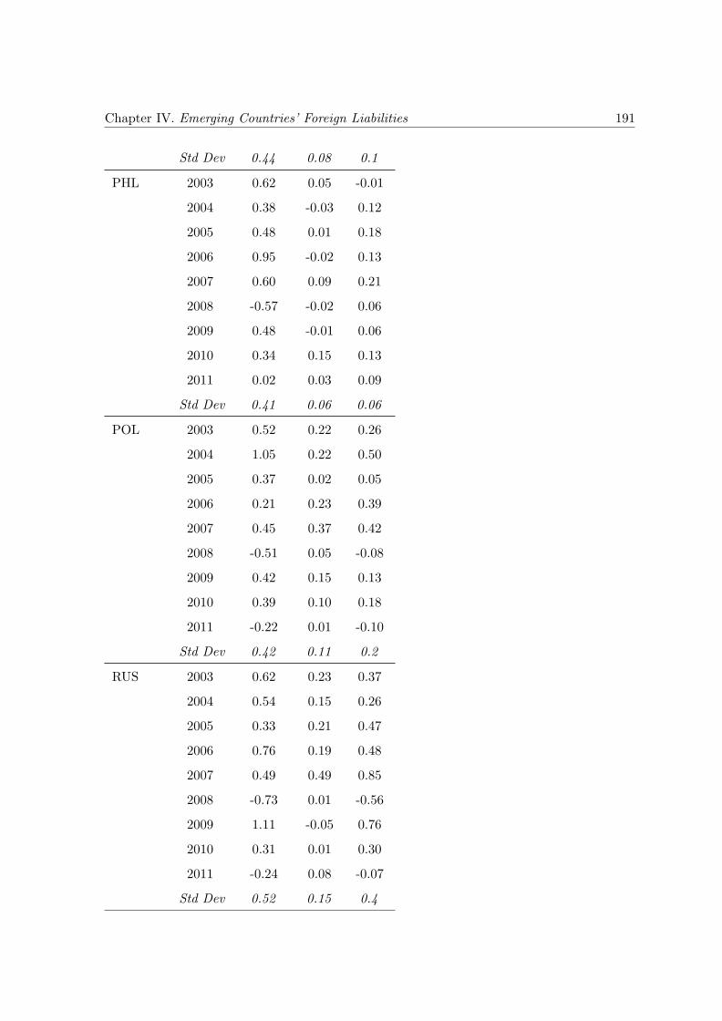
Chapter IV. Emerging Countries’ Foreign Liabilities 191
Std Dev 0.44 0.08 0.1
PHL 2003 0.62 0.05 -0.01
2004 0.38 -0.03 0.12
2005 0.48 0.01 0.18
2006 0.95 -0.02 0.13
2007 0.60 0.09 0.21
2008 -0.57 -0.02 0.06
2009 0.48 -0.01 0.06
2010 0.34 0.15 0.13
2011 0.02 0.03 0.09
Std Dev 0.41 0.06 0.06
POL 2003 0.52 0.22 0.26
2004 1.05 0.22 0.50
2005 0.37 0.02 0.05
2006 0.21 0.23 0.39
2007 0.45 0.37 0.42
2008 -0.51 0.05 -0.08
2009 0.42 0.15 0.13
2010 0.39 0.10 0.18
2011 -0.22 0.01 -0.10
Std Dev 0.42 0.11 0.2
RUS 2003 0.62 0.23 0.37
2004 0.54 0.15 0.26
2005 0.33 0.21 0.47
2006 0.76 0.19 0.48
2007 0.49 0.49 0.85
2008 -0.73 0.01 -0.56
2009 1.11 -0.05 0.76
2010 0.31 0.01 0.30
2011 -0.24 0.08 -0.07
Std Dev 0.52 0.15 0.4
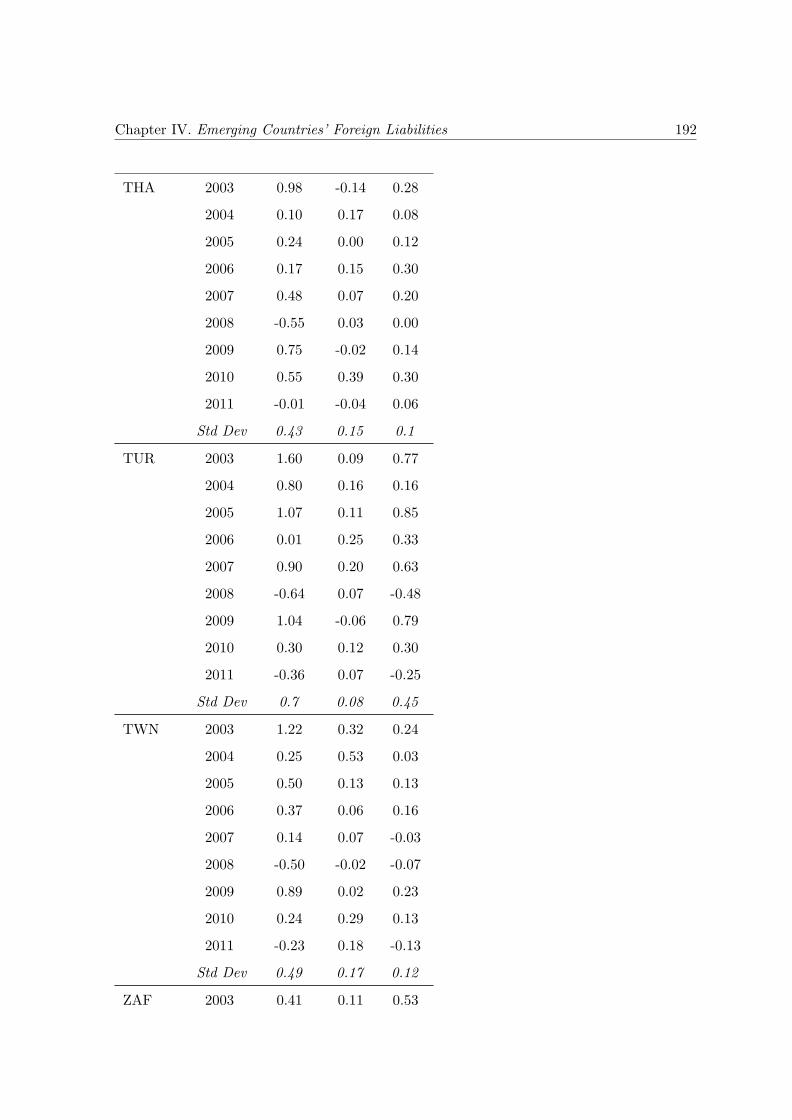
Chapter IV. Emerging Countries’ Foreign Liabilities 192
THA 2003 0.98 -0.14 0.28
2004 0.10 0.17 0.08
2005 0.24 0.00 0.12
2006 0.17 0.15 0.30
2007 0.48 0.07 0.20
2008 -0.55 0.03 0.00
2009 0.75 -0.02 0.14
2010 0.55 0.39 0.30
2011 -0.01 -0.04 0.06
Std Dev 0.43 0.15 0.1
TUR 2003 1.60 0.09 0.77
2004 0.80 0.16 0.16
2005 1.07 0.11 0.85
2006 0.01 0.25 0.33
2007 0.90 0.20 0.63
2008 -0.64 0.07 -0.48
2009 1.04 -0.06 0.79
2010 0.30 0.12 0.30
2011 -0.36 0.07 -0.25
Std Dev 0.7 0.08 0.45
TWN 2003 1.22 0.32 0.24
2004 0.25 0.53 0.03
2005 0.50 0.13 0.13
2006 0.37 0.06 0.16
2007 0.14 0.07 -0.03
2008 -0.50 -0.02 -0.07
2009 0.89 0.02 0.23
2010 0.24 0.29 0.13
2011 -0.23 0.18 -0.13
Std Dev 0.49 0.17 0.12
ZAF 2003 0.41 0.11 0.53
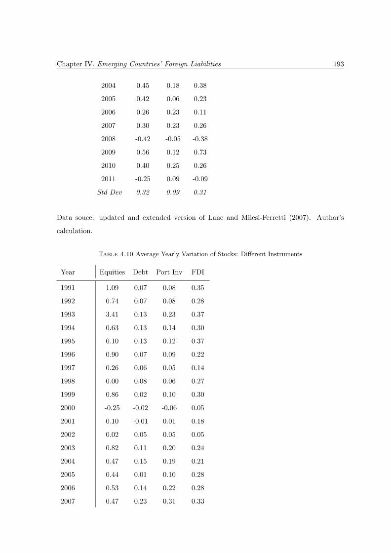
Chapter IV. Emerging Countries’ Foreign Liabilities 193
2004 0.45 0.18 0.38
2005 0.42 0.06 0.23
2006 0.26 0.23 0.11
2007 0.30 0.23 0.26
2008 -0.42 -0.05 -0.38
2009 0.56 0.12 0.73
2010 0.40 0.25 0.26
2011 -0.25 0.09 -0.09
Std Dev 0.32 0.09 0.31
Data souce: updated and extended version of Lane and Milesi-Ferretti (2007). Author’s
calculation.
Table 4.10 Average Yearly Variation of Stocks: Different Instruments
Year Equities Debt Port Inv FDI
1991 1.09 0.07 0.08 0.35
1992 0.74 0.07 0.08 0.28
1993 3.41 0.13 0.23 0.37
1994 0.63 0.13 0.14 0.30
1995 0.10 0.13 0.12 0.37
1996 0.90 0.07 0.09 0.22
1997 0.26 0.06 0.05 0.14
1998 0.00 0.08 0.06 0.27
1999 0.86 0.02 0.10 0.30
2000 -0.25 -0.02 -0.06 0.05
2001 0.10 -0.01 0.01 0.18
2002 0.02 0.05 0.05 0.05
2003 0.82 0.11 0.20 0.24
2004 0.47 0.15 0.19 0.21
2005 0.44 0.01 0.10 0.28
2006 0.53 0.14 0.22 0.28
2007 0.47 0.23 0.31 0.33
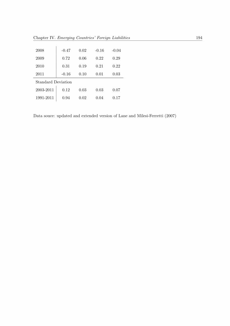
Chapter IV. Emerging Countries’ Foreign Liabilities 194
2008 -0.47 0.02 -0.16 -0.04
2009 0.72 0.06 0.22 0.29
2010 0.31 0.19 0.21 0.22
2011 -0.16 0.10 0.01 0.03
Standard Deviation
2003-2011 0.12 0.03 0.03 0.07
1991-2011 0.94 0.02 0.04 0.17
Data souce: updated and extended version of Lane and Milesi-Ferretti (2007)
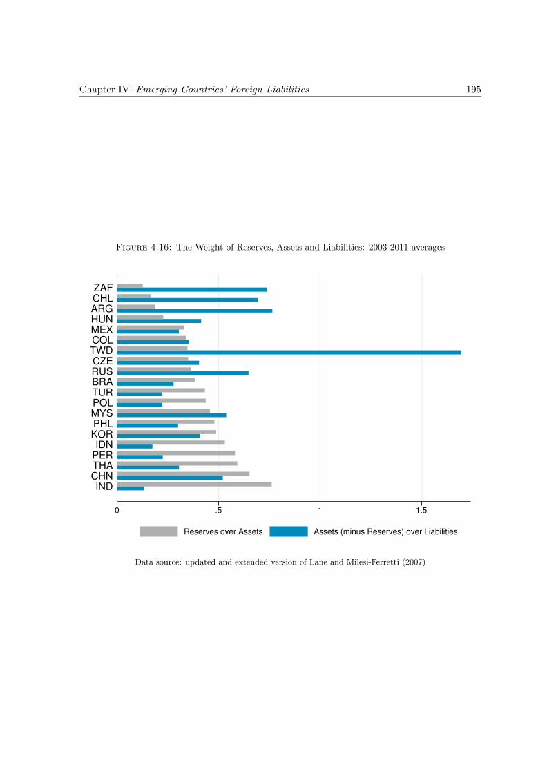
Chapter IV. Emerging Countries’ Foreign Liabilities 195
Figure 4.16: The Weight of Reserves, Assets and Liabilities: 2003-2011 averages
0 .5 1 1.5
INDCHNTHAPERIDN
KORPHLMYSPOLTURBRARUSCZETWDCOLMEXHUNARGCHLZAF
Reserves over Assets Assets (minus Reserves) over Liabilities
Data source: updated and extended version of Lane and Milesi-Ferretti (2007)
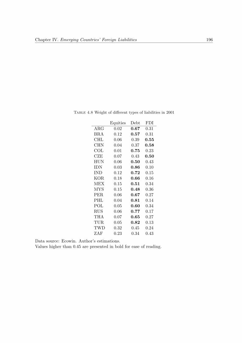
Chapter IV. Emerging Countries’ Foreign Liabilities 196
Table 4.8 Weight of different types of liabilities in 2001
Equities Debt FDI
ARG 0.02 0.67 0.31BRA 0.12 0.57 0.31CHL 0.06 0.39 0.55CHN 0.04 0.37 0.58COL 0.01 0.75 0.23CZE 0.07 0.43 0.50HUN 0.06 0.50 0.43IDN 0.03 0.86 0.10IND 0.12 0.72 0.15KOR 0.18 0.66 0.16MEX 0.15 0.51 0.34MYS 0.15 0.48 0.36PER 0.06 0.67 0.27PHL 0.04 0.81 0.14POL 0.05 0.60 0.34RUS 0.06 0.77 0.17THA 0.07 0.65 0.27TUR 0.05 0.82 0.13TWD 0.32 0.45 0.24ZAF 0.23 0.34 0.43
Data source: Ecowin. Author’s estimations.Values higher than 0.45 are presented in bold for ease of reading.
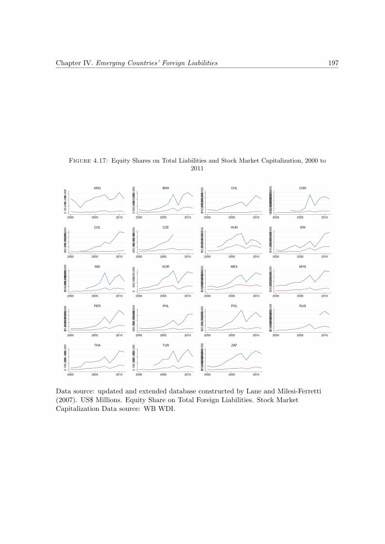
Chapter IV. Emerging Countries’ Foreign Liabilities 197
Figure 4.17: Equity Shares on Total Liabilities and Stock Market Capitalization, 2000 to2011
02
0,0
0040
,00
060
,00
0
2000 2005 2010
ARG
05
00
,00
01
,00
0,0
00
1,5
00
,00
0
2000 2005 2010
BRA
010
0,0
00
20
0,0
00
30
0,0
00
40
0,0
00
2000 2005 2010
CHL
01
,00
0,0
00
2,0
00
,00
03
,00
0,0
00
4,0
00
,00
05
,00
0,0
00
2000 2005 2010
CHN
050
,00
01
00
,00
01
50
,00
02
00
,00
0
2000 2005 2010
COL
02
0,0
00
40
,00
06
0,0
00
80
,00
0
2000 2005 2010
CZE
010
,00
02
0,0
00
30
,00
04
0,0
00
50
,00
0
2000 2005 2010
HUN
010
0,0
00
20
0,0
00
30
0,0
00
40
0,0
00
2000 2005 2010
IDN
050
0,0
00
1,0
00
,00
01
,50
0,0
00
2,0
00
,00
0
2000 2005 2010
IND
05
00
,00
01,0
00
,00
0
2000 2005 2010
KOR
010
0,0
00
20
0,0
00
30
0,0
00
40
0,0
00
50
0,0
00
2000 2005 2010
MEX01
00
,00
02
00
,00
03
00
,00
04
00
,00
0
2000 2005 2010
MYS
020
,00
04
0,0
00
60
,00
08
0,0
00
10
0,0
00
2000 2005 2010
PER
05
0,0
00
10
0,0
00
15
0,0
00
20
0,0
00
2000 2005 2010
PHL
050
,00
01
00
,00
01
50
,00
02
00
,00
0
2000 2005 2010
POL
020
0,0
00
40
0,0
00
60
0,0
00
80
0,0
00
1,0
00
,00
0
2000 2005 2010
RUS
01
00
,00
02
00
,00
03
00
,00
0
2000 2005 2010
THA
01
00
,00
02
00
,00
03
00
,00
0
2000 2005 2010
TUR
020
0,0
00
40
0,0
00
60
0,0
00
80
0,0
00
1,0
00
,00
0
2000 2005 2010
ZAF
Data source: updated and extended database constructed by Lane and Milesi-Ferretti(2007). US$ Millions. Equity Share on Total Foreign Liabilities. Stock MarketCapitalization Data source: WB WDI.
Chapter 5
The Concept of Financialized
Integration and its Estimation for
Emerging Market Economies
Within the context of the rise of financialization in advanced economies, some developing
countries opted for liberalizing their financial markets and capital accounts. This allowed
their integration to the international financial system, characterized, in times of financial-
ization, by the interconnectedness of markets from advanced countries and emerging market
economies (EMEs) through money managers’ balance-sheets and by the high level of sophis-
tication of finance (as discussed in Chapter Two). With the rise of these features, financial
integration could have implications on the determination of exchange-rates of EMEs. To
test this hypothesis, this chapter suggests estimating how important financialization-related
features are in characterizing these countries’ integration. Or, how financialized their inte-
gration is.
Two financialization features are related to integration. The first is the higher impor-
tance of finance at the international level with its decoupling from earlier functions. Note
that this differs from financial integration for focusing on the changing function of finance
internationally, which now follows its own logic (see discussion in Chapter Two). It should
therefore not be measured by the absolute magnitude of integration, but by how it diverges
198
Chapter V. Financialized Integration 199
from the productive economy’s factors. The second aspect is the sophistication of finance,
through its products and innovations of usages, as the rise of carry trading and currency
trading more broadly.
In this sense, a financialized integration is marked by large financial integration and
sizable foreign exchange (FX) transactions relative to the underlying economic activity and
trade. The relative weight of FX markets also points to the sophistication of finance, that
can also be proxied by the weight of derivatives FX contracts.
This chapter discusses the presence of these characteristics in EMEs and advanced
countries. It presents an account of the early 2000s and of current levels, indicating the
velocity of the financialization process in these places. It is important to mention that the
chapter aims at providing a macro picture of integration among EMEs. Analyses of the
institutions behind this phenomenon, or the macro policies that could explain a country’s
higher financial integration are not within the scope of the chapter, and are only briefly
mentioned throughout the text1.
The structure of the chapter Apart from this short introduction, the chapter is di-
vided as follows. Section 5.1 presents the concept of financialized integration, building upon
indicators used in the literature on financial integration and on that of financialization (as
presented in Chapter Two). Sections 5.2 and 5.3 respectively look at the characteristics of
financial integration and the FX markets, revealing the signs of financialized integration in
both EMEs and advanced countries. Section 5.4 constructs an index of financialized integra-
tion. Section 5.5 further discusses the types of integration through a principal components
analysis. Section 5.6 presents concluding remarks and avenues for future research.
Data Used
Two main sets of data are used to characterize financialized integration. The first, the
updated and extended version of the dataset constructed by Lane and Milesi-Ferretti (2007),
that regards financial integration and provides information on the stock of foreign assets and
1The focus on the resulting characteristics instead of on the institutional background is reflected on thechoice for a de facto or an outcome measure of financial integration in this chapter (as will be discussed inSection 5.1).
Chapter V. Financialized Integration 200
liabilities. In this dataset, capital is divided into equities, debt, foreign direct investment
(FDI) and derivatives. Debt includes both “portfolio debt securities” and “other investment”.
Derivatives are not included in this chapter’s analysis given their very low levels2. As the
chapter aims at analyzing the behavior of foreign investors vis-a-vis of EMEs, focus is given
to the liabilities’ side (as discussed in Chapter Four). This dataset was updated until 2011,
thus, that is the year used as estimate for the most recent period. The second set of data used
relates to FX markets: the total size and weight of their derivatives contracts. It is based on
the Bank of International Settlement’s (BIS) Triennial Surveys of FX Markets. The change
in the structure of FX markets is analyzed by comparing two years, 2001 (BIS, 2001) and
2013 (BIS, 2013)3. The 2001 survey was chosen to represent an early stage of the impacts
of financialization on EMEs. The prior survey, conducted in 1998, contains potential biases
from currency-crises and did not include the euro, that had not yet been implemented.
The analysis was done for the currencies for which data are available in both the 2001
and the 2013 surveys. There are 11 emerging currencies: the Brazilian real (BRL), the
Chinese yuan (CNY), the Hungarian forint (HUF), the Indian rupee (INR), the Korean won
(KRW), the Mexican peso (MXN), the Polish zloty (PLN), the Russian ruble (RUB), the
Turkish lira (TRY), the New Taiwanese dollar (TWD), and the South African rand (ZAR).
And 11 currencies from advanced countries: the Australian dollar (AUD), the Canadian
dollar (CAD), the Swiss franc (CHF), the Danish krone (DKK), the euro (EUR), the Pound
sterling (GBP), the Japanese yen (JPY), the Norwegian krone (NOK), the New Zealand
dollar (NZD), the Swedish krona (SEK), and the U.S. dollar (USD, US$)4. These currencies
were defined as currencies of emerging or advanced countries according to the BIS’ own
characterization. Honk Kong and Singapore are not among the 20 EMEs considered in this
thesis – as defined in Chapter Four. Their figures are also mentioned, but not considered in
EMEs’ averages.
Data on countries’ GDP and foreign trade are taken from the World Bank’s World
Development Indicators (World Bank, 2015). To allow comparisons with EWN data, GDP,
2See Footnote 16 on Chapter Four.3Precisely, the survey refers to the contracts that took place in the month of April of the respective year.
The figures refer to average daily transactions.4Figures mentioned in this chapter’s analyses refer to these 24 currencies, not the complete market of the
2001 or 2013 surveys. Note that this is also not the same list of countries from last chapter’s analyses. Alsorefer to the “List of Abbreviations” of countries and currencies in the Thesis’ preamble.
Chapter V. Financialized Integration 201
export and import data were taken in current U.S. dollars (Millions). For building indicators
for the first period, data for 2001 is used. For the second period’s indicators either 2011 or
2013 data is used, depending on whether it is used to build indicators with capital account
data (EWN, where 2011 is the last period) or with FX market data (BIS, where 2013 data is
used). To be clear, indicators of FX markets over GDP include WDI 2013 data, while data
on the financial integration over trade, include WDI 2011 data.
5.1 Measuring Financial Integration
The empirical literature on financial integration uses two main types of indicators. Some
analyses are based on the asset prices (returns) ruling in financial markets of two countries.
Similar prices indicate integration. Other studies use indicators focused on the actual lib-
eralization or integration. These two measures have been named price- and quantity-based
(Garcia-Herrero and Wooldridge, 2007) – which, however, is not the most adequate, given
that they are not only quantities (as will be presented in what follows5). A sounder un-
derstanding might be a separation between a strand that takes a more micro perspective
of financial markets and look at the expected consequences of financial integration in finan-
cial markets, and another that takes a more macro perspective, and investigates the actual
integration or liberalization.
The first strand of the literature assumes that every participant faces a single set of
rules, has equal access and are treated equally (Baele et al., 2004). This would lead to a
trend towards more similar returns of assets of identical risks in integrated markets (or the
observation of the law of one price). A second expected effect of fully integrated markets is
the diversification of country-specific risks that decreases the their significance in the pricing
of assets (Garcia-Herrero and Wooldridge, 2007). Based on these two expected consequences
of integration, two indicators of the degree of integration are used in his literature: the
correlation among asset prices in different countries,6 and the importance of domestic factors
in determining prices (or the arbitrage gap between onshore and offshore rates).
5Frankel (1992), as cited in Prasad et al. (2003), indicates other rather unusual measures of capital marketintegration: saving-investment correlations and interest parity conditions.
6An interesting example of this type of analysis is Phylaktis and Ravazzolo’s (2002) where financial inte-gration is measured by the covariance of excess returns of national stock markets.
Chapter V. Financialized Integration 202
The strand of the literature that takes a more macro perspective examines what is now
known as de jure or de facto measures. While the first analyzes the related legislation and
regulation that could restrain capital mobility, the second focuses on estimations of the actual
flow of capital between countries or the countries’ stock of foreign assets and liabilities.
The most common in the de jure literature is to use indicators of the legal restrictions on
cross-border capital flows based on information from the IMF’s Annual Report on Exchange
Arrangements and Exchange Restrictions. The ones constructed by Garcia-Herrero and
Wooldridge (2007) and Chinn and Ito (2008) are based on a percentage of controls in place.
Several other methodologies have also been proposed, as shown by (Da Silva and Da Fonseca,
2015)7.
Although widely used, such de jure measures of impediments to the free flow of capital
have several shortcomings: restrictions may not be binding, respected or enforced; capital
flows might not have existed in the first place; the measures cover a narrow aspect of all
possible impediments; and they provide the picture of one day, so temporary and permanent
measures are not differentiated (Garcia-Herrero and Wooldridge, 2007). In addition, de jure
measures can be biased in the case of regulatory. Prasad et al. (2003) presents the possibil-
ity of capital flows despite controls in episodes of capital flight from some Latin American
countries in the 1970s and 1980s8. Another way of understanding these shortcomings is the
idea that liberalization does not mean integration, given that it only allows it to take place,
not necessarily inducing it to actually happen (Bekaert and Harvey, 2000) and maybe also
not hindering it from happening.
7Da Silva and Da Fonseca (2015) list other methodologies used in this literature that have different focus,such as: i) different dimensions of liberalization; ii) the accumulation of measures focusing on liberalizingor restricting capital flows through the time; iii) the proportion of restrictions according to different chosendimensions; iv) the intensity of restrictions on capital account according to central bank reports; and v) binaryvariables related to liberalization of stock markets. See Da Silva and Da Fonseca (2015) for reference works ofeach type of methodology. There are also measures which are focused only in one type of capital, as Edisonand Warnock’s (2003) that propose a monthly measure of capital account openness based on the share ofdomestic equities available for foreign purchase.
8For a possibility to overcome some of these shortcomings, see Schindler (2009) who constructed a datasetthat allows for dis-aggregation on asset categories according to inflows or outflows and resident or non-resident.
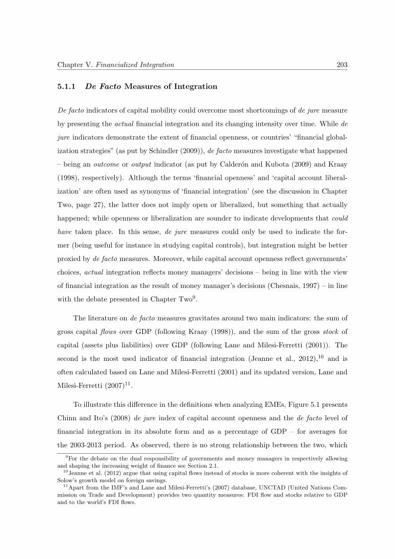
Chapter V. Financialized Integration 203
5.1.1 De Facto Measures of Integration
De facto indicators of capital mobility could overcome most shortcomings of de jure measure
by presenting the actual financial integration and its changing intensity over time. While de
jure indicators demonstrate the extent of financial openness, or countries’ “financial global-
ization strategies” (as put by Schindler (2009)), de facto measures investigate what happened
– being an outcome or output indicator (as put by Calderon and Kubota (2009) and Kraay
(1998), respectively). Although the terms ‘financial openness’ and ‘capital account liberal-
ization’ are often used as synonyms of ‘financial integration’ (see the discussion in Chapter
Two, page 27), the latter does not imply open or liberalized, but something that actually
happened; while openness or liberalization are sounder to indicate developments that could
have taken place. In this sense, de jure measures could only be used to indicate the for-
mer (being useful for instance in studying capital controls), but integration might be better
proxied by de facto measures. Moreover, while capital account openness reflect governments’
choices, actual integration reflects money managers’ decisions – being in line with the view
of financial integration as the result of money manager’s decisions (Chesnais, 1997) – in line
with the debate presented in Chapter Two9.
The literature on de facto measures gravitates around two main indicators: the sum of
gross capital flows over GDP (following Kraay (1998)), and the sum of the gross stock of
capital (assets plus liabilities) over GDP (following Lane and Milesi-Ferretti (2001)). The
second is the most used indicator of financial integration (Jeanne et al., 2012),10 and is
often calculated based on Lane and Milesi-Ferretti (2001) and its updated version, Lane and
Milesi-Ferretti (2007)11.
To illustrate this difference in the definitions when analyzing EMEs, Figure 5.1 presents
Chinn and Ito’s (2008) de jure index of capital account openness and the de facto level of
financial integration in its absolute form and as a percentage of GDP – for averages for
the 2003-2013 period. As observed, there is no strong relationship between the two, which
9For the debate on the dual responsibility of governments and money managers in respectively allowingand shaping the increasing weight of finance see Section 2.1.
10Jeanne et al. (2012) argue that using capital flows instead of stocks is more coherent with the insights ofSolow’s growth model on foreign savings.
11Apart from the IMF’s and Lane and Milesi-Ferretti’s (2007) database, UNCTAD (United Nations Com-mission on Trade and Development) provides two quantity measures: FDI flow and stocks relative to GDPand to the world’s FDI flows.
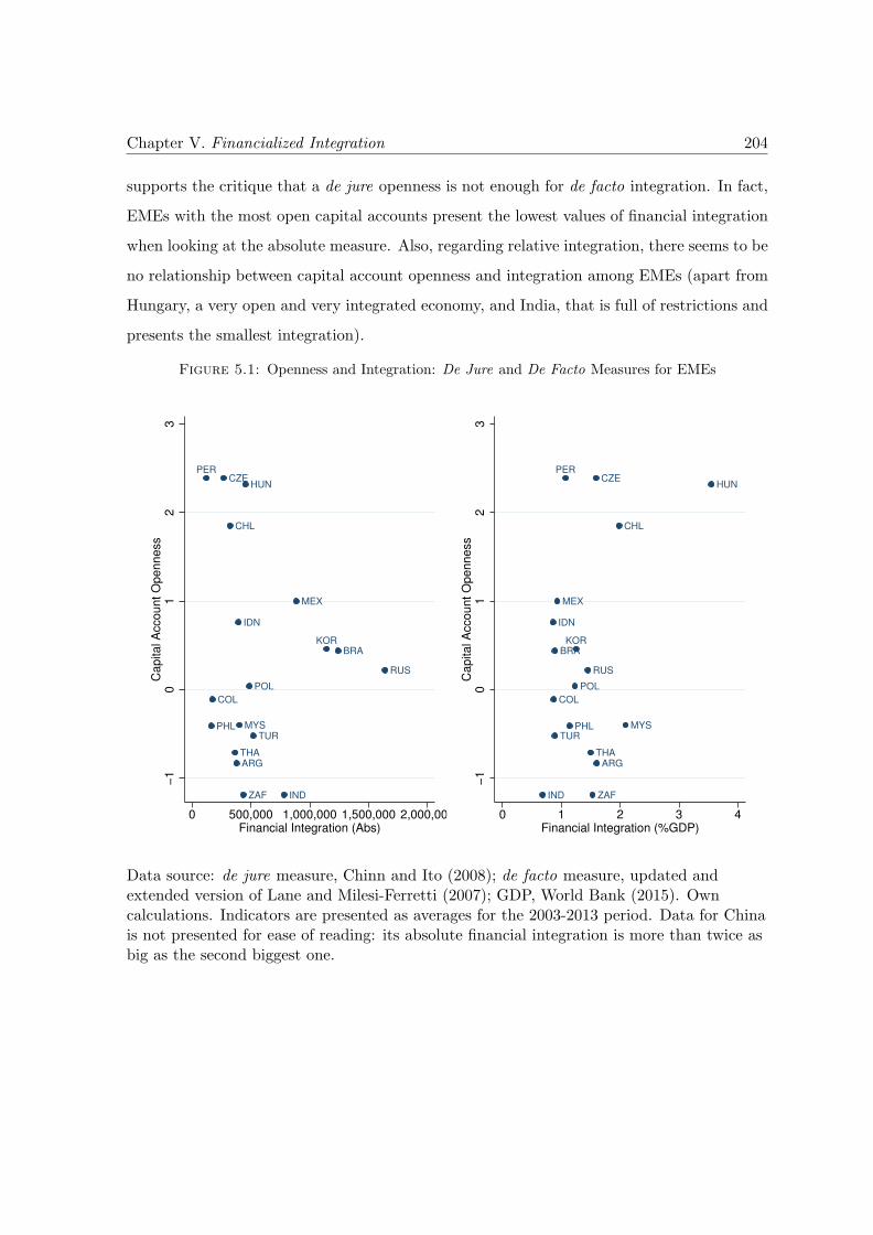
Chapter V. Financialized Integration 204
supports the critique that a de jure openness is not enough for de facto integration. In fact,
EMEs with the most open capital accounts present the lowest values of financial integration
when looking at the absolute measure. Also, regarding relative integration, there seems to be
no relationship between capital account openness and integration among EMEs (apart from
Hungary, a very open and very integrated economy, and India, that is full of restrictions and
presents the smallest integration).
Figure 5.1: Openness and Integration: De Jure and De Facto Measures for EMEs
ARG
BRA
CHL
COL
CZEHUN
IND
IDN
MYS
MEX
PHL
POL
RUS
ZAF
THA
TUR
KOR
PER
−1
01
23
Capital A
ccount
Openness
0 500,000 1,000,000 1,500,000 2,000,000Financial Integration (Abs)
ARG
BRA
CHL
COL
CZEHUN
IND
IDN
MYS
MEX
PHL
POL
RUS
ZAF
THA
TUR
KOR
PER−
10
12
3C
apital A
ccount
Openness
0 1 2 3 4Financial Integration (%GDP)
Data source: de jure measure, Chinn and Ito (2008); de facto measure, updated andextended version of Lane and Milesi-Ferretti (2007); GDP, World Bank (2015). Owncalculations. Indicators are presented as averages for the 2003-2013 period. Data for Chinais not presented for ease of reading: its absolute financial integration is more than twice asbig as the second biggest one.
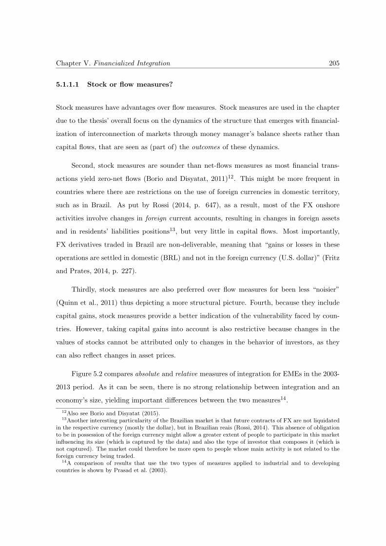
Chapter V. Financialized Integration 205
5.1.1.1 Stock or flow measures?
Stock measures have advantages over flow measures. Stock measures are used in the chapter
due to the thesis’ overall focus on the dynamics of the structure that emerges with financial-
ization of interconnection of markets through money manager’s balance sheets rather than
capital flows, that are seen as (part of) the outcomes of these dynamics.
Second, stock measures are sounder than net-flows measures as most financial trans-
actions yield zero-net flows (Borio and Disyatat, 2011)12. This might be more frequent in
countries where there are restrictions on the use of foreign currencies in domestic territory,
such as in Brazil. As put by Rossi (2014, p. 647), as a result, most of the FX onshore
activities involve changes in foreign current accounts, resulting in changes in foreign assets
and in residents’ liabilities positions13, but very little in capital flows. Most importantly,
FX derivatives traded in Brazil are non-deliverable, meaning that “gains or losses in these
operations are settled in domestic (BRL) and not in the foreign currency (U.S. dollar)” (Fritz
and Prates, 2014, p. 227).
Thirdly, stock measures are also preferred over flow measures for been less “noisier”
(Quinn et al., 2011) thus depicting a more structural picture. Fourth, because they include
capital gains, stock measures provide a better indication of the vulnerability faced by coun-
tries. However, taking capital gains into account is also restrictive because changes in the
values of stocks cannot be attributed only to changes in the behavior of investors, as they
can also reflect changes in asset prices.
Figure 5.2 compares absolute and relative measures of integration for EMEs in the 2003-
2013 period. As it can be seen, there is no strong relationship between integration and an
economy’s size, yielding important differences between the two measures14.
12Also see Borio and Disyatat (2015).13Another interesting particularity of the Brazilian market is that future contracts of FX are not liquidated
in the respective currency (mostly the dollar), but in Brazilian reais (Rossi, 2014). This absence of obligationto be in possession of the foreign currency might allow a greater extent of people to participate in this marketinfluencing its size (which is captured by the data) and also the type of investor that composes it (which isnot captured). The market could therefore be more open to people whose main activity is not related to theforeign currency being traded.
14A comparison of results that use the two types of measures applied to industrial and to developingcountries is shown by Prasad et al. (2003).
Chapter V. Financialized Integration 206
Figure 5.2: Financial Integration: Absolute and Relative Measures Based on Stocks forEMEs
BRA
CHL
COL
HUN
IND
IDN
MYS
MEXPER
POL
RUS
TWN
THA
TUR
ARG
KORPHL
ZAFCZE
01
23
4F
ina
ncia
l In
teg
ratio
n,
% G
DP
0 500,000 1,000,000 1,500,000 2,000,00Financial Integration, Abs
Financial Integration (Absolute value): US$ Millions. Indicators are presented as averagesfor the 2003-2013 period. Data for China is not presented for ease of reading: its absolutefinancial integration is more than two times bigger than the second biggest one.
Which financial integration indicator better suits our purpose? Indicators that
focus on the prices of financial assets are not compatible with an analysis including both
EMEs and advanced countries, given that their assets are substantially different – also due
to the greater exchange rate risk involved with EMEs’ assets15. Secondly, measures based
on capital flows could be biased estimations due to the outlined reasons and, in the specific
case of this chapter’s analyses, due to their recent high volatility in EMEs. Stock variables
were thus chosen.
15As analyzed in Chapter Seven, an institutional investor that invests in its own country has no exchangerate risk. When investing in another advanced country, the risk exists, but is less important than the risk ofinvesting in an EME. The specific risks related to emerging currencies are discussed in Chapter Three, Section3.3.4.
Chapter V. Financialized Integration 207
5.2 From Financial to Financialized Integration
Apart from being used by the literature on financial integration, indicators based on foreign
assets and liabilities have also been used to proxy financialization. For instance, Chesnais
(1997) mentions the ownership of foreign assets in portfolios of U.S. pension funds and
Baker et al. (1998) cites the value of funds raised on international financial markets, i.e.
foreign liabilities. The first is taken in absolute values, and the latter as a percentage of
world exports, yielding in a comparison between financial and trade integration. Another
direct form of comparing financial and commercial integration is to look at their weight in
a country’s balance of payment or GDP (as done by Plihon (2010); see Chapter Two, page
29).
The analyses in this section are based on both absolute and relative measures, with
regards to GDP and trade. Relative measures will be used in the remainder of the chapter as
indicators of financialization, to show, specifically, the part of integration that exceeds what
would have been expected from an economic or trade activity, thus evincing the decoupling
of finance from its prior functions (as discussed in Chapter Two, Section 2.1). By gradually
analyzing relative measures, the section presents considerations on both countries’ integration
as well as financialized integration.
This section also analyzes assets-to-liabilities ratios to demonstrate the role of EMEs
as suppliers of financial assets to international money managers and in the debate on the
rise of carry trading (presented in Chapter Two, section 2.2.2.2). Before these analyses, the
importance of reserves among EMEs’ assets to avoid possible biases in the indicators from
public decisions is discussed.
5.2.1 The Weight of Reserves
When analyzing assets and liabilities, a notable difference among EMEs and advanced coun-
tries is the magnitude of reserves (see Figure 5.3).
Chapter V. Financialized Integration 208
5.2.1.1 The reasons behind the build up of reserves
In the aftermath of the late-1990s crises, EMEs started to significantly increase their hold-
ings of reserves of international assets. Although sometimes called mercantilistic, in most
countries this policy is seen as precautionary (Aizenman and Marion (2003); Aizenman and
Lee (2007); Lee (2004)).
The reasons for being ‘cautious’ are numerous, and EMEs’ increasing vulnerabilities
(as analyzed throughout the thesis) asks for increasingly higher amounts of reserves. The
choice for building up reserves must be understood against the background of the late-1990s
currency crises faced by most of the countries. Indeed, the after-crisis literature pointed out
that one of its reasons was the high short-term debt to reserves ratio (Rodrik and Velasco,
1999) and that holding reserves could decrease the probability of crisis in general (Garcia and
Soto, 2004). As Feldstein (1999) described, in the absence of a lender of last resort16, reserves
are a self insurance which mitigates and prevents crisis: by enabling countries to restrain
currency depreciation, it decreases the expectation of such an incident and speculation on
this direction. With reserves EMEs would also be able to counter act sudden outflows
independently from the IMF; whose reaction at that time came late and attached with
procyclical conditionalities (UNCTAD, 2009)17. The subsequent volatility of floating regimes
is also relevant. To avert crises and decrease volatility, many EMEs decided to accumulate
reserves. The association of a floating regime with FX intervention is known as a ‘dirty-
floating’ regime and the practice of limiting exchange rate fluctuation was labeled ‘fear of
floating’. Intervention would also have resulted from the need to contain inflation pressures
coming from exchange rate changes given that these countries have more relevant pass-
through (Calvo and Reinhart, 2002).
16A lender of last resort, for Bagehot (1873), lends freely, at penalty interest rates, on appropriate collateral.The IMF, on the other hand, “disburses its funds gradually as the stricken countries meet a series of detailedconditions” (Feldstein, 1999).
17Calvo et al. (2012, p. 4) also mentions the role of IMF’s mishandling of the Asian crisis, “which erroneouslytreated those economies as if they were fiscal pro-fligates”.
Chapter V. Financialized Integration 209
5.2.1.2 The optimal level of reserves
Recommendations concerning reserves’ appropriate level changed after the late 1990s crises.
Until then, the IMF recommended levels equivalent to three or four months of the country’s
imports; such focus on trade flows might reflect a different type of integration than the current
one, where financial integration was smaller. This was next substituted for the country’s
short-term debt (known as the Guidotti-Greenspan rule) and by 2001 IMF’s guidance was
to hold reserves well in excess of this level and according to the country’s “macro-economic
fundamentals; the exchange rate regime; the quality of private risk management and financial
sector supervision; and the size and currency composition of the external debt” (Fischer,
2001). Moreover, if the country suffers not only a sudden capital flight from foreign investors,
but also an internal drain, the amount of reserves needed might be even greater as the size
of the internal financial markets should be considered (Obstfeld et al., 2009).
The FX intervention needed for buying reserves must be sterilized, what can be costly
depending on the countries’ interest rates (as it will be seen in Chapter Seven, Section
7.2.5.2). Based on these costs, and on the estimation of the value of the insurance provided
by reserves, some studies estimate the optimal amount of reserves, following Aizenman and
Marion (2003) and Ranciere and Jeanne (2006). The possibility of accurately estimating
this level is however debatable. They involve estimating probabilities of crisis (as in Garcia
and Soto (2004)), or of a sudden stop and the GDP costs associated with it (as in Calvo
et al. (2012)), which are very sensitive to the data utilized and the specification of the model
(Garcia and Soto, 2004). In addition, with the increasing focus on very short-term strategies
(as showed in Chapter Two), and the manifest volatility of FDI and flight of capital in the
form of FDI (as seen in Chapter Three18), the exact estimation of what part of foreign
liabilities is subject to leave the country in moments of turbulence becomes however very
imprecise.
18Evidence in this sense for the case of Brazil is found by Correa et al. (2012), and the turbulence of FDIin EMEs with the GFC can be seen in Figure 4.10 in Chapter Four especially for Russia and Turkey.
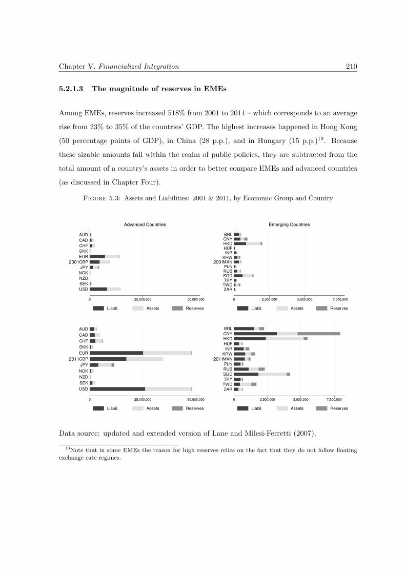
Chapter V. Financialized Integration 210
5.2.1.3 The magnitude of reserves in EMEs
Among EMEs, reserves increased 518% from 2001 to 2011 – which corresponds to an average
rise from 23% to 35% of the countries’ GDP. The highest increases happened in Hong Kong
(50 percentage points of GDP), in China (28 p.p.), and in Hungary (15 p.p.)19. Because
these sizable amounts fall within the realm of public policies, they are subtracted from the
total amount of a country’s assets in order to better compare EMEs and advanced countries
(as discussed in Chapter Four).
Figure 5.3: Assets and Liabilities: 2001 & 2011, by Economic Group and Country
0 25,000,000 50,000,000
2001
USD
SEK
NZD
NOK
JPY
GBP
EUR
DKK
CHF
CAD
AUD
Advanced Countries
Liabil. Assets Reserves
0 25,000,000 50,000,000
2011
USD
SEK
NZD
NOK
JPY
GBP
EUR
DKK
CHF
CAD
AUD
Liabil. Assets Reserves
0 2,500,000 5,000,000 7,500,000
2001
ZARTWDTRYSGDRUBPLNMXNKRW
INRHUFHKDCNYBRL
Emerging Countries
Liabil. Assets Reserves
0 2,500,000 5,000,000 7,500,000
2011
ZARTWDTRYSGDRUBPLNMXNKRW
INRHUFHKDCNYBRL
Liabil. Assets Reserves
Data source: updated and extended version of Lane and Milesi-Ferretti (2007).
19Note that in some EMEs the reason for high reserves relies on the fact that they do not follow floatingexchange rate regimes.
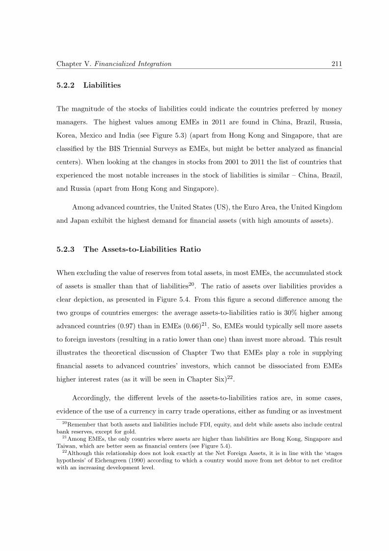
Chapter V. Financialized Integration 211
5.2.2 Liabilities
The magnitude of the stocks of liabilities could indicate the countries preferred by money
managers. The highest values among EMEs in 2011 are found in China, Brazil, Russia,
Korea, Mexico and India (see Figure 5.3) (apart from Hong Kong and Singapore, that are
classified by the BIS Triennial Surveys as EMEs, but might be better analyzed as financial
centers). When looking at the changes in stocks from 2001 to 2011 the list of countries that
experienced the most notable increases in the stock of liabilities is similar – China, Brazil,
and Russia (apart from Hong Kong and Singapore).
Among advanced countries, the United States (US), the Euro Area, the United Kingdom
and Japan exhibit the highest demand for financial assets (with high amounts of assets).
5.2.3 The Assets-to-Liabilities Ratio
When excluding the value of reserves from total assets, in most EMEs, the accumulated stock
of assets is smaller than that of liabilities20. The ratio of assets over liabilities provides a
clear depiction, as presented in Figure 5.4. From this figure a second difference among the
two groups of countries emerges: the average assets-to-liabilities ratio is 30% higher among
advanced countries (0.97) than in EMEs (0.66)21. So, EMEs would typically sell more assets
to foreign investors (resulting in a ratio lower than one) than invest more abroad. This result
illustrates the theoretical discussion of Chapter Two that EMEs play a role in supplying
financial assets to advanced countries’ investors, which cannot be dissociated from EMEs
higher interest rates (as it will be seen in Chapter Six)22.
Accordingly, the different levels of the assets-to-liabilities ratios are, in some cases,
evidence of the use of a currency in carry trade operations, either as funding or as investment
20Remember that both assets and liabilities include FDI, equity, and debt while assets also include centralbank reserves, except for gold.
21Among EMEs, the only countries where assets are higher than liabilities are Hong Kong, Singapore andTaiwan, which are better seen as financial centers (see Figure 5.4).
22Although this relationship does not look exactly at the Net Foreign Assets, it is in line with the ‘stageshypothesis’ of Eichengreen (1990) according to which a country would move from net debtor to net creditorwith an increasing development level.
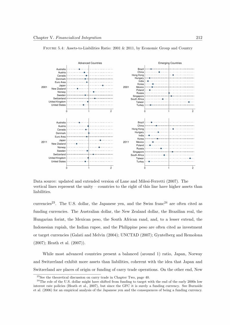
Chapter V. Financialized Integration 212
Figure 5.4: Assets-to-Liabilities Ratio: 2001 & 2011, by Economic Group and Country
0 1 2
2001
United States
United Kingdom
Switzerland
Sweden
Norway
New Zealand
Japan
Euro Area
Denmark
Canada
Austria
Australia
Advanced Countries
0 1 2
2011
United States
United Kingdom
Switzerland
Sweden
Norway
New Zealand
Japan
Euro Area
Denmark
Canada
Austria
Australia
0 1 2
2001
Turkey
Taiwan
South Africa
Singapore
Russia
Poland
Mexico
Korea
India
Hungary
Hong Kong
China
Brazil
Emerging Countries
0 1 2
2011
Turkey
Taiwan
South Africa
Singapore
Russia
Poland
Mexico
Korea
India
Hungary
Hong Kong
China
Brazil
Data source: updated and extended version of Lane and Milesi-Ferretti (2007). Thevertical lines represent the unity – countries to the right of this line have higher assets thanliabilities.
currencies23. The U.S. dollar, the Japanese yen, and the Swiss franc24 are often cited as
funding currencies. The Australian dollar, the New Zealand dollar, the Brazilian real, the
Hungarian forint, the Mexican peso, the South African rand, and, to a lesser extend, the
Indonesian rupiah, the Indian rupee, and the Philippine peso are often cited as investment
or target currencies (Galati and Melvin (2004); UNCTAD (2007); Gyntelberg and Remolona
(2007); Heath et al. (2007)).
While most advanced countries present a balanced (around 1) ratio, Japan, Norway
and Switzerland exhibit more assets than liabilities, coherent with the idea that Japan and
Switzerland are places of origin or funding of carry trade operations. On the other end, New
23See the theoretical discussion on carry trade in Chapter Two, page 40.24The role of the U.S. dollar might have shifted from funding to target with the end of the early 2000s low
interest rate policies (Heath et al., 2007), but since the GFC it is surely a funding currency. See Burnsideet al. (2006) for an empirical analysis of the Japanese yen and the consequences of being a funding currency.
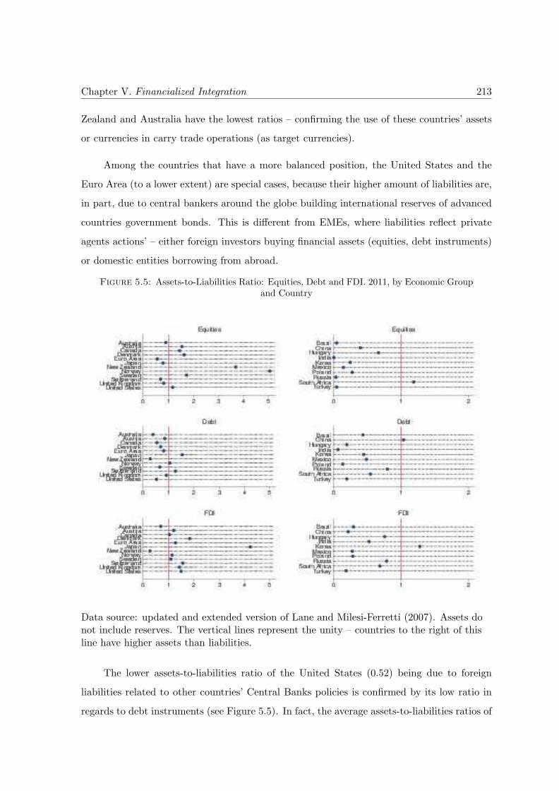
Chapter V. Financialized Integration 213
Zealand and Australia have the lowest ratios – confirming the use of these countries’ assets
or currencies in carry trade operations (as target currencies).
Among the countries that have a more balanced position, the United States and the
Euro Area (to a lower extent) are special cases, because their higher amount of liabilities are,
in part, due to central bankers around the globe building international reserves of advanced
countries government bonds. This is different from EMEs, where liabilities reflect private
agents actions’ – either foreign investors buying financial assets (equities, debt instruments)
or domestic entities borrowing from abroad.
Figure 5.5: Assets-to-Liabilities Ratio: Equities, Debt and FDI. 2011, by Economic Groupand Country
Data source: updated and extended version of Lane and Milesi-Ferretti (2007). Assets donot include reserves. The vertical lines represent the unity – countries to the right of thisline have higher assets than liabilities.
The lower assets-to-liabilities ratio of the United States (0.52) being due to foreign
liabilities related to other countries’ Central Banks policies is confirmed by its low ratio in
regards to debt instruments (see Figure 5.5). In fact, the average assets-to-liabilities ratios of
Chapter V. Financialized Integration 214
advanced countries are higher for equities (1.71) and FDI (1.43), and lower for debt (0.82).
For EMEs, on the other hand, the ratios are low for all three categories, equities (0.31), debt
(0.44), and FDI (0.53) (when Taiwan, Singapore and Hong Kong are not considered). Among
advanced countries, Japan (1.54) and Switzerland (1.27) present the highest ratios regarding
debt instruments, while New Zealand (0.28) and Australia (0.38) present the lowest ones,
confirming the association of these two groups of countries on opposing ends of carry trade
operations.
Among EMEs, the lowest assets-to-liabilities ratio in the form of debt are India, Poland,
Turkey, Hungary and Brazil. Of these five countries, Turkey, Brazil and India are cited in
the literature as target currencies for carry trade operations and are among the five countries
to present the highest interest rate differential with regards to the US Fed Fund rate.
5.2.4 Absolute Financial Integration
Knowing the characteristics of assets and liabilities in the two country groups, the analysis
continues with indicators of financial integration. The first, the sum of assets and liabilities,
is an indicator of absolute integration.
Analyzed through the value of assets plus liabilities of EMEs in 2011, China, Brazil,
Russia and Korea25 are the most financially integrated (see Figure 5.6). Hungary had the
lowest integration level in 2001 (seven times lower than EMEs’ average) and grew 730%
between the two periods. China and India also presented high growth rates. Among advanced
countries, the US, the Euro Area and the United Kingdom are the most integrated. Japan
is next, but with a value three times lower.
5.2.5 Financial Integration Relative to GDP
The evolution of the ratio of assets and liabilities over GDP supports the idea that advanced
countries have undergone a greater process of integration than emerging (or other developing
countries), with a higher than six average ratio in 2011 (see Figure 5.7). The result reflects
25Apart from Hong Kong, Singapore and Taiwan
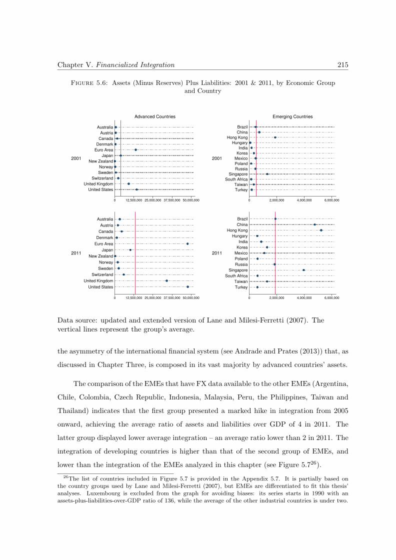
Chapter V. Financialized Integration 215
Figure 5.6: Assets (Minus Reserves) Plus Liabilities: 2001 & 2011, by Economic Groupand Country
0 12,500,000 25,000,000 37,500,000 50,000,000
2001
United States
United Kingdom
Switzerland
Sweden
Norway
New Zealand
Japan
Euro Area
Denmark
Canada
Austria
Australia
Advanced Countries
0 12,500,000 25,000,000 37,500,000 50,000,000
2011
United States
United Kingdom
Switzerland
Sweden
Norway
New Zealand
Japan
Euro Area
Denmark
Canada
Austria
Australia
0 2,000,000 4,000,000 6,000,000
2001
Turkey
Taiwan
South Africa
Singapore
Russia
Poland
Mexico
Korea
India
Hungary
Hong Kong
China
Brazil
Emerging Countries
0 2,000,000 4,000,000 6,000,000
2011
Turkey
Taiwan
South Africa
Singapore
Russia
Poland
Mexico
Korea
India
Hungary
Hong Kong
China
Brazil
Data source: updated and extended version of Lane and Milesi-Ferretti (2007). Thevertical lines represent the group’s average.
the asymmetry of the international financial system (see Andrade and Prates (2013)) that, as
discussed in Chapter Three, is composed in its vast majority by advanced countries’ assets.
The comparison of the EMEs that have FX data available to the other EMEs (Argentina,
Chile, Colombia, Czech Republic, Indonesia, Malaysia, Peru, the Philippines, Taiwan and
Thailand) indicates that the first group presented a marked hike in integration from 2005
onward, achieving the average ratio of assets and liabilities over GDP of 4 in 2011. The
latter group displayed lower average integration – an average ratio lower than 2 in 2011. The
integration of developing countries is higher than that of the second group of EMEs, and
lower than the integration of the EMEs analyzed in this chapter (see Figure 5.726).
26The list of countries included in Figure 5.7 is provided in the Appendix 5.7. It is partially based onthe country groups used by Lane and Milesi-Ferretti (2007), but EMEs are differentiated to fit this thesis’analyses. Luxembourg is excluded from the graph for avoiding biases: its series starts in 1990 with anassets-plus-liabilities-over-GDP ratio of 136, while the average of the other industrial countries is under two.
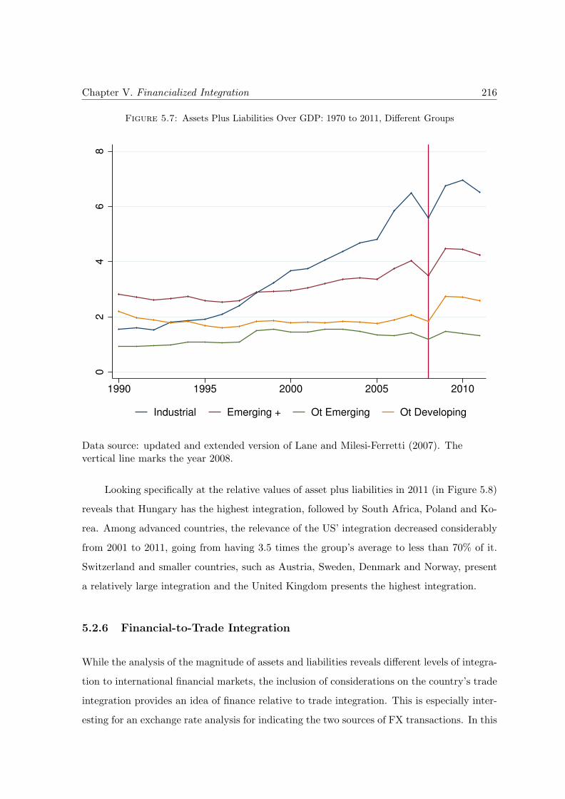
Chapter V. Financialized Integration 216
Figure 5.7: Assets Plus Liabilities Over GDP: 1970 to 2011, Different Groups
02
46
8
1990 1995 2000 2005 2010
Industrial Emerging + Ot Emerging Ot Developing
Data source: updated and extended version of Lane and Milesi-Ferretti (2007). Thevertical line marks the year 2008.
Looking specifically at the relative values of asset plus liabilities in 2011 (in Figure 5.8)
reveals that Hungary has the highest integration, followed by South Africa, Poland and Ko-
rea. Among advanced countries, the relevance of the US’ integration decreased considerably
from 2001 to 2011, going from having 3.5 times the group’s average to less than 70% of it.
Switzerland and smaller countries, such as Austria, Sweden, Denmark and Norway, present
a relatively large integration and the United Kingdom presents the highest integration.
5.2.6 Financial-to-Trade Integration
While the analysis of the magnitude of assets and liabilities reveals different levels of integra-
tion to international financial markets, the inclusion of considerations on the country’s trade
integration provides an idea of finance relative to trade integration. This is especially inter-
esting for an exchange rate analysis for indicating the two sources of FX transactions. In this
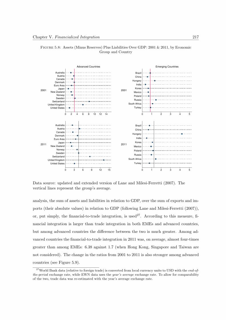
Chapter V. Financialized Integration 217
Figure 5.8: Assets (Minus Reserves) Plus Liabilities Over GDP: 2001 & 2011, by EconomicGroup and Country
0 2 4 6 8 10 12 14
2001
United States
United Kingdom
Switzerland
Sweden
Norway
New Zealand
Japan
Euro Area
Denmark
Canada
Austria
Australia
Advanced Countries
0 3 6 9 12 15
2011
United States
United Kingdom
Switzerland
Sweden
Norway
New Zealand
Japan
Euro Area
Denmark
Canada
Austria
Australia
0 1 2 3 4 5
2001
Turkey
South Africa
Russia
Poland
Mexico
Korea
India
Hungary
China
Brazil
Emerging Countries
0 1 2 3 4 5
2011
Turkey
South Africa
Russia
Poland
Mexico
Korea
India
Hungary
China
Brazil
Data source: updated and extended version of Lane and Milesi-Ferretti (2007). Thevertical lines represent the group’s average.
analysis, the sum of assets and liabilities in relation to GDP, over the sum of exports and im-
ports (their absolute values) in relation to GDP (following Lane and Milesi-Ferretti (2007)),
or, put simply, the financial-to-trade integration, is used27. According to this measure, fi-
nancial integration is larger than trade integration in both EMEs and advanced countries,
but among advanced countries the difference between the two is much greater. Among ad-
vanced countries the financial-to-trade integration in 2011 was, on average, almost four-times
greater than among EMEs: 6.38 against 1.7 (when Hong Kong, Singapore and Taiwan are
not considered). The change in the ratios from 2001 to 2011 is also stronger among advanced
countries (see Figure 5.9).
27World Bank data (relative to foreign trade) is converted from local currency units to USD with the end-of-the-period exchange rate, while EWN data uses the year’s average exchange rate. To allow for comparabilityof the two, trade data was re-estimated with the year’s average exchange rate.
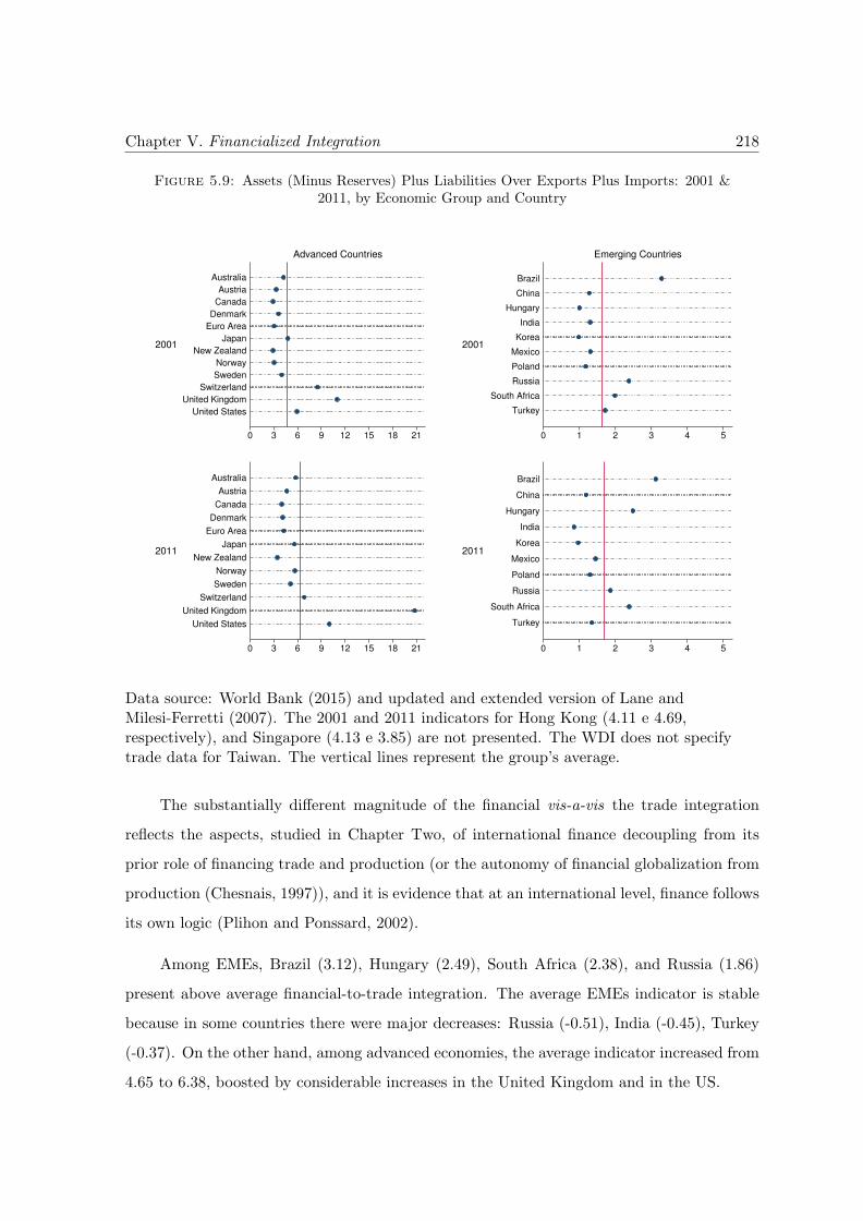
Chapter V. Financialized Integration 218
Figure 5.9: Assets (Minus Reserves) Plus Liabilities Over Exports Plus Imports: 2001 &2011, by Economic Group and Country
0 3 6 9 12 15 18 21
2001
United States
United Kingdom
Switzerland
Sweden
Norway
New Zealand
Japan
Euro Area
Denmark
Canada
Austria
Australia
Advanced Countries
0 3 6 9 12 15 18 21
2011
United States
United Kingdom
Switzerland
Sweden
Norway
New Zealand
Japan
Euro Area
Denmark
Canada
Austria
Australia
0 1 2 3 4 5
2001
Turkey
South Africa
Russia
Poland
Mexico
Korea
India
Hungary
China
Brazil
Emerging Countries
0 1 2 3 4 5
2011
Turkey
South Africa
Russia
Poland
Mexico
Korea
India
Hungary
China
Brazil
Data source: World Bank (2015) and updated and extended version of Lane andMilesi-Ferretti (2007). The 2001 and 2011 indicators for Hong Kong (4.11 e 4.69,respectively), and Singapore (4.13 e 3.85) are not presented. The WDI does not specifytrade data for Taiwan. The vertical lines represent the group’s average.
The substantially different magnitude of the financial vis-a-vis the trade integration
reflects the aspects, studied in Chapter Two, of international finance decoupling from its
prior role of financing trade and production (or the autonomy of financial globalization from
production (Chesnais, 1997)), and it is evidence that at an international level, finance follows
its own logic (Plihon and Ponssard, 2002).
Among EMEs, Brazil (3.12), Hungary (2.49), South Africa (2.38), and Russia (1.86)
present above average financial-to-trade integration. The average EMEs indicator is stable
because in some countries there were major decreases: Russia (-0.51), India (-0.45), Turkey
(-0.37). On the other hand, among advanced economies, the average indicator increased from
4.65 to 6.38, boosted by considerable increases in the United Kingdom and in the US.
Chapter V. Financialized Integration 219
This different path reflects that, among advanced countries, the growth of assets’ trade
was huge while of goods’ trade, only modest. Among developing countries the opposite
happened: the growth in asset trade was rather weak, and trade in goods increased rapidly
(Lane and Milesi-Ferretti, 2007), reflecting the commodities’ boom.
5.2.7 Concluding Remarks
The analyses of financial integration have shown that advanced countries are significantly
more integrated than EMEs. When trade or GDP levels are considered, this difference
decreases, but advanced countries remain more financialized.
The analyses of the assets-to-liabilities ratios support the argument of an increasing
use of canonical carry trade operations. The low assets-to-liabilities ratio of the Brazilian
real, the Turkish lira, and the Indian rupee confirm their use as target currencies. These are
also among the EMEs to present the five highest interest rate differentials with the US Fed
Fund rate28. Among advanced currencies, Japan and Switzerland’s great assets-to-liabilities
ratios support the idea of the high use of the Japanese yen and the Swiss franc as funding
currencies. Other often mentioned funding currencies, the U.S. dollar and the euro, which
hold important foreign liabilities related to developing countries’ reserves policies, and thus,
present lower assets-to-liabilities ratios. The Australian and the New Zealand dollar, notable
target currencies, have the lowest assets-to-liabilities ratio among advanced countries.
The overall lower assets-to-liabilities ratios of EMEs confirms the argument that EMEs
play a role in the international financial system (IFS) of suppliers of financial assets of
a specific class of risk29. As reserves are withdrawn, the asset-to-liability indicators are
focused on the private sphere. When expanded to include the public sphere, the role of
EMEs in international financial markets also includes the purchases of advanced countries
governments’ liabilities: reserves of international assets reached 37% of EMEs’ foreign assets
in 201130. Reserves’ dynamics are however markedly different from that of money managers’
28Fore EMEs’ interest rates see Figures 6.25 and 6.26 in the Appendix of Chapter Six.29The insertion of EMEs in the IFS as suppliers of financial assets is discussed in Chapter Two. The debate
on the specificities of emerging currencies is presented in Chapter Three. In the analysis presented in ChapterSeven, money managers incur an exchange rate risk when investing in assets from both EMEs or advancedcountries other than the one where their liabilities are issued. However, investments in EMEs’ assets areassociated with a safety smaller margin, given that the range of possible exchange rate returns is larger.
30This refers to the 13 EMEs with the largest FX markets studied in this chapter.
Chapter V. Financialized Integration 220
(that will be further discussed in Chapter Seven). It is a stable form of holding capital, with
no intention of gaining with total returns. In some cases this policy is even associated with
sterilization costs that are greater than foreign assets’ returns (Jeanne (2007); Ramos (2010),
Ranciere and Jeanne (2006)).
These policies’ focus on maintaining a high and stable level of assets is also confirmed by
the very marginal use of reserves in the wake of the GFC (Aizenman and Hutchison, 2012).
In addition, being focused on decreasing exchange rate volatility the policy of reserves acts
in the opposite direction of private investors, having (if any) a counter cyclical influence not
only in the emerging currency, but also in the advanced country’s currency. Money managers’
behavior, on the other hand, is marked by speculation with world-wide assets, and might
result in domestic asset prices and exchange rates that are volatile and associated to the
international sphere (as it will be seen in the next chapter).
This difference in the dynamics of (part of) the demand for EMEs’ and advanced coun-
tries’ assets can be seen as an additional form of asymmetry of the IFS; i.e. an asymmetry of
the behavior of demand. The demand of EMEs’ assets is marked by speculation while part of
the demand of advanced countries is marked by stability and counter-cyclical behavior. This
asymmetry derives from the fact that emerging currencies are not used internationally as
reserve of value (as discussed in Chapter Three)31.
5.3 Increasing Importance of FX Transactions
This section discusses FX markets in order to further characterize financial integration,
demonstrating the sophistication of finance and its potential consequences. It analyzes
the changes that took place over time and the differences between EMEs and advanced
economies. It examines the total (absolute or relative) size of FX markets and the relative
weight of derivatives and spot markets. Both measures are used as proxies of financialization
in the literature. The first, the size of FX markets, indicates both the aspect of increasing
importance of finance internationally (as did Chesnais (1997) and Epstein (2005)) and the
31As discussed in Chapter Three, the IFS is also characterized by an asymmetric weight of advanced andEMEs’ assets. In the specific discussed here, the fact that emerging currencies do not exercise a functionof reserve of value internationally is represented by the fact that EMEs’ assets are not used as internationalreserves of public entities of advanced countries.
Chapter V. Financialized Integration 221
sophistication of finance, as it is evidence of the rise of carry trade operations (as argued by
Galati and Melvin (2004)). The second measure, the size of derivatives markets, proxies the
sophistication of FX markets and the importance of operations as derivatives carry trading.
5.3.1 Total FX Market
Between 2001 and 2013 FX markets underwent major changes in different aspects. Its total
size exceeded US$ 4 trillion (daily), four-folding from 2001’s level32. The participation of
emerging currencies in total contracts doubled, achieving 8.4% (see Table 5.6 for details
on the market size of emerging currencies in 2001 and 2013, and Table 5.5 for data on
advanced countries). Although the importance of emerging currencies internationally has
significantly changed, they still count for a small part of total transactions (see Figure 5.14).
It is further evidence of the hypotheses of asymmetries of the international financial and
monetary systems (discussed in Chapter Three).
In 2001, the transactions in the Chinese yuan accounted for only 0.1% of the EMEs’
market, but presented the highest growth rate, 108,385%. The amount of contracts denom-
inated in the Turkish lira and the Hungarian forint also grew significantly (14,746% and
10,678% respectively). The remaining currencies grew less, but still at a high pace: an
average of 806%, almost double of advanced countries’ average (422%).
In 2013, the Mexican peso was the emerging currency to be traded the most, representing
15.7% of total EMEs’ markets (see Figure 5.10). It was followed by the Chinese yuan (that
accounted for 12.5%), the Russian ruble (10.1%), the Turkish lira (7.9%), the Korean won
(7.3%) and the South African rand (7.1%) (apart from the Honk Kong dollar (9.3%), and the
Singaporean dollar (8.7%)). Among advanced economies, the U.S. dollar is by far the most
traded currency, its FX market being more than twice that of the euro, the second biggest
market. The Japanese yen and the Great Britain pound come next.
Among currencies from advanced countries, the order of magnitude of the different
markets has not changed from the 2001 survey. Among emerging currencies the relative
importance of FX markets varied: the Mexican peso and the Korean won remained among
the five most important currencies, but the South African rand, the Polish zloty, and the
32For an overall presentation of the 2013 results, see Rime and Schrimpf (2013).
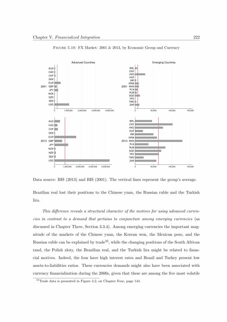
Chapter V. Financialized Integration 222
Figure 5.10: FX Market: 2001 & 2013, by Economic Group and Currency
0 1,000,000 2,000,000 3,000,000 4,000,000
2001
USD
SEK
NZD
NOK
JPY
GBP
EUR
DKK
CHF
CAD
AUD
Advanced Countries
0 1,000,000 2,000,000 3,000,000 4,000,000
2013
USD
SEK
NZD
NOK
JPY
GBP
EUR
DKK
CHF
CAD
AUD
0 50,000 100,000 150,000
2001
ZAR
TWD
TRY
SGD
RUB
PLN
MXN
KRW
INR
HUF
HKD
CNY
BRL
Emerging Countries
0 50,000 100,000 150,000
2013
ZAR
TWD
TRY
SGD
RUB
PLN
MXN
KRW
INR
HUF
HKD
CNY
BRL
Data source: BIS (2013) and BIS (2001). The vertical lines represent the group’s average.
Brazilian real lost their positions to the Chinese yuan, the Russian ruble and the Turkish
lira.
This difference reveals a structural character of the motives for using advanced curren-
cies in contrast to a demand that pertains to conjuncture among emerging currencies (as
discussed in Chapter Three, Section 3.3.4). Among emerging currencies the important mag-
nitude of the markets of the Chinese yuan, the Korean won, the Mexican peso, and the
Russian ruble can be explained by trade33, while the changing positions of the South African
rand, the Polish zloty, the Brazilian real, and the Turkish lira might be related to finan-
cial motives. Indeed, the four have high interest rates and Brazil and Turkey present low
assets-to-liabilities ratios. These currencies demands might also have been associated with
currency financialization during the 2000s, given that these are among the five most volatile
33Trade data is presented in Figure 4.2, on Chapter Four, page 144.
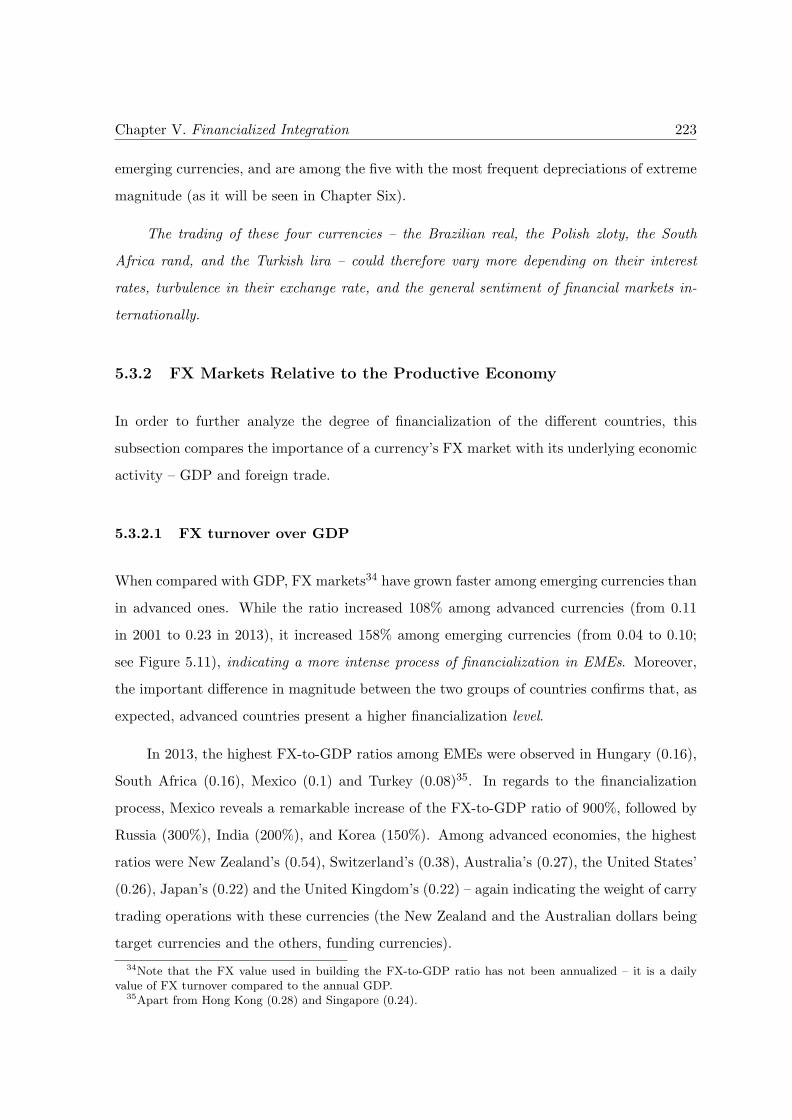
Chapter V. Financialized Integration 223
emerging currencies, and are among the five with the most frequent depreciations of extreme
magnitude (as it will be seen in Chapter Six).
The trading of these four currencies – the Brazilian real, the Polish zloty, the South
Africa rand, and the Turkish lira – could therefore vary more depending on their interest
rates, turbulence in their exchange rate, and the general sentiment of financial markets in-
ternationally.
5.3.2 FX Markets Relative to the Productive Economy
In order to further analyze the degree of financialization of the different countries, this
subsection compares the importance of a currency’s FX market with its underlying economic
activity – GDP and foreign trade.
5.3.2.1 FX turnover over GDP
When compared with GDP, FX markets34 have grown faster among emerging currencies than
in advanced ones. While the ratio increased 108% among advanced currencies (from 0.11
in 2001 to 0.23 in 2013), it increased 158% among emerging currencies (from 0.04 to 0.10;
see Figure 5.11), indicating a more intense process of financialization in EMEs. Moreover,
the important difference in magnitude between the two groups of countries confirms that, as
expected, advanced countries present a higher financialization level.
In 2013, the highest FX-to-GDP ratios among EMEs were observed in Hungary (0.16),
South Africa (0.16), Mexico (0.1) and Turkey (0.08)35. In regards to the financialization
process, Mexico reveals a remarkable increase of the FX-to-GDP ratio of 900%, followed by
Russia (300%), India (200%), and Korea (150%). Among advanced economies, the highest
ratios were New Zealand’s (0.54), Switzerland’s (0.38), Australia’s (0.27), the United States’
(0.26), Japan’s (0.22) and the United Kingdom’s (0.22) – again indicating the weight of carry
trading operations with these currencies (the New Zealand and the Australian dollars being
target currencies and the others, funding currencies).
34Note that the FX value used in building the FX-to-GDP ratio has not been annualized – it is a dailyvalue of FX turnover compared to the annual GDP.
35Apart from Hong Kong (0.28) and Singapore (0.24).
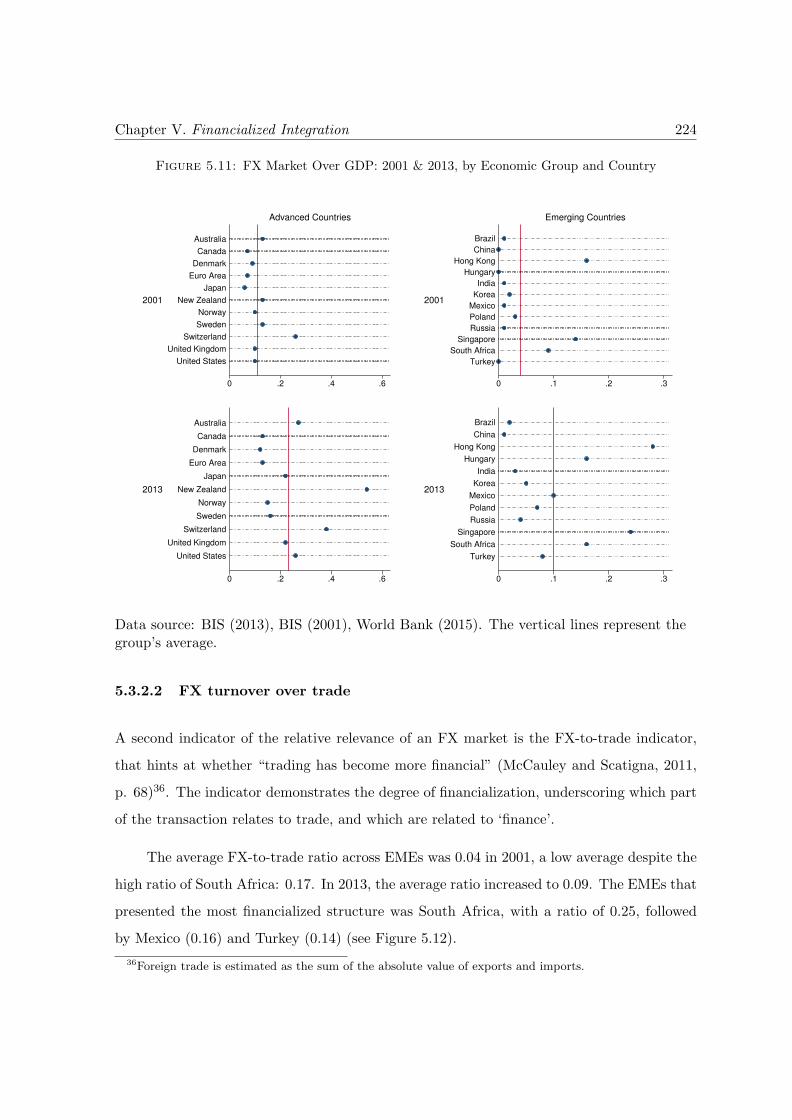
Chapter V. Financialized Integration 224
Figure 5.11: FX Market Over GDP: 2001 & 2013, by Economic Group and Country
0 .2 .4 .6
2001
United States
United Kingdom
Switzerland
Sweden
Norway
New Zealand
Japan
Euro Area
Denmark
Canada
Australia
Advanced Countries
0 .2 .4 .6
2013
United States
United Kingdom
Switzerland
Sweden
Norway
New Zealand
Japan
Euro Area
Denmark
Canada
Australia
0 .1 .2 .3
2001
Turkey
South Africa
Singapore
Russia
Poland
Mexico
Korea
India
Hungary
Hong Kong
China
Brazil
Emerging Countries
0 .1 .2 .3
2013
Turkey
South Africa
Singapore
Russia
Poland
Mexico
Korea
India
Hungary
Hong Kong
China
Brazil
Data source: BIS (2013), BIS (2001), World Bank (2015). The vertical lines represent thegroup’s average.
5.3.2.2 FX turnover over trade
A second indicator of the relative relevance of an FX market is the FX-to-trade indicator,
that hints at whether “trading has become more financial” (McCauley and Scatigna, 2011,
p. 68)36. The indicator demonstrates the degree of financialization, underscoring which part
of the transaction relates to trade, and which are related to ‘finance’.
The average FX-to-trade ratio across EMEs was 0.04 in 2001, a low average despite the
high ratio of South Africa: 0.17. In 2013, the average ratio increased to 0.09. The EMEs that
presented the most financialized structure was South Africa, with a ratio of 0.25, followed
by Mexico (0.16) and Turkey (0.14) (see Figure 5.12).
36Foreign trade is estimated as the sum of the absolute value of exports and imports.
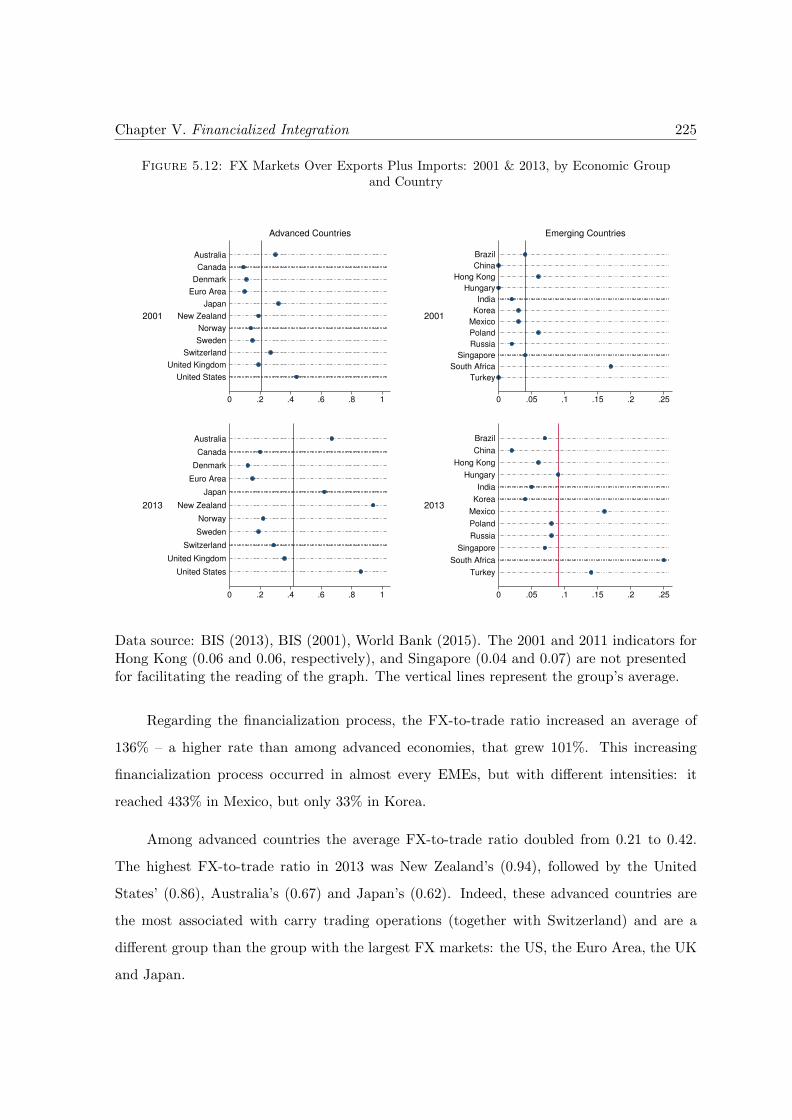
Chapter V. Financialized Integration 225
Figure 5.12: FX Markets Over Exports Plus Imports: 2001 & 2013, by Economic Groupand Country
0 .2 .4 .6 .8 1
2001
United States
United Kingdom
Switzerland
Sweden
Norway
New Zealand
Japan
Euro Area
Denmark
Canada
Australia
Advanced Countries
0 .2 .4 .6 .8 1
2013
United States
United Kingdom
Switzerland
Sweden
Norway
New Zealand
Japan
Euro Area
Denmark
Canada
Australia
0 .05 .1 .15 .2 .25
2001
Turkey
South Africa
Singapore
Russia
Poland
Mexico
Korea
India
Hungary
Hong Kong
China
Brazil
Emerging Countries
0 .05 .1 .15 .2 .25
2013
Turkey
South Africa
Singapore
Russia
Poland
Mexico
Korea
India
Hungary
Hong Kong
China
Brazil
Data source: BIS (2013), BIS (2001), World Bank (2015). The 2001 and 2011 indicators forHong Kong (0.06 and 0.06, respectively), and Singapore (0.04 and 0.07) are not presentedfor facilitating the reading of the graph. The vertical lines represent the group’s average.
Regarding the financialization process, the FX-to-trade ratio increased an average of
136% – a higher rate than among advanced economies, that grew 101%. This increasing
financialization process occurred in almost every EMEs, but with different intensities: it
reached 433% in Mexico, but only 33% in Korea.
Among advanced countries the average FX-to-trade ratio doubled from 0.21 to 0.42.
The highest FX-to-trade ratio in 2013 was New Zealand’s (0.94), followed by the United
States’ (0.86), Australia’s (0.67) and Japan’s (0.62). Indeed, these advanced countries are
the most associated with carry trading operations (together with Switzerland) and are a
different group than the group with the largest FX markets: the US, the Euro Area, the UK
and Japan.
Chapter V. Financialized Integration 226
The FX-to-trade ratios of EMEs are four-times lower than that of advanced countries,
indicating a lower degree of financialization among them. However, the process has been
more intense in EMEs.
5.3.3 Spot and Derivatives Markets
As argued in Chapter Two, derivatives contracts are essential to understand the possible con-
sequences of financial integration on emerging currencies, because their leverage possibilities
make them excellent tools for speculation and because they can also increase exchange rate
volatility for being an extra conduit of determination of spot rates. Derivatives FX markets
also proxy the overall level of sophistication of a country’s markets, evincing the extent of
the investment possibilities offered to money managers.
When analyzing BIS data on derivatives, it must be noted that the dataset only includes
data on over-the-counter (OTC) markets. Indeed, OTC are the predominant places of deriva-
tives trade in most countries, but in Brazil, Korea and India, the derivatives transactions
in organized markets would be most significant (McCauley and Scatigna, 2011)37. However,
according to Fritz and Prates (2014), in Korea, considering only onshore transactions, FX
turnover in the OTC market is higher than exchange-traded turnover.
When looking at emerging and advanced currencies combined, spot contracts increased
more (444%) than derivatives contracts (274%). With the slower growth, derivatives con-
tracts lost weight in total market (from 67% to 59%), but remain larger than spot contracts
(see Figure 5.13 for the absolute size of each type of contract). This is due to the highest
increase of spot contracts among advanced currencies (532% versus 352% of derivatives).
The opposite happened among emerging currencies: derivatives contracts grew faster than
37As put by McCauley and Scatigna (2011, p. 68): “Foreign exchange turnover includes not only over-the-counter but also exchange-traded turnover, which is most significant for the Brazilian real, the Indianrupee and the Korean won.” McCauley and Scatigna (2011) estimate the total size of derivatives markets,adding contracts traded in OTC and organized markets. The data source for the organized markets is howeverproprietary and there are no details on how it is calculated to overcome the incompatibility of the two, givenhow differently operations are closed. That is because in organized markets, when a participant wants to closean operation it makes an opposite operation. In OTC markets, on the other hand, participants take a positionidentical to the old one, but with opposite signs, which leads to double counting of operations that are ‘closed’(Farhi, 1998). On the high liquidity of the derivatives market of the Brazilian real, see Farhi (2006), Farhi(2010), Fritz and Prates (2014), Garcia and Urban (2004), Kaltenbrunner (2010), Prates (2015), Ventura andGarcia (2012), and Rossi (2016).
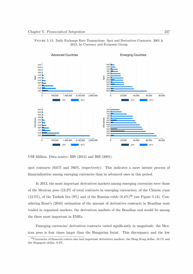
Chapter V. Financialized Integration 227
Figure 5.13: Daily Exchange Rate Transactions: Spot and Derivatives Contracts. 2001 &2013, by Currency and Economic Group
0 700,000 1,400,000 2,100,000 2,800,000
USD
EUR
JPY
GBP
AUD
CAD
CHF
NZD
SEK
NOK
DKK
Spot
2001 2013
0 700,000 1,400,000 2,100,000 2,800,000
USD
EUR
JPY
GBP
AUD
CHF
CAD
SEK
NZD
NOK
DKK
Derivatives
2001 2013
Advanced Countries
0 20,000 40,000 60,000 80,000
MXN
RUB
CNY
HKD
SGD
KRW
ZAR
TRY
INR
BRL
PLN
HUF
TWD
Spot
2001 2013
0 20,000 40,000 60,000 80,000
MXN
CNY
HKD
SGD
TRY
RUB
KRW
ZAR
BRL
INR
PLN
TWD
HUF
Derivatives
2001 2013
Emerging Countries
US$ Million. Data source: BIS (2013) and BIS (2001).
spot contracts (931% and 766%, respectively). This indicates a more intense process of
financialization among emerging currencies than in advanced ones in this period.
In 2013, the most important derivatives markets among emerging currencies were those
of the Mexican peso (13.2% of total contracts in emerging currencies), of the Chinese yuan
(12.5%), of the Turkish lira (9%) and of the Russian ruble (8.4%)38 (see Figure 5.14). Con-
sidering Rossi’s (2016) estimation of the amount of derivatives contracts in Brazilian reais
traded in organized markets, the derivatives markets of the Brazilian real would be among
the three most important in EMEs.
Emerging currencies’ derivatives contracts varied significantly in magnitude: the Mex-
ican peso is four times larger than the Hungarian forint. This discrepancy and the low
38Currencies of financial centers also had important derivatives markets: the Hong Kong dollar, 10.1% andthe Singapore dollar, 9.3%.
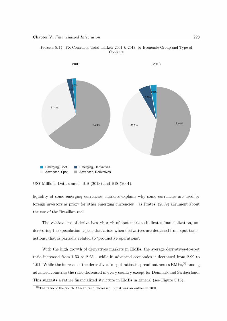
Chapter V. Financialized Integration 228
Figure 5.14: FX Contracts, Total market: 2001 & 2013, by Economic Group and Type ofContract
64.6%
31.2%
2.6%
1.6%
Emerging, Spot Emerging, Derivatives
Advanced, Spot Advanced, Derivatives
2001
53.0%38.6%
5.6%
2.8%
2013
US$ Million. Data source: BIS (2013) and BIS (2001).
liquidity of some emerging currencies’ markets explains why some currencies are used by
foreign investors as proxy for other emerging currencies – as Prates’ (2009) argument about
the use of the Brazilian real.
The relative size of derivatives vis-a-vis of spot markets indicates financialization, un-
derscoring the speculation aspect that arises when derivatives are detached from spot trans-
actions, that is partially related to ‘productive operations’.
With the high growth of derivatives markets in EMEs, the average derivatives-to-spot
ratio increased from 1.53 to 2.25 – while in advanced economies it decreased from 2.99 to
1.91. While the increase of the derivatives-to-spot ratios is spread-out across EMEs,39 among
advanced countries the ratio decreased in every country except for Denmark and Switzerland.
This suggests a rather financialized structure in EMEs in general (see Figure 5.15).
39The ratio of the South African rand decreased, but it was an outlier in 2001.
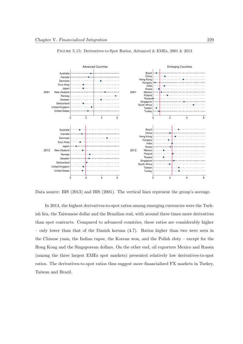
Chapter V. Financialized Integration 229
Figure 5.15: Derivatives-to-Spot Ratios, Advanced & EMEs, 2001 & 2013
0 2 4 6
2001
United States
United Kingdom
Switzerland
Sweden
Norway
New Zealand
Japan
Euro Area
Denmark
Canada
Australia
Advanced Countries
0 2 4 6
2013
United States
United Kingdom
Switzerland
Sweden
Norway
New Zealand
Japan
Euro Area
Denmark
Canada
Australia
0 2 4 6
2001
Turkey
Taiwan
South Africa
Singapore
Russia
Poland
Mexico
Korea
India
Hungary
Hong Kong
China
Brazil
Emerging Countries
0 2 4 6
2013
Turkey
Taiwan
South Africa
Singapore
Russia
Poland
Mexico
Korea
India
Hungary
Hong Kong
China
Brazil
Data source: BIS (2013) and BIS (2001). The vertical lines represent the group’s average.
In 2013, the highest derivatives-to-spot ratios among emerging currencies were the Turk-
ish lira, the Taiwanese dollar and the Brazilian real, with around three times more derivatives
than spot contracts. Compared to advanced countries, these ratios are considerably higher
– only lower than that of the Danish koruna (4.7). Ratios higher than two were seen in
the Chinese yuan, the Indian rupee, the Korean won, and the Polish zloty – except for the
Hong Kong and the Singaporean dollars. On the other end, oil exporters Mexico and Russia
(among the three largest EMEs spot markets) presented relatively low derivatives-to-spot
ratios. The derivatives-to-spot ratios thus suggest more financialized FX markets in Turkey,
Taiwan and Brazil.
Chapter V. Financialized Integration 230
5.3.4 Concluding Remarks
The analyses of the FX markets of advanced and emerging currencies resulted in very dif-
ferent characteristics in the two country groups. FX markets of emerging currencies have
grown at a faster pace. This development was not due to potentially different growth of
GDP or trade. With regards to the debate on financialization, the evidence demonstrates a
decoupling of FX contracts from the globalization of production or trade, and a more intense
process of financialization among emerging currencies and EMEs. Emerging FX markets
are also marked by a higher weight of derivatives contracts, showing the high sophistication
of these markets. As expected, advanced countries’ currencies continued to present a more
financialized integration.
The comparison of the financialization process observed by the relative magnitudes
of integration and FX markets is an interesting evidence of financialization. For instance,
among EMEs, while integration grew 48% more than GDP, FX contracts grew 158% more
than GDP (see Table 5.1 for a summary of these findings). Being a flow, not a stock measure,
FX markets are a smaller part of GDP than financial integration. Its growth, however, was
higher than the growth of integration. This indicates the dissociation of FX transactions
not only from the productive economy (as proxied by GDP or trade), but also from financial
integration itself. These developments demonstrate financialization, underscoring not only a
decoupling from production, but also the new logic of finance at the international level.
As the rise of FX transactions among emerging currencies was concentrated in deriva-
tives contracts, its decoupling from financial integration highlights the innovations of prod-
ucts, and among the innovations of usages, the use of derivatives carry trading.
5.4 Measuring Financialized Integration
As argued in Sections 5.2 and 5.3, some of the discussed indicators are representative of the
aspects of financialization related to integration. These are: the stock of foreign assets and
liabilities relative to i) GDP and to ii) foreign trade, the weight of FX markets relative to iii)
GDP and to iv) foreign trade, and the v) importance of derivatives relative to spot contracts.
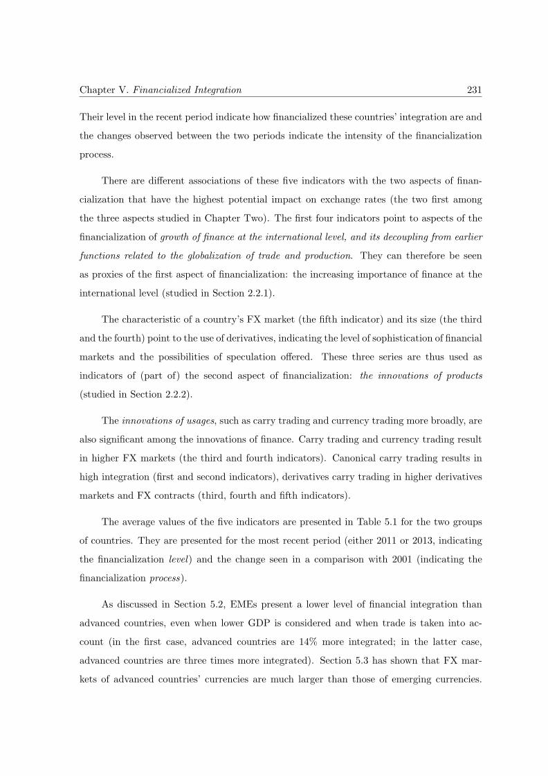
Chapter V. Financialized Integration 231
Their level in the recent period indicate how financialized these countries’ integration are and
the changes observed between the two periods indicate the intensity of the financialization
process.
There are different associations of these five indicators with the two aspects of finan-
cialization that have the highest potential impact on exchange rates (the two first among
the three aspects studied in Chapter Two). The first four indicators point to aspects of the
financialization of growth of finance at the international level, and its decoupling from earlier
functions related to the globalization of trade and production. They can therefore be seen
as proxies of the first aspect of financialization: the increasing importance of finance at the
international level (studied in Section 2.2.1).
The characteristic of a country’s FX market (the fifth indicator) and its size (the third
and the fourth) point to the use of derivatives, indicating the level of sophistication of financial
markets and the possibilities of speculation offered. These three series are thus used as
indicators of (part of) the second aspect of financialization: the innovations of products
(studied in Section 2.2.2).
The innovations of usages, such as carry trading and currency trading more broadly, are
also significant among the innovations of finance. Carry trading and currency trading result
in higher FX markets (the third and fourth indicators). Canonical carry trading results in
high integration (first and second indicators), derivatives carry trading in higher derivatives
markets and FX contracts (third, fourth and fifth indicators).
The average values of the five indicators are presented in Table 5.1 for the two groups
of countries. They are presented for the most recent period (either 2011 or 2013, indicating
the financialization level) and the change seen in a comparison with 2001 (indicating the
financialization process).
As discussed in Section 5.2, EMEs present a lower level of financial integration than
advanced countries, even when lower GDP is considered and when trade is taken into ac-
count (in the first case, advanced countries are 14% more integrated; in the latter case,
advanced countries are three times more integrated). Section 5.3 has shown that FX mar-
kets of advanced countries’ currencies are much larger than those of emerging currencies.
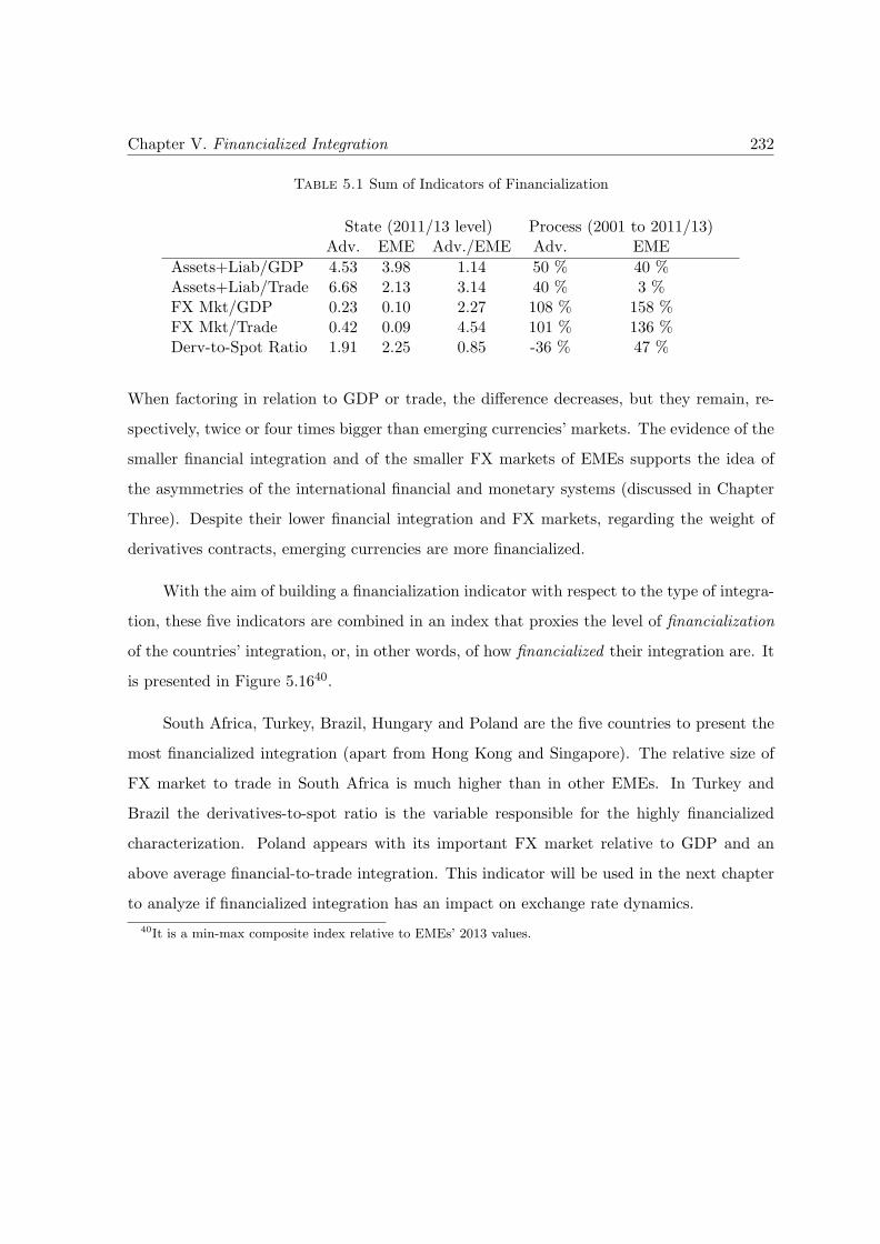
Chapter V. Financialized Integration 232
Table 5.1 Sum of Indicators of Financialization
State (2011/13 level) Process (2001 to 2011/13)Adv. EME Adv./EME Adv. EME
Assets+Liab/GDP 4.53 3.98 1.14 50 % 40 %Assets+Liab/Trade 6.68 2.13 3.14 40 % 3 %FX Mkt/GDP 0.23 0.10 2.27 108 % 158 %FX Mkt/Trade 0.42 0.09 4.54 101 % 136 %Derv-to-Spot Ratio 1.91 2.25 0.85 -36 % 47 %
When factoring in relation to GDP or trade, the difference decreases, but they remain, re-
spectively, twice or four times bigger than emerging currencies’ markets. The evidence of the
smaller financial integration and of the smaller FX markets of EMEs supports the idea of
the asymmetries of the international financial and monetary systems (discussed in Chapter
Three). Despite their lower financial integration and FX markets, regarding the weight of
derivatives contracts, emerging currencies are more financialized.
With the aim of building a financialization indicator with respect to the type of integra-
tion, these five indicators are combined in an index that proxies the level of financialization
of the countries’ integration, or, in other words, of how financialized their integration are. It
is presented in Figure 5.1640.
South Africa, Turkey, Brazil, Hungary and Poland are the five countries to present the
most financialized integration (apart from Hong Kong and Singapore). The relative size of
FX market to trade in South Africa is much higher than in other EMEs. In Turkey and
Brazil the derivatives-to-spot ratio is the variable responsible for the highly financialized
characterization. Poland appears with its important FX market relative to GDP and an
above average financial-to-trade integration. This indicator will be used in the next chapter
to analyze if financialized integration has an impact on exchange rate dynamics.
40It is a min-max composite index relative to EMEs’ 2013 values.
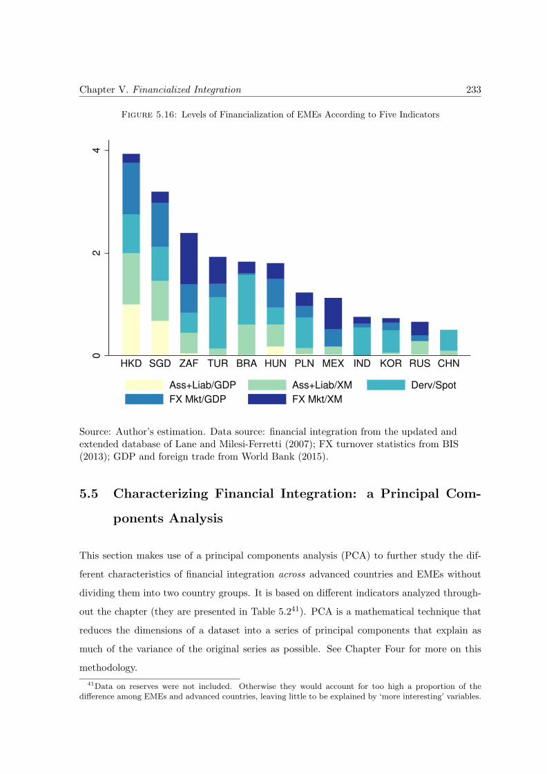
Chapter V. Financialized Integration 233
Figure 5.16: Levels of Financialization of EMEs According to Five Indicators
02
4
HKD SGD ZAF TUR BRA HUN PLN MEX IND KOR RUS CHN
Ass+Liab/GDP Ass+Liab/XM Derv/Spot
FX Mkt/GDP FX Mkt/XM
Source: Author’s estimation. Data source: financial integration from the updated andextended database of Lane and Milesi-Ferretti (2007); FX turnover statistics from BIS(2013); GDP and foreign trade from World Bank (2015).
5.5 Characterizing Financial Integration: a Principal Com-
ponents Analysis
This section makes use of a principal components analysis (PCA) to further study the dif-
ferent characteristics of financial integration across advanced countries and EMEs without
dividing them into two country groups. It is based on different indicators analyzed through-
out the chapter (they are presented in Table 5.241). PCA is a mathematical technique that
reduces the dimensions of a dataset into a series of principal components that explain as
much of the variance of the original series as possible. See Chapter Four for more on this
methodology.
41Data on reserves were not included. Otherwise they would account for too high a proportion of thedifference among EMEs and advanced countries, leaving little to be explained by ‘more interesting’ variables.
Chapter V. Financialized Integration 234
Table 5.2 Variables Used in the PCA
ttasset Total assets minus reservesttliab Total liabilitiesassliab/gdp Assets (minus reserves) plus liabilities over GDPassliab/xm Assets (minus reserves) plus liabilities over exports plus importsttass/ttliab Total assets over total liabilitieseqass/liab Assets-to-liabilities ratio: equitiesdebtass/liab Assets-to-liabilities ratio: debtfdiass/liab Assets-to-liabilities ratio: FDIttfxmkt Total foreign exchange marketttfxmkt/gdp Total foreign exchange market over GDPttfxmkt/xm Total foreign exchange market over exports plus importsderv Total derivatives marketderv/spot Derivatives over spot contracts
The components estimated are presented in Table 5.3. As in Chapter Four, following
the Kaiser rule, only the components whose eigenvalues are greater than one are considered
– in this case, the first four components. With these four series, 83% of the variance of the
original dataset is explained. To understand what the four layers represent, the loadings
of the original variables into each of them is analyzed (see Table 5.4). Values higher than
0.4 were considered a relevant loading. Values lower than that are not printed for ease of
reading.
Table 5.3 Principal Components and Eigenvalues
Component Eigenvalue Difference Proportion Cumulative
Comp1 5.11106 2.2613 0.3932 0.3932Comp2 2.84976 1.23588 0.2192 0.6124Comp3 1.61388 0.430758 0.1241 0.7365Comp4 1.18312 0.355183 0.091 0.8275Comp5 0.827941 0.238479 0.0637 0.8912
The first component (PC 1) is related to the absolute size of FX markets (the total size
and the size of derivatives markets) and to the importance of financial integration (the size
of the stock of assets and of liabilities).
The second component (PC 2) is a series that represents the type of financial integration.
Countries that have high scores in this component tend to have a high asset-to-liability ratio
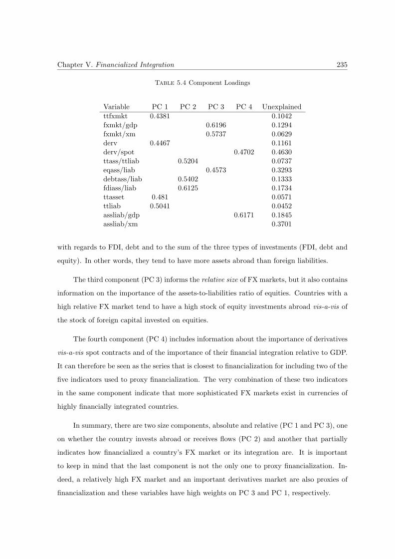
Chapter V. Financialized Integration 235
Table 5.4 Component Loadings
Variable PC 1 PC 2 PC 3 PC 4 Unexplained
ttfxmkt 0.4381 0.1042fxmkt/gdp 0.6196 0.1294fxmkt/xm 0.5737 0.0629derv 0.4467 0.1161derv/spot 0.4702 0.4630ttass/ttliab 0.5204 0.0737eqass/liab 0.4573 0.3293debtass/liab 0.5402 0.1333fdiass/liab 0.6125 0.1734ttasset 0.481 0.0571ttliab 0.5041 0.0452assliab/gdp 0.6171 0.1845assliab/xm 0.3701
with regards to FDI, debt and to the sum of the three types of investments (FDI, debt and
equity). In other words, they tend to have more assets abroad than foreign liabilities.
The third component (PC 3) informs the relative size of FX markets, but it also contains
information on the importance of the assets-to-liabilities ratio of equities. Countries with a
high relative FX market tend to have a high stock of equity investments abroad vis-a-vis of
the stock of foreign capital invested on equities.
The fourth component (PC 4) includes information about the importance of derivatives
vis-a-vis spot contracts and of the importance of their financial integration relative to GDP.
It can therefore be seen as the series that is closest to financialization for including two of the
five indicators used to proxy financialization. The very combination of these two indicators
in the same component indicate that more sophisticated FX markets exist in currencies of
highly financially integrated countries.
In summary, there are two size components, absolute and relative (PC 1 and PC 3), one
on whether the country invests abroad or receives flows (PC 2) and another that partially
indicates how financialized a country’s FX market or its integration are. It is important
to keep in mind that the last component is not the only one to proxy financialization. In-
deed, a relatively high FX market and an important derivatives market are also proxies of
financialization and these variables have high weights on PC 3 and PC 1, respectively.
Chapter V. Financialized Integration 236
For not yielding in a set of components where financialization-related features are gath-
ered in the same component, the PCA cannot be used to provide a typology of countries
according to financialization. Its analysis however results in interesting points. PC 1 is
associated with variables of the absolute size of FX markets and with the level of financial
integration, while the variables that load the most on PC 3 are related to the relative size of
FX markets (relative to GDP and to foreign trade). The fact that the two sets of variables
related to the absolute and the relative sizes of FX markets load in different components
(not being correlated enough to load in the same component) indicates a high level of fi-
nancialization of some FX markets. The countries that present the largest FX markets are
not the same that present the largest FX markets relative to their economy. In other words,
this result indicates that FX markets’ size are independent from the economy’s size or the
magnitude of its foreign trade. Indeed, the correlation between the country scores on these
two components is 0.25, one of the lowest among different components.
Also interesting in a PCA analysis is to see how each country performs in each compo-
nent. This is shown in Figure 5.17; Figure 5.18 only shows EMEs for better visualization.
The different combinations presented in the four plots of Figure 5.17 shows that advanced
countries (with blue circular markers) and EMEs (with red triangles as markers) most often
form two clearly different sets of countries, with the exception of Hong Kong and Singapore,
whose characteristics are more similar to advanced countries (which is in line with their role
as financial centers and their different structures, as seen in Sections 5.2 and 5.3).
Plot (d) is the most revealing to analyze financialization, because it groups most of
the financialization-related variables: the relative size of FX markets (on PC 3), and the
derivatives-to-spot ratios and the international financial integration (on PC 4). When con-
sidering these variables, the most financialized structures are those that have high scores on
both components. Among EMEs, Brazil stands out with relatively high PC 3 and high PC
4, which indicates the high financialization level of its integration. Turkey has a high score
on PC 4 and China on PC 3. But the highest scores are, as expected, those of advanced
countries, as the United Kingdom, Switzerland, Norway, and, to a lesser extent, Sweden.
The combination of the United States, Japan, New Zealand and Australia in a same group
is revealing of their large FX markets (in relative terms), but low derivatives-to-spot ratios
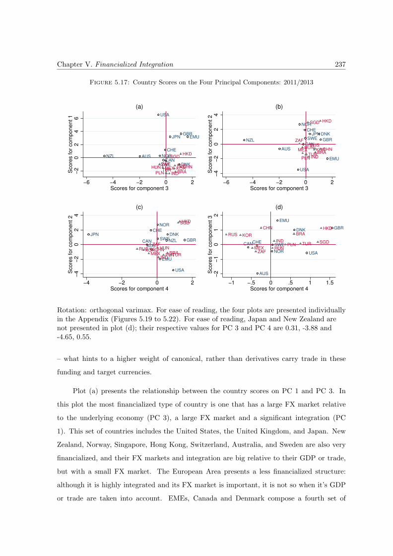
Chapter V. Financialized Integration 237
Figure 5.17: Country Scores on the Four Principal Components: 2011/2013
AUSCAN
DNK
EMUJPN
NZL NOR
CHE
GBR
USA
SWE
BRACHN
INDKORMEXRUSZAF
HKDSGD
HUN
PLNTUR−
20
24
6S
core
s for
com
ponent 1
−6 −4 −2 0 2Scores for component 3
(a)
AUSCAN
DNK
EMU
JPN
NZL
NOR
SWE
CHE
GBR
USA
BRACHNHUN
IND
KORTUR
HKDSGD
PLN
MEXRUS
ZAF
−4
−2
02
4S
core
s for
com
ponent 2
−6 −4 −2 0 2Scores for component 3
(b)
DNK
EMU
JPN
NZL
NOR
SWE
CHE
GBR
USA
AUSCAN
BRACHNHUN
IND
KORMEX
RUSZAF
TURPLN
HKDSGD
−4
−2
02
4S
core
s for
com
ponent 2
−4 −2 0 2Scores for component 4
(c)
AUS
DNK
EMU
NOR
SWE
GBR
USA
CANCHE
BRA
CHN
HUN
IND
KOR
MEX
RUS
ZAF
TURPLN
HKD
SGD
−2
−1
01
2S
core
s for
com
ponent 3
−1 −.5 0 .5 1 1.5Scores for component 4
(d)
Rotation: orthogonal varimax. For ease of reading, the four plots are presented individuallyin the Appendix (Figures 5.19 to 5.22). For ease of reading, Japan and New Zealand arenot presented in plot (d); their respective values for PC 3 and PC 4 are 0.31, -3.88 and-4.65, 0.55.
– what hints to a higher weight of canonical, rather than derivatives carry trade in these
funding and target currencies.
Plot (a) presents the relationship between the country scores on PC 1 and PC 3. In
this plot the most financialized type of country is one that has a large FX market relative
to the underlying economy (PC 3), a large FX market and a significant integration (PC
1). This set of countries includes the United States, the United Kingdom, and Japan. New
Zealand, Norway, Singapore, Hong Kong, Switzerland, Australia, and Sweden are also very
financialized, and their FX markets and integration are big relative to their GDP or trade,
but with a small FX market. The European Area presents a less financialized structure:
although it is highly integrated and its FX market is important, it is not so when it’s GDP
or trade are taken into account. EMEs, Canada and Denmark compose a fourth set of
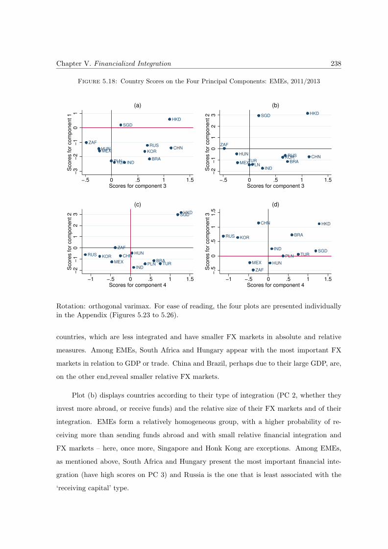
Chapter V. Financialized Integration 238
Figure 5.18: Country Scores on the Four Principal Components: EMEs, 2011/2013
BRA
CHNHUN
IND
KORMEX
RUSZAF
TURPLN
HKD
SGD
−3
−2
−1
01
Score
s for
com
ponent 1
−.5 0 .5 1 1.5Scores for component 3
(a)
BRACHN
HUN
IND
KOR
MEX
RUS
PLN
HKDSGD
ZAF
TUR
−2
−1
01
23
Score
s for
com
ponent 2
−.5 0 .5 1 1.5Scores for component 3
(b)
BRACHN
HUN
IND
KOR
MEX
RUS
ZAF
TURPLN
HKDSGD
−2
−1
01
23
Score
s for
com
ponent 2
−1 −.5 0 .5 1 1.5Scores for component 4
(c)
BRA
CHN
HUN
IND
KOR
MEX
RUS
ZAF
TURPLN
HKD
SGD
−.5
0.5
11.5
Score
s for
com
ponent 3
−1 −.5 0 .5 1 1.5Scores for component 4
(d)
Rotation: orthogonal varimax. For ease of reading, the four plots are presented individuallyin the Appendix (Figures 5.23 to 5.26).
countries, which are less integrated and have smaller FX markets in absolute and relative
measures. Among EMEs, South Africa and Hungary appear with the most important FX
markets in relation to GDP or trade. China and Brazil, perhaps due to their large GDP, are,
on the other end,reveal smaller relative FX markets.
Plot (b) displays countries according to their type of integration (PC 2, whether they
invest more abroad, or receive funds) and the relative size of their FX markets and of their
integration. EMEs form a relatively homogeneous group, with a higher probability of re-
ceiving more than sending funds abroad and with small relative financial integration and
FX markets – here, once more, Singapore and Honk Kong are exceptions. Among EMEs,
as mentioned above, South Africa and Hungary present the most important financial inte-
gration (have high scores on PC 3) and Russia is the one that is least associated with the
‘receiving capital’ type.
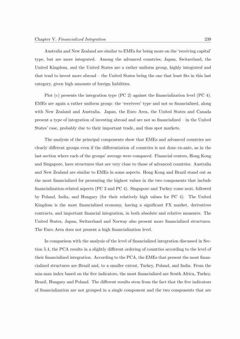
Chapter V. Financialized Integration 239
Australia and New Zealand are similar to EMEs for being more on the ‘receiving capital’
type, but are more integrated. Among the advanced countries, Japan, Switzerland, the
United Kingdom, and the United States are a rather uniform group, highly integrated and
that tend to invest more abroad – the United States being the one that least fits in this last
category, given high amounts of foreign liabilities.
Plot (c) presents the integration type (PC 2) against the financialization level (PC 4).
EMEs are again a rather uniform group: the ‘receivers’ type and not so financialized, along
with New Zealand and Australia. Japan, the Euro Area, the United States and Canada
present a type of integration of investing abroad and are not so financialized – in the United
States’ case, probably due to their important trade, and thus spot markets.
The analysis of the principal components show that EMEs and advanced countries are
clearly different groups even if the differentiation of countries is not done ex-ante, as in the
last section where each of the groups’ average were compared. Financial centers, Hong Kong
and Singapore, have structures that are very close to those of advanced countries. Australia
and New Zealand are similar to EMEs in some aspects. Hong Kong and Brazil stand out as
the most financialized for presenting the highest values in the two components that include
financialization-related aspects (PC 3 and PC 4). Singapore and Turkey come next, followed
by Poland, India, and Hungary (for their relatively high values for PC 4). The United
Kingdom is the most financialized economy, having a significant FX market, derivatives
contracts, and important financial integration, in both absolute and relative measures. The
United States, Japan, Switzerland and Norway also present more financialized structures.
The Euro Area does not present a high financialization level.
In comparison with the analysis of the level of financialized integration discussed in Sec-
tion 5.4, the PCA results in a slightly different ordering of countries according to the level of
their financialized integration. According to the PCA, the EMEs that present the most finan-
cialized structures are Brazil and, to a smaller extent, Turkey, Poland, and India. From the
min-max index based on the five indicators, the most financialized are South Africa, Turkey,
Brazil, Hungary and Poland. The different results stem from the fact that the five indicators
of financialization are not grouped in a single component and the two components that are
Chapter V. Financialized Integration 240
related to financialization are not necessarily composed only by financialization-related indi-
cators, which hinders the strict use of these components as proxies of financialization. The
analysis done in Chapter Six is thus based on the composite index as a proxy for the type of
integration.
5.6 Conclusions
The international financial system might be the place where the consequences of financial-
ization were first seen – one of its main changes, the emergence of the eurodollar market, is
even considered by Bourguinat (1992) to be the first stage of the current phase of capitalism.
With financialization, finance has not only grown in magnitude at the international level, but
this growth has been considered a dissociation from its earlier functions and evidence that
it now follows its own logic (Chesnais (1997); Plihon and Ponssard (2002)). If international
finance follows a different dynamic, the impacts of financial integration on a country are not
the same, which requires an understanding of the characteristics of finance and integration:
as EMEs’ levels of integration vary, so do their types of integration. This chapter’s analyses
of EMEs’ integration has four main contributions.
First, the chapter presents evidence that supports the idea of a decoupling of finance
from productive economy’s factors and from financial integration, not only among advanced
countries, but also among EMEs. This decoupling of finance from its earlier logic is the first
of the three phenomena related to financialization presented in Chapter Two. Part of the
changes of finance (the second phenomena) are evidence of the decoupling.
The dissociation of finance at the international level from the productive economy is
observed in the faster growth of financial integration and FX transactions than that of trade
or GDP. Its dissociation from financial integration is observed in the faster growth of FX
transactions than that of financial integration. In other words, there have been more FX
transactions per patrimonial changes than before. As the transactions are daily and the
patrimonial value is taken by the end of the year, a higher number of transactions might be
associated with more frequent changes inside the year.
Chapter V. Financialized Integration 241
Seen from Kaldor’s (1939) definition of speculation42, this more rapid change might be
understood as a rise of speculation: investors would hold assets more for their changes in
prices (or expected changes) then for the returns paid by the assets, what demands frequently
purchasing and selling the asset. As an important part of the return comes from the exchange
rate variation, this behavior also involves FX transactions and transactions due to expected
changes in the exchange rate. Apart from the exchange rate change, common to each type of
instrument, such behavior is expected to be common with equity investment, given its larger
price variations.
Most of the growth of FX transactions among emerging currencies is related to deriva-
tives, not spot, contracts. In this case, in addition to evincing higher speculation, the discon-
nection of FX transactions from financial integration underscores the rise of derivatives carry
trading – a phenomenon that was identified in a few emerging currencies in the chapter.
The second main contribution of the chapter is related to the different type of integration
of EMEs vis-a-vis of advanced countries. The overall low level of the asset-to-liability ratios
of EMEs when reserves are not considered support the view that EMEs have a function in the
IFS of suppliers of financial assets. The chapter has also argued that the IFS is marked by an
additional asymmetry with regards to emerging and advanced currencies. The demand for
advanced countries’ assets include purchases from developing countries’ public institutions
whose behavior is strongly marked by stability and is counter cyclical. The demand of
EMEs’ assets, on the other hand, stems from international money managers whose behavior
(as analyzed throughout the thesis), is marked by speculation of assets around the globe,
yielding high volatility and high influence of international conditions in the determination
of domestic prices and exchange rates. To further describe this asymmetry, comparing total
reserves from developing countries to US and European foreign liabilities and their impact
on the respective currencies, would be a compelling avenue for future research.
The third contribution of this chapter is the suggestion of the concept of financialized in-
tegration to characterize integration with regards to the presence of financialization features.
The index proposed is focused on indicators that measure the extent of the decoupling of
integration from the economy’s features, from financial integration, and the sophistication
42Kaldor’s (1939) definition of speculation is presented in Chapter Two, page 35.
Chapter V. Financialized Integration 242
level of its FX market. This composite index suggests that South Africa, Turkey, Brazil, Hun-
gary and Poland are the EMEs to present the most financialized integration to international
markets (Figure 5.16). Adding financialization-related features to the relative magnitude of
financial integration, the index presents different results than measures of financial integra-
tion – for instance, the latter do not result in a significant level of financial integration for
Turkey and Brazil43.
The different types of integration were also analyzed through a principal components
analysis, that allowed looking at countries’ characteristics without first grouping them as
emerging or advanced countries. The analyses confirmed that New Zealand and Australia
present some ‘EMEs’ features’ while Hong Kong and Singapore are, in some respects, more
similar to advanced countries than to EMEs. Although it is interesting to further describe
different types of integration, the methodology could not be used for building an index of
financialized integration because the five main indicators of interest are not correlated enough
to be grouped into a single component, and the components where these indicators loaded
the most also group other indicators. However, with these shortcomings in mind, the analysis
still reveals the high level of financialization of Brazil, Turkey and Poland – as done by the
composite index.
Fourth, the chapter contributes to the carry-trading literature by suggesting ways of iden-
tifying currencies used in carry trading operations through the countries’ assets-to-liabilities
ratio (its overall value or only with regards to debt instruments), its FX-to-trade ratios
(combined with the absolute size of FX markets). The first measure is closer to canoni-
cal carry trading currencies and the second one underscores currencies used in derivatives
carry trading. In the literature this identification is generally based on which currencies are
expected to be important given their interest rate levels, or based on their total FX size.
An interesting avenue for future research in this area is the comparison of the evolution of
assets-to-liabilities ratios with FX market sizes and interest rate differentials.
The analyses indicated the presence of canonical carry trading operations with the
currencies of: South Africa and Mexico (according to their FX size relative to GDP or trade),
Hungary (according to its FX magnitude relative to GDP), Brazil and India (according to
43This refers to the size of integration relatively to GDP, presented in Figure 5.8.
Chapter V. Financialized Integration 243
the assets-to-liabilities ratio), and Turkey (for the three mentioned measures). This result is
similar to what is argued in the literature, that indicate these currencies (all except Mexico)
as the most important carry trading currencies among EMEs.
Among advanced countries, the currencies that stand out as important carry trading
currencies are those from: Switzerland (for assets-to-liabilities and FX size relatively to
GDP), the United Kingdom (for its FX size relative to GDP), the US (for its important FX
markets relative to GDP and trade), and New Zealand, Australia, and Japan (for the three
measures). These are the six currencies from advanced countries most cited as carry trading
currencies.
Chapter V. Financialized Integration 244
5.7 Appendix I: List of Countries for Figure 5.7
The list of countries included in the statistics presented in Figure 5.7 is partially based on
Lane and Milesi-Ferretti (2007), but adapted to differentiate EMEs according to this thesis
analysis.
Industrial countries are: Australia, Austria, Belgium, Canada, Denmark, Finland,
France, Germany, Greece, Iceland, Ireland, Italy, Japan, Luxembourg, Netherlands, New
Zealand, Norway, Portugal, Spain, Sweden, Switzerland, the United Kingdom, and the
United States.
Emerging + are countries for which FX market data is available: Brazil, China, Hun-
gary, India, Korea, Mexico, Poland, South Africa, Turkey, Russia, Honk Kong and Singapore.
Other EMEs are: Argentina, Chile, Colombia, Czech Republic, Indonesia, Malaysia,
Peru, the Philippines, Taiwan and Thailand.
Other developing countries are: Albania, Algeria, Angola, Armenia, Azerbaijan, Bahrain,
Bangladesh, Belarus, Benin, Bolivia, Bosnia and Herzegovina, Botswana, Brunei Darussalam,
Bulgaria, Burkina Faso, Cambodia, Cameroon, Chad, Congo, Dem. Rep. of, Congo, Repub-
lic of, Costa Rica, Croatia, Cyprus, Cte d’Ivoire, Dominican Republic, Ecuador, Egypt, El
Salvador, Equatorial Guinea, Estonia, Ethiopia, Fiji, Gabon, Georgia, Ghana, Guatemala,
Guinea, Haiti, Honduras, Iran, Islamic Republic of, Israel, Jamaica, Jordan, Kazakhstan,
Kenya, Korea, Kuwait, Kyrgyz Republic, Lao People’s Dem.Rep, Latvia, Lebanon, Libya,
Lithuania, Macedonia, Madagascar, Malawi, Malaysia, Mali, Malta, Mauritius, Moldova, Mo-
rocco, Mozambique, Myanmar, Namibia, Nepal, Nicaragua, Niger, Nigeria, Oman, Pakistan,
Panama, Papua New Guinea, Paraguay, Qatar, Romania, Rwanda, Saudi Arabia, Senegal,
Serbia, Slovak Republic, Slovenia, Sri Lanka, Sudan, Swaziland, Syrian Arab Republic, Tai-
wan, Tajikistan, Tanzania, Thailand, Togo, Trinidad and Tobago, Tunisia, Turkmenistan,
Uganda, Ukraine, United Arab Emirates, Uruguay, Uzbekistan, Venezuela, Rep. Bol., Viet-
nam, Yemen, Republic of, Zambia, and Zimbabwe.
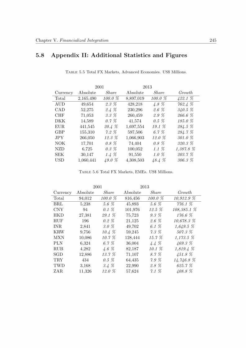
Chapter V. Financialized Integration 245
5.8 Appendix II: Additional Statistics and Figures
Table 5.5 Total FX Markets, Advanced Economies. US$ Millions.
2001 2013Currency Absolute Share Absolute Share Growth
Total 2,165,490 100.0 % 8,897,019 100.0 % 422.1 %
AUD 49,654 2.3 % 428,218 4.8 % 762.4 %CAD 52,275 2.4 % 230,296 2.6 % 340.5 %CHF 71,053 3.3 % 260,459 2.9 % 266.6 %DKK 14,589 0.7 % 41,574 0.5 % 185.0 %EUR 441,545 20.4 % 1,697,554 19.1 % 284.5 %GBP 155,310 7.2 % 597,506 6.7 % 284.7 %JPY 266,050 12.3 % 1,066,903 12.0 % 301.0 %NOK 17,701 0.8 % 74,404 0.8 % 320.3 %NZD 6,725 0.3 % 100,052 1.1 % 1,387.8 %SEK 30,147 1.4 % 91,550 1.0 % 203.7 %USD 1,060,441 49.0 % 4,308,503 48.4 % 306.3 %
Table 5.6 Total FX Markets, EMEs. US$ Millions.
2001 2013Currency Absolute Share Absolute Share Growth
Total 94,012 100.0 % 816,456 100.0 % 10,912.9 %
BRL 5,238 5.6 % 45,893 5.6 % 776.1 %CNY 94 0.1 % 101,976 12.5 % 108,385.1 %HKD 27,381 29.1 % 75,723 9.3 % 176.6 %HUF 196 0.2 % 21,125 2.6 % 10,678.3 %INR 2,841 3.0 % 49,702 6.1 % 1,649.5 %KRW 9,756 10.4 % 59,245 7.3 % 507.3 %MXN 10,086 10.7 % 128,444 15.7 % 1,173.5 %PLN 6,324 6.7 % 36,004 4.4 % 469.3 %RUB 4,282 4.6 % 82,187 10.1 % 1,819.4 %SGD 12,886 13.7 % 71,107 8.7 % 451.8 %TRY 434 0.5 % 64,435 7.9 % 14,746.8 %TWD 3,168 3.4 % 22,990 2.8 % 625.7 %ZAR 11,326 12.0 % 57,624 7.1 % 408.8 %
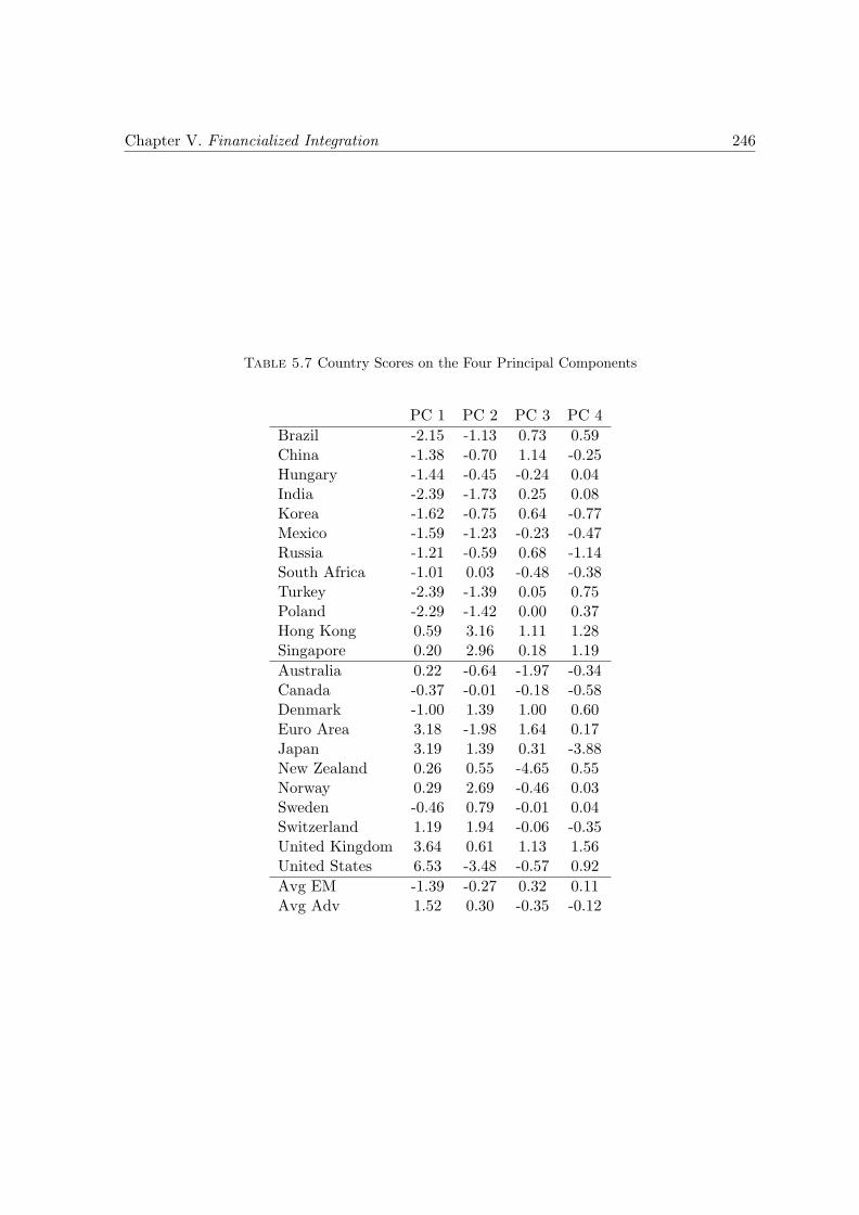
Chapter V. Financialized Integration 246
Table 5.7 Country Scores on the Four Principal Components
PC 1 PC 2 PC 3 PC 4
Brazil -2.15 -1.13 0.73 0.59China -1.38 -0.70 1.14 -0.25Hungary -1.44 -0.45 -0.24 0.04India -2.39 -1.73 0.25 0.08Korea -1.62 -0.75 0.64 -0.77Mexico -1.59 -1.23 -0.23 -0.47Russia -1.21 -0.59 0.68 -1.14South Africa -1.01 0.03 -0.48 -0.38Turkey -2.39 -1.39 0.05 0.75Poland -2.29 -1.42 0.00 0.37Hong Kong 0.59 3.16 1.11 1.28Singapore 0.20 2.96 0.18 1.19
Australia 0.22 -0.64 -1.97 -0.34Canada -0.37 -0.01 -0.18 -0.58Denmark -1.00 1.39 1.00 0.60Euro Area 3.18 -1.98 1.64 0.17Japan 3.19 1.39 0.31 -3.88New Zealand 0.26 0.55 -4.65 0.55Norway 0.29 2.69 -0.46 0.03Sweden -0.46 0.79 -0.01 0.04Switzerland 1.19 1.94 -0.06 -0.35United Kingdom 3.64 0.61 1.13 1.56United States 6.53 -3.48 -0.57 0.92
Avg EM -1.39 -0.27 0.32 0.11Avg Adv 1.52 0.30 -0.35 -0.12
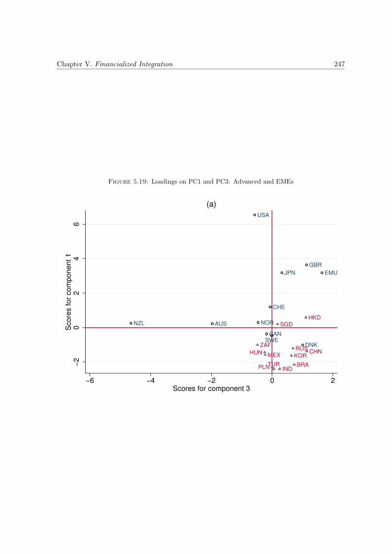
Chapter V. Financialized Integration 247
Figure 5.19: Loadings on PC1 and PC3: Advanced and EMEs
AUS
CAN
DNK
EMUJPN
NZL NOR
CHE
GBR
USA
SWE
BRA
CHN
IND
KORMEXRUS
ZAF
HKDSGD
HUN
PLNTUR−
20
24
6S
co
res f
or
co
mp
on
en
t 1
−6 −4 −2 0 2Scores for component 3
(a)
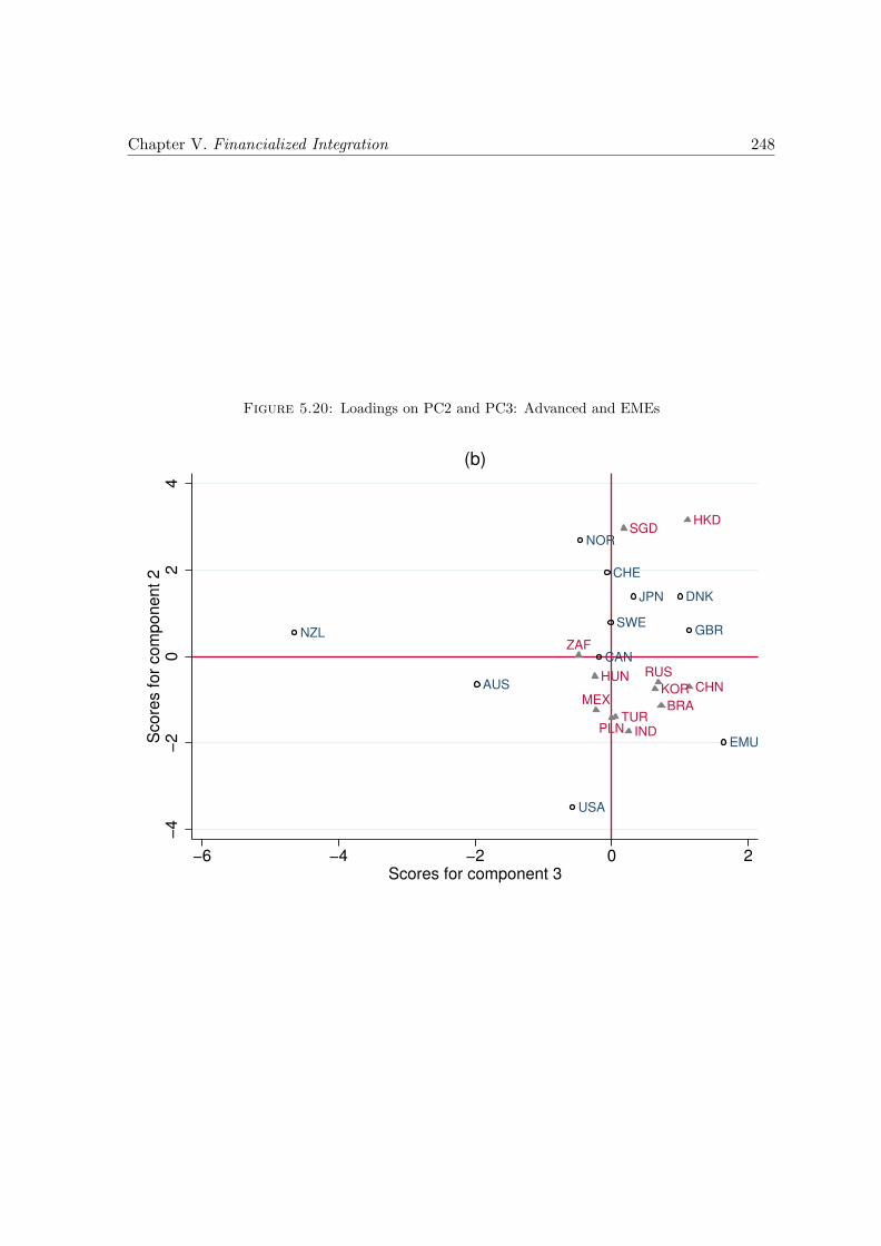
Chapter V. Financialized Integration 248
Figure 5.20: Loadings on PC2 and PC3: Advanced and EMEs
AUS
CAN
DNK
EMU
JPN
NZL
NOR
SWE
CHE
GBR
USA
BRA
CHNHUN
IND
KOR
TUR
HKDSGD
PLN
MEX
RUS
ZAF
−4
−2
02
4S
co
res f
or
co
mp
on
en
t 2
−6 −4 −2 0 2Scores for component 3
(b)
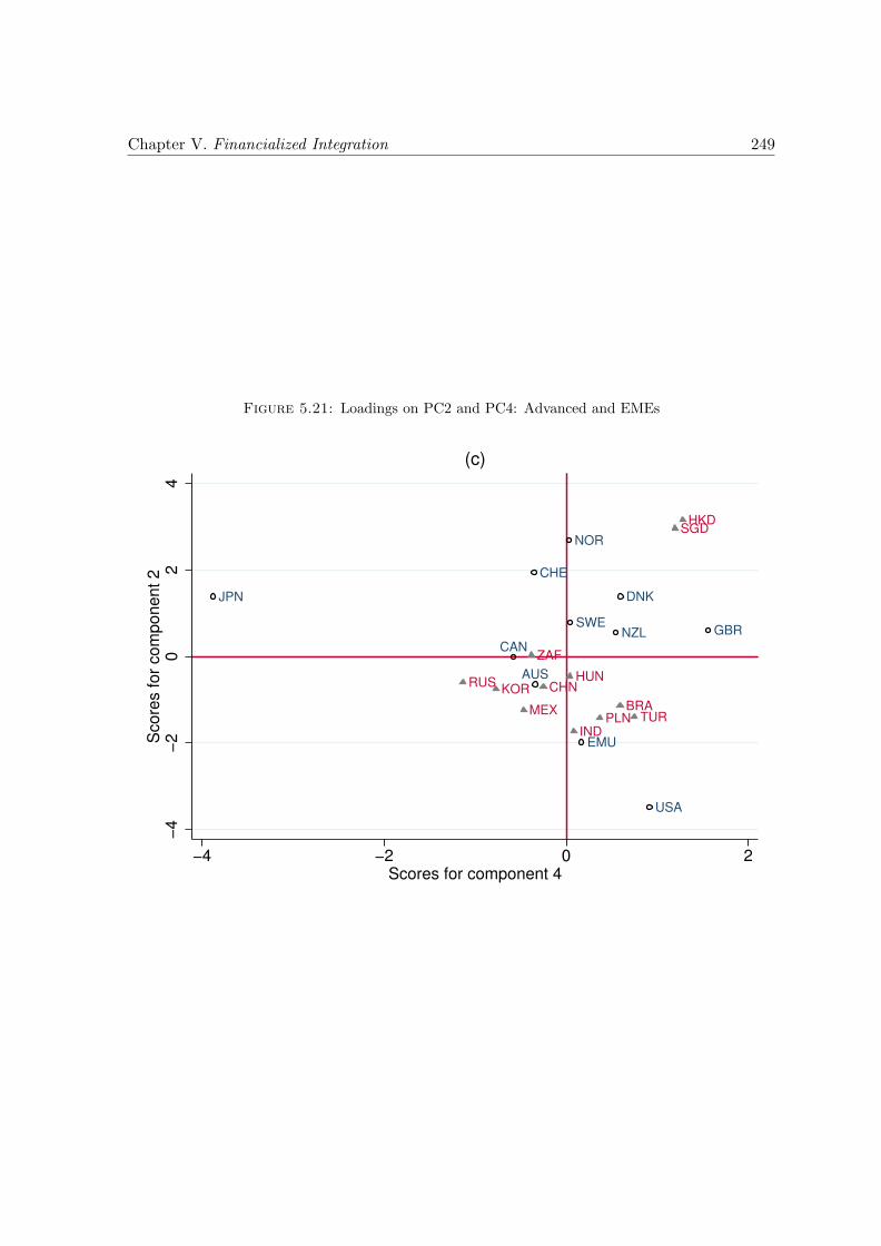
Chapter V. Financialized Integration 249
Figure 5.21: Loadings on PC2 and PC4: Advanced and EMEs
DNK
EMU
JPN
NZL
NOR
SWE
CHE
GBR
USA
AUS
CAN
BRA
CHNHUN
IND
KOR
MEX
RUS
ZAF
TURPLN
HKDSGD
−4
−2
02
4S
co
res f
or
co
mp
on
en
t 2
−4 −2 0 2Scores for component 4
(c)
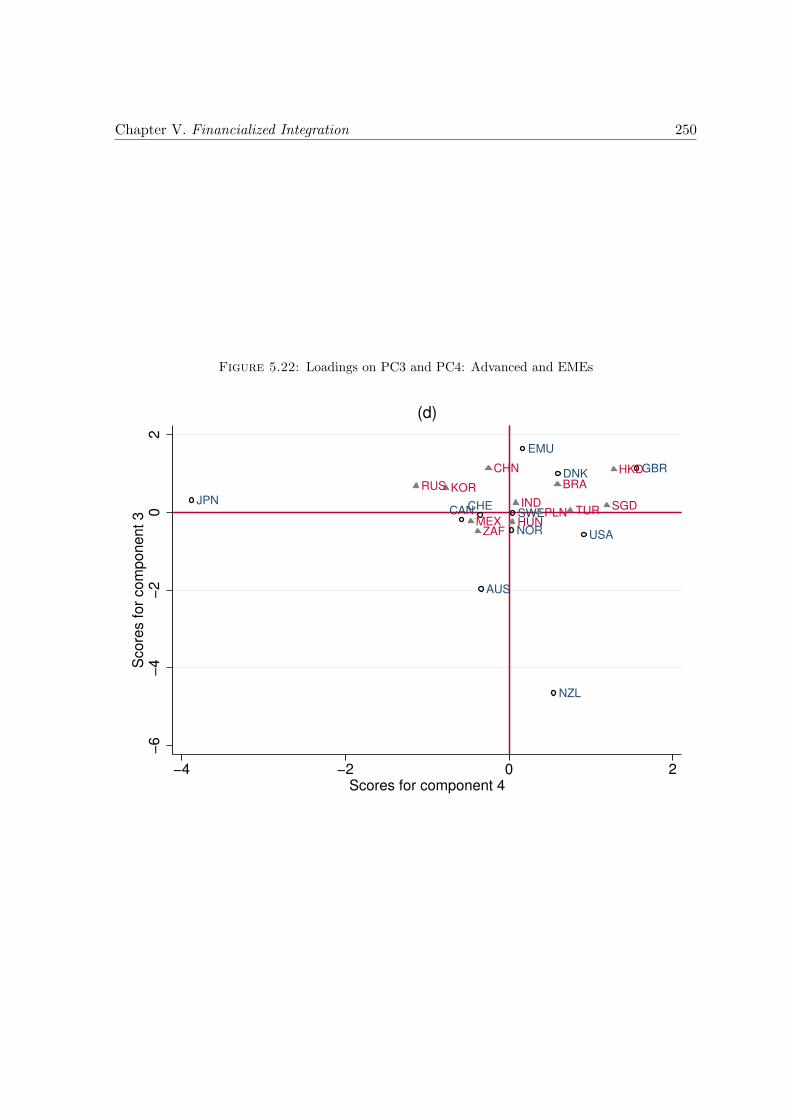
Chapter V. Financialized Integration 250
Figure 5.22: Loadings on PC3 and PC4: Advanced and EMEs
AUS
DNK
EMU
JPN
NZL
NOR
SWE
GBR
USA
CANCHE
BRA
CHN
HUN
IND
KOR
MEX
RUS
ZAF
TURPLN
HKD
SGD
−6
−4
−2
02
Sco
res f
or
co
mp
on
en
t 3
−4 −2 0 2Scores for component 4
(d)
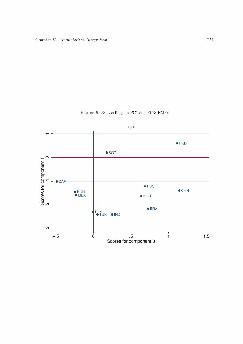
Chapter V. Financialized Integration 251
Figure 5.23: Loadings on PC1 and PC3: EMEs
BRA
CHNHUN
IND
KORMEX
RUS
ZAF
TURPLN
HKD
SGD
−3
−2
−1
01
Sco
res f
or
co
mp
on
en
t 1
−.5 0 .5 1 1.5Scores for component 3
(a)
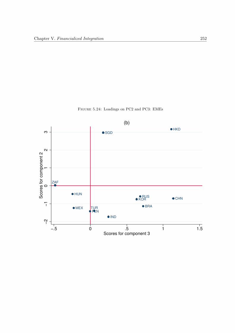
Chapter V. Financialized Integration 252
Figure 5.24: Loadings on PC2 and PC3: EMEs
BRA
CHN
HUN
IND
KOR
MEX
RUS
PLN
HKDSGD
ZAF
TUR
−2
−1
01
23
Sco
res f
or
co
mp
on
en
t 2
−.5 0 .5 1 1.5Scores for component 3
(b)
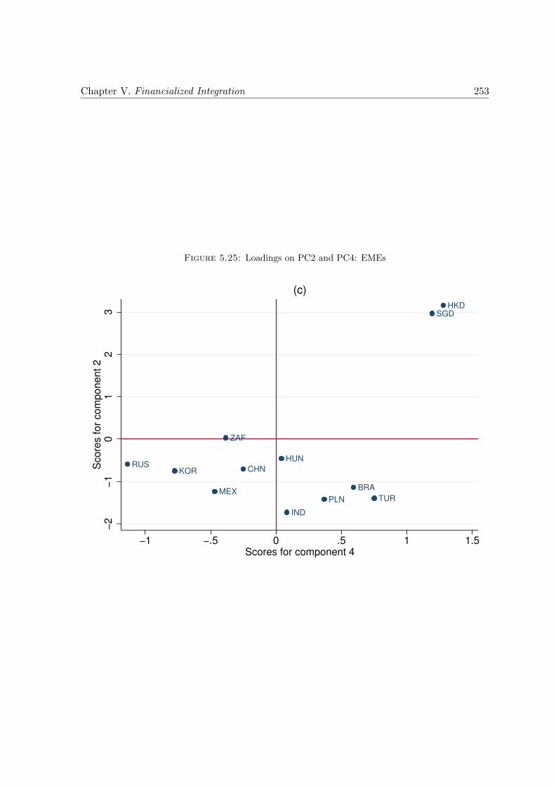
Chapter V. Financialized Integration 253
Figure 5.25: Loadings on PC2 and PC4: EMEs
BRA
CHN
HUN
IND
KOR
MEX
RUS
ZAF
TURPLN
HKDSGD
−2
−1
01
23
Sco
res f
or
co
mp
on
en
t 2
−1 −.5 0 .5 1 1.5Scores for component 4
(c)
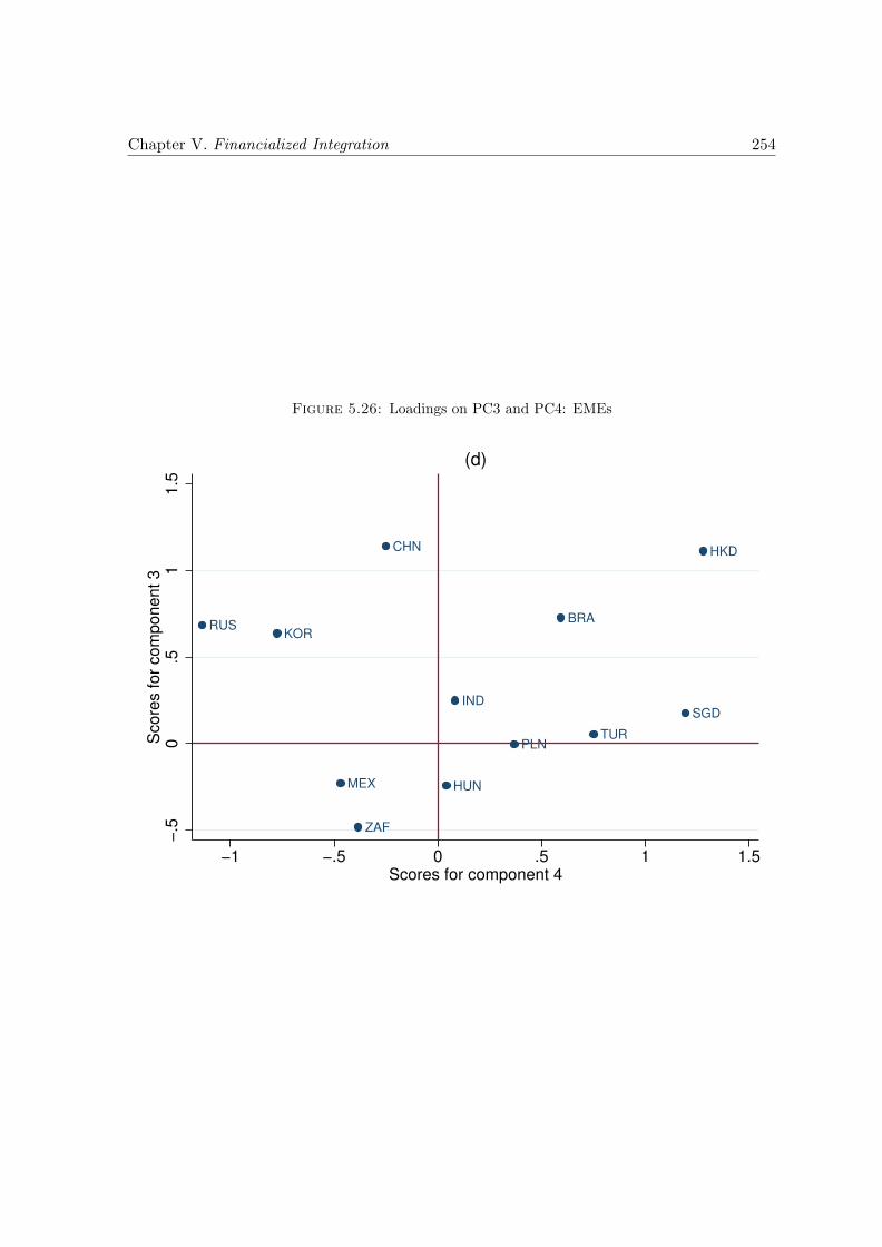
Chapter V. Financialized Integration 254
Figure 5.26: Loadings on PC3 and PC4: EMEs
BRA
CHN
HUN
IND
KOR
MEX
RUS
ZAF
TURPLN
HKD
SGD
−.5
0.5
11
.5S
co
res f
or
co
mp
on
en
t 3
−1 −.5 0 .5 1 1.5Scores for component 4
(d)
Chapter 6
Emerging Countries’ Exchange
Rate Dynamics in Times of
Financialization
As mentioned in the Introduction Chapter, after having opted for floating exchange rate
regimes in the aftermath of the late-1990s currency crises, some emerging market economies
(EMEs) have been intervening in their foreign exchange (FX) markets with the aim of reduc-
ing the exchange rate volatility. The pattern of EMEs’ exchange rates (emerging currencies)
and their association with the international financial scenarios are discussed in the Introduc-
tion Chapter. The path of the 20 emerging currencies since the year 2000 is replicated in
Figure 6.1 for simplicity.
In light of the discussions in Chapters Two and Three, exchange rate volatility is a
potential consequence of a specific type of integration, alongside the higher vulnerability
to the international sphere and correlation with other emerging currencies – these features
that characterize fragility would emerge from a type of integration to international financial
markets that is more marked by characteristics such as the high importance of financial
flows and sophisticated FX markets1 - two features that are increasingly present in times
1Sophisticated FX markets are proxied, in the empirical chapters of this thesis, by the amount of derivativesmarkets and their relative weight.
255
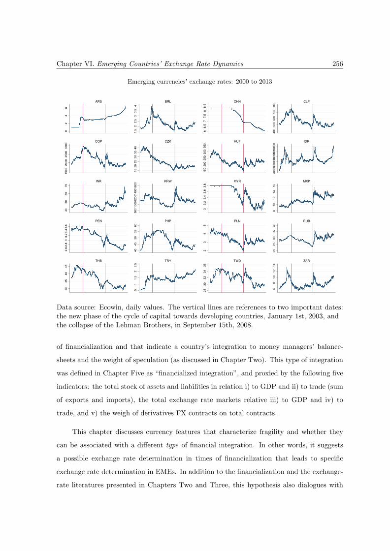
Chapter VI. Emerging Countries’ Exchange Rate Dynamics 256
Emerging currencies’ exchange rates: 2000 to 2013
02
46
ARS
1.5
22
.53
3.5
4
BRL
66
.57
7.5
88
.5
CHN
40
05
00
60
07
00
80
0
CLP
15
00
20
00
25
00
30
00
COP
15
20
25
30
35
40
CZK
15
02
00
25
03
00
35
0
HUF
70
008
00
090
0010
00
01
10
00
12
00
0
IDR
40
50
60
70
INR
80
01
00
01
20
01
40
01
60
0
KRW
33
.23
.43
.63
.8
MYR
81
01
21
41
6
MXP
2.6
2.8
33
.23
.43
.6
PEN
40
45
50
55
60
PHP
23
45
PLN
20
25
30
35
40
RUB
30
35
40
45
THB
.51
1.5
22
.5
TRY
28
30
32
34
36
TWD
68
10
12
14
ZAR
Data source: Ecowin, daily values. The vertical lines are references to two important dates:the new phase of the cycle of capital towards developing countries, January 1st, 2003, andthe collapse of the Lehman Brothers, in September 15th, 2008.
of financialization and that indicate a country’s integration to money managers’ balance-
sheets and the weight of speculation (as discussed in Chapter Two). This type of integration
was defined in Chapter Five as “financialized integration”, and proxied by the following five
indicators: the total stock of assets and liabilities in relation i) to GDP and ii) to trade (sum
of exports and imports), the total exchange rate markets relative iii) to GDP and iv) to
trade, and v) the weigh of derivatives FX contracts on total contracts.
This chapter discusses currency features that characterize fragility and whether they
can be associated with a different type of financial integration. In other words, it suggests
a possible exchange rate determination in times of financialization that leads to specific
exchange rate determination in EMEs. In addition to the financialization and the exchange-
rate literatures presented in Chapters Two and Three, this hypothesis also dialogues with
Chapter VI. Emerging Countries’ Exchange Rate Dynamics 257
two important literatures: the one on the consequences of capital account liberalization or
financial integration, and the push vs. pull debate on the determinants of capital flows.
The analysis in this chapter suggests an impact from exchange rates to growth prospects,
through transmission channels that are not considered in the financial integration literature.
While this chapter’s analysis is based on a type of financial integration, in the literature the
impacts of integration are based on its size or magnitude. The different de facto measures
of integration used in the literature include the absolute or relative importance of either
capital flows or of the stock of foreign assets and liabilities - the latter being sounder for
this thesis’ purposes, as discussed in Chapter Five. Among relative measures, the indicator
of financial integration relative to trade might be the most interesting for emphasizing the
two sources of FX transactions. Throughout the chapter exchange rate features are analyzed
not only against the indicator of financialized integration (focused on the characteristics of
the integration), but also against the indicator of financial-to-trade integration (that focus
on the magnitude). The relationship between the two can be seen in see Figure 6.27 in the
Appendix.
With regards to the push vs. pull literature, by analyzing exchange rate features the
chapter suggests the relevance of the international condition, a push factor. The impact is
analyzed directly on exchange rates, while the literature focuses on consequences on capital
flows and do not necessarily link it to exchange rate dynamics. Sections 6.1 and 6.3 will
present the parallel literature on the consequences of financial integration and the role of
push and pull factors, respectively, to further explain this chapter’s findings.
The structure of the chapter The remainder of the chapter is divided as follows. Section
6.1 presents the literature on the impacts of integration to international financial markets.
The three following sections are dedicated to the potential features of emerging currencies
and their relationships with the type of integration. Section 6.2 examines exchange rate
volatility (from the aspects of deviation and of extreme change). Section 6.3 is focused on
the association between emerging currencies and international liquidity conditions. Section
6.4 discusses the comovement of emerging currencies. Section 6.5 discusses other elements
that could potentially explain emerging currencies’ patterns. Section 6.6 presents concluding
remarks and avenues for future research.
Chapter VI. Emerging Countries’ Exchange Rate Dynamics 258
Methodological Note
Most of the empirical analyses done in this chapter involve the indicator of the level of finan-
cialization of country’s integration, as presented in Chapter Five. The type of integration is
estimated using 2013 data. It is one point that is expected to be representative given the
structural character of the variable – specially for its dependency on stock variables. A more
frequent estimation of this variable is not possible, because it is dependent on data released
every three years (the triennial surveys of the Bank for International Settlements, BIS).
Earlier points could be biased by the GFC: financial integration relative to GDP increased
substantially before the crisis, dropped in 2008, and increased again in what followed; but
apart from that, it has grown in stable fashion - see Figure 5.7. Using data from previous
years would also lead to a different stage of EMEs’ financial insertion, because, as seen in
Chapter Four, EMEs’ integration in 2001 was very different than the current one.
The limited amount of observations surely restricts the possible methodological ap-
proaches. The use of graphical analyses to suggest the potential correlation between two
variables is deemed the most appropriate method. To enrich the analyses, the Pearson cor-
relation coefficient – and coefficients of determination2. were used to quantify the potential
correlation. The Pearson correlation coefficient is a measure of linear correlation between
two variables developed in the late 19th century. It is estimated (for samples) by the formula
in Equation 6.1 (STATA, 2016)3.
r =
∑ni=1(xi − x)(yi − y)
√∑n
i=1(xi − x)2√
∑ni=1(yi − y)2
(6.1)
The Pearson correlation coefficient is therefore based on the relationship between two
series’ observations distance to their mean, pointing to the relationship between the two
series. A coefficient of -1 indicates a perfectly negative linear relationship, 1 indicates a
positive relationship, and 0 indicates no correlation between variables.
2Coefficients of determination are the square of the correlation coefficient between two variables. It givesthe proportion of the variation in one variable that is accounted for by the other (Everitt and Skrondal, 1998,p. 89). See Everitt and Skrondal (1998) for references and details.
3Stata allows the option of adding weights to variables, which was not done in this chapter.
Chapter VI. Emerging Countries’ Exchange Rate Dynamics 259
The resulting correlation coefficients are analyzed together with the respective scatter
plots given the potential weight of outliers in the coefficients. Another concern with potential
bias emerges from the small number of observations. Aiming to avoid them, the respective
significance of the coefficients’ level were added.
It might be worth recalling the similarities between the correlation coefficient and a
regression. In the case of a simple linear regression analysis, its coefficient of determination
(r2) is the same as the square of the correlation coefficient (Everitt and Skrondal, 1998, p.
89)4. Another similarity between these two methods is that they do not imply causality. In
regressions, tests for causalities as the Granger causality test might be run5 (Granger, 1969).
The direction of causality of the analyses conducted in this chapter are however clear from
the theoretical discussion, dismissing causality tests.
All the estimations were done in Stata (11).
On the analyzed countries This chapter follows the “financial-markets-oriented” op-
erational definition of EMEs discussed in Chapter Four (Section 4.1.1). EMEs are: Ar-
gentina, Brazil, Chile, China, Colombia, Czech Republic, Hungary, India, Indonesia, Korea,
Malaysia, Mexico, Peru, Philippines, Poland, Russia, South Africa, Taiwan, Thailand, and
Turkey. Please refer to the “List of Abbreviations” of countries and currencies in the Thesis’
preamble.
Whether a country has a floating or a non-floating regime was defined based on IMF’s
de facto characterization of these countries’ exchange rate arrangements from 2003 to 2013,
presented in table 6.12 in the Appendix. Also note the discussion immediately preceding the
table, that served as a basis to consider the following countries as having a floating exchange
rate regime: Brazil, Chile, Colombia, Czech Republic, India, Indonesia, Korea, Mexico, Peru,
Philippines, Poland, South Africa, Russia, Taiwan, Thailand, and Turkey. The ones with
non-floating regimes are: Argentina, China, and Malaysia.
4In the analyses done in this chapter the best fit for two variables was most often of a linear regressionwith no intercepts. Simple linear regressions and regressions with a dummy variable for the exchange rateregime were run and in most cases the adjusted r2 were better for regressions without the intercept and theintercepts were not significative at the 10% level.
5Such analyses would however probably be hindered in the analyses given the low amount of observationsin this chapter’s study (and thus of degrees of freedom).
Chapter VI. Emerging Countries’ Exchange Rate Dynamics 260
Therefore, from the analyzed 20 emerging currencies, 17 have floating exchange-rate
regimes and three have non-floating regimes. The index of financialized integration is es-
timated for the nine emerging currencies analyzed in BIS Triennial Surveys (in 2001 and
2013): Brazil, China, Hungary, India, Korea, Mexico, Poland, Russia, Taiwan, Turkey and
South Africa. Given that no trade data is available for Taiwan, the financial-to-trade inte-
gration index is estimated for 19 EMEs. Other indicators are estimated for all 20 emerging
currencies. To facilitate the differentiation of the currencies under study, the number of coun-
tries involved in each case is presented in the tables that compare correlation coefficients of
different country groups.
6.1 The Expected Impacts of Integration
Whether or not a country should open its capital account is an important question in eco-
nomic literature. As liberalization becomes the rule across developing countries, the question
has moved from the impacts of liberalization to the impact of a de facto integration – in em-
pirical studies, the substitution from the de jure liberalization proxy to the de facto proxy
of integration is an indication of this shift, as discussed in Chapter Five. The literature is
briefly reviewed in this section, to shed light on how it relates to the debate presented in the
chapter.
The main arguments for capital account liberalization and integration focus on the
possible economic growth from the flow of capital, from abundance to scarcity. Liberalization
would boost investments by making cheaper loans available to residents and reducing risks
for investors by diversifying assets in different countries and markets. According to this
argument, it is noteworthy to mention that opening the capital account would benefit not only
the specific country, but the global economy in general6. The efficiency of domestic financial
markets would be enhanced due to exposure to competing foreign firms; and technologies,
institutions, and property rights would improve with a country’s exposure to global financial
markets and by the ‘macroeconomic discipline’ it imposes (which from another perspective,
6Although this review is only a short overview, it is interesting to highlight that the theoretical backgroundbehind arguing for capital account liberalization are in line with Solow’s (1956) growth model, where capitalis one of the main factors leading to growth (together with labor and productivity) and the loanable fundstheory, which states that savings determine investments (Da Silva and Da Fonseca, 2015).
Chapter VI. Emerging Countries’ Exchange Rate Dynamics 261
might be seen as a loss of policy autonomy). Furthermore, liberalization of the capital account
would allow for consumption smoothing over time, which would be particularly valuable if
borrowed capital were used to improve a country’s ability to produce goods and services (see
Fischer (1997), Kose et al. (2006), Levine and Zervos (1996), Mishkin (2006), and Neely
(1999))7.
The arguments against financial integration are mainly focused on the instability brought
by capital flows, which are a consequence of the procyclicality of financial markets in general
(Borio, 2014) and of portfolio flows specifically, that results in an intensification of boom and
bust cycles (Edwards, 2001) – a reason being that inflows lead to credit booms (Blanchard
et al., 2015) and to financial crisis as illustrated by developing countries across the globe since
the late 1990s. Due to their cyclicality and volatility, capital flows could also be detrimental
to investment (Moguillansky, 2002)8.
Mishkin (2006) and Kose et al. (2006) would respond to counter-arguments based on
the manifest crises, stating that crises emphasize the costs of liberalization, but, in reality,
are just a reflection of the fact that costs are concentrated and immediate, while gains are
dispersed and gradually presented.
But the prevalent argument is that such crises occur in developing countries due to
problems in their financial systems. Several authors point to the early stage of development
of financial markets (see Bekaert et al. (2005), Edwards (2001), and Eichengreen (2001)). The
IMF (2001) posits that the net results of liberalization depend on the strength of domestic
macroeconomic policies and financial structures. Also Eichengreen and Leblang (2003, p.
23-24) argue that the result from capital account liberalization depends on the robustness of
the domestic financial system – and on whether the international financial system is “prone
to costly and disruptive crises”.
Obstfeld (2009, italics added) also argues that the stage of development of countries’
financial markets matters, specifically in increasing exchange rate volatility:
7See Kregel (1996) for criticism on an “utopian” view of the benefits of globalization, including financialglobalization.
8 Moguillansky (2002, p. 57) argues that this would take place due to “the microeconomic effect trans-mitted by the reduced external borrowing capacity of large companies, the flight to quality in the domesticfinancial system (which results in a credit crunch for small and medium-sized enterprises), and the increasein uncertainty for economic agents”.
Chapter VI. Emerging Countries’ Exchange Rate Dynamics 262
In addition, whereas fixed exchange rates have proved dangerous in a context of
open capital markets, a regime of freely floating rates raises problems of exchange-
rate volatility that are particularly severe for emerging economies pending further
evolution in their financial markets. (p. 2)
In a way, these arguments persist since the debate on the sequencing of liberalization
(domestic financial liberalization first, followed by opening the current account, and only
later the capital account9). The debate occurred when the reality of financial markets in
developing countries was completely different. The current evidence of high exchange rate
volatility in countries that have developed financial systems and FX markets make it more
difficult to defend such positions10.
However, it is important to note that the mainstream position on the subject might be
evolving since the GFC, as marked by IMF’s new position on capital controls presented in
Chapter Seven (see Blanchard et al. (2012); Claessens et al. (2010); Ostry et al. (2010); and
Ostry et al. (2011)11).
Empirical findings The empirical results on the overall impact of capital account liberal-
ization portray mixed findings12. Some authors found a positive relationship between capital
account liberalization and growth (Quinn (1997); IMF (2001)), and others found no robust
correlation (Grilli and Milesi-Ferretti (1995); Rodrik (1998))13.
After a great amount of empirical tests, meta-analyses emerged based on those findings.
The elusiveness of the debated is confirmed by Jeanne et al.’s (2012) meta-analysis. Based
9According to the debate on the importance of the gradual liberalization intensified with the Mexican andAsian crises of the 1990s, after having been left aside by the optimistic views of the late 1980s and early 1990s.
10Note that there is also a debate on the different impacts of the different types of flows, consistent with theidea that not every type of capital has the same implications, nor the same patterns (discussed in ChapterFour, Section 4.3). See Reisen and Soto (2001), who depicts a rather benign picture of capital flows. Ingeneral, FDI is seen as the type of inflow that would be the most beneficial for growth. For instance, OECD(2002) argues that given appropriate host-country policies and a basic level of development, FDI facilitatesthe transfer of technological advances and know-how; it increases competition; human capital improves; itintegrates the economy towards the world economy; and it pushes for more positive development of firms. SeeMargeirsson (2015) for references.
11See Fritz and Prates (2014) for a critique on IMF’s new approach to capital account openness and Royand Ramos (2012) that demonstrates the lack of consideration of this new position in the policy recommendedto developing countries.
12For the debate on the Brazilian case see Arida (2003a), Arida (2003b), Arida (2004), Ferrari Filho et al.(2005) and Oreiro (2004).
13In addition to the studies that analyze different countries, also note Henry (2006) analysis based on eventstudies.
Chapter VI. Emerging Countries’ Exchange Rate Dynamics 263
on 2,340 regressions, their results suggest positive findings regarding FDI and equity flows
vis-a-vis banking or debt flows, and among advanced countries, but due to the sensitivity of
the samples used, the evidence is not conclusive. However, the authors’ overall conclusion is
clear:
the international community should not seek to promote totally free trade in
assets even over the long run because free capital mobility seems to have little
benefit in terms of long run growth and because there is a good case to be made
for prudential and non-distortive capital controls. (p. 5)
In fact, it is hard to find positive outcomes from capital account openness. As put
by Rey (2015): “As attested by the most recent surveys reviewing a long list of empirical
papers, it is hard to find robust evidence of an impact of financial openness on growth or on
improved risk sharing” (also see Eichengreen (2001); Kose et al. (2006); and Obstfeld (2009)).
Nevertheless, most conclusions are not as direct as Jeanne et al.’s (2012). Eichengreen and
Leblang (2003) affirm that “results suggest that capital account liberalization is neither
plague nor panacea”. Rey (2015, p. 20) states that “One thing is clear at this stage: we
cannot take them [the gains to international capital flows] for granted”. While Obstfeld
(2009, p. 1, italics added) puts that: “Despite an abundance of cross-section, panel, and
event studies, there is strikingly little convincing documentation of direct positive impacts of
financial opening on the economic welfare levels or growth rates of developing countries”14.
Rey (2015) reminds her reader that the benefits of capital account liberalization should
not be taken for granted and Obstfeld (2009, p. 1) finds the absence of positive results strik-
ing. These positions seem to reflect the fact that mainstream scholars expect, beforehand,
that capital account liberalization could only be positive, given that it is a direct application
of Solow’s and the loanable funds’ theory.
14An important exception among this large skepticism found in the literature is Kose et al. (2006, p. 2),who argues that: “A central conclusion of this paper is that while the rapidly-growing empirical literatureis gradually tilting towards supporting a significant positive role for financial globalization, there are manyunanswered questions about how a country should organize and pace its move. At the same time, we findthere is very little meaningful empirical support to underpin the more polemic claims of those who argue thatcapital account liberalizations (as opposed to, say, inappropriately rigid exchange rate regimes) are the rootproblem behind most developing country financial crises of the past fifteen years.”
Chapter VI. Emerging Countries’ Exchange Rate Dynamics 264
Integration and Exchange Rate Volatility Though abundant, this literature is mostly
focused on the expected final results from liberalization/integration, neglecting the transmis-
sion channels through which these results would be achieved. In regards to exchange rates,
their only potential impact are with respect to crises of pegged regimes. However the issue
of instability brought by financial integration do not only come from financial crisis, or from
crisis related to fixed-exchange rate pegs, but also from its impacts on floating exchange
rates, that might be deleterious for growth.
As mentioned in the Introduction Chapter, “excessive” exchange rate appreciation is
negative for growth and so is exchange rate volatility. And as discussed in Chapter Three
(Section 3.3.4), the integration to international financial markets, and the exposure to money
managers’ behavior might be resulting in exchange rates that follow the cycles of international
financial markets, with major volatility in moments of turbulence and appreciation in periods
of tranquility. Financial integration can therefore be negative for growth through its effect
on the level and the on volatility of the exchange rate.
The debate presented in this chapter could contribute to the literature by analyzing if
the specific exchange rate pattern is related to the type of integration. The chapter might
also contribute to the literature by shifting the focus from the size to the type of integration,
calling attention to the importance of the characteristics of FX markets on creating these
specific exchange rate features. Given that financial integration can bring instability, whether
it allows for more or less speculation is a relevant matter.
6.2 Exchange Rate Volatility
This section examines the first of the three exchange rate features associated with financial-
ized integration: volatility. Its discussion is based on exchange rate deviation from its trend
(the standard deviation), on the features of the distribution of exchange rate changes, and
on the frequency of important exchange rate changes. These features are associated with the
level of financialization of EMEs’ integration.
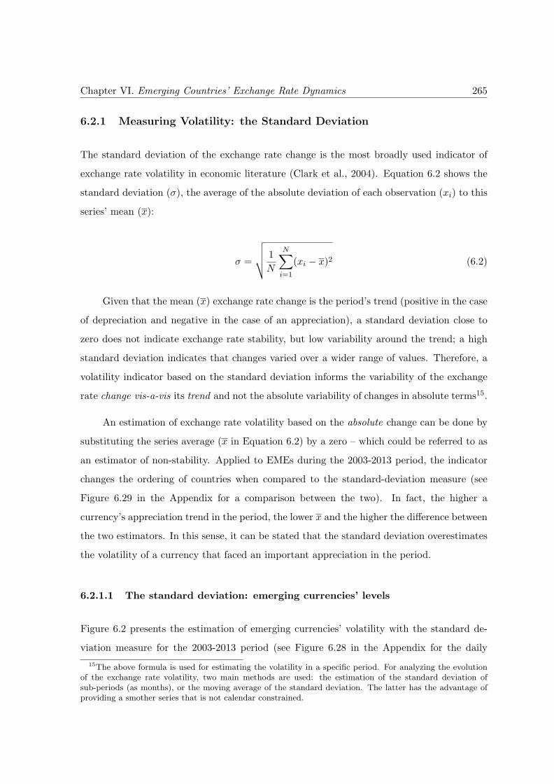
Chapter VI. Emerging Countries’ Exchange Rate Dynamics 265
6.2.1 Measuring Volatility: the Standard Deviation
The standard deviation of the exchange rate change is the most broadly used indicator of
exchange rate volatility in economic literature (Clark et al., 2004). Equation 6.2 shows the
standard deviation (σ), the average of the absolute deviation of each observation (xi) to this
series’ mean (x):
σ =
√
√
√
√
1
N
N∑
i=1
(xi − x)2 (6.2)
Given that the mean (x) exchange rate change is the period’s trend (positive in the case
of depreciation and negative in the case of an appreciation), a standard deviation close to
zero does not indicate exchange rate stability, but low variability around the trend; a high
standard deviation indicates that changes varied over a wider range of values. Therefore, a
volatility indicator based on the standard deviation informs the variability of the exchange
rate change vis-a-vis its trend and not the absolute variability of changes in absolute terms15.
An estimation of exchange rate volatility based on the absolute change can be done by
substituting the series average (x in Equation 6.2) by a zero – which could be referred to as
an estimator of non-stability. Applied to EMEs during the 2003-2013 period, the indicator
changes the ordering of countries when compared to the standard-deviation measure (see
Figure 6.29 in the Appendix for a comparison between the two). In fact, the higher a
currency’s appreciation trend in the period, the lower x and the higher the difference between
the two estimators. In this sense, it can be stated that the standard deviation overestimates
the volatility of a currency that faced an important appreciation in the period.
6.2.1.1 The standard deviation: emerging currencies’ levels
Figure 6.2 presents the estimation of emerging currencies’ volatility with the standard de-
viation measure for the 2003-2013 period (see Figure 6.28 in the Appendix for the daily
15The above formula is used for estimating the volatility in a specific period. For analyzing the evolutionof the exchange rate volatility, two main methods are used: the estimation of the standard deviation ofsub-periods (as months), or the moving average of the standard deviation. The latter has the advantage ofproviding a smother series that is not calendar constrained.
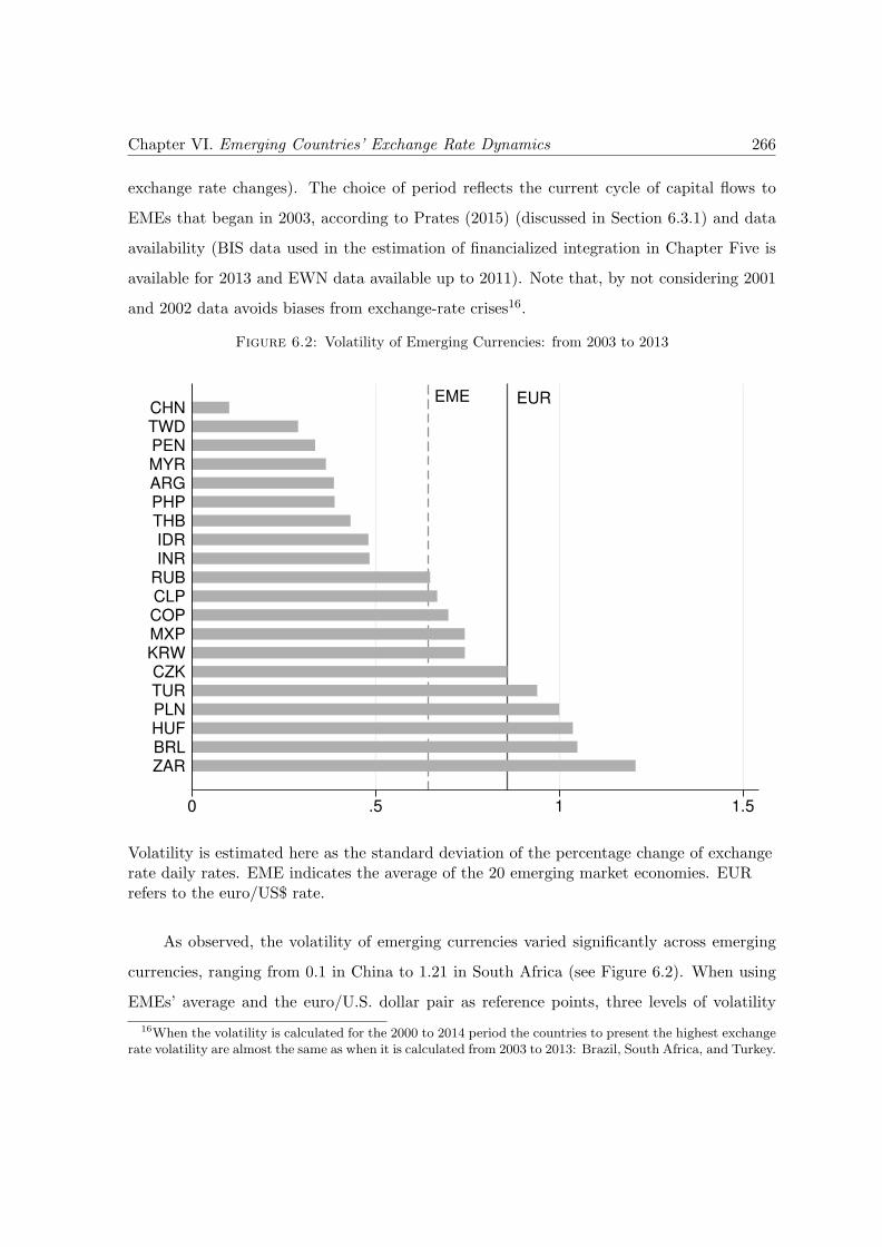
Chapter VI. Emerging Countries’ Exchange Rate Dynamics 266
exchange rate changes). The choice of period reflects the current cycle of capital flows to
EMEs that began in 2003, according to Prates (2015) (discussed in Section 6.3.1) and data
availability (BIS data used in the estimation of financialized integration in Chapter Five is
available for 2013 and EWN data available up to 2011). Note that, by not considering 2001
and 2002 data avoids biases from exchange-rate crises16.
Figure 6.2: Volatility of Emerging Currencies: from 2003 to 2013
EME EUR
0 .5 1 1.5
ZARBRLHUFPLNTURCZK
KRWMXPCOPCLPRUBINRIDRTHBPHPARGMYRPENTWDCHN
Volatility is estimated here as the standard deviation of the percentage change of exchangerate daily rates. EME indicates the average of the 20 emerging market economies. EURrefers to the euro/US$ rate.
As observed, the volatility of emerging currencies varied significantly across emerging
currencies, ranging from 0.1 in China to 1.21 in South Africa (see Figure 6.2). When using
EMEs’ average and the euro/U.S. dollar pair as reference points, three levels of volatility
16When the volatility is calculated for the 2000 to 2014 period the countries to present the highest exchangerate volatility are almost the same as when it is calculated from 2003 to 2013: Brazil, South Africa, and Turkey.
Chapter VI. Emerging Countries’ Exchange Rate Dynamics 267
can be identified17. The first, composed of countries with low exchange rate volatility (lower
than emerging currencies’ average), counts for about half of the sample: the Chinese yuan
(volatility index of 0.1), the Taiwanese dollar (0.29), the Peruvian nuevo sol (0.34), the
Malaysian ringgit (0.36), the Philippine peso (0.39), the Argentinean peso (0.39), the Indian
rupee (0.48), the Indonesian rupiah (0.48), and the Thai bath (0.43). A second group includes
countries with middle-high volatility (between the EMEs’ average and the euro): the Russian
ruble (0.65), the Chilean peso (0.67), the Colombian peso (0.7), the Mexican peso (0.74),
the Korean won (0.74), and Czech Republic (0.86). A group of five countries is on the high-
volatility end (higher than the euro): the South African rand (1.21), the Brazilian real (1.05),
the Hungarian forint (1.04), the Polish zloty (1), and the Turkish lira (0.94).
Volatility: EMEs and the euro’s level As seen in Figure 6.2, when measured by
the standard deviation, emerging currencies average volatility is lower than the level of the
EUR/USD, with only five of the 20 EMEs presenting higher volatility than the euro. When
only EMEs with floating regimes are considered, the average volatility is still lower than the
one of the euro (0.71, against 0.86). De Conti (2011) compared the volatility of emerging
currencies with currencies from advanced countries and reached similar results: the volatility
of emerging countries’ currencies is not necessarily higher than that of advanced countries.
The result contradicts claims that emerging currencies are more volatile due to their
peripheral insertion in the international monetary and financial systems, found in center-
periphery literature on exchange rates, discussed in Chapter Three (Section 3.3.4). De Conti
(2011, p. 101) argues that the low volatility of some emerging currencies lies on differ-
ent macroeconomic domestic policies adopted by (mostly Asian) countries to counter act
volatility. Were these policies not in place, these countries would have a higher “potential
volatility” than the (actual) “observed volatility”. However, as Chapter Three’s review of
the center-periphery analyses of emerging currencies argued, a different insertion would not
necessarily lead to exchange rate volatility in general, but to major depreciation in moments
of crisis (see Section 3.3.4.1).
17The euro/U.S. dollar rate was chosen for representing advanced countries as they are the two mostimportant currencies in the current configuration of the international monetary system. As discussed inChapter Three, the U.S. dollar is the system’s key currency and the euro, used in several countries, is in thesecond-highest position (De Conti, 2011, p. 46).
Chapter VI. Emerging Countries’ Exchange Rate Dynamics 268
6.2.1.2 Explaining different levels: exchange rate regimes
Part of the heterogeneity of volatility estimates is obviously due to the exchange rate regime
adopted. Although most countries had floating regimes in the analyzed period, “craw-like”
regimes prevailed in Argentina and in China and “other managed regime” in Malaysia (IMF,
2014, p. 6-7)18. These three countries are in the low-volatility group. As expected, the
average volatility of currencies with floating regimes is significantly higher than the volatility
of this group of non-floating regimes: 0.71 against 0.28.
The combined choice of exchange rate regime and monetary policy framework – though
not the focus of this thesis – is a noteworthy perspective to understand the volatility of
emerging currencies. From this viewpoint, it is interesting to note that the average volatility
of the 14 countries following an inflation targeting regime with floating exchange rates19 is
higher (0.75) than the average of the broader group of countries with floating exchange rate
regimes (0.71).
6.2.1.3 Explaining different volatility levels: the magnitude and type of financial
integration
The magnitude of financial integration Financial-to-trade integration is the ratio of
financial integration (proxied by the sum of the stock of foreign assets and liabilities) to trade
(proxied by the sum of exports and imports20.
Figure 6.3 shows the relationship between financial-to-trade integration and exchange
rate volatility for EMEs. A positive relationship between the two is observed – countries with
high or mid-high integration tend to have higher-than-average volatility. This relationship,
however, does not seem to be strong. To further analyze whether a relationship exists, a
18See Table 6.12 in the Appendix 6.8 for the definition of the exchange rate arrangements used in thischapter.
19Not including India, that implemented the inflation targeting regime after the period considered in thisanalysis.
20The financial-to-trade indicator can also be thought of as the relative weight of financial integration withregards to GDP compared to the weight of trade integration in relation to GDP. This indicator is used byLane and Milesi-Ferretti (2007) when analyzing the expansion of asset trade in comparison to the expansionof product trade among advanced and developing countries.
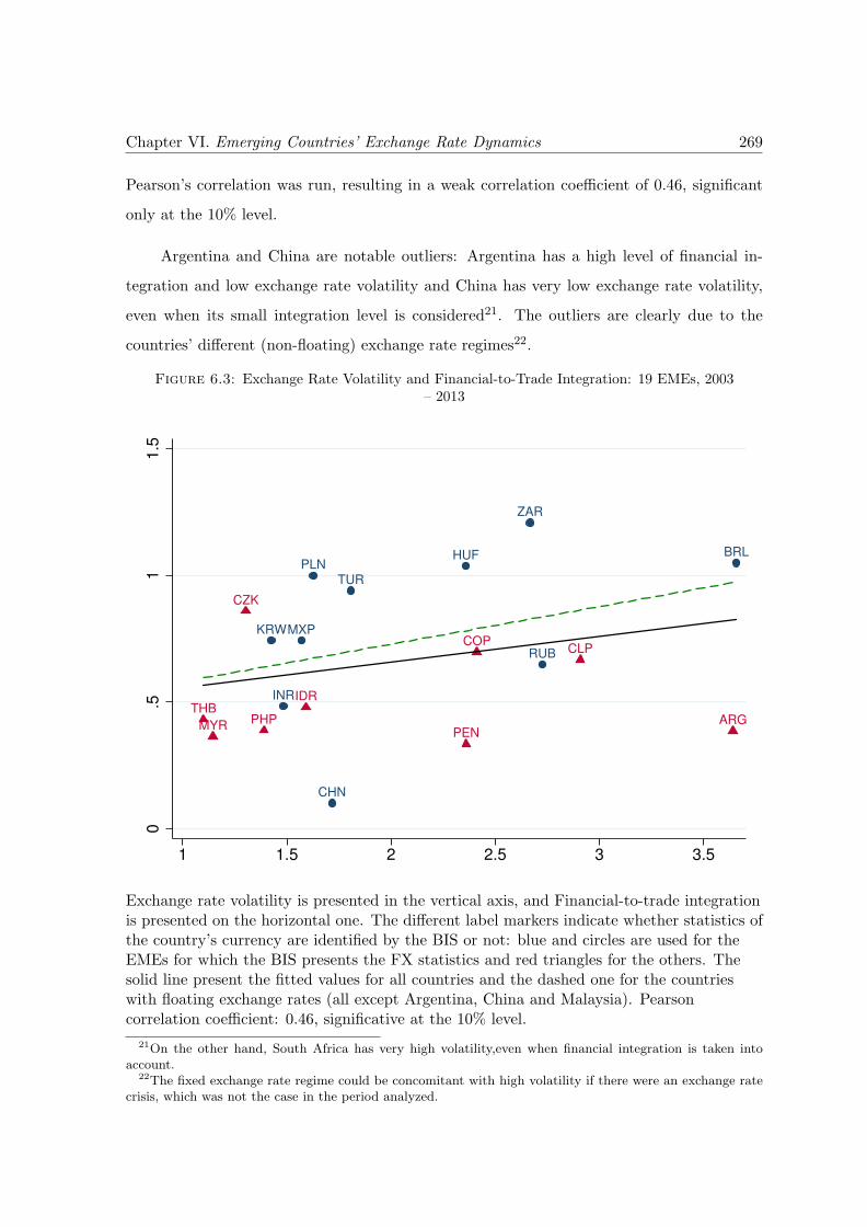
Chapter VI. Emerging Countries’ Exchange Rate Dynamics 269
Pearson’s correlation was run, resulting in a weak correlation coefficient of 0.46, significant
only at the 10% level.
Argentina and China are notable outliers: Argentina has a high level of financial in-
tegration and low exchange rate volatility and China has very low exchange rate volatility,
even when its small integration level is considered21. The outliers are clearly due to the
countries’ different (non-floating) exchange rate regimes22.
Figure 6.3: Exchange Rate Volatility and Financial-to-Trade Integration: 19 EMEs, 2003– 2013
BRL
CHN
HUF
INR
KRWMXP
PLN
RUB
TUR
ZAR
ARG
CLPCOP
CZK
IDR
MYRPEN
PHPTHB
0.5
11
.5
1 1.5 2 2.5 3 3.5
Exchange rate volatility is presented in the vertical axis, and Financial-to-trade integrationis presented on the horizontal one. The different label markers indicate whether statistics ofthe country’s currency are identified by the BIS or not: blue and circles are used for theEMEs for which the BIS presents the FX statistics and red triangles for the others. Thesolid line present the fitted values for all countries and the dashed one for the countrieswith floating exchange rates (all except Argentina, China and Malaysia). Pearsoncorrelation coefficient: 0.46, significative at the 10% level.
21On the other hand, South Africa has very high volatility,even when financial integration is taken intoaccount.
22The fixed exchange rate regime could be concomitant with high volatility if there were an exchange ratecrisis, which was not the case in the period analyzed.
Chapter VI. Emerging Countries’ Exchange Rate Dynamics 270
Indeed, in countries with floating exchange rate regimes the same financial-to-trade
integration level seems to be associated with higher exchange rate volatility. This can be
observed in the difference between the two lines in Figure 6.3: the higher, dashed line rep-
resents the relationship for countries with floating exchange rates, and the solid, lower line,
represents countries with non-floating regimes.
Before analyzing volatility based on the type of financial integration, the role of the
magnitude of the FX markets in explaining volatility together with the financial-to-trade
integration was estimated. The estimation was based on a currency international importance,
enabled by the fact that BIS’ FX surveys are conducted for the most important currencies,
grouping currencies of other EMEs into a “other” or “residual” group. To facilitate this
analysis, the markers of countries in Figure 6.3 are differentiated for these two groups: blue
circles represent EMEs on BIS’ FX statistics and red triangles represent the others. As
observed, these two groups of countries are rather distinct: those with more important FX
markets show higher exchange rate volatility for all levels of financial-to-trade integration.
For instance, the Brazilian real and the Argentinean peso show high levels of financial-to-
trade integration, but the Brazilian real that has important FX market, has much higher
exchange rate volatility. The Hungarian forint and the Colombian (or the Peruvian) pesos are
in the same situation, but with middle levels of financial-to-trade integration. There are also
examples among the currencies of low financial-to-trade integration, such as the Mexican
peso compared with the Indonesia rupiah. In other words, the probability of a currency
with large FX markets to have above-average exchange rate volatility is higher than that
of currencies that have smaller FX markets. China has an important FX market but low
exchange rate volatility but is an exception due to its exchange rate regime. Although not an
exact proxy, the differences between the two groups of countries (with important FX market
or not) is a first evidence of the importance of the amount of FX contracts in explaining
exchange rate volatility.
The type of financial integration Figure 6.4 analyzes exchange rate volatility against
the index of financialized integration. Exchange rate volatility and a more financialized in-
tegration have a clearly positive relationship for floating currencies: the countries with the
most financialized integration – South Africa, Turkey, Brazil, and Hungary – also present the
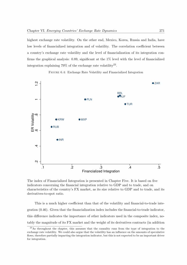
Chapter VI. Emerging Countries’ Exchange Rate Dynamics 271
highest exchange rate volatility. On the other end, Mexico, Korea, Russia and India, have
low levels of financialized integration and of volatility. The correlation coefficient between
a country’s exchange rate volatility and the level of financialization of its integration con-
firms the graphical analysis: 0.89, significant at the 1% level with the level of financialized
integration explaining 79% of the exchange rate volatility23.
Figure 6.4: Exchange Rate Volatility and Financialized Integration
HUF
INR
KRW MXP
PLN
RUB
TUR
ZAR
BRL
.2.4
.6.8
11
.2E
R V
ola
tilit
y
.1 .2 .3 .4 .5Financialized Integration
The index of Financialized Integration is presented in Chapter Five. It is based on fiveindicators concerning the financial integration relative to GDP and to trade, and oncharacteristics of the country’s FX market, as its size relative to GDP and to trade, and itsderivatives-to-spot ratio.
This is a much higher coefficient than that of the volatility and financial-to-trade inte-
gration (0.46). Given that the financialization index includes the financial-to-trade indicator,
this difference indicates the importance of other indicators used in the composite index, no-
tably the magnitude of its FX market and the weight of its derivatives contracts (in addition
23As throughout the chapter, this assumes that the causality runs from the type of integration to theexchange rate volatility. We could also argue that the volatility has an influence on the amounts of speculativeflows, therefore partially impacting the integration indicator, but this is not expected to be an important driverfor integration.
Chapter VI. Emerging Countries’ Exchange Rate Dynamics 272
to the relative magnitude of financial integration relative to GDP) in explaining exchange
rate volatility.
6.2.1.4 On the use of the standard deviation to estimate volatility
As mentioned, the theoretical debate on emerging currencies presented in Chapter Three
discusses specific type of volatility more closely related to major changes in certain moments
than to volatility in general. While the latter aspect is captured by the use of the standard
deviation, the former is not. In addition, the standard deviation estimator is flawed and too
narrow when compared to definitions of volatility.
Dictionary definitions facilitate a discussion on the limitations of the standard deviation
in this specific use. According to the Oxford dictionary, volatility denotes something that is
“liable to change rapidly and unpredictably, especially for the worse”. Deviation is a narrower
concept: “the action of departing from an established course or accepted standard: deviation
from a norm” (“Volatile”, 2015). In these definitions, deviation only partially captures the
three aspects of volatility: velocity, predictability and direction. The first refers to how
rapidly the deviation takes place. In regards to time series of daily changes, velocity refers to
the magnitude of the deviation. This aspect is captured by the standard deviation, which is
formed by the average of every deviation. However, because the standard deviation is based
on averages it would be the same for two very distinct groups: one in which the deviations
are regular and limited to a given value, and another composed mostly by relatively smaller
deviations, but that includes large ones. In other words, the standard deviation is not telling
for being based on averages: relevant changes in value can easily be hidden behind small
variations if the sample period is long enough.
Because it presents the same average without reflecting distribution, the standard devi-
ation does not capture the second aspect of volatility, the predictability of a series. In the two
mentioned groups, the first, with deviations of similar magnitude, is more predictable than
the second, that presents large outliers. However, predictability is very relevant given its
weight on decision-making, especially relating to decisions concerning exchange rates in open
economies. Specifically thinking of the decisions of foreign investors, predictability affects
expectations concerning possible loss of investments.
Chapter VI. Emerging Countries’ Exchange Rate Dynamics 273
This concern calls attention to the third aspect of volatility present in the definition: the
direction of the deviation, an aspect that cannot be captured by the standard deviation, that
is based on absolute deviations24. Predictability seems to be specially relevant for analyzing
exchange rates given the presence of “jumps” (or discontinuities in prices) that characterize
their series. The presence of “jumps” is in fact one of the three “most prominent features of
foreign exchange volatility” for Erdemlioglu et al. (2012, p. 1) and the acknowledgment of
the importance of this and other exchange rate features triggered a new generation of models
that would yield in exchange rates featuring these specific characteristics (see the exchange
rate puzzles in Table 3.1 in Chapter Three).
In other words, the distribution of exchange rate changes are fat-tailed and are in
the realm of what Taleb (2007) called Extremistan. As opposed to Mediocristan, where a
particular unexpected event cannot have a significant consequence on the outcome of total
events, in thick tailed Extremistan the one event can dominate the outcome of all other25.
This feature affects how money managers see a currency, exactly because of their potential
of changing the overall groups average being most important given the representativeness
principle.
On top of these limitations of measures of deviation to characterize volatility, there are
also problems related to the specific application of the standard deviation to time series.
By definition, deviation is a relative concept and the reference point has an important role.
When thinking about a group of individuals in a specific point in time, their deviation to
24It is interesting to note that the shortfall of the standard deviation and the importance of the exchangerate peaks and other characteristics of what we understand as risk have driven to interesting developments inthe estimation of volatility, specially inside finance given the importance of volatility in risk management andportfolio allocation. Reviewing the advances in volatility modeling since the use of the ARCH/GARCH familyto sophisticated models that estimate jumps and combine autoregressive volatility and jumps, Erdemliogluet al. (2012, p. 1) enumerates the features of exchange rate volatility that call for these modeler’s work: “(i) ittends to be autocorrelated; (ii) it is periodic, displaying intraday and intraweek patterns; and (iii) it includesdiscontinuities (jumps) in prices.” While autocorrelation might be more interesting for economic modeling, andintraday volatility is most of the time too short of a periodicity to have economic impact, the discontinuitiesand exchange rate peaks are very important for foreign investment decisions. “The importance of Fat Tailsfor finance is broadly known and has lead to the development of Value at Risk (VaR) from parametricalcalculations that utilizes the Normal distribution to the “Fat-tailed VaR” that utilizes the Skewed Student’sdistribution which accounts not only for the two moments of the Normal (mean and standard Deviation), butalso the skewness and the degrees of freedom (tail fatness)”.
25Mediocristan and Extremistan are Taleb’s (2007) types of environment, or “classes of probability domain”.The author gives an interesting example to differentiate the two terms: the weight of a group of 1000 people(to characterize Mediocristan) and the wealth of this group (to characterize Extremistan). When Bill Gatesenters the group, total weight will not change much, but total wealth will significantly change. With regardsto exchange rates, an interesting example is the total exchange rate variation of an European currency againstthe U.S. dollar that, in few years, drastically changed when the European Monetary System collapsed.
Chapter VI. Emerging Countries’ Exchange Rate Dynamics 274
the group’s average seems to be a sound indicator for characterizing an individual. But
when applied to time series, the definition of normality is not trivial: Should we choose a
specific point in time to be considered the norm? Or a point which would be preferred for
representing some sort of “equilibrium” value? When thinking about a series of percentage
changes, the ideal is a change that deviates from the period’s trend, from a chosen value, or
from zero?
The standard deviation of exchange rate changes to the period’s average – the most
used methodology – also has specific problems: it is based on the deviation from the period’s
average change, or its trends, which might result in biased indicators when the volatility
in different countries is compared, given that their deviations would not be compared to
the same norm. For instance, in the cases just analyzed, for the 2003 to 2008 period,
Brazil’s exchange rate appreciated 49% while India’s depreciated 6%. There is therefore an
underestimation (overestimation) in the case of India where the trend was of depreciation
(appreciated), given that its “norm” was a positive value.
In summary, when characterizing volatility through the use of the standard deviation
only velocity (or the aspect of the magnitude of the deviation) is taken into account and
cross-countries comparisons present comparability issues. In an attempt to overcome these
limitations and better characterize exchange rate volatility including in regards to predictabil-
ity and direction, the next subsections suggest an analyses based on other indicators.
6.2.2 Measuring Volatility: Frequency of Extreme Exchange Rate Changes
6.2.2.1 The role of extreme changes
Exchange rate features as ‘jumps’ call for estimators of volatility that take them into account
not only for methodological reasons, but also because we cannot expect the economic impact
of small exchange rate changes to be the same as the one of a major shock. For instance,
based on French economy data, Berman et al. (2012) argued that exporters can absorb
exchange rate changes in their profit margins; but could exporters also absorb changes of an
exceptional magnitude? Thinking about foreign portfolio investors investing in EMEs, the
impact of exchange rate changes might even be more relevant, given its role in determining
Chapter VI. Emerging Countries’ Exchange Rate Dynamics 275
total returns (a subject that will be discussed in the next chapter). More than change,
direction is also of great importance given the obviously different impact of appreciation and
depreciation of the currency in which assets are labeled.
Apart from the immediate impact of creating uncertainty, extreme exchange rate changes
also impact the memory of agents: given the workings of associative memory in our intu-
itive thinking (or ‘System 1’, as labeled by Kahneman (2011)), the process of constructing
a coherent interpretation of such event will create an association of the currency in question
with risk. And once such association is created it is considered by investors in their deci-
sions, even if unconsciously. These are expected to be of even greater importance in highly
turbulent moments. Indeed, there is evidence that a more unstable currency is seen as riskier
and investors demand a higher risk premium for holding them (Plihon, 2010)26. This is in
line with the representativeness principle, according to which the more available something
is in our memory, the more frequent or likely that event is deemed to be, resulting in agents
overrating the importance of dramatic events (as discussed in Chapter Three, page 97).
To account for these features, this subsection proposes the characterization of exchange
rate volatility based on the probability distribution of the daily exchange rate changes. It
starts by analyzing the basic descriptive statistics of the histograms and then suggests specific
indicators. In doing so, it continues De Conti’s (2011) analysis, who compares exchange rate
volatility in developing and advanced countries with the use of histograms of the daily changes
between July 1994 and December 200927.
6.2.2.2 The range of exchange rate changes
The range of exchange rate changes is a good indicator of volatility of exchange rates because
it highlights the maximum change seen in the country’s currency – which could point to
financial practitioners’ assessments of the potential extent of exchange rate changes.
South Africa’s rand is the currency that presents the highest range of changes between
2003 and 2013, varying 24 p.p. and with the highest daily depreciation. High ranges are
26Evidence in this sense was found by Giovannini and Jorion (1989) who compared the currencies that werepart of the European Monetary System with floating ones (the Japanese yen or the American dollar) andfound that the risk premium asked for the latter ones were greater.
27De Conti’s (2011) analysis of the euro is done from January 2002 to December 2009 (p. 109).
Chapter VI. Emerging Countries’ Exchange Rate Dynamics 276
also seen in Korea (21 p.p.), Brazil (15 p.p.), Mexico (14 p.p.), India (13 p.p.), Hungary (13
p.p.), and Turkey (12 p.p.) – see Table 6.1 for the main statistics of the series of exchange
rate changes. The changes of the euro, on the other hand, have been contained among an
appreciation of 3.9% and depreciation of 3.08%, resulting in a range of 6.97 p.p. in this
period. Seen by the range, the euro is therefore much less volatile than the most volatile
emerging currencies and is only more volatile than the Philippines peso and the Taiwanese
Dollar – with the exception of the Malaysian ringgit and the Chinese yuan that do not follow
a floating regime. The higher range of emerging currencies can also be easily seen in the
larger ranges of the horizontal axis of the histograms presented in Figure 6.5.
6.2.2.3 The tails of the distribution
When analyzed alone, range is a misleading indicator of extreme exchange rate changes if
they are the result of infrequent events – as might be the case for Argentina, for instance.
A deeper analysis of the histograms, looking at the different percentiles of the distribution
provides a more detailed picture – see Figure 6.5 for the individual histograms of emerging
currencies’ daily changes and Table 6.1 for its details.
An analysis of the histograms provides further insights. First, no series seem to follow
a normal distribution: emerging currencies show important peaks (higher probabilities of
cases of very small exchange rate changes) than the Normal curve and have heavy tails. The
distribution of the euro, is different: the core of its deviations occurs among changes that
are of greater magnitude than most of emerging currencies. This is clear in a comparison of
the values corresponding the 10th and 90th percentiles (or the P10 and P90 of Table 6.1, or
the core 80% of the daily changes). As mentioned, considering all daily changes of the euro,
there was a maximum high of 3.08% and a minimum low of -3.90%, but when considering
only the core 80%, the daily changes varied between -1.3% and 1.3%. The Brazilian real, on
the other hand, presented a much larger range in total (from -7.79% to 7.44%), but its core
80% presented a lower range than the euro (from -1.12% to 1.13%). In fact, it was only the
South African rand whose 80% core variations (-1.32% to 1.39%) were more important than
the ones of the euro.
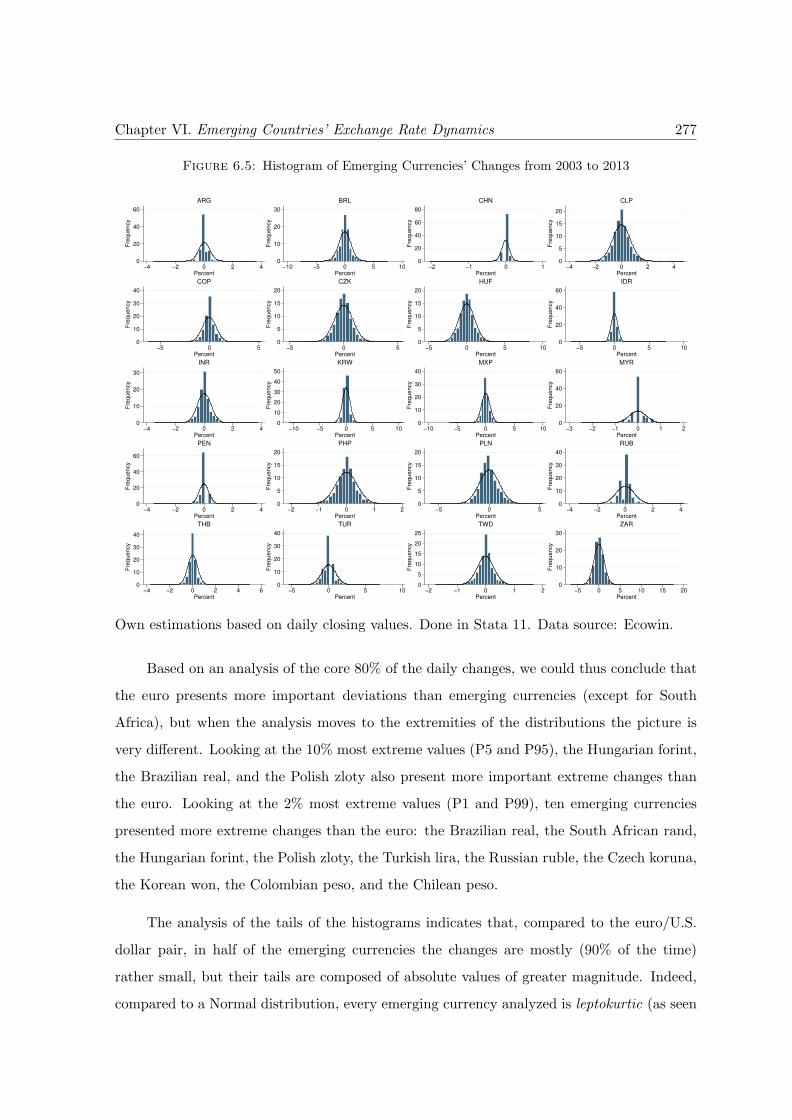
Chapter VI. Emerging Countries’ Exchange Rate Dynamics 277
Figure 6.5: Histogram of Emerging Currencies’ Changes from 2003 to 2013
0
20
40
60
Fre
qu
en
cy
−4 −2 0 2 4Percent
ARG
0
10
20
30
Fre
qu
en
cy
−10 −5 0 5 10Percent
BRL
0
20
40
60
80
Fre
qu
en
cy
−2 −1 0 1Percent
CHN
0
5
10
15
20
Fre
qu
en
cy
−4 −2 0 2 4Percent
CLP
0
10
20
30
40
Fre
qu
en
cy
−5 0 5Percent
COP
0
5
10
15
20
Fre
qu
en
cy
−5 0 5Percent
CZK
0
5
10
15
20
Fre
qu
en
cy
−5 0 5 10Percent
HUF
0
20
40
60
Fre
qu
en
cy
−5 0 5 10Percent
IDR
0
10
20
30
Fre
qu
en
cy
−4 −2 0 2 4Percent
INR
0
10
20
30
40
50
Fre
qu
en
cy
−10 −5 0 5 10Percent
KRW
0
10
20
30
40
Fre
qu
en
cy
−10 −5 0 5 10Percent
MXP
0
20
40
60
Fre
qu
en
cy
−3 −2 −1 0 1 2Percent
MYR
0
20
40
60
Fre
qu
en
cy
−4 −2 0 2 4Percent
PEN
0
5
10
15
20
Fre
qu
en
cy
−2 −1 0 1 2Percent
PHP
0
5
10
15
20
Fre
qu
en
cy
−5 0 5Percent
PLN
0
10
20
30
40
Fre
qu
en
cy
−4 −2 0 2 4Percent
RUB
0
10
20
30
40
Fre
qu
en
cy
−4 −2 0 2 4 6Percent
THB
0
10
20
30
40
Fre
qu
en
cy
−5 0 5 10Percent
TUR
0
5
10
15
20
25
Fre
qu
en
cy
−2 −1 0 1 2Percent
TWD
0
10
20
30
Fre
qu
en
cy
−5 0 5 10 15 20Percent
ZAR
Own estimations based on daily closing values. Done in Stata 11. Data source: Ecowin.
Based on an analysis of the core 80% of the daily changes, we could thus conclude that
the euro presents more important deviations than emerging currencies (except for South
Africa), but when the analysis moves to the extremities of the distributions the picture is
very different. Looking at the 10% most extreme values (P5 and P95), the Hungarian forint,
the Brazilian real, and the Polish zloty also present more important extreme changes than
the euro. Looking at the 2% most extreme values (P1 and P99), ten emerging currencies
presented more extreme changes than the euro: the Brazilian real, the South African rand,
the Hungarian forint, the Polish zloty, the Turkish lira, the Russian ruble, the Czech koruna,
the Korean won, the Colombian peso, and the Chilean peso.
The analysis of the tails of the histograms indicates that, compared to the euro/U.S.
dollar pair, in half of the emerging currencies the changes are mostly (90% of the time)
rather small, but their tails are composed of absolute values of greater magnitude. Indeed,
compared to a Normal distribution, every emerging currency analyzed is leptokurtic (as seen
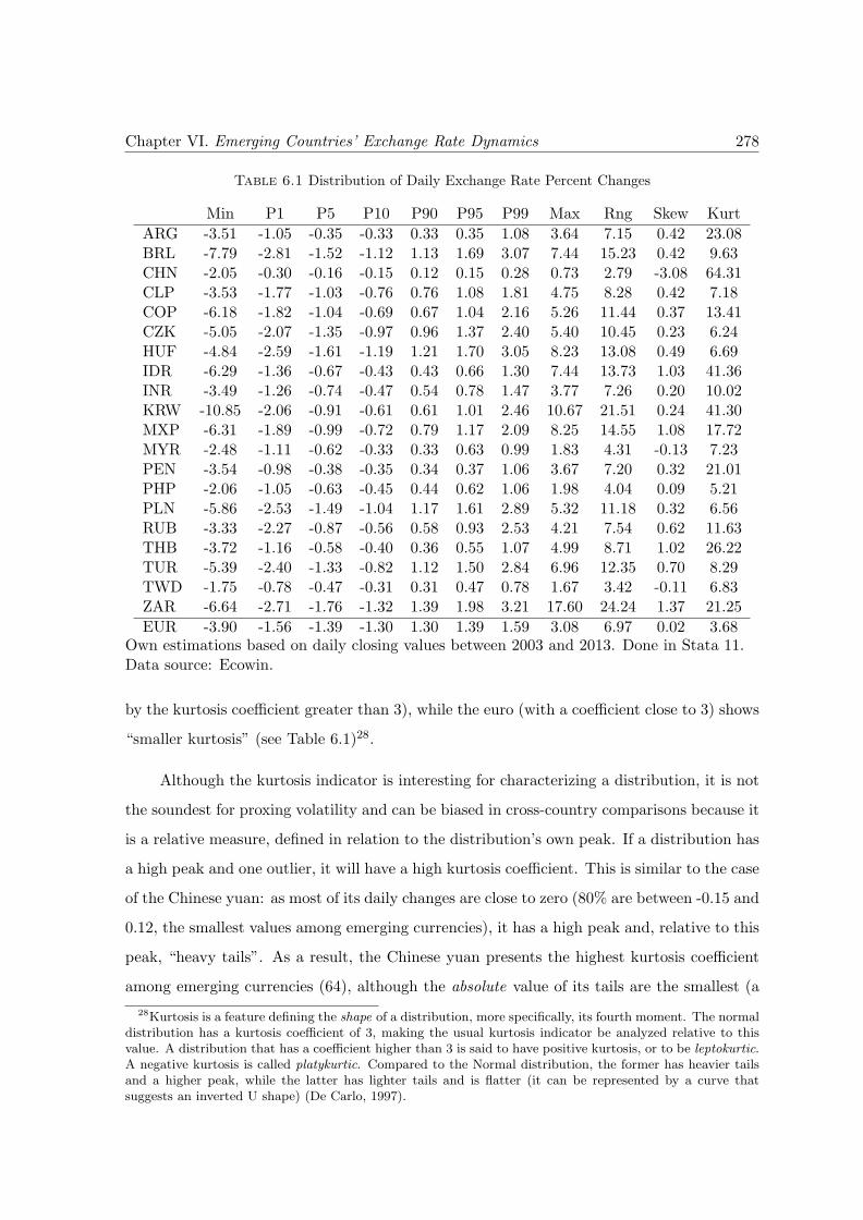
Chapter VI. Emerging Countries’ Exchange Rate Dynamics 278
Table 6.1 Distribution of Daily Exchange Rate Percent Changes
Min P1 P5 P10 P90 P95 P99 Max Rng Skew Kurt
ARG -3.51 -1.05 -0.35 -0.33 0.33 0.35 1.08 3.64 7.15 0.42 23.08BRL -7.79 -2.81 -1.52 -1.12 1.13 1.69 3.07 7.44 15.23 0.42 9.63CHN -2.05 -0.30 -0.16 -0.15 0.12 0.15 0.28 0.73 2.79 -3.08 64.31CLP -3.53 -1.77 -1.03 -0.76 0.76 1.08 1.81 4.75 8.28 0.42 7.18COP -6.18 -1.82 -1.04 -0.69 0.67 1.04 2.16 5.26 11.44 0.37 13.41CZK -5.05 -2.07 -1.35 -0.97 0.96 1.37 2.40 5.40 10.45 0.23 6.24HUF -4.84 -2.59 -1.61 -1.19 1.21 1.70 3.05 8.23 13.08 0.49 6.69IDR -6.29 -1.36 -0.67 -0.43 0.43 0.66 1.30 7.44 13.73 1.03 41.36INR -3.49 -1.26 -0.74 -0.47 0.54 0.78 1.47 3.77 7.26 0.20 10.02KRW -10.85 -2.06 -0.91 -0.61 0.61 1.01 2.46 10.67 21.51 0.24 41.30MXP -6.31 -1.89 -0.99 -0.72 0.79 1.17 2.09 8.25 14.55 1.08 17.72MYR -2.48 -1.11 -0.62 -0.33 0.33 0.63 0.99 1.83 4.31 -0.13 7.23PEN -3.54 -0.98 -0.38 -0.35 0.34 0.37 1.06 3.67 7.20 0.32 21.01PHP -2.06 -1.05 -0.63 -0.45 0.44 0.62 1.06 1.98 4.04 0.09 5.21PLN -5.86 -2.53 -1.49 -1.04 1.17 1.61 2.89 5.32 11.18 0.32 6.56RUB -3.33 -2.27 -0.87 -0.56 0.58 0.93 2.53 4.21 7.54 0.62 11.63THB -3.72 -1.16 -0.58 -0.40 0.36 0.55 1.07 4.99 8.71 1.02 26.22TUR -5.39 -2.40 -1.33 -0.82 1.12 1.50 2.84 6.96 12.35 0.70 8.29TWD -1.75 -0.78 -0.47 -0.31 0.31 0.47 0.78 1.67 3.42 -0.11 6.83ZAR -6.64 -2.71 -1.76 -1.32 1.39 1.98 3.21 17.60 24.24 1.37 21.25
EUR -3.90 -1.56 -1.39 -1.30 1.30 1.39 1.59 3.08 6.97 0.02 3.68Own estimations based on daily closing values between 2003 and 2013. Done in Stata 11.Data source: Ecowin.
by the kurtosis coefficient greater than 3), while the euro (with a coefficient close to 3) shows
“smaller kurtosis” (see Table 6.1)28.
Although the kurtosis indicator is interesting for characterizing a distribution, it is not
the soundest for proxing volatility and can be biased in cross-country comparisons because it
is a relative measure, defined in relation to the distribution’s own peak. If a distribution has
a high peak and one outlier, it will have a high kurtosis coefficient. This is similar to the case
of the Chinese yuan: as most of its daily changes are close to zero (80% are between -0.15 and
0.12, the smallest values among emerging currencies), it has a high peak and, relative to this
peak, “heavy tails”. As a result, the Chinese yuan presents the highest kurtosis coefficient
among emerging currencies (64), although the absolute value of its tails are the smallest (a
28Kurtosis is a feature defining the shape of a distribution, more specifically, its fourth moment. The normaldistribution has a kurtosis coefficient of 3, making the usual kurtosis indicator be analyzed relative to thisvalue. A distribution that has a coefficient higher than 3 is said to have positive kurtosis, or to be leptokurtic.A negative kurtosis is called platykurtic. Compared to the Normal distribution, the former has heavier tailsand a higher peak, while the latter has lighter tails and is flatter (it can be represented by a curve thatsuggests an inverted U shape) (De Carlo, 1997).
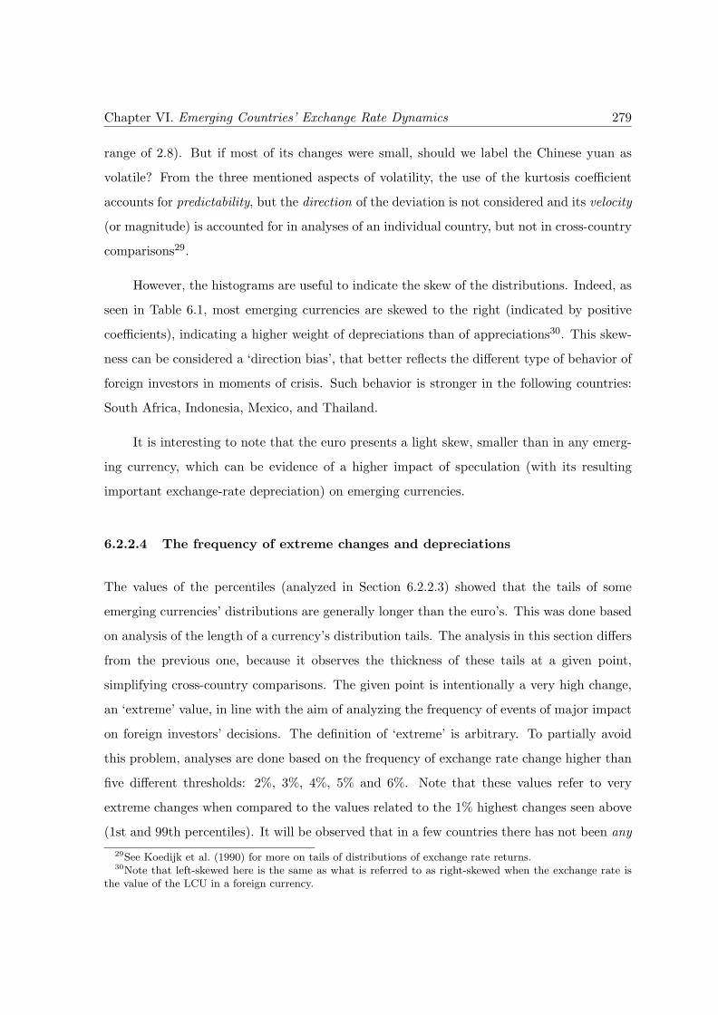
Chapter VI. Emerging Countries’ Exchange Rate Dynamics 279
range of 2.8). But if most of its changes were small, should we label the Chinese yuan as
volatile? From the three mentioned aspects of volatility, the use of the kurtosis coefficient
accounts for predictability, but the direction of the deviation is not considered and its velocity
(or magnitude) is accounted for in analyses of an individual country, but not in cross-country
comparisons29.
However, the histograms are useful to indicate the skew of the distributions. Indeed, as
seen in Table 6.1, most emerging currencies are skewed to the right (indicated by positive
coefficients), indicating a higher weight of depreciations than of appreciations30. This skew-
ness can be considered a ‘direction bias’, that better reflects the different type of behavior of
foreign investors in moments of crisis. Such behavior is stronger in the following countries:
South Africa, Indonesia, Mexico, and Thailand.
It is interesting to note that the euro presents a light skew, smaller than in any emerg-
ing currency, which can be evidence of a higher impact of speculation (with its resulting
important exchange-rate depreciation) on emerging currencies.
6.2.2.4 The frequency of extreme changes and depreciations
The values of the percentiles (analyzed in Section 6.2.2.3) showed that the tails of some
emerging currencies’ distributions are generally longer than the euro’s. This was done based
on analysis of the length of a currency’s distribution tails. The analysis in this section differs
from the previous one, because it observes the thickness of these tails at a given point,
simplifying cross-country comparisons. The given point is intentionally a very high change,
an ‘extreme’ value, in line with the aim of analyzing the frequency of events of major impact
on foreign investors’ decisions. The definition of ‘extreme’ is arbitrary. To partially avoid
this problem, analyses are done based on the frequency of exchange rate change higher than
five different thresholds: 2%, 3%, 4%, 5% and 6%. Note that these values refer to very
extreme changes when compared to the values related to the 1% highest changes seen above
(1st and 99th percentiles). It will be observed that in a few countries there has not been any
29See Koedijk et al. (1990) for more on tails of distributions of exchange rate returns.30Note that left-skewed here is the same as what is referred to as right-skewed when the exchange rate is
the value of the LCU in a foreign currency.
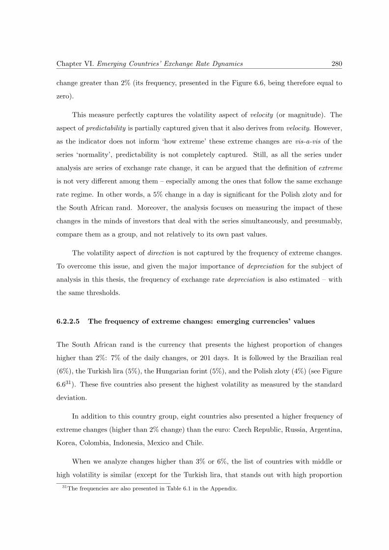
Chapter VI. Emerging Countries’ Exchange Rate Dynamics 280
change greater than 2% (its frequency, presented in the Figure 6.6, being therefore equal to
zero).
This measure perfectly captures the volatility aspect of velocity (or magnitude). The
aspect of predictability is partially captured given that it also derives from velocity. However,
as the indicator does not inform ‘how extreme’ these extreme changes are vis-a-vis of the
series ‘normality’, predictability is not completely captured. Still, as all the series under
analysis are series of exchange rate change, it can be argued that the definition of extreme
is not very different among them – especially among the ones that follow the same exchange
rate regime. In other words, a 5% change in a day is significant for the Polish zloty and for
the South African rand. Moreover, the analysis focuses on measuring the impact of these
changes in the minds of investors that deal with the series simultaneously, and presumably,
compare them as a group, and not relatively to its own past values.
The volatility aspect of direction is not captured by the frequency of extreme changes.
To overcome this issue, and given the major importance of depreciation for the subject of
analysis in this thesis, the frequency of exchange rate depreciation is also estimated – with
the same thresholds.
6.2.2.5 The frequency of extreme changes: emerging currencies’ values
The South African rand is the currency that presents the highest proportion of changes
higher than 2%: 7% of the daily changes, or 201 days. It is followed by the Brazilian real
(6%), the Turkish lira (5%), the Hungarian forint (5%), and the Polish zloty (4%) (see Figure
6.631). These five countries also present the highest volatility as measured by the standard
deviation.
In addition to this country group, eight countries also presented a higher frequency of
extreme changes (higher than 2% change) than the euro: Czech Republic, Russia, Argentina,
Korea, Colombia, Indonesia, Mexico and Chile.
When we analyze changes higher than 3% or 6%, the list of countries with middle or
high volatility is similar (except for the Turkish lira, that stands out with high proportion
31The frequencies are also presented in Table 6.1 in the Appendix.
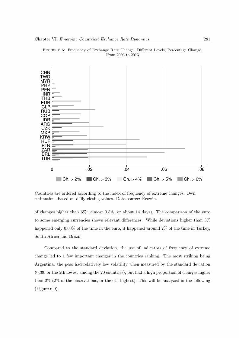
Chapter VI. Emerging Countries’ Exchange Rate Dynamics 281
Figure 6.6: Frequency of Exchange Rate Change: Different Levels, Percentage Change,From 2003 to 2013
0 .02 .04 .06 .08
TURBRLZARPLNHUFKRWMXPCZKARGIDR
COPRUBCLPEURTHBINR
PENPHPMYRTWDCHN
Ch. > 2% Ch. > 3% Ch. > 4% Ch. > 5% Ch. > 6%
Countries are ordered according to the index of frequency of extreme changes. Ownestimations based on daily closing values. Data source: Ecowin.
of changes higher than 6%: almost 0.5%, or about 14 days). The comparison of the euro
to some emerging currencies shows relevant differences. While deviations higher than 3%
happened only 0.03% of the time in the euro, it happened around 2% of the time in Turkey,
South Africa and Brazil.
Compared to the standard deviation, the use of indicators of frequency of extreme
change led to a few important changes in the countries ranking. The most striking being
Argentina: the peso had relatively low volatility when measured by the standard deviation
(0.39, or the 5th lowest among the 20 countries), but had a high proportion of changes higher
than 2% (2% of the observations, or the 6th highest). This will be analyzed in the following
(Figure 6.9).
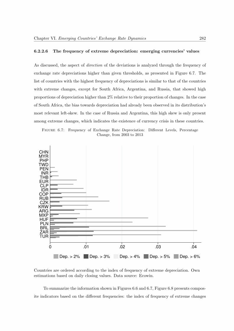
Chapter VI. Emerging Countries’ Exchange Rate Dynamics 282
6.2.2.6 The frequency of extreme depreciation: emerging currencies’ values
As discussed, the aspect of direction of the deviations is analyzed through the frequency of
exchange rate depreciations higher than given thresholds, as presented in Figure 6.7. The
list of countries with the highest frequency of depreciations is similar to that of the countries
with extreme changes, except for South Africa, Argentina, and Russia, that showed high
proportions of depreciation higher than 2% relative to their proportion of changes. In the case
of South Africa, the bias towards depreciation had already been observed in its distribution’s
most relevant left-skew. In the case of Russia and Argentina, this high skew is only present
among extreme changes, which indicates the existence of currency crisis in these countries.
Figure 6.7: Frequency of Exchange Rate Depreciation: Different Levels, PercentageChange, from 2003 to 2013
0 .01 .02 .03 .04
TURZARBRLPLNHUFMXPARGKRWCZKRUBCOPIDRCLPEURTHBINR
PENTWDPHPMYRCHN
Dep. > 2% Dep. > 3% Dep. > 4% Dep. > 5% Dep. > 6%
Countries are ordered according to the index of frequency of extreme depreciation. Ownestimations based on daily closing values. Data source: Ecowin.
To summarize the information shown in Figures 6.6 and 6.7, Figure 6.8 presents compos-
ite indicators based on the different frequencies: the index of frequency of extreme changes
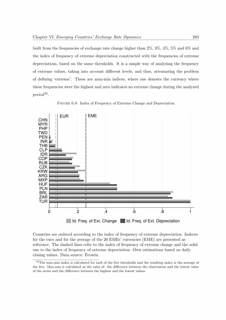
Chapter VI. Emerging Countries’ Exchange Rate Dynamics 283
built from the frequencies of exchange rate change higher than 2%, 3%, 4%, 5% and 6% and
the index of frequency of extreme depreciation constructed with the frequencies of extreme
depreciations, based on the same thresholds. It is a simple way of analyzing the frequency
of extreme values, taking into account different levels, and thus, attenuating the problem
of defining ‘extreme’. These are max-min indices, where one denotes the currency where
these frequencies were the highest and zero indicates no extreme change during the analyzed
period32.
Figure 6.8: Index of Frequency of Extreme Change and Depreciation
EUR EME
0 .2 .4 .6 .8 1
TURZARBRLPLNHUFMXPARGKRWCZKRUBCOPIDRCLPTHBINR
PENTWDPHPMYRCHN
Id. Freq. of Ext. Change Id. Freq. of Ext. Depreciation
Countries are ordered according to the index of frequency of extreme depreciation. Indecesfor the euro and for the average of the 20 EMEs’ currencies (EME) are presented asreference. The dashed lines refer to the index of frequency of extreme change and the solidone to the index of frequency of extreme depreciation. Own estimations based on dailyclosing values. Data source: Ecowin.
32The max-min index is calculated for each of the five thresholds and the resulting index is the average ofthe five. Max-min is calculated as the ratio of: the difference between the observation and the lowest valueof the series and the difference between the highest and the lowest values.
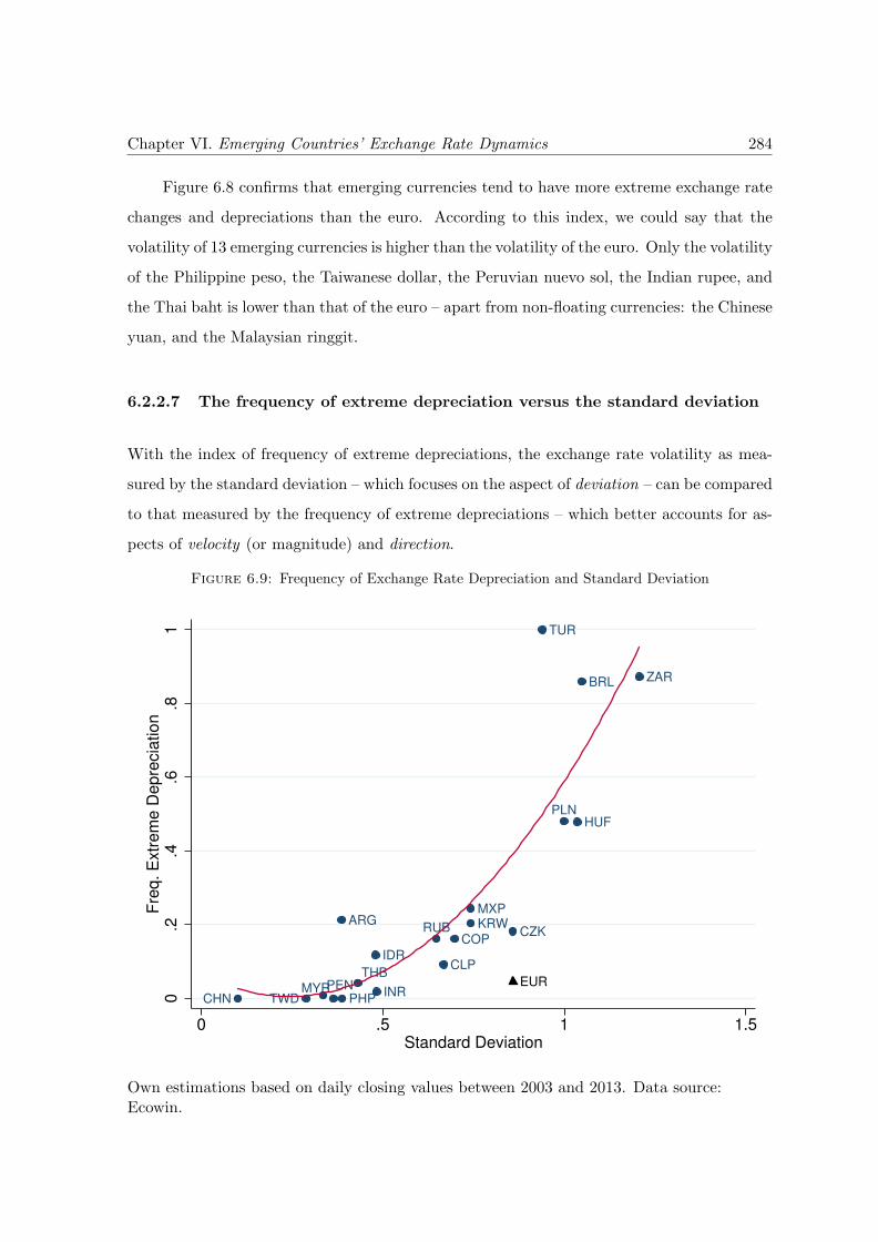
Chapter VI. Emerging Countries’ Exchange Rate Dynamics 284
Figure 6.8 confirms that emerging currencies tend to have more extreme exchange rate
changes and depreciations than the euro. According to this index, we could say that the
volatility of 13 emerging currencies is higher than the volatility of the euro. Only the volatility
of the Philippine peso, the Taiwanese dollar, the Peruvian nuevo sol, the Indian rupee, and
the Thai baht is lower than that of the euro – apart from non-floating currencies: the Chinese
yuan, and the Malaysian ringgit.
6.2.2.7 The frequency of extreme depreciation versus the standard deviation
With the index of frequency of extreme depreciations, the exchange rate volatility as mea-
sured by the standard deviation – which focuses on the aspect of deviation – can be compared
to that measured by the frequency of extreme depreciations – which better accounts for as-
pects of velocity (or magnitude) and direction.
Figure 6.9: Frequency of Exchange Rate Depreciation and Standard Deviation
PLN
RUB
MYRCHN TWD
PENTHB
ARG
BRL
CLP
COPCZK
HUF
IDR
INR
KRWMXP
PHP
TUR
ZAR
EUR
0.2
.4.6
.81
Fre
q.
Extr
em
e D
ep
recia
tio
n
0 .5 1 1.5Standard Deviation
Own estimations based on daily closing values between 2003 and 2013. Data source:Ecowin.
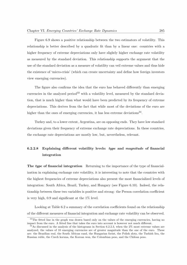
Chapter VI. Emerging Countries’ Exchange Rate Dynamics 285
Figure 6.9 shows a positive relationship between the two estimators of volatility. This
relationship is better described by a quadratic fit than by a linear one: countries with a
higher frequency of extreme depreciations only have slightly higher exchange rate volatility
as measured by the standard deviation. This relationship supports the argument that the
use of the standard deviation as a measure of volatility can veil extreme values and thus hide
the existence of ‘micro-crisis’ (which can create uncertainty and define how foreign investors
view emerging currencies).
The figure also confirms the idea that the euro has behaved differently than emerging
currencies in the analyzed period33 with a volatility level, measured by the standard devia-
tion, that is much higher than what would have been predicted by its frequency of extreme
depreciations. This derives from the fact that while most of the deviations of the euro are
higher than the ones of emerging currencies, it has less extreme deviations34.
Turkey and, to a lower extent, Argentina, are on opposing ends. They have low standard
deviations given their frequency of extreme exchange rate depreciations. In these countries,
the exchange rate depreciations are mostly low, but, nevertheless, relevant.
6.2.2.8 Explaining different volatility levels: type and magnitude of financial
integration
The type of financial integration Returning to the importance of the type of financial-
ization in explaining exchange rate volatility, it is interesting to note that the countries with
the highest frequencies of extreme depreciations also present the most financialized levels of
integration: South Africa, Brazil, Turkey, and Hungary (see Figure 6.10). Indeed, the rela-
tionship between these two variables is positive and strong: the Person correlation coefficient
is very high, 0.9 and significant at the 1% level.
Looking at Table 6.2 a summary of the correlation coefficients found on the relationship
of the different measures of financial integration and exchange rate volatility can be observed.
33The fitted line in the graph was drawn based only on the values of the emerging currencies, having noimpact from the euro. A fitted line that takes the euro into account is however not much different.
34As discussed in the analysis of the histograms in Section 6.2.2.3, when the 2% most extreme values areanalyzed, the values of 10 emerging currencies are of greater magnitude than the one of the euro. Theseare: the Brazilian real, the South African rand, the Hungarian forint, the Polish zloty, the Turkish lira, theRussian ruble, the Czech koruna, the Korean won, the Colombian peso, and the Chilean peso.
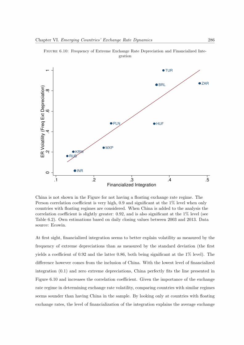
Chapter VI. Emerging Countries’ Exchange Rate Dynamics 286
Figure 6.10: Frequency of Extreme Exchange Rate Depreciation and Financialized Inte-gration
BRL
HUF
INR
KRWMXP
PLN
RUB
TUR
ZAR
0.2
.4.6
.81
ER
Vo
latilit
y (
Fre
q E
xt
De
pre
cia
tio
n)
.1 .2 .3 .4 .5Financialized Integration
China is not shown in the Figure for not having a floating exchange rate regime. ThePerson correlation coefficient is very high, 0.9 and significant at the 1% level when onlycountries with floating regimes are considered. When China is added to the analysis thecorrelation coefficient is slightly greater: 0.92, and is also significant at the 1% level (seeTable 6.2). Own estimations based on daily closing values between 2003 and 2013. Datasource: Ecowin.
At first sight, financialized integration seems to better explain volatility as measured by the
frequency of extreme depreciations than as measured by the standard deviation (the first
yields a coefficient of 0.92 and the latter 0.86, both being significant at the 1% level). The
difference however comes from the inclusion of China. With the lowest level of financialized
integration (0.1) and zero extreme depreciations, China perfectly fits the line presented in
Figure 6.10 and increases the correlation coefficient. Given the importance of the exchange
rate regime in determining exchange rate volatility, comparing countries with similar regimes
seems sounder than having China in the sample. By looking only at countries with floating
exchange rates, the level of financialization of the integration explains the average exchange
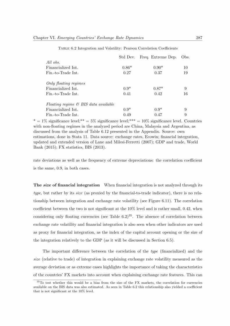
Chapter VI. Emerging Countries’ Exchange Rate Dynamics 287
Table 6.2 Integration and Volatility: Pearson Correlation Coefficients
Std Dev. Freq. Extreme Dep. Obs.All obs.Financialized Int. 0.86* 0.90* 10Fin.-to-Trade Int. 0.27 0.37 19
Only floating regimesFinancialized Int. 0.9* 0.87* 9Fin.-to-Trade Int. 0.41 0.42 16
Floating regime & BIS data availableFinancialized Int. 0.9* 0.9* 9Fin.-to-Trade Int. 0.49 0.47 9
* = 1% significance level;** = 5% significance level;*** = 10% significance level. Countrieswith non-floating regimes in the analyzed period are China, Malaysia and Argentina, asdiscussed from the analysis of Table 6.12 presented in the Appendix. Source: ownestimations, done in Stata 11. Data source: exchange rates, Ecowin; financial integration,updated and extended version of Lane and Milesi-Ferretti (2007); GDP and trade, WorldBank (2015); FX statistics, BIS (2013).
rate deviations as well as the frequency of extreme depreciations: the correlation coefficient
is the same, 0.9, in both cases.
The size of financial integration When financial integration is not analyzed through its
type, but rather by its size (as proxied by the financial-to-trade indicator), there is no rela-
tionship between integration and exchange rate volatility (see Figure 6.11). The correlation
coefficient between the two is not significant at the 10% level and is rather small, 0.42, when
considering only floating currencies (see Table 6.2)35. The absence of correlation between
exchange rate volatility and financial integration is also seen when other indicators are used
as proxy for financial integration, as the index of the capital account opening or the size of
the integration relatively to the GDP (as it will be discussed in Section 6.5).
The important difference between the correlation of the type (financialized) and the
size (relative to trade) of integration in explaining exchange rate volatility measured as the
average deviation or as extreme cases highlights the importance of taking the characteristics
of the countries’ FX markets into account when explaining exchange rate features. This can
35To test whether this would be a bias from the size of the FX markets, the correlation for currenciesavailable on the BIS data was also estimated. As seen in Table 6.2 this relationship also yielded a coefficientthat is not significant at the 10% level.
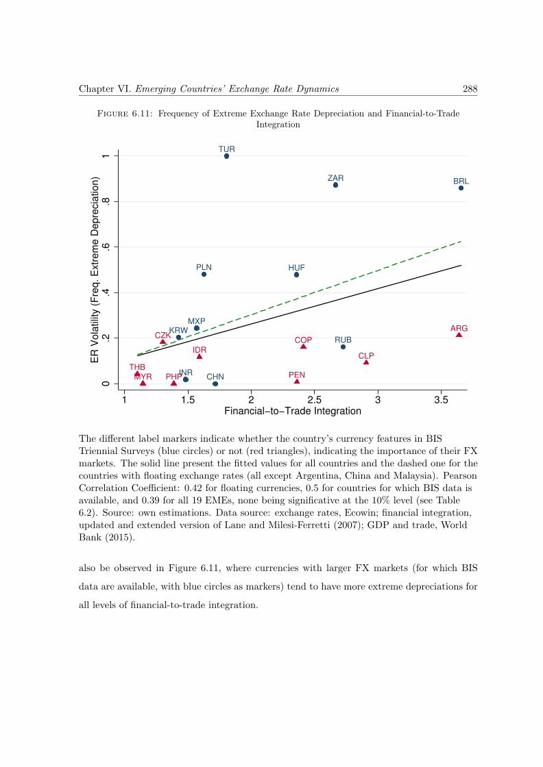
Chapter VI. Emerging Countries’ Exchange Rate Dynamics 288
Figure 6.11: Frequency of Extreme Exchange Rate Depreciation and Financial-to-TradeIntegration
BRL
CHN
HUF
INR
KRWMXP
PLN
RUB
TUR
ZAR
ARG
CLP
COPCZK
IDR
MYR PENPHPTHB
0.2
.4.6
.81
ER
Vo
latilit
y (
Fre
q.
Extr
em
e D
ep
recia
tio
n)
1 1.5 2 2.5 3 3.5Financial−to−Trade Integration
The different label markers indicate whether the country’s currency features in BISTriennial Surveys (blue circles) or not (red triangles), indicating the importance of their FXmarkets. The solid line present the fitted values for all countries and the dashed one for thecountries with floating exchange rates (all except Argentina, China and Malaysia). PearsonCorrelation Coefficient: 0.42 for floating currencies, 0.5 for countries for which BIS data isavailable, and 0.39 for all 19 EMEs, none being significative at the 10% level (see Table6.2). Source: own estimations. Data source: exchange rates, Ecowin; financial integration,updated and extended version of Lane and Milesi-Ferretti (2007); GDP and trade, WorldBank (2015).
also be observed in Figure 6.11, where currencies with larger FX markets (for which BIS
data are available, with blue circles as markers) tend to have more extreme depreciations for
all levels of financial-to-trade integration.

Chapter VI. Emerging Countries’ Exchange Rate Dynamics 289
6.2.3 Concluding Remarks
This section i) presented a discussion on the different measures of exchange rate volatility; ii)
argued for the importance of taking extreme events into account; iii) presented the different
levels of exchange rate volatility among emerging currencies and how they diverge from the
euro/U.S. dollar pair; and iv) analyzed possible causes of volatility.
Regarding different measures of exchange rate volatility, it was argued that the standard
deviation, as it is based on averages, veils the presence of extreme exchange rate changes,
that are crucial in characterizing emerging currencies. Moreover, these extreme changes,
especially the depreciations, can play a major role in how foreign investors view emerging
currencies and thus, how they trade assets labeled in these currencies. A measure of volatility
based on the frequency of extreme exchange-rate depreciations was suggested to deal with
this drawback.
Measuring volatility by the frequency of extreme changes and through the standard
deviation led to different results, and the comparison to the euro created a clearer picture of
the state of volatility among emerging currencies. By analyzing only the standard deviation,
five out of the 17 emerging currencies with a floating regime were more volatile than the
euro. However, when the magnitude of the daily change is the focus of the measure, many
emerging currencies are more volatile (as shown in Table 6.15): through an analysis of the
range, most emerging currencies are more volatile than the euro; when the analysis considers
the frequency of extreme changes, 13 emerging currencies are more volatile than the euro.
In analyzing possible causes of exchange rate volatility, this section presented evidence
that a more financialized integration is associated with higher exchange rate volatility in
emerging currencies – as measured by the two estimators, while estimators of the relative
size of integration do not present any significant relation with exchange rate volatility. The
type of integration has no greater impact on extreme exchange-rate depreciations than on
average deviation.
The next two sections cover two other possible consequences of a financialized integra-
tion to international financial markets: the comovement of different emerging currencies and
the higher importance of international factors in determining these currencies’ path.
Chapter VI. Emerging Countries’ Exchange Rate Dynamics 290
6.3 Influence From International Liquidity Cycles
Attempting to advance on the hypothesis that the type of integration – more or less finan-
cialized – can determine emerging currencies’ features, this section analyzes the impacts of
international financial conditions on emerging currencies. The importance of international
conditions is also studied by the push vs. pull literature, but while the latter focuses on the
impacts on capital flows, the thesis focuses on exchange rates.
6.3.1 International Liquidity Cycles and Capital Flows to EMEs
The literature on the determinants of capital flows has flourished since the 1990s, following
the seminal works of Calvo et al. (1993) and Fernandez-Arias (1996) who differentiated
“push” (external) and “pull” (domestic) determinants of capital flows36.
Several authors have conducted empirical analyses on the relative weight of push and
pull factors on capital flows, without achieving a consensus (see Weiss and Prates (2015)).
When looking specifically at portfolio flows, however, the empirical evidence suggests a pre-
dominance of finance-related push factors (see Rey (2015)). Indeed, that is the finding of
Koepke (2015) based on a qualitative meta-analysis of 40 empirical works. Specifically, the
study concludes that there is strong evidence that portfolio flows suffer negative impacts
from interest rate in mature economies and from global risk aversion; and that there is no
strong evidence of impact from GDP growth in mature economies (for which there is only
some evidence of impact on portfolio flows). The evidence for pull factors, on the other hand,
is weak: there is only some evidence of impact from domestic output growth, asset return
indicators, and country risk indicators.
From another perspective, Koepke’s (2015) results on the different types of flows indicate
that, for portfolio flows (equity and debt), the importance of push factors is more evident,
36Push and pull factors are sometimes seen as the respective correspondents of supply and demand ofcapital, as stated by Ghosh et al. (2014, p. 268): “The literature on this subject has a long tradition oftrying to identify global “push” and domestic “pull” factors in determining flows to recipient economies. Yet,in equilibrium, capital flows must reflect the confluence of supply and demand, so there must be both push(supply-side) and pull (demand-side) factors, and it is hard to attribute the observed flows to one side or theother.” This comparison should however be avoided as demand is determined by both pull and push, andglobal and domestic factors.
Chapter VI. Emerging Countries’ Exchange Rate Dynamics 291
while there are mixed findings for pull factors. Banking flows are the only type that have
clear, strong evidence to the importance of pull factors (but evidence to the role of global risk
aversion, a push factor, is also important). FDI is also subject to mixed evidence. Domestic
output growth (a pull factor) is the only factor for which there is strong evidence.
The major relevance of push factors is also clear in a less formalized literature that
studies the development behind episodes of surges of capital flows to developing countries in
different moments in history. Akyuz (2012) identify four cycles of capital flows to developing
countries in the post-war period: and argue that every cycle was preceded by a hike of
liquidity and low interest rates in reserve-issuing currencies (notably the United States) and
ended with an external shock.
Helleiner (1997) also studies capital flows to developing countries and argues that apart
from internal drivers, the decrease of interest rates in the United States in 1990-91 was highly
important in determining these flows. More recently, Obstfeld (2009) agreed that in both
the current cycle of capital flows to developing countries and in the 1990s one, low global
interest rates were an initial driving force. Ghosh et al. (2014) agree with the importance of
push factors, concluding that:
The picture that emerges from our regression analysis is one in which global
push factors, notably, the real US interest rate and global market uncertainty,
determine whether there will be a surge of capital flows towards EMEs generally,
which helps to explain why surges are synchronized internationally, and why they
recur. (p. 23)
For Brazil, Kaltenbrunner and Painceira (2015) argue that the sudden changes in capital flows
to the country have taken place irrespective of Brazil’s fundamentals, but rather according
to the conditions of international financial markets.
Specifically contemplating emerging countries, the reason behind the predominance of
push factors might be found in the structural characteristics of their currencies. Biancareli
(2011) argues that:
[due to] monetary, financial, and macroeconomic asymmetries, the movement
of private capital flows to developing countries, issuers of currencies that are
Chapter VI. Emerging Countries’ Exchange Rate Dynamics 292
not internationally liquid, is always a consequence of a reduction in liquidity
preference in the international level (or a decrease in risk aversion). (p. 9)
In this sense, pull factors could only reinforce a trend of flows which is determined in the
international sphere. The changing liquidity internationally, from scarcity to abundance,
called “liquidity cycle”37, is therefore the determinant of flows to developing countries. This
would be in line with Hoti’s (2004) findings that capital flows are directed to emerging
markets according to the ruling international financial condition (a push factor), but its
geographic distribution is explained by pull factors.
6.3.2 Liquidity Preference and the VIX Index
As seen, liquidity conditions are a major push factor among the different ones analyzed: both
liquidity itself and liquidity preference (two inverse correlated concepts when dealing with
capital flows to emerging countries). While liquidity preference and risk aversion seem to be
similar concepts, it is important to note that liquidity preference does not assume risk to be
measurable, and is more coherent with a definition of uncertainty as (Knightian) fundamental
uncertainty (as discussed in Chapter Two, page 34). Although available liquidity might
be an important determinant of flows to emerging countries, liquidity preference is more
dynamic and thus more coherent with the rapidly changing “market mood” (in the words
of Hesse et al. (2008)), or the financial markets’ conditions – which, in turn, are much more
relevant for financial (and speculative) flows38. Given that both exchange rates and liquidity
preference are high-frequency data their analysis has the advantage of profiting the most
from the liquidity preference information. In other words, although analyses of capital flows
gain from using liquidity preference as a determinant, studies focused on exchange rates can
(potentially) better grasp its effects.
Proxies of liquidity are not problem-free. Coudert and Gex (2008) proxy liquidity by
“the inverse of average short-term rates of the four largest economies (United States, the Euro
area, United Kingdom and Japan), weighted by GDP”. However, this can be problematic
given that it simultaneously indicates liquidity and return.
37See Biancareli (2007) for an analysis of recent liquidity cycles.38See Chapter Three, Sections 3.3.4 and 3.3.6 for more on liquidity and liquidity preference.
Chapter VI. Emerging Countries’ Exchange Rate Dynamics 293
Analyses focused on measuring risk aversion or liquidity preference mostly use the VIX
index: in 2008, Hesse et al. (2008) argued that there was a consensus on its use and since
then it has been growing in both heterodox39 and mainstream circles: Bekaert et al. (2013)
decompose the VIX as a measure of ‘stock market volatility’ and a residual, “perhaps even
Knightian uncertainty”; Rey (2015) use it as “a measure of uncertainty and risk aversion
of the markets”; Basu and Bundick (2012) states that the VIX measures “aggregate uncer-
tainty”; Forbes and Warnock (2012)40, use the VIX to proxy “overall economic uncertainty
or risk”41.
Alternatives to the VIX exist. Bonizzi (2013) compares the VIX with its FTSE pair,
the FTSE Volatility Index. Ahmed and Zlate (2014) also use the Credit Suisse’s Global
Risk Appetite Index for robustness reasons. Baker et al. (2015) create an indicator based
on counting how many times the word “uncertain*” appears in the Beige Book, released
before each regularly scheduled meeting of the Federal Open Market Committee42. Forbes
and Warnock (2012) also use its older version, VXO, to cover a longer period (before 1990).
Brunnermeier (2008) use the TED spread, the spread between the risky LIBOR and
the risk-free U.S. Treasury bill rate. It is used to proxy “times of crises” or “uncertainty”
and explains how the TED spread widens in times of uncertainty:
In times of uncertainty, banks charge higher interest for unsecured loans, which
increases the LIBOR rate. Further, banks want to get first-rate collateral, which
makes holding Treasury bonds more attractive and pushes down the Treasury
bond rate. For both reasons, the TED spread widens in times of crises. (p. 12)
As with liquidity measures, this risk aversion proxy also suffer from ambiguity for having
two meanings: risk aversion and international funding conditions, which can compromise the
analysis.
39Examples of recent use of the VIX in heterodox literature are varied and include Baumann and Gallagher(2013), Bonizzi (2013), Hoffmann (2013), Kaltenbrunner and Painceira (2009), Kaltenbrunner (2011), Da Silvaand Da Fonseca (2015), Prates and Biancareli (2009), and Weiss and Prates (2015).
40Forbes and Warnock (2012) also consider the use of “the Quality Spread (the difference between MoodysBaa and Aaa corporate bond yields)” to measure “both economic uncertainty as well as risk aversion”.
41Note that the concept of uncertainty in these mainstream authors is not of knightian or fundamental
uncertainty, as used in this thesis. Differently from these mainstream authors, Bruno and Shin (2015), usethe VIX as a proxy of “banks‘ Value-at-Risk” and the “balance sheet capacity of international banks” whichwould, in turn, drive capital flows.
42Given the different available indicators, an interesting methodology might be to use the principal compo-nent of different proxies, as done by Barbosa and Costa (2010), who focus on risk premium.
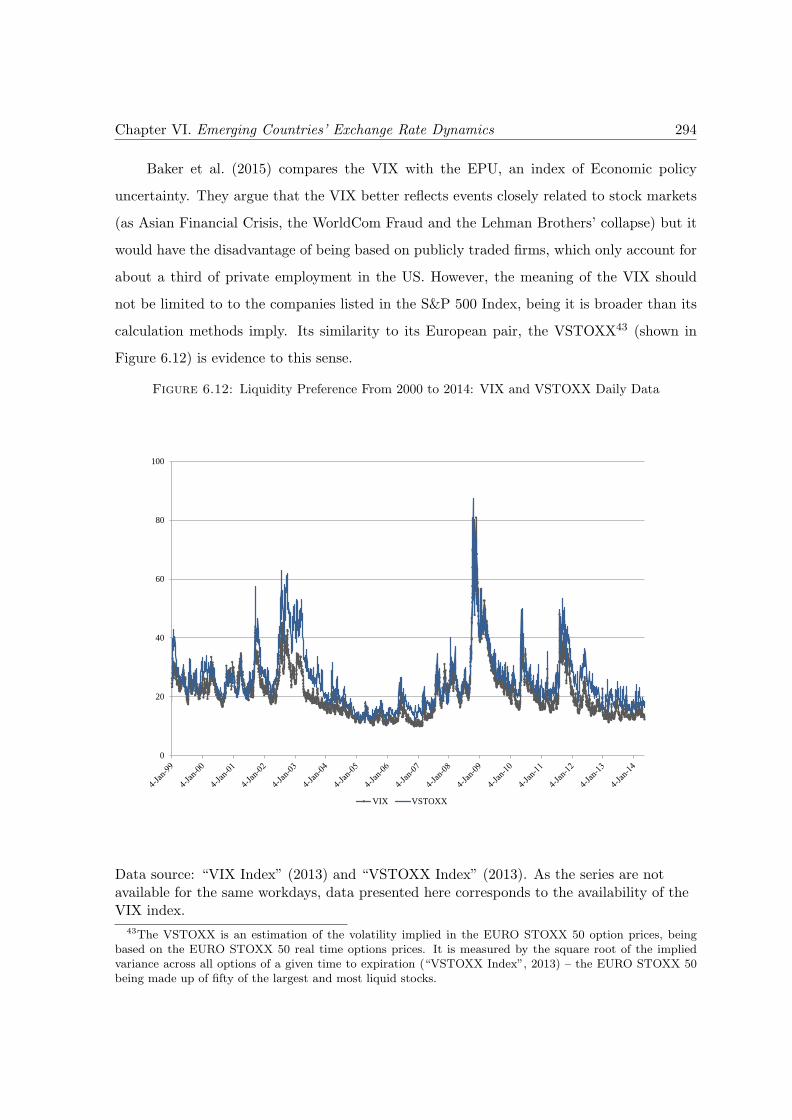
Chapter VI. Emerging Countries’ Exchange Rate Dynamics 294
Baker et al. (2015) compares the VIX with the EPU, an index of Economic policy
uncertainty. They argue that the VIX better reflects events closely related to stock markets
(as Asian Financial Crisis, the WorldCom Fraud and the Lehman Brothers’ collapse) but it
would have the disadvantage of being based on publicly traded firms, which only account for
about a third of private employment in the US. However, the meaning of the VIX should
not be limited to to the companies listed in the S&P 500 Index, being it is broader than its
calculation methods imply. Its similarity to its European pair, the VSTOXX43 (shown in
Figure 6.12) is evidence to this sense.
Figure 6.12: Liquidity Preference From 2000 to 2014: VIX and VSTOXX Daily Data
0
20
40
60
80
100
VIX VSTOXX
Data source: “VIX Index” (2013) and “VSTOXX Index” (2013). As the series are notavailable for the same workdays, data presented here corresponds to the availability of theVIX index.
43The VSTOXX is an estimation of the volatility implied in the EURO STOXX 50 option prices, beingbased on the EURO STOXX 50 real time options prices. It is measured by the square root of the impliedvariance across all options of a given time to expiration (“VSTOXX Index”, 2013) – the EURO STOXX 50being made up of fifty of the largest and most liquid stocks.
Chapter VI. Emerging Countries’ Exchange Rate Dynamics 295
Indeed, although the VIX index is estimated with regards to the S&P500 index44, it
reflects the conditions of financial markets in all major centers, due to the interconnectedness
of global financial markets and, as put by Pusch (2012, p. 5), the particular depth and
therefore central role of US markets in international financial markets.
The Recent Path of the VIX Liquidity preference varied significantly since the 2000s
(shown in Figure 6.12): an long period of low risk aversion occurred from 2003 until the
collapse of the Lehman Brothers; the peak was followed by an notable but temporary decrease
of risk aversion that lasted until fears concerning the stability of the euro arose in 2011. These
ups and downs of the VIX correspond to the cycles of capital flows to emerging countries,
that increased considerably in the beginning of the 2000s, until the Global Financial Crisis
(GFC), decreased with the crisis, and then increased again (see Figure 6.13).
6.3.3 The VIX and Capital Flows
Indeed, several empirical studies use the VIX as a proxy for risk aversion or liquidity pref-
erence internationally and conclude for the importance of these factors in explaining capital
flows45. Ahmed and Zlate (2014), using the VIX on levels, find that the index influences
net capital flows to EMEs. Weiss and Prates (2015) use an annual VIX (created from the
average of monthly data) and find it is significant in determining financial flows to developing
and emerging countries (across different econometric techniques and combination of deter-
minants). Also using the VIX, Obstfeld (2015) finds evidence “consistent with the view that
reductions in global-risk aversion are associated with portfolio shifts toward EMEs.” Bruno
and Shin (2015) use the log of the VIX and find support for the predominance of external
factors and for the relevance of the Fed fund rates in the VIX46. Rey (2015) concludes that
the VIX is important and that it is highly influenced by the Fed fund rate.
44According to the Chicago Board Options Exchange (CBOE), The VIX index is: “The CBOE VolatilityIndex (VIX) is based on the S&P 500 Index (SPX), the core index for U.S. equities, and estimates expectedvolatility by averaging the weighted prices of SPX puts and calls over a wide range of strike prices” (ChicagoBoard Options Exchange, 2015).
45It is interesting to note that the use of the VIX index as a proxy for the ‘mood of international financialmarkets’ had long been used among heterodox circles, and has recently spread o other schools of thought.
46To be precise, the authors find a dual causality: “a cut in the Fed Funds rate is followed by a dampeningof the VIX index, while an increase in the VIX index elicits a response from the Federal Reserve who reactby cutting the target Fed Funds rate” (pg. 4).
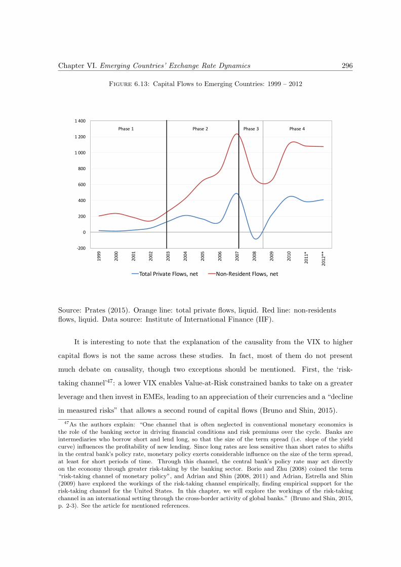
Chapter VI. Emerging Countries’ Exchange Rate Dynamics 296
Figure 6.13: Capital Flows to Emerging Countries: 1999 – 2012
-200
0
200
400
600
800
1 000
1 200
1 400
1999
2000
2001
2002
2003
2004
2005
2006
2007
2008
2009
2010
2011*
2012**
TotalPrivateFlows,net Non-ResidentFlows,net
Phase1 Phase2 Phase3 Phase4
Source: Prates (2015). Orange line: total private flows, liquid. Red line: non-residentsflows, liquid. Data source: Institute of International Finance (IIF).
It is interesting to note that the explanation of the causality from the VIX to higher
capital flows is not the same across these studies. In fact, most of them do not present
much debate on causality, though two exceptions should be mentioned. First, the ‘risk-
taking channel’47: a lower VIX enables Value-at-Risk constrained banks to take on a greater
leverage and then invest in EMEs, leading to an appreciation of their currencies and a “decline
in measured risks” that allows a second round of capital flows (Bruno and Shin, 2015).
47As the authors explain: “One channel that is often neglected in conventional monetary economics isthe role of the banking sector in driving financial conditions and risk premiums over the cycle. Banks areintermediaries who borrow short and lend long, so that the size of the term spread (i.e. slope of the yieldcurve) influences the profitability of new lending. Since long rates are less sensitive than short rates to shiftsin the central bank’s policy rate, monetary policy exerts considerable influence on the size of the term spread,at least for short periods of time. Through this channel, the central bank’s policy rate may act directlyon the economy through greater risk-taking by the banking sector. Borio and Zhu (2008) coined the term“risk-taking channel of monetary policy”, and Adrian and Shin (2008, 2011) and Adrian, Estrella and Shin(2009) have explored the workings of the risk-taking channel empirically, finding empirical support for therisk-taking channel for the United States. In this chapter, we will explore the workings of the risk-takingchannel in an international setting through the cross-border activity of global banks.” (Bruno and Shin, 2015,p. 2-3). See the article for mentioned references.
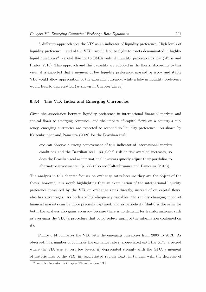
Chapter VI. Emerging Countries’ Exchange Rate Dynamics 297
A different approach sees the VIX as an indicator of liquidity preference. High levels of
liquidity preference – and of the VIX – would lead to flight to assets denominated in highly-
liquid currencies48 capital flowing to EMEs only if liquidity preference is low (Weiss and
Prates, 2015). This approach and this causality are adopted in the thesis. According to this
view, it is expected that a moment of low liquidity preference, marked by a low and stable
VIX would allow appreciation of the emerging currency, while a hike in liquidity preference
would lead to depreciation (as shown in Chapter Three).
6.3.4 The VIX Index and Emerging Currencies
Given the association between liquidity preference in international financial markets and
capital flows to emerging countries, and the impact of capital flows on a country’s cur-
rency, emerging currencies are expected to respond to liquidity preference. As shown by
Kaltenbrunner and Painceira (2009) for the Brazilian real:
one can observe a strong comovement of this indicator of international market
conditions and the Brazilian real. As global risk or risk aversion increases, so
does the Brazilian real as international investors quickly adjust their portfolios to
alternative investments. (p. 27) (also see Kaltenbrunner and Painceira (2015)).
The analysis in this chapter focuses on exchange rates because they are the object of the
thesis, however, it is worth highlighting that an examination of the international liquidity
preference measured by the VIX on exchange rates directly, instead of on capital flows,
also has advantages. As both are high-frequency variables, the rapidly changing mood of
financial markets can be more precisely captured; and as periodicity (daily) is the same for
both, the analysis also gains accuracy because there is no demand for transformations, such
as averaging the VIX (a procedure that could reduce much of the information contained on
it).
Figure 6.14 compares the VIX with the emerging currencies from 2003 to 2013. As
observed, in a number of countries the exchange rate i) appreciated until the GFC, a period
where the VIX was at very low levels; ii) depreciated strongly with the GFC, a moment
of historic hike of the VIX; iii) appreciated rapidly next, in tandem with the decrease of
48See this discussion in Chapter Three, Section 3.3.4.
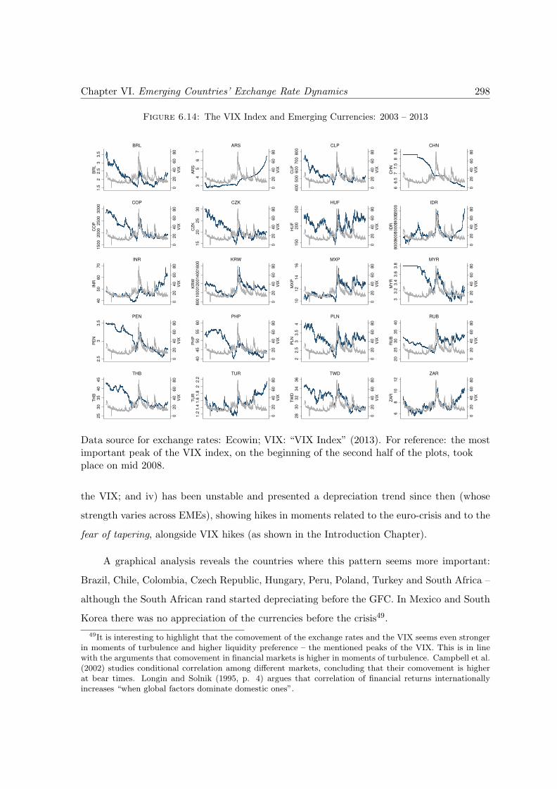
Chapter VI. Emerging Countries’ Exchange Rate Dynamics 298
Figure 6.14: The VIX Index and Emerging Currencies: 2003 – 2013
02
04
06
08
0V
IX
1.5
22
.53
3.5
BR
L
BRL
02
04
06
08
0V
IX
34
56
7A
RS
ARS
02
04
06
08
0V
IX
40
05
00
60
07
00
80
0C
LP
CLP
02
04
06
08
0V
IX
66
.57
7.5
88
.5C
HN
CHN
02
04
06
08
0V
IX
15
00
20
00
25
00
30
00
CO
P
COP
02
04
06
08
0V
IX
15
20
25
30
CZ
K
CZK
02
04
06
08
0V
IX
15
02
00
25
0H
UF
HUF
02
04
06
08
0V
IX
80
009
00
010
00
011
00
012
00
0ID
R
IDR
02
04
06
08
0V
IX
40
50
60
70
INR
INR
02
04
06
08
0V
IX
80
01
00
01
20
01
40
01
60
0K
RW
KRW
02
04
06
08
0V
IX
10
12
14
16
MX
P
MXP
02
04
06
08
0V
IX
33
.23
.43
.63
.8M
YR
MYR
02
04
06
08
0V
IX
2.5
33
.5P
EN
PEN
02
04
06
08
0V
IX
40
45
50
55
60
PH
P
PHP
02
04
06
08
0V
IX
22
.53
3.5
4P
LN
PLN
02
04
06
08
0V
IX
20
25
30
35
40
RU
B
RUB
02
04
06
08
0V
IX
25
30
35
40
45
TH
B
THB
02
04
06
08
0V
IX
1.2
1.4
1.6
1.8
22
.2T
UR
TUR0
20
40
60
80
VIX
28
30
32
34
36
TW
D
TWD
02
04
06
08
0V
IX
68
10
12
ZA
R
ZAR
Data source for exchange rates: Ecowin; VIX: “VIX Index” (2013). For reference: the mostimportant peak of the VIX index, on the beginning of the second half of the plots, tookplace on mid 2008.
the VIX; and iv) has been unstable and presented a depreciation trend since then (whose
strength varies across EMEs), showing hikes in moments related to the euro-crisis and to the
fear of tapering, alongside VIX hikes (as shown in the Introduction Chapter).
A graphical analysis reveals the countries where this pattern seems more important:
Brazil, Chile, Colombia, Czech Republic, Hungary, Peru, Poland, Turkey and South Africa –
although the South African rand started depreciating before the GFC. In Mexico and South
Korea there was no appreciation of the currencies before the crisis49.
49It is interesting to highlight that the comovement of the exchange rates and the VIX seems even strongerin moments of turbulence and higher liquidity preference – the mentioned peaks of the VIX. This is in linewith the arguments that comovement in financial markets is higher in moments of turbulence. Campbell et al.(2002) studies conditional correlation among different markets, concluding that their comovement is higherat bear times. Longin and Solnik (1995, p. 4) argues that correlation of financial returns internationallyincreases “when global factors dominate domestic ones”.
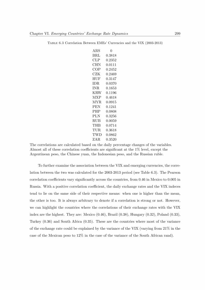
Chapter VI. Emerging Countries’ Exchange Rate Dynamics 299
Table 6.3 Correlation Between EMEs’ Currencies and the VIX (2003-2013)
ARS 0BRL 0.3818CLP 0.2352CHN 0.0111COP 0.2452CZK 0.2469HUF 0.3147IDR 0.0370INR 0.1653KRW 0.1196MXP 0.4618MYR 0.0915PEN 0.1241PHP 0.0808PLN 0.3256RUB 0.0059THB 0.0714TUR 0.3618TWD 0.0862ZAR 0.3520
The correlations are calculated based on the daily percentage changes of the variables.Almost all of these correlation coefficients are significant at the 1% level, except theArgentinean peso, the Chinese yuan, the Indonesian peso, and the Russian ruble.
To further examine the association between the VIX and emerging currencies, the corre-
lation between the two was calculated for the 2003-2013 period (see Table 6.3). The Pearson
correlation coefficients vary significantly across the countries, from 0.46 in Mexico to 0.005 in
Russia. With a positive correlation coefficient, the daily exchange rates and the VIX indeces
tend to lie on the same side of their respective means: when one is higher than the mean,
the other is too. It is always arbitrary to denote if a correlation is strong or not. However,
we can highlight the countries where the correlations of their exchange rates with the VIX
index are the highest. They are: Mexico (0.46), Brazil (0.38), Hungary (0.32), Poland (0.33),
Turkey (0.36) and South Africa (0.35). These are the countries where most of the variance
of the exchange rate could be explained by the variance of the VIX (varying from 21% in the
case of the Mexican peso to 12% in the case of the variance of the South African rand).
Chapter VI. Emerging Countries’ Exchange Rate Dynamics 300
6.3.4.1 Explaining different levels of influence from international conditions
The importance of the type of integration Could the different level of correlation with
the VIX be explained by the type of integration these countries have? Examining the list
of countries with the highest correlation with the VIX, it is found that five out of the six
countries present the most financialized type of integration: Brazil, Hungary, Poland, Turkey
and South Africa. Mexico presented a higher correlation with the VIX than the expected from
its type of integration, but as an outlier, this does not lean against the chapter’s conclusions.
In fact, the presence of Mexico in this list indicates a limitation to using correlation to
measure the relationship between the two variables: the theoretically expected relationship
is that a low and stable VIX leads to exchange rate appreciation (decrease of the LCU value),
while a high level VIX would lead to depreciation (increase of value). However, the correlation
captures only part of this relationship: when a hike of the VIX leads to an exchange rate
depreciation or when a decrease leads to appreciation. The expected impact of a stable VIX
on appreciating exchange rates is not captured.
That is exactly why the Mexican peso presented a higher correlation: it did not appre-
ciate in the pre-GFC period as much as most of the other emerging currencies; it was stable,
as the VIX. The high correlation coefficient of the Mexican peso reflects the high correlation
in this period. The correlation of the other five countries is lessened by the fact that the
behavior between the two variables, though perfect in the sense of performing in the exact
way the theory had predicted, cannot be captured by the correlation coefficient.
Having taken the limitations of the use of the correlation coefficient into account, the
relationship between the correlation of the emerging currencies with the VIX and their level
of financialization are plotted in Figure 6.15 for the floating currencies (all except for China,
who has a low level of financialization of its integration and a low level of correlation of its
exchange rate and the VIX).
The figure makes it clear that the currencies of the countries with more financialized
integration are those with higher correlation with the VIX, while the less financialized have
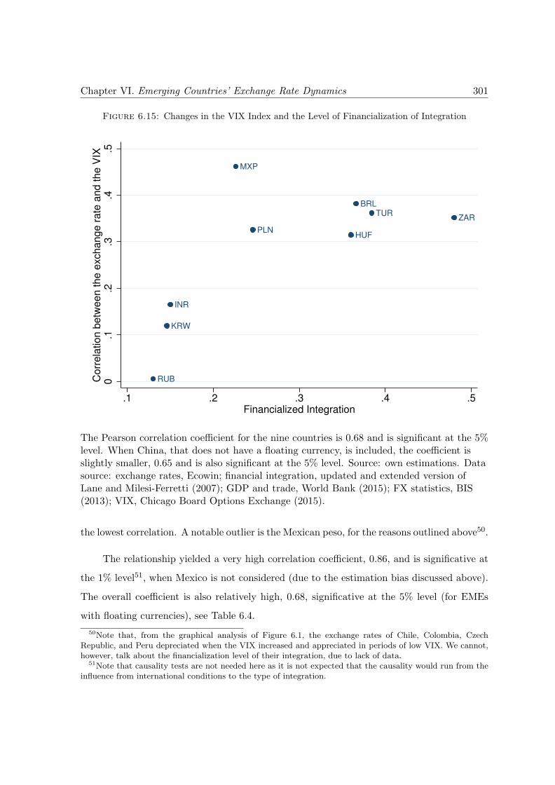
Chapter VI. Emerging Countries’ Exchange Rate Dynamics 301
Figure 6.15: Changes in the VIX Index and the Level of Financialization of Integration
BRL
HUF
INR
KRW
MXP
PLN
RUB
TURZAR
0.1
.2.3
.4.5
Co
rre
latio
n b
etw
ee
n t
he
exch
an
ge
ra
te a
nd
th
e V
IX
.1 .2 .3 .4 .5Financialized Integration
The Pearson correlation coefficient for the nine countries is 0.68 and is significant at the 5%level. When China, that does not have a floating currency, is included, the coefficient isslightly smaller, 0.65 and is also significant at the 5% level. Source: own estimations. Datasource: exchange rates, Ecowin; financial integration, updated and extended version ofLane and Milesi-Ferretti (2007); GDP and trade, World Bank (2015); FX statistics, BIS(2013); VIX, Chicago Board Options Exchange (2015).
the lowest correlation. A notable outlier is the Mexican peso, for the reasons outlined above50.
The relationship yielded a very high correlation coefficient, 0.86, and is significative at
the 1% level51, when Mexico is not considered (due to the estimation bias discussed above).
The overall coefficient is also relatively high, 0.68, significative at the 5% level (for EMEs
with floating currencies), see Table 6.4.
50Note that, from the graphical analysis of Figure 6.1, the exchange rates of Chile, Colombia, CzechRepublic, and Peru depreciated when the VIX increased and appreciated in periods of low VIX. We cannot,however, talk about the financialization level of their integration, due to lack of data.
51Note that causality tests are not needed here as it is not expected that the causality would run from theinfluence from international conditions to the type of integration.
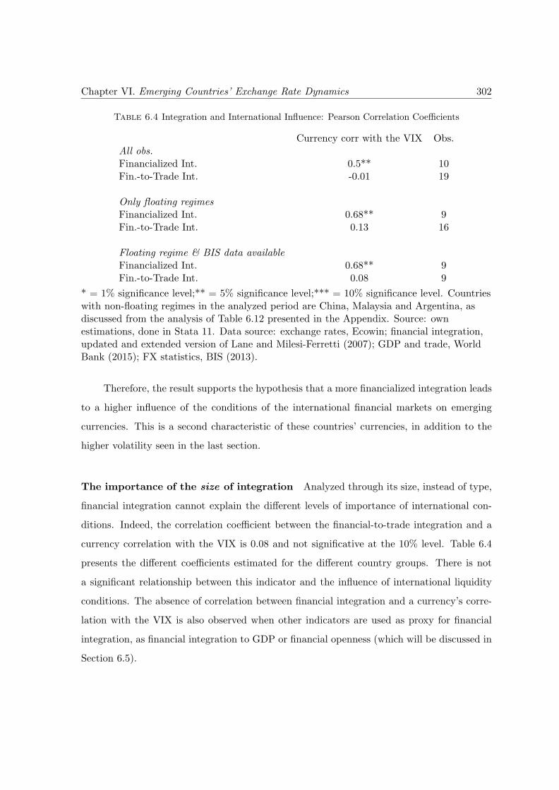
Chapter VI. Emerging Countries’ Exchange Rate Dynamics 302
Table 6.4 Integration and International Influence: Pearson Correlation Coefficients
Currency corr with the VIX Obs.All obs.Financialized Int. 0.5** 10Fin.-to-Trade Int. -0.01 19
Only floating regimesFinancialized Int. 0.68** 9Fin.-to-Trade Int. 0.13 16
Floating regime & BIS data availableFinancialized Int. 0.68** 9Fin.-to-Trade Int. 0.08 9
* = 1% significance level;** = 5% significance level;*** = 10% significance level. Countrieswith non-floating regimes in the analyzed period are China, Malaysia and Argentina, asdiscussed from the analysis of Table 6.12 presented in the Appendix. Source: ownestimations, done in Stata 11. Data source: exchange rates, Ecowin; financial integration,updated and extended version of Lane and Milesi-Ferretti (2007); GDP and trade, WorldBank (2015); FX statistics, BIS (2013).
Therefore, the result supports the hypothesis that a more financialized integration leads
to a higher influence of the conditions of the international financial markets on emerging
currencies. This is a second characteristic of these countries’ currencies, in addition to the
higher volatility seen in the last section.
The importance of the size of integration Analyzed through its size, instead of type,
financial integration cannot explain the different levels of importance of international con-
ditions. Indeed, the correlation coefficient between the financial-to-trade integration and a
currency correlation with the VIX is 0.08 and not significative at the 10% level. Table 6.4
presents the different coefficients estimated for the different country groups. There is not
a significant relationship between this indicator and the influence of international liquidity
conditions. The absence of correlation between financial integration and a currency’s corre-
lation with the VIX is also observed when other indicators are used as proxy for financial
integration, as financial integration to GDP or financial openness (which will be discussed in
Section 6.5).
Chapter VI. Emerging Countries’ Exchange Rate Dynamics 303
6.3.5 The VIX Index, Stock Exchange, and Exchange Rates
Because it affects foreign investors decisions, a change in the VIX index could also affect
markets where these investors keep their assets, which could be observed as a relationship
between the VIX index and EMEs’ stock indices. The subsection analyzes whether such a
relationship has occurred among EMEs in the recent period.
First, the evolution of the EMEs’ major stock exchange indices for the period of 2000 to
2013, presented in Figure 6.16, is examined. As observed, most countries saw an important
hike of their stock markets until the GFC (which is presented as a reference line in the plots),
when they suffered important, but (in most cases) short-lived, losses. The GFC shock was
followed by an important hike in most EMEs and from 2011 onward, due to the Euro crisis,
the most common pattern is a side movement. After the crisis, some markets continued to
gain value (Argentina, the Philippines, Thailand, Turkey and South Africa), but in most of
them the stock index had, in 2013, a similar value as in 2010.
Stock markets in some of the Asian countries and in South Africa52 continued to boom
in the aftermath of the GFC.
The stock indices and the VIX index are plotted against each other in Figure 6.17 for a
better look into the two series53. The plots suggest a stronger relationship between the two
in some countries and also vary for different periods. But generally the two series tend to
move in opposite directions: periods of fall of the VIX index go in tandem with the rise of
the countries’ stock indices. As expected, this relationship is the clearest for the U.S. S&P
500 index, as the VIX is based on the U.S. market – although not being estimated based on
the S&P 500 index.
In order to further analyze this relationship, a correlation between the two was esti-
mated. Given that the relationship seems to evolve through time, different coefficients were
estimated based on 80-day periods (or approximately four months). They are presented in
the form of a moving average (20 days) for ease of reading the graphs (see Figure 6.18).
52Argentina is a third case, where there was no rise and side movement nor only rise. There was a rise,interrupted by a side-movement and a rise.
53The S&P index is also plotted for enabling a comparison between the U.S. and the EMEs’ equity-cyclesand the equity-VIX relationship.
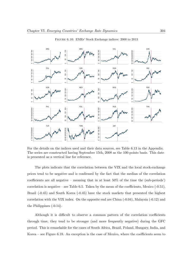
Chapter VI. Emerging Countries’ Exchange Rate Dynamics 304
Figure 6.16: EMEs’ Stock Exchange indices: 2000 to 2013
01
00
20
03
00
40
0
ARG
05
01
00
15
0
BRA
05
01
00
15
02
00
CHL
50
10
01
50
20
02
50
30
0
CHN
05
01
00
15
02
00
COL
05
01
00
15
0
CZE
05
01
00
15
0
HUN
05
01
00
15
0
IND
05
01
00
15
0
KOR
05
01
00
15
02
00
MEX
50
10
01
50
20
0
MYS
05
01
00
15
02
00
PER
50
10
01
50
20
02
50
30
0
PHL
50
10
01
50
20
0
POL
05
01
00
15
02
00
RUS
50
10
01
50
20
02
50
THA
05
01
001
502
002
50
TUR
60
80
10
012
014
016
0
TWN
05
01
00
15
02
00
ZAF
For the details on the indices used and their data sources, see Table 6.13 in the Appendix.The series are constructed having September 15th, 2008 as the 100-points basis. This dateis presented as a vertical line for reference.
The plots indicate that the correlation between the VIX and the local stock-exchange
prices tend to be negative and is confirmed by the fact that the median of the correlation
coefficients are all negative – meaning that in at least 50% of the time the (sub-periods’)
correlation is negative – see Table 6.5. Taken by the mean of the coefficients, Mexico (-0.51),
Brazil (-0.45) and South Korea (-0.45) have the stock markets that presented the highest
correlation with the VIX index. On the opposite end are China (-0.04), Malaysia (-0.12) and
the Philippines (-0.14).
Although it is difficult to observe a common pattern of the correlation coefficients
through time, they tend to be stronger (and more frequently negative) during the GFC
period. This is remarkable for the cases of South Africa, Brazil, Poland, Hungary, India, and
Korea – see Figure 6.18. An exception is the case of Mexico, where the coefficients seem to
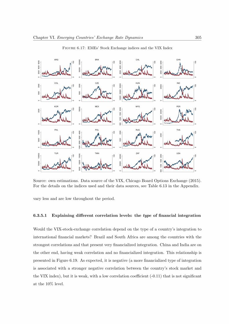
Chapter VI. Emerging Countries’ Exchange Rate Dynamics 305
Figure 6.17: EMEs’ Stock Exchange indices and the VIX Index
01
00
02
00
04
00
06
00
0
ARG
01
00
05
00
00
10
00
00 BRA
01
00
02
00
04
00
06
00
0
CHL
01
00
02
00
04
00
06
00
0
CHN
01
00
01
00
02
00
0
COL
01
00
01
00
02
00
0
CZE
01
00
10
00
02
00
00
30
00
0 HUN
01
00
02
00
00
IND
01
00
02
00
0
KOR
01
00
05
00
00 MEX
01
00
50
01
00
01
50
02
00
0
MYS
01
00
01
00
00
20
00
0
PER
01
00
05
00
01
00
00 PHL
01
00
10
00
20
00
30
00
40
00
POL
01
00
01
00
02
00
0
RUS
01
00
02
00
0
THA
01
00
05
00
00
10
00
00 TUR
01
00
50
00
10
00
01
50
00 TWN
01
00
02
00
00
40
00
0
ZAF
01
00
50
01
00
01
50
02
00
0
USA
Source: own estimations. Data source of the VIX, Chicago Board Options Exchange (2015).For the details on the indices used and their data sources, see Table 6.13 in the Appendix.
vary less and are low throughout the period.
6.3.5.1 Explaining different correlation levels: the type of financial integration
Would the VIX-stock-exchange correlation depend on the type of a country’s integration to
international financial markets? Brazil and South Africa are among the countries with the
strongest correlations and that present very financialized integration. China and India are on
the other end, having weak correlation and no financialized integration. This relationship is
presented in Figure 6.19. As expected, it is negative (a more financialized type of integration
is associated with a stronger negative correlation between the country’s stock market and
the VIX index), but it is weak, with a low correlation coefficient (-0.11) that is not significant
at the 10% level.
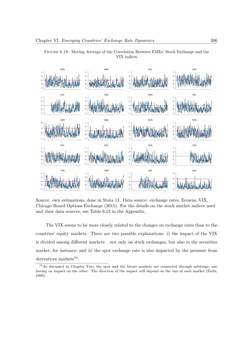
Chapter VI. Emerging Countries’ Exchange Rate Dynamics 306
Figure 6.18: Moving Average of the Correlation Between EMEs’ Stock Exchange and theVIX indices
−1
−.5
0.5
1
ARG
−1
−.5
0.5
1
BRA
−1
−.5
0.5
1
CHL
−1
−.5
0.5
1
CHN
−1
−.5
0.5
1
COL
−1
−.5
0.5
1
CZE
−1
−.5
0.5
1
HUN
−1
−.5
0.5
1
IND
−1
−.5
0.5
KOR
−1
−.5
0.5
1
MEX
−1
−.5
0.5
1
MYS
−1
−.5
0.5
1
PER
−1
−.5
0.5
1
PHL
−1
−.5
0.5
1
POL
−1
−.5
0.5
1
RUS
−1
−.5
0.5
1
THA
−1
−.5
0.5
1
TUR
−1
−.5
0.5
1
TWN
−1
−.5
0.5
1
ZAF
−1
−.5
0.5
USA
Source: own estimations, done in Stata 11. Data source: exchange rates, Ecowin; VIX,Chicago Board Options Exchange (2015). For the details on the stock market indices usedand their data sources, see Table 6.13 in the Appendix.
The VIX seems to be more closely related to the changes on exchange rates than to the
countries’ equity markets. There are two possible explanations: i) the impact of the VIX
is divided among different markets – not only on stock exchanges, but also in the securities
market, for instance; and ii) the spot exchange rate is also impacted by the pressure from
derivatives markets54.
54As discussed in Chapter Two, the spot and the future markets are connected through arbitrage, onehaving an impact on the other. The direction of the impact will depend on the size of each market (Farhi,1999).
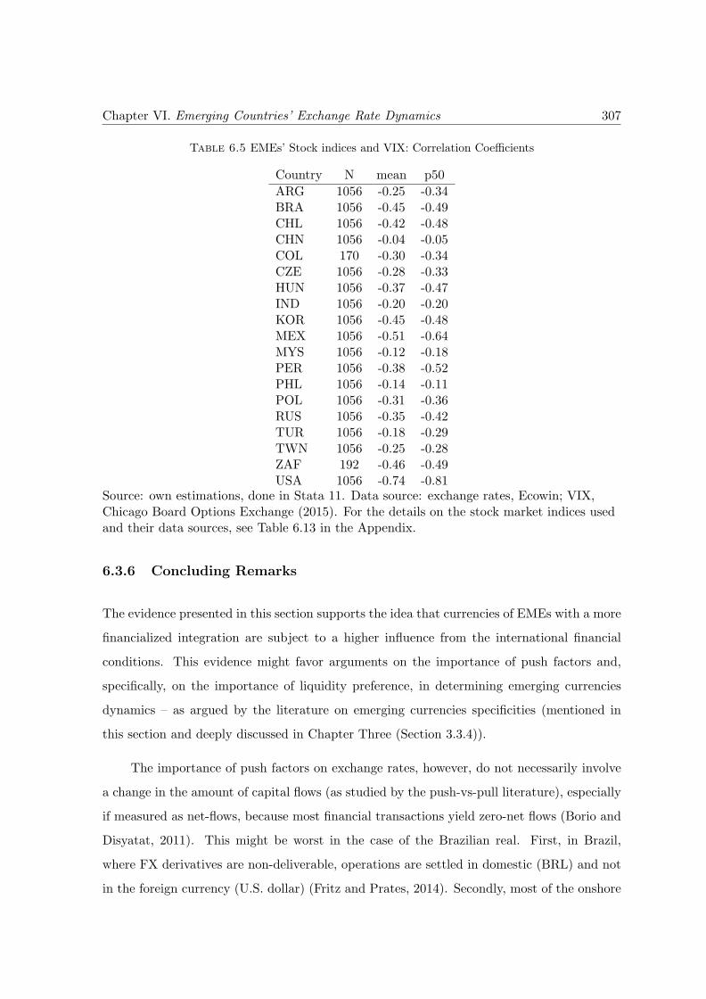
Chapter VI. Emerging Countries’ Exchange Rate Dynamics 307
Table 6.5 EMEs’ Stock indices and VIX: Correlation Coefficients
Country N mean p50
ARG 1056 -0.25 -0.34BRA 1056 -0.45 -0.49CHL 1056 -0.42 -0.48CHN 1056 -0.04 -0.05COL 170 -0.30 -0.34CZE 1056 -0.28 -0.33HUN 1056 -0.37 -0.47IND 1056 -0.20 -0.20KOR 1056 -0.45 -0.48MEX 1056 -0.51 -0.64MYS 1056 -0.12 -0.18PER 1056 -0.38 -0.52PHL 1056 -0.14 -0.11POL 1056 -0.31 -0.36RUS 1056 -0.35 -0.42TUR 1056 -0.18 -0.29TWN 1056 -0.25 -0.28ZAF 192 -0.46 -0.49USA 1056 -0.74 -0.81
Source: own estimations, done in Stata 11. Data source: exchange rates, Ecowin; VIX,Chicago Board Options Exchange (2015). For the details on the stock market indices usedand their data sources, see Table 6.13 in the Appendix.
6.3.6 Concluding Remarks
The evidence presented in this section supports the idea that currencies of EMEs with a more
financialized integration are subject to a higher influence from the international financial
conditions. This evidence might favor arguments on the importance of push factors and,
specifically, on the importance of liquidity preference, in determining emerging currencies
dynamics – as argued by the literature on emerging currencies specificities (mentioned in
this section and deeply discussed in Chapter Three (Section 3.3.4)).
The importance of push factors on exchange rates, however, do not necessarily involve
a change in the amount of capital flows (as studied by the push-vs-pull literature), especially
if measured as net-flows, because most financial transactions yield zero-net flows (Borio and
Disyatat, 2011). This might be worst in the case of the Brazilian real. First, in Brazil,
where FX derivatives are non-deliverable, operations are settled in domestic (BRL) and not
in the foreign currency (U.S. dollar) (Fritz and Prates, 2014). Secondly, most of the onshore
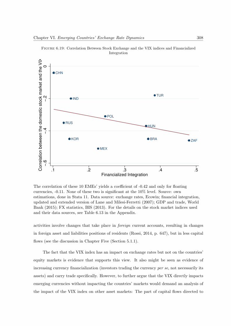
Chapter VI. Emerging Countries’ Exchange Rate Dynamics 308
Figure 6.19: Correlation Between Stock Exchange and the VIX indices and FinancializedIntegration
BRA
CHN
HUN
IND
KOR
MEX
POL
RUS
TUR
ZAF
−.6
−.4
−.2
0C
orr
ela
tio
n b
etw
ee
n t
he
do
me
stic s
tock m
ark
et
an
d t
he
VIX
.1 .2 .3 .4 .5Financialized Integration
The correlation of these 10 EMEs’ yields a coefficient of -0.42 and only for floatingcurrencies, -0.11. None of these two is significant at the 10% level. Source: ownestimations, done in Stata 11. Data source: exchange rates, Ecowin; financial integration,updated and extended version of Lane and Milesi-Ferretti (2007); GDP and trade, WorldBank (2015); FX statistics, BIS (2013). For the details on the stock market indices usedand their data sources, see Table 6.13 in the Appendix.
activities involve changes that take place in foreign current accounts, resulting in changes
in foreign asset and liabilities positions of residents (Rossi, 2014, p. 647), but in less capital
flows (see the discussion in Chapter Five (Section 5.1.1).
The fact that the VIX index has an impact on exchange rates but not on the countries’
equity markets is evidence that supports this view. It also might be seen as evidence of
increasing currency financialization (investors trading the currency per se, not necessarily its
assets) and carry trade specifically. However, to further argue that the VIX directly impacts
emerging currencies without impacting the countries’ markets would demand an analysis of
the impact of the VIX index on other asset markets: The part of capital flows directed to
Chapter VI. Emerging Countries’ Exchange Rate Dynamics 309
stock markets in EMEs is small (as discussed in Chapter Four) and the impact on flows and
then on the exchange rate could take place through other markets.
To be subject to changes in international financial conditions, this second currency
feature, as the first (high volatility), is explained by the type of integration, but not by its
relative magnitude. This suggests the importance of considering the characteristics of FX
markets in explaining emerging currencies patterns.
6.4 Comovement and Correlation of Different Currencies
The main prices in integrated financial markets have a tendency of comovement, as differ-
ent markets become options for portfolio diversification strategies for groups of investors.
Chapter Two discussed that this happens with financialization: as money managers’ port-
folios include both advanced and emerging countries’ markets, asset prices in these markets
are tied together55. Given this effect on asset prices, a strand of the literature on financial
integration uses price-related indicators to characterize integration, as discussed in Chapter
Five.
If international investors have EMEs’ assets in their portfolios, and considering that
demand for their assets impacts not only asset prices but also the exchange rate, EMEs’
exchange rates are also expected to comove. Note that this hypothesis seems to hold at least
for some emerging currencies, as seen by the correlation of their exchange rate paths with
the VIX index.
In order to study the hypothesis of increasing exchange rate comovement, two exercises
are done. First, a Principal Component Analysis (PCA) of the changes in emerging currencies
is done for three different periods in order to analyze whether comovement has increased.
The second is a study of the correlation of different emerging currencies.
55The idea that foreign investors tie financial markets together made Hofmann and Takats (2015), analyzecomovement of interest rates only of countries that are “well integrated in the global financial system”,arguing that it would be an advancement vis-a-vis of other studies given that “global financial and economicintegration (...) determines the strength of investor arbitrage by tying bond market rates to those prevailingin the core economies.”
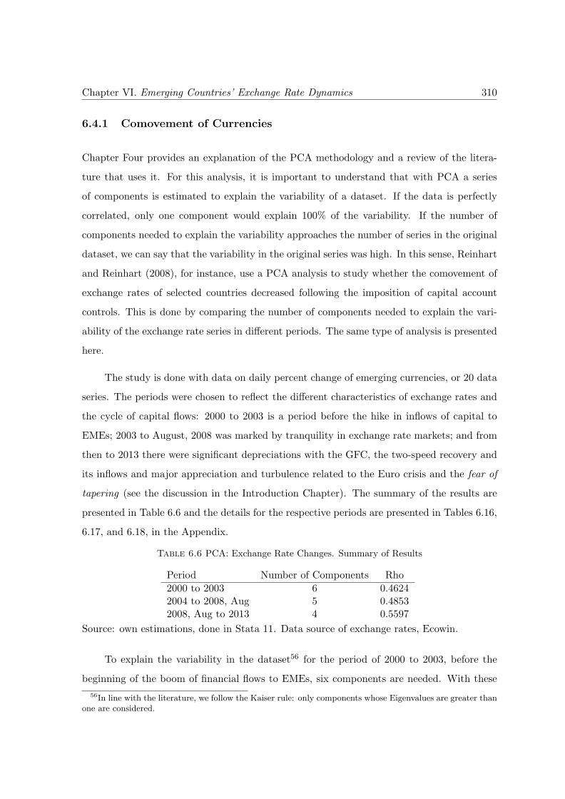
Chapter VI. Emerging Countries’ Exchange Rate Dynamics 310
6.4.1 Comovement of Currencies
Chapter Four provides an explanation of the PCA methodology and a review of the litera-
ture that uses it. For this analysis, it is important to understand that with PCA a series
of components is estimated to explain the variability of a dataset. If the data is perfectly
correlated, only one component would explain 100% of the variability. If the number of
components needed to explain the variability approaches the number of series in the original
dataset, we can say that the variability in the original series was high. In this sense, Reinhart
and Reinhart (2008), for instance, use a PCA analysis to study whether the comovement of
exchange rates of selected countries decreased following the imposition of capital account
controls. This is done by comparing the number of components needed to explain the vari-
ability of the exchange rate series in different periods. The same type of analysis is presented
here.
The study is done with data on daily percent change of emerging currencies, or 20 data
series. The periods were chosen to reflect the different characteristics of exchange rates and
the cycle of capital flows: 2000 to 2003 is a period before the hike in inflows of capital to
EMEs; 2003 to August, 2008 was marked by tranquility in exchange rate markets; and from
then to 2013 there were significant depreciations with the GFC, the two-speed recovery and
its inflows and major appreciation and turbulence related to the Euro crisis and the fear of
tapering (see the discussion in the Introduction Chapter). The summary of the results are
presented in Table 6.6 and the details for the respective periods are presented in Tables 6.16,
6.17, and 6.18, in the Appendix.
Table 6.6 PCA: Exchange Rate Changes. Summary of Results
Period Number of Components Rho
2000 to 2003 6 0.46242004 to 2008, Aug 5 0.48532008, Aug to 2013 4 0.5597
Source: own estimations, done in Stata 11. Data source of exchange rates, Ecowin.
To explain the variability in the dataset56 for the period of 2000 to 2003, before the
beginning of the boom of financial flows to EMEs, six components are needed. With these
56In line with the literature, we follow the Kaiser rule: only components whose Eigenvalues are greater thanone are considered.
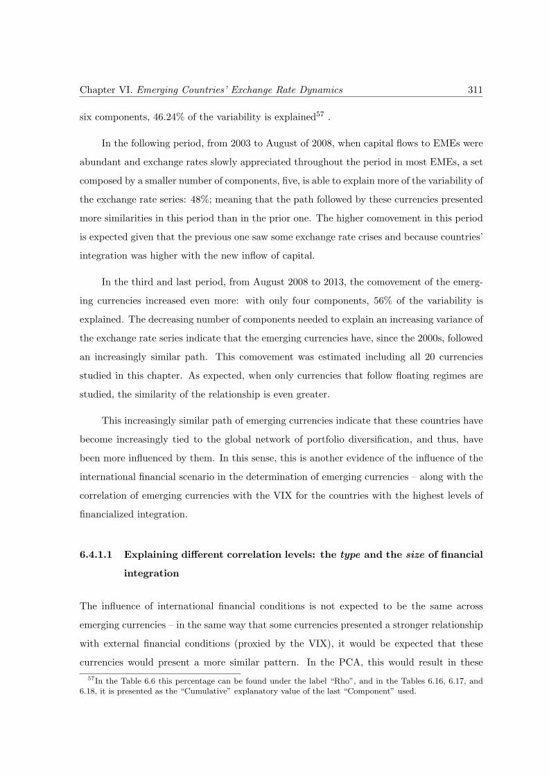
Chapter VI. Emerging Countries’ Exchange Rate Dynamics 311
six components, 46.24% of the variability is explained57 .
In the following period, from 2003 to August of 2008, when capital flows to EMEs were
abundant and exchange rates slowly appreciated throughout the period in most EMEs, a set
composed by a smaller number of components, five, is able to explain more of the variability of
the exchange rate series: 48%; meaning that the path followed by these currencies presented
more similarities in this period than in the prior one. The higher comovement in this period
is expected given that the previous one saw some exchange rate crises and because countries’
integration was higher with the new inflow of capital.
In the third and last period, from August 2008 to 2013, the comovement of the emerg-
ing currencies increased even more: with only four components, 56% of the variability is
explained. The decreasing number of components needed to explain an increasing variance of
the exchange rate series indicate that the emerging currencies have, since the 2000s, followed
an increasingly similar path. This comovement was estimated including all 20 currencies
studied in this chapter. As expected, when only currencies that follow floating regimes are
studied, the similarity of the relationship is even greater.
This increasingly similar path of emerging currencies indicate that these countries have
become increasingly tied to the global network of portfolio diversification, and thus, have
been more influenced by them. In this sense, this is another evidence of the influence of the
international financial scenario in the determination of emerging currencies – along with the
correlation of emerging currencies with the VIX for the countries with the highest levels of
financialized integration.
6.4.1.1 Explaining different correlation levels: the type and the size of financial
integration
The influence of international financial conditions is not expected to be the same across
emerging currencies – in the same way that some currencies presented a stronger relationship
with external financial conditions (proxied by the VIX), it would be expected that these
currencies would present a more similar pattern. In the PCA, this would result in these
57In the Table 6.6 this percentage can be found under the label “Rho”, and in the Tables 6.16, 6.17, and6.18, it is presented as the “Cumulative” explanatory value of the last “Component” used.
Chapter VI. Emerging Countries’ Exchange Rate Dynamics 312
currencies composing a unique component58, given that a component indicates observations
that are more correlated to each other.
When analyzing the components that resulted from the PCA, we see that in the 2003-
2008 period, marked by lower uncertainty (or tranquility, in Minsky’s terms) and low VIX
levels, the set of countries that are grouped in the first component – which, by definition,
is the one that gathers the most similar countries thus explaining the highest part of the
variability of the whole dataset – is the one of low-volatility currencies: the Indian rupee,
the Indonesian rupiah, the Korean won, the Malaysian ringgit and the Philippine peso. That
these currencies presented the most similar paths is a reflection that they presented only
small variations, while others varied significantly, mostly following an appreciation trend,
but not necessarily of the same magnitude. The fact that they are all Asian currencies also
make them subject to the same set of factors.
What is impressive, however, is that the group of currencies that compose the first
component of the PCA conducted for the turbulent 2008-2013 period includes the Brazilian
real59, the Czech koruna, the Hungarian forint, the Mexican peso, the Polish zloty, the
Turkish lira, and the South African rand, which are the currencies that present the highest
volatility. In other words, even with significant deviations in this period, these currencies
presented a more similar path than the low-volatility (small deviations) ones, pointing to the
significance of their comovement. Currencies of small deviations are also highly correlated
among themselves: the Indian rupee, the Korean won, the Russian ruble, and the Chinese
yuan. Figure 6.20 presents these two sets of inter-correlated currencies in the mid-2008 to
2013 period against their respective level of financialized integration.
As shown by Figure 6.20, the group of highly correlated currencies is also similar to the
group of currencies with the most important FX markets and presents the most financialized
type of integration. Indeed, the correlation between the loading on this first component and
the level of financialized integration yields a very high correlation coefficient, 0.77, significant
at the 5% level. The relationship between comovement and the financial-to-trade integration,
the level of financial integration or the financial integration over GDP are not significant.
58The currencies that compose the different components are the ones who have the highest loadings oneach. In Tables 6.16, 6.17, and 6.18, only loading higher than 0.3 (in absolute values) are presented for easeof reading.
59Brazil’s loading, 0.29, is not shown as only values higher than 0.3 are printed.
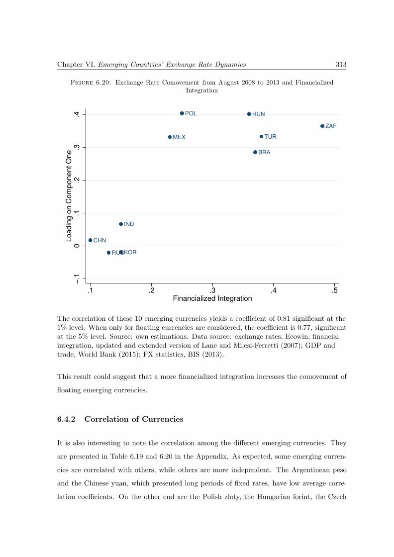
Chapter VI. Emerging Countries’ Exchange Rate Dynamics 313
Figure 6.20: Exchange Rate Comovement from August 2008 to 2013 and FinancializedIntegration
BRA
CHN
HUN
IND
KOR
MEX
POL
RUS
TUR
ZAF
−.1
0.1
.2.3
.4L
oa
din
g o
n C
om
po
ne
nt
On
e
.1 .2 .3 .4 .5Financialized Integration
The correlation of these 10 emerging currencies yields a coefficient of 0.81 significant at the1% level. When only for floating currencies are considered, the coefficient is 0.77, significantat the 5% level. Source: own estimations. Data source: exchange rates, Ecowin; financialintegration, updated and extended version of Lane and Milesi-Ferretti (2007); GDP andtrade, World Bank (2015); FX statistics, BIS (2013).
This result could suggest that a more financialized integration increases the comovement of
floating emerging currencies.
6.4.2 Correlation of Currencies
It is also interesting to note the correlation among the different emerging currencies. They
are presented in Table 6.19 and 6.20 in the Appendix. As expected, some emerging curren-
cies are correlated with others, while others are more independent. The Argentinean peso
and the Chinese yuan, which presented long periods of fixed rates, have low average corre-
lation coefficients. On the other end are the Polish zloty, the Hungarian forint, the Czech
Chapter VI. Emerging Countries’ Exchange Rate Dynamics 314
koruna, the Turkish lira, the South African rand and the Mexican peso present high average
correlation.
It is expected that the currencies of neighboring countries are more correlated among
themselves, given that they have similar ties and that foreign investors build their expecta-
tions upon the same set of variables. For instance, this is observed in the high correlation
among the European emerging currencies. However, relevant correlations are also found
among currencies of different regions. They are listed in Table 6.7.
Table 6.7 Emerging Currencies With Relevant “out of the Region” correlation (2003-2013)
Brazil with Hungary, Poland, Turkey and South AfricaCzech Rep. with Mexico and South Africa
Hungary with Brazil, Mexico and South AfricaMexico with Czech Rep., Hungary, Poland, South Africa and TurkeyPoland with Brazil, Mexico and South Africa
South Africa with Brazil, Czech Rep., Hungary, Mexico, Poland, Russia and TurkeyTurkey with Brazil, Mexico and South Africa
Correlation coefficients considered as “relevant” are the ones above 0.4 (presented in Tables6.19 and 6.20).
From these currencies, six are highly correlated with at least three currencies of other
continents: the Brazilian real, the Hungarian forint, the Mexican peso, the Polish zloty,
the South African rand, and the Turkish lira. This suggests that these currencies have a
higher influence on international financial conditions. Also note that these currencies have
been highly correlated among themselves since the GFC and present the highest levels of
financialized integration.
6.4.3 Concluding Remarks
Several conclusions can be drawn from the evidence presented. First, the higher comovement
of emerging currencies through time as a group results from the increasing integration of
EMEs to the international financial markets (as shown in Chapter Four).
Secondly, the high comovement of currencies of EMEs which have a more financialized
type of integration suggests that the impact of external financial conditions on these curren-
cies is even greater – which was also suggested by the higher correlation of these countries’
Chapter VI. Emerging Countries’ Exchange Rate Dynamics 315
currencies with the VIX. It is worth mentioning that this conclusion excludes the possibility
that higher comovement results from a more similar path of the (mainstream notion of)
‘fundamentals’60. Such hypothesis is excluded given the difference of these countries’ fun-
damentals (Kaltenbrunner and Painceira, 2014) and because the fundamentals could not be
going through such significant changes61.
From a mainstream point of view, and having accepted that these countries fundamen-
tals would not have been evolving in a synchronized fashion, the fact that emerging currencies
follow similar paths explains why their estimations of misalignment tend to evolve in a sim-
ilar way. As shown by Ramos (2012), Cline and Willamson’s estimations of exchange rate
overvaluation for countries such as Brazil, Turkey and South Africa have evolved in a similar
way: they increased from 2009 to 2011, when nominal currencies appreciated, and decreased
from 2011 to 2012, when they depreciated.
Therefore, it can be concluded that a third feature of the currencies of EMEs that have a
more financialized type of integration to international markets exists: they all follow a similar
path – in addition to being more volatile and to suffering higher influence from the conditions
of international financial markets, as discussed in Sections 6.2 and 6.3, respectively.
On the relationship between these results and the debate on the importance of in-
ternational liquidity cycles (discussed in section 6.3), it is interesting to highlight that the
comovement of emerging currencies has increased with higher portfolio inflows (of the 2003-
2008 period) and is at its highest level when external conditions became more volatile (in
the 2008-2013 period). The higher importance of external factors in turbulent periods is in
line with Hoti’s (2004) argument that the international condition determines capital flows
to EMEs, but domestic factors define its geographic location. In the first period, interna-
tional conditions pushed capital flows to emerging countries, but these flows were not the
same across countries as they are also dependent on pull factors, resulting in different ex-
change rate paths. In the second, turbulent period, push factors would have overcome pull
60See Chapter Three for the concept of fundamental as the variable that makes exchange rate a marketclearing price as used among mainstream economists and its use by heterodox authors as a subjective variabledefined by the financial convention ruling among traders.
61This impossibility is known as the third exchange rate puzzle, discussed in Chapter Three, that emergesfrom the observation that the exchange rates are normally much more volatile than the economic variablesthey are supposed to explain.
Chapter VI. Emerging Countries’ Exchange Rate Dynamics 316
ones, leading to the same movement – capital outflows – in every country and thus higher
comovement.
6.5 Other Important Elements in Explaining Emerging Cur-
rency Patterns
This chapter is focused on the relationship between a more financialized type of integration
and some emerging currencies’ features, notably high volatility, high frequency of extreme
exchange rate depreciation, the connection of a country’s exchange rate with international
financial markets’ sentiments and the similarity of patterns.
However, these features can also be influenced by other types of country characteristics.
The exchange rate regime is an obvious first, and its role has been highlighted throughout
the chapter. Other potentially important features are interest rate differential, the monetary
regimes in place, the position of a country’s currency in the hierarchy of currencies, whether
capital account restrictions are in place, and the absolute magnitude of financial integration.
This section examines how these other characteristics relate to the exchange rate features
analyzed. Some have already been described when EMEs were presented in Chapter Four,
and an overview can be found in Table 6.8.
It is important to keep in mind that some of these country characteristics are interde-
pendent: the choice of the monetary and exchange rate regimes can impact the interest rate,
and the size of stock markets and the financial integration level are inseparable. For EMEs,
specifically, Chapter Four showed that in the 2003-2013 period a country had a higher proba-
bility of having a high interest rate differential to the Fed Fund rate when it had a “Floating”
or “Free Floating” exchange rate regime associated with an inflation targeting regime.
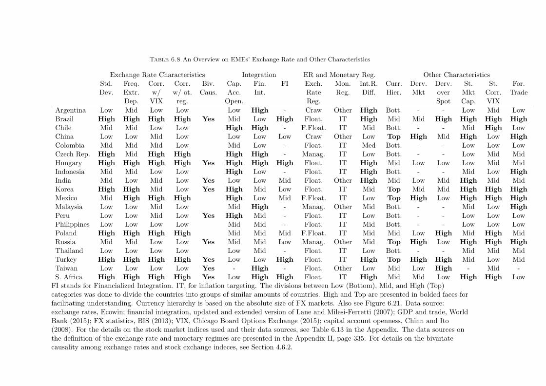
Table 6.8 An Overview on EMEs’ Exchange Rate and Other Characteristics
Exchange Rate Characteristics Integration ER and Monetary Reg. Other CharacteristicsStd. Freq. Corr. Corr. Biv. Cap. Fin. FI Exch. Mon. Int.R. Curr. Derv. Derv. St. St. For.Dev. Extr. w/ w/ ot. Caus. Acc. Int. Rate Reg. Diff. Hier. Mkt over Mkt Corr. Trade
Dep. VIX reg. Open. Reg. Spot Cap. VIX
Argentina Low Mid Low Low Low High - Craw Other High Bott. - - Low Mid LowBrazil High High High High Yes Mid Low High Float. IT High Mid Mid High High High HighChile Mid Mid Low Low High High - F.Float. IT Mid Bott. - - Mid High LowChina Low Low Mid Low Low Low Low Craw Other Low Top High Mid High Low HighColombia Mid Mid Mid Low Mid Low - Float. IT Med Bott. - - Low Low LowCzech Rep. High Mid High High High High - Manag. IT Low Bott. - - Low Mid MidHungary High High High High Yes High High High Float. IT High Mid Low Low Low Mid MidIndonesia Mid Mid Low Low High Low - Float. IT High Bott. - - Mid Low HighIndia Mid Low Mid Low Yes Low Low Mid Float. Other High Mid Low Mid High Mid MidKorea High High Mid Low Yes High Mid Low Float. IT Mid Top Mid Mid High High HighMexico Mid High High High High Low Mid F.Float. IT Low Top High Low High High HighMalaysia Low Low Mid Low Mid High - Manag. Other Mid Bott. - - Mid Low HighPeru Low Low Mid Low Yes High Mid - Float. IT Low Bott. - - Low Low LowPhilippines Low Low Low Low Mid Mid - Float. IT Mid Bott. - - Low Low LowPoland High High High High Mid Mid Mid F.Float. IT Mid Mid Low High Mid High MidRussia Mid Mid Low Low Yes Mid Mid Low Manag. Other Mid Top High Low High High HighThailand Low Low Low Low Low Mid - Float. IT Low Bott. - - Mid Mid MidTurkey High High High High Yes Low Low High Float. IT High Top High High Mid Low MidTaiwan Low Low Low Low Yes - High - Float. Other Low Mid Low High - Mid -S. Africa High High High High Yes Low High High Float. IT High Mid Mid Low High High Low
FI stands for Financialized Integration. IT, for inflation targeting. The divisions between Low (Bottom), Mid, and High (Top)categories was done to divide the countries into groups of similar amounts of countries. High and Top are presented in bolded faces forfacilitating understanding. Currency hierarchy is based on the absolute size of FX markets. Also see Figure 6.21. Data source:exchange rates, Ecowin; financial integration, updated and extended version of Lane and Milesi-Ferretti (2007); GDP and trade, WorldBank (2015); FX statistics, BIS (2013); VIX, Chicago Board Options Exchange (2015); capital account openness, Chinn and Ito(2008). For the details on the stock market indices used and their data sources, see Table 6.13 in the Appendix. The data sources onthe definition of the exchange rate and monetary regimes are presented in the Appendix II, page 335. For details on the bivariatecausality among exchange rates and stock exchange indeces, see Section 4.6.2.
Chapter VI. Emerging Countries’ Exchange Rate Dynamics 318
6.5.1 Exchange Rate Regimes and Monetary Policy Frameworks
As seen in Chapter Four, most EMEs now opt for floating exchange rates and inflation
targeting regimes. Are these choices associated with the currency features analyzed in this
chapter? The four main currency features are highly correlated (see Table 6.8): emerging
currencies with high exchange rate volatility as measured by deviation, tend to have more
frequent extreme exchange rate depreciation, are more correlated with the VIX, and with
other emerging currencies. There are five countries with “high” values in all four currency
characteristics: Brazil, Hungary, Poland, Turkey, and South Africa. All of these countries
have a floating (or free floating) exchange rate and follow an inflation targeting regime – see
Table 6.8 and Figure 6.21.
Conversely, Argentina, China, Malaysia, Peru, the Philippines, Thailand, and Taiwan
are the six countries with “low” values for at least three of the characteristics, and thus,
have the least fragile exchange rates. Among them, three have exchange rates that follow a
craw-like or a managed arrangement and a monetary regime that is not inflation targeting,
and three have floating currency and inflation targeting simultaneously. The combination of
floating and inflation targeting partially explains the presence or not of financialized inte-
gration: more than half of those that have opted for an IT regime with a floating currency
present fragile exchange rates62.
6.5.2 Interest Rate Differential, Currency Hierarchy, Capital Account Open-
ness, Financial Integration
Unlike the exchange rate and monetary regimes, other ‘additional’ elements are quantifiable,
so it is easier to grasp their relationship with currency patterns. This section analyzes how
these elements are related to exchange rate volatility (standard deviation and frequency of
extreme depreciation) and their correlation with the VIX.
Currency Hierarchy As extensively discussed in Chapter Three, the international mone-
tary and financial systems are hierarchic, resulting in an asymmetry of currencies that would
62None of the three that have not opted for these two policies present financialized features. However, thisis influenced from the fact that without a floating exchange rate regime volatility cannot be high.
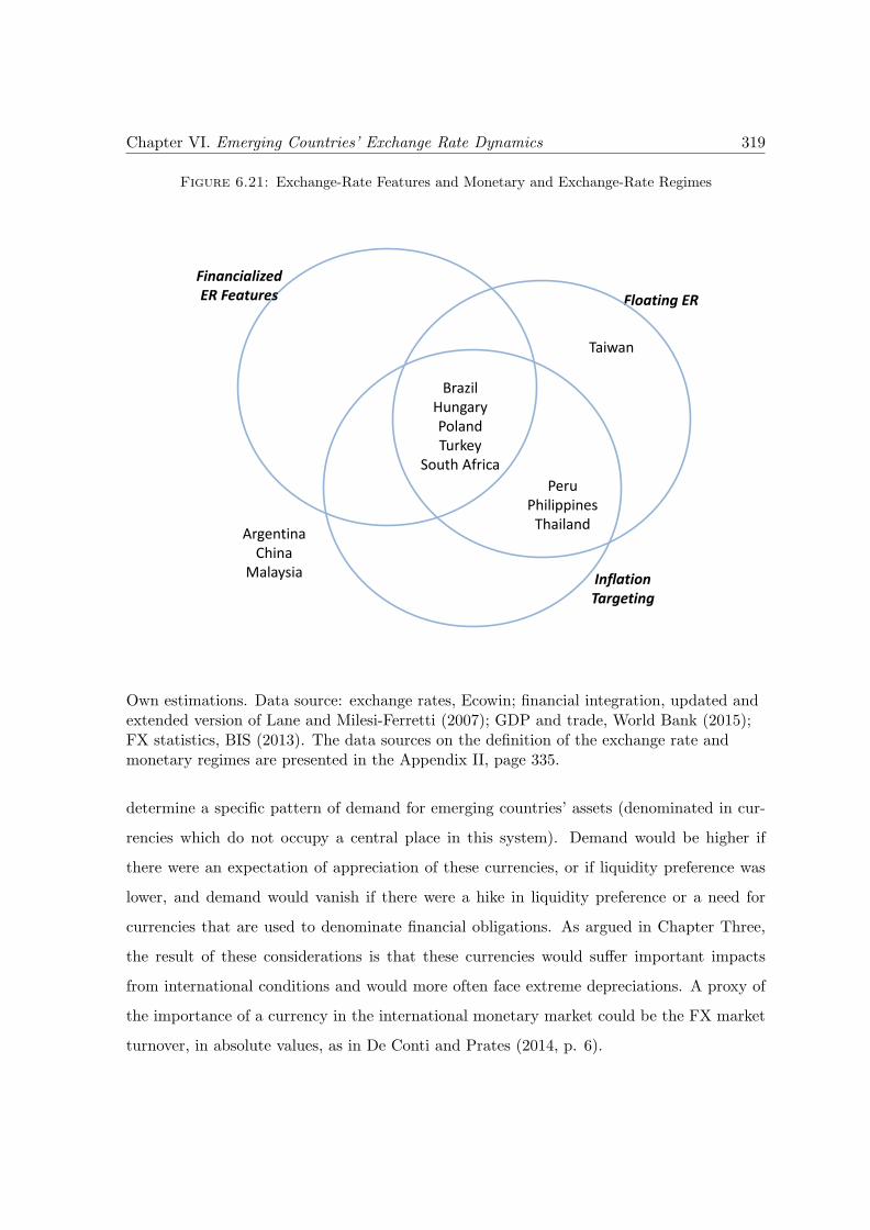
Chapter VI. Emerging Countries’ Exchange Rate Dynamics 319
Figure 6.21: Exchange-Rate Features and Monetary and Exchange-Rate Regimes
Brazil
Hungary
Poland
Turkey
South Africa
Argentina
China
Malaysia Inflation
Targeting
Financialized
ER Features Floating ER
Peru
Philippines
Thailand
Taiwan
Own estimations. Data source: exchange rates, Ecowin; financial integration, updated andextended version of Lane and Milesi-Ferretti (2007); GDP and trade, World Bank (2015);FX statistics, BIS (2013). The data sources on the definition of the exchange rate andmonetary regimes are presented in the Appendix II, page 335.
determine a specific pattern of demand for emerging countries’ assets (denominated in cur-
rencies which do not occupy a central place in this system). Demand would be higher if
there were an expectation of appreciation of these currencies, or if liquidity preference was
lower, and demand would vanish if there were a hike in liquidity preference or a need for
currencies that are used to denominate financial obligations. As argued in Chapter Three,
the result of these considerations is that these currencies would suffer important impacts
from international conditions and would more often face extreme depreciations. A proxy of
the importance of a currency in the international monetary market could be the FX market
turnover, in absolute values, as in De Conti and Prates (2014, p. 6).
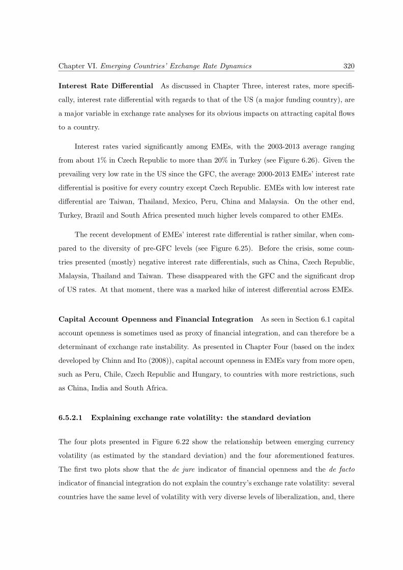
Chapter VI. Emerging Countries’ Exchange Rate Dynamics 320
Interest Rate Differential As discussed in Chapter Three, interest rates, more specifi-
cally, interest rate differential with regards to that of the US (a major funding country), are
a major variable in exchange rate analyses for its obvious impacts on attracting capital flows
to a country.
Interest rates varied significantly among EMEs, with the 2003-2013 average ranging
from about 1% in Czech Republic to more than 20% in Turkey (see Figure 6.26). Given the
prevailing very low rate in the US since the GFC, the average 2000-2013 EMEs’ interest rate
differential is positive for every country except Czech Republic. EMEs with low interest rate
differential are Taiwan, Thailand, Mexico, Peru, China and Malaysia. On the other end,
Turkey, Brazil and South Africa presented much higher levels compared to other EMEs.
The recent development of EMEs’ interest rate differential is rather similar, when com-
pared to the diversity of pre-GFC levels (see Figure 6.25). Before the crisis, some coun-
tries presented (mostly) negative interest rate differentials, such as China, Czech Republic,
Malaysia, Thailand and Taiwan. These disappeared with the GFC and the significant drop
of US rates. At that moment, there was a marked hike of interest differential across EMEs.
Capital Account Openness and Financial Integration As seen in Section 6.1 capital
account openness is sometimes used as proxy of financial integration, and can therefore be a
determinant of exchange rate instability. As presented in Chapter Four (based on the index
developed by Chinn and Ito (2008)), capital account openness in EMEs vary from more open,
such as Peru, Chile, Czech Republic and Hungary, to countries with more restrictions, such
as China, India and South Africa.
6.5.2.1 Explaining exchange rate volatility: the standard deviation
The four plots presented in Figure 6.22 show the relationship between emerging currency
volatility (as estimated by the standard deviation) and the four aforementioned features.
The first two plots show that the de jure indicator of financial openness and the de facto
indicator of financial integration do not explain the country’s exchange rate volatility: several
countries have the same level of volatility with very diverse levels of liberalization, and, there
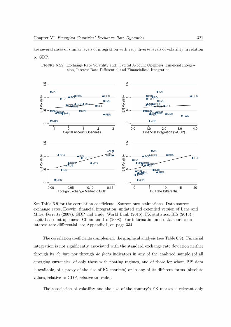
Chapter VI. Emerging Countries’ Exchange Rate Dynamics 321
are several cases of similar levels of integration with very diverse levels of volatility in relation
to GDP.
Figure 6.22: Exchange Rate Volatility and: Capital Account Openness, Financial Integra-tion, Interest Rate Differential and Financialized Integration
CZE
THA
MEX
PER
CHN
MYSPHL
KORCHL
POL
RUSCOL
HUN
ZAF
IND IDNARG
BRATUR
0.5
11.5
ER
Vola
tilit
y
−1 0 1 2 3Capital Account Openness
CZE
TWN
THA
MEX
PER
CHN
MYSPHL
KORCHL
POL
RUSCOL
HUN
ZAF
INDIDNARG
BRATUR
0.5
11.5
ER
Vola
tilit
y
0.0 1.0 2.0 3.0 4.0Financial Integration (%GDP)
MEX
CHN
KOR
POL
RUS
IND
BRATUR
HUN
ZAF
0.5
11.5
ER
Vola
tilit
y
0.00 0.05 0.10 0.15Foreign Exchange Market to GDP
CZE
TWN
THA
MEX
PER
CHN
MYSPHL
KORCHL
POL
RUSCOL
HUN
ZAF
INDIDNARG
BRATUR
0.5
11.5
ER
Vola
tilit
y
0 5 10 15 20Int. Rate Differential
See Table 6.9 for the correlation coefficients. Source: onw estimations. Data source:exchange rates, Ecowin; financial integration, updated and extended version of Lane andMilesi-Ferretti (2007); GDP and trade, World Bank (2015); FX statistics, BIS (2013);capital account openness, Chinn and Ito (2008). For information and data sources oninterest rate differential, see Appendix I, on page 334.
The correlation coefficients complement the graphical analysis (see Table 6.9). Financial
integration is not significantly associated with the standard exchange rate deviation neither
through its de jure nor through de facto indicators in any of the analyzed sample (of all
emerging currencies, of only those with floating regimes, and of those for whom BIS data
is available, of a proxy of the size of FX markets) or in any of its different forms (absolute
values, relative to GDP, relative to trade).
The association of volatility and the size of the country’s FX market is relevant only
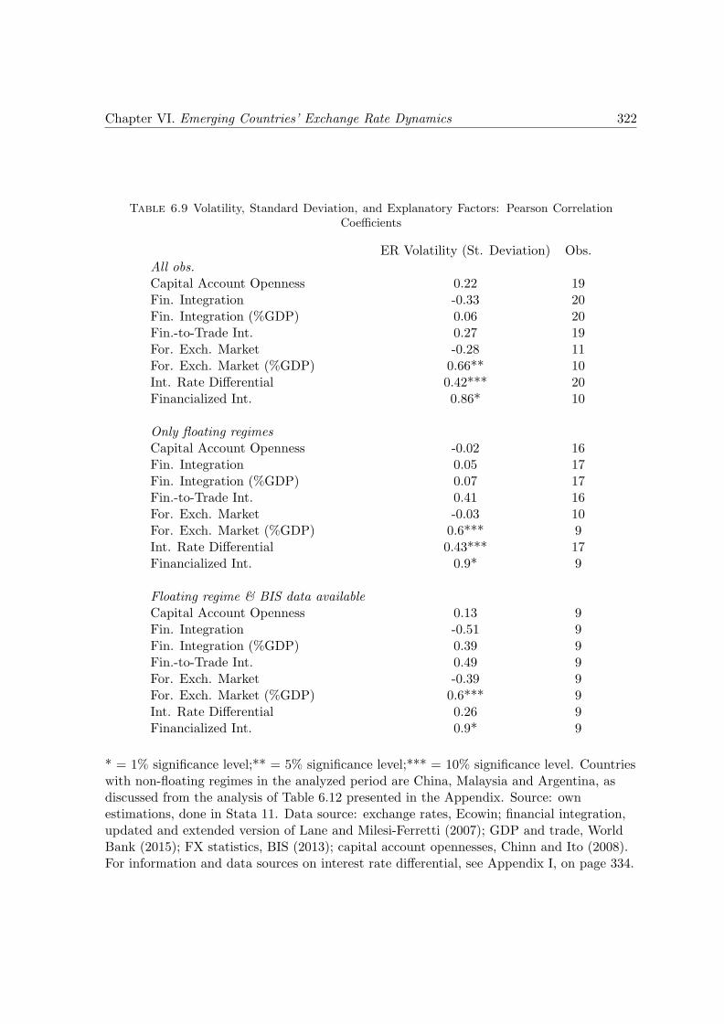
Chapter VI. Emerging Countries’ Exchange Rate Dynamics 322
Table 6.9 Volatility, Standard Deviation, and Explanatory Factors: Pearson CorrelationCoefficients
ER Volatility (St. Deviation) Obs.All obs.Capital Account Openness 0.22 19Fin. Integration -0.33 20Fin. Integration (%GDP) 0.06 20Fin.-to-Trade Int. 0.27 19For. Exch. Market -0.28 11For. Exch. Market (%GDP) 0.66** 10Int. Rate Differential 0.42*** 20Financialized Int. 0.86* 10
Only floating regimesCapital Account Openness -0.02 16Fin. Integration 0.05 17Fin. Integration (%GDP) 0.07 17Fin.-to-Trade Int. 0.41 16For. Exch. Market -0.03 10For. Exch. Market (%GDP) 0.6*** 9Int. Rate Differential 0.43*** 17Financialized Int. 0.9* 9
Floating regime & BIS data availableCapital Account Openness 0.13 9Fin. Integration -0.51 9Fin. Integration (%GDP) 0.39 9Fin.-to-Trade Int. 0.49 9For. Exch. Market -0.39 9For. Exch. Market (%GDP) 0.6*** 9Int. Rate Differential 0.26 9Financialized Int. 0.9* 9
* = 1% significance level;** = 5% significance level;*** = 10% significance level. Countrieswith non-floating regimes in the analyzed period are China, Malaysia and Argentina, asdiscussed from the analysis of Table 6.12 presented in the Appendix. Source: ownestimations, done in Stata 11. Data source: exchange rates, Ecowin; financial integration,updated and extended version of Lane and Milesi-Ferretti (2007); GDP and trade, WorldBank (2015); FX statistics, BIS (2013); capital account opennesses, Chinn and Ito (2008).For information and data sources on interest rate differential, see Appendix I, on page 334.
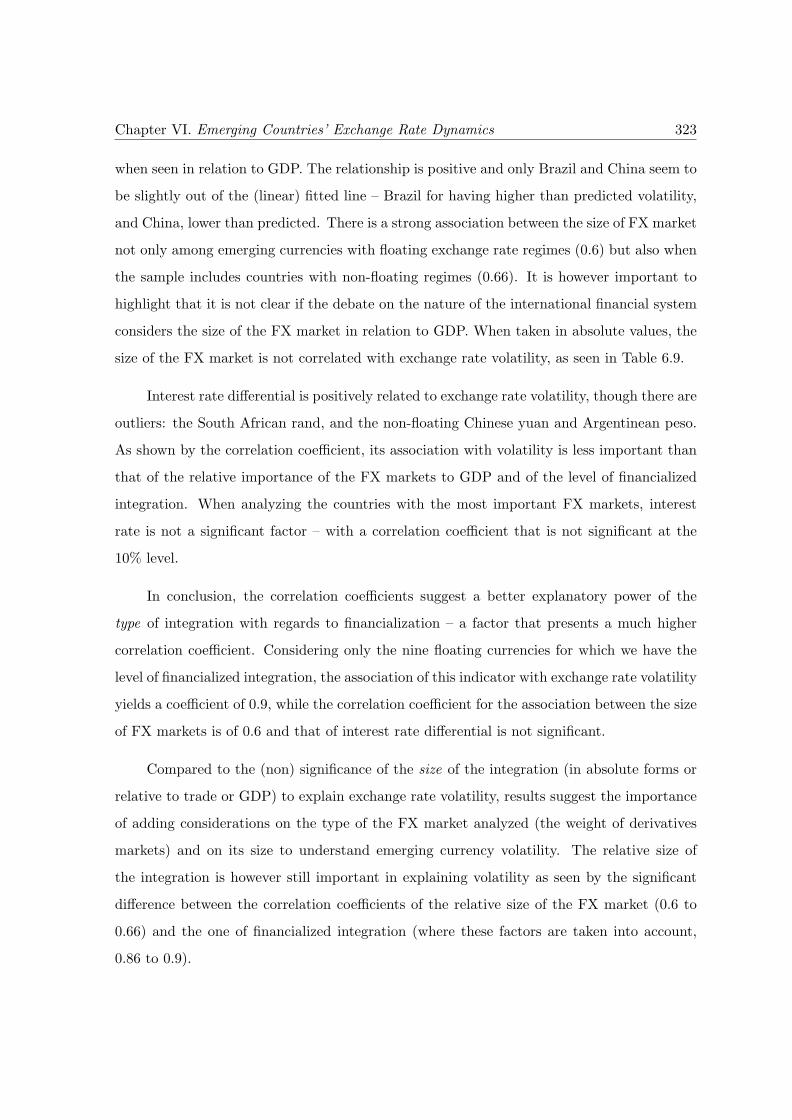
Chapter VI. Emerging Countries’ Exchange Rate Dynamics 323
when seen in relation to GDP. The relationship is positive and only Brazil and China seem to
be slightly out of the (linear) fitted line – Brazil for having higher than predicted volatility,
and China, lower than predicted. There is a strong association between the size of FX market
not only among emerging currencies with floating exchange rate regimes (0.6) but also when
the sample includes countries with non-floating regimes (0.66). It is however important to
highlight that it is not clear if the debate on the nature of the international financial system
considers the size of the FX market in relation to GDP. When taken in absolute values, the
size of the FX market is not correlated with exchange rate volatility, as seen in Table 6.9.
Interest rate differential is positively related to exchange rate volatility, though there are
outliers: the South African rand, and the non-floating Chinese yuan and Argentinean peso.
As shown by the correlation coefficient, its association with volatility is less important than
that of the relative importance of the FX markets to GDP and of the level of financialized
integration. When analyzing the countries with the most important FX markets, interest
rate is not a significant factor – with a correlation coefficient that is not significant at the
10% level.
In conclusion, the correlation coefficients suggest a better explanatory power of the
type of integration with regards to financialization – a factor that presents a much higher
correlation coefficient. Considering only the nine floating currencies for which we have the
level of financialized integration, the association of this indicator with exchange rate volatility
yields a coefficient of 0.9, while the correlation coefficient for the association between the size
of FX markets is of 0.6 and that of interest rate differential is not significant.
Compared to the (non) significance of the size of the integration (in absolute forms or
relative to trade or GDP) to explain exchange rate volatility, results suggest the importance
of adding considerations on the type of the FX market analyzed (the weight of derivatives
markets) and on its size to understand emerging currency volatility. The relative size of
the integration is however still important in explaining volatility as seen by the significant
difference between the correlation coefficients of the relative size of the FX market (0.6 to
0.66) and the one of financialized integration (where these factors are taken into account,
0.86 to 0.9).
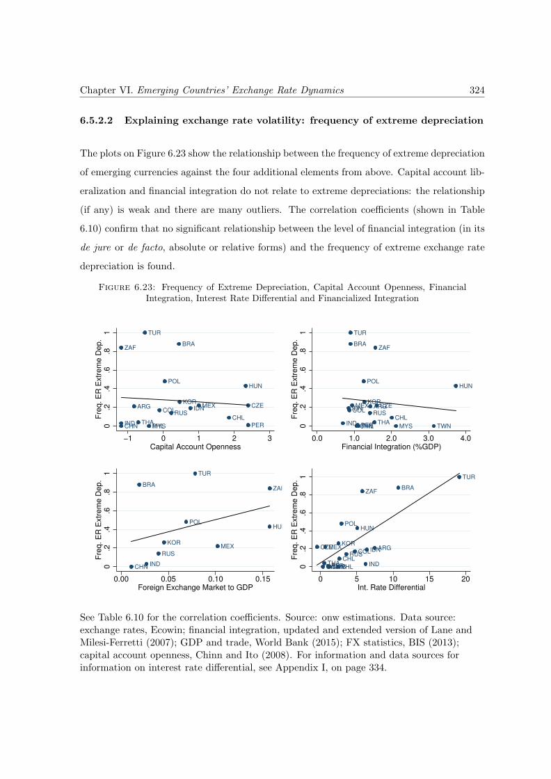
Chapter VI. Emerging Countries’ Exchange Rate Dynamics 324
6.5.2.2 Explaining exchange rate volatility: frequency of extreme depreciation
The plots on Figure 6.23 show the relationship between the frequency of extreme depreciation
of emerging currencies against the four additional elements from above. Capital account lib-
eralization and financial integration do not relate to extreme depreciations: the relationship
(if any) is weak and there are many outliers. The correlation coefficients (shown in Table
6.10) confirm that no significant relationship between the level of financial integration (in its
de jure or de facto, absolute or relative forms) and the frequency of extreme exchange rate
depreciation is found.
Figure 6.23: Frequency of Extreme Depreciation, Capital Account Openness, FinancialIntegration, Interest Rate Differential and Financialized Integration
CZE
THA
MEX
PERCHN MYSPHL
KOR
CHL
POL
RUSCOL
HUN
ZAF
IND
IDNARG
BRA
TUR
0.2
.4.6
.81
Fre
q. E
R E
xtr
em
e D
ep.
−1 0 1 2 3Capital Account Openness
CZE
TWNTHA
MEX
PERCHN MYSPHL
KOR
CHL
POL
RUSCOL
HUN
ZAF
IND
IDN ARG
BRA
TUR
0.2
.4.6
.81
Fre
q. E
R E
xtr
em
e D
ep.
0.0 1.0 2.0 3.0 4.0Financial Integration (%GDP)
MEX
CHN
KOR
POL
RUS
HUN
ZAF
IND
BRA
TUR
0.2
.4.6
.81
Fre
q. E
R E
xtr
em
e D
ep.
0.00 0.05 0.10 0.15Foreign Exchange Market to GDP
CZE
TWNTHA
MEX
PERCHNMYSPHL
KOR
CHL
POL
RUSCOL
HUN
ZAF
IND
IDNARG
BRA
TUR
0.2
.4.6
.81
Fre
q. E
R E
xtr
em
e D
ep.
0 5 10 15 20Int. Rate Differential
See Table 6.10 for the correlation coefficients. Source: onw estimations. Data source:exchange rates, Ecowin; financial integration, updated and extended version of Lane andMilesi-Ferretti (2007); GDP and trade, World Bank (2015); FX statistics, BIS (2013);capital account openness, Chinn and Ito (2008). For information and data sources forinformation on interest rate differential, see Appendix I, on page 334.
Chapter VI. Emerging Countries’ Exchange Rate Dynamics 325
The relative weight of the FX market is loosely related to extreme depreciations and
there are well marked outliers. Observed from the non-significance of the correlation coeffi-
cient, the relative size of FX markets is found to not be an important element – differently
from the analysis of standard deviation.
The interest rate differential impacts extreme depreciations, confirmed by a high corre-
lation coefficient (around 0.7) significant at the 1% level. South Africa is a notable outlier,
with higher depreciations than predicted by other countries’ relationships. India is also an
outlier, because it has lower than predicted depreciations.
The level of financialized integration is the variable capable of explaining the highest
part of the variability of the frequency of extreme depreciations.
6.5.2.3 Explaining exchange rate correlation with the VIX
The explanation power of the additional elements regarding currency correlation with the
VIX (see Figure 6.24) are similar to their power in explaining extreme depreciations: there
is no marked relationship between this exchange rate feature and capital account openness
or financial integration. The latter actually actually presents a negative correlation between
the two, significant at the 10% level (see Table 6.11).
The relationship of the correlation with the VIX and the weight of FX markets is posi-
tive, but not very relevant or with well marked outliers. The correlation coefficients are not
significant. There are several outliers with regards to the interest rate differential, as curren-
cies with very different levels of correlation have rather similar interest rate differentials.
A currency’s correlation with the VIX might be the currency feature that presents
the lowest correlation with the studied explanatory variables. The type of integration is
the only variable with a significative explanation power. However, its power to explain the
international influence on emerging currencies is lower than its power to explain the other
currency features, suggesting that the type of integration explains volatility better than it
explains the weight of the international sphere.
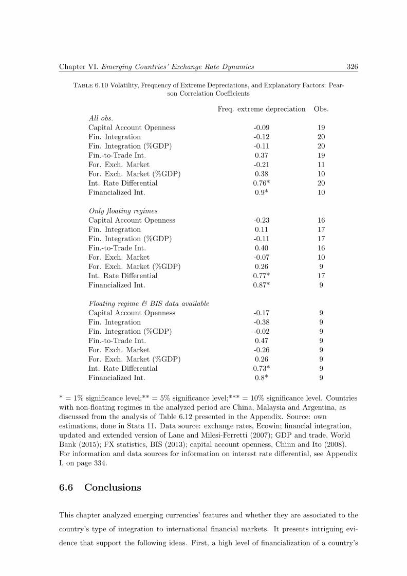
Chapter VI. Emerging Countries’ Exchange Rate Dynamics 326
Table 6.10 Volatility, Frequency of Extreme Depreciations, and Explanatory Factors: Pear-son Correlation Coefficients
Freq. extreme depreciation Obs.All obs.Capital Account Openness -0.09 19Fin. Integration -0.12 20Fin. Integration (%GDP) -0.11 20Fin.-to-Trade Int. 0.37 19For. Exch. Market -0.21 11For. Exch. Market (%GDP) 0.38 10Int. Rate Differential 0.76* 20Financialized Int. 0.9* 10
Only floating regimesCapital Account Openness -0.23 16Fin. Integration 0.11 17Fin. Integration (%GDP) -0.11 17Fin.-to-Trade Int. 0.40 16For. Exch. Market -0.07 10For. Exch. Market (%GDP) 0.26 9Int. Rate Differential 0.77* 17Financialized Int. 0.87* 9
Floating regime & BIS data availableCapital Account Openness -0.17 9Fin. Integration -0.38 9Fin. Integration (%GDP) -0.02 9Fin.-to-Trade Int. 0.47 9For. Exch. Market -0.26 9For. Exch. Market (%GDP) 0.26 9Int. Rate Differential 0.73* 9Financialized Int. 0.8* 9
* = 1% significance level;** = 5% significance level;*** = 10% significance level. Countrieswith non-floating regimes in the analyzed period are China, Malaysia and Argentina, asdiscussed from the analysis of Table 6.12 presented in the Appendix. Source: ownestimations, done in Stata 11. Data source: exchange rates, Ecowin; financial integration,updated and extended version of Lane and Milesi-Ferretti (2007); GDP and trade, WorldBank (2015); FX statistics, BIS (2013); capital account openness, Chinn and Ito (2008).For information and data sources for information on interest rate differential, see AppendixI, on page 334.
6.6 Conclusions
This chapter analyzed emerging currencies’ features and whether they are associated to the
country’s type of integration to international financial markets. It presents intriguing evi-
dence that support the following ideas. First, a high level of financialization of a country’s
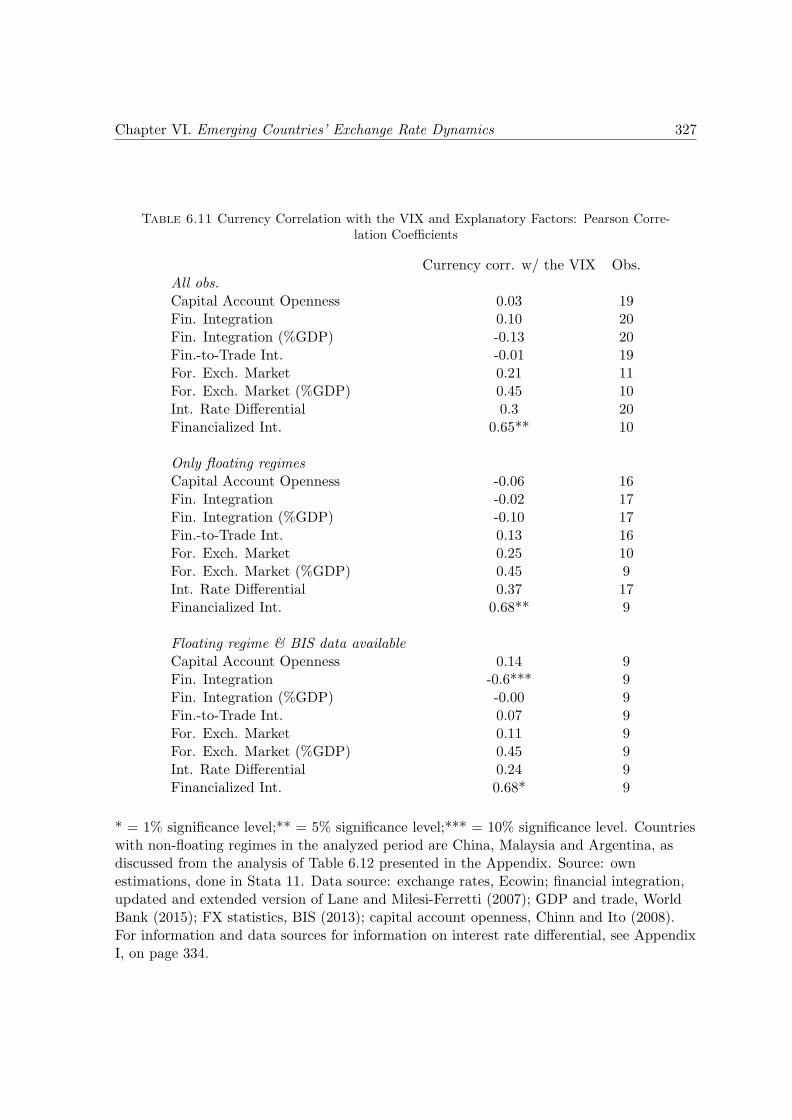
Chapter VI. Emerging Countries’ Exchange Rate Dynamics 327
Table 6.11 Currency Correlation with the VIX and Explanatory Factors: Pearson Corre-lation Coefficients
Currency corr. w/ the VIX Obs.All obs.Capital Account Openness 0.03 19Fin. Integration 0.10 20Fin. Integration (%GDP) -0.13 20Fin.-to-Trade Int. -0.01 19For. Exch. Market 0.21 11For. Exch. Market (%GDP) 0.45 10Int. Rate Differential 0.3 20Financialized Int. 0.65** 10
Only floating regimesCapital Account Openness -0.06 16Fin. Integration -0.02 17Fin. Integration (%GDP) -0.10 17Fin.-to-Trade Int. 0.13 16For. Exch. Market 0.25 10For. Exch. Market (%GDP) 0.45 9Int. Rate Differential 0.37 17Financialized Int. 0.68** 9
Floating regime & BIS data availableCapital Account Openness 0.14 9Fin. Integration -0.6*** 9Fin. Integration (%GDP) -0.00 9Fin.-to-Trade Int. 0.07 9For. Exch. Market 0.11 9For. Exch. Market (%GDP) 0.45 9Int. Rate Differential 0.24 9Financialized Int. 0.68* 9
* = 1% significance level;** = 5% significance level;*** = 10% significance level. Countrieswith non-floating regimes in the analyzed period are China, Malaysia and Argentina, asdiscussed from the analysis of Table 6.12 presented in the Appendix. Source: ownestimations, done in Stata 11. Data source: exchange rates, Ecowin; financial integration,updated and extended version of Lane and Milesi-Ferretti (2007); GDP and trade, WorldBank (2015); FX statistics, BIS (2013); capital account openness, Chinn and Ito (2008).For information and data sources for information on interest rate differential, see AppendixI, on page 334.
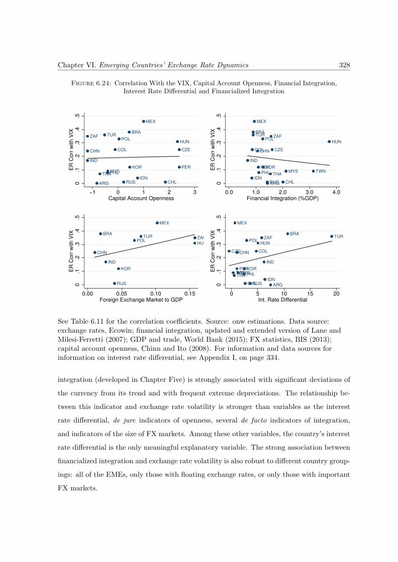
Chapter VI. Emerging Countries’ Exchange Rate Dynamics 328
Figure 6.24: Correlation With the VIX, Capital Account Openness, Financial Integration,Interest Rate Differential and Financialized Integration
CZE
THA
MEX
PER
CHN
MYSPHL
KOR
CHL
POL
RUS
COL
HUN
ZAF
IND
IDN
ARG
BRATUR
0.1
.2.3
.4.5
ER
Corr
with V
IX
−1 0 1 2 3Capital Account Openness
CZE
TWNTHA
MEX
PER
CHN
MYSPHL
KOR
CHL
POL
RUS
COL
HUN
ZAF
IND
IDN
ARG
BRATUR
0.1
.2.3
.4.5
ER
Corr
with V
IX
0.0 1.0 2.0 3.0 4.0Financial Integration (%GDP)
MEX
CHN
KOR
POL
RUS
HUN
ZAF
IND
BRATUR
0.1
.2.3
.4.5
ER
Corr
with V
IX
0.00 0.05 0.10 0.15Foreign Exchange Market to GDP
CZE
TWNTHA
MEX
PER
CHN
MYSPHL
KOR
CHL
POL
RUS
COL
HUN
ZAF
IND
IDN
ARG
BRATUR
0.1
.2.3
.4.5
ER
Corr
with V
IX
0 5 10 15 20Int. Rate Differential
See Table 6.11 for the correlation coefficients. Source: onw estimations. Data source:exchange rates, Ecowin; financial integration, updated and extended version of Lane andMilesi-Ferretti (2007); GDP and trade, World Bank (2015); FX statistics, BIS (2013);capital account openness, Chinn and Ito (2008). For information and data sources forinformation on interest rate differential, see Appendix I, on page 334.
integration (developed in Chapter Five) is strongly associated with significant deviations of
the currency from its trend and with frequent extreme depreciations. The relationship be-
tween this indicator and exchange rate volatility is stronger than variables as the interest
rate differential, de jure indicators of openness, several de facto indicators of integration,
and indicators of the size of FX markets. Among these other variables, the country’s interest
rate differential is the only meaningful explanatory variable. The strong association between
financialized integration and exchange rate volatility is also robust to different country group-
ings: all of the EMEs, only those with floating exchange rates, or only those with important
FX markets.
Chapter VI. Emerging Countries’ Exchange Rate Dynamics 329
The most volatile currencies (as proxied by the standard deviation) are the Brazilian
real, the Hungarian forint, the Polish zloty, the South African rand, and the Turkish lira.
These five, plus the Mexican peso, present the highest frequency of extreme depreciations.
The countries of these six currencies present the most financialized integration (especially
Brazil, Hungary, South Africa, and Turkey).
Secondly, EMEs with a more financialized integration have currencies which are more
correlated with international liquidity conditions – the six more financialized currencies also
present the highest correlation with the VIX. The interest rate differential is also a relevant
variable in explaining the correlation with the VIX, but the level of financialization of its
integration has a higher explanatory power.
Thirdly, floating emerging currencies have been presenting an increasingly similar path;
the aforementioned six countries with more financialized integration have presented a strik-
ingly similar path in the turbulent (most recent) period. These six currencies also present
the highest number of relevant out-of-the-region correlation (correlation with currencies of
other continents).
The comparison of the correlation coefficients of the indicators of the level of financial-
ization of integration with other indicators demonstrate that the type of integration has a
better explanatory power than the size of integration. This is partially opposed to Eichen-
green and Gupta’s (2015) argument on the importance of the magnitude of integration (the
countries’ financial markets size and openness) in determining the impact of ‘tapering talks’
on emerging currencies. On the other hand, it would be in line with Kaltenbrunner and
Painceira’s (2014) hypothesis that the vulnerability of the Brazilian real to international
sphere is due to the country’s “particularly liquid domestic financial markets and advanced
stage of financial integration, which resulted in one of the highest stocks of short-term exter-
nal obligations” (p. 18) – where “advanced” seems to refer not only to the magnitude, but
also to the type of integration, as it is related to extent of use of the country’s “complex set
of very short-term domestic currency assets” (p. 1).
These findings raise important theoretical- and policy-related concerns, and point to
interesting avenues of future research. Regarding the theoretical debate, the evidence of
comovement of currencies indicate a high influence of external factors in determining these
Chapter VI. Emerging Countries’ Exchange Rate Dynamics 330
currencies. Their high correlation with the VIX indicates one possible external factor: the
condition of international financial markets. Such an exchange rate determination seems at
odds with the mainstream theories (see Chapter Three). In mainstream models, the impact of
the international scenario is limited to interest rate differentials, which is a measure of return,
not of uncertainty. Rey (2015) could be said to be an exception, as she argues that global
financial cycles are crucial in determining the exchange rate of countries receiving credit
inflows. However, she uses a different transmission channel, focused on bank constraints that
would vary with changes in risk aversion due to monetary policy changes in a given country63.
However, major exchange rate changes, as those related to the Lehman Brothers’ collapse
or the Euro crisis, are not associated with changes in monetary policies; they are purely
a change of uncertainty levels, intrinsic to financial markets dynamics. In this sense, the
chapter indicates the role of external conditions, rather than country fundamentals, what,
for the case of the GFC, is in line with Kaltenbrunner and Painceira (2014).
The importance of liquidity preference in determining investments in low-liquid curren-
cies (as seen in Chapter Three, Section 3.3.4 and the theory of liquidity cycles) are the most
appropriate theoretical background for these findings. They explain both the comovement
of currencies (as they all have the same characteristic), the correlation with the VIX (that
proxies liquidity preference) and the high frequency of depreciations (due to turbulence of
international financial markets and liquidity preference).
With regards to the pull-vs-push literature, evidence on the high importance of exter-
nal factors in determining exchange rates (comovement among currencies and with the VIX)
supports the idea that pull factors are important in tranquil periods but push factors pre-
dominate in turbulent ones. In addition, the correlation of some emerging currencies with
the VIX supports the view that the importance of push factors is related to the conditions
of international financial markets.
With regards to the literature on the implications of financial integration, the compar-
ison of the importance of the explanation power of level of financialized integration to the
indicators of financial openness and integration, and the size of FX markets revealed the
63Rey (2015, p. 25) states that “one important determinant of the global financial cycle is monetary policyin the centre country, which affects leverage of global banks, credit flows and credit growth in the internationalfinancial system.”
Chapter VI. Emerging Countries’ Exchange Rate Dynamics 331
higher relevance of the first indicator in explaining exchange rate features. It underscores
the relevance of the characteristics or type of a country’s integration instead of its magnitude
in determining emerging currency patterns, especially the ones related to the FX markets.
Given the continuous rise of financialization, these results indicate the need to study the
economic impacts of more volatile exchange rates that frequently undergo sudden changes,
and that reflect the international rather than the domestic context. The emergence and
the consequences of a new pattern of emerging currencies is disregarded by the literature
on the potential impacts of financial integration, because it focuses on the magnitude of
the integration, which is not associated with a given exchange rate pattern (as shown in
Section 6.5). This chapter’s findings indicate valuable considerations for future research,
such as considerations on the type of integration in the literature on the effect of financial
integration through the potential impacts of a new type of exchange rate determination on
growth.
The expected impacts from financial integration in terms of gains from diversification
and risk reduction must also be questioned: if, as portfolio diversification achieves several
countries, their exchange rates start moving in tandem, potential diversification-related gains
vanish. Indeed, international diversification of equity portfolios was first advocated on the ba-
sis of low correlation between markets (Longin and Solnik, 1995), but as integration growths,
correlation increases, and the possible gains from diversification are lost64.
Regarding the literature on exchange rates, the findings on the characteristics of the
emerging currencies with a highly financialized integration support the argument that ex-
change rates no longer serve as an adjustment variable, but rather as an asset price deter-
mined by portfolio diversification (as discussed in Chapter Three). How the decisions on
portfolio diversification take place, especially regarding EMEs’ assets and the role played by
the external environment, is the subject of the next chapter.
The confirmation that emerging currencies are asset prices opens a large spectrum of
exchange rate analyses with techniques that are currently mostly used in financial market
studies. The analyses of comovement of currencies and their comovement with the VIX are a
64There is sizable literature on the financial area that looks at the stability of the correlation matrix ofreturns in different markets and finds that it has not been stable over time. See Longin and Solnik (1995).
Chapter VI. Emerging Countries’ Exchange Rate Dynamics 332
step in this direction. Other analyses include spill over and contagion effects, and asymmetric
or regime-based effects, and advanced techniques for estimating risk and volatility.
Comparing volatility of different time-frames, such as intra-day or monthly changes, on
the characterization of volatility of exchange rates of EMEs’ and advanced countries is an
intriguing possibility for future research. Intra-day volatility might be more important in
places with higher speculation possibilities65. Monthly changes, on the other hand, are inter-
esting for analyses investigating the impact of changes in the exchange rate on uncertainty
and on domestic economy.
Still on avenues for future research, the findings on the consequences of a more finan-
cialized integration on exchange rates invites analysis to uncover explanations for this type
of integration. The relevance of derivatives markets is observed from the different explana-
tory power of the index of financialized integration and the indices of relative integration.
But what determines the size of FX markets and its characteristics? Interest rate levels are
surely an option. As Table 6.15 demonstrates, out of the five currencies that present specific
features in the strongest of forms, four presented high interest rate differentials with the U.S.
rate (Poland presented a medium level).
As discussed in Chapter Two, financial innovations explain the association of high in-
terest rates and large FX markets (of derivatives, in particular). The broad use of carry
trade operations has a clear role in increasing flows to countries with the highest interest
rate levels. This results in appreciation of the target currencies, an incentive for currency
trading – trading the currency itself and gaining from its appreciation. Derivatives markets,
in turn, grow by allowing such operations (carry trading and currency trading) to be realized
with considerably lower amounts, for its leveraging possibilities.
The fact that all five countries with the most financialized integration follow an inflation
targeting regime with a floating exchange rate arrangement raises concern over these coun-
tries’ independence in pursuit of monetary policies. The findings also suggest consequences
to the very use of inflation targeting regimes in EMEs, that must be further studied. If this
65An example where the daily change does not capture the volatility: On May 9th, with the possibility ofcanceling the impeachment process of Brazil’s President, Mrs Rouseff, the Brazilian real depreciated 0.56%,but during the day it achieved a depreciation higher than 5% (Castro, 2016).
Chapter VI. Emerging Countries’ Exchange Rate Dynamics 333
regime is associated with exchange rates that often face extreme depreciations, the impacts
of such depreciations reduce the efficiency of the policy in these countries.
After having presented the macro picture of financialized integration and how it is
related to specific exchange rate features, the next chapter will provide a micro view of
how these features might emerge from money managers’ decisions. Based on this chapter’s
findings on the role of the conditions ruling in international financial markets in determining
exchange rates, the units whose decisions will be analyzed are the money managers. This is
also in line with the idea of interconnection of markets through money managers’ balance-
sheets.
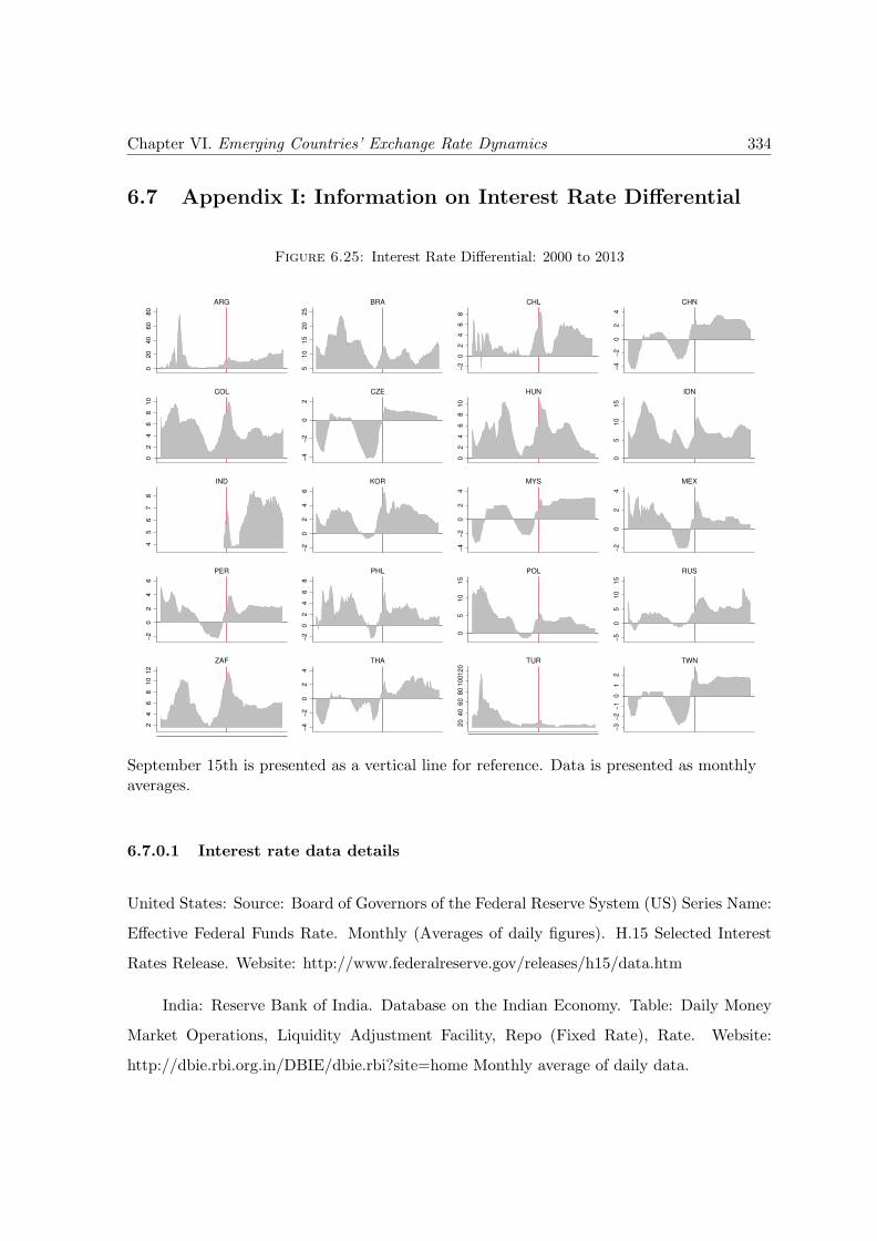
Chapter VI. Emerging Countries’ Exchange Rate Dynamics 334
6.7 Appendix I: Information on Interest Rate Differential
Figure 6.25: Interest Rate Differential: 2000 to 2013
02
04
06
08
0
ARG5
10
15
20
25
BRA
−2
02
46
8
CHL
−4
−2
02
4
CHN
02
46
81
0
COL
−4
−2
02
CZE
02
46
81
0
HUN
05
10
15
IDN
45
67
8
IND
−2
02
46
KOR
−4
−2
02
4
MYS
−2
02
4
MEX
−2
02
46
PER
−2
02
46
8
PHL
05
10
15
POL
−5
05
10
15
RUS
24
68
10
12
ZAF
−4
−2
02
4
THA
20
40
60
80
10
01
20
TUR
−3
−2
−1
01
2
TWN
September 15th is presented as a vertical line for reference. Data is presented as monthlyaverages.
6.7.0.1 Interest rate data details
United States: Source: Board of Governors of the Federal Reserve System (US) Series Name:
Effective Federal Funds Rate. Monthly (Averages of daily figures). H.15 Selected Interest
Rates Release. Website: http://www.federalreserve.gov/releases/h15/data.htm
India: Reserve Bank of India. Database on the Indian Economy. Table: Daily Money
Market Operations, Liquidity Adjustment Facility, Repo (Fixed Rate), Rate. Website:
http://dbie.rbi.org.in/DBIE/dbie.rbi?site=home Monthly average of daily data.
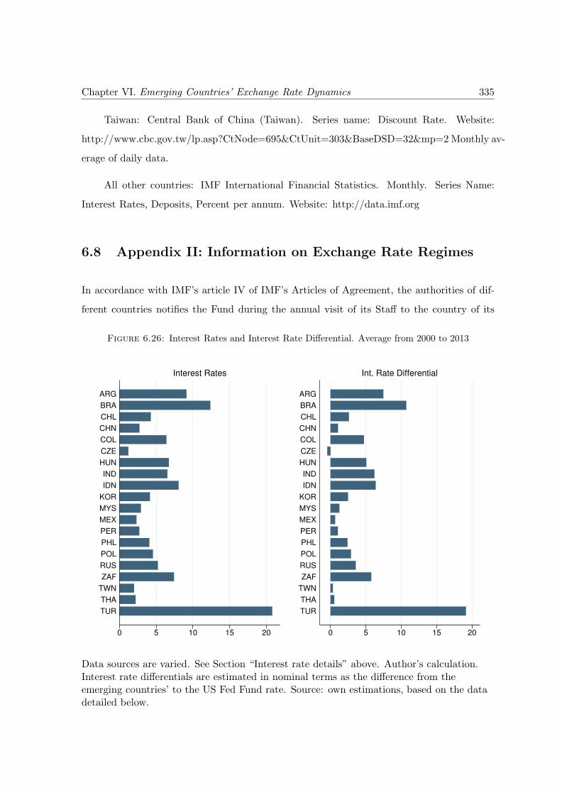
Chapter VI. Emerging Countries’ Exchange Rate Dynamics 335
Taiwan: Central Bank of China (Taiwan). Series name: Discount Rate. Website:
http://www.cbc.gov.tw/lp.asp?CtNode=695&CtUnit=303&BaseDSD=32&mp=2Monthly av-
erage of daily data.
All other countries: IMF International Financial Statistics. Monthly. Series Name:
Interest Rates, Deposits, Percent per annum. Website: http://data.imf.org
6.8 Appendix II: Information on Exchange Rate Regimes
In accordance with IMF’s article IV of IMF’s Articles of Agreement, the authorities of dif-
ferent countries notifies the Fund during the annual visit of its Staff to the country of its
Figure 6.26: Interest Rates and Interest Rate Differential. Average from 2000 to 2013
0 5 10 15 20
TUR
THA
TWN
ZAF
RUS
POL
PHL
PER
MEX
MYS
KOR
IDN
IND
HUN
CZE
COL
CHN
CHL
BRA
ARG
Interest Rates
0 5 10 15 20
TUR
THA
TWN
ZAF
RUS
POL
PHL
PER
MEX
MYS
KOR
IDN
IND
HUN
CZE
COL
CHN
CHL
BRA
ARG
Int. Rate Differential
Data sources are varied. See Section “Interest rate details” above. Author’s calculation.Interest rate differentials are estimated in nominal terms as the difference from theemerging countries’ to the US Fed Fund rate. Source: own estimations, based on the datadetailed below.
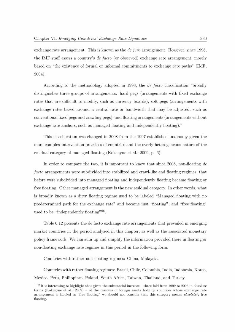
Chapter VI. Emerging Countries’ Exchange Rate Dynamics 336
exchange rate arrangement. This is known as the de jure arrangement. However, since 1998,
the IMF staff assess a country’s de facto (or observed) exchange rate arrangement, mostly
based on “the existence of formal or informal commitments to exchange rate paths” (IMF,
2004).
According to the methodology adopted in 1998, the de facto classification “broadly
distinguishes three groups of arrangements: hard pegs (arrangements with fixed exchange
rates that are difficult to modify, such as currency boards), soft pegs (arrangements with
exchange rates based around a central rate or bandwidth that may be adjusted, such as
conventional fixed pegs and crawling pegs), and floating arrangements (arrangements without
exchange rate anchors, such as managed floating and independently floating).”
This classification was changed in 2008 from the 1997-established taxonomy given the
more complex intervention practices of countries and the overly heterogeneous nature of the
residual category of managed floating (Kokenyne et al., 2009, p. 6).
In order to compare the two, it is important to know that since 2008, non-floating de
facto arrangements were subdivided into stabilized and crawl-like and floating regimes, that
before were subdivided into managed floating and independently floating became floating or
free floating. Other managed arrangement is the new residual category. In other words, what
is broadly known as a dirty floating regime used to be labeled “Managed floating with no
predetermined path for the exchange rate” and became just “floating”; and “free floating”
used to be “independently floating”66.
Table 6.12 presents the de facto exchange rate arrangements that prevailed in emerging
market countries in the period analyzed in this chapter, as well as the associated monetary
policy framework. We can sum up and simplify the information provided there in floating or
non-floating exchange rate regimes in this period in the following form.
Countries with rather non-floating regimes: China, Malaysia.
Countries with rather floating regimes: Brazil, Chile, Colombia, India, Indonesia, Korea,
Mexico, Peru, Philippines, Poland, South Africa, Taiwan, Thailand, and Turkey.
66It is interesting to highlight that given the substantial increase – three-fold from 1999 to 2006 in absoluteterms (Kokenyne et al., 2009) – of the reserves of foreign assets hold by countries whose exchange ratearrangement is labeled as “free floating” we should not consider that this category means absolutely freefloating.
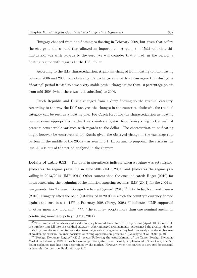
Chapter VI. Emerging Countries’ Exchange Rate Dynamics 337
Hungary changed from non-floating to floating in February 2008, but given that before
the change it had a band that allowed an important fluctuation (+- 15%) and that this
fluctuation was with regards to the euro, we will consider that it had, in the period, a
floating regime with regards to the U.S. dollar.
According to the IMF characterization, Argentina changed from floating to non-floating
between 2006 and 2008, but observing it’s exchange rate path we can argue that during its
“floating” period it used to have a very stable path – changing less than 10 percentage points
from mid-2003 (when there was a devaluation) to 2006.
Czech Republic and Russia changed from a dirty floating to the residual category.
According to the way the IMF analyzes the changes in the countries’ choices67, the residual
category can be seen as a floating one. For Czech Republic the characterization as floating
regime seems appropriated fr this thesis analysis: given the currency’s peg to the euro, it
presents considerable variance with regards to the dollar. The characterization as floating
might however be controversial for Russia given the observed change in the exchange rate
pattern in the middle of the 2000s – as seen in 6.1. Important to pinpoint: the crisis in the
late 2014 is out of the period analyzed in the chapter.
Details of Table 6.12: The data in parenthesis indicate when a regime was established.
†indicates the regime prevailing in June 2004 (IMF, 2004) and ‡indicates the regime pre-
vailing in 2013/2014 (IMF, 2014) Other sources than the ones indicated: Roger (2010) for
dates concerning the beginning of the inflation targeting regimes; IMF (2004) for the 2004 ar-
rangements. For Taiwan: “Foreign Exchange Regime” (2015)68. For India, Nam and Kumar
(2015). Hungary lifted the band (established in 2001) in which the country’s currency floated
against the euro in a +- 15% in February 2008 (Perry, 2008) ** indicates “IMF-supported
or other monetary program”. ***, “the country adopts more than one nominal anchor in
conducting monetary policy” (IMF, 2014).
67“The number of countries that used a soft peg bounced back almost to its previous (April 2011) level whilethe number that fell into the residual category other managed arrangements experienced the greatest decline.In short, countries returned to more stable exchange rate arrangements they had previously abandoned becauseof weakening external balance positions or strong appreciation pressure.” (Kokenyne et al., 2009, p. 2)
68“Foreign Exchange Regime” (2015) reads:“Following the establishment of the Taipei Foreign ExchangeMarket in February 1979, a flexible exchange rate system was formally implemented. Since then, the NTdollar exchange rate has been determined by the market. However, when the market is disrupted by seasonalor irregular factors, the Bank will step in.”
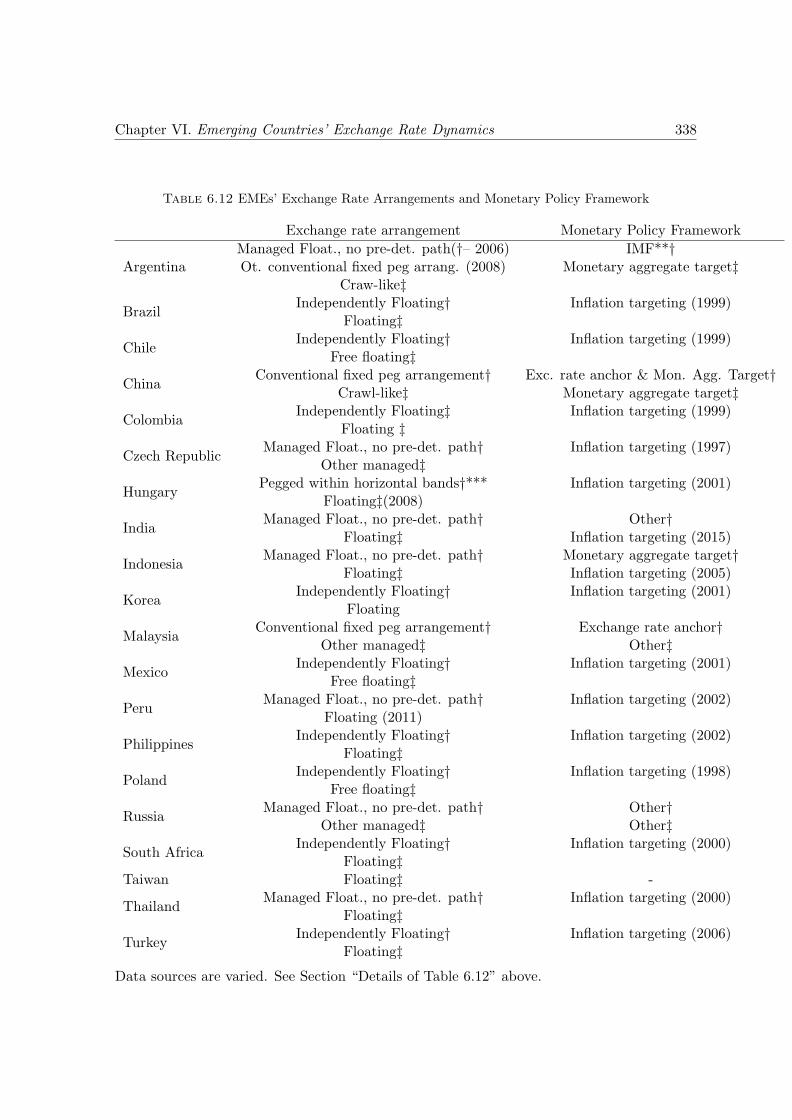
Chapter VI. Emerging Countries’ Exchange Rate Dynamics 338
Table 6.12 EMEs’ Exchange Rate Arrangements and Monetary Policy Framework
Exchange rate arrangement Monetary Policy Framework
ArgentinaManaged Float., no pre-det. path(†– 2006) IMF**†Ot. conventional fixed peg arrang. (2008) Monetary aggregate target‡
Craw-like‡
BrazilIndependently Floating† Inflation targeting (1999)
Floating‡
ChileIndependently Floating† Inflation targeting (1999)
Free floating‡
ChinaConventional fixed peg arrangement† Exc. rate anchor & Mon. Agg. Target†
Crawl-like‡ Monetary aggregate target‡
ColombiaIndependently Floating‡ Inflation targeting (1999)
Floating ‡
Czech RepublicManaged Float., no pre-det. path† Inflation targeting (1997)
Other managed‡
HungaryPegged within horizontal bands†*** Inflation targeting (2001)
Floating‡(2008)
IndiaManaged Float., no pre-det. path† Other†
Floating‡ Inflation targeting (2015)
IndonesiaManaged Float., no pre-det. path† Monetary aggregate target†
Floating‡ Inflation targeting (2005)
KoreaIndependently Floating† Inflation targeting (2001)
Floating
MalaysiaConventional fixed peg arrangement† Exchange rate anchor†
Other managed‡ Other‡
MexicoIndependently Floating† Inflation targeting (2001)
Free floating‡
PeruManaged Float., no pre-det. path† Inflation targeting (2002)
Floating (2011)
PhilippinesIndependently Floating† Inflation targeting (2002)
Floating‡
PolandIndependently Floating† Inflation targeting (1998)
Free floating‡
RussiaManaged Float., no pre-det. path† Other†
Other managed‡ Other‡
South AfricaIndependently Floating† Inflation targeting (2000)
Floating‡Taiwan Floating‡ -
ThailandManaged Float., no pre-det. path† Inflation targeting (2000)
Floating‡
TurkeyIndependently Floating† Inflation targeting (2006)
Floating‡
Data sources are varied. See Section “Details of Table 6.12” above.
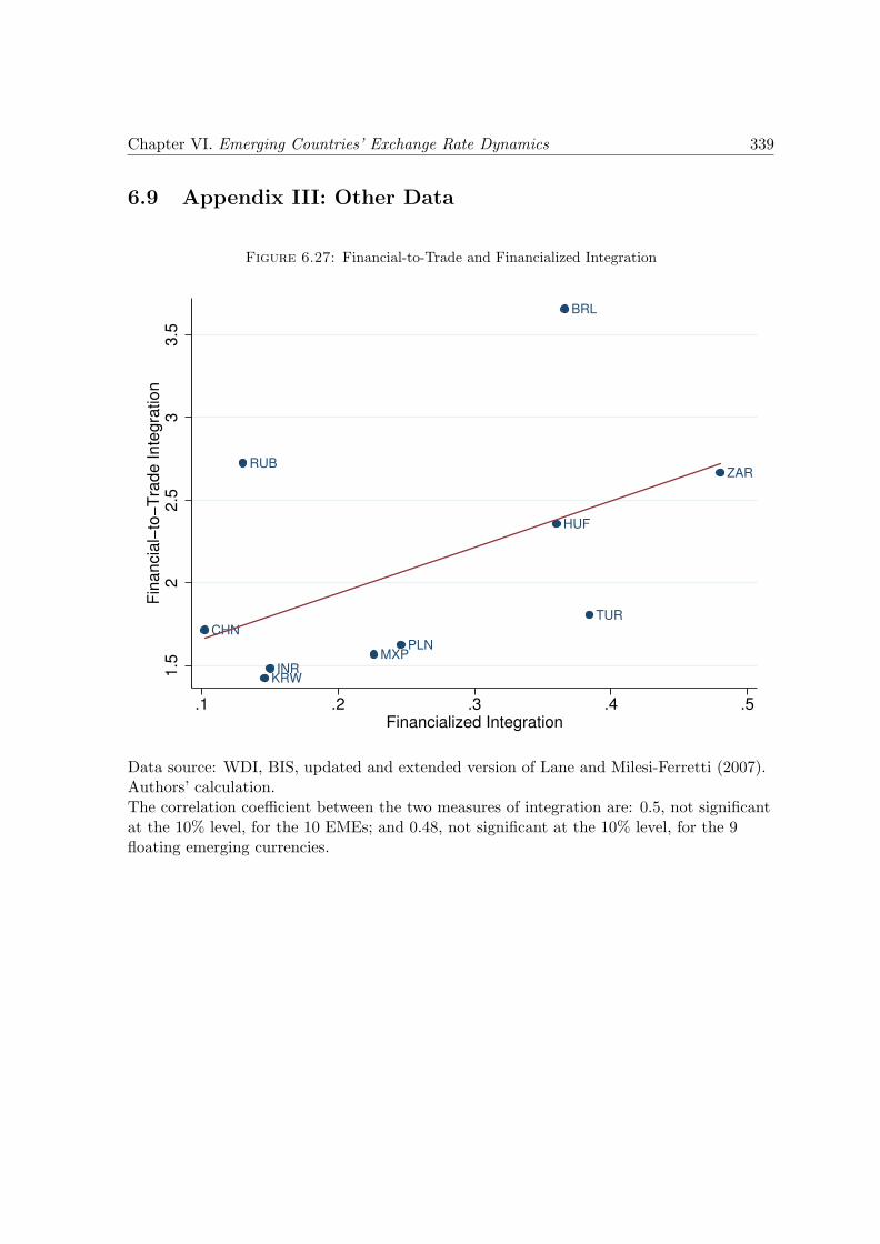
Chapter VI. Emerging Countries’ Exchange Rate Dynamics 339
6.9 Appendix III: Other Data
Figure 6.27: Financial-to-Trade and Financialized Integration
BRL
CHN
HUF
INRKRW
MXPPLN
RUB
TUR
ZAR
1.5
22
.53
3.5
Fin
an
cia
l−to
−T
rad
e I
nte
gra
tio
n
.1 .2 .3 .4 .5Financialized Integration
Data source: WDI, BIS, updated and extended version of Lane and Milesi-Ferretti (2007).Authors’ calculation.The correlation coefficient between the two measures of integration are: 0.5, not significantat the 10% level, for the 10 EMEs; and 0.48, not significant at the 10% level, for the 9floating emerging currencies.
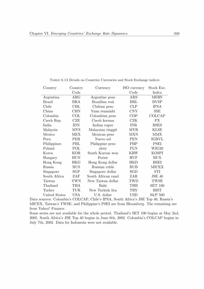
Chapter VI. Emerging Countries’ Exchange Rate Dynamics 340
Table 6.13 Details on Countries Currencies and Stock Exchange indices
Country Country Currency ISO currency Stock Exc.Code Code Index
Argentina ARG Argentine peso ARS MERVBrazil BRA Brazilian real BRL BVSPChile CHL Chilean peso CLP IPSAChina CHN Yuan renminbi CNY SSEColombia COL Colombian peso COP COLCAPCzech Rep. CZE Czech koruna CZK PXIndia IDN Indian rupee INR BSESMalaysia MYS Malaysian ringgit MYR KLSEMexico MEX Mexican peso MXN MMXPeru PER Nuevo sol PEN IGBVLPhilippines PHL Philippine peso PHP PSEIPoland POL zloty PLN WIG20Korea KOR South Korean won KRW KOSPIHungary HUN Forint HUF BUXHong Kong HKG Hong Kong dollar HKD HSEIRussia RUS Russian ruble RUB MICEXSingapore SGP Singapore dollar SGD STISouth Africa ZAF South African rand ZAR JSE 40Taiwan TWN New Taiwan dollar TWD TWSEThailand THA Baht THB SET 100Turkey TUR New Turkish lira TRY BISTUnited States USA U.S. dollar USD S&P 500
Data sources: Colombia’s COLCAP, Chile’s IPSA, South Africa’s JSE Top 40, Russia’sMICEX, Taiwan’s TWSE, and Philippine’s PSEI are from Bloomberg. The remaining arefrom Yahoo! Finance.Some series are not available for the whole period. Thailand’s SET 100 begins at May 2nd,2005. South Africa’s JSE Top 40 begins in June 6th, 2002. Colombia’s COLCAP begins inJuly 7th, 2002. Data for Indonesia were not available.
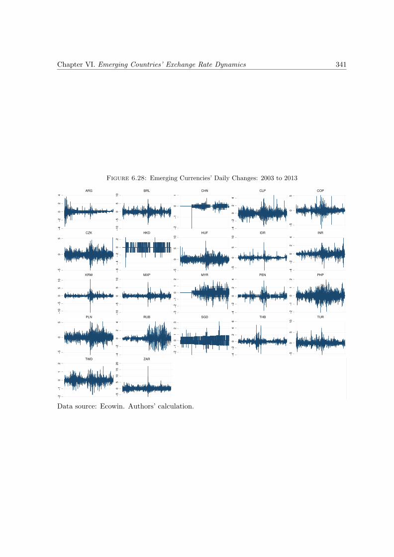
Chapter VI. Emerging Countries’ Exchange Rate Dynamics 341
Figure 6.28: Emerging Currencies’ Daily Changes: 2003 to 2013
−4
−2
02
4
ARG
−1
0−
50
51
0
BRL
−2
−1
01
CHN
−4
−2
02
4
CLP
−5
05
COP
−5
05
CZK
−.6
−.4
−.2
0.2
HKD
−5
05
10
HUF−
50
51
0IDR
−4
−2
02
4
INR
−1
0−
50
51
0
KRW
−1
0−
50
51
0
MXP
−3
−2
−1
01
2
MYR
−4
−2
02
4
PEN
−2
−1
01
2
PHP
−5
05
PLN
−4
−2
02
4
RUB
−2
−1
01
23
SGD
−4
−2
02
46
THB
−5
05
10
TUR
−2
−1
01
2
TWD
−5
05
10
15
20
ZAR
Data source: Ecowin. Authors’ calculation.
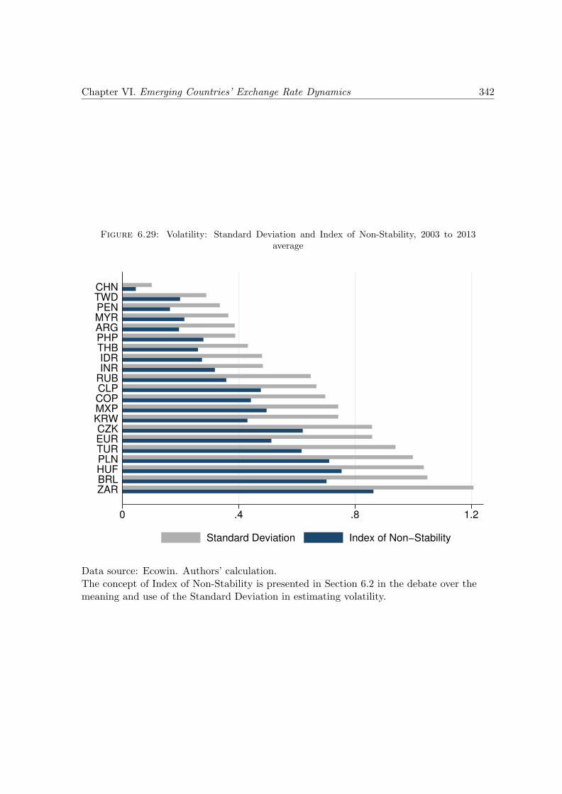
Chapter VI. Emerging Countries’ Exchange Rate Dynamics 342
Figure 6.29: Volatility: Standard Deviation and Index of Non-Stability, 2003 to 2013average
0 .4 .8 1.2
ZARBRLHUFPLNTUREURCZK
KRWMXPCOPCLPRUBINRIDRTHBPHPARGMYRPENTWDCHN
Standard Deviation Index of Non−Stability
Data source: Ecowin. Authors’ calculation.The concept of Index of Non-Stability is presented in Section 6.2 in the debate over themeaning and use of the Standard Deviation in estimating volatility.
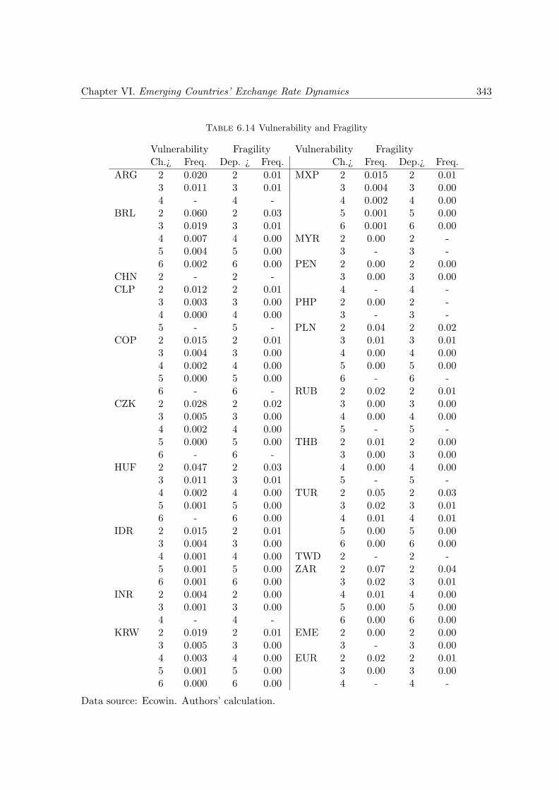
Chapter VI. Emerging Countries’ Exchange Rate Dynamics 343
Table 6.14 Vulnerability and Fragility
Vulnerability Fragility Vulnerability FragilityCh.¿ Freq. Dep. ¿ Freq. Ch.¿ Freq. Dep.¿ Freq.
ARG 2 0.020 2 0.01 MXP 2 0.015 2 0.013 0.011 3 0.01 3 0.004 3 0.004 - 4 - 4 0.002 4 0.00
BRL 2 0.060 2 0.03 5 0.001 5 0.003 0.019 3 0.01 6 0.001 6 0.004 0.007 4 0.00 MYR 2 0.00 2 -5 0.004 5 0.00 3 - 3 -6 0.002 6 0.00 PEN 2 0.00 2 0.00
CHN 2 - 2 - 3 0.00 3 0.00CLP 2 0.012 2 0.01 4 - 4 -
3 0.003 3 0.00 PHP 2 0.00 2 -4 0.000 4 0.00 3 - 3 -5 - 5 - PLN 2 0.04 2 0.02
COP 2 0.015 2 0.01 3 0.01 3 0.013 0.004 3 0.00 4 0.00 4 0.004 0.002 4 0.00 5 0.00 5 0.005 0.000 5 0.00 6 - 6 -6 - 6 - RUB 2 0.02 2 0.01
CZK 2 0.028 2 0.02 3 0.00 3 0.003 0.005 3 0.00 4 0.00 4 0.004 0.002 4 0.00 5 - 5 -5 0.000 5 0.00 THB 2 0.01 2 0.006 - 6 - 3 0.00 3 0.00
HUF 2 0.047 2 0.03 4 0.00 4 0.003 0.011 3 0.01 5 - 5 -4 0.002 4 0.00 TUR 2 0.05 2 0.035 0.001 5 0.00 3 0.02 3 0.016 - 6 0.00 4 0.01 4 0.01
IDR 2 0.015 2 0.01 5 0.00 5 0.003 0.004 3 0.00 6 0.00 6 0.004 0.001 4 0.00 TWD 2 - 2 -5 0.001 5 0.00 ZAR 2 0.07 2 0.046 0.001 6 0.00 3 0.02 3 0.01
INR 2 0.004 2 0.00 4 0.01 4 0.003 0.001 3 0.00 5 0.00 5 0.004 - 4 - 6 0.00 6 0.00
KRW 2 0.019 2 0.01 EME 2 0.00 2 0.003 0.005 3 0.00 3 - 3 0.004 0.003 4 0.00 EUR 2 0.02 2 0.015 0.001 5 0.00 3 0.00 3 0.006 0.000 6 0.00 4 - 4 -
Data source: Ecowin. Authors’ calculation.
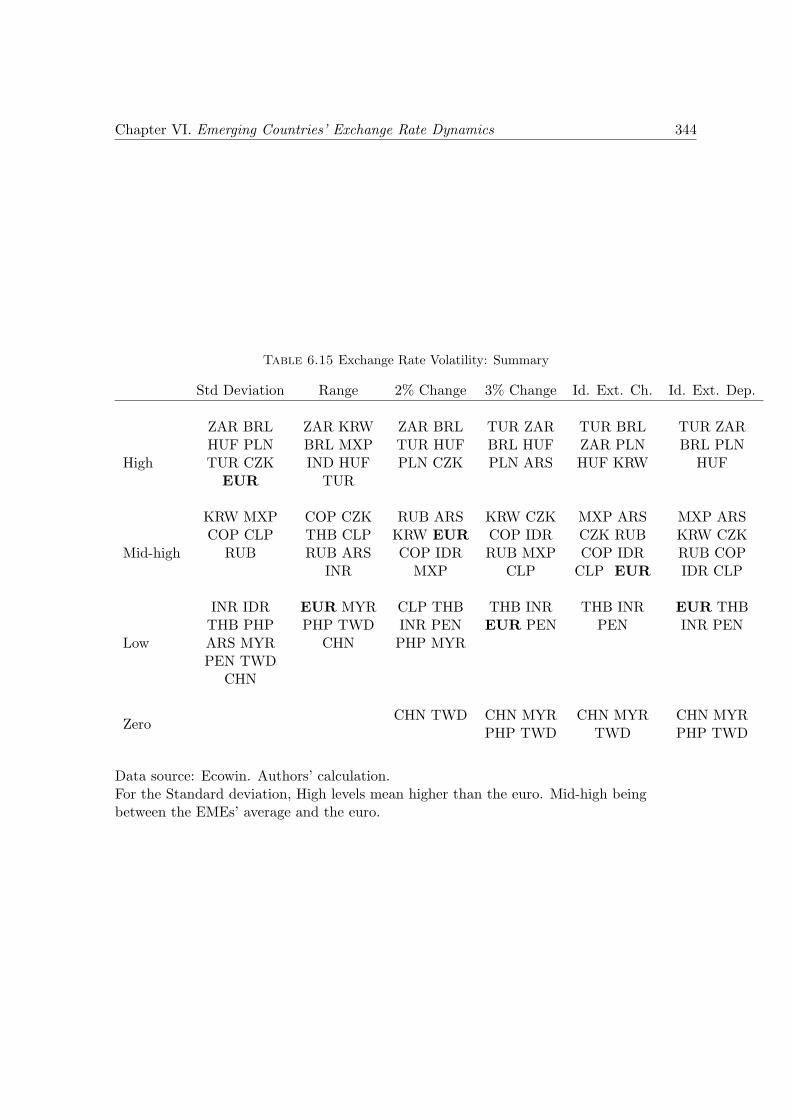
Chapter VI. Emerging Countries’ Exchange Rate Dynamics 344
Table 6.15 Exchange Rate Volatility: Summary
Std Deviation Range 2% Change 3% Change Id. Ext. Ch. Id. Ext. Dep.
High
ZAR BRL ZAR KRW ZAR BRL TUR ZAR TUR BRL TUR ZARHUF PLN BRL MXP TUR HUF BRL HUF ZAR PLN BRL PLNTUR CZK IND HUF PLN CZK PLN ARS HUF KRW HUF
EUR TUR
Mid-high
KRW MXP COP CZK RUB ARS KRW CZK MXP ARS MXP ARSCOP CLP THB CLP KRW EUR COP IDR CZK RUB KRW CZK
RUB RUB ARS COP IDR RUB MXP COP IDR RUB COPINR MXP CLP CLP EUR IDR CLP
Low
INR IDR EUR MYR CLP THB THB INR THB INR EUR THBTHB PHP PHP TWD INR PEN EUR PEN PEN INR PENARS MYR CHN PHP MYRPEN TWD
CHN
ZeroCHN TWD CHN MYR CHN MYR CHN MYR
PHP TWD TWD PHP TWD
Data source: Ecowin. Authors’ calculation.For the Standard deviation, High levels mean higher than the euro. Mid-high beingbetween the EMEs’ average and the euro.
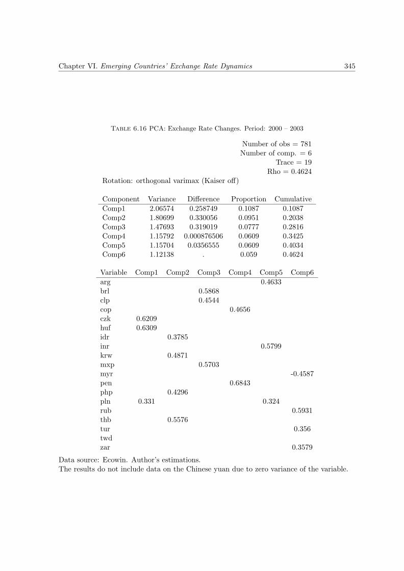
Chapter VI. Emerging Countries’ Exchange Rate Dynamics 345
Table 6.16 PCA: Exchange Rate Changes. Period: 2000 – 2003
Number of obs = 781Number of comp. = 6
Trace = 19Rho = 0.4624
Rotation: orthogonal varimax (Kaiser off)
Component Variance Difference Proportion Cumulative
Comp1 2.06574 0.258749 0.1087 0.1087Comp2 1.80699 0.330056 0.0951 0.2038Comp3 1.47693 0.319019 0.0777 0.2816Comp4 1.15792 0.000876506 0.0609 0.3425Comp5 1.15704 0.0356555 0.0609 0.4034Comp6 1.12138 . 0.059 0.4624
Variable Comp1 Comp2 Comp3 Comp4 Comp5 Comp6
arg 0.4633brl 0.5868clp 0.4544cop 0.4656czk 0.6209huf 0.6309idr 0.3785inr 0.5799krw 0.4871mxp 0.5703myr -0.4587pen 0.6843php 0.4296pln 0.331 0.324rub 0.5931thb 0.5576tur 0.356twdzar 0.3579
Data source: Ecowin. Author’s estimations.The results do not include data on the Chinese yuan due to zero variance of the variable.
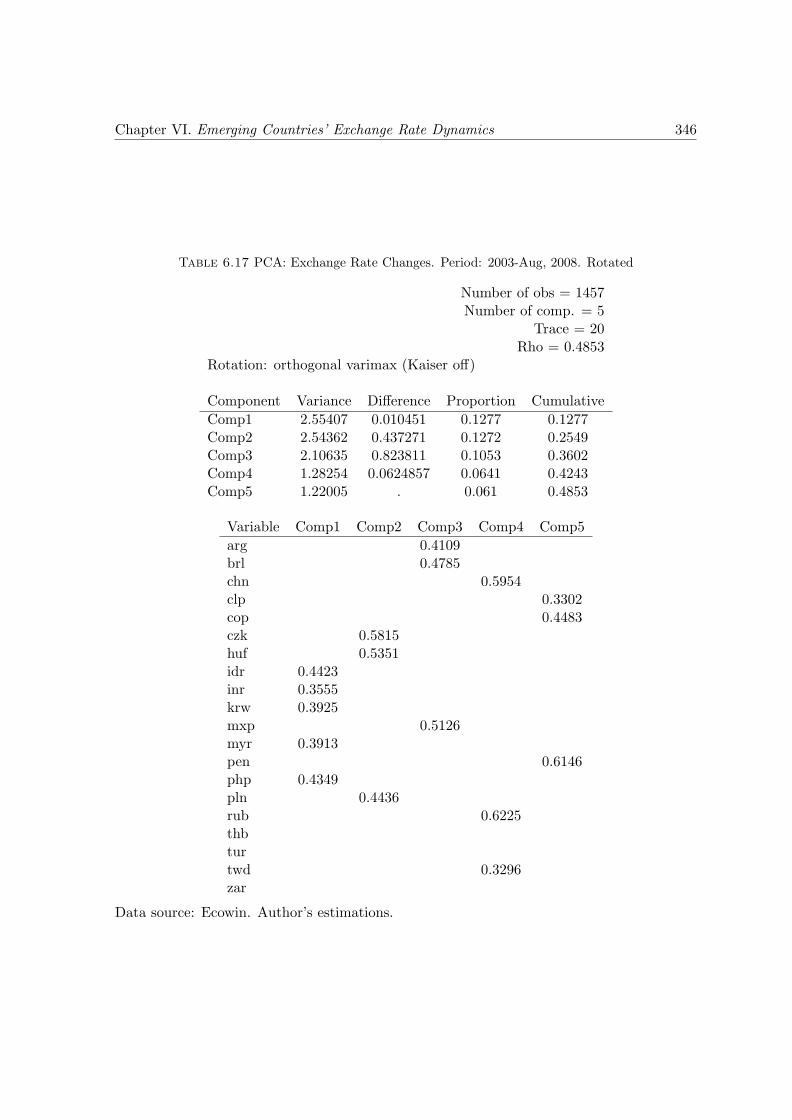
Chapter VI. Emerging Countries’ Exchange Rate Dynamics 346
Table 6.17 PCA: Exchange Rate Changes. Period: 2003-Aug, 2008. Rotated
Number of obs = 1457Number of comp. = 5
Trace = 20Rho = 0.4853
Rotation: orthogonal varimax (Kaiser off)
Component Variance Difference Proportion Cumulative
Comp1 2.55407 0.010451 0.1277 0.1277Comp2 2.54362 0.437271 0.1272 0.2549Comp3 2.10635 0.823811 0.1053 0.3602Comp4 1.28254 0.0624857 0.0641 0.4243Comp5 1.22005 . 0.061 0.4853
Variable Comp1 Comp2 Comp3 Comp4 Comp5
arg 0.4109brl 0.4785chn 0.5954clp 0.3302cop 0.4483czk 0.5815huf 0.5351idr 0.4423inr 0.3555krw 0.3925mxp 0.5126myr 0.3913pen 0.6146php 0.4349pln 0.4436rub 0.6225thbturtwd 0.3296zar
Data source: Ecowin. Author’s estimations.
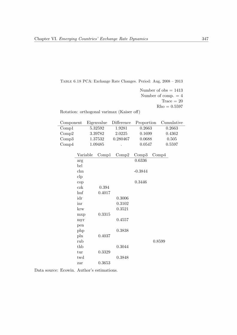
Chapter VI. Emerging Countries’ Exchange Rate Dynamics 347
Table 6.18 PCA: Exchange Rate Changes. Period: Aug, 2008 – 2013
Number of obs = 1413Number of comp. = 4
Trace = 20Rho = 0.5597
Rotation: orthogonal varimax (Kaiser off)
Component Eigenvalue Difference Proportion Cumulative
Comp1 5.32592 1.9281 0.2663 0.2663Comp2 3.39782 2.0225 0.1699 0.4362Comp3 1.37532 0.280467 0.0688 0.505Comp4 1.09485 . 0.0547 0.5597
Variable Comp1 Comp2 Comp3 Comp4
arg 0.6336brlchn -0.3844clpcop 0.3446czk 0.394huf 0.4017idr 0.3006inr 0.3102krw 0.3521mxp 0.3315myr 0.4557penphp 0.3838pln 0.4037rub 0.8599thb 0.3044tur 0.3329twd 0.3848zar 0.3653
Data source: Ecowin. Author’s estimations.
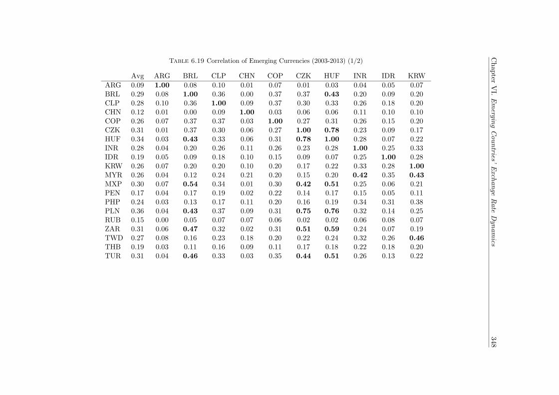
Chap
terVI.Emergin
gCountries’
Exch
ange
Rate
Dyn
amics
348Table 6.19 Correlation of Emerging Currencies (2003-2013) (1/2)
Avg ARG BRL CLP CHN COP CZK HUF INR IDR KRW
ARG 0.09 1.00 0.08 0.10 0.01 0.07 0.01 0.03 0.04 0.05 0.07BRL 0.29 0.08 1.00 0.36 0.00 0.37 0.37 0.43 0.20 0.09 0.20CLP 0.28 0.10 0.36 1.00 0.09 0.37 0.30 0.33 0.26 0.18 0.20CHN 0.12 0.01 0.00 0.09 1.00 0.03 0.06 0.06 0.11 0.10 0.10COP 0.26 0.07 0.37 0.37 0.03 1.00 0.27 0.31 0.26 0.15 0.20CZK 0.31 0.01 0.37 0.30 0.06 0.27 1.00 0.78 0.23 0.09 0.17HUF 0.34 0.03 0.43 0.33 0.06 0.31 0.78 1.00 0.28 0.07 0.22INR 0.28 0.04 0.20 0.26 0.11 0.26 0.23 0.28 1.00 0.25 0.33IDR 0.19 0.05 0.09 0.18 0.10 0.15 0.09 0.07 0.25 1.00 0.28KRW 0.26 0.07 0.20 0.20 0.10 0.20 0.17 0.22 0.33 0.28 1.00MYR 0.26 0.04 0.12 0.24 0.21 0.20 0.15 0.20 0.42 0.35 0.43MXP 0.30 0.07 0.54 0.34 0.01 0.30 0.42 0.51 0.25 0.06 0.21PEN 0.17 0.04 0.17 0.19 0.02 0.22 0.14 0.17 0.15 0.05 0.11PHP 0.24 0.03 0.13 0.17 0.11 0.20 0.16 0.19 0.34 0.31 0.38PLN 0.36 0.04 0.43 0.37 0.09 0.31 0.75 0.76 0.32 0.14 0.25RUB 0.15 0.00 0.05 0.07 0.07 0.06 0.02 0.02 0.06 0.08 0.07ZAR 0.31 0.06 0.47 0.32 0.02 0.31 0.51 0.59 0.24 0.07 0.19TWD 0.27 0.08 0.16 0.23 0.18 0.20 0.22 0.24 0.32 0.26 0.46THB 0.19 0.03 0.11 0.16 0.09 0.11 0.17 0.18 0.22 0.18 0.20TUR 0.31 0.04 0.46 0.33 0.03 0.35 0.44 0.51 0.26 0.13 0.22
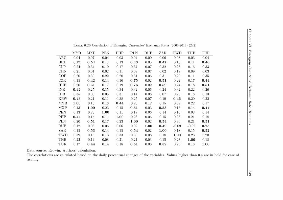
Chap
terVI.Emergin
gCountries’
Exch
ange
Rate
Dyn
amics
349
Table 6.20 Correlation of Emerging Currencies’ Exchange Rates (2003-2013) (2/2)
MYR MXP PEN PHP PLN RUB ZAR TWD THB TUR
ARG 0.04 0.07 0.04 0.03 0.04 0.00 0.06 0.08 0.03 0.04BRL 0.12 0.54 0.17 0.13 0.43 0.05 0.47 0.16 0.11 0.46CLP 0.24 0.34 0.19 0.17 0.37 0.07 0.32 0.23 0.16 0.33CHN 0.21 0.01 0.02 0.11 0.09 0.07 0.02 0.18 0.09 0.03COP 0.20 0.30 0.22 0.20 0.31 0.06 0.31 0.20 0.11 0.35CZK 0.15 0.42 0.14 0.16 0.75 0.02 0.51 0.22 0.17 0.44HUF 0.20 0.51 0.17 0.19 0.76 0.02 0.59 0.24 0.18 0.51INR 0.42 0.25 0.15 0.34 0.32 0.06 0.24 0.32 0.22 0.26IDR 0.35 0.06 0.05 0.31 0.14 0.08 0.07 0.26 0.18 0.13KRW 0.43 0.21 0.11 0.38 0.25 0.07 0.19 0.46 0.20 0.22MYR 1.00 0.13 0.13 0.44 0.20 0.12 0.15 0.39 0.22 0.17MXP 0.13 1.00 0.23 0.15 0.51 0.03 0.53 0.16 0.14 0.44PEN 0.13 0.23 1.00 0.11 0.17 0.06 0.14 0.13 0.08 0.14PHP 0.44 0.15 0.11 1.00 0.23 0.06 0.15 0.33 0.21 0.18PLN 0.20 0.51 0.17 0.23 1.00 0.02 0.54 0.30 0.21 0.51RUB 0.12 0.03 0.06 0.06 0.02 1.00 0.49 -0.09 -0.02 0.75ZAR 0.15 0.53 0.14 0.15 0.54 0.02 1.00 0.18 0.15 0.52TWD 0.39 0.16 0.13 0.33 0.30 0.08 0.18 1.00 0.23 0.20THB 0.22 0.14 0.08 0.21 0.21 0.03 0.15 0.23 1.00 0.18TUR 0.17 0.44 0.14 0.18 0.51 0.03 0.52 0.20 0.18 1.00
Data source: Ecowin. Authors’ calculation.The correlations are calculated based on the daily percentual changes of the variables. Values higher than 0.4 are in bold for ease ofreading.
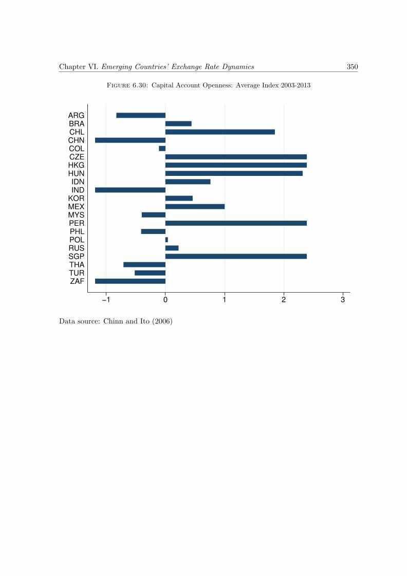
Chapter VI. Emerging Countries’ Exchange Rate Dynamics 350
Figure 6.30: Capital Account Openness: Average Index 2003-2013
−1 0 1 2 3
ZAFTURTHASGPRUSPOLPHLPERMYSMEXKORINDIDN
HUNHKGCZECOLCHNCHLBRAARG
Data source: Chinn and Ito (2006)
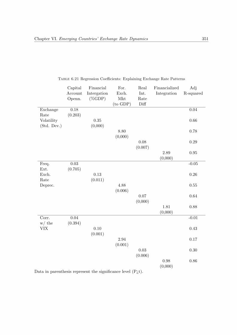
Chapter VI. Emerging Countries’ Exchange Rate Dynamics 351
Table 6.21 Regression Coefficients: Explaining Exchange Rate Patterns
Capital Financial For. Real Financialized AdjAccount Intergation Exch. Int. Integration R-squaredOpenn. (%GDP) Mkt Rate
(to GDP) Diff
Exchange 0.18 0.04Rate (0.203)Volatility 0.35 0.66(Std. Dev.) (0,000)
8.80 0.78(0,000)
0.08 0.29(0.007)
2.89 0.95(0,000)
Freq. 0.03 -0.05Ext. (0.705)Exch. 0.13 0.26Rate (0.011)Deprec. 4.88 0.55
(0.006)0.07 0.64
(0,000)1.81 0.88
(0,000)
Corr. 0.04 -0.01w/ the (0.394)VIX 0.10 0.43
(0.001)2.94 0.17
(0.001)0.03 0.30
(0.006)0.98 0.86
(0,000)Data in parenthesis represent the significance level (P¿t).
Chapter 7
The Fragility of Emerging
Countries’ Exchange Rates Since
the 2000s: a Minskyan Analysis
The exchange rates of a group of emerging market economies (EMEs) have undergone syn-
chronized exchange rate dynamics, characterized by an important appreciation from 2003
to the Global Financial Crisis (GFC) and significant volatility and extreme depreciations in
moments of turbulence in international financial markets. The literature on financialization
argues that with the changes of finance at the international level, exchange rate dynamics
would not be different than that of a financial assets’ price. Heterodox exchange-rate lit-
erature considers some financialization-related innovations. Schulmeister explains the role
of FX traders and their (technical) trading strategies, that results in alternating upwards
and downward trends. Harvey explains investors’ decision-making process under our current
financial convention: it is mostly dependent on the forecast exchange rate that fluctuates
according to the expected changing demand of foreign portfolio investors. Through these
analyses the general characteristics of FX markets is explained: they are marked by ups and
downs determined by portfolio investors expectations.
The behavior of exchange rates of EMEs (emerging currencies) is however, more specific.
As seen in the last chapter, a part of these currencies have been following ups and downs
352
Chapter VII. Exchange Rate Fragility 353
whose alternation is more related to the international financial scenario than the countries’
specific context, and were marked, since 2003, by a long-lasting cycle followed by extreme
changes. Studies of the specific attributes of emerging currencies provide a better account
for their dynamics than the mentioned heterodox approaches by demonstrating how their
attributes explain the changing demand according to the international scenario1.
This chapter proposes an analysis that takes those attributes into account, using a
framework focused on money managers’ decisions and their balance-sheet constraints. Given
the relevance of these investors’ balance-sheets in interconnecting asset markets across ad-
vanced countries and EMEs, the analysis of their decisions results in a description of the
mechanisms determining emerging currencies’ fragility.
The Minskyan framework is chosen for the analysis for three main reasons. First, be-
cause the centrality of balance-sheets in the framework is in line with the role of money
managers’ balance-sheets in times of financialization in interconnecting markets, which de-
termines exchange rates, as argued in Chapter Two. The dynamics of the liabilities side of
balance-sheets are a well known part of Minsky’s analyses due to the role of their ability to
repay debt. However, the core of Minsky’s analysis is on the interactions of liabilities with
assets, which is the basis of the definition of margins of safety, that are based on income
inflows (from the companies’ activities and financial inflows) and debt repayment. Assets’
dynamics are also important in the transmission of crisis given the relevance of a decrease of
inflows due to bankruptcy of a firm in another one.
By focusing on both assets and liabilities, the Minskyan framework allows two essential
attributes of emerging currencies respectively related to money managers’ assets and liabili-
ties to be taken into account: the non use of emerging currencies as reserve of value nor as
denominator of financial contracts internationally, discussed in Chapter Three.
Secondly, Minsky’s framework sheds light on the dynamics of the expansionary phase
of the cycle, the moment when fragility is built. In Tymoigne and Wray’s (2013) words: “in
the Minskyan framework, the most relevant instability is upward” (p. 2). With this focus,
1The dynamics that emerge from emerging currencies attributes was detailed in Chapters Three and Five,and will be briefly mentioned in this chapter.
Chapter VII. Exchange Rate Fragility 354
Minsky’s analysis explains not only exchange rate depreciation, but also its previous appre-
ciation. Although both might be equally undesirable2, crisis episodes receive substantially
more attention on the economic literature.
Thirdly, Minsky’s framework is explicit on interactions among different agents. As
shown in Chapter Three, the heterogeneity of agents is crucial for understanding exchange
rates ups and downs. Heterogeneous agents are a main feature of the most recent main-
stream models, as well as of most exchange-rates heterodox models, but they are not yet
contemplated by the models that deal with the specificities of emerging currencies.
The structure of the chapter Following this introduction, Section 7.1 analyzes Minsky’s
financial instability hypothesis and its use in contexts other than its original one. Section
7.2 suggests how to transpose Minsky’s framework to open economies and money managers’
portfolio allocation decision, allowing the study of the demand for EMEs’ assets. Section 7.3
concludes.
7.1 The Financial Instability Hypothesis
As “a post-Keynesian institutionalist”, Minsky has always provided great attention to the
institutional structure in which his analyses were inserted (Wolfson, 2002, p. 398). In the
financial instability hypothesis, the institutional background is very specific: “a capital-
ist economy with expensive capital assets and a complex, sophisticated financial system”
(Minsky, 1992)3. As production must be financed, capitalist economies are characterized
by a system of borrowing and lending based upon ‘margins of safety’ (Minsky, 1993) – the
‘cushions’ between the cash commitments and the prospective cash receipts involved in the
investment decision (Kregel, 2008). According to the desired margins of safety each firm
(or, more generally, an economic unit) will have a combination of cash inflows and outflows,
which is at the heart of Minsky’s famous hedge, speculative and Ponzi characterization.
2The negative impacts of exchange rate ‘misalignment’ are presented in the Introduction.3The importance of financial conditions in explaining crises is not exclusive to Minsky and is found in
other heterodox authors’ works. See Guttmann et al. (2015) for a review.
Chapter VII. Exchange Rate Fragility 355
The taxonomy of cash flows Hedge is the name given to units whose “flow of funds that
result from the normal functioning of the assets it owns (...) are sufficient to fulfill current and
future expected payment commitments due to liabilities” (Minsky, 1993, p. 80). Speculative
units, on the other hand, are those that “expect the cash flows (...) to be less than the cash
payment commitments in some, typically near-term, periods” (Minsky, 1986, p. 230). A
Ponzi unit “is similar to a speculative financing unit in that, for some near-term periods, the
cash payment commitments exceed the expected cash receipts on account of owned assets”
and not even the interests on debt can be paid (Minsky, 1986, p. 231), demanding new debt
to be issued (Minsky, 1993). A common and simple way Minsky’s characterization is used is:
hedge, when expected inflows cover outflows; speculative, when inflows cover at least interest
payments; and Ponzi when neither the debt nor interests can be paid based on the expected
inflows.
Although this “taxonomy of cash flows” (Minsky, 1986, p. 223) is customary, Minsky
(1993) offers us a broader way of looking at the types of units. For being an enlarged form of
seeing his framework, Minsky (1993) broadens the potential use of his framework to different
contexts. A main point is that speculative and Ponzi are differentiated from hedge units for
having an additional “element of uncertainty in financial relations” (Minsky, 1993, p. 80,
italics added), creating a dependency on future market conditions –“the market terms that
rule at the refunding date”. This additional element impacts speculative and Ponzi units
but not hedge units: “speculative- and Ponzi-financing units have to meet changing financial
market conditions, whereas a hedge unit will be impervious to such changes” (Minsky, 1986,
p. 231). Both speculative and Ponzi depend on future conditions and the differentiation
between them is subtle: margins of safety are shrinked in the case of Ponzi, putting these
units in a worst situation when financial conditions are not as good as expected.
The two theorems After differentiating the units, Minsky (1993) uses the typology to
compose the financial instability hypothesis, divided into two theorems. The first theorem
defines the fragility of the economic system based on the relative presence of each type of
unit:
If hedge finance dominates, then the economy may well be an equilibrium seek-
ing and containing system. In contrast, the greater the weight of speculative
Chapter VII. Exchange Rate Fragility 356
and Ponzi finance, the greater the likelihood that the economy is a deviation
amplifying system. (p. 8)
The fragility of an economy is also determined by the institutions in place and by their ability
to increase liquidity when needed. In Minsky’s (1993, p. 81) words, fragility also depend
on i) “the willingness and the ability of the authorities to refinance units at concessionary
terms”; and ii) on “the in-place power of the authorities to sustain aggregate profits (cash
flows to business) and aggregate wages (...)”4.
The second theorem of the financial instability hypothesis is the increase of fragility over
periods of prolonged prosperity (Minsky, 1992). Alternatively, as put by Minsky (1993):
over a run of good times the structure of units among hedge, speculative and
Ponzi financing changes, so that the weight of hedge financing decreases and the
weight of speculative and Ponzi financing increases. (p. 8)
The evolution of Ponzi units results from the choice of margins of safety being somewhat
dependent on the stability of the economic environment: in a run of good times, expecta-
tions are constantly being confirmed, leading units to reassess their prior decisions as too
conservative and to reduce margins of safety. As summarized by Papadimitriou and Wray
(1998):
It is precisely the apparent ‘stability’ that generates changes of expectations that
leads to the adoption of financial positions that cannot be validated should events
prove to be less favorable than expected – that is, the transformation from robust
(hedge) arrangements to fragile (speculative) positions5. (p. 213)
In a nutshell, given profit-seeking behavior and evolving expectations, tranquility will
motivate units to lower margins of safety moving the economy to a more fragile situation.
4Minsky (1992) indirectly references the importance of Big Bank and Big Government, the institutionsresponsible for the fact that Managerial Capitalism “did not exhibit the serious recessions and depressionsof Finance Capitalism”, the precedent phase on the author’s characterization (Minsky, 1990, p. 23). It isinteresting to highlight that Minsky’s analysis of financial instability cannot be dissociated from his work onthe four stages of the development of capitalism in the United States. See Chapter Two, page 18.
5It is interesting to note that this change in expectations will not only affect productive units, but alsopartner institutions responsible for providing credit. In Minsky’s (1993) words, “during a period dominatedby hedge financing, the structure of financing terms and the performance of markets and institutions thattrade in assets and refinance debts lead profit -seeking clients of banks and markets and the operators ofbanks and the operators in markets to substitute debt for equities and short-term debts for long-term debts”(p. 81).
Chapter VII. Exchange Rate Fragility 357
From a fragile situation a crisis can be triggered by any ‘not-unusual’ shock, or ‘not-abnormal’
event (Minsky, 1993, p. 81).
The role of the ‘not-unusual’ shock The emphasis on the shock being ‘not-unusual’ is
meaningful: it is an event that can occur at any time, but that only leads to a crisis because
the system is in a fragile situation when hit. As a consequence, the crisis is endogenous: it
only occurs because the economy is fragile, and fragility is endogenously built. In Arestis
and Glickman’s (2002) words: “the reasons why a ‘shocking’ event can actually have the
power to shock are emphatically endogenous” (p. 241). What is key is that the build-up
of fragility that allowed the event to be shocking, is endogenous, although the event itself
might be exogenous. Minsky et al. (1982) also considers possibilities in which the unfolding
of the crisis is completely endogenous6.
The spread of the crisis When the ‘not-unusual’ surprise happens, speculative units
are pushed into Ponzi, and hedge units can be pushed into speculative. These speculative
positions are then pushed into Ponzi for a variety of reasons: “the terms on which finance is
available become less favorable, (...) some expectations are revised, income flows that had
been expected are not forthcoming, and so on” (Papadimitriou and Wray, 1998, p. 14). This
spiral is such that “the net worth of Ponzi units will quickly evaporate” and units recur to
“selling positions to make positions” (Minsky, 1992, p. 8), but when “everybody is a seller”,
asset prices collapse, worsening the situation further (Kregel, 2004, p. 577).
7.1.1 Minsky’s Framework Applied to an International Context
Although created with a focus on the fragility of an economy based on the behavior of firms,
the financial instability hypothesis has also been used in other contexts. While most of the
6The most important example of endogenous shock is the evolution of interest rates:“The upper turningpoint is completely endogenous once it is accepted that interest rates rise in an investment boom and thatthe successful functioning of the economy induces profit-seeking bankers and their customers to engage inspeculative financial arrangements and to economize on holdings of money and protected assets” (Minskyet al., 1982, 33). The evolution of other variables can also trigger a crisis in a completely endogenousmanner: “A break in the boom occurs whenever short- and long-term interest rates rise enough so thatattenuation and reversals in present-value relations take place. Often this occurs after the increase in demandfinanced by speculative finance has raised interest rates, wages of labor, and prices of material so that profitmargins and thus the ability to validate the past are eroded” (Minsky, 1986, p. 245).
Chapter VII. Exchange Rate Fragility 358
‘new’ analyses focus on cash inflows and maintain debt-related cash commitments, some
studies keep the focus on inflows and outflows without necessarily relating them to debt.
Minsky himself has used his typology referring to units as other than firms, especially to
analyze the banking system. Minsky (1992) cites as examples of speculative units “govern-
ments with floating debt, corporations with floating issues of commercial paper, and banks”;
Minsky (1993) mentions the United States as a Ponzi unit for having borrowed to pay the in-
terest on outstanding debt; and Minsky (1986, p. 230) classifies units such as New York City
and Brazil as Ponzi. However, it was after the exchange-rate crises in developing countries
in the late 1990s that the enlarged versions of Minsky’s framework increased considerably,
being often applied to a context of international economies where countries are the units of
interest.
These analyses highlight that Minsky’s theories are implicitly targeted at financial crisis
in closed economies (Dymski, 1999), which led Arestis and Glickman (2002) to argue that
Minsky’s work “predates the current era of financial liberalization”. Indeed, regardless of
Minsky’s extensive analyzes of ‘Money Manager capitalism’ and of the late 1980’s currency
attacks, it cannot be said that open economies were the focus of his work. However, the
enlargement of Minsky’s theory to open economies is a logical evolution given the current
context of liberalization and free capital mobility, where “the global economy can be consid-
ered as a closed system of capitalist systems” (Wolfson, 2002)7.
But how can Minsky’s original framework be transposed to the analysis of other con-
texts? The methodology used in most of the literature consists of examining a situation
from ‘the lenses of Minsky’s framework’. More precisely, these studies identify how the most
important Minskyan elements8 manifest in the new context and which elements must be
added9.
7Also see Kregel (2016).8Wolfson (2002, p. 393) prefers the term “main themes of Minsky’s (...) theory”.9In some of these studies, index of fragility are constructed.Finally, it should be mentioned that part of the literature enlarging Minsky’s framework include analysis
based on indeces of fragility. De Paula and Alves Jr (2000), analyzing the effect of changes in the units’attitude in the balance of payments propose an index of external financial fragility based on a country’s mainBOP elements where current and potential foreign currency liabilities are compared to the country’s paymentcapacity. The idea is that this index would indicate a potential need to resort to international capitals marketto renegotiate outstanding financial positions. Schroeder (2002) proposes to track the evolution of fragility inThailand during the 1990s based on an index that results from the transposition of a firm’s balance-sheet toa national economy. The main elements taken into account are the rate of increase of profits, interest ratesand growth, resulting in a hedge, a speculative or a Ponzi profile.
Chapter VII. Exchange Rate Fragility 359
The remainder of the section reviews the use of Minsky’s framework in other contexts,
specifically by identifying how key elements of the original analysis translate to an open-
economy context. The key Minskyan elements identified are: the taxonomy of units according
to their margins of safety; the confirmation of expectations; the interconnection among units;
the ‘not-unusual’ event; the debt-deflation and the spread of the crisis; and the related policy
implications.
7.1.1.1 The taxonomy of units
The most famous Minskyan element is the taxonomy of units into different levels of margins
of safety10. Different forms of classifying a hedge, a speculative or a Ponzi unit in an open
economy context have been proposed, though there is consensus on the key role of units’
exposition to exchange-rate risks on defining the taxonomy.
Arestis and Glickman (2002), studying the financial crisis in Asia in the late 1990s, argue
that given the possibility of being funded in different currencies the classification of different
financing-types becomes blurry. For instance, a firm that finances itself with a long-dated
loan in a foreign currency is classified as a hedge unit domestically but not internationally due
to its vulnerability to the exchange rate. To deal with this double source of risk, the authors
suggest the inclusion of a fourth type of unit: the ‘super-speculative’, a unit that is Ponzi
both domestically and internationally for having short-term funding in foreign currencies.
De Paula and Alves Jr (2000), studying the development of financial fragility in Brazil
after the mid-1990s reforms, agree with the complexity imposed by the “sensitivity to ex-
change variations” (p. 10) and propose to differentiate units that do not run exchange-rate
risks (hedge) from those that do, either with regards to their costs (importers) or revenues
(exporters)11.
10Margins of safety define the behavior of units, that is based on expected cash inflows. If inflows turnout to be different than expected, units can move from one category to the other. In this sense, Minsky’staxonomy might also be seen as a classification of the unit’s situation, that is not necessarily as favorable asit had previously desired.
11From a macro perspective, the result of agents’ attitudes are reflected in the country’s balance of payment,whose main elements are used to build an index of external financial fragility, in which actual and potentialforeign currency liabilities are compared to its payment capacity. This index indicates a potential “need toresort to the international capital markets in order to renegotiate outstanding financial positions” (De Paulaand Alves Jr, 2000, p. 11).
Chapter VII. Exchange Rate Fragility 360
Kregel (2004) analyzes developing countries’ governments that borrow in foreign cur-
rency. It is a structural picture from the analysis of the fragility of the country’s balance of
payments. In order to repay debt, developing countries must use foreign exchange earnings,
which can be of three types: current account surpluses, foreign exchange reserves (which
were accumulated from prior current account surpluses), or more foreign debt. From the ob-
servation that net borrowing by developing countries are usually associated with a negative
current account balance, debt service payment demands external borrowing, characterizing
these countries as Ponzi12.
Although Kregel (2008) does not focus on open economy concerns, he offers a detailed
discussion on margins of safety. The subprime financial crisis is the subject of analysis13
having the subprime mortgage obligations as the central units, whose fragility depends on
the fragility of the securities that back them. There are three types of securities with very
different cash inflow positions depending on their seniority: senior, intermediate, and residual.
Intermediate security receives income only after the senior, and residual security only after
the other two. These different levels of expected income determine margins of safety and their
classification into hedge, speculative and Ponzi profiles – a Ponzi mortgage-backed security
depends on income from a subprime loan.
Kregel’s (2008) therefore differs from the other studies for having at the core of the
classification of units a more uncertain type of income, instead of debt repayment. These
analyses have in common the understanding of Ponzi units as the ones incurring in an
additional element of uncertainty, which is in line with Minsky’s (1993) broader reading of
his taxonomy.
12The broad policy conclusion is on the essence behind Minsky profiles: to better manage its balance-sheetto match earning and commitments. Countries would have two options to overcome this situation. The firstis to build ‘real capital’: to use foreign borrowing to enhance the share of exports in GDP, thus increasingforeign earnings. The second is to increase ‘financial capital’: to increase lenders’ confidence about their owndecisions, so they continue lending in an increasing rate. Kregel (2004) differentiates between using capitalinflows to build real and financial capital, the former is related to the use of foreign lending in investments,ensuring an increase in the share of net exports to GDP, in a way that is later sufficient to pay for the lendingscommitments. Financial capital, on the other hand, refers to increasing a lender’s confidence so they continueto increase lending. Dymski (1999) also raised the importance of increasing real capital, arguing that capitalflows can create imbalances in developing countries if they lack the proper institutional structure to channelflows to productive investments instead of to speculative investments.
13It is interesting to note that, according to Kregel (2008), the GFC was not Minskyan in the most puresense because the decrease in the margins of safety was not due to changes in expectations (as in Minsky),but due to a miss-assessment of risks by the rating agencies.
Chapter VII. Exchange Rate Fragility 361
7.1.1.2 The confirmation of expectations
Another Minskyan element is the confirmation of expectations in a period of boom that has
the major consequences of decreasing the margins of safety. In Wolfson’s (2002) analysis of
the Asian crisis, this point was studied in detail. Wolfson (2002, p. 395) mentions expecta-
tions concerning the continuity of the increase in profits (“as profits grew, expectations of
further profits expanded, which led to further flows of funds”); the continuity of the exchange
rate stability (“as funds poured into Asian markets few investors though it was necessary
to hedge these investments, since exchange rates in these countries have been stable”); and
the continuity of foreign investors’ demand for EMEs’ assets (“lending and investment to
‘emerging market’ became the hot new area in the 1990s”).
When dealing with open economies, it is also important to have in mind the role of
capital flows in confirming the optimistic expectations that were behind them. As put by
Arestis and Glickman (2002, p. 242), an enhanced international position is “interpreted as
evidence of economic health”. Asset-price bubbles also lead to the confirmation of optimistic
expectations. As argued by Dymski (1999, p. 9), “the more rapid the growth of a bubble,
the more certain are participants that the sky will not fall, the more likely a crash”. The
author adds that in the context of open economies, asset-price bubbles could happen more
often, as they can result from important capital inflows or, in an asset-buying economy (with
capital outflows), be driven up by a bubble overseas.
7.1.1.3 The interconnection among units
In Minsky’s original analysis, the interconnection among units takes place through balance-
sheets: the default of one puts the income of others at stake, pushing them into a situation
of decreased margins of safety. This is at the heart of the propagation of a crisis. Wolfson
(2002) underscores the role of carry trade operations funded in Japanese yen, creating a link
between the Asian developing countries and the monetary stance in Japan. The author’s
analysis highlights that carry trading operations are analogous to the yield curve in Minsky’s
analysis, as both create an incentive for borrowing at low, short-term and lending at high,
long-term rates.
Chapter VII. Exchange Rate Fragility 362
7.1.1.4 The ‘not-unusual’ event
The ‘not-unusual’ event is another important element of Minsky’s analyses, that triggers a
crisis if it occurs when the system is at a fragile situation. Wolfson’s (2002) analysis mentions
two events. The rumor of changes in the Japanese monetary stance was key because it directly
affected the continuity of inflows of units: “Apparently, the rumor of increasing interest rates
in Japan was a precipitating factor in the Asian financial crisis, as profits from the carry trade
were threatened” (Wolfson, 2002, p. 396).
However, Wolfson draws more attention to the ‘contagion’ of the crisis from Thailand
to other countries, through the interconnection of balance-sheets, that had an important role
in reversing the until-then optimistic expectations. Although the “spread of financial crisis
from one point to another” (Wolfson, 2002, p. 397) is clearly not what triggered the crisis in
the first place, the author’s inclination toward the contagion event might be due to it being
an endogenous reaction (Wolfson, 2002, p. 395) – which is in line with Wolfson’s (1994)
definition of the not surprise event being an “endogenous reaction to the pressures building
in the financial system” (p. 147). However, the explanation of the crisis through external
events reveals that, in a world marked by important interconnections of different markets,
the possibility of exogenous shocks cannot be denied.
7.1.1.5 Debt-deflation or ‘debt-exchange-rate’ deflation
Debt-deflation is a key element of Minsky’s analysis that explains the spread of the crisis.
Wolfson (2002) suggests that in the Asian crisis, the parallel to this situation was the ‘debt-
exchange-rate interaction’:
as investors fled financial markets in Asia and as exchange rates fell, (...) more
loans were defaulted (...) investors fled financial markets, and the exchange rates
fell further. Thus an interactive process developed that ultimately spiraled down-
ward and intensified the crisis. (p. 395)
It is interesting to note that in the Asian case the change towards an open economy context
resulted in an inversion of the initial focus of decreasing values of assets to increasing values
of liabilities, which was especially important in this case given the currency mismatch.
Chapter VII. Exchange Rate Fragility 363
7.1.1.6 Policy implications
Finally, the correspondent of the lender-of-last-resort, the institution responsible for providing
liquidity to avoid a crisis from taking place, has also been expanded to the context of open
economies. Wolfson (2002) argues that the International Monetary Fund (IMF) can play
such a role internationally given its ability to intervene with hard currency; while Arestis
and Glickman (2002) believe that there is currently no institution to play this role of “Big
Bank”. The latter add that the role of “Big Government” to assure income inflows is also
vacant in an international context.
With regards to policy implications, Arestis and Glickman (2002) and Wolfson (2002)
conclude that, in an open economy, crises demand not only the lender-of-last-resort, but also
capital controls. These allow countries to deal with problems of sudden capital outflows and
also for hindering fragility for being built on, in Wolfson’s (2002) words, “what is necessary
for financial fragility to develop (...) is a lack of regulations and laws limiting foreign financial
investment” (p. 397).
7.1.1.7 Additional open economy elements
Open economy crises have been explained through several elements from Minsky’s framework,
with the addition from other perspectives. The exchange rate, the monetary and economic
conditions overseas, and the above mentioned capital controls were additional elements of
concern in the reviewed literature. As discussed, exchange-rate considerations greatly impact
the very taxonomy of units, given its decisive role in determining their fragility. Wolfson
(2002, p. 396) concluded that “in addition to the characteristics of domestic financial fragility
mentioned by Minsky, we should consider the exchange-rate risk to be an aspect of financial
fragility in the global environment”. To Dymski (1999, p. 3), open economy analysis “requires
that Minsky’s core framework be ‘spatialized’ – that is, it must take explicit account of spatial
economic borders and foreign-exchange constraints”. Arestis and Glickman (2002) highlight
that the possibility of being funded in another currency shows the importance of the exchange
and interest rates as the main ‘novelties’ of the enlarged Minskyan framework. Wolfson
(2002, p. 395) also highlights the role of expected interest rates (“what become increasingly
Chapter VII. Exchange Rate Fragility 364
relevant for borrowers is the stance of monetary policy, and the direction of interest rates,
in the country from which the loans are being made”) and the economic situation in the
country where capital is flowing from.
As this section illustrated, several authors have used Minsky’s framework to study the
rise of fragility in different contexts. This is usually done by identifying how the main el-
ements of the Minskyan framework manifest themselves in the concerned context. Most
elements have equivalents in the international context, and additional elements such as ex-
change rates, interest rates and capital controls were introduced.
7.2 Emerging Currencies’ Fragility
In this section, the rise of fragility in emerging currencies is analyzed by transposing the
elements studied above to the context of money managers’ investment decisions as well as
the causalities of the traditional phases of the cycle – its tranquility and trigger, the build up
of fragility with self-feeding interactions, the ‘not-unusual’ event, and debt-deflation, that,
in this case, is an asset/exchange-rate deflation. Policy implications are also discussed.
The section characterizes the key units of the analysis, the money managers and what
defines their margins of safety, before presenting the analysis of the rise of fragility in the
2000s.
7.2.1 The Economic Units: Money Managers
Minsky’s original analysis focuses on productive units in which assets and liabilities deter-
mine inflows and outflows; their financial commitments must be covered with income from
either business activities or loans, with the constraint of having to meet these commitments.
The decisions on the liability structure change according to expectations concerning future
income, which are based on assessments of past and current activity. Each choice of liability
structure has its respective margin of safety.
As discussed in Chapter Two, the rise of money managers is a marked feature of fi-
nancialization, their decisions being crucial for understanding the dynamics of finance at
Chapter VII. Exchange Rate Fragility 365
the international level. Chapter Three demonstrated the importance of portfolio investors
in determining exchange rates and that the analysis of their behavior is broadly recognized
by the heterodox literature as well as by the most recent mainstream frameworks (behavior
finance, micro-structure, carry trade)14. As discussed in Chapter Six, the conditions of inter-
national financial markets have an impact on emerging currencies, hinting to the crucial role
of money managers, these markets’ key players, in determining emerging currencies. Thus,
money managers are the central units in the analysis of emerging currencies.
In order to continue receiving funding, money managers must be successful in allocat-
ing portfolio – flows migrate to the successful fund managers (Minsky, 1990, p. 32). Money
managers’ survival constraint is maximizing profits, ensuring a return that is at least aligned
with the return of other money managers. More than the return paid by an asset, money
managers are interested in an asset’s total returns, that consists not only of dividends dis-
tributed or interest paid, but also of capital gains (Minsky, 1990), that, in the context of
international portfolio allocation, include exchange rate returns.
Exchange rate changes are also relevant given the new logic of finance at the interna-
tional level. As argued in Chapter Two, and demonstrated from the empirical analyses of
Chapter Five, emerging currencies’ FX transactions are decoupled not only from the coun-
try’s trade, but also from its financial integration. This reveals that assets are frequently
bought and sold, which hints at gains from changes of their value (that include exchange rate
returns) rather than from their returns – called a rise of speculation, according to Kaldor’s
(1939) definition.
The higher focus on exchange rate returns is in line with the increasing financialization of
currencies, the rise of derivatives carry trading and the increase of foreign investors’ exposure
to emerging currencies with the rise of the use of instruments denominated in domestic
currencies as equities (Kaltenbrunner and Painceira, 2014)15.
14Portfolio investment are included in mainstream models since the portfolio models, but their focus wererather on the relevance of interest rates, the behavior of investors being simplified.
15The profitability of canonical carry trade operations also depend on exchange rate returns. Their prof-itability is given by a higher interest rate return differential than the exchange rate depreciation of the targetcurrency, or i∗ − i > ee (Equation 3.24), which implies being reactive to exchange rate changes so as not tolose its returns, and profiting from appreciation of the target currency as a source of returns. The discussionon the rise of the focus on exchange rate returns is presented in Chapter Two, page 41.
Chapter VII. Exchange Rate Fragility 366
Due to their impact on returns, exchange rates gained relevance with the shift of at-
tention from central decisions to assets. It is worth recalling that in the late-1990s crises
exchange rates were fixed. The floating regime gives higher importance to the exchange rate
through the impact of appreciation on money managers’ returns. Exchange rates are also key
in the dynamics that emerge from money managers decisions for being a mechanism through
which a unit affects the other: money managers’ decisions affect emerging currencies that
affect the value of other money managers’ assets. Interest rates were key in Minsky’s original
analysis and in analyses of the Asian crisis, but when central decisions concern assets instead
of liabilities, interest rate lose part of their relevance to exchange rates16.
7.2.2 Exchange Rates and Margins of Safety
Margins of safety have the crucial function of connecting assets and liabilities. In Minsky’s
original analysis, they represent the cushion between the expected incoming cash from as-
sets and the payment commitments relative to the funding of those assets. When Minsky’
framework is transposed to the context of money managers, with the possibility of allocat-
ing their assets abroad, the exchange rate creates a currency mismatch of money managers’
balance-sheets, being a main element of uncertainty of their inflows as liabilities are labeled
in advanced countries’ currencies, but their assets can be labeled in different currencies.
Money managers have three general possibilities for allocating their portfolio: i) in
assets of the country where they have their funding from, ii) in assets of another advanced
country, or iii) in assets labeled in emerging currencies (that are an increasing part of the
EMES’ assets. The exchange rate is the major difference among these three options, as a
return and a risk variable. As demonstrated in the last chapter, the exchange rates of a group
of EMEs vary in larger ranges than that of advanced countries’ currencies, what, for money
managers, means higher profit possibilities and higher risk of loosing capital. Accordingly,
the exchange rate return and risk is not the same in the three cases.
In the first possibility, the money manager is not exposed to any exchange-rate risk
and there is no currency mismatch, thus having the highest margin of safety, representing
16Interest rates still play a major role not only for determining part of money managers’ returns (part beingdue to exchange rate returns), but also for hinting to the possible behavior of financial market participants.
Chapter VII. Exchange Rate Fragility 367
a hedge case. In the other two cases, units are exposed to exchange rates, which are the
parallel to changes in financial markets conditions in Minsky (1993); because they have an
additional element of uncertainty, margins of safety of these money managers are reduced.
These are the cases of speculative and Ponzi units. In line with Minsky (1993), margins
of safety are shrinked in Ponzi units, in this case, the third possibility, due to the higher
frequency of extreme depreciationof emerging currencies (seen in Chapter Six), thus higher
risks of loosing assets’ value.
7.2.3 Self-Feeding Interactions, Tranquility and the Build-up of Fragility
In Minsky’s original analysis, the expansionary phase of the cycle begins in a period of tran-
quility: In a profit-seeking strategy, firms change their liability structures to profit from new
opportunities that arise from innovations or from a changed economic environment. They do
that by constantly, over “each short period”, reassessing the environment and their opportu-
nities (Minsky, 1990, p. 33). As discussed in Chapter Two, innovations (in both technological
and institutional terms) were key for increasing international investments in general and in
EMEs in particular. However, over shorter periods, the main driver of expectations and
decisions about investing in EMEs is the tranquility of the economic environment.
Exchange rate analyses focused on the specificities of emerging currencies highlight the
role of uncertainty and liquidity preference internationally in determining capital flows to
EMEs (as seen in Chapter Three). These analyses are centered in the fact that emerging
currencies provide a lower liquidity premium than the ones of advanced countries. In the
framework of the Keynesian equation on an asset’s own rate of return, the liquidity premium
(l) is one of the attributes of a currency’s returns (r), together with its expected appreciation
(a), its quasi-rent or yield (q), and its carrying costs (c). Liquidity preference is a parameter
that changes how the attribute liquidity is valued (β). The return of emerging currencies and
of currencies of advanced countries (* ) are presented in Equations 3.33 and 3.34, respectively,
reprinted from Chapter Three.
r = a+ q − c+ βl (3.33)
r∗ = a∗ + q∗ − c∗ + βl∗ (3.34)
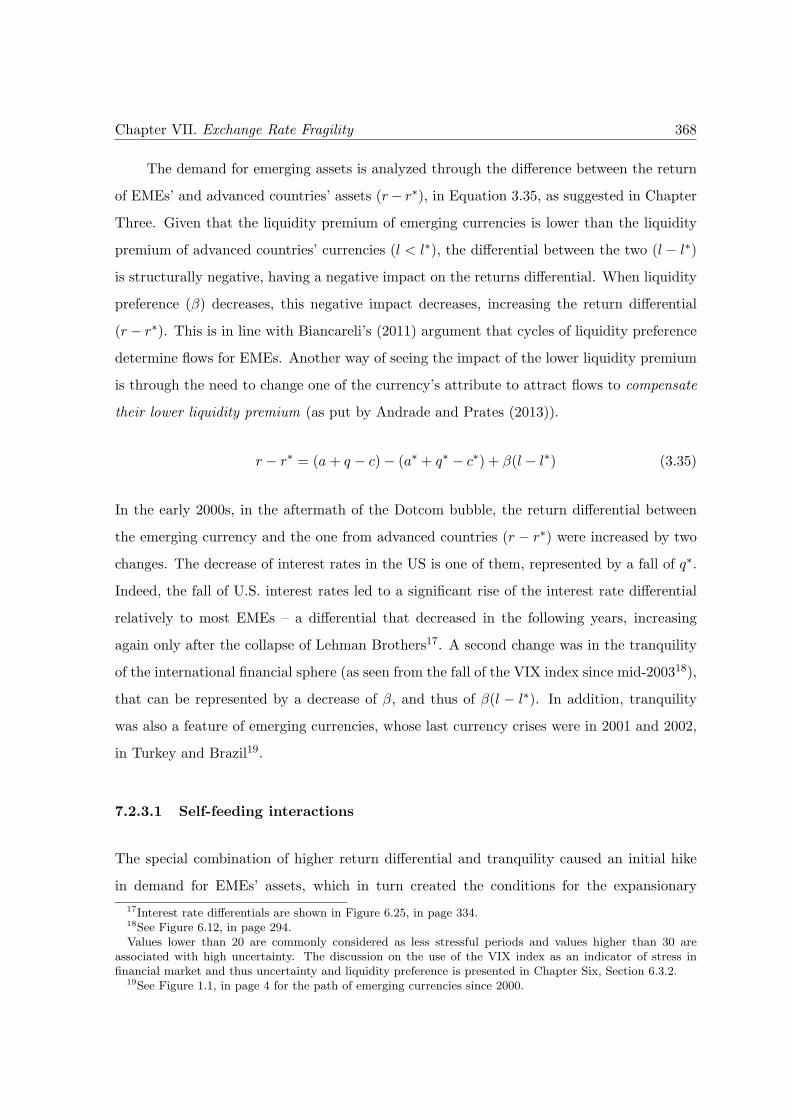
Chapter VII. Exchange Rate Fragility 368
The demand for emerging assets is analyzed through the difference between the return
of EMEs’ and advanced countries’ assets (r− r∗), in Equation 3.35, as suggested in Chapter
Three. Given that the liquidity premium of emerging currencies is lower than the liquidity
premium of advanced countries’ currencies (l < l∗), the differential between the two (l − l∗)
is structurally negative, having a negative impact on the returns differential. When liquidity
preference (β) decreases, this negative impact decreases, increasing the return differential
(r− r∗). This is in line with Biancareli’s (2011) argument that cycles of liquidity preference
determine flows for EMEs. Another way of seeing the impact of the lower liquidity premium
is through the need to change one of the currency’s attribute to attract flows to compensate
their lower liquidity premium (as put by Andrade and Prates (2013)).
r − r∗ = (a+ q − c)− (a∗ + q∗ − c∗) + β(l − l∗) (3.35)
In the early 2000s, in the aftermath of the Dotcom bubble, the return differential between
the emerging currency and the one from advanced countries (r − r∗) were increased by two
changes. The decrease of interest rates in the US is one of them, represented by a fall of q∗.
Indeed, the fall of U.S. interest rates led to a significant rise of the interest rate differential
relatively to most EMEs – a differential that decreased in the following years, increasing
again only after the collapse of Lehman Brothers17. A second change was in the tranquility
of the international financial sphere (as seen from the fall of the VIX index since mid-200318),
that can be represented by a decrease of β, and thus of β(l − l∗). In addition, tranquility
was also a feature of emerging currencies, whose last currency crises were in 2001 and 2002,
in Turkey and Brazil19.
7.2.3.1 Self-feeding interactions
The special combination of higher return differential and tranquility caused an initial hike
in demand for EMEs’ assets, which in turn created the conditions for the expansionary
17Interest rate differentials are shown in Figure 6.25, in page 334.18See Figure 6.12, in page 294.Values lower than 20 are commonly considered as less stressful periods and values higher than 30 are
associated with high uncertainty. The discussion on the use of the VIX index as an indicator of stress infinancial market and thus uncertainty and liquidity preference is presented in Chapter Six, Section 6.3.2.
19See Figure 1.1, in page 4 for the path of emerging currencies since 2000.
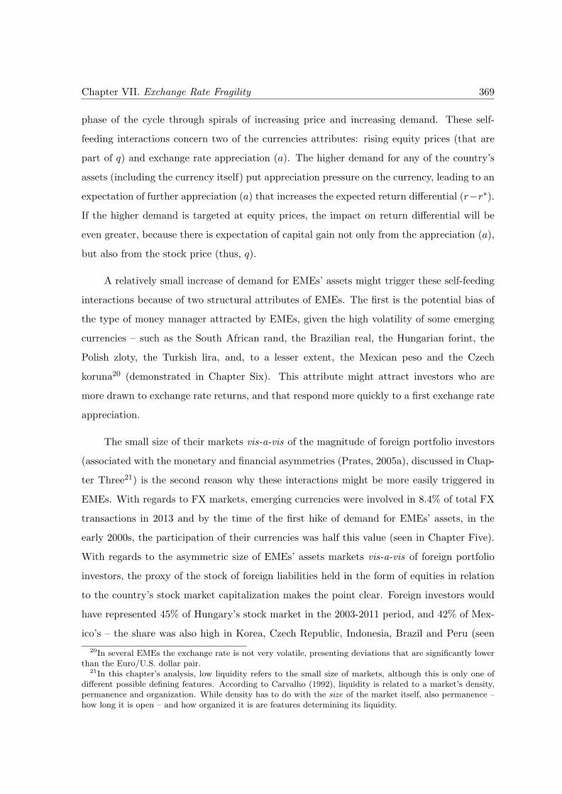
Chapter VII. Exchange Rate Fragility 369
phase of the cycle through spirals of increasing price and increasing demand. These self-
feeding interactions concern two of the currencies attributes: rising equity prices (that are
part of q) and exchange rate appreciation (a). The higher demand for any of the country’s
assets (including the currency itself) put appreciation pressure on the currency, leading to an
expectation of further appreciation (a) that increases the expected return differential (r−r∗).
If the higher demand is targeted at equity prices, the impact on return differential will be
even greater, because there is expectation of capital gain not only from the appreciation (a),
but also from the stock price (thus, q).
A relatively small increase of demand for EMEs’ assets might trigger these self-feeding
interactions because of two structural attributes of EMEs. The first is the potential bias of
the type of money manager attracted by EMEs, given the high volatility of some emerging
currencies – such as the South African rand, the Brazilian real, the Hungarian forint, the
Polish zloty, the Turkish lira, and, to a lesser extent, the Mexican peso and the Czech
koruna20 (demonstrated in Chapter Six). This attribute might attract investors who are
more drawn to exchange rate returns, and that respond more quickly to a first exchange rate
appreciation.
The small size of their markets vis-a-vis of the magnitude of foreign portfolio investors
(associated with the monetary and financial asymmetries (Prates, 2005a), discussed in Chap-
ter Three21) is the second reason why these interactions might be more easily triggered in
EMEs. With regards to FX markets, emerging currencies were involved in 8.4% of total FX
transactions in 2013 and by the time of the first hike of demand for EMEs’ assets, in the
early 2000s, the participation of their currencies was half this value (seen in Chapter Five).
With regards to the asymmetric size of EMEs’ assets markets vis-a-vis of foreign portfolio
investors, the proxy of the stock of foreign liabilities held in the form of equities in relation
to the country’s stock market capitalization makes the point clear. Foreign investors would
have represented 45% of Hungary’s stock market in the 2003-2011 period, and 42% of Mex-
ico’s – the share was also high in Korea, Czech Republic, Indonesia, Brazil and Peru (seen
20In several EMEs the exchange rate is not very volatile, presenting deviations that are significantly lowerthan the Euro/U.S. dollar pair.
21In this chapter’s analysis, low liquidity refers to the small size of markets, although this is only one ofdifferent possible defining features. According to Carvalho (1992), liquidity is related to a market’s density,permanence and organization. While density has to do with the size of the market itself, also permanence –how long it is open – and how organized it is are features determining its liquidity.
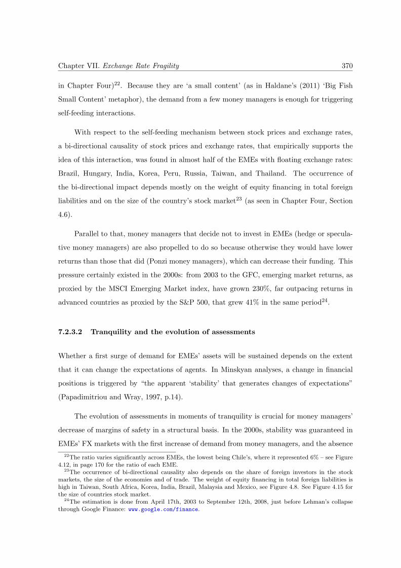
Chapter VII. Exchange Rate Fragility 370
in Chapter Four)22. Because they are ‘a small content’ (as in Haldane’s (2011) ‘Big Fish
Small Content’ metaphor), the demand from a few money managers is enough for triggering
self-feeding interactions.
With respect to the self-feeding mechanism between stock prices and exchange rates,
a bi-directional causality of stock prices and exchange rates, that empirically supports the
idea of this interaction, was found in almost half of the EMEs with floating exchange rates:
Brazil, Hungary, India, Korea, Peru, Russia, Taiwan, and Thailand. The occurrence of
the bi-directional impact depends mostly on the weight of equity financing in total foreign
liabilities and on the size of the country’s stock market23 (as seen in Chapter Four, Section
4.6).
Parallel to that, money managers that decide not to invest in EMEs (hedge or specula-
tive money managers) are also propelled to do so because otherwise they would have lower
returns than those that did (Ponzi money managers), which can decrease their funding. This
pressure certainly existed in the 2000s: from 2003 to the GFC, emerging market returns, as
proxied by the MSCI Emerging Market index, have grown 230%, far outpacing returns in
advanced countries as proxied by the S&P 500, that grew 41% in the same period24.
7.2.3.2 Tranquility and the evolution of assessments
Whether a first surge of demand for EMEs’ assets will be sustained depends on the extent
that it can change the expectations of agents. In Minskyan analyses, a change in financial
positions is triggered by “the apparent ‘stability’ that generates changes of expectations”
(Papadimitriou and Wray, 1997, p.14).
The evolution of assessments in moments of tranquility is crucial for money managers’
decrease of margins of safety in a structural basis. In the 2000s, stability was guaranteed in
EMEs’ FX markets with the first increase of demand from money managers, and the absence
22The ratio varies significantly across EMEs, the lowest being Chile’s, where it represented 6% – see Figure4.12, in page 170 for the ratio of each EME.
23The occurrence of bi-directional causality also depends on the share of foreign investors in the stockmarkets, the size of the economies and of trade. The weight of equity financing in total foreign liabilities ishigh in Taiwan, South Africa, Korea, India, Brazil, Malaysia and Mexico, see Figure 4.8. See Figure 4.15 forthe size of countries stock market.
24The estimation is done from April 17th, 2003 to September 12th, 2008, just before Lehman’s collapsethrough Google Finance: www.google.com/finance.
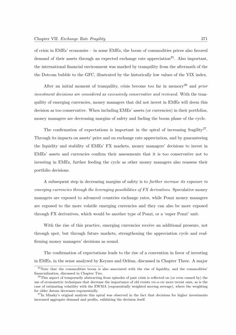
Chapter VII. Exchange Rate Fragility 371
of crisis in EMEs’ economies – in some EMEs, the boom of commodities prices also favored
demand of their assets through an expected exchange rate appreciation25. Also important,
the international financial environment was marked by tranquility from the aftermath of the
the Dotcom bubble to the GFC, illustrated by the historically low values of the VIX index.
After an initial moment of tranquility, crisis become too far in memory26 and prior
investment decisions are considered as excessively conservative and reviewed. With the tran-
quility of emerging currencies, money managers that did not invest in EMEs will deem this
decision as too conservative. When including EMEs’ assets (or currencies) in their portfolios,
money managers are decreasing margins of safety and fueling the boom phase of the cycle.
The confirmation of expectations is important in the spiral of increasing fragility27.
Through its impacts on assets’ price and on exchange rate appreciation, and by guaranteeing
the liquidity and stability of EMEs’ FX markets, money managers’ decisions to invest in
EMEs’ assets and currencies confirm their assessments that it is too conservative not to
investing in EMEs, further feeding the cycle as other money managers also reassess their
portfolio decisions.
A subsequent step in decreasing margins of safety is to further increase its exposure to
emerging currencies through the leveraging possibilities of FX derivatives. Speculative money
managers are exposed to advanced countries exchange rates, while Ponzi money managers
are exposed to the more volatile emerging currencies and they can also be more exposed
through FX derivatives, which would be another type of Ponzi, or a ‘super Ponzi’ unit.
With the rise of this practice, emerging currencies receive an additional pressure, not
through spot, but through future markets, strengthening the appreciation cycle and reaf-
firming money managers’ decisions as sound.
The confirmation of expectations leads to the rise of a convention in favor of investing
in EMEs, in the sense analyzed by Keynes and Orlean, discussed in Chapter Three. A major
25Note that the commodities boom is also associated with the rise of liquidity, and the commodities’financialization, discussed in Chapter Two.
26This aspect of temporarily abstracting from episodes of past crisis is reflected on (or even caused by) theuse of econometric techniques that decrease the importance of old events vis-a-vis more recent ones, as is thecase of estimating volatility with the EWMA (exponentially weighted moving average), where the weightingfor older datum decreases exponentially.
27In Minsky’s original analysis this spiral was observed in the fact that decisions for higher investmentsincreased aggregate demand and profits, validating the decision itself.
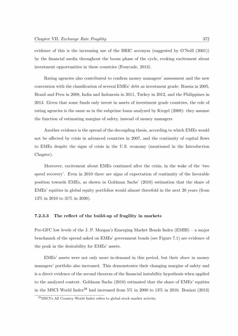
Chapter VII. Exchange Rate Fragility 372
evidence of this is the increasing use of the BRIC acronym (suggested by O’Neill (2001))
by the financial media throughout the boom phase of the cycle, evoking excitement about
investment opportunities in these countries (Fourcade, 2013).
Rating agencies also contributed to confirm money managers’ assessment and the new
convention with the classification of several EMEs’ debt as investment grade: Russia in 2005,
Brazil and Peru in 2008, India and Indonesia in 2011, Turkey in 2012, and the Philippines in
2013. Given that some funds only invest in assets of investment grade countries, the role of
rating agencies is the same as in the subprime loans analyzed by Kregel (2008): they assume
the function of estimating margins of safety, instead of money managers.
Another evidence is the spread of the decoupling thesis, according to which EMEs would
not be affected by crisis in advanced countries in 2007, and the continuity of capital flows
to EMEs despite the signs of crisis in the U.S. economy (mentioned in the Introduction
Chapter).
Moreover, excitement about EMEs continued after the crisis, in the wake of the ‘two
speed recovery’. Even in 2010 there are signs of expectation of continuity of the favorable
position towards EMEs, as shown in Goldman Sachs’ (2010) estimation that the share of
EMEs’ equities in global equity portfolios would almost threefold in the next 20 years (from
13% in 2010 to 31% in 2030).
7.2.3.3 The reflect of the build-up of fragility in markets
Pre-GFC low levels of the J. P. Morgan’s Emerging Market Bonds Index (EMBI) – a major
benchmark of the spread asked on EMEs’ government bonds (see Figure 7.1) are evidence of
the peak in the desirability for EMEs’ assets.
EMEs’ assets were not only more in-demand in this period, but their share in money
managers’ portfolio also increased. This demonstrates their changing margins of safety and
is a direct evidence of the second theorem of the financial instability hypothesis when applied
to the analyzed context. Goldman Sachs (2010) estimated that the share of EMEs’ equities
in the MSCI World Index28 had increased from 5% in 2000 to 13% in 2010. Bonizzi (2013)
28MSCI’s All Country World Index refers to global stock market activity.
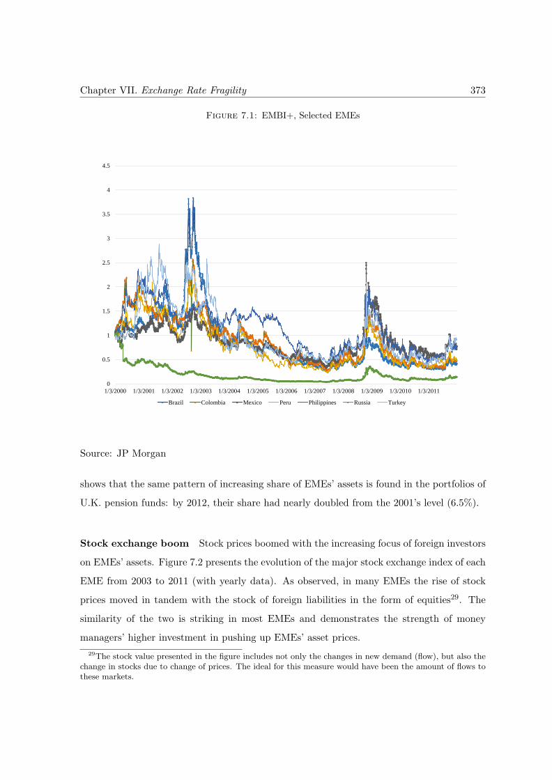
Chapter VII. Exchange Rate Fragility 373
Figure 7.1: EMBI+, Selected EMEs
0
0.5
1
1.5
2
2.5
3
3.5
4
4.5
1/3/2000 1/3/2001 1/3/2002 1/3/2003 1/3/2004 1/3/2005 1/3/2006 1/3/2007 1/3/2008 1/3/2009 1/3/2010 1/3/2011
Brazil Colombia Mexico Peru Philippines Russia Turkey
Source: JP Morgan
shows that the same pattern of increasing share of EMEs’ assets is found in the portfolios of
U.K. pension funds: by 2012, their share had nearly doubled from the 2001’s level (6.5%).
Stock exchange boom Stock prices boomed with the increasing focus of foreign investors
on EMEs’ assets. Figure 7.2 presents the evolution of the major stock exchange index of each
EME from 2003 to 2011 (with yearly data). As observed, in many EMEs the rise of stock
prices moved in tandem with the stock of foreign liabilities in the form of equities29. The
similarity of the two is striking in most EMEs and demonstrates the strength of money
managers’ higher investment in pushing up EMEs’ asset prices.
29The stock value presented in the figure includes not only the changes in new demand (flow), but also thechange in stocks due to change of prices. The ideal for this measure would have been the amount of flows tothese markets.
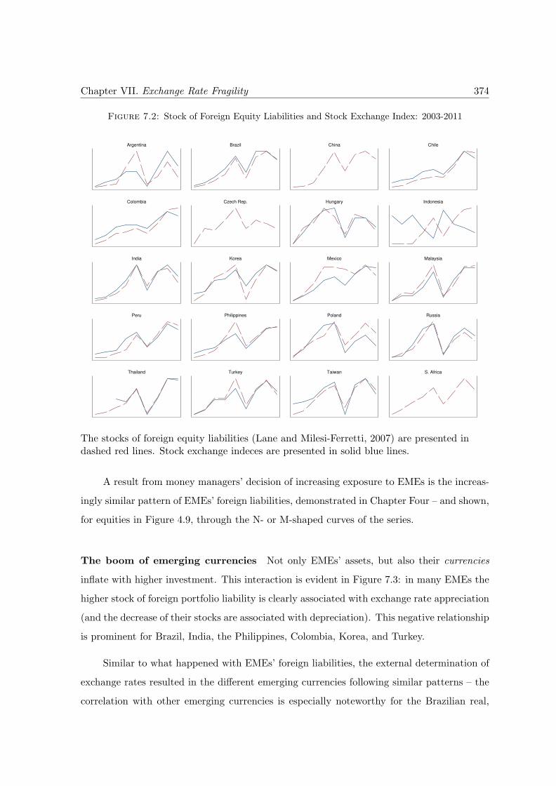
Chapter VII. Exchange Rate Fragility 374
Figure 7.2: Stock of Foreign Equity Liabilities and Stock Exchange Index: 2003-2011
Argentina Brazil China Chile
Colombia Czech Rep. Hungary Indonesia
India Korea Mexico Malaysia
Peru Philippines Poland Russia
Thailand Turkey Taiwan S. Africa
The stocks of foreign equity liabilities (Lane and Milesi-Ferretti, 2007) are presented indashed red lines. Stock exchange indeces are presented in solid blue lines.
A result from money managers’ decision of increasing exposure to EMEs is the increas-
ingly similar pattern of EMEs’ foreign liabilities, demonstrated in Chapter Four – and shown,
for equities in Figure 4.9, through the N- or M-shaped curves of the series.
The boom of emerging currencies Not only EMEs’ assets, but also their currencies
inflate with higher investment. This interaction is evident in Figure 7.3: in many EMEs the
higher stock of foreign portfolio liability is clearly associated with exchange rate appreciation
(and the decrease of their stocks are associated with depreciation). This negative relationship
is prominent for Brazil, India, the Philippines, Colombia, Korea, and Turkey.
Similar to what happened with EMEs’ foreign liabilities, the external determination of
exchange rates resulted in the different emerging currencies following similar patterns – the
correlation with other emerging currencies is especially noteworthy for the Brazilian real,
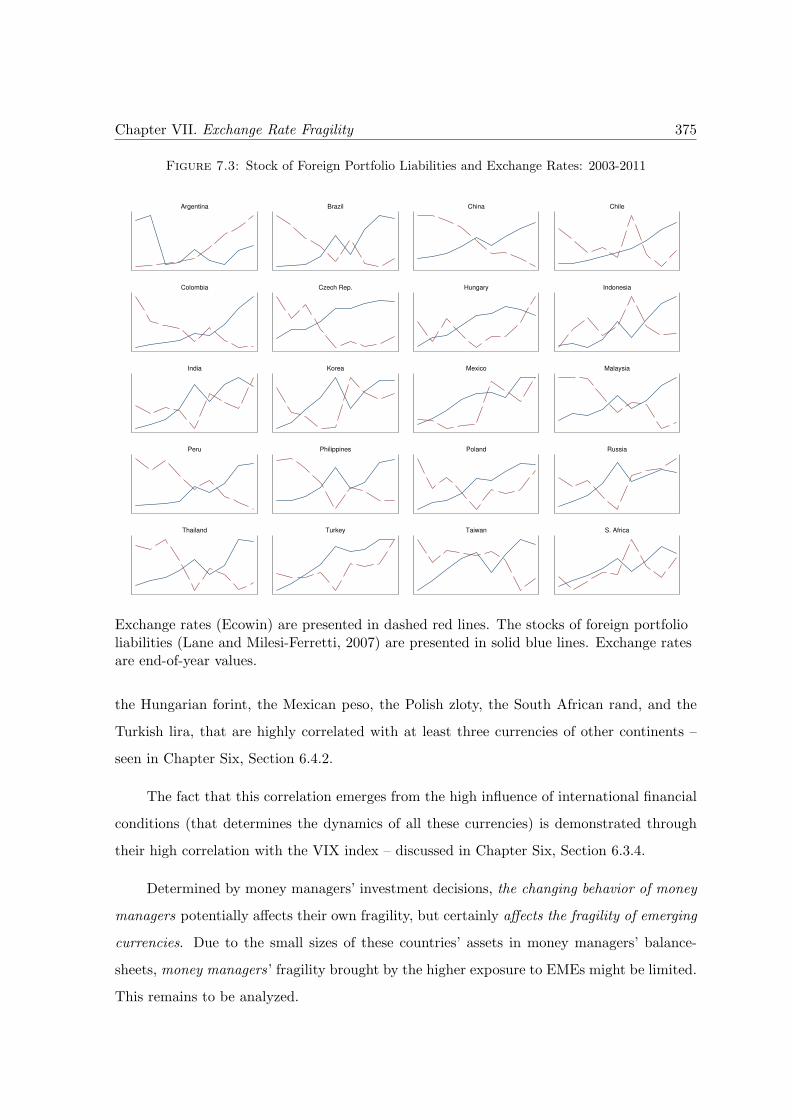
Chapter VII. Exchange Rate Fragility 375
Figure 7.3: Stock of Foreign Portfolio Liabilities and Exchange Rates: 2003-2011
Argentina Brazil China Chile
Colombia Czech Rep. Hungary Indonesia
India Korea Mexico Malaysia
Peru Philippines Poland Russia
Thailand Turkey Taiwan S. Africa
Exchange rates (Ecowin) are presented in dashed red lines. The stocks of foreign portfolioliabilities (Lane and Milesi-Ferretti, 2007) are presented in solid blue lines. Exchange ratesare end-of-year values.
the Hungarian forint, the Mexican peso, the Polish zloty, the South African rand, and the
Turkish lira, that are highly correlated with at least three currencies of other continents –
seen in Chapter Six, Section 6.4.2.
The fact that this correlation emerges from the high influence of international financial
conditions (that determines the dynamics of all these currencies) is demonstrated through
their high correlation with the VIX index – discussed in Chapter Six, Section 6.3.4.
Determined by money managers’ investment decisions, the changing behavior of money
managers potentially affects their own fragility, but certainly affects the fragility of emerging
currencies. Due to the small sizes of these countries’ assets in money managers’ balance-
sheets, money managers’ fragility brought by the higher exposure to EMEs might be limited.
This remains to be analyzed.
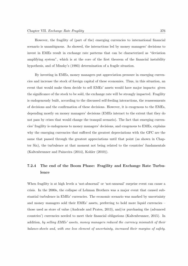
Chapter VII. Exchange Rate Fragility 376
However, the fragility of (part of the) emerging currencies to international financial
scenario is unambiguous. As showed, the interactions led by money managers’ decisions to
invest in EMEs result in exchange rate patterns that can be characterized as “deviation
amplifying system”, which is at the core of the first theorem of the financial instability
hypothesis, and of Minsky’s (1993) determination of a fragile situation.
By investing in EMEs, money managers put appreciation pressure in emerging curren-
cies and increase the stock of foreign capital of these economies. Thus, in this situation, an
event that would make them decide to sell EMEs’ assets would have major impacts: given
the significance of the stock to be sold, the exchange rate will be strongly impacted. Fragility
is endogenously built, according to the discussed self-feeding interactions, the reassessments
of decisions and the confirmation of these decisions. However, it is exogenous to the EMEs,
depending mostly on money managers’ decisions (EMEs interact to the extent that they do
not pass by crises that would change the tranquil scenario). The fact that emerging curren-
cies’ fragility is endogenous to money managers’ decisions, and exogenous to EMEs, explains
why the emerging currencies that suffered the greatest depreciations with the GFC are the
same that passed through the greatest appreciations until that point (as shown in Chap-
ter Six), the turbulence at that moment not being related to the countries’ fundamentals
(Kaltenbrunner and Painceira (2014), Kohler (2010)).
7.2.4 The end of the Boom Phase: Fragility and Exchange Rate Turbu-
lence
When fragility is at high levels a ‘not-abnornal’ or ‘not-unusual’ surprise event can cause a
crisis. In the 2000s, the collapse of Lehman Brothers was a major event that caused sub-
stantial turbulence in EMEs’ currencies. The economic scenario was marked by uncertainty
and money managers sold their EMEs’ assets, preferring to hold more liquid currencies –
those used as store of value (Andrade and Prates, 2013), and/or purchasing the (advanced
countries’) currencies needed to meet their financial obligations (Kaltenbrunner, 2015). In
addition, by selling EMEs’ assets, money managers reduced the currency mismatch of their
balance-sheets and, with one less element of uncertainty, increased their margins of safety.
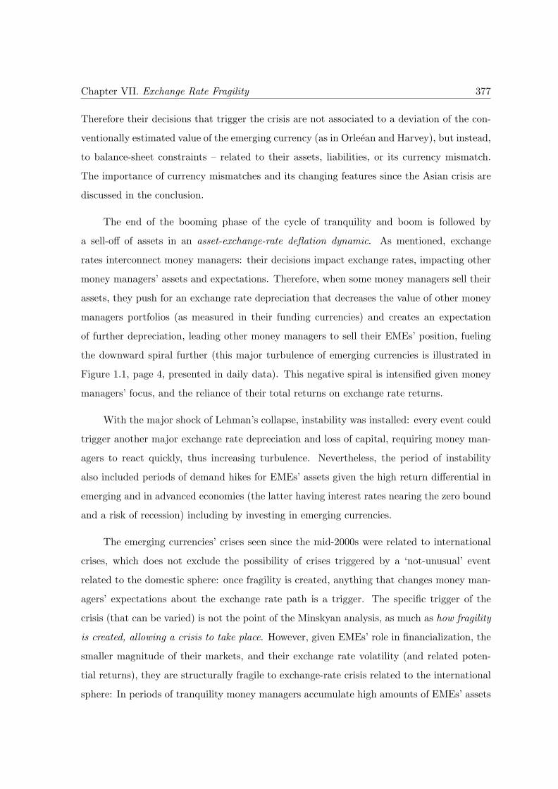
Chapter VII. Exchange Rate Fragility 377
Therefore their decisions that trigger the crisis are not associated to a deviation of the con-
ventionally estimated value of the emerging currency (as in Orleean and Harvey), but instead,
to balance-sheet constraints – related to their assets, liabilities, or its currency mismatch.
The importance of currency mismatches and its changing features since the Asian crisis are
discussed in the conclusion.
The end of the booming phase of the cycle of tranquility and boom is followed by
a sell-off of assets in an asset-exchange-rate deflation dynamic. As mentioned, exchange
rates interconnect money managers: their decisions impact exchange rates, impacting other
money managers’ assets and expectations. Therefore, when some money managers sell their
assets, they push for an exchange rate depreciation that decreases the value of other money
managers portfolios (as measured in their funding currencies) and creates an expectation
of further depreciation, leading other money managers to sell their EMEs’ position, fueling
the downward spiral further (this major turbulence of emerging currencies is illustrated in
Figure 1.1, page 4, presented in daily data). This negative spiral is intensified given money
managers’ focus, and the reliance of their total returns on exchange rate returns.
With the major shock of Lehman’s collapse, instability was installed: every event could
trigger another major exchange rate depreciation and loss of capital, requiring money man-
agers to react quickly, thus increasing turbulence. Nevertheless, the period of instability
also included periods of demand hikes for EMEs’ assets given the high return differential in
emerging and in advanced economies (the latter having interest rates nearing the zero bound
and a risk of recession) including by investing in emerging currencies.
The emerging currencies’ crises seen since the mid-2000s were related to international
crises, which does not exclude the possibility of crises triggered by a ‘not-unusual’ event
related to the domestic sphere: once fragility is created, anything that changes money man-
agers’ expectations about the exchange rate path is a trigger. The specific trigger of the
crisis (that can be varied) is not the point of the Minskyan analysis, as much as how fragility
is created, allowing a crisis to take place. However, given EMEs’ role in financialization, the
smaller magnitude of their markets, and their exchange rate volatility (and related poten-
tial returns), they are structurally fragile to exchange-rate crisis related to the international
sphere: In periods of tranquility money managers accumulate high amounts of EMEs’ assets
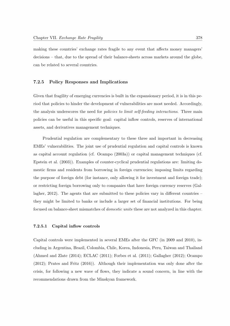
Chapter VII. Exchange Rate Fragility 378
making these countries’ exchange rates fragile to any event that affects money managers’
decisions – that, due to the spread of their balance-sheets across markets around the globe,
can be related to several countries.
7.2.5 Policy Responses and Implications
Given that fragility of emerging currencies is built in the expansionary period, it is in this pe-
riod that policies to hinder the development of vulnerabilities are most needed. Accordingly,
the analysis underscores the need for policies to limit self-feeding interactions. Three main
policies can be useful in this specific goal: capital inflow controls, reserves of international
assets, and derivatives management techniques.
Prudential regulation are complementary to these three and important in decreasing
EMEs’ vulnerabilities. The joint use of prudential regulation and capital controls is known
as capital account regulation (cf. Ocampo (2003a)) or capital management techniques (cf.
Epstein et al. (2003)). Examples of counter-cyclical prudential regulations are: limiting do-
mestic firms and residents from borrowing in foreign currencies; imposing limits regarding
the purpose of foreign debt (for instance, only allowing it for investment and foreign trade);
or restricting foreign borrowing only to companies that have foreign currency reserves (Gal-
lagher, 2012). The agents that are submitted to these policies vary in different countries –
they might be limited to banks or include a larger set of financial institutions. For being
focused on balance-sheet mismatches of domestic units these are not analyzed in this chapter.
7.2.5.1 Capital inflow controls
Capital controls were implemented in several EMEs after the GFC (in 2009 and 2010), in-
cluding in Argentina, Brazil, Colombia, Chile, Korea, Indonesia, Peru, Taiwan and Thailand
(Ahmed and Zlate (2014); ECLAC (2011); Forbes et al. (2011); Gallagher (2012); Ocampo
(2012); Prates and Fritz (2016)). Although their implementation was only done after the
crisis, for following a new wave of flows, they indicate a sound concern, in line with the
recommendations drawn from the Minskyan framework.
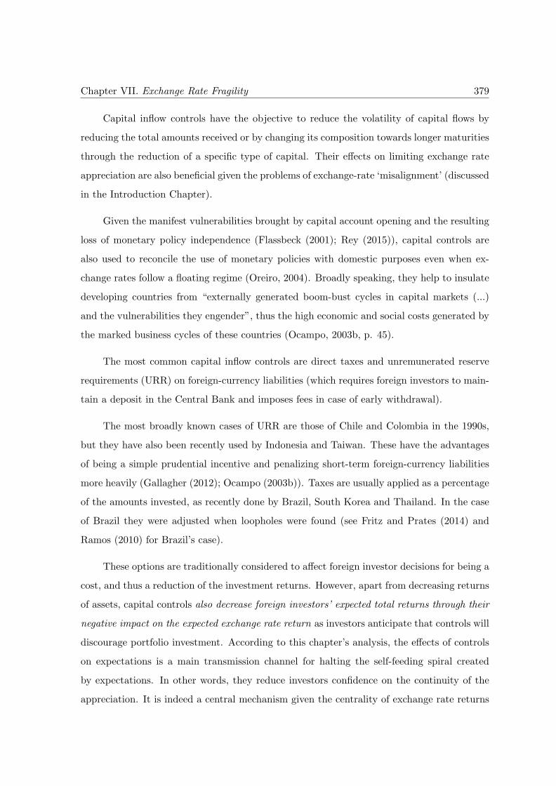
Chapter VII. Exchange Rate Fragility 379
Capital inflow controls have the objective to reduce the volatility of capital flows by
reducing the total amounts received or by changing its composition towards longer maturities
through the reduction of a specific type of capital. Their effects on limiting exchange rate
appreciation are also beneficial given the problems of exchange-rate ‘misalignment’ (discussed
in the Introduction Chapter).
Given the manifest vulnerabilities brought by capital account opening and the resulting
loss of monetary policy independence (Flassbeck (2001); Rey (2015)), capital controls are
also used to reconcile the use of monetary policies with domestic purposes even when ex-
change rates follow a floating regime (Oreiro, 2004). Broadly speaking, they help to insulate
developing countries from “externally generated boom-bust cycles in capital markets (...)
and the vulnerabilities they engender”, thus the high economic and social costs generated by
the marked business cycles of these countries (Ocampo, 2003b, p. 45).
The most common capital inflow controls are direct taxes and unremunerated reserve
requirements (URR) on foreign-currency liabilities (which requires foreign investors to main-
tain a deposit in the Central Bank and imposes fees in case of early withdrawal).
The most broadly known cases of URR are those of Chile and Colombia in the 1990s,
but they have also been recently used by Indonesia and Taiwan. These have the advantages
of being a simple prudential incentive and penalizing short-term foreign-currency liabilities
more heavily (Gallagher (2012); Ocampo (2003b)). Taxes are usually applied as a percentage
of the amounts invested, as recently done by Brazil, South Korea and Thailand. In the case
of Brazil they were adjusted when loopholes were found (see Fritz and Prates (2014) and
Ramos (2010) for Brazil’s case).
These options are traditionally considered to affect foreign investor decisions for being a
cost, and thus a reduction of the investment returns. However, apart from decreasing returns
of assets, capital controls also decrease foreign investors’ expected total returns through their
negative impact on the expected exchange rate return as investors anticipate that controls will
discourage portfolio investment. According to this chapter’s analysis, the effects of controls
on expectations is a main transmission channel for halting the self-feeding spiral created
by expectations. In other words, they reduce investors confidence on the continuity of the
appreciation. It is indeed a central mechanism given the centrality of exchange rate returns
Chapter VII. Exchange Rate Fragility 380
in money managers’ strategies (seen in Chapter Two) and the the magnitude of the returns
of emerging currencies (seen in Chapter Six)30.
Capital controls are subject to criticisms31. However, the most often evoked criticisms
are based on controversial issues: controls limit the benefits from capital account liberaliza-
tion32 and, depending on the market’s features, they would not be effective33 (Ariyoshi et al.
(2000); Carvalho and Garcia (2008); Neely (1999); Forbes (2003); Forbes (2005); Forbes
(2007)). The inconclusiveness of the first debate was presented in Chapter Five34; the con-
troversy on the effectiveness of capital controls will be presented in the following.
Capital controls were also said to only treat symptoms of inconsistent policies or distor-
tions (Neely, 1999), although this argument is outdated in light of GFC-related events (when
capital flew to the countries in crisis) and broader evidence of the high weight of external con-
ditions in determining emerging currencies (as presented in the last chapter). Other concerns
are minor, such as those related to distortion of the decision-making process by companies
and individuals as they try to circumvent controls; implementation issues (Forbes, 2007); and
the claim that they jointly limit desired flows and less desired ones (Ariyoshi et al., 2000),
which is a design issue.
With the GFC, the IMF reviewed its position on capital controls (Roy and Ramos,
2012). IMF (2009, p. 8) stated that large capital inflows “can lead to sharp appreciations,
often followed by abrupt reversals and strong effects on balance sheets” and Ostry et al.
(2010) indicated circumstances when capital controls should be included in countries’ toolkit.
Additionally, the appropriate design of capital controls were analyzed (Ostry et al., 2011).
30For the controls implemented in Brazil in 2009 (IOF, in the Portuguese acronym), Ramos (2010) showsa marked change in expectations of domestic financial agents associated with the announcements of inflowcontrols.
31This criticisms are reflected in the constantly evolving position of international agencies towards controlsand of its use worldwide (Gallagher, 2012).
32As markets are insulated from competition, capital controls would induce them to inefficiency (or reducethe discipline imposed by the market), and would increase firms’ financial costs (Forbes (2003); Forbes (2005);Forbes (2007)).
Note that the evidence of increasingly similar path of EMEs’ assets and currencies demonstrated in ChapterSix put questions on one possible gain from capital account opening, i.e. the reduction of international portfolioinvestors’ risks. This was also argued by Longin and Solnik (1995).
33The effectiveness of capital controls depend on incentives and costs of circumvention (Ariyoshi et al.,2000); or, more precisely, on: “the development of domestic financial market and alternatives in overseasderivatives markets (...); the ability of authorities to monitor inflows; the penalties for avoidance; and, themost difficult to prevent, regulation loopholes” (Carvalho and Garcia, 2008, p. 72).
34 evidence of increasing co-movement among currencies demonstrated in Chapter Six indicates the de-creasing gain of international investors from risk reduction with world-wide portfolio allocation
Chapter VII. Exchange Rate Fragility 381
However, controls are seen as a temporary instrument, while case studies show that these
tools are needed on a permanent basis and in combination with prudential regulation (Fritz
and Prates, 2014).
One criticism on capital controls raised by GFC-related interventions is that they can
have adverse consequences in other economies as flows would be redirected to them, thus
‘beggar-thy-neighbor effects’ (Forbes et al. (2011); Ostry et al. (2010)). This argument
reflects the effectiveness of controls in reducing flows and highlights the need of international
coordination on their implementation (Forbes et al., 2011) and of reforming the international
monetary system, which could enhance the vulnerability of all EMEs at once35.
The efficacy of capital controls is a long-dated empirical controversy36. From the extent
literature, two studies should be highlighted for having very different methodologies. Epstein
et al. (2003) provide a comprehensive analysis of seven experiences based on a detailed
description of their context and conclude the effectiveness of all the cases. With a summary of
30 the results of studies weighted according to their econometric rigor, Magud and Reinhart
(2006) conclude that inflow controls were effective in changing the composition of inflows
towards longer maturities, in making monetary policy more independent, and in reducing
exchange rate pressures.
However, the rigor of this analysis is not the best indicator of accuracy, given the
complexity of the relationships and the numerous variables to be accounted for. One problem
is the difficult task of exchange rate modeling (Williamson, 2000, ch. 4). Moreover, as
this thesis has argued, these analyses should account for every market connected to money
managers’ balance-sheets, including considering possible changes in the financial scenario
where money managers have assets37 and their funding. On the other hand, as a reduction
of total returns and a marked shock in the confidence on the continuity of the exchange rate
appreciation, capital inflow controls are only exempt from impact if every foreign investor
had a free possibility of circumventing controls.
35See more on how the reform of the international monetary system could enhance the situation of all EMEsin the Conclusions Chapter.
36For references that found evidence of effectiveness of capital controls, and others that did not, specificallyin Chile and Colombia, see Ocampo (2003a).
37Note that this is in line with the idea that capital controls have ‘beggar-thy-neighbor effect’ (Forbes et al.,2011).
Chapter VII. Exchange Rate Fragility 382
7.2.5.2 Reserves
The analysis done in this chapter also points to the need of accumulating important amounts
of foreign assets, as done by most EMEs since the 2000s (see Chapter Five, Section 5.2.1).
This policy has a precautionary reason: its use enables EMEs to protect themselves from
crises as those seen in the late 1990s, and from halting appreciation and its inflationary
pressures with the boom of capital inflows to EMEs in the 2000s.
As capital inflow controls, reserves could also avoid fragility from taking place by at-
tenuating appreciation, thus affecting the continuity of the self-feeding cycle. Its effects
through expectations are softer than that of capital controls that usually involve a notori-
ous announcement. Nonetheless, governments’ interventions in FX markets also reverberate
among financial practitioners.
Accumulating large amounts of reserves imply significant sterilization costs38 depending
on the interest differential between the EMEs and the advanced country – that has been
positive and large for most EMEs39. Given these costs, reserves should be used in combination
with policies of capital account management, which decrease the level of reserves needed, or
be specifically combined with taxes on inflows, which reduces total costs with capital account
management by raising recipes40. As put by Andrade and Prates (2013),
In times of boom, they [capital management techniques] control the destabilizing
effects of short-term capital flows as well as the cost and risk of reserve accu-
mulation; in times of bust, they reduce the minimum level of reserves needed to
restrain speculative attacks and alleviate pressures on domestic interest rates. (p.
414)
Accumulating reserves is also filled with inconsistencies. First, who profits from a
country’s large amount of reserves should be analyzed. If the policy results in more stable
38Ramos (2010) estimated the costs of reserves in Brazil (where both reserves and basic interest rates arehigh) at 1% of Brazilian GDP.
39The literature also considers opportunity costs, focusing on the returns of alternative investments (Aizen-man and Marion, 2003) and the social cost of foreign reserves, that compares the cost of reserves with thecosts that firms pay to hedge their borrowing (Rodrik, 2006).
For EMEs’ interest rates see Figures 6.25 and 6.26 in the Appendix of Chapter Six.40Ramos (2010) estimated that in Brazil in 2009/10 the revenues due to the tax on portfolio inflows
amounted to 20% of the yearly sterilization costs.
Chapter VII. Exchange Rate Fragility 383
exchange rates and shields the country from turbulence, the whole economy benefits (the
same can be said about a reserve-policy that has a mercantilist goal). If it is done to
hedge external debt, its benefits are however concentrated on foreign portfolio investors
(UNCTAD, 2007, ch. 4). According to the discussion done in this chapter, this is a relevant
issue, as the attractiveness of a country is key in building fragility. In line with this idea,
Kaltenbrunner and Painceira (2009) highlight the importance of the large amount of reserves
held by Brazil on the attraction of volatile portfolio flows. Furthermore, by increasing the
supply of government bonds, the policy created liquidity for international investors.
Second, by holding important amounts of reserves, EMEs move towards becoming in-
ternational net creditors. They have the assets of advanced countries’ governments and
liabilities with these countries’ investors, resulting in a contradictory situation: EMEs re-
ceive very volatile capital that demands protection to be built, which is done through sending
capital abroad (that also increases the attraction of this type of capital). This inconsistency
raises questions on the advantages of capital account opening.
With the GFC, reserves were not sufficient for shielding EMEs from major turbulence.
There is a debate on whether they were appropriately used. Some authors argue that they
were only modestly used (Aizenman and Hutchison, 2012), while others emphasize their role
in absorbing part of the shock (Calvo et al., 2012). Indeed, a rather small part of reserves was
sold in 2008, but this behavior of EMEs’ central banks might hint to how valued reserves are
for these countries and their fear of losing their investment grade ratings (that were granted
based on these countries’ high level of reserves; Prates (2015).
Despite costs and these inconsistencies, reserves of foreign assets are a much needed
‘cushion’ for counter-balancing money managers’ excessive demand or supply at specific
moments, which, as discussed, is key for attenuating the self-feeding interactions and the
build up of fragile exchange rates.
As discussed in Chapter Five (Section 5.2.1.2), given the magnitude of EMEs’ foreign
liabilities, the increasingly short-term focus of money mangers, and the non-stable pattern
of FDI in some EMEs, substantial amounts of reserves are needed.
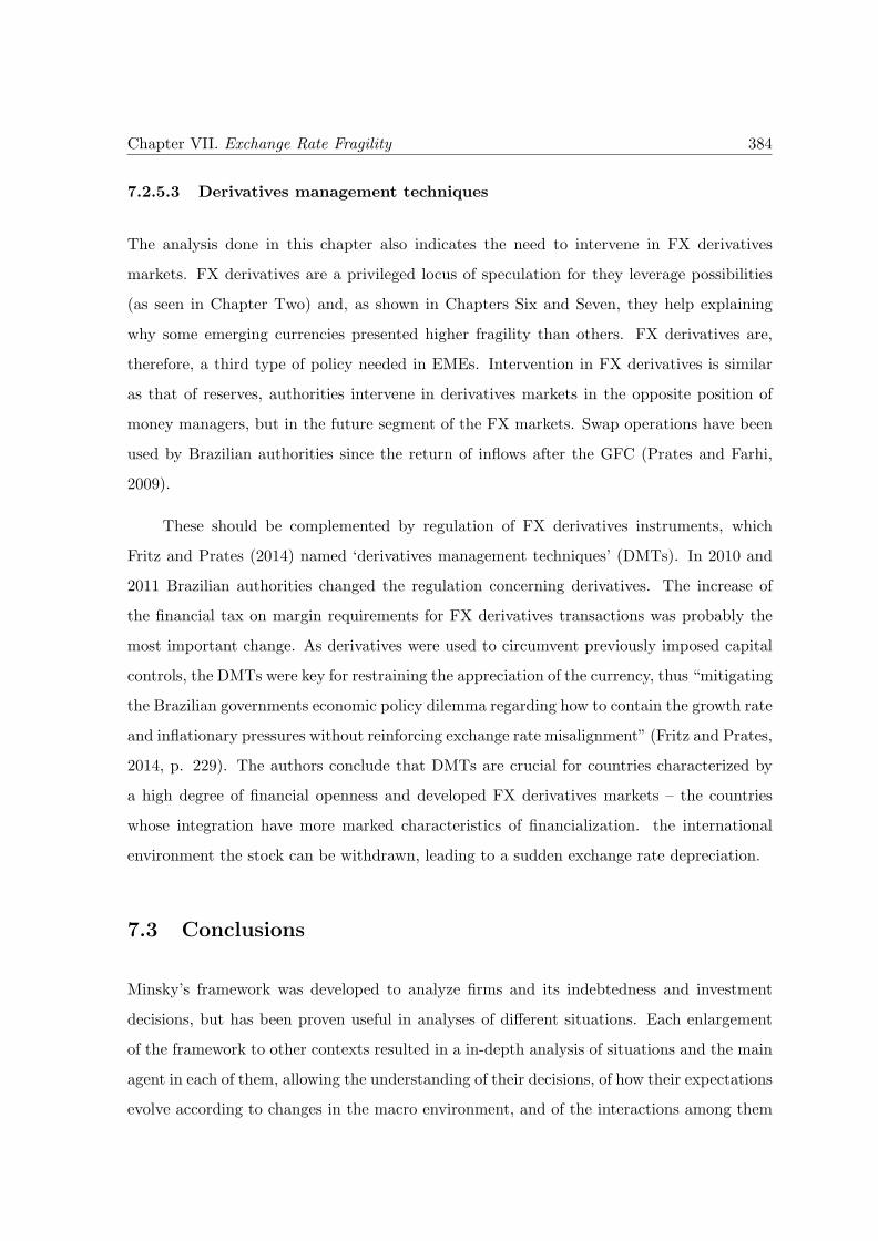
Chapter VII. Exchange Rate Fragility 384
7.2.5.3 Derivatives management techniques
The analysis done in this chapter also indicates the need to intervene in FX derivatives
markets. FX derivatives are a privileged locus of speculation for they leverage possibilities
(as seen in Chapter Two) and, as shown in Chapters Six and Seven, they help explaining
why some emerging currencies presented higher fragility than others. FX derivatives are,
therefore, a third type of policy needed in EMEs. Intervention in FX derivatives is similar
as that of reserves, authorities intervene in derivatives markets in the opposite position of
money managers, but in the future segment of the FX markets. Swap operations have been
used by Brazilian authorities since the return of inflows after the GFC (Prates and Farhi,
2009).
These should be complemented by regulation of FX derivatives instruments, which
Fritz and Prates (2014) named ‘derivatives management techniques’ (DMTs). In 2010 and
2011 Brazilian authorities changed the regulation concerning derivatives. The increase of
the financial tax on margin requirements for FX derivatives transactions was probably the
most important change. As derivatives were used to circumvent previously imposed capital
controls, the DMTs were key for restraining the appreciation of the currency, thus “mitigating
the Brazilian governments economic policy dilemma regarding how to contain the growth rate
and inflationary pressures without reinforcing exchange rate misalignment” (Fritz and Prates,
2014, p. 229). The authors conclude that DMTs are crucial for countries characterized by
a high degree of financial openness and developed FX derivatives markets – the countries
whose integration have more marked characteristics of financialization. the international
environment the stock can be withdrawn, leading to a sudden exchange rate depreciation.
7.3 Conclusions
Minsky’s framework was developed to analyze firms and its indebtedness and investment
decisions, but has been proven useful in analyses of different situations. Each enlargement
of the framework to other contexts resulted in a in-depth analysis of situations and the main
agent in each of them, allowing the understanding of their decisions, of how their expectations
evolve according to changes in the macro environment, and of the interactions among them
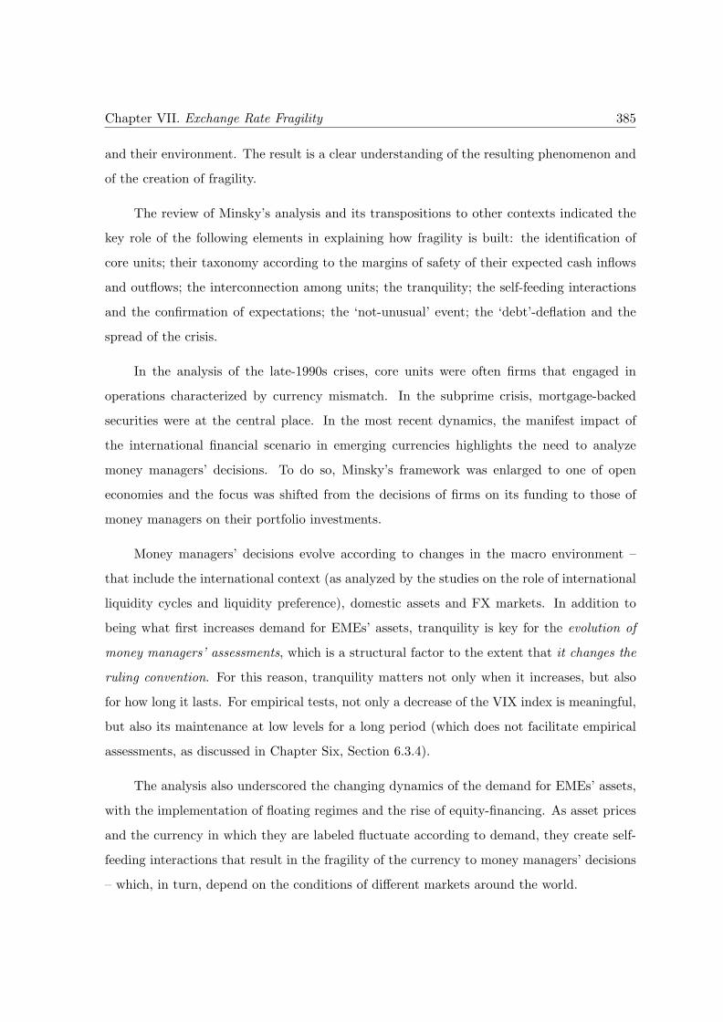
Chapter VII. Exchange Rate Fragility 385
and their environment. The result is a clear understanding of the resulting phenomenon and
of the creation of fragility.
The review of Minsky’s analysis and its transpositions to other contexts indicated the
key role of the following elements in explaining how fragility is built: the identification of
core units; their taxonomy according to the margins of safety of their expected cash inflows
and outflows; the interconnection among units; the tranquility; the self-feeding interactions
and the confirmation of expectations; the ‘not-unusual’ event; the ‘debt’-deflation and the
spread of the crisis.
In the analysis of the late-1990s crises, core units were often firms that engaged in
operations characterized by currency mismatch. In the subprime crisis, mortgage-backed
securities were at the central place. In the most recent dynamics, the manifest impact of
the international financial scenario in emerging currencies highlights the need to analyze
money managers’ decisions. To do so, Minsky’s framework was enlarged to one of open
economies and the focus was shifted from the decisions of firms on its funding to those of
money managers on their portfolio investments.
Money managers’ decisions evolve according to changes in the macro environment –
that include the international context (as analyzed by the studies on the role of international
liquidity cycles and liquidity preference), domestic assets and FX markets. In addition to
being what first increases demand for EMEs’ assets, tranquility is key for the evolution of
money managers’ assessments, which is a structural factor to the extent that it changes the
ruling convention. For this reason, tranquility matters not only when it increases, but also
for how long it lasts. For empirical tests, not only a decrease of the VIX index is meaningful,
but also its maintenance at low levels for a long period (which does not facilitate empirical
assessments, as discussed in Chapter Six, Section 6.3.4).
The analysis also underscored the changing dynamics of the demand for EMEs’ assets,
with the implementation of floating regimes and the rise of equity-financing. As asset prices
and the currency in which they are labeled fluctuate according to demand, they create self-
feeding interactions that result in the fragility of the currency to money managers’ decisions
– which, in turn, depend on the conditions of different markets around the world.
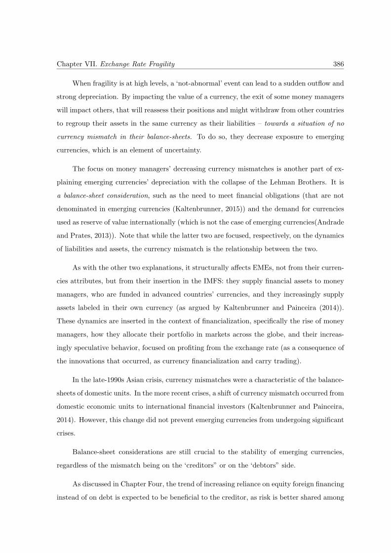
Chapter VII. Exchange Rate Fragility 386
When fragility is at high levels, a ‘not-abnormal’ event can lead to a sudden outflow and
strong depreciation. By impacting the value of a currency, the exit of some money managers
will impact others, that will reassess their positions and might withdraw from other countries
to regroup their assets in the same currency as their liabilities – towards a situation of no
currency mismatch in their balance-sheets. To do so, they decrease exposure to emerging
currencies, which is an element of uncertainty.
The focus on money managers’ decreasing currency mismatches is another part of ex-
plaining emerging currencies’ depreciation with the collapse of the Lehman Brothers. It is
a balance-sheet consideration, such as the need to meet financial obligations (that are not
denominated in emerging currencies (Kaltenbrunner, 2015)) and the demand for currencies
used as reserve of value internationally (which is not the case of emerging currencies(Andrade
and Prates, 2013)). Note that while the latter two are focused, respectively, on the dynamics
of liabilities and assets, the currency mismatch is the relationship between the two.
As with the other two explanations, it structurally affects EMEs, not from their curren-
cies attributes, but from their insertion in the IMFS: they supply financial assets to money
managers, who are funded in advanced countries’ currencies, and they increasingly supply
assets labeled in their own currency (as argued by Kaltenbrunner and Painceira (2014)).
These dynamics are inserted in the context of financialization, specifically the rise of money
managers, how they allocate their portfolio in markets across the globe, and their increas-
ingly speculative behavior, focused on profiting from the exchange rate (as a consequence of
the innovations that occurred, as currency financialization and carry trading).
In the late-1990s Asian crisis, currency mismatches were a characteristic of the balance-
sheets of domestic units. In the more recent crises, a shift of currency mismatch occurred from
domestic economic units to international financial investors (Kaltenbrunner and Painceira,
2014). However, this change did not prevent emerging currencies from undergoing significant
crises.
Balance-sheet considerations are still crucial to the stability of emerging currencies,
regardless of the mismatch being on the ‘creditors” or on the ‘debtors” side.
As discussed in Chapter Four, the trend of increasing reliance on equity foreign financing
instead of on debt is expected to be beneficial to the creditor, as risk is better shared among
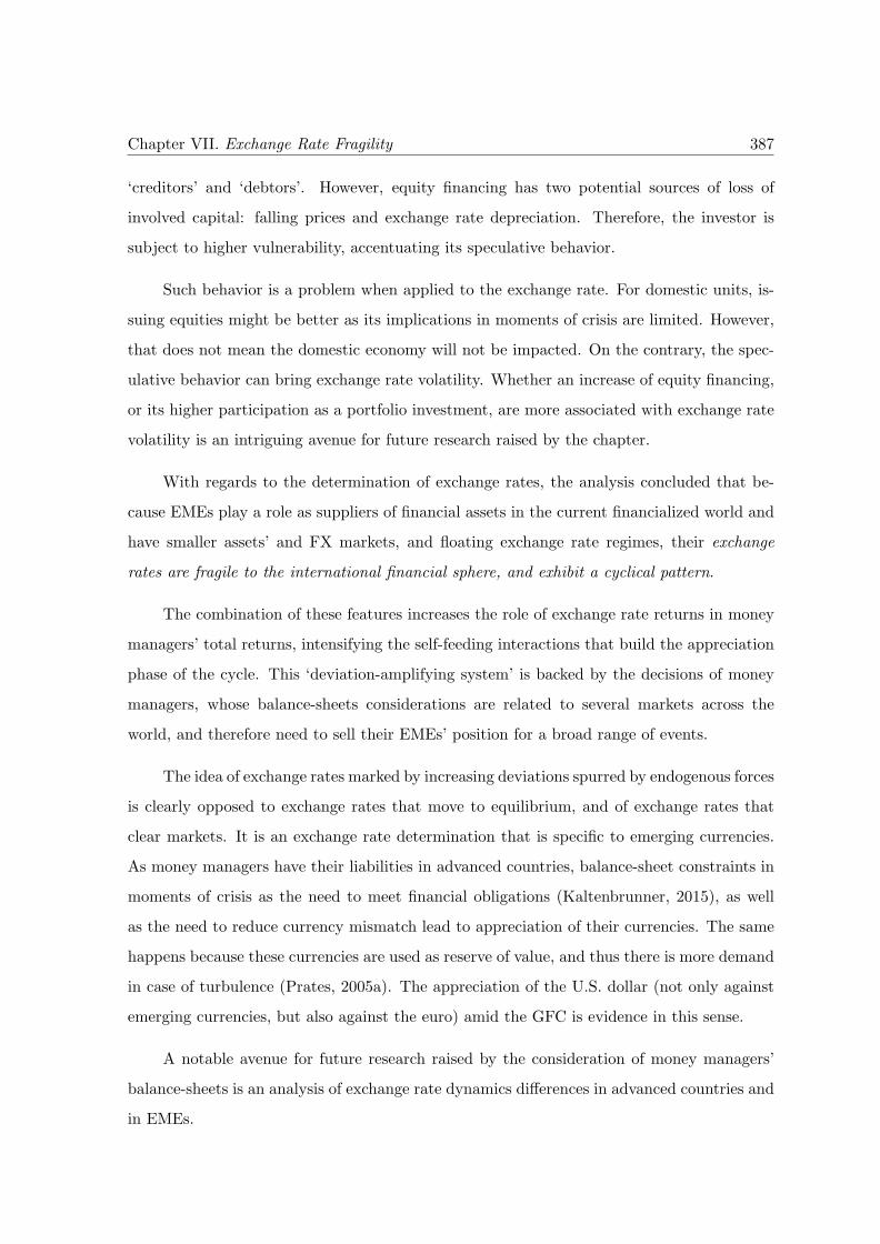
Chapter VII. Exchange Rate Fragility 387
‘creditors’ and ‘debtors’. However, equity financing has two potential sources of loss of
involved capital: falling prices and exchange rate depreciation. Therefore, the investor is
subject to higher vulnerability, accentuating its speculative behavior.
Such behavior is a problem when applied to the exchange rate. For domestic units, is-
suing equities might be better as its implications in moments of crisis are limited. However,
that does not mean the domestic economy will not be impacted. On the contrary, the spec-
ulative behavior can bring exchange rate volatility. Whether an increase of equity financing,
or its higher participation as a portfolio investment, are more associated with exchange rate
volatility is an intriguing avenue for future research raised by the chapter.
With regards to the determination of exchange rates, the analysis concluded that be-
cause EMEs play a role as suppliers of financial assets in the current financialized world and
have smaller assets’ and FX markets, and floating exchange rate regimes, their exchange
rates are fragile to the international financial sphere, and exhibit a cyclical pattern.
The combination of these features increases the role of exchange rate returns in money
managers’ total returns, intensifying the self-feeding interactions that build the appreciation
phase of the cycle. This ‘deviation-amplifying system’ is backed by the decisions of money
managers, whose balance-sheets considerations are related to several markets across the
world, and therefore need to sell their EMEs’ position for a broad range of events.
The idea of exchange rates marked by increasing deviations spurred by endogenous forces
is clearly opposed to exchange rates that move to equilibrium, and of exchange rates that
clear markets. It is an exchange rate determination that is specific to emerging currencies.
As money managers have their liabilities in advanced countries, balance-sheet constraints in
moments of crisis as the need to meet financial obligations (Kaltenbrunner, 2015), as well
as the need to reduce currency mismatch lead to appreciation of their currencies. The same
happens because these currencies are used as reserve of value, and thus there is more demand
in case of turbulence (Prates, 2005a). The appreciation of the U.S. dollar (not only against
emerging currencies, but also against the euro) amid the GFC is evidence in this sense.
A notable avenue for future research raised by the consideration of money managers’
balance-sheets is an analysis of exchange rate dynamics differences in advanced countries and
in EMEs.
Chapter VII. Exchange Rate Fragility 388
The exchange rate determination process suggested in this chapter does not concern
every EME. As presented in Chapter Six, exchange rate dynamics are markedly different
among EME. The group of countries that are more highly influenced by international financial
markets includes Brazil, Hungary, Poland, South Africa, and Turkey.
In comparison to the exchange rate theories presented in Chapter Three, this analysis
denotes a shift in focus from the attributes of emerging currencies, or from expected portfolio
inflows, to the decisions of money managers. It does not contradict those models – a cur-
rency’s liquidity premium and the process through which exchange rate forecasts are built
help explaining money manager’s behavior.
However, looking at exchange rates through their decisions may be a broader framework,
where balance-sheet considerations are neatly accommodated, enabling the analysis of the
role of events not related to the currencies’ attributes or the countries’ fundamentals. This
framework is also in line with the context of financialization, as well as with the importance
of money managers and their characteristics.
The analysis proposed in this chapter differs from other Minskyan analyses for focusing
on the interrelation of two different systems: emerging currencies and financial markets of
advanced countries. By demonstrating the importance of the conditions of the latter in
determining the former, it demonstrates the subordinated place of emerging currencies in
the international monetary and financial system.
Chapter 8
Conclusions
The thesis is centered on how financialization influences emerging currencies’ dynamics. The
analysis has a theoretical and an empirical axis. Theoretically, it analyzed how different
financialization-related phenomena impact exchange rate determination and how the trans-
mission mechanisms brought about by this literature are taken into account by the exchange
rate literature (in Chapters Two and Three, respectively).
Empirically, the financial integration of EMEs and their currencies’ FX markets were
subject to in-depth analyses that aimed at assessing the manifestation of financialization-
related phenomena in these countries (in Chapters Four and Five). The hypothesis of the
impact of financialization on exchange rates was tested by comparing the different levels of
financialization of a country’s integration with the fragility of its exchange rates (as revealed
by the presence of the exchange rate features of concern; in Chapter Six).
Based on the findings from the theoretical and empirical analyses, the thesis proposed
to investigate exchange rates through Minsky’s framework. The analysis presented is in line
with the financialization-related phenomena, accounts for the specificities of EMEs and their
currencies, and results in the exchange rate features found (in Chapter Seven). Through this
framework, the mechanisms at place that determine exchange rate dynamics are presented
in detailed form, allowing an assessment of how vulnerabilities are built, and accordingly,
indicating policy implications.
389
Conclusions 390
The main findings of the analyses developed in the thesis are presented in the Introduc-
tion Chapter. This chapter discusses the main contributions to both fields: financialization
and exchange rates.
8.1 Financialization and EMEs’ Integration
The term financialization is used in many different contexts as reference to various different
phenomena. The review (presented in Chapter Two) indicated three main developments that
are referred to as financialization, for a more precise use of the term:
i) the increasing importance of finance at the international level with the decou-
pling from its earlier functions and logic;
ii) the changes within the financial system, with the sophistication of finance
through major innovations of products and usages, the increasing importance of
markets, and the evolution of banks; and
iii) the changing relationship between finance and other economic sectors, with
the increasing importance of the first and its associated class group, the rentiers.
From a focus on the international level, the thesis suggested a definition of financializa-
tion as the patrimonial and increasingly speculative logic of finance at the international level
– as revealed from the innovations of usages and products and the amounts traded.
As analyzed, the major volumes traded internationally relative to the underlying produc-
tive economy led authors to argue that finance was no longer attached to its prior functions of
financing trade and production, following its own logic. The ‘excess’ increase of finance was
related to financial integration, that grew considerably with liberalization and materialized
in important increases in the volumes traded on the financial account vis-a-vis the current
account. The thesis refers to this phenomenon as the (re)emergence of a patrimonial logic
of finance at the international level.
In addition, the analysis of the recent innovations of usages and products concluded
that these are centered on exchange rate returns, what characterizes the patrimonial logic
Conclusions 391
as increasingly speculative. This argument was confirmed by the marked rise of FX trans-
actions vis-a-vis financial integration in both advanced countries and EMEs. These inno-
vations include FX (foreign exchange) derivatives (a privileged locus for allowing leveraging
one’s exposure to exchange rate returns), and practices focused on exchange rate returns (as
derivatives carry trading and currency financialization more broadly) or that are exposed to
exchange rate returns (as canonical carry trading and equities or other instruments denom-
inated in local currencies). As these practices and products are not used in every country
or currency, financial integration has different rationales in different contexts, what requires
the consideration of their features in analyses of their impacts. This is a major finding of
the thesis and the argument underlying the empirical analyses.
The rise of money managers is a major change seen with financialization that pervades
the three aforementioned developments. They are portfolio investors funded in advanced
countries; small in numbers and managing the major amounts of liquidity available in these
economies, they have a great impact on markets. As the thesis suggests, these institutions
are key in determining exchange rates for creating a network, through their funding and port-
folio allocation choices, where different countries’ markets and currencies are interconnected
through money managers’ balance-sheets.
The thesis argues that with the integration of EMEs to this network, and the use of their
assets and currencies in the most innovative practices, emerging currencies are now subject
to money managers’ decisions, which, based on their balance-sheet constraints, depend on
conditions of the funding markets in advanced countries and markets where they have assets,
across the globe.
Therefore, understanding the exchange rates of EMEs involves understanding the dy-
namics of this network and of money managers balance-sheet constraints. This position is
revealed in different methodological choices of the thesis, such as the utilization of stock
data in empirical studies to characterize this network; and the Minskyan and the SFC ap-
proaches to discuss exchange rates emphasizing the decisions of money managers and how
they interact with the economy more broadly.
Conclusions 392
8.2 Integration and Emerging Currencies’ Dynamics
Although all EMEs are subject to money managers’ decisions for being, by definition, the
developing countries that are the most financially integrated, their currencies’ dynamics
are not all the same, some presenting more turbulence than others. The thesis has raised
the hypothesis that the different exchange rate dynamics are a result of a country’s type of
integration according to the mentioned different rationales.
To test this hypothesis, the thesis proposes an index that characterizes integration in
regards to financialization. This is a strong contrast to analyses of financial integration,
which are based on indicators of magnitude, and a clear consequence of the centrality of the
changes of finance associated with financialization and of the importance given to country
specific dynamics. The indicator of financialization of integration is based on measures of in-
tegration and of the magnitude of FX derivatives markets vis-a-vis the underlying economy:
the stock of foreign assets and liabilities relative to i) GDP and ii) foreign trade; the weight
of FX markets relative to iii) GDP and iv) foreign trade; and v) the importance of deriva-
tives relative to spot FX contracts (as presented in Chapter Five). The analyses conducted
concluded that the EMEs with the most financialized integration are: Brazil, Hungary, South
Africa, and Turkey.
The level of financialization of integration was compared, in Chapter Six, to exchange
rate features that characterize the concerned dynamic of turbulence – volatility and high
frequency of extreme depreciations – and subordination to the international financial sphere.
The index was also compared to emerging currencies’ correlation with emerging currencies of
other continents, reflecting the importance of the external component in their determination.
Based on critical reviews of the methodologies used to estimate currencies features, these
analyzes resulted in a rich depiction of emerging currencies.
The thesis thus tested the association of the currency features with the financialization
level of the integration, revealing a strong relationship: a more financialized integration is
related to exchange rates that are more subordinated to the international financial conditions
and more volatile due to their higher frequency of extreme depreciations. The exchange
rate features were also compared to measures of the magnitude of integration, revealing a
Conclusions 393
higher explanatory power of the type of integration. These results are crucial for studies on
exchange rates, on the determination of capital flows, and on the impacts of integration.
The correlation of exchange rates with the VIX and with other emerging currencies hints
to the impacts of an external component in determining exchange rates, thus to a higher
importance of push forces in determining the demand for these countries’ assets. Although
the analyses of the push vs. pull literature are focused on their impacts on capital flows (as
shown in Chapter Six), their study using exchange rates is complementary and interesting,
making use of more frequent data, it more precisely indicates the impact of the rapidly
changing external conditions, especially given the increasing shot-term focus.
The higher explanatory power of the type, rather than the magnitude, of integration
is most relevant for the literature that analyzes the impact of capital account liberalization
and financial integration on an economy. As shown in Chapter Five, this literature mea-
sures integration through its size, but the focus on magnitudes overlooks impacts of the type
of integration on growth through its impacts on exchange rates. Countries’ integration is
different, and, as shown, so are their impacts on exchange rates. To consider the type of
integration also implies adding concerns over exchange rates, which are indeed an important
transmission channel: in the case of turbulence of nominal rates, through its impact on un-
certainty, and thus on investments (in the case of floating rates); and indirectly, for affecting
the level of the real exchange rate, through its impacts on trade.
A broad implication of the empirical results on exchange rate theories is the need for
theoretical frameworks that are in line with the countries’ type of integration. In a small
open economy that trades a commodity, the price of this good might be the most relevant
variable in explaining the countries’ exchange rate. In the case of EMEs, as the most tur-
bulent exchange rates are the most correlated with the international sphere, the decisions
of international portfolio investors are crucial in understanding exchange rate patterns. Ac-
cordingly, this result indicates the need to analyze exchange rates through the decisions of the
main actors of international financial markets, the money managers. The higher turbulence
of the currencies from highly integrated countries and where FX derivatives are important
underscores the need to consider the role of derivatives FX markets and focus on exchange
rate returns that might be behind the important magnitude of the FX markets.
Conclusions 394
This is done in Chapter Seven through a Minskyan analysis, based on money man-
agers’ decision concerning the desired exchange rate exposure, that evolves with the macro
environment. This analysis is a relevant contribution of the thesis to the use of Minsky’s
approach in other contexts: it suggests a form of transposing his original framework not
only to the international sphere, but also presents the insights when units’ decisions refer to
assets, instead of liabilities – in this case, money managers’ portfolio allocation decisions.
Investment in EMEs’ assets and currencies are affected by the international condition by
the impact of uncertainty. As emerging currencies offer lower liquidity premium, a decrease
of uncertainty and liquidity preference positively impacts demand for emerging currencies.
The tranquility of the currency’s FX markets is also important. It is a feature that progres-
sively increases demand, in tandem with the gradual distance to crisis. This is clear in a
framework with heterogeneous agents: as crises become far in memory some money managers
reassess prior decisions of avoiding more aggressive investment options as too conservative.
Given the centrality of exchange rate returns in times of financialization and the findings on
the volatility of emerging currencies, the more aggressive investment option for the money
manager is the EME’s asset. Accordingly, demand for EMEs’ assets progressively increases
as crisis are forgotten.
Given the small magnitude of EMEs’ markets, a first hike of demand for their assets
caused by any change in their relative return (including a change of liquidity preference
internationally) triggers a self-feeding cycle of higher demand and appreciation: because
the stability of EMEs’ FX markets is ensured and their currencies appreciate, other money
managers will reassess their decisions and increase their investments in these countries. In this
mechanism, money managers’ decisions are confirmed. As it continues, a convention favorable
to EMEs emerges. With the expectation that the appreciation will continue, some money
managers decide to further increase their exposure to emerging currencies by leveraging their
positions with FX derivatives, fueling the appreciation trend further.
Fragility is built through the cycle of increasing appreciation. At this moment, any event
that drives money managers to reassess their decisions can result in extreme depreciation.
These events can be associated to the EMEs or to any other market where money managers
have their assets or funding – in other words, they can be related to money managers’ assets
Conclusions 395
or liabilities or to a desire to decrease their balance-sheet mismatch; these reasons were
named in the thesis as balance-sheet constraints. In this sense, the fact that EMEs are part
of the broad network that connects markets around the globe increases the potential sources
of shock.
The point of the analysis is less to identify one specific cause, but to discuss how fragility
is installed allowing these events to impact emerging currencies. By discussing the build-
up of fragility, the analysis argues that the fragility of emerging currencies is endogenous to
the behavior of money managers, that, in turn, is based on emerging currencies’ features of
high volatility and is intensified with the availability of liquid derivatives FX markets. Their
behavior, combined with the specific features of EMEs’ insertion, allows a self feeding mech-
anism to install, and the build up of fragility that will end up with an extreme depreciation,
or crisis. This is an important outcome of the thesis that contrasts with other exchange rate
models.
This explanation of emerging currencies crisis diverges from those provided by the main-
stream literature (reviewed in Chapter Three) revealing the role of foreign portfolio investors,
instead of governments, in creating the very reasons for the crisis. Given the variety of policy
options (discussed in Chapter Seven), if governments have a role to play in these crises it is
not for having inappropriate policies that lead to misalignments, but for allowing fragility to
take place – which is a ‘negative decision’.
With regards to exchange rate determination more generally, the framework demon-
strates that these fluctuate according to money managers decisions that are not necessarily
related to the country in question, but to their balance-sheet constraints. This greatly con-
trasts with most exchange rate models.
The focus on investors’ decisions differs from models solely focused on macro variables
(as most traditional mainstream frameworks, including portfolio and carry trading models),
but is similar to some heterodox approaches (Orlean, Schulmeister and Harvey) and the
mainstream behavioral finance analyses. It however differs from these latter models for
demonstrating that exchange rates can also be impacted by events that are external to the
country in question. In this sense, it is similar to the heterodox approaches focused on
the specificities of emerging currencies, which emphasize the role of international financial
Conclusions 396
conditions (as Andrade, Prates and Kaltenbrunner), but it includes events other than the ones
related to the advanced countries, such as events in another market where money managers
have assets, as these impact their balance-sheets.
Another important point of divergence between the results of the suggested framework
and the exchange rate theories is the equilibrium seeking behavior. As shown, with the
self-feeding mechanism emerging currencies become a ‘deviation amplifying system’, whose
trend depends on an external determinant. This strongly contrasts the idea of equilibrium
seeking and market clearing pattern of exchange rates put forward by mainstream models
(as analyzed in Chapter Three). Equilibrium-seeking mechanisms are also included in het-
erodox models (as technical trading in Schulmeister or as the deviation of a variable from
its conventionally estimated value, in Orlean and Harvey), and this mechanism might be
at place among emerging currencies. They are however subordinated to cycles depending
on international conditions that are broader, resulting in larger swings of these currencies
marked by major crisis.
Due to emerging currencies attributes and the characteristics of their countries’ inser-
tion, their dynamics are different than those of advanced countries and of other developing
countries. Understanding emerging currencies’ dynamics demand frameworks that allow its
specificities to manifest. The thesis presented three main contributions in this sense.
The first is the modeling of key elements for explaining emerging currencies, such as
liquidity premium and liquidity preference in the SFC framework, which allow their consider-
ation in those models. The thesis has also suggested ways of modeling investors’ expectation
formation and FX trading strategies, which are crucial in times of financialization and allow
important mechanisms to emerge.
Specifically regarding building models focused on explaining emerging currencies’ dy-
namics, the second main contribution was the indication of the features to be accounted
for by comparing currencies from advanced countries and from EMEs: a group of emerging
currencies present higher volatility associated with their higher frequency of extreme depre-
ciation, and their pattern are highly related to international financial markets. The thesis
has also demonstrated that the source of this behavior is the financialized integration of their
countries i.e, they are highly integrated and this integration has a stronger speculative logic.
Conclusions 397
Thirdly, and most importantly, the thesis has presented a framework that details the
mechanisms that lead to these exchange rate dynamics: a currency’s demand depends on
money managers’ decisions on their desired exposure to exchange rate returns and the cur-
rencies’ features; these decisions evolve with the macro environment; depending on the coun-
tries’ integration features, it can trigger more or less important self-feeding mechanisms that
characterize a fragile system. In line with financialization, their balance-sheets constraints
depend on conditions of markets across the globe. Accordingly, various events can suddenly
affect the demand of the currencies.
8.3 Policy Implications
Due to the hierarchical nature of the international monetary and financial systems (IMFS)
emerging currencies are not subject to the same dynamics of central ones, being subordinated
to the international financial conditions. The thesis has shown that the rise of financializa-
tion accentuates ties to the international conditions (including increasing volatility) if an
EME’s assets and currencies are included in money managers’ portfolios through innovative
strategies and products.
Two main alternatives emerge. The first is a reform of the IMFS similar to Keynes’s
suggestion of an ‘International Clearing Union’, a central bank of central banks that would
issue a international currency, as the ‘bancor’, and liquidate countries’ central banks position
(Cintra and Prates, 2013). An international currency to denominate contracts and that allow
countries to trade in their own currencies would decrease the asymmetries of the international
monetary system where the U.S. dollar is the only currency that exercises the three functions
of money, thus reducing the subordination of every other currency, including the ones from
EMEs.
The second alternative includes country-level policies focused on decreasing fragility
given the structural asymmetry. In this sense, the main options are: capital inflow con-
trols, reserves of foreign assets and ‘derivatives management techniques’. As argued in the
last chapter, these policies decrease the impact of money managers’ innovative strategies in
Conclusions 398
building the fragility of emerging currencies. Accordingly, they could attenuate the delete-
rious impacts from the hierarchical nature of the IMFS, and are a crucial step in favoring
long-term investments, trade, and growth through more stable exchange rates and monetary
policy autonomy.

Bibliography
399
Bibliography
Abdalla, I. S. and Murinde, V. (1997). Exchange rate and stock price interactions in emerg-
ing financial markets: evidence on India, Korea, Pakistan and the Philippines. Applied
financial economics, 7(1):25–35.
Aglietta, M. (1999). La globalisation financiere. L’economie mondiale, pages 52–67.
Aglietta, M. and Breton, R. (2001). Financial systems, corporate control and capital accu-
mulation. Economy and Society, 30(4):433–466.
Ahmed, S. and Zlate, A. (2014). Capital flows to emerging market economies: a brave new
world? Journal of International Money and Finance, 48:221–248.
Aizenman, J. and Hutchison, M. M. (2012). Exchange market pressure and absorption by
international reserves: Emerging markets and fear of reserve loss during the 2008–2009
crisis. Journal of International Money and Finance, 31(5):1076–1091.
Aizenman, J. and Lee, J. (2007). International reserves: precautionary versus mercantilist
views, theory and evidence. Open Economies Review, 18(2):191–214.
Aizenman, J. and Marion, N. (2003). The high demand for international reserves in the far
east: What is going on? Journal of the Japanese and international Economies, 17(3):370–
400.
Akyuz, Y. (2012). The boom in capital flows to developing countries: Will it go bust again.
Ekonomi-tek, 1(1):69–96.
Akyuz, Y. and Cornford, A. (2002). Capital flows to developing countries. Governing Glob-
alization: Issues and Institutions, page 108.
400
Bibliography 401
Alexander, S. S. (1952). Effects of a devaluation on a trade balance. Working paper, Inter-
national Monetary Fund.
Amable, B. (2005). Les cinq capitalismes. Diversite des systemes economiques et sociaux
dans la mondialisation. Seuil. Collection Economie Humaine.
Andrade, R. P. and Prates, D. M. (2013). Exchange rate dynamics in a peripheral monetary
economy: A Keynesian perspective. Journal of Post-Keynesian Economics, 35(3):399–416.
Arestis, P., Basu, S., and Mallick, S. (2005). Financial globalization: the need for a single
currency and a global central bank. Journal of Post Keynesian Economics, 27(3):507–531.
Arestis, P. and Glickman, M. (2002). Financial crisis in Southeast Asia: dispelling illusion
the minskyan way. Cambridge Journal of Economics, 26(2):237–260.
Arida, P. (2003a). Ainda a conversibilidade. Revista de Economia Polıtica, 23(3):135–142.
Arida, P. (2003b). Por uma moeda plenamente conversıvel. Revista de economia polıtica,
23(3):151–154.
Arida, P. (2004). Aspectos macroeconomicos da conversibilidade: uma discussao do caso
brasileiro. BM&F, Sao Paulo.
Ariyoshi, M. A., Kirilenko, M. A., Otker, M. I., Laurens, M. B., Kriljenko, M. J. I. C., and
Habermeier, M. K. F. (2000). Capital controls: country experiences with their use and
liberalization. Number 190. International Monetary Fund.
Asensio, A., Charles, S., Lang, D., and Le Heron, E. (2011). Les developpements recents
de la macroeconomie post-keynesienne. Revue de la regulation. Capitalisme, institutions,
pouvoirs, (10).
Avdjiev, S., McCauley, R. N., and Shin, H. S. (2015). Breaking free of the triple coincidence
in international finance. Working Paper 524, Bank for International Settlements (BIS).
Baele, L., Ferrando, A., Hordahl, P., Krylova, E., and Monnet, C. (2004). Measuring financial
integration in the euro area. Occasional Paper Series 14, European Central Bank.
Bagehot, W. (1873). Lombard Street: A description of the money market. King.
Bibliography 402
Baker, D., Epstein, G., and Pollin, R. (1998). Globalization and Progressive Economic Policy.
Cambridge University Press.
Baker, S. R., Bloom, N., and Davis, S. J. (2015). Measuring economic policy uncertainty.
NBER Working Paper 21633, National Bureau of Economic Research.
Balassa, B. (1964). The purchasing-power parity doctrine: a reappraisal. The Journal of
Political Economy, pages 584–596.
Barbosa, L. and Costa, S. (2010). Determinants of sovereign bond yield spreads in the euro
area in the context of the economic and financial crisis. Working Paper 22, Banco de
Portugal.
Basu, S. and Bundick, B. (2012). Uncertainty shocks in a model of effective demand. NBER
Working Paper 18420, National Bureau of Economic Research.
Baumann, B. A. and Gallagher, K. P. (2013). Post-crisis capital account regulation in South
Korea and South Africa. PERI Working Paper Series 230, University of Massachusetts
Amherst, Political Economy Research Institute, Amherst.
Bekaert, G. and Harvey, C. R. (2000). Foreign speculators and emerging equity markets.
The Journal of Finance, 55(2):565–613.
Bekaert, G., Harvey, C. R., and Lundblad, C. (2005). Does financial liberalization spur
growth? Journal of financial Economics, 77(1):3–55.
Bekaert, G., Hoerova, M., and Duca, M. L. (2013). Risk, uncertainty and monetary policy.
Journal of Monetary Economics, 60(7):771–788.
Berman, N., Martin, P., and Mayer, T. (2012). How do different exporters react to exchange
rate changes? The Quarterly Journal of Economics, 127(1):437–492.
Bernanke, B. (2010). Rebalancing the global recovery. Electronic. Speech on the Sixth
European Central Bank Central Banking Conference. Retrieved from: http://www.
federalreserve.gov/newsevents/speech/bernanke20101119a.htm.
Bernanke, B. (2013). Transcript of chairman bernankes press conference: June 19,
2013. Online. Retrieved from http://www.federalreserve.gov/mediacenter/files/
FOMCpresconf20130619.pdf.
Bibliography 403
Bernanke, B. and Gertler, M. (1989). Agency costs, net worth, and business fluctuations.
The American Economic Review, pages 14–31.
Biancareli, A. M. (2007). Integracao, ciclos e financas domesticas: o Brasil na globalizacao
financeira. PhD thesis, Universidade Estadual de Campinas (Unicamp).
Biancareli, A. M. (2011). Brazil, developing economies and private international capital
flows: the (new) challenges in the post-crisis scenario. In 15th conference of the Research
Network Macroeconomics and Macroeconomic Policies (FMM): From crisis to growth.
Bibow, J. (2009). The international monetary (non-)order and the “global capital flows
paradox”. In Finance-led capitalism? : Macroeconomic effects of changes in the financial
sector, pages 219–248. Metropolis Verlag, Marburg.
BIS (2001). Triennial central bank survey of foreign exchange and derivatives market activity
2001.
BIS (2013). Triennial central bank survey of foreign exchange and derivatives market activity
2013.
Blanchard, O., DellAriccia, G., and Mauro, P. (2010). Rethinking macroeconomic policy.
Staff Position Note 3, International Monetary Fund, Washington DC.
Blanchard, O. et al. (2012). Monetary policy in the wake of the crisis. In the Wake of the
Crisis: Leading Economists Reassess Economic Policy, page 7.
Blanchard, O., Giavazzi, F., and Sa, F. (2005). International investors, the US current
account, and the dollar. Brookings Papers on Economic Activity, 2005(1):1–65.
Blanchard, O., Ostry, J. D., Ghosh, A. R., and Chamon, M. (2015). Are capital inflows
expansionary or contractionary? Theory, policy implications, and some evidence. IMF
working Paper 226, International Monetary Fund.
Blecker, R. (2005). Financial globalization, exchange rates and international trade. Finan-
cialization in the World Economy, Northampton, MA and Cheltenham, UK: Edward Elgar,
pages 183–209.

Bibliography 404
Bonizzi, B. (2013). Capital flows to emerging markets: Institutional investors and the post-
crisis environment. Paper prepared for 17th FMM conference of the research network
macroeconomics and macroeconomic policies, Berlin.
Borio, C. (2014). The financial cycle and macroeconomics: What have we learnt? Journal
of Banking & Finance, 45:182–198.
Borio, C. and Disyatat, P. (2011). Global imbalances and the financial crisis: Link or no
link? BIS Working Papers 346, Bank for International Settlements.
Borio, C. and Disyatat, P. (2015). Capital flows and the current account: taking financing
(more) seriously. BIS Working Paper 525, Bank for International Settlements.
Bourguinat, H. (1992). Finance internationale. Presses Universitaires de France (PUF).
Boyer, R. (2000). Is a finance-led growth regime a viable alternative to fordism? a preliminary
analysis. Economy and Society, 29(1):111–145.
Boyer, R. (2004). Theorie de la regulation. 1. Les fondamentaux. La Decouverte, Paris.
Boyer, R., Dehove, M., and Plihon, D. (2004). Les crises financieres. La Documentation
Francaise.
Brainard, W. C. and Tobin, J. (1968). Pitfalls in financial model building. The American
Economic Review, 58(2):99–122.
Branson, W. H. (1974). Stocks and flows in international monetary analysis. In Ando, A.,
Herring, R., and Marston, R., editors, International aspects of stabilization policies, pages
27–51. Federal Reserve Bank of Boston.
Branson, W. H. (1981). Macroeconomic determinants of real exchange rates.
Bresser-Pereira, L. C. (2008). The Dutch disease and its neutralization: a ricardian approach.
Revista de economia polıtica, 28(1):47–71.
Bresser-Pereira, L. C. (2010). The global financial crisis and a new capitalism? Journal of
Post Keynesian Economics, 32(4):499–534.
Brunnermeier, M. K. (2008). Deciphering the liquidity and credit crunch 2007-08. NBER
Working Paper 14612, National Bureau of Economic Research.
Bibliography 405
Brunnermeier, M. K., Nagel, S., and Pedersen, L. H. (2008). Carry trades and currency
crashes. NBER Working Paper 14473, National Bureau of Economic Research.
Bruno, V. and Shin, H. S. (2015). Capital flows and the risk-taking channel of monetary
policy. Journal of Monetary Economics, 71:119–132.
Burnside, C., Eichenbaum, M., Kleshchelski, I., and Rebelo, S. (2006). The returns to cur-
rency speculation. NBER Working Paper 14473, National Bureau of Economic Research.
Calderon, C. and Kubota, M. (2009). Does higher openness cause more real exchange rate
volatility? Policy Research Working Paper Series 4896, World Bank.
Calvo, G., Leiderman, L., and Reinhart, C. (1993). Capital inflows and real exchange rate
appreciation in Latin America: the role of external factors. Staff Papers-International
Monetary Fund, pages 108–151.
Calvo, G. and Reinhart, C. (2002). Fear of floating. Quarterly Journal of Economics,
117(2):379–408.
Calvo, G. A., Izquierdo, A., and Loo-Kung, R. (2012). Optimal holdings of international re-
serves: self-insurance against sudden stop. NBER Working Paper 18219, National Bureau
of Economic Research.
Calvo, S. G. and Reinhart, C. (1996). Capital flows to Latin America: is there evidence of
contagion effects? Policy Research Working Paper 1619, World Bank.
Campbell, R., Koedijk, K., and Kofman, P. (2002). Increased correlation in bear markets.
Financial Analysts Journal, 58(1):87–94.
Carneiro, R. (1999). Globalizacao financeira e insercao periferica. Economia e Sociedade,
13(4):57–92.
Carvalho, B. S. d. M. and Garcia, M. G. (2008). Ineffective controls on capital inflows under
sophisticated financial markets: Brazil in the nineties. In Financial Markets Volatility and
Performance in Emerging Markets, pages 29–96. University of Chicago Press.
Carvalho, F. J. C. (1992). Mr Keynes and the post keynesians. Edward Elgar.
Bibliography 406
Carvalho, F. J. C. (2008). Macroeconomic policy with open capital accounts. Finance-led
Capitalism?: Macroeconomic Effects of Changes in the Financial Sector, 11:273.
Carvalho, F. J. C. (2009). Macroeconomic policy with open capital accounts. In Hein, E.,
Niechoj, T., Spahn, P., and Truger, A., editors, Finance-led capitalism? : Macroeconomic
effects of changes in the financial sector., pages 273–293. Metropolis Verlag, Marburg.
Cassel, G. (1916). The present situation of the foreign exchanges. The Economic Journal,
26(101):62–65.
Castro, J. D. (2016). Apos maior alta em 5 anos dolar perde forca com decisao de re-
nan. Valor Economico. Retrieved from http://www.valor.com.br/financas/4554883/
apos-maior-alta-em-5-anos-dolar-perde-forca-com-decisao-de-renan.
Caverzasi, E. and Godin, A. (2015). Post-keynesian stock-flow-consistent modelling: a survey.
Cambridge Journal of Economics, 39(1):157–187.
Chang, R. and Velasco, A. (2001). A model of financial crises in emerging markets. Quarterly
Journal of Economics, pages 489–517.
Chavance, B. et al. (2007). L’economie institutionnelle. La Decouverte Paris.
Chesnais, F. (1997). La mondialisation du capital. Syros.
Chesnais, F. (2001). La theorie du regime d’accumulation financiarise: contenu, portee et
interrogations. In Article presente au Forum de la regulation, pages 11–12.
Chesnais, F., de Brunhoff, S., and Plihon, D. (1996). La mondialisation financiere: genese,
cout et enjeux. Syros.
Chicago Board Options Exchange, C. (2015). White Paper: The CBOE Volatility Index -
VIX. Online. Retrieved from https://www.cboe.com/micro/vix/vixwhite.pdf.
Chinn, M. D. and Ito, H. (2006). What matters for financial development? capital controls,
institutions, and interactions. Journal of development economics, 81(1):163–192.
Chinn, M. D. and Ito, H. (2008). A new measure of financial openness. Journal of comparative
policy analysis, 10(3):309–322.
Bibliography 407
Chkili, W., Aloui, C., Masood, O., and Fry, J. (2011). Stock market volatility and exchange
rates in emerging countries: A markov-state switching approach. Emerging Markets Re-
view, 12(3):272–292.
Chkili, W. and Nguyen, D. K. (2014). Exchange rate movements and stock market returns in
a regime-switching environment: Evidence for BRICS countries. Research in International
Business and Finance, 31:46–56.
Christie-David, R. and Chaudhry, M. (2001). Currency futures, news releases, and uncer-
tainty resolution. Global Finance Journal, 11(1):109–127.
Chuhan, P., Perez-Quiros, G., and Popper, H. (1996). International capital flows: do short-
term investment and direct investment differ? World Bank Publications, Washington.
Cintra, M. A. M. (1998). A reestruturacao institucional do sistema financeiro americano
(1980/95). Economia e Sociedade, 10:111–39.
Cintra, M. A. M. and Prates, D. M. (2013). Keynes e a hierarquia de moedas: possıveis
licoes para o Brasil, volume 1, pages 175–200.
Claessens, S., Dooley, M. P., and Warner, A. (1995). Portfolio capital flows: hot or cold?
The World Bank Economic Review, 9(1):153–174.
Claessens, S., Laeven, M. L., Igan, D., and Dell’Ariccia, M. G. (2010). Lessons and policy
implications from the global financial crisis. Number 10-44. International Monetary Fund.
Clark, P., Tamirisa, N., Wei, S.-J., Sadikov, A., and Zeng, L. (2004). Exchange rate volatility
and trade flows-some new evidence. IMF Occasional Paper, 235.
Clevenot, M. and Heron, E. L. (2014). Renouveler la macroeconomie postkeynesienne? Les
modeles stock-flux coherent et multi-agents. introduction. Revue de la regulation. Capi-
talisme, institutions, pouvoirs, 16.
Cohen, B. J. (1998). The geography of money. Cornell University Press.
Cole, H. L. and English, W. B. (1992). Two-sided expropriation and international equity
contracts. Journal of International Economics, 33(1-2):77–104.
Bibliography 408
Correa, V. P., Messenberg, R. P., Silva, R. C., and Braga, J. d. M. (2012). Instability of
capital inflows and financial assets returns in the Brazilian economy. In Paper Presented
at the VIII International Conference of the Brazilian Keynesian Association (AKB), Sa0
Paulo. AKB.
Cottani, J. A., Cavallo, D. F., and Khan, M. S. (1990). Real exchange rate behavior and
economic performance in LDCs. Economic Development and Cultural Change, 39(1):61–76.
Coudert, V. and Gex, M. (2008). Does risk aversion drive financial crises? Testing the
predictive power of empirical indicators. Journal of Empirical Finance, 15(2):167–184.
Crotty, J. R. (1990). Owner-manager conflict and financial theories of investment instability:
A critical assessment of Keynes, Tobin, and Minsky. Journal of Post Keynesian Economics,
12(4):519–542.
Da Silva, P. P. and Da Fonseca, M. R. R. (2015). A liberalizao financeira de facto da
economia brasileira: um estudo de seus impactos atravs do modelo MS-VAR. Working
paper, Florianopolis, Brazil.
Davidson, P. (2011). Post Keynesian macroeconomic theory. Edward Elgar Publishing,
second edition.
De Carlo, L. T. (1997). On the meaning and use of kurtosis. Psychological methods, 2(3):292.
De Conti, B. M. (2011). Polıticas cambial e monetaria: os dilemas enfrentados por paıses
emissores de moedas perifericas. PhD thesis, Universidade Estadual de Campinas.
De Conti, B. M. and Prates, D. M. (2014). The international monetary system hierarchy:
determinants and current configuration. In FMM 18th Conference: “Inequality and the
Future of Capitalism”.
De Deos, S. S. (1998). Instabilidade financeira numa economia de mercado de capitais.
Ensaios FEE, 19(2):38–61.
De Grauwe, P. and Grimaldi, M. (2006a). The exchange rate in a behavioral finance frame-
work. Princeton University Press.
De Grauwe, P. and Grimaldi, M. (2006b). Exchange rate puzzles: a tale of switching attrac-
tors. European Economic Review, 50(1):1–33.
Bibliography 409
De Paula, L. F. and Alves Jr, A. J. (2000). External financial fragility and the 1998-1999
Brazilian currency crisis. Journal of Post Keynesian Economics, pages 589–617.
De Paula, L. F., Fritz, B., and Prates, D. M. (2016). Keynes at the periphery: Currency
hierarchy and challenges for economic policy in emerging economies. Online.
Dequech, D. (1999). Expectations and confidence under uncertainty. Journal of Post Key-
nesian Economics, 21(3):415–430.
Dequech, D. (2000). Fundamental uncertainty and ambiguity. Eastern Economic Journal,
26(1):41–60.
Dequech, D. (2001). Bounded rationality, institutions, and uncertainty. Journal of economic
issues, 35(4):911–929.
Diamandis, P. F. and Drakos, A. A. (2011). Financial liberalization, exchange rates and stock
prices: Exogenous shocks in four Latin America countries. Journal of Policy Modeling,
33(3):381–394.
Diamond, D. W. and Dybvig, P. H. (1983). Bank runs, deposit insurance, and liquidity. The
journal of political economy, 91(3):401–419.
Disyatat, P. (2011). The bank lending channel revisited. Journal of money, Credit and
Banking, 43(4):711–734.
Do Nascimento, P. F. and Macedo e Silva, A. C. (2016). Financeirizacao e crescimento: alguns
experimentos stock-flow consistent. In Paper presented at the 42nd ANPEC Meeting,
number 85. Brazilian Association of Graduate Programs in Economics (ANPEC).
Dodd, R. (2002). The role of derivatives in the East Asian financial crisis. International
capital markets: Systems in transition, page 447.
Dodd, R. (2005). Derivatives markets: sources of vulnerability in US financial markets. In
Epstein, G., editor, Financialization and the world economy, pages 149–180. Edward Elgar
Publishing.
Dollar, D. (1992). Outward-oriented developing economies really do grow more rapidly:
evidence from 95 ldcs, 1976-1985. Economic development and cultural change, 40(3):523–
544.
Bibliography 410
Dooley, M. and Hutchison, M. (2009). Transmission of the us subprime crisis to emerging
markets: Evidence on the decoupling–recoupling hypothesis. Journal of International
Money and Finance, 28(8):1331–1349.
Dornbusch, R. (1976). Expectations and exchange rate dynamics. The journal of political
economy, pages 1161–1176.
Dornbusch, R. (1985). Purchasing power parity. Unpublished manuscript, National Bureau
of Economic Research, Mass., USA.
Dornbusch, R. (2001). A primer on emerging market crises. NBER Working Paper 8326,
National Bureau of Economic Research.
Dornbusch, R. and Fischer, S. (1980). Exchange rates and the current account. The American
Economic Review, 70(5):960–971.
Dos Santos, C. H. (2005). A stock-flow consistent general framework for formal Minskyan
analyses of closed economies. Journal of Post Keynesian Economics, 27(4):712–735.
Dos Santos, C. H. (2006). Keynesian theorising during hard times: stock-flow consistent
models as an unexplored ‘frontier’ of keynesian macroeconomics. Cambridge Journal of
Economics, 30(4):541–565.
Dos Santos, C. H. and Zezza, G. (2008). A simplified, ‘benchmark’, stock-flow consistent
(sfc) post-keynesian growth model. Metroeconomica, 59(3):441–478.
Drine, I. and Rault, C. (2004). La PPA est-elle verifiee pour les pays developpes et en
developpement? Un re-examen par l’econometrie des panels non stationnaires. Economie
internationale, 1(97):49–80.
Dumenil, G. and Levy, D. (2003). Economie marxiste du capitalisme. La Decouverte.
Dymski, G. A. (1999). Asset bubbles and Minsky crises in East Asia: A spatialized minsky
approach. Research paper, University of California, Department of Economics.
Eatwell, J. and Taylor, L. (2001). Global finance at risk: the case for international regulation.
New Press.
Bibliography 411
ECLAC (2011). Economic survey of Latin America and the Caribbean 2010-2011. Technical
report, Economic Commission for Latin America and the Caribbean (ECLAC).
Edison, H. and Reinhart, C. M. (2001). Stopping hot money. Journal of Development
Economics, 66(2):533–553.
Edison, H. and Warnock, F. E. (2003). A simple measure of the intensity of capital controls.
Journal of Empirical Finance, 10(1):81–103.
Edwards, S. (2001). Capital mobility and economic performance: Are emerging economies
different? NBER Working Paper 8076, National Bureau of Economic Research.
Eichengreen, B. (1990). Trends and cycles in foreign lending. Technical report, National
Bureau of Economic Research.
Eichengreen, B. (2001). Capital account liberalization: What do cross-country studies tell
us? The World Bank Economic Review, 15(3):341–365.
Eichengreen, B. (2007). The real exchange rate and economic growth. Social and Economic
Studies, pages 7–20.
Eichengreen, B. and Gupta, P. (2015). Tapering talk: the impact of expectations of reduced
federal reserve security purchases on emerging markets. Emerging Markets Review, 25:1–
15.
Eichengreen, B. and Leblang, D. (2003). Capital account liberalization and growth: was Mr.
Mahathir right? International Journal of Finance & Economics, 8(3):205–224.
Eichengreen, B., Rose, A. K., and Wyplosz, C. (1994). Speculative attacks on pegged ex-
change rates: an empirical exploration with special reference to the european monetary
system. NBER Working Paper 4898, National Bureau of economic research.
Eichengreen, B., Rose, A. K., and Wyplosz, C. (1996). Contagious currency crises. NBER
Working Paper 5681, National bureau of economic research.
Eichengreen, B. J., Mussa, M., and Dell’Ariccia, G. (1998). Capital Account Liberalization:
Theoretical and Practical Aspects. International Monetary Fund.
Bibliography 412
Engel, C. (1996). The forward discount anomaly and the risk premium: A survey of recent
evidence. Journal of empirical finance, 3(2):123–192.
Engel, C. and Morley, J. C. (2001). The adjustment of prices and the adjustment of the
exchange rate. NBER Working Paper 8550, National Bureau of Economic Research.
Epstein, G. (2005). Financialization And The World Economy. Edward Elgar Publishing,
Massachusetts.
Epstein, G., Grabel, I., and Jomo, K. S. (2003). Capital management techniques in developing
countries: An assessment of experiences from the 1990s and lessons for the future.
Epstein, G. and Power, D. (2003). Rentier incomes and financial crises: an empirical exam-
ination of trends and cycles in some OECD countries. Canadian Journal of Development
Studies/Revue canadienne d’tudes du dveloppement, 24(2):229–248.
Erdemlioglu, D., Laurent, S., and Neely, C. J. (2012). Econometric modeling of exchange
rate volatility and jumps. Working Paper 8, Federal Reserve Bank of St. Louis.
Evans, M. D. and Lyons, R. K. (1999). Order flow and exchange rate dynamics. Working
Paper 8, National bureau of economic research.
Evans, M. D. and Lyons, R. K. (2005). Meese-rogoff redux: Micro-based exchange rate
forecasting. NBER Working Paper 11042, National Bureau of Economic Research.
Everitt, B. and Skrondal, A. (1998). Cambridge dictionary of statistics. Cambridge University
Press, fourth edition.
Fama, E. F. (1970). Efficient capital markets: A review of theory and empirical work. The
Journal of Finance, 25.
Farhi, M. (1998). O futuro no presente: um estudo dos mercados de derivativos financeiros.
PhD thesis, Universidade Estadual de Campinas (UNICAMP). Instituto de Economia.
Farhi, M. (1999). Derivativos financeiros: hedge, especulacao e arbitragem. Economia e
Sociedade, 8(2):13.
Farhi, M. (2006). O impacto dos ciclos de liquidez no brasil: mercados financeiros, taxa de
cambio, precos e polıtica monetaria. Polıtica economica em foco, 7:152–183.
Bibliography 413
Farhi, M. (2010). Sistema financeiro e desenvolvimento no Brasil, chapter 5. Atitude.
Fawley, B. W. and Neely, C. J. (2013). Four stories of quantitative easing. Review, 95.
Fazzari, S., Ferri, P., and Greenberg, E. (2008). Cash flow, investment, and keynes–minsky
cycles. Journal of Economic Behavior & Organization, 65(3):555–572.
Feldstein, M. (1999). A self-help guide for emerging markets. Scholarly articles, Harvard
University Department of Economics.
Fernandes, A. V. (2008). Microestrutura do mercado cambial brasileiro. Master’s thesis,
PUC-Rio.
Fernandez-Arias, E. (1996). The new wave of private capital inflows: push or pull? Journal
of development economics, 48(2):389–418.
Ferrari Filho, F., Jayme Junior, F. G., Lima, G. T., Oreiro, J. L., and de Paula, L. F. (2005).
Uma avaliacao crıtica da proposta de conversibilidade plena do real. Revista de economia
polıtica., 25(1):133–151.
Fischer, S. (1997). Capital account liberalization and the role of the IMF. Technical report,
International Monetary Fund (IMF), Washington, DC.
Fischer, S. (2001). Opening remarks at the IMF/World Bank International Reserves.
Flassbeck, H. (2001). The exchange rate: economic policy tool or market price? Discussion
Papers 157, United Nations Conference on Trade and Development, Geneva.
Flassbeck, H. and La Marca, M., editors (2007). Coping with globalized finance: Recent Chal-
lenges and Long-term Perspectives. United Nations Conference on Trade and Development,
New York and Geneva. Retrieved from: http://unctad.org/en/Docs/gds20072_en.pdf.
Fleming, J. M. (1962). Domestic financial policies under fixed and under floating exchange
rates. Staff Papers-International Monetary Fund, 9(3):369–380.
Flood, R. P. and Garber, P. M. (1984). Collapsing exchange-rate regimes: some linear
examples. Journal of international Economics, 17(1):1–13.
Flood, R. P. and Garber, P. M. (1987). Gold monetization and gold discipline. In The
Reconstruction of International Monetary Arrangements, pages 183–211. Springer.
Bibliography 414
Flood, R. P. and Marion, N. (1998). Perspectives on the recent currency crisis literature.
Working Paper 6380, National Bureau of Economic Research.
Flood, R. P. and Rose, A. K. (1995). Fixing exchange rates a virtual quest for fundamentals.
Journal of Monetary Economics, 36(1):3–37.
Forbes, K. J. (2003). One cost of the Chilean capital controls: Increased financial constraints
for smalles traded firms. NBER Working Paper 9777, National Bureau of Economic Re-
search.
Forbes, K. J. (2005). Capital controls: mud in the wheels of market efficiency. Working
Paper 4454, MIT Sloan School of Management.
Forbes, K. J. (2007). The microeconomic evidence on capital controls: no free lunch. In
Edwards, S., editor, Capital Controls and Capital Flows in Emerging Economies: Policies,
Practices and Consequences, pages 171–202. University of Chicago Press.
Forbes, K. J. (2010). Why do foreigners invest in the united states? Journal of International
Economics, 80(1):3–21.
Forbes, K. J., Fratzscher, M., Kostka, T., and Straub, R. (2011). Bubble thy neighbor:
direct and spillover effects of capital controls. In 12th Jacques Polak Annual Research
Conference.
Forbes, K. J. and Warnock, F. E. (2012). Capital flow waves: Surges, stops, flight, and
retrenchment. Journal of International Economics, 88(2):235–251.
“Foreign Exchange Regime” (2015). Central Bank of the Republic of China (Taiwan). Re-
trieved from http://www.cbc.gov.tw/ct.asp?xItem=856&CtNode=480&mp=2.
Fourcade, M. (2013). The material and symbolic construction of the brics: Reflections
inspired by the ripe special issue. Review of International Political Economy, 20(2):256–
267.
Frank, N. and Hesse, H. (2009). Financial spillovers to emerging markets during the global
financial crisis. Number 9-104. International Monetary Fund.
Frankel, J. A. et al. (1987). Monetary and portfolio-balance models of exchange rate deter-
mination. University of California, Berkeley, Department of Economics.
Bibliography 415
Frankel, J. A. and Froot, K. A. (1985). Using survey data to test some standard propositions
regarding exchange rate expectations.
Frenkel, R. and Rapetti, M. (2014). The real exchange rate as a target of macroeconomic
policy. In Calcagno, A., Dullien, S., Marquez-Vel’azquez, A., Maystre, N., and Priewe, J.,
editors, Rethinking Development Strategies after the Financial Crisis, volume I, chapter 6,
pages 81–92. UNCTAD and HTW Berlin, New York and Geneva.
Friedman, M. (1953a). The case for flexible exchange rates. In Essays in Positive Economics,
pages 157–203. Chicago University Press, Chicago.
Friedman, M. (1953b). The methodology of positive economics. In Essays in Positive Eco-
nomics. Chicago University Press, Chicago.
Fritz, B. and Prates, D. M. (2014). The new IMF approach to capital account management
and its blind spots: lessons from Brazil and South Korea. International Review of Applied
Economics, 28(2):210–239.
Gagnon, J. and Chaboud, A. (2007). What can the data tell us about carry trades in japanese
yen? Discussion Paper 899, FRB International Finance.
Galati, G. and Melvin, M. (2004). Why has FX trading surged? explaining the 2004 triennial
survey. BIS Quarterly Review.
Gallagher, K. P. (2012). Regaining Control? Capital Controls and the Global Financial
Crisis, pages 109–138. Oxford University Press.
Garcia, M. G. and Urban, F. (2004). O mercado interbancario de cambio no Brasil. Working
Paper 509, [PUC], Rio de Janeiro.
Garcia, P. and Soto, C. (2004). Large hoardings of international reserves: are they worth it.
Working Paper 299, Central Bank of Chile.
Garcia-Herrero, A. and Wooldridge, P. D. (2007). Global and regional financial integration:
progress in emerging markets. BIS Quarterly Review, September.
Gavin, M. (1989). The stock market and exchange rate dynamics. Journal of international
money and finance, 8(2):181–200.
Bibliography 416
Ghosh, A. R., Qureshi, M. S., Kim, J. I., and Zalduendo, J. (2014). Surges. Journal of
International Economics, 92(2):266–285.
Giovannini, A. and Jorion, P. (1989). The time variation of risk and return in the foreign
exchange and stock markets. The Journal of Finance, 44(2):307–325.
Goda, T. and Lysandrou, P. (2014). The contribution of wealth concentration to the subprime
crisis: a quantitative estimation. Cambridge Journal of Economics, 38(2):301–327.
Goda, T., Onaran, O., and Stockhammer, E. (2014). A case for redistribution? income
inequality and wealth concentration in the recent crisis. Working Paper 17, Center for
Research in Economics and Finance, EAFIT University, Medellın.
Godley, W. (2012). Macroeconomics without equilibrium or disequilibrium. Springer.
Godley, W. and Lavoie, M. (2003). Two-country stock-flow-consistent macroeconomics us-
ing a closed model within a dollar exchange regime. Working Paper 10, University of
Cambridge, Centre for Financial Analysis & Policy.
Godley, W. and Lavoie, M. (2005). Simple open economy macro with comprehensive ac-
counting: a two country model. Working Paper 20, University of Cambridge, Centre for
Financial Analysis & Policy.
Godley, W. and Lavoie, M. (2007). Monetary economics. Palgrave Macmillan Basingstoke.
Goldman Sachs (2010). EM equity in two decades: a changing landscape. Global economics
paper, Goldman Sachs.
Goldstein, M. and Mussa, M. (1993). The integration of world capital markets. In Changing
capital markets: implications for monetary policy. Jackson Hole, Wyoming.
Gorton, G. B. (2008). The panic of 2007. Technical report, National Bureau of Economic
Research.
Gradojevic, N., Neely, C. J., et al. (2008). The dynamic interaction of order flows and the
cad/usd exchange rate. Working Paper 6, Federal Reserve Bank of St. Louis.
Granger, C. W. (1969). Investigating causal relations by econometric models and cross-
spectral methods. Econometrica: Journal of the Econometric Society, pages 424–438.
Bibliography 417
Granger, C. W., Huangb, B.-N., and Yang, C.-W. (2000). A bivariate causality between
stock prices and exchange rates: evidence from recent asianflu? The Quarterly Review of
Economics and Finance, 40(3):337–354.
Grilli, V. and Milesi-Ferretti, G. M. (1995). Economic effects and structural determinants of
capital controls. IMF Staff Papers, 42(3):517–551.
Guttmann, R. (2008). A primer on finance-led capitalism and its crisis. Revue de la Rgulation,
3(4):119.
Guttmann, R. et al. (2015). The heterodox notion of structural crisis. Review of Keynesian
Economics, 3(2):194–212.
Gyntelberg, J. and Remolona, E. M. (2007). Risk in carry trades: a look at target currencies
in asia and the pacific. BIS Quarterly Review.
Haldane, A. (2011). The big fish small pond problem. In Institute for New Economic Thinking
Annual Conference, volume 9, Bretton Woods, New Hampshire.
Han, L.-M., Kling, J. L., and Sell, C. W. (1999). Foreign exchange futures volatility: Day-
of-the-week, intraday, and maturity patterns in the presence of macroeconomic announce-
ments. Journal of Futures Markets, 19(6):665–693.
Harvey, J. T. (1998). Heuristic judgement theory. Journal of Economic Issues, 32(1):47–64.
Harvey, J. T. (2001). Exchange rate theory and the fundamentals. Journal of Post Keynesian
Economics, 24(1):3–15.
Harvey, J. T. (2009). Currencies, capital flows and crises: A post Keynesian analysis of
exchange rate determination. Routledge.
Haseeb, K. and Makdisi, S. A. (1982). Arab Monetary Integration: Issues and Prerequisites.
Routledge Kegan & Paul.
Hayes, M. G. (2003). Investment and finance under fundamental uncertainty. PhD thesis,
University of Sunderland.
Heath, A., Galati, G., and McGuire, P. (2007). Evidence of carry trade activity. BIS
Quarterly Review.
Bibliography 418
Hein, E. (2011). Distribution, financialisation and the financial and economic crisis: Im-
plications for post-crisis economic policies. Working Paper 9, Institute for International
Political Economy Berlin.
Helleiner, E. (1996). States and the reemergence of global finance: from Bretton Woods to
the 1990s. Cornell University Press.
Helleiner, G. K. (1997). Capital account regimes and the developing countries. International
Monetary and Financial Issues for the 1990s, 8:1–25.
Henry, P. B. (2006). Capital account liberalization: Theory, evidence, and speculation.
NBER Working Paper 12698, National Bureau of Economic Research.
Hesse, H., Frank, N., and Gonzalez-Hermosillo, B. (2008). Transmission of liquidity shocks:
Evidence from the 2007 subprime crisis. Working Paper 200, IMF.
Ho, L.-C. and Huang, C.-H. (2015). The nonlinear relationships between stock indexes and
exchange rates. Japan and the World Economy, 33:20–27.
Hodge, D. (2008). Economics, realism and reality: a comparison of Maki and Lawson.
Cambridge Journal of Economics, 32(2):163–202.
Hoffmann, A. (2013). Carry trades and speculative manias: evidence from central and eastern
europe. Journal of Post Keynesian Economics, 36(1):15–30.
Hofmann, B. and Bogdanova, B. (2012). Taylor rules and monetary policy: A global ‘great
deviation’? BIS Quarterly Review September.
Hofmann, B. and Takats, E. (2015). International monetary spillovers. BIS Quarterly Review,
page 105.
Hoti, S. (2004). An empirical evaluation of international capital flows for developing countries.
Mathematics and Computers in Simulation, 64(1):143–160.
Hudson, M. (2008). Trends that cant go on forever, wont: financial bubbles, trade and
exchange rates. In Hein, E., Niechoj, T., Spahn, P., and Truger, A., editors, Finance-led
capitalism, pages 249–272. Metropolis, Marburg/Lahn, second edition.
Bibliography 419
Ibarra, C. A. (2010). Exporting without growing: investment, real currency appreciation,
and export-led growth in mexico. The Journal of International Trade & Economic Devel-
opment, 19(3):439–464.
IMF (2001). World Economic Outlook. International Monetary Fund, Washington, DC.
IMF (2004). Classification of Exchange Rate Arrangements and Monetary Policy Frame-
works. International Monetary Fund.
IMF (2009). Initial lessons of the crisis. Paper prepared by the research, monetary and
capital markets, and strategy, policy, and review departments, International Monetary
Fund, Washington DC.
IMF (2014). Annual Report on Exchange Arrangements and Exchange Restriction. Interna-
tional Monetary Fund, Washington DC.
Isard, P. (1977). How far can we push the “law of one price”? The American Economic
Review, 67(5):942–948.
Jeanne, O. (1996). Les modeles de crise de change: un essai de synthese en relation avec la
crise du franc de 1992-1993. Economie & Prevision, 123(2-3):147–162.
Jeanne, O. (2007). International reserves in emerging market countries: too much of a good
thing? Brookings papers on Economic activity, 2007(1):1–55.
Jeanne, O., Subramanian, A., and Williamson, J. (2012). Who needs to open the capital
account. Peterson Institute, Washington, D.C.
Kahneman, D. (2011). Thinking, fast and slow. Macmillan, New York.
Kahneman, D. and Tversky, A. (2000). Choices, values, and frames. Cambridge University
Press, New York.
Kaldor, N. (1939). Speculation and economic stability. The Review of Economic Studies,
7(1):1–27.
Kaltenbrunner, A. (2010). International financialization and depreciation: the Brazilian real
in the international financial crisis. Competition & Change, 14(3-4):296–323.
Bibliography 420
Kaltenbrunner, A. (2011). Currency internationalisation and exchange rate dynamics in
emerging markets: a post Keynesian analysis of Brazil. PhD thesis, SOAS, University of
London, London.
Kaltenbrunner, A. (2015). A post keynesian framework of exchange rate determination: a
Minskyan approach. Journal of Post Keynesian Economics, 38(3):426–448.
Kaltenbrunner, A. and Painceira, J. P. (2009). New forms of external vulnerability: Brazil
in the global financial crisis. Research on money and finance.
Kaltenbrunner, A. and Painceira, J. P. (2014). Developing countries’ changing nature of
financial integration and new forms of external vulnerability: the Brazilian experience.
Cambridge Journal of Economics, 39(5):1281–1306.
Kaltenbrunner, A. and Painceira, J. P. (2015). Developing countries’ changing nature of
financial integration and new forms of external vulnerability: the brazilian experience.
Cambridge Journal of Economics, 39(5):1281–1306.
Kaminsky, G. L. and Reinhart, C. M. (1999). The twin crises: the causes of banking and
balance-of-payments problems. American economic review, 89(3):473–500.
Keynes, J. M. (1936). General theory of employment, interest and money. Harcourt Brace.
Klitgaard, T. and Weir, L. (2004). Exchange rate changes and net positions of speculators
in the futures market. Economic Policy Review, 10(1).
Koedijk, K. G., Schafgans, M. M., and De Vries, C. G. (1990). The tail index of exchange
rate returns. Journal of International Economics, 29(1):93–108.
Koepke, R. (2015). What drives capital flows to emerging markets? A survey of the em-
pirical literature. Munich Personal RePEc Archive Working Paper 62770, Institute of
International Finance, University of Wurzburg, Munich.
Kohler, M. (2010). Exchange rates during financial crises. BIS Quarterly Review, March.
Kokenyne, A., Veyrune, R., Habermeier, K. F., and Anderson, H. (2009). Revised system
for the classification of exchange rate arrangements. Working Paper 211, International
Monetary Fund (IMF).
Bibliography 421
Kolenikov, S. and Angeles, G. (2004). The use of discrete data in PCA: theory, simulations,
and applications to socioeconomic indices. Working Paper, Carolina Population Center,
University of North Carolina, Chapel Hill.
Kose, M. A., Prasad, E., Rogoff, K. S., and Wei, S.-J. (2006). Financial globalization: a
reappraisal. NBER Working Paper 12484, National Bureau of Economic Research.
Koulakiotis, A., Kiohos, A., and Babalos, V. (2015). Exploring the interaction between stock
price index and exchange rates: an asymmetric threshold approach. Applied Economics,
47(13):1273–1285.
Kouri, P. J. (1976). The exchange rate and the balance of payments in the short run and
in the long run: A monetary approach. The Scandinavian Journal of Economics, pages
280–304.
Kraay, A. (1998). In search of the macroeconomic effects of capital account liberalization. Un-
published manuscript, World Bank. Retrieved from http://siteresources.worldbank.
org/DEC/Resources/22237_CALMacroEffects_Manuscript.pdf.
Kregel, J. (1996). Riscos e implicacoes da globalizacao financeira para a autonomia de
polıticas nacionais. Economia e Sociedade, 7:29–49.
Kregel, J. (2004). Can we create a stable international financial environment that ensures
net resource transfers to developing countries? Journal of Post Keynesian Economics,
26(4):573–590.
Kregel, J. (2008). Using Minsky’s cushions of safety to analyze the crisis in the us subprime
mortgage market. International Journal of Political Economy, 37(1):3–23.
Kregel, J. (2016). Minsky’s financial instability analysis. In The Rejuvenation of Political
Economy, chapter 12, page 242. Routledge.
Krippner, G. R. (2005). The financialization of the american economy. Socio-Economic
Review, 3(2):173–208.
Krueger, A. O. (1983). Exchange-rate determination. Cambridge University Press.
Krugman, P. (1979). A model of balance-of-payments crises. Journal of money, credit and
banking, 11(3):311–325.
Bibliography 422
Krugman, P. (2001a). Crises: the next generation. Tel Aviv: Razin.
Krugman, P. (2012 (2001)b). What happened to asia? In Sato, R., Ramachandran, R. V.,
and Mino, K., editors, Global competition and integration, volume 4, chapter 14, page 315.
Springer Science & Business Media.
Krugman, P. and Miller, M. (1993). Why have a target zone? Carnegie-Rochester Conference
Series on Public Policy, 38:279–314.
Krugman, P. R. (1985). Is the strong dollar sustainable?
Kubelec, C. and Sa, F. (2010). The geographical composition of national external balance
sheets: 1980-2005. Working Paper 384, Bank of England.
Kyle, A. S. and Xiong, W. (2001). Contagion as a wealth effect. The Journal of Finance,
56(4):1401–1440.
Lane, P. R. (2001). The new open economy macroeconomics: a survey. Journal of interna-
tional economics, 54(2):235–266.
Lane, P. R. and Milesi-Ferretti, G.-M. (2000). External capital structure: theory and evi-
dence. Working Paper 152, International Monetary Fund.
Lane, P. R. and Milesi-Ferretti, G. M. (2001). The external wealth of nations: measures of
foreign assets and liabilities for industrial and developing countries. Journal of interna-
tional Economics, 55(2):263–294.
Lane, P. R. and Milesi-Ferretti, G. M. (2007). The external wealth of nations mark II:
Revised and extended estimates of foreign assets and liabilities, 1970-2004. Journal of
International Economics, 73(2):223–250.
Lang, D. and De Peretti, C. (2009). A strong hysteretic model of Okuns law: theory and a
preliminary investigation. International Review of Applied Economics, 23(4):445–462.
Lang, D. and Setterfield, M. (2006). History versus equilibrium? on the possibility and realist
basis of a general critique of traditional equilibrium analysis. Journal of Post Keynesian
Economics, 29(2):191–209.
Bibliography 423
Lapavitsas, C. (2009). Financialisation, or the search for profits in the sphere of circulation.
Ekonomiaz, 72(03):98–119.
Lavoie, M. (2000). A post Keynesian view of interest parity theorems. Journal of Post
Keynesian Economics, 23(1):163–179.
Lavoie, M. (2014). Post-Keynesian Economics: New Foundations. Edward Elgar Publishing.
Lavoie, M. and Daigle, G. (2011). A behavioural finance model of exchange rate expectations
within a stock-flow consistent framework. Metroeconomica, 62(3):434–458.
Lazonick, W. and O’sullivan, M. (2000). Maximizing shareholder value: a new ideology for
corporate governance. Economy and Society, 29(1):1335.
Le Cacheux, J. and Touze, V. (2003). Vieillissement et richesse des nations. Revue de
l’OFCE, 3(86):4791.
Lee, J. (2004). Insurance value of international reserves: an option pricing approach. IMF
Working Paper 175.
Levine, R. and Zervos, S. (1996). Stock market development and long-run growth. The
World Bank Economic Review, 10(2):323–339.
Loko, B. and Diouf, M. A. (2009). Revisiting the determinants of productivity growth:
What’s new? Working Paper 225, International Monetary Fund.
Longin, F. and Solnik, B. (1995). Is the correlation in international equity returns constant:
1960–1990? Journal of international money and finance, 14(1):3–26.
Lux, T. and Marchesi, M. (2000). Volatility clustering in financial markets: a microsimulation
of interacting agents. International journal of theoretical and applied finance, 3(04):675–
702.
MacDonald, R. (1995). Long-run exchange rate modeling: a survey of the recent evidence.
Staff Papers-International Monetary Fund, pages 437–489.
MacDonald, R. (2007). Exchange rate economics: theories and evidence. Psychology Press.
Bibliography 424
Macedo e Silva, A. C. and Dos Santos, C. H. (2011). Peering over the edge of the short
period? the keynesian roots of stock-flow consistent macroeconomic models. Cambridge
Journal of Economics, 35(1):105–124.
Magud, N. and Reinhart, C. M. (2006). Capital controls: an evaluation. NBER Working
Paper 11973, National Bureau of Economic Research.
Maki, U. (2003). ‘The methodology of positive economics’ (1953) does not give us the
methodology of positive economics. Journal of Economic Methodology, 10(4):495–505.
Margeirsson, O. (2015). Foreign direct investment: A focused literature. Working Paper 104,
Binzagr Institute for Sustainable Prosperity, Exeter.
Markowitz, H. M. (1968). Portfolio selection: efficient diversification of investments, vol-
ume 16. Yale University Press.
McCauley, R. N. and Scatigna, M. (2011). Foreign exchange trading in emerging currencies:
more financial, more offshore. BIS Quarterly Review, March.
McCombie, J. S. (1993). Economic growth, trade interlinkages, and the balance-of-payments
constraint. Journal of Post Keynesian Economics, 15(4):471–505.
McKinnon, R. I. (1966). Portfolio balance and international payments adjustments. Stanford
University, Research Center in Economic Growth.
McKinnon, R. I. (1973). Money and capital in economic development. Brookings Institution
Press.
McKinnon, R. I. (1982). Currency substitution and instability in the world dollar standard.
The American Economic Review, 72(3):320–333.
Meade, J. E. (1951). The balance of payments, volume 432. Oxford University Press London.
Meese, R. A. and Rogoff, K. (1983). Empirical exchange rate models of the seventies: Do
they fit out of sample? Journal of international economics, 14(1):3–24.
Melitz, J. and Owen, R. (1983). How much simplification is wise in modelling exchange rates?
In De Grauwe, P. and Peeters, T., editors, Exchange Rates in Multicountry Econometric
Models, pages 1–20. Macmillan.
Bibliography 425
Miles, M. A. (1978). Currency substitution, flexible exchange rates, and monetary indepen-
dence. The American Economic Review, 68(3):428–436.
Milesi-Ferretti, G.-M. and Tille, C. (2011). The great retrenchment: international capital
flows during the global financial crisis. Economic Policy, 26(66):289–346.
Minsky, H. P. (1975). John Maynard Keynes. Columbia University Press New York.
Minsky, H. P. (1988). Money manager capitalism, fiscal independence and international
monetary reconstruction. Hyman P. Minsky Archive Papers 431, The Levy Economics
Institute.
Minsky, H. P. (1990). Schumpeter: finance and evolution. Evolving technology and market
structure, pages 51–74.
Minsky, H. P. (1992). The financial instability hypothesis. Hyman P. Minsky Archive Pa-
pers 74, The Levy Economics Institute.
Minsky, H. P. (1993). On the non-neutrality of money. Federal Reserve Bank of New York
Quarterly Review, 18(1):77–82.
Minsky, H. P. (1995). Longer waves in financial relations: financial factors in the more severe
depressions II. Journal of Economic Issues, 29(1):83–96.
Minsky, H. P. (2008 (1986)). Stabilizing an Unstable Economy. McGraw Hill Professional.
Minsky, H. P., Kindleberger, C., and Laffargue, J.-P. (1982). The financial-instability hypoth-
esis: capitalist processes and the behavior of the economy. In Financial Crises: Theory,
history, and policy, pages 13–43. Cambridge University Press.
Miotti, L. and Plihon, D. (2001). Liberalisation financiere, speculation et crises bancaires.
Economie internationale, 85(1):3–36.
Mishkin, F. (2006). The next great globalization.
Missio, F. J., Jayme Junior, F. G., Britto, G., and Oreiro, L. J. (2015). Real exchange rate
and economic growth: New empirical evidence. Metroeconomica, 66(4):686–714.
Moguillansky, G. (2002). Investment and financial volatility in Latin America. Cepal Review.
Bibliography 426
Moosa, I. A. (2004). An empirical examination of the post keynesian view of forward exchange
rates. Journal of Post Keynesian Economics, 26(3):395–418.
Mundell, R. A. (1963). Capital mobility and stabilization policy under fixed and flexible
exchange rates. Canadian Journal of Economics and Political Science/Revue canadienne
de economiques et science politique, 29(04):475–485.
Mundell, R. A. (2001). On the history of the Mundell–Fleming Model. Keynote speech. Staff
Papers Special 47, International Monetary Fund.
Mussa, M. (1976). The exchange rate, the balance of payments and monetary and fiscal
policy under a regime of controlled floating. The Scandinavian Journal of Economics,
pages 229–248.
Nam, R. and Kumar, M. (2015). India sets inflation target in monetary policy
overhaul. Reuters. Retrieved from http://in.reuters.com/article/2015/03/02/
india-rbi-idINKBN0LY0B320150302.
Neely, C. J. (1999). An introduction to capital controls. Federal Reserve Bank of St. Louis
Review, 81(November/December 1999).
Obstfeld, M. (1986). Rational and self-fulfilling balance-of-payments crises. The American
Economic Review, 76(1):72–81.
Obstfeld, M. (1994). The logic of currency crises. NBER Working Paper 4640, National
Bureau of Economic Research.
Obstfeld, M. (1996). Models of currency crises with self-fulfilling features. European economic
review, 40(3):1037–1047.
Obstfeld, M. (1997). Destabilizing effects of exchange-rate escape clauses. Journal of Inter-
national Economics, 43(1):61–77.
Obstfeld, M. (2002). Exchange rates and adjustment: perspectives from the new open econ-
omy macroeconomics. Technical Report 9118, National Bureau of Economic Research.
Obstfeld, M. (2009). International finance and growth in developing countries: What have
we learned? Technical report, National Bureau of Economic Research.
Bibliography 427
Obstfeld, M. (2015). Trilemmas and trade-offs: living with financial globalisation. Paper
commissioned for the Asian monetary policy forum, Singapore, Bank for International
Settlements (BIS).
Obstfeld, M. and Rogoff, K. (1995). Exchange rate dynamics redux. Journal of Political
Economy, 103(3):624–660.
Obstfeld, M. and Rogoff, K. (2000). New directions for stochastic open economy models.
Journal of international economics, 50(1):117–153.
Obstfeld, M. and Rogoff, K. (2001). The six major puzzles in international macroeconomics:
is there a common cause? In NBER Macroeconomics Annual 2000, Volume 15, pages
339–412. MIT press.
Obstfeld, M., Shambaugh, J. C., and Taylor, A. M. (2009). Financial instability, reserves,
and central bank swap lines in the panic of 2008. NBER Working Paper 14826, National
Bureau of Economic Research.
Ocampo, J. A. (2003a). Capital account and countercyclical prudential regulations in devel-
oping countries. In From Capital Surges to Drought, pages 217–244. Springer.
Ocampo, J. A. (2003b). International asymmetries and the design of the international fi-
nancial system. Critical Issues in Financial Reform: A View from the South. Transaction
Publishers, New Brunswick, NJ, pages 45–74.
Ocampo, J. A. (2012). The case for and experience with capital account regulations. Regu-
lating Global Capital Flows for Long-Run Development, Boston: Boston University, pages
13–22.
OECD (2002). Foreign Direct Investment for Development. Organisation for Economic Co-
operation and Development, Paris.
OECD (2008). OECD Benchmark Definition of Foreign Direct Investment. Organisation for
Economic Co-operation and Development.
O’Neill, J. (2001). Building better global economic brics. Goldman Sachs Global
Economics Paper 66. Retrieved from: http://www.content.gs.com/our-thinking/
archive/archive-pdfs/build-better-brics.pdf.
Bibliography 428
Oreiro, J. L. (2004). Autonomia de polıtica economica, fragilidade externa e equilıbrio do
balanco de pagamentos. Revista Economia e Sociedade, 13(2):1–22.
Orhangazi, O. (2008). Financialisation and capital accumulation in the non-financial cor-
porate sector: A theoretical and empirical investigation on the US economy: 1973–2003.
Cambridge Journal of Economics, 32(6):863–886.
Orlean, A. (1999). Le pouvoir de la finance. Odile Jacob.
Orlean, A. (2004). Efficience, finance comportementale et convention: une synthese
theorique. Les crises financieres, Rapport du Conseil d’Analyse Economique, 50:241–270.
Ostry, J. D., Ghosh, A. R., Habermeier, K. F., Chamon, M., Qureshi, M. S., and Reinhardt,
D. (2010). Capital inflows: The role of controls. IMF Staff Position Note 4, International
Monetary Fund, Washington DC.
Ostry, J. D., Ghosh, A. R., Habermeier, K. F., Laeven, L., Chamon, M., Qureshi, M. S.,
and Kokenyne, A. (2011). Managing capital inflows: What tools to use? IMF Working
Paper 6, International Monetary Fund, Washington DC.
Palley, T. (2007). Financialization: what it is and why it matters. Working Paper 525, The
Levy Economics Institute.
Palma, J. G. (2012). How the full opening of the capital account to highly liquid financial
markets led Latin America to two and a half cycles of ’mania, panic and crash’. Cambridge
Working Papers in Economics 1201, Faculty of Economics, University of Cambridge, UK.
Pan, M.-S., Fok, R. C.-W., and Liu, Y. A. (2007). Dynamic linkages between exchange rates
and stock prices: Evidence from East Asian markets. International Review of Economics
& Finance, 16(4):503–520.
Papadimitriou, D. B. and Wray, L. R. (1997). A tribute to hyman p. minsky. Journal of
Economic Issues, 31(2):491–492.
Papadimitriou, D. B. and Wray, L. R. (1998). The economic contributions of Hyman Minsky:
varieties of capitalism and institutional reform. Review of Political Economy, 10(2):199–
225.
Bibliography 429
Pastr, O. (2007). The new banking economics. Edward Elgar.
Perry, J. (2008). Hungary eliminates euro-based trading range for its currency. The Wall
Street Journal. http://www.wsj.com/articles/SB120397086361591431.
Phylaktis, K. and Ravazzolo, F. (2002). Measuring financial and economic integration with
equity prices in emerging markets. Journal of International Money and Finance, 21(6):879–
903.
Phylaktis, K. and Ravazzolo, F. (2005). Stock prices and exchange rate dynamics. Journal
of International Money and Finance, 24(7):1031–1053.
Plihon, D. (1995). Liquidite et investissement : une lecture Keynesienne des mutations
financieres recentes et de leurs consequences. Economies et socites, 29(11):57–91.
Plihon, D. (1997). Les enjeux de la globalisation financier. In La mondialisation au-dela des
mythes, pages 69–79. La Decouverte, Paris.
Plihon, D. (2010). Les taux de change. La Decouverte, Paris.
Plihon, D. (2010 [2003]). Le nouveau capitalisme. La Decouverte, Paris, third edition.
Plihon, D., Couppey-Soubeyran, J., and Saıdane, D. (2006). Les banques: acteurs de la
globalisation financiere. La documentation francaise.
Plihon, D. and Ponssard, J. P. (2002). La monte en puissance des fonds d’investissement:
quels enjeux pour les entreprises? Documentation francaise.
Polak, J. J. (1957). Monetary analysis of income formation and payments problems. Technical
Report 1, International Monetary Fund.
Pollin, R. (2007). The resurrection of the rentier. New Left Review, pages 140–153.
Prasad, E., Rogoff, K., Wei, S.-J., and Kose, M. A. (2003). Effects of financial globalisation
on developing countries: Some empirical evidence. Economic and Political Weekly, pages
4319–4330.
Prates, D. M. (2002). Crises financeiras dos paıses ‘emergentes’: uma interpretacao hetero-
doxa. PhD thesis, Unicamp.
Bibliography 430
Prates, D. M. (2005a). As assimetrias do sistema monetario e financeiro internacional. Revista
de economia contemporanea, 9(2):263–288.
Prates, D. M. (2005b). Resenha crıtica-a literatura convencional sobre crises financeiras nos
paıses” emergentes”: os modelos desenvolvidos nos anos 90. Estudos Economicos (Sao
Paulo), 35(2):359–385.
Prates, D. M. (2007). A alta recente dos precos das commodities. Revista de Economia
Polıtica, 27(3):323–344.
Prates, D. M. (2009). Os determinantes das taxas de cambio nominal e real no Brasil no
perıodo 2003-2007. In Ferreira, F. and Meireles, B., editors, Ensaios Sobre Economia
Financeira. BNDES, Rio de Janeiro.
Prates, D. M. (2015). O regime de cambio flutuante no Brasil: 1999-2012: Especificidades e
dilemas. Instituto de Pesquisa Economica Aplicada.
Prates, D. M. and Biancareli, A. M. (2009). Panorama do ciclo de credito recente: condi-
cionantes e caracterısticas gerais: projeto de estudos sobre as perspectivas da industria
financeiras brasileira e o papel dos bancos publicos.
Prates, D. M. and Cunha, A. M. (2013). Controles de capitais e o perfil do passivo externo
brasileiro: tendencias recentes e perspectivas. Indicadores Economicos FEE, 40(4).
Prates, D. M. and Farhi, M. (2009). A crise financeira internacional, o grau de investimento
e a taxa de cambio do real. Working Paper 164, Universidade Estadual de Campinas
(Unicamp), Instituto de Economia.
Prates, D. M. and Farhi, M. (2015). The shadow banking system and the new phase of the
money manager capitalism. Journal of Post Keynesian Economics, 37(4):568–589.
Prates, D. M. and Farhi, M. (2016). Playing it again: new financial innovations and renewed
financial fragility. Manuscript submitted for publication.
Prates, D. M. and Fritz, B. (2016). Beyond capital controls: regulation of foreign currency
derivatives markets in theRepublic of Korea and Brazil after the Global Financial Crisis.
CEPAL Review, (118).
Bibliography 431
Priewe, J. (2014). An asset price theory of exchange rates. Technical report, HTW Berlin
University of Applied Sciences.
Pusch, T. (2012). The role of uncertainty in the euro crisis: A reconsideration of liquidity
preference theory. No 31, Discussion Papers from University of Hamburg, 31, Zentrum fur
Okonomische und Soziologische Studien.
Quinn, D. (1997). The correlates of change in international financial regulation. American
Political Science Review, 91(03):531–551.
Quinn, D., Schindler, M., and Toyoda, A. M. (2011). Assessing measures of financial openness
and integration. IMF Economic Review, 59(3):488–522.
Ramos, R. A. (2010). How to prevent exchange rate misalignments: Costs and benefits
of capital account management and reserve accumulation in the case of Brazil. Master’s
thesis, HTW Berlin.
Ramos, R. A. (2012). Financial flows and exchange rates: Challenges faced by developing
countries. IPC-IG Working Paper 97, International Policy Centre for Inclusive Growth,
Brasilia.
Ranciere, R. and Jeanne, M. O. (2006). The optimal level of international reserves for
emerging market countries: formulas and applications. International Monetary Fund.
Rapetti, M. (2013). The real exchange rate and economic growth: some observations on
the possible channels. Working Paper 11, Department of Economics, University of Mas-
sachusetts, Amherst.
Rapetti, M., Skott, P., and Razmi, A. (2012). The real exchange rate and economic growth:
are developing countries different? International Review of Applied Economics, 26(6):735–
753.
Razmi, A., Rapetti, M., and Skott, P. (2009). The real exchange rate as an instrument of
development policy. Working Paper 7, University of Massachusetts, Amherst.
Reinhart, C. M. and Reinhart, V. R. (2008). Capital flow bonanzas: An encompassing view
of the past and present. Technical report, National Bureau of Economic Research.
Bibliography 432
Reisen, H. and Soto, M. (2001). Which types of capital inflows foster developing-country
growth? International finance, 4(1):1–14.
Rey, H. (2015). Dilemma not trilemma: the global financial cycle and monetary policy
independence. NBER Working Paper 21162, National Bureau of Economic Research.
Reyes, L. and Mazier, J. (2014). Financialized growth regime: lessons from stock flow
consistent models. Working Paper 16.
Rime, D. R. and Schrimpf, A. (2013). The anatomy of the global FX market through the
lens of the 2013 triennial survey. BIS Quarterly Review, December.
Rodrik, D. (1998). Who needs capital-account convertibility? Essays in international finance,
pages 55–65.
Rodrik, D. (2006). The social cost of foreign exchange reserves. International Economic
Journal, 20(3):253–266.
Rodrik, D. (2008). The real exchange rate and economic growth. Brookings papers on
economic activity, 2008(2):365–412.
Rodrik, D. and Velasco, A. (1999). Short-term capital flows. NBER Working Paper 7364,
National bureau of economic research.
Roger, S. (2010). Inflation targeting turns 20. Finance and Development, 47(1):46–49.
Rogoff, K. (1996). The purchasing power parity puzzle. Journal of Economic literature,
34(2):647–668.
Rogoff, K. (1999). International institutions for reducing global financial instability. NBER
Working Paper 7265, National Bureau of Economic Research.
Rossi, P. L. (2014). Institutionality of the foreign exchange market and exchange rate policy
in Brazil. Economia e Sociedade, 23(3):645–667.
Rossi, P. L. (2016). Taxa de cambio e politıca cambial no Brasil: teoria, instucionalidade,
papel da arbitragem e da especulacao. Sao Paulo.
Rotheim, R. (2003). New Keynesian Economics/Post Keynesian Alternatives. Routledge.
Bibliography 433
Roy, R. and Ramos, R. A. (2012). IMF article IV reports: An analysis of policy recom-
mendations. IPC-IG Working Paper 86, International Policy Centre for Inclusive Growth,
Brasilia.
Samuelson, P. A. (1964). Theoretical notes on trade problems. The Review of Economics
and Statistics, pages 145–154.
Sarno, L. and Taylor, M. P. (1999). Hot money, accounting labels and the permanence of
capital flows to developing countries: an empirical investigation. Journal of Development
Economics, 59(2):337–364.
Schindler, M. (2009). Measuring financial integration: a new data set. IMF Staff Papers,
pages 222–238.
Schroeder, S. K. (2002). A Minskian analysis of financial crisis in developing countries. Tech-
nical report, Schwartz Center for Economic Policy Analysis (SCEPA), The New School.
Schulmeister, S. (1987). An essay on exchange rate dynamics. Discussion Papers 8, WZB
Berlin Social Science Center, Berlin.
Schulmeister, S. (1988). Currency speculation and dollar fluctuations. Banca Nazionoie del
Lavoro Quarterly Review, (167):343–366.
Schulmeister, S. (2008). Components of the profitability of technical currency trading. Ap-
plied Financial Economics, 18(11):917–930.
Schulmeister, S. (2009). On the manic-depressive fluctuations of speculative prices. In Hein,
E., Niechoj, T., Spahn, P., and Truger, A., editors, Finance-led Capitalism, Metropolis-
Verlag, Marburg, pages 309–335. Metropolis Verlag, Marburg, second edition.
Serieux, J. (2008). Financial liberalization and domestic resource mobilization in africa: An
assessment. Working Paper 45, International Poverty Centre.
Shaw, E. (1973). Financial deepening in economic development. New York.
Shin, H. S. (2014). The second phase of global liquidity and its impact on emerging economies.
In Volatile Capital Flows in Korea, pages 247–257. Springer.
Bibliography 434
Shin, H. S. (2016). Global liquidity and procyclicality. In World Bank conference, “The state
of economics, the state of the world”.
Smithin, J. (2002). Interest parity, purchasing power parity,” risk premia,” and post keyne-
sian economic analysis. Journal of Post Keynesian Economics, 25(2):219–235.
“Societe payee pour s’endetter” (2016). Le Monde. Re-
trieved from http://www.lemonde.fr/economie/article/2016/09/07/
sanofi-premiere-societe-francaise-payee-pour-s-endetter_4993852_3234.html.
Solow, R. M. (1956). A contribution to the theory of economic growth. The quarterly journal
of economics, pages 65–94.
STATA (2016). Stata Manual, Correlate. STATA, 13th edition. Retrieved in: http://www.
stata.com/manuals13/rcorrelate.pdf.
Stockhammer, E. (2004). Financialisation and the slowdown of accumulation. Cambridge
Journal of Economics, 28(5):719–741.
Stockhammer, E. (2008). Some stylized facts on the finance-dominated accumulation regime.
Competition & Change, 12(2):184–202.
Stockhammer, E. (2009). The finance-dominated accumulation regime, income distribution
and the present crisis. Working Paper Series 127, Vienna University of Economics and
Business, Vienna.
Stockhammer, E. (2010). Financialization and the global economy. Working paper, Political
Economy Research Institute.
Sula, O. and Willett, T. D. (2009). The reversibility of different types of capital flows to
emerging markets. Emerging Markets Review, 10(4):296–310.
Taleb, N. N. (2007). The black swan: The impact of the highly improbable. Random House.
Tang, K. and Xiong, W. (2010). Index investment and financialization of commodities.
NBER Working Paper 6, National Bureau of Economic Research.
Taylor, A. M. and Taylor, M. P. (2004). The purchasing power parity debate. The Journal
of Economic Perspectives, 18(4):135–158.
Bibliography 435
Taylor, L. (2004). Exchange rate indeterminacy in portfolio balance, Mundell–Fleming and
uncovered interest rate parity models. Cambridge Journal of Economics, 28(2):205–227.
Taylor, L. (2009a). Reconstructing macroeconomics: Structuralist proposals and critiques of
the mainstream. Harvard University Press.
Taylor, M. P. (2009b). Long-run purchasing power parity and real exchange rates: introduc-
tion and overview. Applied Economics Letters, 16(1):1–4.
Tobin, J. (1965). The theory of portfolio selection. The theory of interest rates, pages 3–51.
Tridico, P. (2012). Financial crisis and global imbalances: its labour market origins and the
aftermath. Cambridge Journal of Economics, 36(1):17–42.
Tymoigne, E. and Wray, L. R. (2013). The rise and fall of money manager capitalism:
Minsky’s half century from World War Two to the Great Recession. Routledge.
UNCTAD (2007). Trade and Development Report. United Nations Conference on Trade and
Development.
UNCTAD (2009). Trade and Development Report. United Nations Conference on Trade and
Development.
UNCTAD (2010). World Investment Report. United Nations Conference on Trade and
Development.
UNCTAD (2012). Dont blame the physical markets: financialization is the root cause of oil
and commodity price volatility. Policy Brief 25, United Nations Conference on Trade and
Development.
UNCTAD (2015). Trade and Development Report. United Nations Conference on Trade and
Development.
Ventura, A. and Garcia, M. (2012). Mercados futuro e a vista de cambio no brasil: o rabo
abana o cachorro. Revista Brasileira de Economia, 66(1):21–48.
“VIX Index” (2013). Chicago Board Options Exchange (CBOE). Retrieved from http:
//www.cboe.com/micro/vix/vixintro.aspx.
Bibliography 436
“Volatile” (2015). Oxford Dictionaries. Retrieved from http://www.oxforddictionaries.
com.
“VSTOXX Index” (2013). STOXX. Retrieved from http://www.stoxx.com/indices/
index_information.html?symbol=V2TX.
Weeks, J. (2012). Trade balance and the exchange rate in argentina: An analytical and
empirical exercise. Online.
Weiss, M. A. and Prates, D. M. (2015). Analise empırica dos determinantes dos fluxos de
capitais financeiros para os paıses emergentes e em desenvolvimento. Working paper, AKB
(Brazilian Keynesian Association).
Westerhoff, F. et al. (2009). Exchange rate dynamics: A nonlinear survey. Handbook of
research on complexity, pages 287–325.
“What is happening to the Japanese yen?” (2011). The Guardian. Retrieved from https:
//www.theguardian.com/business/2011/mar/17/japan-yen-question-and-answer.
Willett, T. D., Budiman, A., Denzau, A., Jo, G.-J., Ramos, C., Thomas, J., et al. (2001).
The falsification of four popular hypotheses about international financial behavior during
the asian crisis. The World Economy.
Williamson, J. (1990). What washington means by policy reform. Latin American adjust-
ment: How much has happened.
Williamson, J. (2000). Exchange rate regimes for emerging markets: reviving the intermediate
option. Peterson Institute.
Williamson, J. (2009). Exchange rate economics. Open Economies Review, 20(1):123–146.
Wolfson, M. H. (1994). Financial Crises: Understanding the Postwar U.S. Experience. M.E.
Sharpe.
Wolfson, M. H. (2002). Minsky’s theory of financial crises in a global context. Journal of
Economic Issues, 36(2):393–400.
World Bank (2015). World development indicators 2015. World Bank Publications.
Bibliography 437
Wray, L. R. (2009). The rise and fall of money manager capitalism: a Minskian approach.
Cambridge Journal of Economics, 33(4):807–828.
Yang, S.-Y. and Doong, S.-C. (2004). Price and volatility spillovers between stock prices
and exchange rates: empirical evidence from the G-7 countries. International Journal of
Business and Economics, 3(2):139.


