arX

iv:m

ath/

0410

321v

2 [

mat

h.G

T]

14

Oct

200

4 Fibred and Virtually Fibred hyperboli 3-manifolds in the ensusesJ.O.ButtonSelwyn CollegeUniversity of CambridgeCambridge CB3 9DQU.K.jb128�dpmms. am.a .ukAbstra tFollowing on from work of Dun�eld, we determine the �bred statusof all the unknown hyperboli 3-manifolds in the usped ensus. Wethen �nd all the �bred hyperboli 3-manifolds in the losed ensus anduse this to �nd over 100 examples ea h of losed and usped virtually�bred non-�bred ensus 3-manifolds, in luding the Weeks manifold.We also show that the o-rank of the fundamental group of every 3-manifold in the usped and in the losed ensus is 0 or 1.1 Introdu tionA famous open question of Thurston asks if every �nite volume hyperboli 3-manifold is virtually �bred, that is it has a �nite over that is �bred over the ir le. A �nite volume hyperboli 3-manifold (whi h we assume throughout tobe orientable) is either losed or is the interior of a ompa t 3-manifold withboundary a �nite union of tori, whi h we all the usps. Let us treat this astwo separate questions, one about losed and one about usped 3-manifolds.A reason put forward (for instan e in [26℄, [28℄) as to why this question maynot be true is that there are very few examples known of non-�bred hyperboli 3-manifolds that are virtually �bred. However we have data available in1

1 INTRODUCTION 2the form of the Callahan-Hildebrand-Weeks ensus of nearly 5,000 uspedhyperboli 3-manifolds and the Hodgson-Weeks ensus of nearly 11,000 losedhyperboli 3-manifolds whi h should make a good testing ground. Computerprograms run by Dun�eld [16℄ show that over 87% of the 3-manifolds inthe usped list are �bred, suggesting that non-�bred virtually �bred uspedhyperboli 3-manifolds are not so easy to ome by be ause �bred examplesare so ommon.This of ourse would not apply to losed 3-manifolds M as if M has�nite homology then it is not �bred, and this is the ase for nearly all 3-manifolds in the losed ensus (although re ently [17℄ showed with mammoth omputation that they all have a �nite over with positive �rst Betti number).In this paper we will �nd over 100 examples in the losed ensus of non-�bredvirtually �bred 3-manifolds, in luding 10 from the 30 with smallest volume.All these examples are arithmeti and the �rst is the Weeks manifold, whi h isthe one of minimum volume in the ensus and onje tured to be the minimumvolume hyperboli 3-manifold overall. Also one of the non-�bred virtually�bred examples has positive �rst Betti number, whi h is the �rst known aseof su h a losed 3-manifold.In order to do this we determine the �bred 3-manifolds in the usped and losed ensuses. Our starting point is the list of Dun�eld [16℄ whi h used twoprograms to work out the �bred and non-�bred 3-manifolds in the usped ensus, with 169 ex eptions whi h were left as unknown. We �nd the �bredstatus of all of these unknowns: in fa t 5 are �bred and 164 are not. Afterthis we examine the 128 3-manifolds with positive �rst Betti number in the losed ensus and prove that 87 are �bred with 41 that are not, thus providingthe omplete list of losed �bred 3-manifolds in the ensus. We then utilisethe data given in the program Snap and re ent work of Goodman, Heardand Hodgson to �nd other hyperboli 3-manifolds whi h are ommensurablewith these �bred ones, so are virtually �bred.All our te hniques only require knowledge of the fundamental group ofthe 3-manifolds, as we an utilise a result [35℄ of Stallings. In parti ularwe an apply the Bieri-Neumann-Strebel (BNS) invariant and the Alexan-der polynomial to these fundamental groups. In Se tion 2 we give a briefdes ription of the BNS invariant and demonstrate how it an sometimes beused to determine the �bred status of a hyperboli 3-manifold, using a resultof K. S. Brown. We summarise the Alexander polynomial in Se tion 3.In Se tion 4 we examine the unknown usped 3-manifolds, by �rst ap-plying the BNS invariant and the Alexander polynomial and then working

2 THE BIERI-NEUMANN-STREBEL INVARIANT 3dire tly with the fundamental group. Next in Se tion 5 we use this infor-mation and the knowledge of ommensurability lasses of usped hyperboli 3-manifolds to �nd non-�bred virtually �bred usped hyperboli 3-manifolds.In Se tion 6 we obtain losed ensus �bred hyperboli 3-manifolds from usped ones. We do not quite pi k up all losed �bred 3-manifolds from the ensus in this way, so then we use the Alexander polynomial to demonstratethat most of the rest of the 3-manifolds in the losed ensus with positive�rst Betti number are not �bred, with those that remain shown to be �breddire tly, using �nite overs. In Se tion 7 we then obtain losed non-�bredvirtually �bred hyperboli 3-manifolds whi h are all arithmeti .The o-rank of a �nitely generated group is the largest integer n for whi hthe group has a homomorphism onto the free group of rank n. To �nish wequi kly show in Se tion 8 that all losed and usped ensus 3-manifolds have o-rank 0 or 1.In the Appendix we have �ve tables: the �rst has the Alexander polyno-mials of the unknown usped ensus 3-manifolds and the se ond gives uspednon-�bred virtually �bred hyperboli ensus 3-manifolds. The third displaysall the losed �bred ensus 3-manifolds. Table 4 lists all remaining losed ensus 3-manifolds with positive �rst Betti number, so these are exa tly thenon-�bred 3-manifolds in the losed ensus with positive Betti number, andTable 5 ontains the losed non-�bred virtually �bred ensus 3-manifoldsthat we found.We are taking as our input data the two ensuses whi h ome with Snap-Pea, the related data in Snap and with [20℄, the presentations of fundamentalgroups from SnapPea as given in [18℄ and the list [16℄ of �bred 3-manifoldsin the usped ensus. From then on, we only work with a fundamental grouppresentation and operate either by hand or by using a program that an de-termine, and provide presentations for, all subgroups of a given small indexof a �nitely presented group, su h as Magma or Gap. We would like to thankCraig Hodgson for introdu ing us to the ensuses and the referee for provid-ing helpful omments and useful referen es on re eipt of an earlier draft ofthis paper.2 The Bieri-Neumann-Strebel InvariantIf G is a �nitely generated group with G′ the ommutator subgroup then letβ1(G) be the �rst Betti number of G, that is the number of free summands

2 THE BIERI-NEUMANN-STREBEL INVARIANT 4in the abelianisation G = G/G′. Assuming that b = β1(G) > 0, there existhomomorphisms of G onto Z and the BNS invariant gives us information onwhen their kernels are �nitely generated. This is done in [2℄ by identifyingnon-zero homomorphisms of G into R, up to multipli ation by a positive onstant, with the sphere Sb−1. The BNS invariant of G is an open subset Σof Sb−1, with a homomorphism χ of G onto Z having �nitely generated kernelif and only if χ is in both Σ and −Σ. If G = π1M for M the fundamentalgroup of a ompa t 3-manifold then it is shown that Σ = −Σ. In generalit an be di� ult to �nd Σ but in a paper of K. S. Brown [4℄, an algorithmis given to determine whether or not χ is in Σ in the ase where G is aone relator group. If G has at least three generators then Σ = ∅ so theinteresting ase is when we have a 2-generator, 1-relator group. But ompa torientable irredu ible 3-manifolds with non-empty toroidal boundary alwayshave a presentation with one less relator than the number of generators andin the usped ensus of 3-manifolds many (over 4000 out of 4815) have 2-generator 1-relator fundamental groups.The onne tion with �bred 3-manifolds dates ba k to a theorem of Stallings[35℄ whi h states that if M is ompa t, orientable and irredu ible with π1Mpossessing a surje tion to Z with �nitely generated kernel then M is �bredover the ir le with the kernel being the fundamental group of the �bre.Conversely if M is ompa t, orientable and �bred then of ourse π1M hasthis property and M will be irredu ible ex ept for S2 × S1: in fa t as [21℄Chapter 11 makes lear, if irredu ibility is removed from the hypothesis ofStallings' result then the on lusion still holds provided that M has no sphereboundary omponents (whi h we ould ap o�) and no fake 3- ells (for whi hwe ould invoke the Poin aré onje ture). In any ase we are interested inhyperboli 3-manifolds and these are always irredu ible.Thus the Brown algorithm will determine whether or not most 3-manifoldin the usped ensus �bre. This is what Dun�eld did, using a omputer pro-gram to work through the 3-manifolds M whi h ame with su h a presen-tation and with β1(M) = 1. The e� ien y of the algorithm an be judgedby the fa t that the total running time was about a minute. We outlinehow it works: assume that G =< a, b|r(a, b) > with r redu ed and y li allyredu ed. First suppose β1(G) = 1 so that there is one homomorphism χfrom G onto Z (up to sign), with χ(a) = m and χ(b) = n (where m and n an instantly be found by abelianising). Assume �rst that m, n 6= 0, thenwe work through the relation, drawing a path whi h starts at height 0 andrises or falls a ording to the value under χ of ea h su essive letter in r.

2 THE BIERI-NEUMANN-STREBEL INVARIANT 5When we �nish, we must again be at height 0 and we regard this as beingba k at the starting point, having gone round in a ir le. Then χ has �nitelygenerated kernel if and only if the path rea hes both its maximum and itsminimum only on e.However one generator, say a, ould have zero exponent sum whi h hap-pens if and only if χ(b) = 0, and then the riterion is slightly di�erent: afterall there annot now be a unique maximum. However in pra ti e this aseturns out to be easier to work with, so we will make a de�nition: let us saythroughout that a presentation of a group Γ = 〈g1, . . . , gm|r1, . . . , rk〉 withβ1(Γ) = b ≤ m is in standard form with respe t to g1, . . . , gb if ea h of thesehas zero exponent sum in ea h relation ri. Then these elements generate thein�nite part of Γ with all other generators being of �nite order in Γ. Nowif G = 〈a, b|r〉 is in standard form, we have that ker χ is �nitely generatedif and only if the maximum and minimum o ur twi e, whi h will be eitherend of a single �at path.Given a ompa t orientable irredu ible 3-manifold with n usps, we haveby Mayer-Vietoris that β1(M) ≥ n so that this pro ess an only work on1- usped 3-manifolds. But now suppose that our 2-generator 1-relator groupG has β1(G) = 2. Then there are an in�nite number of homomorphisms fromG onto Z and here Brown's algorithm works in the following way. We drawthe (redu ed and y li ally redu ed) relation on a 2 dimensional grid, and asit has zero exponential sum in both a and b we �nish at the origin. We then onsider the onvex hull C in R

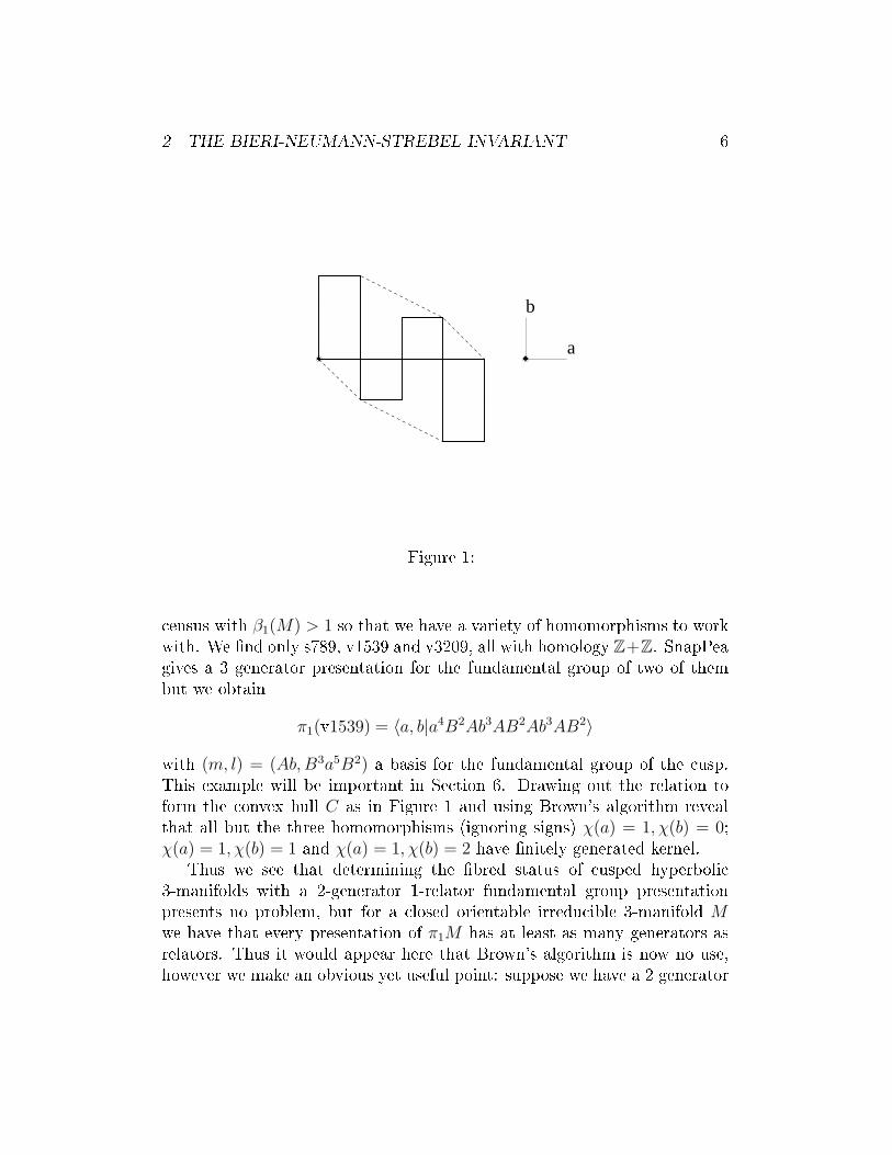
2 of this path and regard a homomorphismfrom G onto Z as a dire tional ve tor, with slope n/m for χ(a) = m, χ(b) = n.Then the homomorphisms with �nitely generated kernel are those with slopelying between (but not in luding) the slope of the outward pointing normalsof two su essive edges of C, provided that the joining vertex, whi h willbe a vertex of the path, has only been passed through on e when the pathhas been tra ed out, along with the verti al homomorphism if and only if Chas a unique horizontal side of length 1 on top, passed through only on e,and similarly for the horizontal homomorphism. In fa t a homomorphism isreally represented by two ve tors with the same slope, pointing in oppositedire tions, and both of these must satisfy the above onditions but again fora 3-manifold group the onditions on ea h of the two ve tors will be true orfalse together be ause C has rotational symmetry of order 2.Example 2.1Let us demonstrate this pro ess. We look for 1- usped 3-manifolds in the

2 THE BIERI-NEUMANN-STREBEL INVARIANT 6���

���

������

������

�����������������������

�����������

a

b

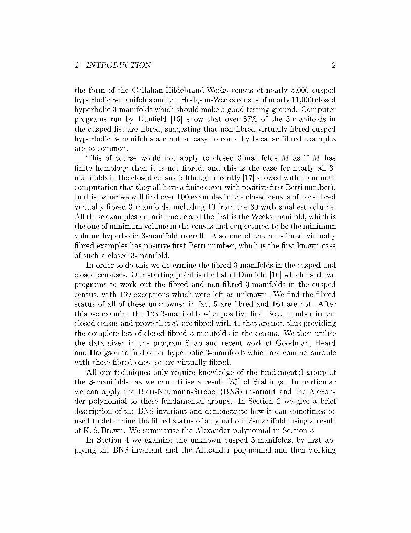
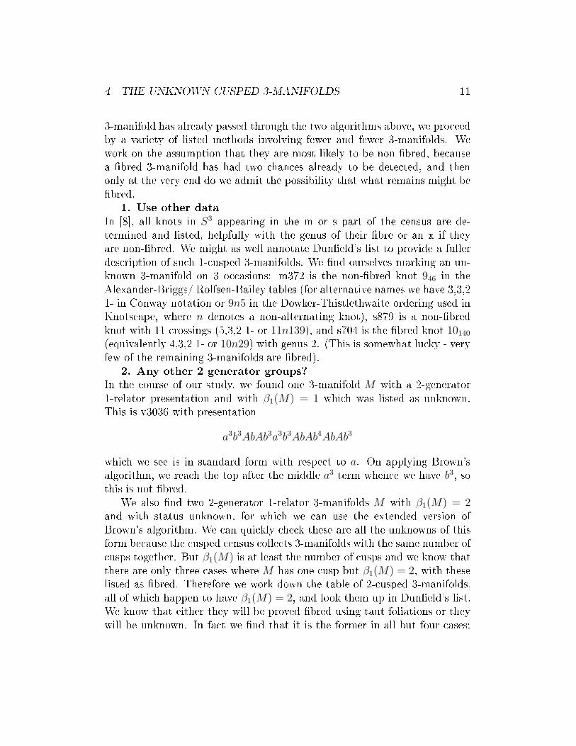
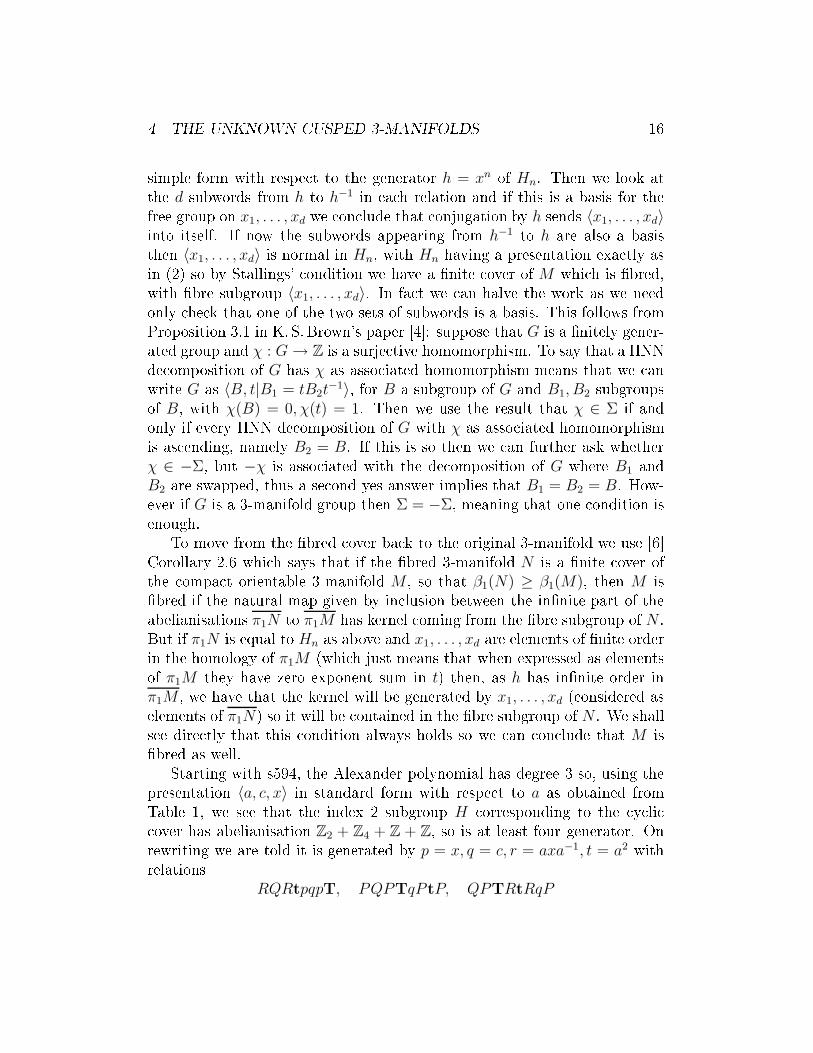
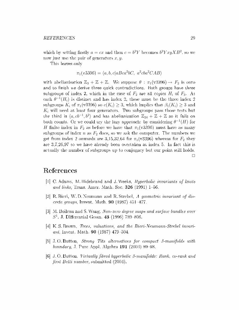
Figure 1: ensus with β1(M) > 1 so that we have a variety of homomorphisms to workwith. We �nd only s789, v1539 and v3209, all with homology Z+Z. SnapPeagives a 3 generator presentation for the fundamental group of two of thembut we obtainπ1(v1539) = 〈a, b|a4B2Ab3AB2Ab3AB2〉with (m, l) = (Ab, B3a5B2) a basis for the fundamental group of the usp.This example will be important in Se tion 6. Drawing out the relation toform the onvex hull C as in Figure 1 and using Brown's algorithm revealthat all but the three homomorphisms (ignoring signs) χ(a) = 1, χ(b) = 0;

χ(a) = 1, χ(b) = 1 and χ(a) = 1, χ(b) = 2 have �nitely generated kernel.Thus we see that determining the �bred status of usped hyperboli 3-manifolds with a 2-generator 1-relator fundamental group presentationpresents no problem, but for a losed orientable irredu ible 3-manifold Mwe have that every presentation of π1M has at least as many generators asrelators. Thus it would appear here that Brown's algorithm is now no use,however we make an obvious yet useful point: suppose we have a 2 generator

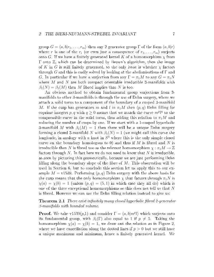
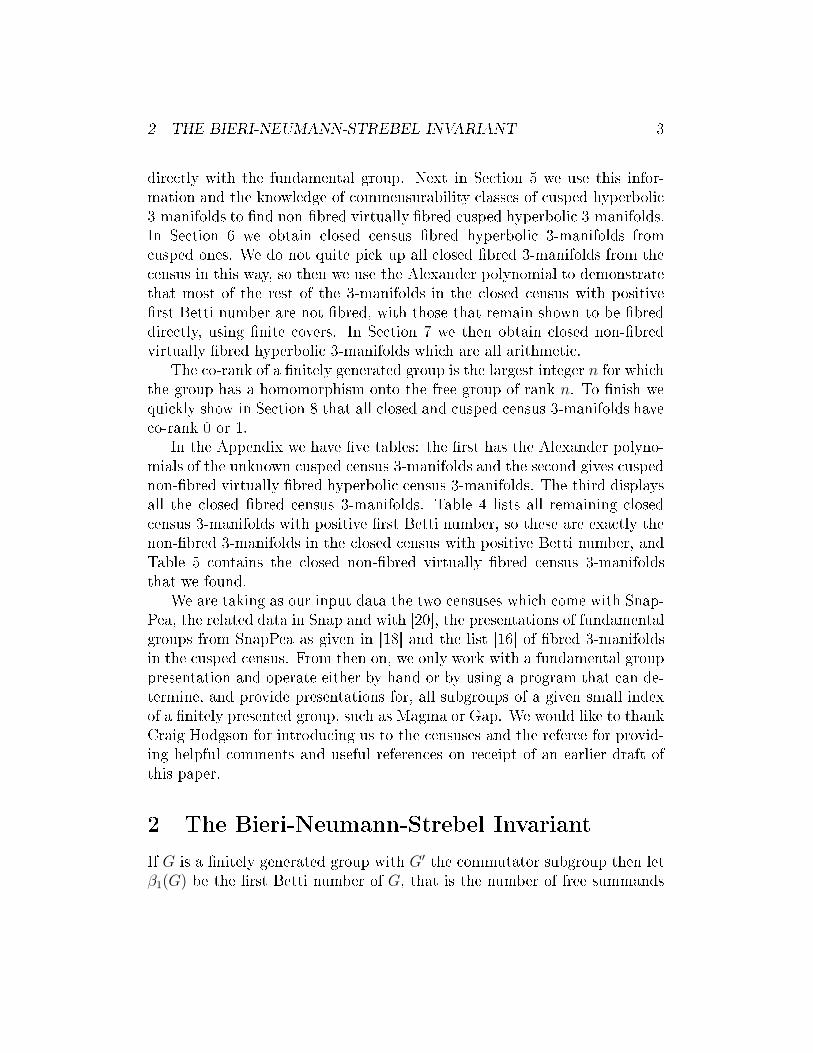
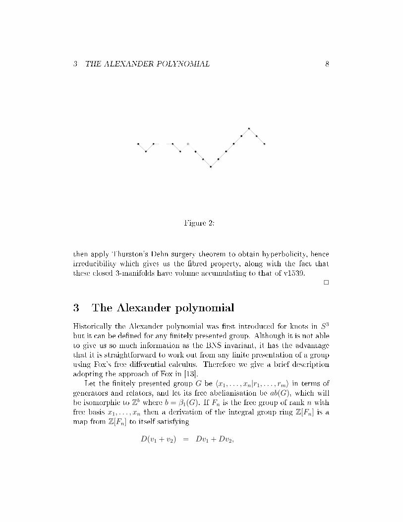
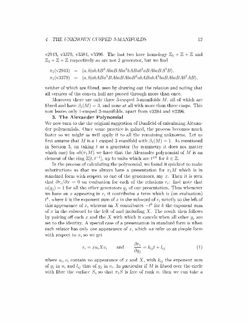
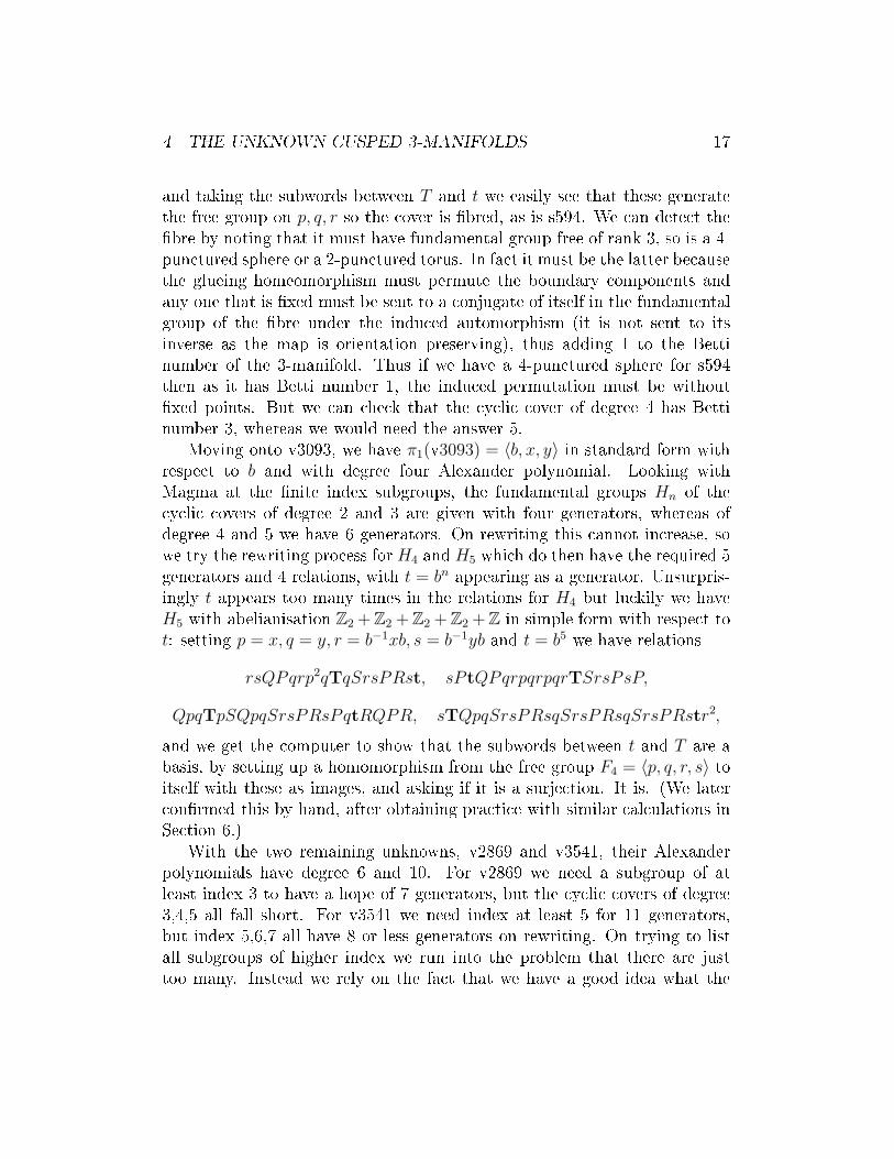
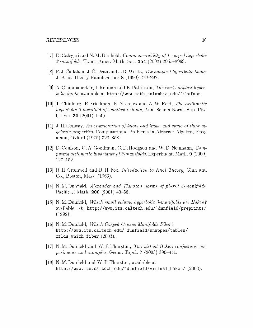
2 THE BIERI-NEUMANN-STREBEL INVARIANT 7group G = 〈a, b|r1, . . . , rm〉 then any 2 generator group Γ of the form 〈a, b|r〉where r is one of the ri (or even just a onsequen e of r1, . . . , rm) surje tsonto G. If we have a �nitely generated kernel K of a homomorphism χ fromΓ onto Z, whi h an be determined by Brown's algorithm, then the imageof K in G is still �nitely generated, so the only issue is whether χ fa torsthrough G and this is easily solved by looking at the abelianisations of Γ andG. In parti ular if we have a surje tion from any Γ = π1M to any G = π1Nwhere M and N are both ompa t orientable irredu ible 3-manifolds withβ1(N) = β1(M) then M �bred implies that N is too.An obvious method to obtain fundamental group surje tions from 3-manifolds to other 3-manifolds is through the use of Dehn surgery, where weatta h a solid torus to a omponent of the boundary of a usped 3-manifoldM . If the usp has generators m and l in π1M then (p, q) Dehn �lling for oprime integers p, q with q ≥ 0 means that we atta h the urve mplq to the ompressible urve in the solid torus, thus adding this relation to π1M andredu ing the number of usps by one. If we start with a 1- usped hyperboli 3-manifold M with β1(M) = 1 then there will be a unique Dehn surgeryforming a losed 3-manifold N with β1(N) = 1 (we might all this urve thelongitude, in analogy with a knot in S3 where this is the only simple losed urve on the boundary homologous to 0) and thus if M is �bred and N isirredu ible then N is �bred too as the relevant homomorphism χ : π1M → Zfa tors through N . In fa t here we do not need to know that N is irredu ible,as seen by pi turing this geometri ally, be ause we are just performing Dehn�lling along the boundary slope of the �bre of M . This observation will beused in Se tion 6, but to on lude this se tion let us apply this to our ex-ample M = v1539. Performing (p, q) Dehn surgery with the above basis forthe usp means that the only homomorphism χ that fa tors through π1N isχ(a) = χ(b) = 1 (unless (p, q) = (5, 1) in whi h ase they all do) whi h isone of the three ex eptional homomorphisms so this does not tell us that Nis �bred. However we an use the Dehn �lling relation instead to give us:Theorem 2.1 There exist in�nitely many losed hyperboli �bred 2-generator3-manifolds with bounded volume.Proof. We take v1539(p,1) and onsider Γ = 〈a, b|mpl〉 whi h surje ts ontoits fundamental group, with β1(Γ) also equal to 1 if p 6= 5. Taking thehomomorphism χ(a) = χ(b) = 1, we draw out the relation as in Figure 2,where we have an ellation along the dotted lines if p > 0 but we still havea unique maximum and minimum, hen e a �nitely generated kernel. We

3 THE ALEXANDER POLYNOMIAL 8������

������

����

���

���

���

���

��������

����

������

������

���

���

���

���

��������

���

���

���

���

��������

���

���

���

���

Figure 2:then apply Thurston's Dehn surgery theorem to obtain hyperboli ity, hen eirredu ibility whi h gives us the �bred property, along with the fa t thatthese losed 3-manifolds have volume a umulating to that of v1539.✷3 The Alexander polynomialHistori ally the Alexander polynomial was �rst introdu ed for knots in S3but it an be de�ned for any �nitely presented group. Although it is not ableto give us so mu h information as the BNS invariant, it has the advantagethat it is straightforward to work out from any �nite presentation of a groupusing Fox's free di�erential al ulus. Therefore we give a brief des riptionadopting the approa h of Fox in [13℄.Let the �nitely presented group G be 〈x1, . . . , xn|r1, . . . , rm〉 in terms ofgenerators and relators, and let its free abelianisation be ab(G), whi h willbe isomorphi to Z

b where b = β1(G). If Fn is the free group of rank n withfree basis x1, . . . , xn then a derivation of the integral group ring Z[Fn] is amap from Z[Fn] to itself satisfyingD(v1 + v2) = Dv1 + Dv2,

3 THE ALEXANDER POLYNOMIAL 9D(v1v2) = (Dv1)τ(v2) + v1Dv2where τ is the trivialiser: namely the ring homomorphism from Z[Fn] to Zwith τ(x) = 1 for all x ∈ Fn. It is a fa t that for ea h free generator xj thereexists a unique derivation Dj , also written ∂/∂xj , su h that ∂xi/∂xj = δij .To al ulate the �partial derivative� ∂w/∂xj for any w ∈ Fn we an use theformal rules

∂xi

∂xj

= δij ,∂x−1

i

∂xj

= −δijx−1i ,

∂(w1w2)

∂xj

=∂w1

∂xj

+ w1∂w2

∂xjwhere generally w2 will be the last letter in the word w = w1w2. Let γ bethe natural map from Z[Fn] to Z[G] and let α be the same from Z[G] toZ[ab(G)]. Then the Alexander matrix A of the presentation is the m × nmatrix with entries

aij = αγ

(

∂ri

∂xj

)

.We de�ne the kth elementary ideal Ek(A) to be the ideal of Z[ab(G)] gener-ated by the (n − k)× (n − k) minors of A if 0 < n − k ≤ m, thus under thisnotation k is the number of olumns that are deleted in forming the minors.Finally we de�ne the Alexander polynomial ∆G to be the generator (up tounits) of the smallest prin ipal ideal ontaining E1(A). To al ulate it we an hoose a basis (t1, . . . , tb) for ab(G), apply the free di�erential al ulus asabove and then form our matrix by evaluating. From here we an determinethe minors and their highest ommon fa tor. Of ourse this would be of littleuse if it depended on the presentation of G, but that it is invariant an beseen dire tly, as shown in [13℄ VII 4.5, by observing that applying a Tietzetransformation to a presentation does not hange the elementary ideals. Al-ternatively we have a topologi al de�nition of the Alexander polynomial, asdes ribed in [30℄ Se tion 2 or [14℄ Se tion 3: if X is a �nite CW- omplexwith π1X = G and f : X̃ → X is the regular over orresponding to thehomomorphism α from G to ab(G) then, taking p ∈ X, the Alexander mod-ule of X over the group ring Z[ab(G)] is H1(X̃, f−1(p); Z). The onne tionbetween the two approa hes is that by taking a free resolution of this module,we obtain the Alexander matrix as above (or rather under our notation itis the transpose of A). The Alexander polynomial ∆G is only de�ned up tounits, thus we an think of ∆G as a Laurent polynomial in Z[t±11 , . . . , t±1

b ] upto multipli ation by ±tk1

1 . . . tkb

b . Of ourse the a tual oe� ients depend onthis basis: sometimes there will be a natural hoi e, su h as for a b- omponent

4 THE UNKNOWN CUSPED 3-MANIFOLDS 10link in S3 where we would take meridians about ea h link. However we mightnot in general have this luxury, although we an always make a hange ofbasis if ne essary by putting ti = ski1

1 . . . skib

b with the ve tors (ki1, . . . , kib)making up an element of GL(b, Z).The utility of the Alexander polynomial for us here is the well knownresult, derived later, that if we have a ompa t 3-manifoldM with β1(M) = 1then its Alexander polynomial ∆M(t), in this ase a Laurent polynomialde�ned up to units and with ∆M(1/t) equal to ∆M (t) times a unit, is moni if M is �bred. We also have by Dun�eld a suitable generalisation of this forthe ase β1(M) ≥ 2 whi h we will use later: Theorem 5.1 of [14℄ states thatif the Alexander polynomial ∆M has no terms with oe� ients that are ±1then M is not �bred: more pre isely let N be the Newton polytope of ∆M ,that is the onvex hull in Rb of the points (k1, . . . , kb) where xk1

1 . . . xkb

b is a(non-trivial) term of ∆M . If none of the verti es of N have oe� ient ±1in ∆M then the Bieri-Neumann-Strebel invariant Σ of π1M is empty and sothere are no homomorphisms onto Z with �nitely generated kernel.4 The unknown usped 3-manifoldsWhen Dun�eld ran his programs on the 4815 3-manifolds in the usped ensus to see whi h were �bred, he �rst set up the omputer to apply Brown'salgorithm to any 3-manifold M with a 2 generator 1 relator presentation andwith β1(M) = 1. As we have seen in Se tion 2, this is guaranteed to terminateand give a de�nite yes/no answer. The program took about a minute in totalto omplete the 4105 examples given to it, 3653 of whi h were �bred and 452of whi h were not.The other algorithm that was applied was La kenby's idea of taut idealtriangulations. We will not be using this be ause our emphasis is on methodswhi h only require knowledge of the fundamental group; we note only thatthis pro ess will not tell us that the 3-manifold is non-�bred but it has norestri tion as above on the number of generators or relators. When this wasapplied to the usped ensus it produ ed 541 further �bred 3-manifolds, aswell as on�rming a lot of the 3-manifolds already known to be �bred byBrown's algorithm. There were some of these that it did not work for, andthe running time was a lot longer.Thus this leaves 169 usped 3-manifolds whose status is unknown. In thisse tion we will determine whether or not these are �bred. As any unknown

4 THE UNKNOWN CUSPED 3-MANIFOLDS 113-manifold has already passed through the two algorithms above, we pro eedby a variety of listed methods involving fewer and fewer 3-manifolds. Wework on the assumption that they are most likely to be non-�bred, be ausea �bred 3-manifold has had two han es already to be dete ted, and thenonly at the very end do we admit the possibility that what remains might be�bred.1. Use other dataIn [8℄, all knots in S3 appearing in the m or s part of the ensus are de-termined and listed, helpfully with the genus of their �bre or an x if theyare non-�bred. We might as well annotate Dun�eld's list to provide a fullerdes ription of su h 1- usped 3-manifolds. We �nd ourselves marking an un-known 3-manifold on 3 o asions: m372 is the non-�bred knot 946 in theAlexander-Briggs/ Rolfsen-Bailey tables (for alternative names we have 3,3,21- in Conway notation or 9n5 in the Dowker-Thistlethwaite ordering used inKnots ape, where n denotes a non-alternating knot), s879 is a non-�bredknot with 11 rossings (5,3,2 1- or 11n139), and s704 is the �bred knot 10140(equivalently 4,3,2 1- or 10n29) with genus 2. (This is somewhat lu ky - veryfew of the remaining 3-manifolds are �bred).2. Any other 2 generator groups?In the ourse of our study, we found one 3-manifold M with a 2-generator1-relator presentation and with β1(M) = 1 whi h was listed as unknown.This is v3036 with presentationa3b3AbAb3a3b3AbAb4AbAb3whi h we see is in standard form with respe t to a. On applying Brown'salgorithm, we rea h the top after the middle a3 term when e we have b3, sothis is not �bred.We also �nd two 2-generator 1-relator 3-manifolds M with β1(M) = 2and with status unknown, for whi h we an use the extended version ofBrown's algorithm. We an qui kly he k these are all the unknowns of thisform be ause the usped ensus olle ts 3-manifolds with the same number of usps together. But β1(M) is at least the number of usps and we know thatthere are only three ases where M has one usp but β1(M) = 2, with theselisted as �bred. Therefore we work down the table of 2- usped 3-manifolds,all of whi h happen to have β1(M) = 2, and look them up in Dun�eld's list.We know that either they will be proved �bred using taut foliations or theywill be unknown. In fa t we �nd that it is the former in all but four ases:

4 THE UNKNOWN CUSPED 3-MANIFOLDS 12v2943, v3379, v3384, v3396. The last two have homology Z5 + Z + Z andZ3 + Z + Z respe tively so are not 2 generator, but we �nd

π1(v2943) = 〈a, b|abAB2AbaBAba3bABab2aBAbaBA3B〉,

π1(v3379) = 〈a, b|abABa3BAbaBAbaB2abABabA3baBAbaBAb2AB〉,neither of whi h are �bred, seen by drawing out the relation and noting thatall verti es of the onvex hull are passed through more than on e.Moreover there are only three 3- usped 3-manifolds M , all of whi h are�bred and have β1(M) = 3, and none at all with more than three usps. Thisnow leaves only 1- usped 3-manifolds, apart from v3384 and v3396.3. The Alexander PolynomialWe now turn to the the original suggestion of Dun�eld of al ulating Alexan-der polynomials. On e some pra ti e is gained, the pro ess be omes mu hfaster so we might as well apply it to all the remaining unknowns. Let us�rst assume that M is a 1- usped 3-manifold with β1(M) = 1. As mentionedin Se tion 3, on taking t as a generator (by symmetry it does not matterwhi h one) for ab(π1M) we have that the Alexander polynomial of M is anelement of the ring Z[t, t−1], up to units whi h are t±k for k ∈ Z.In the pro ess of al ulating the polynomial, we found it qui kest to makesubstitutions so that we always have a presentation for π1M whi h is instandard form with respe t to one of the generators, say x. Then it is seenthat ∂ri/∂x = 0 on evaluation for ea h of the relations ri: �rst note thatα(gj) = 1 for all the other generators gj of our presentation. Thus wheneverwe have an x appearing in ri it ontributes a term whi h is (on evaluation)tk, where k is the exponent sum of x in the subword of ri stri tly to the left ofthis appearan e of x, whereas an X ontributes −tk for k the exponent sumof x in the subword to the left of and in luding X. The result then followsby pairing o� ea h x and the X with whi h it an els when all other gj areset to the identity. A spe ial ase of a presentation in standard form is whenea h relator has only one appearan e of x, whi h we refer to as simple formwith respe t to x, so we get

ri = xuiXvi and ∂ri

∂gj

= kijt + lij (1)where ui, vi ontain no appearan e of x and X, with kij the exponent sumof gj in ui and lij that of gj in vi. In parti ular if M is �bred over the ir lewith �bre the surfa e S, so that π1S is free of rank n, then we an take a

4 THE UNKNOWN CUSPED 3-MANIFOLDS 13presentation for π1M of the form 〈g1, . . . , gn, x|r1, . . . , rn〉, where ri = xgiXvi.Thus ∂ri/∂gj = δijt+lij so that the Alexander polynomial is the hara teristi polynomial of the n×n monodromy matrix −lij indu ed by the glueing map,and hen e is moni with degree n. Thus we look for non-moni Alexanderpolynomials in our al ulations and on lude that these 3-manifolds are non-�bred.In fa t in the ase of a 2-generator 1-relator group G with β1(G) = 1 thereis a straightforward onne tion between Brown's algorithm and the Alexan-der polynomial ∆G: the way to see this is to assume that G = 〈a, b|r〉 is instandard form with respe t to a and then on e the relation is drawn out wenote that the pro ess given of al ulating ∆G is merely that of ounting theappearan e of bs (whi h ontribute +1) and Bs (−1) in the relation at ea hlevel, and these values are the oe� ients of ∆G. In parti ular we obtain avery visual insight into how a 2-generator 1-relator knot ould have moni Alexander polynomial but not be �bred; the relation must rea h its peakmore than on e but all but one of them must an el out. Another example isthat we an easily re ognise 1-pun tured torus bundles amongst hyperboli 3-manifolds with 2-generator 1-relator fundamental groups; if π1M = 〈a, b|r〉with r redu ed and y li ally redu ed is the fundamental group of a hyper-boli 3-manifold M then M is a 1-pun tured torus bundle if and only ifβ1(M) = 1 and the relation lies on only three levels with a unique maximumand minimum when drawn out in standard form. This is be ause hyperboli 1-pun tured torus bundles M must have β1(M) = 1 and the other onditionis exa tly what is needed to on lude that M �bres with Alexander polyno-mial of degree 2, thus the �bre must be a 1-pun tured torus or a 3-pun turedsphere, but the bundle is not hyperboli in the latter ase. Now 1-pun turedtorus bundles might need three generators, as seen by looking at their homol-ogy, but we annot on lude in general that a hyperboli 3-manifold M is a1-pun tured torus bundle if it has a moni quadrati Alexander polynomial.However, if we already know that M is �bred then we an.Returning to the unknown usped 3-manifolds M , all our al ulationsare on 3 generator 2 relator groups so that we put π1M = 〈g1, g2, x|r1, r2〉into standard form with respe t to x and then we al ulate the determinantof the 2 × 2 matrix ∂ri/∂gj . If furthermore our two relations are in simpleform with respe t to x, that is as in (1) whi h happens often, then we antake a short ut as the Alexander polynomial will be (at most) quadrati . We al ulate det(kij) whi h will be the oe� ient of t2, and then det(lij) whi his the onstant. These must be equal whi h a ts as a useful he k, given

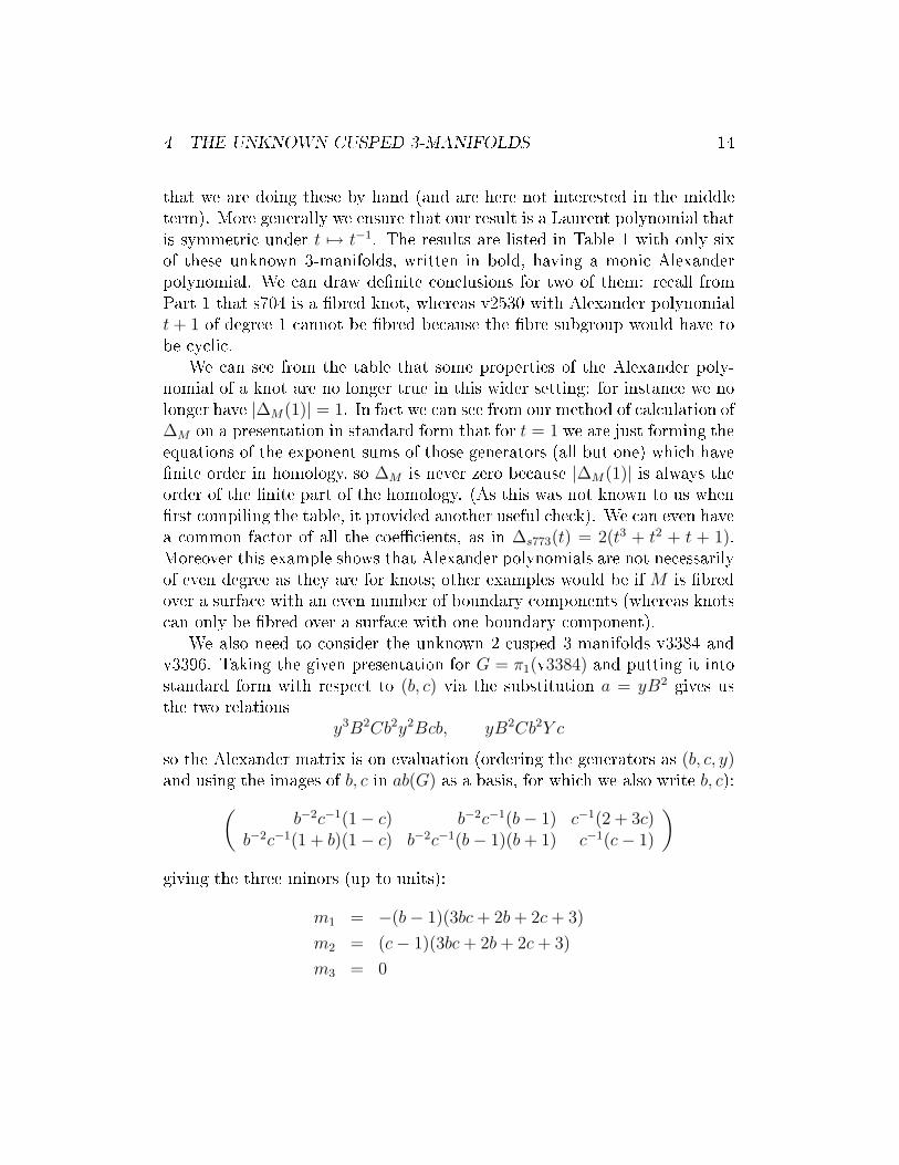
4 THE UNKNOWN CUSPED 3-MANIFOLDS 14that we are doing these by hand (and are here not interested in the middleterm). More generally we ensure that our result is a Laurent polynomial thatis symmetri under t 7→ t−1. The results are listed in Table 1 with only sixof these unknown 3-manifolds, written in bold, having a moni Alexanderpolynomial. We an draw de�nite on lusions for two of them: re all fromPart 1 that s704 is a �bred knot, whereas v2530 with Alexander polynomialt + 1 of degree 1 annot be �bred be ause the �bre subgroup would have tobe y li .We an see from the table that some properties of the Alexander poly-nomial of a knot are no longer true in this wider setting: for instan e we nolonger have |∆M(1)| = 1. In fa t we an see from our method of al ulation of∆M on a presentation in standard form that for t = 1 we are just forming theequations of the exponent sums of those generators (all but one) whi h have�nite order in homology, so ∆M is never zero be ause |∆M(1)| is always theorder of the �nite part of the homology. (As this was not known to us when�rst ompiling the table, it provided another useful he k). We an even havea ommon fa tor of all the oe� ients, as in ∆s773(t) = 2(t3 + t2 + t + 1).Moreover this example shows that Alexander polynomials are not ne essarilyof even degree as they are for knots; other examples would be if M is �bredover a surfa e with an even number of boundary omponents (whereas knots an only be �bred over a surfa e with one boundary omponent).We also need to onsider the unknown 2- usped 3-manifolds v3384 andv3396. Taking the given presentation for G = π1(v3384) and putting it intostandard form with respe t to (b, c) via the substitution a = yB2 gives usthe two relations

y3B2Cb2y2Bcb, yB2Cb2Y cso the Alexander matrix is on evaluation (ordering the generators as (b, c, y)and using the images of b, c in ab(G) as a basis, for whi h we also write b, c):(

b−2c−1(1 − c) b−2c−1(b − 1) c−1(2 + 3c)b−2c−1(1 + b)(1 − c) b−2c−1(b − 1)(b + 1) c−1(c − 1)

)giving the three minors (up to units):m1 = −(b − 1)(3bc + 2b + 2c + 3)

m2 = (c − 1)(3bc + 2b + 2c + 3)

m3 = 0

4 THE UNKNOWN CUSPED 3-MANIFOLDS 15thus the Alexander polynomial is 3bc + 2b + 2c + 3. Similarly the givenpresentation for π1(v3396) is already in standard form with respe t to (b, c) soadopting the same notation we �nd its Alexander polynomial is 2(b−1)(c−1).As mentioned at the end of Se tion 3, this gives us that v3384 and v3396 arenot �bred.4. Fibred after all?We now have to fa e up to the four remaining unknowns s594, v2869, v3093,v3541, and should take seriously the possibility that they are �bred. If sothen we must have a presentationπ1M = 〈t, a1, . . . , ar|tait

−1 = wi〉 (2)where ea h wi is a word in a1, . . . , ar equal to φ∗(ai), for φ∗ the indu edautomorphism of π1M obtained from the glueing homeomorphism φ. Thesewords, as well as a1, . . . , ar, generate the �bre subgroup F whi h will befree of rank r equal to the degree of the Alexander polynomial. Su h apresentation will need more than the three generators that we have beengiven for our 3-manifolds, and it might not be easy to move between the twodi�erent presentations. However some points are lear: as β1(M) = 1, theelements of F are pre isely those in π1M with �nite order in homology, andin looking for a andidate for t, any element generating the in�nite part ofthe homology an be used be ause we an repla e t with kt for any k ∈ F ,and wj with kwjk−1 in the presentation above.In order to get round the number of generators, we use �nite overs. If

π1M is �bred then we will have the y li overs π1Mn of degree n, generatedby the r + 1 elements tn, a1, . . . , ar and with r relations, whi h orrespondto the glueing homeomorphisms φn. When we ask Magma for a presentationof an index n subgroup of our 3 generator 2 relator group, it employs theReidermeister-S hreier pro ess whi h will obtain a presentation of 2n+1 gen-erators and 2n relators, but some of these might be redundant so the output ould be less. Therefore we start with our unknown π1M , using a presenta-tion in standard form with respe t to a generator x. We ask Magma for (thegenerators of) subgroups of index n (it gives a subgroup in ea h onjuga y lass) and pi k the y li over Hn, that is the one with the exponent sum ofx ≡ 0 mod n (whi h is easy to spot by he king this ondition holds for allof the given generators). We then demand a presentation of Hn, hoping notonly that it is d + 1 generator and d relator for d the degree of the Alexan-der polynomial, but also that the presentation 〈h, x1, . . . , xd|r1, . . . , rd〉 is in

4 THE UNKNOWN CUSPED 3-MANIFOLDS 16simple form with respe t to the generator h = xn of Hn. Then we look atthe d subwords from h to h−1 in ea h relation and if this is a basis for thefree group on x1, . . . , xd we on lude that onjugation by h sends 〈x1, . . . , xd〉into itself. If now the subwords appearing from h−1 to h are also a basisthen 〈x1, . . . , xd〉 is normal in Hn, with Hn having a presentation exa tly asin (2) so by Stallings' ondition we have a �nite over of M whi h is �bred,with �bre subgroup 〈x1, . . . , xd〉. In fa t we an halve the work as we needonly he k that one of the two sets of subwords is a basis. This follows fromProposition 3.1 in K. S.Brown's paper [4℄: suppose that G is a �nitely gener-ated group and χ : G → Z is a surje tive homomorphism. To say that a HNNde omposition of G has χ as asso iated homomorphism means that we anwrite G as 〈B, t|B1 = tB2t−1〉, for B a subgroup of G and B1, B2 subgroupsof B, with χ(B) = 0, χ(t) = 1. Then we use the result that χ ∈ Σ if andonly if every HNN de omposition of G with χ as asso iated homomorphismis as ending, namely B2 = B. If this is so then we an further ask whether

χ ∈ −Σ, but −χ is asso iated with the de omposition of G where B1 andB2 are swapped, thus a se ond yes answer implies that B1 = B2 = B. How-ever if G is a 3-manifold group then Σ = −Σ, meaning that one ondition isenough.To move from the �bred over ba k to the original 3-manifold we use [6℄Corollary 2.6 whi h says that if the �bred 3-manifold N is a �nite over ofthe ompa t orientable 3-manifold M , so that β1(N) ≥ β1(M), then M is�bred if the natural map given by in lusion between the in�nite part of theabelianisations π1N to π1M has kernel oming from the �bre subgroup of N .But if π1N is equal to Hn as above and x1, . . . , xd are elements of �nite orderin the homology of π1M (whi h just means that when expressed as elementsof π1M they have zero exponent sum in t) then, as h has in�nite order inπ1M , we have that the kernel will be generated by x1, . . . , xd ( onsidered aselements of π1N) so it will be ontained in the �bre subgroup of N . We shallsee dire tly that this ondition always holds so we an on lude that M is�bred as well.Starting with s594, the Alexander polynomial has degree 3 so, using thepresentation 〈a, c, x〉 in standard form with respe t to a as obtained fromTable 1, we see that the index 2 subgroup H orresponding to the y li over has abelianisation Z2 + Z4 + Z + Z, so is at least four generator. Onrewriting we are told it is generated by p = x, q = c, r = axa−1, t = a2 withrelations

RQRtpqpT, PQPTqP tP, QPTRtRqP

4 THE UNKNOWN CUSPED 3-MANIFOLDS 17and taking the subwords between T and t we easily see that these generatethe free group on p, q, r so the over is �bred, as is s594. We an dete t the�bre by noting that it must have fundamental group free of rank 3, so is a 4-pun tured sphere or a 2-pun tured torus. In fa t it must be the latter be ausethe glueing homeomorphism must permute the boundary omponents andany one that is �xed must be sent to a onjugate of itself in the fundamentalgroup of the �bre under the indu ed automorphism (it is not sent to itsinverse as the map is orientation preserving), thus adding 1 to the Bettinumber of the 3-manifold. Thus if we have a 4-pun tured sphere for s594then as it has Betti number 1, the indu ed permutation must be without�xed points. But we an he k that the y li over of degree 4 has Bettinumber 3, whereas we would need the answer 5.Moving onto v3093, we have π1(v3093) = 〈b, x, y〉 in standard form withrespe t to b and with degree four Alexander polynomial. Looking withMagma at the �nite index subgroups, the fundamental groups Hn of the y li overs of degree 2 and 3 are given with four generators, whereas ofdegree 4 and 5 we have 6 generators. On rewriting this annot in rease, sowe try the rewriting pro ess for H4 and H5 whi h do then have the required 5generators and 4 relations, with t = bn appearing as a generator. Unsurpris-ingly t appears too many times in the relations for H4 but lu kily we haveH5 with abelianisation Z2 + Z2 + Z2 + Z2 + Z in simple form with respe t tot: setting p = x, q = y, r = b−1xb, s = b−1yb and t = b5 we have relations

rsQPqrp2qTqSrsPRst, sP tQPqrpqrpqrTSrsPsP,

QpqTpSQpqSrsPRsPqtRQPR, sTQpqSrsPRsqSrsPRsqSrsPRstr2,and we get the omputer to show that the subwords between t and T are abasis, by setting up a homomorphism from the free group F4 = 〈p, q, r, s〉 toitself with these as images, and asking if it is a surje tion. It is. (We later on�rmed this by hand, after obtaining pra ti e with similar al ulations inSe tion 6.)With the two remaining unknowns, v2869 and v3541, their Alexanderpolynomials have degree 6 and 10. For v2869 we need a subgroup of atleast index 3 to have a hope of 7 generators, but the y li overs of degree3,4,5 all fall short. For v3541 we need index at least 5 for 11 generators,but index 5,6,7 all have 8 or less generators on rewriting. On trying to listall subgroups of higher index we run into the problem that there are justtoo many. Instead we rely on the fa t that we have a good idea what the

4 THE UNKNOWN CUSPED 3-MANIFOLDS 18generators of these parti ular y li overs should look like: if our originalfundamental group G = 〈u, v, t〉 is in standard form with respe t to t thenHn has a generating set tiut−i, tjvt−j , tn for various values of i, j, and onguessing su h a generating set we an ask for the index of Hn in G to he kwe are orre t. Therefore, as we have π1(v2869) = 〈x, y, z〉 in standard formwith respe t to x, we look at the subgroup H generated by xiyx−i, xjzx−j , xnfor i = 0,±1,±2, j = 0,±1,−2 and n = 6. We do indeed �nd that H hasindex 6 in G with abelianisation Z13 + Z and on rewriting we get the magi 7 generator 6 relator presentation, with generators

(a, b, c, d, e, f, t) = (y, z, xyX, Xzx, x2yX2, x2zX2, x6)whi h is in simple form with respe t to t and with the following free basis tobe found between T and t:(F 2eBdBaceBabf, Fef, FBabFeBAbEceBabf, F 2eBdBaeBadBaCAbDbEf 2,

F 2eBdBacAbDbEFeBdBabFeBAbEcef, F 2eBdBacAbDbf).Finally for π1(v3541) = 〈x, y, z〉 in standard form with respe t to z, wetry the subgroups Hn generated by zixz−i, zjyz−j, z−n for i = 0,±1,±2,j = 0,±1,±2 and with n running from 8 to 15. All have the orre t index:for n = 8, 9, 10 we get too few generators again on rewriting but for the othern we get exa tly the required 11 generators and 10 relations. For n = 11 thepresentation is in standard but not in simple form with respe t to t = zn,for the others it is indeed in simple form but with the relations be omingprogressively longer, so we take n = 12. The subgroup has abelianisationZ7 + Z35 + Z + Z + Z with the other 10 generators(a, b, c, d, e, f, g, h, i, j) = (x, y, zxZ, zyZ, Zxz, Zyz, z2xZ2, Z2yz2, Z3yz3, Z4yz4).Happily we �nd a basis between t and T of the form below:(WJ, jwJ, jwfBAweJiCIjaI, jI, jEWaJ, iAJicI, jbDIjEWabFeWJ,

iH, hFEfBAweJidBAweJ, hCIhgFEfBAweJidFWJ)where w = bDCIjaIhGHicH .We have already mentioned in Part 1 the paper [8℄ whi h lists the knotsin S3 from the m and s part of the ensus. Re ently we were informedof [9℄ whi h does the same for the v se tion. Although the table does not

5 VIRTUALLY FIBRED CUSPED 3-MANIFOLDS 19tell us whi h of these knots is �bred (and now does not need to, in lightof this se tion and Dun�eld's list), we �nd in it eight of our unknown 1- usped 3-manifolds in luding the last three to be dealt with. The des riptionsgiven of these three knots are: v3093 is 16n245346 in Knots ape (if it hadbeen an alternating knot then our work would have been in vain be ause wewould have been able to on lude that it was �bred just from the Alexanderpolynomial). Then v2869 and v3541 are given in terms of a (non-alternating)Dowker-Thistlethwaite ode with 18 and 21 rossings respe tively. Althoughthese may not be the minimal rossing numbers, they must ome pretty losebe ause Knots ape tells us they are not in its ensus whi h goes up to 16 rossings. Also we now know the topologi al type of their �bres, be ause asknots in S3 their �bres will have one boundary omponent and genus halfthe degree of the Alexander polynomial.In on lusion we have:Proposition 4.1 The proportion of �bred 3-manifolds in the (orientable) usped ensus is exa tly 4199/4815=0.87206645898...5 Virtually �bred usped 3-manifoldsAs we now know all �bred 3-manifolds in the usped ensus, we turn tohow we an �nd non-�bred virtually �bred examples. The ru ial point isthat a non-�bred hyperboli 3-manifold that is ommensurable with a �bredhyperboli 3-manifold is itself virtually �bred, by onsidering the ommon�nite over, so that the property of being virtually �bred is onstant on ommensurability lasses. Therefore we ought in prin iple to be able touse our �bred 3-manifolds to obtain non-�bred ommensurable examples M .The �rst ase that omes to mind is when π1M is arithmeti , whi h in the usped ase means that it has integral tra es and the invariant tra e �eldis an imaginary quadrati number �eld. Here two arithmeti fundamentalgroups will be ommensurable if they have the same invariant tra e �eld, soon �nding a �bred example we have that all arithmeti hyperboli usped 3-manifolds with this imaginary quadrati number �eld will be virtually �bred.However re ently the paper [20℄ gives an algorithm that determines the ommensurator of any non-arithmeti usped hyperboli 3-manifold and itis then applied to �nd ommensurability lasses for the 3-manifolds in the usped ensus, as well as for hyperboli knots and links for up to twelve ross-ings. Therefore it is worth looking at the 616 non-�bred ensus 3-manifolds

5 VIRTUALLY FIBRED CUSPED 3-MANIFOLDS 20to see if any are in the same ommensurability lass as a �bred 3-manifold,given that we now an re ognise all �bred 3-manifolds in the usped en-sus. Doing this gives us 86 non-�bred virtually �bred usped hyperboli 3-manifolds as listed in Table 2 (a few of whi h would have been known be-fore, see for instan e [7℄ and [22℄). Most of the �bred 3-manifolds ertifyingthat these examples are virtually �bred have more than one usp; moreoverthe four non-�bred 3-manifolds with 2 usps (v2943, v3379, v3384, v3396)all appear thus we an say that any hyperboli 3-manifold in the ensus withmore than one usp is virtually �bred.We an further add to this table be ause the data we are using in ludes ommensurability lasses of knots and links in S3. However, rather thanjust looking for �bred knots and links, we use the re ent result [36℄ that all2-bridge knots and links are virtually �bred. We an identify 2-bridge knotsand links in the tables by their Conway notation. This gives us another 51examples to add to our table. Most of these are themselves non-�bred 2-bridge knots or next to one in the ensus, although a few are shown virtually�bred by being ommensurable with a 2-bridge knot that is not in the usped ensus. We have also two links not from the ensus that make an appearan e:there is the �bred 2-bridge link 8a31 (or 824 in the tables) with Conwaynotation 323 and the non-�bred 2-bridge link 10a171 with Conway notation262 (in fa t the 2- usped 3-manifolds v2943 and v3379 mentioned above arealso 2-bridge links identi�able as 7a11 or 72

3 or 232 and 8a24 or 826 or 242respe tively).One amusing onsequen e of the ubiquity of 2-bridge knots amongst thosewith low rossing number is that just by striking out from the tables of knotswith nine rossings or less the 2-bridge knots and the knots with moni Alexander polynomial (whi h for these rossing numbers will be �bred), wesee that the only ones left that are not known to be virtually �bred arethe ten knots 815 (8a2), 916 (9a25), 925 (9a4), 935 (9a40), 937 (9a18), 938(9a30), 939 (9a32), 941 (9a29), 946 (9n5) and 949 (9n8). There may be a fewmore usped 3-manifolds in the ensus that ould be added to this table byhaving full knowledge of whi h knots and links up to twelve rossings are�bred, but ertainly some non-�bred 3-manifolds are listed alone in their ommensurability lass so this pro ess would not �nish the job o�. Howeverwe have pushed the number of virtually �bred 3-manifolds in the usped ensus up to 4336 whi h is a fra tion over 90%.

6 CLOSED FIBRED HYPERBOLIC 3-MANIFOLDS 216 Closed �bred hyperboli 3-manifoldsIn the Hodgson-Weeks ensus [23℄ of losed hyperboli 3-manifolds, onsistingof just under 11,000 examples (the number given is 11,031 but there are a fewdupli ations), nearly all have �nite �rst homology: only 127 have �rst Bettinumber 1 and above that there is but one 3-manifold with �rst Betti number2. Thus only these few spe ial losed 3-manifolds have a han e of being�bred, but in fa t there is a reason why it is likely to be a good han e. All3-manifolds in the losed ensus are obtained by Dehn surgery on 1- usped3-manifolds from the usped ensus and this pro ess either preserves the �rstBetti number or redu es it by one. Therefore the losed 3-manifolds M withβ1(M) = 1 ome from 1- usped 3-manifolds M ′ with β1(M

′) = 1 or 2. Butthere are only 3 examples of the latter and moreover we now know that thevast majority of 3-manifolds M ′ in the usped ensus are �bred. If so and ifβ1(M

′) = 1 then we have mentioned in Se tion 2 that M must be �bred too.In addition the one losed 3-manifold M with β1(M) = 2 happens to bev1539(5,1), so it is irredu ible and therefore Se tion 2 tells us it is �bred,as well as v1539(-5,1) whi h also appears in the ensus. Otherwise we workthrough the losed 3-manifolds M with β1(M) = 1, seeing if they are surgeryon a 1- usped 3-manifold M ′ that is listed as �bred but whi h is not oneof the three spe ial ases with β1(M′) = 2. In this way we �nd 80 further losed �bred 3-manifolds in the ensus whi h is a big proportion of thosewith positive �rst Betti number. The results are listed in Table 3.As for the remaining 46 losed 3-manifolds M with β1(M) > 0 in the ensus, we al ulate the Alexander polynomial of the given fundamentalgroup presentation whi h proves that all but �ve are not �bred. As we have

β1(M) = 1, we an do this in exa tly the same way as we did for 1- usped3-manifolds, and indeed it is still invariant under t 7→ t−1. Moreover it isagain the ase that if M is �bred over the ir le then ∆M must be moni ,and here the degree of ∆M must be twi e the genus of the �bre: we an seethis from (2) by noting that we need to add a relation for the losed surfa e,but this results in an extra row of zeros on appli ation of the free di�erential al ulus.Our fundamental groups are usually 2 generator, 2 relator with a few 3generator, 3 relator examples but we an use short uts that might avoid al ulating the whole Alexander polynomial. If we have π1M = 〈g, x|r1, r2〉,whi h we always assume is in standard form with respe t to x, then ∂ri/∂x =0, thus the Alexander polynomial is the highest ommon fa tor of the two

6 CLOSED FIBRED HYPERBOLIC 3-MANIFOLDS 22polynomials ∂ri/∂g. But as we know M is hyperboli , if it is �bred then thismust be by a surfa e of genus at least two, so the Alexander polynomial mustbe moni of even degree at least four. We thus al ulate only one polynomial orresponding to the ni est looking relation and if this does not have su ha fa tor then we are done. It turns out, as seen in Table 4, that in all butthree of the ases the polynomial obtained was quarti , non-moni and nota s alar multiple of a moni quarti polynomial, so these 3-manifolds arenot �bred. The three ex eptions were that with v2018(-4,1) a quinti wasobtained whi h fa tors as (t + 1)(t2 + 1)(2t2 − 3t + 2) so this is non-�bred,indeed the other relation gives (t2 + t+1)(t2 +1)(2t2−3t+2) so the last twofa tors are the Alexander polynomial. This 3-manifold will feature again inSe tion 7 where we will �nd that it is virtually �bred. The next ex eptionthat needs to be he ked is v2238(-5,1), but here a quinti is obtained thatfa tors into irredu ibles as (t + 1)(2t4 − t3 − t + 2) so this is �ne. The onlyother problem is v3183(-3,2) whi h yields 2(t4 + 1) so we worry that t4 + 1might be the Alexander polynomial, but looking at the other relation we seethis annot be the ase.As for the three 3 generator ases, we similarly take 2 relations and al- ulate the relevant 2 × 2 determinant; these are all quarti and present noproblems. We treat those losed 3-manifolds whi h ome from the three spe- ial 1- usped 3-manifolds s789, v1539, v3209 separately. For the 2 generatorgroup π1(v1539) we have already stated in Se tion 2 that (Ab, B3a5B2) is abasis for the usp, so taking the relation (Ab)p(B3a5B2)q from v1539(p, q)and substituting a = bx so that it is in standard form with respe t to b givesus the polynomialqt4 + qt3 + (q − p)t2 + qt + qwhereas the original relation gives 0, so this is the Alexander polynomial(ex ept for (p, q) = (5, 1) where β1(M) = 2) and q 6= 0, 1 implies that the3-manifold is not �bred. We now have built up the omplete pi ture for thesehyperboli 3-manifolds as we saw in Se tion 2 that v1539(p, 1) is �bred (andit is lear that v1539(1, 0) has y li fundamental group so is not hyperboli );in parti ular v1539(5,2) that appears in Table 4 is non-�bred. Similarly fors789 we have (abc2, a3cbcA3C) as a basis for the usp and we take this Dehn�lling relation for s789(p, q) along with either one of the two original relations(they result in the same polynomials). We put c = Ax and b = ya to get tworelations in standard form with respe t to a and this yields the Alexander

6 CLOSED FIBRED HYPERBOLIC 3-MANIFOLDS 23polynomialqt4 − qt3 + (p + q)t2 − qt + qso on e again it is not �bred if q 6= 0 or 1 (with π1s789(1, 0) = Z again), sort-ing out s789(-5,2). Finally we do this for v3209, with basis (aCbc2, aCacAcAC)and either one of the original relations, setting a = Cx so that we are in stan-dard form with respe t to c. For v3209(p, q) we have π1v3209(1, 0) = Z andAlexander polynomial

qt4 − 2qt3 + (p + 2q)t2 − 2qt + qwhi h reveals nine losed 3-manifolds in Table 4 as not �bred when q > 1.We guess that s789(p, 1) and v3209(p, 1) are all �bred; not only wouldthis �t into the same pattern as v1539 but we have already seen in Table 3that s789(p, 1) for p = ±5 and v3209(p, 1) for p = ±3 are �bred as they havealternative des riptions as Dehn �llings on 3-manifolds M with β1(M) = 1.We an say that if so, they must have �bres of genus two.However this still leaves in the ensus �ve 3-manifolds v3209(p, 1) forp = ±4,±5, 6 whose status is unknown. In the hope of �nishing this o�, it isworth looking for y li overs whi h we an show are �bred, just as we didwith the remaining 1- usped 3-manifolds in Se tion 4. Happily this worksfor all �ve thus the �bred status of every 3-manifold in the losed ensus isknown: 87 are �bred, 41 are non-�bred with β1(M) = 1 and the rest arenon-�bred with β1(M) = 0. We summarise the details so as to allow the laims to be he ked. All �ve ases are very similar. We put a = xC in ourpresentation and then we have fundamental group 〈a, c, x〉 in standard formwith respe t to c. We know the �bre would be a genus 2 surfa e so we areafter a 5 generator presentation. In ea h ase the y li overs of degree 2and 3 have too few generators (at least on rewriting) but Magma tells usthat the y li over of degree 4 yields a 5 generator presentation of the form〈g1, g2, g3, g4, t〉 for

(g1, g2, g3, g4, t) = (x, cxC, Cbc, c2xC2, c4)

(cbC, cxC, Cbc, c2xC2, c4)

(x, cxC, Cbc, Cxc, c4)where the �rst option is for p = 4,±5, the se ond for p = −4 and the thirdfor p = 6. As t = c4 has in�nite order but all gi have �nite order in thehomology of M , we know the presentation obtained in ea h ase will be in

6 CLOSED FIBRED HYPERBOLIC 3-MANIFOLDS 24standard form with respe t to t. What is most promising is that we always�nd the �rst relation given has no appearan e of t at all (but t does appearin the others). Indeed in all but p = −4 this relation is of length 8 with ea hg±1

i appearing on e, whi h is a relation de�ning the losed surfa e of genus 2.For p = −4 it is of length 12 but as a onsequen e of showing the 3-manifoldis �bred, this relation has to de�ne the genus 2 losed surfa e group as well.We then pro eed just as in Se tion 4 by looking at the subwords from tto T , or from T to t (we did in fa t do both). In all but p = −4 we are givenmore than 5 relations so we are looking for generating sets for the free groupon g1, g2, g3, g4 rather than a free basis, but we always pro eed by taking ourn subwords (where n an be 4, 5 or 6) and using the shorter subwords tokno k letters o� the longer subwords until we have ea h generator gi. We dothis by hand: for p = ±4 the relations are in simple form with respe t to t.For p = 5 the fourth and sixth of the seven relations have two appearan esof t (whereas the �rst relation has none and the rest have one). They areof the form tw1Tw2tu1Tu2 and v1tv2TW2tW1T for uj, vj, wj words in the giso we an on atenate them to obtain a relation in simple form whi h wenow use. For p = −5 we have six relations with the third, �fth and sixth inthis double form but ea h pair of these three an be on atenated as aboveto obtain �ve relations in simple form. Then for p = 6 we are given sevenrelations with the last three simple. We put together the se ond and �fth toobtain tsT , where s = Cxc, whi h we an now insert into the three relationsin double form, resulting in enough relations in simple form to obtain all thegenerators.Finally to show the original 3-manifolds are �bred, we look at the homol-ogy of the degree 4 overs. These are listed below and all have �rst Bettinumber 1 so we are done.3-manifold Homology of overv3209(4,1) Z2 + Z4 + Z4 + Z24 + Zv3209(-4,1) Z2 + Z4 + Z4 + Z8 + Zv3209(5,1) Z5 + Z5 + Z65 + Zv3209(-5,1) Z5 + Z5 + Z15 + Zv3209(6,1) Z2 + Z6 + Z6 + Z42 + ZThus we now know all the �bred 3-manifolds in the losed ensus. Wehave seen that if M ′ is a 1- usped �bred 3-manifold with β1(M

′) = 1 andwe Dehn �ll along its longitude to reate M then M is �bred. We might

7 VIRTUALLY FIBRED CLOSED 3-MANIFOLDS 25expe t that if instead M ′ is non-�bred then M is not but this is unlikely tobe true in full generality. For instan e let us take the 1- usped 3-manifoldm137 (an interesting example as it has a quadrati imaginary invariant tra e�eld but is the �rst in the usped ensus not to have integral tra es). It is not�bred (indeed is not known to be virtually �bred) and is a knot in an integralhomology sphere. We �nd from SnapPea a fundamental group presentationand basis for the usp, whereupon it is easily seen that the group Z is obtainedon Dehn �lling of the longitude thus (assuming Poin aré) M = S2×S1 and sois �bred. (Another 3-manifold M ′ in the ensus with β1(M′) = 1 where Z isobtained on Dehn �lling is the non-�bred s783, as well as the three 1- uspedexamples with β1(M

′) = 2.) However if M ′ is the exterior of a non-trivialknot in S3 then Gabai shows in [19℄ that π1M 6= Z. He goes on to provethat for knots M ′ is �bred if and only if M is, in whi h ase the �bres havethe same genus. Although this seems useful, and ertainly we have in ludedin Table 3 the genus of the �bre of those losed 3-manifolds M where thegiven M ′ is a knot exterior in S3, there was only one ase where this wouldhave proved M is non-�bred: s862 is the non-�bred knot 84 so s862(7,1) inTable 4 is not �bred. In trying to generalise Gabai's result, a onje ture ofBoileau (Problem 1.80 (C) in the Kirby problem list [27℄) states that if K isa null-homotopi knot in a losed orientable irredu ible 3-manifold M then anon-trivial Dehn surgery on M −K produ es a �bred 3-manifold if and onlyif M −K is �bred and it is the longitudinal surgery. Here the trivial surgeryis just �lling in K to obtain M thus destroying the meridian, and a null-homotopi knot an be dete ted be ause the longitude then be omes trivial.A fair variant on this question might be: if M ′ is a 1- usped hyperboli 3-manifold with β1(M′) = 1 where the longitudinal surgery produ es a losed�bred 3-manifold M that is hyperboli then is M ′ �bred? This is true for allexamples we have onsidered.7 Virtually �bred losed 3-manifoldsWe will now use our data to �nd non-�bred virtually �bred losed hyper-boli 3-manifolds. There seem to be even less examples of these than in the usped ase: until this point the only known ones in the literature onsistedof the original idea due to Thurston of the union of two twisted I-bundlesover a non-orientable surfa e, whi h have a �bred double over, and the pairof non-Haken examples in [32℄ (one of whi h is the unique double over of

7 VIRTUALLY FIBRED CLOSED 3-MANIFOLDS 26the other). However, just as in the usped ase, we merely need to �nd non-�bred hyperboli 3-manifolds that are ommensurable with �bred hyperboli 3-manifolds. In parti ular any 3-manifold M in the losed ensus whi h is ommensurable with something in Table 3, but whi h is not in Table 3 itself,is a non-�bred virtually �bred example. We ertainly do not have a full enu-meration of the ommensurability lasses as in the usped ase, so we turn tothe theory of arithmeti Kleinian groups: that is if we have arithmeti hyper-boli 3-manifolds M1, M2 then they are ommensurable if and only if theirinvariant tra e �elds and invariant quaternion algebras are isomorphi . Inthe losed arithmeti ase we are guaranteed more invariant tra e �elds thanjust the imaginary quadrati ones: in fa t the �elds that o ur are pre iselythose with exa tly one onjugate pair of omplex embeddings. In order to de-termine this we utilise the program Snap [34℄ (see [12℄ for a des ription) andlook for the �le snap_data/ losed.fields whi h lists (in order of volume)all losed 3-manifolds in the losed ensus for whi h the invariant tra e �eldand invariant quaternion algebra ould be found. It is known that M = H3/Γis arithmeti if and only if the invariant tra e �eld kΓ has exa tly one omplexpla e, the invariant quaternion algebra AΓ is rami�ed at every real pla e and

Γ has integer tra es. Thus if M is a �bred 3-manifold from Table 3 appear-ing in this list we next look at the �le snap_data/ losed_ ensus_algebraswhi h gives (listed in order of tra e �eld) 3-manifolds grouped together byinvariant tra e �eld, quaternion algebra, and whether or not they are arith-meti . Hen e if M is arithmeti then all 3-manifolds appearing together inthe same grouping as M are ommensurable with M , and so virtually �bred.The results are listed in Table 5. In parti ular we �nd that the Weeks 3-manifold m003(-3,1), onje tured to be the smallest volume losed hyperboli 3-manifold and known [10℄ to be the smallest volume arithmeti 3-manifold,is virtually �bred as it is ommensurable with m289(7,1). The third entrym007(3,1) in the losed ensus is one of the two non-Haken virtually �bred losed 3-manifolds in [32℄ and is alled Vol(3) as it is the onje tured thirdsmallest losed hyperboli 3-manifold. This is known to be arithmeti (see[25℄) so we an add it and the other 3-manifolds that Snap lists in its om-mensurability lass to Table 5. Work of Dun�eld [15℄ determines that out ofthe 246 3-manifolds in the losed ensus with volume less than 3, exa tly 15are Haken. Only one from that list appears here (this is m140(4,1) with vol-ume 2.6667) so all other 3-manifolds in Table 4 with volume less than 3 arenon-Haken virtually �bred hyperboli examples. For other spe i� examplesof Haken non-�bred virtually �bred losed hyperboli 3-manifolds, one an

8 CO-RANK OF THE CENSUS 3-MANIFOLDS 27use Theorem 2 in [32℄ whi h shows that the 3k-fold y li bran hed overM3k of the �gure eight knot is a double twisted I-bundle with β1(M3k) = 0.However we also have, as promised, a losed non-�bred virtually �bred 3-manifold in the form of v2018(-4,1) with positive Betti number. In identallyit an be he ked that this 3-manifold is genuinely a new example and nota union of two twisted I-bundles be ause if so it would have a �bred double over, but all its three index 2 subgroups have �rst Betti number 1. We laimthat this is the �rst known example of its kind: for instan e in [3℄ it is shownthat for every n > 0 there exist non-�bred losed hyperboli 3-manifolds Mnwith β1(Mn) = n but it is not known if they are virtually �bred.We end up with 129 non-�bred virtually �bred 3-manifolds from the losed ensus. One might say that this is only a small proportion of the whole ensus, but of ourse our method only gives rise to arithmeti examplesbe ause (kΓ, AΓ) is not a omplete ommensurability invariant in the non-arithmeti ase. Another point is that all the examples of virtually �bred3-manifolds we have given are ommensurable with �bred 3-manifolds thatne essarily must appear in the ensus, whereas as the volume grows and wehave more and more 3-manifolds one would expe t to have to look furtherfor ommensurable �bred 3-manifolds. This ould explain why we do betterwith the 3-manifolds of smallest volume: of the �rst 51 ensus 3-manifolds(whi h goes up to volume twi e that of the regular ideal tetrahedron), 34 arearithmeti , with 15 of these now known to be virtually �bred.8 Co-rank of the ensus 3-manifoldsThe o-rank c(G) of a �nitely generated group G is the maximum n for whi hthere is a homomorphism from G onto the free group Fn of rank n. Clearlyβ1(G) ≥ c(G) and β1(G) ≥ 1 implies c(G) ≥ 1. This quantity is of algebrai interest and we an think of the property c(G) > 1 as giving rise to oneof the several notions of �largeness� of a group; see for instan e [5℄. But ifG = π1M for M a ompa t orientable 3-manifold (for whi h we write c(M))then we have a geometri interpretation whi h allows us to think of it as ameasure of �largeness� of a 3-manifold: this is be ause c(M) is the maximalnumber of disjointly and properly embedded orientable onne ted surfa esSi for whi h M\ ∪ Si is onne ted (and in this ontext is also alled the utnumber of M). We an ask about the o-rank of 3-manifolds in the losedor usped ensus: this an qui kly be determined for every single one, and it

8 CO-RANK OF THE CENSUS 3-MANIFOLDS 28turns out that we do not have any examples of �large� 3-manifolds here. Aspointed out in [24℄, there is a ( omputationally very ine� ient) pro edureto determine if a �nitely presented group surje ts onto Fn, but it will notprove the non-existen e of su h a surje tion. However, in this setting we haveavailable properties of 3-manifold groups to help us.Theorem 8.1 If M is a 3-manifold appearing in the losed ensus thenc(M) = 0 if β1(M) = 0 and otherwise c(M) = 1. If M is a 3-manifoldappearing in the usped ensus then c(M) = 1.Proof. We only need to do anything when β1(M) > 1. However if so andif M is �bred then β1(M) > c(M). This is Theorem 4.2 in [6℄ but here isa variation on that proof. If β1(M) = c(M) = n with θ : π1M → Fn asurje tive homomorphism then any homomorphism from π1M to Z fa torsthrough θ. If M is �bred then we have our �nitely generated kernel K of ourrelevant surje tive homomorphism in π1M whi h is normal and of in�niteindex, so θ(K) must be be the same in Fn. But non-abelian free groups donot have �nitely generated normal subgroups of in�nite index ex ept for thetrivial group.Thus this sorts out v1539(5,1), the only losed 3-manifold with Bettinumber 2. It also sorts out all usped 3-manifolds M (whi h must haveβ1(M) ≥ 1) ex ept for the four non-�bred examples in Se tion 4 Part 2 withβ1(M) = 2 and the three �bred examples in the ensus with β1(M) = 3. Forthese seven, we have to eliminate the possibility that c(M) = 2.Firstly v2943 and v3379 are 2 generator, so we annot have π1M surje t-ing onto F2 unless π1M = F2 whi h is not true. The given presentation forπ1(v3384) is

〈a, b, c|ab2ab2aCb2ab2abcb, aCAc〉.The se ond relation means that our surje tion θ onto F2 would have to senda and c onto powers of the same element v ∈ F2 be ause that is the onlyway elements an ommute in a non-abelian free group. So u = θ(b) and vmust generate F2, hen e be a free basis, but this is not possible by looking atthe image of the �rst relation whi h would always give a non-trivial relationbetween u and v.This argument also works for the three 3-manifolds s776, v3227, v3383with β1(M) = 3: we know c(M) = 3 is not possible and to eliminate c(M) =2 we use the se ond relations given in ea h ase. Respe tively they are aCAc,bCBc, both of whi h work in exa tly the same way above, and aCb2AcB2,

REFERENCES 29whi h by setting �rstly a = cx and then c = b2Y be omes b2Y xyXB2, so wenow just use the pair of generators x, y.This leaves onlyπ1(v3396) = 〈a, b, c|aBca2bC, a2cba2CAB〉with abelianisation Z3 + Z + Z. We suppose θ : π1(v3396)→ F2 is ontoand to �nish we derive three qui k ontradi tions. Both groups have threesubgroups of index 2, whi h in the ase of F2 are all opies Hi of F3. Asea h θ−1(Hi) is distin t and has index 2, these must be the three index 2subgroups Ki of π1(v3396) so c(Ki) ≥ 3, whi h implies that β1(Ki) ≥ 3 and

Ki will need at least four generators. Two subgroups pass those tests butthe third is 〈a, cb−1, b2〉 and has abelianisation Z24 + Z + Z so it fails onboth ounts. Or we ould try the lazy approa h: by onsidering θ−1(H) forH �nite index in F2 as before we have that π1(v3396) must have as manysubgroups of index n as F2 does, so we ask the omputer. The numbers weget from index 2 onwards are 3,15,32,64 for π1(v3396) whereas for F2 theyare 3,7,26,97 so we have already been overtaken at index 5. In fa t this isa tually the number of subgroups up to onjuga y but our point still holds.

✷Referen es[1℄ C.Adams, M.Hidebrand and J.Weeks, Hyperboli invariants of knotsand links, Trans. Amer. Math. So . 326 (1991) 1�56.[2℄ R.Bieri, W.D.Neumann and R. Strebel, A geometri invariant of dis- rete groups, Invent. Math. 90 (1987) 451�477.[3℄ M.Boileau and S.Wang, Non-zero degree maps and surfa e bundles overS1, J. Di�erential Geom. 43 (1996) 789�806.[4℄ K. S. Brown, Trees, valuations, and the Bieri-Neumann-Strebel invari-ant, Invent. Math. 90 (1987) 479�504.[5℄ J.O.Button, Strong Tits alternatives for ompa t 3-manifolds withboundary, J. Pure Appl. Algebra 191 (2004) 89�98.[6℄ J.O.Button, Virtually �bred hyperboli 3-manifolds: Rank, o-rank and�rst Betti number, submitted (2004).

REFERENCES 30[7℄ D.Calegari and N.M.Dun�eld, Commensurability of 1- usped hyperboli 3-manifolds, Trans. Amer. Math. So . 354 (2002) 2955�2969.[8℄ P. J. Callahan, J. C.Dean and J.R.Weeks, The simplest hyperboli knots,J. Knot Theory Rami� ations 8 (1999) 279�297.[9℄ A.Champanerkar, I.Kofman and E.Patterson, The next simplest hyper-boli knots, available at http://www.math. olumbia.edu/~ikofman[10℄ T.Chinburg, E. Friedman, K.N. Jones and A.W.Reid, The arithmeti hyperboli 3-manifold of smallest volume, Ann. S uola Norm. Sup. PisaCl. S i. 30 (2001) 1�40.[11℄ J.H.Conway, An enumeration of knots and links, and some of their al-gebrai properties, Computational Problems in Abstra t Algebra, Perg-amon, Oxford (1970) 329�358.[12℄ D.Coulson, O.A.Goodman, C.D.Hodgson and W.D.Neumann, Com-puting arithmeti invariants of 3-manifolds, Experiment. Math. 9 (2000)127�152.[13℄ R.H.Cromwell and R.H.Fox, Introdu tion to Knot Theory, Ginn andCo., Boston, Mass. (1963).[14℄ N.M.Dun�eld, Alexander and Thurston norms of �bered 3-manifolds,Pa i� J. Math. 200 (2001) 43�58.[15℄ N.M.Dun�eld, Whi h small volume hyperboli 3-manifolds are Haken?available at http://www.its. alte h.edu/~dunfield/preprints/(1999).[16℄ N.M.Dun�eld, Whi h Cusped Census Manifolds Fiber?,http://www.its. alte h.edu/~dunfield/snappea/tables/mflds_whi h_fiber (2003).[17℄ N.M.Dun�eld and W.P.Thurston, The virtual Haken onje ture: ex-periments and examples, Geom. Topol. 7 (2003) 399�441.[18℄ N.M.Dun�eld and W.P.Thurston, available athttp://www.its. alte h.edu/~dunfield/virtual_haken/ (2003).

REFERENCES 31[19℄ D.Gabai, Foliations and the topology of 3-manifolds, III. J. Di�erentialGeom. 26 (1987) 479�536.[20℄ O.Goodman, D.Heard and C.Hodgson, Commensurators of usped hy-perboli manifolds, available athttp://www.ms.unimelb.edu.au/~oag (2003).[21℄ J.Hempel, 3-manifolds, Ann. of Math. Studies No 86, Prin eton Uni-versity Press, Prin eton, N. J. , 1976.[22℄ C.D.Hodgson, R.G.Meyerho� and J.R.Weeks, Surgeries on the White-head link yield geometri ally similar manifolds, Topology '90 (Colum-bus, OH, 1990), 195�206, Ohio State Univ. Math. Res. Inst. Publ. 1, deGruyter, Berlin, 1992.[23℄ C.D.Hodgson and J.R.Weeks,ftp://www.geometrygames.org/priv/weeks/SnapPea/SnapPeaCensus/ClosedCensus/ClosedCensusInvariants.txt (2001).[24℄ D. F.Holt and S.Rees, Free Quotients of Finitely Presented Groups, Ex-periment. Math. 5 (1996) 49�56.[25℄ K.N. Jones and A.W.Reid, Vol(3) and other ex eptional hyperboli 3-manifolds, Pro . Amer. Math. So . 129 (2001) 2175�2185.[26℄ M.Kapovi h, Hyperboli manifolds and dis rete groups, Progress inMathemati s, 183, Birkhauser Boston, Boston, MA, 2001.[27℄ R.Kirby, Problems in low-dimensional topology, AMS/IP Stud.Adv.Math. 2.2, Geometri Topology, Athens, GA, 1993, 35�473.[28℄ M. La kenby, Heegaard splittings, the virtually Haken onje ture andproperty tau, Preprint, University of Oxford, (2002).[29℄ C.Ma la hlan and A.W.Reid, The arithmeti of hyperboli 3-manifolds,Graduate Texts in Mathemati s, 219, Springer-Verlag, New York, 2003.[30℄ C.T.M Mullen, The Alexander polynomial of a 3-manifold and theThurston norm on ohomology, Ann. S i. É ole Norm. Sup. 35 (2002)153�171.

APPENDIX: GUIDE TO TABLES 32[31℄ D.A.Neumann, 3-manifolds �bering over S1, Pro . Amer. Math. So .58 (1976) 353�356.[32℄ A.W.Reid, A non-Haken hyperboli 3-manifold overed by a surfa ebundle, Pa i� J. Math. 167 (1995) 163�182.[33℄ D.Rolfsen, Knots and links, Mathemati s Le ture Series, 7, Publish orPerish, In ., Berkeley, Calif., 1976.[34℄ Snap, available at http://www.ms.unimelb.edu.au/~snap/ (2003).[35℄ J. Stallings, On �bering ertain 3-manifolds, Topology of 3-manifoldsand related topi s, Prenti e-Hall, Englewood Cli�s, N. J. 1961, 95�100.[36℄ G.Walsh, Great ir le links and virtually �bred knots, available athttp://front.math.u davis.edu/math.GT/0407361 (2004).Appendix: Guide to TablesTable 1: Alexander polynomials of unknown usped ensus 3-manifoldsTable 2: Cusped virtually �bred non-�bred ensus 3-manifoldsTable 3: Closed �bred ensus 3-manifoldsTable 4: Closed non-�bred ensus 3-manifolds with in�nite homologyTable 5: Closed virtually �bred non-�bred ensus 3-manifoldsNotes on TablesTable 1: This lists in the olumn �Name� the 165 usped 3-manifolds Mwith β1(M) = 1 whi h are unknown in Dun�eld's listhttp://www.its. alte h.edu/~dunfield/snappea/tables/mflds_whi h_fiber of �bred and non-�bred usped 3-manifolds. For ea hone, we take the presentation for its fundamental group (as given invirtual_haken_data/manifolds/ usped.gap available athttp://www.its. alte h.edu/~dunfield/virtual_haken/)whi h is always (with the ex eption of v3036 whi h is marked by *2 gen*)generated by a, b, c and with two relations. The �Standard olumn� indi atesthe substitutions we must make, in order, to put the presentation into stan-dard form with respe t to a generator (meaning that the generator has zeroexponent sum in both relations); this generator is then given at the end.

APPENDIX: GUIDE TO TABLES 33Then the olumn �Poly� gives the Alexander polynomial whi h is written ina ompa t form. If a single number n is given without bra kets then thepresentation obtained was in simple form, as des ribed in Se tion 4 Part 3,so that the Alexander polynomial must be of the form nt + m + nt−1. Heren an be obtained qui kly and we do not need to al ulate m, unless n iszero in whi h ase we do and we write 0 = [m]. The bra kets notation thatwe use in general is be ause the Alexander polynomial is equal, up to units,when t is substituted for t−1 and it is non-zero when evaluated at 1. Thus itis either of even degree and in the form

aktk + . . . + a0 + . . . + a−k

k , written [ak, . . . , a0]or of odd degree in the formakt

k + . . . + a1t + a1 + . . . + a−(k−1)k , written (ak, . . . , a1).The six 3-manifolds that have moni Alexander polynomial are printed inbold, as is the leading oe� ient. They are all �bred ex ept v2530.Table 2: Here we list under �Name� the non-�bred virtually �bred usped ensus 3-manifolds that we found (we know they are non-�bred by Dun�eld'slist and the results of Se tion 4) using the �le of usped ommensurability lasses that makes up the data resulting from [20℄ (supplied to us by theauthors, for whi h we thank them). In the olumn �Name of �bred� we listthe �bred 3-manifolds with whi h the listed 3-manifolds are ommensurable,thus showing that they are virtually �bred. The olumn before this is headed�Ratio� and is the ratio of the volume of the virtually �bred 3-manifold(s) tothat of the orresponding group of �bred 3-manifolds. The 3-manifolds with2 or 3 as a supers ript have that number of usps whereas the rest all haveone usp. As mentioned in Se tion 5, we also use 2-bridge knots and links.Here several notations are in use, so we give its name as a ensus 3-manifold(if it is one) as obtained from [8℄ and [9℄, then the Knots ape name ( rossingnumber, a (or n) for (non-)alternating and the referen e number) then theordering in the knot tables started by Alexander and Briggs, and extendedby Rolfsen and Bailey using work of Conway. This only applies for knotswith ten or less rossings and links of nine or less. Then we give the Conwaynotation, needed to on�rm it is 2-bridge, in whi h ase this is just a stringof integers (written together, with two digit numbers denoted [10℄ et ).In order to move between these di�erent notations, the �le has ommen-surability lasses of knots and links up to twelve rossings given under the

APPENDIX: GUIDE TO TABLES 34Knots ape name, whi h it lists as equal to the relevant usped ensus 3-manifold if appropriate. For knots of 10 rossings or less we an use the�le in Knots ape that onverts between its notation and the Rolfsen-Baileytables, then look up the Conway notation in [33℄. For 11 rossing alternatingknots, the original enumeration is due to Little but it was then taken up byConway. We foundhttp://www.indiana.edu/~knotinfo/whi h onverts from Knots ape to Conway notation. To he k this, we thenhavehttp://www.s oriton.demon. o.uk/knots.htmlwhi h allows us to go from Conway notation to braid notation (this table isin order of Little's notation so we on�rm it with Conway in [11℄) whi h we an then enter into Knots ape and ask it to identify the knot, thus taking usba k.There was one ensus knot ea h for 12 and 13 rossings that featured; bygetting Knots ape to draw them it was immediately seen that they were bothtwist knots. For the two links, we used [1℄ to go between Thistlethwaite'snotation as given in the �le and the Rolfsen-Bailey tables by re ognisingvolumes in one ase, whereas for the ten rossing link we re ognised it as a2-bridge link from the pi ture inhttp://www.math.toronto.edu/~drorbn/KAtlas/Links/Finally non-�bred arithmeti 3-manifolds are on�rmed virtually �bredby the symbol An in the �Name of �bred� olumn, where n an be 1,2,3 or7 whi h refers to the imaginary quadrati number �eld whi h is its invarianttra e �eld. As we know of arithmeti �bred usped 3-manifolds with ea hof these invariant tra e �elds, they will be ommensurable with those listedunder �Name�.Table 3: This lists all losed 3-manifolds in the ensus whi h are �bred,as shown in Se tion 6. There are 87 entries listed in order of volume, whi his given in the �rst olumn as it an be time onsuming to �nd a 3-manifoldby hand on name alone. To aid this, the volume is given to 4 de imal pla es,whi h should be enough to �nd the right part of the ensus, and is alwaysrounded down to avoid having to look ba k. The " symbol indi ates a vol-ume whi h is the same as the pre eding volume to the a ura y given in the ensus. Next we give the name of the 3-manifold as listed in the ensus,whi h we take to be

APPENDIX: GUIDE TO TABLES 35ftp://www.geometrygames.org/priv/weeks/SnapPea/SnapPeaCensus/ClosedCensus/ClosedCensusInvariants.txtThe olumn �Z� refers to those 3-manifolds whose homology is Z and adot indi ates this. If the asso iated usped 3-manifold is a knot in S3 (asgiven by [8℄ and [9℄) then the orresponding losed 3-manifold is then surgeryalong a longitude so its �bre will have the same genus as the knot, in whi h ase we put this number in the olumn instead. As shown in Se tion 6, thegenus of the �bre of any of the 3-manifolds in this table an be al ulatedfrom the fundamental group presentation if required. The β2 indi ates theone 3-manifold with homology Z + Z. The �neg� olumn marks with - those3-manifolds that are listed in the ensus as having negatively oriented tetra-hedra present. The program SnapPea has alternative des riptions for some3-manifolds whi h might not involve negative orientations. In the �Alterna-tive� olumn we have in luded su h a des ription in one ase, as well as al-ternative des riptions known to us for 3-manifolds obtained by (p, 1) surgeryon the 3-manifolds s789 and v3209 as this is required to prove they are �bred.Table 4: This lists the remaining 41 losed 3-manifolds in the ensus within�nite homology, along with eviden e to show that they are non-�bred.They are given by volume and name, then in the �Standard� olumn we givethe substitutions we used to put their fundamental groups in standard form,followed by the relevant generator, starting from the presentations given invirtual_haken_data/manifolds/final.gapat http://www.its. alte h.edu/~dunfield/virtual_haken/We note in this olumn that s862 is the (non-�bred) knot 84. In the �Poly� olumn we give the polynomial obtained from the �rst relation, using thesame notation for polynomials as in Table 1 (so the Alexander polynomial isa fa tor of this but we have not on�rmed that they are equal). From Se -tion 6 this polynomial immediately tells us that the 3-manifold is non-�bredex ept for the three indi ated in bold for whi h we refer ba k to that se tion.For a 3-manifold that is (p, q) surgery on s789, v1539 or v3209, we showin Se tion 6 that q 6= 1 implies it is non-�bred and so we mark these with x.Table 5: This lists the losed virtually �bred 3-manifolds found in Se -tion 7; they are all arithmeti . Also they all have �nite homology (hen e arenon-�bred) with one ex eption, marked by the su�x β1 and printed in bold.Again we list volume, name (at 2.5689 we list m130(-3,1) with ? be ause

APPENDIX: GUIDE TO TABLES 36it is given as m130(1,3) in the original ensus but the former in all othersour es) and the olumn �neg� marks those 3-manifolds with negatively ori-ented tetrahedra (at this point we did not have a ess to possible alternativedes riptions).As in Table 2 for the usped ase, in the olumn �Name of �bred� we givethe �bred 3-manifolds from Table 3 with whi h the listed 3-manifolds (puttogether in a group if they are ommensurable and have the same volume)are ommensurable, thus showing that they are virtually �bred. There is one ommensurability lass that is proved virtually �bred by using Vol(3) in [32℄whi h is in the ensus as m007(3,1). We put a zero supers ript on this toremind ourselves it has zero �rst Betti number. We then have in �Ratio� theratio of the volume of the virtually �bred 3-manifolds in ea h group to thatof the orresponding group of �bred 3-manifolds (it happens that the latteralways have the same volume within a group). They are given as fra tionswith small oe� ients; although this is likely to be orre t, it ould be ar-gued that unlike in the usped ase where we are able to use the index of the3-manifold in its ommensurator we have only on�rmed it to the number ofde imal pla es available. This does not on ern us here be ause the aim isto allow qui k a ess to the volumes of those 3-manifolds in the right hand olumn for ease of referen e.

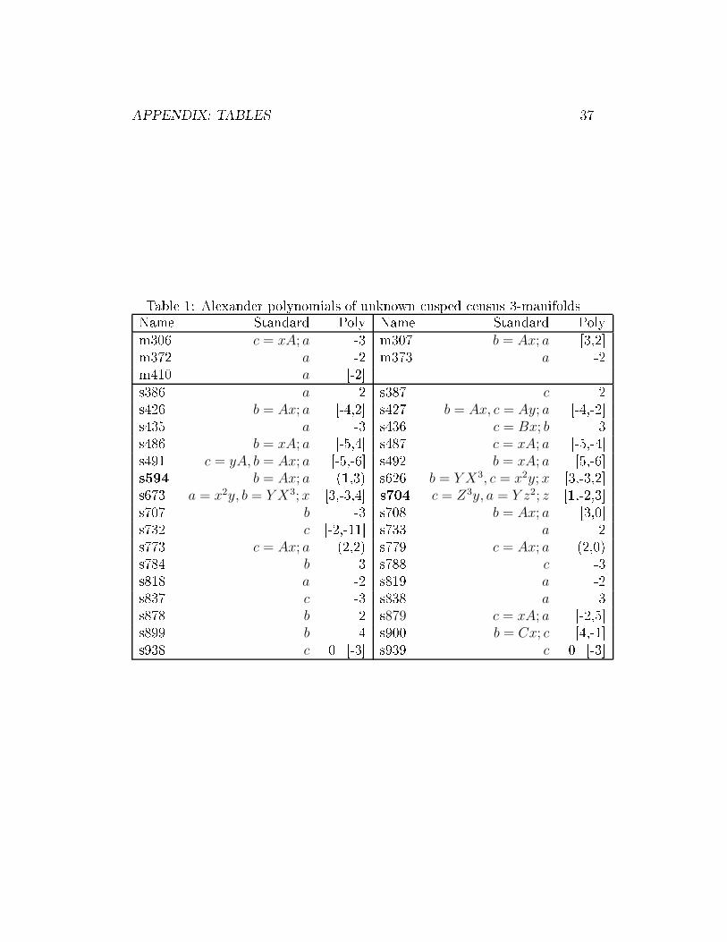
APPENDIX: TABLES 37

Table 1: Alexander polynomials of unknown usped ensus 3-manifoldsName Standard Poly Name Standard Polym306 c = xA; a -3 m307 b = Ax; a [3,2℄m372 a -2 m373 a -2m410 a [-2℄s386 a -2 s387 c -2s426 b = Ax; a [-4,2℄ s427 b = Ax, c = Ay; a [-4,-2℄s435 a -3 s436 c = Bx; b 3s486 b = xA; a [-5,4℄ s487 c = xA; a [-5,-4℄s491 c = yA, b = Ax; a [-5,-6℄ s492 b = xA; a [5,-6℄s594 b = Ax; a (1,3) s626 b = Y X3, c = x2y; x [3,-3,2℄s673 a = x2y, b = Y X3; x [3,-3,4℄ s704 c = Z3y, a = Y z2; z [1,-2,3℄s707 b -3 s708 b = Ax; a [3,0℄s732 c [-2,-11℄ s733 a 2s773 c = Ax; a (2,2) s779 c = Ax; a (2,0)s784 b 3 s788 c -3s818 a -2 s819 a -2s837 c -3 s838 a 3s878 b 2 s879 c = xA; a [-2,5℄s899 b 4 s900 b = Cx; c [4,-1℄s938 c 0=[-3℄ s939 c 0=[-3℄

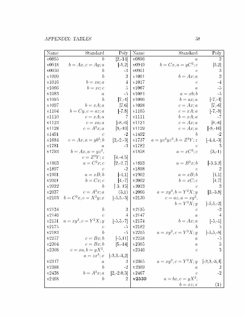
APPENDIX: TABLES 38Name Standard Poly Name Standard Polyv0895 b [2,-14℄ v0896 a 2v0948 b = Ax, c = Ay; a [-5,2℄ v0949 b = Cx, a = yC2; c [5,2℄v0950 b -3 v0951 c 3v1000 b 3 v1001 b = Ax; a -3v1016 b = xa; a 4 v1017 c -4v1066 b = xc; c 5 v1067 a -5v1083 a -5 v1084 a = xb; b -5v1095 b [7,-4℄ v1096 b = ax; a [-7,-4℄v1097 b = xA; a [7,6℄ v1098 c = Ax; a [7,-6℄v1104 b = Cy, c = az; a [-7,8℄ v1105 c = xA; a [-7,-8℄v1110 c = xA; a 7 v1111 b = xA; a -7v1123 c = xa; a [-8,-6℄ v1124 c = Ax; a [8,-6℄v1128 c = A2x; a [8,-10℄ v1129 c = Ax; a [-8,-10℄v1491 c -2 v1492 b -2v1684 c = Ax, a = yb2; b [2,-2,-3℄ v1737 a = yz2yz3, b = Z2Y ; z [-4,4,-3℄v1781 a -3 v1782 c 3v1793 b = Ax, a = yz2, v1858 a = xC2; c (3,-1)c = Z3Y ; z [4,-4,5℄v1863 a = C2x; c [2,-2,7℄ v1893 a = B2x; b [-3,3,2℄v1897 c -2 v1898 c 2v1901 a = xB; b [-4,1℄ v1902 a = xB; b [4,1℄v2001 b = Cx; c [4,-7℄ v2002 b = xC; c [4,7℄v2022 b [-3,-15℄ v2023 c -3v2037 c = A3x; a (3,1) v2066 a = xy3, b = Y 2X; y [3,-3,8℄v2103 b = C2x, c = X2y; x [-5,5,-3℄ v2130 c = az, a = xy2,

b = Y 3X; y [-5,5,-2℄v2134 b 3 v2135 c -3v2146 c 4 v2147 a 4v2151 a = xy3, c = Y 2X; y [-5,5,-7℄ v2174 b = Ax; a [-5,-1℄v2175 c -5 v2182 b 5v2183 b -5 v2205 a = xy2, c = Y 3X; y [-5,5,-8℄v2257 c = Bx; b [-5,11℄ v2258 a -5v2304 c = Bx; b [5,-14℄ v2305 a 5v2308 c = xa, b = yX2, v2346 c 3a = zx3; x [-3,3,-3,2℄v2347 a 3 v2365 a = xy3, c = Y 2X; y [-3,3,-3,4℄v2388 b -2 v2389 a 2v2438 b = A3x; a [2,-2,0,3℄ v2467 c -2v2468 b 2 v2530 a = bx, c = yX2,

b = xz; x (1)

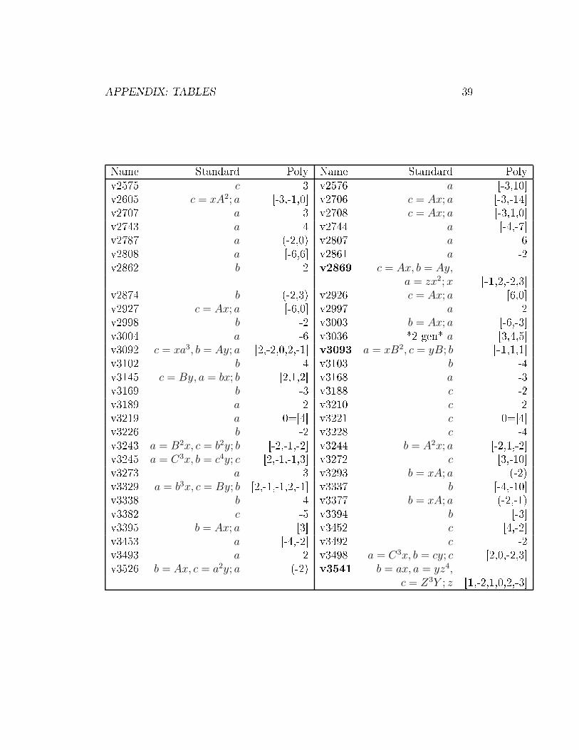
APPENDIX: TABLES 39Name Standard Poly Name Standard Polyv2575 c 3 v2576 a [-3,10℄v2605 c = xA2; a [-3,-1,0℄ v2706 c = Ax; a [-3,-14℄v2707 a 3 v2708 c = Ax; a [-3,1,0℄v2743 a 4 v2744 a [-4,-7℄v2787 a (-2,0) v2807 a 6v2808 a [-6,6℄ v2861 a -2v2862 b 2 v2869 c = Ax, b = Ay,

a = zx2; x [-1,2,-2,3℄v2874 b (-2,3) v2926 c = Ax; a [6,0℄v2927 c = Ax; a [-6,0℄ v2997 a 2v2998 b -2 v3003 b = Ax; a [-6,-3℄v3004 a -6 v3036 *2 gen* a [3,4,5℄v3092 c = xa3, b = Ay; a [2,-2,0,2,-1℄ v3093 a = xB2, c = yB; b [-1,1,1℄v3102 b 4 v3103 b -4v3145 c = By, a = bx; b [2,1,2℄ v3168 a -3v3169 b -3 v3188 c -2v3189 a 2 v3210 c 2v3219 a 0=[4℄ v3221 c 0=[4℄v3226 b -2 v3228 c -4v3243 a = B2x, c = b2y; b [-2,-1,-2℄ v3244 b = A2x; a [-2,1,-2℄v3245 a = C3x, b = c4y; c [2,-1,-1,3℄ v3272 c [3,-10℄v3273 a 3 v3293 b = xA; a (-2)v3329 a = b3x, c = By; b [2,-1,-1,2,-1℄ v3337 b [-4,-10℄v3338 b 4 v3377 b = xA; a (-2,-1)v3382 c -5 v3394 b [-3℄v3395 b = Ax; a [3℄ v3452 c [4,-2℄v3453 a [-4,-2℄ v3492 c -2v3493 a 2 v3498 a = C3x, b = cy; c [2,0,-2,3℄v3526 b = Ax, c = a2y; a (-2) v3541 b = ax, a = yz4,c = Z3Y ; z [1,-2,1,0,2,-3℄

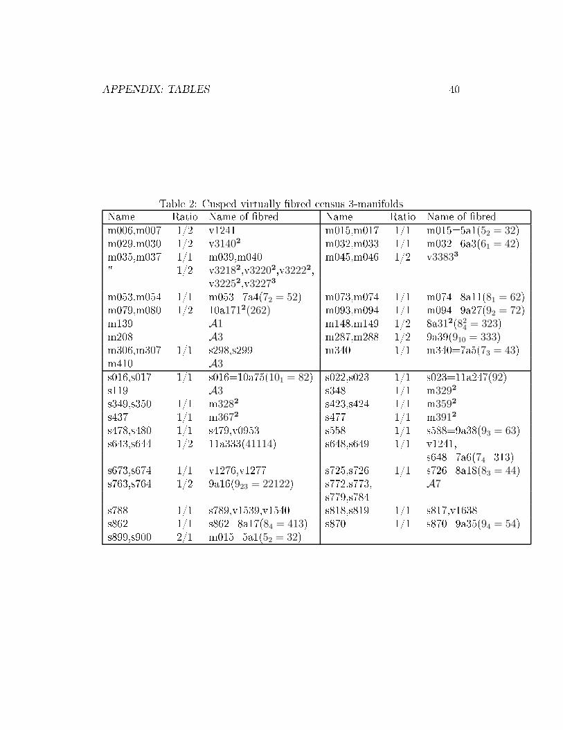
APPENDIX: TABLES 40Table 2: Cusped virtually �bred ensus 3-manifoldsName Ratio Name of �bred Name Ratio Name of �bredm006,m007 1/2 v1241 m015,m017 1/1 m015=5a1(52 = 32)m029,m030 1/2 v31402 m032,m033 1/1 m032=6a3(61 = 42)m035,m037 1/1 m039,m040 m045,m046 1/2 v33833" 1/2 v32182,v32202,v32222,v32252,v32273m053,m054 1/1 m053=7a4(72 = 52) m073,m074 1/1 m074=8a11(81 = 62)m079,m080 1/2 10a1712(262) m093,m094 1/1 m094=9a27(92 = 72)m139 A1 m148,m149 1/2 8a312(82

4 = 323)m208 A3 m287,m288 1/2 9a39(910 = 333)m306,m307 1/1 s298,s299 m340 1/1 m340=7a5(73 = 43)m410 A3s016,s017 1/1 s016=10a75(101 = 82) s022,s023 1/1 s023=11a247(92)s119 A3 s348 1/1 m3292s349,s350 1/1 m3282 s423,s424 1/1 m3592s437 1/1 m3672 s477 1/1 m3912s478,s480 1/1 s479,v0953 s558 1/1 s588=9a38(93 = 63)s643,s644 1/2 11a333(41114) s648,s649 1/1 v1241,s648=7a6(74=313)s673,s674 1/1 v1276,v1277 s725,s726 1/1 s726=8a18(83 = 44)s763,s764 1/2 9a16(923 = 22122) s772,s773, A7s779,s784s788 1/1 s789,v1539,v1540 s818,s819 1/1 s817,v1638s862 1/1 s862=8a17(84 = 413) s870 1/1 s870=9a35(94 = 54)s899,s900 2/1 m015=5a1(52 = 32)

APPENDIX: TABLES 41Name Ratio Name of �bred Name Ratio Name of �bredv0016,v0017 1/1 v0016=12a803 v0024,v0025 1/1 v0025=13a3143([10]2) ([11]2)v0571 1/1 m340=7a5(73 = 43) v0785 1/1 m3572v0819 1/1 m3662,v0820 v0954 1/1 m3882v1010,v1012 1/1 s5062 v1011 1/1 s5032v1035,v1036 1/2 11a365(353) v1112,v1113 1/1 s5492v1152 1/1 s5682 v1168 1/1 s5772v1172 1/1 s5782 v1179 1/1 v11782v1194 1/1 s6022 v1205 1/1 v12042v1210 1/1 s6212 v1229 1/1 s6382v1243 1/1 v1243=11a364(83) v1256 1/1 s6612v1676 1/1 s8312 v1858 A1v2018 1/1 s8762 v2037 1/1 s8802v2078 1/1 s8872 v2158 1/1 s8952v2203 1/1 s8982,v2202 v2238 1/1 s9062v2284,v2285 1/1 v2284=9a36(95 = 513) v2297,v2298 1/1 v2296v2339 1/1 s9142 v2346,v2347 1/1 v2345v2361,v2362 1/1 v2362=10a117 v2467,v2468 1/1 v2469(103 = 64)v2488 1/1 v2488=10a113 v2520 1/1 v2520=11a342(104 = 613) (74)v2575,v2576 1/1 v2574 v2706,v2707 1/1 v2705v2787 A2 v2796,v2797 1/2 11a119(23132)v2858 1/1 v2858=10a114 v2874 A3(108 = 514)v2894 1/1 11a358(65) v29432,v2944 1/1 v29422v3128 1/1 v3126,v31272 v3210 1/1 v3207,v3208,v3209v3243,v3244 1/1 v3246,v3247 v3310 1/1 v3310=7a3(75 = 322)v3377 1/1 v33762,v3378 v33792,v33842 1/1 v33833v33962 1/1 v33932 v3427 1/1 v34262v3457 1/1 v34562 v3492,v3493 1/1 v3490,v3491

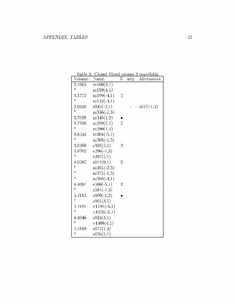
APPENDIX: TABLES 42Table 3: Closed �bred ensus 3-manifoldsVolume Name Z neg Alternative3.1663 m160(3,1)" m159(4,1)3.1772 m199(-4,1) 2" m122(-4,1)3.6638 s942(-2,1) - s957(-1,2)" m336(-1,3)3.7028 m345(1,2) •3.7708 m289(7,1) 2" m280(1,4)3.8534 m304(-5,1)" m305(-1,3)3.9466 s385(5,1) 33.9702 s296(-1,3)" s297(5,1)4.0597 s912(0,1) 2" m401(-2,3)" m371(-1,3)" m368(-4,1)4.4081 s580(-5,1) 2" s581(-1,3)4.4153 s869(-1,2) •" s861(3,1)4.4191 v1191(-5,1)" v1076(-5,1)4.4646 s924(3,1)" v1408(4,1)4.5169 s677(1,3)" s676(5,1)

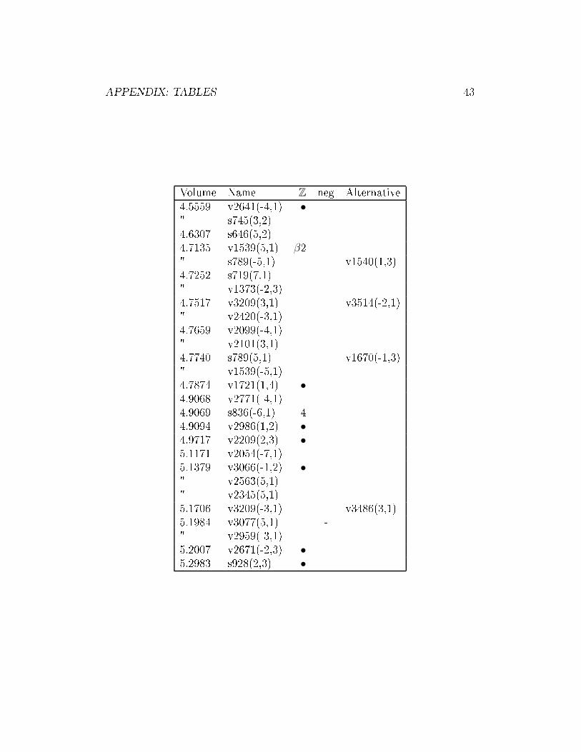
APPENDIX: TABLES 43Volume Name Z neg Alternative4.5559 v2641(-4,1) •" s745(3,2)4.6307 s646(5,2)4.7135 v1539(5,1) β2" s789(-5,1) v1540(1,3)4.7252 s719(7,1)" v1373(-2,3)4.7517 v3209(3,1) v3514(-2,1)" v2420(-3,1)4.7659 v2099(-4,1)" v2101(3,1)4.7740 s789(5,1) v1670(-1,3)" v1539(-5,1)4.7874 v1721(1,4) •4.9068 v2771(-4,1)4.9069 s836(-6,1) 44.9094 v2986(1,2) •4.9717 v2209(2,3) •5.1171 v2054(-7,1)5.1379 v3066(-1,2) •" v2563(5,1)" v2345(5,1)5.1706 v3209(-3,1) v3486(3,1)5.1984 v3077(5,1) -" v2959(-3,1) -5.2007 v2671(-2,3) •5.2983 s928(2,3) •

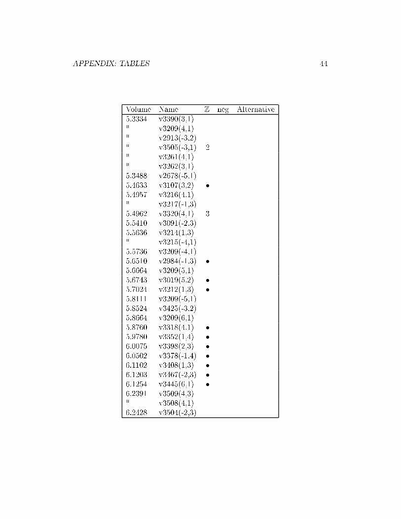
APPENDIX: TABLES 44Volume Name Z neg Alternative5.3334 v3390(3,1)" v3209(4,1)" v2913(-3,2)" v3505(-3,1) 2" v3261(4,1)" v3262(3,1)5.3488 v2678(-5,1)5.4633 v3107(3,2) •5.4957 v3216(4,1)" v3217(-1,3)5.4962 v3320(4,1) 35.5410 v3091(-2,3)5.5636 v3214(1,3)" v3215(-4,1)5.5736 v3209(-4,1)5.6510 v2984(-1,3) •5.6664 v3209(5,1)5.6743 v3019(5,2) •5.7024 v3212(1,3) •5.8111 v3209(-5,1)5.8524 v3425(-3,2)5.8664 v3209(6,1)5.8760 v3318(4,1) •5.9780 v3352(1,4) •6.0075 v3398(2,3) •6.0502 v3378(-1,4) •6.1102 v3408(1,3) •6.1203 v3467(-2,3) •6.1254 v3445(6,1) •6.2391 v3509(4,3)" v3508(4,1)6.2428 v3504(-2,3)

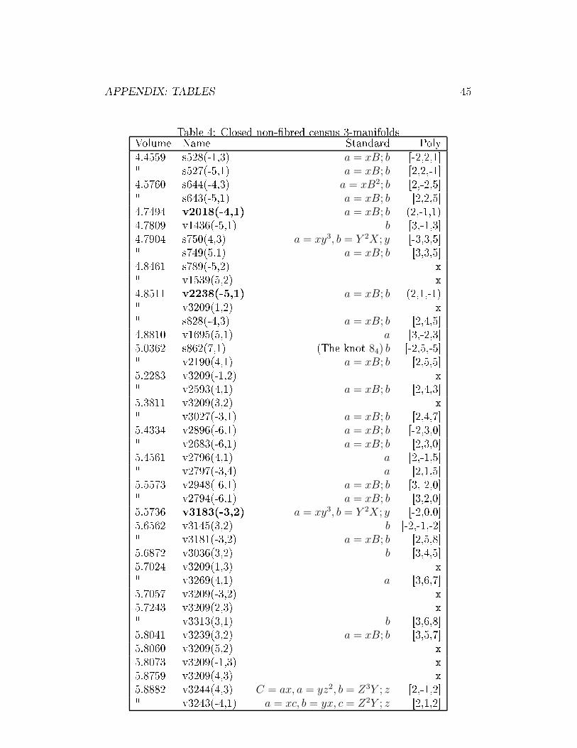
APPENDIX: TABLES 45Table 4: Closed non-�bred ensus 3-manifoldsVolume Name Standard Poly4.4559 s528(-1,3) a = xB; b [-2,2,1℄" s527(-5,1) a = xB; b [2,2,-1℄4.5760 s644(-4,3) a = xB2; b [2,-2,5℄" s643(-5,1) a = xB; b [2,2,5℄4.7494 v2018(-4,1) a = xB; b (2,-1,1)4.7809 v1436(-5,1) b [3,-1,3℄4.7904 s750(4,3) a = xy3, b = Y 2X; y [-3,3,5℄" s749(5,1) a = xB; b [3,3,5℄4.8461 s789(-5,2) x" v1539(5,2) x4.8511 v2238(-5,1) a = xB; b (2,1,-1)" v3209(1,2) x" s828(-4,3) a = xB; b [2,4,5℄4.8810 v1695(5,1) a [3,-2,3℄5.0362 s862(7,1) (The knot 84) b [-2,5,-5℄" v2190(4,1) a = xB; b [2,5,5℄5.2283 v3209(-1,2) x" v2593(4,1) a = xB; b [2,4,3℄5.3811 v3209(3,2) x" v3027(-3,1) a = xB; b [2,4,7℄5.4334 v2896(-6,1) a = xB; b [-2,3,0℄" v2683(-6,1) a = xB; b [2,3,0℄5.4561 v2796(4,1) a [2,-1,5℄" v2797(-3,4) a [2,1,5℄5.5573 v2948(-6,1) a = xB; b [3,-2,0℄" v2794(-6,1) a = xB; b [3,2,0℄5.5736 v3183(-3,2) a = xy3, b = Y 2X; y [-2,0,0℄5.6562 v3145(3,2) b [-2,-1,-2℄" v3181(-3,2) a = xB; b [2,5,8℄5.6872 v3036(3,2) b [3,4,5℄5.7024 v3209(1,3) x" v3269(4,1) a [3,6,7℄5.7057 v3209(-3,2) x5.7243 v3209(2,3) x" v3313(3,1) b [3,6,8℄5.8041 v3239(3,2) a = xB; b [3,5,7℄5.8060 v3209(5,2) x5.8073 v3209(-1,3) x5.8759 v3209(4,3) x5.8882 v3244(4,3) C = ax, a = yz2, b = Z3Y ; z [2,-1,2℄" v3243(-4,1) a = xc, b = yx, c = Z2Y ; z [2,1,2℄

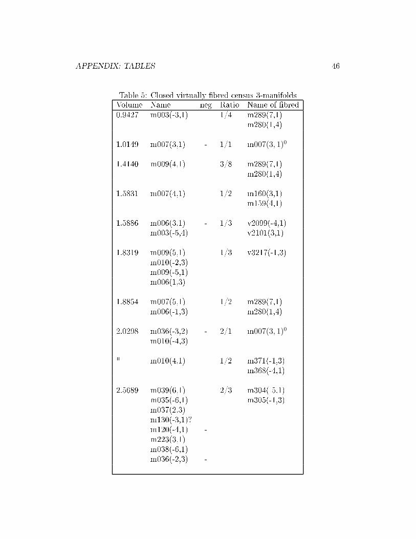
APPENDIX: TABLES 46Table 5: Closed virtually �bred ensus 3-manifoldsVolume Name neg Ratio Name of �bred0.9427 m003(-3,1) 1/4 m289(7,1)m280(1,4)1.0149 m007(3,1) - 1/1 m007(3, 1)01.4140 m009(4,1) 3/8 m289(7,1)m280(1,4)1.5831 m007(4,1) 1/2 m160(3,1)m159(4,1)1.5886 m006(3,1) - 1/3 v2099(-4,1)m003(-5,4) v2101(3,1)1.8319 m009(5,1) 1/3 v3217(-1,3)m010(-2,3)m009(-5,1)m006(1,3)1.8854 m007(5,1) 1/2 m289(7,1)m006(-1,3) m280(1,4)2.0298 m036(-3,2) - 2/1 m007(3, 1)0m010(-4,3)" m010(4,1) 1/2 m371(-1,3)m368(-4,1)2.5689 m039(6,1) 2/3 m304(-5,1)m035(-6,1) m305(-1,3)m037(2,3)m130(-3,1)?m120(-4,1) -m223(3,1)m038(-6,1)m036(-2,3) -

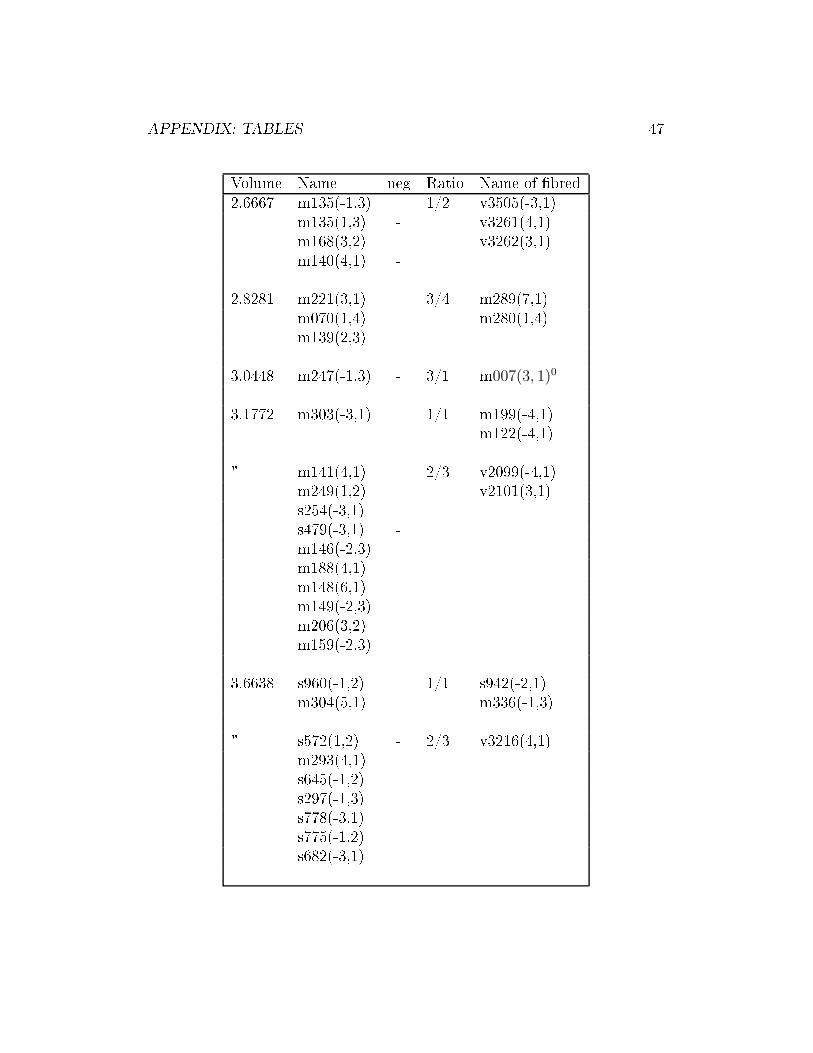
APPENDIX: TABLES 47Volume Name neg Ratio Name of �bred2.6667 m135(-1,3) 1/2 v3505(-3,1)m135(1,3) - v3261(4,1)m168(3,2) v3262(3,1)m140(4,1) -2.8281 m221(3,1) 3/4 m289(7,1)m070(1,4) m280(1,4)m139(2,3)3.0448 m247(-1,3) - 3/1 m007(3, 1)03.1772 m303(-3,1) 1/1 m199(-4,1)m122(-4,1)" m141(4,1) 2/3 v2099(-4,1)m249(1,2) v2101(3,1)s254(-3,1)s479(-3,1) -m146(-2,3)m188(4,1)m148(6,1)m149(-2,3)m206(3,2)m159(-2,3)3.6638 s960(-1,2) 1/1 s942(-2,1)m304(5,1) m336(-1,3)" s572(1,2) - 2/3 v3216(4,1)m293(4,1)s645(-1,2)s297(-1,3)s778(-3,1)s775(-1,2)s682(-3,1)

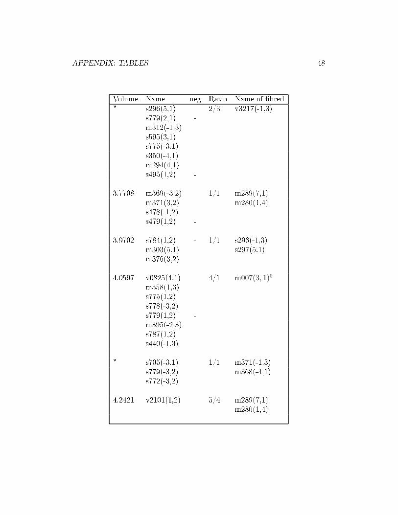
APPENDIX: TABLES 48Volume Name neg Ratio Name of �bred" s296(5,1) 2/3 v3217(-1,3)s779(2,1) -m312(-1,3)s595(3,1)s775(-3,1)s350(-4,1)m294(4,1)s495(1,2) -3.7708 m369(-3,2) 1/1 m289(7,1)m371(3,2) m280(1,4)s478(-1,2)s479(1,2) -3.9702 s784(1,2) - 1/1 s296(-1,3)m303(5,1) s297(5,1)m376(3,2)4.0597 v0825(4,1) 4/1 m007(3, 1)0m358(1,3)s775(1,2)s778(-3,2)s779(1,2) -m395(-2,3)s787(1,2)s440(-1,3)" s705(-3,1) 1/1 m371(-1,3)s779(-3,2) m368(-4,1)s772(-3,2)4.2421 v2101(1,2) 5/4 m289(7,1)m280(1,4)

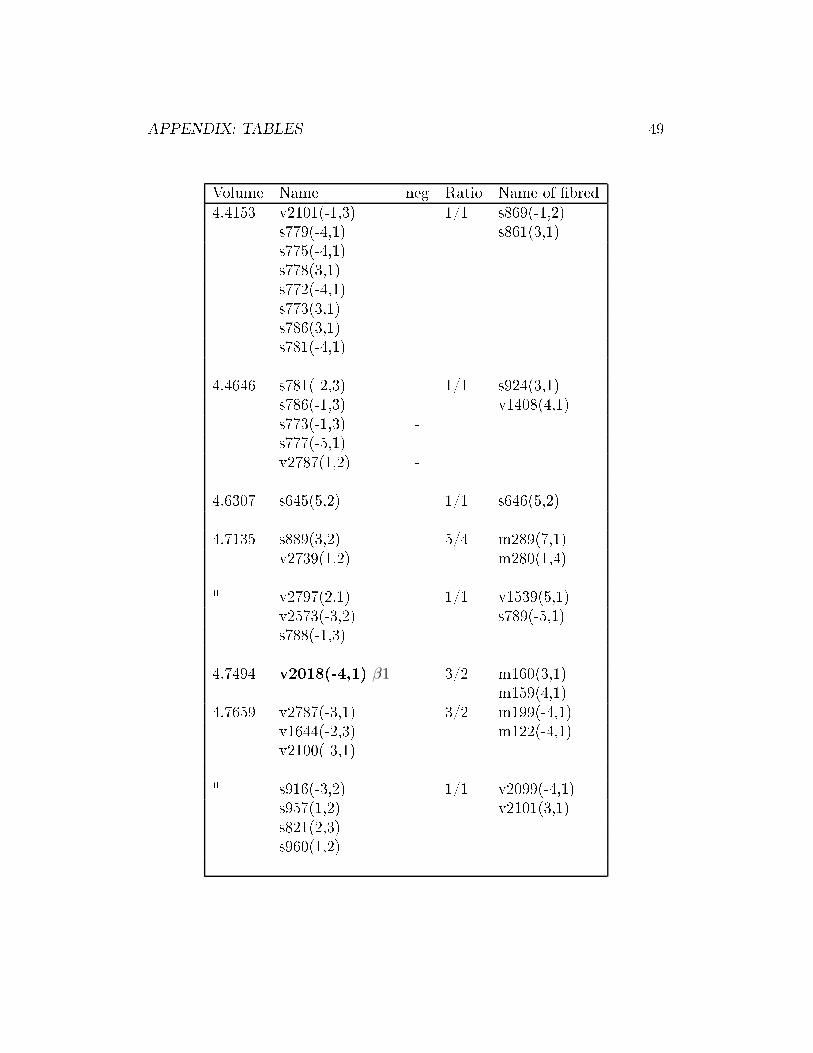
APPENDIX: TABLES 49Volume Name neg Ratio Name of �bred4.4153 v2101(-1,3) 1/1 s869(-1,2)s779(-4,1) s861(3,1)s775(-4,1)s778(3,1)s772(-4,1)s773(3,1)s786(3,1)s781(-4,1)4.4646 s781(-2,3) 1/1 s924(3,1)s786(-1,3) v1408(4,1)s773(-1,3) -s777(-5,1)v2787(1,2) -4.6307 s645(5,2) 1/1 s646(5,2)4.7135 s889(3,2) 5/4 m289(7,1)v2739(1,2) m280(1,4)" v2797(2,1) 1/1 v1539(5,1)v2573(-3,2) s789(-5,1)s788(-1,3)4.7494 v2018(-4,1) β1 3/2 m160(3,1)m159(4,1)4.7659 v2787(-3,1) 3/2 m199(-4,1)v1644(-2,3) m122(-4,1)v2100(-3,1)" s916(-3,2) 1/1 v2099(-4,1)s957(1,2) v2101(3,1)s821(2,3)s960(1,2)

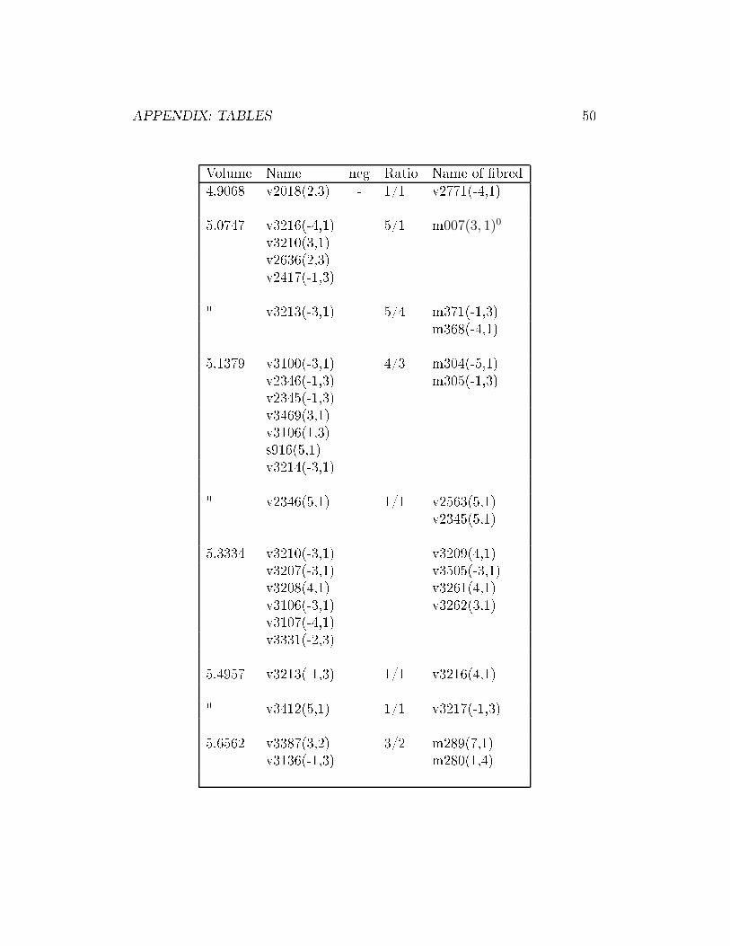
APPENDIX: TABLES 50Volume Name neg Ratio Name of �bred4.9068 v2018(2,3) - 1/1 v2771(-4,1)5.0747 v3216(-4,1) 5/1 m007(3, 1)0v3210(3,1)v2636(2,3)v2417(-1,3)" v3213(-3,1) 5/4 m371(-1,3)m368(-4,1)5.1379 v3100(-3,1) 4/3 m304(-5,1)v2346(-1,3) m305(-1,3)v2345(-1,3)v3469(3,1)v3106(1,3)s916(5,1)v3214(-3,1)" v2346(5,1) 1/1 v2563(5,1)v2345(5,1)5.3334 v3210(-3,1) v3209(4,1)v3207(-3,1) v3505(-3,1)v3208(4,1) v3261(4,1)v3106(-3,1) v3262(3,1)v3107(-4,1)v3331(-2,3)5.4957 v3213(-1,3) 1/1 v3216(4,1)" v3412(5,1) 1/1 v3217(-1,3)5.6562 v3387(3,2) 3/2 m289(7,1)v3136(-1,3) m280(1,4)