Embed Size (px)
Citation preview
J. Math. Pures Appl. 81 (2002) 187–222
Hele–Shaw flow on hyperbolic surfaces
Håkan Hedenmalm, Sergei Shimorin
Department of Mathematics, Lund University, PO Box 118, S-221 00 Lund, Sweden
Received 10 April 2001
Abstract
Consider a complete simply connected hyperbolic surface. The classical Hadamard theorem asserts that at each point of thesurface, the exponential mapping from the tangent plane to the surface defines a global diffeomorphism. This can be interpretedas a statement relating the metric flow on the tangent plane with that of the surface. We find an analogue of Hadamard’s theoremwith metric flow replaced by Hele–Shaw flow, which models the injection of (two-dimensional) fluid into the surface. The Hele–Shaw flow domains are characterized implicitly by a mean value property on harmonic functions. 2002 Éditions scientifiqueset médicales Elsevier SAS. All rights reserved.
AMS classification: 35R35; 35Q35; 31C12; 31A05; 53B20; 53C22
Keywords: Hele–Shaw flow; Mean value identities; Hyperbolic surface; Exponential mapping
1. Introduction
Let Ω be a simply connected two-dimensional Riemannian manifold with aC∞-smooth metric ds. We can always introducelocal isothermal coordinates near any point ofΩ , that is, such coordinates(x, y) that the metric is represented in the formds(x, y)2 = ω(x,y)(dx2 + dy2), for some positive weight functionω. And sinceΩ is orientable as a two-dimensional simply-connected manifold, these local isothermal coordinates can serve as conformal charts for a complex structure onΩ (see[1, pp. 124–126]). The Kœbe uniformization theorem then says thatΩ is conformally equivalent to one of the three sets:the Riemann sphereS = C∪ ∞, the complex planeC, or the open unit diskD. This equivalence, together with the choice ofisothermal coordinates, allows us to identifyΩ with one of the above three setsΩ supplied with the isothermal Riemannianmetric
ds(z)2 = ω(z)|dz|2, z ∈Ω \ ∞. (1.1)
Here,ω is a weight function which is strictly positive andC∞-smooth inΩ \ ∞ and vanishes at infinity ifΩ = S. TheGaussian curvature corresponding to the above isothermal metric (1.1) is given by the expression
κ(z)=− 2
ω(z)(logω)(z), z ∈Ω \ ∞,
where stands for the normalized Laplacian:
=z = 1
4
(∂2
∂x2+ ∂2
∂y2
), z= x + iy.
The Riemannian manifoldΩ is said to behyperbolic if the Gaussian curvature is negative everywhere. For the metric (1.1),this means that logω should be subharmonic inΩ \ ∞. Such functionsω are calledlogarithmically subharmonic. We note
E-mail addresses: [email protected] (H. Hedenmalm), [email protected] (S. Shimorin).
0021-7824/02/$ – see front matter 2002 Éditions scientifiques et médicales Elsevier SAS. All rights reserved.PII: S0021-7824(01)01222-3

188 H. Hedenmalm, S. Shimorin / J. Math. Pures Appl. 81 (2002) 187–222
that this rules out the Riemann sphere as a possibility forΩ , because logω tends to−∞ at infinity, which is not possible fora subharmonic function that is not identically−∞. This observation – that the sphere cannot be supplied with a hyperbolicmetric – can also be easily derived from the Gauss–Bonnet formula [4, p. 417]. In what follows, we deal exclusively withhyperbolic surfacesΩ .
1.1. Metric flow
Fix a pointz0 ∈ Ω . The classical exponential mapping Expz0assigns to each vectorη in the tangent planeTz0(Ω) a point
Expz0(η) on the geodesic starting fromz0 and having a tangent vectorη at z0 so that the length of the portion of this geodesicbetweenz0 and Expz0(η) equals|η|, the length of the vectorη. The classical theorem of Jacques Hadamard [15], [16, pp.729–775] then states that the exponential mapping Expz0
is a diffeomorphism from the tangent planeTz0(Ω) ontoΩ , providedthat the metric is complete (see also [21, p. 74]). We recall that the metric is said to becomplete if all Cauchy sequences areconvergent. If the metric is incomplete, the exponential mapping is a diffeomorphism from some star-shaped (with respect tothe origin) open regionΩ of the tangent planeTz0(Ω) onto the regionΩ∗ of points ofΩ geodesically visible fromz0.
We can interpret Hadamard’s theorem as supplying “polar coordinates” centered aboutz0 on all of Ω . Considering themetric disks
B(z0, t)=z ∈Ω: d(z, z0) < t
,
whered(z, z0) expresses the distance on the surfaceΩ betweenz and z0, we see that the exponential mapping Expz0is
a diffeomorphism which takes a disk of radiust about the origin in the tangent plane (provided that the disk is small enoughtto be contained inΩ) onto the metric diskB(z0, t). This mapping can be considered as the result of a flow of a photonic gasconsisting of noniteracting infinitesimal particles which are injected at a constant rate at the pointz0, and moving with constantspeed along geodesics. Assuming the speed of the particles to be 1, we find that the region they cover at timet ∈]0,+∞[ is themetric diskB(z0, t). The boundary curves∂B(z0, t) are perpendicular to the geodesics emanating fromz0.
If the original manifold is real-analytic, then the exponential mapping is also real-analytic [21, p. 58].
1.2. Hele–Shaw flow
We shall find the analogue of Hadamard’s theorem for a different kind of flow, called Hele–Shaw flow. As before, we fixa point z0 ∈ Ω . We inject a two-dimensional Newtonian fluid at a constant rate atz0 into the surfaceΩ . There is no fluidpresent at the starting time, but immediately thereafter we have a small but growing blob around the injection point. Thetwo-dimensional fluid is a limit case of a three-dimensional one, where we thicken the surface uniformly and then let thethickness tend to zero. LetD(z0, t) be the blob at timet , for positive timest . Physics dictates that the rate of growth should bedetermined by the local fluid pressure. This means that the rate of growth at a boundary pointz ∈ ∂D(z0, t) is proportional tothe gradient∇zG(z, z0) of the Green functionG(z, z0) for the Laplace–Beltrami operator. Following Richardson [33], wecall the movement of the free boundary between the fluid and vacuumHele–Shaw flow. From a mathematical point of view, theabove recipe for how the boundary moves outward suffers from certain limitations. First, it only tells how the boundary movesonce we have a well-behaved nonempty blob in place. It does not say how to obtainD(z0, t) for t close to 0, becauset = 0 isa singular point from this point of view. But it turns out that the domainsD(z0, t) admit other equivalent characterizations interms of certain quadrature identities and obstacle problems, which permits us to study the Hele–Shaw flow rigorously.
Let us now see how to obtain an equivalent description of the Hele–Shaw flow. If the metric on the domainΩ , representingthe surfaceΩ , is given by (1.1), then the normalized two-dimensional volume form is
dΣ(z)= ω(z)dΣ(z), z ∈Ω,where dΣ(z) stands for the normalized area measure in the plane:
dΣ(z)= 1
πdx dy, z= x + iy.
The Laplace–Beltrami operator onΩ is given by
z = 1
ω(z)z, z ∈Ω.
Suppose a functionh is harmonic in a neighborhood ofD(z0, t). Let t ′ be slightly larger thant , but such thath is harmonicon D(z0, t ′) as well. Assuming that the boundaries are smooth, we recall the recipe for how the boundary moves, and applyGreen’s theorem:∫
D(z0,t ′)\D(z0,t )
h(z)dΣ(z)= (t ′ − t)∫
∂D(z0,t )
h(z)∂
∂n(z)G(z, z0)dσ (z)+ o(t ′ − t)= (t ′ − t) h(z0)+ o(t ′ − t).

H. Hedenmalm, S. Shimorin / J. Math. Pures Appl. 81 (2002) 187–222 189
Here, dσ stands for the normalized arc length measure on∂D(z0, t). Letting t ′ approacht , we obtain in the limit that
d
dt
∫D(z0,t )
h(z)dΣ(z)= h(z0).
We integrate this relationship with respect tot , recalling thatD(z0, t) should be empty fort = 0, and obtain
th(z0)=∫
D(z0,t )
h(z)dΣ(z), (1.2)
where we recall thath should be harmonic in a neighborhood ofD(z0, t). The identity (1.2) is known as themean valueproperty, and we shall call the setsD(z0, t) mean value disks on the hyperbolic surfaceΩ . After identification ofΩ with Ω ,this property reads as
th(z0)=∫
D(z0,t )
h(z)ω(z)dΣ(z); (1.3)
here, we think ofD(z0, t) as a subset ofΩ . We show in the present paper that the domainsD(z0, t), satisfying (1.3), do exist(for t from certain intervalt ∈]0, T [). They will be obtained as noncoincidence sets for certain obstacle problems, and we shallsee that these domains are all simply connected and have real analytic boundaries, provided that the weight functionω is realanalytic. Moreover, we shall see that fort ∈]0, T [, the domains satisfying (1.3) are unique up to addition or removal of area-nullsets.
The boundaries∂D(z0, t) of the above domainsD(z0, t) form a one-parameter family of imbedded closed curves in theplane. We consider also the biorthogonal family of curves, the so-calledHele–Shaw geodesics, emanating from the origin andorthogonal to∂D(z0, t) at any point. Physically, these geodesics correspond to the trajectories of fluid particles injected at theorigin at timet = 0. Considering these two families of curves as coordinate lines for “Hele–Shaw polar coordinates”, we obtainwhat we call theHele–Shaw exponential mapping HSexpz0.
It turns out that this mapping admits a rigorous definition and that there exists an analogue of Hadamard’s theorem for it.Namely, HSexpz0 is a real-analytic diffeomorphism defined in some disk, centered at the origin, of the tangent planeTz0(Ω)
into Ω such that it maps disksη ∈ Tz0(Ω): |η| < r centered at the origin (which form, in fact, the Hele–Shaw flow on thetangent plane) onto the Hele–Shaw domainsD(z0, t), with t = r2, and rays emanating from the origin (Hele–Shaw geodesicson Tz0(Ω)) are mapped to Hele–Shaw geodesics onΩ passing throughz0. In case whereΩ is complete, HSexpz0 is a globaldiffeomorphism fromTz0(Ω) ontoΩ .
Assume that the tangent planeTz0(Ω) is identified with the complex planeC supplied with the usual Euclidean norm. Thenthe classical exponential mapping has the following asymptotics nearz0:
Expz0(z)= z0 + ω(0)−1/2z+ O(|z|2)
as|z| → 0.
We shall see that theHele–Shaw exponential mapping that we are about to define has a similar property. For 0< r < +∞,D(z0, r) stands for the Euclidean disk
D(z0, r)=z ∈ C: |z− z0|< r
.
Theorem 1.1(Main Theorem, global version).Assume that Ω is a complete hyperbolic simply connected surface identifiedwith the planar domain Ω which is either the unit disk D or the whole plane C, and the metric on Ω is given by (1.1) interms of the weight function ω. We assume that Ω is a real-analytic surface, which means that ω is real-analytic and strictlypositive. Fix a point z0 ∈ Ω . Then, for each 0< t < +∞, there exists a precompact subdomain D(z0, t) of Ω with the meanvalue property (1.3) for all bounded harmonic functions h on D(z0, t), and as such, it is unique up to addition or removal of anarea-null set. Moreover, there exists a unique C1-diffeomorphism HSexpz0 from the complex plane C onto Ω (the Hele–Shawexponential mapping) such that
• HSexpz0(0)= z0,• each ray z ∈ C \ 0: argz = θ is mapped by HSexpz0 onto a curve in Ω which points in the same direction as the ray
at z0,• HSexpz0 maps each pair consisting of a concentric circle about the origin and a straight line passing through the origin
onto a pair of orthogonal curves, and• for each 0< r < +∞, the domain HSexpz0(D(0, r)) equals the Hele–Shaw flow domain D(z0, r2), up to addition or
removal of area-null sets.

190 H. Hedenmalm, S. Shimorin / J. Math. Pures Appl. 81 (2002) 187–222
It has the following additional properties:
• HSexpz0 is a real-analytic diffeomorphism from C onto Ω , and
• HSexpz0(z)= z0 +ω(0)−1/2z+ O(|z|2) as |z| → 0.
It is interesting to compare the Hele–Shaw disks with the metric disks encountered earlier:D(z0, r2) ⊂ B(z0, r) for all0< r <+∞. For flat surfacesΩ , we have equality,D(z0, r2)= B(z0, r), but the introduction of negative curvature makes theHele–Shaw disks smaller in comparison. This is intuitively reasonable, because the (normalized) area of the Hele–Shaw diskD(z0, r2) equalsr2, whereas that of the metric diskB(z0, r) exceedsr2 on negatively curved surfaces.
We turn to the “local” version of the above theorem, which applies to incomplete manifolds as well. As in the case of metricflow, there appears a part of the surface that is “Hele–Shaw visible” from the given pointz0 ∈ Ω .
Theorem 1.2(Main Theorem, local version).Let the setting be as in the formulation of Theorem 1.1, with the exception that thesurface Ω need no longer be a complete manifold. Then there exists a parameter T with 0< T +∞, such that the assertionsof Theorem 1.1 hold, with the following modifications. The Hele–Shaw flow domains D(z0, t) are well-defined for 0< t < T ,and in case T <+∞, they fail to exist as precompact Jordan domains with the mean value property (1.3) for T < t <+∞. Theproperty HSexpz0(D(0, r))= D(z0, r2) then holds for 0< r <
√T , and HSexpz0 is a diffeomorphism D(0,
√T )→ Ω, where
Ω = HSexpz0(D(0,√T )) is a subdomain of Ω containing z0, which is not precompact in Ω . It constitutes the “Hele–Shaw
visible” part of Ω . In case T =+∞, we have Ω = Ω .
In the context of the above local theorem, it seems natural to callΩ Hele–Shaw complete if T =+∞. Then every (metrically)complete surface is Hele–Shaw complete; however, there are also simple examples of incomplete surfaces that are Hele–Shawcomplete. Intuitively, the reason why the two concepts diverge is that metric completeness requires an infinite (geodesic)distance to the “point at infinity”, whereas Hele–Shaw completeness requires there to be an infinitearea covered by the flow toreach the same point.
The metric flow has a hyperbolic flavor so that the information about an obstruction for the flow has a finite speed ofpropagation, whereas the Hele–Shaw flow is parabolic, because the information travels instantaneously. Nevertheless, the“exponential mapping” from each has the same kind of basic properties.
Remarks. (a) The above-mentioned results, with the obvious modifications, are probably valid in the context ofC∞-smoothsurfaces as well. However, we do not have a proof of this statement.
(b) It would be interesting to have a similar study carried out for higher-dimensional manifolds.(c) We should point out that mean value inequalities for subharmonic functions on manifolds can be found in the literature.
However, if we look only for mean value inequalities for subharmonic functions that imply a mean valueequality for harmonicfunctions, then our only choice are the Hele–Shaw domains. For instance, the mean value inequality of Schoen and Yau [36,p. 75] for metric balls does not have this property unless the manifold has constant curvature.
1.3. Wrapped Hele–Shaw flow
Toward the end of the paper, we develop the concept ofwrapped Hele–Shaw flow, where the flow domains are guaranteedto be simply connected; the price we pay for this is that the actual flow takes place on a Riemann surface sheeted over the givensurface. Wrapped Hele–Shaw flow then makes sense and may be continued indefinitely on compact surfacesS as well. Ourmain theorem applies to the covering surfaceΩ of the hyperbolic compact surfaceS, and the wrapped flow is the projection ofthe ordinary Hele–Shaw flow onΩ to S. The “wrapped Hele–Shaw geodesics” extend infinitely in both directions, and we canask whether they possess ergodic properties.
1.4. Applications
The reason we initially got interested in Hele–Shaw flow is that it offers a powerful method for investigating thebiharmonic operator on hyperbolic surfaces. It turns out that on a Hele–Shaw flow domain, the biharmonic Green function ispositive [18,19]. In the proof of that result, the biharmonic Green function is represented via the so-called Hadamard variationalformula (a special case of the well-known Duhamel principle) as an integral over the flow of slightly simpler functions,analogous to the Poisson kernel for the Laplacian. Those functions, referred to as harmonic compensators, are then in theirturn represented as integrals over the flow of harmonic reproducing kernel functions. The negative Gaussian curvature leads toquite specific information regarding the harmonic reproducing kernel functions on flow domains, which is then used to derive

H. Hedenmalm, S. Shimorin / J. Math. Pures Appl. 81 (2002) 187–222 191
the positivity of the harmonic compensator. In a second step, we get that the biharmonic Green function is positive as well. Thepositivity of the biharmonic Green function on Hele–Shaw flow domains for hyperbolic surfaces has important applications tothe factorization theory of the Bergman space [19,20].
1.5. Notations
For a smooth domainΩ in C, the Sobolev spaceW2(Ω) consists of all functions inL2(Ω) whose distributional partialderivatives up to order 2 are also inL2(Ω). By the Sobolev–Morrey imbedding theorem, the functions inW2(Ω) are inC0,α(Ω), the space of Hölder continuous functions onΩ, for each exponentα, 0< α < 1. We shall say that a functionu isW2-smooth inΩ if it is from the classW2(Ω ′) for some domainΩ ′ containingΩ.
The spaceC1,1(Ω) consists of all continuously differentiable functions onΩ , whose first-order partial derivatives areLipschitz continuous. It coincides with the Sobolev spaceW2,∞(Ω) of functions inL∞(Ω) whose partial derivatives (takenin the distributional sense) of order less than or equal to 2 are also inL∞(Ω). The functions in the latter space may need to beredefined on a set of zero area measure to fit into the first-mentioned space.
If D andΩ are planar domains, thenD Ω means thatD is precompactly contained inΩ . For a pointw ∈ C and a positivereal parameterr , we let
D(w, r)= z ∈ C: |z−w|< r
denote the open circular disk of radiusr aboutw. To shorten the notation, we sometimes writeD(r) for D(0, r). Thecharacteristic function of a setE is denoted by 1E .
The symbols∂z and∂z denote the standard Wirtinger differential operators:
∂z = ∂
∂z= 1
2
(∂
∂x− i
∂
∂y
)and ∂z = ∂
∂z= 1
2
(∂
∂x+ i
∂
∂y
).
Then our normalized Laplacian can be writtenz = ∂z∂z. We use dσ for normalized arc length measure: dσ(z)= |dz|/(2π).We also write|E|σ for the associated normalized length of a subsetE of a rectifiable curve. Similarly, we write|E|Σ for thenormalized area of a Borel subset ofC.
2. The Hele–Shaw obstacle problem
This section is devoted to the existence of domainsD(t) satisfying the mean value identity (1.3). We also establish some ofthe basic properties of these domains.
It is known that the domains appearing in the study of the classical Hele–Shaw flows can be described in terms of certainvariational inequalities, or, equivalently, in terms of obstacle problems (see, for instance, [13]). We use similar arguments, butin the context of the presence of a weight.
LetΩ be a Jordan domain inC with C∞-smooth boundary∂Ω , and letω be aC∞-smooth weight function which is strictlypositive inΩ. We assume thatz0 = 0∈Ω .
LetG=GΩ stand for the Green function for the Laplacian in Ω . We set
Vt (z)= tG(z,0)−∫Ω
G(z, ζ )ω(ζ )dΣ(ζ), z ∈Ω.
This function solves the boundary value problem
Vt = tδ0 − ω in Ω (in the sence of distributions); Vt |∂Ω = 0.
It is superharmonic inΩ \ 0 and it has a negative logarithmic singularity at the origin. Away from the origin, it isC∞-smooth.The functionVt has superharmonic majorants, for instance, sufficiently large positive constants. ThenVt also has a smallestsuperharmonic majorant onΩ , because
• if we are given two superharmonic functions, the minumum of them is superharmonic as well, and• the limit of a decreasing sequence of superharmonic functions is also superharmonic, provided it does not collapse to−∞.
We denote this smallest superharmonic majorant byVt . The setD(t;ω) is then defined as
D(t;ω)= z ∈Ω: Vt (z) < Vt (z)
. (2.1)

192 H. Hedenmalm, S. Shimorin / J. Math. Pures Appl. 81 (2002) 187–222
We define also the function
Ut(z)= Vt (z)− Vt (z), z ∈Ω. (2.2)
The obstacle problem makes sense for all values of the parametert , 0< t <+∞; therefore, the functionUt and the domainsD(t;ω) are well-defined for any positivet . In what follows we shall often drop the dependence onω and simply writeD(t)instead ofD(t;ω). We classifyD(t) as aHele–Shaw domain whenD(t)Ω , and as ageneralized Hele–Shaw domain whenD(t) is too big for this to happen. A physical interpretation is that we get generalized Hele–Shaw flow whent is so big thatthe boundary ofD(t) touches∂Ω , in which case for even biggert the liquid is allowed to stack up on the common boundary∂D(t)∩ ∂Ω .
We want to show that the domainsD(t) satisfy the mean value identity (1.3).
Proposition 2.1.Fix a t , 0< t <+∞. Then the superharmonic envelope function Vt is in C1,1(Ω). It assumes the value Vt = 0on ∂Ω .
Proof. TheC1,1-regularity of Vt follows from general regularity theory for obstacle problems. See, for example, Chapter 1in [10], or the paper [6] by Caffarelli and Kinderlehrer. Perhaps a word should be said about whyVt vanishes on∂Ω . Thefunction
G[−ω](z)=−∫Ω
G(z, ζ )ω(ζ )dΣ(ζ)
is a superharmonic majorant toVt , and it vanishes on∂Ω . The functionVt is sandwiched betweenVt andG[−ω], and boththese functions vanish on∂Ω , which leads to the conclusionVt |∂Ω = 0.
As a consequence, we see that the functionUt is continuous, and, therefore, all the setsD(t) are open.
Proposition 2.2.Fix a t , 0< t < +∞. Then Vt is harmonic in D(t). Moreover, we have Ut = ω1D(t) − t δ0 on Ω , in thesense of distributions.
Proof. First, we show thatVt is harmonic inD(t). To see this, we apply the standard Perron process argument. Indeed, if itwere not harmonic on some small circular disk inD(t), we could replace it in this disk by a harmonic function with the sameboundary values on the small circle, and obtain a function which is smaller (by the maximum principle), and still superharmonicin Ω . This new function remains a majorant toVt if the disk is small enough, in violation of the definition ofVt as the smallestsuperharmonic majorant toVt .
Therefore,
Ut =(Vt − Vt
) =−Vt = ω− tδ0 onD(t).
OnΩ \D(t), Vt andVt coincide, and hence their first- and second-order derivatives coincide almost everywhere there, in viewof [26, p. 53] and the preceding proposition. In particular,Ut = 0 almost everywhere inΩ \D(t). From the known regularityof Ut , the assertion is immediate.Theorem 2.3.Suppose the domain D(t)=D(t;ω) is precompact in Ω . Then for any function h harmonic in D(t),
th(0)=∫D(t)
h(z)ω(z)dΣ(z).
In fact, the above mean value identity holds under the slightly weaker assumption on h that it be W2-smooth on D(t) andharmonic in D(t). Indeed, if a function u is subharmonic in D(t) and W2-smooth in D(t), then
tu(0)∫D(t)
u(z)ω(z)dΣ(z).
Proof. Let the functionh be harmonic in a neighborhood ofD(t). Green’s formula – applied to some smooth domainD′containingD(t) but contained precompactly in the region of harmonicity ofh – yields, together with the previous proposition,∫
D(t)
h(z)ω(z)dΣ(z)− th(0)=∫D′h(z)Ut (z)dΣ(z)= 0,

H. Hedenmalm, S. Shimorin / J. Math. Pures Appl. 81 (2002) 187–222 193
sinceUt = 0 off D(t). The integration on the right-hand side is to be interpreted in the generalized sense of distribution theory.The sought-after mean value property is immediate.
The same arguments, together with the fact thatUt is positive, prove the second assertion of the theorem.Following Gustafsson [13], we say that a planar domainD satisfiesthe moment inequality if
tu(0)∫D
u(z)ω(z)dΣ(z) (2.3)
for anyu subharmonic inD andW2-smooth inD, andD satisfies themean value identity if
tu(0)=∫D
u(z)ω(z)dΣ(z) (2.4)
for anyu harmonic inD andW2-smooth inD (such functions are automatically bounded onD). These properties are veryimportant for the study of Hele–Shaw flows, as is demonstrated by two following propositions.
Proposition 2.4. Fix a t , 0 < t < +∞. Assume that a domain D Ω containing the origin is such that the momentinequality (2.3) holds for some parameter t for any function u subharmonic in D and W2-smooth in D. Then:
(a) D(t)⊂ int(D). Here, int denotes the operation of taking the interior of a set,(b) the sets D and D(t) differ by a set of zero area measure.
Proof. Consider the function
U(z)=−tG(z,0)+∫D
G(z, ζ )ω(ζ )dΣ(ζ), z ∈Ω.
By (2.3), it is positive throughoutΩ , and by the regularizing properties of the Green potential, it is continuous onΩ \ 0. Itvanishes offD, sinceG(z, ·) is harmonic inD for z ∈Ω \D. By continuity,U also vanishes off int(D). The functionVt +Uis a superharmonic majorant toVt ; therefore,Ut U , and we have (a).
To obtain (b), consider a smoothly bordered domainD′ such thatD D′ Ω . We haveU = ω1D − tδ0 in the sense ofdistributions onD′, andU = 0 near the boundary ofD′. We set
v(z)=∫
D′\DG(z, ζ )dΣ(ζ).
This function is harmonic inD andW2-smooth inD; therefore, by (2.3),
0=∫D
v(z)ω(z)dΣ(z)− tv(0)=∫D′vU dΣ =
∫D′vU dΣ =
∫D′\D
U dΣ.
This shows thatU = 0 almost everywhere inΩ \D, and, hence,Ut = 0 almost everywhere inΩ \D. Therefore, we have|D(t) \D|Σ = 0. We should check that|D \D(t)|Σ = 0 as well. To this end, we note thatD andD(t) have the same weightedarea: ∫
D
ω(z)dΣ(z)=∫D(t)
ω(z)dΣ(z)= t
(we substitute constant functions to the moment inequalities). The assertion (b) is now immediate.We see that the moment inequality characterizes domainsD(t) uniquely up to sets of zero area measure. But in the case
whereD(t) is a Jordan domain, it is uniquely characterized by the mean value identity (2.4) alone, as follows from the nextproposition. The argument is taken from Gustafsson’s paper [14].
Proposition 2.5.Suppose t , 0< t <+∞, is such that we have D(t)Ω . Suppose also that some domain D Ω satisfies themean value identity (2.4). Then there exists a domain D∗ ⊃D such that |D∗ \D|Σ = 0 and ∂D∗ ⊂D(t). In particular, ifD(t)is a Jordan domain, then any domain D satisfying (2.4) coincides with D(t) up to addition or removal of an area-null set.

194 H. Hedenmalm, S. Shimorin / J. Math. Pures Appl. 81 (2002) 187–222
Proof. As in the proof of the previous proposition, we consider the function
U(z)=−tG(z,0)+∫D
G(z, ζ )ω(ζ )dΣ(ζ), z ∈Ω.
This time, it need not be positive, but we haveU |Ω\D = 0. Moreover, if we consider the domainD∗ =D ∪ z ∈Ω: U(z) = 0
and the function
v(z)=∫
D∗\DG(z, ζ )sign
[U(z)
]dΣ(z),
we then have
0=∫D
v(z)ω(z)dΣ(z)− tv(0)=∫Ω
vU dΣ =∫Ω
vU dΣ =∫
D∗\D|U |dΣ.
Thus, we haveU = 0 almost everywhere inD∗ \D, so that|D∗ \D|Σ = 0.The functionU −Ut is subharmonic inD∗ (since(U −Ut )= ω · (1D∗ −1D(t))), and it hasU −Ut 0 on∂D∗, sinceU
vanishes there andUt is positive. Therefore, we haveU Ut in D∗, and we conclude thatU 0 inD∗ \D(t). Now, assumethat there exists a pointz0 ∈ ∂D∗ \D(t). We have thenU(z0) = 0 and, on the other hand,U(z) 0 in some neighborhoodN(z0) of the pointz0. SinceU is subharmonic away from the origin, we must haveU(z)= 0 inN(z0), and henceU = 0 inN(z0), which is impossible sinceU = ω1D − tδ0 = ω1D∗ − tδ0.
The following series of propositions establishes some basic properties of the domainsD(t) and functionsVt ,Vt , andUt .
Proposition 2.6.For any positive t , the domain D(t) is connected.
Proof. It is clear that the origin is an interior point ofD(t), becauseVt (z) tends to−∞ asz tends to 0. IfD(t) is disconnected,then we can find a connectivity component – call itD∗(t) – which does not contain the origin. As the origin is an interior pointof D(t), the connected open setD∗(t) is at a positive distance from it. Moreover, we have that∂D∗(t)⊂Ω \D(t), becauseif a sequence of points ofD∗(t) has a limit point inD(t), then all point sufficiently near the limit point are inD∗(t) as well,making the point interior forD∗(t). OnD∗(t), Vt is harmonic, and on∂D∗(t), it equals the functionVt . AsVt is superharmoniconD∗(t) (after all, it is superharmonic onΩ \ 0), we obtain from the maximum principle thatVt Vt onD∗(t), in clearviolation of the definition of the setD(t).
We turn to the basic monotonicity properties of the Hele–Shaw flow.
Proposition 2.7 (Monotonicity). For t , 0< t < +∞, the function Ut = Vt − Vt increases with the parameter t . Also, if theweight ω is increased, Ut decreases, for fixed t . As a consequence, the domain D(t;ω) increases with increasing t , anddecreases with increasing weight ω.
Proof. SinceD(t;ω) is defined as the set whereUt is strictly positive, it suffices to prove monotonicity properties ofUt . Lett, t ′ be related as follows: 0< t < t ′ < +∞. We check thatVt − Vt ′ is superharmonic, so that the functionVt ′ − Vt ′ + Vt issuperharmonic, too. The latter function also majorizesVt , and henceVt Vt ′ − Vt ′ + Vt . It follows thatUt increases witht .
A similar argument shows thatUt decreases as the weightω increases. The details are as follows. Letω′ be a bigger weightthanω: ω ω′ onΩ , and letV ′
t be the potential associated withω′:
V ′t (z)= tG(z,0)−
∫Ω
G(z, ζ )ω′(ζ )dΣ(ζ).
The functionV ′t − Vt is then superharmonic, because(V ′
t − Vt ) = ω − ω′ 0. It follows that the functionVt − Vt + V ′t
is superharmonic, too, and it clearly majorizesV ′t . It is immediate thatV ′
t Vt − Vt + V ′t , which leads toU ′
t Ut (obviousnotation), as asserted.
The assertion regarding the domainD(t;ω) is an immediate consequence of the above monotonicity properties ofUt .

H. Hedenmalm, S. Shimorin / J. Math. Pures Appl. 81 (2002) 187–222 195
We need to know thatD(t)Ω , at least for small positivet . On the other hand, for large positivet , the whole domain getsfilled: D(t)=Ω . This is accomplished by the following proposition.
Proposition 2.8.Let m be the minimum value of ω on Ω , and M the maximum value. Then the following assertions are valid.
(a) If t , 0< t < +∞, is so small that the circular disk D(0,√t/m) is contained in Ω , then D(t) is sandwiched as follows:
D(0,√t/M )⊂D(t)⊂ D(0,
√t/m).
(b) For sufficiently large positive t , we have D(t)=Ω .
Proof. The assertion (a) follows from Proposition 2.7, by comparing the weightω with the constant weightsm andM , forwhich the Hele–Shaw flow consists of circular disks about 0.
To prove (b), it suffices to observe that for sufficiently large positivet ,Vt (z) < 0 for all z ∈Ω , and in this caseVt (z)≡ 0. Formally speaking, the Hele–Shaw domainsD(t;ω) may depend on the choice of the underlying domainΩ . The next
proposition shows that this is not the case, provided thatD(t) is precompact inΩ .
Proposition 2.9. Fix a t , 0 < t < +∞. Let Ω ′ be an open subset of Ω , containing the origin. Let V ′t denote the least
superharmonic majorant to Vt |Ω ′ on Ω ′, and put
D′(t)= z ∈Ω ′: Vt (z) < V ′
t (z).
We then have in general V ′t Vt |Ω ′ , and D′(t)⊂D(t)∩Ω ′. In the other direction, we have the following:
(a) if D(t)⊂Ω ′, then V ′t = Vt |Ω ′ and D′(t)=D(t), and
(b) if D′(t)Ω ′, then V ′t = Vt |Ω ′ and D′(t)=D(t).
Proof. The assertions thatV ′t Vt |Ω ′ andD′(t) ⊂ D(t) ∩Ω ′ are self-evident in view of the definitions of these objects in
terms of least superharmonic majorants. We turn to the assertion (a), that we have the equalitiesV ′t = Vt |Ω ′ andD′(t)=D(t)
provided thatD(t)⊂Ω ′. Given thatD(t)⊂Ω ′, we construct a functionVt onΩ by setting it equal toV ′t onD(t), andVt on
Ω \D(t). It is clear thatVt Vt onΩ . The functionVt equalsV ′t onΩ ′, and is therefore superharmonic there; off the closure
of D(t) it is also superharmonic, becauseVt is superharmonic there. We wish to show thatVt is superharmonic throughoutΩ .It is well known that a function is superharmonic onΩ if we have the appropriate mean value inequality on sufficiently smallcircles about each point ofΩ . We just need to check this for pointsz1 ∈ (Ω \Ω ′) ∩D(t)⊂ ∂D(t). Let ε, 0< ε, be so smallthatD(z1, ε)Ω , and calculate, using the superharmonicity ofVt ,
1
ε
∫∂D(z1,ε)
Vt (z)dσ(z)1
ε
∫∂D(z1,ε)
Vt (z)dσ(z) Vt (z1).
Sincez1 ∈ ∂D(t), we haveVt (z1)= Vt (z1), whenceVt (z1)= Vt (z1), and the mean value inequality has been established. Theminimality of Vt now forces the equalityVt = Vt . The assertionD′(t)=D(t) is immediate.
The assertion (b) is proved in an analogous fashion.2.1. Less smooth obstacles
Suppose for the moment that the weightω is not as smooth as before, say that we only know it is inLp(Ω) for somep,1< p <+∞, and that 0 ω holds throughoutΩ . Let us see what conclusions remain from the previous considerations. Clearly,we can still form the potential functionVt , which is of Sobolev classW2,p away from the origin inΩ , and the superharmonicenvelope functionVt can also be formed, and it is, by the same arguments from Kinderlehrer and Stampacchia [26], inW2,p(Ω).The Sobolev–Morrey imbedding theorem shows thatW2,p(Ω)⊂ C0,α(Ω), for someα, 0< α < 1 (in fact, for 1< p < 2, wecan takeα = 2(p − 1)/p). This means that the defining functionUt = Vt − Vt for the setsD(t) is continuous onΩ \ 0,and hence that the setsD(t) are open, for allt , 0< t < +∞. The same arguments as in Proposition 2.1 show thatVt = 0on ∂Ω . Theorem 2.3 and Propositions 2.4(a), 2.6, 2.7, and 2.9 hold without changes. Ifω is bounded away from 0, thenProposition 2.4(b) holds as well, and the comparison argument of Proposition 2.8 shows thatD(t)Ω for sufficiently smallpositivet .

196 H. Hedenmalm, S. Shimorin / J. Math. Pures Appl. 81 (2002) 187–222
3. Basic continuity properties
We work in the context of the previous section.Ω is a Jordan domain withC∞-smooth boundary. The weightω is strictlypositive andC∞-smooth inΩ. The setsD(t)=D(t,ω) are defined by (2.1).
Let T be the supremum of allt , 0< t < +∞, for whichD(t) is precompact inΩ . The following proposition establishesa continuity property of the weighted Hele–Shaw flow.
Proposition 3.1.Fix a t , 0< t < T . For any given ε, 0< ε, there exists a δ = δ(ε), 0< δ < T − t , such that if t ′ is confined tothe interval t < t ′ < t + δ, then we have the inclusion
D(t ′)⊂D(t)+D(0, ε)= z+ ζ : z ∈D(t), ζ ∈ D(0, ε)
.
Proof. Let Dε(t)=D(t)+D(0, ε) be theε-fattened domain, andD2ε , D3ε be defined similarly. All these domains are openand connected. We suppose thatε is so small thatD3ε(t)Ω . Further, let+t,ε stand for harmonic measure (supported on theboundary) for the domainDε(t) with respect to the interior point 0. Letu ∈W2(Ω) be real-valued and subharmonic inD2ε(t).By the mean value inequality for subharmonic functions, we then have
u(0)∫
∂Dε(t)
u(z)d+t,ε(z). (3.1)
Letψ be a real-valuedC∞-smooth function inC, subject to the following restrictions:
• ψ is radial:ψ(z)=ψ(|z|),• 0 ψ throughoutC,• 0<ψ(z) holds if and only ifz ∈ D, and• ∫
Cψ(z)dΣ(z)= 1.
We now define the dilated functionψε :
ψε(z)= ε−2ψ(ε−1z
), z ∈ C.
We use it to mollify the harmonic measure+ε , setting
νt,ε(z)=ψε ∗+t,ε(z)=∫
∂Dε(t)
ψε(z− ζ )d+t,ε(ζ ), z ∈ C,
which expression represents a positiveC∞-smooth function with support contained inD2ε(t) \D(t). By Sobolev’s imbeddingtheorem, the functionu is continuous onΩ. From the submean value property for circles and the radial symmetry of themollifier ψε , we obtain
u(ζ )∫
D(0,ε)
u(ζ + z)ψε(z)dΣ(z)=∫Ω
u(z)ψε(z− ζ )dΣ(z), ζ ∈Dε(t),
whence it follows that∫∂Dε(t)
u(ζ )d+t,ε(ζ )∫
∂Dε(t)
∫Ω
u(z)ψε(z− ζ )dΣ(z)d+t,ε(ζ )=∫Ω
u(z)νt,ε(z)dΣ(z).
As we combine this with (3.1), we arrive at
u(0)∫Ω
u(z)νt,ε(z)dΣ(z). (3.2)
Note that the mollifierψε can be assumed to enjoy the estimate supCψε 2ε−2, which leads to the same behavior forνt,ε :supC νt,ε 2ε−2. The weightω is bounded away from 0 inΩ , and so the quantity
θ(ε)= supz∈C
νt,ε(z)
ω(z)
is finite for anyε; in fact, it has the asymptoticsθ(ε)= O(ε−2) asε→ 0.

H. Hedenmalm, S. Shimorin / J. Math. Pures Appl. 81 (2002) 187–222 197
Now, we introduce a new weight
ωt,ε(z)= ω(z)1D(t)(z)+ θ(ε)−1νt,ε(z)+ω(z)1Ω\D2ε(t)(z), z ∈Ω,which is smaller than the original weightω. It is less regular thanω, but Propositions 2.4(a) and 2.7 are applicable, by theremarks of the previous section. In view of (3.2) and the moment inequality property ofD(t) (see Theorem 2.3), we get(
t + θ(ε)−1)u(0)
∫D2ε(t)
u(z)ωt,ε(z)dΣ(z),
for all u ∈W2(Ω) that are subharmonic inD2ε(t). This, however, is the moment inequality for the weightωt,ε , which shows,by Proposition 2.4(a), that
D(t + θ(ε)−1;ωt,ε
) ⊂ intD2ε(t).
By the comparison principle (Proposition 2.7), we have the inclusion
D(t + θ(ε)−1;ω) ⊂D(
t + θ(ε)−1;ωt,ε) ⊂ intD2ε(t)⊂D3ε(t).
The assertion is now immediate.It is a consequence of Proposition 3.1 that the reason why the flow stops at the parameter valuet = T is that then, the
boundary∂D(t) hits the outer boundary∂Ω . We also need to know that the flow moves at a positive speed, at least in a situationwith fairly regular boundary.
Proposition 3.2.Fix t , 0< t < T , and suppose that the flow domain D(t) is simply connected with C2-smooth boundary, withthe possible exception of finitely many so-called contact points. Near each contact point, we assume the boundary consists oftwo C2-smooth curves tangent to each other at the point, and that D(t) is what remains when we cut out the thin two-sidedwedge located between the two curves.
Then, to each given δ, 0< δ < T − t , there exists an ε = ε(δ), 0< ε, such that – up to sets of zero area – we have theinclusion
Dε(t)⊂D(t + δ),where Dε(t)=D(t)+D(0, ε).
The geometric situation is illustrated in Fig. 1.
Fig. 1. A flow domainD(t) with three contact points.

198 H. Hedenmalm, S. Shimorin / J. Math. Pures Appl. 81 (2002) 187–222
Proof. For ε with 0< ε, note that we can actually write
Dε(t)=D(t)+D(0, ε),
and supposeε is so small thatDε(t)Ω . Let+ denote the harmonic measure on∂D(t) corresponding to the domainD(t)and the interior point 0. TheC2-smoothness of∂D(t) (although somewhat degenerate at the contact points) entails that+ iscomparable to normalized arc length measureσ , in symbols+ σ |∂D(t), in the sense that there exist positive constantsA
andB such that
Aσ |∂D(t) + Bσ |∂D(t).To see this, we can use the conformal invariance of harmonic measure, and the Kellogg–Warschawski theorem on conformalmaps [31, p. 49]. Letψε be the functionψε(z)= ε−2ψ(ε−1z), where
ψ(z)= 1
2
(1− |z|2)−1/21D(z), z ∈ C.
The functionψε is positive and supported onD(0, ε), and it hasL1(C)-norm 1; it will serve as a mollifier for our purposes. Weform the convolution
νε(z)=ψε ∗+(z)=∫
∂D(t)
ψε(z− ζ )d+(ζ), z ∈ C,
and, as we shall see later, the mollifierψε is tailored in such a way that the functionνε is bounded away from 0 on the opensubset∂D(t)+ D(0, ε) of Ω , which constitutes a sort of “snake” around∂D(t); the functionνε vanishes off the snake. To bemore precise, we shall see that there exist two positive constantsA andB (not the same as above), independent ofε, such that
A
ε νε(z)
B
ε, z ∈ ∂D(t)+D(0, ε). (3.3)
For the moment we shall assume that the above estimate is valid, and indicate how to proceed to obtain the desired assertion.We consider the quantity
θ(ε)= inf
νε(z)
ω(z): z ∈Dε(t) \D(t)
,
and observe thatDε(t)\D(t) is contained in the snake∂D(t)+D(0, ε), so that by estimate (3.3) and the fact thatω is bounded,this function is nonzero. In fact, it behaves likeε−1 asε→ 0.
As in the previous proof, we introduce a new weight
ωε(z)= ω(z)1D(t)(z)+ θ(ε)−1νε(z)+ω(z)1Ω\Dε(t)(z), z ∈Ω,which is larger thanω. It is bounded away from zero inΩ , so that Proposition 2.4 is applicable. As in the proof ofProposition 3.1, we have the moment inequality forνε ,
u(0)∫Ω
u(z)νε(z)dΣ(z),
valid for all functions u ∈ W2(Ω) that are subharmonic inDε(t). In view of the fact thatνε vanishes off the snake∂D(t)+D(0, ε), and, hence, offDε(t), it follows from the moment inequality forD(t) (see Theorem 2.3) that(
t + θ(ε)−1)u(0)
∫Dε(t)
u(z)ωε(z)dΣ(z)
holds, for allu ∈W2(Ω) that are subharmonic inDε(t). This is the moment inequality for the weightωε , and applying Propo-sition 2.4(b) (withDε(t) instead ofD andωε instead ofω), and Proposition 2.7, we get – up to sets of zero area – the inclusion
Dε(t)=D(t + θ(ε)−1;ωε
) ⊂D(t + θ(ε)−1;ω)
.
The assertion of the proposition is immediate from this.We turn to the technical work of verifying the estimate (3.3). Since+ σ |∂D(t), it suffices to obtain it withµε in place
of νε , where
µε(z)=ψε ∗ σ |∂D(t)(z)=∫
∂D(t)
ψε(z− ζ )dσ(ζ ), z ∈ C.

H. Hedenmalm, S. Shimorin / J. Math. Pures Appl. 81 (2002) 187–222 199
Let γ (z, t, ε) be the curveζ ∈ C: z + εζ ∈ ∂D(t), which is a magnified and translated version of the boundary∂D(t).A change of variables yields the identity
µε(z)= 1
2ε
∫D∩γ (z,t,ε)
dσ(ζ )
(1− |ζ |2)1/2 , z ∈ C,
with the usual agreement that the integral over the empty set is 0. The requirement thatz ∈ D(t)+ D(0, ε) is equivalent tohavingD∩ γ (z, t, ε) = ∅, so that we need to show that
A∫
D∩γ (z,t,ε)
dσ(ζ )
(1− |ζ |2)1/2 B (3.4)
holds for some positive constantsA, B, whenever the integration is over a nonempty set. The setD ∩ γ (z, t, ε) then consistsof finitely many curve segments, each of which enters at some point ofT and exits at another. We need only be concerned withvery smallε, in which case the curve segments ofD ∩ γ (z, t, ε) are pretty much straight lines, being blow-ups ofC2-smoothcurves. As a matter of fact, unless we are blowing up near a contact point, there is only one curve, and near a contact point, wehave two, so “finitely many” can be replaced by “one or two”. If there are two curves, it is enough to obtain an estimate (3.4) foreach of them, so it is enough to treat the case of a single curve segment. The curvature of the curve segmentγ = D∩ γ (z, t, ε)is uniformly of the size O(ε) asε→ 0. We recall that if we parametrizeD∩γ (z, t, ε) by ζ = γ (t), wheret runs over a boundedopen intervalI of R, in such a way that the parametrization is at constant speed 1,|γ (t)| ≡ 1, then the curvature is expressedby |γ (t)| (we use dots to indicate differentiation with respect tot ). We fix the parameter intervalI =]t0, t1[⊂ R by requiringthat t0< 0< t1 and thatγ (0)= mint∈I |γ (t)|. We calculate
d2
dt2(∣∣γ (t)∣∣2) = 2
∣∣γ (t)∣∣2 + 2Reγ (t)γ (t)= 2+ 2Reγ (t)γ (t), t ∈]t0, t1[,where the right-hand side is 2+ O(ε) asε→ 0. Hence, for smallε,
3
2 d2
dt2(∣∣γ (t)∣∣2)
5
2, t ∈]t0, t1[.
The first derivative of|γ (t)|2 vanishes fort = 0, so that an integration of the previous estimate yields
3
2t d
dt
(∣∣γ (t)∣∣2) 5
2t, t ∈ [0, t1[,
with an analogous estimate in the remaining interval]t0,0]. At the right endpointt1, the curve intersects the unit circle, and wehave|γ (t1)| = 1. Another integration starting fromt1 gives as result that
3
4
(t21 − t2) 1− ∣∣γ (t)∣∣2 5
4
(t21 − t2), t ∈ [0, t1].
We have an analogous estimate on the remaining interval[t0,0]. Since
t1∫0
dt
(t21 − t2)1/2 =0∫t0
dt
(t20 − t2)1/2 =1∫
0
dt
(1− t2)1/2 = 1
2π,
it follows that the integral expression
∫γ
dσ(ζ )
(1− |ζ |2)1/2 =t1∫t0
dt
(1− |γ (t)|2)1/2
is kept between 2π/√
5 and 2π/√
3, which accomplishes the proof.
4. Regularity of the boundary
In this section we prove that in the case of real-analytic weight functionω the domainsD(t) have regular boundaries whichare represented as unions of a finite number of real analytic simple curves, having at most a finite number of double and cusp
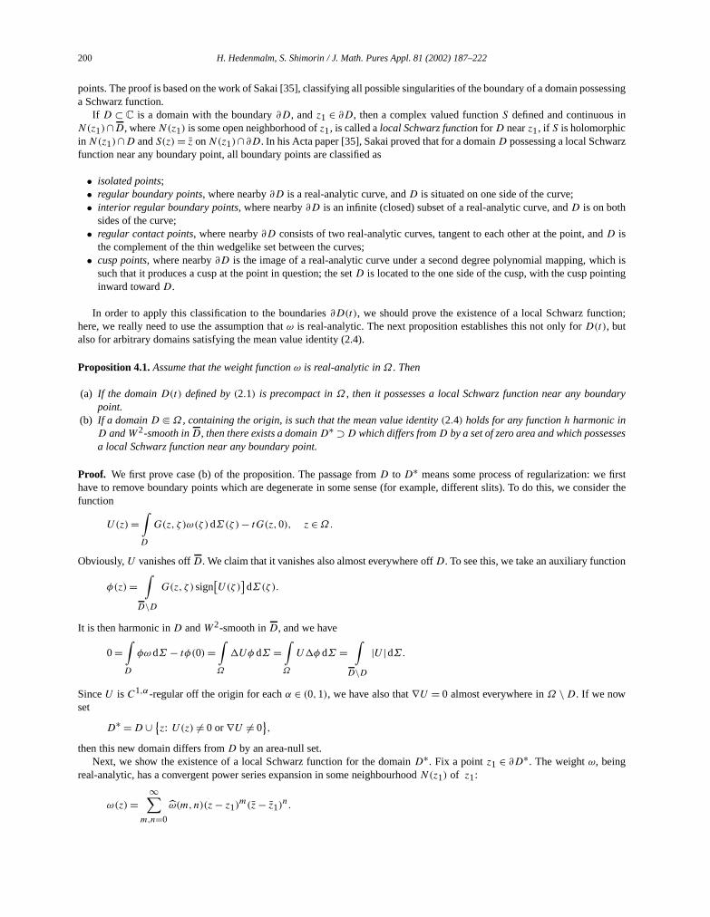
200 H. Hedenmalm, S. Shimorin / J. Math. Pures Appl. 81 (2002) 187–222
points. The proof is based on the work of Sakai [35], classifying all possible singularities of the boundary of a domain possessinga Schwarz function.
If D ⊂ C is a domain with the boundary∂D, andz1 ∈ ∂D, then a complex valued functionS defined and continuous inN(z1)∩D, whereN(z1) is some open neighborhood ofz1, is called alocal Schwarz function forD nearz1, if S is holomorphicinN(z1)∩D andS(z)= z onN(z1)∩∂D. In his Acta paper [35], Sakai proved that for a domainD possessing a local Schwarzfunction near any boundary point, all boundary points are classified as
• isolated points;• regular boundary points, where nearby∂D is a real-analytic curve, andD is situated on one side of the curve;• interior regular boundary points, where nearby∂D is an infinite (closed) subset of a real-analytic curve, andD is on both
sides of the curve;• regular contact points, where nearby∂D consists of two real-analytic curves, tangent to each other at the point, andD is
the complement of the thin wedgelike set between the curves;• cusp points, where nearby∂D is the image of a real-analytic curve under a second degree polynomial mapping, which is
such that it produces a cusp at the point in question; the setD is located to the one side of the cusp, with the cusp pointinginward towardD.
In order to apply this classification to the boundaries∂D(t), we should prove the existence of a local Schwarz function;here, we really need to use the assumption thatω is real-analytic. The next proposition establishes this not only forD(t), butalso for arbitrary domains satisfying the mean value identity (2.4).
Proposition 4.1.Assume that the weight function ω is real-analytic in Ω . Then
(a) If the domain D(t) defined by (2.1) is precompact in Ω , then it possesses a local Schwarz function near any boundarypoint.
(b) If a domain D Ω , containing the origin, is such that the mean value identity (2.4) holds for any function h harmonic inD andW2-smooth inD, then there exists a domainD∗ ⊃D which differs fromD by a set of zero area and which possessesa local Schwarz function near any boundary point.
Proof. We first prove case (b) of the proposition. The passage fromD to D∗ means some process of regularization: we firsthave to remove boundary points which are degenerate in some sense (for example, different slits). To do this, we consider thefunction
U(z)=∫D
G(z, ζ )ω(ζ )dΣ(ζ)− tG(z,0), z ∈Ω.
Obviously,U vanishes offD. We claim that it vanishes also almost everywhere offD. To see this, we take an auxiliary function
φ(z)=∫D\D
G(z, ζ )sign[U(ζ )
]dΣ(ζ).
It is then harmonic inD andW2-smooth inD, and we have
0=∫D
φωdΣ − tφ(0)=∫Ω
Uφ dΣ =∫Ω
Uφ dΣ =∫D\D
|U |dΣ.
SinceU is C1,α-regular off the origin for eachα ∈ (0,1), we have also that∇U = 0 almost everywhere inΩ \D. If we nowset
D∗ =D ∪ z: U(z) = 0 or∇U = 0
,
then this new domain differs fromD by an area-null set.Next, we show the existence of a local Schwarz function for the domainD∗. Fix a pointz1 ∈ ∂D∗. The weightω, being
real-analytic, has a convergent power series expansion in some neighbourhoodN(z1) of z1:
ω(z)=∞∑
m,n=0
ω(m,n)(z− z1)m(z− z1)n.

H. Hedenmalm, S. Shimorin / J. Math. Pures Appl. 81 (2002) 187–222 201
Let
W(z)=∞∑
m,n=0
ω(m,n)
(m+ 1)(n+ 1)(z− z1)m+1(z− z1)n+1,
for z nearz1, and observe thatW(z) = ω(z) there. The function∂zU(z) is of regularity classC0,α , for α ∈ (0,1), awayfrom 0 onΩ, in particular inN(z1), provided that the given neighborhood is small. LetR be the function
R(z)= z1 + 1
ω(z1)∂z
(W(z)−U(z)),
which is well defined nearz1 and of regularity classC0,α there. The∂ derivative ofR is
∂zR(z)= 1
ω(z1)∂z∂z
(W(z)−U(z))= 1
ω(z1)z
(W(z)−U(z)) = ω(z)
ω(z1)1Ω\D∗ (z),
for z nearz1. In particular, ifN(z1) is a small neighborhood ofz1, the functionR is holomorphic inD∗ ∩ N(z1). By theconstruction of the domainD∗, the gradient∇U vanishes at any point of∂D∗, so that forz ∈ ∂D∗ ∩N(z1),
R(z) = z1 + 1
ω(z1)∂zW(z)= z1 + 1
ω(z1)
∞∑m,n=0
ω(m,n)
n+ 1(z− z1)m(z− z1)n+1 = z1 + z− z1 + O
(|z− z1|2)(4.1)
= z+ O(|z− z1|2)
,
where O(|z− z1|2) stands for a real-analytic function of the given magnitude. Let us writeT (z, z) for the real-analytic functionnearz1 expressed by the right-hand side of (4.1), with notation that emphasizes the separate dependence ofz andz; we thinkof T as a holomorphic function of two complex variables near(z1, z1) ∈ C2. We recapture what we know about the functionR:for some small neighborhoodN(z1) of z1 ∈Ω ∩ ∂D∗, we have thatR is Hölder continuous there; moreover, onN(z1) ∩D∗,R is holomorphic, and onN(z1) \D∗,
R(z)= T (z, z)= z+O(|z− z1|2)
.
By the implicit function theorem, ifN(z1) is small, there exists a Hölder continuous functionS on N(z1) such thatR(z) = T (z,S(z)), which is then holomorphic onN(z1) ∩D∗. This is the sought-after Schwarz function. The criterion thatallows us to invoke the implicit function theorem is that∂zT (z1, z1)= 1 = 0.
In the case (a), the proof follows the same arguments, but we use the functionUt defined by (2.2) instead ofU . Clearly,Ut vanishes on∂D(t), and∇Ut vanishes there since at any point of∂D(t), the functionUt has a local minimum. The analyticityof R is a consequence of Proposition 2.2.
In [35], Makoto Sakai mentions that the above construction of a Schwarz function is possible. We have merely filled in thedetails.
Fig. 2. A generic flow domainD(t) according to Sakai.

202 H. Hedenmalm, S. Shimorin / J. Math. Pures Appl. 81 (2002) 187–222
We see that in the case of real-analytic weightω, the boundary∂D(t) is very regular. It is certainly possible forD(t) tobe multiply connected, but the holes have to be pretty well-behaved. In fact, there may be at most finitely many holes withnonempty interior, and the rest of the holes are of the types finitely many (subsets of) interior real-analytic arcs, and finitelymany isolated points (the ones not accounted for already). See Fig. 2 for an illustration of whatD(t)may look like.
5. Logarithmically subharmonic weights
In this section, we add the requirement that the weight functionω is logarithmically subharmonic, which corresponds tonegative Gaussian curvature for the Riemannian metric (1.1). We also assume that the underlying domainΩ is simply connectedand recall thatT is the supremum of thoset > 0 for whichD(t)Ω . We shall show that fort ∈]0, T [, all the domainsD(t)are real-analytic Jordan domains, and that they are uniquely characterized by the mean value identity (2.4). We also prove thatfor T < t <+∞, there exists no Jordan domainD satisfying this identity.
Throughout this section, we assume thatΩ is aC∞-smooth Jordan domain andω is strictly positive, real-analytic andlogarithmically subharmonic inΩ .
5.1. The biharmonic Green function
We shall use the techniques of the biharmonic boundary value problems in the unit disk. LetΓ (z, ζ ), z, ζ ∈ D, stand for thebiharmonic Green function inD, i.e., the solution of the boundary value problem
2zΓ (z, ζ )= δζ (z) for z ∈ D (in the sense of distributions);
Γ (z, ζ )= ∣∣∇zΓ (z, ζ )∣∣ = 0 for z ∈ T = ∂D.
The well-known explicit formula forΓ (z, ζ ) is
Γ (z, ζ )= |z− ζ |2 log
∣∣∣∣ z− ζ1− zζ∣∣∣∣2 + (
1− |z|2)(1− |ζ |2)
, (z, ζ ) ∈ D× D
(see [12, Chapter 7]). It is also known that 0< Γ (z, ζ ) everywhere inD× D.An application of the Green formula shows that an arbitrary functionY(z) which isC4-smooth inD and vanishes on the
boundaryT = ∂D can be represented as
Y(z)=∫D
Γ (z, ζ )2Y(ζ )dΣ(ζ)+ 1
2
∫T
H(ζ, z)∂nY (ζ )dσ(ζ ), z ∈ D, (5.1)
where∂nY (ζ ) denotes the normal derivative ofY in the interior direction, and the functionH(ζ, z) is given as
H(ζ, z)=ζΓ (z, ζ )=(1− |z|2)1− |zζ |2
|1− zζ |2 , (ζ, z) ∈ T ×D.
We see that the functionH(ζ, z) is also positive everywhere inT×D.We shall use also the Green functionGD(z, ζ ) for the Laplacian inD:
GD(z, ζ )= log
∣∣∣∣ z− ζ1− zζ∣∣∣∣2.
The assertion of the next lemma can be found essentially in [8,17].
Lemma 5.1.Assume that a positive function ν ∈C∞(D) is subharmonic in D and such that the identity∫D
h(z)ν(z)dΣ(z)= h(0) (5.2)
holds for any harmonic polynomial h. Then
(a) for any function u ∈W2(D) subharmonic in D,∫D
u(z)dΣ(z)∫D
u(z)ν(z)dΣ(z); (5.3)
(b) for any ζ ∈ T, we have ν(ζ ) 1.

H. Hedenmalm, S. Shimorin / J. Math. Pures Appl. 81 (2002) 187–222 203
Proof. To prove (a), we consider the function
Φ(z)=∫D
GD(z, ζ )(ν(ζ )− 1
)dΣ(ζ).
We haveΦ|T = 0, and sinceΦ = ν − 1 annihilates harmonic polynomials, we have also∇Φ|T = 0. Therefore,Φ can berepresented as
Φ(z)=∫D
Γ (z, ζ )2Φ(ζ )dΣ(ζ)=∫D
Γ (z, ζ )ν(ζ )dΣ(ζ),
and, therefore, it is positive inD. We have then∫D
u(z)(ν(z)− 1
)dΣ(z)=
∫D
u(z)Φ(z)dΣ(z)=∫D
u(z)Φ(z)dΣ(z) 0,
which proves (a).To prove (b), it suffices to substitute functionsun(z)= |r(z)|2n/‖rn‖L2(D), wherer(z)= (1+ ζ z)/2, to (5.3) and then let
n tend to+∞ (see [17, Proposition 1.3]).We shall also need the next lemma.
Lemma 5.2.Let Y be a C∞-smooth real-valued function on D \ 0, with a logarithmic singularity at the origin, such that2Y =δ0 −µ in D, where µ ∈C∞(D) has 0 µ in D. Suppose that Y |T = 0, and that ∂nY 0 on T. Then
Y(z) log |z|2 + 1− |z|2< 0, z ∈ D.
Proof. We represent the functionY by formula (5.1):
Y(z)=∫D
Γ (z, ζ )2Y(ζ )dΣ(ζ)+ 1
2
∫T
H(ζ, z)∂nY (ζ )dσ(ζ ),
where we think of the integration in the sense of distributions. As the functionH(ζ, z) is positive, the expression on the right-hand side only gets larger if we drop the second term:
Y(z)∫D
Γ (z, ζ )(δ0(ζ )−µ(ζ )
)dΣ(ζ)=ζΓ (z,0)−
∫D
Γ (z, ζ )µ(ζ )dΣ(ζ)ζΓ (z,0)= log |z|2 + 1− |z|2,
where we have also used the fact thatΓ is positive. The proof is complete.
5.2. Ruling out holes
We assume thatD(t)Ω . LetD•(t) stand for the simply connected domain obtained fromD(t) by adding all the interiorholes, both the ones with nontrivial interior and the ones that are parts of arcs as well as the isolated points. SinceΩ is simplyconnected, we haveD•(t)Ω . The boundary∂D•(t) is a closed real-analytic curve, with the possible exception of finitelymany contact and cusp points. Letφ :D → D•(t) be the Riemann mapping which sends 0 to 0 (it is unique up to rotationsof D). By the regularity of the boundary,φ extends analytically to a neighborhood ofD, with the cusp points corresponding tosimple zeros ofφ′. We then consider the domainB = φ−1(D(t)), and note thatD \ B is a compact subset ofD. In general,B may look like what is illustrated by Fig. 3.We shall prove that B = D. Introducing the weightν = t−1ω φ|φ′|2, which islogarithmically subharmonic inD, we obtain from Theorem 2.3 that
h(0)=∫B
h(z)ν(z)dΣ(z), (5.4)
for all functionsh of the formh = g φ, with g ∈W2(Ω) harmonic inD(t). We also have the corresponding inequality forsubharmonic functions. The new weightν is real-analytic inD, with zeros at the finitely many points ofT corresponding to thecusps; elsewhere, it is strictly positive.

204 H. Hedenmalm, S. Shimorin / J. Math. Pures Appl. 81 (2002) 187–222
Fig. 3. The mapped flow domainB.
We can interpret the domainB as appearing from an obstacle problem. After all, the functionVt φ has the leastsuperharmonic majorant inD, and one checks thatVt φ is that majorant (by Proposition 2.9(a), withΩ ′ = D•(t), wehave thatVt is the least superharmonic majorant toVt in D•(t); the conformal invariance of the operation of taking the leastsuperharmonic majorant then proves the claim). We calculate that
(Vt φ)(z)=Vt(φ(z)
)∣∣φ′(z)∣∣2 = tδ0(z)− ω φ(z)∣∣φ′(z)∣∣2, z ∈ D,
so that if we define
W(z)= log |z|2 −∫D
GD(z, ζ )ν(ζ )dΣ(ζ), z ∈ D,
we obtainW = t−1Vt φ − t−1P [Vt φ|T], where in general,P [f ] expresses the harmonic extension toD via the Poissonintegral formula of a functionf given on the boundaryT. Let W stand for the least superharmonic majorant toW on D; by theabove,W = t−1Vt φ − t−1P [Vt φ|T].
For 1 r <+∞, let
Wr(z)= r log |z|2 −∫D
GD(z, ζ )ν(ζ )dΣ(ζ), z ∈ D,
and letWr be its least superharmonic majorant onD. We are interested in the open sets
B(r)= z ∈ D: Wr(z) < Wr (z)
.
By Proposition 2.6, the setB(r) is connected for eachr , and by Proposition 2.7, it increases withr . The left end pointr = 1corresponds to dropping the parameter:W1 =W andB(1) = B. The functionWr vanishes on the unit circleT. If Wr(z) 0throughoutD, then the least superharmonic majorant is triviallyWr(z) ≡ 0. In this case, we also have∂nWr(z) 0 on T
(interior normal derivative). Lemma 5.2, applied to the functionY = r−1Wr , provides a converse to this statement: since2Wr = rδ0 −ν, andν is subharmonic, we obtain that the condition∂nWr |T 0 implies
Wr(z) r(log |z|2 + 1− |z|2)
< 0, z ∈ D; (5.5)
and in this case we haveB(r)= D. In other words,
• supDWr 0 if and only if supT ∂nWr 0, and• if supT ∂nWr 0, thenWr < 0 onD, andB(r)= D.
If supT ∂nWr 0 holds forr = 1, then we are done, for thenB = B(1)= D. So, let us suppose instead that 0< supT ∂nW1.The formula definingWr yields
∂nWr (z)=−2(r − 1)+ ∂nW1(z), z ∈ T,

H. Hedenmalm, S. Shimorin / J. Math. Pures Appl. 81 (2002) 187–222 205
and since∂nW1 is in C∞(T) and real-valued, there exists a critical valuer = r1, 1< r1< +∞, such that 0< supT ∂nWr for1 r < r1 and supT ∂nWr 0 for r1 r <+∞; in fact, r1 = 1+ 1
2 supT ∂nW1.The setD \ B(r) is the coincidence set for the obstacle problem, and each point ofD where the smallest concave majorant
of Wr touches the graph of the function definitely belongs to this set. In particular, any point ofD whereWr attains a positivemaximum value is inD \ B(r). Since we know thatD \ B D from Sakai’s classification, andD \ B(r) gets smaller asrincreases, it follows that any such maximum point is in the compactD \B. For eachr with 1 r < r1, the functionWr attainsa positive maximum onD. Let us say that the maximum is attained at the interior pointz(r), which then must belong toD \B.We choose a sequenceρj , j = 1,2,3, . . . , with 1< ρj < r1, and limit ρj → r1 asj →+∞. The pointszj = z(ρj ) are inD \B, and a subsequence of them tends to a pointz∞ ∈ D \B (by compactness). We have that 0<Wρj (zj ), so that in the limit0 Wr1(z∞). But for r = r1, (5.5) holds, which does not permit such a pointz∞ to exist. So, something must be wrong, andthat something is the assumption thatB was not all ofD.
5.3. Ruling out cusps and contact points
We work in the context of the previous subsection. We have proved thatB = D, and hence thatD(t) is simply connected.We shall now demonstrate that the boundary ofD(t) fails to have cusp points. We know that (5.4) (withB = D) holds for allh of the formh = g φ, with g ∈W2(Ω) harmonic onD(t). If h is aC∞-smooth function onD, holomorphic in D, withthe property that it is totally flat (meaning that all derivatives of finite order vanish) at the finitely many points ofT whichare mapped onto cusp or contact points underφ, thenh is of the above formg φ, with a holomorphicg, and (5.4) holdsfor h. The identity (5.4) is preserved under closure with respect to the norm ofL1(D), and an arbitrary analytic polynomialcan be approximated inL1(D) by functionsh from the above-mentioned class. Taking complex conjugates, we obtain that theweight ν possesses the reproducing property (5.2) for arbitrary harmonic polynomialh. By Lemma 5.1(b), we haveν(ζ ) 1for anyζ ∈ T, and, in particular,φ′(ζ ) = 0 for anyζ ∈ T, which shows that the boundary∂D(t) cannot have any cusps.
It remains to show that we cannot have contact points. But if this happened for somet = t0, then by continuity propertiesof domainsD(t), given by Propositions 3.1 and 3.2, we obtain that fort ′ = t0 + δ, with sufficiently smallδ, the domainD(t ′)would have holes. We refer to Fig. 1 for an illustration of the situation. According to Proposition 3.1, the flow domainD(t ′) isjust a little bigger thanD(t) for t ′ close tot , and the only place where topological changes are possible is in small neighborhoodsof the set of contact points. On the other hand, by Proposition 3.2,D(t ′) does indeed contain a whole little neighborhood of eachcontact point, at least up to sets of zero area measure. It remains to show that if the set of contact points forD(t) is nonempty,the domainD(t ′) now has to possess holes. Let us study anouter contact point, where to the one side, we have the unboundedcomponent ofC \D(t), and, to the other, a bounded one. As the contact point fuses, at least part of the bounded componentremains, and it now is a hole, because there is no longer a path to the unbounded component. The existence of holes inD(t ′)is immediate. But holes are impossible by results of the previous subsection, and this shows that the contact points are alsoimpossible.
5.4. Uniqueness of ω-mean-value disks
We have proved that fort ∈]0, T [ all D(t) are Jordan domains. By Proposition 2.5, we conclude that they are uniquely – upto addition or removal area-null sets – characterized by the mean value identity (2.4).
Assume now that a Jordan domainD Ω satisfies this identity for somet > T . By Proposition 4.1(b), there exists a refineddomainD∗ ⊃D which differs fromD by an area-null set and possesses a local Schwartz function near any boundary point. ButsinceD was a Jordan domain,D∗ must coincide withD, and, therefore, we get the existence of a local Schwartz function forD.By Sakai’s classification, the boundary∂D is a finite union of analytic arcs with possible finite number of singularities in theform of inner cusps. By standard approximation arguments, we obtain that the mean value identity (2.4) holds for an arbitraryfunctionh which is holomorphic inD and continuous inD. Now, letφ be the conformal mapping fromD ontoD, such thatφ(0)= 0. By regularity of the boundary∂D, φ is analytic inD. Introducing a new weightν in D, given asν = t−1ω φ · |φ′|2,we see that it satisfies the mean value identity (5.2) for anyh holomorphic inD and continuous inD, and, therefore, for anyharmonic polynomial. Applying Lemma 5.1(a), we get, for any functionu ∈W2(D) subharmonic inD,
u(0)∫D
u(z)dΣ(z)∫D
u(z)ν(z)dΣ(z).
Returning to the domainD, we obtain the moment inequality (2.3) for anyu which isW2-smooth inD and subharmonic inD.By Proposition 2.4,D differs fromD(t) by a set of zero area, which shows thatD(t)Ω and t ∈]0, T [. This contradictionshows that forT < t <+∞, there exists no Jordan domain satisfying the mean value identity (2.4).

206 H. Hedenmalm, S. Shimorin / J. Math. Pures Appl. 81 (2002) 187–222
To summarize all preceding results, we formulate the following theorem.
Theorem 5.3.LetΩ be a bounded and simply connected domain in C withC∞-smooth boundary, and let ω be a weight functionwhich is strictly positive, real-analytic and logarithmically subharmonic in Ω . If the domains D(t) are defined by (2.1), thenthere exists a positive number T such that D(t)Ω for t ∈]0, T [, and that this fails for t ∈ [T,+∞[. For t ∈]0, T [,
• the domains D(t) increase continuously with t , and a portion of ∂D(t) approaches ∂Ω as t→ T ;• all D(t) are Jordan domains with real-analytic boundaries;• the domains D(t) satisfy the moment inequality, and, a fortiori, the mean value identity (see Theorem 2.3); moreover, if
a domain D Ω satisfies the mean value identity (2.4), then D =D(t) up to an area-null set.
For T < t <+∞, there does not exist any Jordan domain D satisfying the mean value identity (2.4).
6. The evolution equation
A classical approach to the study of Hele–Shaw flows consists in considering the conformal mappingsφt from the unitdisk D onto the flow domainsD(t) and examining the evolution equation they satisfy. We want to derive a similar equation inthe context of weighted Hele–Shaw flows, in the case where the weight function depends on an additional parameter.
As before, assume thatΩ ⊂ C is a bounded and simply connected domain withC∞-smooth boundary. This time, we aregiven a one-parameter family of weight functions+s onΩ , where the parameters is confined to some open interval]a, b[ witha < b. We assume+s(z) isC∞-smooth in both variables(z, s) ∈Ω×]a, b[. Let t (s), be a knownC∞-smooth strictly positivefunction on]a, b[, and assume that we have a one-parameter continuous family of Jordan domainsD(s) with real-analyticboundaries so that 0∈D(s)Ω and the mean value identity∫
D(s)
h(z)+s(z)dΣ(z)= t (s)h(0) (6.1)
holds for eachs ∈]a, b[, whereh is an arbitrary function harmonic inD(s). We consider the conformal mappingsχs from D
ontoD(s) normalized byχs(0)= 0,χ ′s (0) > 0.To derive the evolution equation forχs , we consider first the special case whereD(s0)= D for somes0 ∈]a, b[. Fors close
to s0 and a functionh harmonic inD, we write
(t (s)− t (s0)
)h(0)=
[ ∫D(s)
−∫D
]h(z)+s0(z)dΣ(z)+
∫D
h(z)(+s(z)−+s0(z)
)dΣ(z)+ o(s − s0). (6.2)
For s close tos0, we represent the boundary∂D(s) in polar coordinates(r, θ) as
r = 1+ (s − s0)ρ(eiθ )+ o(s − s0);
then the first term of the right-hand side of (6.2) has the asymptotics
2(s − s0)∫T
h(ζ )ρ(ζ )+s0(ζ )dσ(ζ )+ o(s − s0)
ass→ s0. Letting nows tend tos0, we obtain in the limit from (6.2)
t ′(s0)h(0)= 2∫T
h(ζ )ρ(ζ )+s0(ζ )dσ(ζ )+∫D
h(z)∂s+s(z)∣∣s=s0 dΣ(z), (6.3)
where∂s+s denotes the partial derivative of+s with respect tos. The right-most integral in this formula can be rewritten as anintegral overT. To do this, we introduce the sweeping-out operatorP ∗, defined on functionsg from C(D) by
P ∗[g](ζ )=∫D
1− |z|2|1− ζ z|2g(z)dΣ(z), ζ ∈ T. (6.4)

H. Hedenmalm, S. Shimorin / J. Math. Pures Appl. 81 (2002) 187–222 207
It can be considered as an operator adjoint to the operatorP of harmonic extension of functions fromT to D: for any functionsg,h ∈C(D) with h harmonic inD, we have∫
D
h(z)g(z)dΣ(z)=∫T
h(ζ )P ∗[g](ζ )dσ(ζ ). (6.5)
We write equation (6.3) in terms of this sweeping-out operator:
t ′(s0)h(0)=∫T
h(ζ )[2ρ(ζ )+s0(ζ )+P ∗[∂s+s ](ζ )|s=s0
]dσ(ζ ),
for an arbitrary functionh harmonic inD. The only finite Borel measure onT that represents for the origin is normalized arclength measure dσ , which allows us to deduce from the above the expression for the rate of growth of the domainsD(s) for snears0:
ρ(ζ )= t′(s0)− P ∗[∂s+s ](ζ )|s=s0
2+s0(ζ ).
Now, using the formula for conformal mappings of near-circular domains found in Nehari’s book [28, pp. 263–265], we canwrite the expression for the derivative∂sχs at the points = s0:
∂χs
∂s(z)
∣∣∣s=s0
= z∫T
ζ + zζ − z ·
t ′(s0)− P ∗[∂s+s ](ζ )|s=s02+s0(ζ )
dσ(ζ ). (6.6)
To obtain the evolution equation for arbitraryD(s0), we switch coordinates to the unit disk, and set
D(s)= χ−1s0
(D(s)
), χs = χ−1
s0 χs, and +s (z)=+s χs0(z)
∣∣χ ′s0(z)∣∣2.Applying (6.6), we obtain the equation
∂χs
∂s(z)= zχ ′s (z)
∫T
ζ + zζ − z ·
t ′(s)− P ∗[(∂s+s) χs |χ ′s |2](ζ )2+s χs(ζ )|χ ′s(ζ )|2
dσ(ζ ). (6.7)
The next proposition formulates the above discussion in a rigorous fashion.
Proposition 6.1.Let Ω be a simply connected domain and +s(z) a continuous family of strictly positive weights, such thatthe mapping (z, s) #→ +s(z) is C∞-smooth in both variables on Ω×]a, b[. Let t (s), with s ∈]a, b[, be a strictly positiveC∞-smooth function. Assume that there exists a one-parameter family of univalent functions χs :D →Ω , for s ∈]a, b[, whichextend as univalent functions to D(0,1+ ε)→ Ω for some positive ε, and such that the dependence on the parameter s isC∞-smooth. Suppose these mappings χs satisfy the evolution equation (6.7). Define the domains D(s)Ω by D(s)= χs(D).Assume also that the mean value identity (6.1) holds for some fixed s = s1 ∈]a, b[. Then the same identity holds for all s ∈]a, b[.
Proof. By an approximation argument, it suffices to check (6.1) for harmonic polynomialsh. To do this, it suffices to provethat
∂
∂s
∫D(s)
h(z)+s(z)dΣ(z)= t ′(s)h(0) (6.8)
holds for anys ∈]a, b[ and anyh which is harmonic inD(s). After switching coordinates to the unit disk, this is equivalent tothe following statement: ifD(s0)= D, χs0(z)= z, and theχs satisfy (6.6), then for any functionh harmonic inD, (6.8) holdsfor s = s0. Using Green’s formula, we obtain, for real-valuedh,
∂
∂s
∫D(s)
h(z)+s(z)dΣ(z)|s=s0 =∂
∂s
∫D
h(χs(w)
)+s
(χs(w)
)∣∣χ ′s(w)∣∣2 dΣ(w)|s=s0
=∫D
[2Re
(∂(h+s0)∂sχs |s=s0
)+ h∂s+s |s=s0 + 2h+s0 Re(∂sχ
′s
∣∣s=s0
)]dΣ (6.9)
=∫T
hP ∗[∂s+s ]|s=s0 dσ +∫T
2Re(ζ ∂sχs(ζ )|s=s0
)h(ζ )+s0(ζ )dσ(ζ ),

208 H. Hedenmalm, S. Shimorin / J. Math. Pures Appl. 81 (2002) 187–222
where∂ stands for differentiation with respect to the independent complex variable, and∂s is differentiation with respect to thereal parameters. In view of (6.6), we have
2Re(ζ ∂sχs(ζ )|s=s0
)= t ′(s0)− P ∗[∂s+s ](ζ )|s=s0+s0(ζ )
, ζ ∈ T,
and substituting this to the last integral in (6.9), we get the desired conclusion.We return to the context of the preceding sections; there, we have a single weight function+s(z) = ω(z), and consider
t (s) = s. We denote byφt the conformal mapping fromD ontoD(t) normalized by the conditionsφt (0) = 0 andφ′t (0) > 0.The evolution equation (6.7) for the mappingsφt takes the form
∂φt
∂t(z)= zφ′t (z)
∫T
ζ + zζ − z ·
dσ(ζ )
2ω(φt (ζ ))|φ′t (ζ )|2, z ∈ D, (6.10)
or, equivalently,
2Re
(ζ∂φt (ζ )
∂tφ′t (ζ )ω
(φt (ζ )
)) = 1, ζ ∈ T. (6.11)
In the classical caseω= 1, these equations appeared originally in the paper by Vinogradov and Kufarev [38], where they provedthe local existence and uniqueness of the solutions. Equation (6.11) forω= 1 was also derived by Richardson [33]. Physically,the evolution equation (6.10) describes the behavior of the conformal mappings fromD onto the Hele–Shaw flow domains. Thefocus of those investigations was the case of a nonempty possibly irregular blob of fluid at the initial timet = 0, correspondingto a given conformal mappingφ0.
The following theorem establishes local existence and uniqueness for the evolution equation (6.7).
Theorem 6.2.Let Ω be a bounded simply-connected domain, and +s , with s ∈]a, b[, a one-parameter family of weightfunctions strictly positive in Ω . Assume that +s(z) is real-analytic in the variable z and C∞-smooth in s. Also, let t (s) besome C∞-smooth strictly positive function on the interval s ∈]a, b[. For some s0 ∈]a, b[ and ε > 0, let χs0 :D(0,1+ ε)→Ω
be a univalent function. Then there exist positive numbers δ and ε′, and a unique one-parameter family of analytic functionsχs :D(0,1+ ε′)→Ω , with s ∈ (s0 − δ, s0 + δ), univalent on D(0,1+ ε′), such that the χs depend C∞-smoothly on s andsatisfy the evolution equation (6.7). If, in addition, +s(z) and t (s) depend real-analytically on the parameter s, then χs also isreal-analytic in s.
The proof of this theorem follows arguments from the paper by Reissig and von Wolfersdorfer [32], where the same theoremin the classical case+s(z)= 1, t (s)= s was derived from a nonlinear version, due to Nishida and Nirenberg, of the Cauchy–Kovalevskaya theorem. For the sake of completeness, we formulate here this theorem of Nishida and Nirenberg (see [29,30]).
We need the concept of a Banach scale:B = Br r∈ ]r0,r1] is called aBanach scale if
• for eachr ∈]r0, r1], Br is a Banach space,• for each pairr, r ′ ∈ ]r0, r1], with r ′ < r ,Br is a vector subspace ofBr ′ , and the imbeddingBr → Br ′ is a norm contraction.
Note that the spacesBr get smaller asr increases. In connection with a given Banach scale, we want to be able to speak offunctions taking values in it. Assume that we are given a parametric collectionE = Er r∈ ]r0,r1] of subsets of a setE, so thatintersections and unions of the setsEr are well-defined; it is no loss of generality to assume thatEr decreases with increasingr .We takeE = ⋃Er : r ∈]r0, r1]. Similarly, we writeB = ⋃Br : r ∈]r0, r1], which can be thought of as an inductive limitof Banach spaces.
We speak of a functionf :E→ B as an(E,B)-scale function provided thatf (Er) ⊂ Br for eachr ∈]r0, r1]. Supposewe have a topological, differentiable, or even analytic structure on the setE. Then we say that the(E,B)-scale functionf iscontinuous provided that each restrictionf |Er is a continuous mapEr → Br , for r ∈]r0, r1]. It is Cn-smooth (n= 1,2,3, . . .)if each restrictionf |Er is aCn-smooth mapEr → Br , for r ∈]r0, r1]. Similarly, the same definition applies toC∞-smoothmaps, as well as to holomorphic and real-analytic maps.
Theorem 6.3.Assume we have a Banach scale B = Br r∈ ]r0,r1]. Fix s0 > 0 and another positive number R. Let Br(R)denote the open ball of radius R in Br , and form the union B(R)= ⋃Br(R): r ∈]r0, r1]. Assume that we have a mapping(s, f ) #→ L[s, f ], defined for s ∈]–s0, s0[ and f ∈ B(R), which takes values in B = ⋃
r Br , and is such that for some positiveconstants K and C, the following conditions are fulfilled.

H. Hedenmalm, S. Shimorin / J. Math. Pures Appl. 81 (2002) 187–222 209
(i) For all pairs r, r ′ ∈ ]r0, r1] with r ′ < r , L[s, f ] is continuous in s and f as a mapping from ]–s0, s0[×Br(R) into Br ′ ;(ii ) For each r ∈]r0, r1[, the continuous function L[s,0] satisfies∥∥L[s,0]∥∥
Br K
r1 − r ;
(iii ) For all pairs r, r ′ ∈ ]r0, r1] with r ′ < r , all s ∈]–s0, s0[, and all f1, f2 ∈ Br(R), we have∥∥L[s, f1] −L[s, f2]∥∥Br′
C
r − r ′ ‖f1 − f2‖Br .
For positive a, let Ir =]–a(r1 − r), a(r1 − r)[, where r ∈]r0, r1[. We form the parametric collection I = Ir r∈ ]r0,r1[. Then forsufficiently small a the abstract Cauchy–Kovalevskaya problem
dψ
ds(s)= L
[s,ψ(s)
], ψ(0)= 0, (6.12)
has a unique solution ψ : ]–a(r1 − r0), a(r1 − r0)[→ B that is a C1-smooth (I ,B)-scale function with ψ(s) ∈ Br(R)whenever s ∈ Ir .
The proof of Theorem 6.3, as presented in [30], is based on the well-known Picard iterative process from the theory ofordinary differential equations. The analysis of this scheme also shows that this theorem admits an appropriate modificationfor the case of the complex-analytic Cauchy–Kovalevskaya problem. Namely, assume thatL[s,ψ] is defined for complexs ∈ D(0, s0), and that all assumptions of the theorem are fulfilled for these complexs. Form the parametric collectionD = D(0, a(r1 − r))r∈ ]r0,r1[, for sufficiently small positivea (so that in particular,a(r1 − r0) < s0). Suppose thatL[s, f ]is analytic ins andf in the following sense: for any complex-analytic(D,B)-scale functionφ :D(0, a(r1 − r0))→ B(R),the functions #→ L[s,φ(s)] is also analytic ins. Then there exists a unique analytic solutionψ(s) of the above Cauchy–Kovalevskaya problem. The same is true in the real-analytic case: ifL[s, f ] is real analytic ins and f , then the solutionof (6.12) is also real-analytic ins.
We turn to the proof of Theorem 6.2.
Proof. As before, we switch coordinates to the unit disk and assume without loss of generality thats0 = 0 andχs0(z) =χ0(z)= z. First, we rewrite the evolution equation (6.7) in terms of a new “unknown” function
ψs(z)= 1
χ ′s(z)− 1.
To this end, we introduce the following chain of nonlinear operators. Suppose the functionf is holomorphic inD(0, r), forsome radius 1< r <+∞, and uniformly bounded there:
sup∣∣f (z)∣∣: z ∈ D(0, r)
R.
The parameterr is supposed to be close to 1, andR is assumed small. We define
F(z)= F [f ](z)=z∫
0
dw
1+ f (w) , z ∈ D(0, r). (6.13)
Sincef is close to 0, we see thatF(z) is close toz in the uniform metric onD(0, r). We need theHerglotz transform H+:
H+[g](z)=∫T
ζ + zζ − zg(ζ )dσ(ζ ), z ∈ D,
for functionsg ∈ L1(T). Next, we define a nonlinear operatorT[s, f ] by
T[s, f ] = H+[ |1+ f |2
2+s F(t ′(s)− P ∗[|1+ f |−2∂s+s F
])]. (6.14)
Finally, we set
L[s, f ](z)= zf ′(z)T[s, f ](z)− (1+ f (z)) d
dz
(zT[s, f ](z)), z ∈ D.

210 H. Hedenmalm, S. Shimorin / J. Math. Pures Appl. 81 (2002) 187–222
The nonlinear operatorL[s, f ] is well-defined provided that|s| andR are sufficiently small. Since
F [ψs](z)=z∫
0
dw
1+ψs(w) =z∫
0
χ ′s (w)dw = χs(z),
we realize that by the way we have tailored the operatorL[s, f ], the evolution equation (6.7) becomes equivalent to the initialvalue problem
d
dsψs = L[s,ψs], ψ0 = 0. (6.15)
Of course, the functionsχs we obtain fromψs are univalent inD(0, r), as their derivatives are close to 1.We make the same choice of a Banach scale as in [32]:B is formed by the spacesBr , for r ∈]r0, r1], wherer0, r1 are some
fixed (radial) parameters such that 1< r0< r1<+∞ and bothr0 andr1 are close to 1. The spaceBr consists of all functionsholomorphic and continuous up to the boundary in the circular diskD(0, r). We use the uniform norm onD(0, r) as the normin Br .
In order to apply Theorem 6.3, we need to find an analytic extension of the functionT[s, f ](z) to the diskD(0, r). We startby finding an analytic extension of the expression
P ∗[∂s+s F|1+ f |2
](ζ )
from the unit circle to an annulus 1< |ζ |< r . Since+s(z) is real-analytic inz in the closed diskD, it can be represented in theform
+s(z)=+(z, z, s),where+ is some function holomorphic in the first two variables in some neighborhood of the set = (z, z): z ∈ D ⊂ C2
(the diagonal of the closed bidiskD× D). We also have∂s+s(z)= ∂s+(z, z, s). Using the notation
ζ ∗ = 1/ζ
for the point reflected with respect to the unit circleT, we define forf ∈Br(R) (the open ball inBr of radiusR),
Ws(ζ )= W[s, f ](ζ )= 1
ζ
ζ ∗∫ζ
∂s+(F(w),F (ζ∗), s)
(1+ f (w))(1+ f (ζ∗)) dw, r−1< |ζ |< r,
whereF(w) = F [f ](w) was defined by (6.13), and the integration is along the straight line segment connectingζ with ζ∗. Ifthe boundR for the uniform norm off on D(0, r) is small enough, andr is sufficiently close to 1, then the functionWs (ζ ) iswell-defined and continuous in the annulusAr = ζ ∈ C: r−1 |ζ | r. Its restriction to the circleT is
Ws(ζ )= 0 for ζ ∈ T,
and, moreover, it solves the following∂-problem:
∂ζWs (ζ )=− 1
ζ ζ2· ∂s+
(F(ζ ∗),F (ζ ∗), s)(1+ f (ζ ∗))(1+ f (ζ ∗)) =− 1
ζ ζ2· ∂s+s F(ζ
∗)|1+ f (ζ ∗)|2 , ζ ∈Ar.
We introduce the transformed function
Xs(ζ )= X[s, f ](ζ )=∫D
z
ζ − z∂s+s F(z)|1+ f (z)|2 dΣ(z)−
∫C\D
∂s+s F(w∗)|1+ f (w∗)|2
dΣ(w)
ww2(ζ −w) −Ws (ζ ), ζ ∈Ar .
This function is continuous in the annulusAr and, by the above properties of the functionWs(ζ ), we have that the functionXs (ζ ) meets the following conditions:
• Xs(ζ )= P ∗[(∂s+s F)/|1+ f |2](ζ ) for |ζ | = 1;• Xs(ζ ) is holomorphic inζ in the annulus 1< |ζ |< r .
Finally, we define
Ys(ζ )=Y[s, f ](ζ )= (1+ f (ζ ))(1+ f (ζ∗))(t ′(s)−Xs(ζ ))
2+(F(ζ ), F(ζ ∗), s).

H. Hedenmalm, S. Shimorin / J. Math. Pures Appl. 81 (2002) 187–222 211
This function is continuous inAr , holomorphic inζ in the annulus 1< |ζ |< r , and forζ ∈ T, it coincides with the expressionin brackets in formula (6.14) definingT[s, f ]. Now, we see that the formula
T[s, f ](z)= 1
2π i
∫∂D(0,r)
ζ + zζ − zY[s, f ](ζ ) dζ
ζ, z ∈ D(0, r),
defines an analytic extension ofT[s, f ](z) to the diskD(0, r), since Cauchy’s formula permits us to change the path ofintegration. Consequently,L[s, f ](z) admits an analytic extension to the same diskD(0, r).
Routine estimates which are left to the reader show that the operatorL[s, f ], as an operator acting in the scaleB introducedabove satisfies all requirements of Theorem 6.3, provided that the constantR is sufficiently small, andr0, r1 are sufficientlyclose to 1. Applying Theorem 6.3, we obtain the existence and uniqueness of solutionsψs of (6.15). Finally, if+s(z) andt (s)are real-analytic ins, all operators introduced above depend real-analytically ons andf , which shows that the solutionsψs ,and consequently,χs , are also real-analytic ins.
The proof of Theorem 6.2 is complete.Theorem 6.2 immediately applies to the evolution equation (6.10) for the conformal mappingsφt :D →D(t), whereD(t)
is the Hele–Shaw flow domain for parameter valuet . Taking into account Proposition 6.1 and uniqueness of the domainsD(t),we arrive at the following theorem.
Theorem 6.4.In the context of Theorem 5.3, for t ∈]0, T [, let φt be the conformal mapping from D onto D(t), normalized bythe conditions φt (0)= 0 and φ′t (0) > 0. Then (z, t) #→ φt (z) is real-analytic in t and holomorphic in z, for (z, t) ∈ D×]0, T [.Moreover, the mappings φt satisfy the evolution equation (6.10).
7. The exponential mapping near the origin
In this section, we define the Hele–Shaw exponential mapping locally near the origin so that it satisfies those assertions ofTheorem 1.2 which are local to the origin.
We work in the context of Theorems 5.3 and 6.4, and make the additional normalizing assumption thatω(0)= 1. For positivereals, we consider the following domains:
D(s)= 1
sD
(s2
) = z ∈ C: sz ∈D(
s2).
For the parameter values = 0, we putD(0) = D. The domainsD(s) are characterized by the mean value identity (6.1) withrespect to the weight function+s(z)= ω(sz) and witht (s)= 1:∫
D(s)
h(z)+s(z)dΣ(z)= h(0), (7.1)
whereh ranges over all bounded harmonic functions onD(s); this also applies tos = 0. Clearly,+s(z) and t (s) are real-analytic in the variables, so that we may apply Theorem 6.2 withs0 = 0 andχ0(z)= z. This gives us a one-parametric familyof functionsχs , wheres ∈]–δ, δ[ for some positiveδ, defined and univalent in a common diskD(0,1+ ε) with ε > 0, anddepending real-analytically ons, which satisfy the evolution equation (6.7). By Proposition 6.1 and the uniqueness of the thedomainsD(t) satisfying the mean value identity (Theorem 5.3), the functionsχs mapD conformally onto the domainsD(s).In particular, we have
χs(z)= s−1φs2(z), 0< s <√T ; (7.2)
here, as before,φt is the conformal mapping fromD ontoD(t), and we notice that the formula naturally extendsχs up to theparameter value
√T , as indicated. We can defineD(s) for negatives as well, setting it equal to the image of the unit diskD
underχs ; initially, this makes sense at least for−δ < s < 0. By Proposition 6.1, the mean value identity (7.1) holds for negatives as well, and since the function+s(z) does not change under a change of signs in bothz ands, we obtain, from the uniquenessof mean value disks, that
D(−s)=−D(s)= z ∈ C: −z ∈D(s)
. (7.3)
In view of the requirement thatχ ′s(0) > 0 should hold for alls, negative as well as positive, we also get the symmetry relation
χ−s(−z)=−χs(z); (7.4)
in particular,χs andD(s) are well-defined for−√T < s <
√T .

212 H. Hedenmalm, S. Shimorin / J. Math. Pures Appl. 81 (2002) 187–222
For s close to 0, the boundary of the domainD(s) can be represented in polar coordinates(r, θ) as follows:
r = r(θ, s)= 1++∞∑l=1
Rl(θ)sl , (7.5)
where eachRl(θ) is a real-analytic function of the real parameterθ . The next proposition establishes some general propertiesof the functionsRl(θ).
Proposition 7.1. For any l = 1,2,3, . . . , the function Rl(θ) is periodic with period 2π , and in fact, it is a trigonometricpolynomial of degree at most l. Furthermore, it satisfies Rl(θ + π)= (−1)lRl (θ) for all real θ .
Proof. By the symmetry property (7.3) of the domainsD(s), the functionr(θ, s) is unperturbed by the transformation(θ, s) #→ (θ + π,−s), from which we easily read off thatRl(θ + π)= (−1)lRl(θ).
Next, we assume thats > 0 is small. By the mean value identity (7.1) applied to the functionh(z) = zm, for m =0,1,2,3, . . . , we get∫
D(s)
zmω(sz)dΣ(z)= δm,0, m= 0,1,2,3, . . . ,
where the delta is the standard Kronecker symbol. A similar relation holds forh(z) = zm. Writing the integrals in polarcoordinates, we obtain
2π∫0
r(θ,s)∫0
2ρ|m|+1e−imθω(sρeiθ )dρ
dθ
2π= δm,0, m ∈ Z. (7.6)
We now consider the Taylor series expansion ofω near the origin:
ω(z)=+∞∑j,k=0
ωj,kzj zk.
Substituting it into (7.6), we get
2π∫0
r(θ,s)∫0
2+∞∑j,k=0
ωj,ksj+kρj+k+|m|+1ei(j−k−m)θ dρ
dθ
2π= δm,0, m ∈ Z,
which is equivalent to
+∞∑j,k=0
2ωj,k sj+k
j + k+ |m| + 2
(r(·, s)j+k+|m|+2)∧
(k− j +m)= δm,0, m ∈ Z. (7.7)
Here, the symbol(·)∧(j)means thej th Fourier coefficient of the expression with respect to the suppressed variable. Finally, wewant to substitute the expansion (7.5) into this formula. We shall use multi-index notation: a letterα will denote a multi-index
α = (α0, α1, α2, . . .),
whereαj ∈ Z+ = 0,1,2,3, . . . and only a finite number of theαj are different from zero. We write
|α| =∑j
αj ; ‖α‖ =∑j
jαj ; α! =∏j
αj !; Rα(θ)=∏j
Rj (θ)αj .
In the last formula, we takeR0(θ)≡ 1. By the multinomial theorem,
r(θ, s)N =∑
|α|=N
N !α! R
α(θ)s‖α‖,
so that as we substitute this expansion into (7.7), we get∑j,k,α
(j + k+ |m| + 1)!
α! ωj,kRα(k− j +m)sj+k+‖α‖: 0 j, k <+∞, |α| = j + k+ |m| + 2
= 1
2δm,0.

H. Hedenmalm, S. Shimorin / J. Math. Pures Appl. 81 (2002) 187–222 213
Replacing the summation variablek by p= j + k, this becomes∑j,p,α
(p+ |m| + 1)!
α! ωj,p−j Rα(p− 2j +m)sp+‖α‖: 0 j p <+∞, |α| = p+ |m| + 2
= 1
2δm,0.
Identification of coefficients of powers ofs leads to∑j,p,α
(p+ |m| + 1)!
α! ωj,p−j Rα(p− 2j +m): 0 j p <+∞, |α| = p+ |m| + 2,p+ ‖α‖ = l
= 1
2δm,0δl,0, (7.8)
for l = 0,1,2,3, . . . . The summation overj on the left-hand side can be interpreted as a convolution multiplication. To makethis precise, we introduce the functionsWp ,
Wp(θ)=p∑j=0
ωj,p−jei(2j−p)θ , p = 0,1,2,3, . . . , θ ∈ R;
eachWp is a trigonometric polynomial of degree at mostp. We have
p∑j=0
ωj,p−j Rα(p− 2j +m)= (Wp R
α)∧(m).
Thus, forl = 1,2,3, . . . , (7.8) takes the form∑p,α
(p+ |m| + 1)!
α!(WpR
α)∧(m): 0 p <+∞, |α| = p+ |m| + 2,p+ ‖α‖ = l
= 0. (7.9)
In the sum on the left-hand side, onlyR0,R1, . . . ,Rl actually occur inRα , due to the restrictions given onα. Moreover, onlyone term containsRl as a “factor”: this happens for the index parametersp = 0 andα = α(l)= (p+|m|+1,0, . . . ,0,1,0, . . .),where the 1 occurs at thelth place; the term in question thus equalsRl(m). As a consequence, we obtain
Rl(m)=−∑p,α
(p+ |m| + 1)!
α!(WpR
α)∧(m): 0 p <+∞, |α| = p+ |m| + 2,p +‖α‖ = l, α = α(l)
. (7.10)
This equation holds for any integerm, and it gives us a recursive formula for the coefficientsRl(m). A simple inductionargument now shows thatRl(θ) is a trigonometric polynomial of degree at mostl, becauseWpRα is a trigonometric polynomialof degree less than or equal to the degree ofWp (which is p) plus the degree ofRα , which is at most‖α‖, by the inductionassumption.
For s close to 0, says ∈]–δ, δ[, the mappingχs(z) is conformal in a diskD(0,1+ ε), for some fixedε > 0 independentof s, and depends real-analytically on the parameters. Moreover, they are close to the identity mapping (uniformly onD(0,1+ ε), say). Hence, the inverse mappingψs = χ−1
s possesses analogous properties: it, too, is conformal on some opendisk containingD. As a conformal mapping,ψs is characterized by the propertiesψs(0)= 0, ψ ′
s(0) > 0, andψs(D(s))= D.Consider the Taylor expansion ofψs(z)/z with respect tos:
ψs(z)
z= 1+
+∞∑l=1
pl(z)sl . (7.11)
The next proposition establishes that the functionspl possess rather special properties.
Proposition 7.2. For any l = 1,2,3, . . . , the function pl is a polynomial of degree at most l, and it satisfies pl(−z) =(−1)lpl(z), that is, it is even for even l and odd for odd l.
Proof. By the symmetry property (7.4) ofχs , we haveψ−s(−z)=−ψs(z), which impliespl(−z)= (−1)lpl(z).The fact thatψs maps∂D(s) ontoT is conveniently expressed by∣∣ψs(r(θ, s)eiθ )∣∣2 = 1,

214 H. Hedenmalm, S. Shimorin / J. Math. Pures Appl. 81 (2002) 187–222
wherer(θ, s) is the function parametrizing∂D(s) given by (7.5), so that we have∣∣∣∣∣+∞∑l=0
pl(r(θ, s)eiθ )sl ∣∣∣∣∣
2
= r(θ, s)−2, (7.12)
provided that we setp0(z)≡ 1. Writing
r(θ, s)−2 =+∞∑l=0
ql(θ)sl ,
we obtain from (7.5) and Proposition 7.1 thatq0(θ) ≡ 1 and that for anyl = 1,2,3, . . . , ql is a trigonometric polynomial ofdegree at mostl satisfyingql (θ +π)= (−1)lql (θ). Each functionpl is analytic in a neighborhood of the closed diskD, so thatit has a convergent power series expansion
pl(z)=+∞∑m=0
pl (m)zm, z ∈ D,
and substituting this into (7.12), we arrive at
+∞∑j,k=0
+∞∑m,n=0
sj+kpj (m)pk(n) r(θ, s)m+nei(m−n)θ =+∞∑l=0
ql(θ)sl .
We recall from the proof of the previous proposition the multi-index expansion
r(θ, s)m+n =∑
|α|=m+n
(m+ n)!α! Rα(θ)s‖α‖.
Inserting this information into the above identity, we obtain
+∞∑j,k,m,n=0
∑|α|=m+n
(m+ n)!α! pj (m)pk(n)R
α(θ)sj+k+‖α‖ei(m−n)θ =+∞∑l=0
ql(θ)sl .
Comparing Taylor coefficients, we have, forl = 1,2,3, . . . ,
∑j,k,m,n,α
(m+ n)!α! pj (m)pk(n)R
α(θ)ei(m−n)θ : 0 j, k,m,n <+∞, |α| =m+ n, ‖α‖ = l − j − k= ql (θ).
The sum on the left-hand side actually only involves the functionsp0,p1, . . . , pl , and not higher indexpj ’s. Moreover, we canseparate out the terms involvingpl , because they occur precisely whenα = (m+n,0,0, . . .) and(j, k)= (l,0) or (j, k)= (0, l):
2Re[pl
(eiθ )] =
+∞∑m=0
pl (m)eimθ +
+∞∑n=0
pl(n)e−inθ
= ql(θ)−∑
j,k,m,n,α
(m+ n)!α! pj (m)pk(n)R
α(θ)ei(m−n)θ :
0 j, k,m,n <+∞, |α| =m+ n,‖α‖ = l − j − k,
(j, k) = (l,0), (j, k) = (0, l).
A simple induction argument overl now shows the desired assertion thatpl has is a polynomial of degree at mostl. After all,Rα is a trigonometric polynomial of degree at most‖α‖, so that the degree of each term in the sum on the right-hand side hasdegree at mostm + n+ |m− n| = 2maxm,n. And under the induction assumption, each such term vanishes unlessm < l
andn < l. As ql is a trigonometric polynomial of degree at mostl, it follows that the real part ofpl(eiθ ) is a trigonometric
polynomial of degree at mostl as well. But thenpl(z)must be an ordinary polynomial of degree l. The proof is complete.

H. Hedenmalm, S. Shimorin / J. Math. Pures Appl. 81 (2002) 187–222 215
The next item is a lemma from the theory of power series.
Lemma 7.3.Let f (z,w) be a function holomorphic in a neighborhood of (0,0) in C2. Suppose that its power series expansionis of the special form
f (z,w)=+∞∑m=0
m∑n=0
am,nzmwn, (7.13)
which converges near (0,0). Let g be defined by the relation g(z,w) = f (z,w/z) for z = 0. Then g admits an extension toa function holomorphic in both variables in a neighborhood of the origin (0,0).
Proof. Sincef (z,w) is holomorphic near(0,0), its power series is absolutely convergent in a possibly smaller neighborhoodof the origin:
+∞∑m=0
m∑n=0
|am,n|δmεn <+∞,
provided thatδ, ε > 0 are sufficiently small. The functiong(z,w) is represented by the Laurent series
g(z,w)= f (z,w/z)=∞∑m=0
m∑n=0
am,nzm−nwn, (7.14)
which converges absolutely for, say,|z| = δ and|w| = δε. We immediately realize that the Laurent series forg(z,w) is in facta power series, so that the result follows from the following classical statement concerning power series of two variables: if apower series converges absolutely at some point(z,w) with z = 0 andw = 0, then it converges absolutely in a small bidiskabout the origin.
We now introduce a functionµ(z, t) defined first for appropriatez andt > 0 by
µ(z, t)=√t
zψ√t
(z√t
)= 1+
+∞∑l=1
pl
(z√t
)t l/2. (7.15)
By Proposition 7.2 and Lemma 7.3, this function admits an extension to a function analytic in(z, t) near the origin(0,0). Wealso define
H(z, t)= |z|2∣∣µ(z, t)∣∣2.In terms of this functionH , we get the following characterization of the boundaries∂D(s2)= s∂D(s):
z ∈ ∂D(s2
)if and only if H
(z, s2
) = s2. (7.16)
We are now ready to prove the local existence of the desired Hele–Shaw exponential mapping. We want to find a mappingΦ
(the Hele–Shaw exponential mapping HSexp0 from Theorems 1.1 and 1.2) defined and real-analytic near the origin suchthat it maps each small diskD(0, r) diffeomorphically onto the correspondingω-mean-value diskD(r2), and the raysz ∈ C: argz = θ and the circlesz ∈ C: |z| = r are mapped to orthogonal curves. Let us think of the complex variablew as represented by polar coordinatesw= reiθ , and let∂r = ∂/∂r denote the partial differentiation in the radial direction. Thenthe desired mappingΦ must satisfy the following two conditions:
• H(Φ(w), |w|2)= |w|2, and• the vector∂rΦ(w) is orthogonal to the boundary∂D(|w|2).
Differentiating the first requirement, we find that
2Re[∂zH
(Φ(w), |w|2)
r∂rΦ(w)] = 2|w|2[
1− ∂tH(Φ(w), |w|2)]
,
whereas the second requirement is equivalent to the condition
Im[∂zH
(Φ(w), |w|2)
r∂rΦ(w)] = 0.
Combining the above two displayed equations, we obtain a differential equation forΦ:
r∂Φ
∂r(w)= |w|2[1− ∂tH(Φ(w), |w|2)]
Φ(w)µ(Φ(w), |w|2)ν(Φ(w), |w|2) . (7.17)

216 H. Hedenmalm, S. Shimorin / J. Math. Pures Appl. 81 (2002) 187–222
Here,ν(z, s)= µ(z, s)+ z∂zµ(z, s). We search forΦ of the form
Φ(w)=w(1+Ψ(w)), Ψ (0)= 0,
and notice that this implies automatically that the differential ofΦ at the origin is the identity mapping. The differentialequation (7.17) forΦ becomes the following equation forΨ :
r∂Ψ
∂r(w)= 1− ∂tH(Φ(w), |w|2)
(1+Ψ (w))µ(Φ(w), |w|2)ν(Φ(w), |w|2) − 1−Ψ (w), Ψ (0)= 0. (7.18)
If u andv are Cartesian coordinates inw-plane, so thatw = u+ iv, then
r∂
∂r= u ∂
∂u+ v ∂
∂v.
It follows that Eq. (7.18) has the form
u∂Ψ
∂u+ v ∂Ψ
∂v= f (
u,v,Ψ (u, v)), Ψ (0,0)= 0, (7.19)
where on the right-hand side,f is real-analytic in the variablesu, v, andΨ near the origin(0,0,0), and has valuef (0,0,0)= 0.If we think ofΨ andf asR2-valued functions, then (7.19) is a system of two first-order partial differential equations for whichthe origin is a singular point. Such a kind of singularity is said to be ofBriot–Bouquet type. In the scalar one-dimensional case,the theorem of Briot and Bouquet asserts that an equation
udΨ
du= f (
u,Ψ (u)), Ψ (0)= 0,
with f (0,0)= 0 andf real-analytic near the origin, has a unique solutionΨ that is real-analytic near the origin, provided thatthe partial derivative
∂f
∂Ψ(0,0)
is not a positive integer [23, pp. 295–296]. In our vector-valued two-dimensional case, the existence of solutions that are real-analytic near the origin for equations of the type (7.19) depends on the eigenvalues of the 2× 2 Jacobi matrix
J = ∂f
∂Ψ(0,0,0).
It follows from [24, Lemma 1] or [3, Theorem 1] that a sufficient condition for the existence of real-analytic solutions of (7.19)is that none of eigenvalues ofJ is a positive integer. In our case, iff is the right-hand side of (7.18), we have
f (0,0,Ψ )=−2ReΨ + O(|Ψ |2)
as|Ψ | → 0,
which shows that the eigenvalues ofJ are 0 and−2. Thus, (7.18) possesses a solutionΨ that is real-analytic near the origin.We have obtained the local existence near the origin of a real-analytic mappingΦ satisfying (7.17). This function is
a diffeomorphism on a neighborhood of the origin, becauseΦ(w)=w+O(|w|2) asw→ 0. Tracing our arguments backwards,we see thatΦ mapsD(0, r) ontoD(r2), and maps rays and circles emanating from the origin to orthogonal curves.
We can now state the following theorem.
Theorem 7.4.In the context of Theorem 5.3, there exists a unique real-analytic mapping Φ = HSexp0 (it is even unique in theclass of C1-smooth mappings) defined on a neighborhood of the origin such that
• the differential of Φ at the origin is the identity mapping times ω(0)−1/2,• for small positive r , Φ maps circles T(0, r)= ∂D(0, r) diffeomorphically onto ∂D(r2), and• near the origin, each ray w ∈ C: argw = θ is mapped by Φ to a curve orthogonal to ∂D(t) for each small positive t .
Proof. Using an appropriate dilation of the plane, we can reduce the theorem to the caseω(0) = 1. In this case, the abovediscussion shows the existence of a real-analytic mappingΦ satisfying (7.17) and having differential at the origin equal to theidentity mapping. In particular,Φ is a diffeomorphism in some neighborhood of the origin. On the other hand (7.17) impliesthatΦ(w) ∈ ∂D(|w|2) for all sufficiently small|w|, that is,Φ is a real-analytic diffeomorphism from|w| = r into ∂D(r2). Fortopological reasons, such a diffeomorphism must in fact beonto. The last assertion of the theorem (about orthogonal curves)follows from Eq. (7.17).

H. Hedenmalm, S. Shimorin / J. Math. Pures Appl. 81 (2002) 187–222 217
To see that we have uniqueness, assume that we have two mappings,Φ1 andΦ2, satisfying the assertions of the theorem.Then the mappingΦ−1
1 Φ2 is a real-analytic diffeomorphism near the origin which sends all small circlesT(0, r) ontothemselves, maps each rayargw = θ to some ray of the same type, and it has the identity differential at the origin. This ispossible only for the identity mapping, which shows thatΦ1 =Φ2.
8. Global properties of the exponential mapping
We return to the context of the introduction and summarize the results of preceding sections. Given a simply connectedtwo-dimensional Riemannian manifoldΩ with hyperbolic real-analytic Riemannian metric, we identify it with the domainΩ ⊂ C which is either the complex planeC or the unit diskD, so that the metric has the form (1.1) with a real analytic weightfunctionω. That the metric is hyperbolic means thatω is logarithmically subharmonic.
For any Jordan subdomainΩ ′ Ω with C∞-smooth boundary, we define the Hele–Shaw domainsD(t) as thenoncoincidence sets (2.1) for the corresponding obstacle problem. By Proposition 2.9,D(t) does not depend on the choiceof the underlying domainΩ ′, as long as we haveD(t)Ω ′. For any suchΩ ′ Ω , we can define
T (Ω ′)= supt ∈]0,+∞[: D(t)Ω ′,
and then set
T = supT (Ω ′): Ω ′ is a precompact Jordan subdomain ofΩ
.
For anyt ∈]0, T [, we haveD(t)Ω , and by Theorem 2.3,D(t) is anω-mean-value disk, that is, it satisfies (1.3). Moreover,by the uniqueness part of Theorem 5.3, there does not exist any Jordan domain that isω-mean-value disks fort ∈]T,+∞[ incaseT <+∞. For t ∈]0, T [, theω-mean-value disksD(t) are Jordan domains with real-analytic boundaries and they increasecontinuously witht . Moreover, they depend real-analytically on the parametert in the following sense: ifφt is the conformalmapping fromD ontoD(t), normalized by the conditionsφt (0)= 0 andφ′t (0) > 0, thenφt depends real-analytically ont .
By Theorem 7.4, we have a Hele–Shaw exponential mapping HSexp0 defined and real analytic in some diskD(0, δ) andsuch that it maps small circlesT(0, r) diffeomorphically onto Hele–Shaw flow boundaries∂D(r2), and near the origin, eachray argw = θ is mapped to a curve orthogonal to these flow boundaries. We want to extend (uniquely) HSexp0 to the diskD(0,
√T ) in such a way that the extended mapping is a diffeomorphism possessing the same properties. The next theorem
establishes that such an extension can be found.
Theorem 8.1.There exists a unique mapping Φ = HSexp0, defined and real-analytic in D(0,√T ) such that
(a) it maps each circle T(0, r) with r ∈]0,√T [ diffeomorphically onto the flow boundary ∂D(r2), and(b) it maps each ray w ∈ D(0,
√T ): argw = θ to a curve that is orthogonal to all the flow boundaries ∂D(t) with t ∈]0, T [,
and such that(c) Φ has differential at the origin equal to the identity mapping times the scaling factor ω(0)−1/2.
This mapping is a diffeomorphism from the disk D(0,√T ) onto Φ(D(0,
√T ))= ⋃D(t): t ∈]0, T [.
Proof. It is enough to find a unique mapping with desired properties defined in a diskD(0, r0), for any r0 ∈]0,√T [. Fort ∈]0, r20], let ηt = φ−1
t denote the conformal mapping inverse toφt . From the above properties of∂D(t) and hence ofφt , wesee that the functionηt (z) is analytic inz and real analytic int in a neighborhood of the set
Eε =(z, t): z ∈D(t), t ∈ [
ε, r20],
for anyε ∈]0, r20 [. On the other hand, the relation (7.15) and the definition of above functionsψs show that we have
µ(z, t)=√tηt (z)
z
for (z, t) close to the origin(0,0). We use this formula to extend the domain of definition forµ(z, t) to (z, t) in a neighborhoodof the setsEε . As before, we also define the function
H(z, t)= |z|2∣∣µ(z, t)∣∣2,and we see that the functionsµ andH turn out to be well-defined and real-analytic in a neighborhood of the set
E0 = (z, t): z ∈D(t), t ∈ [
0, r20],

218 H. Hedenmalm, S. Shimorin / J. Math. Pures Appl. 81 (2002) 187–222
where we agree thatD(0)= 0. We also have the representation (7.16) for boundaries∂D(t) in terms of the functionH validfor all t ∈ [0, r20].
As in the preceeding section, the desired properties of the mappingΦ are equivalent to Eq. (7.17). By Theorem 7.4, wehave already a real analytic solutionΦ0(w) of (7.17) defined in a neighborhood of some small closed diskD(0, δ). We wantto extendΦ0 to a functionΦ which is defined inD(0, r0) and still satisfies (7.17). SettingΦθ (r)= Φ(reiθ ) for r ∈ [δ, r0], weobtain from (7.17) the following Cauchy problem for the functionsΦθ :
dΦθ (r)
dr= r(1− ∂tH(Φθ (r), r2))
Φθ (r)µ(Φθ (r), r2)ν
(Φθ (r), r
2), Φθ (δ)= Φ0(
δeiθ ). (8.1)
Here, as before,ν = µ + z∂zµ. Taking into account the above definitions of the functionsµ andH , and also the evolutionequation for the conformal mappingsφt in the form (6.11), we can rewrite the last equation in more elegant form:
dΦθ (r)
dr= r
ω(Φθ (r))
η′r2(Φθ (r))
ηr2(Φθ (r)), Φθ (δ)= Φ0(
δeiθ ). (8.2)
By standard theorems in the theory of Ordinary Differential Equations, for any angleθ , there exists a unique solutionΦθ (r) ofEq. (8.2) defined on a maximally extended interval[δ, r1(θ)[, and this solutionΦθ (r) is real-analytic in the parametersθ andr .By Eq. (8.1), we have
H(Φθ (r), r
2) = r2.It follows that for anyr ∈ [δ, r0] ∩ [δ, r1(θ)[, we haveΦθ (r) ∈ ∂D(r2), and the pair(Φθ (r), r2) must belong to the setEδ2,which is a compact subset of the domain of definition of the right-hand side of (8.1). This shows that we must be able to continuethe solution further ifr1(θ) r0, contradicting the maximality of the interval[δ, r1(θ)[. Hence we must haver1(θ) > r0, sothat the solutionΦθ (r) is defined in the whole interval[δ, r0]. As a result, we obtain a real-analytic extensionΦ of Φ0 to thewhole diskD(0, r0).
We already noticed that for anyr ∈]0, r0] and any angleθ , we haveΦ(reiθ ) ∈ ∂D(r2), and, by the uniqueness theorem fromOrdinary Differential Equations (using as input thatΦ0 is one-to-one), we haveΦ(reiθ1) = Φ(reiθ2) for any two angles witheiθ1 = eiθ2. It follows thatΦ is a one-to-one mapping from any circleT(0, r) into the flow boundary∂D(r2), and, for topologicalreasons, this mapping is onto. To prove thatΦ is a real-analytic diffeomorphism ofD(0, r0) ontoD(r20), it remains to check thatit has a nondegenerate differential at any point. SinceΦ maps circlesT(0, r) and raysw ∈ D(0, r0): argw = θ to orthogonalcurves, it suffices to check that∂rΦ(w) = 0 and∂θΦ(w) = 0, wherew = reiθ . The first property follows immediately fromEq. (8.2). The second is also a consequence of this equation, since the variableθ is involved in (8.2) as an initial data, and inthis case we have either∂θΦθ (r) = 0 or ∂θΦθ (r)= 0 identically forr ∈ [δ, r0[, and the latter alternative is clearly impossible.
The uniqueness ofΦ can be proved by the same arguments as we used in the proof of Theorem 7.4.To finish off the proof of our main Theorems 1.1 and 1.2, we need to check that if the original metric onΩ is complete,
thenT =+∞, and that when the latter happens, HSexp0 mapsC ontoΩ . We first compare the√ω(z)|dz|-metric discsB(0, r)
with theω-mean-value disksD(t). Namely, we show thatD(r2) is well-defined and contained inB(0, r) if the latter disk isprecompactly contained inΩ . By Hadamard’s theorem, in case of a complete metric, the metric disksB(0, r) are all precompactin Ω , which shows that we indeed haveT = +∞. In caseT = +∞, we need to check that the union of allD(t) covers thewhole regionΩ . It is clearly sufficient to show that an arbitrary subdomainΩ ′ Ω is contained inD(t) for sufficiently larget .This is easily achieved by obstacle problem arguments.
We turn to the precise statements.
Proposition 8.2.Assume that the metric disk B(0, r) is precompact inΩ for a given r > 0. Then, for any t ∈]0, r2[, the domainD(t) defined by (2.1) for the obstacle problem corresponding to B(0, r) is precompactly contained in B(0, r). In particular,D(t)⊂ B(0,√t) provided that B(0,
√t ) is precompact in Ω .
Proof. The proof of the proposition is based on the following lemma, which was communicated to the authors by BorisKorenblum.
Lemma 8.3.Assume that a positive function ω is subharmonic in the unit disk D and has the reproducing property∫D
h(z)ω(z)dΣ(z)= h(0)

H. Hedenmalm, S. Shimorin / J. Math. Pures Appl. 81 (2002) 187–222 219
for all harmonic polynomials h. Then
1∫0
ω(r)dr 1.
Proof. An application of Fatou’s lemma yields∫D
h(z)ω(z)dΣ(z) h(0)
for any functionh harmonic and positive inD. In particular,∫D
1− |z|2|1− z|2ω(z)dΣ(z) 1. (8.3)
By subharmonicity ofω, we have
ω(r) 1
(1− r)2∫
D(r,1−r)ω(z)dΣ(z)=
∫D
1
(1− r)2 1D(r,1−r)(z)ω(z)dΣ(z)
for anyr ∈]0,1[, and consequently,
1∫0
ω(r)dr ∫D
[ 1∫0
1
(1− r)2 1D(r,1−r)(z)dr]ω(z)dΣ(z).
An explicit calculation shows that
1∫0
1
(1− r)2 1D(r,1−r)(z)dr = 1− |z|2|1− z|2 ,
which – together with (8.3) – proves the lemma.In view of the Cauchy–Bunyakovskiı–Schwarz inequality and rotation invariance, we also have, under the conditions of the
last lemma,
1∫0
√ω(rζ )dr 1, ζ ∈ T.
In geometric language, this inequality means that if the unit diskD is anω-mean-value diskD(1), then the length of any radiusin the metric (1.1) is at most 1. In other words, the metric distance from the origin to any point of∂D(1) is at most 1. Byconformal invariance, this property holds for flow domainsD(1) of arbitrary shape, and we obtain, by similarity arguments,that the metric distance from the origin to any point of∂D(t) is at most
√t .
To conclude the proof of the proposition, assume thatB(0, r) is precompactly contained inΩ . Then the distance from theorigin to any point of∂B(0, r) is r . If we define
Tr = T(B(0, r)
) = supt : D(t)B(0, r)
,
then theω-mean-value diskD(Tr ) is well-defined (sinceTr < T ) and its boundary∂D(Tr ) touches the boundary∂B(0, r) atleast at one point. Since the distance from the origin to the boundary∂D(Tr ) is at most
√Tr , we obtainr
√Tr . The proof is
complete. Thus, in the case of a complete metric (1.1), theω-mean-value disksD(t) are well-defined for allt ∈]0,+∞[. It remains
to check that theω-mean value disksD(t) cover all ofΩ as t → +∞, provided T = +∞. To this end, letΩ ′ be aprecompact Jordan subdomain ofΩ . We consider the obstacle problem corresponding to this subdomain, and define for allt ∈]0,+∞[ generalized Hele–Shaw domainsD′(t) as noncoincidence sets for the obstacle problem, of the form (2.1). ByProposition 2.9, we haveD′(t)⊂D(t) for anyt ∈]0,+∞[, since for eacht , the Hele–Shaw flow domainD(t) can be obtained

220 H. Hedenmalm, S. Shimorin / J. Math. Pures Appl. 81 (2002) 187–222
as the noncoincidence set for the obstacle problem corresponding to some larger subdomainΩ ′′ ⊃Ω ′. On the other hand, byProposition 2.8(b), we haveD′(t)=Ω ′ for sufficiently large positivet , which shows that
Ω ′ ⊂⋃
D(t): t ∈]0,+∞[.The proof of our main Theorems 1.1 and 1.2 is finally complete.
9. Wrapped Hele–Shaw flow
Let us consider Hele–Shaw flow on a compact real-analytic surfaceS. We have an injection pointz0 ∈ S, and at timet = 0,there is no fluid in the surface. We get a small circular-like blob aboutz0 for small positivet , but eventually, ast grows,topological restrictions apply, and two parts of the boundary will meet, and we may develop a hole in the fluid; for instance,this will happen if the surface looks like the surface on a cigar. The end result is that the whole surface is filled at a time thatcorresponds to the area ofS, and then the flow comes to an end. This means that such a question as long term behavior ofgeodesics which makes perfect sense for metric flow cannot be asked in the Hele–Shaw flow context.
To address the issue, we introduce another notion of flow,wrapped Hele–Shaw flow. The understanding is best achievedby considering first a concrete example. So, letS be the unit sphere with the standard Riemannian metric, andz0 the northpole. As we inject fluid into the north pole, we cover increasingly bigger spherical caps, until we reach the critical momentwhen the whole sphere is covered, except for the south pole. At that point, we allow the fluid to grow a second layer, so thatin fact, the fluid flow is taking place on a sheeted surface over the sphere, the south pole being the point where the two sheetsmeet. We then continue the flow, having covered the entire sphere once, and a spherical cap at the south pole once more.The next obstruction occurs at the north pole, and we proceed just as we did at the south pole. As a result, we can trace thetrajectories of the particles injected initially at timet = 0 indefinitely, and in this example they are the great circles passingthrough the north pole. It is natural to call these trajectorieswrapped Hele–Shaw geodesics. Let us see what to do ifS is a moregeneral compact real-analytic surface. To clarify the idea, let us agree thatwe want the wrapped Hele–Shaw geodesics to be themaximal real-analytic continuations of the ordinary Hele–Shaw geodesics emanating from the injection point. As in the caseof the sphere, we need to permit the flow to take place on some other surface sheeted overS. The discussion is simplified ifwe consider the universal covering surfaceΩ of S, which is either the sphere, the plane, or the disk. We focus on hyperboliccompact real-analytic surfacesS. Although the sphere cannot be supplied with a hyperbolic metric, there are plenty of othercompact Riemann surfaces of higher genus (number of “handles”) of this type. Lift the Riemannian metric ofS to the coveringsurfaceΩ . The universal covering surface of a hyperbolic surface is either the unit diskD or the whole complex planeC. Thecomplex plane appears only in rather degenerate cases, such as whenS is the torus with flat metric, and the generic situation isthat ofΩ = D. We have a canonical projectionπ :Ω → S and a discrete groupΓ of conformal automorphisms ofΩ such thatthe projection induces the identificationS= Ω/Γ . Pick a pointz∗0 ∈ Ω such thatπ(z∗0)= z0. The ordinary Hele–Shaw flowstarting atz∗0 in Ω falls under the auspices of our main theorem, so that the corresponding flow domains are always real-analyticJordan domains.The image of that flow under the projection π then equals the wrapped Hele–Shaw flow on S.
The ergodic or chaotic properties of geodesic flow on hyperbolic compact has attracted considerable attention [2]. It wouldbe nice to to have a similar study of the wrapped Hele–Shaw geodesics.
Without the hyperbolicity assumption onS, the flow on the covering surfaceΩ may develop contact points or cusps. Thecontact points are not a serious problem, because we may allow them to continue to flow on different sheets on some surfacesheeted overΩ . But cusps are more serious, and we do not fully understand what happens they are present.
10. Questions
It is desirable to obtain further geometric properties of the Hele–Shaw flow domainsD(t) on a simply connected hyperbolicreal-analytically smooth surfaceΩ . A particularly natural question is whether they are all (geodesically) star-shaped withrespect to the injection pointz0. We do not know the answer. One reason for wanting information of this type is that it wouldmake it easier to extend our main theorem toC∞-smooth surfaces. It may then be possible to find an appropriate approximationprocess to show that the Hele–Shaw flow domainsD(t) are allC∞-smooth Jordan domains under the weaker assumption, andthat would more or less do it. In the case of planar Hele–Shaw flow, this is of course so, the flow domains being circular disksaboutz0. What is perhaps less obvious is that even if we start with some irregular blob which happens to be star-shaped withrespect toz0, then all the domains we get from injecting more fluid into the surface are also star-shaped with respect toz0 (see[7, Theorem 4.1] and [22, Theorem 1]). Convexity, however, is generallynot preserved by such Hele–Shaw flow.
In the introduction, we mentioned the concept of Hele–Shaw completeness. A natural question is whether it depends on theposition of the injection pointz0.

H. Hedenmalm, S. Shimorin / J. Math. Pures Appl. 81 (2002) 187–222 221
Higher-dimensional analogues exist for the classical Hadamard theorem, involving sectional curvature to replace Gaussiancurvature in the two-dimensional setting. We do not know whether such conditions are relevant for possible analogues of ourmain theorem on Hele–Shaw flow.
Acknowledgements
The first author wishes to thank Sigurður Helgason for a clarifying conversation outside Höör in Skåne, Sweden, in thesummer of 1999. He also thanks Peter Larkin Duren for his hospitality and encouragement during the summer of 1998 in AnnArbor, Michigan. He thanks the Erwin Schrödinger Institute in Vienna and in particular its director Peter Michor for offeringa congenial atmosphere in June, 1999. The second author, Sergei Shimorin, thanks the Swedish Natural Science ResearchCouncil (NFR) for its support under grant M-AA/AS 12325-300. He also thanks the Russian Fund for Fundamental Studies forits support under grant 96-01-00693. We thank Boris Korenblum for constructive criticism. We both thank Stefan Jakobsson forinspiration and help with the computer generation of the pictures that appear in the paper. We also extend our thanks to BjörnGustafsson for several helpful comments and general assistance.
References
[1] L. Ahlfors, L. Sario, Riemann Surfaces, Princeton Mathematical Series, Vol. 26, Princeton University Press, Princeton, NJ, 1960.[2] D.V. Anosov, Geodesic flows on closed Riemann manifolds with negative curvature, Proc. Steklov Inst. Math. 90 (1967), Amer. Math.
Soc., Providence, RI, 1969.[3] G. Bengel, R. Gérard, Théorèmes d’existence de solutions holomorphes pour certains systèmes différentiels singuliers. (French) [Theorems
on the existence of holomorphic solutions for certain singular differential systems], C. R. Acad. Sci. Paris Sér. I Math. 294 (10) (1982)333–335.
[4] M. Berger, B. Gostiaux, Differential Geometry: Manifolds, Curves, and Surfaces, Graduate Texts in Math., Vol. 115, Springer-Verlag,New York, 1988.
[5] S. Bergman, The Kernel Function and Conformal Mapping, second, revised edition, Math. Surveys Monographs, Vol. 5, Amer. Math. Soc.,Providence, RI, 1970.
[6] L.A. Caffarelli, D. Kinderlehrer, Potential methods in variational inequalities, J. Anal. Math. 37 (1980) 285–295.[7] E. DiBenedetto, A. Friedman, The ill-posed Hele–Shaw model and the Stefan problem for supercooled water, Trans. Amer. Math.
Soc. 282 (1) (1984) 183–204.[8] P.L. Duren, D. Khavinson, H.S. Shapiro, C. Sundberg, Contractive zero-divisors in Bergman spaces, Pacific J. Math. 157 (1993) 37–56.[9] B. Epstein, M. Schiffer, On the mean-value property of harmonic functions, J. Anal. Math. 14 (1965) 109–111.
[10] A. Friedman, Variational Principles and Free-Boundary Problems, 2nd ed., Krieger, Malabar, FL, 1988.[11] P.R. Garabedian, A partial differential equation arising in conformal mapping, Pacific J. Math. 1 (1951) 485–524.[12] P.R. Garabedian, Partial Differential Equations, Reprint of the 1964 original, AMS Chelsea Publishing, Providence, RI, 1998.[13] B. Gustafsson, Applications of variational inequalities to a moving boundary value problem for Hele Shaw flows, SIAM J. Math. Anal. 16
(1985) 279–300.[14] B. Gustafsson, On quadrature domains and an inverse problem in potential theory, J. Anal. Math. 55 (1990) 172–216.[15] J. Hadamard, Les surfaces à courbures opposées et leurs lignes géodésiques, J. Math. Pures Appl. 4 (1898) 27–73.[16] J. Hadamard, Œuvres de Jacques Hadamard, Vols. 1–4, Editions du Centre National de la Recherche Scientifique, Paris, 1968.[17] H. Hedenmalm, A factorization theorem for square area-integrable analytic functions, J. Reine Angew. Math. 422 (1991) 45–68.[18] H. Hedenmalm, S. Jakobsson, S. Shimorin, A maximum principle à la Hadamard for biharmonic operators with applications to the
Bergman spaces, C. R. Acad. Sci. Paris Sér. I Math. 328 (11) (1999) 973–978.[19] H. Hedenmalm, S. Jakobsson, S. Shimorin, A biharmonic maximum principle for hyperbolic surfaces, Preprint, 2000.[20] H. Hedenmalm, B. Korenblum, K. Zhu, Theory of Bergman Spaces, Graduate Texts in Math., Vol. 199, Springer-Verlag, New York, 2000,
in print.[21] S. Helgason, Differential Geometry, Lie Groups, and Symmetric Spaces, Pure Appl. Math., Vol. 80, Academic Press, New York, 1978.[22] Yu.E. Hohlov, D.V. Prokhorov, A.Ju. Vasil’ev, On geometrical properties of free boundaries in the Hele–Shaw flows moving boundary
problem, Lobachevskii J. Math. 1 (1998) 3–12 (electronic).[23] E.L. Ince, Ordinary Differential Equations, Dover, New York, 1944.[24] S. Kaplan, Formal and convergent power series solutions of singular partial differential equations, Trans. Amer. Math. Soc. 256 (1979)
163–183.[25] L. Karp, A.S. Margulis, Newtonian potential theory for unbounded sources and applications to free boundary problems, J. Anal. Math. 70
(1996) 1–63.[26] D. Kinderlehrer, G. Stampacchia, An Introduction to Variational Inequalities and Their Applications, Academic Press, New York, 1980.[27] C.B. Morrey, L. Nirenberg, On the analyticity of the solutions of linear elliptic systems of partial differential equations, Comm. Pure Appl.
Math. 10 (1957) 271–290.[28] Z. Nehari, Conformal Mapping, Reprinting of the 1952 McGraw-Hill edition, Dover, New York, 1975.

222 H. Hedenmalm, S. Shimorin / J. Math. Pures Appl. 81 (2002) 187–222
[29] L. Nirenberg, Remarks on strongly elliptic partial differential equations, Comm. Pure Appl. Math. 8 (1955) 649–675.[30] T. Nishida, A note on a theorem of Nirenberg, J. Differential Geom. 12 (1977) 629–633.[31] Ch. Pommerenke, Boundary Behaviour of Conformal Maps, Grundlehren Math. Wiss., Vol. 299, Springer-Verlag, Berlin, 1992.[32] M. Reissig, L. von Wolfersdorf, A simplified proof for a moving boundary problem for Hele–Shaw flows in the plane, Ark. Mat. 31 (1993)
101–116.[33] S. Richardson, Hele–Shaw flows with a free boundary produced by the injection of fluid into a narrow channel, J. Fluid Mech. 56 (1972)
609–618.[34] M. Sakai, Quadrature Domains, Lecture Notes in Math., Vol. 934, Springer-Verlag, New York, 1982.[35] M. Sakai, Regularity of a boundary having a Schwarz function, Acta Math. 166 (1991) 263–297.[36] R. Schoen, S.-T. Yau, Lectures on Differential Geometry, Lecture notes prepared by Wei Yue Ding, Kung Ching Chang [Gong Qing
Zhang], Jia Qing Zhong and Yi Chao Xu. Translated from the Chinese by Ding and S.Y. Cheng. Preface translated from the Chinese byKaising Tso. Conference Proceedings and Lecture Notes in Geometry and Topology, Vol. I. International Press, Cambridge, MA, 1994.
[37] H.S. Shapiro, The Schwarz Function and its Generalization to Higher Dimensions, University of Arkansas Lecture Notes in theMathematical Sciences, Vol. 9, Wiley, New York, 1992.
[38] Yu.P. Vinogradov, P.P. Kufarev, On a problem of filtration, Akad. Nauk SSSR Prikl. Mat. Meh. 12 (1948) 181–198 (in Russian).


