Feature Detection and Tracking in Optical Flow onNon-Flat Manifolds

Sheraz Khana,c,d,∗, Julien Lefevreb, Habib Ammaric, Sylvain Bailleta

aDepartment of Neurology, Medical College of Wisconsin, Milwaukee, USA.bUniversity of the Mediterranean Aix-Marseille II / LSIS CNRS 6168, Marseille, France.

cCenter of Applied Mathematics, Ecole Polytechnique France.dDepartment of Neurology, MGH/ Harvard Medical School, Boston, USA.

Keywords: Optical Flow, Helmholtz-Hodge Decomposition, Feature Detection,

Image Processing, Riemannian Formalism, Vector Field.

Abstract

Optical flow is a classical tool to estimate velocity vector fields from objects

on a manifold. The Helmholtz-Hodge Decomposition (HHD) of vector fields has

been used to isolate rotational and divergential features in vector fields, such as

vortices in vector fields. However, the existing HHD techniques operate on flat,

2D domains, which is non-adequate to many potential applications. In this pa-

per, we extend the Helmholtz-Hodge decomposition to vectorfields defined over

any arbitrary surface manifolds. This is achieved using a Riemannian variational

formalism. We illustrate the proposed methodology with thedecomposition of

optical flow vector fields defined on a variety of surface objects using synthetic

and experimental data.

∗Mailing Address: Department of Neurology, Massachusetts General Hospital, Harvard Med-ical School, Boston, MA 02129, Phone: 617-643-5634, Fax 617-948-5966

Preprint submitted to Pattern recognition Letters April 25, 2011

1. Introduction

Optical flow is the apparent motion due to temporal variations in the observed

pattern of brightness. Under certain conditions, optical flow is an adequate match

of the motion field of the displacement of an object, Horn and Schunck (1981).

In most applications, the optical flow is estimated on 2D, i.e. flat, surface man-

ifolds. This is problematic when the object of interest is moving on a non-flat

domain as in the case of flow turbulence over general surfaces. Recently, we in-

troduced a new variational framework to estimate optical-flow vector fields on

non-flat surfaces using a Riemannian formulation, Lefèvre and Baillet (2008).

Here we broaden this framework to detect patterns – such as sources, sinks and

traveling waves – in the spatial distribution of optical flowvector fields by ex-

tending the definition of the Helmholtz-Hodge Decomposition (HHD) to non-flat

domains. This contribution uses the main framework of vector fields on differ-

ential geomtery and its implementation by Finite Element Method (FEM) from

Lefèvre and Baillet (2008). To make this article self contained we revisit impor-

tant concepts in Section II.

The Helmholtz-Hodge Decomposition, Chorin and Marsden (1993), is a tech-

nique to decompose a 2D or 3D continuous vector field into the sum of the three

following components:

• a non-rotational part, deriving from the gradient of a scalar potentialU ;

• a non-diverging part, deriving from the rotational of a scalar or vector po-

tentialA in 2D or 3D, respectively;

• a harmonic partH, whose Laplacian vanishes.

2

From these components, it has been suggested that features of interest, sin-

gularities or vanishing points of the vector field could be detected. These singu-

larities are related to features of a more direct, physical nature, Guo et al. (2005)

such as sources, sinks and vortices (see Section 3.3). Although feature analy-

sis of vector fields have multiple practical applications, only a few studies have

specifically addressed their detection and visualization so far, Scheuermann and

Tricoche (2005).

Furthermore, in most of the current literature, HHD has beendescribed on flat,

2D domains, Guo et al. (2005) or in full 3D geometry, Tong et al. (2003). How-

ever, multiple fields of application – such as: experimentalfluid dynamics and

turbulence, Corpetti et al. (2003), Palit et al. (2005); physiological modeling, Guo

et al. (2006); structural and functional neuroimaging, Lefevre et al. (2009), Khan

et al. (2009) and the compressed representation of large, distributed vector fields,

Scheuermann and Tricoche (2005) – would benefit from a generic and principled

approach to the HHD of vector fields on surface manifolds. Some authors have

suggested that approximations of surface-based HHD could be achieved on poly-

hedral surfaces, Polthier and Preuss (2003), using the local Euclidean geometry

of the manifold, which is problematic with highly curved surface supports.

In the context of optical flow, we have shown in Lefèvre and Baillet (2008) that

the surface curvature needs to be explicitly considered forthe robust estimation of

vector fields within the tangent bundle of the surface support. Moreover, we have

shown that results on convergence of the numerical estimation of the vector field

can be modified by the non-flatness properties of the surface.Therefore HHD

frameworks defines on the euclidean domain, Polthier and Preuss (2003), will not

be adequate on curved manifolds. We have worked on mesh representation of

3

surfaces but we have to mention very recent and promising methods, that are still

applied to euclidian domains at the moment but which are meshless, Petronetto

et al. (2009).

In this article, we extend these results by redefining the HHDof vector fields in

the context of Riemannian geometry for non flat manifolds to avoid shortcoming

of previous methods, Polthier and Preuss (2003), Petronetto et al. (2009) defined

on euclidean geometry.

The aim of this contribution is therefore twofold: first, we redefine the HHD on

2-Riemannian manifolds and second, we highlight its application to the detection

of features in vector fields of the optical flow defined on general surfaces. Section

II briefly revisits the concept of differential geometry andestimation of optical

flow on non-flat surface domains. Section III introduces the new framework for

HHD on 2-Riemannian manifolds. A variety of results are presented in section

IV.

The methods discussed here were implemented in Matlab and are available for

download as a plugin of the Brainstorm academic software forelectromagnetic

brain imaging (http://neuroimage.usc.edu/brainstorm).The code is implemented

in a multi-threaded way, to take advantage of multicore processors available in

current systems.

2. Mathematical backgrounds

This subsection is for introductory purposes; a more detailed description of its

contents is in Do Carmo (1993) and Lefèvre and Baillet (2008).

4

2.1. Differential geometry

In the following section we will considerM a surface (or 2-Riemannian mani-

fold) equipped by a metric or scalar productg(., .) that allows to measure distances

and angles on the surface.

M can be parameterized by local charts(x1,x2). Thus, it is possible to obtain

a normal vector at each point:

np =∂

∂x1×

∂∂x2

.

Note thatnp does not depend on the choice of the parametrization(x1,x2).

GivenU :M → R a function defined on the surface, we can obtain the differ-

entialdU : TM →R which acts onTM the space of vector fields. We have:

dU(v1,v2) =∂U∂x1

v1+∂U∂x2

v2.

Then we define the gradient and divergence operators throughduality:

dU(V) = g(∇M U,V),

∫M

UdivM H = −

∫M

g(H,∇M U).

It is important to note that gradient and divergence are independent of the

parametrization.

Lastly, we have to define two functional spaces that will be useful for a the-

orem in part 3. We defineH1(M ) as the space of differentiable functions on the

manifoldM andΓ1(M ) the space of vector field which satisfy good properties of

regularity (see Druet et al. (2004), Lefèvre and Baillet (2008) for more details).

5

2.2. Optical flow

Under the seminal hypothesis of the conservation of a scalarfield I along

streamlines the optical flowV is a vector field which satisfies:

∂t I +g(V,∇M I) = 0. (1)

Note that the scalar productg(·, ·) is modified by the local curvature ofM ,

the domain of interest. The solution to Eq. 1 is not unique as long as the compo-

nents ofV(p, t) orthogonal to∇M I are left unconstrained. This so-called ‘aperture

problem’ has been addressed by a large number of methods using e.g., regulariza-

tion approaches. These latter may be formalized as the minimization problem of

an energy functional, which both includes the regularity ofthe solution and the

agreement to the model:

E (V) =∫M

[

∂I∂t

+g(V,∇M

I)

]2

dµ+λ∫M

C (V)dµ (2)

wheredµ is a volume form of the manifoldM .

Here we have considered the following regularity factor, which operates quadrat-

ically on the generalized gradient of the expected vector field:

C (V) = Tr(t∇V.∇V). (3)

Note that in order to be an intrinsic tensor, the gradient of avector field must be

defined as the covariant derivative associated to the manifold M . We refer to the

concepts of differential geometry for more information on this notion Do Carmo

(1993).

6

3. Helmholtz-Hodge decomposition on 2-Riemannian manifold

We now introduce an extended framework to perform HHD on surfaces and

show that it can be applied to any vector field defined on a 2-Riemannian manifold,

M .

3.1. Definitions and theorem

First we define scalar and vectorial curls by:

CurlM : H1(M )→ Γ1(M ) curlM : Γ1(M )→ H1(M )

CurlM A = ∇M A×n, curlM H = divM (H×n).

These formulas provide intrinsic expressions that do not depend on the parametriza-

tion of the surface.

We reformulate the results established in Polthier and Preuss (2003). We as-

sume in the following thatM is a closed manifold, i.e. it has no boundaries.

GivenV a vector field inΓ1(M ), there exists functionsU andA (up to an additive

constant) inH1(M ) and a vector fieldH in Γ1(M ) such that:

V = ∇M U +CurlM A+H, (4)

where

curlM (∇M U) = 0, divM (CurlM A) = 0,

divM H = 0, curlM H = 0.

7

To prove this theorem we show howU andA may be constructed.

Following classical constructions, we considerU andA as minimizers of the

two following convex functionals (there are not necessary unique):

∫M

||V−∇M U ||2dµ, (5)∫M

||V−CurlM A||2dµ, (6)

where||.|| is the norm associated to the Riemannian metricg(·, ·).

These two functionals carry a global minimum onH1(M ), which satisfies:

∀φ ∈ H1(M ),

∫M

g(V,∇M φ)dµ =

∫M

g(∇M U,∇M φ)dµ, (7)

∀φ ∈ H1(M ),

∫M

g(V,CurlM φ)dµ =

∫M

g(CurlM A,CurlM φ)dµ. (8)

These two equations will be very important for numerical computations. The

end of the proof can be found in the Appendix.

3.2. Discretization

The two equations, (7) and (8) are crucial since they providethe path to nu-

merical implementations whenH1(M ) is approximated by a subspace of finite

elements (e.g., continuous linear piecewise functions).

We now detail the numerical implementation of Eqs. (9) and (10), which are

defined on a surface tessellation̂M that approximates the ideal manifold. LetN

be the number of nodes in the tessellation, respectively (Fig. 1).

Following the Finite Element Method (FEM), we defineN continuous piece-

wise affine functionsφi , whose values are 1 at nodei and 0 at all other triangle

nodes.

8

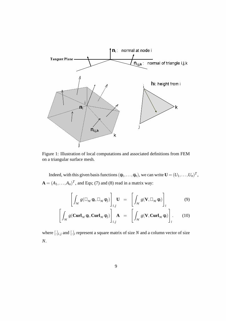
Figure 1: Illustration of local computations and associated definitions from FEMon a triangular surface mesh.

Indeed, with this given basis functions(φ1, . . . ,φn), we can writeU=(U1, . . . ,Un)T ,

A = (A1, . . . ,An)T , and Eqs; (7) and (8) read in a matrix way:

[∫M

g(∇M

φi,∇M φ j)

]

i, j

U =

[∫M

g(V,∇M

φi)

]

i

(9)

[∫M

g(CurlM φi ,CurlM φ j)

]

i, j

A =

[∫M

g(V,CurlM φi)

]

i

. (10)

where[.]i, j and[.]i represent a square matrix of sizeN and a column vector of size

N.

9

The harmonic componentH of the vector fieldV is obtained as:

H = V−∇M U −CurlM A. (11)

Gradient of each basis function is constant on each triangleand can be simply

computed with geometrical quantities (see Lefèvre and Baillet (2008)). So, Eq.

(9) reads:

[

∑T∋i, j

hi

‖ hi ‖2 ·hj

‖ hj ‖2A (T)

]

i, j

U =

[

∑T∋iA (T)V ·

hi

‖ hi ‖2

]

i

, (12)

wherehi is the height taken fromi in the triangleT, A (T) is the surface area of

triangleT.

Similarly, Eq. (10) is discretized as follows:

[

∑T∋i, j

(

hi

‖ hi ‖2 ×n

)

·

(

hj

‖ hj ‖2 ×n

)

A (T)

]

i, j

A=

[

∑T∋iA (T)V·

(

hi

‖ hi ‖2 ×n

)]

i

,

(13)

wheren is the normal to triangleT.

3.3. Feature detection as critical points of potentials

The critical points of a vector field are often classified depending on the eigen-

values of the Jacobian matrix at a point in a vector field. In the present case how-

ever, critical points of the flow may be defined as local extrema of the divergence-

free potentialA (representing rotation) and curl-free potentialU (representing di-

vergence). This definition is coherent with previous works such as Tong et al.

(2003). Feature detection, as critical points in global potential fields is much less

sensitive to noise in the data Tong et al. (2003) and therefore is less prone to false

10

positives, when compared to methods based on the extractionof local Jacobian

eigenvalues, Mann and Rockwood (2002).

A sink (respectively, a source) is defined as a local maximum (respectively,

minimum) ofU . Counterclockwise and clockwise vortex objects are featured by

local maximum and minimum ofA, respectively. SinceH a vector field which has

zero divergence and zero curl, traveling objects may be detected through vector

elements bearing the highest norms in theH vector field.

11

4. Results

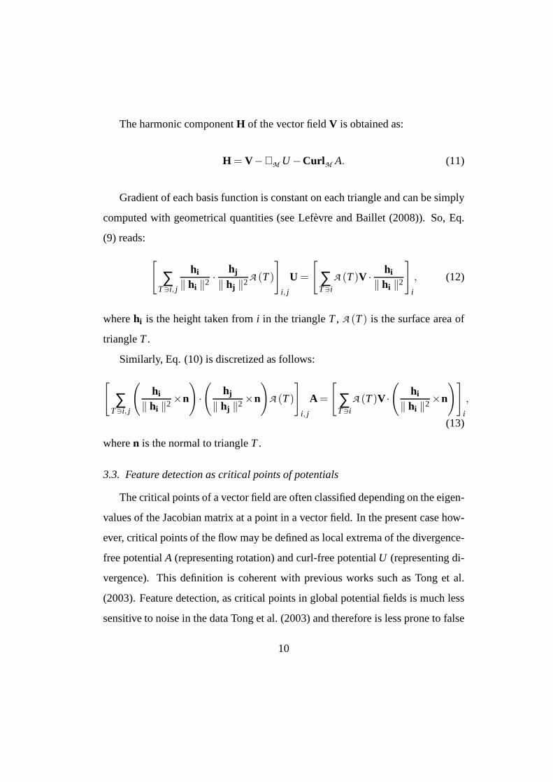
The new methodology is first evaluated by detecting sources and sinks on the

surface of a simplest curved manifold i.e. sphere, In Fig. 4 HHD is applied on

spherical manifold having a rotating vector field (green arrows). Possible time

domain of this vector field can be considered as hurricane (vortex) on the surface

of the earth as viewed from weather satellites.

HHD decomposition is then applied on this vector field. Vortices in rotating

vector fields are identified by critical points inA and shown in a colormap over-

lapping with the vector field. The counter-clockwise rotating vector fields, vortex

is identified by maxima inA, whereas the clockwise rotating vector fields, vortex

is identified by minima inA.

Figure 2: (a) Counter-clockwise rotating vector field, vortex identified by maximain A. (b) Clockwise rotating vector field, vortex identified by minima inA.

12

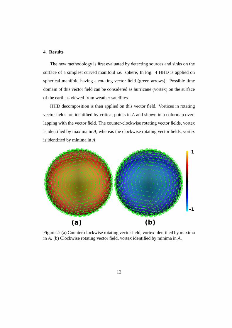
Secondly, HHD is tested on a classical bunny mesh as shown in Fig. 3. Vector

fields containing sources and sinks was synthesized to mimicthe optical flow

of objects of increasing and decreasing sizes (shown in green arrows). Rotating

vectors field was also generated to mimic the optical flow generated by a rotating

vortex. The HHD of these vector fields was performed (U andA are shown in

overlapped textured color on the manifold).

Fig. 3(a) consists of a rotating vector field overlapped withA. Fig. 3(a)

demonstrates that vortices of the original vector field can be identified using HHD

on this arbitrary surface. Similarly, Fig. 3(b) contains diverging vector fields with

A being representing as textured color. Fig. 3(b) shows that sources and sinks of

the vector field can also readily detected through theU component of the HHD.

In Figs. 3(c) and 3(d), contains vector field of rotating and diverging compo-

nents shown, and their correspondingA andU components respectively are repre-

sented as textured colors on the surface manifold. Figs. 3(c) and 3(d) demonstrate

that different types of features in the same vector field can be identified by HHD.

Our colormap shows sources and clockwise vortices in blue (local minima); sinks

and counter-clockwise vortices in red (local maxima).

13

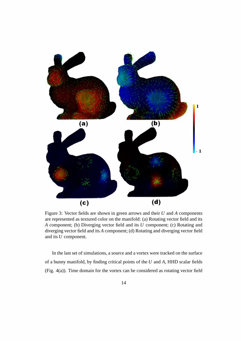
Figure 3: Vector fields are shown in green arrows and theirU andA componentsare represented as textured color on the manifold: (a) Rotating vector field and itsA component; (b) Diverging vector field and itsU component; (c) Rotating anddiverging vector field and itsA component; (d) Rotating and diverging vector fieldand itsU component.

In the last set of simulations, a source and a vortex were tracked on the surface

of a bunny manifold, by finding critical points of theU andA, HHD scalar fields

(Fig. 4(a)). Time domain for the vortex can be considered as rotating vector field

14

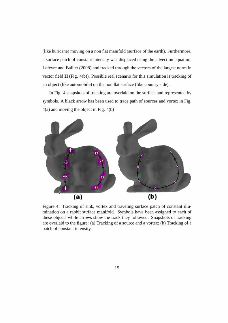
(like huricane) moving on a non flat manifold (surface of the earth). Furthermore,

a surface patch of constant intensity was displaced using the advection equation,

Lefèvre and Baillet (2008) and tracked through the vectors of the largest norm in

vector fieldH (Fig. 4(b)). Possible real scenario for this simulation is tracking of

an object (like automobile) on the non flat surface (like country side).

In Fig. 4 snapshots of tracking are overlaid on the surface and represented by

symbols. A black arrow has been used to trace path of sources and vortex in Fig.

4(a) and moving the object in Fig. 4(b)

Figure 4: Tracking of sink, vortex and traveling surface patch of constant illu-mination on a rabbit surface manifold. Symbols have been assigned to each ofthese objects while arrows show the track they followed. Snapshots of trackingare overlaid to the figure: (a) Tracking of a source and a vortex; (b) Tracking of apatch of constant intensity.

15

We further tested the HHD in a realistic scenario using experimental magne-

toencephalography (MEG) data. The brain response was recorded over 306 MEG

sensors and the cortical currents were constrained on a surface tessellation of the

subject’s brain containing about 50,000 triangle nodes. The cortical currents were

estimated with a regularized minimum-norm inverse model asdetailed in Baillet

et al. (2001). The vector field of the optical flow of these currents were computed

using the method described in Lefèvre and Baillet (2008), asimplemented by

us in the BrainStorm (http://neuroimage.usc.edu/brainstorm). The image shows

U about 30 ms after stimulus onset, where the primary somatosensory brain re-

sponse is expected, as shown with a strong divergent patternover the central sulcus

contralateral to the side of the stimulation.

Time resolved image series of cortical current sources can be obtained by re-

constructing the generators of the magnetic fields that are measured outside the

scalp (see Baillet et al. (2001) for an introduction). The optical flow from MEG

source images representing motion fields of neural current on the surface of the

brain was obtained from its optical flow. HHD was then appliedto detect sources

and sinks.

Results for theU part of the HHD are shown in Fig. 5 to emphasis sources

of cortical currents that evolves with time. A diverging source in the primary

somatosensory cortex was found about 30 ms after the electrical stimulation of

the contralateral index finger: this result was expected from the electrophysiology

of the somatosensory systems.

16

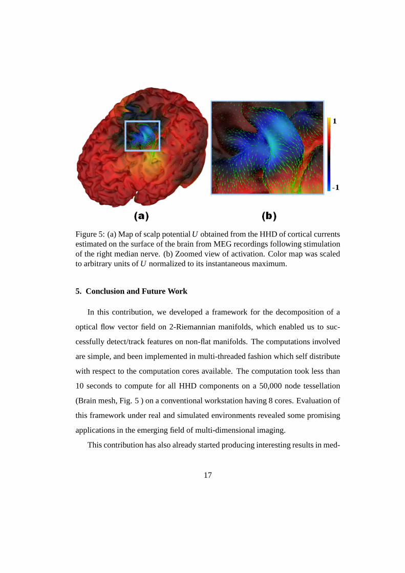
Figure 5: (a) Map of scalp potentialU obtained from the HHD of cortical currentsestimated on the surface of the brain from MEG recordings following stimulationof the right median nerve. (b) Zoomed view of activation. Color map was scaledto arbitrary units ofU normalized to its instantaneous maximum.

5. Conclusion and Future Work

In this contribution, we developed a framework for the decomposition of a

optical flow vector field on 2-Riemannian manifolds, which enabled us to suc-

cessfully detect/track features on non-flat manifolds. Thecomputations involved

are simple, and been implemented in multi-threaded fashionwhich self distribute

with respect to the computation cores available. The computation took less than

10 seconds to compute for all HHD components on a 50,000 node tessellation

(Brain mesh, Fig. 5 ) on a conventional workstation having 8 cores. Evaluation of

this framework under real and simulated environments revealed some promising

applications in the emerging field of multi-dimensional imaging.

This contribution has also already started producing interesting results in med-

17

ical imaging. Some applications of this tool in structural and functional neu-

roimaging are shown in Lefevre et al. (2009), Khan et al. (2009) and Khan et al.

(2010). Applicability of this method on elephant manifoldsare presented in sup-

plementary material.

Future direction for this framework is its extension to the discretization using

higher-order finite element analysis and utilization of this tool in more real world

applications.

6. Appendix

First we will show that the scalar potentialsU andA can be obtained up to a

constant. If we consider two minimizersU1 andU2 for the functional in (5) then

from equation (7) we get:

∀φ ∈ H1(M ),

∫M

g(∇M (U1−U2),∇M φ)dµ= 0

Green’s formula allows to transform this equation (given thatM has no bound-

aries ) :

∀φ ∈ H1(M ),∫M

φdivM ∇M (U1−U2)dµ= 0

which corresponds to the Laplace equation:

∆M (U1−U2) = 0

where∆M = divM ∇M is the Laplace-Beltrami operator.

The same thing can be done for two minimizersA1 andA2 of the functional in

18

(6). So, writingR=U1−U2 andR′ = A1−A2, we have the two conditions:

∆M R= 0, ∆M R′ = 0

Then, multiplying byR the first equation and integrating on the manifold we

get: ∫M

R∆M Rdµ= 0

Green’s formula again yields:

∫M

g(∇M R,∇M R)dµ= 0

Then it follows that∇M R must equals zero andR must be a constant. The same

thing can be applied toR′ which must be constant.

Secondly we will show the conditions on the vector fieldH. Next if we write

H = V−∇M U +CurlM A, we have:

divM H = divM V−divM ∇M U and curlM H = curlM V−curlM CurlM A

since divM CurlM A= 0 and curlM ∇M U = 0. Then:

∀φ ∈ H1(M ),∫M

φdivM Hdµ=∫M

φ(divM V−divM ∇M U)dµ

And by using Green’s formula and equation (7) we obtain:

∀φ ∈ H1(M ),∫M

φdivM Hdµ=∫M

g(V,∇M φ)−∫M

g(∇M U,∇M φ)dµ= 0

19

So we have proved that divM H = 0 and the same strategy can be applied to obtain

curlM H = 0.

References

Baillet, S., Mosher, J., Leahy, R., 2001. Electromagnetic brain mapping. IEEE

Signal Processing Magazine 18(6), 14–30.

Chorin, A., Marsden, J., 1993. A mathematical introductionto fluid mechanics.

Springer.

Corpetti, T., Mémin, E., Pérez, P., 2003. Extraction of singular points from dense

motion fields: an analytic approach. Journal of Mathematical Imaging and Vi-

sion 19, 175–198.

Do Carmo, M., 1993. Riemannian Geometry. Birkhäuser.

Druet, O., Hebey, E., Robert, F., 2004. Blow-up theory for elliptic PDEs in

Riemannian geometry. Princeton University Press, Princeton, N.J., Ch. Back-

ground Material, pp. 1–12.

Guo, Q., Mandal, M., Li, M., 2005. Efficient Hodge–Helmholtzdecomposition of

motion fields. Pattern Recognition Letters 26 (4), 493–501.

Guo, Q., Mandal, M., Liu, G., Kavanagh, K., 2006. Cardiac video analysis using

Hodge–Helmholtz field decomposition. Computers in Biologyand Medicine

36 (1), 1–20.

Horn, B., Schunck, B., 1981. Determining Optical Flow. Artificial Intelligence

17 (1-3), 185–203.

20

Khan, S., Lefèvre, J., Baillet, S., 2009. Feature Extraction from Time-Resolved

Cortical Current Maps using the Helmholtz-Hodge Decomposition. In: 15th

Human Brain Mapping International Conference, Sanfranciso.

Khan, S., Lefèvre, J., Raghavan, M., Baillet, S., 2010. Applications of 2-

Riemannian Helmholtz-Hodge Decomposition to MEG Source Dynamics. In:

17th Int. Conference on Biomagnetism, Dubrovnik.

Lefèvre, J., Baillet, S., June 2008. Optical flow and advection on 2-riemannian

manifolds: a common framework. IEEE Transactions on Pattern Analysis &

Machine Intelligence 30 (6), 1081–92.

URL http://cogimage.dsi.cnrs.fr/publications/2008/LB08

Lefevre, J., F. Leroy, S. K., Dubois, J., Huppi, P., Baillet,S., Mangin, J.,

2009. Identification of Growth Seeds in the Neonate Brain through Surfacic

Helmholtz Decomposition. In: 21st Information Processingin Medical Imag-

ing, Williamsburg.

Mann, S., Rockwood, A., 2002. Computing Singularities of 3DVector Fields with

Geometric Algebra. Proc. IEEE Visualization, 283–289.

Palit, B., Basu, A., Mandal, M., 2005. Applications of the Discrete Hodge

Helmholtz Decomposition to Image and Video Processing. Lecture Notes in

Computer Science 3776, 497.

Petronetto, F., Paiva, A., Lage, M., Tavares, G., Lopes, H.,Lewiner, T., 2009.

Meshless Helmholtz-Hodge Decomposition. IEEE Transactions on Visualiza-

tion and Computer Graphics, 338–349.

21

Polthier, K., Preuss, E., 2003. Identifying vector fields singularities using a dis-

crete hodge decomposition. Visualization and Mathematics3, 113–134.

Scheuermann, G., Tricoche, X., 2005. Topological Methods for Flow Visualiza-

tion. The Visualization Handbook, 341–356.

Tong, Y., Lombeyda, S., Hirani, A., Desbrun, M., 2003. Discrete multiscale vector

field decomposition. ACM Transactions on Graphics 22 (3), 445–452.

22

Supplementary Material for Pattern Recognition Letters

Feature Detection and Tracking in Optical Flow on Non-Flat

Manifolds

In this supplementary material we will show application of aModified Helmholtz-

Hodge Decomposition (HHD) on elephant manifolds.

Fig. 1 shows result in the same spirit as Figs. 3(c) and 3(d). Vector fields are

shown with green arrows. Fig. 1(a) contains vector field consist of rotating and

diverging components. Fig. 1(c) shows same vector field but rotating component 3

and 4 are now identified usingA component of HHD overlapped on to the surface

as texture color. In Fig. 1(d) sources 1 and sink 4 is identified by U component

of HHD. Fig. 1(c) and Fig. 1(c) demonstrate different types of features in same

vector field can be identified by HHD. Our colormap shows sources and clockwise

vortices in blue (local minima); sinks and counter-clockwise vortices in red (local

maxima). Fig. 1(b) represent zoom image of sources and sink detected in Fig.

1(c) and Fig. 1(d).

23

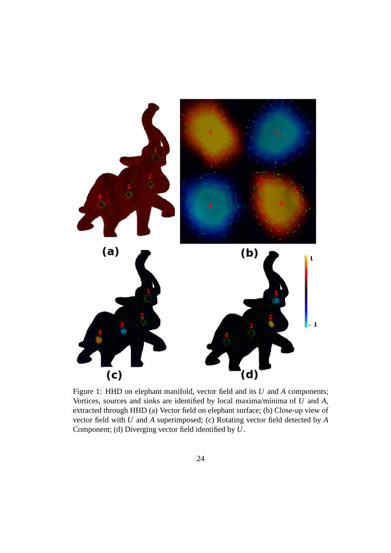
Figure 1: HHD on elephant manifold, vector field and itsU andA components;Vortices, sources and sinks are identified by local maxima/minima of U andA,extracted through HHD (a) Vector field on elephant surface; (b) Close-up view ofvector field withU andA superimposed; (c) Rotating vector field detected byAComponent; (d) Diverging vector field identified byU .

24