Embed Size (px)
Citation preview
International Journal of Computer Vision 52(2/3), 73–95, 2003c© 2003 Kluwer Academic Publishers. Manufactured in The Netherlands.
Feature-Based Image Analysis
MARTIN LILLHOLM AND MADS NIELSENIT University of Copenhagen, Glentevej 67, Copenhagen NV, Denmark
LEWIS D. GRIFFINMedical Imaging Science, King’s College, London, United Kingdom
Received January 18, 2002; Revised November 5, 2002; Accepted December 6, 2002
Abstract. According to Marr’s paradigm of computational vision the first process is an extraction of relevantfeatures. The goal of this paper is to quantify and characterize the information carried by features using image-structure measured at feature-points to reconstruct images. In this way, we indirectly evaluate the concept offeature-based image analysis. The main conclusions are that (i) a reasonably low number of features characterizethe image to such a high degree, that visually appealing reconstructions are possible, (ii) different feature-typescomplement each other and all carry important information. The strategy is to define metamery classes of imagesand examine the information content of a canonical least informative representative of this class. Algorithms foridentifying these are given. Finally, feature detectors localizing the most informative points relative to differentcomplexity measures derived from models of natural image statistics, are given.
Keywords: features, stochastic complexity, statistics of natural images, least commitment, scale-space, imagereconstruction, variational methods
1. Introduction
Marr’s paradigm of computational vision (Marr, 1982)includes an early process of feature detection. Based onthese features, further processing involving semanticsis performed to solve a given visual task. This schemehas been followed in many works on computationalvision: stereo (Kass, 1988), flow (Price, 1990), regis-tration (Maintz et al., 1995), recognition (Wells, 1997),indexing (Schmid and Mohr, 1997), structure from mo-tion (Huang and Netravali, 1994), etc. Many more ref-erences could have been given here. These approachesare all examples of feature-based image analysis. Theaim of this paper is to describe which information in theimage is actually carried by its features, and to quantifythis. The driving example will be image reconstructionbased on image-structure measured at feature-points.
Two different images exhibiting identical featureswill lead to an identical solution of the visual taskunder the feature-based image analysis paradigm. Asonly features are used in the processing, two imagesexhibiting identical features are identical or metameri-cally equivalent. These are denoted metameric images(Koenderink and van Doorn, 1996). The structure onthe space of images dividing it into metamery classes, isalso the structure that divides the solution space of theimage analysis into possibly different solutions underthe feature-based image analysis paradigm.
In this paper, we will study metamery classes ofimages. We will also study extraction of a canoni-cal representative of the metamery class. This rep-resentative should be the simplest possible so thatit reveals only the information imposed by the fea-tures, and no additional arbitrary information. This
74 Lillholm, Nielsen and Griffin
is formalized through the definition of the stochas-tic complexity (Rissanen, 1998) of images inspired bywork on the statistics of natural images (Ruderman andBialek, 1994; Field, 1987; Huang et al., 2000; Huangand Mumford, 1999; Lee et al., 2001).
This definition of stochastic complexity of an imagemakes it possible to define how much information isactually carried by a single feature. This may in turnbe used for defining “features” as points in the imagecarrying the most information about the image (relativeto a given complexity measure). That is, features maybe defined as points of maximal information.
The paper is organized as follows: Firstly, we de-fine localized measurements and the concept of spatialmetamerism. Then the problem of selecting least in-formative representatives is addressed. On the basis ofthis, the information contents of classical scale-spaceblobs and edges (Lindeberg, 1993, 1994, 1996, 1998)is analyzed empirically using a small ensemble of nat-ural image patches. Finally, we derive optimal1 featuredetectors for describing natural images on the basis ofdefinitions of their statistics.
2. Localized Measurements and SpatialMetamerism
Given an image I : � → R, � ⊂ RN (for all com-
putational examples in this paper N = 2), we wish tomeasure its local structure in a finite number of loca-tions in a similar manor to the response of V1 simplecells. Generally, the response of one such cell is mod-eled taking the inner product of a receptive field weight-ing function (RFWF) and the retinal irradiance (Hubeland Wiesel, 1968). Several choices of RFWF modelsare possible, two are however dominant: Gabor func-tions (Daugman, 1985; Jones and Palmer, 1987) andderivatives of Gaussians (Young, 1985; Koenderinkand van Doorn, 1990). As the two families are simi-lar our choice of derivatives of Gaussians is motivatedby their simplicity and their direct geometrical inter-pretations:
The localized Gaussian kernel (for N = 2) of stan-dard deviation σ is given by
Gσ,x0,y0 = 1
2πσ 2e
−(x−x0)2−(y−y0)2
2σ2 ,
and a RFWF fi modeled as a derivative of the Gaussianis then:
fσ,x0,y0 = ∂ p
∂xn∂ymGσ , p = n + m. (1)
This leads to the definition of a measurement c ∈ R asthe inner product of a RFWF and the image:
⟨fσ,x0,y0
∣∣ I⟩ =
∫�
fσ,x0,y0 (x)I (x) dx = c. (2)
Inspired by Gaussian scale-space theory (Koenderink,1984), we can think of a measurement as the corre-sponding derivative2 of the image itself calculated atscale σ . In this way, a set of co-localized measurementsall at the same scale but with order of derivation goingfrom 1 to p, make up the coefficients of the truncatedTaylor-series. Note, that differentiation in this senseis well-posed (Florack et al., 1992), as we derive theGaussian and not the image itself. As a special case, wehave zero-measurements where c = 0. Good examplesare the x and y derivatives of a stationary point in theimage (again measured at scale σ ).
Now assume that a finite set of points of interest or“feature-points” are given. These can each be describedor characterized in terms of a number of measurements;i.e. I satisfies the constraints:
〈 fi | I 〉 =∫
�
fi I dx = ci , i = 1, . . . , K (3)
where the fi ’s are RFWFs each with individual scale,location, and order of derivation.
One could argue that we have fully characterized Iin terms of a number of local measurements. Gener-ally, there will be far fewer measurements than thereare degrees of freedom in I and many images canaccount for the measurements obtained from a spe-cific I . Therefore, a given set of RFWFs and cor-responding measurements define an entire class ofimages—a metamery class. The term metameric is bor-rowed from color science (Koenderink and van Doorn,1996) and is traditionally used about light spectra thatall provoke the same color sensation in a particularobserver. Members of a metamery class are calledmetameric and metamerism based on spatial measure-ments and corresponding measurements is traditionallycalled spatial metamerism (Koenderink and van Doorn,1996; Nielsen and Lillholm, 2001; Tagliati and Griffin,2001; Griffin, 2002).
Once a metamery class has been defined, the no-tion of black components or black images can bedefined. Namely, images which measure to zero forall of the constraining measurements. These are neu-tral elements with respect to the class and addingscaled versions of them to class members does not af-fect class membership—much like adding a 1st order
Feature-Based Image Analysis 75
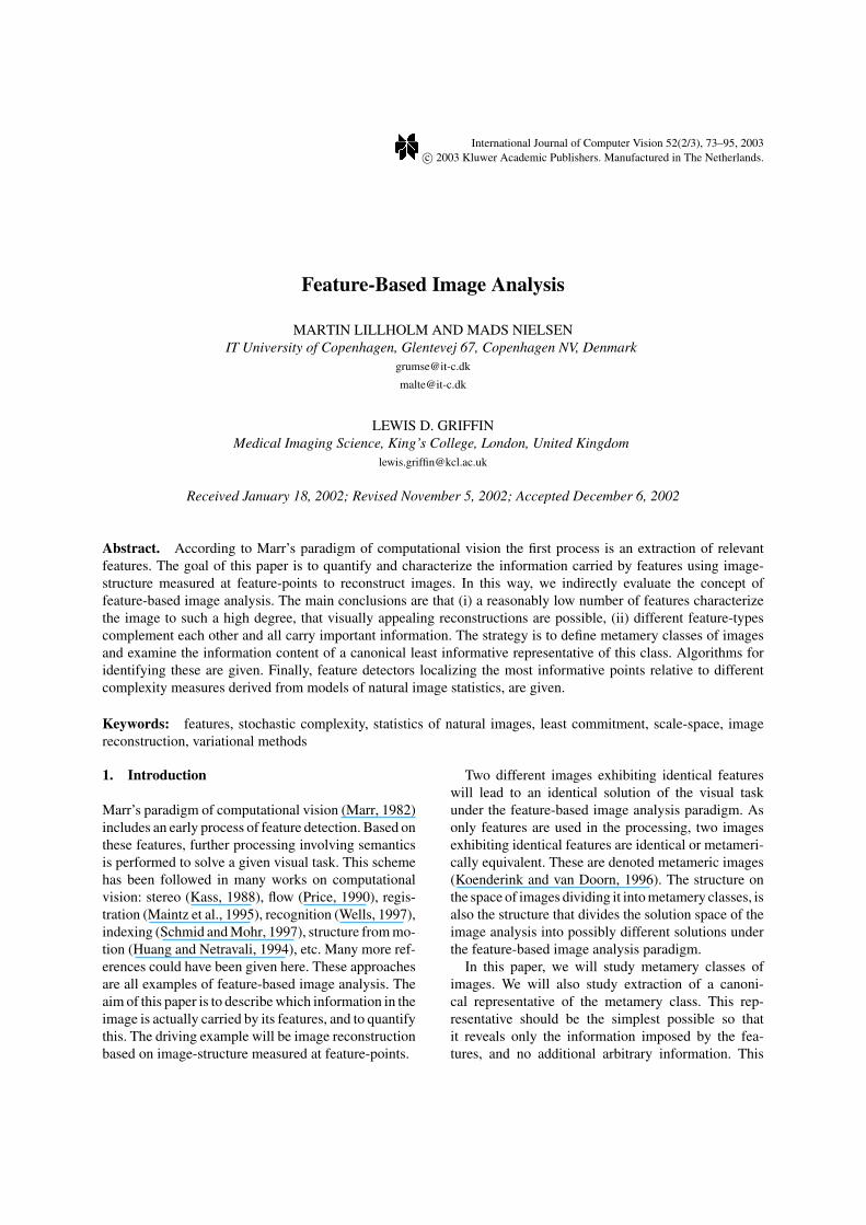
Figure 1. The left image in the top row is a simple black and white image. The red dots in the right image indicate points of interest orfeature-points. In this case along the vertical edge. At each feature point the 1st order differential structure (Ix and Iy ) is measured and definethe constraints of the metamery class. The scale of measurement is close to the inner scale of the image, that is pixel size. The second rowdepicts four members of the metamery class. The leftmost is obtained from natural image patches from the Van Hateren database (van Haterenand van der Schaaf, 1998), the second from regularized uniform noise images. These two members can be thought of as random samples fromthe metamery class. The third and fourth are examples of canonical representatives of the class—the topic of Sections 3 and 4. The bottom rowcontains four images that are black with respect to the metamery class. That is, images which measure to zero for each of the class definingRFWFs.
polynomial does not affect the higher order structureof a function.
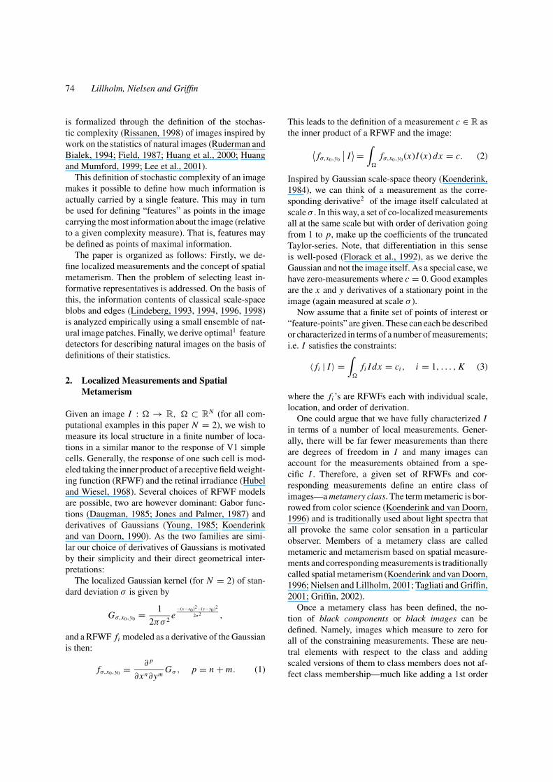
Examples of two images, constraining measure-ments, members of the corresponding metameryclasses, and metamerically black images are given inFigs. 1 and 2. Both examples demonstrate that eventhough we use fairly many constraints, class memberscan be quite different.
3. Representatives of the Metameric Class
A set of measurements define the metamery class andif one does not wish to add further constraints to themetamery class, it is most easily described through
these measurements. This however gives no further in-sight into the class. Another approach pioneered byKoenderink and van Doorn (1996) is to characterize ametamery class of local image patches by a canonicalrepresentative and its structure (for more recent stud-ies see Tagliati and Griffin (2001) and Griffin (2002)).Similarly, we will choose to select a representative fromthe metamery class of images to characterize the class.
Following the approach that the representativeshould reveal the information imposed by the measure-ments, and no further information, we define:
The canonical representative of a metamery class, isthe member of lowest possible information content.
76 Lillholm, Nielsen and Griffin
Figure 2. The left image in the top row is a gray-scale image of an area around Lena’s right eye. The red dots in the second image are edge-likeimage points. At each of these points the 1st order differential structure (Ix and Iy ) is measured and defines the constraints of the metamery class.The scale of measurement is proportional to length of the edge. In the rightmost image, ellipses are centered at points with articulated secondorder structure or blob-like points. At each of these points, we measure the 2nd order structure (Ixx , Iyy , and Ixy ). The second row depicts fourmembers of the metamery class. The leftmost is obtained from natural image patches from the Van Hateren database (van Hateren and van derSchaaf, 1998), the second from regularized uniform noise images. These two members can be thought of as random samples from the metameryclass. The third and fourth are examples of canonical representatives of the class—the topic of Sections 3 and 4. The bottom row contains fourimages that are black with respect to the metamery class. That is, images which measure to zero for each of the class defining RFWFs.
In this way, all information in the representative is im-posed by the measurements, and is not arbitrary.
The “only” problem left is a concise definition ofthe proper measure of information content of an image.In information theoretical terms (Shannon, 1948), theinformation or stochastic complexity (Rissanen, 1998)is defined as the entropy of a distribution p(x):
H (p) = −∫
p(x) log p(x) dx
In this, − log p(x) is the information contents of theinstance x . Likewise, we may define the informationcontents of an image I as − log p(I ) with respect to thedistribution p of images. Hence, the representative is
also the member of maximum likelihood with respectto the distribution p of images. This does not solvethe problem of defining the information contents of animage, but only casts the problem into defining a properdistribution of natural images.
A very simple image model claims pixels to be in-dependently identically Gaussian distributed. This is asimplified measure as it rules out all spatial dependen-cies, which are actually those that characterizes images.However, owned to its simplicity, it serves as an attrac-tive starting point. The distribution of images, pL2 (I ),3
is calculated as follows:
pL2 (I ) =∏x∈�
p(x) =∏x∈�
1√2πσ 2
e− I (x)2
2σ2
Feature-Based Image Analysis 77
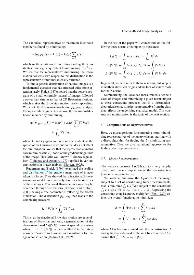
The canonical representative or maximum likelihoodmember is found by minimizing:
− log pL2 (I ) = k1(σ ) + k2(σ )∑x∈�
I (x)2
which in the continuous case, disregarding the con-stants k1 and k2, is equivalent to minimizing
∫�
I 2 dx .We see that the representative minimizing the infor-mation contents with respect to this distribution is therepresentative of minimal intensity variance.
To find a generic distribution of natural images is afundamental question that has attracted quite some at-tention lately. Field (1987) showed that the power spec-trum of a small ensemble natural of images followeda power law similar to that of 2D Brownian motions,which makes the Brownian motion model appealing.We denote this Brownian distribution pL2(|∇ I |) and get,through similar arguments as above, the maximum like-lihood member by minimizing:
− log(
pL2(|∇ I |) (I )) = k1(σ ) + k2(σ )
∑x∈�
|∇ I (x)|2
≈∫
�
|∇ I |2 dx
where k1 and k2 again are constants dependent on thespread of the Gaussian distribution that does not affectthe minimization. We see that the representative in thiscase minimizes the L2 norm of the gradient magnitudeof the image. This is the well-known Tikhonov regular-izer (Tikhonov and Arsenin, 1977) applied in variousapplications in image analysis (Nielsen, 1995).
Ruderman and Bialek (1994) examined the scalingand distribution of the gradient magnitude of imagestaken in a forest. They showed that a fractional Brown-ian motion model more precisely describes the statisticsof these images. Fractional Brownian motions may bedescribed through distributions (Pedersen and Nielsen,2000) having a free parameter α reflecting the fractaldimension. The distribution pLα (|∇ I |) then leads to thecomplexity measure:
Lα(|∇ I |) ≈∫
�
|∇ I |α dx
This is, as the fractional Brownian motion are general-izations of Brownian motions, a generalization of theabove mentioned L2(|∇ I |) norm. A special case ariseswhen α = 1. L1(|∇ I |) is the so-called Total Variationnorm or TV-norm well-known as a regularizer for im-age reconstruction (Rudin et al., 1992).
In the rest of the paper will concentrate on the fol-lowing three norms or complexity measures:
L2(I ) =∫
�
(x, I ) dx =∫
�
|I |2 dx
L1(|∇ I |) =∫
�
(x, Ix , Iy) dx =∫
�
|∇ I | dx
L2(|∇ I |) =∫
�
(x, Ix , Iy) dx =∫
�
|∇ I |2 dx
In general, we will refer to them as norms, but keep inmind their statistical origin and the lack of square rootsfor the 2-norms.
Summarizing, the localized measurements define aclass of images and minimizing a given norm subjectto these constraints produces the, in a information-theoretical sense, simplest representative from the classthat reflects the underlying statistical model. This con-strained minimization is the topic of the next section.
4. Computations of Representatives
Here, we give algorithms for computing norm-minimi-zing representatives of metamery classes, starting witha direct algorithm for finding the L2 minimizing rep-resentative. Then we give variational approaches forfinding other representatives.
4.1. Linear Reconstruction
The variance measure L2(I ) leads to a very simple,direct, and linear computation of the reconstruction(canonical representative):
We wish to minimize the L2-norm of the imagesubject to a set of constraining linear measurements,that is minimize
∫�
I (x)2 dx subject to the constraints∫�
I (x) fi (x) dx = ci , i = 1, . . . , K . Expressing theconstraints using Lagrange multipliers (Fox, 1987), de-fines the overall functional to minimize:
E =∫
�
(x, J ) +K∑
i=0
λi ci dx
=∫
�
(J − µ)2 +K∑
i=0
λi ci dx,
where I has been substituted with the reconstruction Jand f0 has been defined as the unit function over � toensure that
∫�
Jdx = c0 ≡ |�|µ.
78 Lillholm, Nielsen and Griffin
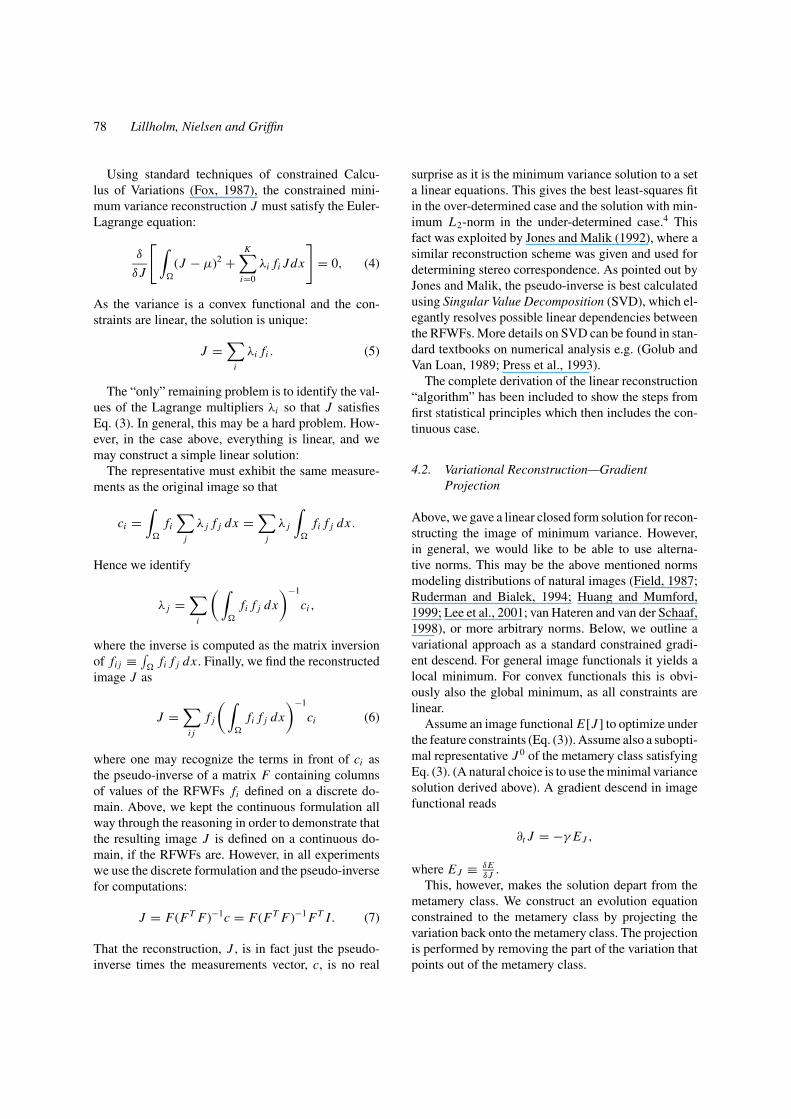
Using standard techniques of constrained Calcu-lus of Variations (Fox, 1987), the constrained mini-mum variance reconstruction J must satisfy the Euler-Lagrange equation:
δ
δ J
[ ∫�
(J − µ)2 +K∑
i=0
λi fi Jdx
]= 0, (4)
As the variance is a convex functional and the con-straints are linear, the solution is unique:
J =∑
i
λi fi . (5)
The “only” remaining problem is to identify the val-ues of the Lagrange multipliers λi so that J satisfiesEq. (3). In general, this may be a hard problem. How-ever, in the case above, everything is linear, and wemay construct a simple linear solution:
The representative must exhibit the same measure-ments as the original image so that
ci =∫
�
fi
∑j
λ j f j dx =∑
j
λ j
∫�
fi f j dx .
Hence we identify
λ j =∑
i
( ∫�
fi f j dx
)−1
ci ,
where the inverse is computed as the matrix inversionof fi j ≡ ∫
�fi f j dx . Finally, we find the reconstructed
image J as
J =∑
i j
f j
( ∫�
fi f j dx
)−1
ci (6)
where one may recognize the terms in front of ci asthe pseudo-inverse of a matrix F containing columnsof values of the RFWFs fi defined on a discrete do-main. Above, we kept the continuous formulation allway through the reasoning in order to demonstrate thatthe resulting image J is defined on a continuous do-main, if the RFWFs are. However, in all experimentswe use the discrete formulation and the pseudo-inversefor computations:
J = F(F T F)−1c = F(F T F)−1 F T I. (7)
That the reconstruction, J , is in fact just the pseudo-inverse times the measurements vector, c, is no real
surprise as it is the minimum variance solution to a seta linear equations. This gives the best least-squares fitin the over-determined case and the solution with min-imum L2-norm in the under-determined case.4 Thisfact was exploited by Jones and Malik (1992), where asimilar reconstruction scheme was given and used fordetermining stereo correspondence. As pointed out byJones and Malik, the pseudo-inverse is best calculatedusing Singular Value Decomposition (SVD), which el-egantly resolves possible linear dependencies betweenthe RFWFs. More details on SVD can be found in stan-dard textbooks on numerical analysis e.g. (Golub andVan Loan, 1989; Press et al., 1993).
The complete derivation of the linear reconstruction“algorithm” has been included to show the steps fromfirst statistical principles which then includes the con-tinuous case.
4.2. Variational Reconstruction—GradientProjection
Above, we gave a linear closed form solution for recon-structing the image of minimum variance. However,in general, we would like to be able to use alterna-tive norms. This may be the above mentioned normsmodeling distributions of natural images (Field, 1987;Ruderman and Bialek, 1994; Huang and Mumford,1999; Lee et al., 2001; van Hateren and van der Schaaf,1998), or more arbitrary norms. Below, we outline avariational approach as a standard constrained gradi-ent descend. For general image functionals it yields alocal minimum. For convex functionals this is obvi-ously also the global minimum, as all constraints arelinear.
Assume an image functional E[J ] to optimize underthe feature constraints (Eq. (3)). Assume also a subopti-mal representative J 0 of the metamery class satisfyingEq. (3). (A natural choice is to use the minimal variancesolution derived above). A gradient descend in imagefunctional reads
∂t J = −γ EJ ,
where EJ ≡ δEδ J .
This, however, makes the solution depart from themetamery class. We construct an evolution equationconstrained to the metamery class by projecting thevariation back onto the metamery class. The projectionis performed by removing the part of the variation thatpoints out of the metamery class.
Feature-Based Image Analysis 79
We denote this approach an observation-constrainedevolution. This is a general approach, and it is easy toshow, that the gradient projection algorithm convergestowards the same solution as a standard direct Euler-Lagrange formulation (Rosen, 1960).
Since the constraints given in Eq. (3) are linear weobtain:
∂t J = −γ (EJ [J ] − EJ [J ] ⊥ M), (8)
where EJ ⊥ Mc is defined as the part of EJ orthogonalto the metamery class:
EJ [J ] ⊥ M =∑
i j
f j
( ∫�
fi f j dx
)−1∫�
fi EJ [J ] dx .
EJ [J ] ⊥ M is derived as the reconstruction (Eq. (6)) ofthe variation EJ . Geometrically explained this is: in thehigh dimensional image space, normals to all constrainthyper-planes are defined by the initial RFWFs. We nowsubtract from the variation a linear combination of thesenormals measuring the same as the variation itself. Theresult is a variation of constraint-measure zero pointingin the steepest descend direction within the metameryclass.
The corresponding discrete formulation (Eq. (7))reads:
EJ [J ] ⊥ Mc = F(F T F)−1 F T EJ [J ].
What remains is to calculate the variations, EJ [J ], forthe L1(|∇ I |) and L2(|∇ I |) norms. As both norms de-pend on J ’s 1st order partial derivatives but not on Jitself, the appropriate, and in this case unconstrained,Euler-Lagrange equation (Fox, 1987) reads:
− d
dx
∂
∂ Jx− d
dy
∂
∂ Jy= 0. (9)
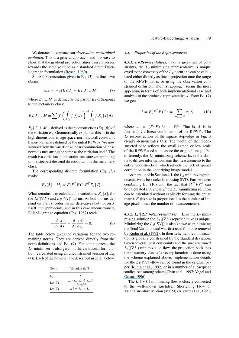
The table below gives the variations for the two re-maining norms. They are derived directly from thenorm-definitions and Eq. (9). For completeness, theL2-minimizer is also given in the variational formula-tion (calculated using an unconstrained version of Eq.(4)). Each of the flows will be described in detail below.
Norm Variation EI [I ]
L2 I
L1(|∇ I |) 2Ix Iy Ixy−Ixx I 2y −Iyy I 2
x
(I 2x +I 2
y )3/2
L2(|∇ I |) �I = Ixx + Iyy
4.3. Properties of the Representatives
4.3.1. L2-Representatives. For a given set of con-straints, the L2 minimizing representative is uniqueowed to the convexity of the L2-norm and can be calcu-lated either directly as linear projection onto the rangeof the RFWF-matrix or using the observation con-strained diffusion. The first approach seems the mostappealing in terms of both implementational ease andanalysis of the produced representative J . From Eq. (7)we get:
J = F(F T F)−1c =∑
i=1,...,N
wi fi , (10)
where w = (F T F)−1c ∈ RN . That is, J is in
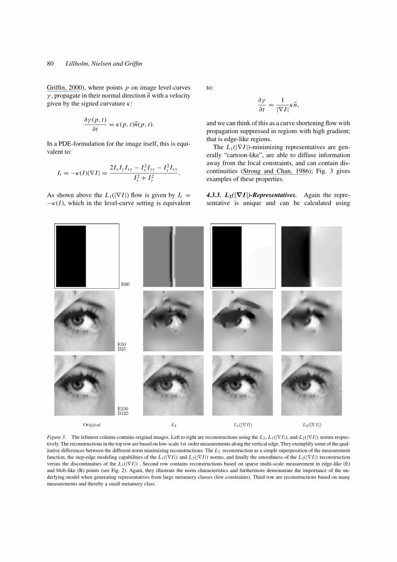
fact simply a linear combination of the RFWFs. TheL2 reconstruction of the square step-edge in Fig. 3clearly demonstrates this: The width of the recon-structed edge reflects the small extend or low scaleof the RFWF used to measure the original image. Putdifferently, the L2 minimizing scheme lacks the abil-ity to diffuse information from the measurements to theentire reconstruction, which reflects the lack of spatialcorrelation in the underlying image model.
As mentioned in Section 4.1, the L2 minimizing rep-resentative is best calculated using SVD. Furthermore,combining Eq. (10) with the fact that (F T F)−1 canbe calculated analytically,5 the L2 minimizing solutioncan be calculated without explicitly forming the entirematrix F (its size is proportional to the number of im-age pixels times the number of measurements).
4.3.2. L1(|∆I|)-Representatives. Like the L2 mini-mizing solution the L1(|∇ I |) representative is unique.Minimizing the L1(|∇ I |) is also known as minimizingthe Total Variation and was first used for noise removalby Rudin et al. (1992). In their scheme, the minimiza-tion is globally constrained by the standard deviation.Given several local constraints and the unconstrainedL1(|∇ I |)-minimization flow, the projection back intothe metamery class after every iteration is done usingthe scheme explained above. Implementation detailsfor the L1(|∇ I |)-flow can be found in the original pa-per (Rudin et al., 1992) or in a number of subsequentstudies; see among others (Chan et al., 1997; Vogel andOman, 1996).
The L1(|∇ I |) minimizing flow is closely connectedto the well-known Euclidean Shortening Flow orMean Curvature Motion (MCM) (Alvarez et al., 1993;
80 Lillholm, Nielsen and Griffin
Griffin, 2000), where points p on image level-curvesγ , propagate in their normal direction �n with a velocitygiven by the signed curvature κ:
∂γ (p, t)
∂t= κ(p, t)�n(p, t).
In a PDE-formulation for the image itself, this is equi-valent to:
It = −κ(I )|∇ I | = 2Ix Iy Ixy − I 2x Iyy − I 2
y Ixx
I 2x + I 2
y
.
As shown above the L1(|∇ I |) flow is given by It =−κ(I ), which in the level-curve setting is equivalent
Figure 3. The leftmost column contains original images. Left to right are reconstructions using the L2, L1(|∇ I |), and L2(|∇ I |) norms respec-tively. The reconstructions in the top row are based on low-scale 1st order measurements along the vertical edge. They exemplify some of the qual-itative differences between the different norm minimizing reconstructions: The L2 reconstruction as a simple superposition of the measurementfunction, the step-edge modeling capabilities of the L1(|∇ I |) and L2(|∇ I |) norms, and finally the smoothness of the L2(|∇ I |) reconstructionversus the discontinuities of the L1(|∇ I |) . Second row contains reconstructions based on sparse multi-scale measurement in edge-like (E)and blob-like (B) points (see Fig. 2). Again, they illustrate the norm characteristics and furthermore demonstrate the importance of the un-derlying model when generating representatives from large metamery classes (few constraints). Third row are reconstructions based on manymeasurements and thereby a small metamery class.
to:
∂γ
∂t= 1
|∇ I |κ�n,
and we can think of this as a curve shortening flow withpropagation suppressed in regions with high gradient;that is edge-like regions.
The L1(|∇ I |)-minimizing representatives are gen-erally “cartoon-like”, are able to diffuse informationaway from the local constraints, and can contain dis-continuities (Strong and Chan, 1986); Fig. 3 givesexamples of these properties.
4.3.3. L2(|∇I|)-Representatives. Again the repre-sentative is unique and can be calculated using
Feature-Based Image Analysis 81
the observation-constrained diffusion scheme. TheL2(|∇ I |) minimizing flow It = �I is the well-known diffusion-equation and the Gaussian kernel isthe Green’s function of the diffusion equation. Imple-mentation details for the L2(|∇ I |)-flow can be foundin a number of scale-space publications among others(Lindeberg, 1994; Weickert, 1998).
The L2(|∇ I |)-minimizing representatives are differ-entiable, are able to diffuse information away from thelocal constraints, and generally “visually appealing”;Fig. 3 gives examples of these properties.
4.3.4. General Comments. We have given a frame-work that from first statistical principles generatesrepresentatives from metamery classes using con-strained minimization from the L2, L1(|∇ I |), andL2(|∇ I |) norms. The specific norms used should beseen as examples; each reflecting the strengths and in-deed limitations of the underlying statistical models fornatural images. They should be seen as approximationsand subject to revision as our knowledge mature.
Figure 3 demonstrates another property of themetamery classes: For a given image, the dimension-ality of a metamery class is dictated by the effectiveresolution of the image and the number of linearly in-dependent 6 constraints. In Fig. 3 the second and thirdrow give examples of a large and a small metameryclasses, where the constraints used in the second row isa subset of the ones used in third row. In the second rowthe difference between the three norm-minimizing rep-resentatives and thus the properties of each underlyingmodel are quite clear. In the third row, a large num-ber of constraints yields a small metamery class andmakes it quite difficult to distinguish the three represen-tatives and thereby the model used. For small metameryclasses any sensible prior will lead to essentially thesame reconstruction.
5. Selecting and Representing Points of Interest
In the previous sections it was established how lo-cal constraints define a metamery class and how con-strained image norm minimization can be used to gen-erate representatives of a class reflecting underlyingassumptions about image statistics.
So far, we have not discussed how to select points ofinterest and how to “code” or characterize them in termsof measurements. In the following, we will briefly dis-cuss the first issue but concentrate on the second andthen return to the selection process in Section 8.
For a given image I , the goal is to select a subsetof the locations in the image as points of interest andthen characterize each of these in terms of a subsetof their local n-jet, j n I (x); that is the correspondinglocalized Gaussian derivatives. Ideally speaking, wecould choose from the entire n-jet for sufficiently largen. We will constrain ourselves to the 4-jet, to make theactual calculations feasible and numerically stable andbecause we have indications from neuro-science, thatthe primate visual system uses receptive fields up to atleast order four (Young, 1985).
The task is now reduced to the one of findinginteresting image points and their individual repre-sentation as a subset of the 4-jet. In principle onecould pre-process the entire scale-space of points, findtheir optimal representations and then select the onesthat convey the most information about the globalimage structure. However, as the information con-veyed by a single measurement is affected by mea-surements already recorded and vice versa, this be-comes a hard optimization problem as is normallythe case for this kind of sparse coding. A simple il-lustration of this can be seen in Fig. 4: intuitively,the most informative points in the original image,are the four corner-points. Four different encoding-schemes are presented and of these especially thelast two give visually similar reconstructions withquite different encodings. A complete solution to thisoptimization problem is however not our goal. Inearly visual processing, features must be detectedand represented individually for the computations tobe tractable. Hence, we seek local detection criteriaand representations that on average yield as much in-formation as possible on the images. In the follow-ing, we therefore discuss selection and representationindependently.
6. Representing Feature Points
For now, we choose to solve the selection process us-ing well-known Gaussian scale-space feature detec-tion as pioneered by Koenderink (1984), Florack et al.(1993), Lindeberg (1993, 1996, 1998) and Florack et al.(1990, 1993). Table 1 summarizes some scale-spacedetection criteria for a selection of standard feature-types. The feature detectors select a number of pointsof interest and their intrinsic scale. In the follow-ing, we will focus on blob- and edge-points. That is,points dominated by their 1st and 2nd order structurerespectively.
82 Lillholm, Nielsen and Griffin
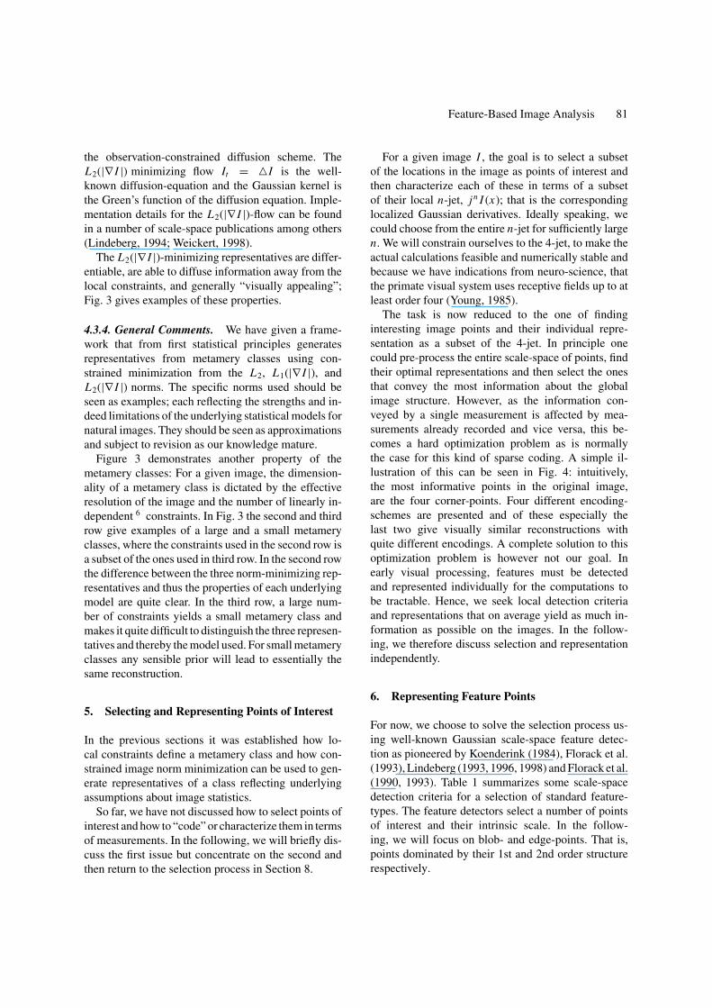
Table 1. Some criteria for feature detection in Gaussian scale-space. v and w are basis vectors ofthe vw-gauge coordinate system, where w is parallel to the gradient direction and v is parallel toisophote direction. The feature strength is normally multiplied by the scale-normalization factor toensure comparable feature responses across scale and γ is a free parameter for feature dependent tuningof the scale selection; see original work by Lindeberg (1993, 1996, 1998) and more recent studies inPedersen and Nielsen (2000) and Majer (2001).
Feature Strength Spatial Scale Scale-normalization γ
Blob �I maxx (�I ) maxσ (�I ) σ 2γ 1
Edge Iw Iww = 0 maxσ (Iw) σγ 1/2
Corner I 2w Ivv maxx (I 2
w Ivv) maxσ (I 2w Ivv) σ 4γ 1
Ridge Ivv Ivw = 0 maxσ (Ivv) σ 2γ 3/4
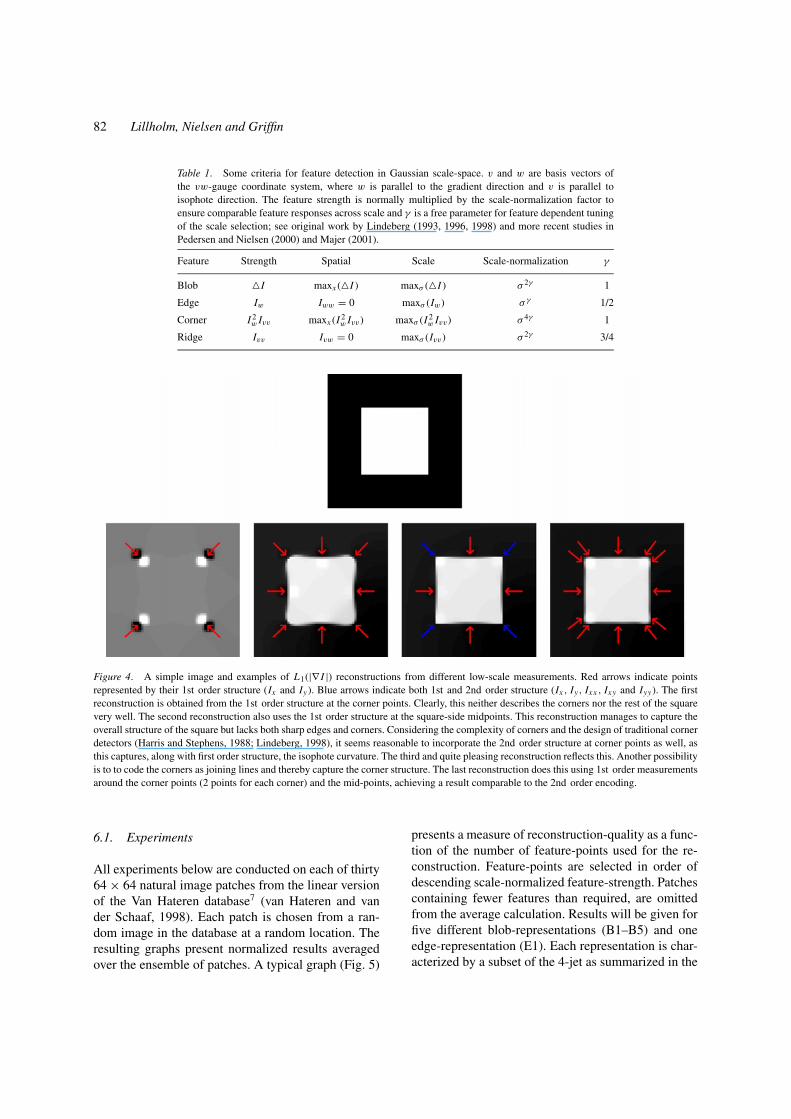
Figure 4. A simple image and examples of L1(|∇ I |) reconstructions from different low-scale measurements. Red arrows indicate pointsrepresented by their 1st order structure (Ix and Iy ). Blue arrows indicate both 1st and 2nd order structure (Ix , Iy , Ixx , Ixy and Iyy ). The firstreconstruction is obtained from the 1st order structure at the corner points. Clearly, this neither describes the corners nor the rest of the squarevery well. The second reconstruction also uses the 1st order structure at the square-side midpoints. This reconstruction manages to capture theoverall structure of the square but lacks both sharp edges and corners. Considering the complexity of corners and the design of traditional cornerdetectors (Harris and Stephens, 1988; Lindeberg, 1998), it seems reasonable to incorporate the 2nd order structure at corner points as well, asthis captures, along with first order structure, the isophote curvature. The third and quite pleasing reconstruction reflects this. Another possibilityis to to code the corners as joining lines and thereby capture the corner structure. The last reconstruction does this using 1st order measurementsaround the corner points (2 points for each corner) and the mid-points, achieving a result comparable to the 2nd order encoding.
6.1. Experiments
All experiments below are conducted on each of thirty64 × 64 natural image patches from the linear versionof the Van Hateren database7 (van Hateren and vander Schaaf, 1998). Each patch is chosen from a ran-dom image in the database at a random location. Theresulting graphs present normalized results averagedover the ensemble of patches. A typical graph (Fig. 5)
presents a measure of reconstruction-quality as a func-tion of the number of feature-points used for the re-construction. Feature-points are selected in order ofdescending scale-normalized feature-strength. Patchescontaining fewer features than required, are omittedfrom the average calculation. Results will be given forfive different blob-representations (B1–B5) and oneedge-representation (E1). Each representation is char-acterized by a subset of the 4-jet as summarized in the
Feature-Based Image Analysis 83
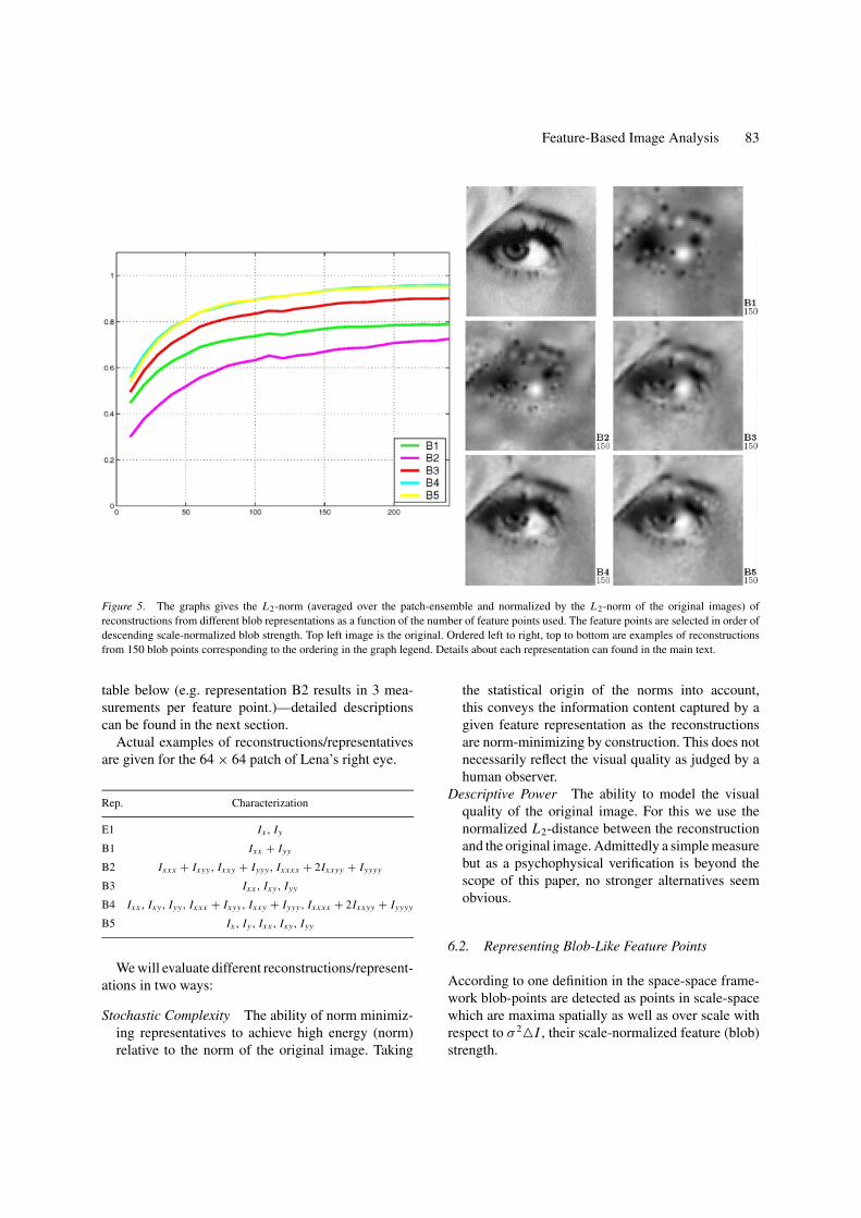
Figure 5. The graphs gives the L2-norm (averaged over the patch-ensemble and normalized by the L2-norm of the original images) ofreconstructions from different blob representations as a function of the number of feature points used. The feature points are selected in order ofdescending scale-normalized blob strength. Top left image is the original. Ordered left to right, top to bottom are examples of reconstructionsfrom 150 blob points corresponding to the ordering in the graph legend. Details about each representation can found in the main text.
table below (e.g. representation B2 results in 3 mea-surements per feature point.)—detailed descriptionscan be found in the next section.
Actual examples of reconstructions/representativesare given for the 64 × 64 patch of Lena’s right eye.
Rep. Characterization
E1 Ix , Iy
B1 Ixx + Iyy
B2 Ixxx + Ixyy , Ixxy + Iyyy , Ixxxx + 2Ixxyy + Iyyyy
B3 Ixx , Ixy , Iyy
B4 Ixx , Ixy , Iyy , Ixxx + Ixyy , Ixxy + Iyyy , Ixxxx + 2Ixxyy + Iyyyy
B5 Ix , Iy , Ixx , Ixy , Iyy
We will evaluate different reconstructions/represent-ations in two ways:
Stochastic Complexity The ability of norm minimiz-ing representatives to achieve high energy (norm)relative to the norm of the original image. Taking
the statistical origin of the norms into account,this conveys the information content captured by agiven feature representation as the reconstructionsare norm-minimizing by construction. This does notnecessarily reflect the visual quality as judged by ahuman observer.
Descriptive Power The ability to model the visualquality of the original image. For this we use thenormalized L2-distance between the reconstructionand the original image. Admittedly a simple measurebut as a psychophysical verification is beyond thescope of this paper, no stronger alternatives seemobvious.
6.2. Representing Blob-Like Feature Points
According to one definition in the space-space frame-work blob-points are detected as points in scale-spacewhich are maxima spatially as well as over scale withrespect to σ 2�I , their scale-normalized feature (blob)strength.
84 Lillholm, Nielsen and Griffin
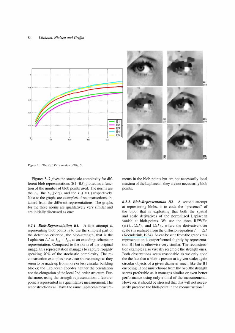
Figure 6. The L1(|∇ I |) version of Fig. 5.
Figures 5–7 gives the stochastic complexity for dif-ferent blob representations (B1–B5) plotted as a func-tion of the number of blob points used. The norms arethe L2, the L2(|∇ I |), and the L1(|∇ I |) respectively.Next to the graphs are examples of reconstructions ob-tained from the different representations. The graphsfor the three norms are qualitatively very similar andare initially discussed as one:
6.2.1. Blob-Representation B1. A first attempt atrepresenting blob points is to use the simplest part ofthe detection criterion, the blob-strength, that is theLaplacean �I = Ixx + Iyy , as an encoding-scheme orrepresentation. Compared to the norm of the originalimage, this representation manages to capture roughlyspeaking 70% of the stochastic complexity. The re-construction examples have clear shortcomings as theyseem to be made up from more or less circular buildingblocks; the Laplacean encodes neither the orientationnor the elongation of the local 2nd order structure. Fur-thermore, using the strength representation, a feature-point is represented as a quantitative measurement: Thereconstructions will have the same Laplacean measure-
ments in the blob points but are not necessarily localmaxima of the Laplacean: they are not necessarily blobpoints.
6.2.2. Blob-Representation B2. A second attemptat representing blobs, is to code the “presence” ofthe blob, that is exploiting that both the spatialand scale derivatives of the normalized Laplaceanvanish at blob-points. We use the three RFWFs:(�I )x , (�I )y and (�I )t , where the derivative overscale t is realized from the diffusion equation It = �I(Koenderink, 1984). As can be seen from the graphs thisrepresentation is outperformed slightly by representa-tion B1 but is otherwise very similar. The reconstruc-tion examples also visually resemble the strength ones.Both observations seem reasonable as we only codethe the fact that a blob is present at a given scale; againcircular objects of a given diameter much like the B1encoding. If one must choose from the two, the strengthseems preferable as it manages similar or even betterperformance using only a third of the measurements.However, it should be stressed that this will not neces-sarily preserve the blob-point in the reconstruction.8
Feature-Based Image Analysis 85
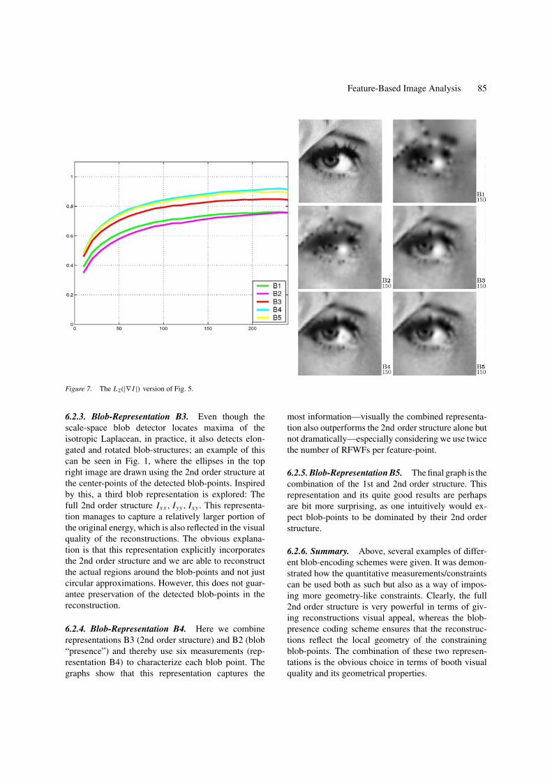
Figure 7. The L2(|∇ I |) version of Fig. 5.
6.2.3. Blob-Representation B3. Even though thescale-space blob detector locates maxima of theisotropic Laplacean, in practice, it also detects elon-gated and rotated blob-structures; an example of thiscan be seen in Fig. 1, where the ellipses in the topright image are drawn using the 2nd order structure atthe center-points of the detected blob-points. Inspiredby this, a third blob representation is explored: Thefull 2nd order structure Ixx , Iyy, Ixy . This representa-tion manages to capture a relatively larger portion ofthe original energy, which is also reflected in the visualquality of the reconstructions. The obvious explana-tion is that this representation explicitly incorporatesthe 2nd order structure and we are able to reconstructthe actual regions around the blob-points and not justcircular approximations. However, this does not guar-antee preservation of the detected blob-points in thereconstruction.
6.2.4. Blob-Representation B4. Here we combinerepresentations B3 (2nd order structure) and B2 (blob“presence”) and thereby use six measurements (rep-resentation B4) to characterize each blob point. Thegraphs show that this representation captures the
most information—visually the combined representa-tion also outperforms the 2nd order structure alone butnot dramatically—especially considering we use twicethe number of RFWFs per feature-point.
6.2.5. Blob-Representation B5. The final graph is thecombination of the 1st and 2nd order structure. Thisrepresentation and its quite good results are perhapsare bit more surprising, as one intuitively would ex-pect blob-points to be dominated by their 2nd orderstructure.
6.2.6. Summary. Above, several examples of differ-ent blob-encoding schemes were given. It was demon-strated how the quantitative measurements/constraintscan be used both as such but also as a way of impos-ing more geometry-like constraints. Clearly, the full2nd order structure is very powerful in terms of giv-ing reconstructions visual appeal, whereas the blob-presence coding scheme ensures that the reconstruc-tions reflect the local geometry of the constrainingblob-points. The combination of these two represen-tations is the obvious choice in terms of booth visualquality and its geometrical properties.
86 Lillholm, Nielsen and Griffin
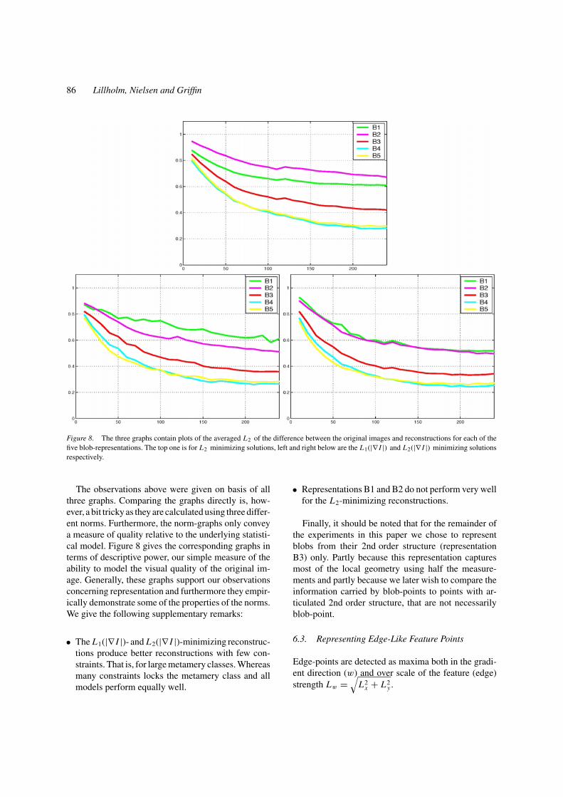
Figure 8. The three graphs contain plots of the averaged L2 of the difference between the original images and reconstructions for each of thefive blob-representations. The top one is for L2 minimizing solutions, left and right below are the L1(|∇ I |) and L2(|∇ I |) minimizing solutionsrespectively.
The observations above were given on basis of allthree graphs. Comparing the graphs directly is, how-ever, a bit tricky as they are calculated using three differ-ent norms. Furthermore, the norm-graphs only conveya measure of quality relative to the underlying statisti-cal model. Figure 8 gives the corresponding graphs interms of descriptive power, our simple measure of theability to model the visual quality of the original im-age. Generally, these graphs support our observationsconcerning representation and furthermore they empir-ically demonstrate some of the properties of the norms.We give the following supplementary remarks:
• The L1(|∇ I |)- and L2(|∇ I |)-minimizing reconstruc-tions produce better reconstructions with few con-straints. That is, for large metamery classes. Whereasmany constraints locks the metamery class and allmodels perform equally well.
• Representations B1 and B2 do not perform very wellfor the L2-minimizing reconstructions.
Finally, it should be noted that for the remainder ofthe experiments in this paper we chose to representblobs from their 2nd order structure (representationB3) only. Partly because this representation capturesmost of the local geometry using half the measure-ments and partly because we later wish to compare theinformation carried by blob-points to points with ar-ticulated 2nd order structure, that are not necessarilyblob-point.
6.3. Representing Edge-Like Feature Points
Edge-points are detected as maxima both in the gradi-ent direction (w) and over scale of the feature (edge)strength Lw =
√L2
x + L2y .
Feature-Based Image Analysis 87
Representations reflecting the edge-strength and-presence representations are straightforward to derivefrom the scale-space detection criteria9 but as for theblobs a suitable compromise between the number ofmeasurements, later comparisons, and resulting visualquality lead us to use, in this case, the full 1st orderstructure (representation E1) as the edge representa-tion for the remainder of this paper. The representationnicely captures both the strength and orientation of theedge points without explicit calculation.
7. Information Carried by Blob- and Edge-Points
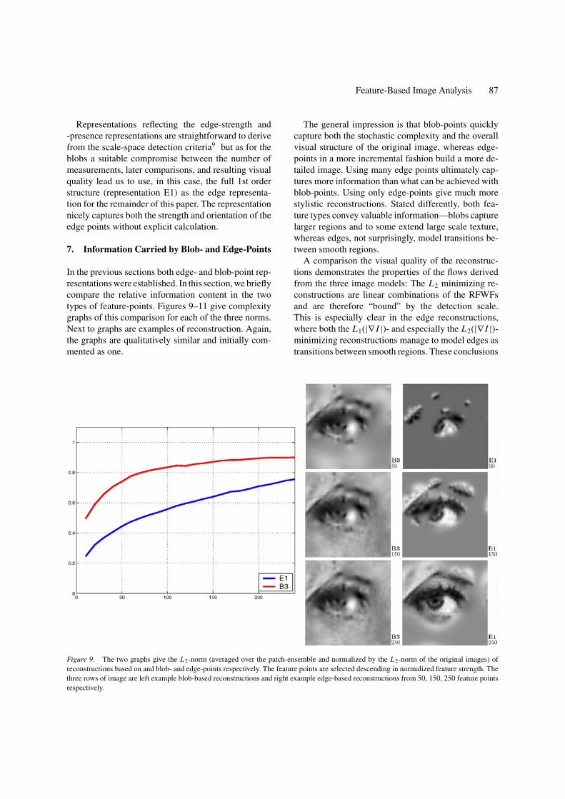
In the previous sections both edge- and blob-point rep-resentations were established. In this section, we brieflycompare the relative information content in the twotypes of feature-points. Figures 9–11 give complexitygraphs of this comparison for each of the three norms.Next to graphs are examples of reconstruction. Again,the graphs are qualitatively similar and initially com-mented as one.
Figure 9. The two graphs give the L2-norm (averaged over the patch-ensemble and normalized by the L2-norm of the original images) ofreconstructions based on and blob- and edge-points respectively. The feature points are selected descending in normalized feature strength. Thethree rows of image are left example blob-based reconstructions and right example edge-based reconstructions from 50, 150, 250 feature pointsrespectively.
The general impression is that blob-points quicklycapture both the stochastic complexity and the overallvisual structure of the original image, whereas edge-points in a more incremental fashion build a more de-tailed image. Using many edge points ultimately cap-tures more information than what can be achieved withblob-points. Using only edge-points give much morestylistic reconstructions. Stated differently, both fea-ture types convey valuable information—blobs capturelarger regions and to some extend large scale texture,whereas edges, not surprisingly, model transitions be-tween smooth regions.
A comparison the visual quality of the reconstruc-tions demonstrates the properties of the flows derivedfrom the three image models: The L2 minimizing re-constructions are linear combinations of the RFWFsand are therefore “bound” by the detection scale.This is especially clear in the edge reconstructions,where both the L1(|∇ I |)- and especially the L2(|∇ I |)-minimizing reconstructions manage to model edges astransitions between smooth regions. These conclusions
88 Lillholm, Nielsen and Griffin
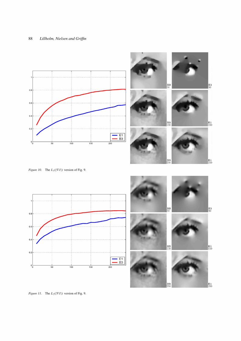
Figure 10. The L1(|∇ I |) version of Fig. 9.
Figure 11. The L2(|∇ I |) version of Fig. 9.
Feature-Based Image Analysis 89
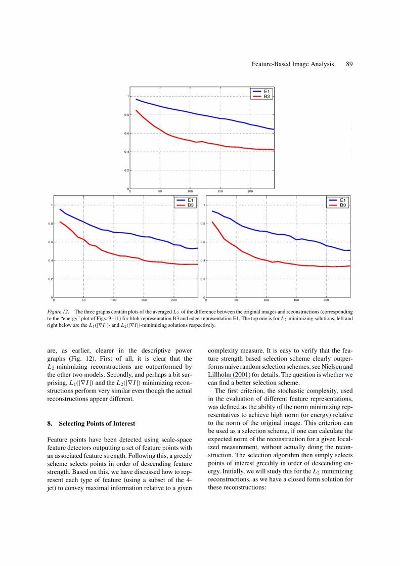
Figure 12. The three graphs contain plots of the averaged L2 of the difference between the original images and reconstructions (correspondingto the “energy” plot of Figs. 9–11) for blob-representation B3 and edge-representation E1. The top one is for L2-minimizing solutions, left andright below are the L1(|∇ I |)- and L2(|∇ I |)-minimizing solutions respectively.
are, as earlier, clearer in the descriptive powergraphs (Fig. 12). First of all, it is clear that theL2 minimizing reconstructions are outperformed bythe other two models. Secondly, and perhaps a bit sur-prising, L1(|∇ I |) and the L2(|∇ I |) minimizing recon-structions perform very similar even though the actualreconstructions appear different.
8. Selecting Points of Interest
Feature points have been detected using scale-spacefeature detectors outputting a set of feature points withan associated feature strength. Following this, a greedyscheme selects points in order of descending featurestrength. Based on this, we have discussed how to rep-resent each type of feature (using a subset of the 4-jet) to convey maximal information relative to a given
complexity measure. It is easy to verify that the fea-ture strength based selection scheme clearly outper-forms naive random selection schemes, see Nielsen andLillholm (2001) for details. The question is whether wecan find a better selection scheme.
The first criterion, the stochastic complexity, usedin the evaluation of different feature representations,was defined as the ability of the norm minimizing rep-resentatives to achieve high norm (or energy) relativeto the norm of the original image. This criterion canbe used as a selection scheme, if one can calculate theexpected norm of the reconstruction for a given local-ized measurement, without actually doing the recon-struction. The selection algorithm then simply selectspoints of interest greedily in order of descending en-ergy. Initially, we will study this for the L2 minimizingreconstructions, as we have a closed form solution forthese reconstructions:
90 Lillholm, Nielsen and Griffin
Given the response c of one localized RFWF f andthe corresponding discrete L2 minimizing reconstruc-tion J :
c =∫
�
f I dx and J = F(F T F)−1c,
where F is a discrete approximation of f , we can cal-culate the L2 norm of J as:
L2(J ) = J T J
= (F(F T F)−1c)T F(F T F)−1c
= c2(F T F)−1.
Assuming that f is a derivate of the Gaussian kernel(Eq. (1)) gives an explicit formulation of the innerproduct:
F T F ≈∫
R2ff dx = 1
βσ 2(p+1), β ∈ R, p = m + n
and thereby the L2-norm of the representative con-strained by f and the corresponding measurement c:
E(J ) = L2(J ) = βc2σ 2(p+1).
We can now calculate the reconstruction energy for allpoints in the scale-space and then select points in or-der of descending energy. This definition gives featurepoints in a broader sense as Points of Maximal Infor-mation relative to the norm (and thereby underlying
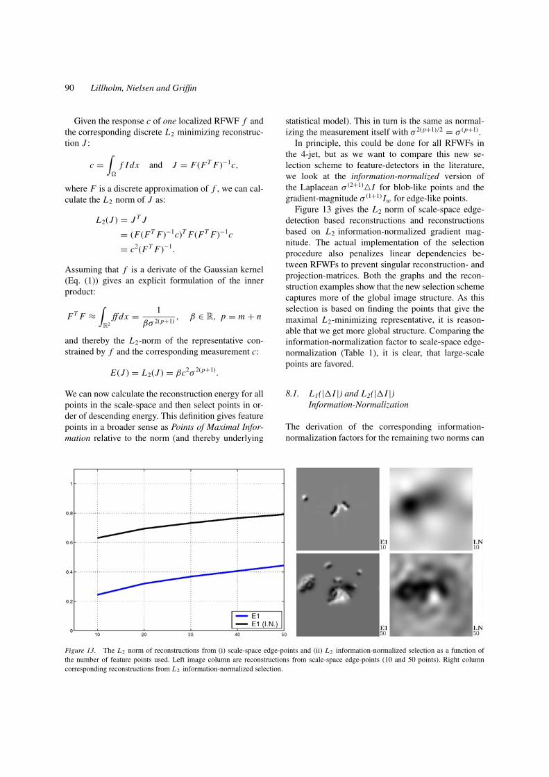
Figure 13. The L2 norm of reconstructions from (i) scale-space edge-points and (ii) L2 information-normalized selection as a function ofthe number of feature points used. Left image column are reconstructions from scale-space edge-points (10 and 50 points). Right columncorresponding reconstructions from L2 information-normalized selection.
statistical model). This in turn is the same as normal-izing the measurement itself with σ 2(p+1)/2 = σ (p+1).
In principle, this could be done for all RFWFs inthe 4-jet, but as we want to compare this new se-lection scheme to feature-detectors in the literature,we look at the information-normalized version ofthe Laplacean σ (2+1)�I for blob-like points and thegradient-magnitude σ (1+1) Iw for edge-like points.
Figure 13 gives the L2 norm of scale-space edge-detection based reconstructions and reconstructionsbased on L2 information-normalized gradient mag-nitude. The actual implementation of the selectionprocedure also penalizes linear dependencies be-tween RFWFs to prevent singular reconstruction- andprojection-matrices. Both the graphs and the recon-struction examples show that the new selection schemecaptures more of the global image structure. As thisselection is based on finding the points that give themaximal L2-minimizing representative, it is reason-able that we get more global structure. Comparing theinformation-normalization factor to scale-space edge-normalization (Table 1), it is clear, that large-scalepoints are favored.
8.1. L1(|�I |) and L2(|�I |)Information-Normalization
The derivation of the corresponding information-normalization factors for the remaining two norms can
Feature-Based Image Analysis 91
be realized using Euler-Lagrange techniques. As the ac-tual derivations are rather cumbersome, we give the fol-lowing result and derive the factors in a more straight-forward manner:
Given one of the proposed norms and one localizedmeasurement c = ∫
�f I dx , the stochastic complexity
if the reconstructed image J is given by:
E(J ) = βcασ g(p), β ∈ R, α ∈ {1, 2}, (11)
where α is the exponent of the norm, p the total orderof derivation, and g(p) is what must be identified foreach norm. One approach is to calculate the norm andthe constraining measurement at different scales andthereby derive g(p):
Stretching an image I by a positive factor h and mea-suring the resulting image Ih with Gaussian derivativesG(p)
hσ of equally stretched standard deviation, gives thefollowing equality:
c =∫
�
G(p)σ I dx = h p
∫h�
G(p)hσ Ih dx .
Inserting into (11), gives the reconstruction energy ofIh measured to
∫�
Ghσ Ih dx = ch−p as
E(Ih) = β(ch−p)α(σh)g(p) (12)
Furthermore, the relationship between the norm of Iand Ih and thereby between their respective reconstruc-tions, is given by h and the norm in question. As anexample, the stretched image Ih has h2 times largerL2-norm than I (for Dom(I ) ⊂ R
2). From this, we
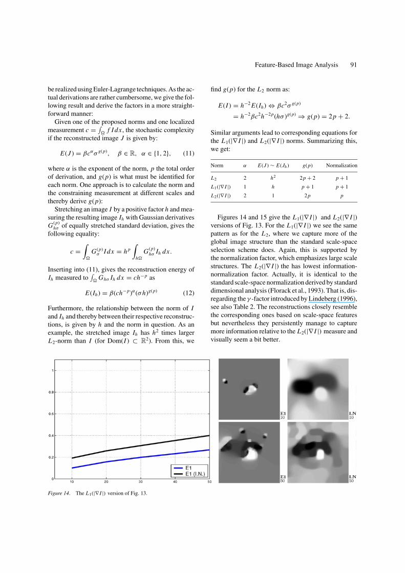
Figure 14. The L1(|∇ I |) version of Fig. 13.
find g(p) for the L2 norm as:
E(I ) = h−2 E(Ih) ⇔ βc2σ g(p)
= h−2βc2h−2p(hσ )g(p) ⇒ g(p) = 2p + 2.
Similar arguments lead to corresponding equations forthe L1(|∇ I |) and L2(|∇ I |) norms. Summarizing this,we get:
Norm α E(J ) ∼ E(Jh ) g(p) Normalization
L2 2 h2 2p + 2 p + 1
L1(|∇ I |) 1 h p + 1 p + 1
L2(|∇ I |) 2 1 2p p
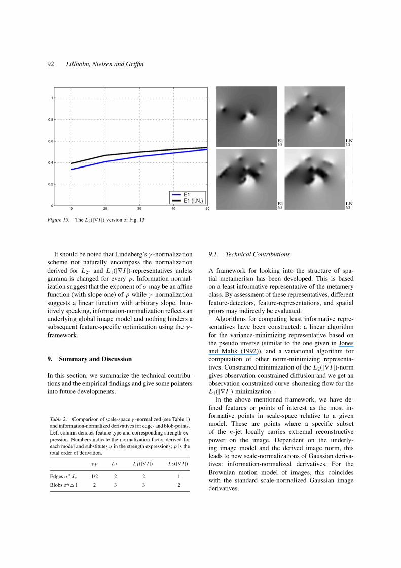
Figures 14 and 15 give the L1(|∇ I |) and L2(|∇ I |)versions of Fig. 13. For the L1(|∇ I |) we see the samepattern as for the L2, where we capture more of theglobal image structure than the standard scale-spaceselection scheme does. Again, this is supported bythe normalization factor, which emphasizes large scalestructures. The L2(|∇ I |) the has lowest information-normalization factor. Actually, it is identical to thestandard scale-space normalization derived by standarddimensional analysis (Florack et al., 1993). That is, dis-regarding the γ -factor introduced by Lindeberg (1996),see also Table 2. The reconstructions closely resemblethe corresponding ones based on scale-space featuresbut nevertheless they persistently manage to capturemore information relative to the L2(|∇ I |) measure andvisually seem a bit better.
92 Lillholm, Nielsen and Griffin
Figure 15. The L2(|∇ I |) version of Fig. 13.
It should be noted that Lindeberg’s γ -normalizationscheme not naturally encompass the normalizationderived for L2- and L1(|∇ I |)-representatives unlessgamma is changed for every p. Information normal-ization suggest that the exponent of σ may be an affinefunction (with slope one) of p while γ -normalizationsuggests a linear function with arbitrary slope. Intu-itively speaking, information-normalization reflects anunderlying global image model and nothing hinders asubsequent feature-specific optimization using the γ -framework.
9. Summary and Discussion
In this section, we summarize the technical contribu-tions and the empirical findings and give some pointersinto future developments.
Table 2. Comparison of scale-space γ -normalized (see Table 1)and information-normalized derivatives for edge- and blob-points.Left column denotes feature type and corresponding strength ex-pression. Numbers indicate the normalization factor derived foreach model and substitutes q in the strength expressions; p is thetotal order of derivation.
γ p L2 L1(|∇ I |) L2(|∇ I |)
Edges σ q Iw 1/2 2 2 1
Blobs σ q� I 2 3 3 2
9.1. Technical Contributions
A framework for looking into the structure of spa-tial metamerism has been developed. This is basedon a least informative representative of the metameryclass. By assessment of these representatives, differentfeature-detectors, feature-representations, and spatialpriors may indirectly be evaluated.
Algorithms for computing least informative repre-sentatives have been constructed: a linear algorithmfor the variance-minimizing representative based onthe pseudo inverse (similar to the one given in Jonesand Malik (1992)), and a variational algorithm forcomputation of other norm-minimizing representa-tives. Constrained minimization of the L2(|∇ I |)-normgives observation-constrained diffusion and we get anobservation-constrained curve-shortening flow for theL1(|∇ I |)-minimization.
In the above mentioned framework, we have de-fined features or points of interest as the most in-formative points in scale-space relative to a givenmodel. These are points where a specific subsetof the n-jet locally carries extremal reconstructivepower on the image. Dependent on the underly-ing image model and the derived image norm, thisleads to new scale-normalizations of Gaussian deriva-tives: information-normalized derivatives. For theBrownian motion model of images, this coincideswith the standard scale-normalized Gaussian imagederivatives.
Feature-Based Image Analysis 93
9.2. Empirical Findings
We have shown that, it is possible to make visuallyappealing reconstructions of images based on classicalscale-space blobs and edges. The second order struc-ture in blobs and first order structure in edge points issufficient for this.
Representing features in scale-space, we have exper-imented using feature strength, feature presence, andlocal geometrical structure. Combinations of featurepresence and local structure carries most information,whereas local structure alone is sufficient for creat-ing visually pleasing reconstructions. Feature strengthalone does not seem sufficient.
In general, blobs carry more information than edge-points. However, edge-points are capable of describingimages to a higher degree of detail, if many points areallowed in the description. That is, individual blobscarry more information on images than individualedge-points, but blobs are not sufficient for describingan image.
Derived from statistics, we have experimentedwith three different image norms for reconstructionsbased on features. The L2(I ) norm has its limita-tions as reconstructions are simple RFWF superpo-sitions and information cannot propagate into otherparts of the image. The gradient-based norms makevisually more pleasing reconstructions, and their un-derlying distributions also compare better to empiri-cal findings. L1(|∇ I |) has a tendency to create morecartoon-like reconstructions as image discontinuitiescan be present, and may be characterized as im-age enhancements. L2(|∇ I |) gives the visually mostpleasing reconstructions, and also compares best toearlier empirical findings on the statistics of naturalimages.
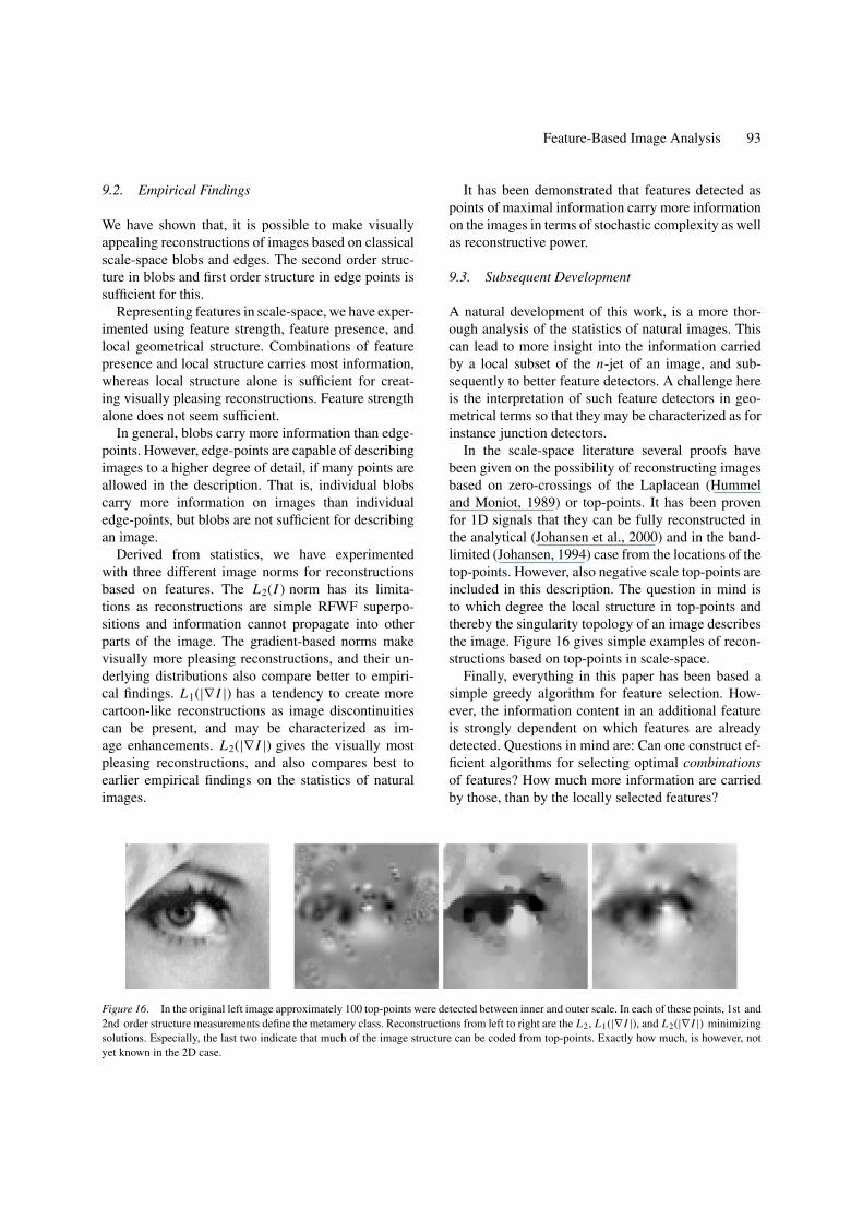
Figure 16. In the original left image approximately 100 top-points were detected between inner and outer scale. In each of these points, 1st and2nd order structure measurements define the metamery class. Reconstructions from left to right are the L2, L1(|∇ I |), and L2(|∇ I |) minimizingsolutions. Especially, the last two indicate that much of the image structure can be coded from top-points. Exactly how much, is however, notyet known in the 2D case.
It has been demonstrated that features detected aspoints of maximal information carry more informationon the images in terms of stochastic complexity as wellas reconstructive power.
9.3. Subsequent Development
A natural development of this work, is a more thor-ough analysis of the statistics of natural images. Thiscan lead to more insight into the information carriedby a local subset of the n-jet of an image, and sub-sequently to better feature detectors. A challenge hereis the interpretation of such feature detectors in geo-metrical terms so that they may be characterized as forinstance junction detectors.
In the scale-space literature several proofs havebeen given on the possibility of reconstructing imagesbased on zero-crossings of the Laplacean (Hummeland Moniot, 1989) or top-points. It has been provenfor 1D signals that they can be fully reconstructed inthe analytical (Johansen et al., 2000) and in the band-limited (Johansen, 1994) case from the locations of thetop-points. However, also negative scale top-points areincluded in this description. The question in mind isto which degree the local structure in top-points andthereby the singularity topology of an image describesthe image. Figure 16 gives simple examples of recon-structions based on top-points in scale-space.
Finally, everything in this paper has been based asimple greedy algorithm for feature selection. How-ever, the information content in an additional featureis strongly dependent on which features are alreadydetected. Questions in mind are: Can one construct ef-ficient algorithms for selecting optimal combinationsof features? How much more information are carriedby those, than by the locally selected features?
94 Lillholm, Nielsen and Griffin
Notes
1. Here, and in the remainder of this paper optimality is relative toa given complexity measure.
2. Using the Fourier-domain it is straight forward to show that〈 ∂ p
∂xn∂ym G, I 〉 = 〈G, ∂ p
∂xn∂ym I 〉.3. We denote this distribution pL2(I ) due the similarity between min-
imizing its negative log-likelihood and minimizing the standardL2 norm squared.
4. The second equality in Eq. (7) shows that the reconstructed imageis in fact the projection of the original image onto the range of F ,where F(FT F)−1 FT is the standard projection operator.
5. Each entry in the matrix is an inner product of two derivatives ofGaussians.
6. Note that localized Gaussian derivatives (of varying standard de-viation) as a model of the RFWFs do not ensure linear indepen-dence.
7. The database contains approximately 4000, 1536 × 1024, 8-bitimages of natural scenes.
8. In general, linear constraints mean that we are only able to pre-serve feature-points detected using linear detection criteria.
9. Strength: Lw ; Presence: Lww, Lwt .
References
Alvarez, L., Guichard, F., Lions, P.L., and Morel, J.M. 1993. Ax-ioms and fundamental equations of image processing: Multiscaleanalysis and p.d.e. Arch. for Rational Mechanics, 123(3):199–257.
Chan, T., Blomgren, P., Mulet, P., and Wong, C.K. 1997. Total vari-ation image restoration: Numerical methods and extensions. InICIP97, pp. III:384–xx.
Daugman, J.G. 1985. Uncertainty relations for resolution in space,spatial frequency, and orientation optimized by two-demensionalvisual cortical filters. Journal of the Optical Society of AmericaA, 1160–1169.
Field, D.J. 1987. Relations between the statistics of natural imagesand the response proporties of cortical cells. J. Optic. Soc. Am.,4(12):2379–2394.
Florack, L.M.J., ter Haar Romeny, B.M., Koenderink, J.J., andViergever, M.A. 1993. Cartesian differential invariants in scale-space. Journal of Mathematical Imaging and Vision, 3(4):327–348.
Florack, L.M.J., ter Haar Romeny, B.M., Koenderink, J.J., andViergever, M.A. 1990. Differential invariants in scale-space. Tech-nical Report 90-20, Computer Vision Research Group (3DCV),Utrecht Biophysics Research Institute (UBI).
Florack, L.M.J., ter Haar Romeny, B.M., Koenderink, J.J., andViergever, M.A. 1992. Scale and the differential structure of im-ages. Image and Vision Computing, 10(6):376–388.
Fox, C. 1987. An Introduction to the Calculus of Variations. DoverPress: NY.
Golub, G.H. and Van Loan, C.F. 1989. Matrix Computations, 2ndedn. Johns Hopkins Press: Baltimore, MD.
Griffin, L.D. 2000. Mean, median and mode filtering of images.Proceedings of the Royal Society A, 456(2004):2995–3004.
Griffin, L.D. 2002. Local image structure, metamerism, norms, andnatural image statistics. Perception, 31(3).
Harris, C. and Stephens, M.J. 1988. A combined corner and edgedetector. In Alvey88, pp. 147–152.
Huang, J., Lee, A.B., and Mumford, D. 2000. Statistics of rangeimages. In CVPR00, pp. I:324–331.
Huang, J. and Mumford, D. 1999. Statistics of natural images andmodels. In CVPR99, pp. I:541–547.
Huang, T.S. and Netravali, A.N. 1994. Motion and structure fromfeature correspondences: A review. PIEEE, 82(2):252–268.
Hubel, D.H. and Wiesel, T.N. 1968. Receptive fields and func-tional architecture of monkey striate cortex. Journal of Physiology,195:215–243.
Hummel, R.A. and Moniot, R. 1989. Reconstructions from zero-crossings in scale-space. ASSP, 37(12):2111–2130.
Johansen, P. 1994. On the classification of top points in scale-space.JMIV, 4:57–67.
Johansen, P., Nielsen, M., and Olsen, O.F. 2000. Branch points inone-dimensional gaussian scale space. JMIV, 13(3):193–203.
Jones, D.G. and Malik, J. 1992. Computational framework for deter-mining stereo correspondence from a set of linear spatial filters.IVC, 10:699–708.
Jones, J.P. and Palmer, L.A. 1987. The two-dimensional spatial struc-ture of simple receptive fields in cat striate cortex. Journal ofNeurophysiology, 58(6):1233–1258.
Kass, M. 1988. Linear image features in stereopsis. IJCV, 1(4):357–368.
Koenderink, J.J. 1984. The structure of images. BioCyber, 50:363–370.
Koenderink, J.J. and van Doorn, A.J. 1990. Receptive-field families.Biological Cybernetics, 63(4):291–297.
Koenderink, J.J. and van Doorn, A.J. 1996. Metamerism in completesets of image operators. In Advances in Image Understading ’96,pp. 113–129.
Lee, A.B., Mumford, D., and Huang, J. 2001. Occlusion models fornatural images: A statistical study of a scale-invariant dead leavesmodel. IJCV, 41(1/2):35–59.
Lindeberg, T. 1993. On scale selection for differential operators. InISRN KTH.
Lindeberg, T. 1994. Scale-space Theory in Computer Vision. KluwerAcademic Press: Boston, MA.
Lindeberg, T. 1996. Edge detection and ridge detection with auto-matic scale selection. In CVPR.
Lindeberg, T. 1998. Feature detection with automatic scale selection.IJCV, 30(2):79–116.
Maintz, J.B.A., van den Elsen, P.A., and Viergever, M.A. 1995. Com-parison of feature-based matching of ct and mr brain images. InCVRMed95.
Majer, P. 2001. The influence of the g-parameter on feature de-tection with automatic scale selection. In M. Kerckhove (Ed.),ScaleSpace01, Vol. 2106 in LNCS. Springer: Berlin.
Marr, D. 1982. Vision: A Computational Investigation into the Hu-man Representation and Processing of Visual Information. W.H.Freeman: San Francisco, CA.
Nielsen, M. 1995. From paradigm to algorithms in computer vision.Ph.D. thesis, Datalogisk Institut Kopenhagen University, Den-mark, Dept. of Computer Science, Universitetsparken 1, DK-2100Kopenhagen 0, Denmark.
Nielsen, M. and Lillholm, M. 2001. What do features tell about im-ages? In M. Kerckhove (Ed.), ScaleSpace01, Vol. 2106 in LNCS.Springer, pp. 39–50.
Pedersen, K.S. and Nielsen, M. 2000. The hausdorff dimension andscale-space normalization of natural images. JVCIR, 11(2):266–277.
Feature-Based Image Analysis 95
Press, W.H., Teukolsky, S.A., Vetterling, W.T., and Flannery, B.P.1993. Numerical Recipes in C: The Art of Scientific Computing.Cambridge University Press: Cambridge, UK.
Price, K.E. 1990. Multi-frame feature-based motion analysis. InICPR90, vol–I, pp. 114–118.
Rissanen, J. 1998. Stochastic Complexity in Statistical Inquiry, 2ndedn. World Scientific Press: Singapore.
Rosen, J.B. 1960. The gradient projection method for nonlinear pro-gramming. Part I. Linear constraints. SIAM, 8(1):181–217.
Ruderman, D.L. and Bialek, W. 1994. Statistics of natural images:Scaling in the woods. Physical Review Letters, 73(6):100–105.
Rudin, L.I., Osher, S., and Fatemi, E. 1992. Nonlinear total variationbased noise removal algorithms. Physica D, pp. 259–268.
Schmid, C. and Mohr, R. 1997. Local grayvalue invariants for imageretrieval. PAMI, 19(5):530–535.
Shannon, C.E. 1948. A mathematical theory of communication. BellSystem Technical Journal, 27:379–423 and 623–656.
Strong, D.M. and Chan, T.F. 1986. Exact solutions to the total varia-tion regularization problem. Technical Report, UCLA Departmentof Mathematics.
Tagliati, E. and Griffin, L.D. 2001. Features in scale space:Progress on the 2D 2nd order jet. In M. Kerckhove (Eds.),Scale-Space 01, Vol. 2106 in LNCS. Springer, pp. 51–62.
Tikhonov, A.N. and Arsenin, V.Y. 1977. Solution of Ill-Posed Prob-lems. Winston and Wiley: Washington, DC.
van Hateren, J.H. and van der Schaaf, A. 1998. Independent com-ponents filters of natural images compared with simple cellsin primary visual cortex. Proc. R. Soc.: Lond. B, 265:359–366.
Vogel, C.R. and Oman, M.E. 1996. Iterative methods for total varia-tion denoising. SIAM Journal on Scientific Computing, 17(1):227–238.
Weickert, J. 1998. Anisotropic Diffusion in Image Processing.Teubner-Verlag.
Wells, W.M. III. 1997. Statistical approaches to feature-based objectrecognition. IJCV, 21(1/2):63–98.
Young, R.A. 1985. The Gaussian derivative theory of spatial vision:Analysis of cortical receptive field line-weighting profiles. Gen.Motors Res. Tech. Rep, GMR-4920.


