Embed Size (px)
Citation preview
Eur. Phys. J. C (2013) 73:2608DOI 10.1140/epjc/s10052-013-2608-2
Special Article - Tools for Experiment and Theory
Fast computation of MadGraph amplitudeson graphics processing unit (GPU)
K. Hagiwara1, J. Kanzaki2,a, Q. Li3,b, N. Okamura4,c, T. Stelzer5,d
1KEK Theory Center and Sokendai, Tsukuba 305-0801, Japan2KEK and Sokendai, Tsukuba 305-0801, Japan3Department of Physics and State Key, Laboratory of Nuclear Physics and Technology, Peking University, Beijing, 100871, China4Department of Radiological Sciences, International University of Health and Welfare, Kitakenamaru, 2600-1 Ohtawara, Tochigi, Japan5Department of Physics, University of Illinois, Urbana, IL 61801, USA
Received: 3 May 2013 / Revised: 6 September 2013 / Published online: 5 November 2013© The Author(s) 2013. This article is published with open access at Springerlink.com
Abstract Continuing our previous studies on QED andQCD processes, we use the graphics processing unit (GPU)for fast calculations of helicity amplitudes for general Stan-dard Model (SM) processes. Additional HEGET codes tohandle all SM interactions are introduced, as well as the pro-gram MG2CUDA that converts arbitrary MadGraph gener-ated HELAS amplitudes (FORTRAN) into HEGET codesin CUDA. We test all the codes by comparing amplitudesand cross sections for multi-jet processes at the LHC asso-ciated with production of single and double weak bosons,a top-quark pair, Higgs boson plus a weak boson or a top-quark pair, and multiple Higgs bosons via weak-boson fu-sion, where all the heavy particles are allowed to decay intolight quarks and leptons with full spin correlations. All thehelicity amplitudes computed by HEGET are found to agreewith those computed by HELAS within the expected numer-ical accuracy, and the cross sections obtained by gBASES,a GPU version of the Monte Carlo integration program,agree with those obtained by BASES (FORTRAN), as wellas those obtained by MadGraph. The performance of GPUwas over a factor of 10 faster than CPU for all processesexcept those with the highest number of jets.
1 Introduction
The start-up of the CERN Large Hadron Collider (LHC)opens a new discovery era of high energy particle physics.
a e-mail: [email protected] e-mail: [email protected] e-mail: [email protected] e-mail: [email protected]
With proton beams colliding at unprecedented energy, it pro-vides us with great opportunities to discover the Higgs bo-son and new physics beyond the Standard Model (SM), withtypical signals involving multiple high pT γ ’s, jets, W ’sand Z’s. Reliable searches for these signatures require agood understanding of all SM background processes, whichis usually done by simulations performed by Monte Carlo(MC) event generators, such as MadGraph [1, 2, 4]. How-ever, the complicated event topology expected for somenew physics signals makes their background simulation timeconsuming, and it is important to increase the computationalspeed for simulations in the LHC data analysis.
In previous studies [5, 6], the GPU (Graphics Pro-cessing Unit) has been used to realize economical andpowerful parallel computations of cross sections by in-troducing a C-language version of the HELAS [7] codes,HEGET (HELAS Evaluation with GPU Enhanced Technol-ogy). HEGET is based on the software development sys-tem CUDA [8] introduced by NVIDIA [9]. For pure QEDprocesses, qq → nγ , with n = 2 to 8, the calculations ran40–150 times faster on the GPU than on the CPU [5]. Forpure QCD processes, gg → ng with n up to 4, qq → ng
and qq → qq + (n − 2)g with n up to 5, 60–100 times bet-ter performance was achieved on the GPU [6]. In this paper,we extend these exploratory studies to cover general SMprocesses, opening the way to perform the complete ma-trix element computation of MadGraph on the GPU. Thecomplexity of the calculations is increased due to new inter-action types and complicated event topologies expected inbackground simulations for various new physics scenarios.We introduce additional HEGET functions to cover all ofthe SM particles and their interactions, and a phase spaceparameterization suited for GPU computations. In order totest all of the new functions and the efficiency of the GPUcomputation in semi-realistic background simulations, we
Page 2 of 39 Eur. Phys. J. C (2013) 73:2608
systematically study multi-jet processes associated with theproduction of SM heavy particles(s), followed by its (their)decay into final states including light quarks and leptons,including full spin correlations. In particular, we report nu-merical results on the following processes:
W/Z + n-jets (n ≤ 4), (1a)
WW/WZ/ZZ + n-jets (n ≤ 3), (1b)
t t + n-jets (n ≤ 3), (1c)
HW/HZ + n-jets (n ≤ 3), (1d)
Htt + n-jets (n ≤ 2), (1e)
Hk + (n − k)-jets via WBF (k ≤ 3, n ≤ 5). (1f)
For the processes (1a) to (1e), we examine all of the majorsubprocesses at the LHC, while for the multiple Higgs pro-duction (1f), we study only the weak-boson fusion (WBF)subprocesses to test the Higgs self interactions.
We present numerical results for the cross sections of pro-cesses in Eqs. (1a)–(1f) computed by using the GPU ver-sion of the Monte Carlo integration program, gBASES [10],with the new HEGET functions in the amplitude calcula-tions, and compare the results with those obtained runningtwo different programs on the CPU, the FORTRAN versionBASES [11] programs with HELAS subroutines and the lat-est version of MadGraph (ver.5) [1]. We also compare theperformance of two versions of the BASES program, one onthe GPU and the other on the CPU.
The paper is structured as follows. In Sect. 2, we presentthe cross section formulae for general SM production pro-cesses at the LHC, and list all of the subprocesses we studyin this report. In Sect. 3, we briefly describe a new phasespace parameterization for efficient GPU computation. InSect. 4, we introduce new HEGET functions for all SM par-ticles and their interactions. In Sect. 5, we introduce the soft-ware used to generate CUDA codes with HEGET functionsfrom FORTRAN amplitude programs with HELAS subrou-tines obtained by MadGraph. In Sect. 6, we review the com-puting environment, basic parameters of the GPU and CPUmachines used in this analysis. Section 7 gives numericalresults of computations of cross sections and comparisonsof performance of GPU and CPU programs. Section 8 sum-marizes our findings. Appendix A explains in more detailour phase space parameterization introduced in Sect. 3. Ap-pendix B explains our method for generating random num-bers on GPU. Appendix C lists all the new HEGET codesintroduced in this paper.
2 Physics processes
In order to test not only the validity and efficiency of ourGPU computation but also its robustness, we examine a se-ries of multi-jet production processes in association with the
SM heavy particle(s) (W , Z, t and H ), followed by their de-cays into light quarks and leptons, that can be backgroundsfor discoveries in many new physics scenarios. In this sec-tion, we list all the subprocesses we study in this paper andgive the definition of multi-jet cross sections that are calcu-lated both on the CPU and on the GPU at later sections.
At the LHC with a collision energy of√
s, the cross sec-tion for general production processes in the SM can be ex-pressed as
dσ =∑
{a,b}
∫∫dxa dxb
× Da/p(xa,Q)Db/p(xb,Q)dσ (s = sxaxb), (2)
where Da/p and Db/p are the parton distribution functions(PDF’s), Q is the factorization scale, xa and xb are the mo-mentum fractions of the partons a and b, respectively, in theright- and left-moving protons,
√s is the subprocess center
of mass energy, and dσ (s) gives the differential cross sec-tion for the 2 → n subprocess
a(pa,λa, ca) + b(pb,λb, cb)
→ 1(p1, λ1, c1) + · · · + n(pn,λn, cn). (3)
The subprocesses cross section can be computed in theleading order as
dσ (s) = 1
2s
1
2 · 2
∑
λi
1
nanb
∑
ci
∣∣M ci
λi
∣∣2dΦn, (4)
where
dΦn = (2π)4δ4
(pa + pb −
n∑
i=1
pi
)n∏
i=1
d3pi
(2π)3 2Ei
, (5)
is the invariant n-body phase space, λi are the helicities ofthe initial and final partons, na and nb are the color degreeof freedom of the initial partons, a and b, respectively. M ci
λi
are the Helicity amplitudes for the process (3), which can begenerated automatically by MadGraph and expressed as
M ci
λi=
∑
l∈diagram
(Mλi)ci
l (6)
where the summation is over all the Feynman diagrams.The subscripts λi stand for a given combination of helici-ties (0 for Higgs bosons, ±1/2 for quarks and leptons, ±1for photons and gluons), and the subscripts ci correspond toa set of color indices (none for colorless particles, 1, 2, 3 forflowing-IN quarks, 1,2,3 for flowing-OUT quarks, and 1 to8 for gluons). Details on color summation in MadGraph canbe found in Ref. [6].
In this paper, we are interested in general SM processes,typically involving the production of heavy resonances with
Eur. Phys. J. C (2013) 73:2608 Page 3 of 39
decays, associated with multiple jet production, which oftenappear as major SM background for new physics signals.The limitation in the number of extra jets, n or n − k inEqs. (1a)–(1f), is primarily due to limitations in the amountof memory available to the GPU as reported in previousstudies [5, 6].
Correlated decays of the heavy particles into the follow-ing channels are calculated:
W∓ → �∓ (–)ν� (� = e,μ), (7a)
Z → �+�− (� = e,μ), (7b)
t → b �+ν� (� = e,μ), (7c)
t → b �− ν� (� = e,μ), (7d)
H → τ+τ−. (7e)
We do not consider τ decays in this report for brevity. Thesame selection cuts are imposed for � = e,μ, τ , so thatthe Higgs boson production cross sections listed in this re-port can be used as a starting point for realistic simulations.A Higgs boson mass of 125 GeV and its branching fractioninto τ+τ−, 0.0405, are used throughout this report.1
For definiteness, we impose the following final state cutsat the parton level. For jets, we require the same conditionsas in Refs. [5, 6]:
|ηi | < ηcutjet = 5, (8a)
pTi > pcutT,jet = 20 GeV, (8b)
pTij > pcutT,jet = 20 GeV. (8c)
Where ηi and pTi are the pseudo-rapidity and the transversemomentum of the i-th jet, respectively, in the pp collisionsrest frame along the right-moving (pz = |p|) proton momen-tum direction, and pTij is the relative transverse momen-tum [13] between the jets i and j defined by
pTij ≡ min(pTi , pTj )ΔRij , (9a)
ΔRij =√
(Δηij )2 + (Δφij )2. (9b)
Here ΔRij measures the boost-invariant angular separationbetween the i and j jets, and Δηij and Δφij are defined asdifferences of pseudorapidities and azimuthal angles of thetwo jets.
For b jets from t decay, we require
|ηb| < ηcutb = 2.5, (10a)
pT,b > pcutT,b = 20 GeV. (10b)
1It should be noted here that the polarized τ decay, based on theτ decay helicity amplitude is available in the framework of Mad-Graph5 [12].
Note that we do not require them to be isolated from otherjets via (8c). For charged leptons, we require
|η�| < ηcut� = 2.5, (� = e,μ, τ), (11a)
pT,� > pcutT,� = 20 GeV, (� = e,μ, τ) (11b)
and for simplicity we treat τ the same as e and μ. Like b jetsfrom t decays, we do not impose isolation cuts for leptons,since performing realistic simulations is not the purpose ofthis study.
We use the set CTEQ6L1 [14] parton distribution func-tions (PDF) for all processes.
2.1 Single W production
The following four types of W production subprocesses arestudied in this paper:
ud → W+ + ng (n = 0,1,2,3,4), (12a)
ug → W+ + d + (n − 1)g (n = 1,2,3,4), (12b)
uu → W+ + ud + (n − 2)g (n = 2,3,4), (12c)
gg → W+ + du + (n − 2)g (n = 2,3,4). (12d)
The subprocess (12a) starts with the leading order α0s , the
subprocess (12b) starts with the next order α1s , and those
of (12c) and (12d) start with the α2s order. These subpro-
cesses give the dominant contributions in pp collisions. Thecorresponding W− production cross sections are smaller inpp collisions since an incoming u-quark in the subprocesses(12a) to (12c) should be replaced by a d-quark, whose PDFis significantly softer than the up-quark PDF in the proton.
2.2 Single Z production
Similarly, the following subprocesses are studied for Z pro-duction:
uu → Z + ng (n = 0,1,2,3,4), (13a)
ug → Z + u + (n − 1)g (n = 1,2,3,4), (13b)
uu → Z + uu + (n − 2)g (n = 2,3,4), (13c)
gg → Z + uu + (n − 2)g (n = 2,3,4). (13d)
As in the case of W+ + n-jets, we examine all of the domi-nant contributions up to 4-jets. It should be noted that thedown quark contribution to the Z + jets cross section isless suppressed than the W− + jets case, since the Z-bosoncouples stronger to the down-quarks than the up-quarks (cf.Γ (Z → dd)/Γ (Z → uu) ≈ 1.3).
Page 4 of 39 Eur. Phys. J. C (2013) 73:2608
2.3 WW production
For the W boson pair production, we study the followingsubprocesses:
uu → W+W− + ng (n = 0,1,2,3), (14a)
ug → W+W− + u + (n − 1)g (n = 1,2,3), (14b)
uu → W+W− + uu + (n − 2)g (n = 2,3), (14c)
uu → W+W+ + dd + (n − 2)g (n = 2,3), (14d)
gg → W+W− + uu + (n − 2)g (n = 2,3). (14e)
The subprocess (14a) starts with the leading order α0s , the
subprocess (14b) starts with the next order α1s , and those
of (14c) to (14e) start with the α2s order. The subprocesses
(14d) are included as the dominant same sign W -pair pro-duction mechanism in pp collisions.
2.4 W+Z production
Similarly, the following subprocesses are studied for W+Z
production:
ud → W+Z + ng (n = 0,1,2,3), (15a)
ug → W+Z + d + (n − 1)g (n = 1,2,3), (15b)
uu → W+Z + ud + (n − 2)g (n = 2,3), (15c)
gg → W+Z + du + (n − 2)g (n = 2,3). (15d)
As in the WW +n-jets case, we consider all of the dominantW+Z production subprocesses up to 3 associated jets. Noteagain that the down quark contribution to the W−Z + jetscross section can be significant because of the large Z cou-pling to the d-quarks.
2.5 ZZ production
The following ZZ production subprocesses are also studied:
uu → ZZ + ng (n = 0,1,2,3), (16a)
ug → ZZ + u + (n − 1)g (n = 1,2,3), (16b)
uu → ZZ + uu + (n − 2)g (n = 2,3), (16c)
gg → ZZ + uu + (n − 2)g (n = 2,3). (16d)
All of the dominant ZZ production subprocesses up to 3associated jets are studied. Note, however, that the down-quark contribution to the qg collision subprocess (16b) hasthe coupling enhancement factor of (Γ (Z → dd)/Γ (Z →uu))2 ≈ 1.7. Although we study only 4 lepton final states,ZZ + jets processes can be backgrounds for new physicssignals with a Z boson plus jets and large missing ET.
2.6 t t production
For t t production, we consider the following subprocesses:
uu → t t + ng (n = 0,1,2,3), (17a)
ug → t t + u + (n − 1)g (n = 1,2,3), (17b)
uu → t t + uu + (n − 2)g (n = 2,3), (17c)
gg → t t + ng (n = 0,1,2,3). (17d)
The subprocess (17a) starts with the leading order α2s , the
subprocess (17b) starts with the next order α3s , and those of
(17c) and (17d) start with the α4s order. Again, only those
subprocesses which give dominant contributions in pp col-lisions are studied in each order.
2.7 W boson associated Higgs production
As for the associate production of the Higgs boson andthe W , we consider the following subprocesses:
ud → HW+ + ng (n = 0,1,2,3), (18a)
ug → HW+ + d + (n − 1)g (n = 1,2,3), (18b)
uu → HW+ + ud + (n − 2)g (n = 2,3), (18c)
gg → HW+ + du + (n − 2)g (n = 2,3). (18d)
All of the subprocesses (18a) to (18d) are obtained by re-placing one gluon in the W + jets subprocesses (12a) to(12d) by H , respectively. The HW− + jets subprocessescorresponding to (18a) to (18c) are suppressed since an in-coming u-quark would be replaced by a softer d-quark inthe proton.
2.8 Z boson associated Higgs production
Likewise, the following subprocesses are studied for HZ
production:
uu → HZ + ng (n = 0,1,2,3), (19a)
ug → HZ + u + (n − 1)g (n = 1,2,3), (19b)
uu → HZ + uu + (n − 2)g (n = 2,3), (19c)
gg → HZ + uu + (n − 2)g (n = 2,3). (19d)
All of the four subprocesses are obtained from the corre-sponding Z + jets subprocesses (13a) to (13d), by replacingone final gluon by H . Again, the down quark contributionsto the subprocesses (19a) to (19c) are less suppressed thanthose to the HW+ production processes (21a) to (21c) dueto the large Z coupling to the d-quark.
Eur. Phys. J. C (2013) 73:2608 Page 5 of 39
2.9 Top quark associated Higgs production
For the Htt production process, the following subprocessesare examined in this paper:
uu → Htt + ng (n = 0,1,2), (20a)
ug → Htt + u + (n − 1)g (n = 1,2), (20b)
uu → Htt + uu, (20c)
gg → Htt + ng (n = 0,1,2). (20d)
All of the subprocesses (20a) to (20d) are obtained, respec-tively, from the t t + jets subprocesses (17a) to (17d) by re-placing one gluon in the final state by a Higgs boson.
2.10 Higgs boson production via weak-boson fusion
In all of the above subprocesses we consider only QCD in-teractions for production of jets and top quarks, while theweak interactions contribute only in W , Z, H productionsand in decays. For Higgs + jets processes, we study weak-boson fusion (WBF) subprocesses which can be identified atthe LHC for various decay modes [15–17]. WW fusion con-tributes to the subprocesses (21a), ZZ fusion contributes tothe subprocesses (21b), both contribute to the subprocesses(21c) and (21d):
ud → H + ud + (n − 2)g (n = 2,3,4), (21a)
uu → H + uu + (n − 2)g (n = 2,3,4), (21b)
ug → H + ud + d + (n − 3)g (n = 3,4), (21c)
gg → H + uu + dd. (21d)
The subprocesses (21a) and (21b) start with the leadingorder α0
s , those in (21c) start with the next order α1s , the
subprocess (21d) occurs at the α2s order. We do not con-
sider gg fusion process, because its simulation requires non-renormalizable vertices [1] which are absent in the minimalset of HELAS codes [7].
2.11 Multiple Higgs bosons productionvia weak-boson fusion
The following multiple Higgs boson production processesare studied in this paper as a test of cubic and quartic vertexfunctions among scalar and vector bosons:
ud → HH + ud + (n − 2)g (n = 2,3), (22a)
uu → HH + uu + (n − 2)g (n = 2,3), (22b)
ud → HHH + ud, (22c)
uu → HHH + uu. (22d)
The quartic scalar boson vertex appears only in the subpro-cesses (22c) and (22d).
3 Algorithm for phase space generation
In this section, we briefly introduce our phase space parame-trization, designed for efficient GPU computing. Details aregiven in Appendix A.
Optimizing code to run efficiently on the GPU requiresseveral special considerations. In addition to the careful useof memory mentioned earlier, one needs to consider thateach “batch” of calculations processed on the GPU must un-dergo identical operations. That has particular consequenceswhen one considers generating momentum in phase spacethat satisfy the appropriate cuts. The efficiency of generat-ing momenta that pass cuts is not particularly important onthe CPU, since one can simply repeatedly generate momentauntil a set is found that pass the cuts. The structure of theGPU however does not allow such flexibility. If the gener-ation program is running on multiple processors, each pro-cessor has one opportunity to generate a valid phase spacepoint before moving forward to calculate the amplitude. Soif the efficiency for generating a point in phase space thatpasses cuts is only 10 % then you loose a factor of 10 incomputing speed.
In previous studies [5, 6] for pure QED and QCD pro-cesses at hadron colliders:
a + b → 1 + · · · + n, (23)
the following phase space parameterization has been usedincluding the integration over the initial parton momentumfractions (see Appendix A for details):
dΣn ≡ dxa dxb dΦn
= Θ(1−xa)Θ(1−xb)
2s(4π)2n−3dyn
n−1∏
i=1
(dyi dp
2T i
dφi
2π
). (24)
With this parameterization, when all the final particles aremassless partons, we can generate phase space points thatsatisfy the rapidity constraints, |ηcut| < ηcut, for all partons(i = 1 to n) and the pT constraints, pTi > pcut
T , for n−1 par-tons (i = 1 to n − 1). Only those phase space points whichviolate the conditions, xa < 1, xb < 1 or pTn > pcut
T , will berejected. Studies in Refs. [5, 6] find that, for example, 78 %,58 %, 42 % and 29 % of generated phase space points sat-isfy the final state cuts,2 for 2–5 photon productions at theLHC, when we choose yi (i = 1 to n), lnp2
Ti and φi (i = 1to n − 1) as integration variables.
We adopt this parameterization of the generalized phasespace in this report, which is extended to account for theproduction and decay of several Breit–Wigner resonances.
2Note this can easily be improved e.g. by introducing ordering in pT,pcut
T < pT1 < pT2 < · · · < pTn, for n-photons or n-gluons. It is thenonly pTn which can go up to
√s/2.
Page 6 of 39 Eur. Phys. J. C (2013) 73:2608
In particular, for process with n-jet plus m-resonance pro-duction
pp → (n − m)j +m∑
k=1
Rk(→ fk) + anything, (25)
when the resonance Rk decays into a final state fk , we pa-rameterize the generalized phase space as follows:
dΣ = dΣn
m∏
k=1
dsk
2πdΦ
(Rk → fk at p2
fk= sk
). (26)
Here dΦ(Rk → fk) is the invariant phase space for theRk → fk decay when the invariant mass of the final statefk is
√sk , and dΣn is the n-body generalized phase space
for n − m massless particles and m massive particles ofmasses
√sk (k = 1 to m). Integration over the invariant mass
squared sk is made efficient by using the standard Breit–Wigner formalism
dsk = (sk − m2k)
2 + (mkΓk)2
mkΓk
d tan−1(
sk − m2k
mkΓk
), (27)
and the transverse momenta are generated as
dp2Tk = (
p2Tk + sk
)d ln
(p2
Tk + sk). (28)
Finally, we note that s-channel splitting of massless par-tons can be accommodated by using the same parameteri-zation Eq. (26), where Rk in Eq. (26) is a virtual parton ofmass
√sk and fk is a set of partons. Instead of the Breit–
Wigner parameterization (27), we simply use ln sk as inte-gration variables.
4 HEGET functions
In this section, we explain the new HEGET functions forcomputing the helicity amplitudes for arbitrary SM pro-cesses. All of the HEGET functions that appear in this reportare listed in Appendix C as List 3 to List 30.
4.1 Wave functions
In the previous works [5, 6], the wave functions for masslessparticles, which are named ixxxxk, oxxxxk and vxxxxk
(k = 0,1,2), have been introduced for fermions and vec-tor bosons. In this report, we introduce wave functions formassive spin 0, 1/2 and 1 particles, which can also beused for massless particles by setting the mass parametersto zero. The naming scheme for HEGET functions followsthat of HELAS subroutines: the HEGET (HELAS) functionnames start with i(I) and o(O) for flow-IN and flow-OUT fermions, respectively, v(V) for vector boson wave
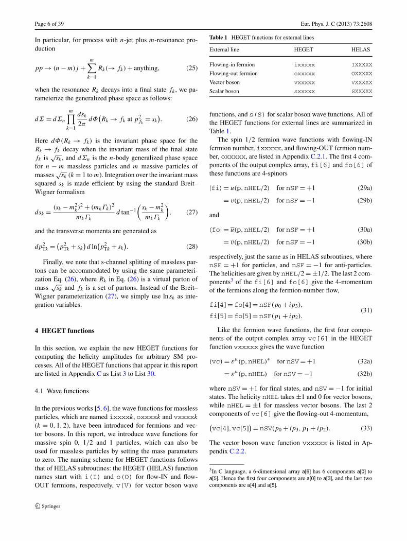
Table 1 HEGET functions for external lines
External line HEGET HELAS
Flowing-in fermion ixxxxx IXXXXX
Flowing-out fermion oxxxxx OXXXXX
Vector boson vxxxxx VXXXXX
Scalar boson sxxxxx SXXXXX
functions, and s(S) for scalar boson wave functions. All ofthe HEGET functions for external lines are summarized inTable 1.
The spin 1/2 fermion wave functions with flowing-INfermion number, ixxxxx, and flowing-OUT fermion num-ber, oxxxxx, are listed in Appendix C.2.1. The first 4 com-ponents of the output complex array, fi[6] and fo[6] ofthese functions are 4-spinors
|fi〉 = u(p,nHEL/2) for nSF= +1 (29a)
= v(p,nHEL/2) for nSF= −1 (29b)
and
〈fo| = u(p,nHEL/2) for nSF= +1 (30a)
= v(p,nHEL/2) for nSF= −1 (30b)
respectively, just the same as in HELAS subroutines, wherenSF = +1 for particles, and nSF = −1 for anti-particles.The helicities are given by nHEL/2 = ±1/2. The last 2 com-ponents3 of the fi[6] and fo[6] give the 4-momentumof the fermions along the fermion-number flow,
fi[4] = fo[4] = nSF(p0 + ip3),
fi[5] = fo[5] = nSF(p1 + ip2).(31)
Like the fermion wave functions, the first four compo-nents of the output complex array vc[6] in the HEGETfunction vxxxxx gives the wave function
(vc) = εμ(p,nHEL)∗ for nSV= +1 (32a)
= εμ(p,nHEL) for nSV= −1 (32b)
where nSV = +1 for final states, and nSV = −1 for initialstates. The helicity nHEL takes ±1 and 0 for vector bosons,while nHEL = ±1 for massless vector bosons. The last 2components of vc[6] give the flowing-out 4-momentum,(vc[4],vc[5]) = nSV(p0 + ip3,p1 + ip2). (33)
The vector boson wave function vxxxxx is listed in Ap-pendix C.2.2.
3In C language, a 6-dimensional array a[6] has 6 components a[0] toa[5]. Hence the first four components are a[0] to a[3], and the last twocomponents are a[4] and a[5].
Eur. Phys. J. C (2013) 73:2608 Page 7 of 39
The function sxxxxx computes the wave function ofa scalar boson, and is listed in Appendix C.2.3. Since thescalar boson does not have any Lorentz indices, the firstcomponent of the output sc[3] is simply unity, 1+ i0. Thelast 2 components give the flowing-out 4-momentum:
(sc[1],sc[2]) = nSS(p0 + ip3,p1 + ip2), (34)
where nSS= +1(−1) when the scalar boson is in the final(initial) state.
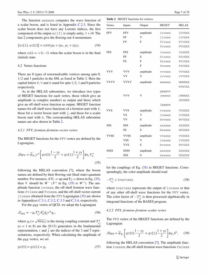
4.2 Vertex functions
There are 8 types of renormalizable vertices among spin 0,1/2 and 1 particles in the SM, as listed in Table 2. Here thecapital letters F, V and S stand for spin 1/2, 1 and 0 particlesrespectively.
As in the HELAS subroutines, we introduce two typesof HEGET functions for each vertex, those which give anamplitude (a complex number) as output and those whichgive an off-shell wave function as output. HEGET functionnames for off-shell wave functions of a fermion start with f,those for a vector boson start with j, and those for a scalarboson start with h. The corresponding HELAS subroutinenames are also shown in Table 2.
4.2.1 FFV: fermion–fermion–vector vertex
The HEGET functions for the FFV vertex are defined by theLagrangian,
LFFV = ψF1γ μ
[gc[0]1 − γ5
2+ gc[1]1 + γ5
2
]ψF2V
∗μ
(35)
following the HELAS convention [7], where the bosonnames are defined by their flowing-out (final state) quantumnumber. For instance, if F1 = up and F2 = down in Eq. (35),then V should be W− (V ∗ in Eq. (35) is W+). The am-plitude function iovxxx, the off-shell fermion wave func-tions fvixxx and fvoxxx, and the off-shell vector currentjioxxx obtained from the FFV Lagrangian (35) are shownin Appendices C.3.1, C.3.2, C.3.3 and C.3.4, respectively.
For the qqg vertex of QCD, we adopt the Lagrangian
Lqqg = −gsTa
ijAa
μqiγμqj , (36)
where gs(= √4παs) is the strong coupling constant and T a
ij
(a = 1 to 8) are the SU(3) generators in the fundamentalrepresentation, i and j are the indices of the 3 and 3 repre-sentations, respectively. When calculating the amplitude ofthe qqg vertex, we set
gc[0] = gc[1] = gs (37)
Table 2 HEGET functions for vertices
Vertex Inputs Output HEGET HELAS
FFV FFV amplitude iovxxx IOVXXX
FF V jioxxx JIOXXX
FV F fvixxx FVIXXX
fvoxxx FVOXXX
FFS FFS amplitude iosxxx IOSXXX
FF S hioxxx HIOXXX
FS F fsixxx FSIXXX
F fsoxxx FSOXXX
VVV VVV amplitude vvvxxx VVVXXX
VV V jvvxxx JVVXXX
VVVV VVVV amplitude wwwwxx WWWWXX
W3W3XX
ggggxx
VVV V jwwwxx JWWWXX
JW3WXX
jgggxx
VVS VVS amplitude vvsxxx VVSXXX
VS V jvsxxx JVSXXX
VV S hvvxxx HVVXXX
SSS SSS amplitude sssxxx SSSXXX
SS S hssxxx HSSXXX
VVSS VVSS amplitude vvssxx VVSSXX
VSS V jvssxx JVSSXX
VVS S hvvsxx HVVSXX
SSSS SSSS amplitude ssssxx SSSSXX
SSS S hsssxx HSSSXX
for the couplings of Eq. (35) in HEGET functions. Corre-spondingly, the color amplitude should read
−T a
ij× (vertex), (38)
where (vertex) represents the output of iovxxx or thatof any other off-shell wave functions for the FFV vertex.The color factor of −T a
ijis then processed algebraically in
integrand functions of the BASES program.
4.2.2 FFS: fermion–fermion–scalar vertex
The FFS vertex of the HEGET functions are defined by theLagrangian
LFFS = ψF1
[gc[0]1 − γ5
2+ gc[1]1 + γ5
2
]ψF2S
∗, (39)
following the HELAS convention [7]. The amplitude func-tion iosxxx, the off-shell fermion wave functions fsixxx
Page 8 of 39 Eur. Phys. J. C (2013) 73:2608
and fsoxxx, and the off-shell scalar current hioxxx areshown in Appendices Appendices C.4.1, C.4.2, C.4.3 andC.4.4, respectively.
4.2.3 VVV: three vector vertex
The HELAS subroutine for the VVV vertex functions are de-fined by the following Yang–Mills Lagrangian
LVVV = −i gc{(
∂μV ∗1ν
)(V
μ∗2 V ν∗
3 − V ν∗2 V
μ∗3
)
+ (∂μV ∗
2ν
)(V
μ∗3 V ν∗
1 − V ν∗3 V
μ∗1
)
+ (∂μV ∗
3ν
)(V
μ∗1 V ν∗
2 − V ν∗1 V
μ∗2
)}, (40)
with a real coupling gc, where the vector boson triple prod-ucts are anti-Hermitian. The amplitude of the VVV vertexis calculated by the HEGET function vvvxxx and the off-shell vector current is computed by jvvxxx, which arelisted Appendices C.5.1 and C.5.2, respectively.
For the electroweak gauge bosons, the coupling gc ischosen as
gc = gWWZ = gW cos θW for WWZ
= gWWA = gW sin θW = e for WWA. (41)
Here the three vector bosons (V1,V2,V3) should be chosenas the cyclic permutations of (W−,W+,Z/A), because ofthe HELAS convention which uses the flowing out quantumnumber for boson names: see Table 16 in Appendix C.5 fordetails. Note (V1μ)∗ = V2μ in the HELAS Lagrangian (40).
The ggg vertex in the QCD Lagrangian can be expressedas
Lggg = gsfabc
(∂μAaν
)(Ab
μAcν
)
= (if abc
)(−igs)
(∂μAaν
)(Ab
μAcν
), (42)
where now the vector boson triple products are Hermitian;(Aa
μ)∗ = Aaμ. We can still use the same vertex functions
vvvxxx and jvvxxx with the real coupling
gc= gs for ggg (43)
and by denoting the corresponding amplitude as
if abc × (vertex), (44)
where (vertex) gives the output of the HEGET functionsvvvxxx or jvvxxx. The associated factor of if abc is thentreated as the color factor in MadGraph [2].
4.2.4 VVVV: four vector vertex
There are two types of VVVV vertex in the SM Lagrangian,one is for SU(2) and the other for SU(3).
As in the case for the VVV vertex, the SU(2) vectorbosons are expressed in terms of
W±μ = 1√
2
(W 1
μ ∓ i W 2μ
), (45a)
W 3μ = cos θWZμ + sin θWAμ. (45b)
The contact four-point vector boson vertex for the SU(2)weak interaction is given by the Lagrangian
LWWWW = −g2W
4εijmεklmWi
μWjν WkμWlν
= −g2W
2
{(W−∗ · W+∗)(W+∗ · W−∗)
− (W−∗ · W−∗)(W+∗ · W+∗)}
+ g2W
{(W−∗ · W 3∗)(W 3∗ · W+∗)
− (W−∗ · W+∗)(W 3∗ · W 3∗)}. (46)
Two distinct subroutines wwwwxx and w3w3xx (see Ta-ble 2) were introduced in HELAS, because there was anattempt to improve their numerical accuracy by combiningthe weak boson exchange contribution to the four-point ver-tices [7]. The attempt has not been successful and we haveno motivation to keep the original HELAS strategy.
Instead, we introduce only one set of HEGET func-tions for the interactions among four distinct vector bosons(V1,V2,V3,V4);
LVVVV = gg{(
V ∗1 · V ∗
4
)(V ∗
2 · V ∗3
)
− (V ∗
1 · V ∗3
)(V ∗
2 · V ∗4
)}. (47)
The corresponding HEGET functions are named as ggggxxfor the amplitude and jgggxx for the off-shell currents.
Because the SU(2) weak boson vertices (46) always havetwo identical bosons (or two channels for the vertex ofW+W−γZ) we further introduce the HEGET functionswwwwxx and jwwwxx which sum over the two contribu-tions internally. The functions are listed in Appendices C.6.1and C.6.2, respectively, and the input fields and correspond-ing couplings are given in Table 17.
As for the QCD quartic gluon coupling
Lgggg = −g2s
4f abef cdeAa
μAbνA
cμAdν, (48a)
= g2s
2f abef cde
{(Aa · Ad
)(Ab · Ac
)
− (Aa · Ac
)(Ab · Ad
)}, (48b)
we can use the HEGET functions ggggxx and jgggxx forthe Lagrangian (47) to obtain the amplitudes and the off-shell gluon currents respectively. For instance, by using the
Eur. Phys. J. C (2013) 73:2608 Page 9 of 39
four-vector vertex amplitude of Γ (g2;V1,V2,V3,V4) forthe Lagrangian (47), we can express the amplitude of ga
1 ,gb
2 , gc3, gd
4 as follows:
Γ(ga
1 , gb2 , gc
3, gd4
) = f abef cdeΓ(g2
s ;ga1 , gb
2 , gc3, g
d4
)
+ f acef dbeΓ(g2
s ;ga1 , gc
2, gd3 , gb
4
)
+ f adcf bceΓ(g2
s ;ga1 , gd
2 , gb3 , gc
4
).
(49)
The off-shell gluon currents are obtained similarly by callingthe HEGET function three times as explained in [5, 6] andrepeated in Appendix C.6 for completeness.
4.2.5 VVS: vector–vector–scalar vertex
The only VVS interaction of the SM appears in the HiggsLagrangian in the form
LVVS = gc(V ∗
1 · V ∗2
)S∗, (50)
where the coupling gc is real and proportional to the Higgsvacuum expectation value (v.e.v.). The HEGET functionsfor the amplitude vvsxxx, the off-shell vector currentjvsxxx, and the off-shell scalar current hvsxxx are givenfor a general complex gc (in GeV units), distinct complexvector bosons (V1 and V2), and a complex scalar field (S),and are listed in Appendices C.7.1, C.7.2 and C.7.3, respec-tively. In the SM, only WWH and ZZH couplings appear.
4.2.6 VVSS: vector–vector–scalar–scalar vertex
The HEGET functions for the VVSS vertex are obtainedfrom the Lagrangian
LVVSS = gc(V ∗
1 · V ∗2
)S∗
3S∗4 . (51)
The amplitude function vvssxx, the off-shell vector cur-rent jvssxx, and the off-shell scalar current hvvsxx arelisted in Appendices C.8.1, C.8.2 and C.8.3, respectively, fora complex gc, distinct complex vector bosons (V1 and V2),and for distinct complex scalars (S3 and S4). In the SM, onlyWWHH and ZZHH couplings appear, and the coupling gc isreal and proportional to the squares of the electroweak gaugecouplings.
4.2.7 SSS: three scalar vertex
In Appendix C.9, we show the HEGET functions for theSSS vertex, which are obtained from the Lagrangian
LSSS = gcS∗1S∗
2S∗3 . (52)
The HEGET functions for the amplitude sssxxx and theoff-shell scalar current hssxxx are given for a complex gc
(in GeV units) and for distinct complex scalars (S1, S2, S3),and are listed in Appendices C.9.1 and C.9.2 respectively.In the SM, the coupling gc is real and proportional to theHiggs v.e.v. and only the H 3 coupling appears.
4.2.8 SSSS: four scalar vertex
The Lagrangian
LSSSS = gcS∗1S∗
2S∗3S∗
4 (53)
gives the HEGET functions for the SSSS vertex: ssssxxfor the amplitude and hsssxx for the off-shell scalar cur-rent, which are listed in Appendices C.10.1 and C.10.2, re-spectively. Here again the HEGET functions are given for acomplex gc, and for the four distinct complex scalar bosons(S1, S2, S3, S4). In the SM, only the H 4 coupling existswhose coupling gc is real and proportional to the ratio ofthe Higgs boson mass and the v.e.v.
5 Generation of CUDA functionsfor Monte Carlo integration
For the Monte Carlo integration of cross sections of thephysics processes on the GPU, all integrand functions haveto be coded using CUDA [8]. In order to prepare these am-plitude functions efficiently we develop an automatic con-version program, MG2CUDA. As input this program takesthe FORTRAN amplitude subroutine, matrix.f gener-ated by MadGraph (ver.4) [2], analyzes the source codeand generates all CUDA functions necessary for the MonteCarlo integration on GPU. MG2CUDA also optimizes gen-erated CUDA codes for execution on the GPU by reducingunnecessary variables and dividing long amplitude functionsinto a set of smaller functions as necessary.
In the following subsections, the major functions ofMG2CUDA are briefly described.
5.1 Generation of HEGET function callsfrom HELAS subroutines
MG2CUDA converts calling sequences of HELAS subrou-tines in matrix.f to those of HEGET functions in the in-tegrand function of gBASES. All HEGET functions for theGPU are designed to have a one-to-one correspondence toHELAS subroutines with the same name, and their argu-ments have the same order and the same variables types.Hence HELAS subroutine calls are directly converted toHEGET function calls.
Page 10 of 39 Eur. Phys. J. C (2013) 73:2608
5.2 Decoding of initial and final state information
MG2CUDA decodes the physics process information,species of initial and final particles, the number of graphsand the number of color bases, written into matrix.f byMadGraph and adopts an appropriate phase space programand prepare header files to store process information andsome constants.
5.3 Division of a long amplitude program
As the number of external particles increases, the numberof Feynman diagrams contributing to the subprocess growsfactorially and the amplitude program generated by Mad-Graph becomes very long. Due to the current limitation ofthe CUDA compiler, a very long amplitude program cannotbe compiled [5, 6] by the CUDA compiler. MG2CUDA di-vides such a long amplitude function program into smallerfunctions which are successively called in the integrandfunction of gBASES.
Among the processes listed in Eqs. (1a)–(1f), several pro-cesses with the maximum number of jets require such de-composition into smaller pieces by MG2CUDA. Those pro-cesses are denoted explicitly in the tables and plots in Sect. 7by an asterisk.
5.4 Decomposition of a color matrix multiplication
Compared to CPU, the memory resources of GPU are quitelimited. Hence, if calculations on GPU require a largeamount of data, the data must reside on slower memory(global memory), and the access to the data becomes a causeof the degradation of performance of GPU programs. Whenthe number of independent color bases of a physics pro-cess becomes large, the data size necessary for the mul-tiplication of color factors also becomes large. For exam-ple, the number of color bases for uu → t t + ggg (17a) is144, and the data size and the total number of multiplica-tions in the color matrix multiplication becomes the orderof (144)2 ∼ 20000. In order to avoid degradation of per-formance of GPU, MG2CUDA decomposes arguments ofthe color matrix into a set of independent color factors andcombines multiplications which have the same factors. Thissignificantly reduces the number of color factors and the to-tal number of multiplications [6]. For the uu → t t + ggg
case, the number of independent factors is only 51 and thereduced number of multiplications becomes ∼3600. Thesecolor factors are stored in the read-only (e.g. constant) mem-ory which GPU can access more quickly than the globalmemory.4
4It should be introduced here that the different approach to the compu-tation of color factors was tried also using GPU and good performancewas obtained [18].
5.5 Reduction of the number of temporary wave functions
During the computation of amplitudes, temporary variablesof wave functions are necessary to keep intermediate parti-cle information. MG2CUDA analyzes the use of these tem-porary variables and recycles variables which are not usedany more in the latter part of the program. This greatlyrelaxes the memory resource requirement. Again for theuu → t t + ggg case, the number of variables used for wavefunctions in original matrix.f is 1607, and it becomesonly 83 after recycling temporary variables.
6 Computing environment
In this section, we introduce our computing environmentused for all computations presented in this paper.
6.1 Computations on GPU
We used a Tesla C2075 GPU processor board produced byNVIDIA [9] to compute cross sections of the physics pro-cesses listed in Eqs. (12a)–(22d). The Tesla C2075 has 448processors (CUDA cores) in one GPU chip, which deliversup to 515 GFLOPS of double-precision peak performance.Other parameters of the board are listed in Table 3. The TeslaC2075 is controlled by a Linux PC with Fedora 14 (64 bit)operating system. CUDA codes executed on the GPU aredeveloped on the host PC with the CUDA 4.2 [8] softwaredevelopment kit.
For the computation of cross sections we use the MonteCarlo integration program, BASES [11]. The GPU versionof BASES, gBASES, has originally been developed in sin-gle precision [10]. In this paper, however, we use the newlydeveloped double precision version of gBASES for all GPUcomputations throughout this report.
6.2 CPU environment
As references of cross section computations and also forpurposes of comparisons of process time, we use the BASES
Table 3 Parameters of Tesla C2075 and CUDA tools
Number of CUDA core 448
Total amount of global memory 5.4 GB
Total amount of constant memory 64 kB
Total amount of shared memory per block 48 kB
Total number of registers available per bloc 32768
Clock rate 1.15 GHz
nvcc CUDA compiler Rel. 4.2 (V0.2.1221)
CUDA driver Ver. 4.2
CUDA runtime Ver. 4.2
Eur. Phys. J. C (2013) 73:2608 Page 11 of 39
Table 4 CPU environment
CPU Intel Core i7 2.67 GHz
Cache size 8192 KB
Memory 6 GB
OS Fedora 13 (64 bit)
gcc 4.4.5 (Red Hat 4.4.5-2)
program in FORTRAN on the CPU [11]. The measurementof total execution time is performed on the Linux PC withFedora 13 (64 bit) operating system. The hardware param-eters and the version of the software used for the executionof the FORTRAN BASES programs are summarized in Ta-ble 4.
As another reference of cross sections we also use thelatest version of MadGraph (ver.5) [1] which has been re-leased in 2011. All numerical results appear in Sect. 7 as“MadGraph” are obtained by this new version of MadGraph.During computations it shows good performance in the exe-cution time and gives us stable results.
7 Results
In this section, we present numerical results of the compu-tations of the total cross sections and a comparison of totalprocess time of gBASES programs on the GPU for the SMprocesses listed in Sect. 2. As references for the cross sec-tions and process time, we also present results obtained byBASES and MadGraph on a CPU. Recent improvements indouble precision calculations on the GPU allows us to per-form all computations in this paper at double precision ac-curacy.
In addition, in the previous papers [5, 6], a simple pro-gram composed of a single event loop without any optimiza-tions for the computation of cross sections was used both onthe GPU and the CPU and their process time for a singleevent loop was compared. In this paper, we compare the to-tal execution time of BASES programs running on the GPUand on a CPU with the same integration parameters. Sincethe total execution time of gBASES includes both processtime on the GPU and the CPU, the comparison gives a morepractical index of the gain in the total process time by usingthe GPU.
For all three programs, gBASES, BASES and MadGraph,we use the same final state cuts, PDF’s and the model param-eters as explained in Sect. 2. All results for the various SMprocesses are obtained for the LHC at
√s = 14 TeV, and
summarized in Tables 5–15, and Figs. 1–11. Some generalcomments are in order here.
First, we test all of the HEGET functions listed in Ap-pendix C against the HELAS subroutines [7] and the am-plitude subroutines for MadGraph (ver.5) by comparing the
helicity amplitudes of all subprocess listed in Sect. 2. Wegenerally find agreement within the accuracy of double pre-cision computation, except for multiple Higgs productionprocesses via weak boson fusion, Eqs. (22c) and (22d).For these processes, the MadGraph amplitude codes givesignificantly smaller amplitudes. We identify the cause ofthe discrepancy as subtle gauge theory cancellation amongweak boson exchange amplitudes. After modifying both theHELAS and HEGET codes to respect the tree-level gaugeinvariance strictly, by replacing all m2
V in the weak bo-son propagators and in the vertices,5 and by setting m2
W −i mWΓW = (g2
W/g2Z)(m2
Z − i mZΓZ) as a default, we findagreement for all the amplitudes. Except for the triple Higgsboson production processes of Eqs. (22c) and (22d), thesemodifications on the code do not give significant differencein the amplitudes.
In Tables 5–15, the results of the process time ratio withthe divided amplitude functions are denoted by an asterisk.In the plots of Figs. 1–11 they are indicated by open cir-cles. By comparing the numbers with and without asterisksin the tables, and also by comparing the heights of the blobswith and without circles in the figures for the same numberof jets, we can clearly observe the loss of efficiency in theGPU computation when the amplitude function is so longthat its division into smaller pieces is needed. For example,among the Z + 4-jets processes only the amplitude functionof the process, uu → Z + uu + gg (13c), has to be divided.It is clearly seen from Table 6 and Fig. 2 that the GPU gainover the CPU is significantly lower (∼5) for this process, ascompared to the other Z + 4-jets processes. A similar trendis observed for all other processes with divided amplitudeprogram.
From Tables 5–15, we find that the results obtained bygBASES with HEGET functions agree with those by theBASES programs with HELAS within the statistics of gen-erated number of events. On the other hand we observe somedeviations of MadGraph results from BASES results as thenumber of jets in the final state, n, increases. It amounts toabout 5–7 % level for processes with the maximum numberof jets. These deviations may be attributed to the differenceof the phase space generation part for multi-jet productions,and require further studies. The program gSPRING [19]which generates events on the GPU by making use of thegrid information of variables optimized by gBASES [10]is being developed, and more detailed comparison betweenMadGraph and its GPU version will be reported elsewhere.
In the following subsections, let us briefly summarize ourfindings for each subprocesses as listed in Sect. 2.
5In our calculations with MadGraph, subroutines for amplitude com-putation are slightly modified to replace all squared massive vector bo-son mass, m2
V , with m2V − i mV ΓV , which is only partly realized in the
original codes.
Page 12 of 39 Eur. Phys. J. C (2013) 73:2608
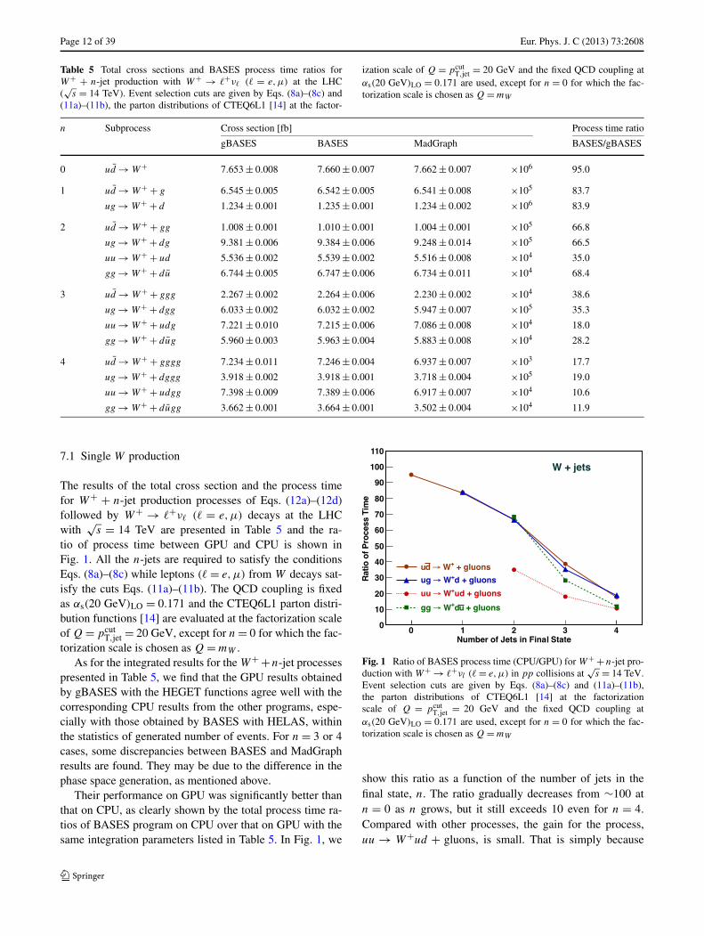
Table 5 Total cross sections and BASES process time ratios forW+ + n-jet production with W+ → �+ν� (� = e,μ) at the LHC(√
s = 14 TeV). Event selection cuts are given by Eqs. (8a)–(8c) and(11a)–(11b), the parton distributions of CTEQ6L1 [14] at the factor-
ization scale of Q = pcutT,jet = 20 GeV and the fixed QCD coupling at
αs(20 GeV)LO = 0.171 are used, except for n = 0 for which the fac-torization scale is chosen as Q = mW
n Subprocess Cross section [fb] Process time ratio
gBASES BASES MadGraph BASES/gBASES
0 ud → W+ 7.653 ± 0.008 7.660 ± 0.007 7.662 ± 0.007 ×10⁶ 95.0
1 ud → W+ + g 6.545 ± 0.005 6.542 ± 0.005 6.541 ± 0.008 ×10⁵ 83.7
ug → W+ + d 1.234 ± 0.001 1.235 ± 0.001 1.234 ± 0.002 ×10⁶ 83.9
2 ud → W+ + gg 1.008 ± 0.001 1.010 ± 0.001 1.004 ± 0.001 ×10⁵ 66.8
ug → W+ + dg 9.381 ± 0.006 9.384 ± 0.006 9.248 ± 0.014 ×10⁵ 66.5
uu → W+ + ud 5.536 ± 0.002 5.539 ± 0.002 5.516 ± 0.008 ×10⁴ 35.0
gg → W+ + du 6.744 ± 0.005 6.747 ± 0.006 6.734 ± 0.011 ×10⁴ 68.4
3 ud → W+ + ggg 2.267 ± 0.002 2.264 ± 0.006 2.230 ± 0.002 ×10⁴ 38.6
ug → W+ + dgg 6.033 ± 0.002 6.032 ± 0.002 5.947 ± 0.007 ×10⁵ 35.3
uu → W+ + udg 7.221 ± 0.010 7.215 ± 0.006 7.086 ± 0.008 ×10⁴ 18.0
gg → W+ + dug 5.960 ± 0.003 5.963 ± 0.004 5.883 ± 0.008 ×10⁴ 28.2
4 ud → W+ + gggg 7.234 ± 0.011 7.246 ± 0.004 6.937 ± 0.007 ×10³ 17.7
ug → W+ + dggg 3.918 ± 0.002 3.918 ± 0.001 3.718 ± 0.004 ×10⁵ 19.0
uu → W+ + udgg 7.398 ± 0.009 7.389 ± 0.006 6.917 ± 0.007 ×10⁴ 10.6
gg → W+ + dugg 3.662 ± 0.001 3.664 ± 0.001 3.502 ± 0.004 ×10⁴ 11.9
7.1 Single W production
The results of the total cross section and the process timefor W+ + n-jet production processes of Eqs. (12a)–(12d)followed by W+ → �+ν� (� = e,μ) decays at the LHCwith
√s = 14 TeV are presented in Table 5 and the ra-
tio of process time between GPU and CPU is shown inFig. 1. All the n-jets are required to satisfy the conditionsEqs. (8a)–(8c) while leptons (� = e,μ) from W decays sat-isfy the cuts Eqs. (11a)–(11b). The QCD coupling is fixedas αs(20 GeV)LO = 0.171 and the CTEQ6L1 parton distri-bution functions [14] are evaluated at the factorization scaleof Q = pcut
T,jet = 20 GeV, except for n = 0 for which the fac-torization scale is chosen as Q = mW .
As for the integrated results for the W+ +n-jet processespresented in Table 5, we find that the GPU results obtainedby gBASES with the HEGET functions agree well with thecorresponding CPU results from the other programs, espe-cially with those obtained by BASES with HELAS, withinthe statistics of generated number of events. For n = 3 or 4cases, some discrepancies between BASES and MadGraphresults are found. They may be due to the difference in thephase space generation, as mentioned above.
Their performance on GPU was significantly better thanthat on CPU, as clearly shown by the total process time ra-tios of BASES program on CPU over that on GPU with thesame integration parameters listed in Table 5. In Fig. 1, we
Fig. 1 Ratio of BASES process time (CPU/GPU) for W+ +n-jet pro-duction with W+ → �+νl (� = e,μ) in pp collisions at
√s = 14 TeV.
Event selection cuts are given by Eqs. (8a)–(8c) and (11a)–(11b),the parton distributions of CTEQ6L1 [14] at the factorizationscale of Q = pcut
T,jet = 20 GeV and the fixed QCD coupling atαs(20 GeV)LO = 0.171 are used, except for n = 0 for which the fac-torization scale is chosen as Q = mW
show this ratio as a function of the number of jets in thefinal state, n. The ratio gradually decreases from ∼100 atn = 0 as n grows, but it still exceeds 10 even for n = 4.Compared with other processes, the gain for the process,uu → W+ud + gluons, is small. That is simply because
Eur. Phys. J. C (2013) 73:2608 Page 13 of 39
Table 6 Total cross sections and BASES process time ratios for Z + n-jet production with Z → �+�− (� = e,μ) at the LHC (√
s = 14 TeV).Event selection cuts, PDF and αs are the same as in Table 5, except for n = 0 for which the factorization scale is Q = mZ
n Subprocess Cross section [fb] Process time ratio
gBASES BASES MadGraph BASES/gBASES
0 uu → Z 4.333 ± 0.004 4.330 ± 0.005 4.334 ± 0.004 ×10⁵ 103.2
1 uu → Z + g 4.143 ± 0.004 4.135 ± 0.004 4.136 ± 0.005 ×10⁴ 81.2
ug → Z + u 7.161 ± 0.007 7.171 ± 0.007 7.162 ± 0.009 ×10⁴ 79.9
2 uu → Z + gg 7.283 ± 0.007 7.290 ± 0.008 7.258 ± 0.010 ×10³ 64.7
ug → Z + ug 5.738 ± 0.003 5.743 ± 0.003 5.718 ± 0.009 ×10⁴ 57.8
uu → Z + uu 3.503 ± 0.003 3.511 ± 0.003 3.475 ± 0.004 ×10³ 31.0
gg → Z + uu 5.301 ± 0.007 5.301 ± 0.007 5.292 ± 0.007 ×10³ 66.3
3 uu → Z + ggg 1.758 ± 0.004 1.766 ± 0.002 1.724 ± 0.002 ×10³ 32.6
ug → Z + ugg 3.918 ± 0.002 3.917 ± 0.002 3.838 ± 0.005 ×10⁴ 36.8
uu → Z + uug 4.897 ± 0.004 4.898 ± 0.005 4.804 ± 0.005 ×10³ 18.1
gg → Z + uug 4.832 ± 0.002 4.839 ± 0.006 4.764 ± 0.006 ×10³ 28.6
4 uu → Z + gggg 5.738 ± 0.011 5.746 ± 0.004 5.514 ± 0.006 ×10² 15.4
ug → Z + uggg 2.694 ± 0.002 2.694 ± 0.001 2.557 ± 0.003 ×10⁴ 19.5
uu → Z + uugg 5.250 ± 0.005 5.259 ± 0.004 4.964 ± 0.005 ×10³ 5.1∗
gg → Z + uugg 3.038 ± 0.002 3.038 ± 0.001 2.901 ± 0.003 ×10³ 11.6
these processes have more Feynman diagrams and a largercolor bases than the other processes with the same numberof jets.
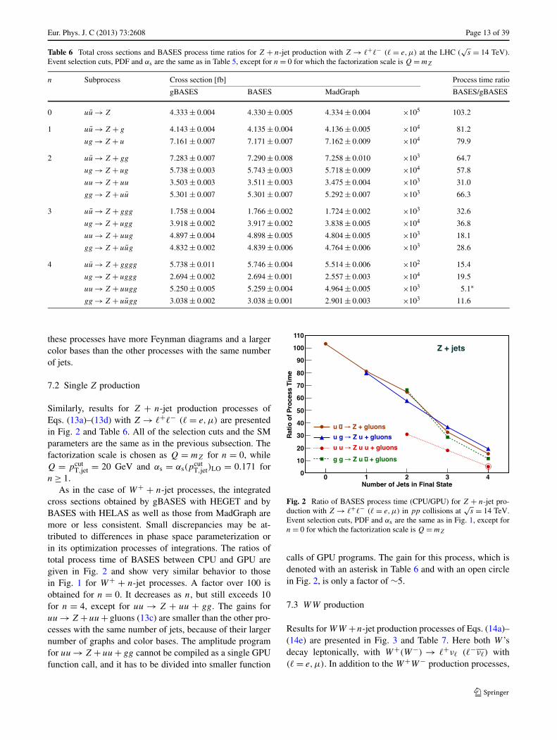
7.2 Single Z production
Similarly, results for Z + n-jet production processes ofEqs. (13a)–(13d) with Z → �+�− (� = e,μ) are presentedin Fig. 2 and Table 6. All of the selection cuts and the SMparameters are the same as in the previous subsection. Thefactorization scale is chosen as Q = mZ for n = 0, whileQ = pcut
T,jet = 20 GeV and αs = αs(pcutT,jet)LO = 0.171 for
n ≥ 1.As in the case of W+ + n-jet processes, the integrated
cross sections obtained by gBASES with HEGET and byBASES with HELAS as well as those from MadGraph aremore or less consistent. Small discrepancies may be at-tributed to differences in phase space parameterization orin its optimization processes of integrations. The ratios oftotal process time of BASES between CPU and GPU aregiven in Fig. 2 and show very similar behavior to thosein Fig. 1 for W+ + n-jet processes. A factor over 100 isobtained for n = 0. It decreases as n, but still exceeds 10for n = 4, except for uu → Z + uu + gg. The gains foruu → Z +uu+ gluons (13c) are smaller than the other pro-cesses with the same number of jets, because of their largernumber of graphs and color bases. The amplitude programfor uu → Z + uu + gg cannot be compiled as a single GPUfunction call, and it has to be divided into smaller function
Fig. 2 Ratio of BASES process time (CPU/GPU) for Z + n-jet pro-duction with Z → �+�− (� = e,μ) in pp collisions at
√s = 14 TeV.
Event selection cuts, PDF and αs are the same as in Fig. 1, except forn = 0 for which the factorization scale is Q = mZ
calls of GPU programs. The gain for this process, which isdenoted with an asterisk in Table 6 and with an open circlein Fig. 2, is only a factor of ∼5.
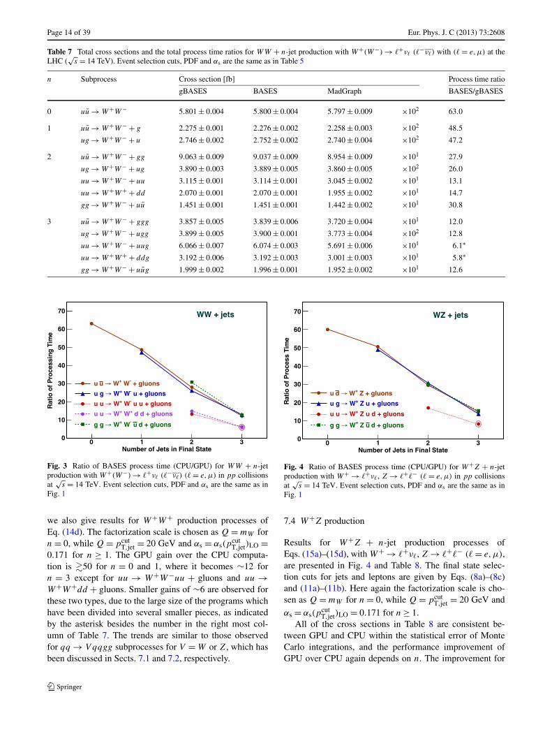
7.3 WW production
Results for WW +n-jet production processes of Eqs. (14a)–(14e) are presented in Fig. 3 and Table 7. Here both W ’sdecay leptonically, with W+(W−) → �+ν� (�−ν�) with(� = e,μ). In addition to the W+W− production processes,
Page 14 of 39 Eur. Phys. J. C (2013) 73:2608
Table 7 Total cross sections and the total process time ratios for WW + n-jet production with W+(W−) → �+ν� (�−ν�) with (� = e,μ) at theLHC (
√s = 14 TeV). Event selection cuts, PDF and αs are the same as in Table 5
n Subprocess Cross section [fb] Process time ratio
gBASES BASES MadGraph BASES/gBASES
0 uu → W+W− 5.801 ± 0.004 5.800 ± 0.004 5.797 ± 0.009 ×10² 63.0
1 uu → W+W− + g 2.275 ± 0.001 2.276 ± 0.002 2.258 ± 0.003 ×10² 48.5
ug → W+W− + u 2.746 ± 0.002 2.752 ± 0.002 2.740 ± 0.004 ×10² 47.2
2 uu → W+W− + gg 9.063 ± 0.009 9.037 ± 0.009 8.954 ± 0.009 ×101 27.9
ug → W+W− + ug 3.890 ± 0.003 3.889 ± 0.005 3.860 ± 0.005 ×10² 26.0
uu → W+W− + uu 3.115 ± 0.001 3.114 ± 0.001 3.045 ± 0.002 ×101 13.1
uu → W+W+ + dd 2.070 ± 0.001 2.070 ± 0.001 1.955 ± 0.002 ×101 14.7
gg → W+W− + uu 1.451 ± 0.001 1.451 ± 0.001 1.442 ± 0.002 ×101 30.8
3 uu → W+W− + ggg 3.857 ± 0.005 3.839 ± 0.006 3.720 ± 0.004 ×101 12.0
ug → W+W− + ugg 3.899 ± 0.005 3.900 ± 0.001 3.773 ± 0.004 ×10² 12.8
uu → W+W− + uug 6.066 ± 0.007 6.074 ± 0.003 5.691 ± 0.006 ×101 6.1∗
uu → W+W+ + ddg 3.192 ± 0.006 3.192 ± 0.003 3.001 ± 0.003 ×101 5.8∗
gg → W+W− + uug 1.999 ± 0.002 1.996 ± 0.001 1.952 ± 0.002 ×101 12.6
Fig. 3 Ratio of BASES process time (CPU/GPU) for WW + n-jetproduction with W+(W−) → �+ν� (�−ν�) (� = e,μ) in pp collisionsat
√s = 14 TeV. Event selection cuts, PDF and αs are the same as in
Fig. 1
we also give results for W+W+ production processes ofEq. (14d). The factorization scale is chosen as Q = mW forn = 0, while Q = pcut
T,jet = 20 GeV and αs = αs(pcutT,jet)LO =
0.171 for n ≥ 1. The GPU gain over the CPU computa-tion is �50 for n = 0 and 1, where it becomes ∼12 forn = 3 except for uu → W+W−uu + gluons and uu →W+W+dd + gluons. Smaller gains of ∼6 are observed forthese two types, due to the large size of the programs whichhave been divided into several smaller pieces, as indicatedby the asterisk besides the number in the right most col-umn of Table 7. The trends are similar to those observedfor qq → V qqgg subprocesses for V = W or Z, which hasbeen discussed in Sects. 7.1 and 7.2, respectively.
Fig. 4 Ratio of BASES process time (CPU/GPU) for W+Z + n-jetproduction with W+ → �+ν�, Z → �+�− (� = e,μ) in pp collisionsat
√s = 14 TeV. Event selection cuts, PDF and αs are the same as in
Fig. 1
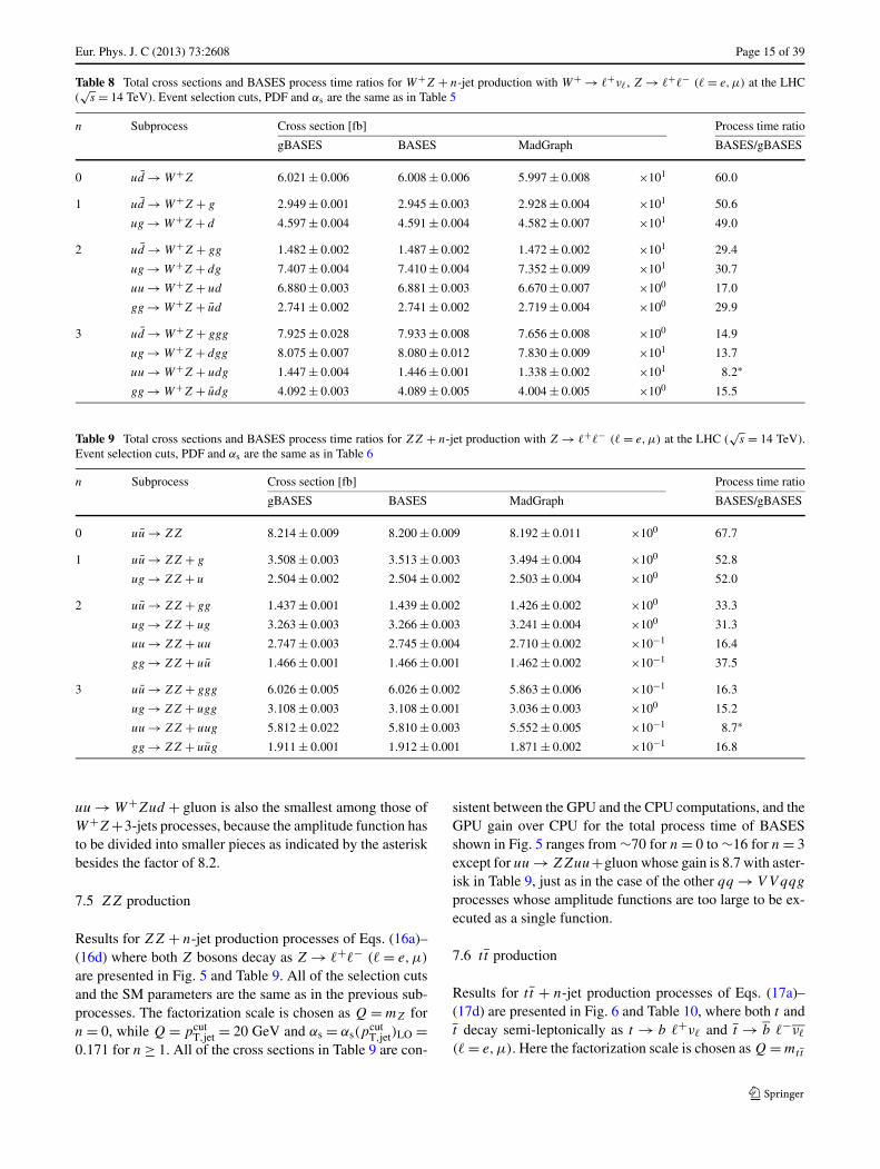
7.4 W+Z production
Results for W+Z + n-jet production processes ofEqs. (15a)–(15d), with W+ → �+ν�, Z → �+�− (� = e,μ),are presented in Fig. 4 and Table 8. The final state selec-tion cuts for jets and leptons are given by Eqs. (8a)–(8c)and (11a)–(11b). Here again the factorization scale is cho-sen as Q = mW for n = 0, while Q = pcut
T,jet = 20 GeV and
αs = αs(pcutT,jet)LO = 0.171 for n ≥ 1.
All of the cross sections in Table 8 are consistent be-tween GPU and CPU within the statistical error of MonteCarlo integrations, and the performance improvement ofGPU over CPU again depends on n. The improvement for
Eur. Phys. J. C (2013) 73:2608 Page 15 of 39
Table 8 Total cross sections and BASES process time ratios for W+Z + n-jet production with W+ → �+ν�, Z → �+�− (� = e,μ) at the LHC(√
s = 14 TeV). Event selection cuts, PDF and αs are the same as in Table 5
n Subprocess Cross section [fb] Process time ratio
gBASES BASES MadGraph BASES/gBASES
0 ud → W+Z 6.021 ± 0.006 6.008 ± 0.006 5.997 ± 0.008 ×101 60.0
1 ud → W+Z + g 2.949 ± 0.001 2.945 ± 0.003 2.928 ± 0.004 ×101 50.6
ug → W+Z + d 4.597 ± 0.004 4.591 ± 0.004 4.582 ± 0.007 ×101 49.0
2 ud → W+Z + gg 1.482 ± 0.002 1.487 ± 0.002 1.472 ± 0.002 ×101 29.4
ug → W+Z + dg 7.407 ± 0.004 7.410 ± 0.004 7.352 ± 0.009 ×101 30.7
uu → W+Z + ud 6.880 ± 0.003 6.881 ± 0.003 6.670 ± 0.007 ×100 17.0
gg → W+Z + ud 2.741 ± 0.002 2.741 ± 0.002 2.719 ± 0.004 ×100 29.9
3 ud → W+Z + ggg 7.925 ± 0.028 7.933 ± 0.008 7.656 ± 0.008 ×100 14.9
ug → W+Z + dgg 8.075 ± 0.007 8.080 ± 0.012 7.830 ± 0.009 ×101 13.7
uu → W+Z + udg 1.447 ± 0.004 1.446 ± 0.001 1.338 ± 0.002 ×101 8.2∗
gg → W+Z + udg 4.092 ± 0.003 4.089 ± 0.005 4.004 ± 0.005 ×100 15.5
Table 9 Total cross sections and BASES process time ratios for ZZ + n-jet production with Z → �+�− (� = e,μ) at the LHC (√
s = 14 TeV).Event selection cuts, PDF and αs are the same as in Table 6
n Subprocess Cross section [fb] Process time ratio
gBASES BASES MadGraph BASES/gBASES
0 uu → ZZ 8.214 ± 0.009 8.200 ± 0.009 8.192 ± 0.011 ×100 67.7
1 uu → ZZ + g 3.508 ± 0.003 3.513 ± 0.003 3.494 ± 0.004 ×100 52.8
ug → ZZ + u 2.504 ± 0.002 2.504 ± 0.002 2.503 ± 0.004 ×100 52.0
2 uu → ZZ + gg 1.437 ± 0.001 1.439 ± 0.002 1.426 ± 0.002 ×100 33.3
ug → ZZ + ug 3.263 ± 0.003 3.266 ± 0.003 3.241 ± 0.004 ×100 31.3
uu → ZZ + uu 2.747 ± 0.003 2.745 ± 0.004 2.710 ± 0.002 ×10⁻¹ 16.4
gg → ZZ + uu 1.466 ± 0.001 1.466 ± 0.001 1.462 ± 0.002 ×10⁻¹ 37.5
3 uu → ZZ + ggg 6.026 ± 0.005 6.026 ± 0.002 5.863 ± 0.006 ×10⁻¹ 16.3
ug → ZZ + ugg 3.108 ± 0.003 3.108 ± 0.001 3.036 ± 0.003 ×100 15.2
uu → ZZ + uug 5.812 ± 0.022 5.810 ± 0.003 5.552 ± 0.005 ×10⁻¹ 8.7∗
gg → ZZ + uug 1.911 ± 0.001 1.912 ± 0.001 1.871 ± 0.002 ×10⁻¹ 16.8
uu → W+Zud + gluon is also the smallest among those ofW+Z+3-jets processes, because the amplitude function hasto be divided into smaller pieces as indicated by the asteriskbesides the factor of 8.2.
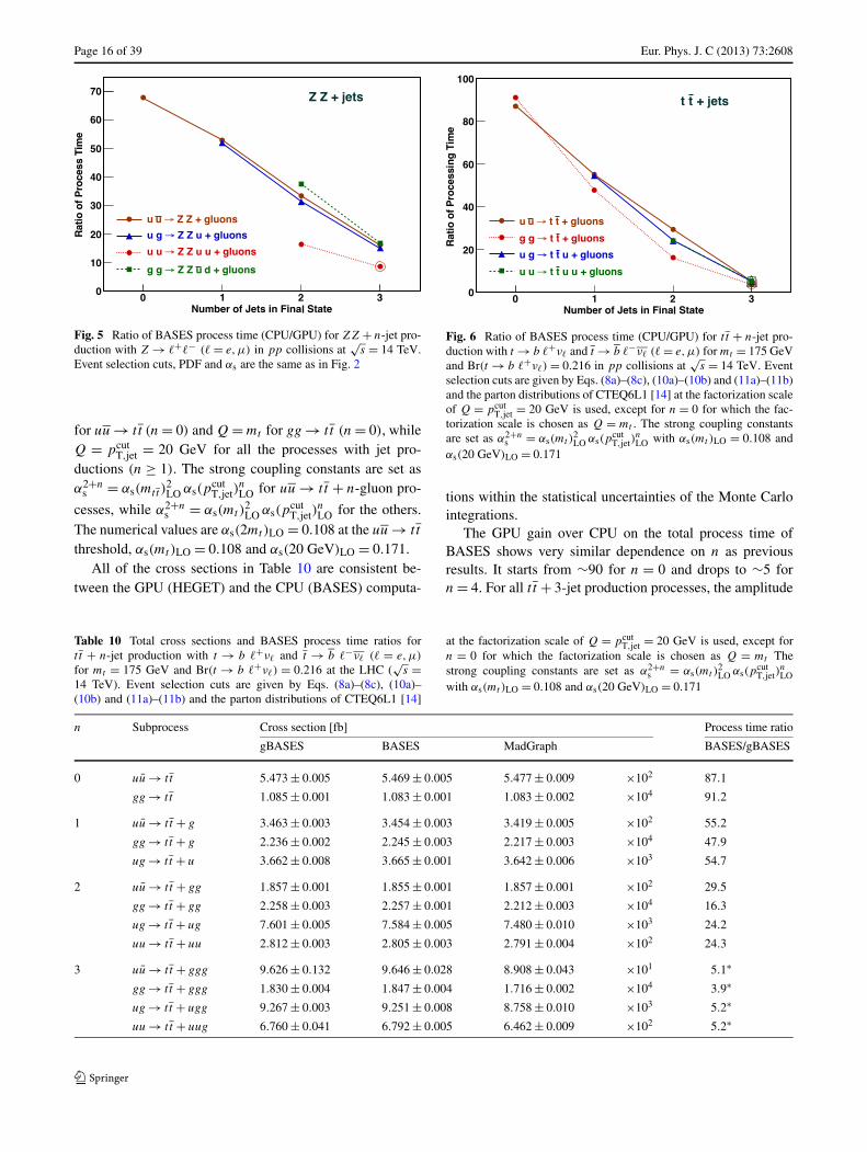
7.5 ZZ production
Results for ZZ + n-jet production processes of Eqs. (16a)–(16d) where both Z bosons decay as Z → �+�− (� = e,μ)
are presented in Fig. 5 and Table 9. All of the selection cutsand the SM parameters are the same as in the previous sub-processes. The factorization scale is chosen as Q = mZ forn = 0, while Q = pcut
T,jet = 20 GeV and αs = αs(pcutT,jet)LO =
0.171 for n ≥ 1. All of the cross sections in Table 9 are con-
sistent between the GPU and the CPU computations, and theGPU gain over CPU for the total process time of BASESshown in Fig. 5 ranges from ∼70 for n = 0 to ∼16 for n = 3except for uu → ZZuu+gluon whose gain is 8.7 with aster-isk in Table 9, just as in the case of the other qq → V V qqg
processes whose amplitude functions are too large to be ex-ecuted as a single function.
7.6 t t production
Results for t t + n-jet production processes of Eqs. (17a)–(17d) are presented in Fig. 6 and Table 10, where both t andt decay semi-leptonically as t → b �+ν� and t → b �−ν�
(� = e,μ). Here the factorization scale is chosen as Q = mtt
Page 16 of 39 Eur. Phys. J. C (2013) 73:2608
Fig. 5 Ratio of BASES process time (CPU/GPU) for ZZ + n-jet pro-duction with Z → �+�− (� = e,μ) in pp collisions at
√s = 14 TeV.
Event selection cuts, PDF and αs are the same as in Fig. 2
for uu → t t (n = 0) and Q = mt for gg → t t (n = 0), whileQ = pcut
T,jet = 20 GeV for all the processes with jet pro-ductions (n ≥ 1). The strong coupling constants are set asα2+n
s = αs(mtt )2LO αs(p
cutT,jet)
nLO for uu → t t + n-gluon pro-
cesses, while α2+ns = αs(mt )
2LO αs(p
cutT,jet)
nLO for the others.
The numerical values are αs(2mt)LO = 0.108 at the uu → t t
threshold, αs(mt )LO = 0.108 and αs(20 GeV)LO = 0.171.All of the cross sections in Table 10 are consistent be-
tween the GPU (HEGET) and the CPU (BASES) computa-
Fig. 6 Ratio of BASES process time (CPU/GPU) for t t + n-jet pro-duction with t → b �+ν� and t → b �−ν� (� = e,μ) for mt = 175 GeVand Br(t → b �+ν�) = 0.216 in pp collisions at
√s = 14 TeV. Event
selection cuts are given by Eqs. (8a)–(8c), (10a)–(10b) and (11a)–(11b)and the parton distributions of CTEQ6L1 [14] at the factorization scaleof Q = pcut
T,jet = 20 GeV is used, except for n = 0 for which the fac-torization scale is chosen as Q = mt . The strong coupling constantsare set as α2+n
s = αs(mt )2LO αs(p
cutT,jet)
nLO with αs(mt )LO = 0.108 and
αs(20 GeV)LO = 0.171
tions within the statistical uncertainties of the Monte Carlointegrations.
The GPU gain over CPU on the total process time ofBASES shows very similar dependence on n as previousresults. It starts from ∼90 for n = 0 and drops to ∼5 forn = 4. For all t t + 3-jet production processes, the amplitude
Table 10 Total cross sections and BASES process time ratios fort t + n-jet production with t → b �+ν� and t → b �−ν� (� = e,μ)
for mt = 175 GeV and Br(t → b �+ν�) = 0.216 at the LHC (√
s =14 TeV). Event selection cuts are given by Eqs. (8a)–(8c), (10a)–(10b) and (11a)–(11b) and the parton distributions of CTEQ6L1 [14]
at the factorization scale of Q = pcutT,jet = 20 GeV is used, except for
n = 0 for which the factorization scale is chosen as Q = mt Thestrong coupling constants are set as α2+n
s = αs(mt )2LO αs(p
cutT,jet)
nLO
with αs(mt )LO = 0.108 and αs(20 GeV)LO = 0.171
n Subprocess Cross section [fb] Process time ratio
gBASES BASES MadGraph BASES/gBASES
0 uu → t t 5.473 ± 0.005 5.469 ± 0.005 5.477 ± 0.009 ×10² 87.1
gg → t t 1.085 ± 0.001 1.083 ± 0.001 1.083 ± 0.002 ×10⁴ 91.2
1 uu → t t + g 3.463 ± 0.003 3.454 ± 0.003 3.419 ± 0.005 ×10² 55.2
gg → t t + g 2.236 ± 0.002 2.245 ± 0.003 2.217 ± 0.003 ×10⁴ 47.9
ug → t t + u 3.662 ± 0.008 3.665 ± 0.001 3.642 ± 0.006 ×10³ 54.7
2 uu → t t + gg 1.857 ± 0.001 1.855 ± 0.001 1.857 ± 0.001 ×10² 29.5
gg → t t + gg 2.258 ± 0.003 2.257 ± 0.001 2.212 ± 0.003 ×10⁴ 16.3
ug → t t + ug 7.601 ± 0.005 7.584 ± 0.005 7.480 ± 0.010 ×10³ 24.2
uu → t t + uu 2.812 ± 0.003 2.805 ± 0.003 2.791 ± 0.004 ×10² 24.3
3 uu → t t + ggg 9.626 ± 0.132 9.646 ± 0.028 8.908 ± 0.043 ×101 5.1∗
gg → t t + ggg 1.830 ± 0.004 1.847 ± 0.004 1.716 ± 0.002 ×10⁴ 3.9∗
ug → t t + ugg 9.267 ± 0.003 9.251 ± 0.008 8.758 ± 0.010 ×10³ 5.2∗
uu → t t + uug 6.760 ± 0.041 6.792 ± 0.005 6.462 ± 0.009 ×10² 5.2∗
Eur. Phys. J. C (2013) 73:2608 Page 17 of 39
Table 11 Total cross sections and BASES process time ratios forHW+ + n-jet production with W+ → �+ν� (� = e,μ) and H →τ+τ− at the LHC (
√s = 14 TeV), for mH = 125 GeV and Br(H →
τ+τ−) = 0.0405. Event selection cuts are given by Eqs. (8a)–
(8c), (10a)–(10b) and (11a)–(11b) and the parton distributions ofCTEQ6L1 [14] at the factorization scale of Q = pcut
T,jet = 20 GeV isused, except for n = 0 for which the factorization scale is chosen asQ = mHW . The strong coupling is fixed at αs(20 GeV)LO = 0.171
n Subprocess Cross section [fb] Process time ratio
gBASES BASES MadGraph BASES/gBASES
0 ud → HW+ 3.612 ± 0.003 3.614 ± 0.003 3.614 ± 0.004 ×100 93.0
1 ud → HW+ + g 1.652 ± 0.001 1.653 ± 0.001 1.643 ± 0.002 ×100 86.7
ug → HW+ + d 9.892 ± 0.010 9.901 ± 0.010 9.854 ± 0.013 ×10⁻¹ 79.2
2 ud → HW+ + gg 6.802 ± 0.009 6.804 ± 0.008 6.765 ± 0.007 ×10⁻¹ 63.0
ug → HW+ + dg 1.242 ± 0.001 1.244 ± 0.002 1.232 ± 0.002 ×100 63.3
uu → HW+ + ud 1.824 ± 0.001 1.822 ± 0.003 1.805 ± 0.001 ×10⁻¹ 27.7
gg → HW+ + du 4.611 ± 0.006 4.614 ± 0.004 4.600 ± 0.007 ×10⁻² 65.9
3 ud → HW+ + ggg 2.660 ± 0.010 2.679 ± 0.006 2.604 ± 0.003 ×10⁻¹ 31.4
ug → HW+ + dgg 1.085 ± 0.002 1.084 ± 0.001 1.053 ± 0.001 ×100 28.6
uu → HW+ + udg 1.915 ± 0.003 1.917 ± 0.001 1.835 ± 0.002 ×10⁻¹ 18.0
gg → HW+ + dug 5.906 ± 0.007 5.902 ± 0.006 5.818 ± 0.007 ×10⁻² 25.3
functions have to be divided into smaller pieces in order tobe processed by the CUDA compiler. The main cause of thelong amplitudes for these processes is the proliferation ofcolor the factor bases which has been observed for all of theQCD 5 jet production process in Ref. [6].
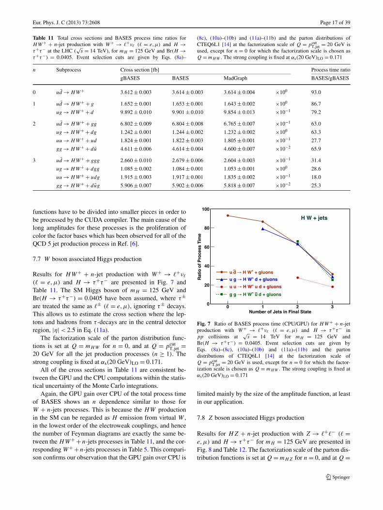
7.7 W boson associated Higgs production
Results for HW+ + n-jet production with W+ → �+ν�
(� = e,μ) and H → τ+τ− are presented in Fig. 7 andTable 11. The SM Higgs boson of mH = 125 GeV andBr(H → τ+τ−) = 0.0405 have been assumed, where τ±are treated the same as �± (� = e,μ), ignoring τ± decays.This allows us to estimate the cross section where the lep-tons and hadrons from τ -decays are in the central detectorregion, |η| < 2.5 in Eq. (11a).
The factorization scale of the parton distribution func-tions is set at Q = mHW for n = 0, and at Q = pcut
T,jet =20 GeV for all the jet production processes (n ≥ 1). Thestrong coupling is fixed at αs(20 GeV)LO = 0.171.
All of the cross sections in Table 11 are consistent be-tween the GPU and the CPU computations within the statis-tical uncertainty of the Monte Carlo integrations.
Again, the GPU gain over CPU of the total process timeof BASES shows an n dependence similar to those forW + n-jets processes. This is because the HW productionin the SM can be regarded as H emission from virtual W ,in the lowest order of the electroweak couplings, and hencethe number of Feynman diagrams are exactly the same be-tween the HW+ +n-jets processes in Table 11, and the cor-responding W+ +n-jets processes in Table 5. This compari-son confirms our observation that the GPU gain over CPU is
Fig. 7 Ratio of BASES process time (CPU/GPU) for HW+ + n-jetproduction with W+ → �+ν� (� = e,μ) and H → τ+τ− inpp collisions at
√s = 14 TeV for mH = 125 GeV and
Br(H → τ+τ−) = 0.0405. Event selection cuts are given byEqs. (8a)–(8c), (10a)–(10b) and (11a)–(11b) and the partondistributions of CTEQ6L1 [14] at the factorization scale ofQ = pcut
T,jet = 20 GeV is used, except for n = 0 for which the factor-ization scale is chosen as Q = mHW . The strong coupling is fixed atαs(20 GeV)LO = 0.171
limited mainly by the size of the amplitude function, at leastin our application.
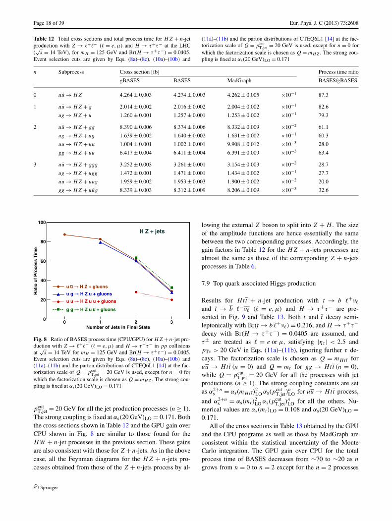
7.8 Z boson associated Higgs production
Results for HZ + n-jet production with Z → �+�− (� =e,μ) and H → τ+τ− for mH = 125 GeV are presented inFig. 8 and Table 12. The factorization scale of the parton dis-tribution functions is set at Q = mHZ for n = 0, and at Q =
Page 18 of 39 Eur. Phys. J. C (2013) 73:2608
Table 12 Total cross sections and total process time for HZ + n-jetproduction with Z → �+�− (� = e,μ) and H → τ+τ− at the LHC(√
s = 14 TeV), for mH = 125 GeV and Br(H → τ+τ−) = 0.0405.Event selection cuts are given by Eqs. (8a)–(8c), (10a)–(10b) and
(11a)–(11b) and the parton distributions of CTEQ6L1 [14] at the fac-torization scale of Q = pcut
T,jet = 20 GeV is used, except for n = 0 forwhich the factorization scale is chosen as Q = mHZ . The strong cou-pling is fixed at αs(20 GeV)LO = 0.171
n Subprocess Cross section [fb] Process time ratio
gBASES BASES MadGraph BASES/gBASES
0 uu → HZ 4.264 ± 0.003 4.274 ± 0.003 4.262 ± 0.005 ×10⁻¹ 87.3
1 uu → HZ + g 2.014 ± 0.002 2.016 ± 0.002 2.004 ± 0.002 ×10⁻¹ 82.6
ug → HZ + u 1.260 ± 0.001 1.257 ± 0.001 1.253 ± 0.002 ×10⁻¹ 79.3
2 uu → HZ + gg 8.390 ± 0.006 8.374 ± 0.006 8.332 ± 0.009 ×10⁻² 61.1
ug → HZ + ug 1.639 ± 0.002 1.640 ± 0.002 1.631 ± 0.002 ×10⁻¹ 60.3
uu → HZ + uu 1.004 ± 0.001 1.002 ± 0.001 9.908 ± 0.012 ×10⁻³ 28.0
gg → HZ + uu 6.417 ± 0.004 6.411 ± 0.004 6.391 ± 0.009 ×10⁻³ 63.4
3 uu → HZ + ggg 3.252 ± 0.003 3.261 ± 0.001 3.154 ± 0.003 ×10⁻² 28.7
ug → HZ + ugg 1.472 ± 0.001 1.471 ± 0.001 1.434 ± 0.002 ×10⁻¹ 27.7
uu → HZ + uug 1.959 ± 0.002 1.953 ± 0.003 1.900 ± 0.002 ×10⁻² 20.0
gg → HZ + uug 8.339 ± 0.003 8.312 ± 0.009 8.206 ± 0.009 ×10⁻³ 32.6
Fig. 8 Ratio of BASES process time (CPU/GPU) for HZ +n-jet pro-duction with Z → �+�− (� = e,μ) and H → τ+τ− in pp collisionsat
√s = 14 TeV for mH = 125 GeV and Br(H → τ+τ−) = 0.0405.
Event selection cuts are given by Eqs. (8a)–(8c), (10a)–(10b) and(11a)–(11b) and the parton distributions of CTEQ6L1 [14] at the fac-torization scale of Q = pcut
T,jet = 20 GeV is used, except for n = 0 forwhich the factorization scale is chosen as Q = mHZ . The strong cou-pling is fixed at αs(20 GeV)LO = 0.171
pcutT,jet = 20 GeV for all the jet production processes (n ≥ 1).
The strong coupling is fixed at αs(20 GeV)LO = 0.171. Boththe cross sections shown in Table 12 and the GPU gain overCPU shown in Fig. 8 are similar to those found for theHW + n-jet processes in the previous section. These gainsare also consistent with those for Z +n-jets. As in the abovecase, all the Feynman diagrams for the HZ + n-jets pro-cesses obtained from those of the Z + n-jets process by al-
lowing the external Z boson to split into Z + H . The sizeof the amplitude functions are hence essentially the samebetween the two corresponding processes. Accordingly, thegain factors in Table 12 for the HZ + n-jets processes arealmost the same as those of the corresponding Z + n-jetsprocesses in Table 6.
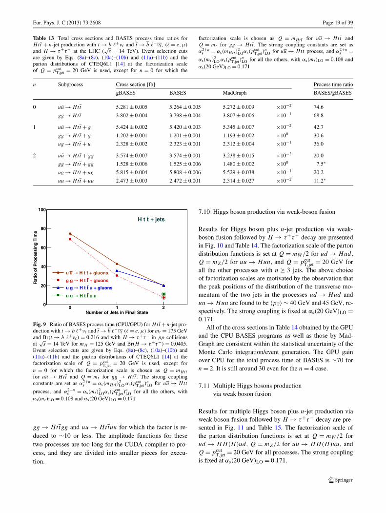
7.9 Top quark associated Higgs production
Results for Htt + n-jet production with t → b �+ν�
and t → b �−ν� (� = e,μ) and H → τ+τ− are pre-sented in Fig. 9 and Table 13. Both t and t decay semi-leptonically with Br(t → b �+ν�) = 0.216, and H → τ+τ−decay with Br(H → τ+τ−) = 0.0405 are assumed, andτ± are treated as � = e or μ, satisfying |ητ | < 2.5 andpTτ > 20 GeV in Eqs. (11a)–(11b), ignoring further τ de-cays. The factorization scale is chosen as Q = mHtt foruu → Htt (n = 0) and Q = mt for gg → Htt (n = 0),while Q = pcut
T,jet = 20 GeV for all the processes with jetproductions (n ≥ 1). The strong coupling constants are setas α2+n
s = αs(mHtt )2LO αs(p
cutT,jet)
nLO for uu → Htt process,
and α2+ns = αs(mt )
2LO αs(p
cutT,jet)
nLO for all the others. Nu-
merical values are αs(mt )LO = 0.108 and αs(20 GeV)LO =0.171.
All of the cross sections in Table 13 obtained by the GPUand the CPU programs as well as those by MadGraph areconsistent within the statistical uncertainty of the MonteCarlo integration. The GPU gain over CPU for the totalprocess time of BASES decreases from ∼70 to ∼20 as n
grows from n = 0 to n = 2 except for the n = 2 processes
Eur. Phys. J. C (2013) 73:2608 Page 19 of 39
Table 13 Total cross sections and BASES process time ratios forHtt + n-jet production with t → b �+ν� and t → b �−ν�, (� = e,μ)
and H → τ+τ− at the LHC (√
s = 14 TeV). Event selection cutsare given by Eqs. (8a)–(8c), (10a)–(10b) and (11a)–(11b) and theparton distributions of CTEQ6L1 [14] at the factorization scaleof Q = pcut
T,jet = 20 GeV is used, except for n = 0 for which the
factorization scale is chosen as Q = mHtt for uu → Htt andQ = mt for gg → Htt . The strong coupling constants are set asα2+n
s = αs(mHtt )2LOαs(p
cutT,jet)
nLO for uu → Htt process, and α2+n
s =αs(mt )
2LO αs(p
cutT,jet)
nLO for all the others, with αs(mt )LO = 0.108 and
αs(20 GeV)LO = 0.171
n Subprocess Cross section [fb] Process time ratio
gBASES BASES MadGraph BASES/gBASES
0 uu → Htt 5.281 ± 0.005 5.264 ± 0.005 5.272 ± 0.009 ×10⁻² 74.6
gg → Htt 3.802 ± 0.004 3.798 ± 0.004 3.807 ± 0.006 ×10⁻¹ 68.8
1 uu → Htt + g 5.424 ± 0.002 5.420 ± 0.003 5.345 ± 0.007 ×10⁻² 42.7
gg → Htt + g 1.202 ± 0.001 1.201 ± 0.001 1.193 ± 0.002 ×100 30.6
ug → Htt + u 2.328 ± 0.002 2.323 ± 0.001 2.312 ± 0.004 ×10⁻¹ 36.0
2 uu → Htt + gg 3.574 ± 0.007 3.574 ± 0.001 3.238 ± 0.015 ×10⁻² 20.0
gg → Htt + gg 1.528 ± 0.006 1.525 ± 0.006 1.480 ± 0.002 ×100 7.5∗
ug → Htt + ug 5.815 ± 0.004 5.808 ± 0.006 5.529 ± 0.038 ×10⁻¹ 20.2
uu → Htt + uu 2.473 ± 0.003 2.472 ± 0.001 2.314 ± 0.027 ×10⁻² 11.2∗
Fig. 9 Ratio of BASES process time (CPU/GPU) for Htt +n-jet pro-duction with t → b �+ν� and t → b �−ν� (� = e,μ) for mt = 175 GeVand Br(t → b �+ν�) = 0.216 and with H → τ+τ− in pp collisionsat
√s = 14 TeV for mH = 125 GeV and Br(H → τ+τ−) = 0.0405.
Event selection cuts are given by Eqs. (8a)–(8c), (10a)–(10b) and(11a)–(11b) and the parton distributions of CTEQ6L1 [14] at thefactorization scale of Q = pcut
T,jet = 20 GeV is used, except forn = 0 for which the factorization scale is chosen as Q = mHtt
for uu → Htt and Q = mt for gg → Htt . The strong couplingconstants are set as α2+n
s = αs(mHtt )2LO αs(p
cutT,jet)
nLO for uu → Htt
process, and α2+ns = αs(mt )
2LOαs(p
cutT,jet)
nLO for all the others, with
αs(mt )LO = 0.108 and αs(20 GeV)LO = 0.171
gg → Httgg and uu → Httuu for which the factor is re-duced to ∼10 or less. The amplitude functions for thesetwo processes are too long for the CUDA compiler to pro-cess, and they are divided into smaller pieces for execu-tion.
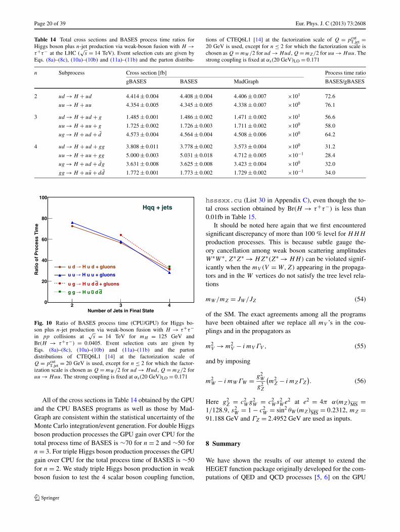
7.10 Higgs boson production via weak-boson fusion
Results for Higgs boson plus n-jet production via weak-boson fusion followed by H → τ+τ− decay are presentedin Fig. 10 and Table 14. The factorization scale of the partondistribution functions is set at Q = mW/2 for ud → Hud ,Q = mZ/2 for uu → Huu, and Q = pcut
T,jet = 20 GeV forall the other processes with n ≥ 3 jets. The above choiceof factorization scales are motivated by the observation thatthe peak positions of the distribution of the transverse mo-mentum of the two jets in the processes ud → Hud anduu → Huu are found to be 〈pT〉 ∼ 40 GeV and 45 GeV, re-spectively. The strong coupling is fixed at αs(20 GeV)LO =0.171.
All of the cross sections in Table 14 obtained by the GPUand the CPU BASES programs as well as those by Mad-Graph are consistent within the statistical uncertainty of theMonte Carlo integration/event generation. The GPU gainover CPU for the total process time of BASES is ∼70 forn = 2. It is still around 30 even for the n = 4 case.
7.11 Multiple Higgs bosons productionvia weak boson fusion
Results for multiple Higgs boson plus n-jet production viaweak boson fusion followed by H → τ+τ− decay are pre-sented in Fig. 11 and Table 15. The factorization scale ofthe parton distribution functions is set at Q = mW/2 forud → HH(H)ud , Q = mZ/2 for uu → HH(H)uu, andQ = pcut
T,jet = 20 GeV for all processes. The strong couplingis fixed at αs(20 GeV)LO = 0.171.
Page 20 of 39 Eur. Phys. J. C (2013) 73:2608
Table 14 Total cross sections and BASES process time ratios forHiggs boson plus n-jet production via weak-boson fusion with H →τ+τ− at the LHC (
√s = 14 TeV). Event selection cuts are given by
Eqs. (8a)–(8c), (10a)–(10b) and (11a)–(11b) and the parton distribu-
tions of CTEQ6L1 [14] at the factorization scale of Q = pcutT,jet =
20 GeV is used, except for n ≤ 2 for which the factorization scale ischosen as Q = mW /2 for ud → Hud , Q = mZ/2 for uu → Huu. Thestrong coupling is fixed at αs(20 GeV)LO = 0.171
n Subprocess Cross section [fb] Process time ratio
gBASES BASES MadGraph BASES/gBASES
2 ud → H + ud 4.414 ± 0.004 4.408 ± 0.004 4.406 ± 0.007 ×101 72.6
uu → H + uu 4.354 ± 0.005 4.345 ± 0.005 4.338 ± 0.007 ×100 76.1
3 ud → H + ud + g 1.485 ± 0.001 1.486 ± 0.002 1.471 ± 0.002 ×101 56.6
uu → H + uu + g 1.725 ± 0.002 1.726 ± 0.003 1.711 ± 0.002 ×100 58.0
ug → H + ud + d 4.573 ± 0.004 4.564 ± 0.004 4.508 ± 0.006 ×100 64.2
4 ud → H + ud + gg 3.808 ± 0.011 3.778 ± 0.002 3.573 ± 0.004 ×100 31.2
uu → H + uu + gg 5.000 ± 0.003 5.031 ± 0.018 4.712 ± 0.005 ×10⁻¹ 28.4
ug → H + ud + dg 3.631 ± 0.008 3.625 ± 0.008 3.423 ± 0.004 ×100 32.0
gg → H + uu + dd 1.772 ± 0.001 1.773 ± 0.002 1.729 ± 0.002 ×10⁻¹ 34.0
Fig. 10 Ratio of BASES process time (CPU/GPU) for Higgs bo-son plus n-jet production via weak-boson fusion with H → τ+τ−in pp collisions at
√s = 14 TeV for mH = 125 GeV and
Br(H → τ+τ−) = 0.0405. Event selection cuts are given byEqs. (8a)–(8c), (10a)–(10b) and (11a)–(11b) and the partondistributions of CTEQ6L1 [14] at the factorization scale ofQ = pcut
T,jet = 20 GeV is used, except for n ≤ 2 for which the factor-ization scale is chosen as Q = mW /2 for ud → Hud , Q = mZ/2 foruu → Huu. The strong coupling is fixed at αs(20 GeV)LO = 0.171
All of the cross sections in Table 14 obtained by the GPUand the CPU BASES programs as well as those by Mad-Graph are consistent within the statistical uncertainty of theMonte Carlo integration/event generation. For double Higgsboson production processes the GPU gain over CPU for thetotal process time of BASES is ∼70 for n = 2 and ∼50 forn = 3. For triple Higgs boson production processes the GPUgain over CPU for the total process time of BASES is ∼50for n = 2. We study triple Higgs boson production in weakboson fusion to test the 4 scalar boson coupling function,
hsssxx.cu (List 30 in Appendix C), even though the to-tal cross section obtained by Br(H → τ+τ−) is less than0.01fb in Table 15.
It should be noted here again that we first encounteredsignificant discrepancy of more than 100 % level for HHH
production processes. This is because subtle gauge the-ory cancellation among weak boson scattering amplitudesW ∗W ∗, Z∗Z∗ → HZ∗(Z∗ → HH) can be violated signif-icantly when the mV (V = W,Z) appearing in the propaga-tors and in the W vertices do not satisfy the tree level rela-tions
mW/mZ = JW/JZ (54)
of the SM. The exact agreements among all the programshave been obtained after we replace all mV ’s in the cou-plings and in the propagators as
m2V → m2
V − i mV ΓV , (55)
and by imposing
m2W − i mWΓW = g2
W
g2Z
(m2
Z − i mZΓZ
). (56)
Here g2Z = c2
Wg2W = c2
Ws2We2 at e2 = 4π α(mZ)MS =
1/128.9, s2W = 1 − c2
W = sin2 θW (mZ)MS = 0.2312, mZ =91.188 GeV and ΓZ = 2.4952 GeV are used as inputs.
8 Summary
We have shown the results of our attempt to extend theHEGET function package originally developed for the com-putations of QED and QCD processes [5, 6] on the GPU
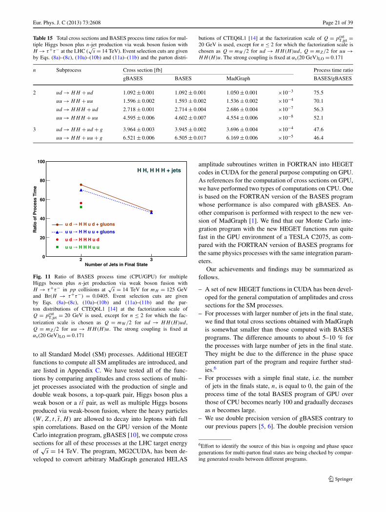
Eur. Phys. J. C (2013) 73:2608 Page 21 of 39
Table 15 Total cross sections and BASES process time ratios for mul-tiple Higgs boson plus n-jet production via weak boson fusion withH → τ+τ− at the LHC (
√s = 14 TeV). Event selection cuts are given
by Eqs. (8a)–(8c), (10a)–(10b) and (11a)–(11b) and the parton distri-
butions of CTEQ6L1 [14] at the factorization scale of Q = pcutT,jet =
20 GeV is used, except for n ≤ 2 for which the factorization scale ischosen as Q = mW /2 for ud → HH(H)ud , Q = mZ/2 for uu →HH(H)u. The strong coupling is fixed at αs(20 GeV)LO = 0.171
n Subprocess Cross section [fb] Process time ratio
gBASES BASES MadGraph BASES/gBASES
2 ud → HH + ud 1.092 ± 0.001 1.092 ± 0.001 1.050 ± 0.001 ×10⁻³ 75.5
uu → HH + uu 1.596 ± 0.002 1.593 ± 0.002 1.536 ± 0.002 ×10⁻⁴ 70.1
ud → HHH + ud 2.718 ± 0.001 2.714 ± 0.004 2.686 ± 0.004 ×10⁻⁷ 56.3
uu → HHH + uu 4.595 ± 0.006 4.602 ± 0.007 4.554 ± 0.006 ×10⁻⁸ 52.1
3 ud → HH + ud + g 3.964 ± 0.003 3.945 ± 0.002 3.696 ± 0.004 ×10⁻⁴ 47.6
uu → HH + uu + g 6.521 ± 0.006 6.505 ± 0.017 6.169 ± 0.006 ×10⁻⁵ 46.4
Fig. 11 Ratio of BASES process time (CPU/GPU) for multipleHiggs boson plus n-jet production via weak boson fusion withH → τ+τ− in pp collisions at
√s = 14 TeV for mH = 125 GeV
and Br(H → τ+τ−) = 0.0405. Event selection cuts are givenby Eqs. (8a)–(8c), (10a)–(10b) and (11a)–(11b) and the par-ton distributions of CTEQ6L1 [14] at the factorization scale ofQ = pcut
T,jet = 20 GeV is used, except for n ≤ 2 for which the fac-torization scale is chosen as Q = mW /2 for ud → HH(H)ud ,Q = mZ/2 for uu → HH(H)u. The strong coupling is fixed atαs(20 GeV)LO = 0.171
to all Standard Model (SM) processes. Additional HEGETfunctions to compute all SM amplitudes are introduced, andare listed in Appendix C. We have tested all of the func-tions by comparing amplitudes and cross sections of multi-jet processes associated with the production of single anddouble weak bosons, a top-quark pair, Higgs boson plus aweak boson or a t t pair, as well as multiple Higgs bosonsproduced via weak-boson fusion, where the heavy particles(W,Z, t, t,H) are allowed to decay into leptons with fullspin correlations. Based on the GPU version of the MonteCarlo integration program, gBASES [10], we compute crosssections for all of these processes at the LHC target energyof
√s = 14 TeV. The program, MG2CUDA, has been de-
veloped to convert arbitrary MadGraph generated HELAS
amplitude subroutines written in FORTRAN into HEGETcodes in CUDA for the general purpose computing on GPU.As references for the computation of cross sections on GPU,we have performed two types of computations on CPU. Oneis based on the FORTRAN version of the BASES programwhose performance is also compared with gBASES. An-other comparison is performed with respect to the new ver-sion of MadGraph [1]. We find that our Monte Carlo inte-gration program with the new HEGET functions run quitefast in the GPU environment of a TESLA C2075, as com-pared with the FORTRAN version of BASES programs forthe same physics processes with the same integration param-eters.
Our achievements and findings may be summarized asfollows.
– A set of new HEGET functions in CUDA has been devel-oped for the general computation of amplitudes and crosssections for the SM processes.
– For processes with larger number of jets in the final state,we find that total cross sections obtained with MadGraphis somewhat smaller than those computed with BASESprograms. The difference amounts to about 5–10 % forthe processes with large number of jets in the final state.They might be due to the difference in the phase spacegeneration part of the program and require further stud-ies.6
– For processes with a simple final state, i.e. the numberof jets in the finals state, n, is equal to 0, the gain of theprocess time of the total BASES program of GPU overthose of CPU becomes nearly 100 and gradually deceasesas n becomes large.
– We use double precision version of gBASES contrary toour previous papers [5, 6]. The double precision version
6Effort to identify the source of this bias is ongoing and phase spacegenerations for multi-parton final states are being checked by compar-ing generated results between different programs.
Page 22 of 39 Eur. Phys. J. C (2013) 73:2608
of gBASES shows not only a good performance in pro-cess time but also good stability for various physics pro-cesses with wide range of integration parameters.
– Due to the limitation of the CUDA compiler, a longCUDA function cannot be compiled. We have includedthe new mechanism to gBASES to handle successiveCUDA functions calls in order to handle a long ampli-tude program as a set of small CUDA functions. The inte-grated results also agree very well with those obtained byBASES in FORTRAN. The performance of these dividedprograms is somewhat lower compared with un-dividedprograms.
Acknowledgements This work is supported by the Grant-in-Aid forScientific Research from the Japan Society for the Promotion of Sci-ence (Nos. 20340064 and 22740155), in part by the National NaturalScience Foundation of China under Grants No. 11205008 as well as agrant from the National Science Foundation (NSF PHY-1068326). Wewish to thank Dave Rainwater for inspiring us with the idea of usingGPU for fast LHC physics simulation and his initial contribution to theproject.
Open Access This article is distributed under the terms of the Cre-ative Commons Attribution License which permits any use, distribu-tion, and reproduction in any medium, provided the original author(s)and the source are credited.
Appendix A: Phase space parameterization
In this appendix, we introduce our phase space parame-trization which is useful for evaluating cross sections anddistributions of hadron collider events efficiently. In orderto take advantage of the high parallel process capability ofGPU computing, it is essential that high fraction of gener-ated phase space points satisfy the final state cuts. We ob-serve that the following final state cuts are most commonlyused for quark and gluon jets in hadron collider experiments:
pTi> pTcut , (A.1)
|ηi | < ηcut. (A.2)
If there are n massless quark and gluon jets in the final state,our parameterization generate phase space points that satisfyall the n conditions on ηi in (A.2), as well as the n − 1 con-ditions for pTi
among the n transverse momenta in (A.1). Asfor the jet separation cuts
pTij≡ min(pTi
, pTj)Rij > pTcut , (A.3)
our parameterization respects them only partially. For k-gluon final states, it respects the constraints for (k −1) com-binations among C2
k combinations. As for 1-quark plus k-gluon final states, we take account of just 1 (q, g) combi-nation among the k combinations. Finally, as for 2-quarkplus k gluon final states, we take care of 2 (q, g) combina-tions only. None of the other combinations of the relative3-momenta are restricted, including none of qq pairs.
A.1 n-Body phase space: a general case
For all the parton collision processes at hadron colliders:
a + b → 1 + · · · + n, (A.4)
the following generalized phase space parameterization hasbeen used including the integration over the initial partonmomentum fractions:
dΣn ≡ dxa dxb dΦn, (A.5)
where dΦn is the n-body invariant phase space elements
dΦn = (2π)4δ4
(pa + pb −
n∑
i=1
pi
)n∏
i=1
d3pi
(2π)32Ei
= (2π)4δ4
(pa + pb −
n∑
i=1
pi
)n∏
i=1
dyi d2pTi
(4π2)2
dφi
2π.
(A.6)
The 4-momentum conservation δ functions are then inte-grated as
dΣn = Θ(1 − xa)Θ(1 − xb)2πdyn
s
n−1∏
i=1
dyi d2pTi
(4π2)2
dφi
2π,
(A.7)
giving our parameterization (24) where
yi = 1
2ln
Ei + piz
Ei − piz
(A.8)
are the rapidity of the ith particle, and
�pTn = −n−1∑
i=1
�pTi, (A.9a)
xa = 1√s
n∑
i=1
(Ei + piZ), (A.9b)
xb = 1√s
n∑
i=1
(Ei − piZ), (A.9c)
are determined by the four momentum conservation.In the parameterization (24), it is clear that all the n final
state cuts for yi (A.2) and (n − 1) of the pT cuts (A.1) canbe implemented directly when all final partons are massless.The conditions, xa,b < 1 and
pTn =√
p2nx + p2
ny > pTcut , (A.10)
should be examined a posteriori, and null value should begiven if any of them is violated. We find that the efficiency of
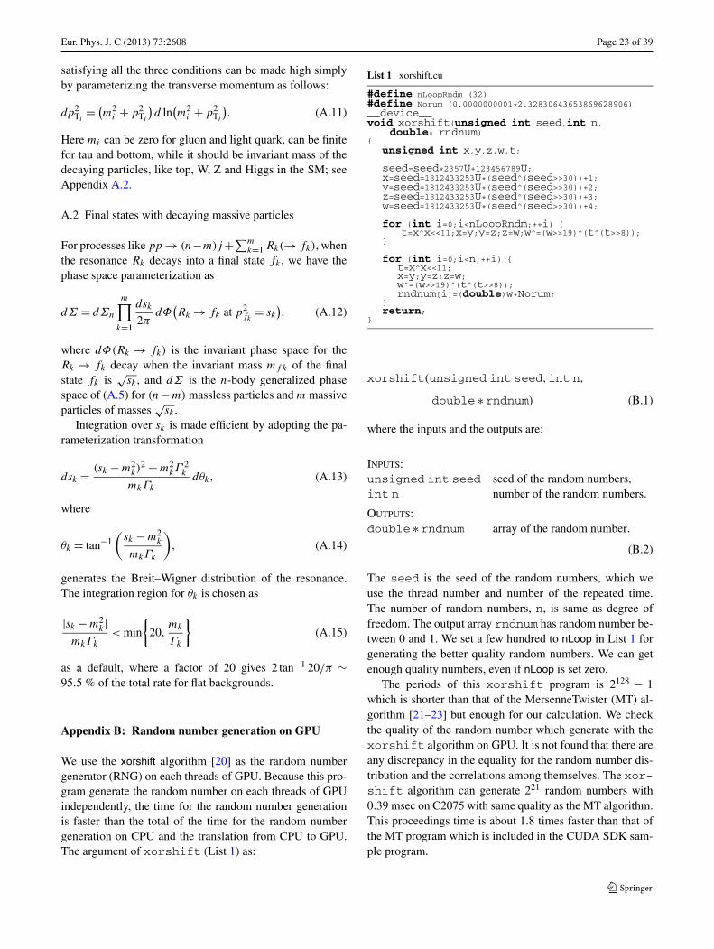
Eur. Phys. J. C (2013) 73:2608 Page 23 of 39
satisfying all the three conditions can be made high simplyby parameterizing the transverse momentum as follows:
dp2Ti
= (m2
i + p2Ti
)d ln
(m2
i + p2Ti
). (A.11)
Here mi can be zero for gluon and light quark, can be finitefor tau and bottom, while it should be invariant mass of thedecaying particles, like top, W, Z and Higgs in the SM; seeAppendix A.2.
A.2 Final states with decaying massive particles
For processes like pp → (n−m)j +∑mk=1 Rk(→ fk), when
the resonance Rk decays into a final state fk , we have thephase space parameterization as
dΣ = dΣn
m∏
k=1
dsk
2πdΦ
(Rk → fk at p2
fk= sk
), (A.12)
where dΦ(Rk → fk) is the invariant phase space for theRk → fk decay when the invariant mass mf k of the finalstate fk is
√sk , and dΣ is the n-body generalized phase
space of (A.5) for (n−m) massless particles and m massiveparticles of masses
√sk .
Integration over sk is made efficient by adopting the pa-rameterization transformation
dsk = (sk − m2k)
2 + m2kΓ
2k
mkΓk
dθk, (A.13)
where
θk = tan−1(
sk − m2k
mkΓk
), (A.14)
generates the Breit–Wigner distribution of the resonance.The integration region for θk is chosen as
|sk − m2k|
mkΓk
< min
{20,
mk
Γk
}(A.15)
as a default, where a factor of 20 gives 2 tan−1 20/π ∼95.5 % of the total rate for flat backgrounds.
Appendix B: Random number generation on GPU
We use the xorshift algorithm [20] as the random numbergenerator (RNG) on each threads of GPU. Because this pro-gram generate the random number on each threads of GPUindependently, the time for the random number generationis faster than the total of the time for the random numbergeneration on CPU and the translation from CPU to GPU.The argument of xorshift (List 1) as:
List 1 xorshift.cu
#define nLoopRndm (32)#define Norum (0.0000000001*2.32830643653869628906)__device__void xorshift(unsigned int seed,int n,
double* rndnum){
unsigned int x,y,z,w,t;
seed=seed*2357U+123456789U;x=seed=1812433253U*(seed^(seed>>30))+1;y=seed=1812433253U*(seed^(seed>>30))+2;z=seed=1812433253U*(seed^(seed>>30))+3;w=seed=1812433253U*(seed^(seed>>30))+4;
for (int i=0;i<nLoopRndm;++i) {t=x^x<<11;x=y;y=z;z=w;w^=(w>>19)^(t^(t>>8));
}
for (int i=0;i<n;++i) {t=x^x<<11;x=y;y=z;z=w;w^=(w>>19)^(t^(t>>8));rndnum[i]=(double)w*Norum;
}return;
}
xorshift(unsigned int seed,int n,
double ∗ rndnum) (B.1)
where the inputs and the outputs are:
INPUTS:unsigned int seed seed of the random numbers,int n number of the random numbers.
OUTPUTS:double ∗ rndnum array of the random number.
(B.2)
The seed is the seed of the random numbers, which weuse the thread number and number of the repeated time.The number of random numbers, n, is same as degree offreedom. The output array rndnum has random number be-tween 0 and 1. We set a few hundred to nLoop in List 1 forgenerating the better quality random numbers. We can getenough quality numbers, even if nLoop is set zero.
The periods of this xorshift program is 2128 − 1which is shorter than that of the MersenneTwister (MT) al-gorithm [21–23] but enough for our calculation. We checkthe quality of the random number which generate with thexorshift algorithm on GPU. It is not found that there areany discrepancy in the equality for the random number dis-tribution and the correlations among themselves. The xor-shift algorithm can generate 221 random numbers with0.39 msec on C2075 with same quality as the MT algorithm.This proceedings time is about 1.8 times faster than that ofthe MT program which is included in the CUDA SDK sam-ple program.
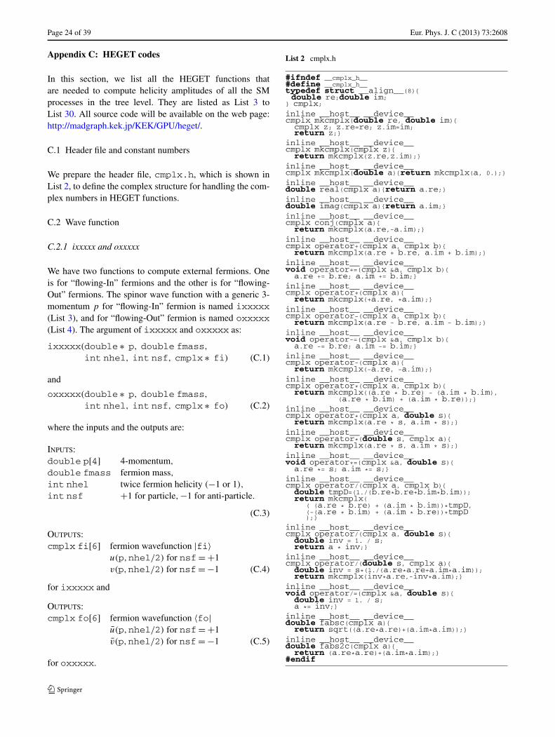
Page 24 of 39 Eur. Phys. J. C (2013) 73:2608
Appendix C: HEGET codes
In this section, we list all the HEGET functions thatare needed to compute helicity amplitudes of all the SMprocesses in the tree level. They are listed as List 3 toList 30. All source code will be available on the web page:http://madgraph.kek.jp/KEK/GPU/heget/.
C.1 Header file and constant numbers
We prepare the header file, cmplx.h, which is shown inList 2, to define the complex structure for handling the com-plex numbers in HEGET functions.
C.2 Wave function
C.2.1 ixxxxx and oxxxxx
We have two functions to compute external fermions. Oneis for “flowing-In” fermions and the other is for “flowing-Out” fermions. The spinor wave function with a generic 3-momentum p for “flowing-In” fermion is named ixxxxx(List 3), and for “flowing-Out” fermion is named oxxxxx(List 4). The argument of ixxxxx and oxxxxx as:
ixxxxx(double ∗ p, double fmass,
int nhel, int nsf, cmplx ∗ fi) (C.1)
and
oxxxxx(double ∗ p, double fmass,
int nhel, int nsf, cmplx ∗ fo) (C.2)
where the inputs and the outputs are:
INPUTS:double p[4] 4-momentum,
double fmass fermion mass,int nhel twice fermion helicity (−1 or 1),
int nsf +1 for particle,−1 for anti-particle.
(C.3)
OUTPUTS:cmplx fi[6] fermion wavefunction |fi〉
u(p,nhel/2) for nsf= +1v(p,nhel/2) for nsf= −1 (C.4)
for ixxxxx and
OUTPUTS:cmplx fo[6] fermion wavefunction 〈fo|
u(p,nhel/2) for nsf= +1v(p,nhel/2) for nsf= −1 (C.5)
for oxxxxx.
List 2 cmplx.h
#ifndef __cmplx_h__#define __cmplx_h__typedef struct __align__(8){double re;double im;
} cmplx;inline __host__ __device__cmplx mkcmplx(double re, double im){cmplx z; z.re=re; z.im=im;return z;}
inline __host__ __device__cmplx mkcmplx(cmplx z){return mkcmplx(z.re,z.im);}
inline __host__ __device__cmplx mkcmplx(double a){return mkcmplx(a, 0.);}
inline __host__ __device__double real(cmplx a){return a.re;}inline __host__ __device__double imag(cmplx a){return a.im;}inline __host__ __device__cmplx conj(cmplx a){return mkcmplx(a.re,-a.im);}
inline __host__ __device__cmplx operator+(cmplx a, cmplx b){return mkcmplx(a.re + b.re, a.im + b.im);}
inline __host__ __device__void operator+=(cmplx &a, cmplx b){a.re += b.re; a.im += b.im;}
inline __host__ __device__cmplx operator+(cmplx a){return mkcmplx(+a.re, +a.im);}
inline __host__ __device__cmplx operator-(cmplx a, cmplx b){return mkcmplx(a.re - b.re, a.im - b.im);}
inline __host__ __device__void operator-=(cmplx &a, cmplx b){a.re -= b.re; a.im -= b.im;}
inline __host__ __device__cmplx operator-(cmplx a){return mkcmplx(-a.re, -a.im);}
inline __host__ __device__cmplx operator*(cmplx a, cmplx b){return mkcmplx((a.re * b.re) - (a.im * b.im),
(a.re * b.im) + (a.im * b.re));}inline __host__ __device__cmplx operator*(cmplx a, double s){return mkcmplx(a.re * s, a.im * s);}
inline __host__ __device__cmplx operator*(double s, cmplx a){return mkcmplx(a.re * s, a.im * s);}
inline __host__ __device__void operator*=(cmplx &a, double s){a.re *= s; a.im *= s;}
inline __host__ __device__cmplx operator/(cmplx a, cmplx b){double tmpD=(1./(b.re*b.re+b.im*b.im));return mkcmplx(
( (a.re * b.re) + (a.im * b.im))*tmpD,(-(a.re * b.im) + (a.im * b.re))*tmpD);}
inline __host__ __device__cmplx operator/(cmplx a, double s){double inv = 1. / s;return a * inv;}
inline __host__ __device__cmplx operator/(double s, cmplx a){double inv = s*(1./(a.re*a.re+a.im*a.im));return mkcmplx(inv*a.re,-inv*a.im);}
inline __host__ __device__void operator/=(cmplx &a, double s){double inv = 1. / s;a *= inv;}
inline __host__ __device__double fabsc(cmplx a){return sqrt((a.re*a.re)+(a.im*a.im));}
inline __host__ __device__double fabs2c(cmplx a){return (a.re*a.re)+(a.im*a.im);}
#endif
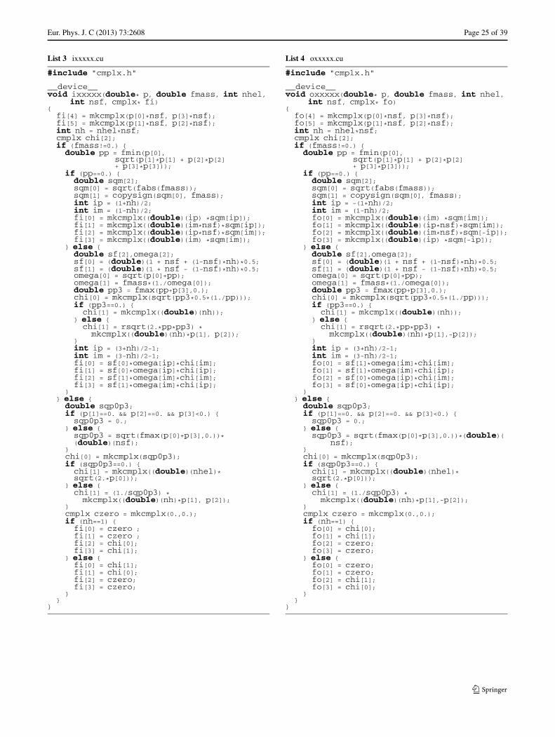
Eur. Phys. J. C (2013) 73:2608 Page 25 of 39
List 3 ixxxxx.cu
#include "cmplx.h"
__device__void ixxxxx(double* p, double fmass, int nhel,
int nsf, cmplx* fi){fi[4] = mkcmplx(p[0]*nsf, p[3]*nsf);fi[5] = mkcmplx(p[1]*nsf, p[2]*nsf);int nh = nhel*nsf;cmplx chi[2];if (fmass!=0.) {double pp = fmin(p[0],
sqrt(p[1]*p[1] + p[2]*p[2]+ p[3]*p[3]));
if (pp==0.) {double sqm[2];sqm[0] = sqrt(fabs(fmass));sqm[1] = copysign(sqm[0], fmass);int ip = (1+nh)/2;int im = (1-nh)/2;fi[0] = mkcmplx((double)(ip) *sqm[ip]);fi[1] = mkcmplx((double)(im*nsf)*sqm[ip]);fi[2] = mkcmplx((double)(ip*nsf)*sqm[im]);fi[3] = mkcmplx((double)(im) *sqm[im]);
} else {double sf[2],omega[2];sf[0] = (double)(1 + nsf + (1-nsf)*nh)*0.5;sf[1] = (double)(1 + nsf - (1-nsf)*nh)*0.5;omega[0] = sqrt(p[0]+pp);omega[1] = fmass*(1./omega[0]);double pp3 = fmax(pp+p[3],0.);chi[0] = mkcmplx(sqrt(pp3*0.5*(1./pp)));if (pp3==0.) {chi[1] = mkcmplx((double)(nh));
} else {chi[1] = rsqrt(2.*pp*pp3) *mkcmplx((double)(nh)*p[1], p[2]);
}int ip = (3+nh)/2-1;int im = (3-nh)/2-1;fi[0] = sf[0]*omega[ip]*chi[im];fi[1] = sf[0]*omega[ip]*chi[ip];fi[2] = sf[1]*omega[im]*chi[im];fi[3] = sf[1]*omega[im]*chi[ip];
}} else {double sqp0p3;if (p[1]==0. && p[2]==0. && p[3]<0.) {sqp0p3 = 0.;
} else {sqp0p3 = sqrt(fmax(p[0]+p[3],0.))*(double)(nsf);
}chi[0] = mkcmplx(sqp0p3);if (sqp0p3==0.) {chi[1] = mkcmplx((double)(nhel)*sqrt(2.*p[0]));
} else {chi[1] = (1./sqp0p3) *mkcmplx((double)(nh)*p[1], p[2]);
}cmplx czero = mkcmplx(0.,0.);if (nh==1) {fi[0] = czero ;fi[1] = czero ;fi[2] = chi[0];fi[3] = chi[1];
} else {fi[0] = chi[1];fi[1] = chi[0];fi[2] = czero;fi[3] = czero;
}}
}
List 4 oxxxxx.cu
#include "cmplx.h"
__device__void oxxxxx(double* p, double fmass, int nhel,
int nsf, cmplx* fo){fo[4] = mkcmplx(p[0]*nsf, p[3]*nsf);fo[5] = mkcmplx(p[1]*nsf, p[2]*nsf);int nh = nhel*nsf;cmplx chi[2];if (fmass!=0.) {double pp = fmin(p[0],
sqrt(p[1]*p[1] + p[2]*p[2]+ p[3]*p[3]));
if (pp==0.) {double sqm[2];sqm[0] = sqrt(fabs(fmass));sqm[1] = copysign(sqm[0], fmass);int ip = -(1+nh)/2;int im = (1-nh)/2;fo[0] = mkcmplx((double)(im) *sqm[im]);fo[1] = mkcmplx((double)(ip*nsf)*sqm[im]);fo[2] = mkcmplx((double)(im*nsf)*sqm[-ip]);fo[3] = mkcmplx((double)(ip) *sqm[-ip]);
} else {double sf[2],omega[2];sf[0] = (double)(1 + nsf + (1-nsf)*nh)*0.5;sf[1] = (double)(1 + nsf - (1-nsf)*nh)*0.5;omega[0] = sqrt(p[0]+pp);omega[1] = fmass*(1./omega[0]);double pp3 = fmax(pp+p[3],0.);chi[0] = mkcmplx(sqrt(pp3*0.5*(1./pp)));if (pp3==0.) {chi[1] = mkcmplx((double)(nh));
} else {chi[1] = rsqrt(2.*pp*pp3) *mkcmplx((double)(nh)*p[1],-p[2]);
}int ip = (3+nh)/2-1;int im = (3-nh)/2-1;fo[0] = sf[1]*omega[im]*chi[im];fo[1] = sf[1]*omega[im]*chi[ip];fo[2] = sf[0]*omega[ip]*chi[im];fo[3] = sf[0]*omega[ip]*chi[ip];
}} else {double sqp0p3;if (p[1]==0. && p[2]==0. && p[3]<0.) {sqp0p3 = 0.;
} else {sqp0p3 = sqrt(fmax(p[0]+p[3],0.))*(double)(
nsf);}chi[0] = mkcmplx(sqp0p3);if (sqp0p3==0.) {chi[1] = mkcmplx((double)(nhel)*sqrt(2.*p[0]));
} else {chi[1] = (1./sqp0p3) *mkcmplx((double)(nh)*p[1],-p[2]);
}cmplx czero = mkcmplx(0.,0.);if (nh==1) {fo[0] = chi[0];fo[1] = chi[1];fo[2] = czero;fo[3] = czero;
} else {fo[0] = czero;fo[1] = czero;fo[2] = chi[1];fo[3] = chi[0];
}}
}
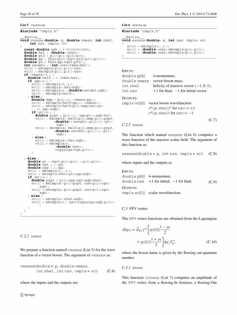
Page 26 of 39 Eur. Phys. J. C (2013) 73:2608
List 5 vxxxxx.cu
#include "cmplx.h"
__device__void vxxxxx(double* p, double vmass, int nhel,
int nsv, cmplx* vc){const double sqh = 0.70710678118655;double hel = (double)(nhel);double pt2 = p[1]*p[1]+p[2]*p[2];double pp = fmin(p[0],sqrt(pt2+p[3]*p[3]));double pt = fmin(pp,sqrt(pt2));int nsvahl = (int)(nsv*fabs(hel));vc[4] = mkcmplx(p[0],p[3])*nsv;vc[5] = mkcmplx(p[1],p[2])*nsv;if (vmass!=0.) {double hel0 = 1.-fabs(hel);if (pp==0.) {vc[0] = mkcmplx(0.,0.);vc[1] = mkcmplx(-hel*sqh);vc[2] = mkcmplx(0.,(double)nsvahl*sqh);vc[3] = mkcmplx(hel0);
} else {double emp = p[0]*(1./(vmass*pp));vc[0] = mkcmplx(hel0*pp*(1./vmass));vc[3] = mkcmplx(hel0*p[3]*emp+hel*pt*
(1./pp)*sqh);if (pt!=0.) {double pzpt = p[3]*(1./(pp*pt))*sqh*hel;vc[1] = mkcmplx( hel0*p[1]*emp-p[1]*pzpt,
(double)(-nsvahl)*p[2]*(1./pt)*sqh);
vc[2] = mkcmplx( hel0*p[2]*emp-p[2]*pzpt,(double)(nsvahl)*p[1]*(1./pt)*sqh);
} else {vc[1] = mkcmplx(-hel*sqh);vc[2] = mkcmplx(0.,
(double)(nsv)*copysign(sqh,p[3]));
}}
} else {double pt = sqrt(p[1]*p[1] + p[2]*p[2]);double rpt = 1./pt;double rpp = 1./pp;vc[0] = mkcmplx(0., 0.);vc[3] = mkcmplx(nhel*pt*rpp*sqh);if (pt!=0.) {double pzpt = p[3]*rpp*rpt*sqh*nhel;vc[1] = mkcmplx(-p[1]*pzpt,-nsv*p[2]*rpt*
sqh);vc[2] = mkcmplx(-p[2]*pzpt, nsv*p[1]*rpt*
sqh);} else {vc[1] = mkcmplx(-nhel*sqh);vc[2] = mkcmplx(0., nsv*copysign(sqh,p[3]))
;}
}}
C.2.2 vxxxxx
We prepare a function named vxxxxx (List 5) for the wavefunction of a vector boson. The argument of vxxxxx as:
vxxxxx(double ∗ p, double vmass,
int nhel, int nsv, cmplx ∗ vc) (C.6)
where the inputs and the outputs are:
List 6 sxxxxx.cu
#include "cmplx.h"
__device__void sxxxxx(double* p, int nss, cmplx* sc){
sc[0] = mkcmplx(1.,0.);sc[1] = (double)(nss)*mkcmplx(p[0],p[3]);sc[2] = (double)(nss)*mkcmplx(p[1],p[2]);
}
INPUTS:double p[4] 4-momentum,
double vmass vector boson mass,int nhel helicity of massive vector (−1,0,1),
int nsv +1 for final, −1 for initial vector.
OUTPUTS:cmplx vc[6] vector boson wavefunction
εμ(p,nhel)∗ for nsv= +1εμ(p,nhel) for nsv= −1.
(C.7)C.2.3 sxxxxx
The function which named sxxxxx (List 6) computes awave function of the massive scalar field. The argument ofthis function as:
sxxxxx(double ∗ p, int nss, cmplx ∗ sc) (C.8)
where inputs and the outputs as
INPUTS:double p[4] 4-momentum,
double nss +1 for initial, −1 for final.
OUTPUTS:cmplx sc[3] scalar wavefunction.
(C.9)
C.3 FFV vertex
The FFV vertex functions are obtained from the Lagrangian
LFFV = ψF1γ μ
[gc[0]1 − γ5
2
+ gc[1]1 + γ5
2
]ψF2V
∗μ, (C.10)
where the boson name is given by the flowing out quantumnumber.
C.3.1 iovxxx
This function iovxxx (List 7) computes an amplitude ofthe FFV vertex from a flowing-In fermion, a flowing-Out
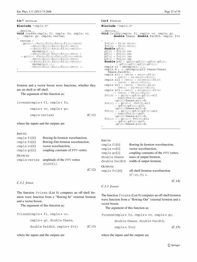
Eur. Phys. J. C (2013) 73:2608 Page 27 of 39
List 7 iovxxx.cu
#include "cmplx.h"
__device__void iovxxx(cmplx* fi, cmplx* fo, cmplx* vc,
cmplx* gc, cmplx& vertex){vertex =gc[0]*( (fo[2]*fi[0]+fo[3]*fi[1])*vc[0]
+(fo[2]*fi[1]+fo[3]*fi[0])*vc[1]-((fo[2]*fi[1]-fo[3]*fi[0])*vc[2])*mkcmplx(0.,1.)
+(fo[2]*fi[0]-fo[3]*fi[1])*vc[3] )+ gc[1]*( (fo[0]*fi[2]+fo[1]*fi[3])*vc[0]
-(fo[0]*fi[3]+fo[1]*fi[2])*vc[1]+((fo[0]*fi[3]-fo[1]*fi[2])*vc[2])*mkcmplx(0.,1.)
-(fo[0]*fi[2]-fo[1]*fi[3])*vc[3] );}
fermion and a vector boson wave functions, whether theyare on-shell or off-shell.
The argument of this function as:
iovxxx(cmplx ∗ fi, cmplx ∗ fo,
cmplx ∗ vc, cmplx ∗ gc,
cmplx vertex) (C.11)
where the inputs and the outputs are
INPUTS:cmplx fi[6] flowing-In fermion wavefunction,
cmplx fo[6] flowing-Out fermion wavefunction,
cmplx vc[6] vector wavefunction,
cmplx gc[2] coupling constants of FFV vertex.
OUTPUTS:cmplx vertex amplitude of the FFV vertex
〈fo|V|fi〉.(C.12)
C.3.2 fvixxx
The function fvixxx (List 8) computes an off-shell fer-mion wave function from a “flowing-In” external fermionand a vector boson.
The argument of this function as:
fvixxx(cmplx ∗ fi, cmplx ∗ vc,
cmplx ∗ gc, double fmass,
double fwidth, cmplx ∗ fvi) (C.13)
where the inputs and the outputs are
List 8 fvixxx.cu
#include "cmplx.h"
__device__void fvixxx(cmplx* fi, cmplx* vc, cmplx* gc,
double fmass, double fwidth, cmplx* fvi)
{fvi[4] = fi[4]-vc[4];fvi[5] = fi[5]-vc[5];double pf[4];pf[0] = fvi[4].re;pf[1] = fvi[5].re;pf[2] = fvi[5].im;pf[3] = fvi[4].im;double pf2 = (pf[0]+pf[3])*(pf[0]-pf[3])
- (pf[1]*pf[1]+pf[2]*pf[2]);cmplx ci = mkcmplx(0.,1.);cmplx d = -1./mkcmplx(pf2-fmass*fmass,fmass*fwidth);
cmplx sl1 = (vc[0] + vc[3])*fi[0]+ (vc[1] - ci*vc[2])*fi[1];
cmplx sl2 = (vc[1] + ci*vc[2])*fi[0]+ (vc[0] - vc[3])*fi[1];
cmplx sr1 = (vc[0] - vc[3])*fi[2]- (vc[1] - ci*vc[2])*fi[3];
cmplx sr2 =-(vc[1] + ci*vc[2])*fi[2]+ (vc[0] + vc[3])*fi[3];
fvi[0] = ( gc[0]*((pf[0]-pf[3])*sl1- conj(fvi[5])*sl2)+gc[1]*fmass*sr1)*d;
fvi[1] = ( gc[0]*( -fvi[5]*sl1+ (pf[0]+pf[3])*sl2)+gc[1]*fmass*sr2)*d;
fvi[2] = ( gc[1]*((pf[0]+pf[3])*sr1+ conj(fvi[5])*sr2)+gc[0]*fmass*sl1)*d;
fvi[3] = ( gc[1]*( fvi[5]*sr1+ (pf[0]-pf[3])*sr2)+gc[0]*fmass*sl2)*d;
}
INPUTS:cmplx fi[6] flowing-In fermion wavefunction,
cmplx vc[6] vector wavefunction,
cmplx gc[2] coupling constants of the FFV vertex,
double fmass mass of output fermion,
double fwidth width of output fermion.
OUTPUTS:cmplx fvi[6] off-shell fermion wavefunction
|f′: vc,fi>.
(C.14)
C.3.3 fvoxxx
The function fvoxxx (List 9) computes an off-shell fermionwave function from a “flowing-Out” external fermion and avector boson.
The argument of this function as:
fvoxxx(cmplx ∗ fo, cmplx ∗ vc, cmplx ∗ gc,
double fmass, double fwidth,
cmplx ∗ fvo) (C.15)
where the inputs and the outputs are
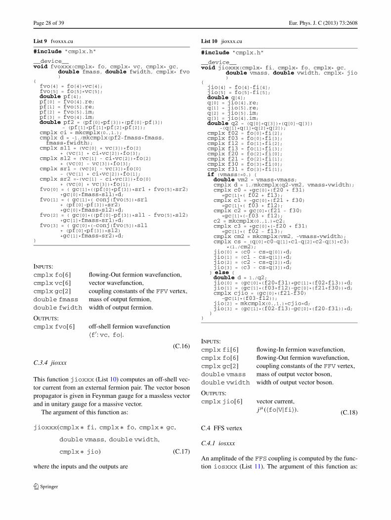
Page 28 of 39 Eur. Phys. J. C (2013) 73:2608
List 9 fvoxxx.cu
#include "cmplx.h"
__device__void fvoxxx(cmplx* fo, cmplx* vc, cmplx* gc,
double fmass, double fwidth, cmplx* fvo)
{fvo[4] = fo[4]+vc[4];fvo[5] = fo[5]+vc[5];double pf[4];pf[0] = fvo[4].re;pf[1] = fvo[5].re;pf[2] = fvo[5].im;pf[3] = fvo[4].im;double pf2 = (pf[0]+pf[3])*(pf[0]-pf[3])
- (pf[1]*pf[1]+pf[2]*pf[2]);cmplx ci = mkcmplx(0.,1.);cmplx d = -1./mkcmplx(pf2-fmass*fmass,fmass*fwidth);
cmplx sl1 = (vc[0] + vc[3])*fo[2]+ (vc[1] + ci*vc[2])*fo[3];
cmplx sl2 = (vc[1] - ci*vc[2])*fo[2]+ (vc[0] - vc[3])*fo[3];
cmplx sr1 = (vc[0] - vc[3])*fo[0]- (vc[1] + ci*vc[2])*fo[1];
cmplx sr2 =-(vc[1] - ci*vc[2])*fo[0]+ (vc[0] + vc[3])*fo[1];
fvo[0] = ( gc[1]*((pf[0]+pf[3])*sr1 + fvo[5]*sr2)+gc[0]*fmass*sl1)*d;
fvo[1] = ( gc[1]*( conj(fvo[5])*sr1+ (pf[0]-pf[3])*sr2)+gc[0]*fmass*sl2)*d;
fvo[2] = ( gc[0]*((pf[0]-pf[3])*sl1 - fvo[5]*sl2)+gc[1]*fmass*sr1)*d;
fvo[3] = ( gc[0]*(-conj(fvo[5])*sl1+ (pf[0]+pf[3])*sl2)+gc[1]*fmass*sr2)*d;
}
INPUTS:cmplx fo[6] flowing-Out fermion wavefunction,
cmplx vc[6] vector wavefunction,
cmplx gc[2] coupling constants of the FFV vertex,
double fmass mass of output fermion,
double fwidth width of output fermion.
OUTPUTS:cmplx fvo[6] off-shell fermion wavefunction
〈f′: vc, fo|.(C.16)
C.3.4 jioxxx
This function jioxxx (List 10) computes an off-shell vec-tor current from an external fermion pair. The vector bosonpropagator is given in Feynman gauge for a massless vectorand in unitary gauge for a massive vector.
The argument of this function as:
jioxxx(cmplx ∗ fi, cmplx ∗ fo, cmplx ∗ gc,
double vmass, double vwidth,
cmplx ∗ jio) (C.17)
where the inputs and the outputs are
List 10 jioxxx.cu
#include "cmplx.h"
__device__void jioxxx(cmplx* fi, cmplx* fo, cmplx* gc,
double vmass, double vwidth, cmplx* jio)
{jio[4] = fo[4]-fi[4];jio[5] = fo[5]-fi[5];double q[4];q[0] = jio[4].re;q[1] = jio[5].re;q[2] = jio[5].im;q[3] = jio[4].im;double q2 = (q[0]+q[3])*(q[0]-q[3])
-(q[1]*q[1]+q[2]*q[2]);cmplx f02 = fo[0]*fi[2];cmplx f03 = fo[0]*fi[3];cmplx f12 = fo[1]*fi[2];cmplx f13 = fo[1]*fi[3];cmplx f20 = fo[2]*fi[0];cmplx f21 = fo[2]*fi[1];cmplx f30 = fo[3]*fi[0];cmplx f31 = fo[3]*fi[1];if (vmass!=0.) {double vm2 = vmass*vmass;cmplx d = 1./mkcmplx(q2-vm2, vmass*vwidth);cmplx c0 = +gc[0]*(f20 + f31)
+gc[1]*( f02 + f13);cmplx c1 = -gc[0]*(f21 + f30)
+gc[1]*( f03 + f12);cmplx c2 = gc[0]*(f21 - f30)
+gc[1]*(-f03 + f12);c2 = mkcmplx(0.,1.)*c2;cmplx c3 = +gc[0]*(-f20 + f31)
+gc[1]*( f02 - f13);cmplx cm2 = mkcmplx(vm2, -vmass*vwidth);cmplx cs = (q[0]*c0-q[1]*c1-q[2]*c2-q[3]*c3)
*(1./cm2);jio[0] = (c0 - cs*q[0])*d;jio[1] = (c1 - cs*q[1])*d;jio[2] = (c2 - cs*q[2])*d;jio[3] = (c3 - cs*q[3])*d;
} else {double d = 1./q2;jio[0] = (gc[0]*(f20+f31)+gc[1]*(f02+f13))*d;jio[1] = (gc[1]*(f03+f12)-gc[0]*(f21+f30))*d;cmplx cjio = (gc[0]*(f21-f30)
-gc[1]*(f03-f12));jio[2] = mkcmplx(0.,1.)*cjio*d;jio[3] = (gc[1]*(f02-f13)-gc[0]*(f20-f31))*d;
}}
INPUTS:cmplx fi[6] flowing-In fermion wavefunction,
cmplx fo[6] flowing-Out fermion wavefunction,
cmplx gc[2] coupling constants of the FFV vertex,double vmass mass of output vector boson,
double vwidth width of output vector boson.
OUTPUTS:cmplx jio[6] vector current,
jμ(〈fo|V|fi〉). (C.18)
C.4 FFS vertex
C.4.1 iosxxx
An amplitude of the FFS coupling is computed by the func-tion iosxxx (List 11). The argument of this function as:
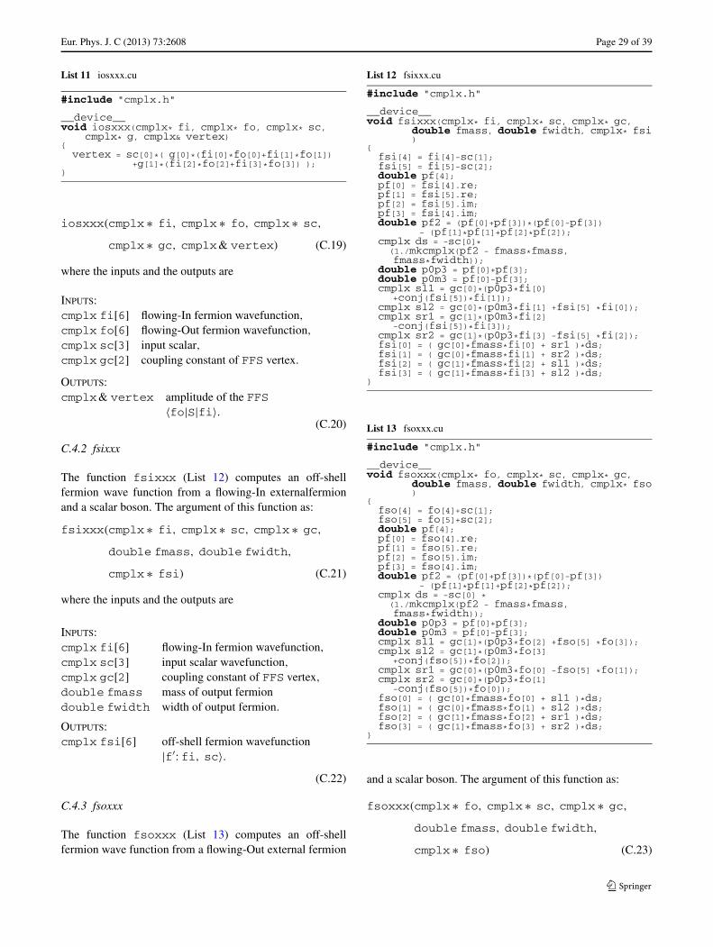
Eur. Phys. J. C (2013) 73:2608 Page 29 of 39
List 11 iosxxx.cu
#include "cmplx.h"
__device__void iosxxx(cmplx* fi, cmplx* fo, cmplx* sc,
cmplx* g, cmplx& vertex){vertex = sc[0]*( g[0]*(fi[0]*fo[0]+fi[1]*fo[1])
+g[1]*(fi[2]*fo[2]+fi[3]*fo[3]) );}
iosxxx(cmplx ∗ fi, cmplx ∗ fo, cmplx ∗ sc,
cmplx ∗ gc, cmplx& vertex) (C.19)
where the inputs and the outputs are
INPUTS:cmplx fi[6] flowing-In fermion wavefunction,
cmplx fo[6] flowing-Out fermion wavefunction,
cmplx sc[3] input scalar,cmplx gc[2] coupling constant of FFS vertex.
OUTPUTS:cmplx& vertex amplitude of the FFS
〈fo|S|fi〉.(C.20)
C.4.2 fsixxx
The function fsixxx (List 12) computes an off-shellfermion wave function from a flowing-In externalfermionand a scalar boson. The argument of this function as:
fsixxx(cmplx ∗ fi, cmplx ∗ sc, cmplx ∗ gc,
double fmass, double fwidth,
cmplx ∗ fsi) (C.21)
where the inputs and the outputs are
INPUTS:cmplx fi[6] flowing-In fermion wavefunction,
cmplx sc[3] input scalar wavefunction,
cmplx gc[2] coupling constant of FFS vertex,
double fmass mass of output fermiondouble fwidth width of output fermion.
OUTPUTS:cmplx fsi[6] off-shell fermion wavefunction
|f′: fi, sc〉.(C.22)
C.4.3 fsoxxx
The function fsoxxx (List 13) computes an off-shellfermion wave function from a flowing-Out external fermion
List 12 fsixxx.cu
#include "cmplx.h"
__device__void fsixxx(cmplx* fi, cmplx* sc, cmplx* gc,
double fmass, double fwidth, cmplx* fsi)
{fsi[4] = fi[4]-sc[1];fsi[5] = fi[5]-sc[2];double pf[4];pf[0] = fsi[4].re;pf[1] = fsi[5].re;pf[2] = fsi[5].im;pf[3] = fsi[4].im;double pf2 = (pf[0]+pf[3])*(pf[0]-pf[3])
- (pf[1]*pf[1]+pf[2]*pf[2]);cmplx ds = -sc[0]*
(1./mkcmplx(pf2 - fmass*fmass,fmass*fwidth));
double p0p3 = pf[0]+pf[3];double p0m3 = pf[0]-pf[3];cmplx sl1 = gc[0]*(p0p3*fi[0]
+conj(fsi[5])*fi[1]);cmplx sl2 = gc[0]*(p0m3*fi[1] +fsi[5] *fi[0]);cmplx sr1 = gc[1]*(p0m3*fi[2]
-conj(fsi[5])*fi[3]);cmplx sr2 = gc[1]*(p0p3*fi[3] -fsi[5] *fi[2]);fsi[0] = ( gc[0]*fmass*fi[0] + sr1 )*ds;fsi[1] = ( gc[0]*fmass*fi[1] + sr2 )*ds;fsi[2] = ( gc[1]*fmass*fi[2] + sl1 )*ds;fsi[3] = ( gc[1]*fmass*fi[3] + sl2 )*ds;
}
List 13 fsoxxx.cu
#include "cmplx.h"
__device__void fsoxxx(cmplx* fo, cmplx* sc, cmplx* gc,
double fmass, double fwidth, cmplx* fso)
{fso[4] = fo[4]+sc[1];fso[5] = fo[5]+sc[2];double pf[4];pf[0] = fso[4].re;pf[1] = fso[5].re;pf[2] = fso[5].im;pf[3] = fso[4].im;double pf2 = (pf[0]+pf[3])*(pf[0]-pf[3])
- (pf[1]*pf[1]+pf[2]*pf[2]);cmplx ds = -sc[0] *
(1./mkcmplx(pf2 - fmass*fmass,fmass*fwidth));
double p0p3 = pf[0]+pf[3];double p0m3 = pf[0]-pf[3];cmplx sl1 = gc[1]*(p0p3*fo[2] +fso[5] *fo[3]);cmplx sl2 = gc[1]*(p0m3*fo[3]
+conj(fso[5])*fo[2]);cmplx sr1 = gc[0]*(p0m3*fo[0] -fso[5] *fo[1]);cmplx sr2 = gc[0]*(p0p3*fo[1]
-conj(fso[5])*fo[0]);fso[0] = ( gc[0]*fmass*fo[0] + sl1 )*ds;fso[1] = ( gc[0]*fmass*fo[1] + sl2 )*ds;fso[2] = ( gc[1]*fmass*fo[2] + sr1 )*ds;fso[3] = ( gc[1]*fmass*fo[3] + sr2 )*ds;
}
and a scalar boson. The argument of this function as:
fsoxxx(cmplx ∗ fo, cmplx ∗ sc, cmplx ∗ gc,
double fmass, double fwidth,
cmplx ∗ fso) (C.23)
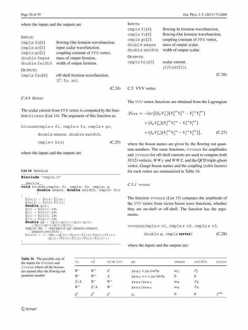
Page 30 of 39 Eur. Phys. J. C (2013) 73:2608
where the inputs and the outputs are
INPUTS:cmplx fo[6] flowing-Out fermion wavefunction,
cmplx sc[3] input scalar wavefunction,
cmplx gc[2] coupling constant of FFS vertex,
double fmass mass of output fermion,
double fwidth width of output fermion.
OUTPUTS:cmplx fso[6] off-shell fermion wavefunction,
〈f′: fo, sc|.(C.24)
C.4.4 hioxxx
The scalar current from FFS vertex is computed by the func-tion hioxxx (List 14). The argument of this function as:
hioxxx(cmplx ∗ fi, cmplx ∗ fo, cmplx ∗ gc,
double smass, double swidth,
cmplx ∗ hio) (C.25)
where the inputs and the outputs are
List 14 hioxxx.cu
#include "cmplx.h"
__device__void hioxxx(cmplx* fi, cmplx* fo, cmplx* g,
double smass, double swidth, cmplx* hio)
{hio[1] = fo[4]-fi[4];hio[2] = fo[5]-fi[5];double q[4];q[0] = hio[1].re;q[1] = hio[2].re;q[2] = hio[2].im;q[3] = hio[1].im;double q2 = (q[0]+q[3])*(q[0]-q[3])
-(q[1]*q[1]+q[2]*q[2]);cmplx dn = -mkcmplx(q2-smass*smass,
smass*swidth);hio[0] = (1./dn)*(g[0]*(fo[0]*fi[0]+fo[1]*fi[1])
+g[1]*(fo[2]*fi[2]+fo[3]*fi[3]));}
INPUTS:cmplx fi[6] flowing-In fermion wavefunction,
cmplx fo[6] flowing-Out fermion wavefunction,
cmplx gc[2] coupling constant of FFS vertex,
double smass mass of output scalar,double swidth width of output scalar.
OUTPUTS:cmplx hio[3] scalar current,
j (〈fo|s|fi〉).(C.26)
C.5 VVV vertex
The VVV vertex functions are obtained from the Lagrangian
LVVV = −igc{(
∂μV ∗1ν
)(V
μ∗2 V ν∗
3 − V ν∗2 V
μ∗3
)
+ (∂μV ∗
2ν
)(V
μ∗3 V ν∗
1 − V ν∗3 V
μ∗1
)
+ (∂μV ∗
3ν
)(V
μ∗1 V ν∗
2 − V ν∗1 V
μ∗2
)}, (C.27)
where the boson names are given by the flowing out quan-tum numbers. The same functions, vvvxxx for amplitudesand jvvxxx for off-shell currents are used to compute bothSU(2) vertices, WWγ and WWZ, and the QCD triple-gluonvertex. Gauge boson names and the coupling (color factors)for each vertex are summarized in Table 16.
C.5.1 vvvxxx
The function vvvxxx (List 15) computes the amplitude ofthe VVV vertex from vector boson wave functions, whetherthey are on-shell or off-shell. The function has the argu-ments:
vvvxxx(cmplx ∗ v1, cmplx ∗ v2, cmplx ∗ v3,
double g, cmplx vertexvertexvertex) (C.28)
where the inputs and the outputs are:
Table 16 The possible sets ofthe inputs for vvvxxx andjvvxxx where all the bosonsare named after the flowing outquantum number
v1 v2 v3 or jvv gc vmass vwidth color
W− W+ Z gWWZ = gW cos θW mZ ΓZ
W− W+ A gWWA = e = gW sin θW 0 0
Z/A W− W+ gWWZ/gWWA mW ΓW
W+ Z/A W− gWWZ/gWWA mW ΓW
ga gb gc gs 0 0 f abc
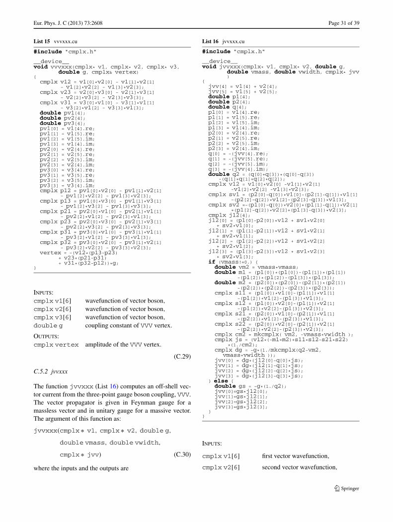
Eur. Phys. J. C (2013) 73:2608 Page 31 of 39
List 15 vvvxxx.cu
#include "cmplx.h"
__device__void vvvxxx(cmplx* v1, cmplx* v2, cmplx* v3,
double g, cmplx& vertex){cmplx v12 = v1[0]*v2[0] - v1[1]*v2[1]
- v1[2]*v2[2] - v1[3]*v2[3];cmplx v23 = v2[0]*v3[0] - v2[1]*v3[1]
- v2[2]*v3[2] - v2[3]*v3[3];cmplx v31 = v3[0]*v1[0] - v3[1]*v1[1]
- v3[2]*v1[2] - v3[3]*v1[3];double pv1[4];double pv2[4];double pv3[4];pv1[0] = v1[4].re;pv1[1] = v1[5].re;pv1[2] = v1[5].im;pv1[3] = v1[4].im;pv2[0] = v2[4].re;pv2[1] = v2[5].re;pv2[2] = v2[5].im;pv2[3] = v2[4].im;pv3[0] = v3[4].re;pv3[1] = v3[5].re;pv3[2] = v3[5].im;pv3[3] = v3[4].im;cmplx p12 = pv1[0]*v2[0] - pv1[1]*v2[1]
- pv1[2]*v2[2] - pv1[3]*v2[3];cmplx p13 = pv1[0]*v3[0] - pv1[1]*v3[1]
- pv1[2]*v3[2] - pv1[3]*v3[3];cmplx p21 = pv2[0]*v1[0] - pv2[1]*v1[1]
- pv2[2]*v1[2] - pv2[3]*v1[3];cmplx p23 = pv2[0]*v3[0] - pv2[1]*v3[1]
- pv2[2]*v3[2] - pv2[3]*v3[3];cmplx p31 = pv3[0]*v1[0] - pv3[1]*v1[1]
- pv3[2]*v1[2] - pv3[3]*v1[3];cmplx p32 = pv3[0]*v2[0] - pv3[1]*v2[1]
- pv3[2]*v2[2] - pv3[3]*v2[3];vertex = -(v12*(p13-p23)
+ v23*(p21-p31)+ v31*(p32-p12))*g;
}
INPUTS:cmplx v1[6] wavefunction of vector boson,
cmplx v2[6] wavefunction of vector boson,
cmplx v3[6] wavefunction of vector boson,
double g coupling constant of VVV vertex.
OUTPUTS:cmplx vertex amplitude of the VVV vertex.
(C.29)
C.5.2 jvvxxx
The function jvvxxx (List 16) computes an off-shell vec-tor current from the three-point gauge boson coupling, VVV.The vector propagator is given in Feynman gauge for amassless vector and in unitary gauge for a massive vector.The argument of this function as:
jvvxxx(cmplx ∗ v1, cmplx ∗ v2, double g,
double vmass, double vwidth,
cmplx ∗ jvv) (C.30)
where the inputs and the outputs are
List 16 jvvxxx.cu
#include "cmplx.h"
__device__void jvvxxx(cmplx* v1, cmplx* v2, double g,
double vmass, double vwidth, cmplx* jvv)
{jvv[4] = v1[4] + v2[4];jvv[5] = v1[5] + v2[5];double p1[4];double p2[4];double q[4];p1[0] = v1[4].re;p1[1] = v1[5].re;p1[2] = v1[5].im;p1[3] = v1[4].im;p2[0] = v2[4].re;p2[1] = v2[5].re;p2[2] = v2[5].im;p2[3] = v2[4].im;q[0] = -(jvv[4].re);q[1] = -(jvv[5].re);q[2] = -(jvv[5].im);q[3] = -(jvv[4].im);double q2 = (q[0]+q[3])*(q[0]-q[3])
-(q[1]*q[1]+q[2]*q[2]);cmplx v12 = v1[0]*v2[0] -v1[1]*v2[1]
-v1[2]*v2[2] -v1[3]*v2[3];cmplx sv1 = (p2[0]-q[0])*v1[0]-(p2[1]-q[1])*v1[1]
-(p2[2]-q[2])*v1[2]-(p2[3]-q[3])*v1[3];cmplx sv2 =-(p1[0]-q[0])*v2[0]+(p1[1]-q[1])*v2[1]
+(p1[2]-q[2])*v2[2]+(p1[3]-q[3])*v2[3];cmplx j12[4];j12[0] = (p1[0]-p2[0])*v12 + sv1*v2[0]
+ sv2*v1[0];j12[1] = (p1[1]-p2[1])*v12 + sv1*v2[1]
+ sv2*v1[1];j12[2] = (p1[2]-p2[2])*v12 + sv1*v2[2]
+ sv2*v1[2];j12[3] = (p1[3]-p2[3])*v12 + sv1*v2[3]
+ sv2*v1[3];if (vmass!=0.) {double vm2 = vmass*vmass;double m1 = (p1[0])*(p1[0])-(p1[1])*(p1[1])
-(p1[2])*(p1[2])-(p1[3])*(p1[3]);double m2 = (p2[0])*(p2[0])-(p2[1])*(p2[1])
-(p2[2])*(p2[2])-(p2[3])*(p2[3]);cmplx s11 = (p1[0])*v1[0]-(p1[1])*v1[1]
-(p1[2])*v1[2]-(p1[3])*v1[3];cmplx s12 = (p1[0])*v2[0]-(p1[1])*v2[1]
-(p1[2])*v2[2]-(p1[3])*v2[3];cmplx s21 = (p2[0])*v1[0]-(p2[1])*v1[1]
-(p2[2])*v1[2]-(p2[3])*v1[3];cmplx s22 = (p2[0])*v2[0]-(p2[1])*v2[1]
-(p2[2])*v2[2]-(p2[3])*v2[3];cmplx cm2 = mkcmplx( vm2, -vmass*vwidth );cmplx js = (v12*(-m1+m2)+s11*s12-s21*s22)
*(1./cm2);cmplx dg = -g*(1./mkcmplx(q2-vm2,
vmass*vwidth ));jvv[0] = dg*(j12[0]-q[0]*js);jvv[1] = dg*(j12[1]-q[1]*js);jvv[2] = dg*(j12[2]-q[2]*js);jvv[3] = dg*(j12[3]-q[3]*js);
} else {double gs = -g*(1./q2);jvv[0]=gs*j12[0];jvv[1]=gs*j12[1];jvv[2]=gs*j12[2];jvv[3]=gs*j12[3];
}}
INPUTS:cmplx v1[6] first vector wavefunction,
cmplx v2[6] second vector wavefunction,
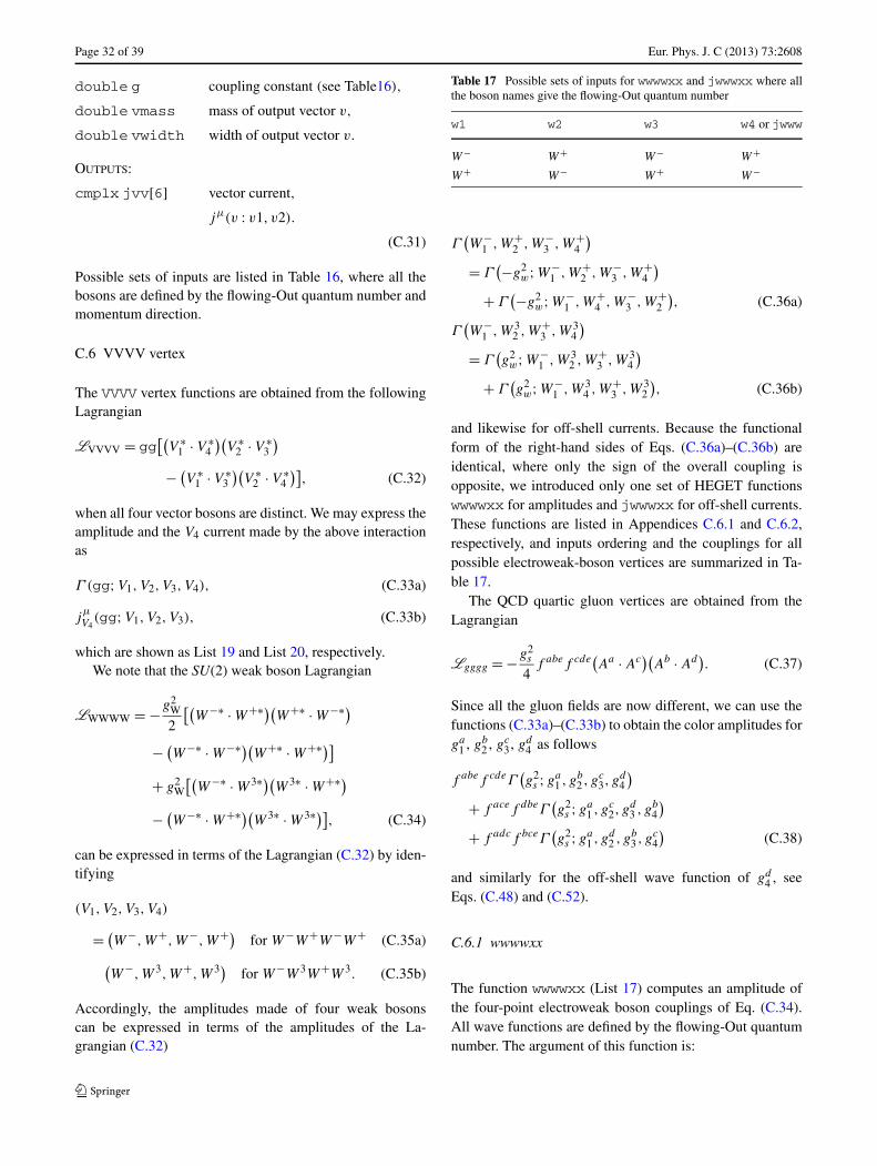
Page 32 of 39 Eur. Phys. J. C (2013) 73:2608
double g coupling constant (see Table16),
double vmass mass of output vector v,
double vwidth width of output vector v.
OUTPUTS:cmplx jvv[6] vector current,
jμ(v : v1, v2).
(C.31)
Possible sets of inputs are listed in Table 16, where all thebosons are defined by the flowing-Out quantum number andmomentum direction.
C.6 VVVV vertex
The VVVV vertex functions are obtained from the followingLagrangian
LVVVV = gg[(
V ∗1 · V ∗
4
)(V ∗
2 · V ∗3
)
− (V ∗
1 · V ∗3
)(V ∗
2 · V ∗4
)], (C.32)
when all four vector bosons are distinct. We may express theamplitude and the V4 current made by the above interactionas
Γ (gg;V1,V2,V3,V4), (C.33a)
jμV4
(gg;V1,V2,V3), (C.33b)
which are shown as List 19 and List 20, respectively.We note that the SU(2) weak boson Lagrangian
LWWWW = −g2W
2
[(W−∗ · W+∗)(W+∗ · W−∗)
− (W−∗ · W−∗)(W+∗ · W+∗)]
+ g2W
[(W−∗ · W 3∗)(W 3∗ · W+∗)
− (W−∗ · W+∗)(W 3∗ · W 3∗)], (C.34)
can be expressed in terms of the Lagrangian (C.32) by iden-tifying
(V1,V2,V3,V4)
= (W−,W+,W−,W+)
for W−W+W−W+ (C.35a)
(W−,W 3,W+,W 3) for W−W 3W+W 3. (C.35b)
Accordingly, the amplitudes made of four weak bosonscan be expressed in terms of the amplitudes of the La-grangian (C.32)
Table 17 Possible sets of inputs for wwwwxx and jwwwxx where allthe boson names give the flowing-Out quantum number
w1 w2 w3 w4 or jwww
W− W+ W− W+
W+ W− W+ W−
Γ(W−
1 ,W+2 ,W−
3 ,W+4
)
= Γ(−g2
w;W−1 ,W+
2 ,W−3 ,W+
4
)
+ Γ(−g2
w;W−1 ,W+
4 ,W−3 ,W+
2
), (C.36a)
Γ(W−
1 ,W 32 ,W+
3 ,W 34
)
= Γ(g2
w;W−1 ,W 3
2 ,W+3 ,W 3
4
)
+ Γ(g2
w;W−1 ,W 3
4 ,W+3 ,W 3
2
), (C.36b)
and likewise for off-shell currents. Because the functionalform of the right-hand sides of Eqs. (C.36a)–(C.36b) areidentical, where only the sign of the overall coupling isopposite, we introduced only one set of HEGET functionswwwwxx for amplitudes and jwwwxx for off-shell currents.These functions are listed in Appendices C.6.1 and C.6.2,respectively, and inputs ordering and the couplings for allpossible electroweak-boson vertices are summarized in Ta-ble 17.
The QCD quartic gluon vertices are obtained from theLagrangian
Lgggg = −g2s
4f abef cde
(Aa · Ac
)(Ab · Ad
). (C.37)
Since all the gluon fields are now different, we can use thefunctions (C.33a)–(C.33b) to obtain the color amplitudes forga
1 , gb2 , gc
3, gd4 as follows
f abef cdeΓ(g2
s ;ga1 , gb
2 , gc3, g
d4
)
+ f acef dbeΓ(g2
s ;ga1 , gc
2, gd3 , gb
4
)
+ f adcf bceΓ(g2
s ;ga1 , gd
2 , gb3 , gc
4
)(C.38)
and similarly for the off-shell wave function of gd4 , see
Eqs. (C.48) and (C.52).
C.6.1 wwwwxx
The function wwwwxx (List 17) computes an amplitude ofthe four-point electroweak boson couplings of Eq. (C.34).All wave functions are defined by the flowing-Out quantumnumber. The argument of this function is:
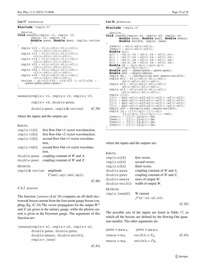
Eur. Phys. J. C (2013) 73:2608 Page 33 of 39
List 17 wwwwxx.cu
#include "cmplx.h"
__device__void wwwwxx(cmplx* v1, cmplx* v2,
cmplx* v3, cmplx* v4,double gwwa, double gwwz, cmplx& vertex)
{cmplx v12 = v1[0]*v2[0]-v1[1]*v2[1]
-v1[2]*v2[2]-v1[3]*v2[3];cmplx v13 = v1[0]*v3[0]-v1[1]*v3[1]
-v1[2]*v3[2]-v1[3]*v3[3];cmplx v14 = v1[0]*v4[0]-v1[1]*v4[1]
-v1[2]*v4[2]-v1[3]*v4[3];cmplx v23 = v2[0]*v3[0]-v2[1]*v3[1]
-v2[2]*v3[2]-v2[3]*v3[3];cmplx v24 = v2[0]*v4[0]-v2[1]*v4[1]
-v2[2]*v4[2]-v2[3]*v4[3];cmplx v34 = v3[0]*v4[0]-v3[1]*v4[1]
-v3[2]*v4[2]-v4[3]*v4[3];vertex = -g*(v12*v34 + v14*v23 -2.*v13*v24) *
(gwwa*gwwa+gwwz*gwwz);}
wwwwxx(cmplx ∗ v1, cmplx ∗ v2, cmplx ∗ v3,
cmplx ∗ v4, double gwwa,
double gwwz, cmplx& vertex) (C.39)
where the inputs and the outputs are
INPUTS:cmplx v1[6] first flow-Out v1 vector wavefunction,
cmplx v2[6] first flow-Out v2 vector wavefunction,
cmplx v3[6] second flow-Out v3 vector wavefunc-tion,
cmplx v4[6] second flow-Out v4 vector wavefunc-tion,
double gwwa coupling constant of W and A,
double gwwz coupling constant of W and Z.
OUTPUTS:cmplx& vertex amplitude
Γ (wm1,wp1,wm2,wp2).
(C.40)
C.6.2 jwwwxx
The function jwwwxx (List 18) computes an off-shell elec-troweak boson current from the four-point gauge boson cou-pling, Eq. (C.34) The vector propagators for the output W±and Z are given in the unitary gauge, while the photon cur-rent is given in the Feynman gauge. The arguments of thisfunction are:
jwwwxx(cmplx ∗ w1, cmplx ∗ w2, cmplx ∗ w3,
double gwwa, double gwwz,
double wmass, double wwidth,
cmplx ∗ jwww)
(C.41)
List 18 jwwwxx.cu
#include "cmplx.h"
__device__void jwwwxx(cmplx* w1, cmplx* w2, cmplx* w3,
double gwwa, double gwwz, double wmass,double wwidth, cmplx* jwww)
{jwww[4] = w1[4]+w2[4]+w3[4];jwww[5] = w1[5]+w2[5]+w3[5];double q[4];q[0] = -(w1[4].re + w2[4].re + w3[4].re);q[1] = -(w1[5].re + w2[5].re + w3[5].re);q[2] = -(w1[5].im + w2[5].im + w3[5].im);q[3] = -(w1[4].im + w2[4].im + w3[4].im);double q2 = (q[0]+q[3])*(q[0]-q[3])
-(q[1]*q[1]+q[2]*q[2]);double gw2 = (gwwa*gwwa)+(gwwz*gwwz);double mw2 = wmass*wmass;cmplx dw = -1./mkcmplx(q2-mw2,wmass*wwidth);cmplx w12 = w1[0]*w2[0]-w1[1]*w2[1]
-w1[2]*w2[2]-w1[3]*w2[3];cmplx w32 = w3[0]*w2[0]-w3[1]*w2[1]
-w3[2]*w2[2]-w3[3]*w2[3];cmplx w13 = w1[0]*w3[0]-w1[1]*w3[1]
-w1[2]*w3[2]-w1[3]*w3[3];cmplx jj[4];jj[0] = gw2*(w1[0]*w32+w3[0]*w12-2.*w2[0]*w13);jj[1] = gw2*(w1[1]*w32+w3[1]*w12-2.*w2[1]*w13);jj[2] = gw2*(w1[2]*w32+w3[2]*w12-2.*w2[2]*w13);jj[3] = gw2*(w1[3]*w32+w3[3]*w12-2.*w2[3]*w13);cmplx cm2 = mkcmplx(mw2,-wmass*wwidth);cmplx jq = (jj[0]*q[0]-jj[1]*q[1]
-jj[2]*q[2]-jj[3]*q[3])*(1./cm2);jwww[0] = (jj[0]-jq*q[0])*dw;jwww[1] = (jj[1]-jq*q[1])*dw;jwww[2] = (jj[2]-jq*q[2])*dw;jwww[3] = (jj[3]-jq*q[3])*dw;
}
where the inputs and the outputs are:
INPUTS:cmplx w1[6] first vector,cmplx w2[6] second vector,cmplx w3[6] third vector,double gwwa coupling constant of W and A,
double gwwz coupling constant of W and Z,
double wmass mass of output W,
double wwidth width of output W.
OUTPUTS:cmplx jwww[6] W current
jμ(w′ : w1,w2,w3).
(C.42)
The possible sets of the inputs are listed in Table 17, inwhich all the bosons are defined by the flowing-Out quan-tum number. The other arguments are
gwwa= gWWA, gwwz= gWWZ,
zmass= mZ, zwidth= ΓZ,
wmass= mW, wwidth= ΓW .
(C.43)
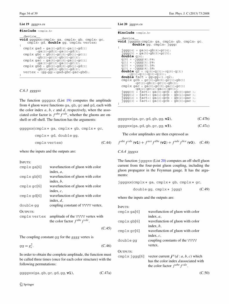
Page 34 of 39 Eur. Phys. J. C (2013) 73:2608
List 19 ggggxx.cu
#include <cmplx.h>
__device__void ggggxx(cmplx* ga, cmplx* gb, cmplx* gc,
cmplx* gd, double gg, cmplx& vertex){cmplx gad = ga[0]*gd[0]-ga[1]*gd[1]
-ga[2]*gd[2]-ga[3]*gd[3];cmplx gbc = gb[0]*gc[0]-gb[1]*gc[1]
-gb[2]*gc[2]-gb[3]*gc[3];cmplx gac = ga[0]*gc[0]-ga[1]*gc[1]
-ga[2]*gc[2]-ga[3]*gc[3];cmplx gbd = gb[0]*gd[0]-gb[1]*gd[1]
-gb[2]*gd[2]-gb[3]*gd[3];vertex = (gg*gg)*(gad*gbc-gac*gbd);
}
C.6.3 ggggxx
The function ggggxx (List 19) computes the amplitudefrom 4 gluon wave functions ga, gb, gc and gd, each withthe color index a, b, c and d , respectively, when the asso-ciated color factor is f abef cde, whether the gluons are on-shell or off-shell. The function has the arguments:
ggggxx(cmplx ∗ ga, cmplx ∗ gb, cmplx ∗ gc,
cmplx ∗ gd, double gg,
cmplx vertex) (C.44)
where the inputs and the outputs are:
INPUTS:cmplx ga[6] wavefunction of gluon with color
index, a,
cmplx gb[6] wavefunction of gluon with colorindex, b,
cmplx gc[6] wavefunction of gluon with colorindex, c,
cmplx gd[6] wavefunction of gluon with colorindex, d,
double gg coupling constant of VVVV vertex.
OUTPUTS:cmplx vertex amplitude of the VVVV vertex with
the color factor f abef cde.
(C.45)
The coupling constant gg for the gggg vertex is
gg= g2s . (C.46)
In order to obtain the complete amplitude, the function mustbe called three times (once for each color structure) with thefollowing permutations:
ggggxx(ga,gb,gc,gd,gg,v1v1v1), (C.47a)
List 20 jgggxx.cu
#include <cmplx.h>
__device__void jgggxx(cmplx* ga, cmplx* gb, cmplx* gc,
double gg, cmplx* jggg){jggg[4] = ga[4]+gb[4]+gc[4];jggg[5] = ga[5]+gb[5]+gc[5];double q[4];q[0] = -jggg[4].re;q[1] = -jggg[5].re;q[2] = -jggg[5].im;q[3] = -jggg[4].im;double q2 = (q[0]+q[3])*(q[0]-q[3])
-(q[1]*q[1]+q[2]*q[2]);double fact = gg*gg*(1./q2);cmplx gcb = gc[0]*gb[0]-gc[1]*gb[1]
-gc[2]*gb[2]-gc[3]*gb[3];cmplx gac = ga[0]*gc[0]-ga[1]*gc[1]
-ga[2]*gc[2]-ga[3]*gc[3];jggg[0] = fact*( ga[0]*gcb - gb[0]*gac );jggg[1] = fact*( ga[1]*gcb - gb[1]*gac );jggg[2] = fact*( ga[2]*gcb - gb[2]*gac );jggg[3] = fact*( ga[3]*gcb - gb[3]*gac );
}
ggggxx(ga,gc,gd,gb,gg,v2v2v2), (C.47b)
ggggxx(ga,gd,gb,gc,gg,v3v3v3). (C.47c)
The color amplitudes are then expressed as
f abef cde (v1v1v1) + f acef dbe (v2v2v2) + f adef bce (v3v3v3). (C.48)
C.6.4 jgggxx
The function jgggxx (List 20) computes an off-shell gluoncurrent from the four-point gluon coupling, including thegluon propagator in the Feynman gauge. It has the argu-ments:
jgggxx(cmplx ∗ ga, cmplx ∗ gb, cmplx ∗ gc,
double gg, cmplx ∗ jggg) (C.49)
where the inputs and the outputs are:
INPUTS:cmplx ga[6] wavefunction of gluon with color
index, a,
cmplx gb[6] wavefunction of gluon with colorindex, b,
cmplx gc[6] wavefunction of gluon with colorindex, c,
double gg coupling constants of the VVVVvertex.
OUTPUTS:cmplx jggg[6] vector current jjjμ(d : a, b, c) which
has the color index dassociated withthe color factor f abef cde.
(C.50)
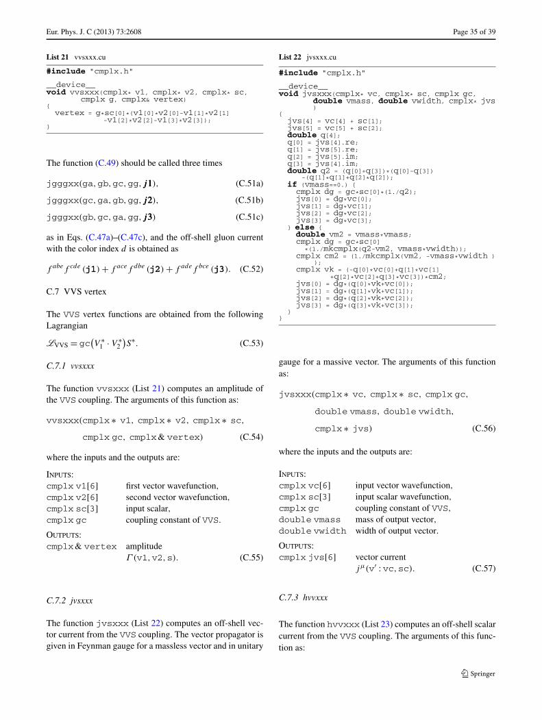
Eur. Phys. J. C (2013) 73:2608 Page 35 of 39
List 21 vvsxxx.cu
#include "cmplx.h"
__device__void vvsxxx(cmplx* v1, cmplx* v2, cmplx* sc,
cmplx g, cmplx& vertex){vertex = g*sc[0]*(v1[0]*v2[0]-v1[1]*v2[1]
-v1[2]*v2[2]-v1[3]*v2[3]);}
The function (C.49) should be called three times
jgggxx(ga,gb,gc,gg,j1j1j1), (C.51a)
jgggxx(gc,ga,gb,gg,j2j2j2), (C.51b)
jgggxx(gb,gc,ga,gg,j3j3j3) (C.51c)
as in Eqs. (C.47a)–(C.47c), and the off-shell gluon currentwith the color index d is obtained as
f abef cde (j1j1j1) + f acef dbe (j2j2j2) + f adef bce (j3j3j3). (C.52)
C.7 VVS vertex
The VVS vertex functions are obtained from the followingLagrangian
LVVS = gc(V ∗
1 · V ∗2
)S∗. (C.53)
C.7.1 vvsxxx
The function vvsxxx (List 21) computes an amplitude ofthe VVS coupling. The arguments of this function as:
vvsxxx(cmplx ∗ v1, cmplx ∗ v2, cmplx ∗ sc,
cmplx gc, cmplx& vertex) (C.54)
where the inputs and the outputs are:
INPUTS:cmplx v1[6] first vector wavefunction,
cmplx v2[6] second vector wavefunction,
cmplx sc[3] input scalar,cmplx gc coupling constant of VVS.
OUTPUTS:cmplx& vertex amplitude
Γ (v1,v2,s). (C.55)
C.7.2 jvsxxx
The function jvsxxx (List 22) computes an off-shell vec-tor current from the VVS coupling. The vector propagator isgiven in Feynman gauge for a massless vector and in unitary
List 22 jvsxxx.cu
#include "cmplx.h"
__device__void jvsxxx(cmplx* vc, cmplx* sc, cmplx gc,
double vmass, double vwidth, cmplx* jvs)
{jvs[4] = vc[4] + sc[1];jvs[5] = vc[5] + sc[2];double q[4];q[0] = jvs[4].re;q[1] = jvs[5].re;q[2] = jvs[5].im;q[3] = jvs[4].im;double q2 = (q[0]+q[3])*(q[0]-q[3])
-(q[1]*q[1]+q[2]*q[2]);if (vmass==0.) {cmplx dg = gc*sc[0]*(1./q2);jvs[0] = dg*vc[0];jvs[1] = dg*vc[1];jvs[2] = dg*vc[2];jvs[3] = dg*vc[3];
} else {double vm2 = vmass*vmass;cmplx dg = gc*sc[0]
*(1./mkcmplx(q2-vm2, vmass*vwidth));cmplx cm2 = (1./mkcmplx(vm2, -vmass*vwidth )
);cmplx vk = (-q[0]*vc[0]+q[1]*vc[1]
+q[2]*vc[2]+q[3]*vc[3])*cm2;jvs[0] = dg*(q[0]*vk+vc[0]);jvs[1] = dg*(q[1]*vk+vc[1]);jvs[2] = dg*(q[2]*vk+vc[2]);jvs[3] = dg*(q[3]*vk+vc[3]);
}}
gauge for a massive vector. The arguments of this functionas:
jvsxxx(cmplx ∗ vc, cmplx ∗ sc, cmplx gc,
double vmass, double vwidth,
cmplx ∗ jvs) (C.56)
where the inputs and the outputs are:
INPUTS:cmplx vc[6] input vector wavefunction,
cmplx sc[3] input scalar wavefunction,
cmplx gc coupling constant of VVS,
double vmass mass of output vector,double vwidth width of output vector.
OUTPUTS:cmplx jvs[6] vector current
jμ(v′ : vc,sc). (C.57)
C.7.3 hvvxxx
The function hvvxxx (List 23) computes an off-shell scalarcurrent from the VVS coupling. The arguments of this func-tion as:
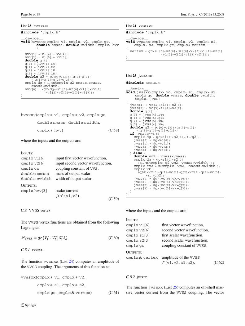
Page 36 of 39 Eur. Phys. J. C (2013) 73:2608
List 23 hvvxxx.cu
#include "cmplx.h"
__device__void hvvxxx(cmplx* v1, cmplx* v2, cmplx gc,
double smass, double swidth, cmplx* hvv)
{hvv[1] = v1[4] + v2[4];hvv[2] = v1[5] + v2[5];double q[4];q[0] = hvv[1].re;q[1] = hvv[2].re;q[2] = hvv[2].im;q[3] = hvv[1].im;double q2 = (q[0]+q[3])*(q[0]-q[3])
-(q[1]*q[1]+q[2]*q[2]);cmplx dg = 1./mkcmplx(q2-smass*smass,
smass*swidth);hvv[0] = -gc*dg*(v1[0]*v2[0]-v1[1]*v2[1]
-v1[2]*v2[2]-v1[3]*v2[3]);}
hvvxxx(cmplx ∗ v1, cmplx ∗ v2, cmplx gc,
double smass, double swidth,
cmplx ∗ hvv) (C.58)
where the inputs and the outputs are:
INPUTS:cmplx v1[6] input first vector wavefunction,
cmplx v2[6] input second vector wavefunction,
cmplx gc coupling constant of VVS,
double smass mass of output scalar,double swidth width of output scalar.
OUTPUTS:cmplx hvv[3] scalar current
j (s′ : v1,v2).(C.59)
C.8 VVSS vertex
The VVSS vertex functions are obtained from the followingLagrangian
LVVSS = gc(V ∗
1 · V ∗2
)S∗
3S∗4 . (C.60)
C.8.1 vvssxx
The function vvssxx (List 24) computes an amplitude ofthe VVSS coupling. The arguments of this function as:
vvssxx(cmplx ∗ v1, cmplx ∗ v2,
cmplx ∗ s1, cmplx ∗ s2,
cmplx gc, cmplx& vertex) (C.61)
List 24 vvssxx.cu
#include "cmplx.h"
__device__void vvssxx(cmplx* v1, cmplx* v2, cmplx* s1,
cmplx* s2, cmplx gc, cmplx& vertex){vertex = gc*s1[0]*s2[0]*(v1[0]*v2[0]-v1[1]*v2[1]
-v1[2]*v2[2]-v1[3]*v2[3]);}
List 25 jvssxx.cu
#include <cmplx.h>
__device__void jvssxx(cmplx* vc, cmplx* s1, cmplx* s2,
cmplx gc, double vmass, double vwidth,cmplx* jvss)
{jvss[4] = vc[4]+s1[1]+s2[1];jvss[5] = vc[5]+s1[2]+s2[2];double q[4];q[0] = jvss[4].re;q[1] = jvss[5].re;q[2] = jvss[5].im;q[3] = jvss[4].im;double q2 = (q[0]+q[3])*(q[0]-q[3])
-(q[1]*q[1]+q[2]*q[2]);if (vmass==0.){cmplx dg = gc*s1[0]*s2[0]*(1./q2);jvss[0] = dg*vc[0];jvss[1] = dg*vc[1];jvss[2] = dg*vc[2];jvss[3] = dg*vc[3];
} else {double vm2 = vmass*vmass;cmplx dg = gc*s1[0]*s2[0]
*(1./mkcmplx( q2-vm2, vmass*vwidth ));cmplx cm2 = mkcmplx( vm2, -vmass*vwidth );cmplx vk =
(q[0]*vc[0]-q[1]*vc[1]-q[2]*vc[2]-q[3]*vc[3])*(1./cm2);
jvss[0] = dg*(vc[0]-vk*q[0]);jvss[1] = dg*(vc[1]-vk*q[1]);jvss[2] = dg*(vc[2]-vk*q[2]);jvss[3] = dg*(vc[3]-vk*q[3]);
}}
where the inputs and the outputs are:
INPUTS:cmplx v1[6] first vector wavefunction,
cmplx v2[6] second vector wavefunction,
cmplx s1[3] first scalar wavefunction,
cmplx s2[3] second scalar wavefunction,
cmplx gc coupling constant of VVSS.
OUTPUTS:cmplx& vertex amplitude of the VVSS
Γ (v1,v2,s1,s2). (C.62)
C.8.2 jvssxx
The function jvssxx (List 25) computes an off-shell mas-sive vector current from the VVSS coupling. The vector

Eur. Phys. J. C (2013) 73:2608 Page 37 of 39
propagator is given in unitary gauge for a massive vector.The arguments of this functions as:
jvssxx(cmplx ∗ vc, cmplx ∗ s1, cmplx ∗ s2,
cmplx gc, double vmass,
double vwidth, cmplx ∗ jvss) (C.63)
where the inputs and the outputs are:
INPUTS:cmplx vc[6] input vector wavefunction,
cmplx s1[3] first scalar wavefunction,
cmplx s2[3] second scalar wavefunction,
cmplx gc coupling constants of VVSS vertex,
double vmass mass of output vector,double vwidth width of output vector.
OUTPUTS:cmplx jvss[6] vector current
jμ(v′ : vc,s1,s2).
(C.64)
C.8.3 hvvsxx
The function hvvsxx (List 26) computes an off-shell scalarcurrent of VVSS coupling. The arguments of this functionas:
hvvsxx(cmplx ∗ v1, cmplx ∗ v2, cmplx ∗ sc,
cmplx gc, double smass,
double swidth, cmplx ∗ hvvs) (C.65)
where the inputs and the outputs are:
List 26 hvvsxx.cu
#include "cmplx.h"
__device__void hvvsxx(cmplx* v1, cmplx* v2, cmplx* sc,
cmplx gc, double smass, double swidth,cmplx* hvvs)
{hvvs[1] = v1[4]+v2[4]+sc[1];hvvs[2] = v1[5]+v2[5]+sc[2];double q[4];q[0] = hvvs[1].re;q[1] = hvvs[2].re;q[2] = hvvs[2].im;q[3] = hvvs[1].im;double q2 = (q[0]+q[3])*(q[0]-q[3])
-(q[1]*q[1]+q[2]*q[2]);cmplx dg = 1./mkcmplx(q2-smass*smass,
smass*swidth);hvvs[0] = -gc*dg*sc[0]*(v1[0]*v2[0]-v1[1]*v2[1]
-v1[2]*v2[2]-v1[3]*v2[3]);}
INPUTS:cmplx v1[6] first vector wavefunction,
cmplx v2[6] second vector wavefunction,
cmplx sc[3] input scalar wavefunction,
cmplx gc coupling constant of VVSS,
double smass mass of output scalar,double swidth mass of output scalar.
OUTPUTS:cmplx hvvs[3] scalar current
j (s′ : v1,v2,sc). (C.66)
C.9 SSS vertex
The SSS vertex functions are obtained from the followingLagrangian
LSSS = gcS∗1S∗
2S∗3 . (C.67)
C.9.1 sssxxx
The function sssxxx (List 27) computes an amplitude ofthe three-scalar coupling, SSS. The arguments of this func-tion as:
sssxxx(cmplx ∗ s1, cmplx ∗ s2, cmplx ∗ s3,
cmplx gc, cmplx& vertex) (C.68)
where the inputs and the outputs are:
INPUTS:cmplx s1[3] first scalar wavefunction,
cmplx s2[3] second scalar wavefunction,
cmplx s3[3] third scalar wavefunction,
cmplx gc coupling constant of SSS.
OUTPUTS:cmplx& vertex amplitude
Γ (s1,s2,s3). (C.69)
C.9.2 hssxxx
The function hssxxx (List 28) computes an off-shell scalarcurrent from the three-scalar coupling, SSS. The arguments
List 27 sssxxx.cu
#include "cmplx.h"
__device__void sssxxx(cmplx* s1, cmplx* s2, cmplx* s3,
cmplx gc, cmplx& vertex){vertex = gc*s1[0]*s2[0]*s3[0];
}
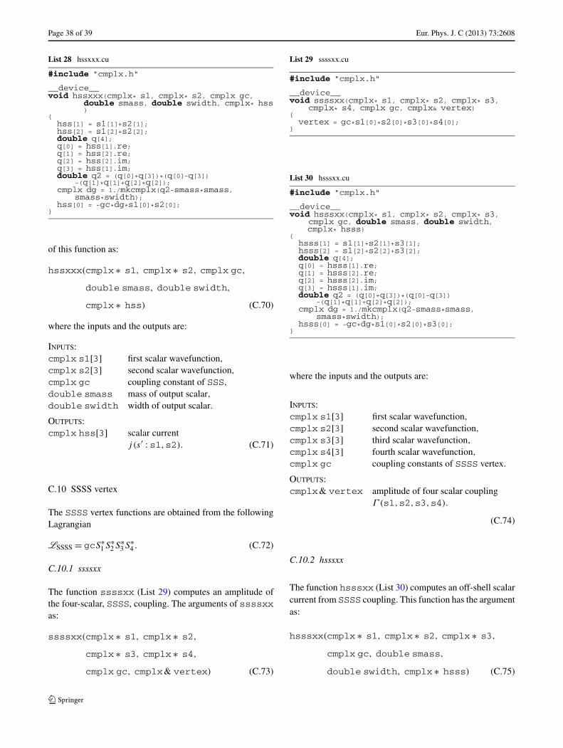
Page 38 of 39 Eur. Phys. J. C (2013) 73:2608
List 28 hssxxx.cu
#include "cmplx.h"
__device__void hssxxx(cmplx* s1, cmplx* s2, cmplx gc,
double smass, double swidth, cmplx* hss)
{hss[1] = s1[1]+s2[1];hss[2] = s1[2]+s2[2];double q[4];q[0] = hss[1].re;q[1] = hss[2].re;q[2] = hss[2].im;q[3] = hss[1].im;double q2 = (q[0]+q[3])*(q[0]-q[3])
-(q[1]*q[1]+q[2]*q[2]);cmplx dg = 1./mkcmplx(q2-smass*smass,
smass*swidth);hss[0] = -gc*dg*s1[0]*s2[0];
}
of this function as:
hssxxx(cmplx ∗ s1, cmplx ∗ s2, cmplx gc,
double smass, double swidth,
cmplx ∗ hss) (C.70)
where the inputs and the outputs are:
INPUTS:cmplx s1[3] first scalar wavefunction,
cmplx s2[3] second scalar wavefunction,
cmplx gc coupling constant of SSS,
double smass mass of output scalar,double swidth width of output scalar.
OUTPUTS:cmplx hss[3] scalar current
j (s′ : s1,s2). (C.71)
C.10 SSSS vertex
The SSSS vertex functions are obtained from the followingLagrangian
LSSSS = gcS∗1S∗
2S∗3S∗
4 . (C.72)
C.10.1 ssssxx
The function ssssxx (List 29) computes an amplitude ofthe four-scalar, SSSS, coupling. The arguments of ssssxxas:
ssssxx(cmplx ∗ s1, cmplx ∗ s2,
cmplx ∗ s3, cmplx ∗ s4,
cmplx gc, cmplx& vertex) (C.73)
List 29 ssssxx.cu
#include "cmplx.h"
__device__void ssssxx(cmplx* s1, cmplx* s2, cmplx* s3,
cmplx* s4, cmplx gc, cmplx& vertex){vertex = gc*s1[0]*s2[0]*s3[0]*s4[0];
}
List 30 hsssxx.cu
#include "cmplx.h"
__device__void hsssxx(cmplx* s1, cmplx* s2, cmplx* s3,
cmplx gc, double smass, double swidth,cmplx* hsss)
{hsss[1] = s1[1]+s2[1]+s3[1];hsss[2] = s1[2]+s2[2]+s3[2];double q[4];q[0] = hsss[1].re;q[1] = hsss[2].re;q[2] = hsss[2].im;q[3] = hsss[1].im;double q2 = (q[0]+q[3])*(q[0]-q[3])
-(q[1]*q[1]+q[2]*q[2]);cmplx dg = 1./mkcmplx(q2-smass*smass,
smass*swidth);hsss[0] = -gc*dg*s1[0]*s2[0]*s3[0];
}
where the inputs and the outputs are:
INPUTS:cmplx s1[3] first scalar wavefunction,
cmplx s2[3] second scalar wavefunction,
cmplx s3[3] third scalar wavefunction,
cmplx s4[3] fourth scalar wavefunction,
cmplx gc coupling constants of SSSS vertex.
OUTPUTS:cmplx& vertex amplitude of four scalar coupling
Γ (s1,s2,s3,s4).
(C.74)
C.10.2 hsssxx
The function hsssxx (List 30) computes an off-shell scalarcurrent from SSSS coupling. This function has the argumentas:
hsssxx(cmplx ∗ s1, cmplx ∗ s2, cmplx ∗ s3,
cmplx gc, double smass,
double swidth, cmplx ∗ hsss) (C.75)
Eur. Phys. J. C (2013) 73:2608 Page 39 of 39
where the inputs and the outputs are:
INPUTS:cmplx s1[3] first scalar wavefunction,
cmplx s2[3] second scalar wavefunction,
cmplx s3[3] third scalar wavefunction,
cmplx gc coupling constant SSSS,
double smass mass of output scalar,double swidth width of output scalar.
OUTPUTS:cmplx hsss[3] scalar current
j (s′ : s1,s2,s3). (C.76)
References
1. J. Alwall, M. Herquet, F. Maltoni, O. Mattelaer, T. Stelzer, J. HighEnergy Phys. 1106, 128 (2011). arXiv:1106.0522 [hep-ph]
2. J. Alwall, P. Demin, S. de Visscher, R. Frederix, M. Herquet, F.Maltoni, T. Plehn, D.L. Rainwater et al., J. High Energy Phys.0709, 028 (2007). arXiv:0706.2334 [hep-ph]
3. T. Stelzer, W.F. Long, Comput. Phys. Commun. 81, 357 (1994).arXiv:hep-ph/9401258
4. F. Maltoni, T. Stelzer, J. High Energy Phys. 0302, 027 (2003).arXiv:hep-ph/0208156
5. K. Hagiwara, J. Kanzaki, N. Okamura, D. Rainwater, T. Stelzer,Eur. Phys. J. C 66, 477 (2010). arXiv:0908.4403 [physics.comp-ph]
6. K. Hagiwara, J. Kanzaki, N. Okamura, D. Rainwater, T. Stelzer,Eur. Phys. J. C 70, 513 (2010). arXiv:0909.5257 [hep-ph]
7. H. Murayama, I. Watanabe, K. Hagiwara. KEK-91-118. http://www.nvidia.com/content/global/global.php9. http://www.nvidia.com/object/cuda_home_new.html
10. J. Kanzaki, Eur. Phys. J. C 71, 1559 (2011). arXiv:1010.2107[physics.comp-ph]
11. S. Kawabata, Comput. Phys. Commun. 41, 127 (1986)12. K. Hagiwara, T. Li, K. Mawatari, J. Nakamura, Eur. Phys. J. C 73,
2489 (2013). arXiv:1212.6247 [hep-ph]13. S. Catani, Y.L. Dokshitzer, M.H. Seymour, B.R. Webber, Nucl.
Phys. B 406, 187 (1993)14. J. Pumplin, D.R. Stump, J. Huston, H.L. Lai, P.M. Nadolsky,
W.K. Tung, J. High Energy Phys. 0207, 012 (2002). arXiv:hep-ph/0201195
15. D.L. Rainwater, D. Zeppenfeld, J. High Energy Phys. 9712, 005(1997). arXiv:hep-ph/9712271
16. D.L. Rainwater, D. Zeppenfeld, K. Hagiwara, Phys. Rev. D 59,014037 (1998). arXiv:hep-ph/9808468
17. N. Kauer, T. Plehn, D.L. Rainwater, D. Zeppenfeld, Phys. Lett. B503, 113 (2001). arXiv:hep-ph/0012351
18. W. Giele, G. Stavenga, J.-C. Winter, Eur. Phys. J. C 71, 1703(2011). arXiv:1002.3446 [hep-ph]
19. J. Kanzaki (in preparation)20. G. Marsaglia, J. Stat. Softw. 8(14), 1 (2003)21. M. Matsumoto, Y. Kurita, ACM Trans. Model. Comput. Simul. 2,
179–194 (1992). doi:10.1145/146382.14638322. M. Matsumoto, Y. Kurita, ACM Trans. Model. Comput. Simul. 4,
254–266 (1994). doi:10.1145/189443.18944523. M. Matsumoto, T. Nishimura, ACM Trans. Model. Comput.
Simul. 8(1), 3–30 (1998). doi:10.1145/272991.272995; see alsohttp://www.math.sci.hiroshima-u.ac.jp/~m-mat/MT/emt.html


