Explorations on high dimensional landscapes

Under review as a workshop contribution at ICLR 2015

EXPLORATIONS ON HIGH DIMENSIONAL LANDSCAPES

Levent SagunDepartment of MathematicsCourant InstituteNew York, NY 10012, [email protected]

V. Ugur GuneyDepartment of PhysicsThe City University of New YorkNew York, NY 10016, [email protected]

Yann LeCunDepartment of Computer ScienceCourant InstituteNew York, NY 10012, [email protected]

ABSTRACT

The question of where a moving particle will come to rest on the landscape downwhich it is moving is a challenging one, especially if the terrain is rugged. Inthis paper we present experimental results of such a movement in two differentcontexts: spherical spin glasses and two-layer networks on the MNIST dataset.The unifying property of the different cases is that if the system is symmetric andcomplex enough, its landscape is trivial in the sense that random initial points anda chosen descent algorithm always lead to the same level of height on the terrain.This indicates the existence of energy barriers in large systems. We further test theexistence of a barrier on a cost surface that theoretically has many zeroes. Withthis observation in mind we believe modifying the model to relocate this barrier isat least as important as finding a good descent algorithm on a fixed landscape.

1 INTRODUCTION

Many problems of practical interest can be rephrased as forms of an optimization problem in whichone needs to locate a point in a given domain that has some optimal energy or cost value.

One such problem arises in the context of learning: Given a set of input-output pairs, one seeks tofind a function whose values roughly match the ones in the set and which also performs well on newinputs. That is, it learns the task described by the set it began with. To this end, a loss function isformed which is optimized over the parameters of the desired function. Performance of this lossminimization is eventually tested against an unknown set of input-output pairs.

Another problem comes from statistical physics: In magnetic materials, the spins are aligned ac-cording to interactions with their neighbors. Over time equilibrium is reached when particles settledown to a configuration that has a reasonably low energy, if not the lowest possible. Stability of thisstate is tested against small fluctuations.

Some machine learning problems, such as deep networks, show suspicious similarity with spinsystems of statistical mechanics. Finding connections between the two became an attractive researcharea Barra et al. (2012). For a nice survey of theoretical results between Hopfield networks andBoltzmann machines, see Agliari et al. (2014). In a slightly different approach Dauphin et al. (2014)

1

arX

iv:1

412.

6615

v2 [

stat

.ML

] 2

5 D

ec 2

014


look into the problem of complicated surfaces in terms of the existence of saddle points. And morerecently, Choromanska et al. (2014) have a nice experimental section devoted to the same subject.

The energy landscapes of spin glasses are of interest in themselves. One of the main questionsconcerns the number of critical points of a given index at a given level. For a detailed analysisof this in spherical spin glasses, see Auffinger et al. (2013), Auffinger & Ben Arous (2013) andAuffinger & Chen (2014). The first of this sequence of papers will be used in this present paperin the corresponding experimental section. It establishes the existence of an energy barrier in theabsence of an external field. The barrier is proven to contain exponentially many local minimawhich are hard to cross, yet the barrier lies just above the ground state. For a similar analysis in aslightly more general context, see Fyodorov (2013), and Fyodorov & Le Doussal (2013). The addedexternal field as a tunable parameter allows for changing the topology of the landscape. Inspiredby this work, Mehta et al. gives a detailed experimental analysis of the case in which there arepolynomially many critical points. For a review of random matrices and extreme value statistics, seeDean & Majumdar (2008).

In this work, we focus on the case that has exponentially many critical points. In such high dimen-sional non-convex surfaces, a moving object is likely to get stuck in a local minimum point or atleast a critical point of some index. A reasonable algorithm should have enough noise to make theparticle jump out of those critical points that have high energy. However, if the landscape has ex-ponentially many critical points that lie around the same energy level, then jumping out of this wellwill lead to another point of similar energy, clearly not resulting in any improvement. The existenceof such a barrier will increase the search time for points that have lower energy values regardless ofthe method of choice. Alternatively, one can attempt to change the system so that the energy barrieris at a different, more favorable value, namely closer to the global minimum. One will of course becurious about the performance of such a point in the learning context, or its stability in the spin glasscontext.

So we ask two questions:

1) Where does the particle get stuck?

2) How good is that point for the task at hand?

We perform experiments in spin glasses and in deep networks to address those questions above. Eventhough they are structurally very different, which is readily apparent in their graph connectivity, thesimilarities we observe in conjunction with previous works lead us to think a more general fact mightbe true that has these two cases as its different examples.

2 MEAN FIELD SPHERICAL SPIN GLASS MODEL

The simplest model of a magnetic material is the one in which atoms have spins up, +1, or down,-1. Considering pairwise interactions between neighbors gives the total energy of the system:−∑ij wiwj wherew represents spin sign of the particle located at position i. Mean field assumption

ignores the lattice geometry of particles and assumes all interactions have equal strength. Introduc-ing a weak external field leads all particles to favor alignment, which incidentially corresponds tothe minimum energy configuration which will be achieved at the point where all of the particles havespin up (or down for that matter). This is a rather simple landscape whose global minimum is easyto achieve. This assumes no frustration, that is, all particles favor alignment. This model is knownas the Currie-Weiss model. If we have an alloy in which some particle pairs favor alignment andsome favor dis-alignment, the picture changes drastically. This introduces a whole new set of con-straints which may not be simultaniously attained, leading to glassy states. One way to model thisis to introduce random interaction coefficients between particles:

∑ij xijwiwj this model, which

has a rather complex energy landscape, is known as the Sherrington-Kirkpatrick model. See Agliariet al. (2014) and Sherrington (2014) for a survey on spin glasses and their connection to complexsystems.

We can also disregard the discrete states and put the points on the sphere and consider p-bodyinteractions of N particles for any p greater than or equal to 2. We have arrived at the model ofinterest for the purposes of this paper. While this model has been studied previously in great detail,

2


our particular focus is on the location of critical points. The main results we will use in this sectionand further details on the model can be found in Auffinger et al. (2013) and references therein.

Taking a point w ∈ SN−1(√N) ⊂ RN and x(·) ∼ Gaussian(0, 1), the Hamiltonian with standard

normal interactions is given by

HN,p(w) =1

Np−12

N∑i1,...,ip=1

xi1,...,ipwi1 ...wip . (1)

As a continuous function on a compact set HN,p attains its minimum. The value of the minimum isalso described in the corresponding paper, which we will recap below. Before moving any furtherwe would like to remark on why there are only polynomially many critical points for p = 2. For∑w2i = N and xij ∼ Gaussian(0,1) the Hamiltonian of the system is given by

H(w) =∑i∼j

wiwjxij = (Mx, x)

which is a quadratic form whereMij =xij+xji

2 is a randomN×N Gaussian Orthogonal Ensemblematrix. This system has 2N critical points at eigenvectors and their corresponding energy values areeigenvalues scaled by N . All the functions described below depend on p. However, we will focuson p = 3, so from now on we drop the 3 when indexing corresponding functions for notationalconvenience.

2.1 EXPERIMENTS INSPIRED BY PREVIOUS THEORETICAL WORK

In this section we simulate the spin glass Hamiltonian with p = 3 such that every point describesstates of N particles and their energies are calculated considering all 3-body interactions. We ini-tialize a point on the sphere by picking a random point on it and then perform gradient descent. TheHamiltonian is

HN (w) =1

N

N∑i,j,k

xijkwiwjwk (2)

where x’s are again i.i.d. standard Gaussian variables. Once they are fixed, we have the landscapewe want to explore.

2.1.1 EXISTENCE OF BARRIER

LetNN,k(u) denote the total number of critical points below level Nu with index k. Auffinger et al.(2013) finds this quantity asymptotically in logarithmic scale. Using that we know:

NN,k(u) � eNΘ(u) (3)

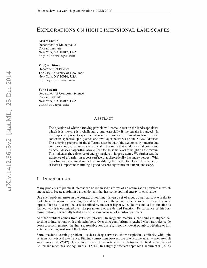
The analytic description of the function Θ(u) can be found in Auffinger et al. (2013). However, weare interested in its qualitative behavior. Clearly the function in (1) is a Gaussian random variableas it is an independent sum of such. It also has a peculiar normalization factor 1/N (p−1)/2. This ischosen for the model so that Var(H) = N . So we have a random field with mean zero and varianceN at each fixed point. We expect its global minimum and global maximum to be roughly symmetric.We also expect this function Θ in (3) to be non-decreasing as it counts the number of critical pointscumulatively. Θ crosses beyond zero (in the p = 2 case described above, the exponent in (3)never crosses beyond zero because that would imply exponentially many critical points.), and keepsincreasing until it becomes constant at a value denoted by −E∞, which is the lowest u for which Θis at its maximum value. This means the exponent stops growing so the number of critical points donot keep increasing in the scale described in (3). Another implication of the size of variance of theHamiltonian is that its extensive quantities scale with N , for which Auffinger et al. (2013) gives,

lim infN→∞

(minw

HN,p(w)

N

)≥ −E0

3


-E¥-E0

-1.65 -1.64 -1.63 -1.62u

-0.005

0.005

0.010

QHuL

Figure 1: Plot of Θ(u). It counts number of critical points at and below level Nu. The line on thetop is for local minima and the one below is for critical points of index 1.

where −E0 is the zero of Θ function. In words, the global minimum of the Hamiltonian on thesphere is bounded from below by −NE0. For our experiments the energy at the ground state andbarrier is calculated to be−N1.657 and−N1.633, respectively. At the level of−N1.633 (the verti-cal line in Figure 1) the landscape is expected to be overwhelmingly (more precisely, exponentiallymany with the highest exponent) full of local minima and of low index saddle points. This leads usto think that this barrier is a first place to get stuck using a descent method. We also have a measureon how far we are from the ground state, which is at the minimum of the Hamiltonian. Cumulativelyspeaking, looking at higher energy levels than the barrier does not increase the number of criticalpoints in the exponential scale. In turn, this means that almost all of the local minima (and saddlepoints of low index) will lie in the same energy level which is just above the actual ground state. Italso tells us that there are very few points at the ground state compared to the exponent of the onesat the barrier. Up to this point in the paper, we have been interpreting previous work.

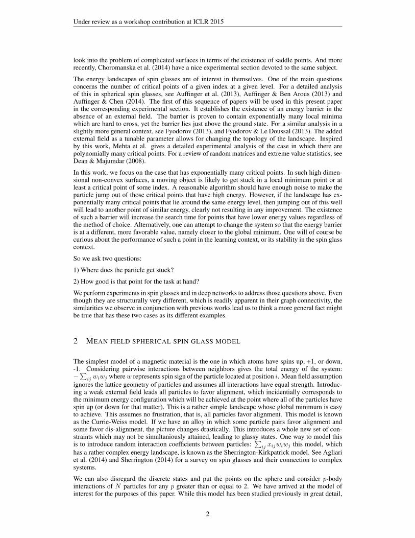
Gradient descent procedure starts with fixing the landscape once and for all, given N , pick N3 i.i.d.standard normals:

1. Pick a random element w of the sphere SN−1(√N) as a starting point for each trial.

2. Iterations: wt+1 = wt − γt∇wH(wt, xt). Note here the constraint that the gradient stayson the sphere. Normalize:

√N wt+1

||wt+1|| ← wt+1 so the point is back on the sphere.

3. Stop when the gradient is practically zero. For each N the experiment is repeated 5000times.

Figure 2: WhenN is large, left tails are touching at the barrier. WhenN is small, there is not enoughroom, and the system gets trapped at bad energy values.

One of the keys for the above theoretical result is that it holds asymptotically true. But then howlarge the dimension should be is a bit unclear. We try a few different N values and find that withincreasing dimension the points get closer to the barrier. Due to the lack of memory of current GPU’s

4


we cannot pushN much higher than 900 and still collect data in a reasonable amount of time. Figure2 shows how the points get closer to the barrier with increasing dimension. This fact, along with theexplanation of the difficulty of crossing the barrier and the layered structure of critical points belowthe barrier, is explained in Choromanska et al. (2014) (whose spin glass code was a courtesy of thefirst author of this paper). We would like to note that similarities end here.

In this paper we take a step further and conduct new experiments to gather more analysis from spinglass data. First of all, we would like to point out the existence of a critical dimension before whichthe landscape is hectic and does not really show any sign of a well-defined barrier. This implies thatin low dimensions the surface is not trivial, but that there are traps that fare badly and those trapsare located at somewhat arbitrary levels. This is also an observation we would like to see in otheroptimization problems in further experiments.

2.2 FINER ANALYSIS OF SPIN GLASS LANDSCAPE

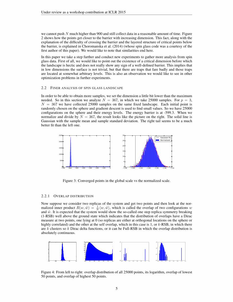
In order to be able to obtain more samples, we set the dimension a little bit lower than the maximumneeded. So in this section we analyze N = 367, in which we take 25000 samples. For p = 3,N = 367 we have collected 25000 samples on the same fixed landscape. Each initial point israndomly chosen on the sphere and gradient descent is used to find small values. So we have 25000configurations on the sphere and their energy levels. The energy barrier is at -599.3. When wenormalize and divide by N = 367, the result looks like the picture on the right. The solid line isGaussian with the sample mean and sample standard deviation. The right tail seems to be a muchbetter fit than the left one.

700 600 500 400 300 200 100 00

500

1000

1500

2000

2500

1.66 1.64 1.62 1.60 1.58 1.56 1.540

5

10

15

20

25

30

Gaussian fit

Normalized

Figure 3: Converged points in the global scale vs the normalized scale.

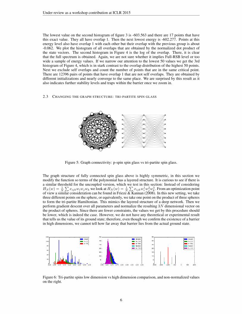
2.2.1 OVERLAP DISTRIBUTION

Now suppose we consider two replicas of the system and get two points and then look at the nor-malized inner product R(w, w) = 1

N 〈w, w〉, which is called the overlap of two configurations wand w. It is expected that the system would show the so-called one step replica symmetry breaking(1-RSB) well above the ground state which indicates that the distribution of overlaps have a Diracmeasure at two points, one lying at 0 (so replicas are either at orthogonal locations on the sphere orhighly correlated) and the other at the self overlap, which in this case is 1, or k-RSB, in which thereare k clusters so k Dirac delta functions, or it can be Full-RSB in which the overlap distribution isabsolutely continuous.

0.2 0.0 0.2 0.4 0.6 0.8 1.0 1.2100

101

102

0.2 0.0 0.2 0.4 0.6 0.8 1.0 1.210-2

10-1

100

101

Figure 4: From left to right: overlap distribution of all 25000 points, its logarithm, overlap of lowest50 points, and overlap of highest 50 points.

5


The lowest value on the second histogram of figure 3 is -603.563 and there are 17 points that havethis exact value. They all have overlap 1. Then the next lowest energy is -602.277. Points at thisenergy level also have overlap 1 with each other but their overlap with the previous group is about-0.062. We plot the histogram of all overlaps that are obtained by the normalized dot product ofthe state vectors. The second histogram in Figure 4 is the log of the overlap. There, it is clearthat the full spectrum is obtained. Again, we are not sure whether it implies Full-RSB level or toowide a sample of energy values. If we narrow our attention to the lowest 50 values we get the 3rdhistogram of Figure 4, which is in stark contrast to the overlap distribution of the highest 50 points.Next we exclude self overlaps and count the number of points that are in the same critical point.There are 12396 pairs of points that have overlap 1 that are not self overlaps. They are obtained bydifferent initializations and nearly converge to the same place. We are surprised by this result as italso indicates further stability levels and traps within the barrier once we zoom in.

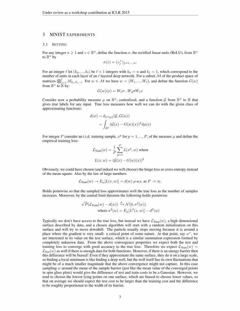
2.3 CHANGING THE GRAPH STRUCTURE: TRI-PARTITE SPIN GLASS

Figure 5: Graph connectivity: p-spin spin glass vs tri-partite spin glass.

The graph structure of fully connected spin glass above is highly symmetric, in this section wemodify the function so terms of the polynomial has a layered structure. It is curious to see if there isa similar threshold for the uncoupled version, which we test in this section: Instead of consideringHN (w) = 1

N

∑xijkwiwjwk we look atHN (w) = 1

N

∑xijkw

1iw

2jw

3k. From an optimization point

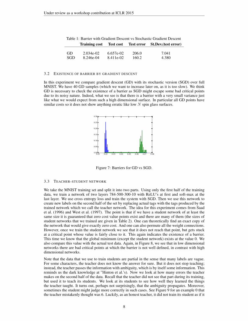
of view a similar consideration can be found in Frieze & Kannan (2008). In this new setting, we takethree different points on the sphere, or equivalently, we take one point on the product of three spheresto form the tri-partite Hamiltonian. This mimics the layered structure of a deep network. Then weperform gradient descent over all parameters and normalize the resulting 3N dimensional vector onthe product of spheres. Since there are fewer constraints, the values we get by this procedure shouldbe lower, which is indeed the case. However, we do not have any theoretical or experimental resultthat tells us the value of its ground state; therefore, even though we confirm the existence of a barrierin high dimensions, we cannot tell how far away that barrier lies from the actual ground state.

Figure 6: Tri-partite spins low dimension vs high dimension comparison, and non-normalized valueson the right.

6


3 MNIST EXPERIMENTS

3.1 SETTING

For any integer n ≥ 1 and z ∈ Rn, define the function σ, the rectified linear units (ReLU), from Rnto Rn by

σ(z) = (z+j )j=1,...,n.

For an integer ` let (k0, ..., k`) be ` + 1 integers with k0 = n and k` = 1, which correspond to thenumber of units in each layer of an ` layered deep network. For a subsetM of the product space ofmatrices

⊗lj=1Mkj ,kj−1

. For w ∈ M we have w = (W1, ...,W`), and define the function G(w)from Rn to R by:

G(w)(x) = W`σ...W2σW1x

Consider now a probability measure µ on Rn, centralized, and a function G from Rn to R thatgives true labels for any input. True loss measures how well we can do with the given class ofapproximating functions:

d(w) = dL2(µ)(G, G(w))

=

∫Rn

(G(x)−G(w)(x))2dµ(x)

For integer P consider an i.i.d. training sample, xp for p = 1, ..., P , of the measure µ and define theempirical training loss:

LTrain(w) =1

P

P∑p=1

L(xp, w) where

L(x,w) = (G(x)−G(w)(x))2

Obviously, we could have chosen (and indeed we will choose) the hinge loss or cross-entropy insteadof the mean square. Also by the law of large numbers:

LTrain(w)→ Eµ[L(x,w)] = d(w) µ-a.s. as P →∞.

Holds pointwise so that the sampled loss approximates well the true loss as the number of samplesincreases. Moreover, by the central limit theorem the following holds pointwise:

√P (LTrain(w)− d(w))

d.−→ N (0, σ2(w))

where σ2(w) = Eµ[L2(x,w)]− d2(w)

Typically we don’t have access to the true loss, but instead we have LTrain(w), a high dimensionalsurface described by data, and a chosen algorithm will start with a random initialization on thissurface and will try to move downhill. The particle usually stops moving because it is around aplace where the gradient is very small: a critical point of some nature. At that point, say w∗, weare interested in its value on the test surface, which is a similar summation expression formed bycompletely unknown data. From the above convergence properties we expect both the test andtraining loss to converge with good accuracy to the true loss. Therefore we expect LTrain(w) ∼LTest(w) as well if there is enough data for both functions. However, if there is an energy barrier thenthis difference will be biased! Even if they approximate the same surface, they do it on a large scale,so finding a local minimum is like finding a deep well, but the well itself has its own fluctuations thatmight be of a much smaller magnitude that the above convergence might not capture. In this casesampling w around the mean of the sample barrier (just like the mean value of the converged pointsin spin glass plots) would give the difference of test and train costs to be a Gaussian. However, wetend to choose the lowest lying points on one surface, which are biased to choose lower values, sothat on average we should expect the test cost to be larger than the training cost and the differenceto be roughly proportional to the width of its barrier.

7


Table 1: Barrier with Gradient Descent vs Stochastic Gradient DescentTraining cost Test cost Test error St.Dev.(test error)

GD 2.034e-02 6.657e-02 206.0 7.041SGD 8.246e-04 8.411e-02 160.2 4.380

3.2 EXISTENCE OF BARRIER BY GRADIENT DESCENT

In this experiment we compare gradient descent (GD) with its stochastic version (SGD) over fullMNIST. We have 40 GD samples (which we want to increase later on, as it is too slow). We thinkGD is necessary to check the existence of a barrier as SGD might escape some bad critical pointsdue to its noisy nature. Indeed, what we see is that there is a barrier with a very small variance justlike what we would expect from such a high dimensional surface. In particular all GD points havesimilar costs so it does not show anything erratic like low N spin glass surfaces.

0.01 0.02 0.03 0.04 0.05 0.06 0.07 0.080.00

0.05

0.10

0.15

0.20

0.25

0.30

Figure 7: Barriers for GD vs SGD.

3.3 TEACHER-STUDENT NETWORK

We take the MNIST training set and split it into two parts. Using only the first half of the trainingdata, we train a network of two layers 784-500-300-10 with ReLU’s at first and soft-max at thelast layer. We use cross entropy loss and train the system with SGD. Then we use this network tocreate new labels on the second half of the set by replacing actual tags with the tags produced by thetrained network which we call the teacher network. The idea for this experiment comes from Saadet al. (1996) and West et al. (1997). The point is that if we have a student network of at least thesame size it is guaranteed that zero cost value points exist and there are many of them (the sizes ofstudent networks that we trained are given in Table 2). One can theoretically find an exact copy ofthe network that would give exactly zero cost. And one can also permute all the weight connections.However, once we train the student network we see that it does not reach that point, but gets stuckat a critical point whose value is fairly close to it. This again indicates the existence of a barrier.This time we know that the global minimum (except the student network) exists at the value 0. Wealso compare this value with the actual test data. Again, in Figure 8, we see that in low dimensionalnetworks there are bad critical points at which the barrier is not well defined, in contrast with highdimensional networks.

Note that the data that we use to train students are partial in the sense that many labels are vague.For some characters, the teacher does not know the answer for sure. But it does not stop teaching;instead, the teacher passes the information with ambiguity, which is by itself some information. Thisreminds us the dark knowledge at ”Hinton et al.’s). Now we look at how many errors the teachermakes on the second half of the data. Recall that the teacher did not see that part during its training,but used it to teach its students. We look at its students to see how well they learned the thingsthe teacher taught. It turns out, perhaps not surprisingly, that the ambiguity propagates. Moreover,sometimes the student might judge more correctly in such cases. See Figure 9 for an example 0 thatthe teacher mistakenly thought was 6. Luckily, as an honest teacher, it did not train its student as if it

8


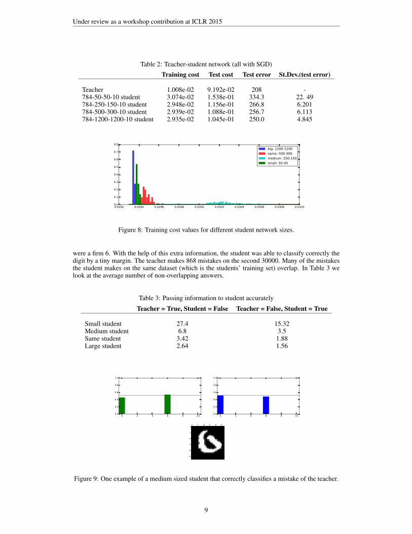
Table 2: Teacher-student network (all with SGD)

Training cost Test cost Test error St.Dev.(test error)

Teacher 1.008e-02 9.192e-02 208 -784-50-50-10 student 3.074e-02 1.538e-01 334.3 22. 49784-250-150-10 student 2.948e-02 1.156e-01 266.8 6.201784-500-300-10 student 2.939e-02 1.088e-01 256.7 6.113784-1200-1200-10 student 2.935e-02 1.045e-01 250.0 4.845

0.0292 0.0294 0.0296 0.0298 0.0300 0.0302 0.0304 0.0306 0.0308 0.03100.0

0.1

0.2

0.3

0.4

0.5

0.6

0.7

0.8

big: 1200-1200

same: 500-300

medium: 250-150

small: 50-50

Figure 8: Training cost values for different student network sizes.

were a firm 6. With the help of this extra information, the student was able to classify correctly thedigit by a tiny margin. The teacher makes 868 mistakes on the second 30000. Many of the mistakesthe student makes on the same dataset (which is the students’ training set) overlap. In Table 3 welook at the average number of non-overlapping answers.

Table 3: Passing information to student accurately

Teacher = True, Student = False Teacher = False, Student = True

Small student 27.4 15.32Medium student 6.8 3.5Same student 3.42 1.88Large student 2.64 1.56

0 2 4 6 8 100.0

0.2

0.4

0.6

0.8

1.0

0 2 4 6 8 100.0

0.2

0.4

0.6

0.8

1.0

0 5 10 15 20 250

5

10

15

20

25

Figure 9: One example of a medium sized student that correctly classifies a mistake of the teacher.

9


4 CONCLUSION

We clearly need further theoretical justification of how large dimensional surfaces look. We wouldalso like to emphasize again that we are not claiming a theoretical tie between spin glasses and deepnetworks; rather, we hint at a more general, more abstract phenomenon that governs the two differentcases. This might indicate a general class of difficult to optimize problems that have a trivial energylandscape. We would like to continue exploring similar landscape features in other fields as well.

ACKNOWLEDGEMENTS

We thank Gerard Ben Arous for valuable discussions. We would like to thank to developers ofTorch7 (Collobert et al. (2011)) which we used for the spin glass experiments and Theano (Bastienet al. (2012) and Bergstra et al. (2010)) which we used for MNIST experiments. We also gratefullyacknowledge the support of NVIDIA Corporation with the donation of the Tesla K40 GPU used forpart of this research.

REFERENCES

Agliari, Elena, Barra, Adriano, Galluzzi, Andrea, Tantari, Daniele, and Tavani, Flavia. A walk inthe statistical mechanical formulation of neural networks. 1948:12, July 2014.

Auffinger, Antonio and Ben Arous, Gerard. Complexity of random smooth functions on the high-dimensional sphere. The Annals of Probability, 41(6):4214–4247, November 2013. ISSN 0091-1798. doi: 10.1214/13-AOP862.

Auffinger, Antonio and Chen, Wei-kuo. Free Energy and Complexity of Spherical BipartiteModels. Journal of Statistical Physics, 157(1):40–59, July 2014. ISSN 0022-4715. doi:10.1007/s10955-014-1073-0.

Auffinger, Antonio, Arous, Gerard Ben, and Cerny, Jiı. Random Matrices and Complexity of SpinGlasses. Communications on Pure and Applied Mathematics, 66(2):165–201, February 2013.ISSN 00103640. doi: 10.1002/cpa.21422.

Barra, Adriano, Genovese, Giuseppe, Guerra, Francesco, and Tantari, Daniele. How glassy areneural networks? Journal of Statistical Mechanics: Theory and Experiment, 2012(07):P07009,2012.

Bastien, Frederic, Lamblin, Pascal, Pascanu, Razvan, Bergstra, James, Goodfellow, Ian J., Bergeron,Arnaud, Bouchard, Nicolas, and Bengio, Yoshua. Theano: new features and speed improvements.Deep Learning and Unsupervised Feature Learning NIPS 2012 Workshop, 2012.

Bergstra, James, Breuleux, Olivier, Bastien, Frederic, Lamblin, Pascal, Pascanu, Razvan, Des-jardins, Guillaume, Turian, Joseph, Warde-Farley, David, and Bengio, Yoshua. Theano: a CPUand GPU math expression compiler. In Proceedings of the Python for Scientific Computing Con-ference (SciPy), June 2010. Oral Presentation.

Choromanska, Anna, Henaff, Mikael, Mathieu, Michael, Arous, Gerard Ben, and LeCun, Yann. TheLoss Surface of Multilayer Networks. November 2014.

Collobert, Ronan, Kavukcuoglu, Koray, and Farabet, Clement. Torch7: A matlab-like environmentfor machine learning. In BigLearn, NIPS Workshop, 2011.

Dauphin, Yann N, Pascanu, Razvan, Gulcehre, Caglar, Cho, Kyunghyun, Ganguli, Surya, and Ben-gio, Yoshua. Identifying and attacking the saddle point problem in high-dimensional non-convexoptimization. In Ghahramani, Z, Welling, M, Cortes, C, Lawrence, N D, and Weinberger, K Q(eds.), Advances in Neural Information Processing Systems 27, pp. 2933–2941. Curran Asso-ciates, Inc., June 2014.

Dean, David S and Majumdar, Satya N. Extreme value statistics of eigenvalues of Gaussianrandom matrices. Physical Review E, 77(4):041108, April 2008. ISSN 1539-3755. doi:10.1103/PhysRevE.77.041108.

10


Frieze, Alan and Kannan, Ravi. A new approach to the planted clique problem. In Hariharan,Ramesh, Mukund, Madhavan, and Vinay, V (eds.), IARCS Annual Conference on Foundationsof Software Technology and Theoretical Computer Science, volume 2 of Leibniz InternationalProceedings in Informatics (LIPIcs), pp. 187–198, Dagstuhl, Germany, 2008. Schloss Dagstuhl–Leibniz-Zentrum fuer Informatik. ISBN 978-3-939897-08-8. doi: http://dx.doi.org/10.4230/LIPIcs.FSTTCS.2008.1752.

Fyodorov, Yan V. High-Dimensional Random Fields and Random Matrix Theory. pp. 40, July2013.

Fyodorov, Yan V and Le Doussal, Pierre. Topology Trivialization and Large Deviations for theMinimum in the Simplest Random Optimization. Journal of Statistical Physics, 154(1-2):466–490, September 2013. ISSN 0022-4715. doi: 10.1007/s10955-013-0838-1.

Hinton, Geoffrey, Vinyals, Oriol, and Dean, Jeff. Dark Knowledge.

Mehta, Dhagash, Hauenstein, Jonathan D, Niemerg, Matthew, Simm, Nicholas J, and Stariolo,Daniel A. Energy Landscape of the Finite-Size Mean-field 2-Spin Spherical Model and TopologyTrivialization. pp. 1–9.

Saad, David, Birmingham, B, and Solla, Sara A. Dynamics of On-Line Gradient Descent Learningfor Multilayer Neural Networks. In Touretzky, D S, Mozer, M C, and Hasselmo, M E (eds.),Advances in Neural Information Processing Systems 8, pp. 302–308. MIT Press, 1996.

Sherrington, David. Physics and Complexity: An Introduction. In Delitala, Marcello and AjmoneMarsan, Giulia (eds.), Managing Complexity, Reducing Perplexity, volume 67 of Springer Pro-ceedings in Mathematics & Statistics, pp. 119–129. Springer International Publishing, Cham,2014. ISBN 978-3-319-03758-5. doi: 10.1007/978-3-319-03759-2.

West, Ansgar H L, Saad, David, and Nabney, Ian T. The Learning Dynamcis of a Universal Ap-proximator. In Mozer, M C, Jordan, M I, and Petsche, T (eds.), Advances in Neural InformationProcessing Systems 9, pp. 288–294. MIT Press, 1997.

11

Documents

Explorations on high dimensional landscapes