Exploration of porous structures with illustrative visualizations

Computers & Graphics 34 (2010) 398–408

Contents lists available at ScienceDirect

Computers & Graphics

0097-84

doi:10.1

� Corr

E-m

dani@ls1 Te2 Te3 Te

journal homepage: www.elsevier.com/locate/cag

Technical Section

Exploration of porous structures with illustrative visualizations

Sergi Grau �, Eduard Verges 1, Dani Tost 2, Dolors Ayala 3

Computer Graphics Division CREB/IBEC, Polytechnical University of Catalonia, Avda Diagonal, 647, 08028 Barcelona, Spain

a r t i c l e i n f o

Keywords:

Illustrative visualization

Porous structures

Topological graph

Volume ray-casting

Transfer functions

Virtual navigation

93/$ - see front matter & 2010 Elsevier Ltd. A

016/j.cag.2010.05.001

esponding author. Tel.: +34 934011938; fax:

ail addresses: [email protected] (S. Grau), eve

i.upc.edu (D. Tost), [email protected] (D. A

l.: +34 934011954; fax: +34 934016050.

l.: +34 934016076; fax: +34 934016050.

l.: +34 934011919; fax: +34 934016050.

a b s t r a c t

The analysis of porous structures from CT images is emerging as a new computer graphics application

that is useful in diverse scientific fields such as BioCAD and geology. These structures are very complex

and difficult to analyze visually when they are presented with traditional rendering techniques. In this

paper, we describe a visualization application based on illustrative techniques for rendering porous

structures. We provide various interactive pore selection mechanisms and visualization styles that

allow users to better perceive the connectivity between pores and how they are distributed by radii

throughout the structure. The application also shows simulations of fluid intrusion or extrusion through

the structure, and it allows users to navigate inside. We describe our application and discuss the

experimental results with phantom models, BioCAD scaffolds, implants and rock samples.

& 2010 Elsevier Ltd. All rights reserved.

1. Introduction

A porous material is a material composed of two differentiatedspaces: the solid and pore (empty) spaces. Normally, the solidspace consists of a single component while the pore space canconsist of several components that are connected to the outside orisolated [12]. Each component of the pore space can berepresented by a set of pores. A pore can be defined as a localaperture of the pore space connected with other pores and withthe exterior through local narrowings called throats.

Porous structures are present in a wide range of scientificfields. Geologists analyze porous rocks to evaluate the potentialvolume of water or oil that they may contain. In the constructionfield, the porosity of building materials is an important issue,because it is related to their weight and drainage capacity. Inmedicine, porosity is one of the fundamental properties of bones,and is used to evaluate characteristics such as the degree ofosteoporosis. Moreover, in the design of biomaterial implants forfracture repair, porosity is a crucial feature to allow bloodcirculation and, hence, tissue growth and healing.

A number of porosimetry technologies have been designed forphysically measuring the porosity of materials. They are essen-tially based on the intrusion of a non-wetting fluid into the porousstructure at incremental pressure levels. The size of the poresis approximated according to the differential intruded fluidvolumes. More recently, analytical methods based on the study

ll rights reserved.

+34 934016050.

[email protected] (E. Verges),

yala).

of 3D scanned images of the structures have been developed tomeasure the porosity virtually. The 3D images are used toconstruct a binary voxel model that represents the solid regionand the pore region. Using region-growing or skeletonization-based methods, it is possible to determine the distribution of poresize.

The numerical results provided by physical porosimetry andvirtual methods are very abstract, so they need to be comple-mented with images. However, most porous materials have a verycomplex structure, so their visualization is difficult to understand.Visually tracking paths through the structures is puzzling, if notimpossible.

In this paper, we propose a novel illustrative application forvisualizing porous materials. It uses 3D scanned images of thematerial and a graph structure of the interconnected pores insideit. The graph is constructed using two different pore spacereconstruction methods described by the authors in previouspapers [24,25]. Users interactively select one or more pores of themodel and our system renders the pores connected to them. Ourmethod provides focus+context clues on the material. It usescolor and opacity ramps to color pores and adjust theirtransparency depending on their size and distance from theselected ones. Moreover, it uses view-dependent cut-away toprovide a better insight into internal paths. The major advantageof our application is that all these effects are obtained in real time.Our system uses a labeled voxel model that stores for each voxel aunique identifier of the pore to which it belongs. The model isrendered using a GPU-driven volume ray-casting that applies anon-purpose computed transfer function. The visualization iscomplemented with a fluid intrusion simulation and a navigationinside the structure. We show several examples of our applicationon phantom data and on two different types of real materials:rocks and bioimplants.

www.elsevier.com/locate/cag

dx.doi.org/10.1016/j.cag.2010.05.001

mailto:[email protected]




dx.doi.org/10.1016/j.cag.2010.05.001

S. Grau et al. / Computers & Graphics 34 (2010) 398–408 399

2. Related work

The related work falls into three categories: BioCAD analysis ofporous structures, graph visualization, and illustrative volumerendering. We briefly discuss them in three separate subsections.

2.1. Porous structure analysis

Porous materials include biological tissues such as bone [23]and biomaterial scaffolds [7], geological materials such assedimentary rocks [8,19] and industrial materials such asconcrete [11]. The essential parameters that are used to evaluatea porous material sample are:

�

Figdat

global porosity: i.e. the proportion of empty volume in relationto the total volume of the sample;
� effective porosity: i.e. the proportion of empty volume reach-
able from outside the sample in relation to the total volume ofthe sample;
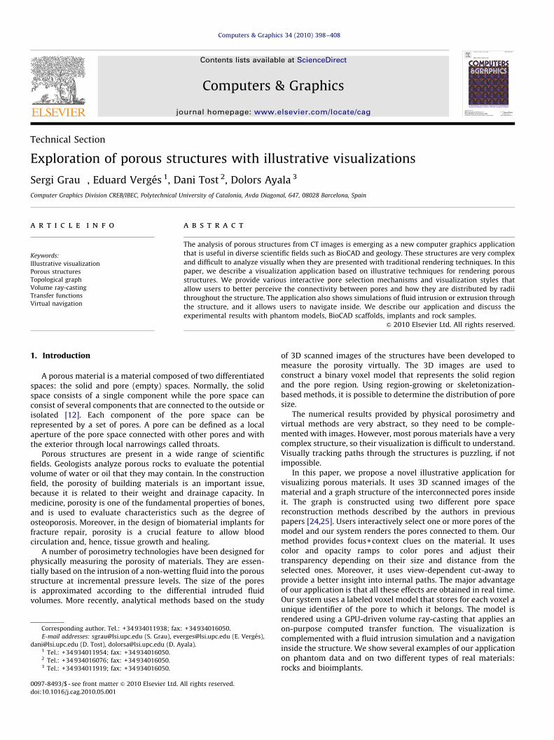
� pore-size distribution.
Mercury intrusion porosimetry is a physical experiment thatcomputes the effective porosity and estimates the pore-sizedistribution of the pore space part connected to the outside. Itinjects mercury at incremental pressures into the samples, inwardsfrom the outside in all directions, and it computes the differentialintruded volumes. Each connected region filled in one iteration isconsidered as being one cylindrical pore with the radius of theintrusion throat. The Washburn equation relates each pressurewith the corresponding radius [10]. The results are shown as acurve with the pore radii in the x-axis and the differential volumein the y-axis. Fig. 1 shows an example of such a curve for asedimentary rock sample. Generally, scientists pay attention to thepeak of the curve which indicates the pore size corresponding tothe maximum amount of the pore space volume. However, themain drawbacks of this physical method are that it does notprovide clues on the internal distribution of the pores and that itdoes not measure the pore space not connected to the outside.

In the last 10 years the quantification of structural properties ofporous structures from CT scanned images has emerged as a validexperimental approach complementary to traditional physicalmeasurements. Given the CT images, a 3D voxel model isconstructed. The global porosity of the materials is then computedby simple empty cell counting [23]. In order to compute the

. 1. Output curve of mercury intrusion porosimetry for the bioimplant foam

aset.

effective porosity, the pore space is divided into connectedcomponents. Moreover, to evaluate the radial distribution of pores,several approaches simulate mercury intrusion porosimetry[10,19,24]. Some methods are based on fitting non-overlappingspheres into the pore region [7,25], while others perform successivemorphological openings [27,8]. Some also reconstruct the porespace topology as a pore connectivity graph [10,7,19,24,25].

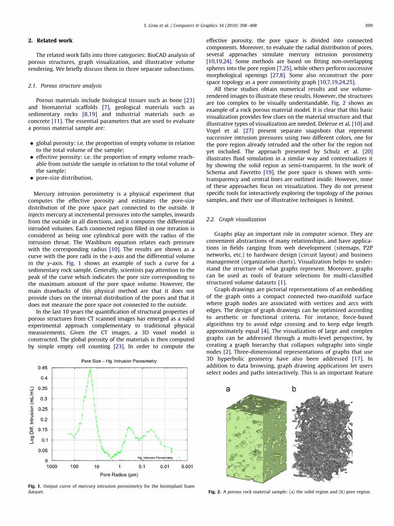
All these studies obtain numerical results and use volume-rendered images to illustrate these results. However, the structuresare too complex to be visually understandable. Fig. 2 shows anexample of a rock porous material model. It is clear that this basicvisualization provides few clues on the material structure and thatillustrative types of visualization are needed. Delerue et al. [10] andVogel et al. [27] present separate snapshots that representsuccessive intrusion pressures using two different colors, one forthe pore region already intruded and the other for the region notyet included. The approach presented by Schulz et al. [20]illustrates fluid simulation in a similar way and contextualizes itby showing the solid region as semi-transparent. In the work ofSchema and Favretto [19], the pore space is shown with semi-transparency and central lines are outlined inside. However, noneof these approaches focus on visualization. They do not presentspecific tools for interactively exploring the topology of the poroussamples, and their use of illustrative techniques is limited.

2.2. Graph visualization

Graphs play an important role in computer science. They areconvenient abstractions of many relationships, and have applica-tions in fields ranging from web development (sitemaps, P2Pnetworks, etc.) to hardware design (circuit layout) and businessmanagement (organization charts). Visualization helps to under-stand the structure of what graphs represent. Moreover, graphscan be used as tools of feature selections for multi-classifiedstructured volume datasets [1].

Graph drawings are pictorial representations of an embeddingof the graph onto a compact connected two-manifold surfacewhere graph nodes are associated with vertices and arcs withedges. The design of graph drawings can be optimized accordingto aesthetic or functional criteria. For instance, force-basedalgorithms try to avoid edge crossing and to keep edge lengthapproximately equal [4]. The visualization of large and complexgraphs can be addressed through a multi-level perspective, bycreating a graph hierarchy that collapses subgraphs into singlenodes [2]. Three-dimensional representations of graphs that use3D hyperbolic geometry have also been addressed [17]. Inaddition to data browsing, graph drawing applications let usersselect nodes and paths interactively. This is an important feature

Fig. 2. A porous rock material sample: (a) the solid region and (b) pore region.

S. Grau et al. / Computers & Graphics 34 (2010) 398–408400

of these applications since it allows users to focus on relevantparts of the graph.

Although, as mentioned in Section 2.1, several pore analysismethods compute the topological graph of pore connectivity, theydo not use it to illustrate the pore space structure. This is becausethe pore graph is very complex and lacks semantic attributes.Pores have no characteristics other than their radius and location.Therefore, it is very difficult—if not impossible—for users toidentify pores in a graph visualization. As an example, thebioimplant sample that we use in the results section has morethan 140 000 nodes and 600 000 edges with an average number of8.7 edges per node.

2.3. Illustrative volume rendering

Recently, more attention has been given to the visual quality ofvolume rendering, not only to add aesthetic value but also toimprove its illustrative potential, i.e. the quantification andquality of information it can convey. Weiskopf et al. [28] propose3D texture-based cut-away techniques to eliminate non-relevantstructures of the volume. Bruckner et al. [6] generate explodedviews of a volume, allowing a visual analysis of all structureswithout occlusions. Rezk-Salama and Kolb [18] and Bruckner et al.[5] perform ghosting effects by showing less relevant features asmore transparent and important features as more opaque. Othereffects such as contour enhancement [9] and using differentshading and rendering styles [26,15,16] have also been success-fully implemented. Recently, the use of multidimensional transferfunctions to classify and illustrate the presence of features inindustrial CT data for non-destructive testing has been proposed.The domain of these transfer functions can be density and featuresize, among others, and features can be explored using specificwidgets [14]. This method is also applied to analyze fiberorientation in concrete samples and form, size and nodularity ofgraphite particles in ductile iron [11].

3. Pipeline overview

The input data are a stack of image slices of the structure. Inour simulations, we have used micro-computed tomographyðmCTÞ images. The visualization of the tagged volume is donewith a GPU-driven volume ray-casting [21]. The pipelinebegins with a data pre-processing which consists of the followingsteps:

�
Segmentation. � Pore space modeling.
After pre-processing, the visualization application uses thetagged voxel model and the graph. It consists of three steps:

�
Pore selection. � Graph connectivity exploration. � Illustrative visualization in one of the following three modes:
3 Direct volume rendering.3 Intrusion simulation.3 Fly-through navigation.

4. Pore space modeling

We deal with samples that are totally internal to the material,so there is no external region in the voxel model. Therefore,after the segmentation, the binarized voxel model represents the

solid region (1-valued voxels) and the pore region (0-valuedvoxels).

The graph construction step performs a partition of the poreregion. The pore graph is such that the node set represents thepores and the edge set the connectivity relationship betweenthem. We create an edge between two pores when these pores are26-connected. The graph is non-directed and it can have cyclesand disconnected components.

In order to construct the graph structure, we apply twomethods described in the previous papers: the virtual porosimeter

(VP) [24] and the pore topology tracker (PTT) [25]. The VP methodsimulates physical mercury intrusion porosimetry. It floods thepore region iteratively using increasing pressure levels, i.e.decreasing intrusion radii. The results of this method arecomparable with those of the physical one, but it has the sametwo drawbacks: it only detects pores connected to the externalsurface, and it does not compute the actual pore shape after thethroat. The PTT method computes the pores as unions anddifferences of adjacent maximal balls of the pore region, satisfyinga set of criteria related to their shape. Depending on theparameters that regulate these criteria, adjacent pores arecollapsed as one. This method settles the former method draw-backs, but its results are not comparable to those obtained withmercury intrusion porosimetry. Therefore, we use both methods.The computed graph stores, for each node, the center, radius,volume and surface of the corresponding pore. For VP the storedradius corresponds to the intrusion throat and for PTT itcorresponds to the radius of the largest maximal ball inscribedin the pore. In both cases, the pore center is approximated as thecenter of the pore’s bounding box.

The tagged volume is computed within the graph construction.It substitutes the binary model. It associates to each voxel aunique value: the solid region identifier if the voxel belongs to thesolid region, or a pore identifier. Pore identifiers are unique andthey can be used to fetch the corresponding nodes of the graph.The tagged volume requires log2(np+1) bits to codify an identifier,np being the number of pores.

5. Pore selection

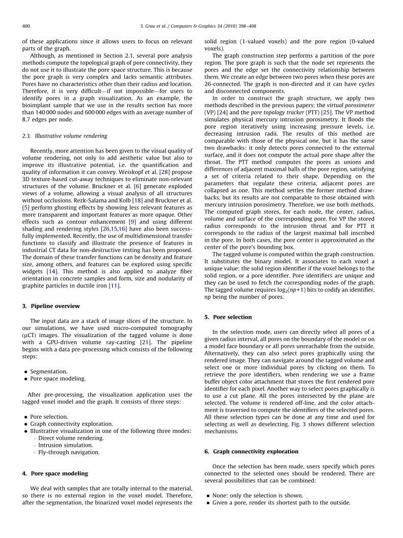
In the selection mode, users can directly select all pores of agiven radius interval, all pores on the boundary of the model or ona model face boundary or all pores unreachable from the outside.Alternatively, they can also select pores graphically using therendered image. They can navigate around the tagged volume andselect one or more individual pores by clicking on them. Toretrieve the pore identifiers, when rendering we use a framebuffer object color attachment that stores the first rendered poreidentifier for each pixel. Another way to select pores graphically isto use a cut plane. All the pores intersected by the plane areselected. The volume is rendered off-line, and the color attach-ment is traversed to compute the identifiers of the selected pores.All these selection types can be done at any time and used forselecting as well as deselecting. Fig. 3 shows different selectionmechanisms.

6. Graph connectivity exploration

Once the selection has been made, users specify which poresconnected to the selected ones should be rendered. There areseveral possibilities that can be combined:

�
None: only the selection is shown. � Given a pore, render its shortest path to the outside.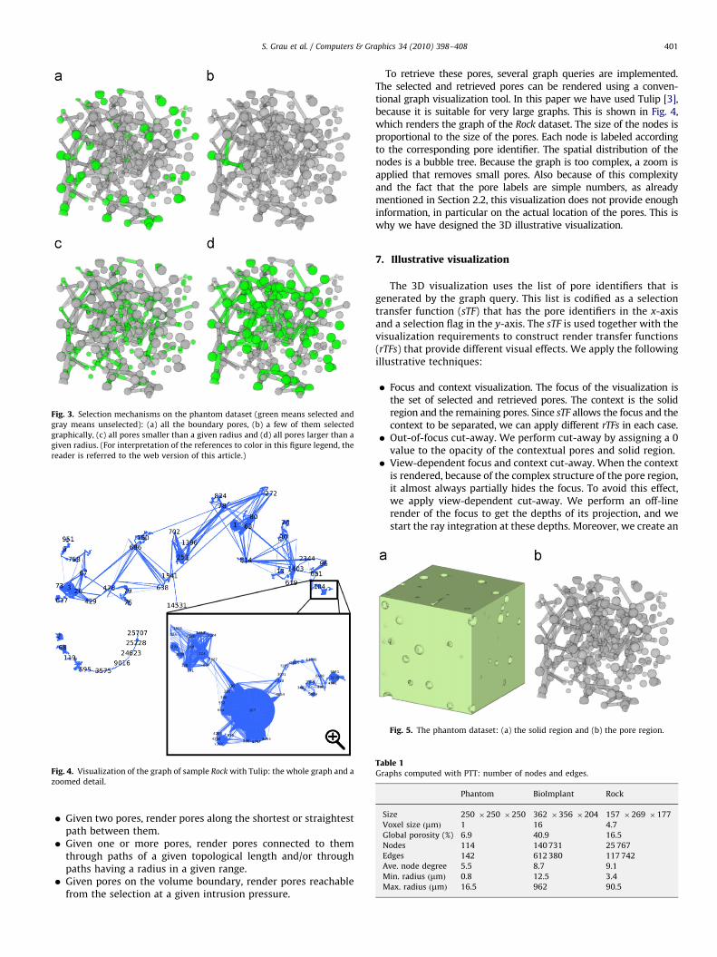

Fig. 5. The phantom dataset: (a) the solid region and (b) the pore region.

Table 1Graphs computed with PTT: number of nodes and edges.

Phantom BioImplant Rock

Size 250 �250 �250 362 �356 �204 157 �269 �177

Fig. 4. Visualization of the graph of sample Rock with Tulip: the whole graph and a

zoomed detail.

Fig. 3. Selection mechanisms on the phantom dataset (green means selected and

gray means unselected): (a) all the boundary pores, (b) a few of them selected

graphically, (c) all pores smaller than a given radius and (d) all pores larger than a

given radius. (For interpretation of the references to color in this figure legend, the

reader is referred to the web version of this article.)


�
Voxel size ðmmÞ 1 16 4.7
Global porosity (%) 6.9 40.9 16.5

Given two pores, render pores along the shortest or straightestpath between them.

Nodes 114 140 731 25 767
� Edges 142 612 380 117 742
Ave. node degree 5.5 8.7 9.1

Given one or more pores, render pores connected to themthrough paths of a given topological length and/or throughpaths having a radius in a given range.

Min. radius ðmmÞ 0.8 12.5 3.4
�
Max. radius ðmmÞ 16.5 962 90.5
Given pores on the volume boundary, render pores reachablefrom the selection at a given intrusion pressure.
To retrieve these pores, several graph queries are implemented.The selected and retrieved pores can be rendered using a conven-tional graph visualization tool. In this paper we have used Tulip [3],because it is suitable for very large graphs. This is shown in Fig. 4,which renders the graph of the Rock dataset. The size of the nodes isproportional to the size of the pores. Each node is labeled accordingto the corresponding pore identifier. The spatial distribution of thenodes is a bubble tree. Because the graph is too complex, a zoom isapplied that removes small pores. Also because of this complexityand the fact that the pore labels are simple numbers, as alreadymentioned in Section 2.2, this visualization does not provide enoughinformation, in particular on the actual location of the pores. This iswhy we have designed the 3D illustrative visualization.

7. Illustrative visualization

The 3D visualization uses the list of pore identifiers that isgenerated by the graph query. This list is codified as a selectiontransfer function (sTF) that has the pore identifiers in the x-axisand a selection flag in the y-axis. The sTF is used together with thevisualization requirements to construct render transfer functions(rTFs) that provide different visual effects. We apply the followingillustrative techniques:

�
Focus and context visualization. The focus of the visualization isthe set of selected and retrieved pores. The context is the solidregion and the remaining pores. Since sTF allows the focus and thecontext to be separated, we can apply different rTFs in each case. � Out-of-focus cut-away. We perform cut-away by assigning a 0
value to the opacity of the contextual pores and solid region.
� View-dependent focus and context cut-away. When the context
is rendered, because of the complex structure of the pore region,it almost always partially hides the focus. To avoid this effect,we apply view-dependent cut-away. We perform an off-linerender of the focus to get the depths of its projection, and westart the ray integration at these depths. Moreover, we create an

Fig(c)

colo


opening of a user-specified width around the focus projection inwhich we interpolate the ray-integration starting point in orderto produce the effect of a view-dependent conical cut-away[13]. Optionally, silhouette edges can be drawn to provide moredepth clues. In addition, we can apply Phong shading to outlinethe shape of the cut-surface (see Fig. 11). Shading can bedisabled to outline the removed region (see Fig. 12).
� Ghosting. We obtain ghosting effects on the focused pores by
assigning to them an opacity inversely proportional to one oftheir characteristics: radius, topological distance to outside,intrusion step and topological distance to another pore. Tomake the opacity dependent only on the pore identifier andnot on the length of the ray through the pore, once the rayenters a pore, we calculate its contribution to the intensityonly once until it exits from the interval.
� Color ramps: The application defines a temperature color ramp
from blue to red to indicate some pore features according tothe visualization query (radii and distances).

We next describe how these techniques are used in thedifferent visualization queries. For clarity, we use a phantomdataset with a reduced number of pores to illustrate theexplanations. Fig. 5 shows a visualization of the phantomdataset. Its characteristics are summarized in Table 1. Results ofreal samples are shown and discussed in Section 8.

Fig. 7. Use of the color ramp with opacity ghosting in the connectivity exploration

of the phantom dataset: maximum connectivity length of 43. (For interpretation of

the references to color in this figure legend, the reader is referred to the web

version of this article.)

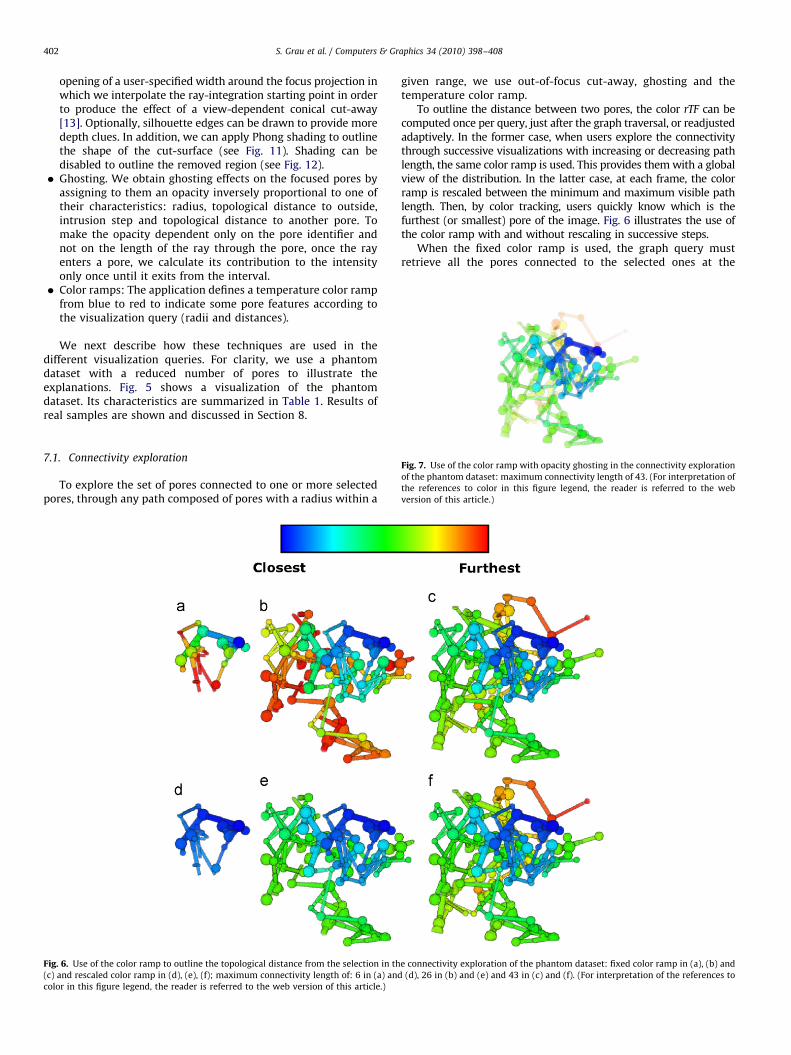
7.1. Connectivity exploration

To explore the set of pores connected to one or more selectedpores, through any path composed of pores with a radius within a

. 6. Use of the color ramp to outline the topological distance from the selection in th

and rescaled color ramp in (d), (e), (f); maximum connectivity length of: 6 in (a) and

r in this figure legend, the reader is referred to the web version of this article.)

given range, we use out-of-focus cut-away, ghosting and thetemperature color ramp.

To outline the distance between two pores, the color rTF can becomputed once per query, just after the graph traversal, or readjustedadaptively. In the former case, when users explore the connectivitythrough successive visualizations with increasing or decreasing pathlength, the same color ramp is used. This provides them with a globalview of the distribution. In the latter case, at each frame, the colorramp is rescaled between the minimum and maximum visible pathlength. Then, by color tracking, users quickly know which is thefurthest (or smallest) pore of the image. Fig. 6 illustrates the use ofthe color ramp with and without rescaling in successive steps.

When the fixed color ramp is used, the graph query mustretrieve all the pores connected to the selected ones at the

e connectivity exploration of the phantom dataset: fixed color ramp in (a), (b) and

(d), 26 in (b) and (e) and 43 in (c) and (f). (For interpretation of the references to


beginning. When users modify the maximum distance that theywant to explore, only the opacity rTF is modified. Therefore, with apath length dist of 1, only the selected pore is rendered. As thelength increases, more pores are made visible. Obviously, if theselection changes, a new graph query must be done.

In both cases, in order to provide ghosting effects, the opacityof the visible pores is computed by assigning to them an opacityinversely proportional to their topological distance from theselected pores. The further a pore is from the selection, the moretransparent it is rendered. This is shown in Fig. 7, whichcorresponds to same query as Fig. 6(f) but using ghosting. Ascan be seen in Fig. 7, the nearest pores are better outlined.

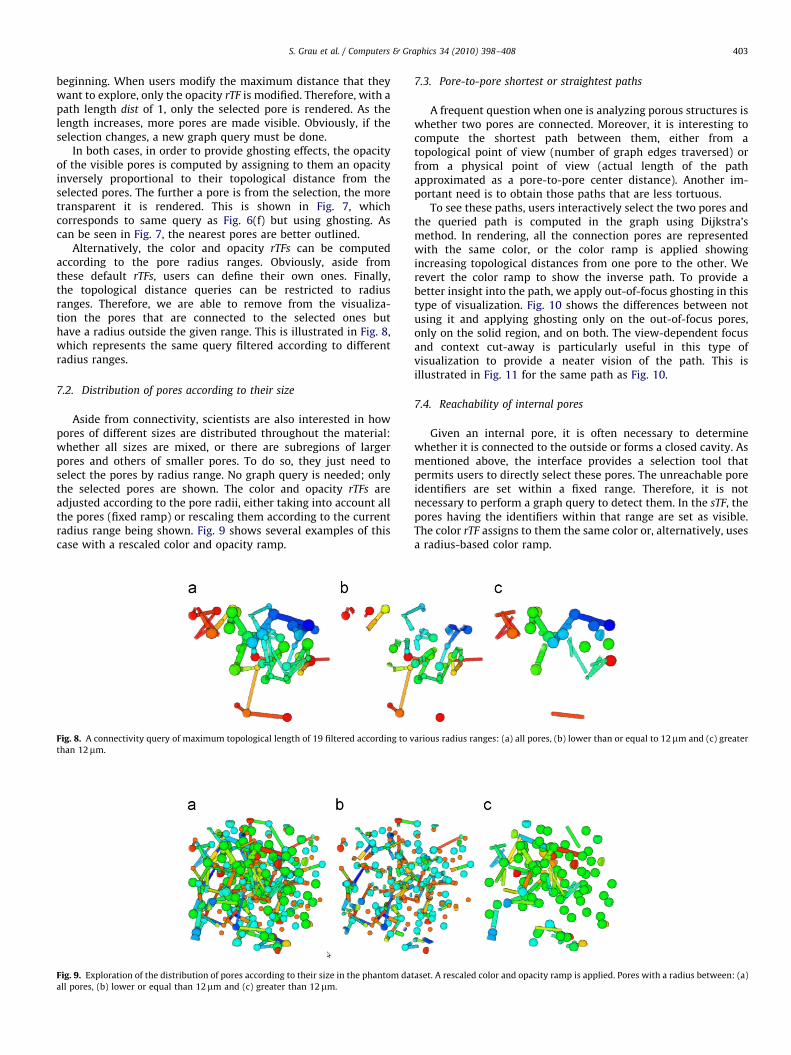
Alternatively, the color and opacity rTFs can be computedaccording to the pore radius ranges. Obviously, aside fromthese default rTFs, users can define their own ones. Finally,the topological distance queries can be restricted to radiusranges. Therefore, we are able to remove from the visualiza-tion the pores that are connected to the selected ones buthave a radius outside the given range. This is illustrated in Fig. 8,which represents the same query filtered according to differentradius ranges.

7.2. Distribution of pores according to their size

Aside from connectivity, scientists are also interested in howpores of different sizes are distributed throughout the material:whether all sizes are mixed, or there are subregions of largerpores and others of smaller pores. To do so, they just need toselect the pores by radius range. No graph query is needed; onlythe selected pores are shown. The color and opacity rTFs areadjusted according to the pore radii, either taking into account allthe pores (fixed ramp) or rescaling them according to the currentradius range being shown. Fig. 9 shows several examples of thiscase with a rescaled color and opacity ramp.

Fig. 9. Exploration of the distribution of pores according to their size in the phantom dat

all pores, (b) lower or equal than 12mm and (c) greater than 12mm.

Fig. 8. A connectivity query of maximum topological length of 19 filtered according to v

than 12mm.

7.3. Pore-to-pore shortest or straightest paths

A frequent question when one is analyzing porous structures iswhether two pores are connected. Moreover, it is interesting tocompute the shortest path between them, either from atopological point of view (number of graph edges traversed) orfrom a physical point of view (actual length of the pathapproximated as a pore-to-pore center distance). Another im-portant need is to obtain those paths that are less tortuous.

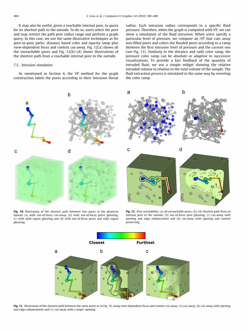
To see these paths, users interactively select the two pores andthe queried path is computed in the graph using Dijkstra’smethod. In rendering, all the connection pores are representedwith the same color, or the color ramp is applied showingincreasing topological distances from one pore to the other. Werevert the color ramp to show the inverse path. To provide abetter insight into the path, we apply out-of-focus ghosting in thistype of visualization. Fig. 10 shows the differences between notusing it and applying ghosting only on the out-of-focus pores,only on the solid region, and on both. The view-dependent focusand context cut-away is particularly useful in this type ofvisualization to provide a neater vision of the path. This isillustrated in Fig. 11 for the same path as Fig. 10.

7.4. Reachability of internal pores

Given an internal pore, it is often necessary to determinewhether it is connected to the outside or forms a closed cavity. Asmentioned above, the interface provides a selection tool thatpermits users to directly select these pores. The unreachable poreidentifiers are set within a fixed range. Therefore, it is notnecessary to perform a graph query to detect them. In the sTF, thepores having the identifiers within that range are set as visible.The color rTF assigns to them the same color or, alternatively, usesa radius-based color ramp.

aset. A rescaled color and opacity ramp is applied. Pores with a radius between: (a)

arious radius ranges: (a) all pores, (b) lower than or equal to 12mm and (c) greater


It may also be useful, given a reachable internal pore, to queryfor its shortest path to the outside. To do so, users select the poreand may restrict the path pore radius range and perform a graphquery. In this case, we use the same illustrative techniques as forpore-to-pore paths: distance based color and opacity ramp plusview-dependent focus and context cut-away. Fig. 12(a) shows allthe unreachable pores and Fig. 12(b)–(d) shows illustrations ofthe shortest path from a reachable internal pore to the outside.

7.5. Intrusion simulation

As mentioned in Section 4, the VP method for the graphconstruction labels the pores according to their intrusion throat

Fig. 11. Illustration of the shortest path between the same pores as in Fig. 10, using view

and edge enhancement and (c) cut-away with a larger opening.

Fig. 10. Illustration of the shortest path between two pores in the phantom

dataset (a) with out-of-focus cut-away, (b) with out-of-focus pores ghosting,

(c) with solid region ghosting and (d) with out-of-focus pores and solid region

ghosting.

radius. Each intrusion radius corresponds to a specific fluidpressure. Therefore, when the graph is computed with VP, we canshow a simulation of the fluid intrusion. When users specify aparticular level of pressure, we compute an rTF that cuts awaynon-filled pores and colors the flooded pores according to a rampbetween the first intrusive level of pressure and the current one(see Fig. 13). Similarly to the distance and radii color ramp, thepressure color ramp can be absolute or adaptive to successivevisualizations. To provide a fast feedback of the quantity ofintruded fluid, we use a simple widget showing the relativeintruded volume in relation to the total volume of the sample. Thefluid extraction process is simulated in the same way by revertingthe color ramp.

-dependent focus and context cut-away: (a) cut-away, (b) cut-away with opening

Fig. 12. Pore reachability: (a) all unreachable pores, (b)–(d) shortest path from an

internal pore to the outside, (b) out-of-focus pore ghosting, (c) cut-away with

opening and edge enhancement and (d) cut-away with opening and context

preserving.


7.6. Navigation

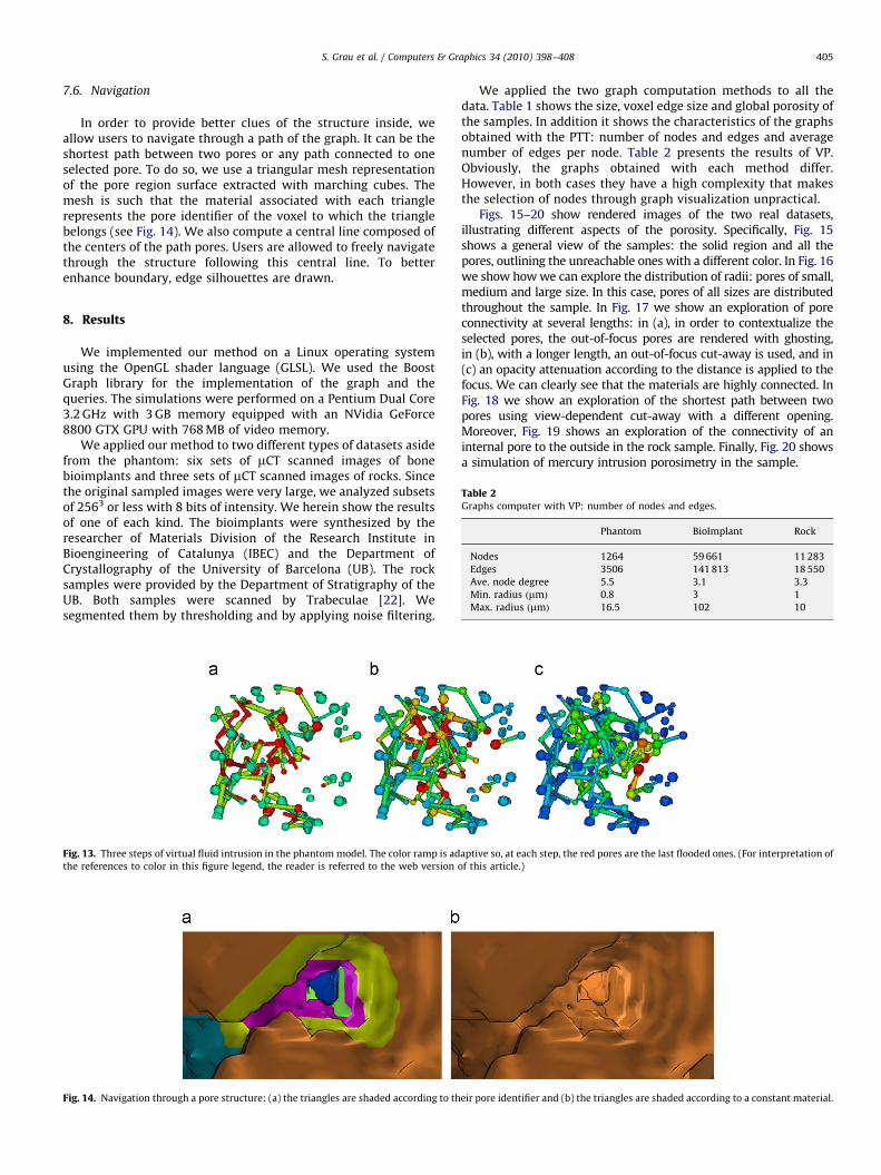
In order to provide better clues of the structure inside, weallow users to navigate through a path of the graph. It can be theshortest path between two pores or any path connected to oneselected pore. To do so, we use a triangular mesh representationof the pore region surface extracted with marching cubes. Themesh is such that the material associated with each trianglerepresents the pore identifier of the voxel to which the trianglebelongs (see Fig. 14). We also compute a central line composed ofthe centers of the path pores. Users are allowed to freely navigatethrough the structure following this central line. To betterenhance boundary, edge silhouettes are drawn.

Table 2Graphs computer with VP: number of nodes and edges.

Phantom BioImplant Rock

Nodes 1264 59 661 11 283

Edges 3506 141 813 18 550

Ave. node degree 5.5 3.1 3.3

Min. radius ðmmÞ 0.8 3 1

Max. radius ðmmÞ 16.5 102 10

8. Results

We implemented our method on a Linux operating systemusing the OpenGL shader language (GLSL). We used the BoostGraph library for the implementation of the graph and thequeries. The simulations were performed on a Pentium Dual Core3.2 GHz with 3 GB memory equipped with an NVidia GeForce8800 GTX GPU with 768 MB of video memory.

We applied our method to two different types of datasets asidefrom the phantom: six sets of mCT scanned images of bonebioimplants and three sets of mCT scanned images of rocks. Sincethe original sampled images were very large, we analyzed subsetsof 2563 or less with 8 bits of intensity. We herein show the resultsof one of each kind. The bioimplants were synthesized by theresearcher of Materials Division of the Research Institute inBioengineering of Catalunya (IBEC) and the Department ofCrystallography of the University of Barcelona (UB). The rocksamples were provided by the Department of Stratigraphy of theUB. Both samples were scanned by Trabeculae [22]. Wesegmented them by thresholding and by applying noise filtering.

Fig. 14. Navigation through a pore structure: (a) the triangles are shaded according to th

Fig. 13. Three steps of virtual fluid intrusion in the phantom model. The color ramp is ad

the references to color in this figure legend, the reader is referred to the web version o

We applied the two graph computation methods to all thedata. Table 1 shows the size, voxel edge size and global porosity ofthe samples. In addition it shows the characteristics of the graphsobtained with the PTT: number of nodes and edges and averagenumber of edges per node. Table 2 presents the results of VP.Obviously, the graphs obtained with each method differ.However, in both cases they have a high complexity that makesthe selection of nodes through graph visualization unpractical.

Figs. 15–20 show rendered images of the two real datasets,illustrating different aspects of the porosity. Specifically, Fig. 15shows a general view of the samples: the solid region and all thepores, outlining the unreachable ones with a different color. In Fig. 16we show how we can explore the distribution of radii: pores of small,medium and large size. In this case, pores of all sizes are distributedthroughout the sample. In Fig. 17 we show an exploration of poreconnectivity at several lengths: in (a), in order to contextualize theselected pores, the out-of-focus pores are rendered with ghosting,in (b), with a longer length, an out-of-focus cut-away is used, and in(c) an opacity attenuation according to the distance is applied to thefocus. We can clearly see that the materials are highly connected. InFig. 18 we show an exploration of the shortest path between twopores using view-dependent cut-away with a different opening.Moreover, Fig. 19 shows an exploration of the connectivity of aninternal pore to the outside in the rock sample. Finally, Fig. 20 showsa simulation of mercury intrusion porosimetry in the sample.

eir pore identifier and (b) the triangles are shaded according to a constant material.

aptive so, at each step, the red pores are the last flooded ones. (For interpretation of

f this article.)

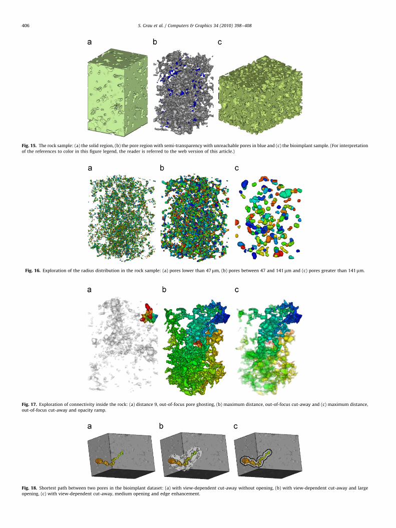
Fig. 17. Exploration of connectivity inside the rock: (a) distance 9, out-of-focus pore ghosting, (b) maximum distance, out-of-focus cut-away and (c) maximum distance,

out-of-focus cut-away and opacity ramp.

Fig. 18. Shortest path between two pores in the bioimplant dataset: (a) with view-dependent cut-away without opening, (b) with view-dependent cut-away and large

opening, (c) with view-dependent cut-away, medium opening and edge enhancement.

Fig. 16. Exploration of the radius distribution in the rock sample: (a) pores lower than 47mm, (b) pores between 47 and 141mm and (c) pores greater than 141mm.

Fig. 15. The rock sample: (a) the solid region, (b) the pore region with semi-transparency with unreachable pores in blue and (c) the bioimplant sample. (For interpretation

of the references to color in this figure legend, the reader is referred to the web version of this article.)


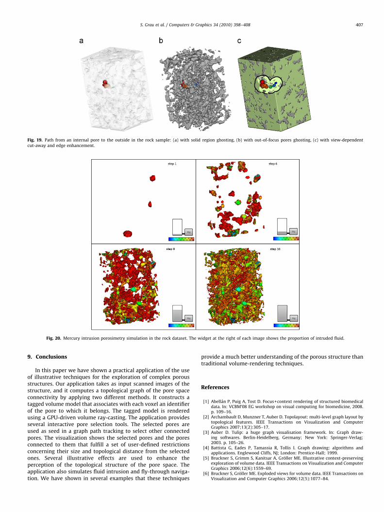
Fig. 20. Mercury intrusion porosimetry simulation in the rock dataset. The widget at the right of each image shows the proportion of intruded fluid.

Fig. 19. Path from an internal pore to the outside in the rock sample: (a) with solid region ghosting, (b) with out-of-focus pores ghosting, (c) with view-dependent

cut-away and edge enhancement.


9. Conclusions

In this paper we have shown a practical application of the useof illustrative techniques for the exploration of complex porousstructures. Our application takes as input scanned images of thestructure, and it computes a topological graph of the pore spaceconnectivity by applying two different methods. It constructs atagged volume model that associates with each voxel an identifierof the pore to which it belongs. The tagged model is renderedusing a GPU-driven volume ray-casting. The application providesseveral interactive pore selection tools. The selected pores areused as seed in a graph path tracking to select other connectedpores. The visualization shows the selected pores and the poresconnected to them that fulfill a set of user-defined restrictionsconcerning their size and topological distance from the selectedones. Several illustrative effects are used to enhance theperception of the topological structure of the pore space. Theapplication also simulates fluid intrusion and fly-through naviga-tion. We have shown in several examples that these techniques

provide a much better understanding of the porous structure thantraditional volume-rendering techniques.

References

[1] Abellan P, Puig A, Tost D. Focus+context rendering of structured biomedicaldata. In: VCBM’08 EG workshop on visual computing for biomedicine, 2008.p. 109–16.

[2] Archambault D, Munzner T, Auber D. Topolayout: multi-level graph layout bytopological features. IEEE Transactions on Visualization and ComputerGraphics 2007;13(2):305–17.

[3] Auber D. Tulip: a huge graph visualisation framework. In: Graph draw-ing softwares. Berlin-Heidelberg, Germany; New York: Springer-Verlag;2003. p. 105–26.

[4] Battista G, Eades P, Tamassia R, Tollis I. Graph drawing: algorithms andapplications. Englewood Cliffs, NJ; London: Prentice-Hall; 1999.

[5] Bruckner S, Grimm S, Kanitsar A, Groller ME. Illustrative context-preservingexploration of volume data. IEEE Transactions on Visualization and ComputerGraphics 2006;12(6):1559–69.

[6] Bruckner S, Groller ME. Exploded views for volume data. IEEE Transactions onVisualization and Computer Graphics 2006;12(5):1077–84.


[7] Cleynenbreugel TV. Porous scaffolds for the replacement of large bonedefects. A biomechanical design study. PhD thesis, Katholieke UniversiteitLeuven; 2005.

[8] Cnudde V, Cwirzen A, Maddchaele B, Jacobs PJS. Porosity and microstructurecharacterization of building stones and concretes. Engineering Geology2009;103:76–83.

[9] Csebfalvi B, Mroz L, Hauser H, Konig A, Groller E. Fast visualization of objectcontours by non-photorealistic volume rendering. Technical Report TR-186-2-01-09, ICGA, Vienna UTech; 2001.

[10] Delerue JF, Perrier E, Yu ZY, Velde B. New algorithms in 3D image analysis andtheir applications to the measurement of a spatialized pore size distributionin soils. Physics and Chemistry of the Earth 1999;24(7):639–44.

[11] Fritz L, Hardwiger M, Geier G, Pittino G, Groller M. A visual approach toefficient analysis and quantification of ductile iron and reinforced sprayedconcrete. IEEE Transactions on Visualization and Computer Graphics2009;15(6):1343–50.

[12] Garboczi EJ, Bentz DP, Martys NS. Digital images and computer modeling. In:Methods in the physics of porous media, vol. 35. New York; London; Orlando,FL (after 1984); Sydney, Australia: Academic Press; 1999. p. 1–41.

[13] Grau S, Puig A. An adaptive cut-away with volume context preservation. In:Advances in visual computing, 5th international symposium, ISVC 2009 (2)2009. p. 847–56.

[14] Hardwiger M, Fritz L, Rezk-Salama C, Hollt T, Geier G, Pabel T. Interactivevolume exploration for feature detection and quantification in industrial CT.IEEE Transactions on Visualization and Computer Graphics 2008;14(6):1507–14.

[15] Kruger J, Schneider J, Westermann R. Clearview: an interactive contextpreserving hotspot visualization technique. IEEE Transactions on Visualiza-tion and Computer Graphics 2006;12(5):1077–2626.

[16] Lu A, Morris C, Ebert D. Non-photorealistic volume rendering using stipplingtechniques. In: IEEE visualization. Washington, DC, USA: IEEE ComputerSociety; 2002. p. 211–8.

[17] Munzner T. Exploring large graphs in 3d hyperbolic space. IEEE ComputerGraphics and Applications 1998;18(4):18–23.

[18] Rezk-Salama C, Kolb A. Opacity peeling for direct volume rendering.Computer Graphics Forum 2006;25(3):597–606.

[19] Schema G, Favretto S. Pore space network characterization with sub-voxeldefinition. Transport in Porous Media 2007;70:181–90.

[20] Schulz WP, Becker J, Wiegmann A, Mukherjee PP, Wang C. Modeling of two-phase behavior in the gas diffusion medium of PEFCs via full morphologyapproach. Journal of the Electrochemical Society 2007;154(4):B419–26.

[21] Stegmaier S. A simple and flexible volume rendering framework for graphics-hardware-based raycasting. In: Groller E, Fujishiro I, editors. Volumegraphics; 2005. p. 187–95.

[22] /http://www.trabeculae.comS.[23] Vanis S, Rheinbach O, Klawonn A, Prymak O, Epple M. Numerical computa-

tion of the porosity of bone substitution materials from synchrotron microcomputer tomographic data. Materialwissenschaft und Werkstofftechnik2006;37(6):469–73.

[24] Verges E, Ayala D, Grau S, Tost D. Virtual porosimeter. Computer-AidedDesign and Applications 2008;5(1–4):557–64.

[25] Verges E, Ayala D, Grau S, Tost D. 3D reconstruction and quantification ofporous structures. Computers & Graphics 2008;32(4):438–44.

[26] Viola I, Kanitsar A, Groller ME. Importance-driven feature enhancement involume visualization. IEEE Transactions on Visualization and ComputerGraphics 2005;11(4):408–18.

[27] Vogel HJ, Tlke J, Schulz VP, Krafczyk M, Roth K. Comparison of a Lattice–Boltzmann model a full-morphology model and a pore network model fordetermining capillary pressure saturation relationships. Vadose Zone Journal2005;4:380–8.

[28] Weiskopf D, Engel K, Ertl T. Volume clipping via per-fragment operations intexture-based volume visualization. In: IEEE visualization. Washington, DC,USA: IEEE Computer Society; 2002. p. 93–100.

http://www.trabeculae.com

Documents

Exploration of porous structures with illustrative visualizations