Embed Size (px)
Citation preview
LICENTIATE THESIS
1996:01 L DIVISION OF ROCK MECHANICS
ISSN 0280 - 8242
ISRN HLU - TH - L -1996/1 - L - - SE
Experimental Study of the Mechanics
of Rock Joints
by
ULF LINDFORS
TEKNISKA HÖGSKOLAN I WLF.11
LULEÅ UNIVERSITY OF TECHNOLOGY
LICENTIATE THESIS 1996:lL
Experimental Study of the Mechanics of
Rock Joints
by
Ulf Lindfors
Division of Rock Mechanics
Lulea University of Technology
Lulea, Sweden
Lulea 1996

I
PREFACE
This thesis is a partial fulfilment for the degree of Technical Licentiate in the field of Rock Mechanics at the Luleå University of Technology. The research work presented here was done during the years 1993 to 1996.
The research presented in this thesis was financed by SKB (Swedish Nuclear Fuel and Waste Management CO.)
I would like to express my appreciation to my supervisor Dr. Erling Nordlund for
all his support, guidance and encouragement during these years. I also wish to thank Dr. Chunlin Li, Tech. Lic. Gunnar Rådberg and Tech. Lic. Jonny Sjöberg
for helpful comments and discussion throughout the work. Thanks are also extended to Mr Mats Billstein, Mr Peter Lundman and Mr Christian Jacobsson;
they all made this part of my life unforgettable.
The laboratory work has with great skill and care been performed by Ulf Mattila and Josef Forslund. Some of the drawings were made by Mrs Monica Leijon and the English language check was done by Meirion Hughes, thanks to all of you.
Further, I would like to thank all of the staff at the Division of Rock Mechanics and other persons who in some way helped me.
Finally, I extend my gratitude to my family who have supported me during all these years.
Luleå, April 1996
Ulf Lindfors
iii
ABSTRACT
The mechanics of rock joints determine to a large extent the behaviour of a jointed rock mass. It is therefore of vital importance to understand the mechanical behaviour of rock joints to be able to analyse the stability of rock slopes and underground excavations.
In this thesis a comprehensive experimental study of the mechanics of rock joints was done. Shear tests were performed on a number of joint samples with the same topography and this is achieved by using concrete replicas of a natural joint. The concrete mixture had relatively high uniaxial compressive strength, similar to weaker rocks such as sandstone and limestone. In these shear tests the normal load conditions and load paths were varied and the results from shear tests on replicas of a natural joint are presented.
Two main types of shear tests were performed, for five different normal stresses, cin = 0.5, 1, 2, 3, 4 MPa, called monotonic shear test and cyclic shear test
respectively. Also two different kinds of compressive tests were carried out to investigate the normal stress - normal displacement characteristics.
In the analysis of these tests, shear stress, dilation and surface degradation were determined for all tests. The connection between asperity size (or angle) and shear strength and dilation was studied and discussed and conclusions drawn.
In this thesis the equipment and procedures used for direct shear tests are described. The thesis also contains a review of methods available for characterisation of rock joints, existing methods for assessing the strength of rock joints and a description of different acoustic emission techniques.
Visual inspection and AE of the compressive tests showed that no damage to the joint surfaces was achieved due to normal loading. Therefore, all damage to the joint surfaces observed after a shear test must originate from the relative shear motion between the two opposite joint surfaces. The Coulomb and the empirical version of Ladanyi and Archambault shear strength criteria seem best to fit the shear strength behaviour in this case.
iv
From these shear tests it was found that the shear resistance and damage to the joint surface depends of four different mechanisms: dilation and climbing over asperities, breakage of asperities, transportation of gouge material and reattachment of gouge material. It is also indicated from the recorded AE that different failure modes occurred during the shear tests.
The work performed during the tests, the weight of the collected gouge material and the areas of the damaged zones showed that a large amount of gouge material is reattached at cyclic tests.
It is shown that the use of fractal geometry to describe the roughness of natural rock joint surfaces is questionable. One reason is that the calculation of fractal dimension requires a very high accuracy of the measuring device and this reduces the possibility to use fractal geometry in practical applications.
The parameters Z2, Z3 and asperity angles (a and arev) were determined at the
surface both before and after the shear test was performed. These parameters indicated that the joint surface becomes smoother as the normal stress increased. However, this trend changed as the normal stress was increased from 3.0 to 4.0 MPa. This occurs since a few larger pieces are tom off the surface during tests with normal stress equal to 4.0 MPa and this creates local failure surface with sharp edges (small and sharp asperities).
The residual tilt angles, determined from tilt tests of sheared surfaces, Z2, (slope) and asperity angles (a and arev) showed a similar dependency of an at low normal stress levels. This indicates that small asperities affect the shear strength and that Z2, (slope ) and asperity angles (a and arev) can be used to estimate shear strength at low normal stress levels.
The peak to peak amplitude is correlated to the residual tilt angle and it indicate that the peak to peak amplitude is a parameter which can be used to estimate the shear strength at low normal stress levels.
Keywords: Rock mechanics, mechanics of rock joints, damage to joint surfaces, joint surface roughness, failure criteria for rock joints.
V
NOTATIONS AND SYMBOLS
Notations and symbols are explained in the text when they first occur but a list is given below together with some important abbreviations.
Roman letters
A = Constant At = Total nominal area of the joint As = Area sheared through a = Constant as = Shear area ratio aL = Interception of log(L)-axis aN = Interception of log(N)-axis b = Constant bs = Slope of log-log plot of spectral density vs. spatial frequency C = Constant c = Cohesion Cp = Apparent cohesion D = Fractal dimension E = Young's modulus Ee = Energy Fu = Normal force Fs = Shear force
fs . Spatial frequency G = System gain g = Number of box grid divisions i = Asperity inclination angle iu = Inclination of large scale undulations JCS = Joint wall compressive strength JCS, = Joint wall compressive strength, field scale JCS() = Joint wall compressive strength, laboratory scale JRC = Joint Roughness Coefficient JRCn = Joint Roughness Coefficient, field scale JRC0 = Joint Roughness Coefficient, laboratory scale k = Constant kn = Normal stiffness of the joint
vi
= Shear stiffness of the joint
Akn° = Initial normal stiffness
Aksi,n = Maximum shear stiffness
= Total profile length L1 = Projection of the ascending part of the properties L(r) = Estimated profile length Ln = Field scale L0 = Laboratory scale AL = Incremental lengths
= Constant N = Number of boxes NE = Energy counts Rd = Schmidt rebound on dry unweathered saw surface R/ = Resistive load for the sensor rw = Schmidt rebound on wet joint surface
= Opening of dividers, x-increment or divider length S(cos) = Power spectral density T = Uniaxial tensile strength
TAE = Time of AE signal without background noise = Constant
tb = Time duration of the burst V = Peak voltage V(t) = Time dependent voltage output of the sensor
= Average rrns noise voltage un = Normal displacement us = Shear displacement Eun = Normal closure Au = Displacement Aus = Part of shear displacement
Aunm = Maximum closure of rock joint, initial joint aperture
Au/ = Individual joint deformation n
Autn = Total deformation
= Deformation of intact rock
tin = Dilation rate at failure = Previous shear displacement
VII
Axh = Digitising increment in the horizontal direction
Z2 = rms of the first derivative of the surface profile Z3 = rms of the second derivative of the surface profile Z4 = The sum of the distances along the profile where the slope is positive
minus the sum of the distances where the slope is negative, divided by the total profile distance
Greek letters
= Asperity angle in forward direction = Asperity angle in backward direction = Tilt (friction) angle = Diameter = Friction angle = Peak friction angle = Residual friction angle = Apparent peak friction angle = Apparent residual friction angle = Apparent reversal friction angle = Apparent reversal friction angle = Basic friction angle = Friction angle for a flat surface
= Statistical average value of friction angle
= Angular difference = Degree of interlocking = Wavelength = Poisson's ratio = Density = Major principal stress at failure = Minor principal stress at failure = Uniaxial compressive strength of solid rock = Normal stress = Effective normal stress = Uniaxial compressive strength of rock material adjacent to the
discontinuity = Shear strength = Components of total shear strength = Peak shear strength
a arev ß 0 $
Op
Or 43 a p
Oar
Orevi
Orev2
Ob
Oµ
0 f
I' 11 X
V
P
01 cs3
Ge
Gn
Gin G• .1
t
Il '14 't P
viii
Tr = Residual shear strength Tm = Shear strength of asperities (shear strength of intact material) Tap = Apparent peak shear strength
Tar = Apparent residual shear strength
trevl = Reversal shear strength
trev2 = Reversal shear strength
Ws = Spatial angular frequency
= Constant
Abbreviations
AE = Acoustic emission ASTM = American Society for Testing and Materials LuTH = Luleå University of Rock Mechanics LVDT = Linear Variable Differential Transformer PAC = Physical Acoustics Corporation SKB = Swedish Nuclear Fuel and Waste Management CO VCO = Voltage Controlled Oscillator MIS = Root mean square
ix
TABLE OF CONTENTS Page
PREFACE
ABSTRACT iii
NOTATIONS AND SYMBOLS
TABLE OF CONTENTS ix
1 INTRODUCTION 1
2 CHARACTERISATION OF SURFACE ROUGHNESS 3 2.1 General 3 2.2 Engineering descriptions of roughness 6 2.3 Descriptive statistics 8 2.4 Fractal dimension 10 2.5 Estimation of JRC using fractal geometry
and descriptive statistics 15
3 MECHANICAL PROPER 1 LES OF ROCK JOINTS 19 3.1 Existing theories for the strength of rock joints 19
3.1.1 Coulomb's criterion 19 3.1.2 Patton's criterion 20 3.1.3 Ladanyi and Archambault's shear strength criterion 22 3.1.4 Barton's criterion 26
3.2 Joint deformation properties 31 3.2.1 Normal deformation behaviour 31 3.2.2 Shear deformation behaviour 35
4 ACOUSTIC EMISSION (AE) AND FAILURE OF ROCK JOINTS 41 4.1 General 41 4.2 Key tenns in AE 42
x
4.3 Monitoring AE 45 4.4 AE signal characteristics 48
4.4.1 Counts 48 4.4.2 Events 49 4.4.3 Energy 49
4.5 Location 51
5 TEST SET-UP AND EXPERIMENTAL PROCEDURE 53 5.1 Sample preparation 53 5.2 Profile measurements 54 5.3 Test set-up for direct shear test 59 5.4 Shear test procedure 61 5.5 Compressive test procedure 63 5.6 Acoustic emission (AE) 63
6 EXPERIMENTAL RESULTS 69 6.1 Direct shear test 69
6.1.1 Deformation and strength 69 6.1.2 Damage to joint surfaces 77 6.1.3 Profile measurement 86
6.2 Acoustic emission 94 6.2.1 General 94 6.2.2 Location 94 6.2.3 Energy count rate 99
6.3 Compressive tests 104 6.3.1 General 104 6.3.2 Normal stiffness of the joint 104
7 ANALYSIS 107 7.1 Characterisation of joint roughness 107
7.1.1 Fractals 107 7.1.2 Z2, Z3 and Z4 110 7.1.3 Asperity angle 117 7.1.4 Peak to peak height of the surface 119
xi
7.2 Failure criteria for rock joints 122
7.2.1 Friction angles 122
7.2.2 Coulomb 125
7.2.3 Barton 126
7.2.4 Ladanyi and Archambault 127
7.3 Surface damage 130 7.3.1 The ratio of work and shear displacement 130 7.3.2 The ratio of work and damaged area 130 7.3.3 The ratio of work and weight of gouge material 132
8 DISCUSSION AND CONCLUSION 135
9 REI-LRENCES 143
APPENDICES 151
Appendix A: Shear stress - shear displacement curves, monotonic tests 152
Appendix B: Shear stress - shear displacement curves, cyclic tests 155
Appendix C: Normal displacement - shear displacement curves, monotonic tests 158
Appendix D: Normal displacement - shear displacement curves, cyclic tests 161

1
1 INTRODUCTION
A rock mass is not a homogeneous material, as it consists of both intact rock and discontinuities such as faults, shear zones, dykes, joints, bedding planes and fissures. The strength, deformability and hydraulic conductivity of the rock mass are strongly affected by the presence of joints and this results in a complex mechanical behaviour quite different from the corresponding intact rocks.
The stability of rock slopes and underground excavations in jointed rock masses, is affected by local discontinuities. Low stresses may permit gravitational sliding along discontinuities while high stresses may result in rock mass failure through sliding along discontinuities combined with failure of intact rock (rock bridges). In cases of extremely high stresses, rock bursts due to sliding along large scale discontinuities may occur.
Different ways to acquire knowledge of the rock mass behaviour are used in engineering, for example i) direct measurements of rock mass properties in the laboratory and in the field, ii) studies of failure case histories and iii) evaluation of the behaviour using physical or mathematical model techniques (Ladanyi and Archambault, 1980). To understand the behaviour, all three methods should be used, but a properly constructed numerical method can reduce testing requirements and costs. Therefore, to analyse and predict the mechanical behaviour of the rock mass surrounding engineering facilities, numerical methods are usually used.
Rock joints are usually rough surfaces with different scales of irregularities. The roughness and strength of the joint surfaces and the frictional resistance of the joint surface material are the characteristic properties of a rock joint. These parameters control the deformation, movement and breakage of asperities during normal compressive and shear loading sequences.
Many commercial programs available today require parameters such as friction angle and cohesion for modelling the behaviour of jointed rock masses. These parameters are normally determined from laboratory tests. Roughness and compressive strength of the joint surface are usually known since these parameters can be determined in the field. The parameters which describe the
2
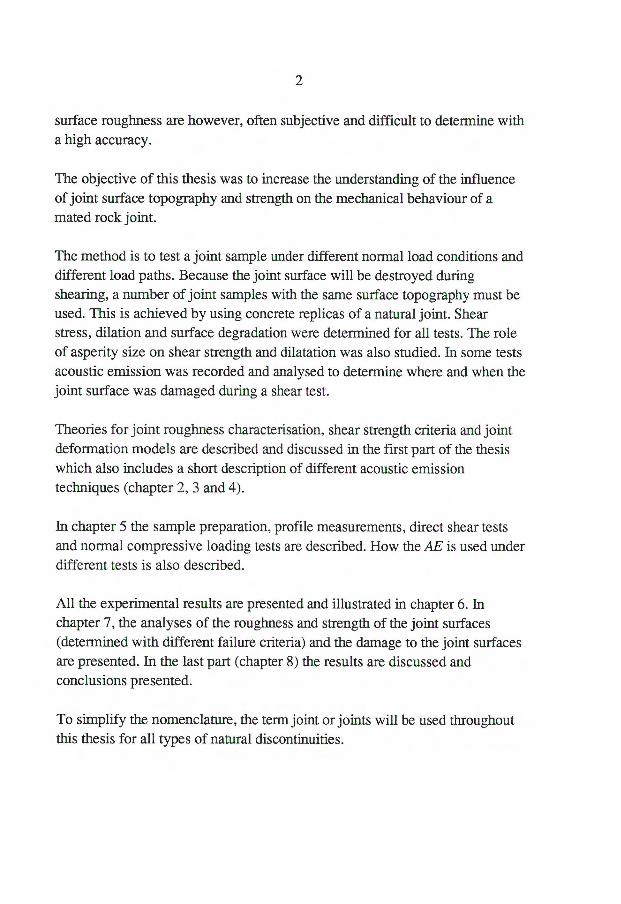
surface roughness are however, often subjective and difficult to determine with a high accuracy.
The objective of this thesis was to increase the understanding of the influence of joint surface topography and strength on the mechanical behaviour of a mated rock joint.
The method is to test a joint sample under different normal load conditions and different load paths. Because the joint surface will be destroyed during shearing, a number of joint samples with the same surface topography must be used. This is achieved by using concrete replicas of a natural joint. Shear stress, dilation and surface degradation were determined for all tests. The role of asperity size on shear strength and dilatation was also studied. In some tests acoustic emission was recorded and analysed to determine where and when the joint surface was damaged during a shear test.
Theories for joint roughness characterisation, shear strength criteria and joint deformation models are described and discussed in the first part of the thesis which also includes a short description of different acoustic emission techniques (chapter 2, 3 and 4).
In chapter 5 the sample preparation, profile measurements, direct shear tests and normal compressive loading tests are described. How the AE is used under different tests is also described.
All the experimental results are presented and illustrated in chapter 6. In chapter 7, the analyses of the roughness and strength of the joint surfaces (determined with different failure criteria) and the damage to the joint surfaces are presented. In the last part (chapter 8) the results are discussed and conclusions presented.
To simplify the nomenclature, the term joint or joints will be used throughout this thesis for all types of natural discontinuities.
3
2 CHARACTERISATION OF SURFACE ROUGHNESS
2.1 General
Surface roughness is very important from the point of view of such fundamental properties as friction, contact deformation, heat and electric current conduction, tightness of contact joints and positional accuracy. For this reason surface roughness has been a subject of experimental and theoretical investigations for many decades (Nowicki, 1985).
It is recognised that the roughness of rock joint surfaces is a factor which influences the development of dilation and as a consequence the strength and deformability of the joint (Patton, 1966). Relations between surface topography, aperture and fluid flow within joints are also well documented (Brown, 1987a; Tsang and Tsang, 1987; Wang et al., 1988).
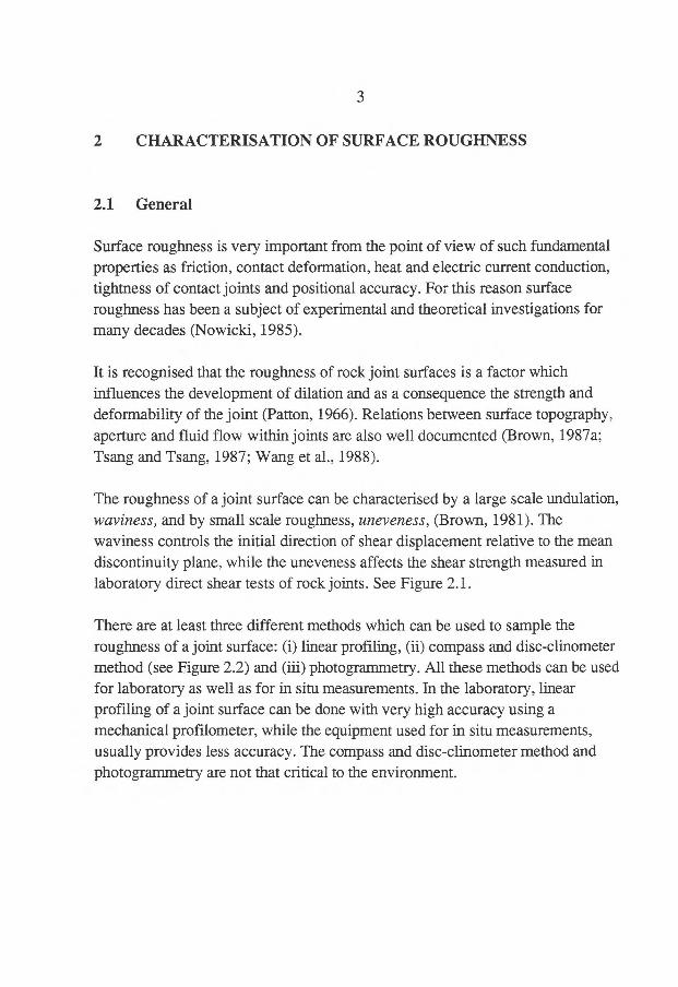
The roughness of a joint surface can be characterised by a large scale undulation, waviness, and by small scale roughness, uneveness, (Brown, 1981). The waviness controls the initial direction of shear displacement relative to the mean discontinuity plane, while the uneveness affects the shear strength measured in laboratory direct shear tests of rock joints. See Figure 2.1.
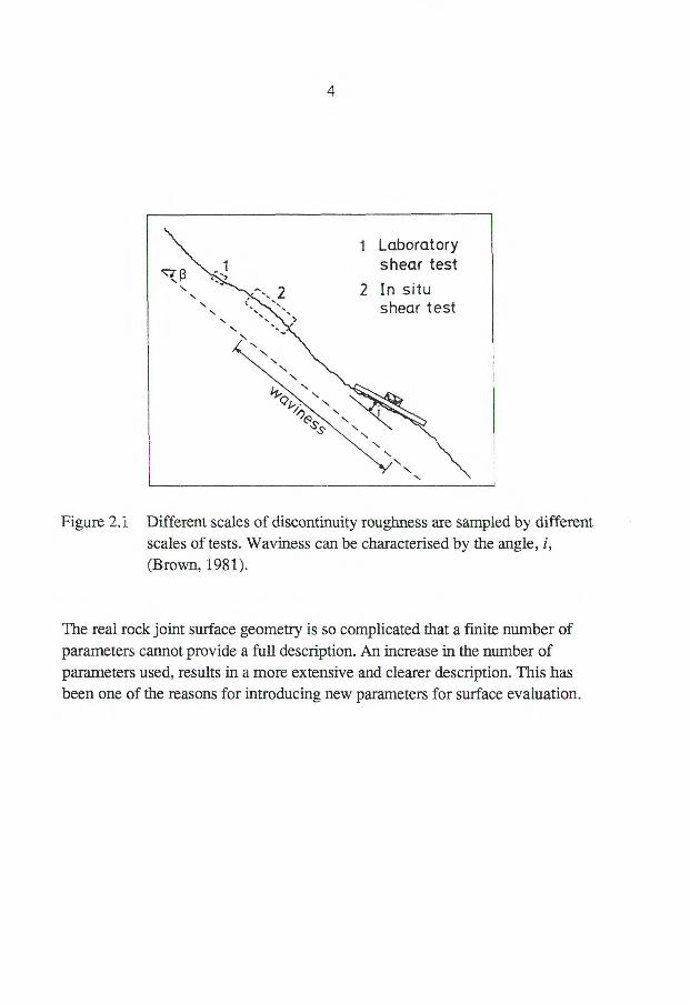
There are at least three different methods which can be used to sample the roughness of a joint surface: (i) linear profiling, (ii) compass and disc-clinometer method (see Figure 2.2) and (iii) photogrammetry. All these methods can be used for laboratory as well as for in situ measurements. In the laboratory, linear profiling of a joint surface can be done with very high accuracy using a mechanical profilometer, while the equipment used for in situ measurements, usually provides less accuracy. The compass and disc-clinometer method and photogrammetry are not that critical to the environment.
1 Laboratory shear test
2 In situ shear test
713
4
Figure 2.1 Different scales of discontinuity roughness are sampled by different scales of tests. Waviness can be characterised by the angle, i, (Brown, 1981).
The real rock joint surface geometry is so complicated that a finite number of parameters cannot provide a full description. An increase in the number of parameters used, results in a more extensive and clearer description. This has been one of the reasons for introducing new parameters for surface evaluation.
\ e.K I
i 2 Level bubble
Dip reading
Alloy disc Clar compass ,
, ,,, "4111I
40
20
0
-20 .....— 5 cm •---10 20 Direction of .----4o potential sliding -40
i III t 10 20 30 40 50 PLATE DIAMETER (cm)
_
-
5
Figure 2.2 A method of recording discontinuity roughness in three dimensions, for cases where the potential direction of sliding is not yet known. Circular discs of different dimensions are fixed in tum to a Clar
compass and clinometer. The dip direction and dip readings are plotted as poles on equal-area nets (Brown, 1981).
6
2.2 Engineering descriptions of roughness
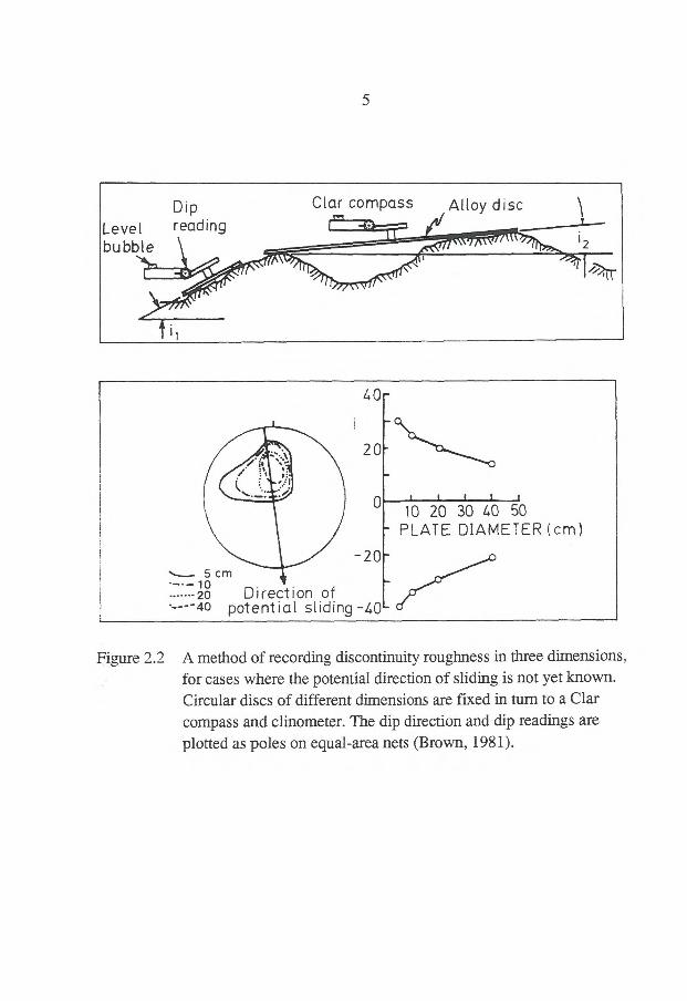
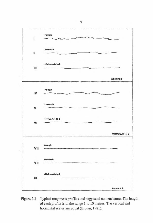
In the preliminary stages of field mapping time limitations may prevent the use of roughness measuring techniques. The descriptions of roughness will be limited to descriptive terms which should be based on two scales of observation (Brown, 1981), namely, a small scale (several centimetres) superimposed on an intermediate scale (several metres). The intermediate scale of roughness is divided into three degrees: stepped, undulating and planar and the small scale of roughness is also divided into three degrees: rough, smooth and slickensided. The direction of the striations or slickensides should be noted as shear strength may vary with direction. Roughness profiles typical of the nine classes are illustrated in Figure 2.3. According to Brown (1981), these nine classes also represent differences in shear strength such as the rough surface is stronger than the smooth which is stronger than the slickensided surface. If a large scale waviness is superimposed on the small and intermediate scales, these characteristics should also be noted, that is, smooth, undulating with large scale waviness x metre wavelength and y metre amplitude. In practice, the estimation of the critical joint roughness has often to be made from either limited and closed joint exposures in the field or joint surfaces in rock cores obtained from boreholes. The estimation of large scale joint roughness from small size joint profile measurements requires an established or accepted relation between joint size and roughness angle.
To date, joint roughness has been considered as a parameter that effectively increases the friction angle of a joint above the base friction angle, Ob, by some angle usually designated i (Patton, 1966). In fundamental terms, i, can be interpreted as the dilation of the joint during shearing. The value of i is not constant but gradually decreases with increasing shear displacement, except in idealised cases such as regular saw tooth joint profiles This makes the determination of the representative value of i for natural rock joints extremely difficult.
Barton and Choubey (1977) developed a peak shear strength criterion which included the influence of joint surface roughness. They used the quantity JRC (Joint Roughness Coefficient) to characterise the roughness. JRC can be estimated either by tilt, push or pull tests on rock samples or by visual comparison with a set of roughness profiles. More details of the criterion are presented in chapter 3.
rough
VII
smooth
VIII
slIckonsidod
Ix
PLANAR
7
rough
IV
smooth
V
slickonsIdod
VI
UNDULATING
Figure 2.3 Typical roughness profiles and suggested nomenclature. The length of each profile is in the range 1 to 10 metres. The vertical and horizontal scales are equal (Brown, 1981).
8
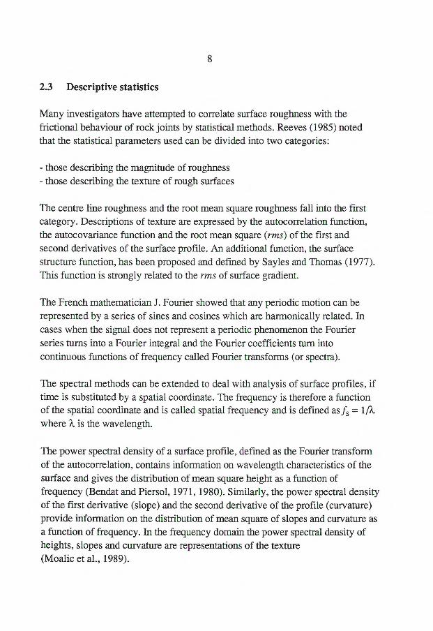
2.3 Descriptive statistics
Many investigators have attempted to correlate surface roughness with the frictional behaviour of rock joints by statistical methods. Reeves (1985) noted that the statistical parameters used can be divided into two categories:
- those describing the magnitude of roughness - those describing the texture of rough surfaces
The centre line roughness and the root mean square roughness fall into the first category. Descriptions of texture are expressed by the autocorrelation function, the autocovariance function and the root mean square (rms) of the first and second derivatives of the surface profile. An additional function, the surface structure function, has been proposed and defined by Sayles and Thomas (1977). This function is strongly related to the rms of surface gradient.
The French mathematician J. Fourier showed that any periodic motion can be represented by a series of sines and cosines which are harmonically related. In cases when the signal does not represent a periodic phenomenon the Fourier series turns into a Fourier integral and the Fourier coefficients turn into continuous functions of frequency called Fourier transforms (or spectra).
The spectral methods can be extended to deal with analysis of surface profiles, if time is substituted by a spatial coordinate. The frequency is therefore a function of the spatial coordinate and is called spatial frequency and is defined as fs = 1/X where X is the wavelength.
The power spectral density of a surface profile, defined as the Fourier transform of the autocorrelation, contains information on wavelength characteristics of the surface and gives the distribution of mean square height as a function of frequency (Bendat and Piersol, 1971, 1980). Similarly, the power spectral density of the first derivative (slope) and the second derivative of the profile (curvature) provide information on the distribution of mean square of slopes and curvature as a function of frequency. In the frequency domain the power spectral density of heights, slopes and curvature are representations of the texture (Moalic et al., 1989).
9
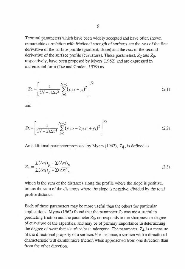
Textural parameters which have been widely accepted and have often shown remarkable correlation with frictional strength of surfaces are the rms of the first derivative of the surface profile (gradient, slope) and the rms of the second derivative of the surface profile (curvature). These parameters, Z2 and Z3, respectively, have been proposed by Myers (1962) and are expressed in incremental form (Tse and Cruden, 1979) as
N-1 1/2
(N— i1)&2 i=1
and
r 1 N-2 1/2
Z3 = [(N _ 2)Ax4 (Yi+2 2Yi+1 + yi)2 1=1
An additional parameter proposed by Myers (1962), Z4, is defined as
E(Axi) E(Axi)n Z4 = P
E(AXi)p ( AXi)n
which is the sum of the distances along the profile where the slope is positive, minus the sum of the distances where the slope is negative, divided by the total profile distance.
Each of these parameters may be more useful than the others for particular applications. Myers (1962) found that the parameter Z2 was most useful in predicting friction and the parameter Z3, corresponds to the sharpness or degree of curvature of the asperities, and may be of primary importance in determining the degree of wear that a surface has undergone. The parameter, Z4, is a measure of the directional property of a surface. For instance, a surface with a directional characteristic will exhibit more friction when approached from one direction than from the other direction.
Z2 = (Yi+1 Yi)21 (2.1)
(2.2)
(2.3)
10
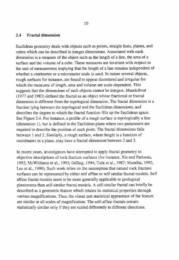
2.4 Fractal dimension
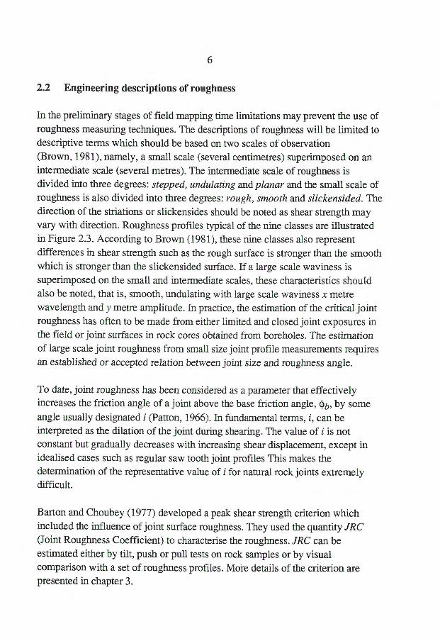
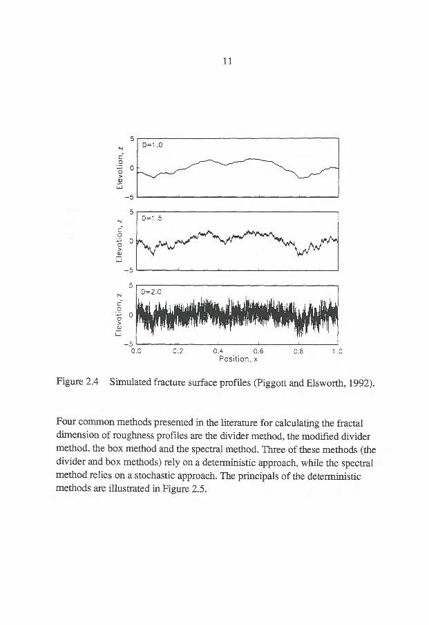
Euclidean geometry deals with objects such as points, straight lines, planes, and cubes which can be described in integer dimensions. Associated with each dimension is a measure of the object such as the length of a line, the area of a surface and the volume of a cube. These measures are invariant with respect to the unit of measurement implying that the length of a line remains independent of whether a centimetre or a micrometer scale is used. In nature several objects, rough surfaces for instance, are found to appear disordered and irregular for which the measures of length, area and volume are scale-dependent. This suggests that the dimensions of such objects cannot be integers. Mandelbrot (1977 and 1983) defined the fractal as an object whose fractional or fractal dimension is different from the topological dimension. The fractal dimension is a fraction lying between the topological and the Euclidean dimensions, and describes the degree to which the fractal function fills up the Euclidean space. See Figure 2.4. For instance, a profile of a rough surface is topologically a line (dimension 1), but is defined in the Euclidean plane where two parameters are required to describe the position of each point. The fractal dimensions falls between 1 and 2. Similarly, a rough surface, where height is a function of coordinates in a plane, may have a fractal dimension between 2 and 3.
In recent years, investigators have attempted to apply fractal geometry to objective descriptions of rock fracture surfaces (for instance, Xie and Pariseau, 1992; McWilliams et al., 1993; Odling, 1994; Turk et al., 1987; Muralha, 1992, Lee et al., 1990). Such work relies on the assumption that natural rock fracture surfaces can be represented by either self affme or self similar fractal models. Self affme fractal models seem to be more generally applicable to geological phenomena than self-similar fractal models. A self-similar fractal can briefly be described as a geometric feature which retains its statistical properties through various magnifications. Thus, the visual and statistical appearance of the feature are similar at all scales of magnification. The self-affine fractals remain statistically slinilar only if they are scaled differently in different directions.
5
-5
5 N
0
5
D=1.0
11
5 N
0 0
LTJ
5
D=2.0
00
0.2
OA 0.6
0.8 Position, x
Figure 2.4 Simulated fracture surface profiles (Piggott and Elsworth, 1992).
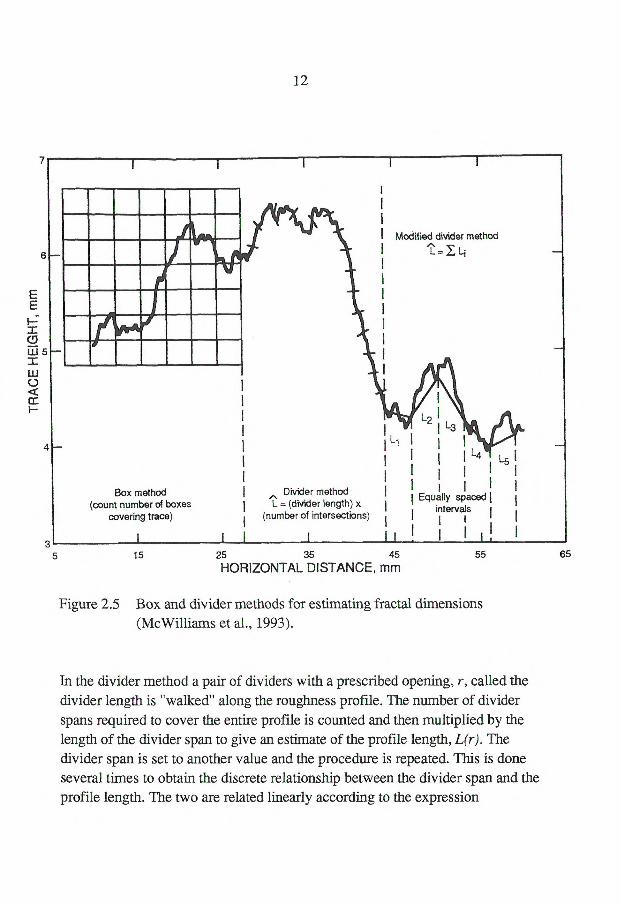
Four common methods presented in the literature for calculating the fractal dimension of roughness profiles are the divider method, the modified divider method, the box method and the spectral method. Three of these methods (the divider and box methods) rely on a deterministic approach, while the spectral method relies on a stochastic approach. The principals of the deterministic methods are illustrated in Figure 2.5.
1
L2 L3
7
6
4
3
Modified divider method
2, Li
Ll
Box method (count number of boxes
covering trace)
Divider method L = (divider length) x
(number of intersections)
I L4 1..5
I I I
Equally spaced intervals i I j
I I
12
5
15 25 35 45
55
65
HORIZONTAL DISTANCE, mm
Figure 2.5 Box and divider methods for estimating fractal dimensions (McWilliams et al., 1993).
In the divider method a pair of dividers with a prescribed opening, r, called the divider length is "walked" along the roughness profile. The number of divider spans required to cover the entire profile is counted and then multiplied by the length of the divider span to give an estimate of the profile length, L(r). The divider span is set to another value and the procedure is repeated. This is done several times to obtain the discrete relationship between the divider span and the profile length. The two are related linearly according to the expression
13
log(L) = aL+ (1 - D)log(r) (2.4)
where aL, is the intercept of the log(L)-axis.
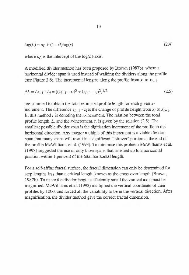
A modified divider method has been proposed by Brown (1987b), where a horizontal divider span is used instead of walking the dividers along the profile (see Figure 2.6). The incremental lengths along the profile from xi to xi+1,
AL = L1+1 - Li= [(xi+i - xi)2 (z1+1 - z)2]1/2
(2.5)
are summed to obtain the total estimated profile length for each given x-increment. The difference zi+ i - zi is the change of profile height from xi to xi+ i. In this method r is denoting the x-increment. The relation between the total profile length, L, and the x-increment, r, is given by the relation (2.5). The smallest possible divider span is the digitisation increment of the profile in the horizontal direction. Any integer multiple of this increment is a viable divider span, but many spans will result in a significant "leftover" portion at the end of the profile McWilliams et al. (1993). To minimise this problem McWilliams et al. (1993) suggested the use of only those spans that fmished up to a horizontal position within 1 per cent of the total horizontal length.
For a self-affine fractal surface, the fractal dimension can only be determined for step lengths less than a critical length, known as the cross-over length (Brown, 1987b). To make the divider length sufficiently small the vertical axis must be magnified. McWilliams et al. (1993) multiplied the vertical coordinate of their profiles by 1000, and forced all the variability to be in the vertical direction. After magnification, the divider method gave the correct fractal dimension.
E 1, I 5.0
a' 4.0 _c
Eir 3.5
3.0
Equa ly spaced intervals
HORZ.DISTANCE (mm)
4.00
3.90
3.60 BASALT TRACE A FR. DN.. 1.22. FR. leiT
LOG
(Lm
m)
3.80
3.70
14
3.50 -1 20 -0.80 -0.40 0.00 0.40 0.80
LOG(r.mm)
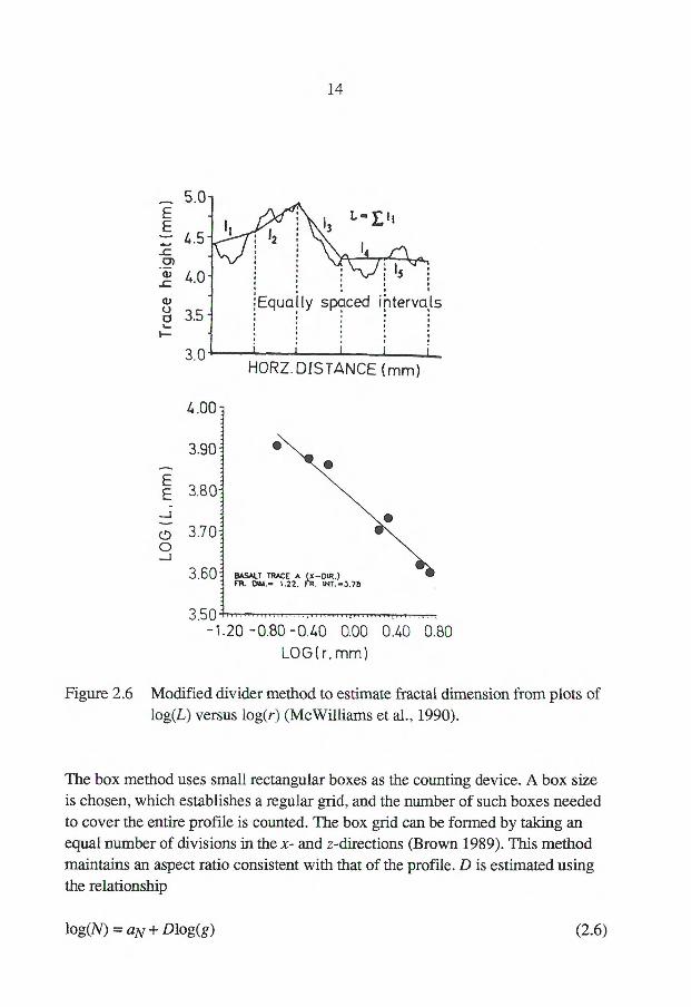
Figure 2.6 Modified divider method to estimate fiactal dimension from plots of log(L) versus log(r) (McWilliams et al., 1990).
The box method uses small rectangular boxes as the counting device. A box size is chosen, which establishes a regular grid, and the number of such boxes needed to cover the entire profile is counted. The box grid can be formed by taking an equal number of divisions in the x- and z-directions (Brown 1989). This method maintains an aspect ratio consistent with that of the profile. D is estimated using the relationship
log(N) = aN + Dlog(g) (2.6)
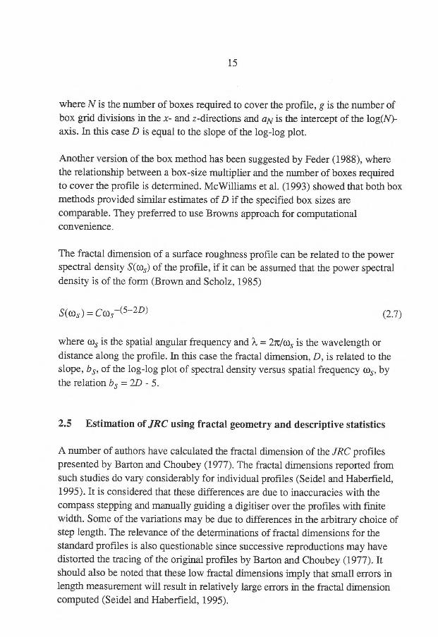
15
where N is the number of boxes required to cover the profile, g is the number of box grid divisions in the x- and z-directions and aN is the intercept of the log(N)-axis. In this case D is equal to the slope of the log-log plot.
Another version of the box method has been suggested by Feder (1988), where the relationship between a box-size multiplier and the number of boxes required to cover the profile is determined. McWilliams et al. (1993) showed that both box methods provided similar estimates of D if the specified box sizes are comparable. They preferred to use Browns approach for computational convenience.
The fractal dimension of a surface roughness profile can be related to the power spectral density S(cos) of the profile, if it can be assumed that the power spectral density is of the form (Brown and Scholz, 1985)
S(04)=C(os —(5-2D) (2.7)
where cos is the spatial angular frequency and X = 2n/cos is the wavelength or distance along the profile. In this case the fractal dimension, D, is related to the slope, bs, of the log-log plot of spectral density versus spatial frequency cos, by the relation bs = 2D - 5.
2.5 Estimation of JRC using fractal geometry and descriptive statistics
A number of authors have calculated the fractal dimension of the JRC profiles presented by Barton and Choubey (1977). The fractal dimensions reported from such studies do vary considerably for individual profiles (Seidel and Haberfield, 1995). It is considered that these differences are due to inaccuracies with the compass stepping and manually guiding a digitiser over the profiles with finite width. Some of the variations may be due to differences in the arbitrary choice of step length. The relevance of the determinations of fractal dimensions for the standard profiles is also questionable since successive reproductions may have distorted the tracing of the original profiles by Barton and Choubey (1977). It should also be noted that these low fractal dimensions imply that small errors in length measurement will result in relatively large errors in the fractal dimension computed (Seidel and Haberfield, 1995).
16
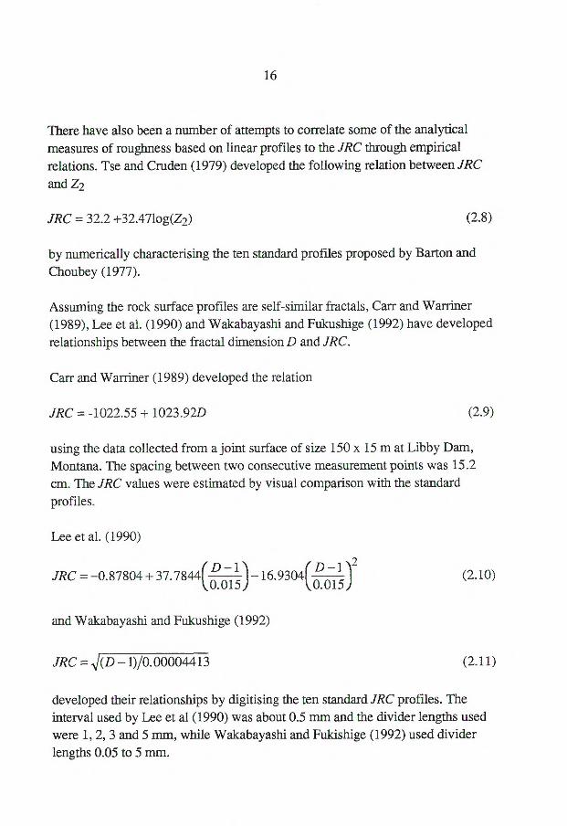
There have also been a number of attempts to correlate some of the analytical measures of roughness based on linear profiles to the JRC through empirical relations. Tse and Cruden (1979) developed the following relation between JRC and Z2
JRC = 32.2 +32.471og(Z2) (2.8)
by numerically characterising the ten standard profiles proposed by Barton and Choubey (1977).
Assuming the rock surface profiles are self-similar fractals, Carr and Warriner (1989), Lee et al. (1990) and Wakabayashi and Fukushige (1992) have developed relationships between the fractal dimension D and JRC.
Carr and Warriner (1989) developed the relation
JRC = -1022.55 + 1023.92D (2.9)
using the data collected from a joint surface of size 150 x 15 m at Libby Dam, Montana. The spacing between two consecutive measurement points was 15.2 cm. The JRC values were estimated by visual comparison with the standard profiles.
Lee et al. (1990)
2 JRC = —0.87804 +37.7844(01)m-115) 16.9304( D-1)
0.015
and Wakabayashi and Fukushige (1992)
JRC = —1)/0.00004413
(2.10)
(2.11)
developed their relationships by digitising the ten standard JRC profiles. The interval used by Lee et al (1990) was about 0.5 mm and the divider lengths used were 1, 2, 3 and 5 mm, while Wakabayashi and Fukishige (1992) used divider lengths 0.05 to 5 mm.
17
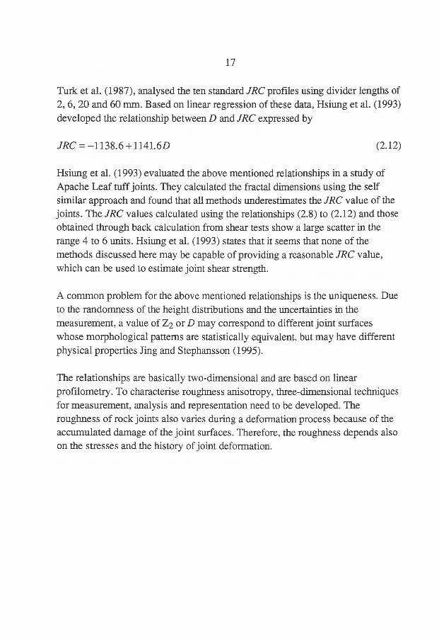
Turk et al. (1987), analysed the ten standard JRC profiles using divider lengths of 2, 6, 20 and 60 mm. Based on linear regression of these data, Hsiung et al. (1993) developed the relationship between D and JRC expressed by
JRC —1138.6 +1141.6D (2.12)
Hsiung et al. (1993) evaluated the above mentioned relationships in a study of Apache Leaf tuff joints. They calculated the fractal dimensions using the self similar approach and found that all methods underestimates the JRC value of the joints. The JRC values calculated using the relationships (2.8) to (2.12) and those obtained through back calculation from shear tests show a large scatter in the range 4 to 6 units. Hsiung et al. (1993) states that it seems that none of the methods discussed here may be capable of providing a reasonable JRC value, which can be used to estimate joint shear strength.
A common problem for the above mentioned relationships is the uniqueness. Due to the randomness of the height distributions and the uncertainties in the measurement, a value of Z2 or D may correspond to different joint surfaces whose morphological patterns are statistically equivalent, but may have different physical properties Jing and Stephansson (1995).
The relationships are basically two-dimensional and are based on linear profilometry. To characterise roughness anisotropy, three-dimensional techniques for measurement, analysis and representation need to be developed. The roughness of rock joints also varies during a deformation process because of the accumulated damage of the joint surfaces. Therefore, the roughness depends also on the stresses and the history of joint deformation.
19
3 MECHANICAL PROPERTIES OF ROCK JOINTS
3.1 Existing theories for the strength of rock joints
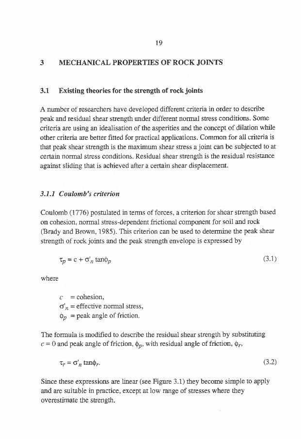
A number of researchers have developed different criteria in order to describe peak and residual shear strength under different normal stress conditions. Some criteria are using an idealisation of the asperities and the concept of dilation while other criteria are better fitted for practical applications. Common for all criteria is that peak shear strength is the maximum shear stress a joint can be subjected to at certain normal stress conditions. Residual shear strength is the residual resistance against sliding that is achieved after a certain shear displacement.
3.1.1 Coulomb's criterion
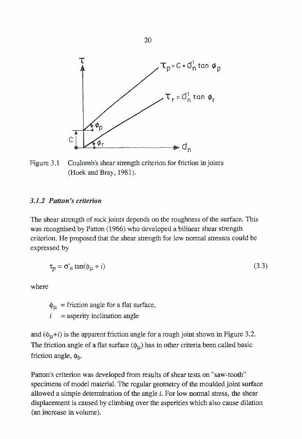
Coulomb (1776) postulated in terms of forces, a criterion for shear strength based on cohesion, normal stress-dependent frictional component for soil and rock (Brady and Brown, 1985). This criterion can be used to determine the peak shear strength of rock joints and the peak strength envelope is expressed by
tp = C ± 6'n tallOp (3.1)
where
c = cohesion, 6'n = effective normal stress,
= peak angle of friction.
The formula is modified to describe the residual shear strength by substituting c = 0 and peak angle of friction,4 with residual angle of friction, Or
Tr = 6'n tall$1)r. (3.2)
Since these expressions are linear (see Figure 3.1) they become simple to apply and are suitable in practice, except at low range of stresses where they overestimate the strength.
T =c+ci l tan 0 P n P
. d n' tan or
d,
20
Figure 3.1 Coulomb's shear strength criterion for friction in joints (Hoek and Bray, 1981).
3.1.2 Patton's criterion
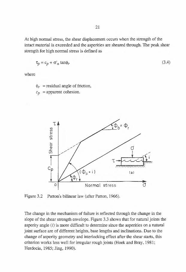
The shear strength of rock joints depends on the roughness of the surface. This was recognised by Patton (1966) who developed a bilinear shear strength criterion. He proposed that the shear strength for low normal stresses could be expressed by
tp = G'n tan(04 + i) (3.3)
where
04 = friction angle for a flat surface,
i = asperity inclination angle
and (04+i) is the apparent friction angle for a rough joint shown in Figure 3.2.
The friction angle of a flat surface (0) has in other criteria been called basic
friction angle, cp b.
Patton's criterion was developed from results of shear tests on "saw-tooth" specimens of model material. The regular geometry of the moulded joint surface allowed a simple determination of the angle i. For low normal stress, the shear displacement is caused by climbing over the asperities which also cause dilation (an increase in volume).
o Normal stress
I
Shear s
tre
ss
t cp
21
At high normal stress, the shear displacement occurs when the strength of the intact material is exceeded and the asperities are sheared through. The peak shear strength for high normal stress is defined as
tp 72 cp ± G'n tanOr (3.4)
where
.1)r = residual angle of friction, Cp = apparent cohesion.
Figure 3.2 Patton's bilinear law (after Patton, 1966).
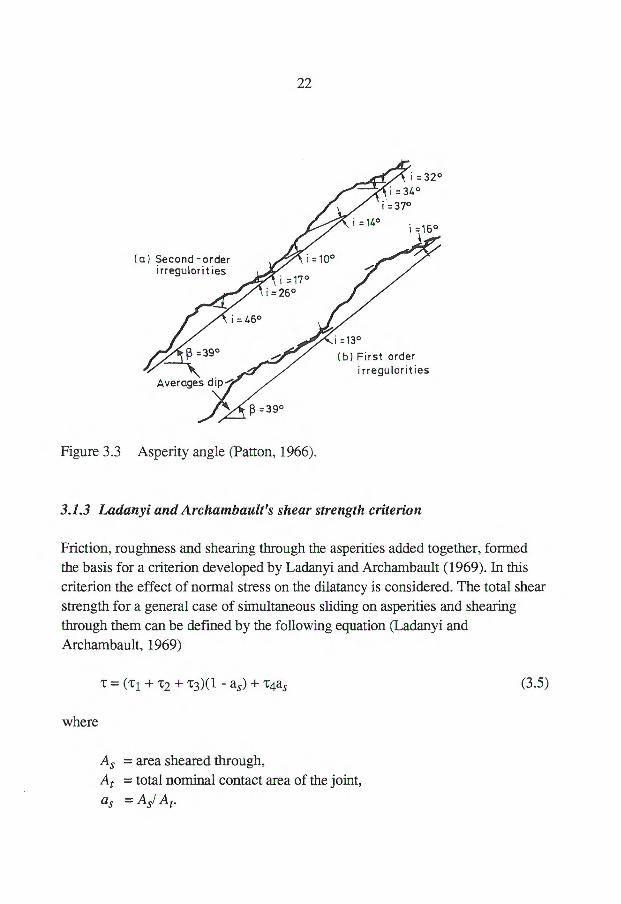
The change in the mechanism of failure is reflected through the change in the slope of the shear strength envelope. Figure 3.3 shows that for natural joints the asperity angle (i) is more difficult to determine since the asperities on a natural joint surface are of different heights, base lengths and inclinations. Due to the change of asperity geometry and interlocking effect after the shear starts, this criterion works less well for irregular rough joints (Hoek and Bray, 1981; Herdocia, 1985; Jing, 1990).
4,
=13:73°4
= 32°
=14°
i=10°
=17°
(a) Second -order irregularities
i =16°
=13°
(b) First order irregularities
Averages dip,'
= 390
=26°
22
Figure 3.3 Asperity angle (Patton, 1966).
3.1.3 Ladanyi and Archambault's shear strength criterion
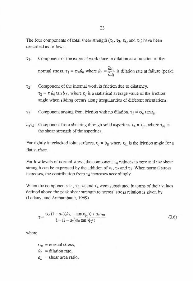
Friction, roughness and shearing through the asperities added together, formed the basis for a criterion developed by Ladanyi and Archambault (1969). In this criterion the effect of normal stress on the dilatancy is considered. The total shear strength for a general case of simultaneous sliding on asperities and shearing through them can be defined by the following equation (Ladanyi and Archambault, 1969)
= + C2 + T3)(1 - as) + T4as (3.5)
where
As = area sheared through, At = total nominal contact area of the joint, as = Asl At.
23
The four components of total shear strength (ci, T2, T3, and T4) have been described as follows:
T1: Component of the external work done in dilation as a function of the
. pun normal stress, T1 = niln where un = is dilation rate at failure (peak). aus
T2: Component of the internal work in friction due to dilatancy.
T2 = T it, tan Of , where Of is a statistical average value of the friction
angle when sliding occurs along irregularities of different orientations.
T3: Component arising from friction with no dilation, T3 --r; an tanep4.
a5t4: Component from shearing through solid asperities T4 = Tin, where 'cm is the shear strength of the asperities.
For tightly interlocked joint surfaces, of. Ou, where 0 is the friction angle for a
flat surface.
For low levels of normal stress, the component '4 reduces to zero and the shear strength can be expressed by the addition of ti, T2 and T3. When normal stress increases, the contribution from T4 increases accordingly.
When the components T1, T2, T3 and T4 were substituted in terms of their values defined above the peak shear strength to normal stress relation is given by (Ladanyi and Archambault, 1969)
as)(lin tan(0µ))+ asTm T
1— (1— as)ün tan(Of
where
an = normal stress,
= dilation rate,
as = shear area ratio.
(3.6)
24
Both it n and as depend on the level of normal stress. It is difficult to determine these two parameters especially in field and at large scale. Therefore Ladanyi and Archambault (1980) defined these parameters using the empirical relations
= (1 Gn )' tanz 710 j
(3.7)
as = 1— (1 (5r1 )l, (3.8) T1Gj
where
= uniaxial compressive strength of the rock material adjacent to the discontinuity,
= 1.5 (dimensionless constant), k = 4.0 (dimensionless constant).
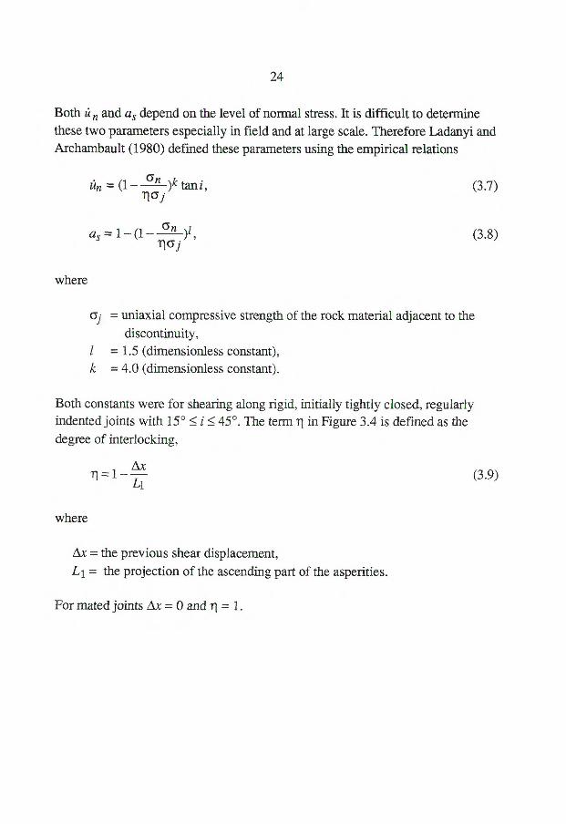
Both constants were for shearing along rigid, initially tightly closed, regularly indented joints with 15° i 45°. The term ri in Figure 3.4 is defined as the degree of interlocking,
, Ax 11 =1-- —
Li
where
Ax = the previous shear displacement, L1 = the projection of the ascending part of the asperities.
For mated joints Ax = 0 and = 1.
(3.9)
25
DIRECTION OF SHEARING
11111> % AAt 11.
1
1, AA AX
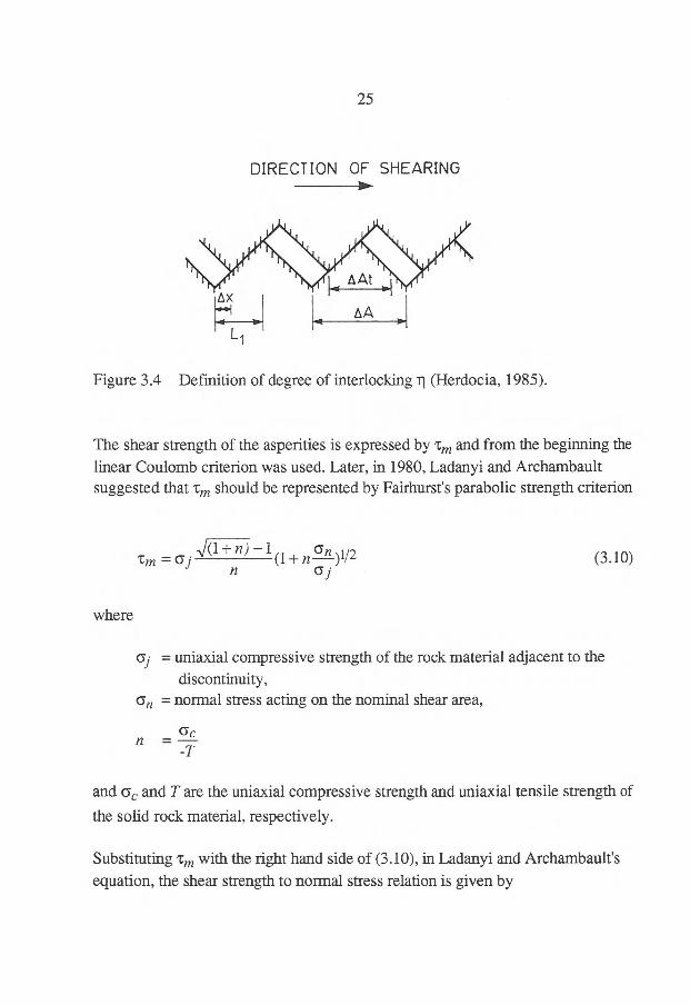
Figure 3.4 Definition of degree of interlocking Ti (Herdocia, 1985).
The shear strength of the asperities is expressed by 'cm and from the beginning the linear Coulomb criterion was used. Later, in 1980, Ladanyi and Archambault suggested that -cm should be represented by Fairhurst's parabolic strength criterion
(3.10)
where
= uniaxial compressive strength of the rock material adjacent to the discontinuity,
san = normal stress acting on the nominal shear area,
n Gc
-T
and sac and T are the uniaxial compressive strength and uniaxial tensile strength of
the solid rock material, respectively.
Substituting 'cm with the right hand side of (3.10), in Ladanyi and Archambault's equation, the shear strength to normal stress relation is given by
26
=
AI(1+ n) —1 (1+ n—) as )(tin + asG j Gn 1/2
n G (3.11)
1 — (1 — as )/in tan Of
The expression for shear strength of joints from Ladanyi and Archambault is well suited in principle. Some of the inputs, for example lb as and tin are sometimes difficult to evaluate for natural joints and must often be assumed (Hoek and Bray, 1981; Herdocia, 1985; Jing, 1990).
3.1.4 Barton's criterion
Another well known criterion for the shear strength of rock joints with irregular asperities is the Barton's criterion (Barton, 1976). This is an empirical relationship between the normal stress and the shear strength, based on a large number of experimental data. The expression has the same form as Patton's bilinear criterion but the dilation angle varies as a function of the applied normal stress. Barton proposed that the shear strength of rock joints at low to moderate normal stresses and with rough surfaces may be written (Barton, 1976; Barton and Choubey, 1977)
where
G', tan[JRC log io (JCS/G') Ob] (3.12)
a'n = effective normal stress, JCS = Joint wall Compressive Strength, JRC = Joint Roughness Coefficient, Ot, = basic friction angle.
The basic friction angle is obtained from residual tilt tests on flat unweathered rock surfaces which were most frequently prepared using a diamond saw (and sand blasted).
At high normal stresses JCS is replaced with the stress difference (a1 - a3) where G1 is the major principal stress at failure and G3 is the minor principal stress at failure (Barton, 1976). The shear strength is then represented by
27
tp = G'n tan[J RC logio ((al - 63)/2) + Pb]. (3.13)
The JRC value can be determined by different methods:
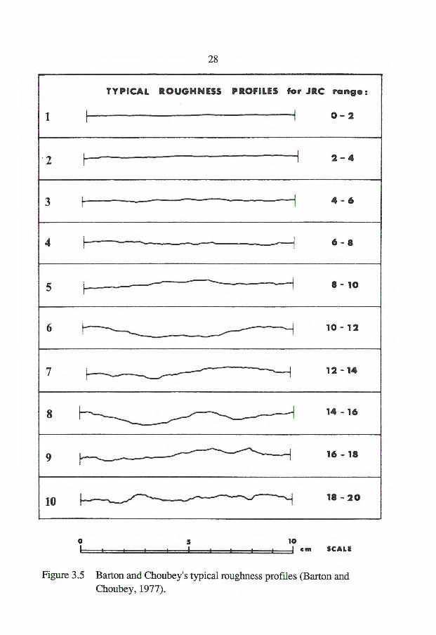
i) By visual comparison with typical profiles (see Figure 3.5) given by Barton and Choubey (1977).
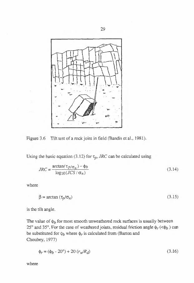
ii) By back calculation from tilt tests (see Figure 3.6) where a rock specimen containing a part of the joint is tilted slowly until sliding occurs (Barton and Choubey, 1977).
28
i
TYPICAL ROUGHNESS PROFILES for JRC range:
0 - 2 I
2 2 - 4 }---
3 4 - 6
4 6 - 8
5 --- ,i 8-10
6 1--- ,—. --i to - 12
7 1 ----------____„------'------ 12 -14
8 14 -16 —'------. --,''------------
9 --------------- --, 16 - 18
10 18 - 20 ----,____•—•----....-•" -----"-.../ N-...i
10 1 I I I I cm SCALE
Figure 3.5 Barton and Choubey's typical roughness profiles (Barton and Choubey, 1977).
Using the basic equation (3.12) for tp, JRC can be calculated using
arctan(tp/an ) — JRC —
logio(JCS I n) (3.14)
29
Figure 3.6 Tilt test of a rock joint in field (Bandis et al., 1981).
where
ß = arctan (tp/an) (3.15)
is the tilt angle.
The value of ob for most smooth unweathered rock surfaces is usually between 25° and 35°. For the case of weathered joints, residual friction angle (J:Ir (<4) can
be substituted for Of, where Or is calculated from (Barton and Choubey, 1977)
= - 20°) + 20 (rwiRd) (3.16)
where
where
JRC n = JRC0 (L
-0.02JRC0 n
(3.17)
(3.18)
and
—0.03JRC0 JCS n = JCS0( z )
30
= calculated friction angle, epb = basic friction angle estimated from residual tilt tests on dry
unweathered sawed surfaces, Rd = Schmidt rebound on dry unweathered sawed surfaces, r = Schmidt rebound on wet joint surface.
Both JRC and JCS are scale dependent and to correct for scale, the following relations can be used (Barton et al., 1985).
JRCn = JRC value for field scale, JRC0 = JRC value for laboratory scale, JCS, = JCS value for field scale, JCS° = JCS value for laboratory scale (nominal length of L0 = 100 mm),
Ln = field scale, L0 = laboratory scale.
The following form of shear strength criterion for field application is suggested at large scale (Barton and Bandis, 1982; Bandis, 1992)
where
= CY n ta4JRCn logior jCS1+ + iu) Gn
(3.19)
ju ---- inclination of large scale undulations.
ft (Fixed)
0 Normal force Normal force
0 Normal force
Joint
Normal force
Concrete block
31
3.2 Joint deformation properties
The behaviour (strength, deformation and conductivity) of discontinuous rock masses under changing stress is strongly affected by the joint deformation. The deformation of a rock mass is assumed to be the sum of deformation of the intact rock and of the joints in the rock mass. For low stresses the deformation is mostly elastic but for high stresses, it is a combination of elastic and plastic deformation. The terms, normal stiffness RIO and shear stiffness (ks) proposed by Goodman (Goodman et al., 1968) describe the rate of change of normal stress (on) with respect to normal displacement (un) and the shear stress (t) with respect to shear displacement (us), respectively.
3.2.1 Normal deformation behaviour
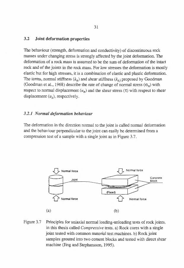
The deformation in the direction normal to the joint is called normal deformation and the behaviour perpendicular to the joint can easily be determined from a compression test of a sample with a single joint as in Figure 3.7.
(a) (b)
Figure 3.7 Principles for uniaxial normal loading-unloading tests of rock joints, in this thesis called Compressive tests. a) Rock cores with a single joint tested with common material test machines. b) Rock joint samples grouted into two cement blocks and tested with direct shear machine (Ting and Stephansson, 1995).
Cn
com
ple
te c
losu
re
••:§" N`b
opening and reclosure
initial normal stress
32
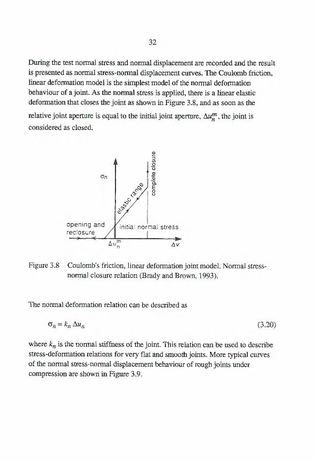
During the test normal stress and normal displacement are recorded and the result is presented as normal stress-normal displacement curves. The Coulomb friction, linear deformation model is the simplest model of the normal deformation behaviour of a joint. As the normal stress is applied, there is a linear elastic deformation that closes the joint as shown in Figure 3.8, and as soon as the
relative joint aperture is equal to the initial joint aperture, Aunm, the joint is
considered as closed.
Figure 3.8 Coulomb's friction, linear deformation joint model. Normal stress-normal closure relation (Brady and Brown, 1993).
The normal deformation relation can be described as
°n kn un (3.20)
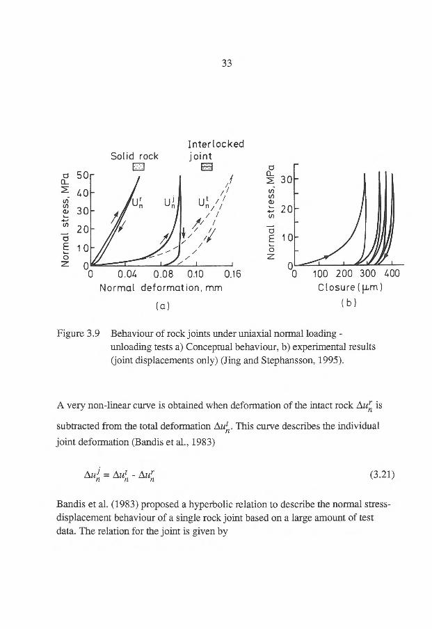
where kn is the normal stiffness of the joint. This relation can be used to describe stress-deformation relations for very flat and smooth joints. More typical curves of the normal stress-normal displacement behaviour of rough joints under compression are shown in Figure 3.9.
No
rmal
stre
ss, M
PG
Interlocked joint
1E21 Solid rock
50
40
30
20
10
oo 0.04 0.08 0.10
Normal deformation, mm
(a)
0.16 100 200 300 400
Closure ( p.m)
( b )
33
Figure 3.9 Behaviour of rock joints under uniaxial normal loading - unloading tests a) Conceptual behaviour, b) experimental results (joint displacements only) (Jing and Stephansson, 1995).
A very non-linear curve is obtained when deformation of the intact rock Aunr is
subtracted from the total deformation Aunt . This curve describes the individual
joint deformation (Bandis et al., 1983)
AUJ = Au - n n n (3.21)
Bandis et al. (1983) proposed a hyperbolic relation to describe the normal stress-displacement behaviour of a single rock joint based on a large amount of test data. The relation for the joint is given by
a - bAui n
Aui n Gn = (3.22)
34
where
a and b = material constants,
Gn = normal stress.
Using this equation the normal stiffness, kn, of the rock joint can be expressed as
(3.23)
where
k = 1/a = initial normal stiffness,
Au m = alb = maximum closure of the rock joint (initial aperture of the n joints)
and
Aui 1 n = the variable relative aperture (affects both the conductivity
Aum n and deformability).
For both mated and unmated conditions, a similar hyperbolic model for the normal deformation of rock joints was proposed by Goodman (1976). This model is given by
t Au
n AO' — Aun
j
n
(3.24)

G nAUM le n
kn = (3.25)
(Aum — Aun)Aun n
35
and from this, the normal stiffness is given by
where
Aun = normal closure,
Au"' = maximum closure, n , A, t = material parameters.
Bandis et al's (1983) model assumes that for a normal displacement equal to zero there exists an initial normal stiffness. Goodman's (1976) model on the other hand assumes that when the initial normal stress is equal to zero, the normal stiffness is also zero.
3.2.2 Shear deformation behaviour
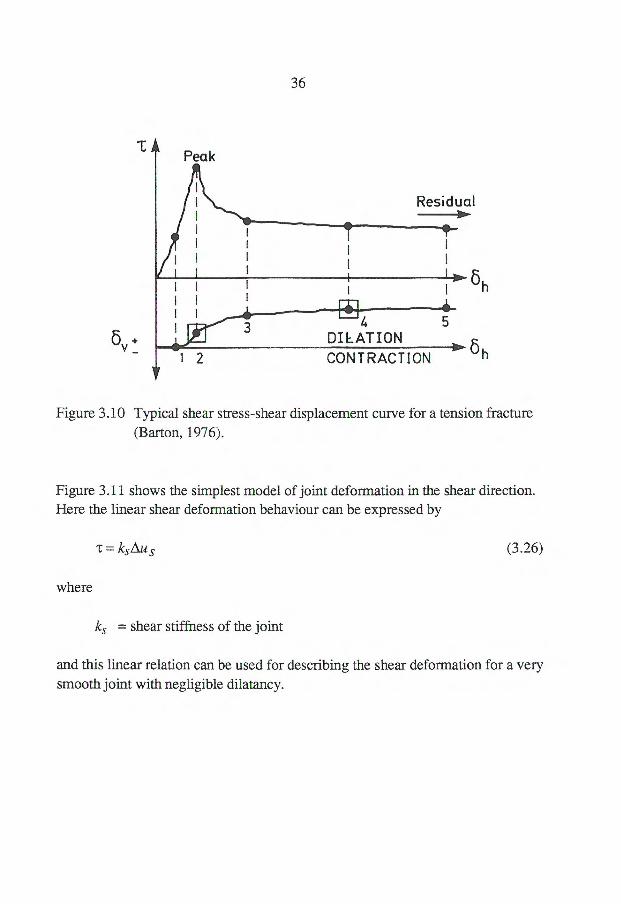
The deformation of a joint in the direction tangential to the joint surface is called the shear deformation and the shear behaviour of rock joints is often determined from direct shear tests. During the test, shear stress, normal and shear displacement is recorded. A typical shear stress-shear displacement curve is shown in Figure 3.10.
Peak
+ v _
Residual
36
5 DILATION
ön CONTRACTION
Figure 3.10 Typical shear stress-shear displacement curve for a tension fracture (Barton, 1976).
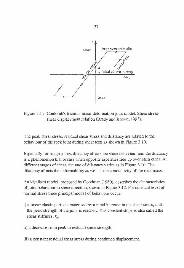
Figure 3.11 shows the simplest model of joint deformation in the shear direction. Here the linear shear deformation behaviour can be expressed by
= ksAus (3.26)
where
ks = shear stiffness of the joint
and this linear relation can be used for describing the shear deformation for a very smooth joint with negligible dilatancy.
Tmax
- <ö•
irrecoverable slip
cb
initial shear stress Us
37
"[max
Figure 3.11 Coulomb's friction, linear deformation joint model. Shear stress- shear displacement relation (Brady and Brown, 1993).
The peak shear stress, residual shear stress and dilatancy are related to the behaviour of the rock joint during shear tests as shown in Figure 3.10.
Especially for rough joints, dilatancy affects the shear behaviour and the dilatancy is a phenomenon that occurs when opposite asperities ride up over each other. At different stages of shear, the rate of dilatancy varies as in Figure 3.10. The dilatancy affects the deformability as well as the conductivity of the rock mass.
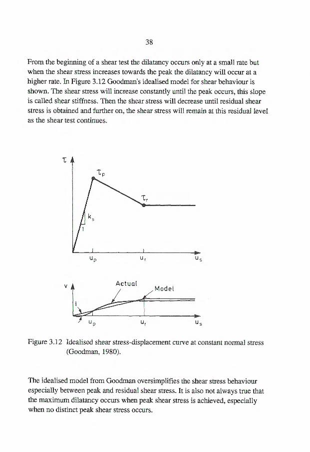
An idealised model, proposed by Goodman (1980), describes the characteristics of joint behaviour in shear direction, shown in Figure 3.12. For constant level of normal stress three principal modes of behaviour occur:
i) a linear elastic part, characterised by a rapid increase in the shear stress, until the peak strength of the joint is reached. This constant slope is also called the shear stiffness, ks,
ii) a decrease from peak to residual shear strength,
iii) a constant residual shear stress during continued displacement.
r
1
1
38
From the beginning of a shear test the dilatancy occurs only at a small rate but when the shear stress increases towards the peak the dilatancy will occur at a higher rate. In Figure 3.12 Goodman's idealised model for shear behaviour is shown. The shear stress will increase constantly until the peak occurs, this slope is called shear stiffness. Then the shear stress will decrease until residual shear stress is obtained and further on, the shear stress will remain at this residual level as the shear test continues.
IA
Up U r
U s
Actual Modet
)1 u P Ur
Figure 3.12 Idealised shear stress-displacement curve at constant normal stress (Goodman, 1980).
The idealised model from Goodman oversimplifies the shear stress behaviour especially between peak and residual shear stress. It is also not always true that the maximum dilatancy occurs when peak shear stress is achieved, especially when no distinct peak shear stress occurs.
39
A large number of experimental studies show that the shear stiffness (ks), for
natural joints, usually depends on the normal stress (Bandis et al., 1981; Sun et al., 1985; Jing, 1990). An empirical relations between the variation of shear stiffness as a function of normal stress have been proposed by Jing (1990)
7, an in an \Lyn KS s (0 < n < c),
G c c (3.27)
ks =
(G n = ac), (3.28)
ks = 0
(an = 0)
(3.29)
where
= maximum shear stiffness through extrapolating data from shear tests,
an = normal stress, ac = uniaxial compressive strength of the rock material.
A large number of shear tests with different normal stress are necessary to be able
to determine Vs?'.
41
4 ACOUSTIC EMISSION (AE) AND FAILURE OF ROCK JOINTS
4.1 General
When transient elastic waves are generated by the rapid release of energy from one or several sources in a material, these waves can be detected in the form of acoustic emission. This could happen when a material is loaded and the restored energy from loading is released when fracture propagation occurs and the phenomenon has been described in ASTM E610-77. The term "acoustic emission" is an acoustic wave generated by the material and the term "acoustic emission signal" is the electrical signal produced by a sensor in response to this wave. The characteristics of the signal are determined by the mechanism which generated the emission, the means by which it travels through the material and the sensors which transform the emission into the signal (Beattie, 1983). In materials which are basically polycrystalline in nature, acoustic emission may originate as follows (Li et al., 1988):
- micro level as a result of dislocations, - macro level as a result of grain boundary movements or initiation and
propagation of fractures between and through mineral grains, - mega level as a result of fracturing and failure of large areas of material or
relative motion between structural units.
Research about acoustic emission (AE) has been done in the following areas of rock mechanics (Hardy, 1981; Koemer et al., 1981):
- monitoring of all types of stressed rock masses in hard rock mines, coal mines and other underground structures,
- monitoring of slope stability, - monitoring of rock bursts and roof falls, - monitoring of surface subsidence,
During recent decades the application of the acoustic emission technique to determine in situ stresses has been under development, but so far with little success (Li, 1993).
42
When acoustic emission is used in a wide range of different materials, there are a number of different terms for AE or the mechanical behaviour it represents. These include: micro seismic activity, rock noise, seismic-acoustic activity, and subaudible noise (Hardy, 1972). There is an obvious risk of misunderstanding when there is no overall standing name convention.
4.2 Key terms in AE
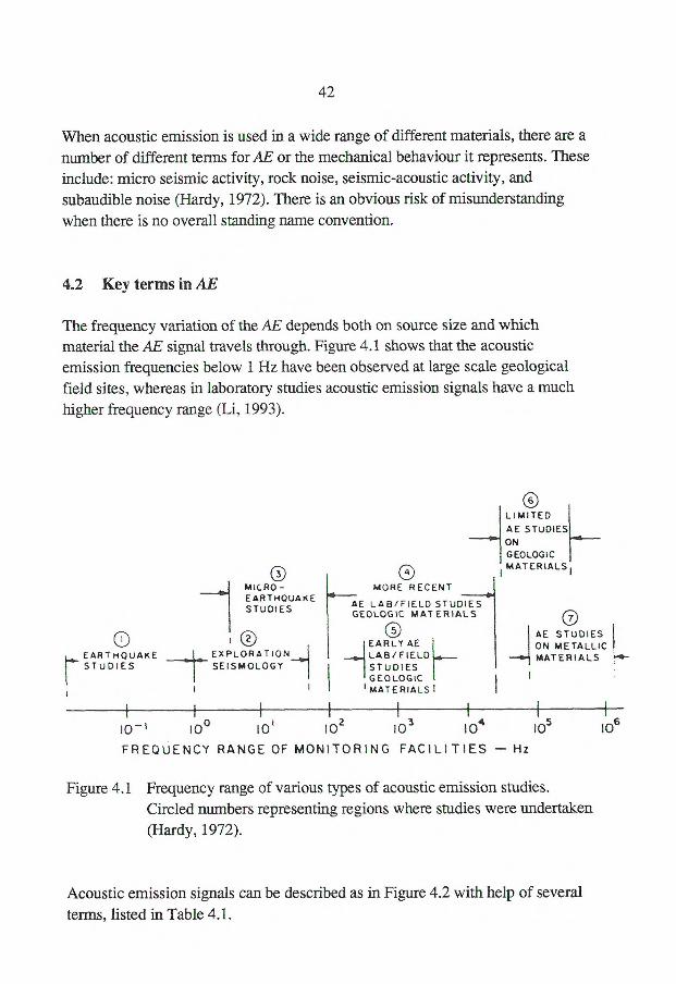
The frequency variation of the AE depends both on source size and which material the AE signal travels through. Figure 4.1 shows that the acoustic emission frequencies below 1 Hz have been observed at large scale geological field sites, whereas in laboratory studies acoustic emission signals have a much higher frequency range (Li, 1993).
LIMITED
AE STUDIES ON GEOLOGIC MATERIALS
MICRO-EARTNOuAKE STUDIES
MORE RECENT m
AE LAB/FIELD STUDIES GEOLOGIC MATERIALS
(I)
.......
1 AE STUDIES ON METALLIC
I•MATERIALS ,-•-•
EARLY AE LAB/ FIELD STUDIES GEOLOGIC
I MATERIALS
EARTHOuAKE ...EXPLORATION
r
›- STUDIES SEISMOLOGY
10 o 10-1 10i 10
2 10
3 10
4 10
5 10
6
FREQUENCY RANGE OF MONITORING FACILITIES — Hz
Figure 4.1 Frequency range of various types of acoustic emission studies. Circled numbers representing regions where studies were undertaken (Hardy, 1972).
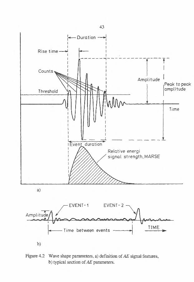
Acoustic emission signals can be described as in Figure 4.2 with help of several terms, listed in Table 4.1.
1.0
I Duration ---"J
Rise t i me •—•.1
P --1
Counts 1
Amplitude
Threshold
Event duration
Relative energi signal strength. MARSE
Peak to peak amplitude
Time
43
a)
/— EVENT-1 EVENT-2
Amplitude
Time between events
TIME
b)
Figure 4.2 Wave shape parameters, a) definition of AE signal features, b) typical section of AE parameters.
44
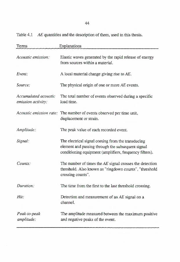
Table 4.1 AE quantities and the description of them, used in this thesis.
Terms Explanations
Acoustic emission: Elastic waves generated by the rapid release of energy from sources within a material.
Event: A local material change giving rise to AE.
Source: The physical origin of one or more AE events.
Accumulated acoustic The total number of events observed during a specific emission activity: load time.
Acoustic emission rate: The number of events observed per time unit, displacement or strain.
Amplitude: The peak value of each recorded event.
Signal: The electrical signal coming from the transducing element and passing through the subsequent signal conditioning equipment (amplifiers, frequency filters).
Counts:
The number of times the AE signal crosses the detection threshold. Also known as "ringdown counts", "threshold crossing counts".
Duration: The time from the first to the last threshold crossing.
Hit: Detection and measurement of an AE signal on a channel.
Peak-to-peak
The amplitude measured between the maximum positive amplitude: and negative peaks of the event.
45
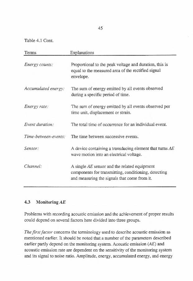
Table 4.1 Cont.
Terms Explanations
Energy counts:
Proportional to the peak voltage and duration, this is equal to the measured area of the rectified signal envelope.
Accumulated energy: The sum of energy emitted by all events observed during a specific period of time.
Energy rate: The sum of energy emitted by all events observed per time unit, displacement or strain.
Event duration: The total time of occurrence for an individual event.
Time-between-events: The time between successive events.
Sensor: A device containing a transducing element that turns AE wave motion into an electrical voltage.
Channel:
A single AE sensor and the related equipment components for transmitting, conditioning, detecting and measuring the signals that come from it.
4.3 Monitoring AE
Problems with recording acoustic emission and the achievement of proper results could depend on several factors here divided into three groups.
The first factor concerns the terminology used to describe acoustic emission as mentioned earlier. It should be noted that a number of the parameters described earlier partly depend on the monitoring system. Acoustic emission (AE) and acoustic emission rate are dependent on the sensitivity of the monitoring system and its signal to noise ratio. Amplitude, energy, accumulated energy, and energy
III III I i 1 1111111 I I i I {Ill
11 i i 111111111111111(1 II Ill!
46
rate are similarly dependent on sensitivity and signal to noise ratio, but are also dependent on the frequency response of the overall monitoring system.
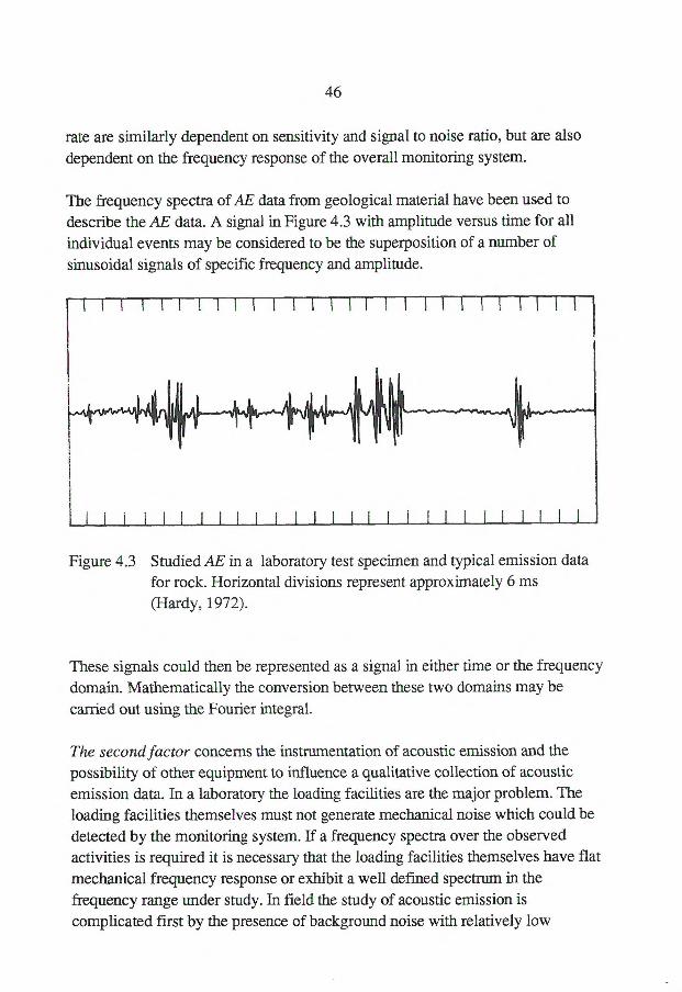
The frequency spectra of AE data from geological material have been used to
describe the AE data. A signal in Figure 4.3 with amplitude versus time for all individual events may be considered to be the superposition of a number of sinusoidal signals of specific frequency and amplitude.
Figure 4.3 Studied AE in a laboratory test specimen and typical emission data for rock. Horizontal divisions represent approximately 6 ms (Hardy, 1972).
These signals could then be represented as a signal in either time or the frequency domain. Mathematically the conversion between these two domains may be carried out using the Fourier integral.
The second factor concerns the instrumentation of acoustic emission and the possibility of other equipment to influence a qualitative collection of acoustic emission data. In a laboratory the loading facilities are the major problem. The loading facilities themselves must not generate mechanical noise which could be detected by the monitoring system. If a frequency spectra over the observed activities is required it is necessary that the loading facilities themselves have flat mechanical frequency response or exhibit a well defined spectrum in the frequency range under study. In field the study of acoustic emission is complicated first by the presence of background noise with relatively low
10
.io 2
47
frequency (100-20000 Hz) from humans or machines. This background noise must be selectively removed by filtering.
There is also the rapid attenuation of frequency that occurs especially when the stress wave is propagated through very fractured geological material. Field observations are complicated by the difficulty of accurately determining micro seismic source locations due to unknowns in the velocity of the propagation and the complexities of geologic structures involved.
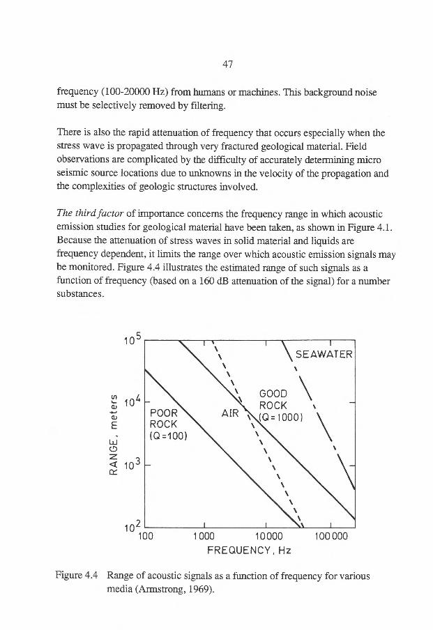
The third factor of importance concerns the frequency range in which acoustic emission studies for geological material have been taken, as shown in Figure 4.1. Because the attenuation of stress waves in solid material and liquids are frequency dependent, it limits the range over which acoustic emission signals may be monitored. Figure 4.4 illustrates the estimated range of such signals as a function of frequency (based on a 160 dB attenuation of the signal) for a number substances.
100 1 000 10 000
100 000
FREQUENCY, Hz
Figure 4.4 Range of acoustic signals as a function of frequency for various media (Armstrong, 1969).
48
A number of successful acoustic emission studies have been carried out on small specimens of geological materials over a number of frequency intervals in the range 300 Hz to 200-300 kHz.
4.4 AE signal characteristics
From the shape and characteristics of an AE wave the character of the AE signal is derived. It is therefore very useful to look at the characteristics of the AE signal since they are the reflection of the AE wave characteristics.
From looking at the AE signal shape it is possible to identify the emission mechanism that causes the AE, distinguish different AE sources and reduce background noise. Some characteristics are easy to measure but give a less qualitative description of the AE wave and some are instead difficult to measure but give a good description of the wave.
Some characteristics that are useful for studying the AE wave (or AE signal) are described further in the following parts of the chapter.
4.4.1 Counts
Measuring counts is the easiest and therefore one of the most useful methods of analysing AE. Counts are the number of times the AE signal is equal to or crosses the threshold. Therefore, the number of counts is a prediction of the size of the AE signal. For instance, a large AE signal usually has a large duration and amplitude which gives a large number of counts but the number of counts depends on the gain-threshold (and the asymmetry of the signal) (Beattie, 1983). Of course, then the threshold must be kept constant when comparing different materials and test occasions and also the different attenuation from different materials must be taken into consideration (PAC, 1988).
AE counts can be used as a prediction that AE is occurring and also give a rough estimate of the rate and amount of the emission.
49
4.4.2 Events
An event is a local change in the material giving rise to AE and also defined as a detected AE burst (or AE wave). This is more a characteristic of the AE signal instead of the AE. The AE signal is modulated so only the burst envelope is left, then the number of envelopes are counted.
This means that the event count will be correct only when all the AE waves have the same attenuation. Problems also occur when the events occur with so short time in between that they start to overlap in time. To avoid these problems, the duration can be measured and the event counter locked out until the first signal is finished. As soon as the events are processed by an electronic counter they can be handled in the same way as the AE count.
One event can, if the AE wave travels through two very different materials, by reflection be detected as two hits by an AE measurement system. An AE event can be equivalent to an AE hit if the AE wave is measured under certain strict conditions so reflections from different boundaries can be removed. Still counting events is a useful tool for source location using a multi channel system.
4.4.3 Energy
The energy is the characteristic of AE that can be defined by
00 Ee -= —1 iV (t)2 dt
0 (4.1)
where
Ee = energy, -= resistive load for the sensor,
V(t) = time dependent voltage output of the sensor
this equation assumes a large signal (produced by a large AE wave) to noise ratio. For presence of noise, energy is defined by
50
1 Ee =— $11'.(t)dt
1771 --V -TAE
RI o
n (4.2)
where
TAE = time of the AE signal without background noise,
= average rms noise voltage.
The signal energy can also be measured by multiplying the square of the peak amplitude with the signal duration (Beatti, 1983).
Energy is one of the characteristics used to describe an AE signal or AE wave, produced in the laboratory. But in field the main reason to use energy is to recognise AE signals or AE waves with either very large amplitude or duration if the expected failure produces such signals. Otherwise the AE count is a more useful analysis method in field.
Because of the difficulty to measure energy (Beatti, 1983), the parameter energy counts have been provided to PAC instrumentation systems and it has been described as "related to the area under the AE event wave form envelope curve".
From sensors and preamplifiers the raw signal enters the AE system and is amplified by an amount selected by the operator, then the signal is rectified so all negative peaks become positive. The signal envelope is a voltage curve which then is fed into a VCO (Voltage Controlled Oscillator) and the frequency of oscillation pulses increase with higher envelope curve. The sum of pulses from the VCO are the energy counts (Mitchell, 1990).
The relation between energy counts and the area under the envelope curve can be explained by using a burst signal in the system, then study the peak voltage and duration time. The relation is described by the equation
51
NE = kVtbG (4.3)
where
NE = energy counts, V =; peak voltage of the burst, tb L.= time duration of the burst, G = system gain, k = constant.
Since this equation is based on a sinusoidal burst signal the relation still holds for general AE events.
4.5 Location
Generally, source location techniques require a network of AE sensors positioned at different points on the structure. The technique requires also precise arrival time data of AE signals recorded over a number of sensors (Lockner, 1993). As these arrival times are determined, the coordinates of each source, P-velocity of the material and the hypocenter of the event can be estimated. This is possible for more advanced techniques and the problems here usually contain a minimum of four unknown, the three dimensional coordinates and the unknown time of the event. Therefore, at least four sensors are needed to do location in three dimensional space (Labuz et al., 1988).
There are four different location techniques available,
i) Linear location, requires at least two sensors and well defined velocity. Locates a point on a line (or a line on a plane).
ii) Zonal location (first hit), locates only a zone were AE occurs and needs only one sensor.
iii) Computed location (Planar), requires well defined velocity and 3-4 sensors. Can locate a point on a 2-D surface.
52
iv) Computed (3D), requires well defined velocity and 4-5 sensors, locates a point in a 3-D surface.
The Triangular Location method is based on the Computed (Planar) techniques. The sensors are forming rows of isosceles triangles over the measured surface in the Triangular Location method.
AE source location is almost the same as earthquake location procedure except for scaling due to sample size, source dimension and frequency content (Lockner, 1993). AE was used to study rock bursts in mines in the 1940s (Lord and Koerner, 1978), but in laboratory induced rock failure, 3D source location have been performed during the last 25-30 years (Scholz, 1968 ). Concerning shear localisation, it has been observed in geological materials in the size of thin sections prepared for microscope and up to zones that are hundreds of kilometres and perhaps 20-30 kilometres in width (Evans and Wong, 1985).
53
5 TEST SET-UP AND EXPERIMENTAL PROCEDURE
5.1 Sample preparation
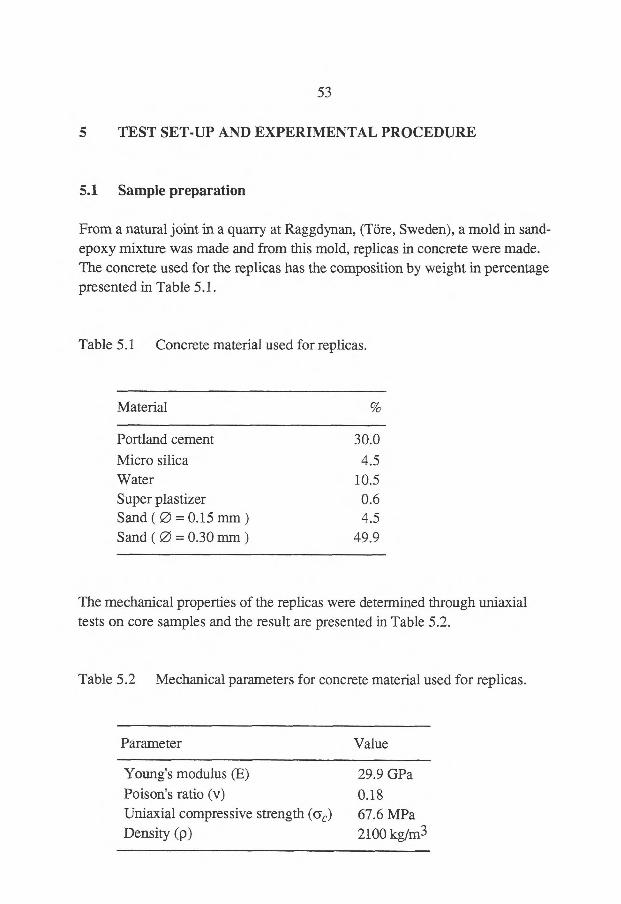
From a natural joint in a quarry at Raggdynan, (Töre, Sweden), a mold in sand-epoxy mixture was made and from this mold, replicas in concrete were made. The concrete used for the replicas has the composition by weight in percentage presented in Table 5.1.
Table 5.1 Concrete material used for replicas.
Material %
Portland cement 30.0
Micro silica 4.5 Water 10.5 Super plastizer 0.6 Sand ( 0 = 0.15 mm ) 4.5 Sand ( 25 = 0.30 mm ) 49.9
The mechanical properties of the replicas were determined through uniaxial tests on core samples and the result are presented in Table 5.2.
Table 5.2 Mechanical parameters for concrete material used for replicas.
Parameter Value
Young's modulus (E)
29.9 GPa Poison's ratio (v)
0.18 Uniaxial compressive strength (ac)
67.6 MPa
Density (p)
2100 kg/m3
54
The basic friction angle, 4, which is the shear strength of a flat non-dilatant surface, was determined from tilt tests on sawn surfaces. For the material used in the present study, sh 28°. A detailed description of a tilt test can be
found in Bandis et al. (1981).
Each sample consists of an upper and a lower block with joint surface 170*250 mm and 250* 250 min, respectively. The upper joint surface was chosen to be shorter in the shear direction than the lower surface in order to keep the nominal contact area constant during shearing. Each block (lower and upper) was cast into larger concrete blocks with standard dimensions 280*280*140 mm which are compatible with the size of each sample holder in the shear box used in the tests.
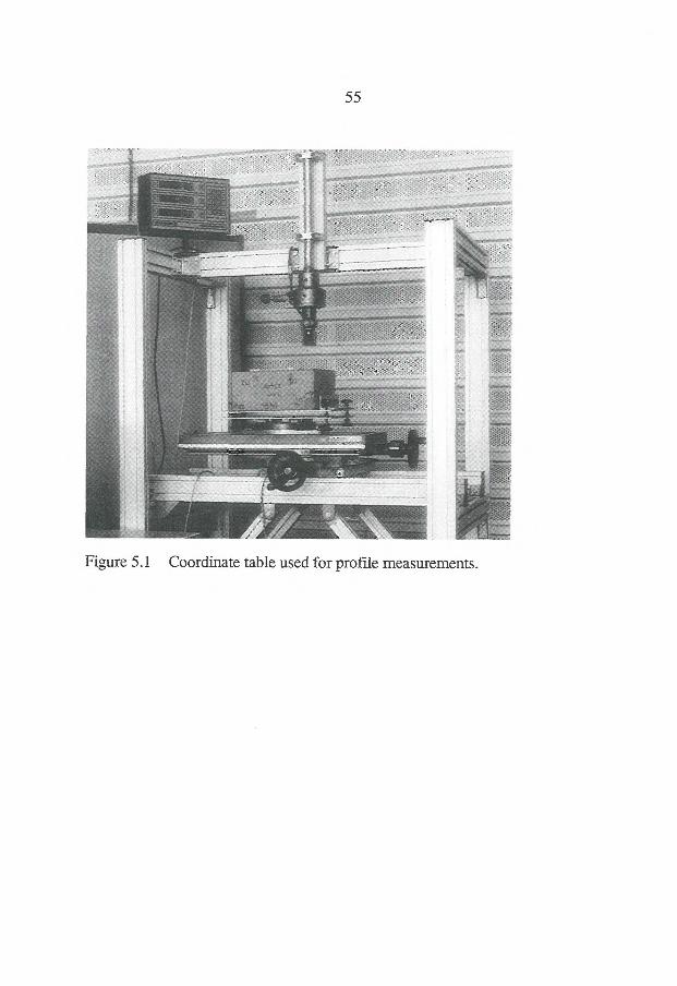
5.2 Profile measurements
For profile measurements, a DANPOS - system shown in Figure 5.1 was used, containing different measurement systems for the horizontal position (x-y-direction) and the vertical direction (z-direction), respectively. A linear incremental gauge system with a resolution of 10 pm was used for the x-y-direction. In the z-direction a laser system from KEYENCE (model LB-081) with range a of +/- 15 mm and a resolution of 81.un was used. Data output from the laser system and the gauge system was sent through an A/D converter and then stored in a computer according to Figure 5.2.
55
Figure 5.1 Coordinate table used for profile measurements.
(6)
9 )( 8 )
(
56
( 3 )
( 2 ) (1)
=2 CZ
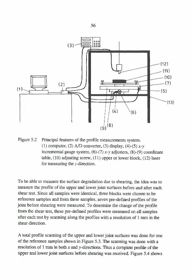
Figure 5.2 Principal features of the profile measurements system. (1) computer, (2) A/D converter, (3) display, (4)-(5) x-y incremental gauge system, (6)-(7) x-y adjusters, (8)-(9) coordinate table, (10) adjusting screw, (11) upper or lower block, (12) laser for measuring the z-direction.
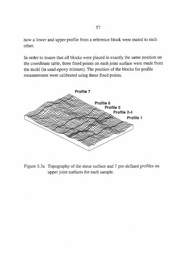
To be able to measure the surface degradation due to shearing, the idea was to measure the profile of the upper and lower joint surfaces before and after each shear test. Since all samples were identical, three blocks were chosen to be reference samples and from these samples, seven pre-defined profiles of the joint before shearing were measured. To determine the change of the profile from the shear test, these pre-defined profiles were measured on all samples after each test by scanning along the profiles with a resolution of 1 mm in the shear direction.
C
A total profile scanning of the upper and lower joint surfaces was done for one of the reference samples shown in Figure 5.3. The scanning was done with a resolution of 1 nimmn both x and y-directions. Thus a complete profile of the upper and lower joint surfaces before shearing was received. Figure 5.4 shows
57
how a lower and upper profile from a reference block were mated to each other.
In order to insure that all blocks were placed in exactly the same position on the coordinate table, three fixed points on each joint surface were made from the mold (in sand-epoxy mixture). The position of the blocks for profile measurement were calibrated using these fixed points.
Profile 7 ..••••••• •••- - •... • ....e;t:•..,---..-- Jr."... ••;•• -,-.2•••4%•::;•4••
..........ze•re,4•Z•zet•••••• •--•;.• • P••'•-;=iek•Z•sew•zz•-•••*••••• "...."••
....1›....e..,...._• •- ..-,... ,.. • ...,-.e., • 4.'".•.Z. -••••• Ave,.---z. •;-!---••.1e4"- -..;:e •• ...›..-"- -........ ----------------------- A:. • .....42,,,,,...z 4... 4"... i›......... -....4`----- .0> • • .04..ree- ••• ....
4r. ' ,Pi .1. .1.• ........ .. 4......---.... • • • e. Ar
,4$1,e›..-.# #4, • .. #0....-z„....>-......--...„..........."4.., .....4.7.4:94.
"..... 41“. ...........Z.,-.4,,,,,,,Z41,..........*,......,............4., ...40...› ....... •• 4 ••••••• • ... eel> •••"""':-. •7:- -.0.4,••••4:••••-.....•• .. •., ......--e--...". • • ......2---•••••••• •- 4,4422:•..- -..e.---= r,--4----.....-""..- ------.›.- ..... .... ... ,....eder.,...,.....e•e; .,.,. ••-• ...,.......-.."- - -e.er.i.-.... -...........,•40,4,1,1›.. "4,..le.......--",•"..--,..--'...."4,74/1..• .4.1̀ .......•-4,,,,.4,--,,Z,Z.". # ....1..",-..!!•„#...."4.#1.. 4., ..111.`""ile....., 4.46,' ...en...0KP; , • 1•40....• ...._#•,,--....--... -,.•••••.•414,,,e4,... •• •••••••• • • • 4... • •.• ...'• •....• 4.4. • ....2.+•• '*-- ......."4".• ea> • ".• %KIP .." • ...... ..e........,.......104.,...• eip le .....• -- • .,.. - ... 4,4,. •••...,- .1.....••••••wre, 41.4..4,- •-2,;•-••••Zez..•.....,....,,,•• •••>•..."0"4.,•,,,,..---- Atoreret•-4....•-•-••••••• *it. ""e..e.e....z-Z•:.17-2--: =we. .4-e-••• 'reje•- "1.----:$-̀,---_---4,•--;.••44:- -- - • - -- •••• '.4%., •••• • • el• ....."-- •--2.."•• • ....e.- .'44,...ej..1. - e. -,... -..- ....-.4....• • •,.. j, 4Mr4A--z-e--1.1.2ircif.... • .• eire:',.......e.eite.....>-. -.:. »- .."4". ••••••4•2>--.--e-..,,• ••......rep•i.e.:;-,•••••••••- - - ---Kree". ...... ............ ....4•4-e-t.--
---seeeez=zZe.=t Zee" ..,......e.......e.. ......zze..
Figure 5.3a Topography of the shear surface and 7 pre-defined profiles on upper joint surfaces for each sample.
....... Profile 5 Profile 6..
Profile 2-4
Profile 1
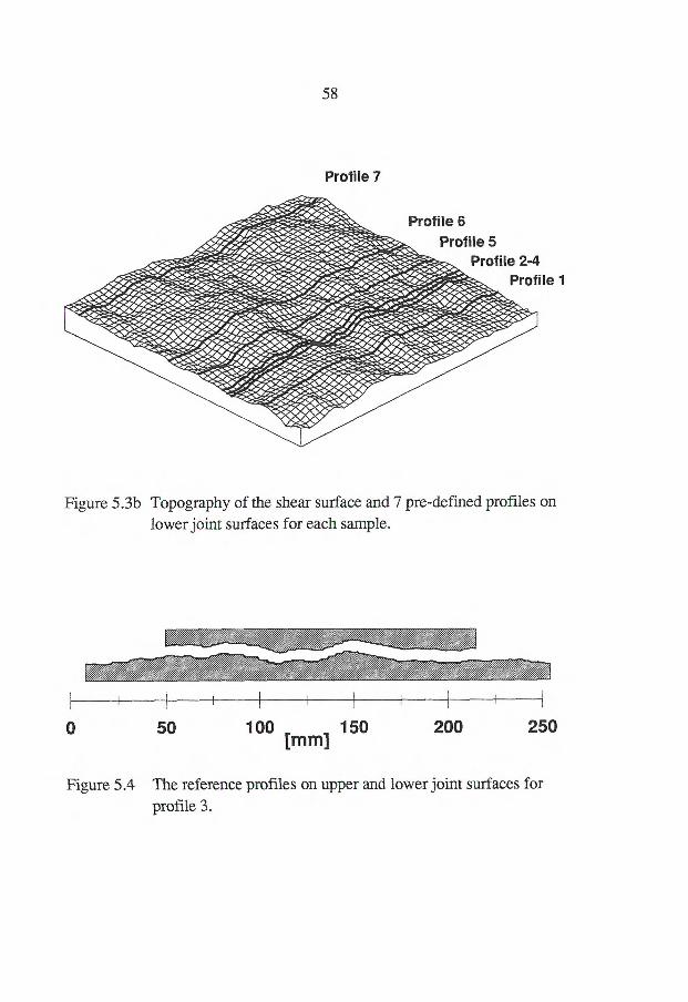
58
Profile 7
4,4%2e...op:re. -•*Z.Ze;"_--4;::-ie-'••.,-•-'reree•... 40theeepegese;*41,,
,,,.
el%ere. e./.••-• ................. ireir-Zrier• ... "Pa .:. /... .... Zee .:*****, .............41.4e. .....% . ...... ....... eIde ...."'" .. .. .***,.."...***. ....AO. .... ....-e-----a-1'..zet. ""--t-e-eli•••-e-Z-e...,...4Fett..zete.zzz_z„,...-1:__ ....-....e.- 4,...--..-......-...-..e.,..-....--e,•••,ze-t...e,ta. 4,,,.....e.,............-..... ... ......e. at", . „,..•_ .. .........•..... ...........r. • 4.....4,-.........e.e..• ... .... •.on-........ * 4. ... ..- . e .. -*,..... ... .. e e ... - .. ..... ........... 41...44.7,-... - -............ier. • .... ......... ... ... ........ ....... • 4. ree ee- - .re - ..-- -e. ir •e-e-zeir e- ...eir je,I, • 41.4. ....... ..eie •,....-..e.4"......› -!----,:-.. ,,,, 4....Z.,"....---."--.....".....• --e-e."..-,.....,• e....•• •,. ••• •••••,. • • .• • --.•-....•,•••%.••• or, ,....._iers,e_.... irme,r,,..... _„...,....... 4, ir it. es*-:-...eir ..... er--"--- • er. • ir•-••-• ....."e ..4, ereer. • • e-e4reire.- eie-,,, ir., e...- .......... .II. ...... ..- e.lir iii,e,............,.........e...
..... 44„..... ... .....2...,,_ .„„ ..r..--........,....--4›.., le 4.424 4. le...-4.1.1.4 4. * 4. ...,....,,,i. . *'...- .......",e"-..e....1.4P4.
'4..1'. -... ---4.••••••••-•-•""...eeeer• e'4,- 41.10.-ze.,:-'-'7,...eed. 41, ....".....- ----zdito. ..ez-z-e..e., .... .r....eieree....... e.....eZieedge* e. .41 -see +.1e,11Ne...› It". Ii...41»,'....1014 ••••• e.... ...- 1fr... e. iZeleeieet..ellr 1.. ....,,e. re,* 4 4,..... _ ..........er,... • •.„, i i, .....,.. 11•,.... ,,,,,..._4,.... ......,..i* • e 4'••••- .....• 4, .....- 41 * *J. ere, 4,, • .......-.....,........ ....
#̀4.....',... 4' / •-•44:••••teiKee-,...:>>-=.94'7.9?›;".4.4.4eZ-44>'",,bee.-e* -"eerie..., 1.4.e. le.„4.,.......e.e."--"; - - -e-tze.e. *47- *41.- - z---_-%."--4...• ....„;„......,...,....." • 4.,.......4....._...., .7.0.,ezzz-ez,---•,„,, --.1zo.......e.- -----z-- --,.. - • tee, tie, or."..-- - er----4.t-zz-e----...-z.24.---11.-2....-ee. .....:,,,e.zee,,...4.- .....--.........---„c,---.....-zz,--......--......- -- -• - 9. ...-- .. * .....- .0* ..,...........* ........ .... ............... ......e —...-,...,„*...„.....,. ......... ..... I. 44,••• ...,..4-...„e"....,..1,-,_.-'4.401401i.e.er•9•11.•%••••••Alle 'elte•-
••••"*".....•.'•641ir ..e, lee •••• ......."-.40•• ••.Z.Zele..... • --",--Zeb...e,e4.4-zeKte, ...• ....--.44. • ••••••-•,•.• - _. • .....- ..- • --• ,..,..** ... 4y
• e. IP • e
e. 4,-.2.....•
Figure 5.3b Topography of the shear surface and 7 pre-defined profiles on lower joint surfaces for each sample.
A
}
Profile 6 Profile 5
Profile 2-4 Profile 1
0
Figure 5.4
50 100 150 [mm]
200 250
The reference profiles on upper and lower joint surfaces for profile 3.
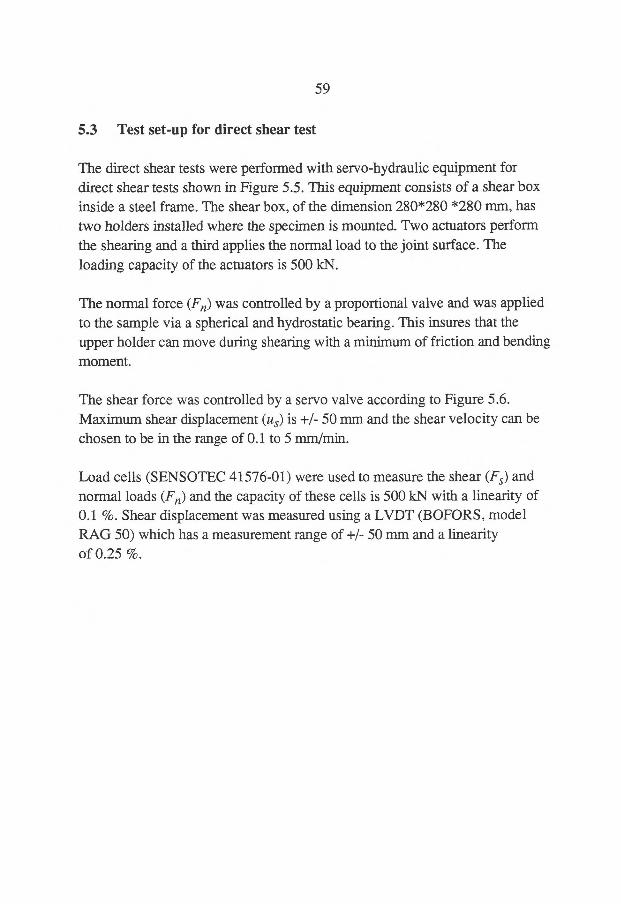
59
5.3 Test set-up for direct shear test
The direct shear tests were performed with servo-hydraulic equipment for direct shear tests shown in Figure 5.5. This equipment consists of a shear box inside a steel frame. The shear box, of the dimension 280*280 *280 mm, has two holders installed where the specimen is mounted. Two actuators perform the shearing and a third applies the normal load to the joint surface. The loading capacity of the actuators is 500 IN.
The normal force (Fa) was controlled by a proportional valve and was applied to the sample via a spherical and hydrostatic bearing. This insures that the upper holder can move during shearing with a minimum of friction and bending moment.
The shear force was controlled by a servo valve according to Figure 5.6. Maximum shear displacement (us) is +/- 50 mm and the shear velocity can be chosen to be in the range of 0.1 to 5 mm/min.
Load cells (SENSOTEC 41576-01) were used to measure the shear (Fa) and
normal loads (Fa) and the capacity of these cells is 5001(N with a linearity of 0.1 %. Shear displacement was measured using a LVDT (BOFORS, model RAG 50) which has a measurement range of +/- 50 mm and a linearity of 0.25 %.
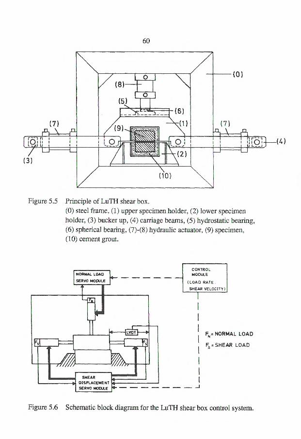
(2)
(7 )
\
(3)
60
(0)
(7) \
1-717d7 (4)
Li L _
(9)
(10)
Figure 5.5 Principle of LuTH shear box. (0) steel frame, (1) upper specimen holder, (2) lower specimen holder, (3) bucker up, (4) carriage beams, (5) hydrostatic bearing, (6) spherical bearing, (7)-(8) hydraulic actuator, (9) specimen, (10) cement grout.
NORMAL LOAD le_
SERVO MODULE
SHEAR DISPLACEMENT SERVO MODULE
CONTROL MODULE
(LOAD RATE.
SHEAR VELOCITY)
Fri = NORMAL LOAD
= SHEAR LOAD
• 4-
Figure 5.6 Schematic block diagram for the LuTH shear box control system.
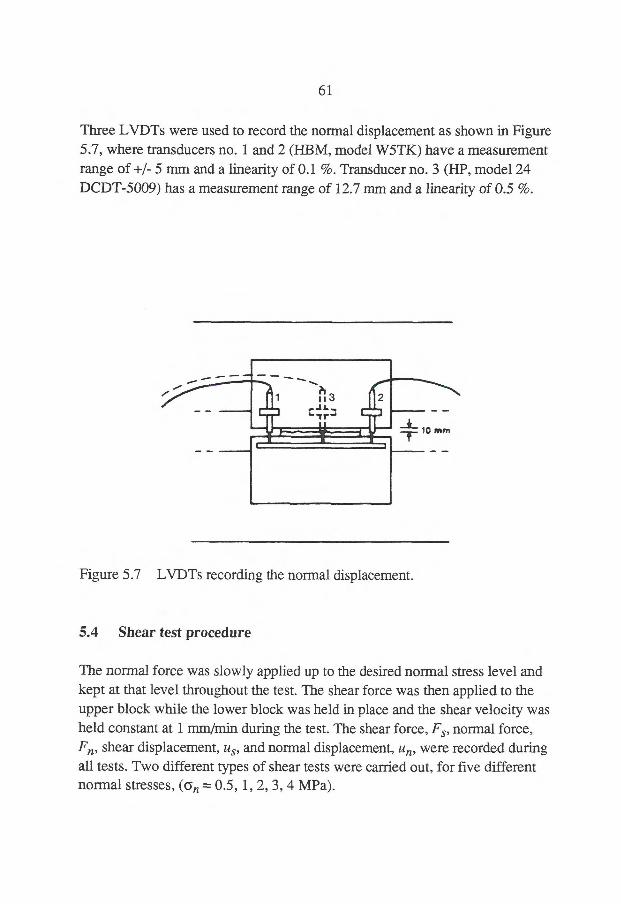
61
Three LVDTs were used to record the normal displacement as shown in Figure 5.7, where transducers no. 1 and 2 (HBM, model W5TK) have a measurement range of +/- 5 mm and a linearity of 0.1 %. Transducer no. 3 (HP, model 24 DCDT-5009) has a measurement range of 12.7 mm and a linearity of 0.5 %.
Figure 5.7 LVDTs recording the normal displacement.
5.4 Shear test procedure
The normal force was slowly applied up to the desired normal stress level and kept at that level throughout the test. The shear force was then applied to the upper block while the lower block was held in place and the shear velocity was held constant at 1 min/min during the test. The shear force, Fs, normal force,
shear displacement, us, and normal displacement, un, were recorded during all tests. Two different types of shear tests were carried out, for five different normal stresses, (an = 0.5, 1, 2, 3, 4 MPa).
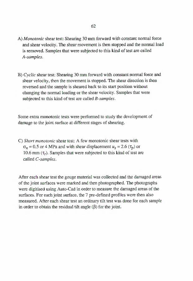
62
A) Monotonic shear test: Shearing 30 mm forward with constant normal force and shear velocity. The shear movement is then stopped and the normal load is removed. Samples that were subjected to this kind of test are called A-samples.
B) Cyclic shear test: Shearing 30 mm forward with constant normal force and shear velocity, then the movement is stopped. The shear direction is then reversed and the sample is sheared back to its start position without changing the normal loading or the shear velocity. Samples that were subjected to this kind of test are called B-samples.
Some extra monotonic tests were performed to study the development of damage to the joint surface at different stages of shearing.
C) Short monotonic shear test: A few monotonic shear tests with Gn = 0.5 or 4 MPa and with shear displacement us = 2.6 (tp) or
10.6 mm (Tr). Samples that were subjected to this kind of test are
called C-samples.
After each shear test the gouge material was collected and the damaged areas of the joint surfaces were marked and then photographed. The photographs were digitised using Auto-Cad in order to measure the damaged areas of the surfaces. For each joint surface, the 7 pre-defined profiles were then also measured. After each shear test an ordinary tilt test was done for each sample in order to obtain the residual tilt angle (ß) for the joint.
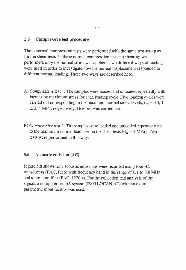
63
5.5 Compressive test procedure
Three normal compression tests were performed with the same test set-up as for the shear tests. In these normal compression tests no shearing was performed, only the normal stress was applied. Two different ways of loading were used in order to investigate how the normal displacement responded to different normal loading. These two ways are described here.
A) Compressive test 1: The samples were loaded and unloaded repeatedly with increasing maximum stress for each loading cycle. Five loading cycles were carried out corresponding to the maximum normal stress levels, Gn = 0.5, 1, 2, 3, 4 MPa, respectively. One test was carried out.
B) Compressive test 2: The samples were loaded and unloaded repeatedly up to the maximum normal load used in the shear tests (Gn = 4 MPa). Two tests were performed in this way.
5.6 Acoustic emission (AE)
Figure 5.8 shows how acoustic emissions were recorded using four AE-transducers (PAC, Pico) with frequency band in the range of 0.1 to 0.8 MHz and a pre-amplifier (PAC, 1220A). For the collection and analysis of the signals a computerised AE system (8900 LOCAN AT) with an external parametric input facility was used.
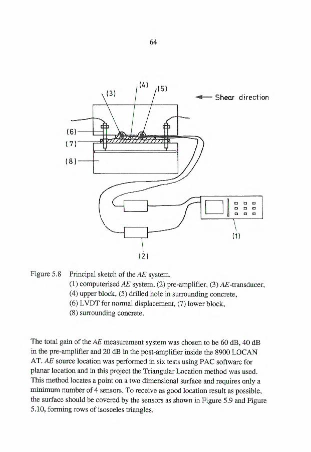
(3) Shear direction
(4) (5)
• I ....re...a sigiehlemwer..uratdrarArArawa: (6)
(7)
(8)
(2)
64
Figure 5.8 Principal sketch of the AE system. (1) computerised AE system, (2) pre-amplifier, (3) AE-transducer, (4) upper block, (5) drilled hole in surrounding concrete, (6) LVDT for normal displacement, (7) lower block, (8) surrounding concrete.
The total gain of the AE measurement system was chosen to be 60 dB, 40 dB in the pre-amplifier and 20 dB in the post-amplifier inside the 8900 LOCAN AT. AE source location was performed in six tests using PAC software for planar location and in this project the Triangular Location method was used. This method locates a point on a two dimensional surface and requires only a minimum number of 4 sensors. To receive as good location result as possible, the surface should be covered by the sensors as shown in Figure 5.9 and Figure 5.10, forming rows of isosceles triangles.
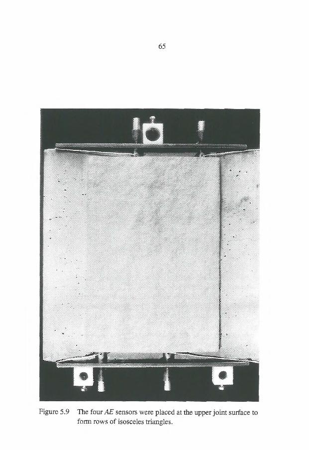
65
Figure 5.9 The four AE sensors were placed at the upper joint surface to form rows of isosceles triangles.
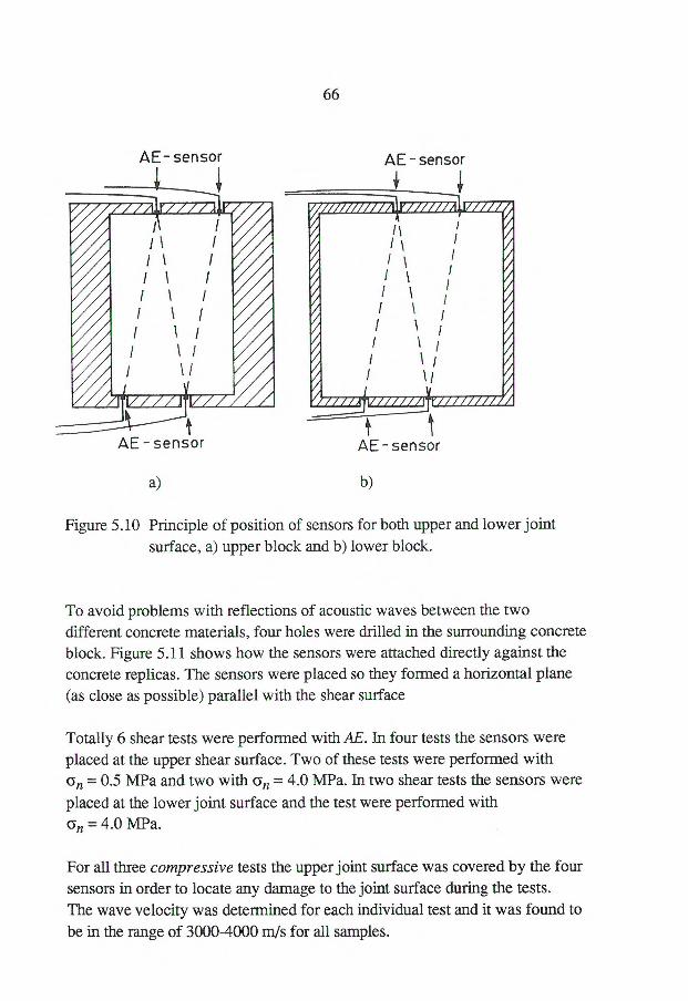
66
AE- sensor
AE - sensor
AE - sensor
a) b)
Figure 5.10 Principle of position of sensors for both upper and lower joint surface, a) upper block and b) lower block.
To avoid problems with reflections of acoustic waves between the two different concrete materials, four holes were drilled in the surrounding concrete block. Figure 5.11 shows how the sensors were attached directly against the concrete replicas. The sensors were placed so they formed a horizontal plane (as close as possible) parallel with the shear surface
Totally 6 shear tests were performed with AE. In four tests the sensors were placed at the upper shear surface. Two of these tests were performed with 6n = 0.5 MPa and two with an = 4.0 MPa. In two shear tests the sensors were
placed at the lower joint surface and the test were performed with 6n = 4.0 MPa.
For all three compressive tests the upper joint surface was covered by the four sensors in order to locate any damage to the joint surface during the tests. The wave velocity was determined for each individual test and it was found to be in the range of 3000-4000 m/s for all samples.
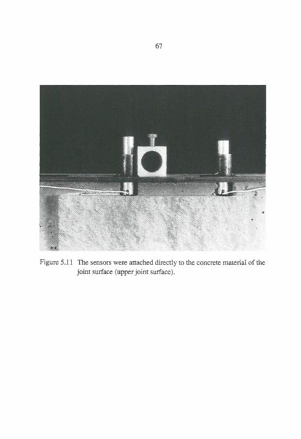
67
Figure 5.11 The sensors were attached directly to the concrete material of the joint surface (upper joint surface).

68
69
6 EXPERIMENTAL RESULTS
6.1 Direct shear test
6.1.1 Deformation and strength
Normal stress, an, is defined as the normal force divided by the total area of the
upper surface of the joint.
Shear stress
Two main different types of shear tests were carried out, for five different normal stresses, an = 0.5, 1.0, 2.0, 3.0 and 4.0 MPa. In each test, shear and normal force, and shear and normal displacement were recorded. A group of extra monotonic shear tests with CYn = 0.5 or 4.0 MPa and short shear displacement
were also performed called C-samples.
Figure 6.1 (monotonic tests) and Figure 6.2 (cyclic tests) show typical shear stress versus shear displacement curves. At low normal stress (an = 0.5 MPa)
there is almost no difference between tp and tr and for very high normal stress
(c5n = 4.0 MPa) the residual shear stress never reaches a constant level during the
tests.
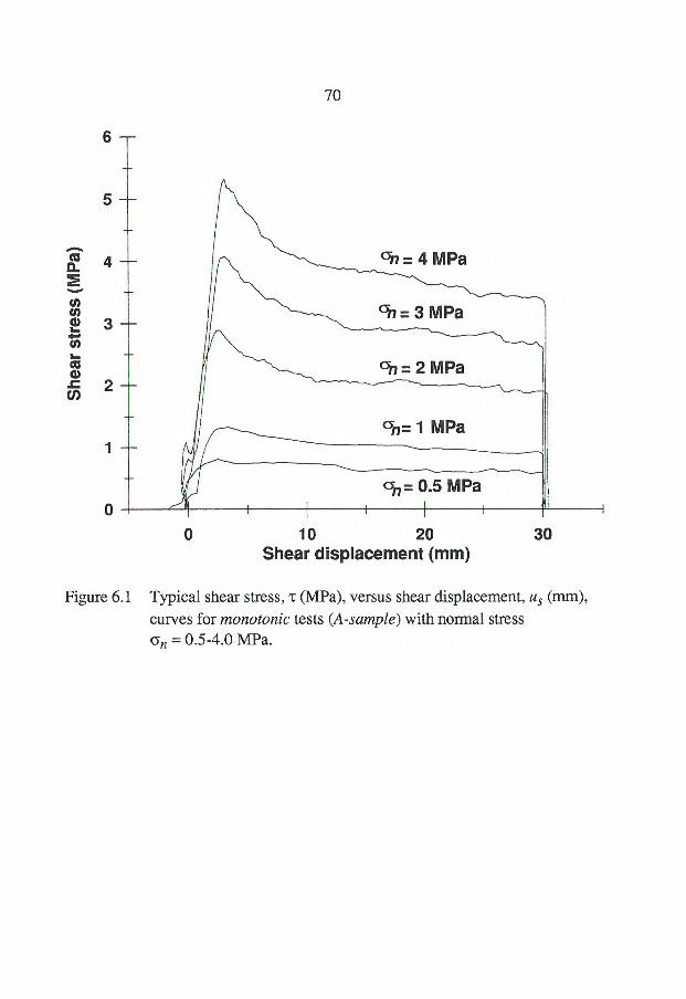
an= 4 MPa
------\„____
an= 3 MPa
an = 2 MPa
6
5
4
3
2
--
-
-
-
-
- an= 1 MPa
1
an= 0.5 MPa
0 I I I 1
-
70
0 10 20
30 Shear displacement (mm)
Figure 6.1 Typical shear stress, 'r (MPa), versus shear displacement, us (mm),
curves for monotonic tests (A-sample) with normal stress Gn = 0.5-4.0 MPa.
Sh
ear
stress
(M
Pa
)
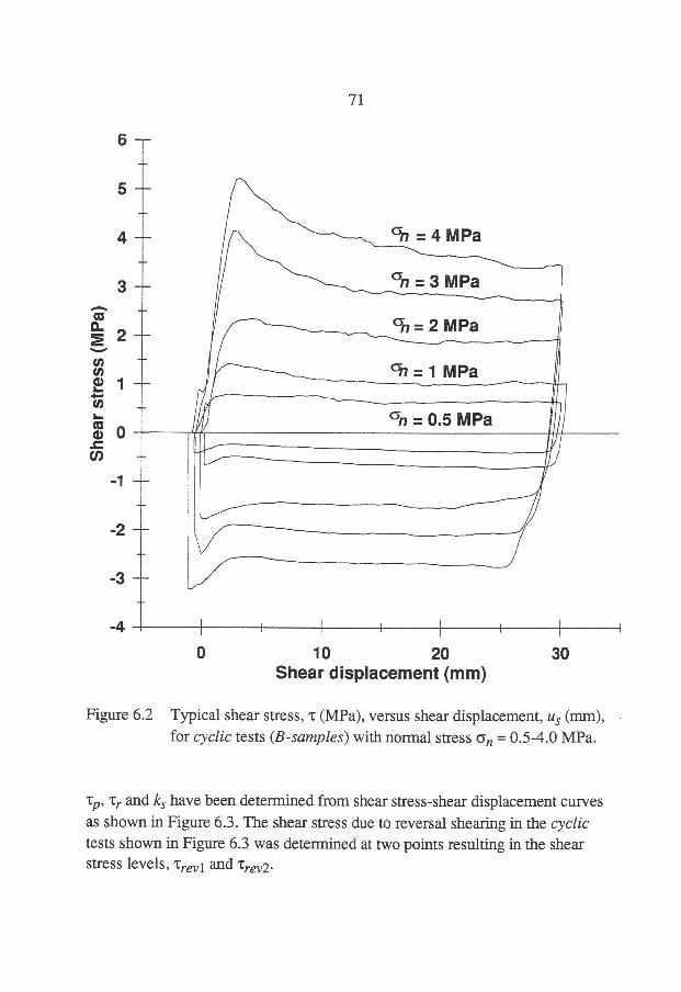
6
5
an = 4 MPa
a n = 3 MPa
cin = 1 MPa
II = 0.5 MPa
-4
71
4
3 —
-2 —
-3 —
0
10 20
30 Shear displacement (mm)
Figure 6.2 Typical shear stress, t (MPa), versus shear displacement, us (mm), for cyclic tests (B-samples) with normal stress an = 0.5-4.0 MPa.
tp, Tr and lcs have been determined from shear stress-shear displacement curves as shown in Figure 6.3. The shear stress due to reversal shearing in the cyclic tests shown in Figure 6.3 was determined at two points resulting in the shear stress levels, Trey]. and Treo.
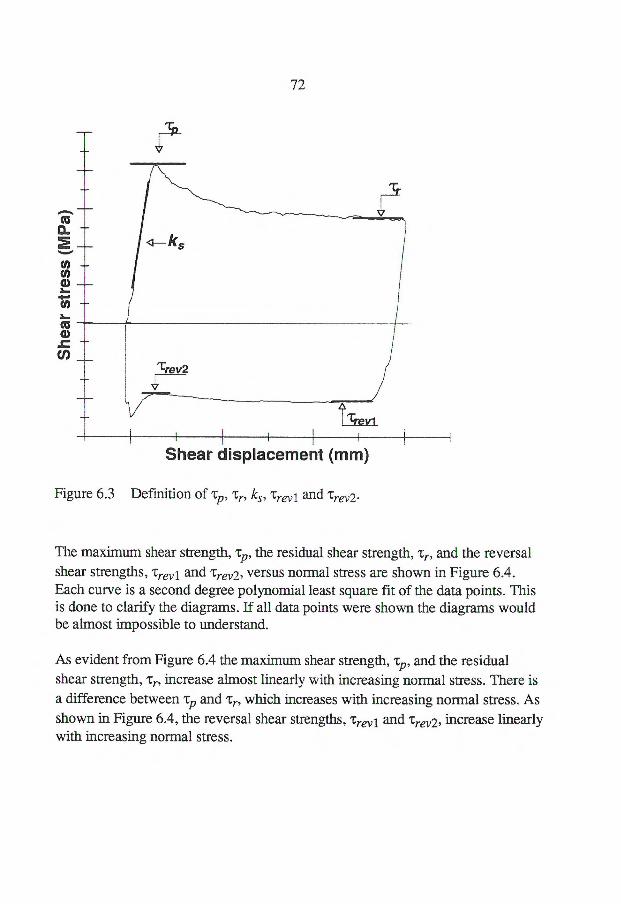
72
Shear displacement (mm)
Figure 6.3 Definition of Tp, Tr, ks, Trevl and trev2.
The maximum shear strength, tp, the residual shear strength, Tr, and the reversal shear strengths, trevl and trev2, versus normal stress are shown in Figure 6.4. Each curve is a second degree polynomial least square fit of the data points. This is done to clarify the diagrams. If all data points were shown the diagrams would be almost impossible to understand.
As evident from Figure 6.4 the maximum shear strength, tp, and the residual shear strength, Tr, increase almost linearly with increasing normal stress. There is a difference between tp and Tr, which increases with increasing normal stress. As shown in Figure 6.4, the reversal shear strengths, Trevl and Trev2, increase linearly with increasing normal stress.
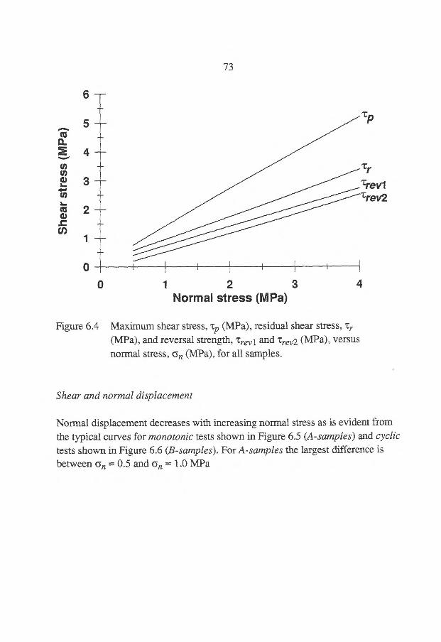
6
5
4
3
2
1
0
Sh
ear
stre
ss (
MP
a)
73
IT
trevi trev2
-
-
^
-
-
-
0
1 2 3
4 Normal stress (MPa)
Figure 6.4 Maximum shear stress, tp (MPa), residual shear stress, Tr
(MPa), and reversal strength, Trey], and trev2 (MPa), versus normal stress, an (MPa), for all samples.
Shear and normal displacement
Normal displacement decreases with increasing normal stress as is evident from the typical curves for monotonic tests shown in Figure 6.5 (A-samples) and cyclic
tests shown in Figure 6.6 (B-samples). For A-samples the largest difference is between C5n = 0.5 and an = 1.0 MPa
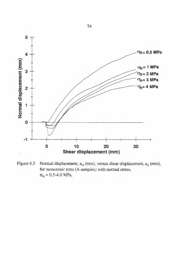
1 -1
No
rmal
dis
pla
cem
ent
(mm
)
an= 1 MPa
'zYn= 2 MPa an= 3 MPa
97= 4 MPa
74
0 10 20
30 Shear displacement (mm)
Figure 6.5 Normal displacement, un (mm), versus shear displacement, us (mm), for monotonic tests (A-samples) with normal stress, an = 0.5-4.0 MPa.
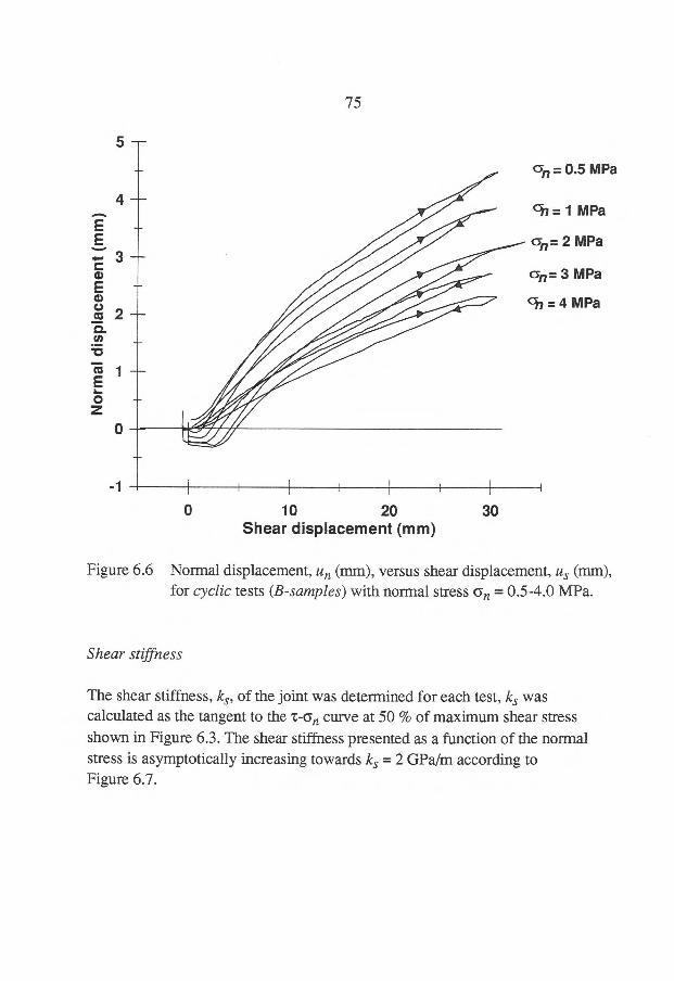
75
_
No
rma l dis
pla
cem
ent (
mm
)
4 — -
3 —
-
2 —
-
1 — -
0
-
5
an = 0.5 MPa
an = 1 MPa
an= 2 MPa
G3 MPa
an = 4 MPa
1 0 10 20
30
Shear displacement (mm)
Figure 6.6 Normal displacement, un (mm), versus shear displacement, us (mm), for cyclic tests (B-samples) with normal stress an = 0.5-4.0 MPa.
Shear stiffness
The shear stiffness, ks, of the joint was determined for each test, ks was calculated as the tangent to the t-an curve at 50 % of maximum shear stress shown in Figure 6.3. The shear stiffness presented as a function of the normal stress is asymptotically increasing towards ks = 2 GPaim according to Figure 6.7.
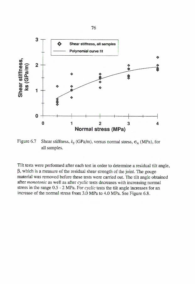
3
-
76
4> Shear stiffness, all samples
Polynomial curve fit
o
-
-
0
0
1 2 3
4 Normal stress (MPa)
Figure 6.7 Shear stiffness, ks (GPa/m), versus normal stress, an (MPa), for all samples.
Tilt tests were performed after each test in order to determine a residual tilt angle, ß, which is a measure of the residual shear strength of the joint. The gouge material was removed before these tests were carried out. The tilt angle obtained after monotonic as well as after cyclic tests decreases with increasing normal stress in the range 0.5 - 2 MPa. For cyclic tests the tilt angle increases for an increase of the normal stress from 3.0 MPa to 4.0 MPa. See Figure 6.8.
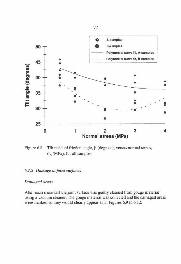
e o
-
50
45
77
•
30 — t
..., ......
.....
•
25
o II
ei . •
Q A-samples
e B-samples
Polynomial curve fit, A-samples
— Polynomial curve fit, B-samples
o
1 2 3 4 Normal stress (MPa)
Figure 6.8 Tilt residual friction angle, 13 (degrees), versus normal stress, (5n. (MPa), for all samples.
6.1.2 Damage to joint surfaces
Damaged areas
After each shear test the joint surface was gently cleaned from gouge material using a vacuum cleaner. The gouge material was collected and the damaged areas were marked so they would clearly appear as in Figures 6.9 to 6.12.
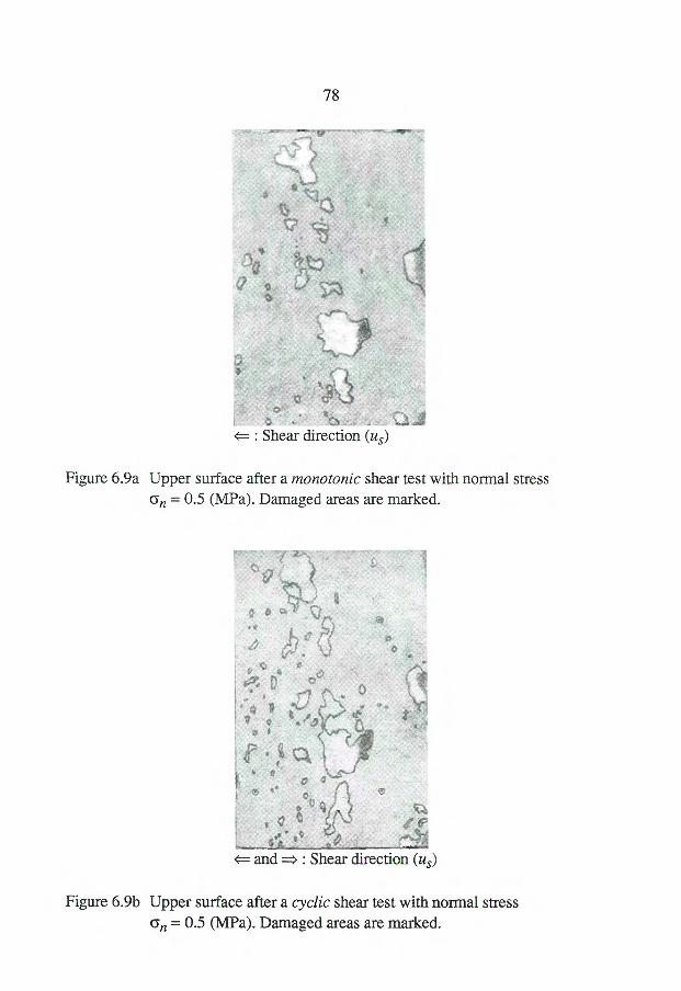
0
78
: Shear direction (us)
Figure 6.9a Upper surface after a monotonic shear test with normal stress an = 0.5 (MPa). Damaged areas are marked.
and =>: Shear direction (us)
Figure 6.9b Upper surface after a cyclic shear test with normal stress an = 0.5 (MPa). Damaged areas are marked.
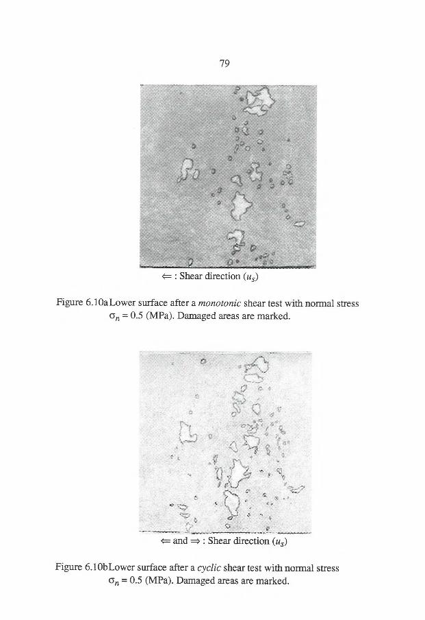
79
: Shear direction (us)
Figure 6.10a Lower surface after a monotonic shear test with normal stress an = 0.5 (MPa). Damaged areas are marked.
and : Shear direction (us)
Figure 6.10bLower surface after a cyclic shear test with normal stress an = 0.5 (MPa). Damaged areas are marked.
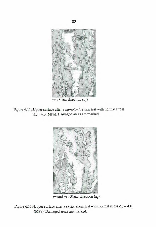
80
: Shear direction (us)
Figure 6.11a Upper surface after a monotonic shear test with normal stress csn = 4.0 (MPa). Damaged areas are marked.
and : Shear direction (us)
Figure 6.11bUpper surface after a cyclic shear test with normal stress an = 4.0 (MPa). Damaged areas are marked.
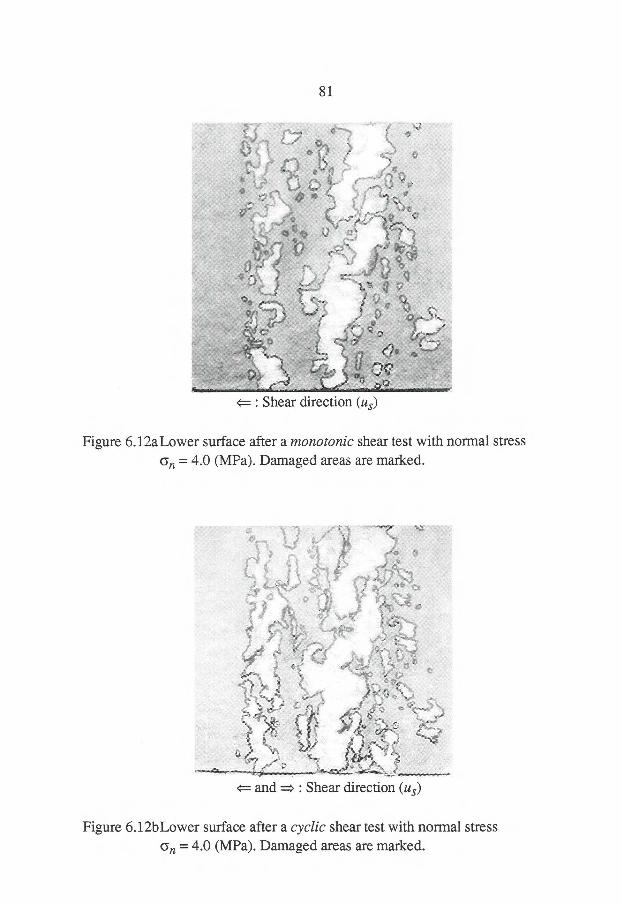
81
: Shear direction (us)
Figure 6.12a Lower surface after a monotonic shear test with normal stress son = 4.0 (MPa). Damaged areas are marked.
and => : Shear direction (us)
Figure 6.12bLower surface after a cyclic shear test with normal stress Gn = 4.0 (MPa). Damaged areas are marked.
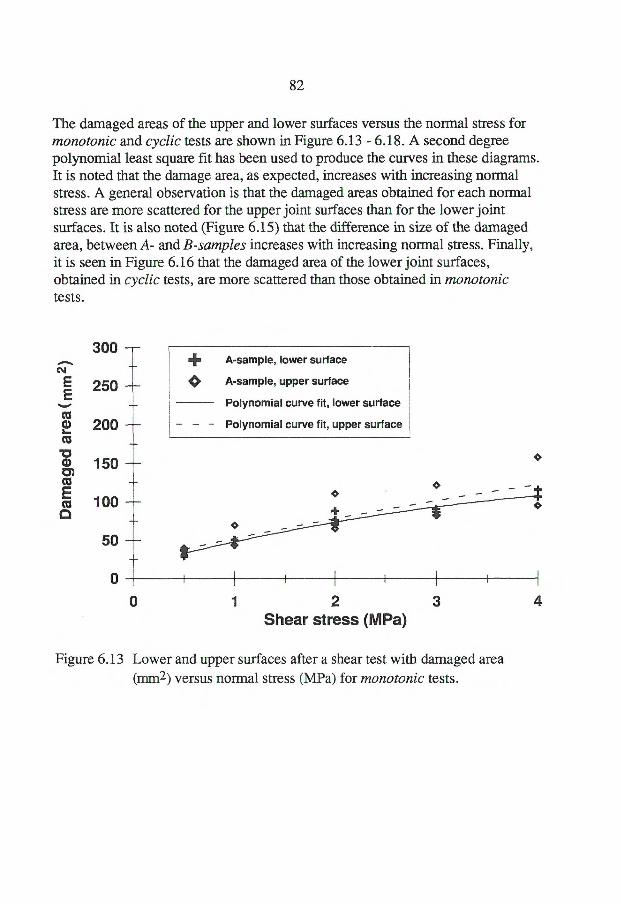
+ A-sample, lower surface
Q A-sample, upper surface
Polynomial curve fit, lower surface
- Polynomial curve fit, upper surface
e
82
The damaged areas of the upper and lower surfaces versus the normal stress for monotonic and cyclic tests are shown in Figure 6.13 - 6.18. A second degree polynomial least square fit has been used to produce the curves in these diagrams. It is noted that the damage area, as expected, increases with increasing normal stress. A general observation is that the damaged areas obtained for each normal stress are more scattered for the upper joint surfaces than for the lower joint surfaces. It is also noted (Figure 6.15) that the difference in size of the damaged area, between A- and B-samples increases with increasing normal stress. Finally, it is seen in Figure 6.16 that the damaged area of the lower joint surfaces, obtained in cyclic tests, are more scattered than those obtained in monotonic tests.
Dam
age
d a
rea (m
m2)
300 — _
250 _
200
150 ,-
100 _
50
0
0
1 2
3
4 Shear stress (MPa)
Figure 6.13 Lower and upper surfaces after a shear test with damaged area (i-p 2) versus normal stress (MPa) for monotonic tests.
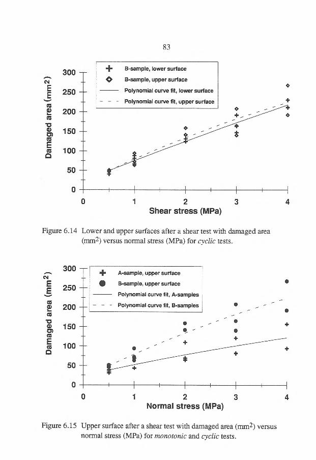
- • -
+ 50
1 i
1 2 3 Normal stress (MPa)
4
i i 1 1 1 t
300 -
250 -
200 -
150 -
100
Dam
age
d a
rea
(mm
2)
83
-
50 _
o
e
.1. B-sample, lower surface
Q B-sample, upper surface
Polynomial curve fit, lower surface
Polynomial curve fit, upper surface
1 1 1 1 o o
i i i i
1 3 4 2 Shear stress (MPa)
Figure 6.14 Lower and upper surfaces after a shear test with damaged area (mm2) versus normal stress (MPa) for cyclic tests.
- -
•- -- .....
+
-
-
Dam
aged
are
a (m
m2
)
100
•
o o
Figure 6.15 Upper surface after a shear test with damaged area (mm2) versus normal stress (MPa) for monotonic and cyclic tests.
300
250
200 -
150 -
+ A-sample, upper surface
• B-sample, upper surface
Polynomial curve fit, A-samples
Polynomial curve fit, B-samples
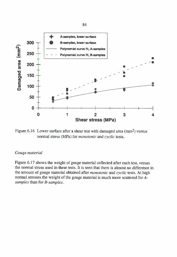
- • 200 — - •
0 1 3 4
-
S •
-$- -
I- S
50 -
0
2 Shear stress (MPa)
- - 150
100
--
mi. A-samples, lower surface
• B-samples, lower surface
Polynomial curve fit, A-samples
— Polynomial curve fit, B-samples
84
300 _
250 — - •
Figure 6.16 Lower surface after a shear test with damaged area (mm2) versus normal stress (MPa) for monotonic and cyclic tests.
Gouge material
Figure 6.17 shows the weight of gouge material collected after each test, versus the normal stress used in these tests. It is seen that there is almost no difference in the amount of gouge material obtained after monotonic and cyclic tests. At high normal stresses the weight of the gouge material is much more scattered for A-samples than for B-samples.
Dam
aged
are
a (m
m2)
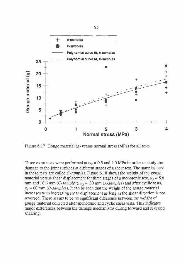
25
20
15
10
5 Go
uge
ma
teri
a
-I- A-samples
e B-samples
Polynomial curve fit, A-samples
Polynomial curve fit, B-samples
•
85
0
0
1 2
3 4 Normal stress (MPa)
Figure 6.17 Gouge material (g) versus normal stress (MPa) for all tests.
Three extra tests were performed at an = 0.5 and 4.0 MPa in order to study the damage to the joint surfaces at different stages of a shear test. The samples used in these tests are called C-samples. Figure 6.18 shows the weight of the gouge material versus shear displacement for three stages of a monotonic test, us = 5.6 mm and 10.6 mm (C-samples), us = 30 mm (A-samples) and after cyclic tests, us = 60 mm (B-samples). It can be seen that the weight of the gouge material increases with increasing shear displacement as long as the shear direction is not reversed. There seems to be no significant difference between the weight of gouge material collected after monotonic and cyclic shear tests. This indicates major differences between the damage mechanisms during forward and reversed shearing.
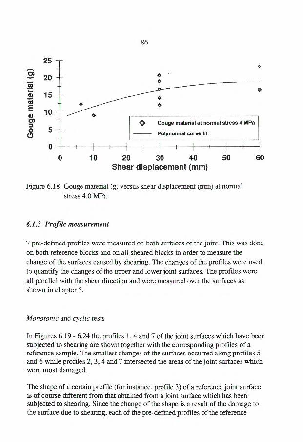
25
86
Go
uge
ma
teri
al (g
)
20
Q Gouge material at normal stress 4 MPa
Polynomial curve fit
15 —
10 —
5
0 0 10 20 30 40 50 60
Shear displacement (mm)
Figure 6.18 Gouge material (g) versus shear displacement (mm) at normal stress 4.0 MPa.
6.1.3 Profile measurement
7 pre-defmed profiles were measured on both surfaces of the joint. This was done on both reference blocks and on all sheared blocks in order to measure the change of the surfaces caused by shearing. The changes of the profiles were used to quantify the changes of the upper and lower joint surfaces. The profiles were all parallel with the shear direction and were measured over the surfaces as shown in chapter 5.
Monotonic and cyclic tests
In Figures 6.19 - 6.24 the profiles 1, 4 and 7 of the joint surfaces which have been subjected to shearing are shown together with the corresponding profiles of a reference sample. The smallest changes of the surfaces occurred along profiles 5 and 6 while profiles 2, 3, 4 and 7 intersected the areas of the joint surfaces which were most damaged.
The shape of a certain profile (for instance, profile 3) of a reference joint surface is of course different from that obtained from a joint surface which has been subjected to shearing. Since the change of the shape is a result of the damage to the surface due to shearing, each of the pre-defmed profiles of the reference
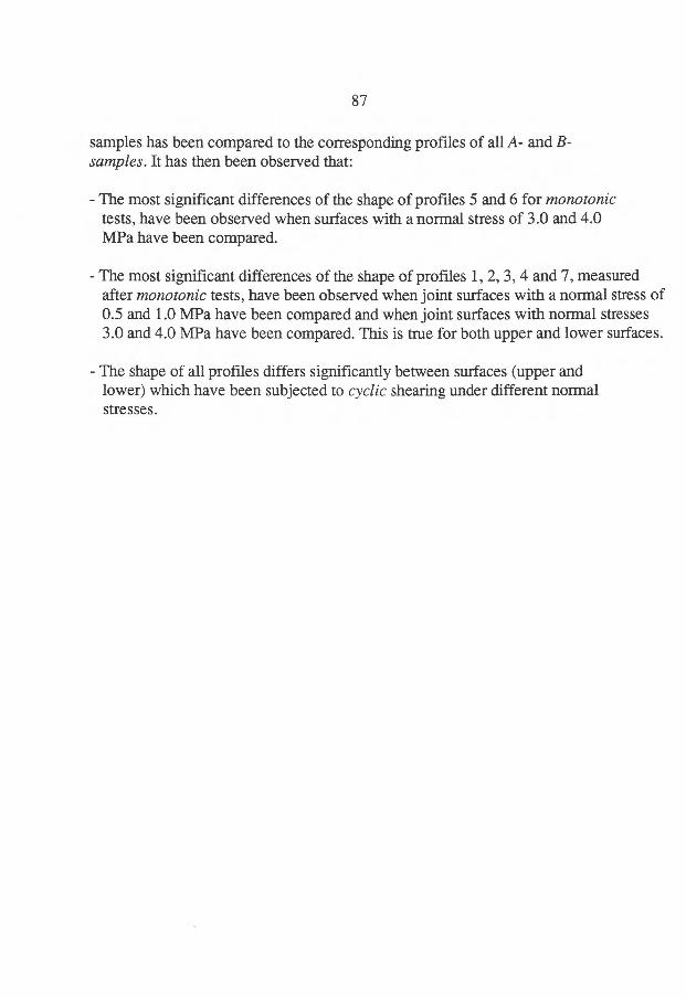
87
samples has been compared to the corresponding profiles of all A- and B-samples. It has then been observed that:
- The most significant differences of the shape of profiles 5 and 6 for monotonic tests, have been observed when surfaces with a normal stress of 3.0 and 4.0 MPa have been compared.
- The most significant differences of the shape of profiles 1, 2, 3, 4 and 7, measured after monotonic tests, have been observed when joint surfaces with a normal stress of 0.5 and 1.0 MPa have been compared and when joint surfaces with normal stresses 3.0 and 4.0 MPa have been compared. This is true for both upper and lower surfaces.
- The shape of all profiles differs significantly between surfaces (upper and lower) which have been subjected to cyclic shearing under different normal stresses.
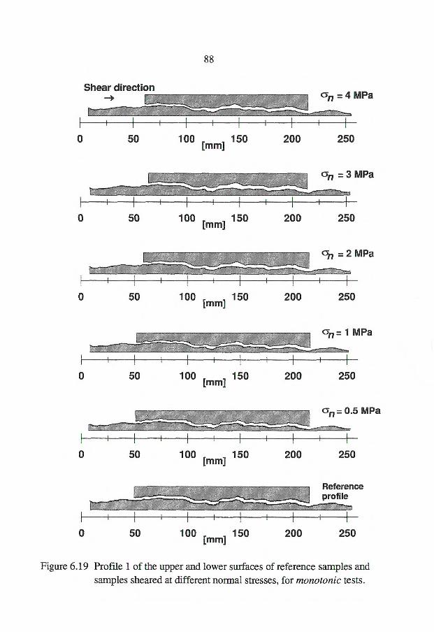
88
Shear direction -+ a = 4 MPa
0 50 100 150 [mm] 200 250
an =3 MPa
0 50 100 150 [mm] 200 250
= 2 MPa
0 50 100 150 [mm] 200
... 4..r/
250
= 1 MPa
0 50 100 150 [mm]
AY...794,
200
%
250
en= 0.5 MPa .
yy7
0 1
50
z
I 1 I 100 150 [mm] 200
4
I
250
Reference profile
0 1
50 100 150 [mm] 200 1
250
Figure 6.19 Profile 1 of the upper and lower surfaces of reference samples and samples sheared at different normal stresses, for monotonic tests.
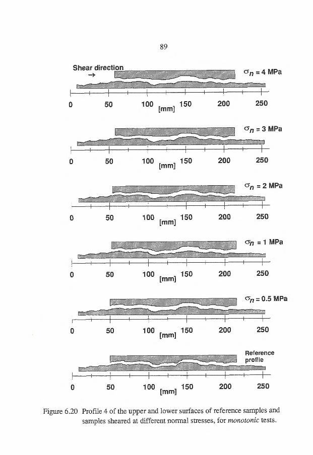
89
Shear direction —> Gn = 4 MPa
0 50 100 150 200 250 [mm]
Gn =3 MPa
0 50 100 150 200 250 [mm]
(517 = 2 MPa V •
A
4
0 50 100 150 200 250 [mm]
C5n = 1 MPa
A
0 50 100 150 200 250 [mm]
6n = 0.5 MPa
0 50 100 150 200 250 [mm]
Reference profile
0 50 100 150 200 250 [mm]
Figure 6.20 Profile 4 of the upper and lower surfaces of reference samples and samples sheared at different normal stresses, for monotonic tests.
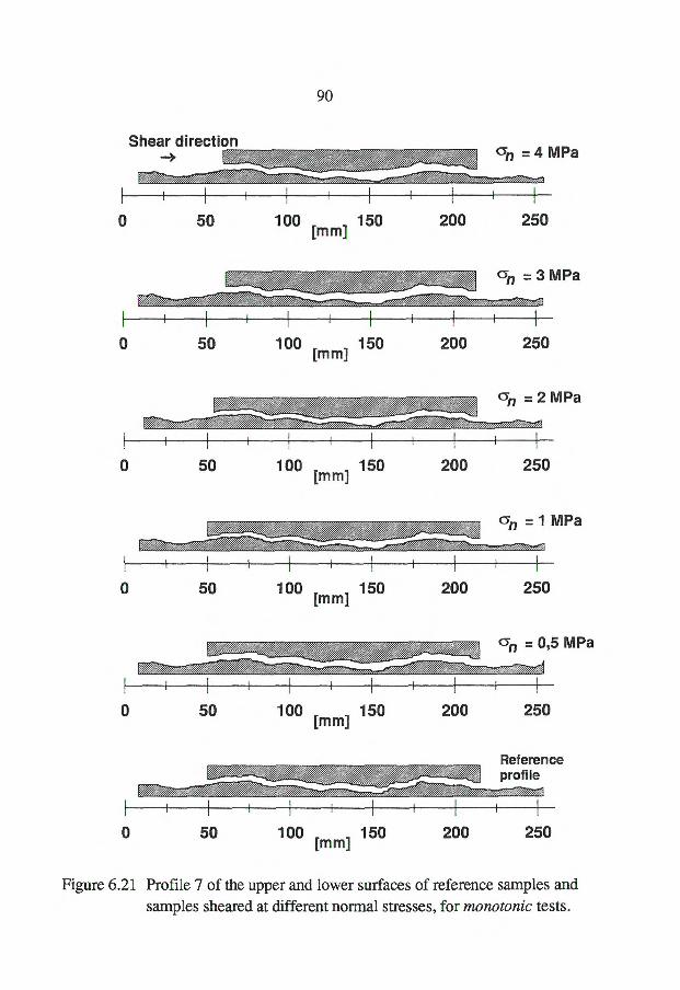
90
Shear direction --> PA =4 MPa
0 50 100 150 200 250 [mm]
/ =3 MPa
0 50 100 150 200 250 [mm]
= 2 MPa
0 50 100 150 200 250 [mm]
= 1 MPa
0 50 100 150 200 250 [mm]
z - - 0,5 MPa n
0 50 100 150 200 250 [mm]
Reference z profile
0 50 100 150 200 250 [mm]
Figure 6.21 Profile 7 of the upper and lower surfaces of reference samples and samples sheared at different normal stresses, for monotonic tests.
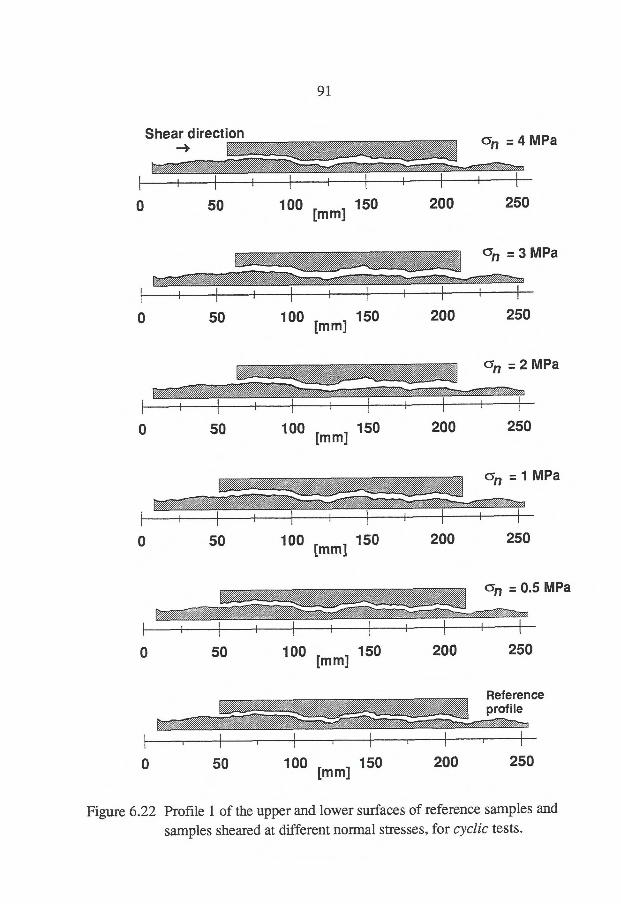
91
Shear direction = 4 MPa
zz/
0 50 100 150 200 250 [mm]
(3.n 3 MPa
0 50 100 150 200 250 [mm]
Gn = 2 MPa
0 50 100 150 200 250 [mm]
Gn = 1 MPa
0 50 100 150 200 250 [mm]
an = 0.5 MPa
»WA
0 50 100 150 200 250 [mm]
Reference profile
0 50 100 150 200 250 [mm]
Figure 6.22 Profile 1 of the upper and lower surfaces of reference samples and samples sheared at different normal stresses, for cyclic tests.
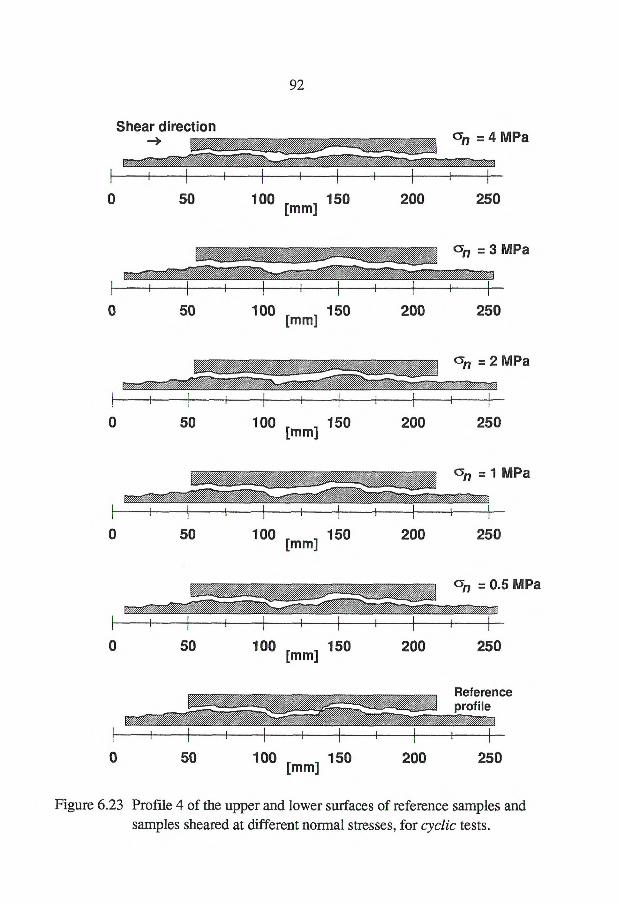
92
Shear direction —> =4an MPa
0 50 100 150 [mm]
200 250
on = 3 MPa y
0 I
50 I
100 150 [mm]
200 250
an = 2 MPa
4
0 50 100 150 [mm]
200 250
on = i MPa
0 50 100 150 [mm] 200 250
an -- 0.5 MPa
0 50 100 150 [mm]
,
I I I
200 250
Reference profile
0 50 100 150 [mm]
I
200 250
Figure 6.23 Profile 4 of the upper and lower surfaces of reference samples and samples sheared at different normal stresses, for cyclic tests.
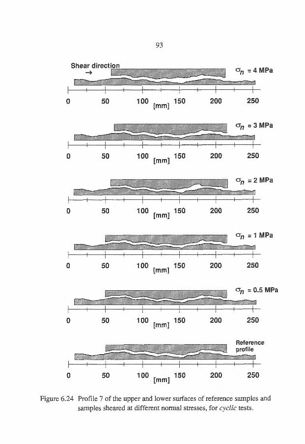
ZZ/ an =3 MPa
Reference profile
0 50
0 50
0 50
•
0 50
p.
0 50
0 50
111111111i
100 150 200 250 [mm]
A:94 w A
100 150 200 250 [mm]
crn = 2 MPa
A
100 150 200 250 [mm]
an = 1 MPa
100 150 200 250 [mm]
C5n= 0.5 MPa
Ae,/ A
100 150 200 250 [mm]
100 150 200 250 [mm]
//
93
Shear direction
cY = 4 MPa
//
Figure 6.24 Profile 7 of the upper and lower surfaces of reference samples and samples sheared at different normal stresses, for cyclic tests.
94
6.2 Acoustic emission
6.2.1 General
Acoustic emission (AE) was monitored in six monotonic tests, with applied normal stress Gn = 0.5 MPa (test 13A, 14A) and an = 4.0 MPa (test 15A, 16A,
17A and 18A). In tests 17A and 18A the AE transducers were attached to the lower block while in the rest of the tests (13A, 14A, 15A and 16A) the transducers were attached to the upper block. AE was also recorded in three compressive tests of the joint and in these tests, the normal stress and normal displacement were recorded.
AE was recorded and analysed with the aid of the 8900 LOCAN AT-system. Planar source location (triangular location) in the horizontal plane and AE amplitude, counts, hits and energy were determined during each test. Since the AE amplitude, the counts, the hits and the energy counts show the same behaviour, only energy counts are presented. This is due to the fact that AE itself is a measure of energy release.
6.2.2 Location
To be able to identify the located AE source activity at different stages of a shear test the total shear displacement was divided into appropriate intervals. The first and second parts of each shear test correspond to the shear displacement intervals 0 - 2 mm and 2-5.5 mm (which included shear stress peak), respectively. The rest of each test was divided into parts 3-7, where parts 3-6 correspond to 3.5 mm each and the last interval, part 7, corresponds to 7 mm of shear displacement at the end of the test.
The distribution of AE events (sources) over the upper joint surface for the tests 16A and 17A is shown in Figures 6.25 and 6.26. These distributions show a 17-20 mm wide undisturbed zone on each side of the joint surface starting at the boundary where the AE transducers are attached to the sample and parallel to the shear direction. This means that no AE sources were located in the areas which are close to the AE transducers. For example no AE sources were located at profile 7 (17 mm from one side parallel with shear direction) but
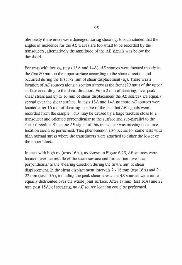
95
obviously these areas were damaged during shearing. It is concluded that the angles of incidence for the AE waves are too small to be recorded by the transducers, alternatively the amplitude of the AE signals was below the threshold.
For tests with low tan (tests 13A and 14A), AE sources were located mostly in the first 80 mm on the upper surface according to the shear direction and occurred during the first 1-2 mm of shear displacement (us). There was a location of AE sources along a section almost at the front (20 mm) of the upper surface according to the shear direction. From 2 mm of shearing, over peak shear stress and up to 16 mm of shear displacement the AE sources are equally spread over the shear surface. In tests 13A and 14A no more AE sources were located after 16 mm of shearing in spite of the fact that AE signals were recorded from the sample. This may be caused by a large fracture close to a transducer and oriented perpendicular to the surface and sub-parallel to the shear direction. Since the AE signal of this transducer was missing no source location could be performed. This phenomenon also occurs for some tests with high normal stress where the transducers were attached to either the lower or the upper block.
In tests with high an (tests 16A), as shown in Figure 6.25, AE sources were
located over the middle of the shear surface and formed into two lines perpendicular to the shearing direction during the first 2 mm of shear displacement. In the shear displacement intervals 2 - 18 mm (test 16A) and 2 - 22 nun (test 15A), including the peak shear stress, the AE sources were more equally distributed over the whole joint surface. After 18 mm (test 16A) and 22 mm (test 15A) of shearing, no AE source location could be performed.
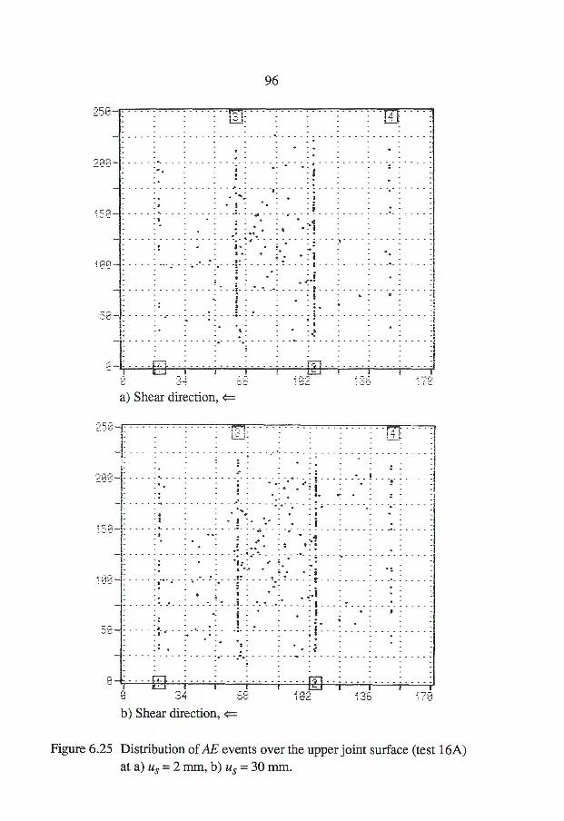
i • t
'• a I '6
S.
••••
. •
96
. •t
[21
a) Shear direction,
3 68
132
73 b) Shear direction,
Figure 6.25 Distribution of AE events over the upper joint surface (test 16A) at a) us = 2 mm, b) us = 30 mm.
97
In the tests 17A and 18A (an = 4.0 MPa), the transducers were attached to the lower block. Figure 6.26 shows the distribution of AE sources over the lower joint surface recorded during the shear displacement intervals 0 - 2 mm (Figure 6.26a) and 0 - 30 mm (Figure 6.26b). It is seen that the AE sources were clustered into two zones of the joint surface at an early stage of the shear test. The same behaviour is observed for the rest of the shear test. The distribution of AE sources in test 18A was similar with respect to shear displacement and location in the shear displacement interval 0 - 11.5 mm. After 11.5 mm of shear displacement, no more AE sources could be located. The zones where the AE sources were located coincide roughly with the observed damaged areas of the lower surface.
The source location is performed using planar source location theory in the horizontal plane (2D). Since the joint surface is a three dimensional surface and the transducers were not exactly located in the mean plane of the joint surface, a 3D source location would have given a more exact location of the surface damage. The use of a 2D source location system on a 3D surface can also explain why some locations of AE sources were formed into two lines perpendicular to shearing direction. Other factors that may affect the source location is the accuracy of the source location software provided by PAC and the differences in frequency content of different events.
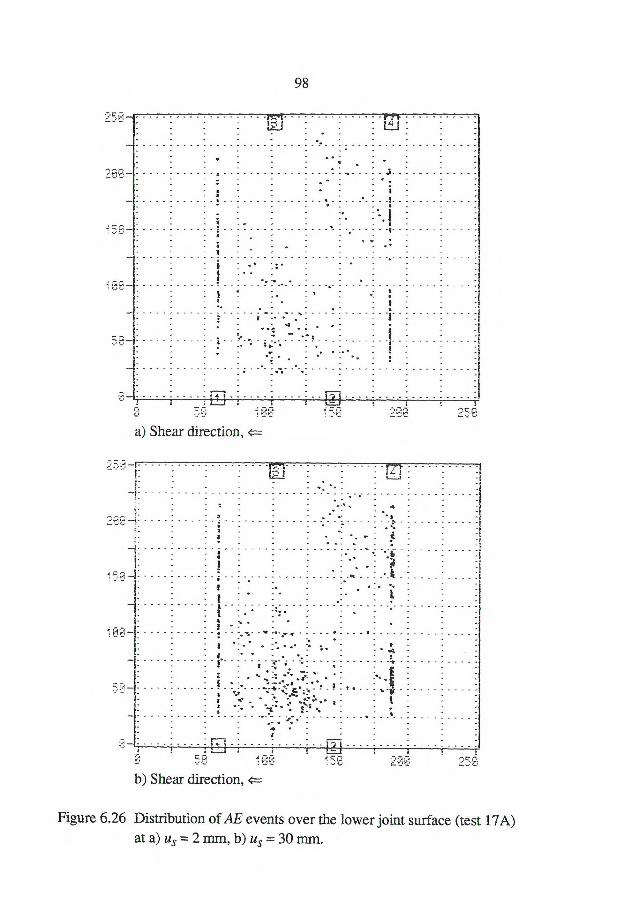
TA'S r7-1 tjj
•
1
• • .
— •
98
3ZL.7:
150 7f-32
a) Shear direction,
479, 3.4 .!
a
. • •
• S":1 — -•• • ix. •
• •
•
I • a a
a
*a •
;
FiCi
b) Shear direction,
Figure 6.26 Distribution of AE events over the lower joint surface (test 17A) at a) us 2 mm, b) us = 30 mm.
• e • . •••• • 3, •
- . • 3 • • Za• • • 3 • ••
1:111.:1
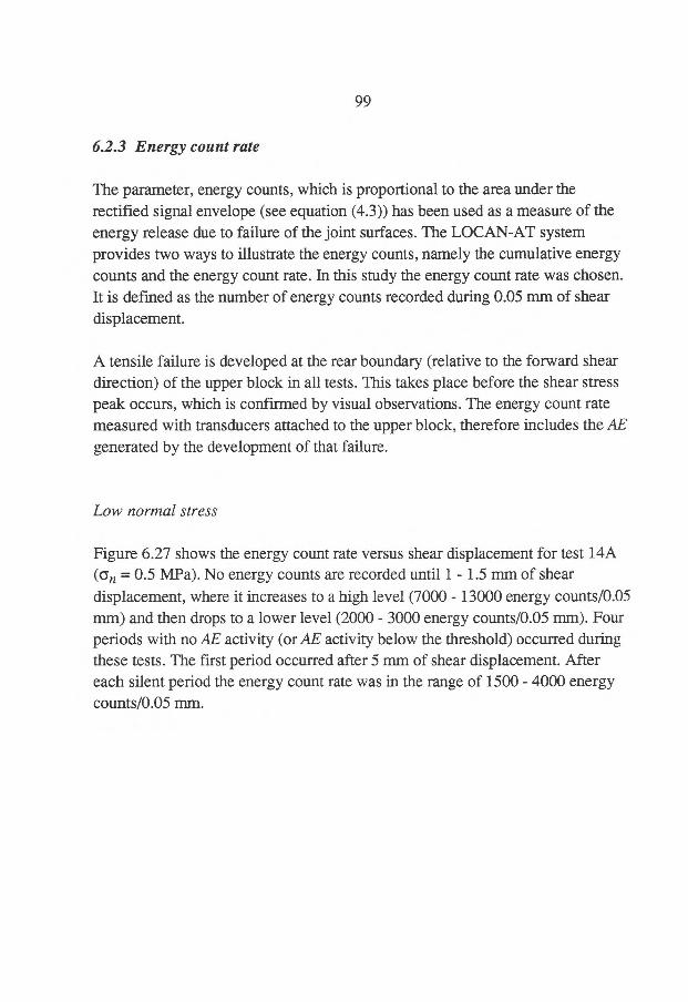
99
6.2.3 Energy count rate
The parameter, energy counts, which is proportional to the area under the rectified signal envelope (see equation (4.3)) has been used as a measure of the energy release due to failure of the joint surfaces. The LOCAN-AT system provides two ways to illustrate the energy counts, namely the cumulative energy counts and the energy count rate. In this study the energy count rate was chosen. It is defined as the number of energy counts recorded during 0.05 mm of shear displacement.
A tensile failure is developed at the rear boundary (relative to the forward shear direction) of the upper block in all tests. This takes place before the shear stress peak occurs, which is confirmed by visual observations. The energy count rate measured with transducers attached to the upper block, therefore includes the AE generated by the development of that failure.
Low normal stress
Figure 6.27 shows the energy count rate versus shear displacement for test 14A ((yn = 0.5 MPa). No energy counts are recorded until 1 - 1.5 mm of shear displacement, where it increases to a high level (7000 - 13000 energy counts/0.05 mm) and then drops to a lower level (2000 - 3000 energy counts/0.05 mm). Four periods with no AE activity (or AE activity below the threshold) occurred during these tests. The first period occurred after 5 mm of shear displacement. After each silent period the energy count rate was in the range of 1500 - 4000 energy counts/0.05 mm.
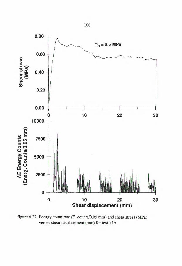
100
7500 -
5000
2500
I
k
0
IF!' ii riliUlMi 1
10 20 Shear displacement (mm)
0
30
Figure 6.27 Energy count rate (E. counts/0.05 mm) and shear stress (MPa) versus shear displacement (mm) for test 14A.
101
High normal stress
In tests 15A and 16A the energy count rate increased to its maximum value (45000 - 65000 energy counts/0.05 mm) already after 0.05 mm of shear displacement but dropped almost immediately to a low level (2000 energy counts/0.05 mm). This was followed by a short period of silence after 2.5 mm of shear displacement as shown in Figure 6.28. Three more periods without AE occurred in the residual stage of the shear tests. Between these silent periods the energy count was in the range of 1000 - 5000 energy counts/0.05 mm.
In tests where the transducers were attached to the upper block the tensile failure of the rear end (relative to forward shearing) of the upper block generates a large number of AE events. The AE energy count rate therefore becomes much higher as a result of the rear end failure than the energy count rate measured at shear stress peak. In some of the tests a fracture which is sub-parallel to the shear direction also developed. The propagation of this fracture also generates AE which is superimposed on the AE caused by the development of the surface damage. If the AE generated from the failure of the rear end and from the development of the fracture is removed from the record, the energy count rate recorded during tests 15A and 16A, shows a behaviour similar to that measured during tests where the transducers were placed on the lower blocks (17A and 18A). This modification of the energy count rate is possible since visual observations as well as the AE data show when these two failures occur.
The AE generated by the failure of the rear end of the upper block has to pass through the joint to be recorded by transducers attached to the lower block. It is evident that only parts of the joint surfaces are in contact during the tests which indicates that the joint itself constitutes a very bad interface for elastic wave propagation. Therefore it is unlikely that the rear end failure of the upper block can be recorded by transducers placed on the lower block. The difference between AE characteristics measured with transducers on the upper and lower blocks, respectively, should therefore not differ much except for differences in the development of damage to the two surfaces. If the upper surface, for instance, suffers more from the shearing the AE activity would be higher in the upper than in the lower block.
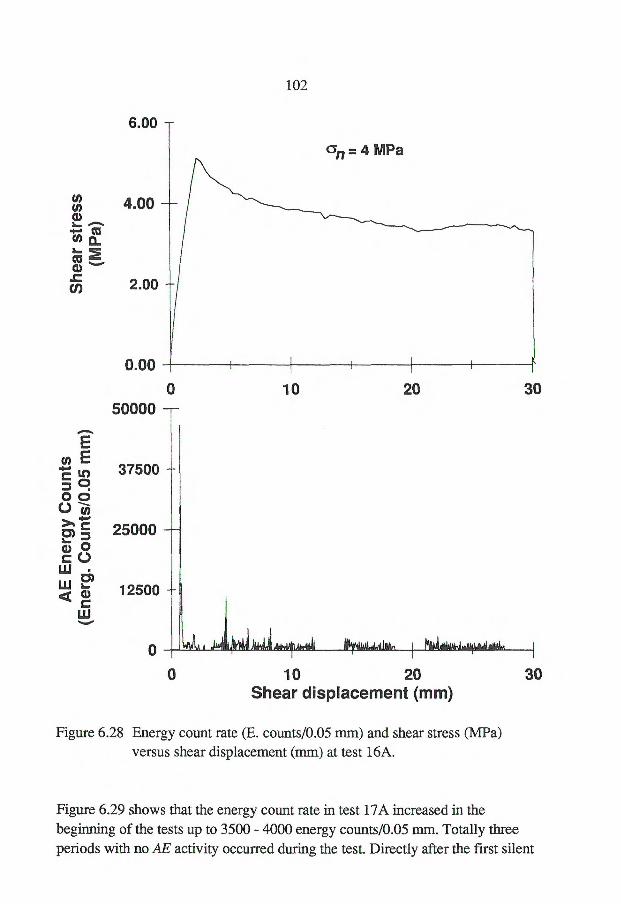
6.00
102
an = 4 MPa
4.00
2.00
}
I
1
r
0.00 1
I
0
10 20
30 Shear displacement (mm)
Figure 6.28 Energy count rate (E. counts/0.05 mm) and shear stress (MPa) versus shear displacement (mm) at test 16A.
Figure 6.29 shows that the energy count rate in test 17A increased in the beginning of the tests up to 3500 - 4000 energy counts/0.05 mm. Totally three periods with no AE activity occurred during the test. Directly after the first silent
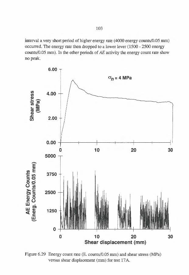
103
interval a very short period of higher energy rate (4000 energy counts/0.05 mm) occurred. The energy rate then dropped to a lower lever (1500 - 2500 energy counts/0.05 mm). In the other periods of AE activity the energy count rate show no peak.
6.00
cn = 4 MPa
3750 -
2500 —
1250
I
10 20 Shear displacement (mm)
0
30
Figure 6.29 Energy count rate (E. counts/0.05 mm) and shear stress (MPa) versus shear displacement (mm) for test 17A.
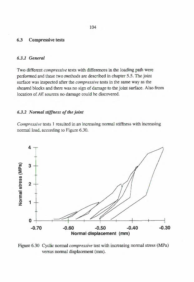
104
6.3 Compressive tests
6.3.1 General
Two different compressive tests with differences in the loading path were performed and these two methods are described in chapter 5.5. The joint surface was inspected after the compressive tests in the same way as the sheared blocks and there was no sign of damage to the joint surface. Also from location of AE sources no damage could be discovered.
6.3.2 Normal stiffness of the joint
Compressive tests 1 resulted in an increasing normal sti 'less with increasing normal load, according to Figure 6.30.
4
3
Nor
mal
str
ess
(MP
a)
-
2 —
-
-1
o
-0.70 -0.60 -0.50 -0.40 -0.30 Normal displacement (mm)
Figure 6.30 Cyclic normal compressive test with increasing normal stress (MPa) versus normal displacement (mm).
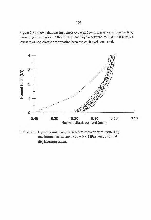
Nor
mal
forc
e (k
N)
0
-0.40 -0.30 -0.20 -0.10 0.00 Normal displacement (mm)
0.10
105
Figure 6.31 shows that the first stress cycle in Compressive tests 2 gave a large remaining deformation. After the fifth load cycle between an = 0-4 MPa only a
low rate of non-elastic deformation between each cycle occurred.
Figure 6.31 Cyclic normal compressive test between with increasing maximum normal stress (a, = 0-4 MPa) versus normal
displacement (mm).

106
107
7 ANALYSIS
7.1 Characterisation of joint roughness
The joint surface roughness before (reference samples) and after shearing, have been characterised using different methods. The fractal dimension, D, the parameters Z2, Z3, 4 (Myers, 1962), the asperity angle, the friction angles and the peak to peak amplitude have been determined for the upper and lower surfaces along the pre-defined profiles.
The lengths of the measured parts of the profiles, are divided in three groups, i) Total profile. ii) Shear part which is equal to the length of the profile of the surface that is
involved in the shearing process. iii) Local part, which is the part of the profile over the most damaged area of the
surface.
Since the results are very similar for the Total profile and Shear part of the profile, only the results from Shear and Local parts are presented here.
7.1.1 Fra ctals
The fractal dimension can be determined in several ways as described in chapter 2. In this study, the modified divider method has been used. The joint surfaces were assumed to be self-affme fractals and the vertical coordinate has been multiplied by 1000 to overcome the crossover length problem. As the divider increments approach the end of the profile trace some part of the trace will be left as remainders. McWilliams et al. (1993) suggested that only those x - increment that fmish up at a horizontal position within 1 per cent of the of the horizontal length should be used. In the present study 1.5 mm has been used as an acceptable remainder.
The largest x-increments were those that required at least N repetitions to cover the profile being studied. Two different sets of calculations were done, where N was chosen to be 20 and 40, respectively. In the following text the fractal
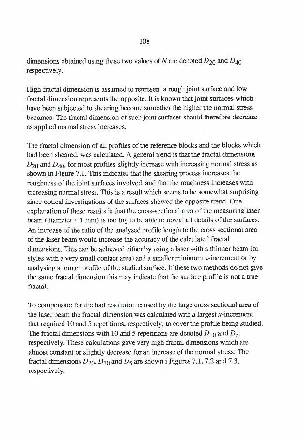
108
dimensions obtained using these two values of N are denoted D20 and D40
respectively.
High fractal dimension is assumed to represent a rough joint surface and low fractal dimension represents the opposite. It is known that joint surfaces which have been subjected to shearing become smoother the higher the normal stress becomes. The fractal dimension of such joint surfaces should therefore decrease as applied normal stress increases.
The fractal dimension of all profiles of the reference blocks and the blocks which had been sheared, was calculated. A general trend is that the fractal dimensions D20 and D40, for most profiles slightly increase with increasing normal stress as shown in Figure 7.1. This indicates that the shearing process increases the roughness of the joint surfaces involved, and that the roughness increases with increasing normal stress. This is a result which seems to be somewhat surprising since optical investigations of the surfaces showed the opposite trend. One explanation of these results is that the cross-sectional area of the measuring laser beam (diameter 1 mm) is too big to be able to reveal all details of the surfaces.
An increase of the ratio of the analysed profile length to the cross sectional area of the laser beam would increase the accuracy of the calculated fractal dimensions. This can be achieved either by using a laser with a thinner beam (or styles with a very small contact area) and a smaller minimum x-increment or by analysing a longer profile of the studied surface. If these two methods do not give the same fractal dimension this may indicate that the surface profile is not a true fractal.
To compensate for the bad resolution caused by the large cross sectional area of the laser beam the fractal dimension was calculated with a largest x-increment that required 10 and 5 repetitions, respectively, to cover the profile being studied. The fractal dimensions with 10 and 5 repetitions are denoted D10 and D5, respectively. These calculations gave very high fractal dimensions which are almost constant or slightly decrease for an increase of the normal stress. The fractal dimensions D20, D10 and D5 are shown i Figures 7.1, 7.2 and 7.3, respectively.
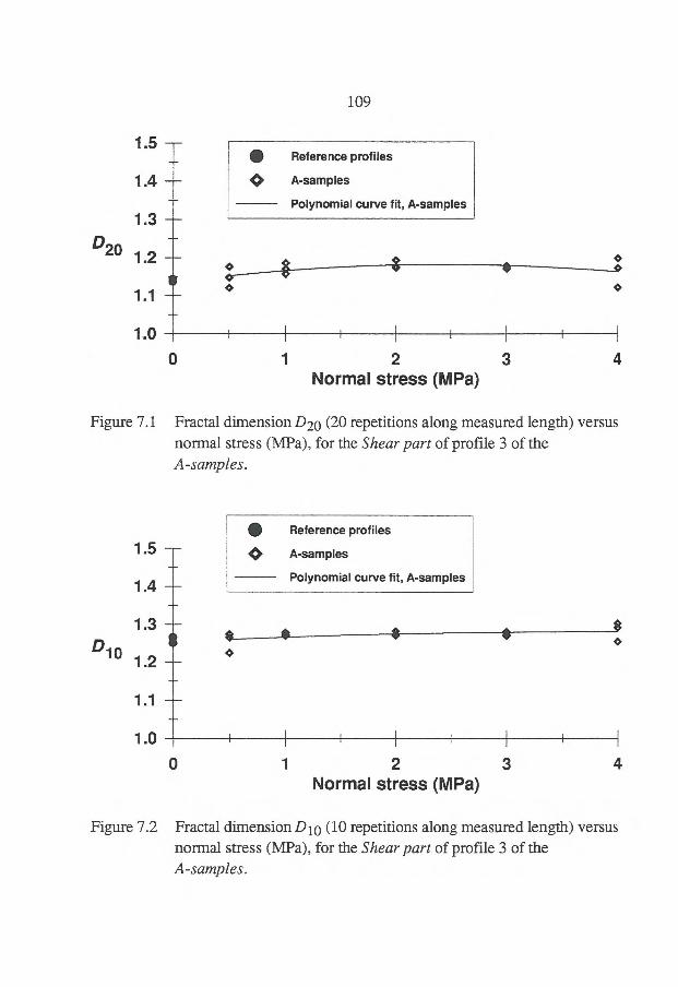
1.5
1.4
109
• Reference profiles
4> A-samples
Polynomial curve fit, A-samples
$
1.0
0
1 2 3 4 Normal stress (MPa)
Figure 7.1 Fractal dimension D20 (20 repetitions along measured length) versus normal stress (MPa), for the Shear part of profile 3 of the A-samples.
Reference profiles
1.5 A-samples
1.4 Polynomial curve fit, A-samples
_ 1.3 * s S le
D10 1.2
1 * o
o
_ 1.1
_ 1.0 1 I 1 I 1 I 1 I
0 1 2 3 4 Normal stress (MPa)
Figure 7.2 Fractal dimension D10 (10 repetitions along measured length) versus normal stress (MPa), for the Shear part of profile 3 of the A-samples.
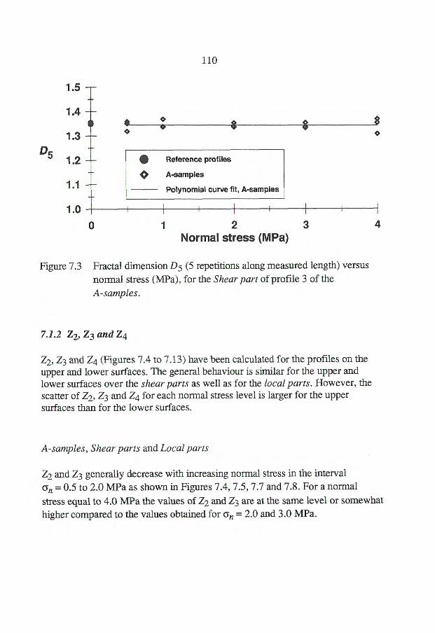
* o
o o $ 8 $
o --
1.5 —
110
• Reference profiles
e A-samples
Polynomial curve fit, A-samples
1.0
i
1
i
1
i
1
i
1
o
1 2
3 4 Normal stress (MPa)
Figure 7.3 Fractal dimension D5 (5 repetitions along measured length) versus normal stress (MPa), for the Shear part of profile 3 of the
A-samples.
7.1.2 Z2, Z3 and Z4
Z2, Z3 and Z4 (Figures 7.4 to 7.13) have been calculated for the profiles on the upper and lower surfaces. The general behaviour is similar for the upper and lower surfaces over the shear parts as well as for the local parts. However, the scatter of Z2, Z3 and Z4 for each normal stress level is larger for the upper surfaces than for the lower surfaces.
A-samples, Shear parts and Local parts
Z2 and Z3 generally decrease with increasing normal stress in the interval an = 0.5 to 2.0 MPa as shown in Figures 7.4, 7.5, 7.7 and 7.8. For a normal
stress equal to 4.0 MPa the values of Z2 and Z3 are at the same level or somewhat higher compared to the values obtained for an = 2.0 and 3.0 MPa.
D5 1.2
1.1
-
-
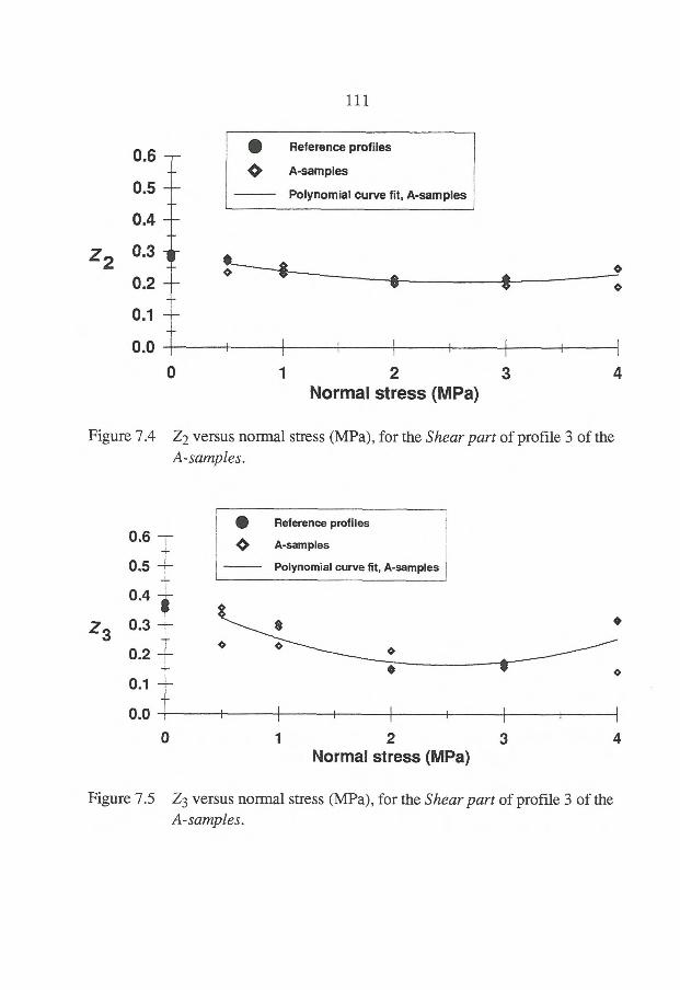
0.6 —
0.5 —
0.4
Z2
0.2
0.1 0.1
0.0
• Reference profiles
Q A-samples
Polynomial curve fit, A-samples
111
0
1 2 3 4 Normal stress (MPa)
Figure 7.4 Z2 versus normal stress (MPa), for the Shear part of profile 3 of the A-samples.
0.6
0.5
0.4 4
Z3 0.3
0.2
0.1
0.0
• Reference profiles
• A-samples
Polynomial curve fit, A-samples
0 1 2 3
4 Normal stress (MPa)
Figure 7.5 Z3 versus normal stress (MPa), for the Shear part of profile 3 of the A-samples.
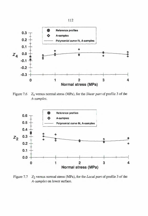
112
• Reference profiles e A-samples
Polynomial curve fit, A-samples
o
*
1
1
1
1
0.6
0.5
0.4
Z2 0.3
0.2
0.1
0.0
• Reference profiles
$ o *
# o
o
Q A-samples
Polynomial curve fit, A-samples
0.3 _
0.2 _
0.1
Z4 • -0.1 --
-0.2
-0.3 0
e e— - — - $ - -----$
!
1 2 3 4 Normal stress (MPa)
i
1
Figure 7.6 Z4 versus normal stress (MPa), for the Shear part of profile 3 of the A-samples.
0
1
2
3 Normal stress (MPa)
Figure 7.7 Z2 versus normal stress (MPa), for the Local part of profile 3 of the A-samples on lower surface.
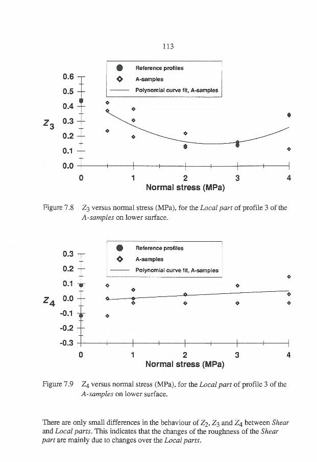
113
• Reference profiles
0.6
0.5
0.4
— e A-samples
curve fit, A-samples — Polynomial
S o — e *
Z3 0.3 —
0.2 _
o o e
0.1 e _
0.0
0
1 2
3 4 Normal stress (MPa)
Figure 7.8 Z3 versus normal stress (MPa), for the Local part of profile 3 of the A-samples on lower surface.
0.3
0.2
0.1
Z4 -0.1 •
_
-0.2 _
-0.3
• Reference profiles
e A-samples
Polynomial curve fit, A-samples
e
o
-
-
• o _ e
1
1
1
1
o
o
1
1 1
i
0
1 2 3 4 Normal stress (MPa)
Figure 7.9 Z4 versus normal stress (MPa), for the Local part of profile 3 of the A-samples on lower surface.
There are only small differences in the behaviour of Z2, Z3 and Z4 between Shear and Local parts. This indicates that the changes of the roughness of the Shear part are mainly due to changes over the Local parts.
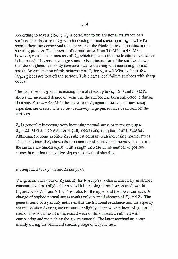
114
According to Myers (1962), Z2 is correlated to the frictional resistance of a surface. The decrease of Z2 with increasing normal stress up to an = 2.0 MPa should therefore correspond to a decrease of the frictional resistance due to the shearing process. The increase of normal stress from 3.0 MPa to 4.0 MPa, however, results in an increase of Z2, which indicates that the frictional resistance is increased. This seems strange since a visual inspection of the surface shows that the roughness generally decreases due to shearing with increasing normal stress. An explanation of this behaviour of Z2 for an = 4.0 MPa, is that a few larger pieces are torn off the surface. This creates local failure surfaces with sharp edges.
The decrease of Z3 with increasing normal stress up to Gn = 2.0 and 3.0 MPa shows the increased degree of wear that the surface has been subjected to during shearing. For Gn = 4.0 MPa the increase of Z3 again indicates that new sharp asperities are created when a few relatively large pieces have been tom off the surfaces.
Z4 is generally increasing with increasing normal stress or increasing up to an = 2.0 MPa and constant or slightly decreasing at higher normal stresses. Although, for some profiles Z4 is almost constant with increasing normal stress. This behaviour of Z4 shows that the number of positive and negative slopes on the surface are almost equal, with a slight increase in the number of positive slopes in relation to negative slopes as a result of shearing.
B-samples, Shear parts and Local parts
The general behaviour of Z2 and Z3 for B-samples is characterised by an almost constant level or a slight decrease with increasing normal stress as shown in Figures 7.10, 7.11 and 7.13. This holds for the upper and the lower surfaces. A change of applied normal stress results only in small changes of Z2 and Z3. The general trend of Z2 and Z3 indicates that the frictional resistance and the asperity sharpness after shearing are constant or slightly decrease with increasing normal stress. This is the result of increased wear of the surfaces combined with compacting and reattaching the gouge material. The latter mechanism occurs mainly during the backward shearing stage of a cyclic test.
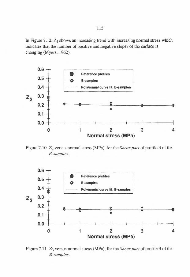
115
In Figure 7.12, Z4 shows an increasing trend with increasing normal stress which indicates that the number of positive and negative slopes of the surface is changing (Myers, 1962).
0.6 — -
0.5
0.4
Z2 0-3 -t•
0.2 _._.
0.1 -
• Reference profiles
* B-samples
Polynomial curve fit, B-samples
e $-------8 e $ $
0.0
0
1 2 3 4 Normal stress (MPa)
Figure 7.10 Z2 versus normal stress (MPa), for the Shear part of profile 3 of the B-samples.
0.6 — • Reference profiles
0.5 * B-samples
0.4 Polynomial curve fit, B-samples $
Z3 0.3
-
0.2
0.1 -- fit e 8 o
o o o $
---
0.0
0
1 2 3 4 Normal stress (MPa)
Figure 7.11 Z3 versus normal stress (MPa), for the Shear part of profile 3 of the B-samples.
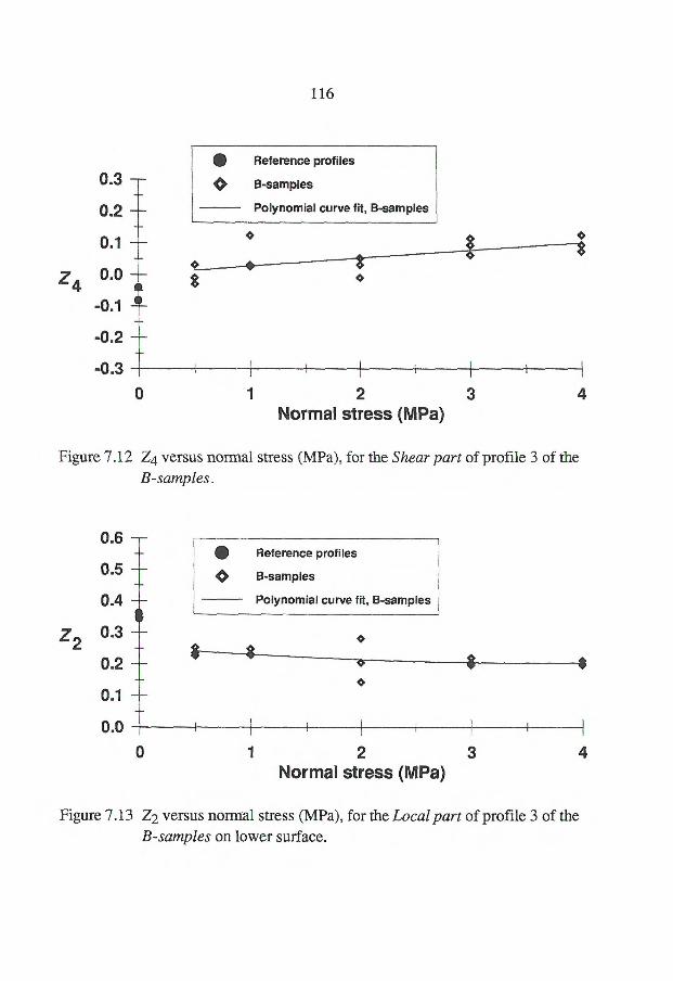
116
0.3
0.2 —
0.1 —
Z4 0.0 -;-
-0.1
-0.2
• Reference profiles
e B-samples
Polynomial curve fit, B-samples
-0.3
0
1 2 3 4 Normal stress (MPa)
Figure 7.12 Z4 versus normal stress (MPa), for the Shear part of profile 3 of the B-samples.
0.6
0.5 —
0.4
Z2 0-3
0.2
0.1
0.0
• Reference profiles
• B-samples
Polynomial curve fit, B-samples
0
1 2 3 4 Normal stress (MPa)
Figure 7.13 Z2 versus normal stress (MPa), for the Local part of profile 3 of the B-samples on lower surface.
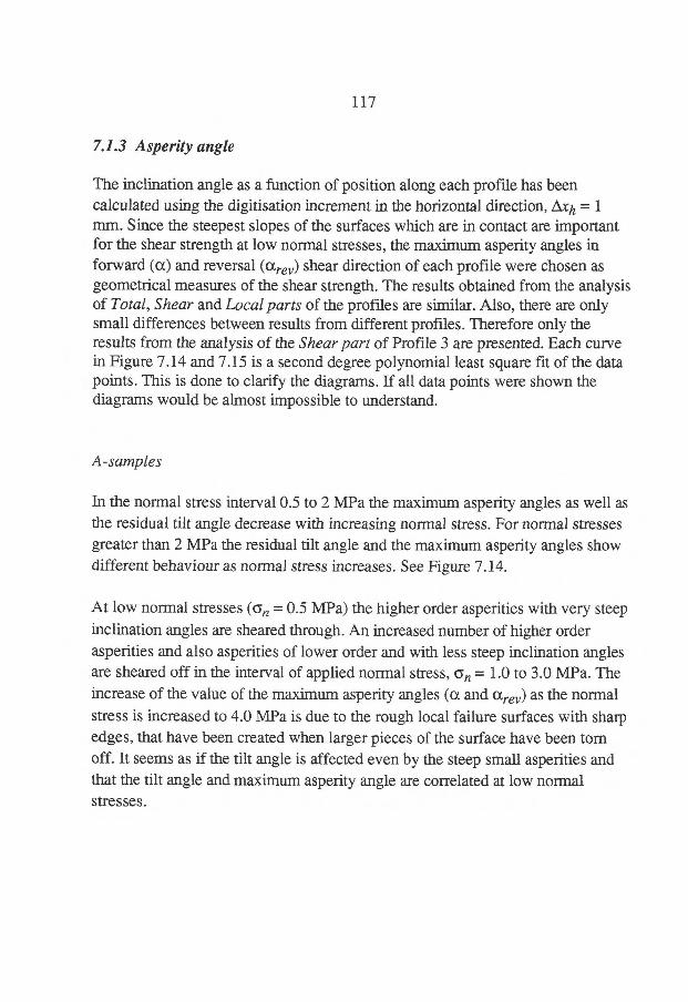
117
7.1.3 Asperity angle
The inclination angle as a function of position along each profile has been calculated using the digitisation increment in the horizontal direction, Axh = 1 mm. Since the steepest slopes of the surfaces which are in contact are important for the shear strength at low normal stresses, the maximum asperity angles in forward (a) and reversal (arev) shear direction of each profile were chosen as geometrical measures of the shear strength. The results obtained from the analysis of Total, Shear and Local parts of the profiles are similar. Also, there are only small differences between results from different profiles. Therefore only the results from the analysis of the Shear part of Profile 3 are presented. Each curve in Figure 7.14 and 7.15 is a second degree polynomial least square fit of the data points. This is done to clarify the diagrams. If all data points were shown the diagrams would be almost impossible to understand.
A-samples
In the normal stress interval 0.5 to 2 MPa the maximum asperity angles as well as the residual tilt angle decrease with increasing normal stress. For normal stresses greater than 2 MPa the residual tilt angle and the maximum asperity angles show different behaviour as normal stress increases. See Figure 7.14.
At low normal stresses (an = 0.5 MPa) the higher order asperities with very steep inclination angles are sheared through. An increased number of higher order asperities and also asperities of lower order and with less steep inclination angles are sheared off in the interval of applied normal stress, an = 1.0 to 3.0 MPa. The increase of the value of the maximum asperity angles (a and ar) as the normal stress is increased to 4.0 MPa is due to the rough local failure surfaces with sharp edges, that have been created when larger pieces of the surface have been tom off. It seems as if the tilt angle is affected even by the steep small asperities and that the tilt angle and maximum asperity angle are correlated at low normal stresses.
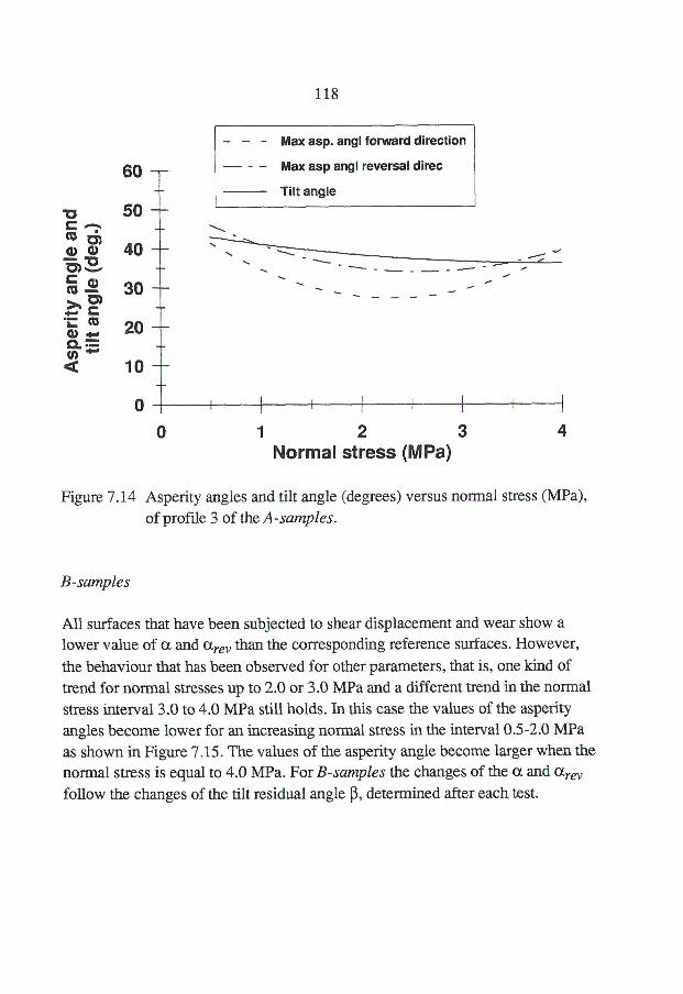
c
@)G)
c m,
60
50
40
30
41) 20 C2. =
10
0
Max asp. angl forward direction
Max asp angl reversal direc
Tilt angle
_
118
0
1 2 3
4 Normal stress (MPa)
Figure 7.14 Asperity angles and tilt angle (degrees) versus normal stress (MPa), of profile 3 of the A-samples.
B-samples
All surfaces that have been subjected to shear displacement and wear show a lower value of ct and °trey than the corresponding reference surfaces. However,
the behaviour that has been observed for other parameters, that is, one kind of trend for normal stresses up to 2.0 or 3.0 MPa and a different trend in the normal stress interval 3.0 to 4.0 MPa still holds. In this case the values of the asperity angles become lower for an increasing normal stress in the interval 0.5-2.0 MPa as shown in Figure 7.15. The values of the asperity angle become larger when the normal stress is equal to 4.0 MPa. For B-samples the changes of the a and arev follow the changes of the tilt residual angle ß, determined after each test.
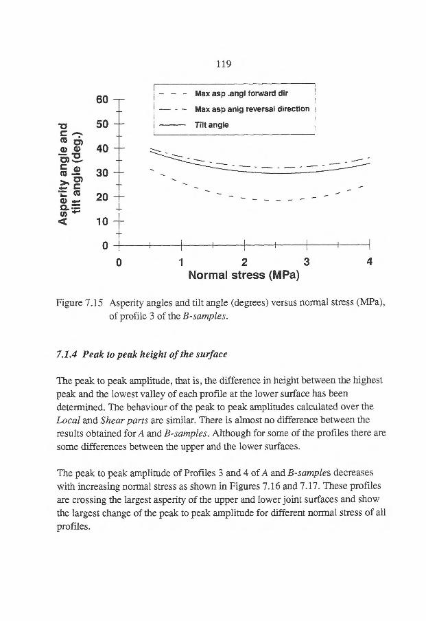
119
60
• 50 c
ti) 41) a) 40 01 C a)
30 — ▪ 05
e c 20
10
0
Max asp .angl forward dir
Max asp anlg reversal direction
Tilt angle
0
1 2 3
4 Normal stress (MPa)
Figure 7.15 Asperity angles and tilt angle (degrees) versus normal stress (MPa), of profile 3 of the B-samples.
7.1.4 Peak to peak height of the surface
The peak to peak amplitude, that is, the difference in height between the highest peak and the lowest valley of each profile at the lower surface has been determined. The behaviour of the peak to peak amplitudes calculated over the Local and Shear parts are similar. There is almost no difference between the results obtained for A and B-samples. Although for some of the profiles there are some differences between the upper and the lower surfaces.
The peak to peak amplitude of Profiles 3 and 4 of A and B-samples decreases with increasing normal stress as shown in Figures 7.16 and 7.17. These profiles are crossing the largest asperity of the upper and lower joint surfaces and show the largest change of the peak to peak amplitude for different normal stress of all profiles.
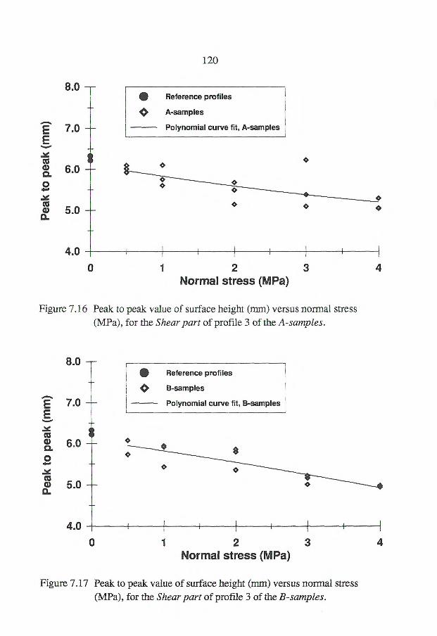
120
• Reference profiles
Q A-samples
Polynomial curve fit, A-samples
_ 8
6.0
-
5.0 —
-
4.0
8.0
-
7.0
o o
1
0
1 2 3 4 Normal stress (MPa)
Figure 7.16 Peak to peak value of surface height (mm) versus normal stress (MPa), for the Shear part of profile 3 of the A-samples.
Pea
k to
pea
k (m
m)
8.0
• Reference profiles
Q B-samples
Polynomial curve fit, B-samples
-
Pea
k to
pea
k (m
m)
7.0
_ 8
6.0
-
5.0 —
-
4.0
i
I
i
1
i
1
i
1
o
1 2
3
4 Normal stress (MPa)
Figure 7.17 Peak to peak value of surface height (mm) versus normal stress (MPa), for the Shear part of profile 3 of the B-samples.
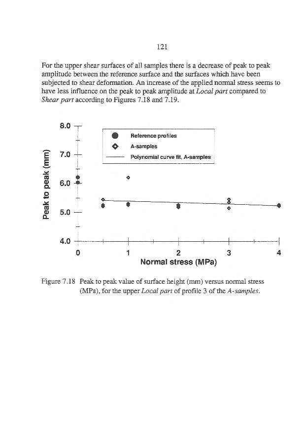
6.0 e
-
121
For the upper shear surfaces of all samples there is a decrease of peak to peak amplitude between the reference surface and the surfaces which have been subjected to shear deformation. An increase of the applied normal stress seems to have less influence on the peak to peak amplitude at Local part compared to Shear part according to Figures 7.18 and 7.19.
8.0
_
-
•
Pea
k to
pea
k (m
m)
7.0
5.0
o *
4.0
• Reference profiles
Q A-samples
Polynomial curve fit, A-samples
o
* $ $ o
0 1 2 3 Normal stress (MPa)
Figure 7.18 Peak to peak value of surface height (mm) versus normal stress (MPa), for the upper Local part of profile 3 of the A-samples.
4
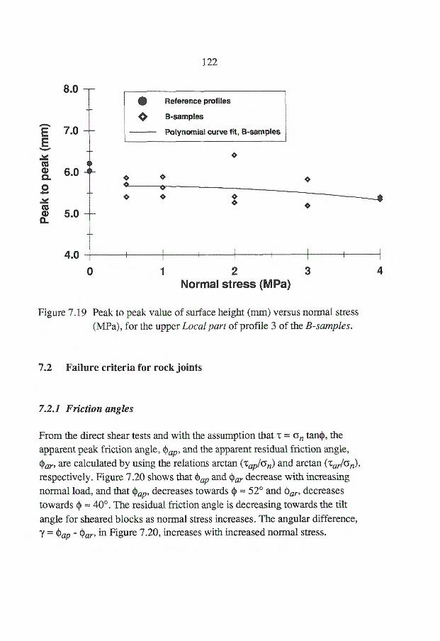
--
122
8.0 • Reference profiles
CO B-samples
Polynomial curve fit, B-samples
o
e
o o o
e
e
4.0 i
i
1
1
0 1 2 3
4 Normal stress (MPa)
Figure 7.19 Peak to peak value of surface height (mm) versus normal stress (MPa), for the upper Local part of profile 3 of the B-samples.
7.2 Failure criteria for rock joints
7.2.1 Friction angles
From the direct shear tests and with the assumption that t = Gn tanO, the apparent peak friction angle, Oap, and the apparent residual friction angle, Oar, are calculated by using the relations arctan (tap/an) and arctan (Tar/(5n),
respectively. Figure 7.20 shows that Oap and Oar decrease with increasing normal load, and that Oap, decreases towards 0 ----- 52° and Oar, decreases towards 0 .-- 40°. The residual friction angle is decreasing towards the tilt angle for sheared blocks as normal stress increases. The angular difference, 7 = 'lap - Oar, in Figure 7.20, increases with increased normal stress.
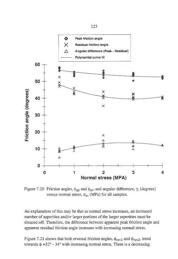
123
60
50
‘,/ Peak friction angle X Residual friction angle
46, Angular difference (Peak - Residual)
fit Polynomial curve
x
x
40 — 0-
x
30
20 A
A 10 A
A
0
0 1 2 3
4 Normal stress (MPA)
Figure 7.20 Friction angles, Oap and e'ar' and angular difference, 'y, (degrees) versus normal stress, an, (MPa) for all samples.
An explanation of this may be that as normal stress increases, an increased number of asperities and/or larger portions of the larger asperities must be sheared off. Therefore, the difference between apparent peak friction angle and apparent residual friction angle increases with increasing normal stress.
Figure 7.21 shows that both reversal friction angles, Orevi and 4Prev2, trend towards (1)=32° - 340 with increasing normal stress. There is a decreasing
Fri
ctio
n a
ng
le (d
egre
es)
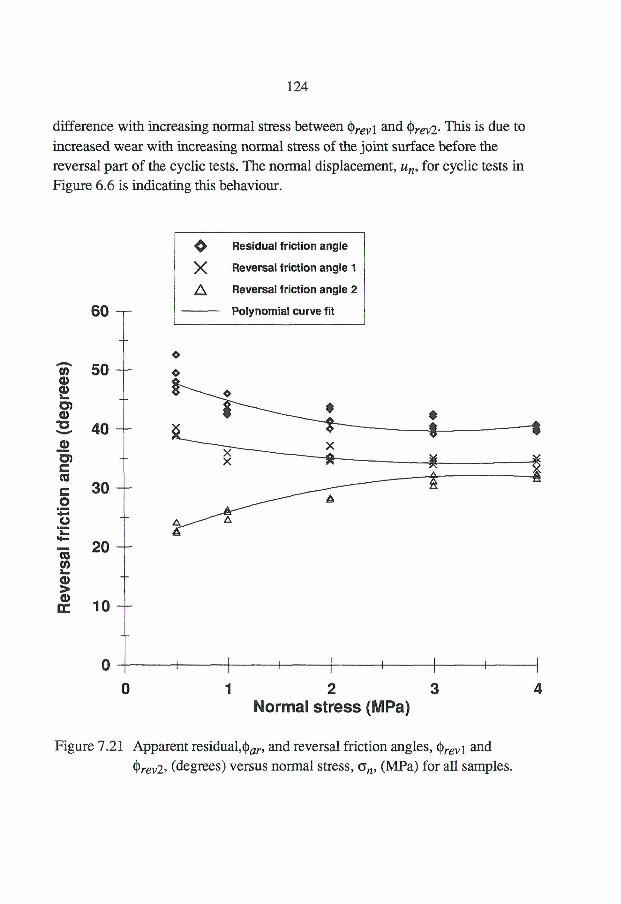
60
--
50
-
40
-
30
-
20
-
10 Rev
ersa
l fri
ctio
n a
ng
le (
deg
rees
) 124
difference with increasing normal stress between Orev1 and Orev2. This is due to increased wear with increasing normal stress of the joint surface before the reversal part of the cyclic tests. The normal displacement, un, for cyclic tests in Figure 6.6 is indicating this behaviour.
Q Residual friction angle X Reversal friction angle 1
A Reversal friction angle 2
Polynomial curve fit
o
-
0 1 2 3 Normal stress (MPa)
Figure 7.21 Apparent residual,Oar, and reversal friction angles,
O Orevi and
rev2 , (degrees) versus normal stress, Gn, (MPa) for all samples.
4 0
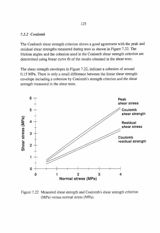
4 --
3 —
She
ar s
tres
s (M
Pa)
2 _
125
7.2.2 Coulomb
The Coulomb shear strength criterion shows a good agreement with the peak and residual shear strengths measured during tests as shown in Figure 7.22. The friction angles and the cohesion used in the Coulomb shear strength criterion are determined using linear curve fit of the results obtained in the shear tests.
The shear strength envelopes in Figure 7.22, indicate a cohesion of around 0.15 MPa. There is only a small difference between the linear shear strength envelope including a cohesion by Coulomb's strength criterion and the shear strength measured in the shear tests.
Peak shear stress
5 Coulomb shear strength _
Residual shear stress
Coulomb residual strength
1 _
o
0 1 2 3
4 Normal stress (MPa)
Figure 7.22 Measured shear strength and Coulomb's shear strength criterion (MPa) versus normal stress (MPa).
6
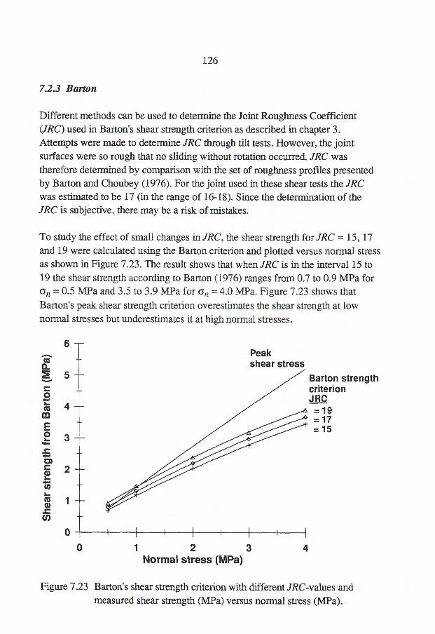
Barton strength criterion JRC = 19 = 17 = 15
Sh
ear
stre
ngth
fro
m B
art
on
(M
Pa
) Peak shear stress
5 — -
4 — -
3 — -
2
1 -- -
1 2 3 Normal stress (MPa)
o o 4
6 —
1 1 I
126
7.2.3 Barton
Different methods can be used to determine the Joint Roughness Coefficient (JRC) used in Barton's shear strength criterion as described in chapter 3. Attempts were made to determine JRC through tilt tests. However, the joint surfaces were so rough that no sliding without rotation occurred. JRC was therefore determined by comparison with the set of roughness profiles presented by Barton and Choubey (1976). For the joint used in these shear tests the JRC was estimated to be 17 (in the range of 16-18). Since the determination of the JRC is subjective, there may be a risk of mistakes.
To study the effect of small changes in JRC, the shear strength for JRC = 15, 17 and 19 were calculated using the Barton criterion and plotted versus normal stress as shown in Figure 7.23. The result shows that when JRC is in the interval 15 to 19 the shear strength according to Barton (1976) ranges from 0.7 to 0.9 MPa for san = 0.5 MPa and 3.5 to 3.9 MPa for Gn = 4.0 MPa. Figure 7.23 shows that Barton's peak shear strength criterion overestimates the shear strength at low normal stresses but underestimates it at high normal stresses.
Figure 7.23 Barton's shear strength criterion with different JRC-values and measured shear strength (MPa) versus normal stress (MPa).
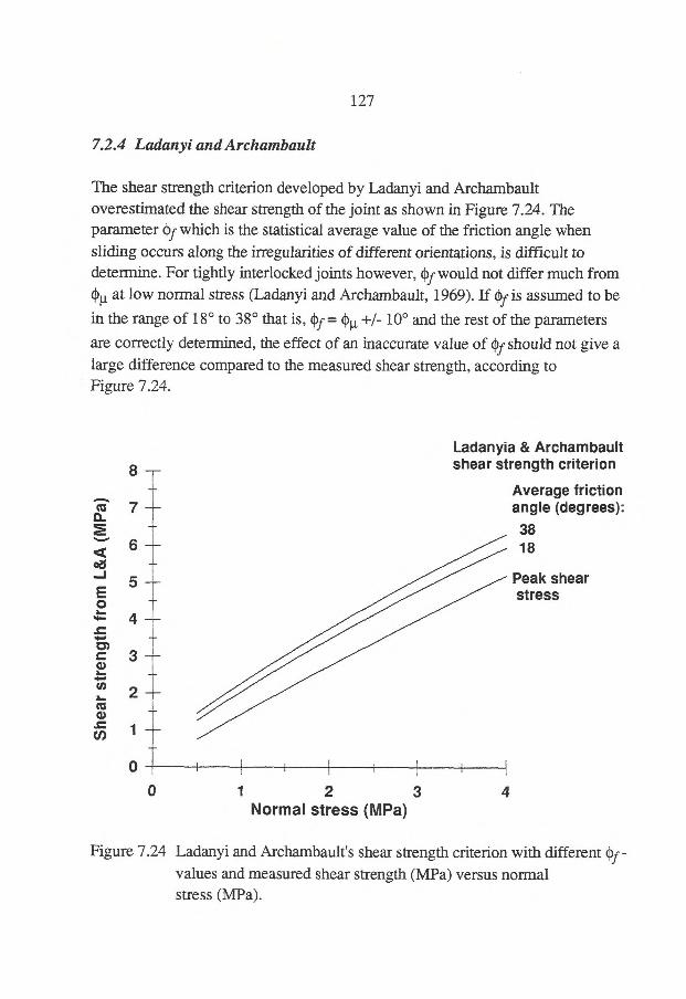
5 — -
o o
1
1 2 3 Normal stress (MPa)
! i I 1 i i
4 I
127
7.2.4 Ladanyi and Archambault
The shear strength criterion developed by Ladanyi and Archambault overestimated the shear strength of the joint as shown in Figure 7.24. The parameter Of which is the statistical average value of the friction angle when
sliding occurs along the irregularities of different orientations, is difficult to determine. For tightly interlocked joints however, Of would not differ much from eg at low normal stress (Ladanyi and Archambault, 1969). If Of is assumed to be
in the range of 18° to 38° that is, Of = 01.1 +1- 10° and the rest of the parameters
are correctly determined, the effect of an inaccurate value of cly should not give a large difference compared to the measured shear strength, according to Figure 7.24.
Ladanyia & Archambault
8 — shear strength criterion
_ Average friction
7 — angle (degrees):
_ 38 6
18 _
Peak shear stress
4
3 — -
2 — -
1 -^
Sh
ear
str
eng
th fro
m L
&A
(M
Pa)
_
Figure 7.24 Ladanyi and Archambault's shear strength criterion with different Of - values and measured shear strength (MPa) versus normal stress (MPa).
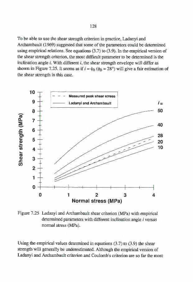
Sh
ear
str
en
gth
(M
Pa)
10
9
8
7
6
5
4
3
2
1
- Measured peak shear stress
Ladanyi and Archambault
40
50
28 20 10
128
To be able to use the shear strength criterion in practice, Ladanyi and Archambault (1969) suggested that some of the parameters could be determined using empirical relations. See equations (3.7) to (3.9). In the empirical version of the shear strength criterion, the most difficult parameter to be determined is the inclination angle i. With different i, the shear strength envelope will differ as shown in Figure 7.25. It seems as if i =b (ob = 28°) will give a fair estimation of the shear strength in this case.
I i 1
0 1 2 3
4 Normal stress (MPa)
Figure 7.25 Ladanyi and Archambault shear criterion (MPa) with empirical determined parameters with different inclination angle i versus normal stress (MPa).
Using the empirical values determined in equations (3.7) to (3.9) the shear strength will generally be underestimated. Although the empirical version of Ladanyi and Archambault criterion and Coulomb's criterion are so far the most
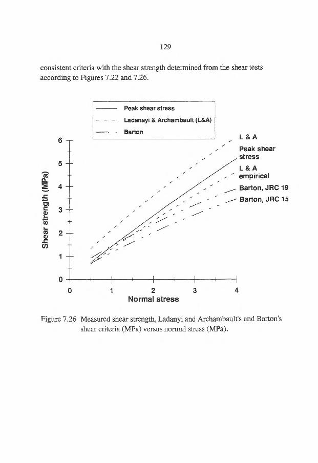
- _ -
Peak shear stress
Ladanayi & Archambault (L&A)
Barton
, , stress
6
5
4
3 -
2 - S
hea
r str
eng
th (
MP
a)
o
o
129
consistent criteria with the shear strength determined from the shear tests according to Figures 7.22 and 7.26.
, L & A
, Peak shear
, , , , , ..,
, , ,
-- , , ,
-- .. , . - , ,
' - ------ , -
i i i i i i i i
L & A , empirical
------ Barton, JRC 19 ,
,-- Barton, JRC 15
...•
I'
,
1 2 3 4 Normal stress
,
r r
,
r
Figure 7.26 Measured shear strength, Ladanyi and Archambault's and Barton's shear criteria (MPa) versus normal stress (MPa).
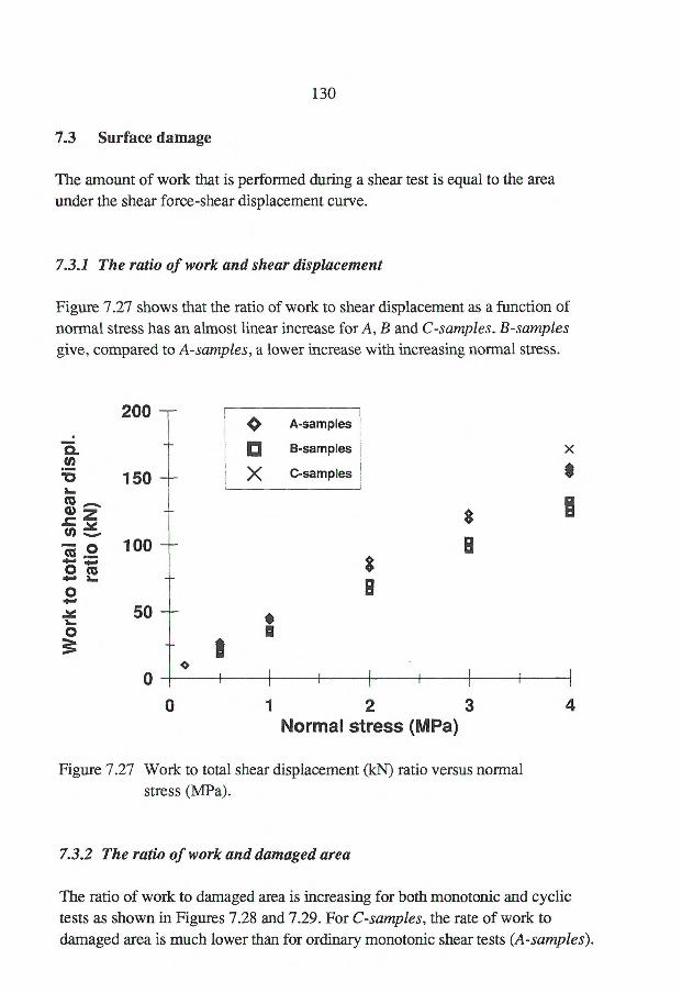
x
4
130
7.3 Surface damage
The amount of work that is performed during a shear test is equal to the area under the shear force-shear displacement curve.
7.3.1 The ratio of work and shear displacement
Figure 7.27 shows that the ratio of work to shear displacement as a function of normal stress has an almost linear increase for A, B and C-samples. B-samples give, compared to A-samples, a lower increase with increasing normal stress.
e A-samples
171. D B-samples
150 X C-samples
co—' z • P 100 B cu o $
200
50
o
0
0
1 2 3 Normal stress (MPa)
Figure 7.27 Work to total shear displacement (kN) ratio versus normal stress (MPa).
7.3.2 The ratio of work and damaged area
The ratio of work to damaged area is increasing for both monotonic and cyclic tests as shown in Figures 7.28 and 7.29. For C-samples, the rate of work to damaged area is much lower than for ordinary monotonic shear tests (A-samples).
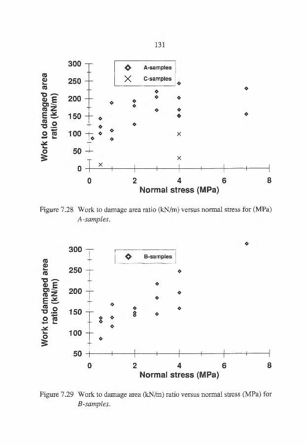
300 Q A-samples
250 — X C-samples
200 •
4:* 150 o
100 4>
50
x 0
x
e B-samples , 1 o
1
o o
o
44' 0
0
131
0
2 4 6
8 Normal stress (MPa)
Figure 7.28 Work to damage area ratio (kN/m) versus normal stress for (MPa) A-samples.
tt
2 ca 7:1 a) E o)-- as z
300
250
200
..._
_
E -..... co
— e -0 2 150
.Y 0 ri.
e
145 100 o
50 2 4 6
8
Normal stress (MPa)
Figure 7.29 Work to damage area (kN/m) ratio versus normal stress (MPa) for B-samples.
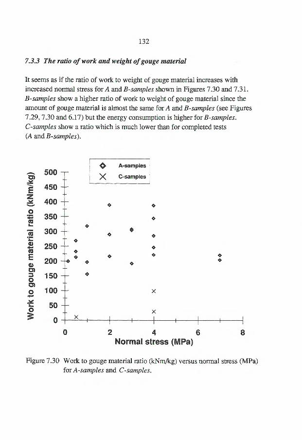
Wo
rk t
o g
ou
ge
mat
eri
al r
atio
(kN
m/k
g) 500
450
400
350
300
250
200
150
100
50
0
132
7.3.3 The ratio of work and weight of gouge material
It seems as if the ratio of work to weight of gouge material increases with increased normal stress for A and B-samples shown in Figures 7.30 and 7.31. B-samples show a higher ratio of work to weight of gouge material since the amount of gouge material is almost the same for A and B-samples (see Figures 7.29,7.30 and 6.17) but the energy consumption is higher for B-samples. C-samples show a ratio which is much lower than for completed tests (A and B-samples).
e A-samples
X C-samples
0
2 4 6
8 Normal stress (MPa)
Figure 7.30 Work to gouge material ratio (kNmikg) versus normal stress (MPa) for A-samples and C-samples.
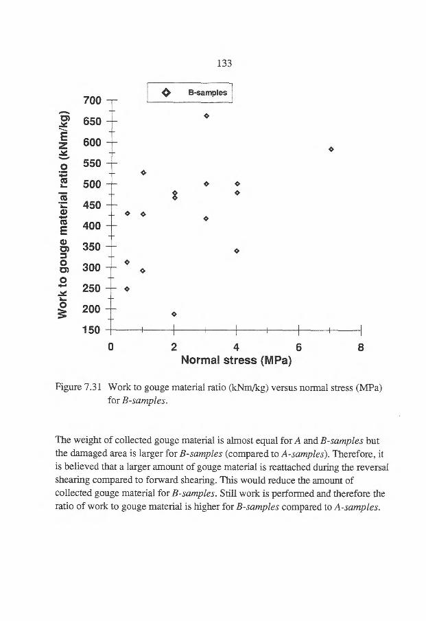
133
B-samples
o
o
$
o
o
1
i
!
i
i
i
1
4> 700
_
650 — _
600 _
550 -,- e
500
450 _ o o
400 _
350 _
300 o
e
250 _
o
200 --
150 f
0
2 4 6 8 Normal stress (MPa)
Figure 7.31 Work to gouge material ratio (kNinikg) versus normal stress (MPa) for B-samples.
The weight of collected gouge material is almost equal for A and B-samples but the damaged area is larger for B-samples (compared to A-samples). Therefore, it is believed that a larger amount of gouge material is reattached during the reversal shearing compared to forward shearing. This would reduce the amount of collected gouge material for B-samples. Still work is performed and therefore the ratio of work to gouge material is higher for B-samples compared to A-samples.
Wo
rk t
o g
ou
ge m
ate
ria
l ra
t io (
kN
m/k
g)

134
135
8 DISCUSSION AND CONCLUSION
A comprehensive experimental study of the performance of rough rock joints has been conducted. Three main issues have been addressed: i) the mechanics of rock joints, ii) the characterisation of the damage to the joint surfaces due to shearing and iii) the characterisation of joint roughness and its relevance for the physical properties of the joint.
To be able to investigate the influence of normal stress and shear path on the mechanical behaviour of the rock joint 40 replicas of a mated natural joint have been made and tested. The concrete mixture used in this study has a relatively high uniaxial compressive strength, ac = 67.6 MPa, similar to that of sedimentary rocks such as sandstone and limestone. Differences in the mechanical behaviour of the joint due to scale effects were not investigated. The effect of the shear box stiffness on the results obtained is unknown at the present time since no other shear test equipment has been used.
Two different types of shear tests have been carried out, for five different normal stresses, an = 0.5, 1, 2, 3, 4 MPa, namely monotonic shearing in one direction (30 mm) and cyclic shearing forward (30 mm) and then backward to the initial position. A number of extra monotonic shear tests have been conducted to study the development of damage to the joint surfaces at different stages of the shear test. Also, two monotonic tests and one cyclic test were performed with a higher normal stress, an = 7 MPa, in order to study if the failure mechanism changes at higher normal stress.
After each test the gouge material has been collected and the damaged areas of the joint surfaces have been marked and photographed.
To be able to study the damage to the joint surfaces due to shearing the upper and lower surfaces have to be measured before and after each shear test. Seven profiles in the shear direction were defmed so that each profile on the upper surface was in contact with the corresponding profile on the lower surface. Since all samples were identical, the upper and lower joint surfaces of three reference samples were chosen to represent the conditions before shearing. After each shear test the joint surfaces were measured.
136
The mechanics of rock joints
Two different compressive tests were carried out to investigate the normal stress - normal displacement characteristics. AE was recorded in these tests in order to study the development of damage to the joint surfaces. The AE and a visual inspection after each test revealed no signs of damage to the surfaces due to the compressive loading. Hence, all damage to the joint surfaces observed after each shear test must originate from the relative shear motion between the two opposite joint surfaces.
There are at least four different mechanisms which contribute to the shear resistance and the development of damage to the joint surfaces: dilation/contraction and climbing over asperities, breakage of asperities (tensile, shear or crushing), transportation of gouge material and reattachment of gouge material.
These mechanisms usually occurred more or less at the same time during the shear tests in this study. At shear stress peak the shear resistance is mainly due to interlocking of asperities. This was caused by asperities with very steep inclination angles, which also made it impossible to performed a correct tilt test without rotation. Further shear displacement required breakage of these asperities for all normal stresses. The reversal stage of the shear test is characterised by the presence of a large amount of gouge material. An additional number of asperities were sheared through and a large amount of gouge material was reattached at the same time as the joint surfaces contract.
In six shear tests AE was recorded and source location performed. The transducers were attached to the upper block in four tests and to the lower block in two tests. A general observation is that the AE activity at different stages of the shear tests was so low that no AE could be detected. After each such period of silence a new interval of AE activity occurred.
The asperities which are interlocking the upper and lower surfaces and prevent the shear movement are relatively few and small in tests with low normal stress. In each of these tests AE was not detectable during 9 nun of shearing (parts of silence) due to almost pure sliding and dilation during shearing. Visual inspection of samples from monotonic tests showed that almost all damage to the surfaces,
137
observed after ordinary monotonic tests (us = 30 mm, A-samples), was done at shear stress peak (us --- 2 mm, C-samples).
In tests with high normal stress the number and size of these interlocking asperities increased compared to tests with low normal stress. They were also more equally distributed over the joint surfaces and controlled the shear movement during longer periods of the shear tests due to less dilation compared to tests with low normal stress. The total shear displacement with no detectable AE was around 6 mm and is assumed to be due to failure of very small asperities combined with transportation and reattachment of gouge material. Visual inspection of C-samples, (us ----. 2 mm) with an = 4.0 MPa showed a damaged area which is 30 - 50 % of that observed after 30 mm of shear displacement (A-sample) at the same normal stress level.
The damaged area increased as normal stress increased. For instance, after the monotonic tests with normal stress equal to 0.5 MPa and 4.0 MPa and a total shear displacement of 30 mm, 7 to 9 % and 22 to 37 %, respectively, of the total contact surfaces were damaged due to shearing. Here the total contact surface means the area of the upper surface (170*250 mm) plus the area of the lower surface which was involved in the shearing process (200*250 mm). After cyclic tests the damaged area caused by 30 mm of forward and backward shearing with normal stress equal to 0.5 MPa and 4.0 MPa is 10 to 15 % and 36 to 54 %, respectively, of the total contact surface. The weight of gouge material collected after each test is, however, almost the same for monotonic and cyclic tests carried out at the same normal stress level.
The work which has been performed during a test divided by the weight of gouge material increases with increasing normal stress. The increase is higher for cyclic tests which indicates that gouge material is lost during cyclic tests and that work is performed to reattach gouge material. This is also shown by the shear strength at the end of the reverse shearing where there is an increase of the shear strength and the upper and lower joint surfaces can not be fully mated.
A number of different shear strength criteria have been compared to the shear strength measured during the shear tests. There is only a small difference between the linear shear strength by the Coulomb shear strength criterion and shear strength measured during the tests. The empirical version of the Ladanyi and Archambault shear strength criterion also shows good agreement with the
138
experimental results while the theoretical version seems to overestimate the shear strength. Barton's shear strength criterion on the other hand underestimates the shear strength of the joint. JRC had to be determined by comparison with the set of roughness profiles presented by Barton and Choubey (1977). The inaccuracy of this method may have contributed to the discrepancy between measured and calculated shear strength.
Characterisation of roughness of joint surfaces
Two different types of shear tests have been carried out for five different normal stresses which resulted in different degrees of damage to the joint surfaces. This means, theoretically, that 10 new joints with different joint surfaces were obtained (made). Although, due to variations of the compressive strength of the joint surfaces there may be some differences in roughness between joints which have been subjected to the same normal stress and shear path. In order to quantify the damage to the surface the data from the profile measurements have been analysed using fractal geometry and descriptive statistics. The fractal dimension,
D, and the rms of the first and second derivative of the surface profiles, Z2 and Z3, respectively, have been calculated. The peak to peak amplitude of the joint surfaces, and the maximum asperity angle in the forward (a) and reversed (arev)
shear directions, respectively, have also been determined. Some of these parameters have been compared to the residual tilt angle determined after each shear test.
The fractal dimension of all profiles of the reference samples and the samples which had been sheared, was calculated assuming a self affine model. The results from this study show that the use of fractal geometry to describe the roughness of natural rock joint surfaces is questionable. One reason of this conclusion is that the calculation of the fractal dimension requires data which can only be obtained using a measuring device with a very high accuracy or by using data from profile measurements of a very large joint surface. This reduces the possibility to use fractal geometry in practical applications. Another problem for the fractal dimension is the uniqueness. Due to the randomness of the height distributions and the uncertainties in the measurement, a value of D may correspond to different joint surfaces whose morphological patterns are statistically equivalent, but may have different physical properties.
139
The parameters Z2 (slope), Z3 (sharpness of asperities) and the asperity angles a and ar ev for the shear and local parts of the measured profiles decrease as normal stress increases. This behaviour indicates that the higher the applied normal stress is the smoother the joint surfaces become. However, this trend is changed for monotonic tests with normal stress greater than 3.0 MPa. An explanation of this behaviour is that a few larger pieces are tom off the surface during tests with higher normal stress (4.0 MPa). This creates local failure surfaces with sharp edges. The maximum asperity angles (a and ar ), Z2 (slope) and the residual tilt angle show a similar dependency of an at low normal stress levels which indicates that small asperities affect the shear strength in this normal stress interval.
There is almost no difference in the behaviour of the peak to peak amplitude between A and B-samples. The largest changes in the peak to peak amplitude were observed for profiles 3 and 4 which are crossing the largest asperity (wave length -,-- 80 mm) of the upper and lower joint surfaces. The peak to peak amplitude show the same trend as the maximum asperity angles, Z2 and tilt angle for all samples sheared with normal stress up to 3.0 MPa.
Summary of Conclusions
• AE and visual inspections of the joint surfaces after different compressive tests and shear tests showed that all damage to the joint surface after shearing originate from shear movement between the two opposite joint surfaces.
• Four different mechanisms which contribute to the shear resistance and the development of damage to the joint surface: dilation/contraction and climbing over asperities, breakage of asperities, transportation of gouge material and reattachment of gouge material.
• At shear stress peak the shear resistance is mainly due to interlocking of asperities.
• The reversal stage of the shear test is characterised by the presence of a large amount of gouge material and work is performed to reattach gouge material.
140
• The Coulomb shear strength criterion and the empirical version of the Ladanyi and Archambault strength criterion show good agreement with the shear strength behaviour of the joint.
• It is shown that the use of fractal geometry to describe the roughness of natural rock joint surfaces is questionable. One reason is that the calculation of fractal dimension requires a very high accuracy of the measuring device and this reduces the possibility to use fractal geometry in practical applications.
• The higher the applied normal stress is the smoother the joint surfaces become but this trend is changed for monotonic tests with normal stress greater than 3.0 MPa as local failure surfaces with sharp edges are created.
• Small asperities are assumed to affect the shear strength at low normal stress levels, the maximum asperity angle (ce and cxrev) and Z2 (slope) can, therefore
be measures of the shear strength of a joint at low normal stress levels.
• The residual tilt angle is correlated to the peak to peak amplitude. This indicates that the peak to peak amplitude is a parameter which can be used to estimated the shear strength at low normal stress levels.
Recommendations for future research
This study has shown that the roughness parameters available today either require very accurate measurements of surface profiles or some kind of shear test to be determined satisfactorily. Also, a number of these parameters are more or less based on two-dimensional measurements of the joint surface roughness. To characterise roughness as a measure of the shear strength it is not sufficient to use two-dimensional models. Three-dimensional techniques for measurement and analysis need be developed, together with models which describe the physical processes in a rock joint during different stages of the shearing process.
Laboratory shear tests on natural rock joints (not replicas) should be conducted to study the failure process and how the roughness of the joint surfaces affects the behaviour at different normal stress levels and scales. 3D source location (AE) should be used to study the development of the damage to the two surfaces at different stages of the shear tests and at different normal stress levels.
141
These tests together with measurements of the joint surfaces before and after the shearing, should be used to establish models for the strength of rock joints based on physical features of the surfaces such as peak to peak amplitude and dominant wavelengths of undulations/asperities. A comprehensive field investigation should also be carried out in order to study the scale effects of the roughness and also differences in scaling laws for joints developed due to different geological processes.

142
143
9 REFERENCES
Armstrong, B.H. 1969. Bulletin of the Seismological Society of America. BSSAA, Vol. 59 No. 3 pp. 1259-1279.
Bandis, S. C. 1992. Engineering properties and characterization of rock discontinuities. In Comprehensive Rock Engineering. Principles, Practice & Projects. Volume 1: Fundamentals pp. 155-183.
Bandis, S., Lumsden, A.C. and Barton, N.R. 1981. Experimental studies of scale effects on the shear behaviour of rock joints. Int. J. Rock Mech. Min. Sci. & Geomech. Abstr. Vol. 18 pp. 1-21.
Barton, N. 1976. The shear strength of rock and rock joints. Int. J. Rock Mech. Min. Sci. & Geomech. Abstr. Vol. 13 pp. 255-279.
Barton, N. and Bandis, S. 1982. Effects of block size on the shear behaviour of jointed rock. Proc. 23d. Symp. on Rock Mech. Berkeley, Colorado, U.S. pp. 739-760.
Barton, N., Bandis, S. and Bakhtar, K. 1985. Strength, deformation and conductivity coupling of rock joints. Int. J. Rock Mech. Min. Sci. & Geomech. Abstr. Vol. 22 No. 3, pp. 121-140.
Barton, N. and Choubey, V. 1977. The shear strength of rock joints in theory and practice. Rock Mechanics, Vol.10/1-2, pp. 1-54.
Beattie, A.G. 1983. Acoustic emission, principles and instrumentation. Journal of Acoustic Emission, Vol. 2, No 2, pp. 95-128.
Bendat, J.S. and Piersol, A.G. 1971. Random data: Analysis and measurement procedures. Wiley-Interscience.
Bendat, J.S. and Piersol, A.G. 1980. Engineering applications of correlation and spectral analysis. John Wiley & Sons.
144
Brady, B.H.G. and Brown, E.T. 1985. Rock mechanics for underground mining. London, George Allen & Unwin, pp. 86-134.
Brady, B.H.G. and Brown, E.T. 1993. Rock mechanics for underground mining. Second edition. London, George Allen & Unwin.
Brown, E.T. 1981. Rock characterization testing and monitoring, ISRM Suggested methods. Pergamon Press.
Brown, S and Scholz, C.H. 1985. Broad bandwidth study of the topography of natural rock surfaces. Journal of Geophysical Research., Vol. 90, No. B14, pp. 12,575-12,582.
Brown, S.R. 1987a. Fluid flow through rock joints: The effect of surface roughness, Journal of Geophysical Research, Vol. 92, pp. B1337-1347.
Brown, S.R. 1987b. A note on the description of surface roughness using fractal dimension. Geophysical Research Letters, Vol. 14, No. 11, pp. 1095-1098.
Brown, S.R. 1989. Fractal dimension of rough surfaces and some geophysical records. Sandia Laboratories, Sandia, NM, Tech. Rep. SAND89-1934j.
Carr, J.R. and Warriner, J.B. 1989. Relationship between the fractal dimension and joint roughness coefficient. Bull. Association of Engineering Geologists, XXVI (2), pp. 253-263.
Evans, B. and Wong, T.-F. 1985. Shear localization in rocks induced by tectonic deformation. Mechanics of Geomaterials, Rocks, Concretes, Soils. pp. 189-210.
Feder, J. 1988. Fractals. Plenum Press, New York and London.
Goodman, R.E. 1976. Methods of geological engineering in discontinuous rocks. West Publishing Company, San Francisco.
Goodman, R.E. 1980. Introduction to rock mechanics. John Wiley & Sons, New York.
145
Goodman, R.E., Taylor, R.L. and Brekke T.A. 1968. A model for the mechanics of jointed rock. J. Soil Mech. Fdns. Div. Proc. Am. Soc. civ. Engrs. 94(SM3). pp. 637-659.
Hardy, H.R. Jr. 1972. Applications of acoustic emission techniques to rock mechanics research. Acoustic Emissions, ASTM STP 505, American Society for Testing and Materials pp. 41-83.
Hardy, H.R. Jr. 1981. Applications of acoustic emission techniques to rock and rock structures. A state-of-the-art review. Acoustic Emissions in Geotechnical Engineering Practice, ASTM STP 750, American Society for Testing and Materials, pp. 4-92.
Herdocia, A. 1985. Shear tests of artificial joints. Licentiate Thesis 1985:013 L, Division of Rock Mechanics, Luleå University of Technology, 116 p.
Hoek, E, and Bray, J.W. 1981. Rock slope engineering. Institution of Mining and Metallurgy, London, UK.
Hsiung, S.M., Ghosh, A., Ahola, M.P. and Chowdhury, A.H. 1993. Assessment of conventional methodologies for joint roughness coefficient determination. Int. J. Rock Mech. Min. Sci. & Geoemch. Abstr. Vol. 30, No. 7, pp. 825-829.
Jing, L. 1990. Numerical modelling of jointed rock masses by distinct element method for two, and three-dimensional problems. Doctoral Thesis 1990:90 D, Division of Rock Mechanics, Luleå University of Technology, 226 p.
Jing, L. and Stephansson, 0. 1995. Mechancis of rock joints: Experimental aspects. Proc. 2nd International Conference on the Mechanics of Jointed and Faulted Rock, Vienna, Austria, pp. 37-47.
Koerner, R.M., McCabe,W.M. and Lord, A.E. Jr. 1981. Overview of acoustic emission monitoring of rock structures. Rock Mechanics, Vol. 14, pp. 27-35.
146
Labuz, J.F., Chang, H.S., Dowding, C.H. and Shah, S.P. 1988. Parametric study of acoustic emission location using only four sensors.
Ladanyi, B. and Archambault, G. 1969. Simulation of shear behaviour of a jointed rock mass. Proc. 11th U.S. Symp. on Rock Mechanics, Berkeley, U.S. pp. 105-125.
Ladanyi, B. and Archambault, G. 1980. Direct and indirect determination of shear strength of rock mass. Society of mining engineers of AIME, AIME annual meeting, Las Vegas, Nevada, Feb. 24-28, 1980.
Lee, Y.-H., Carr, J.R., Barr, D.J. and Haas, C.J. 1990. The fractal dimension as a measure of the roughness of rock discontinuity profiles. Int. J. Rock Mech. Min. Sei. & Geomech. Abstr., Vol. 27, No. 6, pp. 453-464.
Li, C. 1993. Deformation and failure of brittle rocks under compression. Division of Rock Mechanics, Luleå Univerity of Technology, Doctoral Thesis 1993:118 D.
Li, C. Nordlund, E. and Stephansson, 0. 1988. Determination of stress and damage levels of rock using acoustic emission and the Kaiser effect. Research report, Tuleå 1988:15.
Lockner, D. 1993. The role of Acoustic emission in the study of rock fracture. Int. J. Rock Mech. Min. Sei. & Geomech. Abstr. Vol. 30, No 7, pp. 883-899.
Lord, A.E.Jr. and Koemer, R.M. 1983. Acoustic emissions in geological materials. Journal of Acoustic Emission, Vol. 2, No. 3, pp. 195-219.
Mandelbrot, B.B. 1977. Fractals - Form, chance and dimension, Freeman, San Francisco.
Mandelbrot, B.B. 1983. The fractal geometry of mature, Freeman, San Francisco.
147
McWilliams, P.C. and Kerkering, J.C. 1990. Fractal characterization of rock fracture roughness for estimating shear strength. Proc. International Conference on the Mechanics of Jointed and Faulted Rock, Vienna, Austria, pp. 331-336.
McWilliams, P.C., Kerkering, J.C. and Miller, S.M. 1993. Estimation of shear strength using fractals as a measure of rock fracture roughness. Report of investigations/1993 RI 9447, Bureau of Mines.
Mitchell. J.R. 1987. Unravelling the mysteries of energy counts. Acoustic emission Tech notes, Physical Acoustics corporation.
Moalic, H., Fitzpatrick, J.A. and Torrance, A.A. 1989. A spectral approach to the analysis of rough surfaces . ASME Journal of Tribology. Vol. 111, pp. 359-363.
Muralha, J. 1992. Fractal dimension of joint roughness surfaces. Proc. Conference on Fractured and Jointed Rock Masses, Lake Tahoe, California, USA, pp. 205-212.
Myers, N.O. 1962. Characterization of surface roughness. Wear, 5, pp. 182-189.
Nowicki, B. 1985. Multiparameter representation of surface roughness. Wear, 102, pp. 161-176.
Odling, N.E. 1994. Natural fracture profiles, fractal dimension and joint roughness coefficients. Rock Mech. Rock Eng., 27 (3), pp. 135-153.
PAC. 1988. 8900 LOCAN AT users manual. Physical Acoustics Corporation.
Patton, F.D. 1966. Multiple modes of shear failure in rock. Doctoral Thesis, University of Illinois.
Patton, F.D. 1966. Multiple modes of shear failure in rock. Proc. ist congr., Int. Soc. Rock Mech., Lisbon, Portugal, pp. 509-513.
148
Piggott, A.R. and Elsworth, D. 1992. A comparison of methods of characterizing fracture surface roughness. Proc. Conference on Fractured and Jointed Rock Masses, Lake Tahoe, California, USA, pp. 471-477.
Reeves, M.J. 1985. Rock surface roughness and frictional strength. Int. J. Rock Mech. Min. Sei. & Geomech. Abstr. Vol. 22, No. 6, pp. 429-442.
Sayles, R.S. and Thomas, T.R. 1977. The spatial representation of surface roughness by means of the structure function: A practical alternative to correlation. Wear, 42, pp. 263-277.
Schulz, C.H. 1968. Experimental study of the fracturing process in brittle rocks. Rock J. Geophysical Research, 73, pp 1447-1454.
Seidel, J.P. and Haberfield, C.M. 1995. Towards and understanding of joint roughness. Rock Mech. Rock Eng., 28 (2), pp. 69-92.
Sun, Z., Gerrard, C. and Stephansson, 0. 1985. Rock joint compliance tests for compression and shear loads. Int. J. Rock Mech. Min. Sci. & Geomech. Abstr. Vol. 22, No. 4, pp. 197-213.
Tsang, Y.W. and Tsang, C.F. 1987. Channel model of flow through fractured media. Water Resources Research, Vol. 23, pp. 467-479.
Tse, R. and Cruden, D.M. 1979. Estimating joint roughness coefficient. Int. J. Rock Mech. Min. Sei. & Geomech. Abstr., Vol. 16, pp. 303-307.
Turk, N., Greig,M.J., Dearman, W.R. and Amin, F.F. 1987. Characterization of rock joint surfaces by fractal dimension. Proc. 28th US Symposium on Rock Mechanics, Tucson. Arizona, USA, pp. 1223-1236.
Wakabayashi, N and Fukushige, I. 1992. Experimental study on the relation between fractal dimension and shear strength. Proc. Conference on Fractured and Jointed Rock Masses, Lake Tahoe, California, USA, PP. 119-124.

149
Wang, J.S.Y, Narasimhan, T.N. and Scholz, C.H. 1988. Aperture correlation of a fractal fracture. Journal of Geophysical Research, Vol. 93, pp. B2216-2224.
Xie, H. and Pariseau, W.G. 1992. Fractal estimation of joint roughness coefficients. Proc. Conference on Fractured and Jointed Rock Masses, Lake Tahoe, California, USA, pp. 125-131.

150
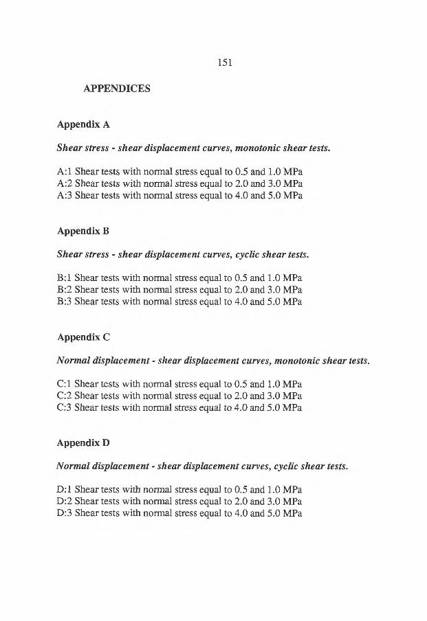
151
APPENDICES
Appendix A
Shear stress - shear displacement curves, monotonic shear tests.
A:1 Shear tests with normal stress equal to 0.5 and 1.0 MPa A:2 Shear tests with normal stress equal to 2.0 and 3.0 MPa A:3 Shear tests with normal stress equal to 4.0 and 5.0 MPa
Appendix B
Shear stress - shear displacement curves, cyclic shear tests.
B:1 Shear tests with normal stress equal to 0.5 and 1.0 MPa B:2 Shear tests with normal stress equal to 2.0 and 3.0 MPa B:3 Shear tests with normal stress equal to 4.0 and 5.0 MPa
Appendix C
Normal displacement - shear displacement curves, monotonic shear tests.
C:1 Shear tests with normal stress equal to 0.5 and 1.0 MPa C:2 Shear tests with normal stress equal to 2.0 and 3.0 MPa C:3 Shear tests with normal stress equal to 4.0 and 5.0 MPa
Appendix D
Normal displacement - shear displacement curves, cyclic shear tests.
D:1 Shear tests with normal stress equal to 0.5 and 1.0 MPa D:2 Shear tests with normal stress equal to 2.0 and 3.0 MPa D:3 Shear tests with normal stress equal to 4.0 and 5.0 MPa
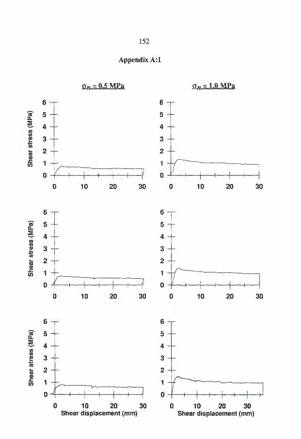
10 20 30 0 10 20 30
Sh
ear s
tres
s (M
Pa)
o i 1
6
5
4
3
2
1
152
She
ar s
tres
s (M
Pa)
Appendix A:1
an = 0.5 MPa Gn = 1.0 MPa
6 6
5 5
4 4
3 3
2 2
1 1
0 (TT t I I II 0
0 10 20 30 0 10
20
30
She
ar s
tres
s (M
Pa)
6
5
4
3
2
1
0
6
5
4
3
2
1
0
0 10 20 30
0 10 20 30 Shear displacement (mm)
Shear displacement (mm)

153
Appendix A:2
an = 2.0 MPa an = 3.0 MPa
Sh
ear
stre
ss (
MP
a)
6
5
4
3
2
1
0
6
5
4
3
2
1
0
0
10
20
30
0
10
20
30
Sh
ear st
ress
(M
Pa)
6
5
4
3
6
5
4 —
3 —
2 —
2
1 1
0 0
0 10 20 30 0 10 20 30
6
5
6
5
Sh
ear
stre
ss (
MP
a )
4
3
4 —
3 —
2 —
1 —
2
1
0 o
0 10 20 30 Shear displacement (mm)
0 10 20 30 Shear displacement (mm)
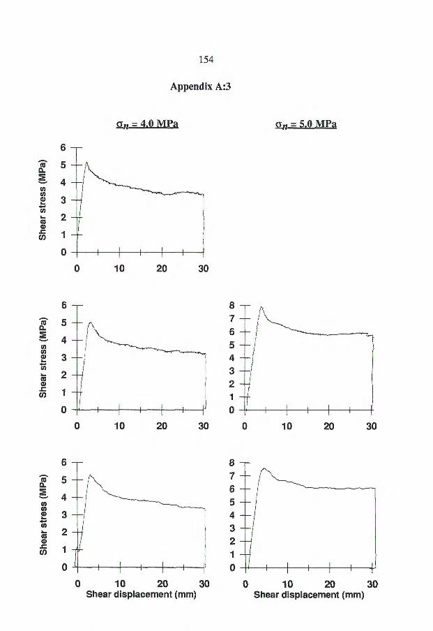
i I I i I i i I 1
10 20 30
Sh
ear
stre
ss (
MP
a)
6
5
4
3
2
1
0
154
Appendix A:3
t:517,= 4.0 MPa an = 5.0 MPa
Sh
ear st
ress
(M
Pa)
6
5
4
3
2
1
0
10
20
30
6
7
6
5
4
3
2
1
0
Sh
ear
stre
ss (
MP
a)
0 10 20 30 Shear displacement (mm)
0 10 20 30 Shear displacement (mm)
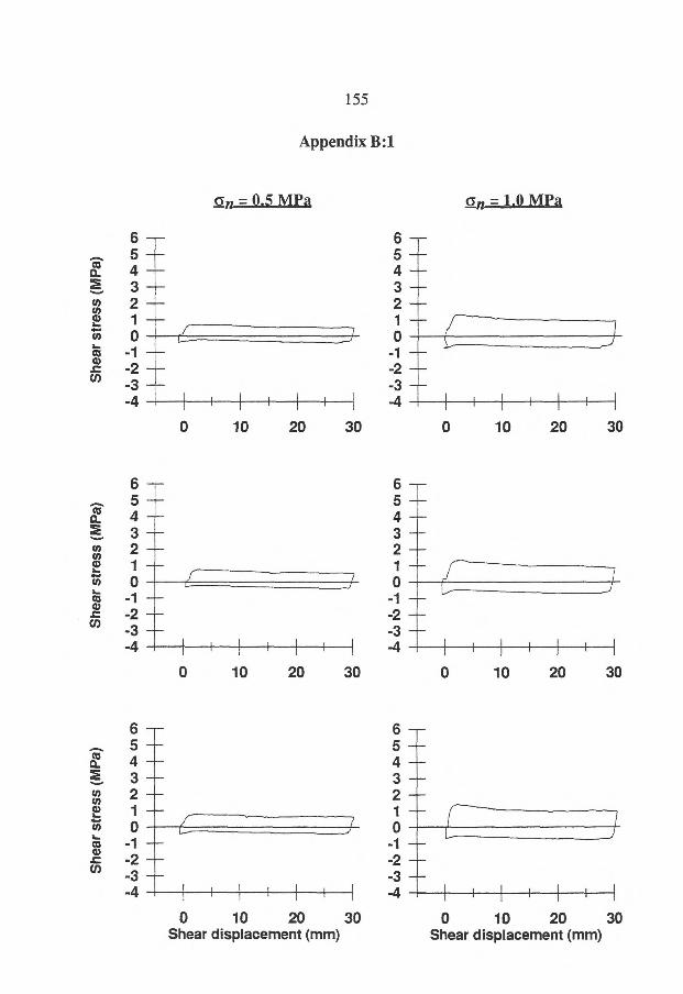
6 6 5 5 4 4 3 3 2 2 1 1 0 0
-1 -1 -2 -2 -3 -3 -4 -4
0 10 20 30
6 6 5 5 4 4 3 3 2 2
1 lo
-1 -2 -2 -3 -3 4 i I i I I -4
0 10 20 30
6 6 5 5 4 4 3 3 2 2 1 1 0 1 o
-1 -1 -2 -2 -3 -3 -4 III -4
C
0 10 20 30
I I I- 1 1 1 1
She
ar s
tres
s (M
Pa)
S
hear
str
es
s (
MP
a)
She
ar s
tres
s (M
Pa)
C
0 10 20 30
155
Appendix B:1
= 0.5 MPa G = 1.0 MPa
0 10 20 30 0 10 20 30 Shear displacement (mm) Shear displacement (mm)
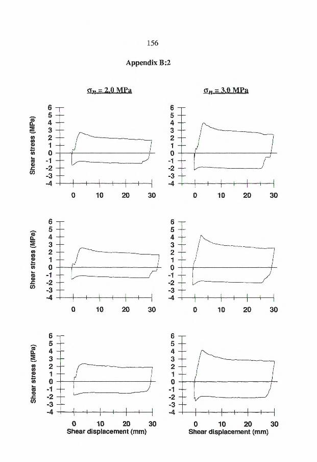
-4
She
ar s
tres
s (M
Pa)
6 5 4 3 2 1 0
-1 -2 -3
6 5 4 — 3 — 2 — 1 — 0 -1 — -2 — -3 4 1 i 1 i + i 1
0 10 20 30 0 10 20 30
Sh
ear s
tres
s (M
Pa)
6 5 4 3 2 i o
-1 -2 -3 -4
>V
156
She
ar s
tres
s (M
Pa)
Appendix B:2
gn = 2.0 MP g an = 3.0 MPa
6 6 — 5 5 — 4 — 4— 3 3— 2 — 2—
-1 — 0
rf 0
-1 —
1 — 1 —
../ -2 -2 — .v -3 -3 4 1 i 1 1 I I I i -4 i 1 E i 1 -I
0 10 20 30 10 20 30
,r
I i i i i 1 i i 1
6 5 4 — 3 — 2 — 1 — o
''1 — -2 — -3
0 10 20 30 0 10 20 30
Shear displacement (mm) Shear displacement (mm)
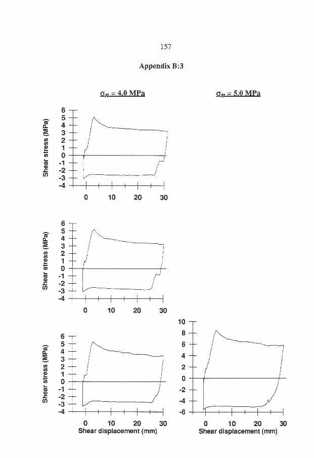
0 10 20 30 Shear displacement (mm)
Sh
ear
stre
ss (
MP
a)
-2 -3 -4
6 5 4 3 2 1 0
-1
157
Appendix B:3
an = 4.0 MP g Gn = 5.0 MPa
6 5- -
co eL 4 3 3 — u9 2 — ;12 1 —7) 0 hi-1 — a) .c -2 — cn
-3 — -4 i I i i
0 10 20 30
I I I i i I I I
0 10 20 30
10
8
6
4
2
6 5—
Q-
as 4 —
! 3 —
0 2 — cn 22 1
o as -1 — -c -2 — CD
-3 — -4
-2
-4
0 10 20 30 Shear displacement (mm)
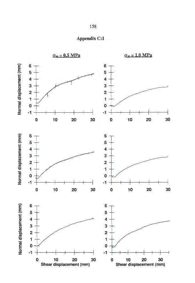
No
rmal d
isp
lacem
en
t (m
m)
No
rmal
dis
pla
cem
ent
(mm
) N
orm
al d
isp
lacem
en
t (m
m)
Li 0 "
IV
CA
4>
Cil 0
) 1 o
-i p
a c
a 4
. al c
)
0
j II
l 1
In
II
o
-,. o
IV
0
o
-
-
-
2£
o -
L r
o c
o 4
L, c.r
i cs)
o
IIII
0 —
-
." 0
" I
V (
.4 4
:1
C
M C
7)
- -
--
-
—i•
0 —
I ro
(..
.) A
. C
ri C
7)
0rIfilill
0
1 1
1
1
1
F3 mniaddli
Cl)
7"
CD
CD
0.0
(7)
-a
r»
(.)
(Di'.)
3
0
CD a 3
C3
30
_
0
ca _
__
0
-
o
-
tv
0 —
43
o
o
-
ci
II
CO
S
CD
07
C
I CD
3
(o 1
2 9
i. '
3
3
--
_
-
-
_

159
Appendix C:2
on --7- 2.0 MPa Gn = 3.0 MPg
6
5
4
3
2
1 0
1
0
10
20
30
0
10
20
30
6
5
4
3 —
2 —
1 —
o 1
0 10 20 30 0 10 20 30
Nor
mal
dis
p lac
emen
t (m
m)
6
5 5
4 4
3 3
2 2
1 1
0 0
-1 -1 0 10 20 30
Shear displacement (mm)
I I I I I 0 10 20 30
Shear displacement (mm)
Nor
ma l disp
lace
men
t (m
m)
6 5 4 3 2 1 0
-1
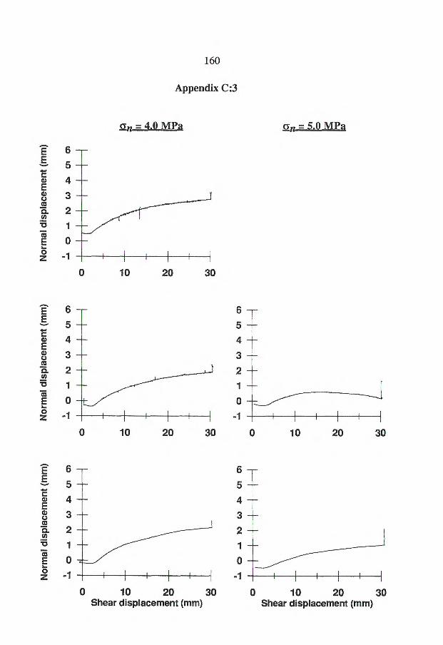
160
Appendix C:3
Gn = 4.0 MPa an = 5.0 MPg
Nor
mal
dis
plac
emen
t (m
m)
-1
0 10 20 30
Nor
mal disp
lace
men
t (m
m)
6 5
4
3
2
1
0
-1
0 10 20 30
5
4
3
2
1
0
-1
6
5 4
3
2 1
0
-1
10 20 30
6
5
4
3
2
1
0
-1 I I Nor
mal
dis
plac
emen
t (m
m)
0 10 20 30 0 10 20 30 Shear displacement (mm) Shear displacement (mm)
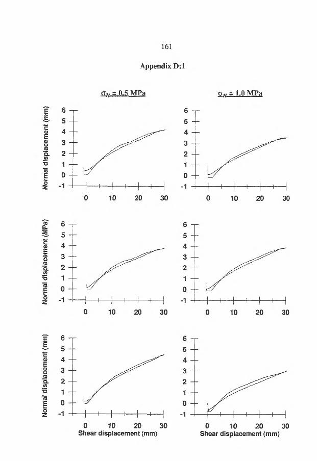
an = 0.5 MPg an = 1.0 MPa
0 10 20 30 0 10 20 30
0 10 20 30 0 10 20 30
161
Appendix D:1
0 10 20 30 Shear displacement (mm)
0 10 20 30 Shear displacement (mm)
No
rmal
dis
pla
cem
ent (
mm
)
6
5
4
3
2
1
0
1
6
5
4
3
2
1
0
1
Nor
mal
dis
plac
e men
t (M
Pa)
6 5
4
3
2 1
0
-1
6
5
4
3
2
1
0
1
Nor
mal
dis
plac
eme n
t (m
m)
6
5
4
3
2
1
0
-1 1 I I 1 I i 1
6
5
4
3
2
1
0
-1
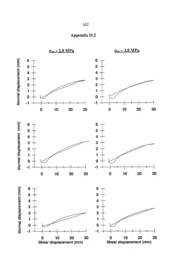
Nor
mal
dis
plac
emen
t (m
m)
6
5
4
3
2 1
0
-1 1 1 i 1 i 1
6 — 5 4 3 - 2
1
0
1
162
Appendix D:2
an = 2.0 MPa an = 3.0 MPa
0 10 20 30 0 10 20 30
Nor
mal
dis
plac
emen
t (m
m)
6
5
4
3
2
1
0
-1
6
5
4
3
2
1
0
-1
0 10 20 30
0 10 20 30
Nor
mal
dis
plac
emen
t (m
m)
6
5
4
3
2
1
0
-1 0 10 20 30
Shear displacement (mm) 0 10 20 30
Shear displacement (mm)
6
5
4
3
2 1 0
-1
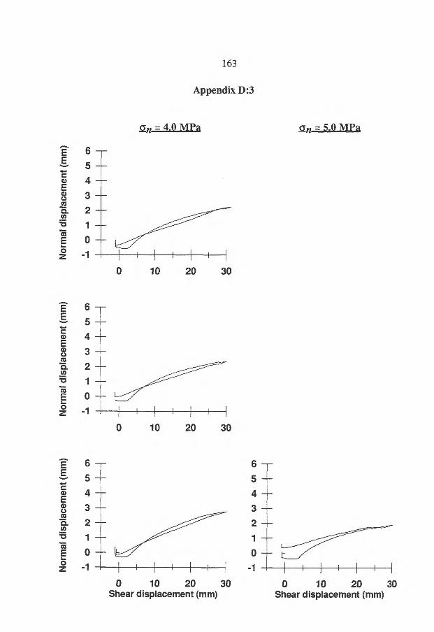
" 0 "
N
I 4
3
C.7
1 C
D
Cl)
m-
0
cp
9-i) 0: in •0-•'
IT °
C
2 C
D
3
(1)
= iv
3
3
ca
o
0
...1.
0
IV
0
CO
0
" 0 " ro
ca
.4
. CJ
1 cr
)
0
Icr
8
II
re
o
£:a mpuaddv
ca
o
No
rmal
dis
pla
cem
ent
(mm
) N
orm
al d
isp
lacem
en
t (m
m)
No
rmal
dis
pla
cem
ent
(mm
)
ta
II