Exchange rate pass-through and inflation A nonlinear time

Journal of International Money and Finance 32 (2013) 512e527

Contents lists available at SciVerse ScienceDirect

Journal of International Moneyand Finance

journal homepage: www.elsevier .com/locate/ j imf

Exchange rate pass-through and inflation: A nonlinear timeseries analysis

Mototsugu Shintani a,*, Akiko Terada-Hagiwara b, Tomoyoshi Yabu c

aDepartment of Economics, Vanderbilt University, Nashville, TN 37235, USAb Economics and Research Department, Asian Development Bank, Mandaluyong City 1550, Manila, Philippinesc Faculty of Business and Commerce, Keio University, Minato-ku, Tokyo 108-8345, Japan

JEL Classification:C22E31F31

Keywords:Import pricesInflation indexationPricing-to-marketSmooth transition autoregressive modelsSticky prices

* Corresponding author. Tel.: þ1 615 322 2196; fE-mail addresses: mototsugu.shintani@vanderb

[email protected] (T. Yabu).

0261-5606/$ e see front matter � 2012 Elsevier Lhttp://dx.doi.org/10.1016/j.jimonfin.2012.05.024

a b s t r a c t

This paper investigates the relationship between the exchange ratepass-through (ERPT) and inflation by estimating a nonlinear timeseries model. Based on a simple theoretical model of ERPT deter-mination, we show that the dynamics of ERPT can be wellapproximated by a class of smooth transition autoregressive(STAR) models using the past inflation rate as a transition variable.We employ several U-shaped transition functions in the estimationof the time-varying ERPT to US domestic prices. The estimationresult suggests that declines in the ERPT during the 1980s and1990s are associated with lowered inflation.

� 2012 Elsevier Ltd. All rights reserved.

1. Introduction

Within the framework of new open economy macroeconomic models, the degree of exchange ratepass-through (ERPT) into domestic prices is one of the key elements in evaluating international spill-over effects of monetary policy. Over the past decade, a number of empirical studies have investigatedwhether ERPT, defined as the response of domestic inflation rates to the changes in exchange rates (or

ax: þ1 615 343 8495.ilt.edu (M. Shintani), [email protected] (A. Terada-Hagiwara), tomoyoshi.

td. All rights reserved.

mailto:[email protected]




www.sciencedirect.com/science/journal/02615606

www.elsevier.com/locate/jimf

http://dx.doi.org/10.1016/j.jimonfin.2012.05.024



M. Shintani et al. / Journal of International Money and Finance 32 (2013) 512e527 513

in marginal costs), decreased during the 1980s and 1990s.1 If there was a reduction in ERPT, it is naturalto conjecture some interaction between the ERPT and the inflation rate because the timing corre-sponds, in many countries, to a period of low and stable inflation. This view is emphasized by Taylor(2000), who states that “the lower pass-through should not be taken as exogenous to the infla-tionary environment (p.1390).”

The purpose of this paper is to investigate Taylor’s hypothesis on the positive relationship betweenthe ERPTand inflation by estimating a nonlinear time series model. In particular, we employ the class ofsmooth transition autoregressive (STAR) models so that the degree of ERPT to domestic prices can bedetermined by the lagged domestic inflation rate. Most previous empirical studies on the positiveassociation between ERPT and inflation focus on the cross-country evidence, including the analyses byCalvo and Reinhart (2002), Choudhri and Hakura (2006), and Devereux and Yetman (2010). This paperdiffers from the existing studies in that we examine the role of inflation in the time-varying ERPT underthe time series modeling framework.

In the empirical literature on the nonlinear adjustment of real exchange rates, STAR models havebeen popularly employed in many studies, including Michael et al. (1997), Taylor and Peel (2000),Taylor et al. (2001), and Kilian and Taylor (2003), among others. However, STAR models have rarelybeen used in analyses of the ERPT.2 While nonlinear mean reversion of real exchange rates implies thefull ERPT in the long-run, it does not imply the time-varying ERPT. We employ several U-shapedtransition functions in STAR models to consider alternative forms of time-varying ERPT. Our method isapplied to monthly US import and domestic price data and evaluates fluctuations of ERPT during theperiod from 1975 to 2007.

To motivate our nonlinear regression approach, we first present a simple theoretical model ofimporting firms where the ERPT becomes a nonlinear function of the past inflation rate. Our model isclosely related to a model of ERPT developed by Devereux and Yetman (2010) so that the optimal pricelevel depends directly on the nominal exchange rate, which corresponds to the marginal cost, and thatimporting firms endogenously select the probability of adjusting their price to an optimal level.However, our model differs from their model in several aspects. First, for every period, a fraction offirmsmake a finite-period Taylor (1980) type staggered contract of an inflation indexation rule. Second,each firm faces the problem of opting out of a contract. When firms opt out, they can set an optimalprice by paying a fixed cost. Because the ERPT increases if more firms set an optimal price, and theprobability of opting out depends on the past inflation rate, our model predicts that ERPT depends onthe lagged inflation. This prediction is in contrast to the case of Devereux and Yetman (2010) where theERPT depends on the steady-state inflation level of the economy. We show that the dynamics of ERPTpredicted by the theoretical model can be well approximated by the STAR structure, and that the pastdecline during the 1980s and 1990s and the recent increase in the ERPT to US prices are well explainedby the STAR model.

The remainder of the paper is organized as follows. Section “Theoretical motivation” brieflydescribes the prediction from the theoretical model. Section “Econometric procedures” introduces theempirical model. Estimation results are provided in the section “Empirical results”, followed by“Conclusions” in the next section.

2. Theoretical motivation

In this section, we briefly describe our theoretical model of importing firms, which predicts that theERPT depends on the lagged inflation.3 The basic setup is similar to Devereux and Yetman (2010) in thatimporting firms are monopolistic competitors who import differentiated intermediate goods fromabroad. A representative domestic final good producer purchases all the imported intermediate goods

1 See, for example, Goldberg and Knetter (1997), Otani et al. (2003), Campa and Goldberg (2005), Sekine (2006) andMcCarthy (2007).

2 One of the few exceptions is a study of UK import prices by Herzberg et al. (2003). However, their study did not findsupporting evidence on nonlinearity.

3 The details of the model are provided in the Appendix.

M. Shintani et al. / Journal of International Money and Finance 32 (2013) 512e527514

and combines them to produce a final output. Pricing contracts between the importers and the finalgood producer are valid for N(�2) periods long, and a constant fraction 1/N of all importing firms writetheir contracts in any given time period. However, firms are allowed to opt out during the contractperiod and to deviate from the contract pricing rule by paying a fixed cost F(>0). During the firstN*(�1)periods of the contract, firms follow the contract pricing rule and fully index their prices to aggregateinflation pt of the initial contract period. If firms opt out of the contract after N* periods, for theremaining periods of the contract N�N*, they can charge the desired price pt ¼ st þ p�t þ mwhere st isthe nominal exchange rate, p�t is the foreign currency price and m is a mark-up. Since the marginal costst þ p�t is assumed to follow a randomwalk process (with the variance of its increment s2), all the firmsentering into new contracts at time t set their price at pt . Therefore, for firms that write their contractsat time t and opt out at time tþN*, the entire price path is given byfpt ; pt þ pt ;.; pt þ ðN� � 1Þpt ; ptþN� ;.; ptþðN�1Þg.

We follow Ball et al. (1988), Romer (1990), and Devereux and Yetman (2002, 2010), amongothers, and re-formulate the firm’s optimization behavior so that the probability of (not) changingits price to the desired price level is endogenously determined. Let kðtÞ be the (conditional) prob-ability that a firm under contract in the current period will maintain the contract price in the nextperiod. Here, a superscript t in parenthesis signifies that this probability applies to all the firmsentering into new contracts at time t, but not to firms in other cohorts. After setting the newcontract price at t, the firms observe the aggregate inflation pt and choose kðtÞ to minimize theexpected loss function given by

Lt ¼ Et

24XN�1

j¼1

�bkðtÞ

�j�pt þ jpt � ptþj

�235 þ 1� kðtÞ

kðtÞXN�1

j¼1

�bkðtÞ

�j XN�j

[¼1

b[�1

!F (1)

where b is a discount factor. The above function implies that the loss is an increasing function of theinflation rate in absolute value. As the inflation rate rises (relative to the size of the fixed cost), the firmcan minimize loss by avoiding the inflation indexation. This strategy leads to a lower kðtÞ (or a shorteraverage length of N*). In an extreme case of a high inflation, kðtÞ ¼ 0 (or N*¼ 1) is selected witha pricing path given by fpt ; ptþ1;.; ptþðN�1Þg. In the other extreme case of a low inflation, kðtÞ ¼ 1(or N*¼N) can be selected with a pricing path given by fpt ; pt þ pt ; pt þ 2pt ;.; pt þ ðN � 1Þptg. Ingeneral, between the two extreme cases, the solution becomes a function of the inflation rate and canbe expressed as kðtÞ ¼ kðptÞ.

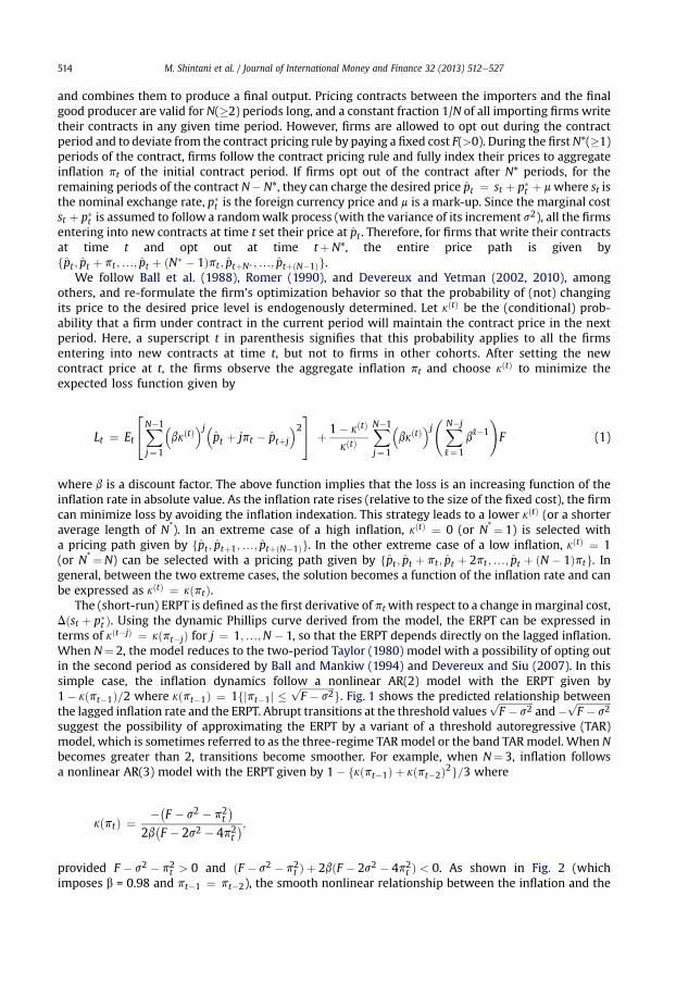
The (short-run) ERPT is defined as the first derivative of ptwith respect to a change inmarginal cost,Dðst þ p�t Þ. Using the dynamic Phillips curve derived from the model, the ERPT can be expressed interms of kðt�jÞ ¼ kðpt�jÞ for j ¼ 1;.;N � 1, so that the ERPT depends directly on the lagged inflation.When N¼ 2, the model reduces to the two-period Taylor (1980) model with a possibility of opting outin the second period as considered by Ball and Mankiw (1994) and Devereux and Siu (2007). In thissimple case, the inflation dynamics follow a nonlinear AR(2) model with the ERPT given by1� kðpt�1Þ=2 where kðpt�1Þ ¼ 1fjpt�1j �

ffiffiffiffiffiffiffiffiffiffiffiffiffiffiF � s2

pg. Fig. 1 shows the predicted relationship between

the lagged inflation rate and the ERPT. Abrupt transitions at the threshold valuesffiffiffiffiffiffiffiffiffiffiffiffiffiffiF � s2

pand�


p

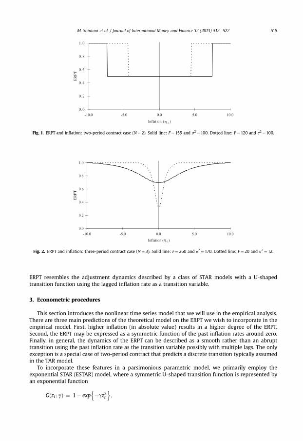
suggest the possibility of approximating the ERPT by a variant of a threshold autoregressive (TAR)model, which is sometimes referred to as the three-regime TARmodel or the band TARmodel. When Nbecomes greater than 2, transitions become smoother. For example, when N¼ 3, inflation followsa nonlinear AR(3) model with the ERPT given by 1� fkðpt�1Þ þ kðpt�2Þ2g=3 where

kðptÞ ¼ ��F � s2 � p2t�

2b�F � 2s2 � 4p2

t�;

provided F � s2 � p2t > 0 and ðF � s2 � p2

t Þ þ 2bðF � 2s2 � 4p2t Þ < 0. As shown in Fig. 2 (which

imposes b = 0.98 and pt�1 ¼ pt�2), the smooth nonlinear relationship between the inflation and the

0.0

0.2

0.4

0.6

0.8

1.0

-10.0 -5.0 0.0 5.0 10.0

t-1)

ER

PT

Fig. 2. ERPT and inflation: three-period contract case (N¼ 3). Solid line: F¼ 260 and s2¼170. Dotted line: F¼ 20 and s2¼12.

0 .0

0 .2

0 .4

0 .6

0 .8

1 .0

-10.0 -5.0 0.0 5.0 10.0

Inflation ( t-1)

ER

PT

Fig. 1. ERPT and inflation: two-period contract case (N¼ 2). Solid line: F¼ 155 and s2¼100. Dotted line: F¼ 120 and s2¼100.


ERPT resembles the adjustment dynamics described by a class of STAR models with a U-shapedtransition function using the lagged inflation rate as a transition variable.

3. Econometric procedures

This section introduces the nonlinear time series model that we will use in the empirical analysis.There are three main predictions of the theoretical model on the ERPT we wish to incorporate in theempirical model. First, higher inflation (in absolute value) results in a higher degree of the ERPT.Second, the ERPT may be expressed as a symmetric function of the past inflation rates around zero.Finally, in general, the dynamics of the ERPT can be described as a smooth rather than an abrupttransition using the past inflation rate as the transition variable possibly with multiple lags. The onlyexception is a special case of two-period contract that predicts a discrete transition typically assumedin the TAR model.

To incorporate these features in a parsimonious parametric model, we primarily employ theexponential STAR (ESTAR) model, where a symmetric U-shaped transition function is represented byan exponential function

Gðzt ;gÞ ¼ 1� expn�gz2t

o;


where zt is a transition variable and g (>0) is a parameter defining the smoothness of the transition. It isa popularly used STAR model originally proposed by Haggan and Ozaki (1981) and later generalized byGranger and Teräsvirta (1993) and Teräsvirta (1994) among others. Since our objective is to determinethe relationship between pt and Dðst þ p�t Þ, we estimate a bivariate variant of the ESTAR modelsspecified as

pt ¼f0þXNj¼1

f1;jpt�jþXN�1

j¼0

f2;jD�st�jþp�t�j

�þ0@XN

j¼1

f3;jpt�jþXN�1

j¼0

f4;jD�st�jþp�t�j

�1AGðzt ;gÞþ 3t ;

(2)

where 3t wi.i.d.ð0;s23Þ. Note that the lag length of pt and Dðstþp�t Þ on the right-hand side of (2) comesfrom the prediction of the theoretical model provided in the Appendix. While our theoretical modelalso suggests multiple transition variables, here we consider a parsimonious specification and usea moving average of the past inflation rates as a single transition variable, zt ¼d�1Pd

j¼1pt�j.4 In this

ESTAR framework, our interest is to obtain the time-varying ERPT defined as

ERPT ¼ f2;0 þ f4;0Gðzt ;gÞ:

We impose a restriction 0 � f2;0 � 1 and f2;0 þ f4;0 ¼ 1 so that the ERPT falls in the range of [0, 1].In addition to the ESTARmodel, our primary model in the analysis, we also consider another class of

STAR models based on a different U-shaped transition function constructed from a combination of twologistic functions. This variant of logistic STAR (LSTAR) models has been considered in Granger andTeräsvirta (1993) and Bec et al. (2004) and is sometimes referred to as the three-regime LSTARmodel. Here, we simply call the model a dual (or double) LSTAR (DLSTAR) model to emphasize thepresence of two logistic functions.5 The transition function in the DLSTAR model is given by

Gðzt ;g1;g2; c1; c2Þ ¼ ð1þ expf � g1ðzt � c1ÞgÞ�1þð1þ expfg2ðzt þ c2ÞgÞ�1

where g1, g2 (>0) are parameters defining the smoothness of the transition in the positive and negativeregions, respectively, and c1, c2 (> 0) are location parameters. The definitions of all other variables andparameters remain the same as in the ESTAR model. The function of our interest, the ERPT, is similarlycomputed as

ERPT ¼ f2;0 þ f4;0Gðzt ;g1;g2; c1; c2Þ:

The reason for considering this alternative specification of the transition function is two-fold. First,as pointed out by van Dijk et al. (2002), the transition function in the ESTAR model collapses toa constant when g approaches infinity. Thus the model does not nest the TAR model with an abrupttransition as predicted by the theory when there are only two cohorts of firms in the economy. Incontrast, the DLSTAR model includes the TAR model by letting g1 and g2 tend to infinity. Second, andmore importantly, the model can incorporate both symmetric (g1¼ g2¼ g and c1¼ c2¼ c) andasymmetric (g1 s g2 and c1 s c2) adjustments between the positive and negative regions. Therefore,we can investigate the case beyond our simple model that predicts a symmetric relationship betweenthe ERPT and the lagged inflation rate. In the estimation of DLSTAR models, we employ both specifi-cations of symmetric and asymmetric adjustments.

4 As in Kilian and Taylor (2003), we can also employ the transition variable, zt ¼ffiffiffiffiffiffiffiffiffiffiffiffiffiffiffiffiffiffiffiffiffiffiffiffiffiffiffiffiffiffiffid�1

Pdj¼1 p

2t�j

q, which yields a similar

parsimonious specification. The main result turns out to be unaffected even if our transition variable is replaced by thisalternative.

5 We use this terminology since the model differs from the multiple regime STAR models defined in van Dijk et al. (2002).


Note that all specifications in our analysis can be represented as

pt ¼ x0tf1 þ Gðzt ; qÞx0tf2 þ 3t ;

where xt ¼ ð1;pt�1;.;pt�N;Dðst þ p�t Þ;.;Dðst�Nþ1 þ p�t�Nþ1ÞÞ0, zt ¼ d�1Pdj¼1 pt�j and q ¼ g for

ESTAR models, q ¼ ðg; cÞ0 for symmetric DLSTAR models, q ¼ ðg1;g2; c1; c2Þ0 for asymmetric DLSTARmodels, respectively. In our analysis, we follow van Dijk et al. (2002) and employ the Lagrangemultiplier (LM)-type test for linearity against the class of STAR models, based on the artificial model ofthe form:

pt ¼ x0tb0 þ x0tztb1 þ x0tz2t b2 þ x0tz

3t b3 þ et : (3)

Let ~et ¼ pt � x0t~b0 be the regression residual from (3) with restrictions b1 ¼ b2 ¼ b3 ¼ 0 and et be

the residual from the full regression (3). Then, the LM test statistic can be computed asLM ¼ TðSSR0 � SSR1Þ=SSR0 where SSR0 ¼ P

~e2t and SSR1 ¼ Pe2t . The LM statistic asymptotically

follows c2 distribution with 3ð2N þ 1Þ degree of freedom under the null hypothesis of linearity. Toimprove the finite sample size property, Teräsvirta (1994) also recommends the F version of the LM teststatistics given by

FL ¼ ðSSR0 � SSR1Þ=3ð2N þ 1ÞSSR1=ðT � 4ð2N þ 1ÞÞ :

The F statistic approximately follows F distribution with 3ð2N þ 1Þ and T � 4ð2N þ 1Þ degrees offreedom under the null hypothesis. In addition, we also employ a heteroskedasticity-robust variant ofthe LM test suggested by Granger and Teräsvirta (1993) and denote the test statistic by LM*.

As discussed in Teräsvirta (1994), the auxiliary regression (3) can be further used to choose thespecification among alternative STAR models. In our context, the F test for H0: b3¼ 0 against H1:b3s 0 can be used as a test for an ESTAR model against an asymmetric DLSTAR model (F3). Similarly,the F test for H0 : b1 ¼ 0jb3 ¼ 0 against H1 : b1s0jb3 ¼ 0 can be used as a test for a symmetricDLSTAR model against an ESTAR model ðF1j3Þ. Finally, the F test for H0 : b1 ¼ b3 ¼ 0 againstH1 : b1s0 and b3s0 can be used as a test for a symmetric DLSTAR model against an asymmetricDLSTAR model (F13).6

4. Empirical results

4.1. Data and the linearity test

All the data we use in the STAR estimation are taken from International Financial Statistics (IFS) ofthe International Monetary Fund. First, the main regressor in the ERPT regression is the monthly logchanges in nominal exchange rate and import price in foreign currency. Since the Bureau of LaborStatistics constructs the US import price index using US dollar prices paid by the US importer, Dðst þ p�t Þis simply computed as 100� ðln IMPt � ln IMPt�1Þ where IMPt is the import price after makinga seasonal adjustment using X-12-ARIMA procedure. The import prices are based either on “free onboard (f.o.b.)” foreign port or “cost, insurance, and freight (c.i.f.)” US port transaction prices, dependingon the practices of the individual industry. In either case, under our assumption of a constant icebergtransaction cost (proportional to import price in domestic currency), the same formula can be used tocompute the monthly log changes in the prices of imported goods, excluding the cost of transaction.

6 The set of restrictions follows from the fact that a third-order Taylor approximation of the transition function ofa symmetric DLSTAR model is given by Gðzt ;g; cÞzðg3c=24� gc=2Þ þ ðg3c=8Þz2t , while both zt and z3t appear for an asymmetricDLSTAR model similar to a single LSTAR model. The details of the derivation are available from the authors upon request.

-4.0

-3.0

-2.0

-1.0

0.0

1.0

2.0

3.0

4.0

1975 1980 1985 1990 1995 2000 2005

Infl

atio

n ra

te

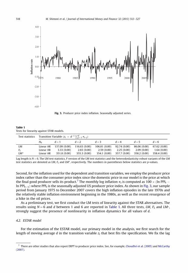
Fig. 3. Producer price index inflation. Seasonally adjusted series.

Table 1Tests for linearity against STAR models.

Test statistics Transition Variable ðzt ¼ d�1Pdj¼1 ptejÞ

H0 d¼ 1 d¼ 2 d¼ 3 d¼ 4 d¼ 5 d¼ 6

LM Linear AR 137.09 (0.00) 116.63 (0.00) 106.81 (0.00) 92.74 (0.00) 86.06 (0.00) 67.62 (0.00)FL Linear AR 3.33 (0.00) 2.83 (0.00) 2.59 (0.00) 2.25 (0.00) 2.09 (0.00) 1.64 (0.00)LM* Linear AR 351.8 (0.00) 355.3 (0.00) 354.1 (0.00) 357.7 (0.00) 358.2 (0.00) 358.4 (0.00)

Lag length is N¼ 6. The LM test statistics, F version of the LM test statistics and the heteroskedasticity-robust variants of the LMtest statistics are denoted as LM, FL and LM*, respectively. The numbers in parentheses below statistics are p-values.


Second, for the inflation used for the dependent and transition variables, we employ the producer priceindex rather than the consumer price index since the domestic price in our model is the price at whichthe final good producer sells its product.7 The monthly log inflation pt is computed as 100� ðln PPIt �ln PPIt�1Þwhere PPIt is the seasonally adjusted US producer price index. As shown in Fig. 3, our sampleperiod from January 1975 to December 2007 covers the high inflation episodes in the late 1970s andthe relatively stable inflation environment beginning in the 1980s, as well as the recent resurgence ofa hike in the oil prices.

As a preliminary test, we first conduct the LM tests of linearity against the STAR alternatives. Theresults using N¼ 6 and d between 1 and 6 are reported in Table 1. All three tests, LM, FL and LM*,strongly suggest the presence of nonlinearity in inflation dynamics for all values of d.

4.2. ESTAR model

For the estimation of the ESTAR model, our primary model in the analysis, we first search for thelength of moving average d in the transition variable zt that best fits the specification. We fix the lag

7 There are other studies that also report ERPT to producer price index. See, for example, Choudhri et al. (2005) and McCarthy(2007).


length N¼ 6 and search for the value of d between 1 and 6 that minimizes the sum of squared residualsfrom the nonlinear least squares regression of (2). This search procedure leads to the choice of d¼ 3.We then adopt a general-to-specific approach, as suggested by van Dijk et al. (2002), in arriving at thefinal specification. Starting with a model with N¼ 6, we sequentially remove the lagged variables forwhich the t statistic of the corresponding parameter is less than 1.0 in absolute value. The resulting finalspecification and the estimates for the ESTAR model are as follows:

pt ¼ 0:099ð3:118Þ

þ0:123ð2:322Þ

pt�1 þ 0:200ð4:706Þ

pt�3 � 0:081ð1:689Þ

pt�4 þ 0:336ð9:746Þ

D�st þ p�t

�þ 0:093ð2:803Þ

D�st�1 þ p�t�1

�þ 0:074

ð1:859ÞD�st�4 þ p�t�4

�þ 0:039ð1:349Þ


�þ h0:752ð2:103Þ

�1:352ð3:400Þ

pt�5

þ 0:664ð19:246Þ

D�st þ p�t

�� 0:569ð2:849Þ


�� 0:300ð1:393Þ


�iGðzt ; gÞ þ 3t ;

Gðzt ; gÞ ¼ 1� exp

8>>>>>>>>><>>>>>>>>>:

�0:076ð4:777Þ

0@13

X3j¼1

pt�j

1A2

0:4772

9>>>>>>>>>=>>>>>>>>>;;

R2 ¼ 0:606; se ¼ 0:476; obs ¼ 396; LMð1Þ ¼ 0:146; LMð1� 12Þ ¼ 0:189

where t-statistics in absolute values are given in parentheses below the parameter estimates, R2

denotes the coefficient of determination, se is the standard error of the regression, obs is the number ofobservations, LM (1) and LM (1e12) are p-values for Lagrange multiplier test statistics for first-order,and up to 12th-order serial correlations in the residuals, respectively.

Note that the estimate of the scaling parameter g is expressed in terms of the transition variablezt ¼ 3�1P3

j¼1 pt�j divided by its sample standard deviation 0.477. The model performs well in terms

0.0

0.2

0.4

0.6

0.8

1.0

-5.0 -4.0 -3.0 -2.0 -1.0 0.0 1.0 2.0 3.0 4.0 5.0

Transition variable (zt)

ER

PT

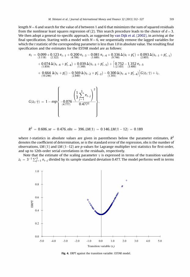
Fig. 4. ERPT against the transition variable: ESTAR model.

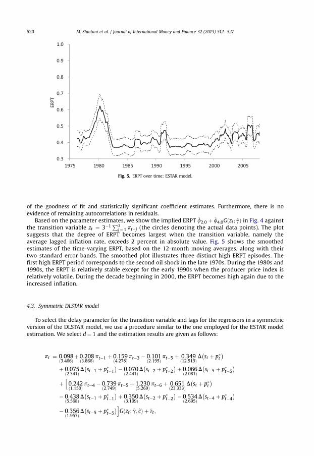
Fig. 5. ERPT over time: ESTAR model.


of the goodness of fit and statistically significant coefficient estimates. Furthermore, there is noevidence of remaining autocorrelations in residuals.

Based on the parameter estimates, we show the implied ERPT f2;0 þ f4;0Gðzt ; gÞ in Fig. 4 againstthe transition variable zt ¼ 3�1P3

j¼1 pt�j (the circles denoting the actual data points). The plotsuggests that the degree of ERPT becomes largest when the transition variable, namely theaverage lagged inflation rate, exceeds 2 percent in absolute value. Fig. 5 shows the smoothedestimates of the time-varying ERPT, based on the 12-month moving averages, along with theirtwo-standard error bands. The smoothed plot illustrates three distinct high ERPT episodes. Thefirst high ERPT period corresponds to the second oil shock in the late 1970s. During the 1980s and1990s, the ERPT is relatively stable except for the early 1990s when the producer price index isrelatively volatile. During the decade beginning in 2000, the ERPT becomes high again due to theincreased inflation.

4.3. Symmetric DLSTAR model

To select the delay parameter for the transition variable and lags for the regressors in a symmetricversion of the DLSTAR model, we use a procedure similar to the one employed for the ESTAR modelestimation. We select d¼ 1 and the estimation results are given as follows:

pt ¼ 0:098ð3:466Þ

þ0:208ð3:866Þ

pt�1 þ 0:159ð4:278Þ

pt�3 � 0:101ð2:195Þ

pt�5 þ 0:349ð12:519Þ

D�st þ p�t

�þ 0:075

ð2:341ÞD�st�1 þ p�t�1

�� 0:070ð2:441Þ


�þ 0:066ð2:081Þ


�þh0:242ð1:150Þ

pt�4 � 0:739ð2:749Þ

pt�5 þ 1:230ð5:269Þ

pt�6 þ 0:651ð23:333Þ

D�st þ p�t

�� 0:438

ð5:568ÞD�st�1 þ p�t�1

�þ 0:350ð3:109Þ


�� 0:534ð2:695Þ


�� 0:356

ð1:957ÞD�st�5 þ p�t�5

�iGðzt ; g; cÞ þ 3t ;


0B 8>>< �

pt�1� 1:474�9>>=1C�1 0

B 8>>< 0pt�1þ 1:474

19>>=1C�1

Gðzt ;g;cÞ¼BB@1þexp>>:�5:130ð2:924Þ

ð21:283Þ0:686 >>;

CCA þBB@1þexp>>:5:130ð2:924Þ

BB@ ð21:283Þ0:686

CCA>>;CCA ;

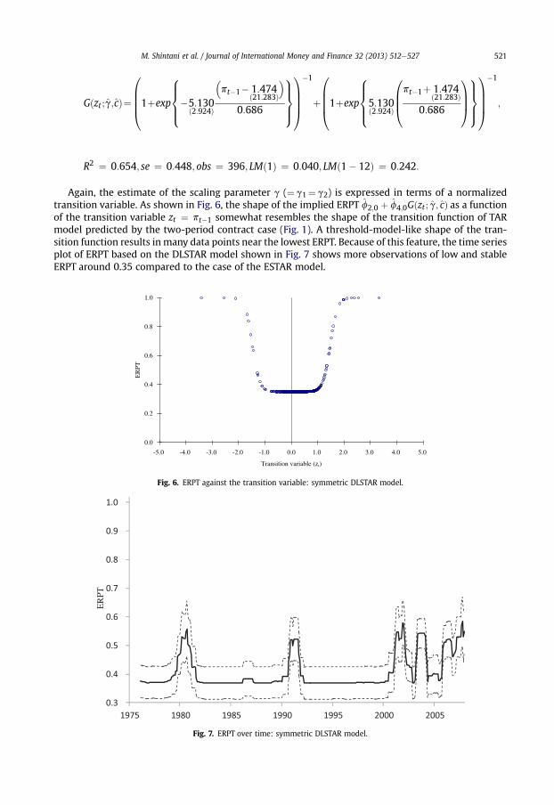
R2 ¼ 0:654; se ¼ 0:448; obs ¼ 396; LMð1Þ ¼ 0:040; LMð1� 12Þ ¼ 0:242:

Again, the estimate of the scaling parameter g (¼ g1¼ g2) is expressed in terms of a normalizedtransition variable. As shown in Fig. 6, the shape of the implied ERPT f2;0 þ f4;0Gðzt ; g; cÞ as a functionof the transition variable zt ¼ pt�1 somewhat resembles the shape of the transition function of TARmodel predicted by the two-period contract case (Fig. 1). A threshold-model-like shape of the tran-sition function results in many data points near the lowest ERPT. Because of this feature, the time seriesplot of ERPT based on the DLSTAR model shown in Fig. 7 shows more observations of low and stableERPT around 0.35 compared to the case of the ESTAR model.

0.0

0.2

0.4

0.6

0.8

1.0

-5.0 -4.0 -3.0 -2.0 -1.0 0.0 1.0 2.0 3.0 4.0 5.0

Transition variable (z )

ER

PT

Fig. 6. ERPT against the transition variable: symmetric DLSTAR model.

ER

PT

Fig. 7. ERPT over time: symmetric DLSTAR model.


4.4. Asymmetric DLSTAR model

We now turn to the estimation of the asymmetric version of the DLSTAR model to incorporate thepossibility of asymmetric adjustment. Minimizing the sum of the squared residuals yields the choice ofd¼ 1. The final specification of the model with parameter estimates is as follows:

pt ¼ 0:095ð3:349Þ

þ0:270ð4:183Þ

pt�1 þ 0:153ð4:094Þ

pt�3 � 0:105ð2:326Þ

pt�5 þ 0:341ð12:352Þ

D�st þ p�t

�þ 0:062

ð1:879ÞD�st�1 þ p�t�1

�� 0:078ð2:747Þ


�þ 0:064ð2:071Þ


�þh� 0:198

ð1:722Þpt�1 � 0:510

ð1:979Þpt�5 þ 1:001

ð4:666Þpt�6 þ 0:659

ð23:868ÞD�st þ p�t

�� 0:338

ð3:324ÞD�st�1 þ p�t�1

�þ 0:417ð3:352Þ


�� 0:298ð2:685Þ


�� 0:482

ð2:699ÞD�st�5 þ p�t�5

�iGðzt ; g1; g2; c1; c2Þ þ 3t ;

Gðzt ; g1; g2; c1; c2Þ ¼

0BBB@1þ exp

8>><>>:� 5:762

ð1:129Þ

�pt�1 � 1:591

ð14:924Þ

�0:686

9>>=>>;

1CCCA

�1

þ

0BBB@1þ exp

8>><>>:55:253

ð1:124Þ

�pt�1 þ 1:293

ð156:218Þ

�0:686

9>>=>>;

1CCCA

�1

;

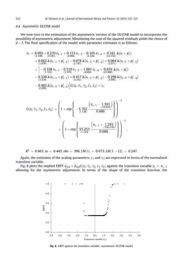
R2 ¼ 0:663; se ¼ 0:443; obs ¼ 396; LMð1Þ ¼ 0:073; LMð1� 12Þ ¼ 0:247:

Again, the estimates of the scaling parameters g1 and g2 are expressed in terms of the normalizedtransition variable.

Fig. 8 plots the implied ERPT f2;0 þ f4;0Gðzt ; g1; g2; c1; c2Þ against the transition variable zt ¼ pt�1allowing for the asymmetric adjustment. In terms of the shape of the transition function, the

0.0

0.2

0.4

0.6

0.8

1.0

-5.0 -4.0 -3.0 -2.0 -1.0 0.0 1.0 2.0 3.0 4.0 5.0

Transition variable (zt)

ER

PT

Fig. 8. ERPT against the transition variable: asymmetric DLSTAR model.

ER

PT

Fig. 9. ERPT over time: asymmetric DLSTAR model.


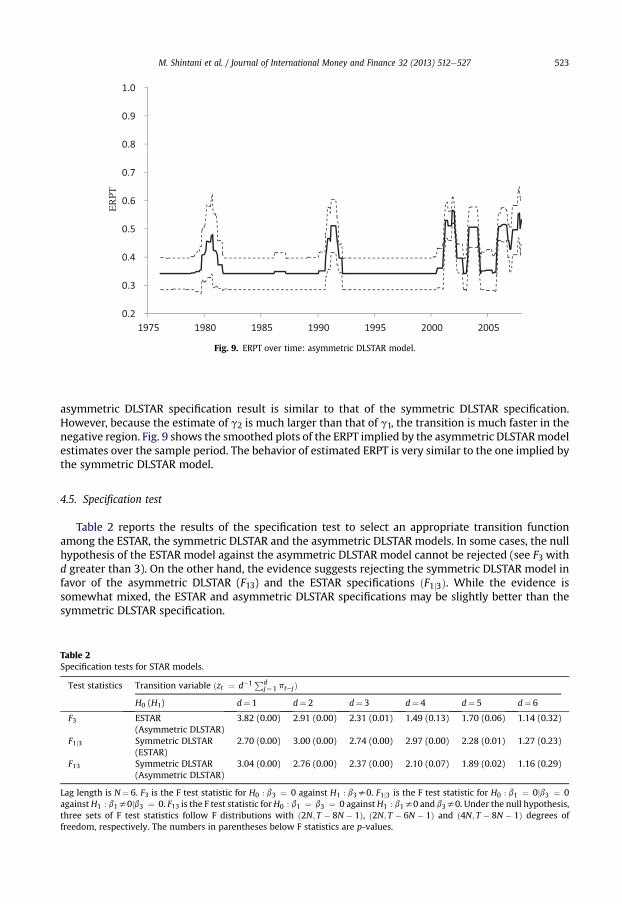
asymmetric DLSTAR specification result is similar to that of the symmetric DLSTAR specification.However, because the estimate of g2 is much larger than that of g1, the transition is much faster in thenegative region. Fig. 9 shows the smoothed plots of the ERPT implied by the asymmetric DLSTARmodelestimates over the sample period. The behavior of estimated ERPT is very similar to the one implied bythe symmetric DLSTAR model.

4.5. Specification test

Table 2 reports the results of the specification test to select an appropriate transition functionamong the ESTAR, the symmetric DLSTAR and the asymmetric DLSTAR models. In some cases, the nullhypothesis of the ESTAR model against the asymmetric DLSTAR model cannot be rejected (see F3 withd greater than 3). On the other hand, the evidence suggests rejecting the symmetric DLSTAR model infavor of the asymmetric DLSTAR (F13) and the ESTAR specifications ðF1j3Þ. While the evidence issomewhat mixed, the ESTAR and asymmetric DLSTAR specifications may be slightly better than thesymmetric DLSTAR specification.

Table 2Specification tests for STAR models.

Test statistics Transition variable ðzt ¼ d�1Pdj¼ 1 ptejÞ

H0 (H1) d¼ 1 d¼ 2 d¼ 3 d¼ 4 d¼ 5 d¼ 6

F3 ESTAR(Asymmetric DLSTAR)

3.82 (0.00) 2.91 (0.00) 2.31 (0.01) 1.49 (0.13) 1.70 (0.06) 1.14 (0.32)

F1j3 Symmetric DLSTAR(ESTAR)

2.70 (0.00) 3.00 (0.00) 2.74 (0.00) 2.97 (0.00) 2.28 (0.01) 1.27 (0.23)

F13 Symmetric DLSTAR(Asymmetric DLSTAR)

3.04 (0.00) 2.76 (0.00) 2.37 (0.00) 2.10 (0.07) 1.89 (0.02) 1.16 (0.29)

Lag length is N¼ 6. F3 is the F test statistic for H0 : b3 ¼ 0 against H1 : b3s0. F1j3 is the F test statistic for H0 : b1 ¼ 0jb3 ¼ 0against H1 : b1s0jb3 ¼ 0. F13 is the F test statistic forH0 : b1 ¼ b3 ¼ 0 against H1 : b1s0 and b3s0. Under the null hypothesis,three sets of F test statistics follow F distributions with ð2N; T � 8N � 1Þ, ð2N; T � 6N � 1Þ and ð4N; T � 8N � 1Þ degrees offreedom, respectively. The numbers in parentheses below F statistics are p-values.


5. Conclusion

In this paper, we show that the STAR models, the parsimonious parametric nonlinear time seriesmodels, offer a very convenient framework in examining the relationship between the ERPT andinflation. First, a simple theoretical model of ERPT determination suggests that the dynamics of ERPTcan be well approximated by a class of STAR models with lagged inflation as a transition variable.Second, we can employ various U-shaped transition functions in the estimation of the time-varyingERPT. When this procedure is applied to US import and domestic price data, we find the supportingevidence of nonlinearity in ERPT dynamics. Our empirical results imply that the period of low ERPT islikely to be associated with the low inflation.

According to our model, the degree of ERPT varies over time because the fraction of importing firmsopting out from the contract is endogenously determined by importing firms’ optimization behavior. Inthe model, however, all imports are treated as if they are invoiced in the producer’s (exporter’s)currency. An alternative approach in introducing a time-varying ERPT is to use a model in whichexporting firms endogenously choose between producer currency pricing (PCP) and local currencypricing (LCP). For example, a recent study by Gopinath et al. (2010) extends the model of Engel (2006)and investigates the role of the invoice currency in determining the observed ERPT. Our analysis doesnot consider this channel partly becausewe do not have data on individual exporters’ invoice currency.Incorporating the effect of currency choice in our estimation procedure seems to be a promisingdirection for further analysis.

Acknowledgment

The authors gratefully acknowledge an anonymous referee, the Editor, Mick Devereux, Ippei Fuji-wara, Naohisa Hirakata, Kevin Huang, Nobu Kiyotaki, Takushi Kurozumi, Keisuke Otsu, ShigenoriShiratsuka and seminar and conference participants at the Georgia Institute of Technology, OsakaUniversity, the University of Texas at Arlington and the 2009 Far East and South Asia Meeting of theEconometric Society for their helpful comments and discussions. Shintani gratefully acknowledgesfinancial support by the National Science Foundation Grant SES-1030164. The views expressed in thepaper are those of the authors and are not reflective of those of the Asian Development Bank.

Appendix: Model of importers

In this appendix we provide a full description of the theoretical model and derive its implicationsdiscussed in Section 2. There is a continuum of monopolistically competitive importing firms, each ofwhich imports a differentiated intermediate good from abroad and sells it to a representative domesticfinal good producer. In each time period, a constant fraction 1 / N of all importing firms and the finalgood producer write their pricing contracts of N periods long. An importing firm that writes the pricingcontract at time t e j (for j ¼ 0;1;.;N � 1) and imports a good i˛½0;1�, at time t is facing a demandgiven by

Ctði; t � jÞ ¼�Ptði; t � jÞPtðt � jÞ

��q

Ctðt � jÞ

where q> 1 is a constant elasticity of substitution. Here, Ptði; t � jÞ is the price of a good iimported by a firm with a contract beginning in period t� j. Ptðt � jÞ ¼ ðR 10 Ptði; t � jÞ1�qdiÞ1=ð1�qÞ isthe price index for the composite intermediate good sold by importing firms whose contractsbegin in period t� j. Ctðt � jÞ is the demand for the corresponding composite good. The elasticityof substitution among composite intermediate goods sold by each fraction 1/N of all importingfirms is assumed to be one, and thus aggregate price index at time t (in log) ispt ¼ N�1PN�1

j¼0 ptðt � jÞ where ptðt � jÞ ¼ lnPtðt � jÞ.All the differentiated intermediate goods are imported at the same foreign currency price, P�t , which

is beyond the control of importers. The importer’s profit, in terms of the domestic currency, at time t isgiven by


Ptði; t � jÞ ¼ Ptði; t � jÞCtði; t � jÞ � ð1þ sÞStP�t Ctði; t � jÞwhere St is the nominal exchange rate, and s is the iceberg transportation cost the importer must bear.The importer’s desired price, which maximizes the profit under flexible price economy, is

Ptði; t � jÞ ¼ q

q� 1ð1þ sÞStP�t

where q=ðq� 1Þ, and ð1þ sÞStP�t represent the mark-up and marginal cost, respectively. By taking a logof the desired price, which is same across all the importing firms ðPt ¼ Ptði; t � jÞÞ, we have pt ¼ st þp�t þ m where st ¼ ln St and m ¼ ln ðq=ðq� 1ÞÞ þ ln ð1þ sÞ. Both st and p�t are assumed to follow(possibly mutually correlated) random walk processes with a variance of the sum of each increment,Dðst þ p�t Þ, given by s2.

In the initial period of the contract, importers set the price at pt . For the rest of the contractperiod, they fully index their initial price pt to the aggregate inflation rate given by pt ¼ pt � pt�1.Note that prices are indexed to inflation of the initial period only, instead of following the period-by-period lagged inflation indexation rule as in Christiano et al. (2005). While the latterpricing scheme can be also introduced in our model, the former assumption greatly simplifies theanalysis.

In reality, contracts written for fixed periods can, in special circumstances, be re-negotiated. Bypaying a fixed cost, firms can opt out of the contract and reset their price at the desired level. Forexample, in Devereux and Siu (2007), each firm observes its fix cost, which is assumed to be i.i.d.across firms, after setting its (two-period) contract price. Consequently, the pricing in the secondperiod becomes state-dependent with all firms facing the same probability of opting out in thesecond period. We also let firms make their decision in a sequential manner by assuming that theaggregate inflation is not observed by individual firms at the time of the contract. However, instead offormally deriving the state-dependent pricing solution, we follow Ball et al. (1988), Romer (1990), andDevereux and Yetman (2002, 2010), among others, and re-formulate the firm’s optimization behaviorso that the probability of (not) changing its price to the desired price level is endogenously deter-mined. Let kðtÞ be the conditional probability that a firm will not opt out of the contract, provided thatthe firm is in the contract in the current period. After setting the new contract price pt at t, the firmsobserve the aggregate inflation pt and choose kðtÞ to maximize their profit. As in Walsh (2003), we canrewrite the intertemporal profit maximization condition using the expected squared deviation of theactual price from the desired price in each period.

(A) Two-period contract case

When N¼ 2, an optimal value of kðtÞ is selected by minimizing the expected loss function given by

Lt ¼ EthbkðtÞðpt þ pt � ptþ1Þ2

iþ b�1� kðtÞ

�F

¼ bF � b�F � s2 � p2

t�kðtÞ

where b is a discount factor and F is a fixed cost. Here we exclude the possibility of F < s2, sincethe loss is always minimized by setting kðtÞ ¼ 0 in such a case. When F � s2, the firm selects kðtÞ ¼ 1 ifp2t � F � s2 and kðtÞ ¼ 0 if p2

t > F � s2. Thus, for the given values of F and s2, kðtÞ is simply a function ofpt. When we use the same argument, for any firms entering into contracts at time t e j, kðt�jÞ isa function of pt�j given by kðpt�jÞ ¼ 1fjpt�jj �


pg. Using the definition of the aggregate price

index, we have

pt ¼ 12ðptðtÞ þ ptðt � 1ÞÞ ¼ �

st þ p�t þ m� � kðpt�1Þ

2D�st þ p�t

� þ kðpt�1Þ2

pt�1


since the firms with new contracts set their price ptðtÞ at the desired price, pt ¼ st þ p�t þ m, and thefirms with contracts made in the previous period set their price ptðt � 1Þ atð1� kðpt�1ÞÞpt þ kðpt�1Þðpt�1 þ pt�1Þ. The inflation dynamics are written as

pt ¼�1� kðpt�1Þ

2

�D�st þ p�t

� þ kðpt�2Þ2


� þ kðpt�1Þ2

pt�1 �kðpt�2Þ

2pt�2:

We follow Devereux and Yetman (2010), among others, and consider the (short-run) ERPT in termsof the first derivative of pt with respect to Dðst þ p�t Þ, or

ERPT ¼ 1� kðpt�1Þ2

;

which depends on the lagged inflation, pt�1. When�ffiffiffiffiffiffiffiffiffiffiffiffiffiffiF � s2

p� pt�1 �


p, kðpt�1Þ takes a value of

one and the ERPT becomes 0.5. On the other hand, when jpt�1j>ffiffiffiffiffiffiffiffiffiffiffiffiffiffiF � s2

p, themodel predicts a full ERPT.

(B) Three-period contract case

When N¼ 3, the loss function becomes a quadratic function of kðtÞ given by

Lt ¼EthbkðtÞðptþpt�ptþ1Þ2þ

�bkðtÞ

�2ðptþ2pt�ptþ2Þ2iþb�1�kðtÞ

�ð1þbÞFþb2kðtÞ

�1�kðtÞ

�F

¼bð1þbÞF�b�F�s2�p2

t

�kðtÞ�b2

�F�2s2�4p2

t

��kðtÞ�2

:

The first-order condition yields the optimal kðtÞ given by

kðptÞ ¼ ��F � s2 � p2t�

2b�F � 2s2 � 4p2

t�

provided F � s2 � p2t > 0 and ðF � s2 � p2

t Þ þ 2bðF � 2s2 � 4p2t Þ < 0. In this case, kðtÞ is a smooth

function of the inflation rate pt. Otherwise, kðtÞ becomes a corner solution taking a value of either 0 or 1.In particular, if F � s2 � p2

t > 0 and ðF � s2 � p2t Þ þ 2bðF � 2s2 � 4p2

t Þ � 0, then kðptÞ ¼ 1. IfF � s2 � p2

t � 0, then kðptÞ ¼ 0. The aggregate price is given by

pt ¼13ðptðtÞþptðt�1Þþptðt�2ÞÞ

¼ �stþp�t��kðpt�1Þþkðpt�2Þ2

3D�stþp�t

��kðpt�2Þ23

D�st�1þp�t�1

�þkðpt�1Þ

3pt�1þ

2kðpt�2Þ23

pt�2

where the second equality follows from ptðt�1Þ¼ ð1�kðpt�1ÞÞptþkðpt�1Þðpt�1þpt�1Þ andptðt�2Þ¼ ð1�kðpt�2Þ2Þptþkðpt�2Þ2ðpt�2þ2pt�2Þ. The inflation dynamics are given by

pt ¼ 1� kðpt�1Þ þ kðpt�2Þ2

3

!D�st þ p�t

� � 13

�kðpt�2Þ2�kðpt�2Þ � kðpt�3Þ2

�D�st�1 þ p�t�1

�

þ kðpt�3Þ23


� þ kðpt�1Þ3

pt�1 þ13

�2kðpt�2Þ2�kðpt�2Þ

�pt�2 �

2kðpt�3Þ23

pt�3:

The ERPT is given by

ERPT ¼ 1� kðpt�1Þ þ kðpt�2Þ23

which now depends on pt�1 and pt�2.


(C) N-period contract case

Using a similar argument, for general N, the current inflation becomes a function of pt�j forj ¼ 1;.;N and Dðst�j þ p�t�jÞ for j ¼ 0;.;N � 1. The ERPT for any N is given by

ERPT ¼ 1�PN�1

j¼1 k�pt�j

�jN

where kðpt�jÞ is a nonlinear function of pt�j. The second term N�1PN�1j¼1 kðpt�jÞj represents the fraction

of firms adapting the indexation rule and the ERPT can now vary from 1/N to 1. In general, the ERPT isa smooth nonlinear function of lagged inflation rates, with its dynamics possibly approximated by STARmodels with a U-shaped transition function.

References

Ball, L., Mankiw, N.G., 1994. Asymmetric price adjustment and economic fluctuations. Economic Journal 104, 247e261.Ball, L., Mankiw, N.G., Romer, D., 1988. The new Keynesian economics and the output-inflation trade-off. Brookings Papers on

Economic Activity 1, 1e65.Bec, F., Ben Salem,M., Carrasco, M., 2004. Detectingmean reversion in real exchange rates from amultiple regime STARmodel. Mimeo.Calvo, G.A., Reinhart, C.M., 2002. Fear of floating. Quarterly Journal of Economics 117 (2), 379e408.Campa, J.M.,Goldberg, L.S., 2005. Exchange ratepass-throughtodomesticprices.ReviewofEconomicsandStatistics 87 (4), 679e690.Choudhri, E.U., Hakura, D.S., 2006. Exchange rate pass-through to domestic prices: does the inflationary environment matter?

Journal of International Money and Finance 25 (4), 614e639.Choudhri, E.U., Faruqee, H., Hakura, D.S., 2005. Explaining the exchange rate pass-through in different prices. Journal of

International Economics 65 (2), 349e374.Christiano, L.J., Eichenbaum, M., Evans, C.L., 2005. Nominal rigidities and the dynamic effects of a shock to monetary policy.

Journal of Political Economy 113, 1e45.Devereux, M.B., Siu, H.E., 2007. State dependent pricing and business cycle asymmetries. International Economic Review 48 (1),

281e310.Devereux, M.B., Yetman, J., 2002. Menu costs and the long-run output-inflation trade-off. Economics Letters 76, 95e100.Devereux, M.B., Yetman, J., 2010. Price adjustment and exchange pass-through. Journal of International Money and Finance 29,

181e200.Engel, C., 2006. Equivalence results for optimal pass-through, optimal indexing to exchange rates, and optimal choice of

currency for export pricing. Journal of the European Economic Association 4 (6), 1249e1260.Goldberg, P.K., Knetter, M.M., 1997. Goods prices and exchange rates: what have we learned? Journal of Economic Literature 35,

1243e1272.Gopinath, G., Itskhoki, O., Rigobon, R., 2010. Currency choice and exchange rate pass-through. American Economic Review 100

(1), 304e336.Granger, C.W.J., Teräsvirta, T., 1993. Modelling Nonlinear Economic Relationships. Oxford University Press, Oxford.Haggan, V., Ozaki, T., 1981. Modelling nonlinear random vibrations using an amplitude-dependent autoregressive time series

model. Biometrika 68 (2), 189e196.Herzberg, V., Kapetanios, G., Price, S., 2003. Import prices and exchange rate pass-through: Theory and evidence from the

United Kingdom. Bank of England Working Paper, No. 182.Kilian, L., Taylor, M.P., 2003. Why is it so difficult to beat the random walk forecast of exchange rates? Journal of International

Economics 60, 85e107.McCarthy, J., 2007. Pass-through of exchange rates and import prices to domestic inflation in some industrialized economies.

Eastern Economic Journal 33 (4), 511e537.Michael, P., Nobay, A.R., Peel, D.A., 1997. Transaction costs and nonlinear adjustments in real exchange rates: an empirical

investigation. Journal of Political Economy 105, 862e879.Otani, A., Shiratsuka, S., Shirota, T., 2003. The decline in the exchange rate pass-through: evidence from Japanese import prices.

Bank of Japan Monetary and Economic Studies 21 (3), 53e81.Romer, D., 1990. Staggered price setting with endogenous frequency of adjustment. Economics Letters 32, 205e210.Sekine, T., 2006. Time-varying exchange rate pass-through: Experiences of some industrial countries. BISWorking Paper, No. 202.Taylor, J.B., 1980. Aggregate dynamics and staggered contracts. Journal of Political Economy 88, 1e23.Taylor, J.B., 2000. Low inflation, pass-through, and the pricing power of firms. European Economic Review 44, 1389e1408.Taylor, M.P., Peel, D.A., 2000. Nonlinear adjustment, long-run equilibrium and exchange rate fundamentals. Journal of Inter-

national Money and Finance 19, 33e53.Taylor, M.P., Peel, D.A., Sarno, L., 2001. Nonlinear mean-reversion in real exchange rates: toward a solution to the purchasing

power parity puzzles. International Economic Review 42, 1015e1042.Teräsvirta, T., 1994. Specification, estimation, and evaluation of smooth transition autoregressive models. Journal of the

American Statistical Association 89, 208e218.van Dijk, D., Teräsvirta, T., Franses, P., 2002. Smooth transition autoregressive models: a survey of recent developments.

Econometrics Reviews 21, 1e47.Walsh, C.E., 2003. Monetary Theory and Policy, second ed. MIT Press, Cambridge.

Documents

Exchange rate pass-through and inflation A nonlinear time