Embed Size (px)
Citation preview

Exceptional Periodicity
and Magic Star Algebras
II : Gradings and HT-Algebras
Piero Truini1,2, Alessio Marrani3,4, and Michael Rios5
1 Quantum Gravity Research,101 S. Topanga Canyon Rd. 1159 Los Angeles, CA 90290 - USA
2INFN, sezione di Genova,Via Dodecaneso 33, I-16146 Genova, Italy
3Museo Storico della Fisica e Centro Studi e Ricerche “Enrico Fermi”,Via Panisperna 89A, I-00184, Roma, Italy
4 Dipartimento di Fisica e Astronomia Galileo Galilei, Universita di Padova,and INFN, sezione di Padova, Via Marzolo 8, I-35131 Padova, Italy
5Dyonica ICMQG,5151 State University Drive, Los Angeles, CA 90032, USA
[email protected], [email protected], [email protected]
ABSTRACT
We continue the study of Exceptional Periodicity and Magic Star algebras, which provide non-Lie,countably infinite chains of finite dimensional generalizations of exceptional Lie algebras. We analyzethe graded algebraic structures arising in the Magic Star projection, as well as the Hermitian part ofrank-3 Vinberg’s matrix algebras (which we dub HT-algebras), occurring on each vertex of the MagicStar.
arX
iv:1
910.
0791
4v1
[m
ath.
RT
] 1
6 O
ct 2
019

Contents
1 Introduction 1
2 The Magic Star algebra LMS 1
3 3-5 gradings and 3-linear products 3
4 HT-algebras 6
5 HT-pairs 10
6 Further Developments 10
A Associativity of the trace 11
1 Introduction
The aim of the present paper, the second of a series, is to continue the rigorous formulation ofExceptional Periodicity. Such a formulation was started in [EP1], in which we proved the existence ofcountably infinite, periodic chains of finite dimensional generalisations of the exceptional Lie algebras;in particular, e8 has been shown to be part of a countably infinite family of algebras (named MagicStar algebras). By confining ourselves to the simply laced cases, in [EP1] we also determined the innerderivations and automorphisms of the Magic Star algebras.
The present paper focuses on the grading structures of the Magic Star algebras, in particular the
3-grading of e(n)7 and the 5-grading of e
(n)8 , and on the HT-algebras, which occur in each vertex of
the Magic Star projection of Magic Star algebras, in the very same way cubic simple Jordan algebrasoccur in each vertex of the Magic Star projection of exceptional Lie algebras [Tr, Mu]. Remarkably,HT-algebras were introduced some time ago by Vinberg in the study of homogeneous convex cones[Vi]. Endowed with a suitable commutative product, these algebras generalize cubic simple Jordanalgebras, to which they reduce at the first n = 1 level of Exceptional Periodicity, [Tr, Mu].
The paper is organized as follows.In Sec. 2 we recall the definition of the algebra LMS introduced in [EP1]. We summon up in
particular the definition and main properties of the asymmetry function, lying at the core of thealgebra product, that are extensively used in the present paper. In Sec. 3 we analyze the 3-gradedand 5-graded structures which can be inferred by the shape of the Magic Star projection of Magic Staralgebras. Then, Sec. 4 deals with a generalization of cubic Jordan algebras given by HT-algebras,occurring on each of the six vertices of the Magic Star projection. Further structures named HT-pairs,which generalize the Jordan pairs [Lo], are introduced in Sec. 5. Finally, Sec. 6 considers some futuredevelopments. An Appendix concludes the paper.
2 The Magic Star algebra LMS
We here recall the definition of the Magic Star algebra LMS, where LMS is either e(n)6 or e
(n)7 or e
(n)8
(please see [EP1] for the details).We denote by R the rank of LMS. We recall that N = 4(n+1), n = 1, 2, ..., hence R = N −2 = 4n+2
for e(n)6 , R = N − 1 = 4n+ 3 for e
(n)7 , R = N = 4n+ 4 for e
(n)8 .
Let V be a Euclidean space of dimension R and {k1, ..., kR} an orthonormal basis in V . The set Φ ofgeneralized roots of LMS splits into ΦO and ΦS , where:
ΦO = {(±ki ± kj) ∈ Φ}
ΦS = {12(±k1 ± k2 ± ...± kN ) ∈ Φ}
(2.1)

We introduce the basis ∆ = {α1, ..., αR} of Φ, with αi = ki−ki+1 , 1 ≤ i ≤ R−2, αR−1 = kR−2 +kR−1
and αR = −12(k1 + k2 + ...+ kN ); we order ∆ by setting αi < αi+1:
∆ = {k1 − k2 < k2 − k3 < ... < kR−2 − kR−1 < kR−2 + kR−1 < − 12(k1 + k2 + ...+ kN )} (2.2)
The Magic Star algebra LMS is constructed as in [EP1]:
a) we select the set of ordered simple generalized roots ∆ = {α1 < ... < αR} of Φ
b) we select a basis {h1, ..., hR} of the R-dimensional vector space H over F and set hα =∑R
i=1 cihifor each α ∈ Φ such that α =
∑Ri=1 ciαi
c) we associate to each α ∈ Φ a one-dimensional vector space Lα over F spanned by xα
d) we define LMS = H⊕
α∈Φ Lα as a vector space over F
e) we give LMS an algebraic structure by defining the following multiplication on the basis BLS ={h1, ..., hR}∪{xα | α ∈ Φ}, extended by linearity to a bilinear multiplication LMS×LMS → LMS:
[hi, hj ] = 0 , 1 ≤ i, j ≤ R[hi, xα] = −[xα, hi] = (α, αi)xα , 1 ≤ i ≤ R , α ∈ Φ[xα, x−α] = −hα[xα, xβ] = 0 for α, β ∈ Φ such that α+ β /∈ Φ and α 6= −β[xα, xβ] = ε(α, β)xα+β for α, β ∈ Φ such that α+ β ∈ Φ
(2.3)
where ε(α, β) is the asymmetry function defined as follows:
Definition 2.1. Let L denote the lattice of all linear combinations of the simple generalized roots withinteger coefficients
L =
{R∑i=1
ciαi | ci ∈ Z , αi ∈ ∆
}(2.4)
the asymmetry function ε(α, β) : L× L→ {−1, 1} is defined by:
ε(α, β) =
R∏i,j=1
ε(αi, αj)`imj for α =
R∑i=1
`iαi , β =
R∑j=1
mjαj (2.5)
where αi, αj ∈ ∆ and
ε(αi, αj) =
−1 if i = j
−1 if αi + αj is a root and αi < αj
+1 otherwise
(2.6)
The main properties of the asymmetry function are listed in the Propositions 5.1 and 5.2 of [EP1],whose statements we reproduce next:
Proposition 2.2. The asymmetry function ε satisfies, for α, β, γ, δ ∈ L, α =∑miαi and β =
∑niαi:
i) ε(α+ β, γ) = ε(α, γ)ε(β, γ)ii) ε(α, γ + δ) = ε(α, γ)ε(α, δ)
iii) ε(α, α) = (−1)12
(α,α)−m2Rn−12
iv) ε(α, β)ε(β, α) = (−1)(α,β)−mRnR(n−1)
v) ε(0, β) = ε(α, 0) = 1vi) ε(−α, β) = ε(α, β)−1 = ε(α, β)vii) ε(α,−β) = ε(α, β)−1 = ε(α, β)

Proposition 2.3. If α, β, α+ β ∈ Φ then:
i) ε(α, α) = −1 α ∈ Φii) ε(α, β) = −ε(β, α) α, β, (α+ β) ∈ Φ antisymmetryiii) ε(α, β) = ε(β, α+ β) if α, α+ β ∈ Φ , β ∈ Liv) ε(α, β) = ε(β, α− β) if α, α− β ∈ Φ , β ∈ L
3 3-5 gradings and 3-linear products
The Magic Star (from now on abbreviated by MS) reveals the presence of both a 3-graded and a5-graded structure, see figures 1, 2. We state this in the following two Propositions, whose proof easily
follows from the figures and the tables 1, 2, for the cases e(n)6 and e
(n)8 (similarly for e
(n)7 ).
Proposition 3.1. Let us denote by g0 the subalgebra of LMS lying in the center of MS and by T(r,s)
the subalgebra of LMS spanned by the generators associated to the (r, s)-set of roots in the tables1 and 2, for (r, s) = (±1,±1), (0,±2). Notice that T(r,s) is also a subalgebra with trivial product:[T(r,s), T(r,s)] = 0. Then the subalgebra gIII := g0⊕C⊕T(r,s)⊕T(−r,−s) is three graded, C representingany complex multiple of the Cartan associated to the root along the axis of the grading (the (r, s)direction in the tables 1 ÷ 2). The subalgebra g0 ⊕C is in grade 0 and T+ := T(r,s) (T− := T(−r,−s))
is in grade 1 (-1). If LMS = e(n)8 , in [EP1] we noticed that gIII = e
(n)7 .
Figure 1: The Magic Star and a 3-graded subalgebra
Proposition 3.2. LMS has a five-graded structure: take for instance gIII = g0 ⊕C⊕ T(0,2) ⊕ T(0,−2)
then LMS = (gIII ⊕C)⊕ (T(1,1) + 1(1,3) + T(1,−1) + 1(1,−3)) + (T(−1,1) + 1(−1,3) + T(−1,−1) + 1(−1,−3))⊕1(2,0) ⊕ 1(−2,0), where C represents any complex multiple of the Cartan associated to the root k1 − k2
associated to the grading and 1(r,s) denotes the one-dimensional vector space spanned by xα, withα = ±(k2 − k3) for (r, s) = ±(−1, 3); α = ±(k3 − k1) for (r, s) = ±(−1,−3) and α = ±(k1 − k2) for(r, s) = ±(2, 0), see tables 1 ÷ 2.The subalgebra gIII ⊕ C is in grade 0; F+ := (T(−1,1) + 1(−1,3) + T(−1,−1) + 1(−1,−3)) and F− :=(T(−1,1) + 1(−1,3) + T(−1,−1) + 1(−1,−3)) are in grade 1 and -1; 1(±2,0) is in grade ±2.
Definition 3.3. The 3-grading gIII := g0 ⊕ C ⊕ T+ ⊕ T−allows us to introduce a 3-linear product( , , ) : T+ × T+ × T+ → T+, once we define a conjugation ζ : T+ → T−:
(x, y, z) := [[x, ζ(y)], z] (3.1)

generalized roots (r, s) # of roots
±(k1 − k2) ±(2, 0) 2±(k2 − k3) ±(−1, 3) 2±(k3 − k1) ±(−1,−3) 2
±ki ± kj 4 ≤ i < j ≤ N − 3 2(N − 6)(N − 7)(0, 0)
12(±(k1 + k2 + k3)± k4 ± ...± u) even # of + 2N−5
k1 + k2 , −k3 ± ki i = 4, ..., N − 3 2N − 11(0, 2)
12(k1 + k2 − k3 ± k4 ± ...± u) even # of + 2N−6
−k1 − k2 , k3 ± ki i = 4, ..., N − 3 2N − 11(0,−2)
12(−k1 − k2 + k3 ± k4 ± ...± u) even # of + 2N−6
−k2 − k3 , k1 ± ki i = 4, ..., N − 3 2N − 11(1, 1)
12(k1 − k2 − k3 ± k4 ± ...± u) even # of + 2N−6
k2 + k3 , −k1 ± ki i = 4, ..., N − 3 2N − 11(−1,−1)
12(−k1 + k2 + k3 ± k4 ± ...± u) even # of + 2N−6
−k1 − k3 , k2 ± ki i = 4, ..., N − 3 2N − 11(−1, 1)
12(−k1 + k2 − k3 ± k4 ± ...± u) even # of + 2N−6
k1 + k3 , −k2 ± ki i = 4, ..., N − 3 2N − 11(1,−1)
12(k1 − k2 + k3 ± k4 ± ...± u) even # of + 2N−6
Table 1: The Magic Star for e(n)6 ; u := kN−2 + kN−1 + kN
alternatively we can define two 3-linear products on the pair (T+, T−):
(xσ, y−σ, zσ) := [[xσ, y−σ], zσ] , xσ, zσ ∈ T σ , y−σ ∈ T−σ , σ = ± (3.2)
Analogously the 5-grading and a conjugation κ : F+ → F−, allow us to introduce a 3-linear product( , , ) : F+ × F+ × F+ → F+:
(x, y, z) := [[x, κ(y)], z] (3.3)
or two 3-linear products on the pair (F+, F−):
(xσ, y−σ, zσ) := [[xσ, y−σ], zσ] , xσ, zσ ∈ F+ , y−σ ∈ F− , σ = ± (3.4)
Remark 3.4. We remark that the spaces in grade ±2 are one-dimensional, namely the 5-grading isof contact type [Sa].
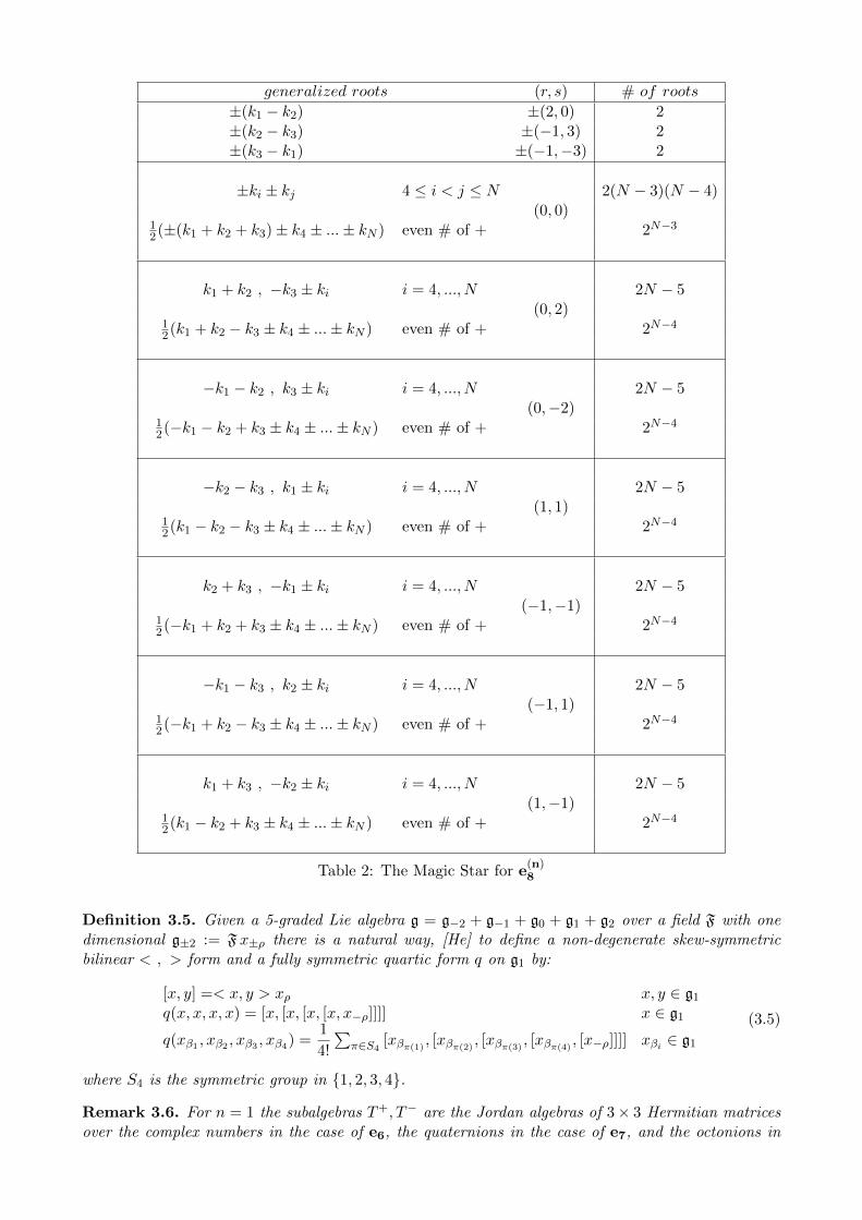
generalized roots (r, s) # of roots
±(k1 − k2) ±(2, 0) 2±(k2 − k3) ±(−1, 3) 2±(k3 − k1) ±(−1,−3) 2
±ki ± kj 4 ≤ i < j ≤ N 2(N − 3)(N − 4)(0, 0)
12(±(k1 + k2 + k3)± k4 ± ...± kN ) even # of + 2N−3
k1 + k2 , −k3 ± ki i = 4, ..., N 2N − 5(0, 2)
12(k1 + k2 − k3 ± k4 ± ...± kN ) even # of + 2N−4
−k1 − k2 , k3 ± ki i = 4, ..., N 2N − 5(0,−2)
12(−k1 − k2 + k3 ± k4 ± ...± kN ) even # of + 2N−4
−k2 − k3 , k1 ± ki i = 4, ..., N 2N − 5(1, 1)
12(k1 − k2 − k3 ± k4 ± ...± kN ) even # of + 2N−4
k2 + k3 , −k1 ± ki i = 4, ..., N 2N − 5(−1,−1)
12(−k1 + k2 + k3 ± k4 ± ...± kN ) even # of + 2N−4
−k1 − k3 , k2 ± ki i = 4, ..., N 2N − 5(−1, 1)
12(−k1 + k2 − k3 ± k4 ± ...± kN ) even # of + 2N−4
k1 + k3 , −k2 ± ki i = 4, ..., N 2N − 5(1,−1)
12(k1 − k2 + k3 ± k4 ± ...± kN ) even # of + 2N−4
Table 2: The Magic Star for e(n)8
Definition 3.5. Given a 5-graded Lie algebra g = g−2 + g−1 + g0 + g1 + g2 over a field F with onedimensional g±2 := Fx±ρ there is a natural way, [He] to define a non-degenerate skew-symmetricbilinear < , > form and a fully symmetric quartic form q on g1 by:
[x, y] =< x, y > xρ x, y ∈ g1
q(x, x, x, x) = [x, [x, [x, [x, x−ρ]]]] x ∈ g1
q(xβ1 , xβ2 , xβ3 , xβ4) =1
4!
∑π∈S4
[xβπ(1) , [xβπ(2) , [xβπ(3) , [xβπ(4) , [x−ρ]]]] xβi ∈ g1
(3.5)
where S4 is the symmetric group in {1, 2, 3, 4}.
Remark 3.6. For n = 1 the subalgebras T+, T− are the Jordan algebras of 3× 3 Hermitian matricesover the complex numbers in the case of e6, the quaternions in the case of e7, and the octonions in

Figure 2: The Magic Star and a 5-grading
the case of e8. With the 3-linear product T+ becomes a Jordan triple system, [Lo].The pair (T+, T−)is a Jordan Pair, [Lo]. Still for n = 1, F+ is a Freudenthal triple system, [He] and (F+, F−) is aKantor Pair, [Al].
4 HT-algebras
We now concentrate on the set of roots T(r,s) on a tip of the Magic Star. In order to fix one, let usconsider T(1,1) and denote it simply by T. The reader will forgive us if we shall be concise wheneverthere is no risk of misunderstanding and use T to denote both the set of roots and the set of elementsin LMS associated to those roots. An element of T is an F-linear combination of xα, xβ, ... for α, β, ...in T(1,1). We give T an algebraic structure with a commutative product, thus mimicking the casen = 1 when T is a Jordan algebra.
Remark 4.1. Let us first show what happens in the case n = 1, in particular for e8. It is provenin [Ma14] that T = J(1,1) is the Jordan Algebra J8
3 of 3 × 3 Hermitian matrices over the octonions.Let us denote by P1 := E11, P2 := E22, P3 := E33 the three trace-one idempotents, whose sum is theidentity in J8
3, Eii representing the matrix with a 1 in the (ii) position and zero elsewhere.Let us identify the algebra d4 ⊂ f4 ⊂ e6 ⊂ e6 ⊕ ac2 ⊂ e8 with the roots ±ki ± kj, 4 ≤ i < j ≤ 7 andP1, P2, P3 with the elements of J(1,1) which are left invariant by d4, [Jac]. This uniquely identifiesP1, P2, P3 with the roots k1 + k8, k1 − k8 and −k2 − k3. Since e7 ⊂ e8 is 3-graded, one can define a3-linear product on J(1,1), [McC], and a Jordan product through the correspondence with the quadraticformulation of Jordan algebras.
Still in the case of e8 (e(n)8 for n = 1), if we identify the e8 generators corresponding to the
roots in ΦO with the bosons and those corresponding to the roots in ΦS with the fermions, then the11 bosons in T are k1 ± kj, j = 4, ..., 8 and −k2 − k3. The three bosons k1 ± k8 and −k2 − k3,correspond to the three diagonal idempotents xP1, xP2, xP3, which are left invariant by d4, whose rootsare ±ki ± kj , 4 ≤ i < j ≤ 7.The remaining 8 vectors (bosons) and the 2x8 spinors (fermions) are linked by triality. Notice thatone spinor has 1
2(k1− k2− k3 + k8) fixed and even number of + signs among ±k4± k5± k6± k7, whilethe other one has 1
2(k1− k2− k3− k8) fixed and odd number of + signs among ±k4± k5± k6± k7. Sothey are both 8 dimensional representations of d4.Therefore a generic element of J8
3 is a linear superposition of 3 diagonal elements plus one vector andtwo spinors (or a bispinor). The vector can be viewed as the (12) octonionic entry of the matrix (plusits octonionic conjugate in the (21) position) and the two 8-dimensional spinors as the (31) and (23)entry (plus their respective octonionic conjugate in the (31) and (23) position).
Mutatis mutandis, analogous results hold for all finite dimensional exceptional Lie algebra; theMagic Star projection (depicted in Fig. 3) of the corresponding root lattice onto a plane determinedby an a2 root sub-lattice has been introduced by Mukai [Mu], and later investigated in depth in [Tr]

(see also [Ma14]), with a different approach exploiting Jordan Pairs [Lo]; see also the discussion in[TRM18] and [TRM18-2].
Figure 3: The Magic Star of finite dimensional exceptional Lie algebras [Mu, Tr]. Jq3 denotes a simpleJordan algebra of rank-3, parametrized by q = dimRA = 1, 2, 4, 8 for A = R,C,H,O, correspondingto f4, e6, e7, e8, respectively. In the case of g2 (corresponding to q = −2/3), the Jordan algebra is
trivially the identity element : J−2/33 ≡ I := diag(1, 1, 1).
One can then do the same for n ≥ 1 and consider the most general case e(n)8 (the other two cases
e(n)6 and e
(n)7 being a restriction of it; for a detailed treatment of f
(n)4 , see [EP3]).
Let us denote xP1, xP2 and xP3 the elements of LMS in T associated to the roots ρ1 := k1 + kN ,ρ2 := k1 − kN and ρ3 := −k2 − k3:
xP1 ↔ ρ1 := k1 + kN ; xP2 ↔ ρ2 := k1 − kN ; xP3 ↔ ρ3 := −k2 − k3 (4.1)
They are left invariant by the Lie subalgebra dN−4 = d4n, whose roots are ±ki±kj , 4 ≤ i < j ≤ N−1.We denote by TO the set of roots in T ∩ ΦO, by T ′O the set of roots in TO that are not ρ1, ρ2, ρ3
and by TS the set of roots in T ∩ ΦS . In the case we are considering, where T = T(1,1) we have
T ′O = {k1± kj , j = 4, ..., N − 1} and TS = {12(k1− k2− k3± k4± ...± kN )}, even # of +. We further
split TS into T+S = {1
2(k1− k2− k3± k4± ...+ kN )} and T−S = {12(k1− k2− k3± k4± ...− kN )}. Then
v ∈ T ′O is an 8n-dimensional vector and s± are 24n−1-dimensional chiral spinors of d4n.We write a generic element x of T as x =
∑λixPi + xv + xs+ + xs− where
xv =∑α∈T ′O
λvαxα (4.2)
xs± =∑α∈T±S
λs±α xα (4.3)
We view λvα as a coordinate of the vector λv and λs±α as a coordinate of the spinor λs
±. The
conjugation properties of the vector and chiral spinor representations of d4n imply the existence ofthe symmetric bilinear forms ωv and ωs (whose explicit expressions are computed in [EP4]). We willdenote by λv (λs
±) the vector (spinor) in the dual space with respect to such bilinear forms. We can
therefore view x as a 3× 3 Hermitian matrix: λ1 λv λs+λv λ2 λs−λs+ λs− λ3
(4.4)

whose entries have the following F-dimensions:
• 1 for the scalar diagonal elements λ1, λ2, λ3;
• 8n for the vector λv;
• 24n−1 for the spinors λs± .
Remark 4.2. We see that only for n = 1 the dimension of the vector and the spinors is the same,whereas for n > 1 the entries in the (12), (21) position have different dimension than those in the(31), (13), (23), (32) position. Nevertheless, we define in equation (4.5) a commutative product of theelements in T , which then becomes a generalization of the Jordan algebra J8
3 in a very precise sense,which we will henceforth name HT-algebra. The set of matrices (4.4) is contained in a cubic matrixalgebra [Vi], whose product is the standard block matrix product; blockwise, by the representationtheory of d4n, such a product suitably exploits the gamma matrices (also named Dirac matrices) (seee.g. [Ha]) of d4n itself. In a forthcoming paper [EP4], we will investigate this matrix algebra further;we think that this is indeed a rank-3 T-algebra [Vi].
Remark 4.3. Considering all non-trivial Magic Star algebras [EP1] (i.e. f(n)4 , e
(n)6 , e
(n)7 and e
(n)8 ),
we can state the following result (anticipated in [TRM17]): there exists an1 a2 projection of the MagicStar algebras (namely, of the corresponding generalized root lattice), such that a Magic Star structurepersists, with suitable generalizations of rank-3 Jordan algebras Jq
3 (given by the aforementioned HT-algebras) occurring on the tips of the persisting Magic Star! The Magic Star projection of Magic Staralgebras is depicted in Fig. 4.
Figure 4: The Magic Star projection Magic Star algebras. Tq,n3 denotes an HT-algebra [Vi, EP4],
parametrized by q = dimRA = 1, 2, 4, 8 for A = R,C,H,O, and n ∈ N, corresponding to f(n)4 [EP3],
e(n)6 , e
(n)7 , e
(n)8 , respectively. We remind that the smallest exceptional Lie algebra g2 (corresponding
to q = −2/3) cannot be EP-generalized, because it does not enjoy a spin factor embedding [TRM18],
and because J−2/33 ≡ I [TRM17, EP1].
Definition 4.4. We denote by I the element I := xP1 + xP2 + xP3 and by I− the Cartan involutionof I, namely the element I− := −xP1 − xP2 − xP3 of T := T(−1,−1), where xP1, xP2 and xP3 are
1Such a projection is not unique; as for the Magic Star projection of exceptional Lie algebras, depicted in Figure3, also for the Magic Star projection of Magic Star algebras, depicted in Figure 4, there are four possible equivalentprojections.

associated to the roots −k1 − kN , −k1 + kN and k2 + k3.
We give T an algebraic structure by introducing the commutative product, see Proposition 4.8:
x ◦ y :=1
2[[x, I−], y] , x, y ∈ T (4.5)
We introduce the trace (see Proposition 4.8) tr(x) ∈ F for x ∈ T in the following way:
for x = `1xP1 + `2xP2 + `3xP3 +∑
α 6=ρ1,ρ2,ρ3
`αxα tr(x) = `1 + `2 + `3 (4.6)
We denote by tr(x, y) := tr(x ◦ y) and by x2 := x ◦ x. For each x ∈ T we define
x# = x2 − tr(x)x− 1
2(tr(x2)− tr(x)2)I (4.7)
and we say that x is rank-1 if x# = 0.Let us also introduce N(x) ∈ F for x ∈ T in the following way:
N(x) =1
6
{tr(x)3 − 3tr(x)tr(x2) + 2tr(x3)
}=
1
3tr(x#, x) (4.8)
where x2 = x ◦ x and x3 = x ◦ x2.
Remark 4.5. Notice that tr(x#) = −12(tr(x2) − tr(x)2), therefore x# = 0 implies x2 = tr(x)x: a
rank-1 element of T is either a nilpotent or a multiple of a primitive idempotent u ∈ T : u2 = u andtr(u) = 1.
Remark 4.6. Since by (4.8) a rank-1 element x has N(x) = 0 any element of T falls into the followingclassification:
rank-1: x# = 0rank-2: x# 6= 0 , N(x) = 0rank-3: N(x) 6= 0
(4.9)
Examples of rank-2 and rank-3 elements are xP1 + xP2 and I respectively.
Definition 4.7. Let us define D the LMS Lie subalgebra dN−3 if LMS = e(n)6 , dN−2 ⊕ a1 if LMS =
e(n)7 , dN if LMS = e
(n)8 , spanned by {xα , α ∈ ΦO}; see remark 3.1 of [EP1].
We can prove the following
Proposition 4.8. The product x, y → x ◦ y is commutative. With respect to this product the elementI ∈ T is the identity and the elements xP1, xP2, xP3 ∈ T are trace-one idempotents, hence are rank-1elements of T . All xα ∈ T but xP1, xP2, xP3 are nilpotent and traceless, hence they are also rank-1elements of T . The form x→ tr(x) is a trace form, namely tr(x, y) is bilinear and symmetric in x, yand the associative property tr(x ◦ y, z) = tr(x, y ◦ z) holds for every x, y, z ∈ T .
Proof. If x, y ∈ T they are linear combinations of elements xα, xβ, ... associated to roots α, β, ...whose sum is not a root. Therefore [x, y] = 0. Moreover, since I− ∈ D, Proposition 6.1 of [EP1] yieldsthat adI− is a derivation, hence:
[[x, I−], y] + [[I−, y], x] = 0 ⇒ [[x, I−], y] = [[y, I−], x] ⇒ x ◦ y = y ◦ x (4.10)
We also have[xPi,−xPj ] = δijhρi , i, j = 1, 2, 3 (4.11)
and for any α ∈ T(1,1), being ρ1 + ρ2 + ρ3 = 2k1 − k2 − k3, see tables 1 and 2:
I ◦ xα =1
2[[I, I−], xα] =
1
2[hρ1 + hρ2 + hρ3 , xα] =
1
2(ρ1 + ρ2 + ρ3, α)xα = xα (4.12)

By linearity this extends to any x ∈ T .Moreover:
xPi ◦ xPi =1
2[[xPi, I
−], xPi] =1
2[hρi , xPi] =
1
2(ρi, ρi)xPi = xPi (4.13)
Obviously tr(xP1) = tr(xP2) = tr(xP3) = 1.
We now show that xα ∈ T is nilpotent if α 6= k1 ± kN ,−k2 − k3.Suppose xα ◦ xα 6= 0 then either 2α − k1 − kN or 2α − k1 + kN or 2α + k2 + k3 is a root. If α ∈ ΦO
then 2α− k1∓ kN = k1± 2ki∓ kN is a root if and only if ki = kN , whereas 2α+ k2 + k3 is not a root.If α ∈ ΦS then nor 2α− k1 ∓ kN nor 2α+ k2 + k3 are roots. Therefore α 6= k1 ± kN ,−k2 − k3 impliesx2α = 0 and, obviously, tr(xα) = 0 and rank(xα)= 1.
Finally, from the definition of the product x, y → x ◦ y and the definition of the trace it easilyfollows that tr(x, y) is bilinear. The associativity of the trace is proven in Proposition A.2 in App.A. �
5 HT-pairs
Definition 5.1. We define HT-pair the pair P = (T+, T−) where T+ (T−) is the F-vector spacegenerated by {x+
α |α ∈ T(1,1) a(resp. {x−α |α ∈ T(−1,−1)) so that the roots associated to T+ and T−
are on opposite tips of the Magic Star. Define the maps Ux±y∓ = 1
2 [[x+, y−], x+] quadratic in x± andlinear in y∓, such that Ux± : T∓ → T±. Define the linearization V of U : Vx,yz = (Ux+z−Ux−Uz)y =12([[x, y], z] + [[z, y], x]) for x, z ∈ T± and y ∈ T∓. We have Vx,yx = 2Uxy.
Remark 5.2. We remark that only in the case n = 1, due to the Jacobi identity, Vx,yz = [[x, y], z] forall x, z ∈ T±, y ∈ T∓. In this case, the HT-pairs become Jordan pairs [Lo].
Definition 5.3. We define an idempotent of the HT-pair P as the pair (x, y) such that Uxy = x andUyx = y.
Then, one can prove the following
Proposition 5.4. The rank-1 elements xα for α ∈ T , be they nilpotent or primitive idempotent, canbe completed to become idempotents of P.
Proof. For x = xα take y = − 2
(α, α)x−α then Uxy =
1
(α, α)[hα, xα] = xα and Uyx =
1
(α, α)
2
(α, α)[hα, x−α] =
− 2
(α, α)x−α = y. �
For many aspects the language of HT-pairs inside e(n)8 is more natural than that of HT-algebras.
A detailed investigation of the properties of such structures is beyond the scope of the present paper,and it is left for further future work.
6 Further Developments
A number of research venues stems from the novel non-Lie, infinitely countable chains of finite di-mensional generalizations of exceptional Lie algebras provided by Magic Star algebras, introduced in[EP1] and in the present paper, after the anticipation given in [TRM17]. We here list some of thedevelopments which we plan to report on in the near future.
Firstly, we will consider in detail the violation of the Jacobi identity determining the non-Lie natureof Magic Star algebras. As anticipated in [EP1], such a violation occurs due to the non-trivial (i.e. non-Abelian) nature of the spinorial subsector of the Magic Star algebras. In fact, Magic Star algebrasare not simply non-reductive extensions of (pseudo-)orthogonal Lie algebras by some translational(i.e. Abelian) spinor generators (as it holds for the electric-magnetic duality Lie algebra of N = 2

supergravity coupled to homogeneous non-symmetric scalar manifolds in D = 3, 4, 5 Lorentzian space-time dimensions [dWVP, dWVVP]), but rather they are characterized by non-translational (i.e., non-Abelian) spinorial extensions, whose non-trivial commutation relations with all generators generalize,in the very spirit of Exceptional Periodicity, the commutation relations characterizing exceptional Liealgebras in their “spin factor embedding decompositions” (cfr. [TRM18], as well as Remark 3.1 of[EP1]).
As pointed out also in [EP1], we remind that Exceptional Periodicity provides a way to go beyonde8 (and the whole set of exceptional Lie algebras but g2) which is very different from the way providedby affine and (extended) Kac-Moody algebras [Kac], which also appeared as symmetries for (super)gravity models reduced to D = 2, 1, 0 dimensions (see e.g. [Ni, TW]), as well as near spacelikesingularities in supergravity [Da]. In the near future, we plan to analyze in detail the relation betweenMagic Star algebras and (generalized) Kac-Moody (and possibly Borcherds) algebras.
Also, in the forthcoming paper [EP3] we will deal with the determination of the inner derivations
of HT-algebras, highlighting the relation with the Magic Star algebra f(n)4 ; subsequently, we will study
further larger symmetry algebras (such reduced structure, conformal and possibly quasi-conformalsymmetries), analyzing similarities and differences with the electric-magnetic duality Lie algebras ofN = 2 supergravity coupled to homogeneous non-symmetric scalar manifolds in D = 3, 4, 5 Lorentzianspace-time dimensions [dWVP, dWVVP].
Concerning further physical applications, we envisage potential applications of Exceptional Pe-riodicity and Magic Star algebras in Quantum Gravity, stemming from the considerations in [Tr],[Ma16, TRM18-2, Tr19]. We aim at a consistent model of elementary particle physics and space-timeexpansion at the early stages of the Universe based on the idea that interactions, defined in a purelyalgebraic way, are the fundamental objects of the theory, whereas space-time, hence gravity, is anemergent entity. Within this perspective, the failure of the Jacobi identity in the spinor sector ofMagic Star algebras might be related to dark matter /dark energy degrees of freedom, and the non-Abelian nature of the spinor component of Magic Star algebras would play a key role in order to havenon-trivial interactions among bosons and fermions in such algebras, which are not superalgebras norZ2-graded algebras.
In our view, a synthesis of spectral algebraic geometry (suitably generalized in a non-associativesense within HT-algebras) and Exceptional Periodicity can yield to the unification of various ap-proaches to Quantum Gravity, thus providing a new lens for searching a non-perturbative theory ofall matter, forces and space-time.
Acknowledgements
We thank Willem de Graaf for useful discussions on T-algebras and enlightening feedback on an earlyversion of the manuscript.
A Associativity of the trace
We recall that in section 4 we have fixed T := T(1,1). Therefore we refer to the row (1, 1) of table 2 forthe explicit expression of the roots involved in T and −k1± kN , k2 + k3 for the roots in I− appearingin the commutative product (4.5).In the proofs that will follow, we make use of the following identities (see (3.10), (3.11) and (3.13) of[EP1], here with N = R):
kN−1 = 12(αN−1 − αN−2)
ki = αi + ki+1 =∑N−2
`=i α` + 12(αN−1 − αN−2) , 1 ≤ i ≤ N − 2
kN = −2αN −∑N−2
`=1 `α` − N−12 (αN−1 − αN−2)
(A.1)
from which we obtain, for 1 ≤ i < j ≤ N − 1 and forcing∑s
`=r α` = 0 if r > s:

ki + kj =∑N−3
`=i α` +∑N−2
`=j α` + αN−1
ki − kj =∑j−1
`=i α`
1 ≤ i < j ≤ N − 1 (A.2)
±ki − kN = 2αN +∑i−1
`=1 `α` +∑N−3
`=i (`± 1)α` + (2n+ 1±12 )αN−2
+(2n+ 1 + 1±12 )αN−1 , i ≤ N − 2
±kN−1 − kN = 2αN +∑N−3
`=1 `α` + (2n+ 1∓12 )αN−2 + (2n+ 1 + 1±1
2 )αN−1
(A.3)
Let us introduce the notation x±vµ, µ = 0, ..., N − 5, to denote the vectors:
x±vµ =
{x±vi := xk1±ki+3
1 ≤ i ≤ N − 5x±vo := ±xk1±kN−1
(A.4)
A generic vector in T is a linear combination of the vectors x±vµ. We need the following
Lemma A.1. We have the following products among scalars and vectors in the notations (4.1), (A.4):
i) xPi ◦ xPj = δijxPiii) xPi ◦ xβ = 1
2(ρi, β)xβiii) x±vµ ◦ x∓vµ = 1
2(xP1 + xP2)
iv) x±vµ ◦ x∓vν = 0 µ 6= ν
v) x±vµ ◦ x±vν = 0
(A.5)
Proof. The first two equations i) and ii) are easily proven:
xPi ◦ xPj = 12 [[xPi,−xP1 − xP2 − xP3], xPj ] = 1
2 [hρi , xPj ] = δijxPixPi ◦ xβ = 1
2 [hρi , xβ] = 12(ρi, β)xβ
(A.6)
We now prove iii). Since [xvi, xP3] = 0 we get:
x±vµ ◦ x∓vµ = (−1)δµ0 12 [−ε(k1 ± ki,−k1 − kN )ε(±ki − kN , k1 ∓ ki)xP2
−ε(k1 ± ki,−k1 + kN )ε(±ki + kN , k1 ∓ ki)xP1](A.7)
We now show that:
ε(k1 + ki,−k1 ∓ kN )ε(ki ∓ kN , k1 − ki) =
ε(k1 − ki,−k1 ∓ kN )ε(−ki ∓ kN , k1 + ki) =
{−1 for i ≤ N − 2
1 for i = N − 1(A.8)
Using i), ii), vi) of Proposition 2.2, as well as Proposition 2.3, being the arguments of both termsroots whose sum is a root, we get
ε(k1 + ki,−k1 ∓ kN )ε(ki ∓ kN , k1 − ki) =ε(k1 − ki, ki ∓ kN )ε(−k1 ∓ kN , k1 + ki) =ε(k1 − ki, ki + k1 − k1 ∓ kN )ε(−k1 + ki − ki ∓ kN , k1 + ki) =ε(k1 − ki,−k1 ∓ kN )ε2(k1 − ki, k1 + ki)ε(−ki ∓ kN , k1 + ki) =ε(k1 − ki,−k1 ∓ kN )ε(−ki ∓ kN , k1 + ki)
(A.9)
Since 2ki is in the lattice L we can add and subtract 2ki in any argument of ε. By doing so weobtain
ε(k1 − ki,−k1 ∓ kN )ε(−ki ∓ kN , k1 + ki) =−ε(k1 − ki,−k1 ∓ kN )ε(k1 − ki, ki ± kN )ε(2ki, ki ± kN ) =−ε(k1 − ki, ki − k1)ε(2ki, ki ± kN ) = ε(2ki, ki ± kN )
(A.10)
Because of (2.5), whenever one argument of ε is an even multiple of a simple root, that argumentcan be neglected, as it would contribute with a factor +1. Therefore, by (A.1) and (A.3), one obtains
ε(2ki, ki ± kN ) = ε(αN−1 − αN−2, ki ± kN ) (A.11)

Since the ordering of the simple roots is αi < αj if i < j, and since ε(αj , αi) = 1 if αj > αi (hencej > i), ε(αi, αi) = −1 and ε(αN−2, αN−1) = 1, because αN−2 + αN−1 /∈ Φ, we get, for i ≤ N − 2
ε(2ki, ki ± kN ) = ε(αN−1 − αN−2,1∓ 1
2αN−2 +
3∓ 1
2αN−1) = −1 , i ≤ N − 2 (A.12)
and for i = N − 1
ε(2kN−1, kN−1 ± kN ) = ε(αN−1 − αN−2,1± 1
2αN−2 +
3∓ 1
2αN−1) = 1 , i = N − 1 (A.13)
We have thus proven (A.8), from which iii) follows.
The equations iv) and v) are trivial, since, for 4 ≤ i, j ≤ N − 1, k1 ± ki − k1 ± kN + k1 ± kj =k1 ± ki ± kj ± kN is not a root unless kj = −ki. �
We can proceed to prove the main result of this Appendix.
Proposition A.2. The form x→ tr(x) is associative, namely tr(x◦y, z) = tr(x, y ◦z) holds for everyx, y, z ∈ T .
Proof. By linearity it is sufficient to prove the associativity for the generators of LMS in T :
tr(xα, xβ ◦ xγ) = tr(xα ◦ xβ, xγ) , α, β, γ ∈ T (A.14)
We keep using the notation ρ1 := k1 + kN , ρ2 := k1 − kN , ρ3 := −k2 − k3.
Notice that xα ◦ (xβ ◦ xγ) = 0 does not imply (xα ◦ xβ) ◦ xγ = 0.Let α = k1 + k4, β = k1 − k4, γ = k1 − k4 then xα ◦ (xβ ◦ xγ) = 0 (since xβ ◦ xγ = 0) whereas(xα ◦ xβ) ◦ xγ 6= 0. However tr(xα, xβ ◦ xγ) = tr(xα ◦ xβ, xγ) = tr(xγ) = 0.
We prove the associativity of the trace by checking case by case when α (or β or γ) is a scalar P(xP1 or xP2 or xP3) or a vector V or a spinor S. We say P ◦ V ∈ V to mean that the ◦ product of ascalar and a vector is a vector, and similarly for other combinations of P, V, S. We also respectivelydenote by TR1 and TR2 the left-hand and right-hand sides of (A.14).
PPP) tr(xPi , xPj ◦ xP`) = δj`tr(xPi ◦ xPj ) = δijδj` = tr(xPi ◦ xPj , xP`).
PPV) Since (P ◦ P ) ◦ V and P ◦ (P ◦ V ) are either 0 or vectors then TR1 = TR2 = 0
PPS) Since (P ◦ P ) ◦ S and P ◦ (P ◦ S) are either 0 or spinors then TR1 = TR2 = 0
PVV) Because of Lemma A.1,TR1 = TR2 = 0 unless one vector is x±vµ and the other is x∓vµ. We have
tr(xPi , x±vµ ◦ x∓vµ) = 1
2 tr(xPi ◦ (xP1 + xP2)) = 12(δi1 + δi2); on the other hand tr(xPi ◦ x±vµ, x∓vµ) =
12(δi1 + δi2)tr(x±vµ, x
∓vµ) = 1
2(δi1 + δi2)12 tr(xP1 + xP2) = 1
2(δi1 + δi2).
PVS) Since (P ◦ V ) ◦ S, P ◦ (V ◦ S), V ◦ (P ◦ S) are either 0 or spinors then TR1 = TR2 = 0
PSS) We must show thattr(xPi, xs1 ◦ xs2) = tr(xPi ◦ xs1 , xs2) (A.15)
Since xPi ◦ xs1 ∝ xs1 , if xs1 ◦ xs2 = 0 then TR1 = TR2 = 0.Suppose now xs1 ◦ xs2 6= 0. We denote by ρs the root associated to the spinor xs. Then eitherρs1 + ρs2 = k1 − k2 − k3 ± kN and
ρs1 − k1 ∓ kN + ρs2 = −k2 − k3 (A.16)
or, ρs1 + ρs2 = k1 − k2 − k3 ± ki, for 4 ≤ i ≤ N and
ρs1 + k2 + k3 + ρs2 = k1 ± ki (A.17)
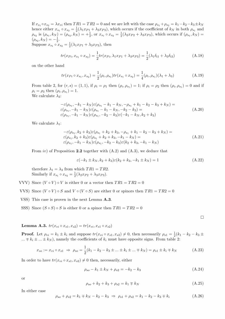
If xs1 ◦xs2 = λxvi then TR1 = TR2 = 0 and we are left with the case ρs1 +ρs2 = k1−k2−k3±kNhence either xs1 ◦ xs2 = 1
2(λ1xP1 + λ3xP3), which occurs if the coefficient of kN in both ρs1 andρs2 is (ρs1 , kN ) = (ρs2 , kN ) = +1
2 , or xs1 ◦ xs2 = 12(λ2xP2 + λ3xP3), which occurs if (ρs1 , kN ) =
(ρs2 , kN ) = −12 .
Suppose xs1 ◦ xs2 = 12(λ1xP1 + λ3xP3), then
tr(xPi, xs1 ◦ xs2) =1
2tr(xPi, λ1xP1 + λ3xP3) =
1
2(λ1δi1 + λ3δi3) (A.18)
on the other hand
tr(xPi ◦ xs1 , xs2) =1
2(ρi, ρs1)tr(xs1 ◦ xs2) =
1
4(ρi, ρs1)(λ1 + λ3) (A.19)
From table 2, for (r, s) = (1, 1), if ρi = ρ1 then (ρi, ρs1) = 1; if ρi = ρ2 then (ρi, ρs1) = 0 and ifρi = ρ3 then (ρi, ρs1) = 1.We calculate λ3:
−ε(ρs1 ,−k1 − kN )ε(ρs1 − k1 − kN ,−ρs1 + k1 − k2 − k3 + kN ) =ε(ρs1 ,−k1 − kN )ε(ρs1 − k1 − kN ,−k2 − k3) =ε(ρs1 ,−k1 − kN )ε(ρs1 ,−k2 − k3)ε(−k1 − kN , k2 + k3)
(A.20)
We calculate λ1:
−ε(ρs1 , k2 + k3)ε(ρs1 + k2 + k3,−ρs1 + k1 − k2 − k3 + kN ) =ε(ρs1 , k2 + k3)ε(ρs1 + k2 + k3,−k1 − kN ) =ε(ρs1 ,−k1 − kN )ε(ρs1 ,−k2 − k3)ε(k2 + k3,−k1 − kN )
(A.21)
From iv) of Proposition 2.2 together with (A.2) and (A.3), we deduce that
ε(−k1 ± kN , k2 + k3)ε(k2 + k3,−k1 ± kN ) = 1 (A.22)
therefore λ1 = λ3 from which TR1 = TR2.Similarly if xs1 ◦ xs2 = 1
2(λ2xP2 + λ3xP3).
VVV) Since (V ◦ V ) ◦ V is either 0 or a vector then TR1 = TR2 = 0
VVS) Since (V ◦ V ) ◦ S and V ◦ (V ◦ S) are either 0 or spinors then TR1 = TR2 = 0
VSS) This case is proven in the next Lemma A.3.
SSS) Since (S ◦ S) ◦ S is either 0 or a spinor then TR1 = TR2 = 0
�
Lemma A.3. tr(xvi ◦ xs1, xs2) = tr(xvi, xs1 ◦ xs2)
Proof. Let ρvi = k1 ± ki and suppose tr(xvi ◦ xs1, xs2) 6= 0, then necessarily ρs1 = 12(k1 − k2 − k3 ±
...∓ ki ± ...± kN ), namely the coefficients of ki must have opposite signs. From table 2:
xso := xvi ◦ xs1 ⇒ ρso =1
2(k1 − k2 − k3 ± ...± ki ± ...∓ kN ) = ρs1 ± ki ∓ kN (A.23)
In order to have tr(xvi ◦ xs1, xs2) 6= 0 then, necessarily, either
ρso − k1 ± kN + ρs2 = −k2 − k3 (A.24)
orρso + k2 + k3 + ρs2 = k1 ∓ kN (A.25)
In either caseρso + ρs2 = k1 ∓ kN − k2 − k3 ⇒ ρs1 + ρs2 = k1 − k2 − k3 ∓ ki (A.26)

and
tr(xvi ◦ xs1, xs2) = 14ε(k1 ± ki,−k1 ∓ kN )ε(±ki ∓ kN , ρs1)×
[ε(ρs1 ± ki ∓ kN ,−k1 ± kN )ε(ρs1 − k1 ± ki,−ρs1 + k1 − k2 − k3 ∓ ki)+ε(ρs1 ± ki ∓ kN , k2 + k3)ε(ρs1 + k2 + k3 ± ki ∓ kN ,−ρs1 + k1 − k2 − k3 ∓ ki)]
(A.27)
Since ρs1 − k1 ± ki and ρs1 + k2 + k3 ± ki ∓ kN are roots then, using i) of Proposition 2.3 and (A.22):
tr(xvi ◦ xs1, xs2) = −14ε(k1 ± ki,−k1 ∓ kN )ε(±ki ∓ kN , ρs1)×
[ε(ρs1 ± ki ∓ kN ,−k1 ± kN )ε(ρs1 − k1 ± ki,−k2 − k3)+ε(ρs1 ± ki ∓ kN , k2 + k3)ε(ρs1 + k2 + k3 ± ki ∓ kN , k1 ∓ kN )] =−1
4ε(k1 ± ki,−k1 ∓ kN )ε(±ki ∓ kN , ρs1)×ε(ρs1 ± ki ∓ kN ,−k1 ± kN )ε(ρs1,−k2 − k3)×[ε(k1 ∓ ki, k2 + k3) + ε(±ki ∓ kN , k2 + k3)ε(k2 + k3, k1 ∓ kN )] =−1
4ε(k1 ± ki,−k1 ∓ kN )ε(±ki ∓ kN , ρs1)×ε(ρs1 ± ki ∓ kN ,−k1 ± kN )ε(ρs1,−k2 − k3)×[ε(k1 ∓ ki, k2 + k3) + ε(k1 ∓ ki, k2 + k3)] =−1
2ε(k1 ± ki,−k1 ∓ kN )ε(±ki ∓ kN , ρs1)×ε(ρs1 ± ki ∓ kN ,−k1 ± kN )ε(ρs1,−k2 − k3)ε(k1 ∓ ki, k2 + k3)
(A.28)
Let us denote xs1 ◦ xs2 = λ+xs+ + λ−xs− + λxv. From (A.26):
ρs± = ρs1 + ρs2 − k1 ± kN = −k2 − k3 ∓ ki ± kNρv = ρs1 + ρs2 + k2 + k3 = k1 ∓ ki
(A.29)
Since ρs± is not a root then xs± = 0 and xs1 ◦ xs2 = λxv. Together with iii) of Lemma A.1 thisimplies
tr(xvi, xs1 ◦ xs2) = λ =− 1
2ε(ρs1, k2 + k3)ε(ρs1 + k2 + k3,−ρs1 + k1 − k2 − k3 ∓ ki)(−1)δi,N−1 =
12ε(ρs1, k2 + k3)ε(ρs1 + k2 + k3, k1 ∓ ki)(−1)δi,N−1
(A.30)
Therefore, in order to prove associativity, we must prove that:
−ε(k1 ± ki,−k1 ∓ kN )ε(±ki ∓ kN , ρs1)×ε(ρs1 ± ki ∓ kN ,−k1 ± kN )ε(k1 ∓ ki, k2 + k3) =ε(ρs1 + k2 + k3, k1 ∓ ki)(−1)δi,N−1
(A.31)
We have ε(±ki ∓ kN , ρs1) = −ε(ρs1,±ki ∓ kN ) since, from (A.23), ρs1 ± ki ∓ kN is a root. Thereforewe can write the left-hand side as:
ε(k1 ± ki,−k1 ∓ kN )ε(ρs1,−k1 ± ki)ε(±ki ∓ kN ,−k1 ± kN )ε(k1 ∓ ki, k2 + k3) (A.32)
Moreover ε(k1 ∓ ki, k2 + k3) = ε(k2 + k3, k1 ∓ ki), by iv) of Proposition 2.2, and the equality (A.31)reduces to
ε(k1 ± ki,−k1 ∓ kN )ε(±ki ∓ kN ,−k1 ± kN ) = (−1)δi,N−1 (A.33)
By iii) of Proposition 2.2, we have ε(k1 ± ki,−k1 ∓ kN ) = −ε(−k1 ∓ kN , k1 ± ki). By adding andsubtracting −k1 ∓ kN on the right-hand side and, using i) of Proposition 2.3 together with vii) ofProposition 2.2, we get ε(k1 ± ki,−k1 ∓ kN ) = ε(−k1 ∓ kN ,±ki ∓ kN ). The left-hand side of (A.33)becomes:
ε(k1 ± ki,−k1 ∓ kN )ε(±ki ∓ kN ,−k1 ± kN ) =ε(−k1 ∓ kN ,±ki ∓ kN )ε(±ki ∓ kN ,−k1 ± kN ) =−ε(−k1 ∓ kN ,±ki ∓ kN )ε(−k1 ± kN ,±ki ∓ kN ) = −ε(2k1,±ki ∓ kN ) =−ε(αN−1 − αN−2,±ki ∓ kN ) = (−1)δi,N−1
(A.34)
The last two equalities can be easily proven using (A.1) and (A.3).We have therefore proven that tr(xvi ◦ xs1, xs2) = tr(xvi, xs1 ◦ xs2) if tr(xvi ◦ xs1, xs2) 6= 0.

Finally suppose tr(xvi ◦ xs1, xs2) = 0.If ρs1 = 1
2(k1 − k2 − k3 ± ... ± ki ± ... ± kN ) then tr(xvi ◦ xs1, xs2) = 0, as already shown. In thiscase the vector xs1 ◦ xs2 has component ki either 0 or ±1 and, from iv), v) of Lemma A.1 alsotr(xvi, xs1 ◦ xs2) = 0.If ρs1 = 1
2(k1− k2− k3± ...∓ ki± ...± kN ) then we must have ρs1 + ρs2 6= k1− k2− k3∓ ki, otherwisetr(xvi ◦ xs1, xs2) 6= 0. Then neither ρs1 + ρs2 − k1 ± kN = k1 ∓ ki nor ρs1 + ρs2 + k2 + k3 = k1 ∓ kihence, by Lemma A.1, tr(xvi, xs1 ◦ xs2) = 0. �
References
[Al] B. Allison, J. Faulkner, Elementary groups and invertibility for Kantor pairs, Comm. Algebra 27,519-556 (1999).
[Da] T. Damour and M. Henneaux, E10, BE 10 and arithmetical chaos in superstring cosmology, Phys.Rev. Lett. 86, 4749–4752 (2001), hep-th/0012172. T. Damour, M. Henneaux, B. Julia and H.Nicolai, Hyperbolic Kac-Moody algebras and chaos in Kaluza-Klein models, Phys. Lett. B509,323–330 (2001), hep-th/0103094.
[dWVP] B. de Wit, A. Van Proeyen, Special geometry, cubic polynomials and homogeneous quater-nionic spaces, Commun. Math. Phys. 149 (1992) 307-334, hep-th/9112027.
[dWVVP] B. de Wit, F. Vanderseypen, A. Van Proeyen, Symmetry structure of special geometries,Nucl.Phys. B400 (1993) 463-524, hep-th/9210068.
[EP1] P. Truini, A. Marrani, M. Rios, Exceptional Periodicity and Magic Star Algebras. I : Founda-tions, arXiv:1909.00357 [math.RT].
[EP3] P. Truini, W. De Graaf, A. Marrani, Exceptional Periodicity and Magic Star Algebras. III : The
Algebra f(n)4 and the Derivations of HT-Algebras; in preparation.
[EP4] P. Truini, W. De Graaf, A. Marrani, Exceptional Periodicity and Magic Star Algebras. IV :Cubic T-Algebras; in preparation.
[Ha] M. Hazewinkel, Dirac Matrices, in : Encyclopedia of Mathematics, Springer Science+BusinessMedia B.V. / Kluwer Academic Publishers, 2001.
[He] F.W. Helenius, Freudenthal triple systems by root system methods, J. of Algebra 357, 116-137(2012), arXiv:1005.1275v1 [math-RT].
[Jac] N. Jacobson: “Exceptional Lie Algebras”, Lecture Notes in Pure and Applied Mathematics 1(M. Dekker, 1971).
[Kac] V.G. Kac : “Infinite Dimensional Lie Algebras”, third edition (Cambridge University Press,Cambridge, 1990).
[Lo] O.Loos : Jordan Pairs, Lect. Notes Math. 460, (Springer, 1975).
[Ma14] A. Marrani and P. Truini, Exceptional Lie Algebras, SU (3 ) and Jordan Pairs Part 2: Zorn-type Representations, J. Phys. A47 (2014) 265202, arXiv:1403.5120 [math-ph].
[Ma16] A. Marrani and P. Truini, Exceptional Lie Algebras at the very Foundations of Space andTime, p Adic Ultra. Anal. Appl. 8 (2016) no.1, 68-86, arXiv:1506.08576 [hep-th].
[McC] K. McCrimmon : “A Taste of Jordan Algebras” (Springer-Verlag New York Inc., New York,2004).
[Mu] S. Mukai, Simple Lie algebra and Legendre variety, Nagoya Suri Forum, 3 (1996), 1-12.

[Ni] H. Nicolai, The integrability of N= 16 supergravity, Phys. Lett. B194, 402 (1987). R. P. Geroch,A method for generating solutions of Einstein’s equations, J. Math. Phys. 12, 918–924 (1971). R. P.Geroch, A method for generating new solutions of Einstein’s equation. 2, J. Math. Phys. 13, 394–404 (1972). B. Julia, in : “Lectures in applied mathematics”, vol. 21, p. 355. AMS-SIAM, 1985. B.Julia, Group Disintegrations. Invited paper presented at Nuffield Gravity Workshop, Cambridge,Eng., Jun 22 - Jul 12, 1980. S. Mizoguchi, E 10 symmetry in one-dimensional supergravity, Nucl.Phys. B528, 238–264 (1998), hep-th/9703160.
[Sa] N. Cantarini, A. Ricciardo, A. Santi, Classification of Simple Linearly Compact Kantor TripleSystems over the Complex Numbers, J. Algebra 514, 468 (2018), arXiv:1710.05375 [math.QA].
[Tr] P. Truini, Exceptional Lie Algebras, SU (3 ) and Jordan Pairs, Pacific J. Math. 260, 227 (2012),arXiv:1112.1258 [math-ph].
[Tr19] P. Truini, Vertex operators for an expanding universe, invited paper in Symmetries and Order:Algebraic Methods in Many Body Systems, Yale 5-6 October 2018, in honor of Francesco Iachello,on the occasion of his retirement; arXiv:1901.07916 [physics.gen-ph].
[TRM17] P. Truini, M. Rios, A. Marrani, The Magic Star of Exceptional Periodicity, Contemp. Math.721 (2019), 277-297, arXiv:1711.07881 [hep-th].
[TRM18] A. Marrani, P. Truini, M. Rios, The Magic of Being Exceptional, J. Phys. Conf. Ser. 1194(2019) no.1, 012075, arXiv:1811.11208 [hep-th].
[TRM18-2] P. Truini, A. Marrani, M. Rios, Magic Star and Exceptional Periodicity: an approach toQuantum Gravity, J. Phys. Conf. Ser. 1194 (2019) no.1, 012106, arXiv:1811.11202 [hep-th].
[TW] A. G. Tumanov and P. West, E11 in 11D, Phys. Lett. B758 (2016) 278, 1601.03974 [hep-th].
[Vi] E.B. Vinberg, The theory of Convex Homogeneous Cones, in Transaction of the Moscow Mathe-matical Society for the year 1963, 340-403, American Mathematical Society, Providence RI 1965.