EVOLUTION OF THE SYNCHROTRON SPECTRUM IN

EVOLUTION OF THE SYNCHROTRON SPECTRUM IN MARKARIAN 421 DURING THE 1998 CAMPAIGNChiharu Tanihata,

1,2Jun Kataoka,

3Tadayuki Takahashi,

1,2and Greg M. Madejski

4

Received 2002 October 25; accepted 2003 October 14

ABSTRACT

The uninterrupted 7 day ASCA observations of the TeV blazar Mrk 421 in 1998 have clearly revealed thatX-ray flares occur repeatedly. In this paper, we present the results of the time-resolved spectral analysis of thecombined data taken by ASCA, RXTE, BeppoSAX, and the Extreme Ultraviolet Explorer (EUVE ). In this object—and in many other TeV blazars—the precise measurement of the shape of the X-ray spectrum, which reflects thehigh-energy portion of the synchrotron component, is crucial in determining the high-energy cutoff of theaccelerated electrons in the jet. Thanks to the simultaneous broadband coverage, we measured the 0.1–25 keVspectrum resolved on timescales as short as several hours, providing a great opportunity to investigate thedetailed spectral evolution at the flares. By analyzing the time-subdivided observations, we parameterize theevolution of the synchrotron peak, where the radiation power dominates, by fitting the combined spectra with aquadratic form [where the �F� flux at the energy E obeys log �F� Eð Þ ¼ log

��F�; peak

�� const

�log E�

log Epeak

�2]. In this case, we show that there is an overall trend that the peak energy Epeak and peak flux �F�; peak

increase or decrease together. The relation of the two parameters is best described as Epeak / �F0:7�; peak for the

1998 campaign. Similar results were derived for the 1997 observations, while the relation gave a smaller indexwhen both 1997 and 1998 data were included. On the other hand, we show that this relation, and also the detailedspectral variations, differs from flare to flare within the 1998 campaign. We suggest that the observed features areconsistent with the idea that flares are due to the appearance of a new spectral component. With the availability ofthe simultaneous TeV data, we also show that there exists a clear correlation between the synchrotron peak fluxand the TeV flux.

Subject headings: BL Lacertae objects: individual (Markarian 421) — galaxies: active — radiation mechanisms:nonthermal — X-rays: galaxies

1. INTRODUCTION

The uninterrupted 7 day ASCA observation of the TeVblazar Mrk 421 in 1998 has revealed that day-scale X-rayflares seen in previous observations were probably unresolvedsuperpositions of many smaller flares (Takahashi et al. 2000).The nearly continuous observation allowed not only the pos-sibility of tracking the individual flares entirely from the riseto decay, but it also enabled quantitative statistical tests of thetime series by employing the power spectrum or the structurefunction (Kataoka et al. 2001; Tanihata et al. 2001).

The main characteristic of blazars is their high flux ob-served from radio to �-rays, coupled with strong variabilityand strong polarization. These properties are now successfullyexplained by the scenario in which blazars are active galacticnuclei (AGNs) possessing jets aligned close to the line of sightand, accordingly, the Doppler-boosted nonthermal emissionfrom the jet dominates other emission components (e.g.,Blandford & Konigl 1979; Urry & Padovani 1995). This iswhat makes blazars critical in understanding jets in AGNs.

The broadband spectra of blazars consist of two peaks, onein the radio-to–optical-UV range (and in some cases, reachingto the X-ray band) and the other in the hard X-ray–to–�-rayregion. The high polarization of the radio-to-optical emission

suggests that the lower energy peak is produced via the syn-chrotron process by relativistic electrons in the jet. The higherenergy peak is believed to be due to Compton upscattering ofseed photons by the same population of relativistic electrons.Several possibilities exist for the source of the seed photons;these can be the synchrotron photons internal to the jet (Jones,O’Dell, & Stein 1974; Ghisellini & Maraschi 1989), but theycan also be external, such as from the broad emission lineclouds (Sikora, Begelman, & Rees 1994) or the accretion disk(Dermer, Schlickeiser, & Mastichiadis 1992; Dermer &Schlickeiser 1993).

The blazars with peak synchrotron output in the X-rayrange also emit strongly in the �-ray energies, and thebrightest of those have been detected in the TeV range withground-based Cerenkov arrays. These are the so-called TeVblazars. In TeV blazars, variability of the synchrotron flux ismeasured to be the strongest and most rapid in the X-ray band,and thus it provides the best opportunity to study the electronsthat are accelerated to the highest energies. In particular, thesynchrotron peak is a very important observable in twoaspects: first, because the flux at the peak represents the totalemitted power from the blazar and second, because the peakfrequency reflects the maximum energy of radiating particlesgained in the acceleration process.

Mrk 421 is among the closest known blazars, at a redshift of0.031, and it was the first blazar (and also the first extra-galactic source) discovered to be a TeV emitter. It was firstdetected as a weak source by EGRET (Lin et al. 1992), and 9months later, Whipple detected a clear signal from this objectbetween 0.5 and 1.5 TeV (Punch et al. 1992; Petry et al. 1996).Flux variability on various timescales has been observed,

1 Institute of Space and Astronautical Science, 3-1-1 Yoshinodai, Saga-mihara 229-8510, Japan; [email protected].

2 Department of Physics, University of Tokyo, 7-3-1 Hongo, Bunkyo-ku,Tokyo 113-0033, Japan.

3 Department of Physics, Tokyo Institute of Technology, Tokyo 152-8551,Japan.

4 Stanford Linear Accelerator Center, Stanford, CA 94309-4349.

759

The Astrophysical Journal, 601:759–770, 2004 February 1

# 2004. The American Astronomical Society. All rights reserved. Printed in U.S.A.

including a very short flare with a duration of �1 hr (Gaidoset al. 1996). Ever since, Mrk 421 has been repeatedly confirmedto be a TeV source by various ground-based telescopes. It hasalso been one of the most studied blazars and a target of severalmultiwavelength campaigns (Macomb et al. 1995; Maraschiet al. 1999; Takahashi et al. 2000).

The multiwavelength campaign of Mrk 421 in 1998 wasone of the first opportunities to observe a blazar in the TeVrange using several telescopes located in different locations inthe world, so as to have coverage as continuous as possible(Aharonian et al. 1999; Piron et al. 2001). Observations inother frequencies included X-ray observations by ASCA,RXTE (Takahashi et al. 2000), and BeppoSAX (Maraschi et al.1999; Fossati et al. 2000a, 2000b), EUV observations by theExtreme Ultraviolet Explorer (EUVE ), optical observationwith BVRI filters organized by the WEBT collaboration,5 andradio observations at the Metsahovi Radio Observatory.

In this paper, we present the results of the spectral analysisof X-ray and EUV data during the 1998 April campaign. Inparticular, we estimate the location of the synchrotron peak inthe �F� spectrum. So far, quantitative studies of the variationof the synchrotron peak have been conducted only for the twobrightest blazars, Mrk 421 and Mrk 501. The largest variationof the synchrotron peak energy was observed in Mrk 501 byBeppoSAX; the peak energy shifted �2 orders of magnitude(Pian et al. 1998). Collecting data from different epochs(separated by as much as �2 yr), Tavecchio et al. (2001) haveshown a relation of the form Epeak / Fn

0:1 100 keV, with n � 2.A similar analysis was done by Fossati et al. (2000b) for theMrk 421 data obtained by BeppoSAX in 1997 and 1998,showing a relation of Epeak / Fn

0:1 10 keV, with n ¼ 0:55. Inthis paper we describe a continuous 7 day variation of thesynchrotron peak, which allows us to investigate the dynam-ical change of the synchrotron spectrum during the flares.

We first describe the observations and data analysis in x 2.The results of spectral analysis are described in x 3; a sum-mary of the results and a discussion of our findings, withemphasis on the temporal evolution of the spectrum, arepresented in x 4.

2. OBSERVATION AND DATA ANALYSIS

The week-long multifrequency campaign of Mrk 421 wascarried out in 1998 April (Takahashi et al. 2000). The goal ofthis paper is to study the evolution of the high-energy syn-chrotron spectrum as a function of time during the campaignand also the correlation with the TeV flux. This requires thebest possible spectral coverage in the X-ray range, for whichwe assembled all available data collected during the cam-paign, including pointings by X-ray observatories ASCA,RXTE, and BeppoSAX, as well as EUVobservations by EUVE.

2.1. ASCA

Mrk 421 was observed continuously with ASCA for 7 days(except for the Earth occultation), 1998 April 23.97–30.8 UT(PI: T. Takahashi). The ASCA detectors—two SISs (SolidState Imaging Spectrometers; Burke et al. 1991; Yamashitaet al. 1997) and two GISs (Gas Imaging Spectrometers;Ohashi et al. 1996)—were in operation. We refer to Tanihataet al. (2001) for the details of the observation modes and datareduction. The obtained spectra were rebinned so that all binshave the same statistics.

Since late 1994, the efficiency of both SIS detectors below�1 keV has been decreasing over time. The problem is be-lieved to be caused by the increased residual dark current leveland also by the decrease in the charge transfer efficiency, al-though an effort is still underway to model the effects. While ithas been reported that it may be possible to parameterize thedegradation by an additional absorption column as a functionof time (Yaqoob et al. 2000), since our observation concernsthe precise shape of the continuum spectrum, we used only thedata obtained by the GISs for spectral analysis. (Note that theX-ray spectra in Fig. 2 of Takahashi et al. 2000 show the dataobtained by the SISs. Because the SISs were used, there is toostrong a decrease of inferred flux at the lower energy, which isdue to instrumental effects described above.)

2.2. RXTE

The RXTE observations (PI: G. M. Madejski) were mainlycoordinated to coincide with the ASCA observation period butwere conducted, mostly, only during the low-backgroundorbits. The RXTE extends the ASCA bandpass to a higherenergy with the PCA (Proportional Counter Array; 2–60 keV)and HEXTE (High Energy X-Ray Timing Experiment; 15–200 keV) instruments. However, because both the flux fromthe source and the sensitivities of the detectors decreasetoward higher energies, in the analysis below we use only thedata from the PCA, in the energy range 3–25 keV.All data reduction was performed using the HEASOFT

software packages, based on the REX script, provided by theRXTE Guest Observer Facility (GOF). The screening criteriaexcluded data from times when the elevation angle from theEarth’s limb was lower than 10� and data acquired during theSouth Atlantic Anomaly (SAA) passages. Since the Propor-tional Counter Units (PCUs) are activated during the SAApassage, we used the data only from times after the back-ground level had dropped to the quiescent level and becomestable, typically 30 minutes after the peak of an SAA passage.For the best signal-to-noise ratio, we selected events only

from the top xenon layer and excluded events from other gaslayers. For maximum consistency among the observations, weused only the three detectors that were turned on for all theobservations (known as PCU0, PCU1, and PCU2). Since thePCA is not an imaging detector, blank-sky observations mustbe used to estimate the background spectrum. For these, weused the background models provided by the RXTE GOF toevaluate the background during each observation. We notethat the residual background contamination of the data withinthe energy bandpass we selected was always significantlylower than the source counts. The mean net RXTE PCA countrate from Mrk 421 in the 10–20 keV range for the three PCUsnamed above was at least �3 counts s�1, while the totalresiduals from the blank sky in this energy range plus thefluctuations of the cosmic X-ray background were lower than0.2 counts s�1 (see the HEASARC Web site regarding theRXTE PCA background), providing confidence that an im-precise background subtraction did not affect our results.

2.3. BeppoSAX

The BeppoSAX observations (PI: L. Chiappetti) started 3days before the ASCA observations (Maraschi et al. 1999;Fossati et al. 2000a, 2000b). We use the data obtained by theLECS (Low Energy Concentrator Spectrometer; 0.1–10 keV),which extends the bandpass to a lower energy, and also theMECS(MediumEnergyConcentratorSpectrometer;1.3–10keV).5 See http://www.to.astro.it/blazars/webt.

TANIHATA ET AL.760 Vol. 601

The data analysis was based on the linearized event files, to-gether with the appropriate background event files and responsematrices, provided by the BeppoSAX Science Data Center(SDC). Data reduction was performed using the standardHEASOFT software, XSELECT.

We extracted the source photons from a circular regioncentered at the source with a radius of 80 for both LECS andMECS. For the background photons, we constructed thespectra by extracting the photons from the same detectorregions, using blank-sky observations. Each spectrum wasrebinned using the grouping templates provided by theBeppoSAX SDC, and we limited the energy range to 0.12–4.0 keV for LECS and 1.65–10.5 keV for MECS, as sug-gested in the Handbook for BeppoSAX NFI Spectral Analysis(Fiore, Guainazzi, & Grandi 1999).6

2.4. EUVE

The EUVE observations covered the entire campaign ofMrk 421 from April 19.4 to May 1.2 (PI: T. Takahashi). Thesource photons were extracted in a 120 aperture. In order toestimate the absolute flux in the EUV range, we normalized itto be consistent with the data obtained simultaneously by theother observatories. Given that the EUV spectrum is difficultto determine within the rather limited bandpass, we used onlythe observed integrated count rate (see Marshall, Fruscione, &Carone 1995). For this, we used the period when the obser-vations by all observatories overlapped (MJD 50,927.03–50,927.34; x 3.1). During this period, the average EUVE countrate was 0:46 � 0:01 counts s�1. At the same time, the 0.13–0.18 keV flux derived from the combined LECS, MECS, GIS,and PCA spectrum gives �F� ¼ 1:78 � 0:04ð Þ � 10�10 ergscm�2 s�1, where the error represents the statistical error.

An additional uncertainty arises from the fact that the dif-ference in the spectral shape is not taken into account. Thiscan be estimated from the results in Marshall et al. (1995).Taking NH ¼ 1:5� 1020 cm�2 for Mrk 421, assuming that thespectrum index varies from 0.5 to 1.0, the flux density wouldvary from 1363 to 1394 �Jy for 1 count s�1 in the EUVE range.This gives an additional 2.5% error as a systematic error.

In the following analysis, we use the above value forscaling the observed EUVE count rate to flux. Thus,

�F� EUVEð Þ ¼ 1:78� 10�10 Fcts s�1

0:46

� �ergs s�1 cm�2; ð1Þ

where Fcts s�1 is the EUVE count rate.

3. RESULTS

3.1. The Shape of the 0.1–25 keV Spectrum

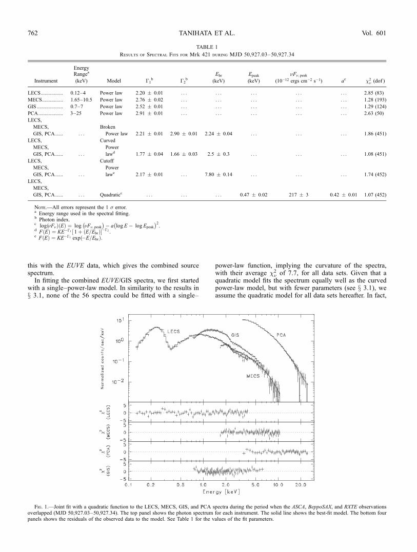
During April 24, observations by all three X-ray satellites,ASCA, BeppoSAX, RXTE, and also EUVE happened to exactlyoverlap continuously for 26.5 ks (MJD 50,927.03–50,927.34).This provides us with high-quality data over a very broadenergy coverage, spanning more than 2 decades, from 0.12 to25 keV. The net exposures during the overlapping 26.5 ksperiod were 9.1, 13.3, 3.6, and 5.5 ks for GIS, PCA, LECS,and MECS, respectively.

We first fitted the spectrum for each instrument with apower-law model, with a low-energy absorption fixed to the

Galactic value, NH ¼ 1:5� 1020 cm�2 (Elvis, Lockman, &Wilkes 1989). The results are shown in the top half of Table 1,suggesting that the fit is not adequate for any of the individualinstruments. This certainly suggests that a more complexmodel, rather than just a simple power-law function, is re-quired to describe the spectrum.

The shape of the synchrotron spectrum is determined fromthe energy distribution of the radiating electrons, which cutsoff at the high energy representing the acceleration limit. Asdescribed in x 1, the high-energy end of the synchrotronspectrum in TeV blazars is located in the X-ray range; this ismost likely the reason that the high-quality X-ray data cannotbe described by a single power law.

Given the curved spectrum for each instrument, we fittedthe combined X-ray spectrum with various functions to modelthe shape of the observed curvature. We note that our aim isnot to develop the shape of the curvature from first principlesbut rather to reproduce the observed data. For this reason, weconsidered the following models for comparison: (1) a brokenpower law, (2) a curved power law, (3) a power law with anexponential cutoff, and (4) a quadratic function in the log �–log �F�ð Þ plane. The curved power law that we define below issimilar to the broken power law, but the change in the spectralindex is not discrete. The form we attempt is F Eð Þ ¼KE��1 1þ E=Ebrð Þ½ ��2 . The form for the exponentially cutoff power law is F Eð Þ ¼ KE��1 exp �E=Ebrð Þ, and the qua-dratic function is described as log �F�ð Þ Eð Þ ¼ log

��F�; peak

��

a�log E � log Epeak

�2.

Since there are slight differences in the cross-calibrationbetween the instruments, we allow the normalization to varyfor each instrument. For all results below, the flux is nor-malized to the GIS value, unless otherwise noted. The NH isfixed to the Galactic value.

By fitting the spectrum with the models above, we firstfound that the power law with an exponential cutoff is not agood representation of the data: the model cutoff is too sharpat high energies. The broken power law is also not acceptable,and the curved power law is significantly better. We also findthat the quadratic function fits the spectrum surprisingly well.The fitted spectra and the residuals to the quadratic model areshown in Figure 1, where all LECS, MECS, GIS, and PCAspectra are shown to be well described with this single func-tion. The results of the spectral fits by the four models aresummarized in the bottom half of Table 1.

3.2. The Time-resolved Spectra

The EUVE observation covered the whole campaign (April19.4–May 1.2) and thus completely overlapped our 7 dayASCA observation. This adds a data point at 0.13–0.18 keV, inaddition to the ASCA spectrum in the 0.7–7 keV range, pro-viding us the best opportunity to study the continuous spectralvariability. In fact, this is the longest continuous monitoring ofthis object so far, spanning the 0.13–7 keV range.

We divided the whole observation into shorter segments,with each having a duration of 10 ks. In order to combine theGIS and EUVE data, the GIS count rate spectra must first beconverted to the source flux spectra, as the EUVE count ratedata convert directly into flux (x 2.4). For this, we first fittedthe GIS spectrum with a curved power-law model with Gal-actic absorption. This gives the source spectrum in the GISenergy range. Note that this procedure depends on the selectedmodel, but as long as it describes the spectrum well, thisshould introduce the smallest possible bias. We then combined

6 The Handbook for BeppoSAX NFI Spectral Analysis is available at ftp://www.sdc.asi.it/pub/sax/doc/software_docs/saxabc_v1.2.ps.gz.

EVOLUTION OF Mrk 421 SYNCHROTRON SPECTRUM 761No. 2, 2004

this with the EUVE data, which gives the combined sourcespectrum.

In fitting the combined EUVE/GIS spectra, we first startedwith a single–power-law model. In similarity to the results inx 3.1, none of the 56 spectra could be fitted with a single–

power-law function, implying the curvature of the spectra,with their average �2

� of 7.7, for all data sets. Given that aquadratic model fits the spectrum equally well as the curvedpower-law model, but with fewer parameters (see x 3.1), weassume the quadratic model for all data sets hereafter. In fact,

TABLE 1

Results of Spectral Fits for Mrk 421 during MJD 50,927.03–50,927.34

Instrument

EnergyRangea

(keV) Model �1b �2

b

Ebr

(keV)

Epeak

(keV)

�F�; peak

(10�12 ergs cm�2 s�1) ac �2� (dof )

LECS................. 0.12–4 Power law 2.20 � 0.01 . . . . . . . . . . . . . . . 2.85 (83)

MECS................ 1.65–10.5 Power law 2.76 � 0.02 . . . . . . . . . . . . . . . 1.28 (193)

GIS .................... 0.7–7 Power law 2.52 � 0.01 . . . . . . . . . . . . . . . 1.29 (124)

PCA................... 3–25 Power law 2.91 � 0.01 . . . . . . . . . . . . . . . 2.63 (50)

LECS,

MECS,

GIS, PCA...... . . .

Broken

Power law 2.21 � 0.01 2.90 � 0.01 2.24 � 0.04 . . . . . . . . . 1.86 (451)

LECS,

MECS,

GIS, PCA...... . . .

Curved

Power

lawd 1.77 � 0.04 1.66 � 0.03 2.5 � 0.3 . . . . . . . . . 1.08 (451)

LECS,

MECS,

GIS, PCA...... . . .

Cutoff

Power

lawe 2.17 � 0.01 . . . 7.80 � 0.14 . . . . . . . . . 1.74 (452)

LECS,

MECS,

GIS, PCA...... . . . Quadraticc . . . . . . . . . 0.47 � 0.02 217 � 3 0.42 � 0.01 1.07 (452)

Note.—All errors represent the 1 � error.a Energy range used in the spectral fitting.b Photon index.c log �F�ð Þ Eð Þ ¼ log

��F�; peak

�� a

�log E � log Epeak

�2.

d F Eð Þ ¼ KE��1 1þ E=Ebrð Þ½ ��2 .e F Eð Þ ¼ KE��1 exp �E=Ebrð Þ.

Fig. 1.—Joint fit with a quadratic function to the LECS, MECS, GIS, and PCA spectra during the period when the ASCA, BeppoSAX, and RXTE observationsoverlapped (MJD 50,927.03–50,927.34). The top panel shows the photon spectrum for each instrument. The solid line shows the best-fit model. The bottom fourpanels shows the residuals of the observed data to the model. See Table 1 for the values of the fit parameters.


because of the energy gap between the EUVE and GIS, the fitwith a curved power-law model resulted in multiple minima inthe �2 plane (since the parameters are correlated), and theexact value of the best-fit parameters depended highly on theinitial value.

We checked whether the fit was adequate for all data seg-ments. The �2

� for each fit (Fig. 2, bottom panel ) ranged from0.71 to 1.45. The number of degrees of freedom ranged from 60to 187, which gave P �2ð Þ > 5% for 53 out of the total of 56data points. For the other three data points (corresponding totimes 230–240, 270–280, and 450–460 ks), we found severalline or edgelike structures in the spectra, which resulted in anincrease of the �2

� . Although it is not clear whether this is due tosome systematic effect or is a true property of the source, sinceour aim is to model the continuum spectrum correctly, weexcluded the energy ranges where those features are present.This improved the fit significantly ( plus signs). With this, all56 spectra were well described with the quadratic function.

The time evolution of the derived parameters in the fit isshown in the top three panels in Figure 2: the peak flux,peak energy, and the curvature parameter a (see definition inTable 1). The peak energy is observed to shift between 0.5 and1.2 keV, where a general trend is found such that thepeak energy is higher when the peak flux is higher. This isplotted as the filled circles in Figure 3. The fit results arelisted in Table 2.

We do note that the actual validity of using a quadraticfunction in the entire 0.1–25 keV range was checked in detail(including an examination of trends in residuals) only for the

epoch when the overlapping BeppoSAX, ASCA, and RXTEobservations were available. Since we measured only theEUVE flux below 0.7 keV in the combined EUVE/GIS fit, thederived peak location can depend on the model function weassume. For instance, if any function were allowed, the peakcould be located at any energy within the gap. For this reason,we emphasize that the derived peak location is the estimatedpeak, assuming that the spectrum gap can be extrapolated withthe same quadratic function, and also that the error bar de-scribes only the statistical error.

We also analyzed the BeppoSAX data during the campaign.Furthermore, in order to make a comparison with dataobtained from another campaign, we also analyzed theBeppoSAX data obtained in 1997 (PIs: G. Vacanti and L.Chiappetti). We divided the observation into segments of thesame 10 ks duration and fitted the combined LECS/MECSspectra with a quadratic function. For the BeppoSAX data, wealso fitted the spectra with a curved–power-law model forcomparison. The derived peak flux and peak energy from bothmodels are listed in Table 3. In fitting the combinedLECS/MECS spectra, the normalizations were allowed to varyindependently, and the values in Table 3 were normalized tothe MECS2 value. The fitting results show that although thereis one less spectral fit parameter in the quadratic function, bothmodels equally represent the observed spectra. In contrast tothe combined EUVE/GIS data, there is no energy gap in theBeppoSAX data, which provides support that our assumedquadratic form is appropriate in estimating the peak locationin the EUVE/GIS case. The derived peak flux and peak energyusing both functions are similar, but we also note that thequadratic function gives a slightly lower peak energy than thecurved–power-law function.

The derived peak flux and peak energy, assuming the qua-dratic model, for the BeppoSAX observations are shown in

Fig. 2.—Time evolution of the spectrum fit parameters to the combinedEUVE and ASCA spectra, assuming a quadratic function (see text): peak flux(top), peak energy (second), and curvature parameter (third; see definition inTable 1). The flux is in units of 10�12 ergs cm�2 s�1, and peak energy is inkeV. The bottom panel shows the reduced �2 for each of the fits. Three out ofthe 56 spectra showed a poor fit [P �2ð Þ < 5%] due to several line or edgelikestructures; the fit is significantly improved ( plus signs) after excluding theenergy ranges that included these structures.

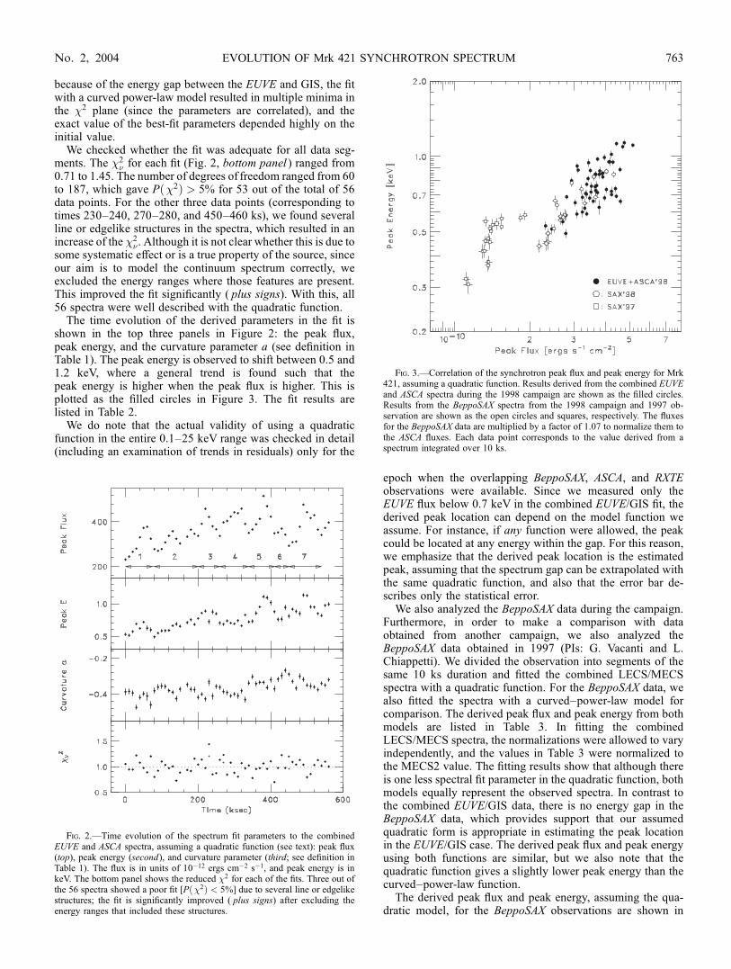
Fig. 3.—Correlation of the synchrotron peak flux and peak energy for Mrk421, assuming a quadratic function. Results derived from the combined EUVEand ASCA spectra during the 1998 campaign are shown as the filled circles.Results from the BeppoSAX spectra from the 1998 campaign and 1997 ob-servation are shown as the open circles and squares, respectively. The fluxesfor the BeppoSAX data are multiplied by a factor of 1.07 to normalize them tothe ASCA fluxes. Each data point corresponds to the value derived from aspectrum integrated over 10 ks.


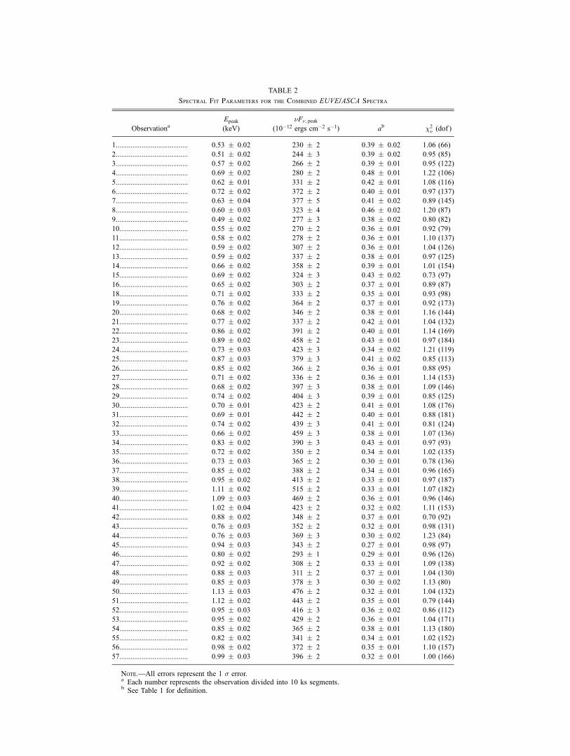
TABLE 2

Spectral Fit Parameters for the Combined EUVE/ASCA Spectra

ObservationaEpeak

(keV)

�F�; peak

(10�12 ergs cm�2 s�1) ab �2� (dof )

1....................................... 0.53 � 0.02 230 � 2 0.39 � 0.02 1.06 (66)

2....................................... 0.51 � 0.02 244 � 3 0.39 � 0.02 0.95 (85)

3....................................... 0.57 � 0.02 266 � 2 0.39 � 0.01 0.95 (122)

4....................................... 0.69 � 0.02 280 � 2 0.48 � 0.01 1.22 (106)

5....................................... 0.62 � 0.01 331 � 2 0.42 � 0.01 1.08 (116)

6....................................... 0.72 � 0.02 372 � 2 0.40 � 0.01 0.97 (137)

7....................................... 0.63 � 0.04 377 � 5 0.41 � 0.02 0.89 (145)

8....................................... 0.60 � 0.03 323 � 4 0.46 � 0.02 1.20 (87)

9....................................... 0.49 � 0.02 277 � 3 0.38 � 0.02 0.80 (82)

10..................................... 0.55 � 0.02 270 � 2 0.36 � 0.01 0.92 (79)

11..................................... 0.58 � 0.02 278 � 2 0.36 � 0.01 1.10 (137)

12..................................... 0.59 � 0.02 307 � 2 0.36 � 0.01 1.04 (126)

13..................................... 0.59 � 0.02 337 � 2 0.38 � 0.01 0.97 (125)

14..................................... 0.66 � 0.02 358 � 2 0.39 � 0.01 1.01 (154)

15..................................... 0.69 � 0.02 324 � 3 0.43 � 0.02 0.73 (97)

16..................................... 0.65 � 0.02 303 � 2 0.37 � 0.01 0.89 (87)

18..................................... 0.71 � 0.02 333 � 2 0.35 � 0.01 0.93 (98)

19..................................... 0.76 � 0.02 364 � 2 0.37 � 0.01 0.92 (173)

20..................................... 0.68 � 0.02 346 � 2 0.38 � 0.01 1.16 (144)

21..................................... 0.77 � 0.02 337 � 2 0.42 � 0.01 1.04 (132)

22..................................... 0.86 � 0.02 391 � 2 0.40 � 0.01 1.14 (169)

23..................................... 0.89 � 0.02 458 � 2 0.43 � 0.01 0.97 (184)

24..................................... 0.73 � 0.03 423 � 3 0.34 � 0.02 1.21 (119)

25..................................... 0.87 � 0.03 379 � 3 0.41 � 0.02 0.85 (113)

26..................................... 0.85 � 0.02 366 � 2 0.36 � 0.01 0.88 (95)

27..................................... 0.71 � 0.02 336 � 2 0.36 � 0.01 1.14 (153)

28..................................... 0.68 � 0.02 397 � 3 0.38 � 0.01 1.09 (146)

29..................................... 0.74 � 0.02 404 � 3 0.39 � 0.01 0.85 (125)

30..................................... 0.70 � 0.01 423 � 2 0.41 � 0.01 1.08 (176)

31..................................... 0.69 � 0.01 442 � 2 0.40 � 0.01 0.88 (181)

32..................................... 0.74 � 0.02 439 � 3 0.41 � 0.01 0.81 (124)

33..................................... 0.66 � 0.02 459 � 3 0.38 � 0.01 1.07 (136)

34..................................... 0.83 � 0.02 390 � 3 0.43 � 0.01 0.97 (93)

35..................................... 0.72 � 0.02 350 � 2 0.34 � 0.01 1.02 (135)

36..................................... 0.73 � 0.03 365 � 2 0.30 � 0.01 0.78 (136)

37..................................... 0.85 � 0.02 388 � 2 0.34 � 0.01 0.96 (165)

38..................................... 0.95 � 0.02 413 � 2 0.33 � 0.01 0.97 (187)

39..................................... 1.11 � 0.02 515 � 2 0.33 � 0.01 1.07 (182)

40..................................... 1.09 � 0.03 469 � 2 0.36 � 0.01 0.96 (146)

41..................................... 1.02 � 0.04 423 � 2 0.32 � 0.02 1.11 (153)

42..................................... 0.88 � 0.02 348 � 2 0.37 � 0.01 0.70 (92)

43..................................... 0.76 � 0.03 352 � 2 0.32 � 0.01 0.98 (131)

44..................................... 0.76 � 0.03 369 � 3 0.30 � 0.02 1.23 (84)

45..................................... 0.94 � 0.03 343 � 2 0.27 � 0.01 0.98 (97)

46..................................... 0.80 � 0.02 293 � 1 0.29 � 0.01 0.96 (126)

47..................................... 0.92 � 0.02 308 � 2 0.33 � 0.01 1.09 (138)

48..................................... 0.88 � 0.03 311 � 2 0.37 � 0.01 1.04 (130)

49..................................... 0.85 � 0.03 378 � 3 0.30 � 0.02 1.13 (80)

50..................................... 1.13 � 0.03 476 � 2 0.32 � 0.01 1.04 (132)

51..................................... 1.12 � 0.02 443 � 2 0.35 � 0.01 0.79 (144)

52..................................... 0.95 � 0.03 416 � 3 0.36 � 0.02 0.86 (112)

53..................................... 0.95 � 0.02 429 � 2 0.36 � 0.01 1.04 (171)

54..................................... 0.85 � 0.02 365 � 2 0.38 � 0.01 1.13 (180)

55..................................... 0.82 � 0.02 341 � 2 0.34 � 0.01 1.02 (152)

56..................................... 0.98 � 0.02 372 � 2 0.35 � 0.01 1.10 (157)

57..................................... 0.99 � 0.03 396 � 2 0.32 � 0.01 1.00 (166)

Note.—All errors represent the 1 � error.a Each number represents the observation divided into 10 ks segments.b See Table 1 for definition.

Figure 3 as the open circles (for 1998) and squares (for 1997).Note that the BeppoSAX data points in Figure 3 are multipliedby a normalization factor of 1.07, which we adopted from thecombined fit in x 3.1 It can be seen that the results during the1998 campaign lie on a slope similar to that for the resultsderived from the EUVE/GIS data during the same campaign.

The relation of peak flux �F�; peak and peak energy Epeak forthe EUVE/GIS data set can be best described with a power-lawfunction, Epeak / �F�

�; peak, where � ¼ 0:72 � 0:02 (or � ¼0:76 � 0:02 in the form Epeak / F�

0:1 10 keV; see descriptionbelow). Including also the BeppoSAX data points during 1998,the index becomes � ¼ 0:77 � 0:02 (� ¼ 0:72 � 0:02). It canbe seen that the data from 1997 lie on a somewhat differentslope. The relation derived from the 1997 data alone gives� ¼ 0:96 � 0:09 (� ¼ 0:79 � 0:06), slightly steeper than theindex derived from the 1998 campaign. Fitting all the data

together, we obtain � ¼ 0:59 � 0:01 (� ¼ 0:50 � 0:01). Allerrors correspond to a 1 � error.

A similar analysis was performed by Fossati et al. (2000b)for the 1997 and 1998 BeppoSAX data. Fossati et al. (2000b)note a tight relationship between the measured integrated 0.1–10 keV flux F0:1 10 keV and the peak energy Epeak such thatEpeak / F�

0:1 10 keV, with � ¼ 0:55 � 0:05, similar to the indexderived from our results including all data sets. For a directcomparison, we fitted simultaneously the 1997 and 1998 datapoints for BeppoSAX only. This gave � ¼ 0:52 � 0:02(� ¼ 0:45 � 0:01). The estimated � is slightly smaller than thatreported in Fossati et al. (2000b), which might be the result ofa different subdivision of the observations. Nonetheless,it is worth noting that the slope derived from the combineddata appears be softer (smaller � or �) than for each epochconsidered alone.

TABLE 3

Spectral Fit Parameters for the BeppoSAX Spectra

Quadratic Curved Power Law

Date ObservationaEpeak

(keV)

�F�; peak

(10�12 ergs

cm�2 s�1) ab �2� (dof )

Epeak

(keV)

�F�; peak

(10�12 ergs

cm�2 s�1) �2� (dof )

1997 Apr 29...... 1 0.54 � 0.03 137 � 3 0.48 � 0.02 0.99 (126) 0.56 � 0.02 146 � 6 0.96 (125)

2 0.46 � 0.02 124 � 2 0.48 � 0.02 1.21 (126) 0.49 � 0.02 125 � 4 1.23 (125)

3 0.50 � 0.01 131 � 2 0.46 � 0.01 1.16 (126) 0.53 � 0.01 134 � 3 1.15 (125)

1997 Apr 30...... 1 0.53 � 0.03 132 � 4 0.48 � 0.02 1.24 (126) 0.55 � 0.04 127 � 5 1.25 (125)

2 0.47 � 0.02 127 � 3 0.47 � 0.02 0.88 (126) 0.50 � 0.02 132 � 5 0.85 (125)

3 0.55 � 0.03 124 � 3 0.51 � 0.02 0.85 (126) 0.58 � 0.03 123 � 4 0.84 (125)

4 0.52 � 0.01 129 � 2 0.47 � 0.01 0.81 (126) 0.55 � 0.01 130 � 2 0.79 (125)

1997 May 1....... 1 0.45 � 0.03 129 � 4 0.45 � 0.02 1.11 (126) 0.48 � 0.03 131 � 6 1.11 (125)

2 0.57 � 0.03 144 � 3 0.44 � 0.02 1.03 (126) 0.59 � 0.03 146 � 4 1.03 (125)

3 0.58 � 0.02 178 � 4 0.49 � 0.02 0.84 (126) 0.61 � 0.03 170 � 5 0.85 (125)

4 0.52 � 0.01 143 � 2 0.44 � 0.01 1.03 (126) 0.55 � 0.02 145 � 2 1.01 (125)

1997 May 2....... 1 0.57 � 0.02 171 � 3 0.46 � 0.01 0.86 (126) 0.60 � 0.02 174 � 4 0.85 (125)

1997 May 3....... 1 0.42 � 0.03 120 � 4 0.48 � 0.02 0.97 (126) 0.39 � 0.06 116 � 4 0.96 (125)

2 0.42 � 0.02 123 � 3 0.44 � 0.02 1.13 (126) 0.41 � 0.05 120 � 4 1.14 (125)

1997 May 4....... 1 0.31 � 0.02 105 � 4 0.50 � 0.03 1.23 (126) 0.22 � 0.09 104 � 5 1.25 (125)

2 0.32 � 0.02 103 � 3 0.50 � 0.02 1.23 (126) 0.32 � 0.05 103 � 4 1.24 (125)

1997 May 5....... 1 0.38 � 0.02 127 � 4 0.47 � 0.02 1.24 (126) 0.42 � 0.03 131 � 5 1.24 (125)

2 0.37 � 0.02 127 � 3 0.46 � 0.02 1.24 (126) 0.40 � 0.03 129 � 4 1.25 (125)

1998 Apr

21–22 ................ 1 0.69 � 0.04 341 � 8 0.42 � 0.02 1.04 (126) 0.69 � 0.04 357 � 13 1.01 (125)

2 0.85 � 0.02 404 � 6 0.42 � 0.01 1.12 (126) 0.93 � 0.03 397 � 7 1.06 (125)

3 0.87 � 0.02 378 � 5 0.37 � 0.01 1.03 (126) 0.91 � 0.03 379 � 6 1.04 (125)

4 0.83 � 0.03 337 � 5 0.37 � 0.01 0.93 (126) 0.87 � 0.04 337 � 7 0.94 (125)

5 0.74 � 0.03 300 � 5 0.34 � 0.01 0.90 (126) 0.72 � 0.04 310 � 7 0.86 (125)

6 0.78 � 0.03 274 � 4 0.37 � 0.01 1.31 (126) 0.82 � 0.03 274 � 5 1.33 (125)

7 0.64 � 0.03 239 � 4 0.33 � 0.02 1.04 (126) 0.68 � 0.03 235 � 5 1.02 (125)

8 0.67 � 0.03 236 � 5 0.38 � 0.02 0.95 (126) 0.70 � 0.04 235 � 6 0.96 (125)

1998 Apr

23–24 ................ 1 0.65 � 0.03 309 � 8 0.44 � 0.02 1.11 (126) 0.70 � 0.05 287 � 8 1.06 (125)

2 0.58 � 0.03 257 � 6 0.38 � 0.02 1.07 (126) 0.62 � 0.03 257 � 8 1.08 (125)

3 0.56 � 0.02 247 � 5 0.40 � 0.02 0.90 (126) 0.58 � 0.02 254 � 7 0.88 (125)

4 0.58 � 0.03 248 � 6 0.43 � 0.02 1.04 (126) 0.61 � 0.03 239 � 7 1.01 (125)

5 0.57 � 0.02 253 � 5 0.44 � 0.02 0.86 (126) 0.60 � 0.02 251 � 7 0.87 (125)

6 0.52 � 0.02 233 � 5 0.44 � 0.02 1.17 (126) 0.53 � 0.03 227 � 6 1.18 (125)

7 0.49 � 0.02 220 � 5 0.43 � 0.02 1.34 (126) 0.51 � 0.03 218 � 6 1.36 (125)

8 0.46 � 0.03 219 � 7 0.38 � 0.02 1.07 (126) 0.44 � 0.06 213 � 8 1.08 (125)

9 0.45 � 0.03 217 � 7 0.42 � 0.02 1.04 (126) 0.34 � 0.09 203 � 7 1.01 (125)

10 0.44 � 0.03 203 � 5 0.40 � 0.02 1.14 (126) 0.39 � 0.06 194 � 6 1.14 (125)

Note.—All errors represent the 1 � error.a Each number represents the observation divided into 10 ks segments.b See Table 1 for definition.

EVOLUTION OF Mrk 421 SYNCHROTRON SPECTRUM 765

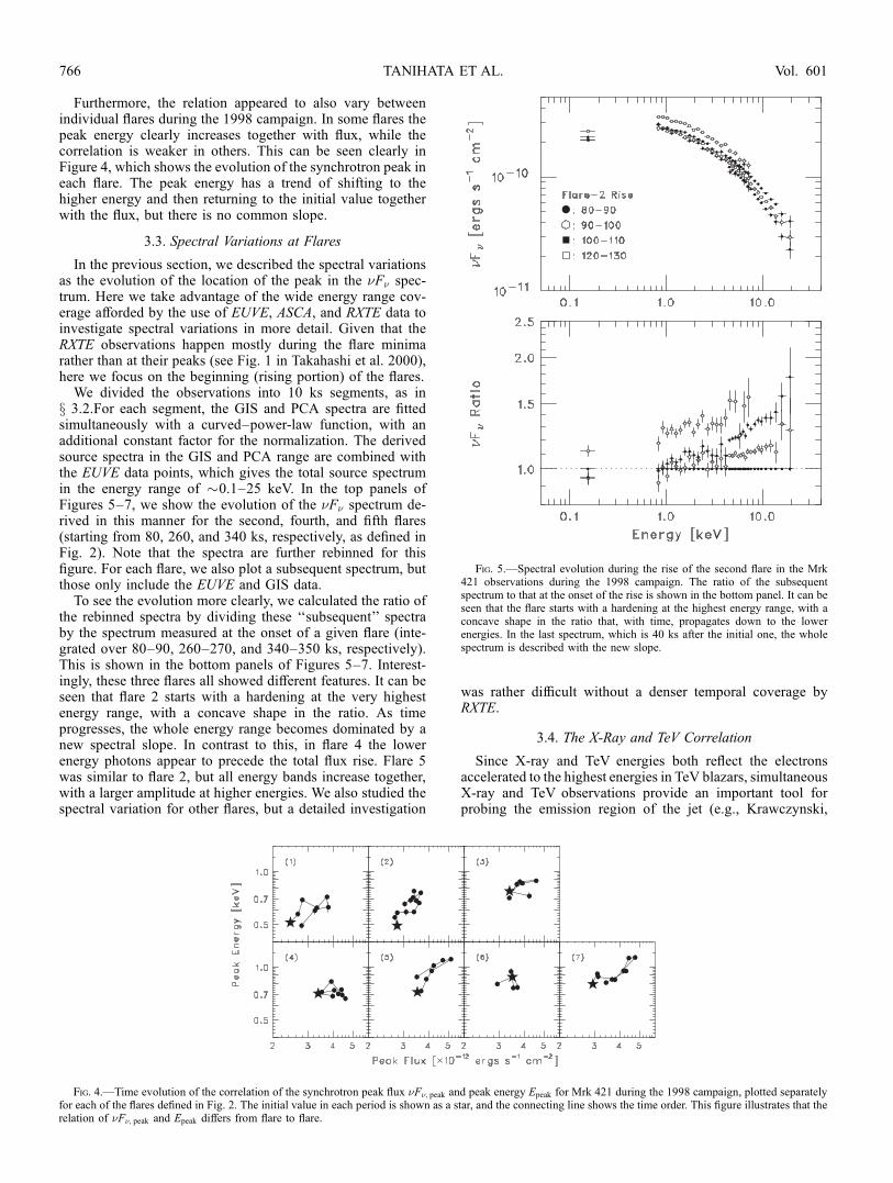
Furthermore, the relation appeared to also vary betweenindividual flares during the 1998 campaign. In some flares thepeak energy clearly increases together with flux, while thecorrelation is weaker in others. This can be seen clearly inFigure 4, which shows the evolution of the synchrotron peak ineach flare. The peak energy has a trend of shifting to thehigher energy and then returning to the initial value togetherwith the flux, but there is no common slope.

3.3. Spectral Variations at Flares

In the previous section, we described the spectral variationsas the evolution of the location of the peak in the �F� spec-trum. Here we take advantage of the wide energy range cov-erage afforded by the use of EUVE, ASCA, and RXTE data toinvestigate spectral variations in more detail. Given that theRXTE observations happen mostly during the flare minimarather than at their peaks (see Fig. 1 in Takahashi et al. 2000),here we focus on the beginning (rising portion) of the flares.

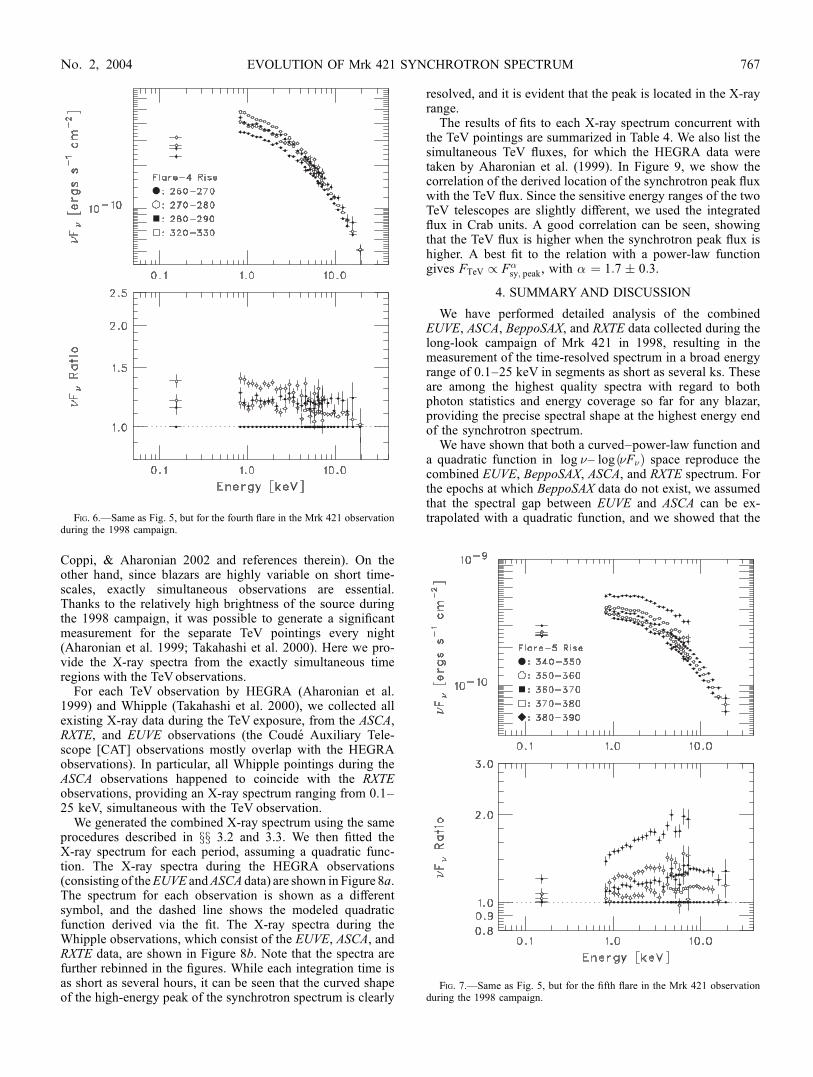
We divided the observations into 10 ks segments, as inx 3.2.For each segment, the GIS and PCA spectra are fittedsimultaneously with a curved–power-law function, with anadditional constant factor for the normalization. The derivedsource spectra in the GIS and PCA range are combined withthe EUVE data points, which gives the total source spectrumin the energy range of �0.1–25 keV. In the top panels ofFigures 5–7, we show the evolution of the �F� spectrum de-rived in this manner for the second, fourth, and fifth flares(starting from 80, 260, and 340 ks, respectively, as defined inFig. 2). Note that the spectra are further rebinned for thisfigure. For each flare, we also plot a subsequent spectrum, butthose only include the EUVE and GIS data.

To see the evolution more clearly, we calculated the ratio ofthe rebinned spectra by dividing these ‘‘subsequent’’ spectraby the spectrum measured at the onset of a given flare (inte-grated over 80–90, 260–270, and 340–350 ks, respectively).This is shown in the bottom panels of Figures 5–7. Interest-ingly, these three flares all showed different features. It can beseen that flare 2 starts with a hardening at the very highestenergy range, with a concave shape in the ratio. As timeprogresses, the whole energy range becomes dominated by anew spectral slope. In contrast to this, in flare 4 the lowerenergy photons appear to precede the total flux rise. Flare 5was similar to flare 2, but all energy bands increase together,with a larger amplitude at higher energies. We also studied thespectral variation for other flares, but a detailed investigation

was rather difficult without a denser temporal coverage byRXTE.

3.4. The X-Ray and TeV Correlation

Since X-ray and TeV energies both reflect the electronsaccelerated to the highest energies in TeV blazars, simultaneousX-ray and TeV observations provide an important tool forprobing the emission region of the jet (e.g., Krawczynski,

Fig. 5.—Spectral evolution during the rise of the second flare in the Mrk421 observations during the 1998 campaign. The ratio of the subsequentspectrum to that at the onset of the rise is shown in the bottom panel. It can beseen that the flare starts with a hardening at the highest energy range, with aconcave shape in the ratio that, with time, propagates down to the lowerenergies. In the last spectrum, which is 40 ks after the initial one, the wholespectrum is described with the new slope.

Fig. 4.—Time evolution of the correlation of the synchrotron peak flux �F�; peak and peak energy Epeak for Mrk 421 during the 1998 campaign, plotted separatelyfor each of the flares defined in Fig. 2. The initial value in each period is shown as a star, and the connecting line shows the time order. This figure illustrates that therelation of �F�; peak and Epeak differs from flare to flare.


Coppi, & Aharonian 2002 and references therein). On theother hand, since blazars are highly variable on short time-scales, exactly simultaneous observations are essential.Thanks to the relatively high brightness of the source duringthe 1998 campaign, it was possible to generate a significantmeasurement for the separate TeV pointings every night(Aharonian et al. 1999; Takahashi et al. 2000). Here we pro-vide the X-ray spectra from the exactly simultaneous timeregions with the TeVobservations.

For each TeV observation by HEGRA (Aharonian et al.1999) and Whipple (Takahashi et al. 2000), we collected allexisting X-ray data during the TeV exposure, from the ASCA,RXTE, and EUVE observations (the Coude Auxiliary Tele-scope [CAT] observations mostly overlap with the HEGRAobservations). In particular, all Whipple pointings during theASCA observations happened to coincide with the RXTEobservations, providing an X-ray spectrum ranging from 0.1–25 keV, simultaneous with the TeV observation.

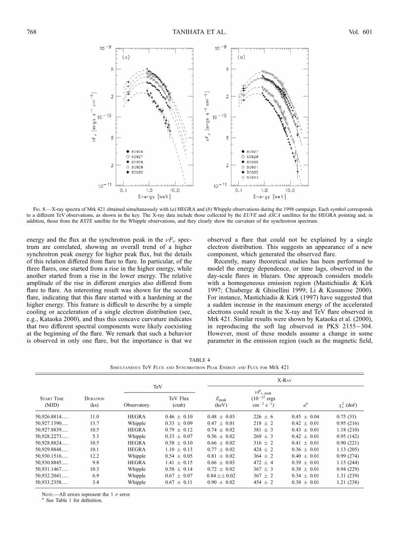
We generated the combined X-ray spectrum using the sameprocedures described in xx 3.2 and 3.3. We then fitted theX-ray spectrum for each period, assuming a quadratic func-tion. The X-ray spectra during the HEGRA observations(consisting of theEUVE andASCA data) are shown in Figure 8a.The spectrum for each observation is shown as a differentsymbol, and the dashed line shows the modeled quadraticfunction derived via the fit. The X-ray spectra during theWhipple observations, which consist of the EUVE, ASCA, andRXTE data, are shown in Figure 8b. Note that the spectra arefurther rebinned in the figures. While each integration time isas short as several hours, it can be seen that the curved shapeof the high-energy peak of the synchrotron spectrum is clearly

resolved, and it is evident that the peak is located in the X-rayrange.

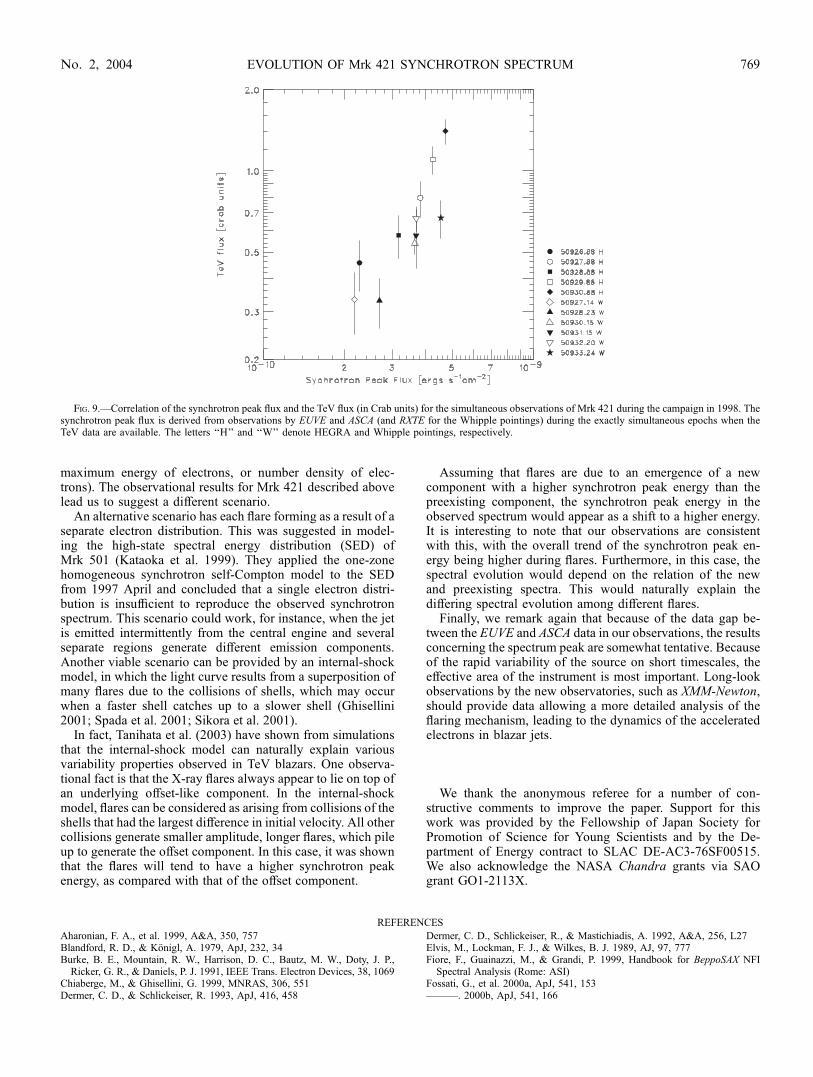
The results of fits to each X-ray spectrum concurrent withthe TeV pointings are summarized in Table 4. We also list thesimultaneous TeV fluxes, for which the HEGRA data weretaken by Aharonian et al. (1999). In Figure 9, we show thecorrelation of the derived location of the synchrotron peak fluxwith the TeV flux. Since the sensitive energy ranges of the twoTeV telescopes are slightly different, we used the integratedflux in Crab units. A good correlation can be seen, showingthat the TeV flux is higher when the synchrotron peak flux ishigher. A best fit to the relation with a power-law functiongives FTeV / F�

sy; peak, with � ¼ 1:7 � 0:3.

4. SUMMARY AND DISCUSSION

We have performed detailed analysis of the combinedEUVE, ASCA, BeppoSAX, and RXTE data collected during thelong-look campaign of Mrk 421 in 1998, resulting in themeasurement of the time-resolved spectrum in a broad energyrange of 0.1–25 keV in segments as short as several ks. Theseare among the highest quality spectra with regard to bothphoton statistics and energy coverage so far for any blazar,providing the precise spectral shape at the highest energy endof the synchrotron spectrum.

We have shown that both a curved–power-law function anda quadratic function in log �– log �F�ð Þ space reproduce thecombined EUVE, BeppoSAX, ASCA, and RXTE spectrum. Forthe epochs at which BeppoSAX data do not exist, we assumedthat the spectral gap between EUVE and ASCA can be ex-trapolated with a quadratic function, and we showed that theFig. 6.—Same as Fig. 5, but for the fourth flare in the Mrk 421 observation

during the 1998 campaign.

Fig. 7.—Same as Fig. 5, but for the fifth flare in the Mrk 421 observationduring the 1998 campaign.


energy and the flux at the synchrotron peak in the �F� spec-trum are correlated, showing an overall trend of a highersynchrotron peak energy for higher peak flux, but the detailsof this relation differed from flare to flare. In particular, of thethree flares, one started from a rise in the higher energy, whileanother started from a rise in the lower energy. The relativeamplitude of the rise in different energies also differed fromflare to flare. An interesting result was shown for the secondflare, indicating that this flare started with a hardening at thehigher energy. This feature is difficult to describe by a simplecooling or acceleration of a single electron distribution (see,e.g., Kataoka 2000), and thus this concave curvature indicatesthat two different spectral components were likely coexistingat the beginning of the flare. We remark that such a behavioris observed in only one flare, but the importance is that we

observed a flare that could not be explained by a singleelectron distribution. This suggests an appearance of a newcomponent, which generated the observed flare.Recently, many theoretical studies has been performed to

model the energy dependence, or time lags, observed in theday-scale flares in blazars. One approach considers modelswith a homogeneous emission region (Mastichiadis & Kirk1997; Chiaberge & Ghisellini 1999; Li & Kusunose 2000).For instance, Mastichiadis & Kirk (1997) have suggested thata sudden increase in the maximum energy of the acceleratedelectrons could result in the X-ray and TeV flare observed inMrk 421. Similar results were shown by Kataoka et al. (2000),in reproducing the soft lag observed in PKS 2155�304.However, most of these models assume a change in someparameter in the emission region (such as the magnetic field,

TABLE 4

Simultaneous TeV Flux and Synchrotron Peak Energy and Flux for Mrk 421

TeV

X-Ray

Start Time

(MJD)

Duration

(ks) Observatory

TeV Flux

(crab)

Epeak

(keV)

�F�; peak

(10�12 ergs

cm�2 s�1) aa �2� (dof )

50,926.8814..... 11.0 HEGRA 0.46 � 0.10 0.48 � 0.03 226 � 6 0.45 � 0.04 0.75 (33)

50,927.1390..... 13.7 Whipple 0.33 � 0.09 0.47 � 0.01 218 � 2 0.42 � 0.01 0.95 (216)

50,927.8839..... 10.5 HEGRA 0.79 � 0.12 0.74 � 0.02 381 � 3 0.43 � 0.01 1.18 (210)

50,928.2273..... 5.3 Whipple 0.33 � 0.07 0.56 � 0.02 269 � 3 0.42 � 0.01 0.95 (142)

50,928.8824..... 10.5 HEGRA 0.58 � 0.10 0.66 � 0.02 316 � 2 0.41 � 0.01 0.90 (221)

50,929.8848..... 10.1 HEGRA 1.10 � 0.13 0.77 � 0.02 424 � 2 0.36 � 0.01 1.13 (205)

50,930.1516..... 12.2 Whipple 0.54 � 0.05 0.81 � 0.02 364 � 2 0.40 � 0.01 0.99 (274)

50,930.8845..... 9.8 HEGRA 1.41 � 0.15 0.66 � 0.03 472 � 4 0.39 � 0.01 1.15 (244)

50,931.1467..... 10.3 Whipple 0.58 � 0.14 0.72 � 0.02 367 � 3 0.38 � 0.01 0.94 (229)

50,932.2041..... 6.9 Whipple 0.67 � 0.07 0.84�� 0.02 367 � 2 0.34 � 0.01 1.31 (239)

50,933.2358..... 3.4 Whipple 0.67 � 0.11 0.90 � 0.02 454 � 2 0.38 � 0.01 1.21 (238)

Note.—All errors represent the 1 � error.a See Table 1 for definition.

Fig. 8.—X-ray spectra of Mrk 421 obtained simultaneously with (a) HEGRA and (b) Whipple observations during the 1998 campaign. Each symbol correspondsto a different TeV observations, as shown in the key. The X-ray data include those collected by the EUVE and ASCA satellites for the HEGRA pointing and, inaddition, those from the RXTE satellite for the Whipple observations, and they clearly show the curvature of the synchrotron spectrum.


maximum energy of electrons, or number density of elec-trons). The observational results for Mrk 421 described abovelead us to suggest a different scenario.

An alternative scenario has each flare forming as a result of aseparate electron distribution. This was suggested in model-ing the high-state spectral energy distribution (SED) ofMrk 501 (Kataoka et al. 1999). They applied the one-zonehomogeneous synchrotron self-Compton model to the SEDfrom 1997 April and concluded that a single electron distri-bution is insufficient to reproduce the observed synchrotronspectrum. This scenario could work, for instance, when the jetis emitted intermittently from the central engine and severalseparate regions generate different emission components.Another viable scenario can be provided by an internal-shockmodel, in which the light curve results from a superposition ofmany flares due to the collisions of shells, which may occurwhen a faster shell catches up to a slower shell (Ghisellini2001; Spada et al. 2001; Sikora et al. 2001).

In fact, Tanihata et al. (2003) have shown from simulationsthat the internal-shock model can naturally explain variousvariability properties observed in TeV blazars. One observa-tional fact is that the X-ray flares always appear to lie on top ofan underlying offset-like component. In the internal-shockmodel, flares can be considered as arising from collisions of theshells that had the largest difference in initial velocity. All othercollisions generate smaller amplitude, longer flares, which pileup to generate the offset component. In this case, it was shownthat the flares will tend to have a higher synchrotron peakenergy, as compared with that of the offset component.

Assuming that flares are due to an emergence of a newcomponent with a higher synchrotron peak energy than thepreexisting component, the synchrotron peak energy in theobserved spectrum would appear as a shift to a higher energy.It is interesting to note that our observations are consistentwith this, with the overall trend of the synchrotron peak en-ergy being higher during flares. Furthermore, in this case, thespectral evolution would depend on the relation of the newand preexisting spectra. This would naturally explain thediffering spectral evolution among different flares.

Finally, we remark again that because of the data gap be-tween the EUVE and ASCA data in our observations, the resultsconcerning the spectrum peak are somewhat tentative. Becauseof the rapid variability of the source on short timescales, theeffective area of the instrument is most important. Long-lookobservations by the new observatories, such as XMM-Newton,should provide data allowing a more detailed analysis of theflaring mechanism, leading to the dynamics of the acceleratedelectrons in blazar jets.

We thank the anonymous referee for a number of con-structive comments to improve the paper. Support for thiswork was provided by the Fellowship of Japan Society forPromotion of Science for Young Scientists and by the De-partment of Energy contract to SLAC DE-AC3-76SF00515.We also acknowledge the NASA Chandra grants via SAOgrant GO1-2113X.

REFERENCES

Aharonian, F. A., et al. 1999, A&A, 350, 757Blandford, R. D., & Konigl, A. 1979, ApJ, 232, 34Burke, B. E., Mountain, R. W., Harrison, D. C., Bautz, M. W., Doty, J. P.,Ricker, G. R., & Daniels, P. J. 1991, IEEE Trans. Electron Devices, 38, 1069

Chiaberge, M., & Ghisellini, G. 1999, MNRAS, 306, 551Dermer, C. D., & Schlickeiser, R. 1993, ApJ, 416, 458

Dermer, C. D., Schlickeiser, R., & Mastichiadis, A. 1992, A&A, 256, L27Elvis, M., Lockman, F. J., & Wilkes, B. J. 1989, AJ, 97, 777Fiore, F., Guainazzi, M., & Grandi, P. 1999, Handbook for BeppoSAX NFISpectral Analysis (Rome: ASI)

Fossati, G., et al. 2000a, ApJ, 541, 153———. 2000b, ApJ, 541, 166

Fig. 9.—Correlation of the synchrotron peak flux and the TeV flux (in Crab units) for the simultaneous observations of Mrk 421 during the campaign in 1998. Thesynchrotron peak flux is derived from observations by EUVE and ASCA (and RXTE for the Whipple pointings) during the exactly simultaneous epochs when theTeV data are available. The letters ‘‘H’’ and ‘‘W’’ denote HEGRA and Whipple pointings, respectively.


Gaidos, J. A., et al. 1996, Nature, 383, 319Ghisellini, G. 2001, in ASP Conf. Ser. 227, Blazar Demographics and Physics,ed. P. Padovani & C. M. Urry (San Francisco: ASP), 85

Ghisellini, G., & Maraschi, L. 1989, ApJ, 340, 181Jones, T. W., O’Dell, S. L., & Stein, W. A. 1974, ApJ, 188, 353Kataoka, J. 2000, Ph.D. thesis, Univ. TokyoKataoka, J., Takahashi, T., Makino, F., Madejski, G. M., Tashiro, M., Urry,C. M., & Kubo, H. 2000, ApJ, 528, 243

Kataoka, J., et al. 1999, ApJ, 514, 138———. 2001, ApJ, 560, 659Krawczynski, H., Coppi, P. S., & Aharonian, F. 2002, MNRAS, 336, 721Li, H., & Kusunose, M. 2000, ApJ, 536, 729Lin, Y. C., et al. 1992, ApJ, 401, L61Macomb, D. J., et al. 1995, ApJ, 449, L99Maraschi, L., et al. 1999, ApJ, 526, L81Marshall, H. L., Fruscione, A., & Carone, T. E. 1995, ApJ, 439, 90Mastichiadis, A., & Kirk, J. G. 1997, A&A, 320, 19Ohashi, T., et al. 1996, PASJ, 48, 157

Petry, D., et al. 1996, A&A, 311, L13Pian, E., et al. 1998, ApJ, 492, L17Piron, F., et al. 2001, A&A, 374, 895Punch, M., et al. 1992, Nature, 358, 477Sikora, M., Begelman, M. C., & Rees, M. J. 1994, ApJ, 421, 153Sikora, M., Byazejowski, M., Begelman, M. C., & Moderski, R. 2001, ApJ,554, 1 (erratum 561, 1154)

Spada, M., Ghisellini, G., Lazzati, D., & Celotti, A. 2001, MNRAS, 325, 1559Takahashi, T., et al. 2000, ApJ, 542, L105Tanihata, C., Takahashi, T., Kataoka, J., & Madejski, G. M. 2003, ApJ,584, 153

Tanihata, C., Urry, C. M., Takahashi, T., Kataoka, J., Wagner, S. J., Madejski,G. M., Tashiro, M., & Kouda, M. 2001, ApJ, 563, 569

Tavecchio, F., et al. 2001, ApJ, 554, 725Urry, C. M., & Padovani, P. 1995, PASP, 107, 803Yamashita, A., et al. 1997, IEEE Trans Nucl. Sci., 44, 847Yaqoob, T., et al. 2000, ASCA GOF Calibration Memo ASCA-CAL-00-06-01,ver. 1.0 (Greenbelt: NASA)

TANIHATA ET AL.770

Documents

EVOLUTION OF THE SYNCHROTRON SPECTRUM IN