Embed Size (px)
Citation preview

Evaluation of road service levels through the software GLS2004.xls
Pasquale Colonna Dept. of Highways and Transportation - Polytechnic University of Bari, Italy
Manuela Maizza Dept. of Highways and Transportation - Polytechnic University of Bari, Italy
Simona d’Amoja Dept. of Highways and Transportation - Polytechnic University of Bari, Italy
Vittorio Ranieri Dept. of Highways and Transportation - Polytechnic University of Bari, Italy
Synopsis In the choices regarding roads, there is more and more the necessity to specify parameters which define the road service quality considering all points of view: user, owner/manager and external community. As a consequence, we defined a procedure based on a model that, through the evaluation of 54 significant elements, defined “indicators” of the road service, succeeded in associating to every road section a single synthetic parameter, expression of the quality of road service offered, called Global Level of Service – GLS. These procedure takes account of all the parameters involved with the right weight. The Global Level of Service, with its structure, is a very versatile tool, that, with the aid of Geographical Information System, enables to reach the following aims: in operation phase, it enables to start the procedures of planned maintenance and management,
identifying the priority of operations; in design phase, the GLS method with GIS use becomes a necessary tool to make choices, helping in
identifying the best design option; in driving phase, it gives the users a tool giving informations about route, after having decided an origin,
a destination and the time of departure, according to priority scales which favour different indicators according to personal needs (travel time, comfort, landscape, etc….).
The single indicators’ algorithms and the GLS algorithm have been implemented in a software called GLS2004.xls which allows the user a fast input of the indicator’s values during survey phase and an easy execution of the operations required by the procedure. So, GLS2004.xls was created in order to computerize the procedure able to determine the GLS of each road section considered as a part of the road network of our interest. This software was subsequently applied to a road network in the northern part of Bari district having the towns of Bisceglie, Molfetta, Terlizzi, Ruvo and Corato as vertices. The network was classified from a functional point of view and it was created a Geographical Information System which enabled to analyse results and to value the efficiency of the proposed methodology.

Evaluation of road service levels through the software GLS2004.xls
During these years the concept of road service quality changed according to the evolution of needs of the subjects interested in the presence of a road on an area. Until the 60’s, roads were considered an exclusive prerogative of the owners and of the managers of facilities. Beginning from the 60’s, in connection with the increase of vehicular traffic, it became clear that for a good management of a road, it is necessary to consider the quality of the service offered by a road; so it was introduced the concept of road capacity and other considerations based on vehicular density; later, it wasn’t possible any longer to accept a level of service based only on vehicular density, but it was necessary to widen the horizon considering all the parameters involved from all points of view: user, owner/manager and external community [1, 2, 3, 4]. Besides, the growing sensitization of public opinion about road safety, comfort and environment made the users perceive the road serviceability as a right, continuously comparing between perceived and demanded (desired) quality of service. In the choices regarding roads, there is more and more the necessity to specify parameters which define the road service quality considering all points of view: user, owner/manager and external community. So, it was established a criterion in order to define a new “Global” Level of Service, able to take account of all the parameters involved with the right weight. As a consequence, we defined a procedure based on a model that, through the evaluation of 54 significant elements, defined “indicators” of the road service, succeeded in associating to every road section a single synthetic parameter, expression of the quality of road service offered, called Global Level of Service – GLS [5, 6]. The Global Level of Service, with its structure, is a very versatile tool, that, with the aid of Geographical Information System, enables to reach the following aims: in operation phase, it enables to start the procedures of planned maintenance and management,
identifying the priority of operations, considering the function of the road in the whole network and in the context of socio-economical trends of development fixed by each Administration; in this way, the Public Administrations will be able to verify and to compare the different efficiency levels of management offices.
in design phase, the GLS method with GIS use becomes a necessary tool to make choices, helping in identifying the best design option; in fact, in new infrastructures’ designs, the direct comparison among GLS values of different design choices can be very important in the choice;
in driving phase, it gives the users a tool able to give informations about route, after having decided an origin, a destination and the time of departure, according to priority scales which favour different indicators according to personal needs (travel time, comfort, landscape, etc….).
The old administrative road classification required an in-depth study about functional road classification, aiming at defining a classification which characterizes primary, principal, secondary and local roads according to their function in the network and to the movement offered. Then, the optimal maximum values for these kinds of roads have been defined and it was possible, in operating phase, to relate absolute GLS values with these optimal values for each kind of road. In this way it was obtained the GLS “efficiency” value that enables to estimate road service quality apart from its function, expressing better the user’s expectation. Regarding the indicators, some of them were modified, some were eliminated and some were added according to the new developments about road geometry and to the introduction of new “Functional and geometric standards for road construction” (Decree 5th November 2001) [7]. In order to make the method’s application easier, the single indicators algorithms and the GLS algorithm were implemented in a software called GLS2004.xls which allows the user a fast input of indicator’s values during survey phase and an easy execution of the operations required by the procedure. So, GLS2004.xls was created in order to computerize the procedure able to determine the GLS of each road section considered as a part of the road network of our interest. In operating phase of this methodology the software was applied to a road network in the northern part of Bari district having the towns of Bisceglie, Molfetta, Terlizzi, Ruvo and Corato as vertices. The network was classified from a functional point of view and it was created a Geographical Information System which enabled to analyse results and to value the efficiency of the proposed methodology. Through this method it’s simple for an operational agency to start planned management activities, identifying the road sections requiring an urgent intervention, according to different GLS values which characterize the section and defining in this way an operational priority scale. Regarding the user, he can start a journey knowing in advance the service quality offered by road network and he can choose, according to different parameters and to his own needs, a route, deciding to reduce trip time or preferring the environmental trip aspect.

GLOBAL LEVEL OF SERVICE (GLS): THE METHODOLOGY The methodology of determination of GLS presents many using opportunities and it can be developed with other control techniques and with the optimization of road plans. The procedure is based upon an elementary concept: quality of road service is the sum of the valuations that we can give to a finished number of elementary qualities (performance indicators), each of which has a different importance in the overall assessment. Elementary qualities have been called road service “indicators”. Global Level of Service’s aim is taking account not only of the owner point of view (as happened until the 60’s), but also of the user and of the environmental points of view. As a consequence, an appropriate evaluation has to be done in order to assess the importance of a single parameter for the specific point of view. A way of evaluation has to be associated with each indicator, by which it is possible to assign a numerical value to the examined road section, depending on its contribution to road serviceability. Therefore, we identified the way of valuation and the survey methods in an univocal manner, for each indicator. The introduced indicators are characterized by fast and cheap surveys, and have to represent phenomena in an objective way. Being the number of indicators too high (54), it was necessary to gather them according to homogeneity criterion; so, we defined 6 homogeneous groups [8, 9]: 1. Safety (S);
a. Geometric characteristics (G) aB1B. horizontal alignment characteristics – (GL); aB2B. geometrical section characteristics – (GS);
b. Structural characteristics – (St); c. Functional characteristics – (F); d. External interferences – (E);
2. Travel time - (T); 3. Services – (R); 4. Environment – (A); 5. Traffic condition (Q); 6. Comfort – (C). The operating methodology adopted in this research project was the following: 1. state of art of the performance indicators in Italy and in the U.S.A; 2. road reclassification and application of GLS “efficiency” concept; 3. reorganization and rationalization of the indicators; 4. assignment of new evaluations criteria to the indicators and new survey methods; 5. evaluation of operational and maintenance costs of facilities; 6. methodology implementation through the software GLS2004.xls; 7. creation of Geographical Information System and analysis of results. In the appendix you can find the logical scheme for GLS evaluation (see Figure 10). INDICATORS The methodology for GLS assessment includes different indicators requiring different methods for judgements attribution. Some indicators are intrinsically objectively measurable, as, for evaluating, it’s possible to apply very simple mathematical expressions, coming from road design standards. Indicators belonging to this category are called “intrinsically assessable objectively indicators”. For each of these indicators, appropriate survey forms were created. Indicator’s name, belonging group, meaning, mathematical expression, possible corrective coefficient for divided or undivided carriageways, score interval (value), measurement methods and tools, score scale, variability, monitoring frequency and finally operators able to measure the indicator, are represented in these survey forms [10]. The corrective coefficient is multiplied by the indicator’s value when the road (from the point of view of that indicator) is in disadvantage situation; sometimes it happens for the divided highways and sometimes for the undivided highways. Therefore the coefficient has a restrictive function, always included between 0 and 1. In this way the final GLS value is influenced in a right way in advance, as the GLS value of a road, disadvantaged by its carriageway, will never be equal to the maximum value (that is: 1). In a first stage of research, in evaluating indicators’ score, we used subjective evaluations made by surveyors who assigned a qualitative assessment to the indicators (such as: excellent, good, …, poor).

In order to improve such a kind of subjective evaluation, we used an objective evaluation not influenced by surveyor’s opinion [10]. For each of the indicators called “intrinsically not assessable objectively indicators”, a special survey/evaluation form was created; these forms contain some questions by which it is possible to get an evaluation of the indicator as much as possible objective, taking as a starting point the “Guide lines for road safety analysis”, by the Italian Ministry of Transport and Infrastructures [11]. All these forms should be filled for each homogeneous road section. Typical examples of these forms are represented in Tables 1, 2, 3. In the appendix you can find the list of indicators (see Table 7).
Tab 1: Survey Form – A01 “Acoustic pollution” GROUP ENVIRONMENT INDICATOR A01 MEANING Acoustic pollution SECTION OF APPLICABILITY Normal, Viaduct, Tunnel
MATHEMATICAL EXPRESSION
dB(A) T0
dtp
(t)p
1t-
2t
1log10Leq
20
2A = T(A),
⎥⎥⎥
⎦
⎤
⎢⎢⎢
⎣
⎡
∫
LeqBAB: equivalent continuous level of weighed sound pressure “A” considered in a slot starting at instant tB1B and ending at instant tB2B; pBAB(t): instant value of weighed sound pressure “A” of sound signal measured in Pascal (Pa); pB0B = 20 µ Pa is the reference sound pressure. If Leq < D and Leq < N A01 = 1 ⇒In the other cases:
A01 = nLeqN
LeqD
n
i
ii /21
∑=
⎥⎥⎥⎥
⎦
⎤
⎢⎢⎢⎢
⎣
⎡ +, where:
n = survey sections number for which Leq value is calculated (Equivalent Level of weighed sound pressure “A”); LeqBiB = Equivalent Level of weighed sound pressure “A” measured every 3 km along an homogeneous section; D = day value of reference Leq; N = night value of reference Leq.
INTERVAL 0 - 1
MEASUREMENT METHOD Continuous along road section, related to a medium weekly day and night values measured to receptors every 3 km along section.
MEASUREMENT TOOL Central of surveying INDICATOR VARIABILITY Variable during the time MONITORING FREQUENCE Annual (one survey has to last one week at least) QUALIFIED PERSONNEL Technicians

Tab 2: Survey Form – R02 “Frequency of rest areas”
GROUP SERVICES INDICATOR R02 MEANING Frequency of rest areas SECTION OF APPLICABILITY Normal
MATHEMATICAL EXPRESSION
R02 = v · mx j∑
, with:
v = value attributed to indicator according score table.
xBj = B
npi∑
, j = 1, 2,….m, i = 1, 2,….nB
m = number of rest areas located in the section including the whole homogeneous section plus 100 km (maximum distance in score table) preceding the beginning of homogeneous section and 100 km subsequent the end of the section; n = number of questions contained on attached form; PBi B= value attributed to indicator as specified in the following table. NB2: If the rest area is absent because not provided for the typology of road, the value attributed to indicator is “irrelevant”.
INTERVAL 0-1 MEASUREMENT METHOD Continuous along road section MEASUREMENT TOOL Telecamera
vBiB 1 Up to one rest area every 30 km 0,75 Up to one rest area every 50 km 0,5 Up to one rest area every 75 km 0,25 Up to one rest area every 100 km
0 One rest area along a distance superior to 100 km or no rest areas
i irrelevant (weights equal to 0) PBiB See attached form
1 Yes 0,5 Uncertain
SCORE
0 NO INDICATOR VARIABILITY Constant during the time MONITORING FREQUENCE Annual QUALIFIED PERSONNEL Roadmen
Tab 3: Questions Form – R02 R02
1 Rest areas respect standard dimensions. Yes Uncertain NO
2 Vehicles safety is guaranteed in acceleration and deceleration manoeuvring.
Yes Uncertain NO
3
Acceleration/deceleration lanes are located at a distance from junction not shorter than stopping sight distance.
Yes Uncertain NO
4 Acceleration/deceleration lanes are located at a distance from short ray horizontal curves not shorter than stopping sight distance.
Yes Uncertain NO
5 Acceleration/deceleration lanes are located at a distance from the tops of convex altimetrical connection not shorter than stopping sight distance.
Yes Uncertain NO
6 The main flow is enough visible to vehicles leaving rest area, and vice versa.
Yes Uncertain NO
7 The kind of rest (short or long term) is fit for the functional category of road.
Yes Uncertain NO
8 The maintenance conditions of services in rest area are satisfactory. Yes Uncertain NO
ROAD FUNCTIONAL CLASSIFICATION In order to go over the old road administrative classification, we studied a new functional classification comparing different classifications proposed by different authors [7, 12, 13, 14, 15]. This functional classification establishes a hierarchy in road network defined on the basis of movement served by roads, or road function in the network. Therefore we have: • PRIMARY ROAD (transit, flowing function; long distance travel); • PRINCIPAL ROAD (distribution from primary to secondary and sometimes to local network; medium
distance travel); • SECONDARY ROAD (penetration into local network; reduced distance travel); • LOCAL ROAD (access function; short distance travel).
Tab 4: Comparison between functional classifications by different authors Ministerial standards FHWA HCM 2000 LAMM
Primary network A
Principal network
Arterials (rural/urban) Freeways
B
Secondary network Collectors (rural/urban)
Highways (multilane, two-
lane) C
Local network Local (rural/urban) Urban streets D
E For each kind of road (“kind” identified according to functional classification), maximum GLS values are defined according to road importance; so a Primary road will be characterized by maximum GLS value equal to 1, a Principal road will be characterized by maximum GLS value equal to 0,9, a Secondary road by a value equal to 0,8 and a Local one by a value equal to 0,5, as specified in Table 5.
Tab 5: Functional Classification and GLSBmaxBB
Type of road GLSBmaxB
Primary road (transit, flowing function) 1 Principal road (distribution function) 0,9 Secondary road (penetration function) 0,8 Local road (access function) 0,5
After the assessment of the numerical GLS value of a surveyed road, we can determine the so called GLS “efficiency” (hBGLSB) of the road under examination: hBGLSB = GLS/GLSBmaxB. It is the ratio between the estimated value of GLS and the maximum GLS value for that kind of road. Comparing efficiency values of different roads, it will be possible to assert that a road has a better quality of service than another, apart from their function. The introduction of this concept is useful, since the simple comparison between numerical values of GLS could let someone believe that (e.g.) a Principal road characterized by GLS value equal to 0,85 has a quality of service worse than a Primary road characterized by GLS value equal to 0,90. On the contrary, if we consider that the maximum GLS value of Primary roads is 1 and the maximum GLS value of Principal roads is 0,90, the efficiency will be: • GLS/GLSBmaxB = 0,85/0,90 = 0,94 for the Principal road; • GLS/GLSBmaxB = 0,9/1,0 = 0,90 for the Primary road. So the efficiency of the principal road is better and the Principal road is characterized by a global level of service better than the primary road, apart from its function [16, 17]. We also defined an efficiency scale classified by letters: A, B, C, D, E, F, G. Depending on road function, its Global Level of Service can range from a maximum theoretical value (corresponding to the presence of all the possible services characterized by maximum efficiency, from every point of view), to a minimum acceptable value (able to guarantee at least the essential functionality). Between these extremes it’s possible to look for some limit values, in order to identify appropriate intervals, by which it is possible to classify shortly the Quality of Service offered by the road infrastructure, on the basis

of its function. Therefore, for each kind of road, an efficiency scale was created and represented in the following way.
Tab 6: GLS efficiency scale hBGLSPB
kP (*) = GLS efficiency
Level A 0.85 < hBGLSB < 1,00 Level B 0.67 < hBGLSB < 0.85 Level C 0.50 < hBGLSB < 0.67 Level D 0.30 < hBGLSB < 0.50 Level E 0.20 < hBGLSB < 0.30 Level F 0.13 < hBGLSB < 0.20 Level G hBGLSB < 0.13
(*) K indicates kind of road (functional classification) EVALUATION OF OPERATIONAL AND MAINTENANCE COSTS OF FACILITIES Subsequently we dealt with an evaluation study of the operational and maintenance costs of facilities that a public authority should bear, considering all the instrumentation necessary for an efficient management, starting from the hypothesis of implementing a software related to the monitoring of facilities. Thus, it was necessary to make considerations about the costs in case of purchase or in case of hire of the instrumentation necessary for monitoring [18]. This study is very important for every authority intending to acquire all the instruments necessary to a good territorial management. So, the fist step was to determine the yearly survey costs due to the use of the most common instruments (GPS, Grip tester, laser profilometer and traffic counter) in three cases: in case of an amortization in 5 years of the purchase costs of instrumentation, in case of purchase without any amortization and in case of hire. From a global analysis of the costs it appeared that, after the first 5 years of administration, the purchase costs of instrumentation, combined in 15 years of monitoring, are lower than the hire costs. From a more specific analysis related to the single instrument, it’s possible to deduce that it’s more favourable the hire for the use of the GPS and of the grip tester, while for the use of the profilometer and of the counters it’s more favourable the purchase. This solution (called mixed) was represented in the following picture with the expected costs in the cases of only purchase or only hire of the complete instrumentation. Finally we determined the whole cost of the implementation of software, covering the production and post-production management costs. Global management costs, by year, are represented in Figure 1 for a 100 km road network. The future developments of research could consider also the costs not considered directly in the present conceiving of the Global Level Service (and in the related algorithm).
€ 150.286€ 166.764
€ 202.022€ 218.499
€ 234.977€ 251.455
€ 267.932
€ 303.190€ 319.668
€ 336.146€ 352.623
€ 369.101
€ 117.331€ 100.853
€ 133.808
€ 0
€ 100.000
€ 200.000
€ 300.000
€ 400.000
€ 500.000
€ 600.000
€ 700.000
0 1 2 3 4 5 6 7 8 9 10 11 12 13 14 15 16ANNI
EUR
O
MISTOACQUISTO SENZA AMMORTAMENTONOLEGGIO
SOLUZIONE MISTA:- Acquisto di profilometro e contatori;- Noleggio di griptester e GPS AQ
Figure 1 : Comparison between global costs in case of only purchase of complete instrumentation
(magenta), only hire (yellow) or mixed solution (blue) for a 100 km road network

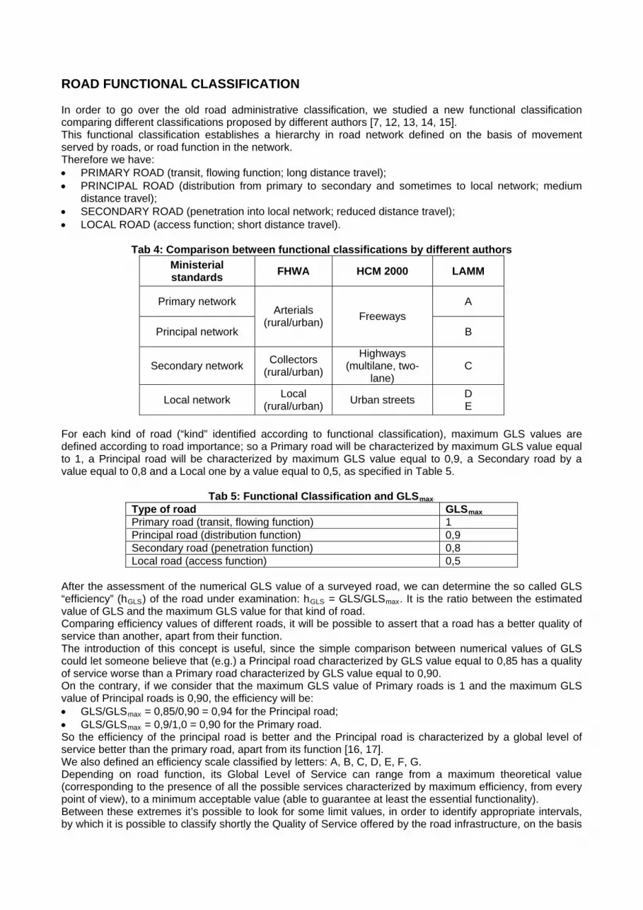
GLS2004 SOFTWARE: PECULIARITIES AND IMPLEMENTATION TO A ROAD NETWORK In operating phase, the single indicators’ algorithms and the GLS algorithm were implemented in a software called GLS2004.xls which allows the user a fast input of the indicator’s values during survey phase and an easy execution of the operations required by the procedure. This application with GIS representation were tested in a PhD Thesis [18]. The original software version (LSA2000.xls) was constituted by three principal electronic sheets called: “Input Table”, “GLS” and “Final Table”. The algorithms of 54 indicators were implemented separately creating a single electronic sheet for each indicator. So, the surveyor will insert the indicator’s data in the relative electronic sheet [figure 00]. The values resulting from these electronic sheets are linked with Input Table; after having inserted input data, the second sheet, called “GLS”, enables us to calculate the final GLS values automatically. For each group of indicators the software provides the values related to different points of view (user, owner and environment) and to the global one. Besides, it provides the values of the indicators related to general parameters S, T, R, A, Q, C, and the GLS value of the whole road section, for each point of view. The Final Table is a sheet structured similarly to Input Table, in which a single road section corresponds to each line, but the columns associated to the section show the following values, in the order: • name of section and kind of section, • length of section in metres, • holding company, • total GLS of section, • (IBxuB)t, (IBxpB)t, (IBxeB)t = values of the indexes for the whole section, related respectively to user, owner and
environment points of view, • values related, in the order, to geometrical characteristics GL and GS, structural characteristics St,
functional characteristics F, external interferences E; • values related, in the order, to general parameters Safety S, Travel Time T, Services R, Environment A,
Traffic Conditions Q, Comfort C. The data processing in the algorithm and the consequent appearance of the results directly in the
Final Table occur clicking on the macro Transport, placed on the left superior corner of the sheet Input Table, after having put a capital X in the first column on the line related to the road section for which we want to know the values, and after having clicked on the button related to the kind of section we are considering (Normal, Viaduct or Tunnel).
After having obtained the GLS values in the Final Table, we passed to the building of the calculation sheet “Efficiency”. In this sheet we implemented a classification of the network under examination, according to the road functions in the network itself and to the served movement. Then we calculated the GLS “efficiency” for all the road sections dividing the global values obtained in the Final Table by 1, 0,9, 0,8 or 0,5, that are the maximum ideal values fixed respectively for primary, principal, secondary and local roads.
The “Final” and “Efficiency” Tables are essential tables, since they are necessary for the subsequent creation of the Geographic Information System.
In the end of the paragraph we show the screen images related to the calculation sheets of the indicator GS04, to the Input Table sheet and to the GLS sheet ( see Figures 2, 3, 4).
This methodology was tested on a road network having Bisceglie, Molfetta, Terlizzi, Ruvo and Corato municipalities as vertices. Inside this polygon we surveyed different kinds of roads: highways (primary roads), statal roads (principal roads), provincial roads, municipal roads (secondary roads) and local roads, for a total length of 108,15 Km.
This methodology could be developed by creating an interfacial linking software able to link the “Efficiency Table” with one or more Geographical Information Systems, so giving maps in real time, after the input of data (that could be obtained by the Internet). This development would let our methodology combine with other control techniques and with the optimization of road plans.
In this study we dwelled upon the implementation of a Geographical Information System able to give useful informations about the area under examination for all road operators.
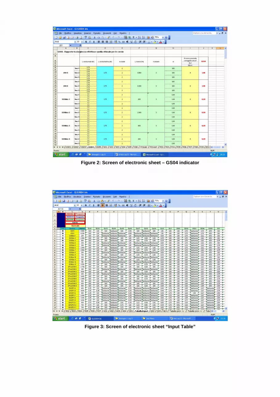
Figure 2: Screen of electronic sheet – GS04 indicator
Figure 3: Screen of electronic sheet “Input Table”
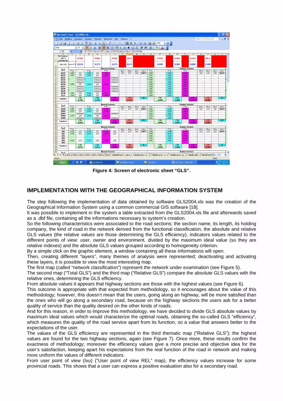
Figure 4: Screen of electronic sheet “GLS”.
IMPLEMENTATION WITH THE GEOGRAPHICAL INFORMATION SYSTEM The step following the implementation of data obtained by software GLS2004.xls was the creation of the Geographical Information System using a common commercial GIS software [18]. It was possible to implement in the system a table extracted from the GLS2004.xls file and afterwards saved as a .dbf file, containing all the informations necessary to system’s creation. So the following characteristics were associated to the road sections: the section name, its length, its holding company, the kind of road in the network derived from the functional classification, the absolute and relative GLS values (the relative values are those determining the GLS efficiency), indicators values related to the different points of view: user, owner and environment, divided by the maximum ideal value (so they are relative indexes) and the absolute GLS values grouped according to homogeneity criterion. By a simple click on the graphic element, a window containing all these informations will open. Then, creating different “layers”, many themes of analysis were represented; deactivating and activating these layers, it is possible to view the most interesting map. The first map (called “network classification”) represent the network under examination (see Figure 5). The second map (“Total GLS”) and the third map (“Relative GLS”) compare the absolute GLS values with the relative ones, determining the GLS efficiency. From absolute values it appears that highway sections are those with the highest values (see Figure 6). This outcome is appropriate with that expected from methodology, so it encourages about the value of this methodology; however, this doesn’t mean that the users, going along an highway, will be more satisfied than the ones who will go along a secondary road, because on the highway sections the users ask for a better quality of service than the quality desired on the other kinds of roads. And for this reason, in order to improve this methodology, we have decided to divide GLS absolute values by maximum ideal values which would characterize the optimal roads, obtaining the so-called GLS “efficiency”, which measures the quality of the road service apart from its function, so a value that answers better to the expectations of the user. The values of the GLS efficiency are represented in the third thematic map (“Relative GLS”); the highest values are found for the two highway sections, again (see Figure 7). Once more, these results confirm the exactness of methodology; moreover the efficiency values give a more precise and objective idea for the user’s satisfaction, keeping apart his expectations from the real function of the road in network and making more uniform the values of different indicators. From user point of view (Ixu) (“User point of view REL” map), the efficiency values increase for some provincial roads. This shows that a user can express a positive evaluation also for a secondary road.

Regarding Total Safety indicator ( “Total Safety” map), the provincial road SP23, linking Corato and Molfetta municipalities, (and the two local sections of former statal road SS16 leading to municipalities) are characterized by the lowest values (see Figures 8, 9). Regarding Environmental Indicator ( “Total Environment” map) the highest values are obtained for some secondary roads, the middle values for the primary roads and for some secondary roads, and the lowest values for the local roads. From this analysis it’s easy for the holding company to identify the road sections needing an intervention that will be more or less urgent according to the GLS values characterizing the section and to fix the priority of intervention. So it’s possible to start up procedures of programmed management and maintenance through which an employee of a remote office assigned to road maintenance, after having received a work order, is able to identify all the informations regarding the object of intervention through the GIS. Consequently he can transmit them to the operators and immediately carry in the system the changes made with the intervention. In such a way it’s possible to improve the automation of the daily operations of the working teams and meanwhile to make the up-to-date informations available for all the offices involved. Besides, the user can set out on a journey knowing in advance the quality of the service of the road network and can choose the route according to his needs preferring sometimes the minimization of the journey duration, sometimes the environmental and landscape aspect. On the other hand, thanks to the very relevant services offered by the WebGIS, it’s possible, through the Internet, to obtain the geographical informations in different forms such as maps, data, images, analysis, etc... and so to acquire on-line informations in real time. The new technologies are heading towards complex systems able to send the data obtained from a sensor, set on a vehicle, directly to the storage system of a software having an interfacial link with one or more Geographical Information Systems on the Web, so giving the maps in real time and setting at zero the survey time on site.
Figure 5: Screen of “Network Classification” thematic map
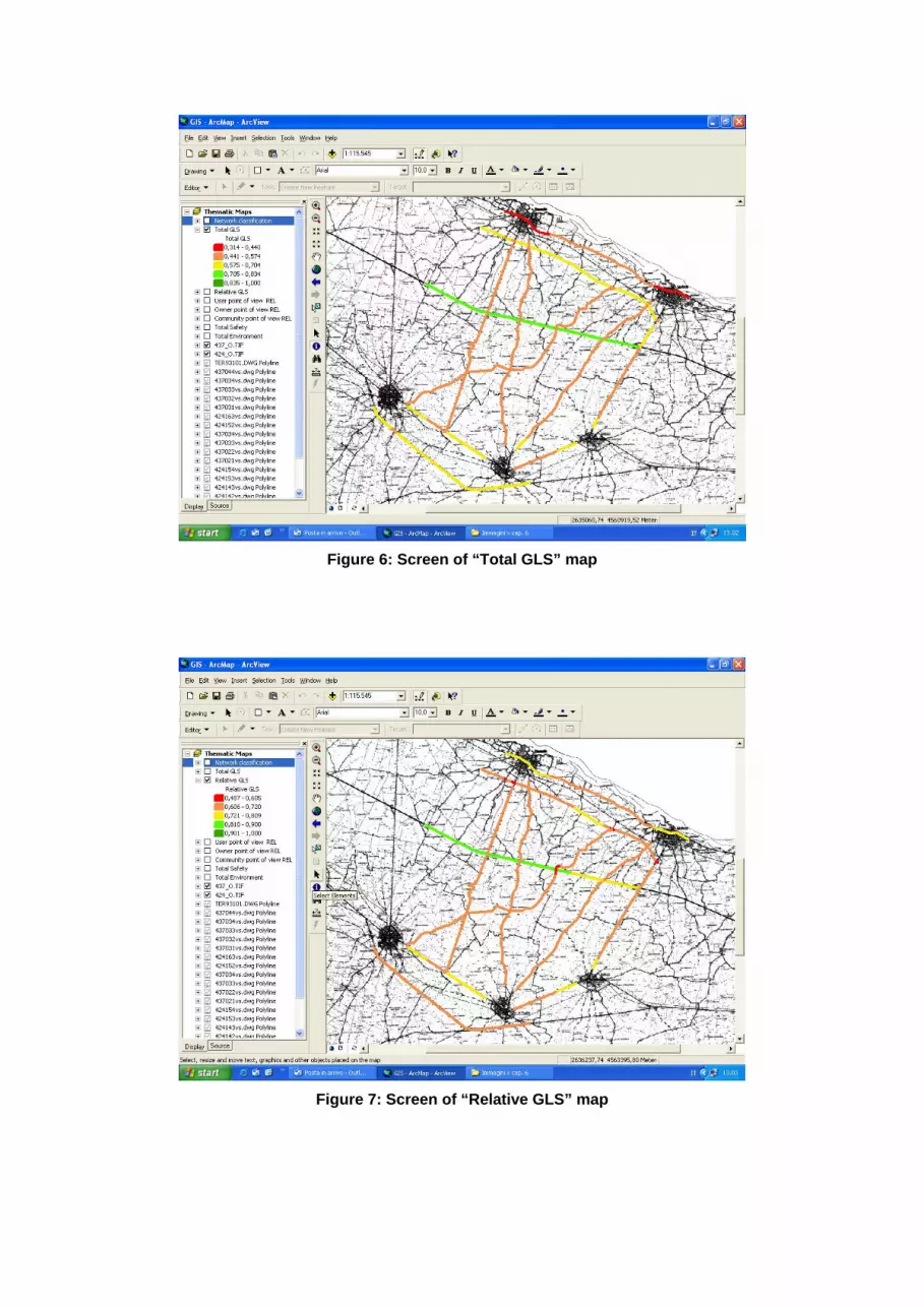
Figure 6: Screen of “Total GLS” map
Figure 7: Screen of “Relative GLS” map

Figure 8: Screen of “Total Safety” map
Figure 9: cross detail; aerial mapping scale 1:5.000.

CONCLUSION This research project worked out a methodology to define road service quality: The Global Level of Service – GLS, dwelling carefully upon its implementation through the GLS2004.xls software and upon the creation of the related Geographical Information System. In the operational phase of this method it’s possible to associate to each road section a single synthetic parameter, expression of road service quality offered. This method, if associated with GIS thematic maps can be a valid tool for road network analysis. If we know GLS road values, we can create thematic maps where indicator values are pointed out in order to specify the peculiarities of that particular road section. We can aggregate these indicators or we can represent them separately for different points of view (user, owner and environment), highlighting the best and/or the worst elements of each road section, and letting everyone (technicians and not) read clearly every factor, for each option. We faced an in-depth study about functional road classification, aimed at defining a classification which characterizes primary, principal, secondary and local roads according to their function in the network and to the movement offered. Then, the optimal maximum values for these kinds of roads were defined and it was possible, in operating phase, to relate absolute GLS values with these optimal values for that kind of road. In this way we obtained the GLS “efficiency” value that enables to estimate road service quality apart from its function, expressing better the user’s expectation. Every indicator has an identifying form including the different informations characterizing. The indicators were subdivided into “intrinsically assessable objectively indicators” and “intrinsically not assessable objectively indicators”. In order to calculate the value of the first ones we used mathematical expressions; regarding the second ones special survey/evaluation forms were created for each indicator; these forms, through some questions, give an evaluation of the indicator as much as possible objective. In order to make methodology application easier, the single indicators’ algorithms and the GLS algorithm were implemented in a software called GLS2004.xls which allows the user a fast input of indicators values during survey phase and an easy execution of the operations required by the procedure. This software calculates automatically the GLS absolute values, the general parameters values (Safety, Travel time, Services, Environment, Traffic condition, Confort), the values related to different points of view (user, owner and environment) and the GLS efficiency values, that’s the relative values. In operating phase of this methodology the software was applied to a road network in the northern part of Bari district having the towns of Bisceglie, Molfetta, Terlizzi, Ruvo and Corato as vertices. The network was classified from a functional point of view and it was created a Geographical Information System which enabled to analyse results and to value the efficiency of the proposed methodology. By this method it’s simple for an operational agency to start planned management activities, identifying the road sections requiring an urgent intervention, according to different GLS values which characterize the section and defining in this way an operational priority scale. Regarding the user, he can start a journey knowing in advance the service quality offered by road network and he can choose, according to different parameters and to his own needs, a route, deciding to reduce trip time or preferring the environmental trip aspect. Thanks to the very relevant services offered by the WebGIS, it’s possible, through the Internet, to obtain the geographical informations in different forms such as maps, data, images, analysis, etc... and so to acquire on-line informations in real time. Combining Geographical Information Systems with GPS systems, the new technologies are heading towards complex systems able to send the data obtained from a sensor, set on a vehicle, directly to the storage system of a software having an interfacial link with one or more Geographical Information Systems on the Web, so giving the maps in real time and setting at zero the survey time on site. REFERENCES [1] COLONNA, P. (1998), “Proposta di determinazione della qualità del servizio di viabilità atteso ed offerto”, in: Atti del XXIII Congresso Nazionale AIPCR, Verona. [2] COLONNA, P. (1999), “The quality of service in terms of road serviceability as a fundamental parameter for taking technical and strategic choices that concern road network infrastructures”, in: Proceedings of the XXI Road International Congress, PIARC, Kuala Lumpur (Le strade, Special Issue n° 1349 July-Agoust 1999). [3] COLONNA, P. (2000), “La qualità del servizio di viabilità ed il livello di servizio globale GLS quali parametri fondamentali per le scelte tecniche, economiche e strategiche relative alle infrastrutture viarie”, in: Atti del X convegno “Infrastrutture viarie del XXI Secolo: classificazione e riqualificazione del patrimonio esistente”, SIIV, Acireale. [4] COLONNA, P. (2000), “Proposta di determinazione della qualità del servizio di viabilità atteso ed offerto”, in: 7° Seminario AIIT, Bari.

[5] Autori vari, (2002), “Atti congressuali del XXIV Convegno Nazionale Stradale”, AIPCR, St. Vincent (AO). [6] D’AMOJA S. (2002), “Definizione di un metodo basato sul livello della qualità del servizio di viabilità per le scelte tecniche, economiche, gestionali e strategiche relative alle infrastrutture stradali”, Tesi di dottorato di ricerca in: “Infrastrutture stradali e sistemi di trasporto”, Università degli Studi di Napoli Federico II, Napoli. [7] Ministero dei Lavori Pubblici, (2001), Ispettorato Generale per la Circolazione e la Sicurezza Stradale, “Norme funzionali e geometriche per la costruzione delle strade”, Roma. [8] COLONNA P., D’AMOJA S., MAIZZA M., RANIERI V. (2002), “Il GLS come strumento di misura della qualità del servizio di viabilità: verifica del parametro sicurezza”, in: Atti congressuali del XXIV Convegno Nazionale Stradale, AIPCR, Saint Vincent (AO). [9] COLONNA P., D’AMOJA S., MAIZZA M., RANIERI V. (2002), “The quality of the road service as a fundamental parameter in the technical, economic and strategic choices regarding safety and the road infrastructures”, in: Proceedings of 2nd International Conference “On Safe Roads in the XXIth Century”, Budapest Ungheria. [10] COLONNA P., D’AMOJA S., RANIERI V. (2001), “Il Livello di Servizio Globale (GLS) quale parametro per la valutazione della qualità del servizio di viabilità”, in: Atti dell’XI Convegno Nazionale, SIIV, Verona. [11] Ministero delle Infrastrutture e dei Trasporti (2001), Ispettorato Generale per la sicurezza e la circolazione stradale, “Linee guida per le analisi di sicurezza delle strade”. [12] FEDERAL HIGHWAY ADMINISTRATION (1999), “System and Use Characteristics, Functional Classification”, 1999 Status of the Nation’s Surface Transportation: Conditions and Performance Report, Chapter 2. [13] FEDERAL HIGHWAY ADMINISTRATION (2001), “Functional Classification”, Flexibility in Highway Design, Chapter 3. [14] TRANSPORTATION RESEARCH BOARD (2000), National Research Council, Highway Capacity Manual, Washington, D.C. [15] LAMM R., PSARIANOS B., MAILAENDER T. (1999), “Road classification”, in: Highway Design and Traffic Safety Engineering Handbook, Chapter 3. [16] COLONNA P., D’AMOJA S., MAIZZA M., RANIERI V. (2003), “Il Global Level of Service come strumento di misura delle performance stradali”, Le Strade, Special issue, Proceedings of XXIInd World Road Congress, PIARC, Durban, South Africa, Italian Report. [17] COLONNA P., D’AMOJA S., MAIZZA M., RANIERI V. (2003), “The quality of service in terms of road serviceability as a fundamental parameter for taking technical, economical and strategic choices that concern road network infrastructures”, in: Proceedings of XXIIP
ndP World Road Congress, PIARC, Durban,
South Africa. [18] MAIZZA M. (2004), “Methods for evaluating and representing road service levels”, Doctorate Thesis in: “Road and Transport Systems, Environment and Technological Innovation”, Polytechnic of Bari.

APPENDIX
HHHOOOMMMOOOGGGEEENNNEEEOOOUUUSSS RRROOOAAADDD SSSEEECCCTTTIIIOOONNNSSS SSSEEELLLEEECCCTTTIIIOOONNN
AAANNNAAALLLYYYSSSIIISSS SSSEEECCCTTTIIIOOONNN BBBYYY SSSEEECCCTTTIIIOOONNN AAANNNDDD NNNUUUMMMEEERRRIIICCCAAALLL VVVAAALLLUUUEEE AAASSSSSSIIIGGGNNNAAATTTIIIOOONNN TTTOOO IIINNNDDDIIICCCAAATTTOOORRRSSS
GGGRRROOOUUUPPP IIINNNDDDIIICCCAAATTTOOORRR CCCAAALLLCCCUUULLLAAATTTIIIOOONNN FFFOOORRR EEEAAACCCHHH RRROOOAAADDD SSSEEECCCTTTIIIOOONNN AAANNNDDD FFFOOORRR EEEAAACCCHHH PPPOOOIIINNNTTT OOOFFF VVVIIIEEEWWW (((UUU,,, OOO,,, EEE))):::
( ) ( ) ( )∑
∑∑
∑∑
∑ ⋅=
⋅=
⋅=
i
i
i
i
i
i
Xe
XeiXe
Xp
XpiXp
Xu
XuiXu P
PXP
PXP
PX III
GGGLLLOOOBBBAAALLL IIINNNDDDIIICCCAAATTTOOORRR CCCAAALLLCCCUUULLLAAATTTIIIOOONNN (((GGGEEENNNEEERRRAAALLL PPPAAARRRAAAMMMEEETTTEEERRR)))
αααααα
epu
eXepXpuXuX
IIII ++
⋅+⋅+⋅=
GGGLLLOOOBBBAAALLL LLLEEEVVVEEELLL OOOFFF SSSEEERRRVVVIIICCCEEE FFFOOORRR SSSIIINNNGGGLLLEEE RRROOOAAADDD SSSEEECCCTTTIIIOOONNN CCCAAALLLCCCUUULLLAAATTTIIIOOONNN
ββββββββββββ
CAQRTS
cCAAQQRRTTSS
n
IIIIIIGLS +++++
+⋅+⋅+⋅+⋅+⋅=
⋅
GGGLLLOOOBBBAAALLL LLLEEEVVVEEELLL OOOFFF SSSEEERRRVVVIIICCCEEE CCCAAALLLCCCUUULLLAAATTTIIIOOONNN
∑⋅
=n road
nnroad L
LGLSGLS
Figure 10: Logical scheme for GLS evaluation

Tab 7: Indicators
1) Check of coordination of vertical and horizontal alignments : GL01∈[0,1]; 2) Road where stopping sight distance is guaranteed: GL02∈[0,1]; 3) Mean value of the ratio “actual horizontal curve radius”/”theoretical horizontal curve radius for vehicle dynamic equilibrium”:
GL03∈[0,1]; 4) Coordination between consecutive curves: GL04∈[0,1] 5) Comparison of straight alignments lengths LB0 Band radius of interposed curves R: GL05∈[0,1]; 6) Check of horizontal tangents length: GL06∈[0,1]; 7) Percentage of horizontal curves with clothoids: GL07∈[0,1]; 8) Curvature Change rates: GL08∈[0,1]; 9) Percentage og horizontal curves with correct super elevation: GL09∈[0,1]; 10) Sections at which passing sight distance is ensured: GL10∈[0,1]. 11) Grades related to the road type: GL11∈[0,1]; 12) Respect of minimum and maximum cross slope: GS01∈[0,1] 13) Ratio between actual shoulder width and the ideal one: GS02∈[0,1] 14) Ratio between actual sidewalk width and the ideal one: GS03∈[0,1] 15) Ratio between actual lanes width and the ideal one: GS04∈[0,1] 16) Ratio between actual lateral clearance and the ideal one: GS05∈[0,1] 17) Pavement Friction coefficient (C.A.T.); S01 ∈[0,1]; 18) Roughness: S02 ∈[0,1]; 19) Level of joints functional effectiveness: S03 ∈[0,1]; 20) Level of bearings functional effectiveness: S04 ∈[0,1]; 21) Runoff effectiveness: S05 ∈[0,1]. 22) Level of suitability of tunnel facing: S06 ∈[0,1]. 23) Level of suitability of road signals: F01 ∈[0,1]; 24) Level of suitability of road barriers: F02 ∈[0,1]; 25) Presence/effectiveness of control devices, alert systems and fire control: F03 ∈[0,1]; 26) Level of effectiveness of ventilation systems: F04 ∈[0,1]; 27) Presence of wind barriers: F05 ∈[0,1]; 28) Condition of road nightime visibility devices: F06 ∈[0,1]; 29) Presence/effectiveness of illumination systems: F07 ∈[0,1]; 30) Presence and organization of deicing systems: F08 ∈[0,1]; 31) Presence of anti dazzle devices: F09 ∈[0,1]. 32) Frequency of private access: number/km; E01 ∈[0,1]; 33) Frequency of signalled intersections: number/km; E02 ∈[0,1]; 34) Frequency of intersections without traffic lights: number/km; E03 ∈[0,1]; 35) Frequency of intersections with grade separation with aceleration/deceleration lanes: number/km; E04 ∈[0,1]; 36) Presence of pedestrian crosswalks; E05 ∈[0,1] 37) Delays due to work areas: T01 ∈[0,1]; 38) Delays due to accidents: T02 ∈[0,1]; 39) Delays due to toll payment: T03 ∈[0,1]; 40) Real travel time: T04 ∈[0,1]. 41) Frequency of lays-by: R01 ∈[0,1]; 42) Frequency of rest areas: R02 ∈[0,1]. 43) Frequency of service stations: R03 ∈[0,1]; 44) Weather, traffic and accident information: R04 ∈[0,1]; 45) Presence of police and emergency services: R05 ∈[0,1]; 46) Presence of GPS: R06 ∈[0,1]; 47) Presence of SOS devices: R07 ∈[0,1] 48) Acoustic pollution: A01 ∈[0,1]; 49) Air pollution: A02 ∈[0,1]; 50) Visual impact: A03 ∈[0,1] 51) Route beauty: A04 ∈[0,1]. 52) Ratio between ADT and road capacity: Q01 ∈[0,1]; 53) Percentage of slow traffic: heavy vehicles, RV’s and buses: Q02 ∈[0,1]; 54) Ratio between commuter and non commuter: Q03 ∈[0,1].