Embed Size (px)
Citation preview

i TAFI Final Report – FRDC 1999/162
FRDC FINAL REPORT
EVALUATING THE EFFECTIVENESS OF
MARINE PROTECTED AREAS AS A
FISHERIES MANAGEMENT TOOL
Colin Buxton, Neville Barrett, Malcolm Haddon, Caleb Gardner & Graham Edgar
July 2006
FRDC Project No. 1999/162

National Library of Australia Cataloguing-in-Public ation Entry
Buxton, Colin David, 1954-
Evaluating the Effectiveness of Marine Protected Areas as a Fisheries Management Tool
Bibliography. Includes index.
ISBN 1 86295 161 6
1. Marine Protected Areas – Australia – Fisheries Management 2. Marine Reserves – Fisheries – Models 3. MPAs – Effects of Fishing – Lobster – Abalone – Reef fishes I. Buxton, Colin, 1954-. II. Tasmanian Aquaculture and Fisheries Institute.
597.5609946
Tasmanian Aquaculture and Fisheries Institute, University of Tasmania, Private Bag 49, Hobart, Tasmania 7001. E-mail: Colin [email protected].
Ph. (03) 6227 7256 Fax (03) 6227 8035
The opinions expressed in this report are those of the author/s and are not necessarily those of the Tasmanian Aquaculture and Fisheries Institute.
Tasmanian Aquaculture and Fisheries Institute, University of Tasmania 2006.
Copyright protects this publication. Except for purposes permitted by the Copyright Act, reproduction by whatever means is prohibited without the prior written permission of the Tasmanian Aquaculture and Fisheries Institute.

MPAs as Fisheries Management Tools
i TAFI Final Report – FRDC 1999/162
EVALUATING THE EFFECTIVENESS OF MARINE PROTECTED AREAS AS A FISHERIES MANAGEMENT TOOL
Colin Buxton, Neville Barrett, Malcolm Haddon,
Caleb Gardner & Graham Edgar

Introduction
TAFI Final Report – FRDC 1999/162 ii
Table of Contents
NON TECHNICAL SUMMARY.............................................................................................................7
ACKNOWLEDGEMENTS ....................................................................................................................10
BACKGROUND......................................................................................................................................12
NEED........................................................................................................................................................13
OBJECTIVES..........................................................................................................................................15
METHODS...............................................................................................................................................15
RESULTS.................................................................................................................................................16
CHAPTER 1. EXAMINING UNDERWATER VISUAL CENSUS TECHNIQUES FOR T HE ASSESSMENT OF POPULATION STRUCTURE AND BIODIVERSITY IN TEMPERATE COASTAL MARINE PROTECTED AREAS ......................................................................................18
SUMMARY..........................................................................................................................................18
CHAPTER 2. CHANGES WITHIN THE TASMANIAN MARINE RESERVES IN THE DECADE FOLLOWING PROTECTION ............................................................................................23
SUMMARY..........................................................................................................................................23 INTRODUCTION ................................................................................................................................23 METHODS...........................................................................................................................................26 Reserve descriptions .............................................................................................................................26 Sites examined ......................................................................................................................................28 Location of sites....................................................................................................................................29 Census methods.....................................................................................................................................29 Sampling periods and times ..................................................................................................................31 Analysis.................................................................................................................................................33 RESULTS................................................................................................................................................36 Maria Island ..........................................................................................................................................36 Tinderbox Reserve................................................................................................................................58 Ninepin Point ........................................................................................................................................70 Bicheno .................................................................................................................................................77 Boundary effects ...................................................................................................................................86 DISCUSSION...........................................................................................................................................87 Reef fishes.............................................................................................................................................87 Invertebrates and cryptic fishes.............................................................................................................93 Macroalgae..........................................................................................................................................100 Summary of the changes after a decade of protection.........................................................................101 Limitations of the study and recommendations for future designs ......................................................102 Conclusions.........................................................................................................................................103 APPENDICIES - TABLES OF SPECIES AND ABUNDANCES RECORDED DURING THE TASMANIAN MPA STUDY
BETWEEN 1992-2002. ..........................................................................................................................106
CHAPTER 3. BASELINE SURVEYS OF NEW OR PROPOSED MPAS IN TEMPERATE AUSTRALIA..........................................................................................................................................139
SUMMARY ...........................................................................................................................................139 INTRODUCTION....................................................................................................................................139 SURVEYS CONDUCTED.........................................................................................................................140 Tasmania.............................................................................................................................................140

MPAs as Fisheries Management Tools
iii TAFI Final Report – FRDC 1999/162
Victoria ............................................................................................................................................... 141 New South Wales................................................................................................................................ 142 Western Australia ............................................................................................................................... 143 South Australia ................................................................................................................................... 143
CHAPTER 4. BIASES ASSOCIATED WITH THE USE OF UNDERWATER VISUAL CENSUS TECHNIQUES TO QUANTIFY FISH DENSITY AND SIZE-STRUCT URE................................ 144
INTRODUCTION.................................................................................................................................... 144 METHODS............................................................................................................................................ 145 Sites studied........................................................................................................................................ 145 Underwater visual transect techniques................................................................................................ 146 Changes in density following algal clearance ..................................................................................... 147 Comparison of visual and capture-resight density estimates............................................................... 147 Variation in density estimates between divers, sites and time............................................................. 148 Effect of macroalgal cover on density estimates................................................................................. 149 Sampling errors associated with size estimates by divers ................................................................... 150 RESULTS.............................................................................................................................................. 150 Changes in density following algal clearance ..................................................................................... 150 Comparison of visual and capture-resight density estimates............................................................... 160 Variation between divers, sites and time in density estimates............................................................. 161 Effect of macroalgal cover on density estimates................................................................................. 163 Sampling errors associated with size estimates by divers ................................................................... 166 DISCUSSION......................................................................................................................................... 170 Effects of canopy clearance ................................................................................................................ 170 Errors in visual estimates of fish density by divers............................................................................. 173 Errors in visual estimates of fish length by divers.............................................................................. 178 Summary............................................................................................................................................. 180
CHAPTER 5. PATTERNS OF FISH MOVEMENT ON EASTERN TA SMANIAN ROCKY REEFS....................................................................................................................................................183
SUMMARY ........................................................................................................................................... 183 INTRODUCTION.................................................................................................................................... 183 MATERIALS AND METHODS................................................................................................................. 184 Sites studied........................................................................................................................................ 184 Fish tagging ........................................................................................................................................ 186 Habitat manipulation........................................................................................................................... 187 Assessment of displacement and home range ..................................................................................... 187 RESULTS.............................................................................................................................................. 187 DISCUSSION......................................................................................................................................... 195
CHAPTER 6. MOVEMENT AND GROWTH OF LOBSTERS WITHIN THE MARIA ISLAND MARINE RESERVE............................................................................................................................. 198
INTRODUCTION.................................................................................................................................... 198 METHODS............................................................................................................................................ 200 Recapture study at Maria Island ......................................................................................................... 200 Catch sampling data............................................................................................................................ 201 RESULTS.............................................................................................................................................. 204 Captures/recaptures............................................................................................................................. 204 Short-term movements........................................................................................................................ 205 Long-term movements ........................................................................................................................ 205 Size distribution of lobsters within the reserve ................................................................................... 208 Comparison of fished and unfished size distribution.......................................................................... 209 Von Bertalanffy Growth Curves using Faben’s Method..................................................................... 210 Outside Reserve .................................................................................................................................. 213 Transition Matrices from Tagging Data.............................................................................................. 213 Comparison of Growth Descriptions .................................................................................................. 213 Density-Dependent Effects on Growth ............................................................................................... 214 DISCUSSION......................................................................................................................................... 215 Rock Lobster Movement..................................................................................................................... 215

Introduction
TAFI Final Report – FRDC 1999/162 iv
Population structure ............................................................................................................................216 Growth Descriptions ...........................................................................................................................217
CHAPTER 7. MOVEMENTS OF THE SOUTHERN ROCK LOBSTER JASUS EDWARDSII IN TASMANIA, AUSTRALIA ..................................................................................................................220
ABSTRACT...........................................................................................................................................220 INTRODUCTION....................................................................................................................................220 METHODS............................................................................................................................................221 Description of tagging.........................................................................................................................221 Magnitude of movement .....................................................................................................................223 Direction of movement of individual lobsters captured on repeated occasions ..................................225 Direction of movement in single recapture events ..............................................................................226 RESULTS..............................................................................................................................................227 Magnitude of movement .....................................................................................................................227 Direction of movement of individual lobsters captured on repeated occasions. .................................231 Direction of movement in single recapture events ..............................................................................233 DISCUSSION.........................................................................................................................................236 APPENDICES.........................................................................................................................................239
CHAPTER 8. SPATIAL VARIATION IN SIZE AT ONSET OF M ATURITY OF FEMALE SOUTHERN ROCK LOBSTER JASUS EDWARDSII AROUND TASMANIA, AUSTRALIA AND THE EFFECT OF DENSITY...............................................................................................................240
SUMMARY ...........................................................................................................................................240 INTRODUCTION....................................................................................................................................240 METHODS............................................................................................................................................241 Sample sites and specimen collection .................................................................................................241 Statistical analyses ..............................................................................................................................242 RESULTS..............................................................................................................................................243 DISCUSSION.........................................................................................................................................246 CONCLUSIONS......................................................................................................................................248
CHAPTER 9. DOES PLEOPOD SETATION PROVIDE A MEASURE OF MATURITY IN FEMALE SOUTHERN ROCK LOBSTERS JASUS EDWARDSII?................................................250
SUMMARY ...........................................................................................................................................250 INTRODUCTION....................................................................................................................................250 METHODS............................................................................................................................................251 Sample sites and specimen collection .................................................................................................251 Contrasting SOM estimates based on presence of ovigerous setae with those based on presence of external eggs .......................................................................................................................................252 Monthly/seasonal patterns in SOM estimates .....................................................................................252 Statistical analyses ..............................................................................................................................253 RESULTS..............................................................................................................................................254 Monthly/seasonal patterns in SOM estimates .....................................................................................255 DISCUSSION.........................................................................................................................................256
CHAPTER 10. MPAS AND FISHERIES: SIMPLE MODELS.......................................................261
INTRODUCTION....................................................................................................................................261 Background.........................................................................................................................................261 How to study the effects of MPAs on fisheries. ..................................................................................262 MODELLING STRATEGY .......................................................................................................................262 Simple Models ....................................................................................................................................263 Complex but General Models .............................................................................................................264 Complex Fishery Specific Models ......................................................................................................264 The Model...........................................................................................................................................265 The Hastings and Botsford model.......................................................................................................266 Model Implementation........................................................................................................................268 RESULTS..............................................................................................................................................268 Hastings and Botsford Model – No MPA...........................................................................................268 DISCUSSION.........................................................................................................................................271

MPAs as Fisheries Management Tools
v TAFI Final Report – FRDC 1999/162
APPENDIX 10.1. MODEL SPECIFICATION. ............................................................................................. 273 Marine Protected Area Model – by Hastings and Botsford (1999)..................................................... 273
CHAPTER 11. MPAS AND FISHERIES: GENERAL MODELLING. .......................................... 276
INTRODUCTION.................................................................................................................................... 276 The Need for a Size-Structured Model ............................................................................................... 276 METHODS............................................................................................................................................ 278 Verbal Model Description .................................................................................................................. 278 Spatial Scales...................................................................................................................................... 279 Initial Stock Conditions ...................................................................................................................... 279 RESULTS.............................................................................................................................................. 282 Effects of Fishing on Productivity (No MPA; Region 1).................................................................... 282 Effect of Fishing on Equilibrium Size-Structure (No MPA)............................................................... 284 Effects of Fishing on Productivity with MPA Implemented ............................................................... 285 Effect of Movement Rate.................................................................................................................... 289 Effects of Fishing on Productivity (No MPA; Region 5).................................................................... 292 Effects of Fishing on Productivity with MPA (Region 5)................................................................... 294 Assumption of No Reduction in Catch ............................................................................................... 297 DISCUSSION......................................................................................................................................... 299 MPAs and Fisheries Management ...................................................................................................... 299 General Impacts of Implementing an MPA ........................................................................................ 299 Benefits from Adult Movement (Spillover) ........................................................................................ 300 Impacts on Stock Biomass.................................................................................................................. 301 Impacts on Egg Production................................................................................................................. 301 Depletion Rates................................................................................................................................... 302 MPAs for Fishery Management .......................................................................................................... 302 Implementing MPAs and Decreasing Catches.................................................................................... 302 Conclusions......................................................................................................................................... 303 APPENDIX 11.1. MODEL SPECIFICATION. ............................................................................................ 304 Marine Protected Area Model – Specification.................................................................................... 304 The Model .......................................................................................................................................... 304 APPENDIX 11.2. BASE CASE MODEL PARAMETERS. ............................................................................ 310
CHAPTER 12. MPAS AND FISHERIES: FISHERY SPECIFIC M ODELS................................. 313
INTRODUCTION.................................................................................................................................... 313 The Expansion of the Size-Structured Model ..................................................................................... 313 METHODS............................................................................................................................................ 315 Verbal Model Description .................................................................................................................. 315 Catch History...................................................................................................................................... 316 Growth Transition Matrices................................................................................................................ 316 Initial Size-Structure and Recruitment Time Series............................................................................ 317 MPA Simulations (Model Projections)............................................................................................... 318 Block Closures.................................................................................................................................... 319 RESULTS.............................................................................................................................................. 320 Model projection without an MPA ..................................................................................................... 320 Model projection with closures in Region 1 ....................................................................................... 323 Model projection with closures in Region 5 ....................................................................................... 327 All Region Closures............................................................................................................................ 330 Catch-Rate Implications...................................................................................................................... 336 DISCUSSION......................................................................................................................................... 339 Legal-Sized Biomass .......................................................................................................................... 339 Egg-Production................................................................................................................................... 340 Catch-Rates......................................................................................................................................... 341 Fleet Dynamics in Response to Closure.............................................................................................. 342 The Value of MPAs for Fisheries Management.................................................................................. 343 MPAs - An Apparently Simple Solution to a Complex Problem? ...................................................... 345 APPENDIX 12.1. MODEL SPECIFICATION.............................................................................................. 347 Marine Protected Area Model – Specification.................................................................................... 347 The Model .......................................................................................................................................... 347

Introduction
TAFI Final Report – FRDC 1999/162 vi
APPENDIX 12.2. STATISTICAL BLOCK CHARACTERISTICS.....................................................................350 APPENDIX 12.3. GENERATING GROWTH TRANSITION MATRICES.........................................................352 APPENDIX 12.4. THE YEARLY STOCK ASSESSMENT MODEL................................................................357 APPENDIX 12.5. BASE CASE MODEL PARAMETERS..............................................................................368
BENEFITS AND ADOPTION..............................................................................................................370
FURTHER DEVELOPMENT..............................................................................................................371
PLANNED OUTCOMES......................................................................................................................371
CONCLUSIONS....................................................................................................................................372
REFERENCES ......................................................................................................................................374
APPENDIX 1: INTELLECTUAL PROPERTY .................. ...............................................................391
APPENDIX 2: STAFF INVOLVED ....................................................................................................391

Introduction
7 TAFI Final Report – FRDC 1999/162
1999/162 Evaluating the effectiveness of Marine Protected Areas as a fisheries management tool
PRINCIPAL INVESTIGATOR Professor Colin Buxton
ADDRESS University of Tasmania Tasmanian Aquaculture and Fisheries Institute
Marine Research Laboratories Private Bag 49 TAS 7001 Telephone: 03 62277256 Fax: 03 62278035
NON TECHNICAL SUMMARY
OUTCOMES ACHIEVED TO DATE
The survey protocol agreed at a national project workshop has been used in baseline surveys undertaken in new or proposed MPAs in Western Australia, Victoria, Tasmania and New South Wales. The Victorian State Government has since established an ongoing MPA monitoring program using the project survey protocols.
The study has clearly demonstrated the effects of closure on plant and animal communities in the reserves, and through a comparison with fished sites is revealing much about the effects of fishing on reef communities. This has direct applications for fisheries assessments under the EPBC Act.
Models suggest that MPAs are limited in terms of their usefulness as a fisheries management tool, especially for the Tasmanian rock lobster and abalone fisheries, but also for quota-managed fisheries in general.
Marine Protected Areas (MPAs) are being proclaimed around the world with the stated primary purposes of enhancing fisheries stocks and/or conserving marine biodiversity. In Australia, in response to a joint State/Commonwealth agreement to establish a National Representative System of MPAs (NRSMPA) to protect marine biodiversity, the focus is on their conservation role. However, fisheries enhancement is often suggested as an additional benefit of protection, potentially offsetting the cost of area closure in some cases.
This study aimed to contribute to the debate on the positive and negative effects of the establishment of MPAs, documenting changes that have occurred in reserves following establishment, and particularly, attempting to understand more about their role as a fisheries management tool. It builds on a program initiated following the establishment of Tasmania’s first ‘no-take’ MPAs a decade ago.
Changes within the MPAs over the period indicated that fishing has had a substantial influence on the demographic structure of many species, particularly those targeted by

Introduction
TAFI Final Report – FRDC 1999/162 8
fishers. The magnitude of change detected appeared to be dependant on the susceptibility of species to capture, the remoteness of protected locations and to the MPA configuration itself. Changes within the more remote Maria Island reserve (the largest area studied), relative to fished reference sites, included increases in the abundance of lobsters and certain fish species and increases in the mean size of rock lobsters (responses typical of protected areas studied elsewhere in the world), as well as a decrease in the abundance of prey species such as urchins and abalone.
Not all species increased in size and/or abundance, and for several fish species there was no significant change. At Maria Island there was also a 30% decline in the abundance of common urchins within the reserve, which may be the first Tasmanian evidence of cascading ecosystem effects related to protection from fishing. Abalone numbers were also observed to decline sharply over the period sampled. This change was interesting in that one possible explanation was an inverse relationship between predators (lobsters) and prey (abalone). If shown to be correct this finding is likely to have significant consequences for integrated, ecosystem based management of these two species.
Clearly the survey showed that MPAs, even of a relatively small size (Maria Island covers 7km of coastline), could effectively achieve conservation objectives, especially for exploited species that were resident or sedentary in nature.
A study of small-scale movement patterns of fishes showed that with few exceptions fish species showed high fidelity to site. Animals were generally resighted <100 m from initial tagging site and with individuals remaining near the tagging site throughout the 1-year duration of study. Influences on distance moved attributable to the variables body length, sex, water temperature and time since tagging were insignificant compared to variation between individuals. Patterns of movement were also generally consistent at all three study sites. Home ranges of some species were found to be affected by the presence of macroalgae, with animals emigrating from artificially cleared patches. The sedentary nature of these small- to medium-sized reef fish species indicated that relatively small marine protected areas (≈1 km diameter) could provide adequate protection to these fishes but suggest limited “spillover” benefits to fisheries in the form of emigrants to surrounding areas.
The population structure of lobsters (J. edwardsii) within the Maria Island reserve after a decade of protection was substantially changed from levels prior to protection. Relative to adjacent fished areas, the abundance of females was 2.4 times greater and the abundance of legal sized females 16.8 times greater. For males these values were 4.1 and 18.6 greater respectively. The recovery of the lobster population in the Maria Island provided a reference against which the effects of fishing on a range of population biological characteristics could be examined. These included movement, growth and maturity.

Introduction
9 TAFI Final Report – FRDC 1999/162
Modelling the effects of MPAs was focussed on rock lobsters and abalone due to the importance of both fisheries, extensive historical datasets and differences in certain biological characteristics such as larval dispersal. Some aspects of the biology of lobsters required additional research prior to this modelling, such as the effect of increased density inside MPAs on growth, reproduction and movement. This research revealed the following:
- There was no evidence of large-scale, unidirectional migration. Tag-recaptures indicated high site fidelity with the majority of animals moving no detectable distance after periods of one to two years between capture events. This low level of movement suggested limited potential for spillover of biomass from MPAs.
- Growth in the reserve appeared slower than it was adjacent to the reserve and when closely examined it was apparent that a small proportion of the females outside the reserve were able to moult more than once in a year. It suggested that stock rebuilding inside MPAs might be slower than predicted by extrapolation of growth data collected from fished areas.
- There was a distinct spatial cline of carapace length at 50% maturity with the largest sizes being found at northwestern sites (110 mm carapace length) and the smallest sizes at southwestern sites (59 mm carapace length). This cline in size at maturity was the reverse of that described for the same species at similar latitudes in New Zealand and suggests that maturity in J. edwardsii is not primarily regulated by temperature as suggested previously.
To model the effects and implications of MPAs on fisheries, a strategy was adopted of first exploring the properties of a generally applicable simple model followed by a length-based model that was specific to the rock lobster fishery and which incorporated catch and catch rate history.
The simple model predicted population increases in both biomass and size-structure for the reserve and could be used to support the claim that, under certain constraints, a fishery managed solely through the agency of MPAs could provide a similar yield to one managed through more traditional means. However, for many species with limited larval dispersal rates the use of MPAs alone would lead to areas of relatively high quality marine environment literally surrounded by a sea of overfished and depleted areas. The more complex model highlighted a major concern when displaced effort was focused on a few of the more productive blocks. This led to these areas becoming depleted, serial displacement of catch and ultimately rapid fishery decline. It was concluded that closures displacing large amounts of abalone catch were thus a very risky management option because of a pre-disposition to serial depletion in this species.
Because abalone larval dispersal was limited, further more complex modelling was confined to rock lobster where several general conclusions became apparent. Firstly, because of the dynamics of growth and recruitment, there was a time lag before any positive effects of an MPA became apparent. The effects of large MPAs (affecting > 5% catch) tended to only become apparent after several years and the effects of small MPAs (affecting < 0.5% catch) would be hard to detect. Secondly, in an exploited

Introduction
TAFI Final Report – FRDC 1999/162 10
population, introducing an MPA was equivalent to increasing the Total Allowable Catch or the effort outside the reserve. Introducing an MPA without reducing catch was likely to have negative effects upon most fisheries where adult movement was limited in extent, leading to reductions in total stock size and egg production. The effects would be least in lightly depleted stocks where total biomass was high relative to an unfished state. Thirdly, the impact of introducing an MPA would depend on the biology of the species concerned and the state of depletion of the stock. If the stock was already in a highly depleted state, an MPA could hasten fishery collapse. On the other hand, if a stock had already collapsed then a reserve could provide some benefit in terms of protecting mature biomass and egg production. Finally, given the assumptions of the generalized model, it appeared that it would be better to improve current management controls, in particular the match between size limits and the growth characteristics, rather than introduce large MPAs to improve the fishery.
In the Tasmanian lobster and abalone fisheries where catch and effort are effectively limited, it was concluded that the introduction of MPAs as a fisheries management tool would be inferior to present management options. Indeed, if introduced without reducing catch or effort by amounts equivalent to that in the prospective closed area, closed areas were a risky strategy that could lead to a degradation of the fishery (this appears to be a general conclusion for species with low movement rates).
Furthermore, if a fishery is being managed in accordance with ESD principles, which by definition means that the ecosystem in which it operates is not threatened by the fishery or fishing practices, then fishing should not be a key threatening process. It follows from this argument that true ESD fisheries management offers a potentially better outcome than no-take MPAs for biodiversity conservation.
This is not to suggest that MPAs do not have a place in marine and coastal management. Spatial management of fisheries has a long tradition (eg spawning grounds) and there are a number of fisheries that benefit from spatial closures. In addition they are useful where other forms of fisheries management are unavailable or poorly applied. Importantly, this study clearly demonstrates the value of MPAs as reference areas for research on the biology of exploited species and in understanding the ecosystem effects of fishing. Both add to the fisheries management toolbox and lead to a greater fisheries resource security.
ACKNOWLEDGEMENTS
We would like to thank the many people who have assisted with the survey components of the study, including Alastair Morton, Cath Samson, Dave Andrews, Jon Bryan, Brett Hislop, Sam Ibbott and Simon Wilcox for assistance with fieldwork and data entry. The survey results in Chapter 2 are the culmination of a 10-year study initiated in 1992 through an Ocean Rescue 2000 grant to Peter Bosworth and Alex Schaap of the DPIWE. It was later supported with funding from ARC, NHT and Coasts and Clean Seas, in addition to the present study.

Introduction
11 TAFI Final Report – FRDC 1999/162
The baseline surveys described in Chapter 3 required the collaborative involvement of State agencies across temperate Australia, without whose involvement this work could not have been undertaken. In Western Australia thanks are due to Chris Simpson and Kevin Bancroft from the Marine Conservation Branch of Conservation and Land Management (CALM), WA for organising funding, logistic support and diving assistance, and John Huissman for field assistance with macroalgal identification. In South Australia, thanks are due to Bryan McDonald from the Department of Environment and Heritage for organising funding and logistic support, to Scoresby Shepherd and the South Australian Research & Development Insitute for organisational and logistic support and to Chris Halstead and Ally Bloomfield for field assistance. In Victoria thanks are due to Lawrence Ferns and Don Hough from Natural Resources and Environment Vistoria for organising funding and logistic support, and to Matthew Edmunds for field assistance. In New South Wales, thanks are due to the NSW Marine Parks Authority for funding and logistic support, in particular to Tim Lynch from the Jervis Bay Marine Parks Authority, for organisational and diving support, and Fran for vessel support. In Tasmania, thanks are due to Alastair Morton and Cath Samson for ongoing assistance throughout the project. Funding from the Australian Research Council to Graham Edgar supported the fish movement and diver bias studies in Chapters 4&5. Bob Connell, Joe Valentine and Julian Harrington assisted with diving and trapping.
The growth data described in Chapter 6 (lobster movement and growth) was supported by data collected by the TAFI Rock Lobster Section. We thank Cath Samson and Phil Ziegler for assistance with fieldwork, and in particular the crew of the RV Challenger, Matt Francis and Jac Gibson, for their efforts often in difficult conditions. Data presented in Chapter 7 were collected through the efforts of numerous people involved in the tagging of rock lobsters around Tasmania over the last three decades. The following made especially substantial contributions: Dave Tarbath, Rod Pearn, Malcolm Hart, Steve Bishop, Mick Murphy, Mark Cornelius, Vic Holthouse, Jac Gibson, Andrew Cawthorn, Graeme Ewing, Chris Rhodes, Bill Ramsden, Craig MacKinnon and Allison Phillips.
The analyses presented in Chapter 8 relied on data collected from a range of projects over several years, usually with FRDC, DPIWE and Industry support. Especially important contributions since 1989 were made by Craig Mackinnon, Jac Gibson, Matt Francis, Andrew Cawthorn, Rod Pearn, Philippe Ziegler, Alison Phillips, Jo Beukers-Stewart, Graham Ewing, Sam Ibbott, Pip Cohen, Dave Tarbath, Bob Kennedy and Peter Terry.
The analyses presented in Chapter 9 relied on extensive data-sets collected by numerous people over several decades including data collected by CSIRO in the 1960s. Contributions since 1989 were made by Stewart Frusher, Jac Gibson, Matt Francis, Andrew Cawthorn, Rod Pearn, Craig Mackinnon, Philippe Ziegler, Sam Ibbott, Pip Cohen and Steve Bishop.

Introduction
TAFI Final Report – FRDC 1999/162 12
BACKGROUND
Marine Protected Areas (MPAs) are being proclaimed around the world with the primary purposes of enhancing fisheries stocks and/or conserving marine biodiversity (Plan Development Team 1990, Ward et al. 2001). By 1992 a total of 303 MPAs had been declared within Australia (Zann 1995) and this process has continued in the following decade, particularly in response to the joint State/Commonwealth agreement to establish a National Representative System of MPAs (NRSMPA) to protect marine biodiversity (ANZEEC 1999). While the current focus of MPA establishment within Australia is on the conservation role that they may play, fisheries enhancement is often suggested an additional benefit of protection, potentially offsetting the cost of area closure in some cases.
Fisheries benefits associated with area protection include the suggestion that yield may be enhanced because the MPA will act as a propagation area and/or as a source of surplus fishable biomass migrating from the reserve. Additional benefits may include insurance against stock collapse, protection of stock genetic diversity and simplified enforcement (Gell and Roberts 1992).
Protection of spawner biomass in MPAs is now a well established fact (Ward et al. 2001). An initial study conducted on inshore reefs in Tasmania between 1992 and 1997 showed that the density and mean size of several exploited species were significantly greater in MPAs when compared to control sites and that the effect of protection was related to the size of the reserve (Edgar and Barrett 1999). Studies elsewhere in the world provided the same results (reviews by Roberts and Hawkins 2000, Roberts and Polunin 1991, Ward et al. 2001, Gell and Roberts 2002). Despite the large number of MPAs declared over the past two decades, there is little quantitative information in Australia or elsewhere in the world that rigorously examines whether other management aims are achieved.
The tacit acceptance that fishery enhancement aims are achieved with the declaration of MPAs is urgently in need of validation. In particular, closure may result in redirected effort and greater fishing pressure on open areas and there exists a need to quantitatively assess the biotic consequences of such action. This is fundamental for assessing whether MPAs provide a yield and/or propagation benefit to exploited marine populations. An increase in biomass within an MPA is of no value to a fishery if there has been a greater loss of biomass outside the MPA through effort displacement. That is, we need to establish the net impact of MPAs, especially for quota-managed species.
The plan to establish a NRSMPA in Australia has been resisted by the fishing sector (Ward et al. 2001) because of a perceived loss of yield proportional to the area of the closure and the lack of critical evidence to support the proposed benefits to fisheries (including insurance against stock collapse, sources of eggs and larvae and improvement in yield). To resolve this conflict we urgently need to model the potential impacts and provide the empirical ground-truthing of the effects of area closure on the fishery. While there has been a substantial increase in the number of publications that model possible fisheries effects of closed areas (e.g. Hastings and Botsford 1999,

Introduction
13 TAFI Final Report – FRDC 1999/162
Gerber et al. 2003), most are based on broad generalisations and assumptions. Intuitive benefits in terms of stock recovery of sedentary species have been demonstrated (reviews by Ward et al. 2001, Gell and Roberts 2002), however, other benefits are far from predictable and the scant information on this subject yields results that are species specific and dependent on the behaviour of the species. There is a growing awareness that generalised models are inappropriate and each case needs to be examined in its own merit. As the limited size of no-take areas currently under consideration in temperate Australia mitigates against the study of potential benefits for highly migratory species, initial model development may best be restricted to relatively sedentary species where empirical confirmation of predicted outcomes may be more likely to be achievable.
The ubiquity of indirect secondary interactions between species in marine ecosystems probably results in only a small proportion of species being adequately conserved under directed fisheries management (eg. quota management). For example the exploitation of rock lobsters was found to completely alter the invertebrate community associated with South African reefs (Barkai and Branch 1988) and strongly influence the density of sea urchins on New Zealand reefs (Shears and Babcock 2002, 2003). In Australia and New Zealand the removal of wrasses has been found to increase the survival of juvenile sea urchins (Andrew and Choat 1982), with high numbers of sea urchins denuding reefs of seaweed (Choat and Andrew 1986, Fletcher 1987, Andrew and Underwood 1993, Shears and Babcock 2003) and possibly affecting densities of rock lobsters (Andrew and MacDiarmid 1991). The presence of seaweed in turn affects the densities of fishes (Choat and Ayling 1987, Jones 1992).
There is now a substantial international literature documenting the ecosystem effects of fishing and how these effects are mediated through the loss of top-down control of community structure in a trophic cascade (e.g. reviews by Dayton et al. 1998, Tegner and Dayton 2000, Pinnegar et al. 2000, Jackson et al. 2001). In the absence of historical baseline data, the use of MPAs as scientific reference areas may play a vital role in assessing the magnitude of ecosystem effects of fishing at a local and regional scale and developing an understanding of their underlying causes. If these changes are substantial and the causes are understood, it may be possible to adapt management strategies to ensure fishing in Australia is both economically and ecologically sustainable.
NEED
In concert with the establishment of MPAs around the world and the current push to increase the number and size of no-take areas, it has been argued that these areas may be of benefit to fisheries management. Suggested benefits include moving fisheries harvests towards more sustainable yield, rebuilding depleted stocks, an insurance against stock collapse and the protection of essential habitat.
But as with all management tools, potential and real benefits need to be rigorously assessed. This knowledge base is currently lacking.

Introduction
TAFI Final Report – FRDC 1999/162 14
A core component of this project included making a major theoretical contribution to the general understanding of MPAs for fisheries management, incorporating several new parameters into a model examining the fishery effects of closure. These include effort displacement; existing management tools (input controls and total allowable catch); larval dispersal where possible (research on larval dispersal of rock lobster has focused on Tasmania); fleet dynamics; and spatial variation in biological parameters.
The plan to establish a National System of Marine Protected Areas in Australia has been resisted by the fishing sector because of a perceived loss of yield proportional to the area of the closure and the lack of critical evidence to support the proposed benefit to fisheries (including insurance against stock collapse, sources of eggs and larvae and improvement in yield). To resolve this conflict there was a need to model the potential impacts and provide the empirical ground-truthing of the effects of area closure on the fishery.
Equally, given that most commercially exploited reef species are long lived and that MPAs require several years for the effects of closure to manifest themselves, there is a need to provide baseline information on the status of proposed sites. This information can then be used in the future as a reference point with which to evaluate the success of MPAs in meeting their management objectives. By establishing baseline surveys at a range of locations across temperate Australia, changes following protection may be examined at a range of spatial scales, and a range of MPA sizes, levels of protection, habitats, and pre- and post-protection fishing effort, aiding in the interpretation of the cause of any change that may occur. From the perspective of collecting empirical data on ecosystem effects of fishing, there is a need to maintain adequate assessment of changes that occur once an area has been closed. Prior to this study, monitoring of existing reserve sites in Tasmania had been ongoing for a period of greater than five years. It was important to continue this work because analysis after five years of initial survey provided no indication that population changes of exploited species had stabilised. The biomass of rock lobsters within reserves, for example, continued to increase throughout the five years of the study. There was clearly a need to continue the survey in order to properly document long-term changes that occur as a result of closure. This information is fundamental to the evaluation of MPAs as a coastal management tool. This study was initiated at an opportune time to evaluate the fishery implications of MPAs. This is partly because the development of the NRSMPA was at an early stage of development and could benefit from a clearer understanding of the influence of MPAs on major commercial fisheries such as lobsters and abalone. It is also because new reserves were being established and required effective baseline assessments to be undertaken if their true reference area values were to be gained, and because an ongoing study of existing Tasmanian reserves required support to document changes following protection over a decade time scale.

Introduction
15 TAFI Final Report – FRDC 1999/162
While not a direct objective of the study, it is important to note that continued monitoring of existing MPAs can also provide baseline data against which to assess other anthropogenic perturbations, including identification of the effects of introduced species (e.g. Japanese kelp, North Pacific seastar), overfishing, oil spills and even global warming.
OBJECTIVES
The objectives of the study were fourfold:
1. To model the effects of closure on the rock lobster and abalone fisheries, with particular reference to: the redirection of effort; potential benefit in terms of additional biomass and as a recruitment source; and location, size and number of the MPAs.
2. To quantify relative abundance of selected fish, invertebrates and plant populations at representative sites prior to establishment of MPAs, and to identify changes in relative abundance following reserve establishment. This will be achieved by:
- Continuing the study of the effects of closure on the populations of exploited species inside and adjacent to MPAs, and
- Establishing baseline surveys of proposed temperate MPA sites in southern Australia (e.g. Jervis Bay, NSW; Kent Group of Islands, Tas.; Wilsons Promontory, Vic.; Jurien Bay, W.A.) to evaluate before and after effects of closure.
3. To develop National guidelines for the assessment of MPAs in Australia, with particular reference to exploited species.
4. To provide specific management recommendations on the appropriate location, configuration and size of MPAs that will provide effective enhancement for coastal fisheries, and, to quantify the impacts of MPAs on local fisheries where they are proposed for reasons other than enhancing the fishery.
During the course of the project, however, several complimentary studies were undertaken to improve our understanding of key biological parameters of lobsters in relation to MPAs and their use in the modelling. These included growth, movement and size at maturity of lobsters.
METHODS
The methods employed are described under the relevant section of each Chapter below.

Introduction
TAFI Final Report – FRDC 1999/162 16
The modelling component of the project chose to focus on relatively sedentary species (rock lobster and abalone) for several reasons:
- While intuitive benefits in terms of stock recovery of sedentary species have been demonstrated, other benefits are far from predictable and the scant information on this subject yields results that are species specific and dependent on the behaviour of the species.
- There is a growing awareness that generalised models are inappropriate and each case needs examination on its own merit.
- Furthermore, the size of the no-take areas under consideration mitigates against the study of the benefits for highly migratory species, which range freely between protected and unprotected sites.
- Finally, empirical confirmation of models based on sedentary species is most likely to be achievable (recognising that models for migratory species are not well advanced at this stage).
RESULTS
The results of this study are presented in the following eight chapters. Prior to the establishment of the interstate baseline surveys a joint workshop was organised by TAFI and NRE (Vic.) to examine the underwater visual census (UVC) techniques proposed to be used to collect the baseline data. The results of this workshop have been published separately (Barrett and Buxton 2002), however a summary of this is presented here as Chapter 1.
Chapter 2 presents the detailed results of ongoing monitoring of changes in Tasmanian marine reserves. The time series of results were examined over a ten-year period following protection of these areas.
Chapter 3 details the results of baseline surveys initiated in Tasmania, Western Australia, Victoria and New South Wales and includes detailed data reports for the proposed MPA at Jurien Bay and the now proclaimed MPA at Jervis Bay.
Chapter 4 details the results of a study examining the influence of diver bias during underwater census of reef assemblages. By comparing both inter diver variability and the variability in abundance estimates derived from differing methods (divers and fish traps) an indication of the potential biases associated with diver census were obtained, allowing clearer interpretation of census results (in Chapters 2&3) and an evaluation of the reliability of this method for monitoring change in MPAs.
Chapter 5 details the results of a study examining the movement patterns of a range of typical Tasmanian reef fishes at a range of sites. This involved the recapture of tagged fishes both through trapping and visual census over periods of up to one year, with the aim of providing movement information on these species for incorporation into future models examining the effect of MPAs on these species.

Introduction
17 TAFI Final Report – FRDC 1999/162
Chapter 6 documents the results of studies of lobster movement and growth within the Maria Island Marine Reserve conducted to obtain information for inclusion in the models discussed in previous chapters. This information includes fine scale movement patterns and growth rates and population structure in a population approaching natural densities.
Chapter 7 examines the large -scale movements of lobsters in Tasmanian waters, and in conjunction with the fine-scale movement data from Chapter 6, provides critical information for the modelling chapters.
Chapter 8 details the variability of size at maturity of lobsters around Tasmania and provides additional information required for the modelling in chapters 10 to 12.
Chapter 9 provides a validation of the methods used in Chapter 8 to determine size at maturity.
Chapters 10 to 12 include detailed modelling of the effect of MPAs on abalone and rock lobster fisheries using data obtained in the course of managing these fisheries, including fishery dependent and fishery independent data derived from a wide range of sources, including this study.

Visual Census Techniques
TAFI Final Report – FRDC 1999/162 18
Chapter 1. Examining Underwater Visual Census techniques for the assessment of population structure and biodiversity in temperate coastal marine protected areas
Proceedings of a workshop sponsored by FRDC, the Tasmanian Aquaculture and Fisheries Institute and the Victorian Department of Natural Resources and Environment – Marine Research Laboratories, Hobart, October 1999. SUMMARY The Tasmanian Aquaculture and Fisheries Institute and the Victorian Department of Natural Resources and Environment conducted a two-day joint workshop in October 1999 to examine underwater visual census techniques for the assessment of population structure and biodiversity in temperate coastal marine protected areas. The proposed outcome of the workshop was to establish a consensus on the most appropriate methodologies to use and to standardise methodologies across the temperate Australian states. The workshop goals included determining the types and magnitude of biotic change we want to detect, examining UVC techniques currently in use worldwide, and exploring alternative techniques.
A clear outcome from the workshop was that as the current round of MPAs are being developed from a biodiversity perspective; most managers felt that monitoring should be related to this. Because biodiversity is such a broad concept, monitoring should also be broadly based, involving sampling at a range of scales from seascapes, through communities, to populations of individual species. Gary Davis outlined how such a broadly based monitoring program was developed in the Californian Channel Islands.
The availability of funding was identified as a major limiting factor in establishing broadly based monitoring programs, and it was clear that funding will be predominantly a state responsibility and be related to individual MPA management. To give an indication of what can be achieved within the current Australian funding network, Hugh Sweatman discussed the types of monitoring being conducted on the GBR with moderate funding, and Graham Edgar discussed monitoring on a shoestring budget in Tasmanian MPAs. Managers will have to accept that existing resources are limited and monitoring programs need to be targetted and have clear and achievable goals. To achieve these goals we need good experimental design, and Mick Keough discussed ways of achieving this with MPAs. One of the most critical points in this design is in determining the effect size that we consider significant. The discussion on this subject, including the types of change as well as magnitude, ranged widely from habitats to individual species. Although there was no overall consensus, it was considered at the species level, a 100% change in abundance and a 20% change in mean size might be significant in many cases.
Representatives from individual states and the Commonwealth indicated that monitoring in temperate MPAs was currently limited, with the exception of Tasmania and a program currently being developed in Victoria. This lack of monitoring is in part related to the lack of MPAs in many areas as yet, and partly due to funding restrictions.

Visual Census Techniques
19 TAFI Final Report – FRDC 1999/162
Current monitoring programs are focused on visual census of reef communities for practical purposes although many managers indicated that broader monitoring was desired, including other habitats, and species.
A discussion aimed at developing a consensus on appropriate visual census methodology accepted that the current techniques in use in the Tasmanian and Victorian studies were valid, and that with sufficient replication of sites, would detect the types and magnitude of changes that were of interest to managers. This methodology is restricted to shallow reefs however, and many of the managers present were interested in exploring and developing methodologies over a wider range of habitat types and species, with some questioning the value of adopting a standard methodology between states. It was evident that if a standard and broadly based methodology is to be developed, a series of workshops will be needed; each examining clearly defined habitats, species and techniques.
A full copy of this Technical Report can be viewed at:
http://www.utas.edu.au/tafi/PDF_files/Tech_Report_11_Barrett.pdf
SUMMARY OF THE CURRENTLY USED MONITORING DESIGN AND ITS RATIONALE.
Rationale
Visual census techniques are non-destructive and permit the collection of a large amount of data on a range of species within a short period. As a consequence, we consider that they provide the most effective technique for monitoring species at shallow-water sites in MPAs. We further suggest that MPA monitoring programs should generally cover a broad range of taxa because, in addition to heavily-exploited species that are predicted to recover in new MPAs, significant secondary effects of fishing may occur that will otherwise go undetected.
The monitoring method used in the current design involves underwater visual census of densities of fishes, invertebrates and plants along single 200 m transects at replicated sites within different management zones (sanctuary, scientific reference areas, and open to fishing). Sites are fixed, with sampling repeated in the same month in different years to minimise seasonal effects. The 200 m transect distance is subdivided into four contiguous 50 m long blocks, which are 10 m wide in censuses for mobile fishes, 1 m wide for censuses of mobile macro-invertebrates and cryptic fishes, and comprised five positions set at 10 m intervals for plants and sessile invertebrates.
This ‘extended-transect’ sampling design was selected to maximise the amount of information gathered at each site by three divers, each with a single tank of air. Three sites can be surveyed per day, weather conditions permitting. Pilot trials indicated that if divers reduced the amount of information collected per site, for example by surveying two rather than four 100 m long blocks, then site coverage would not have increased greatly because of the lengthy time required to move between sites (pull anchor, gear up for diving, set transect lines). Collection of additional information at each site would require either more dive personnel or reduced site coverage.

Visual Census Techniques
TAFI Final Report – FRDC 1999/162 20
The overriding consideration when planning the monitoring design was that temporal change in protected zones provided the primary focus of study. Consequently, spatial variation at the site level that interferes within the detection of the temporal signal was minimised as much as possible. This was done by censusing fixed sites through time, surveying species along a single depth contour, sampling in the same season in different years, and aggregating data over a long distance (200 m) per site.
The collection of data from four 50-m long blocks is best viewed as an approach to increase the precision of estimates of mean values for a 50 m block at a site. Information on spatial substructure within sites – in the form of data from the four contiguous 50 m-long transects – should not be used to assess variance within sites. Rather the 200 m transect was subdivided into four blocks so that data are more easily compared with results of other investigators, who often use transect lengths of 50 m. Also, partitioning allows inter-site comparisons of particular habitat types. For example, if a sea urchin barren extends for the first 70 m of a transect followed by 130 m of Sargassum, then the first 50 m block provides data on species assemblages in sea urchin barrens, the second 50 m block data on ecotonal zones, and the third and fourth blocks data on fucoid algal habitats. Differences in effects of MPA zoning in urchin barrens versus algal habitat can then be assessed using these data.
The extended-transect design represented a compromise between power and generality, lying intermediate along the spectrum from more general studies that involve random replicate transects at each site, and more powerful studies with a single fixed-transect permanently attached to the seabed.
The extended-transect design is considerably more powerful than a random-transect design, but with less generality in associated statistical tests. Although an understanding of within-site variation can be central for studies with other aims, individual sites had no intrinsic importance in this MPA study. Our interest was focused on within- and between-zone effects, with sites providing replicate information for analyses. Advantages of a random-transect method over our method are: (i) sites encompass a greater total area of seabed because a range of depths are surveyed at each site rather than a single depth contour, increasing generality, and (ii) information is gathered on spatial variation within sites. However, for a study of MPA effects, we considered that these advantages were greatly outweighed by disadvantages. These include: (i) lost diving time during periods when divers move to the start of different replicate transects, resulting in reduced data collection per site, (ii) spatial noise associated with randomised placement of transects that obscures the fundamental temporal signal, (iii) difficulties in truly randomising transect placement, and spatial biases associated with haphazard placement, and (iv) confounding with depth as a consequence of some sites being relatively flat with little depth range, and others being steeply-sloping and encompassing a large depth range. We suggest that depth is better included as an explicit variable within analyses, rather than contributing to spatial noise between replicates.

Visual Census Techniques
21 TAFI Final Report – FRDC 1999/162
A design involving transects that are permanently attached to the seabed would be more powerful at detecting temporal effects than our design, but at some minor cost in generality and at considerable extra cost in dive time. The cost in generality for a physically-fixed transect design relates to the fact that our transects were relocated on each sampling event within a band that extended ca. 1 m in depth (due in large part to different tidal heights at the time of each survey) and ca. 20 m in horizontal extent (due to imprecision in site relocation). Thus, some spatial ‘noise’ is added to the temporal ‘signal’ in our design, reducing power but also reducing the possibility that overall conclusions are affected by anomalous siting of one or more transects.
The major reasons for not utilising a physically-fixed transect were twofold. Firstly, we recognised aesthetic values associated with diving in MPAs, and considered that 200 m long ropes or chains permanently attached to the seabed in sanctuary zones, or permanent star picket markers, would represent a visual intrusion to divers. The presence of a permanent transect line, including wave-induced movement that abrades algae, could also potentially affect the habitat and thus the ecosystem components censused along the transect.
Secondly, despite the theoretical increase in power to detect temporal signal for physically-fixed transect designs, power is adversely affected in a practical sense by reduced replication. Considerable dive time is required initially to set up permanent transect lines and seabed markers. If transect lines are left attached between surveys, then they need maintenance, perhaps with replacement after two or three years. If lines are strung on each survey between permanent markers such as star pickets, then dive time is reduced by the extra time required to locate markers and set the line.
Statistical analysis
The monitoring design described above comprises a standard replicated Before-After-Control-Impact (BACI) design that can be analysed using ANOVA, with year and management zone fixed factors. Ideally, such a design should be balanced with the same number of sites inside and outside each of the different management zones investigated. Nevertheless, much information on variation within and between zones is lost with an ANOVA approach because sites in all zones of the same type are considered equal. Variation between sites in biological response to protection from fishing (resulting from factors such as distance from the reserve boundary, or level of pre-existing fishing pressure) possess intrinsic interest and should be recognised, rather than adding to noise between replicates. An additional disadvantage of ANOVA designs for long-term monitoring programs is that time components need to be blocked in some way.
We suggest that ANOVA is most useful as a statistical tool in the early stages of monitoring programs when little time series data are available. ANOVA also provides the only practical method for assessing power in pilot studies, other than in the rare situation when the response variate to be examined can be predictively modelled.

Visual Census Techniques
TAFI Final Report – FRDC 1999/162 22
We consider that curvilinear modelling techniques comprise the most useful methods for investigating MPAs. Using non-linear regression, for example, relationships between effect size and time since MPA declaration, effect size and management zone size, effect size and distance from the MPA boundary, effect size and habitat complexity, and effect size and fishing pressure prior to declaration of the MPA, can be quantified. Effect size is estimated most simply as the difference between the value of a metric at any point in time and the mean of baseline values for that metric prior to restrictions on fishing.
Relative changes over time in the plant and animal communities are also usefully examined graphically with non-metric multidimensional scaling (MDS), metric multidimensional scaling (Principal Coordinate Analysis in particular) and Canonical Analysis of Principal Components (CAP). In most cases, data input to matrices for multivariate analyses are square root transformed to reduce the influence of the most abundant species, and converted to a symmetric matrix of biotic similarity between pairs of sites using the Bray-Curtis similarity index, which is relatively insensitive to data sets with many zero values.
Underwater visual census methodology
At each reef site the abundance and size structure of large fishes, the abundance of cryptic fishes and benthic invertebrates, and the percent cover of macroalgae, corals and other cover-forming invertebrates, are each censused separately along four 50 m long transects. The transect lines are laid end to end along a fixed depth contour. Some reefs are relatively flat with no obvious contour to follow. For these reefs sketch maps are created to allow similar positions to be relocated on subsequent surveys.
For fish transects, the density and estimated size-class of fish within 5 m of each side of the line are recorded on waterproof paper, with the diver swimming up one side of the line and then back along the other in the middle of a 5 m wide lane. Size-classes of total fish length used in the study were 25, 50, 75, 100, 125, 150, 200, 250, 300, 350, 375, 400, 500, 625, 750, 875 and 1000+ mm.
Cryptic fishes and megafaunal invertebrates (large molluscs, echinoderms, crustaceans) are next counted along the transect lines used for the fish survey by recording animals within 1 m of one side of the line (a total of four 1 m x 50 m transects).
The area covered by different macroalgal, coral, sponge and other attached invertebrate
species are then quantified by placing a 0.25 m2 quadrat at 10 m intervals along the transect line and determining the percent cover of the various plant species. Cover is assessed by counting the number of times each species occurred directly under the 50 positions on the quadrat at which perpendicularly placed wires crossed each other (a total of 1.25 m2 for each of the 50 m sections of transect line).
The position of each site is recorded using a hand held GPS based on the WGS84 Datum System, with position recorded in degrees and decimal minutes. All data are entered onto an Excel spreadsheet and checked for errors.

Changes Within Tasmanian MPAs
23 TAFI Final Report – FRDC 1999/162
Chapter 2. Changes within the Tasmanian Marine Reserves in the decade following protection
SUMMARY Tasmania’s first ‘no-take’ MPAs were established in September 1991 for conservation purposes. At this time a monitoring program was initiated to document changes occurring in the MPAs and to compare these with changes at external (fished) reference locations. By surveying reef fishes, invertebrates and plants on an annual basis, a comprehensive database has been established allowing some understanding of natural variability at this temporal scale and the extent that fishing, introduced species and range-extensions of habitat modifying species can influence this. Changes within the MPAs over this period indicate that fishing has had a substantial influence on the demographic structure of many species, particularly those targeted by fishers, although the magnitude of change detected depends on the susceptibility of species to capture, the remoteness of protected locations and MPA design. Changes within the remote Maria Island MPA (the largest) relative to reference sites have included increases in the abundance of lobsters and susceptible fish (Latridopsis forsteri), increases in the mean size of rock lobsters and a decrease in the abundance of prey species such as urchins and abalone. A 30% decline in the abundance of common urchins within the Maria Island reserve may be the first Tasmanian evidence of cascading ecosystem effects related to protection from fishing, while a strong decline in abalone numbers suggests an inverse relationship between exploited predatory species (presumably lobsters) and abalone. These results show MPAs at the Maria Island scale (7km) can be effective conservation reserves and invaluable reference areas for determining and understanding the effects of fishing in the absence of historical baseline data.
INTRODUCTION Currently the Tasmanian mainland has four no-take marine reserves. They were established in September 1991 for conservation purposes, under the commonly held belief within the community that fishing had substantially altered inshore assemblages of fish and other target species and that some areas needed to be set aside for conservation purposes (Edgar and Barrett 1997). This was not an unrealistic assumption, as at the time the reserves were initially proposed, an increasing international literature was documenting serious anthropogenic impacts on inshore marine ecosystems (e.g. Mann 1982 in Nova Scotia, and Tegner and Dayton 1981, and Cowen 1983, in California), and some Tasmanian coastal species were known to be in decline (e.g. Harries and Croome 1989).
Over the past decade similar concerns worldwide have led to a tremendous increase in interest in MPAs and the roles that they can play in the ecologically sustainable management of coastal ecosystems. The roles that have been advocated include the direct management of fish stocks (by protecting spawner biomass), the provision of biological information for management of stocks (e.g. natural rates of growth and mortality), an understanding the ecosystem effects of fishing, and the protection of biodiversity. These have most recently been reviewed in Roberts and Hawkins (2000), Ward et al. (2001) and Gell and Roberts (2002).

Changes Within Tasmanian MPAs
TAFI Final Report – FRDC 1999/162 24
In Australia the potential role of MPAs in managing coastal ecosystems has led to the incorporation of MPAs within the recently developed Oceans Policy (Commonwealth of Australia 1998) as a core element for achieving sustainable use of Australia’s oceans, and has also led to the establishment of the National Representative System of Marine Protected Areas (NRSMPA) program (ANZECC 1998). This program is a collaboration between the Commonwealth and State governments to identify, select and declare MPAs that are consistent with Commonwealth and State conservation criteria.
One of the problems with implementing these policies in a practical way has been the relative lack of empirical data on the effectiveness of MPAs in achieving their stated aims, and an understanding of the range of factors that contribute to a successful outcome. For example, at the time the Tasmanian reserves were declared, there was a fairly scarce literature documenting changes in temperate protected areas following protection (exceptions include Bell 1983, Buxton and Smale 1989, Cole et al. 1990, Bennett and Attwood 1991) primarily due to the comparative rarity of established MPAs at that time. While the literature has increased over the past decade (e.g. Francour 1994, Babcock et al. 1999, Chapman and Kramer 1999, Edgar and Barrett 1999, Cole et al. 2000, Paddack and Estes 2000, Willis et al. 2003, Shears and Babcock 2002, 2003) and has been extensively examined in the cascade of reviews that have mirrored the increasing international interest in MPAs (e.g. Roberts and Polunin 1991, 1993, Jones et al. 1993, Attwood et al. 1997, Ward et al. 2001, Gell and Roberts 2002) the range of examples is still insufficient to predict many of the changes that may occur on a regional scale and at a level greater than a single species. Much of the early literature focussed on target species and bycatch, and demonstrated that as a general rule target species increase in size and abundance within MPAs in response to protection, and that this increase could often be surprisingly large in areas subject to long-term fishing. Now that a number of MPAs have been established for biologically significant time periods (e.g., the Cape Rodney to Okakari Point reserve at Leigh in NZ, established in 1977) studies examining the secondary effects of the removal of fishing are starting to produce results, with emerging evidence that the top-down regulation of food chains is becoming re-established within MPAs (reviews by Pinnegar et al. 2000, Tegner and Dayton, 2000, Sumaila et al. 2000) and demonstrating the ubiquity of the predator – grazer – primary producer paradigm developed by Mann (1982) for Canadian reef systems. In a regional sense, Shears and Babcock (2002, 2003) have recently demonstrated top-down control of community structure on temperate reefs in two northeastern New Zealand marine reserves, whereby lobsters and predatory fishes at natural densities limit destructive overgrazing by urchins. As the New Zealand reserves studied by Shears and Babcock share a number of species in common with southern Australian waters (including the lobster Jasus edwardsii) and have similar assemblage structures on their reefs, it is quite possible that the patterns observed there are broadly applicable to temperate Australian waters and in particular, Tasmanian marine reserves. The establishment of the Tasmanian no-take reserves in 1991 provided a unique opportunity to test the assumption that led to their declaration (i.e. that fishing had substantially altered coastal biotic assemblages, particularly with regard to target and bycatch species) and to examine the generality of the results of the existing limited

Changes Within Tasmanian MPAs
25 TAFI Final Report – FRDC 1999/162
MPA and “effects of fishing” literature available at that time (e.g. Buxton and Smale 1989, Cole et al. 1990, Bennett and Attwood 1991, Mann 1982). The declaration of the reserves effectively established a natural controlled experiment or manipulation, where the removal of fishing pressure was the treatment. This type of experiment provided an ability to partition changes due to natural variability and environmental cycles from those due to anthropogenic effects. Such experiments, conducted at realistic spatial scales, can usually only be conducted in marine reserves, and highlight the critical importance of MPAs as reference areas for understanding the effects of fishing. The establishment of the Tasmanian reserves also offered another unique opportunity, the ability to obtain a time series of data on change from the beginning of protection, examining the divergence of assemblages in protected and fished areas using an experimental BACI type design with replicate sites within treatments. This design overcomes a flaw with many studies that either do not have a “before” component and therefore cannot readily differentiate between differences due to habitat and protection effects, or lack generality as they are based on observations of a single site within treatments. Furthermore the availability of a long time series allows the significance of trends to be examined rather than differences between endpoints, greatly reducing the chance of type 1 errors where significant differences are implied when in fact they are the result of chance occurrences.
By studying changes in all four Tasmanian MPAs, differences associated with protection could be examined across a range of habitats, reserve designs, (including shape and size), and differing levels of fishing pressure. Although there obviously may be some interactions between these factors, the inclusion of a range of locations does allow some interpretation of the most likely influences on change and an understanding of the generality of observed changes at a regional scale.
This study was instigated at a time when the impact of fishing on Tasmanian coastal systems was inferred, but there was little empirical evidence either in Tasmania or elsewhere to quantify the magnitude of these impacts. Therefore the major aim of the study was to determine, using quantitative methods, if there were any identifiable effects of the removal of fishing pressure within reserves on:
1) Target species (e.g. scalefish, abalone, lobsters),
2) Bycatch (particularly due to the use of non-selective gillnets by both recreational and commercial fishermen in Tasmanian waters), and
3) Ecosystems (through predator, grazer, and primary producer interactions).
The outcome of this was to determine what possible management implications there were for:
1) MPA design and management,
2) Target species management, and
3) Coastal conservation, through management of biodiversity and ecosystems.

Changes Within Tasmanian MPAs
TAFI Final Report – FRDC 1999/162 26
This latter component was particularly important because there is increasing evidence fishing is having widespread and substantial ecosystem effects (Jennings and Kaiser 1998, Dayton et al.1998, Pinnegar et al. 2000), the establishment of “natural” baseline or reference areas is essential to differentiate anthropogenic impacts from natural processes. Using MPAs as a reference for “natural” conditions enables the identification of the magnitude of anthropogenic impacts, and if necessary, ability to manage these impacts to restore degraded systems to levels acceptable by the wider community, balancing sustainable fisheries with conservation outcomes.
The results presented here build on those of Edgar and Barrett (1999) where the changes arising after the five years of protection were examined in some detail.
METHODS
Reserve descriptions
The four Tasmanian “no-take” marine reserves included in this study (Fig. 1) differ in their intended roles and the assemblages they protect. The largest reserve, at Maria Island on the Tasmanian east coast, is a regional conservation reserve initially intended to protect a variety of habitats representative of the Tasmanian east coast, ranging from sheltered embayments to exposed open coast. Many of the habitats intended for protection were excised from the proposed reserve prior to declaration, with the majority of the coast currently protected within the reserve being defined as slightly exposed. The protected zone within the reserve extends for approximately seven kilometres of coast, including several rocky headlands and patch reefs that are isolated from each other by sandy beaches.
The Ninepin Point reserve was intended to protect a unique assemblage of plants and animals in the D’Entrecasteaux Channel, on slight to moderately exposed reef at the mouth of the Huon River. At Ninepin Point tannin stained river water overlies clearer marine water, producing an unusual situation where light is strongly attenuated by the surface waters. This results in a marked compression of the photic zone. Invertebrates not normally found in inshore waters are locally abundant here due to the absence of competition by algae at depths below seven metres, and conditions are ideal for the growth of red algae, resulting in an unusually high diversity of red algal species. As this reserve was originally intended to protect an assemblage of sedentary species, it is particularly small, extending as a 500m arc of protection from the end of Ninepin Point.
The Tinderbox reserve was intended to protect a range of inshore estuarine influenced assemblages at the intersection of the River Derwent estuary and the D’Entrecasteaux Channel. Such habitats are not found within the larger Maria Island conservation reserve, as it is located in marine waters 10 kilometres offshore and away from the influence of freshwater inputs. A further role intended for the Tinderbox reserve was the protection of an area close to Hobart that was a popular recreational dive location and extensively used for dive training and education. The habitats protected their range from sheltered reef and sediments at the western end, to slight/moderately exposed reef at the eastern end, extending over two kilometres of coastline.

Changes Within Tasmanian MPAs
27 TAFI Final Report – FRDC 1999/162
11
10
12
Mercury Passage
Orford
9
8
Maria Island
56
3
2
4
1
7
5 Km
Tasmania
Bicheno
5Waubs Bay
4
1
2
GovernorIsland
500 m
3
D'Entrecasteaux Channel
1
Tinderbox
1 Km
3
4
2
Bruny Island
Derwent River
Huon Is3
2
Huon River
1 Km
1
Verona Sands
Charlotte cove
D'Entrecasteaux Channel
Ninepin Pt
11
10
12
Mercury Passage
Orford
9
8
Maria Island
56
3
2
4
1
7
5 Km
11
10
12
Mercury Passage
Orford
9
8
Maria Island
56
3
2
4
1
7
5 Km
Tasmania
Bicheno
5Waubs Bay
4
1
2
GovernorIsland
500 m
3
Bicheno
5Waubs Bay
4
1
2
GovernorIsland
500 m
3
D'Entrecasteaux Channel
1
Tinderbox
1 Km
3
4
2
Bruny Island
Derwent River
D'Entrecasteaux Channel
1
Tinderbox
1 Km
3
4
2
Bruny Island
Derwent River
Huon Is3
2
Huon River
1 Km
1
Verona Sands
Charlotte cove
D'Entrecasteaux Channel
Ninepin Pt
Huon Is3
2
Huon River
1 Km
1
Verona Sands
Charlotte cove
D'Entrecasteaux Channel
Ninepin Pt
Figure 2.1. Location of sites surveyed. Approximate reserve boundary positions are shown. Site numbers within each region correspond to site names and details shown in Table 2.1.

Changes Within Tasmanian MPAs
TAFI Final Report – FRDC 1999/162 28
The Bicheno marine reserve was intended to protect in an easily accessible location, exposed shallow to deep reef habitats typical of the eastern Tasmanian coast, and habitats that were under-represented in the original reserve proposed for Maria Island. As the MIMR was eventually declared with no exposed coast protected within it, the Bicheno reserve currently contains the only exposed coast found in the Tasmanian reserve system. An additional role of the Bicheno reserve was for recreational diving, particularly commercial “ecotourism” diving associated with a nearby dive centre. The reserve extends for approximately 1.2 kilometres along the offshore coast of Governor Island situated near the township of Bicheno. It includes reef to 40 m depth in an oceanic setting.
Sites examined
The locations of the four Tasmanian marine reserves and their respective census sites, including reference locations, are shown in Figure 2.1. Site names and positions are shown in Table 2.1. For the Maria Island Marine Reserve (MIMR) six sites were established within the reserve and ten external reference sites (chosen for their similarity to the reserve sites) were examined during the initial survey in autumn 1992. The external sites were then compared for their similarity to the reserve sites using multivariate analysis of the assemblage data, and the six sites with assemblages most closely resembling the reserve assemblages were selected for ongoing monitoring in the following years (Edgar and Barrett 1997). The six sites chosen within the MIMR cover a substantial proportion of the total reef area within the reserve, as much of the remaining area of the reserve consists of sandy beaches or very shallow reef with little offshore extension. The surveys were generally restricted to the five-metre depth contour to reduce depth related variability in the comparisons. This depth was chosen because:
1. It was representative of core habitat at the Maria Island, Tinderbox and Ninepin Point Marine Reserves.
2. Reefs in shallower water were often difficult to census due to wave induced turbulence.
3. Diving times at this depth were not limited by decompression schedules.
4. Few reefs at Maria Island extended to depths greater than six metres.
At Tinderbox only two sites were located within the reserve due to the lack of availability of suitable habitat at five metres, and two reference sites were situated nearby in habitats selected to match the reference site as closely as possible. The Ninepin Point reserve contains one site internally and two reference sites. Like Tinderbox, insufficient reef was available at five metres for additional sites to be located within this reserve, however, two reference sites were established due to the abundance of similar habitat within this location. At Bicheno two sites were initially established within the reserve at five metres, with two closely matched external sites chosen in close proximity to match the exposure of the reserve sites. Following the initial Bicheno survey in spring 1993 it was realised that the exposed nature of this location meant that surveys in 5m were in a highly turbulent zone with little diversity of

Changes Within Tasmanian MPAs
29 TAFI Final Report – FRDC 1999/162
fishes, invertebrates of algae. In subsequent years additional sites were added at 10m (see Table 2.1) both within the reserve and at control sites, to document changes at a depth strata more representative of this location.
Location of sites
The sites were chosen so that their centres could be readily visually re-located to within +/- 5m longshore of the original survey position. All sites were close to shore, minimising offshore distance errors, and were situated adjacent to easily recognised shore features. Position offshore was determined by the 5 m depth contour which was usually situated on a depth gradient sufficient for offshore positioning to be determined to within +/- 5 m. Following the acquisition of a differential GPS in 1999 positions were able to be recorded to an accuracy of +/- 5 m and these are shown in Table 2.1.
Census methods
Introduction
The underwater visual census methods described here are those currently in use in Tasmania, Victoria, New South Wales and Western Australia for assessing population structure and biodiversity on temperate reef systems. The methods were originally developed for assessing the effectiveness of Tasmanian MPAs (Edgar and Barrett 1997, 1999), and based on commonly used techniques (e.g. Russell 1997, McCormick and Choat 1987, Lincoln Smith 1988, 1989). The suitability of this methodology for assessing the magnitude of biotic change in temperate MPAs was an objective of this study and the subject of a FRDC sponsored workshop in 1999 (Barrett and Buxton 2002) and has been further reviewed by the Victorian government Department of Natural Resources and the Environment (NRE) as part of their commitment to long-term monitoring of Victorian MPAs. Both the FRDC workshop and the NRE review found these methods to be appropriate for the purposed discussed above. The methods described here have been developed within the framework of being non-destructive (for use in MPAs) and gathering as much data as possible on a wide range of species, including fishes, invertebrates and macroalgae. This broad census of biota allows changes to be examined at the species level (for fished, bycatch or key species) and more widely at the biodiversity and ecosystem levels.
As information was required on the abundance of fish, invertebrates and macroalgae, three different census methods were used to obtain reliable quantitative abundance estimates on these widely differing groups. At each reef site, the abundance and size structure of large fish, the abundance of cryptic fishes and benthic invertebrates, and the percentage cover of macroalgae were censused separately.

Changes Within Tasmanian MPAs
TAFI Final Report – FRDC 1999/162 30
Suprabenthic Fishes
The densities and sizes of suprabenthic fishes were estimated at each site by laying four 50m transect lines along the 5m depth contour and recording on waterproof paper the number and estimated size of fish observed by a diver while slowly swimming above the algal canopy along the centre of a 5m wide swathe up one side and then down the other side of the line. A total of 4 x 500m2 transects were thus censused for large fish at each site. Fish sizes are recorded in size categories: 25, 50, 75, 100, 125, 150, 200, 250,
300, 350, 375, 400, 500, 625, 750, 875 and 1000+ mm. Calibration of size estimates was based on comparison of observed fish lengths with a scale-bar on the underwater slates carried by divers. Care was taken to minimise the duplicate counting of individuals, especially fishes obviously attracted to the divers.
Invertebrates and cryptic fishes
Invertebrates and cryptic fish were censused along the same transect lines (four 50m lines) established for the suprabenthic fish surveys. A diver thoroughly searched the seabed for a distance of 1 m from the transect line, investigating all visible crevices and overhangs but not overturning boulders. The distance of 1m was measured by a 1m-length section of conduit carried by each diver. This also aided in the capture of lobsters. Macroalgae were swept away from the transect to obtain a clear view of the substrate. Most mobile megafaunal (approximately >20 mm length) invertebrates were counted, including decapod crustaceans (crabs, rock lobster and hermit crabs, but excluding shrimps), large gastropods (whelks, tritons, abalone), selected bivalves (scallops, excluding mussels and oysters), octopus, crinoids (feather stars), asteroids (seastars), echinoids (sea urchins) and holothurians (sea cucumbers). Other invertebrates such as annelids (worms), polyplacophorans (chitons), shrimps and ophiuroids (brittle stars) were not counted as they were mostly cryptic and too numerous to be properly counted in the time available per survey. For abalone the maximum shell length of each animal was measured in situ to the nearest mm with callipers, until at least 20 abalone had been measured on each 50 m transect. The carapace length of lobsters was also measured where possible. Measurements were restricted to lobsters greater than 30 mm carapace length and to situations where the animal could be captured and handled without damage. Where lobsters could not be captured, estimates of carapace length were obtained by holding callipers as close to the lobsters as possible. Estimated size data were only used in the analysis where indicated.
Macroalgae
The percentage cover of macroalgal species and encrusting invertebrates (sponges, ascidians, octocorals, bryozoans) was quantified by placing a 0.5 x 0.5m quadrat at 10 m intervals along the four 50m transect lines and estimating the percent cover of the all plant species in each quadrat. Twenty quadrats were thus sampled per site. The quadrat was divided into a grid of 7 x 7 perpendicular wires, giving 50 points (including one corner) per sample position, under each of which the cover of each species present was recorded. Initially the cover or overstorey species were recorded, and then these were swept aside exposing the understorey species for counting. Point-counts were recorded for each lowest identifiable taxon, usually to species level. Unknown or unidentifiable species were assigned functional categories including: ‘unidentified thallose reds’, ‘unidentified erect corallines’, ‘encrusting corallines’, ‘ unidentified filamentous reds’, ‘unidentified filamentous browns’ and ‘unidentified small browns’.

Changes Within Tasmanian MPAs
31 TAFI Final Report – FRDC 1999/162
Site protocols
The location of each site was determined from visual marks, site photographs and sounder positioning prior to the use of differential GPS in 2000 and conventional GPS in 2001, following the discontinuation of selective availability (the intentional position wobble imposed by the US military). With both methods the positioning of the centre point of each site during repeat surveys was estimated to be within 10m of the original survey. The boat anchor was used to mark the position of the site. Starting at the anchor a diver then swam out a 100m transect line in each direction along the 5m depth contour, thus a 200m length of transect line was established which was subdivided into four 50 m segments for the purposes of the census. After the transect was established the diver would swim away from the line for 10 minutes to minimise interaction with fishes attracted to the disturbance, then count fishes as described previously. Once the fish counts were completed, transects were searched for invertebrates and cryptic fish, with the algal census usually being conducted concurrently by separate divers. Using this method, between two and three sites could be surveyed each day.
Sampling periods and times
The sampling periods were restricted to two “seasons” within each survey year. These periods were usually late February to late April for “autumn” surveys and September for “Spring” surveys. The timing of the surveys was dependent on prevailing weather conditions and the availability of suitable underwater visibility (estimated by the distance that markers along the transect line could be clearly differentiated). Not all sites were surveyed in all years due to the lack of funding in some years. Complete autumn and spring surveys were undertaken in all reserves in 1992, 1993 and 1997 with less detailed surveys being undertaken in other years and then usually restricted to the MIMR (see Table 2.1). Spring surveys (September) were restricted to between 0930 and 1600 hours and autumn surveys (February to April) to between 0900 and 1700 to avoid poor lighting because of low sun angle and periods of lower fish activity. Due to the limited ability to sight fish and increased fish avoidance at low visibilities, fish censuses were not attempted for visibilities less than 5m, and usually not undertaken unless visibility was 7m or greater.

Changes Within Tasmanian MPAs
TAFI Final Report – FRDC 1999/162 32
Table 2.1. Details of sites surveyed during monitoring of Tasmanian marine reserves between 1992 and 2002. Positions are in decimal degrees using WGD 86 datum. Suffix s denotes spring.
Location Site name Code Latitude Longitude Depth Year of survey Maria Island Reserve sites
Darlington Jetty 1 42.5781 148.0607 5 92, 92s, 93, 93s, 94, 95, 96, 97, 97s,
98, 99, 99s, 00, 00s, 01, 01s, 02 Hopgrounds Beach 2 42.604 148.0449 5 " Painted Cliffs 3 42.594 148.0491 5 " Return Point 4 42.6305 148.0229 5 " Magistrates Point North 5 42.5842 148.0532 5 " Magistrates Point South 6 42.5878 148.0505 5 " Control sites Isle du Nord 7 42.5638 148.066 5 " Green Bluff 8 42.7217 148.0101 5 " Point Leseuer 9 42.6623 148.0056 5 " Point Holme Lookout 10 42.5546 147.9468 5 " Spring Beach 11 42.5851 147.9143 5 " Okehampton Bay 12 42.5255 147.9679 5 " Tinderbox Reserve sites
Central 1
43.060 147.330 5 92, 92s, 93, 93s, 94, 95, 96, 97, 97s,
99, 99s, 00, 00s, 01, 01s, 02 Pearsons Point 2 43.053 147.343 5 " Control sites Lucas Point 3 43.039 147.338 5 " Dennes Point 4 43.065 147.351 5 " Ninepin Point Reserve site Ninepin Point 1 43.286 147.166 5 92, 92s, 93, 93s, 94, 95, 96, 97, 97s, 99, 00, 01, 02 Control sites Charlotte Cove light 2 43.274 147.141 5 " Huon Island light 3 43.296 147.140 5 " Bicheno Reserve sites SE Governor Island 1 41.876 148.313 5 92s, 93, 93s, 94, 97, 97s, 99, 00, 01, 02 North Governor Island 2 41.872 148.311 5 " SE Governor Island 1 41.876 148.313 10 92s, 93, 93s, 94, 97, 97s, 99, 00, 01, 02 North Governor Island 2 41.872 148.311 10 93s, 94, 97, 97s, 99, 00, 01, 02 Control sites Blow Hole 3 41.881 148.308 5 92s, 93, 93s, 94, 97, 97s, 99, 00, 01, 02 Harvey's Farm Point 4 41.905 148.315 5 " Blow Hole 3 41.881 148.308 10 92s, 93, 93s, 94, 97, 97s, 99, 00, 01, 02 Waubs Bay 5 41.872 148.302 10 99, 00, 01, 02

Changes Within Tasmanian MPAs
33 TAFI Final Report – FRDC 1999/162
Analysis
Univariate analysis
The experimental design for this study was based on a Before-After-Control-Impact (BACI) design, with before and after comparisons to be made between reserve (impact) and fished (control) treatments. Multiple sites examined within each treatment gave generality to any observed response with time. When changes in Tasmanian marine reserves were first investigated in detail (after five years of protection) univariate changes in abundance and size estimates were examined by ANOVA (Barrett and Edgar 1999). In this analysis a two-factor orthogonal ANOVA was used to examine data from two seasons in 1992 and 1997, with season and reserve as fixed factors. The log (x +1) difference between years (i.e. 1997-1992) was used for each site as the statistical parameter of interest, with transect data at each site pooled to give a mean site value. A log transformation was used as this reduced heterogeneity and gave greater significance to multiplicative rather than additive changes. To examine whether the significant differences detected by ANOVA were the result of long-term trends, the data were assessed by calculating Spearman rank correlation coefficients relating time since protection to the difference between untransformed mean values from reserve and reference sites for each year. If the magnitude of difference between reserve and reference mean values increased or decreased monotonically over the sampling period, this change was indicated by a significant Spearman rank correlation.
In the analysis of the current study, given that a ten year time series was now available to examine trends through time rather than just the endpoints, alternative approaches were explored to incorporate the significance of increasing divergence between treatments through time. The first of these approaches was to continue the analysis using the Spearman rank correlation coefficient. This method, while simple, was appropriate as it was directly focussed on the parameter of biological significance, i.e. an increasing divergence between the mean values within each treatment through time. As it was a non-parametric rank order test, it was not unduly influenced by non-linearity in the rate of divergence, thus was ideally suited to analysing biological systems where the rates and timing of divergence were unpredictable. The main disadvantage of this test was that it is necessary to pool all values within each treatment so that the difference between treatment means can be obtained, therefore losing information variation between sites within years. This was compensated to some extent by the increased power given to tests with greater site replication as a result of lower inter-annual variance due to the increased replication. In the analysis, the statistical package SYSTAT was used to calculate Spearman rank values on untransformed differences between reserve and reference area means of the parameters of interest in the years and seasons shown in Table 2.1 for each reserve location using a simple correlation of rank-order data in a pair-wise comparison. The double-sided critical values of the Spearman rank correlation coefficient rs were obtained from Zar (1996), using n-2 degrees of freedom and where n = the number of time points sampled.
An additional analysis was developed to examine the significance of differences in the “shape” of long-term trends between treatments. This analysis would ideally not only detect an accumulated divergence between treatments through time, but also detect biologically meaningful situations where treatments differ significantly at some point during the time series, while having similar relationship at the beginning and end of the

Changes Within Tasmanian MPAs
TAFI Final Report – FRDC 1999/162 34
time series. This type of change was unlikely to be detected by the Spearman rank correlation approach. In this analysis the site values within each treatment were first normalised over the entire time series of interest. A third order polynomial curve was then fitted to the normalised data for each treatment and the normalised data from both treatments. The third order polynomial terms from the curves of best-fit derived in EXCEL were compared in a Chi-squared test of the ability of the common curve to explain a similar degree of the observed variance to the two treatment curves, with a significant difference arising when the two treatment curves provided a better fit to the data than the common curve. Third order terms were considered to be the most appropriate common model to describe observed trends. They provided the best compromise between simplistic linear and parabolic models produced by first and second order polynomials and the unrealistically complex models produced by 4th and higher order terms. For the data from Maria Island, a Chi-squared distribution was developed empirically by taking the site values associated with the six sites within each of the reserve and reference treatments, and randomising them to produce a distribution of all possible differences and their probability. For Tinderbox this was not possible as only two sites were present within each treatment, limiting the number of random combinations that could be produced. Here values were compared with conventional Chi-squared tables for significance estimation. As significance values were consistently less conservative using tables than using the randomisation method on Maria Island data, significant results from Tinderbox may need to be interpreted with caution. In many cases this may be interpreted by comparing the degree of similarity between standard and randomised Chi-squared from the Maris Is significance tests on the same parameter of interest, as presumably the data will share a similar Chi-squared distribution. No tests were undertaken for the Bicheno reserve using this method as few significant relationships were predicted from Spearman rank correlations, and because for the 10 m depth Bicheno sites insufficient sites were available to properly conduct this test. This method proved to be most robust in comparisons where the parameter of interest had few zero values and where average values were significantly above zero. Results using this method of analysis were therefore only shown where the data was suitable. Likewise, as the analysis was time-consuming, analysis was only undertaken when an examination of summary data (presented as tables in the Appendix) indicated the possibility of a significant divergence occurring between treatments.
Parameters of interest: The univariate parameters of interest in this study included the abundance per site of a wide range of fish and invertebrate species, the mean size per site of common fishes, lobster and abalone, and the percentage cover per site of common macroalgal species. While effort was focussed on common and exploited species, a large number of species were examined for significant trends, as the response of assemblages within reserves following protection was not readily predictable.
Common and exploited species include the fishes: Notolabrus tetricus (blue-throated wrasse), N. fucicola (purple wrasse), Latridopsis forsteri (bastard trumpeter), Acanthaluteres vittiger (toothbrush leatherjacket) and Cheilodactylus spectabilis (banded morwong), as well as Jasus edwardsii (southern rock lobster), Haliotis rubra (black-lip abalone) and the common sea urchin Heliocidaris erythrogramma. For macroalgae the most common species were examined for evidence of long-term trends, including Ecklonia radiata, Cystophora retroflexa and Sargassum fallax. In addition, ecological groupings of algae were also examined as these may respond more generally

Changes Within Tasmanian MPAs
35 TAFI Final Report – FRDC 1999/162
to changes. Grouping of interest included total cover, canopy cover (the cover of large brown algae that form an overstorey above other species), red algal cover and the cover of Sargassum species. Red algal species were included as these may be particularly influenced by grazer species and Sargassum species were included as these were not always easily distinguished and growth often responds in a similar manner to environmental variation.
In some analyses the abundance data was split into size categories for further examination. For fishes the size categories of interest were the number of fishes greater than 250 mm and 300 mm. These categories were chosen as unpublished TAFI research on gillnet selectivity suggested that nets commonly in use in Tasmanian waters selected for fishes of 300 mm and above (J. Lyle, pers. comm.). This size-based analysis was used on the two most commonly encountered resident reef fishes that grow to sizes in excess of 300 mm, N. tetricus and N. fucicola when they were encountered in sufficient numbers to do so. For the invertebrates this size-based approach was also used on J. edwardsii and H. rubra. Size categories for these species were chosen on the basis of biological and fishery characteristics. The J. edwardsii size classes were based on immature, mature but sublegal, mature and legal. The H.rubra size classes were based on small animals that may normally be cryptic (hidden), non-cryptic but sublegal, non-cryptic and legal.
A size-based analysis was also used on categorical fish data. Categories were all resident fishes greater than 250 mm and 300 mm and the number of species (richness) with individual representatives greater than 250 and 300 mm per site. The first analysis examined the total number of fishes that were removed per site by fishing practices that target larger fish, while the species richness based approach examined the number of species that were likely to be encountered by a recreational diver on a typical dive, and was sensitive to the general disappearance of rarer species that might not be detected in individual abundance trends.
Multivariate analysis
Species richness: For fishes, invertebrates and macroalgae the total number of species encountered per site was calculated and examined as a univariate statistic using the Spearman rank and polynomial comparisons discussed previously.
Assemblage data: Changes in the assemblages of fishes, invertebrates and macroalgae through time were examined for each reserve and their associated control sites by obtaining similarity values between and within pooled reserve and pooled control abundance data for each year of the study using the Bray-Curtis similarity index on transformed data. For fishes and invertebrates the abundance data was forth root transformed. For fishes, the pelagic species were removed from the dataset as some species (e.g. Trachurus declivus) randomly occurred at sites in large numbers, significantly influencing the assemblage present. As the macroalgal data used was percentage cover, a square root transformation was used prior to calculating the Bray-Curtis similarity index. Similarity matrices were calculated using PRIMER, and this program was also used to graphically represent the resulting relationships using multi-dimensional scaling (MDS) for interpretation of assemblage changes through time.

Changes Within Tasmanian MPAs
TAFI Final Report – FRDC 1999/162 36
RESULTS Maria Island
Fishes
Fish abundance: A total of 78 species of fishes were recorded on fish transects associated within the Maria Island region during the years 1992 to 2002, and their abundances per treatment are summarised in Appendix 2.1. Many of these species were rarely encountered or had distributions limited to a small number of sites, and these are not examined further other than for their contribution to assemblage data. The abundances of the most common species are shown in Fig. 2.2. Of these, the site attached wrasses form a distinct group whose abundance showed a remarkable stability through time. These include Dotalabrus aurantiacus (Castleneau’s wrasse), Pictilabrus laticlavius (senator wrasse), Pseudolabrus psittaculus (rosy wrasse), N. fucicola (purple wrasse) and N. tetricus (blue-throated wrasse). Most other resident species were less stable or less abundant, including Meuschenia australis (brown banded leatherjacket), Acanthaluteres vittiger (toothbrush leatherjacket), Cheilidactylus spectabilis (banded morwong), Diodon nicthemerus (globefish), Aplodactylus arctidens (marblefish), Pseudophycis spp. (cod) and Pempheris multiradiatus (common bullseye). Several of these species showed clear patterns that could explain part of the observed variability. For common bullseyes much of this variation was primarily due to large changes between years in the abundance of conspicuous schools of newly recruited juveniles, while for toothbrush leatherjackets, chance encounters between divers and large mobile schools contribute to the variability. M. australis underwent a strong recruitment pulse in 1999 that was recorded again in 2000 but disappeared in subsequent years, while another recruitment pulse resulted in C. spectabilis juveniles of approximately 300mm length becoming notably more abundant at Maria Island from 2000 onwards.
Two species underwent clear cyclic patterns of abundance over this time. Notolabrus tetricus, the most common large fish on reefs in this region, declined in abundance for the first five years then increased to original levels over the next five, with much of this cycling being due to large changes in the abundance of fishes below 200 mm. Trachinops caudimaculatus (blotch-tailed trachinops), a small schooling reef associated planktivore, underwent a very significant cycle, increasing in abundance by more than an order of magnitude from 1992 to 1999 and then declining to original levels by 2002. Changes of this magnitude were not observed in any other reef associated species, with the exception of Dinolestes lewini (yellow-fin pike), a mobile schooling species that does not appear to be home-ranging on the scale of an individual reef. Changes between years could be related more to chance encounters with schools than to cycles in abundance. Likewise, pelagic schooling species such as Trachurus declivis (jack mackerel) were occasionally sighted in large numbers on transects (Fig 2.2) and were highly variable between years, with this variability presumably related as much to chance encounters as to temporal patterns.

Changes Within Tasmanian MPAs
37 TAFI Final Report – FRDC 1999/162
Trachinops caudimaculatus
0
500
1000
1500
2000
2500
3000
1992 1993 1994 1995 1996 1997 1998 1999 2000 2001 2002
Dinolestes lewini
0
200
400
600
1992 1993 1994 1995 1996 1997 1998 1999 2000 2001 2002
Trachurus declivus
0
200
400
1992 1993 1994 1995 1996 1997 1998 1999 2000 2001 2002
Pempheris multiradiatus
0
50
100
150
200
250
1992 1993 1994 1995 1996 1997 1998 1999 2000 2001 2002
Latridopsis forsteri
0
10
20
30
40
50
1992 1993 1994 1995 1996 1997 1998 1999 2000 2001 2002
internal
external
Pseudophycis spp.
0
1
2
3
4
5
6
7
8
1992 1993 1994 1995 1996 1997 1998 1999 2000 2001 2002
Dotalabrus auranticus
0
5
10
15
20
1992 1993 1994 1995 1996 1997 1998 1999 2000 2001 2002
Pictilabrus laticlavius
0
10
20
30
40
1992 1993 1994 1995 1996 1997 1998 1999 2000 2001 2002
Notolabrus fucicola
0
10
20
30
40
1992 1993 1994 1995 1996 1997 1998 1999 2000 2001 2002
Pseudolabrus psittaculus
0
2
4
6
8
10
1992 1993 1994 1995 1996 1997 1998 1999 2000 2001 2002
Year
Abu
nda
nce
Figure 2.2. Comparison between Maria Island marine reserve and external reference sites of the mean abundance per site (+/- se) of common fishes encountered during the years 1992 to 2002. Abundances are N/2000 m2.

Changes Within Tasmanian MPAs
TAFI Final Report – FRDC 1999/162 38
Notolabrus tetricus
0
50
100
150
200
250
1992 1993 1994 1995 1996 1997 1998 1999 2000 2001 2002
internal
externalNeoodax balteatus
0
50
100
150
200
250
1992 1993 1994 1995 1996 1997 1998 1999 2000 2001 2002
Meuschenia australis
0
10
20
30
1992 1993 1994 1995 1996 1997 1998 1999 2000 2001 2002
Acanthaluterus vittiger
0
50
100
150
200
1992 1993 1994 1995 1996 1997 1998 1999 2000 2001 2002
Cheilodactylus spectabalis
0
1
2
3
4
5
1992 1993 1994 1995 1996 1997 1998 1999 2000 2001 2002
7
Odax cyanomelas
0
1
2
3
4
1992 1993 1994 1995 1996 1997 1998 1999 2000 2001 2002
Diodon nichthemerus
0
2
4
6
8
1992 1993 1994 1995 1996 1997 1998 1999 2000 2001 2002
Aplodactylus arctidens
0
1
2
3
4
1992 1993 1994 1995 1996 1997 1998 1999 2000 2001 2002
year
Abu
nda
nce
Notolabrus tetricus
0
50
100
150
200
250
1992 1993 1994 1995 1996 1997 1998 1999 2000 2001 2002
internal
externalNotolabrus tetricus
0
50
100
150
200
250
1992 1993 1994 1995 1996 1997 1998 1999 2000 2001 2002
internal
externalNeoodax balteatus
0
50
100
150
200
250
1992 1993 1994 1995 1996 1997 1998 1999 2000 2001 2002
Neoodax balteatus
0
50
100
150
200
250
1992 1993 1994 1995 1996 1997 1998 1999 2000 2001 2002
Meuschenia australis
0
10
20
30
1992 1993 1994 1995 1996 1997 1998 1999 2000 2001 2002
Acanthaluterus vittiger
0
50
100
150
200
1992 1993 1994 1995 1996 1997 1998 1999 2000 2001 2002
Meuschenia australis
0
10
20
30
1992 1993 1994 1995 1996 1997 1998 1999 2000 2001 2002
Acanthaluterus vittiger
0
50
100
150
200
1992 1993 1994 1995 1996 1997 1998 1999 2000 2001 2002
Cheilodactylus spectabalis
0
1
2
3
4
5
1992 1993 1994 1995 1996 1997 1998 1999 2000 2001 2002
7
Cheilodactylus spectabalis
0
1
2
3
4
5
1992 1993 1994 1995 1996 1997 1998 1999 2000 2001 2002
7
Odax cyanomelas
0
1
2
3
4
1992 1993 1994 1995 1996 1997 1998 1999 2000 2001 2002
Diodon nichthemerus
0
2
4
6
8
1992 1993 1994 1995 1996 1997 1998 1999 2000 2001 2002
Aplodactylus arctidens
0
1
2
3
4
1992 1993 1994 1995 1996 1997 1998 1999 2000 2001 2002
year
Abu
nda
nce
Figure 2.2 (cont.). Comparison between Maria Island marine reserve and external reference sites of the mean abundance per site (+/- se) of common fishes encountered during the years 1992 to 2002. Abundances are N/2000 m2.
For the majority of species no clear differences in abundance arose between the protected and fished sites over time. Some species, such as N. tetricus displayed consistent differences in the relative abundances between treatments due to treatment related differences in preferred habitat, while others, such as N. fucicola, were equally common between treatments. The one species that did show clear differences in abundance due to protection from fishing was L. forsteri. This species underwent a substantial increase in abundance within the reserve in the first five years following protection, an increase that did not occur at the reference locations. Figure 2.3 shows the size distribution of L. forsteri during selected years between 1992 and 2002.

Changes Within Tasmanian MPAs
39 TAFI Final Report – FRDC 1999/162
A strong recruitment pulse of newly settled juveniles occurred in the spring of 1993 and as these grew in size over the subsequent years they were recorded during surveys. The peak in abundance was reached in 1997, after which the larger individuals were not sighted in surveys. Smaller recruitment pulses occurred in other years, resulting in a residual population remaining within the reserve in the years following 1997. Due to the decline in abundance within the reserve following 1997 the overall divergence between treatments was not found to be significant over the ten year period when assessed as a Spearman correlation value (Table 2.2), however the difference between treatment curves were found to be weakly significant using the polynomial curve comparison (Table 2.3). Both significance tests were weakened by the almost complete absence of L. forsteri from the reference sites during the study.
Fish length: With the exception of L. forsteri (Fig. 2.3), no individual species displayed an obvious shift in size distribution within the reserve over the ten-year period of protection. The changes in L. forsteri were due to inter-annual variation in recruitment pulse strength and growth subsequent to these pulses, and were markedly different between fished sites and the reserve, with few L. forsteri being found at fished sites. N. tetricus was the most abundant large fish at Maria Island and the mean size and size distribution of this species was examined for evidence of divergence between treatments and shifts through time (Figs 2.4 & 2.5). While the overall mean length did vary between years in response to substantial inter-annual variation in the abundance of individuals less than 200 mm length there was no significant divergence through time between treatments (Table 2.2). An examination of the length frequency distribution indicated that large N. tetricus had not increased in abundance within the reserve between 1992 and 2002, and an analysis of the relative abundance of N. tetricus in size classes greater than 250mm length and greater than 300mm length found no significant difference between the treatments over this period.
To determine whether the abundance of large fishes had increased in the reserve following protection, the fish data were examined in a range of categories. These categories included all fishes (excluding pelagics and other non resident species) greater than 250mm length, all fishes greater than 300mm length, the same categories with L. forsteri removed, and the species richness of fishes within these size categories. Few statistically significant divergences were detected between treatments through time for any of these comparisons (Table 2.2, Table 2.3) with the exception of the abundance of fish species greater than 250 mm, and overall fish species richness (Table 2.3). L. forsteri was excluded from some tests because this species could numerically dominate the data. Three of the categories examined are shown in Fig. 2.6. In all these categories larger fish became numerically more abundant within the reserve sites than in the control sites in the first few years following protection, and this difference remained relatively constant until 2000 before declining to low levels in 2002.
As this pattern did not show a continually increasing trend for larges fishes within the reserve over this time it lacked statistical significance, however, despite this there was a clear trend for a treatment related effect in the intermediate years, particularly for overall fish species richness.

Changes Within Tasmanian MPAs
TAFI Final Report – FRDC 1999/162 40
Table 2.2. Spearman rank correlation coefficients and related significance values for testing serial convergence or divergence between mean annual values at reserve and control locations.
Species/ Location Maria Is. Sig.? Tinderbox Sig.? Ninepin Pt Sig.? Bicheno 5m Sig.? Bicheno 10m Sig.?
cases, df 17,15 15,13 12,10 10,8 10,8 Fish
Cheilodactylus spectabilis 0.44 0.43 x 0.92 0.005 -0.1 Caesioperca razor 0.096 x 0.26 x x Dinolestes lewini -0.35 -0.17 0.36 0.17 0.045 Latridopsis forsteri 0.32 0.65 0.01 x 0.55 0.13 Meuschenia australis 0.24 0.74 0.01 -0.13 -0.48 0.095 Notolabrus fucicola 0.033 0.086 -0.28 0.75 0.05 0.78 0.05 N. fucicola > 300 mm 0.38 x x 0.73 0.62 Notolabrus tetricus 0.4 0.47 0.83 0.01 -0.17 0.54 N. tetricus >300 mm 0.29 0.59 0.05 -0.036 -0.38 0.59 N. tetricus length -0.2 0.089 -0.38 x x Acanthaluteres vittiger -0.44 0.004 0.25 0.64 0.49 Pictilabrus laticlavius -0.081 -0.24 -0.18 x 0.42 Trachinops caudimaculatus 0.018 0.58 -0.011 x x Fish species richness 0.25 0.42 -0.008 0.23 0.13 Fish species >300 mm 0.48 0.74 0.01 -0.38 0.11 0.6 Fish species >250 mm -0.069 0.72 0.01 0.58 0.23 0.5 Fishes > 250 mm 0.37 0.7 0.01 -0.17 0.66 0.62 Fishes > 300 mm 0.33 0.61 0.05 0.025 0.68 0.55 Fishes >250 mm exc. Latridopsis 0.3 0.64 0.02 x x x Fishes > 300 mm exc. Latridopsis 0.3 0.77 0.005 x x x Invertebrates Jasus edwardsii 0.67 0.01 0.73 0.01 -0.094 0.16 -0.17 Jasus (115 mm +) 0.86 0.001 0.76 0.005 -0.25 0.096 0.33 Jasus size 0.850 0.001 0.393 x x x Plagusia chabrus -0.18 -0.25 -0.08 -0.091 -0.39 Haliotis rubra -0.76 0.001 -0.725 0.01 0.036 0.097 -0.85 0.05 Haliotis (30-130 mm) -0.762 0.001 x x 0.024 -0.62 Haliotis (135 mm +) 0.005 x x 0.18 -0.49 Haliotis mean size (large category) 0.831 0.001 x x x x Heliocidaris erythrogramma -0.559 0.05 -0.66 0.02 -0.31 -0.58 -0.71 Centrostephanus rodgersii -0.64 0.02 x x -0.19 -0.059 Pleuroplocha australasia -0.12 -0.34 x x Amblypneustes/Holopneustes -0.66 0.01 -0.15 -0.078 0.67 x Goniocidaris tubaria -0.12 -0.77 0.005 0.34 -0.48 -0.49 Nectria ocellata -0.044 -0.18 0.097 x -0.39 Petricia vernicina -0.018 -0.37 0.22 x x Tosia australis 0.081 -0.097 x x x Uniophora granifera 0.065 -0.37 x x x Cenolia spp. 0.32 -0.18 -0.72 0.05 -0.34 -0.3 invertebrate species richness -0.05 -0.68 0.02 -0.39 -0.6 -0.52 Algae Note algae has 1 less case and d.f. than fish and invertebrates Acrocarpia panniculata 0.371 0.72 0.01 -0.1 x x Carpoglossum confluens -0.206 -0.12 x x x Caulerpa brownii 0.62 0.05 x x x x Caulerpa trifaria -0.754 0.005 0.16 0.18 x x Cystophora retroflexa -0.363 x x x Durvillaea potatorum x x x 0.59 x Ecklonia radiata 0.86 0.001 -0.066 -0.1 -0.66 0.52 Lessonia corrugata x 0.64 0.05 x 0.27 0.58 Macrocystis pyrifera x 0.13 0.16 x x Phyllospora comosa -0.703 0.01 x x -0.2 -0.042 Sargassum decipiens 0.374 x x x x Sargassum fallax 0.426 -0.19 0.17 x x Sargassum verruculosum 0.54 0.05 0.18 -0.31 x x Undaria pinnatifida 0.432 0.63 0.05 x x x Zonaria spp. -0.129 0.72 1 x x x Algal species richness 0.504 0.29 0.82 0.05 -0.72 0.15 Total algal cover 0.315 0.22 0.79 0.05 -0.042 -0.65

Changes Within Tasmanian MPAs
41 TAFI Final Report – FRDC 1999/162
Table 2.3. Significance testing of shape difference between treatment responses. Values obtained from Chi-squared tests of the significance of differences in the shape terms of third order polynomials curves fitted to the time series of site values for reserve and control treatments obtained between 1992 and 2002. This test should detect differences in trends between treatments that are not necessarily related to continuous divergence. For the Maria Island data the large number of replicate sites allowed an observed Chi2 distribution to be calculated from randomised empirical data for each parameter of interest. The 95% quantile values in the table indicate the Chi2 value estimated by the randomisation to give a significance level of 0.05. P values indicate the predicted significance level using a standard Chi-squared distribution. For Maria Island a significant outcome of less than 0.05 is shown (S) when the Chi-squared value exceeds the randomised 95% quantile (95% Q). For Tinderbox, this is shown when P<0.05.
Maria Island Tinderbox Species or grouping P value 95% Q Chi2 Sig.? P value Chi2 Sig.?
Fishes Notolabrus tetricus 0.83 8.1 1.5 0.051 9.44 N. tetricus > 300 mm 0.22 7.7 5.7 0.099 7.78 N. tetricus size 0.63 6.6 2.6 0.23 5.62 Latridopsis forsteri 0.07 8.6 8.7 S 0.024 11.24 S Meuschenia australis 0.99 3.4 0.11 0.043 9.83 S Notolabrus fucicola 0.9 9.5 1 x x Fishes > 250 0.01 12.9 12.2 0.055 9.3 Fishes > 300 0.8 11.4 8.2 0.089 8.1 Fishes >300 exc Latridopsis 0.24 9.4 5.5 0.0047 15 S Fishes > 250 exc Latridopsis 0.092 9.5 7.9 0.48 3.5 Fish species > 250 mm 0.076 8.2 8.5 S 0.38 4.2 Fish species > 300mm 0.092 7.9 7.9 0.019 11.78 S Fish species richness 0.12 4.87 7.24 S 0.77 1.8 Invertebrates Crustaceans Jasus edwardsii 0.01 11.3 13.2 S 0.024 11.2 S Jasus counts > 110 0.0082 10.7 13.7 S 0.0015 17.5 S Jasus no est >110 0.011 10.5 13.1 S x x Molluscs Haliotis rubra 0.00014 20.8 22.8 S 0.18 6.1 Haliotis (30-130 mm) 2.8E-10 22.8 50.5 S x x Haliotis > 130 mm 0.98 20.9 0.41 x x Echinoderms Amblypneustes ovum 0.49 3.4 Centrostephanus rodgersii 0.43 3.8 9.8 x x Cenolia trichoptera 0.65 15.9 2.5 0.48 3.5 Goniocidaris tubaria 0.06 15.2 9.1 0.026 11.1 S Heliocidaris erythrogramma 0.047 15.4 9.6 0.00077 19.1 S Holopneustes/Amblypneustes 0.053 9.3 15.2 0.5 3.2 Invertebrate species richness 0.015 13.4 12.3 0.0058 14.5 S Algae Ecklonia radiata 0.021 11.5 11.5 S x x

Changes Within Tasmanian MPAs
TAFI Final Report – FRDC 1999/162 42
Species richness and fish assemblages: The mean number of species encountered per site is shown in Fig. 2.6. While there was a decline in species richness at fished sites compared to protected sites in the first five years of the study, this decline reversed over the following years and by 2002 there was no evidence of long-term treatment related changes in species richness.
The relationship between fish assemblage data from both treatments was examined using a Bray-Curtis similarity index on fourth root transformed abundance data of all resident species. The relationship is presented in Fig. 2.7 using MDS to give the best 2D representation of the Bray-Curtis similarities. Both autumn and spring survey data is included in this plot and there are several notable features. Firstly there is a well-defined left to right break between reserve and control means, indicating a consistent difference being maintained between treatments presumably due to intrinsic site related differences. Secondly, while the assemblages have wandered through time, the start (‘92) and end points (‘02) are close to each other in both treatments, suggesting long-term changes were minimal. Thirdly, in both treatments there was a clear seasonal component to the assemblage data with spring surveys appearing at the top of the plot and autumn surveys at the bottom. Clearly seasonal trends are greater than changes occurring over a decade, suggesting that long-term assemblage changes have been minimal over the years examined.
1992
0
20
25 75 125 200 300 375 500 750 900
1994
0
20
25 75 125 200 300 375 500 750 900
1996
0
20
40
60
25 75 125 200 300 375 500 750 900
1997
0
20
40
60
25 75 125 200 300 375 500 750 900
1999
0
20
40
60
25 75 125 200 300 375 500 750 900
2001
0
20
40
60
25 75 125 200 300 375 500 750 900
2002
0
20
40
60
25 75 125 200 300 375 500 750 900
reserveexternal
Abu
ndan
ce p
er tr
eatm
ent
Total length (mm)
1992
0
20
25 75 125 200 300 375 500 750 900
1994
0
20
25 75 125 200 300 375 500 750 900
1996
0
20
40
60
25 75 125 200 300 375 500 750 900
1997
0
20
40
60
25 75 125 200 300 375 500 750 900
1999
0
20
40
60
25 75 125 200 300 375 500 750 900
2001
0
20
40
60
25 75 125 200 300 375 500 750 900
2002
0
20
40
60
25 75 125 200 300 375 500 750 900
reserveexternal
Abu
ndan
ce p
er tr
eatm
ent
Total length (mm)
Figure 2.3. Size distribution of bastard trumpeter (Latridopsis forsteri) per year within the Maria Island marine reserve and at external reference sites between 1992 and 2002. Abundances are total abundance per treatment (N/12000 m2).

Changes Within Tasmanian MPAs
43 TAFI Final Report – FRDC 1999/162
Year
Tot
al le
ngth
(m
m)
Notolabrus tetricus length
150
170
190
210
230
250
270
290
310
1992 1993 1994 1995 1996 1997 1998 1999 2000 2001 2002
Internal
External
Year
Tot
al le
ngth
(m
m)
Notolabrus tetricus length
150
170
190
210
230
250
270
290
310
1992 1993 1994 1995 1996 1997 1998 1999 2000 2001 2002
Internal
External
Figure 2.4. Mean length of blue-throated wrasse (Notolabrus tetricus) per year within the Maria Island marine reserve and at external reference sites between 1992 and 2002. Means are the average of site means within treatments (+/- se).
1992
0
50
100
150
200
25 75 125 200 300 375 500 750 900
internal
external
internal = 770external = 277
1994
0
50
100
150
200
25 75 125 200 300 375 500 750 900
internal = 340external = 221
1996
0
50
100
150
200
25 75 125 200 300 375 500 750 900
internal = 606external = 148
1998
0
50
100
150
200
25 75 125 200 300 375 500 750 900
internal = 407external = 111
2000
0
50
100
150
200
25 75 125 200 300 375 500 750 900
internal = 809external = 342
2002
0
50
100
150
200
25 75 125 200 300 375 500 750 900
internal = 938external = 266
Length in mm
Fre
que
ncy
per
trea
tme
nt
Figure 2.5. Size distribution of blue-throated wrasse (Notolabrus tetricus) per year within the Maria Island marine reserve and at external reference sites between 1992 and 2002. Abundances are total abundance per treatment (N/12000 m2). Only data from every second year is shown.

Changes Within Tasmanian MPAs
TAFI Final Report – FRDC 1999/162 44
Year
Ab u
ndan
c e p
er s
ite
Fishes > 350 mm
0
10
20
30
40
50
60
70
92 93 94 95 96 97 98 99 00 01 02
reserve
external
Fishes > 350 mm, excluding Latridopsis
0
10
20
30
40
50
92 93 94 95 96 97 98 99 00 01 02
Species richness of fishes > 350 mm
0
2
4
6
8
10
92 93 94 95 96 97 98 99 00 01 02
Fish species richness
0
5
10
15
20
92 93 94 95 96 97 98 99 00 01 02
Figure 2.6. Mean abundance per site of fishes and fish species richness within the Maria Island marine reserve and external reference sites between 1992 and 2002. Abundances are number per 2000 m2 (+/- se).
92R
93R
94R95R
96R97R98R99R00R
01R02R
92.5R
93.5R
97.5R
99.5R00.5R
01.5R
92C
93C
94C95C
96C
97C
98C
99C
00C
01C 02C
92.5C
93.5C
97.5C
99.5C00.5C
01.5C
Stress: 0.17
92R
93R
94R95R
96R97R98R99R00R
01R02R
92.5R
93.5R
97.5R
99.5R00.5R
01.5R
92C
93C
94C95C
96C
97C
98C
99C
00C
01C 02C
92.5C
93.5C
97.5C
99.5C00.5C
01.5C
Stress: 0.17
92R
93R
94R95R
96R97R98R99R00R
01R02R
92.5R
93.5R
97.5R
99.5R00.5R
01.5R
92C
93C
94C95C
96C
97C
98C
99C
00C
01C 02C
92.5C
93.5C
97.5C
99.5C00.5C
01.5C
Stress: 0.17
92R
93R
94R95R
96R97R98R99R00R
01R02R
92.5R
93.5R
97.5R
99.5R00.5R
01.5R
92C
93C
94C95C
96C
97C
98C
99C
00C
01C 02C
92.5C
93.5C
97.5C
99.5C00.5C
01.5C
Stress: 0.17
Figure 2.7. 2-D MDS plot of the similarity between fish assemblages present during autumn and spring within the Maria Island marine reserve and at external reference sites between 1992 and 2002. Reserve assemblages are denoted by the suffix R and reference assemblages by C. Autumn surveys are shown as integer values and spring surveys with a 0.5 suffix. Similarities were calculated using the Bray-Curtis similarity index on fourth root transformed abundance data.

Changes Within Tasmanian MPAs
45 TAFI Final Report – FRDC 1999/162
Invertebrates and cryptic fishes
Abundance
A total of 20 species of cryptic fish and 46 species of mobile megafaunal invertebrates were recorded on the invertebrate transects associated with the Maria Island region between 1992 and 2002, with their abundances per treatment shown in Appendix 2.2. Many of these species were either rarely encountered and displayed no obvious trends in abundance through time, or had their distribution restricted to a limited number of sites. These species were not examined further other than for their contribution to assemblage structure. Of the rare species, several cryptic fishes were of note including the green moray (Gymnothorax prasinus) that had not been previously recorded for Tasmanian waters, and the white ear (Parma microlepis) that had previously not been reported south of Bicheno. Two other species rarely sighted in Tasmanian waters, the red velvetfish (Gnathanacanthus goetzeei) and the warty prowfish (Aetapcus maculatus) were recorded on a regular basis within this region but at low densities.
The abundance of the most common invertebrate species encountered are shown in Fig. 2.8. Many of these were relatively stable through time, with notable exceptions being the long-spined urchin (Centrostephanus rodgersii) and the large turbo (Turbo undulatus). The large increase in C. rodgersii in autumn 2000 was almost entirely due to increases at two sites (Isle du Nord and Green Bluff) hence the large standard error. This increase appears to have remained at a similar level in the two subsequent years. As a similar increase did not occur within the reserve, there was a statistically significant divergence between treatments when assessed as a Spearman Rank correlation (p < 0.02, Table 2.2), although this result needs to be treated with some caution due to the limited number of sites with C. rodgersiis. Turbo undulatus appeared in very large numbers of small animals at one site (Spring Beach) in 1999, producing a pulse in abundance with high standard error, however, this pulse had disappeared completely in the following year.
The remaining species generally displayed variations in abundance within +/- 50% of their long term mean value, including the echinoderms Cenolia trichoptera (common featherstar), Heliocidaris erythrogramma (common urchin), Goniocidaris tuberia (pencil urchin), Nectria ocellata (ocellate seastar), Petricia vernicina (velvet star), Tosia australis (biscuit star), Plagusia chabrus (red bait crab) and Trizopagurus strigimanus (red hermit crab). The majority of these species displayed relatively random patterns of variation through time. However, exceptions include C. trichoptera, which appears to have undergone a generally increasing trend in abundance within the reserve relative to control sites over the past decade (although not statistically significant), and P. chabrus which displayed a cyclic pattern in abundance over the decade, a pattern more pronounced at the control sites than within the reserve. H. erythrogramma appeared to display random variation in abundance within the first seven years of the study and then a constant decline of approximately 30% within the reserve over the following four years. A similar decline was not observed at the reference sites where abundances increased slightly over this time. The decline in urchin numbers within the reserve relative to reference sites was weakly significant when examined as a Spearman Rank correlation of difference with time (p = 0.05, Table 2.2), however, this was not

Changes Within Tasmanian MPAs
TAFI Final Report – FRDC 1999/162 46
assessed as being a significant trend when best fit polynomial trends were fitted to the time series (Table 2.3). Two species that did show clear differences through time were the black lip abalone (H. rubra) and southern rock lobster (J. edwardsii). Size information was collected in addition to abundance data for these two species, and these results are discussed in detail below.
Abalone
The abundance of H. rubra appeared to cycle over the decade 1992 to 2002 with peaks in 1992 and 1998, with this pattern evident in both reserve and control treatments (Fig. 2.8). A similar pattern was also evident in abalone biomass estimates derived from size frequency data and from an abalone length-weight relationship from this region obtained by the TAFI abalone research section (Fig. 2.9).
The most notable component of the abundance time series was the relative decline in abalone numbers within the reserve with respect to the control sites over the period of the study. This decline was highly significant, whether examined as a Spearman Rank value (p < 0.001, Table 2.2) or as a difference in polynomial trends (p <0.05, Table 2.3). An examination of the length/frequency distribution of H. rubra revealed that the decline in abundance was primarily due to a significant decline in smaller size classes in the reserve relative to the control sites (Fig. 2.10). Individuals less than 120 mm shell-length were common within the reserve in 1992, while they were virtually absent by 2002. This trend was most easily visualised in Fig. 2.11, where abundance per year is shown in three broad size classes. The arbitrarily chosen classes were 35-84 mm (a size at which abalone were normally cryptic in this region), 85-134 mm (emergent abalone at or below the legal size limit of 132 mm), and those 135 mm or greater (legal sized animals). Individuals within the smallest size category were rarely sighted due to their cryptic nature. In the intermediate size category (sub-legal) there was a tenfold decline in abundance within the reserve between 1992 and 2002 and this decline was not observed at the reference sites. At the reference sites the abundance in this category varied from year to year but was not notably different in 2002 than in 1992. Overall, the decline in small abalone within the reserve relative to the reference sites was also highly significant whether assessed using Spearman Rank values (p <0.001, Table 2.2) or comparing polynomial trends (p < 0.05, Table 2.3). In the largest size category (legal sized), the abundance within the reserve remained relatively stable during the study, and although the abundance of large abalone fluctuated more markedly over this period, no significant divergence was detected between treatments in the abundance of large abalone between 1992 and 2002 (Tables 2.2 & 2.3).

Changes Within Tasmanian MPAs
47 TAFI Final Report – FRDC 1999/162
Comanthus trichoptera
0
200
400
600
92 93 94 95 96 97 98 99 00 01 02
internal
external
Heliocidaris erythrogramma
0
200
400
600
800
92 93 94 95 96 97 98 99 00 01 02
Centrostephanus rodgersii
0
10
20
30
92 93 94 95 96 97 98 99 00 01 02
Goniocidaris tubaria
0
20
40
92 93 94 95 96 97 98 99 00 01 02
Nectria ocellata
0
8
16
92 93 94 95 96 97 98 99 00 01 02
Tosia australis
0
10
20
30
40
50
92 93 94 95 96 97 98 99 00 01 02
Haliotis rubra
0
50
100
92 93 94 95 96 97 98 99 00 01 02
Turbo undulatus
0
50
100
150
200
250
92 93 94 95 96 97 98 99 00 01 02
Jasus edwardsii
0
10
20
92 93 94 95 96 97 98 99 00 01 02
Plagusia chabrus
0
5
10
15
92 93 94 95 96 97 98 99 00 01 02
Petricia vernicina
0
3
6
9
92 93 94 95 96 97 98 99 00 01 02
Trizopagurus strigimanus
0
4
8
92 93 94 95 96 97 98 99 00 01 02
Year
Abu
ndan
ce p
er
site
Figure 2.8. Mean abundance per site of mobile megafaunal invertebrates within the Maria Island marine reserve and at external reference sites during autumn surveys between 1992 and 2002. Abundances are number per site (N/200 m2 +/- se).

Changes Within Tasmanian MPAs
TAFI Final Report – FRDC 1999/162 48
Abalone Biomass
0
5
10
15
20
25
30
35
1992 1993 1994 1995 1996 1997 1998 1999 2000 2001 2002
reserve
external
Year
Bio
mas
s (k
g)
Abalone Biomass
0
5
10
15
20
25
30
35
1992 1993 1994 1995 1996 1997 1998 1999 2000 2001 2002
reserve
external
Year
Bio
mas
s (k
g)
Figure 2.9. Estimated mean abalone biomass per site (200m2 +/- se) within the Maria Island marine reserve and at external reference sites between 1992 and 2002. The estimate is based on the length frequency of abalone at each site and empirical length/weight relationships of abalone derived for this region by abalone researchers at TAFI.
Figure 2.10. Length frequency distributions of Haliotis rubra measured within the Maria Island marine reserve and at external reference sites between 1992 and 2002.
Length (mm)
Fre
que
ncy
1992
0
20
40
60
80
100
40 60 80 100 120 140 160 180
InternalExternalInternal =420
External = 254
1994
0
20
40
60
80
100
40 60 80 100 120 140 160 180
Internal =313External = 139
1996
0
20
40
60
80
100
40 60 80 100 120 140 160 180
Internal =206External = 118
2000
0
20
40
60
80
100
40 60 80 100 120 140 160 180
Internal =172External = 178
1998
0
20
40
60
80
100
40 60 80 100 120 140 160 180
Internal =200External = 292
2002
0
20
40
60
80
100
40 60 80 100 120 140 160 180
Internal =171External = 145

Changes Within Tasmanian MPAs
49 TAFI Final Report – FRDC 1999/162
Reserve
0
100
200
300
400
1992 1993 1994 1995 1996 1997 1998 1999 2000 2001 2002
135-200 mm
85-134 mm
35-84 mm
External
0
100
200
300
400
1992 1993 1994 1995 1996 1997 1998 1999 2000 2001 2002
Year
Abu
nda
nce
Reserve
0
100
200
300
400
1992 1993 1994 1995 1996 1997 1998 1999 2000 2001 2002
135-200 mm
85-134 mm
35-84 mm
External
0
100
200
300
400
1992 1993 1994 1995 1996 1997 1998 1999 2000 2001 2002
Year
Abu
nda
nce
Figure 2.11. Abundance per size category (shell length) of Haliotis rubra within the Maria Island marine reserve and at external reference sites between 1992 and 2002. The minimum legal size for abalone during this period was 132 mm shell length. Abundances are N/1200 m2.
135
140
145
150
155
160
1992 1993 1994 1995 1996 1997 1998 1999 2000 2001 2002
internal
external
Year
Me
an
she
ll le
ng
th (
mm
)
135
140
145
150
155
160
1992 1993 1994 1995 1996 1997 1998 1999 2000 2001 2002
internal
external
Year
Me
an
she
ll le
ng
th (
mm
)
Figure 2.12. Mean size of Haliotis rubra within the legal sized category measured within the Maria Island marine reserve and at external reference sites between 1992 and 2002. The number of abalone used to derive each estimate is shown in Figure 11. As well as showing a decline in the abundance of small abalone, the length frequency distribution of abalone (Fig 2.10) indicated that there had also been an increase in the abundance of large abalone in the reserve relative to the reference sites, and therefore potentially an increase in mean size. Since a direct comparison of mean size between treatments would have been biased by the absence of small abalone in the reserve in the latter years of the study, the mean size of the 135 mm + length animals was examined as these displayed relatively constant abundance over the period of interest. There was a significant increase in the mean size of abalone in this category within the reserve

Changes Within Tasmanian MPAs
TAFI Final Report – FRDC 1999/162 50
relative to reference sites (P < 0.001, Table 2.2), with the reserve mean size increasing by 10 mm between 1992 and 2002 and the reference areas remaining relatively stable. The notable anomaly in 1995 (where sizes appear to have been overestimated) may be due to the low numbers of large abalone encountered during that year (see Fig. 2.11).
Rock lobster
The abundance of Jasus edwardsii appeared to have changed markedly over the duration of the study (Fig. 2.8). At the reference sites, there was a distinct cycle in abundance, with peaks in 1998 and 1999 corresponding to years of high recruitment of small juveniles to the population. These recruitment events were evident when the size distribution of measured lobsters was examined as a length/frequency plot (Figure 12.3). Following the years of high recruitment, abundance declined in the reference locations to levels similar to those encountered in 1992.
1992
0
5
10
15
20
40 60 80 100 120 140 160 180
Reserve =15External = 36
1993
0
5
10
15
20
40 60 80 100 120 140 160 180
Reserve =31External =26
1995
0
5
10
15
20
40 60 80 100 120 140 160 180
Reserve =34External = 33
1997
0
5
10
15
20
40 60 80 100 120 140 160 180
Reserve =54External = 48
2000
0
5
10
15
20
40 60 80 100 120 140 160 180
Reserve =51External = 22
2002
0
5
10
15
20
40 60 80 100 120 140 160 180
Reserve =51External = 22
2001
0
5
10
15
20
40 60 80 100 120 140 160 180
Reserve
ExternalInternal =67External =42
1996
0
5
10
15
20
40 60 80 100 120 140 160 180
Internal =30External =21
1999
0
5
10
15
20
40 60 80 100 120 140 160 180
Reserve =47External = 62
1998
0
5
10
15
20
40 60 80 100 120 140 160 180
Reserve =61External = 66
Fre
quen
cy
Figure 2.13. Length/frequency distribution of Jasus edwardsii measured within the Maria Island marine reserve and at external reference sites in selected years between 1992 and 2002.

Changes Within Tasmanian MPAs
51 TAFI Final Report – FRDC 1999/162
Within the reserve itself, the population increased significantly in proportion to the reference areas (p < 0.01, Table 2.2), with the increase within the reserve between 1992 and 2002 being approximately 250%. Much of this increase appeared to be in “legal” sized lobsters, those greater than 110 mm carapace length (Fig. 2.13), with a substantial accumulation of lobsters in the 150 to 180 mm range appearing by 2002. Lobsters above the legal minimum size were absent from the survey data in 1992 (Fig. 2.13) and while they became abundant within the reserve in subsequent years, they remained absent or rare at the reference sites. The comparison between size distributions within the reserve and at the reference sites was most evident when this was summarised into size categories. Figure 2.14 shows the distribution of lobsters in three categories corresponding closely to immature lobsters (35-87 mm), sub-legal mature lobsters (88-112 mm) and mature legal sized lobsters (113 mm+). While the abundance in the two smaller size classes underwent a clear cycle over the duration of the study in both treatments, there was no evidence of divergence between treatments through time. For the large size class there was a substantial divergence between treatments. This was significant whether examined as a Spearman rank value (p<0.001, Table 2.2) or as a difference between polynomial trends (p < 0.05, Table 2.3). Within the reserve legal sized lobsters increased substantially in abundance over the duration of the study, from being virtually absent at the beginning to forming more than 60% of the measured population by 2002. At the fished sites, legal sized lobsters were rarely encountered, and showed no sign of increasing abundance over this period.
Reserve sites
0
20
40
60
80
1992 1993 1994 1995 1996 1997 1998 1999 2000 2001 2002
113+ mm
88 -112mm
35-87mm
External sites
0
20
40
60
80
1992 1993 1994 1995 1996 1997 1998 1999 2000 2001 2002
Year
Abu
nda
nce
Reserve sites
0
20
40
60
80
1992 1993 1994 1995 1996 1997 1998 1999 2000 2001 2002
113+ mm
88 -112mm
35-87mm
External sites
0
20
40
60
80
1992 1993 1994 1995 1996 1997 1998 1999 2000 2001 2002
Year
Abu
nda
nce
Figure 2.14. Abundance of Jasus edwardsii by size class for lobsters measured within the Maria Island marine reserve and at external reference sites between 1992 and 2002.
An obvious consequence of the substantial increase in abundance of large lobsters within the reserve has been a significant increase in mean length compared with the

Changes Within Tasmanian MPAs
TAFI Final Report – FRDC 1999/162 52
external control sites (p < 0.001, Table 2.2). This increase within the reserve has been from approximately 90 mm to 120 mm over the duration of the study, while size has remained relatively constant at the external sites, with 78 mm being the long term average (Fig. 2.15). When the size and abundance figures are combined to produce biomass estimates based on the formula B = 0.000271*L3.135 (S. Frusher, Tasmanian Aquaculture & Fisheries Institute, unpublished data) relating east coast lobster biomass (B) in grams with carapace length (L) in mm, the total biomass was estimated to have increased within the reserve to 19.6 times the initial value in 1992 over the ten year study. The value at the reference sites remained relatively stable over this period, with no increasing trend between years (Fig. 2.16).
Jasus carapace length
40
50
60
70
80
90
100
110
120
130
1992 1993 1994 1995 1996 1997 1998 1999 2000 2001 2002
reserve
external
Year
Me a
n ca
rapa
ce l e
ngth
(m
m) Jasus carapace length
40
50
60
70
80
90
100
110
120
130
1992 1993 1994 1995 1996 1997 1998 1999 2000 2001 2002
reserve
external
Year
Me a
n ca
rapa
ce l e
ngth
(m
m)
Figure 2.15. Mean carapace length (mm) for lobsters measured within the Maria Island marine reserve and at external reference sites between 1992 and 2002.
Lobster biomass - Maria Island
0
4
8
12
16
1992 1993 1994 1995 1996 1997 1998 1999 2000 2001 2002
reserve
external
Year
Bio
ma
ss (
kg/2
00m2 )
Lobster biomass - Maria Island
0
4
8
12
16
1992 1993 1994 1995 1996 1997 1998 1999 2000 2001 2002
reserve
external
Year
Bio
ma
ss (
kg/2
00m2 )
Figure 2.16. Estimated mean biomass per site of lobsters measured within the Maria Island marine reserve and at external reference sites between 1992 and 2002.

Changes Within Tasmanian MPAs
53 TAFI Final Report – FRDC 1999/162
Species richness and assemblage structure
The number of species of cryptic fishes and large invertebrates encountered per site is shown in Fig. 2.17. Invertebrate species richness remained relatively stable over the duration of the study, with the reference sites having consistently greater diversity and no evidence of a divergence between treatments. Cryptic fishes were more variable through time but did not display any evidence of treatment related changes in species richness.
The relationship between invertebrate assemblage data from both treatments was examined using a Bray-Curtis similarity index on fourth-root transformed abundance data for all species encountered. The relationship is presented in Fig. 2.18 using MDS to give the best 2D representation of the Bray-Curtis similarities.
Invertebrate species richness
0
5
10
15
20
1992 1993 1994 1995 1996 1997 1998 1999 2000 2001 2002
internal
external
Cryptic fish species richness
0
2
4
6
1992 1993 1994 1995 1996 1997 1998 1999 2000 2001 2002
internal
external
Algal species richness
0
10
20
30
1992 1993 1995 1996 1997 1998 1999 2000 2001 2002
internal
external
Year
Spec
ies
per
site
Figure 2.17. Mean species richness per site for invertebrates, cryptic fishes and macroalgae counted within the Maria Island marine reserve and at external reference sites between 1992 and 2002.

Changes Within Tasmanian MPAs
TAFI Final Report – FRDC 1999/162 54
The MDS plot was characterised by a well-defined left to right break between control and reserve values indicating that there was consistently more similarity within treatments than between treatments. While the assemblages within treatments have varied through time, the plot indicated that there has been no obvious divergence between treatments through time, nor long-term directional change. Although the endpoints (’92 & ‘02) of the reserve assemblage are widely separated compared with the control endpoints, this change was similar in magnitude to the difference between 1992 and 1993 values, suggesting that change over the decade was within the scale of inter-annual variability.
92r
93r 94r
95r
96r
97r
98r
99r
00r
01r
02r
92c
93c94c95c96c
97c
98c
99c
00c01c
02c
Stress: 0.16
92r
93r 94r
95r
96r
97r
98r
99r
00r
01r
02r
92c
93c94c95c96c
97c
98c
99c
00c01c
02c
Stress: 0.16
Figure 2.18. 2-D MDS plot of the similarity between mobile megafaunal invertebrate assemblages present during autumn within the Maria Island marine reserve and at external reference sites between 1992 and 2002. Reserve assemblages are denoted by the suffix r and reference assemblages by c. Similarities were calculated using the Bray-Curtis similarity index on fourth-root transformed abundance data. Macroalgae
Species level trends
A total of 98 species of algae were recorded from the algal surveys within the Maria Island region over the duration of the study (Appendix 2.3). While this was not a comprehensive listing of all species encountered (as some species were unable to be reliably identified during field surveys) it did represent a reliable description of the common species found. Many of the algae were infrequently sighted, patchily distributed and low in abundance, and these were not examined here other than for their contribution to assemblage structure and total cover. Within the reserve Ecklonia radiata was the dominant canopy forming species, with Cystophora retroflexa and several Sargassum species also being important at some sites. Seirococcus axillaris, Carpoglossum confluens and Zonaria species were the most commonly encountered understory species, although a mixed assemblage of red algal species also contributed a notable component at many sites. The reference sites were on average slightly more exposed than the reserve sites, and, as a consequence, the exposed water species Phyllospora comosa partially replaced the Cystophora and Sargassum species to become co-dominant with Ecklonia radiata.
The percentage cover of these and some of the other common species found within this region are shown in Fig 2.19. Several trends were evident in this figure, perhaps the most notable of these being the cycle in abundance of Cystophora retroflexa. This

Changes Within Tasmanian MPAs
55 TAFI Final Report – FRDC 1999/162
species underwent a substantial decline in the first five years of the study, particularly within the reserve, however it displayed some recovery in the latter years and there was no evidence of divergence between the reserve and control treatments during the study. The cover of Ecklonia radiata also underwent substantial change over this period with a significant increase in cover occurring within the reserve sites relative to controls when examined as a Spearman rank value (P < 0.001, Table 2.2), or as a comparison of polynomial terms (P < 0.05, Table 2.3). Most of this relative change occurred in the first five years of the study where Ecklonia steadily increased in abundance within the reserve and remained constant at the external sites. Subsequent to 1997, Ecklonia underwent a distinct cycle in abundance. The marked drop between spring 2000 and autumn 2001 was due to an unusually warm water summer where Ecklonia plants were observed to have substantially decayed blades.
Carpoglossum confluens
0
8
16
92 92.5
93 93.5
95 96 97 97.5
98 99 99.5
00 00.5
01 01.5
02
Cystophora retroflexa
0
10
20
30
92 92.5
93 93.5
95 96 97 97.5
98 99 99.5
00 00.5
01 01.5
02
Ecklonia radiata
0
20
40
60
92 92.5
93 93.5
95 96 97 97.5
98 99 99.5
00 00.5
01 01.5
02
Phyllospora comosa
0
20
40
60
92 92.5
93 93.5
95 96 97 97.5
98 99 99.5
00 00.5
01 01.5
02
Sargassum spp.
0
10
20
92 92.5
93 93.5
95 96 97 97.5
98 99 99.5
00 00.5
01 01.5
02
Seirococcus axillaris
0
10
20
30
92 92.5
93 93.5
95 96 97 97.5
98 99 99.5
00 00.5
01 01.5
02
internal
external
Undaria pinattifida
0
4
8
12
92 92.5
93 93.5
95 96 97 97.5
98 99 99.5
00 00.5
01 01.5
02
Zonaria spp.
0
10
20
92 92.5
93 93.5
95 96 97 97.5
98 99 99.5
00 00.5
01 01.5
02
Caulerpa flexilis
0
5
10
15
20
25
92 92.5
93 93.5
95 96 97 97.5
98 99 99.5
00 00.5
01 01.5
02
Caulerpa trifaria
0
7
14
92 92.5
93 93.5
95 96 97 97.5
98 99 99.5
00 00.5
01 01.5
02
Year
Pe
rce
nta
ge
co
ver
pe
r si
te
Figure 2.19. Percentage cover of common macroalgae within the Maria Island marine reserve and at external reference sites between 1992 and 2002. Values shown are the mean of site means (+/- se).

Changes Within Tasmanian MPAs
TAFI Final Report – FRDC 1999/162 56
Phyllospora comosa was another species that underwent cyclic changes in abundance during the study (Fig. 2.19), most notably within the reference sites where it was most abundant. During this time the cover of Phyllospora within the reference sites doubled from 20% in 1992 to 40% in 2002. While this increase was weakly reflected in the reserve sites, changes within the reserve were small, representing a significant divergence between treatments (P < 0.01, Table 2.2). The change in Phyllospora cover was reflected in Sargassum species (primarily S. verruculosum, S. decipiens and S. fallax), with the cover of these undergoing a marked decline within the reference sites, a decline significantly greater than that observed within the reserve (P < 0.05, Table 2.2).
Several other species displayed patterns of interest, including the green algae Caulerpa flexilis. This algae showed marked differences in abundance between seasons, forming up to 15% cover within the reserve sites in Spring and less than 2% during the Autumn surveys (Fig. 2.19). The introduced brown algae Undaria pinnatifida is an annual species that also displayed large differences in abundance between spring and autumn, appearing as small mature plants during the spring surveys and, if present at all, as decaying holdfasts and sporophylls during the autumn. The abundance of Undaria varied throughout the decade but there was no evidence of a trend for increasing abundance over this time in either the reserve or at the external sites (Fig. 2.19).
General cover
Despite some large changes in the abundance of dominant species over the duration of the study, the overall percentage cover of canopy forming species and the combined cover of all species varied little over this time (Fig. 2.20). While the overall cover was relatively stable, the cover of red algae did appear to undergo a marked cyclic variation in response to environmental variables, particularly within the reserve where the cover increased from 11% in 1996 to 24% in 1998 before declining again (Fig. 2.20).
Species richness and algal assemblage structure
The overall species richness of macroalgae within the survey sites was relatively stable over the duration of the study and showed no evidence of a long-term divergence between treatments (Fig. 2.17). The reserve sites consistently displayed higher diversity, suggesting the slight difference in average exposure between treatments was influencing diversity at the site scale.
The relationship between macroalgal assemblages from both treatments was examined using a Bray-Curtis similarity index on square-root transformed percentage cover data. This moderately strong transformation should represent a balance between the influence of the dominant cover forming species and the contribution of the numerous minor species encountered during the surveys. The relationship is presented in Fig. 2.21 using MDS to give the best 2D representation of the Bray-Curtis similarities. There are several notable features within this figure. Firstly there is a well-defined left to right break between the mean annual values for the reserve and control treatments indicating there was a consistent difference in assemblages between treatments through time. Secondly, both reserve and reference assemblages have undergone a degree of directional change over the duration of the study. While these changes were in a similar direction, the change within the reserve was substantially greater than that observed at the reference sites.

Changes Within Tasmanian MPAs
57 TAFI Final Report – FRDC 1999/162
0
40
80
120
92 93 95 96 97 98 99 00 01 02
Internal
ExternalCanopy species
0
40
80
120
160
92 93 95 96 97 98 99 00 01 02
Total cover
0
10
20
30
92 93 95 96 97 98 99 00 01 02
Red algal cover
Year
Perc
enta
ge c
over
per
site
0
40
80
120
92 93 95 96 97 98 99 00 01 02
Internal
ExternalCanopy species
0
40
80
120
160
92 93 95 96 97 98 99 00 01 02
Total cover
0
10
20
30
92 93 95 96 97 98 99 00 01 02
Red algal cover
Year
Perc
enta
ge c
over
per
site
Figure 2.20. Percentage cover of algal canopy species, all algal species and red algal species within the Maria Island marine reserve and at external reference sites between 1992 and 2002. Values shown are the mean of site means (+/- se).
92r92.5r
93r93.5r
95r96r97r
97.5r
98r99r
99.5r
0r0.5r
01r
01.5r
02r
92c
92.5c
93c93.5c
95c96c
97c97.5c98c
99.5c99c
00c0.5c01c
01.5c
02c
Stress: 0.14
92r92.5r
93r93.5r
95r96r97r
97.5r
98r99r
99.5r
0r0.5r
01r
01.5r
02r
92c
92.5c
93c93.5c
95c96c
97c97.5c98c
99.5c99c
00c0.5c01c
01.5c
02c
Stress: 0.14
Figure 2.21. 2-D MDS plot of the similarity between macroalgal assemblages present during autumn and spring within the Maria Island marine reserve and at external reference sites between 1992 and 2002. Reserve assemblages are denoted by the suffix r and reference assemblages by c. Autumn surveys are denoted by integer values for the year, while spring surveys are denoted by the year with suffix .5. Similarities were calculated using the Bray-Curtis similarity index on square- root transformed percentage cover data.

Changes Within Tasmanian MPAs
TAFI Final Report – FRDC 1999/162 58
Thirdly, while there was a seasonal component to the assemblage data, this only accounted for a small component of the observed variability when compared to the long-term changes that have occurred. A SIMPER analysis of the species contributing mostly to the long-term change within the reserve indicated that in order of importance Ecklonia, C. retroflexa, C. flexillis and Phyllospora contributed more than 40% of the overall trend, with a wide range of minor species contributing to the remaining component of change.
Tinderbox Reserve
Fishes
Abundance
A total of 53 species of fishes were encountered during surveys associated with the Tinderbox marine reserve between 1992 and 2002 and their abundances for each survey are shown in Appendix 2.4. Many of these species were rarely encountered, showed no obvious pattern through time and are not discussed further. The most commonly encountered species were the blue-throated wrasse (N. tetricus), senator wrasse (P. laticlavius) purple wrasse (N. fucicola), bastard trumpeter (L. forsteri), toothbrush leatherjacket (A. vittiger), common bullseye (P. multiradiatus), little rock whiting (N. balteatus) and the blotch-tailed trachinops (T. caudimaculatus). The abundance of these species is shown in Fig. 2.22. A number of these underwent cyclic changes in abundance over the duration of the study, including N. balteatus, P. multiradiatus, N. tetricus, L. forsteri and T. caudimaculatus. The most marked change was with Trachinops, which underwent a substantial increase in abundance between 1994 and 1998, particularly within the reserve.
L. forsteri numbers increased sharply in 1996 in both the reserve and fished areas as a result of a strong recruitment. Subsequently there appears to be a more sustained recruitment into the reserve, not mirrored in the fished areas (Fig. 2.22). Abundance in the years following 1996 appears to be the result of more recruitment events post establishment of the reserve. The size distribution of L. forsteri at Tinderbox (Fig. 2.23) suggests that by the year 2000, fishes derived from these recruitment events were dominating the population within the reserve. While numbers of L. forsteri have increased markedly since 1992 throughout the region as evidenced by the increases in the fished sites, the population within the reserve has displayed a greater recovery than that at the external reference sites (Fig. 2.22), a result that was significant whether assessed as either a Spearman rank value (p < 0.01, Table 2.2) or as a comparison of polynomial trends (p < 0.05, Table 2.3). The recovery was primarily due to the presence of large fishes within the reserve that were markedly less abundant at the fished sites (Fig. 2.23). Over the duration of the study there was an eightfold greater abundance of L. forsteri > 350 mm length in the reserve than at the fished sites (288 vs 35), whereas the abundance of L. forsteri < 350 mm was similar between treatments (82 vs 84).
In the analysis of results, the brown-banded leatherjacket (M. australis) also showed a statistically significant divergence between treatments (p < 0.01, Table 2.2), however, the overall number of individuals was low (Appendix 2.4) and insufficient to infer any trend.

Changes Within Tasmanian MPAs
59 TAFI Final Report – FRDC 1999/162
Latridospis forsteri
0
30
60
90
92 92.5 93 93.5 94 95 96 97 97.5 99 99.5 00 01 01.5 02
Neoodax balteatus
0
40
80
120
160
92 92.5 93 93.5 94 95 96 97 97.5 99 99.5 00 01 01.5 02
internal
external
Notolabrus fucicola
0
10
20
30
40
50
60
92 92.5 93 93.5 94 95 96 97 97.5 99 99.5 00 01 01.5 02
Notolabrus tetricus
0
10
20
30
40
50
60
70
92 92.5 93 93.5 94 95 96 97 97.5 99 99.5 00 01 01.5 02
Pempheris multiradiatus
0
100
200
300
400
92 92.5 93 93.5 94 95 96 97 97.5 99 99.5 00 01 01.5 02
Acanthaluteres vittiger
0
40
80
120
160
92 92.5 93 93.5 94 95 96 97 97.5 99 99.5 00 01 01.5 02
Pictilabrus laticlavius
0
10
20
30
40
50
60
70
92 92.5 93 93.5 94 95 96 97 97.5 99 99.5 00 01 01.5 02
Trachinops caudimaculatus
0
1000
2000
3000
92 92.5 93 93.5 94 95 96 97 97.5 99 99.5 00 01 01.5 02
Year
Latridospis forsteri
0
30
60
90
92 92.5 93 93.5 94 95 96 97 97.5 99 99.5 00 01 01.5 02
Latridospis forsteri
0
30
60
90
92 92.5 93 93.5 94 95 96 97 97.5 99 99.5 00 01 01.5 02
Neoodax balteatus
0
40
80
120
160
92 92.5 93 93.5 94 95 96 97 97.5 99 99.5 00 01 01.5 02
internal
externalNeoodax balteatus
0
40
80
120
160
92 92.5 93 93.5 94 95 96 97 97.5 99 99.5 00 01 01.5 02
internal
external
Notolabrus fucicola
0
10
20
30
40
50
60
92 92.5 93 93.5 94 95 96 97 97.5 99 99.5 00 01 01.5 02
Notolabrus fucicola
0
10
20
30
40
50
60
92 92.5 93 93.5 94 95 96 97 97.5 99 99.5 00 01 01.5 02
Notolabrus tetricus
0
10
20
30
40
50
60
70
92 92.5 93 93.5 94 95 96 97 97.5 99 99.5 00 01 01.5 02
Notolabrus tetricus
0
10
20
30
40
50
60
70
92 92.5 93 93.5 94 95 96 97 97.5 99 99.5 00 01 01.5 02
Pempheris multiradiatus
0
100
200
300
400
92 92.5 93 93.5 94 95 96 97 97.5 99 99.5 00 01 01.5 02
Pempheris multiradiatus
0
100
200
300
400
92 92.5 93 93.5 94 95 96 97 97.5 99 99.5 00 01 01.5 02
Acanthaluteres vittiger
0
40
80
120
160
92 92.5 93 93.5 94 95 96 97 97.5 99 99.5 00 01 01.5 02
Pictilabrus laticlavius
0
10
20
30
40
50
60
70
92 92.5 93 93.5 94 95 96 97 97.5 99 99.5 00 01 01.5 02
Trachinops caudimaculatus
0
1000
2000
3000
92 92.5 93 93.5 94 95 96 97 97.5 99 99.5 00 01 01.5 02
Year
Figure 2.22. Comparison between Tinderbox marine reserve and external reference sites of the mean abundance per site (+/- se) of common fishes encountered during the years 1992 to 2002. Abundances are N/2000 m2.

Changes Within Tasmanian MPAs
TAFI Final Report – FRDC 1999/162 60
Size:
As the most abundant large fish within the Tinderbox reserve, N. tetricus was examined for comparative change in demographic structure between the reserve population and the reference population following protection. While no divergence in the mean size was detected (Table 2.2), a statistically significant divergence occurred between the number of N. tetricus in categories of greater than 250 mm and 300 mm estimated total length (p < 0.05, Table 2.2) with large wrasse within the reserve increasing in abundance following protection, while at external sites their numbers remained relatively stable (Fig. 2.23).
0
10
20
30
1992
0
10
20
30
2001/02
1999/00
1997/98
1995/96
1993/94
0
10
20
30
0
10
20
30
ReferenceReserve
0
10
20
30
200 250 300 350 400 500
0
10
20
30
200 250 300 350 400 500
Length (mm)
Abu
ndan
ce
Figure 2.23. Comparison between Tinderbox marine reserve and external reference sites of the length frequency of Latridopsis forsteri during the years 1992 to 2002. Data from surveys are pooled into two year blocks to reduce sampling noise. Abundances are N/4000 m2.
The fish assemblage data was also examined for changes in size structure across all resident species using fish abundance data and species richness data. Over the duration of the study, the abundance of fishes greater than 250 mm and 300 mm increased significantly within the reserve compared with the reference areas (p < 0.01, p < 0.05, Table 2.2), with the abundance of fishes > 300 mm increasing tenfold within the reserve and remaining stable at the external sites (Fig. 2.23). As L. forsteri accounted for a substantial proportion of the large fishes in the latter years, this trend was also examined without L. forsteri (Fig. 2.23). While the overall change was of a reduced magnitude (approximately a fourfold increase within the reserve), indicating that L. forsteri made a substantial contribution to the large fish sighted, it was still a significant

Changes Within Tasmanian MPAs
61 TAFI Final Report – FRDC 1999/162
increase relative to the control sites, whether assessed as a Spearman rank value (p < 0.005, Table 2.2) or as a difference in shape between the polynomial trends (P = 0.0047, Table 2.3).
Fish species > 300 mm
0
2
4
6
8
10
92 92.5 93 93.5 94 95 96 97 97.5 99 99.5 00 01 01.5 02
Fishes > 300 mm excluding Latridopsis
0
5
10
15
20
25
30
35
92 92.5 93 93.5 94 95 96 97 97.5 99 99.5 00 01 01.5 02
Internal
External
N. tetricus > 300 mm
0
2
4
6
8
10
12
14
16
92 92.5 93 93.5 94 95 96 97 97.5 99 99.5 00 01 01.5 02
All fish > 300 mm
0
10
20
30
40
50
60
70
80
90
100
92 92.5 93 93.5 94 95 96 97 97.5 99 99.5 00 01 01.5 02
Year
Abu
ndan
ce p
er
site
Figure 2.23. Comparison between Tinderbox marine reserve and external reference sites of the mean abundance per site (+/- se) of fishes within the summary categories in each plot, counted on surveys during the years 1992 to 2002. Abundances are N/2000 m2.
The species richness of fishes greater than 300 mm displayed a similar trend to the total number of large fishes (Fig. 2.23) with the number of species encountered within this size grouping per site increasing significantly within the reserve when compared with the control sites (p < 0.01, Table 2.2, p = 0.019, Table 2.3). Over the decade of the study the average species richness of large fishes at sites within the reserve increased from approximately two per site to approximately five per site, with the average at the control sites remaining relatively constant.
Species richness and assemblage structure:
Little change was detected in the species richness of fish assemblages at Tinderbox over the duration of the study (Fig. 2.24), with the overall number of species encountered per site remaining relatively constant through time and no indication of divergence between reserve and control sites over this time. When the similarity between assemblages was examined using the Bray-Curtis similarity index on fourth-root transformed abundance data and presented using MDS (Fig. 2.25) the plot was characterised by a well-defined left to right break between control and reserve values indicating that there was consistently more similarity within treatments than between treatments. While the

Changes Within Tasmanian MPAs
TAFI Final Report – FRDC 1999/162 62
assemblages within treatments have varied through time, the plot indicates that there has been no obvious divergence between treatments through time, nor long-term directional change. Assemblage change within treatments over the decade of the study was within the scale of both inter-annual and inter-seasonal variability.
Invertebrate species richness
0
5
10
15
20
25
92 92.5 93 93.5 94 95 96 97 97.5 99 99.5 00 01 01.5 02
Fish species richness
0
5
10
15
20
92 92.5 93 93.5 94 95 96 97 97.5 99 99.5 00 01 01.5 02
Internal
External
Year
Invertebrate species richness
0
5
10
15
20
25
92 92.5 93 93.5 94 95 96 97 97.5 99 99.5 00 01 01.5 02
Fish species richness
0
5
10
15
20
92 92.5 93 93.5 94 95 96 97 97.5 99 99.5 00 01 01.5 02
Internal
External
Year
Figure 2.24. Comparison between Tinderbox marine reserve and external reference sites of the mean species richness per site (+/- se) of fishes and invertebrates counted on surveys during the years 1992 to 2002. Abundances are N/2000 m2.
92r
92c
92.5r
92.5c93r
93c
93.5r
93.5c
94r
94c
95r
95c
96r
96c
97r97c97.5r
97.5c
99r99c
00r00c 00.5r
00.5c
01r
01c
01.5r
01.5c02r02c
Stress: 0.2
92r
92c
92.5r
92.5c93r
93c
93.5r
93.5c
94r
94c
95r
95c
96r
96c
97r97c97.5r
97.5c
99r99c
00r00c 00.5r
00.5c
01r
01c
01.5r
01.5c02r02c
Stress: 0.2
Figure 2.25. 2-D MDS plot of the similarity between fish assemblages present during autumn within the Tinderbox marine reserve and at external reference sites between 1992 and 2002. Reserve assemblages are denoted by the suffix r and reference assemblages by c. Autumn surveys are denoted as integer values and spring surveys by year with suffix + 0.5. Similarities were calculated using the Bray-Curtis similarity index on fourth-root transformed abundance data. Invertebrates and cryptic fishes
Abundance
A total of 18 cryptic fishes and 40 mobile megafaunal invertebrates were recorded surveys within the Tinderbox region between 1992 and 2002 (Appendix 2.5). Figure 26 summarises the patterns of variation in abundance of the most common species. Many of the remaining species were either rarely encountered or patchily distributed in space or time. Of these two species were of note. The records of Parma microlepis (scaleyfin) and C. rodgersii (long-spined urchin) mark the southern-most recorded observations of

Changes Within Tasmanian MPAs
63 TAFI Final Report – FRDC 1999/162
these species at the time, indicating that this location was becoming influenced by vagrant warmer water species. Within the more common species (Fig 2.26) Coscinasterias muricata (eleven-arm star) was of interest in that it underwent a substantial recruitment event in 1999, with juvenile animals being super-abundant on the reef during that year. By 2000, the numbers had essentially returned to background levels. While C. muricata is commonly encountered on reefs it is generally more abundant on sediments. On reefs it is usually observed as large animals, however in 1999 most individuals counted were small, suggesting a recent recruitment event rather than an unexplained aggregation. Other species displaying interesting trends included the common featherstar (C. trichoptera), which underwent a marked decline in abundance over the duration of the study, declining approximately threefold in both the reserve and control sites. Cyclical patterns were evident in the abundance of the sea cucumber (Stichopus mollis) and firebrick star (Petricia vernicina), although with P. vernicina this pattern appeared to be restricted to the reserve. Several species displayed significantly different patterns between the reserve and control sites over the duration of the study. Goniocidaris tubaria (pencil urchin) declined markedly within the reserve while remaining relatively constant at the external sites. This difference was significant whether assessed as a spearman rank value (p < 0.005, Table 2.2), or as a difference in polynomial trends (p = 0.026, Table 2.3). However this result needs to be treated with some caution as the naturally low abundance of this species at the control locations may have masked any decline there. A similar pattern was observed with H. erythrogramma (the common urchin) where numbers declined within the reserve towards the latter years of the study, while remaining relatively constant at the external sites. This difference was significant whether assessed as a spearman rank value (p < 0.02, Table 2.2), or as a difference in polynomial trends (p = 0.0008, Table 2.3). J. edwardsii abundances increased to more than twice the original number within the reserve during the study while numbers at external sites remained relatively constant (Fig. 2.26). This was a significant divergence between treatments when assessed as a Spearman rank value (p < 0.01, Table 2.2). This difference appeared to be primarily due to a marked increase in the number of large lobsters within the reserve (Fig. 2.27). The increase in large lobsters was examined and found to be significant whether assessed as a Spearman rank value (p < 0.005, Table 2.2) or as a polynomial trend (p = 0.0015, Table 2.3). The abundance of sub-legal animals appeared to vary in a cyclical pattern during the study (Fig. 2.27), with a peak in 1999 that was substantially greater than that recorded in 1992. A calculation of the biomass of lobsters based on their size distribution and the known length weight relationship for the region indicated that by 2002 the biomass had increased to 8.6 times the 1992 value within the reserve, while at the external sites the biomass was 0.98 times the 1992 value.

Changes Within Tasmanian MPAs
TAFI Final Report – FRDC 1999/162 64
Year
Abu
nda
nce
Comanthus trichoptera
0
500
1000
1500
2000
2500
1992 1993 1994 1995 1996 1997 1999 2000 2001 2002
Coscinasterias muricata
0
100
200
300
400
500
600
700
1992 1993 1994 1995 1996 1997 1999 2000 2001 2002
internal
external
Goniocidaris tubaria
0
102030
405060
708090
100
1992 1993 1994 1995 1996 1997 1999 2000 2001 2002
Haliotis rubra (Tinderbox)
0
10
20
30
40
50
60
70
1992 1993 1994 1995 1996 1997 1999 2000 2001 2002
Heliocidaris erythrogramma
0
400
800
1200
1992 1993 1994 1995 1996 1997 1999 2000 2001 2002
Jasus edwardsii
0
50
100
1992 1993 1994 1995 1996 1997 1999 2000 2001 2002
Stichopus mollis
0
5
10
15
20
25
1992 1993 1994 1995 1996 1997 1999 2000 2001 2002
Petricia vernicina
0
5
10
15
20
25
1992 1993 1994 1995 1996 1997 1999 2000 2001 2002
Tosia magnifica
0
5
10
15
20
25
1992 1993 1994 1995 1996 1997 1999 2000 2001 2002
Holopneustes inflatus
0
10
20
30
40
50
60
1992 1993 1994 1995 1996 1997 1999 2000 2001 2002
Figure 2.26. Comparison between Tinderbox marine reserve and external reference sites of the mean abundance per site (+/- se) of common mobile megafaunal invertebrates encountered during the years 1992 to 2002. Abundances are N/200 m2.

Changes Within Tasmanian MPAs
65 TAFI Final Report – FRDC 1999/162
The blacklip abalone (H. rubra) increased in abundance at the external sites during the study while within the reserve abundances remained at a low level (Fig. 2.26). This trend was significant when assessed as a Spearman rank value of differences between treatments (p < 0.01, Table 2.2), however it needs to be treated with caution, as the abundances within the reserve were low and variable, possibly masking any increasing trend there. As the reserve abundances were low there was insufficient data to assess whether juvenile abalone had undergone a similar decline to that observed at Maria Island.
Reserve
0
20
40
60
80
100
1992 1993 1994 1995 1996 1997 1999 2000 2001 2002
113+ mm
88 -112mm
35-87mm
External
0
20
40
60
80
100
1992 1993 1994 1995 1996 1997 1999 2000 2001 2002
Year
Abu
ndan
ceReserve
0
20
40
60
80
100
1992 1993 1994 1995 1996 1997 1999 2000 2001 2002
113+ mm
88 -112mm
35-87mm
External
0
20
40
60
80
100
1992 1993 1994 1995 1996 1997 1999 2000 2001 2002
Year
Abu
ndan
ce
Figure 2.27. Abundance of Jasus edwardsii by size class, with estimated size class distribution based on lobsters measured within Tinderbox marine reserve and at external reference sites between 1992 and 2002. Abundances are the number per 400 m2, with size classes of carapace length corresponding approximately to immature (35-87 mm), mature sub-legal (88-112 mm) and mature legal (113+ mm) animals.
Invertebrate species richness and assemblage structure
A small decrease was detected in the species richness of invertebrate assemblages within the Tinderbox reserve over the duration of the study (Fig. 2.24), with the overall number of species encountered per site declining marginally through time, giving a significant Spearman rank value (p < 0.02) for divergence between reserve and control sites. This divergence was approximately equivalent to a decline in one or two species within the reserve and a similar increase at the external sites. Within the reserve this most likely related to the marked decline in T. magnifica, G. tubaria and H. inflatus numbers (Appendix 2.5, Fig 2.26).
When the similarity between assemblages was examined using the Bray-Curtis similarity index on fourth-root transformed abundance data and presented using MDS (Fig. 2.28), the plot was generally characterised by a well-defined left to right break between control and reserve values indicating that there was usually more similarity

Changes Within Tasmanian MPAs
TAFI Final Report – FRDC 1999/162 66
within treatments than between treatments. This pattern differed in 2002, however, when the reserve assemblage nested within the historical range of the control assemblage. This convergence appeared to be related to a reduction in the abundance of H. erythrogramma within the reserve to levels similar to the reference sites, and to the marked decline of G. tubaria, T. australis and T. magnifica within the reserve in 2002. These latter species were originally common within the reserve and rare at the reference sites and were conspicuous elements differentiating the reserve and reference treatments prior to 2002 (Appendix 2.5). The assemblages within both treatments appear to have varied directionally through time, although this change does not appear to be treatment related as both treatments moved a similar distance and in a similar direction between 1992 and 2002 (Fig. 2.28). The most notable component within the assemblages that may be responsible for this change is the abundance of C. trichoptera, as this species is numerically dominant in both treatments and has undergone a marked decline between 1992 and 2002. Seasonal changes in assemblage structure appeared to be generally lower than the variation between years.
92r
92.5r93r
93.5r
94r
95r96r 97r
97.5r
99r
99.5r00r
01r
01.5r02r
92c
92.5c93c
93.5c
94c
95c
96c
97c
97.5c
99c
99.5c
00c
01c 01.5c
02c
Stress: 0.17
92r
92.5r93r
93.5r
94r
95r96r 97r
97.5r
99r
99.5r00r
01r
01.5r02r
92c
92.5c93c
93.5c
94c
95c
96c
97c
97.5c
99c
99.5c
00c
01c 01.5c
02c
Stress: 0.17
Figure 2.28. 2-D MDS plot of the similarity between mobile megafaunal invertebrate assemblages present during autumn and spring within the Tinderbox marine reserve and at external reference sites between 1992 and 2002. Reserve assemblages are denoted by the suffix r and reference assemblages by c. Autumn surveys are denoted as integer values and spring surveys by year + 0.5. Similarities were calculated using the Bray-Curtis similarity index on fourth-root transformed abundance data.
Macroalgae
Species level trends
A total of 77 species of macroalgae were recorded during the algal surveys within the Tinderbox region between 1992 and 2002, and the overall mean percentage cover of each species recorded per treatment in each year is summarised in Appendix 2.6. The mean abundance per year of some of the more common species is shown in Fig. 2.29. The dominant algal species in this region was E. radiata, which formed approximately 30% cover in both treatments (Fig. 2.29). While the cover of this species fluctuated somewhat over the duration of the study, there was no obvious trend to the fluctuations,

Changes Within Tasmanian MPAs
67 TAFI Final Report – FRDC 1999/162
and no divergence between treatments was observed. The remaining algal cover consisted of a broad mixture of species, including Carpoglossum, Acrocarpia and a mix of Sargassum species, with few species exceeding 10% cover at any one time. Acrocarpia panniculata was moderately common at the reference sites in 1992 but declined by more than 60% over the duration of the study, a decline that differed significantly between the reserve and reference locations (p < 0.01, Table 2.2) as the reserve cover fluctuated over this period but did not show any long-term trend. A mix of Sargassum species, most notably S. fallax and S. verruculosum were also conspicuous components of the flora in most years (Fig. 2.29). While these underwent substantial fluctuations in abundance during the study there was no obvious trend, with seasonal fluctuations being similar to those experienced over longer time frames. In Appendix 6, the grouping Sargassum spp. relates to non-fertile plants that could not be positively identified but that are likely to be S. fallax.
The giant string kelp Macrocystis pyrifera underwent a substantial cycle in abundance during the study. At the reference sites where it was most abundant, it declined from 5% cover in 1992 to a low of 1% in 1996 before increasing to 10% cover in 2000 (Fig. 2.29). The actual surface canopy cover was far greater than that estimated by quadrats placed on the seabed, and in 2000 the surface canopy cover of Macrocystis at Lucas Point (one of the reference locations) approached 100% cover above the 5 m depth contour.
Below the canopy species, red algal species contributed up to 40% of the cover, with the most common and stable of these being Callophyllis species (Fig. 2.29).
During the study the introduced kelp U. pinnatifida became established within the reserve, first appearing adjacent to the boat-ramp and then slowly spreading throughout the general region. It first became evident on transects during the spring 1999 survey where it was present as a few isolated plants. During the spring 2001 survey it was a dominant cover forming species at the central Tinderbox site adjacent to the boat-ramp, forming up to 100% cover in areas previously occupied by urchin barrens, and had spread as isolated plants throughout the Tinderbox region. The cover of this species is shown in Fig. 2.29.
When the total cover of red algal species, canopy forming species and the total algal cover was examined, no obvious divergence arose between the reserve and control flora. Although the overall cover in these groupings fluctuated between years, no obvious long-term trends were evident (Fig. 2.29).
Algal species richness and assemblage data
The average algal species richness within treatments varied throughout the study (Fig. 2.30), and appeared to vary in a cyclic pattern with a notable peak in 1995. Much of the variation in the species recorded was related to differences in the number of red algal species encountered, with ephemeral red algae dominating the overall species composition (Appendix 2.6). When the similarity between assemblages was examined using the Bray-Curtis similarity index on square-root transformed percentage cover data and presented using MDS (Fig. 2.31), the plot was characterised by a well-defined left to right break between reserve and control values indicating that there was usually more similarity within treatments than between treatments. Seasonal differences within

Changes Within Tasmanian MPAs
TAFI Final Report – FRDC 1999/162 68
treatments appeared to be generally small when compared to longer-term changes. The most notable long-term change was within the reserve assemblage, where a substantial shift occurred between 1992 and 2002. While this shift appears large, a SIMPER analysis of the results indicated that most of this was attributable to changes in the abundance of Ecklonia, Macrocystis and Phacelocarpus. Of these, only the Macrocystis change was of biological significance, with a Macrocystis stand developing at the Pierson’s Point site in 2000 and remaining into 2002.

Changes Within Tasmanian MPAs
69 TAFI Final Report – FRDC 1999/162
Acrocarpia panniculata
0
5
10
15
20
25
92 92.5 93 93.5 94 95 96 97 97.5 99 99.5 00 01 01.5 02
Undaria pinnatifida
0
5
10
15
20
25
92 92.5 93 93.5 94 95 96 97 97.5 99 99.5 00 01 01.5 02
Ecklonia radiata
0
30
60
90
92 92.5 93 93.5 94 95 96 97 97.5 99 99.5 00 01 01.5 02
reserve
external
Sargassum spp.
0
5
10
15
20
25
30
92 92.5 93 93.5 94 95 96 97 97.5 99 99.5 00 01 01.5 02
Macrocystis pyrifera
0
6
12
18
92 92.5 93 93.5 94 95 96 97 97.5 99 99.5 00 01 01.5 02
Total cover
0
50
100
150
92 92.5 93 93.5 94 95 96 97 97.5 99 99.5 00 01 01.5 02
Canopy cover
0
50
100
150
92 92.5 93 93.5 94 95 96 97 97.5 99 99.5 00 01 01.5 02
Callophyllis spp.
0
5
10
15
20
25
92 92.5 93 93.5 94 95 96 97 97.5 99 99.5 00 01 01.5 02
Year
Pe
rcen
tage
cov
er
Red algal cover
0
20
40
60
80
92 92.5 93 93.5 94 95 96 97 97.5 99 99.5 00 01 01.5 02
reserve
external Carpoglossum confluens
0
5
10
15
20
25
92 92.5 93 93.5 94 95 96 97 97.5 99 99.5 00 01 01.5 02
Figure 2.29. Comparison between Tinderbox marine reserve and external reference sites of the mean percentage cover per site of common macroalgal species, the cover of canopy forming species and all algal species encountered during the years 1992 to 2002. Values are the mean of site means (+/- se).

Changes Within Tasmanian MPAs
TAFI Final Report – FRDC 1999/162 70
Year
Algal species richness
0
10
20
30
92 92.5 93 93.5 94 95 96 97 97.5 99 99.5 00 01 01.5 02
reserve
external
Spe
cie
s
Year
Algal species richness
0
10
20
30
92 92.5 93 93.5 94 95 96 97 97.5 99 99.5 00 01 01.5 02
reserve
external
Spe
cie
s
Algal species richness
0
10
20
30
92 92.5 93 93.5 94 95 96 97 97.5 99 99.5 00 01 01.5 02
reserve
external
Spe
cie
s
Figure 2.30. Comparison between Tinderbox marine reserve and external reference sites of the mean species richness of common macroalgal species encountered on surveys during the years 1992 to 2002. Values are the mean of site means (+/- se).
92r
92.5r93r
93.5r
94r
95r96r97r
97.5r 99r
99.5r
00r01r
01 .5r
02r
92c92.5c
93c
93.5c
94c95c
96c 97c97.5c
99c
99.5c
00c
01c01 .5c
02c
Stress: 0.1392r
92.5r93r
93.5r
94r
95r96r97r
97.5r 99r
99.5r
00r01r
01 .5r
02r
92c92.5c
93c
93.5c
94c95c
96c 97c97.5c
99c
99.5c
00c
01c01 .5c
02c
Stress: 0.13
Figure 2.31. 2D MDS plot of the similarity between mobile macroalgal assemblages present during autumn and spring within the Tinderbox marine reserve and at external reference sites between 1992 and 2002. Reserve assemblages are denoted by the suffix r and reference assemblages by c. Autumn surveys are denoted as integer values and spring surveys by year with suffix + 0.5. Similarities were calculated using the Bray-Curtis similarity index on square-root transformed percentage cover data.
Ninepin Point
Fishes
Abundance
A total of 40 species of fish were recorded on fish transects within the Ninepin Point region between 1992 and 2002 (Appendix 2.7). Of these, the mean abundances of the most abundant resident species are shown in Figure 2.32. N. tetricus was the most common large reef resident, followed by P. laticlavius. Two other wrasse species, P. psittaculus and N. fucicola, were also regularly encountered. The barber perch C. rasor tended to form aggregations and was occasionally encountered in large numbers, while

Changes Within Tasmanian MPAs
71 TAFI Final Report – FRDC 1999/162
the small schooling planktivore T. caudimaculatus was regularly encountered in large numbers. Although not shown in Fig. 2.32, several other species were commonly encountered within the fish assemblages of this region. These included the leatherjackets A. vittiger, and M. australis, the wrasse D. aurantiacus and two small fishes P. multiradiatus and N. balteatus. The yellow-tail pike D. lewinii was occasionally encountered in large numbers and is characteristic of this location, although it is not clear to what extent this schooling species displays an affinity to a home reef.
Caesioperca rasor
0
200
400
600
92 92.5 93 93.5 94 95 96 97 97.5 99 99.5 00 01 02
Notalobrus fucicola
0
10
20
30
40
50
60
70
92 92.5 93 93.5 94 95 96 97 97.5 99 99.5 00 01 02
internal
external
Notolabrus tetricus
0
60
120
180
92 92.5 93 93.5 94 95 96 97 97.5 99 99.5 00 01 02
Pictilabrus laticlavius
0
5
10
15
20
25
30
35
40
92 92.5 93 93.5 94 95 96 97 97.5 99 99.5 00 01 02
internal
external
Pseudolabrus psittaculus
0
6
12
18
92 92.5 93 93.5 94 95 96 97 97.5 99 99.5 00 01 02
Trachinops caudimaculatus
0
5000
10000
92 92.5 93 93.5 94 95 96 97 97.5 99 99.5 00 01 02
Year
Abu
ndan
ce
Caesioperca rasor
0
200
400
600
92 92.5 93 93.5 94 95 96 97 97.5 99 99.5 00 01 02
Caesioperca rasor
0
200
400
600
92 92.5 93 93.5 94 95 96 97 97.5 99 99.5 00 01 02
Notalobrus fucicola
0
10
20
30
40
50
60
70
92 92.5 93 93.5 94 95 96 97 97.5 99 99.5 00 01 02
internal
external
Notolabrus tetricus
0
60
120
180
92 92.5 93 93.5 94 95 96 97 97.5 99 99.5 00 01 02
Notalobrus fucicola
0
10
20
30
40
50
60
70
92 92.5 93 93.5 94 95 96 97 97.5 99 99.5 00 01 02
internal
external
Notolabrus tetricus
0
60
120
180
92 92.5 93 93.5 94 95 96 97 97.5 99 99.5 00 01 02
Pictilabrus laticlavius
0
5
10
15
20
25
30
35
40
92 92.5 93 93.5 94 95 96 97 97.5 99 99.5 00 01 02
internal
external
Pictilabrus laticlavius
0
5
10
15
20
25
30
35
40
92 92.5 93 93.5 94 95 96 97 97.5 99 99.5 00 01 02
internal
external
Pseudolabrus psittaculus
0
6
12
18
92 92.5 93 93.5 94 95 96 97 97.5 99 99.5 00 01 02
Trachinops caudimaculatus
0
5000
10000
92 92.5 93 93.5 94 95 96 97 97.5 99 99.5 00 01 02
Year
Abu
ndan
ce
Figure 2.32. Comparison between Ninepin Point marine reserve and external reference sites of the mean abundance per site (+/- se) of common fish encountered during the years 1992 to 2002. Abundances are N/2000 m2. The value for the external treatment is missing in 1999, and the reserve treatment lacks a standard error as only one site was surveyed within the reserve due to the lack of suitable habitat. Notolabrus tetricus was the only species to display any significant divergence between treatments (p < 0.01, Table 2.2), with overall abundance at the external sites undergoing a 50% reduction during the study while remaining stable within the reserve site (Fig. 2.32). This change did not appear to be related to changes in the abundance of larger fishes subject to fishing, as no significant divergences in the abundance of large wrasse were detected between the treatments (Table 2.2). Trachinops was the only other

Changes Within Tasmanian MPAs
TAFI Final Report – FRDC 1999/162 72
species to display a notable pattern in abundance, undergoing a substantial increase in abundance at both reserve and reference locations over the decade, increasing more than tenfold within the reserve during this time
Fish assemblages
The MDS plot of fish assemblage relationships within the Ninepin Point region is shown in Fig. 2.33. In this plot the assemblages at the control sites closely resembled those within the reserve and there was considerable overlap between both assemblages through time. Changes on seasonal and annual time scales were of a similar magnitude to those over a decade and there was no evidence of directional change over the duration of the study, nor divergence between treatments.
92c
92.5c
93c93.5c
94c95c96c97c
97.5c99c
00c
01c
02c92r
92.5r
93r
93.5r94r
95r
96r
97r
97.5r
99r 00r
01r
02r
Stress: 0.18
92c
92.5c
93c93.5c
94c95c96c97c
97.5c99c
00c
01c
02c92r
92.5r
93r
93.5r94r
95r
96r
97r
97.5r
99r 00r
01r
02r
Stress: 0.18
Figure 2.33. 2-D MDS plot of the similarity between fish assemblages present during autumn and spring within the Ninepin Point marine reserve and at external reference sites between 1992 and 2002. Reserve assemblages are denoted by the suffix r and reference assemblages by c. Autumn surveys are denoted as integer values and spring surveys by year + 0.5. Similarities were calculated using the Bray-Curtis similarity index on fourth-root transformed abundance data. Invertebrates and cryptic fishes
Abundance
A total of 11 cryptic fish species and 31 megafaunal invertebrate species were recorded during invertebrate transects within the Ninepin Point region between 1992 and 2002. The abundance of these species per treatment and year is presented in Appendix 2.8, and the mean values per site of the more common species are shown in Fig. 2.34. Overall, the invertebrate assemblages at these sites were dominated by an abundance of C. trichoptera and H. erythrogramma, with G. tubaria, P. vernicina and P. dubeni being relatively common. Over the duration of the study C. trichoptera numbers increased markedly within both treatments, although this increase was greatest within the reference sites, resulting in a weakly significant divergence in treatments being detected (p <0.05, Table 2.2). A number of other species appeared to undergo cyclic changes in abundance during the study including N. ocellata, P. vernicina, P. dubeni and H. rubra, however these were generally small, and maximum values were usually

Changes Within Tasmanian MPAs
73 TAFI Final Report – FRDC 1999/162
within 2-3 times the minimum values. The exception was P. dubeni that was completely absent from the 2000 surveys and rare in the subsequent years.
Comanthus trichoptera
0
200
400
600
800
1000
1200
1400
1992 1993 1994 1995 1996 1997 1999 2000 2001 2002
Heliocidaris erythrogramma
0
100
200
300
400
500
1992 1993 1994 1995 1996 1997 1999 2000 2001 2002
internal
external
Goniocidaris tubaria
0
20
40
60
80
100
1992 1993 1994 1995 1996 1997 1999 2000 2001 2002
Nectria ocellata
0
4
8
12
16
1992 1993 1994 1995 1996 1997 1999 2000 2001 2002
Petricia vernicina
0
10
20
30
1992 1993 1994 1995 1996 1997 1999 2000 2001 2002
Pentagonaster dubeni
0
4
8
12
16
1992 1993 1994 1995 1996 1997 1999 2000 2001 2002
Haliotis rubra
0
5
10
15
20
25
30
1992 1993 1994 1995 1996 1997 1999 2000 2001 2002
Jasus edwardsii
0
5
10
15
20
1992 1993 1994 1995 1996 1997 1999 2000 2001 2002
Year
Abu
ndan
ce
Figure 2.34. Comparison between the Ninepin Point marine reserve and external reference sites of the mean abundance per site (+/- se) of common fish encountered during the years 1992 to 2002. Abundances are N/2000 m2. The value for the external treatment is missing in 1999, and the reserve treatment lacks a standard error as only one site was surveyed within the reserve due to the lack of suitable habitat.
The exploited species H. rubra and J. edwardsii showed no evidence of treatment related change in size or abundance following protection of the reserve. Within this

Changes Within Tasmanian MPAs
TAFI Final Report – FRDC 1999/162 74
region of the D’Entrecasteaux Channel the majority of abalone were in shallower water than the 5 m depth at which transects were conducted, and abalone were rarely sighted. The lobsters, while present, were patchily distributed and restricted to clumps of favourable habitat that only constituted a small section of the transect area. Due to this patchy distribution and a lack of replicate sites within the protected area, insufficient lobsters were encountered to determine the extent of any trend. While it was evident that the number of large post-legal sized lobsters had increased following protection, insufficient numbers were sighted to develop meaningful length frequency plots or to conduct significance tests.
Invertebrate assemblage data
The Bray-Curtis similarity between the invertebrate assemblages surveyed within the Ninepin Point region during the study is shown in Fig. 2.35. There was some overlap of the space occupied by reserve and reference area assemblages over the decade of the study, indicating that the assemblages within treatments were closely matched. There were no clear long-term trends evident in the assemblage data, with seasonal and annual changes being of similar magnitude to changes over a ten-year time-frame. While there was some distance between the 1992 to 2002 values, this was similar in magnitude and direction in both treatments suggesting that similar processes had structured these assemblages.
92r
92.5r
93r
93.5r
94r
95r
96r
97r97.5r99r
00r
01r
02r
92c
92.5c
93c93.5c
94c
95c
96c
97c97.5c
99c
00c
01c
02c
Stress: 0.1992r
92.5r
93r
93.5r
94r
95r
96r
97r97.5r99r
00r
01r
02r
92c
92.5c
93c93.5c
94c
95c
96c
97c97.5c
99c
00c
01c
02c
Stress: 0.19
Figure 2.35. 2-D MDS plot of the similarity between mobile megafaunal invertebrate assemblages present during autumn and spring within the Ninepin Point marine reserve and at external reference sites between 1992 and 2002. Reserve assemblages are denoted by the suffix r and reference assemblages by c. Autumn surveys are denoted as integer values and spring surveys by year with suffix + 0.5. Similarities were calculated using the Bray-Curtis similarity index on fourth-root transformed abundance data.
Macroalgae
Individual species cover
The algal assemblage at Ninepin Point and at the adjacent reference sites was characterised by high species diversity, with a total of 84 species or genus groupings being recorded during the study (Appendix 2.9). Red algal species formed a notable component of both algal cover and species composition, with Sonderopelta coriaceae

Changes Within Tasmanian MPAs
75 TAFI Final Report – FRDC 1999/162
and Thamnoclonium dichotomum being conspicuous components of the flora, contributing between 20-30% of the total cover in most years (Fig. 2.36).
Ecklonia radiata
0
5
10
15
20
25
30
35
1992 1993 1994 1995 1996 1997 1999 2000 2001 2002
reserveexternal
Sonderopelta coriaceae
0
10
20
30
1992 1993 1994 1995 1996 1997 1999 2000 2001 2002
Zonaria spp.
0
5
10
15
20
1992 1993 1994 1995 1996 1997 1999 2000 2001 2002
Ecklonia radiata
0
5
10
15
20
25
30
35
1992 1993 1994 1995 1996 1997 1999 2000 2001 2002
reserveexternal
Sonderopelta coriaceae
0
10
20
30
1992 1993 1994 1995 1996 1997 1999 2000 2001 2002
Zonaria spp.
0
5
10
15
20
1992 1993 1994 1995 1996 1997 1999 2000 2001 2002
Sargassum species
0
5
10
15
20
25
1992 1993 1994 1995 1996 1997 1999 2000 2001 2002
Total cover
0
40
80
120
160
1992 1993 1994 1995 1996 1997 1999 2000 2001 2002
Canopy cover
0
6
12
18
1992 1993 1994 1995 1996 1997 1999 2000 2001 2002
Thamnoclonium dichotomum
0
5
10
15
20
25
1992 1993 1994 1995 1996 1997 1999 2000 2001 2002
Year
Perc
enta
ge c
over
Carpoglossum confluens
0
5
10
15
20
25
1992 1993 1994 1995 1996 1997 1999 2000 2001 2002
Ecklonia radiata
0
5
10
15
20
25
30
35
1992 1993 1994 1995 1996 1997 1999 2000 2001 2002
reserveexternalEcklonia radiata
0
5
10
15
20
25
30
35
1992 1993 1994 1995 1996 1997 1999 2000 2001 2002
reserveexternal
Sonderopelta coriaceae
0
10
20
30
1992 1993 1994 1995 1996 1997 1999 2000 2001 2002
Sonderopelta coriaceae
0
10
20
30
1992 1993 1994 1995 1996 1997 1999 2000 2001 2002
Zonaria spp.
0
5
10
15
20
1992 1993 1994 1995 1996 1997 1999 2000 2001 2002
Zonaria spp.
0
5
10
15
20
1992 1993 1994 1995 1996 1997 1999 2000 2001 2002
Sargassum species
0
5
10
15
20
25
1992 1993 1994 1995 1996 1997 1999 2000 2001 2002
Total cover
0
40
80
120
160
1992 1993 1994 1995 1996 1997 1999 2000 2001 2002
Canopy cover
0
6
12
18
1992 1993 1994 1995 1996 1997 1999 2000 2001 2002
Thamnoclonium dichotomum
0
5
10
15
20
25
1992 1993 1994 1995 1996 1997 1999 2000 2001 2002
Year
Perc
enta
ge c
over
Carpoglossum confluens
0
5
10
15
20
25
1992 1993 1994 1995 1996 1997 1999 2000 2001 2002
Figure 2.36. Comparison between Ninepin Point marine reserve and external reference sites of the mean percentage cover per site of common macroalgal species and the cover of canopy forming species and all algal species encountered during the years 1992 to 2002. Values are the mean of site means (+/- se). The remaining cover was dominated by the brown algae E. radiata, C. confluens, Zonaria species and Sargassum species (Fig. 2.36). The total cover of algae remained fairly stable during the study, with cover being approximately 100% in both treatments. One notable component of this cover, however, was the particularly low cover of canopy forming species. At Ninepin Point the algal flora at 5m depth is light-limited due to the input of tannin rich waters from the adjacent Huon River, with canopy forming species such as Ecklonia and Sargassum being largely replaced by a suite of smaller red algal species more tolerant of low-light conditions.

Changes Within Tasmanian MPAs
TAFI Final Report – FRDC 1999/162 76
Over the duration of the study there was no apparent divergence between treatments in the abundance of common species, and Ecklonia was the only species to display any long-term cyclical pattern in abundance. Between 1992 and 1996 the cover of Ecklonia within the reserve underwent a twofold increase before declining by a similar amount by 2002. A similar trend was observed at the reference sites (Fig. 2.36).
Algal assemblage data
The similarity between assemblages was examined using the Bray-Curtis similarity Index on square-root transformed percentage cover data and presented using MDS (Fig. 2.37). This plot was characterised by a top to bottom break between control and reserve values, indicating that there was consistently more similarity within treatments than between treatments over this time scale. When the difference between treatments was examined using SIMPER analysis it was found to be predominantly due to small differences in the cover of dominant species rather than a marked difference in the species present.
92r
92.5r93r 93 .5r
94r
95r
96r97r
97.5r
99r
00r
01r
02r
92c
92.5c
93c93.5c95c
96c97c97.5c
99c
00c01c
02c
Stress: 0.2
92r
92.5r93r 93 .5r
94r
95r
96r97r
97.5r
99r
00r
01r
02r
92c
92.5c
93c93.5c95c
96c97c97.5c
99c
00c01c
02c
Stress: 0.2
Figure 2.37. 2-D MDS plot of the similarity between algal assemblages present during autumn and spring within the Ninepin Point marine reserve and at external reference sites between 1992 and 2002. Reserve assemblages are denoted by the suffix r and reference assemblages by c. Autumn surveys are denoted as integer values and spring surveys by year + 0.5. Similarities were calculated using the Bray-Curtis similarity index on square-root transformed percentage cover data. In both the reserve and reference treatments there appears to have been a directional shift in the assemblage structure between 1992 and 2002, with both treatments shifting a similar distance and in a similar direction. This indicates there has been no treatment related response in the assemblage structure over this time period. A SIMPER analysis of the underlying causes of the shift indicates that it is primarily due to variations in the abundance of annual red algal species that fluctuate in abundance in response to varying environmental conditions. These include Hymenena curdieana and Jenerettia lobata, species that increased in cover from 0% to near 10% between 1992 and 2002. Changes

Changes Within Tasmanian MPAs
77 TAFI Final Report – FRDC 1999/162
in the cover of perennial species such as Ecklonia made little contribution to the overall assemblage shift.
Bicheno
Fishes
Abundance
The fish assemblages at Bicheno were surveyed at both 5m and at 10m. These surveys commenced in spring 1992, with two internal and two external sites at the 5m depth contour, and one internal and one external site at 10m. In spring 1993, an additional internal site was added to the 10m surveys, and in autumn 1999 an extra external site was added. This variation in site replication for the 10m data has obvious implications for analysis and interpretation of results. In the statistical analysis shown in Table 2.2 only data form the original two sites was used. At 5m, a total of 37 species were encountered during the study (Appendix 2.10), with the assemblage being dominated by the resident species N. fucicola, A. vittiger and O. cyanomelas (herring cale), with C. spectabilis (banded morwong) and N. tetricus being regularly sighted. Mobile coastal species such as Arripis spp. (Australian salmon) and T. declivis were occasionally sighted in large numbers, as was the warm temperate vagrant Atypichthys strigatus (mado sweep).
The temporal variation of the most commonly encountered resident species is shown in Fig. 2.38. Of these, two species appeared to display a significant treatment effect, with C. spectabilis undergoing a substantial decline at the external sites with respect to the reserve sites (p < 0.005, Table 2.2) and N. fucicola undergoing a marked increase in abundance within the reserve while external numbers remained stable (p < 0.05, Table 2.2). The N. fucicola increase within the reserve was predominantly due to a large number of fish in a single size class (200-250 mm) and did not contribute to an increase in the abundance of large fishes.
No obvious long-term cycles in the abundance of common species were apparent over the duration of the study, with the possible exception of the peak in N. fucicola numbers within the reserve in 2000/2001. As this was not evident at the control sites, it was unclear if the observed pattern was the result of inter-annual variation in recruitment or a treatment effect. A. vittiger underwent large changes in abundance from year to year (Fig. 2.38), however, as this species was frequently encountered as large mobile feeding aggregations, the observed pattern may be due to chance encounters with aggregations in some years but not in others, rather than inter-annual variation in abundance.
At 10m, a total of 49 species were recorded during the surveys (Appendix 2.11), with the increase in species recorded relative to the 5m surveys being related to the lower degree of exposure encountered at 10m. At 5m the wave action is often very high at Bicheno, making this an unstable habitat to occupy. The resident species at 10m were characterised by an increased abundance of C. spectabilis and a lower abundance of N. fucicola, with N. fucicola being partially replaced by N. tetricus. Another wrasse, P. psittaculus (rosy wrasse), also became a conspicuous element at 10m (Fig. 2.37). Other commonly encountered species included A. vittiger, O. cyanomelas and D. lewini. Several species were of note in that they were the southernmost records of their distribution. This includes the Maori wrasse Opthalmolepis lineolatus and the one spot

Changes Within Tasmanian MPAs
TAFI Final Report – FRDC 1999/162 78
puller Chromis hypsilepis. While adult Chromis were never sighted in spring (suggesting they did not survive the winter) adult Maori wrasse were regularly sighted from 2000 onwards, indicating that environmental conditions had changed sufficiently for them to become established.
Cheilodactylus spectabilis
0
5
10
1992spring
1993 1993spring
1994 1997 1997spring
1999 2000 2001 2002
Notolabrus fucicola
0
60
120
180
1992spring
1993 1993spring
1994 1997 1997spring
1999 2000 2001 2002
internal
external
Notolabrus tetricus
0
2
4
6
8
10
12
14
1992spring
1993 1993spring
1994 1997 1997spring
1999 2000 2001 2002
Odax cyanomelas
0
5
10
15
20
1992spring
1993 1993spring
1994 1997 1997spring
1999 2000 2001 2002
Acanthaluteres vittiger
0
100
200
300
400
1992spring
1993 1993spring
1994 1997 1997spring
1999 2000 2001 2002
Year
Abu
ndan
ce
Cheilodactylus spectabilis
0
5
10
1992spring
1993 1993spring
1994 1997 1997spring
1999 2000 2001 2002
Cheilodactylus spectabilis
0
5
10
1992spring
1993 1993spring
1994 1997 1997spring
1999 2000 2001 2002
Notolabrus fucicola
0
60
120
180
1992spring
1993 1993spring
1994 1997 1997spring
1999 2000 2001 2002
internal
external
Notolabrus tetricus
0
2
4
Notolabrus fucicola
0
60
120
180
1992spring
1993 1993spring
1994 1997 1997spring
1999 2000 2001 2002
internal
external
Notolabrus tetricus
0
2
4
6
8
10
12
14
1992spring
1993 1993spring
1994 1997 1997spring
1999 2000 2001 2002
Odax cyanomelas
0
5
10
15
20
1992spring
1993 1993spring
1994 1997 1997spring
1999 2000 2001 2002
6
8
10
12
14
1992spring
1993 1993spring
1994 1997 1997spring
1999 2000 2001 2002
Odax cyanomelas
0
5
10
15
20
1992spring
1993 1993spring
1994 1997 1997spring
1999 2000 2001 2002
Acanthaluteres vittiger
0
100
200
300
400
1992spring
1993 1993spring
1994 1997 1997spring
1999 2000 2001 2002
Year
Abu
ndan
ce
Acanthaluteres vittiger
0
100
200
300
400
1992spring
1993 1993spring
1994 1997 1997spring
1999 2000 2001 2002
Year
Abu
ndan
ce
Year
Abu
ndan
ce
Figure 2.38. Comparison between Bicheno marine reserve and external reference sites of the mean abundance per site (+/- se) of common fish encountered at 5 m depth during the years 1992 to 2002. Abundances are N/2000 m2. Number of sites is 2.
The temporal variation of the most commonly encountered resident species is shown in Fig. 2.39, and needs to be interpreted in the light of additional sites being added throughout the study. N. fucicola appeared to undergo a similar pattern of increase within the reserve to the 5m data, and as this increase was not recorded at the external sites, it produced a treatment effect that was significant when comparing differences through time arising between the original reserve and reference sites (p< 0.05, Table 2.2). A similar pattern was observed with N. tetricus, although this was weaker and not statistically significant (Table 2.2). No other obvious long-term trends were evident in the fish data. A. vittiger varied substantially in abundance from year to year in a similar manner to the 5m sites, although there was a lack of correspondence between the peak years in the 5m and 10m datasets suggesting the variability was due to chance

Changes Within Tasmanian MPAs
79 TAFI Final Report – FRDC 1999/162
encounters with feeding aggregations rather than temporal patterns on an annual scale. The decline in C. spectabilis observed in the external sites in 5m was not evident in the 10m data, however the lack of site replication at this depth limits the interpretation of results.
Cheilodactylus spectabilis
0
6
12
18
1992
spring
1993 1993
spring
1994 1997 1997
spring
1999 2000 2001 2002
Notolabrus fucicola
0
10
20
30
40
50
60
70
1992
spring
1993 1993
spring
1994 1997 1997
spring
1999 2000 2001 2002
internal
external
Notolabrus tetricus
0
20
40
60
1992
spring
1993 1993
spring
1994 1997 1997
spring
1999 2000 2001 2002
Acanthaluteres vittiger
0
60
120
180
1992
spring
1993 1993
spring
1994 1997 1997
spring
1999 2000 2001 2002
Pseudolabrus psittaculus
0
5
10
15
20
1992
spring
1993 1993
spring
1994 1997 1997
spring
1999 2000 2001 2002
Year
Abu
ndan
ce
Cheilodactylus spectabilis
0
6
12
18
1992
spring
1993 1993
spring
1994 1997 1997
spring
1999 2000 2001 2002
Cheilodactylus spectabilis
0
6
12
18
1992
spring
1993 1993
spring
1994 1997 1997
spring
1999 2000 2001 2002
Notolabrus fucicola
0
10
20
30
40
50
60
70
1992
spring
1993 1993
spring
1994 1997 1997
spring
1999 2000 2001 2002
internal
external
Notolabrus fucicola
0
10
20
30
40
50
60
70
1992
spring
1993 1993
spring
1994 1997 1997
spring
1999 2000 2001 2002
internal
external
Notolabrus tetricus
0
20
40
60
1992
spring
1993 1993
spring
1994 1997 1997
spring
1999 2000 2001 2002
Acanthaluteres vittiger
0
60
120
180
1992
spring
1993 1993
spring
1994 1997 1997
spring
1999 2000 2001 2002
Notolabrus tetricus
0
20
40
60
1992
spring
1993 1993
spring
1994 1997 1997
spring
1999 2000 2001 2002
Acanthaluteres vittiger
0
60
120
180
1992
spring
1993 1993
spring
1994 1997 1997
spring
1999 2000 2001 2002
Pseudolabrus psittaculus
0
5
10
15
20
1992
spring
1993 1993
spring
1994 1997 1997
spring
1999 2000 2001 2002
Year
Abu
ndan
ce
Figure 2.39. Comparison between Bicheno marine reserve and external reference sites of the mean abundance per site (+/- se) of common fish encountered at 10 m depth during the years 1992 to 2002. Abundances are N/2000 m2. Data is from one reserve site until spring 1993, and one reference site until autumn 1999. Number of sites in replicated years is 2. Fish assemblages
The similarity between fish assemblages at Bicheno was examined using the Bray-Curtis similarity index on fourth-root transformed abundance data, and the resulting relationships at both 5m and 10m depth are presented using MDS (Fig. 2.40). At both 5m and 10m depth there was a substantial degree of overlap between treatments indicating the assemblages within treatments were closely matched. For the fish at 10m, the 2002 assemblages within the reserve and at the external sites were almost identical. There was no evidence of divergence between treatments at either depth, nor any indications of long-term directional change. Differences between years and seasons were of a similar magnitude to differences over a decade.

Changes Within Tasmanian MPAs
TAFI Final Report – FRDC 1999/162 80
92.5r
92.5c
93r
93c
93.5r
93.5c
94r
94c97r
97c
97.5r
97.5c
99r99c
00r00c
01r
01c 02r02c
Stress: 0.1810 m
92.5r
92.5c
93r
93c
93.5r93.5c
94r
94c
97r
97c
97.5r
97.5c
99r
99c
00r
00c
01r
01c
02r
02c
Stress: 0.195 m
92.5r
92.5c
93r
93c
93.5r
93.5c
94r
94c97r
97c
97.5r
97.5c
99r99c
00r00c
01r
01c 02r02c
Stress: 0.1810 m
92.5r
92.5c
93r
93c
93.5r
93.5c
94r
94c97r
97c
97.5r
97.5c
99r99c
00r00c
01r
01c 02r02c
Stress: 0.18
92.5r
92.5c
93r
93c
93.5r
93.5c
94r
94c97r
97c
97.5r
97.5c
99r99c
00r00c
01r
01c 02r02c
Stress: 0.1810 m
92.5r
92.5c
93r
93c
93.5r93.5c
94r
94c
97r
97c
97.5r
97.5c
99r
99c
00r
00c
01r
01c
02r
02c
Stress: 0.195 m
92.5r
92.5c
93r
93c
93.5r93.5c
94r
94c
97r
97c
97.5r
97.5c
99r
99c
00r
00c
01r
01c
02r
02c
Stress: 0.19
92.5r
92.5c
93r
93c
93.5r93.5c
94r
94c
97r
97c
97.5r
97.5c
99r
99c
00r
00c
01r
01c
02r
02c
Stress: 0.195 m
Figure 2.40. 2-D MDS plots of the similarity between fish assemblages present at 5 m and 10 m depth during autumn and spring within the Governor Island marine reserve and at adjacent external reference sites between spring 1992 and autumn 2002. Reserve assemblages are denoted by the suffix r and reference assemblages by c. Autumn surveys are denoted as integer values and spring surveys by year + 0.5. Similarities were calculated using the Bray-Curtis similarity index on fourth-root transformed abundance data.
Invertebrates and cryptic fishes
Abundance
The invertebrate assemblages at Bicheno were surveyed at both 5m and 10m depth. At 5m, a total of 7 cryptic fish species and 36 species of invertebrates were recorded during the study (Appendix 2.12). The assemblage was characterised by the presence of a range of exposed water species including Turbo undulatus and Thais orbita, and the inter-annual variation in abundance of some of the more common species within this assemblage is shown in Fig. 2.41. Most species displayed substantial inter-annual variation in abundance, presumably at least in part as a response to the highly exposed and unstable nature of the habitat occupied. For most species there was also a marked difference in abundance between reference and reserve means throughout the study, possibly reflecting small differences in shelter structure between sites. There was no evidence of divergence in abundance between treatments as a result of protection, or any other obvious long-term trends.
At 10m, a total of 9 cryptic fishes and 31 invertebrates were recorded during the study (Appendix 2.13). The dominant species at 10m were similar to those found at 5m with a few minor differences, including increased numbers of C. trichoptera and H. erythrogramma that presumably were related to the decrease in turbulence with depth. The abundance of some of the most common species recorded during the study is shown in Fig. 2.42. This needs to be interpreted with caution, however, as it includes data from additional sites in some years. One of the external sites was slightly less exposed and had more shelter structure than the other site, and the inclusion of this site in 1999 substantially increased the average values for C. trichoptera, H. erythrogramma and C. rodgersii.

Changes Within Tasmanian MPAs
81 TAFI Final Report – FRDC 1999/162
Comanthus trichoptera
0
100
200
300
400
500
1993 1994 1997 1999 2000 2001 2002
Heliocidaris erythrogramma
0
5
10
15
20
1993 1994 1997 1999 2000 2001 2002
internal
external
Haliotis rubra
0
40
80
120
160
1993 1994 1997 1999 2000 2001 2002
Turbo undulatus
0
100
200
300
1993 1994 1997 1999 2000 2001 2002
Thais orbita
0
100
200
300
400
1993 1994 1997 1999 2000 2001 2002
Jasus edwardsii
0
1
2
3
4
5
1993 1994 1997 1999 2000 2001 2002
Centrostephanus
0
2
4
6
8
10
1993 1994 1997 1999 2000 2001 2002
Year
Ab u
ndan
ce
Figure 2.41. Comparison between the Governor Island marine reserve and external reference sites of the mean abundance per site (+/- se) of common mobile megafaunal invertebrates encountered at 5 m depth during the years 1992 to 2002. Abundances are N/2000 m2. Number of sites is 2.
The only notable divergence between treatments between 1992 and 2002 was a weakly significant decline in H. rubra abundance within the reserve when this was examined using the time series from the original reserve site and reference site (p<0.05, Table 2.2). As the total number of abalone encountered was relatively small, this change could not be examined to see whether it was size related.

Changes Within Tasmanian MPAs
TAFI Final Report – FRDC 1999/162 82
Comanthus trichoptera
0
1000
2000
3000
1993 1994 1997 1999 2000 2001 2002
Heliocidaris erythrogramma
0
20
40
60
80
1993 1994 1997 1999 2000 2001 2002
internal
external
Haliotis rubra
0
10
20
30
40
50
1993 1994 1997 1999 2000 2001 2002
Turbo undulatus
0
40
80
120
160
1993 1994 1997 1999 2000 2001 2002
Thais orbita
0
60
120
180
1993 1994 1997 1999 2000 2001 2002
Jasus edwardsii
0
2
4
6
8
10
12
1993 1994 1997 1999 2000 2001 2002
Centrostephanus
0
5
10
15
20
25
1993 1994 1997 1999 2000 2001 2002
Year
Abu
ndan
ce
Figure 2.42. Comparison between the Governor Island marine reserve and external reference sites of the mean abundance per site (+/- se) of common mobile megafaunal invertebrates encountered at 10 m depth during the years 1992 to 2002. Abundances are N/2000 m2. For the reserve sites there was one site in 1993. This was increased to two sites in 1994. For the reference sites there was a single site until 1997. This was increased to two sites from 1999.
Over the duration of the study few obvious long-term changes were observed. One of the exceptions was C. rodgersii. While historically the southern limit of this species was northern Bass Strait, it has undergone a range extension in recent years and is now commonly encountered along the Tasmanian east coast. It was present at low numbers

Changes Within Tasmanian MPAs
83 TAFI Final Report – FRDC 1999/162
within the reserve at the beginning of the study and reached a peak in abundance in spring 1997 (Table 2.13) before declining to a level where it was not recorded on transects in 2002. Numbers were consistently low at the original reference site throughout the study, however, they were substantially higher at the additional site added in Waubs Bay in 1999, and increased there between 1999 and 2002.
Assemblage structure
The similarity between invertebrate assemblages at Bicheno was examined using the Bray-Curtis similarity Index on fourth-root transformed abundance data, and the resulting relationships from both the 5m and 10m depth ranges are presented using MDS (Fig. 2.43). At 5m there was a clear separation of reserve and reference assemblages throughout the study resulting from marked differences between treatments in the abundance of common species, including C. rodgersii, H. erythrogramma and T. orbita. There was no indication of a divergence between treatments and no obvious directional change over the duration of the study, with annual and seasonal variability being on a similar scale to longer-term changes. At 10m the pattern was similar with the exception that the reserve and reference values overlapped substantially, reflecting the similarity in assemblage structure between the sites involved.
92.5r
93r 93.5r
94r
97r
97.5r
99r
00r01r
02r
92.5c
93c
93.5c94c
97c
97.5c 99c
00c
01c02c
Stress: 0.165 m 92.5r
93r
93.5r
94r97r
97.5r
99r
00r01r
02r92.5c
93c
93.5c
94c
97c
97.5c
99c
00c 01c
02c
Stress: 0.2310 m
92.5r
93r 93.5r
94r
97r
97.5r
99r
00r01r
02r
92.5c
93c
93.5c94c
97c
97.5c 99c
00c
01c02c
Stress: 0.165 m
92.5r
93r 93.5r
94r
97r
97.5r
99r
00r01r
02r
92.5c
93c
93.5c94c
97c
97.5c 99c
00c
01c02c
Stress: 0.16
92.5r
93r 93.5r
94r
97r
97.5r
99r
00r01r
02r
92.5c
93c
93.5c94c
97c
97.5c 99c
00c
01c02c
Stress: 0.165 m 92.5r
93r
93.5r
94r97r
97.5r
99r
00r01r
02r92.5c
93c
93.5c
94c
97c
97.5c
99c
00c 01c
02c
Stress: 0.2310 m 92.5r
93r
93.5r
94r97r
97.5r
99r
00r01r
02r92.5c
93c
93.5c
94c
97c
97.5c
99c
00c 01c
02c
Stress: 0.2392.5r
93r
93.5r
94r97r
97.5r
99r
00r01r
02r92.5c
93c
93.5c
94c
97c
97.5c
99c
00c 01c
02c
Stress: 0.2310 m
Figure 2.43. 2-D MDS plots of the similarity between mobile megafaunal invertebrate assemblages present at 5 m and 10 m depth during autumn and spring within the Governor Island marine reserve and at adjacent external reference sites between spring 1992 and autumn 2002. Reserve assemblages are denoted by the suffix r and reference assemblages by c. Autumn surveys are denoted as integer values and spring surveys by year + 0.5. Similarities were calculated using the Bray-Curtis similarity index on fourth-root transformed abundance data. The 10 m values are from sites repeatedly sampled since 1992 and do not include values from sites added since.
Macroalgae
Individual species cover
Algal surveys were conducted at Bicheno from spring 1992 to autumn 2002 at depths of 5m and 10m. At 5m depth a total of 40 algal species were recorded during the surveys

Changes Within Tasmanian MPAs
TAFI Final Report – FRDC 1999/162 84
(Appendix 2.14), with the assemblage being dominated by Durvillaea potatorum, E. radiata, P. comosa and Lessonia corrugata (Fig. 2.44). These species together usually provided more than 100% cover, with the remaining species rarely contributing more than 1% cover each. There was no obvious divergence in the abundance of any of the common species between treatments over the duration of the study, and few conspicuous long-term trends were evident. The one species displaying some variation in abundance during the study was Ecklonia, which underwent a substantial increase in abundance between 1997 and 1999 before declining sharply between 2000 and 2001, particularly at the external sites. The decline corresponded to an observed widespread dieback of Ecklonia in the summer of 2000/2001 at both Bicheno and Maria Island during unusually warm sea temperatures in summer.
Durvillaea potatorum
0
20
40
60
1993 1994 1997 1999 2000 2001 2002
Ecklonia radiata
0
10
20
30
40
1993 1994 1997 1999 2000 2001 2002
reserve
external
Lessonia corrugata
0
4
8
12
16
1993 1994 1997 1999 2000 2001 2002
Phyllospora comosa
0
40
80
120
1993 1994 1997 1999 2000 2001 2002
Year
Pe
rce
nta
ge c
ove
r
Figure 2.44. Comparison between the Governor Island marine reserve and external reference sites at Bicheno of the mean percentage cover per site of common macroalgal species encountered at 5 m depth during the years 1993 to 2002. Values are the mean of site means (+/- se). Two sites are included per treatment.
At 10m a total of 46 species of algae were recorded during the study (Appendix 2.15) with the assemblages being dominated by Ecklonia and Phyllospora (Fig. 2.45), with these species together contributing most of the total cover. While red algal species contributed between 10 and 20% of the total cover (Fig. 2.45), this cover included a wide range of species, with no single species being abundant (Appendix 2.15). No obvious divergence occurred between treatments for any species and no long-term trends were evident, with the exception of a decline in the abundance of Ecklonia between 2000 and 2001, mirroring the decline observed at 5m.

Changes Within Tasmanian MPAs
85 TAFI Final Report – FRDC 1999/162
Ecklonia radiata
0
20
40
60
1993 1994 1997 1999 2000 2001 2002
Phyllospora comosa
0
20
40
60
80
100
1993 1994 1997 1999 2000 2001 2002
reserve
external
Year
Perc
enta
ge c
over
Total cover
0
40
80
120
160
1993 1994 1997 1999 2000 2001 2002
Red algal cover
0
10
20
30
40
1993 1994 1997 1999 2000 2001 2002
Figure 2.45. Comparison between the Governor Island marine reserve and external reference sites at Bicheno of the mean percentage cover per site of common macroalgal species, all species combined (Total cover) and red algal species encountered at 10 m depth during the years 1993 to 2002. Values are the mean of site means (+/- se). For reserve values there was one site in 1993 and two sites in the remaining years. For the external values there was one site until 1997, with two sites from 1999. Assemblage structure
The similarity between macroalgal assemblages at Bicheno was examined using the Bray-Curtis similarity Index on square-root transformed abundance data, and the resulting relationships at both 5m and 10m depth are presented in Fig. 2.46 using MDS. At 5m the assemblages displayed a substantial overlap between the two treatments, with no evidence of divergence between treatments. While there was some indication of a shift in the assemblages over the duration of the study, this was not markedly greater than inter-annual differences. The shift appears to be related to an overall decline in Ecklonia and increase in Phyllospora this period.
At 10m there was almost complete overlap between the reserve and control assemblages in the sites repeatedly surveyed throughout the study (Fig. 2.46). There was no evidence of divergence between treatments and the long-term changes were of a similar magnitude to those occurring over annual and seasonal time scales.

Changes Within Tasmanian MPAs
TAFI Final Report – FRDC 1999/162 86
92.5r
93r
93.5r
94r
97r
97.5r
99r00r
01r
02r
92.5c
93c
93.5c
94c97c
97.5c
99c
00c
01c02c
Stress: 0.175 m
92.5r
93r
93.5r
94r
97r97.5r
99r
00r
01r
02r
92.5c 93c
93.5c
94c
97c
97.5c
99c
00c
01c
02c
Stress: 0.210 m92.5r
93r
93.5r
94r
97r
97.5r
99r00r
01r
02r
92.5c
93c
93.5c
94c97c
97.5c
99c
00c
01c02c
Stress: 0.175 m 92.5r
93r
93.5r
94r
97r
97.5r
99r00r
01r
02r
92.5c
93c
93.5c
94c97c
97.5c
99c
00c
01c02c
Stress: 0.1792.5r
93r
93.5r
94r
97r
97.5r
99r00r
01r
02r
92.5c
93c
93.5c
94c97c
97.5c
99c
00c
01c02c
Stress: 0.175 m
92.5r
93r
93.5r
94r
97r97.5r
99r
00r
01r
02r
92.5c 93c
93.5c
94c
97c
97.5c
99c
00c
01c
02c
Stress: 0.2
92.5r
93r
93.5r
94r
97r97.5r
99r
00r
01r
02r
92.5c 93c
93.5c
94c
97c
97.5c
99c
00c
01c
02c
Stress: 0.210 m
Figure 2.46. 2-D MDS plots of the similarity between macroalgal assemblages present at 5 m and 10 m depth during autumn and spring within the Governor Island marine reserve and at adjacent external reference sites between spring 1992 and autumn 2002. Reserve assemblages are denoted by the suffix r and reference assemblages by c. Autumn surveys are denoted as integer values and spring surveys by year + 0.5. Similarities were calculated using the Bray-Curtis similarity index on fourth-root transformed abundance data. The 10 m values are from sites repeatedly sampled since 1992 and do not include values from sites added since.
Boundary effects
Several of the key parameters that displayed a response to protection within reserves were examined for a relationship with distance from a reserve boundary. For fishes, the parameters of interest were the number of large resident fishes and the species richness of large fishes (Fig. 2.47). For both parameters, there was a weak trend for an increase across reserve boundaries, with no obvious increase with distance within the reserves or decrease with distance outside the reserves. As the plots are a combination of data from all reserves, there is some confounding of this relationship due to regional differences in fishing pressure and habitats.
Distance from Boundary (km)
Abu
nda
nce
pe
r si
te
Fishes > 300 mm length
0
10
20
30
40
50
60
-11 -10 -9 -8 -7 -6 -5 -4 -3 -2 -1 0 1 2 3 4
Maria IslandBichenoNinepin PointTinderbox
Fish species > 300 mm length
0
1
2
3
4
5
6
7
-11 -10 -9 -8 -7 -6 -5 -4 -3 -2 -1 0 1 2 3 4
Distance from Boundary (km)
Abu
nda
nce
pe
r si
te
Fishes > 300 mm length
0
10
20
30
40
50
60
-11 -10 -9 -8 -7 -6 -5 -4 -3 -2 -1 0 1 2 3 4
Maria IslandBichenoNinepin PointTinderbox
Fish species > 300 mm length
0
1
2
3
4
5
6
7
-11 -10 -9 -8 -7 -6 -5 -4 -3 -2 -1 0 1 2 3 4
Figure 2.47. Relationship between the distance from the reserve boundary of each site and i) the number of large fishes per site in 2002, ii) the number of fish species with large individuals per site in 2002. Positive distance represents sites within reserves.

Changes Within Tasmanian MPAs
87 TAFI Final Report – FRDC 1999/162
The lobster size relationship was clearer (Fig. 2.48), and showed a marked transition near the reserve boundary. There is some evidence of average size increasing sharply at the reserve boundaries, and continuing to a distance of at least 3 km within the reserves.
40
80
120
160
-12 -10 -8 -6 -4 -2 0 2 4
Maria IslandBichenoNinepin PointTinderbox
Lobster size
Distance from reserve boundary
Me
an c
arap
ace
len
gth
(m
m)
40
80
120
160
-12 -10 -8 -6 -4 -2 0 2 4
Maria IslandBichenoNinepin PointTinderbox
Lobster size
Distance from reserve boundary
Me
an c
arap
ace
len
gth
(m
m)
Figure 2.48. Relationship between the mean size (+/- se) of lobsters per site during the years 2000-2002 and the distance from the reserve boundary. Size measurements taken over a three year period at each site were pooled to ensure mean values per site were calculated from a minimum of 7 samples. Sites with insufficient samples were excluded. Positive distance represents sites within reserves.
DISCUSSION Until recently the changes that are likely to occur following the protection of coastal systems from fishing have been difficult to predict, primarily because of the lack of empirical pre-fishing baseline data (Dayton et al. 1998) but also because of our general lack of knowledge on temporal variability in populations and assemblages, species interactions, fishing at multiple levels of the food chain, the temporal scale of recovery and relative levels of fishing effort. This study was instigated at a time when many of these factors were unknown but when evidence was emerging from the international literature that many species were being overfished (examples reviewed in Pauly et al. 1998, Jackson et al. 2001) and that this overfishing may have wider ecosystem implications (e.g. Breen and Mann 1976, Tegner and Dayton 2000). Within Tasmania there were suggestions that some coastal reef fishes were heavily exploited (Harries and Lake 1985, Harries and Croome 1989) and if this level of exploitation was typical of Tasmanian fishery species, coastal ecosystems may have also been substantially altered.
This study, examining changes that occurred in Tasmanian MPAs following a decade of protection from fishing, built on those documented after 5 years of protection (Edgar and Barrett 1999). They suggested that there have indeed been changes in most of the Tasmanian MPAs that could be attributed to the effects of fishing and that in many cases these changes were accumulating with time since protection.
Reef fishes
Latridopsis forsteri
For the reef fishes, changes following protection were most notable in the bastard trumpeter L. forsteri, a species particularly vulnerable to fishing, and in fish

Changes Within Tasmanian MPAs
TAFI Final Report – FRDC 1999/162 88
assemblages at locations subject to heavy fishing pressure. L. forsteri is a schooling species, that from the results of this study, appears to be a long-term reef resident to 400mm body length with scales of movement that are tens of metres (see chapter on fish movement). Schools appear to move freely over home reefs, making them particularly susceptible to capture in gillnets. These nets are widely used by both recreational and commercial fishers in Tasmanian waters and L. forsteri is actively targeted by both user groups (Murphy and Lyle 1999). The susceptibility of L. forsteri to net fishing was highlighted by Harries and Croome (1989) who documented a substantial decline in the abundance of L. forsteri over the last century and suggested that this species was heavily overfished.
Our results from the Maria Island and Tinderbox reserves indicate that L. forsteri has made a significant recovery in the protected areas. While numbers fluctuate from year to year in response to inter-annual variability in recruitment, the difference between fished and unfished areas suggests that fishing was responsible for the decline in abundance of this species on inshore coastal reefs. Of concern was the observation that, within the Maria Island and Tinderbox reserves, trumpeter greater than 500mm length (the approximate size at maturity according to Harries and Lake1995, Murphy and Lyle 1999) were not recorded. This suggested that they were emigrating before reaching maturity either to adjacent reefs or to deeper offshore reefs. If they migrated to adjacent reefs then there is a high probability that they could be captured before reproducing, hence negating a major benefit of protection in the reserve. Given that the fishery targetted juvenile fishes, research is needed to determine how this fishery is being sustained. Two options are possible, mature trumpeter are resident on deeper offshore reefs where they currently may have a refuge from net fishing, or recruitment is being sustained by populations found on the Tasmanian west coast where they are afforded partial protection by the highly exposed coastline that limits the ability of fishers to use nets in inshore waters.
Changes within individual reserves
Within the large MIMR several changes in the fish assemblage were noted after 5 years of protection (Edgar and Barrett 1999), including increases in species richness of fishes, the species richness of fishes greater than 325mm length, the total number of fishes greater than 325mm in length, and the mean size of N. tetricus. While these changes were expected to continue in subsequent years it now appears that this has not been the case, and with the notable exception of L. forsteri abundance, no significant treatment related divergence in any characteristics of the fish assemblages was detected between 1992 and 2002. In most cases there was a notable divergence between treatments in the years 1993 to 2000, suggesting numbers within the reserve had responded positively to protection from fishing during this time. However, as differences did not necessarily increase monotonically between years, and declined sharply between 2000 and 2002 for unknown reasons, this change could not be described with the statistical methods used here.

Changes Within Tasmanian MPAs
89 TAFI Final Report – FRDC 1999/162
For species richness (an index of diversity), numbers within the reserve and at external reference sites in 2002 were at similar levels to 1992, with the differences detected after five years of protection having declined to non-significant values during the subsequent five years. For the total number of large fishes greater than 325 mm length, the large divergence between the reserve and reference locations in the years 1992 to 1997 was primarily due to the contribution of L. forsteri, which increased in abundance by two orders of magnitude in the reserve over this time (Edgar and Barrett 1999). As L. forsteri numbers have subsequently declined within the reserve in response to emigration of mature fishes and lower levels of recruitment, this change has reduced the overall divergence between fished and reserve locations from the 1997 value, resulting in a non-significant long-term trend.
In a similar manner, N. tetricus length, which was initially found to have diverged significantly between treatments after five years of protection, did not appear to show any pattern of divergence in the following five years, and in 2002 the mean length of N. tetricus was at a similar level to 1992 (see Fig. 2.4). While the mean length of N. tetricus did vary substantially from year to year in response to variation in cohort strength, there was no constant pattern, suggesting the 1997 result was a chance occurrence (Type I error). Such errors can occur in before and after comparisons using ANOVA, where temporal variability is not incorporated in significance testing. Both the N. tetricus size and fish species richness results demonstrate the value of a long-term time series in interpreting ecological changes, allowing short-term trends, cyclic patterns and chance deviations to be differentiated from the longer term trends. Despite sufficient replication in our dataset at the site level, the BACI approach used in our analysis of changes after five years of protection was susceptible to treatment related inter-annual variation in year class strength that could have occasionally led to the assumption of significant trends when in fact they were chance outcomes. In the case of large fishes this was a “fishing” effect of treatment (with Latridopsis numbers influencing the result). In the case of N. tetricus size, this was possibly due to confounding of sites at the spatial scale. By necessity, reference sites were more widely separated than reserve sites, resulting in differential recruitment processes between treatments in any particular year.
At Tinderbox, changes in the fish assemblage contrasted sharply with Maria Island. Here the protected assemblage diverged from the fished areas in a number of ways, including a significant increase in the number of L. forsteri, the number of large fish (greater than 250 mm and 300 mm length and both including and excluding L. forsteri), the species richness of fishes greater than 250 mm and 300 mm total length, and the abundance of N. tetricus greater than 300 mm length. These changes were either not evident after five years of protection or were only weakly significant (Edgar and Barrett 1999), suggesting that changes are accumulating through time in this MPA, albeit slowly. In the case of large fish greater than 300 mm length, this represented a ten-fold increase in numbers since 1992, or a four-fold increase if the contribution of L. forsteri was excluded. For the species richness of larger fishes (greater than 300 mm length), the change represented a doubling in the number of species sighted over this time. These changes were substantial and biologically significant, suggesting that fishing had markedly altered the size structure of fishes within the reserve prior to protection.

Changes Within Tasmanian MPAs
TAFI Final Report – FRDC 1999/162 90
At Bicheno and Ninepin Point very few significant changes were noted over the duration of the study. At Ninepin Point the overall abundance of N. tetricus had increased relative to the reference sites. However, the average size of N. tetricus had not increased over this time, and the result was due to a decline outside the reserve rather than an increase within it. The observed result was probably related to the low number of sites surveyed and with these being influenced by spatial variation in recruitment. At Bicheno, the abundance of N. fucicola had substantially increased within the reserve in recent years relative to the reference sites, although this has not translated into an increase in the number of large N. fucicola. The increase corresponded to a switch from solitary to schooling behaviour in this species in the reserve, that may be density related. As N. fucicola were not actively targeted by fishers prior to the reserve declaration, and the size classes involved in this increase were below the size selected for by nets, this increase was not readily explained. One possibility was that N. fucicola numbers had increased substantially over the last decade and that the development of a live wrasse fishery over this period that actively targeted N. fucicola on the Tasmanian east coast using handlines (Murphy and Lyle 1999), might have prevented this increase from being observed at the fished sites.
The other notable change at Bicheno was a significant divergence between the reserve and reference locations in the abundance of the banded morwong Cheilodactylus spectabilis at the 5m depth sites. This change was related to a fivefold decline in the abundance of C. spectabilis observed at sites outside the reserve. This was not a surprising result as an intensive targeted live fishery developed for this species during the 1990’s (Murphy and Lyle 1999), with Bicheno being one of the main areas targeted. Prior to 1992 fishers did not target this species although it may have been an accidental bycatch of the broader gillnet fishery. While changes in C. spectabilis density were not detected at the 10m sites, this was not unexpected as only one external site was censused until 1999 due to time constraints. This thus weakened the ability to detect anything other than gross level changes.
Processes influencing change within reserves
For fishes, the overall results from all reserves and across all species suggested that a number of forces affected the extent that reserved areas diverged from fished areas following protection. These included:
1. The susceptibility of individual species to capture.
2. Reserve location (habitat effects).
3. Reserve design and size.
4. Fishing pressure prior to and during the study.
5. Temporal duration and replication of the study.
6. Spatial extent and replication, including power and generality.
7. Biases associated with monitoring techniques.

Changes Within Tasmanian MPAs
91 TAFI Final Report – FRDC 1999/162
Many of these factors have been identified as potential influences in previous studies (e.g. Buxton and Smale 1989, Francour 1994, Dufour et al. 1995, Russ and Alcala 1996, Chapman and Kramer 1999, Edgar and Barrett 1999), and are discussed in several recent MPA reviews (e.g. Ward et al. 2001, Gell and Roberts 2002). However, the available literature is still relatively scarce and there are yet insufficient examples to untangle the processes responsible for responses in MPAs following protection. Because of its broad nature (examining a wide range of species in number of reserves and habitats and in areas subject to differences in fishing effort), this study provides several new findings that illustrate the relative importance of these processes.
For example the study demonstrated that L. forsteri was a species that was particularly vulnerable to gillnet fishing. Even at remote locations such as Maria Island, fishing intensity prior to 1992 was probably sufficient to severely impact stocks of this species. Recovery was not immediate due to inter-annual variation in recruitment and a lack of long-term population storage (because of adult emigration). Recovery was also not a simple process of a gradual increase that eventually reached an asymptote. Instead recovery occurred stochastically following occasional recruitment that caused variable peaks in abundance. These peaks, nevertheless, were substantially higher in the protected sites. Anecdotal evidence suggested that this species had large recruitment events on an approximately 7-10 year timescale. As new recruits appeared to reside within the reserve for a period of 4-5 years before emigrating it was likely that the abundance of this species within the reserve would always be highly variable. This suggested that the duration and temporal replication of a study was a key component in understanding the benefit that MPAs may provide to a particular species. Furthermore, for “snapshot” surveys, the conclusion made about the degree of recovery may not reflect the biological processes occurring over time.
The failure of Latridopsis to recover within either the Ninepin Point or Bicheno reserves may have been related to habitat as all four reserves differ greatly in the habitats they represent. Noting that L. forsteri was recorded at both Ninepin Point and Bicheno during this study and in previous surveys (Edgar 1982, 1983), the most probable explanation was that both of these reserves were simply too small to protect the species. Both reserves were heavily fished at their boundaries, with gillnets constantly set on the boundaries over the summer months during suitable weather. Lobster pots were also constantly set on the reserve boundary at Bicheno and were observed to have a substantial fish bycatch. At Bicheno the furthest point from the boundary is 450m, and at Ninepin Point this distance was 500m. Continuous reef occurred along the coast from the central section of the reserve across the boundary in both cases.
From the limited information on the species (Murphy and Lyle 1999, Paul 2000) and related species (Latridopsis ciliaris), it was likely that daily movements of individuals were on a scale similar to the distance protected by the reserves, and therefore given the fishing effort on the boundaries, it was very unlikely that this species would be afforded any protection by small reserves. At Maria Island the larger size of the reserve meant that the populations of L. forsteri were protected by both distance from the boundary and by frequent habitat boundaries in the form of long sandy beaches that prevent movement. At Tinderbox, suitable habitat was restricted to a section of reef running for approximately 1.6 km eastwards from Tinderbox Beach to the reserve boundary. With

Changes Within Tasmanian MPAs
TAFI Final Report – FRDC 1999/162 92
the western end of the reef protected, and western movements restricted by the presence of the beach, it appeared that this section of reef was sufficient in length to provide some protection for this species. However it was unclear to what extent recovery may have occurred if the reserve was larger. Certainly if future reserves intended to conserve this “typical’ Tasmanian reef species, they would need to either incorporate suitable habitat boundaries within their design or be large enough to limit the loss of resident species with similar home ranges (one of which may be the banded morwong).
While the L. forsteri results illustrated many of the factors influencing the extent that reserves recover following protection, additional lessons were available from the remaining species. The overall fish assemblage result suggested that, with the exception of L. forsteri, there had been little overall change at Maria Island that was attributable to recovery from the effects of fishing. While this may be due to a lack of power to be able to detect biologically meaningful changes (particularly when examining the abundance of minor species), it appeared unlikely, as even weak trends were not evident in the data. Similarly, the time period studied so far was probably insufficient to detect changes in species that were long-term residents, but which recruited sporadically. While this might be the case, such species were likely to be uncommon and would not unduly influence the generality of the results. It was most likely that at the time the reserve was declared in September 1991, fishing had not greatly affected the reef fish assemblages within the Maria Island region, with the notable exception of L. forsteri, and possibly other rarer net-susceptible species such as the draughtboard shark (Cephaloscyllium laticeps) This location was relatively remote and the reef fishes there may have been only subject to light fishing pressure prior to 1991.
In contrast to the Maria Island marine reserve, there were marked changes within the Tinderbox reserve, particularly with respect to the size class of fishes protected there. The overall tenfold increase in large (>300 mm length) resident reef fishes within the reserve, coupled with an increase in the species richness of large fishes, suggested that prior to declaration of the reserve fishing had substantially altered the size composition of fishes found there. The Tinderbox reserve was situated next to a popular boat-ramp that was less than a 10-minute drive from the suburbs of Hobart, and while no quantitative data exist, it was certainly subject to significantly greater fishing pressure prior to protection than was Maria Island.
Both the Ninepin Point and Bicheno reserves were also situated near popular fishing locations, however, unlike Tinderbox, the reserves did not show marked recovery from fishing following protection. With both these reserves, a large part of this observation may be explained by the small size of the reserves relative to the daily scale of fish movements, with losses across the boundary countering any benefit of protection. As the coast adjacent to the Governor Island reserve at Bicheno was exposed to large swells it was also possible that gillnetting in this area prior to protection was low and that the area was afforded some de-facto protection by the inability of fishers to use nets in exposed waters.
The implications of these results were that fishing pressure undoubtedly varies around the coastline in response to distance from population centres, exposure to weather and swells, and the ability of fishers to deploy gear such as gillnets. At relatively remote locations such as Maria Island, pressure prior to 1991 was probably insufficient to alter

Changes Within Tasmanian MPAs
93 TAFI Final Report – FRDC 1999/162
stocks notably from natural levels (with the exception of the vulnerable L. forsteri), while at the same time areas such as Tinderbox which are closer to population centres were relatively heavily impacted, unless they were afforded some natural protection such as high levels of wave exposure. Invertebrates and cryptic fishes
Long-term patterns
With the exception of exploited species, the abundance of most common invertebrates remained remarkably stable over the ten-year duration of the study, generally varying less than +/- 50% from the long-term mean value. This suggested that many of these species were long-lived with “inter-generation storage” within a population buffering against the effects of inter-annual variability in recruitment. It also indicated that as a general rule the sampling design used in this study was adequate to detect biologically significant “treatment” related effects, as the inter-annual variability due to sampling error must have been relatively low. Some species did vary significantly between years; two distinct examples being T. undulatus in the Maria Island and Bicheno study areas and C. muricata in the Tinderbox study area. Both species were typically present at low levels in most years but experienced a strong recruitment pulse (seen as juveniles) in one single year. These pulses were transient, indicating that either post-recruitment mortality or emigration restored populations of these species to background levels in the subsequent years. Interpretation of the significance of such transient data required a long-term dataset, and highlighted one of the advantages of a long-term time series approach to understanding natural change in coastal systems and differentiating these from reserve related effects.
Cyclic patterns
While most changes were not large, a number of species underwent distinct cycles in population abundance over the duration of the study. The cause of these cycles remains unknown but may at least partly be explained by inter-annual variability in recruitment that was in turn related to large-scale oceanographic processes. While this required further investigation, some evidence of temporal changes in recruitment patterns was given by the presence of green moray (Gymnothorax prasinus) at Maria Island, Maori wrasse (Opthalmolepis lineolatus) and one-spot puller (Chromis hypsolepis) at Bicheno. These fishes represent either vagrants or southern range extensions, and had not been previously recorded in east coast Tasmania. This was reinforced by the increasing abundance of the long spine urchin C. rodgersii in the study during the 1990’s. This species had not been recorded from Tasmanian mainland waters prior to the 1970’s when a small population was first noted in northeastern Tasmania (Dartnell 1980). Subsequently the range extension has been observed southward to at least Tinderbox (Appendix 2.5). At sites surveyed at five metres depth at Bicheno the abundance of C. rodgersii increased during the 1990’s to a peak in 1997 before declining to zero in 2002 (Appendix 2.12). A similar pattern was observed at the 10m deep sites with the exception of the new 10m deep site added in 1999. At this slightly more sheltered site C. rodgersii numbers increased between 1999 and 2002 and presently formed small barrens. In the Maria Island study area there was an increase in abundance throughout the 1990’s, reaching a peak in abundance in 2000 that has since remained relatively constant. This range extension was consistent with the observation

Changes Within Tasmanian MPAs
TAFI Final Report – FRDC 1999/162 94
that Tasmania has come under increasing influence of East Australian Current waters during the past two decades (Harris et al. 1992, Crawford et al. 1999), and that the average water temperature has increased by up to one degree Celsius over this period (Crawford et al. 1999), providing both an advection mechanism for larvae of northern species to extend their range southward and a temperature regime more suitable to their survival. The results provide documentary evidence of the types of change occurring within the Tasmanian coastal biota in response to changing environmental conditions, allowing for the first time in Tasmanian waters, an insight into what types of natural variability to expect over a ten-year time frame. When coupled with a comparison of fished and unfished areas they allowed an interpretation of the extent that effects of fishing might modulate that response.
Protection effects
Over the duration of the study the abundance and/or size of several common invertebrate species displayed a significant divergence between fished and unfished locations. The responses were not identical, with varying levels of significance and magnitudes of divergence between reserves requiring some degree of interpretation of likely patterns and causes.
Lobsters (Jasus edwardsii)
Within both the Maria Island marine reserve and the Tinderbox marine reserve, the total abundance of lobsters and the abundance of legal sized lobsters increased significantly over the duration of the study, representing a substantial divergence from the pattern observed at the fished reference sites. At the reference sites total abundance varied between years due to variation in recruitment from year to year rather than increases in the abundance of larger animals. Within the MIMR the total abundance of lobsters increased three fold over the study period, most of which was due to the increasing abundance of legal sized lobsters, a size class that was extremely rare in the reserve in 1992. At the fished reference sites legal sized lobsters remained rare for the duration of the study, clear evidence that the change within the reserve was in response to protection from fishing. The increase in legal sized lobsters within the reserve led to a substantial accumulation of large lobsters, including males with carapace lengths in excess of 180 mm. Over the 10 year period the biomass increase was estimated to be 19.6 times the 1996 value and did not appear to have stabilised suggesting that resource availability is not limiting population growth as this stage. A notable feature of the lobster abundance figures from the Maria Island study was the cyclic pattern in the abundance of sub-legal sized animals, particularly in the smaller 35-87 mm size class. This pattern was similar between treatments, with peaks in 1994 and 1998 indicating that lobster stocks within this region varied substantially from year to year in response to recruitment strength and that variation in sub-legal sized animals may exceed 50% of peak values between years. Despite this variability the abundance of sub-legal sized animals did not display any treatment related divergence, suggesting that the presence of a significantly increased biomass of large lobsters within the reserve had not influenced levels of recruitment and survivorship of juveniles. The results from Tinderbox were similar to those at Maria Island, although the overall contribution of large legal sized lobsters to the population within the reserve was

Changes Within Tasmanian MPAs
95 TAFI Final Report – FRDC 1999/162
slightly less, but also more variable from year to year, presumably as a response to the smaller number of sites sampled. At Bicheno and Ninepin Point, the lack of a significant difference between treatments was thought to be related to the sampling methods and lack of replication rather than absence of an effect. However, it was likely that poaching and boundary effects in these very small reserves would have reduced the magnitude of change relative to Tinderbox and Maria Island, making the detection of change more difficult. Within the Bicheno reserve lobsters were patchily distributed in response to available shelter and generally occurred at depths below 5m due to the highly exposed nature of this coast. While large lobsters were observed to be abundant within suitable habitat within the reserve this habitat was restricted to a relatively small number of crevice or boulder features distributed amongst an expansive background of low flat granite, and therefore greater replication of sites was needed if some of these features were to be included within a robust sampling design. A similar problem occurred within the Ninepin Point reserve where the lack of site replication (primarily due to the limited availability of reef within the reserve) combined with relatively low lobster densities prevented the detection of treatment related differences despite a few large animals being found during random site inspections. The overall ability of the methods used within this study to detect biologically meaningful change at the reserve level for species such as lobsters is discussed later. For lobsters, the general pattern of the results was similar to that reported from other temperate regions where lobsters formed the basis of the fishery, including the Florida Keys (Hunt et al. 1991) and north eastern New Zealand (MacDairmid and Breen 1993, Kelly et al. 2000), where increases of up to 260% in abundance were reported following closure (Kelly et al. 2000). While some of the early increases within the reserve at Leigh in NZ have been countered by intense fishing on the outer reserve boundary following the discovery by fishermen of offshore feeding migrations of lobsters (MacDairmid and Babcock 1999, Kelly et al. 2000), the initial results from Leigh suggest that the changes reported may be typical of exploited lobster stocks subject to intense fishing while protected by a minimum legal size. Abalone (Haliotis rubra)
Like lobsters, the blacklip abalone H. rubra were heavily exploited along much of the Tasmanian east coast prior to declaration of the reserves, and an initial hypothesis was that abalone abundances would increase within reserves following protection. This was not the case, however, and within the MIMR abalone abundances appeared to decline from the outset, with abundances by 2002 falling to only 50% of those recorded a decade earlier. This decline was clearly treatment related, as abundances within the fished reference locations remained relatively constant over this time. A subsequent analysis revealed that the decline was the result of a seven-fold reduction in the abundance of sub-legal sized animals, while the abundance of those above the minimum legal size remained relatively constant.

Changes Within Tasmanian MPAs
TAFI Final Report – FRDC 1999/162 96
There are several possible causes of the observed decline including:
1. Increased predation on juvenile abalone due to increased predator abundance particularly lobsters.
2. Increased cryptic behaviour due to increased predator density or increased conspecific competition for space.
3. Increased mortality due to intra or inter-specific competition for resources, including food.
While a series of manipulative experiments is needed to untangle the exact nature of the abalone decline, there was good correlative evidence to suggest that lobsters may play a pivotal role in the observed decline. Firstly, with lobster biomass increasing to 19 times the original value within the MIMR over the duration of the study, lobsters would be expected to have an increasing impact on their food supply. Abalone are known dietary items of lobsters (Edmunds 1996) and lobsters predominantly forage nocturnally (Frusher et al. 1999) at a similar time that cryptic abalone emerge to graze (Craig Mundy, Tasmanian Aquaculture & Fisheries Institute – pers comm.). Secondly, no other potential predator species were observed to increase in abundance within the MIMR during the study, particularly to the numbers that would be needed to impact the abalone populations. In addition, while the mean size of legal sized abalone within the reserve increased slightly over the study (in response to protection from fishing), the overall number of legal sized abalone did not changed notably and the total abalone biomass declined. This would suggest that intra-specific competition for resources wais unlikely, as was inter-specific competition, as there was no indication of increases in the abundance of potential resource competitors over this time. Abalone abundances within the other reserves displayed varying patterns during the study. At Ninepin Point, abalone abundances underwent a distinct cycle, peaking in 1996 before declining to low levels in subsequent years. While there was a weakly significant treatment effect, with numbers increasing in the reserve with respect to the fished sites, the numbers involved were small and not biologically meaningful. At Tinderbox, while numbers increased slightly within the reserve, they increased more substantially at the reference sites, resulting in an overall significant treatment effect. As abundances within the reserve were low it could not be determined whether the observed pattern displayed the same size related trend observed at Maria Island. As abalone numbers (including the sub-legal size class) were particularly low within the Tinderbox reserve, it is likely that either the habitat was marginal for this species or that localised recruitment failure had occurred in this region due to past overfishing. Population crashes were reported for this species in areas adjacent to high human population density in NSW (McShane 1999) and it is possible a similar situation may have occurred at Tinderbox. Regardless of the cause, if trends in abalone abundances are to be followed with more certainty, additional replication is needed to identify trends. At Bicheno the observed pattern varied with depth, with no response being observed at 5m and a weak decline within the reserve relative to the reference site being observed at 10m. As the latter test was based on the results from a single reserve and reference site and differences were small, it was unlikely to be a biologically meaningful result. The patchy distribution of abalone along transects at Bicheno

Changes Within Tasmanian MPAs
97 TAFI Final Report – FRDC 1999/162
(similar to lobsters) and the lack of replication at 10m from the beginning of the study limited our ability to observe small changes in relative abundance between treatments, and like Tinderbox, additional replication would have been needed to identify the trends occurring. Regardless of this, the temporal and depth replication at Bicheno was sufficient to detect any biologically meaningful trend such as a doubling in relative abundance. No such change was observed, suggesting changes were within the scale of natural year-to-year variability. If the decline in abalone within the MIMR is shown to be related to predation by lobsters it will be the first documented evidence of an ecosystem cascade involving direct lobster-abalone interactions. While lobster-urchin-kelp interactions have been suggested by studies in Nova-Scotia (Breen and Mann 1976), California (Tegner and Dayton 1981) and New Zealand (Shears and Babcock 2002, 2003), and ecosystem cascades have been extensively reviewed in recent years (e.g. Dayton et al. 1998, Pinneger et al. 2000, Tegner and Dayton 2000), lobster-abalone interactions have not been reported as important other than during an anomalous event in South Africa. In this case an invasion of lobsters resulted in the loss of urchins that were used by juvenile abalone as a protective shelter and food supply (Day 1998). As this shelter mechanism also has been reported in the US, with urchin density being correlated with the abundance of juvenile abalone (Rodgers-Bennet and Pearse 2001), there is some generality to this pattern and it may partially explain our result from Maria Island. The decline in juvenile abalone numbers within the MIMR was, however, substantially greater than the observed changes in urchin abundance and the most parsimonious explanation was direct predation on abalone by lobsters rather than urchin interactions. If this is the case, these results have a number of widespread implications. Firstly, in some habitats where abalone are particularly abundant, they are likely to be an important part of the grazer community. While blacklip abalone feed mainly on drift algae (McShane 1999) there is some evidence that they also selectively graze attached algae, altering the mix of algal and sessile invertebrate species present near aggregations (Shepherd 1973). It follows that the effect lobster fishing has on abalone abundances in core abalone habitats may be analogous to the lobster-urchin interaction in core urchin habitats which has been identified as a major ecosystem effect of fishing on temperate reefs (e.g. Tegner and Dayton 2000, Shears and Babcock 2003). The development of commercial abalone fisheries may limit the natural process of this ecosystem cascade, however, as abalone fishing is likely to be sufficiently intense to regulate abalone numbers in Tasmanian waters (Officer and Tarbath 2000), mainland Australia (e.g. Andrew et al. 1997), and elsewhere (e.g. Tegner and Dayton 2000). Certainly the evidence suggests that the intensity of abalone fishing throughout the world is such that predation by humans will often more than counter the changes resulting from the removal of other predatory species by fishing. In a recent review, Dayton et al. (1998) noted that due to the sliding baseline effect (where historical baselines are missing and present baselines are already altered to an unknown extent by either direct or indirect effects of fishing), and by fishing at multiple levels of the food chain, it was very difficult to determine the overall nature of species interactions on reef systems. Dayton et al. (1998) cite an example for abalone where Cox (1962) reported abalone numbers to have increased substantially from natural levels in California following the decimation of sea otters, a natural predator of abalone. This increase resulted in the development of an abalone fishery that subsequently reduced abalone to

Changes Within Tasmanian MPAs
TAFI Final Report – FRDC 1999/162 98
low numbers, masking any observable effect of the removal of predators (otters, lobsters) on abalone populations. The second implication of our results was that in some habitats, abalone populations may not be adequately protected within MPAs when their predators were also protected and were increasing in abundance. This suggested that abalone sanctuary zones may need to be specifically designed to reduce abalone predation, rather than designed to provide broader outcomes, if the role of the protected area was to improve abalone stocks, either for conservation of an overfished species, or to maintain a critical spawning biomass and the export of larvae for fisheries propagation (Shepherd and Brown 1993). In particular, conservation of endangered Californian species of abalone (Rogers-Bennett et al. 2000, Tegner, 2000; Rogers-Bennett et al. 2002) should not rely solely on the concept of fully-protected MPAs or translocation of individuals into areas where predators are also fully protected. These findings also have important implications for the value of no-take areas as reference areas for assessing the condition of adjacent fished stocks as the abundances in no-take areas that have returned to natural levels may not reflect the “natural” abundance in the adjacent fishery if only targeted abalone fishing ceased. The third implication of the rock lobster monitoring data is that there may be a strong interaction between lobster and abalone fisheries in Tasmania, southern Australia, New Zealand and perhaps further afield. As these fisheries are the most economically valuable in Tasmania, there is a clear economic imperative to co-manage these species and to understand the broader implication of their interactions with other key components of the ecosystem, including sea urchins. Sea urchins
Heliocidaris
The common urchin, H. erythrogramma, was the most abundant urchin recorded during the study, and, with the occasional exception of C. trichoptera, was also the dominant mobile invertebrate species recorded on transects within all reserves. Within both the MIMR and TMR this species underwent significant declines that were not observed at the external reference sites and were equivalent to 30% at Maria Island and 40% at Tinderbox over the 10 year period. In both cases this decline did not occur until after 1998, and several years more data were needed to identify the true nature of the response. This pattern was not surprising, however, given that a number of studies and reviews (e.g. Mann 1982, Cowen 1983, Tegner and Levin 1983) suggest that urchin numbers are likely to respond to changing predator density, and that large predators may take many years to recover to sufficiently high levels of abundance within protected areas to alter prey densities. As the decline in urchin density was correlated with a large increase in lobster biomass, and lobsters were known urchin predators (e.g. Shears and Babcock 2002, Pedersen 2003), it was probable that the observed reduction in urchin density was related to increased lobster predation, at least at Maria Island. As discussed with regard to the abalone decline, lobsters were the only known predator to increase in abundance within the MIMR, with fish predator abundance other than L. forsteri remaining relatively stable.

Changes Within Tasmanian MPAs
99 TAFI Final Report – FRDC 1999/162
A likely mechanism for the urchin decline was that in the first few years following protection, the lobster biomass within the reserves was insufficient to substantially change urchin numbers and that few lobsters were sufficiently large to consume large urchins. By 1997, after 5 years of protection, lobster biomass had increased by at least ten times and large lobsters comprised a substantial proportion of the population (Edgar and Barrett 1999). This increase may then have been sufficient to initiate a decline in urchin numbers that was accelerating with increasing lobster biomass and average size. Such a delayed response in a prey species may be usual following protection of previously fished areas where top predators were substantially reduced by fishing. From observations of the recovery of the reserve at Leigh in NE New Zealand, Shears and Babcock (2003) suggest that the re-imposition of top-down control through a trophic cascade can be a long-term process. While urchin barrens may be an artefact of fishing at Leigh, the control of urchin numbers and recovery of barrens within that reserve took nearly 25 years from the time of protection. Recent experimental work conducted within the MIMR (Pedersen 2003) adds support to the observation of urchin decline and the proposed mechanism for that decline. In a series of tethering experiments, Pedersen found that urchin mortality rates were significantly higher within the reserve than adjacent fished areas and that large urchins were subject to little mortality outside the reserve. In caging experiments, he demonstrated that for lobster predation, only large lobsters were able to consume large urchins, and that other predators such as wrasse played only a minor role in urchin mortality. While observations were needed over a longer time frame to understand the extent that populations of urchins will decline following the re-establishment of top-down regulation by natural levels of predation, these results and those of Pedersen (2003) suggest that fishing has altered urchin densities in Tasmanian waters. Whether a similar tenfold reduction on urchin density that has been reported in the Leigh reserve in New Zealand is seen here remains to be ascertained, but the presence of extensive Heliocidaris urchin barrens along the Tasmanian north coast and in sheltered waters in Eastern and south-eastern Tasmania, suggests that the effects of fishing on urchins may be more substantial than has previously been recognised. While urchin abundances did not show any treatment related effects at Bicheno and Ninepin Point, this may be due more to the absence of any observed recovery in predator numbers within these small reserves than a lack of generality between areas. Goniocidaris
Two other urchin species were also observed to undergo significant declines in abundance following protection of the reserves. The pencil urchin G. tubaria underwent a 10-fold reduction within the Tinderbox reserve between 1992 and 2002. This decline was not observed in the other reserves, however, with the exception of Ninepin Point, where the abundance of G. tubaria was too low to reliably examine trends. Presumably the decline of G. tubaria at Tinderbox was related to increased levels of predation. Because both predatory fishes and lobsters have increased in abundance within this reserve it was not possible to partition possible causes without conducting manipulative experiments.

Changes Within Tasmanian MPAs
TAFI Final Report – FRDC 1999/162 100
Centrostephanus
The other urchin species to display a significant treatment related effect was the long-spined urchin C. rodgersii at Maria Island, where numbers within the reserve and reference sites were similar until 1999, at which time they underwent a significant divergence, with numbers increasing markedly at the external sites and declining within the reserve. This pattern was not repeated at Bicheno where the numbers at 5m depth were too low to observe trends and where insufficient replication was available at 10m (single reserve and reference site) to overcome variability due to the patchy distribution of preferred habitat and the observed clumping of C. rodgersii into small aggregations. From the two reserve sites followed at Bicheno since 1994 it did appear that C. rodgersii numbers declined sharply between 2001 and 2002 (see Appendix 2.14), although it was not clear whether this was a reserve effect or a general trend within the region. The Maria Island results need to be interpreted with some caution, however, as they were strongly influenced by a single reference site just north of the reserve (Isle Du Nord) that possessed unusually high abundances. If this site was excluded from the analysis the result was not significant. While the trend suggested there may be some influence of protection from fishing on the relative abundance of C. rodgersii at Maria Island, the habitats within the reserve may not be preferred by C. rodgersii and therefore the reserve may not be the most appropriate location to examine the influence of protection on C. rodgersii abundance. Abundances were generally much higher at Bicheno and research within this reserve may yet reveal the extent that C. rodgersii abundance varied between protected and fished locations. As the H. erythrogramma results suggested that top-down regulation was only recently evident within the Tasmanian reserves, it would be worthwhile initiating a more focused and replicated long-term study in core C. rodgersii habitat within the Bicheno region to document whether the abundance of this species was able to be regulated by predation at near natural levels. The answer has substantial implications for coastal management, as C. rodgersii has significantly expanded its range in Tasmanian waters over the past two decades and now forms extensive barrens in the Kent Group of Islands in Bass Strait (Barrett and Edgar 1992) and in NE Tasmania (Barrett and Wilcox 2001) and has recently been documented to form barrens on the outer coast of Maria island (Johnston et al. 2004). These barren formations represent substantial alterations to the function of reef ecosystems in NE and Eastern Tasmanian waters and may have important consequences for fisheries and conservation values. It is therefore important to understand the degree that current fishing practices are modulating C. rodgersii abundance and barren formation, and long-term observations of trends within MPAs, coupled with appropriate experimental research should provide that understanding.
Macroalgae
While many algal species underwent cyclic variation in abundance over the duration of the study in response to changing environmental conditions, for most reserves there was little evidence of changes through time being related to treatment effects, either at the species or assemblage level. While assemblage structure did change from year to year, changes were usually of a similar magnitude and direction in reserve and reference treatments.

Changes Within Tasmanian MPAs
101 TAFI Final Report – FRDC 1999/162
The exception to this was the Maria Island region where the reserve assemblage underwent a greater rate of change than the reference assemblage over the duration of the study. Much of this difference was due to an increase in E. radiata within the reserve relative to the reference sites, and an increase in P. comosa at the reference sites relative to the reserve sites, with these increases being balanced by an overall decline in the cover of C. retroflexa and Sargassum species. It was not clear whether this observed pattern was a treatment effect or whether it was due to a scale effect of the experimental design, and several more years of data may be needed to discern this. As grazer numbers did not appear to have changed markedly between treatments between 1992 and 2002, there was no correlative evidence to suggest that the observed changes were related to the types of trophic cascades reported elsewhere (e.g. Shears and Babcock 2002, 2003), when reserves are protected for biologically meaningful time spans. At present the most parsimonious explanation for the differences arising may be a scaling effect. The algal assemblages may be responding to localised environmental variables such as incident wave action and water temperature, and, because the reserve sites were more spatially related than the reference sites, they may have tracked these changes in a more homogeneous way. While this was only a possible explanation, it did highlight the problems in designing MPA monitoring programs, as reference sites could not by definition be scattered throughout the protected area to ensure they were at a similar scale, subject to similar environmental conditions and located in identical habitats to the reserve sites. Summary of the changes after a decade of protection
While many changes have occurred in Tasmania’s four marine reserves in the decade following their protection from fishing, there is no simple unifying pattern of change, as a wide range of factors have contributed to the overall response. These factors include reserve location (spatial difference in habitats and assemblages), reserve configuration (shape and size), fishing pressure (prior to and during the study), biology and ecology (inter-annual variation in recruitment and other parameters as well as species interactions) and in oceanography (currents, climate change). At the individual species level it is clear that for particularly valuable target species (rock lobster, abalone, fish) fishing pressure has substantially altered the abundance and size structure of populations on reefs around much of the coastline and that recovery within reserves is both substantial and expected. Likewise for species with life history characteristics that make them particularly vulnerable to fishing (such as bastard trumpeter), even low levels of effort may result in the widespread depletion of stocks resulting in substantial relative increases in abundances occurring within reserves following protection where the reserve design provides adequate protection to the species in question. For many other fished species the extent of change appears to be related to the effectiveness of the reserve configuration and the intensity of fishing prior to protection. The smaller reserves were observed to be ineffective when they are on a similar scale to the daily movements of resident fishes, and areas close to population centres subject to higher fishing effort appeared to display greater change than relatively more remote locations.

Changes Within Tasmanian MPAs
TAFI Final Report – FRDC 1999/162 102
There has been some evidence of cascading effects of fishing, with both urchin and abalone numbers showing signs of decline in response to the increasing abundance of large predators (most notably rock lobsters), although these changes are at an early stage. Additional surveys over the next decade are needed to determine whether the abalone decline is attributable to an increase in predation or whether other factors are involved. At present the declining abundance of key grazer species within the MIMR and TMR has not had any identifiable influence on the macroalgal assemblages within them, with overall algal densities remaining relatively unchanged. While a shift in the algal assemblage within the MIMR has occurred over the past decade, this is thought to be related more to a local-scale effect than an effect of protection. Although the results described here have many limitations due to logistical constraints and the biases of the methods used, they give a reasonable indication of the general trends occurring following protection of the marine reserves and the relative magnitude of these trends compared with natural variability within the system. This provides a good basis for hypothesis testing and a strong baseline reference for developing more detailed studies examining features of interest. The complex nature of the response to protection of each reserve and the species within them and the time scales over which these responses occur are only now becoming evident and being appreciated. This emphasised the need for long time series. Limitations of the study and recommendations for future designs
The limitations of the methods used in this study were discussed in some detail in Edgar and Barrett (1999). They include biases involved with the methods used, spatial confounding caused by differences in the separation of reserve and reference sites and the lack of power associated with changes in reserves with a low degree of site replication. Of these, the greatest problem is associated with obtaining sufficient site replication within reserves and at appropriately matched reference sites. Without sufficient replication at the site level it is difficult to determine whether the changes that are detected are related to localised trends or are general patterns, so changes required to provide a statistically significant result may be unrealistically large. Ideally the degree of site replication used in the Maria Island study (six reserve and six control) would be a minimum value, particularly where the abundance of species of interest are low. There were numerous occasions where trends were apparent to divers within the smaller reserves but where the results of the quantitative analysis did not show this. Several design problems were encountered at Bicheno where changes within the reserve were evident to divers but not detected during the study. The first of these was that the availability of suitable structured shelter habitat for lobsters, abalone, urchins and some fishes was relatively sparse. While these animals were often abundant within this habitat, few structured areas were encountered on transects, resulting in low counts and non-significant results. This problem would have been alleviated with greater site replication to ensure this habitat type was better represented within both protected and fished treatments, or by a different census technique that targeted structurally-complex habitats. The second problem was that most changes at Bicheno were apparent at depths below 10m, the maximum depth that transects were conducted. While dive time constraints limited maximum depths able to be surveyed, the exposed nature of the Bicheno coastline meant that many species of interest were found below the turbulent

Changes Within Tasmanian MPAs
103 TAFI Final Report – FRDC 1999/162
zone. If similar coasts are to be effectively surveyed in future studies, the current technique may need to be modified to allow information to be collected on assemblages from 15 to 20m depth. In this study the original statistical design was based on tests using a two-factor ANOVA with season (spring and autumn) and treatment (fished/protected) as fixed factors. The difference between initial and final year values at each site was used as the data value. For analysis of the ten year dataset it was decided to use the temporal data series instead, as the before and after approach used in the ANOVA design ignored important information on long-term trends and it was these trends that were of most interest. The two methods used (Spearman rank correlation and comparison of fitted curves) each had their own problems but were somewhat complimentary in detecting change. The Spearman rank method did not detect changes if there was not a continuously increasing trend, even if, in the final year, the treatments had diverged substantially. An example of this is the result for L. forsteri at Maria Island. The comparison of curves method did detect the difference between treatments in L. forsteri numbers at Maria Island, however, it was generally insensitive to changes when there was marked variability between sites. While new methods are currently being developed to analyse time series data of this type (Alan Stewart-Oaten, pers. comm., 6th International Temperate Reef Symposium, Christchurch), the simple approach to analysis used here appeared sufficient to detect biologically meaningful changes, and provide some interpretation of the types of trends involved. As many of the changes that occur in reserves following protection were likely to be cyclical in nature (such as Latridopsis abundance) there is unlikely to be any one statistical approach that is correct, and attempting to place statistical values on even the most obvious of trends may prove to become increasingly difficult. Conclusions
Value of reserves as reference areas
The results from this long-term study of Tasmanian protected areas, and from experimental studies undertaken within them, highlighted the value of marine reserves as reference areas for understanding the effects of fishing on coastal species and systems and placing these in perspective with natural environmental changes. There was evidence that fishing had substantially altered the abundance and size structure of vulnerable species such as lobsters and bastard trumpeter, that impacts on fish stocks may be related to distance from population centres and that lobsters may play an important role in the regulation of grazer species. As the reserves continue to approach a more stable or un-impacted state, and provide opportunities to experimentally test the hypothesis developed from observation of change within them, they should significantly contribute to our understanding and management of reef systems. This understanding will be enhanced by the establishment of a system of reserves at a regional scale, allowing a fuller understanding of the processes occurring at that scale and how they vary in response to environmental differences between regions (e.g. the relatively sheltered north coast compared with the highly exposed west coast).

Changes Within Tasmanian MPAs
TAFI Final Report – FRDC 1999/162 104
Value of long-term time-series monitoring
Several of the results from this study clearly indicated the value of a time-series approach to understanding changes following protection. As many biological factors were variable in space and time, a simple before and after comparison of change through time was subject to the chance that either the before or after value was outside the long-term average and therefore the significance and magnitude of change would be either under or overestimated. In addition, the overall pattern of change could be missed, resulting in an incomplete understanding of the processes involved. The results for the bastard trumpeter provided an excellent example of this, where recruitment variation over long time-scales substantially influenced the observed degree of recovery of this species within reserves. A low abundance year sampled in a simple BACI comparison would have substantially undervalued the conservation benefits that reserves provided for this species, whereas the time-series approach provided a fuller understanding of the variability involved and the causes behind it.
Benefits for fisheries management
The information provided by this study had a range of fishery management implications that could contribute to the sustainable management of coastal reef species. At the single species level it was clear the both stocks of bastard trumpeter and lobsters on the Tasmanian east and southeast coasts had been substantially altered by fishing, and for bastard trumpeter, this had been in a fishery targeting immature fishes. The trumpeter results suggested that if an immature fishery was to be sustainable for this species, greater use of closed “nursery” areas might be the only option for future management. For reef fishes in general, the overall impacts (with the exception of bastard trumpeter), appear to be slight in remote locations but quite substantial near population centres. Therefore future management options might include measures aimed at reducing effort in populated areas. The observation that lobsters were implicated in the control of grazer abundance (including both urchins and abalone), coupled with the extent that lobster stocks had declined from natural levels in eastern Tasmanian waters, had perhaps the greatest overall management implication for the long-term. While it was unclear to what extent lobster fishing may have altered grazer abundances and algal assemblages from natural levels, the results obtained from a continued long-term time series together with manipulative experiments in Tasmania’s existing and future marine reserves will eventually provide an answer. It will then be up to stakeholders (managers, industry and the community) to decide on an acceptable balance between fishing effort and conservation values.
Interactions between lobsters and both abalone and long-spined urchins (C. rodgersii) have substantial management implications, the former because of the interaction between two highly valuable fisheries, and the latter because of the implications for the productivity of coastal reefs following urchin barren formation, including negative association with abalone (Andrew et al. 1998). While the understanding of both these interactions is still at an early stage it is an area in urgent need of improvement if we are to be confident of sustainably managing our two most valuable reef fisheries.
Lessons for conservation management
Two of the most important outcomes of this study for conservation management are those relating to reserve design and the potential ecosystem effects of fishing. Fish

Changes Within Tasmanian MPAs
105 TAFI Final Report – FRDC 1999/162
assemblages (most notably those including bastard trumpeter) failed to recover at the surveyed depths within the two smallest reserves following protection, and given the small size of these reserves relative to the likely home ranges of resident fish species, the most likely explanation was a high rate of movement (loss) from the protected to the adjacent fished areas. If the intended role of a reserve includes the protection of resident fishes their home range size must be taken into account in reserve planning. Habitat barriers such as the transition from reef to sand appear to minimise loss and the incorporation of such barriers within the reserve boundary would enhance the protection provided to mobile species.
As the results suggest that lobsters may play an important role in regulating grazer numbers on coastal reefs in this region, it was possible that the assemblages of plants and animals on these reefs may have been more substantially influenced by current levels of fishing than had been previously recognised. Observations of future changes within the Tasmanian reserves provide the only real opportunity of quantifying the extent of this impact and placing it in perspective with the natural variability of coastal systems. This highlighted the important role that reserves had as a reference for both conservation based management.
Need for more information on fishing effort
The disparity between the changes in fish assemblages within the MIMR and TMR suggested that the Tinderbox region was subject to substantially greater fishing effort than the Maria Island region prior to protection and therefore the observed recovery at Tinderbox was more substantial. While this was probably the case given the relative population densities in the two areas, the lack of information on both recreational and commercial fishing in the areas adjacent to the reserves reduced the overall strength of the conclusions. The collection of this information during the period of protection would provide a valuable contribution to our understanding of the effectiveness of MPAs by being able to relate the magnitude of differences arising between protected and fished areas to the extent of fishing pressure prior to, and during protection. It is highly likely that the extent of fishing prior to, and during the period of protection will have a great influence on the degree of recovery observed, and at least for fishes, may account for much of the variability recorded in the current literature.

Changes Within Tasmanian MPAs
TAFI Final Report – FRDC 1999/162 106
APPENDICIES - TABLES OF SPECIES AND ABUNDANCES RECORDED DURING THE TASMANIAN MPA STUDY BETWEEN 1992-2002. Appendix 2.1. Summary of fish abundance recorded from the Maria Island region in the decade 1992 to 2002. Abundance is the total count per treatment (N/12000m 2).
Year 92 92.5 93 93.5 94 95 96 97 97.5 98 99 99.5 00 00.5 01 01.5 02 92 92.5 93 93.5 94 95 96 97 97.5 98 99 99.5 00 00.5 01 01.5 02
Species/ Treatment Reserve Control Acanthaluteres spilomelanurus 9 18 36 5 3 1 23 1 46 5 78 10 2 2 Aetapcus maculatus 1 1 Aplodactylus arctidens 3 9 1 8 11 10 9 5 6 4 8 4 5 1 1 4 1 1 2 2 2 2 1 Apogon conspersus 3 1 1 1 18 4 2 2 Aracana aurita 16 3 5 7 1 8 5 6 4 5 7 2 8 4 2 2 1 4 3 1 2 2 2 1 1 1 3 2 2 1 2 Arothron firmamentum 2 Arripis spp. 300 8 Atypichthys strigatus 22 2 11 122 13 5 6 2 27 4 1 19 10 22 3 Brachaluteres jacksonianus 1 1 Caesioperca lepidoptera 2 1 1 1 1 Caesioperca rasor 6 6 4 20 18 4 6 3 5 554 152 328 182 530 66 278 327 2 309 428 7 254 111 667 106 417 Caranx dentex 1 5 Cephaloscyllium laticeps 1 2 1 2 2 4 3 1 4 2 2 3 4 1 2 2 1 1 1 1 Cheilodactylus nigripes 1 2 1 Cheilodactylus spectabilis 6 1 7 1 7 4 13 12 8 4 1 19 5 12 4 14 7 5 5 4 5 13 8 4 1 4 4 2 5 4 7 5 7 Chromis hypsilepis 1 Conger verreauxi 1 3 1 1 1 1 Cristiceps australis 1 Dasyatis brevicaudatus 1 Dinolestes lewini 4 14 50 184 49 1 2 4 20 34 103 9 29 1 1690 168 42 60 91 19 95 9 143 Diodon nichthemerus 12 4 18 9 17 17 25 20 11 24 12 5 18 10 7 10 4 4 9 4 18 7 8 6 5 6 5 1 3 4 6 5 2 1 Dotalabrus aurantiacus 53 8 16 12 13 14 13 10 8 10 37 18 27 12 10 7 32 18 7 8 4 3 5 13 10 1 6 10 5 12 4 3 6 11 Ellerkeldia maccullochi 1 Engraulis australis 800 2 200 Enoplosus armatus 1 1 4 Eubalichthys gunnii 1 1 4 4 5 1 2 7 2 Forsterygion varium 1 1 Genypterus tigerinus 2 2 1 1 1 1 Gnathanacanthus goetzii 1 1 1 1 Haletta semifasciata 1 1 1 2 2 1 1 Heteroclinus johnstoni 1 Heteroclinus tristis 2 1 1 1 1 Hippocampus abdominalis 2 1 2 2 2 2 1 Hyporhamphus melanochir 40 Latridopsis forsteri 1 1 3 1 19 44 83 160 75 50 80 40 77 17 44 10 45
1 2 10
1
1

Changes Within Tasmanian MPAs
107 TAFI Final Report – FRDC 1999/162
Appendix 2.1. (Cont.). Summary of fish abundances recorded from Maria Island in the decade 1992 to 2002. Abundances are the total count per treatment (N/12000 m2).
Year 92 92.5 93 93.5 94 95 96 97 97.5 98 99 99.5 00 00.5 01 01.5 02 92 92.5 93 93.5 94 95 96 97 97.5 98 99 99.5 00 0.5 01 01.5 02 Species/ Treatment Reserve Control
Latris lineata 3 3 1 Lotella rhacinus 1 1 Melambaphes zebra 1 2 2 3 1 Mendosoma allporti 4 Meuschenia australis 16 1 30 3 32 10 13 7 26 22 25 92 30 35 17 7 8 3 12 6 16 3 7 7 1 2 31 10 27 12 19 4 7 Meuschenia freycineti 4 2 16 4 8 6 2 3 2 1 1 8 8 4 4 4 5 2 4 1 4 2 9 2 5 1 1 Myliobatis australis 1 1 Nemadactylus macropterus 1 2 2 4 Neoodax balteatus 529 46 347 35 99 436 979 270 28 212 73 15 244 37 37 23 70 40 11 81 15 31 173 56 104 22 75 97 18 65 7 23 4 24 Neosebastes scorpaenoides 1 1 1 3 5 8 5 3 2 1 2 2 1 Norfolkia clarkei 1 1 Notalabrus fucicola 120 130 132 215 68 90 90 174 115 57 48 228 64 190 49 120 57 56 67 150 101 70 98 66 85 74 69 60 55 77 68 47 61 41 Notalabrus tetricus 770 409 627 320 340 449 606 470 215 407 501 467 809 508 779 612 938 277 120 263 128 221 165 148 154 41 111 178 136 342 168 448 166 266 Octopus sp. 1 1 1 1 Odax acroptilus 2 1 3 1 1 2 Odax cyanomelas 4 1 2 2 1 3 1 4 2 5 9 6 2 4 2 8 3 8 5 4 8 3 2 7 5 14 4 8 Paratrachichthys trailli 11 Parequula melbournensis 17 48 26 2 62 13 1 2 1 1 37 2 8 Parma microlepis 1 4 2 2 1 3 Pempheris multiradiatus 59 268 267 198 401 331 441 2 461 731 127 800 15 309 13 53 356 373 232 146 181 51 168 166 97 91 100 129 350 316 109 33 Penicipelta vittiger 582 19 741 36 192 27 87 36 5 18 30 15 65 39 76 13 31 299 136 321 65 566 62 122 426 18 182 275 73 150 71 289 135 273 Pentaceropsis recurvirostris 1 2 1 1 1 1 2 1 1 1 1 2 2 1 2 Phyllopteryx taeniolatus 1 1 1 Pictilabrus laticlavius 155 14 121 40 86 65 85 74 14 69 76 19 102 26 70 50 106 75 20 46 39 55 33 80 73 4 25 41 18 26 12 47 34 59 Platycephalus bassensis 1 2 1 Pseudolabrus psittaculus 30 7 29 7 10 9 9 7 2 16 12 10 10 5 3 12 12 16 3 9 2 2 6 4 7 1 8 8 4 4 1 11 3 6 Pseudophycis bachus 4 26 2 4 6 17 9 1 7 6 1 3 1 3 1 1 2 2 10 17 4 5 3 1 Pseudophycis barbatus 1 2 1 2 2 1 1 Raja whitleyi 1 Sardinops neopilchardus 550 20 Scorpaena papilosa 5 1 1 Scorpis aequipinnis 2 10 2 Scorpis lineolatus 4 1 4 43 19 22 Sepia apama 1 1 4 Seriolella brama 30 250

Changes Within Tasmanian MPAs
TAFI Final Report – FRDC 1999/162 108
Appendix 2.2. Invertebrate and cryptic fish species recorded from surveys within the Maria Island region between 1992 and 2002. Abundances are the total recorded per treatment (N/2000 m2).
Year 92 92.5 93 93.5 94 95 96 97 97.5 98 99 99.5 0 0.5 01 1.5 02 92 92.5 93 93.5 94 95 96 97 97.5 98 99 99.5 00 0.5 01 1.5 02
Species/ Treatment Reserve Control Cryptic fishes
Aetapcus maculatus 1 1 2 1 1 1 1 2 2 3 2 4 1 1 1 1 1
Bovichtus angustifrons 1 1 1 1 3 1 1 1 2
Cephaloscyllium laticeps 1 1 2 2 5 1 1 2
Conger verreauxi 1 1 1 1 1 2 1 1
Cristiceps australis 1 1 2
Genypterus tigerinus 1 1 1 1 1
Gnathanacanthus goetzii 3 2 2 1 2 1 3 1 1 3 1 1 2 3 1 1 1 1 2
Gymnothorax prasinus 1 1
Heteroclinus johnstoni 1 2 2 1 1 2 2 1 1 1 4 2 2 1 1 4 5 1 2 1 1 1
Heteroclinus perspicillatus 1 1
Heteroclinus tristis 6 2 2 1 3 2 1 1 2 1 2 2 2 2 2 1 1
Hippocampus abdominalis 3 2 5 1 1 1 2 1
Neosebastes scorpaenoides 1 1 1 5 3 1 3 2
Nesogobius spp. 1 1 1
Norfolkia clarkei 12 1 2 16 4 10 10 3 3 3 6 3 27 1 2 4 24 13 2 9 10 1 1 4 7 7
Parablennius tasmanianus 1
Parascyllium ferrugineum 1
Parma microlepis 1 1 1 1 2 4 1
Phyllopteryx taeniolatus 1
Scorpaena papilosa 14 1 13 3 3 12 13 10 9 5 11 3 19 6 12 8 12 54 15 12 6 16 24 22 12 7 11 16 3 17 11 26 13 16
Echinoderms
Allostichaster polyplax 1 1
Amblypneustes spp. 1 4 3 3 2 2 2 4 4 1 1 1
Astrostole scabra 3 2 1 3 1 1 2 2 1 5 1
Centrostephanus rodgersii 1 2 3 2 5 3 1 8 9 5 2 14 3 3 6 3 11 22 5 10 9 13 8 24 39 19 18 44 77 53 66 60 68
Comanthus tasmaniae 4 22 8 23 40 123 4 81 116 13 14 19 8 41 23 70 34 27 33 7 34 156 179 20 59 219 30 123 55 32 141 60 58 69
Comanthus trichoptera 360 229 450 409 595 597 973 822 1238 1196 1114 706 546 1414 1601 1875 1554 1994 1625 1211 1092 1292 1129 1509 1227 1265 1550 2250 1154 1675 1960 1970 2171 2227
Coscinasterias muricata 1 3 2 1 1 4 2 2 1 2 2
Fromia polypora 1 3 2 4 1 1 1 2 3 1 3 4
Goniocidaris tubaria 14 13 24 14 24 22 13 25 36 32 33 21 24 24 21 11 23 132 91 74 56 69 88 65 79 91 68 90 82 81 103 89 60 69
Heliocidaris erythrogramma 2548 1296 2015 1498 1891 2066 1710 1966 1998 2133 1960 1103 1758 1714 1611 1619 1415 3249 2309 1949 1444 2090 2224 2675 2179 2329 2531 2856 2045 2367 2148 2885 2760 3267
Holopneustes inflatus 1 1 2 4 3 5 2 1 4 5 3 1 4 2 10 1 5 14 4 12 1 4
Nectria ocellata 7 14 2 2 4 10 9 8 14 13 6 11 9 10 22 5 11 53 35 17 18 21 24 30 29 42 19 29 29 24 28 36 25 19

Changes Within Tasmanian MPAs
109 TAFI Final Report – FRDC 1999/162
Appendix 2.2. (Cont.). Invertebrate and cryptic fish species recorded from surveys within the Maria Island region between 1992 and 2002. Abundances are the total recorded per treatment (N/2000 m2).
Year 92 92.5 93 93.5 94 95 96 97 97.5 98 99 99.5 00 0.5 01 1.5 02 92 92.5 93 93.5 94 95 96 97 97.5 98 99 99.5 00 0.5 01 1.5 02
Species/ Treatment Reserve Control Patiriella calcar 2 1
Patiriella gunnii 1
Pentagonaster dubeni 2 1 16
Petricia vernicina 22 14 9 9 5 4 6 8 11 13 13 10 13 15 22 18 16 31 24 16 15 18 19 27 26 34 33 20 38 18 24 23 27 22
Smilasterias multipara 1
Tosia australis 37 44 40 32 39 62 28 48 29 30 29 28 28 36 51 15 24 156 119 105 165 173 134 103 116 140 120 149 63 143 147 169 127 87
Tosia magnifica 2 4 7 1 3 3 2 4 2 10 6
Uniophora granifera 1 10 2 3 1 4 1 3 4 2 3 1 1
Crustaceans
Hermit u/i 4 18 3 2
Jasus edwardsii 15 23 31 16 38 34 30 54 82 61 47 95 51 72 67 55 65 36 32 26 28 29 33 21 48 25 66 62 49 22 20 42 31 21
Pagurid sp. 13 1 7 6 4 1 7 1 8 12 4 3 4 12 13 2 14 9 6 6 1 1 6 3 1 8
Plagusia chabrus 9 3 9 5 11 17 7 9 13 9 11 6 17 16 19 11 22 34 27 36 26 41 18 16 16 11 20 27 52 29 41 59 47 68
Trizopagurus strigimanus 11 14 12 9 21 16 23 11 12 16 10 5 5 9 8 6 9 30 33 9 33 34 15 22 17 32 4 20 5 10 21 22 16 20
Molluscs
Agnewia tritoniformis 1
Aploactisoma milesii 1 1
Aplysia sp. 6 2 1 1 3 1 12 5 8 10 1 1 1
Argobuccinium vexillum 1 2 1 2 3
Cabestana spp. 1 3 1 2 5 2 2 2 1 2 6 5 2 4 7 10 4 1
Charonia rubicunda 5 2 2 4 2 1 1 1 1 1 2 5 4 6 3 5 4 4 5 4
Chlamys asperimus 1 1 1
Conus anemone 1
Cymatium parthenopeum 1 2 1
Equichlamys bifrons 1 1
Haliotis rubra 420 327 208 264 313 135 206 253 281 200 268 297 172 192 137 171 156 254 188 81 101 139 59 118 229 324 292 263 249 178 216 209 145 175
Mesopeplum sp. 2 1 1
Nectocarcinus tuberculatus 2 2 2 1 2 2 2 2 1 2 2 9 2 3 26 2 2 1 2 4 1 2 2 1 2
Octopus sp. 1 1
Octopus tetricus 1
Penion mandarinus 2 2 1 1 2 2 2 2 1 2 1 3 2 1
Penion maxima 1 1 1 1
Phasianella australis 1
Phasionellaventricosa 1 1 2
Pleuroploca australasia 2 4 8 7 19 17 8 13 3 7 9 3 6 22 8 6 9 10 5 2 8 10 2 14 3 6 3 15 13 8 3 2 5 5
Ranella australasia 2 1 1 1 1 1 1 1 6 1 1 2 1

Changes Within Tasmanian MPAs
TAFI Final Report – FRDC 1999/162 110
Appendix 2.2. (Cont.). Invertebrate and cryptic fish species recorded from surveys within the Maria Island region between 1992 and 2002. Abundances are the total recorded per treatment (N/2000 m2). Year 92 92.5 93 93.5 94 95 96 97 97.5 98 99 99.5 0 0.5 1 1.5 2 92 92.5 93 93.5 94 95 96 97 97.5 98 99 99.5 0 0.5 1 1.5 2
Species/ Treatment Reserve Control Sassia subdistorta 3
Scutus antipodes 3 1 4 1 1 11 16 3 7
Sepia apama 1 1 1
Stichopus mollis 4 8 2 14 1 17 5 4 22 6 4 9 4 6 5 10 16 4 6 5 10 1 9 17 4 1 12 1 6 1 17 3
Thais orbita 1 1 2 1 3 2 3 9 5 4 2 11 6 1 5 1 9 7 12 2
Turbo undulatus 2 1 75 149 89 86 20 63 32 2 1 29 32 58 258 85 245 33 32 507 59 48 60 3 29 11 716 50 91 77 122 181 96

Changes Within Tasmanian MPAs
111 TAFI Final Report – FRDC 1999/162
Appendix 2.3. Average percentage cover by treatment of algal species recorded on surveys within the Maria Island region between 1992 and 2002. Year 92 92.5 93 93.5 95 96 97 97.5 98 99 99.5 00 0.5 01 01.5 02 92 92.5 93 93.5 95 96 97 97.5 98 99.5 99C 00 0.5 01 01.5 02
Species/ Treatment Reserve Control Abjohnia laetevirens 0 0 0 0 0 0 0 0 0 0 0 0 0.08 0 0 0 0 0 0 0 0 0 0 0 0 0 0 0 0 0 0 0 Acrocarpia paniculata 1.77 2.28 3.27 2.27 1.85 0.87 3.27 2.15 1.55 4.43 4.72 3.08 2.57 1.48 4.95 2.47 1.03 1.78 1.48 1.85 0.78 0.38 0.72 0.83 1.1 1.08 1.72 1.37 1.65 1.62 0.52 1.18 Areschougia spp. 0 0 0 0 0 0 0 0 0 0.15 0 0.1 0.2 0.28 0.07 0 0 0 0 0 0 0 0 0 0 0 0 0 0 0.17 0.07 0 Asparagopsis spp. 0 0 0 0 0 0 0 0 0 0.18 0 0 0 0 0 0 0 0 0 0 0 0 0 0 0.17 0 0 0.18 0 0 0.58 0 Asperococcus bullosus 0 0 0 0 0 0 0 0 0 0 0 0 0 0 0 0 0 0 0 0.3 0 0 0 0 0 0 0 0 0 0 0 0 Ballia callitricha 0.07 0.28 0.35 0.12 0.12 0.22 0.32 0.02 0.17 0.22 0.18 0.22 0.03 0.3 0.18 0.17 0.45 0.13 0.23 0.5 0.57 0.13 0.43 0.72 0.68 0.5 0.22 0.38 0.43 0.63 0.58 0.6 Ballia scoparia 0 0 0 0 0 0.03 0 0 0 0.03 0.03 0 0 0.03 0.03 0 0 0 0 0 0.05 0.02 0.03 0 0.05 0.25 0.08 0 0 0 0 0.05 Bangia spp. 0 0 0 0 0 0 0 0 0 0 0 0 0 0 0 0 0.12 0 0.03 0 0 0 0 0 0 0 0 0 0 0 0 0 Bellotia eriophorum 0 0 0 0 0 0 0 0 0 0 0 0 0 0 0 0 0 0 0 0.03 0 0 0 0 0 0 0 0 0 0.05 0 0 Callophyllis lambertii 0 0 0 0 0 0 0 0 0.67 0.6 0.07 0.45 0.05 0 0 0 0 0 0 0 0 0 0 0 0.02 0.3 0.42 0.13 0.18 0 0 0 Carpoglossum confluens 7.5 9.18 9.88 7.57 4.52 6.47 5.97 8.18 7.43 8.18 6.3 7.28 7.87 6.28 9.72 5.88 3.92 3.53 2.6 3.08 1.85 1.95 3.05 6.47 3.07 4.35 2.32 3.75 4.03 4.83 2.1 2.4 Carpomitra costata 0 0.17 0 0 0.35 0.02 0.07 0.35 0.08 0.13 0.17 0.08 0.4 0.07 0.33 0.43 0.17 0.23 0 0.35 0.05 0.05 0.4 0.08 0.15 0.6 0.08 0.17 0.17 0.2 0.67 0.32 Caulerpa annulata 0 0 0 0 0 0 0 0 0 0 0 0 0 0 0 0 0 0 0 0 0 0 0 0 0 0 0 0 0.23 0 0 0.13 Caulerpa brownii 0.23 0 0.48 0.68 0.6 0.17 0.17 0.5 0.72 0.78 0.18 1.35 1.12 0.88 1.12 2.22 0.38 0 0.02 0.03 0.67 0.1 0 0 0 0.43 0.15 0.13 0.17 0 0.57 0.28 Caulerpa flexilis 0.48 11.5 1.93 13.2 1.28 1.4 1.7 11.9 2.43 0.73 17.2 0.63 17 1.13 12 0.97 0.63 3.08 2.13 7.3 0.42 0.2 0.05 1.87 0.12 3.68 0.05 0.05 3.35 0.03 3.15 0.23 Caulerpa geminata 0.22 1.37 0.52 0.67 1.77 0.75 1.9 1.73 0.53 0.13 1.35 0.88 0.95 1.05 0.03 0.5 0.12 0.07 0.08 0.28 0 0.13 0.05 0.03 0.17 0.07 0.25 0.65 0.35 0.55 0.12 0.53 Caulerpa longifolia 0.03 1.32 0 1.03 0.02 0.73 0.37 0.12 0 0.28 0.03 0 0 0 0.28 0.03 0 0 0 0 0 0.03 0 0.15 0 0 0.02 0 0 0 0 0 Caulerpa remotifolia 0 0.32 0 0 0 0 0 0 0 0 0 0 0 0 0 0 0 0 0 0 0 0 0 0 0 0 0 0 0 0 0 0 Caulerpa scalpelliformis 0.3 0 1.85 1.03 1.85 0.73 1.07 0.42 0.18 0.68 0.8 4.15 1.08 4.45 2.8 4.93 0 0 0 0 0.05 0.15 0.02 0 0 0 0.2 0.05 0 0.15 0.03 0.2 Caulerpa simplisciuscula 0 0 0 0 0 0 0.12 0 0.22 0 0 0.35 0 0 0.03 0 0 0 0 0 0 0 0 0 0 0 0 0 0 0 0 0 Caulerpa trifaria 4.78 6.77 4.75 8.9 7 3.23 3.85 3 3.13 2.73 2.55 2.15 1.5 4.15 3.13 2.13 0.7 0.03 0.28 0.28 0.2 0.15 0.08 0.25 0 0.35 0.07 0.47 0.1 0.38 0.77 0.67 Caulocystis cephalornithos 1.05 0.48 1.73 1.62 0.73 0.45 1.43 1.05 1.4 1.38 2.88 1.87 2.5 1.13 2.9 1.8 1.12 0.15 0.63 0.07 0.5 0.32 0.18 0 0 0.08 0.17 0 0.18 0.17 0 0.3 Chaetomorpha billardieri 0 0 0 0 0 0 0 0 0 0 0 0.42 0.03 0 0 0 0 0 0 0 0 0 0 0 0 0 0 0 0 0 0 0 Chaetomorpha sp. 0 0.12 0 0 0.17 0.98 5.77 0.6 0.02 0 0 0 0 0 0 0 0 0 0 0 0.13 0 0.02 0 0 0 0 0 0 0 0 0 Champia viridis 0.05 3.93 0 0.37 0.17 0.05 0.13 0.12 0.37 0.35 0.13 0.15 0.17 0.78 0.88 0.15 0 0.1 0 0.02 0.05 0.2 0.22 0 0.13 0.05 0.07 0.08 0.02 0.07 0.1 0 Cladophora spp. 0 0 0 0 0.05 0.02 0 0 0 0 0 0 0 0 0 0 0 0 0 0.23 0 0 0 0.02 0 0 0 0 0 0 0 0 Cladostephus spongiosus 0 0 0.03 0 0 0.12 0.02 0 0 0 0 0 0 0 0 0.18 0 0 0 0 0 0 0 0 0 0 0.07 0.02 0 0 0 0 Codium harveyi 0 0 0 0.1 0.1 0.2 0.12 0 0.22 0.8 0 0.4 0 0.2 0 0 0 0.1 0 0.5 0.05 0.07 0 0 0.07 0 0.1 0 0 0.28 0 0 Codium pomoides 0 0 0.02 0 0 0 0 0 0 0 0 0 0 0 0 0 0 0 0 0 0 0 0 0 0.02 0 0 0 0 0 0 0 Codium spp. 1.17 1.27 0.95 0.48 0 0 0.3 1.5 0.02 0 1 0.05 0.07 0.12 0.2 0.53 0.88 0.08 1.35 0 0 0 0 0 0 0.22 0 0.12 0 0 0.12 0.52 Colpomenia sinuosa 0 0 0 0 0 0 0 0 0.02 0 0 0 0 0 0 0 0 0 0 0 0 0 0 0 0.02 0 0 0.02 0 0 0 0.2 Craspedecarpes ramentosus 0 0 0 0 0 0 0 0 0 0 0 0 0 0 0 0 0 0 0 0 0 0 0 0 0 0.02 0 0 0 0 0 0 Cystophora grevillea 0 0 0.02 0 0.07 1.05 0 0 0.07 0 0 0 0 0 0 0 0 0 0 0 0 0 0 0 0 0 0 0 0 0 0 0 Cystophora monilifera 0 0 0 0 0 0 0 0 0 0 0 0 0 0 0 0 0 0 0 0 0 0 0 0 0 0 0 0 0 0 0 0.05

Changes Within Tasmanian MPAs
TAFI Final Report – FRDC 1999/162 112
Appendix 2.3. (Cont.). Average percentage cover by treatment of algal species recorded on surveys within the Maria Island region between 1992 and 2002.
Year 92 92.5 93 93.5 95 96 97 97.5 98 99 99.5 0 0.5 1 1.5 2 92 92.5 93 93.5 95 96 97 97.5 98 99.5 99C 0 0.5 1 1.5 2
Species/ Treatment Reserve Control Cystophora moniliformis 1.12 1.87 0.83 0.73 1.83 0.53 0.68 0.6 0.23 0.68 1.17 0.92 0.48 1.63 0.85 1.02 1.5 0.43 0.38 0.73 0.93 0.38 0.35 0.9 0.18 0.42 0.32 0.65 0.33 0.53 0.37 0.67 Cystophora platylobium 0 0 0 0 0 0 0 0 0 0 0 0 0 0 0 0 0 0 0 0.18 0 0 0 0 0 0 0 0 0 0 0 0.05 Cystophora retorta 0.67 2.65 0.73 0.22 0.15 0.1 0.07 0.15 0 0 0.17 0 0.42 0.27 0.12 0.42 0.18 0 0.1 0 0.1 0 0 0 0 0.03 0.1 0.15 0 0 0 0.15 Cystophora retroflexa 22 17.4 18.7 25.4 12.2 6.82 4.33 3.6 4.1 2.88 6.13 3.27 8.3 4.73 7.97 13.4 11.2 10.1 19.7 14.3 11.3 9.17 7.52 4.98 9.45 4.2 4.35 6.82 3.15 5.3 3.98 9.33 Cystophora subfarcinata 0 0 0 0 0 0.02 0 0.12 0 0 0.38 0.33 0.07 0.9 0.42 0.52 0.72 0 0 0 0 0.05 0 0 0 0 0 0 0 0 0 0 Delisea spp. 0 0 0 0 0 0 0 0 0 0 0 0 0 0 0 0 0.02 0.13 0 0.05 0.03 0.07 0.05 0 0 0 0.02 0.18 0 0 0 0 Dictymenia harveyana 0 0.07 0.12 0.02 0.22 0.1 0.07 0.42 0.4 0.22 2.52 0 0.53 0.13 0.95 0.1 0 0 0 0 0 0 0 0 0 0.15 0.03 0 0.07 0 0 0 Dictyopteris muelleri 0.22 0.15 0.43 0.08 0.22 0.22 0.2 0 0.4 0.95 0 0.6 0 0.82 0.13 0.42 0.15 0.1 0.02 0.03 0.02 0 0.05 0 0.05 0 0.02 0 0 0.17 0.07 0.88 Dictyota dichotoma 0 0 0 0 0 0 0 0 0 0 0 0 0 0.03 0 0 0 0.12 0 0.08 0 0 0 0 0.02 0 0 0 0 0 0 0 Echinothamnion hystrix 0.05 0 0 0 0 0 0 0 0 0 0 0.32 0.05 2.2 0 0.35 0 0 0 0 0 0 0 0 0 0 0 0 0 0 0 0.03 Ecklonia radiata 15.5 19.1 19.2 27.1 27.7 32.3 34.3 46.3 30.4 30.3 38 34.9 43.1 21 35 26.7 32.3 31.7 30.8 36.3 29.8 34.8 36.3 40.8 26.6 40.8 32.9 30 34.5 17.4 27.1 25.8 Erythroclonium 0 0 0 0 0 0 0 0 0 0 0 0 0.03 0 0.08 0.03 0 0 0 0 0 0 0 0 0 0 0 0 0 0 0 0 Euptilota articulata 0 0 0 0 0.02 0.07 0 0.27 0.07 0.13 0 0.02 0.08 0.02 0.02 0 0.02 0.05 0 0.03 0.02 0.03 0.02 0 0.12 0 0 0.03 0 0 0 0.1 Gelidium glandulaefolium 0 0 0 0 0 0 0 0 0 0 0 0.38 0 0 0 0.07 0 0 0 0 0 0 0 0 0 0 0 0 0 0 0 0 Grateloupia filicina 0 0 0 0 0 0 0 0 0 0 0 0 0 0 0 0 0 0 0 0 0.02 0 0 0 0 0 0 0 0 0 0 0 Haliptalon roseum 0 0 0 0 0 0 0 0 0.88 0 0 0.45 0 0 0 0 0 0 0 0 0 0 0 0 0.25 0 0 0.3 0 0 0 0 Halophila australis 0 0 0 0 0 0 0 0 0 0 0 0 0 0 0 0 0 0 0 0 0 0 0 0 0 0 0 0 0 0 0 0 Halopteris spp. 0.32 0.2 0.45 0.12 0.05 0.17 0.23 0.15 0.03 0.03 0.02 0.17 1.12 0.1 0 0.48 0.78 0.57 0.55 0.37 0.27 0.32 0.37 0.87 0.07 0.3 0.97 0.42 0.63 1.67 1.07 0.65 Hemineura frondosa 0.53 0.03 0.07 0.07 0.18 0.37 0.37 0.23 0.23 0.28 0.27 0.18 0.97 0.02 0.17 0.12 0 0.4 0 0.07 0.02 0.1 0.07 0.05 0.12 0.15 0.13 0.03 0.08 0.02 0.03 0 Heterozostera tasmanica 0.42 0.05 2.22 0.28 1.27 0.55 0.03 0 0.53 0.33 0.37 0.28 0 0.07 0.18 0.23 0.05 0 0 0 0.02 0.23 0 0 0 0 0 0 0 0 0 0 Hormosira banksii 0 0 0 0 0 0 0 0 0.47 0 0 0 0 0 0 0 0 0 0 0 0 0 0 0 0 0 0 0 0 0 0 0 Hymenemia curdea 0 0 0 0 0 0 0 0 0 0 0 0.27 0 0 0 0.1 0 0 0 0 0 0 0 0 0 0 0 0 0 0 0 0 Hypnea ramentacea 0.03 0 0 0 0 0.05 0 0 0 0.05 0 0 0 0 0 0 0.03 0 0 0 0 0 0.07 0 0 0 0 0.08 0 0 0 0 Jeanerettia pedicellata 0 0 0 0 0 0 0 0 0 0 0 0 0 0 0 0.1 0 0 0 0 0 0 0 0 0 0.07 0 0 0 0 0 0 Jeannerettia lobata 0.42 0.08 0.03 0 0.03 0.13 0.08 0.2 0.15 0.42 0 0.18 0 0 0 0 0 0 0 0.05 0.05 0 0.13 0.02 0.28 0 0.02 0 0 0 0 0 Laurencia elata 0 0 0 0 0 0 0 0 0 0 0 0 0.03 0.33 0.32 0 0 0 0 0 0 0 0 0 0.03 0 0 0 0 0 0 0.12 Laurencia spp. 0 0.02 0 0.22 0 0.12 0 0.23 0.07 0.17 0.07 0.05 0 0.13 0.07 0 0 0 0.32 0 0 0.38 0 0.07 0 0.2 0.1 0 0 0.1 0 0 Lenormandia marginata 0.37 0.23 0.08 0.08 0.18 0.42 0.65 0.95 1.07 0.55 0.18 1.05 0.85 0.68 0.32 0.43 0.4 0.25 0.48 0.52 0.25 0.73 1.02 1.67 1.03 0.48 0.43 0.78 0.68 0.28 0.58 0.7 Lessonia corrugata 0 0 0 0 0 0 0 0 0 0 0 0 0 0 0 0 0 0 0 0 0 0 0 0 0 0 0 0 0 0.1 0 0 Lobophora variegata 0 0 0 0 0 0 0 0 0 0 0 0 0 0 0 0 0 0 0 0 0 0 0 0 0 0 0 0 0.03 0.05 0 0 Macrocystis pyrifera 0.13 0 0 0 0 0 0.05 0 0 0 0 0 0 0 0 0 0 0 0 0 0 0 0 0 0 0 0 0 0 0 0 0 Melanthalia obtusata 0 0 0.18 0 0 0 0 0 0 0 0 0 0.05 0 0.1 0.05 0 0 0 0 0 0 0 0 0 0 0 0.3 0.13 0 0 0.02

Changes Within Tasmanian MPAs
113 TAFI Final Report – FRDC 1999/162
Appendix 2.3. (Cont.). Average percentage cover by treatment of algal species recorded on surveys within the Maria Island region between 1992 and 2002. Year 92 92.5 93 93.5 95 96 97 97.5 98 99 99.5 0 0.5 1 1.5 2 92 92.5 93 93.5 95 96 97 97.5 98 99.5 99C 0 0.5 1 1.5 2
Species/ Treatment Reserve Control Pachydictyon paniculatum 0 0 0 0 0 0 0 0 0 0 0 0 0 0 0 0.07 0 0 0 0 0 0 0 0 0 0 0 0 0 0 0 0 Perithalia cordata 0 0 0 0 0 0 0 0 0 0 0 0 0 0 0 0 0 0.03 0 0 0 0.03 0 0 0 0 0 0 0 0.03 0 0 Phacelocarpus alatus 0 0 0 0 0 0 0 0 0 0 0 0 0 0 0 0 0 0 0 0 0 0 0 0 0.02 0 0 0 0 0 0 0.1 Phacelocarpus peperocarpus 0.33 0 0 0.02 0 0.02 0 0.05 0.08 0 0.52 0.25 0.17 0 0.1 0 0.12 0.13 0.23 0.25 0.07 0.13 0.32 0.1 0.02 0.32 0.13 0.13 0.38 0.1 0.15 0.25 Phyllospora comosa 1.03 4.78 0.95 0.67 1.8 1.35 0.7 4.78 3.63 7.87 4.17 3.62 5.33 5.08 4.03 8.27 22.5 30.9 30.6 27.6 24.3 31.4 35.8 36.8 32.9 37.3 31.4 44.4 47.6 39.2 39.8 42.8 Plocamium angustum 2.93 1.07 1.95 1.8 1.72 2.18 3.33 2.42 3.07 3.32 1.9 2.78 2.63 3.02 3.47 4.1 1.98 1.73 1.53 1.45 1.5 1.28 2.53 2.2 2.9 0.67 1.78 2.15 1.33 2.13 2.83 3.07 Plocamium cartilagineum 0 0 0 0 0 0 0 0 0.03 0 0.05 0 0 0 0 0 0.12 0.12 0.1 0.18 0.03 0.08 0.13 0.28 0.12 0.03 0.17 0.15 0.1 0.2 0.12 0 Plocamium costatum 0 0 0.07 0 0 0.1 0 0 0 0 0.32 0 0 0 0 0 0 0 0 0 0 0.15 0 0 0 0.22 0 0.02 0 0 0.07 0 Plocamium dilatatum 0.32 0.57 0.08 0.27 0.12 0.58 0.05 0.3 0.1 0.03 0.05 0.13 0.62 0.17 0.27 0.33 0.27 0.52 0.85 0.83 0.52 0.57 0.38 1.37 0.62 0.32 0.12 0.18 0.6 0.17 0.35 0.63 Plocamium leptophyllum 0 0 0 0 0 0 0 0 0.03 0 0 0.03 0 0 0 0 0.05 0 0 0 0 0 0.02 0 0 0 0.03 0.03 0 0 0.07 0.03 Plocamium mertensii 0 0 0 0 0 0 0 0 0 0 0 0 0 0 0 0 0.15 0 0 0 0 0 0 0 0 0 0 0 0 0 0 0 Pterocladia capillacea 0 0 0 0 0.02 0 0 0 0 0 0 0 0 0 0 0 0 0 0 0 0.08 0 0 0 0 0 0 0 0 0 0 0 Ptilonia australicum 0 0 0 0.03 0 0.02 0 0 0 0.05 0.15 0.03 0.03 0.1 0 0 0 0 0.22 0.35 0.05 0.03 0.05 0.1 0.03 0.08 0.1 0.22 0.12 0.27 0 0.22 Rhodomenia sp. 0 0.35 0.07 0.23 0.32 0.83 0.52 0.32 0.67 1.4 1.27 2.07 2.3 1.6 1.97 1.78 0 0.38 0.25 0.08 0.18 0.25 0.07 0.62 0.38 0.22 0.3 0.52 0.38 0.72 0.73 0.57 Sargassum decipiens 0.13 4.72 1.93 2.42 2.47 0.78 0.68 1.35 1 1.38 4.02 2.08 3.58 1.5 6.88 1.3 0.05 1.72 2.23 1.03 2.62 0.88 1.7 0.37 0.97 0.78 1.63 0.45 0.13 0.83 0.6 0.4 Sargassum fallax 4.53 4.63 3.72 9.03 4.25 2.48 2.68 3.65 2.58 2.23 3.63 1.3 5.2 3.2 4.05 2.32 2.37 2.2 2.58 4.07 3.27 2.03 2.02 5.07 0.65 2.98 1.52 3.08 2.33 1.52 3.68 3.23 Sargassum heteromorphum 0 0 0 0 0 0 0 0 0.05 0 0 0 0 0 0 0 0 0 0 0 0 0 0 0 0 0 0 0 0 0 0 0 Sargassum varians 0 0 0 0 0 0 0 0 0 0 0 0 0 0 0 0 0 0 0 0 0 0 0 0 0 0 0 0 0 0 0 0.72 Sargassum verruculosum 2.52 0.23 1.62 0.87 1.42 1.05 0.7 1.22 0.45 2.57 0.95 2.38 0.43 5.2 1.53 3.8 1.85 0.08 0 0.18 0 0.1 0.03 0.27 0 0 0.18 0 0.03 0 0.03 0.25 Sargassum vestitum 0.12 0 0 0 0.03 0 0.18 0 0 0.08 0 0.07 0 0 0 0 0.68 0.08 0.38 0 0.15 0 0.15 0 0 0.67 0.28 0.2 0 0 0 0 Scytosiphon lomentaria 0 0 0 0 0 0 0 0 0 0 0 0 0.25 0 0 0 0 0 0 0 0 0 0 0 0 0 0 0 0 0 0 0 Seirococcus axillaris 3.53 5.43 3.4 2.18 5.43 2.38 4.87 3.77 1.37 2.1 1.78 4.3 4.68 4.1 5 7.42 6.93 9 6.2 7.97 8.67 7.42 9.33 12.5 8.5 9.22 8 7.92 7.1 8.43 9.18 7.35 Sonderopelta coriacea 0.9 2.33 1.45 1.85 1.8 1.37 2.68 2.72 2.2 1.6 2 1.9 2.42 2 1.85 2.22 1.77 2.7 0.98 1.42 1.48 1.13 2.12 2.4 1.3 1.35 1.27 2 1.93 1.52 0.95 2.95 Sonderopelta/Peyssonelia 0 0 0 0 0 0 0 0 0 0 0 0.87 2.42 0 0.33 2.22 0 0 0 0 0 0 0 0 0 0 0 0.98 1.93 0 0 2.95 Sporochnus sp. 0 0 0 0 0 0 0 0 0 0 0 0 0 0.05 0 0 0 0 0 0 0 0 0 0 0 0 0 0 0 0 0 0 Sporochnus spp. 0 0 0 0.08 0 0 0.47 0 0 0 0 0.05 0 0 0 0 0.03 0 0 0 0 0 0 0 0 0.05 0 0 0 0 0 0 Stenogramme interrupta 0 0 0 0 0 0 0 0 0.02 0.05 0 0.07 0 0 0 0 0 0 0 0 0 0 0 0 0.02 0.15 0.02 0 0 0 0 0.12 Thamnoclonium dichotomum 0.3 0 0.08 0.23 0.2 0.35 0.42 0.37 0.32 0.25 0.45 0.35 0.55 0.63 0.15 0.42 0.3 0.13 0.05 0 0.15 0.62 0.53 0.73 0.23 0.43 0.12 0.25 0.5 0.43 0.3 0.47 Ulva spp. 0.77 0.58 0.23 1.27 0.05 1.18 0.45 0.52 0.68 1.23 0.03 0.47 0.17 0.28 0.35 0.05 0.05 0.1 0.02 0.28 0 0 0 0 0.05 0 0.17 0.1 0 0.07 0.07 0.18 Undaria pinattifida 0 0.02 0.02 0.37 0 0.57 0.05 6.97 0.52 0.23 1.62 0.07 2.53 0.02 2.78 0.03 0 1.18 0 5.43 0.12 0.3 0.1 1.7 0.17 1.15 0 0 0.17 0 0.22 0.02 Xiphophora gladiata 0.03 0 0 0 0 0 0 0 0 0 0 0 0 0 0 0 0 0.13 0 0 0.07 0 0 0 0 0 0 0.07 0 0 0 0 Zonaria angustata 9.92 14.9 11.3 12.9 8.2 5.15 7.48 11.4 10 7.05 11.4 12 10.5 14.9 12.3 15 6.35 10.3 6.67 9.58 5.6 3.67 4.15 5.82 5.72 8.33 4.52 5.55 9.53 11.8 10.1 10.6

Changes Within Tasmanian MPAs
TAFI Final Report – FRDC 1999/162 114
Appendix 2.4. Summary of fish abundances recorded from the Tinderbox region in the decade 1992 to 2002. Abundances are the total count per treatment (N/4000 m2).
Year 92 92.5 93 93.5 94 95 96 97 97.5 99 0 0.5 1 1.5 2 92 92.5 93 93.5 94 95 96 97 97.5 99 0 0.5 1 1.5 2
Species/ Treatment Reserve Control Acanthaluteres spilomelanurus 0 4 2 51 7 7 2 1 Aplodactylus arctidens 1 1 1 1 1 4 13 2 4 1 1 3 2 2 2
Apogon conspersus 4 1 2 1 3 1 1 1 Aracana aurita 7 1 2 3 7 4 13 14 6 7 1 4 2 3 1 2 1 3 9 2 15 14 10 3 2 1
Atherinason hepsetoides 43 355 Atypichthys strigatus 3 2 Brachaluteres jacksonianus 1 8 Caesioperca lepidoptera 1 3 1 Caesioperca rasor 4 3 1 1 1 1 1 Cephaloscyllium laticeps 3 1 2 1 1 3 1 1 Cheilodactylus nigripes 1 1 1 1 1 1 3 3 1 2 4 2 1 1 Cheilodactylus spectabilis 2 1 2 1 1 2 3 6 4 4 6 1 2 3 1 3 4
Conger verreauxi 1 1 Dinolestes lewini 42 50 60 6 2 33 2
Diodon nichthemerus 2 5 5 3 3 2 3 1 4 5 2 1 2 1 1 1 Dotalabrus aurantiacus 4 3 14 8 15 1 2 5 2 2 1 7 5 6 4 2 1 4 2 1
Eubalichthys gunnii 1 2 1 1 1 2 Forsterygion varium 2 4 4 1 1 1 Gnathanacanthus goetzii 1 Haletta semifasciata 2 Hippocampus abdominalis 1 2 2 2 1 1 Kathetostoma laeve 1 Latridopsis forsteri 5 1 1 57 8 4 77 5 84 48 51 34 2 2 46 2 3 25 3 10 5 13 8
Lotella rhacinus 1 Meuschenia australis 4 1 1 4 3 4 4 1 5 4 1 2 1 1 1 Meuschenia freycineti 1 1 1 2 Myliobatis australis 1 Nemadactylus macropterus 7 Neoodax balteatus 34 35 53 82 69 172 94 34 21 36 32 19 33 33 33 32 1 34 21 21 95 27 22 7 19 4 22 38 7 10
Neosebastes scorpaenoides 1 1 Norfolkia clarkei 2 2

Changes Within Tasmanian MPAs
115 TAFI Final Report – FRDC 1999/162
Appendix 2.4. (Cont.). Summary of fish abundances recorded from the Tinderbox region in the decade 1992 to 2002. Abundances are the total count per treatment (N/4000 m2). Year 92 92.5 93 93.5 94 95 96 97 97.5 99 0 0.5 1 1.5 2 92 92.5 93 93.5 94 95 96 97 97.5 99 0 0.5 1 1.5 2
Species/ Treatment Reserve Control Notolabrus fucicola 2 2 8 4 3 4 8 2 8 1 18 2 4 8 21 17 5 2 7 5 27 8 7 6 6 64 6 Notolabrus tetricus 67 25 42 30 46 40 36 35 44 42 38 53 67 103 82 35 49 26 33 61 18 38 26 25 27 11 54 37 31 51
Octopus sp. 1 Odax cyanomelas 1 Paratrachichthys trailli 2 Parequula melbournensis 3 Pempheris multiradiatus 142 3 385 311 165 138 76 9 227 175 283 160 203 65 146 64 5 75 136 310 581 60 24
Penicipelta vittiger 7 11 26 8 8 32 1 10 21 21 37 5 15 59 1 12 13 122 2 7 1 149 3 63 4 2
Pentaceropsis recurvirostris 1 2 1 3 1 1 1
Phyllopteryx taeniolatus 1 Pictilabrus laticlavius 84 9 41 55 69 78 26 27 21 29 27 36 39 21 40 55 16 15 12 62 14 31 28 28 47 3 41 25 16 20
Pseudolabrus psittaculus 3 2 8 2 3 14 3 3 3 3 1 6 2 4 3 3 2 1 7 Pseudophycis bachus 6 3 2 1 1 2 2 4 8 3 3 1 2 1 2 1 1 2 1 1
Pseudophycis barbatus 1 Sardinops neopilchardus 200 Scorpaena papilosa 1 Scorpis lineolatus 1 1
Siphonognathus beddomei 6 7 17 1 1 8 2 1
Trachinops caudimaculatus 509 40 169 184 195 747 2424 2813 2738
3607
2514
1187
2145 1052
957 37 1 9 56 165 66 29 902 45 158 438 10 63
Trachurus declivis 7
Upeneichthys vlaminghii 1 Urolophus cruciatus 2 1 1 3 3 1 10 1 2 2 2 6 1 3 1 Urolophus paucimaculatus 2

Changes Within Tasmanian MPAs
TAFI Final Report – FRDC 1999/162 116
Appendix 2.5. Summary of mobile megafaunal invertebrate and cryptic fish abundances recorded from the Tinderbox region in the decade 1992 to 2002. Abundances are the total count per treatment (N/400 m2). Year 92 92.5 93 93.5 94 95 96 97 97.5 99 99.5 00 01 01.5 02 92 92.5 93 93.5 94 95 96 97 97.5 99 99.5 00 01 01.5 02
Species/ Treatment Reserve Control Cryptic fish Cephaloscyllium laticeps 1 Conger verreauxi 1 1 2 1 1 Cristiceps australis 1 Forsterygion varium 2 1 16 5 1 4 3 1 Gnathanacanthus goetzii 1 Heteroclinus johnstoni 1 1 1 1 2 1 1 2 1 Heteroclinus perspicillatus 1 Heteroclinus tristis 1 1 1 3 1 1 1 1 1 Heteroclinus wilsoni 4 Hippocampus abdominalis 2 1 1 1 1 1 1 1 Norfolkia clarkei 2 1 2 1 10 5 5 5 5 2 8 1 3 3 1 3 6 1 Parablennius tasmanianus 2 Parma microlepis 1 1 1 Scorpaena papilosa 14 1 2 3 10 5 2 8 2 17 22 3 13 8 2 1 4 2 1 4 4 5 1 6 13 3 3 Bovichtus angustifrons 2 1 1 Neosebastes scorpaenoides 1 1 1 1 Nesogobius sp. 3 Paratrachichthys trailli 1 Echinoderms Amblypneustes spp. 6 3 5 2 85 11 1 4 3 1 8 4 23 58 84 43 6 Asterias amurensis 2 Astrostole scabra 1 1 1 Centrostephanus rodgersii 1 Comanthus tasmaniae 62 165 41 132 65 3 39 17 176 40 11 14 104 24 247 16 58 65 165 29 118 36 162 160 15 11 11 60 40 Comanthus trichoptera 2520 1851 1141 1699 1128 1262 1396 912 1253 1401 1050 649 708 957 762 1851 704 769 1170 818 1091 1084 487 643 1018 854 591 281 425 293 Coscinasterias muricata 9 9 5 3 9 3 2 1 12 599 399 20 5 3 2 2 1 1 383 39 16 4 1 Goniocidaris tubaria 95 57 45 39 9 33 42 22 10 14 6 22 14 9 5 4 2 2 3 4 4 6 10 5 1 5 3 2 2 Heliocidaris erythrogramma 1165 938 872 939 811 1126 1198 1163 740 1313 839 923 703 895 584 591 374 442 346 216 408 416 441 503 785 747 523 479 717 551 Holopneustes inflatus 7 26 8 9 4 6 1 4 1 49 39 42 70 6 11 6 4 11 54 34 1 1 4 9 Nectria ocellata 4 3 1 1 1 2 1 1 3 1 1 1 1 1 3 1 1 1 Patiriella brevispina 3 2 Petricia vernicina 2 11 7 8 10 4 13 16 10 21 9 19 16 21 5 2 2 1 2 2 1 4 2 1 4 11 1

Changes Within Tasmanian MPAs
117 TAFI Final Report – FRDC 1999/162
Appendix 2.5. (Cont.). Summary of mobile megafaunal invertebrate and cryptic fish abundances recorded from the Tinderbox region in the decade 1992 to 2002. Abundances are the total count per treatment (N/400 m2). Year 92 92.5 93 93.5 94 95 96 97 97.5 99 99.5 00 01 01.5 02 92 92.5 93 93.5 94 95 96 97 97.5 99 99.5 00 01 01.5 02
Species/ Treatment Reserve Control Stichopus mollis 24 57 22 45 12 4 7 45 15 13 5 1 7 2 14 6 6 11 5 8 19 24 41 29 11 2 16 7 Tosia australis 6 2 14 11 5 25 11 7 12 14 21 15 6 1 1 2 1 Tosia magnifica 22 19 19 9 22 14 12 11 22 3 9 13 2 2 1 Uniophora granifera 13 15 9 6 2 1 4 1 3 23 14 11 5 Crustaceans Jasus edwardsii 20 14 12 7 6 29 32 24 58 90 40 44 51 23 59 28 8 10 26 12 12 25 19 32 25 34 22 13 9 10 Nectocarcinus tuberculatus 3 3 1 1 2 2 2 1 1 3 3 1 1 Pagurid sp. 3 1 1 1 1 4 3 1 3 1 18 Plagusia chabrus 6 4 1 2 2 2 4 2 1 7 7 8 14 7 6 8 8 15 3 5 10 6 4 4 22 19 26 7 24 9 Trizopagurus strigimanus 3 1 1 5 2 3 1 1 4 2 3 3 3 2 2 8 1 7 3 2 7 9 Moluscs Aplysia sp. 5 1 1 2 1 1 2 1 Argobuccinium vexillum 1 Cabestana tabulata 2 1 4 5 2 1 2 5 26 45 79 Charonia rubicunda 2 8 Chlamys asperimus 1 Conocladus australis 1 Cymatium parthenopeum 2 Fusinus noveahollandiae 3 Haliotis rubra 26 9 15 28 7 13 11 8 14 13 13 7 13 20 30 24 22 33 40 25 15 5 21 46 47 83 31 41 48 69 Octopus sp. 2 1 Ostrea angasi 1 Penion mandarinus 1 2 1 2 2 1 1 7 1 Penion maxima 1 1 Pleuroploca australasia 10 2 4 1 3 2 2 4 3 1 2 3 1 1 1 1 1 4 4 4 1 Ranella australasia 1 1 1 1 1 Scutus antipodes 1 2 2 3 1 Thais orbita 4 4 1 3 2 23 11 27 14 12 13 1 4 2 13 Turbo undulatus 1 34 20 42

Changes Within Tasmanian MPAs
TAFI Final Report – FRDC 1999/162 118
Appendix 2.6. Summary of the percentage cover of macroalgal species recorded from surveys in the Tinderbox region in the decade 1992 to 2002. Year 92 92.5 93 93.5 94 95 96 97 97.5 99 99.5 00 01 01 .5 02 92 92.5 93 93.5 94 95 96 97 97.5 99 99.5 00 01 01 .5 02
Species/ Treatment Reserve Control Acrocarpia paniculata 0 2.55 2.6 3.95 6.15 2.15 1.45 3.2 1.25 1.75 1.9 5.65 4.3 1.95 2.4 16.8 14.6 12 13.5 9.7 6.45 5.9 5.15 8 5.55 2.1 3.2 4.4 6.65 4.5 Areschougia spp. 0 0 0 0 0 0 0 0 0 0 0 0.25 0.1 0.7 0 0 0 0 0 0 0 0 0 0 0 0 0.2 0.15 0 0 Asperococcus bullosus 1.05 0 0 0 0 0 0 0 0 0 0 0 0 0 0 0 0 0 0 0 0 0 0 0 0 0 0 0 0 0 Ballia callitricha 0.1 1.15 0.55 0.5 0.15 0.2 0.5 0.55 0.05 0.05 0.3 0 0.4 0.1 0.3 0.2 1.6 1.2 0.75 1.25 0.95 2.35 1.75 2 0.3 0.75 0.4 0.9 0.2 1 Ballia scoparia 0 0 0 0 0 0 0 0 0 0 0 0 0 0 0 0 0 0 0 0 0 0 0 0 0 0.2 0 0 0 0 Bangia spp. 0 0 0 0 0 0 0 0 0 0 0 0 0 0 0 0.35 0.15 0 0 0.1 0 0 0 0 0 0 0 0 0 0 Bellotia eriophorum 0 0 0 0 0 0 0 0 0 0 0 0 0 0 0 0 0 0 0.05 0 0 0 0 0 0 0 0 0 0 0 Callophyllis spp. 0.65 0.65 3.3 2.1 2.55 2.5 1.8 0.85 0.9 0.85 0.25 3.5 3.9 1.65 2.1 0.95 1.15 3.7 3.55 8.15 7.05 6.75 6.7 2.85 3.7 2.4 6 12.4 10.1 8.05 Carpoglossum confluens 7.55 10.4 11.3 8.4 7.3 6.7 7.1 7.45 4.5 5.75 5.6 5.9 6.2 6.9 5.45 9.9 10.9 2.95 11.8 5.7 4.75 6.95 7.1 8.4 6.4 7.4 9.1 9.15 7.5 2.9 Carpomitra costata 0 0 0 0 0 0 0 0 0 0 0 0 0 0 0 0 0 0 0 0 0 0 0 0 0.05 0.1 0 0 0 0 Caulerpa brownii 0 0 0 0 0 0.15 0 0 0 0 0 0 0 0 0 0 0 0 0 0 0.5 0 0 0 0 0 0 0 0 0 Caulerpa flexilis 0 0 0 0 0 0 0 0 0 0 0.65 0 0 0 0 0 0 0 0 0 0 0 0 0 0 0 0 0 0 0 Caulerpa geminata 0.35 0 0.55 0.45 0.2 0.45 0.4 0.3 0 1.75 1.25 1.3 1.05 0 0.5 0 0 0 0 0 0 0 0 0 0 0 0.2 0 0 0.05 Caulerpa longifolia 0.05 0 0.05 0.6 2.9 0 0.15 0.05 0 0 1.2 0 0.5 0 0.1 0 0 0 0 0.5 0 0 0 0 0.1 0 0 0.3 0 0 Caulerpa simplisciuscula 0.05 0 0 0 0.15 0.05 0.05 0.15 0 0.4 0 1.1 1.85 0.15 0.65 3.25 0 0.05 1.9 0.4 1 1.45 3.85 1.9 0.3 1.95 1.4 2.2 2.1 2.25 Caulerpa trifaria 0.85 1.45 1.55 0.45 2.8 0.45 1 1.3 1.25 2.9 1.9 1.7 4.1 0.95 4.65 0.4 0.15 0.05 0.35 2.05 2.1 0.85 0.15 0.2 0.3 0.8 0.6 3 5 0.5 Caulocustis uvifera 0 0 0 0 0 0 0 0 0 0.05 0 0 0 0 0 0 0 0 0 0 0 0 0 0 0 0 0 0 0 0 Caulocystis cephalornithos 0 0 0.5 0 0.25 0.1 0.1 0.45 0 0 0 0 0 0 0 0 0.1 0 0 1.3 0.45 0 0 0 0.1 0.2 0 0 0 0 Ceramium spp. 0 0 0 0 0 0 0 0 0 0 0.25 0 0 0 0 0 0 0 0 0 0 0 0 0 0 1.3 0 0 0 0 Champia viridis 0.15 0.3 0 0 0.2 0.1 0.1 0.1 0 0.05 0.2 0 0 0 0.3 0 0.35 0 0.25 0 0.3 0.85 0.55 0.05 0.4 0.6 0.25 0 0.5 0.35 Cladophora spp. 0 0 0 0 0 0 0 0 0 0 0 0 0 0 0 0 0 0 0.25 0 0 0 0 0 0 0 0 0 0 0 Cladostephus spongiosus 0 0 0 0 0 0 0 0 0 0 0 0 0 0 0.6 0 0 0 0 0 0 0 0 0 0 0 0 0 0 0 Codium pomoides 0 0 0 0 0 0 0.1 0.05 0.05 0 0 0 0 0 0 0 0 0 0 0 0 0 0 0 0 0 0 0 0 0 Codium spp. 0.05 0 0.05 0 0 0 0 0 0 0 0 0 0 0.1 0 0 1.65 0 0 0 0 0 0 0.05 0 0 0 0 0 0 Craspedecarpes ramentosus 0 0 0 0 0 0 0 0 0 0 0 0 0 0 0 0 0 0 0 0 0 0 0 0 0 0.45 0 0 0 0 Cystophora moniliformis 0 0 0 0 0 0 0 0 0 0 0 0 0 0 0 0 0.35 0 0.05 1 0 0 0 0 0 0 0 0.15 0 0 Cystophora retroflexa 1.7 0 0 0 0 0 0 0 0 0 0 0 0 0 0 1.05 0 0 0 0 0 0.05 0 0 0 0 0 0 0 0 Delisea spp. 0.15 0 0 0.05 0.75 0.85 0.35 0.35 0 0 0 0 0 0 0.7 1.4 0 1.15 0 0.7 0.25 1.75 0.2 0 1.5 0 0 0 0 0.35 Dictyopteris muelleri 0 0 0 0 0.25 0 0 0 0.1 0.1 0 0 0.2 0 1.1 0 0 0 0 0.25 0 0 0 0 0 0 0 0 0 0 Dictyota dichotoma 0 0 0 0 0 0 0 0 0 0 0 0 0 0 0 0 0 0 0.05 0 0 0 0 0 0 0 0 0 0 0 Echinothamnion hystrix 0 0 0 0 0 0 0 0 0 0 0 0 0 0 1.1 0 0 0.3 0 0.65 0.1 0.2 0 0 0 0 0.15 0 0.5 0.4 Echinothamnion sp. 0 0 0 0 0 0 0 0 0 0 0 0 0 0 0 0 0 0 0 0 0 0 0 0 0 0 0 1.05 0 0 Ecklonia radiata 37.8 33.7 42.8 25.1 29 24.2 20.3 27.2 21.4 28 15.4 23 26.6 20.6 31.3 43.8 38.8 32.8 24.1 32.2 28.4 24.3 18.9 26.1 24.9 23.5 26.2 29.6 20.8 46.6

Changes Within Tasmanian MPAs
119 TAFI Final Report – FRDC 1999/162
Appendix 2.6. (Cont.). Summary of the percentage cover of macroalgal species recorded from surveys in the Tinderbox region in the decade 1992 to 2002. Year 92 92.5 93 93.5 94 95 96 97 97.5 99 99.5 00 01 01 .5 02 92 92.5 93 93.5 94 95 96 97 97.5 99 99.5 00 01 01 .5 02
Species/ Treatment Reserve Control Euptilota articulata 0 0 0.55 0.15 0.45 0.55 0.5 0.35 0.05 0.15 0 0.9 0.4 2.7 0.95 0.95 0.75 2.5 1.9 2 1.7 1.8 1.85 3.15 0.55 0.75 0.7 1.05 1.15 2.35 Filamentous browns 0 0 1.25 0 0 0 0 0 0 0.9 6.25 3 0.5 0 1.3 0 0 0 0 0 0 0 0 0 0 0 0 0 0 0 Filamentous red algae 1.45 1.45 0.95 17.1 8.3 0.85 0 0.1 8.8 0.2 2.5 2.2 0 0 1.1 0 0 0.3 0.95 1.65 0.55 0.5 0.35 0.6 0 0 0 1.85 0.15 0.4 Fillamentous greens 0 0 0 0 0 0 0 0 0 0 0 0 0.35 0.2 0 0 0 0 0 0 0 0 0 0 0 0 0 0 0 0 Gelidium glandulaefolium 0 0 0 0 0 0 0 0 0 0 0 0 0 0 0 0 0 0 0 0 0 0 0 0 0.25 0 0 0 0 0 Gigartina sp. 0 0 0 0 0 0 0 0 0 0 0 0 0 0 0.1 0 0 0 0 0 0 0 0 0 0 0 0 0 0 0 Grateloupia filicina 0 0 0 1.05 0 0 0 0 0 0 0 0 0 0 0 0 0 0 0.2 0 0 0 0 0 0 0 0 0 0 0 Halophila australis 0 0 0 0 0.05 0 0 0 0 0 0 0 0 0 0 0 0 0 0 0 0 0 0 0 0 0 0 0 0 0 Halopteris spp. 0 0.2 0 0.1 0 0.05 0.1 0 0 0 0.1 0.1 0 0 0 0 0.45 0 0 0.1 0.5 0 0.05 0 0.05 0 0.35 0.25 0.35 1.55 Hemineura frondosa 0.5 0.3 0 1.05 1.8 0.3 0.1 0.35 0.75 0.25 1.15 0.7 1.05 1.75 1 0.3 1.05 0.05 1.65 1.9 0.35 0.15 0.65 1.25 0.55 3.15 0.05 1.95 4.75 0.9 Heterozostera tasmanica 0 0 0 0 0.05 0 0 0.2 2.2 0 0 0 0 0 0 0 0 0 0 0 0 0 0 0 0 0 0 0 0 0 Hypnea ramentacea 0 0 0 0 0 0 0 0 0 0 0 0 0 0 0 0 0 0 0 1 0.15 0 0 0 0 0 0 0 0 0 Jeanerettia pedicellata 0 0 0 0 0 0 0 0 0 0 0 0 0 0 0.65 0 0 0 0 0 0 0 0 0 0 0 0 0 0 0 Jeannerettia lobata 1.65 3.85 0.15 1.95 1.8 1.85 0.1 0.45 0.35 0.95 0 1.65 1.2 1 0 1.55 0.35 1.2 1.65 2.2 1.1 1 2.7 2.65 2.1 3.2 1.15 4.4 7.4 4.9 Laurencia elata 0 0 0 0 0 0 0 0 0 0 0 0 0 0.15 1.25 0 0 0 0 0 0 0 0 0 0 0 0 0 0.2 0.6 Laurencia spp. 0 0.6 0 0 0 0 0 0 0 0 0 0.2 0.25 0.4 0 0 0 0 0.85 0 0 0.5 0 1.4 0 0.1 0 0 0 0 Lenormandia marginata 0.35 2.75 1.7 4.9 3.3 1.9 3.95 3.6 4.65 2.25 1.5 7.35 5.5 1.05 3.45 1.65 1.5 1.75 0.65 4.9 2.25 3.45 4.55 2.8 2 2.8 6.5 2.15 4.45 3.8 Lessonia corrugata 1.45 0.2 0 1.45 0 1.3 2.6 3.4 1.75 0.25 0.3 2.5 0.25 1.6 0.5 7.85 5.2 21.4 6.55 15.1 8.5 13.1 23 13.6 4.65 2 3.9 4.9 0 2.9 Macrocystis pyrifera 0 0 0 0 0.15 0 0 0.15 0 0 0 5.2 4.15 5.15 1.45 3.2 4.6 4.3 3.95 3.45 2.25 0.95 2 2.1 3.5 3.1 9.85 6.9 5 7.7 Nemastoma feredayae 0 0 0 0 0 0 0 0 0 0 0 0 0 0 0.1 0 0 0 0 0 0 0 0 0 0 0 0 0.8 0 0.3 Other thallous red alga 2.9 5.75 0.75 1.5 4.7 4.4 6.9 3.55 4.9 0 0.25 0 0 1.2 0 5.35 3.6 1.65 0.35 5.45 2.05 2.25 1.3 3.25 2 3.6 0.4 0 1.2 0.1 Perithalia cordata 0 0 0 0 0 0 0 0 0 0 0 0 0 0 0 0.7 2 9.3 3.7 4.45 2.35 5.4 11.7 2.9 6.1 0.45 5.2 1.5 1.6 2.55 Phacelocarpus alatus 0 0 0 0 0 0 0 0 0 0 0 0 0 0 7.4 0 0 0 0 0 0 0 0 0 0 0 0 0 0 0 Phacelocarpus peperocarpus 0.65 0.7 0.4 0 0.1 0.15 0.3 0.25 0.65 0.8 0.1 1.15 4.2 2.3 0.85 9.4 5.55 5.4 5 7.4 9.75 6.9 8.55 11.6 4.85 12.9 13.5 11.9 11.4 10.3 Plocamium angustum 2.6 0.35 0.9 3.85 1.1 1.95 0.55 2.3 2.2 1 1 1.9 3.7 1.35 1.75 2.45 1.15 2.75 1.05 4.35 3.05 4.55 9.5 5.45 3.55 2.1 4.75 6.15 1.4 5.3 Plocamium cartilagineum 0 0 0 0 0 0 0 0 0 0 0.4 0 0 2.3 0 0 0 0 0 2.45 0 0 0 0 0 0 0 0.1 0 0 Plocamium costatum 0 0 0 0 0 0.75 0.2 0 0 0 0 0 0.4 0 0.3 0 0 0 0 0 0 0 0 0 0 0 0 0 0.3 0 Plocamium dilatatum 1 1.3 1.65 2.25 1.45 1.2 0.95 0.65 0.65 0.65 1.15 1.05 1.7 4.2 3.8 0.05 0 0 0 0.35 0.4 0.3 0.45 0 0.4 0.2 0.35 0.4 1.4 2.05 Plocamium mertensii 0 0 0 0 0 0 0.4 0 0.35 0 0 0 0 0 0 0 0 0 0 0 0 0 0 0 0 0 0 0 0 0 Plocamium potagiatum 0 0 0 0 0 0 0 0.8 0 0 0 0 0 0 0 0 0 0 0 0 0 0 0.1 0 0 0 0 0 0 0 Posidonia australis 0 0 0 0 0 0 0 0 0 0 0 0 0 1.45 0 0 0 0 0 0 0 0 0 0 0 0 0 0 0 0 Pterocladia lucida 0 0 0 0 0 0 0 0 0 0 0 0 0 0 0 0 0 0 0 0 0 0 0 0 0 0.35 0 0 0 0 Ptilonia australicum 0 0 0 0 0.15 0 0 0 1.45 0.45 0 0.1 0.4 0 0.8 0 0 0.3 0.6 0.4 0.3 0.3 0.3 0.6 0.35 0.85 0.45 0 0.3 0.6

Changes Within Tasmanian MPAs
TAFI Final Report – FRDC 1999/162 120
Appendix 2.6. (Cont.). Summary of the percentage cover of macroalgal species recorded from surveys in the Tinderbox region in the decade 1992 to 2002. Year 92 92.5 93 93.5 94 95 96 97 97.5 99 99.5 00 01 01 .5 02 92 92.5 93 93.5 94 95 96 97 97.5 99 99.5 00 01 01 .5 02
Species/ Treatment Reserve Control Rhodomenia sp. 1.4 0.3 1.55 1.15 0.75 0 0 0 0 2.9 4.4 1.9 2.5 1.8 3.85 0 0.05 0.2 8.2 0.1 0 0.25 0 0.05 0 0.1 0.75 0.1 0.8 0.5 Sargassum decipiens 0 0 0.85 0 0.3 0.6 0 0 0 0 0 0 0 0 0 0 0 0 0 0 0 0 0 0 0 0 0 0 0 0 Sargassum fallax 0 0 0 0 0 0 0 0 0 1.5 0.2 3.7 4.9 7.8 3.65 0 0 0 0 0 0 0 0 0 0 0.15 0.2 0.9 0.7 0.45 Sargassum spp. 0.95 5.25 7.6 5.5 6.65 4.3 4.5 2.35 4.25 0.3 1.2 0.15 0.2 0 0 0.05 0.15 0.15 0.2 0 0 0 0 0.55 0.25 0 0 0 0 0 Sargassum verruculosum 0.05 6.2 1.45 0 0 0.7 0.9 2.95 0 0.5 0.2 1.3 3.7 5.95 1.3 3.2 3.25 7.3 4.3 1.75 3.75 1.5 8.05 6.4 6.55 4.95 2.6 6.5 5.45 0.75 Sargassum vestitum 0 0 0 0 0.3 0 0 0 0 0 0 0 0 0 0 0 0 0 0 0.1 0.1 0.45 0 0 0.05 0 0 0 0 0 Schizymenia sp. 0 0 0 0 0 0 0 0 0 0 0 0 0 0 0 0.15 0 0 0 0 0 0 0 0 0 0 0 0 0 0 Sonderopelta/Peyssonelia 0 0.2 0.05 0 0 3 0.3 0.05 0.3 0.2 0.6 0.2 1.65 0.5 0.1 0 0 0 0 0 0.2 0 0 0 0.2 0 0.1 0 0.1 0.8 Sporochnus spp. 0.35 0 0 0 0 0 0 0 0 0 0 0 0 0 0 0 0 0 0 0 0 0 0 0 0 0 0 0 0 0 Thamnoclonium dichotomum 0.15 0 0 0 0 0.25 0 0.2 0.45 0.85 0 0.05 0.55 0.45 0.2 0 0 0 0 0 0 0 0 0 0 0 0.55 0.4 0 0 Ulva spp. 0 0 0 0 0 0.05 0 0 0 0 0 0.8 0 0.1 0 0 0 0.05 0 0 0.15 0.05 0.15 0.15 0.2 0 0.25 0.6 0 0.4 Undaria pinattifida 0 0 0 0 0 0 0 0 0 0 0.15 0 0 10.7 1.6 0 0 0 0 0 0 0 0 0 0 0 0 0 0 0 Xiphophora chondrophylla 0 0 0 0 0 0 0 0 0 0 0 0 0 0 0 0 0 0 0 0 0 0 0 0 0 0.25 0 0 0 0 Xiphophora gladiata 0 0 0 0 0 0 0 0 0 0 0 0.9 0 0 0 0 1.3 0 0 0 0 0 0 0 0 0 0 0 0.25 0 Zonaria spp 1.25 5.05 2.6 1.9 0.55 1 1.85 0.65 0.55 0.85 0.1 0.25 0.55 0.75 0.15 0.1 0.4 0.05 0 0 0.5 0.35 0.35 0 0.1 0 0 0.1 0.05 0

Changes Within Tasmanian MPAs
121 TAFI Final Report – FRDC 1999/162
Appendix 2.7. Summary of fish abundances recorded from the Ninepin Point region in the decade 1992 to 2002. Abundances are the total count per treatment (N/2000 m2 for the Reserve and N/4000 m2 for the Control). Year 92 92.5 93 93.5 94 95 96 97 97.5 99 00 01 02 92 92.5 93 93.5 94 95 96 97 97.5 99 00 01 02
Species/ Treatment Reserve Control Acanthaluteres spilomelanurus 14 1 1 Aplodactylus arctidens 1 2 1 2 Apogon conspersus 1 1 Aracana aurita 1 1 2 9 1 1 Caesioperca lepidoptera 1 Caesioperca rasor 110 26 121 7 98 8 2 107 12 31 28 48 63 912 127 361 85 308 89 124 297 103 172 150 57 229 Caranx dentex 55 Cephaloscyllium laticeps 2 2 1 1 Cheilodactylus nigripes 2 1 1 2 1 4 1 Conger verreauxi 1 1 Dinolestes lewini 2 4 212 975 1 427 330 2 59 15 72 140 Diodon nichthemerus 1 2 1 3 3 4 2 1 1 1 1 1 Dotalabrus aurantiacus 3 7 2 4 6 2 18 2 1 2 1 2 1 1 5 1 Forsterygion varium 1 2 1 1 5 2 Genypterus tigerinus 1 Heteroclinus tristis 1 Latridopsis forsteri 1 3 Lotella rhacinus 1 Meuschenia australis 2 4 4 5 2 2 1 1 2 4 9 3 2 4 1 2 1 3 1 5 12 Neoodax balteatus 8 3 15 7 8 15 9 10 3 11 25 16 1 17 5 57 23 17 25 11 25 12 24 44 46 14 Neosebastes scorpaenoides 1 2 1 Notolabrus fucicola 1 17 9 5 2 6 9 28 5 1 5 3 7 25 1 11 19 2 5 36 32 26 11 22 Notolabrus tetricus 64 62 55 37 57 20 14 41 22 36 18 72 56 250 207 171 143 127 52 79 133 90 88 39 88 124 Omegophora armillata 1 1 Paratrachichthys trailli 3 Parequula melbournensis 1 Parma microlepis 1 Pempheris multiradiatus 81 18 51 11 13 4 1 125 1 4 3 2 8 5 5 15 8 Penicipelta vittiger 1 2 1 3 3 1 1 2 1 2 2 6 6 22 8 1 4 145 1 Pentaceropsis recurvirostris 1 1 2 1 Pictilabrus laticlavius 16 20 19 2 19 9 6 18 14 13 3 13 5 16 58 19 14 26 5 28 34 35 35 7 12 21 Pseudolabrus psittaculus 5 2 3 1 2 2 1 1 18 6 10 5 5 6 5 3 3 2 1 6 Pseudophycis bachus 2 1 1 3 4 10 2 4 4 4 5 7 3 12

Changes Within Tasmanian MPAs
TAFI Final Report – FRDC 1999/162 122
Appendix 2.7. (Cont.). Summary of fish abundances recorded from the Ninepin Point region in the decade 1992 to 2002. Abundances are the total count per treatment (N/2000 m2 for the Reserve and N/4000 m2 for the Control). Year 92 92.5 93 93.5 94 95 96 97 97.5 99 00 01 02 92 92.5 93 93.5 94 95 96 97 97.5 99 00 01 02
Species/ Treatment Reserve Control Scorpaena papilosa 1 Scorpis lineolatus 2 Siphonognathus beddomei 3 1 Thamnaconus degeni 1 Trachinops caudimaculatus 375 924 1170 198 1454 870 2625 1117 3140 5496 1625 5028 3578 2747 3330 2532 2364 2035 4043 11785 6272 10010 2299 9202 9130 8339 Trachurus declivis 80 Urolophus paucimaculatus 1

Changes Within Tasmanian MPAs
123 TAFI Final Report – FRDC 1999/162
Appendix 2.8. Summary of mobile megafaunal invertebrate and cryptic fish abundances recorded from the Ninepin Point region in the decade 1992 to 2002. Abundances are the total count per treatment (N/200 m2 for the reserve and N/400 m2 for the control). Year 92 92.5 93 3.5 94 95 96 97 97.5 99 00 01 02 92 92.5 93 3.5 94 95 96 97 97.5 99 00 01 02
Species/ Treatment Reserve Control Cryptic fishes Bovichtus angustifrons 1 Conger verreauxi 1 Cristiceps australis 1 1 Forsterygion varium 1 10 1 2 1 1 1 6 4 3 7 4 6 Gnathanacanthus goetzii 1 Heteroclinus johnstoni 1 1 1 1 1 2 1 1 1 Heteroclinus tristis 1 1 1 2 1 1 Neosebastes scorpaenoides 1 1 2 1 Norfolkia clarkei 1 1 6 1 2 2 2 1 7 7 6 3 2 2 3 2 Parablennius tasmanianus 1 1 Scorpaena papilosa 7 1 2 1 2 1 1 1 14 11 12 3 2 3 15 1 1 2 2 2 8 6 Echinoderms Amblypneustes spp. 5 2 7 2 1 3 6 11 1 2 6 8 2 Astrostole scabra 1 Comanthus tasmaniae 2 6 10 8 9 1 4 9 18 136 12 2 16 31 6 3 8 Comanthus trichoptera 149 145 228 210 309 237 539 399 383 729 387 495 545 194 283 329 364 479 482 890 725 994 1737 1306 1325 1586 Coscinasterias muricata 1 Goniocidaris tubaria 45 32 26 40 13 27 49 45 29 29 39 39 22 102 54 82 54 50 60 99 44 73 75 33 47 37 Heliocidaris erythrogramma 92 121 229 135 70 203 198 181 265 235 166 161 189 425 257 478 376 370 481 715 612 650 792 647 546 406 Holopneustes inflatus 5 2 2 4 1 2 4 3 2 1 7 5 1 1 1 5 2 Nectria ocellata 9 9 7 9 6 6 4 5 12 6 3 1 3 14 5 6 13 4 9 11 18 15 16 12 8 9 Paranepanthia grandis 1 1 2 1 1 Pentagonaster dubeni 7 7 2 1 5 5 11 9 7 1 4 14 12 20 4 12 14 10 16 13 1 Petricia vernicina 5 10 16 15 20 12 22 24 23 19 6 11 16 10 12 11 20 14 19 29 25 29 19 7 10 13 Stichopus mollis 4 2 1 1 1 5 1 3 2 2 1 1 1 4 2 1 7 2 Tosia australis 1 5 1 Tosia magnifica Uniophora granifera 1 1 Crustaceans Jasus edwardsii 3 2 6 1 3 7 6 4 4 7 5 12 1 3 6 8 6 4 7 17 3 13 21 4 12 16 Nectocarcinus tuberculatus 1 1 1 3 1 1 2 Pagurid sp. 1 1 3 1 1 1 1 2

Changes Within Tasmanian MPAs
TAFI Final Report – FRDC 1999/162 124
Appendix 2.8. (Cont.). Summary of mobile megafaunal invertebrate and cryptic fish abundances recorded from the Ninepin Point region in the decade 1992 to 2002. Abundances are the total count per treatment (N/200 m2 for the reserve and N/400 m2 for the control). Year 92 92.5 93 3.5 94 95 96 97 97.5 99 00 01 02 92 92.5 93 3.5 94 95 96 97 97.5 99 00 01 02
Species/ Treatment Reserve Control Plagusia chabrus 3 1 1 Trizopagurus strigimanus 2 2 1 2 1 1 1 1 Molluscs Aplysia sp. 2 1 1 Argobuccinium vexillum 1 Cabestana spp. 4 2 1 Charonia rubicunda 1 Haliotis rubra 1 5 4 2 9 17 19 9 7 2 5 3 4 16 5 13 13 24 21 29 30 26 15 13 8 16 Octopus sp. 1 Penion mandarinus 1 1 1 2 Pleuroploca australasia 5 2 1 2 Thais orbita 2 2 Turbo undulatus 4

Changes Within Tasmanian MPAs
125 TAFI Final Report – FRDC 1999/162
Appendix 2.9. Summary of the percentage cover of macroalgal species recorded from surveys in the Ninepin Point region in the decade 1992 to 2002.
Year 92 92.5 93 93 .5 94 95 96 97 97.5 99 00 01 02 92 92.5 93 93.5 95 96 97 97.5 99 00 01 02
Species/ Treatment Reserve Control Acrocarpia paniculata 0 1.9 6.2 2.9 0 0.9 0 0.2 0.6 0 0.1 0 0.5 2.4 4 4.45 3.9 2.4 2.8 1.7 2.95 1 0.45 2.05 1.3 Acrosorium uncinatum 0 0 0 0 0 0 0 0 0 2.7 0.5 0 0 0 0 0 0 0 0 0 0 1.5 0 0 0
Areschougia congesta 0 0 0 0 0 0 0 0 0 0 0 0.5 0 0 0 0 0 0 0 0 0 0 0 0 0
Asparagopsis spp. 0 0 0 0 0 0 0 0 0 0 0 0 0 0 0 0 0 0 0 0 0 0 0 1.5 0.1
Ballia callitricha 0 0.8 0 0.5 0.8 0 0 0.2 0.9 0.5 0 0.3 0 0.1 0.15 0.1 0 0.05 0 0 0.15 0.1 0.25 0 0.65
Ballia scoparia 0 0 0 0 0 0 0.1 0 0.2 0 0 0.5 1.7 0 0 0 0 0 0 0 0 0 0 0 0
Bangia spp. 0 0 0.8 0 0 0 0 0 0 0 0 0 0 0.25 0 0.8 0 0 0 0 0 0 0 0 0 Bellotia eriophorum 0 0 0 0 0 0 0 0 0.3 0 0 0 0 0 0 0 0 0 0 0 0 0 0 0 0 Callophyllis spp 0 0.1 0.6 0.6 0.8 0.8 1.3 0.6 1.1 1 2.4 3.1 1.8 0.85 1.2 0.75 0.55 1.4 1.95 1.45 0.85 1.3 1.3 0.9 3.2
Carpoglossum confluens 11.7 19.3 14.5 13.2 13.2 9.2 9 8.3 17.2 14.4 11.1 22.8 22.1 6.55 9.9 4.65 7.15 7.85 8.7 8.25 11.9 9.6 8.45 6.4 12.9
Carpomitra costata 0 0 0 0 0 0 0 0 0 0 0 0 0 0 0 0 0 0 0 0 0 0 0 0.15 0.2
Caulerpa brownii 0 0 0 0 0 0 0 0 0 0.8 0 0 0 0 0 0 0 0 0 0 0 0 0 2.25 0.35
Caulerpa flexilis 1.5 0 0 5.7 0 0 0 0 0 0 0 0 0 0 0.9 0 3.8 0 0 0 0.65 0 0 0 0
Caulerpa geminata 0 0.6 0.2 1.3 1.7 0.1 0 0.6 1.4 0 0 0.4 0 0.15 0.7 0.5 0.4 1 0.1 0.7 0.25 1 1.5 0.1 0.1
Caulerpa scalpelliformis 0 0 0.1 0 0.2 3.7 0.8 3.5 4.4 3.4 6.8 1.8 0.5 0 0 0 0 0 0 0 0 0 0 0 0
Caulerpa simplisciuscula 0 0 0 0 0 0 0 0.1 0 0 0 0 0 0 0 0 0 0 0 0 0 0 0 0 0
Caulerpa trifaria 14.4 0.9 0 3 4 0 0.4 0.9 2.4 0 8.4 2.4 3 2.05 7.4 0.2 3.45 0 0 0.4 0 0.25 6 5.75 3.65
Chaetomorpha sp. 0 0 0 0 0 0 0 0 0 0 0 0 0 0 0.05 0 0 0 0 0 0 0 0 0 0.15
Champia viridis 0 0 0 1.5 0 0.3 0.1 1.8 0.2 0 0 0 0 0 0 0 1.25 0.65 0.6 4.9 0.6 0.45 0 0 0.95
Codium pomoides 0 0 0.1 0 0 0 0 0 0 0 0 0 0 0 0 0 0 0 0 0 0 0 0 0 0
Colpomenia perigrina 0 0 0 0 0 0 0 0 0 0 0 0 0 0 0 0 0 0 0 0 0 0 0.05 0 0
Craspedecarpes ramentosus 0 0 0 0 0 0 0 0 0 0 0 0 0.3 0 0 0 0 0 0 0 0 0 0 0 0
Cystophora moniliformis 0 0 0 0 0 0 0 0 0 0 0 0 0 0 0.7 0.75 0 0.35 0.05 0 0 0 0 0 0
Cystophora retroflexa 0 0.5 0 0 0 0.2 0 0 0 0 0 0 0 0.55 0.2 0.15 0.1 0.2 1.1 0 0.25 0 0.4 0.95 0.45
Delisea spp. 0 0 0.6 1.1 0 0.1 0 0.7 0 1.2 0.8 0.5 0 1.95 0 0.3 0.6 0 0 0.35 0 0 0.75 0 0.45
Dictymenia tridens 0 0 0 0 0 0 0 0 0 0 0 0 0.4 0 0 0 0 0 0 0 0 0 0 0 0
Dictyopteris muelleri 5.6 0 0.6 0 0.7 0 0.2 0.5 0 0.1 0 0 0.2 2.4 0 1.2 0 0.5 0 0.5 0 0 0.65 0.7 0.45
Distromium spp. 0 0 0 0 0.1 0 0 0 0 0 0 0 0 0 0 0 0 0 0 0 0 0 0 0 0
Echinothamnion hystrix 2.7 0 0 0 0.2 0 0.4 0 0 0 0 5.2 3 0 0 0 0 0 0 0 0 0 0 3.3 0 Ecklonia radiata 13.7 17.7 17.4 11.7 22.9 20.7 31.7 31.1 33.5 13.3 22.7 21 11.9 3.25 13.5 7 7.25 11.6 13.7 18.6 9.05 4.1 6.15 10.4 11.9 Erythremenia minuta 0 0 0 0 0 0 0 0 0 0 0.2 0 0 0 0 0 0 0 0 0 0 0 0 0 0
Erythroclonium 0 0 0 0 0 0 0 0 0 0 0 0 0 0 0 0 0 0 0 0 0 0 0.05 0 0
Euptilota articulata 0 0 0 0.2 0 0 0 0 0 0 0 0 0.3 0 0 0 0 0 0 0 0 0 0 0 0

Changes Within Tasmanian MPAs
TAFI Final Report – FRDC 1999/162 126
Appendix 2.9. (Cont.). Summary of the percentage cover of macroalgal species recorded from surveys in the Ninepin Point region in the decade 1992 to 2002.
Year 92 92.5 93 93 .5 94 95 96 97 97.5 99 00 01 02 92 92.5 93 93.5 95 96 97 97.5 99 00 01 02
Species/ Treatment Reserve Control Filamentous browns 0 0 0 0 0 0 0 0 0 0 0 0 0 0 0.15 0 0 0 0 0 0 0 0 0.2 0
Filamentous red algae 2.5 0 4.4 3.8 3 3.6 0.5 0 1.1 0 3.1 2.1 0 10.5 0 2.75 0.5 0.8 1.3 0 0 0 3.8 2.2 0.1 Gelinaria ulvoidea 0 0 0 0 0 0 0 0 0 0 0 0 0 0 0 0 0 0 0 0 0 0 0 0 0.1 Grateloupia filicina 0 0 0 0 0 0 0 0 0 0 0 0 0 0 0 0 0.1 0 0 0 0 0 0 0 0 Haliptalon roseum 0 0 0 0 0 0 0 0 0 0 0 0 0 0 0 0 0 0 0 0 0 0 0.2 0 0
Halopteris spp. 0.1 0 0.6 0 0.3 0 0.5 1.1 1 1.1 3.4 3.8 2.6 0 0 0 0 0 0 0.1 0.15 0 0 0.1 0 Hemineura frondosa 0 0 0 0 0 0.2 0 0.1 0 0 0 0 0 0 0.05 0 0.05 0 0 0 0 0.05 0 0 0.1 Homeostrichus olsenii 0 0 0 0 0 0 0 0 0 0 0 0 0 0 0 0.1 0 0.1 0 0 0 0 0 0 0
Hymenena curdieana 0 0 0 0 0 0 0 0 0 0.4 0 0 9.4 0 0 0 0 0 0 0 0 2.85 0 0 8.95
Hypnea ramentacea 0 0 0 0 0.1 0 0 0 0 0 0 0 0 0 0 0 0 0 0 0 0 0 0 0 0
Jeannerettia lobata 0 0 9.4 0 0 5.4 1.9 4.8 0 2.7 1.9 3 10.4 0.7 0 3.3 0.85 2.1 0.35 2.8 0.25 1.7 3.9 0.4 1
Kallymenia spp. 0 0 0 0 0 0 0 0 0 0 0 0 0 0 0 0 0 0 0 0 0 0.85 2.9 2.2 0
Laurencia elata 0 0 0 0 0 0 0 0 0 0 0 0 0.4 0 0 0 0 0 0 0 0 0 0 0 0
Laurencia spp. 0 0 0 0 0 0 0 0 0 0 0 0 0 0 0 0 0 0 0 0 0.35 0 0 0 0
Lenormandia marginata 1 2 4.1 1.1 1.8 0.3 1.8 4.2 1.8 3.2 4.3 2.3 1.9 0.75 2.8 2 1.15 1.55 2.3 3.05 1.1 3 3 0.7 2
Lessonia corrugata 0 0 0 0 0 0 0 0 0 0 0 0 0 0 0.25 0 0 0 0 0 0 0 0 0 0
Macrocystis pyrifera 0 0 0 0.4 0 3.4 1.6 1.2 2.9 3.8 0.2 0 0 0.25 0.6 0.45 0.65 0.6 1.7 1.2 1.7 2.95 0.15 0.75 0.4
Melanthalia obtusata 0 0 0 0 0 0 0 0 0 0 0 0 0 0.05 0 0 0 0 0.2 0 0 0 0 0.3 0.1
Metamastophora flabellata 0 0 0 0 0 0 0 0 0 0.1 0.2 0 0 0 0 0 0 0 0 0 0 0 0 0 0
Myriogramme gunniana 0 0 0 0 0 0 0 0 0 0 4.9 0 0 0 0 0 0 0 0 0 0 0 0 0 0
Nemastoma feredayae 0 0 0 0 0 0 0 0 0 0 0.4 0 0.2 0 0 0 0 0 0 0 0 0 0.75 0 0
Other thallous red alga 21.2 3.7 7 9.7 17.3 2.7 13.6 5.1 8.4 3 1.5 6.8 0 21.8 12.2 13.1 5.35 8.35 6.9 4 9.95 2.8 5.6 0.6 0.2
Perithalia cordata 0 0.2 0.1 0.2 0 0.4 0 0 0.9 8.7 3.2 0 0.5 0.2 1.45 0.8 1 3.25 0.1 2.65 3.65 2 1.5 1 3.9
Peyssonelia novaehollandiae 0 0 0 0 0 0 0 0 0 1.4 0 0 0 0 0 0 0 0 0 0 0 0.4 0 0 0
Phacelocarpus alatus 0 0 0 0 0 0 0 0 0 0 0 0 0 0 0 0 0 0 0 0 0 0.4 0 0 0
Phacelocarpus peperocarpus 0 1.6 0 0 0.1 0.1 0 0 0 0 0 2 6 0.7 0.65 1.35 0 0.35 0.45 0.5 2.8 0.6 1.1 3.45 1.85 Phyllospora comosa 0 0 0 0 0 0 0 2.4 0.2 0 0.2 0.4 0 0.1 0.15 0 0 0 0 0 0.15 1.6 0.45 0.1 0.05 Plocamium angustum 2.2 0 1.1 0.3 0 0.8 0.1 0.2 0.3 0.6 0.2 1.1 1.7 1.6 1.05 0.6 1.05 0.9 0.7 2.2 0.3 1.55 2.1 1 0.65
Plocamium cartilagineum 0 0 0 0 0 0 0 0 0 0 0 0 0 0 0.4 0 0 0 0 0 0.1 0 0 0 0
Plocamium costatum 0 0 0 0 0 0 0 0 0 0 0 0 0 0 0 0 0 0 0 0 0 0 0 0.4 0
Plocamium dilatatum 1 0.6 0.4 0.8 2.8 1.8 3.4 0 1.3 0 0 5.2 0.9 0.15 0 0 0.4 0.1 0 0.15 0.25 0 0 0 1.7
Plocamium leptophyllum 0 0 0 0 0.3 0 0 0 0 0 0 0 0 0 0 0 0 0 0 0 0 0 0 0 0
Plocamium mertensii 0 0 0.1 0 0.9 0.6 0 0 0 0 0 0 0 0.15 0 0.15 0.25 0.3 0.15 1.2 1.35 0 0 0.1 1.8
Plocamium potagiatum 0 0 0 0 0 0 0 0.4 0 0.3 1.2 0 0 0 0 0.25 0 1.2 0 0.1 0 0.35 1.8 0 0

Changes Within Tasmanian MPAs
127 TAFI Final Report – FRDC 1999/162
Appendix 2.9. (Cont.). Summary of the percentage cover of macroalgal species recorded from surveys in the Ninepin Point region in the decade 1992 to 2002. Year 92 92.5 93 93 .5 94 95 96 97 97.5 99 00 01 02 92 92.5 93 93.5 95 96 97 97.5 99 00 01 02
Species/ Treatment Reserve Control Pterocladia pinnata 0 0 0 0 0 0 0 0 0 0 0 0 0.3 0 0 0 0 0 0 0 0 0 0 0 0.15 Ptilonia australicum 0 0 0.9 1.7 0.9 1.1 0.2 0.1 1.8 0 0.3 0.4 1.5 0 0 1.2 0.4 0.85 1.8 0.5 0.9 0.3 0.3 0.4 1.35 Rhodomenia sp. 0 0 0 1.5 1 1.1 0 0 3.9 1.9 5.2 4.8 2.9 0.1 0 0 3.9 0 0 0 2.5 1.15 2.2 3.1 3.2 Rhodophyllis membranacea 2.6 0 0 0 0 0 0 0 0 0 0 0 0 0 0 0 0 0 0 0 0 0 0 0 0 Sargassum decipiens 0 0 0 0 0 0 0 0 0 0 0 0 0 0 0.2 0 0.3 0.1 0.3 0 0.2 0 0 0 0
Sargassum fallax 0 0 0 0 0 0 0 0 0 2.7 1.3 4.4 5.3 0 0 0 0 0 0 0 0 0.6 8.6 6.95 4.95
Sargassum sonderi 0 0 0 0 0 0 0 0 0 0 0.6 0 0.2 0 0 0 0 0 0 0 0 0 0 0 0
Sargassum spp. 1.5 0.6 7.7 1.6 2.5 7.4 1.8 1.8 1.4 0 0 0 0 6.8 1.05 2.55 2.8 1.95 5 3.5 3.85 0 0 0 0
Sargassum verruculosum 0 0 3.6 3 1 3 1.8 0.8 0 0.4 0.4 0 1.2 1 0 2.05 0.05 0.7 1.85 1.8 0 0.6 2 1.7 1.15
Sargassum vestitum 0 0 0 0 0 0 0 0 0 0 0 0.2 0 0 0 0 0 0 0 0.3 0 0.1 0 0 0
Schizymenia sp. 0 0 0 0 0 0 0 0 0 0 0 0 0 1.4 0 0 0 0 0 0 0 0 0 0 0
Seirococcus axillaris 0 0 0 0 0 0 0 0 0 0.2 0 0 0 0 0 0 0 0 0 0 0.2 0 0.2 2.4 0
Solieria robusta 0 0 0 0 0 0 0 0 0 0 0.6 0 0 0 0 0 0 0 0 0 0 0 0 0 0
Sonderopelta/Peyssonelia 12.6 26.2 11.3 12.9 14.7 4.4 20.7 18.2 10.4 12.7 10.5 9 13.6 15.9 27.5 17.1 19.9 11.7 18.6 18 24.8 20.3 19.5 12.9 20.7
Stenogramme interrupta 0 0 0 0 0 0 0 0 0 0.4 0.4 0 0 0 0 0 0 0 0 0 0 0 0.4 0 0
Thamnoclonium dichotomum 1.4 0 5.5 1.1 3.8 6.2 8.2 7.9 5.3 5.9 4.7 0 6.5 1.6 0 8.15 0.8 3.6 9.8 7.35 4.15 6.35 5.65 12.9 6.15
Thamnophyllis lacerata 0 0 0 0 0 0 0 0 0 0 0 0 0 0 0 0 0 0 0 0 0 0.1 0 0 0
Ulva spp. 0 0 0 0 0 0 0 0 0 0 0 0 0 0.85 0 0 0 0 0 0.1 0 0 0.1 0 0.2
Xiphophora gladiata 0 0 0 0 0 0 0 0 0 0 0 0 0 0 0 0 0 0 0 0 0 0 0.2 0.35 0
Zonaria spp. 5.3 6.5 5.8 4.3 6.8 3.9 2.3 2.6 1.5 1.5 3.9 4.7 6.5 6.65 2.9 3.3 3.05 5.85 5.6 3.95 4.6 6.15 4.65 3.85 8.4

Changes Within Tasmanian MPAs
TAFI Final Report – FRDC 1999/162 128
Appendix 2.10. Summary of fish abundances recorded at 5 m depth from the Bicheno region in the decade 1992 to 2002. Abundance in count per treatment (N/4000 m2).
Year 92.5 93 93.5 94 97 97.5 99 00 01 02 92.5 93 93.5 94 97 97.5 99 00 01 02
Species/ Treatment Reserve Control Aplodactylus arctidens 1 3 2 1 4 3 1 1 3 1 3 2 4 1 3 Apogon conspersus 8 1 Aracana aurita 2 Arripis spp. 100 303 Atypichthys strigatus 4 45 15 12 10 99 10 32 4 Caesioperca lepidoptera 12 2 1 3 Caesioperca rasor 1 Caranx dentex 1 50 25 Cephaloscyllium laticeps 1 Cheilodactylus spectabilis 1 10 7 9 7 8 7 11 11 9 5 9 5 5 5 1 1 2 1 1 Dinolestes lewini 6 4 1 9 3 5 9 62 4 9 7 29 10 Diodon nichthemerus 2 1 1 3 1 1 1 5 1 1 Girella elevata 1 Girella tricuspidata 1 Heteroclinus tristis 2 1 Latridopsis forsteri 1 3 2 2 2 1 6 1 1 1 Melambaphes zebra 20 1 3 12 2 1 16 Meuschenia australis 2 12 2 9 1 2 7 1 1 1 2 1 Meuschenia freycineti 1 Meuschenia hippocrepis 1 Neoodax balteatus 1 2 1 2 3 1 Notolabrus fucicola 67 37 20 41 67 36 97 179 179 92 15 29 32 22 43 25 16 17 17 15 Notolabrus tetricus 5 5 1 4 1 2 9 11 1 7 1 4 3 9 5 5 12 Odax cyanomelas 9 16 8 9 6 6 16 23 24 17 2 12 18 13 1 14 11 7 16 Parika scaber 1 Pempheris multiradiatus 155 8 65 8 50 45 11 53 Penicipelta vittiger 36 249 13 124 12 11 364 175 128 52 13 142 25 64 5 8 54 30 35 20 Pentaceropsis recurvirostris 1 1 2 Pictilabrus laticlavius 1 1 1 2 1 1 1 1 Pseudolabrus psittaculus 2 1 1 1 1 1 1 Pseudophycis bachus 1 Scorpis aequipinnis 3 Scorpis lineolatus 3 2 9 1 1 15 1 8 Sepioteuthis australis 1 Trachinops caudimaculatus 1 100 1 1 1 Trachurus declivis 2 55 3 4 50 12 Upeneichthys vlaminghii 1

Changes Within Tasmanian MPAs
129 TAFI Final Report – FRDC 1999/162
Appendix 2.11. Summary of fish abundances recorded at 10 m depth from the Bicheno region in the decade 1992 to 2002. Abundances are the total count per site (N/2000 m2). Site values are given due to the imbalance between sites between years.
Year 92.5 93 93.5 94 97 97.5 99 00 01 02 92.5 93 93.5 94 97 97.5 99 01 01 02
Treatment (Reserve/Control) Reserve Control Species/ Site 1 1 1 2 1 2 1 2 1 2 1 2 1 2 1 2 1 2 1 1 1 1 1 1 1 2 1 2 1 2 1 2
Acanthaluteres spilomelanurus 2 Aplodactylus arctidens 1 4 2 1 6 1 1 2 4 2 3 1 3 Apogon conspersus 1 3 2 2 Aracana aurita 1 1 1 1 1 2 1 1 3 Arripis spp. 4 Atypichthys strigatus 2 2 30 37 5 6 3 1 Bovichtus angustifrons 1 Caesioperca lepidoptera 1 1 5 3 5 2 1 2 1 1 1 18 6 2 Caesioperca rasor 1 6 5 2 Caranx dentex 30 250 Cephaloscyllium laticeps 1 1 Cheilodactylus nigripes 1 Cheilodactylus spectabilis 7 14 5 15 5 12 8 4 8 6 8 4 14 17 10 6 3 3 7 3 1 2 2 2 6 2 3 2 Chromis hypsilepis 4 2 2 8 Conger verreauxi 1 1 Cristiceps australis 2 Dinolestes lewini 5 1 34 1 6 9 16 25 1 1 9 1 56 15 13 38 15 6 9 3 2 9 7 9 46 20 20 72 Diodon nichthemerus 2 1 1 2 1 1 2 3 Dotalabrus aurantiacus 1 1 1 1 1 Girella elevata 1 Girella tricuspidata 2 Latridopsis forsteri 1 9 2 1 1 1 1 2 Lotella rhacinus 1 1 Melambaphes zebra 1 3 1 Meuschenia australis 1 1 1 1 17 1 1 2 6 1 11 3 2 2 1 1 Meuschenia freycineti 2 Neoodax balteatus 2 2 1 1 1 1 3 2 1 2 2 1 1 1 1 Notalabrus fucicola 3 11 2 6 10 2 14 26 8 9 14 35 8 62 10 61 1 24 4 4 2 4 7 7 2 2 2 4 7 1 3 Notalabrus tetricus 4 5 3 6 3 6 11 3 2 10 4 48 16 18 1 11 3 5 2 7 1 1 2 1 3 7 3 4 2 Odax cyanomelas 1 1 1 2 4 4 3 3 9 3 4 9 3 3 1 5 1 3 1 3 4 2 5 2 10 4 5 4 4 3 Ophthalmolepis lineolatus 2 1 5 1 2 2 Parequula melbournensis 2 Parika scaber 1 Parma microlepis 1 1 1

Changes Within Tasmanian MPAs
TAFI Final Report – FRDC 1999/162 130
Appendix 2.11. (Cont.). Summary of fish abundances recorded at 10 m depth from the Bicheno region in the decade 1992 to 2002. Abundances are the total count per site (N/2000 m2). Site values are given due to the imbalance between sites between years.
Year 92.5 93 93.5 94 97 97.5 99 00 01 02 92.5 93 93.5 94 97 97.5 99 01 01 02
Treatment (Reserve/Control) Reserve Control Species/ Site 1 1 1 2 1 2 1 2 1 2 1 2 1 2 1 2 1 2 1 1 1 1 1 1 1 2 1 2 1 2 1 2
Pempheris multiradiatus 2 82 15 12 64 1 30 382 75 2 47 59 2 1 57 1 16 38 1 88 211 55 72 5 115 5 45 Penicipelta vittiger 9 47 23 16 29 77 10 39 16 9 32 15 170 21 62 9 48 4 39 8 21 12 3 1 21 13 26 15 24 5 10 Pentaceropsis recurvirostris 3 5 1 5 2 6 1 2 2 2 1 1 3 3 Phyllopteryx taeniolatus 2 Pictilabrus laticlavius 2 2 1 2 3 2 1 1 5 2 2 6 4 3 1 1 2 2 3 10 3 2 1 6 1 2 Pseudolabrus psittaculus 11 19 3 2 5 4 5 4 1 4 13 4 2 7 1 4 1 1 6 2 1 10 10 2 2 9 11 1 4 Pseudophycis bachus 1 1 Scorpis aequipinnis 1 1 Scorpis lineolatus 5 2 4 3 28 Seriolella brama 250 Siphamia cephalotes 2 Siphonognathus attenuatus 1 1 Siphonognathus beddomei 1 Siphonognathus tanyourus 1 1 Trachinops caudimaculatus 9 20 11 23 1 51 5 20 Trachurus declivis 200 30 2

Changes Within Tasmanian MPAs
131 TAFI Final Report – FRDC 1999/162
Appendix 2.12. Summary of mobile megafaunal invertebrate and cryptic fish abundances recorded at 5 m depth from the Bicheno region in the decade 1992 to 2002. Abundances are the total count per treatment (N/400 m2). Year 92.5 93 93.5 94 97 97.5 99 00 01 02 92.5 93 93.5 94 97 97.5 99 00 01 02
Species/ Treatment Reserve Control Cryptic fish Bovichtus angustifrons 1 2 1 Cephaloscyllium laticeps 1 Cristiceps australis 1 Heteroclinus johnstoni 1 1 2 Heteroclinus tristis 1 1 1 Norfolkia clarkei 1 1 Scorpaena papilosa 2 1 2 1 1 1 Echinoderms Amblypneustes spp. 30 13 Astrostole scabra 2 5 4 1 1 1 11 1 2 11 5 6 12 10 Centrostephanus rodgersii 3 4 3 1 2 6 9 1 3 4 Comanthus tasmaniae 28 8 12 9 2 6 9 7 26 22 104 40 1 41 74 Comanthus trichoptera 6 27 74 46 9 78 79 29 27 95 22 386 379 250 83 425 485 239 225 456 Coscinasterias muricata 1 1 1 9 5 1 6 1 1 4 Fromia polypora 1 1 1 1 2 Goniocidaris tubaria 2 1 2 1 2 Heliocidaris erythrogramma 9 1 14 2 3 3 26 4 19 15 6 Holopneustes inflatus 13 19 15 4 1 44 6 36 49 1 1 1 2 4 2 Nectria ocellata 2 1 1 1 5 2 Patiriella brevispina 83 Patiriella calcar 1 4 6 526 33 Pentagonaster dubeni 2 Petricia vernicina 1 Stichopus mollis 2 1 6 1 1 3 1 1 5 2 3 1 5 Tosia australis 1 1 Tosia magnifica 1 Crustaceans Jasus edwardsii 9 4 5 2 3 2 2 2 3 3 1 Nectocarcinus tuberculatus 1 1 1 1 4 1 Pagurid sp. 1 12 1 1 1 1 9 1 2 2 1 Plagusia chabrus 6 7 6 5 1 25 6 3 5 12 4 35 36 25 12 18 22 8 17 43 Trizopagurus strigimanus 5 5 4 1 6 1 2 5 1 2 7 3 1 2 3

Changes Within Tasmanian MPAs
TAFI Final Report – FRDC 1999/162 132
Appendix 2.12. (Cont.). Summary of mobile megafaunal invertebrate and cryptic fish abundances recorded at 5 m depth from the Bicheno region in the decade 1992 to 2002. Abundances are the total count per treatment (N/400 m2 ). Year 92.5 93 93.5 94 97 97.5 99 00 01 02 92.5 93 93.5 94 97 97.5 99 00 01 02
Species/ Treatment Reserve Control Molluscs Agnewia tritoniformis 16 21 Aplysia sp. 10 26 3 8 1 1 3 Argobuccinium vexillum 1 1 1 Cabestana spp. 0 0 1 0 0 0 0 5 9 4 0 0 0 0 0 0 0 1 0 1 Charonia rubicunda 1 2 1 1 1 Cymatium parthenopeum 5 1 Haliotis rubra 117 32 92 23 72 53 62 72 27 36 52 58 93 130 141 54 73 19 16 41 Octopus sp. 1 Penion mandarinus 1 1 Pleuroploca australasia 2 Ranella australasia 1 6 3 7 7 1 4 2 Thais orbita 491 386 256 202 33 57 1 66 135 95 5 17 6 6 1 1 4 Turbo undulatus 150 58 38 46 27 28 16 20 132 92 214 247 270 159 6 15 44 15 88 36

Changes Within Tasmanian MPAs
133 TAFI Final Report – FRDC 1999/162
Appendix 2.13. Summary of mobile megafaunal invertebrate and cryptic fish abundances recorded at 10 m depth from the Bicheno region in the decade 1992 to 2002. Abundances are the total count per site (N/200 m2 ) with individual site data shown due to the imbalance between sites between years. Year 92 93 93.5 94 97 97.5 99 99 00 01 02 92 93 93.5 94 97 97.5 99 00 01 02
Treatment (Reseve/control) Reserve Control Species/Site 1 1 1 2 1 2 1 2 1 2 1 2 1 2 1 2 1 2 1 1 1 1 1 1 1 2 1 2 1 2 1 2
Cryptic fish
Apogon conspersus 1 1
Chromis hypsilepis 2
Diodon nichthemerus 2
Heteroclinus johnstoni 1 1 1 1
Heteroclinus perspicillatus 1 1
Heteroclinus tristis 1 1 1 1
Parma microlepis 1 1
Parma victoriae 1
Scorpaena papilosa 1 1 1 1 1 1 1 1 1 1
Echinoderms
Amblypneustes spp. 94 12 6 15 4 3
Astrostole scabra 4 2 1 1 10 1 2 2 2 1 1 2 1 1
Centrostephanus rodgersii 11 5 4 6 10 7 23 13 6 13 7 4 7 8 1 1 1 2 2 6 13 22
Comanthus tasmaniae 3 6 46 16 17 1 2 1 1 21 17 2 1 1 14 29 85 2 5 16 4 13 71
Comanthus trichoptera 541 237 60 94 111 67 68 49 266 76 503 75 100 78 224 180 164 137 41 106 172 64 50 128 127 2151 119 719 168 2193 182 2439
Coscinasterias muricata 1 2 1 1 1 4
Fromia polypora 2 1 1 1 1 2 1 1 1 2
Goniocidaris tubaria 5 1 1 4 1 1 2 1 1 2 1 1 2 21 7 1 15 9Heliocidaris erythrogramma 20 12 6 13 11 9 23 7 7 12 15 19 4 5 2 25 1 12 1 2 1 3 4 35 1 36 6 41 4 70
Holopneustes inflatus 52 2 2 5 3 29 14 6 8 1 1 4 21 54 7 2 4 7
Nectria ocellata 7 3 1 4 1 1 1 1 1 1 1 3 1 1 2 2 2
Petricia vernicina 1 4 2 1 2 2 2
Stichopus mollis 8 2 1 2 4 6 2 1 3 2 1 1 2 3 2 4

Changes Within Tasmanian MPAs
TAFI Final Report – FRDC 1999/162 134
Appendix 2.13. (Cont.). Summary of mobile megafaunal invertebrate and cryptic fish abundances recorded at 10 m depth from the Bicheno region in the decade 1992 to 2002. Abundances are the total count per site (N/200 m2 ) with individual site data shown due to the imbalance between sites between years. Year 92 93 93.5 94 97 97.5 99 99 00 01 02 92 93 93.5 94 97 97.5 99 00 01 02
Treatment (Reseve/control) Reserve Control Species/Site 1 1 1 2 1 2 1 2 1 2 1 2 1 2 1 2 1 2 1 1 1 1 1 1 1 2 1 2 1 2 1 2
Crustaceans
Jasus edwardsii 3 1 2 6 3 5 4 10 6 1 2 5 1 2 1 1 4 10 1 2 6 4 5
Nectocarcinus tuberculatus 1 2 1 1 3 1 1
Pagurid sp. 4 2 1 4
Plagusia chabrus 9 3 1 2 3 2 3 1 5 4 3 4 3 3 7 1 4 3 2 4 3 1 2 2 2 1 3 7 11 9 5
Trizopagurus strigimanus 6 2 8 2 6 1 2 12 2 1 1 1 2 3 1 4 1 3 1 1
Molluscs
Aploactisoma milesii 1
Aplysia sp. 2 1 9 1 1 2 1 1 1
Argobuccinium vexillum 2 2 1
Cabestana spp. 5 3 2 9 2 1 4 1 2 1 1 2
Charonia rubicunda 4 2 1 1 1 1 1 1 1
Cymatium spp. 1 1 1
Haliotis rubra 57 46 5 38 13 21 21 19 10 29 1924 12 32 5 14 7 11 14 11 8 4 5 7 16 47 4 15 5 26 7 10
Octopus sp. 1
Penion mandarinus 1
Pleuroploca australasia 1
Ranella australasia 1 9 8 1 6 2 3
Thais orbita 3 246 45 12 15 95 16 4 162 35 1 5 1
Turbo undulatus 12 11 8 506 33 145 6 26 69 111 2 16 2 43 1 9 37 20 7 11 18 32 8 4 1 29 11

Changes Within Tasmanian MPAs
135 TAFI Final Report – FRDC 1999/162
Appendix 2.14. Summary of the percentage cover of macroalgal species at 5 m depth recorded from surveys in the Bicheno region in the decade 1992 to 2002. Year 92.5 93 93.5 94 97 97.5 99 0 1 2 92.5 93 93.5 94 97 97.5 99 0 1 2
Species/ Treatment Reserve Control Acrocarpia paniculata 0 0 0 0 0 0 0 0 0 0 0 0 0 0 0 0 0 0 0 0.1 Ascidians 0 0 0 0 0 0 0 0 0.3 2.4 0 0 0 0 0 0 0 0 0 0.1 Ballia callitricha 0.5 0.35 0 0.3 0.7 0.8 0.4 2.15 0.15 0.45 0.2 0 0.05 0.3 0.25 0.05 0.1 0.3 0.3 0.1 Ballia scoparia 0 0 0 0 0 0 0 0 0 0 0 0 0 0 0 0 0 0 0.5 0 Callophyllis lambertii 0 0 0 0 0 0 0 0 0 0 0 0 0 0 0 0 0.4 0 0 0 Callophyllis spp. 0 0 0 0 0 0 0 0 0 0 0.05 0 0.35 0 0.05 0 0.4 0 0.1 0.1 Carpomitra costata 0.2 0 0 0 0 0 0 0 0 0 0 0 0 0 0 0 0 0 0.35 0.1 Codium dimorphum 0.55 0.7 0.75 0.85 3.7 0.4 0.3 0.85 1.25 2.55 2.4 0.05 0.2 0.2 0.3 0 0.8 0.05 0.45 0.55 Cystophora moniliformis 0 0 0 0 0 0 0 0 0 0 0 0 0 0 0 0 0 0 0.05 0 Cystophora xiphocarpa 0 0.5 0 0 0 0 0 0 0 0 0.9 0.2 0.25 0 0 0 0 0 0 0 Dictyota dichotoma 0.9 0 0 0 0 0 0 0 0 0 5 0 0 0 0 0 0 0 0 0 Durvillaea potatorum 7.5 16.3 5.3 17.5 33.9 13.6 16.9 15 21.1 23.2 22 4.15 12.3 13.5 19 6.55 15.8 5.85 8 10.9 Ecklonia radiata 22 16.7 21.7 16.7 5.45 12.3 14.8 8.15 4.7 9.2 9.7 14.4 10.3 10.7 9.5 22.1 29.1 35.2 11.3 6.9 Ectocarpus spp. 0 0 0 0 0 0 0 0 0 8.65 0 0 0 0 0 0 0 0 0 0 Euptilota articulata 0 0 0 0 0 0 0 0 0 0 0 0 0 0 0 0 0 0.05 0 0 Filamentous red algae 0.1 0 0 0.5 0 0 0 0 0 0 0.45 0 0.25 0 0 0 0.1 0 0 0 Gelidium australe 0 0 0 0 0 0 0.25 0 0 0 0 0 0 0 0 0 0 0 0 0 Gelidium glandulaefolium 0 0 0 0 0 0 0 0 0.05 0.3 0 0 0 0 0 0 0 0 0.15 0.15 Gelidium spp. 0 0 0 0 0 0 0.4 0.4 0 0.1 0 0 0 0 0 0 0.15 0.55 0 0 Gigartina sp. 0 0 0 0 0 0 0 0 0.35 0.15 0 0 0 0 0 0 0 0 0.1 0.2 Halopteris spp. 0 1.85 0.2 0 0 0 0 0 0.1 0.1 0.65 2.55 1 0.1 0 0 2.85 0.5 0.6 2.05 Hemineura frondosa 0 0 0.35 0 0 0 0 0 0 0 0 0 0 0 0 0.1 0 0 0 0 Leathesia difformis 0 0 0 0 0 0 0 0 0 0 0 0 0 0 0 0 0.2 0 0 0 Lenormandia marginata 0 0 0 0.1 0 0 0 0.15 0.8 0.05 0 0 0 0 0 0 0 0 0.4 0 Lenormandia muelleri 0 0 0 0 0 0 0.1 0 0 0 0 0 0 0 0 0 0 0 0 0 Lessonia corrugata 0.7 7 5 0 1.25 0.2 2.9 3 4.35 0 7.75 4.75 0.1 1.9 0.25 3.15 0.25 0.5 0.7 0.15 Melanthalia obtusata 0 0 0 0 0 0.75 0 0 0 0 0 0 0 0.25 0 0 0 0 0 0 Other thallous red alga 3.85 0.8 0.2 0.25 2.15 0.05 0.3 0 0 0.5 0.9 0.2 1.25 0.2 0.45 0.25 0 0 0 0.05 Perithalia cordata 0 0 0 0 0 0 0 0 0 0 1.15 0 0 0 0 0 0 0 0 0 Phacelocarpus peperocarpus 0 0.05 0.15 0 0 0 0 0 0 0 0 0.05 0 0 0.2 0 0 0 0 0 Phyllospora comosa 47.4 54.4 83.3 76.9 66.8 82.7 77.7 73.7 68 68.5 58.8 60.4 82.1 79.4 72.9 88.7 60.7 76.1 80 85.3 Plocamium angustum 0.05 0 0 0 0 0 0 0 0 0 0 0 0 0 0.1 0.05 0.25 0 0 0 Plocamium cartilagineum 0 0 0 0 0 0 0 0 0 0 0 0 0 0 0 0.2 0 0.1 0 0

Changes Within Tasmanian MPAs
TAFI Final Report – FRDC 1999/162 136
Appendix 2.14. (Cont.). Summary of the percentage cover of macroalgal species at 5 m depth recorded from surveys in the Bicheno region in the decade 1992 to 2002. Year 92.5 93 93.5 94 97 97.5 99 0 1 2 92.5 93 93.5 94 97 97.5 99 0 1 2
Species/ Treatment Reserve Control Plocamium dilatatum 0 0 0.35 0 0 0 0.35 0 0 0 0.15 0 0 0 0 0.05 0 0 0 0 Plocamium potagiatum 0 0.05 0 0 0 0 0 0 0 0 0 0 0 0 0 0 0 0 0 0 Rhodomenia sp. 0 0 0.1 0 0 0 0.1 0 0.1 0.1 0 0 0 0 0 0 0 0.1 0 0 Sargassum spp. 0 0.6 0.1 0 0 0 0 0 0 0 0.6 0.95 0 0.1 0 0.15 0 0 0.2 0 Sargassum varians 0 0 0 0 0 0 0 0 0 0 0 0 0 0 0 0 0 0 0 0.1 Sargassum vestitum 0 0.35 0 0 0 0 0 0 0 0 0 0 0 0 0 0 0 0 0 0 Sonderopelta/Peyssonelia 0 0 0.05 0 0 0 0 0 0 0 0 0 0 0 0 0.2 0.1 0 0.75 0 Ulva spp. 1.85 0 0.05 0 0 0 0 0 0.1 0 0 0 0.1 0 0 0 0.1 0 0 0.6 Xiphophora gladiata 0.35 0.8 0.15 0 0.6 0 0 0.45 1.35 0.45 0.9 0 0.85 0.25 0.4 0 0.4 0 0.25 3.6 Zonaria spp 0 0 0.05 0 0 0 0 0 0 0 0 0.15 0.55 0 0 0.35 1.15 1.2 0.65 0.3

Changes Within Tasmanian MPAs
137 TAFI Final Report – FRDC 1999/162
Appendix 2.15. Summary of the percentage cover of macroalgal species recorded at 10 m depth from surveys in the Bicheno region in the decade 1992 to 2002. Results are from sites 12.1 and 13.1 only. Year 92.5 93 93.5 94 97 97.5 99 0 1 2 92.5 93 93.5 94 97 97.5 99 0 1 2
Species/ Treatment Reserve Control Acrocarpia paniculata 0.3 1.1 0.6 0.6 Ballia callitricha 0.4 0.6 1.9 1.7 2.9 0.5 2.4 1.6 1.3 0.6 0.4 0.2 1.8 1 2.4 1.2 2.1 0.6 2.1 3.2 Ballia scoparia 0.1 0.2 0.2 0.5 Callophyllis rangiferinus 0.3 0.2 0.1 0.4 0.3 3.1 0.3 1.8 0.2 1.8 2.2 Carpomitra costata 0.1 0.1 0.2 0.1 0.2 0.4 0.3 0.1 0.2 0.2 0.9 Caulerpa brownii 0.4 Chaetomorpha sp. 0.4 0.3 Chlanidophora microphylla 0.4 Cladophora spp. 0.3 0.1 Codium dimorphum 0.3 Craspedecarpes ramentosus 0.9 Cystophora platylobium 0.7 0.7 1.2 0.1 Cystophora xiphocarpa 2.8 1.6 0.7 0.5 Dictyopteris muelleri 0.3 Dictyota dichotoma 0.6 0.3 Ecklonia radiata 15.9 36 25.4 31 23 44.1 22 29 15 25 19.4 39 30.3 40 39 42.8 23 42 19 23 Euptilota articulata 0.1 0.1 0.1 0.6 0.1 0.7 0.5 Gelidium australe 0.7 Gelidium glandulaefolium 0.3 0.1 0.3 Gigartina sp. 0.2 Halopteris spp. 0.2 0.1 Hemineura frondosa 1 0.4 Lenormandia marginata 0.2 0.4 0.1 0.3 2.1 0.6 1 0.8 0.2 0.4 0.5 0.4 0.4 0.9 0.4 0.8 Lenormandia smithiae 0.2 Lessonia corrugata 2.5 0.5 1.5 3.5 4.2 0.3 Lobophora variegata 0.2 Melanthalia obtusata 0.4 0.4 0.9 2.5 0.2 0.5 0.6 0.3 Phacelocarpus peperocarpus 0.6 0.9 0.1 0.5 0.2 0.7 0.6 2 0.5 1 0.8 0.9 1.6 0.9 1.3 1.1 2.2 0.8 Phyllospora comosa 48.8 54 60 60 78 69.6 74 86 79 80 56 52 61 61 79 78.5 76 66 57 83 Plocamium angustum 0.3 0.6 0.8 0.5 0.5 0.2 0.7 0.1 0.3 1.9 0.6 0.9 0.8 0.1 0.2 1.4 Plocamium cartilagineum 0.9 0.2 0.3 0.4 0.1 0.3 0.2 Plocamium costatum 0.2 0.4 Plocamium dilatatum 0.1 0.5 0.4 0.2 0.5 0.3 2.5 0.7 0.2 0.2 0.2 Plocamium leptophyllum 0.1 0.2 Ptilonia australicum 0.2 0.3 0.6 0.1 0.5 0.2

Changes Within Tasmanian MPAs
TAFI Final Report – FRDC 1999/162 138
Appendix 2.15. (Cont.). Summary of the percentage cover of macroalgal species recorded at 10 m depth from surveys in the Bicheno region in the decade 1992 to 2002. Results are from sites 12.1 and 13.1 only. Year 92.5 93 93.5 94 97 97.5 99 0 1 2 92.5 93 93.5 94 97 97.5 99 0 1 2
Species/ Treatment Reserve Control Rhodomenia sp. 2.5 1.6 0.7 0.6 1.1 2.5 1.8 1.7 1.1 0.1 0.5 1.3 1.6 1.4 2.7 3.1 2 2 Sargassum spp. 0.1 Sargassum vestitum 0.2 0.3 Sonderopelta coriacea 1 2.1 0.7 0.2 Sonderopelta/Peyssonelia 2.4 2.5 0.1 1.1 1.2 0.4 0.3 1 1.3 0.3 0.4 0.3 0.8 Thamnoclonium dichotomum 0.1 Ulva spp. 0.1 Xiphophora gladiata 0.4 2.5 0.5 0.1 0.1 0.5 Zonaria angustata 0.2 0.6 Zonaria turneriana 0.2 0.2 0.1
Interstate Baseline Surveys
139 TAFI Final Report – FRDC 1999/162
Chapter 3. Baseline surveys of new or proposed MPAs in temperate Australia
SUMMARY During this project baseline surveys have been undertaken in new or proposed MPAs in Western Australia, Victoria, Tasmania and New South Wales. The Victorian State Government has established an ongoing MPA monitoring program using the project survey protocols. In all cases, the survey data obtained during this study has been supplied to the collaborating State agency, providing a sound baseline for future studies examining the effects of MPA closure. The adoption of identical survey techniques in all areas means that a baseline dataset is available to examine changes in reef biota at a range of spatial scales. This dataset should be invaluable for examining the effects of fishing on inshore coastal reef ecosystems and for evaluation the performance of MPAs in delivering proposed objectives. At present the quantitative nature of this dataset is being used to improve our understanding of the relative abundance of the biota of temperate Australian reefs as well as biogeographical patterns and processes that underpin spatial variability.
INTRODUCTION Despite an increasing literature documenting changes to biota in marine protected areas following the cessation of fishing (see recent reviews by Ward et al. 2001, Gell and Roberts 2002), most studies lack information on the biota existing at the time reserves were declared. For this reason they often confound the effect of protection from fishing with the intrinsic ecological differences between sites investigated inside and outside protected areas (Edgar and Barrett 1999, Willis et al. 2003). While the importance of obtaining baseline data before the establishment of protected areas is well recognised in almost every review of this field (e.g. Ward et al. 2001, Halpern 2003), baseline data is rarely obtained. This is due to the difficulty in convincing managers and funding agencies of the value of such data (mostly because it will only have relevance in 5 to ten years time), and the difficulty in convincing scientists to collect data that is not experimental or readily publishable..
In Australia the development of the National Representative System of Marine Protected Areas (NRSMPA) program (ANZECC 1998), led to a collaborative agreement between the Commonwealth and State governments to establish a Comprehensive, Adequate and Representative (CAR) system of MPAs for all coastal waters. In inshore temperate waters this program has led to the proclamation of several new MPAs including: - an extensive network of no-take MPAs being established in Victorian State waters, - marine parks being established at the Solitary Islands, Lord Howe Island and Jervis
Bay in NSW, - a marine reserve encompassing all state waters around Macquarie Island (Tas), - and advanced proposals for MPAs at Port Davey and the Kent Group of Islands in
Tasmania and at Jurien Bay in WA. While the NRSMPA focus is on establishing MPAs to protect biodiversity, MPAs may play a number of additional roles in the management of marine systems. These include:

Interstate Baseline Surveys
TAFI Final Report – FRDC 1999/162 140
- direct fisheries enhancement associated with protection of spawner biomass and emigration of surplus fishable biomass, and
- improved fisheries management through a better understanding of key biological parameters such as growth, natural mortality and maximum size that are essential for maximising yield, but may not be readily determined in an existing fishery.
Due to the ubiquity of indirect secondary interactions between species in marine ecosystems, currently only a small proportion of species are probably being adequately conserved under directed fisheries management (eg. quota management). By comparison with fished areas, MPAs offer the opportunity to understand the ecosystem effects of fishing and provide information for a more holistic approach to fisheries management. In this research program we have initiated baseline surveys in a range of proposed (and in some cases now existing) MPA sites in southern Australia to begin the process of evaluating the before and after effects of closure. The broad aim of this program is to evaluate the ability of MPAs to provide information for the management of sustainable fishery-ecosystem interactions and for understanding the extent (if any) that fisheries have currently altered reef ecosystems. By examining closed areas over a broad range of spatial scales, the eventual results should provide a more general and broadly applicable understanding of the effects of closure than is presently available within temperate Australia. Additional benefits of this baseline data include the establishment of a reference for assessing the effects of introduced species, changes associated with natural environmental cycles, impacts of oil spills and the influence of global warming.
SURVEYS CONDUCTED Due to resource limitations, baseline surveys were limited to jurisdictions where MPAs had a high likelihood of becoming established and where logistical support was provided by State agencies.
Tasmania
The Tasmanian component was restricted to a single baseline survey at the Kent Group of Islands and at adjacent island groups. It was initially proposed to also conduct surveys at Port Davey and a number of locations in Tasmania proposed by industry. However, a restructure of the planning process associated with the development of the Tasmanian State Marine Protected Area Strategy (DPIWE 2000), led to significant delays and uncertainty in the process. Given this uncertainty, surveys were delayed until definite proposals were developed. Although proposals for both the Kent Group and Port Davey are currently being developed, the uncertainty of eventual location of boundaries and restrictions within Port Davey meant that an appropriate baseline could not be established in the timeframe of this study. During the preparation of this final report the Tasmanian Government declared a MPA at Port Davey and a baseline survey was undertaken by TAFI in March 2004 with funding support from the Tasmanian Government.
The Kent Group survey was undertaken in June 2000 using FRV Challenger due to the remoteness of the region. A total of 20 sites were surveyed within the Kent Group, at the adjacent Hogan and Curtis islands, and Inner Sisters Passage (northern Flinders

Interstate Baseline Surveys
141 TAFI Final Report – FRDC 1999/162
Island). The survey methods were the standard protocols used for reef surveys described in this report (Barrett & Buxton 2002) and which follow the methods of Edgar and Barrett (1999). This survey revisited sites established during an initial quantitative survey of the region in 1992, the report from which was published as Barrett and Edgar (1993). That report describes site details and gives detailed descriptions of the general biota at each site. The data obtained has been entered onto the TAFI environment section database (M drive, Marine Reserves Survey Data) for use in subsequent years and the data has been checked for errors. A preliminary comparison with the 1992 data suggests that the assemblages at most sites have remained relatively unchanged over this period and that site relationships with respect to each other remain unchanged. As the sites involved in this survey and the general biota within them were described in detail in Barrett and Edgar (1992), the results of the 2000 survey are not summarised here.
Outcome: The current draft proposal for a MPA at the Kent Group (RPDC 2003) has been extensively based on the findings of this study. The RPDC preferred option includes approximately 70% of the coastline of the Kent Group in a fully protected zone and the remaining 30% in a lobster and abalone fishing only zone. If this eventuates, the baseline survey will represent 12 sites within the general protection zone and nine sites at adjacent fished islands. With respect to lobster and abalone fishing, the design will have 11 fished sites and 10 protected sites.
Victoria
Baseline surveys were established at Wilsons Promontory and were continued from a previous survey at Port Phillip Heads (PPH) that had been initiated prior to the beginning of the FRDC funded study. The PPH study was initiated in autumn 1998 by Graham Edgar (University of Tasmania) and funded through an ARC postdoctoral fellowship. It was facilitated by the Victorian Department of Natural Resources and the Environment (NRE) with logistic support provided by their Environment Division staff. A second survey was conducted in spring 1998 with funding by NRE and logistic support by their Environment Division. During these surveys a total of 15 sites were surveyed in the Port Phillip Heads region in each season, with sites balanced between fished areas and areas proposed for protection in the draft MPA proposal developed for that area at the time. The site details and results of these surveys are documented in Barrett and Edgar (1998), a report produced for NRE. In May/June 1999 a third survey of the area was undertaken in collaboration between TAFI (with FRDC funding) and MAFRI, with TAFI staff training MAFRI staff and a private consultant in the techniques used. NRE have commissioned several subsequent surveys of this area, with the surveys going out to open tender and the work being undertaken by a consultant. NRE holds the results of all baseline surveys while TAFI holds the results of the 1998 and May/June 1999 surveys on its Marine Environment database.
In November 1999, a baseline survey was established at Wilsons Promontory in collaboration with NRE and assisted by a consulting firm (Australian Marine Ecology). AME were contracted by NRE to undertake surveys of Victorian waters and were trained by TAFI staff as an extension component of this study. This survey was based on a draft plan available for the area at the time, and resulted in the survey of an even number of sites in fished areas and in areas proposed for protection. In total 26 sites

Interstate Baseline Surveys
TAFI Final Report – FRDC 1999/162 142
were surveyed on coastal reefs using the standard methods used in previous surveys. All sites at Wilsons Promontory were surveyed at 10 m depth due to the exposed nature of this coast. Surveys at greater depth would have severely restricted dive times, while turbulence prevented quantitative surveys in shallower waters. These sites were re-surveyed in November 2000 in collaboration with NRE and their consultants. The data of these surveys are held by both TAFI and NRE, for use in subsequent analysis of changes following protection of this area. In addition to the surveys conducted during this study, NRE contracted the consultants to complete a June 2000 survey and subsequent surveys in 2001. As part of their contractual obligations to NRE, the consults have provided a detailed data-report to NRE documenting the methods used, the sites surveyed and containing an overview of the abundance of common species. Because of this, it was deemed unnecessary duplicate the reporting process, particularly as NRE have committed to ongoing surveys of this area.
Outcome: With the establishment of a comprehensive system of MPAs in Victorian waters in 2003, NRE has initiated an ongoing program to undertake baseline surveys in many of the new MPAs. These are tendered out by NRE as consultancies and are based on the model of consultant involvement NRE developed for surveys at Port Phillip Heads and Wilsons Promontory. The methods used in Victoria for sub-tidal reef monitoring are identical to those used in our existing studies, and before adoption they were peer reviewed by a joint TAFI and NRE workshop on appropriate survey techniques (Barrett and Buxton 2002), sponsored by FRDC. These techniques were subsequently reviewed internally by the Victorian Chief Scientist and NRE following several years of data collection and were deemed appropriate for ongoing studies.
New South Wales
While three new marine parks have been established in New South Wales in recent years (Solitary Islands, Lord Howe Island and Jervis Bay), the Jervis Bay Marine Park was the only location within the temperate zone brief of this study. Surveys were undertaken at Jervis Bay in April 2000, 2001 and 2003 in collaboration with the Jervis Bay Marine Park Authority (JBMPA), who provided diver and logistic support. The 2003 survey was also supported by Booderee National Park (Environment Australia) which manages Commonwealth waters within Jervis Bay.
This study builds on an initial survey undertaken in April 1996 by the University of Tasmania (Graham Edgar and Neville Barrett), with logistic support provided by the HMAS Creswell naval base. A total of 18 sites were surveyed throughout Jervis Bay in this initial survey, which was expanded in the FDRC funded surveys to 26 sites in 2000 and 2001 and 28 sites in 2003. This was necessary to maintain an appropriate mix of fished and protected sites in the survey. The proposed zoning plan for the NSW park continually changed during stakeholder negotiations, and in 2002 the Commonwealth unexpectedly protected their waters adjacent to Bowen Island. These boundary changes resulted in imbalances in the design of the baseline, requiring additional sites to be added in subsequent surveys to restore the balance. The final zones were declared in November 2002. The results of the 1996, 2000 and 2001 surveys are held in the databases of TAFI and the JBMPA. The 1996, 2000 and 2001 data has been checked for errors, and documented in a detailed data report prepared for the JBMPA and TAFI.

Interstate Baseline Surveys
143 TAFI Final Report – FRDC 1999/162
Western Australia
Surveys in Western Australia were restricted to Jurien Bay, as the Jurien Bay proposal was the only temperate MPA under active consideration by the WA Government during the period of this study. Baseline surveys at Jurien Bay were undertaken in October 1999 and 2000 in collaboration with the Marine Conservation Branch of the Western Australian Department of Conservation and Land Management (CALM). A total of 25 sites were surveyed each year, with sites evenly distributed across the three types of management zone proposed at the time. These zones included general use zones, sanctuary zones (no-take) and scientific reference areas (no-take with the exception of lobsters). The data from the surveys at Jurien Bay has been entered onto the TAFI database and supplied to the CALM. This data has been checked for errors and a detailed data report has been prepared for the MCB and TAFI. Subsequent to the FRDC funded surveys, an additional survey was undertaken at Jurien Bay in October 2003 to mark the declaration of the Marine Park. This survey was funded by the Western Australian Government.
South Australia
With the exception of the joint State and Commonwealth Great Australian Bight (GAB) Marine Park, no new coastal MPAs were established in South Australia either immediately prior to, or over the duration of this project, and no new proposals were under active consideration. The remoteness, exposure, depth and access issues associated with the GAB Marine Park meant that a baseline survey could not be conducted there using our standard method. Subsequent to the completion of the FRDC funded project, a baseline survey was undertaken at the Allthorpes Islands, an area identified as a potential MPA location. This survey was conducted in collaboration with SARDI and the SA Department of Environment and Heritage.

Diver Bias in UVC
TAFI Final Report – FRDC 1999/162 144
Chapter 4. Biases associated with the use of underwater visual census techniques to quantify fish density and size-structure.
INTRODUCTION Underwater visual census (UVC) techniques, as with all field census methods, are selective in focus with respect to factors such as size, appearance and behaviour of target organisms. As a consequence, studies of species assemblages are inevitably biased because of differential visibility of organisms and a proportion of the population not being detectable by the particular method used at time of sampling. Surveys involving direct observation by divers include additional bias associated with behaviour, experience and subjective decision-making of the individual. Given that bias can never be completely eliminated, the challenge is to recognise its extent and minimise its effect thereby reducing misinterpretation of results.
Although a few studies have used remotely-operated equipment such as nets, grabs, cameras or videos, the majority of recent ecological surveys of species associated with shallow subtidal reefs have involved diver based UVC. Surveys of plant and sessile invertebrate density typically involve the random or haphazard placement of quadrats (Dethier et al., 1993; Benedetti-Cecchi et al., 1996), while transects are generally used to quantify densities of organisms distributed at larger spatial scales, particularly fishes and epibenthic invertebrates. For fishes, the main categories of UVC method used are: (i) strip transects – where density is estimated by a diver swimming or being towed
along a strip of known or estimated length and width, (ii) time transects – where a diver records the number of animals sighted during a
fixed time interval, (iii) line transects – where a diver swims along a line and estimates the distance and
direction of target organisms from that line, (iv) point counts – where the density (area counts) or distance and direction
(distance counts) of organisms are estimated by a diver scanning through 360° from a fixed point or while descending to a fixed point, and
(v) rapid visual techniques – where a diver lists fish species sighted in rank order of initial encounter for each species (DeMartini and Roberts, 1982; Sanderson and Solonsky, 1986; Thresher and Gunn, 1986; Mapstone and Ayling, 1993; Kulbicki, 1998).
For more detailed descriptions of these methods see Kingsford and Battershill (1998). All methods can involve in situ recording of data by diver or post hoc examination of video or photo records. Choice of the optimal UVC method will vary with the particular situation depending on aims of study and logistic constraints. In addition this will depend on the characteristics of target species (density, patchiness, animal size, mobility, behavioural response to divers, crypsis), level of training of data gatherers, water clarity, depth, habitat type, current speed and wave exposure. Amongst the plethora of UVC techniques, strip transect methods are most widely used by ecologists (Cappo and Brown, 1996), and have also been our preferred method for monitoring long-term changes in marine protected areas (MPAs) (Buxton and Smale 1989, Edgar and Barrett, 1997; Edgar et al., 1997; Edgar and Barrett, 1999). Yet despite

Diver Bias in UVC
145 TAFI Final Report – FRDC 1999/162
general application, biases associated with different UVC methods not been well studied. What is known is that different techniques applied to the same fish community can generate quite different results (Davis and Anderson, 1989; Connell et al., 1998; Kulbicki and Sarramega, 1999; Willis et al., 2000). Also, within strip transect protocols, factors such as transect dimension (Sale and Sharp, 1983) and observer speed (Lincoln Smith, 1988) can greatly affect counts. In the present study we assessed the extent to which several poorly-examined biases associated with UVC methods can confound interpretation of abundance and size-frequency data. Sampling biases examined included accuracy of size and density estimates made for different species, by different divers, and at different sites and times. Accuracy was assessed by comparing density estimates obtained using strip transect methods with values independently calculated using a capture-resight method based on underwater resights of fish with unique colour-coded tags. When considering sampling error, it is important to recognise that biases that remain consistent with respect to absolute number for different sites, times and divers are unlikely to greatly affect interpretation of results in comparative studies. Moreover, random errors that add noise to data and affect precision of estimates should not greatly confound studies, other than reducing the power of analyses (and in extreme cases perhaps resulting in Type II statistical errors). However, bias that is inconsistent in time or place is likely to generate misleading interpretations. One potential source of inconsistent bias was differing detectability of fishes in different habitats. This bias was of considerable concern in monitoring studies of effectiveness of MPAs (Edgar and Barrett, 1999). In particular, high rates of fish and lobster predation within MPAs were found to reduce sea urchin populations in some situations, which allowed urchin-engineered barren grounds to transform to kelp forests (Shears and Babcock, 2002; Shears and Babcock, 2003). The possibility therefore exists that even with no change in absolute fish density within MPAs relative to external reference sites, transect counts may decline in MPAs if the efficiency of divers in sighting fish declines amongst kelp forest that regenerates in former barren grounds. As part of the current study, we assessed this potential problem by clearing laminarian and fucoid kelps from large blocks of seabed to determine whether the detectability of common fishes in strip transects differs between cleared and vegetated habitat patches.
METHODS Sites studied
Fishes were censused using both underwater visual transect and fish trapping methods at three rocky reef sites separated by ≈50 km distance in eastern Tasmania (Fig. 5.1, Chapter 5). Transects and trapping were undertaken within four to five day sampling occasions at time intervals of 0, 1 week, 1 month, 3 months, 6 months and 1 year after initiation of study at each site. Surveys commenced on 21 Feb 2000 at Return Point (42.633°S 148.025°E), 3 Oct 2000 at Little Swanport (42.276°S 148.015°E) and 6 Feb 2001 at Lobster Point (42.964°S 147.667°E). Because of poor weather, sampling at Lobster Point was omitted on the 1 week sampling occasion. Underwater visibility ranged between 5 m and 9 m at Lobster Point, 5 m and 20 m at Return Point, and 6 m and 10 m at Swanport.

Diver Bias in UVC
TAFI Final Report – FRDC 1999/162 146
On each sampling occasion a 200 m subtidal transect line was laid parallel with the shore in 3-6 m water depth. The transect line was relocated within 1 m on each sampling occasion by reference to permanent markers on the seabed. Reef at all sites was bounded at its deeper edge in 5-7 m depth by sand and extended linearly along the coast in a 30-70 m wide swathe. The sandstone reef at Lobster Point was heavily dissected with numerous rocks and crevices, whereas the low dolerite reefs at Return Point and Little Swanport were less structurally heterogeneous but still possessed occasional boulders, shelves and crevices. Habitats at all sites were dominated by a variety of fucoid and laminarian algal species. Ecklonia radiata and Sargassum verruculosum were predominant at Lobster Point, Cystophora subfarcinata, Cystophora moniliformis, Caulocystis cephalornithos, Sargassum decipiens and S. verruculosum at Return Point, and Phyllospora comosa at Little Swanport. Taxonomic authorities for all species discussed here are listed in (Edgar, 1997). Underwater visual transect techniques
Visual censuses of (i) fishes, (ii) large macro-invertebrates and cryptic fishes, and (iii) plants were undertaken using protocols described previously for reef monitoring studies of marine protected areas (Edgar and Barrett, 1997; Edgar et al., 1997; Edgar and Barrett, 1999). For estimates of non-cryptic fishes, a diver swam beside the transect line at a distance of 2.5 m, recording on a waterproof notepad the abundance and size structure of fishes in a 5 m wide swathe (i.e., from the transect line to a distance 2.5 m past the diver). Divers swam slowly, estimating the number of the different fish species sighted within each 10 m length of transect. The size of each fish was estimated and transcribed within 25-mm size-classes. The survey process was then repeated when the diver returned along the other side of the transect line, with data from two adjoining sides of the transect added together. Twenty 10 m x 10 m blocks were thus censused, with data from 10 m x 50 m blocks generally aggregated. Three different divers (NSB, AJM and GJE) undertook fish censuses during the study, with five replicate surveys generally conducted on each sampling occasion. The divers all possessed considerable experience (>100 hours) in underwater visual transect work. Large macro-invertebrates (echinoderms other than ophiuroids, large molluscs, large crustaceans) and cryptic fishes were counted along transect lines by recording animals in the same 10 m transect intervals as used for the fish survey, but within 1 m of one side of the line. Three replicate surveys were generally undertaken on each sampling occasion, with four different divers used overall (NSB, AJM, CRS and GJE). Plant cover was quantified by placing a 0.25 m2 quadrat at 10 m intervals along the transect line and estimating the percentage area of reef substrata covered by different macroalgal species. Percentage cover was assessed by counting the number of times each species occurred directly under 50 positions on the quadrat at which perpendicularly placed wires crossed each other. Quadrats were located at the midpoint of 10 m blocks used for fish and macro-invertebrate counts. Two replicate surveys, occasionally more, were undertaken on each sampling occasion. Only one diver was used (NSB), other than at Return Point where plants were surveyed on the first four sampling occasions by a second diver (GJE).

Diver Bias in UVC
147 TAFI Final Report – FRDC 1999/162
Changes in density following algal clearance
In order to assess whether macroalgal cover affected densities of local organisms and visual estimates of fish density, divers cleared large patches of canopy-forming macroalgae between the first and second sampling occasions. All large macroalgae were removed by pulling out plants by hand from either side of the transect in two 50 m long 12 m wide blocks. The cleared blocks were centred on the transect line and separated by 50 m distance; hence, one 50 m cleared and one 50 m control block alternated in each direction from the midpoint of the 200 m transect. The effect of algal clearance on fish, invertebrate and macro-algal species richness and abundance was statistically examined using analysis of variance (ANOVA). In order to reduce heteroscedasticity, and because multiplicative changes were considered more important than additive changes, abundance data were Ln (x+1) transformed for analyses of significance involving F-tests, other than species richness data. Relative changes over time in biotic relationships between cleared and reference areas were also examined graphically using non-metric multidimensional scaling (MDS). The data matrix was Ln (x+1) transformed for faunal abundance data but not for algal percent cover data, and then converted to a symmetric matrix of biotic similarity between pairs of sites using the Bray-Curtis similarity index. The stress statistic was calculated to assess whether the two dimensional MDS display provided an accurate depiction of relationships. Clarke (1993) suggests that a useful display is obtained with stress <0.2. Comparison of visual and capture-resight density estimates
The absolute number of common fish species frequenting the transect area was estimated using capture-resight (CMR) techniques crossed between two sampling methods. Fishes were initially captured in fish traps baited with abalone viscera. They were then marked individually with colour-coded t-bar tags locked into the base of the dorsal fin (Edgar et al., in review). Tags were marked with three coloured plastic rings (six colours: black, blue, green, red, white, yellow) that had been heat shrunk over the serial number, allowing underwater visual recognition of 216 colour combinations. Tagging was completed in less than 15 minutes onboard the capture boat, with fishes released within 2 m of the capture location following a 5 minute holding period to ensure recovery from the shock of tagging. Traps were set for 1/2 hour intervals each 10 m along the 200 m transect line, near the centre of each block used during visual census. The complete line of traps was set and pulled 3-4 times on each sampling occasion, with the exceptions of 7 times during the initial sampling occasion at Swanport and 2 times during the second and fifth sampling occasions at Return Point. In order to estimate absolute density, animals tagged during the first (0 week) and second (1 week) sampling occasions provided initial capture information. Recaptures were recorded as visual re-sightings on the third (4 week) sampling occasion (i.e., approximately three weeks after initial tagging). Data from visual censuses for animals less than the minimum size of animals captured in traps (150 mm length) were excluded

Diver Bias in UVC
TAFI Final Report – FRDC 1999/162 148
from analysis. Later sampling occasions were not utilised for density estimates because rates of tag shedding, fish mortality and emigration may have been unacceptably high. The total population size of common species was estimated using the NOREMARK statistical program to calculate Bowden’s Estimator (White, 1996), a variant of the Minta-Mangel Index (Minta and Mangel, 1989). Bowden’s Estimator, and associated 95% confidence intervals, were calculated using information for each common species on the variance of sighting frequencies of each fish marked with a decipherable tag plus number of untagged fish and tagged fish with undecipherable tags (White, 1996). Estimates calculated by NOREMARK relate to the fish population that frequents the 200 m x 10 m transect site; however, a proportion of that population will be roving outside the study area at any time when visual censuses are conducted. Densities (N) within the transect area were therefore determined after correction for animals displaced long-shore and cross-shore outside the transect area as: N = B.(n200/n2000).(n10/nw) where B is Bowden’s estimator, ni is the number of tagged fish sighted during searches along distance i, and w is the mean width of the reef adjacent to the transect line from 1 m depth to the sand edge. The long-shore correction factor n200/n2000 was assessed by swimming an extended transect along the coast for 1 km each direction from the centre of the transect line, and recording the number of tagged animals sighted inside and outside the 200 m long transect area. Long-shore transects were undertaken on at least 8 occasions over the course of the study for each site. The cross-shore correction factor n10/nw was assessed using data on distance moved between underwater re-sightings within the transect area. The number of tagged fish resighted in the 10 m wide area located 5 m each side of initial sighting location (n10) was related to total number of fish resighted within w/2 m distance for each species and location, where w is mean width of reef habitat utilisable by fishes adjacent to the transect strip. The mean width of reef habitat was calculated from rectified aerial photographs as the offshore distance from just below low water mark to the sand edge. Mean width of reef was estimated to be 30 m at Return Point, 40 m at Lobster Point and 50 m at Swanport. Variation in density estimates between divers, sites and time
The relative importance of three factors – diver, site and time – in affecting visual density estimates for common species was assessed by distinguishing different variance components using ANOVA. The ANOVA model used included random spatial factors ‘site’ (3 levels) and ‘block’ (2 levels nested within site), temporal factors ‘month’ (5 levels, representing sampling occasions from 1 mo to 12 mo) and ‘day’ (2 levels, representing different days within a sampling occasion, and therefore nested within month), and ‘diver’ (2 levels).

Diver Bias in UVC
149 TAFI Final Report – FRDC 1999/162
The data set used was that obtained for the algal clearance experiment, but with the elimination of information for the 50 m manipulated (cleared) sections of transect. Thus, the ‘block’ factor included aggregated data for 50 m sections of undisturbed (control) habitat to the east and west of the midpoint of the study area. Data for the 1 week sampling occasion were also excluded from analysis because this sampling occasion was not censused at Lobster Point. Some data obtained by non-principal divers were also excluded. For both fish and macro-invertebrate transects, one diver (AJM) was used on all sampling occasions at all sites and a second diver (NSB fish, CRS macro-invertebrates) used at two sites and partially used at the third site. For treatment combinations lacking information from the second diver, data from a third diver (GJE) were used to maintain a symmetric model design. Variability between data collected by the second and third divers should not greatly affect outcomes, given that such variability will largely express itself as an increased ‘diver x site’ interaction term. Plant data were largely collected by a single diver, hence no analysis of this data set was made. Variance components were calculated using non-transformed data. The statistical significance of the major treatment effects was also assessed using F-tests. In contrast to calculation of variance components, data for variates other than species richness were Ln(x+1) transformed before inclusion in the ANOVAs used to calculate F-values. Effect of macroalgal cover on density estimates
The hypothesis that fish density is visually underestimated by divers in the presence of dense macroalgal cover was assessed by comparing observed changes in fish density in experimentally-cleared blocks with changes in control blocks, both for trap and visual estimate data. Trap data provided an index of fish density that is unaffected by the visual efficiency of divers. Several specific predictions were tested using the ratio of fish density in cleared blocks to density in control blocks (the clearance ratio), as follows:
1. If fish density and visual efficiency are both unaffected by canopy clearance then clearance ratios for both visual and trap data should not change following habitat manipulation, and should approximately equal 1 (assuming no major pre-existing differences between control and manipulated blocks).
2. If fish density is unaffected by algal clearance but visual efficiency of divers increases then the clearance ratio for visual data should rise following habitat manipulation whereas the clearance ratio for trap data should remain constant.
3. If fish migrate into cleared areas following manipulation then clearance ratios for both visual and trap data should rise.
4. If fish emigrate from cleared areas following manipulation then clearance ratios for both visual and trap data should decline.

Diver Bias in UVC
TAFI Final Report – FRDC 1999/162 150
Sampling errors associated with size estimates by divers
Errors made by divers when estimating fish length have been determined by comparing the estimated length of tagged fish sighted underwater with direct length measurements of the same fish after trapping. The three divers used to estimate fish length were experienced but lacked specific size-calibration training with objects of known size underwater. In analyses, length estimates for the same fish have been considered independent, providing that re-sightings were made by different divers or on different days. Two components of visual error have been considered: (i) systematic errors in accuracy associated with divers consistently under- or over-estimating the length of fishes (bias), and (ii) the variability in diver estimates of fish of a particular size (precision). Size error was calculated as the difference between observed and measured size of animals. Precision has been determined as the standard deviation of bias measurements. RESULTS Changes in density following algal clearance
Changes in algal assemblages over the 12-mo period following plant clearance are shown as MDS plots for the three sites (Fig. 4.1). Algal assemblages at all sites were extremely diverse, with a total of 74 plant species possessing >5% cover in all quadrats recorded. Different macro-algal species dominated at different sites, hence variation between sites was much greater than that associated with experimental treatments. Within sites, algal assemblages changed little through the year for control blocks but exhibited a major change immediately after algal clearance in manipulated blocks, returning to near control values after 12 mo. Fish assemblages generally showed comparable biotic patterns between sites, times and treatments as for plant assemblages, but with some differences in magnitude. Sites possessed lower biotic distinctiveness for fishes than for plants. Seasonal variation for fishes was greater than that observed for plants, and a higher level of overlap was evident between treatment and control blocks, particularly for the Return Point site (see Fig. 4.1).

Diver Bias in UVC
151 TAFI Final Report – FRDC 1999/162
13
Stress: 0.14
Lobster Pt
Return Pt
Swanport
5
4
6
12
3465
1
235
4
6
3
4
6513
5
4
6
2
34
6
5
1
A 1
Stress: 0.13
Lobster Pt
Return Pt
Swanport
5
4
6
12
3
4
6
5
123
5
4
6
3
4 65
1
3
54
6
3
4
6
5
12
3
1B
1
2
3
Stress: 0.09Lobster Pt
Swanport
5
4
6
1
2
3
4
6
5
1
2
5
4
6
3
4
6
513
54
6
2
3
4
6
5
1
231
C
1
Return Pt
2
Figure 4.1. MDS output showing changes in macroalgal (A), fish (B) and macro-invertebrate (C) assemblages following plant manipulation experiment. Changes over time in blocks cleared of macroalgae are shown with dashed arrows and in control blocks with solid arrows. Sampling occasions are 1: before; 2: 1 week post-disturbance; 3: 1 mo post-disturbance; 4: 3 mo post-disturbance; 5: 6 mo post-disturbance; 6: 1 yr post-disturbance.

Diver Bias in UVC
TAFI Final Report – FRDC 1999/162 152
Invertebrate assemblages were highly localised with respect to site. Patterns in control blocks over time were similar to those in clearance blocks, with the exception of Lobster Point (see Fig. 4.1). Stress values associated with all three plots were low (≤0.14), indicating that the figures provide good diagrammatic representations of biotic patterns. Clarke (1993) suggested that an MDS display is useful if the stress value is <0.2. The effect of algal clearance on abundance of individual species and fish, invertebrate and macro-algal species richness was assessed using ANOVA (Table 4.1). Taxa included in this table were the most abundant and widely distributed species plus taxonomic groups considered to be potentially important. The mixed-model ANOVA used involved fixed factors ‘algal clearance’ (2 levels), ‘sampling occasion’ (5 levels) and random factor ‘site’ (3 levels). A blocking factor (2 levels) relating to direction east or west of the midpoint of the transect area was also included in the model. Data for sand and encrusting coralline algal cover have not been included in Table 4.1 because the quadrat method proved unreliable for accurate determination of these variates. Divers experienced difficulty consistently quantifying live encrusting coralline algae from within a complex mosaic of living, bleached and dead plants interspersed amongst turfing algae, while cover of sand was negligible other than in cracks and depressions between boulders, and embedded amongst holdfasts and rhizoids of plants. Nevertheless, the limited data available and observations indicated that neither variate exhibited consistent patterns of change during experiments. All taxa examined showed highly significant variation between sites, and most taxa showed highly significant variation in ‘site x occasion’ and ‘site x clearance’ interaction terms. The majority of taxa also possessed a high level of variation between sampling occasions, however, this variation was rarely consistent between sites. The general ANOVA model used, which considered site a random factor and therefore related to the whole region, did not produce a significant occasion effect for any taxa. With respect to effects of algal clearance on the biotic community, the major factors of interest amongst the ANOVA output were ‘occasion x clearance’ and ‘site x occasion x clearance’ and, to a lesser extent, ‘clearance’. If marked changes occurred in blocks following clearance of algae relative to control blocks then one or both of the ‘occasion x clearance’ and ‘site x occasion x clearance’ terms should become significant, depending on whether changes were consistent at different sites. General differences between cleared and control blocks, including pre-existing differences prior to habitat manipulation, should produce a significant ‘clearance’ term.

Diver Bias in UVC
153 TAFI Final Report – FRDC 1999/162
Table 4.1. Mean-square values generated by ANOVAs using data on species richness, log (x+1) abundance (fishes and invertebrates) and cover (macroalgae) with factors site, sampling occasion and algal clearance. Degrees of freedom are 2 (site), 4 (occasion), 1 (clearance), 267 (fishes), 155 (invertebrates) and 91 (macroalgae) for the error term. Turbo undulates and Undaria pinnatifida were exceptional due to their absence from one site, hence degrees of freedom reduced accordingly. Significance was assessed by F-test with site a random factor and occasion and clearance considered fixed: ***, p<0.001; **, 0.001<p<0.01; *, 0.01<p<0.05; #, p>0.05 when site considered a random factor but p<0.05 if considered fixed.
Taxa Site Occasion Clearance Site*
Occasion Site*
Clearance Occasion* Clearance
Site*Occasion* Clearance Error
Fishes Fish species richness 2090*** 934.4# 1.0 515*** 137** 24.5 11.1 22.8 Notolabrus fucicola 309*** 8.8 4.4 21.2*** 12.4* 10.8# 8.7* 4.0 Notolabrus tetricus 753*** 115.5# 73.8* 24.5*** 9.5* 9.1* 1.7 2.8 Acanthaluteres vittiger 74.7*** 110# 132*** 49.5*** 0.6 17.1# 7.8* 3.1 Pictilabrus laticlavius 174*** 35.4# 0.03 14.1*** 6.0*** 3.1# 1.3 0.8 Neoodax balteatus 49.9*** 18.1# 11.0# 5.4*** 3.7* 2.6# 1.0 0.9 Trachinops caudimaculatus 3110*** 65.3# 2.4 29.9*** 25.1* 13.0 8.1 7.8 Macro-invertebrates and cryptic fishes Cryptic fish species richness 44.4*** 21.7# 3.1 11.4*** 1.8 0.7 2.5 2.1 Invertebrate species richness 701*** 31.2# 12.9 42.8*** 4.8 14.2 8.8 11.5 Scorpaena papillosa 13.2*** 4.6# 1.2 3.4*** 0.9 0.4 0.6 0.6 Turbo undulates 9960*** 6.7# 65.4# 19.2*** 34.8*** 8.5# 4.0 2.7 Heliocidaris erythrogramma 2890*** 6.0 25.3# 4.6 26.7*** 4.9 3.1 3.0 Tosia australis 255*** 5.3# 0.7 8.3*** 2.1 1.3 1.1 1.3 Cenolia trichoptera 17.2*** 3.5# 0.6 3.6*** 8.1*** 1.1 0.5 0.8 Haliotis ruber 566*** 7.1# 0.7 5.3** 0.8 2.1 2.0 1.7 Macro-algae Algae species richness 2880*** 43.6# 245# 37.2* 88.3** 148# 44.2* 17.2 Total plant cover 28800*** 31800# 321000*** 12100*** 4230 55700** 5960*** 1500 Kelp 24500*** 45400# 278000*** 12200*** 416 51300** 4960*** 1320 Undaria pinnatifida 2980*** 2820# 5450# 4210*** 1540*** 1370# 2110*** 65.4 Caulerpa spp. 1960** 2370# 8560# 618 2510** 429 1070* 401 Geniculate coralline algae 493*** 87.3# 66 29.8 47.1 7.4 2.6 17.7 Red algae (non-coralline) 49600*** 1470# 1910# 1390*** 1120** 127 306.9 205.9

Diver Bias in UVC
TAFI Final Report – FRDC 1999/162 154
Total plant cover declined from ≈120% to ≈40% following canopy removal (Fig. 4.2), whereas kelp cover declined from ≈100% to ≈6% (Fig. 4.3). By the end of the 12-mo experiment, kelp cover had recovered to half initial values at Return Point and Swanport, and one-third initial values at Lobster Point. Plant cover in control blocks notably declined to half initial values at Swanport during the 12-mo course of the experiment. Data have been presented in figures for three treatment categories, depending on whether information was collected from the three 10 m transect segments at the centre of the 50 m long clearance and control blocks, or within 10 m either side of clearing boundaries (the ‘ecotone’). The latter category was not incorporated into the ANOVA but is shown in figures so that any species that associated directly with clearance boundaries could be distinguished. Amongst the algal taxa that comprised the category ‘kelp’, recovery of stringy fucoids in the genera Cystophora and Sargassum was considerably more rapid than the laminarians E. radiata and Macrocystis pyrifera, or the massive flat-branched fucoid P. comosa. After 12 months, Cystophora spp. and Sargassum spp. as a group had recovered to 36%, 62% and 46% of initial values in cleared patches at Lobster Point, Return Point and Swanport, respectively.
Control
Ecotone
Cleared
Cov
er (
%)
Lobster Pt SwanportReturn Pt
0
10
20
30
40
50
60
70
80
90
100
A
129630Months
129630 129630F M A FM J J A S O N D J F M A FM J J A S O N D J MF M J J A SO N D J O
Control
Ecotone
Cleared
Control
Ecotone
Cleared
Cov
er (
%)
Lobster Pt SwanportReturn Pt
0
10
20
30
40
50
60
70
80
90
100
A
129630Months
129630 129630F M A FM J J A S O N D J F M A FM J J A S O N D J MF M J J A SO N D J OA
129630Months
129630 129630F M A FM J J A S O N D J F M A FM J J A S O N D J MF M J J A SO N D J O
Figure 4.2. Mean changes over time in plant cover (±SE) during the year following macroalgal removal from 50 m x 12 m blocks at three sites. Data were categorised as belonging to the central 30 m region of cleared or control blocks, or at the ecotone (<10 m from the clearing boundary).

Diver Bias in UVC
155 TAFI Final Report – FRDC 1999/162
0
10
20
30
40
50
60
70
Control
Ecotone
Cleared
Cov
er (
%)
Lobster Pt SwanportReturn Pt
A
129630Months
129630 129630F M A FM J J A S O N D J F M A FM J J A S O N D J MF M J J A SO N D J O
0
10
20
30
40
50
60
70
Control
Ecotone
Cleared
Control
Ecotone
Cleared
Cov
er (
%)
Lobster Pt SwanportReturn Pt
A
129630Months
129630 129630F M A FM J J A S O N D J F M A FM J J A S O N D J MF M J J A SO N D J OA
129630Months
129630 129630F M A FM J J A S O N D J F M A FM J J A S O N D J MF M J J A SO N D J O
Figure 4.3. Mean changes over time in cover (±SE) of fucoid and laminarian algae during the year following macroalgal removal from 50 m x 12 m blocks at three sites. Data were categorised as belonging to the central 30 m region of cleared or control blocks, or at the ecotone (<10 m from the clearing boundary).
By contrast, neither M. pyrifera nor P. comosa plants were recorded after 12 mo at Swanport – the only site where they were present. These two species possessed 32% and 56% cover, respectively, at the start of the experiment. Ecklonia radiata was not recorded in cleared patches after 12 mo at Return Point, albeit possessing a low initial cover (6%), but at the other site where present (Lobster Point) recovered to 30% of initial values in cleared patches.
The wrasse Notolabrus tetricus was the only taxon other than total algal and kelp cover that produced a significant ANOVA result for the ‘occasion x clearance’ treatment when site is considered a random factor. Observed N. tetricus at all sites showed maximum difference between cleared and control blocks after 3 mo (Fig. 4.4), with densities on that sampling occasion in cleared blocks approximately double densities in control blocks. Notolabrus tetricus density was also strongly affected by intra-annual effects, probably largely related to seasonal recruitment strength.

Diver Bias in UVC
TAFI Final Report – FRDC 1999/162 156
Control
Ecotone
Cleared
Lobster Pt SwanportReturn Pt
0
1
2
3
4
5
6
7
8
9
10
A
129630Months
129630 129630F M A FM J J A S O N D J F M A FM J J A S O N D J MF M J J A SO N D J O
Den
sity
(/1
00 m
2 )
Control
Ecotone
Cleared
Control
Ecotone
Cleared
Lobster Pt SwanportReturn Pt
0
1
2
3
4
5
6
7
8
9
10
A
129630Months
129630 129630F M A FM J J A S O N D J F M A FM J J A S O N D J MF M J J A SO N D J OA
129630Months
129630 129630F M A FM J J A S O N D J F M A FM J J A S O N D J MF M J J A SO N D J O
Den
sity
(/1
00 m
2 )
Figure 4.4. Mean changes over time in abundance (±SE) of the wrasse Notolabrus tetricus during the year after macroalgal removal from 50 m x 12 m blocks at three sites. Data were categorised as belonging to the central 30 m region of cleared or control blocks, or at the ecotone (<10 m from the clearing boundary). If a more specific model is applied relating to the specific case of the three sites investigated only (i.e., ‘site’ is considered a fixed rather than random factor in the ANOVA), another seven taxa produced significant ‘occasion x clearance’ results. However, four of these taxa also possessed a higher order ‘site x occasion x clearance’ interaction, as did the taxon Caulerpa species. None of the turfing algae showed a consistent response to the habitat manipulation, including Caulerpa species, branched coralline algae and fleshy red algae, when species belonging to these groups were aggregated. Caulerpa species possessed a significant ‘site x occasion x clearance’ interaction; however, inspection of data indicated that this resulted more from changes over time in control blocks than canopy removal blocks, and that changes were inconsistent between sites and also for each of the eight different Caulerpa species recorded during the study. This significant result was probably a Type II statistical error resulting from the large number of tests made. Algal species richness also produced a significant ‘site x occasion x clearance’ interaction term in the ANOVA, but in this case as a consequence of the removal of large laminarian and fucoid plants. Following canopy removal, the number of plant species per quadrat declined by 3 at Return Point and 1 at Lobster Point and Swanport, with recovery to initial values within 12 mo at all sites (Fig. 4.5).

Diver Bias in UVC
157 TAFI Final Report – FRDC 1999/162
Control
Ecotone
Cleared
Alg
al s
peci
es
Lobster Pt SwanportReturn Pt
0
2
4
6
8
A
129630Months
129630 129630F M A FM J J A S O N D J F M A FM J J A S O N D J MF M J J A SO N D J O
Control
Ecotone
Cleared
Control
Ecotone
Cleared
Alg
al s
peci
es
Lobster Pt SwanportReturn Pt
0
2
4
6
8
0
2
4
6
8
A
129630Months
129630 129630F M A FM J J A S O N D J F M A FM J J A S O N D J MF M J J A SO N D J OA
129630Months
129630 129630F M A FM J J A S O N D J F M A FM J J A S O N D J MF M J J A SO N D J O
Figure 4.5. Mean changes over time in algal species richness during the year following macroalgal removal from 50 m x 12 m blocks at three sites. Data were categorised as belonging to the central 30 m region of cleared or control blocks, or at the ecotone (<10 m from the clearing boundary).
The introduced laminarian kelp Undaria pinnatifida exhibited major changes following habitat manipulation (Table 4.1, Fig. 4.6). For the two sites investigated within the current range of this plant, U. pinnatifida increased in density to cover ≈35% of reef substrata in cleared blocks during the sporophyte growing season, whereas in control blocks cover was only ≈7%. Undaria pinnatifida is an annual species, developing largest sporophytes during late spring, a season that coincided with the 6 mo sampling occasion at Return Point and 12 mo sampling occasion at Swanport. Common fish species affected by algal clearance, as indicated by a significant fixed factor ‘occasion x clearance’ term in the ANOVA, comprised Notolabrus fucicola (Fig. 4.7), Acanthaluteres vittiger (Fig. 4.8), P. laticlavius (Fig. 4.9) and Neoodax balteatus (Fig. 4.10), with the first two of these species also showing significant ‘site x occasion x clearance’ interactions. Amongst these species, P. laticlavius was consistently more abundant in cleared blocks compared to control blocks, whereas A, vittiger and N. balteatus showed the opposite response. The response of N. fucicola to habitat manipulation was inconsistent between sampling occasions and sites, hence probably represents a Type II statistical error. Macro-invertebrate taxa and cryptic fishes showed little response to habitat manipulation, other than the gastropod Turbo undulatus. This herbivorous gastropod declined to half initial abundance in cleared blocks (Fig. 4.11).

Diver Bias in UVC
TAFI Final Report – FRDC 1999/162 158
Control
Ecotone
Cleared
Cov
er (
%)
SwanportReturn Pt
0
10
20
30
40
50
A
Months129630 129630
F M A FM J J A S O N D J MF M J J A SO N D J O
Control
Ecotone
Cleared
Control
Ecotone
Cleared
Cov
er (
%)
SwanportReturn Pt
0
10
20
30
40
50
A
Months129630 129630
F M A FM J J A S O N D J MF M J J A SO N D J OA
Months129630 129630
F M A FM J J A S O N D J MF M J J A SO N D J O
Figure 4.6. Mean changes over time in cover (±SE) of the introduced kelp Undaria pinnatifida during the year after macroalgal removal from 50 m x 12 m blocks at three sites. Data were categorised as belonging to the central 30 m region of cleared or control blocks, or at the ecotone (<10 m from the clearing boundary).
Control
Ecotone
Cleared
Lobster Pt SwanportReturn Pt
0
1
2
3
4
5
6
7
8
A
129630Months
129630 129630F M A FM J J A S O N D J F M A FM J J A S O N D J MF M J J A SO N D J O
Den
sity
(/1
00 m
2 )
Control
Ecotone
Cleared
Control
Ecotone
Cleared
Lobster Pt SwanportReturn Pt
0
1
2
3
4
5
6
7
8
0
1
2
3
4
5
6
7
8
A
129630Months
129630 129630F M A FM J J A S O N D J F M A FM J J A S O N D J MF M J J A SO N D J OA
129630Months
129630 129630F M A FM J J A S O N D J F M A FM J J A S O N D J MF M J J A SO N D J O
Den
sity
(/1
00 m
2 )
Figure 4.7. Mean changes over time in abundance (±SE) of the wrasse Notolabrus fucicola during the year following macroalgal removal from 50 m x 12 m blocks at three sites. Data were categorised as belonging to the central 30 m region of cleared or control blocks, or at the ecotone (<10 m from the clearing boundary).

Diver Bias in UVC
159 TAFI Final Report – FRDC 1999/162
Control
Ecotone
Cleared
Lobster Pt SwanportReturn Pt
2
4
6
8
10
12
A
129630Months
129630 129630F M A FM J J A S O N D J F M A FM J J A S O N D J MF M J J A SO N D J O
Den
sity
(/1
00 m
2 )
0
Control
Ecotone
Cleared
Control
Ecotone
Cleared
Lobster Pt SwanportReturn Pt
2
4
6
8
10
12
A
129630Months
129630 129630F M A FM J J A S O N D J F M A FM J J A S O N D J MF M J J A SO N D J OA
129630Months
129630 129630F M A FM J J A S O N D J F M A FM J J A S O N D J MF M J J A SO N D J O
Den
sity
(/1
00 m
2 )
0
Figure 4.8. Mean changes over time in abundance (±SE) of Acanthaluteres vittiger during the year following macroalgal removal from 50 m x 12 m blocks at three sites. Data were categorised as belonging to the central 30 m region of cleared or control blocks, or at the ecotone (<10 m from the clearing boundary).
Control
Ecotone
Cleared
Lobster Pt SwanportReturn Pt
0
0.5
1.0
1.5
2.0
A
129630Months
129630 129630F M A FM J J A S O N D J F M A FM J J A S O N D J MF M J J A SO N D J O
Den
sity
(/1
00 m
2 )
Control
Ecotone
Cleared
Control
Ecotone
Cleared
Lobster Pt SwanportReturn Pt
0
0.5
1.0
1.5
2.0
A
129630Months
129630 129630F M A FM J J A S O N D J F M A FM J J A S O N D J MF M J J A SO N D J OA
129630Months
129630 129630F M A FM J J A S O N D J F M A FM J J A S O N D J MF M J J A SO N D J O
Den
sity
(/1
00 m
2 )
Figure 4.9. Mean changes over time in abundance (±SE) of Pictilabrus laticlavius during the year following macroalgal removal from 50 m x 12 m blocks at three sites. Data were categorised as belonging to the central 30 m region of cleared or control blocks, or at the ecotone (<10 m from the clearing boundary.

Diver Bias in UVC
TAFI Final Report – FRDC 1999/162 160
Control
Ecotone
Cleared
Lobster Pt SwanportReturn Pt
0
0.5
1.0
1.5
2.0
2.5
3.0
3.5
A
129630Months
129630 129630F M A FM J J A S O N D J F M A FM J J A S O N D J MF M J J A SO N D J O
Den
sity
(/1
00 m
2 )
Control
Ecotone
Cleared
Control
Ecotone
Cleared
Lobster Pt SwanportReturn Pt
0
0.5
1.0
1.5
2.0
2.5
3.0
3.5
A
129630Months
129630 129630F M A FM J J A S O N D J F M A FM J J A S O N D J MF M J J A SO N D J OA
129630Months
129630 129630F M A FM J J A S O N D J F M A FM J J A S O N D J MF M J J A SO N D J O
Den
sity
(/1
00 m
2 )
Figure 4.10. Mean changes over time in abundance (±SE) of Neoodax balteatus during the year following macroalgal removal from 50 m x 12 m blocks at three sites. Data were categorised as belonging to the central 30 m region of cleared or control blocks, or at the ecotone (<10 m from the clearing boundary).
O
Control
Ecotone
Cleared
SwanportReturn Pt
0
0.25
0.5
0.75
1.0
1.25
A
Months129630 129630
F M A FM J J A S O N D J MF M J J A SO N D J0
5
10
15
20
25
Den
sity
(m
-2)
O
Control
Ecotone
Cleared
Control
Ecotone
Cleared
SwanportReturn Pt
0
0.25
0.5
0.75
1.0
1.25
A
Months129630 129630
F M A FM J J A S O N D J MF M J J A SO N D J0
5
10
15
20
25
Den
sity
(m
-2)
Figure 4.11. Mean changes over time in abundance (±SE) of Turbo undulatus during the year following macroalgal removal from 50 m x 12 m blocks at three sites. Data were categorised as belonging to the central 30 m region of cleared or control blocks, or at the ecotone (<10 m from the clearing boundary).
Comparison of visual and capture-resight density estimates
Total population numbers of common large fish species within the study area, as calculated by capture-resight techniques, are compared to visual transect estimates in

Diver Bias in UVC
161 TAFI Final Report – FRDC 1999/162
Table 4.2. The significance of differences between population estimates was assessed using 95% confidence intervals generated by each of the two techniques. Populations of the majority of fish species were underestimated by visual census techniques, most typically by about half. The extent of visual underestimate was, however, spatially consistent for species investigated at different sites. The poorest concordance between estimates was evident for the monacanthid species Meuschenia australis and Meuschenia freycineti, which were underestimated by an order of magnitude in visual transects. The other monacanthid investigated, A. vittiger, showed a visual underestimate of about half at Return Point that was significant for one but not both methods. Underestimates in visual sightings by factors of 30-70% were evident for P. laticlavius, Aplodactylus arctidens, Cheilodactylus spectabilis, Pentaceropsis recurvirostris, Pseudolabrus psittaculus and Pseudophycis bachus; however, for most of these species sample sizes were low and differences in estimated abundances between methods were not consistently significant for the two techniques. The two most abundant fishes, N. fucicola and N. tetricus, showed a high degree of agreement in population estimates for the two methods, with this outcome being consistent at all sites with sufficient animals for population estimates. One species, the open water latrid Latridopsis forsteri, appeared to be consistently overestimated by visual techniques.
Variation between divers, sites and time in density estimates
Variance components for major treatment effects relating to common fish species sighted on transects are shown in Table 4.3. Variation between divers was inconsequential in all cases, other than for N. balteatus, which exhibited high variability in census estimates between divers at different sites. High levels of variability between sites were evident for the majority of taxa. However, in the case of A. vittiger, the variability at the scale of 100 m between blocks within a site overwhelmed variation at the 100 km scale between sites. Between block variation was also greater than between site variation for Aracana auratus.
Variation between sites was generally of a similar magnitude to temporal variation between months (i.e., between sampling occasions). Variation between days (within the one week period of a sampling occasion) was negligible other than for N. fucicola. For this species, variance between days was very large.

Diver Bias in UVC
TAFI Final Report – FRDC 1999/162 162
Table 4.2. Comparison of total population estimates of fishes >150 mm length determined using visual transect and capture-resight (CR) techniques in 200 m x 10 m blocks at three sites. Confidence intervals (95%), as calculated using both techniques, are also given, as are factors used to correct for proportion of the total CR population that is displaced long-shore and cross-shore at any particular instant. Where the CR estimate lies outside the confidence interval for visual estimate, and vice versa, significance is indicated: * p<0.05, ** p<0.01, *** p<0.001.
Species Location
Visual block
estimate
Visual Confidence
interval (95%) CMR total population
Long-shore correction
Cross-shore correction
CR block estimate
Confidence interval (95%)
Acanthaluteres vittiger Return Point 9.7 1.8 - 17.6* 58 1 0.31 18.2 7.8 – 42.0 Acanthaluteres vittiger Swanport 24.5 9.1 - 39.8 132 0.88 0.31 36.3 17.1 - 77.8 Aplodactylus arctidens Lobster point 4.2 1.4 - 6.9*** 48 1 0.25 12 12.0 - 12.3* Cheilodactylus spectabilis Return Point 2.5 0.9 - 4.2 4 1 1 4 3.0 – 4.0* Latridopsis forsteri Swanport 7.9 2.7 - 13.1 12 1 0.25 3 2.8 – 3.0* Meuschenia australis Return Point 2.2 0.7 - 3.7*** 36 0.94 0.33 11.2 5.0 - 25.2* Meuschenia australis Swanport 0.9 0.2 - 1.6*** 54 1 0.2 10.8 5.6 - 21.4* Meuschenia freycineti Lobster point 6.3 2.3 - 10.3*** 426 0.6 0.25 63.9 46.4 - 88.2* Meuschenia freycineti Return Point 1.1 0 - 2.3*** 94 0.63 0.33 19.6 11.5 – 34.0* Notolabrus fucicola Lobster point 8.2 5.5 – 11.0* 39 0.71 0.41 11.4 6.4 - 21.3 Notolabrus fucicola Return Point 24.4 15.9 - 32.9 91 0.75 0.36 24.4 21.7 - 27.9 Notolabrus fucicola Swanport 59.5 39.4 - 79.7 203 0.67 0.3 41.1 36.0 – 47.0* Notolabrus tetricus Return Point 83.4 62.1 - 104.8 185 0.93 0.42 72.9 59.9 - 89.5 Notolabrus tetricus Swanport 32.5 25.8 - 39.1 109 0.98 0.33 34.9 27.2 - 44.5 Pentaceropsis recurvirostris Lobster point 0.4 0 - 0.9 4 0.67 0.25 0.7 0.7 - 0.9* Pictilabrus laticlavius Lobster point 20.3 12.9 - 27.6*** 86 1 0.43 36.6 30.2 - 44.3* Pictilabrus laticlavius Return Point 12.5 7.2 - 17.7*** 86 1 0.43 37.3 28.2 - 49.9* Pseudolabrus psittaculus Lobster point 3.7 2.0 - 5.5** 15 1 0.43 6.4 6.4 - 6.8* Pseudophycis bachus Lobster point 2 1.0 – 3.0* 7 1 0.47 3.3 0.9 – 17.0

Diver Bias in UVC
163 TAFI Final Report – FRDC 1999/162
Residual error was by far the most important source of variance for all species. Thus, variation between density estimates made by a single diver on a day within a block was great. Residual error was also large when the total number of species per transect block was examined, but not to the same proportional extent as for individual species. Data for the most common species observed during macro-invertebrate transects generally showed less patchiness between blocks, and a proportionately less important residual error term (Table 4.4), than for fishes. However, a contrary pattern was evident for invertebrate species richness, which possessed an extremely large residual error. In the case of the sea urchin Heliocidaris erythrogramma, variation between sites considerably exceeded residual error. The abundant gastropod T. undulatus would presumably have generated a similar pattern; however, no analysis was undertaken for that species because of its absence from one site (Lobster Point).
Effect of macroalgal cover on density estimates
Changes in the clearance ratio (fish density in control blocks/fish density in cleared blocks) during the year following habitat manipulation are shown in Fig. 12 for six common fish species. To be comparable to trap data, only visual data for individuals larger than the minimum size recorded in traps (150 mm) have been included. Two species, N. tetricus and P. laticlavius, exhibited patterns consistent with no change in absolute fish density but increased observer efficiency in cleared patches.
For both species, clearance ratios were equivalent for both visual and trapping data prior to the habitat manipulation, but the clearance ratio for visual data increased rapidly immediately after the manipulation whereas for trap data the ratio oscillated with no consistent change through the year. After 1 year, the clearance ratio for visual data approached pre-clearance values, consistent with reduced diver efficiency as algal biomass recovered.
For N. tetricus, clearance ratios differed significantly between visual and trap data during the three sampling occasions following clearance, as is evident from the non-overlapping standard error bars shown in Fig. 4.12. Assuming a baseline clearance ratio of 1, and that pot clearance ratios below this value represent sampling variability, divers apparently underestimated fish densities by a factor of ≈70% in heavily vegetated patches. This conclusion is consistent with increases in fish density observed by divers in cleared patches following habitat manipulation (Fig. 4.4, Table 4.1). The increases in fish density observed in cleared patches therefore probably resulted from increased diver visual acuity rather than movement of fish into patches and an absolute increase in fish density.

Diver Bias in UVC
TAFI Final Report – FRDC 1999/162 164
Table 4.3. Estimated variance components (σ2) for major treatment effects, as calculated from ANOVA based on a model with random factors site (3 levels), block (2 levels nested within site), month (5 levels), day (2 levels nested within month) and diver (2 levels). Additional interaction terms were calculated but were typically very low. Significance of factors was assessed using F-test after ln(x+1) transformation (other than for total species), and is indicated by: * p<0.05, ** p<0.01, *** p<0.001.
Treatment Aracana auratus
Acanthaluteres vittiger
Meuschenia freycineti
Neoodax balteatus
Notolabrus fucicola
Notolabrus tetricus
Pictilabrus laticlavius
Trachinops caudimaculatus
Total species
Site 0.29 0 0.145* 0.26 6.52 17.21 1.21* 770 1.72 Block 0.42*** 26.5** 0.008 0.13* 0.48* 6.48*** 0.14 240*** 0.57*** Month 0.14* 90.6** 0.123* 0.59 0 3.91 1.00** 166 1.34** Day 0 0 0 0 13.82* 2.65 0 9 0 Diver 0 0 0 0 0.02 0 0 0 0 Site*Diver 0 0 0 0.61 0 0.39 0.11 0 0 Error 1.87 243.2 0.61 13.99 29.35 31.79 3.81 3140 3.14
Table 4.4. Estimated variance components (σ2) for major treatment effects, as calculated from ANOVA based on a model with random factors site (3 levels), block (2 levels nested within site), month (5 levels), day (2 levels nested within month) and diver (2 levels). Significance of factors was assessed using F-test after ln(x+1) transformation (other than for total species), and is indicated by: * p<0.05, ** p<0.01, *** p<0.001.
Treatment Cenolia
trichoptera Haliotis rubra
Heliocidaris erythrogramma
Tosia australis
Invertebrate species
Site 0 13.78* 4170 3.302 0 Block 2.34*** 0.36** 2840*** 0.772*** 0.280** Month 0.82* 8.76 101** 0.373 0.134 Day 1.14 2.22 22 0.014 0 Diver 0 0.29 0 0.061 0 Site*Diver 0 1.15 0 0.013 0 Error 8.26 14.24 1410 8.479 2.385

Diver Bias in UVC
165 TAFI Final Report – FRDC 1999/162
0
0.5
1.0
1.5
2.0Visual
Trap
Cle
ara
nce
rat
io (
%)
Pictilabrus laticlavius
Acanthaluteres vittiger
Notolabrus fucicola
Notolabrus tetricusMeuschenia freycineti
Meuschenia australis
0
0.5
1.0
1.5
2.0
2.5
0
0.5
1.0
1.5
2.0
2.5
3.0
3.5
0
0.5
1.0
1.5
2.0
2.5
before 1 wk 1 mo 3 mo 6 mo 12 mo0
0.5
1.0
1.5
2.0
2.5
3.0
0
0.5
1.0
1.5
2.0
2.5
before 1 wk 1 mo 3 mo 6 mo 12 mo0
0.5
1.0
1.5
2.0Visual
Trap
Cle
ara
nce
rat
io (
%)
Pictilabrus laticlavius
Acanthaluteres vittiger
Notolabrus fucicola
Notolabrus tetricusMeuschenia freycineti
Meuschenia australis
0
0.5
1.0
1.5
2.0
2.5
0
0.5
1.0
1.5
2.0
2.5
3.0
3.5
0
0.5
1.0
1.5
2.0
2.5
before 1 wk 1 mo 3 mo 6 mo 12 mobefore 1 wk 1 mo 3 mo 6 mo 12 mo0
0.5
1.0
1.5
2.0
2.5
3.0
0
0.5
1.0
1.5
2.0
2.5
before 1 wk 1 mo 3 mo 6 mo 12 mobefore 1 wk 1 mo 3 mo 6 mo 12 mo Figure 4.12. Changes over time in the clearance ratio (fish density in cleared blocks/fish density in control blocks) for visual census and trap data. Mean values for three sites are shown, as is associated SE for different sites. SE bars are truncated for clarity when overlapping, and no SE bar is shown when data from only one site were available. Site data were excluded from analysis on occasions when mean density per block <0.5 during a sampling occasion. Divers may also sight P. laticlavius more efficiently in areas lacking dense vegetation, with sighting rates in manipulated blocks about 30% greater than a basal rate of 1 in uncleared areas. However, mean values presented in Fig. 4.12 possess large overlapping confidence intervals for visual and pot clearance ratios, hence observed differences lack statistical significance and may result from sample variability. Further study is required to determine if observed trends for this species are real. Clearance ratios for the other four common fishes are also quite variable and possess large confidence intervals; however, none of these species appear to be affected by

Diver Bias in UVC
TAFI Final Report – FRDC 1999/162 166
differential diver sighting efficiency related to algal cover. The monacanthids M. australis and M. freycineti and the wrasse N. fucicola tended to show a slight increase in both pot and visual clearance ratios following the habitat manipulation, suggestive of a slight attraction to cleared blocks for these species. By contrast, A. vittiger declined rapidly in cleared blocks relative to control blocks, a result consistent with a positive plant/animal association and the significant change in ‘treatment x occasion’ effect detected in ANOVA (Table 4.1).
Sampling errors associated with size estimates by divers
The size-distributions of visually resighted fish have been compared to size-distributions of directly-measured individuals caught in traps in Fig. 4.13. Normal curves calculated from mean, standard deviation and sample size for each data set are also shown to give a clearer indication of the differences in capture selectivity between divers and traps. Size-frequency distributions based on estimated sizes generally showed reasonable concordance with comparable plots for directly-measured individuals, with the exception of A. vittiger, a species with very low sample size. However, for all species other than M. freycineti, curves based on visual estimates were displaced slightly to the right, indicating that divers tended to overestimate fish lengths. Moreover, plots based on visual estimates generally approached a normal distribution, whereas fish trap data, particularly for N. fucicola and N. tetricus, often showed considerable skewness related to size selectivity of traps. Overall differences in diver error have been compared in Table 4.5, where bias error was calculated for each sighting as the percentage difference between direct measurement and visual estimate of fish size. Mean size bias ranges from a 3.9% underestimate by divers for M. freycineti to an 11% overestimate for N. tetricus. The precision (i.e., standard deviation of bias determinations) varies from 9% for P. laticlavius to 17% for A. vittiger, although the latter value is based on relatively few sightings and may be inaccurate. No significant increase was found in bias values with time at liberty between initial tagging and resighting for any species, as should occur with growth of individuals. This relationship was assessed by regression, with strongest association for A. vittiger, r2 = 0.26, n = 12, p = 0.09). Size bias also was not greatly affected by site nor by differences between divers (Table 4.5), neither in terms of systematic bias nor precision. However, bias did vary with the length of fishes, confounding the direct comparisons shown in Table 4.5. The disproportionately low mean bias value evident at Lobster Point was influenced by the presence of numerous large fish at that site, and the disproportionately high mean value for Diver 1 was affected by that diver operating only at Return Point, a site with a predominance of small fish.

Diver Bias in UVC
167 TAFI Final Report – FRDC 1999/162
0
20
40
60
80
100
120
Pictilabrus laticlavius
Length (mm)450400350300250200150
Trap curve
Visual curve
Trap measurement
Visual estimate
0
1
2
3
4
5
Acanthaluteres vittiger N
um
ber
0
20
40
60
80
100
120 Notolabrus fucicola
0
20
40
60
80 Notolabrus tetricus
0
2
4
6
8Meuschenia freycineti
4504003503002502001500
2
4
6
8
Meuschenia australis
0
20
40
60
80
100
120
Pictilabrus laticlavius
Length (mm)450400350300250200150 450400350300250200150
Trap curve
Visual curve
Trap measurement
Visual estimate
0
1
2
3
4
5
0
1
2
3
4
5
Acanthaluteres vittiger N
um
ber
0
20
40
60
80
100
120 Notolabrus fucicola
0
20
40
60
80 Notolabrus tetricus
0
2
4
6
8
0
2
4
6
8Meuschenia freycineti
450400350300250200150 4504003503002502001500
2
4
6
8
0
2
4
6
8
Meuschenia australis
Figure 4.13. Number of tagged fish in different size classes for both trap captures and underwater visual resights for the six most common species. Normal curves calculated from mean, standard deviation and sample size for each data set and species are also shown. Table 4.5. Mean bias (difference between measured length of individual fish and
size as estimated by divers) and precision (standard deviation of bias) for six common fishes at three sites.
Variate Bias (%) Precision (%) Number Species
Acanthaluteres vittiger 6.7 17.2 12 Meuschenia australis 5.6 15.0 16 Meuschenia freycineti -3.9 10.9 24 Notolabrus fucicola 6.9 14.4 406 Notolabrus tetricus 11.0 15.4 318
Pictilabrus laticlavius 8.2 8.8 171 Site
Lobster Pt 3.7 10.5 194 Return Pt 11.7 15.3 388 Swanport 6.9 13.6 381
Diver 1 13.0 14.6 182 2 8.9 12.3 370 3 5.5 14.8 411

Diver Bias in UVC
TAFI Final Report – FRDC 1999/162 168
Variation in diver bias with size of fish is shown in Fig. 4.14, where mean bias is plotted against fish length binned in 25 mm intervals for each common species and for all fishes combined. Overall, fish length was visually overestimated by 20% for individuals of 175 mm total length, decreasing to an underestimate of 8% for fishes of 400 mm. The correlation between bias values and fish length for all fishes was highly significant (r2 = 0.96, n = 10, p<0.001).
450400350300250200150-20
-10
0
10
20
30
M. australis
M. freycineti
N. fucicola
N. tetricus
P. laticlavius
P. bacchus
Overall
Length (mm)
Bia
s (%
)
y = 43.821 - 0.13852x R^2 = 0.961
450400350300250200150 450400350300250200150-20
-10
0
10
20
30
M. australis
M. freycineti
N. fucicola
N. tetricus
P. laticlavius
P. bacchus
Overall
Length (mm)
Bia
s (%
)
y = 43.821 - 0.13852x R^2 = 0.961
Figure 4.14. Relationship between fish length and bias in estimated fish length. The overall trend is shown for all species combined, and values are also plotted for individual species provided that >4 sightings were recorded. Size bias associated with fish length was largely independent of species, generally being within a 5% range within size-classes for species with adequate data. Divers accurately estimated the size of 300 mm fishes regardless of species, but consistently overestimated sizes of smaller individuals and underestimated sizes of larger animals (Fig. 4.14). Analysis of covariance (ANCOVA) for mean bias data for fish size-classes of the four most frequently resighted species, as shown in Fig. 4.14, revealed no significant difference in slope (i.e., ‘species x length’ interaction; F = 1.02, df = 3/14, p = 0.41) nor between species (F = 1.40, df = 3/17, p = 0.28; interaction term removed from analysis), but a highly significant overall relationship with fish length (F = 186.2, df = 1/17, p<0.001). Different divers showed slightly different trends in their level of bias with respect to fish length, although the direction of trend was similar for all three divers involved in the study (Fig. 4.15). While Diver 2 appeared to overestimate the size of the smallest animals to a greater extent than the other two divers, data for this diver possessed high sample variability at small fish size as a result of him sighting few small tagged fish (only 5 and 14 individuals sighted at 175 mm and 200 mm length, respectively, compared to an average of 40 for these size classes for the other two divers). At larger size classes, data shown in Fig. 4.15 for Diver 1 were more limited and consequently

Diver Bias in UVC
169 TAFI Final Report – FRDC 1999/162
more variable than for the other two divers. Differences between divers were revealed as a significant difference in slope in the ANCOVA relating size error to diver and fish length (‘diver x length’ interaction; F = 6.61, df = 2/20, p = 0.006). Bias in size estimates was similar at different sites for fish of a particular length. The ANCOVA relating bias to site and fish length showed no significant ‘site x length’ interaction (F = 1.47, df = 2/16, p = 0.26) nor difference between sites (F = 1.41, df = 2/18, p = 0.30), but again a highly significant relationship with fish length (F = 159.8, df = 1/19, p<0.001).
400350300250200150-10
0
10
20
30
40
Diver 1Diver 2Diver 3
Length (mm)
Bia
s (%
)
400350300250200150 400350300250200150-10
0
10
20
30
40
Diver 1Diver 2Diver 3
Diver 1Diver 2Diver 3
Length (mm)
Bia
s (%
)
Figure 4.15. Relationship between fish length and bias in size-estimates by different divers.
The precision of size estimates (i.e., standard deviation of bias) varied between different fish size classes (Fig. 4.16; r2 = 0.72, n = 10, p = 0.002), with a general increase at large body size. Patterns were complicated by a significant ‘species x length’ interaction (F = 8.82, df = 3/14, p = 0.002) for the ANCOVA involving precision and the four species resighted most often. Estimates for P. laticlavius were apparently more precise at large body size than for other species. No ‘diver x length’ interaction was evident for the ANCOVA relating precision to diver and length (F = 1.68, df = 2/20, p = 0.21); however, an effect of ‘diver’ was evident (F = 14.32, df = 2/22, p<0.001). Whereas very little overall difference in precision was measured between divers (mean = 14.6, 12.3, 14.8 for divers 1, 2, 3, respectively), differences became significant when the effect of fish length was taken into account. Diver 2 exhibited better precision within each size category (mean precision within size-class = 7.4) than Divers 1 and 3 (mean precision = 12.4 and 11.8, respectively). Thus, the greater precision within a size-class shown by Diver 2 counterbalanced a relatively high rate of overestimation at small body size by that diver (Fig. 4.15), leading to similar overall precision as the other two divers.

Diver Bias in UVC
TAFI Final Report – FRDC 1999/162 170
Site showed no significant effect when precision was analysed by ANCOVA (F = 0.98, df = 2/18, p = 0.40), nor was the ‘site x length’ interaction (F = 0.08, df = 2/16, p = 0.93) significant.
4504003503002502001502
4
6
8
10
12
14
16
18
M. australis
M. freycineti
N. fucicola
N. tetricus
P. laticlavius
P. bacchus
Overall
Length (mm)
Pre
cisi
on (
%)
450400350300250200150 4504003503002502001502
4
6
8
10
12
14
16
18
M. australis
M. freycineti
N. fucicola
N. tetricus
P. laticlavius
P. bacchus
Overall
Length (mm)
Pre
cisi
on (
%)
Figure 4.16. Relationship between fish length and precision (standard deviation of bias) of size visually estimated by divers. The overall trend is shown for all species combined, and values are also plotted for individual species provided that >4 sightings were recorded. DISCUSSION Effects of canopy clearance
Sunlit temperate reefs worldwide are typically either dominated by dense beds of laminarian or fucoid algae, or comprise open areas of substrata with a floral predominance of coralline algae (Tegner and Dayton, 2000). Open areas can be carpeted by articulated corallines and other turfing algae (Fowler-Walker and Connell, 2002), or may consist of ‘barren grounds’ (Andrew and Underwood, 1989) – bare coralline-algal-encrusted rock that is ‘engineered’ by the destructive overgrazing of macrophytes by sea urchins and other herbivorous invertebrates. Macroalgal-beds and open barren grounds can vary over short spatial and temporal scales, and in many areas represent alternate states (Ebling et al., 1985; Harrold and Reed, 1985; Chapman and Johnson, 1990; Tegner and Dayton, 1991; Shears and Babcock, 2003). Numerous observational and experimental studies have been undertaken in barren grounds, with general agreement amongst investigators that the biota inhabiting such areas is quite different to that present in algal-dominated areas (Schiel and Foster, 1986; Tegner and Dayton, 2000). For example, elimination of the kelp E. radiata by the echinoid Centrostephanus rodgersii in New South Wales causes increased coralline algal cover and grazing limpet densities (Fletcher, 1987), and is associated with declines in abalone populations (Andrew et al., 1998). In New Zealand, Babcock et al.

Diver Bias in UVC
171 TAFI Final Report – FRDC 1999/162
(1999) found overall primary and secondary productivity differed substantially between macroalgal-dominated reefs and barren grounds. Given the reported magnitude of community-level transformation associated with barrens formation and outcomes of clearance experiments elsewhere (Fletcher, 1987; Kennelly and Underwood, 1993; Benedetti-Cecchi et al., 2001; Melville and Connell, 2001), unexpectedly little change in algal populations was detected in our study following canopy removal. Other than for species directly manipulated by divers and the introduced kelp Undaria pinnatifida, no change was detected amongst species in experiments. Thus, turfing algae, including Caulerpa spp., foliose rhodophytes and articulated corallines, were not clearly affected by canopy removal, either positively to factors such as increased light or water flow, or negatively to increased UV irradiation or wave turbulence at the seabed. The poor response amongst algal taxa in this clearance experiment compared to other studies may be related to kelp density (Melville and Connell, 2001), although cover of laminarian and fucoid algae at the start of experiments was high, averaging ≈100%. This level is typical for reefs in the region (Edgar and Barrett, unpublished data). Turfing algae should respond less readily to removal of a sparse algal canopy than a dense canopy because the presence of the latter inhibits photosynthesis and growth of turfing plants to a greater extent. When a dense canopy is removed the physical environment at the seabed should change greatly. Alternatively, the abundance of stringy fucoid algae at our study sites, as opposed to the laminarian kelps with flat thalli generally studied elsewhere, may have allowed considerable light to penetrate the canopy and reach the understory layer. This supposition is, however, also unlikely given that Benedetti-Cecchi et al. (2001) found changes in numerous algal taxa within 4 months following clearance of stringy Cystoseira spp. on northern Italian intertidal reefs. The most likely reason for the poor turfing algal response in our experiments was that the canopy represented a mosaic of species interspersed with turfing algae rather than a monospecific canopy overlying coralline-algal-encrusted rock, as described in most other studies. The diversity of macroalgae was high at our study sites, as was the amount of macrophytic cover remaining (≈40%) after canopy removal. Moreover, fucoid algae recovered rapidly in cleared blocks. Hence, although our cleared patches showed similarity to urchin barren grounds in lacking canopy algae, they were not completely analogous because a considerable biomass of turfing macroalgae persisted and canopy-forming species recovered rapidly. Outcomes of our experiment were consistent with concurrent field manipulations undertaken independently with smaller clearance areas (16 m2) at a site 10 km south of Swanport (Valentine and Johnson, 2003). In all Tasmanian experiments, stringy fucoid algae belonging to the genera Cystophora and Sargassum recovered in cleared patches more rapidly than laminarian algae (E. radiata and M. pyrifera) and fucoid algae with broad-thalli (P. comosa, Carpoglossum confluens and Seiroccoccus axillaris). These patterns were evident despite both sets of experiments being affected by an anomalously hot summer and autumn in early 2001 that caused extensive regional mortality of broad-thalli kelp plants, particularly within our control plots at Swanport (see Fig. 4.4). Longer-term experimentation is required to assess whether recovery of

Diver Bias in UVC
TAFI Final Report – FRDC 1999/162 172
broad-thalli algae occurs more rapidly during ‘normal’ years than in our experiments, and also whether larger broad-thalli algae eventually exclude stringy fucoids in formerly-cleared areas or are negatively-affected by their presence. The one striking change following algal manipulation in our experiments was the seasonal predominance of U. pinnatifida in cleared patches. This introduced kelp preferentially establishes in urchin barren grounds along the Tasmanian east coast (Valentine and Johnson, 2003), as well as within cleared areas in the present experiments. It is an annual species that apparently cannot compete well with large perennial brown algae, and is inhibited from establishing dense populations amongst natural kelp beds (Valentine and Johnson, 2003). However, spores that settle in cleared patches and barren grounds are able to develop to a large size during the spring sporophyte growing season. For plants and animals in general, assemblages stressed by anthropogenic impacts show less resistance to invasion (Nichols et al., 1990; Lodge, 1993; Moyle and Light, 1996; D’Antonio et al., 1999; Reusch and Williams, 1999). The preference for cleared areas shown by U. pinnatifida illustrates this point and suggests a further conservation benefit of marine protected areas (MPAs), namely that benthic communities in MPAs will be more resistant to invasion by exotic species. Undaria pinnatifida selectively propagates in sea urchin barrens, hence is likely to be inhibited from settling in adequately-enforced MPAs where the presence of numerous rock lobster and predatory fishes eventually control urchin numbers and inhibit barrens formation (Babcock et al., 1999; Shears and Babcock, 2002; Shears and Babcock, 2003).
Results of MDS indicated that the macro-invertebrate assemblage exhibited less response to canopy clearance than the plant community, and much less response than the fishes. The discrepancy between this result and rapid changes in invertebrate populations recorded in other studies indicates that most macro-invertebrate taxa are probably primarily associating with the turfing algal layer or seabed rather than with canopy plants. Amongst the common invertebrate species, only the grazing gastropod T. undulatus showed a clear effect following canopy removal. Numerous broken Turbo shells on the seabed following algal clearance indicates that the decline in numbers of this species was probably caused by relatively high predation pressure in cleared areas. As in other studies (Ebeling and Laur, 1985; Ebling et al., 1985; Carr and 1989; DeMartini and Roberts, 1990), numerous observed changes were detected for fish species following algal canopy clearance. Amongst the seven fish species that were sufficiently abundant for adequate analysis (see Table 4.1), only two species (Trachinops caudimaculatus and Scorpaena papillosa) showed no statistically-significant response to clearance. Changes observed following manipulation may have resulted from direct associations between fishes and plants, both positive and negative, or may represent sampling artefacts caused by greater diver detectability of fishes in areas lacking dense algal cover. The three fishes exhibiting clearest observed changes following algal clearance were the wrasse N. tetricus, which doubled in abundance in cleared blocks (Fig. 4.4), and A. vittiger and N. balteatus, which both halved in numbers following algal manipulation. In concurrent trapping experiments, N. tetricus was not caught in fish traps in

Diver Bias in UVC
173 TAFI Final Report – FRDC 1999/162
proportionately higher numbers within cleared patches (Edgar et al., in review). Thus, the most likely cause of the higher numbers of this species observed during visual transects was that they were increasingly visible to divers in open areas rather than having immigrated into the cleared patches. The responses of A. vittiger and N. balteatus to algal removal were more direct, representing a preference for densely-vegetated habitats. Fish trap data revealed a decline in A. vittiger numbers in cleared patches (Edgar et al., in review), and declines in density were also found in a Victorian clearance study involving the same species (Jones, 1992). Personal observations (GJE and NSB) at the study sites indicate that both species feed on epifaunal invertebrates and filamentous epiphytes amongst the algal canopy. In addition to providing protection from predators (Guidetti, 2000), the presence of a dense plant canopy probably supports many of the most abundant fish populations in kelp forests through the productivity of associated food resources. Densities of small ‘mesograzers’, such as amphipods, polychaetes and gastropods, provide the bulk of the diets of the majority of small demersal fishes in vegetated habitats (Edgar and Shaw, 1995). Mesograzers generally occur in the tens of thousands per square metre amongst seaweeds (Edgar, 1983), and are likely to be at least an order of magnitude more abundant in kelp forests than open barren grounds. Conversely, some fish species are negatively affected by the presence of dense kelp (Jones, 1992; McClanahan et al., 1999). Across southern Australia, fish communities associated with urchin barrens generally tend to be dominated by planktivorous and omnivorous species, whereas carnivores that consume mesograzers and herbivores more typically predominate in kelp-dominated habitat and near ecotones (GJE and NSB, unpublished data). Given the extent to which canopy loss affects many fish species, any consideration of ecosystem changes that accompany transformation of vegetated areas to urchin barrens requires an assessment of changes to associated fish populations, as well as the more readily-documented changes to plants and invertebrates. Errors in visual estimates of fish density by divers
As virtually every investigator using underwater visual census (UVC) techniques reiterates, all methods used to estimate fish density involve biases of some kind. Despite suffering from a number of sampling errors that tend to result in underestimates (Brock, 1982), we consider that strip transects provide the most practical method for obtaining relative abundance estimates for whole fish communities. Capture-resight methods and home range mapping generally provide more accurate population estimates (Thresher and Gunn, 1986; McCormick and Choat, 1987; Cappo, 1995), but require the visual recognition of individual animals and entail huge logistic costs. Destructive sampling methods (explosives, poisons or electricity; Williams and Hatcher, 1983; Howard, 1989) also can provide considerably more accurate estimates of animal density than strip transects for small areas (<100 m2), but, in addition to ethical issues, such methods have low precision for large areas as a consequence of the long diver time required to survey each replicate.

Diver Bias in UVC
TAFI Final Report – FRDC 1999/162 174
One of the most comprehensive studies of biases associated with different UVC methods, Thresher and Gunn (1986). They concluded that, while the most appropriate census method will depend on aims of the study and available labour, ‘instantaneous area counts’, ‘instantaneous variable distance point counts’ and ‘line counts’ are generally preferable to strip transect methods. For instantaneous area counts, numbers of fish were counted within a circumscribed area surrounding the diver during a particular moment, while the distance of each individual fish from a stationary observer was noted for a single instant in instantaneous variable distance point counts. Line counts are comparable to instantaneous variable distance point counts, but with divers moving along a transect line and estimating the direction and distance of individual fish out from the line. We concur with the suggestion of Thresher and Gunn (1986) that alternate UVC methods to strip transects are preferable in some circumstances, such as the census of low-density mobile fish in conditions of good water clarity. However, their data set appears to have been misinterpreted and the disadvantages of strip transect techniques consequently overstated with respect to other methods. Their criticism of strip transects was based on the technique possessing lower precision than instantaneous methods, generating ranks for order of abundance of species that were different to point counts, and being greatly affected by the detectability of fishes (notably in relation to fish behaviour, habitat type and water clarity). The first two of these criticisms remain to be adequately tested. Thresher and Gunn (1986) calculated the precision of density estimates for different techniques using the coefficient of variation (CV = standard error/mean), which declines with the square root of replicate number. They considered that 15 instantaneous counts conducted 1 minute apart at the same site through a 15 minute interval represented independent data points, generating 600 replicates from five sites for calculation of the CV, compared to 10 replicates for strip transect data. In these circumstances, the lower CV calculated for instantaneous counts is not surprising. However, instantaneous data collected a minute apart through a 15-minute interval are likely to be pseudoreplicated (Hurlbert, 1984). A more appropriate comparison would involve the mean value for each 15-minute interval being considered a replicate, and 40 rather than 600 replicates used. Such an analysis would likely show a similar if not higher CV than for transect data. Moreover, the five sites investigated by Thresher and Gunn (1986) using point counts only extended for 30 m distance each, compared to 500 m for each of their five strip transects. In these circumstances, data collected over 5 x 30 m total distance should show good agreement in abundance ranks for different species for different methods, and reduced rank correlation with data obtained using 5 x 500 m strip transects from a much more extensive span of habitats. However, the latter will likely provide the more accurate assessment of relative abundance of species at the regional scale, rather than being inaccurate because it is different from point count data made using three different methods. The criticism that strip transects are greatly affected by variation in fish detectability is certainly valid, with line transects better accommodating some but not all such bias, as exemplified by the comprehensive study of (Kulbicki, 1998). Nevertheless, our study

Diver Bias in UVC
175 TAFI Final Report – FRDC 1999/162
indicates that biases in detectability associated with changing habitat type, water clarity and diver are possibly not as great as widely perceived. The detectability advantage of line transects over strip transects probably also declines in temperate areas where underwater visibility is poor and no detectability correction is possible for some species. On eastern Tasmanian reefs, underwater visibility is typically about 8 m and fish are generally difficult to distinguish at distances >5 m. Few fish that actively avoid divers would be included in counts using line transects but not strip transects. Such animals would need to stop between 2.5 m and 5 m distance from the diver and thus be located within the margin of visibility that lies outside the strip transect swathe. Conversely, fishes can be attracted to divers from distances that are much greater than the limits of visibility, and no UVC method can adequately estimate densities of such species (Cole, 1994). The great practical advantage of strip transects over line transects is evident when diverse assemblages or high population densities are censused – divers undertaking line transects tend to become overwhelmed by the range of possible targets, particularly when fish are attracted to divers. During line transects, divers need to make continuous decisions on which fish is next with respect to distance and direction, and whether to move the line further or count more fish at the same location. This situation is further complicated by circling fish, and when a variety of species and size-ranges are present. By contrast, the diver is generally moving forward during strip transects with attracted fish following in a wake behind, such that the few fish that overtake the diver and move in front can usually be noticed and excluded. In our study, visual density estimates based on strip transects were not found to be greatly affected by habitat variation associated with different sites and cleared versus uncleared blocks, nor by variability between divers, nor by day-to-day variation within each week-long sampling occasion (Tables 4.1, 4.3 and 4.4). The latter included effects of changing underwater visibility. For most taxa, residual error (i.e., variation in counts made by a single diver within a block within the one day) accounted for by far the largest source of variance. This outcome implies that the 50 m transect blocks were either insufficiently long to adequately encompass the patchiness of target taxa, or considerable variation occurred on the time scale of hours within a day. Consideration should be given to using longer transect lines, as in our MPA monitoring studies where 200 m long transects are utilised as replicates (Edgar and Barrett, 1999), and to an investigation of variability in counts at time scales of hours and minutes. The possibility that variability between divers can confound analysis of UVC data has been emphasised by several authors, most notably Thompson and Mapstone (1997). Regardless, the main question to be addressed with respect to diver variability is not whether data obtained by two observers will be identical, as clearly this is unlikely, but whether such variation is large compared to other factors and will affect interpretation of differences in the primary factors of interest. On the basis of our study using experienced observers, diver variability was insignificant compared to site and month differences for all variables examined, other than a site x diver interaction detected for N. balteatus. A comparably low between-diver effect was found by Thompson and Mapstone (1997). These investigators concluded that training improved agreement

Diver Bias in UVC
TAFI Final Report – FRDC 1999/162 176
between divers in strip transect counts, but such improvement was variable amongst taxa and was slight (their figures imply generally <20% after 24 days training). For one indicator, observer-estimated precision of estimated mean abundances, results on the last (24th) day of training were better than on the initial day of training for apparently only two of the eight taxa examined and were worse for five taxa. Important in this context is that training of observers carries a substantial cost, which is calculated either in terms of additional field expenses and salaries, or, more usually, reduced replication during surveys and reduced power of statistical tests. Clearly, given the large amount of spatial variability encountered during visual censuses, time spent in the field is generally better spent collecting usable data rather than undertaking prolonged diver training. This is particularly the case in spatial analyses where confounding associated with diver variability can be removed using a balanced design that involves the same combination of divers at different sites. The importance of diver training will be greatest in studies where temporal rather than spatial or spatio-temporal comparisons are of most interest, including long-term monitoring studies of the health of coral reefs. Interpretation of results of such studies may be affected if different groups of divers with no calibration training are used for collecting data in different time intervals. Behaviour of different fish species appears to greatly affect absolute but not relative estimates of fish density. In comparisons between strip transect and capture-resight estimates of population density, we found major differences between fish species in their detectability by diver; however, these differences tended to be consistent between different sites for individuals in the 150-400 mm size range examined (Table 4.2). The monacanthids M. australis and M. freycineti exhibited the poorest detectability amongst the species studied, with both species tending to be underestimated by an order of magnitude at all locations in strip transects when compared to capture-resight population estimates. These two species are large and slow-swimming but show obvious avoidance behaviour to divers, hiding behind obstructions and facing the diver with a narrow body profile. Much of the population probably remained concealed in rock crevices during diver censuses. While not directly investigated here, small fishes are also likely to show disproportionately low levels of detectability by diver. Size-frequency distributions based on strip transects for wrasses and monacanthids included few individuals at sizes <150 mm (Edgar and Barrett, unpublished data). This represents a likely consequence of low detectability of these animals, at least in part, in conjunction with seasonal recruitment of small animals and relatively rapid growth rates through small size-categories. Studies elsewhere indicate that small cryptic fishes can be underestimated by up to an order of magnitude, even during meticulous searches of small areas (Brock, 1982; Ackerman and Bellwood, 2000; Willis, 2001). At the other extreme of the detectability scale, the latrid L. forsteri was apparently overestimated using strip transects, perhaps because divers sometimes recorded this conspicuous schooling fish during both up and back legs along the transect line. The two abundant wrasses N. fucicola and N. tetricus generated almost identical density estimates using strip transect and capture-resight methods. While we prefer to think that this agreement in density estimates indicates a close approximation to true population

Diver Bias in UVC
177 TAFI Final Report – FRDC 1999/162
numbers, another possibility is that errors of a similar magnitude were incorporated in both methods. Densities of most fish species were underestimated by a factor of ≈2 using strip transect compared to capture-resight methods (Table 4.2). Twofold underestimates were also the most common outcome in a study of Californian kelp forest fishes by (Davis and Anderson, 1989) – the only prior comparison of visual and capture-resight estimates for temperate reef fish assemblages. Given the biases associated with detectability of fishes in strip transect censuses, and errors in the calculation of capture-resight estimates, the similarity of density estimates calculated by the two methods was unexpectedly high. Amongst the 12 fish species examined, only five species (A. arctidens, M. australis, M. freycineti, P. laticlavius and P. psittaculus) generated unequivocally-significant (α = 0.05) lower density estimates using the strip transect techniques. Notably, for the three of these species investigated at more than one site, differences in density were consistently significant at all sites. Differences between estimates were here considered significant only when the mean determined by strip transect fell outside the 95% confidence interval for capture-resight, and also vice versa. A test significant in one direction but not the other was considered non-significant because a wide confidence interval associated with one technique indicates the likelihood that the estimate of the mean is poor and for statistical reasons could lie outside the confidence interval generated by the other technique. Differences between estimates made using transect and capture-resight methods may be due to errors associated with either or both of these methods. While direct biases should be low for capture-resight data when fish are captured for tagging using a different method to that used for resight, any tagged fish that loses its tag, dies or emigrates from the study area will cause an overestimation of population size. Errors also rapidly compound in capture-resight calculations of population density because of the number of multiplicative components in formulae, each component with some associated error. In particular, errors associated with cross-shore and long-shore correction factors were unknown but assumed to be negligible in calculations of confidence intervals associated with abundance of animals in transect blocks. Given small sample sizes of tagged fish on which these correction factors are based, this assumption is probably invalid in many cases, hence confidence intervals for capture-resight estimates are generally larger than indicated in Table 4.2. Moreover, confidence intervals associated with Bowden’s Estimator also tended to be anomalously low in cases where a single tagged fish was repeatedly resighted, such as occurred with L. forsteri. The contention that much of the difference between population estimates generated by the two methods is due to statistical noise associated with capture-resight calculations rather than bias in visual strip transects is supported by the strong negative relationship between density observed in strip transects and extent of underestimate. Species listed in Table 2 that were sighted frequently at a site, and therefore with better capture-resight population estimates due to relatively precise determination of the ratio of tagged to untagged fish in different blocks, showed good agreement between methods in estimated population density. By contrast, species with low visual density counts tended to show relatively poor correspondence in population estimates between methods. The relationship between increasing methodological agreement and density in

Diver Bias in UVC
TAFI Final Report – FRDC 1999/162 178
visual transects may, however, be largely driven by data for the two most abundant fishes N. fucicola and N. tetricus. A wider range of species in other habitat types should be examined to clarify this issue. The close agreement between methods in population numbers for N. tetricus implies that estimates made visually using strip transects in vegetated habitats accurately reflect absolute densities for this wrasse. Nonetheless, this outcome is inconsistent with results of the habitat manipulation experiment, where a ≈70% rise in fish numbers occurred following clearance of the algal canopy, despite trapping data indicating no true increase in fish density in cleared areas. Resolution of this discrepancy between studies requires additional experimentation, but presumably largely relates to statistical noise in the calculation of four different population estimates (strip transect estimates in vegetated and unvegetated blocks, capture-resight estimates, trapping estimates), and probably also to differences in the minimum fish size cut-off for the two techniques. Divers tended to over-estimate sizes of 175 mm animals by 20%, hence animals placed by divers in the 150-mm size-class were primarily 125-mm individuals, a subset of the total population not caught in pots or included in mark-resight population estimates. If this size-class is excluded from diver observations of population density, strip transect density decreases by 13% and 4% at Return Point and Swanport, respectively, for N. tetricus. Biases associated with changing detectability in cleared versus vegetated habitats were negligible or undetectably low for the other five species examined (see Fig. 4.12). Consequently, although exceptional species such as N. tetricus may exist, it is unlikely that long-term monitoring studies will be greatly confounded by changes in fish detectability that arise through habitat change (for example through trophic cascades in MPAs). The possibility that counts are affected by changing habitat could theoretically arise if fish detectability is disproportionately low within heavily vegetated areas. For example, increasing predation pressure within MPAs reduces sea urchin density, allowing barren grounds to transform to kelp forests (Shears and Babcock, 2002; Shears and Babcock, 2003). In this scenario, fish counts using strip transects will decline in MPAs relative to external reference sites even when no change in absolute fish density has occurred. Although not directly examined here, the most important factor to confound monitoring studies of MPAs using UVC methods is probably changing behaviour of fish species following reserve protection. This problem also affects catch-per-unit-effort comparisons (Davidson, 2001). Such confounding can occur when fish outside MPAs avoid divers, perhaps as a behavioural response to spear fishers (Jouvenel and Pollard, 2001), or when fish are attracted to divers within MPAs, as can occur in response to hand-feeding (Cole, 1994; Willis et al., 2000). In such a situation, alternatives to UVC need to be utilised, such as baited underwater video (Willis et al., 2000).
Errors in visual estimates of fish length by divers
Two approaches can be used to compensate for diver bias in visual size estimates. Divers can be trained using objects of known size, most commonly plastic shapes or dead fish (Bell et al., 1985), to accurately estimate fish lengths underwater.

Diver Bias in UVC
179 TAFI Final Report – FRDC 1999/162
Alternatively, data collected using the intrinsic size-awareness of divers can be adjusted post hoc to compensate for bias. Although diver rather than data adjustment is generally applied, we prefer the data adjustment approach, primarily because of the considerable advantage of fully using diver time underwater to collect data, rather than partly in the secondary and more tedious task of sighting artificial objects. For the most accurate estimates using data adjustment protocols, logistic effort is required to tag fish to allow each divers ‘bias vs fish length curve’ to be calculated. These curves appear to be quite robust, with low levels of variation encountered in the present study between species and between sites, and unexpectedly low levels of variation between divers who lacked calibration training with respect to objects of known size (see Fig. 4.15). Surveys at Return Point and Lobster Point were undertaken a year apart, hence little drift in diver perceptions of fish size apparently occurred over at least this time scale. The problem of drift in diver perceptions probably also makes data adjustment more accurate than diver adjustment. Divers whose size acuity is trained by reference to objects of known size tend to slowly revert to intrinsic perceptions in less than six months (Bell et al., 1985). The extent of such drift for a trained diver at any particular time is generally unknown after initial training has been completed. Moreover, to date the assumption that divers trained to estimate size of fixed artificial objects can equally estimate sizes of mobile objects at variable distance from the observer remains to be adequately tested. Studies where size bias is assessed by spearing animals after a diver estimates size (Ebeling and Laur, 1985; McCormick and Choat, 1987; Bellwood and Alcala, 1988), also may not accurately reflect size observations in the transect situation, where estimates are often made on the basis of a fleeting glance at an animal, rather than a concentrated visual assessment. Some of the precision error identified in our data set probably relates to insufficient time for a diver to adequately confirm size estimates. The requirement in our method that fish be visually identified by colour-coded tag meant that fish sighted fleetingly were effectively excluded from size-error assessments; however, personal experience indicates that divers also tended to focus more on getting an accurate colour code rather than on concentrating on the size of the animal. Our estimates of size error should be considered high rather than low. Included within the data set were an unknown number of animals where the colour-coded tag had been misidentified by divers and size error was wrongly calculated for two different animals. The lack of correspondence between tagged and sighted animals in this situation can introduce very large errors (>30% bias) for particular fish. The presence of misidentified fish was indicated by the number of tags recorded by divers (6%) that did not correspond with a tag combination actually used. A problem in this respect was that the darker-coloured tags tended to lighten with time, with faded black tags converging on blue or even faded red in some situations. It would be naïve to consider that all such errors were recognised by filtering data before analysis, and that no incorrect tag colour combination written down by a diver corresponded with a tag used on another fish. Also, although not detected by the power of tests, the majority of animals would have grown slightly between tagging and resighting, with this growth wrongly attributed to

Diver Bias in UVC
TAFI Final Report – FRDC 1999/162 180
diver error in analyses. Data for tagged individuals recaptured in pots indicate that growth of most species was slow – an increase in the two month period following tagging of approximately 10%, 6%, 6%, 2%, 2% and 1% body length for A. vittiger, M. australis, M. freycineti, P. laticlavius, N. fucicola and N. tetricus, respectively. These length increases were too low compared to other variability to be detected as increase in diver bias with time at liberty. When assessed overall, diver estimates of fish length underwater were ≈7% greater than measured lengths (see Table 4.5), a minor value considering growth, possible inclusion of misidentified fish, and that the 25-mm interval size-class categories used by divers may encompass a range >10% (e.g., 150-175 mm). Our overall bias estimates were similar between divers and slightly greater than the average error of 4.6% reported by Bellwood and Alcala (1988), who compared visual estimates with measured lengths of fish after spearing. Nevertheless, focus on an overall value obscures substantial visual underestimates of sizes of small fishes (≈20%) and overestimates of sizes of large individuals (≈8%). Divers possessed a strong tendency to make increasingly inaccurate size estimates as fish size deviated in either direction from ≈300 mm. However, because this tendency was largely independent of fish species, site, and, to a lesser extent, diver, such bias can be corrected with simple adjustment to size-classes in data analyses where information on absolute size of animals is important (such as for biomass calculation). For relative comparisons of size involving spatial or temporal factors, no adjustment is necessary unless high precision is required, in which case correction for individual biases of different divers should be undertaken. In this context, further data is required to determine whether the large overestimate at smallest fish size shown for Diver 2 in Figure 4.15 is accurate or reflects statistical error associated with the small sample size of 5 individuals sighted. The precision as well as accuracy of size estimates made by divers also changed with fish length, declining from ≈13% at 200 mm fish length to ≈8% at 400 mm length. This decline probably largely resulted from the size-class categories used by divers becoming proportionally narrower at large fish sizes. For example, the span between 175 mm and 200 mm size-classes represents a difference of 14%, compared to 7% for the difference between 375 mm and 400 mm size-class categories. Given that the precision of size estimates was similar to the percentage change spanned by each size-category, divers are evidently able to estimate fish sizes with a high degree of precision. Divers in fact appear capable of discriminating fish sizes at a finer resolution than utilised in the present study, at least for the smallest size-classes. For studies requiring highly-precise visual estimates of fish size, consideration should be given to the use of 10-mm interval size-classes at fish lengths <200 mm. Summary
Removal of canopy-forming plants produced less change to turfing algal and macro-invertebrate assemblages than reported in comparable studies conducted in other regions, with the magnitude of change lower than variation between sites and comparable to variation between months. The diversity and biomass of turfing algal taxa on Tasmanian reefs, and the rapidity with which fucoid algae regenerated, probably

Diver Bias in UVC
181 TAFI Final Report – FRDC 1999/162
damped effects of canopy clearance on the understory plant community. The introduced annual kelp U. pinnatifida exhibited the only pronounced response to canopy removal amongst algal taxa, with a fivefold increase in cleared blocks compared to control blocks. A feature of marine protected areas is that they should better resist this invasive species because lobster and other predators in protected areas should exert greater control on sea urchin overgrazing and restrict the creation of barren grounds, which are a habitat preferred by Undaria. More generally, this observation supports the need for ecologically sustainable management of coastal reef fisheries such that an adequate stock level of predators is maintained to ensure appropriate trophic function.
Large invertebrates were more associated with turfing algae or the reef substratum than the macroalgal canopy. The herbivorous gastropod T. undulatus showed the strongest response to clearing amongst common macro-invertebrate species, with a halving of population numbers. By contrast, the effect of canopy removal on the fish community was considerable. Several fish species responded immediately to algal clearance, most notably the odacid N. balteatus and the monacanthid A. vittiger, both of which feed directly on epifauna and epiphytes associated with the canopy. The wrasse N. tetricus exhibited a positive response to algal clearance; however, this change was probably more related to lower visual acuity of divers in vegetated blocks than real change in animal densities. Any consideration of the ecosystem effects of loss of canopy-forming algae on temperate reefs, whether as a consequence of climatic variation, sea urchin overgrazing or pollution, should include assessment of indirect changes to fish communities as these can be profound.
Estimates of reef fish densities made by divers visually censusing strip transects differed from those calculated independently using capture-resight methods other than for the two most abundant species, the wrasses N. tetricus and N. fucicola. Populations of the two monacanthids M. australis and M. freycineti were underestimated by an order of magnitude in strip transects, while populations of the open-water latrid L. forsteri were overestimated. Populations of another seven fish species were underestimated by a factor of two in strip transects, although this difference was non-significant for most statistical tests. The magnitude of difference in estimate made by the two methods was consistent for each species at different sites studied. For all common fish species observed in strip transects, variation in density estimates between divers was extremely low compared to variation between sites and between months. Variation in density estimates between different days within a week and between 50 m blocks located 50 m apart was also negligible, however, residual error associated with variation by a single diver within a block and day was high. Biases associated with changing detectability of fishes in open versus densely-vegetated habitats were assessed by algal removal experiments, and were found to be negligible or non-significantly low for five of the six species examined. The exceptional species – N. tetricus – exhibited a 70% rise in fish sighted by diver following algal clearance despite trapping data indicating no true increase in fish numbers. Diver estimates of fish length were on average 7% greater than measured lengths; however, divers possessed a strong tendency to make increasingly inaccurate size estimates as fish length deviated in either direction from 300 mm. Lengths of 175-mm animals were underestimated by ≈20% and 400-mm fishes were overestimated by

Diver Bias in UVC
TAFI Final Report – FRDC 1999/162 182
≈10%. These changes in diver bias with fish size were largely independent of fish species, site and diver. The precision of size estimates, as indicated by the standard deviation of bias, also varied with fish size, with values varying from ≈13% at 200 mm fish length to ≈8% at 400 mm length. The decline in precision at small body size largely reflected size intervals used by divers to bin data. Divers appear capable of making more precise size estimates than the 25-mm interval used.
These results suggest that while there are numerous biases associated with UVC, the biases are generally small and the standard survey methods used by researchers involved with MPA performance assessment in temperate Australia are valid. The FRDC funded workshop ‘Examining underwater visual census for the assessment of population structure and biodiversity in temperate coastal marine protected areas’ (Barrett and Buxton 2002) concluded that the methods currently used were appropriate, and with sufficient replication, would detect the types and magnitude of changes of interest to managers and researchers. Our results add to this conclusion but also identify areas where improvements may be made. As most variability for fish abundance was at the between replicate scale, additional replication within sites is recommended where possible. The abundance of some species, such as the monacanthids M. australis and M. freycinetti are markedly underestimated by UVC, and if they are of particular interest to managers they may require census by supplementary methods such as the fish traps used here or by baited underwater video (Willis et al. 2000).

Fish Movement Patterns
183 TAFI Final Report – FRDC 1999/162
Chapter 5. Patterns of fish movement on eastern Tasmanian rocky reefs
SUMMARY Small scale movement patterns of fishes on three eastern Tasmanian reefs were assessed by divers visually resighting 1040 individuals of 16 species marked with unique colour-coded tags. With the possible exception of the monacanthid Acanthaluteres vittiger, common species showed high fidelity to site, with animals generally resighted <100 m from initial tagging site and with individuals remaining near the tagging site throughout the 1 year duration of study. In terms of overall movement patterns for common species, the wrasses Pictilabrus laticlavius (standard deviation of movement distance = 6 m) and Notolabrus tetricus (sd = 23 m) were more sedentary than the wrasse Notolabrus fucicola (sd = 51 m) and the monacanthids Meuschenia australis (sd = 55 m) and Meuschenia freycineti (sd = 70 m). Influences on distance moved attributable to the variables body length, sex, water temperature and time since tagging were insignificant compared to variation between individuals, other than movement distance increasing with body length for N. tetricus. Patterns of movement were also generally consistent at all three sites, although mean distance moved by N. fucicola was double at Swanport and Return Point compared to Lobster Point. Home ranges of N. tetricus but not P. laticlavius were affected by the presence of macroalgae, with animals emigrating from artificially cleared patches. The sedentary nature of these small- to medium-sized reef fish species indicates that relatively small marine protected areas (≈1 km diameter) could provide adequate protection to these fishes but few “spillover” benefits to fisheries in the form of emigrants to surrounding areas.
INTRODUCTION Studies of fish movement have historically been undertaken at scales >1 km to delineate stocks for fisheries management purposes (e.g., Hislop 1982, Pollock 1982, Hilborn & Walters 1992, Boje 2002). By contrast, a large proportion of more recent studies have been aimed at assessing small-scale (<100 m) movement patterns of fishes, particularly on reefs (e.g. Buxton & Allen 1989, Cappo 1995, Cole et al. 2000, Meyer et al. 2000, Ingram & Patterson 2001, Willis et al. 2001). This recent activity has been catalysed by realisations that the majority of reef fishes possess restricted home ranges and that dispersal distance is perhaps the most critical factor in assessments of the conservation and fishery enhancement values of marine protected areas (MPAs) for exploited fishes and invertebrates (Corless et al. 1997, Chapman & Kramer 2000, Munro 2000, Ingram & Patterson 2001).
In Tasmania, as elsewhere, fishers remain to be fully convinced of the value of MPAs (Kriwoken & Haward 1991), in part because of the paucity of empirical data assessing effectiveness and a general reliance on theoretical arguments for advocacy. MPAs can benefit fisheries in two main ways: (i) by providing a reservoir of eggs and larval propagules that have the potential to replenish distant areas, and (ii) through “spillover” – the active movement of juvenile and adult fishes out from high population refuges within MPAs (Rowley 1994, Bohnsack 1989). The spillover value of MPAs depends largely on the density gradient across the MPA periphery and distances moved by

Fish Movement Patterns
TAFI Final Report – FRDC 1999/162 184
different species (Corless et al. 1997). The converse side of these relationships is that the conservation values of MPAs and scientific values as reference areas are negatively affected by fish movement.
Species with individuals that typically move distances greater than the width of an MPA will not be fully protected from fishing, hence cannot be expected to substantially increase in population biomass within MPAs (Guenette & Pitcher 1999, Martell et al. 2000). Highly sedentary species are also unlikely to generate much spillover value because few individuals will become available for capture in surrounding areas (Corless et al. 1997). Consequently, MPAs should provide maximal spillover benefits for species with intermediate movement capabilities, or with both sedentary and mobile phases.
Barrett (1995), in a study of six common temperate reef associated fish species, found that small home range sizes were the rule rather than the exception. Four labrid species possessed small (<100 m) home ranges (Notolabrus tetricus, Notolabrus fucicola, Pictilabrus laticlavius and Pseudolabrus psittaculus), while two monacanthids (Acanthaluteres vittiger and Meuschenia australis) were considered to be nomadic.
The present study expands on this earlier work by quantifying the extent to which site, water temperature, size, sex and habitat affect dispersal patterns.
MATERIALS AND METHODS Sites studied
Fishes were tagged and patterns of dispersal investigated on three eastern Tasmanian reef sites separated by distances of 30 to 100 km (Fig. 5.1). Sampling generally occurred during a one week period (a “sampling occasion”) at time intervals of 0, 1 week, 1 month, 3 months, 6 months and 1 year after initiation of study at each site. Tagging commenced on 21 Feb 2000 at Return Point (42.633°S 148.025°E), 3 Oct 2000 at Swanport (42.276°S 148.015°E) and 6 Feb 2001 at Lobster Point (42.964°S 147.667°E). Because of poor weather, sampling at Lobster Point did not occur on the 1 week sampling occasion.
Subtidal reefs, bounded on one side by the intertidal shore and on the other side by sand, extended as narrow bands 20-50 m wide parallel with the shore at all sites. Due to the linearity of this habitat type, movement of fishes was recorded as distance along a transect extending parallel with the shoreline. Fish at each site were tagged at 3-6 m depth along a 200 m long fixed transect line that was subdivided into 10 m blocks. Visual searches for tagged fish extended an additional 1 km in each direction out from the central fixed transect.
The reef at Lobster Point was composed of sandstone with numerous crevices and a large block structure. It descended to sand and sparse seagrass at 7 m depth. At the northern end, the reef gradually decreased in depth out from the end of the transect for 400 m before reaching a long beach (Fig. 5.1). At the southern end, the reef continued for one kilometre in depths to 5 m before reaching another extensive sandy beach.

Fish Movement Patterns
185 TAFI Final Report – FRDC 1999/162
Tasmania Little Swanport site
200 m
Lobster Point site
Return Point site
200 m
200 m
Figure 5.1. Sites investigated at Lobster Point, Return Point and Little Swanport. Light grey represents land, dark grey represents subtidal reef and white represents sand.
At Return Point, the reef was composed of dolerite and was primarily low flat platform, extending to a maximum of 5 m depth with occasional small boulders providing some structure. The reef continued 80 m eastwards from the end of the central transect, decreasing to less than 3 m depth before reaching a small beach of 50 m length. Past the beach an isolated reef extended for ≈150 m along the coast, followed by a 1 km length sandy beach and another reef of approximately 300 m length. This distant reef was censused on each sampling occasion; however no tagged fish were sighted. At the

Fish Movement Patterns
TAFI Final Report – FRDC 1999/162 186
northern end, reef extended 50 m beyond the transect to a short beach (40-50 m length) before continuing a further 700 m to an extensive sandy beach. At Little Swanport the reef was composed of low flat dolerite with occasional shelves and crevices and extended to a maximum of 7 m depth. The reef was approximately 300 m in length, with shallow (less than 3 m) reef extending approximately 50 m beyond the central transect to sandy the large reef system of Boags Point, extending for over a kilometre. All reefs were routinely searched during the study, however only the northern 500 m of the Boags Point reef was searched due to the large amount of reef available.
Offshore from the central reefs, at a distance between 40-80 m, were two small patch reefs. To the north of the central reef, beyond a 200 m long beach was a reef of 500 m length, and to the south of the central reef, beyond a 500 m long beach, was habitat at all sites was dominated by a variety of fucoid and laminarian algal species, with plant cover generally close to 100%. Ecklonia radiata and Sargassum verruculosum were predominant at Lobster Point, Cystophora subfarcinata, Cystophora moniliformis, Caulocystis cephalornithos, Sargassum decipiens and S. verruculosum at Return Point, and Phyllospora comosa at Swanport.
Fish tagging
Fish were initially captured in standard C-traps (260 mm x 60 mm entrance baited with abalone viscera), and then tagged using colour coded t-bar tags locked into the base of the dorsal fin (Barrett 1995). Tagging was completed in less than 15 minutes onboard the capture boat, with fishes released within 2 m of the capture location following a short (5 minute) holding period to ensure that they had recovered from any acute effects of tagging.
Three coloured plastic rings in combinations of six colours (blue, black, red, green, white, and base colour yellow) were heat shrunk over the manufactured tag identification number, allowing underwater visual recognition of 216 (= 6 x 6 x 6) colour combinations. Additional tag combinations were achieved by placing tags on left and right sides of the body. The total length and sex (if recognisable by external morphology) of each fish was recorded on each trapping occasion.
Traps were set for 1/2 hour intervals at fixed positions marked by small floats set 10 m apart along the central 200 m transect parallel with the shore. Four traps were operated continuously and moved progressively along the transect line. The line of traps was set and pulled 3-4 times on each sampling occasion, with the exceptions of 7 times during the initial sampling occasion at Swanport and 2 times during the second and fifth sampling occasions at Return Point. Fish captured in traps were not tagged after the 1 mo sampling occasion; however, previously-tagged animals were noted. A few additional fish (4 at Lobster Point, 5 at Return Point, 8 at Swanport) were captured for tagging on the initial sampling occasion by setting 25 m long 105 mm mesh gillnets perpendicular to the shore.
Divers searched systematically for tagged fish along longitudinal transects extending along the focal reef and adjacent reefs located within 2 km. Searches were undertaken from one end to the other at least four times on each sampling occasion, with the diver

Fish Movement Patterns
187 TAFI Final Report – FRDC 1999/162
noting on an underwater notepad colour code, species, position of tag on body, and location of fish. Within the central 200 m transect area, fish location was assessed most accurately by reference to transect lines set prior to each survey and positioned on fixed markers on the seabed at 10m intervals.
Habitat manipulation
In order to assess whether macroalgal cover affected movement of fishes, divers cleared canopy-forming macroalgae from patches along the central 200 m transect between the first and second sampling occasions. All large macroalgae were removed by pulling out plants by their holdfasts from two 50 m long 12 m wide patches that were separated by 50 m along the transect line. The 200 m central transect thus included two alternating 50 m cleared and control blocks.
Fish translocation after habitat manipulation was assessed by comparing the mean location along the 200 m transect on the initial sampling occasion (i.e., prior to macroalgal clearance) with location on subsequent sampling occasions. Each tagged individual was categorised according to its initial location, as present within the cleared area, ecotone (i.e., ≤10 m from clearing boundary), or control area with undisturbed macroalgal canopy. Only two wrasse species N. tetricus and P. laticlavius were investigated in this experiment because mean home ranges of other species extended further than the scale of the clearings.
Assessment of displacement and home range
Two variables associated with fish movement were considered in analyses, displacement from initial tagging site and the standard deviation of fish position along the extended transect line. Displacement refers to the shortest linear distance between initial tagging site and location of recapture or resighting, relating to two data points only. Because the initial tagging site provides the point of reference for all comparisons although sometimes at the edge of the home range, displacement provides an inappropriate indicator for animals with numerous resightings. An alternative home range metric was used for analyses involving multiple resighting points – the standard deviation of position at which an individual fish is resighted along the longitudinal transect. Thus, for example, an individual tagged at the 10 m position and resighted at 40 m and 50 m positions along the transect has displacement values of 30 m and 40 m and a standard deviation of 20.8 m. A reasonable index of home range diameter is 1.96 x standard deviation of position – a total of 95% of resightings occur within this distance of the mean sighting position,
RESULTS During the study 1040 fish were tagged, comprising 386 individuals at Lobster Point, 356 at Return Point, and 298 at Swanport. These animals belonged to 16 species; however, half of the species were only captured on a single occasion (refer to Table 5.1) thus provided negligible information.
The majority of tagged fish were identifiably resighted on at least one occasion, with 1038 recaptures in traps and 1598 reliable resightings by divers. Additional visual resightings (70 at Lobster Point, 291 at Return Point, 293 at Swanport) could not be matched with the original tag records because the tag could not be discerned underwater

Fish Movement Patterns
TAFI Final Report – FRDC 1999/162 188
due to algal fouling, tag deterioration or distance, or because the diver wrote down an invalid tag colour combination.
Table 5.1. Tagging summary. Number of individuals tagged for each species, number of tagged fish resighted in pots or visual transects, proportion of tagged fish resighted, maximum number of occasions that an individual of the species was resighted, mean number of times that
each individual was resighted.
Species
Site
Size range(mm)
Tagged
Resighted
Resighted (% of total)
Maximum resightings
Mean resightings
Acanthaluteres vittiger Lobster Pt 283 1 0 0 0 0
Return Pt 188-310 23 8 35 3 0.5
Swanport 218-283 19 8 42 7 1.3
Aplodactylus arctidens Lobster Pt 405 1 1 100 1 1.0
Return Pt 403-460 3 0 0 0 0
Swanport 352-515 6 0 0 0 0
Cephaloscyllium laticeps Swanport 840 1 0 0 0 0
Cheilodactylus spectabilis Return Pt 298 1 1 100 7 7.0
Diodon nichthemerus Return Pt 255 1 0 0 0 0
Haletta semifasciata Return Pt 176 1 0 0 0 0
Latridopsis forsteri Swanport 323 1 1 100 5 5.0
Meuschenia australis Lobster Pt 201-323 19 5 26 2 0.3
Return Pt 170-382 39 18 46 6 0.9
Swanport 208-299 35 13 37 5 0.7
Meuschenia freycineti Lobster Pt 200-461 258 77 30 10 0.6
Return Pt 202-472 54 9 17 3 0.2
Swanport 299-428 4 0 0 0 0
Neosebastes scorpaenoides Return Pt 340 1 0 0 0 0
Notolabrus fucicola Lobster Pt 225-370 22 14 64 6 1.5
Return Pt 162-350 76 56 74 20 3.8
Swanport 158-383 176 147 84 37 5.8
Notolabrus tetricus Lobster Pt 319-324 3 3 100 10 5.7
Return Pt 154-441 109 81 74 17 3.5
Swanport 167-429 55 42 76 22 3.6 Pentaceropsis recurvirostris Lobster Pt 275 1 1 100 3 3.0
Pictilabrus laticlavius Lobster Pt 188-294 77 50 65 18 2.8
Return Pt 173-277 48 28 58 8 1.5
Swanport 213 1 0 0 0 0
Pseudolabrus psittaculus Lobster Pt 188 1 1 100 3 3.0
Pseudophycis bachus Lobster Pt 296-364 3 1 33 9 3.0

Fish Movement Patterns
189 TAFI Final Report – FRDC 1999/162
The proportion of fish resighted varied greatly between species studied (Table 5.1), but consistent patterns were maintained at different sites. For the six most abundant species, ≈75%, 75% and 60% of the tagged labrids N. fucicola, N. tetricus and P. laticlavius were resighted, as were ≈40%, 40% and 25% of the monacanthids A. vittiger, M. australis and Meuschenia freycineti. The only tagged individuals of the scyliorhinid shark Cephaloscyllium laticeps, the diodontid Diodon nichthemerus, the odacid Haletta semifasciata and the scorpaenid Neosebastes scorpaenoides were not sighted again during the study.
Individuals of most species were consistently resighted for up to 3 months, with considerably fewer individuals resighted on the 6 month and 1 year sampling occasions (Table 5.2), probably largely due to tag loss. The proportion of the wrasses resighted on the later sampling occasions was considerably greater than for the monacanthids.
Table 5.2. Number of individuals of each species resighted on different sampling occasions. Multiple resightings of an individual not included.
Species Sampling occasion <1 mo 1 mo 3 mo 6 mo 12 mo
Total tagged
Acanthaluteres vittiger 11 5 3 1 1 43 Aplodactylus arctidens 1 10 Cheilodactylus spectabilis 1 1 Latridopsis forsteri 1 1 1 1 1 1 Meuschenia australis 13 17 12 5 93 Meuschenia freycineti 42 44 21 8 7 316 Notolabrus fucicola 173 139 82 48 12 274 Notolabrus tetricus 81 78 47 18 27 167 Pentaceropsis recurvirostris 1 1 1 Pictilabrus laticlavius 52 46 32 7 8 126 Pseudophycis bachus 1 1 1 3
Total 376 332 201 83 61 1040
In terms of overall movement patterns, P. laticlavius, N. tetricus and A. vittiger were more sedentary than M. australis, M. freycineti and N. fucicola. This is indicated in Table 5.3, where the mean standard deviation of position along the transect for individual fish is presented for different sites and species. The standard deviation of position is considered a surrogate for home range size here. While no generality can be discerned from fishes with only a single individual tagged, four of these species moved short distances (<20 m) between resightings (Aplodactylus arctidens, Latridopsis forsteri, P. psittaculus and Pseudophycis bachus) whereas a further two species (Cheilodactylus spectabilis and Pentaceropsis recurvirostris) were resighted at distances >50 m.
Common fish species other than A. vittiger appeared to be home ranging, based on the high proportion of animals resighted and individuals consistently being observed close to the initial tagging location. Individuals tended to displace a similar distance from initial tagging location on the first day as over the total year of censusing (Fig. 5.2). In addition to the species shown in Fig. 5.2, the single tagged L. forsteri was consistently sighted on all sampling occasions through the year within 25 m distance of the initial tagging site.

Fish Movement Patterns
TAFI Final Report – FRDC 1999/162 190
Table 5.3. Fish resightings. Mean standard deviation of position along transect (m) of individual fish resighted by diver during longitudinal swims. The number of fish resighted is
also shown.
Species Standard deviation Number
Lobster Pt Return Pt Swanport Overall Lobster Pt Return Pt Swanport Overall Acanthaluteres vittiger 36.9 12.6 18.0 2 7 9 Aplodactylus arctidens 3.5 3.5 1 1 Cheilodactylus spectabilis 51.0 51.0 1 1 Latridopsis forsteri 13.6 13.6 1 1 Meuschenia australis 35.4 64.4 24.7 55.2 2 11 2 15 Meuschenia freycineti 62.1 92.9 70.1 20 7 27 Notolabrus fucicola 22.2 57.3 50.8 50.9 10 45 137 192 Notolabrus tetricus 10.8 25.7 19.2 23.2 3 79 39 121 Pentaceropsis recurvirostris 92.8 92.8 1 1 Pictilabrus laticlavius 6.7 5.3 6.2 46 23 69 Pseudolabrus psittaculus 2.5 2.5 1 1 Pseudophycis bachus 3.4 3.4 1 1
Weeks6050403020100
0
10
20
Pictilabrus laticlavius
Lobster Pt
Return Pt
Swanport
60504030201000
1020304050607080
Acanthaluteres vittiger
Dis
tanc
e (m
)
60504030201000
20
40
60
80
100
120
140
Meuschenia freycineti
Weeks
Dis
tanc
e (m
)
60504030201000
20406080
100120140160
Meuschenia australis
Dis
tanc
e (m
)
60504030201000
20
40
60
80
100
120
140Notolabrus fucicola
60504030201000
10
20
30
40
50
60
Notolabrus tetricus
Figure 5.2. Mean displacement (±SD) from initial tagging site for the six most abundant reef species on different sampling occasions. Data points on y-axis represent distance moved between resightings on the day of tagging. Trap recapture data were not included because the trap line extended only 200 m distance, rather than the 2 km distance used in diver swims. For visual clarity, standard deviation bars extending off graph have been removed, and locations slightly displaced laterally if overlapping.

Fish Movement Patterns
191 TAFI Final Report – FRDC 1999/162
Although displacement appears to increase through the year in Fig. 5.2 for A. vittiger, N. fucicola and P. laticlavius, such trends were low in comparison to variability between individuals. Changes in mean displacement through the year were not statistically significant for the three wrasses – the only species with sufficient data for meaningful tests – when data were analysed using a General Linear Covariance Model for three dependent variables (distance moved versus time, animal length and site, with site a categorical variable, refer to Table 5.4). Significant differences in displacement with site were detected for N. fucicola, with fish at Return Point moving greatest distance and Lobster Point least (Fig. 5.2). Displacement also significantly varied with body length for N. tetricus.
A scattergram relating standard deviation of position along transect to body length for N. tetricus (Fig. 5.3) indicates that small animals were generally more sedentary (SD<20 m) compared to large individuals. This trend was not affected by sex. Males of this species – a protogynous hermaphrodite – possessed ranges comparable to ranges of large females. This conclusion is supported by an F-test of home range size (standard deviation in position along transect) for females versus males, which was non-significant (df = 1/89, F = 1.19, p = 0.278). Analogous F-tests for the other common species A. vittiger, M. australis, M. freycineti and P. laticlavius (N. fucicola excluded because sexes were morphologically indistinguishable) also all proved non-significant (p<0.05). A lack of significant correlation was also evident between home range and body length for all five common species other than N. tetricus, where n=118, R2 = 0.056, p = 0.010.
Figure 5.3. Relationship between body length of Notolabrus tetricus and home range, as indicated by the standard deviation in position along transect for resighted individuals. The regression of best fit (SD = - 3.20 + 0.11. L, R2 = 0.056) is also shown.
450400350300250200150
0
50
100
150
200
250
Juvenile/female
Male
Length (mm)
Site
loca
tion
SD
(m
)

Fish Movement Patterns
TAFI Final Report – FRDC 1999/162 192
Table 5.4. Results of General Linear Covariance Model (displacement from initial tagging site versus time since tagging and total length, and the categorical variable site) using data for
resighted individuals. All three factors were considered fixed, so no generality for the region can be inferred. In order to avoid pseudoreplication associated with multiple data from a single
animal, only a single data point for each individual was included – the longest time period since initial tagging. Interaction terms were initially included and found non-significant in all
cases, so were excluded from the model.
Factor Df MS F P Notolabrus fucicola
Weeks 1 5407 1.94 0.165
Site 2 9334 3.35 0.037
Length 1 3484 1.25 0.265
Error 165 2786
Notolabrus tetricus
Weeks 1 1552 0.92 0.340
Site 2 3403 2.02 0.138
Length 1 11564 6.86 0.010
Error 101 1685
Pictilabrus laticlavius
Weeks 1 5.24 0.089 0.766
Site 1 0.12 0.002 0.964
Length 1 23.10 0.393 0.534
Error 52 58.79
Effects of water temperature on movement patterns were assessed using standard deviation of position along transect within a sampling occasion for those individuals sighted at least twice on a sampling occasion. Correlations relating water temperature to home range size were non-significant (p < 0.05) for all common species: M. australis R2 = 0.017, n = 10; M. freycineti R2 = 0.063, n = 15; P. laticlavius R2 = 0.000, n = 84; N. fucicola R2 = 0.000, n = 196; N. tetricus R2 = 0.020, n = 98).
The very low proportion of total variation (<10%) attributable to size, sex, water temperature and time for all species indicates that distance moved by fish was predominantly affected by temporal factors operating at scales <1 day and by variation amongst individuals of similar size and sex. In order to determine whether an individual maintained either a large or small home range size relative to other individuals for long periods, the home range sizes of individuals sighted more than once on different sampling occasions were compared by correlation analysis.
The hypothesis tested was that individuals found to possess small home ranges (sensu standard deviation of position) on the first sampling occasion also possessed comparably small ranges on the second sampling occasion. Alternatively, home range size may not differ markedly between individuals, with differences in home range size between individuals on any sampling occasion related to stochastic sampling error, in

Fish Movement Patterns
193 TAFI Final Report – FRDC 1999/162
which case home range size on the first sampling occasion has no value in predicting home range size on subsequent occasions.
Results for N. tetricus, N. fucicola and P. laticlavius – the three species with sufficient data for adequate analysis – indicate no significant correlation for N. fucicola (n = 65, R2 = 0.008, p > 0.05) nor P. laticlavius (n = 19, R2 = 0.09, p > 0.05) but a significant correlation for N. tetricus (n = 28, R2 = 0.365, p < 0.001). Some N. tetricus individuals possess small ranges that are maintained for long periods, while other individuals consistently range more widely. This result for N. tetricus is presumably a consequence of size-related differences in home range size depicted in Figure 5.3.
Variable home range size for N. tetricus is further indicated by strong kurtosis of distribution patterns in plots of frequency of occurrence of sighted animals in 20 m blocks along longitudinal transects out from the mean location at which each individual was sighted (Fig. 5.4). The g2 statistic of kurtosis for N. tetricus (= 15.2) is highly significant (p<0.001), as would be expected in a composite curve that includes animals with similar mean values but differing standard deviations (Zar, 1974). Other species examined possessed substantially lower kurtosis (g2 = 1.88-5.31, Fig. 5.4); however, N. fucicola, P. laticlavius and M. freycineti were also highly significantly (p<0.01) leptokurtic. Thus, each of the four most abundant species possessed significantly more animals at distant locations than would be expected by models based on a normal distribution. Note that standard deviations calculated for these curves are generally greater than those shown in Table 5.3 for different species because binned data assume a central mean value even though data points were concentrated at the lower end of each 20 m block rather than being evenly distributed. Standard deviations shown in Table 5.3 are therefore the more accurate. No indication of bimodality in distribution patterns was found for any species, as would occur if individuals frequented two areas and travelled rapidly between them. This was assessed by plotting curves similar to those shown in Fig. 5.4, but only for individuals with ranges extending >100 m. If a species typically occurs at the extremes of its range, then such a plot will be bimodal, with relatively few individuals at the centre of the range. Plots for all species were strongly univariate and possessed similar characteristics to those shown in Fig. 5.4. Short (20-60 m) sand barriers did not greatly impede the movement of common fish species, other perhaps than P. laticlavius, which possessed an extremely small home range and could not be tested. Sand barriers were crossed at Return Point by 13, 7, 3 and 1 observed N. fucicola, N. tetricus, M. freycineti and M. australis, respectively. By comparison, at similar distances (>100 m) away from the central block at Lobster Point – a site lacking intervening sand barriers – only 3 M. freycineti were sighted. At Swanport, 21 and 4 different N. fucicola were sighted on adjacent patch reefs 20 m and 80 m, respectively, offshore from the central block. The majority of these animals (15) were apparently within home ranges as they were subsequently resighted back in the central transect area, as were 7 of the distant N. fucicola, 1 N. tetricus and 1 M. freycineti at Return Point. Longer sand (>100 m) barriers to movement have not been assessed here, although we note that no tagged fishes were sighted on reefs isolated by sand barriers >100 despite regular searches on distant reefs at Return Point and Little Swanport.

Fish Movement Patterns
TAFI Final Report – FRDC 1999/162 194
Figure 5.4. Frequency of occurrence of tagged individuals resighted in 20 m blocks at increasing distance out from centre (mean location) within home range. Thus, for example, 60% of individuals of A. vittiger were sighted within a 20 m block extending 10 m either side of the centre of the home range. Number of animals (n), standard deviation (sd), kurtosis statistic (g2) and best approximation normal curve (dashed line) are also shown. Data includes only animals resighted in pots or transects on two or more occasions, and is corrected for potential pot captures outside 200 m transect line by assuming that the number of such captures is equivalent to the proportion of animals sighted outside central 200 m area. Data from all sites are amalgamated, with negative distances indicating locations west or south of central point.
The presence of macroalgal cover affected movement patterns of N. tetricus but not P. laticlavius. Individuals of N. tetricus in unmanipulated habitat displaced a mean distance of 11.0 m between the initial and subsequent sampling occasions, whereas animals initially located in areas cleared of dominant macroalgae or within 10 m of the clearing boundary displaced an average of 17.8 m and 21.3 m, respectively (Table 5.5). Two-way ANOVA (Habitat and Site fixed factors) indicated that this change was significant (df = 2/60, F = 4.35, p = 0.017), as was the site effect (df = 1/60, F = 4.21, p = 0.045) but not habitat x site interaction (df = 2/60, F = 2.76, p = 0.071). No individuals from cleared areas were amongst tagged fish detected on adjacent reefs, hence clearing appeared to displace animals to the nearest undisturbed macroalgal habitat rather than long distances.
05
1015
2025
-100 -50 0 50 100
x 0.
01
0
510
15
2025
-100 -50 0 50 100
x 0.
01
0102030405060
-100 -50 0 50 100
x 0.
01
05
10152025
-100 -50 0 50 100
x 0.
01
010203040506070
-100 -50 0 50 100
x 0.
01
0
20
40
60
80
-100 -50 0 50 100
x 0.
01
Pictilabrus laticlavius
Acanthaluteres vittiger
Meuschenia freycineti
Meuschenia australis
Notolabrus fucicola
Notolabrus tetricus
Distance (m)
Fre
quen
cy (
%)
n=7sd=14.6g2=1.88
n=56sd=8.7g2=4.58
n=30sd=73.7g2=5.31
n=13sd=59.9g2=2.16
n=95sd=36.8g2=15.2
n=181sd=60.3g2=2.43

Fish Movement Patterns
195 TAFI Final Report – FRDC 1999/162
Pictilabrus laticlavius moved a mean distance of ≈8 m between initial and subsequent sampling occasions regardless of habitat manipulation (Table 5.5). No significant habitat (df = 2/46, F = 0.057, p = 0.94), site (df = 1/46, F = 0.67, p = 0.42) nor interaction (df = 2/46, F = 0.07, p = 0.93) effects were detected by two-way ANOVA for this species.
Table 5.5. Mean displacement between initial and subsequent sampling occasions for animals initially present (i) in areas subsequently cleared of dominant macroalgae, (ii) within 10 m of
clearing boundaries, and (iii) in control areas with undisturbed macroalgal canopy. Insufficient Notolabrus tetricus were tagged at Lobster Point and Pictilabrus laticlavius at Swanport for
analysis.
Habitat Notolabrus tetricus Pictilabrus laticlavius
Return Pt Swanport Overall Lobster Pt Return Pt Overall
Control 11.6 9.8 11.0 7.7 8.7 8.0
Boundary 14.6 36.3 21.3 6.7 10.2 8.1
Cleared 15.7 19.6 17.8 8.3 9.9 8.8
Overall 14.1 18.5 16.2 7.7 9.6 8.3
DISCUSSION Results of the macroalgal removal experiments indicated differing behavioural responses to clearance for the two wrasse species P. laticlavius and N. tetricus. P. laticlavius was little affected by macroalgal habitat removal whereas N. tetricus displaced an average distance of ≈10 m to the nearest undisturbed habitat. Mean standard deviations of position for N. tetricus presented in Table 5.3 and Figures 5.3 and 5.4, and displacement distances shown in Figure 5.2, should therefore be considered as overstated because data partly include information from individuals affected by habitat manipulation. Mean movement data for other common species are unlikely to have been greatly affected by the manipulation experiment because home ranges either extended further than the scale of the manipulation or were apparently unaffected.
Studies on temperate reefs indicate that both kelp-dominated and sea urchin barren habitats are prevalent in the Australian and New Zealand region, and that these habitat types can represent alternate states (Jones & Andrew 1990, Shears & Babcock 2003). Transformation between these states is suggested to be partly mediated by trophic cascades involving overfishing of fish and lobster predators, which acts to increase densities of grazing sea urchins, in turn causing loss of kelp cover in some circumstances (Babcock et al. 1999, Shears & Babcock 2002). Our results indicate that loss of kelp can result in further ecosystem ripples, in the form of changes to behaviour of the abundant wrasse species N. tetricus. Because of territoriality (Barrett 1995), such changes perhaps also affect survival of this species.
Amongst the most unexpected outcomes of the present study was the insignificant influence on fish movement attributable to environmental factors. Patterns of movement at temporal scales <1 day were only slightly less than those observed at

Fish Movement Patterns
TAFI Final Report – FRDC 1999/162 196
scales from 2 d to 1 yr, and variation between individuals was greater than that associated with site, water temperature, size and sex of animals. Movement patterns of most reef species therefore appear to be amenable to modelling with relatively few parameters, providing that kurtosis (long-tailed) in the distribution of movement distance is recognised. Significant kurtosis in home range size was evident in all four species with sufficient data for adequate analysis, and is probably even more extreme than depicted because distance moved by animals outside the bounds of the study has not been considered.
With the possible exception of A. vittiger, common reef fish species investigated here were all found to possess small home ranges, with distances between resightings generally <100 m. Results were consistent at all three sites and with results at the Arch Rock site studied previously by Barrett (1995). Our findings also accord with most other recent studies of reef fishes, both tropical and temperate, where the majority of species have been found to be highly sedentary (Corless et al. 1997, Chapman & Kramer 1999, Cole et al. 2000, Munro 2000), and in some cases to actively return to home sites when artificially displaced (Hartney 1996, Corless et al. 1997). The major implication of these results for MPA design is that even small (<1 km diameter) reserves protected from fishing should show positive benefits within boundaries for many species. However, the majority of small- and medium-sized reef fishes in MPAs are unlikely to contribute greatly to fisheries on adjacent reefs in the form of spillover, particularly for MPAs of large size.
These conclusions contrast with those of Griffiths & Wilke (2002), who suggest that, because of spillover, sparid fishes on South African temperate reefs will not be adequately protected in MPAs less than a minimum of 45 km length. However, they applied a relatively stringent criterion that MPAs should be at least three times the ‘travel range length’ of species (= radius from tagging site that includes 95% of recaptures). They also noted that sparids were considerably more mobile than other fish families (86% of sparids but only 29% of other fish families had maximum recorded displacements of >30 km), and that the majority of recaptures for all species were made at the initial tagging site (1 km resolution). Clearly, generalisations about MPA design will always depend on somewhat arbitrary decisions on degree of protection sought and individual characteristics of species of most interest, with some species invariably requiring very large areas to achieve reasonable protection.
Estimates of fish movement are also affected by methods used, primarily because different techniques possess different temporal and spatial grain and extent. Studies reliant on visual resighting of marked animals inevitably suffer from a lack of information on dispersal of animals at large spatial scales (>1 km) and on nocturnal movement. Visual techniques fill the middle ground in spatial and temporal scales between studies based on acoustic or electronic tags and those utilising the commercial fishery sector to supply tag returns. Different methods of studying fish movement possess complementary strengths and weaknesses (Kearney 1989).
Long-distance movement of fishes is best addressed using archival tags (Kasai et al. 2000, Eckert & Stewart 2001, West & Stevens 2001) or satellite tags (Kasai et al. 2000, Eckert & Stewart 2001, West & Stevens 2001) or returns from commercial fishers rather than visual resightings. However, limitations associated with tagging returns

Fish Movement Patterns
197 TAFI Final Report – FRDC 1999/162
contributed by fishers include a lack of data for spatial scales <1 km (often <10 km), high error rates associated with misreporting, and the absence of information for non-commercial species. Acoustic tagging provides the most accurate information on short term fish movement patterns (Meyer et al. 2000, Connolly et al. 2002), including nocturnal migration, but is presently limited by detection range limits associated with the cost of placing many receivers, by the small number of replicate animals studied as a consequence of the cost of numerous transmitters, and by the size of transmitters, which precludes study of animals with small body size (Zeller 1999). These limitations, which also affect the value of archival tags, will presumably decline with improving technology.
Visual techniques currently provide the only reliable mechanism for obtaining data on movement of fish with small body size for hundreds of replicate individuals in multi-species assemblages. However, the main weakness of these methods is that estimates of movement generally rely on the untested assumption that few tagged animals emigrate from the study area.
If the main reason that tagged fish were not resighted during the present study was that they emigrated, then the mean distances moved by species, and spillover fishery benefits, have been underestimated. Alternative explanations for animals not having been resighted are that they died or remained in the study area undetected. The latter is most likely for the smallest wrasse P. laticlavius, which was well camouflaged amongst weed and rock crevices, and suffered high rates of tag-shedding because of its small body size relative to the tag. This species also exhibited small home ranges and no indication of movement >50 m. At the opposite extreme was A. vittiger, a species with few long-term tag resightings, and which exhibited increasing distance moved from initial tagging site with time (see Fig. 5.2). Nevertheless, even for this species, factors other than emigration plausibly account for the scarcity of resighted individuals. A. vittiger is cryptic, has a very short lifespan that would permit few individuals to survive a year (Barrett 1995), and possesses a soft body that induces high rates of tag loss.
Overall, based on the small number of sightings on distant reefs, high observed rates of scarring associated with tag loss, relatively high proportion of visual resightings where tags were obscured by fouling (29%), and the generally small proportion of the estimated total population within the study area that was sighted on a given sampling occasion, we consider that few individuals of the common species other than possibly A. vittiger moved long distances from the central 200 m transect line. However, larger species not reliably resighted, such as A. arctidens, C. laticeps and N. scorpaenoids (see Table 5.1), probably emigrated. In this context we note that fishery tagging studies in Tasmania have reported C. spectabilis to move up to 48 km, and L. forsteri to move >100 km (Murphy & Lyle 1999), but that the single individuals of these species tagged in the present study were sedentary (Table 5.1). Some species clearly possess both residential and nomadic traits, either through a proportion of individuals remaining sedentary while others roam, or through migration (Johannes 1981, Attwood & Bennett 1994, Attwood & Bennett 1995, Martell et al. 2000, Meyer et al. 2000). Such species presumably generate the greatest spillover benefits from MPAs to fisheries.

Lobster Movement and Growth at Maria Island
TAFI Final Report – FRDC 1999/162 198
Chapter 6. Movement and growth of lobsters within the Maria Island Marine Reserve
INTRODUCTION It has frequently been suggested that MPAs offer positive benefits for fishery management, either as a direct management lever, or through the provision of information useful for stock assessment (reviews by Ward et al. 2001; Gell and Roberts 2003). However, the overall effect of an MPA on a fishery depends upon the life history of target species, the level and method of management in the fishery, and the configuration of the protected areas. For example, highly mobile species such as pelagic fish may gain little protection from relatively small MPAs, whereas sedentary species could receive maximum protection, with few individuals emigrating to provide spill-over benefits to adjacent fisheries. Optimal benefits to fisheries are argued for species with intermediate dispersal characteristics and where MPAs are designed to provide a compromise between protection and spill-over across their boundaries (Sanchez-Lizaso et al. 2000). These benefits are suggested to be greatest when population density within protected areas increases to a point where resources become limiting and animals respond by moving to lower density areas (Rakitin and Kramer 1996). Current management practices will obviously play an important role in the extent that MPAs can influence fisheries on particular species. In general, the protection of spawner biomass and any spill-over of large fish provided by MPAs will be of greater benefit in an otherwise unregulated and heavily fished fishery than in one subject to stringent management controls based on appropriate biological and fishery data. The models used to determine target reference points and limits for the management of each fishery often rely on estimates and assumptions about the life history characteristics of the species involved. These include the assumption of density dependence influencing the stock dynamics in unfished populations, estimates of natural mortality, growth rates and maximum individual sizes, all of which may vary on a regional basis and are often determined from fished populations. These estimates may be difficult to determine accurately and without bias in an existing fishery where abundances and size structures have been substantially altered from natural levels. Studies of unfished populations in protected areas provide the opportunity of obtaining information on the biological characteristics of target species without the bias introduced by selective fishing mortality. These data are particularly important in the parameterisation of models developed to manage and understand fisheries (e.g. Hastings and Botsford 1999; Beverton and Holt 1957). Information includes natural growth rates, maximum size, and the extent that the stock dynamics of the target species are influenced by density. One of the cornerstones of modern fisheries theory has been the assumption that unfished populations are at some dynamic equilibrium size determined by their environment and that density dependent processes may alter growth rates and other life history characteristics such as size at maturity and per capita reproductive output (Beverton and Holt 1957). In general terms the principle is that as population size declines, natural mortality brought about through intra-specific competition is greatly reduced and the survivorship of larval/juvenile animals is increased. In addition, growth rates may increase. This new arrangement of the population dynamics is maintained through the steady removal of animals such that

Lobster Movement and Growth at Maria Island
199 TAFI Final Report – FRDC 1999/162
fishing mortality replaces natural mortality. The assumption is that fishing can therefore increase growth rates and productivity by reducing populations to levels where density dependent compensatory effects become important. However, reef ecologists have found that this may not always be the case as the lack of availability of new recruits from larval sources or post settlement mortality of new recruits may lead to populations rarely achieving even a dynamic equilibrium let alone population saturation (e.g. Doherty 1981; Victor 1983; Doherty and Williams 1988; Hixon 1991). Following a decade of protection an unfished population of the southern rock lobster (Jasus edwardsii) within a Tasmanian MPA was examined to determine whether any evidence of density dependent changes have arisen in the rates of growth and movement. Published evidence from two other similar species, J. lalandii and J. tristiani, suggest that growth rate increased following a reduction in population density due to fishing (Beyers and Goosen 1987; Pollock and Goosen 1991; Pollock 1991). This suggested that unexploited populations of Jasus species may be capable of regularly reaching population densities at which resources are limiting. McGarvey et al. (1999) found evidence that growth rates increased with decreasing density for J. edwardsii in South Australia, however, these results, which related CPUE (a proxy for density) inversely with growth rates, were potentially confounded with spatial patterns in growth rates and levels of recruitment. To overcome such confounding effects, estimates of growth rate within a protected area were compared with estimates obtained from immediately adjacent fished populations. The various areas sampled were not coincident so there was still the possibility of confounding effects, however, the reserve was literally an island within the fished areas with which it was being compared and it was deemed less likely to be a significant issue. Descriptions of growth, population size structure and maximum size of the Tasmanian rock lobster, J. edwardsii, were obtained from the protected population at Maria Island on the east coast of Tasmania (Fig. 6.1), and compared to those derived from fished populations to determine whether more realistic values could be obtained from the reserve population. The implicit assumption in much of fisheries science that the biological characteristics of a species determined from fished populations constitute an adequate approximation of what would be obtained from unfished populations. This assumption was tested in this study. The movement patterns of J. edwardsii play a critical role in determining the extent to which spillover effects may contribute to enhancement in the adjacent fishery. The two critical questions were: Was movement rate density dependent? And was the rate of spill-over (emigration) of adults into adjacent fished areas sufficient to prevent the unfished population reaching the levels of abundance and size structure expected in an unfished stock. Evidence from movement studies of J. edwardsii in New Zealand suggests that this species generally has high site fidelity, spending extended periods in relatively small areas of inshore reef (Kelly 2001). However, they may also undertake periodic movements of up to 12 km from home sites, even crossing extensive areas of open bottom, in response to moulting, reproductive and feeding cycles (Kelly 2001). In addition, a small proportion of the population may undergo larger seasonal migrations in response to unknown environmental factors (McKoy 1983; Annala and Bycroft 1983).

Lobster Movement and Growth at Maria Island
TAFI Final Report – FRDC 1999/162 200
In Tasmania, Gardner et al. (2003) examined movement patterns of J. edwardsii using tag-recapture data from commercial fishers and found that over an annual time-scale, for each sex, area and season, the magnitude of the population average movement was generally less than 1 km and 90% of individual animals had moved less than 5 km. They found that the lowest magnitude of movement occurred in the south of Tasmania, which is known to have the highest lobster density. In this study we extend the work of Gardner et al. to examine annual movements of J. edwardsii at a finer scale resolution (50 m). The spatial variability in the New Zealand movement data suggests that local conditions, including habitat quality and connectivity, may play an important part in the extent of movement detected. If that is the case, site-specific movement patterns may need to be incorporated into the description of other population parameters from protected areas. The combined results of this study should provide sufficient information to assess the extent that biological data obtained from an unfished population of an exploited species can be used to improve fishery management certainty and the extent that this data can be used to improve our modelling of the fishery effects of MPAs in species with limited movements such as J. edwardsii.
METHODS Recapture study at Maria Island
As the objective of this study was to examine growth and movement of J. edwardsii in an unfished population, observations were made in and around the Maria Island marine reserve, on the east coast of Tasmania. This was chosen as the best available location both because of the documented rock lobster population recovery and the extent of suitable reef available for potting. The strategy adopted was of generating tag/recapture data on rock lobster growth, which at the same time provided information that could be used to investigate movement rates. The study within the reserve focussed on the reef at Magistrates Point (Fig. 6.1) as this population was known to be unfished due to its proximity to the ranger station. The reef was also of a sufficient size and isolation to provide a good compromise between tag saturation and total sample size. Lobster tagging was first conducted in March 2000 from the research vessel, RV Challenger, using an array of 50 craypots set on each of four nights. This standard amount of effort allowed direct comparison with equivalent routine monitoring sites outside the reserve. Pots were set in 50m x 50m blocks along a one kilometre transect with all lobsters returned to the same blocks after tagging, allowing small scale movements to be examined through time. A total of 937 lobsters in the range from 80mm C.L. to 189 mm C.L. were abdominally tagged in March 2000 using individually marked T-bar tags supplied by Hallprint Pty Ltd. The smallest size to be tagged was 80 mm, thus avoiding the potential for mortality involved with tagging smaller individuals. The tagging method used is identical to that used by the TAFI rock lobster catch sampling program (e.g. Gardner et al. 2003) allowing direct comparison of growth estimates between datasets. In March 2001, lobster potting was repeated at Magistrates Point to obtain an indication of growth and movement over a one-year period using an identical methodology and number of pot-lifts. This second survey resulting in 1247 lobsters tagged and 268

Lobster Movement and Growth at Maria Island
201 TAFI Final Report – FRDC 1999/162
recaptured. In the week following the recapture exercise at Magistrates Point, several adjacent reefs (Fig. 6.1) were intensively potted for evidence of migration from Magistrates Point during the previous year or during the previous week. This involved an additional four nights with 50 pots set each night, resulting in the capture and tagging of approximately 800 lobsters. No lobsters from the 2000 or 2001 tagging at Magistrates Point were captured during this time on these adjacent reefs, indicating that movements were minimal. A final field trip to Maria Island was conducted in March 2002. The survey repeated the same pattern used in 2001, with 50 pots set on Magistrates Point each night for four nights and an additional four nights potting on adjacent reefs with 50 pots per night. 1280 lobsters were tagged and 695 were recaptured at Magistrates Point during the first week of the survey, while 334 were tagged and 107 were recaptured on the adjacent reefs (Table 6.1).
At capture, lobsters were tagged and assessed using the standard protocols used by the TAFI rock lobster catch sampling program (against which they were to be compared). Lobster carapace length was measured to the nearest mm using vernier callipers, the lobsters were sexed, any damage was recorded as either new or old, and carapaces were assessed for the cleanliness of the shell as an index of the probability of recent moulting. Following tagging, one pleopod was clipped to enable identification as a tagged lobster in a subsequent year even if the tag had been shed. In addition, pleopod clipping permitted the determination of whether the lobster had moulted during its time at large. During the first year of the study all lobsters were also tagged using cable-ties at the base of the antennae to allow underwater identification during an associated PhD study (Ziegler 2002). None of these antennal tags were recovered in 2001, suggesting that all recaptured lobsters had moulted at least once during the intervening year.
For logistic reasons the 2002 survey was conducted two weeks earlier than the 2001 and 2000 surveys. Unfortunately, this resulted in the recapture of a large proportion of females that had not moulted since being tagged the year before. In the previous surveys a few soft-shelled females were identified, suggesting moulting had occurred only a few weekdays prior to the survey period. It appears that moulting was delayed in 2002 relative to the other years; whether this was because of changed environmental conditions or was simply within normal variation in moulting times is not known. The timing of moulting in males does not appear to be related to reproductive cycles, with males reported to undergo moulting in spring in northern New Zealand (MacDairmid 1989), therefore the 2002 data was valid for determining male growth.
Catch sampling data
Information on growth of lobsters in the Tasmanian fishery has been collected in Tasmanian waters over the past decade as one of the objectives of a catch sampling program in which a large number of lobsters have been tagged and recaptured in lobster pots identical in construction to those used in the Maria Island reserve study. Several of the routine sampling sites used in this program are adjacent to Maria Island, allowing comparison of growth between exploited and unexploited populations in a similar geographical location. The locations used for growth comparisons are Hellfire Bluff, Boy in the Boat and East Maria Island (Fig. 6.1). Only data from 20m depth or less was

Lobster Movement and Growth at Maria Island
TAFI Final Report – FRDC 1999/162 202
used, as McGarvey et al. (1999) demonstrated growth rates of J. edwardsii declined with depth below 20m, and data for comparison within the Maria Island marine reserve was from depths 15m or less. Catch sampling data from the years 1992 to 2002 was pooled to give sufficient replication for growth comparisons to be made. Only tagged animals that had been at liberty for less than 2.1 years were used in the analysis of growth. This was deemed necessary to avoid the increase in variation in growth patterns that arise with longer periods at liberty.
Maria Island
Painted Cliffs Reef
Reserve Boundary
5m
10m
20m
30m
Painted Cliffs (south)
Magistrates Point
Outer Darlington ReefDarlington
Jetty Reef Hellfire
Bluff
Boy in the Boat
East MariaIsland
Maria Island
Mercury Passage
N
5km
200m
Maria Island
Painted Cliffs Reef
Reserve Boundary
5m
10m
20m
30m
Painted Cliffs (south)
Magistrates Point
Outer Darlington ReefDarlington
Jetty Reef Hellfire
Bluff
Boy in the Boat
East MariaIsland
Maria Island
Mercury Passage
N
5km
200m
Figure 6.1. Location of reefs within the Maria Island Marine Reserve used in the lobster growth and movement study (left), and general location of sampling areas potted in fished waters adjacent to Maria Island during the TAFI rock lobster catch sampling program (right).
Generation of Growth Descriptions from Tagging Data
The description of growth in marine organisms has a long history but when the organisms are difficult to age, or cannot be aged accurately, then the options available are restricted. In this study, rock lobsters, both inside and outside the Maria Island Reserve, were tagged using standard methods, so that on recapture they would provide information concerning their length at tagging, their time at liberty, and their final size on recapture. Using such data, growth can be described in two ways, either as a continuous process using a function relating the expected growth increment for a given time elapsed, or as a more discontinuous process using a size transition matrix that describes the probabilities of growing from one size-class into another size-class during a given time period. The first approach might use an equation such as the von Bertalanffy growth curve to describe growth and could be applied to any arbitrary time

Lobster Movement and Growth at Maria Island
203 TAFI Final Report – FRDC 1999/162
interval (e.g. Fabens 1965). The second, using transition matrices, can only be applied over the specific time period for which the transition matrix has been derived (e.g. yearly, or three-monthly; see Punt et al. 1997).
The growth of individual rock lobsters is, of course, discontinuous because of the nature of moulting. However, for a population of crustaceans, average growth could well be described as if it were a continuous process, depending upon the degree of synchronicity of moulting within the population.
Transition Matrices from Tagging Data
Using a transition matrix to model growth implies that growth can only be described for specified time periods. Because of this, the available tag/recapture data needs to be amalgamated into the specified time periods prior to analysis. Thus, as with the method described by Punt et al. (1997), tagging events and recapture events can be grouped into seasonal or 3-monthly periods (see Appendix 3 of Chapter 12). One weakness with this approach is that if an animal is tagged and recaptured after moulting within the same 3-monthly period there is no way in which the data can be used. Secondly, there is no way of distinguishing an animal that is captured at the start of a 3-month period and recaptured at the end of the next (a period of almost 6 months), from an animal tagged right at the end of a 3-month period and recaptured one or two days after, once the following 3-month period had started. In practice, this would be a function of the distribution of tagging and recapture sampling events, but the principle involved constitutes a real problem and only gets worse the longer the period over which tagging data is amalgamated.
The data derived from within the Maria Island marine reserve study was, by its design, approximately yearly in interval. Thus, within the reserve, the only amalgamation necessary was over the brief period of sampling while the tagging occurred. However, the data from outside the unfished area was collected in a less discrete fashion so more amalgamation was required. Outside the reserve the available tagging data was collected more continuously through time so data needed to be amalgamated into three month periods and a yearly transition matrix generated from combining four 3-monthly matrices. It was decided that to retain the greatest degree of comparability between the growth estimates, only the Fabens method would be used to generate the growth transition matrices for both the marine reserve and the areas outside.
Fabens Methods
This presents an alternative estimation strategy using the more classic Fabens method of analysing tag/recapture information.
( )( ) ( )2ˆ 1 0,K ttL L L e N σ− ∆
∞∆ = − − + (6.1)
where L∞ is the average maximum size, K is the von Bertalanffy growth rate, ̂L∆ is the expected growth increment given a starting carapace length of Lt and a time increment of ∆t, and Ν(0,σ2) represents normally distributed residual errors (Fabens 1965; Haddon 2001). If this is fitted using maximum likelihood methods these will be identical to those produced by a least squared residual error method but will provide an estimate of variability about the trend (i.e. an estimate of σ from within the normal residual errors).

Lobster Movement and Growth at Maria Island
TAFI Final Report – FRDC 1999/162 204
It has been argued that the variance of the residuals about any trend in growth increment should reduce with initial length (Sullivan et al. 1990). However, when data are available for a tight time interval, then the observed increment data appear to be relatively evenly distributed about the expected increments (see Fig. 6.10 ahead). Therefore, to fit the Fabens growth model to the available data the following negative log-likelihood should be minimized:
( )2
2
ˆ
ˆ2
1
1
ˆ2
i iL Ln
i
LL Ln e σ
πσ
− ∆ −∆
=
− = −
∑ (6.2)
where n is the number of observations of growth increment available and σ is the standard deviation of the residual errors about the expected growth increment. These analyses needed to be conducted for each sex separately, for animals within and outside the reserves.
RESULTS Captures/recaptures.
The overall capture and recapture rate at the study site was relatively good, with large numbers of lobsters being tagged in each year relative to the effort involved, and a large number of these being recaptured in subsequent years (Table 6.1). A total of 4059 lobsters were tagged over the duration of the study, resulting in 1041 recaptures, of which 214 were recaptures during the session in which they were tagged, 682 were recaptures after a one year period and the rest (145) were recaptures after two years at large. A total of 41 lobsters were killed during the study representing 0.78% of the total catch. All of the deaths were caused by octopus predation within pots, with the exception of one small lobster that was fatally pierced by the claw of a large lobster. Table 6.1. Lobster recapture results. Summary by reef of lobsters tagged, recaptured or killed during the lobster movement and growth study at Maria Island in the years 2000, 2001 and 2002.
Reef system/Year 2000 2001 2002
Tagged Dead Tagged Recaptured Dead Tagged Recaptured Dead
Magistrates Point 937 9 1247 268 8 1280 695 11
Darlington Jetty 0 0 215 3 3 185 47 2
Outer Darlington reef 0 0 97 2 3 98 54 2
Painted Cliffs 0 0 59 0 0 39 5 1
Painted Cliffs (South) 0 0 38 0 2 12 1 0

Lobster Movement and Growth at Maria Island
205 TAFI Final Report – FRDC 1999/162
Short-term movements
A large number of lobsters were recaptured during the sampling period in which they were tagged or initially recaptured (a period of less than four days). During this time 85% of animals were recaptured within a maximum of 100m from where they were originally recorded (Fig. 6.2), with only 4% of animals moving distances greater than 200m. These are overestimates of the distance moved due to the 50m block design used to simplify field logistics. Some individuals were recorded on adjacent reefs searched in 2001 and 2002 (Fig. 6.2), indicating that a small proportion of lobsters were moving distances of up to 1 km over this time scale and over sand barriers of 200m and 500m (Fig. 6.1). Likewise, a small number of lobsters tagged on the adjacent reefs were subsequently found on Magistrates Point (Fig. 6.2). There was no evidence of directionality in the short-term movements.
South North
Movement off reef Movement onto reef
0
10
20
30
40
50
60
70
80
90
350 250 150 50 50 150 250 350 450 550
South North
Movement off reef Movement onto reef
Movement (M)
Rec
aptu
res
0
10
20
30
40
50
60
70
80
90
350 250 150 50 50 150 250 350 450 550
South North
Movement off reef Movement onto reef
0
10
20
30
40
50
60
70
80
90
350 250 150 50 50 150 250 350 450 550
South North
Movement off reef Movement onto reef
Movement (M)
Rec
aptu
res
0
10
20
30
40
50
60
70
80
90
350 250 150 50 50 150 250 350 450 550
Figure 6.2. Short-term movements of lobsters tagged (or initially resighted) and recaptured at Magistrates Point within each sampling period (a 4 day period) in the years 2001 and 2002.
Long-term movements
A total of 827 lobsters were recaptured in the study area after a period of one or two years at large. Of these, over 85% were recaptured within 150m of the block in which they were tagged, and 95% were recaptured within 400m of the tagged site (Fig. 6.3). Like the short-term movements, this may represent an overestimation of the actual distance moved due to the nature of the 50m block design used to simplify field operations. A small number of individuals were found to move between reefs, representing approximately 3% of the recaptures and a similar proportion to those moving between reefs within individual sampling periods. Because no lobsters were tagged on the external reefs in 2000, observing movements onto Magistrates Point was not possible in 2001, hence the estimation of such movements came from the 2002 year only. The reduced number of tags implied the estimate of the amount of movement to that reef would be less precise than the estimate of the amount of movement recorded from that reef.

Lobster Movement and Growth at Maria Island
TAFI Final Report – FRDC 1999/162 206
There was no indication of directional movements over the duration of the study, with the movement plot (Fig. 6.3) truncating at a similar distance to the north and south of the position of tagging. The central area of the plot was slightly skewed to the north, however, this appeared to be due to small (up to 50m) differences in the positioning of the buoys that marked the boundary of movement blocks between years, rather than movement of lobsters.
0
50
100
150
200
250
300
750 650 550 450 350 250 150 50 50 150 250 350 450 550 650 750
South North
Movement off reef Movement onto reef
0
50
100
150
200
250
300
750 650 550 450 350 250 150 50 50 150 250 350 450 550 650 750
South North
Movement off reef Movement onto reef
0
50
100
150
200
250
300
750 650 550 450 350 250 150 50 50 150 250 350 450 550 650 750
South North
Movement off reef Movement onto reef
Movement (M)
Rec
aptu
res
0
50
100
150
200
250
300
750 650 550 450 350 250 150 50 50 150 250 350 450 550 650 750
South North
Movement off reef Movement onto reef
0
50
100
150
200
250
300
750 650 550 450 350 250 150 50 50 150 250 350 450 550 650 750
South North
Movement off reef Movement onto reef
0
50
100
150
200
250
300
750 650 550 450 350 250 150 50 50 150 250 350 450 550 650 750
South North
Movement off reef Movement onto reef
Movement (M)
Rec
aptu
res
Figure 6.3. Movement based on recaptures of lobsters on the Magistrates Point reef after a one or two-year period after capture. Movements onto and off this reef are from the adjacent reefs shown in Figure 6.1. 409 lobsters were tagged on the adjacent reefs in 2001 while searching for movements from tagging at Magistrates Point in 2000, resulting in the proportion of lobsters identified to be moving onto the Magistrates Point reef. Commercial fishermen made four additional recaptures.
The small number of tagged lobsters that moved between reefs (relative to the number that remained on home reefs) generally appeared to involve an exchange between the main Magistrates Point reef where most lobsters were tagged, the offshore reef east of Darlington and the reef extending northwards from the Darlington Jetty to the reserve boundary (Fig. 6.4). The larger number of lobsters moving from Magistrates Point rather than to it, would be at least partly explained by the higher number of lobsters initially tagged there (see Table 6.1 for details of number tagged per reef) and the extra year that lobsters were tagged at Magistrates Point relative to the other reefs. These movements demonstrated that lobsters were capable of moving between reefs and crossing sand barriers of up to 500m, but that this movement was restricted to a small proportion of the population. Movements across the reserve boundary into the adjacent fishery were not specifically addressed in this study, however, due to an ongoing tag reporting program run by TAFI, a proportion of tagged lobsters captured by fishermen were reported. To date, four recaptures of lobsters tagged in the reserve have been reported by fishermen. Three of these were from Isle du Nord, a small island 300m north of the reserve boundary. The lobsters were initially tagged near the boundary, and the recaptures represented movements of approximately 500 m along continuous reef that extends from the reserve to Isle du Nord. The fourth movement was of a 133mm CL male to Spring Beach on the Tasmanian coastline adjacent to Maria Island. This movement was approximately 12 km and involved crossing 12 km of sandy habitat.

Lobster Movement and Growth at Maria Island
207 TAFI Final Report – FRDC 1999/162
Darlington JettyTo reserve boundary
n=45n=948
Painted Cliffs Reefn=5
Painted Cliffs Patch Reef (South)
n=1
Outer Darlington Reefn=26
20
4
4
81
10
0
Darlington JettyTo reserve boundary
n=45
Magistrates Pointn=948
Painted Cliffs Reefn=5
Painted Cliffs Patch Reef (South)
n=1
Outer Darlington Reefn=26
20
4
4
81
10
0
Darlington JettyTo reserve boundary
n=45n=948
Painted Cliffs Reefn=5
Painted Cliffs Patch Reef (South)
n=1
Outer Darlington Reefn=26
20
4
4
81
10
0
Darlington JettyTo reserve boundary
n=45
Magistrates Pointn=948
Painted Cliffs Reefn=5
Painted Cliffs Patch Reef (South)
n=1
Outer Darlington Reefn=26
20
4
4
81
10
0
Figure 6.4. Flow diagram of movement patterns of lobsters moving between reefs between years at Maria Island. Values in boxes are the number of individuals recaptured within the reef system they were initially tagged in. Values in arrows are the number of individuals moving between reef systems. Lobsters were tagged at Magistrates Point in all years, however lobsters at the remaining sites were only tagged in the two subsequent years, resulting in the data having two years in which movements from Magistrates Point could be detected, but only one year for the remaining sites.
The size distribution of lobsters moving between reefs appeared to be biased towards animals of approximately 130mm carapace length for both males and females (Fig. 6.5), and although this pattern is partly due to trap selectivity, this pattern is still evident when the distribution of sizes in Fig. 6.5 is compared with the overall length frequency of lobsters tagged during the study (Fig 6.6).
0
2
4
6
8
10
12
14
90 100 110 120 130 140 150 160 170 180Carapace length (mm)
Rec
aptu
res
Female
Male
0
2
4
6
8
10
12
14
90 100 110 120 130 140 150 160 170 180Carapace length (mm)
Rec
aptu
res
Female
Male
Figure 6.5. Size distribution of lobsters moving between reefs at Maria Island.

Lobster Movement and Growth at Maria Island
TAFI Final Report – FRDC 1999/162 208
0
50
100
150
200
50 60 70 80 90 100
110
120
130
140
150
160
170
180
190
200
Fm
Fp
Fi
01020304050607080
50 60 70 80 90 100
110
120
130
140
150
160
170
180
190
200
01020304050607080
50 60 70 80 90 100
110
120
130
140
150
160
170
180
190
200
01020304050607080
50 60 70 80 90 100
110
120
130
140
150
160
170
180
190
200
0
50
100
150
200
50 60 70 80 90 100
110
120
130
140
150
160
170
180
190
200
Fm
Fp
Fi
0
50
100
150
200
50 60 70 80 90 100
110
120
130
140
150
160
170
180
190
200Fm
Fp
Fi
2000 Females
2001 Females
2000 Males
2001 Males
2002 Females 2002 Males
Carapace length (mm)
Fre
que
ncy
0
50
100
150
200
50 60 70 80 90 100
110
120
130
140
150
160
170
180
190
200
Fm
Fp
Fi
01020304050607080
50 60 70 80 90 100
110
120
130
140
150
160
170
180
190
200
01020304050607080
50 60 70 80 90 100
110
120
130
140
150
160
170
180
190
200
01020304050607080
50 60 70 80 90 100
110
120
130
140
150
160
170
180
190
200
0
50
100
150
200
50 60 70 80 90 100
110
120
130
140
150
160
170
180
190
200
Fm
Fp
Fi
0
50
100
150
200
50 60 70 80 90 100
110
120
130
140
150
160
170
180
190
200Fm
Fp
Fi
2000 Females
2001 Females
2000 Males
2001 Males
2002 Females 2002 Males
Carapace length (mm)
Fre
que
ncy
Figure 6.6. Size distribution of lobsters captured in research lobster pots within the Maria Island Marine Reserve in 2000, 2001 and 2002. In 2001 approximately 50% of lobster pots had escape gaps for juvenile lobsters left open, resulting in a truncation in the frequency of lobsters captured below 100 mm carapace length relative to the 2000 and 2002 results. The labels Fm, Fp & Fi refer to mature females (Fm), partially mature (Fp) and immature (Fi).
Size distribution of lobsters within the reserve
An indication of the size distribution of lobsters within the reserve was given by the length frequency of lobsters captured during the sampling events in 2000, 2001 and 2002 (Fig. 6.6). Although this was influenced by the selectivity of the pots for lobsters greater than 70mm, and the potential for larger lobster to exclude smaller lobsters, it did indicate that there was now a substantial proportion of the population above the minimum legal size limit, and an accumulation of lobsters in the larger size class where growth slows. For both males and females the shift towards more animals in the larger size classes continued between 2000 and 2002, suggesting the population had not yet reached a “natural” age structure, particularly with respect to maximum age and size. The reduction in the relative abundance of small lobsters (100mm and below) between 2000 and 2002, coupled with several shifting peaks in the size frequency of both sexes, suggested that inter-annual variability in recruitment was occurring and was influencing the size structure of the population. The relative absence of small female lobsters in 2001 was due to juvenile lobster escape gaps being left open on approximately 50% of the pots used, allowing many lobsters below 100mm carapace length to escape.

Lobster Movement and Growth at Maria Island
209 TAFI Final Report – FRDC 1999/162
Comparison of fished and unfished size distribution
The size distribution of lobsters captured within the reserve in 2002 (a population unfished since September 1991) was compared with the size distribution of lobsters captured in fished areas in the vicinity of Maria Island during routine catch sampling between 1992 and 2002 (Fig. 6.6). In this figure the distribution of lobsters in the fishery was standardised to give the same proportion of lobsters below the legal size limit, under the assumption that this was similar between these areas, an assumption based on results of visual surveys of fished and unfished lobster size structure in this region (Chapter 2). Prior to protection of the reserve it was likely that the size structure within the reserve was similar to that shown for the fished areas in Fig. 6.7, and therefore it appeared to have undergone a substantial alteration in the following decade, with a marked accumulation of large lobsters in both sexes. There was a distinct dichotomy between the sexes, however, with female lobsters within the reserve in 2002 rarely being found larger than 140mm carapace length while male lobsters had reached at least 190mm, and one individual was recorded at 200mm CL. If the size distribution of lobsters at the external sites is taken to be a true representation of the distribution prior to protection, the distribution sampled by pots within the reserve in 2002 represented an increase (within the size range selected by pots) to 2.4 times the number of females and to 4.1 times the number of males in the decade following protection. This also represented an increase to 15.8 times the number of legal sized females and to 18.6 times the number of legal sized males. When this is converted to biomass using the equation relating biomass (B, in grams) with carapace length (L, in mm) for growth on the Tasmanian east coast B = 0.000271L3.135 (S. Frusher – unpublished data), and the fished and unfished data standardised to have equal biomass in the sub-legal size classes, the total female biomass was estimated to have increased to 3.86 times the original value, female legal sized biomass had increased to 19.8 times and female mature biomass had increased to 4.21 times the original value. This latter calculation was based on an average size at maturity of 85mm, calculated from Fig. 6.8. Since egg production is closely related to biomass it was estimated that egg production had increased to approximately 4 times the level present before protection. For males, the total biomass was estimated to have increased to 8.46 times and legal sized biomass to 28.3 times the level before protection. A caveat to these comparisons between pot-derived size structures from fished and unfished areas was that the proportion of smaller lobsters entering pots may be influenced by the relative abundance of large lobsters. If the presence of large lobsters reduces the chance of catching small lobsters then the abundance of small lobsters would be underestimated in protected areas relative to fished areas. This would lead to an overestimate of the extent of change in large lobster numbers relative to the number of small lobsters within the protected areas, an issue developed further in the discussion.

Lobster Movement and Growth at Maria Island
TAFI Final Report – FRDC 1999/162 210
Figure 6.7. Comparison of size distribution of lobsters sampled within the Maria Island marine reserve in autumn 2002 with the distribution of lobsters sampled in nearby fished locations at depths of 20 m or less by routine catch sampling by the TAFI rock lobster research section between 1992 and 2002. Standard research traps were used in both sampling areas with escape gaps closed. For ease of comparison, the number of lobsters below the legal size limit (110 mm male, 105 mm female) was standardised to the same number per treatment by multiplying the external female values by 0.563 and males by 0.332.
Von Bertalanffy Growth Curves using Faben’s Method
Female Rock Lobster
With female rock lobster, inside the reserve, a problem arose in 2002 that involved the timing of moulting. It eventuated that the peak moulting period is at a time close to the period of sampling each year. Because of this, in 2002, many females had not yet moulted following the period of almost a year that had passed since they were tagged. The regeneration of the clipped pleopods was used as an indication of moulting animals tagged between the 4th and 7th of April 2000 and recovered between 20th and 23rd March 2001. However, this selection resulted in a sample of only 106 animals (Fig. 6.8).
With the data from outside the reserve, tags were returned relatively continuously through time so, in an effort to limit the variability due to excessive periods at liberty, the time between tagging and recapture was restricted to those tags where this ∆t was less than 2.1 years (which led to a sample of 542 animals).
The differences between the scatterplots and of the growth parameters inside and outside the reserve is very marked, with female rock lobster inside the reserve being apparently characterized by growing more slowly but to a much larger size than those outside the reserve (Figs, 6.8 and 6.9).
Carapace length (mm)
Fre
q uen
cyFemales
0
20
40
60
80
100
120
140
160
180
60 70 80 90 100 110 120 130 140 150 160 170 180 190 200
reserve
externalMales
0
20
40
60
80
60 70 80 90 100 110 120 130 140 150 160 170 180 190 200
Carapace length (mm)
Fre
q uen
cyFemales
0
20
40
60
80
100
120
140
160
180
60 70 80 90 100 110 120 130 140 150 160 170 180 190 200
reserve
externalMales
0
20
40
60
80
60 70 80 90 100 110 120 130 140 150 160 170 180 190 200

Lobster Movement and Growth at Maria Island
211 TAFI Final Report – FRDC 1999/162
-2
0
2
4
6
8
10
80 90 100 110 120 130 140Length at Tagging mm
Gro
wth
Incr
emen
t
-2
0
2
4
6
8
10
-2
0
2
4
6
8
10
80 90 100 110 120 130 140Length at Tagging mm
Gro
wth
Incr
emen
t
Figure 6.8. Observed growth increments for female rock lobster within the Maria Island Marine Reserve. The circles are data from 2000 to 2001. The crosses are the expected growth increments, these do not fall exactly on a line as there were recaptures over a number of days, which slightly alters the time at liberty. From 106 animals the L∞ was 151.42, the K value was
0.06147, and the σ was 1.4598.
Figure 6.9. Observed growth increments for female rock lobster outside the Maria Island Marine Reserve. The black circles are the observed growth increments, while the blue crosses are the expected growth increments for the optimum fit. From 542 animals the L∞ was
112.217, the K value was 0.410899, and the σ was 2.98559.
-5
0
5
10
15
20
25
30
35
60 70 80 90 100 110 120 130 140
Carapace Length at Tagging mm
Gro
wth
Incr
emen
t mm
-5
0
5
10
15
20
25
30
35
60 70 80 90 100 110 120 130 14060 70 80 90 100 110 120 130 140
Carapace Length at Tagging mm
Gro
wth
Incr
emen
t mm

Lobster Movement and Growth at Maria Island
TAFI Final Report – FRDC 1999/162 212
Male Rock Lobsters
The peak spawning period for male lobsters does not appear to be close to the March/April period of sampling inside the reserve so the lack of moulting experienced with tagged female was not an issue for males. This meant that data exists from within each year of tagging, where tagged animals were recaptured within days of tagging, between years of tagging i.e. at liberty for year long periods, and those animals tagged and not recaptured for two years (Fig. 6.10).
-5
0
5
10
15
20
25
30
35
60 80 100 120 140 160 180 200Carapace Length at Tagging
Gro
wth
Incr
emen
t
-5
0
5
10
15
20
25
30
35
-5
0
5
10
15
20
25
30
35
60 80 100 120 140 160 180 20060 80 100 120 140 160 180 200Carapace Length at Tagging
Gro
wth
Incr
emen
t
Figure 6.10. Observed growth increments for male rock lobster inside the Maria Island Marine Reserve (see Fig. 6.1). The three groups of tag returns are from a few days at liberty (squares), one year at liberty (circles), and two years at liberty (dots). Regular circles represent the expected growth increments in each case. Using all available data, from 479 animals L∞ =
209.12, K = 0.11838, and σ = 3.2651.
The data from outside the Marine Protected Area are less discrete in their time intervals but, as with the females, the maximum time at liberty was limited to 2.1 years, which still included 494 individuals (Fig. 6.11). As with the female rock lobsters, the effects of fishing on the size structure of lobsters were very apparent.
As with the females, the differences between the scatterplots and the growth parameters were very marked, with rock lobster inside the reserve again being characterized by growing more slowly but to a much larger size than those outside the reserve (Figs 6.10 and 6.11). A comparison of the growth parameter values indicated a consistent pattern of distortion in the fished populations compared to the unfished animals (Table 6.2). In each case, the maximum size of growth was biased low outside the reserve, while the growth rate was biased high. Variability about the expected growth increments was also greater outside the reserve.

Lobster Movement and Growth at Maria Island
213 TAFI Final Report – FRDC 1999/162
-505
1015202530354045
60 80 100 120 140 160 180 200Carapace Length at Tagging mm
Gro
wth
Incr
emen
t mm
-505
1015202530354045
-505
1015202530354045
60 80 100 120 140 160 180 20060 80 100 120 140 160 180 200Carapace Length at Tagging mm
Gro
wth
Incr
emen
t mm
Figure 6.11. Observed growth increments for male rock lobster outside the Maria Island Marine Reserve. The black circles are the observed growth increments, while the blue circles are the expected growth increments for the optimum fit. From 494 animals L∞ = 128.975, K =
0.50627, and σ = 3.8819.
Table 6.2. Comparison of the von Bertalanffy growth curve parameters from inside and outside the Maria Island Marine Reserve for each sex. The ratio In:Out is simply the ratio of each parameter in turn, i.e. the value inside divided by the value outside.
Females L-infinity K Sigma Inside Reserve 151.422 0.0615 1.4598
Outside Reserve 112.217 0.4109 2.9856 Ratio In:Out 1.349 0.150 0.489
Males
Inside Reserve 209.118 0.1183 3.2651 Outside Reserve 128.974 0.5063 3.8819 Ratio In : Out 1.621 0.234 0.841
Transition Matrices from Tagging Data
Using the estimates of the growth parameters plus the estimate of variation around the growth increments, yearly growth transition matrices were generated. The different implications from each were compared by considering the equilibrium population structure that would be obtained under different the conditions of fishing and no fishing.
Comparison of Growth Descriptions
The different growth transition matrices were applied to a constant recruitment rate and a constant natural and fishing mortality rate to determine the predicted equilibrium size structure of the population (Fig. 6.12 and 6.13). Outside the reserve the estimates of the maximum carapace length were biased severely low and this was reflected in the prediction that there would be a peak of animals just above the legal limit in females

Lobster Movement and Growth at Maria Island
TAFI Final Report – FRDC 1999/162 214
and two size classes with a peak just above the legal limit for males. The prediction using the growth description derived from inside the reserve suggested that part of the catch would be made up of larger animals with occasional females up to 145mm and males up to 165mm. While these were rare in the fishery they do still occur.
Rel
ativ
e P
ropo
rtio
n
0.00
0.05
0.10
0.15
0.20
0.25
0.30
85 95 105
115
125
135
145
155
165
175
185
195
205
Female
0.00
0.05
0.10
0.15
0.20
0.25
0.30
0.35
85 95 105
115
125
135
145
155
165
175
185
195
205
Carapace Length mm
Male
Out Reserve
In Reserve
Rel
ativ
e P
ropo
rtio
n
0.00
0.05
0.10
0.15
0.20
0.25
0.30
85 95 105
115
125
135
145
155
165
175
185
195
205
Female
0.00
0.05
0.10
0.15
0.20
0.25
0.30
0.35
85 95 105
115
125
135
145
155
165
175
185
195
205
Carapace Length mm
Male
Rel
ativ
e P
ropo
rtio
n
0.00
0.05
0.10
0.15
0.20
0.25
0.30
85 95 105
115
125
135
145
155
165
175
185
195
205
Female
0.00
0.05
0.10
0.15
0.20
0.25
0.30
0.00
0.05
0.10
0.15
0.20
0.25
0.30
85 95 105
115
125
135
145
155
165
175
185
195
205
Female
0.00
0.05
0.10
0.15
0.20
0.25
0.30
0.35
85 95 105
115
125
135
145
155
165
175
185
195
205
Carapace Length mm
Male
0.00
0.05
0.10
0.15
0.20
0.25
0.30
0.35
0.00
0.05
0.10
0.15
0.20
0.25
0.30
0.35
85 95 105
115
125
135
145
155
165
175
185
195
20585 95 105
115
125
135
145
155
165
175
185
195
205
Carapace Length mm
Male
Out Reserve
In Reserve
Out Reserve
In Reserve
Figure 6.12. Relative proportions of different size classes of rock lobster for each sex using growth transition matrices generated from data taken inside a reserve and immediately outside the reserve. The instantaneous rates of natural and fishing mortality were set at 0.1 and 0.6 respectively. Selectivity was defined as knife-edge and was at 105mm for females and 110mm for males.
Density-Dependent Effects on Growth
The production of the growth transition matrices demonstrated that there were significant differences between the apparent growth inside the marine reserve and that outside the reserve. Closer consideration of the available data suggested a mechanism for the differences. The data from inside the reserve was limited to tag returns from approximately one year. When these were compared to tag-returns from immediately outside the reserve that have also only been at liberty for approximately one year a pattern of growth becomes apparent (Fig. 6.13).

Lobster Movement and Growth at Maria Island
215 TAFI Final Report – FRDC 1999/162
-2
0
2
4
6
8
10
12
14
16
18
70 80 90 100 110 120
Carapace Length at Tagging mm
Mou
lt In
crem
ent m
m
-2
0
2
4
6
8
10
12
14
16
18
-2
0
2
4
6
8
10
12
14
16
18
70 80 90 100 110 12070 80 90 100 110 120
Carapace Length at Tagging mm
Mou
lt In
crem
ent m
m
Figure 6.13. Observed moult increment for female rock lobsters less than 115 mm carapace length that had been at liberty for periods between 0.94 and 1.12 years. The open circles were from animals inside the Maria Island marine reserve, the dots and crosses were from animals immediately outside the reserve (the dots were for increments less than 9 mm and the crosses were for increment of 9 mm or greater).
An inspection of the moult increments of rock lobsters that had been at liberty for approximately one year suggested that within the reserve female lobsters only ever moult once in a year. However, outside the reserve the observed moult increments suggested that some animals were able to moult twice in the same period (Fig. 6.13). Using an analysis of covariance on the separate regression lines, no significant difference was found between the regressions for those animals that appeared to have experienced only one moult (F1,155 = 2.15, P = 0.145). In addition, the gradients of the regressions for the animals appearing to experience one moult were not different from the gradient of those experiencing two moults (F1,179 = 1.445, P = 0.231), but the intercepts were very different (F1,180 = 422.65, P < 0.0001).
DISCUSSION Rock Lobster Movement
The overall fine scale movement patterns of J. edwardsii at Maria Island, both over the short term (week scale) and long term (year scale) were consistent with those described for this species in New Zealand (Kelly 2001). Greater than 90% of animals were recaptured at a distance of 200m or less from the point of initial capture, thus demonstrating home ranging behaviour with extremely high site fidelity. These fine scale results were also consistent with the results of a coarse scale study of J. edwardsii movement in Tasmania (Gardner et al. 2003), where 90% of animals were recaptured within 5km of the point of initial capture. While some large scale migrations have been reported for J. edwardsii in southern New Zealand (McKoy 1983, Annala and Bycroft 1983), it appears that these migrations are rare and are triggered by localised environmental cues. Migrations of this scale have not been reported elsewhere in New Zealand (Kelly 2001) or in Tasmania (Gardner et al. 2002).

Lobster Movement and Growth at Maria Island
TAFI Final Report – FRDC 1999/162 216
While the majority of animals were recaptured close to the point of initial capture, a small number did move to adjacent reef systems, and in one case move approximately 12 km across open sand to a distant reef system, indicating that lobsters are capable of undertaking larger scale movements. These results were again consistent with the observations of Kelly (2001) who tracked the daily movement patterns of J. edwardsii in northern New Zealand over a one-year period and found that while they had high site fidelity, 70% of animals occasionally left the home reef for short periods to forage over offshore areas of sand or patch reef, ranging up to 3 km from the home reef in this time. The movements appeared to be related to reproduction, moulting (MacDairmid 1991) and feeding cycles (Kelly et al. 1999), with the greatest movements of males associated with the greatest rate of feeding (Kelly 1999, Kelly et al. 1999).
Overall the study suggested that movements of J. edwardsii were generally very small and despite a small proportion of the animals moving between reefs, the vast majority of animals were likely to be retained within the marine reserve. While this can be seen as a good conservation outcome, it suggested that fisheries enhancement though biomass export would be low.
On the other hand these conclusions need to be treated with some caution because a similar study by Kelly (2001) found that tag recapture studies can both overestimate and underestimate the overall degree of movement depending on the time scales and spatial scales that observations are made. In the case of lobsters in north-eastern New Zealand, trapping of lobsters on inshore reefs on an annual basis would have missed the occasional but biologically important offshore movement of lobsters and would have underestimated their ability to move. This movement certainly was initially not understood by either the scientific community or by local fishermen. Although the New Zealand reserve boundary extended several hundred meters past the reef boundary, it was not sufficient to protect the feeding range of lobsters based within the reserve. The discovery of this movement pattern by local fishers led to target fishing in this area and a subsequent collapse in the abundance and size of lobsters within the reserve, particularly for male lobsters (Kelly et al. 2001). Such movement patterns are unlikely to be restricted to north-eastern New Zealand, and it is important that they are considered in MPA design in Australian waters.
Population structure
The population structure within the Maria Island marine reserve after a decade of protection was substantially changed from pre-protection levels. If the population structure at adjacent fished sites was a suitable reference for the pre-protection structure in the reserve, it suggested there had been a significant increase in the abundance of lobsters within the reserve, particularly in the larger size classes. Relative to the fished areas, the abundance of females was now 2.4 times the original level and the abundance of legal sized females was now 16.8 times the original level. For males these values were 4.1 and 18.6 respectively. While it was possible that the catch selectivity of the pots used in the survey had some influence on the size distribution of captured lobsters, the shape of the selectivity curves for sub-legal lobsters at the fished and unfished sites were nearly identical. This suggested the increased abundance of large lobsters within the reserve had little influence on the proportion of smaller lobsters taken in the reserve relative to fished areas. The diver estimates of abundance suggest lobster numbers

Lobster Movement and Growth at Maria Island
217 TAFI Final Report – FRDC 1999/162
increased to 3.5 times pre-protection levels over the decade of protection (Chapter 2), and while the dive surveys were not able to differentiate sexes, this estimate was close to the 3.0 fold increase from the original level estimate derived from the pooled abundances of males and females obtained from the pot survey. The general agreement between these two methods suggests that the potting results were giving a reasonable description of the magnitude of change within the reserve, with the potting estimates being slightly more conservative than those derived from dive surveys. A caveat to these comparisons, however, was that in comparisons between pot-derived size structures from fished and unfished areas, the proportion of smaller lobsters entering pots may be influenced by the relative abundance of large lobsters (Frusher 2002). If the presence of large lobsters reduces the chance of catching small lobsters then the abundance of small lobsters would be underestimated in protected areas relative to fished areas. This would lead to an overestimate of the extent of change in large lobster numbers within the protected areas. Despite this caveat the similarity of the estimates derived from both the dive and pot based surveys suggested both methods were providing a reliable estimate of the magnitude of change. The increase in lobster abundance within the Maria Island reserve closely reflected the increase documented for the Leigh reserve in northern New Zealand (MacDairmid and Breen 1993), where lobster abundances increased to nearly five times the pre-protection levels in the first eight years of protection from fishing. Like Maria Island, the increase was predominantly due to an increase in the abundance of large legal sized lobsters, suggesting it was a direct result of protection from fishing. In a comparison, across several marine reserves in northern New Zealand, Kelly et al. (2000) found that the mean density of lobster populations increased by between 3.9 and 9.5% per annum depending on the depth strata surveyed, and rates of recovery differed between reserves depending on local factors including strength of recruitment. This contrasts with the rate of recovery within the Maria Island reserve, which was estimated to be between 20 and 25% per annum depending on the survey method used. As an additional comparison, Kelly et al. (2000) estimated the biomass of legal sized lobsters in northeastern New Zealand was approximately 1/10th of unfished values, an estimate very close to the potting survey estimate in this study, about 1/11 of unfished values for the pooled value of males and females. Obviously the rates and total extent of recovery will differ substantially between areas depending on stock depletion, growth rates, recruitment and the minimum legal size of the fishery, however while the Tasmanian and New Zealand results differ due to these factors, they both confirm that fishing at current levels can substantially alter the population structure of lobster stocks and that for biomass, this level may be up to or in excess of one order of magnitude.
Growth Descriptions
Overcoming bias due to effect of fishing on growth estimates
There may be a large bias in the estimates of growth parameters for rock lobster obtained from fished populations. This is usually due to the selective removal of faster growing animals by the fishery and the consequences this has for growth and mortality estimates based on capture-recapture of tagged lobsters in areas subject to fishing. The magnitude of the bias has important ramifications for the analysis of the population dynamics. At times when the stock levels are relatively depleted, the effect of the bias

Lobster Movement and Growth at Maria Island
TAFI Final Report – FRDC 1999/162 218
would be small, but in earlier years when lobsters were more abundant, and in the future (during the predicted rebuilding) the productivity of the stocks may be severely underestimated. If rebuilding were to occur and the old estimates of the growth parameters were to be used, the dynamics of rebuilding would be severely distorted. The prediction is that there would be a large build up in numbers of animals immediately above the legal size limits. In reality, as has been seen in the Maria Island marine reserve, the population would begin accumulating animals above 200mm in carapace length for males and up to 150mm for females. If the stock assessment continued to use such biased estimates, then, in the future, as the stock began to rebuild in the different assessment regions, the outcomes of the assessment modelling would become more and more biased.
Marine protected areas have great value in providing unbiased estimates of parameters relating to stock productivity. As stocks in the different assessment regions have widely varying population parameters, MPAs established on a regional basis have the potential to provide significant benefits to the lobster fishery by providing information for the refinement of management models, particularly those relating to spatial management.
Growth Comparisons between fished and protected areas
A direct comparison of growth between fished and protected areas was not considered possible due the effect of bias associated with removal of faster growing animals by the fishery (discussed previously). All tagging associated with both the fishery data and the Maria Island study was based on animals greater than 80mm carapace length. While lobsters within the Maria Island reserve were tagged across a wide size range (80-195 mm), the fishery in this region effectively removes all legal sized animals (greater than 105mm CL for females and 110mm CL for males). This reduced the size range that the fished and unfished populations could be compared to between 80 and 105mm (or 110mm depending on sex). This small window of size range where comparisons could be made was insufficient to make a meaningful comparison of growth given the selective removal of faster growing animals by the fishery. While this difficulty could be overcome by tagging smaller size classes it was not undertaken during this study as (i) the effect of the fishing associated bias was not recognised until the growth comparisons were made and (ii) such a comparison would have required similar tagging in the fished population rather than using existing data, thus doubling the effort required.
Despite the general inability to compare growth between populations, there was a pattern evident within the female growth comparisons. The generation of the growth transition matrices ignored the number of moults that an animal may have had during the time period that may have elapsed. When the tag return data were inspected visually, there was an indication that a small proportion of the females outside the reserve were able to moult more than once in a year. This pattern was not observed in males or in females within the reserve. The extra moults of some females in the fished population would provide an explanation for the apparent increase in the growth rate of the population outside the reserve. Whether this ability to moult twice in a year was brought about by the decrease in density of rock lobster outside the reserve, or was an artefact of the differing capture intervals between reserve and fishery datasets is not known. If it was a real trend, it might have been due to a density-dependent response to stock depletion, perhaps deriving from a decrease in competition between individuals.

Lobster Movement and Growth at Maria Island
219 TAFI Final Report – FRDC 1999/162
Alternatively, it could be considered that the density of animals in the reserve acts to reduce the potential growth rate of rock lobsters, possibly through competition for food. The number of observations is limited, so these conclusions can only be considered as tentative. It is, however, the only evidence that there may be a density-dependent effect on growth rates in Tasmanian waters. If this is the case it is not mediated through a change in the moult increment for a given carapace length but rather through an increase in the moulting rate.
Evidence for density-dependent limitation of growth in J. edwardsii at Maria Island was limited, despite suggestions that growth in this species was density-dependent in South Australia (McGarvey et al. 1999), and that other Jasus species display density-dependent growth (e.g. Beyers and Goosen 1987, Pollock 1991). There were several possible explanations. It could have been due to a lack of density dependence within the Maria Island reserve at the present time. The lobster population in this reserve was still building, and may not yet have reached maximum capacity, whether recruitment limitation or post-settlement processes determine that capacity. Alternatively it may have been due to the absence of density dependent growth in this region of the Tasmanian coastline. Lastly, it may have been due to an inability to compare growth between populations due to the effect of fishing associated bias.
Future studies examining density dependent growth in lobsters need to be aware of the complications associated with selective removal of tagged animals and overcome them either by tagging a wider size range if juvenile animals or by protecting tag-recapture locations with temporary area closures to protect faster growing animals during the course of the study.
Growth of animals greater than the minimum legal size.
The results demonstrate that MPAs such as the Maria Island reserve are particularly valuable as fishery reference areas for determining the natural population parameters of commercially exploited species. The selective bias of fishing means that not only are growth estimates altered by fishing, but also animals larger than the minimum legal size are absent in heavily fished areas. This makes interpretation of growth beyond this size particularly difficult. This latter point is important in any fishery or portion of a fishery where the current size limits are not set for the optimal yield per recruit. This is the case in the Tasmanian lobster fishery (see Chapter 12) where an increasing gradient in growth rate from south to north means that few locations are likely to achieve optimal yield. Future management options attempting to rectify this using spatially varying minimum size limits will need reliable growth data on post-legal sized lobsters, the size range currently not available from the Tasmanian fishery. The results of this study suggest that the regional MPAs currently being established in Tasmanian waters may be one way of reliably obtaining this information in the future if they are suitably selected to incorporate representative habitat of commercially exploited species.

Broadscale Lobster Movement Patterns in Tasmania
TAFI Final Report – FRDC 1999/162 220
Chapter 7. Movements of the southern rock lobster Jasus edwardsii in Tasmania, Australia
ABSTRACT The magnitude and direction of movements of spiny lobsters Jasus edwardsii (Hutton) around Tasmania were examined from 39,000 tag-recapture events that occurred between 1973 and 2001. There was no evidence of large-scale, unidirectional migration, as has been observed elsewhere in the same species. Tag-recaptures indicated high site fidelity with the majority of animals moving no detectable distance after periods of one to two years between capture events. Sex, female maturity and geography influenced the magnitude of lobster movement with significant interaction between these factors. Site had a pronounced influence on the magnitude of movement with consistently greater movement in areas in the north of the State. The lowest magnitude of movement occurred in areas in the south, which are known to have highest lobster density. The effect of female maturity on magnitude of movement was influenced by site with greater movement by immature females than mature in the north-east, but not in the north-west. The direction of movement of animals recaptured on at least five occasions (n=434) was not significantly unidirectional in any instance although about 20% of these animals exhibited axial bi-directional movement. Significantly unidirectional movement from single recapture events was detected in the majority of areas for males in summer and females in spring, which may be associated with biological events of moulting and larval release respectively.
INTRODUCTION Jasus edwardsii is an important commercial species across its range in southern Australia and New Zealand. Management of the fisheries for this species is conducted by several different agencies with considerable effort directed to describing biological aspects such as growth and maturity that differ between regions (Punt et al., 1997; Hobday and Punt, 2001). Although assessments incorporate spatial differences in biology, and even movement of the fleet, the ability of animals to move between regions is generally discounted and excluded from stock assessments. Proposals for the development of marine protected areas (MPAs) across the range of J. edwardsii have generated a need for more detailed information on spatial distribution and movement. Preliminary research suggests that effort displaced by MPAs can harm lobster stocks in areas remaining open to fishing, especially under fisheries managed by quota controls (Gardner et al., 2000). The implications of this are that MPAs need to be implemented carefully with sound information to evaluate risks. Information about movement patterns of lobsters can assist with this process of evaluating MPAs as it influences “spillover” of biomass across MPA boundaries.
Lobsters move between locations for a range of biological reasons, and this influences the scale and pattern of movement. Herrnkind (1980) segregated types of movement into categories of “homing”, “nomadism” and “migration”. Homing typically involves short distance movement between dens within a home range. Nomadism and migration both involve longer-range movement, which Booth (1997) considered to be more than 5 km in a review of movement of Jasus species. Unlike nomadism, migration involves

Broadscale Lobster Movement Patterns in Tasmania
221 TAFI Final Report – FRDC 1999/162
group directedness and periodicity and can have a range of functions such as contranatant movement to facilitate future recruitment (Booth, 1984; McKoy and Leachman, 1982), or offshore movements in conjunction with moulting (Kelly, 2001). Movement as described by any of these categories has the potential to produce significant movement across boundaries of MPAs.
Booth (1997) noted that studies based on the capture of animals in traps, external tagging and recapture, have low precision for detecting small-scale movements. Other drawbacks include the bias produced by the spatial distribution of the effort imposed when tagging and recapturing animals. This means that migratory corridors can be missed and information on the route taken between capture events is lost. Further, small-scale movements and movements back and fourth between areas can be missed. Nonetheless, these data can be used validly to detect the large-scale nomadism and migratory movements that are of interest in modelling the effect of MPAs on lobsters. Patterns of large-scale movement in J. edwardsii appear to be highly variable between regions. Counter-current migrations of immature animals have been detected in an area stretching over several hundred kilometres in southern New Zealand (McKoy, 1983; Annala and Bycroft, 1993), although most tagging in Australian waters indicated that animals were non-migratory (Booth, 1997). Pearn (1994) analysed movement of tagged animals in Tasmania, Australia, using a subset of the data used for analyses in this paper and concluded that immature females and similar sized males appeared to migrate south-west to deeper water in Tasmania’s far north-west. In the context of modelling the effect of MPAs, this spatial variability in the scale of mobility implies that probable rates of movements cannot be generalised for the species, but should be analysed for different areas separately. Regions were analysed in this study down to the level of fishery reporting block (Fig. 7.1). These are at a finer scale than the regions of Booth (1997) who showed regionally consistent patterns, typically over stretches of 100 km coastline. We also attempted to assess whether movements were migratory or nomadic.
METHODS Description of tagging
Movement information presented here is drawn from tagging projects designed to assess other fisheries related parameters, rather than work targeted specifically at movement. Most of this sampling was through research fishing surveys where areas of coastal reef important to the commercial fishing industry were sampled three times per year over a period of several years (Frusher et al. 1998). Lobsters were captured for both initial tagging and later recapture using baited commercial traps. Tagging effort by researchers has generally targeted areas selected by fishing industry committees as being of greatest importance for commercial fishing effort. An exception is tagging conducted in areas closed to fishing – these data have been excluded throughout due to the potential for bias from unequal spatial distribution of tagging and recapture effort. A total of 139,124 lobsters were ventrally tagged in the second abdominal somite using individually marked t-bar tags (Hallprint Pty Ltd, 27 Jacobsen Crescent, Holden Hill, SA 5088, Australia) between August 1973 and April 2001. The majority of tagging was by researchers (116,479), although animals were also tagged and released by commercial fishers (22,554) and recreational fishers (91). On a state-wide basis, tagging was split evenly between sexes with 68,593 females and 70,416 males tagged (sex was

Broadscale Lobster Movement Patterns in Tasmania
TAFI Final Report – FRDC 1999/162 222
not recorded for 115 individuals), although the sex ratio varied between regions (Table 7.1). Tagging work by researchers in southern areas tended to focus on males as females grow slowly in these areas and contribute relatively little to the fishery (Punt et al., 1997). Conversely, tagging in the north was mainly by commercial fishers who tagged animals that they were discarding, such as ovigerous females or females during months when only males could be landed. As a result of these regionally skewed sex ratios in tag releases, analyses of movement presented here are generally split by sex.
The majority of animals tagged were less than the minimum legal-size of 105 mm carapace length (CL) in females and 110 mm CL in males (n=116,135; 83%) although legal animals were also tagged (n=22,989; 17%). Maturity of female lobsters was recorded for 90% of animals based on the presence of setose pleopods, with 49,467 (80%) mature and 12,116 (20%) classed as immature (no pleopodal setae or only partially setose). Few animals were tagged below 80 mm CL to avoid tagging induced mortality; this minimum size of tagged animals effectively excluded immature females from being tagged except in the northern regions of Tasmania. The location of tag recaptures was broadly distributed around Tasmanian with considerable variation in coverage between blocks (Fig. 7.1). A total of 38,997 individual recaptures were reported, primarily from either research fishing surveys (28,666) or commercial fishers (9,713). Reporting of recaptures by commercial fishers was encouraged through a lottery although a lack of participation was apparent. Reporting rate by the fishing industry was estimated by Frusher and Hoenig (2001) and found to be low, even in the far north west where returns were highest (0.2-0.23). This low reporting rate may be a source of bias in movement data although we are unable to assess this. Industry representatives report that an impediment to higher reporting rates is the large number of tagged animals captured in areas targeted by research fishing programs; in these areas, fishers often only report a small percentage of the total number of tagged animals that are captured. This behaviour would be expected to bias reporting rate so that there is an increased probability of inclusion of data from animals that move further away from the site of release. Returns from processors and amateur fishers were excluded due to low precision in the reported location. In contrast, location information from commercial fishers or researchers was obtained from either marine charts or GPS. Despite the restriction of data to these sources, sampling error in location was inevitably introduced through sources such as drift of animals after release and lack of precision in reporting. For this reason, a radius of error in location data was used so that change in location within this radius was not considered evidence of movement. This radius of error was 0.371 km (0.2 nm) for locations determined by GPS or 0.926 km (0.5 nm) for locations determined from charts.

Broadscale Lobster Movement Patterns in Tasmania
223 TAFI Final Report – FRDC 1999/162
Table 7.1. Spatial distribution of tagged releases and recaptures of southern rock lobster Jasus edwardsii by commercial fishers and researchers. Data for blocks shown in Figure 7.1 are
grouped into eight broader areas of the Tasmanian fishery, equivalent to the regions used for fisheries management. Total recaptures reported by recreational fishers, processors, and marine
police were less than 2% of the total and are excluded. Sex ratio is females: males, so that values less than one represent a greater proportion of males. Percent of total commercial catch
in each area is based on the number of lobsters captured from 1990 to 2000.
Area
1-8
(NNW) 9-12 (NW)
13-14 (SW)
15-20 (SSW)
21-23 (SSE)
24-27 (SE)
28-29 (NE)
30-37 (NNE)
N tagged Fisher 11634 2938 1485 1870 934 633 974 2086 Researcher 11247 875 8339 35882 9289 37912 2699 10236 Sex ratio of releases 1.31 1.77 1.02 0.37 1.19 1.30 1.37 1.50 N recaptured Fisher 2951 388 809 1698 921 1561 298 1099 Researcher 574 6 2554 10775 2198 12388 95 295 Sex ratio of recaptures 1.68 1.15 0.88 1.52 1.00 1.43 0.87 0.64 % commercial catch 16.6 14.1 12.2 26.7 9.5 6.2 5.2 9.5
Most of the analyses of movement presented are based solely on returns from commercial fishers as their effort was distributed more broadly than that of research fishing surveys. Research surveys were mainly conducted aboard research vessels and the same site was fished in both the initial tagging operation and later recapture operations; these surveys were thus biased against the recapture of animals moving larger distances. It is important to acknowledge that the distribution of the commercial fishing effort that collected the data presented here is a reflection of normal fleet dynamics, and thus not uniformly distributed. Nonetheless, we believe the risk of bias is reduced by both the extensive nature of the tag-recapture data set, and the uniformly high exploitation rate on fully selected legal-size animals in Tasmanian coastal waters (Frusher et al., 1998; Frusher and Hoenig, 2001).
Magnitude of movement
Data drawn from recaptures by commercial fishers only were used to examine the influence of block (site), sex, and maturity on the magnitude of lobster movement. Movement was then described in relation to those factors shown to be significant to provide information for future fisheries modelling. The effects of block (site), sex and maturity on movement were tested using log-linear modelling (significance evaluated with log-linear likelihood ratio chi-square (G2) values) due to the clearly non-normal distribution of the data. This distribution resulted from the large number of recaptures where no movement was detectable (Fig. 7.2). Continuous data (time at large and straight-line distance moved) were converted to frequency counts. Distance moved was grouped into arbitrary categories of: 1 km for ≤ 2 km, 2 km for >2 km and ≤ 4 km, and a single category for movements greater than 4 km. Time at large was split into categories or intervals of 6 m for ≤1 yr, 1yr for >1 yr and ≤ 4 yr, and a single category for movements > 4 yr.

Broadscale Lobster Movement Patterns in Tasmania
TAFI Final Report – FRDC 1999/162 224
Data initially was analysed by sex and was restricted to returns from commercial fishers and blocks where at least 200 returns had been received (blocks 1, 3, 10, 14, 19, 20, 22, 23, 27, 31, 33, 36; Fig. 7.1). The factor “sex” subsequently was split into males, mature females (with ovigerous setae), and immature females (partially setose or non-setose) and reanalysed for northern blocks only (1, 3, 33, 36) as immature females in the south were generally too small to tag (<80 mm CL). Male size at maturity is highly variable around the State and generally also below 80 mm CL (Turner et al., in press), so the influence of male maturity on movement could not be assessed. Each frequency cell in the log-linear statistical model was increased by the addition of 0.5 prior to analysis to overcome analytical errors caused by zero frequency counts.
TASMANIA
0-1010-100100-1000
>100001000-10000
0 50
Kilometers
100
3333333333333333333333333333333333333333333333333(1357)(1357)(1357)(1357)(1357)(1357)(1357)(1357)(1357)(1357)(1357)(1357)(1357)(1357)(1357)(1357)(1357)(1357)(1357)(1357)(1357)(1357)(1357)(1357)(1357)(1357)(1357)(1357)(1357)(1357)(1357)(1357)(1357)(1357)(1357)(1357)(1357)(1357)(1357)(1357)(1357)(1357)(1357)(1357)(1357)(1357)(1357)(1357)(1357)
1111111111111111111111111111111111111111111111111(1938)(1938)(1938)(1938)(1938)(1938)(1938)(1938)(1938)(1938)(1938)(1938)(1938)(1938)(1938)(1938)(1938)(1938)(1938)(1938)(1938)(1938)(1938)(1938)(1938)(1938)(1938)(1938)(1938)(1938)(1938)(1938)(1938)(1938)(1938)(1938)(1938)(1938)(1938)(1938)(1938)(1938)(1938)(1938)(1938)(1938)(1938)(1938)(1938)
2222222222222222222222222222222222222222222222222(7)(7)(7)(7)(7)(7)(7)(7)(7)(7)(7)(7)(7)(7)(7)(7)(7)(7)(7)(7)(7)(7)(7)(7)(7)(7)(7)(7)(7)(7)(7)(7)(7)(7)(7)(7)(7)(7)(7)(7)(7)(7)(7)(7)(7)(7)(7)(7)(7)
144°
4444444444444444444444444444444444444444444444444(67)(67)(67)(67)(67)(67)(67)(67)(67)(67)(67)(67)(67)(67)(67)(67)(67)(67)(67)(67)(67)(67)(67)(67)(67)(67)(67)(67)(67)(67)(67)(67)(67)(67)(67)(67)(67)(67)(67)(67)(67)(67)(67)(67)(67)(67)(67)(67)(67)
5555555555555555555555555555555555555555555555555(19)(19)(19)(19)(19)(19)(19)(19)(19)(19)(19)(19)(19)(19)(19)(19)(19)(19)(19)(19)(19)(19)(19)(19)(19)(19)(19)(19)(19)(19)(19)(19)(19)(19)(19)(19)(19)(19)(19)(19)(19)(19)(19)(19)(19)(19)(19)(19)(19)
11111111111111111111111111111111111111111111111111111111111111111111111111111111111111111111111111(77)(77)(77)(77)(77)(77)(77)(77)(77)(77)(77)(77)(77)(77)(77)(77)(77)(77)(77)(77)(77)(77)(77)(77)(77)(77)(77)(77)(77)(77)(77)(77)(77)(77)(77)(77)(77)(77)(77)(77)(77)(77)(77)(77)(77)(77)(77)(77)(77)
7777777777777777777777777777777777777777777777777(3)(3)(3)(3)(3)(3)(3)(3)(3)(3)(3)(3)(3)(3)(3)(3)(3)(3)(3)(3)(3)(3)(3)(3)(3)(3)(3)(3)(3)(3)(3)(3)(3)(3)(3)(3)(3)(3)(3)(3)(3)(3)(3)(3)(3)(3)(3)(3)(3)
6666666666666666666666666666666666666666666666666(2)(2)(2)(2)(2)(2)(2)(2)(2)(2)(2)(2)(2)(2)(2)(2)(2)(2)(2)(2)(2)(2)(2)(2)(2)(2)(2)(2)(2)(2)(2)(2)(2)(2)(2)(2)(2)(2)(2)(2)(2)(2)(2)(2)(2)(2)(2)(2)(2)
9999999999999999999999999999999999999999999999999(46)(46)(46)(46)(46)(46)(46)(46)(46)(46)(46)(46)(46)(46)(46)(46)(46)(46)(46)(46)(46)(46)(46)(46)(46)(46)(46)(46)(46)(46)(46)(46)(46)(46)(46)(46)(46)(46)(46)(46)(46)(46)(46)(46)(46)(46)(46)(46)(46)
12121212121212121212121212121212121212121212121212121212121212121212121212121212121212121212121212(43)(43)(43)(43)(43)(43)(43)(43)(43)(43)(43)(43)(43)(43)(43)(43)(43)(43)(43)(43)(43)(43)(43)(43)(43)(43)(43)(43)(43)(43)(43)(43)(43)(43)(43)(43)(43)(43)(43)(43)(43)(43)(43)(43)(43)(43)(43)(43)(43)
8888888888888888888888888888888888888888888888888(3)(3)(3)(3)(3)(3)(3)(3)(3)(3)(3)(3)(3)(3)(3)(3)(3)(3)(3)(3)(3)(3)(3)(3)(3)(3)(3)(3)(3)(3)(3)(3)(3)(3)(3)(3)(3)(3)(3)(3)(3)(3)(3)(3)(3)(3)(3)(3)(3)
10101010101010101010101010101010101010101010101010101010101010101010101010101010101010101010101010(222)(222)(222)(222)(222)(222)(222)(222)(222)(222)(222)(222)(222)(222)(222)(222)(222)(222)(222)(222)(222)(222)(222)(222)(222)(222)(222)(222)(222)(222)(222)(222)(222)(222)(222)(222)(222)(222)(222)(222)(222)(222)(222)(222)(222)(222)(222)(222)(222)
15151515151515151515151515151515151515151515151515151515151515151515151515151515151515151515151515(1)(1)(1)(1)(1)(1)(1)(1)(1)(1)(1)(1)(1)(1)(1)(1)(1)(1)(1)(1)(1)(1)(1)(1)(1)(1)(1)(1)(1)(1)(1)(1)(1)(1)(1)(1)(1)(1)(1)(1)(1)(1)(1)(1)(1)(1)(1)(1)(1)
13131313131313131313131313131313131313131313131313131313131313131313131313131313131313131313131313(103)(103)(103)(103)(103)(103)(103)(103)(103)(103)(103)(103)(103)(103)(103)(103)(103)(103)(103)(103)(103)(103)(103)(103)(103)(103)(103)(103)(103)(103)(103)(103)(103)(103)(103)(103)(103)(103)(103)(103)(103)(103)(103)(103)(103)(103)(103)(103)(103)
14141414141414141414141414141414141414141414141414141414141414141414141414141414141414141414141414(249)(249)(249)(249)(249)(249)(249)(249)(249)(249)(249)(249)(249)(249)(249)(249)(249)(249)(249)(249)(249)(249)(249)(249)(249)(249)(249)(249)(249)(249)(249)(249)(249)(249)(249)(249)(249)(249)(249)(249)(249)(249)(249)(249)(249)(249)(249)(249)(249)
16161616161616161616161616161616161616161616161616161616161616161616161616161616161616161616161616(146)(146)(146)(146)(146)(146)(146)(146)(146)(146)(146)(146)(146)(146)(146)(146)(146)(146)(146)(146)(146)(146)(146)(146)(146)(146)(146)(146)(146)(146)(146)(146)(146)(146)(146)(146)(146)(146)(146)(146)(146)(146)(146)(146)(146)(146)(146)(146)(146)
20202020202020202020202020202020202020202020202020202020202020202020202020202020202020202020202020(223)(223)(223)(223)(223)(223)(223)(223)(223)(223)(223)(223)(223)(223)(223)(223)(223)(223)(223)(223)(223)(223)(223)(223)(223)(223)(223)(223)(223)(223)(223)(223)(223)(223)(223)(223)(223)(223)(223)(223)(223)(223)(223)(223)(223)(223)(223)(223)(223)
18181818181818181818181818181818181818181818181818181818181818181818181818181818181818181818181818(21)(21)(21)(21)(21)(21)(21)(21)(21)(21)(21)(21)(21)(21)(21)(21)(21)(21)(21)(21)(21)(21)(21)(21)(21)(21)(21)(21)(21)(21)(21)(21)(21)(21)(21)(21)(21)(21)(21)(21)(21)(21)(21)(21)(21)(21)(21)(21)(21)
19191919191919191919191919191919191919191919191919191919191919191919191919191919191919191919191919(1294)(1294)(1294)(1294)(1294)(1294)(1294)(1294)(1294)(1294)(1294)(1294)(1294)(1294)(1294)(1294)(1294)(1294)(1294)(1294)(1294)(1294)(1294)(1294)(1294)(1294)(1294)(1294)(1294)(1294)(1294)(1294)(1294)(1294)(1294)(1294)(1294)(1294)(1294)(1294)(1294)(1294)(1294)(1294)(1294)(1294)(1294)(1294)(1294)
21212121212121212121212121212121212121212121212121212121212121212121212121212121212121212121212121(187)(187)(187)(187)(187)(187)(187)(187)(187)(187)(187)(187)(187)(187)(187)(187)(187)(187)(187)(187)(187)(187)(187)(187)(187)(187)(187)(187)(187)(187)(187)(187)(187)(187)(187)(187)(187)(187)(187)(187)(187)(187)(187)(187)(187)(187)(187)(187)(187)
Hobart17171717171717171717171717171717171717171717171717171717171717171717171717171717171717171717171717
(13)(13)(13)(13)(13)(13)(13)(13)(13)(13)(13)(13)(13)(13)(13)(13)(13)(13)(13)(13)(13)(13)(13)(13)(13)(13)(13)(13)(13)(13)(13)(13)(13)(13)(13)(13)(13)(13)(13)(13)(13)(13)(13)(13)(13)(13)(13)(13)(13)
148°146°
35353535353535353535353535353535353535353535353535353535353535353535353535353535353535353535353535(6)(6)(6)(6)(6)(6)(6)(6)(6)(6)(6)(6)(6)(6)(6)(6)(6)(6)(6)(6)(6)(6)(6)(6)(6)(6)(6)(6)(6)(6)(6)(6)(6)(6)(6)(6)(6)(6)(6)(6)(6)(6)(6)(6)(6)(6)(6)(6)(6)
36363636363636363636363636363636363636363636363636363636363636363636363636363636363636363636363636(250)(250)(250)(250)(250)(250)(250)(250)(250)(250)(250)(250)(250)(250)(250)(250)(250)(250)(250)(250)(250)(250)(250)(250)(250)(250)(250)(250)(250)(250)(250)(250)(250)(250)(250)(250)(250)(250)(250)(250)(250)(250)(250)(250)(250)(250)(250)(250)(250)
34343434343434343434343434343434343434343434343434343434343434343434343434343434343434343434343434(69)(69)(69)(69)(69)(69)(69)(69)(69)(69)(69)(69)(69)(69)(69)(69)(69)(69)(69)(69)(69)(69)(69)(69)(69)(69)(69)(69)(69)(69)(69)(69)(69)(69)(69)(69)(69)(69)(69)(69)(69)(69)(69)(69)(69)(69)(69)(69)(69)
40° S
37373737373737373737373737373737373737373737373737373737373737373737373737373737373737373737373737(89)(89)(89)(89)(89)(89)(89)(89)(89)(89)(89)(89)(89)(89)(89)(89)(89)(89)(89)(89)(89)(89)(89)(89)(89)(89)(89)(89)(89)(89)(89)(89)(89)(89)(89)(89)(89)(89)(89)(89)(89)(89)(89)(89)(89)(89)(89)(89)(89)
33333333333333333333333333333333333333333333333333333333333333333333333333333333333333333333333333(441)(441)(441)(441)(441)(441)(441)(441)(441)(441)(441)(441)(441)(441)(441)(441)(441)(441)(441)(441)(441)(441)(441)(441)(441)(441)(441)(441)(441)(441)(441)(441)(441)(441)(441)(441)(441)(441)(441)(441)(441)(441)(441)(441)(441)(441)(441)(441)(441)
22222222222222222222222222222222222222222222222222222222222222222222222222222222222222222222222222(405)(405)(405)(405)(405)(405)(405)(405)(405)(405)(405)(405)(405)(405)(405)(405)(405)(405)(405)(405)(405)(405)(405)(405)(405)(405)(405)(405)(405)(405)(405)(405)(405)(405)(405)(405)(405)(405)(405)(405)(405)(405)(405)(405)(405)(405)(405)(405)(405)
25252525252525252525252525252525252525252525252525252525252525252525252525252525252525252525252525(7)(7)(7)(7)(7)(7)(7)(7)(7)(7)(7)(7)(7)(7)(7)(7)(7)(7)(7)(7)(7)(7)(7)(7)(7)(7)(7)(7)(7)(7)(7)(7)(7)(7)(7)(7)(7)(7)(7)(7)(7)(7)(7)(7)(7)(7)(7)(7)(7)
24242424242424242424242424242424242424242424242424242424242424242424242424242424242424242424242424(2)(2)(2)(2)(2)(2)(2)(2)(2)(2)(2)(2)(2)(2)(2)(2)(2)(2)(2)(2)(2)(2)(2)(2)(2)(2)(2)(2)(2)(2)(2)(2)(2)(2)(2)(2)(2)(2)(2)(2)(2)(2)(2)(2)(2)(2)(2)(2)(2)
TASMANIA
30303030303030303030303030303030303030303030303030303030303030303030303030303030303030303030303030(3)(3)(3)(3)(3)(3)(3)(3)(3)(3)(3)(3)(3)(3)(3)(3)(3)(3)(3)(3)(3)(3)(3)(3)(3)(3)(3)(3)(3)(3)(3)(3)(3)(3)(3)(3)(3)(3)(3)(3)(3)(3)(3)(3)(3)(3)(3)(3)(3)
29292929292929292929292929292929292929292929292929292929292929292929292929292929292929292929292929(131)(131)(131)(131)(131)(131)(131)(131)(131)(131)(131)(131)(131)(131)(131)(131)(131)(131)(131)(131)(131)(131)(131)(131)(131)(131)(131)(131)(131)(131)(131)(131)(131)(131)(131)(131)(131)(131)(131)(131)(131)(131)(131)(131)(131)(131)(131)(131)(131)
28282828282828282828282828282828282828282828282828282828282828282828282828282828282828282828282828(167)(167)(167)(167)(167)(167)(167)(167)(167)(167)(167)(167)(167)(167)(167)(167)(167)(167)(167)(167)(167)(167)(167)(167)(167)(167)(167)(167)(167)(167)(167)(167)(167)(167)(167)(167)(167)(167)(167)(167)(167)(167)(167)(167)(167)(167)(167)(167)(167)
41° S
32323232323232323232323232323232323232323232323232323232323232323232323232323232323232323232323232(3)(3)(3)(3)(3)(3)(3)(3)(3)(3)(3)(3)(3)(3)(3)(3)(3)(3)(3)(3)(3)(3)(3)(3)(3)(3)(3)(3)(3)(3)(3)(3)(3)(3)(3)(3)(3)(3)(3)(3)(3)(3)(3)(3)(3)(3)(3)(3)(3)
31313131313131313131313131313131313131313131313131313131313131313131313131313131313131313131313131(238)(238)(238)(238)(238)(238)(238)(238)(238)(238)(238)(238)(238)(238)(238)(238)(238)(238)(238)(238)(238)(238)(238)(238)(238)(238)(238)(238)(238)(238)(238)(238)(238)(238)(238)(238)(238)(238)(238)(238)(238)(238)(238)(238)(238)(238)(238)(238)(238)
43° S23232323232323232323232323232323232323232323232323232323232323232323232323232323232323232323232323
(329)(329)(329)(329)(329)(329)(329)(329)(329)(329)(329)(329)(329)(329)(329)(329)(329)(329)(329)(329)(329)(329)(329)(329)(329)(329)(329)(329)(329)(329)(329)(329)(329)(329)(329)(329)(329)(329)(329)(329)(329)(329)(329)(329)(329)(329)(329)(329)(329)
27272727272727272727272727272727272727272727272727272727272727272727272727272727272727272727272727(1367)(1367)(1367)(1367)(1367)(1367)(1367)(1367)(1367)(1367)(1367)(1367)(1367)(1367)(1367)(1367)(1367)(1367)(1367)(1367)(1367)(1367)(1367)(1367)(1367)(1367)(1367)(1367)(1367)(1367)(1367)(1367)(1367)(1367)(1367)(1367)(1367)(1367)(1367)(1367)(1367)(1367)(1367)(1367)(1367)(1367)(1367)(1367)(1367)
44° S
26262626262626262626262626262626262626262626262626262626262626262626262626262626262626262626262626(185)(185)(185)(185)(185)(185)(185)(185)(185)(185)(185)(185)(185)(185)(185)(185)(185)(185)(185)(185)(185)(185)(185)(185)(185)(185)(185)(185)(185)(185)(185)(185)(185)(185)(185)(185)(185)(185)(185)(185)(185)(185)(185)(185)(185)(185)(185)(185)(185)
42° S
Figure 7.1. Quarter degree blocks used for spatial division of movement information, and the number of recaptured tagged lobsters originating from each of these blocks. Shading of blocks is scaled to the number of recaptures from all sources (researchers, amateurs, processors, fishers, marine police). Most of the analyses of movement were drawn from tag returns by commercial fishers; the number of these recaptures in each block is shown in parentheses.
In order to provide parameters for incorporating movement into other fisheries modelling of the Tasmanian rock lobster resource, the magnitude of movement was described by fitting curves to the observed cumulative proportion of lobsters that had moved distances up to 15 km, by standard least squares regression. The function to describe the cumulative proportion of lobsters moving apparent straight-line distances (P(r)) was modified from Gregory and Labisky (1986) to incorporate animals where no movement was detected and to remove scaling for time (as different periods of time at large were modelled separately):

Broadscale Lobster Movement Patterns in Tasmania
225 TAFI Final Report – FRDC 1999/162
)exp(1)( arrP −×Ζ−=
where r is the distance of apparent straight line movement (km), Z is the coefficient for the proportion of the sample where no movement was detected, and a is the index of dispersion or slope. In addition to providing parameters for other fisheries models, these models served to smooth the observed cumulative proportion of animals that had moved, which assisted in visualisation of general trends.
Direction of movement of individual lobsters captured on repeated occasions
To assess if individual lobsters recaptured on more than one occasion exhibited a pattern in the direction of movement, data was selected for animals that had been recaptured a minimum of five times while moving a detectable distance. A total of 434 individual lobsters fulfilled these criteria with recaptures recorded by either commercial vessels or by research fishing. Time at large for these recaptures to take place ranged up to nine years, with two animals recaptured after moving on five occasions in a single year; in most cases, recaptures spanned three or four years. These individuals with multiple recaptures were concentrated in blocks 19 (n=140), 22 (n=51) and 27 (n=230) with less than 10 animals in blocks 3, 10, 23 and 33.
Figure 7.2. Magnitude of movement of southern rock lobsters in relation to time at large, for all recaptures pooled. Although probability of movement increases with time at large, as indicated by the rising 95% boundary (solid line), the majority of animals remain at locations indistinguishable from the site of release, so that data is clearly non-normal. To test if movement over these multiple recaptures was non-random, the distribution of recapture angles was evaluated by the Rayleigh test for randomness of circular distribution (Batschelet, 1981). Calculations were as follows, where x = movement in an east-west orientation and y = movement in a north-south orientation:
∑= θsin.1
nx
1424 1412 1116 931 2069 752 339 270
1
2
3
4
5
>4 km
>2,≤4 km
>1,≤2 km
>0,≤1 km
0 km
≤3 m >3,≤6 m >6,≤9 m >9,≤12m >1,≤2 y >2,≤3 y >3,≤ 4 y >4 y
Time
Dis
tanc
e

Broadscale Lobster Movement Patterns in Tasmania
TAFI Final Report – FRDC 1999/162 226
∑= θcos.1
ny
where θ is the angle in degrees from true north and n= number of observations, with the mean vector angle, θ :
=x
yArcTanθ if 0>x , or:
+=x
yArcTan180θ if 0<x
and the mean vector length, R , is obtained using Pythagoras theorem:
2/122 )( yxR +=
It also was hypothesised that this non-random movement could be bi-directional in opposite directions (axial), for instance if there tended to be seasonal movement back and fourth between inner and outer regions of a reef. To test if movement of lobsters was axial, angles were doubled and reduced modulo 360º (Batschelet, 1981). The Rayleigh test was then repeated for each of the 434 individual animals with multiple recaptures. A true mean vector angle was then calculated by halving the mean vector angle obtained from the doubled raw data. Where movement of individuals was significantly axial (P<0.05), further analyses were undertaken to investigate if the direction of axial movement of individuals had a consistent pattern within local populations. Mean vector angles of individual animals (each drawn from at least five recapture events) were used to calculate mean sample vector angles and mean sample vector length for each of three blocks where sufficient data was available (19, 22 and 27). These distributions were then tested for randomness by Rayleigh’s test.
Direction of movement in single recapture events
Data from single recapture events were used to evaluate the effect of season and sex on the direction of lobster movement; where individual animals were recaptured on multiple occasions, each event was treated as a separate recapture. Data was drawn from recaptures by commercial fishing vessels only. Only those animals that had recorded movement were included. Mean vector and mean vector angle were scaled to movement of lobsters and time at large as:
∑= θsin.1
t
r
nx
∑= θcos.1
t
r
ny

Broadscale Lobster Movement Patterns in Tasmania
227 TAFI Final Report – FRDC 1999/162
Where θ is the angle in degrees from true north, r = apparent “straight-line” distance moved (km), t = time between capture events (proportion of year) and n= number of observations.
Randomness in direction of movement for populations around the coast was then tested using the Rayleigh test, as per analyses of individual animals. As the number of observations was large in most samples (ie >30), an adjusted statistic was calculated as:
2nRz =
and evaluated using the z-statistic table of Batschelet (1981).
In a review of movement of Jasus species, Booth (1997) considered that direction of movement varied between seasons. We determined whether our data was consistent with this hypothesis, based on the season during which the recapture occurred. This analysis was restricted to animals at large for less than 12 months. Where time-at-large was greater than three months animals will have had the opportunity to move in more than one season; in these animals we grouped data based on the season that recapture occurred, which would be expected to merge seasonal patterns to some extent. As noted by Booth (1997), data collected through tag-recapture has low precision for detecting small-scale or seasonal movement, so a result of no apparent direction may be due to low precision, rather than lack of seasonal direction movement by lobsters. Given this, results from our analysis are mainly of value in defining the magnitude and direction of movement in those areas where a significant result is detected.
RESULTS Magnitude of movement
Results from the full order log-linear model for block, sex (male and female), time indicated that the 4-way interaction term was significant (P<0.001). Likewise, the 4-way interaction was significant (P<0.001) when sex was split into three groups (males, mature females, and immature females) for northern blocks only. We interpret these results to imply that the distance moved by lobsters increases with time between capture events, and the nature of this relationship varies with sex, female maturity, and block.
Model fits to the cumulative proportion of males and females moved in each block, for varying time intervals are shown in Figure 7.3. Spatial patterns are apparent in these data with the magnitude of movement generally greater in northern blocks than southern blocks, and greater on the mid-west coast than on the mid-east coast. Although sex appeared to have a significant effect on distance moved, the magnitude of this difference appeared small with similar spatial patterns for males and females (Fig. 7.3). A small proportion of lobsters from west-coast blocks moved larger distances of >6 km although few animals from the east coast moved distances this great, even with one to two years between capture events, except in the north-eastern blocks (33 and 36). Parameter values for these model fits are documented in Appendix 7.1.

Broadscale Lobster Movement Patterns in Tasmania
TAFI Final Report – FRDC 1999/162 228
0
1
2
3
4
5
6
0
0.1
0.2
0.3
0.4
0.5
0.6
0.7
0.8
0.9
1
Cu
mu
lati
ve p
rop
.
Dis
tanc
e (k
m)
Block
Males (0-6 months)
0
1
2
3
4
5
6
0
0.1
0.2
0.3
0.4
0.5
0.6
0.7
0.8
0.9
1
Cu
mu
lati
ve p
rop
.
Dis
tanc
e (k
m)
Block
Females (0-6 months)
Figure 7.3. Model fits of the cumulative proportion of lobsters that moved distances from 0-6 km for different spatial blocks, split by categories of time at large and sex. Models were fitted to cumulative data from 0 to 15 km, but predicted values are shown only up to 6 km. Spatial blocks around the coast line are arranged with north-west blocks on the left of the x-axis, southern blocks mid-way on the axis, and north-eastern blocks on the right. The number of individual recaptured lobsters used for model fits are shown in parentheses. Models were only fitted where n>20; blocks with less were retained in the plot to provide appropriate spacing, but values are simply averages of the fitted model on either side of that block.

Broadscale Lobster Movement Patterns in Tasmania
229 TAFI Final Report – FRDC 1999/162
0
1
2
3
4
5
6
0
0.1
0.2
0.3
0.4
0.5
0.6
0.7
0.8
0.9
1
Cu
mu
lati
ve p
rop
.
Dis
tanc
e (k
m)
Block
Males (7-12 months)
0
1
2
3
4
5
6
0
0.1
0.2
0.3
0.4
0.5
0.6
0.7
0.8
0.9
1
Cu
mu
lati
ve p
rop
.
Dis
tanc
e (k
m)
Block
Females (7-12 months)
Figure 7.3 continued. Model fits of the cumulative proportion of lobsters that moved distances from 0-6 km for different spatial blocks, split by categories of time at large and sex. Models were fitted to cumulative data from 0 to 15 km, but predicted values are shown only up to 6 km. Spatial blocks around the coast line are arranged with north-west blocks on the left of the x-axis, southern blocks mid-way on the axis, and north-eastern blocks on the right. The number of individual recaptured lobsters used for model fits are shown in parentheses. Models were only fitted where n>20; blocks with less were retained in the plot to provide appropriate spacing, but values are simply averages of the fitted model on either side of that block.

Broadscale Lobster Movement Patterns in Tasmania
TAFI Final Report – FRDC 1999/162 230
0
1
2
3
4
5
6
0
0.1
0.2
0.3
0.4
0.5
0.6
0.7
0.8
0.9
1
Cu
mu
lati
ve p
rop
.
Dis
tanc
e (k
m)
Block
Males (1-2 years)
0
1
2
3
4
5
6
0
0.1
0.2
0.3
0.4
0.5
0.6
0.7
0.8
0.9
1
Cu
mu
lati
ve p
rop
.
Dis
tanc
e (k
m)
Block
Females (1-2 years)
Figure 7.3 continued. Model fits of the cumulative proportion of lobsters that moved distances from 0-6 km for different spatial blocks, split by categories of time at large and sex. Models were fitted to cumulative data from 0 to 15 km, but predicted values are shown only up to 6 km. Spatial blocks around the coast line are arranged with north-west blocks on the left of the x-axis, southern blocks mid-way on the axis, and north-eastern blocks on the right. The number of individual recaptured lobsters used for model fits are shown in parentheses. Models were only fitted where n>20; blocks with less were retained in the plot to provide appropriate spacing, but values are simply averages of the fitted model on either side of that block.

Broadscale Lobster Movement Patterns in Tasmania
231 TAFI Final Report – FRDC 1999/162
Although the maturity of female lobsters appeared to have a significant effect on magnitude of movement, the nature of this effect was not clear (Fig. 7.4). In the north-western block 1, the majority of immature females appeared to move less than mature females in the initial six months after release, yet movement was similar for animals recaptured 12-24 months after release. In the block immediately to the south (block 3), movement was broadly similar between both immature and mature females for all time periods. Fewer lobsters were recaptured from blocks in the north-west (blocks 33 and 36) although there was a general pattern of greater probability of movement by immature females than mature. A consistent pattern in all blocks was for a greater proportion of immature females to move larger distances (eg >6 km) than mature females, although the magnitude of this difference was small in blocks 1 and 3.
Figure 7.4. Model fits of the cumulative proportion of female lobsters that moved distances from 0-6 km for north-western (left) and north-eastern (right) blocks, split by categories of time at large and maturity. Fits for data from lobsters recaptured 7-12 months after release are omitted for clarity. Models were fitted to cumulative data from 0 to 15 km, but predicted values are shown only up to 6 km. Models were only fitted where n>20.
Direction of movement of individual lobsters captured on repeated occasions.
None of the 434 lobsters recaptured on at least five occasions after moving a detectable distance had significantly unidirectional movement (P>0.05). Significant axial movement was detected in 74 animals (approximately 20% of the sample; P<0.05) originating from 4 of 7 blocks (axial movement was detected in 0 of 3 animals from block 3, 0 of 1 from block 10, 24 of 116 from block 19, 5 of 46 from block 22, 0 of 8 from block 23, 44 of 186 from block 27, and 1 of 1 from block 33). Axial movement of individuals was grouped for blocks 19, 22 and 27 to test if axial movement was in a
Block 1
0
0.2
0.4
0.6
0.8
1
0 1 2 3 4 5 6Distance (km)
Cum
ulat
ive
pro
port
ion
Immat. (0-6 months, n=109)
Immat. (1-2 years, n=105)
Mat. (0-6 months, n=219)
Mat. (1-2 years, n=116)
Block 3
0
0.2
0.4
0.6
0.8
1
0 2 4 6Distance (km)
Cum
ulat
ive
pro
port
ion
Immat. (0-6 months, n=79)
Immat. (1-2 years, n=95)
Mat. (0-6 months, n=92)
Mat. (1-2 years, n=97)
Block 33
0
0.2
0.4
0.6
0.8
1
0 2 4 6Distance (km)
Cum
ulat
ive
pro
port
ion
Immat. (0-6 monthsn=28)Mat. (0-6 months, n=67)
Block 36
0
0.2
0.4
0.6
0.8
1
0 2 4 6Distance (km)
Cum
ulat
ive
pro
port
ion
Immat. (0-6 monthsn=20)
Immat. (1-2 years, n=31)
Mat. (0-6 months, n=24)
Mat. (1-2 years, n=35)

Broadscale Lobster Movement Patterns in Tasmania
TAFI Final Report – FRDC 1999/162 232
consistent direction within each of these blocks (Fig. 7.5). This analysis indicated two patterns, first that axial movements were significantly non-random (P<0.05) for individuals within each block. Secondly, the mean vector angles of pooled axial movements from each block were in a similar direction, roughly west-north-west to east-south-east.
Figure 7.5. Direction of movement of animals recaptured on multiple occasions with significantly axial movement. The finer lines represent the frequency of axial distributions of mean vectors from individual animals and are significantly different from random in each block (P<0.05). The heavy single vector is the axial mean sample vector of all animals grouped for each block. Plots are scaled to the maximum frequency. Data has been pooled in three blocks: 27 (eastern, N= 44), 22 (south-eastern, N=5), and 19 (south, N=24).
Given that the similar directions of these pooled movements was observed in blocks from regions of the coastline with quite different orientations, we were concerned that these results were due to some sampling error, such as a repeated fault in the reporting of GPS locations. However, no consistent factor could be identified in the collection of this data from animals recaptured on multiple occasions. Data were obtained from numerous individual fishers with no consistent involvement of particular individuals, although research staff initially released most animals, albeit over various years. Likewise, there was no consistent year for recaptures of animals with axial movement. Time at liberty did not appear to influence the likelihood of detection of axial distribution in movement direction (Fig. 7.6). Chi-square tests indicated that individuals with axial distribution were not more prevalent in either sex, either for all data grouped, or split by block, (P>0.20).
W
N
S
E W
N
S
E
W
N
S
E

Broadscale Lobster Movement Patterns in Tasmania
233 TAFI Final Report – FRDC 1999/162
Figure 7.6. Time at large between first and last recapture for rock lobsters with significantly axial movement in relation to those with apparently random movement (data is pooled for all
blocks).
Direction of movement in single recapture events
The direction of movement of lobsters was significantly different from random (P<0.05) within many of the blocks for males, females, or both sexes combined (Fig. 7.7). The orientation of unidirectional movement generally had little consistency between blocks, although direction of movement was generally towards the south-east in south-eastern blocks (20-22), towards the south in north-eastern blocks (33 and 36), and towards the north-west in north-western blocks (1, 4 and 10). Despite these local patterns, our results indicate that there is no broader regional consistency in unidirectional movement, such as consistent unidirectional movement along either the west or east-coasts for either sex. The vectors shown in Figure 7.7 are a function of both magnitude of movement and the consistency in direction of movement among individuals within an assemblage; the lengths of sample vectors approach zero if the direction of movement of individuals is in opposite directions. These vectors are generally longer in northern blocks, which may be a reflection of the greater magnitude of movement in these blocks (Fig. 7.3). The vector of immature females in block 33 was noteworthy and indicates a strong southerly unidirectional distribution.
Seasonal patterns in the direction of movement are shown in Figure 7.8. Male movement was significantly unidirectional in summer for 8 of the 14 blocks with > 15 recaptures with detectable movement for this season. Mature female movement was significantly unidirectional in spring recaptures in 4 of the 6 blocks with > 15 recaptures with movement for this season. Movement of immature females was significantly unidirectional in summer but not winter in each of the three blocks with sufficient data.
0
20
40
60
80
100
0 1 2 3 4 5 6 7 8 9
total years at large
lob
ste
r, r
an
do
m (
n)
0
5
10
15
20
25
30
lob
ste
rs, b
imo
da
l (n
)
random
bimodal

Broadscale Lobster Movement Patterns in Tasmania
TAFI Final Report – FRDC 1999/162 234
A A
A
A f
f
f
f
f
i
i
i
m m
m
m
m
m
m
m
m
m
m
m
m
m
m
m
m
m
m
m
A
A
A
A
A
A
A
A
A
A
A
A A
A
A
A
f
f
f
f
f
f
f
f
f
f
f
f
i
i
i
i
f
f
f
i
A m
f
Figure 7.7. Direction of movement of male (m), mature female (f), immature female (i) and all data combined (A), Jasus edwardsii movement in Tasmania. Data is for only those lobsters that moved, and were recaptured by commercial fishers in the indicated season. Radial plots correspond to each quarter degree assessment block, defined by the grid rectangles. Vectors in radial plots are mean movement vectors at the mean angle of movement for each group where n>15. Symbols in circles have significantly unidirectional distribution (P<0.05). Scaling circles on each radial plot represent 1 km/annum.

Broadscale Lobster Movement Patterns in Tasmania
235 TAFI Final Report – FRDC 1999/162
Immature females, by season
S
A
A
W
W
W
Sp
Sp
S
S
A
Sp
Sp
Sp
Sp
Mature females, by season
S
S
S
S
S
S
S
S
S
A
A
A
A
A
A
A
W
W
W
W
W
W
W
Sp
Sp
Sp
Figure 7.8. Seasonal patterns in the direction of male, mature female and immature female Jasus edwardsii movement in Tasmania. Data is for only those lobsters that moved, and were recaptured by commercial fishers in the indicated season. Radial plots correspond to each quarter degree assessment block, defined by the grid rectangles. Vectors in radial plots are mean movement vectors at the mean angle of movement for each season where N>10 (S = summer, A = autumn, W = winter, Sp = spring). Season symbols in circles have significantly unidirectional distribution (P<0.05), and those underlined have small sample size (N<15). Scaling circles on radial plots represent 1 km/annum.

Broadscale Lobster Movement Patterns in Tasmania
TAFI Final Report – FRDC 1999/162 236
DISCUSSION This study showed that most Jasus edwardsii around the Tasmanian coastline move less than the resolution of movement that could be detected by tag-recapture, even over periods of greater than one year between capture events. In most areas, generally more than 90% of animals moved less than the arbitrary value of 5 km chosen by Booth (1997) to define large-scale movement. This indicates that there is no large-scale nomadism or migration across broad areas of the Tasmanian coastline, as has been reported for the same species in southern New Zealand (McKoy, 1983). Nonetheless, some regional patterns and effects of sex, maturity and season on movement were detected which may be of value for management and modelling of the rock lobster resource.
The magnitude of movement varied between regions for each sex. Regional trends were apparent with more animals moving in northern areas than southern areas, and more animals undertaking large-scale movements on the west-coast than on the east. Reefs on the west-coast are more extensive than on the east which may contribute to the greater number of animals moving larger distances, as animals would be less likely to encounter reef boundaries.
Greater movement by immature animals was reported by McKoy (1983) and Annala and Bycroft (1993), and we observed a similar pattern in north-eastern Tasmania, although not in the north-west. Booth (1997) suggested that this greater movement of females while immature may facilitate larval release in areas more favourable for larval survival.
Very little movement was detected in blocks 19 and 20 in the far south where over 99% of females reach maturity at a size below the minimum size tagged (80mm; Gardner et al., 2001). It is noteworthy that these regions in the far south also have extremely high densities with catches in research samples of 50 traps often averaging over 50 lobsters per trap and individual traps occasionally catching over 200 lobsters (Gardner et al., 2001). The virtual absence of large-scale movement in these southern areas indicates that high lobster density doesn’t necessarily stimulate large-scale movement. This observation is contrary to the speculation of Edgar and Barrett (1999) and other MPA proponents that crowding may well enhance movement and biomass export from Tasmanian MPAs.
The direction of movement of individuals recaptured on multiple occasions provides some indication of the extent of migratory movement versus nomadism. None of the movement patterns of the 434 individual animals captured on at least five repeat occasions were consistent with a single unidirectional migration. Although this test will not detect curved migration routes, the large sample size gives weight to the conclusion that large-scale, unidirectional migration did not occur. In contrast to the test for unidirectional movement, approximately 20% of both males and females in three blocks on the east and south coasts were shown to have axial movement. The number of separate recapture records for each of the 434 animals tested is low in the context of tests for axial movement so the power to detect significant axial movement is low. Consequently, little can be made of the ratio of animals that were seen to exhibit axial movement versus those that did not. This type of movement pattern is consistent with

Broadscale Lobster Movement Patterns in Tasmania
237 TAFI Final Report – FRDC 1999/162
observations by MacDiarmid (1991) and Kelly (2001) of seasonal movement between inshore and offshore areas by both males and females.
A surprising outcome from this analysis of animals recaptured on multiple occasions was that the angle of axial movement was consistent between each of the three blocks analysed; roughly west-south-west to east-north-east. This pattern was consistent despite the different orientation of the coastline in each area. We are uncertain of the mechanism or biological function of this similar direction, although it may be a result of a magnetic sense, which appears to be present in the Western Atlantic spiny lobster Panulirus argus (Lohmann et al., 1995).
In general, movement of lobsters between single recapture events also indicated that movement was not associated with a unidirectional migration event, such as the contranatant movement of animals in southern New Zealand (McKoy, 1983). The length of mean sample vectors for each sex, area and season were generally less than 1 km which is a function of both small magnitude of movement and lack of a unidirectional mode for the population. An exception to this broader observation was the movement in the north-east of the State, which tended to be unidirectional to the south. Likewise, movement tended to be unidirectional and south-easterly in the south-east, although the magnitude of movement in this region was very small. Both of these regional patterns involve movement on a much smaller scale than has been observed in unidirectional migrations elsewhere. For instance, Street (1971) reported average movement rates of 4.5 to 6.5 km/d by J. edwardsii in southern New Zealand yet mean sample vector length of J. edwardsii in this study rarely exceeded 1 km/annum.
Although there did not appear to be large-scale unidirectional migration events, movement was not necessarily simply nomadic, as unidirectional patterns were apparent in data split by season. The movement of males was unidirectional in most of the blocks with sample size greater than 15 animals during summer months (8 of 14 blocks). Both MacDiarmid (1991) and Kelly (2001) observed high levels of movement between depths in male J. edwardsii during this season, which appeared to be associated with post-moulting activity and feeding. Our observations of movement of female lobsters in Tasmanian were also consistent with these detailed studies of populations of J. edwardsii in New Zealand (MacDiarmid, 1991; Kelly, 2001). Movement of mature females was significantly unidirectional in four of the six blocks that had >15 recaptures in spring. MacDiarmid (1991) and Kelly (2001) considered that movement of mature females during this period was associated with egg-bearing and larval release toward the seaward edge of reefs. McKoy and Leachman (1982) also observed groups of female J. edwardsii moving beyond the seaward edge of reefs onto soft bottom prior to larval release in New Zealand. Unpublished research trawl logs from the FRV Challenger indicate that similar behaviour may occur in Tasmania with records of the collection of large ovigerous females on soft bottom during spring in Area 29 – one of the regions where significantly unidirectional movement of mature females was detected in this study (Unpublished logs, Tasmanian Aquaculture and Fisheries Institute). While the analysis of movement direction presented in this study provides some indication of migration events between inshore and offshore areas, this issue could be specifically addressed in future research by analysis of movement trends in relation to depth, or more detailed observation of individuals by acoustic tracking (Kelly, 2001).

Broadscale Lobster Movement Patterns in Tasmania
TAFI Final Report – FRDC 1999/162 238
In summary, J. edwardsii in Tasmania do not appear to undergo large-scale unidirectional movement. Our results indicate that lobsters have high site fidelity, although we note that the precision of estimates of small-scale movement is low from tag-recapture data. Movements back and fourth between local areas were indicated by the axial distribution of approximately 20% of the animals recaptured on multiple occasions. Data from single recapture events suggest that this axial movement may be due to seasonal events similar to those observed in New Zealand, that is, moulting of males and larval release by females.
Evaluating the impact of MPAs on fished stocks is a complex process typically involving modelling and the consideration of numerous factors including the displacement of effort from MPAs into open areas, the dynamics of the fishing fleet, and biological parameters influencing productivity (Stockhausen et al., 2000). Movement or diffusion of lobsters to and from MPAs is only one of these parameters but is important to consider because it influences both stock rebuilding within the MPA and the potential for spillover of biomass. The spatial variation in the magnitude of movement detected in our study indicates that locally derived data is required to model the potential effects of MPAs on lobster stocks, and that estimates of movement cannot simply be extrapolated from elsewhere. This contrasts with the claim that MPAs provide less data-intensive management options, as noted by Jennings (2000). The spatial variation in movement of Jasus edwardsii may have contributed to the variable performance of existing Tasmanian marine reserves in increasing lobster biomass within reserve boundaries (Edgar and Barrett, 1999).
The direction of diffusion of animals across MPA boundaries in most areas would not be expected to be uniform, based on the small-scale unidirectional distributions detected in many of the areas. This may also have implications for the design of MPAs and can now be incorporated into modelling exercises. An important observation for the modelling of the impact of MPAs in Tasmania is that higher density of lobsters does not lead to increased rates of movement as the lowest rates of movement were observed in southern areas that have highest lobster density. Finally, we note that small-scale movements such as daily foraging ranges could not be detected using the methods described in this study and these could also be important in the evaluation of effects of MPAs on rock lobster populations. Additional research using methods such as diver surveys or acoustic tracking are required to describe movement at this level of detail (eg MacDiarmid et al., 1991; Kelly, 2001).

Broadscale Lobster Movement Patterns in Tasmania
239 TAFI Final Report – FRDC 1999/162
APPENDICES Appendix 7.1. Parameter values for models of the cumulative proportion of lobsters moving straight-line distance estimates. These parameters are for the
model: )exp(1)( arrP −×Ζ−= where r is the distance of apparent straight-line movement (km), Z is the coefficient for the proportion of the sample where no movement was detected, and a is the index of dispersion or slope. Blocks are shown in Figure 7.1.
Block Males Parameter 1 3 10 14 19 20 22 23 29 31 33 36 0-6 months a 0.843295 0.486774 1.581342 1.269241 3.36264 2.343674 1.209262 1.390335 2.461981 0.360481 Z 0.23196 0.418098 0.296637 0.091233 0.09975 0.077261 0.063138 0.153073 0.164879 0.223253 7-12 months a 0.688729 0.429626 0.50308 0.478777 1.281688 1.477445 0.857974 1.747948 1.134331 1.371397 0.405083 0.158229 Z 0.381356 0.414626 0.328877 0.357137 0.14017 0.05831 0.056725 0.092967 0.215375 0.218508 0.609166 0.439837 1-2 six s a 0.608749 0.411669 0.449189 0.541134 0.764353 3.008202 0.575696 0.854366 1.523058 0.445449 0.387945 0.296761 Z 0.400215 0.290959 0.669876 0.40464 0.19002 0.108896 0.353308 0.211914 0.292803 0.383779 0.965923 0.544312 Females 0-6 months a 0.836174 0.503537 0.817097 0.2929 1.474266 1.451954 2.087611 1.62063 1.98797 0.627097 0.340746 3.90301 Z 0.344294 0.368852 0.458984 0.308111 0.085777 0.018184 0.042626 0.061619 0.15641 0.073714 0.268313 0.060289 7-12 months a 0.893211 0.495412 0.638576 0.600995 1.600469 1.452228 4.750575 1.297693 1.631315 1.56606 0.636601 0.362779 Z 0.341155 0.371778 0.60027 0.39134 0.050949 0.018183 0.075038 0.075565 0.201963 0.140886 0.277255 0.483236 1-2 yr a 0.724887 0.358345 0.671058 0.649706 0.786489 0.94212 0.71136 1.297701 1.885568 0.841917 0.406356 0.387329 Z 0.483972 0.345992 0.655706 0.188465 0.014378 0.024359 0.196625 0.126683 0.20498 0.362896 0.634847 0.486043

Spatial variability in Lobster Maturity
TAFI Final Report – FRDC 1999/162 240
Chapter 8. Spatial variation in size at onset of maturity of female southern rock lobster Jasus edwardsii around Tasmania, Australia and the effect of density
SUMMARY The size at onset of maturity (SOM) of female Jasus edwardsii was estimated at 50 sites around Tasmania, Australia, based on the presence of ovigerous setae. There was a distinct spatial cline of carapace length at 50% maturity with the largest sizes being found at northwestern sites (110 mm carapace length; CL) and the smallest sizes at southwestern sites (59 mm CL). This cline in SOM was the reverse of that described for the same species at similar latitudes in New Zealand and suggests that SOM in J. edwardsii is not primarily regulated by temperature as suggested previously. The effects of latitude, longitude and their interaction largely explained spatial variation in SOM. Catch of total lobsters per potlift, including undersize, was used as a proxy for density at each site. Although the interaction between density and latitude was significant, the magnitude of the effect was small. The effect of density on female SOM was also investigated by comparison of SOM estimates from two marine reserves with adjacent fished sites but there was no evidence of a decline in SOM with increasing density as predicted. These results contribute to spatial management of the resource and imply that density-dependant reduction of SOM in MPAs need not be considered when modelling their impact on Tasmanian lobster stocks.
INTRODUCTION The Tasmanian rock lobster fishery is based almost entirely on Jasus edwardsii with around 1500 tonnes landed each year. A feature of this fishery is the large spatial variation in growth rates, with growth increments of females from northern areas over 5 mm per annum across a range of sizes, while those in the south have growth increments of 1 mm per annum and less (Punt et al. 1997). Size at onset of maturity (SOM) in female lobsters is considered to be age-specific rather than size-specific so this spatial trend in growth around Tasmania also influences SOM (Pollock & Goosen 1991). Information on spatial variation in female SOM around Tasmania was analysed here and relates to many aspects of fisheries management as the estimation or prediction of the reproductive output of stocks is used as a performance measure in the Tasmanian fishery, and the SOM could be used in models to determine size limits.
Variation in SOM may result from the influence of a range of factors such as depth, temperature, density and food availability. We attempted to examine the basis for observed differences in SOM between sites by examining patterns in relation to depth, latitude and longitude, and density. The possible influence of density is of special interest as it can be manipulated by changes in fisheries management. The issue of density-dependent effects on exploited species has been recognised for decades as being important for fisheries modelling although it is typically difficult to examine (Beverton & Holt 1957; Sanchez Lizaso et al. 2000). Analyses presented here for J. edwardsii contrasted estimates of SOM from sites of different density both between different fished areas and also between fished areas and marine protected areas (MPAs).
Changes in population dynamics due to density is of particular interest currently because of the promotion of MPAs as fishery management tools. Increase in density of

Spatial variability in Lobster Maturity
241 TAFI Final Report – FRDC 1999/162
lobsters inside an MPA is generally interpreted to mean an increase in reproductive output within the MPA, although potential changes to SOM in response to density would be expected to moderate or alter the extent of any change. Evaluating the impact of MPAs on the entire resource, including both fished and unfished areas, has only been accomplished through modelling where processes such as displacement of effort and spatial differences in stocks can be assessed. Modelling exercises on the effect of MPAs on the Tasmanian J. edwardsii resource have indicated that MPAs in most areas would have negative impacts on the stock with predicted declines in both total biomass and total reproductive output (Gardner et al. 2000; Haddon et al. 2003). However, these analyses did not consider density dependent changes in SOM, which have the potential, assuming an increase in SOM with density, to bias the conclusions towards making the impacts of MPAs even worse. Possible responses to cessation in fishing and increased density inside MPAs are not predictable; raised density in MPAs has been reported to lead to increased rather than decreased growth rates in the sparid Chrysoblephus laticeps (Buxton 1993) and the spiny lobster Panulirus argus (Davis & Dodrill 1989), apparently due to improved habitat conditions.
METHODS
Sample sites and specimen collection
141,685 female rock lobsters Jasus edwardsii were collected using baited traps set from commercial and research vessels from 1963 to 2002. Data were collected for general stock assessment purposes rather than research targeted at collecting maturity data. Sites for sampling were distributed around the Tasmanian coast covering most areas important to lobster fishing. All sites used here were sampled on more than 2 occasions, usually over a period of several years. Size of females was recorded as carapace length (CL, the distance from the base of the antennal platform to the dorsal, posterior margin of the carapace along the midline). The females were classified as mature based on the development of ovigerous setae on the endopodite of pleopods. In some cases, pleopods had slight development of setae and observers classed these animals as “partially setose”; these were classed as immature for analyses conducted here (Gardner & Mills unpublished (note to Editor - this is currently in review elsewhere)). The latitude, longitude and depth from each site were based on the midpoint of all trap locations recorded at the site. Catch per unit effort (CPUE) from each site was calculated as total number of animals / total pot lifts, including males, females, undersize and legal-sized animals. This served as a proxy for density although we acknowledge that this assumption can be flawed, especially where samples are collected at different times of the year when catchability may vary markedly (Ziegler et al. 2002a).
Detailed comparison of the effect of density on SOM was made at two marine protected areas (MPA) in the south east of the State, Maria Island MPA (148.058˚E, 42.578˚S) and Crayfish Point MPA (147.353˚E, 42.952˚S). Estimated SOM from the Maria Island MPA was compared with those from nearby fished sites at Point Lesueur (148.007˚E, 42.659˚S), Hellfire Bluff (147.933˚E, 42.740˚S), Boy in the Boat (148.025˚E, 42.741˚S) and Cape Mauraoud (148.133˚E, 42.666˚S) on the east coast of Tasmania. Density of lobsters in the Maria Island MPA was estimated using diver transects in 1997 by Edgar & Barrett (1999) and found to be around 260% higher relative to nearby fished sites

Spatial variability in Lobster Maturity
TAFI Final Report – FRDC 1999/162 242
including Point Lesueur and Boy in the Boat. Further relative increase in density at the Maria Island MPA has been recorded between the time of those diver surveys and the collection of the SOM data from Maria Island MPA presented here (2000, 2001 and 2002; Neville Barrett, TAFI, unpublished). Estimated SOM from the Crayfish Point MPA was contrasted with that from Glenvar Point (147.397E, 43.008S), an area popular with recreational fishers. Diver transects at Crayfish Point in 2000 by Ziegler et al. (2002b) led to similar estimates of density to those from Maria Island MPA by Edgar & Barrett (1999; 4.75 per 100 m2 and 5.6 per 100 m2 respectively). No transect data are available from the fished site at Glenvar Point although density of legal-sized lobsters is clearly much reduced by recreational fishing; a 3 day survey by 4 divers at Glenvar Point in 2002 captured 615 lobsters, only 2 of which were above the minimum legal size, while over 50% of lobsters observed by Ziegler et al. (2002b) were above the minimum legal size at the nearby Crayfish Point MPA.
Statistical analyses
Sample sizes were variable and ranged between 119 and 34028 females at a single site. Data were analysed from 81 sites although it was not possible to obtain reliable estimates of SOM from 31 of these. This inability to produce reliable estimates of SOM occurred in some instances due to small sample sizes. In addition, some of the samples from southern sites contained few immature animals due to their smaller SOM and selectivity of traps (Ziegler et al. 2002b). Hence, despite large samples of several hundred animals, poor model fits were obtained on occasion as samples contained mainly mature females. Those analyses were excluded from results presented here.
The proportion of females that were classed mature (P) was modelled for each site with
a logistic function of the form:( ) ( )( )bxabxa eeP ++ += 1 , maximising the log likelihood
derived from using the logit transformation (Neter et al., 1990). These models were then used to estimate the size at which 50% and 95% of the population were mature (L50% and L95%). Estimation of uncertainty around these estimates followed the method of Turner et al. (2002). Briefly, 95% confidence limits around model fits were estimated from 1000 simulations for each area in a bootstrapping routine where data were randomly sampled with replacement from each of the size bins (Haddon 2001). The middle 95% of the bootstrap replicates constituted the confidence interval. Confidence limits derived by this method reflect the uneven distribution of certainty around estimates of SOM; we typically had less certainty towards the lower bound due to smaller sample sizes of individuals classed as immature than those classed as mature.
The effects of latitude, longitude, depth, density (CPUE) and second-degree interactions on SOM was analysed using standard least square regression on the estimates of SOM from each of the 50 sites.

Spatial variability in Lobster Maturity
243 TAFI Final Report – FRDC 1999/162
RESULTS
Standard least squares regression indicated that the factors of depth, depth x latitude, depth x longitude, depth x density and longitude x density did not significantly affect L50% (P>0.12). These factors were subsequently removed from the full model and the effect of remaining factors examined. Of these, latitude, longitude and their interaction appeared to have most significant and substantial influence on L50% (F-ratio and probability respectively: 99.8,<0.0001; 13.4,<0.001; 13.5,<0.001). Density appeared to have no effect on L50% (F-ratio = 1.4; P=0.25) yet the interaction term latitude x density was marginally significant (F-ratio = 4.0; P=0.051).
Figure 8.1. Spatial variation in L50% for female southern rock lobsters Jasus edwardsii around Tasmania. The 50 sample sites where estimates of L50% were collected are shown by points that are coloured coded to actual estimate of SOM from each site. Contour lines indicate the model-estimated continuum of changing SOM with latitude and longitude as estimated from the sites shown.
Examination of individual sites showed that we had low resolution for detection of an effect of depth on the SOM. That is, although there was an extensive range in sites from different latitudes and longitude, there were few instances where there was contrast in depths between sites across broad areas of the fishery. Thus there was low power to detect an effect of depth and this may be an important factor influencing SOM despite the lack of influence on our model fits.

Spatial variability in Lobster Maturity
TAFI Final Report – FRDC 1999/162 244
Given the apparent importance of latitude, longitude and their interaction, a linear model based solely on these factors was used to estimate parameters that describe the spatial pattern of L50% around Tasmania (L50% = 112.422 – 10.266Lat + 2.733Long + (-41.876Lat x –146.406Long), where latitude and longitude around Tasmania are considered negative; Fig.8.1). While this model described most of the variation in L50% between sites, it failed to capture all of the variation (Fig. 8.2). The more complex model that included factors of density and density x latitude made only a minor change to the overall model fit and also failed to capture all of the variation that was observed between sites (Fig. 8.2). Note that density (as estimated by catch rate) is strongly influenced by latitude, particularly for west coast sites, which implies that these two factors are not independent (Fig. 8.3).
50
60
70
80
90
100
110
120
1 3 5 7 9
11
13
15
17
19
21
23
25
27
29
31
33
35
37
39
41
43
45
47
49
s ite number (from NW to S to NE)
L50%
(m
m +
/- 9
5% c
onfid
ence
lim
its)
Figure 8.2. Actual estimates of L50% of female southern rock lobsters Jasus edwardsii from 50 sites around Tasmania relative to model estimates. Two models are shown, one fitted to latitude, longitude and their interaction (solid line), the other incorporating the additional factors of density (based on CPUE) and the density x latitude interaction. Confidence limits around point estimates were obtained by bootstrapping. Sample sizes for each site are shown above.
39
40
41
42
43
44
0 10 20 30
Catch rate (lobsters per potlift)
Latit
ude
Figure 8.3. Catch rate (as total lobsters per potlift) in relation to latitude for all sites around Tasmania. Solid points are from the west coast while hollow points are from the east (separated by 147ºE).

Spatial variability in Lobster Maturity
245 TAFI Final Report – FRDC 1999/162
The fitted logistic curve for SOM from the Maria Island MPA fell within the curves from surrounding areas, hence there was no evidence that increased density within the MPA influenced the size at onset of maturity (Fig. 8.4). Examination of confidence limits around these model fits supports this conclusion with overlap between the Maria Island MPA and other sites except Boy in the Boat (both L50% and L95%) and Hellfire Bluff (L95%). Only one site, Boy in the Boat, had significantly higher SOM, which would be the expected pattern if higher density in the MPA suppressed growth and SOM. Estimates of size at onset of maturity from Crayfish Point MPA and Glenvar Point differed significantly at both the 50% and 95% maturity points. However, the pattern of the two curves is opposite to that which would suggest that onset of maturity is being suppressed by the higher density (Fig. 8.5).
0.000
0.200
0.400
0.600
0.800
1.000
60 70 80 90 100 110 120
Carapace length (mm)
Pro
port
ion
mat
ure
Pt Lesueur(n=157)
Maria Is MPA(n=1597)
Boy in the Boat(n=4797)
Hellf ire Bluff(n=1324)
Cp Maurouard(n=997)
78 80 82 84 86 88 90
HB MPA CM BB PLL50%90 92 94 96 98 100 102 104
HB MPA CM BBPLL95%
Figure 8.4. Modelled SOM at the Maria Island MPA and adjacent sites open to fishing within a 30 km radius. Upper plots show the 95% confidence limits for estimated L50% and L95% for the Maria Island MPA (MPA), Hellfire Bluff (HB), Cape Maurouard (CM), Boy in the Boat (BB) and Point Lesueur (PL). Carapace length is plotted on the X-axis in all cases.

Spatial variability in Lobster Maturity
TAFI Final Report – FRDC 1999/162 246
00.10.20.30.40.50.60.70.80.9
1
55 65 75 85 95 105
Carapace length (mm)
Pro
port
ion
ma
ture
(+
/- 9
5%
co
nfid
ence
lim
its)
Figure 8.5. Size at onset of maturity estimates for female lobsters from the Crayfish Point MPA (curve to the right) and Glenvar Point (curve to the left) with 95% confidence limits. These sites are within 20 km. Glenvar point is heavily fished.
DISCUSSION Spatial variation in SOM of female Jasus edwardsii was pronounced and mainly explained by change in latitude with a pronounced decline in SOM from north to south. At far northern sites, estimates of female SOM exceeded 110 mm CL while estimates for southern sites were often less than 65 mm CL. Southern rock lobsters are also fished to the north of this region but SOM does not continue to increase. SOM for populations off western Victoria that are influenced by cold water upwellings in summer was estimated at 90 mm CL, while SOM for populations off eastern Victoria was estimated at 110 mm CL (Hobday & Ryan 1997). The spatial pattern observed around Tasmania was equivalent to that described for growth of J. edwardsii around Tasmania by Punt et al. (1997) which is consistent with the hypothesis that SOM in female lobsters is age-specific rather than size-specific (Pollock & Goosen 1991). Management of the Tasmanian resource with the current single spatial regime is clearly challenging due to the large spatial variation in growth rates and concomitant female SOM and it is unlikely that harvest is optimised.
Although female SOM around Tasmania appeared to change in a predictable way relative to longitude and latitude, these factors are not a mechanism for altering SOM, rather they are likely to be a proxy for some other factor such as lobster density or water temperature. Water temperature would appear an obvious candidate as it declines with increasing latitude and tends to be warmer off the south east coast than off the south west (Cresswell 2000). That is, the spatial pattern in water temperature around Tasmania is positively correlated with changes in female J. edwardsii SOM. Remarkably, the opposite trend has been reported for New Zealand populations of J. edwardsii where SOM appears negatively correlated with temperature (Annala et al. 1980). That study spanned greater latitudes (35˚-46˚S) than reported here (39.5˚-43.5˚S) and also examined female SOM at numerous sites. Note that there has been no

Spatial variability in Lobster Maturity
247 TAFI Final Report – FRDC 1999/162
genetic difference detected between these two populations and it is believed that larval transport occurs between the two regions (Booth et al. 1990; Ovendon et al. 1992).
Given the opposite and distinct patterns, how can the spatial patterns in female SOM around Tasmania and New Zealand be explained? Another factor that is correlated with latitude in Tasmania is lobster density, with research catch rates of total lobsters generally over ten times higher in the south west than in the north west. Increase in density is expected to lead to reduced food availability and growth, which in turn is generally considered to reduce SOM (Breen 1994; Sanchez Lizaso et al. 2000). The effect of density on growth and SOM can be examined by comparison between sites, including fished and unfished areas, but there is also some evidence of the effect of density on growth from historical accounts of fishers. John Olaf (“Big Jack”) Norling fished areas in the far north east of Tasmania prior to the 1950s and used to obtain very high catch-rates of around 1000 lobsters per day from 40 traps worked from a sailboat. He reported that “those days the (lobsters) were very small and you had to measure them (to check if they were greater than the minimum legal size). As the years went on they got larger and larger” (Kerr 1997). This account appears to indicate that growth increased as density was reduced by fishing so that a change in SOM may also be expected.
A decline in SOM with increasing density of lobsters was reported in other Jasus species (J. lalandii and J. tristani; Beyers & Goosen 1987; Pollock & Shannon, 1987; Pollock 1991) and also in Nephrops norvegicus (Tuck et al. 2000). A possible exception to this pattern is the Hawaiian rock lobster, Panulirus marginatus where a decline in female SOM has been reported with decline in density caused by fishing (Polovina 1989; DeMartini et al. 2003). However, those comparisons between samples at different density did not examine error around estimates of SOM and thus could not assess if the apparent change was simply due to sample error. In data collected from Tasmania, we detected little evidence of an effect of density on female SOM, apart from the north-south cline in both SOM and density, which could also be attributed to other factors such as temperature. In spatial comparisons, the interaction term between density and latitude was significant, but the magnitude of the effect was small and inclusion of it in the spatial model did little to improve model fit. Comparison between samples taken inside and outside Tasmanian MPAs also indicated that any effect of density on female SOM was of low magnitude. In New Zealand, there appeared to be some evidence of effects of density on female SOM from the North Island with higher estimates of SOM from the lower density west coast relative to the east coast. However, estimated SOM from the Leigh Marine Reserve by MacDiarmid (1989; 87.5 mm CL) were greater than estimates by Annala et al. (1980; 79 mm CL) from fished populations at Whitianga, which is around100 km distant. In summary, there is limited support for density of J. edwardsii being the mechanism responsible for the spatial trends in SOM in Tasmania and New Zealand.

Spatial variability in Lobster Maturity
TAFI Final Report – FRDC 1999/162 248
The mechanisms regulating spatial variation in female SOM of J. edwardsii remains unclear and does not appear to be simply temperature or density alone. Other factors and interactions may be involved such as prey availability and prey type, shelter availability, predator interactions and intraspecific interactions. For example, growth rates in lobsters are influenced by social interactions (Thomas et al. 2003) and this appears to lead to a substantial reduction in female SOM of J. edwardsii in culture, even when supplied with excess food. The majority of female lobsters reared in tanks with water drawn from the Crayfish Point MPA produced eggs only two years after settlement and at 55 mm CL (Smith 2004) yet wild animals in the MPA mature at around 85 mm CL. Understanding the mechanisms regulating female SOM may be important for fisheries management where those processes can change through time, such as through change in ecosystems, lobster density or water temperature. Such changes would be expected to alter the effect of fisheries management rules designed to maintain egg production.
This examination of the effects of density on SOM of Tasmanian J. edwardsii populations was intended to contribute to the evaluation of the impacts of Marine Protected Areas (MPAs). An increase in lobster density is routinely observed inside even small MPAs (McDiarmid & Breen 1993; Edgar & Barrett 1999) because movement and thus emigration is very low, especially in areas of higher density (Gardner & Ziegler 2001; Gardner et al. in press). Although it has been known for many decades that reduction in productivity would be underestimated when fishing mortality was reduced, unless density-dependant processes were considered, these processes are rarely evaluated inside MPAs (Beverton & Holt 1957; Buxton 1993; Sanchez Lizaso et al. 2000).
Predicting the outcomes of the implementation of MPAs is not straightforward, as both negative and positive impacts on the total stock are possible so population modelling is typically required. Gardner et al. (2000) and Haddon et al. (2003) showed that the outcome of MPAs in Tasmania on populations of J. edwardsii will generally be negative in terms of total biomass and egg production due to displaced fishing effort and existing controls on catch. However, neither of those modelling studies incorporated density dependent effects on female SOM in MPAs. Results shown here provide no evidence that density-dependent changes in female SOM should be incorporated into modelling of the impacts of MPAs on Tasmanian J. edwardsii stocks, although density-dependent changes in other factors such as growth, natural mortality and life span could be important.
CONCLUSIONS Spatial patterns in female J. edwardsii SOM around Tasmania are pronounced and opposite to that which would be predicted from previous research on the same species around New Zealand. This lack of a consistent pattern between the two areas suggests that the mechanism for spatial variation in SOM is not simply temperature as suggested for New Zealand populations by Annala et al. (1980). We found no evidence that density has a substantial effect on female SOM so this is also unlikely to be the mechanism for spatial variation. Understanding density dependent population regulation processes is important when modelling the probable impacts of MPAs and these can be bottom-up (food availability) or top-down (predator). The outcomes of each of these processes on SOM would be expected to differ, with top-down processes

Spatial variability in Lobster Maturity
249 TAFI Final Report – FRDC 1999/162
unlikely to impact on growth or SOM (Seitz & Lipcius 2001). The apparent lack of a change in SOM with increasing density in Tasmanian MPAs suggests that top-down processes may be more important for regulating density of J. edwardsii in Tasmania. Understanding the factors that control spatial variation in female J. edwardsii SOM would be valuable for ongoing management, especially if changing environment and stock sizes impact on SOM and thus ongoing management of the reproductive output of stocks.

Estimating Lobster Maturity
TAFI Final Report – FRDC 1999/162 250
Chapter 9. Does pleopod setation provide a measure of maturity in female southern rock lobsters Jasus edwardsii?
SUMMARY Processes affecting the estimation of the size at onset of maturity (SOM) using ovigerous setae were investigated in southern rock lobsters Jasus edwardsii. Comparison of estimates of SOM based on ovigerous setae in samples collected during summer months (December-March) with those based on the presence of external eggs from winter months (June-August) indicated that ovigerous setae provide an accurate classification of maturity. Females with partially developed setation on pleopods are frequently observed in research catch-sampling projects and their maturity status was unclear. It appears that these females with partially developed setae are most appropriately classed as immature, based on comparison between estimates of SOM based on presence of external eggs or setae. The seasonal timing of field sampling affected estimates of SOM based on ovigerous setae, however, tag-recapture data indicated that this was not associated with a loss of setae during a second annual moult. Estimates of SOM for populations of Jasus edwardsii around Tasmania can be based on maturity classification using ovigerous setae but care should be taken to ensure seasonal timing of sampling is consistent.
INTRODUCTION The size at onset of maturity (SOM) of female lobsters is an important parameter for lobster fisheries worldwide as it influences management through size limits and targets for egg production. Size at onset of maturity in lobsters is usually quantified by a logistic curve that spans the transition from small immature animals to large mature animals. In this process of modelling maturity, observations are taken from the population of interest with individuals classed as either mature or immature.
The classification of female lobsters as mature can be made on the basis of several characters including ovarian development, the presence of external eggs, endopodite processes of pleopods bearing ovigerous setae, sperm within seminal receptacles or spermatophore (tar spot), and the morphometry of the abdomen, legs or pleopod exopodite (Krouse, 1973; Plaut, 1993; Hobday and Ryan, 1997; Minagawa and Sano, 1997). Size at onset of maturity in Jasus species is most often based on observations of the endopodite of pleopods –where ovigerous setae are well developed the animals are classed as mature (eg Booth, 1984; Cockcroft and Goosen, 1995; Hobday and Ryan, 1997). This measure of maturity is related to the need for setae for egg attachment after extrusion, thus there is an expectation that females without setose endopodites would be unable to successfully brood eggs.
One of the reasons that many researchers favour determining SOM on the basis of ovigerous setae is that samples can be collected throughout the year, rather than only during the egg-bearing season. Sampling females while they are ovigerous can be logistically difficult for many lobster species due to reduced catchability (Ziegler et al. 2002a). In addition, maturity data is normally collected as part of larger catch sampling exercises that are not targeted to this specific issue; the use of a secondary indicator of maturity such as pleopod setation enables data to be collected throughout the year. For these reasons, many biologists use the system of classification of maturity based on

Estimating Lobster Maturity
251 TAFI Final Report – FRDC 1999/162
ovigerous setae, although as noted by MacDiarmid (1989), this carries assumptions that are seldom considered.
This paper examines several of these assumptions in the use of pleopod setation for classifying the maturity status of southern rock lobsters Jasus edwardsii around Tasmania, Australia. Female lobsters in these populations produce a single egg clutch annually. Egg extrusion usually occurs in April-May and eggs hatch in September-October. For most of Tasmania, females above the size that is routinely tagged (80 mm carapace length) only moult once per annum, just before egg extrusion, although in northern areas a second moult can occur (Fielder and Olsen 1967).
We examined several issues relating to classifying maturity based on the setation of pleopods. First, females often moult pass through a transitional moult stage between non-setose and setose categories where the pleopods have developed setation but much less than a typical “setose” female. These animals have been classed as “partially-setose” in historical records and their maturity status was unclear. Secondly, the validity of the use of setose state as an indirect measure of maturity was examined by contrasting setose state with the classification of maturity based on ovigerous state during the winter months when eggs are brooded. An associated issue was the potential for females to alter their setae by moults through the year, that is, to revert back to a non-setose state during the non-breeding season. Data for SOM estimation based on pleopod setation are often collected throughout the year so we examined the potential for the timing of sampling seasonally to affect estimates of SOM. Lastly, we assessed the use of pleopod setation as a basis for tracking onset of maturity in tagged animals. METHODS
Sample sites and specimen collection
Data for this research were drawn from historical records of catch sampling around Tasmania from 1963 to 2002. Females were collected in baited traps set from commercial and research vessels and their size recorded as carapace length (CL, the distance from the base of the antennal platform to the dorsal, posterior margin of the carapace along the midline). Data were collected for general stock assessment purposes rather than research targeted at collecting maturity data. The research presented here focuses on sites where repeated samples were collected, especially for assessing seasonal trends. Two sites were selected for analysis of data on a month-by-month basis: a northern site, Porkies Break, which is off western King Island and the Crayfish Point MPA in the south (Fig. 9.1). These sites represent extremes of growth with most animals at the Porkies Break site moulting twice per year while females at the Crayfish Point site usually only moult annually (Fielder and Olsen 1967). Broader time steps of comparison in data between periods when females are ovigerous/non-ovigerous were investigated in data from a further 10 sites (Sandstone Bluff, Port Davey, Maatsuyker Island, The Friars, Cataraqui Point, Ille de Gulf, Point Hibbs, DeWitt Island, East Maria Island and Boy in the Boat).
Individual animals were tracked through time using individually coded T-bar tags (Hallprint™) inserted ventrally into the abdomen.

Estimating Lobster Maturity
TAFI Final Report – FRDC 1999/162 252
Females were classified as mature based on the development of setae on the endopodite of pleopods. In some cases, slight development of setae was observed and these animals were classed as “partially setose”.
#Y
#Y
#Y
#Y
#Y#Y
#Y
#Y#Y
#Y
#Y
#Y
Porkies Break
Point Hibbs
Port Davey
Maatsuyker Island Ille de Gulf
The Friars
Sandstone Bluff
DeWitt Island
East Maria Island Boy in the Boat
Cataraqui Point
Crayfish Point
200 0 200 Kilometers
N
Figure 9.1. Sample sites for examination of maturity.
Contrasting SOM estimates based on presence of ovigerous setae with those based on presence of external eggs
Samples collected during winter months included ovigerous females, that is, animals where maturity could be observed directly, rather than inferred from the development of ovigerous setae. Samples collected from June to August were used to estimate SOM based on presence or absence of external eggs. These estimates were compared with estimates from the same sites based on ovigerous setae in samples collected from December to March, which is outside the egg-bearing season. Data for these analyses were collected between 1992 and 2002 and pooled across years. Effort was made to collect subsequent surveys at the same location for each survey by deploying traps within defined quadrangles or by attempting to reset traps precisely on GPS marks.
Monthly/seasonal patterns in SOM estimates
We investigated the potential for the seasonal timing of sampling to influence estimates of SOM by three approaches. First, we examined the incidence of animals reverting back to a non-setose state from a setose state following the release of larvae in late Spring (Booth 1984; MacDiarmid 1989). This was examined using the tag recapture history of individual animals from Porkies Break (NW) and Crayfish Point (SE); did any animals transit from mature to immature as classified by setal development? Secondly, we determined SOM based on setal development from multiple separate monthly samples from these two sites and examined temporal variation. Thirdly, the seasonal timing of transition from non-setose to setose was examined from tag-

Estimating Lobster Maturity
253 TAFI Final Report – FRDC 1999/162
recapture data from Crayfish Point, Boy in the Boat and Sandstone Bluff. Data from these sites were combined to increase sample size of lobsters that were released as non-setose females and recaptured as setose females. A total of 496 recaptures fitted these criteria. Surveys at Crayfish Point included two periods of regular samples each month, one for a period of 6 months, the other for 16 months, that were especially useful for investigating seasonal timing of transition to setose. Sample periods were condensed into bimonthly groups giving a maximum of 6 surveys per annum. Lobsters were released on each of the 6 possible bimonthly sample periods and these were combined for different years, for example, lobsters released in the sample period of February/March in 1997 and 1999 were treated as a being in a single release event. Although this process increases sample size, it is based on the untested assumption that broad seasonal timing of transition from non-setose to setose does not vary between years. Recapture histories often included multiple recaptures. All recaptures more than 28 months after the first release survey were excluded as these tended to consist of multiple recaptures of females that had become setose much earlier and thus were of little value for determining seasonal timing of transition from non-setose to setose.
Statistical analyses
CL was used to scale female size in all analyses. The proportion of females that were mature (P), based on presence or absence of setae or eggs, was modelled for each site
with a logistic function of the form:( ) ( )( )bxabxa eeP ++ += 1 , maximising the Log
likelihood derived from using the logit transformation (Neter et al., 1990). These models were then used to estimate the size at which 50% and 95% of the population were mature (L50% and L95%). Estimation of uncertainty around these estimates followed the method of Turner et al. (2002). 95% confidence limits around model fits were estimated from 1000 simulations for each area in a bootstrapping routine where data were randomly sampled with replacement from each of the 3 mm size bins (Haddon, 2001). The middle 95% of the bootstrap replicates constituted the confidence interval. Confidence limits derived by this method reflect the uneven distribution of certainty around estimates of SOM; we typically had less certainty towards the lower bound due to smaller sample sizes of individuals classed as immature than those classed as mature.
Analyses of SOM were only conducted when sample sizes were >90 individuals. However, while this limit appeared acceptable for samples from northern areas where immature animals were well represented in samples, some of the samples from southern sites contained few immature animals due to their slower growth rates and selectivity of traps used for sampling. Hence, despite large samples of several hundred animals, model fits were likely to be misleading on occasion as samples contained mainly mature females. Those analyses were excluded from results presented here.

Estimating Lobster Maturity
TAFI Final Report – FRDC 1999/162 254
Resighting histories from trapping surveys were analysed to determine the seasonal timing of transition from non-setose to setose using Arnason-Schwartz (AS) tag/recapture models (Arnason 1973; Schwartz et al. 1993), a multistate generalisation of Cormack-Jolly-Seber (CJS) models (Cormack 1964; Jolly 1965; Seber 1965). While CJS models provide a generalised framework for maximum-likelihood estimation of survival and resighting probabilities, multistate models provide increase model flexibility by allowing animals to transit from one state to another, for example between spatial areas or between levels of maturity as in this application (Brownie et al. 1993). Models were fitted using the program MARK (White and Burnham 1999).
We estimated survival and resighting probabilities for each survey occasion and the probability of lobsters transiting from immaturity to maturity in the period between consecutive surveys. The fully parameterised (saturated) AS model can be represented by φ(ts)ρ(ts)ψ(ts). That is the likelihoods of survival (φ), resighting (ρ) and maturity transition (ψ)are a function of time of survey (t) and state (s = lobster with or without setae). Here, with 14 bi-monthly time periods and 2 states, the unconstrained saturated model has 84 parameters; 28 (2x14) parameters for each of φ, ρ and ψ. All models were initially structured using the identity design matrix and sin link function, as this provided meaningful estimates for the greatest number of parameters.
Model fitting commenced with a reduced model that set parameters for the transition from setose to non-setose to zero. A series of reduced models were chosen a-priori to test feasible hypotheses that could simplify the model and thus increase precision in estimation of the transition parameters that were of interest (Lebreton et al. 1992). Normalised AIC weights were used to determine the more parsimonious option when choosing whether to accept or reject hypotheses.
RESULTS Contrasting SOM estimates based on ovigerous setae with those based on presence of external eggs
Estimates of SOM based on presence and absence of ovigerous setae on pleopods provided similar estimates of SOM as determined by the presence or absence of eggs in winter for most sites (Fig. 9.2). Estimates were significantly different (P<0.05) at only 2 sites, Cataraqui Point in the far north and DeWitt Island in the far south. The estimates of maturity based on berried vs non-berried was significantly greater than that derived from setal observations at Cataraqui Point, while the reverse was true at DeWitt Island. Few animals were classed as “partially-setose” so the inclusion or exclusion of these animals from the category of “immature” in analyses based on ovigerous setae had little impact on estimates of maturity at all sites except Port Davey. At that site, the classification of numerous animals as “partially setose” led to an apparent under-estimate of SOM when these animals were considered to be “mature”.

Estimating Lobster Maturity
255 TAFI Final Report – FRDC 1999/162
50
60
70
80
90
100
110
120
130
Cat
araq
uiP
oint
Por
t Dav
ey
Boy
in th
eB
oat
Eas
t Mar
iaIs
land
Hel
lfire
Blu
ff
San
dsto
neB
luff
Ille
de G
ulfe
Maa
tsuy
ker
Isla
nd DeW
ittIs
land
The
Fria
rs
cara
pace
leng
th (
mm
)
no external eggsno ovigerous setae and partially setoseno ovigerous setae
559 789 1297 756 499 10610 870 5816 1925 2286 1241 934 1131 362 458 8445 1694 7672 3117 3652
Figure 9.2. Estimates of L50% (+/- 95% confidence limits) from nine Tasmanian sites where the immature category was based on either: (i) lack of external eggs (June-August only); (ii) no ovigerous setae (December to March only) or; (iii) no ovigerous setae or animals classed as “partially developed” with sparse ovigerous setae (December to March only.) Sample sizes for each analysis is shown with external egg samples upper and setose samples lower.
Monthly/seasonal patterns in SOM estimates
Tag recapture data were analysed to determine if animals reversed their maturity status as assessed by ovigerous setae; do females grow ovigerous setae and then lose them again? At both sites, a small proportion of those animals with ovigerous setae on release were subsequently recaptured and recorded without ovigerous setae or only partially setose (14 of 1499 or 0.9% at Crayfish Point and 30 of 2143 or 1.4% at Porkies Break).
Of the 44 animals from both sites where a change from setose to non-setose was recorded, 14 were identified as data recording errors because they were recaptured within the same month without changing size and were classed as setose. Of the remaining 30 animals, only 5 were recaptured below the 95% SOM for the site as estimated by presence of external eggs (96 mm and 125 mm CL at Crayfish Point and Porkies Break respectively). This indicates that few of the animals where a change from setose to non-setose was recorded were likely to be first-year breeders.
Monthly estimates of SOM from Crayfish Point and Porkies Break varied significantly from month to month although generally without any clear trend (Fig. 9.3). There was some indication of higher estimates from spring samples (Sep-Nov) at Porkies Break but not at Crayfish Point. This trend was also apparent when data were pooled for all years (Fig. 9.4). This spring period is around the time of larval release from females. When data from different years were pooled (Fig. 9.4) the month with lowest estimated SOM at both sites was around the time of reduced catchability associated with mating and egg extrusion (March –May; Ziegler et al., 2002a).

Estimating Lobster Maturity
TAFI Final Report – FRDC 1999/162 256
The Arnason-Schwartz (AS) tag/recapture model used examine the seasonal timing of transition of female lobsters from non-setose to setose was reduced through examination of a series of hypotheses. It appeared that survival was constant between survey periods but separate parameters were required for setose and non-setose females. Making resighting probability equivalent for both setose and non-setose females increased parsimony of the model. The effect of making resighting probability equivalent for surveys was not evaluated because it was known that effort (pot lifts) varied between surveys. As noted in methods, the probability of transition from setose to non-setose females was set to zero.
The hypothesis that timing of transition from non-setose to setose was constant through the year was tested and rejected by using a single parameter rather than separate parameters for each survey. Lastly, we attempted to improve estimates of parameters describing transition to setose state for each bimonthly period by using a single parameter for all matching periods, for example by using a single parameter for all transitions between December/January and February/March. This reduced the number of transition parameters to 6 but the model was found to be less parsimonious than one with a transition parameter between each survey period. Parameter estimates for the transition from non-setose to setose appeared to have two seasonal peaks, one prior to April May when egg extrusion occurs and another separated by around six months in the period between September and December (Fig. 9.5).
DISCUSSION Several researchers have previously differentiated between “size at onset of maturity” or SOM and “size at onset of breeding” SOB in Jasus species (e.g. Silberbauer, 1971; Booth, 1984; Montgomery, 1992; Hobday and Ryan, 1997). SOM estimates were based on the presence of ovigerous setae while SOB estimates were based on the presence of external eggs during the brooding period. This separation recognised that the presence or absence of ovigerous setae on the endopodite of pleopods may not necessarily reflect the maturity status of the individual. Estimates of these two measures in this study were not significantly different at most sites, which suggests that they are equivalent. However, significant differences were observed at DeWitt Island and Cataraqui Point. The nature of these differences was not consistent, with a larger estimate for SOM based on presence of external eggs than ovigerous setae at Cataraqui Point and the opposite at DeWitt Island. The cause of these differences is unknown although they may be a function of interaction between onset of maturity, size and catchability, or perhaps SOM has altered between surveys pooled for different years (Polovina, 1989). However, most importantly, the lack of consistency suggests that there is no systematic bias from the use of ovigerous setae as an indicator of maturity.
Booth (1984) observed a much smaller SOM as defined by the presence of ovigerous setae than SOB as defined by the presence of external eggs in New Zealand populations of Sagimarius verreauxi (syn. Jasus verreauxi). This difference was attributed to the development of ovigerous setae prior to the development of functional maturity. However, Montgomery (1992) observed no significant difference in these measures in populations of the same species off the coast of New South Wales, Australia. These contrasting results illustrate the importance of quantifying the error around estimates of SOM if comparisons are made, such as between sites or between different criteria for defining maturity. Montgomery (1992) also considered that the classification of females

Estimating Lobster Maturity
257 TAFI Final Report – FRDC 1999/162
as immature based on setose state carries an element of subjectivity and that this introduces a risk of different results between studies.
70
80
90
100
110
120
130
140
150
Jul-6
3
Feb-
64
Sep
-64
Apr
-65
Nov
-87
Jun-
88
Jan-
89
Aug
-89
Mar
-90
Oct
-90
May
-91
Dec
-91
Jul-9
2
Feb-
93
Sep
-93
Apr
-94
Nov
-94
Jun-
95
Jan-
96
Aug
-96
Mar
-97
Oct
-97
Ca
rap
ace
len
gth
(m
m +
/- 9
5%
CL
)
158 184 151 671 319 109 547 99 169 195 109 107 115 241 345 215 385 212 140 211 177 220 106 120 107 196 98 133
70
75
80
85
90
95
100
105
110
Nov
-96
Feb-
97
May
-97
Aug
-97
Nov
-97
Feb-
98
May
-98
Aug
-98
Nov
-98
Feb-
99
May
-99
Aug
-99
Nov
-99
Feb-
00
May
-00
Aug
-00
Nov
-00
Feb-
01
May
-01
Aug
-01
Nov
-01
Feb-
02
Ca
rap
ace
len
gth
(m
m +
/- 9
5%
CL
)
302 197 167 178 1449 804 555 146 339 1465 159 652 106 152 246 326
Figure 9.3. Estimates of L50% (solid points) and L95% (hollow points) SOM (+/- 95% confidence limits) from monthly samples taken at Porkies Break (upper) and Crayfish Point (lower). Maturity was based on the presence/absence of ovigerous setae with “partially setose” females considered immature. Shaded areas represent summer (broad band) and the month when most females moult (April, narrow band). Note that the time scale for the Porkies Break series is discontinuous. Sample sizes are shown above each point.

Estimating Lobster Maturity
TAFI Final Report – FRDC 1999/162 258
90
100
110
120
130
140
Jan
Feb
Ma
r
Ap
r
Ma
y
Jun
Jul
Aug
Se
p
Oct
No
v
Dec
Ca
rap
ace
len
gth
(m
m +
/- 9
5%
CL
)
205 468 621 560 485 1454 901 710
60
70
80
90
100
110
120
Jan
Feb
Ma
r
Ap
r
Ma
y
Jun
Jul
Aug
Se
p
Oct
No
v
Dec
Ca
rap
ace
len
gth
(m
m +
/- 9
5%
CL
)
1200 2198 292 377 223 143 197 2347 1796
Figure 9.4. Estimates of L50% (solid points) and L95% (hollow points) SOM (+/- 95% confidence limits) from monthly samples pooled across years taken at Porkies Break (upper) and Crayfish Point (lower). Maturity was based on the presence/absence of setae with “partially setose” females considered immature. Sample sizes are shown above each point.
0
0.050.1
0.15
0.20.25
0.3
0.35
0.40.45
0.5
Tra
nsiti
on p
aram
eter
est
imat
e (y
ear
1; +
/- S
E)
0
0.10.2
0.3
0.40.5
0.6
0.7
0.80.9
1
Tra
nsiti
on p
aram
eter
est
imat
e (y
ear
2; +
/- S
E)
Year 1Year 2
Oct/N
ov
Dec/Jan
Feb/M
ar
Apr/M
ay
Jun/Jul
Aug/S
ep
Oct/N
ov
Dec/Jan
Feb/M
ar
Figure 9.5. Probability (± 1SE) of female lobsters transiting from non-setose to setose. Actual probability estimates are biased as the proportion of females yet to transit is lower for year 2 than for year 1, however, relative magnitude of parameter estimates indicates seasonal trends.
Estimating Lobster Maturity
259 TAFI Final Report – FRDC 1999/162
We observed an element of subjectivity in classification of individuals as “partially setose” by at-sea observers. This classification appeared to result from low level development of setae and uncertainty on the part of the observer. Classification of individual lobsters as “partially setose” in the context of maturity makes as little sense as a classification of “partially pregnant” in a mammal – clearly the individual should fall into either of the categories of immature and mature. At most sites, very few animals were classed as “partially setose” and there was no significant difference between estimates of SOM whether these animals were treated as immature or mature. However, samples from Port Davey contained a large number of records of “partially setose” animals and SOM estimates were biased lower when these animals were considered mature. The implication from this is that only those females with fully developed ovigerous setae should be considered mature.
MacDiarmid (1989a) considered that another factor that may bias estimates of SOM where animals are classified as mature on the basis of ovigerous setae is the timing of sampling. There are several reasons why seasonal timing may be a concern including interactions between maturity, size and movement or catchability. MacDiarmid (1989b) identified another potential source of seasonal bias by tracking tagged lobsters in a reserve in north eastern New Zealand. The main moulting period for females in this area was early winter, May to July, but around 3% of the tagged females moulted for a second time in summer and reverted back to a non-setose state. We investigated the potential for this bias to occur in Tasmania but found no conclusive evidence of any loss of ovigerous setae during a second summer moult. Although records from a small proportion of tagged and recaptured females indicated a loss of ovigerous setae, many of these records were clearly the result of recording errors, which suggests that several of the remainder may also have been errors. Also supporting the conclusion that these records were merely data recording errors is the size of most the females – most records were for animals well above L95% rather than around the SOM, as per MacDiarmid’s (1989b) observations.
Although there does not appear to be potential for a seasonal bias of Tasmanian SOM estimates based on ovigerous setae due to loss of setae during a summer moult, other seasonal processes appear to affect estimates. Estimates of SOM from both Porkies Break and Cataraqui Point were commonly significantly different between months. Estimates of SOM appeared to show trends across months, especially at Porkies Break, which indicates that a seasonal process was influencing results, rather than merely random variation in estimates. The nature of this process is unclear as there was little similarity in trends between the two sites, except that SOM estimates from both sites were lowest around March/April, which is just prior to the main annual moult period for females (Fielder and Olsen, 1967). This suggests that some process that influences the composition of catches is influencing estimates of SOM, such as movement or catchability, both of which vary seasonally and in relation to maturity of females (Gardner et al., 2003; Ziegler et al., 2002a). MacDiarmid (1989b) noted that larger females tend to moult before smaller females, which could also influence the composition of catches taken during this period.
Seasonal timing of sampling in relation to the moult from non-setose to setose state also appears to have the potential to affect estimates of SOM. Our analysis of tag-recapture data from southern sites shows that a peak in the transition or moult to maturity, based

Estimating Lobster Maturity
TAFI Final Report – FRDC 1999/162 260
on setal development, occurs prior to the main period of egg extrusion in April/May. In southern areas this period is also the time of the single annual moult (Ziegler et al., 2002a). Females that transit from non-setose to setose during this period appear to produce eggs immediately following this moult, based on the scarcity of setose non-ovigerous females in samples from June/July. Immature, non-setose females also appear to moult and become setose in the period around 6 months later, between September and December. It is conceivable that this influx of new recruits into the setose group could influence estimates of SOM from samples taken before or after.
Regardless of the cause of the variation in estimates of SOM between months, these observations have a repercussion for sample design; where the aim of sampling to estimate SOM is to compare between treatments such as site or density, the seasonal timing of sampling has the potential to bias results. Thus, different samples should ideally be taken from the same period and avoiding times of the major biological events of moulting, mating and larval release.
The potential flaws in classifying maturity by ovigerous setae has prompted other researchers to explore alternative methods, although these typically have their own biases or flaws. Even the use of presence or absence of external eggs can produce misleading results as a portion of the mature population can be found without eggs during the peak egg-bearing period. This can be caused by failure to mate (MacDiarmid and Butler, 1999) or simply asynchrony in timing of extrusion, which is more common in tropical species (Briones- Fourzan and Lozano-Alvarez, 1992). The process of fitting a logistic curve to data such as these where the upper bound of 100% is never reached usually involves scaling proportions to an upper limit, which is chosen subjectively (King 1995).
Measurement of ovarian development (eg Annala et al., 1980) allows maturity to be established with certainty and is not affected by the ability of the female to successfully mate and produce external eggs. However, this method is time consuming, destructive, and female size is recorded prior to the winter moult and egg extrusion (in Jasus species where egg extrusion is shortly after moulting; MacDiarmid 1989a). Booth (1984) investigated the use of tag-recapture data to estimate the size at transition to maturity in S. verreauxi. This method tends to be biased towards larger SOM because early maturing females are excluded from the original sample of animals that were tagged and released because of reduced catchability (Ziegler et al., 2002b). Multi-state tagging models are suitable for dealing with the transition to maturity and could overcome this bias by including all tagging data (White and Burnham, 1999), although models dealing with the covariate of size both before and after the transition to maturity are presently unavailable.
In summary, single-observation samples of female Jasus edwardsii where maturity state is categorised on the basis of ovigerous setae appear to provide robust estimates of SOM. In Tasmania, the incidence of female Jasus edwardsii losing ovigerous setae during a summer moult appears to be at negligible levels, if it does occur at all. Seasonal variation in sampling can influence estimates of SOM and should be avoided where SOM is being compared, such as between sites and years.

Simple MPA-Fishery Interaction Models
261 TAFI Final Report – FRDC 1999/162
Chapter 10. MPAs and Fisheries: Simple Models
INTRODUCTION
Background
Marine protected areas (MPAs), also called marine reserves, no-take zones, marine sanctuaries etc., are frequently presented as an alternative to more traditional methods of managing commercial fisheries, especially where there is a lack of data, or the failure of traditional methods (Roberts and Hawkins 1999, Gell and Roberts 2002, Pauly et al. 2002, Lubchenco et al. 2003). A relatively simple argument is used to support the use of MPAs as a means of managing fisheries. If a sufficient area is protected from fishing then the species will recover to a more natural population age structure, the larger females will help generate more eggs in total and the area will consequently act as a reproductive center, replenishing areas outside the MPA (Anon. 1990, Buxton 1996). Proponents of MPAs have also argued that fisheries will benefit from spillover, insurance against overfishing, simplified enforcement (Anon. 1990, Roberts and Polunin 1991, Buxton 1996) and that once established, MPAs could reduce expenditure on expensive and inconclusive fisheries research (Armstrong and Reithe 2001). In the extreme view, MPAs are taken to be the complete answer to all marine management problems (Hastings and Botford 1999, Brax 2002, Sulu et al. 2002), ignoring the many non-fishing impacts, terrestrial and marine, that can affect marine productivity (Jameson et al. 2002). The claim that MPAs offer a general alternative to traditional fisheries management is misleading on several counts. The potential or claimed benefits would not be appropriate for migratory or highly sedentary species where movement either prohibits protection or inhibits spillover of propagules and/or recruits. There is also no clear understanding of the problem of how large an area is needed and where best to locate MPAs for maximum benefit to the stock (McNeill and Fairweather 1993, Francour et al. 2001, Botsford et al. 2003). A great deal more information and understanding is required about hydrological patterns and the related dispersal and movement patterns of the species under consideration (Tilney et al.1996, Stockhausen et al. 2000). The claim that the implementation of MPAs is relatively simple compared to more traditional fisheries management (Bohnsack 1993), can only be regarded as an exaggeration. If the location of the MPAs is not to be arbitrary then a great deal of information is required to select appropriate sites. There is also little understanding of the impact of displaced effort that is likely to occur under any MPA scenario. There are, however, studies that indicate that MPAs can be useful as a means of managing fisheries where there is a lack of information or absence of traditional management regulations (Russ and Alcala 1996, Johannes 1998).
Clearly, there is a need for more study on the potential impacts of MPAs upon fisheries, and consequently, whether they offer any benefits to the fisheries management toolbox.

Simple MPA-Fishery Interaction Models
TAFI Final Report – FRDC 1999/162 262
How to study the effects of MPAs on fisheries.
There are three ways of investigating the claim that MPAs provide for effective fisheries management of commercial fish stocks.
1. Compare established MPAs with similar areas outside that are exposed to commercial fishing. This would need to involve demonstrating that the catches outside the MPA derive, at least in part, to production from the MPA (e.g. Attwood and Bennett 1994). Ideally, such work would involve multiple species and replicated studies.
2. Experimental manipulation of whole systems aimed at testing the efficacy of MPAs. These could be artificial systems of smaller natural systems (e.g. isolated coral islands – Russ & Alcala 1996, 2004).
3. Modelling the dynamics of fished populations spatially, simulating the impact of closing at least part of the fishery.
The modelling approach has the advantage of relative speed of implementation, flexibility, and range of outputs. However, there has already been a wide range of models published each rather different from the rest (Hastings and Botsford 1999, Walters and Bonfil 1999, Guénette and Pitcher 1999). Unfortunately, there has been no minimum model specification identified that would at least ensure that the important issues and factors are included when modelling MPAs. The modelling to date, has therefore, not surprisingly, led to a range of alternative, not necessarily consistent conclusions (Jennings 2002).
In the present study, the objective was to model the effects of MPAs on rock lobster and abalone fisheries in Tasmania, with particular reference to the redirection of fishing effort, potential benefits in terms of additional biomass from spillover and as a recruitment source.
MODELLING STRATEGY Modelling any dynamic population process requires that the important factors involved (growth rates of individuals, mortality rates, maximum population density, movement of adults and juveniles, etc.) be represented by some set of mathematical equations. These equations are arranged to simulate or mimic the dynamics of the modelled situation to some selected degree of realism. No model is perfect because there is always some level of abstraction. For example, an important and often un-stated assumption in much biological modelling is that certain processes (selectivity, growth rates, etc.) remain constant through time (the assumption of stationarity). The assumption of stationarity is an abstraction; in fact, all assumptions constitute abstractions from reality.
The art of modelling involves finding a level of abstraction from the real world that still continues to reflect the behaviour that one is trying to model (e.g. the relative stock size dynamics). Ideally, any abstraction adopted will neglect only those aspects of reality that have minor influences on the dynamics being modelled. The confidence that one has when attempting to apply the results of a modelling process is partly a function of how closely a model reflects the facts of a particular situation; this is the balance

Simple MPA-Fishery Interaction Models
263 TAFI Final Report – FRDC 1999/162
between generality and realism (Maynard-Smith 1974, Haddon 2001). Thus, at a trivial level, a model that incorporates the age- or size-structure of a population would be expected to be more realistic than one that represents the population as biomass undifferentiated by size or age. Further, a model that uses the exact catch history of a fished population will be more realistic than one that merely uses a plausible or hypothetical catch history. It might be thought that in all cases it would be best to generate the most realistic model possible, however, there is a trade-off between generality and realism. If a model is very specific then any conclusions being drawn from it can only be expected to apply to the specific situation being modelled. It is difficult to separate the general response to a change (e.g. introducing an MPA) from a response to a change to a particular situation (e.g. introducing an MPA in block 4H3 in northern Tasmania). That is, would a different response occur if a different particular situation were being changed? If a more general conclusion is desired then it is necessary to produce a more generally applicable model that is less dependent upon the idiosyncrasies of a particular situation.
The general approach we have used, when modelling the effect of introducing an MPA in the range of a commercial fishery, is one of comparing the stock dynamics both with and without the MPA. Of course, the bare minimum spatial description required in such modelling is the dynamics of the population within a reserve along with the dynamics outside a reserve. The essence of this is that the spatial dynamics must be explicit. This opens the possibility of the properties of the stock in different areas being different (e.g. in terms of growth, movement, recruitment), which might influence the success or otherwise of implementing a closed area. The more detailed the information about the separate areas the more specific the model will be and the more different questions can be asked of it. Conversely, the more general a model is, the fewer the questions it can answer. There are thus a number of strategies available for modelling the effects of closing areas within a fishery. The exact approach will depend upon the particular question being considered. The objective of the current project, while appearing to be specific, is also very general. Because the implied questions are so broad the analytical strategy adopted here was to begin with simple but general models, progressing to more complex but still reasonably general models, finishing with complex but fishery specific models. The latter are so specific that they incorporate the catch and catch rate history of particular fisheries (Tasmanian rock lobster). This analytical strategy was adopted because the conclusions derived from these three levels of model have different degrees of generality and realism. Together they provide a more complete answer to the question of what impacts MPAs have when they are implemented in a fishery. Simple Models Simple but general models have the least degree of reality but lead to conclusions that might be expected to apply, at least to some degree, to the effects of all MPA and fisheries interactions. It would not be surprising if the conclusions from such modelling did not apply to a particular case but nevertheless, the results of such modelling are taken to approximate what might be considered to be the average behaviour of the systems. Because simple models are relatively easy to understand and can be made to reflect what might be considered as a reasonable set of assumptions about nature, their

Simple MPA-Fishery Interaction Models
TAFI Final Report – FRDC 1999/162 264
results can be very persuasive and influential. Rather than exceptions demonstrating that the simple models are incorrect, more often, with such models, exceptions behave in a manner akin to “the exception proves the rule”. For example, the idea that close competitors cannot coexist derives from a simple model and much of competition theory was generated from discussion of this conclusion (Hardin 1960, Pontin 1982). We will discuss a simple model and use it to demonstrate that such models must have a minimum specification if they are not to risk producing misleading or possibly confusing results. This contributes to understanding why there have been divergent conclusions in previous attempts to model the effects of MPAs using simple models.
Complex but General Models
Complex but still general models have a far greater degree of reality (in terms of the description of population dynamics and potential spatial structure) than the simple models. However, conclusions drawn from complex models can only be applied to fished species whose dynamics can reasonably be described by the model structure used (still relatively broad). The models developed here were general in that no specific catch history, spatial growth variation, recruitment variation, or variable movement, were included in their dynamics. Thus, any conclusions reached were related to the effects of local closures on stock dynamics and not confounded by the effects of differential growth or catch differences between areas. With these complex but general models, all areas within them contain populations with identical biological properties of growth, recruitment, and movement. In this way, which particular area was closed became irrelevant but the general impacts of closing, say 10%, of a stock to fishing could be determined. Because the catch history and recruitment were constant, all that was needed was to set a recruitment level that was consistent with the imposed catch history. One of the more complex issues considered was how best to simulate the fleet dynamics (the spread of effort and catch) once the MPA was implemented. This was difficult because there was no specific information available on how each fishing fleet would respond to a closure that might occur, especially if it were in a relatively productive area.
Complex Fishery Specific Models
Complex but fishery specific models (or tactical models sensu Leah et al. 2003) are more realistic in that they incorporate known catch history for a species. These models were used to ask very specific questions (such as what would happen if area X or area Y were closed?). In this case, the same description of stock dynamics (except for recruitment) was used in the complex but general models. However, in order to mimic the stock dynamics realistically it was necessary to incorporate a formal stock assessment of the fisheries concerned. This was necessary primarily so as to be able to include an estimate of the specific recruitment history that occurred through the history of the fishery. The assessment usually determines the level of biomass present and the history of recruitment that would be consistent with the observed history of catches and catch rates. As will be seen, the results and conclusions from these models were often determined by the idiosyncrasies of the particular fisheries being modelled (the closure of some areas can have a greater effect than closing other areas). We will need to provide a description of the model structure (for this we will be able to use the

Simple MPA-Fishery Interaction Models
265 TAFI Final Report – FRDC 1999/162
description given for the complex but general models) as well as the assessment process by which we fitted the spatial model to the specific fisheries being considered.
The analytical objective of this chapter was to describe the results and formal structure of the simplest models investigated. This takes the form of a critique of a simple but influential MPA model presented by Hastings and Botsford (1999). This model was extended by removing one of their fundamental assumptions (constant and equally spread dispersal), which has the effect of radically altering their conclusions.
The Model
A question (and objection) often raised when considering MPAs for fisheries management is how such a system could be implemented without having a negative impact upon the yield able to be taken from the remaining fishery? That is, if part of the fishery is closed it appears at first sight clear that yields must diminish. Hastings and Botsford (1999) produced a simple surplus production model with which they explored this question. They attempted to determine the proportion of coastline that should be excluded from commercial fishing in order to provide for sustainable levels of fishing outside the MPA that produced the same yield as possible without MPA.
The Hasting and Botsford model is described in more detail below but essentially covers a simple closed system where survivorship and productivity is matched with catch. There is no attempt to include size- and age-structure, adult density dependence or, importantly, the nature of larval dispersal (extensive vs restricted).
Hastings and Botsford (1999) concluded that, in general, the optimal fraction of the coastline from which to exclude fishing would always be less than the fraction of adults allowed to escape harvest under traditional management techniques. With their model it was always possible to obtain an equivalent yield from a commercial fishery managed solely through the benefits accrued from the implementation of MPAs. This is a very strong statement that could have great influence in the debate over the value of MPAs.
In their brief paper they do not explore all of the consequences of their model. Some of the assumptions they did not investigate appear to make their case for MPAs even stronger. They assume, for example, that there will be no reproduction outside the MPAs in scenarios with an MPA, and by ignoring this component of reproduction they are implying there would be no other form of fishery management involved. Given their conclusion, that it is possible to obtain the same yield as regular fisheries management through the use of MPAs, this appears to make their argument all the more persuasive.
There are a number of assumptions used in their model that affect the outcomes quite significantly. The three major assumptions are that:
1. There is no adult density dependence. Adult numbers are not constrained by the presence of other adults.
2. Juvenile mortality only occurs at the point of settlement and this is a density dependent relationship with the density of juveniles attempting to settle. This merely says that total population size is limited through juvenile density-dependence.

Simple MPA-Fishery Interaction Models
TAFI Final Report – FRDC 1999/162 266
3. Larval dispersal is assumed to be uniform over the entire coastline, even when reproduction only occurs within the MPA. This is a key assumption and limits this model to those species, which have extremely widespread larval dispersal and settlement.
The Hastings and Botsford model
Essentially there are only two equations needed to define their model (see Fig. 10.1), the first defines the stock dynamics while the second defines the potential yield. Thus, the basic dynamics of the population are described by: 1(1 )[ ( )]t t t Jn H an f mn− −= − + (10.1)
where a is adult survival rate, nt is the adult density at time t (total coastline standardized to = 1, thus nt also = adult nos.), m is the settling larvae/juveniles per adult (a reproductive rate), f(mn) is a density-dependent function defining the density of the population that successfully reaches maturity, J is the age at maturity, and finally, H is the proportion of the population harvested. Thus, the stock in year t is made up of the surviving adults from the previous year (ant-1) plus the production deriving from the number of adults from J years ago (f(mnt-J)), minus the catch (equivalent to multiplying by (1-H). Hastings and Botsford state that their results and conclusions do not depend upon the particular equations used to describe the density dependent term, f(mn).
xHarvest Rate
Yield/Catch
Population
Surviving Adults
RecruitmentPopulation
Recruitment
Surviving Adults
Population
xHarvest Rate
Yield/Catch
Population
Surviving Adults
RecruitmentPopulation
Recruitment
Surviving Adults
Population
Figure 10.1. Schematic diagram of the dynamics of the simple production model described by Hastings and Botsford. The recruitment is a function of an earlier population level, and they claim any recruitment relationship will hold. The catch is determined by the harvest rate and the surviving adults are those left after fishing and natural mortality.
At equilibrium, all references to t can be eliminated, leading to:
(1 )[ ( )]n H an f mn= − + (10.2)
expanding Eq. (10.2) gives:

Simple MPA-Fishery Interaction Models
267 TAFI Final Report – FRDC 1999/162
[ ( )] [ ( )]n an f mn H an f mn= + − + (10.3)
The maximum sustainable yield Yh would be where the harvest, H, was maximized in the equilibrium equation:
{ [ ( )]}hY Max H an f mn= + (10.4)
substituting into Eq. (10.3) gives:
( ) hn an f mn Y= + − (10.5)
which, by rearranging:
[ ( )]hY an f mn n= + − (10.6)
The equilibrium without harvesting is:
( )( ) n an f mn n an f mn= + → − = (10.7)
which is equivalent to:
( )
(1 )
f mnn
a=
− (10.8)
Equation (10.8) describes a set of equilibria and not a unique solution. Rather than fixing a value it scales the relationship between the number of adults and the number of juveniles. For example, if a = 0.5 then clearly n = 2f(mn). Thus, whichever value of adult survival (a) is provided (it must be less than 1), there will be an inverse relationship between n and f(mn). This has implications for the assumption of no adult density dependence when the relationship is pushed to its limits (i.e. a tends to 1.0). Hastings and Botsford also refer to the number of juveniles produced as a fraction of the coastline in MPAs i.e. the only reproduction that occurs happens inside reserves. By definition:
rtl cmn= (10.9)
where l is the number (not density) of juveniles produced, c is the fraction of the coastline in reserves and nr
t is the density of organisms in reserves. They make the simplifying assumption that the larvae or juveniles are uniformly dispersed across the distribution range of the species and so suggest that the density of settling juveniles is independent of location. As the total area of coast line is set equal to one, and only animals inside the reserve reproduce (because all mature animals outside the reserve are taken in the fishery), then the density of post-dispersal larvae is equal to Eq. (10.9), both inside the marine reserve and in the fished areas outside. Thus, the dynamics inside the reserve, i.e. following the number of adults within the reserves, how many juveniles they produce, and how many juveniles land inside the reserve, where there is no harvest, are given by:

Simple MPA-Fishery Interaction Models
TAFI Final Report – FRDC 1999/162 268
( )1r r rt t t jn an f cmn− −= + (10.10)
The maximum sustainable yield can now be determined by searching for the proportion of coastline in reserves (c), which would maximize the equilibrium number of larvae that settle outside the reserves:
( ) ( ){ }1 rr tY Max c f cmn= − (10.11)
which is influenced by the equilibrium condition:
( )r r rn an f cmn= + (10.12)
in a manner analogous to Eqs (10.7) and (10.8).
Model Implementation
A set of equations in which the density dependent juvenile production term is stated explicitly, is provided in Appendix 10.1. We use these equations, based on the logistic equation, to demonstrate that Hastings and Botsford’s conclusions certainly hold when used with a typical linear density-dependent relationship. However, the “simplifying” assumption of wide-dispersal of the larvae is a major problem if the results are to be applied to all fisheries. This assumption implies that larval dispersal is both very successful and very widespread. Clearly there are many species that do not have widespread larval or juvenile dispersal so, by making this assumption for all species, a significant bias is introduced into the conclusions of their model.
In addition to describing a particular example of Hasting and Botsford’s model we have also extended their simple model to have a more general description of larval description. We enable the scale of dispersal to range from very restricted to effectively uniform over the distribution. As such, Hastings and Botsford’s model is a special case of our more general model.
RESULTS
Hastings and Botsford Model – No MPA
The dynamics of this model reflect the set of parameters given to the model’s structure. Equations (10.13) and (10.15) are delay-difference equation versions of the logistic model and the dynamic behaviour possible ranges from an asymptotic equilibrium to complete mathematical chaos. With such a simple model, extraction of a harvest can be demonstrated to have the effect of stabilizing chaos or a stable limit cycle (Haddon, 2001). By setting the model to various initial conditions it is possible to determine the harvest rate necessary to maximize a stable level of yield. At the same time it is possible to search for the proportion of the coastline needed to be placed into an MPA in order to obtain the same level of yield. The model without an MPA can generate a maximum stable yield of different levels depending on the two parameters (m, K) and the harvest rate, H. With lower harvest rates it is possible to obtain an array of different dynamic behaviours from the model (Fig. 10.2). More stable behaviour at lower harvest rates is only possible with lower rates of juvenile settlement per adult.

Simple MPA-Fishery Interaction Models
269 TAFI Final Report – FRDC 1999/162
0
500
1000
1500
2000
2500
3000
0 10 20 30 40 50 60Generations
Yie
ld
H = 0.2
H = 0.62
H = 0.675
H = 0.744
0
500
1000
1500
2000
2500
3000
0 10 20 30 40 50 60Generations
Yie
ld
H = 0.2
H = 0.62
H = 0.675
H = 0.744
Figure 10.2. The yield through time from the simple Hastings and Botsford model when there is no MPA - adult survivorship of 0.8, an initial adult density of 1000, a rate of 6 settling juveniles per adult, an age of maturity of 2, and a juvenile carrying capacity of 12,000. A harvest rate of 0.2 leads to a stable limit cycle; increasing the harvest rate eventually leads to a stable equilibrium. The maximum yield of 2,803 units is obtained with a harvest rate of 0.744.
With an MPA introduced, an equivalent yield can be obtained, using the same model parameters, when the proportion of coastline in MPA is equal to 6.45%. With larger proportions in MPA, once again an array of dynamic behaviour is possible (Fig. 10.3).
Alternative values for the rate of juvenile settlement per adult lead to somewhat different dynamic behaviour but it was always possible to find a proportional area of the coast that would lead to the equivalent equilibrium yield (Table 10.1). In fact, as the rate of settlement of juveniles per adult decreased the precision with which the equivalent yield was obtained decreased but the differences were always minor. As the reproductive rate (defined as the number of settling juveniles per breeding adult) increases the dynamics of the model become unstable but productivity increases. Eventually, the proportion of the coast required to be in an MPA becomes relatively minor. Conversely, as the reproductive rate declines the proportion of coast required to be within an MPA increases (Table 10.1).

Simple MPA-Fishery Interaction Models
TAFI Final Report – FRDC 1999/162 270
0
500
1000
1500
2000
2500
3000
0 10 20 30 40 50 60Generations
Yie
ld
c = 0.22
c = 0.15
c = 0.1
c = .0645
0
500
1000
1500
2000
2500
3000
0 10 20 30 40 50 60Generations
Yie
ld
c = 0.22
c = 0.15
c = 0.1
c = .0645
Figure 10.3. The yield from the simple Hastings and Botsford model with an MPA - adult survivorship of 0.8, an initial adult density of 1000, a rate of 6 settling juveniles per adult, an age of maturity of 2, and a juvenile carrying capacity of 12,000. A proportion of coastline of 0.22 leads to a stabilizing oscillatory equilibrium, decreasing the proportion of coast in MPA eventually leads to a stable equilibrium. The maximum yield of 2,803 units is obtained with an MPA proportion of 6.45% of the coast.
Because of the simplifying assumptions it is only the equilibrium behaviour of the models that is of interest and it would be a mistake to attempt to interpret the parameters too closely. A settlement rate of surviving juveniles of 1.0 constitutes simple replacement, so larger values constitute quite rapid population growth.
When the assumption of uniform juvenile dispersal is altered so that the distribution can be limited (Eq. (10.18)), then the matching of yield from systems with and without MPAs becomes a function of the spread of juvenile settlement. When the standard deviation of juvenile spread, sigma, is set to 10.0, then the results are equivalent to those from the unmodified Hastings and Botsford (1990) model (Table 10.1, Column 4). This is because the model is effectively equivalent with broad larval dispersal leading to similar recruitment right across the range. However, when sigma is set to smaller values, then for a given sized MPA, the productivity of the system is lowered (Table 10.2). As the normal distribution describing the spread of juvenile settlement becomes narrower, then obviously, the reserve width required for there to be only 9.52% of juveniles inside the reserve becomes smaller (Table 10.2). But this leads to pathological behaviour on the part of the model such that the density of adults within the reserve, required to generate the optimum number of juveniles outside the reserve (1450 breeding adults) reaches extreme densities (over 200,000 times as dense as if the adults were spread over the whole coast). For this reason we restricted analyses to given areas of coast in MPA and compared the yields with an equivalent system without an MPA.

Simple MPA-Fishery Interaction Models
271 TAFI Final Report – FRDC 1999/162
Table 10.1. Changing harvest rates and proportions of coastline in MPAs to obtain the same commercial fishery yield, as defined by the simple production models in Eqs. (10.13) and (10.15). The left hand column of the Maximum Equilibrium Harvest is from the model with no MPA and the right hand side from the model with an MPA. With lower settlement rates, the influence of adult survivorship on the model dynamics becomes greater. In addition, the proportion of the coast required in MPA increases. Settlement rate of juveniles per adult
Maximum Equilibrium Harvest
Harvest rate without MPA
Proportion of coastline in MPA
1 1919.97 1912.48 0.2857 0.3386 1.5 2253.33 2251.93 0.3939 0.2363 2 2430.00 2429.60 0.473 0.1821 3 2613.33 2613.27 0.583 0.1250 4 2707.50 2707.49 0.655 0.0952 5 2764.80 2764.80 0.706 0.0769 6 2803 0.744 0.0645 10 2881 0.831 0.0392
Table 10.2. The effect of changing the rate of dispersal of settling juveniles (Sigma) on Yield when the proportion of coastline in MPA = 0.0952 (cf. Table 10.1). The Equilibrium column refers to whether the equilibrium is stable or a Stable Limit Cycle (SLC). Those results ending with a stable limit cycle only have the average yield over five years. The column titled Proportion of Coast in MPA related to the width of the MPA required to obtain 9.52% of juveniles inside the reserve.
Sigma Yield Equilibrium Proportion of Coast in
MPA 10 2707.48 Stable 0.0952 1 2702.36 Stable 0.0915
0.5 2640.11 Stable 0.0816 0.2 1880.55 Stable 0.0473 0.1 955.38 SLC 0.0239 0.05 241.51 SLC 0.0120 0.02 14.94 SLC 0.0048
DISCUSSION It has been demonstrated that simple models can be used to support the claim that, under certain constraints, a fishery managed solely through the agency of MPAs could provide a similar yield to one managed through more traditional means. However, for many species the use of MPAs alone would lead to areas of relatively high quality marine environment surrounded literally by a sea of overfished and depleted areas. By ignoring juvenile dispersal but making the population control dependent upon juvenile density, the model by Hastings and Botsford is invalid for most harvested species. However, despite the problems, the simple model showed that MPAs need not necessarily lead to reduced yields.

Simple MPA-Fishery Interaction Models
TAFI Final Report – FRDC 1999/162 272
It should be noted that the claims for these simple models only relate to equilibrium conditions. However, the time taken to reach equilibrium conditions might be very long if the stock inside an MPA has to rebuild before it can make serious contributions to the stock’s reproduction. Because of the time delay introduced by the age of recruitment, the MPA modified models were invariably less stable than the straight harvest rate models (in which there is no time delay).
It can be argued that the best design of MPA under circumstances of very limited larval dispersal would be a series of small MPAs sufficiently close together to allow for the limited dispersal. It could be concluded, therefore, that the shorter the average dispersal distance of recruiting juveniles, the greater the number of small MPAs there should be along the coast. In the extreme case of animals such as abalone, which have extremely limited larval dispersal range (in the order of 100s of metres), this would imply that there would need to be MPAs introduced at a similar physical scale over the entire distributional range.
It would easily be possible to modify the model further to allow for a mixture of reproduction both within and outside of the MPA. This would entail that not all mature animals outside the reserve are taken in the fishery. Under such circumstances the area of coastline needed under MPA control to obtain an equivalent yield would be decreased. However, rather than pursue that line of investigation it was decided that it would be more productive to develop a more sophisticated model of the population dynamics that included the size-structure of the stocks (to simplify application to abalone and rock lobster), individual growth (an important part of production), and other biologically more realistic facets of the dynamics. These more complex, but still general models are described in the following chapter.

Simple MPA-Fishery Interaction Models
273 TAFI Final Report – FRDC 1999/162
APPENDIX 10.1. MODEL SPECIFICATION.
Marine Protected Area Model – by Hastings and Botsford (1999) Verbal Model Description
The coastline is represented as a linear extent with a length standardized to one (so that numbers also equal density). A Marine Protected Area (MPA) is represented as a proportion of the coastline represented by the parameter c. Their model is very simple because all it does is match the recruitment and survivorship against catch. If we elect to use a simple logistic model to represent the juvenile density-dependence we can represent their model Eq. (10.1), without a Marine Protected Area, by Eq. (10.13):
( )0
1
0
1 1 0t Jt t t J
N t
mNN H aN mN t
K−
− −
=
= − + − >
(10.13)
and the expected yield by:
t tY HN= (10.14)
This can be modified in a manner analogous to Eqs (10.9) to (10.12) so that the number of animals inside a reserve can be represented by:
0
1
0
1 0
r
rr r r t Jt t t J
N t
mNN aN c mN t
K−
− −
=
= + − >
(10.15)
which implies there is no movement of adults (only adult natural mortality) plus the c proportion of the total juvenile production (which only comes from adults inside the reserve, i.e. no reproduction outside the reserve) assumed to settle inside the reserve. The yield, in this case is the complement of the proportion of the coastline under reserve (i.e. 1- c) times the juvenile production from the adults inside the reserve. This assumes that the fishery takes all animals outside the reserve that are old enough to enter the fishery:
( )1 1r
r t Jt t J
mNY c mN
K−
−
= − −
(10.16)

Simple MPA-Fishery Interaction Models
TAFI Final Report – FRDC 1999/162 274
While we have given initial conditions these are not really important. The emphasis here is on the equilibrium behaviour. Can the system with reserves produce the same yield as the system without reserves? This is the same as asking under what circumstances can the yields, as defined by Eqs. (10.14) and (10.16), become equal at equilibrium?
Generalized Hastings and Botsford Model
Hastings and Botsford (1999) make the assumption that the juvenile dispersal is uniform over the entire distribution of the species. This assumption rather limits the domain of applicability of this model and can be easily generalized to enable a wide range of ability for juvenile dispersal to be modelled. In this case we use a normal probability density function to describe the extent of distribution from the centre of any MPA. When the standard deviation used to describe a normal probability density curve is set to a large number this can be used to simulate wide dispersal (Fig.10.4). Alternatively, if the standard deviation is set to a small number then the spread of dispersal is greatly limited (Fig. 10.4).
0 0.2 0.4 0.6 0.8 1Coastline Distribution
Den
sity
of S
ettli
ng J
uven
iles
σσσσ = 0.05σσσσ = 0.2
σσσσ = 0.5
σσσσ = 10.0
0 0.2 0.4 0.6 0.8 1Coastline Distribution
Den
sity
of S
ettli
ng J
uven
iles
σσσσ = 0.05σσσσ = 0.2
σσσσ = 0.5
σσσσ = 10.0
Figure 10.4. The changes to the density of settling juveniles brought about by varying the standard deviation (σ) of a normal distribution used to describe the dispersal across the species’ distribution (Eq.). A large value for σ approximates to uniform dispersal while a small σ leads to most juveniles settling locally to their origin.
The dispersal pattern or spread of juveniles can be modelled by considering the proportion of juvenile production that lands within a reserve and that which settles outside a reserve. This would entail including the width of the MPA into the definition of the normal probability density function used to describe juvenile settlement density by location:
( ) ( )2 2
2 2/ 2 / 2
2 21 1
2 2
x X x Xx X c x X c
J
x x
P e dx e dxσ σ
σ π σ π
− − − − = + = −
=−∞ =−∞
= −∫ ∫ (10.17)
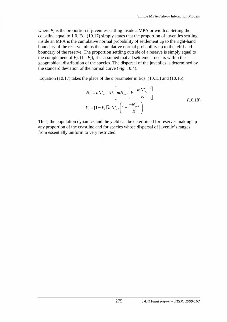
Simple MPA-Fishery Interaction Models
275 TAFI Final Report – FRDC 1999/162
where PJ is the proportion if juveniles settling inside a MPA or width c. Setting the coastline equal to 1.0, Eq. (10.17) simply states that the proportion of juveniles settling inside an MPA is the cumulative normal probability of settlement up to the right-hand boundary of the reserve minus the cumulative normal probability up to the left-hand boundary of the reserve. The proportion settling outside of a reserve is simply equal to the complement of PJ, (1 - PJ); it is assumed that all settlement occurs within the geographical distribution of the species. The dispersal of the juveniles is determined by the standard deviation of the normal curve (Fig. 10.4).
Equation (10.17) takes the place of the c parameter in Eqs. (10.15) and (10.16):
( )
1 1
1 1
rr r r t Jt t J t J
rr t J
t J t J
mNN aN P mN
K
mNY P mN
K
−− −
−−
= + −
= − −
(10.18)
Thus, the population dynamics and the yield can be determined for reserves making up any proportion of the coastline and for species whose dispersal of juvenile’s ranges from essentially uniform to very restricted.

General MPA-Fishery Interaction Models
TAFI Final Report – FRDC 1999/162 276
Chapter 11. MPAs and Fisheries: General Modelling INTRODUCTION
The Need for a Size-Structured Model
To model the effects and implications of MPAs for fisheries, a modelling strategy was adopted of first exploring the properties of generally applicable simple models, then general length based models, followed by length based models specific to the rock lobster fishery (see previous Chapter for a discussion of the strategy). In the discussion of the simple models of Chapter 10, population dynamics were described using a surplus-production model. In such models, populations are treated as undifferentiated biomasses that have inputs (recruitment, individual growth) and outputs (natural mortality and fishing mortality). This may be adequate for a basic treatment of stock dynamics, but if more realistic modelling is required then some improvement in the description of the stock dynamics is also required. This is principally achieved through an improved description of processes impacting the population. The original aim was to model the impacts of MPAs in rock lobster and abalone. However, the adult movement rate of abalone is at least an order of magnitude smaller than for rock lobster. In addition, evidence is accumulating to suggest that recruitment tends to be a relatively local affair, with localized stocks that collapsed 20 years ago still not recovering (Craig Mundy, TAFI, pers. comm.). In this instance, when we model a hypothetical abalone stock, closing a population leads to that population increasing in size in both biomass and size-structure. This has only insignificant effects upon surrounding populations, which decline by expected amounts due to the increased fishing mortality brought on by displaced catch. Even if the growth and egg production equations or parameters were different they would have no positive effect on populations outside of the MPAs. Once again, because of the displaced catch, MPAs would have local benefit by generalized negative effects.
This result is consistent with the findings of the simple but general modelling, described in the previous chapter, which indicated that if larval dispersal is highly constrained, an MPA entails no advantages to surrounding fisheries. A major disadvantage highlighted in the more complex model is that if the displaced effort is focused on only a few of the more productive blocks, this can lead to these becoming depleted with further displacement of catch until a serial depletion occurs and the fishery rapidly declines. It was concluded that closures displacing large amounts of abalone catch were a very risky management option because of a pre-disposition to serial depletion in this species. The original intention of the modelling component of the study was to consider the impact of MPAs on fisheries for both rock lobster and abalone. However, because of the very restricted movement dynamics of abalone together with their very limited larval dispersal, the focus shifted to rock lobster. Rock lobster cannot be aged with any precision or confidence, so rather than use an age-structured population model, a size-structured model was suggested. This follows the fate of different size-classes rather than different cohorts and requires a detailed description of individual growth. The present stock assessment of the Tasmanian rock

General MPA-Fishery Interaction Models
277 TAFI Final Report – FRDC 1999/162
lobster is based upon such a size-structured population model (Punt and Kennedy 1997, Hobday and Punt 2001), but lacks the spatial detail required to study the effects of introducing an MPA. It was overly restrictive to confine the study to two types of area (inside and outside the MPA) as was done in the simple models described in the previous chapter. In order to simulate alternative fleet dynamics (i.e. describe alternative responses to the closure of part of a fishery), it was necessary to include multiple areas in the spatial detail of the model. Having multiple areas also introduced the possibility of having a range of biological properties that might reflect the geographical distribution of things such as growth rates and recruitment.
Tasmanian rock lobster and abalone growth characteristics are spatially variable. For example, rock lobsters in the north of the state have relatively rapid growth while in the south they grow relatively slowly. Positively associated with the speed of growth is the final size to which the animals grow. Thus, in the north many of the animals reach the legal minimum length before they attain sexual maturity while in parts of the south the majority of females never attain the legal minimum length. Such variations have many implications for the outcomes of MPA establishment. The Tasmanian fisheries for both the rock lobster and abalone each have a detailed array of statistical reporting blocks for which there is catch and effort data. Not surprisingly, some of these statistical reporting blocks are very much more productive than others because of variation in catch, effort, productivity, growth and presumably recruitment. In the consideration of the complex but specific models (Chapter 12), this has many implications for the outcomes of implementing an MPA in an active commercial fishery. However, for the purposes of this chapter, such spatial variations constituted idiosyncratic noise and constrained the ability to clearly perceive the impacts of introducing MPAs. That is, when such variations are included in a model it needs to be determined whether the lack or otherwise of an impact with an MPA is related only to the presence of the MPA, and is not being mixed up with the effects of the particular circumstances of the specific fishery being modelled. For example, there are a number of statistical reporting blocks around Tasmania from which very little catch is ever taken. From the point of view of the abalone or rock lobster fisheries, if any of those blocks were ever completely closed then, it would have little or no detectible impact. Clearly, interactions between the introduction of an MPA and the details of the particular fishery lead to the outcomes of such introductions being obscured. To generate results and consequent conclusions that are applicable to more than just the specific fisheries being modelled, a strategy for avoiding the idiosyncratic effects relating to a specific fishery is needed. The strategy adopted here was one of using a single description of growth for each area together with constant recruitment and equal catch histories. This had the disadvantage of removing any similarity with a real fishery but the advantage that any conclusions drawn would be related primarily to the impacts of introducing the MPA. The objective of this part of the study was to describe the formal structure of the complex but general models and provide a summary of their main results. These models formed the basis of the complex but specific model of the Tasmanian rock lobster fishery described in Chapter 12.

General MPA-Fishery Interaction Models
TAFI Final Report – FRDC 1999/162 278
METHODS
Verbal Model Description
The MPA model was constructed around a spatially explicit, length- and sex-based single-species description of population dynamics. The explicit spatial structure was an essential aspect of the model because it provided the flexibility to have 50 or more separate spatial blocks each with a unique set of biological properties. Those chosen for this study included the growth characteristics of the individuals (by sex), natural mortality rate, and the initial size structure of the population.
It is important to note, however, that the model is open-ended and could easily be expanded to include other information relating to the dynamics of the population if these were available. So for example it was possible to include historical data on catches of the target species, but for the general version of the model used here the catch history in each case was hypothetical and assumed to be constant.
The geographical scale that can be used in the model should, clearly, not be finer than the limitations imposed by the spatial resolution of the data availability from the fishery and the biology of the species. Without this it would be best not to have too many geographical blocks represented in the model (Fig. 11.1).
43
42
147
41
7C3 7G4
3D4 3E3 3E4 3F3 3F4 3G3 3G4 3H3 3H4
3C1
7H3
3C2 3D1 3D2 3E1 3E2 3F1 3F2 3G1 3G2 3H1
7H4
3H2
7C1 7C2 7D1 7D2 7E1 7E2 7F1
7C4
7F2 7G1 7G2 7H1 7H2
6C3 6C4 6D3 6D4 6E3
7D3
6E4 6F3 6F4 6G3 6G4 6H3 6H4
6C1 6C2 6D1
7D4
6D2 6E1 6E2 6F1 6F2 6G1 6G2 6H1 6H2
5C3
7E3
5C4 5D3 5D4 5E3 5E4 5F3 5F4 5G3 5G4 5H3
7E4
5H4
5C1 5C2 5D1 5D2 5E1 5E2 5F1 5F2 5G1
7F3
5G2 5H1 5H2
4C3 4C4 4D3 4D4 4E3 4E4 4F3
7F4
4F4 4G3 4G4 4H3 4H4
4C1 4C2 4D1 4D2 4E1
7G3
4E2 4F1 4F2 4G1 4G2 4H1 4H2
3C3 3C4 3D3
43
42
147
41
7C3 7G4
3D4 3E3 3E4 3F3 3F4 3G3 3G4 3H3 3H4
3C1
7H3
3C2
7C3 7G4
3D4 3E3 3E4 3F3 3F4 3G3 3G4 3H3 3H4
3C1
7H3
3C2 3D1 3D2 3E1 3E2 3F1 3F2 3G1 3G2 3H1
7H4
3H2
7C1 7C2 7D1 7D2 7E1 7E2 7F1
7C4
7F2 7G1 7G2 7H1 7H2
6C3 6C4 6D3 6D4 6E3
7D3
6E4 6F3 6F4 6G3 6G4 6H3 6H4
6C1 6C2 6D1
7D4
6D2 6E1 6E2 6F1 6F2 6G1 6G2 6H1 6H2
5C3
7E3
5C4 5D3 5D4 5E3 5E4 5F3 5F4 5G3 5G4 5H3
7E4
5H4
5C1 5C2 5D1 5D2 5E1 5E2 5F1 5F2 5G1
7F3
5G2 5H1 5H2
4C3 4C4 4D3 4D4 4E3 4E4 4F3
7F4
4F4 4G3 4G4 4H3 4H4
4C1 4C2 4D1 4D2 4E1
7G3
4E2 4F1 4F2 4G1 4G2 4H1 4H2
3C3 3C4 3D3
Figure 11.1. Half-degree statistical reporting blocks around Tasmania used in the rock lobster fishery. The abalone fishery has a different set of reporting blocks. The three letter labels are their respective names. The thicker, darker lines denote the assessment regions used around Tasmania (labelled with degrees latitude and longitude), with Region 1 in the bottom right hand side, going up the east coast are regions 1 to 4. Coming down the west coast are regions 5 to 8.

General MPA-Fishery Interaction Models
279 TAFI Final Report – FRDC 1999/162
In the case of the Tasmanian rock lobster there are over thirty years of statistical reporting data, with over fifteen years at a resolution of half-degree blocks (Fig. 11.1). Most of the commercial catch of rock lobster can be accounted for by dealing with only thirty of the half-degree blocks. For the purposes of the complex but general model we used ten blocks (populations), which simplifies closing 10% of the coastline.
Spatial Scales
The underlying algorithm describing the dynamics of the system had a number of major steps. The coastline on which the MPA was to be introduced was implicit in the number of block or “populations” defined at the outset. The resolution of the model was at the scale implied for each block and the geographical scale was also implicitly defined in the movement rates between blocks. In Tasmania, neither rock lobster or abalone move very far as adults, with most abalone moving less than 100 metres (Prince et al, 1988), and rock lobster generally not moving more than 1000 metres over periods of up to 24 months (Gardner et al. 2003).
From this information the proportion of adults moving between blocks gave an indication of the geographical scale of the modelled blocks. The MPA constituted closure of a single block and this was surrounded by a number of fished blocks of varying relative size. The spatial structure and biological detail of the different populations were defined in a particular input file that was referenced when the coastline representation was built. Data relevant to each block was transferred to the program data-structures representing the different populations.
Initial Stock Conditions
In this version of the model it was elected to begin each population at equilibrium in terms of its size-structure and population size. Using a hypothetical and unvarying catch level the stock was then fished for a given number of years so that it attained the level of depletion implied by this combination of details. In addition to the details of the history of a particular fishery, its present status in terms of whether the stock was rebuilding or declining would also have a strong influence over the outcomes of introducing an MPA into the fishery. To cover this eventuality and retain the generality of the conclusions the behaviour of the modelled populations was examined assuming they were in equilibrium with the fishing pressure being applied. Therefore, after having applied a given fishing mortality for a set number of years the stock would have been depleted to a level dependent upon the applied constant catch level.
This depletion period was ten years at a constant high catch level followed by ten years at a constant lowered catch. This pattern was required to allow the size-structure to attain a new equilibrium before further analysis. At this point, the catch required to maintain the stock in equilibrium (the surplus production) was determined and fishing was continued at this level. The alternatives then considered were normal fishing for a further 25 years or the introduction of an MPA in one of the populations (Fig. 11.2).
The equations describing the dynamics of the spatially structured population are presented in Appendix 11.1 along with other equations describing the various

General MPA-Fishery Interaction Models
TAFI Final Report – FRDC 1999/162 280
performance measures used (e.g. egg production, fishing mortality rates and stock size indicators such as mature biomass, legal biomass).
Equilibrium Size Structureand Population Size
A constant fishing mortality is applied for 10 years, followed
by 10 years of reduced catch
The catch required tomaintain the population atequilibrium is determined.
Fishery projected for further 25 years
at constant catch
An MPA is introduced(a population is closed to fishing)
Effort redistributed (if the TAC is not reduced) and fishery projected for 25 years
Stock Status Determined:Size Structure, etc.
Repeat asRequired
Figure 11.2. Schematic diagram illustrating the organization of the analyses. By repeating this process using different levels of initial constant fishing mortality the effect of the level of initial depletion on the impacts of introducing an MPA can be investigated.
0.00
0.02
0.04
0.06
0.08
0.10
0.12
60
75
90
10
5
12
0
13
5
15
0
16
5
18
0
19
5
21
0
Carapace Length mm
Rel
ativ
e P
ropo
rtio
n Male
Female
Figure 11.3. The equilibrium size structure in the absence of fishing for the modelled rock lobster population using the size transition matrices from Assessment Region 1, an instantaneous natural mortality rate of 0.1, and an initial recruitment rate of 150,000 (per population).
The size structure of each population was described using 31 size-classes from 60mm up to 210mm (5 mm bins). All recruitment occurred into the 60mm size-class. The growth transition matrix used to describe the growth of animals in the base-case stock

General MPA-Fishery Interaction Models
281 TAFI Final Report – FRDC 1999/162
was taken from changes in carapace length of rock lobsters from the Tasmanian Stock Assessment Region 1 (Southeast; Fig. 11.1). When grown without fishing mortality and with a constant recruitment, this led to an equilibrium size structure for the stock that illustrated the much larger size to which males grow relative to females (Fig. 11.3).
A total of ten populations, each with identical growth and recruitment were used in the simulations. The legal minimum length was set at the current values in the Tasmanian fishery, 105 mm for males and 110 mm for females.
The dynamics of the hypothetical stock of ten populations were followed through time with or without fishing, and with or without an MPA. By growing the population without fishing the equilibrium stock structure was defined (see Fig. 11.3). Fishing mortality was then imposed on the unfished stock and the consequent depletion in biomass and numbers monitored. At any stage the maximum surplus production from the stock could be determined. This was the catch level that if applied would leave the stock at the same productivity level each year (i.e. it would leave the population in equilibrium; the surplus production). Because each population had identical biological characteristics, it was irrelevant which population was closed. We thus generated a base case against which all other instances are compared. The assumptions of this base case were represented by the list of parameters used in constructing the model (Appendix 11.2).
The equivalence of all populations meant that the redistribution of catch lost through closing one of the populations was simplified. It was not necessary to include a model of fleet dynamics because fishing effort was assumed to apply equally across all populations; this was equivalent to assuming that effort was distributed according to abundance or relative catch rates. Of course, on closing an area the available legal-sized biomass was immediately reduced by one tenth but the closed legal-sized biomass was increased by exactly that amount. The stock was then projected forward for a further 25 years, monitoring any population changes within the MPA and the effect of the redistribution of catch on the open stock. It is important to note that when the MPA was introduced the Total Allowable Catch was not reduced.
The base case used data on the growth characteristics and size at maturity from Assessment Region 1 in the southeast (see Fig. 11.1). Rock lobster from that Region are relatively slow growing and mature at a small size relative to most areas around Tasmania. To act as an immediate contrast, the analyses were replicated using the growth characteristics and size at maturity information from Region 5. These animals grow more rapidly, achieve a much larger final size in both sexes, and their size at maturity is much greater (see Appendix 11.2).

General MPA-Fishery Interaction Models
TAFI Final Report – FRDC 1999/162 282
RESULTS Effects of Fishing on Productivity (No MPA; Region 1).
Excess level of fishing pressure is applied to the stock until it is depleted to the desired level, a function of the catch taken. After the ten-year depletion period and the following ten years of stabilization, it was possible to determine the surplus production at the derived depletion level (Fig. 11.4), by searching for the catch level that maintains the stock as close as possible to the biomass status in year 20 of the simulation. Repeating this process for many different initial catch levels produced a curve of surplus production against legal biomass depletion levels (Figs 11.5 and 11.6). The productivity of the stock as a function of the depletion of legal biomass or total biomass was determined in part by the legal minimum lengths selected for the species concerned (Fig. 11.6). The base-case model used the current minimum legal length for Tasmanian rock lobsters that were set historically, without paying any attention to optimising yields. The smaller the minimum legal length the greater the negative impact of depletion on productivity in more depleted stocks (anything less than 30% unfished legal biomass in Fig. 11.6); at the same time the maximum productivity of the stock declined, as would be expected from classical yield-per-recruit considerations (Fig. 11.6).
0
0.05
0.1
0.15
0.2
0.25
0 10 20 30 40Year of Simulation
Fis
hing
Mor
tlaity
Rat
e F
0
2000
4000
6000
8000
10000
12000
14000
16000
18000
20000
Lega
l Sto
ck B
iom
as
Fishing Mortality
Legal Biomass
Figure 11.4. In this example, starting at unfished equilibrium, the modelled stock experiences 10 years of 1500 t catch followed by 35 years at 658.4 t, leading to an equilibrium at 36.89% of unfished legal-sized biomass. This percent decline is measured from the unfished state in year 1 to the final year of the simulation.

General MPA-Fishery Interaction Models
283 TAFI Final Report – FRDC 1999/162
0
10
20
30
40
50
60
70
80
90
100
0 4 8 12 16 20
Year of Simulation
Per
cent
Unf
ishe
d Le
gal B
iom
ass
500
1000
1500
2000
257.9
480.6
658.3
756.3
0
100
200
300
400
500
600
700
800
0 10 20 30 40 50 60 70 80 90 100
Percent Unfished Legal Biomass
Sur
plus
Pro
duct
ion
257.9
480.6
658.3
756.3
Catch per Year Surplus Production
Lower production due to 10% MPA
0
10
20
30
40
50
60
70
80
90
100
0 4 8 12 16 20
Year of Simulation
Per
cent
Unf
ishe
d Le
gal B
iom
ass
500
1000
1500
2000
257.9
480.6
658.3
756.3
0
100
200
300
400
500
600
700
800
0 10 20 30 40 50 60 70 80 90 100
Percent Unfished Legal Biomass
Sur
plus
Pro
duct
ion
257.9
480.6
658.3
756.3
Catch per Year Surplus Production
Lower production due to 10% MPA
Figure 11.5. The percent-unfished legal biomass and consequent surplus production calculated at differing degrees of stock depletion. When the ten hypothetical populations were fished at high levels for ten years (catch per year) different degrees of stock depletion occurred. At each of these levels of stock depletion there was a catch level that could be maintained through time, which was defined as the surplus production (left hand panel). By trying many different catch per year levels the curve of surplus production against stock depletion level was determined (right hand panel). If one of the 10 hypothetical populations was closed to fishing then the available productivity was immediately reduced to only 90% of the original (the lower line in the right hand panel).
0
100
200
300
400
500
600
700
800
0 20 40 60 80 100Percent Unfished Legal Biomass
Equ
ilibr
ium
Yie
ld
A
B
Figure 11.6. Two production curves for the modelled population. Curve A has minimum legal lengths of 105mm and 110 mm for females and males while curve B has LMLs of 80 and 85 mm respectively. The former are the current LMLs in Tasmania.
A consideration of the total stock biomass depletion levels that were possible provided a better illustration of the effect of different legal minimum lengths (Fig. 11.7). As less of the biomass was protected by a smaller legal size limit, the total biomass depletion level was lowered. With the smaller LMLs it was possible to see the turnover in the production curve as the depletion of the stock proceeded (Figs 11.6 and 11.7).

General MPA-Fishery Interaction Models
TAFI Final Report – FRDC 1999/162 284
0
100
200
300
400
500
600
700
800
0 20 40 60 80 100Percent Unfished Total Biomass
Equ
ilibr
ium
Yie
ld
A
B
Figure 11.7. The equilibrium yield obtainable from different degrees of depletion of total biomass (rather than only the legal-sized proportion; Figure 11.6). As in Fig. 11.6, curve A relates to minimum legal lengths of 105mm and 110 mm for females and males while curve B has LMLs of 80 and 85 mm respectively.
With a larger LML, it was not possible to lower the total biomass below a certain threshold (determined by the growth characteristics and the LML). Where this threshold biomass includes mature animals, there will always be a given biomass that was producing recruits, which is the protection afforded to a stock through the use of an appropriately selected legal minimum size.
Effect of Fishing on Equilibrium Size-Structure (No MPA)
As the level of legal biomass depletion increased, so did the instantaneous fishing mortality rate needed to keep the stock at a stable size (Fig. 11.8). In addition to altering the surplus production, stock depletion also altered the size-structure exhibited if the stock was then held in equilibrium (Fig. 11.9).
0.0
0.1
0.2
0.3
0.4
0.5
0.6
0.7
0.8
0 10 20 30 40 50 60Percent Unfished Legal Biomass
Inst
anta
neou
s F
0.0
0.1
0.2
0.3
0.4
0.5
0.6
0.7
0.8
0 10 20 30 40 50 60Percent Unfished Legal Biomass
Inst
anta
neou
s F
Figure 11.8. The instantaneous fishing mortality rate required to maintain the stock at equilibrium at different levels of depletion of the legal sized biomass (with an LML of 105mm for females and 110mm for males). Below a legal biomass of 10% the F required is extreme.

General MPA-Fishery Interaction Models
285 TAFI Final Report – FRDC 1999/162
0100002000030000400005000060000700008000090000
100000
60 80 100 120 140 160 180 200Carapace Length
Equ
ilibr
ium
Num
bers
100.0
57.7
26.3
8.8
Male
020000400006000080000
100000120000140000160000180000200000
60 80 100 120 140Carapace Length
100.0
57.726.3
8.8
Female
0100002000030000400005000060000700008000090000
100000
60 80 100 120 140 160 180 200Carapace Length
Equ
ilibr
ium
Num
bers
100.0
57.7
26.3
8.8
Male
0100002000030000400005000060000700008000090000
100000
60 80 100 120 140 160 180 200Carapace Length
Equ
ilibr
ium
Num
bers
100.0
57.7
26.3
8.8
Male
020000400006000080000
100000120000140000160000180000200000
60 80 100 120 140Carapace Length
100.0
57.726.3
8.8
Female
020000400006000080000
100000120000140000160000180000200000
60 80 100 120 140Carapace Length
100.0
57.726.3
8.8
Female
Figure 11.9. Relative size frequency distributions for rock lobsters given different depletion levels (the percent unfished legal-sized biomass at equilibrium). The numbers near each line refer to the depletion level. The unexploited distribution is determined by the growth description for rock lobster in the south east of Tasmania. Numbers of animals below legal size are reduced in scenarios with greater depletion due to the effects of the stock recruitment relationship. Note: The vertical line represents the LML for each sex. The y- and x-axes are on different scales in the two graphs.
Effects of Fishing on Productivity with MPA Implemented
In the base-case model the maximum stock productivity occurred when the legal biomass was depleted to approximately 14% of the unfished biomass (see Fig. 11.6). When the stock was only lightly depleted the introduction of an MPA led to the open biomass experiencing slightly increased levels of fishing mortality, which led to an increase in the level of depletion. This had the effect of increasing the productivity of the stock remaining open to fishing and a new equilibrium was produced (Fig. 11.10). However, the nett result was that the total legal biomass of the entire stock decreased slightly from a total of 9,973 t (without an MPA) to 9,957 t with an MPA. That is, the increase in legal sized biomass inside the MPA failed to make up for the decrease outside the MPA brought on by the increase in fishing mortality deriving from the displaced catch.
A slightly greater level of depletion led to a similar outcome except that the new equilibrium took far longer to be attained (Fig. 11.11). In this case, the total legal biomass was again smaller overall after the introduction of the MPA.
The size-structure of the stock inside the MPA moved towards the equilibrium structure (Fig. 11.12), although the reduction in recruitment brought about by the stock depletion affected the level of rebuilding, as did the 1% movement rate.
Once the stock becomes more seriously depleted, to just above the point of maximum productivity, the impact of introducing an MPA without making equivalent reductions in catch became more immediately apparent. In this case, the increase in fishing mortality outside the MPA did not lead to a new equilibrium but rather led to runaway depletion and ever increasing levels of fishing mortality required to maintain catches outside the MPA (Fig. 11.13).

General MPA-Fishery Interaction Models
TAFI Final Report – FRDC 1999/162 286
0.00
0.02
0.04
0.06
0.08
0.10
0.12
0 10 20 30 40Year of Simulation
Fis
hing
Mor
talit
y F
Without MPA
With MPA
02000400060008000
100001200014000160001800020000
0 10 20 30 40Year of Simulation
Sto
ck B
iom
ass Without MPAOpen Biomass
Closed Biomass
With MPA
0.00
0.02
0.04
0.06
0.08
0.10
0.12
0 10 20 30 40Year of Simulation
Fis
hing
Mor
talit
y F
Without MPA
With MPA
0.00
0.02
0.04
0.06
0.08
0.10
0.12
0 10 20 30 40Year of Simulation
Fis
hing
Mor
talit
y F
Without MPA
With MPAWith MPA
02000400060008000
100001200014000160001800020000
0 10 20 30 40Year of Simulation
Sto
ck B
iom
ass Without MPAOpen Biomass
Closed Biomass
With MPA
02000400060008000
100001200014000160001800020000
0 10 20 30 40Year of Simulation
Sto
ck B
iom
ass
02000400060008000
100001200014000160001800020000
02000400060008000
100001200014000160001800020000
0 10 20 30 40Year of Simulation
Sto
ck B
iom
ass Without MPAWithout MPAOpen Biomass
Closed Biomass
With MPA
Figure 11.10. Impacts on fishing mortality and biomass distribution when an MPA is introduced after the stock is only lightly depleted to 57.88% of unfished legal biomass. Without an MPA, the F required for stability was 0.0491, whereas with an MPA it became 0.0584 (left panel). Without an MPA the legal sized stock biomass is steady at 9,973 t (right panel). With an MPA, as expected, the open legal stock biomass is immediately decreased on the introduction of the MPA. However, the increased F leads to a slightly greater level of depletion through time leading to a new equilibrium of 8,434 t of biomass exposed to fishing. In the MPA the stock biomass increases from the initial 997.3 t up to a maximum of 1,525 t. The combined legal stock biomass in both open and closed areas becomes 9,957 t, slightly down (0.16%) from the situation where there is no MPA.
0
0.05
0.1
0.15
0.2
0.25
0 10 20 30 40Year of Simulation
Fis
hing
Mor
talit
y F
0
5000
10000
15000
20000
0 10 20 30 40Year of Simulation
Lega
l Sto
ck B
iom
ass
t
With MPA
Without MPA
Open Biomass
Closed Biomass0
0.05
0.1
0.15
0.2
0.25
0 10 20 30 40Year of Simulation
Fis
hing
Mor
talit
y F
0
5000
10000
15000
20000
0 10 20 30 40Year of Simulation
Lega
l Sto
ck B
iom
ass
t
With MPA
Without MPA
Open Biomass
Closed Biomass
Figure 11.11. Impacts on fishing mortality and biomass distribution when an MPA was introduced after the stock were depleted to 36.89% of unfished legal biomass. Without an MPA the F required for stability was 0.1092, whereas with an MPA it became 0.1446, although this value had not stabilized after 25 years (left panel). Without an MPA the legal sized stock biomass was steady at 6,362 t (right panel). With an MPA, once again, the increased F led to a greater level of depletion through time leading to a new legal biomass of 4,890 t of biomass exposed to fishing. Inside the MPA the legal biomass increased from the initial 636 t up to a maximum of 1,393 t. The combined legal stock biomass in both open and closed areas became 6,284 t, slightly down (1.23%) from the situation where there was no MPA. As with the fishing mortality, the legal biomass levels had not reached a stable equilibrium after 25 years.

General MPA-Fishery Interaction Models
287 TAFI Final Report – FRDC 1999/162
0
25000
50000
75000
100000
125000
150000
60 80 100 120 140 160 180 200Carapace Length mm
Rel
ativ
e F
requ
ency
0250005000075000
100000125000150000175000200000
60 70 80 90 100 110 120 130 140Carapace Length mm
Males Females
Unfished
FishedMPA
0
25000
50000
75000
100000
125000
150000
60 80 100 120 140 160 180 200Carapace Length mm
Rel
ativ
e F
requ
ency
0250005000075000
100000125000150000175000200000
60 70 80 90 100 110 120 130 140Carapace Length mm
0
25000
50000
75000
100000
125000
150000
60 80 100 120 140 160 180 200Carapace Length mm
Rel
ativ
e F
requ
ency
0
25000
50000
75000
100000
125000
150000
60 80 100 120 140 160 180 200Carapace Length mm
Rel
ativ
e F
requ
ency
0250005000075000
100000125000150000175000200000
60 70 80 90 100 110 120 130 140Carapace Length mm
0250005000075000
100000125000150000175000200000
60 70 80 90 100 110 120 130 140Carapace Length mm
0250005000075000
100000125000150000175000200000
60 70 80 90 100 110 120 130 140Carapace Length mm
Males Females
Unfished
FishedMPA
Figure 11.12. Impact on stock size-structure when an MPA was introduced after the legal biomass was depleted to 36.89% of unfished biomass. The outer solid-line in each panel illustrates the unfished size-structure of the stock for each sex; the inner solid-line represents the size-structure of the fished populations. What was not obvious was the reduction in recruitment levels leading to the generally lower numbers in each size class, even below the LML. The dotted line between the two solid-lines represents the size-structure of the stock within the MPA. The rebuilding towards the equilibrium state was obvious. The fine vertical lines were just below the LML for each sex. Note that the y- and x-axes have different scales on the two graphs.
00.10.20.30.40.50.60.70.80.9
0 5 10 15 20 25 30 35 40 45Year of Simulation
Fis
hing
Mor
talit
y F
0
2000400060008000
1000012000
1400016000
0 5 10 15 20 25 30 35 40 45Year of Simulation
Fis
hing
Mor
talit
y F
With MPA
Without MPA0
0.10.20.30.40.50.60.70.80.9
0 5 10 15 20 25 30 35 40 45Year of Simulation
Fis
hing
Mor
talit
y F
0
2000400060008000
1000012000
1400016000
0 5 10 15 20 25 30 35 40 45Year of Simulation
Fis
hing
Mor
talit
y F
0
2000400060008000
1000012000
1400016000
0 5 10 15 20 25 30 35 40 45Year of Simulation
Fis
hing
Mor
talit
y F
With MPA
Without MPA
Figure 11.13. Impacts on fishing mortality and biomass distribution when an MPA was introduced after the stock was depleted to 16.45% of unfished legal biomass. Without an MPA the F required (left panel) for stability was 0.3097, whereas with an MPA the fishing mortality steadily increased becoming 0.7426 after 25 years. Without an MPA the legal sized stock biomass was steady at 2,837 t (right panel). With an MPA, starting at such a depleted state led to the legal biomass open to fishing steadily declining without a new equilibrium being reached. After 25 years there was 1,410 t of legal biomass exposed to fishing, while inside the MPA the legal biomass increased from the initial 285 t up to 1,217 t. The combined legal stock biomass in both open and closed areas becomes 2,627 t, once again down (7.4%) from the situation where there was no MPA.

General MPA-Fishery Interaction Models
TAFI Final Report – FRDC 1999/162 288
Finally, if we introduced an MPA once the stock was depleted beyond the point of maximum productivity, the stock biomass exposed to fishing was rapidly depleted to the point that the TAC could not be taken; effectively the fishery had collapsed (not the stock). The biomass inside the MPA, however, reached levels greater than that outside the reserve (Fig.11.14). This is a critical prediction as it demonstrated the worst-case scenario of the reserve being surrounded by a collapsed fishery – a jewel in a sea of degraded habitat.
0
0.2
0.4
0.6
0.8
1
1.2
1.4
1.6
0 5 10 15 20 25 30 35 40 45Year of Simulation
Fis
hing
Mor
talit
y F
Without MPA
With MPA
0500
100015002000250030003500400045005000
0 5 10 15 20 25 30 35 40 45Year of Simulation
Lega
l Bio
mas
s t
Without MPA
0
0.2
0.4
0.6
0.8
1
1.2
1.4
1.6
0 5 10 15 20 25 30 35 40 45Year of Simulation
Fis
hing
Mor
talit
y F
Without MPA
With MPA
0500
100015002000250030003500400045005000
0 5 10 15 20 25 30 35 40 45Year of Simulation
Lega
l Bio
mas
s t
Without MPA
Figure 11.14. Impacts on fishing mortality and biomass distribution when an MPA was introduced after the stock was depleted to below its maximum productivity (9.545% of unfished legal biomass). Without an MPA the F required (left panel) for stability was 0.6084, whereas with an MPA the fishing mortality steadily increased to reach a maximum at about 15 years followed by a slight decline becoming 1.4028 after 25 years. Without an MPA the legal sized stock biomass was steady at 1,645 t (right panel; note the changed y-axis relative to earlier graphs). With an MPA, starting at such a depleted state led to the legal biomass open to fishing steadily declining until the biomass exposed to fishing was less than that inside the MPA. Eventually the TAC can no longer be completely taken and more recruits derive from the MPA than the open fishery.
While the depletion level of the legal biomass remained above that which gave rise to the maximum productivity, the total egg production behaves akin to the legal biomass (Fig. 11.15). That is, introducing an MPA led to a net reduction in the total legal-sized biomass and in egg production. However, when the legal sized biomass was below the depletion level that generated the maximum productivity, the number of eggs produced by the system with an MPA was greater than the numbers produced without the MPA (Fig. 11.15). At all stages there was an increase in egg production from within the MPA but, until the fishery had collapsed, this failed to make up for the reduction in the egg production from the population exposed to fishing (Fig. 11.16).

General MPA-Fishery Interaction Models
289 TAFI Final Report – FRDC 1999/162
0.98
0.99
1.00
1.01
1.02
1.03
1.04
1.05
0.0 10.0 20.0 30.0 40.0 50.0 60.0 70.0 80.0Percent of Unfished Legal Biomass
Egg
Pro
duct
ion:
With
out/W
ith M
PA
0.98
0.99
1.00
1.01
1.02
1.03
1.04
1.05
0.0 10.0 20.0 30.0 40.0 50.0 60.0 70.0 80.0Percent of Unfished Legal Biomass
Egg
Pro
duct
ion:
With
out/W
ith M
PA
Figure 11.15. The ratio of egg production without an MPA to egg production with an MPA relative to the percent of unfished legal biomass (depletion). Values greater than 1.0 indicate that more eggs are produced without an MPA than with an MPA. With very little depletion there was barely a difference between the two situations but as depletion starts to become more severe then the contribution of eggs from the reserve population comes to dominate so that at very high levels of stock depletion (90%), more eggs would be produced with an MPA than without one. This is essentially a state of fishery collapse.
1000
1050
1100
1150
1200
1250
1300
1350
1400
0 5 10 15 20 25 30 35 40Percent of Legal Biomass
Egg
Pro
duct
ion
x 10
9
With MPA
Without MPA
1000
1050
1100
1150
1200
1250
1300
1350
1400
0 5 10 15 20 25 30 35 40Percent of Legal Biomass
Egg
Pro
duct
ion
x 10
9
With MPA
Without MPA
Figure 11.16. Total egg production against percent of legal sized biomass in the base case. Egg production with an MPA was only greater overall when the legal sized biomass was reduced below that needed to produce the maximum productivity.
Effect of Movement Rate
All the previous analyses were conducted with a standard rate of movement of 1% of adults shifting between populations/blocks each year. Gardner et al. (2003), in an analysis of movement from 39,000 tag recoveries concluded that the majority of animals moved “… no detectable distance after periods of 1 to 2 years between capture events.” Even taking measurement error into account the lack of observed movement in Tasmanian rock lobster means that the 1% adult movement assumed to occur in the

General MPA-Fishery Interaction Models
TAFI Final Report – FRDC 1999/162 290
model was likely to be excessive. Not surprisingly, when the proportion of movement was increased the effect of the MPA on available legal biomass alters (Fig. 11.17). In this example, with 1% adult movement the introduction of a MPA led to increasing fishing mortality and no biomass equilibrium. Increasing adult movement (10 and 30%) led to the system reaching a new equilibrium. Thus, with higher movement rates, the impact of introducing a MPA was not as detrimental to the fishery as it was with lower movement rates.
As the proportion of adult movement increased, the negative effects of increasing fishing mortality outside the reserve were reduced. Considering the fishing mortality changes that occurred with different levels of adult movement (Fig. 11.18), increased adult movement could alter the effect of introducing an MPA from what would be an unstable situation leading to fishery collapse to one where a new equilibrium was reached (see Fig. 11.17). Similarly, the increase in fishing mortality on the stocks open to fishing, following the introduction of a MPA, was readily apparent. With only 1% movement the fishing mortality began to ramp up, quickly becoming unsustainable. As adult movement rates increased the outcome moved towards a new equilibrium, which was attained with greater speed as the proportion moving increased.
0
500
1000
1500
2000
2500
3000
3500
4000
4500
0 10 20 30 40
Year of Simulation
Lega
l Bio
mas
s t
Without MPA
With MPA0.01
0.01
0.1
0.10.3
0.3
0
500
1000
1500
2000
2500
3000
3500
4000
4500
0
500
1000
1500
2000
2500
3000
3500
4000
4500
0 10 20 30 40
Year of Simulation
Lega
l Bio
mas
s t
Without MPA
With MPA0.01
0.01
0.1
0.10.3
0.3
Figure 11.17. The impact of different assumed adult movement rates on changes to legal biomass when a MPA is introduced. The bold numbers to the right of the biomass curves represent the proportion of adults moving between blocks each year.
While increases in the movement rate could ameliorate the negative effects of increases in fishing mortality and decreases in legal biomass (Figs 11.17 & 11.18) the movement of larger animals out of the MPA also had an impact on the size-structure of the stock both inside and outside of the MPA (Figs.11.19 & 11.20).

General MPA-Fishery Interaction Models
291 TAFI Final Report – FRDC 1999/162
0.0
0.1
0.2
0.3
0.4
0.5
0.6
0 5 10 15 20 25 30 35 40 45
Year of Simulation
Fis
hing
Mor
talit
y 0.01
0.10.3
Without MPA
With MPA
0.0
0.1
0.2
0.3
0.4
0.5
0.6
0 5 10 15 20 25 30 35 40 45
Year of Simulation
Fis
hing
Mor
talit
y 0.01
0.10.3
Without MPA
With MPA
Figure 11.18. The influence of movement rate on the instantaneous fishing mortality rate following the introduction of an MPA.
0
20000
40000
60000
80000
100000
120000
140000
160000
180000
70 80 90 100 110 120 130Female Carapace Length mm
Rel
ativ
e F
requ
ency
Unfished
Without MPA
Outside MPA 0.01
Outside MPA 0.1
Inside MPA 0.01
Inside MPA 0. 1
0
20000
40000
60000
80000
100000
120000
140000
160000
180000
70 80 90 100 110 120 130Female Carapace Length mm
Rel
ativ
e F
requ
ency
Unfished
Without MPA
Outside MPA 0.01
Outside MPA 0.1
Inside MPA 0.01
Inside MPA 0. 1
Figure 11.19. Changes to the equilibrium size-structure of female rock lobster under different levels of adult movement (other circumstances equivalent to the situation displayed in Figs. 11.17 & 11.18). The outer thick black line is the unfished size-structure. All curves shared the same trajectory up until the size-class prior to the legal minimum length (105mm). Inside the MPA with 1% movement the size-structure approximated the unfished levels except for the effect of reduced recruitment following stock depletion (thick blue line). The fine line immediately inside this line represented the size-structure inside the MPA when there was 10% adult movement. It is closer to the line representing the size-structure when there is no MPA present. With greater movement the size-structure inside the MPA moves even closer to the no-MPA situation. Similarly, the size-structure outside the MPA moves closer to the no-MPA line as adult movement rates increase.
The changes to the size-structure brought about by changes in adult movement are more marked outside the MPA than inside. In both cases the size-structure converges on the size-structure exhibited by a system without an MPA. However, outside the MPA, with 30% adult movement, the size-structure is very close to that obtained without an MPA, whereas inside the MPA there is still some visible increase in the relative numbers at size (Figs. 11.19 & 11.20).

General MPA-Fishery Interaction Models
TAFI Final Report – FRDC 1999/162 292
0
10000
20000
30000
40000
50000
60000
70000
80000
90000
100000
60 80 100 120 140 160 180 200Male Carapace Length mm
Rel
ativ
e F
requ
ency
Unfished
Inside MPA 0.01
Inside MPA 0.1
Inside MPA 0.3
Outside MPA 0.01
Without MPA
Outside MPA 0.1
Outside MPA 0.30
10000
20000
30000
40000
50000
60000
70000
80000
90000
100000
60 80 100 120 140 160 180 200Male Carapace Length mm
Rel
ativ
e F
requ
ency
Unfished
Inside MPA 0.01
Inside MPA 0.1
Inside MPA 0.3
Outside MPA 0.01
Without MPA
Outside MPA 0.1
Outside MPA 0.3
Figure 11.20. Changes to the equilibrium size-structure of male rock lobster under different levels of adult movement (1%, 10% and 30%). The outer thick black line is the unfished size-structure. All curves share approximately the same trajectory up until the size-class prior to the legal minimum length (110mm). As the movement rate of adults increases, the size-structure both inside and outside the MPA converge on the equilibrium size-structure obtained without implementing an MPA.
Effects of Fishing on Productivity (No MPA; Region 5)
In Tasmania, despite spatial differences in growth and maturity, the same LML are used in the north and south of the state; 105mm for females and 110mm for males. When the model population parameters relating to growth and size at maturity reflected those in the northwest of Tasmania (Region 5), several differences in the dynamics were apparent. The yield curve for the usual LML exhibited the classical turn over in productivity as depletion proceeded, with a maximum productivity produced at a legal biomass depletion level of approximately 26.57%. With LMLs of 130mm and 135mm the production curve still turns over but with a higher maximum yield being produced at a depletion level of 22.19%. Finally, with LMLs of 145mm and 150mm it becomes difficult to deplete the stock beyond the point of maximum production (a risk averse strategy), and yet the stock is more productive still when depleted to approximately 18.35% (Fig. 11.21; Table 11.2). The three different sets of LMLs also had implications for the equilibrium size-structure in the absence of an MPA. A different fishing mortality rate was required to maintain the legal biomass depletion level at the level that implied the highest level of productivity (Fig. 11.21; Table 11.2). It became clear that the larger the LML the steeper the drop-off in the size-structure (Fig. 11.22). These results indicated that the present Tasmania-wide set of legal minimum lengths (105mm for females and 110mm for males) was far from optimal in terms of yield-per-recruit and could mean that stock recovery from a state of depletion to the left of the maximum yield could be more difficult to attain. The massive amount of biomass in the accumulation of large males meant that the biomass depletion had little visible effect on the size-structure until depletion reached high levels.

General MPA-Fishery Interaction Models
293 TAFI Final Report – FRDC 1999/162
550
750
950
1150
1350
1550
1750
0.0 10.0 20.0 30.0 40.0 50.0 60.0 70.0 80.0
Percent of Unfished Legal Biomass
Equ
ilibr
ium
Yie
ld t
145+150
130+135
105+110
550
750
950
1150
1350
1550
1750
0.0 10.0 20.0 30.0 40.0 50.0 60.0 70.0 80.0
Percent of Unfished Total Biomass
145+150
130+135
105+110
550
750
950
1150
1350
1550
1750
550
750
950
1150
1350
1550
1750
0.0 10.0 20.0 30.0 40.0 50.0 60.0 70.0 80.0
Percent of Unfished Legal Biomass
Equ
ilibr
ium
Yie
ld t
145+150
130+135
105+110
550
750
950
1150
1350
1550
1750
0.0 10.0 20.0 30.0 40.0 50.0 60.0 70.0 80.0
Percent of Unfished Total Biomass
145+150
130+135
105+110
550
750
950
1150
1350
1550
1750
0.0 10.0 20.0 30.0 40.0 50.0 60.0 70.0 80.0
Percent of Unfished Total Biomass
145+150
130+135
105+110
Figure 11.21. The equilibrium yield obtained at different degrees of depletion of total legal biomass (left hand panel) and total biomass (right hand panel). The pairs of numbers at the end of each curve related to the legal minimum lengths for females and males respectively. The 105 and 110mm are the current LMLs in Tasmania. Clearly, in the north west (Region 5) it would be better to have LMLs of 130 and 135 or even 145 and 150mm so as to optimise the yield produced and prevent dangerous levels of stock depletion. In the plot of total biomass it becomes extremely difficult to deplete the stock below about 30% with LMLs of 145 and 150mm.
0
5000
10000
15000
20000
25000
30000
35000
60 80 100 120 140 160 180 200
Unfished
105-110
145-150
0
50000
100000
150000
200000
250000
300000
60 80 100 120 140 160 180 200
Rel
ativ
e F
requ
ency
Males
0
10000
20000
30000
40000
50000
60000
70000
60 80 100 120 140 160 180 200Carapace Length mm
Unfished
145-150
105-1100
20000
40000
60000
80000
100000
60 80 100 120 140 160 180 200Carapace Length mm
Rel
ativ
e F
requ
ency
Females
0
5000
10000
15000
20000
25000
30000
35000
60 80 100 120 140 160 180 200
Unfished
105-110
145-150
0
5000
10000
15000
20000
25000
30000
35000
60 80 100 120 140 160 180 200
Unfished
105-110
145-150
0
50000
100000
150000
200000
250000
300000
60 80 100 120 140 160 180 200
Rel
ativ
e F
requ
ency
Males
0
50000
100000
150000
200000
250000
300000
60 80 100 120 140 160 180 200
Rel
ativ
e F
requ
ency
Males
0
10000
20000
30000
40000
50000
60000
70000
60 80 100 120 140 160 180 200Carapace Length mm
Unfished
145-150
105-1100
10000
20000
30000
40000
50000
60000
70000
60 80 100 120 140 160 180 200Carapace Length mm
Unfished
145-150
105-1100
20000
40000
60000
80000
100000
60 80 100 120 140 160 180 200Carapace Length mm
Rel
ativ
e F
requ
ency
Females
0
20000
40000
60000
80000
100000
60 80 100 120 140 160 180 200Carapace Length mm
Rel
ativ
e F
requ
ency
Females
Figure 11.22. The effect of three different sets of LML upon the equilibrium size-structure of rock lobster at the stock’s most productive level of depletion. The right-hand panels were larger scale representations of the left-hand panels, with the first and last size classes removed. The left-hand panel illustrated the expectation for the unfished stock in Region 5, that of a major build-up of biomass in the largest size-class in males. Because of this the decline in legal biomass was quite marked even though there were many relatively large animals remaining. As expected, because of the higher fishing mortality (Table 11.2), the largest LML led to the steepest drop-off in size-structure. The relatively flat size-structure of males under the LML and the build-up of females under the LML in each case were due to the relatively rapid growth rate in this region.

General MPA-Fishery Interaction Models
TAFI Final Report – FRDC 1999/162 294
Table 11.2. Properties of the point of maximum yield on the surplus production curve (Fig. 11.21) for the three sets of Legal Minimum Lengths (LML; first female then male). F-Equilibrium was the fishing mortality rate required to maintain the stock at its most productive once it had been depleted to the required level (Depletion%). Relative Productivity was the ratio of the maximum production, given a particular set of LML, with that produced by the 105-110 LML. LML 105-110 130-135 145-150 F-Equilibrium 0.143 0.2109 0.308 Depletion % 26.57 22.19 18.35 Relative Productivity 1.0000 1.1022 1.1469
Effects of Fishing on Productivity with MPA (Region 5)
As in Region 1, when an MPA was introduced into a lightly depleted stock a new equilibrium was achieved in which fishing mortality outside the MPA was slightly higher. The biomass outside the MPA was somewhat reduced, by an amount similar to the increase inside the reserve. The net effect was to very slightly reduce legal-sized biomass (Fig. 11.23).
0.000
0.005
0.010
0.015
0.020
0.025
0.030
0.035
0.040
0.045
0 5 10 15 20 25 30 35 40 45Year of Simulation
Fis
hing
Mor
talit
y F
With MPA
Without MPA
0
5000
10000
15000
20000
25000
30000
35000
40000
45000
0 5 10 15 20 25 30 35 40 45Year of Simulation
Tot
al L
egal
Bio
mas
s Open Biomass
Closed Biomass
With MPA
Without MPA
0
5000
10000
15000
20000
25000
30000
35000
40000
45000
0 5 10 15 20 25 30 35 40 45Year of Simulation
Tot
al L
egal
Bio
mas
s Open Biomass
Closed Biomass
With MPA
Without MPA
Figure 11.23. Impacts on fishing mortality and biomass distribution on introduction of an MPA (stock at 75.47% of unfished legal biomass). Without an MPA the F required (left panel) for stability was 0.0223, whereas with an MPA it became 0.0256. Without an MPA the legal sized stock biomass was steady at 31,078t (right panel). With an MPA, a new equilibrium of 27,156t of biomass exposed to fishing arose, while in the MPA legal biomass stabilized at 3,886t. The combined legal stock biomass in both open and closed areas became 31,042t, slightly down (0.12%) from the situation where there was no MPA.

General MPA-Fishery Interaction Models
295 TAFI Final Report – FRDC 1999/162
At a somewhat greater level of depletion a new equilibrium was achieved except that it took far longer to be attained (Fig. 11.24).
0
0.05
0.1
0.15
0.2
0.25
0 5 10 15 20 25 30 35 40 45Year of Simulation
Fis
hing
Mor
talit
y
With MPA
Without MPA
0
5000
10000
15000
20000
25000
30000
35000
40000
45000
0 5 10 15 20 25 30 35 40 45Year of Simulation
Lega
l Bio
mas
s t
Open Biomass
Closed Biomass
Without MPA
0
0.05
0.1
0.15
0.2
0.25
0 5 10 15 20 25 30 35 40 45Year of Simulation
Fis
hing
Mor
talit
y
With MPA
Without MPA
0
5000
10000
15000
20000
25000
30000
35000
40000
45000
0 5 10 15 20 25 30 35 40 45Year of Simulation
Lega
l Bio
mas
s t
Open Biomass
Closed Biomass
Without MPA
Figure 11.24. Impacts of the introduction of an MPA on fishing mortality and biomass distribution (stock at 35.47% of unfished legal biomass). Without an MPA the F required (left panel) for stability was 0.1021, whereas with an MPA it became 0.1443, but without attaining an equilibrium. Without an MPA the legal sized stock biomass was steady at 14,698 t (right panel). With an MPA a new equilibrium arose of 10,613 t of biomass exposed to fishing, while in the MPA legal biomass reached 3,362 t without stabilizing. The combined legal-sized biomass in both open and closed areas became 13,975 t, which was 5% down from the situation where there was no MPA.
The effect on the size-structure of the population within and outside of the MPA was strongly marked using population parameters from Region 5 (Figs. 11.25 & 11.26). The size-structure inside the MPA was not identical to the original unfished state because of the reduced recruitment deriving from the state of depletion (Fig. 11.25). In the fished population there were still large numbers of large animals present, which was a function of the rapid growth rate. The major effect of depletion on male rock lobsters from Region 5 was to remove the accumulated biomass in the largest size-class.
0
50000
100000
150000
200000
250000
300000
60 80 100 120 140 160 180 200Carapace Length mm
Rel
ativ
e F
requ
ency Male
0
5000
10000
15000
20000
25000
30000
60 80 100 120 140 160 180 200Carapace Length mm
Rel
ativ
e F
requ
ency
In MPA
No MPA
Outside MPA0
50000
100000
150000
200000
250000
300000
60 80 100 120 140 160 180 200Carapace Length mm
Rel
ativ
e F
requ
ency Male
0
5000
10000
15000
20000
25000
30000
60 80 100 120 140 160 180 200Carapace Length mm
Rel
ativ
e F
requ
ency
In MPA
No MPA
Outside MPA
Figure 11.25. The effect of introducing an MPA on the population size-structure of males after the stock has been depleted to its most productive state (~26.5% of unfished legal biomass). Male growth rates in Region 5 are very fast and most of the biomass in an unfished state would be accumulated above 200mm carapace length (left panel). To clarify the effect of introducing a MPA the first and last size-classes were omitted from the right hand panel.

General MPA-Fishery Interaction Models
TAFI Final Report – FRDC 1999/162 296
In Region 5 female rock lobsters grew much faster and bigger than their more southerly counterparts. The impact of introducing an MPA into such a population was to move the size-structure of animals inside the MPA towards that seen in the unfished size-structure, while the size-structure outside the MPA declines further, moving towards smaller animals (Fig. 11.26). If movement rates were increased then, as before, the size structures moved towards becoming similar to the size-structure of animals produced when no MPA was introduced.
0
20000
40000
60000
80000
100000
120000
60 80 100 120 140 160 180 200Carapace Length mm
Rel
ativ
e F
requ
ency Unfished
0
10000
20000
30000
40000
50000
60000
60 80 100 120 140 160 180 200Carapace Length mm
Rel
ativ
e F
requ
ency In MPA
Outside MPA
No MPA
0
20000
40000
60000
80000
100000
120000
60 80 100 120 140 160 180 200Carapace Length mm
Rel
ativ
e F
requ
ency Unfished
0
10000
20000
30000
40000
50000
60000
60 80 100 120 140 160 180 200Carapace Length mm
Rel
ativ
e F
requ
ency In MPA
Outside MPA
No MPA
Figure 11.26. Effect of introducing an MPA on the size-structure of female rock lobster from Region 5. The left hand panel illustrated the unfished equilibrium size-structure and the two curves deriving from introducing the MPA. The right hand panel omits the top and bottom size-class to expand the view of the changes incurred (the unfished equilibrium line was also omitted for clarity).
Once the stock was depleted to a point where it was past the point of maximum productivity (easily possible in Region 5 with the current LML) then the negative impact of introducing an MPA became very clear (Fig. 11.27). The fishing mortality outside the MPA increased rapidly and did not attain equilibrium except when the fishery had collapsed and was depleted to very low levels.
00.20.40.60.8
11.21.41.61.8
0 5 10 15 20 25 30 35 40 45Year of Simulation
Fis
hing
Mor
talit
y F
With MPA
No MPA0
2000
4000
6000
8000
10000
12000
14000
0 5 10 15 20 25 30 35 40 45Year of Simulation
Lega
l Bio
mas
s t
No MPA
Open Biomass
Outside
Inside0
0.20.40.60.8
11.21.41.61.8
0 5 10 15 20 25 30 35 40 45Year of Simulation
Fis
hing
Mor
talit
y F
With MPA
No MPA0
2000
4000
6000
8000
10000
12000
14000
0 5 10 15 20 25 30 35 40 45Year of Simulation
Lega
l Bio
mas
s t
No MPA
Open Biomass
Outside
Inside
Figure 11.27. Impact of introducing an MPA onto a stock with population properties akin to Region 5 and at a depletion level (16.65%) well below the point of maximum production. The final plateau in the fishing mortality merely reflected various constraints built into the model, it did not permit extreme fishing mortalities that would imply unrealistically small catch rates. The legal biomass outside the MPA fell to well below that inside the MPA. At this level of biomass reduction the TAC was significantly under-achieved. Without an MPA the legal biomass could remain stable at 6,847t. With an MPA the legal biomass outside the MPA dropped dramatically to 1,103t and inside the MPA rose to 2,771t, a combined total of only 2,837t (only 58.7% of the biomass without an MPA).

General MPA-Fishery Interaction Models
297 TAFI Final Report – FRDC 1999/162
The effect of introducing an MPA into Region 5 appeared more marked, and the fishery collapse was more rapid and extreme than when the simulation represented the biology of animals from Region 1 (Fig. 11.13). This was partly due to the LML being set at too small a size for the growth characteristics of the region. At this LML the depletion level and consequent reduction in productivity was far more extreme (Fig. 11.21). The drastic reduction in legal biomass led to a massive reduction in egg production so that, unlike in Region 1, even after stock collapse there was no net benefit in terms of egg production (Fig. 11.28).
0.0
0.5
1.0
1.5
2.0
2.5
3.0
0 20 40 60 80
Percent of Unfished Legal Biomass
Egg
Pro
duct
ion:
No
MP
A/M
PA
0
500
1000
1500
2000
2500
3000
3500
0 20 40 60 80
Percent of Unfished Legal Biomass
Egg
Pro
duct
ion
x 10
9No MPA
With MPA0.0
0.5
1.0
1.5
2.0
2.5
3.0
0 20 40 60 80
Percent of Unfished Legal Biomass
Egg
Pro
duct
ion:
No
MP
A/M
PA
0.0
0.5
1.0
1.5
2.0
2.5
3.0
0 20 40 60 80
Percent of Unfished Legal Biomass
Egg
Pro
duct
ion:
No
MP
A/M
PA
0
500
1000
1500
2000
2500
3000
3500
0 20 40 60 80
Percent of Unfished Legal Biomass
Egg
Pro
duct
ion
x 10
9No MPA
With MPA0
500
1000
1500
2000
2500
3000
3500
0 20 40 60 80
Percent of Unfished Legal Biomass
Egg
Pro
duct
ion
x 10
9E
gg P
rodu
ctio
n x
109
No MPA
With MPA
Figure 11.28. The ratio of egg production outside the MPA to that inside the MPA as a function of legal biomass depletion level. As with Region 1, initially there is only a slight decline in the relative egg production as stock depletion continues but as it reaches and passes the point of maximum stock production the fishery rapidly collapses when an MPA is introduced and this leads to a marked reduction in the total relative egg production in the system with an MPA (left panel). The absolute egg production declines linearly with depletion level when there is no MPA (right panel). However, with an MPA, absolute egg production deviates below a linear relationship up until depletion passes the level of maximum production whereupon egg production plummets with the fishery collapse and the relative contribution of the MPA rises markedly, though not enough to offset the losses. The plateau at the bottom of the egg production curve with an MPA reflects the biomass limit that the model does not permit the stock to pass below.
Assumption of No Reduction in Catch
One of the key assumptions in the analyses above was that there would be no equivalent reduction in catch to balance the implementation of an MPA. It was therefore considered to be important that the outcomes of reducing effort appropriately at the same time as introducing an MPA be made apparent. These were to be compared to not reducing catch and to reducing catch by the same amount, but without introducing an MPA (Fig. 11.29). For example (dotted line in Fig 11.29), with 30% legal biomass remaining the egg production would be reduced by about 2% (MPA only), increased by about 4.5% (MPA and 10% catch reduction), and increased by almost 6%.

General MPA-Fishery Interaction Models
TAFI Final Report – FRDC 1999/162 298
At low levels of depletion implementing an MPA without adjusting the catch only has a minor depressive effect on both egg production and total biomass. At more severe levels of depletion the depressive effects increase in a non-linear manner such that at about 16% depletion level egg production and total biomass are 4% and 6% down on the situation without an MPA (see Fig. 11.29). If the catch is reduced by 10% concurrently with the implementation of an MPA, after 25 years, egg production has increased about 8% above the fished case and total biomass has risen by 45%. However, if catch was simply reduced by 10% and no MPA implemented, then egg production increases by just over 10% and total biomass increases by about 50%. That is, the MPA has acted to dampen the benefit of the catch reduction on egg production and total biomass. Clearly, if ecosystem functionality were related to stock size then catch reductions would achieve more than closed areas alone.
0.9
1.0
1.1
1.2
1.3
1.4
1.5
1.6
10 20 30 40 50 60 70Percent Unfished Legal Biomass
Pro
port
iona
l Tot
al B
iom
ass
Fished
10% Catch Reductiononly
10%With MPA
MPA only0.94
0.96
0.98
1.00
1.02
1.04
1.06
1.08
1.10
1.12
10 20 30 40 50 60 70Percent Unfished Legal Biomass
Pro
port
iona
l Egg
Pro
duct
ion
Fished
10% Catch Reductiononly
10%WithMPA
MPA only0.9
1.0
1.1
1.2
1.3
1.4
1.5
1.6
10 20 30 40 50 60 70Percent Unfished Legal Biomass
Pro
port
iona
l Tot
al B
iom
ass
Fished
10% Catch Reductiononly
10%With MPA
MPA only0.94
0.96
0.98
1.00
1.02
1.04
1.06
1.08
1.10
1.12
10 20 30 40 50 60 70Percent Unfished Legal Biomass
Pro
port
iona
l Egg
Pro
duct
ion
Fished
10% Catch Reductiononly
10%WithMPA
MPA only
Figure 11.29. Changes to the proportion of relative egg production and total legal biomass that arise under three scenarios: 10% MPA only, 10% catch reduction only, and a 10% MPA with a 10% catch reduction. All scenarios were compared to the base case of equilibrium fishing at each level of depletion (marked as ‘Fished’). The left hand panel illustrates the effect of increased levels of depletion of legal biomass on egg production over a 25-year simulation. If a 10% MPA was implemented and catch was not appropriately decreased it resulted in a steady decline in the egg production. If a 10% reduction in catch was introduced with the MPA then the line labelled “With MPA” resulted. If there is a 10% reduction in catch and no MPA implemented then the line labelled “10% catch reduction” results.

General MPA-Fishery Interaction Models
299 TAFI Final Report – FRDC 1999/162
DISCUSSION MPAs and Fisheries Management
In the debate over the value of using MPAs for fisheries management purposes at least four positive outcomes are commonly claimed for MPAs, including:
- Large areas closed to fishing will act as reproductive centers and replenish areas both outside and inside the reserves (Anon 1990, Roberts and Hawkins 2002).
- They are an alternative to existing fisheries management where information is absent (Johannes, 1996).
- The bigger the area the better for fisheries (Nilsson 1998).
- Larval sources would provide most benefits to fisheries (Stockhausen et al. 2000).
However, negative outcomes have also been discussed, including:
- Migratory species would not benefit (Parrish 1999).
- Highly mobile species would receive reduced benefit (Kramer and Chapman 1999).
- Fisheries for sedentary, benthic species, with limited larval dispersal, receive little benefit from MPAs (Kramer and Chapman 1999).
- Displaced fishing effort can harm the fishery remaining outside the reserve (Haddon et al. 2003).
- Except in fortuitous circumstances, MPAs can only be optimized for single species, which would compromise the broader objective of maintenance of multi-species diversity.
The modelling conducted for this chapter was focused, in the first instance, on what would happen in an hypothetical rock lobster fishery if a relatively large MPA (10% of the coastline and fishery) was introduced but the catch from the fishery was not reduced by an equivalent amount. Without the reduction in catch then effort previously applied to the area now closed was displaced to other productive regions in the fishery. The model conclusions relate to a specific set of conditions and biological assumptions, nevertheless, the conclusions are general.
General Impacts of Implementing an MPA
In terms of recovery of stock biomass, of egg production, and general sustainability the introduction of a relatively large MPA, without appropriately reducing the catch, had negative impacts of varying intensity. In general, the imposition of extra catch from the area remaining open obviously led to a higher fishing mortality rate and an increase in the level of stock depletion. If the catch levels were held constant then the stock was able to attain a new, more productive equilibrium level at which its surplus production matched the catch required of it.

General MPA-Fishery Interaction Models
TAFI Final Report – FRDC 1999/162 300
Attaining this new equilibrium was only possible if the stock was not depleted to a level close to the maximum productivity. Under such circumstances, the extra production required could not be generated from increasing the stock’s productivity and, instead, the catch led to depleting the stock further until it became less productive, which in turn led the fishery to collapse (Fig. 11.30). Of course, in the presence of an MPA the stock does not entirely collapse because of the fish in the protected area, but the fishery would becomes unsustainable and the TAC would not be caught.
400
420
440
460
480
500
520
540
50 52 54 56 58 60
Percent Unfished Legal Biomass
Sur
plus
Pro
duct
ion
47.7t/pop
With MPA
No MPA
53t/pop
57.7%52.1%
429 t
No MPA
600
620
640
660
680
700
720
740
760
10 15 20 25 30 35
Percent Unfished Legal Biomass
Sur
plus
Pro
duct
ion
69.8t/pop
Collapse?
77.6t/pop
30.4%13.8%
With MPA
Figure 11.30. Illustrating the mechanism by which the introduction of an MPA impacts on the legal biomass of the stock (each panel is a magnified subset of the curves in Fig. 11.5). In each case, the upper curve represents the surplus production at a given percent of unfished legal biomass (depletion). With only slight depletion (left hand panel), a yield of 477t implies a catch of 47.7t from each of 10 populations (large dot on upper curve). By closing one population to fishing, the immediate surplus production is reduced to 90% of the original, which can only sustainably produce ~429t. To compensate, ~53t must be taken from the remaining 9 populations to obtain the original 477t total catch. Thus, the stock is depleted down from 57.7% to 52.1%. In the more heavily depleted situation (right hand panel), closing one population (10% MPA) requires an adjustment from 69.8t from each of 10 populations to 77.6t from the remaining 9 populations. This is not possible because the maximum productivity of the 9 populations is only ~680 t, a shortfall of ~20 t from the original catch. This extra 20t must come from stock biomass, which, if the catch is maintained, moves the fishery into an unsustainable cycle of increasing depletion, rising fishing mortality, and eventual fishery collapse.
Benefits from Adult Movement (Spillover)
The expectation is that movement or spillover of adult animals, plus increased egg production from an MPA, would provide a nett benefit to the stock as a whole. However, if movement of adults is only minor (as is the case with Tasmanian rock lobster, and even more so with Tasmanian abalone) then adult movement can only provide a slight input of extra biomass to the fished stock. If movement is more significant (e.g. 10-20% of adults move each year), then the negative effects of MPAs on stock size are ameliorated. However, as movement increases the size-structure of the populations inside the MPA begin to alter towards that exhibited by a fished stock without an MPA. In effect, the protection offered to the animals by the MPA becomes reduced as a function of their mobility. That is, the benefits to the population inside the MPA are lost to increasing degrees as movement rates increase.

General MPA-Fishery Interaction Models
301 TAFI Final Report – FRDC 1999/162
There is a time lag between implementing an MPA and its population rebuilding to an extent where adult movement and egg production begin to increase significantly above the original rates. This time lag is important because of the potential damage that may be done to the stock remaining open to fishing before any of the ameliorating influences of the MPA can come into force.
Impacts on Stock Biomass
The cessation of catch within an MPA leads to the size-structure moving towards the unfished state, and hence the biomass of the population of animals inside the MPA increases (Roberts and Polunin 1991). However, because of non-linear effects of fishing mortality on stock biomass (see Fig. 11.29) the displaced catch from the MPA leads to a greater than intuitively expected reduction in biomass outside the MPA. The nett effect is to decrease the overall total and mature biomass levels. In the complex but general model with identical blocks, the benefit of increasing the biomass within the MPA is obtained at the cost of a disproportionate reduction of the biomass outside the MPA.
Impacts on Egg Production
The impacts of introducing an MPA on the egg production of the stock were analogous to those on stock biomass. Egg production inside the MPA increased rapidly, however, the decline in productive animals outside the MPA more than offset the benefits of the MPA, such that the nett effect of introducing an MPA was to decrease egg production. Once again, the only time that a positive effect on egg production was observed occurred under conditions where there had already been a fishery collapse and the biomass outside the MPA was smaller than that inside. When the legal minimum length (LML) was set at an inappropriately small size it was possible to deplete a stock to a level far below maximum productivity (see Fig. 11.21), leading to a severe fishery collapse. If the LML was reset to a more appropriate level, the stock became far more robust and productive. The negative effects of MPAs on stock biomass and egg production were more severe when there was a mis-match between the LML and the growth characteristics of the population (see Fig. 11.21). It must be remembered that in this case the model was simulating a homogeneous stock, the populations of which had identical biological properties. When a stock was made up of populations having different properties the conclusions could be different (see the next chapter on complex but specific models).
The analysis conducted here assumed that recruitment occurred in proportion to the available biomass. That is, that there were no source populations and no sinks. Clearly if it were possible to identify a source population then enclosing it inside an MPA would make good sense, unless it was already adequately protected by the legal minimum length. However, puerulus collection around Tasmania indicates that good years for recruitment in some places do not always match good years in other places. Thus, sinks, if they can be called that, are not a constant from year to year. This does not imply that sources are also variable, but no strong evidence exists that indicates otherwise (Bruce et al., 2001; Bestley, 2001)

General MPA-Fishery Interaction Models
TAFI Final Report – FRDC 1999/162 302
Depletion Rates
Of great interest was the fact that stock depletion can occur in the populations that remained open but this may only occur at such a slow rate so as not to be detectable until stock depletion is far advanced towards fishery collapse. Such slow depletion towards eventual fishery collapse would provide a challenge for any management regime. Under a stochastic environment of recruitment this would be even more difficult to detect.
MPAs for Fishery Management
It is true that when a fishery collapses an MPA provides for a fishery (albeit a greatly reduced one), however, it is only when the fishery collapses and the biomass inside the reserve becomes similar to the biomass outside the reserve that any positive effects are felt. As a partial step in the recovery from a fishery collapse (along with greatly reduced catches or total closure), there may be some advantages to an MPA but otherwise, where conventional fishery management methods are producing positive effects, MPAs only produce negative effects on a fishery. On the other hand, continuing the simulations until the fishery completely collapses is an unrealistic scenario. In countries where the legislation permits, it is hoped that when signs of fishery collapse become apparent, efforts would be made to restrain catch and prevent such an event from occurring. The slow depletion rates observed under some circumstances in the modelling indicate that caution would be prudent. Importantly, in most cases, the MPA appeared to have only minor effects, however, significant impacts were only detectible after several to many years. This implies that long-term depletion could be occurring without it being easily detectible. The Tasmanian rock lobster fishery, as an example, already has effective limits on effort and catch. There is evidence that the stock has begun to rebuild since the introduction of the quota management system and there is no evidence of recruitment limitation. The modelling above indicates strongly that the legal minimum length in the north of the State should be rather larger than it currently is, but otherwise the management appears to be working to produce a sustainable fishery. In this instance, the model indicates that conventional fishery management will lead to a more positive fishery result than could be achieved if large MPAs were introduced. Indeed, introduction of a large MPA, without a concomitant reduction in catch, would lead to negative impacts on a fishery like the Tasmanian rock lobster.
Implementing MPAs and Decreasing Catches
Most of the analyses above were made with the assumption that any displaced catch would not be deleted from the fishery. This assumption was made because it matched both the expected behaviour of management organizations (which appear loathe to pay compensation to fishers) Even if catches were to be reduced it would appear that there are greater benefits overall to the stock if catches were reduced across the whole stock and an MPA was not implemented. The benefits to stock rebuilding, in terms of stock biomass and subsequent egg production are greater if a real reduction in catches occurs on its own. If an MPA is implemented at the same time then the benefits accrue through the development of the stock inside the MPA. However, this relative increase is smaller

General MPA-Fishery Interaction Models
303 TAFI Final Report – FRDC 1999/162
than the accrued benefits if the whole stock experiences a lowered fishing mortality rate (a reduced catch). Overall this study suggests that in an idealized and equilibrium based model fishery, MPAs are not as beneficial as other fishery management techniques (such as a well set TAC combined with well set size limits). This is not to say that the present management could not be improved. The benefits to production and sustainability through increasing the size limits in the north of Tasmania are clear. Such an innovation would be far more risk averse than introducing an MPA.
Conclusions
In summary the following general conclusions arise from this study:
- Because the effects of large MPAs (affecting > 5% catch) tend to only become apparent over many years, the effects of small MPAs (affecting < 0.5% catch) would be hard to detect at a fishery level.
- Because of the dynamics of growth and recruitment, there is a time lag before any positive effects of an MPA become apparent.
- In an exploited population, introducing an MPA is equivalent to increasing the TAC, catch, or effort outside the reserve.
- Introducing an MPA without reducing catch is likely to have negative effects upon most fisheries where adult movement is limited in extent. This will lead to reductions in total stock size and egg production. The effects would be least in only lightly depleted stocks where total biomass is high relative to an unfished state.
- The impact of introducing an MPA will depend on the biology of the species concerned, the state of depletion of the stock, and whether the catch is to be reduced appropriately.
- If the stock is already in a highly depleted state, an MPA can hasten fishery collapse if it is large and if TAC is not reduced appropriately.
- If a stock is already collapsed then an MPA could provide it with some benefit in terms of protecting mature biomass and egg production.
- Given the assumptions of the generalized modelling it would be better to improve current management controls (in particular, the match between size limits and the growth characteristics) rather than introducing any large MPAs.

General MPA-Fishery Interaction Models
TAFI Final Report – FRDC 1999/162 304
APPENDIX 11.1. MODEL SPECIFICATION. Marine Protected Area Model – Specification
Objectives
The objective of this modelling was to simulate the effect of closing an area previously fished to determine the impact on both the closed area and the remaining fishery. The Model
The Population Dynamics
The numbers in each size class are represented using a vector N. In the following, the usual convention of depicting vector and matrices using a bold, non-italicized font will be used:
s,ptN (11.1)
which represents numbers of animals in each size class where s represents sex, p represents population, and t represents year. Every year of the simulation the stock dynamics follow the same sequence of six steps applied to each size-class, of each sex, in each population.
1. Half of the natural mortality is applied to each population.
2. Any remaining animals then experience growth appropriate to each sex and population.
3. The Instantaneous Fishing mortality (modified by gear selectivity) required to remove the TAC is calculated and then applied across the size-classes (i.e. the model is conditioned on catch). If a population is closed to fishing the catch that should have come from that population is distributed among the remaining populations according to the fleet dynamics model selected. If a population is depleted to such an extent that its allocated catch cannot be taken then the remaining catch required is also allocated to remaining populations.
4. Any recruitment occurs to the smallest size class.
5. The remaining half of natural mortality is applied.
6. Any movement that occurs among recruited populations happens.
The first two steps can be represented by:
( )/2Me−=s,p s,p s,pt+0.5 tN G N (11.2)

General MPA-Fishery Interaction Models
305 TAFI Final Report – FRDC 1999/162
where e-M/2 represents the survivorship following the application of half the natural mortality and G represents the growth transition matrix by sex and population. The dynamics within a year are represented by the subscript t + 0.5, which is to suggest that all fishing mortality occurs instantaneously in the middle of the year. The 0.5 does not really imply half way through the year but rather indicates the ordering of events. In this yearly time-step model, the 0.5 suggests that growth occurs after half of the natural mortality has occurred; later equations will use other time subscripts to denote the ordering of events. Equation (11.2) therefore provides a description of the exploitable population.
The diagonal of the survivorship matrix, S, following fishing mortality is designated:
, 1 LML
LMLLs F
l
e lλ−
<=
≥s ptS (11.3)
where sL is the selectivity for size class l, F is the fully selected instantaneous fishing mortality, and λ is a modifier to allow for the shorter fishing season available for females and for the fact that ovigerous females must be returned alive to the water (for males λ = 1 while for females λ = 0.75; the model does not appear to be sensitive to this parameter). The vectors of survivorship are filled with ones up to the legal minimum length (LML) for the separate sexes, which assumes no discard mortality. The instantaneous fishing mortality rate is determined at the level that will give rise to the catch to be removed from the population (either the historical catch or the proportion of the TAC allocated to the population, see later). Applying the survivorships leads to a revised count of animals in each size-class:
=s,p s,p s,pt+0.6 t t+0.5N S N (11.4)
The remaining half of the natural mortality is applied (as a survivorship):
/2Me−=s,p s,pt+0.7 t+0.6N N (11.5)
Recruitment is then added, only to the first size class, by using a vector with only the first size class populated:
= +s,p s,pt+1 t+0.7 tN N R (11.6)
The whole sequence of operations can be compressed into a single equation:
( )( )/2 /2M Me e− − = +
s,p s,p s,p s,pt+1 t t tN S G N R (11.7)
The only remaining operation required to complete the dynamics is to include a description of movement of recruited animals among populations. Any movement expected amongst populations is made more complicated by the size-structure of those populations, which implies that a matrix representation of the process would be clumsy. Instead, we need to remember that the populations are arranged linearly along or around a coast. Thus, movement can be represented as the proportion of all size-classes that move into an adjacent population. This can be represented formally as:

General MPA-Fishery Interaction Models
TAFI Final Report – FRDC 1999/162 306
( )12 2
p pp µ µµ= − + +s,p s,p s,p+1 s,p-1
t+1 t+1 t+1 t+1N N N N (11.8)
where µp is the probability or proportion of the available population, p, that moves out of a population area into adjacent areas. Thus, population p retains 1-µ of its total but gains µp/2 of its two neighbouring populations p-1 and p+1.The superscript, p, permits the possibility of having different movement rates from different populations. Available information for Tasmania suggested that a constant and low level of movement best matched Tasmanian conditions, so the p superscript was ignored and a constant proportion of movement was assumed for all populations. If it were desired to make different size classes have different mobility then this could be achieved through the use of a vector analogous to selectivity coefficients, which could modify the µp for each size-class. In the models presented here this option was not developed further as there was no evidence to suggest different sized animals moved by different amounts.
Various indicators of stock performance can be obtained as the dynamics of the array of populations unfolds through simulated time. For example the exploitable biomass in any particular year can easily be calculated. Equation (11.2) can be converted to a biomass by combining the vector of size-classes with a vector of weight at size and a vector of selectivity for legal sized animals. If this is summed over both sexes and all open populations, this provides an estimate of total exploitable biomass:
e st LB =∑∑ s s,p
t+0.5s p
s W N (11.9)
where etB is the exploitable biomass, Ws is a vector of weight at size for each sex and
sL is the selectivity for legal sized animals, which differs between the two sexes s.
Numerous auxiliary equations are required to generate this description of stock dynamics.
Selectivity
Selectivity, sL, which is used to modify the fully selected fishing mortality rate as it is applied to different size-classes, is represented via the standard logistic equation:
( ) 50
95 50Ln 19
01
1
L L LL L
L LML
s L LML
e
−− −
<
= ≥
+
(11.10)
where L is the length class l, L50 is the size at which 50% of the size class are selected by the fishing gear, and L95 is the size at which 95% of the size class is selected. These two parameters must be provided to the model.
Length to Weight Relationship
The body weight to carapace length relationship is defined by:

General MPA-Fishery Interaction Models
307 TAFI Final Report – FRDC 1999/162
ss s b
LW a L= =sW (11.11)
where the s superscripts denote sex, the a and b are the power relationship parameters describing the weight to length curve. No differences have been found to exist between the various regions of the Tasmanian fishery, although the sexes differed markedly.
Growth Transition Matrices
The growth transition matrices were derived from tagging-recapture data. There are three major problems to overcome when constructing a size-transition matrix using tag-return data. Firstly, tag-return data is usually recorded on a daily time scale whereas transition matrices need to apply over much longer time scales (thus, data has to be lumped into distinct time periods). Secondly, most methods of generating size-transition matrices assume that growth occurs continuously whereas Crustacea grow in a series of incremental moults. What this means is that for many of the larger size classes there will be many records where no growth occurs (within the bounds of measurement error). Finally, if the size-classes selected are larger than the predicted growth increments then animals may never be able to leave a given size-class. For example, if a rock lobster from the south-west of Tasmania can take two or more years to grow through even a 2 mm size class, then they could accumulate in a smaller size-class than they should and, indeed, may never be able to leave that size-class.
In the Tasmanian rock lobster assessment model, growth is modelled at a time step of 3 months, so that 3-monthly transition matrices are required. However, for the MPA simulations, the population dynamics are considered at an annual time step, so only a single annual transition matrix is required. We thus require a single transition matrix for each sex for each population. Fishery information is primarily available on an assessment scale region, so when simulating the Tasmanian fishery, the various statistical reporting blocks around the State are divided among eight assessment regions. Therefore a total of 16 transition matrices are required, 8 regions and two sexes.
The modelled populations are divided into a range of size classes starting at 60mm and, increasing in 5mm increments up to 210mm (31 size classes). In all cases, the maximum growth of males is expected to be greater than for females. The lower limit was chosen as representing relatively easily recognized cohorts in each population. Lt represents the size classes, where t represents the time period.
Using the Fabens (1965) version of the von Bertalanffy growth curve, the deterministic expected size for animals in each size class after one time interval would be:
( )( )1ˆ Max L 1 ,0K
t t t tL L L e ε−+ ∞ = + − − + (11.12)
The maximum constraint is to prevent negative size increments. Stochasticity of growth is included for each size class by assuming that the actual size distribution of animals from each size class will be distributed about the average expected size in accordance with a given probability density distribution (in Eq. (11.12) this is represented by εt). Sullivan et al (1990) used a gamma distribution but for rock lobsters the normal distribution appears to provide an adequate description of the growth (Punt et al, 1997).

General MPA-Fishery Interaction Models
TAFI Final Report – FRDC 1999/162 308
Thus, the transition probabilities from size-class i into size-class j are given by:
2
21
ˆ
2
,
1
2
j j
i
i
L LL
i j
L
P eσ
πσ
+
∆ −∆ − = ∫ (11.13)
This generates a matrix in which only the diagonal and sub-diagonal elements are filled, the rest is filled with zeros.
Equilibrium Population Structure
In the absence of fishing there is only natural mortality influencing the stock dynamics. Given average recruitment, stable natural mortality and balanced movement between areas (which can thus be ignored), the population will eventually achieve a stable size structure. This can be determined by running the dynamics repeatedly until stability is achieved, alternatively one can use the deterministic relationship:
* *= +N GSN R (11.14)
* *− =N GSN R (11.15)
( )* − =N I GS R (11.16)
( ) 1* −= −N I GS R (11.17)
where N* represents the equilibrium stock structure. The unfished structure is used when determining the effects of fishing on population size structures and exploitable biomass. Because the fishery has been prosecuted for so long (Winstanley, 1973) and we only have widespread detailed data going back to 1970 it is not possible to start the population at equilibrium when using the real data. Instead, as in the standard stock assessment model, an initial period of five years is used to generate a size-structure that is assumed to be in equilibrium with the fishing mortality as applied over the years 1965 to 1969, assuming average stock recruitment was occurring over the same period (see next chapter).
Stock Recruitment
In the complex but general model we are using an equal distribution of recruits across the hypothetical coastline. We elected to use a Beverton and Holt stock recruitment relationship to describe the recruitment dynamics Eq. (11.18).
Mt
t Mt
BR
B
αβ
=+
(11.18)
where the BM is the mature biomass. Note that there is no term for random variation (e.g. eε) as might be expected. This is because we are working with an equilibrium model and stochastic variation is therefore unnecessary. A different arrangement is used with the complex but specific model described in the next chapter.

General MPA-Fishery Interaction Models
309 TAFI Final Report – FRDC 1999/162
By setting initial recruitment levels to a level that would permit a workable catch to be taken we needed to search for stock recruitment parameters that will lead to the same recruitment levels when the stock is in its initial state. One thing that could be altered is the relative steepness of the recruitment curve; a steeper curve will represent a more productive stock.
Egg Production
Egg production is a combination of the number of eggs produced by a female of length L with the numbers of females of each size and the proportion of females of that length that are mature. Using the equations produced by Punt & Kennedy (1997) we can describe the fecundity versus length relationship as:
Vbl V lV a L= (11.19)
where Vl is the number of eggs produced by a mature female of length l, aV and bV are constants of the power relationship. The proportion of females Ql, that are mature is represented by:
( )1/ 1 if 64
0 otherwise
lLl
l
e L mmQ
α β− + >=
(11.20)
Equations (11.19) and (11.20) are combined with the numbers of females at time t to determined the egg production:
ft l l t
l
EP QV N=∑ (11.21)
The egg production by particular populations, particularly the one closed into an MPA can also be determined.

General MPA-Fishery Interaction Models
TAFI Final Report – FRDC 1999/162 310
APPENDIX 11.2. BASE CASE MODEL PARAMETERS. Parameter values and diagrams illustrating the initial conditions or characteristics used to describe the populations.
Table A11.1. Parameter values used to define the base case model used in all comparisons of with and without MPA fishing.
Percent of adults moving between populations each year. 1
Number of populations 10
Years of depletion (initial excess fishing mortality) 10
Years of re-stabilization (lowered F) 10 Year of projection (beyond re-stabilization and following introduction of an MPA
25
Weight at Length Female a 0.000271
Weight at Length Female b 3.135
Weight at Length Male a 0.000285
Weight at Length Male b 3.114
Minimum Length Class 60
Width of Size Class 5
Number of Size Classes 31
Natural Mortality M 0.1
Beverton & Holt α, for whole stock in Region 1 3300000
Beverton & Holt α, for whole stock in Region 5 2100000
Beverton & Holt β, for whole stock 2000
Legal Minimum Length LML Male 110
Legal Minimum Length LML Female 105
Selectivity L95 Females 118.747
Selectivity L50 Females 86.117
Selectivity L95 Males 130.333
Selectivity L50 Males 88.488
Initial Recruitment per population and sex in Region 1 150000
Initial Recruitment per population and sex in Region 5 100000
aV a constant relating fecundity to length 0.181
bV a constant relating fecundity to length 2.969
Size at Maturity constant α for Region 1 20.6678
Size at Maturity constant β for Region 1 0.27219
Size at Maturity constant α for Region 5 20.4988
Size at Maturity constant β for Region 5 0.18478

General MPA-Fishery Interaction Models
311 TAFI Final Report – FRDC 1999/162
0
0.2
0.4
0.6
0.8
1
60 85 110 135 160 185 210
Carapace Length mm
Sel
ectiv
ity C
oeffi
cien
t AverageF
AverageM
Figure A11.1. Selectivity curves for male and female rock lobster used for all populations.
0
500000
1000000
1500000
2000000
2500000
3000000
3500000
0 5000 10000 15000 20000 25000 30000Mature Biomass t
Rec
ruitm
ent N
umbe
rs
50020005000
10000
Figure A11.2. Beverton & Holt subsequent recruitment to mature biomass relationship; the numbers at the end of each line are the β values where, in each case the α value is 3,300,000. In the base case model a value of 2,000 was used for the β value.

General MPA-Fishery Interaction Models
TAFI Final Report – FRDC 1999/162 312
0.00
0.25
0.50
0.75
1.00
50 70 90 110 130 150 170 190Carapace Length mm
Pro
port
ion
Mat
ure
Region 1
Region 5
0.00
0.25
0.50
0.75
1.00
0.00
0.25
0.50
0.75
1.00
50 70 90 110 130 150 170 190Carapace Length mm
Pro
port
ion
Mat
ure
Region 1
Region 5
Figure A11.3. Proportion mature at size for female rock lobsters. Parameters are determined for Tasmanian rock lobsters in the different assessment areas. The LML is 105mm in both areas (fine vertical line) and illustrates that all females are mature in Region 1 before entering the fishery whereas in Region 5 only about 25% are mature when they first become vulnerable to the fishery.

Complex MPA-Fishery Interaction Models
313 TAFI Final Report – FRDC 1999/162
Chapter 12. MPAs and Fisheries: Fishery Specific Models
INTRODUCTION
The Expansion of the Size-Structured Model
The previous chapter considered the implications that could be drawn from using a complex but general model to simulate the effects that an MPA might have on a commercial fishery. In that model we simplified the dynamics by having the same description of growth in each area, having equal recruitment from a given stock recruitment relationship, and finally, having an equal harvest rate. It meant that the idiosyncrasies of the fishery were avoided, but it also made the conclusions very general.
This chapter develops the model further so that it more closely reflects a real fishery situation. Data from the Tasmanian rock lobster fishery were again used to parameterise the model. The stock assessment for this fishery is based upon a size-structured population model (Punt and Kennedy, 1997; Hobday and Punt, 2001), and the fishery has a relatively long history of data collection (1970 to 2002). The assessment model treats the eight different assessment regions around Tasmania as separate stocks, only bringing them together when producing projections into the future. This combination for projection is necessary because of the need to distribute the total yearly catch around the different assessment regions, just as is done with this MPA model.
Data requirements included details of the most significant aspects of production such as stock-size, catches, growth, recruitment and size-distribution. The model was based around the standard Tasmanian fisheries statistical reporting blocks (Fig. 12.1) and the dynamics were modelled with a time-step of one year. The catch from each reporting block was therefore allocated to particular modelled blocks in accordance with the historical information available from the fishery. It was not necessary to include all blocks in the model as some only had trivial or zero reported catches. As stated in the previous chapter, Tasmanian rock lobster growth varies with sex and location on the coast. It was therefore also necessary to generate new growth transition matrices based around one-year periods for each of the eight assessment areas and for each sex. The remaining information required (that is, time-series of size-distributions, available biomass, and recruitment levels), was obtained by generating a stock assessment of the Tasmanian rock lobster at a time step of one year. A recruitment time-series was derived because the stock recruitment relationship, assumed in the previous chapter, was not known. This information was also necessary to enable the projection of the stock assessment into the future when determining the effects of introducing an MPA somewhere in the fishery. Beyond the development of the one-year time-step stock assessment model it was also necessary to distribute the estimated stock-sizes and recruitments obtained across the multiple blocks that made up each assessment region. It was not feasible to generate a strict assessment at the spatial level of the fifty statistical blocks used because in many of them, catches were less than 5 tonnes per annum and their dynamics were not fully

Complex MPA-Fishery Interaction Models
TAFI Final Report – FRDC 1999/162 314
described by the fishery. For example, movement was ignored in the stock assessment model but it would be quite possible for the total catch of a minor block to derive from a major block, even at a movement rate of only 1%. In effect the spatially explicit fishery model was applied to the known fishery and then this was treated as the known system (Fig. 12.2), projected forward under different management situations (with or without an MPA in different locations around the coast).
The objective of this chapter was to describe the formal structure of a complex fishery specific model (hereafter called the MPA model), and to use this model to explore the effects of MPAs on a real fishery.
43
42
147
41
7C3 7G4
3D4 3E3 3E4 3F3 3F4 3G3 3G4 3H3 3H4
3C1
7H3
3C2 3D1 3D2 3E1 3E2 3F1 3F2 3G1 3G2 3H1
7H4
3H2
7C1 7C2 7D1 7D2 7E1 7E2 7F1
7C4
7F2 7G1 7G2 7H1 7H2
6C3 6C4 6D3 6D4 6E3
7D3
6E4 6G3 6G4 6H3 6H4
6C1 6C2 6D1
7D4
6D2 6E1 6H1 6H2
5C3
7E3
5C4 5D3 5D4 5E3 5H3
7E4
5H4
5C1 5C2 5D1 5D2 5E2 5F1 5F2 5G1
7F3
5H1 5H2
4C3 4C4 4D3 4D4 4E3 4E4 4F3
7F4
4F4 4G3 4G4 4H3 4H4
4C1 4C2 4D1 4D2 4E1
7G3
4E2 4F1 4F2 4G1 4G2 4H1 4H2
3C3 3C4 3D3
2
1
3
45
6
7
8
43
42
147
41
7C3 7G4
3D4 3E3 3E4 3F3 3F4 3G3 3G4 3H3 3H4
3C1
7H3
3C2
7C3 7G4
3D4 3E3 3E4 3F3 3F4 3G3 3G4 3H3 3H4
3C1
7H3
3C2 3D1 3D2 3E1 3E2 3F1 3F2 3G1 3G2 3H1
7H4
3H2
7C1 7C2 7D1 7D2 7E1 7E2 7F1
7C4
7F2 7G1 7G2 7H1 7H2
6C3 6C4 6D3 6D4 6E3
7D3
6E4 6G3 6G4 6H3 6H4
6C1 6C2 6D1
7D4
6D2 6E1 6H1 6H2
5C3
7E3
5C4 5D3 5D4 5E3 5H3
7E4
5H4
5C1 5C2 5D1 5D2 5E2 5F1 5F2 5G1
7F3
5H1 5H2
4C3 4C4 4D3 4D4 4E3 4E4 4F3
7F4
4F4 4G3 4G4 4H3 4H4
4C1 4C2 4D1 4D2 4E1
7G3
4E2 4F1 4F2 4G1 4G2 4H1 4H2
3C3 3C4 3D3
2
1
3
45
6
7
8
Figure 12.1. Half-degree statistical reporting blocks around Tasmania used in the rock lobster fishery. The three letter labels are their respective names. The thicker darker lines denote the assessment regions used around Tasmania (labelled with degrees latitude and longitude). The assessment Region labels are the large bold numbers around the map.

Complex MPA-Fishery Interaction Models
315 TAFI Final Report – FRDC 1999/162
STOCK-ASSESSMENT MODEL8 Regions, 1970 - 2001
Available Biomass&Recruitment NumbersSize-Structurex Year
Growth x Region x Sex
Distribute across 50 Blocks in proportion to previous catches
MPA MODEL(with/without MPA)
Close particular Blocks &project for ten years
Legal Biomass,Egg-ProductionSize-Structure
Catch x Year x BlockFishery Statistics
Figure 12.2. Schematic diagram illustrating the relationships and origins of information used in the simulation of the effects of introducing an MPA into a real fishery. Model data and other inputs are shown in the first row of cells. Model outputs are in the lower-left cell.
METHODS Verbal Model Description
The MPA model was constructed around the spatially explicit, length- and sex-based single-species model of population dynamics described in the previous chapter (Appendix 12.1). It was length-based because rock lobster have not been aged and sex-based because males grow to a larger size.
The time-step used was one year, which for the lobster fishery was the quota year (Mar 1st – Feb 28th/29th) and not the calendar year. Quotas were introduced for the first time in March 1998. In total, 86 half-degree statistical reporting blocks have reported catches since 1992/1993. The model focussed upon the top 50 blocks, accounting for between 95.0% and 98.2% of all catches in each year, and ignoring blocks with a catch of less than one tonne per year (Appendix 12.2). With annual average catches within blocks ranging from 124.3t down to 1.18t, the catches from individual blocks made up between 8.29% to 0.08% of the Total Allowable Catch (TAC) of 1,500t (Appendix 12.2).
The MPA model accounted for the population dynamics of rock lobster in 50 separate spatial blocks each with its own combination of inputs, history and properties. These properties included the growth characteristics of the individuals (by sex), natural mortality rate, the initial size structure of the population, recruitment numbers through time and the movement rate between blocks. The history in each case was the catch history as recorded in the commercial catch and effort database.

Complex MPA-Fishery Interaction Models
TAFI Final Report – FRDC 1999/162 316
Catch History
The stock assessment for the rock lobster fishery in Tasmania estimates that current spawning biomass is approximately 12% of unfished spawning biomass Statewide.
Catch data were available from fishery statistics at the half-degree block level back to 1992, and at the one-degree block level back to 1983. Prior to this only summary data were available at the geographical scale of the eight assessment regions. For that reason the modelling was limited to post-1983 (Fig. 12.3).
Catches from one-degree blocks from 1983 to 1992 were allocated to component half-degree blocks according to the average proportion of the catches obtained within the sub-blocks of each of the one-degree blocks during the period from 1992/1993 to 1996/1997.
Growth Transition Matrices
One of the principle drivers of productivity in the rock lobster fishery was the growth of individual rock lobsters. In the catch-at-size model, growth was described using a transition matrix, the columns of which contained the probabilities of growing from a given initial size-class into each of the following set of size-classes (Fig. 12.4). By multiplying the numbers at size (the vector of numbers in each size-class) by the transition matrix, the outcomes were the numbers at size after growth. Numerous methods exist for fitting such a growth transition matrix to tagging information. Using the method described by Punt et al. (1997) the yearly transition matrices were generated by multiplying four, three-monthly matrices, one for each season. This was necessary because the tagging information came from recoveries that were not specifically designed for determining growth and hence were spread through the year (see Appendix 12.3 for details of methods).
0
500
1000
1500
2000
2500
1983
/198
4
1985
/198
6
1987
/198
8
1989
/199
0
1991
/199
2
1993
/199
4
1995
/199
6
1997
/199
8
1999
/200
0
2001
/200
2
Quo
ta Y
ear
Cat
ch t
0
500
1000
1500
2000
2500
1983
/198
4
1985
/198
6
1987
/198
8
1989
/199
0
1991
/199
2
1993
/199
4
1995
/199
6
1997
/199
8
1999
/200
0
2001
/200
2
Quo
ta Y
ear
Cat
ch t
Figure 12.3. Catch history in the Tasmanian rock lobster fishery since the start of the 1983/1984 quota year (Mar 1st – Feb 28/29th). A quota of 1500t was introduced in 1998/1999, which is why the catch is stable from that date onwards (Gardner et al., 2004).

Complex MPA-Fishery Interaction Models
317 TAFI Final Report – FRDC 1999/162
A limitation in using transition matrices to describe growth is that they describe growth as an iterative process rather than a continuous process. This has the potential to provide an excellent description of crustacean growth (through iterative moulting) but only if the periods that the transition matrices represent match the moulting periods of the animal.
0.00
0.05
0.10
0.15
0.20
0.25
0.30
0.35
62.5
72.5
82.5
92.5
102
.5
112
.5
122
.5
132
.5
142
.5
152
.5
162
.5
172
.5
182
.5
192
.5
202
.5
212
.5
Center of Size Class mm
Pro
port
ion
Gro
win
g in
to C
lass
0.00
0.05
0.10
0.15
0.20
0.25
0.30
0.35
62.5
72.5
82.5
92.5
102
.5
112
.5
122
.5
132
.5
142
.5
152
.5
162
.5
172
.5
182
.5
192
.5
202
.5
212
.5
Center of Size Class mm
Pro
port
ion
Gro
win
g in
to C
lass
Figure 12.4. Proportion of animals growing from size-class 77.5mm (greyed marker) into each of the following size-classes. Most grow into either the 97.5 or 102.5 mm size-classes but smaller numbers grow both larger and smaller. In many cases, especially in the larger size-classes, there will be a proportion that does not grow out of the original size-class.
Another problem with transition matrices is that tagging data needs to be aggregated over particular time periods and the growth occurring during that time is captured in the transition probabilities. In this way aggregation of tag returns from three-month intervals adds noise to the estimation procedure. For example, an animal may be tagged at the start of a 3-month period and be recaptured almost 6 months later, providing information about the transition probabilities between the two three month periods. However, after aggregation, such an animal would be equivalent to an animal tagged at the end of a given 3-month period and recaptured a few days later, but within the next 3-month period.
Initial Size-Structure and Recruitment Time Series
The objective was to match the MPA model as closely as possible to the real Tasmanian rock lobster fishery. Thus, to obtain the relative size-structure and number-at-size of males and females at the start of the 1983/1984 quota year it was necessary to assess the dynamics of the Tasmanian stock at a one-year time step. This assessment would also provide the predicted recruitment time-series required. In addition, the stock assessment would also provide a time-series of expected stock biomass levels against which to compare the predicted time series in the MPA model.
While the MPA model was essentially similar to the assessment model in its mathematical structure it differed markedly in the degree of spatial detail, the timing of growth and the fact that it was fitted solely to catch by weight, catch by number and catch rate data. All methods and equations are given in Appendix 4. The assessment

Complex MPA-Fishery Interaction Models
TAFI Final Report – FRDC 1999/162 318
model considered the fishery at the level of 8 assessment regions (see Fig. 12.1). To implement the MPA model it was necessary to distribute the assessment outputs of initial size-structure, recruitment through time and stock size from the 8 regions across the 50 blocks used. This distribution across half-degree blocks was achieved by determining the relative proportion of yield taken from each of the blocks within each of the assessment regions. These proportions differed through the history of the fishery and this variation was taken into account when the time-series of recruitments was spread among the 50 blocks (Fig. 12.5; Appendix 12.2). In addition the proportional yield in 1983/1984 was used to distribute the total population numbers from the size-structure information into each of the 50 blocks.
Proportion of Total Regional Yield from each Block 1983/1984 – 2001/2002
Block 1
Block 50
Recruitment by Region by Year from Assessment1983/1984 – 2001/2002
Rec
ruitm
ent i
n ea
ch b
lock
eac
h ye
arA
sses
smen
t Reg
ion
1
Rec
ruitm
ent i
n ea
ch b
lock
eac
h ye
arA
sses
smen
t Reg
ion
8
Proportion of Total Regional Yield from each Block 1983/1984 – 2001/2002
Block 1
Block 50
Recruitment by Region by Year from Assessment1983/1984 – 2001/2002
Rec
ruitm
ent i
n ea
ch b
lock
eac
h ye
arA
sses
smen
t Reg
ion
1
Rec
ruitm
ent i
n ea
ch b
lock
eac
h ye
arA
sses
smen
t Reg
ion
8
Figure 12.5. Schematic illustrating the allocation of the recruitment numbers from each of the 8 sub-assessments making up the Tasmanian assessment, across the 50 blocks being used to describe the stock dynamics in the investigation of the effects of MPAs. The actual assessment was conducted across all years of data, 1970/1971 to 2001/2002, but only the results from 1983/1984 onwards were used.
MPA Simulations (Model Projections)
The dynamics of the Tasmanian rock lobster population were simulated from 1983/1984 to 2001/2002. These simulations were projected forwards in time, with and without one of the blocks being closed to fishing. The catch that should have been taken from the closed block was distributed across the remaining blocks. The details of the projection are provided in Appendix 12.1. The outputs monitored from the simulations included the legal-sized biomass and the egg-production, both within and outside any closed blocks. In addition, the size-

Complex MPA-Fishery Interaction Models
319 TAFI Final Report – FRDC 1999/162
structure within the block to be closed was followed through time to follow the extent of any rebuilding. In each of the eight assessment regions, blocks having both relatively large and relatively small catches were closed to determine the relative effect of different scales of closure on the Statewide total stock and how that interacted with geographical location. In total, the effects of closing 27 of the 50 blocks, one at a time, were investigated (Appendix 12.2).
The projections required a knowledge of what the total catches were to be, which blocks those catches were to be taken from, and the recruitment to the population each year. The total catches were simply the TAC that was set, and this was maintained at 1,500t in all simulations. The distribution of catches among blocks was modelled as the average catch of the previous five years for each block. While this was obviously a simplification it was also the basis of the distribution of the annual recruitments generated for the projections and so was equivalent to an assumption that catches would be distributed approximately in accordance with biomass and implied catch rates, along with historical behaviour patterns. If the total catch from a block (which included commercial and recreational catches) equalled more than 90% of the available legal biomass then the excess catch was distributed among the other open blocks in proportion to their available legal biomass. This continued the assumption that catches would be distributed according to available legal-biomass and implied catch-rates.
Recruitment levels were vital for the continuation of the dynamics of the projections. They derive from characterizing the predicted recruitment time-series from the stock assessment model (see Appendix 12.4). The mean and standard deviation of the log-normal residuals from the assessment model were used to generate the random annual recruitment levels required for the projections. Because the recruitment time-series derived from the assessment model were only well estimated up to approximately 1999 or 2000, random recruitment levels were determined from 2001/2002 onwards to provide for the periods about which the assessment model provided little information (see Appendix 12.1). Because the recruitment time-series used in the projections had a stochastic element no single model run could characterize the average outcome of such projections. To account for this each simulation of a situation consisted of 1,000 runs of the MPA model. The model outputs were stored and percentile descriptions of the outcomes were tabulated and graphed for interpretation. Each of the model runs had a unique set of random recruitment levels for the projections (Fig. 12.6).
Block Closures
The main purpose of the MPA model was to compare the normal fishery, where all statistical blocks were open to fishing, to several scenarios where individual blocks were closed to fishing. In the complex but general model the outcomes of introducing an MPA were considered in all cases as if the stock were being fished at the level required to maintain equilibrium with fishing. In the present model, however, there was a definite Total Allowable Commercial Catch (TACC) and the outcomes were not expected to reach equilibrium. It was therefore possible to evaluate the performance of the closure in terms of legal biomass, egg-production and catch-rate both inside and outside the MPA.

Complex MPA-Fishery Interaction Models
TAFI Final Report – FRDC 1999/162 320
0
1
2
3
4
5
6
7
1982 1987 1992 1997 2002 2007 2012
Ann
ual R
ecru
itmen
t (M
illio
ns)
0
1
2
3
4
5
6
7
1982 1987 1992 1997 2002 2007 2012
Ann
ual R
ecru
itmen
t (M
illio
ns)
Figure 12.6. Constant recruitment pattern across the stock up until 2000/2001, after which random recruitment levels are introduced for each simulation run of the MPA model. The black line is a single set of recruitment values, while there are three further examples (green, red, and blue) from different model runs. Note that the variability and magnitude of recruitment of the simulated recruitment time-series provides a good semblance of the observed recruitment time-series.
To evaluate the effect of different levels effort displacement, blocks with a range of catches were closed. Similarly it was also necessary to compare the geographical location of closure because the size-at-maturity and growth rates vary markedly between the regions. The combinations chosen are listed in Appendix 12.2. RESULTS
Model projection without an MPA
Legal-Sized Biomass
The relationships between the monthly- and yearly assessment models, and the MPA model, can be illustrated by considering the predicted legal biomass through time (Fig. 12.7). The MPA model was derived by distributing the outputs of the yearly-assessment model (operating at the eight-assessment region scale) across the 50 statistical blocks. The MPA model was then used to project the dynamics forward under a TACC of 1,500t without a closure.
The yearly-model was started in 1983 because commercial catch and effort data were available on a daily basis from that date. The predicted legal biomass from the two assessment models converged in 1989 following which they compared very well. The general trend, in terms of legal biomass averaged across blocks, was one of recovery from depletion (Fig. 12.7). This recovery trend was also true of egg-production, and size-structure (see below).

Complex MPA-Fishery Interaction Models
321 TAFI Final Report – FRDC 1999/162
0
1000
2000
3000
4000
5000
1970 1975 1980 1985 1990 1995 2000 2005 2010
Tot
al L
egal
Bio
mas
sMonthly
Assessment Model
Projectionperiod
Median
Lower 95%
Upper 95%MPA Model
Yearly
Assessment Year
0
1000
2000
3000
4000
5000
1970 1975 1980 1985 1990 1995 2000 2005 2010
Tot
al L
egal
Bio
mas
sMonthly
Assessment Model
Projectionperiod
Median
Lower 95%
Upper 95%MPA Model
YearlyYearly
Assessment Year
Figure 12.7. Tasmanian rock lobster population projected forward ten years from 2001/2002 using the MPA model based on the 50 main statistical blocks (in terms of catches) with all blocks open to fishing. The years are quota years, such that 1975 refers to 1975/1976, etc. The median and upper and lower percentiles refer to the stock status in the final year (2011/2012) summarized across the 1,000 simulation runs. The importance of recruitment variability for stock recovery is made apparent by the predicted range of the 95% confidence interval, the upper curve derived from many years of good recruitment and the lower curve from poor years of recruitment.
Table 12.1. Predicted levels of total legal biomass in tonnes when the MPA model is projected forward 10 years on the basis of a constant TACC of 1,500t, no closures, recruitment variability matching that expressed since 1970/1971, and catches being geographically distributed in a manner equivalent to current practices. The median is the median value in the final year of the 1,000 simulated projections while the upper and lower 95% are the percentiles of the model outcomes for the final year (Fig. 12.7).
Quota Year Lower 95% Median Upper 95% 2001/2002 3027.248 3027.248 3027.248 2002/2003 3068.736 3069.087 3069.515 2003/2004 3127.758 3173.686 3229.433 2004/2005 3171.964 3320.471 3506.523 2005/2006 3170.720 3430.428 3739.353 2006/2007 3129.301 3507.053 3948.983 2007/2008 3062.644 3580.630 4140.504 2008/2009 3014.925 3664.732 4334.458 2009/2010 3005.006 3756.497 4534.564 2010/2011 2993.415 3839.119 4730.364 2011/2012 2995.924 3932.503 4908.219
The projection of total legal biomass indicated that under current management and TACC levels, the stock would most likely rebuild over the next ten years to levels that were available in the mid-1980s. There was an implied stock rebuilding rate of approximately 3% per annum that would lead to significant improvements in catch rates and the economics of fishing the resource. Obviously, this was an average result and was dependent upon the recruitment variation expressed over the years of projection. If there were a number of years of relatively poor recruitment then stock rebuilding would

Complex MPA-Fishery Interaction Models
TAFI Final Report – FRDC 1999/162 322
be low. Conversely, if the recruitment levels were above average, then the outcome would be much higher levels of rebuilding, equivalent to an average rate of approximately 6.6% per annum (Table 12.1). Over the ten years of projection the total legal-sized biomass increased by 905t, an increase of 29.9%.
Egg-Production
The model predicts a significant change in legal-sized biomass (Table 12.1) but this does not translate into a corresponding increase in egg-production (Fig. 12.8). The reason for this is because a large proportion of the mature biomass is below the LML (Fig. 12.9). The relative changes to the number of mature females (as opposed to biomass) will be highly dependent upon recruitment. There was a shift of numbers from smaller into larger size classes (Fig. 12.9), but a large decrease in the number of females below the LML can more than offset the increased egg-production produced by the rebuilding of legal-sized biomass above the LML, leading to an overall reduction in egg-production within an MPA.
1000
1100
1200
1300
1400
1500
1600
2000 2002 2004 2006 2008 2010 2012
Egg
Pro
duct
ion
(Bill
ions
)
Projection Year
95%CI
95%CI
1000
1100
1200
1300
1400
1500
1600
2000 2002 2004 2006 2008 2010 2012
Egg
Pro
duct
ion
(Bill
ions
)
Projection Year
95%CI
95%CI
Figure 12.8. Projected egg-production for the Tasmanian rock lobster fishery without closures. Increases in egg-production were only slight despite a significant rise in mature female biomass (Table 12.1); this is because the numbers of mature females do not alter greatly during the rebuilding of biomass. The central line is the median production level flanked by the upper and lower 95 percentile level from the 1,000 simulations. Note the Y-axis starts at 1000.
Recruitment variation plays a large part in egg-production because a large proportion of the mature biomass is below the legal-size limit (Fig. 12.9).

Complex MPA-Fishery Interaction Models
323 TAFI Final Report – FRDC 1999/162
0
500
1000
1500
2000
60 80 100 120 140 160Size Class mm
Abs
olut
e N
umbe
rs (
'000
s)
LML
2001Good
Median
Poor
0
500
1000
1500
2000
0
500
1000
1500
2000
60 80 100 120 140 160Size Class mm
Abs
olut
e N
umbe
rs (
'000
s)
LML
2001Good
Median
Poor
Figure 12.9. The absolute total numbers of females in each size class at the two ends (2001/2002 and 2011/2012 quota years) of three simulation runs, one with good recruitment (black), one with median recruitment (blue), and one with only poor recruitment (green). In this instance, in 2001/2002 (red line) there were 14.6 million females with a legal biomass of 1189t, while in 2011/2012, with good recruitment there were 17.1 million females and legal biomass of 2,149t, with median recruitment there were 14.7 million and 1693t, while with poor recruitment there were only 12.4 million weighing 1085t.
Model projection with closures in Region 1
The effect of closure was examined under two scenarios, one where catch was relatively high (Block 7G2) and one where catch was low (Block 7H1). In each case the legal sized biomass and egg production was compared to the baseline situation where no MPA existed.
Legal-Sized Biomass
Block 7G2 (average annual catch – 49.5t):
Legal-sized biomass in the closed area increased by 585% (from 116t to 679t, an increase of 563t), however, in the blocks exposed to fishing the increase in legal-sized biomass was only 90t, approximately a 3% increase from 2001/2002 to 2011/2012.The aggregate effect on total legal sized biomass following the closure of block 7G2 (see Fig.12.1) is shown in Figure 10. In effect, closing block 7G2 led to a nett loss in total legal-sized biomass of 135t.

Complex MPA-Fishery Interaction Models
TAFI Final Report – FRDC 1999/162 324
Assessment Projection
A
0
1000
2000
3000
4000
5000
1988 1992 1996 2000 2004 2008 2012
Tot
al L
egal
Bio
mas
s t
Biomass Exposed to Fishing
Biomass in MPANo MPAscenario
B
0
1000
2000
3000
4000
5000
1998 2000 2002 2004 2006 2008 2010 2012
Assessment Projection
A
0
1000
2000
3000
4000
5000
0
1000
2000
3000
4000
5000
1988 1992 1996 2000 2004 2008 2012
Tot
al L
egal
Bio
mas
s t
Biomass Exposed to FishingBiomass Exposed to Fishing
Biomass in MPANo MPAscenarioNo MPAscenario
B
0
1000
2000
3000
4000
5000
1998 2000 2002 2004 2006 2008 2010 2012
Figure 12.10. Predicted legal-sized biomass through the assessment period and into the projection period, with and without closure in block 7G2. In panel A, the red line represents the no-MPA scenario indicative of the rebuilding that should occur given median levels of recruitment. The dotted lines are the 95% confidence intervals from the 1000 simulations for the no-MPA scenario. The fine black line represents the projection of total legal biomass when block 7G2 is closed to fishing and demonstrates the small nett loss (135t) over the no-MPA scenario (red line). Panel B separates the biomass exposed to fishing from the total. At the start of the projection, the legal-sized biomass is dropped by 49.5t (the catch from 7G2). The subsequent increase in biomass in the fished areas is only minor and so the increase outside the MPA is 815t less than without an MPA (panel B), meaning that the fishing mortality needs to be relatively higher to maintain the TACC. Inside the MPA, legal biomass increases to 708t, which is 135t less than needed to offset the decrease in rebuilding outside.
Under this scenario the average harvest rate would be 0.481 (1500/3117.6), which compares with 0.381 (1500/3932.5) for the stock without an MPA i.e. the advent of the reserve decreases the reduction in harvest rate brought about by the rebuilding (Table 12.4). The potential for rebuilding the fishery was severely reduced, the stock open to fishing only growing by approximately 3% during the 10 years of projections instead of 3% per annum (Fig. 12.10). The median biomass exposed to fishing would barely achieve the expectation for stock rebuilding, especially as there were several years of poor recruitment. The implication was that catch-rates under this scenario would be approximately 20% lower than they would be without the MPA. Because catch rates strongly influence the economics of fishing closing block 7G2 to fishing would impose a substantial financial opportunity cost on the fishery.
Block 7H1 (low average annual catch = 6.618t):
The model predictions following the closure of block 7H1 (see Fig. 12.1) are shown in Figure 11. Legal-sized biomass in the closed area increased by 222% (from 56t to 125t). The displaced catch (6.618t) only had a minor effect on the relative increase in legal-sized biomass in the blocks open to fishing. Thus, the legal biomass increased by 24.4% or 738t instead of the 905t without an MPA. Under this scenario the average harvest rate was 0.398 (1500/3765.6), compared to 0.381 for the stock without an MPA. This suggested a catch rate of 95.8 % of that without an MPA.

Complex MPA-Fishery Interaction Models
325 TAFI Final Report – FRDC 1999/162
Assessment Projection
A
Biomass Fished
Biomass in MPA
No MPAscenario
B
0
1000
2000
3000
4000
5000
1988 1992 1996 2000 2004 2008 2012
Tot
al L
egal
Bio
mas
s t
0
1000
2000
3000
4000
5000
1998 2000 2002 2004 2006 2008 2010 2012
Assessment Projection
A
Biomass FishedBiomass Fished
Biomass in MPA
No MPAscenarioNo MPAscenario
B
0
1000
2000
3000
4000
5000
0
1000
2000
3000
4000
5000
1988 1992 1996 2000 2004 2008 2012
Tot
al L
egal
Bio
mas
s t
0
1000
2000
3000
4000
5000
0
1000
2000
3000
4000
5000
1998 2000 2002 2004 2006 2008 2010 2012
Figure 12.11. A comparison of the legal biomass available with no-MPA and when block 7H1 is closed to fishing. In panel A, the red line represents the no-MPA scenario indicative of the rebuilding that should occur given median levels of recruitment. The dotted lines are the 95% confidence intervals from the 1000 simulations for the no-MPA scenario. The nett effect is that the total legal biomass across the stock is depressed by 1.07% of that without an MPA (a nett loss of 42.4t, barely visible as a black line in panel A). The legal-sized biomass available to fishing is167t less than without an MPA (panel B), however, the biomass inside block 7H1 increases to 124t.
The effect of closing a minor block in terms of displaced catch, such as 7H1, was minor relative to the effect of closing 7G2. The potential for rebuilding across the stock was only slightly reduced so that the stock open to fishing grew by about 24.4 % during the 10 years of projections (without an MPA it grows by 29.9 %). This suggested that the median biomass exposed to fishing would almost achieve the expectation deriving from an average series of recruitment levels during the projection years. Catch rates in the fishery with the MPA would be approximately 4% lower than without the MPA, which to an individual fisher might be an insignificant amount. There would only be a minor total financial opportunity cost if a block like 7H1 were closed to fishing.
Egg-Production
Block 7G2 (average annual catch = 49.469t):
With the closure of block 7G2 egg-production inside the MPA increased from approximately 88 to 110 billion eggs per year, a 24% increase. However, outside the MPA, egg-production fell by almost 4%, down from approximately 1326 to 1273 billion. The combined egg-production inside and outside of the MPA was less than the egg-production from a no-MPA situation because the gains inside the MPA did not offset the losses outside (Fig. 12.12).

Complex MPA-Fishery Interaction Models
TAFI Final Report – FRDC 1999/162 326
1000
1100
1200
1300
1400
1500
1600
2000 2002 2004 2006 2008 2010 2012
Egg
Pro
duct
ion
(Bill
ions
)
No-MPAMPA 3C4
1000
1100
1200
1300
1400
1500
1600
2000 2002 2004 2006 2008 2010 2012
Egg
Pro
duct
ion
(Bill
ions
)
1000
1100
1200
1300
1400
1500
1600
1000
1100
1200
1300
1400
1500
1600
2000 2002 2004 2006 2008 2010 20122000 2002 2004 2006 2008 2010 2012
Egg
Pro
duct
ion
(Bill
ions
)
No-MPAMPA 3C4
Figure 12.12. Annual egg-production from the 2000 quota-year onwards when block 7G2 (in Region 1) is closed or open to fishing. The red line represents the potential egg-production with no MPA and the dotted blue lines represent the 95% confidence intervals from the 1000 simulation runs. The black line represents the reduction in total egg production derived from closing block 7G2 to fishing, a difference of about 30 billion eggs or about 1.98% of no-MPA production. Note the y-axis begins at 1000, which visually exaggerates the difference between the two situations.
Block 7H1 (average annual catch = 6.618t):
The closure of block 7H1 to fishing displaces only 6.618 t of catch with little effect (Fig. 12.13).
1000
1100
1200
1300
1400
1500
1600
2000 2002 2004 2006 2008 2010 2012
Egg
Pro
duct
ion
(Bill
ions
)
1000
1100
1200
1300
1400
1500
1600
1000
1100
1200
1300
1400
1500
1600
2000 2002 2004 2006 2008 2010 20122000 2002 2004 2006 2008 2010 2012
Egg
Pro
duct
ion
(Bill
ions
)
Figure 12.13. Annual egg-production from the 2000 quota-year onwards, with and without making block 7H1 (in Region 1) an MPA. In this instance the median, upper and lower 95 percentile lines from the MPA case (red line and blue dotted lines) barely differ from the no-MPA case (black line). This indicates that the nett change in egg-production from closing 7H1 and displacing such a small amount of catch was trivial. The absolute difference is about 1.3 billion eggs or about 0.1% of no-MPA production. It would be difficult to detect such a small change.
Annual egg-production inside the MPA increased from approximately 16.7 to 18.9 billion (a 13.2% increase), however, outside the egg-production fell by almost 0.5%, from approximately 1397.5 to 1390.7 billion. The combined egg-production almost equated to the egg-production from a no-MPA situation, although there was a nett loss

Complex MPA-Fishery Interaction Models
327 TAFI Final Report – FRDC 1999/162
of 1.3 billion (Fig. 12.13). Once again the gains inside the MPA did not offset the losses outside the MPA.
Model projection with closures in Region 5
Legal-Sized Biomass
Block 3C4 (average annual catch = 112.66 t):
Over the ten years of closure the legal-sized biomass in block 3C4 (see Fig.12.1 for location) increased to 1231.2% of the starting biomass (from 117.4t to 1446t, a gain of 1328.5t), however, in the blocks exposed to fishing rebuilding was stopped and there was a decrease in legal-sized biomass of 93.5 t, approximately a 3.2% decrease (from 2951.6t down to 2858.1t). Closing block 3C4 led to a nett gain, in terms of total legal-sized biomass, of 371.6t (a 9.4 % increase; Fig. 12.14).
0
1000
2000
3000
4000
5000
1988 1992 1996 2000 2004 2008 2012
Tot
al L
egal
Bio
mas
s t
0
1000
2000
3000
4000
5000
1998 2000 2002 2004 2006 2008 2010 2012
Assessment Projection
ABiomass Fished
Biomass in MPA
No MPAscenario
B
0
1000
2000
3000
4000
5000
0
1000
2000
3000
4000
5000
1988 1992 1996 2000 2004 2008 2012
Tot
al L
egal
Bio
mas
s t
0
1000
2000
3000
4000
5000
0
1000
2000
3000
4000
5000
1998 2000 2002 2004 2006 2008 2010 2012
Assessment Projection
ABiomass Fished
Biomass in MPA
No MPAscenarioNo MPAscenario
B
Figure 12.14. Total legal biomass with or without block 3C4 (Region 5) being an MPA. In panel A, the red line and blue dotted lines represent the rebuilding under a no-MPA scenario plus the 95% confidence intervals from the 1000 simulations. The black line represents the effect of closing block 3C4 to fishing. The nett effect is that the total legal biomass across the stock is increased by 9.4% of that without an MPA (a increase of 371.6t). The legal-sized biomass available to fishing is, of course, far less than without an MPA (panel B) by a total of 1074t, implying that rebuilding in the population open to fishing has stopped and the biomass is reducing (the fine horizontal lines are to illustrate this reduction more clearly). This, in turn, implies that the average fishing mortality must be significantly higher and catch rates lower than before the MPA was introduced.
The average harvest rate would be 0.525 (1500/2858.1), which compared with 0.381 for the stock without an MPA, suggesting a catch rate of only 72.7% of that without an MPA.
Given a closure of block 3C4, the potential for rebuilding across the fished stock was severely reduced so that the stock open to fishing actually declined by about 3.2% during the 10 years of projections (Fig. 12.14). This suggested that the median biomass exposed to fishing, rather than rebuilding would begin to decline along with catch rates. The upper 95% confidence interval on this fished biomass indicated that even if there were a series of years of excellent recruitment, the rebuilding would not equal the median of the no-MPA case. The implication of this was that catch rates in the fishery

Complex MPA-Fishery Interaction Models
TAFI Final Report – FRDC 1999/162 328
and the fishable legal-sized biomass would most likely start to decline, which would involve a large financial cost on the fishery rather than just an opportunity cost. If there were a link between egg-production and subsequent recruitment then the disadvantage in terms of legal-biomass, of introducing block 3C4 as an MPA might be offset as there was an increase in egg-production from the large increase in legal-sized biomass in the closed block (Fig. 12.16). If benefits did arise from increased egg-production they would only arise after at least 10 or more years.
Block 3D3 (average annual catch = 12.333t):
Over the ten years of closure the legal-sized biomass in block 3D3 (see Fig.12.1 for location) increased to 3336.1% of the starting biomass (from 17.8t to 592.8t, a gain of 575.1t). In the remaining blocks exposed to fishing there was an increase in legal-sized biomass of 337.3t, approximately an 11.1% increase (from 3051.3t to 3388.6t). Closing block 3C4 led to a nett gain, in terms of total legal-sized biomass, of 48.9t (a 1.24 % increase; Fig. 12.15).
0
1000
2000
3000
4000
5000
1988 1992 1996 2000 2004 2008 2012
Tot
al L
egal
Bio
mas
s t
0
1000
2000
3000
4000
5000
1998 2000 2002 2004 2006 2008 2010 2012
Assessment Projection
A
Biomass Fished
Biomass in MPANo MPAscenario
B
0
1000
2000
3000
4000
5000
1000
2000
3000
4000
5000
1988 1992 1996 2000 2004 2008 2012
Tot
al L
egal
Bio
mas
s t
0
1000
2000
3000
4000
5000
0
1000
2000
3000
4000
5000
1998 2000 2002 2004 2006 2008 2010 2012
Assessment ProjectionAssessment Projection
A
Biomass Fished
Biomass in MPANo MPAscenarioNo MPAscenario
B
Figure 12.15. Total legal biomass, with or without block 3D3 (Region 5) being closed to fishing. In panel A, the red line and the blue dotted lines represent the rebuilding through the projection period for the no-MPA scenario along with the 95% confidence limits from the 1000 simulations. The barely distinguishable black line relates to the effect of closing block 3D3 to fishing. The nett effect is that the total legal biomass across the stock is increased by 1.24% of that without an MPA (a increase of 48.9 t). The legal-sized biomass available to fishing is less than without an MPA (panel B) by a total of 543.9 t, meaning that the average fishing mortality must be significantly higher and catch rates lower than it would have been without an MPA.
The average harvest rate would be 0.443 (1500/3388.6), which compares with 0.381 for the stock without an MPA; suggesting a catch rate of 86.2% of that without an MPA.
Given a closure of block 3D3, the potential for rebuilding across the fished stock is reduced so that the stock open to fishing increases by only about 11.05% during the 10 years of projections (Fig. 12.15). This suggests that the median biomass exposed to fishing, continues to rebuild but at only about half the rate without an MPA. The implication of this is that catch rates in the fishery and the fishable legal-sized biomass would only improve slowly, so there would be a financial opportunity cost in terms of the efficiency of fishing.

Complex MPA-Fishery Interaction Models
329 TAFI Final Report – FRDC 1999/162
Egg-Production
Block 3C4 (average annual catch = 112.66 t):
The closure of block 3C4 to fishing displaces 112.66 t of catch with consequently large effects on biomass and consequent egg-production (Fig. 12.16). Egg-production inside the closure builds from approximately 10.1 to 124.3 billion (a 1133.3% increase). Outside the MPA, egg-production falls by almost 5.9% from approximately 1404.4 down to 1322.8 billion. The combined egg-production of MPA and outside of MPA is greater than the egg-production from a no-MPA situation, with a nett gain of 36.2 billion (Fig. 12.16). In this case, the gains inside the MPA more than offset the losses outside the MPA, although the effects are only visible after three or four years and only attain a 2.56 % increase over the no-MPA case.
1000
1100
1200
1300
1400
1500
1600
2000 2002 2004 2006 2008 2010 2012
Egg
Pro
duct
ion
(Bill
ions
)
No-MPAMPA 3C4
1000
1100
1200
1300
1400
1500
1600
1000
1100
1200
1300
1400
1500
1600
2000 2002 2004 2006 2008 2010 20122000 2002 2004 2006 2008 2010 2012
Egg
Pro
duct
ion
(Bill
ions
)
No-MPAMPA 3C4
Figure 12.16. Projected egg-production from 2000/2001 onwards with or without block 3C4 closed to fishing. In this instance the median line from the no-MPA case (red line, with blue dotted 95% confidence lines) was significantly lower than for the MPA case (black line). This indicates an overall improvement in egg-production from closing 3C4. The absolute difference is about 36.2 billion eggs or an increase of about 2.56% of the no-MPA production.
Block 3D3 (average annual catch = 12.333 t):
The closure of block 3D3 to fishing displaces only 12.33 t of catch with consequently small effects (Fig. 12.17). Egg-production inside the closure builds from approximately 1.65 to 51.1 billion (a 2997.1% increase). Outside the MPA, egg-production falls by almost 3.4% from approximately 1412.6 down to 1365.2 billion. The combined egg-production of MPA and outside of MPA is 0.38% greater than the egg-production from a no-MPA situation, with a nett gain of 5.35 billion (Fig. 12.17). In this case, the gains inside the MPA offset the losses outside the MPA.

Complex MPA-Fishery Interaction Models
TAFI Final Report – FRDC 1999/162 330
1000
1100
1200
1300
1400
1500
1600
2000 2002 2004 2006 2008 2010 2012
Egg
Pro
duct
ion
(Bill
ions
)
1000
1100
1200
1300
1400
1500
1600
1000
1100
1200
1300
1400
1500
1600
2000 2002 2004 2006 2008 2010 20122000 2002 2004 2006 2008 2010 2012
Egg
Pro
duct
ion
(Bill
ions
)
Figure 12.17. Projected egg-production from 2000/2001 onwards with or without block 3D3 (Region 5) closed to fishing. In this instance the median line from the no-MPA case (red line, with blue dotted 95% confidence lines) was vert slightly lower than for the MPA case (black line). This indicates a slight improvement in egg-production from closing 3D3. The absolute difference is about 5.35 billion eggs or an increase of about 0.38% of the no-MPA production.
All Region Closures
Legal-Sized Biomass
The effect of creating an MPA by closing a specific block varied greatly and was related to the average annual catch that was displaced as well as the region in which the closed block was situated. The changes to legal-sized biomass within the MPA, outside the MPA and overall are summarised in (Table 12.2). The effect of closure on the overall stock biomass was positive in the north and northwest but was negative towards the south of the State (Table 12.2; Fig. 12.18). Closures in Regions 4, 5, and 6 led to small increases or decreases in biomass. Regions further south (1, 2, 3, 7 and 8) produced decreases of varying intensity (Fig. 12.18). Block 3C4 was a significant outlier, producing a large overall increase in legal-sized biomass. The fishing mortality rate in this block has been high and hence the stock present there was relatively depleted. There was thus a great potential for rebuilding in this block.

Complex MPA-Fishery Interaction Models
331 TAFI Final Report – FRDC 1999/162
Table 12.2. Legal biomass inside the MPA and in remaining fished areas following the individual closure of 27 different blocks (refer to Fig. 12.1 for block location). AvC is the average annual catch displaced by the closure. The 2002 and 2011 columns are the projected legal-sized biomass in the 2001/2002 and 2001/2012 quota years respectively. Catch in tonnes/year are described for the closed block (MPA) and remaining blocks in the State (Fished). The % column denotes the percentage change to the legal-sized biomass, while ∆Biom denotes the absolute biomass change. Finally, the Overall column denotes the impact on the stock-wide legal-sized biomass. The averages are for Regions 4, 5, and 6 (north) and 1, 2, 3, 7, and 8 (south).
MPA Fished
Region Block AvC 2002 2011 % ∆∆∆∆Biom 2002 2011 % ∆∆∆∆Biom Overall
1 7G2 49.5 116.4 680.0 484.2 563.6 2952.7 3117.6 5.6 164.9 -135.0
1 7G1 32.6 112.5 649.0 476.9 536.5 2956.6 3165.4 7.1 208.8 -118.1
1 7H1 6.6 56.0 124.6 122.3 68.5 3013.0 3765.6 25.0 752.5 -42.4
1 7G3 34.9 68.5 500.4 630.9 431.9 3000.6 3315.6 10.5 315.0 -116.5
2 6H1 55.5 183.5 665.2 262.4 481.7 2885.6 3046.3 5.6 160.7 -221.0
2 6G4 5.6 17.8 464.4 2507.5 446.6 3051.3 3366.8 10.3 315.5 -101.3
3 5H3 47.7 138.2 833.7 503.1 695.5 2930.9 3033.8 3.5 102.9 -65.0
3 5H1 36.9 49.0 234.8 379.2 185.8 3020.1 3630.8 20.2 610.7 -67.0
4 4H3 97.3 146.2 301.6 106.3 155.4 2922.9 3661.7 25.3 738.8 30.9
4 3H4 6.2 19.8 222.1 1023.4 202.4 3049.3 3703.9 21.5 654.6 -6.4
4 3H3 36.6 87.3 405.3 364.3 318.0 2981.8 3545.9 18.9 564.1 18.7
5 3C4 112.7 117.4 1446.0 1131.2 1328.5 2951.6 2858.1 -3.2 -93.5 371.6
5 4D1 59.5 113.4 329.7 190.7 216.3 2955.7 3662.5 23.9 706.9 59.8
5 4D2 13.1 26.9 180.7 572.1 153.8 3042.2 3751.3 23.3 709.1 -0.5
5 3D3 12.3 17.8 592.8 3236.1 575.1 3051.3 3388.6 11.1 337.3 48.9
5 4D4 50.5 58.4 143.5 145.6 85.0 3010.7 3848.3 27.8 837.7 59.3
6 5D2 86.1 111.5 534.8 379.5 423.3 2957.6 3481.2 17.7 523.6 83.4
6 5E3 4.1 19.9 90.6 354.2 70.6 3049.2 3818.2 25.2 769.1 -23.7
6 5D4 58.4 142.4 240.5 68.9 98.1 2926.7 3676.7 25.6 750.0 -15.3
6 5D1 32.6 54.9 627.9 1043.4 573.0 3014.2 3320.7 10.2 306.5 16.1
7 6E3 121.1 180.6 453.1 151.0 272.6 2888.5 3250.9 12.5 362.3 -228.5
7 6E1 21.8 56.2 204.3 263.5 148.1 3012.9 3643.0 20.9 630.1 -85.2
7 6D4 2.961 14.7 493.6 3247.7 478.9 3054.3 3386.2 10.9 331.9 -52.6
8 7E2 124.3 126.5 719.4 468.8 593.0 2942.6 2909.6 -1.1 -33.0 -303.4
8 7E1 3.3 48.3 366.0 658.5 317.7 3020.8 3493.6 15.7 472.8 -72.9
8 7F3 103.4 187.8 443.6 136.2 255.8 2881.3 3220.2 11.8 338.9 -268.7
8 7F4 56.5 110.6 273.4 147.3 162.9 2958.5 3497.5 18.2 539.0 -161.5
Average Northern Regions 718.0 350.0 18.9 567.0 53.6
Average Southern Regions 696.0 375.9 11.8 351.5 -135.9
Average Regions 4 & 5 (north) 846.2 379.3 18.6 556.9 72.8 Average Regions 1 & 8 (south) 390.6 366.3 11.6 344.9 -152.3

Complex MPA-Fishery Interaction Models
TAFI Final Report – FRDC 1999/162 332
-400
-300
-200
-100
0
100
200
300
400
1 2 3 4 5 6 7 8Region
Ove
rall
Bio
mas
s C
hang
e
-400
-300
-200
-100
0
100
200
300
400
1 2 3 4 5 6 7 8Region
Ove
rall
Bio
mas
s C
hang
e
Figure 12.18. The effect on the overall stock biomass of separately closing 27 different blocks in the eight different regions (see Table 12.2). The fine horizontal line represents zero change. The curve is only indicative because the regional values are arbitrary and merely represent an ordering around the coast. The exceptional high positive value relates to block 3C4.
There was considerable variability in the response to the amount of catch displaced from closed blocks (Fig. 12.19). This figure further illustrates the effect that region had on the outcome.
-350
-250
-150
-50
50
150
250
350
0 25 50 75 100 125Displaced Average Annual Catch t
Ove
rall
Bio
mas
s C
hang
e
-350
-250
-150
-50
50
150
250
350
0 25 50 75 100 125Displaced Average Annual Catch t
Ove
rall
Bio
mas
s C
hang
e
Figure 12.19. The effect on the total stock legal-sized biomass of displacing different amounts of catch through closing 27 particular blocks (See Table 12.2). The variability of the response increased with displaced catch. Crossed circles represent blocks in the three northern and north-western regions, 4, 5, and 6, while open circles represent the five more southerly regions, 1, 2, 3, 7, and 8. The fine lines through the data points represent regression lines.
The closure of blocks in assessment Regions 4, 5, and 6, mainly produced positive responses or only slightly negative responses, whereas closures of blocks from the more southerly Regions, 1, 2, 3, 7, and 8, always led to an overall reduction in total legal-sized biomass. This difference in response related to differences in the growth rates between the south and the north of the State. There was a distinct relationship between displaced average annual catch and the scale of the negative total effect for the Regions 1, 2, 3, 7, and 8 (F = 54.3, df 1,9, P < 0.0001; ∆Biomass = 1.82 DisplC – 50.11; Fig. 12.19). Ignoring the strong effect of block 3C4 the remaining blocks in Regions 4, 5,

Complex MPA-Fishery Interaction Models
333 TAFI Final Report – FRDC 1999/162
and 6 only exhibited weak evidence for a relationship between the change in total biomass and displaced annual average catch (F = 4.15, df 1,9, P = 0.072; ∆Biomass = 0.613 DisplC – 0.816; Fig. 12.19). Block 3C4 was an exception that appeared to be the result of the large average annual catch and consequent depletion in the block, such that large increases in biomass would accrue if the area was closed.
Egg-Production
There were many similarities between the effects of closure on the legal-sized biomass and egg-production. The effects also tended to vary relative to the assessment Regions in which the closed blocks were located (Table 12.3; Fig. 12.20). Closure of blocks within the northern and north-western Regions, especially 4, 5, and 6 tended to lead to an overall increase in the State-wide egg-production, or, at worst, a slight decrease. On the other hand, closure of blocks from the southern Regions invariably led to decreases in State-wide egg-production (Fig. 12.20).
-50
-40
-30
-20
-10
0
10
20
30
40
1 2 3 4 5 6 7 8
Region
Cha
nge
in T
otal
Egg
-Pro
duct
ion
-50
-40
-30
-20
-10
0
10
20
30
40
1 2 3 4 5 6 7 8
Region
Cha
nge
in T
otal
Egg
-Pro
duct
ion
Figure 12.20. The change in the stock-wide total egg-production produced by closing 27 different blocks from different assessment Regions around Tasmania (data in Table 12.3). The fine horizontal line indicates no overall change. The curved line is only meant to be suggestive of the relationship; the Regions are only a crude ordering of the coastline of Tasmania. Region 1 is the southeast, region 4 the northeast, region 5 the northwest and region 8 the southwest (cf. Fig. 12.1).
The maximum increase in annual egg-production (32.6 billion) came from closing block 3C4 in Region 5. It is important to note, however, that this was only a 2.56% increase over the egg-production that would have arisen in the no-MPA scenario. With no-MPA there was an increase of 5.6 billion over the ten years, equivalent to the average increase brought about by a closure in one of the northerly Regions (Table 12.3). Variation in the level of the effect of closure derived primarily from the amount of annual catch displaced by the closure. Thus, on average, the more the displaced catch the greater the effect (Fig. 12.21). Once again, the relative impact of closure was correlated to differences in relative growth rates and size-at-maturity.
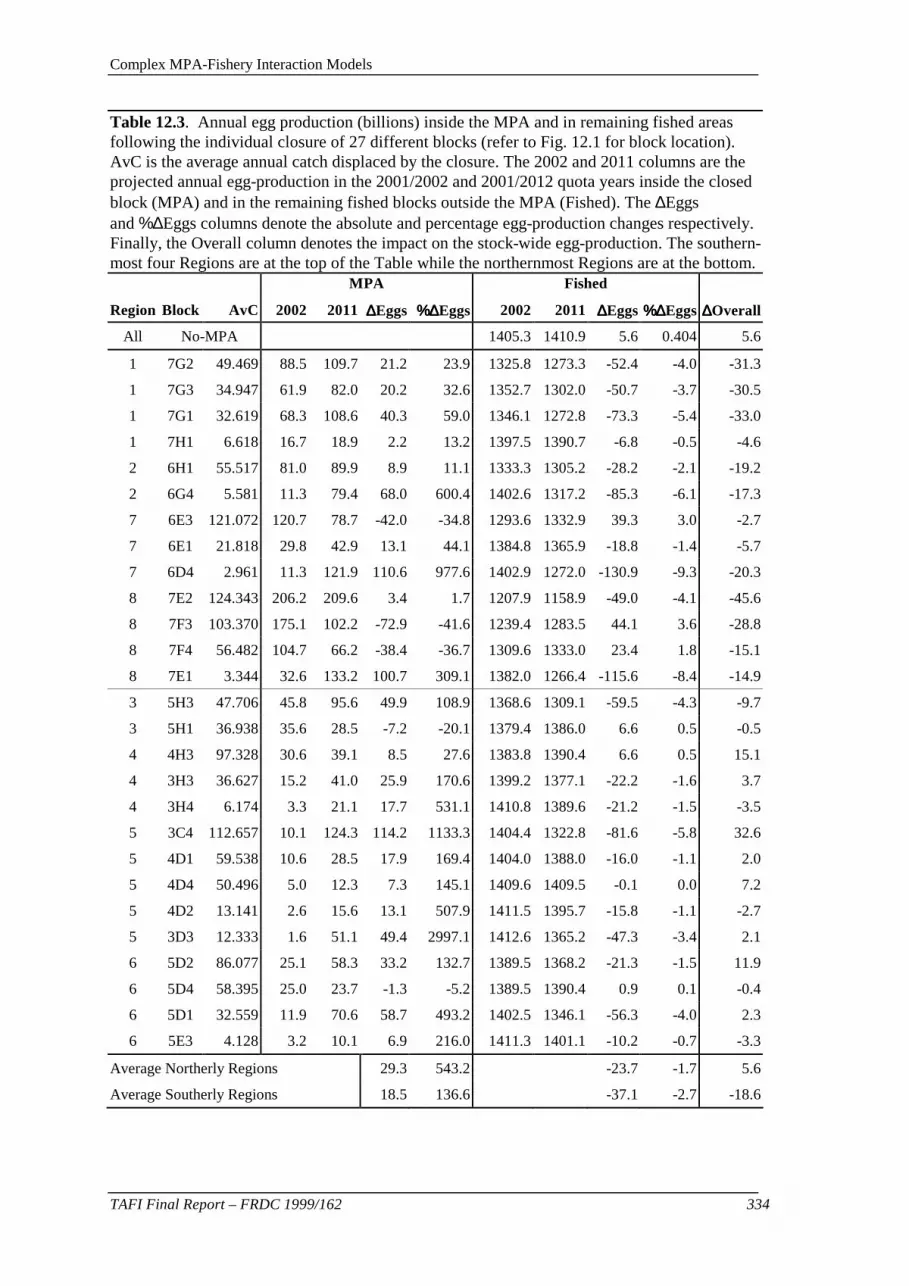
Complex MPA-Fishery Interaction Models
TAFI Final Report – FRDC 1999/162 334
Table 12.3. Annual egg production (billions) inside the MPA and in remaining fished areas following the individual closure of 27 different blocks (refer to Fig. 12.1 for block location). AvC is the average annual catch displaced by the closure. The 2002 and 2011 columns are the projected annual egg-production in the 2001/2002 and 2001/2012 quota years inside the closed block (MPA) and in the remaining fished blocks outside the MPA (Fished). The ∆Eggs and %∆Eggs columns denote the absolute and percentage egg-production changes respectively. Finally, the Overall column denotes the impact on the stock-wide egg-production. The southern-most four Regions are at the top of the Table while the northernmost Regions are at the bottom.
MPA Fished
Region Block AvC 2002 2011 ∆∆∆∆Eggs %∆%∆%∆%∆Eggs 2002 2011 ∆∆∆∆Eggs %∆%∆%∆%∆Eggs ∆∆∆∆Overall
All No-MPA 1405.3 1410.9 5.6 0.404 5.6
1 7G2 49.469 88.5 109.7 21.2 23.9 1325.8 1273.3 -52.4 -4.0 -31.3
1 7G3 34.947 61.9 82.0 20.2 32.6 1352.7 1302.0 -50.7 -3.7 -30.5
1 7G1 32.619 68.3 108.6 40.3 59.0 1346.1 1272.8 -73.3 -5.4 -33.0
1 7H1 6.618 16.7 18.9 2.2 13.2 1397.5 1390.7 -6.8 -0.5 -4.6
2 6H1 55.517 81.0 89.9 8.9 11.1 1333.3 1305.2 -28.2 -2.1 -19.2
2 6G4 5.581 11.3 79.4 68.0 600.4 1402.6 1317.2 -85.3 -6.1 -17.3
7 6E3 121.072 120.7 78.7 -42.0 -34.8 1293.6 1332.9 39.3 3.0 -2.7
7 6E1 21.818 29.8 42.9 13.1 44.1 1384.8 1365.9 -18.8 -1.4 -5.7
7 6D4 2.961 11.3 121.9 110.6 977.6 1402.9 1272.0 -130.9 -9.3 -20.3
8 7E2 124.343 206.2 209.6 3.4 1.7 1207.9 1158.9 -49.0 -4.1 -45.6
8 7F3 103.370 175.1 102.2 -72.9 -41.6 1239.4 1283.5 44.1 3.6 -28.8
8 7F4 56.482 104.7 66.2 -38.4 -36.7 1309.6 1333.0 23.4 1.8 -15.1
8 7E1 3.344 32.6 133.2 100.7 309.1 1382.0 1266.4 -115.6 -8.4 -14.9
3 5H3 47.706 45.8 95.6 49.9 108.9 1368.6 1309.1 -59.5 -4.3 -9.7
3 5H1 36.938 35.6 28.5 -7.2 -20.1 1379.4 1386.0 6.6 0.5 -0.5
4 4H3 97.328 30.6 39.1 8.5 27.6 1383.8 1390.4 6.6 0.5 15.1
4 3H3 36.627 15.2 41.0 25.9 170.6 1399.2 1377.1 -22.2 -1.6 3.7
4 3H4 6.174 3.3 21.1 17.7 531.1 1410.8 1389.6 -21.2 -1.5 -3.5
5 3C4 112.657 10.1 124.3 114.2 1133.3 1404.4 1322.8 -81.6 -5.8 32.6
5 4D1 59.538 10.6 28.5 17.9 169.4 1404.0 1388.0 -16.0 -1.1 2.0
5 4D4 50.496 5.0 12.3 7.3 145.1 1409.6 1409.5 -0.1 0.0 7.2
5 4D2 13.141 2.6 15.6 13.1 507.9 1411.5 1395.7 -15.8 -1.1 -2.7
5 3D3 12.333 1.6 51.1 49.4 2997.1 1412.6 1365.2 -47.3 -3.4 2.1
6 5D2 86.077 25.1 58.3 33.2 132.7 1389.5 1368.2 -21.3 -1.5 11.9
6 5D4 58.395 25.0 23.7 -1.3 -5.2 1389.5 1390.4 0.9 0.1 -0.4
6 5D1 32.559 11.9 70.6 58.7 493.2 1402.5 1346.1 -56.3 -4.0 2.3
6 5E3 4.128 3.2 10.1 6.9 216.0 1411.3 1401.1 -10.2 -0.7 -3.3
Average Northerly Regions 29.3 543.2 -23.7 -1.7 5.6
Average Southerly Regions 18.5 136.6 -37.1 -2.7 -18.6

Complex MPA-Fishery Interaction Models
335 TAFI Final Report – FRDC 1999/162
In terms of egg-production the large potential gains in legal-biomass possible in the north led to large gains in egg-production. This was also greatly affected by the fact that the minimum legal length in the north of the State tended to be below the size-at-maturity for females while in the south of the State (especially Region 8) relatively few females grew above the legal minimum length. The effect of the displaced catch was different when the more southerly Regions 1, 2, 3, 7 and 8 were compared with the more northerly Regions 4, 5 and 6 (Figs. 12.21 & 12.22). Closures in the southerly Regions all led to negative overall impacts on total egg-production (Table 12.3). This implied that the improvements in egg-production in the closed area were never sufficient to make up for the extra losses of egg-production outside the MPA. The regression of change in total egg-production against displaced average annual catch was not significant for the southerly Regions (1, 2, 3, 7, and 8; F = 1.43, df = 1, 13, P = 0.253; ∆EggProd = 28.65 - 0.978 DisplC; Fig. 12.21). By comparison the regression for the more northerly and westerly Regions (4, 5, and 6) was significant (F = 30.45, df = 1, 10, P < 0.0003; ∆EggProd = 3.094 DisplC + 30.19; Fig. 12.21).
-50
-40
-30
-20
-10
0
10
20
30
40
0 25 50 75 100 125Displaced Average Annual Catch t
Cha
nge
in T
otal
Egg
-Pro
duct
ion
-50
-40
-30
-20
-10
0
10
20
30
40
0 25 50 75 100 125Displaced Average Annual Catch t
Cha
nge
in T
otal
Egg
-Pro
duct
ion
Figure 12.21. The change in the stock-wide total egg-production produced by closing 27 different blocks from different assessment Regions around Tasmania, each with a different displaced average annual catch (Fig. 12.1). The horizontal line indicates no overall change. Crossed circles represent blocks in the three north and north-western regions, 4, 5, and 6, while open circles represent the five south and southern-eastern regions, 1, 2, 3, 7, and 8.
In some cases, especially in Regions 7 and 8, but also in Regions 3 and 6, closing a block actually reduced its egg-production (Table 12.3). This occurred where the block was only lightly fished and a significant proportion of the mature female biomass was below the legal limit. The adjustment to the size-structure of the population during re-building did not always lead to an increase in egg-production despite there always being an increase in legal-sized biomass. This was dependent upon the recruitment time-series during each simulation.

Complex MPA-Fishery Interaction Models
TAFI Final Report – FRDC 1999/162 336
-50
-40
-30
-20
-10
0
10
20
30
40
-400 -300 -200 -100 0 100 200 300 400Overall Change to Legal-Sized Biomass
Ove
rall
Cha
nge
to E
gg-P
rodu
ctio
n
-50
-40
-30
-20
-10
0
10
20
30
40
-400 -300 -200 -100 0 100 200 300 400Overall Change to Legal-Sized Biomass
Ove
rall
Cha
nge
to E
gg-P
rodu
ctio
n
Figure 12.22. A comparison of the overall effect of closure of the various blocks on the stock-wide total legal-sized biomass and the related stock-wide total egg-production. Crossed circles represent blocks in the three northern and north-westerly Regions, 4, 5, and 6, while open circles represent the five more southern and south-easterly regions, 1, 2, 3, 7, and 8. The diagonal is a regression describing the relationship (F = 61.11, df = 1,25, P < 0.00001; ∆EggProd = 0.108 ∆LegBiom – 2.297).
Catch-Rate Implications
In all cases where blocks were closed the legal-sized biomass remaining open to fishing was reduced and, after projection, ended up some fraction of what legal-sized biomass there would have been without the MPA. The same TACC had to come from the available legal-sized biomass so the expectation was that the average harvest rate would be higher and the catch-rate lower. There was still a relationship between Regions and the expected relative impact on catch-rates but it was somewhat obscured by the effects of the displaced average annual catch (Fig. 12.23; Table 12.4).
-20
0
20
40
60
80
100
1 2 3 4 5 6 7 8Region
Per
cent
of n
o-M
PA
Cat
ch-R
ate
-20
0
20
40
60
80
100
1 2 3 4 5 6 7 8Region
Per
cent
of n
o-M
PA
Cat
ch-R
ate
Figure 12.23. The relationship between a closure in an assessment Region and the affect on the catch-rate relative to what would be expected without a closure. The curved line is a best-fitting polynomial but was only meant to be indicative of the trend.

Complex MPA-Fishery Interaction Models
337 TAFI Final Report – FRDC 1999/162
There was also a relationship between the displaced catch from a closure and the expected catch-rate expressed as a percentage of that without a closure (Fig. 12.24). This relationship was extremely variable and was influenced by the degree of depletion of the closed block and the geographical location of the closure. The average trend of the northernmost four Regions was certainly higher than that of the southern four Regions but the variation over both was sufficiently large not to draw any firm generalizations (Fig. 12.25).
-20
0
20
40
60
80
100
0 20 40 60 80 100 120Displaced Average Annual Catch t
Per
cent
of n
o-M
PA
Cat
ch-R
ate
-20
0
20
40
60
80
100
0 20 40 60 80 100 120Displaced Average Annual Catch t
Per
cent
of n
o-M
PA
Cat
ch-R
ate
Figure 12.24. The relationship between the displaced average annual catch from a block closure and the affect on the average catch-rate relative to what would be expected without a closure (Table 12.4). The curved line is a best-fitting polynomial, however, the variability is clearly very great.
-5
0
5
10
15
20
25
30
0 20 40 60 80 100 120
Displaced Average Annual Catch t
Per
cent
Cha
nge
in C
atch
-Rat
e
-5
0
5
10
15
20
25
30
0 20 40 60 80 100 120
Displaced Average Annual Catch t
Per
cent
Cha
nge
in C
atch
-Rat
e
Figure 12.25. The relationship between the displaced average annual catch from a closure and the affect on the catch-rate relative to what would be expected without a closure. The horizontal line at 28.13% indicates the expected increase in catch-rates in 2011/2012 when no closure is implemented. Crossed circles represent blocks in the three northerly regions, 4, 5, and 6, while open circles represent the five southerly regions, 1, 2, 3, 7, and 8.

Complex MPA-Fishery Interaction Models
TAFI Final Report – FRDC 1999/162 338
Table 12.4. The effects on catch-rate of closing 27 different blocks to fishing in different regions (see Fig. A12.1 for block locations). AvC was the average annual catch displaced by the closure. The 2002 and 2011 columns were the available legal biomass in the 2001/2002 and 2001/2012 quota years following projection, inside the MPA and in the fished blocks outside the MPA. The %∆Biom column denoted the percentage biomass change, while the ∆Biom column denoted the absolute change to legal-sized biomass. The %∆CPUE was the expected percentage change to the catch-rates relative to that experienced in 2002/2003. Negative values in these columns denote where stocks were being depleted instead of rebuilding. The southern-most four Regions were at the top of the Table while the northernmost Regions were at the bottom.
Region Block AvC 2002 2011 %∆Biom ∆Biom %∆CPUE Relative
%Change
All No-MPA 0.000 3069.087 3932.503 28.133 863.416 28.13 100.00
1 7G2 49.469 2952.702 3117.584 5.584 164.882 5.58 19.85
1 7G3 34.947 3000.641 3315.636 10.498 314.995 10.50 37.31
1 7G1 32.619 2956.586 3165.372 7.062 208.786 7.06 25.10
1 7H1 6.618 3013.047 3765.579 24.976 752.532 24.98 88.78
2 6H1 55.517 2885.560 3046.258 5.569 160.698 5.57 19.80
2 6G4 5.581 3051.264 3366.805 10.341 315.541 10.34 36.76
7 6E3 121.072 2888.530 3250.879 12.544 362.349 12.54 44.59
7 6E1 21.818 3012.892 3642.977 20.913 630.084 20.91 74.34
7 6D4 2.961 3054.343 3386.242 10.866 331.900 10.87 38.63
8 7E2 124.343 2942.604 2909.637 -1.120 -32.967 -1.12 -3.98
8 7F3 103.370 2881.267 3220.184 11.763 338.917 11.76 41.81
8 7F4 56.482 2958.510 3497.534 18.219 539.024 18.22 64.76
8 7E1 3.344 3020.847 3493.617 15.650 472.770 15.65 55.63
3 5H3 47.706 2930.854 3033.778 3.512 102.925 3.51 12.48
3 5H1 36.938 3020.122 3630.78 20.220 610.659 20.22 71.87
4 4H3 97.328 2922.882 3661.726 25.278 738.844 25.28 89.85
4 3H3 36.627 2981.805 3545.926 18.919 564.121 18.92 67.25
4 3H4 6.174 3049.311 3703.925 21.468 654.615 21.47 76.31
5 3C4 112.657 2951.65 2858.131 -3.168 -93.519 -3.17 -11.26
5 4D1 59.538 2955.673 3662.528 23.915 706.855 23.92 85.01
5 4D4 50.496 3010.678 3848.344 27.823 837.666 27.82 98.90
5 4D2 13.141 3042.201 3751.328 23.310 709.128 23.31 82.86
5 3D3 12.333 3051.316 3388.567 11.053 337.251 11.05 39.29
6 5D2 86.077 2957.578 3481.161 17.703 523.583 17.70 62.93
6 5D4 58.395 2926.722 3676.697 25.625 749.975 25.63 91.09
6 5D1 32.559 3014.176 3320.689 10.169 306.513 10.17 36.15
6 5E3 4.128 3049.156 3818.245 25.223 769.089 25.22 89.66
Average Northerly Regions 18.943 67.335 Average Southerly Regions 11.773 41.849

Complex MPA-Fishery Interaction Models
339 TAFI Final Report – FRDC 1999/162
The only obvious generalization to be made was that any closure at the scale of a block had a negative effect upon catch-rate and therefore would have an adverse effect upon the economics of the Tasmanian rock lobster fishery. There were two blocks, however, whose closure completely negated the potential for stock rebuilding and led to the beginning of a stock decline, which, without intervention would lead to collapse; these were 7E2 and 3C4.
DISCUSSION
Legal-Sized Biomass
The outcomes from the MPA model were consistent with the predictions from the general model described in Chapter 11. As expected, the particular outcome of closing a statistical block in the Tasmanian rock lobster fishery (without an appropriate reduction in the TACC) was very dependent upon which block was closed. Because the biological properties of growth and size at first maturity differed so markedly around the coast of Tasmania the relative impact of closure tended to reflect the details of growth rate, productivity and the state of depletion at the start of projections.
All closures in the more southerly regions (1, 2, 3, 7, and 8) led to reductions in the overall legal biomass, despite the fact that in all cases there were large increases in legal-sized biomass inside the closed blocks (Table 12.3). In all of these cases the increases inside the MPA were too small to offset the decreases outside the MPA. Thus, the negative effects of the displaced catch were greater than the increases due to the release from fishing mortality. There was a reasonably clear linear relationship between the extent of the decrease and the level of displaced annual average catch (Fig. 12.19). Thus, closure of blocks with a relatively small catch had a correspondingly small effect.
Most closures in the more northerly regions (4, 5, and 6) led to increases in the stock-wide legal-sized biomass, although some led to small decreases. Only in the case of a single block (3C4 in region 5) was the increase large. In those blocks where there were decreases, these were not as great as the closure of more southerly blocks with approximately the same displaced annual average catch. There was no obvious linear relationship between the extent of change in legal biomass and the level of displaced annual average catch in northerly blocks, although if block 3C4 was omitted a linear relationship became apparent with a gradient only slightly greater than zero.
The most obvious difference between the northern and southern regions related to the growth patterns in these different areas. Northern animals (Regions 4,5, 6) grew at a much faster rate and to a much larger final size than their southern counterparts (Regions 1,2,3,7,8). Notwithstanding the growth patterns, the average percentage increase in legal-sized biomass inside the MPA was approximately equal in the northern and southern region and the average absolute increase in biomass was 25t greater in the south (Table 12.2). The distinction between growth rates is better illustrated by a comparison of Regions 1 and 8 (southern most) with Regions 4 and 5 (northern most) where the percentage change in legal-sized biomass in the north is twice that in the south (Table 12.2). In the fished blocks, closures in northern regions did not slow the average rebuild of exploitable legal biomass as much as closures in the southern regions, both in terms of percent increase and absolute increase (Table 12.2).

Complex MPA-Fishery Interaction Models
TAFI Final Report – FRDC 1999/162 340
As a result, the average overall change from a closure in the northern regions was an increase of about 54 tonnes while closures in the southern regions led to a decrease of about 136 tonnes. Thus, the overall changes were not solely due to differences in the rebuilding capacity of the closed block, but also the capacity of the open blocks to absorb the displaced catch and continue rebuilding.
Egg-Production
With the different patterns of growth between the northern and southern regions there is also a mismatch between the minimum legal length and the size-at-maturity around the State. In region 8, for example, the majority of females never reach the LML. Thus, around the State, the delay between a recruitment event and those recruits growing into the fishery is inversely proportional to growth rate and is the longest in region 8. Conversely, especially in regions 4 and 5, a large proportion of females do not attain sexual maturity until much larger than the LML. In a previous chapter (Fig. 11.21), it was clearly shown that a larger LML in region 5 would eventually lead to a much more productive stock. This would require an LML of 125 mm or even 145 mm instead of the current 105 mm for females, but there would be advantages both in terms of stock resilience as well as total productivity. Difference in size-at-maturity by region had substantial implication for egg-production. A large number of mature females in the southern regions are protected from fishing because they never attain the legal size. Little or no relationship between total egg production and displaced average annual catch was apparent in the southerly regions. However, in the more northerly regions the effect of displaced average annual catch with closures was positive and approximately linear (see Fig. 12.21). This is the reverse of what was seen with legal-sized biomass, where a clear relationship was exhibited by closures in the southern regions, but not in northern regions (see Fig. 12.19).
Generally there was a simple linear relationship between the overall change to legal-sized biomass and the overall change to egg-production. For this reason only closures that led to positive changes in legal-sized biomass led to increases in total egg-production. In the best case, 32.6 billion eggs increased the total egg-production during the 10-year projection period, a 2.56% increase over what would have arisen given no-MPA. Even if there were a relationship between total egg-production and subsequent recruitment, such a small increase would be difficult to detect. However, noting that recruitment levels have declined over the last 40 years (Frusher et al. 2003), any measures that lead to increases in egg-production might be considered by management. Any management measure introduced to increase egg-production will involve a significant time-delay before any potential benefits would accrue to the fishery. In the model such egg-production increases took three or four years to develop, a delay brought about by the time it takes for rock lobsters to grow. This had to be combined with an 18 to 24 month planktonic larval period, followed by the four or five years before new recruits enter the fishery. In addition, as demonstrated by the recruitment variability between regions described in the annual assessment (Appendix 12.4), there was no guarantee that any particular area selected for an MPA was always going to be a source of recruits each year into the future (Bruce et al. 2000). Any potential benefits would have to be considered in terms of long-term average benefits across many years.

Complex MPA-Fishery Interaction Models
341 TAFI Final Report – FRDC 1999/162
If there were to be any large closures around Tasmania then in terms of egg-production an area in the northerly Regions is to be preferred. However, some closures led to reductions in both total legal-sized biomass and total egg-production, so site selection should not be random.
Catch-Rates
One of the difficulties in the interpretation of the overall catch-rate information was that it constituted an average across the State. While movement of rock lobster across an MPA boundary was minor in proportional terms, once there had been a build up of stock size within the MPA and assuming there was suitable habitat across the MPA boundary, there would be reasonable absolute numbers of animals leaving the MPA. Because of this a good fishing strategy would be to place pots on the MPA boundary, which has been observed in this and other studies (Kelly et al. 2001). If the lobsters were more mobile (as has been reported in Victoria and South Australia), then this boundary fishing strategy would become more significant and the positive effects of the MPA on legal-sized biomass within the MPA would diminish.
Generally, the effects considered in this study were averaged across the blocks remaining open to fishing. Given that catch was distributed according to expected legal-sized biomass levels in each block (and hence by implied catch-rates), a consideration of the average effect across the State was reasonable.
There were broad patterns in the effects on statewide catch rates but these were obscured by the extreme variability in the response in different regions (Figs. 12.24 and 12.25). The level of displaced average annual catch in any region also influenced the variability of responses. In all cases the rebuilding of the stock open to fishing (which included the minimal movement of animals out of the MPA) was some fraction of that which would have occurred had there been no-MPA. This implied that in all cases with an MPA there would have been a decline in average catch-rate but in some cases this decline would only be very slight. For example, closure of block 4D4 displaced about 50.5t of catch from region 5 but, assuming average recruitment across the projection period, this only led to a minimal reduction in projected catch-rates (Fig. 12.25). The model suggested that because of the rebuilding of stock biomass with the present TACC, on average, over the projection period, catch-rates would improve by about 28% over those in 2002/2003 without an MPA. By comparison, a closure in the northerly regions would lead, on average, to catch-rates improving by approximately 19%, while a closure in the southerly regions would result in only 11.5% over the projection period. Improved catch-rates mean that fewer fishing trips are required to catch the same amount of quota. Thus, such catch-rate losses (23% and 59% respectively) would constitute a significant economic opportunity loss brought about by implementing an MPA. Other management or socio-economic benefits would thus need to be compelling to make MPAs a preferred option in the management of the Tasmanian rock lobster fishery.

Complex MPA-Fishery Interaction Models
TAFI Final Report – FRDC 1999/162 342
It was, however, apparent that closure of some of the minor blocks (in terms of catch) would only have led to only a minor and possibly undetectable effect on the fishery. Under such circumstances it was tempting to ignore the impact. However, there remained a potential problem related to fleet dynamics. There may be only a very minor cost if a small block were to be closed but this assumes the cost is equally spread across all fishers. In practise, as fishing tends to be relatively local, only a sub-set of the fleet would be likely to experience the increased costs. So while the total cost may not be great it could be significant if it were focused on only a few individual fishers. Offsetting this might be the localized gains in catch-rates that should be experienced on the borders of the MPA.
There were two blocks (7E2 in region 8 and 3C4 in region 5) where closure led to the fished stock actually reducing in size rather than rebuilding. Both were a displacement of 110t, but the effect was not only relative to the size of the displaced catch because other blocks (>110t) did not produce the same effect. Clearly, a combination of the level of displaced catch and the resilience of the remaining blocks contributed to the stock decline. Obviously, closure of such blocks would be a very risky management strategy. Interestingly, these two blocks spanned the full latitudinal extent of the fishery, emphasizing the individual nature of the response and the difficulty in producing generalizations.
Fleet Dynamics in Response to Closure
In modelling the block closures it was assumed that the displaced catch would be distributed into the blocks remaining open to fishing in proportion to the average catch expected from these blocks relative to the total catch (commercial plus recreational). In some cases the available legal-sized biomass in a block was not sufficient to permit the allocated catch being taken. In such depletion cases, if a maximum harvest rate was exceeded then the maximum permissible proportion of the available biomass was taken and the remainder of the expected catch was later distributed across the remaining undepleted blocks in proportion to their available biomass. This was a very conservative strategy and one that was least likely to lead to a negative impact of introducing an MPA. A more likely and realistic scenario would be fishers distributing their displaced catch into just a few of the principle fishing areas, rather than distributing the displaced catch across all open blocks. The main outcome of this behaviour would be a greater likelihood of some blocks becoming depleted and stock rebuilding failing.

Complex MPA-Fishery Interaction Models
343 TAFI Final Report – FRDC 1999/162
The Value of MPAs for Fisheries Management
The underlying aim of this work was to evaluate large-scale fishery closures as a fisheries management tool. There is a growing literature suggesting that no-take Marine Protected Areas have value as an alternative to more traditional fisheries management measures (see Lubchenko et al., 2003), supported in general by population modelling (Gerber et al. 2003).
It is generally acknowledged, however, that our understanding of the effects of MPAs is still in its infancy and more work needs to be done on tactical models that interrogate MPA questions on a fishery specific basis. The modelling strategy adopted in this present work was to use an array of different models, each with somewhat different properties, to investigate different aspects of the introduction of MPAs in Tasmania and their effect on abalone and rock lobster fisheries. The simple models (based on a minimal model definition that included the major sources of productivity: growth, recruitment, and sources of mortality) showed that the effect of an MPA depended upon the life-history characteristics of the species concerned. Thus, if it were true that abalone only have extremely limited larval dispersal and extremely limited adult movement, then neither large nor small-scale MPAs would provide any advantage to a fishery (except where the fishery had collapsed). Under such circumstances, if it were required that areas closed to fishing be used as a management tool for other purposes, then it would be advantageous to consider an array of closed areas interspersed with open areas, all on a physical scale reflecting the dispersal abilities of the species concerned. To maximise fishery benefits for abalone one might require closed areas on a scale of 100s of metres of coastline. While the simple models led to important conclusions with regard to the scale of closures for fisheries management success, because of their simplified structure, they were also rather limited with regard to details spatial effects. Conversely, if larval dispersal was wide-spread, as is the case with rock lobsters, then a single large closure might be argued to have advantages for a fishery. Such simple models fail to account for several highly significant parameters such as spatial differences in growth rate, size at maturity and fleet dynamics. We therefore advocate that they should thus be used with great caution.
In order to investigate the details of the spatially dynamic responses to a large-scale closure within a fished system, a complex but general model was generated to focus on the effect of closure within a generic quota managed rock-lobster fishery. This work expanded on the implication of closing large-areas to fishing and, by imposing uniformity on all the modelled populations, it was possible to focus solely on the effects of the MPA. It was thus possible to consider the interactions between closure and stock productivity (growth and recruitment). Generally, if catch was displaced from an area the negative effects in the remaining fished areas were greater than the positive effects associated directly with the closure due to the displacement of effort and the maintanance of catch levels. Using this model it was possible to determine the effect of movement rate on the effectiveness of the MPAs. At relatively low movement rates the stock size and size-distribution within an MPA rebuilds to approximate that which might be expected in the absence of fishing. Even a movement rate of 1% leads to some

Complex MPA-Fishery Interaction Models
TAFI Final Report – FRDC 1999/162 344
difference from completely unfished scenario. As the movement rate increased the effectiveness of the MPA at protecting the enclosed species decreased. Interestingly, a movement rate of 30% per annum still permitted some rebuilding within a large scale MPA, although it reached only a fraction of that possible with a movement rate of 1%. With low movement rates it was difficult to find a positive benefit to introducing an MPA in this modelled rock lobster fishery. With higher movement rates, a large MPA might provide for a viable fishery of equivalent yield to a fishery without an MPA. The outcomes were highly dependent upon the life-history characteristics of the species concerned. Once again the physical scale of the MPA relative to the degree of movement by adults and larvae was pivotal to whether an MPA would be beneficial or not. It was noted that while an MPA might lead to a useful fishery in areas adjacent to the reserve, if the species had a high level of movement, the population within the MPA would not differ greatly from a fished population, so the management objectives, especially ecosystem objectives might not be achieved.
The work with the complex but general model was based upon the assumption that on the introduction of a large closed area there would be no concomitant reduction in total catch or effort equivalent to that expressed in the reserve. While this is in accord with previous experience in Australia and elsewhere, it is possible that MPAs would be introduced in systems that had not already collapsed and that the catch or effort would be appropriately reduced. Under such circumstances introducing an MPA is either the same as not introducing an MPA or is better than not introducing an MPA, depending on the criteria used to assess the state of the fishery. The complex but general model was useful but it still referred to an abstract system that, because populations are generally not homogeneous, would only occur in nature in unusual circumstances. To get around that issue and to determine what effects would occur if a large-scale MPA were introduced into a particular fishery, the Tasmanian rock lobster fishery was modelled by sub-dividing the fishery into 50 half-degree blocks with contained populations. Fishery data was available at that scale and the model was fitted to real data wherever possible. While the conclusions from the complex but specific modelling were consistent with the complex but general modelling there was great variability in the response to closure of particular blocks. Much of this variation could be explained in terms of species and fisheries characteristics: the growth patterns exhibited in different parts of the distribution of the species, the interaction of the size-at-maturity of females and the legal minimum limit, and the histories of catch and effort in different blocks. In order to investigate the behaviour of the known fishery in response to a large-scale closure it was necessary to project its dynamics forward from the present state (determined from the current assessment). In the absence of a deterministic spawning-stock to subsequent recruitment relationship, the projections had to include a stochastic element when describing recruitment. Thus, details of the state of depletion of the various blocks were not known deterministically. The outcome of any particular projection was partly determined by the growth pattern exhibited in the block, the size-at-maturity relative to the legal minimum length and the details of depletion around the coastline.

Complex MPA-Fishery Interaction Models
345 TAFI Final Report – FRDC 1999/162
Fortunately, the current state of the rock lobster fishery in Tasmania suggests that, if future recruitment is average or better than average, there should be significant stock rebuilding (assuming that the management (TACC) remains at its present level). It was therefore possible to assess the relative performance of the fishery by comparing it with the expected outcomes in the absence of a large-scale closure. The closure of some blocks led to an increase in stock-wide legal-sized biomass, which also led to an increase in the total egg-production. However, in the majority of cases the outcome was a loss to total biomass and a loss to total egg-production. In addition, in no case did the introduction of a closure lead to a better performance in terms of catch-rates in the blocks remaining open to the fishery. In two instances, following block closure, the rebuilding was reversed and the stock remaining open to fishing began to decline. Because in all cases there was a decrease in the improvements to the potential catch-rate that would be obtained if there were no closure, it was concluded that introducing a large MPA would impose a real economic lost opportunity cost on the future fishery. The general conclusion for Tasmanian rock lobster, where adults only move relatively small distances, was that the introduction of a large MPA would be a riskier management strategy than continuing the present stock rebuilding strategy.
MPAs - An Apparently Simple Solution to a Complex Problem?
The fact that history is littered with failed fisheries leaves no doubt that successful fisheries management is difficult. Modern fisheries management is concerned with more than a single species approach, and is moving rapidly towards ecosystem based management in which the impact and context of the fishery in the environment is given full consideration. It attempts to operationalise the commitment most jurisdictions in Australia and elsewhere have shown to ecologically sustainable development (ESD) in fisheries.
This also provides a context for the consideration of MPAs, although in Australia the current push for the establishment of a network of reserves under the NRSMPA is argued on the need to secure the conservation of biodiversity, not to improve fisheries management. Implicit in this argument is the suggestion that biodiversity is indeed threatened and that MPAs offer a solution to the problem. Neither are well documented (although it is recognized that MPAs offer a reliable way of studying this issue). Threats to biodiversity include habitat degradation, fisheries and other extractive uses, harmful algal blooms, global warming, pollution, runoff (both freshwater and saltation), introduced marine pests.

Complex MPA-Fishery Interaction Models
TAFI Final Report – FRDC 1999/162 346
Internationally, it is evident that fisheries are considered a key threatening process (Ballantine 1999, Lubchenco et al. 2003). Fisheries have generally been managed as open access common property resources and inadequate regulation of user groups is seen to be the major cause of over-exploitation (Carr et al. 2003). Despite the notion of open access having been long discredited as a viable management regime for fisheries (Hardin, 1960), there are still many fisheries around the world where such access rights are still upheld as being the most fair. Most notably this still occurs in many fisheries in the United States of America. While it is true that open access provides for a simple solution to a difficult social problem in management it neglects the fact that invariably open access leads to either economic inefficiency or unsustainable levels of catch.
Underlying the difficulties associated with managing access to the right to fish is that of social equity. When deciding how to allocate access rights managers must be seen to be acting in a manner that is fair to all. One advantage of MPAs over other forms of management is that they have an intrinsic social equity in that nobody has access to the resources in the closed area. This makes them a very attractive option to managers who need to address the social equity issues as well as sustainability issues. The apparent inability or political unwillingness to control effort leads some analysts to conclude that MPAs offer the only viable alternative to failed fisheries management (eg see Sladek Nowlis and Roberts 1999).
While the uncontrolled effort argument may be applicable to some or many fisheries, particularly in developed northern hemisphere countries, it is not a general paradigm. Australia is widely acknowledged for its management of fisheries (Mace 1997), many of which have strict quota and effort limitation.
In the Tasmanian lobster and abalone fisheries where effort is effectively limited, it is demonstrated that the introduction of MPAs as a fisheries management tool would be inferior to present management options. Indeed if MPAs are introduced without reducing catch or effort by amounts equivalent to that in the prospective closed area, they are a risky strategy and may lead to a degradation of the fishery (this appears to be a general conclusion for species with low movement rates where TACs are used as a primary management tool).
Furthermore this is suggesting that if it can be demonstrated that a fishery is being managed in accordance with ESD principles (by definition this means that the ecosystem in which it operates is not threatened by the fishery or fishing practices), then fishing should not be a key threatening process. It follows then, from this argument that true ESD fisheries management offers a potentially better outcome than the NRSMPA for biodiversity conservation.
This is not to suggest that MPAs do not have a place in marine and coastal management. Spatial management of fisheries has a long tradition (eg spawning grounds) and there are a number of fisheries that benefit from spatial closures. This study clearly demonstrates their value for understanding the ecological effects of fishing, thus leading to a greater fisheries resource security.

Complex MPA-Fishery Interaction Models
347 TAFI Final Report – FRDC 1999/162
APPENDIX 12.1. MODEL SPECIFICATION
Marine Protected Area Model – Specification Objectives
The objective of this modelling was to simulate the effect of closing an area previously fished to determine the impact on both the closed area and the remaining fishery.
The Model
The Population Dynamics
The numbers in each size class are represented using a vector N. In the following, the usual convention of depicting vector and matrices using a bold, non-italicized font will be used:
s,ptN A12.1
which represents numbers of animals in each size class where s represents sex, p represents population, t represents year. Every year of the simulation the stock dynamics follow the same sequence of six steps applied to each size-class, of each sex, in each population.
1. Half of the natural mortality is applied to each population.
2. Any remaining animals then experience growth appropriate to each sex and population.
3. The Instantaneous Fishing mortality (modified by gear selectivity) required to remove the TAC is calculated and then applied across the size-classes (i.e. the model is conditioned on catch). If a population is closed to fishing the catch that should have come from that population is distributed among the remaining populations according to the fleet dynamics model selected. If a population is depleted to such an extent that its allocated catch cannot be taken then the remaining catch required is also allocated to remaining populations.
4. Any recruitment occurs to the smallest size class.
5. The remaining half of natural mortality is applied.
6. Any movement that occurs among recruited populations happens.
The first two steps can be represented by:
( )/2Me−=s,p s,p s,pt+0.5 tN G N A12.2
where e-M/2 represents the survivorship following the application of half the natural mortality and G represents the growth transition matrix by sex and population. The dynamics within a year are represented by the subscript t + 0.5, which is to suggest that all fishing mortality occurs instantaneously in the middle of the year. The 0.5 does not really imply half way through the year but rather indicates the ordering of events. In this

Complex MPA-Fishery Interaction Models
TAFI Final Report – FRDC 1999/162 348
yearly time-step model, the 0.5 suggests that growth occurs after half of the natural mortality has occurred; later equations will use other time subscripts to denote the ordering of events. Equation (11.2) therefore provides a description of the exploitable population.
The diagonal of the survivorship matrix, S, following fishing mortality is designated:
, 1 LML
LMLLs F
l
e lλ−
<= ≥
s ptS A12.3
where sL is the selectivity for size class l, F is the fully selected instantaneous fishing mortality, and λ is a modifier to allow for the shorter fishing season available for females and for the fact that ovigerous females must be returned alive to the water (for males λ = 1 while for females λ = 0.75; the model does not appear to be sensitive to this parameter). The vectors of survivorship are filled with ones up to the legal minimum length (LML) for the separate sexes, which assumes no discard mortality. The instantaneous fishing mortality rate is determined at the level that will give rise to the catch to be removed from the population (either the historical catch or the proportion of the TAC allocated to the population, see later). Applying the survivorships leads to a revised count of animals in each size-class:
=s,p s,p s,pt+0.6 t t+0.5N S N A12.4
The remaining half of the natural mortality is applied (as a survivorship):
/2Me−=s,p s,pt+0.7 t+0.6N N A12.5
Recruitment is then added, only to the first size class, by using a vector with only the first size class populated:
= +s,p s,pt+1 t+0.7 tN N R A12.6
The whole sequence of operations can be compressed into a single equation:
( )( )/2 /2M Me e− − = +
s,p s,p s,p s,pt+1 t t tN S G N R A12.7
The only remaining operation required to complete the dynamics is to include a description of movement of recruited animals among populations. Any movement expected amongst populations is made more complicated by the size-structure of those populations, which implies that a matrix representation of the process would be clumsy. Instead, we need to remember that the populations are arranged linearly along or around a coast. Thus, movement can be represented as the proportion of all size-classes that move into an adjacent population. This can be represented formally as:
( )12 2
p pp µ µµ= − + +s,p s,p s,p+1 s,p-1
t+1 t+1 t+1 t+1N N N N A12.8

Complex MPA-Fishery Interaction Models
349 TAFI Final Report – FRDC 1999/162
where µp is the probability or proportion of the available population, p, that moves out of a population area into adjacent areas. Thus, population p retains 1-µ of its total but gains µp/2 of its two neighbouring populations p-1 and p+1.The superscript, p, permits the possibility of having different movement rates from different populations. Available information for Tasmania suggested that a constant and low level of movement best matched Tasmanian conditions, so the p superscript was ignored and a constant proportion of movement was assumed for all populations. If it were desired to make different size classes have different mobility then this could be achieved through the use of a vector analogous to selectivity coefficients, which could modify the µp for each size-class. In the models presented here this option was not developed further as there was no evidence to suggest different sized animals moved by different amounts.
Various indicators of stock performance can be obtained as the dynamics of the array of populations unfolds through simulated time. For example the exploitable biomass in any particular year can easily be calculated. Equation (11.2) can be converted to a biomass by combining the vector of size-classes with a vector of weight at size and a vector of selectivity for legal sized animals. If this is summed over both sexes and all open populations, this provides an estimate of total exploitable biomass:
e st LB =∑∑ s s,p
t+0.5s p
s W N A12.9
where etB is the exploitable biomass, Ws is a vector of weight at size for each sex and
sL is the selectivity for legal sized animals, which differs between the two sexes s.

Complex MPA-Fishery Interaction Models
TAFI Final Report – FRDC 1999/162 350
APPENDIX 12.2. STATISTICAL BLOCK CHARACTERISTICS Table A12.1. Statistical blocks used in the MPA simulations sorted by mean catch. The catch was averaged between 1983/1984 and 2001/2002, and then scaled to total 1,500t,
close to the current TAC. The StDev is the standard deviation of catches and CoeffVar is the coefficient of variation. By using these 50 blocks instead of the total of 86 containing data, > 95% of all catches are accounted for in each year. The bolded blocks and Regions
were examined for the effect of closure.
Block Region Mean Catch StDev CoeffVar Cumulative% Percent
7E2 8 124.343 44.3447 0.3566 8.29 8.29 6E3 7 121.072 35.4014 0.2924 8.07 16.36 3C4 5 112.657 28.4863 0.2529 7.51 23.87 7F3 8 103.370 30.2469 0.2926 6.89 30.76 4H3 4 97.328 39.5072 0.4059 6.49 37.25 5D2 6 86.077 18.1269 0.2106 5.74 42.99 4D1 5 59.538 21.6732 0.3640 3.97 46.96 5D4 6 58.395 14.1918 0.2430 3.89 50.85 7F4 8 56.482 13.7757 0.2439 3.77 54.62 6H1 2 55.517 22.7508 0.4098 3.70 58.32 4D4 5 50.496 14.1840 0.2809 3.37 61.69 7G2 1 49.469 14.5767 0.2947 3.30 64.98 5H3 3 47.706 14.5345 0.3047 3.18 68.16 5H1 3 36.938 12.4731 0.3377 2.46 70.63 3H3 4 36.627 20.6172 0.5629 2.44 73.07 7G3 1 34.947 6.0010 0.1717 2.33 75.40 7G1 1 32.619 11.0229 0.3379 2.17 77.57 5D1 6 32.559 9.3003 0.2856 2.17 79.74 6H3 2 30.721 14.1970 0.4621 2.05 81.79 4H1 4 30.401 13.4340 0.4419 2.03 83.82 4C2 5 30.242 13.4128 0.4435 2.02 85.83 4D3 5 23.329 8.0857 0.3466 1.56 87.39 3G4 4 21.871 11.9013 0.5442 1.46 88.85 6E1 7 21.818 6.3953 0.2931 1.45 90.30 4H2 4 20.035 9.5843 0.4784 1.34 91.64 4C4 5 16.790 8.8990 0.5300 1.12 92.76 7E4 8 13.532 6.8164 0.5037 0.90 93.66 4D2 5 13.141 4.5252 0.3444 0.88 94.53 3D3 5 12.333 4.6620 0.3780 0.82 95.36 4G4 4 8.908 5.6855 0.6382 0.59 95.95 7H1 1 6.618 8.6358 1.3049 0.44 96.39 3H4 4 6.174 4.0325 0.6532 0.41 96.80 6G4 2 5.581 7.1672 1.2843 0.37 97.18 4H4 4 4.381 2.5185 0.5749 0.29 97.47 5E3 6 4.128 5.2890 1.2811 0.28 97.74 4G2 4 3.693 2.7362 0.7409 0.25 97.99 4C1 5 3.380 3.7684 1.1149 0.23 98.21 7E1 8 3.344 2.3816 0.7122 0.22 98.44 5C2 6 2.962 4.5211 1.5266 0.20 98.63
7 2.951 3.8760 1.3136 0.20 98.83 5D3 6 2.579 1.8130 0.7031 0.17 99.00 4E3 5 2.151 3.0131 1.4005 0.14 99.15 4E1 5 2.088 2.9421 1.4092 0.14 99.29 3C2 5 1.731 0.9640 0.5569 0.12 99.40 6G2 2 1.645 1.9976 1.2145 0.11 99.51 3G1 4 1.619 1.0802 0.6671 0.11 99.62 7E3 8 1.597 0.9034 0.5657 0.11 99.73 3G3 4 1.499 0.9946 0.6636 0.10 99.83 7F2 8 1.433 0.7927 0.5531 0.10 99.92 3D1 5 1.184 0.9264 0.7823 0.08 100.00

Complex MPA-Fishery Interaction Models
351 TAFI Final Report – FRDC 1999/162
43
42
147
41
7C3 7G4
3D4 3E3 3E4 3F3 3F4 3G3 3G4 3H3 3H4
3C1
7H3
3C2 3D1 3D2 3E1 3E2 3F1 3F2 3G1 3G2 3H1
7H4
3H2
7C1 7C2 7D1 7D2 7E1 7E2 7F1
7C4
7F2 7G1 7G2 7H1 7H2
6C3 6C4 6D3 6D4 6E3
7D3
6E4 6F3 6F4 6G3 6G4 6H3 6H4
6C1 6C2 6D1
7D4
6D2 6E1 6E2 6F1 6F2 6G1 6G2 6H1 6H2
5C3
7E3
5C4 5D3 5D4 5E3 5E4 5F3 5F4 5G3 5G4 5H3
7E4
5H4
5C1 5C2 5D1 5D2 5E1 5E2 5F1 5F2 5G1
7F3
5G2 5H1 5H2
4C3 4C4 4D3 4D4 4E3 4E4 4F3
7F4
4F4 4G3 4G4 4H3 4H4
4C1 4C2 4D1 4D2 4E1
7G3
4E2 4F1 4F2 4G1 4G2 4H1 4H2
3C3 3C4 3D3
43
42
147
41
7C3 7G4
3D4 3E3 3E4 3F3 3F4 3G3 3G4 3H3 3H4
3C1
7H3
3C2
7C3 7G4
3D4 3E3 3E4 3F3 3F4 3G3 3G4 3H3 3H4
3C1
7H3
3C2 3D1 3D2 3E1 3E2 3F1 3F2 3G1 3G2 3H1
7H4
3H2
7C1 7C2 7D1 7D2 7E1 7E2 7F1
7C4
7F2 7G1 7G2 7H1 7H2
6C3 6C4 6D3 6D4 6E3
7D3
6E4 6F3 6F4 6G3 6G4 6H3 6H4
6C1 6C2 6D1
7D4
6D2 6E1 6E2 6F1 6F2 6G1 6G2 6H1 6H2
5C3
7E3
5C4 5D3 5D4 5E3 5E4 5F3 5F4 5G3 5G4 5H3
7E4
5H4
5C1 5C2 5D1 5D2 5E1 5E2 5F1 5F2 5G1
7F3
5G2 5H1 5H2
4C3 4C4 4D3 4D4 4E3 4E4 4F3
7F4
4F4 4G3 4G4 4H3 4H4
4C1 4C2 4D1 4D2 4E1
7G3
4E2 4F1 4F2 4G1 4G2 4H1 4H2
3C3 3C4 3D3
1
2
3
45
6
7
8
43
42
147
41
7C3 7G4
3D4 3E3 3E4 3F3 3F4 3G3 3G4 3H3 3H4
3C1
7H3
3C2 3D1 3D2 3E1 3E2 3F1 3F2 3G1 3G2 3H1
7H4
3H2
7C1 7C2 7D1 7D2 7E1 7E2 7F1
7C4
7F2 7G1 7G2 7H1 7H2
6C3 6C4 6D3 6D4 6E3
7D3
6E4 6F3 6F4 6G3 6G4 6H3 6H4
6C1 6C2 6D1
7D4
6D2 6E1 6E2 6F1 6F2 6G1 6G2 6H1 6H2
5C3
7E3
5C4 5D3 5D4 5E3 5E4 5F3 5F4 5G3 5G4 5H3
7E4
5H4
5C1 5C2 5D1 5D2 5E1 5E2 5F1 5F2 5G1
7F3
5G2 5H1 5H2
4C3 4C4 4D3 4D4 4E3 4E4 4F3
7F4
4F4 4G3 4G4 4H3 4H4
4C1 4C2 4D1 4D2 4E1
7G3
4E2 4F1 4F2 4G1 4G2 4H1 4H2
3C3 3C4 3D3
43
42
147
41
7C3 7G4
3D4 3E3 3E4 3F3 3F4 3G3 3G4 3H3 3H4
3C1
7H3
3C2
7C3 7G4
3D4 3E3 3E4 3F3 3F4 3G3 3G4 3H3 3H4
3C1
7H3
3C2 3D1 3D2 3E1 3E2 3F1 3F2 3G1 3G2 3H1
7H4
3H2
7C1 7C2 7D1 7D2 7E1 7E2 7F1
7C4
7F2 7G1 7G2 7H1 7H2
6C3 6C4 6D3 6D4 6E3
7D3
6E4 6F3 6F4 6G3 6G4 6H3 6H4
6C1 6C2 6D1
7D4
6D2 6E1 6E2 6F1 6F2 6G1 6G2 6H1 6H2
5C3
7E3
5C4 5D3 5D4 5E3 5E4 5F3 5F4 5G3 5G4 5H3
7E4
5H4
5C1 5C2 5D1 5D2 5E1 5E2 5F1 5F2 5G1
7F3
5G2 5H1 5H2
4C3 4C4 4D3 4D4 4E3 4E4 4F3
7F4
4F4 4G3 4G4 4H3 4H4
4C1 4C2 4D1 4D2 4E1
7G3
4E2 4F1 4F2 4G1 4G2 4H1 4H2
3C3 3C4 3D3
1
2
3
45
6
7
8
Figure A12.1. Half-degree statistical reporting blocks around Tasmania used in the rock lobster fishery. The three letter labels are their respective names. The thicker darker lines denote the assessment regions used around Tasmania (labelled with degrees latitude and longitude). The assessment Region labels are the large bold numbers around the map. Each of the statistical reporting blocks used (Table A12.2.1) is marked with the block dots.

Complex MPA-Fishery Interaction Models
TAFI Final Report – FRDC 1999/162 352
APPENDIX 12.3. GENERATING GROWTH TRANSITION MATRICE S Using the Fabens (1965) version of the von Bertalanffy growth curve, the deterministic expected size for animals in each size class after one time interval during which growth occurs would be:
( )( )1ˆ Max L 1 ,0K
t t t tL L L e ε−+ ∞ = + − − + A12.10
The constraint to be greater than zero is to prevent negative size increments. Stochasticity of growth is included for each size class by assuming that the actual size distribution of animals from each size class after growth will be distributed about the average expected size in accordance with a given probability density distribution (in Eq. 12.10 this is represented by εt). Sullivan et al (1990) used a gamma distribution but for rock lobsters the normal distribution appears to provide an adequate description of the growth (Punt et al, 1997). Thus, the transition probabilities from size-class i into size-class j are given by:
2
21
ˆ
2
,1
2
j j
i
i
L L
L
i jL
P eσ
πσ
+
∆ −∆−
= ∫ A12.11
This generates a matrix in which only the diagonal and sub-diagonal elements are filled, while the rest is filled with zeros.
In practice there are numerous steps required to generate a growth transition matrix from tagging data. With transition matrices the expected growth is treated solely as a function of initial size; the time increment relates to the duration to which the transition matrix applies (e.g. 3 mths, 12 mths, etc.). To generate transition matrices it is therefore necessary to aggregate the available data into time periods, e.g. 3 monthly periods, which means that exact periods of time at liberty are lost. This contrasts with using Fabens method or extensions to it (Francis, 1995) where the time at liberty (time for growth) is part of the calculation.
Treating time available for growth as a continuum assumes that growth is also continuous, which in Crustacea, of course, it isn’t. With seasonal transition matrices one is calculating the probabilities of shifting size class between two periods. With the Fabens method, the calculations are of the expected size increase given a particular time at liberty. That is, transition matrices can provide a better approximation to describing the strategy of growing via a moulting process than the use of Fabens method, because it permits the possibility of a zero growth increment. On the other hand, the assumption is made that there is no growth within any particular three-month period (i.e. tags recaptured within the same 3-monthly period are ignored, even if growth has occurred). Clearly, there are positives and negatives when using this approach.
Fitting growth models to the tagging data is rather different in each case. In the Fabens Method (FM) one compares the expected growth increment with the observed growth increment; initial size and time at liberty are both used in the calculations. The residual error structure of this comparison might generally be expected to be normally distributed, although the variance associated with the expected increments might not be

Complex MPA-Fishery Interaction Models
353 TAFI Final Report – FRDC 1999/162
constant. It is possible that a constant coefficient of variation or a power function might be used to describe how the variance changes with expected increment. In the case of transition matrices the comparison is between the numbers/proportions in each size class in the recaptured animals against the expected numbers/proportions in the tagged animals. The residual error structure best suited to comparing multiple classes moving into multiple classes is the multinomial distribution, but an approximate answer can be produced using a simple least squares normal approximation (perhaps as a first step towards using the multinomial).
A further significant issue when attempting to fit a transition matrix is that if the criterion used to determine the optimum fit is, as usual, just the minimum sum of squares or negative log-likelihood, then there is a risk of bias when the numbers of observations in the upper size limits are limited (see Fig. A12.2).
0
20
40
60
80
100
120
140
67 75 83 91 99 107
115
123
131
139
147
155
163
171
179
Carapace Length mm
Fre
quen
cy
Observed
Expected
0
20
40
60
80
100
120
140
67 75 83 91 99 107
115
123
131
139
147
155
163
171
179
Carapace Length mm
Fre
quen
cy
Observed
Expected
Figure A12.2 An optimum fit between the observed numbers in each size class (derived from tag returns), and the expected numbers predicted by growing the size-distribution of the tagged animals at the time of their tagging, using the transition matrix for Region 5 females. The mass of observation in the central size-classes can outweigh any influence of observations from the larger size-classes.
The optimum fit for this distribution can indicate an L∞ of about 144mm because this permits a close fit to the majority of the data. The few observation above this hypothetical L∞ can only contribute a small amount to the overall likelihood or SSQ and so is likely to be ignored by the fitting process with its simplified mathematical criterion. Biologically, we also need to have an L∞ that permits growth to occur up to and including the maximum seen, especially as we are using tagging data to generate this fit. In practice, all this means is that the parameter values obtained will not necessarily be realistic but they nevertheless, allow an adequate fit to the observed data and provide for an adequate simulation of growth. Using Punt et al’s (1997) approach there are a number of steps required:
• All negative growth increments removed.
• Only animals recaptured within 2 years (a maximum of 2 years or 8 quarters from the tagging quarter) were included.
• Only animals that were recaptured once were included (to avoid biasing the analysis towards slower growing individuals; Punt et al., 1997).

Complex MPA-Fishery Interaction Models
TAFI Final Report – FRDC 1999/162 354
• All animals that were recaptured in the same quarter of the same year in which they were tagged are ignored (assumed to have zero growth).
• Allocate animals into their respective quarter years for their time of tagging and time of recapture.
• Use the growth parameters selected to generate four transition matrices to grow animals from each quarter into the next. Thus G1 would grow from Quarter1 (Q1) into Quarter2 (Q2), G2 would grow from Q2 into Q3, G3 would grow from Q3 into Q4, and G4 would complete the year by growing from Q4 back into Q1.
• Each combination of available tagging quarter with each recapture quarter would have a particular combination of transition matrices (Table A12.3.1).
Table A12.2 The sequence of growth transition matrices that, when multiplied by the numbers-at-size at time t, Nt, give rise to the predicted Nt+1 in the respective quarters. There are a maximum of 32 different combinations when the data are restricted to a maximum of
two years at liberty (i.e. a maximum of 8 quarter between capture and recapture). The sequence of transition matrices in each case relates to the order in which tagging data would
need to be multiplied to generate the expected recapture data. Thus, G4G3G2G1, implies tagging in the first quarter of a year growing for a full year and being recaptured in the
following first quarter of the next year. EndQ StartQ1 StartQ2 StartQ3 StartQ4
2 G1
3 G2G1 G2
4 G3G2G1 G3G2 G3
5 G4G3G2G1 G4G3G2 G4G3 G4
6 G1G4G3G2G1 G1G4G3G2 G1G4G3 G1G4
7 G2G1G4G3G2G1 G2G1G4G3G2 G2G1G4G3 G2G1G4
8 G3G2G1G4G3G2G1 G3G2G1G4G3G2 G3G2G1G4G3 G3G2G1G4
9 G4G3G2G1G4G3G2G1 G4G3G2G1G4G3G2 G4G3G2G1G4G3 G4G3G2G1G4
10 G1G4G3G2G1G4G3G2 G1G4G3G2G1G4G3 G1G4G3G2G1G4
11 G2G1G4G3G2G1G4G3 G2G1G4G3G2G1G4
12 G3G2G1G4G3G2G1G4
• Use the various combinations of growth transition matrix (described in Table A12.2) in combination with the numbers-at-size for each combinations of quarter-years to generate the expected numbers-at-size at the time of recapture.
• Use negative log-likelihoods (multinomial likelihoods) to optimize the total fit between the observed recapture sizes and the expected recapture sizes (Fig. A12.2). Given vectors of observed numbers-at-size (Li) and a corresponding vector of
expected numbers-at-size (ˆiL ), with n size-classes, the likelihood calculation is:
{ }1
ˆ| , ,
ˆ
ni
ii i
LLL L L K L Ln
Lσ∞
=
− = −∑∑
A12.12

Complex MPA-Fishery Interaction Models
355 TAFI Final Report – FRDC 1999/162
In the calculations used in the MPA modelling there were a total of nine parameters for the four transition matrices. They all shared a common maximum average size L∞, but each transition matrix had its own estimate of growth rate Kt and of variability of the growth about the expected values, σt. While the MPA model and the rock lobster assessment model both operated at a one-year time interval, because the tagging data available was spread through each year it was necessary to compile a set of four, three-monthly transition matrices and multiply them together to obtain the yearly transition matrix. The spread of tags through the years when they were available meant that each of the 32 possible quarter-year combinations were not equally represented (Table A12.3).
Table A12.3. Number of observations in each of the 32 possible combinations of tagging quarter and recapture quarter; not all
combinations are represented. After negative growth increments, recaptures within quarters, and multiple recaptures are removed there were a total of 1917 observations available in assessment Region 5 for
males and 1814 for females. FirstQ SecondQ Male Female
1 1 67 49 1 2 133 85 1 3 90 80 1 4 73 67 1 5 115 111 1 6 44 28 1 7 42 20 1 8 19 27 1 9 20 32 2 2 13 6 2 3 131 65 2 4 81 69 2 5 158 104 2 6 56 28 2 7 53 22 2 8 18 22 2 9 38 30 3 3 15 40 3 4 86 155 3 5 190 226 3 6 117 131 3 7 92 110 3 8 37 65 3 9 48 64 4 4 3 11 4 5 29 28 4 6 13 7 4 7 13 9 4 8 21 35 4 9 20 22 2 10 10 8 3 10 39 27 3 11 20 16 4 10 4 2 4 11 5 3 4 12 4 10 Total 1917 1814

Complex MPA-Fishery Interaction Models
TAFI Final Report – FRDC 1999/162 356
Only sufficient data was available to fit transition curves to each of the sexes separately from Regions 1, 2, 4, 5, and 8. To produce transition matrices for the remaining Regions 3, 6, and 7 it was necessary to combine value from the available matrices. The transition probabilities for Region 3 were assumed to be an average of those for Regions 2 and 4, Region 6 was taken as an average of Regions 2 and 5, and finally, 7 was the average of 2 and 8.
Table A12.4 Fitted growth parameter values for the five different Regions and two sexes for which there were sufficient numbers of tag returns (Tags). The parameters are from the von Bertalanffy curve in Eq. A3.2. The indices 1 to 4 relate to the four three-monthly transition
matrices fitted to the data. Region Tags L ∞∞∞∞ K1 K2 K3 K4 σσσσ1 σσσσ2 σσσσ3 σσσσ4
1F 1061 137.12 0.16771 0.1922 0.1641 0.0908 0.0299 0.8987 0.0197 1.1969
1M 750 158.53 0.00001 0.1487 0.3174 0.1721 1.8093 0.4151 2.2926 1.0341
2F 3177 162.67 0.14422 0.1363 0.1260 0.1068 0.6782 0.1750 0.4122 0.4181
2M 2778 132.90 0.00001 0.2434 0.3944 0.3916 3.1465 0.7120 4.9284 1.0077
4F 576 199.71 0.10154 0.0969 0.0800 0.0961 3.9897 0.0158 0.8915 0.3956
4M 476 140.43 0.46794 0.2916 0.5471 0.5612 4.6985 6.2061 5.6671 0.5313
5F 1814 166.55 0.12752 0.4072 0.1621 0.1672 0.8531 3.2952 0.4728 0.8185
5M 1917 228.56 0.00001 0.2953 0.0266 0.2847 1.3873 4.3158 2.1229 3.3390
8F 2623 132.92 0.15982 0.0743 0.1453 0.0717 0.2225 2.2541 0.0004 0.9199
8M 5212 175.39 0.08748 0.1016 0.1515 0.0823 0.4690 0.5243 0.6538 0.6357
An AD-Model builder (Fournier, 2000) routine was constructed to perform the maximum likelihood fitting according to Eq. 3.3, for all available data from each Region and for each sex. In each case the final quality of fit of the expected and observed numbers-at-size was excellent (e.g. Fig A12.2).

Complex MPA-Fishery Interaction Models
357 TAFI Final Report – FRDC 1999/162
APPENDIX 12.4. THE YEARLY STOCK ASSESSMENT MODEL The basic dynamics are described by equations that are, not surprisingly, very similar to the equations used in the MPA model and, in matrix notation are:
( )/2 /2 / 2M Me e− −+ = +s s s s
t 1 t tN S G N R A12.13
tH=s sS I - s A12.14
where Nst represents a vector of animals across the size-classes used, of sex s in year t,
Ss is a square matrix of survivorships following fishing mortality, in which only the diagonal elements are populated, ss is the selectivity of the gear on animals of sex s (assumed constant across years), Ht is the fully selected (ss = 1) exploitation or harvest rate during year t, Gs is the square growth transition matrix for a one year time period for sex s, M is the instantaneous rate of natural mortality (assumed to be independent of both size and year), and Rt is the recruitment in year t (into the first size-class). Hobday & Punt (2001) provide a description of a very similar model without using the matrix notation.
Recruitment is assumed to occur into the first size class only:
0.5 ε= tstR Re A12.15
which is half the mean recruitment multiplied by a log-normal recruitment residual εt for year t. The mean recruitment and the recruitment residuals for each year, are estimated parameters in the assessment.
The fully selected total harvest rate during year t, Ht, is calculated with the assumption that the entire catch is taken in the middle of the year (after half the natural mortality has been expressed and growth has occurred):
/2
Comm rect t
t M
C CH
e−
+=∑ s s s s
t ts
s W G N A12.16
which includes the commercial and recreational catches (illegal catches are ignored, assumes they are insignificant). Eq. 12.16 assumes the selectivity patterns, ss
t, of both sectors are equivalent and that discard mortality is negligible. Growth is assumed to have occurred before most fishing mortality occurs. This is a reasonable assumption given that the quota year begins in March, most growth occurs in April/May or Sep/Oct, and most catch is taken over summer.
The strict relationship between the catches in the model and the reported catches mean this model is effectively conditioned upon catch.
Numerous auxiliary equations are required to generate this description of stock dynamics.

Complex MPA-Fishery Interaction Models
TAFI Final Report – FRDC 1999/162 358
Selectivity
Selectivity at length, sL, which is used to modify the fully selected harvest rate as it is applied to different size-classes, is represented via the standard logistic equation:
( ) 50
95 50Ln 19
01
1
L L LL L
L LML
s L LML
e
−− −
<
= ≥
+
A12.17
where L is the length class l, L50 is the size at which 50% of the size class are selected by the fishing gear, and L95 is the size at which 95% of the size class is selected. These two parameters must be provided to the model.
Length to Weight Relationship
The body weight to carapace length relationship is defined by:
ss s b
LW a L= =sW A12.18
where the s superscripts denote sex, the a and b are the power relationship parameters describing the weight to length curve. No differences have been found to exist between the various regions of the Tasmanian fishery, although the sexes differed markedly.
Growth Transition Matrices
The growth transition matrices were derived from tagging-recapture data. There are three major problems to overcome when constructing a size-transition matrix using tag-return data. Firstly, tag-return data is usually recorded on a daily time scale whereas transition matrices need to apply over much longer time scales (thus, data has to be lumped into distinct time periods). Secondly, most methods of generating size-transition matrices assume that growth occurs continuously whereas Crustacea grow in a series of incremental moults. What this means is that for many of the larger size classes there will be many records where no growth occurs (within the bounds of measurement error). Finally, if the size-classes selected are larger than the predicted growth increments then animals may never be able to leave a given size-class. For example, if a rock lobster from the south-west of Tasmania can take two or more years to grow through even a 2 mm size class, then they could accumulate in a smaller size-class than they should and, indeed, may never be able to leave that size-class.
In the Tasmanian rock lobster assessment model, growth is modelled at a time step of 3 months, so that 3-monthly transition matrices are required. However, for the MPA simulations, the population dynamics are considered at an annual time step, so only a single annual transition matrix is required. We thus require a single transition matrix for each sex for each population. Fishery information is primarily available on an assessment scale region, so when simulating the Tasmanian fishery, the various statistical reporting blocks around the State are divided among eight assessment regions. Therefore a total of 16 transition matrices are required; 8 regions and two sexes.

Complex MPA-Fishery Interaction Models
359 TAFI Final Report – FRDC 1999/162
The modelled populations will be divided into a range of size classes starting at 60mm and, increasing in 5mm increments up to 210mm (31 size classes). In all cases, the maximum growth of males is expected to be greater than for females. The lower limit was chosen as representing relatively easily recognized cohorts in each population. The size classes are represented by Lt, where t represents the time period.
Using the Fabens (1965) version of the von Bertalanffy growth curve, the deterministic expected size for animals in each size class after one time interval would be:
( )( )1ˆ Max L 1 ,0K
t t t tL L L e ε−+ ∞ = + − − + A12.19
The maximum constraint is to prevent negative size increments. Stochasticity of growth is included for each size class by assuming that the actual size distribution of animals from each size class will be distributed about the average expected size in accordance with a given probability density distribution (in Eq. 12.19 this is represented by εt). Sullivan et al (1990) used a gamma distribution but for rock lobsters the normal distribution appears to provide an adequate description of the growth (Punt et al, 1997), provided that some effort is made to modify the variability of each distribution across all size classes. Thus, the transition probabilities from size-class i into size-class j are given by:
2
21
ˆ
2
,
1
2
j j
i
i
L LL
i j
L
P eσ
πσ
+
∆ −∆ − = ∫ A12.20
This generates a matrix in which only the diagonal and sub-diagonal elements are filled, the rest is filled with zeros. Details of the fitting methods used is described in Appendix 3.
Egg Production
Egg production is a combination of the number of eggs produced by a female of length L with the numbers of females of each size and the proportion of females of that length that are mature. Using the equations produced by Punt & Kennedy (1997) we can describe the fecundity versus length relationship as:
Vbl V lV a L= A12.21
where Vl is the number of eggs produced by a mature female of length l, aV and bV are constants of the power relationship. The proportion of females, Ql, that are mature is represented by:
( )1/ 1 if 64
0 otherwise
lLl
l
e L mmQ
α β− + >=
A12.22
Equations 12.21 and 12.22 are combined with the numbers of females at time t to determined the egg production:

Complex MPA-Fishery Interaction Models
TAFI Final Report – FRDC 1999/162 360
ft l l t
l
EP QV N=∑ A12.23
The egg production by particular populations, particularly the one closed into an MPA can also be determined.
Initial Conditions
Despite there being a large amount of information available there is insufficient historical data to project from an unexploited equilibrium state. Following Punt & Kennedy (1997), it is possible to assume the population was in equilibrium with respect to an estimated initial exploitation rate (Hinit) at the beginning of the time series of data available and the average recruitment level; both are estimable parameters. It is possible to determine the equilibrium size-structure of a population from average recruitment, growth, and a constant natural mortality (see Equilibrium Population Structure in previous chapter). Effectively this approach does the same but instead of assuming no fishing it finds the equilibrium size-structure and population size at the start of the fishery by assuming a constant average recruitment R , constant growth G, a constant initial annual harvest rate Hinit, and a constant natural mortality rate M:
( ) 1* −= −N I GS R A12.24
where G is the growth transition matrix, N* is the equilibrium numbers at size, I is an identity matrix, and S is the total survivorship, as a square matrix:
( )( )Minite H−=S I A12.25
By projecting N* forward from 1965 to 1970 any slight perturbations in the size-structure are smoothed and the fitting procedure can then proceed to adjust the remaining parameters (the recruitment residuals) to optimise the match between the observed and expected catches by weight, catches by number, and catch-rates (Fig. A12.3).

Complex MPA-Fishery Interaction Models
361 TAFI Final Report – FRDC 1999/162
Num
bers
at S
ize
Num
bers
at S
ize
Num
bers
at S
ize
Num
bers
at S
ize
. . . . . . . . . . . . . . . . . . . . . . . .
65 70 0183
Selectivity by Size; Weight by Size; Catchability
Mod
elP
aram
eter
s
Initial Harvest Rate
Average Recruitment
+Log-normal Recruitment Residuals
ExpectedCatches as Biomass; Catch as Numbers; Catch Rates
Comparison with Observed Catches and Rates
min
imiz
e –v
e Lo
gLik
elih
ood
Num
bers
at S
ize
Num
bers
at S
ize
Num
bers
at S
ize
Num
bers
at S
ize
. . . .
Num
bers
at S
ize
Num
bers
at S
ize
. . . . . . . . . . . . . . . . . . . . . . . .
65 70 018365 70 0183
Selectivity by Size; Weight by Size; Catchability
Mod
elP
aram
eter
s
Initial Harvest Rate
Average Recruitment
+Initial Harvest Rate
Average Recruitment
+Log-normal Recruitment Residuals
ExpectedCatches as Biomass; Catch as Numbers; Catch Rates
Comparison with Observed Catches and Rates
min
imiz
e –v
e Lo
gLik
elih
ood
Figure A12.3. Schematic of the structure and flow of information through the stock assessment model. The model is initiated in 1965 as the equilibrium population size and size-structure resulting from an initial harvest rate and the average recruitment. The dynamics from 1970 to the present are determined by the recruitment residuals through time. The size-structure information (by sex) is used to estimate catches and catch rates, which, in turn, are used with maximum likelihood to optimise the fit of the model to observed data.
The Likelihood Functions
The process of fitting the model to data from the fishery entails using non-linear minimization software to modify the parameters so that the match between the data observed from the fishery and the predicted values is optimised. Three negative log-likelihoods are constructed that consider catch-as-numbers, catch-as-biomass, and catch-rates. The use of catch-as-biomass is sometimes needed to begin the minimization but as the model is effectively conditioned on catches, the weighting given to this source of likelihood is eventually set to zero or very close to zero.
With 32 years of data there are 34 parameters to be estimated. These are the initial commercial harvest rate, the average recruitment level, and the 32 recruitment residuals. The recruitment residuals dominate the dynamics of the modelled process (growth parameters are estimated separately). In addition to the formal likelihood calculations some form of constraint or penalty on the scale of recruitment variation is necessary to prevent an over-domination of the results by the recruitment residuals. It is also a reasonable strategy to add to the penalty a function that keeps the initial harvest rate away from zero and one, both of which are considered extremely unlikely (this makes the fitting procedure more robust). Log-likelihood contributions are required for each of the data sources (catch-as-biomass, catch-as-numbers, and catch-rates); being log-likelihoods these can be added together. In addition, a penalty, limiting recruitment variation and extremes for the initial commercial harvest rate, is also included.

Complex MPA-Fishery Interaction Models
TAFI Final Report – FRDC 1999/162 362
Catch-as-Biomass Data
In some cases it was necessary to include a likelihood for catches as biomass to obtain an approximate model fit. Once found, the likelihood for catches as biomass could be set to zero to remove its influence. The contribution of the catch-as-biomass data to the total likelihood function was given by:
( )2
2
ˆ1exp
22
B Bt t
C Bt Bt B
LnC LnCL
C σπσ
− = −
∏ A12.26
where / 2ˆ B S C Mt l t
S l
C s H e−=∑∑ S S StW G N , Ht
C is the harvest rate due to commercial
fishing, sl is the selectivity for length l, Wl is the weight of length class l, and the S and l subscripts denote sex and length class. This is the sum of numbers at size after half of natural mortality, growth, and selective fishing has occurred. In practice, a simplified log-likelihood is used that can be derived from Eq. 12.26 (Haddon, 2001, p.95):
( ) ( ) 1ˆ2 2 1
2C Bt t
nLL Ln Ln
Cπ σ= − + + + ∑ A12.27
where the constant summation term at the end can be omitted for simplicity and:
( )
22001
1970
ˆ
ˆ
B Bt t
t
LnC LnC
nσ =
−=
∑ A12.28
is the maximum likelihood estimate of the variability (hence you use of n and not n-1). The number of observations in this case was 32 catches as biomass, 32 catches as numbers and 32 catch rates, from 1970 to 2001.
Catch-as-Number Data
Catch-as-number provides a different perception of catches and can be included in the likelihood calculations in a manner equivalent to the catches-as-biomass. The contribution of the catch-as-biomass data to the total likelihood function was given by:
( )2
2
ˆ1exp
22
N Nt t
N Nt Nt N
LnC LnCL
C σπσ
− = −
∏ A12.29
where /2ˆ N
t
S Ml t
S l
C s H e−=∑∑ S StG N . Where Ht is the harvest rate by commercial
fishers (note the omission of W). Once again, in practice, a simplified log-likelihood is used that can be derived from Eq. 12.26 (Haddon, 2001, p.95):

Complex MPA-Fishery Interaction Models
363 TAFI Final Report – FRDC 1999/162
( ) ( ) 1ˆ2 2 1
2N Nt t
nLL Ln Ln
Cπ σ= − + + + ∑ A12.30
where the constant summation term at the end can be omitted for simplicity and:
( )
22001
1970
ˆ
ˆ
N Nt t
t
LnC LnC
nσ =
−=
∑ A12.31
Catch-Rate Data
The catch-rate data can be included in the likelihood function by:
( )( )2
2
1exp
22
et t
CEt qt q
LnI Ln qBL
I σπσ
− = −
∏ A12.32
where σq is the standard deviation of the variations in the catchability coefficient, q, It is
the catch-rate index for year t, and e
tB is the exploitable biomass in the middle of the
year:
( )( )/2 1 / 2e M C Rt t t
s l
B e H H−= − +∑∑ s s sts W N A12.33
By including half of the total harvest rate (made up of the harvest rate due to commercial fishing, HC, combined with that due to recreational fishing, HR), the catch-rate is the average across the fishery. The exploitable biomass is therefore defined as the biomass available to the fishery minus half the total annual catch.
While it is possible to treat the catchability coefficient as an estimable parameter, it is also possible to use a closed form maximum likelihood estimate of q, based upon the classic relationship It = qB leading to q = I/B:
( )/ˆ exp
et t
t
Ln I Bq
n
=
∑ A12.34
which is the geometric mean of the I/B. As with the previous source of likelihood a simplified log-likelihood is easier to implement in practice:
( ) ( ) 1ˆ2 2 1
2CEt t
nLL Ln Ln
Iπ σ= − + + + ∑ A12.35
once again the constant summation term at the end can be omitted for simplicity and:

Complex MPA-Fishery Interaction Models
TAFI Final Report – FRDC 1999/162 364
( )( )22001
1970ˆ
et t
t
LnI Ln qB
nσ =
−=
∑ A12.36
Penalty Function
When fitting the model, in order to prevent unrestrained variation in the recruitment residuals, a penalty function is used that is a ratio of the squared recruitment residuals with a given level of recruitment variation σR:
2
22R
RR
Pεσ
= A12.37
In addition to limiting the recruitment variability a penalty function is required to force the initial commercial harvest rate to avoid the possible extremes of zero and one. A standard method for doing this is to use:
( )( )50
100.0 0.5 /0.5init
TH initP Abs H= − A12.38
With this penalty function the maximum value is set by the first value, in this case if the initial harvest rate approaches zero or one the penalty approaches 100. The 0.5 is the value about which the penalty function ranges and the 50 determines at what value of initial harvest rate the penalty function begins to have an influence (Fig. A12.3).
Total Likelihood
The total likelihood is the combination of all three likelihoods, each modified by a weighting, plus the penalty functions:
-veLL = WtCLLC + WtNLLN + WtCELLCE + PR + PHinit
where the weights can be used to investigate the relative influence of each data source.
0
20
40
60
80
100
2
0 0.2 0.4 0.6 0.8 1
Variable to be Penalty Limited
Pen
alty
550
0
20
40
60
80
100
2
0 0.2 0.4 0.6 0.8 1
Variable to be Penalty Limited
Pen
alty
550
Figure A12.3 The effect of different exponents on the penalty function described by Eq. 12.38. As the exponent gets bigger the penalty function only begins to contribute very close to the extremes that are to be avoided.

Complex MPA-Fishery Interaction Models
365 TAFI Final Report – FRDC 1999/162
Assessment Results
Legal-Sized Biomass
The analysis generates predicted time-series of legal-sized biomass. By plotting the predicted legal-sized biomass against the catches taken in the same region it is possible to obtain a visual representation of how harvest rates have altered through time (Fig.A12.4., A12.5.; Table A12.5).
0
100
200
300
400
500
600
1970 1974 1978 1982 1986 1990 1994 1998
Region 1
0
100
200
300
400
1970 1974 1978 1982 1986 1990 1994 1998
Region 2
0
100
200
300
1970 1974 1978 1982 1986 1990 1994 1998
Region 3
0
200
400
600
800
1000
1200
1970 1974 1978 1982 1986 1990 1994 1998
Region 4
0100200300400500600700800900
1970 1974 1978 1982 1986 1990 1994 1998
Bio
mas
s t
Region 8
0
100
200
300
400
500
1970 1974 1978 1982 1986 1990 1994 1998
Bio
mas
s t
Region 7
0
100
200
300
400
1970 1974 1978 1982 1986 1990 1994 1998
Bio
mas
s t
Region 6
0
200
400
600
800
1000
1200
1970 1974 1978 1982 1986 1990 1994 1998
Bio
mas
s t
Region 5
0
100
200
300
400
500
600
1970 1974 1978 1982 1986 1990 1994 1998
Region 1
0
100
200
300
400
1970 1974 1978 1982 1986 1990 1994 1998
Region 2
0
100
200
300
1970 1974 1978 1982 1986 1990 1994 1998
Region 3
0
200
400
600
800
1000
1200
1970 1974 1978 1982 1986 1990 1994 1998
Region 4
0
100
200
300
400
500
600
1970 1974 1978 1982 1986 1990 1994 1998
Region 1
0
100
200
300
400
1970 1974 1978 1982 1986 1990 1994 1998
Region 2
0
100
200
300
1970 1974 1978 1982 1986 1990 1994 1998
Region 3
0
200
400
600
800
1000
1200
1970 1974 1978 1982 1986 1990 1994 1998
Region 4
0100200300400500600700800900
1970 1974 1978 1982 1986 1990 1994 1998
Bio
mas
s t
Region 8
0
100
200
300
400
500
1970 1974 1978 1982 1986 1990 1994 1998
Bio
mas
s t
Region 7
0
100
200
300
400
1970 1974 1978 1982 1986 1990 1994 1998
Bio
mas
s t
Region 6
0
200
400
600
800
1000
1200
1970 1974 1978 1982 1986 1990 1994 1998
Bio
mas
s t
Region 5
Figure A12.4. A comparison of the predicted legal-sized biomass (blue lines) and the observed catches (red lines) in the eight assessment regions. Clearly, the early 1990s was a period when the Tasmanian rock lobster fishery was under severe stress (the lines were close together).

Complex MPA-Fishery Interaction Models
TAFI Final Report – FRDC 1999/162 366
0
500
1000
1500
2000
2500
3000
3500
4000
4500
5000
1970 1975 1980 1985 1990 1995 2000
Tot
al L
egal
Bio
mas
s t
0
500
1000
1500
2000
2500
3000
3500
4000
4500
5000
1970 1975 1980 1985 1990 1995 2000
Tot
al L
egal
Bio
mas
s t
Figure A12.5. Total legal biomass across all assessment regions from 1970/1971 to 2001/2002. The low point for the stock was in 1993/1994 and 1994/1995. Since 1998/1999, when a quota management system that limited catch was introduced, the stock has exhibited signs of continued recovery and re-building (See Table A12.4.1).
Table A12.5. Estimated total legal biomass in each of the 8 assessment regions and the total stock. Not all regions are showing the same level of rebuilding (Fig. A12.4.3).
Quota Year Region 1 Region 2 Region 3 Region 4 Region 5 Region 6 Region 7 Region 8 Total 1970/1971 456.68 252.33 237.36 821.4 722.77 257.49 356.36 540.65 3645.04 1971/1972 548.91 260.75 253.62 804.73 800.59 195.13 340.7 520.44 3724.87 1972/1973 504.76 282.41 253.39 875.67 839.77 155.44 290.24 538.11 3739.79 1973/1974 358.83 291.55 205.03 884.97 818.29 203.25 307.42 646.1 3715.44 1974/1975 401.46 327.95 235.66 974.09 921.21 235.49 303.13 577.55 3976.54 1975/1976 331.23 300.82 210.72 1007.05 948.66 227.21 308.15 487.09 3820.93 1976/1977 305.42 292.23 199.02 895.75 940.27 220.15 305.41 495.62 3653.87 1977/1978 318.52 321.81 202.24 786.86 914.76 220.92 315.61 534.27 3614.99 1978/1979 364.91 353.81 209.1 892.07 871.88 267.32 363.72 656.7 3979.51 1979/1980 405.78 344.17 224.1 971.22 824.91 275.53 411.04 735.42 4192.17 1980/1981 417.87 327.38 213.2 1042.6 917.35 323.35 443.5 771.48 4456.73 1981/1982 392.57 277.97 194.08 1017.6 891.4 331.82 437.49 675.61 4218.54 1982/1983 424.61 280.29 191.05 936.99 1016.74 359.1 445.79 728.08 4382.65 1983/1984 406.93 288.78 204.1 883.55 962.81 374.51 459.02 692.15 4271.85 1984/1985 386.44 295.47 215.78 873.76 1010.85 363.55 461.33 615.66 4222.84 1985/1986 352.74 261.16 196.6 960.51 860.36 297.76 368.08 539.74 3836.95 1986/1987 303.35 231.61 182.45 929.93 720.52 232.52 315.6 506.37 3422.35 1987/1988 314.59 210.5 156.29 811.64 769.11 236.5 322.19 579.86 3400.68 1988/1989 327.44 215.39 154.05 656.35 651.13 273.7 322.98 629.51 3230.55 1989/1990 303.91 227.27 171.91 607.5 654.85 275.89 286.27 525.6 3053.2 1990/1991 312.18 187.63 131.21 541.88 670.04 256.06 284.1 555.33 2938.43 1991/1992 315.18 175.83 110.18 491.14 622.18 264.29 307.83 570.99 2857.62 1992/1993 246.06 150.02 107.84 457.98 560.27 326.54 320.25 500.93 2669.89 1993/1994 214.47 130.36 85.04 392.93 578.43 266.83 300.48 414.23 2382.77 1994/1995 203.47 134.56 86.2 375.13 598.69 240.08 300.66 473.11 2411.9 1995/1996 255.96 166.16 114.01 468.4 511.69 214.83 351.14 559.3 2641.49 1996/1997 272.74 165.21 120.77 562.91 538.88 234.17 339.99 557.83 2792.5 1997/1998 243.93 142.23 100.48 539.53 596.81 255.59 291.92 521.45 2691.94 1998/1999 236.32 138.57 96.83 525.93 529.65 251.97 299.84 529.47 2608.58 1999/2000 245.65 160.66 103.47 613.27 582.98 295.2 291.94 507.92 2801.09 2000/2001 265.09 167.77 99.04 653.18 620.92 277.32 293.77 502.22 2879.31 2001/2002 289.43 205.81 136.37 708.62 642.68 266.29 299.89 455.43 3004.52

Complex MPA-Fishery Interaction Models
367 TAFI Final Report – FRDC 1999/162
Recruitment Time-Series
The analyses generate time-series of recruitment levels for each assessment region (Fig. A12.6). In assessment regions 1 to 7 the recruitment levels are approximately equivalent in their ranges. Assessment region 8 is an exception in that the predicted recruitment levels are at least three times greater than anywhere else, although the estimated average recruitment is similar to region 1 (Table A12.6). In all time-series the final few years are generally uninformative. This is because there is a time lag between the recruitment and consequent catches so the model cannot make predictions about periods for which it has no information (Table A12.6).
1970 1975 1980 1985 1990 1995 2000
Region 4
Region 30
200000
400000
600000
800000
1000000
1200000
0
200000
400000
600000
800000
1000000
1200000
1970 1975 1980 1985 1990 1995 2000
Region 2
Region 1
1970 1975 1980 1985 1990 1995 2000
Rec
ruitm
ent L
evel
s
Region 5
Region 6
0
100000
200000
300000
400000
500000
600000
700000
800000
900000
0
500000
1000000
1500000
2000000
2500000
3000000
3500000
4000000
4500000
5000000
1970 1975 1980 1985 1990 1995 2000
Rec
ruitm
ent L
evel
s
Region 8
Region 7
1970 1975 1980 1985 1990 1995 2000
Region 4
Region 30
200000
400000
600000
800000
1000000
1200000
0
200000
400000
600000
800000
1000000
1200000
1970 1975 1980 1985 1990 1995 2000
Region 2
Region 1
1970 1975 1980 1985 1990 1995 2000
Region 4
Region 30
200000
400000
600000
800000
1000000
1200000
0
200000
400000
600000
800000
1000000
1200000
0
200000
400000
600000
800000
1000000
1200000
0
200000
400000
600000
800000
1000000
1200000
1970 1975 1980 1985 1990 1995 2000
Region 2
Region 1
1970 1975 1980 1985 1990 1995 2000
Rec
ruitm
ent L
evel
s
Region 5
Region 6
0
100000
200000
300000
400000
500000
600000
700000
800000
900000
0
500000
1000000
1500000
2000000
2500000
3000000
3500000
4000000
4500000
5000000
1970 1975 1980 1985 1990 1995 2000
Rec
ruitm
ent L
evel
s
Region 8
Region 7
1970 1975 1980 1985 1990 1995 2000
Rec
ruitm
ent L
evel
s
Region 5
Region 6
0
100000
200000
300000
400000
500000
600000
700000
800000
900000
0
500000
1000000
1500000
2000000
2500000
3000000
3500000
4000000
4500000
5000000
0
100000
200000
300000
400000
500000
600000
700000
800000
900000
0
500000
1000000
1500000
2000000
2500000
3000000
3500000
4000000
4500000
5000000
1970 1975 1980 1985 1990 1995 2000
Rec
ruitm
ent L
evel
s
Region 8
Region 7
Figure A12.6 Predicted recruitment levels for each of the eight assessment regions. The fine lines represent the estimated average recruitment level.
Table A12.6. Estimated average recruitment levels for the eight assessment regions. The time-lag, in years, between recruitment to the smallest size-class and entering the fishery means that final few years in each region are uninformative about recruitment. Region 1 is exceptional in that the average recruitment level tends to be greater than most of the
predicted values, hence the predicted values are all only fractions of the so-called average. In Region 8, the reverse is the case, where most of the predicted recruitments
deviate above the predicted initial average.
Region Geometric Mean Recruitment Level
Time-Lag between recruitment and fishery
1 1055890 3 2 490087 3 3 429719 2 4 442764 2 5 383178 2 6 190425 3 7 356986 4 8 1085545 6

Complex MPA-Fishery Interaction Models
TAFI Final Report – FRDC 1999/162 368
APPENDIX 12.5. BASE CASE MODEL PARAMETERS Parameter values and diagrams illustrating the initial conditions or characteristics used to describe the populations.
Table A12.7 Parameter values used to define the base case model used in all comparisons of with and without MPA fishing.
Percent of adults moving between populations each year. 1
Number of populations 50
Years of mimicking normal stock dynamics 1983 - 2001 19
Year of projection following introduction of an MPA 2002-2011 10
Weight at Length Female a 0.000271
Weight at Length Female b 3.135
Weight at Length Male a 0.000285
Weight at Length Male b 3.114
Minimum Length Class 60
Width of Size Class 5
Number of Size Classes 31
Natural Mortality M 0.1
Statewide Legal Minimum Length LML Male 110
Statewide Legal Minimum Length LML Female 105
Average Selectivity L95 Females 118.747
Average Selectivity L50 Females 86.117
Average Selectivity L95 Males 130.333
Average Selectivity L50 Males 88.488
aV a constant relating fecundity to length 0.181
bV a constant relating fecundity to length 2.969
Size at Maturity constant α for Region 1 20.6678
Size at Maturity constant β for Region 1 0.27219
Size at Maturity constant α for Region 5 20.4988
Size at Maturity constant β for Region 5 0.18478
0
0.2
0.4
0.6
0.8
1
60 85 110 135 160 185 210
Carapace Length mm
Sel
ectiv
ity C
oeffi
cien
t AverageFAverageM
Figure A12.7 Selectivity curves for male and female rock lobster used for all populations.

Complex MPA-Fishery Interaction Models
369 TAFI Final Report – FRDC 1999/162
0.00
0.25
0.50
0.75
1.00
50 70 90 110 130 150 170 190Carapace Length mm
Pro
port
ion
Mat
ure
Region 1
Region 5
0.00
0.25
0.50
0.75
1.00
0.00
0.25
0.50
0.75
1.00
50 70 90 110 130 150 170 190Carapace Length mm
Pro
port
ion
Mat
ure
Region 1
Region 5
Figure A12.8. Proportion mature at size for female rock lobsters. Parameters are determined for Tasmanian rock lobsters in the different assessment areas. The LML is 105mm in both areas (fine vertical line) and illustrates that all females are mature in Region 1 before entering the fishery whereas in Region 5 only about 25% are mature when they first become vulnerable to the fishery.

References
TAFI Final Report – FRDC 1999/162 370
BENEFITS AND ADOPTION
The quantitative survey techniques described in the workshop proceedings have been adopted as standard methodology for monitoring MPA performance in all jurisdictions across temperate Australia. This will enable direct comparison of results from a wide range of areas. During this study these methods were used in baseline surveys of new or proposed MPAs in New South Wales, Tasmania, South Australia and Western Australia. State agencies are continuing to expand these surveys, with a large program now also established in Victoria. Ultimately the results of these surveys should make an invaluable contribution to our understanding of MPA performance and the ecosystem effects of fishing throughout temperate Australia.
The Tasmanian government in their MPA strategy has incorporated the understanding gained through the study of long-term changes in Tasmanian MPAs. This work is widely quoted in the international literature as one of the benchmark studies of changes that take place following the proclamation of MPAs. It continues to provide information on effective MPA design, ecosystem effects of fishing, and the condition of individual fisheries, including lobsters and some species of scalefish. While it is not possible to quantify much of the adoption arising from this information, dissemination of this information through publications and conferences has led to an increasing awareness of these issues by a wide range of stakeholders.
The individual studies of movement and growth of lobsters at Maria Island MPA have made a valuable contribution to our knowledge of this species, particularly in demonstrating the extent that growth estimates may be biased when derived from tagged animals in a fishery. Studies examining broadscale movement patterns and spatial patterns in the size at maturity of lobsters provided additional information for fine-tuning the Tasmanian lobster assessment model. The results highlight the value of using MPAs to obtain more accurate parameters for assessment models. The outcome has been an improved assessment and hence greater security in the management of the fishery, with benefits flowing to all stakeholders, particularly the fishing sector.
The modelling work that has been done will make a significant contribution to the understanding of the value of MPAs as a fisheries management tool, especially in Tasmania, but also in other Australian jurisdictions. The outcomes of this understanding are difficult to quantify, but we hope that they will contribute to the discussion and understanding of the NSRMPA, no-take MPAs and ecosystem based management of fisheries. The models provide a framework to assess the overall benefits and costs of establishing closed areas, especially in the context of lobster and abalone fisheries.

References
371 TAFI Final Report – FRDC 1999/162
FURTHER DEVELOPMENT
This study has initiated baseline assessment programs in proposed MPAs in several temperate Australian States. It is essential that these studies be maintained at some level following declaration. This will enable assessments of the effect of MPAs and provide the information on which performance of area closures in temperate Australia can be evaluated.
For similar reasons the continuation of the long-term monitoring program in Tasmania is desirable because the changes observed have not stabilised, even after 10 years.
This study was focussed on examining the effect of MPA on fisheries, although mostly from a modelling perspective. Comparatively little has been done to establish performance criteria for MPAs, in terms of both fisheries and conservation objectives and/or impacts.
We suggest that no-take MPAs provide the only unequivocal framework on which the ecosystem effects of fishing on shallow rocky reef systems can be assessed. Researchers and managers should be strongly encouraged to integrate them as far as possible in the development of ecosystem-based management. Opportunity clearly exists to use this understanding for accreditation processes such as MSC and the EPBC Act.
There is considerable potential to use MPAs for the purpose of improving the estimates of parameters used in stock assessment.
Strategic and tactical modelling of the effects of MPAs is in its infancy. This study was confined to relatively sedentary reef dwelling species. However, there is a need to build on this work and extend the models to examine the effect of MPA on other species, including those that are more mobile.
PLANNED OUTCOMES
As defined in the original proposal, the major planned outcomes of the project were:
- To construct a model that assessed the positive and negative effects of area closure on fisheries.
- The adoption of the model outcomes in the planning process of the establishment and location of MPAs.
- Production of statistical models the quantify relationships between (i) fishing pressure and changes in the abundance and diversity of plant and animal species, (ii) the size of MPAs versus effectiveness, and (iii) density of animals versus distance from the MPA boundaries.
- Identification of indirect effects of fishing on community structure.

References
TAFI Final Report – FRDC 1999/162 372
The model produced provides a clearer understanding of the effect of MPAs in the Tasmanian rock lobster and abalone fisheries, with some important findings for quota-managed fisheries in general.
The ongoing survey of Tasmanian MPAs provides the longest continuous dataset of this sort in the southern hemisphere, second only to a similar study of the Channel Islands in California. This study has clearly demonstrated the effects of closure on plant and animal communities in the reserves, and through a comparison with fished sites is revealing much about the effects of fishing on reef communities.
During the course of the study, several additional outcomes were achieved, most in relation to a better understanding of the growth, movement and maturity of lobsters. This information has been included in the MPA model parameterisation, providing a greater more confidence in its outputs.
A significant outcome has been a greater demonstration and realisation of the important role that MPAs can play in understanding and managing fisheries and the effects of fishing.
CONCLUSIONS
Changes that have taken place in Tasmanian MPAs since their establishment in 1991 indicate that fishing has had a substantial influence on the demographic structure of many species, especially those targeted by fishers. While some of these may be described as typical responses to protection (eg increases in mean size and abundance), not all species respond in this way. Importantly, some species decline in abundance while others show no change at all. Overall these changes describe the effects of fishing on the environment, predator-prey relationships and consequent cascading effects related to protection from fishing. In this way MPAs offer much to fisheries management particularly in understanding ecological effects of fishing and ecosystem based fisheries management.
A further major opportunity made possible through the study of MPAs is to obtain an understanding the biological parameters of target species without the confounding effect of fishing mortality. For example, in this study significant insights were obtained into the movement, growth and maturity of lobsters by comparing fished and unfished populations.
Clearly the survey showed that MPAs, even of a relatively small size (Maria Island covers 7km of coastline), could effectively achieve conservation objectives, especially for exploited species that were resident or sedentary in nature.
On the other hand, the sedentary nature of most of the reef associated fishes and invertebrates suggested limited “spillover” benefits to fisheries in the form of emigrants to surrounding areas.

References
373 TAFI Final Report – FRDC 1999/162
For the Tasmanian lobster and abalone fisheries where catch and effort are effectively limited, it was concluded that the introduction of MPAs as a fisheries management tool would be inferior to present management options. Importantly, if introduced without reducing catch or effort by amounts equivalent to that in the prospective closed area, reserves were seen as a risky strategy that could lead to a degradation of the fishery. This appears to be a general conclusion for species with low movement rates managed in a quota system.

References
TAFI Final Report – FRDC 1999/162 374
REFERENCES
Ackerman, J.L. and Bellwood, D.R. (2000). Reef fish assemblages: A re-evaluation using enclosed rotenone stations. Marine Ecology Progress Series 206: 227-237.
Andrew, N.L. and Choat, J.H.(1982). The influence of predation and conspecific adults on the abundance of juvenile Evechinus chloroticus (Echinoidea: Echinometridae). Oecologia 54: 80-87.
Andrew, N.L. and MacDiarmid, A.B. (1991). Interrelations between sea urchins and spiny lobsters in northeastern New Zealand. Marine Ecology Progress Series 70: 211-222.
Andrew, N.L. and Underwood, A.J. (1993). Density-dependent foraging in the sea urchin Centrostephanus rodgersii on shallow subtidal reefs in New South Wales, Australia. Marine Ecology Progress Series 99: 89-98.
Andrew, N.L. and Underwood, A.J. (1989). Patterns of abundance of the sea urchin Centrostephanus rodgersii (Agassiz) on the central coast of New South Wales, Australia. Journal of Experimental Marine Biology and Ecology 131: 61-80.
Andrew, N.L., Worthington, D.C. and Brett, P.A. (1997). Size structure and growth of individuals suggest high exploitation rates within the fishery for black-lip abalone Haliotis rubra, in NSW, Australia. Molluscan Research 18: 275-87. Andrew, N.L., Worthington, D.G., Brett, P.A., Bentley, N., Chick, R.C. and Blount, C. (1998). Interactions between the abalone fishery and sea urchins in New South Wales. New South Wales Fisheries Research Institute, Final Report to the Fisheries Research and Development Corporation, 63 pp. Annala, J.H., McKoy, J.L., Booth, J.D. and Pike, R.B. (1980). Size at the onset of sexual maturity in female Jasus edwardsii (Decapoda: Palinuridae) in New Zealand. New Zealand Journal of Marine and Freshwater Research 14: 217-227. Annala, J.H. and Bycroft, B. (1993). Movements of rock lobsters (Jasus edwardsii) tagged in Fiordland, New Zealand. New Zealand Journal of Marine and Freshwater Research 27: 183-90. Anon. (1990). The potential of marine fishery reserves of reef fish management in the U.S. Southern Atlantic. NOAA Technical Memorandum NMFS-SEFC-261. 40pp. ANZECC (1998). Guidelines for establishing the National Representative System of Marine Protected Areas. Australian and New Zealand Environment and Conservation Council, Task Force on Marine Protected Areas. December 1998. Environment Australia, Canberra. 15pp. Armstrong, D.A., Wainwright, T.C., Jensen, G.C., Dinnel, P.A. and Anderson, H.B. (1993) Taking refuge from bycatch issues: red King crab (Paralithodes camtschaticus) and trawl fisheries in the Eastern Berin Sea. Canadian Journal of Fisheries and Aquatic Sciences 50: 1993-2000. Armstrong, C. and Reithe, S. (2001) Economics of marine protected areas: papers, discussions and issues: a conference held at the UBC Fisheries Centre, July 2000. Fisheries Center Research Report 9: 11-18. Arnason, A.N. (1973). The estimation of population size, migration rates and survival in a stratified population. Research in Population Ecology 15: 1-8. Attwood, C.G. and Bennett, B.A. (1994). Variation in dispersal of galjoen (Coracinus capensis) (Teleostei: Coracinidae) from a marine reserve. Canadian Journal of Fisheries and Aquatic Science 51: 1247-1257.

References
375 TAFI Final Report – FRDC 1999/162
Attwood, C.G. and Bennett, B.A. (1995). Modelling the effect of marine reserves on the recreational shore-fishery of the south-western Cape, South Africa. South African Journal of Marine Science 16: 227-240. Babcock, R.C., S. Kelly, S. Shears, N.T., Walker, J.W. and Willis, T.J. (1999). Changes in community structure in temperate marine reserves. Marine Ecology Progress Series 189: 125-134. Barkai, A. and G.M. Branch (1988). The influence of predation and substratal complexity on recruitment to settlement plates: a test of the theory of alternate states. Journal of Experimental Marine Biology and Ecology 124: 215-237. Barrett, N.S. (1995). Short and long-term movement patterns of six temperate reef fishes (Families: Labridae and Monacanthidae). Marine and Freshwater Research 46: 853-860. Barrett, N.S. and Buxton C. (2002). (Eds.) Examining underwater visual census techniques for the assessment of population structure and biodiversity in temperate coastal marine protected areas – Workshop proceedings. Tasmanian Aquaculture and Fisheries Institute Technical Report Series 11: 114p. Barrett, N.S. and Edgar, G.J. (1993). A survey of potential marine reserve locations in Bass Strait. Report to Australian Parks and Wildlife Service from Tasmanian Department of Sea Fisheries.42p. Barrett, N.S. and Edgar, G.J. (1998). Baseline Biological Surveys of Port Phillip Heads, Victoria. Report to the Victorian Department of Natural Resources and Environment. 20p. Batschelet, E. (1981). Circular statistics in biology. Academic press, New York, NY. 372 p. Bell, J.D., Craik, G.J.S., Pollard, D.A. and Russell, B.C. (1985). Estimating the length frequency distributions of large reef fish underwater. Coral Reefs 4: 41-44. Bellwood, D.R. and Alcala, A.C. (1988). The effect of minimum length specification on visual estimates of density and biomass of coral reef fishes. Coral Reefs 7: 23-27.
Benedetti-Cecchi, L., Airoldi, L., Abbiati, M. and Cinelli, F. (1996). Estimating the abundance of benthic invertebrates: a comparison of procedures and variability between observers. Marine Ecology Progress Series 138: 93-101.
Benedetti-Cecchi, L., Pannacciulli, F., Bulleri, F., Moschella, P.S., Airoldi, L., Relini, G. and Cinelli, F. (2001). Predicting the consequences of anthropogenic disturbance: Large-scale effects of loss of canopy algae on rocky shores. Marine Ecology Progress Series 214: 137-150.
Bestly, S. (2001). Oceanic transport of southern rock lobster (Jasus edwardsii) larvae. CSIRO Marine Laboratories-Hobart. Hobart: 62p.
Beverton, R.J. and Holt, S.J. (1957). On the dynamics of exploited fish populations. Fisheries and Food Investigation Series II, Lond 19: 1-533. Beyers, C.J. and Goosen, P.C. (1987). Variation in fecundity and sexual maturity of female rock lobster Jasus lalandii in the Benguela ecosystem. South African Journal of Marine Science 5: 513-21. Bohnsack, J.A. (1989). Are high densities of fishes at artificial reefs the result of habitat limitation or behavioural preference? Bulletin of Marine Science 44: 631-645. Bohnsack, J.A. (1993)—Marine reserves: They enhance fisheries, reduce conflicts and protect resources. Oceanus. Fall 1993: 63-71. Boje, J.( 2002). Intermingling and seasonal migrations of Greenland halibut (Reinhardtius hippoglossoides) populations determined from tagging studies. Fisheries Bulletin 100: 414-422.

References
TAFI Final Report – FRDC 1999/162 376
Booth, J.D. (1984a). Size at onset of breeding in female Jasus verreauxi (Decapoda: Palinuridae) in New Zealand. New Zealand Journal of Marine and Freshwater Research 18: 159-169.
Booth, J.D. (1984b). Movements of packhorse lobsters (Jasus verreauxi) tagged along the eastern coast of the North Island, New Zealand. New Zealand Journal of Marine and Freshwater Research 18: 275-281.
Booth, J.D. (1997). Long-distance movements in Jasus spp. and their role in larval recruitment. Bulletin of Marine Science 61: 111-128.
Booth, J.D., Street, R.J. and Smith, P.J. (1990). Systematic status of the rock lobster Jasus edwardsii from New Zealand and J. novaehollandiae from Australia. New Zealand Journal of Marine and Freshwater Research 24: 239-249.
Botsford, L.W., Castilla, J.C. and Peterson, C.H. (1997). The management of fisheries and marine ecosystems. Science 277: 509-515.
Botsford, L.W., Micheli, F. & Hastings, A. (2003). Principles for the design of marine reserves. Ecological Applications 13(1): Supplement S25-S31.
Brax, J. (2002). Zoning the Oceans: Using the National Marine Sanctuaries Act and the Antiquities Act to Establish Marine Protection Areas and Marine Reserves in America. Ecology Law Quarterly 29: 71-129.
Briones-Fourzan, P. and Lozano-Alvarez, E. (1992). Aspects of the reproduction of Panulirus inflatus (Bouvier) and P. gracilis Streets (Decapoda:Palinuridae) from the Pacific Coast of Mexico. Journal of
Crustacean Biology 12: 41-50.
Breen, P.A. (1994). Population dynamics and stock assessment of lobsters: a review. Crustaceana 67: 239-255.
Breen, P.A. and Mann, K.H. (1976). Destructive grazing of kelp by sea urchins in eastern Canada. Journal of the Fisheries Research Board of Canada 33: 1278-83. Brock, R.E. (1982). A critique of the visual census method for assessing coral reef fish populations. Bulletin of Marine Science 32: 269-276. Bruce, B., Bradford, R., Griffin, D. Gardner, C. and Young, J.. (2000). A synthesis of existing data on larval rock lobster distribution in southern Australia. Hobart, CSIRO. Burnham, K.P. and Anderson, D.R. (1998). Model selection and inference: a practical information-theoretic approach. Springer-Verlag, New York.
Burnham, K.P., White, G.C. and Anderson, D.R. (1995). Model selection in the analysis of capture-recapture data. Biometrics, 51: 888-898. Buxton, C.D. (1993). Life history changes in exploited reef fishes on the east coast of South Africa. Environmental Biology of Fishes 36: 47-63. Buxton, C.D. (1996). The role of Marine Protected Areas in the management of reef fish: A South African example. In: Thackway, R. (ed) 1996. Developing Australia’s representative system of marine protected areas: Criteria and guidelines for identification and selection. Ocean Rescue 2000 Workshop Series 2: 114-124.
Buxton, C.D. and Allen, J.C. (1989). Mark and recapture studies of two reef sparids in the Tsitsikamma Coastal National Park. Koedoe 32: 39-45.

References
377 TAFI Final Report – FRDC 1999/162
Buxton, C.D. and Smale, M. J. (1989). Abundance and distribution patterns of three temperate marine reef fish (Teleostei: Sparidae) in exploited and unexploited areas off the southern Cape coast. Journal of Applied Ecology 26: 441-451. Cappo, M. (1995). The population biology of the temperate reef fish Cheilodactylus nigripes in an artificial reef environment. Transactions of the Royal Society of South Australia 119: 113-122. Cappo, M. and Brown, I.W. (1996). Evaluation of sampling methods for reef fish populations of commercial and recreational interest. CRC Reef Research Centre, Townsville, Qld. (Australia). Carr, M.H. (1989). Effects of macroalgal assemblages on the recruitment of temperate zone reef fishes. Journal of Experimental Marine Biology and Ecology 126: 59-76. Carr, M.H. and Reed, D.C. (1993). Conceptual issues relevant to marine harvest refuges: Examples from temperate reef fishes. Canadian Journal of Fisheries and Aquatic Sciences 50: 2019-2028. Carr, M.H., Neigel, J.E., Estes, J.A., Andelman, S. Warner, R.R. and Largier, J.L. 2003. Comparing marine and terrestrial ecosystems: Implications for the design of coastal marine reserves. Ecological Applications 13(1): Supplement S90-S107. Chapman, A.R. and Johnson, C.R. (1990). Disturbance and organization of macroalgal assemblages in the Northwest Atlantic. Hydrobiologia 192: 77-121 pp.
Chapman, M.R. and Kramer, D.L. (1999). Gradients in coral reef fish density and size across the Barbados Marine Reserve boundary: Effects of reserve protection and habitat characteristics. Marine Ecology Progress Series 181: 81-96. Chapman, M.R. and Kramer, D.L. (2000). Movements of fishes within and among fringing coral reefs in Barbados. Environmental Biology of Fishes 57: 11-24. Childress, M.J. (1997). Marine reserves and their effects on lobster populations: report from a workshop. Marine and Freshwater Research 48: 1111-1114. Choat, J. H. and Andrew, N.L. (1986). Interactions amongst species in a guild of subtidal benthic herbivores. Oecologia 68: 387-394.
Choat, J. H. and Ayling,T. (1987). The relationship between habitat structure and fish faunas on New Zealand reefs. Journal of Experimental Marine Biology and Ecology 110: 257-284. Christie, P; White, A. and Deguit, E. (2002). Starting point or solution? Community-based marine protected areas in the Philippines. Journal of Environmental Management 66: 441-454. Cockcroft, A.C. and Goosen, P.C. (1995). Shrinkage at moulting in the rock lobster Jasus lalandii and associated changes in reproductive parameters. South African Journal of Marine Science 16: 195-203.
Cole, R.G. (1994). Abundance, size structure, and diver-oriented behaviour of three large benthic carnivorous fishes in a marine reserve in northeastern New Zealand. Biological Conservation 70: 93-99.
Cole, R.G., Villouta, E. and Davidson, R.J. (2000). Direct evidence of limited dispersal of the reef fish Parapercis colias (Pinguipedidae) within a marine reserve and adjacent fished areas. Aquatic Conservation: Marine and Freshwater Ecosystems 10: 421-36. Commonwealth of Australia. (1998). Australia’s Oceans Policy. Environment Australia, Canberra. www.environment.gov.au/marine/oceans/ocnpol.pdf Connell, S.D., Samoilys, M.A., Lincoln Smith, M.P. and Leqata, J. (1998). Comparisons of abundance of coral-reef fish: Catch and effort surveys vs visual census. Australian Journal of Ecology 23: 579-586.

References
TAFI Final Report – FRDC 1999/162 378
Connolly, R.M., Melville A.J., and Preston, K.M. (2002). Patterns of movement and habitat use by leafy seadragons tracked ultrasonically. Journal of Fish Biology 61: 684-695. Corless, M., Hatcher, B.G., Hunte, W, and Scott, S. (1997). Assessing the Potential for Fish Migration From Marine Reserves to Adjacent Fished Areas in the Soufriere Marine Management Area, St. Lucia. Proceedings of the Gulf Caribbean Fisheries Institute 49: 71-98. Cormack, R.M. (1964). Estimates of survival from the sighting of marked animals. Biometrika 51: 429-438. Crawford, C.M, Edgar, G.J. and Creswell, G.R. (1999). The Tasmanian region. In Sheppard, C. (Ed.), Seas at the Millenium, Elsevier, Oxford. Cresswell, G. (2000). Currents of the continental shelf and upper slope of Tasmania. Papers and Proceedings of the Royal Society of Tasmania 133: 21-30. Dartnell, A. (1980). Tasmanian Echinoderms. Fauna of Tasmania handbook no. 3, Fauna of Tasmania Committee, University of Tasmania, 83p. Davis, G.E. (2002). Environmental vital signs monitoring to assess marine protected area performance. A case study from Chanel Islands National Park, California. In: Barrett, N and C. Buxton, C. (Eds) Examining underwater visual census techniques for the assessment of population structure and biodiversity in temperate coastal marine protected areas. Tasmanian Aquaculture and Fisheries institute Technical Report Series No 11, 10-28. Davis, G.E., Haaker, P.L. and Richards, D.V. (1998). The perilous condition of white abalone, Haliotis sorenseni, Bartsch, 1940. Journal of Shellfish Research 17: 871-75. D’Antonio, C.M., Dudley, T.L. and Mack, M. (1999). Disturbances and biological invasions: direct effects and feedbacks. In: Walker, L.R. (Ed.), Ecosystems of Disturbed Ground. Elsevier, Amsterdam, pp. 429– 468. Day, E.G. (1998). Ecological interactions between abalone (Haliotis midae) juveniles and sea urchins (Parechinus angulosus) off the south-west coast of South Africa. Unpublished Ph.D.thesis, University of Cape Town, South Africa, 174 pp. Dayton, P.K., Tegner, M.J., Edwards, P.B. & Riser, K.L. (1998). Sliding baselines, ghosts and reduced expectations in kelp forest communities. Ecological Applications 8: 309-22. Davidson, R.J. (2001). Changes in population parameters and behaviour of blue cod (Parapercis colias; Pinguipedidae) in Long Island - Kokomohua Marine Reserve, Marlborough Sounds, New Zealand. Aquatic Conservation- Marine and Freshwater Ecosystems 11: 417-435.
Davis, G.E. and Anderson, T.W. (1989). Population estimates of four kelp forest fishes and an evaluation of three in situ assessment techniques. Bulletin of Marine Science 44: 1138-1151.
Davis, G.E. and Dodrill, J.W. (1989) Recreational fishery and population dynamics of spiny lobsters, Panulirus argus, in Florida Bay, Everglades National Park, 1977-1980. Bulletin of Marine Science 44: 78-88.
DeMartini, E.E. and Roberts, D. (1982). An empirical test of biases in the rapid visual technique for species-time censuses of reef fish assemblages. Marine Biology 70: 129-134.
DeMartini, E.E. and Roberts, D.A. (1990). Effects of giant kelp (Macrocystis) on the density and abundance of fishes in a cobble-bottom kelp forest. Bulletin of Marine Science 46: 289-300.
DeMartini, E.E., DiNardo, G.T., and Williams, H.A. (2003). Temporal changes in population density, fecundity, and egg size of the Hawaiian spiny lobster (Panulirus marginatus) at Necker Bank, Northwestern Hawaiian Islands. Fishery Bulletin 101: 22-31.

References
379 TAFI Final Report – FRDC 1999/162
Dethier, M.N., Graham, E.S., Cohen, S. and Tear, L.M. (1993). Visual versus random-point percent cover estimations: 'objective' is not always better. Marine Ecology Progress Series 96: 93-100.
Doherty, P. (1981). Coral reef fishes: Recruitment-limited assemblages? Proceedings of the 4th International Coral Reef Symposium Vol 2, 465-70. Doherty, P. and Williams, D. Mc.B (1988). Are local populations of coral reef fishes equilibrial assemblages? The empirical database. Proceedings of the 6th International Coral Reef Symposium Vol 1, 131-39. Dugan, J.E. and Davis, G.E. (1993). Application of marine refugia to coastal fisheries management. Canadian Journal of Fisheries and Aquatic Sciences 50: 2029-2042. Dufour, V., Jouvenel, J.V. and Galzin, R. (1995). Study of a Mediterranean reef fish assemblage. Comparisons of population distributions between depths in protected and unprotected areas over one decade. Aquatic Living Resources 8: 17-25. Ebeling, A.W. and Laur, D.R. (1985). The influence of plant cover on surfperch abundance at an offshore temperate reef. Environmental Biology of Fishes 12: 169-179.
Ebling, A.W., Laur, D.R. and Rowley, R.J., (1985). Severe storm disturbance and reversal of community structure in a Southern California kelp forest. Marine Biology 84: 287-294. Eckert, S.A., and Stewart, B.S. (2001). Telemetry and satellite tracking of whale sharks, Rhincodon typus, in the Sea of Cortez, Mexico, and the north Pacific Ocean. Environmental Biology of Fishes 60: 1-3. Edgar, G.J. (1983). The ecology of south-east Tasmanian phytal animal communities. II. Seasonal change in plant and animal populations Journal of Experimental Marine Biology and Ecology 70: 159-179.
Edgar, G.J. (1997). Australian Marine Life. Reed Books, Melbourne, Vic., 544 pp.
Edgar, G.J. and Shaw, C. (1995). The production and trophic ecology of shallow-water fish assemblages in southern Australia. II. Diets of fishes and trophic relationships between fishes and benthos at Western Port, Victoria Journal of Experimental Marine Biology and Ecology 194: 83-106.
Edgar, G.J., Moverley, J., Barrett, N.S., Peters, D., and Reed, C. (1997). The conservation-related benefits of a systematic marine biological sampling program: the Tasmanian reef bioregionalisation as a case study. Biological Conservation 79: 227-240. Edgar, G.J. and Barrett N.S. 1997. Short term monitoring of biotic change in Tasmanian marine reserves. Journal of Experimental Marine Biology and Ecology 213: 261-79. Edgar, G.J. and Barrett N.S. (1999). Effects of the declaration of marine reserves on Tasmanian reef fishes, invertebrates and plants. Journal of Experimental Marine Biology and Ecology 242: 107-44. Edgar, G.J., Barrett, N.S., Morton, A.J., Samson, C.R., in review. Patterns of fish movement on eastern Tasmanian rocky reefs. Environmental Biology of Fishes. Edmunds, M. (1996). The ecology of juvenile southern rock lobster, Jasus Edwardsii. Unpublished Ph.D. thesis, University of Tasmania. Fielder, D.R. and Olsen, A.M. (1967). Synopsis of biological data on the southern spiny lobster Jasus lalandei (H. Milne Edwards) 1837. Australian and New Zealand Meeting on Decapod Crustacea, 24-28 October, Sydney 1967. pp. 2614-2664.

References
TAFI Final Report – FRDC 1999/162 380
Fletcher, W.J. (1987). Interactions among subtidal Australian sea urchins, gastropods, and algae: Effects of experimental removals. Ecological Monographs 57: 89-109.
Fowler-Walker, M.J. and Connell, S.D. (2002). Opposing states of subtidal habitat across temperate Australia: consistency and predictability in kelp canopy-benthic associations. Marine Ecology Progress Series 240: 49-56.
Francour, P. (1994). Pluriannual analysis of the reserve effect on ichthyofauna in the Scandola natural reserve (Corsica, Northwestern Mediterranean). Oceanologica ACTA 17: 309-17. Frusher, S.D., Kennedy, R.B. and Gibson, I.D. (1998). Preliminary estimates of exploitation rates in the Tasmanian rock lobster (Jasus edwardsii) fishery using the change-in-ratio and index-removal techniques with tag-recapture data. Pages 63-71 in J. G. Jamieson and A. Campbell, eds. Proceedings of the North Pacific Symposium on Invertebrate Stock assessment and Management., Vol. 125. Special Publication, Canadian Journal of Fisheries and Aquatic Science. Frusher, S., Prescott, J. and Edmunds, M. (1999). Chapter 12 Southern Rock Lobsters, in N. Andrew (Ed.) Under Southern Seas, the ecology of Australia’s rocky reefs. University of New South Wales Press, Sydney, pp. 106-13. Frusher, S.D. and Hoenig, J.M. (2001). Estimating natural and fishing mortality and tag reporting rate of southern rock lobster (Jasus edwardsii) from a multiyear tagging model. Canadian Journal of Fisheries and Aquatic Science 58: 2490-2501. Frusher, S.D., Hoenig, J.M. and Gardner, C. (2003). Have changes in selectivity masked recruitment declines in crustacean trap fisheries? Fisheries Research 65: 467-474. Gardner, C., Frusher, S., and Ibbott, S. (2000) Preliminary modelling of the effect of marine reserves on the catch, egg production, and biomass of rock lobsters in Tasmania. Tasmanian Aquaculture and Fisheries Institute Technical Report 12. Pp 36. Gardner, C., Frusher, S. and Eaton, L. (2001). Tasmanian rock lobster fishery 1999/2000. Tasmanian Aquaculture and Fisheries Institute Assessment Report. 88 p. Gardner, C. and Ziegler, P. (2001). Are catches of southern rock lobster Jasus edwardsii a true reflection of their abundance underwater? Tasmanian Aquaculture and Fisheries Institute Final Report. Pp 11. Gardner, C., Frusher, S., Haddon, M. and Buxton, C. (2003). Movements of the southern rock lobster Jasus edwardsii in Tasmania, Australia. Bulletin of Marine Science 73(3): 653-671. Gardner, C., MacKinnon, C., Haddon, M. and Frusher, S. (2004) Tasmanian Rock Lobster Fishery 2002/03 Tasmanian Aquaculture and Fisheries Institute Assessment Report. 89 p. Gerber, LR., Botsford, L.W., Hastings, A., Possingham, H.P., Gaines, S.D., Palumbi, S.R. and Andelman, S. (2003). Population models for marine reserve design: A retrospective and prospective synthesis. Ecological Applications 13(1): Supplement S47-S64. Gell, F.R. and Roberts C.M. (2002). The fishery effects of marine reserves and fishery closures. WWF-US, 1250 24th Street NW, Washington, DC 20037 USA, 89p. Gregory, D.R. and Labisky, R.F. (1986). Movements of the spiny lobster Panulirus argus in south Florida. Canadian Journal of Fisheries and Aquatic Science 43: 2228-2234. Griffiths, M.H., and Wilke, C.G. (2002). Long-term movement patterns of five temperate-reef fishes (Pisces : Sparidae): implications for marine reserves. Marine and Freshwater Research 53: 233-244. Guénette, S., Lauck, T. and Clark, C. (1998). Marine reserves: from Beverton and Holt to the present. Reviews in Fish Biology and Fisheries 8: 251-272.

References
381 TAFI Final Report – FRDC 1999/162
Guenette, S., and Pitcher. T.J. (1999). An age-structured model showing the benefits of marine reserves in controlling overexploitation. Fisheries Research 39: 295-303. Guidetti, P. (2000). Differences among fish assemblages associated with nearshore Posidonia oceanica seagrass beds, rocky-algal reefs and unvegetated sand habitats in the Adriatic Sea. Estuarine and Coastal Shelf Science 50: 515-529.
Haddon, M. (2001). Modelling and Quantitative Methods in Fisheries. Chapman and Hall, London.
Haddon, M., Buxton, C., Gardner, C., Barrett, N. (2003). Modelling the effect of introducing MPAs in a commercial fishery: a rock lobster example. In: Beumer, J.P., Grant, A., Smith, D.C. (Eds). Aquatic protected areas: What works best and how do we know? World Congress on Aquatic Protected Areas, Cairns, Australia, 2002. Pp. 428-436.
Hall, C.A.S. (1988). What constitutes a good model and by whose criteria? Ecological Modelling 43: 125-127.
Hardin, G. (1960). The competitive exclusion principle. Science 131: 1292-1297.
Harries, D.N. and P.S. Lake 1985. Aspects of the biology of inshore populations of bastard trumpeter, Latridopsis forsteri (Castelnau, 1872) in Tasmanian waters. Tasmanian Fisheries Research 27: 19-43. Harries, D.N. and R.L. Croome 1989. A review of past and present inshore gill netting in Tasmania with particular reference to the bastard trumpeter Latridopsis forsteri Castelnau. Papers and Proceedings of the Royal Society of Tasmania 123: 97-110. Harris, G.P., F.B. Griffiths and L.A. Clementson 1992. Climate and the fisheries off Tasmania- interactions of physics, food chains and fish. South African Journal of Marine Science 12: 585-97. Harrold, C. and Reed, D.C., (1985). Food availability, sea urchin grazing, and kelp forest community structure. Ecology 66: 1160-1169.
Hartney, K.B. 91996). Site fidelity and homing behaviour of some kelp-bed fishes. Journal of Fish Biology 49: 1062-1069. Hastings, A. and Botsford, L.W. (1999). Equivalence in yield from marine reserves and traditional fisheries management. Science 284: 1536-7. Herendeen, R.A. (1988). The role of models in ecology. Ecological Modelling 43: 133-136. Herrnkind, W.F. (1980). Spiny lobsters: patterns of movement. Pages 349-407 in J.S. Cobb and B.F. Phillips, eds. The Biology and Management of Lobsters, Vol. 1. Physiology and behaviour. Academic Press, New York. 463 p. Hilborn, R., and Walters, C.J. (1992). Quantitative fisheries stock assessment. Choice, dynamics and uncertainty. Chapman and Hall, New York. Hislop, J.R.G. (1982). The principles of tagging experiments. Scottish Fisheries Bulletin 47: 3-6. Hixon, M. (1991). Predation as a process structuring coral reef fish communities, pp. 475-508. In: P. Sale ed., The ecology of fishes on coral reefs. Academic Press, San Diego. Hobday, D.K. and Ryan, T.J. (1997). Contrasting sizes at sexual maturity of southern rock lobsters (Jasus edwardsii) in the two Victorian fishing zones: implications for total egg production and management. Marine and Freshwater Research 48: 1009-1014.

References
TAFI Final Report – FRDC 1999/162 382
Hobday, D. and Punt, A.E. (2001). Size-structured population modelling and risk assessment of the Victorian southern rock lobster, Jasus edwardsii, fishery. Marine and Freshwater Research 52: 1495-1507. Howard, R.K. (1989). The structure of a nearshore fish community of Western Australia: Diel patterns and the habitat role of limestone reefs. Environmental Biology of Fishes. 24: 93-104. Hunt, J. H., Matthews, T.R., Forcucci, D., Hedin, B.S. and Bertelsen, R.D. (1991). Management implications in trends in the population dynamics of the Caribbean spiny lobster Panulirus argus, at Looe Key national Marine Sanctuary. NOAA Contract No 50-DGNC-6-0093, Final Report. Hurlbert, S.H. (1984). Pseudoreplication and the design of ecological field experiments. Ecologica Monographs 54: 187-211. Ingram, G.W., and Patterson, W.F. (2001). Movement Patterns of Red Snapper (Lutjanus campechanus), Greater Amberjack (Seriola dumerili), and Gray Triggerfish (Balistes capriscus) in the Gulf of Mexico and the Utility of Marine Reserves as Management Tools. Proceedings of the Gulf Caribbean Fisheries Institute 52: 686-699. Jackson, J.B., Kirby, M.X., Berger, W.H., Bjorndal, K.A. Botsford, L.W. and 14 others (2001). Historical overfishing and the recent collapse of coastal ecosystems. Science 293: 629-38. Jennings, S. (2000). Patterns and prediction of population recovery in marine reserves. Reviews in Fish Biology and Fisheries 10: 209-231. Jameson, SC., Tupper, M.H., and Ridley, J.M. (2002) The three screen doors: Can marine "protected" areas be effective? Marine Pollution Bulletin 44: 1177-1183. Jennings, S. and Kaiser, M.J. (1998). The effects of fishing on marine ecosystems. Advances in Marine Biology 34: 201-352. Jolly, G.M. (1965). Explicit estimates from capture-recapture data with both death and immigration –stochastic model. Biometrika 52: 225-247. Johannes, R.E. (1981). Words of the Lagoon. University of California Press, Berkeley. 245 pp. Jones, G.P. & N.L. Andrew. 1990. Herbivory and patch dynamics on rocky reefs in temperate Australasia: The roles of fish and sea urchins. Australian Journal of Ecology 15: 505-520. Johannes, R.E. (1998). The case for data-less marine resource management: examples from tropical nearshore finfisheries. Trends in Ecology and Evolution 13: 243-246. Jones, G.P. (1992). Interactions between herbivorous fishes and macro-algae on a temperate rocky reef. Journal of Experimental Marine Biology and Ecology 159: 217-235.
Jouvenel, J.Y. and Pollard, D.A., (2001). Some effects of marine reserve protection on the population structure of two spearfishing target-fish species, Dicentrarchus labrax (Moronidae) and Sparus aurata (Sparidae), in shallow inshore waters, along a rocky coast in the northwestern Mediterranean Sea. Aquatic Conservation in Marine and Freshwater Ecosystems 11: 1-9. Kasai, A., Sakamoto, W., Mitsunaga, Y., and Yamamoto, S. (2000). Behaviour of immature yellowtails (Seriola quinqueradiata) observed by electronic data-recording tags. Fisheries Oceanography 9: 259-270. Kearney, R.E. (1989). Keynote address: Tagging -- solution or problem? Australian Government Publishing Service, Canberra, A.C.T. (Australia). 8-20 pp. Kriwoken, L.K. & M. Haward. 1991. Marine and estuarine protected areas in Tasmania, Australia: The complexities of policy development. Ocean Shoreline Management 15: 143-163.

References
383 TAFI Final Report – FRDC 1999/162
Kelly, S. (2001). Temporal variation in the movement pattern of the spiny lobster Jasus edwardsii. Marine and Freshwater Research 52: 323-31 Kelly, S., MacDairmid, A.B. and Babcock, R.C. (1999). Characteristics of spiny lobster, Jasus edwardsii, aggregations in exposed reef and sandy areas. Marine and Freshwater Research 50: 409-16. Kelly, S., Scott, D., MacDairmid, A.B. & Babcock, R.C. 2000. Spiny lobster, Jasus edwardsii, recovery in New Zealand marine reserves. Biological Conservation 92: 359-69. Kelly, S., MacDairmid, A.B., Scott, D. and Babcock, R. (2001). In Sumaila, U.R., Alder, J and Weingartener, G. (Eds) The value of a spill-over fishery for spiny lobsters around a marine reserve in northern New Zealand. Economics of marine protected areas: papers, discussions and issues: a conference held at the UBC Fisheries Centre, July 2000, pp 99-113. Kennelly, S.J. and Underwood, A.J. (1993). Geographic consistencies of effects of experimental physical disturbance on understorey species in sublittoral kelp forests in central New South Wales. Journal of Experimental Marine Biology and Ecology 168: 35-58.
Kerr, G. (1997). Of Men Boats and Crayfish: An Oral History of the Norling Family. Portland, Victoria, Mains’l Books.
King, M. (1995). Fisheries Biology, Assessment and Management. Blackwell, Melbourne.
Krouse, J.S. (1973). Maturity, sex ratio, and size composition of the natural population of American lobster, Homarus americanus, along the Maine coast. Fishery Bulletin 71: 165-173.
Kulbicki, M. (1998). How the acquired behaviour of commercial reef fishes may influence the results obtained from visual censuses. Journal of Experimental Marine Biology and Ecology 222: 1-2.
Kulbicki, M. and Sarramega, S., (1999). Comparison of density estimates derived from strip transect and distance sampling for underwater visual censuses: a case study of Chaetodontidae and Pomacanthidae. Aquatic Living Resources 12: 315-325. Lauck, T., Clark, C.W., Mangel, M. and Munro, G.R. (1998). Implementing the precautionary principle in fisheries management through marine reserves. Ecological Applications 8(1) Supplement: S72-S78. Lebreton, J.D., Burnham, K.P., Clobert, J and Anderson, D.R.. (1992). Modelling survival and testing biological hypothesis using marked animals: a unified approach with case studies. Ecological Monographs 62: 67-118. Lincoln Smith, M.P. (1988). Effects of observer swimming speed on sample counts of temperate rocky reef fish assemblages. Marine Ecology Progress Series 43: 223-231. Lincoln Smith, M.P. (1989). Improving multispecies rocky ref fish censuses by counting different groups of species using different procedures. Environmental Biology of Fishes 26: 29-37. Lodge, D.M. (1993). Biological invasions: lessons for ecology. Trends in Ecology and Evolution 8: 133-137. Lohmann, K.J., Pentcheff, N.D., Nevitt, G.A., Stetten, G.D., Zimmer-Faust, R.K., Jarrard, H.E. and Boles, L.C. (1995). Magnetic orientation of spiny lobsters in the ocean: experiments with undersea coil systems. Journal of Experimental Biology 198: 2041-2048. Lubchenco, J., Palumbi, S.R., Gaines, S.D. and Andelman, S. (2003). Plugging a hole in the ocean: the emerging science of marine reserves. Ecological Applications 13(1) Supplement: S3-S7. Mann, K.H. (1982). Kelp, sea urchins and predators: a review of strong interactions in rocky subtidal systems of eastern Canada 1970-1980. Netherlands Journal of Sea Research 16: 414-23.

References
TAFI Final Report – FRDC 1999/162 384
Mann, K.H. and Breen, P.A. (1972). The relationship between lobster abundance, sea urchins, and kelp beds. Journal of the Fisheries Research Board of Canada 29: 603-605. McCormick, M.I. and Choat, J.H. (1987). Estimating total abundance of a large temperate-reef fish using visual strip transects. Marine Biology 96: 469-78. MacDiarmid, A.B. - 1989a. Size at onset of maturity and size-dependent reproductive output of female and male spiny lobsters, Jasus edwardsii (Hutton) (Decapoda, Palinuridae). Journal of Experimental Marine Biology and Ecology 127: 229-243. MacDairmid , A.B. (1989b). Moulting and reproduction of the spiny lobster Jasus edwardsii (Decapoda : Palinuridae) in northern New Zealand. Marine Biology 103: 303-10. MacDairmid , A.B. (1991). Seasonal changes in depth distribution, sex ration and size frequency of the spiny lobster Jasus edwardsii on a coastal reef in northern New Zealand. Marine Ecology Progress Series 70: 129-41. MacDiarmid, A.B., Hickey, B. and Maller, R.A. (1991). Daily movement patterns of the spiny lobster Jasus edwardsii (Hutton) on a shallow reef in northern New Zealand. Journal of Experimental Marine Biology and Ecology 147: 185-205. MacDairmid , A.B. & Breen, P.A. (1993). Spiny lobster population chnges in a marine reserve. In Battershill, C.N., Schiel,D.R., Jones, G.P., Creese, R.G. and MacDairmid, A.B. (Eds) Proceedings of the second international temperate ref symposium. NIWA Marine: Wellington, New Zealand, pp. 47-56. MacDiarmid, A. B. and Butler, M.J. (1999). Sperm economy and limitation in spiny lobsters. Behavioural Ecology and Sociobiology 46: 14-24.
Mace, P.M. (1997). Developing and sustaining world fisheries: The state of the science and management. In: Developing and sustaining world fisheries resources (Eds) Hancock, D.A., Smith D.C., Grant, A. Beumer, J.P. 2nd World Fisheries Congress Proceedings, CSIRO Publishing, Collingwood. pp 1-22.
Mapstone, B.D. & Ayling, A.M., (1993). An investigation of optimum methods and unit sizes for the visual estimation of abundances of some coral reef organisms. Report to the Great Barrier Reef Marine Park Authority, Townsville, 72 pp.
McClanahan, T.R., Hendrick, V., Rodrigues, M.J. and Polunin, N.V.C. (1999). Varying responses of herbivorous and invertebrate-feeding fishes to macroalgal reduction on a coral reef. Coral Reefs 18: 195-203.
McCormick, M.I. and Choat, J.H., (1987). Estimating total abundance of a large temperate-reef fish using visual strip transects. Marine Biology 96: 469-478.
McGarvey, R., Ferguson, G.J. and Prescott, J.H. (1999). Spatial variation in mean growth rates at size of southern rock lobster, Jasus edwardsii, in South Australian waters. Marine and Freshwater Research 50: 333-42.

References
385 TAFI Final Report – FRDC 1999/162
McKoy, J.L. (1983). Movements of rock lobsters, Jasus edwardsii (Decapoda : Palinuridae) tagged near Sewart Island, New Zealand. New Zealand Journal of Marine and Freshwater Research 17: 357-66.
McKoy, J.L. and Leachman, A.. (1982). Aggregations of ovigerous female rock lobsters, Jasus edwardsii (Decapoda: Panuliridae). New Zealand Journal of Marine and Freshwater Research 16: 141-146.
McNeill, S.E. and Fairweather, P.G. (1993). Single large or several small marine reserves: an experimental approach with seagrass fauna. Journal of Biogeography 20: 429-440.
Martell, S.J.D., Walters, C.J. and Wallace, S.S. (2000). The use of marine protected areas for conservation of lingcod (Ophiodon elongatus). Bulletin of Marine Science 66: 729-743. Melville, A.J. and Connell, S.D., (2001). Experimental effects of kelp canopies on subtidal coralline algae. Austral Ecology 26: 102-108.
Meyer, C.G., Holland, K.N., Wetherbee, B.M., and Lowe, C.G. (2000). Movement patterns, habitat utilization, home range size and site fidelity of whitesaddle goatfish, Parupeneus porphyreus, in a marine reserve. Environmental Biology of Fishes 59: 235-242. Minagawa, M. and Sano, M. (1997). Oogenesis and ovarian development cycle of the spiny lobster Panulirus japonicus (Decapoda:Palinuridae). Marine and Freshwater Research 48: 875-887. Minta, S. and Mangel, M., (1989). A simple population estimate based on simulation for capture-recapture and capture-resight data. Ecology 70: 1738-1751.
Montgomery, S.S. (1992). Sizes at first maturity and at onset of breeding in female Jasus verreauxi (Decapoda: Palinuridae) from New South Wales waters, Australia. Australian Journal of Marine and Freshwater Research 43: 1373-1379.
Moyle, P.B. and Light, T., (1996). Fish invasions in California: do abiotic factors determine success? Ecology 77: 1666–1670. Munro, J.L. (2000). Outmigration and Movement of Tagged Coral Reef Fish in a Marine Fishery Reserve in Jamaica. Proceedings of the Gulf Caribbean Fisheries Institute 51: 557-568. Murphy, R.J. and Lyle, J.M. (1999). Impact of gillnet fishing on inshore temperate reef fishes, with particular reference to banded morwong. Final Report to Fisheries Research and Development Corporation from the Tasmanian Aquaculture and Fisheries Institute. FRDC Project No. 95/145. 136p. Murray, S.N., Ambrose, R.F., Bohnsack, J.A., Botsford, L.W., Carr, M.H., Davis, G.E., Dayton, P.K., Gotshall, D., Gunderson, D.R., Hixon, M.A., Lubchenco, J., Starr, R.M., Tegner, M.J. and Yoklavich, M.M. (1999). No-take reserve networks: sustaining fishery populations and marine ecosystems. Fisheries 24: 11-25. Neter, J., Kutner,M.H., Nachtsheim, C.J. and Wasserman, W. (1990). Applied Linear Statistical Models. 4th Ed. Irwin, Chicago. Nichols, F.H., Thompson, J.K. and Schemel, L., (1990). Remarkable invasion of San Francisco Bay California, USA, by the Asian clam Potamocorbula amurensis: II. Displacement of a former community Marine Ecology Progress Series 66: 95-101. Nilsson, P. (1998). Criteria for the selection of Marine Protected Areas; an analysis. Report 4834, Swedish Environmental Protection Agency, Stockholm, 54p. Officer, R.A. and Tarbath, D.B. (2000). Fishery Assessment Report: Tasmanian Abalone Fishery 1999. Fishery Assessment Report, Tasmanian Aquaculture and Fisheries Institute, University of Tasmania, 65 p.

References
TAFI Final Report – FRDC 1999/162 386
Ovendon, J.R., Brasher, D.J., and White, R.W.G. (1992) Mitochondrial DNA analyses of the red rock lobster Jasus edwardsii supports an apparent absence of population subdivision throughout Australasia. Marine Biology 112: 319-326. Paddack, M.J. and Estes, J.A. (2000). Kelp forest populations in marine reserves and adjacent exploited areas of central California. Ecological Applications 10: 855-870. Parrish, R. (1999). Marine reserves for fisheries management: why not. California Cooperative Oceanic Fisheries Investigation Report 40: 77-86. Paul, L. (2000). New Zealand Fishes. Identification, natural history and fisheries. Reed Books, Auckland, NZ, 253p. Pauly, D., Christensen, V., Dalsgaard. HJ. Froese, R, and Torres, F.J. (1998). Fishing down marine food webs. Science 279: 860-63. Pauly, D., V. Christensen, V., Guenette, S., Pitcher, T.J., Sumaila, U.R., Walters, C.J., Watson, R. and Zeller, D. (2002). Towards sustainability in world fisheries. Nature 418: 689-695. Pearn, R. (1994). Rock lobster tagging shows movement occurs. Fishing Today 7(5): 27-29. Pedersen, H. (2003). Population dynamics of the sea urchin Heliocidaris erythrogramma on the east coast of Tasmania. Unpublished Ph.D. thesis, University of Tasmania. Pinnegar, J.K., Polunin, N.V., Francour, P., Badalamenti, F., Chemello, R., Harmelin-Vivien, M., Hereu, B, Milazzo, M., Zabala, M., D’Anna, G. and Pipetone, C. (2000). Trophic cascades in benthic marine ecosystems: lessons for fisheries and protected-area management. Environmental Conservation 27: 179-200. Plan Development Team 1990. The potential of marine fisheries reserves for reef management in the US Southern Atlantic. JA Bohnsack (Ed) NOAA-TECH-MEM, NMFS-SEFC-261. 40p Plaut, I. (1993). Sexual maturity, reproductive season and fecundity of the spiny lobster Panulirus penicillatus from the Gulf of Eilat (Aqaba), Red Sea. Australian Journal of Marine and Freshwater Research 44: 527-535.
Pollock, B.R. (1982). Movements and migrations of yellowfin bream, Acanthopagrus australis (Guenther), in Moreton Bay, Queensland as determined by tag recoveries. Journal of Fish Biology 20: 245-252. Pollock, D.E. (1991). Population regulation and stock-recruitment relationship in some crayfish and lobster populations. In: Crustacean egg production. Crustacean Issues, ed. A. Wenner and A. Kuris, pp 247-66. Rotterdam : Balkema. Pollock, D.E. (1991). Spiny lobster at Tristan da Cunha, South Africa: inter island variation in growth and population structure. South African Journal of Marine Science 10: 1-12. Pollock, D.E., and Shannon, L.V. (1987). Response of rock lobster populations in the Benguela ecosystem to environmental change – a hypothesis. South African Journal of Marine Science 5: 887-899. Pollock, D.E. and Goosen, P.C. (1991). Reproductive dynamics of two Jasus species in the south Atlantic region. South African Journal of Marine Science 10: 141-7. Polovina, J. J. (1989). Density dependence in spiny lobster, Panulirus marginatus, in the northwestern Hawaiian islands. Canadian Journal of Fisheries and Aquatic Sciences 46: 660-65. Pontin, A.J. (1982). Competition and Coexistence of Species. Pitman Advanced Publishing Program. London.

References
387 TAFI Final Report – FRDC 1999/162
Prince, J.D., Sellers, T.L., Ford, W.B. and Talbot, S.R.(1988). Recruitment, growth, mortality and population structure in a southern Australian population of Haliotis rubra (Mollusca, Gastropoda). Marine Biology 100: 75-82. Punt, A.E. and Kennedy, R.B. (1997). Population modelling of Tasmanian rock lobster, Jasus edwardsii, resources. Marine and Freshwater Research 48: 967-980. Punt, A.E., Kennedy, R.B., and Frusher, S.D. 1997: Estimating the size transition matrix for Tasmanian rock lobster, Jasus edwardsii. Marine and Freshwater Research 48: 981-992. Reusch, T.B.H. and Williams, S.L. (1999). Macrophyte canopy structure and the success of an invasive bivalve. Oikos 84: 398-416. Roberts, C.M. (1998). Sources, sinks, and the design of marine reserve networks. Fisheries 23: 16-19. Roberts, C.M. and Polunin, N.V.C. (1991). Are marine reserves effective in management of reef fisheries. In T.J. Pitcher (Ed). Reviews in Fish Biology and Fisheries 1: 65-91. Roberts, C. and Hawkins, J. (1999). Extinction risk in the sea. Trends in Ecology and Evolution 14: 241-246. Roberts, C.M. and Hawkins, J.P. (2000). Fully-protected marine reserves: a guide. WWF Endangered Seas Campaign, Washington, DC, 89p. Rogers-Bennett, L., Haaker, P. and Karpov, K. (2000). Selecting and evaluating marine protected areas for abalone in California. Journal of Shellfish Research 19: 530-531. Rodgers-Bennett, L & Pearse, J.S. (2001). Indirect benefits of MPA’s for juvenile abalone. Conservation Biology 15: 642-47. Rogers-Bennett, L., Haaker, P.L., Karpov, K.A. and Kushner, D.J. (2002). Using Spatially Explicit Data to Evaluate Marine Protected Areas for Abalone in Southern California. Conservation Biology 16: 1308-1317. Rowley, R.J. (1994). Marine reserves in fisheries management. Aquatic Conservation in Marine and Freshwater Ecosystems 4: 233-254. Russ, G.R. and Alcala, A.C. (1996). Do marine reserves export adult fish biomass? Evidence from Apo Island, central Philippines. Marine Ecology Progress Series 132: 1-9. Russell, B.C. 1977. Population and standing crop estimates for rocky reef fishes of north eastern New Zealand. New Zealand Journal of Marine and Freshwater Research 11: 929-40. Sale, P.F. and Sharp, B.J. (1983). Correction for bias in visual transect censuses of coral reef fishes. Coral Reefs 2: 37-42.
Salomon, A.K., Waller, N.P., McIlhagga, C., Yung, R.L., and Walters, C. (2002) Modeling the trophic effects of marine protected area zoning policies: A case study. Aquatic Ecology 36: 85-95.
Sanchez-Lizaso, J.L., Goni, R., Renones, O., Garcia-Charton, J.A., Galzin, R. Bayle, J.T., Sanchez-Jerez, P., Perez-Ruzafa, A. and Ramos, A.A. (2000). Density dependence in marine protected populations: a review. Environmental Conservation 27: 144-58.

References
TAFI Final Report – FRDC 1999/162 388
Sanderson, S.L. and Solonsky, A.C. (1986). Comparison of a rapid visual and a strip transect technique for censusing reef fish assemblages. Bulletin of Marine Science 39: 119-129.
Schiel, D.R. and Foster, M.S., (1986). The structure of subtidal algal stands in temperate waters. Oceanography and Marine Biology: An Annual Review 24: 265-307.
Schmidt, K.F. (1997). ‘No-take’ zones spark fisheries debate – News. Science 277: 489-491.
Schwartz, C.J., Schweigert, J.F. and Arnason, A.N. (1993). Estimating migration rates using tag-recovery data. Biometrics, 49: 177-193.
Seber, J.A.F. (1965). A note on the multiple recapture census. Biometrika 52: 249-259.
Seitz, R.D. and Lipcius, R.N. (2001). Variation in top-down and bottom-up control of marine bivalves at differing spatial scales. ICES Journal of Marine Science 58: 689-699.
Shears, N.T. & Babcock, R.C. (2002). Marine reserves demonstrate top-down control of community structure on temperate reefs. Oecologia 132: 131-42. Shears, N.T & Babcock, R.C. (2003). Continuing trophic cascade effects after 25 years of no-take marine reserve protection. Marine Ecology Progress Series 246: 1-16. Shepherd, S.A. and Brown, L.D. (1993). What is an abalone stock: Implications for the role of refugia in conservation. Canadian Journal of Fisheries and Aquatic Science 50: 2001-9. Silberbauer, B.I. (1971). The biology of the South African rock lobster Jasus lalandii (H. Milne-Edwards). I. Development. Invest. Rep. Div. Sea Fish. S. Afr. 92: 1-70. Smith, G.G. (2004). Maternal and nutritional factors affecting larval competency in the spiny lobster, Jasus edwardsii. Unpublished PhD thesis, University of Tasmania, Launceston, Australia. Street, R.J. (1971). Rock lobster migration off Otago. Comm. Fish. (NZ) 10: 16-17. Stockhausen, W.T., Lipcius, N., and Hickey, B.M. (2000). Joint effects of larval dispersal, population regulation, marine reserve design, and exploitation on production and recruitment in the Caribbean Spiny Lobster. Bulletin of Marine Science 66: 957-990. Sulu, R., Cumming, R., Wantiez, L., Kumar, L., Mulipola, A., Lober, M., Sauni, S., Poulasi, T. and Pakoa, K. (2002). Status of coral reefs in the Southwest Pacific to 2002: Fiji, Nauru, New Caledonia, Samoa, Solomon Islands, Tuvalu and Vanuatu. Int. Coral Reef Intiative, Paris (France); Australian Inst. of Marine Sciences, Townsville (Australia); World Fish Center, Manila (Philippines); IOC, Paris (France); UNEP, Nairobi (Kenya) Convention for Biological Diversity Status of coral reefs of the World: 181-201. Sumaila, U.R. (1998). Protected marine reserves as fisheries management tools: a bioeconomic analysis. Fisheries Research 37: 287-296. Tegner, M.J. (1993). Southern California abalones: Can stocks be rebuilt using marine harvest refugia? Canadian Journal of Fisheries and Aquatic Sciences 50: 2010-2018. Tegner, M.J., (2000). California abalone fisheries: What we've learned and where we go from here. Journal of Shellfish Research 19: 626-27 Tegner, M.J. and Levin, L.A. (1983). Spiny lobsters and sea urchins: analysis of a predator-prey interaction. Journal of Experimental Marine Biology and Ecology 73:125-50. Tegner, M.J. and Dayton, P.K. (1991). Sea urchins, El Ninos, and the long term stability of Southern California kelp forest communities. Marine Ecology Progress Series 77: 49-63.

References
389 TAFI Final Report – FRDC 1999/162
Tegner, M.J. and Dayton, P.K. (2000). Ecosystem effects of fishing in kelp forest communities. ICES Journal of Marine Science 57: 579-89. Tegner, M.J. and Dayton, P.K. (2000). Ecosystem effects of fishing in kelp forest communities. ICES Journal of Marine Science 57: 579-589. Thomas, C.W., Carter, C.G., and Crear, B.J. (2003). Feed availability and its relationship to survival, growth, dominance and the agonistic behaviour of the southern rock lobster, Jasus edwardsii, in captivity. Aquaculture 215: 45-65. Thompson, A.A. and Mapstone, B.D. (1997). Observer effects and training in underwater visual surveys of reef fishes. Marine Ecology Progress Series 154: 53-63.
Thresher, R.E. and Gunn, J.S. (1986). Comparative analysis of visual census techniques for highly mobile, reef-associated piscivores (Carangidae). Environmental Biology of Fishes 17: 93-116. Tilney, R.L., Nelson, G., Radloff, S.E. & Buxton, C.D. (1996). Ichthyoplankton distribution and dispersal in the Tsitsikamma National Park marine reserve, South Africa. South African Jornal of Marine Science 17: 1-14. Trippel, E.A. (1995). Age at maturity as a stress indicator in fisheries. Bioscience 45: 759-71. Tuck, I.D., Atkinson, R.J., and Chapman, C.J. 2000: Population biology of the Norway lobster, Nephrops norvegicus (L.) in the Firth of Clyde, Scotland. II. Fecundity and size at onset of sexual maturity. ICES Journal of Marine Science 57: 1227-1239.
Turner, K., Gardner, C and Swain, R. (2002). Onset of maturity in male southern rock lobsters Jasus edwardsii in Tasmania, Australia. Invertebrate Reproduction and Development 42: 129-135. Valentine, J.P. and Johnson, C.R., (2003). Establishment of the introduced kelp Undaria pinnatifida in Tasmania depends on disturbance to native algal assemblages. Journal of Experimental Marine Biology and Ecology, in press. Victor, B.C. (1983). Recruitment and population dynamics of a coral reef fish. Science 219: 419-20. Walters, C.J. and Bonfil, R. (1999). Multispecies spatial assessment models for the British Columbia groundfish trawl fishery. Canadian Journal of Fisheries and Aquatic Sciences 56: 601-628. Ward, T.J., Heinemann, D and Evans, N. (2001). The role of marine reserves as fishery management tools. A review of concepts, evidence and international experience. Bureau of Rural Sciences, Canberra, Australia, 192p. White, G.C., 1996. NOREMARK Reference Manual. Department of Fishery and Wildlife, Colorado State University, Fort Collins, USA.
White, G.C. and Burnham, K.P. (1999). Program MARK: Survival estimation from populations of marked animals. Bird Study, 46 Supplement: 120-138.
Williams, D.M. and Hatcher, A.I. (1983). Structure of fish communities on the outer slopes of inshore, midshelf and outershelf reefs of the Great Barrier Reef. Marine Ecology Progress Series 10: 239-250.
Willis, T.J. (2001). Visual census methods underestimate density and diversity of cryptic reef fishes. Journal of Fish Biology 59: 1408-1411.
Willis, T.J., Millar, R.B. and Babcock, R.C. (2000). Detection of spatial variability in relative density of fishes: Comparison of visual census, angling, and baited underwater video. Marine Ecology Progress Series 198: 249-260.

References
TAFI Final Report – FRDC 1999/162 390
Willis, T.J., Parsons, D.M., and Babcock, R.C. (2001). Evidence for long-term site fidelity of snapper (Pagrus auratus) within a marine reserve. New Zealand Journal of Marine and Freshwater Research 35: 581-590. Willis, T.J., Millar, R.B. and Babcock, R.C. (2003). Protection of exploited fishes in temperate regions: high density and biomass of snapper Pagrus auratus (Sparidae) in northern New Zealand marine reserves. Journal of Applied Ecology 40: in press. West, G.J. and Stevens, J.D. (2001). Archival tagging of school shark, Galeorhinus galeus, in Australia: initial results. Environmental Biology of Fish 60: 1-3. Zann, L.P. (1995). Our sea, our future. Major findings of the state of the marine environment report for Australia. Great Barrier Reef Marine Park Authority, Townsville, Queensland. Zarr, J.H. (1996). Biostatistical analysis 3rd edn. Prentice Hall, Upper Saddle River, NJ. Zeller, D.C. 1999. Ultrasonic telemetry: its application to coral reef fisheries research. Fisheries Bulletin 97: 1058-1065. Ziegler, P.E. (2002). Catchability of the southern rock lobster, Jasus edwardsii. Unpublished Ph.D. thesis, University of Tasmania. 135p. Ziegler, P.E., Frusher, S., Johnson, C.R. & Gardner, C. (2002a). Catchability of the southern rock lobster Jasus edwardsii. I. Effects of sex, season and catch history. Marine and Freshwater Research 53: 1143-1148. Ziegler, P.E., Johnson, C.R., Frusher, S. & Gardner, C. (2002b). Catchability of the southern rock lobster Jasus edwardsii. II. Effects of size. Marine and Freshwater Research 53: 1149-1159.

References
391 TAFI Final Report – FRDC 1999/162
APPENDIX 1: INTELLECTUAL PROPERTY
There is no intellectual property arising from this study, other than ownership of data derived during Tasmanian and Interstate MPA surveys. This data may be made available on request, however TAFI and collaborating agencies retain the right to control access to this data for the purpose of publication in the primary literature.
APPENDIX 2: STAFF INVOLVED
Prof. Colin Buxton, Tasmanian Aquaculture and Fisheries Institute, University of Tasmania (Marine Research laboratories)
Dr Cath Samson, Tasmanian Aquaculture and Fisheries Institute, University of Tasmania (Zoology Department)
Dr Neville Barrett, Tasmanian Aquaculture and Fisheries Institute, University of Tasmania (Marine Research laboratories)
Dr Graham Edgar, Tasmanian Aquaculture and Fisheries Institute, University of Tasmania (Zoology Department)
Dr Caleb Gardner, Tasmanian Aquaculture and Fisheries Institute, University of Tasmania (Marine Research laboratories)
Assoc. Prof. Malcolm Haddon, Tasmanian Aquaculture and Fisheries Institute, University of Tasmania (Marine Research laboratories)
Mr Alastair Morton, Tasmanian Aquaculture and Fisheries Institute, University of Tasmania (Marine Research laboratories)
Dr John Huisman, University of Western Australia
Mr Matthew Francis, Tasmanian Aquaculture and Fisheries Institute, University of Tasmania (Marine Research laboratories)
Mr Jac Gibson, Tasmanian Aquaculture and Fisheries Institute, University of Tasmania (Marine Research laboratories)
Mr Julian Harrington, Tasmanian Aquaculture and Fisheries Institute, University of Tasmania (Marine Research laboratories)
Mr David Mills, Tasmanian Aquaculture and Fisheries Institute, University of Tasmania (Marine Research laboratories)


