Evaluating Spanish Pension Expenditure under Alternative

This PDF is a selection from a published volume from theNational Bureau of Economic Research

Volume Title: Social Security Programs and Retirementaround the World: Fiscal Implications of Reform

Volume Author/Editor: Jonathan Gruber and David A. Wise,editors

Volume Publisher: University of Chicago Press

Volume ISBN: 0-226-31017-5; 978-0-226-31017-6

Volume URL: http://www.nber.org/books/grub07-1

Publication Date: October 2007

Title: Evaluating Spanish Pension Expenditure under AlternativeReform Scenarios

Author: Michele Boldrin, Sergi Jimenez-Martin

URL: http://www.nber.org/chapters/c0059

9.1 Introduction

In this chapter we evaluate the quantitative impact that a number of al-ternative reform scenarios may have on the total expenditure for publicpensions in Spain. We consider five scenarios: the first three are commonto the other countries considered in this volume, while the second two cor-respond to specific reforms adopted by the Spanish government in 1997and 2002.

Each reform scenario consists of changes to one or more of the consti-tutive elements of a public pension system: retirement age, replacementrate as a function of the number of contributive years, penalization forearly retirement, and contribution rate. The kind of reforms consideredhere, similar to those debated in many advanced countries, would havebeen politically unthinkable twenty or thirty years ago, when most of thecurrent work force began its contributive careers. Hence, the changes con-sidered, should they be implemented, would certainly take most contribu-tors off guard and would engender, for given contributive histories andwage profiles, substantial changes in their net position toward the social se-curity administration. While workers are likely to react to the change ofrules by modifying their behavior when a reform takes place, it is also clearthat a completely satisfactory reaction is feasible only for workers who are

351

9Evaluating Spanish PensionExpenditure AlternativeReform Scenarios

Michele Boldrin and Sergi Jiménez-Martín

Michele Boldrin is a professor of economics at Washington University in St. Louis. SergiJiménez-Martin is an associate professor of economics at Universitat Pompeu Fabra.

We are grateful to the National Science Foundation, the University of Minnesota Grant-in-Aid program, the BEC2002-04294-C02-01 and SEC2005-08783-C04-01, and the Fun-dación Banco Bilboa Vizcaya Argentaria (FBBVA) for financial support.

at the very beginning of their contributive histories. In other words, re-forming pension systems will mechanically affect expenditure by changingthe relationship between past work histories, contributions, and expectedbenefits in such a way that it cannot be undone by the reaction of the eco-nomic agents. We call this the mechanical effect, to distinguish it from thebehavioral one. The latter is meant to measure the variation in expenditurebrought about by the changing behavior of the workers facing a differentincentive system. Our evaluation aims at providing a separate quantitativeevaluation of these two effects.

To accomplish this, we strive to model the behavioral response of differ-ent individuals to the changing incentives provided by each reform sce-nario. We use the results from previous microeconometric studies of Span-ish retirement patterns (especially Boldrin, Jiménez-Martín and Peracchi[2004]) to capture the behavioral responses of different individuals. Suchbehavioral responses have been estimated by means of a family of reduced-form models of retirement behavior in which various financial measures ofthe incentive to retirement are used.

In keeping with the tradition of this series, we consider both commonscenarios, which apply equally to each country in the group, and nationalscenarios, which are meant to capture hypotheses of reform historicallyrelevant for the specific country under examination. In the case of Spain,we simulate the impact of the 1997 reform (which was fully implemented atthe end of 2002) and of the 2002 amendment to the same reform; from nowon, respectively, the reform and the amendment. See table 9.1 for a sum-mary description of these measures.

Our quantitative findings can be summarized in two sentences. For allthe reforms considered, the financial impact of the mechanical effect is or-der of magnitudes larger than the behavioral impact. For the two Spanishreforms, we find once again that their effect on the outstanding liability ofthe Spanish social security system is negligible: neither the mechanicalnor the behavioral effect amounts to much for the 1997 reform, and theyamount to very little for the 2002 amendment.

The reason for the first finding is, quite simply, that the underlying be-havioral model, which is meant to map changes in financial incentives intochanges in retirement patterns, explains a very small proportion of themeasured variability in actual retirement behavior and, of that small por-tion, the part that is captured by the financial incentives is just a fraction.Hence, changing financial incentives does not seem to make much of adifference (at least according to our sample) to the behavioral modeladopted in these studies and to the estimation we have performed. The rea-son for the second finding is that, given the structure of the current Span-ish labor force and given the contributive histories of its members, the re-form and the amendment make little difference: for most individuals, the

352 Michele Boldrin and Sergi Jiménez-Martin

social security wealth calculations give very similar numbers with both theold and the new rules. Further, as the new rules change incentives to re-tirement only very slightly, we predict that people’s behavior will also onlyvery slightly change. If the reforms had been introduced to reduce publicpension expenditure, then our conclusion is that they are very ineffectiveand badly designed. If they had been introduced to pretend something wasbeing done without doing anything, then they can be declared a success.

9.2 Background of the System

9.2.1 Public Programs for Old-Age Workers

We provide here a brief description of the pre-1997 social security sys-tem reform. Changes introduced by the reform and the amendment arenoted later. For more details on the Spanish social security system, we re-fer the reader to Boldrin, Jiménez-Martín, and Peracchi (1999, 2001).

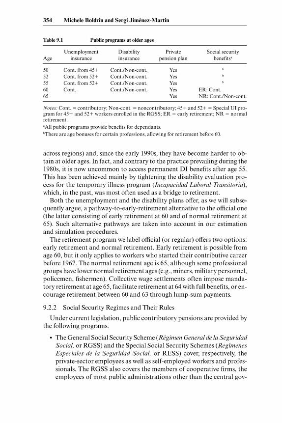
Table 9.1 summarizes the programs available after age 50. Leaving asideprivate pensions, there are three public programs that affect the behaviorof old age workers: unemployment benefits, disability benefits, and retire-ment pensions.

Unemployment benefits are generally conditional on previous periodsof contributions and are available only for workers in the General Regime(RGSS) of the Spanish social security (S3) system.1 There are two continu-ation programs for those who have exhausted their entitlement to contrib-utory unemployment benefits: one for those aged over 45 (UB45� pro-gram) and the other for those aged over 52 (UB52� program). The latter isa special subsidy for unemployed people who are older than 52, lack otherincome sources, have contributed to unemployment insurance for at leastsix years in their life and, except for age, satisfy all requirements for an old-age pension.

The S3 system provides insurance against both temporary and perma-nent illness or disability. Contributory disability (DI) benefits are far moregenerous than any other old-age program, since they are not subject topenalties for young age or insufficient years of contribution.2 Disability in-surance benefits are subject to approval by a medical examiner (notoriously,the tightness of admissibility criteria used by examiners varies over time and

Spanish Pension Expenditure under Alternative Reform Scenarios 353

1. People enrolled in any of the special regimes (RESS) either have no access to unemploy-ment benefits (self-employed and household employees) or have special unemployment pro-grams (farmers and fishermen).

2. For a discussion of noncontributory disability pensions and other marginal insuranceschemes (which are not relevant to the following analysis and have little or no impact on theretirement decisions of the workers we are considering) see Boldrin, Jiménez-Martín, andPeracchi (1999).

across regions) and, since the early 1990s, they have become harder to ob-tain at older ages. In fact, and contrary to the practice prevailing during the1980s, it is now uncommon to access permanent DI benefits after age 55.This has been achieved mainly by tightening the disability evaluation pro-cess for the temporary illness program (Incapacidad Laboral Transitoria),which, in the past, was most often used as a bridge to retirement.

Both the unemployment and the disability plans offer, as we will subse-quently argue, a pathway-to-early-retirement alternative to the official one(the latter consisting of early retirement at 60 and of normal retirement at65). Such alternative pathways are taken into account in our estimationand simulation procedures.

The retirement program we label official (or regular) offers two options:early retirement and normal retirement. Early retirement is possible fromage 60, but it only applies to workers who started their contributive careerbefore 1967. The normal retirement age is 65, although some professionalgroups have lower normal retirement ages (e.g., miners, military personnel,policemen, fishermen). Collective wage settlements often impose manda-tory retirement at age 65, facilitate retirement at 64 with full benefits, or en-courage retirement between 60 and 63 through lump-sum payments.

9.2.2 Social Security Regimes and Their Rules

Under current legislation, public contributory pensions are provided bythe following programs.

• The General Social Security Scheme (Régimen General de la Seguridad

Social, or RGSS) and the Special Social Security Schemes (Regímenes

Especiales de la Seguridad Social, or RESS) cover, respectively, theprivate-sector employees as well as self-employed workers and profes-sionals. The RGSS also covers the members of cooperative firms, theemployees of most public administrations other than the central gov-


Table 9.1 Public programs at older ages

Unemployment Disability Private Social securityAge insurance insurance pension plan benefitsa

50 Cont. from 45� Cont./Non-cont. Yes b



60 Cont. Cont./Non-cont. Yes ER: Cont.65 Yes NR: Cont./Non-cont.

Notes: Cont. � contributory; Non-cont. � noncontributory; 45� and 52� � Special UI pro-gram for 45� and 52� workers enrolled in the RGSS; ER � early retirement; NR � normalretirement.aAll public programs provide benefits for dependants.bThere are age bonuses for certain professions, allowing for retirement before 60.

ernments, and all unemployed individuals who comply with the mini-mum number of contributory years upon reaching 65. The RESS in-clude five special schemes:

1. Self-employed (Régimen Especial de Trabajadores Autónomos

[RETA]).2. Agricultural workers and small farmers (Régimen Especial

Agrario [REA]).3. Domestic workers (Régimen Especial de Empleados de Hogar

[REEH]).4. Sailors (Régimen Especial de Trabajadores del Mar [RETM]).5. Coal miners (Régimen Especial de la Minería del Carbón

[REMC]).• The scheme for government employees (Régimen de Clases Pasivas

[RCP]) includes public servants employed by the central governmentand its local branches. In this study we do not consider this regime.

Legislation approved by the Spanish parliament in 1997 established theprogressive elimination of all the special regimes but RETA by the end ofyear 2001. At the moment, however, this piece of legislation has not beenimplemented, and the special regimes are still active.

9.2.3 Rules of the RGSS

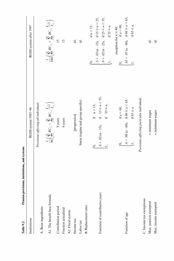
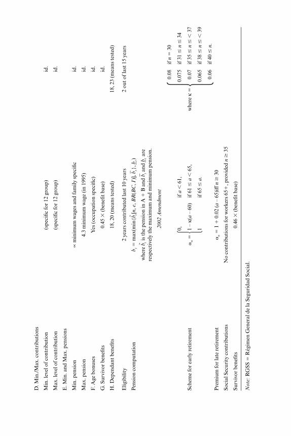
This subsection describes the rules, since 1985, governing the old-ageand survivors’ pensions in the RGSS. The changes introduced by the 1997reform (R97) and the 2002 (A02) amendment will be illustrated as we pro-gress. A summary of the basic technical aspects of the pre- and post-1997systems can be found in table 9.2.

Financing and Eligibility

The RGSS is a pure pay-as-you-go scheme. Contributions are a fixedproportion of covered earnings, defined as total earnings, excluding pay-ments for overtime work, between a floor and a ceiling that vary by broadlydefined professional categories. Eleven categories are currently distin-guished, but the effective number of ceilings and floors for covered earn-ings is only four.

The current RGSS contribution rate is 28.3 percent, of which 23.6 per-cent is attributed to the employer and the remaining 4.7 percent to theemployee. A tax rate of 14 percent is levied on earnings from overtimework.

Entitlement to an old-age pension requires at least fifteen years of con-tributions. As a general rule, recipiency is conditional on having reachedage 65, and is incompatible with income from any kind of employment re-quiring affiliation with the Social Security system.


Tab

le 9

.2P

ensi

on p

rovi

sion

s, in

stit

utio

ns, a

nd s

yste

ms

Inst

itut

ions

RG

SS s

yste

m 1

985–

96R

GSS

sys

tem

aft

er 1

997

Pro

visi

ons

aff

ecti

ng a

ll i

ndiv

iduals

A. B

asic

ingr

edie

nts

A1.

The

ben

efit b

ase

form

ula

�∑24 j�1

BC

t–j�

∑96

j�25

BC

t–j

��∑24 j�

1

BC

t–j�

∑180

j�25

BC

t–j

�C

ontr

ibut

ion

peri

od8

year

s15

Fra

ctio

n ac

tual

ized

6 ye

ars

13

A2.

Fis

cal s

yste

m

Inco

me

tax

[pro

gres

sive

]id

.

Lab

or ta

xlin

ear

(reg

ime

and

grou

p sp

ecifi

c)id

.

B. R

epla

cem

ent r

ates

Fun

ctio

n of

con

trib

utiv

e ye

ars

�� ex

cept

ion

for

n�

40:

Fun

ctio

n of

age

��

Pro

visi

ons

aff

ecti

ng p

art

icula

r in

div

iduals

C. I

ncom

e ta

x ex

empt

ions

Max

. pen

sion

exe

mpt

ed∝

min

imum

wag

esid

.

Max

. inc

ome

exem

pted

∝m

inim

um w

ages

id.

if a

�60

,

if 6

0 �

a�

65,

if 6

5 �

a.

0, .65

�.0

7 (a

– 60

),

1,

if a

�60

,

if 6

0 �

a�

65,

if 6

5 �

a.

0, .6 �

.08

(a–

60),

1,

if n

�15

,

if 1

5 �

n�

25,

if 2

5 �

n�

35,

if 3

5 �

n.

0, .5 �

.03

(n–

15),

.8 �

.02

(n–

25),

1,

ifn

�15

,

if15

�n

�35

,

if35

�n.

0, .6 �

.02

(n–

15),

1,

I t–25

� I t–j

1� 18

0

I t–25

� I t–j

1 � 96

D. M

in./M

ax. c

ontr

ibut

ions

Min

. lev

el o

f con

trib

utio

n(s

peci

fic fo

r 12

gro

up)

id.

Max

. lev

el o

f con

trib

utio

n(s

peci

fic fo

r 12

gro

up)

id.

E. M

in. a

nd M

ax. p

ensi

ons

Min

. pen

sion

∝m

inim

um w

ages

and

fam

ily s

peci

ficid

.

Max

. pen

sion

4.3

min

imum

wag

e (i

n 19

95)

id.

F. A

ge b

onus

esY

es (o

ccup

atio

n sp

ecifi

c)id

.

G. S

urvi

vor

bene

fits

0.45

�(b

enefi

t bas

e)id

.

H. D

epen

dant

ben

efits

18, 2

0 (m

eans

test

ed)

18, 2

3 (m

eans

test

ed)

Elig

ibili

ty2

year

s co

ntri

bute

d la

st 1

0 ye

ars

2 ou

t of l

ast 1

5 ye

ars

Pen

sion

com

puta

tion

bt�

max

(min

{bt[n

, e, B

R(B

C, I

)], b�

t}, b �t

)

whe

re b

tis

the

pens

ion

in A

�B

and

b�tan

d b �t

are

resp

ecti

vely

the

max

imum

and

min

imum

pen

sion

.

20

02

Am

end

men

t

Sche

me

for

earl

y re

tire

men

t

n��

whe

re κ

�

�P

rem

ium

for

late

ret

irem

ent

n

�1

�0.

02 (a

– 65

)iff

n�

30

Soci

al S

ecur

ity

cont

ribu

tion

sN

o co

ntri

buti

ons

for

wor

kers

65�

, pro

vide

d n

�35

Surv

ivor

ben

efits

0.46

�(b

enefi

t bas

e)

No

te:

RG

SS �

Rég

imen

Gen

eral

de

la S

egur

idad

Soc

ial.

if n

�30

if 3

1 �

n�

34

if 3

5 �

n�

�37

if 3

8 �

n�

�39

if 4

0 �

n.

0.08

0.07

5

0.07

0.06

5

0.06

if a

�61

,

if 6

1 �

a�

65,

if 6

5 �

a.

0, 1 –

κ(a

– 60

)

1

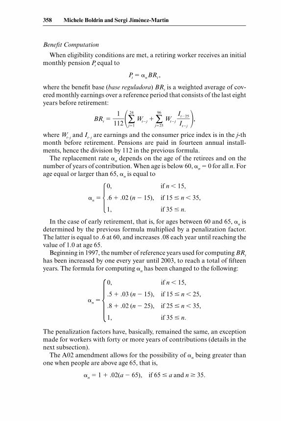
Benefit Computation

When eligibility conditions are met, a retiring worker receives an initialmonthly pension Pt equal to

Pt � nBRt ,

where the benefit base (base reguladora) BRt is a weighted average of cov-ered monthly earnings over a reference period that consists of the last eightyears before retirement:

BRt � �∑24

j�1

Wtj � ∑96

j�25

Wtj �,

where Wt–j and It–j are earnings and the consumer price index is in the j-thmonth before retirement. Pensions are paid in fourteen annual install-ments, hence the division by 112 in the previous formula.

The replacement rate n depends on the age of the retirees and on thenumber of years of contribution. When age is below 60, n � 0 for all n. Forage equal or larger than 65, n is equal to

n � �In the case of early retirement, that is, for ages between 60 and 65, n is

determined by the previous formula multiplied by a penalization factor.The latter is equal to .6 at 60, and increases .08 each year until reaching thevalue of 1.0 at age 65.

Beginning in 1997, the number of reference years used for computing BRt

has been increased by one every year until 2003, to reach a total of fifteenyears. The formula for computing n has been changed to the following:

n � �The penalization factors have, basically, remained the same, an exceptionmade for workers with forty or more years of contributions (details in thenext subsection).

The A02 amendment allows for the possibility of n being greater thanone when people are above age 65, that is,

n � 1 � .02(a 65), if 65 � a and n � 35.

if n � 15,

if 15 � n � 25,

if 25 � n � 35,

if 35 � n.

0,

.5 � .03 (n 15),

.8 � .02 (n 25),

1,

if n � 15,

if 15 � n � 35,

if 35 � n.

0,

.6 � .02 (n 15),

1,

It25�Itj

1�112


In all of our simulations we use the pre-1997 formula, which was in placeover the relevant sample period. We consider the impact of the 1997 reformand the 2002 amendment when examining alternative policies (see, respec-tively, R97 and A02 in section 9.7).

Outstanding pensions are fully indexed to price inflation, as measuredby the consumer price index. Until 1986, pensions were also indexed to realwage growth.

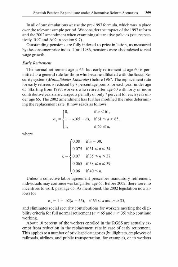
Early Retirement

The normal retirement age is 65, but early retirement at age 60 is per-mitted as a general rule for those who became affiliated with the Social Se-curity system (Mutualidades Laborales) before 1967. The replacement ratefor early retirees is reduced by 8 percentage points for each year under age65. Starting from 1997, workers who retire after age 60 with forty or morecontributive years are charged a penalty of only 7 percent for each year un-der age 65. The 2002 amendment has further modified the rules determin-ing the replacement rate. It now reads as follows:

n � �where

� ��Unless a collective labor agreement prescribes mandatory retirement,

individuals may continue working after age 65. Before 2002, there were noincentives to work past age 65. As mentioned, the 2002 legislation now al-lows for

n � 1 � .02(a 65), if 65 � a and n � 35,

and eliminates social security contributions for workers meeting the eligi-bility criteria for full normal retirement (a � 65 and n � 35) who continueworking.

About 10 percent of the workers enrolled in the RGSS are actually ex-empt from reduction in the replacement rate in case of early retirement.This applies to a number of privileged categories (bullfighters, employees ofrailroads, airlines, and public transportation, for example), or to workers

if n � 30,

if 31 � n � 34,

if 35 � n � 37,

if 38 � n � 39,

if 40 � n.

0.08

0.075

0.07

0.065

0.06

if a � 61,

if 61 � a � 65,

if 65 � a,

0,

1 �(65 a),

1,


who were laid off during cases of industrial restructuring regulated by spe-cial legislation. These exemption rights are portable in proportion to thenumber of years spent working in the privileged sector.

Maximum and Minimum Pension

Pensions are subject to a ceiling, legislated annually and roughly equalto the ceiling on covered earnings. The 2000 ceiling corresponds to about4.3 times the minimum wage (salario mínimo interprofesional [SMI]) andabout 1.6 times the average monthly earnings in the manufacturing andservice sectors. If the initial old-age pension, as previously computed, is be-low a minimum, then the minimum pension is paid. The latter is also legis-lated annually. Other things being equal, minimum pensions are higher forthose who are older than 65 or who have a dependent spouse.

In the last decade, minimum pensions grew at about the same rate asnominal wages, whereas maximum pensions grew at the rate of inflation.The ratio between the minimum old-age pension and the minimum wagehas been increasing steadily from the late 1970s (it was 75 percent in 1975)until reaching almost 100 percent in the early 1990s. The percentage ofRGSS retirees receiving a minimum pension has been declining steadily,from over 75 percent in the late 1970s to 27 percent in 1995.

Family Considerations

A pensioner receives a fixed annual allowance for each dependent childwho is younger than 18 or is disabled. In 2000, this allowance was equal to48,420 pesetas for each child under 18, and to 468,720 pesetas (45 percentof the annualized minimum wage) for each disabled child.

Survivors (spouse, children, other relatives) may receive a fraction of thebenefit base of the deceased if the latter was a pensioner or died before re-tirement after contributing for at least 500 days in the last five years. Thebenefit base is computed differently in the two cases. If the deceased was apensioner, the benefit base coincides with the pension. If the deceased wasworking, it is computed as an average of covered earnings over an uninter-rupted period of two years, chosen by the beneficiary, among the last sevenyears immediately before death. If death occurred because of a work acci-dent or a professional illness, then the benefit base coincides with the lastearnings.

The surviving spouse gets 45 percent of the benefit base of the deceased(46 percent after the 2002 amendment, a fraction that will be further in-creased in forthcoming years). In case of divorce, the pension is divided be-tween the various spouses according to the length of their marriage withthe deceased. Such a pension is compatible with labor income and anyother old-age or disability pension, but is lost if the spouse remarries.

Each of the surviving children gets 20 percent of the benefit base untilthe age of 18 (raised to 23 percent in 1997). An orphan who is the sole ben-


eficiary may receive up to 65 percent of the benefit base. If there are severalsurviving children, the sum of the pensions to the surviving spouse (if any)and the children cannot exceed 100 percent of the benefit base.

A Spanish peculiarity is the pension in favor of family members. Thispension entitles other surviving relatives (e.g., parents, grandparents, sib-lings, nephews) to 20 percent of the benefit base of the principal if they sat-isfy certain eligibility conditions (older than 45, do not have a spouse, donot have other means of subsistence, have been living with and dependingeconomically upon the deceased for the last two years). To this pension,one may add the 45 percent survivors’ pension if there is no survivingspouse or eligible surviving children.

9.2.4 Special Schemes

In this section we sketch the main differences between the general andthe special schemes. Whereas rules and regulations for sailors and coal min-ers are very similar to the ones for the general scheme, special rules applyto the self-employed, farmers, agricultural workers, domestic helpers, anda few other categories not discussed here, such as part-time workers, art-ists, travelling salespeople, and bullfighters. Beside the differences in the SStax rate and the definition of covered earnings, an important difference isthe fact that affiliates of the special schemes have no early-retirement op-tion (exceptions are made for miners and sailors).

The rest of this section focuses on the special schemes for self-employedworkers (RETA) and farmers (REA), which together represent 93 percentof the affiliates of the special schemes, and 86 percent of the pensions theypay out.

Self-employed

While the SS tax rate is the same for the RETA and the general scheme(28.3 percent in 2000), covered earnings are computed differently, as theself-employed are essentially free to choose their covered earnings betweena floor and a ceiling that are legislated annually. Not surprisingly, in lightof the strong progressivity of Spanish personal income taxes, a suspi-ciously large proportion of self-employed workers report earnings equal tothe legislated floor until they reach age 50. After that age one observes asudden increase in reported covered earnings. This behavior exploits the fi-nite memory in the formula for the calculation of the initial pension.

In 2000, the RETA contributive floor and ceiling were equal to 116,160pesetas (pta) and 407,790 pta per month respectively, corresponding to 1.4and 5 times the minimum wage, and to .5 and 1.9 times the average earn-ings in manufacturing and services. To reduce misreporting of earnings onthe part of the self-employed, a different ceiling applies to self-employedaged over 50 who had not reported higher earnings in previous years. In


2000, the latter was only 219,000 pta per month, roughly equal to averagemonthly earnings.

A crucial difference with respect to the general scheme is that, under theRETA, recipiency of an old-age pension is compatible with maintainingthe self-employed status. The implications of this provision for the retire-ment behavior of self-employed workers are discussed later.

Other important provisions are the following: RETA only requires fiveyears of contributions in the ten years immediately before the death of theprincipal in order to qualify for survivors’ pensions. Under RETA, the lat-ter is 50 percent of the benefit base. If the principal was not a pensioner atthe time of death, the benefit base is computed as the average of coveredearnings over an uninterrupted period of five years, chosen by the benefi-ciary among the last ten years before the death of the principal.

Farmers

In this case, both the SS tax rate and the covered earnings differ with re-spect to the general scheme. Self-employed farmers pay 19.75 percent of atax base that is legislated annually and is only weakly related to averageearnings. In 2000, this was equal to 91,740 pta per month, correspondingto 1.24 times the minimum wage and about 40 percent of average monthlyearnings in the manufacturing and service sectors.

Farm employees, instead, pay 11.5 percent of a monthly base that de-pends on their professional category and is also legislated annually. In ad-dition, for each day of work, their employer must pay 15.5 percent of adaily base that also varies by professional category and is legislated annu-ally.

9.3 Key Ingredients of the Retirement Models

In this section we review the main steps taken in order to estimatereduced-form retirement models. First, we describe the sample and the char-acteristics of the earning processes. Then we construct the various mea-sures of social security incentives. In the last part we review the results fromthe estimated models.

9.3.1 The Sample

Our main microeconomic dataset is based on administrative recordsfrom the Spanish Social Security Administration (Historiales Laborales de

la Seguridad Social [HLSS]). The sample consists of 250,000 individualwork histories randomly drawn from the historical files of SS affiliates(Fichero Histórico de Afiliados [FHA]). The sample includes only individ-uals aged over 40 on July 31, 1998, the date at which the files were prepared.The sample contains individuals from the RGSS and the five special re-gimes—RETA, REA, REEH, RTMC, and RTMAR. As we mentioned


earlier, civil servants and other central government employees are not cov-ered by the SS administration and are not considered in this study.

The dataset consists of three files. The first file (the history file, or H) con-tains the work history of individuals in the sample. Each record in this filedescribes a single employment period of the individual. As we argue later,the work histories are very accurate for periods or histories that began af-ter the mid-1960s. The second file (covered earnings file, or CE) containsannual averages of covered earnings (bases de cotización) from 1986 to1995. The third file (benefits file, or B) contains information on the lifetimeSS benefits received by individuals in the sample. Benefits are classified byfunction (retirement, disability, survival, etc.) and initial amount received.To be more precise, the benefits file contains the initial benefit amount andthe length of the period during which the benefit was received. A fourth file(relatives file, or R) is also available; it reports some benefits paid to rela-tives of the individual while members of his or her household.

For each individual in the sample who contributed to SS during the1986–1995 period, the CE file reports the annual average of covered earn-ings together with the contributions paid. For individuals enrolled in eitherthe RGSS or the RTMC, covered earnings are a doubly censored (fromabove and below) version of real earnings. This is due to the existence oflegislated ceilings and floors, as reported earlier. For people enrolled in SSregimes other than RGSS and RTMC, covered earnings are chosen by theindividual within given ceilings and floors (see section 9.2 for details) and,consequently, in this case there is no clear link between covered and actualearnings.

For each employment spell in the HLSS-H file, we know age, sex, andmarital status of the person, the duration of the period (in days), thetype of contract (in particular, we can distinguish between part-time andfull-time contracts), the social security regime, the contributive group, thecause for the termination of the period, the sector of employment (4-digitsSIC), and the region of residence (52 Spanish provinces). For each indi-vidual in the H file who has received some benefits at any point, we knowmost of the information that the SS Administration uses to compute themonthly benefits to be paid. In particular, we know the initial and currentpension, the benefit base (base reguladora), the number of contributiveyears, the current integration toward the minimum pension (complementos

por el mínimo), the date pension was claimed, the date it was awarded, thetype of benefits, and so on. See Boldrin, Jiménez-Martín, and Peracchi(2004) for a description of the demographic characteristics of the sampleand the sample selection rules.

9.3.2 Earnings Distribution, Earnings Histories, and Projections

As commented in section 9.3.1, we do not observe earnings directly butonly covered earnings. Covered earnings are a doubly censored version of


earnings for workers in the RGSS or Regimen Trabajadores Mineria Car-bon (RTMC), while they are very weakly related to true earnings for work-ers in the RETA because of the presence of both legislated tariffs and wide-spread tax fraud.

RGSS and RTMC

To deal with the top-censoring problem, we proceed as follows. First, weestimate a Tobit model for covered earnings. Then we use the estimated pa-rameters to impute the earnings of the censored observations and to esti-mate an earning function using imputed earnings for those affected by theceilings. Finally, we generate true earnings for all the individuals in the topcensored groups, by using the estimated regression function and adding anindividual, random noise component.

From the individual profile of covered earnings ct between year T – k andyear T we impute the individual profile of true real earnings (wt , t � T – k,. . . , T). Given this information, we project earnings forward and back-ward in the following way.

• Forward: here we assume zero real growth, hence wT�m � wT for m �1, . . . , M.

• Backward: wT–k–1 � wT–k � g(aT–k–1) for l � 1, . . . , L. The function g(�)corrects for the growth of log earnings imputable to age a and is de-fined as:

g (aTkl ) � 1 � aTkl � 2 � a2Tkl 1 � aTk 2 � a2

Tk.

The s are the estimated coefficients from a fixed-effects earningsequation, the details of which are available upon request. The correc-tion is specific for each combination of sex and contributive group.

We further correct backward the log of average earnings to control forthe variation of the average productivity of the Spanish economy in the pe-riod 1960–1985, which is the time horizon of our backward projection.

RETA

As already pointed out, for individuals enrolled in the RETA, coveredearnings are very weakly related to true earnings. The self-employed arefree to choose their benefit base between an annual floor and ceiling, andpractically all choose the floor. This implies that there is no way in whichtrue earnings for the self-employed can be recovered from the HLSSdataset. We are therefore forced to assume that the earnings and the con-tributive profile coincide. Thus, we project (real) earnings given the ob-served profile of (real) contributions as follows:

• Backward: wt–k–l � ct–k, for l � 1, . . . , L,• Forward: wt�m � ct(1 � g)m, for m � 1, . . . , M with g � 0.005.


In other words, we assume that contributions were constant up to thefirst time they are observed, while they grow at a constant annual rate of 0.5percent thereafter.

It is important to recall, from section 9.2, that current Spanish legisla-tion allows the self-employed to begin drawing retirement pensions with-out retiring, at least as long as they keep managing their own business.Hence, in the dynamic choice of the self-employed, the opportunity cost ofretiring is not measured by the loss of future earnings but, instead, by thefact that contributions can no longer be accumulated to increase futurepensions, and marginal income taxes must be paid on pensions. This im-plies that for the self-employed, maximization of the (net of taxes) SocialSecurity payoff is a very reasonable, objective function.

9.3.3 Evaluation of Social Security Incentives

Assumptions

For every male worker in the wage sample who is enrolled either in theRGSS or in the RETA we assume that: (a) he is married to a nonworkingspouse, (b) his wife is three years younger, and (c) his mortality corre-sponds to the baseline male mortality from the most recent available lifetables (INE 1995).

For every female in the wage sample we assume that: (a) she is marriedto either a retiree or a worker entitled to retirement benefits, (b) her hus-band is four years older, and (c) her mortality is the baseline female mor-tality from the most recent available life tables (INE 1995).

For both men and women we further assume that (d) starting at age 55and until age 65, there are three pathways to retirement: the UB52� pro-gram, DI benefits, and early retirement. At each age, an individual has anage-specific probability of entering retirement using any of these three pro-grams. However, the following restrictions are important in characterizingthe actual usage of the three pathways to retirement.

1. No person has access to early retirement before age 60.2. After age 60, a person cannot claim UB52� and can only claim early

retirement or DI benefits.3. A self-employed person enrolled in RETA can never claim UB52�

benefits.

This implies that, in practice, pathways for retirement are relativelysimple. For people in the RGSS, either they retire before 60 via the UB52�or the DI benefits program or they retire after 60 via the DI (most unlikely,though, since 1992) or the retirement program. People in the RESS eithergo via the DI benefits or the retirement program, with the likelihood of theformer being low and decreasing from age 60 onward.


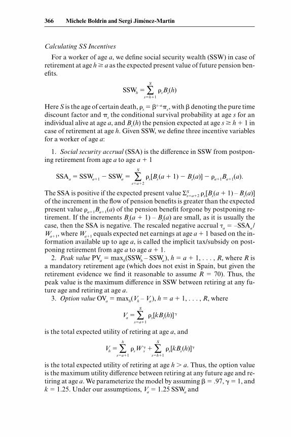
Calculating SS Incentives

For a worker of age a, we define social security wealth (SSW) in case ofretirement at age h � a as the expected present value of future pension ben-efits.

SSWh � ∑S

s�h�1

�sBs(h)

Here S is the age of certain death, �s � s–a�s, with denoting the pure timediscount factor and �s the conditional survival probability at age s for anindividual alive at age a, and Bs(h) the pension expected at age s � h � 1 incase of retirement at age h. Given SSW, we define three incentive variablesfor a worker of age a:

1. Social security accrual (SSA) is the difference in SSW from postpon-ing retirement from age a to age a � 1

SSAa � SSWa�1 SSWa � ∑S

s�a�2

�s[Bs(a � 1) Bs(a)] �a�1Ba�1(a).

The SSA is positive if the expected present value ΣSs�a�2 �s[Bs(a � 1) – Bs(a)]

of the increment in the flow of pension benefits is greater than the expectedpresent value �a�1Ba�1(a) of the pension benefit forgone by postponing re-tirement. If the increments Bs(a � 1) – Bs(a) are small, as it is usually thecase, then the SSA is negative. The rescaled negative accrual �a � –SSAa /Wa�1, where Wa�1 equals expected net earnings at age a � 1 based on the in-formation available up to age a, is called the implicit tax/subsidy on post-poning retirement from age a to age a � 1.

2. Peak value PVa � maxh(SSWh – SSWa ), h � a � 1, . . . , R, where R isa mandatory retirement age (which does not exist in Spain, but given theretirement evidence we find it reasonable to assume R � 70). Thus, thepeak value is the maximum difference in SSW between retiring at any fu-ture age and retiring at age a.

3. Option value OVa � maxh(Vh – Va ), h � a � 1, . . . , R, where

Va � ∑S

s�a�1

�s[kBs(h)]�

is the total expected utility of retiring at age a, and

Vh � ∑h

s�a�1

�sW s� � ∑

S

s�h�1

�s[kBs(h)]�

is the total expected utility of retiring at age h � a. Thus, the option valueis the maximum utility difference between retiring at any future age and re-tiring at age a. We parameterize the model by assuming � .97, � � 1, andk � 1.25. Under our assumptions, Va � 1.25 SSWa and


Vh � ∑h

s�a�1

�sWs � 1.25 SSWh .

If expected earnings are constant at Wa (as assumed by our earningsmodel), then

Vh Va � Wa ∑h

s�a�1

�s � 1.25(SSWh SSWa ),

that is, the peak value and the option value are proportional to each otherexcept for the effect due to the term Σh

s�a�1�s .The restrictions embodied in assumption (d) require us to combine the

incentive measures Ij from the various programs ( j � UB, DI, R, where UBdenotes unemployment benefits, DI disability benefits, and R the retire-ment programs) as follows:

I � �where pa

DI denotes the probability of observing a transition from employ-ment into disability at age a. Since the self-employed have no access toUB52� benefits, the combined incentives from age 55 to age 59 for mem-bers of this group change to

I � paDIIDI � IR(1 pa

DI ), 55 � a � 59.

We have followed a regression-based approach to compute the uncondi-tional probability of qualifying for a disability pension (see table 9.3; seealso Boldrin, Jiménez-Martín, and Peracchi [2004] for a description).

9.3.4 The Reduced-Form Retirement Model

This section briefly illustrates the explanatory power of our incentivemeasures (accrual, peak value, and option value) for retirement behavior.The results reported here are distilled from the extensive econometric anal-ysis conducted in Boldrin, Jiménez-Martín, and Peracchi (2004), to whichthe reader is referred for all relevant details.

We follow a regression-based approach to model the effect of social se-curity wealth, incentive measure (either accrual, peak, or option value),and individual demographic characteristics on the decision to retire in1995, conditional on being active at the end of 1994. Retirement probabili-ties are assumed to have the probit form

Pr(Ri � 1) � �(�1SSWi � �2Ii � ��3Xi ),

where R is a binary indicator of retirement, � is the distribution functionof a standard normal, I denotes the incentive measure, and X is a vector of

if 55 � a � 60,

if 60 � a � 65,

if 65 � a,

paDIIDI � IUB(1 pa

DI ),

paDIIDI � IR(1 pa

DI ),

IR,


Tab

le 9

.3P

robi

t mod

els

of th

e 19

95 re

tire

men

t rat

es

Acc

rual

Pea

kO

ptio

n va

lue

M1

M2

M1

M2

M1

M2

Coe

f.SE

Coe

f.SE

Coe

f.SE

Coe

f.SE

Coe

f.SE

Coe

f.SE

Male

RG

SS

: 16,1

91 o

bse

rvati

ons

SSW

.003

44.0

0128

.007

49.0

0152

.008

71.0

0149

.013

87.0

0170

.010

80.0

0165

.006

27.0

0186

ME

.000

33.0

0012

.000

71.0

0014

.000

87.0

0015

.001

36.0

0017

.001

09.0

0017

.001

61.0

0018

Ince

ntiv

e–.

0090

6.0

0430

–.00

130

.004

89.0

0147

.002

45.0

0448

.002

54.0

0884

.001

11.0

1032

.001

15M

E–.

0008

8.0

0042

–.00

012

.000

46.0

0015

.000

24.0

0044

.000

25.0

0089

.000

11.0

0102

.000

11C

onst

ant

–1.6

42.5

0046

–1.1

97.5

3053

–1.4

95.4

9230

–1.2

73.5

2863

–1.3

60.4

9665

–1.2

62.5

3657

R2

.336

.373

.341

.380

.342

.381

Log

-lik

elih

ood

–3,7

91–3

,579

–3,7

66–3

,544

–3,7

58–3

,534

Fem

ale

RG

SS

: 3,8

52 o

bse

rvati

ons

SSW

.009

70.0

0325

.018

12.0

0419

.011

38.0

0345

.020

22.0

0438

.011

76.0

0381

.021

75.0

0477

ME

.000

90.0

0030

.001

62.0

0038

.001

07.0

0033

.001

85.0

0040

.001

11.0

0036

.001

99.0

0044

Ince

ntiv

e–.

0092

.007

10–.

0058

0.0

0755

.001

35.0

0490

.003

93.0

0527

.002

47.0

0202

.003

61.0

0210

ME

–.00

086

.000

66–.

0005

3.0

0068

.000

13.0

0046

.000

36.0

0048

.000

23.0

0019

.000

33.0

0019

Con

stan

t–.

4766

.645

79–.

2204

.742

17–.

3112

.642

44–.

2072

.748

80–.

3301

.648

92–.

3375

.759

22R

2.3

27.3

55.3

27.3

56.3

26.3

56L

og-l

ikel

ihoo

d–8

97.8

–860

.1–8

97.7

–858

.5–8

97.9

–858

.5

Male

RE

TA

: 4,3

55 o

bse

rvati

ons

SSW

.008

70.0

0496

.007

26.0

1174

–.00

068

.006

95.0

0992

.012

38.0

0757

.009

38.0

0501

.014

51M

E.0

0117

.000

67.0

0096

.001

55–.

0000

9.0

0092

.001

31.0

0163

.001

00.0

0124

.000

66.0

0191

Ince

ntiv

e–.

0470

3.0

1212

.010

50.0

1440

–.02

915

.009

00.0

1432

.010

56–.

0092

0.0

0729

.001

87.0

0758

ME

–.00

630

.001

62.0

0138

.001

90–.

0038

5.0

0119

.001

88.0

0139

–.00

122

.000

97.0

0025

.001

00C

onst

ant

–2.0

79.6

8022

–1.5

421.

2772

–1.8

48.7

2708

–1.6

444

1.28

19–2

.107

.704

36–1

.324

1.28

3R

2.1

68.2

52.1

66.2

53.1

67.2

53L

og-l

ikel

ihoo

d–1

,201

–1,0

79–1

,203

–1,0

78–1

,202

–1,0

79

Fem

ale

RE

TA

: 2,0

51 o

bse

rvati

ons

SSW

.003

16.0

0643

–.00

176

.011

13.0

0188

.007

32–.

0024

8.0

1119

.003

42.0

1334

–.01

475

.017

81M

E.0

0047

.000

95–.

0002

5.0

0156

.000

28.0

0108

–.00

035

.001

57.0

0051

.001

99–.

0020

7.0

0250

Ince

ntiv

e.0

1813

.010

96.0

2538

.012

07.0

0849

.009

79.0

1824

.010

39.0

0241

.014

48.0

0739

.017

36M

E.0

0268

.001

62.0

0355

.001

69.0

0126

.001

45.0

0256

.001

46.0

0036

.002

15.0

0104

.002

44C

onst

ant

–3.3

583.

5687

–3.6

783.

7786

–3.1

753.

5836

–2.4

573.

8070

–3.2

593.

6326

–1.8

763.

9571

R2

.142

.197

.141

.196

.140

.195

Log

-lik

elih

ood

–638

.5–5

97.9

–639

.4–5

98.5

–639

.8–5

98.9

No

tes:

M1

�m

odel

wit

h a

linea

r ag

e tr

end;

M2

�m

odel

wit

h ag

e du

mm

ies;

Coe

f. �

coeffi

cien

t; S

E �

stan

dard

err

or; M

E �

mar

gina

l eff

ect;

RG

SS �

Rég

-im

en G

ener

al d

e la

Seg

urid

ad S

ocia

l; R

ET

A �

Rég

imen

Esp

ecia

l de

Tra

baja

dore

s A

utón

omos

.

predictors that include individual earnings and sociodemographic charac-teristics. The socioeconomic and earnings information is richer for theRGSS than for the RETA. This, coupled with the widespread misreportingof earnings that characterizes the affiliates to RETA, makes a quantitativeanalysis of their retirement patterns a very difficult task. Regression resultsfor RETA, in fact, are much poorer than those for RGSS and, in any case,should be taken with caution.

For each one of the three incentive measures (accrual, peak, and optionvalue) we have used the following specification for the set of predictors X.The latter contains an eligibility dummy for attainment of a minimumof fifteen years of contributions; three industry-specific variables: thefraction of collective wage settlements having a clause favoring early re-tirement, the presence of rules permitting retirement at age 64 withoutpenalty, and the existence of mandatory retirement at age 65; differentmeasures of seniority on the job and in the labor market (length of thecurrent employment spell and its square, number of years of contributionand its square, number of years since first employment); dummies forschooling level and contributive group (only for people in the RGSS); dum-mies for part-time work and sector of occupation (only for people in theRGSS); the expected wage and our estimate of the lifetime earnings netpresent value and their squares; the net present value of expected wages un-til the year in which either the peak value or the option value reach theirmaximum.

A Summary of Estimation Results

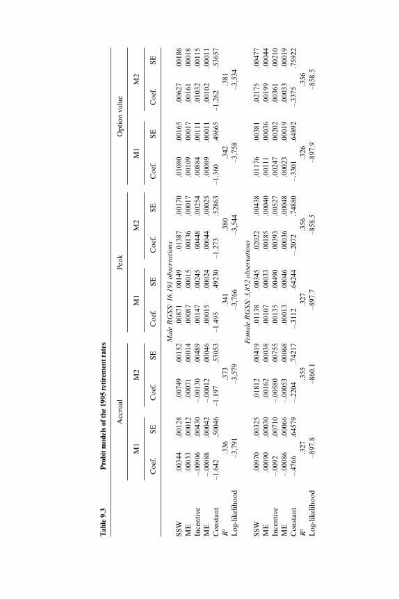
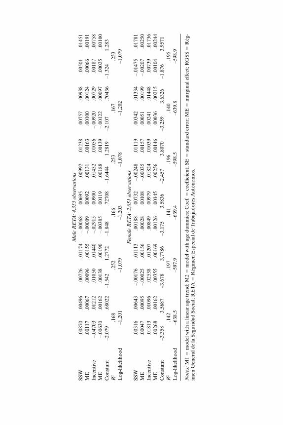
The results obtained for each incentive measure are presented separatelyby sex and social security regime in table 9.3. In each case, we have consid-ered two specifications for the age effect: a linear time trend (M1) and age-specific dummies (M2). The models have been fit to the observed transi-tions between 1994 and 1995. We show, for each combination of sex andregime, the estimates of the probit coefficients, their estimated standard er-rors, and the implied probability effect. Since we report the results from alarge number of models, we concentrate on the variables of interest. Thecomplete set of results is available from the authors upon request.

Quite obviously, M2 provides a uniformly better fit than M1 and, in par-ticular, captures the hazard peaks at 60 and 65, which M1 fails to fit; on anyother aspect, though, the qualitative as well as most of the quantitative per-formances of the two models are equivalent. Hence, the comments that fol-low apply, unless stated otherwise, to both specifications. The SSW term ispositive and significant in all cases. Contradictory results are obtained in-stead for the three incentive variables. In fact, while the accrual usuallyshows the expected (negative) sign, both the peak and the option valueshow the wrong (positive) sign. Further, neither SSW nor the incentivevariables are significant for people enrolled in RETA, indicating that the


SSW and the financial variables do not capture retirement incentives forindividuals enrolled in RETA. Measures of fitness, such as the R2, are ei-ther mediocre or poor, suggesting that a great deal of retirement variabil-ity cannot be captured by our incentive indicators. This is particularly truefor people enrolled in the special regimes (RETA). These relatively poor re-sults are discussed at length in Boldrin, Jiménez-Martín, and Peracchi(2004) and we will not go back to them here. They do suggest, though, thatthe quantitative impact that a change in the financial incentives may haveon predicted retirement behavior is bound to be either negligible or small.The implied probability effects are minuscule, suggesting that only abnor-mally large variations in the incentive measures may be able to have a quan-titatively sizable effect on early retirement. As a consequence of this fact,when evaluating the policy reforms we concentrate our attention mostly onchanges in SSW and on the effect of variables other than the pure financialincentive variables. As the forthcoming analysis underlines, reforming thelegislated early and normal retirement age appears to be the most reliableand effective way of altering existing retirement patterns.

9.4 Simulation Methodology

9.4.1 Policy Simulations

The main aim of this paper is to investigate the budgetary implicationsof pension system reforms. In the simulations we consider five policies, ofwhich the last two are specific to the Spanish case:

R1: Three-Year Reform. A reform of the existing system, consisting of athree-year increase in both the early and the normal retirement age(ERA and NRA, respectively), while keeping all other aspects of theSpanish social security system unchanged.

R2: Actuarial Reform. This reform introduces the following change to thebase Spanish pension system: a 6 percent annual actuarial adjustmentper year away from the normal retirement age. Benefits become availableat the existing ERA (60), and retirements after the NRA receive a posi-tive 6 percent adjustment per year. This actuarial adjustment is alsoapplied to disability benefits.

R3: Common Reform. This reform implies the following changes to thebase system: (a) ERA at 60, (b) NRA at 65, (c) a replacement rate at age65 equal to 60 percent of the gross (but net of the employers contribu-tions) average lifetime earnings (on the best 40 earnings years before re-tirement or the first age of eligibility, whichever comes first), and an ac-tuarial adjustment of 3.6 percent per year from age 60 to 70 (this impliesa replacement rate of 42 percent at age 60 and 78 percent at age 70). No-tice that (a) and (b) correspond to the current Spanish system, whereas


the actuarial adjustment for retirement before age 65 is less favorablethan the one currently used in Spain. Also, the current Spanish system ismore generous for retirement at age 65 and has no actuarial adjustmentfor postponing retirement after that age.

R97: The retirement regime created by the 1997 Spanish reform.A02: The previous regime, as altered by the amendment introduced in

2002.

We recall that the 1997 reform, described in section 9.2, implies the fol-lowing changes in the basic benefit formula and in the penalties related toage and contributive history: (a) the number of years of contribution usedto construct the benefit base is increased from eight, as prescribed by the1985 legislation, to fifteen, (b) workers retiring after the age of 60 with 40or more contributive years are charged an actuarial adjustment of only 7percent (instead of 8 percent) for each year under age 65, and (c) thepenalty for insufficient contributions is such that the replacement rate (ra-tio between pension and BR) is

n � �The 2002 amendment has introduced the following changes, which are

also illustrated in section 9.2: (a) a generalized penalization rule for earlyretirement, starting at age 61; (b) a new incentive scheme for those retiringafter the age 65 with at least 35 years of contributions; (c) an increase insurvivor benefits.

For each of the five policies we carry out the following simulations:

S1: Starting from the model with a linear trend (M1), we modify the SSWand incentive measures in accordance with the new policy. Specifically,in the calculation of SSW, we increase by three years the early and thenormal retirement ages and shift by three years the age-specific proba-bility of receiving DI-UI benefits.

S2: Starting this time from M2, we modify the SSW and incentive measuresaccording to the assumed policy changes. We also change the probabili-ties of receiving DI benefits, by setting them to zero after age 60, butleave untouched the coefficients on the age dummies.

S3: Again using M2, in addition to the changes described in S2, we alsoshift the coefficients on the age dummies by three years, so that the en-tire age profile of the retirement hazard shifts forward by three years.Specifically, in the calculation of SSW, we increase by three years theearly and the normal retirement ages, and shift by three years the age-specific probability of receiving DI-UI benefits.

if n � 15,

if 15 � n � 25,

if 25 � n � 35,

if 35 � n.

0,

.5 � .03(n 15),

.8 � .02(n 25),

1,


9.4.2 Simulation Sample

We use individuals born in 1940 (aged 55 in 1995) extracted from thesample described previously, since the zero real-growth assumption seemsto be very unrealistic for younger cohorts. We have concentrated on work-ers enrolled in either the general regime (RGSS) or the self-employed re-gime (RETA). These two groups cover practically 90 percent of the affili-ates to the Spanish social security.

Given that the base sample (HLSS) is not completely representative ofthe regional distribution of Spanish employment, we have constructed abalanced random sample by sampling (with replacement) from the HLSS,using the population weights of the six territorial areas into which Spain isdivided by the Labor Force Survey (EPA). The rebalancing procedure hasbeen further refined by taking into account, within each of the six regions,the composition of the labor force by sex and by contributive regime. In asecond step, weights have been assigned to each observation in order toreplicate the population number of workers born in 1940 who were activein the labor market in 1995 (farmers and civil servants excluded).

9.4.3 Baseline Case and Family Assumptions

Our baseline case makes the same assumptions as in Boldrin, Jiménez-Martín, and Peracchi (2004) with regard to interest and mortality rates.The other assumptions are illustrated next.

Marital Status Assumptions

We have used family data from the Spanish Labor Force Survey to obtaininformation on the marital status of individuals born in 1940. The mainfindings, which we try to replicate in our simulations, are the following:

• Male: 95 percent married and 5 percent single. Among those married,75.2 percent have a nonworking spouse and the rest a working spouse.In both cases the spouse was (on average), born in 1943 (aged 52).

• Female: 74 percent married and 26 percent single. Among those mar-ried, 34.5 have a nonworking spouse (presumably retired) and the resta working spouse. In both cases the spouse (on average) was born in1937 (aged 58).

Two remarks are relevant with respect to the way in which the benefits ofsurvivorship are handled in the simulation exercises.

1. Since survivor and retirement benefits are fully compatible (up tothe amount of the maximum pension) there is no necessity to correct fordouble counting in the Spanish case. Whenever the maximum pension ceil-ing is supposed to take effect, this is applied to the total pension paymentsaccruing to the survivor.

2. Survivor benefits accruing to members of the 1940 cohort in force of


their having a working spouse are not accounted for (i.e., are not included inthe computation of the SSW for a member of the 1940 cohort) since they areincluded in the computation of benefits for the cohort the spouse belongs to.

Dependant Assumptions

As noted previously, our dataset does not provide sufficient informationon marital status or on the number and age of dependants. In our projec-tions, we handle this inconvenience by using information extracted fromthe Spanish Labor Survey over the 1995–2001 period. From such data wecompute the average number of dependants (per worker) in each of the sixregions (Catalonia, South, Centre or Castilla, Madrid, East, and North).We also distinguish by the sex and age of the individual worker. In otherwords, we assume that the factors determining the number of dependantsare age, sex, and region of residence. Then we regress the data so collectedfor each of the seven years comprised by the EPA sample, and for each re-gion of residence and sex cell with respect to the age of the worker and itssquare. Next, we use these regressions to predict, for people born in 1940,the average number of dependants when they reach the age between 55 and70. After that age we assume that the number of dependants (spouse ex-cluded) drops to zero. In order to impute the benefits for dependants in thecalculation of the SSW, we assume that all of them receive the legislatedminimum (see Boldrin, Jiménez-Martín, and Peracchi [2004] for data andlegislation).

9.4.4 Computing Expected Expenditure for Those Who Retirebefore Fifty-five

The goal here is to estimate the total expenditure for pension paymentsto those members of the 1940 cohort who retired before the year 1995 (i.e.,before reaching the age of 55) and whose retirement behavior we will nottry to model. While during the 1980s and early 1990s the number of Span-ish workers retiring before age 55 was considerable, this practice has beendropping remarkably quickly during the last decade. As we have alreadypointed out, this is due to a substantial tightening of the requirements foraccessing DI benefits and the sharp reduction in the usage of subsidizedearly retirement as an instrument for handling industrial restructuring.

The relevant information in our sample has the following form. We haveinformation on the initial benefits for all the workers belonging to the 1940cohort who retired before 1998 (age 58). This allows us to reconstruct theSSW of those workers in pesetas of the reference year (1995 in our case).To proceed further we need three additional assumptions.

1. Anyone retiring before age 55 did it through the DI program.2. None of the five reforms being considered will affect the benefits of

those workers who retire before age 55 by means of the DI program.


3. The marital status and the number of dependant entitled to benefitsfor people in this group are the same as for the average member of the co-hort.

This allows us to estimate the (after-income taxes) net present value, inmillions of 2001 euros, of the SSW attributable to members of the 1940 co-hort who retired before the age of 55. This is euro 1,360.4 and 289.6, formale and females, respectively. These values are to be added to those ob-tained in tables 9.9 and 9.10.

9.4.5 Computing Expected Expenditure

Our aim is to compute the lifetime net present value (NPV) of the pen-sion expenditure for a given cohort C aged a in year t. We are endowed witha sample of N observations from which we want to project expenditure fora working population of size M. There are two ways of leaving the laborforce: retirement and death. Under such circumstances, the expected netpresent value of the benefits payments for person i of cohort C is given by:

NPVBPi � ∑S

h�a

[�hi (R; X ) SSWhi � �hi (d; X )SSW dhi ]; i � 1, . . . , N,

where �hi (R; X ) and �hi(d; X ) are, respectively, the conditional probabili-ties (at age a) of retirement and death at age h. Both of them may depend—or not—on individual characteristics (X ). In our exercise, the retirementprobabilities do depend on individual characteristics and the probability ofdying does not (except for the sex of the individual). Obviously, the retire-ment probabilities at each age depend on individual characteristics in ac-cordance with the retirement probabilities estimated previously.

Selecting the adequate weights (which depend on individual character-istics) for each observation and summing up over individuals we obtain theprojected benefits payments for a given cohort C:

NPVBPC � ∑N

i�1

NPVPEi � Wi (X ); i � 1, . . . , N,

where Wi (X ) is the share of individuals of type i in the population, accord-ing to the vector of characteristics X.

The net present value of social security contributions is given

NPVTPC � ∑N

i�1

NPVTPi � Wi (X ); i � 1, . . . , N,

where the net present value of social security contributions for an individ-ual of type i in cohort C has been computed as

NPVTPi � ∑S

h�a

[1 �hi (R; X ) �hi (d; X )]Cdhi ,


and C dhi are the social security contributions paid at age h by an individual

of type i. Finally, the projected expenditure (benefits–taxes) is given by

NPVPEC � NPVBPC NPVTPC .

9.4.6 Elevation to the Population

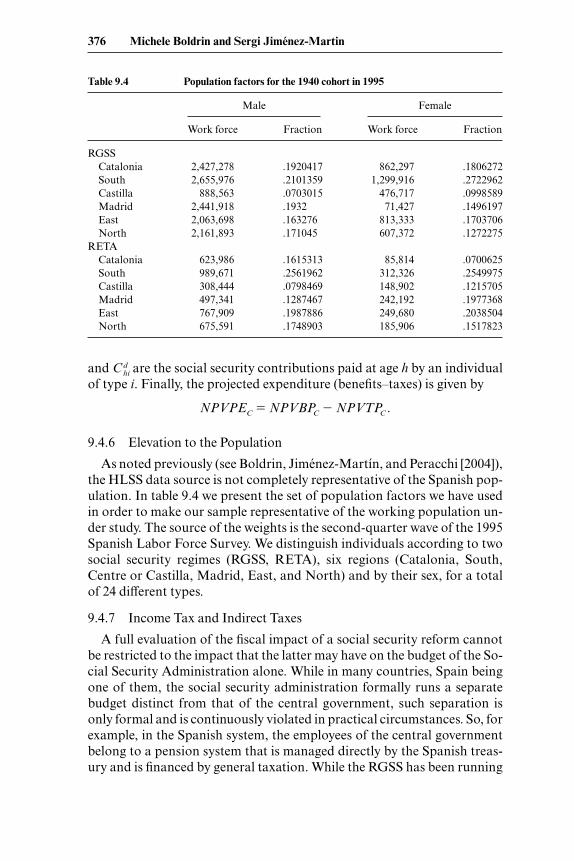
As noted previously (see Boldrin, Jiménez-Martín, and Peracchi [2004]),the HLSS data source is not completely representative of the Spanish pop-ulation. In table 9.4 we present the set of population factors we have usedin order to make our sample representative of the working population un-der study. The source of the weights is the second-quarter wave of the 1995Spanish Labor Force Survey. We distinguish individuals according to twosocial security regimes (RGSS, RETA), six regions (Catalonia, South,Centre or Castilla, Madrid, East, and North) and by their sex, for a totalof 24 different types.

9.4.7 Income Tax and Indirect Taxes

A full evaluation of the fiscal impact of a social security reform cannotbe restricted to the impact that the latter may have on the budget of the So-cial Security Administration alone. While in many countries, Spain beingone of them, the social security administration formally runs a separatebudget distinct from that of the central government, such separation isonly formal and is continuously violated in practical circumstances. So, forexample, in the Spanish system, the employees of the central governmentbelong to a pension system that is managed directly by the Spanish treas-ury and is financed by general taxation. While the RGSS has been running


Table 9.4 Population factors for the 1940 cohort in 1995

Male Female

Work force Fraction Work force Fraction

RGSSCatalonia 2,427,278 .1920417 862,297 .1806272South 2,655,976 .2101359 1,299,916 .2722962Castilla 888,563 .0703015 476,717 .0998589Madrid 2,441,918 .1932 71,427 .1496197East 2,063,698 .163276 813,333 .1703706North 2,161,893 .171045 607,372 .1272275

RETACatalonia 623,986 .1615313 85,814 .0700625South 989,671 .2561962 312,326 .2549975Castilla 308,444 .0798469 148,902 .1215705Madrid 497,341 .1287467 242,192 .1977368East 767,909 .1987886 249,680 .2038504North 675,591 .1748903 185,906 .1517823

a current account surplus during the last few years, this was not the case inthe past and, most likely, will not be the case again in the near future. Inprevious years, the annual deficits of the RGSS (and of the various regimeslisted in the RESS) were covered by transfers from the central government.In fact, part of the current surplus of the RGSS is due to the fact that, pro-gressively, since the 1985 reform, a number of functions originally pertain-ing to the RGSS have been transferred or are being financed directly bygeneral taxation (Social Security social services [INSERSO], noncontrib-utive pensions, part of the minimum pension payments, some disabilitypayments, etc.). More generally, it is quite obvious that surpluses anddeficits of the public pension system are surpluses and deficits of the cen-tral government, which guarantees the payment of future pensions via itspower of taxation, and which considers the net present value of current andfuture pension entitlements as part of the public debt. This implies that afull picture of the fiscal effect of a reform can be achieved only by addingto the net present value calculations we just illustrated—the impact ofchanging work and retirement patterns on other sources of fiscal revenues.

Among the latter, income taxes take the lion’s share. By retiring, an in-dividual not only stops contributing to the pension system and starts draw-ing a pension; he or she also starts paying income taxes on a pension thatis usually substantially smaller than the previous labor income. This effectis further magnified by the existence, in many countries, of a strongly pro-gressive income taxation and a number of exemptions for low incomes,among which pensions loom large, at least in the case of Spain. Finally,moving from work to retirement also implies a number of changes in theconsumption habits of an individual, which may also affect his or her ex-posure to other forms of taxation, such as VAT. While we do take this effectinto account in our estimations, a word of caution should be added. Mostof the VAT impact is due not so much to changes in the composition of con-sumption baskets (VAT rates are fairly homogenous) but to the lower in-come level of pensioners. One is therefore led to assume, as we do here, thata relatively stable relationship exists between income and sales/consump-tion taxes. While this may be a correct first-order approximation, it shouldbe interpreted with care, as it may easily overestimate the reduction in in-direct taxation that follows retirement. The reason is obvious: VAT is aconsumption tax, hence the portion of disposable income that is saved isnot burdened with VAT. Saving propensities drop substantially after re-tirement, which may imply that the amount of VAT paid, as a percentageof one’s income or income taxes, does not stay constant but increases afterretirement.

These caveats notwithstanding, we proceeded as follows. For each indi-vidual in the 1940 cohort, and for each age from 55 onward, we computedthe total income taxes paid; that is, the sum of the income taxes paid as anactive worker (assuming that our estimated labor income at that age, and


in that year coincided with the totality of his or her income) and as a retiree(again, assuming the pension received coincided with her or his total in-come). Additionally, we have tried to impute the VAT taxes paid, startingfrom the income taxes and multiplying by a VAT factor defined as:

VAT � PT/T,

where PT consists of VAT plus other sales and consumption taxes, and Tis total income taxes. The resulting VAT factor, using national accountsdata for 1995–2001 is 0.92.3

The total tax receipts from a pension system, ignoring the general equi-librium effects, are therefore given by:

Total Taxes � SS contribution � (1 � VAT) Income Taxes.

The difference between total taxes under the base case and under each ofthe five reforms quantifies the fiscal impact of that reform.

9.5 Results

Overall, the results are mixed, and in a sense, as we should make clear aswe proceed with the discussion, not fully satisfactory. Recall our distinc-tion (see introduction) between a mechanical and a behavioral effect of apolicy reform. As we argued there, to the extent that individuals who are inthe middle, or toward the end, of their working history are faced with achange of rules to which they cannot appropriately respond, the first effectis always present. The second will come about only if two conditions are si-multaneously realized: (1) the reform affects the financial incentives to ei-ther retire or continue working, and (2) people respond strongly to varia-tions in such financial incentives.

Basically, as one would have expected from the low ability of our re-duced-form estimations to capture the variability of retirement behaviors,while the five reforms do affect the two incentive indicators, the latter donot induce strong behavioral responses on the part of workers. More pre-cisely, the fraction of workers whom, we estimate, would postpone retire-ment age is quite small, and the number of years by which retirement ispostponed is also small. As a consequence, the overall fiscal impact of thevarious reforms is due mostly to the mechanical component, with little be-ing added by the change in workers’ behavior. While this statement should(and will [see the analysis of individual reforms, regime by regime, in therest of this section]) be qualified, we think it summarizes decently well theoverall picture. We are inclined to say that, if our estimations of the behav-ior of Spanish workers past age 55 were to be taken at face value, then themost effective way of postponing retirement would be to simply legislate a


3. See the Bank of Spain web site, at www.bde.es.

shift in the early and normal retirement ages without bothering to modifythe other rules.

9.5.1 Results by Regime and Gender

Since the results are fairly homogeneous across sexes, we present de-tailed results only for males. Results for females are available on request.However, our comments cover both groups without distinguishing be-tween them. Obviously, as female labor-force participation is still substan-tially low in Spain, the actual magnitude involved is rather different be-tween men and women.

RGSS

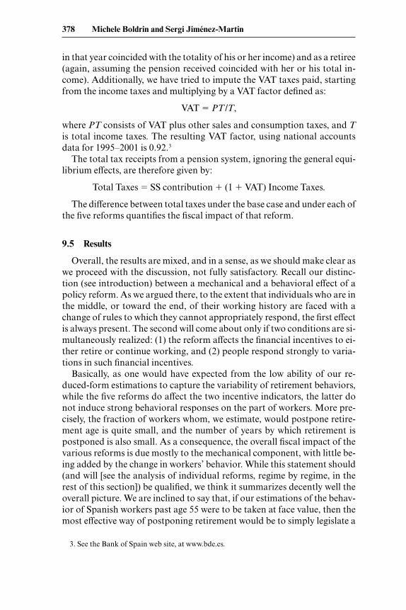
We begin our analysis of results from the RGSS. Figure 9.1 reports SSWby age for the S3 model. We have collected the five reforms in three groups,one for each panel; to allow for ease of comparison with the status quo, thelatter is reported in each panel. In the first panel, we compare the statusquo with the R1 reform in its two versions, S2 and S3. As S3 differs fromS2 only in the retirement hazard, SSW estimates are identical. They areboth lower than in the base case, especially at the crucial ages between 55and 65. The reduction is substantial and, in particular, this reform alsoshifts forward the SSW age profile in such a way that the maximum is now


Fig. 9.1 SSW by age of labor force exit: A, RGSS; B, Option Value; C, S3 model

A B

C

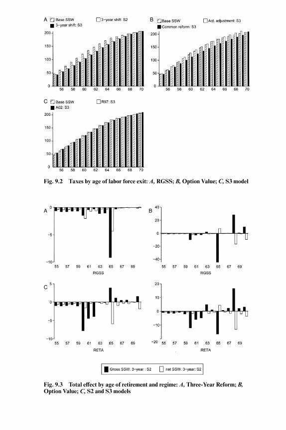
Fig. 9.2 Taxes by age of labor force exit: A, RGSS; B, Option Value; C, S3 model

A

C

B

Fig. 9.3 Total effect by age of retirement and regime: A, Three-Year Reform; B,Option Value; C, S2 and S3 models

A B

C

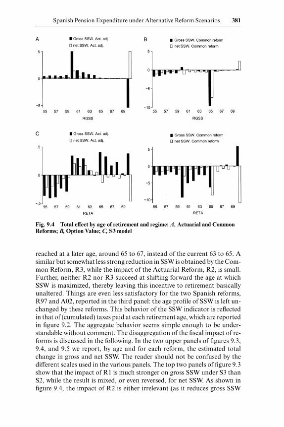
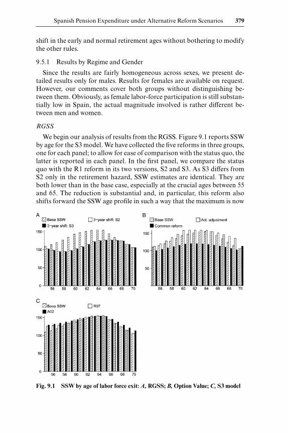
reached at a later age, around 65 to 67, instead of the current 63 to 65. Asimilar but somewhat less strong reduction in SSW is obtained by the Com-mon Reform, R3, while the impact of the Actuarial Reform, R2, is small.Further, neither R2 nor R3 succeed at shifting forward the age at whichSSW is maximized, thereby leaving this incentive to retirement basicallyunaltered. Things are even less satisfactory for the two Spanish reforms,R97 and A02, reported in the third panel: the age profile of SSW is left un-changed by these reforms. This behavior of the SSW indicator is reflectedin that of (cumulated) taxes paid at each retirement age, which are reportedin figure 9.2. The aggregate behavior seems simple enough to be under-standable without comment. The disaggregation of the fiscal impact of re-forms is discussed in the following. In the two upper panels of figures 9.3,9.4, and 9.5 we report, by age and for each reform, the estimated totalchange in gross and net SSW. The reader should not be confused by thedifferent scales used in the various panels. The top two panels of figure 9.3show that the impact of R1 is much stronger on gross SSW under S3 thanS2, while the result is mixed, or even reversed, for net SSW. As shown infigure 9.4, the impact of R2 is either irrelevant (as it reduces gross SSW

Fig. 9.4 Total effect by age of retirement and regime: A, Actuarial and CommonReforms; B, Option Value; C, S3 model


A B

C

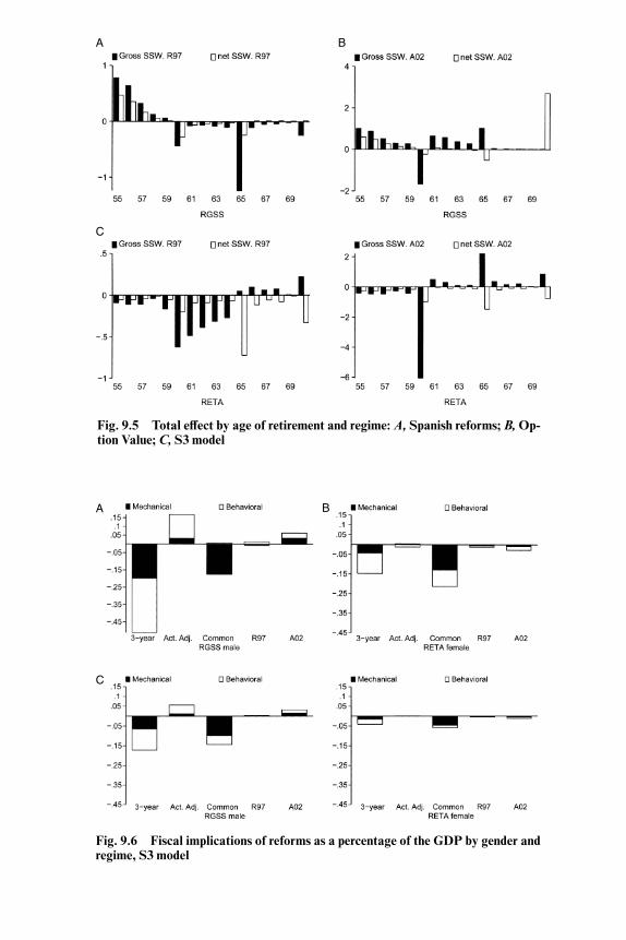
Fig. 9.5 Total effect by age of retirement and regime: A, Spanish reforms; B, Op-tion Value; C, S3 model

A B

C

Fig. 9.6 Fiscal implications of reforms as a percentage of the GDP by gender andregime, S3 model

A B

C

only for people retiring very late, while at the same time increasing their netSSW) or it goes in the wrong direction, slightly increasing SSW at earlierretirement ages. Reform R3, instead, does reduce SSW substantially at thenormal retirement age and, by an almost negligible amount, at earlier dates(figure 9.6, top panels). Finally, in the top panels of figure 9.5, the twoSpanish reforms seem to cause a negligible, and most of the time unde-sired, effect on SSW wealth at all retirement ages considered.

The impact of the five reforms on the distribution of retirement ages canbe found in figure 9.7, which is also structured in three panels to facilitatecomparison. Results are straightforward: R97 and A02 have no impact onretirement ages; both the Actuarial and the Common Reform shift the dis-tribution only very mildly to the right, making the peak at age 65 more pro-nounced. The R1 reform has a much stronger impact, in the S3 version inparticular, on the distribution of retirement ages. This is not very surpris-ing. The current peaks at 60 and 65 are moved to 63 and 68, respectively,while the rest remain roughly the same.

Let us now closely consider the fiscal impact of the various reforms. Thiscan be done by studying tables 9.5 and 9.6. A large amount of informationis reported in these tables, hence we outline only the main features. In table9.5 we have reported, for each reform, a breakdown of the different com-ponents of the total fiscal impact: reduction in benefits, increase in payroll


Fig. 9.7 Distribution of age of labor force exit: A, RGSS; B, Option Value; C, S3model

C

A B

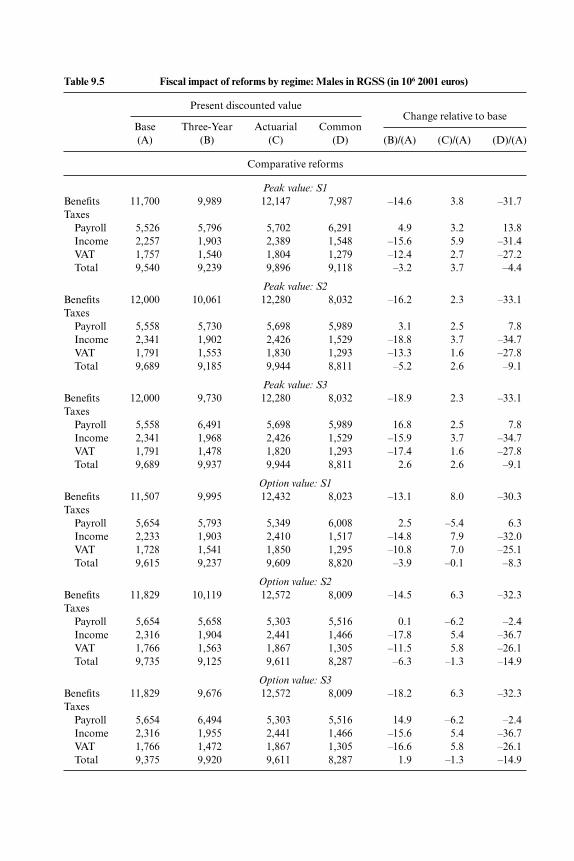
Table 9.5 Fiscal impact of reforms by regime: Males in RGSS (in 106 2001 euros)

Present discounted valueChange relative to base

Base Three-Year Actuarial Common(A) (B) (C) (D) (B)/(A) (C)/(A) (D)/(A)

Comparative reforms

Peak value: S1

Benefits 11,700 9,989 12,147 7,987 –14.6 3.8 –31.7Taxes

Payroll 5,526 5,796 5,702 6,291 4.9 3.2 13.8Income 2,257 1,903 2,389 1,548 –15.6 5.9 –31.4VAT 1,757 1,540 1,804 1,279 –12.4 2.7 –27.2Total 9,540 9,239 9,896 9,118 –3.2 3.7 –4.4

Peak value: S2

Benefits 12,000 10,061 12,280 8,032 –16.2 2.3 –33.1Taxes


Peak value: S3

Benefits 12,000 9,730 12,280 8,032 –18.9 2.3 –33.1Taxes

Payroll 5,558 6,491 5,698 5,989 16.8 2.5 7.8Income 2,341 1,968 2,426 1,529 –15.9 3.7 –34.7VAT 1,791 1,478 1,820 1,293 –17.4 1.6 –27.8Total 9,689 9,937 9,944 8,811 2.6 2.6 –9.1

Option value: S1

Benefits 11,507 9,995 12,432 8,023 –13.1 8.0 –30.3Taxes

Payroll 5,654 5,793 5,349 6,008 2.5 –5.4 6.3Income 2,233 1,903 2,410 1,517 –14.8 7.9 –32.0VAT 1,728 1,541 1,850 1,295 –10.8 7.0 –25.1Total 9,615 9,237 9,609 8,820 –3.9 –0.1 –8.3

Option value: S2

Benefits 11,829 10,119 12,572 8,009 –14.5 6.3 –32.3Taxes

Payroll 5,654 5,658 5,303 5,516 0.1 –6.2 –2.4Income 2,316 1,904 2,441 1,466 –17.8 5.4 –36.7VAT 1,766 1,563 1,867 1,305 –11.5 5.8 –26.1Total 9,735 9,125 9,611 8,287 –6.3 –1.3 –14.9

Option value: S3

Benefits 11,829 9,676 12,572 8,009 –18.2 6.3 –32.3Taxes

Payroll 5,654 6,494 5,303 5,516 14.9 –6.2 –2.4Income 2,316 1,955 2,441 1,466 –15.6 5.4 –36.7VAT 1,766 1,472 1,867 1,305 –16.6 5.8 –26.1Total 9,375 9,920 9,611 8,287 1.9 –1.3 –14.9

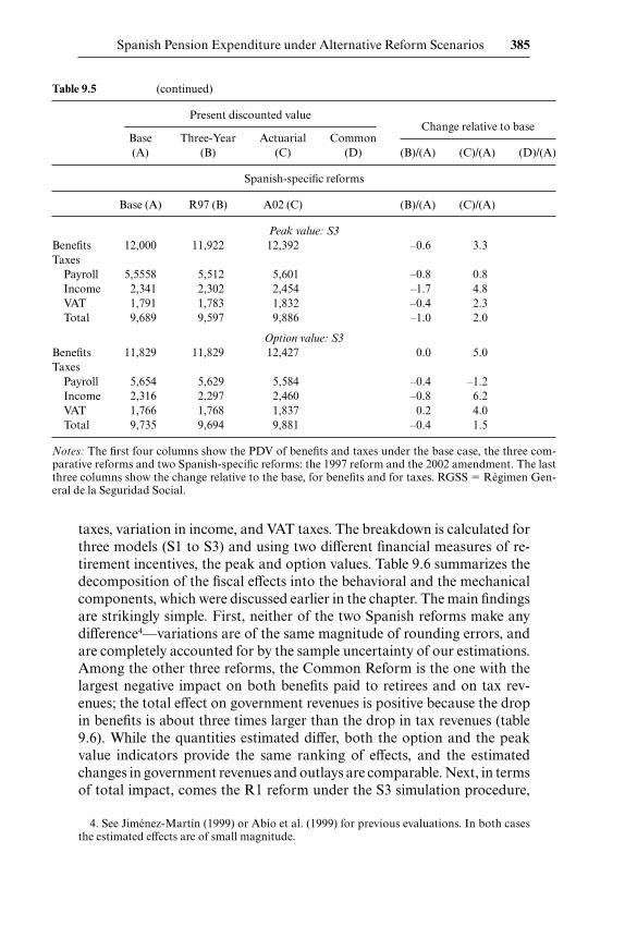
taxes, variation in income, and VAT taxes. The breakdown is calculated forthree models (S1 to S3) and using two different financial measures of re-tirement incentives, the peak and option values. Table 9.6 summarizes thedecomposition of the fiscal effects into the behavioral and the mechanicalcomponents, which were discussed earlier in the chapter. The main findingsare strikingly simple. First, neither of the two Spanish reforms make anydifference4—variations are of the same magnitude of rounding errors, andare completely accounted for by the sample uncertainty of our estimations.Among the other three reforms, the Common Reform is the one with thelargest negative impact on both benefits paid to retirees and on tax rev-enues; the total effect on government revenues is positive because the dropin benefits is about three times larger than the drop in tax revenues (table9.6). While the quantities estimated differ, both the option and the peakvalue indicators provide the same ranking of effects, and the estimatedchanges in government revenues and outlays are comparable. Next, in termsof total impact, comes the R1 reform under the S3 simulation procedure,


4. See Jiménez-Martín (1999) or Abío et al. (1999) for previous evaluations. In both casesthe estimated effects are of small magnitude.

Table 9.5 (continued)



Spanish-specific reforms

Base (A) R97 (B) A02 (C) (B)/(A) (C)/(A)

Peak value: S3

Benefits 12,000 11,922 12,392 –0.6 3.3Taxes

Payroll 5,5558 5,512 5,601 –0.8 0.8Income 2,341 2,302 2,454 –1.7 4.8VAT 1,791 1,783 1,832 –0.4 2.3Total 9,689 9,597 9,886 –1.0 2.0

Option value: S3

Benefits 11,829 11,829 12,427 0.0 5.0Taxes

Payroll 5,654 5,629 5,584 –0.4 –1.2Income 2,316 2,297 2,460 –0.8 6.2VAT 1,766 1,768 1,837 0.2 4.0Total 9,735 9,694 9,881 –0.4 1.5

Notes: The first four columns show the PDV of benefits and taxes under the base case, the three com-parative reforms and two Spanish-specific reforms: the 1997 reform and the 2002 amendment. The lastthree columns show the change relative to the base, for benefits and for taxes. RGSS � Régimen Gen-eral de la Seguridad Social.

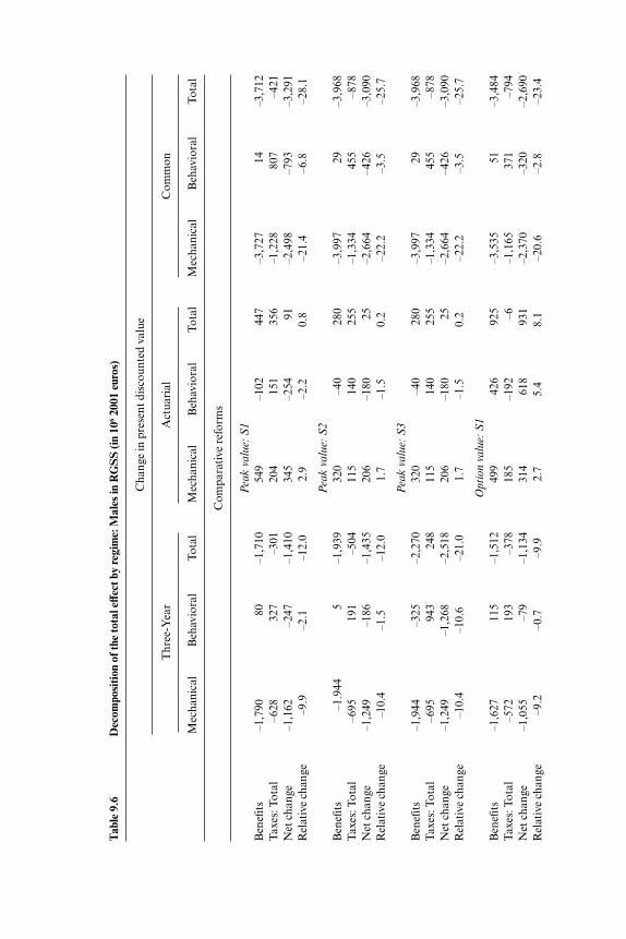
Tab

le 9

.6D

ecom

posi

tion

of t

he to

tal e

ffec

t by

regi

me:

Mal

es in

RG

SS

(in

106

2001

eur

os)

Cha

nge

in p

rese

nt d

isco

unte

d va

lue

Thr

ee-Y

ear

Act

uari

alC

omm

on

Mec

hani

cal

Beh

avio

ral

Tota

lM

echa

nica

lB

ehav

iora

lTo

tal

Mec

hani

cal

Beh

avio

ral

Tota

l

Com

para

tive

ref

orm

s

Pea

k v

alu

e: S

1

Ben

efits

–1,7

9080

–1,7

1054

9–1

0244

7–3

,727

14–3

,712

Tax

es: T

otal

–628

327

–301

204

151

356

–1,2

2880

7–4

21N

et c

hang

e–1

,162

–247

–1,4

1034

5–2

5491

–2,4

98–7

93–3

,291

Rel

ativ

e ch

ange

–9.9

–2.1

–12.

02.

9–2

.20.

8–2

1.4

–6.8

–28.

1

Pea

k v

alu

e: S

2

Ben

efits

–1.9

445

–1,9

3932

0–4

028

0–3

,997

29–3

,968

Tax

es: T

otal

–695

191

–504

115

140

255

–1,3

3445

5–8

78N

et c

hang

e–1

,249

–186

–1,4

3520

6–1

8025

–2,6

64–4

26–3

,090

Rel

ativ

e ch

ange

–10.

4–1

.5–1

2.0

1.7

–1.5

0.2

–22.

2–3

.5–2

5.7

Pea

k v

alu

e: S

3

Ben

efits

–1,9

44–3

25–2

,270

320

–40

280

–3,9

9729

–3,9

68T

axes

: Tot

al–6

9594

324

811

514

025

5–1

,334

455

–878

Net

cha

nge

–1,2

49–1

,268

–2,5

1820

6–1

8025

–2,6

64–4

26–3

,090

Rel

ativ

e ch

ange

–10.

4–1

0.6

–21.

01.

7–1

.50.

2–2

2.2

–3.5

–25.

7

Opt

ion v

alu

e: S

1

Ben

efits

–1,6

2711

5–1

,512

499

426

925

–3,5

3551

–3,4

84T

axes

: Tot

al–5

7219

3–3

7818

5–1

92–6

–1,1

6537

1–7

94N

et c

hang

e–1

,055

–79

–1,1

3431

461

893

1–2

,370

–320

–2,6

90R

elat

ive

chan

ge–9

.2–0

.7–9

.92.

75.

48.

1–2

0.6

–2.8

–23.

4

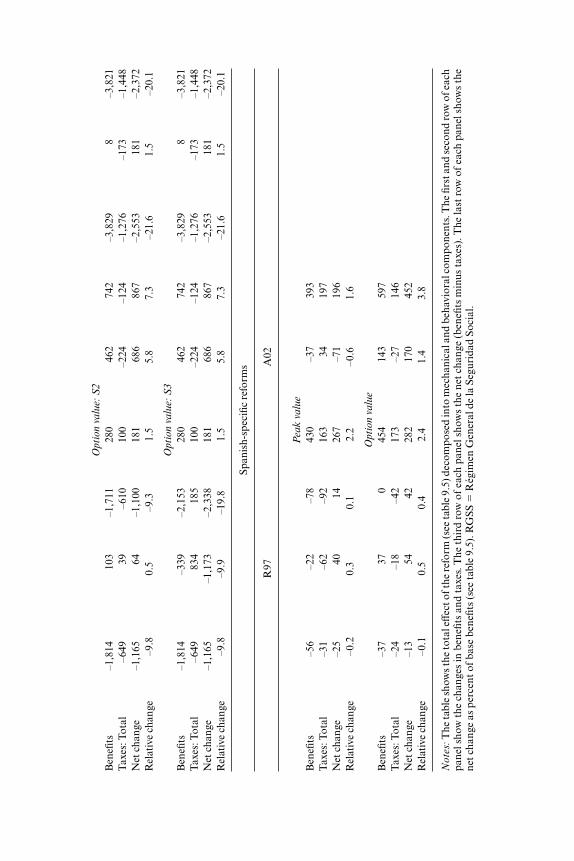
Opt

ion v

alu

e: S

2

Ben

efits

–1,8

1410

3–1

,711

280

462

742

–3,8

298

–3,8

21T

axes

: Tot

al–6

4939

–610

100

–224

–124

–1,2

76–1

73–1

,448

Net

cha

nge

–1,1

6564

–1,1

0018

168

686

7–2

,553

181

–2,3

72R

elat

ive

chan

ge–9

.80.

5–9

.31.

55.

87.

3–2

1.6

1.5

–20.

1

Opt

ion v

alu

e: S

3

Ben

efits

–1,8

14–3

39–2

,153

280

462

742

–3,8

298

–3,8

21T

axes

: Tot

al–6

4983

418

510

0–2

24–1

24–1

,276

–173

–1,4

48N

et c

hang

e–1

,165

–1,1

73–2

,338

181

686

867

–2,5

5318

1–2

,372

Rel

ativ

e ch

ange

–9.8

–9.9

–19.

81.

55.

87.

3–2

1.6

1.5

–20.

1

Span

ish-

spec

ific

refo

rms

R97

A02

Pea

k v

alu

e

Ben

efits

–56

–22

–78

430

–37

393

Tax

es: T

otal

–31

–62

–92

163

3419

7N

et c

hang

e–2

540

1426

7–7

119

6R

elat

ive

chan

ge–0

.20.

30.

12.

2–0

.61.

6

Opt

ion v

alu

e

Ben

efits

–37

370

454

143

597

Tax

es: T

otal

–24

–18

–42

173

–27

146

Net

cha

nge

–13

5442

282

170

452

Rel

ativ

e ch

ange

–0.1

0.5

0.4

2.4

1.4

3.8

No

tes:

The

tabl

e sh

ows

the

tota

l eff

ect o

f the

ref

orm

(see

tabl

e 9.

5) d

ecom

pose

d in

to m

echa

nica

l and

beh

avio

ral c

ompo

nent

s. T

he fi

rst a

nd s

econ

d ro

w o

f eac

hpa

nel s

how

the

cha

nges

in b

enefi

ts a

nd t

axes

. The

thi

rd r

ow o

f ea

ch p

anel

sho

ws

the

net

chan

ge (

bene

fits

min

us t

axes

). T

he la

st r

ow o

f ea

ch p

anel

sho

ws

the

net c

hang

e as

per

cent

of b

ase

bene

fits

(see

tabl

e 9.

5). R

GSS

�R

égim

en G

ener

al d

e la

Seg

urid

ad S

ocia

l.

that is, assuming that retirement ages are effectively shifted three yearsdown, pretty much by fiat. This reform also yields an important improve-ment of the government net position; most of it comes from a reduction inthe net present value of benefits, with a small residual due to increase in to-tal taxation. In particular, the substantial increase in payroll contributionsgenerated by the longer worklife is almost completely balanced by the re-duction in income and VAT revenues that the reform induces. Next, in termsof change in the fiscal position, is the R1 reform as estimated under the S2hypothesis; directions of change are the same as in the S3 version but, obvi-ously, the quantities are much smaller. Finally, R2 is predicted to have a neg-ative impact on the fiscal position of government, as the small increase intax revenues it induces is more than compensated by an increase in benefitspaid, leading to a small but visible worsening of the government net posi-tion.

A second look at table 9.6 also shows that, as anticipated earlier, the be-havioral impact of the reforms we consider is rather limited. Most of thesavings comes from the mechanical aspects of the change; that is, the factthat by suddenly reducing benefits or lengthening working lives one cap-tures the workers off guard, especially the older workers, and this leads tosubstantial savings for the public purse. For this reason, mechanical effectsare orders of magnitude larger than the behavioral ones, uniformly acrossreforms and independently of the financial indicator adopted. Notice that,at least in the case of R3 and R1 � S3, the relative reduction of governmentnet outlays is substantial, oscillating between –18.0 and –30.0 percent, de-pending on the financial indicator adopted.

RESS

Move next to estimates for workers enrolled in the special regimes, ofwhich RETA is by far the most important, and upon which most of our datarely. Results here are dirtier, especially when it comes to forecasting the im-pact of each specific reform on retirement patterns by age. This is due, asdiscussed earlier, to the very low explanatory power of our financial mea-sures of incentive to retirement, which in the case of the self-employed cap-ture a small portion of the actual retirement patterns. In any case, the anal-ysis proceeds in the same fashion as for the RGSS and results are organizedlikewise. However, we omit the corresponding SSW and tax figures.

The two lower panels of figures 9.3 to 9.5 contain the relevant infor-mation. In figure 9.3 we see that, similarly to RGSS, the impact of R1 ongross SSW is substantially stronger under S3 than S2, and that, contrary toRGSS, the same ranking of relative impact applies to net SSW. The impactof R2 is either irrelevant (as it reduces SSW only for people retiring eithervery early or very late) or it goes in the wrong direction, slightly increasingSSW at currently observed retirement ages (between 60 and 69). ReformR3, instead, does reduce SSW substantially and across the whole spectrumof possible retirement ages, with a somewhat stronger impact at 60 and 65


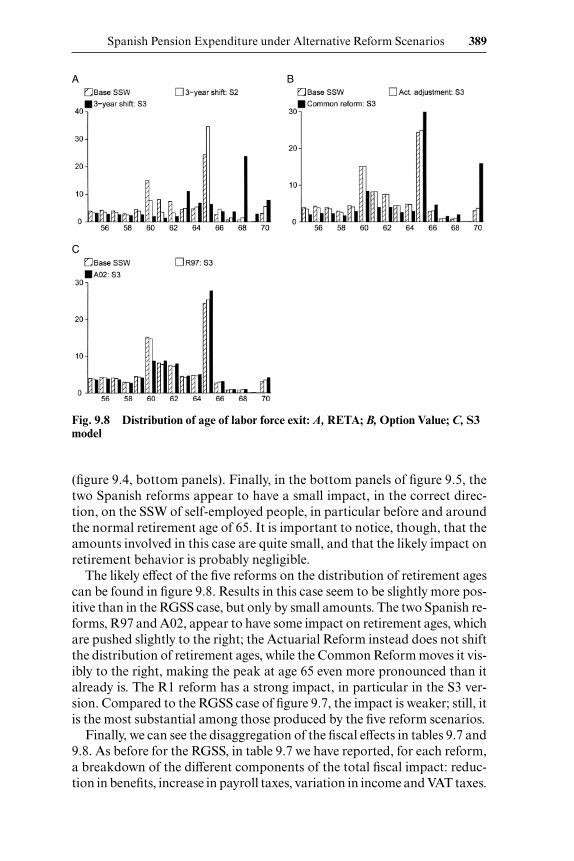
(figure 9.4, bottom panels). Finally, in the bottom panels of figure 9.5, thetwo Spanish reforms appear to have a small impact, in the correct direc-tion, on the SSW of self-employed people, in particular before and aroundthe normal retirement age of 65. It is important to notice, though, that theamounts involved in this case are quite small, and that the likely impact onretirement behavior is probably negligible.

The likely effect of the five reforms on the distribution of retirement agescan be found in figure 9.8. Results in this case seem to be slightly more pos-itive than in the RGSS case, but only by small amounts. The two Spanish re-forms, R97 and A02, appear to have some impact on retirement ages, whichare pushed slightly to the right; the Actuarial Reform instead does not shiftthe distribution of retirement ages, while the Common Reform moves it vis-ibly to the right, making the peak at age 65 even more pronounced than italready is. The R1 reform has a strong impact, in particular in the S3 ver-sion. Compared to the RGSS case of figure 9.7, the impact is weaker; still, itis the most substantial among those produced by the five reform scenarios.

Finally, we can see the disaggregation of the fiscal effects in tables 9.7 and9.8. As before for the RGSS, in table 9.7 we have reported, for each reform,a breakdown of the different components of the total fiscal impact: reduc-tion in benefits, increase in payroll taxes, variation in income and VAT taxes.


Fig. 9.8 Distribution of age of labor force exit: A, RETA; B, Option Value; C, S3model

A B

C

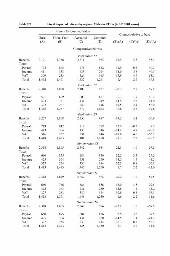
Table 9.7 Fiscal impact of reforms by regime: Males in RETA (in 106 2001 euros)

Present Discounted ValueChange relative to base


Comparative reforms

Peak value: S1

Benefits 2,191 1,786 2,311 985 –18.5 5.5 –55.1Taxes

Payroll 773 865 775 852 11.9 0.3 10.3Income 411 353 433 244 –14.0 5.6 –40.5VAT 309 253 324 145 –17.9 4.9 –53.1Total 1,492 1,471 1,532 1,241 –1.4 2.7 –16.8

Peak value: S2

Benefits 2,340 1,868 2,403 987 –20.2 2.7 –57.8Taxes


Peak value: S3

Benefits 2,237 1,808 2,350 987 –19.2 5.1 –55.9Taxes

Payroll 719 812 717 789 12.9 –0.3 9.7Income 413 354 433 246 –14.4 4.9 –40.5VAT 316 257 331 146 –18.6 4.6 –53.9Total 1,448 1,423 1,481 1,180 –1.7 2.2 –18.5

Option value: S1

Benefits 2,318 1,805 2,342 984 –22.1 1.0 –57.5Taxes

Payroll 660 875 684 856 32.5 3.5 29.5Income 425 364 431 250 –14.5 1.4 –41.2VAT 327 254 330 144 –22.3 0.8 –56.1Total 1,413 1,493 1,445 1,250 5.7 2.2 –11.6

Option value: S2

Benefits 2,318 1,849 2,342 984 –20.2 1.0 –57.5Taxes


Option value: S3

Benefits 2,318 1,805 2,342 984 –22.1 1.0 –57.5Taxes

Payroll 660 875 684 856 32.5 3.5 29.5Income 425 364 431 250 –14.5 1.4 –41.2VAT 327 254 330 144 –22.3 0.8 –56.1Total 1,413 1,493 1,445 1,250 5.7 2.2 –11.6

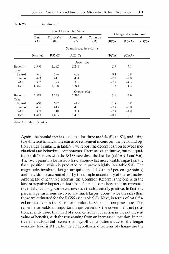
Again, the breakdown is calculated for three models (S1 to S3), and usingtwo different financial measures of retirement incentives, the peak and op-tion values. Similarly, in table 9.8 we report the decomposition between me-chanical and behavioral components. There are quantitative, but not qual-itative, differences with the RGSS case described earlier (tables 9.5 and 9.6).The two Spanish reforms now have a somewhat more visible impact on thefiscal position, which is predicted to improve slightly (see table 9.8). Themagnitudes involved, though, are quite small (less than 5 percentage points)and may still be accounted for by the sample uncertainty of our estimates.Among the other three reforms, the Common Reform is the one with thelargest negative impact on both benefits paid to retirees and tax revenues;the total effect on government revenues is substantially positive. In fact, thepercentage variations involved are much larger (about twice the size) thanthose we estimated for the RGSS (see table 9.8). Next, in terms of total fis-cal impact, comes the R1 reform under the S3 simulation procedure. Thisreform also yields an important improvement of the government net posi-tion; slightly more than half of it comes from a reduction in the net presentvalue of benefits, with the rest coming from an increase in taxation, in par-ticular a substantial increase in payroll contributions due to the longerworklife. Next is R1 under the S2 hypothesis; directions of change are the



Present Discounted ValueChange relative to base



Base (A) R97 (B) A02 (C) (B)/(A) (C)/(A)

Peak value

Benefits 2,340 2,272 2,243 –2.9 –4.1Taxes

Payroll 591 594 632 0.4 6.8Income 423 411 414 –2.8 –2.0VAT 332 323 318 –2.7 –4.3Total 1,346 1,328 1,364 –1.3 1.3

Option value

Benefits 2,318 2,245 2,205 –3.1 –4.9Taxes

Payroll 660 672 699 1.8 5.8Income 425 413 413 –2.9 –3.0VAT 327 318 311 –2.9 –4.9Total 1,413 1,403 1,423 –0.7 0.7

Note: See table 9.5 notes.

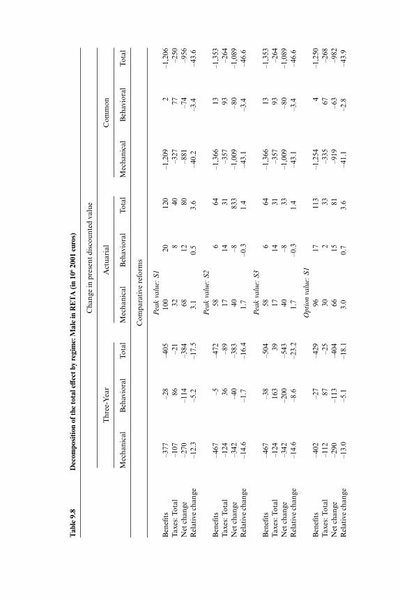
Tab

le 9

.8D

ecom

posi

tion

of t

he to

tal e

ffec

t by

regi

me:

Mal

e in

RE

TA

(in

106

2001

eur

os)

Cha

nge

in p

rese

nt d

isco

unte

d va

lue

Thr

ee-Y

ear

Act

uari

alC

omm

on

Mec

hani

cal

Beh

avio

ral

Tota

lM

echa

nica

lB

ehav

iora

lTo

tal

Mec

hani

cal

Beh

avio

ral

Tota

l

Com

para

tive

ref

orm

s

Pea

k v

alu

e: S

1

Ben

efits

–377

–28

–405

100

2012

0–1

,209

2–1

,206

Tax

es: T

otal

–107

86–2

132

840

–327

77–2

50N

et c

hang

e–2

70–1

14–3

8468

1280

–881

–74

–956

Rel

ativ

e ch

ange

–12.

3–5

.2–1

7.5

3.1

0.5

3.6

–40.

2–3

.4–4

3.6

Pea

k v

alu

e: S

2

Ben

efits

–467

–5–4

7258

664

–1,3

6613

–1,3

53T

axes

: Tot

al–1

2436

–89

1714

31–3

5793

–264

Net

cha

nge

–342

–40

–383

40–8

833

–1,0

09–8

0–1

,089

Rel

ativ

e ch

ange

–14.

6–1

.7–1

6.4

1.7

–0.3

1.4

–43.

1–3

.4–4

6.6

Pea

k v

alu

e: S

3

Ben

efits

–467

–38

–504

586

64–1

,366

13–1

,353

Tax

es: T

otal

–124

163

3917

1431

–357

93–2

64N

et c

hang

e–3

42–2

00–5

4340

–833

–1,0

09–8

0–1

,089

Rel

ativ

e ch

ange

–14.

6–8

.6–2

3.2

1.7

–0.3

1.4

–43.

1–3

.4–4

6.6

Opt

ion v

alu

e: S

1

Ben

efits

–402

–27

–429

9617

113

–1,2

544

–1,2

50T

axes

: Tot

al–1

1287

–25

302

33–3

3567

–268

Net

cha

nge

–290

–113

–404

6615

81–9

19–6

3–9

82R

elat

ive

chan

ge–1

3.0

–5.1

–18.

13.

00.

73.

6–4

1.1

–2.8

–43.

9

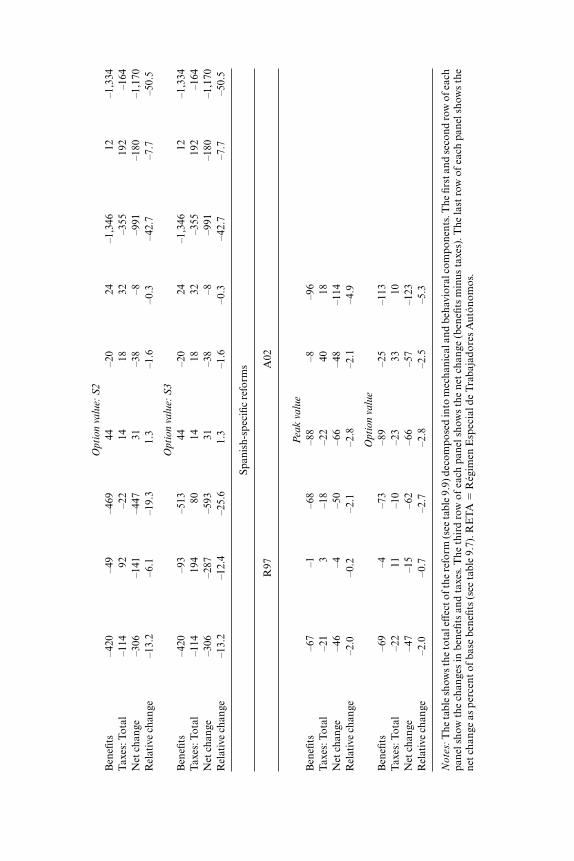
Opt

ion v

alu

e: S

2

Ben

efits

–420

–49

–469

44–2

024

–1,3

4612

–1,3

34T

axes

: Tot

al–1

1492

–22

1418

32–3

5519

2–1

64N

et c

hang

e–3

06–1

41–4

4731

–38

–8–9

91–1

80–1

,170

Rel

ativ

e ch

ange

–13.

2–6

.1–1

9.3

1.3

–1.6

–0.3

–42.

7–7

.7–5

0.5

Opt

ion v

alu

e: S

3

Ben

efits

–420

–93

–513

44–2

024

–1,3

4612

–1,3

34T

axes

: Tot

al–1

1419

480

1418

32–3

5519

2–1

64N

et c

hang

e–3

06–2

87–5

9331

–38

–8–9

91–1

80–1

,170

Rel

ativ

e ch

ange

–13.

2–1

2.4

–25.

61.

3–1

.6–0

.3–4

2.7

–7.7

–50.

5

Span

ish-

spec

ific

refo

rms

R97

A02

Pea

k v

alu

e

Ben

efits

–67

–1–6

8–8

8–8

–96

Tax

es: T

otal

–21

3–1

8–2

240

18N

et c

hang

e–4

6–4

–50

–66

–48

–114

Rel

ativ

e ch

ange

–2.0

–0.2

–2.1

–2.8

–2.1

–4.9

Opt

ion v

alu

e

Ben

efits

–69

–4–7

3–8

9–2

5–1

13T

axes

: Tot

al–2

211

–10

–23

3310

Net

cha

nge

–47

–15

–62

–66

–57

–123

Rel

ativ

e ch

ange

–2.0

–0.7

–2.7

–2.8

–2.5

–5.3

No

tes:

The

tabl

e sh

ows

the

tota

l eff

ect o

f the

ref

orm

(see

tabl

e 9.

9) d

ecom

pose

d in

to m

echa

nica

l and

beh

avio

ral c

ompo

nent

s. T

he fi

rst a

nd s

econ

d ro

w o

f eac

hpa

nel s

how

the

cha

nges

in b

enefi

ts a

nd t

axes

. The

thi

rd r

ow o

f ea

ch p

anel

sho

ws

the

net

chan

ge (

bene

fits

min

us t

axes

). T

he la

st r

ow o

f ea

ch p

anel

sho

ws

the

net c

hang

e as

per

cent

of b

ase

bene

fits

(see

tabl

e 9.

7). R

ET

A �

Rég

imen

Esp

ecia

l de

Tra

baja

dore

s A

utón

omos

.

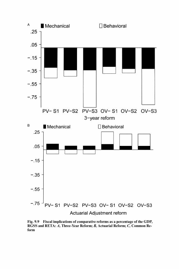
Fig. 9.9 Fiscal implications of comparative reforms as a percentage of the GDP,RGSS and RETA: A, Three-Year Reform; B, Actuarial Reform; C, Common Re-form

A

B

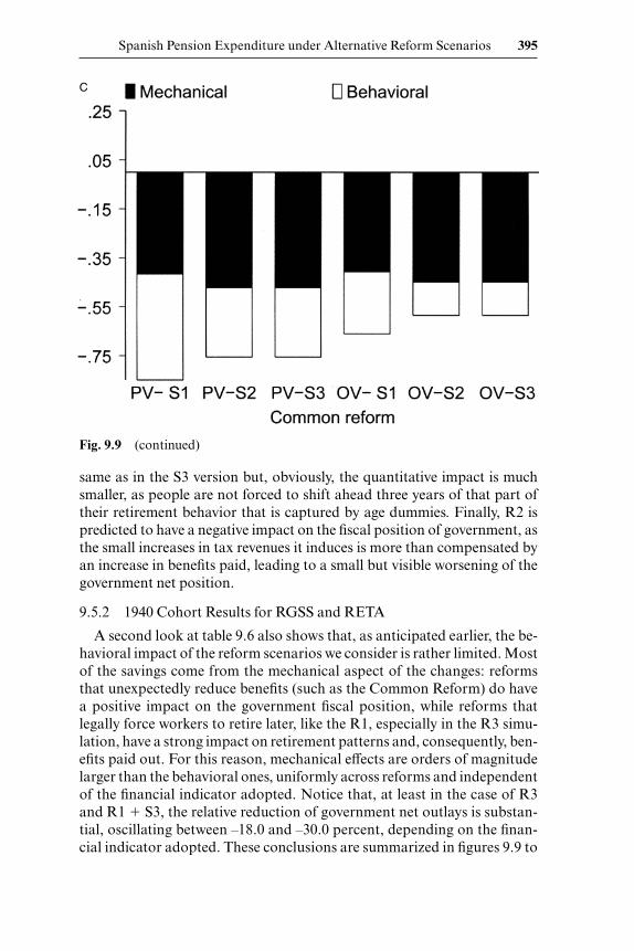
same as in the S3 version but, obviously, the quantitative impact is muchsmaller, as people are not forced to shift ahead three years of that part oftheir retirement behavior that is captured by age dummies. Finally, R2 ispredicted to have a negative impact on the fiscal position of government, asthe small increases in tax revenues it induces is more than compensated byan increase in benefits paid, leading to a small but visible worsening of thegovernment net position.

9.5.2 1940 Cohort Results for RGSS and RETA

A second look at table 9.6 also shows that, as anticipated earlier, the be-havioral impact of the reform scenarios we consider is rather limited. Mostof the savings come from the mechanical aspect of the changes: reformsthat unexpectedly reduce benefits (such as the Common Reform) do havea positive impact on the government fiscal position, while reforms thatlegally force workers to retire later, like the R1, especially in the R3 simu-lation, have a strong impact on retirement patterns and, consequently, ben-efits paid out. For this reason, mechanical effects are orders of magnitudelarger than the behavioral ones, uniformly across reforms and independentof the financial indicator adopted. Notice that, at least in the case of R3and R1 � S3, the relative reduction of government net outlays is substan-tial, oscillating between –18.0 and –30.0 percent, depending on the finan-cial indicator adopted. These conclusions are summarized in figures 9.9 to

Fig. 9.9 (continued)


C

9.11. Figure 9.9 reports the fiscal effect of each reform by gender andregime, using simulation S3; figure 9.10 reports the total (RGSS plusRETA) fiscal effect of each reform for both simulations S1 and S3. We dis-tinguish, in each case, between mechanical and behavioral effect. The sameinformation is reported, in numerical form, in tables 9.9 and 9.10. All thequantities reported in these tables and figures, we recall, are relative to the1940 cohort; that is to say, we compute the positive/negative variations inpension expenditure and tax revenues that are induced by applying each ofthe five reforms to the 1940s cohort only. At the same time, it should alsobe noted that the numbers we report are net present value estimations, thatis, they correspond to the net present value, at the time of reform, of thevariations induced by the reform itself over the remaining life of the cohort.They do not correspond, therefore, to variations in annual flows.

Our model predicts that the two Spanish reforms, R97 and A02, have anegligible total fiscal effect, that the Actuarial Reform (R2) would worsenthe fiscal position of the government, and that, finally, the R1 and theCommon Reform (R3) would improve it. The largest effect is predicted forthe R1 reform under the S3 simulation scenarios, that is, when that portionof current retirement patterns that is captured by age dummies is shifted tothe right of exactly three years. The net amount saved, in this case, is sub-stantial: about 0.80 percentage points of GDP. In the other two cases (R1without the impact of age dummies, and R3), the amounts saved are, re-spectively, around 0.35 and 0.55 percentage points of GDP. While these arelarge amounts, they are not so large in relation to either the annual expen-diture for social security pensions (which is about 10 percentage points ofGDP) or to the size of outstanding Spanish pension debt, which is esti-mated to range around 200 percentage points of GDP. Even by multiply-ing these quantities by a factor of fifty (that is, even assuming that savingsof similar size can be achieved during the next fifty years for each cohortborn between 1940 and 1990) we would still be projecting total savingsequal to, at best, 20 percent of the outstanding pension debt. From thisperspective, the savings that can be achieved via the reforms consideredhere are somewhat modest and, probably, still below the level that appearsto be desirable. Finally, we should note that, in all cases but R2 � S3, mostof the savings come from the mechanical aspect. Only R2 � S3 shows alarge behavioral effect, which is due to the fact that, by shifting the agedummies to the right, we are in fact assuming that Spanish workers will vol-untarily choose to translate their age-related retirement patterns forwardthree years. One should keep in mind that, once a reform is implemented,workers will adjust their behavior optimally (from their viewpoint) to thechanged circumstances. After a few years, such adjustment is likely to elim-inate or at least greatly reduce the savings that we estimate to accrue via themechanical channel. This would leave, in the long run, only the impact of


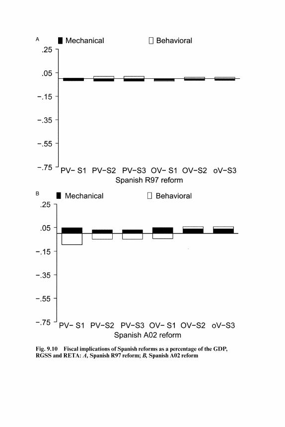
Fig. 9.10 Fiscal implications of Spanish reforms as a percentage of the GDP,RGSS and RETA: A, Spanish R97 reform; B, Spanish A02 reform

A

B

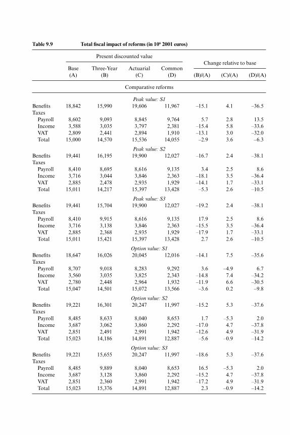
Table 9.9 Total fiscal impact of reforms (in 106 2001 euros)



Comparative reforms

Peak value: S1

Benefits 18,842 15,990 19,606 11,967 –15.1 4.1 –36.5Taxes


Peak value: S2

Benefits 19,441 16,195 19,900 12,027 –16.7 2.4 –38.1Taxes


Peak value: S3

Benefits 19,441 15,704 19,900 12,027 –19.2 2.4 –38.1Taxes

Payroll 8,410 9,915 8,616 9,135 17.9 2.5 8.6Income 3,716 3,138 3,846 2,363 –15.5 3.5 –36.4VAT 2,885 2,368 2,935 1,929 –17.9 1.7 –33.1Total 15,011 15,421 15,397 13,428 2.7 2.6 –10.5

Option value: S1

Benefits 18,647 16,026 20,045 12,016 –14.1 7.5 –35.6Taxes

Payroll 8,707 9,018 8,283 9,292 3.6 –4.9 6.7Income 3,560 3,035 3,825 2,343 –14.8 7.4 –34.2VAT 2,780 2,448 2,964 1,932 –11.9 6.6 –30.5Total 15,047 14,501 15,072 13,566 –3.6 0.2 –9.8

Option value: S2

Benefits 19,221 16,301 20,247 11,997 –15.2 5.3 –37.6Taxes

Payroll 8,485 8,633 8,040 8,653 1.7 –5.3 2.0Income 3,687 3,062 3,860 2,292 –17.0 4.7 –37.8VAT 2,851 2,491 2,991 1,942 –12.6 4.9 –31.9Total 15,023 14,186 14,891 12,887 –5.6 –0.9 –14.2

Option value: S3

Benefits 19,221 15,655 20,247 11,997 –18.6 5.3 –37.6Taxes

Payroll 8,485 9,889 8,040 8,653 16.5 –5.3 2.0Income 3,687 3,128 3,860 2,292 –15.2 4.7 –37.8VAT 2,851 2,360 2,991 1,942 –17.2 4.9 –31.9Total 15,023 15,376 14,891 12,887 2.3 –0.9 –14.2

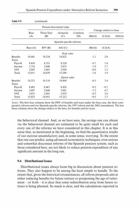
the behavioral channel. And, as we have seen, the savings one can obtainvia the behavioral channel are estimated to be quite small for each andevery one of the reforms we have considered in this chapter. It is in thissense that, as mentioned at the beginning, we find the quantitative resultsof our exercise unsatisfactory and, in some sense, worrying. To the extentthat one can predict, using advanced econometric techniques, even seriousand somewhat draconian reforms of the Spanish pension system, such asthose considered here, are not likely to reduce pension expenditure of anysignificant amount in the long run.

9.6 Distributional Issues

Distributional issues always loom big in discussions about pension re-forms. They also happen to be among the least simple to handle. To theextent that, given the historical circumstances, all reform proposals aim ateither reducing benefits for future retirees or postponing the age of retire-ment—or both—it is clear that some redistribution away from future re-tirees is being planned. So much is clear, and the calculations reported in






Base (A) R97 (B) A02 (C) (B)/(A) (C)/(A)

Peak value

Benefits 19,441 19,234 19,822 –1.1 2.0Taxes

Payroll 8,410 8,351 8,524 –0.7 1.4Income 3,716 3,646 3,853 –1.9 3.7VAT 2,885 2,862 2,920 –0.8 1.2Total 15,011 14,859 15,296 –1.0 1.9

Option value

Benefits 19,221 19,118 19,869 –0.5 3.4Taxes

Payroll 8,485 8,467 8,426 –0.2 –0.7Income 3,687 3,644 3,861 –1.2 4.7VAT 2,851 2,841 2,925 –0.3 2.6Total 15,023 14,951 15,212 –0.5 1.3

Notes: The first four columns show the PDV of benefits and taxes under the base case, the three com-parative reforms and two Spanish-specific reforms: the 1997 reform and the 2002 amendment. The lastthree columns show the change relative to the base, for benefits and for taxes.

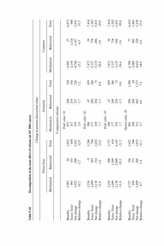
Tab

le 9

.10

Dec

ompo

siti

on o

f the

tota

l eff

ect o

f ref

orm

s (i

n 10

620

01 e

uros

)

Cha

nge

in p

rese

nt d

isco

unte

d va

lue

Thr

ee-Y

ear

Act

uari

alC

omm

on

Mec

hani

cal

Beh

avio

ral

Tota

lM

echa

nica

lB

ehav

iora

lTo

tal

Mec

hani

cal

Beh

avio

ral

Tota

l

Com

para

tive

ref

orm

s

Pea

k v

alu

e: S

1

Ben

efits

–2,9

0756

–2,8

5287

2–1

0876

4–6

,902

27–6

,875

Tax

es: T

otal

–985

555

–430

317

219

536

–2,1

581,

214

–944

Net

cha

nge

–1,9

22–5

00–2

,421

555

–327

228

–4,7

44–1

,187

–5,9

31R

elat

ive

chan

ge–1

0.2

–2.7

–12.

92.

9–1

.71.

2–2

5.2

–6.3

–31.

5

Pea

k v

alu

e: S

2

Ben

efits

–3,2

36–9

–3,2

4650

6–4

745

9–7

,472

58–7

,414

Tax

es: T

otal

–1,0

9930

5–7

9417

720

938

6–2

,337

754

–1,5

83N

et c

hang

e–2

,138

–314

–2,4

5232

9–2

5673

–5,1

35–6

96–5

,831

Rel

ativ

e ch

ange

–11.

0–1

.6–1

2.6

1.7

–1.3

0.4

–26.

4–3

.6–3

0.0

Pea

k v

alu

e: S

3

Ben

efits

–3,2

36–5

00–3

,737

506

–47

459

–7,4

7258

–7,4

14T

axes

: Tot

al–1

,099

1,50

941

017

720

938

6–2

,337

754

–1,5

83N

et c

hang

e–2

,138

–2,0

09–4

,147

329

–256

73–5

,135

–696

–5,8

31R

elat

ive

chan

ge–1

1.0

–10.

3–2

1.3

1.7

–1.3

0.4

–26.

4–3

.6–3

0.0

Opt

ion v

alu

e: S

1

Ben

efits

–2,7

2710

6–2

,621

801

596

1,39

8–6

,708

77–6

,632

Tax

es: T

otal

–918

372

–546

290

–266

24–2

,086

605

–1,4

81N

et c

hang

e–1

,809

–266

–2,0

7551

186

21,

373

–4,6

22–5

28–5

,150

Rel

ativ

e ch

ange

–9.7

–1.4

–11.

12.

74.

67.

4–2

4.8

–2.8

–27.

6

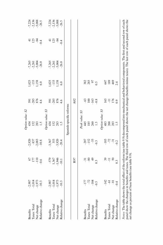
Opt

ion v

alu

e: S

2

Ben

efits

–2,9

8767

–2,9

2043

459

11,

025

–7,2

6541

–7,2

24T

axes

: Tot

al–1

,014

177

–837

152

–285

–133

–2,2

6112

5–2

,136

Net

cha

nge

–1,9

73–1

10–2

,083

283

876

1,15

8–5

,004

–84

–5,0

88R

elat

ive

chan

ge–1

0.3

–0.6

–10.

81.

54.

66.

0–2

6.0

–0.4

–26.

5

Opt

ion v

alu

e: S

3

Ben

efits

–2,9

87–5

79–3

,567

434

591

1,02

5–7

,265

41–7

,224

Tax

es: T

otal

–1,0

141,

367

353

152

–285

–133

–2,2

6112

5–2

,136

Net

cha

nge

–1,9

73–1

,946

–3,9

2028

387

61,

158

–5,0

04–8

4–5

,088

Rel

ativ

e ch

ange

–10.

3–1

0.1

–20.

41.

54.

66.

0–2

6.0

–0.4

–26.

5

Span

ish-

spec

ific

refo

rms

R97

A02

Pea

k v

alu

e: S

3

Ben

efits

–177

–31

–207

445

–63

382

Tax

es: T

otal

–72

–80

–152

185

100

285

Net

cha

nge

–104

49–5

526

0–1

6397

Rel

ativ

e ch

ange

–0.5

0.3

–0.3

1.3

–0.8

0.5

Opt

ion v

alu

e: S

3

Ben

efits

–142

39–1

0348

316

564

7T

axes

: Tot

al–6

1–1

1–7

220

0–1

118

9N

et c

hang

e–8

150

–31

283

176

469

Rel

ativ

e ch

ange

–0.4

0.3

–0.2

1.5

0.9

2.4

No

tes:

The

tabl

e sh

ows

the

tota

l eff

ect o

f the

ref

orm

(see

tabl

e 9.

9) d

ecom

pose

d in

to m

echa

nica

l and

beh

avio

ral c

ompo

nent

s. T

he fi

rst a

nd s

econ

d ro

w o

f eac

hpa

nel s

how

the

cha

nges

in b

enefi

ts a

nd t

axes

. The

thi

rd r

ow o

f ea

ch p

anel

sho

ws

the

net

chan

ge (

bene

fits

min

us t

axes

). T

he la

st r

ow o

f ea

ch p

anel

sho

ws

the

net c

hang

e as

per

cent

of b

ase

bene

fits

(see

tabl

e 9.

9).

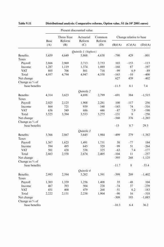
Table 9.11 Distributional analysis: Comparative reforms, Option value, S1 (in 106 2001 euros)

Present discounted value

Three-Year Actuarial Common Change relative to baseBase Reform Reform Reform(A) (B) (C) (D) (B)/(A) (C)/(A) (D)/(A)

Quintile 1 (highest)

Benefits 5,439 4,649 5,868 4,638 –790 429 –801Taxes

Payroll 2,866 2,969 2,713 2,753 103 –153 –113Income 1,287 1,119 1,374 1,089 –168 87 –197VAT 805 706 861 716 –99 6.9 –89Total 4,957 4,794 4,947 4,558 –163 –10 –400

Net change 627 439 –402Change as % of

base benefits –11.5 8.1 7.4

Quintile 2

Benefits 4,314 3,623 4,698 2,799 –691 384 –1,515Taxes

Payroll 2,025 2,125 1,908 2,281 100 –117 256Income 864 721 939 548 –143 74 –316VAT 636 549 686 446 –87 7.9 –190Total 3,525 3,394 3,533 3,275 –131 8 –250

Net change –560 376 –1,265Change as % of

base benefits –13 8.7 29.3

Quintile 3

Benefits 3,366 2,867 3,645 1,984 –499 279 –1,382Taxes



base benefits –11.7 8 –33.4

Quintile 4

Benefits 2,993 2,594 3,202 1,591 –399 209 –1,402Taxes



base benefits –10.3 6.4 36.2

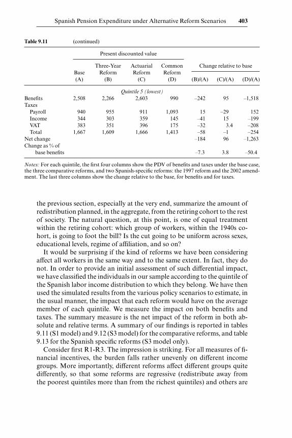
the previous section, especially at the very end, summarize the amount ofredistribution planned, in the aggregate, from the retiring cohort to the restof society. The natural question, at this point, is one of equal treatmentwithin the retiring cohort: which group of workers, within the 1940s co-hort, is going to foot the bill? Is the cut going to be uniform across sexes,educational levels, regime of affiliation, and so on?

It would be surprising if the kind of reforms we have been consideringaffect all workers in the same way and to the same extent. In fact, they donot. In order to provide an initial assessment of such differential impact,we have classified the individuals in our sample according to the quintile ofthe Spanish labor income distribution to which they belong. We have thenused the simulated results from the various policy scenarios to estimate, inthe usual manner, the impact that each reform would have on the averagemember of each quintile. We measure the impact on both benefits andtaxes. The summary measure is the net impact of the reform in both ab-solute and relative terms. A summary of our findings is reported in tables9.11 (S1 model) and 9.12 (S3 model) for the comparative reforms, and table9.13 for the Spanish specific reforms (S3 model only).

Consider first R1-R3. The impression is striking. For all measures of fi-nancial incentives, the burden falls rather unevenly on different incomegroups. More importantly, different reforms affect different groups quitedifferently, so that some reforms are regressive (redistribute away fromthe poorest quintiles more than from the richest quintiles) and others are





Quintile 5 (lowest)

Benefits 2,508 2,266 2,603 990 –242 95 –1,518Taxes

Payroll 940 955 911 1,093 15 –29 152Income 344 303 359 145 –41 15 –199VAT 383 351 396 175 –32 3.4 –208Total 1,667 1,609 1,666 1,413 –58 –1 –254


base benefits –7.3 3.8 –50.4

Notes: For each quintile, the first four columns show the PDV of benefits and taxes under the base case,the three comparative reforms, and two Spanish-specific reforms: the 1997 reform and the 2002 amend-ment. The last three columns show the change relative to the base, for benefits and for taxes.

Table 9.12 Distributional analysis: Comparative reforms, Option value, S3 (in 106 2001 euros)




Benefits 5,510 4,554 5,888 4,599 –955 378 –911Taxes

Payroll 2,906 3,310 2,716 2,591 404 –190 –315Income 1,320 1,146 1,390 1,063 –174 70 –257VAT 810 681 861 713 –129 6.3 –97Total 5,035 5,136 4,966 4,367 101 –69 –669

Net change –1,056 447 –242Change as % of


Quintile 2

Benefits 4,438 3,551 4,731 2,816 –887 293 –1,622Taxes

Payroll 1,995 2,346 1,873 2,115 351 –122 120Income 899 748 950 535 –151 51 –364VAT 649 529 689 452 –120 6.1 –197Total 3,544 3,623 3,513 3,102 79 –31 –441



Quintile 3

Benefits 3,501 2,813 3,688 1,990 –689 187 –1,512Taxes




Quintile 4

Benefits 3,151 2,543 3,272 1,597 –608 121 –1,554Taxes




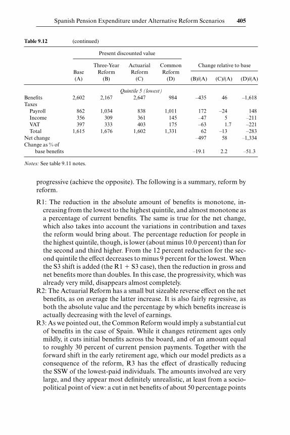
progressive (achieve the opposite). The following is a summary, reform byreform.

R1: The reduction in the absolute amount of benefits is monotone, in-creasing from the lowest to the highest quintile, and almost monotone asa percentage of current benefits. The same is true for the net change,which also takes into account the variations in contribution and taxesthe reform would bring about. The percentage reduction for people inthe highest quintile, though, is lower (about minus 10.0 percent) than forthe second and third higher. From the 12 percent reduction for the sec-ond quintile the effect decreases to minus 9 percent for the lowest. Whenthe S3 shift is added (the R1 � S3 case), then the reduction in gross andnet benefits more than doubles. In this case, the progressivity, which wasalready very mild, disappears almost completely.

R2: The Actuarial Reform has a small but sizeable reverse effect on the netbenefits, as on average the latter increase. It is also fairly regressive, asboth the absolute value and the percentage by which benefits increase isactually decreasing with the level of earnings.

R3: As we pointed out, the Common Reform would imply a substantial cutof benefits in the case of Spain. While it changes retirement ages onlymildly, it cuts initial benefits across the board, and of an amount equalto roughly 30 percent of current pension payments. Together with theforward shift in the early retirement age, which our model predicts as aconsequence of the reform, R3 has the effect of drastically reducingthe SSW of the lowest-paid individuals. The amounts involved are verylarge, and they appear most definitely unrealistic, at least from a socio-political point of view: a cut in net benefits of about 50 percentage points





Quintile 5 (lowest)

Benefits 2,602 2,167 2,647 984 –435 46 –1,618Taxes

Payroll 862 1,034 838 1,011 172 –24 148Income 356 309 361 145 –47 5 –211VAT 397 333 403 175 –63 1.7 –221Total 1,615 1,676 1,602 1,331 62 –13 –283



Notes: See table 9.11 notes.

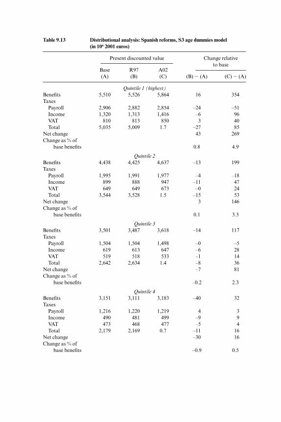
Table 9.13 Distributional analysis: Spanish reforms, S3 age dummies model (in 106 2001 euros)

Change relative Present discounted valueto base

Base R97 A02(A) (B) (C) (B) (A) (C) (A)


Benefits 5,510 5,526 5,864 16 354Taxes

Payroll 2,906 2,882 2,854 –24 –51Income 1,320 1,313 1,416 –6 96VAT 810 813 850 3 40Total 5,035 5,009 1.7 –27 85

Net change 43 269Change as % of

base benefits 0.8 4.9

Quintile 2

Benefits 4,438 4,425 4,637 –13 199Taxes

Payroll 1,995 1,991 1,977 –4 –18Income 899 888 947 –11 47VAT 649 649 673 –0 24Total 3,544 3,528 1.5 –15 53

Net change 3 146Change as % of

base benefits 0.1 3.3

Quintile 3

Benefits 3,501 3,487 3,618 –14 117Taxes

Payroll 1,504 1,504 1,498 –0 –5Income 619 613 647 –6 28VAT 519 518 533 –1 14Total 2,642 2,634 1.4 –8 36

Net change –7 81Change as % of

base benefits –0.2 2.3

Quintile 4

Benefits 3,151 3,111 3,183 –40 32Taxes

Payroll 1,216 1,220 1,219 4 3Income 490 481 499 –9 9VAT 473 468 477 –5 4Total 2,179 2,169 0.7 –11 16

Net change –30 16Change as % of

base benefits –0.9 0.5

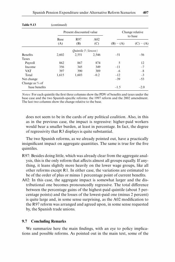
does not seem to be in the cards of any political coalition. Also, in thisas in the previous case, the impact is regressive: higher-paid workerswould bear a smaller burden, at least in percentage. In fact, the degreeof regressivity that R3 displays is quite substantial.

The two Spanish reforms, as we already pointed out, have a practicallyinsignificant impact on aggregate quantities. The same is true for the fivequintiles.

R97: Besides doing little, which was already clear from the aggregate anal-ysis, this is the only reform that affects almost all groups equally. If any-thing, it leans slightly more heavily on the lower wage groups, like allother reforms except R1. In either case, the variations are estimated tobe of the order of plus or minus 1 percentage point of current benefits.

A02: In this case, the aggregate impact is somewhat larger and the dis-tributional one becomes pronouncedly regressive. The total differencebetween the percentage gains of the highest-paid quintile (about 5 per-centage points) and the losses of the lowest-paid one (minus 2 percent)is quite large and, in some sense surprising, as the A02 modification tothe R97 reform was arranged and agreed upon, in some sense requestedby, the Spanish trade unions.

9.7 Concluding Remarks

We summarize here the main findings, with an eye to policy implica-tions and possible reforms. As pointed out in the main text, some of the



Change relative Present discounted valueto base

Base R97 A02(A) (B) (C) (B) (A) (C) (A)

Quintile 5 (lowest)

Benefits 2,602 2,551 2,546 –51 –56Taxes

Payroll 862 867 874 5 12Income 356 345 349 –11 –7VAT 397 390 389 –6 –8Total 1,615 1,603 –0.2 –12 –3

Net change –39 –53Change as % of

base benefits –1.5 –2.0

Notes: For each quintile the first three columns show the PDV of benefits and taxes under thebase case and the two Spanish-specific reforms: the 1997 reform and the 2002 amendment.The last two columns show the change relative to the base.

quantitative estimates reported should be taken with (more than) the usualgrain of salt, as they are based on estimations of reduced-form behavioralequations that appear to have only a limited power to capture observed re-tirement patterns. This caveat is particularly important for the affiliates tothe RETA, for which none of the financial measures of retirement incentiveseem to play a major role in affecting decisions. Once this is understood, ourfindings can be summarized, reform by reform, as follows.

The Actuarial Reform is probably the least effective among the threecomparison reforms considered in the volume. This evaluation appliesboth in terms of expenditure, retirement patterns, and redistributionaleffect. Furthermore, most of the fiscal gains are accrued via the mechani-cal channel, which suggests that little would be gained in the long run byimplementing the Actuarial Reform in Spain.

The Three-Year Reform may have an impact that is likely to becomequite strong if, by changing legislation, one also affects in the same direc-tion the behavioral component of retirement, which seems to be capturedpurely by age dummies. In other words, if legislating 68 as the common re-tirement age leads most people who now retire at 65 to retire at 68, thenthe gains in labor-force participation of the elderly, achievable via the R1scenario, could be substantial. Correspondingly, the fiscal gains could besizable even if, as we argued earlier, once we compare the magnitude ofthese fiscal gains to the outstanding implicit social security debt of Spain,the actual reduction would be likely to be around 15 percentage points atmost. Further, some redistributional aspects of the R1 reform need to beadjusted to make it politically acceptable. The direction in which it redis-tributes wealth, from future retirees to the working population, is prob-ably acceptable, but the distribution of that burden within the retiringcohorts seems much less acceptable, as it falls disproportionately on thelowest-earning groups. This is an aspect that deserves further examina-tion.

The same goes for the Common Reform. The latter does not really shiftretirement patterns uniformly but, rather, cuts in about half the exit rateat age 60 (which corresponds to early retirement in Spain), and which ismostly used by the lower wage earners. At the same time, it reduces bene-fits, and therefore outstanding SSW, quite drastically. Also, this reform,like the previous one, suffers from having a very regressive bias, whichmakes it politically unfeasible. The fiscal gains accrued entail drastic re-ductions in the SSW and in the yearly pension payments of workers be-longing to the lower 60 percent of the wage distribution.

The two Spanish reforms are the least effective of the group. In bothcases the total SSW varies very little, retirement patterns remain almostidentical (a very mild shift to the right is predicted for the RETA affiliates),and the net fiscal effect is tiny. Also, these reforms are regressive when onelooks at within-cohorts redistribution. The amount of regressivity is, nat-urally, limited by the small reduction in aggregate SSW. Still, and quite par-


adoxically, the 2002 Amendment seems to make the overall Spanish reformmore regressive than it was after the 1997 change. In any case, there is noreason to believe that the very minor improvement in the government fis-cal position that A02 engenders will be sufficient to contain the forthcom-ing Spanish pension deficit.

Appendix

Data and Variables

In this section we define the variables that have been employed in the spec-ification of the reduced-form probit. The data source is the HLSS, unlessstated otherwise.

Variables from HLSS

Experience, Education, and Occupation

• Period: length of the current period in the dataset.• History: history in the dataset, that is, length of participation in the la-

bor market.• Part-time: indicator variable that takes the value 1 if the individual

does not work full time.• Fraction working: history divided by potential experience (time

elapsed since first time observed in the dataset).• Temporary illness: length of history spent in temporary illness.• Sector: one-digit SIC industry classification.• Contributive group: ten groups, from college to unskilled blue collar

workers.• Education: proxy for the level of education, constructed as follows: all

individuals in contributive group 1 (i.e., college), are assigned to thecollege level of the educational variable. People belonging to con-tributive groups 2, 3, and 4 are assigned to the high school (diploma)category. People in all other contributive groups are assigned to ageneric class labelled less than high school.

• Years of contributions: number of years contributed.• Eligibility indicator: a dummy variable that takes the value 1 if the in-

dividual meets the contributive threshold (fifteen years of contribu-tions); zero otherwise.

Earnings and Pension Variables

• Covered earnings or pensionable earnings: monthly amount uponwhich SS taxes are levied.


• Monthly earnings: methods of computation (for workers in RGSS) asdescribed in section 9.3.2.

• Pension amount: see section 9.2 for a detailed description.• Average life cycle earnings: constructed on the basis of a fixed-effect

model for each contributive group.• Expected earnings: see section 9.3.2 for a description.• Expected earnings peak indicator: discounted sum of the expected

earnings from the present to the year the peak is reached.• Expected earnings OV indicator: discounted sum of the expected

earnings from the present to the year the option value is maximized.• Minimum pension indicator: a dummy variable that takes value 1 if

the individual’s expected retirement pension falls below the minimumretirement pension.

• Censoring earnings indicators: two dummy variables. The first takesvalue 1 if the individual’s level of contributions falls below the mini-mum (mandatory) level of contributions. The second takes value 1 ifthe individual’s level of contribution is greater than the maximum levelof contributions.

Variables from the Collective Settlements Register (Estadística de

Convenios Colectivos [ECC])

Since we do not have direct information about regulations affecting spe-cific workers, we use the Spanish register of collective settlements in orderto construct proxies for such regulations. In particular, using the ECC (seeJiménez-Martín [1998] for a brief description of the source) we have con-structed three indicators of the coverage of early and mandatory retire-ment provisions for each (two-digit) industry.

• Early-retirement indicator: fraction (weighted by employment) of col-lective settlements, including a provision favoring early retirement.

• Retirement at 64: fraction (weighted by employment) of collective set-tlements, including a provision to facilitate retirement of workers aged64 without incurring age penalty. This variable only applies to peopleaged 64 enrolled in RGSS.

• Mandatory retirement at 65: fraction (weighted by employment) ofcollective settlements, including a provision promoting mandatory re-tirement at 65. This variable only applies to people aged 65 enrolled inRGSS.

The Spanish Labor Force Survey (EPA)

EPA: a quarterly CPS-like survey of roughly 60,000 Spanish households. Itcontains fairly detailed information on labor-force status, education, and


family background variables, but no information on wages and income.Publicly released cross-sectional files are available from 1976 onward.Starting with 1987, INE also releases the so-called Encuesta de Poblacion

Activa Enlazada (EPAL), which is the panel version of EPA obtained by ex-ploiting the rotating cross-section nature of the original survey. It containsfewer variables than EPA, but it permits the following of individuals for upto six consecutive quarters.

References

Abío, G., H. Bonin, J. Gil, and C. Patxot. 1999. El impacto intergeneracional de lareforma de las pensiones en España: Un enfoque de contabilidad generacional.Cuadernos Económicos de ICE 65:101–16.

Boldrin, M., S. Jiménez-Martín, and F. Peracchi. 1999. Social security and retire-ment in Spain. In Social Security Programs and Retirement around the World, ed.J. Gruber and D. Wise, 305–82. Chicago: Chicago University Press.

———. 2001. Sistema de pensiones y mercado de trabajo en España. Madrid: Fun-dación BBV.

———. 2004. Micro-modelling of retirement behavior in Spain. In Social securityand retirement around the world: Micro-estimation, ed. J. Gruber and D. Wise,499–578. Chicago: Chicago University Press.

Instituto Nacional de Estadística (INE). 1995. Proyecciones de la población de Es-paña. Madrid: Instituto Nacional de Estadística.

Instituto Nacional de Estadística (INE). Encuesta de población activa. Microdatafiles from 1995-II to 2001-II, various issues. Madrid: Instituto Nacional de Es-tadística.

Jiménez-Martín, S. 1998. Indexation and wage change settlements: Evidence fromSpanish manufacturing firms. Oxford Bulletin of Economics and Statistics60:449–84.

Jiménez-Martín, S. 1999. El impacto de la reforma de 1997 en los incentivos y ladeuda implícita de la Seguridad Social. Economístas 84:200–208.


Documents

Evaluating Spanish Pension Expenditure under Alternative