Embed Size (px)
Citation preview
AMERICAN JOURNAL OF PHYSICAL ANTHROPOLOGY 89935-256 (1992)
Estimation of Age Structure in Anthropological Demography LYLE W KONIGSBERG AND SUSAN R FRANKENBERG Department of Anthropology, Uncversrty of Tennessee, Knoxville, Tennessee 37996
KEY WORDS puter simulation
Paleodemography, Iterated age-length key, Com-
ABSTRACT The past decade has produced considerable debate over the feasibility of paleodemographic research, with much attention focusing on the question of reliability of age estimates. We show here that in cases where age is estimated rather than known, the traditional method of assigning individu- als to age classes will produce biased estimates of age structure. We demon- strate the effect of this bias both mathematically and by computer simulation, and show how a more appropriate method from the fisheries literature (the “iterated age length key”) can be used to estimate age structure. Because it is often the case that ages are also estimated for extant groups, we suggest that our results are relevant to the general field of anthropological demography, and that it is time for us to improve the statistical basis for age structure estimation. We further suggest that the oft noted paucity of older individuals in skeletal collections is a simple result of the use of inappropriate methods of age estimation, and that this problem can be rectified in the future by using maximum likelihood estimates of life table or hazard functions incorporating the uncertainty of age estimates. o 1992 Wiley-Liss, Inc
Over the past decade the field of paleode- mography has undergone a resurgence of ac- tivity that has led to a number of contribu- tions to method and theory (Meindl et al., 1983; Sattenspiel and Harpending, 1983; Buikstra et al., 1986; Johansson and Horow- itz, 1986; Boldsen, 1988; Gage, 1988; Milner et al., 1989; Paine, 1989a,b; Siven, 1991; Whittington, 1991). Much of the recent in- terest in paleodemography has focused on analytical problems that plague this area of research. In the main, these analytical diffi- culties are not unique to paleodemography, but rather are symptomatic of anthropologi- cal demography in general. The stumbling- blocks faced in many anthropological de- mography studies, and virtually all paleodemographic studies are that: 1) popu- lation growth rate may not be known, 2) samples may not be representative, and 3) ages are usually estimated rather than known. The first problem has been dis- cussed by Sattenspiel and Harpending (19831, Johansson and Horowitz (1986),
Buikstra et al. (1986), Gage (19881, Horo- witz et al. (1988), Paine (1989a,b), and Mil- ner et al. (19891, and some suggestions have been made concerning remedies to the prob- lem of unknown growth rates. The second problem has been discussed by Weiss (1973:12-13) for living and skeletal popula- tions and by Walker et al. (1988) in the pa- leodemographic setting. The third problem of unknown ages has seen heated debate in the paleodemographic literature (Bocquet- Appel and Masset, 1982, 1985; Van Gerven and Armelagos, 1983; Bocquet-Appel, 1986; Greene et al., 1986; Lanphear, 1989; Pion- tek and Weber, 1990), and serves as the ba- sis for this paper.
While the quality of age estimates is much better for extant populations with systems of vital registration, in the absence of writ- ten records anthropological demographic studies must rely on reported or estimated
Received August 6,1991; accepted March 9.1992.
0 1992 WILEY-LISS. INC
236 L.W. KONIGSBERG AND S.R. FRANKENRERG
ages that are often inexact (see e.g., Roberts, 1956:328; Chagnon, 1972:270; Nee1 and Weiss, 1975:27; Cavalli-Sforza, 1977:276). Indeed, Townsend and Hammel(1990) have recently suggested that the age structure of subadults might be best studied using den- tal age estimates (from numbers of erupted teeth) rather than reported ages. If age esti- mates in extant populations are determined on the basis of morphology or behavior, then the distinction against paleodemography be- gins to blur. As an example, consider the rase o f the Semai, where Fix (1977.37) ar- gues that many subadults were incorrectly aged because the census-takers defined age classes on behavioral or social characteris- tics. Van de Walle’s (1968:13) comments on demography in Tropical Africa are also par- ticularly telling. He noted that “all African demographic surveys share the problem of trying to record the ages of people who do not know their exact ages and are not funda- mentally interested in knowing them.”
Only recently have researchers empha- sized that uncertainty in age estimates does (and should) cast some doubt on results from anthropological demography studies. For example, Gage et al. (1989:48) note “The high rate of aging in the paleodemographic tables and in the Yanomama is particularly intriguing. It may be a result of the error intrinsic in estimating ages in ethnographic populations and ages at death in paleopopu- lations, or it might represent some real dif- ference in the dynamics of aging in these populations.” In a similar vein, Howell (1982) presented the following scenario:
Two alternative interpretations arise from this con- sideration of the Libben life table. The more straightforward interpretation is to conclude that we now have empirical evidence in the form of this skeletal collection that life was far more difficult for prehistoric people in North America than we have observed it to be anywhere in the world dur- ing the 19th and 20th centuries. The alternative in- terpretation is to treat the results as a “reductio ad absurdum” shedding doubt an the literal accuracy of the life table itself. Perhaps the wisest course at this point i s to try to design research which tests hypotheses derived from the first alternative, while research on techniques of aging and sexing skele- tons and studies on the preservation probabilities of human skeletal material continue.
TABLE 1. Example of reference sample age estimation information from McKeni and SterciartS (1957) third
component of the pubic symphysis
Component stage . --____
Age at death‘ 0 1 2 3 4 5 _____.-.__-. .. __-..___.._ _____ ~
16.50-24.49 202 29 2 3 0 0 24.50-30.49 0 14 29 16 2 0 30.50-39.49 0 0 5 1 2 2 6 2 39.50 + 0 0 0 0 5 2
‘Years,
It is this latter endeavor that WP pnrwe here. We depart, however, from the recent concern with identifying better “age mark- ers” and methods of scoring them (see, e.g., Iscan, 1989a1, and instead focus strictly on the statistical basis for estimating age struc- ture of populations.
Starting from the position that much of anthropological demography, and all of pa- leodemography, is based on age data that are not known with certainty, we examine recent developments from wildlife manage- ment that will be useful in analyzing prob- lems in human biology. In particular, we borrow heavily from the fisheries literature, where the problem of age structure estima- tion from morphology has been dealt with in an elegant manner (Kimura, 1977; Westr- heim and Ricker, 1978; Clark, 1981; Bar- too and Parker, 1983; Fournier and Breen, 1983; Kimura and Chikuni, 1987). We begin with a discussion of the traditional methods for population age structure estimation ap- plied in paleodemography, and then proceed to consider more appropriate methods that should have broad applicability in both pa- leodemography in specific, and anthropolog- ical demography in general. Following a dis- cussion of a univariate method for discrete age indicators (due to Kimura and Chikuni, 1987), we present our extensions to the con- tinuous indicator and multivariate cases.
TRADITIONAL AGE ESTIMATION: A BAY ESlAN APPROACH
As an example of a traditional means for estimating an age distribution in an anthro- pological sample, we present in Table 1 a collapsed version of NIcKern and Stewart’s
ESTIMATION OF AGE STRUCTURE 237
viduals in intervals be restricted to whole numbers.
By summing the column for stage 2, and then dividing the number in each age group by the column total, all we have done is ap- ply Bayes theorem. Specifically, we have found the probability of being in a particular age class conditional on our knowledge of the indicator state. We can formalize this procedure with the inclusion of just a few extra symbols. Lettingp,, be the probability from the reference sample of being age a conditions! on being in indicator state t, and conversely pla be the probability of being in indicator state i conditional on being in age interval a, Bayes theorem gives:
(1957) tabulation of component I11 pubic symphyseal development against age for their sample of Korean War dead. We refer to the Korean War dead, or any other sam- ple of known aged individuals as a “refer- ence” sample, as this sample provides the reference information on age development which we wish to apply to a sample with unknown ages, The sample with unknown ages we will refer to as a “target” sample. The target sample could be a living anthro- pological population or a paleodemographic sample, as in lhe cuiieiii e~diiiple. :xi the case of a living population, the target sample may be aged on the basis of a morphological indicator (see e.g., Townsend and Hammel, 1990) or with reference to reported ages.
The reference sample will have its oyn age distribution, which we symbolize as d,, where a represents the discontinuous age classes indexed from 1 to ui. There are conse- quently w number of age classes, not neces- sarily of equal length. In the example from McKern and Stewart (see Table 11, there are four age classes, with da, the proportion of deaths in each age interval equal to 0.6762, 0.1748, 0.1289, and 0.0201. Using the infor- mation on distributions of pubic symphyseal component stages against ages, we wish to estimate the age distribution [or a target sample, which we symbolize as d,. Many dif- ferent ways have previously been suggested for assigning ages on the basis of indicator states, but we will use a fairly simple method here.
If in the target sample we observe an indi- vidual to be in a particular stage of the indi- cator state, say stage 2 of the third pubic symphyseal component, then we will proba- bilistically assign this individual to each age category on the basis of the reference sam- ple. For this example, if we observe an indi- vidual to be in stage 2, then the reference sample tells us that the individual has 2/36 (or 0.056) chance of being age 16.50 to 24.49, 29/36 (or 0.806) chance of being age 24.50 to 30.49, 5/36 (or 0.139) chance of being age 30.50 to 39.49, and 0136 (or 0.000) chance of being 39.50 years old or older. The fact that an individual is fractionally assigned to age intervals should pose no problem, as there is no reason to require that the number of indi-
Returning to our original example, if a pubic symphysis is observed to be in stage 2 of the third symphyseal component, then we can find the probability that the individual is between 24.50 and 30.49 years of age as (0.4754 x 0.1748)/(0.0085 x 0.6762 + 0.4754 x 0.1748 + 0.1111 x0.1289) = 0.81, identi- cal with the previous calculation.
Although the use of Bayes theorem above appears to be an annoying and tedious way to write something that we can find on much simpler terms, use of the theorem allows us to examine mathematically the validity of various arguments put forth originally by Bocquet-Appel and Masset (1982) and by Van Gerven and Armelagos (1983). Addi- tionally, use of the theorem demonstrates that this more or less traditional approach to age estimation is identical to the “age length key” method first published in the 1930s in the fisheries literature. The “age length key” method, which relies on the dis- tribution of discretized measurements of fish lengths against known ages in a refer- ence sample to estimate ages from lengths in a target sample, is identical to the Bayesian approach we have just described. More im- portantly, the method has been shown to produce biased estimates of the age distribu- tion in most reasonable circumstances
238 L.W. KONIGSBERG AND S.R. FRANKENBERG
(Kimura, 1977; Westerheim and Ricker, 1978), and has consequently been revised by Kimura and Chikuni (1987).
While our descriptions of the Bayesian method, or “age length key,” has so far cen- tered on the estimation of ages for single individuals, the method can easily be ap- plied to a complete target sample of individ- uals. If f l is the frequency of individuals in the target sample observed to be in age indi- cator state i, where i i_s indexed from 1 to n, then the estimates of d, in the target sample are:
An important point to note in equation 2 is that the estimates of the age distribution in the target sample appear to be at least par- tially dependent on the age distribution of the reference sample. Clearly, this is not a desirable property of an estimator, as we would like to think that the reference sample age distribution and the estimate of the target sample age distribution are independent. In order to clarify the nature of the relationship between target and reference age distributions, we consider a number of special cases in the following sections.
AN ABYSMAL AGE INDICATOR Bocquet-Appel and Masset (1982) make
the argument that if age prediction is very uncertain, then the estimated age distribu- tion for a target sample will approximate the age distribution of the reference sample. Mensforth (1990) has referred to this as a problem of “age mimicry,” and attempts to show through an empirical example that his specific target distribution differs from his reference. We show here that the (esti- mated) target and reference sample age dis- tributions will be equal if the age indicator is abysmal (i.e., unrelated to age).
If a suggested “age” indicator bears no re- lationship whatsoever to age, thenp,, = lln for all a, where n is the number of indicator
states. In other words, for any age a we ex- pect a uniform distribution of indicator states. Substitutingp, = lln in equation 2 yields:
(3)
so that the estimated target sample age dis- tribution exactly equals the reference sam- ple age distribution. This is the ultimate “age mimicry,” but of course we can safely assume that no “age” indicator is completely independent of age. Consequently, we con- sider an equally unlikely special case, where the age indicator is perfectly correlated with age.
A PERFECT AGE INDICATOR If an age indicator assigns individuals to
age classes with complete certainty, then for an age class a, there will be only one proba- bility pla equal to one, while all other pLa for the age class will equal zero. Furthermore, it must be the case that the number of indica- tor states is equal to the number of age classes. In this case, equation 2 can be re- written as:
where 6, equals 1 when a = i, and 0 other- wise. The reference age distribution is no- where to be found in equation 4, and in point of fact not only are the target and reference age distributions independent, but the tar- get distribution is estimated with complete certainty. Unfortunately, the search for a perfect age indicator is probably futile, so this second case is no more realistic than the first.
ESTIMATION OF AGE STRUCTURE 239
BIAS IN THE TRADITIONAL METHOD OF AGE ESTIMATION
Both the cases of an abysmal age indicator and a perfect age indicator are clearly unre- alistic. They represent opposite ends of a continuum, with any real age indicator lying somewhere in between. Age indicators are neither perfect, nor are they completely un- related to age. As a consequence of this fact, when the Bayesian approach (or “age length key”) is applied to an anthropological or pa- leodemographic target sample, we will get an estimated age distribution which is nei- ther a complete “mimic” of the reference sample nor completely independent of the reference. Given this fact, there is little rea- son to make empirical comparisons of refer- ence and target age distributions (e.g., Van Gerven and Armelagos, 1983; Mensforth, 1990) or of estimated and real age distribu- tions (Piontek and Weber, 1990; Lanphear, 1989). We know a priori (see Kimura, 1977; Westrheim and Ricker, 1978) that the esti- mated target age distribution will be biased in virtually all cases. Using the “age length key” (or Bayesian method), an unbiased esti- mate of the age structure will only be pro- duced when the reference and target sample have the same age distribution, when the reference sample has a uniform age distri- bution, or when the age indicator is perfect.
Bocquet-Appel (1986) suggested that if the reference sample has a uniform age dis- tribution, then the target sample age distri- bution will be estimated independent of the reference. In Bayesian terms, Bocquet-Ap- pel argues for selecting an “uninformative prior” in order to avoid the relationship be- tween the target and reference age distribu- tions. In this case, d, = l f w for all a, where w is the number of age classes. Returning to equation 2:
where, like in equation 4, the reference age distribution is not included. While this solu- tion does consequently remove the problem of dependence between the target and refer- ence age distributions, it is not in general a practical way to proceed. The chief problem with selecting a reference sample with a uni- form age distribution is that this requires discarding data, which certainly cannot be an efficient way to proceed. Fortunately, Kimura and Chikuni (1987) have recently shown that an earlier simple method due to Chi!c,uni, known as thc “”icratcd agc !cn,“,E: key” solves the problems of the Bayesian es- timator described above, while not requiring a uniform age distribution in the reference sample. In the following, we describe the “it- erated age length key” within the frame- work of maximum likelihood estimation, and then extend the technique to cover mul- tiple age indicators, as well as continuous indicators (such as counts of Haversian ca- nals, or numbers of incremental bands in cementum). At each juncture we will demon- strate the use of maximum likelihood esti- mation in comparison to more traditional means of age estimation when applied to simulated data sets. MAXIMUM LIKELIHOOD ESTIMATION OF
THE AGE DISTRIBUTION In order to obtain maximum likelihood es-
timates (NILE) of the target sample age dis- tribution, we need to use information from the reference sample in order to obtain the target sample age distribution most likely to have produced the observed distribution of target sample (age) indicator states. We can write the indicator state distribution for the target sample as F,, where now the capital F denotes counts within each indicator state i. The sum of the F, is equal to N, the total number of individuals, or in the case of pa- leodemography, skeletons. Again, we let a lower case n be the number of indicator states. From these parameters the probabil- ity of obtaining an individual in the target sample who is in a particular indicator state i (symbolized asp,) is:
240 L.W. KONIGSBERG AND S.R. FRANKENBERG
where the probability now depends on the unknown age distribution of the target sam- ple (rather than on the age distribution of the reference sample) and the conditional probabilities pL0 of indicator state given age in the reference sample. In other words, we make one of Howell’s (1976) uniformitarian assumptions (that the target and reference samples age in the same way) but do not impose aspects of the reference sample age distribution on the target sample.
Using equation 6 and the multinomial theorem, the probability of obtaining the en- tire set of individuals (or skeletons) arrayed across indicator states in the target sample is:
This is the likelihood of the estimated target sample age structure conditional on the ob- served indicator state data, which we sym- bolize as L(d,lFJ. The maximum likelihood estimate of d, is then the vector of propor- tions in age classes for the target sample at which L(d,lFJ is maximized. Because this maximum will also be identified if the likeli- hood is converted into a log scale, and be- cause the factorial term in equation 7 is in- variant to changes in d,, the maximum likelihood estimate will also occur when the following function is maximized:
that the “iterated age length key” is an EM algorithm that provides maximum likeli- hood estimates of d, has already been pre- sented in Kimura and Chikuni. The inter- ested reader is referred to their important work, as well as to Dempster et al. (1977). Following Kimura and Chikuni (1987), we do repeat the “iterated age length key” method here in simple terms so that it can be used to obtain maximum likelihood esti- mates of d,.
In the “iterated age length key” method xve begin with an initial estimate of d,, for which Kimura and Chikuni (1987) suggest a uniform distribution. In point of fact, any distribution that does not contain zeros and which spms to one is acceptable. From this initial d, distribution the estimated proba- bility of being age a conditional on being in age indicator state i is calculated from Bayes theorem as:
This is an expectation step (or “E” step), in that the expected values ofp,, are found con- ditional on the current estimates of d, for the target sample. This “age length key” from equation 9 can then be applied to the observed distribution of indicator states in the target sample to obtain a new estimate of the target sample age distribution:
The maximum of this equation (and the cor- responding maximum likelihood estimates) can be found by numerical methods, but by far the simplest method is to apply an itera- tive algorithm due to Kimura and Chikuni (1987).
Kimura and Chikuni point out that an it- erative application of the “age length key” method used in the fisheries literature con- stitutes an expectation-maximization (or “ E M ) algorithm. EM algorithms are two- step iterative methods that lead to maxi- mum likelihood solutions in many practical applications (Dempster et al., 1977). Proof
We use the prime symbol to indicate that equation 10 gives a new estimate of the age distribution. This is a maximization step (or “ M step) in that we are finding the maxi- mum likelihood estimate d, at the current estimates of pa,. Now the current maximum likelihood estimate of the age distribution (from equation 10) can be inserted into equa- tion 9 to obtain a new estimate of the proba- bility of being age a conditional on being in age indicator state i. The result from equa- tion 9 can be reapplied in equation 10, and the cycling continued until the estimated age distribution converges. Because the log-
ESTIMATION OF AGE STRUCTURE 241
TABLE 2. Probabilities of being in uarious stages of McKern and Stewart’s 119571 third pubic symphyseal component conditional on known age
Comnonent stare ~
Ace class’ 0 1 2 3 4 5
16.5-21.4 21.5-22.4 22.5-23.4 23.5-24.4 24.5-25.4 25.5-26.4 26.5-27.4 27.5-28.4 28.5-30.4 30.5-39.4 39.5-50.0
‘Years.
0.9882 0.7619 0.5172 0.1875 0.0000 0.0000 0.0000 0.0000 0.0000 0.0000 0.0000
0.0118 0.2381 0.4828 0.5000 0.3750 0.3846 0.3333 0.1538 0.0000 0.0000 0.0000
likelihood can be calculated at any step us- ing equation 8, the simplest procedure is to define convergence as the point where the change in the log-likelihood between any two steps is less than some very small value. In the following section, we apply both the “iterated age length key” and the Bayesian age estimation method to simulated data in order to demonstrate the desirable proper- ties of the former method.
APPLICATION OF THE MAXIMUM LIKELIHOOD METHOD FOR ESTIMATING
AGE STRUCTURE We can continue with the example of age
estimation begun previously with the third pubic symphyseal component in Table 1. Ta- ble 2 lists the probabilities of being in varr- ous component stages (McKern and Stewart originally numbered these 0 to 5, so we pre- serve their coding here) conditional on age. These probabilities were obtained from McKern and Stewart’s (1957) Table 25, and they represent the age information from the reference sample (p,,) necessary to apply the “iterated age length key” method. Although age ranges are not as greatly collapsed as in Table 1, we have grouped some ages to- gether where the pubic stage cannot dis- criminate between age classes or where the data were sparse.
In order to simulate a target sample whose age structure differed from the Mc- Kern and Stewart sample, but whose indi- viduals aged in similar fashion, we under- took the following Monte Carlo procedure.
0.0000 0.0000 0.0000 0.1250 0.3750 0.5385 0.2500 0.5385 0.6000 0.1111 0.0000
0.0000 0.0000 0.0000 0.1875 0.2500 0.0769 0.4167 0.3077 0.2667 0.2667 0.0000
0.0000 0.0000 0.0000 0.0000 0.0000 0.0000 0.0000 0.0000 0.1333 0.5778 0.7143
0.0000 0.0000 0.0000 0.0000 0.0000 0.0000 0.0000 0.0000 0 0000 0.0444 0.2857
We first drew a sample of 500 deaths from a mortality profile (see Moore et al., 1975, for this procedure) which differed substantially from that of the McKern and Stewart war dead. We then stochastically applied the in- formation in Table 2 for each individual to probabilistically assign a pubic stage condi- tional on their age. Following this, the as- signed pubic stages were used to estimate the age-at-death structure for the simulated target sample. The d, distribution was esti- mated both by the Bayesian method and us- ing the maximum likelihood “iterated age length key” method. We repeated this simu- lation 100 times.
Figure 1 shows a comparison of the Mc- Kern and Stewart probability of death func- tion, the generating probability of death function, and the average estimated proba- bility of death function (across 100 repli- cates) using the Bayesian method. Com- parison of these three curves clearly demonstrates that the Bayesian method re- covers the reference sample age distribution rather than the target sample through much of the later years. This is an undesirable feature of a technique that we consider to most closely approximate that traditionally used by paleodemographers. In contrast, in Figure 2, where the age structure is ob- tained by maximum likelihood estimation, there is a much better fit between the esti- mated target sample age distribution and the true age distribution of the target.
While the example given here is drawn from a paleodemographic setting, applica- tions for living populations are obvious. In
242
1.0 , 1= 0.9 4 3 a, u 0.8 (c
0 2? 0.7
a 0.6 (d a 2 0.5 Q
._I - .-
0.0
L.W. KONIGSBERG AND S.R. FRANKENBERG
- h
17 22 23 24 25 26 27 28 29 31 40
Age
Fig. 1. Comparison of the probability of death functions from the Bayesian method of estimation from the pubic symphysis, the generating target sample, and the reference sample (McKern and Stewart, 1957).
1 .o
J= 0.9- 3 a, Q 0.8 Y- O 2? 0.7
5 0.6 - (d a
.- -
0.5 g
; 0.2
a 0.1 -
o 0.4 ’c 0 Q) 0.3- Q
.-
CD
f - McKern and Stewart
Target
MLE method I
- - - - - - - - . I I
0 0 ~~ ~ - - _ _ - - - __ 17 22 23 24 25 26 27 28 29 31 40
Age
Fig 2 Comparison of the probability of death functions from the maximum likelihood method of estimation (MLE) from the pubic symphysis, the generating target sample, and the reference sample (McKern and Stewart, 1957)
cases where morphological or behavioral data have been used to determine ages, the researcher must know the conditional distri- bution of the indicator against known age in a reference sample. This information can then be used to find the maximum likelihood estimates of the age distribution for the tar-
get sample. In cases where the researcher is using reported ages to estimate the demo- graphic structure, it may be possible to spec- ify the conditional distribution of reported against real age for a portion of the popula- tion which is subject to vital registration. For example, Bairagi et al. (1982) and Cald-
243 ESTIMATION OF AGE STRUCTURE
well (1966) present such information for children’s ages in Bangladesh and Ghana, respectively. Additionally, Bhat (1990) has recently presented a method for estimating these conditional distributions which does not require a reference sample, but which does have stringent data requirements and carries a number of assumptions.
MULTIVARIATE FORM OF THE “ITERATED AGE LENGTH KEY”
The results from Figures 1 and 2 suggest that thc maximurr, likclihoad mcthor! pro- duces unbiased age structure estimates, while the traditional method is biased. This demonstration is, however, rather simplistic because only a single age indicator is used. There have been a number of calls now for “multifactorial aging” methods (Acsadi and Nemeskeri, 1970; Meindl et al., 1983; Love- joy et al., 1985; Iscan, 1989131, correctly not- ing that more than just one criterion should be applied when estimating ages from mor- phological observations. In this section we extend Kimura and Chikuni’s (1987) results to cover more than one age indicator, so we can examine the performance of “multifacto- rial aging” methods.
In the Bayesian method, if we consider (for example) three age indicators repre- sented as i, j , and k , then equation 2 general- izes to:
where n,, nJ, and nk signify the number of states within age indicators i, j , and k, and Pqkrr is the probability from the reference sample of being in the ith, jth, and kth states of the three age indicators conditional on being in the uth age class. For the maximum likelihood estimator of d,, the log-likelihood function shown in equation 8 can be general- ized to:
where FUk indicates the counts of numbers of individuals in the target sample cross-clas-
sified by age indicators i , j , and k. Similarly, the EM algorithm or “age length key” equa- tions shown in equations 9 and 10 general- ize to:
a = l
and
where f i f h represents the frequency of indi- viduals in the target sample observed to be in the ith, j th , and kth states of the three age indicators (summing to one across all i, j , and k).
AN EXAMPLE OF THE MAXIMUM LIKELIHOOD ESTIMATION OF AGE
STRUCTURE FROM MULTIPLE DISCONTINUOUS CHARACTERS
In order to apply equation 11 (the Baye- sian method) or equations 13 and 14 (the maximum likelihood method) it is necessary to have reference sample information where multiple indicator states are cross-classified against known age. Because of the immense size of such a table, this kind of information is rarely if ever published in the literature. For example, the original tabulations for the McKern and Stewart war dead study i1957) present numerous classifications of single indicators against age, but never a cross- classification of even so few as two indica- tors against age. Similarly, this kind of in- formation is unavailable from most of the more extensive modern studies of age deter- mination methods (Suchey et al., 1984; Webb and Suchey, 1985; Loth and Iscan, 1989; Meindl and Lovejoy, 1989) in humans. As a result of the paucity of this kind of information in humans, in the following ex- ample we utilize multiple morphological ob- servations on a reference skeletal sample from the Cayo Santiago rhesus macaque col- ony.
Falk et al. (1989) have recently reported on the progression of endocranial suture clo- sure using a sample of 330 rhesus monkeys from the Cay0 Santiago skeletal collection.
244 L.W. KONIGSBERG AND S.R. FRANFXNBERG
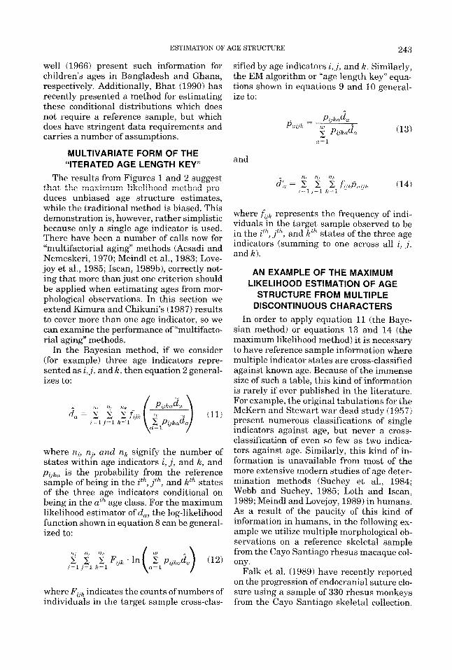
TABLE 3. Cross-tabulation of number of m,oiikeys o f known age against endocranial suture closure states for Cay0 Santiago rhesus macauues‘
Age iyr I - 0 00-0 99
1.00-1.99
2.00-2.99
3.00-3.99
4.00-4.99
No.
1 7 1 1 2 2 2 1
11 2 1 7 3 3 1 1
-
i0,1,0) 7 (0,1,1) 2 10,2,01 5 (0,2,1) 2 ( 1 , L O ) 3 (1,1,1) 1 (1,2,0) 1 i2,1,1) 1 (2,2,1) 1 (0,1,0) 2 (O,l,l) 6 (0,2,0) 5 (0,2,1) 4 (0,2,2) 1 (1,1,0) 3 il,1,1) 2 (1,2,0) 3 (1,2,1) 4 (2,1,1) 1 (2,2,0) 1 (2,2,1) 2 (0,1,0) 6 <O. l . l ! 1 ‘O,%,O’ 3 (0,2,1) 2 11,1,0) 2 (1M) 6 (1,2,0) 4 (1,2,1) 2 (1,2,2) 1 (2,1,0) 2 (2,1>1) 2 i2.2,O) 2 (2,2,1) 6 (2,2,2) 2 (3.2.1) 3
Age (yr!
5 00-5 99 __ __ ___
6.00-6.99
7.00-7.99
8.00-8.99
9.00-9.99
10.00-14.99
15.00 +
(13.2) i2,1,1) i2,2,1) i3,1,1) (32’0) (3,2,1) (3,2,2) (2.2.1)
No.
1 1 1
_ _
2 1
2 2 1 5 8 1 1 9 4
1 10 6 1 1 1
2 ‘5 1 9
20 1 1 2
99 iy
After Falk et al., 1989. of listed sutures is hasilar, sphenotemporal, and caudal squamosal. 0 = open, 1 = closing, 2 = closed, 3 = ohliterated.
They scored a series of sutures as open (O), closing (l), closed (2 ) , or obliterated (3) (see Falk et al., 1989, for further definitions of these states). For this example, we consider closure of three sutures: the basilar, sphe- notemporal, and caudal squamosal sutures,
because their development spans much of macaque ontogeny. Table 3 contains a sum- mary of the tabulation of suture closure states against age for 340 rhesus macaques. An additional 10 macaques over the original Falk et al. (1989) sample are included in this
ESTIMATION OF AGE STRUCTURE 245
1 0
.r, 0.9 CEl Q) ~3 0.8
O,o-?-- - ~- -r- 0 1 2 3 4 5 6 7 8 9 10 15
Age
Fig 3 Comparison of the probability of death functions from the Bayeslan method of estimation from cranial suture closure in rhesus macaques, the generating target sample, and the reference sample (Falk et a1 , 1989)
table because of the less stringent require- ments concerning missing data. Although with 12 age classes and three indicators each with four states there should be 768 cells within Table 3, 670 of the cells con- tained no observations, so they are not in- cluded here.
In order to form target samples against which to apply the Bayesian and maximum likelihood methods, we formed bootstrap samples out of the original observations on the 340 macaques. So that the age structure of the target samples would systematically differ from the reference sample, we first simulated 340 deaths using the life table ob- tained from census data (Sade et al., 1976). The life table from census data and from the skeletal sample are by no means equivalent, because of the nonrandom factors that have affected formation of the skeletal sample and collection of the endocranial suture clo- sure data. Specifically, newborns are sub- stantially underrepresented in the skeletal sample used here, in large measure because endocasts (the source for the suture closure data, see Falk et al., 1989) cannot usually be made on these younger animals. After form- ing a target sample age-at-death distribu- tion, we sampled with replacement from each age class in the reference sample, se-
lecting the number of individuals based on the simulated number of deaths within in- tervals. Because of the fact that we sampled with replacement, this is a bootstrap sam- ple, or more correctly, a bootstrap sample which is stratified on age.
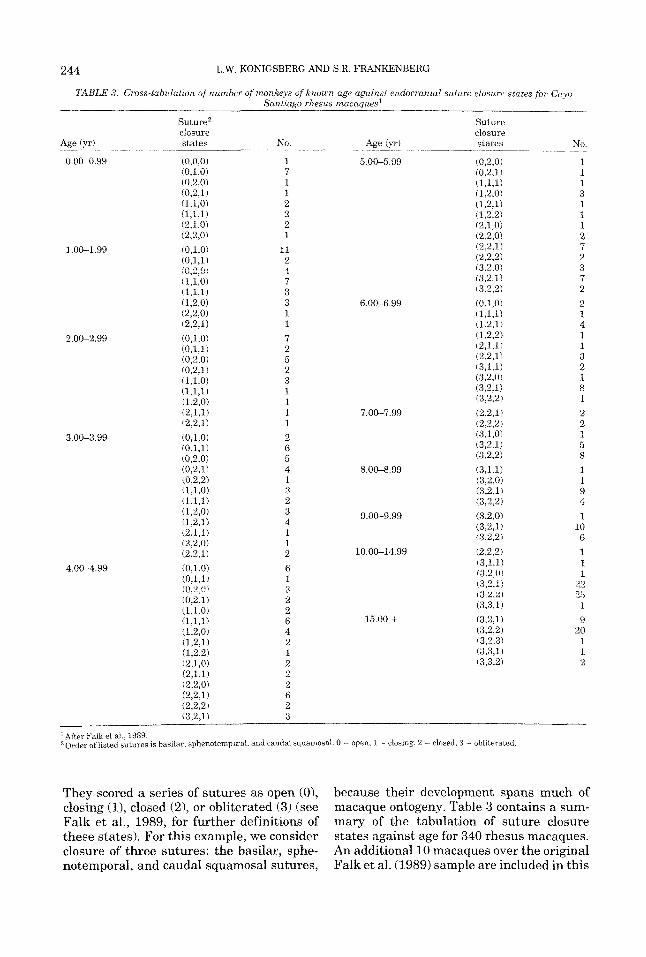
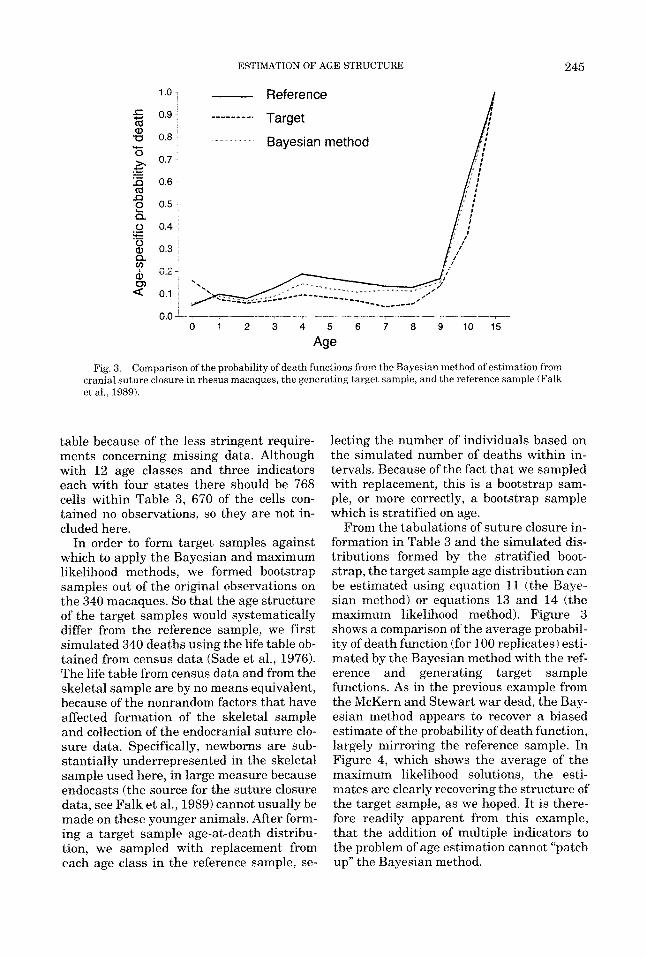
From the tabulations of suture closure in- formation in Table 3 and the simulated dis- tributions formed by the stratified boot- strap, the target sample age distribution can be estimated using equation 11 ithe Baye- sian method) or equations 13 and 14 (the maximum likelihood method). Figure 3 shows a comparison of the average probabil- ity of death function (for 100 replicates) esti- mated by the Bayesian method with the ref- erence and generating target sample functions. As in the previous example from the McKern and Stewart war dead, the Bay- esian method appears to recover a biased estimate of the probability of death function, largely mirroring the reference sample. In Figure 4, which shows the average of the maximum likelihood solutions, the esti- mates are clearly recovering the structure of the target sample, as we hoped. It is there- fore readily apparent from this example, that the addition of multiple indicators to the problem of age estimation cannot “patch up” the Bayesian method.
246
1 .o
0.9
a, u 0.8 T;j
Y- O I
0.7- 1 5 0.6-
(d 1 a
.- -
0.5
0 0.4 Y- o a) 0.3 Q
.-
3 0.2
a 0.1 0,
L.W. KONIGSBERG AND S.R. FRANKENBERG
- Reference
Target
MLE method
--------.
7 0 0 - _ - ~ - - ----̂ __ - ___- ___ 0 1 2 3 4 5 6 7 8 9 1 0 1 5
Age
Fig 4 Comparison of the probability of death functions from the maximum likelihood method of estimation (MLE) from cranial suture closure in rhesus macaques, the generating target sample, and the reference sample (Falk et a1 , 1989)
L 0
S
0 f
~ __ _ _ _ _ _ _ - - 1 6 , - - -
- Target i Reference
0 8 ' Bayesian method
0 4 - 1 ( ) - - ___ __ ~ -_
* MLE method
I
- 0 4 -
-0 8
- 1 2; 1
- _ - - 1 6 -_ ~ _ ~ - -
-1 - 0 8 - 0 6 - 0 4 - 0 2 0 0 2 0 4 0 6
Logit of True Target Mortality
Fig. 5 . Plot of logits of estimated and observed mortality for Cay0 Santiago macaques against the logit of true target mortality.
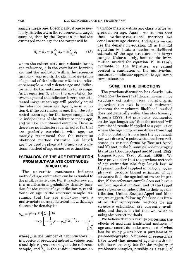
To more clearly represent the relationship between the estimated target and reference sample age distributions, Figure 5 shows a plot of mortality in logit scale (see Brass and Coale, 1968:127-129; Brass, 1969). Following Brass, the logit is defined as %ln[(l - LJl,.., where 1, is survivorship to age x. Figure 5 is a plot of logits from the estimated target mortality (by Bayesian and
maximum likelihood methods), the true tar- get mortality, and the reference mortality, all plotted against the logits of the true tar- get mortality. On the logit scale, a plot of the estimated mortality profile (against the true target) which precisely equalled the true target profile would pass through the origin and have a slope of one (shown as a solid line in Figure 5). Table 4 shows summary statis-
ESTIMATION OF AGE STRUCTURE 247
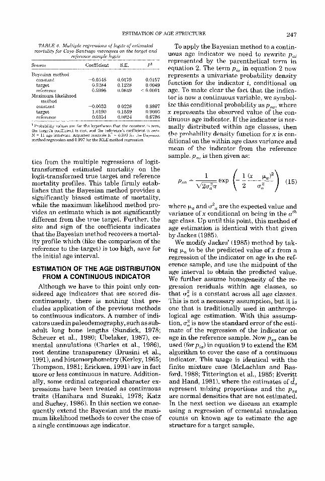
TABLE 4. Multiple regressions of logits of estimated mortality for Cay0 Santiago macaques on the target and
reference sample lopits
Source Coefficient S.E. Pl
Bayesian method constant --0,0548 0.0179 0.0157 target 0.5284 0.1228 0.0049 reference 0.5996 0.0649 c_ 0.0001
Maximum likelihood method
constant -0.0033 0.0228 0.8867 target 1.0190 0.1559 0.9060 reference 0.0354 0.0824 0.6786
‘Probability vdlues are for the hypotheses that the constant is zero, the target’s coefficient IS one, and the reference’s coefficient is zero N - 11 age intervals Aajustea muitipie E* = v 9 7 3 fi,, , l iZ s ~ ~ ~ , ~ ~ ~ ~ method regression and 0 997 for the MLE method regression
tics from the multiple regressions of logit- transformed estimated mortality on the logit-transformed true target and reference mortality profiles. This table firmly estab- lishes that the Bayesian method provides a significantly biased estimate of mortality, while the maximum likelihood method pro- vides an estimate which is not significantly different from the true target. Further, the size and sign of the coefficients indicates that the Bayesian method recovers a mortal- ity profile which (like the comparison of the reference to the target) is too high, save for the initial age interval.
ESTIMATION OF THE AGE DISTRIBUTION FROM A CONTINUOUS INDICATOR
Although we have to this point only con- sidered age indicators that are scored dis- continuously, there is nothing that pre- cludes application of the previous methods to continuous indicators. A number of indi- cators used in paleodemography, such as sub- adult long bone lengths (Sundick, 1978; Scheuer et al., 1980; Ubelaker, 1987), ce- mental annulations (Charles et al., 19861, root dentine transparency (Drusini et al., 1991 1, and histomorphometry (Kerley, 1965; Thompson, 1981; Ericksen, 1991) are in fact more or less continuous in nature. Addition- ally, some ordinal categorical character ex- pressions have been treated as continuous traits (Hanihara and Suzuki, 1978; Katz and Suchey, 1986). In this section we conse- quently extend the Bayesian and the maxi- mum likelihood methods to cover the case of a single continuous age indicator.
To apply the Bayesian method to a contin- uous age indicator we need to rewrite pa, represented by the parenthetical term in equation 2. The term pLa in equation 2 now represents a univariate probability density function for the indicator i, conditional on age. To make clear the fact that the indica- tor is now a continuous variable, we symbol- ize this conditional probability asp,,, where x represents the observed value of the con- tinuous age indicator. If the indicator is nor- mally distributed within age classes, then the prohahility density function forx is con- ditional on the within age class variance and mean of the indicator from the reference sample. p,, is then given as:
where pa and CT’, are the expected value and variance ofx conditional on being in the ath age class. Up until this point, this method of age estimation is identical with that given by Jackes (1985).
We modify Jackes’ (1985) method by tak- ing pa to be the predicted value of x from a regression of the indicator on age in the ref- erence sample, and use the midpoint of the age interval to obtain the predicted value. We further assume homogeneity of the re- gression residuals within age classes, so that C T ~ is a constant across all age classes, This is not a necessary assumption, but it is one that is traditionally used in anthropo- logical age estimation. With this assump- tion, C T ~ is now the standard error of the esti- mate of the regression of the indicator on age in the reference sample. Now pxa can be used (for p L J in equation 9 to extend the EM algorithm to cover the case of a continuous indicator. This usage is identical with the finite mixture case (McLachlan and Bas- ford, 1988; Titterington et al., 1985; Everitt and Hand, 19811, where the estimates of da represent mixing proportions and the pZa are normal densities that are not estimated. In the next section we discuss an example using a regression of cementa1 annulation counts on known age to estimate the age structure for a target sample.
248 L.W. KONIGSBERG AND S.R. F W K E N B E R G
AN EXAMPLE OF THE MAXIMUM LIKELIHOOD ESTIMATION OF AGE
STRUCTURE FROM A CONTINUOUS CHARACTER
For our example of a continuous character used in age estimation we consider counts of cementum annulations (Condon et al., 1986). Cementum annulations are annual rings that form in cementum, the material lining tooth roots. Although these rings are counted, and are therefore discrete, Condon et al. (1986) treat these variables by linear regression. L\ie consider the annuli as a con- tinuous trait whose observation ultimately reduces the scale to a discontinuous count. As a consequence of this treatment, an an- nuli count of, for example, 20 rings is consid- ered here to represent a trait value between 19.5 and 20.5.
In a sample of 55 individuals of known age, Condon et al. (1986) obtained a correla- tion between annuli counts and age in years of 0.858. From the summary statistics pro- vided in their article, the variance-covari- ance matrix for age and cementum annula- tion counts can be calculated as:
p03.7095 1 5 5 . 4 0 2 ~ (16) = 155.4026 161.0389
where age is listed before annuli counts, and the mean age and cementum counts were 32.2 years and 32.95, respectively. These summary statistics describe the bivariate normal distribution which we take to repre- sent the reference sample. In order to simu- late target samples whose pattern of aging followed that of the reference sample, but whose age distribution differed we used the following procedure. Letting T be the Cholesky decomposition of V (i.e., T’T = V), p be a 2 x 1 vector containing the mean age and mean cementum count (32.2 and 32.95, respectively), 2 be an N x 2 matrix of ran- dom standard normal deviates, and 1, be an N x 1 vector of ones where n is the number of individuals, we can write the matrix R as:
R = (T’Z’ + pl’J‘ (17)
R is an N x 2 matrix whose first column contains simulated ages and whose second
column contains simulated cementum an- nulation counts. Further, the bivariate rela- tionship from this simulated data will ap- proximate that for the original Condon et al. (1986) sample.
We simulated 500 R matrices, and then bootstrap sampled from each matrix 300 in- dividuals with an age-at-death structure taken from Weiss’ (1973) model MT 15:30 (life expectancy at age 15 equal to 15 years and survivorship to age 15 equal to 0.30). Because the Condon et al. (1986) sample did not include any individuals under 10 years old we also eliminated any of these individu- als. To estimate the age structure for these simulated target populations we applied the information from the Condon et al. (1986) reference sample. Specifically, from the summary statistics in Condon et al. (1986) the regression of cementa1 annulations on age would be x = 8.385779 + 0.762864Cy) where x is the cementum annulation count and y is the age in years. The standard error of the estimate from this regression is 6.579478 annulations. Consequently, for any observed annulation count the probabil- ity of that count conditional on age is given by the normal density in equation 15 with mean equal to 8.385779 + 0.762864(a), where a is the midpoint of the age interval, and standard deviation equal to 6.579478.
We applied the EM algorithm to this prob- lem, and also took the more traditional route of estimating ages at death from simulated counts using the Condon ct nl. rcgrcssion o f y = 0.4 + 0.965~~3~). Figure 6 shows a com- parison of the average (across 500) esti- mated age-at-death structure from this tra- ditional approach against the generating Weiss model and the normally distributed reference age-at-death distribution. Clearly, the estimated age-at-death structure does not follow the probability of death function from which it was generated (the Weiss model), and in some respects appears to be following the structure of the reference sam- ple instead. The comparable graph (Figure 7) shows the vastly superior performance of the maximum likelihood method, in which the generating age distribution is well esti- mated.
A n interesting feature from Figure 6 is that the estimated age distribution of the
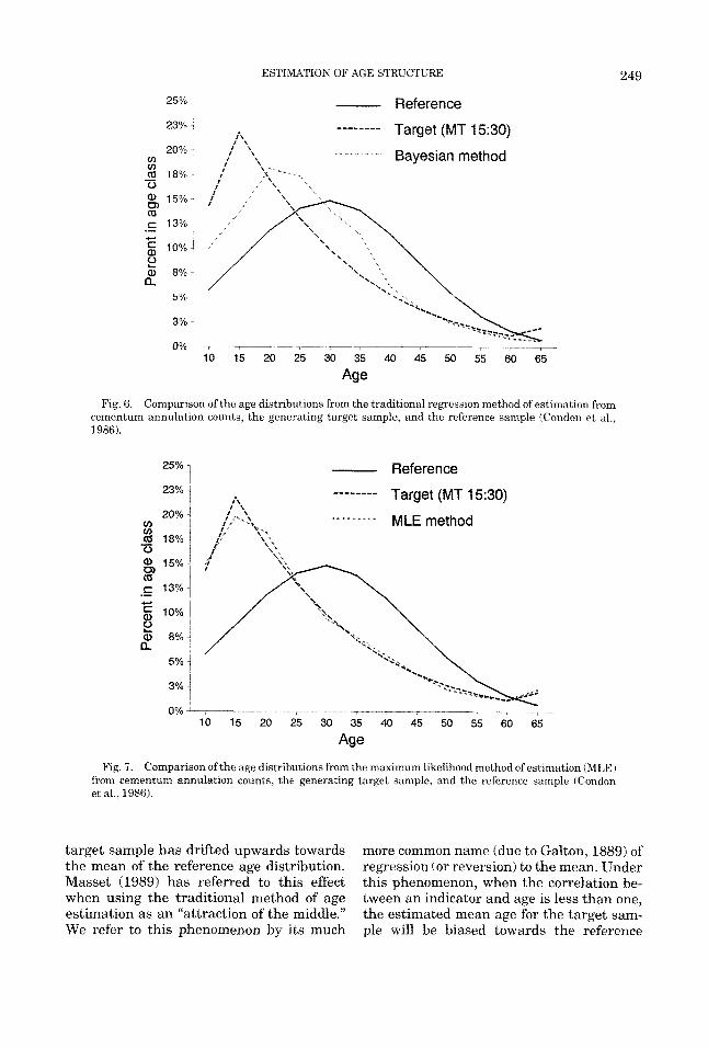
ESTIMATION OF AGE STRUCTURE 249
25% - Reference 23%
15% a c 13% .- c g 10% e a, 8%- a
---i----- - 7-v 7 - - 7 -- -7 10 15 20 25 30 35 40 45 50 55 60 65
Age
Fig. 6. Comparison of the age distributions from the traditional regression method of estimation from cementum annulation counts, the generating target sample, and the reference sample (Condon et al., 1986).
- Reference 25% 1 23% j
20% i
5% 1
0% 3%L -----r---- --_ 7 10 15 20 25 30 35 40 45 50 55 60 65
Age
Fig. 7. Comparison of the age distributions from the maximum likelihood method of estimation (MLE) from cementum annulation counts, the generating target sample, and the reference sample (Condon et al., 1986).
target sample has drifted upwards towards the mean of the reference age distribution. Masset (1989) has referred to this effect when using the traditional method of age estimation as an “attraction of the middle.” We refer to this phenomenon by its much
more common name (due to Galton, 1889) of regression (or reversion) to the mean. Under this phenomenon, when the correlation be- tween an indicator and age is less than one, the estimated mean age for the target sam- ple will be biased towards the reference
250 L.W. KONIGSRERG AND S.R PRANKENBERG
sample mean age. Specifically, if age is nor- mally distributed in the reference and target samples, then by the Bayesian method the estimated mean age for the target will be:
where the subscripts t and r denote target and reference, p is the correlation between age and the indicator within the reference sample, u represents the standard deviation uf dge d i d uf the iiidieatui vi.itihiii the iefci- ence sample, a and x denote age and indica- tor, and the bar notation stands for average. As in equation 3, when the correlation be- tween age and the indicator is zero, the esti- mated target mean age will precisely equal the reference mean age. Again, as in equa- tion 4, if the correlation is one, then the esti- mated mean age for the target sample will be independent of the reference mean age, and will be an unbiased estimate. Because there are no indicators identified so far that are perfectly correlated with age, we strongly recommend that the maximum likelihood method (“iterated age length key”) be used in place of the incorrect tradi- tional method of age structure estimation.
ESTIMATION OF THE AGE DISTRIBUTION FROM MULTIVARIATE CONTINUOUS
INDICATORS The univariate continuous indicator
method of age estimation can be extended to the multivariate case. For this extensionp,, is a multivariate probability density func- tion for the vector of age indicators x, condi- tional on age in the reference sample. As- suming that the age indicators have a multivariate normal distribution within age classes, the density is:
(19)
where p is the number of age indicators, p, is a vector of predicted indicator values from a multiple regression on age in the reference sample, and Z, is the residual variance-co-
variance matrix within age class a after re- gression on age. Again, we assume that these variance-covariance matrices are equal across age classes, and again we can use the density in equation 19 in the EM algorithm to obtain a maximum likelihood estimate of the age structure of a target sample. Unfortunately, because the infor- mation needed for equation 19 is rarely available in the literature, we cannot present a simulation of the multivariate continuous indicator approach to age struc- ture estimation.
SOME FUTURE DIRECTIONS The previous discussion has clearly indi-
cated how the more traditional means of age structure estimation from morphological characters can lead to biased estimates, whereas the maximum likelihood method does not generally suffer this shortcoming. Emura (1977:318) previously commented on the “age length key” that the method “will give biased results if applied to a population where the age composition differs from that of the population from which the age length key was drawn,” a point which has been reit- erated in various forms by Bocquet-Appel and Masset in the human paleodemography literature (Bocquet-Appel and Masset, 1982; Bocquet-Appel, 1986; Masset, 1989). We have proven here that the previous methods of age estimation (the “age length key” or Bayesian method) applied in paleodemogra- phy will producc binscd estimates of age structure if: 1 j the age indicators are imper- fect, 2) the reference sample does not have a uniform age distribution, and 3 ) the target and reference samples differ in their age dis- tribution. Unlike Bocquet-Appel and Mas- set, we suggest, following the fisheries liter- ature, that appropriate methods for age structure estimation are currently avail- able, and that it is vital that we switch to using the correct methods.
We believe that our results concerning the effects of applying traditional methods of age assessment do make sense out of what has for many years been a puzzlement in paleodemography. A number of researchers have noted that means of age-at-death dis- tributions are very low for the majority of prehistoric samples, possibly as a result of
ESTIMATION OF AGE STRUCTURE 251
paleodemographers underaging older adults (Weiss, 197359, Asch, 1976:41-43; Bod- dington 1987:188-191; Gage et al., 1989:48). We suggest that this problem is the result of using the traditional (Bayesian-like) ap- proach to age estimation based on reference samples that have fairly young age distribu- tions. Further, we suggest, as do Bocquet- Appel and Masset (1982), that many of the observed differences between paleodemo- graphic life tables are due to the specific reference samples that were used to derive age estimates For Pxam-ple, in 8 stndy of26 life tables from prehistoric North America, Buikstra and Konigsberg (1985:329) sum- marized the probability of death functions by principal components analysis, and noted that:
We believe that this first principal component is simply measuring the extent to which older individ- uals have been underaged or perhaps systemati- cally excluded from the mortuary pattern. We note also that when we compare the various sites for their scores on the first principal component, there is no patterning with respect to ancient subsistence strategy, chronology, or geographic location.
In a recent publication, Buikstra (1991:178) went on to summarize this study, noting that “we . . . removed what we felt to be the effect of distinctive traditions of age estima- tion among our colleagues through principal components analysis.” We suggest here that the “distinctive traditions” are largely based on the particular reference samples empha- sized in various analyses. Typically, re- searchers who emphasize reference samples with younger age distributions will recover target sample age distributions that are younger than what they would have ob- tained using an older aged reference sample. It is important to note, however, that the traditional approach only leads to bias in the age estimates, it does not lead to Mens- forth‘s (1990) complete “age mimicry.” In any event, using the maximum likelihood aproach we have discussed here would re- move this bias.
We have not discussed the question of effi- ciency of estimates. We would obviously like to know not only what the “correct” esti- mates of life table parameters are, but what level of confidence we may have in their esti-
mation. Prior to the maximum likelihood methods described here, which include in- formation on the imprecision of age estima- tion, all confidence intervals (as well as sta- tistical tests) generated for life tables or survival analyses have been based on the assumption that ages were precisely known. Whittington (1991:174) incisively noted this shortcoming, when (in reference to his sur- vival analysis for Copan) he wrote “these and all subsequent significance levels re- flect only error due to finite sample size and do not take into account assi,=ment err(trc in sex, phase, or age, which were difficult, if not impossible, to quantify.” Clearly, the as- sumption that ages are known (when they are not) will lead to false power in tests and confidence intervals that are too small. The unpleasant consequence of this assumption is that in using traditional life table meth- ods with individuals apportioned to inter- vals as if ages were known, we often may find “significant” results because we have not accounted for the fact that ages are esti- mated. The correct confidence intervals from the maximum likelihood method (that account for age estimation uncertainty) can, however, be obtained using standard likeli- hood methods. The standard errors of esti- mates are found as the square roots of the diagonal values from the inverse of the in- formation matrix (see Edwards, 1984). The information matrix is the matrix of the neg- ative of the second partial derivatives of the log-likelihood with respect to all possible pairs of parameters. This matrix can be found either by numerical methods or using the analytical derivatives given by Kimura and Chikuni (1987).
A second area of interest we have not con- sidered is the ability to compare different anthropological or paleodemographic sam- ples to determine where important similari- ties or differences may lie. Although there has been considerable discussion of this problem (e.g., Lovejoy, 1971; Konigsberg, 1985; Gage, 1988; Paine, 1989a) all previous methods again start from the untenable as- sumption that ages are unambiguously known. In what is probably the commonest case in paleodemography, we wish to com- pare two death samples to determine whether or not they are significantly differ-
252 L.W. KONIGSBERC AN
ent. If we let d, be a vector representing the maximum likelihood estimate of the age-at- death distribution for the first paleodemo- graphic sample, d, be a similar vector forthe second paleodemographic sample, and d, a vector for the two samples pooled together, then the likelihood ratio test for equality of the two samples is:
D S.R. FRANKENBERG
-2[lnL(d,lF,) - lnL(dliFl) - lnL(cf,IF,)l (20)
where the F vectors (or matrices) represent infnrmatinn from age inrlicatnrs and InT, means log-likelihood. Under the null hy- pothesis of equality, equation 20 is asymp- totically chi-square distributed with degrees of freedom equal to one less than the num- ber of age intervals. One degree of freedom is lost because of the linear constraint that the sum of the age distribution must equal one. For small samples, where the asymp- totic approach to a chi-square distribution may be unacceptable, the probability of ob- taining a likelihood ratio equal to or more extreme than that in equation 20 can be ap- proximated by Monte Carlo methods.
A future direction that we expect to see in anthropological demography and paleode- mography is the incorporation of uncer- tainty of age estimates into reduced param- eterizations of life table functions. For example, hazards analysis, which reduces the mortality parameters to a small set, has recently been used in a number of anthropo- logical demography studies (Gage, 1988; Weiss, 1989; Whittington, 1991). There are two numerical methods for including our current results into hazards models or other models with reduced numbers of parame- ters. The first, and most tedious method, is to retain the EM algorithm. In this case, we start with some initial guess a t the hazards (or other) parameter; and estimate d,. Then the distribution of d , is used in equation 9 (the E step), followed by equation 19 (the M step) to produce a new estimate of d,. These d, are then used to find the maximum likeli- hood estimate of the hazards (or other) pa- rameters, whish in turn are used to find new estimates of d,. The process is then started anew. This may be a very slow procedure, because the M step is computaticnally costly, and many iterations may be neces- sary to reach convergence. A simpler alter-
native is to rewrite the log-likelihood equa- tion (equation 8 or 12) parameterized with the hazards, and then numerically maxi- mize this new likelihood.
While the discussion from this paper pre- sents a somewhat bewildering trail of sug- gestions for the future of paleodemography and anthropological demography, the truth of the matter is that we have been using inappropriate methods for many years. We no longer need to use these incorrect meth- ods, and we certainly should not persist in hlithely caltiilating and piihlishing life tn- bles based on uncertain data, presented un- der the guise of certainty. As should be clear from this paper, there is much work that needs to be done in anthropological demog- raphy, and the bulk of this work must focus on collecting and presenting in useable fash- ion age estimation data that can be widely applied. While this may seem to be a droll prospect for the future, we should be clear in pointing out that the MLE methods dis- cussed here all operate on finding the condi- tional distributions of morphological or be- havioral characteristics against known age. This is the domain of human growth studies, so the MLE method provides a strong impe- tus for uniting human growth and demogra- phy within the common field of human biol- O g Y .
It should also be clear from our work that much of the age assessment information available for humans is not presented in a form that is useful for paleodemography or anthropological demographic research. The tables we present to summarize age indica- tor information can serve as models for the kind of information that will be necessary to apply maximum likelihood methods to the problem of age structure estimation. Specif- ically, in studies of reference samples (i.e., samples with known ages) if the indicator is a discontinuous character, then the tabula- tion of the indicator states against known age categories should be presented (see Ta- ble 1). For multiple indicators, the multiway cross-classification is necessary (see Table 3) . While the full multiway table would take considerable room to publish, in most cases many of the cells will be empty and conse- quently do not need to be shown. For a con- tinuous indicator the author should provide the requisite bivariate statistics (mean age,
ESTIMATION OF AGE STRUCTURE 253
mean indicator value, and the agehndicator variance-covariance matrix), while for mul- tiple indicators the summary statistics for the complete multivariate distribution should be presented. In this latter case, the statistics consist of the vector of indicator means, the mean age, and the variance-co- variance matrix between all indicators and age.
In addition to the problem of how to present age indicator information, we must also deal with the problem of how to select age indicators that will be usefui ill a:itLi~- pological demography. The problem of selec- tion of age indicators ultimately relates to one of the “uniformitarian assumptions” (Howell, 1976), that all human populations age in similar fashion and at identical rates. If this assumption is unwarranted, then the reference sample probabilities used in equa- tions 2 and 9 will lead to age estimation er- rors when applied to a target sample from a different population, and as a consequence the estimated age structure distribution will be biased. In some instances it may be possi- ble to internally calibrate an age indicator in the target sample by comparison against other indicators in that sample (see Jantz and Owsley, 19921, but this does not com- pletely remove the “uniformitarian assump- tion.”
Much confusion on the “uniformitarian assumption” has arisen from the misconcep- tion that paleodemography and forensic an- thropology t the source of many age indicator studies) have common goals in age estima- tion. A paleodemographer may well be satis- fied with a method of age estimation which is unbiased when applied across different populations, but is not particularly sensitive to the details of age progression. From a sta- tistical standpoint, the paleodemographer must emphasize lack of bias and the pres- ence of high consistency in the selection of age indicators. Conversely, forensic anthro- pologists can often select age indicators that are population specific and thus emphasize indicators that give efficient estimates, pro- vided that the anthropologist can identify the relevant population. As an example of these different goals in age estimation, it is instructive to look at a recent study of auric- ular surface aging applied in a forensic set- ting. Murray and Murray (1991:1162) note
that the auricular surface aging method is “equally applicable across race and sex,” which would of course make it a useful indi- cator in paleodemography. On the other hand, they further note that “the rate of de- generative change is too variable to be used as a single criterion for the estimation of age; the range of estimation error is simply too large for forensic purposes” (Murray and Murray, 1991:1162). While this inefficient and inconsistent age estimator may not be useful forensically, it is precisely its stability across “race” and scx that malrcs it so attrac- tive for paleodemography. The take home message is that for demographic purposes we must select indicators that are likely to fit Howell’s (1976) “uniformitarian assump- tion,” and then demonstrate that there is low between-group variation for these indi- cators.
In closing, we call for a reexamination of the bases for paleodemography, and at- tempts to put the field on a more rational and scientific basis. Maples’ (1989:323) statement on age estimation procedures is particularly telling concerning the current status of data used in paleodemographic in- terpretations: “Age determination is ulti- mately an art, not a precise science. Many areas of scientific data must be evaluated, but the final best estimate results from a subjective weighting of the results of all of the techniques that were employed.” While we agree that the current status of age esti- mation in paleodemography is largely that of an “art,” we see no apparent reason why we should not strive to make it a science.
ACKNOWLEDGMENTS We thank Drs. John Blangero and Sarah
Williams-Blangero for their comments on an earlier draft of this paper. The macaque cra- nial suture closure data used here were col- lected by Dr. R. Criss Helmkamp under funding from NIH (Public Health Service grant 7 R01 NS24904) to Drs. Dean Falk, James Cheverud, and Michael Vannier. We thank Dr. Falk for permission to use these data.
LITERATURE CITED Acsadi G and Nemeskeri J (1970) History of Human Life
Asch D (1976) The Middle Woodland Population of the Span and Mortality. Budapest: Akademiai Kiado.
254 L.W. KONIGSBERG AN
Lower Illinois Valley: A Study in Paleodemographic Methods. Northwestern University Archaeological Program, Scientific Papers, No. 1, Evanston, 111.
Bairagi R, Aziz KMA, Chowdhury MK, and Edmonston B (1982) Age misstatement for young children in rural Bangladesh. Demography 19t447-458.
Bartoo NW and Parker KR (1983) Stochastic age-fre- quency estimation using the von Bertalanffy growth equation. Fishery Bulletin 81:91-96.
Bhat PNM (1990) Estimating transition probabilities of age misstatement. Demography 27t149-163.
Bocquet-Appel J-P (1986) Once upon a time: Paleode- mography. Mitteil. Berlin Gesell. Anthropol. Ethnol. Urges. 7r127-133.
Bocquet-Appel <J-P and Masset C (1982) Farewell to pa- leodemography. J . Hum. Evol. 11:321-333.
Bocquet-Appel J-P and Masset C (1985) Paleodemogra- phy: Resurrection or ghost? J . Hum. Evol. 14:107-111.
Boddington A (1987) From bones to population: The problem of numbers. In A Boddington, AN Garland, and RC Janaway (eds.): Death, Decay and Recon- struction: Approaches to Archaeology and Forensic Science. Wolfeboro, N.H.: Manchester University Press, pp. 180-197.
Boldsen J L (1988) Two methods for reconstructing the empirical mortality profile. Hum. Evol. 3:335-342.
Brass W (1969) A generation method for projecting death rates. In F Bechhofer (ed.): Population Growth and the Brain Drain. Edinburgh: Edinburgh Univer- sity Press, pp. 75-91.
Brass W and Code AJ (1968) Methods of analysis and estimation. In W Brass, AJ Coale, P Demeny, DF Heisel, F Lorimer, A Romaniuk, and E Van De Walle (eds.): The Demography of Tropical Africa. Princeton: Princeton University Press, pp. 88-139.
Buikstra J E (1991) Out of the appendix and into the dirt: Comments on thirteen years of bioarchaeological research. In ML Powell, PS Bridges, and AMW Mires (eds.): What Mean These Bones? Studies in South- eastern Rioarchaeology. Tuscaloosa: University of Al- abama Press, pp. 172-188.
Buikstra JE and Konigsberg LW (19851 Paleodemug-a- phy: Critiques and controversies. Am. Anthropol.
Buikstra JE, Konigsberg LW, and Bullington J (1986) Fertility and the development of agriculture in the prehistoric midwest. Am. Antiq. 51r528-546.
Caldwell JC (1966) Study of age misstatement among young children in Ghana. Demography 3t477-490.
Cavalli-Sforza LL (1977) Biological research on African pygmies. In GA Harrison (ed.): Population Structure and Human Variation. New York Cambridge Univer- sity Press, pp. 273-284.
Chagnon NA (1972) Tribal social organization and ge- netic microdifferentiation. In GA Harrison and AJ Boyce (eds.): The Structure of Human Populations. Oxford: Clarendon, pp. 252-282.
Charles DK, Condon K, Cheverud JM, and Buikstra J E (1986) Cementum annulation and age determination in Homo sapiens. 1. Tooth variability and observer error. Am. J. Phys. Anthropol. 71r311-320.
87:316-333.
1) S.R. F W K E N B E R G
Clark WG (1981) Restricted least-squares estimates of age composition from length composition. Can. J . Fish. Aquat. Sci. 38:297-307.
Condon K, Charles DK, Cheverud JM, and Buikstra JE (1986) Cementum annulation and age determination in Homo sapiens. 2. Estimates and accuracy. Am. J . Phys. Anthropol. 7Ir321-330.
Dempster AP, Laird NM, and Rubin DB (1977) Maxi- mum likelihood estimation from incomplete data via the EM algorithm. J. R. Statist. SOC., Ser. B 39:1-39.
Drusini A, Calliari I, and Volpe A (1991) Root dentine transparency: age determination of human teeth us- ing computerized densitometric analysis. Am. J . Phys. Anthropol. 85:25-30.
Edwards AWF (1984) Likelihood. Cambridge: Cam- bridge University Press.
Ericksen MF (1991) Histologic estimation of age a t death using the anterior cortex of the femur. Am. J . Phys. Anthropol. 84r171-179.
Everitt BS and Hand DJ (1981) Finite Mixture Distrihu- tions. New York: Chapman and Hall.
Falk D, Konigsberg L, Helmkamp RC, Cheverud J , Van- nier M, and Hildebolt C (1989) Endocranial suture closure in rhesus macaques (Macaca mulatta). Am. J . Phys. Anthropol. 80:417-428.
Fix AG (1977) The Demography of the Semai Senoi. Museum of Anthropology, University of Michigan, An- thropological Papers, No. 62.
Fournier DA and Breen PA (1983) Estimation of abalone mortality rates with growth analysis. Trans. Am. Fish. SOC. 112:403411.
Gage TB (1988) Mathematical hazard models of mortal- ity: An alternative to model life tables. Am. J . Phys. Anthropol. 76:429-441.
Gage TB, McCullough JM, Weitz CA, Dutt JS, and Abel- son A (1989) Demographic studies and human popula- tion biology. In MA Little and JD Haas (eds.): Human Population Biology: A Transdisciplinary Science. New York: Oxford University Press, pp. 45-65.
Galton F (1889) Natural Inheritance. London: Mac- Millan.
Greene DL, Van Gerven DP, and Armeiagos GJ (19861 Life and death in ancient populations: Bones of con- tention in paleodemography. Hum. Evol. 1:193-207.
Hanihara K and Suzuki T (1978) Estimation of age from the pubic symphysis by means of multiple regression analysis. Am. J. Phys. Anthropol. 48:233-240.
Horowitz S and Armelagos G, with Wachter K (1988) On generating birth rates from skeletal populations. Am. J . Phys. Anthropol. 76:189-196.
Howell N (1976) Toward a uniformitarian theory of hu- man paleodemography. In RH Ward and KM Weiss (eds.): The Demographic Evolution of Human Popula- tions. New York: Academic, pp. 25-40.
Howell N (1982) Village composition implied by a paleo- demographic life table: The Libben site. Am. J. Phys. Anthropol. 59:263-269.
Iscan MY(ed.)(1989a)Age Markers in the Human Skel- eton. Springfield, Ill.: C.C. Thomas.
Iscan MY (198913) Research srategies in age estimation: The multiregional approach. In MY Iscan (ed.): Age
ESTIMATION OF 255
Mensforth RP (1990) Paleodemography of the Carlston Annis (Bt-5) Late Archaic skeletal population. Am. J. Phys. Anthropol. 82:81-99.
Milner GR, Humpf DA, and Harpending HC (1989) Pat- tern matching of age-at-death distributions in paleo- demographic analysis. Am. J . Phys. Anthropol. 80:49- 58.
Moore JA, Swedlund AC, and Armelagos GJ (1975) The use of life tables in paleodemography. In AC Swed- lund (ed.): Population Studies in Archaeology and Bi- ological Anthropology: A Symposium. Am. Antiq. 40:57-70.
Murray KA and Murray TM (1991) A test of the auricu- lar surface aging technique. J . Forensic Sci. 36: 1162- llfi9.
Nee1 JV and Weiss JXM (1975) The genetic structure of a tribal population, the Yanomama Indians: XII. Biode- mographic studies. Am. J. Phys. Anthropol. 42t25-42.
Paine RR (1989a) Model life table fitting by maximum likelihood estimation: A procedure to reconstruct pa- leodemographic characteristics from skeletal age dis- tributions. Am. J. Phys. Anthropol. 79.5-61.
Paine RR (1989b) Model life tables as a measure of bias in the Grasshopper Pueblo skeletal series. Am. Antiq. 54:820-824.
Piontek J and Weber A (1990) Controversy on paleode- mography. Int. J. Anthropol. 5r71-83.
Roberts DF (1956) A demographic study of a Dinka vil- lage. Hum. Biol. 28:323-349.
Sade DS, Cushing K, Cushing P, Dunaif J, Figuerora A, Kaplan JR, Lauer C, Rhodes D, and Schneider J (1976) Population dynamics in relation to social struc- ture on Cay0 Santiago. Yrbk. Phys. Anthropol.
Sattenspiel L and Harpending H (1983) Stable popula- tions and skeletal age. Am. Antiq. 48r489-498.
Scheuer JL, Musgrave JH, and Evans SP (1980) The estimation of late fetal and perinatal age from limb bone length by linear and logarithmic regression. Ann. Hum. Biol. 7r257-265.
Sivpn C-H !1991 f C h estimating mortalities from osteo- logical age data. Int. J. Anthropol. 6t97-110.
Suchey JM, Owings PA, Wisely DV, and Noguchi TT (1984) Skeletal aging of unidentified persons. In TA Rathbun and J E Buikstra (eds.1: Human Identifica- tion: Case Studies in Forensic Anthropology. Spring- field, Ill.: C.C. Thomas, pp. 278-297.
Sundick RI (1978) Human skeletal growth and age de- termination. Homo 29:228-249.
Thompson DD (1981) Microscopic determination of age at death in skeletons. J . Forensic Sci. 26t470-475.
Titterington DM, Smith AFM, and Makov UE (1985) Statistical analysis of finite mixture distributions. New York John Wiley and Sons.
Townsend N and Hammel EA (1990) Age estimation from the number of teeth erupted in young children: An aid to demographic surveys. Demography 27t165- 174.
Ubelaker DH (1987) Estimating age at death from im- mature human skeletons: An overview. J . Forensic Sci. 32:1254-1263.
AGE STRUCTURE
2Or253-262.
Markers in the Human Skeleton. Springfield: C.C. Thomas, pp. 325-339.
Jackes MK (1985) Pubic symphysis age distributions. Am. J . Phys. Anthropol. 68r281-299.
Jantz RL and Owsley DW (1992) Growth and dental development in young Arikara children. In DW Ows- ley and RL Jantz (eds.): Skeletal Biology of Plains Populations. Washington, D.C.: Smithsonian Institu- tion (in press).
Johansson SR and Horowitz S (1986) Estimating mor- tality in skeletal populations: Influence of the growth rate on the interpretation of levels and trends during the transition to agriculture. Am. J . Phys. Anthropol.
K3tz L) 21?d Siuchey .lM ~,198G) Age rleterminntion of the male 0s Pubis. Am. J . Phys. Anthropol. 69:427%435.
Kerley ER (1965) The microscopic determination of age in human bone. Am. J . Phys. Anthropol. 23r149-163.
Kimura DK (1977) Statistical assessment of the age- length key. J . Fish. Res. Board Can. 34:317-324.
Kimura DK and Chikuni S (1987) Mixtures of empirical distributions: An iterative application of the age- length key. Biometrics 43r23-35.
Konigsberg LW (1985) Demography and mortuary prac- tice a t Seip Mound One. Midcont. J . Archaeol. IOr123- 148.
Lanphear KM (1989) Testing the value of skeletal sam- ples in demographic research: A comparison with vital registration samples. Int. J . Anthropol. 4r185-193.
Loth SR and Iscan MY (1989) Morphological assessment of age in the adult: The thoracic region. In MY Iscan (ed. j: Age Markers in the Human Skeleton. Spring- field, Ill.: C.C. Thomas, pp. 105-135.
Lovejoy CO (1971) Methods for the detection of census error in paleodemography. Am. Anthropol. 73t101- 109.
Lovejoy CO, Meindl RS, Mensforth RP, and Barton TJ (1985) Multifactorial determination of skeletal age at death: A method and blind tests of its accuracy. Am. J . Phys. Anthropol. 68rl-14.
Maples WR l1:39ni Thc practical application of age-esti- mation techniques. In MY Iscan (ed.): Age Markers in the Human Skeleton. Springfield: C.C. Thomas, pp. 319-324.
Masset C (1989) Age estimation on the basis of cranial sutures. In MY Iscan (ed.): Age Markers in the Hu- man Skeleton. Springfield: C.C. Thomas, pp. 71-103.
McKern TW and Stewart TD (1957) Skeletal Age Changes in Young American Males. Environmental Protection Res. Div. (Natick, Mass.), Tech. Rep. EP- 98.
McLachlan GJ and Basford Kl3 (1988) Mixture Models: Inference and Applications to Clustering. New York: Marcel Dekker.
Meindl RS and Lovejoy CO (1989) Age changes in the pelvis: Implications for paleodemography. In MY Is- can (ed.): Age Markers in the Human Skeleton. Springfield, Ill.: C.C. Thomas, pp. 137-168.
Meindl RS, Lovejoy CO, and Mensforth RP (1983) Skele- tal age at death: Accuracy of determination and impli- cations for human demography. Hum. Biol. 55r73-87.
71 :233-250.

L.W. KONIGSBERG AND S.R. FFLANKENBERG 256
Van de Walk E (1968) Characteristics of African demo- graphic data. In W Brass, AJ Coale, P Demeny, DF Heisel, F Lorimer, A Romaniuk, and E Van de Walk (eds.): The Demography of Tropical Africa. Princeton: Princeton University Press, pp. 12-86.
Van Gerven DP and Armelagos GJ (1983) “Farewell to paleodemography?” Rumors of its death have been greatly exaggerated. J . Hum. Evol. 12,353-360.
Walker PL, Johnson JR, and Lambert PM (1988) Age and sex biases in the preservation of human skeletal remains. Am. J. Phys. Anthropol. 76r183-188.
Webb PA0 and Suchey JM (1985) Epiphyseal union of the anterior iliac crest and medial clavicle in a modern multiracial sample of American males and females. Am. J. Phys. Anthropol. 68,457466.
Weiss KM (1973) Demographic Models for Anthropol- ogy. Memoirs of the American Society for Archaeol- ogy. Washington, D.C., No.27.
Weiss KM (1989) A survey of human biodemography. J. Quant. Anthropol. 1: 79-1 5 1.
Westrheim SJ and Ricker WE (1978) Bias in using an age-length key to estimate age-frequency distribu- tions. J . Fish. Res. Board Can. 35:184,189.
Whittington SL (1991 1 Detection of significant demo- graphic differences between subpopulations of prehis- panic Maya from Copan, Honduras, by survival anal- ysis. Am. J. Phys. Anthropol. 85,167-184,