Embed Size (px)
Citation preview
Banco Central de Chile Documentos de Trabajo
Central Bank of Chile Working Papers
N° 455
Diciembre 2007
ESTIMATING THE OUTPUT GAP FOR CHILE
Rodrigo Fuentes Fabián Gredig Mauricio Larraín
La serie de Documentos de Trabajo en versión PDF puede obtenerse gratis en la dirección electrónica: http://www.bcentral.cl/esp/estpub/estudios/dtbc. Existe la posibilidad de solicitar una copia impresa con un costo de $500 si es dentro de Chile y US$12 si es para fuera de Chile. Las solicitudes se pueden hacer por fax: (56-2) 6702231 o a través de correo electrónico: [email protected]. Working Papers in PDF format can be downloaded free of charge from: http://www.bcentral.cl/eng/stdpub/studies/workingpaper. Printed versions can be ordered individually for US$12 per copy (for orders inside Chile the charge is Ch$500.) Orders can be placed by fax: (56-2) 6702231 or e-mail: [email protected].

BANCO CENTRAL DE CHILE
CENTRAL BANK OF CHILE
La serie Documentos de Trabajo es una publicación del Banco Central de Chile que divulga los trabajos de investigación económica realizados por profesionales de esta institución o encargados por ella a terceros. El objetivo de la serie es aportar al debate temas relevantes y presentar nuevos enfoques en el análisis de los mismos. La difusión de los Documentos de Trabajo sólo intenta facilitar el intercambio de ideas y dar a conocer investigaciones, con carácter preliminar, para su discusión y comentarios. La publicación de los Documentos de Trabajo no está sujeta a la aprobación previa de los miembros del Consejo del Banco Central de Chile. Tanto el contenido de los Documentos de Trabajo como también los análisis y conclusiones que de ellos se deriven, son de exclusiva responsabilidad de su o sus autores y no reflejan necesariamente la opinión del Banco Central de Chile o de sus Consejeros. The Working Papers series of the Central Bank of Chile disseminates economic research conducted by Central Bank staff or third parties under the sponsorship of the Bank. The purpose of the series is to contribute to the discussion of relevant issues and develop new analytical or empirical approaches in their analyses. The only aim of the Working Papers is to disseminate preliminary research for its discussion and comments. Publication of Working Papers is not subject to previous approval by the members of the Board of the Central Bank. The views and conclusions presented in the papers are exclusively those of the author(s) and do not necessarily reflect the position of the Central Bank of Chile or of the Board members.
Documentos de Trabajo del Banco Central de Chile Working Papers of the Central Bank of Chile
Agustinas 1180 Teléfono: (56-2) 6702475; Fax: (56-2) 6702231
Documento de Trabajo Working Paper N° 455 N° 455
ESTIMATING THE OUTPUT GAP FOR CHILE
Rodrigo Fuentes Fabián Gredig Mauricio Larraín Gerencia de Investigación Económica
Banco Central de Chile Gerencia de Investigación Económica
Banco Central de Chile UC at Berkeley
Resumen En el presente trabajo presentamos estimaciones de la brecha del producto y del crecimiento del producto potencial para Chile durante el período 1986-2005 utilizando tres diferentes metodologías: (i) función de producción, (ii) aproximación por el filtro de Kalman (univariado y multivariado) y (iii) VAR estructural. Las estimaciones de brecha de producto muestran un alto grado de coherencia entre si. Los métodos sugieren que al inicio de la muestra la economía se encontraba sobre calentada con brechas positivas de magnitud considerable. Desde 1993 hasta la crisis asiática la brecha fue positiva pero pequeña. A partir de la crisis las estimaciones entregan un valor negativo de brecha con una suave tendencia a cerrarse hacia el final del período considerado. Para evaluar las distintas medidas de brecha, se compara cuan cercana se encuentran las estimaciones en tiempo real con respecto a las ex-post, y en cuanto ayuda las medida de brecha a predecir inflación futura. Con respecto a las estimaciones del crecimiento del producto potencial los métodos también arrojan resultados similares. Para el período completo se estima una tasa de crecimiento del producto de tendencia en torno al 5.6%. Sin embargo, existen diferencias marcadas entre sub-períodos, mostrando particularmente una disminución de la tasa de crecimiento en el período posterior a la recesión de 1999. Abstract In this paper we estimate the output gap and the growth rate of potential output in Chile for the 1986-2005 period, using three different methods: (i) a production function approach, (ii) a Kalman filter approach (univariate and multivariate), and (iii) a structural vector autoregression (SVAR). A high degree of consistency was found among all measures in terms of the sign of the output gap. According to all methods, economic overheating is observed at the beginning of the sample; from 1993 until the Asian Crisis the gap is not very large but is always positive, after the Asian Crisis the gap measures show a smooth tendency to a level close to zero. In order to compare the output gaps generated under the different methodologies, we evaluate the real-time performance of the output gap measures and measure how well the output gap can help forecast future inflation. Regarding the potential output growth, the methods yield broadly similar estimations. Over the complete sample, the average potential growth rate is around 5.6%. However, there seems to be important differences across sub-periods, particularly the growth rate is below the average in the period after the 1999 recession. _______________ We thank Pablo Pincheira, Klaus Schmidt-Hebbel, José Luis Torres, Rodrigo Valdés, and the participants to internal and open seminars at the Central Bank of Chile, and the VII Central Banks’ Researchers Network Meeting for helpful discussions. The views and conclusions presented in the papers are exclusively those of the authors and do not reflect the position of the Central Bank of Chile or of the Board members. E-mail: [email protected], [email protected].
1
1. Introduction The output gap is defined as the difference between the actual level of production and the potential output of an economy. A sustained positive output gap is indicative of demand pressures and a signal that inflationary pressures are building up. Conversely, a level of real output below its potential, i.e., a negative output gap, is a signal that inflationary pressures are decreasing. Given that the main goal of most central banks is price stability, estimating the output gap is central to the conduct of monetary policy. A measure of this variable will be needed to assess whether the projected path of output that is implied by current monetary policy will drive inflation in a direction that is consistent with price-level stability. Despite the importance of potential output, there is not a clear definition of it. In the context of structural models, it could be interpreted as the level of production achieved under complete price flexibility. In the traditional textbook, this is known as full-employment output. In this case, a structural model needs to be developed to define the frictionless equilibrium. An alternative interpretation is to consider potential output as the level of output on its long-term trend. This definition opens a discussion on whether the time series of output is trend or difference stationary. The technique used to obtain the long-term trend will depend on the answer to that issue. Along with the measure of the output gap, policy makers are also interested in a measure of the growth rate of the economy’s potential output. This variable is one of the major catalysts for improvement in living standards. Its evolution is also of importance for the conduct of monetary policy. For example, changes in potential output growth can significantly affect aggregate demand and inflation through their influence on income expectations and asset prices. In the case of Chile, this variable is also important because it is an input for projecting the structural fiscal surplus (or deficit) according to the structural surplus rule, and it is also an input for estimating the natural rate of interest in the context of the dynamic stochastic general equilibrium model of the Central Bank. Potential output and the output gap are not directly observable, so estimates have to be inferred from the data. Various methods for estimating potential output and the output gap have been developed in the literature.1 However, substantial uncertainty surrounds these estimates. In this paper we estimate the output gap and the growth rate of potential output in Chile for the 1986-2005 period, using three different methods: (i) a production function approach, (ii) a Kalman filter approach (univariate and multivariate), and (iii) a structural vector autoregression (SVAR). The measures of the gaps are compared in terms of how well they explain future inflation pressures, and how close the ex-post measures are to their real-time counterparts. We also use the methods to estimate the growth rate of potential output and compare it with the steady-state growth rate provided by a neoclassical growth model.
1 For Chile, Gallego and Johnson (2001) summarize the literature on estimation of growth rate of potential output for Chile and they produce their own estimation using a set of methods including the production function approach, univariate and multivariate methods. See also Contreras and García (2002) for an application of the production function approach, and Chumacero and Gallego (2002) for problems found when using real time estimation of the output gap for Chile.
2
The paper continues as follows. Section 2 presents estimations of the output gap under the three alternative methods. Section 3 compares the methods using two different metrics. Section 4 shows the results, under different methods, for the growth rate of potential output. Section 5 concludes.
2. Estimation of the output gap There are two basic alternatives for estimating potential output: estimation of structural relationships and statistical filtering. The first approach attempts to isolate the effects of structural and cyclical influences on output using economic theory, while the second approach separates a time series into permanent and cyclical components. In this paper, among the methods that use economic theory we choose the production function approach and the SVAR, and among the statistical methods we use the Kalman filter approach. In the case of the production function methodology, several variants have been applied in the literature.2 Here we use a variant of Solow’s model to estimate the steady-state growth rate of output and a variant of the Menashe and Yakhin (2004) approach to estimate the output gap. For the Kalman filter approach, based on Kuttner (1994), Apel and Janson (1999), and Laubach and Williams (2003), we also consider some alternative formulations depending on the equations used to characterize the economy. In particular, we estimate four models: a univariate HP filter and three alternative multivariate filters including a Phillips curve, a Phillips and an IS curve, and a Phillips curve and the Okun’s law, respectively. Finally, for the SVAR we follow the seminal work of Blanchard and Quah (1989).
2.1 The production function approach This section follows the production function approach developed in Menashe and Yakhin (2004). The idea is that the output gap could be expressed as the gap in labor and capital utilization rate. The derivation is straightforward. The aggregate production function of the economy can be written as: log log log( ) (1 ) logt t t t tY A V K Lα α= + + − , (1) where Y stands for total output, K for capital stock, L for labor, A for total factor productivity, and V for the utilization index of the capital stock. The parameter α is the capital–output elasticity that we set equal to 0.4 for the case of Chile3. In the same vein, we can define potential output or full employment output (* denotes variables that are at their full-employment level) as:
* * * * *log log log( ) (1 ) logt t t t tY A V K Lα α= + + − (2)
2 For a review, see De Masi (1997), for different methodologies see Gallego and Johnson (2001), Contreras and García (2002), Willman (2002), Menashe and Yakhin (2004), and Musso and Westermann (2005). 3 The capital share obtained from the national accounts is 0.5. On the other hand, Gollin (2002) argues that the national accounts tend to overestimate the capital share; his estimation for developed countries is around 0.3. We use 0.4 as an average between these two numbers, since the capital share should be higher for LDCs than for developed countries.

3
Note that V* is equal to 1 since it means 100% of utilization of capital. Subtracting equation (2) from equation (1), we obtain the gap as a percentage of potential output. Denoting log of capital letters by small letters, we have:
* * * * *( ) ( ) (1 )( )t t t t t t t t t ty y a a k k l lα ν ν α α− = − + − + − + − − . The gap in the capital factor is given by the rate of utilization of the stock, since the total stock of capital is potentially available for use by the firms, k=k*. In addition, Menashe and Yakhin (2004) argue that the difference between actual TFP and “potential” TFP represent the supply side and it is not important for estimating the output gap as a measure of inflationary pressure, once the capital utilization rate has been deducted from it4. Moreover, this difference behaves as a white noise process, so the expected value of that difference is zero. Thus, the output gap can be written as the capital utilization gap and the labor gap, each one weighted by the corresponding elasticity.
* * *( ) (1 )( )t t t t t ty y l lα ν ν α− = − + − − . Estimations are carried out using quarterly data from the first quarter of 1986 to the last quarter of 2005. For purposes of estimating with the production function approach, we use data of gross domestic product at constant 2003 prices and the number of workers employed in the economy. To estimate the rate of capital utilization, we follow Fuentes, Larraín and Schmidt-Hebbel (2006), where cyclical utilization is the cyclical component of a Hodrick-Prescott filter applied to the actual series of energy consumption. Since we are working with quarterly data, the only information available is the electricity produced. We use production of electricity by the Interconnected Central System, which accounts for 80% of all energy produced in the country.5 The gap in employment is estimated using the differences between the employment rates calculated from the actual unemployment rate, and the full employment rate from the NAIRU estimated by the Kalman filter approach (Model 4), which we describe below.
2.2 Kalman filter approach The Kalman filter is a recursive procedure that allows computing an optimal estimation of an unobserved state vector in time t, based on the information available at time t. In general, unobserved variables can be identified assuming that they affect observed variables and follow a known underlying process. We will refer to a univariate filter method when the observed variables include only the (log of) GDP level, and we will refer to a multivariate filter method when we use more than one observational equation to estimate the output gap and the potential output. Usually, the GDP (seasonally adjusted) is decomposed into two unobserved components, the trend component (potential output) and the cyclical component (the output gap). Then, assuming that both the trend and the cyclical components evolve as an underlying autoregressive or random walk process, we can obtain estimates for these two unobserved components. However, this kind of estimation usually shows poor real-time precision and
4 This assumption requires an accurate estimation of the capital utilization rate, measurement errors in the capital utilization or unemployment gap will be reflected in the TFP series. 5 This series is available only from the first quarter of 1988, so for this method the sample runs from the first quarter of 1988 to the last quarter of 2005.

4
lack of theoretical support. Fortunately, we can use additional information coming from economic theory to improve the estimation of potential output and the output gap. In particular, we know that the output gap helps to explain both inflation dynamics and unemployment development; then, we can additionally base our estimations on a semi-structural framework by incorporating some economic relationships instead of relying only on mechanical univariate filters. This section describes the alternative models we use to assess the output gap and the growth rate of potential output using the Kalman filter algorithm. Based on previous literature, we explore four alternative models: i) the HP univariate filter, ii) a multivariate filter that includes a Phillips curve, iii) a multivariate filter that includes both a Phillips curve and an IS curve, and iv) a multivariate filter that includes both a Phillips curve and Okun’s law.6 The evaluation of alternative models is also necessary to evaluate which economic relationships are most useful to estimate the output gap, as we explore in section 3. Model 1 (M1) The HP filter is one of the most popular tools to decompose series into a trend component and a cyclical component. Given ty the (log of) GDP, its trend component ( *
ty ) is obtained by solving the following optimization problem:
*
2 1* * * * * 21 1 1{ } 1 2
min ( ) [( ) ( )]t
T Tt t t t t ty t t
y y y y y yλ −+ −= =
− + − − −∑ ∑ ,
where 1λ controls the smoothness of *
ty . The larger 1λ , the smoother the trend component of ty . The standard practice is to use 1 1600λ = for series at a quarterly frequency. Alternatively, this minimization problem can be represented as a state-space form, as follows:
* ct t ty y y= + (3) * *
1 1t t ty y g− −= + (4) *
1g
t t tg g ε−= + (5) c ct ty ε= (6)
Variables c
ty and tg represent the cyclical component of ty (the output gap) and the trend growth, respectively. c
tε and gtε are residual terms of mean 0 and variances 2
cσ and 2gσ ,
respectively. The smoothness of the trend component is controlled by constraining the relative variance of c
tε to gtε ( 2
cσ / 2gσ ) to be equal to 1λ . The system can be estimated by
maximum likelihood using the Kalman filter, being the equation (3) the signal equation and equations (4)-(6) the transitional equations of the system.
6 See Kuttner (1994), Apel and Jansson (1999), Ogunc and Ece (2004), Laubach and Williams (2003), and Graff (2004).

5
The HP filter is a specific case of a more complex model of unobserved components where potential output can be affected by a stochastic shock, and the trend growth or the output gap can evolve as autoregressive processes. Our simpler model, however, cannot be rejected by estimations, and final estimates are very similar with the results from the more flexible system. Model 2 (M2) Univariate filters can be enhanced by incorporating additional information coming from macroeconomic relationships such as the Phillips curve, Okun’s law or the IS curve. The usage of macroeconomic relationships is expected to ameliorate the known end-of-sample bias of univariate filters and add some theoretical support to pure statistical methods. In the first place, we add the usual backward-looking Phillips curve as a second signal equation in the system presented above. This macroeconomic relationship establishes that inflation deviations are positively linked to the output gap; therefore, the evolution of the inflation rate can give us useful information to determine the actual evolution of the GDP trend:
* '1,1 1
ˆ ˆ ( )P Q yt p t p q t q t q t tp q
y y xπ ππ α π α α ε− − −= == + − + +∑ ∑ , (7)
where, ˆtπ is the inflation deviation from target and 1,tx is a vector comprising other
determinants of inflation. tπε is a white noise process of mean 0 and variance 2
πσ . Finally, p and q correspond to the lags of inflation deviations and output gap, respectively, necessary for an adequate tracking of the dynamics of inflation rate deviations. As in the previous case, the relative variance of c
tε to gtε ( 2
cσ / 2gσ ) is restricted to be equal to 1λ and
the system can be estimated by maximum likelihood. Model 3 (M3) For this third model, we add the standard backward-looking IS curve to the original univariate system as a second observational equation:
* * * '2,1 1
( ) ( ) ( )S Vy r yt t s t s t s v t v t v t ts v
y y y y r r xβ β β ε− − − −= =− = − + − + +∑ ∑ , (8)
where tr is the real monetary policy rate (MPR) and *
tr is the neutral real interest rate, with s and v lags, respectively. 2,tx is a vector of other controls and y
tε is a white process of
mean 0 and variance 2yσ . Note that *
tr is unobservable; then, we must incorporate more transitional equations into the state-space model. Following Laubach and Williams (2003), we relate the neutral real interest rate to trend growth:
* rt t tr cg ε= + , (9)
where r
tε is a residual term of mean 0 and variance 2rσ . The smoothness of *
tr is controlled by constraining the relative variance of y
tε to rtε ( 2
yσ / 2rσ ) to be equal to 2λ . As we can see,
6
Model 3 (equations 3 to 9) forms a semi-structural macroeconomic model that incorporates economic theory to help identify unobservable variables. Model 4 (M4) To capture the information contained by the labor market regarding output gap development, instead of adding the IS curve (and a transitional equation for the neutral real rate of interest), Model 4 adds Okun’s law and a transitional equation for the NAIRU ( *
tu ) to Model 2.
* *1 1( ) ( )u u
t t t t tu u y yβ ε− −− = − + (10) ** *
1u
t t tu u ε−= + (11) Model 4 is formed by equations (3) to (7) and (10) to (11), where u
tε is a residual term of mean 0 and variance 2
uσ . The smoothness of *tu is controlled by constraining the relative
variance of ytε to r
tε ( 2uσ / *
2u
σ ) to be equal to 3λ . Estimation To apply the Kalman filter algorithm, we must fit each model into a state-space form:
1 1t t tA vξ ξ+ += + (12) ' 't t t ty B x C wξ= + + , (13)
where tξ is a vector of states, ty a vector of observables, tx a vector of predetermined variables, and A, B, and C are matrices of parameters to be estimated. tv and tw are vectors of residual terms of mean zero, with E( tv 'vτ )=Q for t=τ (0 otherwise), and E( tw 'wτ )=R for t=τ (0 otherwise). Equation (12) is known as the state or transitional equation, while equation (13) is known as the observational equation. Using the state-space form, it is straightforward to write down the likelihood function, which can be estimated by maximum likelihood.
( ) ( ) ( )1| 1 | 1 | 1
11 ˆ ˆ' ' ' ' ' '22 2
| 1(2 ) ' et t t t t t t t t t
n y B x C C P C R y B x C
t tL C P C Rξ ξ
π−
− − −⎧ ⎫− − − + − −⎨ ⎬− −⎩ ⎭
−= + , where n is the number of observables and | 1t tP − is the MSE associated to | 1t tξ − , the forecast
of tξ based on the information at time t-1.7
7 More details on the ML estimation and the Kalman filter can be found in Hamilton (1994) and Harvey (1989).
7
In the estimation we use seasonally-adjusted data for the (core) inflation rate (CPIX1), the real GDP, and the unemployment rate.8 Inflation deviations are computed using the official Central Bank of Chile’s inflation targets since 1991. For the previous period we used one-year-ahead inflation forecasts. Four lags of inflation deviations are used in equation (7) to eliminate residual correlation, and one lag for both output and interest rate gaps in equations (7) and (8). As additional controls, in the Phillips curve (in vector 1,tx ) we include the percentage deviation of both the oil-price inflation and the real exchange rate from their respective HP trends. Meanwhile, in the IS curve (in vector 2,tx ) we include the real exchange rate deviation. To check the robustness of the estimates, in addition to the standard value for the smoothness parameter 1λ (1600), we use 1λ equal to 400, 800, 2400, and 2800 as alternative options. Since estimations of trend GDP and the output gap are not very sensitive to 2λ for Model 3 —and to 3λ for Model 4—, we only report results using
2λ =160 and 3λ =600.9
2.3 Structural VAR The estimation of the output gap via SVAR is based on the work of Blanchard and Quah (1989). These authors develop a macroeconomic model such that real output is affected by demand-side and supply-side shocks. According to the natural rate hypothesis, demand-side shocks have no long-run effect on real output. On the supply side, productivity shocks are assumed to have permanent effects on output. Blanchard and Quah (1989) estimate a bivariate vector autoregression system using output and unemployment data and identify structural supply and demand shocks by using the long-run restriction that the latter can have only temporary effects on real output. The structural model is expressed as an infinite moving average representation of output growth and unemployment, such that:
0
= ( )t t i t ii
x A L Aε ε∞
−=
=∑ (14)
Here, = [ ]'
t t tx y uΔ is a vector of stationary covariance variables (Δ is the first-difference operator) with expected value zero, and A(L) is a 2x2 lag polynomial. = [ ]s d '
t t tε ε ε is a vector of exogenous, unobserved structural shocks, i.e. the supply and demand shock, that satisfies [ ]= 0tE ε and ='
t tE Iε ε⎡ ⎤⎢ ⎥⎣ ⎦ . To identify the structural model, we first estimate the autoregressive reduced-form VAR of the model:
0
= ( )p
t t t i t i ti
x L x e x e−=
Φ + = Φ +∑ , (15)
where Φ(L) is a 2x2 lag polynomial of order p, et is a vector of estimated reduced-form 8 CPIX1 inflation excludes oil, perishable goods, and some regulated utilities. 9 These are central values for a range of smoothing parameters that produce plausible estimates for model coefficients, output gap, and trend growth. Estimates based on alternative configurations are available upon request.
8
residuals with [ ]= 0tE e , and ='t tE e e⎡ ⎤ Σ⎢ ⎥⎣ ⎦ .
This reduced form can be inverted using the Wold decomposition, resulting in the reduced-form moving-average representation:
0
= ( )t t i t ii
x C L e C e∞
−=
=∑ , (16)
where C(L) is a lag polynomial that can be expressed in terms of Φ(L), as follows:
1( ) [1 ( ) ]C L L L −= −Φ . From equations (14) and (16), we can observe that the reduced-form innovations (e) are linearly related to the structural innovations (ε). The reduced-form residuals are related to the structural residuals by:
0=t te A ε (17) where A0 is a 2x2 matrix of the contemporaneous effects of the structural innovations. It follows that:
0 0= '' 't t t tE e e A E Aε ε⎡ ⎤ ⎡ ⎤⎢ ⎥ ⎢ ⎥⎣ ⎦ ⎣ ⎦ (18)
And, since ='
t tE Iε ε⎡ ⎤⎢ ⎥⎣ ⎦ , then:
0 0 'A A =Σ . (19) To recover the structural innovations, it is necessary to provide sufficient restrictions to identify the elements of matrix A0. The symmetric 2x2 matrix 0 0 'A AΣ= imposes three of the four restrictions that are required, and therefore we need only one more identifying restriction. This restriction is based on economic theory. It states that demand shocks have no permanent effects on output, that is:
0
(1, 2) 0ii
A∞
=
=∑ , (20)
where Ai(i,j) represents the element in row i and column j of matrix Ai. The residuals from the unrestricted VAR and the estimated parameters of A0 can be used to construct the vector of exogenous structural shocks. Since potential output corresponds to the permanent component of output in the system, the equation for growth in potential output can be derived using the vector of supply shocks:
*
0
(1,1) st i t
i
y A ε∞
=
Δ =∑ . (21)
9
Similarly, growth in the output gap is given by:
0
(1, 2)c dt i t
i
y A ε∞
=
Δ =∑ (22)
For purposes of the estimation, we use seasonally-adjusted data of real GDP (in log-difference) and the unemployment rate (in level). The model described above assumes that the variables have zero expected value. We subtract the sample mean from the series. However, after the Asian Crisis in 1998, there seems to be a structural change in the behavior of the series of the real output growth rate and unemployment in Chile. We therefore separate the sample before and after the first quarter of 1998, and use two separate means for the sub-periods. Including a sufficient number of lags of the reduced-form VAR to eliminate serial correlation from the residuals is crucial, as using a lag structure that is too parsimonious can significantly bias the estimation of the structural components. The Akaike and Schwarz criteria suggest an optimal lag of one (p=1) and we therefore estimate a first-order VAR. According to equation (22), growth in the output gap depends on an infinite summation of shocks. In practice, we summed over only ten quarters.10 In order to obtain the level of the output gap, one must sum c
tyΔ . This calculation will be sensitive to the starting point chosen. Following the results found in previous studies for Chile (see, for example, Contreras and García, 2002), we assume that real output was equal to its potential in the fourth quarter of 1994.11 We then adjust the level of the output gap so that an output gap of zero would be obtained for the last quarter of 1994.
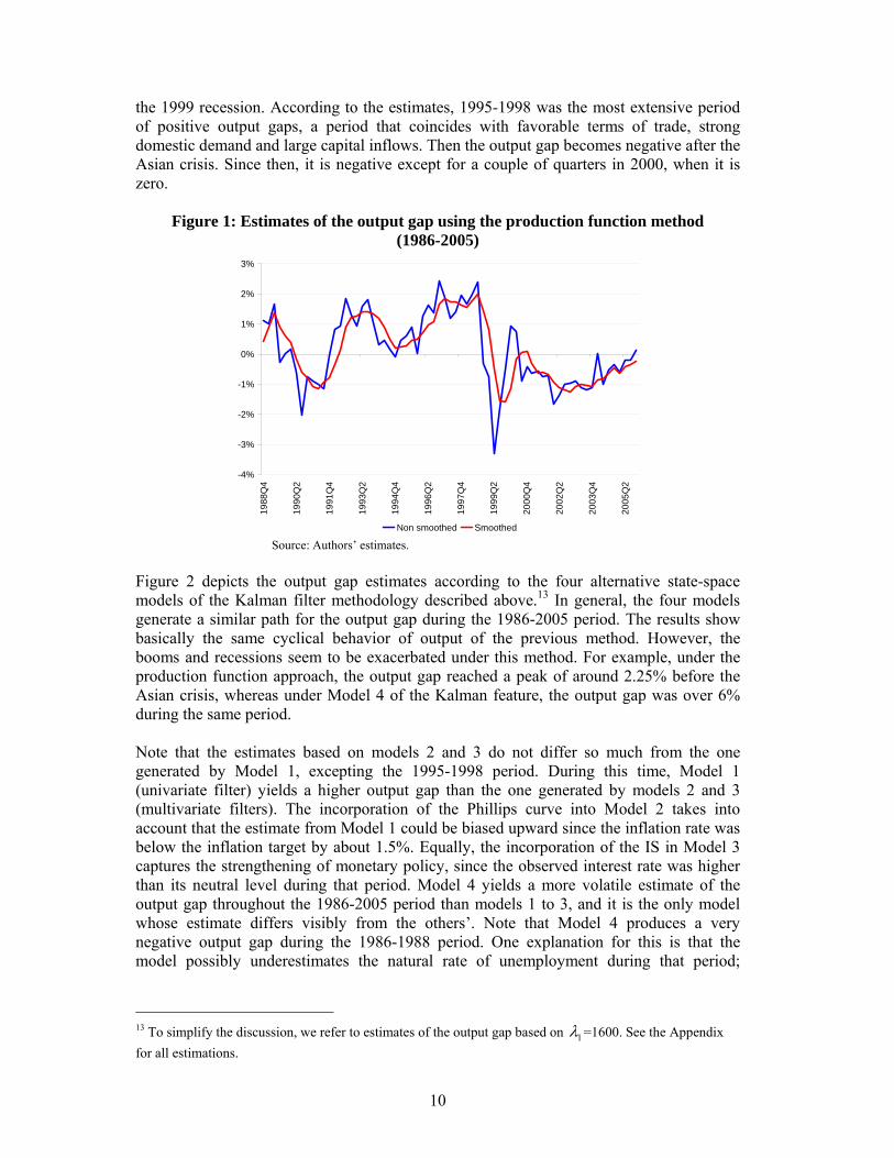
2.4 Analysis of the results We now present the estimation results using the methodologies described above. Here the result and simple comparisons across methods are conducted, postponing for the next section a more formal comparison of the different methods under alternative metrics. Figure 1 presents the evolution of the estimated gap in each quarter and also the gap series smoothed (moving average over four quarters) using the production function approach. The series are consistent in the sense that they capture the idea that in 1989 the economy was overheated and that in 1990-1991 there was a downturn. In the early nineties, the new commitment with inflation targeting and the accelerated growing process of the previous years led the Central Bank to tighten monetary policy to prevent inflation pressures. This strengthening of monetary policy led to a negative output gap during the early nineties. We can also observe that actual output was very close to potential output at the end of 1994, just as previous literature for Chile has reported (García and Contreras, 2002).12 Thereafter, estimates for the 1995-1998 period averaged a positive output gap, reaching its peak before
10 Using more than 10 quarters yields very similar results. 11 In the past, the Central Bank of Chile has used this date to handle the problem of the level of other economic variables. 12 Which is precisely the date used to calculate the level of the output gap with the SVAR methodology.
10
the 1999 recession. According to the estimates, 1995-1998 was the most extensive period of positive output gaps, a period that coincides with favorable terms of trade, strong domestic demand and large capital inflows. Then the output gap becomes negative after the Asian crisis. Since then, it is negative except for a couple of quarters in 2000, when it is zero.
Figure 1: Estimates of the output gap using the production function method (1986-2005)
-4%
-3%
-2%
-1%
0%
1%
2%
3%19
88Q
4
1990
Q2
1991
Q4
1993
Q2
1994
Q4
1996
Q2
1997
Q4
1999
Q2
2000
Q4
2002
Q2
2003
Q4
2005
Q2
Non smoothed Smoothed Source: Authors’ estimates.
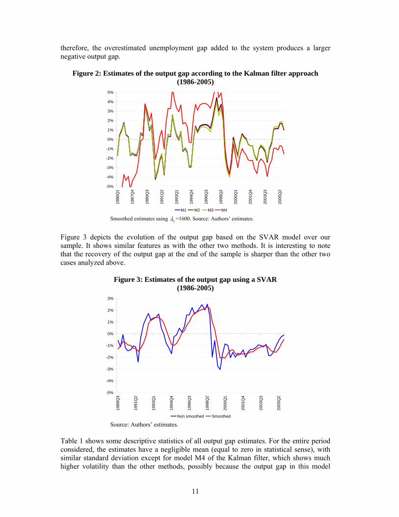
Figure 2 depicts the output gap estimates according to the four alternative state-space models of the Kalman filter methodology described above.13 In general, the four models generate a similar path for the output gap during the 1986-2005 period. The results show basically the same cyclical behavior of output of the previous method. However, the booms and recessions seem to be exacerbated under this method. For example, under the production function approach, the output gap reached a peak of around 2.25% before the Asian crisis, whereas under Model 4 of the Kalman feature, the output gap was over 6% during the same period. Note that the estimates based on models 2 and 3 do not differ so much from the one generated by Model 1, excepting the 1995-1998 period. During this time, Model 1 (univariate filter) yields a higher output gap than the one generated by models 2 and 3 (multivariate filters). The incorporation of the Phillips curve into Model 2 takes into account that the estimate from Model 1 could be biased upward since the inflation rate was below the inflation target by about 1.5%. Equally, the incorporation of the IS in Model 3 captures the strengthening of monetary policy, since the observed interest rate was higher than its neutral level during that period. Model 4 yields a more volatile estimate of the output gap throughout the 1986-2005 period than models 1 to 3, and it is the only model whose estimate differs visibly from the others’. Note that Model 4 produces a very negative output gap during the 1986-1988 period. One explanation for this is that the model possibly underestimates the natural rate of unemployment during that period;
13 To simplify the discussion, we refer to estimates of the output gap based on 1λ =1600. See the Appendix for all estimations.
11
therefore, the overestimated unemployment gap added to the system produces a larger negative output gap.
Figure 2: Estimates of the output gap according to the Kalman filter approach (1986-2005)
-5%
-4%
-3%
-2%
-1%
0%
1%
2%
3%
4%
5%
1986
Q1
1987
Q4
1989
Q3
1991
Q2
1993
Q1
1994
Q4
1996
Q3
1998
Q2
2000
Q1
2001
Q4
2003
Q3
2005
Q2
M1 M2 M3 M4 Smoothed estimates using 1λ =1600. Source: Authors’ estimates.
Figure 3 depicts the evolution of the output gap based on the SVAR model over our sample. It shows similar features as with the other two methods. It is interesting to note that the recovery of the output gap at the end of the sample is sharper than the other two cases analyzed above.
Figure 3: Estimates of the output gap using a SVAR (1986-2005)
-5%
-4%
-3%
-2%
-1%
0%
1%
2%
3%
1989
Q3
1991
Q2
1993
Q1
1994
Q4
1996
Q3
1998
Q2
2000
Q1
2001
Q4
2003
Q3
2005
Q2
Non smoothed Smoothed Source: Authors’ estimates.
Table 1 shows some descriptive statistics of all output gap estimates. For the entire period considered, the estimates have a negligible mean (equal to zero in statistical sense), with similar standard deviation except for model M4 of the Kalman filter, which shows much higher volatility than the other methods, possibly because the output gap in this model

12
follows more closely the labor market development (unemployment gap) than the rest of the methods, which show great volatility.
Table 1: Output gap estimates, descriptive statistics
Method Mean St. dev. Production function 0.14% 1.0% Kalman filter M1 -0.02% 1.8% M2 -0.09% 1.8% M3 -0.11% 1.8% M4 -0.13% 3.2% SVAR -0.39% 1.3% Source: Authors' estimations.
These similarities can be appreciated in figure 4 that shows the gap estimated with the production function approach, Kalman filter models M3 and M414, and Structural VAR. Just like the table reports, we can observe that the mean among methods is similar, but volatility is quite different. Apparently, the four measures move together but with differences in levels.
Figure 4: Output gap estimates, alternative methods
-6%
-4%
-2%
0%
2%
4%
6%
1986
Q1
1987
Q4
1989
Q3
1991
Q2
1993
Q1
1994
Q4
1996
Q3
1998
Q2
2000
Q1
2001
Q4
2003
Q3
2005
Q2
M3 M4 PF SVAR Smoothed estimates. For models M3 and M4, 1λ =1600. Source: Authors’ estimates.
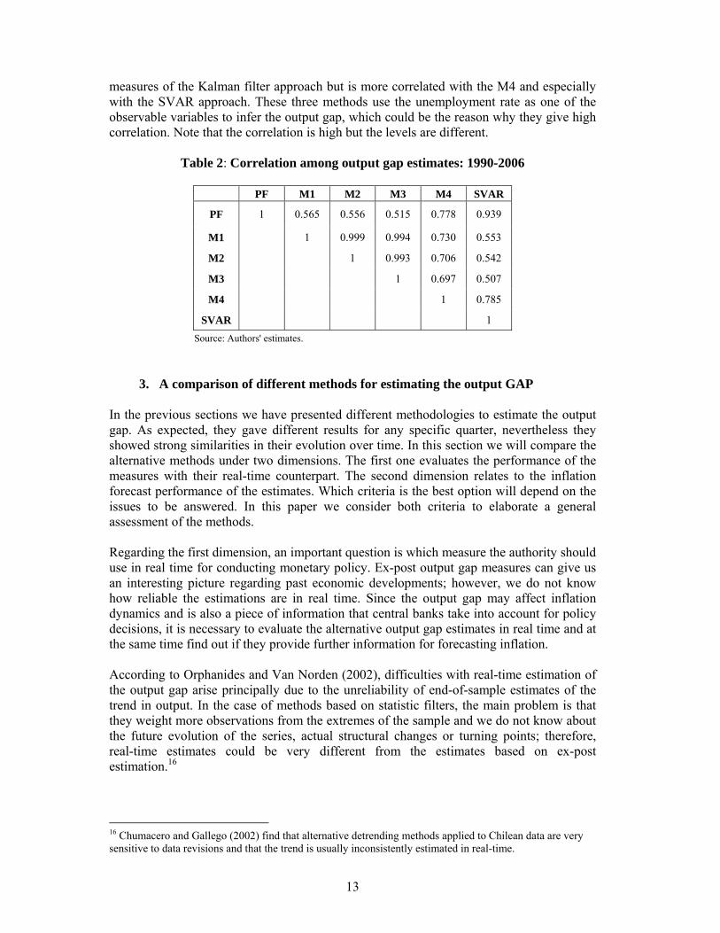
The correlation across the four measures selected is presented in table 2. As expected, M1, M2 and M3 show the highest correlation.15 M4 tends to be more highly correlated with the SVAR model than the other three measures obtained from the Kalman filter estimation. The production function estimate is relatively poorly correlated with the first three 14 M1 and M2 yield similar results as M3. Moreover, the latter encompasses the first two, so we report only M3. M4 yields a different result and it is reported as another measure. 15 It seems that both the Phillips and the IS curves do not provide so much more information than the univariate case. Orphanides and Van Norden (2002), find that using inflation measures to estimate the output gap could not improve the results, especially in real-time estimation.
13
measures of the Kalman filter approach but is more correlated with the M4 and especially with the SVAR approach. These three methods use the unemployment rate as one of the observable variables to infer the output gap, which could be the reason why they give high correlation. Note that the correlation is high but the levels are different.
Table 2: Correlation among output gap estimates: 1990-2006
PF M1 M2 M3 M4 SVAR
PF 1 0.565 0.556 0.515 0.778 0.939
M1 1 0.999 0.994 0.730 0.553
M2 1 0.993 0.706 0.542
M3 1 0.697 0.507
M4 1 0.785
SVAR 1 Source: Authors' estimates.
3. A comparison of different methods for estimating the output GAP In the previous sections we have presented different methodologies to estimate the output gap. As expected, they gave different results for any specific quarter, nevertheless they showed strong similarities in their evolution over time. In this section we will compare the alternative methods under two dimensions. The first one evaluates the performance of the measures with their real-time counterpart. The second dimension relates to the inflation forecast performance of the estimates. Which criteria is the best option will depend on the issues to be answered. In this paper we consider both criteria to elaborate a general assessment of the methods. Regarding the first dimension, an important question is which measure the authority should use in real time for conducting monetary policy. Ex-post output gap measures can give us an interesting picture regarding past economic developments; however, we do not know how reliable the estimations are in real time. Since the output gap may affect inflation dynamics and is also a piece of information that central banks take into account for policy decisions, it is necessary to evaluate the alternative output gap estimates in real time and at the same time find out if they provide further information for forecasting inflation. According to Orphanides and Van Norden (2002), difficulties with real-time estimation of the output gap arise principally due to the unreliability of end-of-sample estimates of the trend in output. In the case of methods based on statistic filters, the main problem is that they weight more observations from the extremes of the sample and we do not know about the future evolution of the series, actual structural changes or turning points; therefore, real-time estimates could be very different from the estimates based on ex-post estimation.16
16 Chumacero and Gallego (2002) find that alternative detrending methods applied to Chilean data are very sensitive to data revisions and that the trend is usually inconsistently estimated in real-time.
14
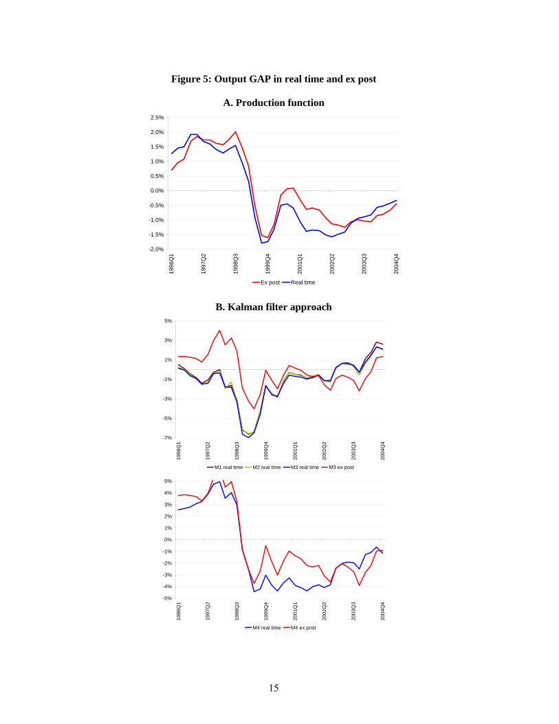
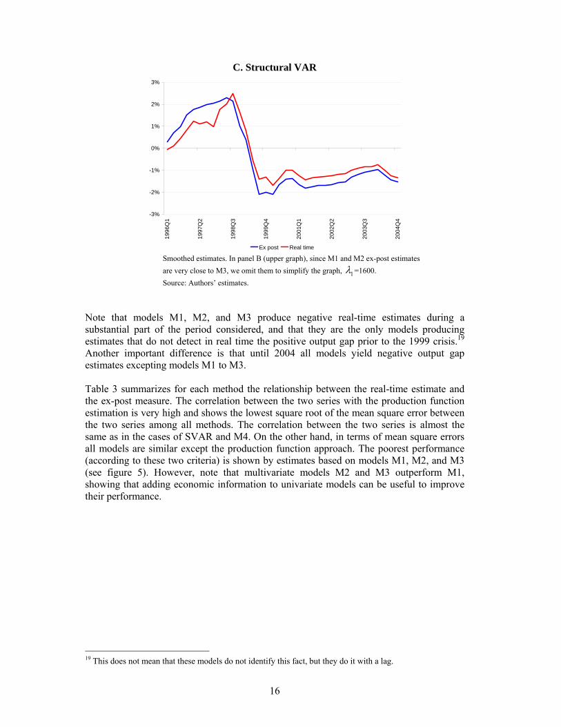
Another difficulty arises from seasonality and posterior data revisions. There are different methods to deal with seasonality in series of high frequency, but real-time seasonal adjustment also differs from ex-post adjustments. On the other hand, since information about production arrives with lags, the GDP series is continuously revised, making the estimation of the output gap more complex. In this study we do not consider these two aspects, leaving them as potential issues to explore deeply in future research.17 In this sense, we will be conducting our real-time exercise as quasi real time since we will be working with the information available at each moment of time, but the figures used are those already revised. To evaluate the real-time performance of the output gap measures presented we assess the correlation and the root mean squared errors (RMSE) between ex-post and real-time estimates. The exercise will be carried out for the 1996-2004 sample. We start in 1996, because we must consider a minimum number of observations to obtain reliable estimates of the real-time regression at the beginning of the exercise. We eliminate the final year (2005) since ex-post and real-time estimates are very similar by construction at the end of the sample. Figure 5 compares output gap estimates using real-time and ex-post data. Estimates based on the production function model (panel A) show strong correlation and real-time estimates follow closely the evolution of ex-post estimates.18 Estimates based on the Kalman filter approach (panel B) show different performances depending on the specification used. Models 1 to 3 yield similar real-time output gap estimates and these differ substantially from ex-post estimates. Real-time estimates from Model 4 show higher correlation with ex-post estimates and they are also quite close in levels. Real-time and ex-post estimates based on a SVAR model (panel C) show strong correlation too. However, the real-time measure is more than one percent above the level of the ex-post measure during the 1999-2004 period.
17 According to Orphanides and Van Norden (2002), revisions in published data are not the principal source of revisions in output gap estimates but the unreliability of potential output estimates. 18 Regarding performance, output gap estimates based on the production function approach have the advantage that the parameters of the production function used in the estimation are fixed (ex-post), whereas for the other models the parameters are estimated recursively, incorporating more uncertainty to real-time estimates. In the production function approach we use a real time data for the natural rate of unemployment estimated in model 4 by the Kalman Filter.
15
Figure 5: Output GAP in real time and ex post
A. Production function
-2.0%
-1.5%
-1.0%
-0.5%
0.0%
0.5%
1.0%
1.5%
2.0%
2.5%
1996
Q1
1997
Q2
1998
Q3
1999
Q4
2001
Q1
2002
Q2
2003
Q3
2004
Q4
Ex post Real time
B. Kalman filter approach
-7%
-5%
-3%
-1%
1%
3%
5%
1996
Q1
1997
Q2
1998
Q3
1999
Q4
2001
Q1
2002
Q2
2003
Q3
2004
Q4
M1 real time M2 real time M3 real time M3 ex post
-5%
-4%
-3%
-2%
-1%
0%
1%
2%
3%
4%
5%
1996
Q1
1997
Q2
1998
Q3
1999
Q4
2001
Q1
2002
Q2
2003
Q3
2004
Q4
M4 real time M4 ex post
16
C. Structural VAR
-3%
-2%
-1%
0%
1%
2%
3%
1996
Q1
1997
Q2
1998
Q3
1999
Q4
2001
Q1
2002
Q2
2003
Q3
2004
Q4
Ex post Real time Smoothed estimates. In panel B (upper graph), since M1 and M2 ex-post estimates are very close to M3, we omit them to simplify the graph, 1λ =1600. Source: Authors’ estimates.
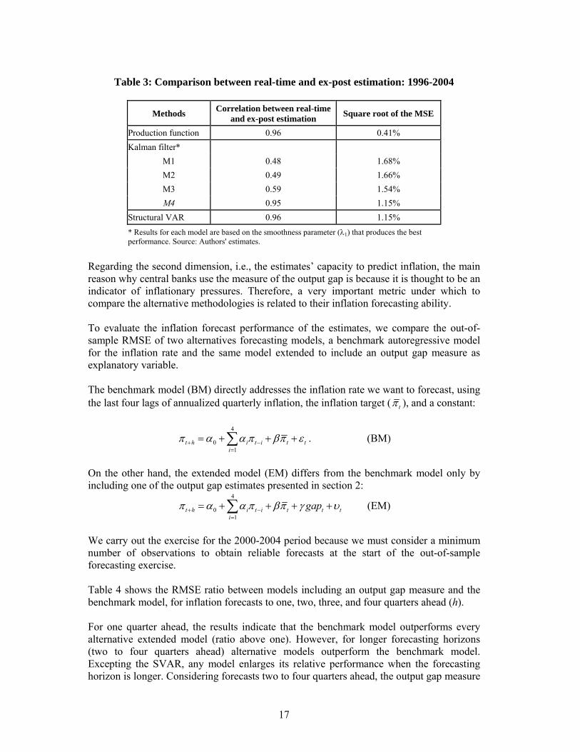
Note that models M1, M2, and M3 produce negative real-time estimates during a substantial part of the period considered, and that they are the only models producing estimates that do not detect in real time the positive output gap prior to the 1999 crisis.19 Another important difference is that until 2004 all models yield negative output gap estimates excepting models M1 to M3. Table 3 summarizes for each method the relationship between the real-time estimate and the ex-post measure. The correlation between the two series with the production function estimation is very high and shows the lowest square root of the mean square error between the two series among all methods. The correlation between the two series is almost the same as in the cases of SVAR and M4. On the other hand, in terms of mean square errors all models are similar except the production function approach. The poorest performance (according to these two criteria) is shown by estimates based on models M1, M2, and M3 (see figure 5). However, note that multivariate models M2 and M3 outperform M1, showing that adding economic information to univariate models can be useful to improve their performance.
19 This does not mean that these models do not identify this fact, but they do it with a lag.
17
Table 3: Comparison between real-time and ex-post estimation: 1996-2004
Methods Correlation between real-time and ex-post estimation Square root of the MSE
Production function 0.96 0.41% Kalman filter*
M1 0.48 1.68% M2 0.49 1.66% M3 0.59 1.54% M4 0.95 1.15%
Structural VAR 0.96 1.15% * Results for each model are based on the smoothness parameter (λ1) that produces the best performance. Source: Authors' estimates.
Regarding the second dimension, i.e., the estimates’ capacity to predict inflation, the main reason why central banks use the measure of the output gap is because it is thought to be an indicator of inflationary pressures. Therefore, a very important metric under which to compare the alternative methodologies is related to their inflation forecasting ability. To evaluate the inflation forecast performance of the estimates, we compare the out-of-sample RMSE of two alternatives forecasting models, a benchmark autoregressive model for the inflation rate and the same model extended to include an output gap measure as explanatory variable. The benchmark model (BM) directly addresses the inflation rate we want to forecast, using the last four lags of annualized quarterly inflation, the inflation target ( tπ ), and a constant:
4
01
t h i t i t ti
π α α π βπ ε+ −=
= + + +∑ . (BM)
On the other hand, the extended model (EM) differs from the benchmark model only by including one of the output gap estimates presented in section 2:
4
01
t h i t i t t ti
gapπ α α π βπ γ υ+ −=
= + + + +∑ (EM)
We carry out the exercise for the 2000-2004 period because we must consider a minimum number of observations to obtain reliable forecasts at the start of the out-of-sample forecasting exercise. Table 4 shows the RMSE ratio between models including an output gap measure and the benchmark model, for inflation forecasts to one, two, three, and four quarters ahead (h). For one quarter ahead, the results indicate that the benchmark model outperforms every alternative extended model (ratio above one). However, for longer forecasting horizons (two to four quarters ahead) alternative models outperform the benchmark model. Excepting the SVAR, any model enlarges its relative performance when the forecasting horizon is longer. Considering forecasts two to four quarters ahead, the output gap measure
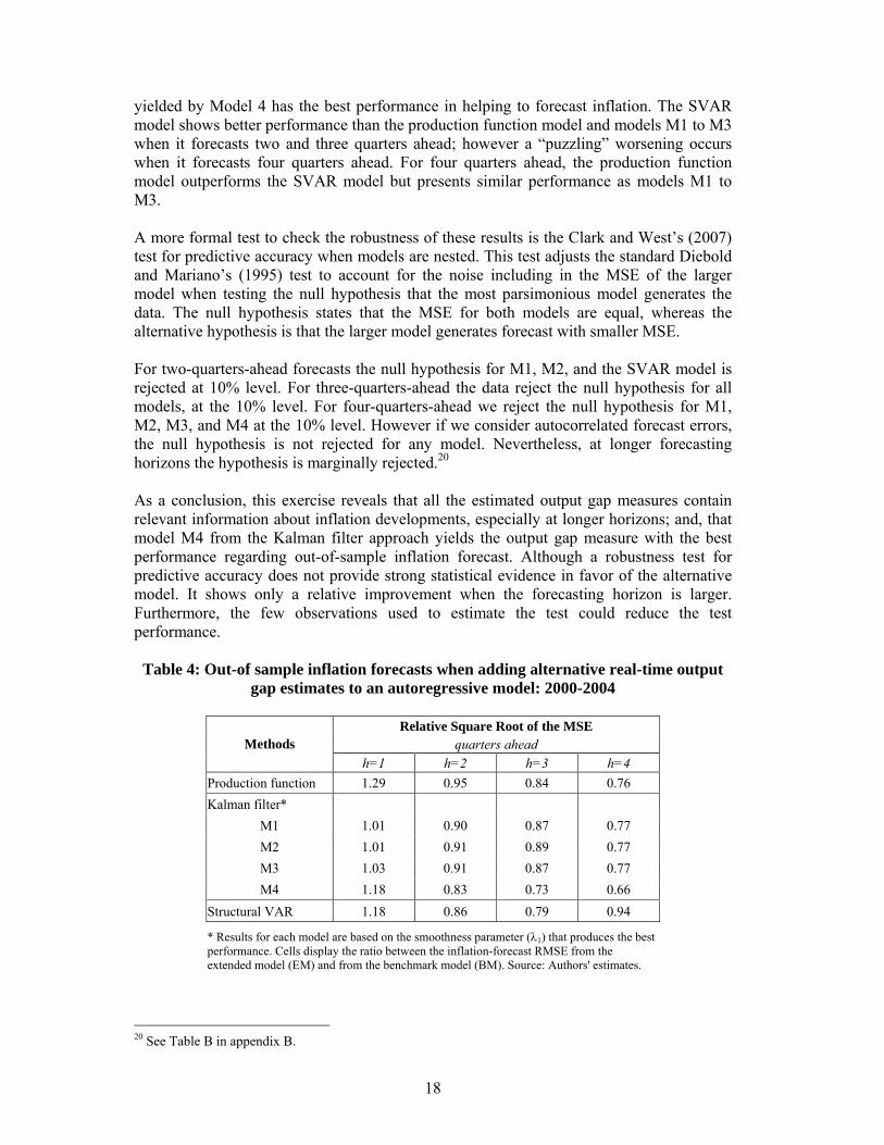
18
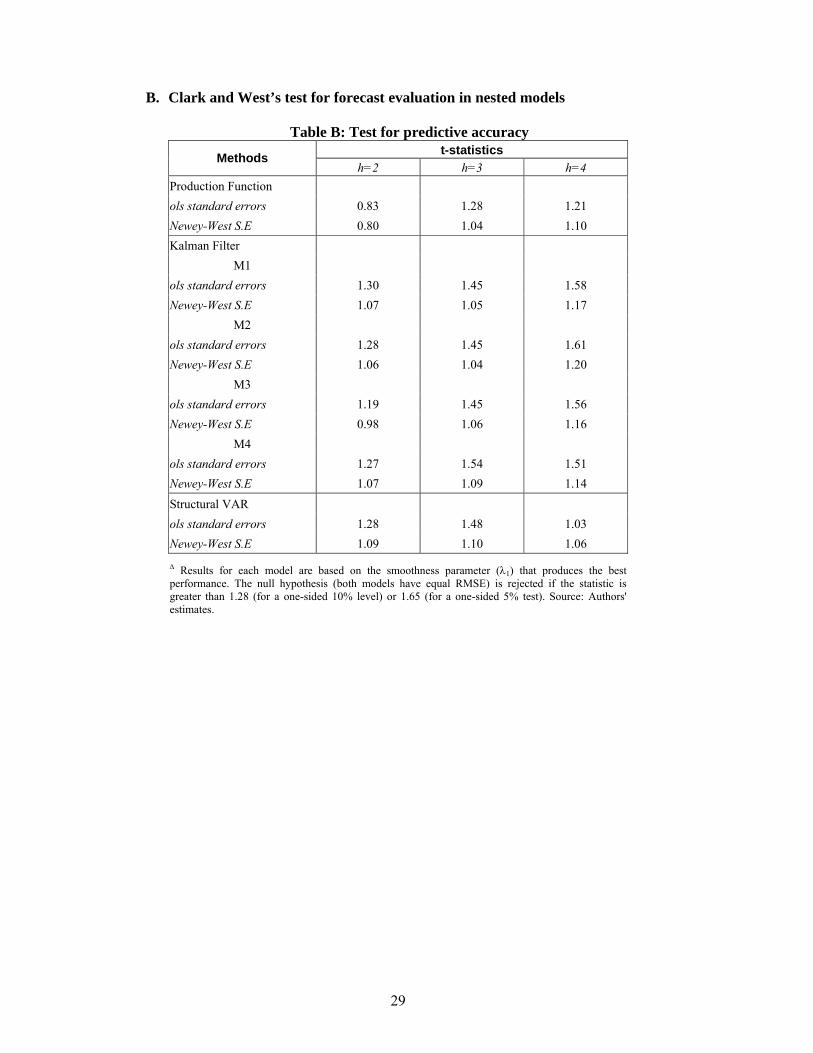
yielded by Model 4 has the best performance in helping to forecast inflation. The SVAR model shows better performance than the production function model and models M1 to M3 when it forecasts two and three quarters ahead; however a “puzzling” worsening occurs when it forecasts four quarters ahead. For four quarters ahead, the production function model outperforms the SVAR model but presents similar performance as models M1 to M3. A more formal test to check the robustness of these results is the Clark and West’s (2007) test for predictive accuracy when models are nested. This test adjusts the standard Diebold and Mariano’s (1995) test to account for the noise including in the MSE of the larger model when testing the null hypothesis that the most parsimonious model generates the data. The null hypothesis states that the MSE for both models are equal, whereas the alternative hypothesis is that the larger model generates forecast with smaller MSE. For two-quarters-ahead forecasts the null hypothesis for M1, M2, and the SVAR model is rejected at 10% level. For three-quarters-ahead the data reject the null hypothesis for all models, at the 10% level. For four-quarters-ahead we reject the null hypothesis for M1, M2, M3, and M4 at the 10% level. However if we consider autocorrelated forecast errors, the null hypothesis is not rejected for any model. Nevertheless, at longer forecasting horizons the hypothesis is marginally rejected.20 As a conclusion, this exercise reveals that all the estimated output gap measures contain relevant information about inflation developments, especially at longer horizons; and, that model M4 from the Kalman filter approach yields the output gap measure with the best performance regarding out-of-sample inflation forecast. Although a robustness test for predictive accuracy does not provide strong statistical evidence in favor of the alternative model. It shows only a relative improvement when the forecasting horizon is larger. Furthermore, the few observations used to estimate the test could reduce the test performance.
Table 4: Out-of sample inflation forecasts when adding alternative real-time output gap estimates to an autoregressive model: 2000-2004
Relative Square Root of the MSE
quarters ahead Methods h=1 h=2 h=3 h=4
Production function 1.29 0.95 0.84 0.76 Kalman filter*
M1 1.01 0.90 0.87 0.77 M2 1.01 0.91 0.89 0.77 M3 1.03 0.91 0.87 0.77 M4 1.18 0.83 0.73 0.66
Structural VAR 1.18 0.86 0.79 0.94
* Results for each model are based on the smoothness parameter (λ1) that produces the best performance. Cells display the ratio between the inflation-forecast RMSE from the extended model (EM) and from the benchmark model (BM). Source: Authors' estimates.
20 See Table B in appendix B.

19
4. The growth rate of potential output
In this section we will answer a different question, which is the growth rate of potential output. From the output gap estimated in the previous sections is possible to estimate the growth rate of potential output. Additionally we use a different methodology to estimate a growth rate of output in steady state. In this case we move to a different paradigm since we would like to estimate a long run growth rate. In what follows we will use the gaps estimated in previous sections to calculate the growth rate of potential output. Later we will use a neoclassical growth model approach to estimate the growth rate of output in steady state. The difference between the measure here and the previous estimation of the growth rate of potential output is the underlying conceptual framework. In this section we use a stylized growth model to estimate the implied growth rate in steady state, while the models used before are more related to the decomposition of output series between a cyclical and a trend component. None of them make any assumption about a long term steady state growth rate; they rather concentrate in the estimation of output gap using semi structural macro models.
4.1 The growth rate of potential output Potential output is the sum of the actual output and the output gap. Given the output gaps for the different methodologies computed in the previous section, we can obtain alternative measures of the potential output, and therefore measures of a time-varying potential output growth rate. Table 5 summarizes the average potential growth rate for each method for our entire sample and different periods. For the complete sample (1987-2005) the average potential growth rate varies from 5.4% to 5.9% depending on the method used. The lowest figure comes from the SVAR method, while the highest figure from the Kalman filter M3 model.
Table 5: Growth rate of potential output: 1987-2005
Methods 1987-1989 1990-1994 1995-1999 2000-2005 1987-2005** Production function - 7.32% 5.74% 4.02% 5.87% Kalman filter*
M1 7.56% 8.07% 5.36% 3.64% 5.86% M2 7.65% 8.04% 5.35% 3.65% 5.87% M3 7.58% 8.05% 5.36% 3.66% 5.87% M4 5.18% 7.56% 5.96% 4.02% 5.64%
Structural VAR - 7.38% 5.71% 3.62% 5.44% * Results for each model are based on the smoothness parameter (λ1) that produces the best performance. ** 1990-2005 for Production Function and SVAR methods. Source: Authors' estimates.
20
The results also show that the average potential growth rate varies across the sub-periods analyzed. For example, the sub-period with the highest average potential growth rate is 1990-1994, with the growth rate ranging from 7.3% to 8.1%. These years correspond to the middle period of what has been termed the “golden” period of growth in Chile (1986-1997).21 At the other end, the sub-period with the lowest average growth rate is 2000-2005. During these years, the potential growth rate varied from 3.6% to 4.0% according to different methods. These results suggest that there seems to be a structural change that lowered the potential output growth after the Asian Crisis. In summary, the data shows different regimes of growth, and to evaluate what is the future growth rate of potential output it is necessary to make an assessment of what regime will prevail in the future.
4.2 The growth rate of the trended output using production function This section uses the contributions of Solow (1956, 1957) to compute a steady-state growth rate of output. The long term growth rate of output will depend on the growth rate of each productive factor plus the growth rate of total factor productivity. Using quarterly data from 1986 to 2005, we decompose the growth rate using the traditional growth accounting methodology: ˆ ˆ ˆ ˆ(1 )Y K L TFPα α− − − = , (23)
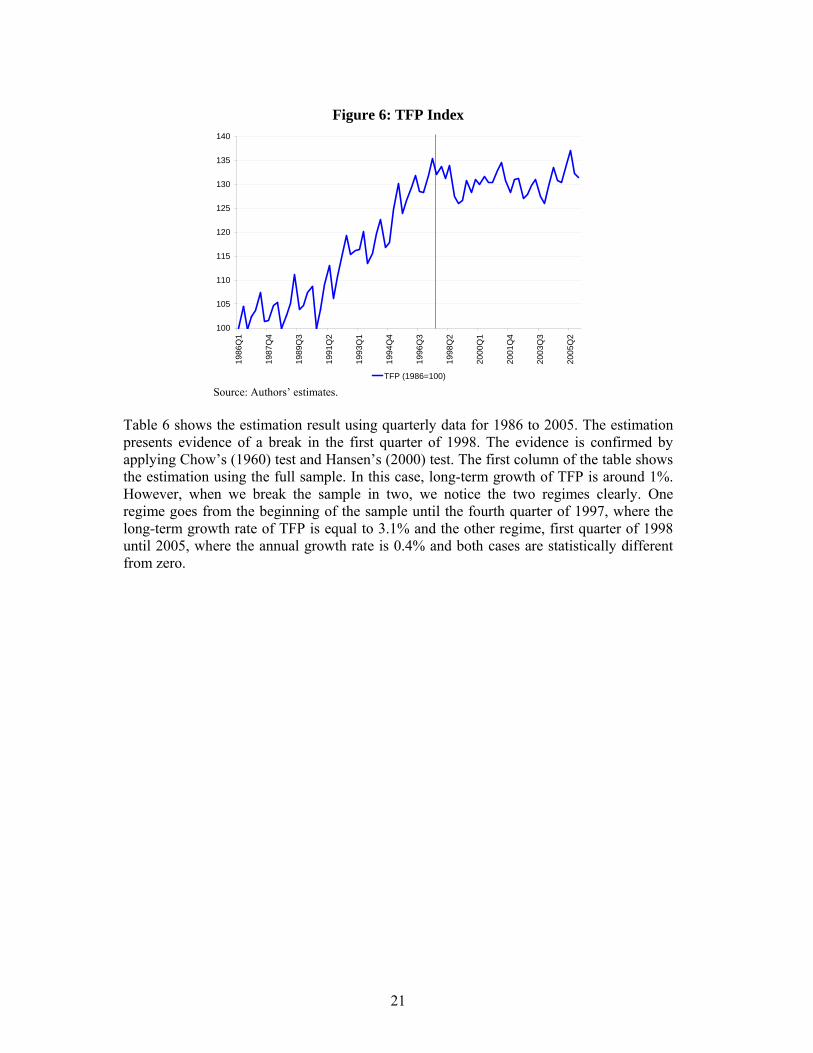
where the hat over each variable denotes growth rate, K is corrected by capacity utilization (using energy consumption) and L is corrected by years of schooling. As before, the capital–output elasticity is estimated equal to 0.4. Using the estimated growth rate of total output, we build an index of TFP that is shown in figure 6. The figure shows the “golden” years of the Chilean growth period, 1986-1997, but starting in 1998 TFP flattens showing a very low growth rate. It seems that, starting in 1998, TFP had a structural break. To find the long-run growth rate, a simple econometric model is estimated. Given that there is evidence that TFP is trend stationary, we estimate:
0 1 1ln lnt t i t tTFP t TFP Dβ β γ δ ε−= + + + +∑ , where Dit presents dummy variables to control for seasonality in TFP, t is the time trend and ε represents the stochastic disturbance. The parameter 1 /(1 )β γ− represents the long run growth rate of TFP and is our parameter of interest.
21 See Gallego and Loayza (2003).
21
Figure 6: TFP Index
100
105
110
115
120
125
130
135
140
1986
Q1
1987
Q4
1989
Q3
1991
Q2
1993
Q1
1994
Q4
1996
Q3
1998
Q2
2000
Q1
2001
Q4
2003
Q3
2005
Q2
TFP (1986=100) Source: Authors’ estimates.
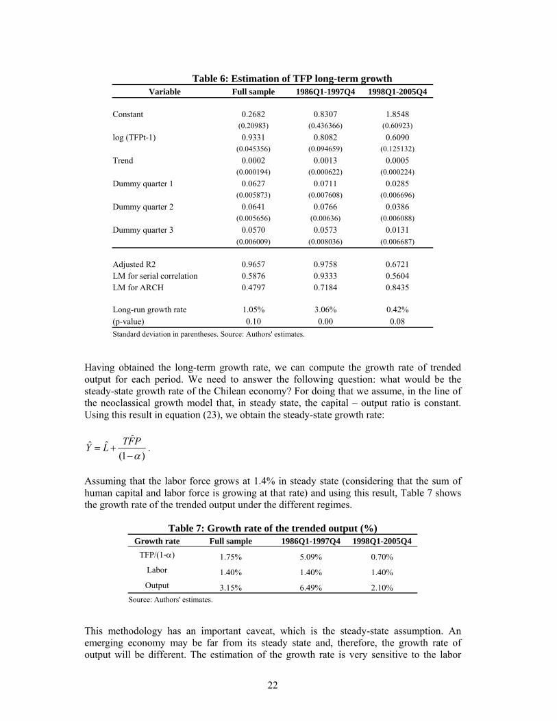
Table 6 shows the estimation result using quarterly data for 1986 to 2005. The estimation presents evidence of a break in the first quarter of 1998. The evidence is confirmed by applying Chow’s (1960) test and Hansen’s (2000) test. The first column of the table shows the estimation using the full sample. In this case, long-term growth of TFP is around 1%. However, when we break the sample in two, we notice the two regimes clearly. One regime goes from the beginning of the sample until the fourth quarter of 1997, where the long-term growth rate of TFP is equal to 3.1% and the other regime, first quarter of 1998 until 2005, where the annual growth rate is 0.4% and both cases are statistically different from zero.
22
Table 6: Estimation of TFP long-term growth
Variable Full sample 1986Q1-1997Q4 1998Q1-2005Q4 Constant 0.2682 0.8307 1.8548 (0.20983) (0.436366) (0.60923) log (TFPt-1) 0.9331 0.8082 0.6090 (0.045356) (0.094659) (0.125132) Trend 0.0002 0.0013 0.0005 (0.000194) (0.000622) (0.000224) Dummy quarter 1 0.0627 0.0711 0.0285 (0.005873) (0.007608) (0.006696) Dummy quarter 2 0.0641 0.0766 0.0386 (0.005656) (0.00636) (0.006088) Dummy quarter 3 0.0570 0.0573 0.0131 (0.006009) (0.008036) (0.006687) Adjusted R2 0.9657 0.9758 0.6721 LM for serial correlation 0.5876 0.9333 0.5604 LM for ARCH 0.4797 0.7184 0.8435 Long-run growth rate 1.05% 3.06% 0.42% (p-value) 0.10 0.00 0.08 Standard deviation in parentheses. Source: Authors' estimates.
Having obtained the long-term growth rate, we can compute the growth rate of trended output for each period. We need to answer the following question: what would be the steady-state growth rate of the Chilean economy? For doing that we assume, in the line of the neoclassical growth model that, in steady state, the capital – output ratio is constant. Using this result in equation (23), we obtain the steady-state growth rate:
ˆˆ ˆ(1 )TFPY L
α= +
−.
Assuming that the labor force grows at 1.4% in steady state (considering that the sum of human capital and labor force is growing at that rate) and using this result, Table 7 shows the growth rate of the trended output under the different regimes.
Table 7: Growth rate of the trended output (%) Growth rate Full sample 1986Q1-1997Q4 1998Q1-2005Q4
TFP/(1-α) 1.75% 5.09% 0.70% Labor 1.40% 1.40% 1.40% Output 3.15% 6.49% 2.10%
Source: Authors' estimates.
This methodology has an important caveat, which is the steady-state assumption. An emerging economy may be far from its steady state and, therefore, the growth rate of output will be different. The estimation of the growth rate is very sensitive to the labor

23
force participation and the growth rate of human capital, which could be higher in steady state. Moreover, it seems that the Chilean economy was converging to a different steady state before 1998. One wonders what explains these two different steady states and how the Chilean economy can go back to is old track. These questions remain unsolved.
5. Summary and conclusions The output gap, defined as actual minus potential output, is an important variable for economic policy decision-making. Given the important role that central banks assign to the output gap in forecasting inflation, knowledge of this variable will be central in the conduct of monetary policy. The output gap, however, is not directly observable and therefore obtaining an accurate measure presents an important challenge to the monetary authority in assessing the extent of inflationary pressures in the economy. Similarly, the growth rate of potential output is also an important variable for policy making. This paper has presented estimates of the output gap and potential output growth for Chile during the 1986-2005 period according to three different methods: (i) production function approach, (ii) Kalman filter and (iii) Structural VAR. Several measures were examined due to the uncertainty associated with measuring potential output. A high degree of consistency was found among all measures in terms of the sign of the output gap. According to all methods, economic overheating is observed at the beginning of the sample; from 1993 until the Asian Crisis the gap is not very large but is always positive, after the Asian Crisis the gap turns negative and stays there for several quarters. In order to compare the output gaps generated under the different methodologies, we evaluate the real-time performance of the output gap measures and measure how well the output gap can help forecast future inflation. According to the results, the production function approach seems to outperform the other measures in terms of real-time accuracy. The real-time and ex-post output gap measures present the highest correlation, and the difference between both series present the lowest square root of the MSE. Regarding the predictive power of the output gap with respect to future inflation, Model 4 from the Kalman filter approach (Phillips curve and Okun’s law) yields the output gap measure with the best performance regarding out-of-sample inflation forecast. The estimates of potential output growth according to the different measures are also broadly similar. Over the complete sample, the average potential growth rate ranged from 5.4% to 5.9%. However, there seems to be important differences across sub-periods. For example, during 1990-1994 the potential growth rate was in the range of 7.3%-8.1%, and after the Asian Crisis it fell to the range of 3.6%-4.0%, suggesting a negative structural change in the potential growth rate after 1998. Finally, the steady-state growth rate of the trended output for the entire sample is somewhat above 3%, and also presents an important structural break after the Asian Crisis. What regime will be present in the years to come is the key question to asses the future growth performance of the Chilean economy.
24
References
Blanchard, O. and D. Quah (1989). “The Dynamic Effects of Aggregate Supply and Demand Disturbances,” American Economic Review 79, 655-673. Apel M. and P. Jansson (1999). “System Estimates of Potential Output and the NAIRU,” EmpiricalEconomics 24: 373-338. Chow, G. (1960). “Tests of Equality Between Sets of Coefficients in Two Linear Regressions,” Econometrica, 28: 591-605. Chumacero, R. and F. Gallego (2002). “Trends and Cycles in Real-Time,” Estudios de Economía, Vol. 29, N°2. Clark, T.E. and K.D. West (2007). “Approximately Normal Tests for Equal Predictive Accuracy in Nested Models,” Journal of Econometrics 138, 291–311. Contreras, G. and P. García (2002). “Estimating Gaps and Trends for the Chilean Economy,” in N. Loayza and R. Soto (editors) Economic Growth: Sources, Trends and Cycles, Central Bank of Chile, Santiago. De Masi, P. (1997). “IMF Estimates of Potential Output: Theory and Practice,” IMF Working Paper 97/177. Diebold, F.X. and R.S. Mariano (1995). “Comparing predictive accuracy,” Journal of Business and Economic Statistics 13, 253–263. Gallego, F. and C. Johnson (2001). “Teorías y Métodos de Medición del Producto de Tendencia : Una Aplicación al Caso de Chile,” Revista Economía Chilena, Vol. 4, N°2. Gallego, F. and N. Loayza (2003). “The Golden Period for Growth in Chile: Explanations and Forecasts,” in N. Loayza and R. Soto (editors) Economic Growth: Sources, Trends and Cycles, Central Bank of Chile, Santiago. Graff, M. (2004). “Estimates of the Output Gap in Real Time: How Well Have We Been Doing?” Discussion Paper Series DP2004/04, Reserve Bank of New Zealand. Gollin, D., (2002). “Getting income shares right.” Journal of Political Economy 110, 458– 474. Hamilton, J. D. (1994). Time Series Analysis, Princeton University Press. Hansen, B. (2000). “Sample Splitting and Threshold Estimation,” Econometrica 68(3): 575-603. Harvey, A. C. (1989). Forecasting, Structural Time Series Models and the Kalman Filter, Cambridge University Press.
25
Kuttner, K. N. (1994). “Estimating Potential Output as a Latent Variable,” Journal of Business and Economic Statistics, 12(3), 361-368. Laubach, T. and J. C. Williams (2003). “Measuring the Natural Rate of Interest,” The Review of Economics and Statistics, 85(4), 1063-1070. Menashe, Y. and Y. Yakhin (2004). “Mind the Gap: Structural and Nonstructural Approaches to Estimating Israel’s Output Gap,” Israel Economic Review 2(2):79-106. Musso, A. and T. Westermann (2005). “Assessing Potential Output Growth in the Euro Area: A Growth Accounting Perspective,” Occasional Papers Series 22, European Central Bank. Ogunc F. and D. Ece (2004). “Estimating the Output Gap for Turkey: an Unobserved Components Approach,” Applied Economic Letters, 11, 177-182. Orphanides A. and S. Van Norden (2002). “The Unreliability of Output-Gap Estimates in Real Time,” The Review of Economics and Statistics 84(4), 569-583. Solow, R. (1956). “A Contribution to the Theory of Economic Growth,” Quarterly Journal of Economics, Vol. 70. Solow, R. (1957). “Technological Change and the Aggregate Production Function,” The Review of Economics and Statistics, Vol. 39. Taylor, J. B. (1993). “Discretion versus Policy Rules in Practice,” Carnegie-Rochester Conference Series on Public Policy 39, 195-214. Willman, A. (2002). “Euro Area Production Function and Potential Output: A Supply Side System Approach,” Working Paper Series 153, European Central Bank.
26
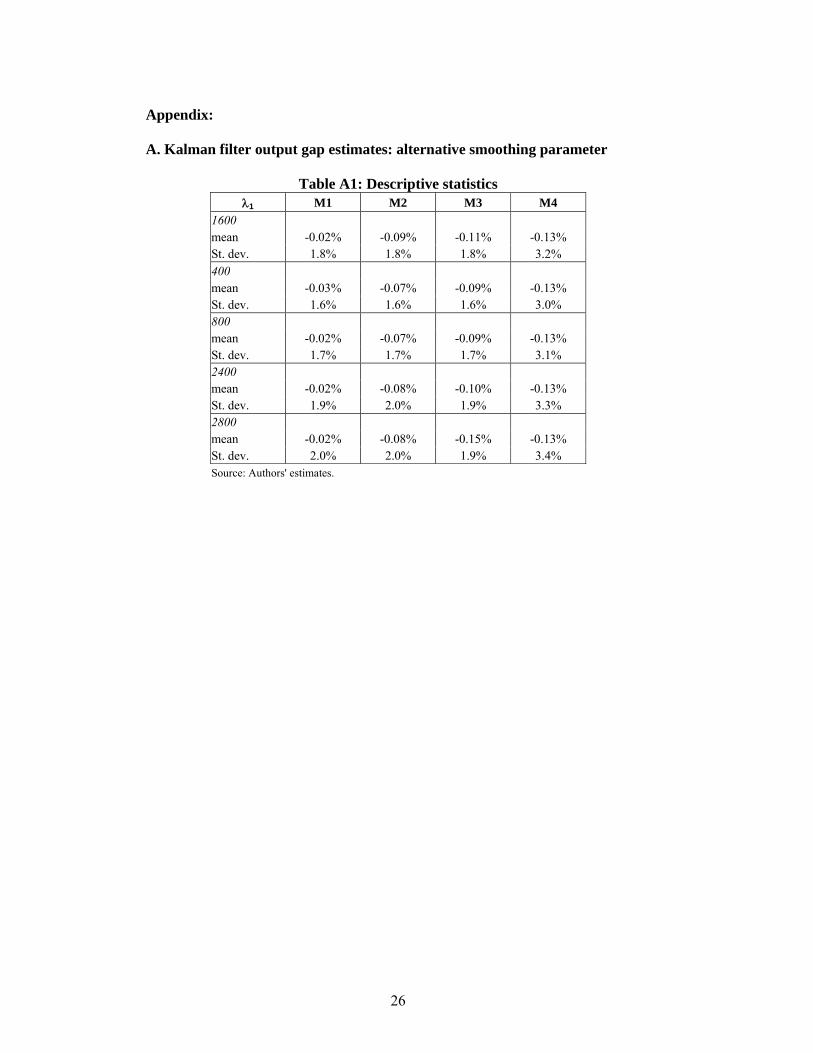
Appendix: A. Kalman filter output gap estimates: alternative smoothing parameter
Table A1: Descriptive statistics
λ1 M1 M2 M3 M4 1600 mean -0.02% -0.09% -0.11% -0.13% St. dev. 1.8% 1.8% 1.8% 3.2% 400 mean -0.03% -0.07% -0.09% -0.13% St. dev. 1.6% 1.6% 1.6% 3.0% 800 mean -0.02% -0.07% -0.09% -0.13% St. dev. 1.7% 1.7% 1.7% 3.1% 2400 mean -0.02% -0.08% -0.10% -0.13% St. dev. 1.9% 2.0% 1.9% 3.3% 2800 mean -0.02% -0.08% -0.15% -0.13% St. dev. 2.0% 2.0% 1.9% 3.4% Source: Authors' estimates.
27
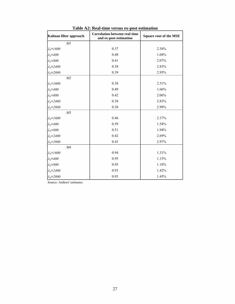
Table A2: Real-time versus ex-post estimation
Kalman filter approach Correlation between real time and ex-post estimation Square root of the MSE
M1 λ1=1600 0.37 2.54%
λ1=400 0.48 1.68%
λ1=800 0.41 2.07%
λ1=2400 0.38 2.83%
λ1=2800 0.39 2.95% M2
λ1=1600 0.38 2.51%
λ1=400 0.49 1.66%
λ1=800 0.42 2.06%
λ1=2400 0.38 2.83%
λ1=2800 0.38 2.98% M3
λ1=1600 0.46 2.37%
λ1=400 0.59 1.54%
λ1=800 0.51 1.94%
λ1=2400 0.42 2.69%
λ1=2800 0.43 2.97% M4
λ1=1600 0.94 1.31%
λ1=400 0.95 1.15%
λ1=800 0.95 1.18%
λ1=2400 0.93 1.42%
λ1=2800 0.93 1.45% Source: Authors' estimates.
28
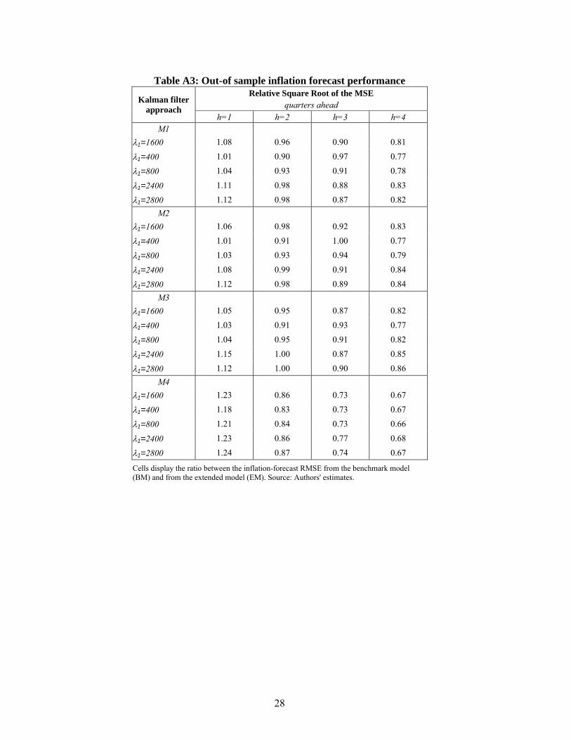
Table A3: Out-of sample inflation forecast performance
Relative Square Root of the MSE quarters ahead Kalman filter
approach h=1 h=2 h=3 h=4
M1 λ1=1600 1.08 0.96 0.90 0.81
λ1=400 1.01 0.90 0.97 0.77
λ1=800 1.04 0.93 0.91 0.78
λ1=2400 1.11 0.98 0.88 0.83
λ1=2800 1.12 0.98 0.87 0.82 M2
λ1=1600 1.06 0.98 0.92 0.83
λ1=400 1.01 0.91 1.00 0.77
λ1=800 1.03 0.93 0.94 0.79
λ1=2400 1.08 0.99 0.91 0.84
λ1=2800 1.12 0.98 0.89 0.84 M3
λ1=1600 1.05 0.95 0.87 0.82
λ1=400 1.03 0.91 0.93 0.77
λ1=800 1.04 0.95 0.91 0.82
λ1=2400 1.15 1.00 0.87 0.85
λ1=2800 1.12 1.00 0.90 0.86 M4
λ1=1600 1.23 0.86 0.73 0.67
λ1=400 1.18 0.83 0.73 0.67
λ1=800 1.21 0.84 0.73 0.66
λ1=2400 1.23 0.86 0.77 0.68
λ1=2800 1.24 0.87 0.74 0.67
Cells display the ratio between the inflation-forecast RMSE from the benchmark model (BM) and from the extended model (EM). Source: Authors' estimates.
29
B. Clark and West’s test for forecast evaluation in nested models
Table B: Test for predictive accuracy t-statistics Methods
h=2 h=3 h=4 Production Function ols standard errors 0.83 1.28 1.21 Newey-West S.E 0.80 1.04 1.10 Kalman Filter�
M1 ols standard errors 1.30 1.45 1.58 Newey-West S.E 1.07 1.05 1.17
M2 ols standard errors 1.28 1.45 1.61 Newey-West S.E 1.06 1.04 1.20
M3 ols standard errors 1.19 1.45 1.56 Newey-West S.E 0.98 1.06 1.16
M4 ols standard errors 1.27 1.54 1.51 Newey-West S.E 1.07 1.09 1.14 Structural VAR ols standard errors 1.28 1.48 1.03 Newey-West S.E 1.09 1.10 1.06
Δ Results for each model are based on the smoothness parameter (λ1) that produces the best performance. The null hypothesis (both models have equal RMSE) is rejected if the statistic is greater than 1.28 (for a one-sided 10% level) or 1.65 (for a one-sided 5% test). Source: Authors' estimates.

Documentos de Trabajo Banco Central de Chile
Working Papers Central Bank of Chile
NÚMEROS ANTERIORES PAST ISSUES
La serie de Documentos de Trabajo en versión PDF puede obtenerse gratis en la dirección electrónica: www.bcentral.cl/esp/estpub/estudios/dtbc. Existe la posibilidad de solicitar una copia impresa con un costo de $500 si es dentro de Chile y US$12 si es para fuera de Chile. Las solicitudes se pueden hacer por fax: (56-2) 6702231 o a través de correo electrónico: [email protected].
Working Papers in PDF format can be downloaded free of charge from: www.bcentral.cl/eng/stdpub/studies/workingpaper. Printed versions can be ordered individually for US$12 per copy (for orders inside Chile the charge is Ch$500.) Orders can be placed by fax: (56-2) 6702231 or e-mail: [email protected]. DTBC-454 Un Nuevo Marco Para la Elaboración de los Programas de Impresión y Acuñación Rómulo Chumacero, Claudio Pardo y David Valdés
Diciembre 2007
DTBC-453 Development Paths and Dynamic Comparative Advantages: When Leamer Met Solow Rodrigo Fuentes y Verónica Mies
Diciembre 2007
DTBC-452 Experiences With Current Account Deficits in Southeast Asia Ramon Moreno
Diciembre 2007
DTBC-451 Asymmetric Monetary Policy Rules and the Achievement of the Inflation Target: The Case of Chile Fabián Gredig
Diciembre 2007
DTBC-450 Current Account Deficits: The Australian Debate Rochelle Belkar, Lynne Cockerell y Christopher Kent
Diciembre 2007
DTBC-449 International Reserves Management and the Current Account Joshua Aizenman
Diciembre 2007
DTBC-448 Estimating the Chilean Natural Rate of Interest Rodrigo Fuentes y Fabián Gredig
Diciembre 2007
DTBC-447 Valuation Effects and External Adjustment: A Review Pierre-Oliver Gourinchas
Diciembre 2007
DTBC-446 What drives the Current Account in Commodity Exporting Countries? The cases of Chile and New Zealand Juan Pablo Medina, Anella Munro y Claudio Soto
Diciembre 2007
DTBC-445 The Role of Interest Rates and Productivity Shocks in Emerging Market Fluctuations Mark Aguiar y Guita Gopinath
Diciembre 2007
DTBC-444 Financial Frictions and Business Cycles in Middle Income Countries Jaime Guajardo
Diciembre 2007
DTBC-443 Stocks, Flows and Valuation Effects of Foreign Assets and Liabilities: Do They Matter? Alfredo Pistelli, Jorge Selaive y Rodrigo Valdés
Diciembre 2007
DTBC-442 Latin America's Access to Nternational Capital Markets: Good Behavior or Global Liquidity? Ana Fostel y Graciela Kaminsky
Diciembre 2007
DTBC-441 Crises in Emerging Market Economies: A Global Perspective Guillermo Calvo
Diciembre 2007
DTBC-440 On Current Account Surpluses and the Correction of Global Imbalances Sebastián Edwards
Diciembre 2007
DTBC-439 Current Account And External Financing: An Introduction Kevin Cowan, Sebastián Edwards y Rodrigo Valdés
Diciembre 2007


