Estimating capacity loadings from workcenter arrival and departure events

Journal of ManufacZuring System, s Vol. 17/No. 1

1998

Estimating Capacity Loadings from Workcenter Arrival and Departure Events Mwtuel D. Rossett i , University of Virginia, Charlottesville, Virginia Gordon M. Clark, The Ohio State University, Columbus, Ohio

Abstract Manufacturing firms rely on automatic data collection sys-

tems to replace labor-intensive data collection methods. Most systems concentrate on locating and counting parts without regard to transaction times; however, by capturing and pro- cassing event times, additional system characteristics can be inferred. Using product arrival and departure event transac- tions b~ed on bar code technology, this research develops a methodology for estimating the amount of workload in a workcerrter with a parallel server structure commonly found in practice. This paper presents an evaluation of the accuracy and precision of the resulting workload estimators under conditions of varying product mix. It was found that the relative proportion of products in the production mix can have a significant effect on estimator performance. For production mixes that change infrequently, the estimator was within 5% of the true workcenter load in 98% of the experiments. The estimator is simple and can be continually updated as new data are collected. This research illustrates the value-added benefits to be gained in utilizing bar code timing information for developing estimates of workcenter load especially within computer-automated shop floor control systems.

Keywords: Computer-integrated Manufacturing, Shop Floor Control, Automatic Identification, Capacity Planning, Simulation, Regression Analysis

Introduction The important benefits of computer-integrated

manufacturing (CIM) include the improved planning of future operations and the timely control of the manufacturing facility. CIM systems depend on well- designed shop floor control systems to have access to timely and accurate data concerning the activities of the shop floor. Shop floor control systems depend on automatic data collection devices such as program- mable logic controllers and bar code scanners to react to and to record events that occur on the shop floor. For information on shop floor control systems, see Bauer et al.,~ Mabert, ~ and Hill? Computerized shop floor control systems and their associated automatic data collection devices permit the collection of potentially large amounts of dynamic event-oriented data. smith 4 presents typical examples of dynamic

event data, such as material movement started, material movement completed, setup started, setup ended, processing started, processing ended, operator arrives, operator departs. CIM data consists of both static data in the form of part geometry data, bills of materials, and so on and the dynamic data collected from the shop floor control system. The use of auto- maritally collected data has not been exploited to its fullest for the purpose of planning and control.

Consider the typical use of bar coding on the fac- tory floor. Each part will have a unique bar code to identify its type. When the part arrives at a workcenter, an operator will scan the bar code using a bar code reader attached to a microcomputer. The computer will capture the part type, its location, and pos- sibly the transaction time. This allows someone to query the shop floor control system concerning the location of the part. When the part finishes processing within the workcenter, the operator again scans the bar code. Most systems concentrate on locating and counting parts without regard to transaction times; however, an important question to answer is how long each part spends on each resource within the workcenter. The answering of such a question depends on the number and location of the scanning stations within the workcenter. If scanniug occurs before and after the use of each resource, then this information can be captured and stored for statistical processing. The requirement of scanning before and aRer each resource adds non, value-added work to the product. In addition, automated equipment is not typically designed to record and store this type of information. In most production facilities, the scanning only occurs upon arrival and departure of parts to the workcenter as a whole. This does not allow direct observation of the time a part was on individual resources. Thus, the total workload for a workcenter is not directly observable from automat- ically collected data. The number and location of scanning points in the system determines the quali-

65

Journal of Manufacturing Systems Vol. 17/No. 1 1998

ty and quantity of data obtained from the system and how the data will be stored, analyzed, and used for decision making. The fact is, automated event data is often ignored because it is too difficult to capture, store, and organize it for useful purposes.

This research represents an effort to demonstrate the practical value of capturing, storing, and organizing CIM system event-oriented data and the value of estimating system characteristics from the data. Specifically, an estimation methodology is developed that allows the inference of operation times and workcenter loads from bar code scanning that occurs only upon the arrival and departure of parts to the workcenter as a whole. Operation times refer to the total time to perform the production operation on the product, which includes the processing time but may also include allowances for such time elements as setup, facility disruptions, and rework. Operation times can thus serve as the fundamental element in determining the capacity of manufacturing systems. Workcenter load or the projected capacity of the workcenter can then be inferred given a particular mix of products. The methodology can serve as a basis for automating inputs to Capacity Requirements Planning (CRP) and Material Requirements Planning (MRP) systems (see Vollmann, Berry, and WhybarlP).

The methodology presented in this paper was developed based on interaction with AT&T Network Systems located in Columbus, Ohio. The methodology was developed to be used in any manufacturing facility having bar code scanning that occurs only upon the arrival and departure of parts to the workcenter as a whole. In addition, the workeenter must have a parallel workstation structure as described later in this paper. The methodology was applied to AT&T's circuit pack production line, which involves the manufacture and assembly of circuit boards for communication equipment packages. This manufacturing system is representative of commonly encoun- tered systems in industry; the results should be of importance to other firrns with similar manufactur- hag configurations.

The goals of this paper are:

1. To present an overview of the methodology for estimating workcenter loading from arrival and departure events

2. To evaluate the accuracy and precision of the proposed estimators under varying production mixes

3. To demonstrate the practical value of capturing, storing, and organizing event-oriented data for planning and control

Research involving extraction and use of both static and dynamic CIM system data will become increas- ingly important as manufacturing f'Lrms move toward completely automated shop floor control systems.

System Description The research sponsors selected circuit pack pro-

duction as a system for focusing the efforts to develop and test estimation procedures that utilize event- oriented CIM system data. Figure 1 depicts the workcenter flow where a box in the figure, such as the one labeled "Machine Inspection," indicates a workcenter. A set of circuit boards that are processed together and are of the same type are called a lot. Each lot of circuit boards requires components to be placed on the boards either by automated insertion machines or by hand for larger components. The boards are then sent to the soldering workcenter to be processed by a soldering/reflow oven. Final hand assembly of external packaging is performed, and the circuit pack is then sent to functional and final systems testing.

Figure 2 illustrates the workcenter structure to be examined in this paper. Bar code scanning occurs when a product exits a workcenter. The workcenter consists of a number of parallel identical resources. The resources are parallel in that any one of them can perform the necessary work, and identical in the sense that the mean operation times are the same for each resource. That is, the mean operation times only depend on the product code. A single queue feeds these machines, and the order of items of work in the queue cannot be accurately predicted from the workcenter arrival times. The system is essentially a multielass-customer, multiple-server queueing system in which the lots are the customers and the resources are the servers. By chaining together this basic parallel workcenter structure, most manufacturing flow processes can be represented.

Rossetti and Clark e utilize bar code scanning data to estimate the mean operation times for this system configuration. The only requirement is that bar code scanning occurs before processing occurs in the workcenter and after processing is completed in the workcenter. An overview of the methodology is

66

Journal of Manufacturing Systems Vol. 17/No. 1

1998

I Machine Insertion

Hand Insertion

S o l ~

Rnal Assembly

Functional Test

Systems Test

f ~ r e 1 Circuit Pack Work Row

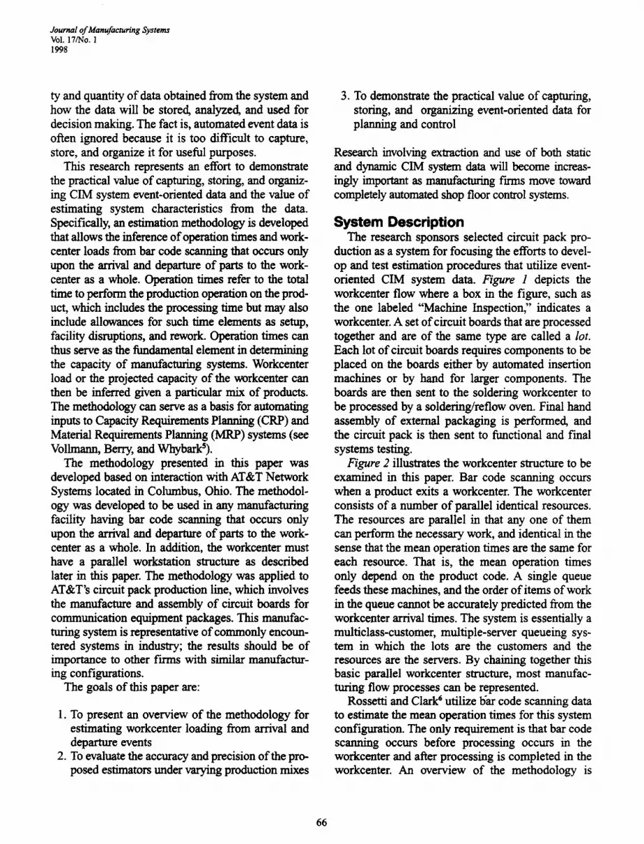
given in Figure 3. The methodology involves product information in the form of bill of materials, workcenter data such as names and functionality, shiR and calendar data for inferring actual operating times, daily inventory balances for calibrating the procedure, and bar code scanning information in the form of product code and time stamps. In addition, the location of the scan is required with an indica- tion of whether the part is entering or leaving a workcenter. These data are taken from appropriate CIM system databases, and middicware routines were written to extract the data from the shop floor control system. The data is merged and used to partially reconstruct the sample path behavior of the workcenter. This involves presenting the data to a simulation program in the form of an event trace while adding additional inference rules to recreate the behavior of the system. The output of this process is inferred busy time, product counts, number of products, and number of shifts over a pre- scribed data collection period. For more information on this process, see Rossetti and Clark/The following section describes how mean operation times can be estimated and then used to estimate the expected workload for the workcenter.

• l [ ] m Queue

~ 0 Resource 1

[ ] © Re= rce3

[ ] Item of work

[ ] Q Reso~'ce c

Figure 2 Workcenter with Pmmllel Facilities

Mathematical Model This section presents a least-squares model that

can be used to estimate the expected workload for a workcenter given estimated mean operation times. Rossetti and Clark ~ provide more details of the model and an evaluation of the estimated mean operation times.

It is assumed that the shop floor control system and other data sources can provide the busy rime for a workcenter and the production counts by product type over a data collection period that has been divided into fixed-length time buckets. 0t is defined as the mean operation time for product/. For a workcenter, the available data are:

Let Yj = total busy time for a workcenter during time bucketj

Let X# = amount of product i produced during time bucket j

Let K = number of product types observed during the data collection period

Let N = number of time buckets observed during the data collection period

The value of Yj represents the total amount of busy time for a workcenter. By using the arrival and departure events, one can partially reconstruct the sample path of the workcenter. The reconstruction permits the calculation of Yi but does not permit the dh-ect observation of the operation times for each product. See Rossetti and Clark 6 for details on the sample path reconstruction. Although the operation times cannot be directly observed, the mean operation times can still be indirectly estimated through the use of a functional relationship.

67


IProductlBOM Dm~ Busy time per ~ff~

~ Nunfi3er of shiC4ts ~

! Times ~ Workcenter

Figure $ Overview of Estimadon Methodology

Because Ot is the mean time to produce one unit of product i, the multiplication X 0 × O~ represents the mean time to produce X¢ products of type i during time bucket j . By summing the quantifies X¢ × Ot over all the products, the result is the total amount of expected busy time for time bucketj. So, the following linear model is proposed:

K Yj =ZXoOi +~. j j=I,...,N (1)

i=1

The term ej represents the error in using ~gl XoO, to estimate Yj. Estimates for 0i can be obtained by mini- mizing the error in a least-squares sense. The least- squares problem can be represented as f'mding those values of 0~ that satisfy the following:

1 nan s s = - x o, (2 ) i=1

subject to: 0i >0 i=l,...,K (3)

The number of parameters for this model is K, so that N--> K is required for proper estimation. Readers are cautioned to note that even though linear regression techniques are being applied to estimate the parameters of the linear model, the standard normality- based inference procedures associated with linear regression do not apply for this model. Many of the underlying assumptions of those inference procedures are violated, such as normality of the errors. In addition, the X0 values are random variables rather

than fixed predefined values based on an experimental design. Because the workcenter has a finite maximum capacity, there can be extreme collinearity among the X 0. This can result in serious bias when estimating 0j. For more on the analytical properties of this model, see Rossetti 8 and Rossetti and Clark. 9

Throughout the following sections, an estimator is denoted with the symbo l " " ; for example, an estimator of 0~ is denoted by 0i. It is noted that the workload requirements for a given amount of product to produce is the sum over all products of the amount of product to produce times the mean operation times. For example, suppose there are two products with mean operation times 01 = 20 and 05 = 10 minutes per product. Furthermore, suppose that the production schedule calls for 100 type 1 products and 200 type 2 products to be produced for a week. Then the workload requirement for that week would be 100 × 20 + 200 x 10 = 4000 minutes. If the estimated values of

A A

01 and 05 are 01 = 19 and 05 = 11, then the predicted workload requirement would be 100 × 19 + 200 × 11 = 4100 minutes. Note that the predicted workload based on estimated mean operation times is an appli- cation of the linear model given in Eq. (1) to predict Y given values for the X's. The remainder of this paper discusses the evaluation of the accuracy and precision of the workcenter load estimators.

Simulation Investigation of Estimator Performance

To assess the statistical properties of the estimates for workcenter load, the parallel workcenter structure

68


1998

was simulated under a variety of experimental conditions. Given a specified production mix, the simulation model of the parallel workcenter generates the busy time and product count data. The least-squares model is then used to estimate the mean operation times from the simulated data. To cheek the ability of the model to predict workcenter load, test schedules are then generated based on varying production mixes that are not necessarily the same as the production mix used to fit the linear model. A schedule refers to an amount of each product to be produced over a fixed time horizon. Using the estimated mean operation times and the test schedules, estimates of the expected workcenter load are obtained. The rest of this section discusses the methodology used to evaluate the estimates of workcenter load. First are given the experimental inputs and notation, and then a description of a typical experiment. The experimental outputs and notations are then presented along with a discussion of the major results.

Experimental Inputs and Notation The major factors examined include the number

of product types, number of time buckets, arrival process parameters, and service process parameters. For a complete discussion of the factors and experimental parameter settings, see Rossetti and Clark. 6

The probability that an arrival is of type i is the proportion of the total number of products that arrive to the workcenter to those that are of type i. The jth production mix is referred to as the set of probabilities, Mj = {'th, ~2, .... "rrjr}, where K is the total number of products that can arrive. The production mix associated with a future schedule is referred to as a scheduled production mix. An important problem in estimating the mean operation times and thus the workcenter load for a future schedule is the fact that the production mix may change for each schedule. The problem of a changing production mix influ- ences the estimation process in two major ways:

1. In the actual production environment, the production mixes used to develop the linear model can vary significantly over time.

2. The scheduled production mix may be significantly different from the observed production mixes used during model estimation.

For the purpose of testing the predictive ability of the model, the variation in the production mixes used

during model estimation is not as severe a problem as is the possibility that the scheduled production mix is significantly different from the observed production mixes used to fit the model. In actuality, the variation in the observed production mixes should improve the predictive ability of the model. This is due to the fact that variation in the observed production mixes will increase the likelihood that a scheduled production mix would have been observed during the estimation process. For this reason, the production mix probabilities are fixed during a replication simulation. The production mix used within the simulation is referred to as the simulated production mix or, where the con- text is clear, as simply the production mix. The performance of the estimators is then checked when the scheduled production mix becomes significantly different from the simulated production mix across a variety of experimental conditions. This allows for a more challenging test of the performance of the procedure.

Description of a Typical Experiment An experiment consists of the simulation of the par-

allel workeenter at the specified factor levels, estimation of the product operation times based on the data obtained from the simulation, and estimation of workcenter load for 23 randomly generated schedules based on 23 randomly generated scheduled production mixes. The size of each time bucket was fixed at a value of 480 minutes. Each experiment was simulated for a total of (N + 20) × 480 minutes, where the f'LrSt 20 time buckets (9600 minutes) were discarded as a warmup period. Each experiment was replicated R = 50 times, yielding 50 estimates of the mean operation time for each product. Thus, each replication has one trLxed simulated production mix and 23 scheduled production mixes for testing. The linear model was evaluated at the 50 estimates of the mean operation times to yield 50 estimates of workeenter load for each of the 23 randomly generated test schedules.

Schedule Generation from Scheduled Production Mixes

As noted earlier, the predicted workcenter load based on estimated mean operation times is an appli- cation of the linear model given in Eq. (1) to predict Y given values for the X's. A generated schedule is an observed sample of the X's for a scheduled production mix. The purpose of generating schedules

69

Journal of Manufacturing Systems Vol. 17/No. I 1998

based on different scheduled production mixes is to evaluate the performance of the estimation process when the production mix associated with a schedule is different than the simulated production mix.

The schedules were generated according to the algorithm given in Rossetti and Clark 6 and described as follows. The aggregate arrival rate for the production mix is scaled to a weekly basis. Each individual arrival probability in the production mix is multiplied by the weekly aggregate arrival rate to yield a weekly arrival rate for each product. The individual weekly arrival rates for each product are then multiplied by a scale factor to yield an upper limit, and divided by the same scale factor to yield a lower limit to be used as parameters of a uniform distribution for that product. Each uniform distribution is sampled to yield a uniformly distributed arrival rate for the corre- sponding product. The arrival rates are summed to yield a total rate. The individual rates are then divided by the total rate to yield the proportion of the total that can be attributed to each product. The above process yields a scheduled production mix. The scheduled production mix generation process was performed for the following scale factors (1.5, 2, 3, 4, 5, 6, 7, 8, 9, 10), yielding 10 randomly generated production mixes. To generate the schedules associated with each production mix, the aggregate arrival rate was multiplied by the individual arrival probabilities for each of the generated mixes, yielding an arrival rate for each product. The arrival rates were then used as the parameters for Poisson distributions, which generated the amount of product to arrive for that week.

Ten additional scheduled production mixes were generated by inverting the previous 10 mixes such that if product i had the highest proportion and product j had the lowest proportion in the generated mix, then the new generated mix would have product i and j switched (the second highest was switched with the second lowest proportion, third highest with the third lowest, and so on). The production mix used in the simulation and its inverse were also used along with a production mix with all products having equal proportions. Thus, a total of 23 production mixes were generated for each experimental setting. A schedule was generated for each generated production mix and used to evaluate the linear model's ability to predict the workcenter's load.

The method used to generate the production mixes allows mixes to be generated that are "close" or "far" from the production mix used to develop the linear model. This distance is controlled by the value of the scale factor. The distance is measured using Euclidean point-to-point distance, as follows:

1

d = ~i - ~zl (4)

where ¢rj is the probability for product type i in the A •

production mix and ~'~ is the probability for production type i for the scheduled production mix. Because "tr~ and 'n'~ are probabilities, the range of d is 0 --- d - V~. Later experiments consider those mixes that have d - (0.25)V2 -- 0.35 as representative of those product mixes that may occur in a slowly changing product mix environment. The next section presents the notation used for the experimental outputs.

Experimental Outputs and Notation This section presents the notation used to repre-

sent the statistical properties of predicting the expected workload requirements for the workcenter based on the estimated mean operation times and generated schedules. The quality of the predicted expected workload relative to true workload is assessed in terms of estimates of bias and variance. The performance of the predicted expected workload is also evaluated by estimating the probability that the estimator will be within .4-.y x 100% of the true value. The following notation and terms are used to describe the experimental outputs. Given the factors and levels specified in Table 1, there are J = (# K × # C V × # M i x e s × # N ) = ( 3 X 3 × 5 × 4 ) = 1 8 0 total experiments each replicated R = 50 times with N = 23 generated scheduled production mixes.

Notation for Experimental Outputs Let 0~, be an estimate of the mean operation time

for product i on replication r of experimentj Let ~qjn be the true expected workload for a sched-

ule generated from the production mix used to sim- alate experiment j, where if Zin is the planned amount of product i to be produced for schedule n,

i=1

70


1998

Table l Overall Factors and Levels

K = number of products N = number of time buckets CV = coefficient of variation of operation times Mj =jth production mix

Factor Levels

K 2, 4, 8 N 64, 128, 256, 512

CV 0.09, 0.18, 0.45 Mix M,, M2, M3, M,, Ms

Let ~j,,. be an estimate of the true expected workload for schedule n on replication r of experiment j , where

K

i=l A

Let PLEj,,. be the predicted expected workload error, PLE, that is, the error in estimating the true expected workload, "qj., with Oj~., for production schedule n on experiment j of replication r, where

PLEj., = ~ . - ~lj..

Let PLREj,,r be the predicted workload relative error, PLRE, that is, the relative error in estimating the true workload, xl#,, with ~. . , for production schedule n on experimentj of replication r, where

A A

PLREj., xb~ xD,,r "qin

Let Bias be an estimate of the bias of the estimator Let 6- be an estimate of the standard deviation of

the estimator Let ~ be an estimate of the mean squared error

of the estimator Let/3('y) be an estimate for the probability that an

estimator is within ~ × 100% of the true value

Summary of Experimental ResuRs and Discussion

This section presents a summary of the results from the experiments, which give evidence as to the overall accuracy and precision of the predicted expected workload. Also discussed are the trends and important factors identified in the results. For further results, refer to Rossetti?

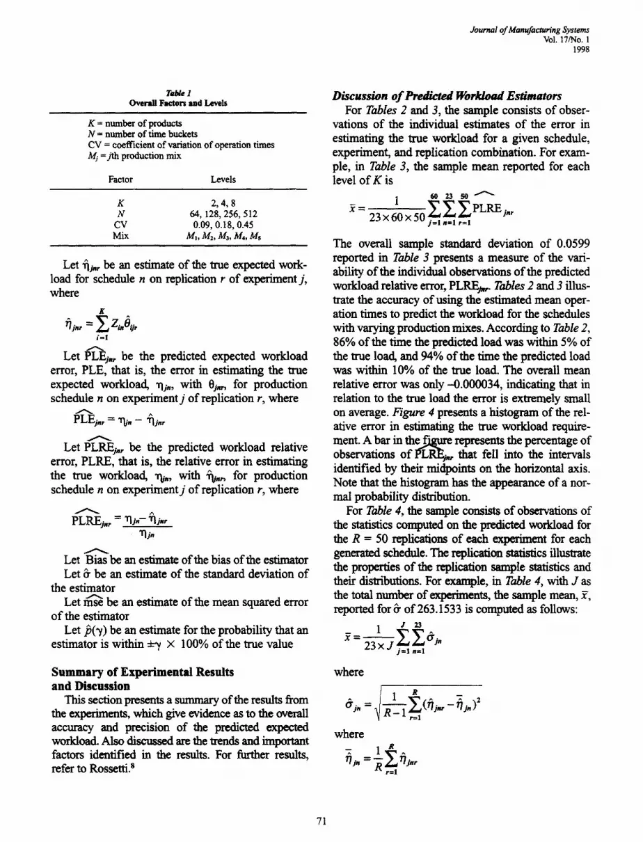
Discussion o f Predicted Workload Estimators For Tables 2 and 3, the sample consists of obser-

vations of the individual estimates of the error in estimating the true workload for a given schedule, experiment, and replication combination. For example, in Table 3, the sample mean reported for each level of K is

6 0 2 3 5 0 ~

! ZZZPL ., 23 x 60 x 50 j=t .=I ,=t

The overall sample standard deviation of 0.0599 reported in Table 3 presents a measure of the variability of the individual observations of the predicted workload relative error, PLRE,~,. Tables 2 and 3 illus- Irate the accuracy of using the estimated mean operation times to predict the workload for the schedules with varying production mixes. According to Table 2, 86% of the time the predicted load was within 5% of the true load, and 94% of the time the predicted load was within 10% of the true load. The overall mean relative error was only -0.000034, indicating that in relation to the true load the error is extremely small on average. Figure 4 presents a histogram of the relative error in estimating the true workload requirement. A bar in t h e ~ represents the percentage of observations of PLRE~r that fell into the intervals identified by their midpoints on the horizontal axis. Note that the histogram has the appearance of a nor- mal probability distribution.

For Table 4, the sample consists of observatiom of the statistics computed on the predicted workload for the R = 50 replications of each experiment for each generated schedule. The replication statistics illustrate the properties of the replication sample statistics and their distributions. For example, in Table 4, with J as the total number of experiments, the sample mean, £, reported for& of 263.1533 is computed as follows:

2 3 x J jn j = l n=l

where

] 1 R

where 1 R

r=l

71


Table2 Predicted Load Error Summary Statistics

K = 2 K = 4 K = 8 Overall

sample* mean 24.715 65.6606 --4.8761 28.4998 sample std. dev. 508.7245 644.2482 188.7018 487.1574 maximum 5270.12 7116.137 2831.858 7116.137 upper quartile 116.146 174.057 27.041 82.9266 median -5.6122 15.819 0.0841 1.6563 lower quartile -108.063 -87.2927 -29.4795 -67.6393 minimum -7626.91 -6256.63 -2988.80 -7626.91 sample size 69000 69000 69000 207000 ~h(0.05) 0.9278 0.8339 0.8327 0.8648 b(0.10) 0.9786 0.9171 0.9271 0.9409 b(0.15) 0.9917 0.9526 0.9605 0.9683

A

Mote: The sample consists of observations of PLE 0" for 60 experiments x 50 replications x 23 mixes.

Table3 Predicted Load Relative grrer Summary Statistics

K = 2 K = 4 K = 8 Overall

sample* mean -0.0019 0.0015 -0.00059 -0.000034 sample std. dev. 0.0339 0.0742 0.0641 0.0599 maximum 0.5008 0.8169 0.6336 0.8169 upper quartile 0.0061 0.0133 0.0107 0.0098 median -0.00033 0.00134 0.000033 0.00025 lower quartile -0.0065 -0.0075 -0.0110 -0.00809 minimum -0.9358 -1.5131 -0.898 -1.5131 sample size 69000 69000 69000 207000

A *Note: The sample consists of observations of PLRE#, for 60 experiments × 50 replications X 23 mixes.

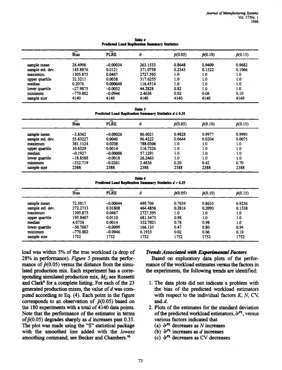
Thus, the value of 263.1533 for the sample mean of 6" reports the average over the experiments of the sample standard deviation of the estimator based on 50 replications. As such, it presents a measure of the average variability of the estimator over all experimental conditions. From the quartile information of/3(0.05) for the predicted load estimate, it is noted that while on average 86% of the time the estimates were within 5% of the true mean operation time, in 75% of the experiments/~(0.05) was greater than 0.82.

For Tables 5 and 6, the sample is the same as in Table 4, except now the statistics are grouped by the factor d, which represents how close the production mix used is to the simulated production mix as defined by Eq. (4). For Tables 5 and 6, a value of d _< 0.35 can be considered as a relatively small change in the product mix (d _< 0.35 translates into the scheduled production mix being less than 25% of the maximum possible change in the simulated production mix). The classification of the observations

0.30 ' 1 0.25" 0.20"

~ 0.15' 0.10" 0.05.

0.00.

F/gum 4 Hi~egram for Predicted Lead Relative Error (~"~LRE0,)

by d indicates that d has a major effect on the performance of the predicted workload estimates. In Table 5, with d < 0.35, 98% of the time the predicted workload was within 5% of the true workload. In Table 6, with d > 0.35, 70% of the time the predicted work-

72


1998

Table4 Predicted Lead Replication Snmmltry StltgJlgJC$

Bias PLRE 6 p(0.05) /3(0.10) /3(0.15)

sample mean sample std. dev. maximum upper quartile median lower quartile minimum sample size

28.4998 -0.00034 263.1533 0.8648 0.9409 0.9682 185.8876 0.0121 371.0758 0.2343 O. 1522 O. 1066 1305.875 0.0467 2727.595 1.0 1.0 1.0 32.3211 0.0038 317.6255 1.0 1.0 1.0 0.2076 0.000048 116.4514 1.0 1.0 1.0 -27.9875 -0.0032 44.2828 0.82 1.0 1.0 -770.802 -0.0946 2.4636 0.02 0.06 0.10 4140 4140 4140 4140 4140 4140

Tab/e $ Predicted Lead Replication Summary Statistics d < 0.35

Bias PLRE # p(0.05) #(0.1 O) p(0.15)

sample mean sample std. dev. maximum upper quartile median lower quartile minimum sample size

-3.6362 -0.00026 86.6021 0.9828 0.9977 0.9995 55.63227 0.0040 96.4222 0.0644 0.0204 0.0075 381.1124 0.0208 788.0306 1.0 1.0 1.0 10.6329 0.0014 116.7326 1.0 1.0 1.0 -0.1927 -0.00006 57.1291 1.0 1.0 1.0 -18.8588 -0.0018 26.2463 1.0 1.0 1.0 -332.719 -0.0261 2.4636 0.20 0.42 0.70 2388 2388 2388 2388 2388 2388

Table6 Predicted Load Replieattion Summary statistics d > 0.35

Bias PLRE 6- p(0.05) /3(0.10) p(0.15)

sample mean 72.3017 ---0.00044 499.706 0.7039 0.8635 0.9256 sample std. dev. 272.2713 0.01808 464.4856 0.2816 0.2093 0.1538 maximum 1305.875 0.0467 2727.595 1.0 1.0 1.0 upper quartile 195.8407 0.0110 681.3475 0.98 1.0 1.0 median 4.0758 0.0014 352.7021 0.78 0.98 1.0 lower quartile -50.7687 -0.0099 166.133 0.47 0.80 0.94 minimum -770.802 -0.0946 6.1933 0.02 0.06 O. 10 sample size 1752 1752 1752 1752 1752 1752

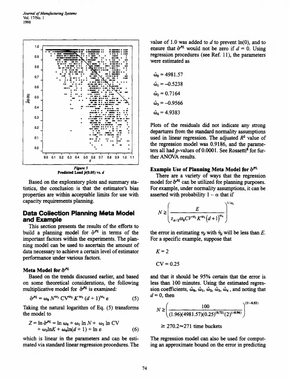
load was within 5% of the true workload (a drop of 28% in performance). Figure 5 presents the performance of ~0.05) versus the distance from the simulated production mix. Each experiment has a corre- sponding simulated production mix, M~; see Rossetti and Clarl~ for a complete listing. For each of the 23 generated production mixes, the value of d was computed according to Eq. (4). Each point in the figure corresponds to an observation of ~(0.05) based on the 180 experiments with a total of 4140 data points. Note that the performance of the estimator in terms olin(0.05) degrades sharply as d increases past 0.35. The plot was made using the "S" statistical package with the smoothed line added with the lowess smoothing command; see Becker and Chambers. 1°

Trends Associated with ~ e n t a l Factors Based on exploratory data plots of the perfor-

mance of the workload estimates versus the factors in the experiments, the following U'ends are identified:

1. The data plots did not indicate a problem with the bias of the predicted workload estimators with respect to the individual factors K, N, CV, andd.

2. Plots of the estimates for the standard deviation of the predicted workload estimators, 6 "~L, versus various factors indicated that (a) b tL decreases as N increases (b) b 'ez increases as d increases (c) b -'L decreases as CV decreases

73

Journal of Manufacturing Systons Vol. 17/No. 1 1998

1.0

0,9

0.8

0.7

0.6

0.5

0.4 I

• m % ,

e o • e s • o e e • •

- ,. . %- . - - . . e • 4 m u d o o o o e o o •

s s e • • o m e o m e m * • • • m e • e • • • • • • e e e o 0 • D e 0 0 • "_-": . - - - - . .. • ~. ." . . . .

• .--..0"- : - _ - . . . . . . m • ~ o o e e o o e • m e ,

• o e e e a • e o a • • • • e e o e • • e s •

• s e e ) o o • e e e •

. . . ~ : . - . • e J ° e * • ~ 0 e •

o m • • o ~ e • e o e • •

9 • • • • ~ m e •

• • o e e •

I I i

oJ2 o'.3 o:, o'.6 o.8 ;.o a

0.3 ] - I

0.2 ] -1 0.1

0.0 ~ "1

o:o 0:,

F/~re 5 Predicted Load ~0.05) vs. d

Based on the exploratory plots and summary statistics, the conclusion is that the estimator's bias properties are within acceptable limits for use with capacity requirements planning.

Data Collection Planning Meta Model a n d E x a m p l e

This section presents the results of the efforts to build a planning model for b J'L in terms of the important factors within the experiments. The planning model can be used to ascertain the amount of data necessary to achieve a certain level of estimator performance under various factors.

Meta M o d e l for 6 a'L Based on the trends discussed earlier, and based

on some theoretical considerations, the following multiplicative model for b zL is examined:

b "eL = tOo N 0'~ CV °'~ K °̀3 (d + 1) '°' e (5)

Taking the natural logarithm of Eq. (5) transforms the model to

Z = In ~*L = In tOo + tO1 In N + to2 In CV + tO3ing + tO4In(d + 1) + In e (6)

which is linear in the parameters and can be estimated via standard linear regression procedures. The

value of 1.0 was added to d to prevent In(0), and to ensure that 6 a'z would not be zero if d = 0. Using regression procedures (see Ref. 11), the parameters were estimated as

&0 = 4981.57

&l =-0.5238

~2 = 0.7164

&3 =-0.9566

&4 = 4.9383

Plots of the residuals did not indicate any strong departures from the standard normality assumptions used in linear regression. The adjusted R 2 value of the regression model was 0.9186, and the parameters all hadp-values of 0.0001. See Rossetti s for further ANOVA results.

E x a m p l e Use of P l a n n i n g Meta Mode l for ~PL There are a variety of ways that the regression

model for 0 J'L can be utilized for planning purposes. For example, under normality assumptions, it can be asserted with probability 1 - o~ that if

I / N - > . E__

zu/eWoCV '°2 K w' (d + 1) °'

the error in estimating ~ with ~i will be less than E. For a specific example, suppose that

K = 2

CV = 0.25

and that it should be 95% certain that the error is less than 100 minutes. Using the estimated regression coefficients, ~o, ~ , &2, &3, &4, and noting that d = 0, then

( 100 / ''~-°"~' N > (,(1.96)(4981.57)(--0.25)(0a2)(2)(_0.~ ~ )

-> 270.2~-271 time buckets

The regression model can also be used for comput- ing an approximate bound on the error in predicting

74

Journal of Manufaciuring Systems Vol. 17/No. 1

1998

the workload for a different production mix. For example, suppose 0~ has been estimated under the following conditions:

N = 300

K = 2

CV -- 0.25

"n'l = 0.7

'rr2 = 0.3

and there should be an approximate upper bound on the error in predicting the workload associated with a schedule that has a production mix with ~i = 0.4 and "rq = 0.6. If the regression model is true, then with probability I - ct

E <- z~n a~o N o'' CV m K °'3 (d + 1) '°'

For the given data and estimates of to, i = 1, 2, 3, 4 and d = 0.42, so that with probability 0.95

E -< (1.96)(4981.57)(300) -°~ (0.25) 0.72 (2) "°'~s (0.42 + 1) 4"~

<-- 542.6 minutes

Stm~ary, and Conclusions This paper presented and evaluated a methodolo-

gy that utilizes CIM system data in the form of bar code scanning data to estimate the workload for a workcenter with a parallel facility structure. The simulation results indicate that the method can achieve the accuracy and precision necessary for use in CRP. The sensitivity to various experimental factors was explored. It was found that the percentage of products in the production mix can have a significant effect on estimator performance. In addition, the estimator's performance can degrade significantly if the observed production mix used to develop the linear model is significantly different from the production mix associated with the schedule for which workloads are desired. A planning model was presented that can be used to estimate the amount of data required under the various experimental conditions.

The methodology illustrated in Figure 3 was

implemented with a set of computer programs for the circuit pack production line. Due to proprietary considerations, no specific estimation results are presented, but instead only general results are discussed. Workcenter arrival and departure data was collected for approximately three months. The total number of products under consideration was 96; however, the workcenter was divided into 20 small- er queueing systems to which the method could be applied for only the products that visit those subsys- tems. The maximum number of products that had to be estimated at any one time was 12. The results indicated that for high-volume products the estimates were of acceptable quality; however, not enough observations of low-volume products were available to accurately predict workload for mixes containing only low-volume products.

Data collection procedure problems also influ- ence the quality of the estimators. The first data collection problem occurred during the bar code scanning of products departing workcenters. Rather than bar code scanning products after completing the operation, the products were allowed to accumulate and then were bar code scanned at convenient points in time, such as the end of a shift. This scanning procedure puts into suspect the arrival and departure event times on which the busy time inference is based. For example, it might be inferred that there were more products waiting to be processed than there actually were. The second data collection problem also affects the busy time inference. The problem involves the lack of full knowledge of whether or not the resources have operators present at any given point in time. Enforcement of proper data collection is therefore necessary. As an alternative, one could consider the complete automation of data entry through radio-frequency devices. To improve the accuracy of the estimates, the possibility is being explored of using time series methods to update the estimates as more data are collected over time and to predict how the product mix is varying over time. The methodology could be incorporated into any supervisory control and data acquisition (SCADA) system attached to the shop floor.

As with many information value-added applica- tions, there exists a trade-offbetween the amo u n t and quality of information gained and the cost and/or complexity of obtaining the information. The estimation of workloads depends on the estimation of mean

75

Journal of Manufacturing @stems Vol. 17/No. 1 1998

operation times, which can be estimated via automatic data collection systems based on bar code scanning technology. Rossetti and ClarlP developed and evaluated estimators for mean operation times using both simulated and actual shop floor control data. Thus, traditional methods, such as manual time study, can be reduced. An integrated systems approach to the design of the data collection system can significantly improve planning and control by ensuring that the collection of operation times is planned for during the conceptual stages of the system. The possibility exists to estimate other shop floor quantities, such as queue times and product lead times. In the past, data concerning the shop floor was inaccurate, untimely, and unavailable. Today's computerized shop floor control systems are data rich but information poor. This research addressed the fundamental challenge of extracting information from dam-rich environments to enhance manufacturing decision making.

Acknowledgments The authors would like to thank AT&T Network

Systems in Columbus, Ohio, for the support of this research, especially Martin Gussman, the project liaison.

References I. A. Bauer, R. Bowdon, J. Browne, J. Duggan, and G. Lyons, Shop

Floor Control Systems: From Design to Implementation (London: Chapman and Hall, 1994).

2. V.A. Mabert, "Shop Floor Monitoring and Control Systems" in Handbook of Industrial Engineerin~ 2nd ed., Gavriel Salvendy, ed. (New York: John Wiley & Sons, 1992).

3. J.M. Hill, "Automatic Identification Systems," in Production Handbook~ 4th ed., John A. White, ed. (NewYork: John Wiley & Sons, Inc., 1987).

4. Spencer B. Smith, 1989. Computer Based Production and Inventory Control (Englewood CTdfs, NJ: Prentice-Hall, 1989).

5. T.E. Vollmann, W.L. Berry, and D.C. Whybark, Manufacturing Planning and Control Systems (New York: Dow Jones Irwin, 1988).

6. M.D. Rossetti and G.M. Clark, "Estimating Operation Times from Workcenter Arrival and Departure Events;' Working Paper SYS-MDR-4- 1994 (Charlottesville, VA: Dept. of Systems Engineering, Univ. of Virginia, 1994).

7. M.D. Rossetti and G.M Clark, "Estimation of Facility Operation Times for Use in Capacity Requirements Planning" project report submit- ted to AT&T Network Systems (Columbus, OH: 1993).

8. M.D. Rossetti, "Queueing Service Parameter Estimation from Event Oriented Production Control Data," Phi) dissertation (Columbus, OH: The Ohio State Univ., 1992).

9. M.D. Rossetti and G.M. Clark, "Estimating Expected Sojourn Times for an Exiting Markov Renewal Process," Communications in Statistics-- Theory and Methods (v24, n2, 1995), pp553-579. 10. R.A. Becker and J.M. Chambers, 1984. "S": An Interactive Environment for Data Analysis and Graphics, Wadsworth Statistics/Probability Series (Murray Hill, N J: Bell Laboratories, Inc., 1984). II. SAS User's Guide: Statistica, Version 5 ed. (Cary, NC: SAS Institute, 1985).

Authors' Biographies Manuel D. Rossetti is an assistant professor in the systems engineering

department at the University ofVirgi'nia_ He received his BSIE degree from the University of Cincinnati in 1985 and his MSc in 1988 and PhD in 1992, both in indusa-ial and systems engineering from The Ohio State University. His research interests include the design, analysis, and implementation of automatic data collection systems using object-oriented methods, simulation, stochastic modeling, and artificial intelligence techniques. Dr. Rossetti is an associate member of RE and a member of its OR division. He is also a member of INFORMS and the Society for Computer Simulation.

Gordon M. Clark is a professor emeritus in the Department of Industrial, Welding and Systems Engineering at The Ohio State University. He received his BIE degree from The Ohio State University in 1957, MSc in industrial engineering from the University of Southern California in 1965, and PhD degree from The Ohio State University in 1969. His current research interests include integrated manufacturing decision support systems in a CIM environment and the development of manufacturing cost models. He is a member of the editorial board for the Journal of Opemtiona Management and is currently a member of a multidisciplinary team that performs manu~cturing assessments.

76

Documents

Estimating capacity loadings from workcenter arrival and departure events