Embed Size (px)
Citation preview
HAL Id: tel-03253754https://tel.archives-ouvertes.fr/tel-03253754
Submitted on 8 Jun 2021
HAL is a multi-disciplinary open accessarchive for the deposit and dissemination of sci-entific research documents, whether they are pub-lished or not. The documents may come fromteaching and research institutions in France orabroad, or from public or private research centers.
L’archive ouverte pluridisciplinaire HAL, estdestinée au dépôt et à la diffusion de documentsscientifiques de niveau recherche, publiés ou non,émanant des établissements d’enseignement et derecherche français ou étrangers, des laboratoirespublics ou privés.
Essays in venture capital financeJohn Lewis
To cite this version:John Lewis. Essays in venture capital finance. Business administration. Université Paris sciences etlettres, 2020. English. �NNT : 2020UPSLD014�. �tel-03253754�
Préparée à l’Université Paris Dauphine
Essays in venture capital finance
Soutenue par
John Howard LEWISLe 09 Juillet 2020
École doctorale no543
Ecole Doctorale SDOSE
Spécialité
FINANCE
Composition du jury :
Edith GINGLINGERProfesseur, Université Paris Dauphine - PSLPrésident
David ROBINSONProfesseur, Duke UniversityRapporteur
Ludovic PHALIPPOUProfesseur, Oxford UniversityRapporteur
Jose Miguel GASPARProfesseur, ESSECExaminateur
Armin SCHWIENBACHERProfesseur de finance, SKEMA et UniversitéLille 2Examinateur
Gilles CHEMLADirecteur de recherches, CNRS, UniversitéParis Dauphine - PSL et Professeur, ImperialCollege Business SchoolDirecteur de thèse


0.1. ACKNOWLEDGEMENTS 1
0.1 Acknowledgements
First and foremost, I would like to thank my supervisor Gilles Chemla for stickingwith me through this journey. Without his patience, guidance and good humor Iwould not have been able to complete my thesis. He has been the best example ofhow to be an educator. I hope that I am able to do as much for my students as hehas done for me. Luck was with me when I met Gilles.
I would like to thank my coauthors Maija Halonen-Akatwijuka, Richard Fairchildand Caroline Genc. Working with them greatly improved my ability to conduct re-search. It was an enjoyable experience and I look forward to collaborating with themin the future. I would like to further thank Richard for providing encouragementduring my studies and inviting me to present my entrepreneurship experience andresearch to his MBA students.
The faculty at Dauphine made this a rewarding and enjoyable experience. Ireceived comments and encouragement from Edith Ginglinger and Tamara Nefedovaat a time when I needed it. Fabrice Riva always had time for a pleasant conversationand interest in my projects. A reference from him was instrumental in helping meobtain my first serious teaching position some 10 years ago. I thank Edith, Tamaraand Fabrice for all they have done for me.
Through the conferences organized by Dauphine, I was able to meet David Robin-son, discuss my research and look at things from a different angle. I was also able toattend seminars by Jose-Miguel Gaspar where I finally learned the statistics whichhad eluded me. I thank both of these professors for spending time with me so Icould reach another level of understanding.
I would like to thank the following people for helpful comments on the earlydrafts of this work: Utpal Bhattacharya, Béatrice Boulu-Reshef, Gilles Chemla,Jérôme Dugast, Oliver Hart, Richard Fairchild,Edith Ginglinger, Antoine Mandel,Tamara Nefedova, David Robinson, Laura Starks, Ken Teed, the seminar audienceat Bristol University, seminar participants at the Université Paris Dauphine - PSL,and the ECBA workshops in Bath and Paris.
The students in the Finance Lab have been supportive, fun and amazingly tal-ented. I am very glad that I had their support and assistance. It was a pleasuregoing to the office everyday. There were numerous times my fellow students weremy first line of support. In particular I want to thank my coauthor Caroline Gencfor her unflagging good mood, intelligence, patience, hard work and dilligence. Iwould also like to thank Hugo Marin for his assistance with statistics, R, TeX andSaturday lunches.
I would also like thank my past students at IAE Gustave Eiffel - UPEC and TheCitadel Military College. Your inquisitive minds kept me interested in research and
1

2
spurred me on to complete the PhD.Going back further, I would like to thank my undergraduate professors Rodney
Canfield and Randy Tuler for sparking an interest in learning and providing someof my earliest research experiences.
This would not have been possible without the support of my family. My wifeMargaret was ever patient as I worked on the PhD. My children Isabelle and Jackspurred me on with gentle teasing that has now become family folklore. Any sacrificeduring my time studying was borne by my family. For that, I am profoundly grateful.
2
Contents
0.1 Acknowledgements . . . . . . . . . . . . . . . . . . . . . . . . . . . . 1
1 Introduction 51.1 L’industrie du capital risque . . . . . . . . . . . . . . . . . . . . . . . 61.2 Thesis overview . . . . . . . . . . . . . . . . . . . . . . . . . . . . . . 91.3 The venture capital industry . . . . . . . . . . . . . . . . . . . . . . . 101.4 Thesis overview . . . . . . . . . . . . . . . . . . . . . . . . . . . . . . 13
2 Contracts as reference points in VC 152.1 Introduction . . . . . . . . . . . . . . . . . . . . . . . . . . . . . . . . 162.2 Related literature . . . . . . . . . . . . . . . . . . . . . . . . . . . . . 172.3 The model . . . . . . . . . . . . . . . . . . . . . . . . . . . . . . . . . 18
2.3.1 No renegotiation . . . . . . . . . . . . . . . . . . . . . . . . . 192.3.2 Renegotiation . . . . . . . . . . . . . . . . . . . . . . . . . . . 19
2.4 Optimal contract . . . . . . . . . . . . . . . . . . . . . . . . . . . . . 21
2.4.1 Overlapping self-enforcing ranges . . . . . . . . . . . . . . . . 212.4.2 Disconnected self-enforcing ranges . . . . . . . . . . . . . . . . 222.4.3 VC contracts as reference points . . . . . . . . . . . . . . . . . 24
2.5 Extensions . . . . . . . . . . . . . . . . . . . . . . . . . . . . . . . . . 282.5.1 Indexation . . . . . . . . . . . . . . . . . . . . . . . . . . . . . 282.5.2 E’s participation constraint . . . . . . . . . . . . . . . . . . . 292.5.3 n states . . . . . . . . . . . . . . . . . . . . . . . . . . . . . . 29
2.6 Conclusion . . . . . . . . . . . . . . . . . . . . . . . . . . . . . . . . . 292.7 Figures . . . . . . . . . . . . . . . . . . . . . . . . . . . . . . . . . . . 31
3 Surf VC investment waves at your own risk 353.1 Introduction . . . . . . . . . . . . . . . . . . . . . . . . . . . . . . . . 363.2 Related literature . . . . . . . . . . . . . . . . . . . . . . . . . . . . . 393.3 Data . . . . . . . . . . . . . . . . . . . . . . . . . . . . . . . . . . . . 423.4 VC investment waves and performance . . . . . . . . . . . . . . . . . 43
3.4.1 Identification of waves . . . . . . . . . . . . . . . . . . . . . . 43
3

4 CONTENTS
3.4.2 Performance Measure . . . . . . . . . . . . . . . . . . . . . . . 443.4.3 Performance with respect to waves . . . . . . . . . . . . . . . 45
3.5 Who invests when ? . . . . . . . . . . . . . . . . . . . . . . . . . . . . 483.5.1 Explanatory variables . . . . . . . . . . . . . . . . . . . . . . . 483.5.2 Experience and network . . . . . . . . . . . . . . . . . . . . . 493.5.3 Past performance and liquidity . . . . . . . . . . . . . . . . . 50
3.6 Conclusion . . . . . . . . . . . . . . . . . . . . . . . . . . . . . . . . . 513.7 Figures . . . . . . . . . . . . . . . . . . . . . . . . . . . . . . . . . . . 523.8 Tables . . . . . . . . . . . . . . . . . . . . . . . . . . . . . . . . . . . 54
4 Are Bridge Loans a Bridge to Nowhere? 654.1 Introduction . . . . . . . . . . . . . . . . . . . . . . . . . . . . . . . . 664.2 Related literature . . . . . . . . . . . . . . . . . . . . . . . . . . . . 694.3 Bridge loans . . . . . . . . . . . . . . . . . . . . . . . . . . . . . . . 704.4 Data . . . . . . . . . . . . . . . . . . . . . . . . . . . . . . . . . . . . 724.5 Funds and companies with bridge loans . . . . . . . . . . . . . . . . 754.6 Success of investments with bridge loans . . . . . . . . . . . . . . . . 774.7 Bridge loans and the last fund . . . . . . . . . . . . . . . . . . . . . 804.8 Success of investments and elapsed time of fund . . . . . . . . . . . . 834.9 Robustness checks . . . . . . . . . . . . . . . . . . . . . . . . . . . . 854.10 Conclusion . . . . . . . . . . . . . . . . . . . . . . . . . . . . . . . . . 874.11 Tables . . . . . . . . . . . . . . . . . . . . . . . . . . . . . . . . . . . 894.12 Appendix . . . . . . . . . . . . . . . . . . . . . . . . . . . . . . . . . 89References . . . . . . . . . . . . . . . . . . . . . . . . . . . . . . . . . . . . 101
4

Chapter 1
Introduction
5
6 CHAPTER 1. INTRODUCTION
1.1 L’industrie du capital risque
Le capital risque est une importante source de financement dans le processus decréation des grandes entreprises côtées et de l’activité économique associée. Plus de20% de la capitalisation des entreprises côtées en Bourse aux Etat-Unis provient defonds spécialisés en capital risque. Ces fonds sont également responsables de 44%des dépenses en recherche et développement des entreprises côtées aux Etat-Unis(Gornall & Strebulaev, 2015). Les fonds de capital risque ont créé entre 5 et 7%des emplois (Puri & Zarutskie, 2012). De plus, les start-up financées par du capital-risque représentent 35% des introductions en Bourse (Da Rin, Hellmann, & Puri,2013). Sans l’aide du capital risque, les nouvelles entreprises rencontreraient desdifficultés pour se financer auprès des acteurs traditionnels comme les banques oules marchés de capitaux.
Les sociétés de capital-risque sont des structures uniques organisées dans le butde fournir du capital risqué à forte rentabilité. Ces firmes investissent dans desentreprises qui n’ont pas encore une direction expérimentée, un marché ou un produitexistant. De ce fait, la structure de l’industrie du capital risque et les instrumentsde financement utilisés sont adaptés à ces profils d’entreprises à risque élevé.
L’industrie du capital-risque est organisée en grande majorité en fonds de sociétéen commandite. Les associés de chaque fonds fournissent des capitaux à responsabil-ité limitée et n’ont pas de responsabilités opérationnelles. La direction opérationnellegère le fond ainsi que le processus d’investissement, et engage une responsabilité per-sonnelle plus importante. La direction du fonds de capital risque travaille avec lesentreprises faisant partie du portefeuille du fonds et reçoit un paiement de la partdes associés du fonds pour leur travail (Sahlman, 1990).
Les fonds de capital risque se spécialisent dans le financement des entreprisesen phase de démarrage. Ces entreprises sont généralement innovantes et ont uneespérance de rentabilité élevée au moment de l’investissement. Toutefois, la majoritédes investissements échouent. De ce fait, la direction du fonds de capital risque seconcentre sur le financement d’entreprises pour lesquelles la sortie à fort taux derendement à un horizon de 3 à 7 ans est possible (Sahlman, 1990; Puri & Zarutskie,2012).
Les sociétés de capital risque recherchent typiquement à avoir un taux internede rendement (TIR) positif. La direction du fonds reçoit généralement 1 à 2.5% dumontant total de capital sous gestion en commissions et 20% des profits dépassantun seuil contractuellement fixé (Phalippou & Gottschalg, 2009). Un fonds de capitalrisque a en général une durée de vie comprise entre 5 et 10 ans avant que les revenusgénérés soient distribués aux associés du fond (Sahlman, 1990). La plupart desfonds sous gestion sont investis durant les trois premières années de vie du fonds
6
1.1. L’INDUSTRIE DU CAPITAL RISQUE 7
(Zarutskie, 2007).Les capital-risqueurs à succès affirment souvent que les critères d’investissement
des fonds de capital risque se basent sur une analyse de l’équipe ayant fondé l’entrepriseet sur la taille du marché visé (T. F. Hellmann & Puri, 2000).
L’entreprise recevant un financement provenant d’un fonds de capital risqueest examinée selon un processus propre à chaque fonds dans le but d’analyserl’équipe dirigeante, le marché visé, le produit conçu ainsi que les risques spécifiquesà l’entreprise financée (Gorman & Sahlman, 1989; MacMillan, Siegel, & Narasimha,1985). L’investissement a pour objectif d’accélérer le processus de croissance de lafirme et, in fine, d’avancer la date de sortie du fonds en capital-risque. Au fil destours de financement et à mesure que des investisseurs sont ajoutés, le fonds decapital risque est de moins en moins enclin à mettre fin au projet (Wiltbank, Dew,& Read, 2015).
Les informations sur les potentiels investissements sont suivis par les associés etles gérants du fonds de capital risque. Les sociétés de capital risque ne financentgénéralement pas la totalité du projet. Ils travaillent généralement avec un syndicatde co-investisseurs associés à d’autres fonds de capital risque pour financer le projet.Le syndicat de fonds recueille ensuite le maximum de données sur les entreprisesfinancées afin d’éclairer le processus décisionnel lors du premier tour de financementainsi que pour les suivants. De nombreux fonds de capital risque ont une base dedonnées, propriétaire ou commerciale, répertoriant les actions des autres fonds decapital et leurs estimations de la valeur des entreprises qu’ils financent.
Lors du processus de syndication, les fonds de capital risque sont capables d’avoirune image claire des entreprises dans lesquelles les autres fonds de capital risqueont investi en analysant les résultats des investissements leur ayant été présenté.Généralement, un investisseur invité à joindre un syndicat reçoit des informationsconcernant les membres du syndicat. Même si un fonds de capital risque ne rejointpas le syndicat, il peut avoir accès aux annonces relatives aux investissements dusyndicat. Un fonds de capital risque peut juger de la qualité d’un autre fonds decapital risque en analysant leurs efforts de suivi (Hopp & Rieder, 2011).
Les sociétés de capital risque ont des orientations et charactéristiques différentesque celles des société de capital investissement et des entreprises côtées en Bourse(Boone & Mulherin, 2011). Les fonds de capital risque se concentrent en effet sur lefinancement des entreprises privées. Le syndicat d’investissement permet des trans-ferts d’information concernant les entreprises financées entre les fonds du syndicat(Casamatta & Haritchabalet, 2007). L’interaction entre les fonds durant le proces-sus de création du syndicat d’investissement (Lerner, 1994) crée potentiellement desbiais comportementaux.
Puisque la plupart des fonds investissent la totalité du capital sous gestion durant
7
8 CHAPTER 1. INTRODUCTION
la troisième année de vie du fonds, le capital risqueur connaît une période de forteactivité suivie par une activité de surveillance des entreprises financées. Durant lapériode de surveillance (de la troisième à la dixième année de vie du fonds), le capital-risqueur crée généralement un nouveau fonds afin de pouvoir réaliser de nouveauxinvestissements. Ainsi, le capital-risqueur lève des fonds régulièrement. Un tauxde rendement interne positif pour le fonds existant du capital-risqueur renvoie unsignal positif et l’aide à lever du capital pour son nouveau fonds de capital risque(Kuckertz, Kollmann, Röhm, & Middelberg, 2015).
Après qu’un fonds de capital risque cible une entreprise innovante, le fonds utilisedivers instruments financiers afin d’assurer le financement des entreprises composantson portefeuille. Ces instruments comprennent notamment différents instruments dedette et de capital tels que les actions ordinaires, les actions privilégiées, la dette se-nior, convertible et autres instruments hybrides (P. A. Gompers, 1999; Marx, 1998).Ces instruments de financement peuvent être complexes et difficiles à comprendrepar l’entrepreneur sans expérience ou dépourvu de conseil. La complexité des con-trats a évolué de façon à limiter les risques des nouvelles technologies, des marchésnon développés et des équipes de direction non expérimentées, ce qui est propre àl’investissement en capital risque (Chemla, Habib, & Ljungqvist, 2007).
Le montant de financement intégral n’est pas procuré en un seul transfert par lefonds. Le capital risqueur investit en plusieurs étapes. A chaque étape, l’entreprisede capital risque réévalue la firme et décide de continuer à y investir ou de réduire sespertes (Kaplan & Strömberg, 2004; Sahlman, 1990). Le financement par étape estégalement utilisé pour s’assurer que l’entrepreneur fournit de l’effort et n’utilise pasdes techniques d’habillage de comptes (Cornelli & Yosha, 2003). Krohmer, Lauter-bach, and Calanog (2009) étudient le calendrier des différentes étapes et suggèrentque le recours au financement par étape au début de l’investissement augmente leschances de succès relativement à un recours plus tardif.
Les contrats ont évolué afin de gérer les risques et les problèmes liés au finance-ment par le capital risque et cela peut être une source de frictions entre le capitalrisqueur et l’entrepreneur dès lors que l’entrepreneur découvre la signification et leseffets des différentes variétés de clauses présentes dans les contrats. Tant les frictionsque la complexité peuvent réduire la création de valeur des entreprises financées parle capital risque lorsque l’entrepreneur ou le capital risqueur abandonne le projet ouréduit ses efforts.
Etant donné que le capital risqueur travaille sur des horizons de long terme avecdes informations intangibles, il pourrait y avoir une plus grande marge de manoeu-vre pour réagir aux investissements dans le cadre de la finance comportementale.Collecter les fonds et trouver des bonnes entreprises nécessite une solide réputationsur le marché vis a vis des investisseurs et des entrepreneurs.
8
1.2. THESIS OVERVIEW 9
1.2 Thesis overview
Un des volets de la littérature sur le capital risque s’intéresse aux contrats (Admati& Pfleiderer, 1994; Chemla et al., 2007; Kaplan & Strömberg, 2004). Ces articlesde recherche se concentrent notamment sur la structure du contrat entre le capitalrisqueur et l’entrepreneur. Les différentes clauses sont mises en place dans le butde maximiser la rentabilité du capital risqueur et d’inciter l’entrepreneur a fournirl’effort approprié. La recherche s’est essentiellement focalisée sur les clauses quiprotègent l’entreprise de capital risque de résultats défavorables (clauses de liquiditépréférentielle, de ratchets, de droits au prorata, d’obligation de sortie conjointe,de sortie forcée etc...). Toutefois, la littérature ne fait pas référence à la façondont l’optimisation des contrats, en faveur du capital risqueur, pourrait réduire larentabilité effective de la société de capital risque.
Dans le premier chapitre, nous avons créé, avec mes coauteurs Maija Halonen-Akatwijuka et Richard Fairchild, un modèle théorique de contrats comme pointsde références. Nous y avons discuté le cas où il pourrait être avantageux pourl’entreprise de capital risque de rendre une partie du surplus à l’entrepreneur. Lemodèle suggère au capital risqueur d’accorder à l’entrepreneur un surplus afin decréer une meilleure relation. Malgré un pouvoir de négociation ex-ante, le capitalrisqueur n’est pas tenu de faire cela. Néanmoins, cela éviterait une dégradation dela relation ainsi que la réalisation d’une perte sèche.
Les travaux de Hart and Moore (2008) et Hart (2009) sur les contrats constituentle point de départ de ce modèle. Nous avons appliqué leurs idées aux contrats decapital risque en considérant qu’un surplus additionnel pourrait être favorable aucapital risqueur dans le cas où la rentabilité espérée du projet deviendrait inférieure àsa valeur initiale espérée. Avec le surplus additionnel, l’entrepreneur a une incitationà exercer un effort et maximiser la potentielle valeur de sortie. Sans ce surplus, ilpourrait abandonner le projet et créer une perte sèche.
La plupart des capital risqueurs soutiennent que leurs principaux critères d’investissementsont l’équipe de direction de l’entreprise et la taille du marché (T. F. Hellmann& Puri, 2000). Cependant, Bill Gross, un célèbre et brillant capital risqueur, aavancé que le timing avait été le facteur le plus important de ses deux décenniesd’investissement. A partir des données de Thomson One Banker, il a été possible dereprésenter graphiquement les pics de l’activité d’investissement au cours du temps.
En partant de cette observation, nous avons examiné avec mon coauteur CarolineGenc, les vagues d’investissement dans le capital risque. Nous nous sommes appuyéssur la méthodologie utilisée pour les vagues de fusion-acquisition afin d’identifier lesvagues d’investissement de capital risque. Après avoir mis en évidence ces vagues,nous avons construit le réseau social des syndicats d’investissement afin de déter-
9
10 CHAPTER 1. INTRODUCTION
miner si le réseau et le timing de l’investissement avaient des effets sur la performancede l’investissement.
Un autre sujet qui a retenu l’attention de la littérature est le financement et lefinancement par étape notamment. A ma connaissance, la littérature ne discute pasdes investissements de court-terme et des crédits relais (“bridges loans"). Il s’agitd’investissements temporaires et de court terme mis en place jusqu’à l’obtentiond’un financement permanent. Les prêts relais représentent un peu plus de 10 % del’ensemble des investissements de la base de données Thomson One Banker, avecpour la plupart une durée supérieure à 6 mois.
Les capital risqueurs ont commencé à attirer l’attention sur l’utilisation de cesprêts relais dans l’industrie (Muse, 2016; Suster, 2010; F. Wilson, 2011). Leuranalyse a conclu que le recours aux prêts relais n’était pas une évolution positivepour l’industrie. Leurs commentaires ainsi que le nombre de crédit relais enregistrédans la base de données ont servi de catalyseur pour le dernier chapitre sur les bridgesloans. Plus particulièrement, ces prêts ont été étudiés au niveau des investissementset des fonds.
A l’échelle des investissements, c’est le taux de réussite des entreprises ayant reçuun prêt relais qui a été analysé. L’effet sur le succès des sorties, a également étéexaminé en s’appuyant sur le timing de tous les investissements et sur le timing descrédits relais pendant la durée de vie du fond de capital risque. Enfin, l’effet desprêts relais sur la capacité des entreprises de capital risque à lever d’autres fonds aété exploré.
1.3 The venture capital industry
Venture capital is an important source of financing for the creation of large publiccompanies and the associated economic activity. Over 20 percent of the marketcapitalization of publicly listed companies in the United States received their initialfinancing through venture capital. These companies also accounted for 44 percentof the research and development expenditures by exchange traded firms (Gornall& Strebulaev, 2015). Venture companies created between 5 and 7 percent of newjobs (Puri & Zarutskie, 2012). Finally, startups financed with venture capital were35 percent of Initial Public Offerings (IPO) (Da Rin et al., 2013). Even with thesemeasures of economic activity, as startups the new firms would have difficulty raisingfunds from traditional sources of finance such as banks or the public markets.
Venture capital firms are unique structures organized to provide high-risk andhigh return investment capital. VC Firms will invest in companies which did nothave a proven market, product or experienced management team. As such, theindustry structure and financing instruments are specialized to this risk profile.
10
1.3. THE VENTURE CAPITAL INDUSTRY 11
The venture capital industry is organized, for the most part, as limited part-nership funds. The limited partners provide capital with limited liability and nomanagement responsibilities. The managing partners manage the fund, accept ahigher level of liability, manage the investment process, work with the portfoliocompanies and receive payment for their work on behalf of the limited partners(Sahlman, 1990).
The funds are focused on financing early stage companies. Typically these com-panies are innovative and had a high expected return at the time of investment.However, the majority of the investments do not succeed. Therefore, managingpartners focus on financing companies which can exit with a high internal rate ofreturn for the investment horizon of 3 to 7 years (Sahlman, 1990; Puri & Zarutskie,2012).
Venture firms are typically focused on a positive Internal Rate of Return (IRR)for the fund. The managing partner is usually paid a 1% to 2.5% fee on funds undermanagement and 20% of the profits above a hurdle rate (Phalippou & Gottschalg,2009). A typical venture fund had a life of between 5 and 10 years before theproceeds are distributed to the limited partners (Sahlman, 1990). Most of the fundwas invested in the first 3 years (Zarutskie, 2007).
The criteria for venture capital investments are often stated to be, by successfulventure capitalists, an analysis of the founding team and the size of the market forthe products of the funded company (T. F. Hellmann & Puri, 2000). The ventureinvestment process was focused on analysis of these two factors.
The company which receives investment from the venture firm was vetted usinga process, individual to each venture firm, which examines the entrepreneurial team,the market, product, risks and other factors (Gorman & Sahlman, 1989; MacMillanet al., 1985). The investment was intended to speed up the process of exiting thecompany at the terminal value determined during the due diligence and analysis ofthe company. As a venture firm invests in more rounds, and additional investors areadded, the venture capitalists are less likely to terminate a project (Wiltbank et al.,2015).
Information on investment candidates was tracked by partners and associates.Venture firms do not usually finance the entire deal and work with a number ofco-investors to syndicate the financing across several venture firms. The syndicationefforts, personal introductions, databases queries, newsletters and press releases areused to build an information set on target companies. This information was usedto make investment decisions in the first and subsequent investment rounds. Manyventure firms had a database of the actions by their peers and relative valuations ofcompanies or they subscribe to commercial databases with this information.
During the syndication process, venture firms are able to get a clear picture of
11
12 CHAPTER 1. INTRODUCTION
the companies other venture capitalists are actively investing by following the resultsof deals they were presented. Typically, a firm receives the basic information and anidea of the existing members in the syndicate when they are invited to participate.Even if a firm did not join the syndicate, they will be able to follow the resultsthrough announcements of the investment. An investment firm was able to gaugethe quality and type of another firm that did invest in the company through theirtracking efforts (Hopp & Rieder, 2011).
Venture investments have different guidelines and characteristics than privateequity and public companies (Boone & Mulherin, 2011). Venture fund firms fo-cus on private companies. This permits information transfer between cooperatinginvestment firms as they build syndicates to make an investment (Casamatta &Haritchabalet, 2007). The interaction of the firms, as they build syndicates (Lerner,1994), provides an opportunity for the propagation of behavioral factors. Venturefirms learn about industries and companies that are receiving increased attention asother venture firms present companies for co-investment.
Since most funds fully invest their capital in the first third of the life of a fund, theventure capitalist had a period of high activity followed by monitoring companies fortheir exit. During the monitoring period of the fund (the latter half to two thirds)the venture capitalists must create another fund to support their structure throughnew investments. The venture capitalist has the perennial task of raising additionalfunds every few years. A positive IRR for their existing fund was beneficial to theventure capitalists as they raise capital for follow on funds (Kuckertz et al., 2015).
After a VC firm locates an innovative company, they use a variety of financial in-struments to finance companies in their portfolio of investments. These instrumentsinclude different debt and equity instruments such as common equity, preferred eq-uity, senior debt, convertible debt and other hybrids (P. A. Gompers, 1999; Marx,1998). The investment instruments can be complex and difficult for an entrepreneurto understand without experience or specialized guidance. The complexity of thecontracts evolved to limit the risks from new technologies, undeveloped markets andinexperienced management, which was inherent in venture funding (Chemla et al.,2007).
The full financing amount was not provided as one transfer of funds. The venturecapitalist invests in stages. At each stage the VC firm can re-evaluate the companyand decide to continue financing the venture or cut their losses (Kaplan & Ström-berg, 2004; Sahlman, 1990). Staging was also used to ensure that the entrepreneurexpends effort and was not window-dressing (Cornelli & Yosha, 2003). Krohmer etal. (2009) considered the timing of staging and suggested that staging at the begin-ning of the investment provided a greater chance for a successful exit rather thanstaging later in the investment.
12
1.4. THESIS OVERVIEW 13
The contracts evolved to handle the risks and problems with venture financingand may be a source of friction between the venture capitalist and the entrepreneuras the entrepreneur discovers the meaning and effects of the various contract clauses.Both the friction and the complexity may reduce the value-creating ability of venturecapital backed firms as entrepreneur or venture capitalist abandon the project orapply less effort.
Since the venture capitalist works on long time horizons, with intangible infor-mation, there might be larger scope to react to investment under behavioral finance.Gathering funds and finding good companies requires a solid reputation in the mar-ket with both limited partners and entrepreneurs.
1.4 Thesis overview
One strand of the venture capital literature was concerned with the contracting ofventure capital deals (Admati & Pfleiderer, 1994; Chemla et al., 2007; Kaplan &Strömberg, 2004). These research papers are concerned with the structure of thecontract between the VC and the entrepreneur. The different clauses are analyzedwith respect to maximizing the return for the VC and ensuring that the entrepreneurapplied adequate effort. The research was predominantly for clauses which protectedthe VC firm from adverse outcomes (liquidity preferences, ratchets, puts, pro-ratarights, drag-along, tag-along, etc). The literature did not mention how the opti-mization of the contracts, in favor of the VC, may reduce the actual return the VCfirms receive.
In the first essay, a theoretical model for contracts as reference points was createdwith my coauthors Maija Halonen-Akatwijuka and Richard Fairchild, we discussedthe case where it might be advantageous for the VC Firm to give back some of thesurplus to the entrepreneur. The model proposed that the venture capitalist grantsome surplus to the entrepreneur in order to create a smoother relationship. TheVC was not required to do so even though they had ex-ante bargaining power. Thiswould avoid a souring of the relationship and a dead weight loss.
The starting point for this model was the work by Hart and Moore (2008) andHart (2009) in their work on general contracts. We applied these ideas to the case ofventure contracting where the additional surplus would benefit the venture capitalistif the expected return of the project dropped below the initial expected value. Withthe extra surplus, the entrepreneur had an incentive to exert effort and maximizethe possible exit value. If the entrepreneur did not have this surplus, they mightleave the project and create a dead loss.
Most venture capitalists state that their investment criteria are the companymanagement team and the market size (T. F. Hellmann & Puri, 2000). However,
13
14 CHAPTER 1. INTRODUCTION
a well know and successful VC, Bill Gross, had stated that timing was the mostimportant factor in his two decades of investing (Gross, 2015). From the data inThomson One Banker, it was possible to graph spikes in investment activity overtime.
Using this starting point, my coauthor, Caroline Genc, and I examined invest-ment waves in venture capital. We used the methods for merger and acquisitionwaves to compute venture capital investments waves. After calculating the waves,we computed the social network for the investment syndicates to determine if therewas an effect on the investment performance from the network and timing of theinvestment.
Another topic which had attention in the literature was financing and staging.As far as I know, there the literature did not discuss short-term investing and bridgeloans. These are usually short-term and temporary investments until a permanentfinancing round can be completed. The number and duration of bridge loans in theThomson One Banker database was just over 10% of all investment transactions andmost were longer than 6-months in duration.
The venture capitalists raised the attention of the use of bridge loans in theindustry (Muse, 2016; Suster, 2010; F. Wilson, 2011). Their analysis concludedthat the use of bridge loans was not a positive development for the industry. Fromtheir comments, and the number of bridge loans recorded in the data base, thisprovided the catalyst for the final essay on bridge loans. In particular, the loanswere examined at the deal and fund level.
At the deal level, the success rate for companies which received bridge loanswas analyzed. The effect on successful exits based on the timing of all investmentsand the timing of bridge loans, within the life of the VC fund, was also examined.Finally, the effect of bridge loans on the ability of VC firms to raise follow-on fundswas explored.
14
Chapter 2
Contracts as reference points inventure capital
joint work with Richard Fairchild, University of BathMaija Halonen-Akatwijuk, University of Bristol
Abstract : We apply contracts as reference points (Hart and Moore (2008)and Hart (2009)), to venture capital. We find that the venture capital-ist, VC, chooses to leave some surplus above reservation utility for theentrepreneur, E, even when they have all ex ante bargaining power, toguarantee a smoother ex post relationship. However, renegotiation canoccur in equilibrium leading to souring of the relationship and deadweightlosses. Therefore not all profitable projects can be funded. VC benefitsfrom costlier renegotiation as E will accept a lower equity share withouttriggering renegotiation. Under some parameter values even E can ben-efit from costlier renegotiation if it pushes VC to offer high equity shareto E in order to avoid triggering renegotiation.
15
16 CHAPTER 2. CONTRACTS AS REFERENCE POINTS IN VC
2.1 Introduction
Venture capitalists provide an important source of finance for new firms, who oftenhave difficulty obtaining funds through traditional channels, such as banks or thegeneral public. Hence, the venture capital sector has the potential to be a sourceof considerable economic growth and wealth-creation. However, the value-creatingability of venture-capital-backed firms may be adversely affected by the complex re-lationships that exist between venture capitalists and entrepreneurs. Hence, venturecapitalists and entrepreneurs have developed sophisticated contracts that attemptto overcome these problems (Klausner & Litvak, 2001; Kaplan & Strömberg, 2003;Tykvová, 2007). In this paper we take the novel approach of contracts as refer-ence points, as developed by Hart and Moore (2008) and Hart (2009), and apply itto venture capital. To our knowledge this is the first application of contracts asreference points to financial contracting.
The contract VC and E write forms expectations what each party is entitled to.If the party receives what they are entitled to under the original contract, they feelwell treated. But if the other party forces renegotiation, the relationship sours andleads to ex post holdup. Despite the deadweight losses caused by holdup, a partymay initiate renegotiation when they are in a strong bargaining position. We showthat even when VC has all the ex ante bargaining power they choose to make anequity share offer that leaves some surplus to E above their reservation utility toensure a smoother ex post relationship. Despite this, renegotiation can still occur inequilibrium reducing the surplus left for VC even further. Therefore VC’s fundingdecision is inefficient.
We furthermore show that VC benefits from costlier renegotiation. Greaterholdup benefits VC because E accepts a lower equity offer without challenging it.On the other hand greater holdup reduces surplus when renegotiation does occur.The positive effect is dominant because renegotiation occurs in equilibrium withprobability less than half. E’s payoff, on the other hand, broadly decreases inrenegotiation costs since he has to accept a lower equity offer. However, undersome parameter values it is possible that also E benefits from costlier renegotiationif it pushes VC to make a high equity offer to avoid renegotiation all together.
Indexing may help to eliminate inefficient renegotiation but E still receives sur-plus above their reservation utility and therefore the funding decision remains inef-ficient.
Kaplan and Strömberg (2003) analyze real-world venture capital contracts, relat-ing their features to venture capital theory. They find that these contracts addressagency problems, asymmetric information and the problems of incomplete contractsby separately allocating cash flow rights and control rights to VCs and Es. Further-
16
2.2. RELATED LITERATURE 17
more, these rights are often contingent on observable performance measures. Con-sistent with Aghion and Bolton (1992) and Dewatripont and Tirole (1994), Kaplanand Strömberg (2003) suggests that control shifts between the E and the VC indifferent states. Furthermore, and particularly relevant to our model, Kaplan andStrömberg (2003) find that VCs include contractual devices, such as noncompeteand vesting provisions, to mitigate the hold-up problem.
This paper proceeds as follows: The literature review is in section 2.2. Section 2.3is a description of the model. In section 2.3.2, the model is modified for renegotiation.Section 2.4 is a discussion of the optimal contract and different cases. Extensionsto the model are discussed in section 2.5. Section 2.6 concludes.
2.2 Related literature
Incentive problems may exist at all stages of the relationship. Double-sided effort-shirking at the initial venture-creation stage has been analyzed (Casamatta, 2003;Repullo & Suarez, 2004; Fairchild, 2004; Keuschnigg & Nielsen, 2004; T. Hellmann,2006; De Bettignies & Brander, 2007; De Bettignies & Chemla, 2008), as well ashold-up/renegotiation problems as the venture nears IPO (Cestone, 2014; Bigus,2006; Landier, 2001; Chemla et al., 2007; Ueda, 2004; Yerramilli, 2004; De Bet-tignies, 2008). Some of these papers have analyzed the use of control to mitigatethese problems. Closer to our analysis, Chemla et al. (2007) analyze whether thenegotiated cash flow rights (in the form of equity, options, drag-along and tag-alongrights) can mitigate ex post hold-up/renegotiation problems.
More recently, it has been recognized that venture-backed performance may alsobe affected by behavioral and emotional factors. The performance of venture cap-italist/entrepreneur dyads may be affected (positively or negatively) by reciprocalfeelings of fairness, trust, empathy and spite ((Busenitz, Moesel, Fiet, & Barney,1997; Cable & Shane, 1997; Sapienza & Korsgaard, 1996; De Clercq & Sapienza,2001; Shepherd & Zacharakis, 2001; Utset, 2002)).
Kaplan and Strömberg (2004) analyse real-world venture capital contracts, relat-ing their features to venture capital theory. They find that these contracts addressagency problems, asymmetric information and the problems of incomplete contractsby separately allocating cash flow rights and control rights to VCs and Es. Further-more, these rights are often contingent on observable performance measures. Consis-tent with Aghion and Bolton (1992) and Dewatripont and Tirole (1994), Kaplan andStrömberg (2004)’s analysis suggests that control shifts between the E and the VCin different states. Furthermore, and particularly relevant to our model, Kaplan andStrömberg (2004) find that VCs include contractual devices, such as non-competeand vesting provisions, to mitigate the hold-up problem. De Bettignies and Chemla
17

18 CHAPTER 2. CONTRACTS AS REFERENCE POINTS IN VC
(2008) considered the value of the outside option with the difference that they wereconcerned with star managers and not a model for all entrepreneurs.
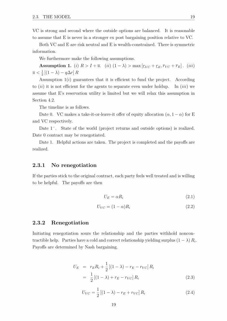
2.3 The model
Consider an entrepreneur, E, who has an idea for an innovative start-up project,requiring investment funds I > 0. E lacks personal finance, and so approaches aventure capitalist, VC, for the required funds. VC has all the bargaining power exante and makes a take-it-or-leave-it offer on equity share α subject to E receivingtheir reservation utility u. However, at some stage in the venture’s development,the parties can threaten to holdup each other, possibly forcing renegotiation of theterms of the contract.
We take the view, developed by Hart and Moore (2008) and Hart (2009), thatthe original contract forms a reference point. The contract forms the expectationswhat each party is entitled. If the party receives what he is entitled to under theoriginal contract, they feel well treated. But if the other party forces renegotiation,the relationship sours. As a consequence the parties withhold non-contractiblehelpful actions.
For the full project returns to be realized, each party must take helpful actionsex post. Helpful actions are too complex to be described in ex ante contract butex post some helpful actions become contractible. If all helpful actions are taken,project value is RH with probability p or RL with probability (1− p) where RL < RH
and R = pRH + (1− p)RL. If only contractible actions are taken, project value is(1− λ)Ri for i = L,H. Withdrawal of noncontractible helpful actions leads to aloss of surplus equal to λRi. Suppose the project value is close to −∞ if no helpfulactions are taken.
Agent is willing to be helpful if they feel well treated, that is, if they get theequity share under the original contract. Renegotiation leads to cold but correctrelationship. Only contractible helpful actions are taken.
Staged financing and planned renegotiation are common in financial contractsbetween VC and E. In such a situation renegotiation creates a win-win and isfriendly. Our focus is not on such renegotiation. We focus on unplanned renego-tiation which may be framed in terms of raising funding but is triggered by highrelative outside option of one party. Such renegotiation is unfriendly and leads tosouring of the relationship.
Outside options at the time of potential renegotiation are assumed to be rERi
for E and rV CRi for VC where 0 ≤ ri ≤ 1 for i = E, V C. Consider a binary casewhere the outside options are rV C > rE > 0 with probability q and rV C = rE > 0with probability (1− q). Denote ∆r = (rV C − rE) . We have two states: one where
18
2.3. THE MODEL 19
VC is strong and second where the outside options are balanced. It is reasonableto assume that E is never in a stronger ex post bargaining position relative to VC.
Both VC and E are risk neutral and E is wealth-constrained. There is symmetricinformation.
We furthermore make the following assumptions.Assumption 1. (i) R > I + u. (ii) (1− λ) > max [rV C + rE, rV C + rE] . (iii)
u < 12 [(1− λ)− q∆r]R
Assumption 1(i) guarantees that it is efficient to fund the project. Accordingto (ii) it is not efficient for the agents to separate even under holdup. In (iii) weassume that E’s reservation utility is limited but we will relax this assumption inSection 4.2.
The timeline is as follows.Date 0. VC makes a take-it-or-leave-it offer of equity allocation (α, 1−α) for E
and VC respectively.Date 1−. State of the world (project returns and outside options) is realized.
Date 0 contract may be renegotiated.Date 1. Helpful actions are taken. The project is completed and the payoffs are
realized.
2.3.1 No renegotiation
If the parties stick to the original contract, each party feels well treated and is willingto be helpful. The payoffs are then
UE = αRi (2.1)
UV C = (1− α)Ri (2.2)
2.3.2 Renegotiation
Initiating renegotiation sours the relationship and the parties withhold noncon-tractible help. Parties have a cold and correct relationship yielding surplus (1− λ)Ri.
Payoffs are determined by Nash bargaining.
UE = rERi + 12 [(1− λ)− rE − rV C ]Ri
= 12 [(1− λ) + rE − rV C ]Ri (2.3)
UV C = 12 [(1− λ)− rE + rV C ]Ri (2.4)
19
20 CHAPTER 2. CONTRACTS AS REFERENCE POINTS IN VC
E will not initiate renegotiation if and only if their payoff according to the originalcontract (2.1) is larger than what they can obtain by renegotiating (2.3) .
α ≥ 12 [(1− λ) + rE − rV C ] ≡ αL (2.5)
Similarly, VC will not initiate renegotiation if and only if their payoff in (2.2) isgreater than in (2.4) .
(1− α) ≥ 12 [(1− λ)− rE + rV C ]
⇔ α ≤ 12 [(1 + λ) + rE − rV C ] ≡ αH (2.6)
Therefore renegotiation and holdup can be avoided if and only if
αL ≤ α ≤ αH (2.7)
We refer to (2.7) as a self-enforcing range. To avoid holdup VC has to choose αat date 0 contract so that it falls in the self-enforcing range. The difficulty is thatαL and αH are random variables realized at date 1−. Furthermore, VC’s maininterest is not in avoiding the holdup but in maximizing their own expected payoff.Therefore VC aims to minimize α but they have to take into account that too lowα may trigger holdup ex post.
Using equations (2.5) and (2.6) we can work out the self-enforcing range in eachstate.
αL = 12 [(1− λ)−∆r] (2.8)
αH = 12 [(1 + λ)−∆r] (2.9)
αL = 12 (1− λ) (2.10)
αH = 12 (1 + λ) (2.11)
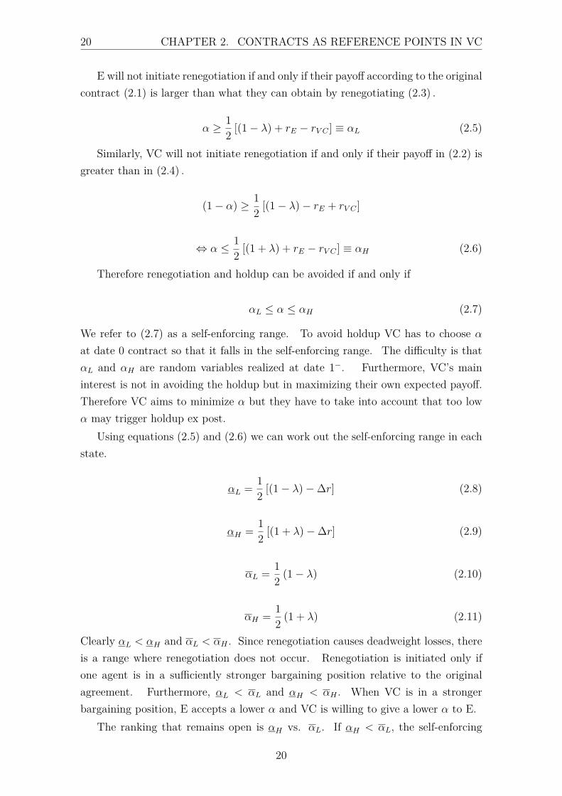
Clearly αL < αH and αL < αH . Since renegotiation causes deadweight losses, thereis a range where renegotiation does not occur. Renegotiation is initiated only ifone agent is in a sufficiently stronger bargaining position relative to the originalagreement. Furthermore, αL < αL and αH < αH . When VC is in a strongerbargaining position, E accepts a lower α and VC is willing to give a lower α to E.
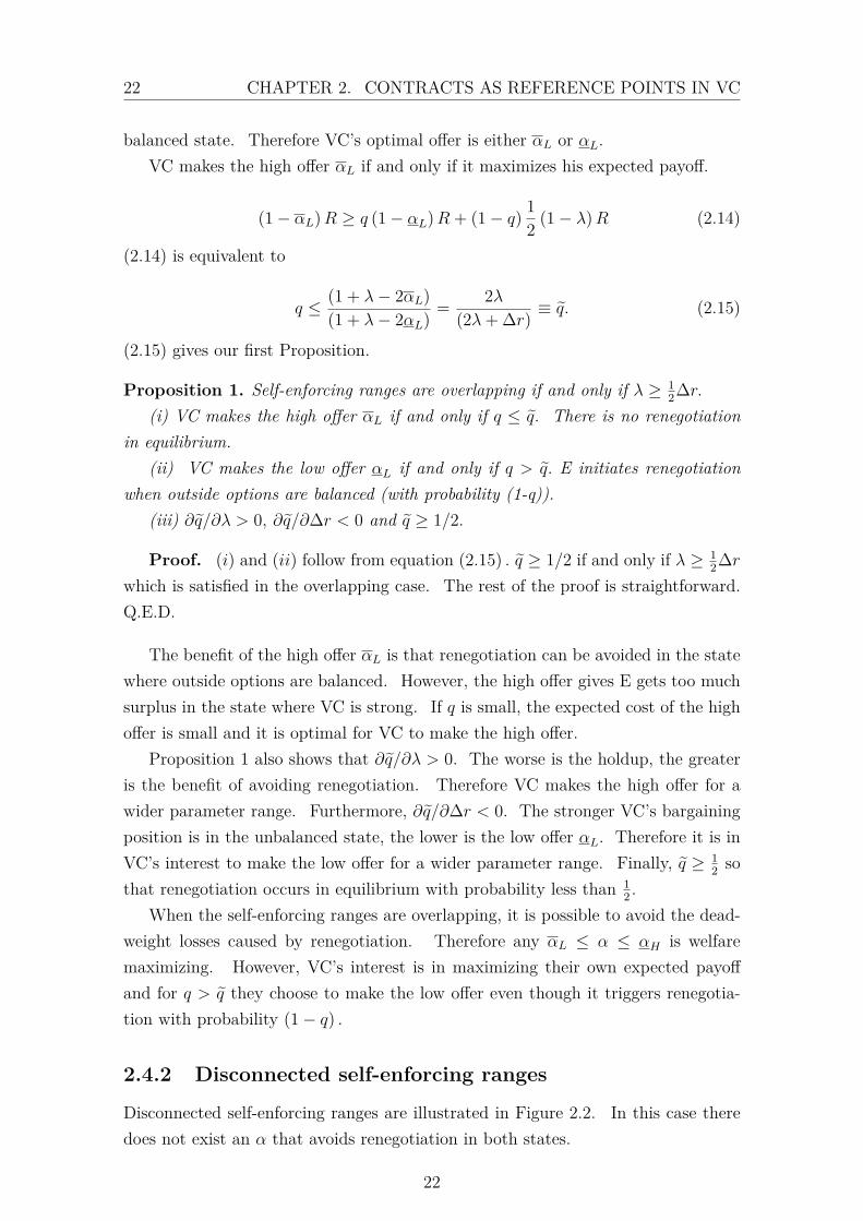
The ranking that remains open is αH vs. αL. If αH < αL, the self-enforcing
20

2.4. OPTIMAL CONTRACT21
ranges are disconnected: αL < αH < αL < αH . α that falls within the self-enforcingrange in one state is outside of it in the other state. While if αL ≤ αH , the self-enforcing ranges are overlapping: αL < αL ≤ αH < αH . Then it is possible to findα that is within the self-enforcing range in both states. Comparison of (2.9) and(2.10) shows that the self-enforcing ranges are overlapping if and only if
λ ≥ 12∆r.
αL is decreasing in λ since the worse is the holdup, the lower α E will accept. WhileαH is increasing in λ because the worse is the holdup, the higher share VC is willingto give away. Therefore for high enough λ we have αL ≤ αH .
2.4 Optimal contract
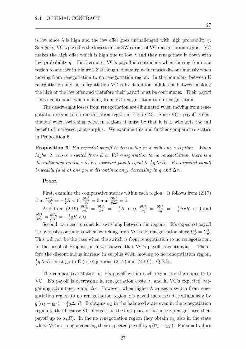
2.4.1 Overlapping self-enforcing ranges
We start the analysis from the case of overlapping self-enforcing ranges as demon-strated in Figure 2.1. VC aims to minimize their offer of equity share to E but hasto take into account potential ex post holdup.
If VC makes a high offer αL, there is no renegotiation in either state as αL fallswithin the self-enforcing range in both states. VC’s expected payoff is then
U1V C = (1− αL)R (2.12)
where superscript 1 denotes no renegotiation. It is never optimal to offer α > αL
since α = αL is enough to avoid holdup in both states and higher α would simplygive more surplus to E.
Alternatively VC can make a low offer αL. By this offer VC can avoid holdupin the state where they are strong. But E will renegotiate in the state where theoutside options are balanced (with probability (1 − q)). By renegotiating E getshalf of the surplus but due to holdup the surplus drops to (1− λ)R. VC’s expectedpayoff is then
U2V C = q (1− αL)R + (1− q) 1
2 (1− λ)R (2.13)
where superscript 2 denotes E renegotiation. VC would never make an offer belowαL because it would be renegotiated in every state leading to deadweight losses.Furthermore, any offer αL < α < αL is strictly dominated by α = αL. Offeringmore than is strictly required in the state where VC is strong would simply givesurplus away to E as the offer is not high enough to avoid renegotiation in the
21
22 CHAPTER 2. CONTRACTS AS REFERENCE POINTS IN VC
balanced state. Therefore VC’s optimal offer is either αL or αL.VC makes the high offer αL if and only if it maximizes his expected payoff.
(1− αL)R ≥ q (1− αL)R + (1− q) 12 (1− λ)R (2.14)
(2.14) is equivalent to
q ≤ (1 + λ− 2αL)(1 + λ− 2αL) = 2λ
(2λ+ ∆r) ≡ q̃. (2.15)
(2.15) gives our first Proposition.
Proposition 1. Self-enforcing ranges are overlapping if and only if λ ≥ 12∆r.
(i) VC makes the high offer αL if and only if q ≤ q̃. There is no renegotiationin equilibrium.
(ii) VC makes the low offer αL if and only if q > q̃. E initiates renegotiationwhen outside options are balanced (with probability (1-q)).
(iii) ∂q̃/∂λ > 0, ∂q̃/∂∆r < 0 and q̃ ≥ 1/2.
Proof. (i) and (ii) follow from equation (2.15) . q̃ ≥ 1/2 if and only if λ ≥ 12∆r
which is satisfied in the overlapping case. The rest of the proof is straightforward.Q.E.D.
The benefit of the high offer αL is that renegotiation can be avoided in the statewhere outside options are balanced. However, the high offer gives E gets too muchsurplus in the state where VC is strong. If q is small, the expected cost of the highoffer is small and it is optimal for VC to make the high offer.
Proposition 1 also shows that ∂q̃/∂λ > 0. The worse is the holdup, the greateris the benefit of avoiding renegotiation. Therefore VC makes the high offer for awider parameter range. Furthermore, ∂q̃/∂∆r < 0. The stronger VC’s bargainingposition is in the unbalanced state, the lower is the low offer αL. Therefore it is inVC’s interest to make the low offer for a wider parameter range. Finally, q̃ ≥ 1
2 sothat renegotiation occurs in equilibrium with probability less than 1
2 .
When the self-enforcing ranges are overlapping, it is possible to avoid the dead-weight losses caused by renegotiation. Therefore any αL ≤ α ≤ αH is welfaremaximizing. However, VC’s interest is in maximizing their own expected payoffand for q > q̃ they choose to make the low offer even though it triggers renegotia-tion with probability (1− q) .
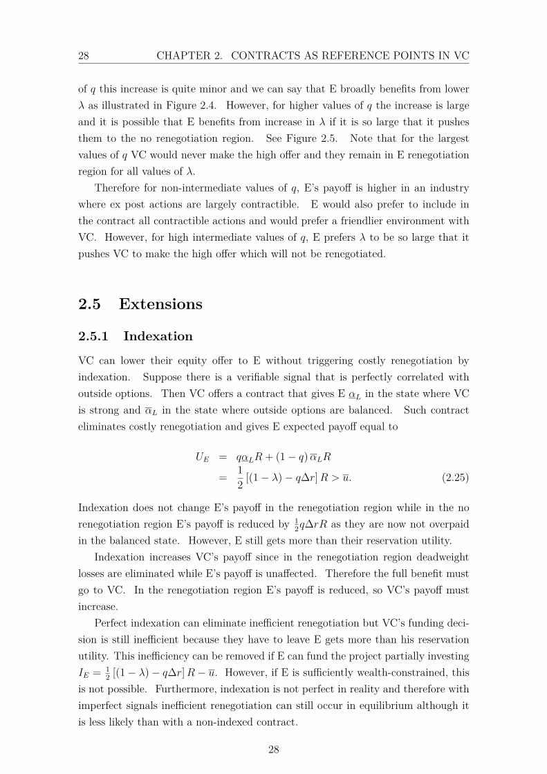
2.4.2 Disconnected self-enforcing ranges
Disconnected self-enforcing ranges are illustrated in Figure 2.2. In this case theredoes not exist an α that avoids renegotiation in both states.
22
2.4. OPTIMAL CONTRACT23
When VC makes the high offer αL, E will not renegotiate it. However, VChimself will trigger renegotiation when they are in a strong bargaining position.VC’s expected payoff from making the high offer αL is
U3V C = q
12 [(1− λ) + ∆r]R + (1− q) (1− αL)R. (2.16)
where superscript 3 denotes VC renegotiation. Alternatively, VC can make the lowoffer αL and E renegotiates it when outside options are balanced. VC’s expectedpayoff from making the low offer αL is
U2V C = q (1− αL)R + (1− q) 1
2 (1− λ)R.
VC makes the high offer αL if and only if
q12 [(1− λ) + ∆r]R + (1− q) (1− αL)R ≥ q (1− αL)R + (1− q) 1
2 (1− λ)R
⇔ q ≤ 1 + λ− 2αL2 + 2λ− 2αL − 2αL − rV C + rE
= 12
This result is summarized in Proposition 2.
Proposition 2. Self-enforcing ranges are disconnected if and only if λ ≤ 12∆r.
(i) VC makes the high offer αL if and only if q ≤ 12 . VC initiates renegotiation
when they are in a strong bargaining position (with probability q).(ii) VC makes the low offer αL if and only if q > 1
2 . E initiates renegotiationwhen outside options are balanced (with probability (1-q)).
In the disconnected case both αL and αL work well in one state but triggercostly renegotiation in the other state. VC’s optimal offer then simply minimizesthe probability of renegotiation. VC’s interests are aligned with social welfare inthis case.
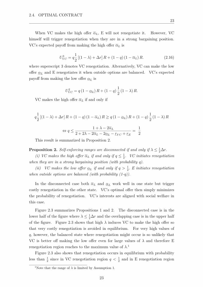
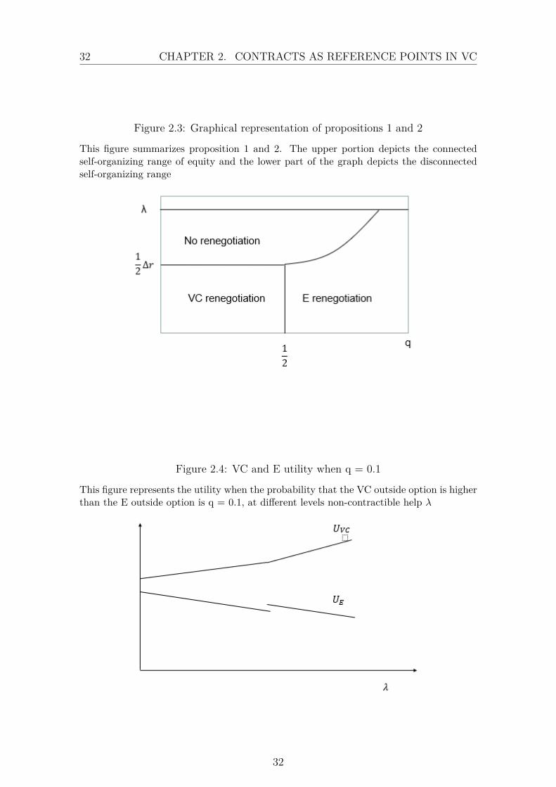
Figure 2.3 summarizes Propositions 1 and 2. The disconnected case is in thelower half of the figure where λ ≤ 1
2∆r and the overlapping case is in the upper halfof the figure. Figure 2.3 shows that high λ induces VC to make the high offer sothat very costly renegotiation is avoided in equilibrium. For very high values ofq, however, the balanced state where renegotiation might occur is so unlikely thatVC is better off making the low offer even for large values of λ and therefore Erenegotiation region reaches to the maximum value of λ.1
Figure 2.3 also shows that renegotiation occurs in equilibrium with probabilityless than 1
2 since in VC renegotiation region q < 12 and in E renegotiation region
1Note that the range of λ is limited by Assumption 1.
23
24 CHAPTER 2. CONTRACTS AS REFERENCE POINTS IN VC
(1− q) < 12 . Finally, the boundary between E renegotiation and no renegotiation is
positively sloping. The payoffs within the no renegotiation region do not dependon q while within the E renegotiation region the higher is q the less likely it is thatE triggers renegotiation. Therefore VC makes the low offer for higher values of λresulting in the positively sloping boundary.
2.4.3 VC contracts as reference points
E’s expected payoff when there is no renegotiation equals
U1E = αLR = 1
2 (1− λ)R. (2.17)
While E’s expected payoff when either they or the VC renegotiates is
U2E = qαLR + (1− q) 1
2 (1− λ)R = 12 [(1− λ)− q∆r]R (2.18)
U3E = q
12 [(1− λ)−∆r]R + (1− q)αLR = 1
2 [(1− λ)− q∆r]R = U2E (2.19)
The expression for E’s payoff does not depend on whether it is E or VC who triggersrenegotiation. When VC makes the low offer αL E renegotiates it up to αL in thebalanced state (although now αL includes the deadweight loss). While when VCmakes the high offer αL, they renegotiate it down to αL (including the deadweightloss) when they are in a strong bargaining position. That is why E’s expected payoffequals qαLR + (1− q)αLR = 1
2 [(1− λ)− q∆r]R no matter who initiates renego-tiation. Note that although the expressions are equivalent in both renegotiationcases, the payoffs are not since the different regions arise in equilibrium for differentparameter values. We will return to this later.
Equations (2.17) − (2.19) show that UE > u under Assumption 1. VC aims tominimize the equity offer to E but has to take into account that too low offer cantrigger costly renegotiation in some states. Although VC has all the bargainingpower, he chooses to leave some surplus above u to E to guarantee a smootherex post relationship. (In Section 4.2 we explore higher values of u in which caseparticipation constraint can become binding for some parameter values.)
Proposition 3. Under the optimal contract UE > u.
VC’s expected payoff for each region can be written as
U1V C = (1− αL)R = 1
2 (1 + λ)R (2.20)
24

2.4. OPTIMAL CONTRACT25
U2V C = q (1− αL)R + 1
2 (1− q) (1− λ)R
= 12 (1 + λ)R + 1
2q∆rR− (1− q)λR (2.21)
U3V C = 1
2q [(1− λ) + ∆r]R + (1− q) (1− αL)R
= 12 (1 + λ)R + 1
2q∆rR− qλR (2.22)
We can show that VC’s funding decision is inefficient. Not all profitable projectsfor which R ≥ I+u will be funded. This is because E’s payoff is strictly greater thanu and, furthermore, renegotiation can occur in equilibrium leading to deadweightlosses.
Proposition 4. VC’s funding decision is inefficient.
Proof.
It is efficient to fund projects for which R ≥ I + u. VC funds projects for whichUV C ≥ I. VC’s funding decision is inefficient if and only if UV C < R− u which issatisfied since
UV C + u < UV C + UE ≤ R.
The first inequality is satisfied since E’s participation constraint is not binding.The second (weak) inequality is satisfied since costly renegotiation may occur withpositive probability.
Q.E.D.
We will next turn to comparative statics.
Proposition 5. VC’s expected payoff is increasing in λ and weakly increasing in qand ∆r.
Proof.
First, we examine the comparative statics within each region. It follows from(2.20) that ∂U1
V C
∂λ= 1
2R > 0, ∂U1V C
∂q= 0 and ∂U1
V C
∂∆r = 0.From (2.21) we have ∂U2
V C
∂λ= 1
2 (2q − 1)R > 0 since q > 12 in the region where E
renegotiates, ∂U2V C
∂q=(λ+ 1
2∆r)R > 0 and ∂U2
V C
∂∆r = 12qR > 0.
From (2.22) we obtain ∂U3V C
∂λ= 1
2 (1− 2q)R > 0 since q < 12 in the region where
VC renegotiates, ∂U3V C
∂q=(
12∆r − λ
)R > 0 since this is the disconnected case and
∂U3V C
∂∆r = 12qR > 0.
25

26 CHAPTER 2. CONTRACTS AS REFERENCE POINTS IN VC
Second, we need to verify that VC’s payoff is continuous when switching from oneregion to another. Since the critical boundary between the regions is determinedby U1
V C = U2V C and U3
V C = U2V C we only need to verify the continuity between U1
V C
and U3V C . Substituting the boundary value λ = 1
2∆r in the third term in (2.16), weobtain
U3V C = 1
2 (1 + λ)R + 12q∆rR− q
12∆rR = 1
2 (1 + λ)R = U1V C .
Therefore VC’s payoff is continuous between U1V C and U3
V C . Q.E.D.
Proposition 5 shows that VC benefits from costlier renegotiation. Higher λ hastwo effects on VC’s expected payoff.
∂U2V C
∂λ= −qR∂αL
∂λ− 1
2 (1− q)R > 0 (2.23)
∂U3V C
∂λ= −1
2qR− (1− q)R∂αL∂λ
> 0 (2.24)
Higher λ results in E accepting a lower equity share without triggering renegotiation,∂αL
∂λ= ∂αL
∂λ= −1
2 , benefiting VC. On the other hand, when renegotiation does occur,higher λ reduces surplus and VC’s payoff. The positive effect dominates because inequilibrium renegotiation occurs with probability less than 1
2 , that is, in equilibrium(1− q) < 1
2 in (2.23) and q < 12 in (2.24) .
λ depends on the opportunity to holdup as only noncontractible helpful actionscan be withdrawn. VC’s expected payoff is then higher in an industry wherehigher proportion of ex post helpful actions are noncontractible such as humancapital intensive industries. Furthermore, it may be in VC’s interest to leave outfrom the contract some actions that could be contracted on.
Alternatively or additionally, λ depends on the strength of the reaction. VCwould benefit from creating an environment with more hostile reaction to renegoti-ation and keeping E on their toes.2 Then VC has two instruments to keep E frominitiating renegotiation: ex ante equity offer that leaves E some surplus above u anda hostile reaction to ex post renegotiation.
VC’s expected payoff is also (weakly) increasing in the probability that he is ina strong bargaining position, q, and the degree of their bargaining advantage, ∆r.3
Since VC’s payoff is increasing in λ and q, VC’s payoff is the highest in theNE corner of E renegotiation region in Figure 2.3. VC makes the low offer which
2However, that is limited by E’s participation constraint. λ cannot be so high that that E’sexpected payoff goes below u.
3Within the no renegotiation region VC’s payoff does not depend on q or ∆r. In the renego-tiation region their payoff is strictly increasing in q or ∆r.
26
2.4. OPTIMAL CONTRACT27
is low since λ is high and the low offer goes unchallenged with high probability q.Similarly, VC’s payoff is the lowest in the SW corner of VC renegotiation region. VCmakes the high offer which is high due to low λ and they renegotiate it down withlow probability q. Furthermore, VC’s payoff is continuous when moving from oneregion to another in Figure 2.3 although joint surplus increases discontinuously whenmoving from renegotiation to no renegotiation region. In the boundary between Erenegotiation and no renegotiation VC is by definition indifferent between makingthe high or the low offer and therefore their payoff must be continuous. Their payoffis also continuous when moving from VC renegotiation to no renegotiation.
The deadweight losses from renegotiation are eliminated when moving from rene-gotiation region to no renegotiation region in Figure 2.3. Since VC’s payoff is con-tinuous when switching between regions it must be that it is E who gets the fullbenefit of increased joint surplus. We examine this and further comparative staticsin Proposition 6.
Proposition 6. E’s expected payoff is decreasing in λ with one exception. Whenhigher λ causes a switch from E or VC renegotiation to no renegotiation, there is adiscontinuous increase in E’s expected payoff equal to 1
2q∆rR. E’s expected payoffis weakly (and at one point discontinuously) decreasing in q and ∆r.
Proof.
First, examine the comparative statics within each region. It follows from (2.17)that ∂U1
E
∂λ= −1
2R < 0, ∂U1E
∂q= 0 and ∂U1
E
∂∆r = 0.And from (2.19) ∂U2
E
∂λ= ∂U3
E
∂λ= −1
2R < 0, ∂U2E
∂q= ∂U3
E
∂q= −1
2∆rR < 0 and∂U2
E
∂∆r = ∂U3E
∂∆r = −12qR < 0.
Second, we need to consider switching between the regions. E’s expected payoffis obviously continuous when switching from VC to E renegotiation since U2
E = U3E.
This will not be the case when the switch is from renegotiation to no renegotiation.In the proof of Proposition 5 we showed that VC’s payoff is continuous. There-fore the discontinuous increase in surplus when moving to no renegotiation region,12q∆rR, must go to E (see equations (2.17) and (2.19)). Q.E.D.
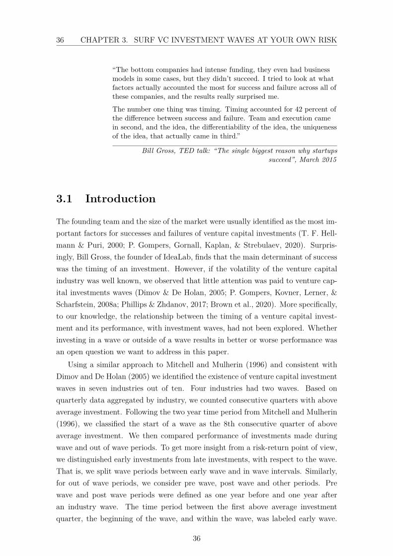
The comparative statics for E’s payoff within each region are the opposite toVC. E’s payoff is decreasing in renegotiation costs λ, and in VC’s expected bar-gaining advantage, q and ∆r. However, when higher λ causes a switch from rene-gotiation region to no renegotiation region E’s payoff increases discontinuously byq (αL − αL) = 1
2q∆rR. E obtains αL in the balanced state even in the renegotiationregion (either because VC offered it in the first place or because E renegotiated theirpayoff up to αLR). In the no renegotiation region they obtain αL also in the statewhere VC is strong increasing their expected payoff by q (αL − αL) . For small values
27
28 CHAPTER 2. CONTRACTS AS REFERENCE POINTS IN VC
of q this increase is quite minor and we can say that E broadly benefits from lowerλ as illustrated in Figure 2.4. However, for higher values of q the increase is largeand it is possible that E benefits from increase in λ if it is so large that it pushesthem to the no renegotiation region. See Figure 2.5. Note that for the largestvalues of q VC would never make the high offer and they remain in E renegotiationregion for all values of λ.
Therefore for non-intermediate values of q, E’s payoff is higher in an industrywhere ex post actions are largely contractible. E would also prefer to include inthe contract all contractible actions and would prefer a friendlier environment withVC. However, for high intermediate values of q, E prefers λ to be so large that itpushes VC to make the high offer which will not be renegotiated.
2.5 Extensions
2.5.1 Indexation
VC can lower their equity offer to E without triggering costly renegotiation byindexation. Suppose there is a verifiable signal that is perfectly correlated withoutside options. Then VC offers a contract that gives E αL in the state where VCis strong and αL in the state where outside options are balanced. Such contracteliminates costly renegotiation and gives E expected payoff equal to
UE = qαLR + (1− q)αLR
= 12 [(1− λ)− q∆r]R > u. (2.25)
Indexation does not change E’s payoff in the renegotiation region while in the norenegotiation region E’s payoff is reduced by 1
2q∆rR as they are now not overpaidin the balanced state. However, E still gets more than their reservation utility.
Indexation increases VC’s payoff since in the renegotiation region deadweightlosses are eliminated while E’s payoff is unaffected. Therefore the full benefit mustgo to VC. In the renegotiation region E’s payoff is reduced, so VC’s payoff mustincrease.
Perfect indexation can eliminate inefficient renegotiation but VC’s funding deci-sion is still inefficient because they have to leave E gets more than his reservationutility. This inefficiency can be removed if E can fund the project partially investingIE = 1
2 [(1− λ)− q∆r]R− u. However, if E is sufficiently wealth-constrained, thisis not possible. Furthermore, indexation is not perfect in reality and therefore withimperfect signals inefficient renegotiation can still occur in equilibrium although itis less likely than with a non-indexed contract.
28
2.6. CONCLUSION 29
2.5.2 E’s participation constraint
In Assumption 1 we assumed that E’s reservation utility is limited, u < 12 [(1− λ)− q∆r]R.
Under this assumption E’s participation constraint is not binding under the optimalcontract. If u can take higher values, then VC has to increase their offer from αL
or αL to satisfy E’s participation constraint. Consider the case of perfect indexing.
The highest payoff VC can guarantee to E is to offer αH in the balanced stateand αH in the state where VC is strong. This gives E expected payoff equal to
UE = qαHR + (1− q)αHR
= q12 [(1 + λ)−∆r]R + (1− q) 1
2 (1 + λ)R
= 12 [(1 + λ)− q∆r]R
Therefore for any u ∈[
12 [(1− λ)− q∆r]R, 1
2 [(1 + λ)− q∆r]R]VC offers α ∈
[αL, αH ] and α ∈ [αL, αH ] such that E’s participation constraint holds with equality.If u > 1
2 [(1 + λ)− q∆r]R, the relationship is not feasible as VC cannot guaranteeto renegotiate down very large equity offers ex post.
2.5.3 n states
In our main model there are two states for outside options. Now suppose thatthere are n states and denote by ∆ri i = 1, 2, ..., n the difference in outside optionsin state i. Denote by ∆rmax the largest difference and assume that there exists astate where VC and E have balanced outside options but E is never in a strongerbargaining position than E so that the minimum value for ∆ri equals zero. Finally,denote by αiL and αiH the critical equity shares in state i.
Self-enforcing ranges are overlapping if max αiL ≤ min αiH which is equivalentto λ ≥ 1
2∆rmax. Then VC can avoid renegotiation by offering α = 12 (1− λ) to E.
Otherwise VC renegotiates in all the states where α > αiH and E renegotiates in allthe states where α < αiL.
2.6 Conclusion
We have applied contracts as reference points approach to venture capital. Wefind that E’s participation constraint is not binding even when VC has all ex antebargaining power. VC chooses to leave some surplus to E to guarantee a smootherex post relationship. Project funding is inefficient due to E’s additional surplus
29

30 CHAPTER 2. CONTRACTS AS REFERENCE POINTS IN VC
and renegotiation occurring in some states. VC’s expected payoff is increasing inrenegotiation costs as E will accept a lower equity offer.
We will extend the analysis to contractual clauses such as vesting arrangementsand noncompete clauses which enable VC to lower the equity offer to E. Further-more, we will relax the assumption that it is efficient for VC and E not to separateeven under holdup and introduce a state where the company is liquidated or E isreplaced.
30
2.7. FIGURES 31
2.7 Figures
Figure 2.1: Overlapping self-enforcing ranges
This figure represents the range of equity share α offered to the entrepreneur when theVC is in a strong position and when the E and VC have balanced outside options
Figure 2.2: Disconnected self-enforcing ranges
This figure represents a range of equity offers which does not avoid renegotiation
31
32 CHAPTER 2. CONTRACTS AS REFERENCE POINTS IN VC
Figure 2.3: Graphical representation of propositions 1 and 2
This figure summarizes proposition 1 and 2. The upper portion depicts the connectedself-organizing range of equity and the lower part of the graph depicts the disconnectedself-organizing range
Figure 2.4: VC and E utility when q = 0.1
This figure represents the utility when the probability that the VC outside option is higherthan the E outside option is q = 0.1, at different levels non-contractible help λ
32

2.7. FIGURES 33
Figure 2.5: VC and E utility when q = 0.6
This figure represents the utility when the probability that the VC outside option is higherthan the E outside option is q = 0.6, at different levels of non-contractible help λ
33

34 CHAPTER 2. CONTRACTS AS REFERENCE POINTS IN VC
34

Chapter 3
Surf VC investment waves at yourown risk
joint work with Caroline Genc, Université Paris Dauphine -PSL
Abstract : Although the volatility of the venture capital industry is wellknown, it is not known if investing in a wave or outside of a wave resultsin better or worse performance. In this paper, we investigated, in aninvestment wave context, the relationship between the timing of a ven-ture capital investment and its performance. We argue that investmentsmade before a wave, or early in a wave, provided a higher probability ofsuccess relative to those made in a wave or in any other period. We showthat venture capitalists, with industry experience and high specialization,were more likely to invest earlier in waves when the VC were well con-nected to investors in an industry by a social network. Without industryconnections, they delayed their investments, to within the wave, whichhad a lower success rate.
35
36 CHAPTER 3. SURF VC INVESTMENT WAVES AT YOUR OWN RISK
“The bottom companies had intense funding, they even had businessmodels in some cases, but they didn’t succeed. I tried to look at whatfactors actually accounted the most for success and failure across all ofthese companies, and the results really surprised me.
The number one thing was timing. Timing accounted for 42 percent ofthe difference between success and failure. Team and execution camein second, and the idea, the differentiability of the idea, the uniquenessof the idea, that actually came in third.”
Bill Gross, TED talk: “The single biggest reason why startupssucceed”, March 2015
3.1 Introduction
The founding team and the size of the market were usually identified as the most im-portant factors for successes and failures of venture capital investments (T. F. Hell-mann & Puri, 2000; P. Gompers, Gornall, Kaplan, & Strebulaev, 2020). Surpris-ingly, Bill Gross, the founder of IdeaLab, finds that the main determinant of successwas the timing of an investment. However, if the volatility of the venture capitalindustry was well known, we observed that little attention was paid to venture cap-ital investments waves (Dimov & De Holan, 2005; P. Gompers, Kovner, Lerner, &Scharfstein, 2008a; Phillips & Zhdanov, 2017; Brown et al., 2020). More specifically,to our knowledge, the relationship between the timing of a venture capital invest-ment and its performance, with investment waves, had not been explored. Whetherinvesting in a wave or outside of a wave results in better or worse performance wasan open question we want to address in this paper.
Using a similar approach to Mitchell and Mulherin (1996) and consistent withDimov and De Holan (2005) we identified the existence of venture capital investmentwaves in seven industries out of ten. Four industries had two waves. Based onquarterly data aggregated by industry, we counted consecutive quarters with aboveaverage investment. Following the two year time period from Mitchell and Mulherin(1996), we classified the start of a wave as the 8th consecutive quarter of aboveaverage investment. We then compared performance of investments made duringwave and out of wave periods. To get more insight from a risk-return point of view,we distinguished early investments from late investments, with respect to the wave.That is, we split wave periods between early wave and in wave intervals. Similarly,for out of wave periods, we consider pre wave, post wave and other periods. Prewave and post wave periods were defined as one year before and one year afteran industry wave. The time period between the first above average investmentquarter, the beginning of the wave, and within the wave, was labeled early wave.
36
3.1. INTRODUCTION 37
Thus, pre wave and early wave investments were investments occurring in times ofhigher uncertainty compared to in wave or post wave investments. We classify theremaining investment times as out of wave or other periods.
We provided evidence that investments made before a wave, or early in a wave,present higher chances of success relative to those made in a wave or in any otherperiod. As we did not have data on the actual returns of investments, we baseour success definition on the nature of the exit. We consider that an investmentwas successful if the company went public, was acquired or merged (Cochrane,2005; Hochberg, Ljungqvist, & Lu, 2007; Phalippou & Gottschalg, 2009; Nanda,Samila, & Sorenson, 2020) . Hence, our results suggested that, although pre waveand early wave periods were characterized as high uncertainty, investing in themhad a higher success rate. On the contrary, in wave and post wave investmentsdecrease the success probability by almost 3 percentage points. In our empiricalspecification, we control for time-varying economic conditions that potentially affectVC investments by including time fixed effects. We also control for time-invariantindustry characteristics through industry fixed effects. Without year fixed effects,we observed an upward bias in our results, suggesting that the timing of the wavesplay an important role. Indeed, most of the first waves occur in periods of favorableeconomic conditions. By testing our hypothesis, individually, on the first industrywaves and second waves, when they existed, we confirmed that first waves had largereffects than the second waves. Controlling for time fixed effects, we found that ourmain results were stronger for the first waves. This was probably due to the largernumber of observations for the first waves. Nevertheless, we provided evidence thatin industries with two waves, investments occurring in the second wave were stillmore likely to fail compared to out of wave periods.
Our findings were in line with the theoretical predictions of Lee and Sunesson(2008) concerning private equity waves. We empirically supported the decreasingpattern of performance during venture capital waves. Higher risk was thus associatedwith higher return. On the contrary, delaying investments to reduce risk or waitingto “share the blame” was more likely to predict failure. An alternative approachwas that pre and early wave periods were less risky than they were perceived amongventure capitalists. Those who invest in such periods may be more aware of theactual risk. Regarding the under performance of in wave investments, our resultswere consistent with prior research on private equity (Kaplan & Stromberg, 2009;Robinson & Sensoy, 2016) and merger wave (Moeller, Schlingemann, & Stulz, 2005;Yan, 2011; Duchin & Schmidt, 2013).
We further explored firm and fund level factors that influence the decision toinvest in a given time category. For instance, P. Gompers et al. (2008a) showed thatVC firms that invest the most during favorable public market signals were those
37
38 CHAPTER 3. SURF VC INVESTMENT WAVES AT YOUR OWN RISK
with the most industry experience. In addition, they argue that such VC firms didnot overreact to public signals since there was no evidence of a negative impact ontheir performance.
In our analysis, we determine the profiles of VC firms that were more likely toinvest in the different timing categories we study in this paper. More specifically, weexamined industry specific characteristics like experience, specialization and socialnetwork. As liquidity was an important factor which drives wave (Harford, 2005),we also investigate if funds with more liquidity invest in specific periods. Withoutaccess to data about capital committed by limited partners, we base our analysis ona liquidity ratio, constructed from the amounts invested by funds at each investmentdate. All of these characteristics, as well as the outcome of an investment itself, wereclosely related to the quality of the VC. Even though Nanda et al. (2020) did notfind evidence of VCs’ ability to find optimal places and times to invest, they arguethat initial successes had persistent effects explaining future success. Thus, we alsoconcentrate on past fund performance.
We found that VCs with industry experience and industry specialization weremore likely to invest in wave or one year after. Also, VC firms that were morespecialized in an industry were less prone to invest in pre wave or early wave periods.These results suggested that experienced and specialized VC firms were less likely totake risk by investing in high uncertainty periods. This may appear quite surprisingat first glance since concentrated expertise was expected to predict early entry inindustry waves, as suggested by Dimov and De Holan (2005). One might expect VCswith better reputation, more industry experience or specialization to have enoughknowledge and resources to invest earlier.
Considering that network was a key element in venture capital to detect goodinvestment opportunities and to better perform (Hochberg et al., 2007), we reana-lyze these characteristics while also including the social networks of VC firms. Weobserved that being well connected in the industry of the investment significantlydecreases the probability of investing during an industry wave. VCs who had in-dustry experience, and who were well connected in their industry, were more likely,by 35.9 percentage points, to invest early in a wave. Knowing that the performanceassociated with such investments was positive, VCs who were experienced and wellconnected in an industry might be more aware of the actual risk behind early in-vestments. As far as more specialized VCs were concerned, we showed that beingspecialized and well connected in an industry reduces the probability of investingin wave by 25.4 percentage points. Therefore, specialized investors who invested inwave or post wave, were less connected. We did not find evidence that VCs investin wave rather than early in a wave due to liquidity constraints. More fund liquidityincreases the probability of investing early in a wave by 15.9 percentage points, less
38
3.2. RELATED LITERATURE 39
liquidity did not increase the probability of investing in a wave. Hence, investorsdecide to delay their investments, probably due to the high perceived risk of earlyinvestments. However, we confirm that decisions to invest post wave may be re-lated to liquidity issues. As less constrained VCs were probably those with moresuccessful exit records, we verify if similar results were obtained with past perfor-mance. Consistently, we found that VCs with high successful exit rates were morelikely to invest in the pre wave and early wave periods. Those with low past per-formance were more likely to invest post wave. By contrast, past fund exit rate didnot influence the decision to invest in wave. If pre wave and early wave investments’outcome may be explained by VC firms’ past successes, this was not the case for inwave investments. Our findings suggested that the actual risk of early investmentsmight be lower than it appears. Experienced or specialized investors, who were wellconnected in an industry, may assess early investment risk more accurately.
This paper contributes to the literature in several aspects. To our knowledge,it was the first one to study the relationship between performance and the timingof venture capital investments with respect to waves. It was also the first empiricalstudy on waves that clearly distinguished early wave and in wave investments andsheds light on the performance pattern during the wave. While prior research onlycompares in wave and out of wave investments, our approach enable us to examinedit from a risk and return view. From a practical point of view, our findings implythat investors should reassess the risk associated with pre wave and early waveinvestments. In addition, our paper contribute to the venture capital literature byidentifying the characteristics of VCs who time their investments. Compared toprevious studies, with social network analysis, we were able to separate what wasdriven by experience, i.e the knowledge of the industry, and what was due to thesocial network of a VC firm.
The remainder of the paper was organized as follows: After reviewing the relatedliterature in section 4.2, section 4.4 describes the data. Section 3.4 investigates therelation between timing and performance. VC firm timing decisions, with respectto their characteristics,were explored in Section 3.5. Section 3.6 concludes.
3.2 Related literature
Even though the venture capital industry was known to be volatile, there were fewstudies focusing on venture capital waves (Dimov & De Holan, 2005; P. Gomperset al., 2008a; Phillips & Zhdanov, 2017) or private equity waves (Lee & Sunesson,2008; Brown et al., 2020). Most of the research on waves concentrated on M&A andIPO waves and investigated their drivers. More specifically, two hypotheses werecompeting in the literature to explain waves creation. The neoclassical one suggested
39
40 CHAPTER 3. SURF VC INVESTMENT WAVES AT YOUR OWN RISK
that waves emerge as a response to economic, regulatory or technological shocks(Gort, 1969; Mitchell & Mulherin, 1996; Mulherin & Boone, 2000; Maksimovic &Phillips, 2001; Andrade, Mitchell, & Stafford, 2001; Harford, 2005; Gugler, Mueller,& Yurtoglu, 2006). Harford (2005) also empathized that liquidity was required totrigger a wave. Without liquidity, the reallocation of assets was difficult and industryshocks were not sufficient to trigger the waves. The behavioral approach explainedwaves through overvaluation or overreaction to perceived investment opportunities(Shleifer & Vishny, 2003; Rhodes-Kropf & Viswanathan, 2004; Lamont & Stein,2006). In line with these studies, while Dimov and De Holan (2005) provided supportfor the existence of venture capital investment waves, P. Gompers et al. (2008a) arguethat VCs with the most industry experience react to public market signals, but theydid not overreact. By exploring both VC investment and merger activity around theworld, Phillips and Zhdanov (2017) supported that active M&A markets predictedVC investments waves.
However, little was known about the relationship between the timing of a ven-ture capital investment and its performance in a wave context. Whether investingin a wave or outside of a wave resulted in better or worse performance was stillan open question. Lee and Sunesson (2008) theoretically established that the av-erage fund performance followed a decreasing pattern during private equity waves.Kaplan and Schoar (2005) showed that experienced and well-informed venture cap-italists’ performance was persistent and less sensitive to industry cycles and wavescompared to new entrants, especially in boom periods. Nanda and Rhodes-Kropf(2018) argue that VC firms benefited from persistent effects of their initial success.They did not find evidence of VCs’ ability to find optimal places and times to in-vest. Nevertheless, when choosing new industries or areas to invest, previous successdid not help outperform those without any initial success (Nanda & Rhodes-Kropf,2018). Considering private equity waves, Kaplan and Stromberg (2009) found thatbuyout funds raised in high fundraising years exhibited lower performance, in ab-solute terms, compared to funds raised in bust periods. Consistently, (Robinson &Sensoy, 2016) underlined that periods of high private equity fund raising predictedlow cash flows and market returns. Regarding merger waves, even though Mitchelland Mulherin (1996) did not focus on performance, they suggested that takeoversoccurring in these periods under performed. Moeller et al. (2005) showed that ac-quiring firm shareholders had large losses during the merger wave at the end ofthe 1990’s. Consistently, on-the-wave mergers were shown to be value destroyingas measured by the acquirer stock returns (Yan, 2011; Duchin & Schmidt, 2013).However, Maksimovic, Phillips, and Yang (2013) stated that mergers which occurredon-the-wave had higher productivity increases.
In this paper, we compared performance of investments made during venture
40
3.2. RELATED LITERATURE 41
capital wave and out of wave years. For that purpose, we split wave periods betweenearly wave and in wave intervals. Similarly, for out of wave periods, we consider prewave, post wave and other periods. To our knowledge, this study was the first oneto investigate investment performance in venture capital wave context. In addition,we explore firm and fund level factors that influence the decision to invest in a giventime category.
Investing earlier in a wave or before it, that was in periods of high uncertainty,meant accepting a high degree of risk. After the initial move into an industry, anincrease in the valuation of investments may occur and trigger the wave (Goriatchev,2002). In a dynamic behavioral approach of private equity waves, Lee and Sunesson(2008) stated that the average fund performance followed a decreasing pattern, sothat the latest entrants under performed the industry. We empirically exploredif these predictions held for venture capital investment waves. Thus, we expectedearly wave investments to be more likely to succeed relative to in wave or post waveinvestments. Hence, higher risk should be associated with higher return. On thecontrary, delaying investments to reduce such a risk or waiting to “share the blame”was expected to predict failure.
Moreover, Lee and Sunesson (2008) showed that younger partnerships performedbadly and were less likely to raise a follow-on fund. This likelihood was even lowerwhen they entered the market in boom times as expectations were high. Syndica-tion was a common feature in venture capital industry. As it was more frequentlyobserved, when the uncertainty level was high (Bygrave, 1987; Robbie, Wright, &Chiplin, 1997), we should have observed an increase in the number of syndicationsat the beginning of waves or early in waves. Among the reasons that justified thewillingness to syndicate, there was risk diversification (R. Wilson, 1968), informationsharing (Bygrave, 1987), mitigation of information asymmetries between the initialinvestor and later round investors (Admati & Pfleiderer, 1994), sharing evaluationskills for a second opinion (Lerner, 1994) or benefit from complementary skills andresources (Brander, Amit, & Antweiler, 2002). Brander et al. (2002) showed thatreturns and volatility were higher when investments were syndicated relative to in-dependent investments. Casamatta and Haritchabalet (2007) attributed this to animprovement in the selection process by gathering information on investment op-portunities through syndication. While there was no significant evidence about therelationship between syndicate size and the level of excess returns (Hege, Palomino,& Schwienbacher, 2008), the quality of a VC’s informal network was shown to bepositively correlated with his performance (Hochberg et al., 2007). Hence, amongVC firm level characteristics, we examined whether highly connected investors weremore likely to invest in periods of greater uncertainty and whether they performedwell in such periods. In addition, we explore the role played by experience in tim-
41
42 CHAPTER 3. SURF VC INVESTMENT WAVES AT YOUR OWN RISK
ing investments with respect to waves. P. Gompers et al. (2008a) found VC firmswith more industry experienced were those who reacted the most to public signalswithout reducing their performance. We then analyzed if more experienced or morespecialized VCs preferred to invest earlier or later relative to waves. Lastly, weverified if liquidity and past performance explained investment timing choices.
3.3 Data
Our dataset included venture capital deals contained in the Thompson One BankerPrivate Equity data base from 1995 to 2017. Available data from 1990 through 1994were excluded due to missing observations and to the smaller number of deals. Asthis paper was focused on venture capital investment waves, after defining the wavesand our main variables, we restricted our analysis to investments made betweenJanuary 1997 and September 2016. To identify industry waves, we followed Mitchelland Mulherin (1996) and considered that a wave begins after two years of aboveaverage investment in an industry. We removed the first two years of data as wecreated the beginning of the two year moving average to compute waves. For eachwave, we were interested in observations from the pre-wave (here defined as oneyear before the wave) to the post-wave (one year after the wave) periods. The lastwave we had in our dataset ended in March 2016 for the consumer related industry.Hence, for most of our observations, we did not know if the last year of data was apre-wave period. This was why we stopped our analysis, before the end of our dataset, in September 2016.
Even though the data source did not cover all venture capital deals, it providedround level information that was useful to track the history of investments at the VCfirm, fund and company level. However, data reported by the venture firms were notalways updated. Thus, we verified through internet searches if the firms reported asactive were actually active. Further verification showed, when the full history andclosing documents were available, the totals reported in Thomson One Banker werecoherent with the deal documents except for information by round which did notmatch exactly. This may be due to venture firms reporting both the totals for theinvestment round and their individual contribution to the round.
We then restricted our attention to investments made in the USA where theventure capital industry was more active. This provided a significant number ofobservations to study waves. Our sample consisted of 211 117 unique investmentsmade in 33 330 different companies by 7585 VC firms and 14 560 funds. Table 3.1to 3.3 described our data at the VC firm, fund and company levels. For our mainanalysis, we did not exclude follow on investments by a venture capital firm in asame company. A portfolio company may appear multiple times for the same VC
42
3.4. VC INVESTMENT WAVES AND PERFORMANCE 43
firm or fund if they reinvested in it. To identify effects of timing on performance, wekeep the re-investments for VC firms. Limiting the sample to the initial investmentmade by a VC firm in a company would introduce some bias. Indeed, if a failurewas due to an investment made in the wave while the first investment was made outof the wave, keeping only the first investment would attribute the failure to the outof wave timing. However, for robustness concerns, we also test our regressions on asub-sample excluding follow on investments and including controls for their timing.
3.4 VC investment waves and performance
3.4.1 Identification of waves
To identify venture capital investment waves, we followed the methodology of Mitchelland Mulherin (1996). We considered that a wave existed if, during a period of twoyears, the number of investments in an industry exceeded the average number ofinvestments in that industry. Our analysis was based on quarterly data aggregatedby industry. We compared the total number of quarterly investments made in anindustry (Industry Total) to the moving averages of the industry (Industry TotalMA). We then counted consecutive quarters for which Industry Total was higherthan Industry Total MA. Once the count met the defined threshold, we consideredthat the start of the wave. Once this threshold had been reached, all followingquarters with above average investments belonged to the in Wave period for thatindustry. The time period between the first above average investment quarter, thatwas the beginning of the wave, and the in wave period was called the early waveperiod. We also define pre wave and post wave periods as one year before and oneyear after the wave. The final above average investment quarter (the final in wavequarter) indicated the end of the wave. The main results reported in this paperwere obtained with a threshold of two years as in Mitchell and Mulherin (1996).
In Figure 3.1, we observed the evolution of the number of investments in eachindustry over time. Figure 3.2 visualized industry waves created from the counts ofconsecutive above average quarters for each industry. A count higher than 7 wasaccepted as an industry wave. Thus, we found that there were two waves in four ofthe industries while there was no wave in Communications and Media, ComputerHardware and Other Products industries.
In table 3.4, we reported the dates and the length of the waves for each industry.The first wave occurred during the last quarter of 1997 in the two main industries ofour sample. The last wave was the second one for the Consumer Related industrywhich started during the last quarter of 2013 and ended during the 1st quarter of2016. The Biotechnology sector had the longest wave of the sample with 23 quarters.
43
44 CHAPTER 3. SURF VC INVESTMENT WAVES AT YOUR OWN RISK
The number of successful exits was reported in table 3.5. For each phase of thewave, as defined in section 4.4, the total number of successful exits were listed. Thetotal exits were further broken down by the status of the company at the exit. Afinal row contained the results for all other time periods not defined by a wave. Thewave periods had 44,190 successful exits compared to 43,789 for all other periods.The majority of successful exits were investments made in one of the wave periodseven though the longest wave was 23 quarters and the total investment time, for theother periods, was 76 quarters.
Table 3.6 contained the descriptive statistics for the variables used in the analysisof the investment waves. The table was split into panels for the full sample in thedatabase, then, each phase of the wave and a final panel for post wave. The meanSuccess Rate was the highest for the Pre Wave in Panel B, at 56%, followed by EarlyWave at 53%. Early Wave and Pre Wave had a roughly 13 to 15 percent highersuccess rate than the mean rates for the other periods. These two phases of thewave also had the highest mean Fund Sequence by 0.11 to 0.19. The highest meanIndustry Specialization and Industry Experience were during the In Wave period.
3.4.2 Performance Measure
To identify the timing effects on performance, we based our analysis on a com-monly accepted definition of a successful exit. Determining whether an investmentin a company was successful or not was hard to accurately measure without thefull investment history and exit information for the company. The Thomson OneBanker Database had sparse investment information such as the amount invested,the valuation at investment, exit purchase price and deal terms (liquidity prefer-ences, ratchet, etc.). Without this information, we calculated the success variablebased on available information. This was difficult as, for example, an acquisitioncould be a success to the VC firm holding a liquidity preference and a failure toother firms and the entrepreneurs, who did not hold a liquidity preference. Whencompanies reported the status of “active” or “acquisition”, it was not possible to de-termine how well the company performed and whether or not it provided a positivereturn to the VC firm. Without a complete investment history and purchase price,we were not able to compute the internal rate of return. Therefore, we based oursuccess definition on the nature of the exit only. Following a widely used definitionof success, we consider an investment as successful if it resulted either in an IPO, aMerger or an Acquisition (Cochrane, 2005; Hochberg et al., 2007; Nanda et al., 2020;Phalippou & Gottschalg, 2009). We extended this definition to companies that were“Active”; in “Pending Acquisition”, or “In Registration” for robustness checks. Re-garding firms with an “Active” status for this second definition, we excluded those
44
3.4. VC INVESTMENT WAVES AND PERFORMANCE 45
who were marked as such for more than 7 years, following the method of (Phalippou& Gottschalg, 2009), since a typical VC fund life was 10 years (Sahlman, 1990) andmost investments were made within the first 3 years (Zarutskie, 2010).
In addition to the binary success variable, we also defined an Exit Rate vari-able. For most observations, Exit was informative about the future outcome of theinvestment. Exit Rate was the current rate, from the previous investments, of thefund when it makes an investment in a new company at the investment date. TheExit Rate was not updated until the last investment of a company. If, at the lastinvestment date, the reported stage was “Seed”, “Early Stage” or “Bridge Loan” wedid not consider that the firm was in stage which would normally exited and wasnot counted as a success.
Almost 80% of the successful exits corresponded to an acquisition. As half ofthe observations were from Computer Software and Services and Internet Specificindustries, half of the mergers and acquisitions appear in these industries as well.Almost 30% of the IPOs were in these two sectors while 17% were in the Biotechnol-ogy sector. We also observed that 46% of the companies in the Communications andMedia industry were successful while they only represent 7% of all successful com-panies. Regarding the whole sample, around 34% of the companies, which received46% of the investment rounds, agreed with our definition of success.
3.4.3 Performance with respect to waves
We first examined how investing in the different timing categories changed the like-lihood of a successful exit. We explored whether investments made before a wave,or early in a wave, were less likely to exit through an IPO or M&A , compared toother periods. We also documented the success rate of investments made during awave or after it.
Our main estimation approach was a series of linear probability models. Wechose this method to introduce year and industry fixed effects. The waves wereindustry specific and occurred at different time periods. Time fixed effects enabledus to control for time-varying economic conditions that potentially affected VCinvestments. With industry fixed effects we controlled for time-invariant industrycharacteristics. Thus, we were able to isolate what was due to the time period orindustry.
The following equation corresponds to our empirical specification that identifiedhow the outcome was affected by the timing of an investment:
Exiti = β0+β1Pre Waveis+β2Early Waveis+β3In Waveis+β4Post Waveis+β′Xi+ηs+ηt+εi
where Exiti was a dummy variable that equals one if investment i made in industry
45
46 CHAPTER 3. SURF VC INVESTMENT WAVES AT YOUR OWN RISK
s at time t had a successful exit (either IPO or M&A). Pre Waveis, Early Waveis,In Waveis and Post Waveis were dummy variables which take the value one if theinvestment date corresponded to one of the timing categories of industry s. The ref-erence group here was Other Periodsis which had the value of 1 when the investmentdate was not in one of the named wave time periods. ηs and ηt were respectivelyindustry and time fixed effects. Xi represented a vector of additional controls suchas the lagged fund exit rate, the number of VC firms investing in a company and thefund sequence. We had not included variables that were correlated with the timingcategories or explain the past fund success rate.
Table 3.7 reported the results obtained when considering all waves from all in-dustries. Columns (1) and (2) included only industry fixed effects. Time fixedeffects were added in columns (3) and (4). Column (1) confirmed that there weresignificant differences between investing earlier and investing later in a wave rela-tive to out of wave periods. An early wave investment had a 9.5 percentage higherchance to succeed compared to investments made outside of a wave period. Onthe contrary, investing in wave decreased the success probability by 1.2 percentagepoints. Column (2) introduced pre-wave and post-wave periods which respectivelyrepresented one year before and one year after a wave. The results reported in thiscolumn were interpreted with respect to out of wave periods that were neither preor post wave. The probability of having a successful exit, increased significantly, bymore than 10 percentage points, when an investment was made one year before awave (12.5 percentage points) or early in a wave (10.7 percentage points). Whilecolumn (2) did not suggest that in wave or post wave investments decreased thislikelihood, including time fixed effects in column (4) supported it. With time fixedeffects, columns (3) and (4) indicated that the results in columns (1) and (2) weresubjected to an upward bias, due to the timing of the waves themselves. Some ofthe industry waves, especially the first waves, occurred during favorable macroe-conomic conditions. After controlling for time fixed effects, our results supportedthat the timing of an investment, with respect to a wave, played an important role.When the decision to invest in a specific industry was made before, or just whenthe industry begins a wave, the probability of success increased by more than 1.5percentage points. If, however, the decision to invest was made once the industryattracted many VC firms, the probability of ending up with a successful exit fell byalmost 3 percentage points.
The decision to invest before or early in a wave was a risky one. There washigher perceived uncertainty in such periods compared to in wave or post waveperiods. However, our findings suggested that VC firms that accepted more risk, byinvesting earlier, did not reduce their performance. Hence, the risk as measured bythe volatility of success was not as high as it may appear.
46

3.4. VC INVESTMENT WAVES AND PERFORMANCE 47
Since we did not have the investment deal terms, we could not compare thevaluations across companies and wave periods. It was possible that the highersuccess rate was due to risk adjusted pricing. Investments early in the wave mayhave a lower valuation and require a lower exit price. It may also be possible thatthe in wave valuations were higher and were too high for a successful exit. The earlyinvestments had an advantage on pricing and provided time to reach traction foran exit. Without detailed deal information, we cannot rule out this reason for theresults. However, for whatever reason, under-priced risk or accurately priced risk,the results for investment timing were supported by the analysis.
Table 3.10 presents the coefficients for each timing category alone, to enablecomparisons with all other periods. It includes both time and industry fixed effects.The results were in line with the above analysis.
The results were stronger when we focused on the first waves of each industry.Table 3.8 confirms that the first waves occurred during favorable conditions. Thecoefficients in the first two columns, were all positive and significant. Investing inany timing category, was associated with an increase in the success probability untilwe added time fixed effects. Early wave and pre wave investments, made duringthe first industry waves, had an almost 20 percent higher chance to succeed relativeto investments occurring in other periods. Note that the other period variable nowincluded the second wave investments. Once adding time fixed effects, the last twocolumns demonstrated that, although the magnitude was lowered, pre wave andearly wave investments were still positively correlated with success. However, asobserved in the last column, the coefficients’ signs flip for in wave and post wave.This supported the idea that late wave and post wave investments reduced thelikelihood of a successful exit by almost 4 percentage points.
Table 3.9 concentrated only on second waves. Thus, the results should be ana-lyzed with respect to all other periods, including the first wave. Columns (1) and(2) suggested that investing during the second wave of an industry, or after it, de-creased the probability of success relative to investing outside of these periods. Thiswas consistent with table 3.8, supporting the conjecture that first waves occurred ineconomic periods more favorable to success. After applying time fixed effects, foundin columns (3) and (4), we observed that, with the exception of in wave, all othertiming categories lost significance. This result was still robust when we restrict oursample to industries with two investment waves. To avoid any downward bias, wealso excluded industries for which the end of the second wave was close to our lastsample date (Computer Software and Services / Consumer Related). There was nosignificant change.
47
48 CHAPTER 3. SURF VC INVESTMENT WAVES AT YOUR OWN RISK
3.5 Who invests when ?
Very little was known about firm-level or fund-level characteristics that could explainthe decisions to invest during a wave period. P. Gompers et al. (2008a) showedthat VC firms that invest the most, during favorable public market signals, werethose with the most industry experience. In addition, they argue that such VCfirms did not overreact to public signals since there was no evidence of a negativeimpact in their performance. However, we did not know who invests the mostduring VC investment waves. The following subsection examined the profiles of VCfirms who invested in the different timing categories we studied in this paper. Thecharacteristics we examined were mainly related to the investment experience andthe social network of the VC firm. As liquidity was an important factor drivinga wave (Harford, 2005), we also investigated when firms with more fund liquiditytimed their investment. Unfortunately, we did not have access to data about capitalcommitted by limited partners. We base our analysis on a liquidity ratio constructedfrom the amounts invested by funds at each investment date. This will enable us tounderstand whether VC firms investing before, or early in a wave, was due to fundliquidity.
3.5.1 Explanatory variables
Industry experience was a dummy variable which equaled one when the totalnumber of investments made by the VC firm, in the corresponding industry, washigher than the average number of investments in that industry. A VC firm wasconsidered experienced in an industry if they had more investments in an industrythan the average.
Industry specialization represented the share of the VC firm’s portfolio in theindustry in which the investment was made. The higher this ratio, the more spe-cialized a VC firm was in the industry.
Industry eigen corresponded to the eigen vector centrality measure of the VC firm,computed for the industry in which the investment was made. It reflected how wellconnected was a VC firm throughout the industry in which it invests.
Fund exit rate reflected the proportion of a fund’s investments that exited viaIPO or M&A. It was a lagged value. See section 3.4.2 for more detail.
Fund liquidity represented the ratio of the difference between the total amountinvested by a fund and the amount invested up to the investment date, over thetotal amount invested. A high fund liquidity ratio meant that the VC firm had notinvested a high proportion of their total capital.
48
3.5. WHO INVESTS WHEN ? 49
3.5.2 Experience and network
Table 3.11 reported how industry experience, specialization and social network con-tributed to the investment in the timing category defined, which was the dependentvariable. It suggested that being experienced in an industry implied that the VCfirm was more likely to invest in wave. Similarly, industry specialization increasedthis probability by 8.3 percentage points. We observed that industry specializationlowered the probability of investing in pre wave or early wave periods. These resultssuggested that experienced and specialized VC firms were less likely to accept riskby investing in high uncertainty periods. This may appear quite surprising at firstglance since concentrated expertise was expected to predict early entry in industrywaves, as suggested by Dimov and De Holan (2005). One might expect VCs with abetter reputation, more industry experience or specialization to have the knowledgeand resources to invest earlier.
We considered that a large social network was a key element in venture capi-tal to detect good investment opportunities and higher fund returns (Hochberg etal., 2007), we reevaluated investment experience and industry experience with a so-cial network measure. When we looked at the coefficients associated with IndustryEigen, we saw that being well connected in the industry of the investment decreasedthe probability of investing in wave. However, it did not confirm that a well con-nected VC firm was more likely to invest earlier. We reanalyzed these last results intable 3.12 through interaction effects, to better understand how industry experience,specialization and network influenced investment decisions.
While the results observed in table 3.11 did not show a clear picture on earlyinvestments and social networks, table 3.12 provided more information. When we in-teracted industry experience and the eigen vector centrality measure (Exp × Eigen),we observed that the probability to invest in the increasing part of a wave increasedby 35.9 percentage points. Hence, being well connected in an industry conditionallyon being experienced increased significantly the probability of investing earlier in awave. VC firms with the most industry experience accepted more risk if they werewell connected. This finding was in line with the positive correlation between earlywave investments and success. We also noticed that well connected and experiencedVC Firms did not invest in periods that were far from the waves. Regarding indus-try specialization, column (3) revealed that being specialized did not systematicallyincrease the probability of investing in wave. On the contrary, being specializedand well connected in an industry reduced the probability of investing in wave by25.4 percentage points. Therefore, specialized investors who were shown to investin wave or post wave, were essentially the less connected ones. The VC firms whowere experienced or specialized and also well connected in an industry, might be
49
50 CHAPTER 3. SURF VC INVESTMENT WAVES AT YOUR OWN RISK
more aware of the actual risk behind early and late investments.
3.5.3 Past performance and liquidity
Tables 3.13 and 3.14 reported how liquidity and past fund exit rates explained thedecision to invest in a specific time period. Fund exit rate reflected the proportionof a fund’s investments that exited via IPO or M&A. Fund liquidity was the ratio of,the difference between the total amount invested by a fund and the amount investedup to the investment date, over the total amount invested. To interpret our resultsas predictions, we used lagged values for both of these variables.
Table 3.13 established that both explanatory variables significantly impacted thedecision to invest. One of the most important drivers of early investments appearedto be fund liquidity. More available liquidity at a fund level increased the probabilityof investing early in a wave by 15.9 percentage points. Therefore, VCs who investedearly, were not necessarily motivated due to their ability to identify good investmentopportunities. It may have been be due to lower liquidity constraints compared toother VCs who invested later. Columns (2) and (5) showed that funds with highsuccessful exit rates were more likely to invest in pre wave and early wave periods.This finding implied that, one of the reasons why pre wave and early wave periodspredicted a successful exit, may be the quality of the VC firms investing in suchperiods or the persistence of their initial success (Nanda et al., 2020).
While we could extend the previous explanations to post wave investments, theydid not hold for in wave investments. Column (1) of table 3.14, showed that fundliquidity increased the probability of investing in wave as well. Hence, it was notonly a matter of liquidity why VCs decided whether to invest earlier or later in awave. In column (2), we observed that the past fund exit rate did not influence thedecision to invest in wave. This lead us to think that in wave investments predictfailure independently of VCs’ quality.
Nevertheless, columns (3) and (4) supported that, post wave investments weremore likely to occur if a fund did not have liquidity and if it had a low exit rate.Investing one year after a wave did not seem to be a choice made by VCs. However,columns (5) and (6) provided further insights. Low fund liquidity increased theprobability of investing in periods that were far from waves. At the same time, suchfunds were more likely to exhibit lower success rates compared to those investingpost wave. Therefore, we cannot attribute a post wave investment failure to thequality of the VC. Indeed, post wave investments were less likely to succeed relativeto investments made in other periods.
50

3.6. CONCLUSION 51
3.6 Conclusion
In this paper we investigated, for the first time, in a wave context, the relationshipbetween the timing of a venture capital investment and its performance. We explorewhether investing in a wave or outside of a wave impacts the investment outcome.More specifically, we split wave periods between early wave and in wave periods, tobetter understand the pattern of performance during the wave. In addition, regard-ing out of wave periods, we examined quarters preceding and following waves. Basedon a similar approach to Mitchell and Mulherin (1996) and using quarterly data ag-gregated by industry, we identified 11 industry waves. Two out of ten industries hadtwo waves while three of them had none.
We provided evidence that, although pre wave and early wave periods werecharacterized by high uncertainty, investing in such periods presented higher chancesof success relative to in wave or any other period. On the contrary, in wave andpost wave investments decreased the success probability by almost 3 percentagepoints. This result was consistent with prior research on private equity (Kaplan& Stromberg, 2009; Robinson & Sensoy, 2016) and merger waves (Moeller et al.,2005; Yan, 2011; Duchin & Schmidt, 2013). Our findings empirically supportedthe decreasing pattern of performance during venture capital waves. Higher riskwas thus associated with higher return. On the contrary, delaying investmentsto reduce risk or waiting to “share the blame” was more likely to predict failure.Therefore, investors should reassess the risk associated with pre wave and earlywave investments. Those who already invest in early periods, were probably awareof the actual risk behind early investments. We found that they were VCs withindustry experience and specialization who were well connected in their industry.In addition, they were more likely to have liquidity and high past success records.However, those investing in wave did not appear to have any liquidity constraint.Delaying their investments until in wave seemed to be a decision they take. Sucha preference had, however, more chances to predict a failure, independently of thequality of the VC firm.
51

52 CHAPTER 3. SURF VC INVESTMENT WAVES AT YOUR OWN RISK
3.7 Figures
Figure 3.1: Investments over time by industry
This figure plots the evolution of the number of investments in each industry over timefrom 1997 to 2017
52
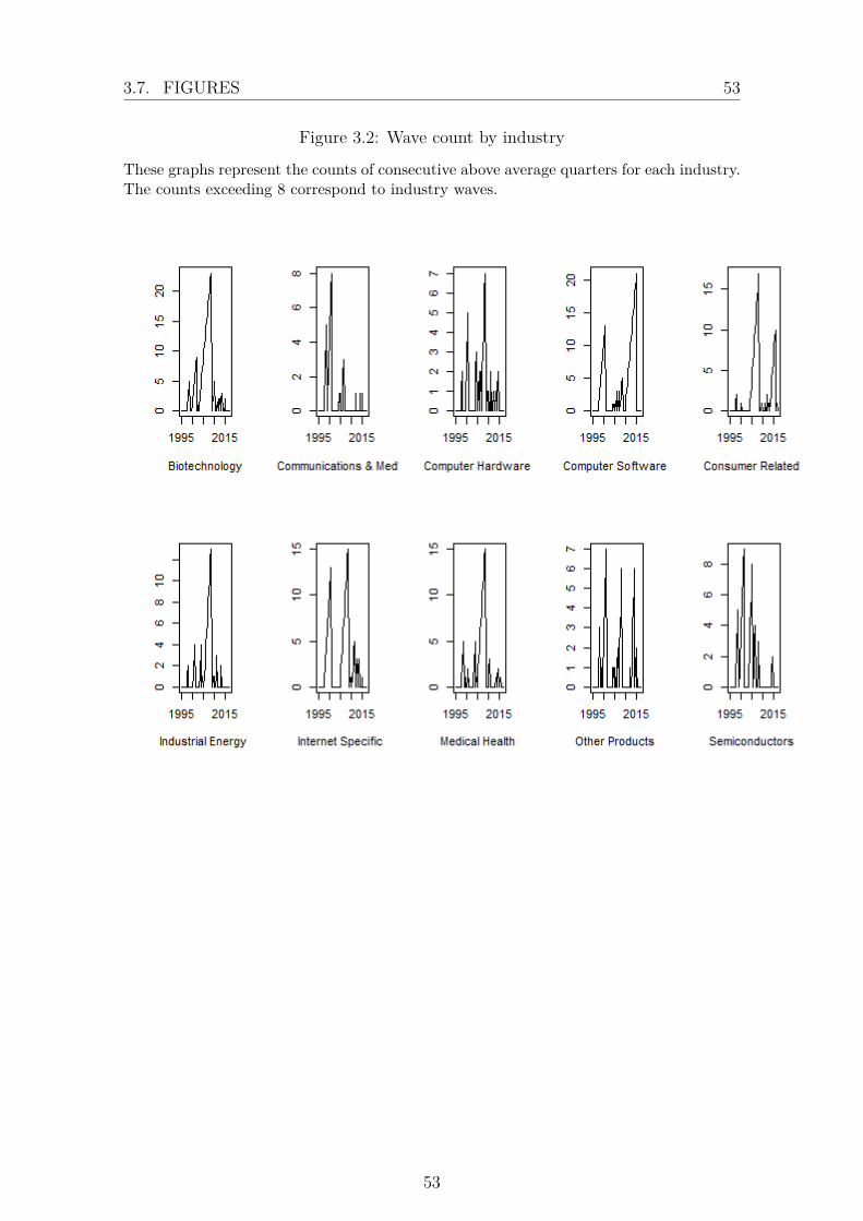
3.7. FIGURES 53
Figure 3.2: Wave count by industry
These graphs represent the counts of consecutive above average quarters for each industry.The counts exceeding 8 correspond to industry waves.
53
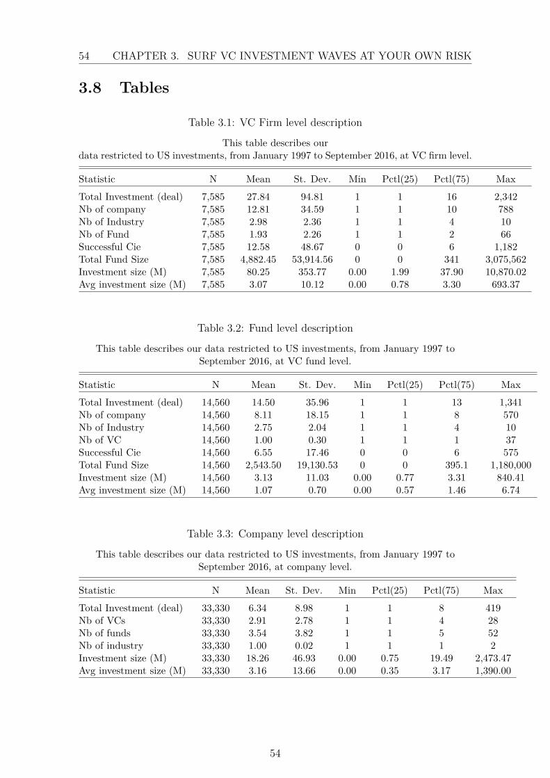
54 CHAPTER 3. SURF VC INVESTMENT WAVES AT YOUR OWN RISK
3.8 Tables
Table 3.1: VC Firm level description
This table describes ourdata restricted to US investments, from January 1997 to September 2016, at VC firm level.
Statistic N Mean St. Dev. Min Pctl(25) Pctl(75) Max
Total Investment (deal) 7,585 27.84 94.81 1 1 16 2,342Nb of company 7,585 12.81 34.59 1 1 10 788Nb of Industry 7,585 2.98 2.36 1 1 4 10Nb of Fund 7,585 1.93 2.26 1 1 2 66Successful Cie 7,585 12.58 48.67 0 0 6 1,182Total Fund Size 7,585 4,882.45 53,914.56 0 0 341 3,075,562Investment size (M) 7,585 80.25 353.77 0.00 1.99 37.90 10,870.02Avg investment size (M) 7,585 3.07 10.12 0.00 0.78 3.30 693.37
Table 3.2: Fund level description
This table describes our data restricted to US investments, from January 1997 toSeptember 2016, at VC fund level.
Statistic N Mean St. Dev. Min Pctl(25) Pctl(75) Max
Total Investment (deal) 14,560 14.50 35.96 1 1 13 1,341Nb of company 14,560 8.11 18.15 1 1 8 570Nb of Industry 14,560 2.75 2.04 1 1 4 10Nb of VC 14,560 1.00 0.30 1 1 1 37Successful Cie 14,560 6.55 17.46 0 0 6 575Total Fund Size 14,560 2,543.50 19,130.53 0 0 395.1 1,180,000Investment size (M) 14,560 3.13 11.03 0.00 0.77 3.31 840.41Avg investment size (M) 14,560 1.07 0.70 0.00 0.57 1.46 6.74
Table 3.3: Company level description
This table describes our data restricted to US investments, from January 1997 toSeptember 2016, at company level.
Statistic N Mean St. Dev. Min Pctl(25) Pctl(75) Max
Total Investment (deal) 33,330 6.34 8.98 1 1 8 419Nb of VCs 33,330 2.91 2.78 1 1 4 28Nb of funds 33,330 3.54 3.82 1 1 5 52Nb of industry 33,330 1.00 0.02 1 1 1 2Investment size (M) 33,330 18.26 46.93 0.00 0.75 19.49 2,473.47Avg investment size (M) 33,330 3.16 13.66 0.00 0.35 3.17 1,390.00
54
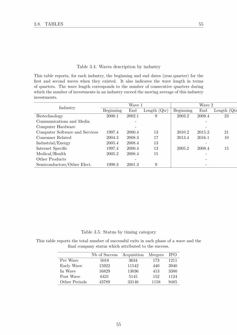
3.8. TABLES 55
Table 3.4: Waves description by industry
This table reports, for each industry, the beginning and end dates (year.quarter) for thefirst and second waves when they existed. It also indicates the wave length in termsof quarters. The wave length corresponds to the number of consecutive quarters duringwhich the number of investments in an industry exceed the moving average of this industryinvestments.
Industry Wave 1 Wave 2Beginning End Length (Qtr) Beginning End Length (Qtr)
Biotechnology 2000.1 2002.1 9 2003.2 2008.4 23Communications and Media - -Computer Hardware - -Computer Software and Services 1997.4 2000.4 13 2010.2 2015.2 21Consumer Related 2004.3 2008.3 17 2013.4 2016.1 10Industrial/Energy 2005.4 2008.4 13 -Internet Specific 1997.4 2000.4 13 2005.2 2008.4 15Medical/Health 2005.2 2008.4 15 -Other Products - -Semiconductors/Other Elect. 1999.3 2001.3 9 -
Table 3.5: Status by timing category
This table reports the total number of successful exits in each phase of a wave and thefinal company status which attributed to the success.
Nb of Success Acquisition Mergers IPOPre Wave 5018 3634 173 1211Early Wave 15922 11542 440 3940In Wave 16829 13036 413 3380Post Wave 6421 5145 152 1124Other Periods 43789 33146 1158 9485
55
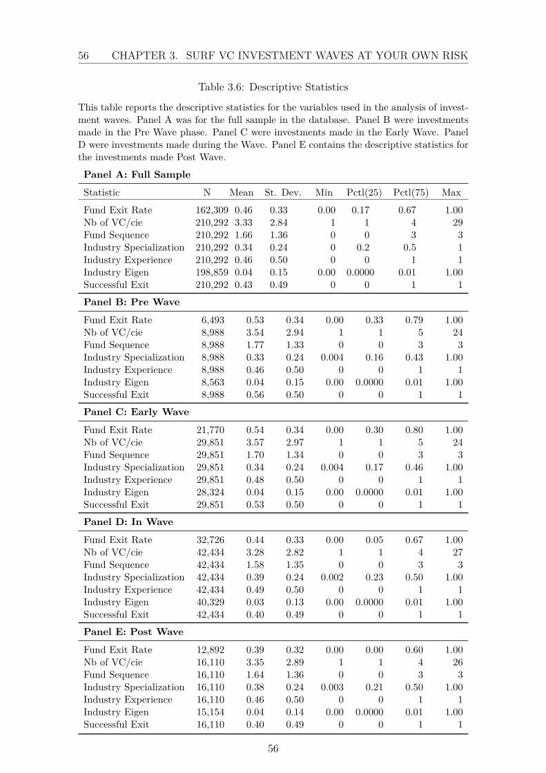
56 CHAPTER 3. SURF VC INVESTMENT WAVES AT YOUR OWN RISK
Table 3.6: Descriptive Statistics
This table reports the descriptive statistics for the variables used in the analysis of invest-ment waves. Panel A was for the full sample in the database. Panel B were investmentsmade in the Pre Wave phase. Panel C were investments made in the Early Wave. PanelD were investments made during the Wave. Panel E contains the descriptive statistics forthe investments made Post Wave.
Panel A: Full Sample
Statistic N Mean St. Dev. Min Pctl(25) Pctl(75) Max
Fund Exit Rate 162,309 0.46 0.33 0.00 0.17 0.67 1.00Nb of VC/cie 210,292 3.33 2.84 1 1 4 29Fund Sequence 210,292 1.66 1.36 0 0 3 3Industry Specialization 210,292 0.34 0.24 0 0.2 0.5 1Industry Experience 210,292 0.46 0.50 0 0 1 1Industry Eigen 198,859 0.04 0.15 0.00 0.0000 0.01 1.00Successful Exit 210,292 0.43 0.49 0 0 1 1
Panel B: Pre Wave
Fund Exit Rate 6,493 0.53 0.34 0.00 0.33 0.79 1.00Nb of VC/cie 8,988 3.54 2.94 1 1 5 24Fund Sequence 8,988 1.77 1.33 0 0 3 3Industry Specialization 8,988 0.33 0.24 0.004 0.16 0.43 1.00Industry Experience 8,988 0.46 0.50 0 0 1 1Industry Eigen 8,563 0.04 0.15 0.00 0.0000 0.01 1.00Successful Exit 8,988 0.56 0.50 0 0 1 1
Panel C: Early Wave
Fund Exit Rate 21,770 0.54 0.34 0.00 0.30 0.80 1.00Nb of VC/cie 29,851 3.57 2.97 1 1 5 24Fund Sequence 29,851 1.70 1.34 0 0 3 3Industry Specialization 29,851 0.34 0.24 0.004 0.17 0.46 1.00Industry Experience 29,851 0.48 0.50 0 0 1 1Industry Eigen 28,324 0.04 0.15 0.00 0.0000 0.01 1.00Successful Exit 29,851 0.53 0.50 0 0 1 1
Panel D: In Wave
Fund Exit Rate 32,726 0.44 0.33 0.00 0.05 0.67 1.00Nb of VC/cie 42,434 3.28 2.82 1 1 4 27Fund Sequence 42,434 1.58 1.35 0 0 3 3Industry Specialization 42,434 0.39 0.24 0.002 0.23 0.50 1.00Industry Experience 42,434 0.49 0.50 0 0 1 1Industry Eigen 40,329 0.03 0.13 0.00 0.0000 0.01 1.00Successful Exit 42,434 0.40 0.49 0 0 1 1
Panel E: Post Wave
Fund Exit Rate 12,892 0.39 0.32 0.00 0.00 0.60 1.00Nb of VC/cie 16,110 3.35 2.89 1 1 4 26Fund Sequence 16,110 1.64 1.36 0 0 3 3Industry Specialization 16,110 0.38 0.24 0.003 0.21 0.50 1.00Industry Experience 16,110 0.46 0.50 0 0 1 1Industry Eigen 15,154 0.04 0.14 0.00 0.0000 0.01 1.00Successful Exit 16,110 0.40 0.49 0 0 1 1
56
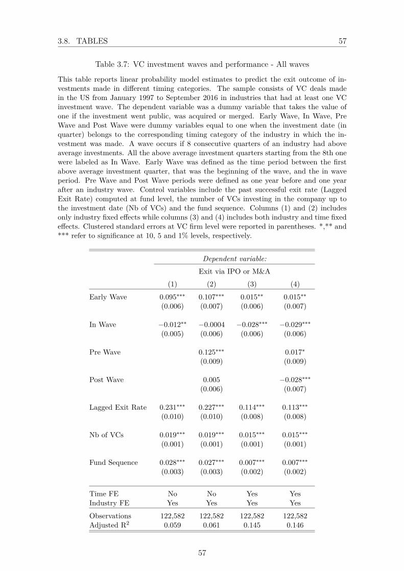
3.8. TABLES 57
Table 3.7: VC investment waves and performance - All waves
This table reports linear probability model estimates to predict the exit outcome of in-vestments made in different timing categories. The sample consists of VC deals madein the US from January 1997 to September 2016 in industries that had at least one VCinvestment wave. The dependent variable was a dummy variable that takes the value ofone if the investment went public, was acquired or merged. Early Wave, In Wave, PreWave and Post Wave were dummy variables equal to one when the investment date (inquarter) belongs to the corresponding timing category of the industry in which the in-vestment was made. A wave occurs if 8 consecutive quarters of an industry had aboveaverage investments. All the above average investment quarters starting from the 8th onewere labeled as In Wave. Early Wave was defined as the time period between the firstabove average investment quarter, that was the beginning of the wave, and the in waveperiod. Pre Wave and Post Wave periods were defined as one year before and one yearafter an industry wave. Control variables include the past successful exit rate (LaggedExit Rate) computed at fund level, the number of VCs investing in the company up tothe investment date (Nb of VCs) and the fund sequence. Columns (1) and (2) includesonly industry fixed effects while columns (3) and (4) includes both industry and time fixedeffects. Clustered standard errors at VC firm level were reported in parentheses. *,** and*** refer to significance at 10, 5 and 1% levels, respectively.
Dependent variable:Exit via IPO or M&A
(1) (2) (3) (4)
Early Wave 0.095∗∗∗ 0.107∗∗∗ 0.015∗∗ 0.015∗∗
(0.006) (0.007) (0.006) (0.007)
In Wave −0.012∗∗ −0.0004 −0.028∗∗∗ −0.029∗∗∗
(0.005) (0.006) (0.006) (0.006)
Pre Wave 0.125∗∗∗ 0.017∗
(0.009) (0.009)
Post Wave 0.005 −0.028∗∗∗
(0.006) (0.007)
Lagged Exit Rate 0.231∗∗∗ 0.227∗∗∗ 0.114∗∗∗ 0.113∗∗∗
(0.010) (0.010) (0.008) (0.008)
Nb of VCs 0.019∗∗∗ 0.019∗∗∗ 0.015∗∗∗ 0.015∗∗∗
(0.001) (0.001) (0.001) (0.001)
Fund Sequence 0.028∗∗∗ 0.027∗∗∗ 0.007∗∗∗ 0.007∗∗∗
(0.003) (0.003) (0.002) (0.002)
Time FE No No Yes YesIndustry FE Yes Yes Yes Yes
Observations 122,582 122,582 122,582 122,582Adjusted R2 0.059 0.061 0.145 0.146
57

58 CHAPTER 3. SURF VC INVESTMENT WAVES AT YOUR OWN RISK
Table 3.8: VC investment waves and performance - First waves
This table reports linear probability model estimates to predict the exit outcome of in-vestments made in different timing categories of the first industry waves. The sampleconsists of VC deals made in the US from January 1997 to September 2016 in industriesthat had at least one VC investment wave. The dependent variable was a dummy variablethat takes the value of one if the investment went public, was acquired or merged. EarlyWave , In Wave , Pre Wave and Post Wave were dummy variables equal to one when theinvestment date (in quarter) belongs to the corresponding timing category of the industryin which the investment was made. The number associated with each timing category (1)refers to the industry’s wave number (first waves). A wave occurs if 8 consecutive quartersof an industry had above average investments. All the above average investment quartersstarting from the 8th one were labeled as In Wave. Early Wave was defined as the timeperiod between the first above average investment quarter, that was the beginning of thewave, and the in wave period. Pre Wave and Post Wave periods were defined as one yearbefore and one year after an industry wave. Control variables include the past successfulexit rate (Lagged Exit Rate) computed at fund level, the number of VCs investing inthe company up to the investment date (Nb of VCs) and the fund sequence. Columns(1) and (2) includes only industry fixed effects while columns (3) and (4) includes bothindustry and time fixed effects. Clustered standard errors at VC firm level were reportedin parentheses. *,** and *** refer to significance at 10, 5 and 1% levels, respectively.
Dependent variable:Exit via IPO or M&A
(1) (2) (3) (4)
Early Wave 1 0.174∗∗∗ 0.192∗∗∗ 0.033∗∗∗ 0.032∗∗∗
(0.008) (0.008) (0.008) (0.009)
In Wave 1 0.092∗∗∗ 0.110∗∗∗ −0.043∗∗∗ −0.043∗∗∗
(0.007) (0.007) (0.009) (0.009)
Pre Wave 1 0.204∗∗∗ 0.040∗∗∗
(0.012) (0.012)
Post Wave 1 0.131∗∗∗ −0.038∗∗∗
(0.008) (0.010)
Lagged Exit Rate 0.216∗∗∗ 0.208∗∗∗ 0.114∗∗∗ 0.113∗∗∗
(0.010) (0.010) (0.008) (0.008)
Nb of VCs 0.018∗∗∗ 0.018∗∗∗ 0.015∗∗∗ 0.015∗∗∗
(0.001) (0.001) (0.001) (0.001)
Fund Sequence 0.027∗∗∗ 0.025∗∗∗ 0.007∗∗∗ 0.007∗∗∗
(0.003) (0.002) (0.002) (0.002)
Time FE No No Yes YesIndustry FE Yes Yes Yes Yes
Observations 122,582 122,582 122,582 122,582Adjusted R2 0.065 0.073 0.146 0.146
58
3.8. TABLES 59
Table 3.9: VC investment waves and performance - Second waves
This table reports linear probability model estimates to predict the exit outcome of in-vestments made in different timing categories of the second industry waves. The sampleconsists of VC deals made in the US from January 1997 to September 2016 in industriesthat had two VC investment wave. The dependent variable was a dummy variable thattakes the value of one if the investment went public, was acquired or merged. Early Wave, In Wave , Pre Wave and Post Wave were dummy variables equal to one when the in-vestment date (in quarter) belongs to the corresponding timing category of the industryin which the investment was made. The number associated with each timing category(2) refers to the industry’s wave number (second waves). A wave occurs if 8 consecutivequarters of an industry had above average investments. All the above average investmentquarters starting from the 8th one were labeled as In Wave. Early Wave was defined as thetime period between the first above average investment quarter, that was the beginning ofthe wave, and the in wave period. Pre Wave and Post Wave periods were defined as oneyear before and one year after an industry wave. Control variables include the past suc-cessful exit rate (Lagged Exit Rate) computed at fund level, the number of VCs investingin the company up to the investment date (Nb of VCs) and the fund sequence. Columns(1) and (2) includes only industry fixed effects while columns (3) and (4) includes bothindustry and time fixed effects. Clustered standard errors at VC firm level were reportedin parentheses. *,** and *** refer to significance at 10, 5 and 1% levels, respectively.
Dependent variable:Exit via IPO or M&A
(1) (2) (3) (4)
Early Wave 2 −0.032∗∗∗ −0.048∗∗∗ −0.006 −0.006(0.008) (0.008) (0.009) (0.009)
In Wave 2 −0.132∗∗∗ −0.150∗∗∗ −0.015∗∗ −0.015∗∗
(0.008) (0.008) (0.007) (0.007)
Pre Wave 2 0.002 −0.003(0.012) (0.012)
Post Wave 2 −0.214∗∗∗ −0.003(0.010) (0.009)
Lagged Exit Rate 0.232∗∗∗ 0.220∗∗∗ 0.114∗∗∗ 0.114∗∗∗
(0.010) (0.010) (0.008) (0.008)
Nb of VCs 0.019∗∗∗ 0.019∗∗∗ 0.015∗∗∗ 0.015∗∗∗
(0.001) (0.001) (0.001) (0.001)
Fund Sequence 0.027∗∗∗ 0.025∗∗∗ 0.007∗∗∗ 0.007∗∗∗
(0.003) (0.003) (0.002) (0.002)
Time FE No No Yes YesIndustry FE Yes Yes Yes Yes
Observations 122,582 122,582 122,582 122,582Adjusted R2 0.060 0.066 0.145 0.145
59
60 CHAPTER 3. SURF VC INVESTMENT WAVES AT YOUR OWN RISK
Table 3.10: VC investment waves and performance - All waves
This table reports linear probability model estimates to predict the exit outcome of in-vestments made in different timing categories. The sample consists of VC deals madein the US from January 1997 to September 2016 in industries that had at least one VCinvestment wave. The dependent variable was a dummy variable that takes the value ofone if the investment went public, was acquired or merged. Early Wave, In Wave, PreWave and Post Wave were dummy variables equal to one when the investment date (inquarter) belongs to the corresponding timing category of the industry in which the in-vestment was made. A wave occurs if 8 consecutive quarters of an industry had aboveaverage investments. All the above average investment quarters starting from the 8th onewere labeled as In Wave. Early Wave was defined as the time period between the firstabove average investment quarter, that was the beginning of the wave, and the in waveperiod. Pre Wave and Post Wave periods were defined as one year before and one yearafter an industry wave. Control variables include the past successful exit rate (LaggedExit Rate) computed at fund level, the number of VCs investing in the company up tothe investment date (Nb of VCs) and the fund sequence. All estimations include bothindustry and time fixed effects. Clustered standard errors at VC firm level were reportedin parentheses. *,** and *** refer to significance at 10, 5 and 1% levels, respectively.
Dependent variable:Exit via IPO or M&A
(1) (2) (3) (4)
Early Wave 0.021∗∗∗
(0.006)
In Wave −0.031∗∗∗
(0.006)
Pre Wave 0.018∗∗
(0.009)
Post Wave −0.028∗∗∗
(0.007)
Lagged Exit Rate 0.114∗∗∗ 0.114∗∗∗ 0.114∗∗∗ 0.114∗∗∗
(0.008) (0.008) (0.008) (0.008)
Nb of VCs 0.015∗∗∗ 0.015∗∗∗ 0.015∗∗∗ 0.015∗∗∗
(0.001) (0.001) (0.001) (0.001)
Fund Sequence 0.007∗∗∗ 0.007∗∗∗ 0.007∗∗∗ 0.007∗∗∗
(0.002) (0.002) (0.002) (0.002)
Time FE Yes Yes Yes YesIndustry FE Yes Yes Yes Yes
Observations 122,582 122,582 122,582 122,582Adjusted R2 0.145 0.145 0.145 0.145
60

3.8. TABLES 61
Table 3.11: Industry experience, specialization and network
This table reports linear probability model estimates to analyze which characteristics ofVCs predict their likelihood to invest in a given time period with respect to an industrywave. The sample consists of VC deals made in the US from January 1997 to September2016 in industries that had at least one VC investment wave. The dependent variables aredummy variables equal to one when the investment date (in quarter) belongs to the corre-sponding timing category of the industry in which the investment was made. A wave occursif 8 consecutive quarters of an industry had above average investments. All the above av-erage investment quarters starting from the 8th one were labeled as In Wave. Early Wavewas defined as the time period between the first above average investment quarter, thatwas the beginning of the wave, and the in wave period. Pre Wave and Post Wave periodswere defined as one year before and one year after an industry wave. Other Periods wereperiods that belong to none of the previous four categories. Among the explanatory vari-ables, Industry Experience was a dummy variable equals to one whenever the total numberof investments made by the VC firm, in the corresponding industry, was higher than theaverage number of investments of that industry. A VC was considered as experiencedin an industry if they had more investments in this industry than the average. IndustrySpecialization represents the share of the VC firm’s portfolio in the industry in which theinvestment was made. The higher was this ratio the more specialized was a VC firm inan industry. Industry Eigen was a network measure. It corresponds to the eigen vectorcentrality of the VC firm, computed for the industry in which the investment was made.Namely, it reflects how well connected was a VC firm in the industry in which it invests.All estimations include industry fixed effects. Clustered standard er-rors at VC firm level were reported in parentheses. *,** and*** refer to significance at 10, 5 and 1% levels, respectively.
Dependent variable:Pre Wave Early Wave In Wave Post Wave Other Periods
(1) (2) (3) (4) (5)
Industry Experience −0.002 −0.001 0.016∗∗ 0.001 −0.013(0.002) (0.005) (0.006) (0.003) (0.008)
Industry Specialization −0.036∗∗∗ −0.081∗∗∗ 0.083∗∗∗ 0.033∗∗∗ 0.002(0.004) (0.012) (0.011) (0.006) (0.019)
Industry Eigen 0.007 0.014 −0.055∗∗∗ 0.001 0.030(0.008) (0.026) (0.018) (0.010) (0.044)
Industry FE Yes Yes Yes Yes Yes
Observations 149,928 149,928 149,928 149,928 149,928Adjusted R2 0.004 0.005 0.052 0.007 0.073
61
62 CHAPTER 3. SURF VC INVESTMENT WAVES AT YOUR OWN RISK
Table 3.12: Industry experience, specialization and network
This table reports linear probability model estimates to analyze which characteristics ofVCs predict their likelihood to invest in a given time period with respect to an industrywave. The sample consists of VC deals made in the US from January 1997 to September2016 in industries that had at least one VC investment wave. The dependent variablesare dummy variables equal to one when the investment date (in quarter) belongs to thecorresponding timing category of the industry in which the investment was made. A waveoccurs if 8 consecutive quarters of an industry had above average investments. All theabove average investment quarters starting from the 8th one were labeled as In Wave.Early Wave was defined as the time period between the first above average investmentquarter, that was the beginning of the wave, and the in wave period. Pre Wave and PostWave periods were defined as one year before and one year after an industry wave. OtherPeriods were periods that belong to none of the previous four categories. Among theexplanatory variables, Industry Experience was a dummy variable equals to one wheneverthe total number of investments made by the VC firm, in the corresponding industry, washigher than the average number of investments of that industry. A VC was considered asexperienced in an industry if they had more investments in this industry than the average.Industry Specialization represents the share of the VC firm’s portfolio in the industry inwhich the investment was made. The higher was this ratio the more specialized was a VCfirm in an industry. Industry Eigen was a network measure. It corresponds to the eigenvector centrality of the VC firm, computed for the industry in which the investment wasmade. Namely, it reflects how well connected was a VC firm in the industry in which itinvests. Exp × Eigen was an interaction term between industry experience and industrynetwork. Specialization × Eigen was an interaction term between industry specializationand network. All estimations include industry fixed effects. Clustered standard errors atVC firm level were reported in parentheses. *,** and *** refer to significance at 10, 5 and1% levels, respectively.
Dependent variable:Pre Wave Early Wave In Wave Post Wave Other Periods
(1) (2) (3) (4) (5)
Industry Experience −0.002 −0.003 0.014∗∗ 0.001 −0.010(0.002) (0.005) (0.006) (0.003) (0.008)
Industry Specialization −0.038∗∗∗ −0.079∗∗∗ 0.090∗∗∗ 0.035∗∗∗ −0.008(0.004) (0.011) (0.011) (0.006) (0.018)
Industry Eigen −0.075 −0.305∗ −0.285 0.076 0.568(0.087) (0.168) (0.219) (0.123) (0.385)
Exp × Eigen 0.061 0.359∗∗ 0.329 −0.043 −0.679∗
(0.087) (0.160) (0.213) (0.125) (0.366)
Specialization × Eigen 0.056 −0.096 −0.254∗∗ −0.083 0.357(0.072) (0.257) (0.111) (0.074) (0.432)
Industry FE Yes Yes Yes Yes Yes
Observations 149,928 149,928 149,928 149,928 149,928Adjusted R2 0.004 0.005 0.052 0.007 0.073
62
3.8. TABLES 63
Table 3.13: Liquidity, performance and early investments
This table reports linear probability model estimates to analyze how potentially availableliquidity and past performance impacted VCs’ likelihood to make early times investments.The sample consists of VC deals made in the US from January 1997 to September 2016in industries that had at least one VC investment wave. The dependent variables weredummy variables equal to one when the investment date (in quarter) belongs to the cor-responding timing category of the industry in which the investment was made. A waveoccurs if 8 consecutive quarters of an industry had above average investments. Early Wavewas defined as the time period between the first above average investment quarter, thatwas the beginning of the wave, and the 8th above average quarter. Pre Wave was definedas one year before an industry wave. The two explanatory variables were lagged variables.Fund Exit Rate reflects the proportion of a fund’s investments that exited via IPO orM&A. It was computed in a way to capture information at the investment date. Namely,a success was considered as realized after the last investment date of the company if thereported stage was “Seed”, “Early Stage” or “Bridge Loan”. Fund liquidity representsthe ratio of, the difference between the total amount invested by a fund and the amountinvested up to the investment date, over the total amount invested. All estimations in-clude industry fixed effects. Clustered standard errors at VC firm level were reportedin parentheses. *,** and *** refer to significance at 10, 5 and 1% levels, respectively.
Dependent variable:Pre Wave Early Wave
(1) (2) (3) (4)
Fund Liquidity 0.043∗∗∗ 0.159∗∗∗
(0.003) (0.006)
Fund Exit Rate 0.026∗∗∗ 0.102∗∗∗
(0.003) (0.008)
Industry FE Yes Yes Yes Yes
Observations 163,129 122,582 163,129 122,582Adjusted R2 0.005 0.004 0.019 0.011
63
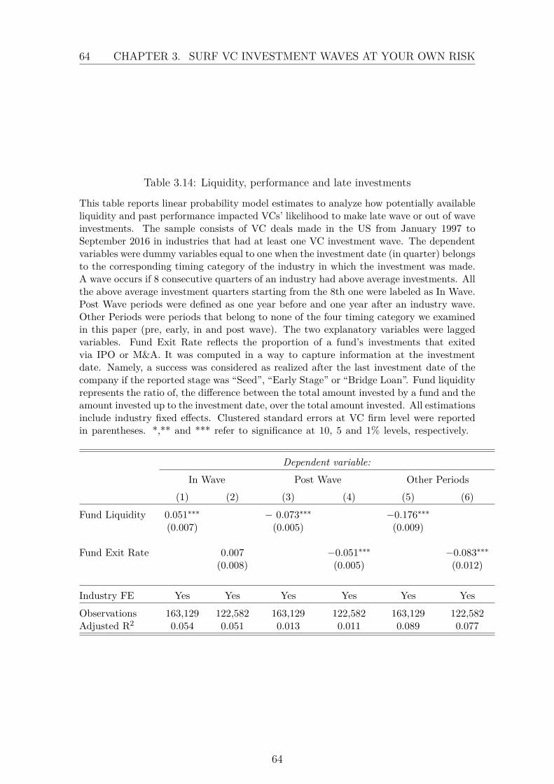
64 CHAPTER 3. SURF VC INVESTMENT WAVES AT YOUR OWN RISK
Table 3.14: Liquidity, performance and late investments
This table reports linear probability model estimates to analyze how potentially availableliquidity and past performance impacted VCs’ likelihood to make late wave or out of waveinvestments. The sample consists of VC deals made in the US from January 1997 toSeptember 2016 in industries that had at least one VC investment wave. The dependentvariables were dummy variables equal to one when the investment date (in quarter) belongsto the corresponding timing category of the industry in which the investment was made.A wave occurs if 8 consecutive quarters of an industry had above average investments. Allthe above average investment quarters starting from the 8th one were labeled as In Wave.Post Wave periods were defined as one year before and one year after an industry wave.Other Periods were periods that belong to none of the four timing category we examinedin this paper (pre, early, in and post wave). The two explanatory variables were laggedvariables. Fund Exit Rate reflects the proportion of a fund’s investments that exitedvia IPO or M&A. It was computed in a way to capture information at the investmentdate. Namely, a success was considered as realized after the last investment date of thecompany if the reported stage was “Seed”, “Early Stage” or “Bridge Loan”. Fund liquidityrepresents the ratio of, the difference between the total amount invested by a fund and theamount invested up to the investment date, over the total amount invested. All estimationsinclude industry fixed effects. Clustered standard errors at VC firm level were reportedin parentheses. *,** and *** refer to significance at 10, 5 and 1% levels, respectively.
Dependent variable:In Wave Post Wave Other Periods
(1) (2) (3) (4) (5) (6)
Fund Liquidity 0.051∗∗∗ − 0.073∗∗∗ −0.176∗∗∗
(0.007) (0.005) (0.009)
Fund Exit Rate 0.007 −0.051∗∗∗ −0.083∗∗∗
(0.008) (0.005) (0.012)
Industry FE Yes Yes Yes Yes Yes Yes
Observations 163,129 122,582 163,129 122,582 163,129 122,582Adjusted R2 0.054 0.051 0.013 0.011 0.089 0.077
64
Chapter 4
Are Bridge Loans a Bridge toNowhere?
Abstract : Bridge loans are temporary loans between financing rounds oras a stopgap to failure. Just under 11% of the 35,939 venture fundedcompanies in the Thomson One Banker, from 1995 through 2017, re-ceived bridge loans. In that universe of companies, 6% went public while0.06% of companies with bridge loans went public. By a broader mea-sure of success, 40% of the companies successfully exited while it was0.7% for companies with bridge loans. This paper examines why venturecapitalists used bridge loans in a significant number of their investmentseven though the instrument had a low success rate. The analysis providesevidence that bridge loans may be employed to manage fund IRR, be aresult of local bias and an example of late-staging.
65
66 CHAPTER 4. ARE BRIDGE LOANS A BRIDGE TO NOWHERE?
4.1 Introduction
Venture capitalists use a variety of financial instruments to fund companies in theirportfolio. These instruments include debt and equity instruments such as commonequity, preferred equity, senior debt, convertible debt and bridge loans (P. A. Gom-pers, 1999; Marx, 1998). Even though 11 percent of the transactions in ThomsonOne Banker, from 1995 to 2017 were bridge loans, the existing literature did notexplore bridge loans and the circumstances which make them an efficient choice.
The goal of this paper is to examine the economics of bridge loans and theiraffect on investment outcomes for the general partners, limited partners and portfoliocompany. I examined the characteristics of the venture capital firms who used bridgeloans as a financing instrument and the companies which received them to determineif there were identifiable strategies and benefits of using bridge loans. Due to thelength of the history, it was possible to determine if bridge loans contributed topositive exits.
To explore why 11% of the companies had bridge loans and determine the char-acteristics of the VC firms and companies with bridge loans, the 228,418 ventureinvestment transactions from Thomson One Banker, covering 1995 to 2017, wereanalyzed (Descriptive statistics are in tables 4.1 to 4.3). The data had informationabout the VC firm, VC fund, the company and the investment characteristics. Thestatus of companies in the database are listed in table 4.4 to 4.6.
Across the 15,593 distinct funds in the data base, 3,676 funds used bridge loansand 2,236 used more than one bridge loan. An even smaller amount, 383 funds, usedmore than ten bridge loans. Independent private partnerships (table 4.5) financedfirms with the highest number of bridge loans at 2,708. As a percentage of theirtotal investments, some venture types used a high percentage of bridge loans. Someexamples were: government programs, the largest, at 31%, evergreen funds at 14%and business angels at 14%. Even though the percentages were high, the totalnumber of bridge investments for these 3 types was less than those by independentprivate partnerships. Evergreen funds contained, among other structures, familyoffices and trusts.
Companies which received bridge loans had a 0.7% success rate, using a broadmeasure of success, compared to 40% for companies without a bridge loan. Usingan IPO as the measure of success, 0.06% of companies with bridge loans went publicwhile it was 6% for those without bridge loans. For comparison, companies withstandard venture debt had a 56% success rate. The failure rate for companies withbridge loans was similar to firms in financial distress (Gilson, 1997; Kahl, 2002).
There are numerous papers on the structure of venture capital firms and theuse of staging in venture investments (Kaplan & Strömberg, 2004; Sahlman, 1990).
66
4.1. INTRODUCTION 67
The work by Kaplan and Strömberg did not include bridge loans as a financinginstrument or as one of the investment stages. This paper will concentrate solely onbridge loans. Cornelli and Yosha (2003) provided a rationale for the use of stagingto cancel poor performance investments and window-dressing by the entrepreneur.As with Kaplan and Strömberg, Cornelli and Yosha did not consider bridge loansor window-dressing by the venture capitalist.
VC firms may used bridge loans due to incentive conflicts with the payout struc-ture of the funds they manage for the limited partners. Bridge loans prevent aportfolio company from failing and, thereby, reducing the fund internal rate of re-turn. Barber and Yasuda (2017) demonstrate that private equity firms manage theirfund net asset value when raising a new fund without discussing how it could bemanaged. This paper provides evidence consistent with these findings that VC fundgeneral partners can manage the fund IRR with bridge loans.
Since VC firms receive a 2 percent management fee on the assets in the fund(Klonowski, 2010), there was a direct benefit to the VC firm from temporarilyrescuing the portfolio company from failure when the VC firm was raising a newfund. This temporary improvement in fund IRR assists the VC firm when theyraise a fee generating follow-on fund (Kollmann, Kuckertz, & Middelberg, 2014) ormake capital calls and prolong the life of the fund. Using bridge loans, as examinedin this paper, an inexperienced VC may temporarily improve the fund IRR whilethey raise a fee generating follow-on fund. An experienced venture capitalist didnot use bridge loans when they raised a new fund. However, an experienced VCwould benefit from maintaining a stable fund IRR to continue receiving capital calls.Ninety seven percent of VC funds, who used bridge loans, employed the bridge loanin the last quarter of the life of the fund (table 4.6) while, in the universe of all VCfunds, invested just 25% in the final quarter.
The VC firm, in another form of an incentive conflict, may use bridge loans toshow effort and activity when they did not have good projects to fund. This wassimilar to the problem Special Purpose Acquisition Companies (SPAC) had whenforced to make an investment within a short time-frame. VC firms had a limitedtime to invest and return capital. It may be, as Dimitrova (2017) had found withSPACs, that it was beneficial to the managing partners to make a bad investmentwhile it destroys value in the SPAC. Bridge loans had a negative impact on fundIRR but demonstrate activity and effort.
Key findings of the paper were that companies which were financed with bridgeloans had a very low success rate; VC Firms used bridge loans with a local bias tocompanies within the same state; Experienced VC firms used fewer bridge loans; Alarger number of co-investors reduced the use of bridge loans; As the use of bridgeloans increased in a fund, there was a greater chance it was the last fund; Investments
67
68 CHAPTER 4. ARE BRIDGE LOANS A BRIDGE TO NOWHERE?
at the end of the fund life had a low success rate; As fund liquidity decreased, thesuccess rate of investments decreased; and over 95% of bridge loans were utilized inthe last quarter of the fund life.
I extend the results from Barber and Yasuda (2017) that bridge loans may be amethod VC firms used to manage interim fund performance. I extend the papers byAtanasova and Chemla (2020) and Hochberg and Rauh (2013) and provide evidencethat bridge loans were an indicator of a familiarity bias which was used to supportcompanies in the same American state as the VC firm. It is possible that VC firmswant to show effort to the local limited partners or believe that more time andattention would improve the outcome. To test this conjecture, the firm, fund andcompany characteristics were regressed against a dummy variable which was set to1 if the company received a bridge loan. The results (table 4.7) provided evidencethat the use of a bridge loan was influenced by local bias, experience of the VC firmand the number of previous successes.
As mentioned above, companies financed with a bridge loan had a lower successrate. The dummy variable indicating success, which was a modified measure createdby Phalippou and Gottschalg (2009), was regressed against VC firm and companycharacteristics. Table 4.8 demonstrates that the largest indicator for a failed invest-ment, of those in the data base, was the use of a bridge loan. The VC firm internallydecided to extend a bridge loan to their portfolio company. The analysis was checkedfor self-selection using the Heckman correction (table 4.9) and confirmed that therewas self-selection which leads to a higher failure rate.
To test whether bridge loans contributed to the inability of VC firms to raise anew fund, a dummy variable was created for a VC Firm’s last fund. This dummyvariable was regressed against VC fund characteristics to examine if bridge loanswere used more often by firms in their last fund. The results (table 4.10) demon-strates that this was the case unless the VC firm had high experience. A highexperience VC used fewer bridge loans. However, if a high experience VC did usea large number of bridge loans, there was interaction between bridge loans and ex-perience which provided a slight increase in the probability the the firm had raisedits last fund. This was also checked for self-selection with a maximum likelihoodHeckman correction , which supported the conjecture that there was self selectionand the use of bridge loans increased the chance that the current fund was the lastfund.
The decision to raise a new fund was endogenous to the VC firm. The assumptionin the paper was that the VC Firm chose to raise a new fund and was unsuccessful.It is also possible that the VC Firm chose to close the firm without raising a newfund.
From an analysis of the investment dates, relative to the life of the fund, most
68
4.2. RELATED LITERATURE 69
bridge loans were made in the last quarter of the fund life. To test if the timean investment was made during the life of a fund had an impact on the successrate, the success rate was regressed against the elapsed time for bridge loans andall investments. A further regression was made on the liquidity of the fund todetermine if there was a relation between the liquidity of the fund and the timingof investments and bridge loans. The results (table 4.12) illustrated that the closeran investment was made to the end of a fund, the lower the success rate. As fundliquidity decreased, the success rate of investments decreased.
This paper proceeds as follows: Section 4.2 is a short review of related literature.Section 4.3 is a short discussion of bridge loans and their use in both venture capitaland real estate. Section 4.4 describes the data and descriptive statistics. Section 4.5examines the use of bridge loans. Section 4.6 looks at the effect bridge loans had onthe success of an investment. Section 4.7 focused on the use of bridge loans and thelast fund. Section 4.8 is an analysis of the effect on success the timing of investment,during the life of the fund, for bridge loans and all investments. Robustness checkswere discussed in section 4.9. Section 4.10 concludes.
4.2 Related literature
Barber and Yasuda (2017) demonstrated firms practice NAV management whenraising a follow-on fund with interim results of the previous fund. The analysis inthis paper suggests VC firms may manage their IRR with bridge loans when raisinga follow-on fund. Arcot, Fluck, Gaspar, and Hege (2015) discussed investmentstrategies of firms under pressure to raise a fund or exit. Bridge loans may be amethod for handling this pressure compared to the secondary buyouts in their paper.
Krohmer et al. (2009) discuss staging at different times in the life of a VC firm.They provided evidence that staging as an initial investment reduces the effectof asymmetric information with the entrepreneur while staging, after the initialinvestment, had a negative effect on investment returns. They did not discuss thetype of instruments for late staging. This paper suggests bridge loans were aninvestment instrument for, unplanned, late staging.
Giot and Schwienbacher (2007) discuss the characteristics of the deal structureand timing for a successful exit. They used a hazard function to determine theprobability of an IPO or a trade sale based on the age of the firm and the timingof the investments. Venture capitalist may use a bridge loan to extend the life of afirm to permit a trade sale.
Cumming and Dai (2010) demonstrated that venture capitalists prefer to investin companies which were physically close to their offices. Giot and Schwienbacher(2007) found that the success of a trade sale increased if there was one venture
69
70 CHAPTER 4. ARE BRIDGE LOANS A BRIDGE TO NOWHERE?
capitalist in proximity. The local bias might be influenced by the limited partners.Hochberg and Rauh (2013) provided evidence that state pension plans and invest-ment authorities invest in local fund managers (VC, Mutual, Pension) and this maybe a motivation for VC firms to use bridge loans to avoid company closures in theirhome state. This was supported by Atanasova and Chemla (2020), who found thatpension plans overweight venture investments in local managers and related industryinvestments. Financing from investors in the same state as the venture firm werean important source of Limited Partner investment and the VC firms may want toensure continued investment. This paper provides evidence, consistent with previ-ous research, that local limited partners had an influence on the investment policyand success rate in venture capital.
There is heavy pressure on venture capitalists, as reported by Ljungqvist andRichardson (2003), to raise new funds before the investments in their current fundexited. An important factor in raising a new fund was the performance of theprevious fund. Kaplan and Schoar (2005) demonstrated that higher performingfunds had an easier time raising a new fund. This was supported by Kollmannet al. (2014) as they found that it was the most important factor in raising a newfund. For funds that did not have companies which exited, they must report interimresults when raising capital. This leads to NAV manipulation as found by Barberand Yasuda (2017). The use of bridge loans was a way for venture capitalists tomanage the reported returns of their open fund and delay bad news.
4.3 Bridge loans
Bridge loans are temporary financial instruments used by venture capitalists toprovide short term financing, rescue firms from financial distress or as an initialinvestment (Glazer, 1989). Although bridge loans were widely used, there was littleresearch about their contribution to the return on investment in a venture fundedcompany or the motivation for using this financing instrument. Of 100,532 financerounds, from the Thomas One Banker database, examined in this paper, 10,200were funded with bridge loans by 16,391 co-investors. Venture capital firms usedbridge loans in a significant number of their investments despite numerous venturecapitalists (VC) stating that bridge loans provide negative return for both the VCfirm and the entrepreneur (Muse, 2016; Suster, 2010; F. Wilson, 2011). The failurerate for companies with bridge loans was similar to firms in financial distress (Gilson,1997; Kahl, 2002).
Bridge loans were also employed in real-estate and corporate finance deals (Glazer,1989) where the purchase of a property was contingent on the sale of another prop-erty or the property was to be held for a short period. Bridge loans in venture
70
4.3. BRIDGE LOANS 71
backed firms were not related to bridge loans in other areas as the collateral wasusually intangible assets as opposed to real property.
The classic case was a bridge loan which provides temporary financing whilemore permanent financing was under negotiation. The negotiation for the long-term financing had begun, with a high probability of completion, before the bridgeloan was granted. The bridged financing can be a normal venture round or thelead-up to an initial public offering (IPO) (Sahlman, 1990).
For the expenses of an Initial Public Offering (IPO), the bridge funding, whichwas a debt instrument, had lower legal fees and was easier to negotiate (Marx, 1998).This was the case for 25 companies, of the 3,877, which received bridge loans.
Pre-IPO and short-term bridge loans were not discussed in this paper. The focusof this paper was on bridge loans made to companies which cannot raise fundingfrom outside their current investors.
There were several operational issues which may prompt the need for a short-term bridge loan. All venture firms in a syndicate might not have the time toreview the documents or their outside legal counsel might not be available. Thereciuld be occasions when one or more of the venture syndicate might have to makea capital call to their limited partners. There could also be situations where onefirm may want to fund their commitment in the next quarter or month to avoid anunscheduled capital call.
Delays in funding, by one or more venture firms, were temporary operationalproblems. They were not strategy problems or a reflection on the suitability of thecompany for investment. The company has negotiated a follow-on round and waswithin performance levels specified by the venture firms.
The short-term bridge loan, due to VC firm operational issues, was repaid fromthe proceeds of the permanent financing. Failure to provide the funding, afterthe agreed upon delay, will cause the shirking firm to be excluded from future co-investment opportunities with the remaining group of investors. The strong socialfactors in venture funding were important to keep the bridge loan a true short termloan (Bénabou & Tirole, 2006).
The venture capitalist may genuinely have had confidence in the company al-though it was not self-financing, nor can it attract investment from a third party.The bridge loan was intended to rescue the company from a temporary hardshipor provide time to find a new investor. If a new firm did not invest, the bridgeloan becomes a long-term investment without reimbursement in the near-term. Thebridge loans rescue the portfolio company, in the short-term, from failing.
71
72 CHAPTER 4. ARE BRIDGE LOANS A BRIDGE TO NOWHERE?
4.4 Data
The data was a subset of venture capital deals from the Thomson One BankerPrivate Equity database. Daily transactional data for venture capital transactions,recorded in the United States, from 1995 through June 2017 were downloaded. Afterremoving records with missing identifiers and erroneous entries, there were 228,418transactions within 100,532 investment rounds for 35,939 companies. For reference,there were a further 215,533 transactions for the rest of the world during this period.
The database includes information about the company which received the invest-ment, the venture firm which made the investment, a few deal parameters and theinvestor syndicate which made the investment. Each investment round for a com-pany was captured in the database. There were 37 variables downloaded for eachtransaction. This paper used a subset of 19 variables with 7 variables computedfrom the downloaded variables, which were listed in table 4.1.
Table 4.1 reports summary statistics, at the individual round level, for the vari-ables in the database. The average VC firm was an independent private partnershipwhich had invested just over half of their capital. Their mean total investment was168 Million USD and the deals had a 53% mean success rate.
Table 4.2 aggregated the deal level data, of table 4.1, to company level. At thecompany level, the average fund had $143 million of capital and the mean investmentwas $47 million. Forty percent of the companies had a successful exit. 10.8% of thecompanies received a bridge loan.
Aggregated to the fund level, in table 4.3, the mean investment was $3.05 millionin 14.04 companies. The fund had an average of 1.36 IPOs and 7.51 companies witha successful exit. The variables at the fund level were the sum of the deal levelvariables.
VC firms report the status of their companies, in Thomson One Banker, as one ofthe following: Acquisition, Active, Bankruptcy – Chapter 11, Bankruptcy – Chapter7, Defunct, In Registration, LBO, Merger, Pending Acquisition and Went Public.The status variable did not have a more descriptive range for companies which weremarked as active. It was not possible to determine from the status of "Acquisition,”whether the company provided a return on capital or the amount.
Stating if an investment in a company was successful was difficult to determinewithout the full investment history and exit information. The Thomson One Bankerhad sparse investment information such as the amount invested, the valuation atinvestment, exit purchase price and deal terms such as liquidity preference.
Without deal terms, the label of success from the investment direction variablewould be arbitrary as it is possible to show a higher valuation but negate it witha liquidity preference, among other methods. In this case, an acquisition could be
72
4.4. DATA 73
a success to the VC firm holding the liquidity preference and a failure to the cc-investors and entrepreneurs, who did not hold a liquidity preference. The sale ofthe company for the return of some capital rather than a return on capital, wouldbe marked as a success and, therefore, the successful exits were over-counted in thispaper.
Even with these limitations, there were two generally accepted methods to labelan investment as a success or failure. P. Gompers, Kovner, Lerner, and Scharfstein(2008b) accepted any status except bankruptcy and defunct as a success. This paperfollows a stricter definition of success as used by Phalippou and Gottschalg (2009)and Tian (2011). Firms which were in the database and marked as ‘Active’ for morethan 7 years, without additional financing rounds, were marked as a failure.
The companies go through an additional filter which marks a company as afailure if the status was set to ‘Active’ for 3 or more years after the fund made itslast investment. A typical VC fund had a life of 10 years (Sahlman, 1990) and mostinvestments were made within the first 3 years (Zarutskie, 2007). After the 10-yearlife of the fund, there was a monitoring period for several years, on behalf of thelimited partners, for companies which did not exit. The hope was that the companywill exit within that time frame. In this paper, it assumed that a company whichdid not exit after three years of monitoring will not exit. After this process wasapplied, the companies had their status changed from active to Computed Defunct.In table 4.4, 49.3% of the companies where changed to Computed Defunct.
A recent paper by Wiltbank et al. (2015), stated that 75% of founders receivedno payment at the sale of the company. This was evidence that success at exit wasnot necessarily for all participants in a deal and supports the use of the computeddefunct method.
Even with this over-counted success variable, the analysis was supported by thedata. Changing the success variable to include just companies with an IPO, theeffects were stronger. This paper used the over-counted success rate for analysis.
Table 4.4 includes the counts for each status, as reported by the venture capi-talist. In the third column, the statuses for all companies with bridge loans werebroken out. Just 0.064% of the companies with bridge loans went public (statusof "In Registration" was added to "Went Public") while the full database of compa-nies had 6.35% go public. Very few of the companies, which received bridge loans,had further investment or exits. The vast majority simply stayed in the VC fundportfolio without further activity.
The venture firms self-reported the stage of the company receiving the investment(Seed, Series A, Bridge Loan, etc.). The analysis was concerned with the self-reported stage of bridge loan. From this variable, Bridge Loan was set to true forthe round the company received a bridge loan investment.
73
74 CHAPTER 4. ARE BRIDGE LOANS A BRIDGE TO NOWHERE?
A binary variable for the Last Fund was set to true if this was the last fund fora VC Firm. It is possible to set this variable by looking ahead and checking if anew fund was raised after the existing fund. There may have been cases where theventure firm attempted to raise a follow-on fund without raising the fund. The VCfirms did not self-report if they were raising a follow-on fund. It is not possible todetermine if the VC Firm could not raise a fund or simply decided to close the firm.Therefore, the decision may be self-selected by the VC Firm.
The VC firms report a fund size, which was stored in the variable Fund Size, inmillions of USD. The year the fund was created was stored in Fund Year.
Equity Bin was a variable which put the total investment, in a company, intoone of 7 bins based on the investment amount. The VC funds had different levelsof funds under management and therefore, had different limits on the amounts theymay invest in each portfolio company. To provide a linear range, the amount investedin each company is placed in one of seven bins.
In Thomson One Banker, the funds were labeled with a specific type. The VCtypes were alpha numeric characters and the ordering was not useful for analysis.The variable VC Type, for the type of VC firm, contains a numeric identifier tomaintain the following order: Business/Community Development Program, Univer-sity Development Program, Individuals, Angel, Government, Non-Private Equity,SBIC, Other, Other Banking/Financial Institution, Corporate PE/Venture Fund,Independent Private Partnership, Endowment, Foundation or Pension Fund, Fundof Funds, Investment Bank, Investment Advisory Affiliate, Retail, Secondary Pur-chase, and Evergreen. The ordering moves from temporary one-off programs, togovernmentally assisted programs and then to longer-term funds. VC types at thebeginning of the order tend to provide initial funding while those at the end fundlater stage investments.
Table 4.5 lists the number of VC types within the full database. It also liststhe use of bridge loans by VC Type. The majority of bridge loans were offered byIndependent Private Partnership, the largest VC type, at 2708 bridge loans.
Liquidity of the fund, stored in Pct Fund Invested was calculated by taking thecumulative amount invested, at each investment, and dividing it by the total amountinvested by the fund. This was a proxy for the liquidity of the fund as the venturefirms did not report the capital committed, or called, from their limited partners.
Each company had the total amount invested, both equity and debt, stored inthe variable Tot Est Equity. It was cumulative over each investment round. Theround number, for each transaction, was stored in Round. The date of the roundwas in Investment Date. The data base was indexed by Investment Date, Company,VC Fund Name and Round.
The Total Investors contained the sum of investors for each company. The
74
4.5. FUNDS AND COMPANIES WITH BRIDGE LOANS 75
variable Pct Same State was the sum of investors located in the same state asthe company divided by Total Investors.
Investment Elapsed Time was the time, as a percentage of the life of the fund, forthe investment in a company. Bridge Elapsed Time was the same, but for bridge loaninvestments. For companies with bridge loans, Bridge Elapsed Time and InvestmentElapsed Time were the same for the investment round where the company receiveda bridge loan.
Table 4.6 contains the elapsed investment times, for all investments and bridgeloans, by quarter. It also splits out the timing for the largest VC Type, IndependentPrivate Partnership and a separate row for all VC types. Bridge loans were almostentirely (97%) done in the last quarter of the fund life. In comparison, just over halfof the non-bridge loan investments were made in the first half of the fund and 30%,or less, were made in the last quarter of the fund.
The final calculated variable was Experienced VC. This variable was set to oneif the fund invested in more than the mean number of investments in an industryduring the life of the fund.
4.5 Funds and companies with bridge loans
Before determining if bridge loans influenced the success rate of investments, itwould be useful to explore the conditions and characteristics which prompt the useof a bridge loan in a financing round.
With an emphasis on interpersonal relationships with their portfolio companiesand industry peers, venture capitalists become very involved with the managementteams they fund. The venture capitalist may genuinely believe the firm needs a smallbridge loan to step through temporary under-performance. It was not possible todetermine the thought process of the venture capitalists when deciding to use abridge loan. However, it was possible to see some identifying characteristics of theVC firm and company in the bridge loan transaction.
The analysis was done with a series of linear regressions on the dependent vari-ableln(SumBridgeLoans), the number of bridge loan investments made by the VC fundThe following equation contains the different factors which were significant in de-termining the use of bridge loans in an investment round (table 4.7).
75
76 CHAPTER 4. ARE BRIDGE LOANS A BRIDGE TO NOWHERE?
ln(SumBridgeLoan) = β0 + β1Roundit + β2EquityBinit + β3ln(Fund Size)it
+ β4ln(Total Investors)it + β5Pct Fund Investedit
+ β6 ln (ln(Numb IPOs)it) + β7ln(Numb Successes)i,t
+ β8ln(Experienced VC)it + β9Pct Same Stateit
+ ηf + ηg + ηh(4.1)
Where ln(Sum Bridge Loans) was the number of bridge loan investments madeby the VC fund u. Round was the median investment round number for each fundEquity Bin was the placement of the median equity amount in 7 bins. ln(Fund Size)was the natural log of the fund size for fund u. Total Investors was the maximumnumber of co-investors for the fund Pct Fund Invest was the maximum percentageof the fund invested. The number of companies from fund u, which exited withan IPO, was in Number IPOs. Number Success was the count of successful exits,for fund u, which was the broader measure of success, as discussed in section 4.4.Experienced VC was the the number of experienced VC investments as defined insection 4.4. Pct Same State was the percentage of investments, by all co-investors,which were in the same state as the VC Firm The analysis was across differentgroupings of indicators and fixed effects for fund year, VC Type and domicile state.The variables were described in section 4.4.
The first four columns of table 4.7 had the investment information from the dealand information about the VC Fund. They had the same variables and differed bythe application of fixed effects. In the first column there were no fixed effects. Thefollowing columns added fixed effects for the Fund Year, VC Type and the FundState. Column 5 (IPO) controlled for the number of IPOs a fund generated. Incolumn 6 (Success) the control variable for the number of successes by the VC fundwas added while the IPO variable was removed. The next column (Experience)adds the experience the VC fund had in different industries and retained the successvariable. The final column (State) added the percentage of investors in the samestate.
Over the first 4 columns there were no significant differences with different fixedeffects applied. The variables remained economically important and significant.Without controlling for success rates and venture capital experience (column 4), theuse of bridge loans was higher in later investment rounds, when a larger amount wasinvested in the company, the fund size was larger and there were more co-investors.The only variable which had a negative coefficient was the Pct Fund Invested.
When the variable ln(Numb IPOs) was added in column 5, the variable EquityBin changed sign to negative and remained negative in the following columns. Com-
76
4.6. SUCCESS OF INVESTMENTS WITH BRIDGE LOANS 77
panies which had a large investment (equity bin was large), a bridge loan, whichwere in the first two bins, would not suffice to finance a company in the latter bins.The coefficient for ln(Numb IPOs) was positive and may reflect the use of bridgeloans to finance the expenses for going public, although those instances were few innumber (25 cases).
In column 6 the number of IPOs was dropped and the number of successful exitswas added to the equation. The coefficient for the variable ln(Numb Success) waseconomically important and significant. The variable for the total number of co-investors changed to negative and increased in magnitude. Based on the definitionof success (section 4.4), if co-investors did not believe that the company would havean IPO or high return at exit, they would be less likely to vote to add a bridge loanfinancing round. In the next section (4.6) evidence was provided that there was alower success rate with the use of bridge loans.
In a syndicate of many VC firms, some may have a policy against the use ofbridge loan, others would not be constrained by a low success rate or the need toraise additional funds. With a large syndicate, it would be more difficult to have allparticipants agree to fund a failing company or employ a bridge loan.
The variable for the percentage of the fund invested also changed sign to positivein column 6. As with the change in sign for total investors, a VC firm would possiblymake an investment, while their liquidity was low, to provide an exit in a lower returnportfolio company while they might cut their losses and save their capital for anotheropportunity with higher expected return.
In column 8 (State) the percentage of co-investors who were in the same stateas the company and VC firm, was added to the regression. With this addition PctFund Invested was no longer significant. Having a larger percentage of investorsin the same state increased the use of bridge loans. Venture firms which raise andinvest funds in the same state as their portfolio companies may have had morepressure from limited partners, potential limited partners and fear of reputationdamage that may encourage them to keep companies solvent (Atanasova & Chemla,2020; Hochberg & Rauh, 2013).
4.6 Success of investments with bridge loans
There was a limit to the number of negative IRR projects the venture capitalistcan fund, which may enhance their personal cash flows, before their reputation wasdamaged by poor investment results. Therefore, the venture capitalist manages exitsand cash flows strategically. The investment in negative IRR projects, as discussedby Ljungqvist and Richardson (2003), include the market conditions and the needto build a reputation in the market.
77
78 CHAPTER 4. ARE BRIDGE LOANS A BRIDGE TO NOWHERE?
Negative IRR projects may not be apparent to limited partners in venture capi-tal funds due to the way the fund IRR is calculated. Over time, the limited partnerswill be able to see companies in the portfolio which did not grow, received addi-tional investment or exited. The venture capitalist may carry an investment at thevaluation from the last transaction for the life of the fund irregardless of the currentvalue. Phalippou and Gottschalg (2009) compute the returns of private equity overa long term and assign an IRR of zero to investments which remain in the fundwithout further investment or an exit at the liquidation of the fund. Using thismethod they computed lower actual returns than those published by private equityfirms. The final IRR cannot be computed until the fund was liquidated. Until thattime, absent an offer to purchase or invest, the venture capitalist had discretion indetermining the valuation of the investments.
The inability of firms, with bridge loans, to exit with a positive IRR was similarto other firms in financial distress as described by Gilson (1997). Similar results werefound by Kahl (2002) where he further suggested that the workout from a distressedfinancial position was actually a controlled liquidation. The venture capitalists mightalso have used the bridge loan as a liquidation method to reduce the loss from animmediate shutdown of the firm.
To determine if companies with bridge loans had a lower success rate, the fol-lowing equation was tested with a probit regression (table 4.8):
Successi,t = β0 + β1BridgeLoani,t + β2Roundi,t + β3ln(Tot Est Equity)i,t+ β4ln(Fund Size)i,t + β5Total Investorsi,t + β6Pct Fund Investedi,t+ β7ExperieincedV Ci,t + β8PctSameStatei,t
(4.2)Where Success was a dummy variable which was set to 1 if the company had
a successful exit, and 0 otherwise, as described in section 4.4. Bridge Loan was adummy variable which was set to 1 if the company received a bridge loan in thecurrent round of funding. The current investment round was in the variable Roundfor company i at time t. The variable ln(Tot Est Equity) was the natural log of thetotal estimated investment received by the company i at time t. The natural logof the size of the fund, making the investment in the company i and time t, was inthe variable emphln(Fund Size). The variable Total Investors was the total numberof investors, in the company, at the current round. Pct Fund Invested was thepercentage of the VC fund invested at time t. Experienced VC was a calculation ofthe previous investment experience by the VC fund which invested in the company.Pct in Same State was the percentage of investors, in company i at time t, who werelocated in the same state as the company. The variables were described in section
78
4.6. SUCCESS OF INVESTMENTS WITH BRIDGE LOANS 79
4.4.The first column of table 4.8 (Bridge) examined the effect on success with just
the dummy variable BridgeLoan The variable was significant and the coefficient forBridgeLoan was -1.720. The results provided evidence that bridge loans were asignificant negative indicator of success.
In column 2 (Investment), the round and total estimated equity invested in thecompany were added. The coefficients were both positive, economically importantand significant. As a company attracts capital in multiple rounds, there was agreater chance of success. This was also true for total estimated equity. There was anincreased chance of success as more capital was invested in the company. A companywhich was able to attract a large amount of capital, over multiple investment rounds,would have a high expected return and market traction.
The next column (Experience) added information about the VC firm and theirexperience. The natural log of the fund size was significant but not economicallyimportant. A larger fund would be able to invest a larger amount in a company whilestaying below their percentage of funds limit. The Total Investors in the companyhad an economically important and significant effect on a successful exit. Withmore investors, there was more available capital and a greater chance of finding achampion within the co-investors and, therefore, more investment.
The percentage of the VC fund invested had a significant negative impact on asuccessful exit. As VC Firms run to the end of their fund, they may hit their limitof investment in a company or lack the liquidity to provide additional funds to theirportfolio company.
An experienced VC had a significant positive effect on the success of the portfoliocompany. Experienced VC may pick higher quality companies and may also assistin the acquisition of their portfolio companies.
The final column (State) includes the variable Pct in Same State, which was thepercentage of total investors who were in the same state as the portfolio company.A higher percentage of investors in the same state had a negative impact on thesuccess of the portfolio company and was a significant variable. This may be due tothe local bias discussed in the previous sections.
The results in table 4.8 demonstrated that the use of a bridge loan was the highestnegative magnitude for the success of a portfolio company. There was the questionof self-selection for the variable Bridge Loan. The venture capitalist decided to usea bridge loan as a financial instrument. There were no external triggers for thebridge loan. To determine if the self-selection problem was significant, a maximumlikelihood Heckman correction was performed for the variable BridgeLoan (table4.9).
The selection formula was based on the regression found in table 4.8 for the
79
80 CHAPTER 4. ARE BRIDGE LOANS A BRIDGE TO NOWHERE?
bridge loan. The Heckman correction used the method by Certo, Busenbark, Woo,and Semadeni (2016) and emphtoomet2008sample. The results confirm that the useof bridge loans was self selected (ρ = -0.766 and significant) and reduced successfulexits. Thus, the results from table 4.8 were supported by the original regression andthe Heckman correction. A detailed discussion of the Heckman correction, as it wasapplied here, was in section 4.9.
4.7 Bridge loans and the last fund
Bridge loans may benefit the venture firm for reasons not directly related to companyresults. The VC firm may keep the company in the portfolio with a neutral IRR untilother investments provide covering positive returns. The introduction of a negativeIRR investment may be important when raising follow-on funds. Ljungqvist andRichardson (2003) discuss the pressures on the venture partners to raise follow-onfunds several years after the previous fund had been fully invested. The new fundmust be raised before the existing fund had many, or any, exits; especially high IRRexits. Without the counterbalancing high IRR companies, there could be reluctanceto recognize low or negative IRR investments.
A reputation for successful investments was required to attract high quality en-trepreneurs and raise funds for succession venture funds. Kaplan and Schoar (2005)stated that better performing funds had an easier time raising follow on funds.Kollmann et al. (2014) determined that the track record of a firm was the mostimportant factor in raising a new fund. They found the trust and controllabilityby limited partners were also important factors. Kuckertz et al. (2015) refine theinterplay of track record and trust in fund raising. Track record was, in their paper,the third most important factor.
There was a timing mismatch between the realized investments in portfolio com-panies and the need to raise additional capital for the active investment process. Aventure capitalist had an incentive to invest in a company that did not perform wellso as to prevent it from damaging the internal rate of return in the fund. The mainselling point for a new fund was the IRR of the current fund. Until the companieshave had a public offering or trade sale, the IRR was largely computed based on thevaluation of follow-on investment rounds or appraisals by the venture firm. Venturecapitalists called attention to this behavior (Ehrenberg, 2010) due to the difficultclimate in raising funds following the financial crisis of 2007.
The limited partners of the venture firm may have an agency problem with theirventure capitalist general partners based on the pay structure and the control theventure capitalist had over timing and valuation of investments. Sahlman (1990)demonstrated that the general partner had the ability to increase the value of their
80
4.7. BRIDGE LOANS AND THE LAST FUND 81
option on successful exits by making negative IRR investments in portfolio compa-nies.
Bartlett III (2006) discussed the agency risk in his analysis of a large universeof venture deals where he examined the contracts for both the limited partners inthe VC firm and the companies which received an investment from the VC firm.The limited partners had a claw-back mechanism to take back 20 percent paymentsfrom venture capitalists which were artificially elevated. The return of performancepayments to the venture capitalists would be returned if the fund IRR drops fromone period to the next. This might happen if one or more companies in the portfoliowere closed and the loss recognized. This may explain the large number of companieswhich receive bridge loans and then no further investment for many years.
To examine if VC firms used bridge loans when they raised new venture funds,the following equation was used in a probit regression (table 4.10):
LastFundt+1 = β0 + β1ln(Sum Bridge Loans)i,t + β2ln (Fund Year)i,t+ β3ln(Fund Size)i,t + β4VC Typei,t + β5 ln(Total Investors)i,t+ β6ln(Sum Experienced VC)i,t + β7ln(Sum Same Statei,t+ β8Interact Bridge:Expi,t
(4.3)Where Last Fund was a dummy variable set to 1 if the current fund was the
last fund for VC firm, and 0 otherwise. ln(Sum Bridge Loan was the sum of bridgeloans the fund used for investments Fund Year was a variable which contains theyear the fund was created. Ln(Fund Size) was the natural log of the dollar amountof the fund. VC Type was the type of VC Firm for the fund ln(Total Investors) wasthe maximum number of co-investors the fund had in their investments. ln(SumExperienced VC) was the sum of experienced VC investments, as described in 4.4.ln(Sum Same State) was the percentage of co-investors who were located in thesame state as the company. Interact Bridge:Exp was the interaction variable betweenBridge Loan) and ln(sum Experienced VC) The independent variables were discussedin Section 4.4.
Table 4.10 provides evidence that experienced venture capitalists were more likelyto raise a follow-on fund and their current fund would not be their last fund. If theexperience of the venture capitalist was not considered, the use of bridge loans wouldprevent the current fund from being the last fund, as shown in column 1.
In the second column (VC firm) additional indicators for the VC firm were addedto the regression. The use of bridge loans, having a large fund, and a VC Type at thehigher range (independent partnership, corporate venture capital, investment fundor evergreen fund) were beneficial in preventing the current fund from becoming
81
82 CHAPTER 4. ARE BRIDGE LOANS A BRIDGE TO NOWHERE?
the last fund. Having a large amount of co-investors increased the chance that thecurrent fund would be the last fund.
When the experience of the VC was added in the third column, the sign ofbridge loan switched from negative to positive. As in table 4.8, experienced VCcontributed to the success of raising a new fund. With the inclusion of the indicatorfor an experienced VC, the use of a bridge loan was not a beneficial factor in raisinga new fund.
It is possible that some experienced VC used bridge loans when they were tryingto raise a fund. That was tested in column 5 (Experience Interact) which addedan interaction variable between Bridge Loan and ln(Sum Experienced VC). Thevariable, which was positive, significant and economically relevant, increased thechance of the current fund becoming the last fund.
Experienced VC were aware of the use of bridge loans and may use them tacticallyrather than as a blanket policy. The use of bridge loans was consistent with thefollowing theory that experienced VC may solicit other funds to join them in issuingbridge loans to failing companies during a period when they were raising a fund.If the cooperating fund was not already a co-investor on the deal in question, theoutside VC firm can provide a third party valuation. This can increase the valuationon a small investment, further aiding the original VC firm as they raise a fund.
The external VC firm would benefit if this was a reciprocal agreement. At sometime in the future, the external VC firm may need a VC firm to provide a valuationfor a bridge round or provide the final piece for a syndication.
Limited partners may very well be aware of the tactical use of bridge loans andtake that into account when investing in a follow-on fund with a VC firm. Theinteraction term may be demonstrating this mechanism.
When the sum of investors in the same state was added, column 6, the significanceof the interaction term was removed, the magnitude decreases and the error termincreases considerably. The local bias leads to the use of more bridge loans, lowerchances of a follow-on fund and successful exits. However, it did not eliminatesuccessful and follow-on funds. There may be adequate success for a VC firm tocontinue following a local bias so as to create a new fund and receive managementfees.
The use of a bridge loan was a decision made by the venture firm. There wasno external requirement that they provide a company with a bridge loan. For theregressions in table 4.10, a Heckman correction was run on the variable Bridge Loan.The results of the Heckman correction were in table 4.11.
The basis for the selection equation on the bridge loan variable was the equationfrom table 4.8. The results confirm that the use of a bridge loan was self-selected(ρ = 0.565 and significant) and increased the chance that the current fund was the
82
4.8. SUCCESS OF INVESTMENTS AND ELAPSED TIME OF FUND 83
last fund. A detailed discussion of the Heckman correction, as it was applied here,was in section 4.9.
4.8 Success of investments and elapsed time offund
Puri and Zarutskie (2012) state that venture capital was patient capital for the first4 to 5 years following investment. After 5 years the failure rate for VC backed firmsincreases. They argued that it was due to the patience of the venture capitalist whilethey wait for the investment idea to come to fruition. At the end of the 5 years,they hypothesize, the venture firm concentrated effort on the investments that wereexpected to return high multiples on investment.
The 5 year point also coincides with the full commitment timing in a venturefund by Zarutskie (2010). She measures the lifespan of venture funds at 10 yearswith most investment completed in the first 3 years of the fund. Typical investmentslast between 3 and 5 years before exit. Raising new funds coincides with the firstexits and the full commitment of the existing fund. The 5-year patient capital maybe until the new fund was raised.
Investing after the 5 year period would be an example of late staging, as describedby Krohmer et al. (2009). They further stated that late staging did not reduce theasymmetric information, as did early investment staging, and was not a successfulinvestment strategy. From 95 to 97 percent of bridge investments were in the lastquarter of the life of the fund (table 4.6). Using the investment timing definitionsfrom Zarutskie (2010) and Puri and Zarutskie (2012), bridge loans were late stageinvestments in both the life of the portfolio companies and the fund. To determineif the late stage investments and late stage bridge loans had different success rates,the following probit regressions was used, at the deal level, for bridge investmentsand all investments:
Successi,t = β0 + β1Pct Fund Investedi,t + β2Bridge Elapsed Timei,t+ β3Investment Elapsed Timei,t
(4.4)
Where Success was a dummy variable which was set to 1 if the company hada successful exit, and 0 otherwise, as described in section 4.4. Pct Fund Investedwas the percentage of the fund which has been invested at the time an investmentwas made in company i at time t. Bridge Elapsed Time was the percentage of time,since the first investment by the fund, when a bridge loan was offered to company iat time t. The final variable, Investment Elapsed Time was the percentage of time,
83
84 CHAPTER 4. ARE BRIDGE LOANS A BRIDGE TO NOWHERE?
since the first investment by the fund, when an investment was made in company iat time t.
Pct Fund Invested was included in the equation as a control to determine ifliquidity was the main factor or if the late staging was the predominant factor.Column 1, of table 4.12, had Pct Fund Invested as the sole independent variable.The coefficient was large (-0.519) and significant. As more of the total availablefunds, liquidity, were utilized, there was a lower chance of a successful exit.
In column 2 Bridge Elapsed Time was the only variable regressed against successand had a much higher negative, and significant, coefficient (-2.356). The timingof a bridge loan was a strong indicator of a failed investment. Combining bothliquidity and the timing of the bridge loan, column 3, both variables keep a similarmagnitude and significance.
In column 3 the marginal effects of the Bridge Elapsed Time was -90% and forPct Fund Invested was -15%. The use of bridge loans late in the life of the fund,and when the fund was mostly invested, might be similar to the liquidity premiumdiscussed by Robinson and Sensoy (2016). Venture firms may use a bridge loan tomanage the IRR to ensure inflows of capital via capital calls. Since the data base didnot have the history of capital calls and IRR computations, this cannot be verified.It is a possible explanation worthy of further analysis given a more complete database.
In comparison, when the success was regressed against the Investment ElapsedTime (column 4), the coefficient was negative (-0.426) and significant. This providesevidence that investments late in the life of the fund and, by definition, in the lifeof the companies in the portfolio, were less successful. The coefficient for all in-vestments (-0.426) was considerably lower than that for bridge loan timing (-2.356).This was an indicator that bridge loans were almost always a failure while elapsedtime for all investments had companies which were on their way to a successfulexit. Some non-bridge loan investments did fail, but far less than investments thatreceived bridge loans.
Column 5 was a final regression to examine liquidity and timing, for all invest-ments on the success of investments. The coefficient for the Investment ElapsedTime drops by about 50% to -0.215. Liquidity, and other factors, had more of aninfluence on the success for non-bridge loan investments than for bridge loans.
Bridge loans were almost exclusively late staging with a very high failure rate.Late staging for the remainder of investments (non bridge loan) also had a negativeinfluence on success, yet at a much lower rate.
84
4.9. ROBUSTNESS CHECKS 85
4.9 Robustness checks
Several methods were used to check the robustness of the regressions. The re-gressions were reported with robust errors. To test for self-selection, a Heckmancorrection both the maximum likelihood and 2-step methods were applied to thevariable emphBridge Loan as the firm self-selected to use that instrument.
The regressions in tables 4.7, 4.8, 4.10 and 4.12 were reported with robust er-rors using the R packages Sample Selection (Toomet, Henningsen, et al., 2008) andStargazer (Hlavac, 2015). The robust errors were calculated using different meth-ods, in addition to those provided by the package Sample Selection. The differentcalculation methods provided similar results.
The difference between the standard errors and robust errors was in the thirdor fourth decimal place. There was no discernible difference in the error terms fortables 4.7 to 4.12. Therefore, the standard errors were not reported in the paper.
Computing the Heckman correction on the variable bridge loan was done withboth the maximum likelihood and 2-step methods. In the 2-step method, the InverseMills Ratio was computed. For the maximum likelihood method, ρ was calculateddirectly. The outcomes from both methods were similar in sign, magnitude andsignificance.
The variable Bridge Loan was a dummy variable set to 1 if the VC firm selecteda bridge loan as the financing instrument in a transaction. The variable was aggre-gated to the fund level, from the transaction data, and stored in Sum Bridge Loans.The use of a bridge loan was self-selected by the VC firms. There were no regulatoryor other requirements to use a bridge loan. Therefore, Heckman correction for thehypotheses in this paper should indicate a self-selection bias. In the case of the use ofbridge loans, when the variable was used in the analysis of successful exits in section4.6, the inverse Mills ratio regression should be negative and significant. This wasinterpreted as the self-selected use of a bridge loan reduced the chance of a successfulexit from an investment in a portfolio company. When the Heckman correction wasapplied to the use of bridge loans in the last fund, as presented in section 4.7, theinverse Mills ratio should be positive and significant. This was interpreted as theuse of a bridge loan was self-selected and increases the chance of the fund being thelast fund for a VC firm. This was the case for the Heckman correction using boththe 2-step and maximum likelihood method.
The selection equation for the bridge loan was based on the regressions in section4.5 and in table 4.7. The Heckman correction required a boolean variable as theindependent variable of the selection equation. The variable ln(Sum Bridge Loan)was converted to a boolean by setting the variable Bridge Loan, stored in the fundaggregated data base, to 1 if the variable (Sum Bridge Loan) was greater than zero,
85

86 CHAPTER 4. ARE BRIDGE LOANS A BRIDGE TO NOWHERE?
otherwise it was set to 0. The remainder of variables, for the Heckman correction,were taken directly from table 4.7.
The equation for the Heckman correction for successful exits was as follows (thedescription of the variables can be found in section 4.4) :
BridgeLoan = β0 + β1Roundit + β2EquityBinit + β3VC Typeit
+ β4ln(Fund Size)it + β5ln(Total Investors)it
+ β6ln(Experienced VC)it + β7Pct Same Stateit
(4.5)
The outcome equation was as follows:
ln(SumSuccess) = β0 + β1ln(Experienced VC)it + β2ln(Tot Est Equity)it
+ β3Pct Fund Investedit(4.6)
The variables in the outcome equation were the variables in the equation forsuccess (table 4.7) which did not overlap with the selection equation, except for thevariable ln(Experienced VC). The overlapped variable had a high magnitude coef-ficient for the success equation in section 4.6. If ln(Experienced VC) was removed,the results of the Heckman correction were similar with a much higher constant inthe outcome equation regression results.
The regression results for this equation were stored in table 4.9, for the maximumlikelihood method, and table 4.13 (in the appendix), for the 2-step method. Thevalue of ρ, under the maximum likelihood method was -0.766 and significant top<0.01. For the 2-step method, the value for ρ was -0.406 and the inverse Millsratio was -0.306 with significance p<0.01. Both methods support the hypothesispresented in section 4.6.
The equation for the Heckman correction for the last fund was as follows (it wasidentical to the previous selection equation):
BridgeLoan = β0 + β1Roundit + β2EquityBinit + β3VC Typeit
+ β4ln(Fund Size)it + β5ln(Total Investors)it
+ β6ln(Experienced VC)it + β7Pct Same Stateit
(4.7)
The outcome equation was as follows:
LastFund = β0 + β1ln(Experienced VC)it + β2Pct Same Stateit
+ β3Fund Yearit(4.8)
86

4.10. CONCLUSION 87
As for the previous Heckman equation, the selection equation came from table4.7. The outcome equation came from table 4.10. The two overlapping high magni-tude variables were ln(Experienced VC) and ln(Same State). The non-overlappingvariable was Fund Year.
There were differences between the maximum likelihood and 2-step methods.They both had the same sign and were significant. With the maximum likelihoodmethod, the value for ρ was 0.565 and significant to p<0.01. For the 2-step method,ρ was 0.271 and the inverse Mills ratio was 0.125, significant to p<0.1. Both methodssupport the hypothesis from section 4.7 that using a bridge loan was self selectedand increases the chance of the current fund being the last fund for the VC firm.The 2-step method had a lower significance, yet adequate for the hypothesis.
4.10 Conclusion
In this paper I examined, for the first time, bridge loans in venture capital. Iexplored why 11% of venture backed companies received a bridge loan as a financinginstrument even though the success rate was very low (less than 1%).
An empirical examination of the full set of venture capital investments in theUnited States during the period from 1995 through 2017, as found in Thomson OneBanker, was done to explain the use of bridge loans by VC firms. From the sampleof 228,418 transactions, it was determined that companies which received bridgeloans had a lower success rate; VC firms tactically utilized bridge loans to manageIRR when they raised new funds. Bridge loans were a late staging instrumentwhich occurred at the same time a typical fund would raise a new fund. VC Firmsdemonstrated a local bias through the use of bridge loans with companies in theirhome state.
These results were consistent with prior research in venture capital investments(Giot & Schwienbacher, 2007; Kaplan & Strömberg, 2004; Sahlman, 1990). Thelocal bias was consistent with existing findings for venture capital, mutual fundsand pension funds (Atanasova & Chemla, 2020; Bénabou & Tirole, 2006; Hochberg& Rauh, 2013). It was also consistent with the research on managing fund IRR(Barber & Yasuda, 2017; Giot & Schwienbacher, 2007; Krohmer et al., 2009).
Bridge loans seem to benefit general partners more than they assist companiesin the VC firm portfolio or limited partners. There were a very small amount ofbridge loans which were used to cover the expenses of going public (25 out 3,676).This strategic use for IPOs was also widely known. Limited partners may also beaware the tactical use of bridge loans, as discussed in this paper, and may maketheir investment choices where a minimal number of bridge loans were permitted inthe portfolio.
87

88 CHAPTER 4. ARE BRIDGE LOANS A BRIDGE TO NOWHERE?
With a more detailed data base (deal terms, valuations and exit terms) it wouldbe possible to make more absolute conclusions. Despite the limited informationavailable from Thomson One Banker, a suggestion for the industry was possible.Limited partners should add a question to their due diligence checklist about theuse of bridge loans by the VC firms under review for investment.
88
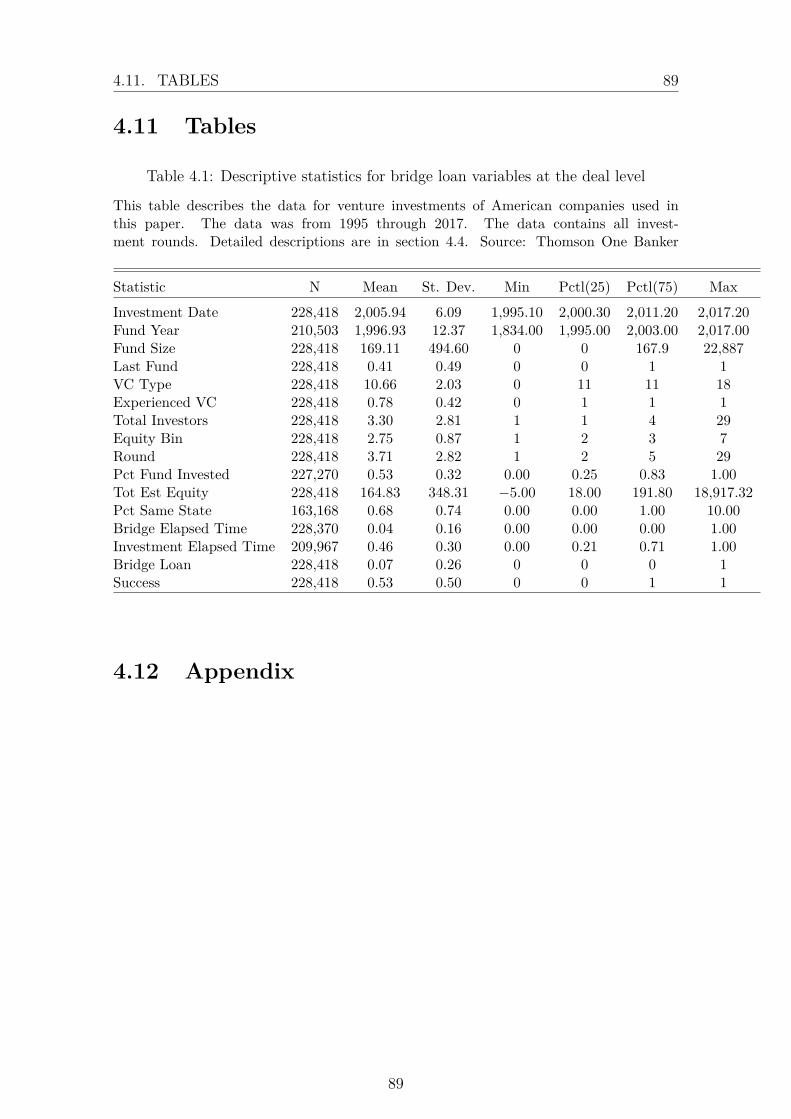
4.11. TABLES 89
4.11 Tables
Table 4.1: Descriptive statistics for bridge loan variables at the deal level
This table describes the data for venture investments of American companies used inthis paper. The data was from 1995 through 2017. The data contains all invest-ment rounds. Detailed descriptions are in section 4.4. Source: Thomson One Banker
Statistic N Mean St. Dev. Min Pctl(25) Pctl(75) Max
Investment Date 228,418 2,005.94 6.09 1,995.10 2,000.30 2,011.20 2,017.20Fund Year 210,503 1,996.93 12.37 1,834.00 1,995.00 2,003.00 2,017.00Fund Size 228,418 169.11 494.60 0 0 167.9 22,887Last Fund 228,418 0.41 0.49 0 0 1 1VC Type 228,418 10.66 2.03 0 11 11 18Experienced VC 228,418 0.78 0.42 0 1 1 1Total Investors 228,418 3.30 2.81 1 1 4 29Equity Bin 228,418 2.75 0.87 1 2 3 7Round 228,418 3.71 2.82 1 2 5 29Pct Fund Invested 227,270 0.53 0.32 0.00 0.25 0.83 1.00Tot Est Equity 228,418 164.83 348.31 −5.00 18.00 191.80 18,917.32Pct Same State 163,168 0.68 0.74 0.00 0.00 1.00 10.00Bridge Elapsed Time 228,370 0.04 0.16 0.00 0.00 0.00 1.00Investment Elapsed Time 209,967 0.46 0.30 0.00 0.21 0.71 1.00Bridge Loan 228,418 0.07 0.26 0 0 0 1Success 228,418 0.53 0.50 0 0 1 1
4.12 Appendix
89
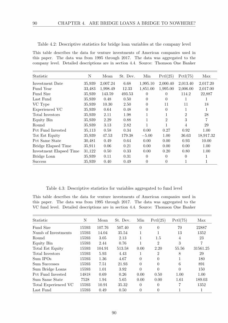
90 CHAPTER 4. ARE BRIDGE LOANS A BRIDGE TO NOWHERE?
Table 4.2: Descriptive statistics for bridge loan variables at the company level
This table describes the data for venture investments of American companies used inthis paper. The data was from 1995 through 2017. The data was aggregated to thecompany level. Detailed descriptions are in section 4.4. Source: Thomson One Banker
Statistic N Mean St. Dev. Min Pctl(25) Pctl(75) Max
Investment Date 35,939 2,007.24 6.68 1,995.10 2,000.40 2,013.40 2,017.20Fund Year 33,483 1,998.49 12.33 1,851.00 1,995.00 2,006.00 2,017.00Fund Size 35,939 143.59 493.53 0 0 114.2 22,887Last Fund 35,939 0.48 0.50 0 0 1 1VC Type 35,939 10.30 2.50 0 11 11 18Experienced VC 35,939 0.64 0.48 0 0 1 1Total Investors 35,939 2.11 1.98 1 1 2 28Equity Bin 35,939 2.29 0.88 1 2 3 7Round 35,939 3.13 2.82 1 1 4 29Pct Fund Invested 35,113 0.58 0.34 0.00 0.27 0.92 1.00Tot Est Equity 35,939 47.53 179.38 −5.00 1.00 36.63 18,917.32Pct Same State 30,481 0.49 0.64 0.00 0.00 0.93 10.00Bridge Elapsed Time 35,911 0.06 0.21 0.00 0.00 0.00 1.00Investment Elapsed Time 31,122 0.50 0.33 0.00 0.20 0.80 1.00Bridge Loan 35,939 0.11 0.31 0 0 0 1Success 35,939 0.40 0.49 0 0 1 1
Table 4.3: Descriptive statistics for variables aggregated to fund level
This table describes the data for venture investments of American companies used inthis paper. The data was from 1995 through 2017. The data was aggregated to theVC fund level. Detailed descriptions are in section 4.4. Source: Thomson One Banker
Statistic N Mean St. Dev. Min Pctl(25) Pctl(75) Max
Fund Size 15593 107.76 507.40 0 0 70 22887Numb of Investments 15593 14.04 35.54 1 1 13 1352Round 15593 3.05 2.13 1 1.5 4 23Equity Bin 15593 2.44 0.76 1 2 3 7Total Est Equity 15593 104.91 513.58 0.00 2.20 55.56 31561.25Total Investors 15593 5.93 4.43 1 2 8 29Sum IPOs 15593 1.36 4.67 0 0 1 180Sum Successes 15593 7.51 21.93 0 0 6 891Sum Bridge Loans 15593 1.01 3.92 0 0 0 150Pct Fund Invested 14818 0.69 0.26 0.00 0.50 1.00 1.00Sum Same State 7528 1.94 5.65 0.00 0.00 1.61 189.03Total Experienced VC 15593 10.91 35.32 0 0 7 1352Last Fund 15593 0.49 0.50 0 0 1 1
90

4.12. APPENDIX 91
Table 4.4: Status of companies with computed defunct companies
This table describes the status of the companies, as self-reported by the venturefirms. The computed defunct status was described in section 4. The data was ag-gregated to the company level. The first column was the reported status. It wasfollowed by the count of companies in that status. Column 3 was the percentageof companies by status. Column 4 was the count of companies which had a bridgeloan in an investment round. Column 5 had the status percentages for those com-panies. Detailed descriptions are in section 4.4. Source: Thomson One Banker
Status Count % Total Bridge Loans % Bridge Loans
Acquisition 8432 23.460% 101 0.280%Active 2343 6.520% 135 0.380%Bankruptcy - Chapter 11 106 0.290% 1 0.003%Bankruptcy - Chapter 7 90 0.250% 0 0Defunct 3717 10.340% 0 0LBO 648 1.800% 5 0.010%Merger 331 0.920% 1 0.003%Other 16 0.040% 12 0.030%Pending Acquisition 259 0.720% 12 0.030%Went Public 2225 6.190% 19 0.050%In Registration 41 0.110% 4 0.010%Private Company (Non-PE) 1 0.003% 0 0Computed Defunct 17730 49.330% 3599 10.010%
91
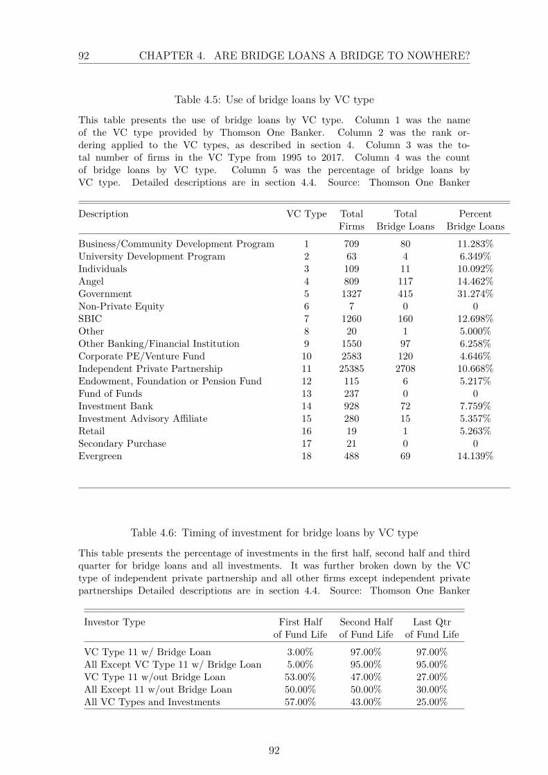
92 CHAPTER 4. ARE BRIDGE LOANS A BRIDGE TO NOWHERE?
Table 4.5: Use of bridge loans by VC type
This table presents the use of bridge loans by VC type. Column 1 was the nameof the VC type provided by Thomson One Banker. Column 2 was the rank or-dering applied to the VC types, as described in section 4. Column 3 was the to-tal number of firms in the VC Type from 1995 to 2017. Column 4 was the countof bridge loans by VC type. Column 5 was the percentage of bridge loans byVC type. Detailed descriptions are in section 4.4. Source: Thomson One Banker
Description VC Type Total Total PercentFirms Bridge Loans Bridge Loans
Business/Community Development Program 1 709 80 11.283%University Development Program 2 63 4 6.349%Individuals 3 109 11 10.092%Angel 4 809 117 14.462%Government 5 1327 415 31.274%Non-Private Equity 6 7 0 0SBIC 7 1260 160 12.698%Other 8 20 1 5.000%Other Banking/Financial Institution 9 1550 97 6.258%Corporate PE/Venture Fund 10 2583 120 4.646%Independent Private Partnership 11 25385 2708 10.668%Endowment, Foundation or Pension Fund 12 115 6 5.217%Fund of Funds 13 237 0 0Investment Bank 14 928 72 7.759%Investment Advisory Affiliate 15 280 15 5.357%Retail 16 19 1 5.263%Secondary Purchase 17 21 0 0Evergreen 18 488 69 14.139%
Table 4.6: Timing of investment for bridge loans by VC type
This table presents the percentage of investments in the first half, second half and thirdquarter for bridge loans and all investments. It was further broken down by the VCtype of independent private partnership and all other firms except independent privatepartnerships Detailed descriptions are in section 4.4. Source: Thomson One Banker
Investor Type First Half Second Half Last Qtrof Fund Life of Fund Life of Fund Life
VC Type 11 w/ Bridge Loan 3.00% 97.00% 97.00%All Except VC Type 11 w/ Bridge Loan 5.00% 95.00% 95.00%VC Type 11 w/out Bridge Loan 53.00% 47.00% 27.00%All Except 11 w/out Bridge Loan 50.00% 50.00% 30.00%All VC Types and Investments 57.00% 43.00% 25.00%
92
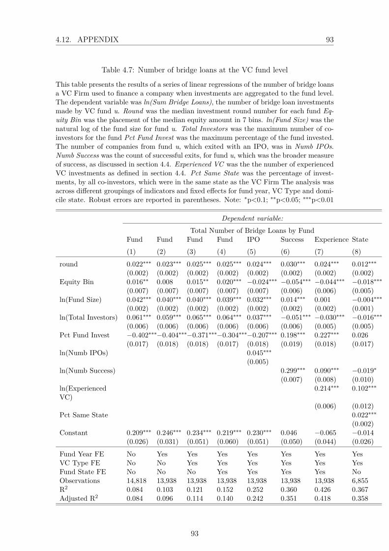
4.12. APPENDIX 93
Table 4.7: Number of bridge loans at the VC fund level
This table presents the results of a series of linear regressions of the number of bridge loansa VC Firm used to finance a company when investments are aggregated to the fund level.The dependent variable was ln(Sum Bridge Loans), the number of bridge loan investmentsmade by VC fund u. Round was the median investment round number for each fund Eq-uity Bin was the placement of the median equity amount in 7 bins. ln(Fund Size) was thenatural log of the fund size for fund u. Total Investors was the maximum number of co-investors for the fund Pct Fund Invest was the maximum percentage of the fund invested.The number of companies from fund u, which exited with an IPO, was in Numb IPOs.Numb Success was the count of successful exits, for fund u, which was the broader measureof success, as discussed in section 4.4. Experienced VC was the the number of experiencedVC investments as defined in section 4.4. Pct Same State was the percentage of invest-ments, by all co-investors, which were in the same state as the VC Firm The analysis wasacross different groupings of indicators and fixed effects for fund year, VC Type and domi-cile state. Robust errors are reported in parentheses. Note: ∗p<0.1; ∗∗p<0.05; ∗∗∗p<0.01
Dependent variable:Total Number of Bridge Loans by Fund
Fund Fund Fund Fund IPO Success Experience State(1) (2) (3) (4) (5) (6) (7) (8)
round 0.022∗∗∗ 0.023∗∗∗ 0.025∗∗∗ 0.025∗∗∗ 0.024∗∗∗ 0.030∗∗∗ 0.024∗∗∗ 0.012∗∗∗
(0.002) (0.002) (0.002) (0.002) (0.002) (0.002) (0.002) (0.002)Equity Bin 0.016∗∗ 0.008 0.015∗∗ 0.020∗∗∗ −0.024∗∗∗ −0.054∗∗∗ −0.044∗∗∗ −0.018∗∗∗
(0.007) (0.007) (0.007) (0.007) (0.007) (0.006) (0.006) (0.005)ln(Fund Size) 0.042∗∗∗ 0.040∗∗∗ 0.040∗∗∗ 0.039∗∗∗ 0.032∗∗∗ 0.014∗∗∗ 0.001 −0.004∗∗∗
(0.002) (0.002) (0.002) (0.002) (0.002) (0.002) (0.002) (0.001)ln(Total Investors) 0.061∗∗∗ 0.059∗∗∗ 0.065∗∗∗ 0.064∗∗∗ 0.037∗∗∗ −0.051∗∗∗ −0.030∗∗∗ −0.016∗∗∗
(0.006) (0.006) (0.006) (0.006) (0.006) (0.006) (0.005) (0.005)Pct Fund Invest −0.402∗∗∗−0.404∗∗∗−0.371∗∗∗−0.304∗∗∗−0.207∗∗∗ 0.198∗∗∗ 0.227∗∗∗ 0.026
(0.017) (0.018) (0.018) (0.017) (0.018) (0.019) (0.018) (0.017)ln(Numb IPOs) 0.045∗∗∗
(0.005)ln(Numb Success) 0.299∗∗∗ 0.090∗∗∗ −0.019∗
(0.007) (0.008) (0.010)ln(ExperiencedVC)
0.214∗∗∗ 0.102∗∗∗
(0.006) (0.012)Pct Same State 0.022∗∗∗
(0.002)Constant 0.209∗∗∗ 0.246∗∗∗ 0.234∗∗∗ 0.219∗∗∗ 0.230∗∗∗ 0.046 −0.065 −0.014
(0.026) (0.031) (0.051) (0.060) (0.051) (0.050) (0.044) (0.026)
Fund Year FE No Yes Yes Yes Yes Yes Yes YesVC Type FE No No Yes Yes Yes Yes Yes YesFund State FE No No No Yes Yes Yes Yes NoObservations 14,818 13,938 13,938 13,938 13,938 13,938 13,938 6,855R2 0.084 0.103 0.121 0.152 0.252 0.360 0.426 0.367Adjusted R2 0.084 0.096 0.114 0.140 0.242 0.351 0.418 0.358
93
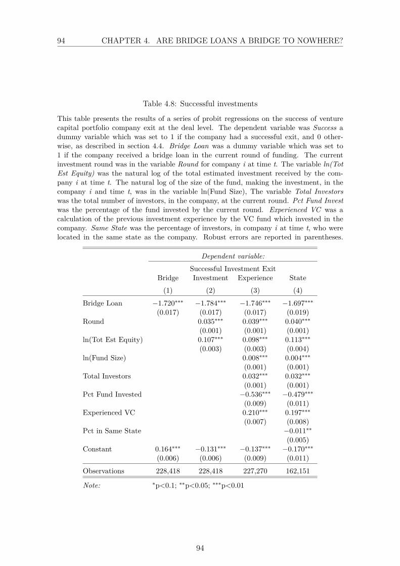
94 CHAPTER 4. ARE BRIDGE LOANS A BRIDGE TO NOWHERE?
Table 4.8: Successful investments
This table presents the results of a series of probit regressions on the success of venturecapital portfolio company exit at the deal level. The dependent variable was Success adummy variable which was set to 1 if the company had a successful exit, and 0 other-wise, as described in section 4.4. Bridge Loan was a dummy variable which was set to1 if the company received a bridge loan in the current round of funding. The currentinvestment round was in the variable Round for company i at time t. The variable ln(TotEst Equity) was the natural log of the total estimated investment received by the com-pany i at time t. The natural log of the size of the fund, making the investment, in thecompany i and time t, was in the variable ln(Fund Size), The variable Total Investorswas the total number of investors, in the company, at the current round. Pct Fund Investwas the percentage of the fund invested by the current round. Experienced VC was acalculation of the previous investment experience by the VC fund which invested in thecompany. Same State was the percentage of investors, in company i at time t, who werelocated in the same state as the company. Robust errors are reported in parentheses.
Dependent variable:Successful Investment Exit
Bridge Investment Experience State(1) (2) (3) (4)
Bridge Loan −1.720∗∗∗ −1.784∗∗∗ −1.746∗∗∗ −1.697∗∗∗
(0.017) (0.017) (0.017) (0.019)Round 0.035∗∗∗ 0.039∗∗∗ 0.040∗∗∗
(0.001) (0.001) (0.001)ln(Tot Est Equity) 0.107∗∗∗ 0.098∗∗∗ 0.113∗∗∗
(0.003) (0.003) (0.004)ln(Fund Size) 0.008∗∗∗ 0.004∗∗∗
(0.001) (0.001)Total Investors 0.032∗∗∗ 0.032∗∗∗
(0.001) (0.001)Pct Fund Invested −0.536∗∗∗ −0.479∗∗∗
(0.009) (0.011)Experienced VC 0.210∗∗∗ 0.197∗∗∗
(0.007) (0.008)Pct in Same State −0.011∗∗
(0.005)Constant 0.164∗∗∗ −0.131∗∗∗ −0.137∗∗∗ −0.170∗∗∗
(0.006) (0.006) (0.009) (0.011)
Observations 228,418 228,418 227,270 162,151
Note: ∗p<0.1; ∗∗p<0.05; ∗∗∗p<0.01
94
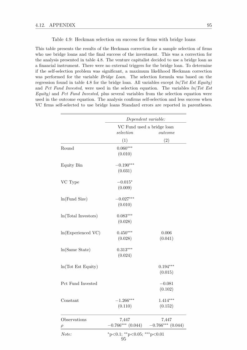
4.12. APPENDIX 95
Table 4.9: Heckman selection on success for firms with bridge loans
This table presents the results of the Heckman correction for a sample selection of firmswho use bridge loans and the final success of the investment. This was a correction forthe analysis presented in table 4.8. The venture capitalist decided to use a bridge loan asa financial instrument. There were no external triggers for the bridge loan. To determineif the self-selection problem was significant, a maximum likelihood Heckman correctionwas performed for the variable Bridge Loan. The selection formula was based on theregression found in table 4.8 for the bridge loan. All variables except ln(Tot Est Equity)and Pct Fund Invested, were used in the selection equation. The variables ln(Tot EstEquity) and Pct Fund Invested, plus several variables from the selection equation wereused in the outcome equation. The analysis confirms self-selection and less success whenVC firms self-selected to use bridge loans Standard errors are reported in parentheses.
Dependent variable:VC Fund used a bridge loanselection outcome
(1) (2)
Round 0.060∗∗∗
(0.010)
Equity Bin −0.190∗∗∗
(0.031)
VC Type −0.015∗
(0.009)
ln(Fund Size) −0.027∗∗∗
(0.010)
ln(Total Investors) 0.083∗∗∗
(0.028)
ln(Experienced VC) 0.450∗∗∗ 0.006(0.028) (0.041)
ln(Same State) 0.313∗∗∗
(0.024)
ln(Tot Est Equity) 0.194∗∗∗
(0.015)
Pct Fund Invested −0.081(0.102)
Constant −1.266∗∗∗ 1.414∗∗∗
(0.110) (0.152)
Observations 7,447 7,447ρ −0.766∗∗∗ (0.044) −0.766∗∗∗ (0.044)
Note: ∗p<0.1; ∗∗p<0.05; ∗∗∗p<0.0195
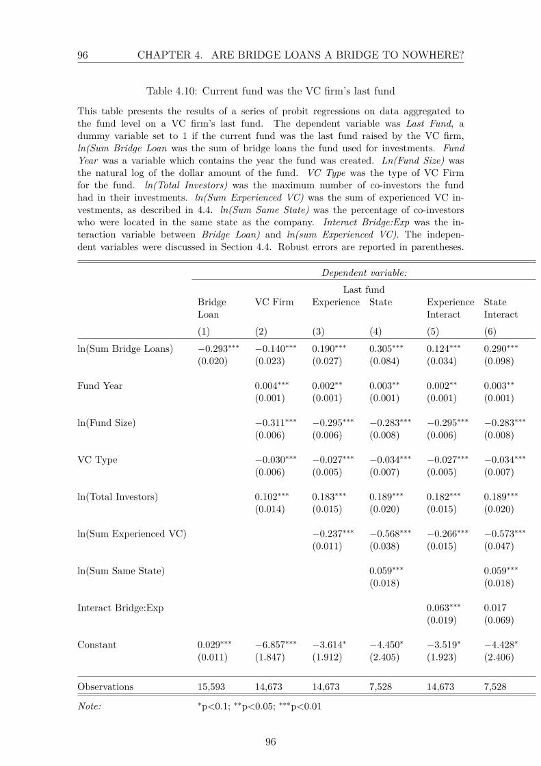
96 CHAPTER 4. ARE BRIDGE LOANS A BRIDGE TO NOWHERE?
Table 4.10: Current fund was the VC firm’s last fund
This table presents the results of a series of probit regressions on data aggregated tothe fund level on a VC firm’s last fund. The dependent variable was Last Fund, adummy variable set to 1 if the current fund was the last fund raised by the VC firm,ln(Sum Bridge Loan was the sum of bridge loans the fund used for investments. FundYear was a variable which contains the year the fund was created. Ln(Fund Size) wasthe natural log of the dollar amount of the fund. VC Type was the type of VC Firmfor the fund. ln(Total Investors) was the maximum number of co-investors the fundhad in their investments. ln(Sum Experienced VC) was the sum of experienced VC in-vestments, as described in 4.4. ln(Sum Same State) was the percentage of co-investorswho were located in the same state as the company. Interact Bridge:Exp was the in-teraction variable between Bridge Loan) and ln(sum Experienced VC). The indepen-dent variables were discussed in Section 4.4. Robust errors are reported in parentheses.
Dependent variable:Last fund
BridgeLoan
VC Firm Experience State ExperienceInteract
StateInteract
(1) (2) (3) (4) (5) (6)
ln(Sum Bridge Loans) −0.293∗∗∗ −0.140∗∗∗ 0.190∗∗∗ 0.305∗∗∗ 0.124∗∗∗ 0.290∗∗∗
(0.020) (0.023) (0.027) (0.084) (0.034) (0.098)
Fund Year 0.004∗∗∗ 0.002∗∗ 0.003∗∗ 0.002∗∗ 0.003∗∗
(0.001) (0.001) (0.001) (0.001) (0.001)
ln(Fund Size) −0.311∗∗∗ −0.295∗∗∗ −0.283∗∗∗ −0.295∗∗∗ −0.283∗∗∗
(0.006) (0.006) (0.008) (0.006) (0.008)
VC Type −0.030∗∗∗ −0.027∗∗∗ −0.034∗∗∗ −0.027∗∗∗ −0.034∗∗∗
(0.006) (0.005) (0.007) (0.005) (0.007)
ln(Total Investors) 0.102∗∗∗ 0.183∗∗∗ 0.189∗∗∗ 0.182∗∗∗ 0.189∗∗∗
(0.014) (0.015) (0.020) (0.015) (0.020)
ln(Sum Experienced VC) −0.237∗∗∗ −0.568∗∗∗ −0.266∗∗∗ −0.573∗∗∗
(0.011) (0.038) (0.015) (0.047)
ln(Sum Same State) 0.059∗∗∗ 0.059∗∗∗
(0.018) (0.018)
Interact Bridge:Exp 0.063∗∗∗ 0.017(0.019) (0.069)
Constant 0.029∗∗∗ −6.857∗∗∗ −3.614∗ −4.450∗ −3.519∗ −4.428∗
(0.011) (1.847) (1.912) (2.405) (1.923) (2.406)
Observations 15,593 14,673 14,673 7,528 14,673 7,528
Note: ∗p<0.1; ∗∗p<0.05; ∗∗∗p<0.01
96
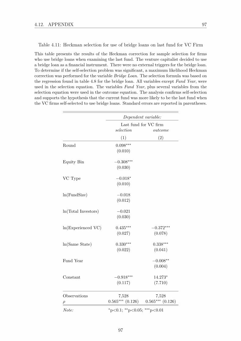
4.12. APPENDIX 97
Table 4.11: Heckman selection for use of bridge loans on last fund for VC Firm
This table presents the results of the Heckman correction for sample selection for firmswho use bridge loans when examining the last fund. The venture capitalist decided to usea bridge loan as a financial instrument. There were no external triggers for the bridge loan.To determine if the self-selection problem was significant, a maximum likelihood Heckmancorrection was performed for the variable Bridge Loan. The selection formula was based onthe regression found in table 4.8 for the bridge loan. All variables except Fund Year, wereused in the selection equation. The variables Fund Year, plus several variables from theselection equation were used in the outcome equation. The analysis confirms self-selectionand supports the hypothesis that the current fund was more likely to be the last fund whenthe VC firms self-selected to use bridge loans. Standard errors are reported in parentheses.
Dependent variable:Last fund for VC firm
selection outcome(1) (2)
Round 0.098∗∗∗
(0.010)
Equity Bin −0.308∗∗∗
(0.030)
VC Type −0.018∗
(0.010)
ln(FundSize) −0.018(0.012)
ln(Total Investors) −0.021(0.030)
ln(Experienced VC) 0.435∗∗∗ −0.372∗∗∗
(0.027) (0.078)
ln(Same State) 0.330∗∗∗ 0.338∗∗∗
(0.022) (0.041)
Fund Year −0.008∗∗
(0.004)
Constant −0.918∗∗∗ 14.273∗
(0.117) (7.710)
Observations 7,528 7,528ρ 0.565∗∗∗ (0.126) 0.565∗∗∗ (0.126)
Note: ∗p<0.1; ∗∗p<0.05; ∗∗∗p<0.01
97
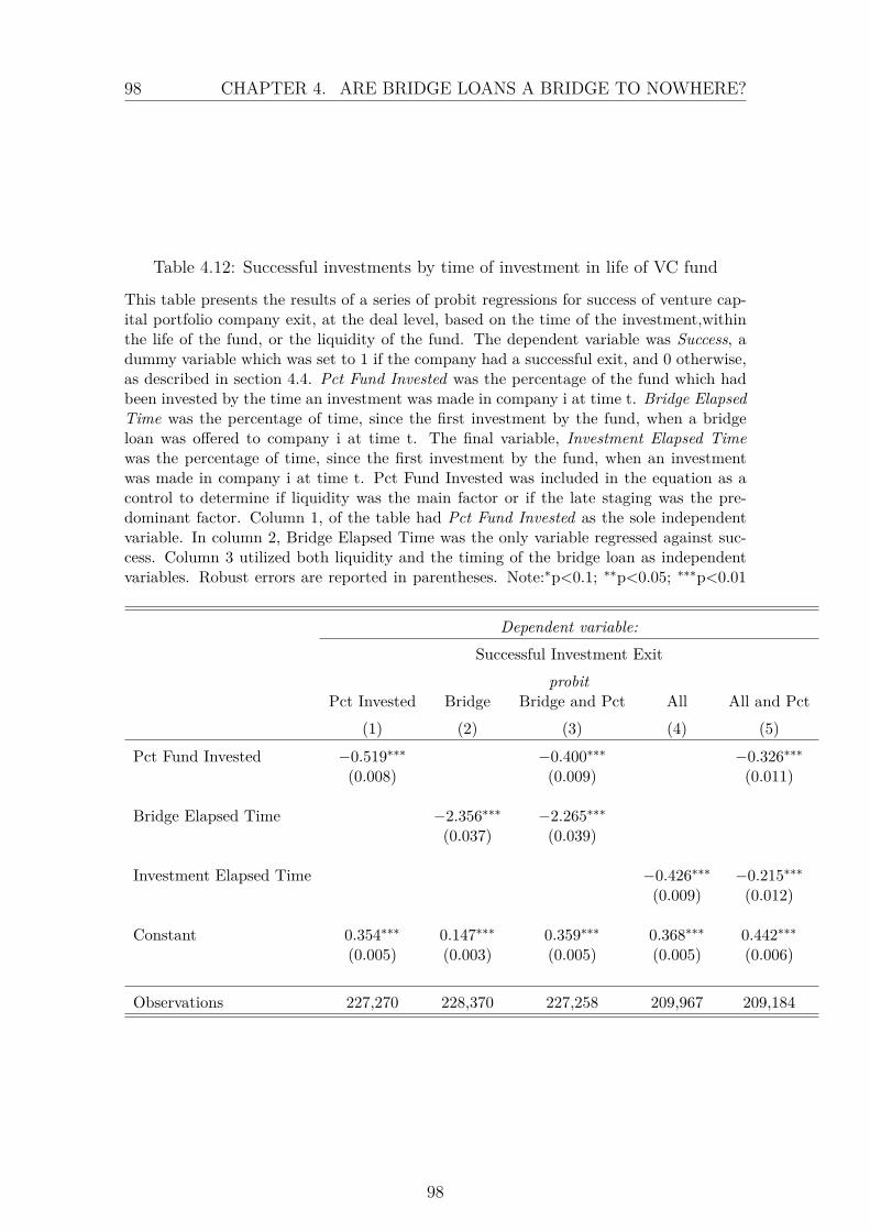
98 CHAPTER 4. ARE BRIDGE LOANS A BRIDGE TO NOWHERE?
Table 4.12: Successful investments by time of investment in life of VC fund
This table presents the results of a series of probit regressions for success of venture cap-ital portfolio company exit, at the deal level, based on the time of the investment,withinthe life of the fund, or the liquidity of the fund. The dependent variable was Success, adummy variable which was set to 1 if the company had a successful exit, and 0 otherwise,as described in section 4.4. Pct Fund Invested was the percentage of the fund which hadbeen invested by the time an investment was made in company i at time t. Bridge ElapsedTime was the percentage of time, since the first investment by the fund, when a bridgeloan was offered to company i at time t. The final variable, Investment Elapsed Timewas the percentage of time, since the first investment by the fund, when an investmentwas made in company i at time t. Pct Fund Invested was included in the equation as acontrol to determine if liquidity was the main factor or if the late staging was the pre-dominant factor. Column 1, of the table had Pct Fund Invested as the sole independentvariable. In column 2, Bridge Elapsed Time was the only variable regressed against suc-cess. Column 3 utilized both liquidity and the timing of the bridge loan as independentvariables. Robust errors are reported in parentheses. Note:∗p<0.1; ∗∗p<0.05; ∗∗∗p<0.01
Dependent variable:Successful Investment Exit
probitPct Invested Bridge Bridge and Pct All All and Pct
(1) (2) (3) (4) (5)
Pct Fund Invested −0.519∗∗∗ −0.400∗∗∗ −0.326∗∗∗
(0.008) (0.009) (0.011)
Bridge Elapsed Time −2.356∗∗∗ −2.265∗∗∗
(0.037) (0.039)
Investment Elapsed Time −0.426∗∗∗ −0.215∗∗∗
(0.009) (0.012)
Constant 0.354∗∗∗ 0.147∗∗∗ 0.359∗∗∗ 0.368∗∗∗ 0.442∗∗∗
(0.005) (0.003) (0.005) (0.005) (0.006)
Observations 227,270 228,370 227,258 209,967 209,184
98
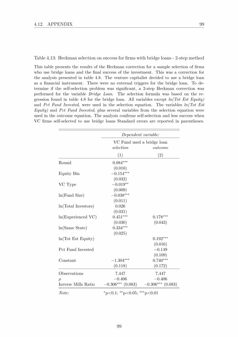
4.12. APPENDIX 99
Table 4.13: Heckman selection on success for firms with bridge loans - 2-step method
This table presents the results of the Heckman correction for a sample selection of firmswho use bridge loans and the final success of the investment. This was a correction forthe analysis presented in table 4.8. The venture capitalist decided to use a bridge loanas a financial instrument. There were no external triggers for the bridge loan. To de-termine if the self-selection problem was significant, a 2-step Heckman correction wasperformed for the variable Bridge Loan. The selection formula was based on the re-gression found in table 4.8 for the bridge loan. All variables except ln(Tot Est Equity)and Pct Fund Invested, were used in the selection equation. The variables ln(Tot EstEquity) and Pct Fund Invested, plus several variables from the selection equation wereused in the outcome equation. The analysis confirms self-selection and less success whenVC firms self-selected to use bridge loans Standard errors are reported in parentheses.
Dependent variable:VC Fund used a bridge loanselection outcome
(1) (2)
Round 0.084∗∗∗
(0.010)Equity Bin −0.154∗∗∗
(0.032)VC Type −0.019∗∗
(0.009)ln(Fund Size) −0.038∗∗∗
(0.011)ln(Total Investors) 0.026
(0.031)ln(Experienced VC) 0.451∗∗∗ 0.178∗∗∗
(0.030) (0.043)ln(Same State) 0.334∗∗∗
(0.025)ln(Tot Est Equity) 0.192∗∗∗
(0.016)Pct Fund Invested −0.149
(0.109)Constant −1.304∗∗∗ 0.740∗∗∗
(0.118) (0.172)
Observations 7,447 7,447ρ −0.406 −0.406Inverse Mills Ratio −0.306∗∗∗ (0.083) −0.306∗∗∗ (0.083)
Note: ∗p<0.1; ∗∗p<0.05; ∗∗∗p<0.01
99

100 CHAPTER 4. ARE BRIDGE LOANS A BRIDGE TO NOWHERE?
Table 4.14: Heckman selection for use of bridge loans on last fund for VC Firm -2-step method
This table presents the results of the Heckman correction for sample selection for firms whouse bridge loans when examining the last fund. The venture capitalist decided to use abridge loan as a financial instrument. There were no external triggers for the bridge loan.To determine if the self-selection problem was significant, a 2-step Heckman correctionwas performed for the variable Bridge Loan. The selection formula was based on theregression found in table 4.8 for the bridge loan. All variables except Fund Year, wereused in the selection equation. The variables Fund Year, plus several variables from theselection equation were used in the outcome equation. The analysis confirms self-selectionand supports the hypothesis that the current fund was more likely to be the last fund whenthe VC firms self-selected to use bridge loans. Standard errors are reported in parentheses.
Dependent variable:Last fund for VC firm
selection outcome(1) (2)
Round 0.099∗∗∗
(0.009)Equity Bin −0.293∗∗∗
(0.031)VC Type −0.019∗∗
(0.009)ln(Fund Size) −0.037∗∗∗
(0.011)ln(Total Investors) −0.015
(0.030)ln(Experienced VC) 0.446∗∗∗ −0.171∗∗∗
(0.029) (0.024)ln(Same State) 0.322∗∗∗ 0.112∗∗∗
(0.024) (0.021)
Fund Year −0.003∗∗
(0.001)Constant −0.913∗∗∗ 6.152∗∗
(0.110) (2.884)
Observations 7,528 7,528ρ 0.271 0.271Inverse Mills Ratio 0.125∗ (0.066) 0.125∗ (0.066)
Note: ∗p<0.1; ∗∗p<0.05; ∗∗∗p<0.01
100
References 101
References
Admati, A. R., & Pfleiderer, P. (1994). Robust Financial Contracting and the Roleof Venture Capitalists. The Journal of Finance, 49 (2), 371–402.
Aghion, P., & Bolton, P. (1992). An incomplete contracts approach to financialcontracting. The review of economic Studies, 59 (3), 473–494.
Andrade, G., Mitchell, M., & Stafford, E. (2001). New Evidence and Perspectiveson Mergers. , 18.
Arcot, S., Fluck, Z., Gaspar, J.-M., & Hege, U. (2015). Fund managers under pres-sure: Rationale and determinants of secondary buyouts. Journal of FinancialEconomics, 115 (1), 102–135.
Atanasova, C., & Chemla, G. (2020). Familiarity breeds alternative investment:Evidence from corporate defined benefit pension plans. Available at SSRN2468290 .
Barber, B. M., & Yasuda, A. (2017). Interim fund performance and fundraising inprivate equity. Journal of Financial Economics, 124 (1), 172–194.
Bartlett III, R. P. (2006). Venture capital, agency costs, and the false dichotomy ofthe corporation. UCLA L. Rev., 54 , 37.
Bénabou, R., & Tirole, J. (2006). Incentives and prosocial behavior. Americaneconomic review, 96 (5), 1652–1678.
Bigus, J. (2006). Staging of venture financing, investor opportunism and patentlaw. Journal of Business Finance & Accounting, 33 (7-8), 939–960.
Boone, A. L., & Mulherin, J. H. (2011). Do private equity consortiums facilitatecollusion in takeover bidding? Journal of Corporate Finance, 17 (5), 1475–1495.
Brander, J. A., Amit, R., & Antweiler, W. (2002). Venture-Capital Syndication:Improved Venture Selection vs. The Value-Added Hypothesis. Journal of Eco-nomics Management Strategy, 11 (3), 423–452.
Brown, G. W., Harris, R. S., Hu, W., Jenkinson, T., Kaplan, S. N., & Robinson,D. T. (2020). Can investors time their exposure to private equity? KenanInstitute of Private Enterprise Research Paper(18-26.).
Busenitz, L. W., Moesel, D. D., Fiet, J. O., & Barney, J. B. (1997). The framingof perceptions of fairness in the relationship between venture capitalists andnew venture teams. Entrepreneurship Theory and Practice, 21 (3), 5–22.
Bygrave, W. D. (1987). Syndicated investments by venture capital firms: A net-working perspective. Journal of Business Venturing, 2 (2), 139–154.
Cable, D. M., & Shane, S. (1997). A prisoner’s dilemma approach to entrepreneur-venture capitalist relationships. Academy of Management review, 22 (1), 142–176.
101
102 CHAPTER 4. ARE BRIDGE LOANS A BRIDGE TO NOWHERE?
Casamatta, C. (2003). Financing and advising: optimal financial contracts withventure capitalists. The journal of finance, 58 (5), 2059–2085.
Casamatta, C., & Haritchabalet, C. (2007). Experience, screening and syndicationin venture capital investments. Journal of Financial Intermediation, 16 (3),368–398.
Certo, S. T., Busenbark, J. R., Woo, H.-s., & Semadeni, M. (2016). Sample se-lection bias and heckman models in strategic management research. StrategicManagement Journal, 37 (13), 2639–2657.
Cestone, G. (2014). Venture capital meets contract theory: risky claims or formalcontrol? Review of Finance, 18 (3), 1097–1137.
Chemla, G., Habib, M. A., & Ljungqvist, A. (2007). An analysis of shareholderagreements. Journal of the European Economic Association, 5 (1), 93–121.
Cochrane, J. H. (2005). The risk and return of venture capital. Journal of financialeconomics, 75 (1), 3–52.
Cornelli, F., & Yosha, O. (2003). Stage financing and the role of convertible secu-rities. The Review of Economic Studies, 70 (1), 1–32.
Cumming, D., & Dai, N. (2010). Local bias in venture capital investments. Journalof Empirical Finance, 17 (3), 362–380.
Da Rin, M., Hellmann, T., & Puri, M. (2013). A survey of venture capital research.In Handbook of the economics of finance (Vol. 2, pp. 573–648). Elsevier.
De Bettignies, J.-E. (2008). Financing the entrepreneurial venture. ManagementScience, 54 (1), 151–166.
De Bettignies, J.-E., & Brander, J. A. (2007). Financing entrepreneurship: Bankfinance versus venture capital. Journal of Business Venturing, 22 (6), 808–832.
De Bettignies, J.-E., & Chemla, G. (2008). Corporate venturing, allocation of talent,and competition for star managers. Management science, 54 (3), 505–521.
De Clercq, D., & Sapienza, H. J. (2001). The creation of relational rents in venturecapitalist-entrepreneur dyads. Venture Capital: An International Journal ofEntrepreneurial Finance, 3 (2), 107–127.
Dewatripont, M., & Tirole, J. (1994). A theory of debt and equity: Diversityof securities and manager-shareholder congruence. The quarterly journal ofeconomics, 109 (4), 1027–1054.
Dimitrova, L. (2017). Perverse incentives of special purpose acquisition companies,the “poor man’s private equity funds”. Journal of Accounting and Economics,63 (1), 99–120.
Dimov, D., & De Holan, P. M. (2005). Venture Capital Firm Knowledge andTechnological Boom-and-Bust Cycles. SSRN Electronic Journal.
Duchin, R., & Schmidt, B. (2013). Riding the merger wave: Uncertainty, reducedmonitoring, and bad acquisitions. Journal of Financial Economics, 107 (1),
102

References 103
69–88.Ehrenberg, R. (2010). The vc market: An adaptive system. http://
informationarbitrage.com/post/1260655542/the-vc-market-an-adaptive-system. (Accessed: 2019-06-10)
Fairchild, R. (2004). Financial contracting between managers and venture capi-talists: the role of value-added services, reputation seeking, and bargainingpower. Journal of Financial Research, 27 (4), 481–495.
Gilson, S. C. (1997). Transactions costs and capital structure choice: Evidence fromfinancially distressed firms. The Journal of Finance, 52 (1), 161–196.
Giot, P., & Schwienbacher, A. (2007). Ipos, trade sales and liquidations: Modellingventure capital exits using survival analysis. Journal of Banking & Finance,31 (3), 679–702.
Glazer, A. S. (1989). Acquisition bridge financing by investment banks. BusinessHorizons, 32 (5), 49–54.
Gompers, P., Gornall, W., Kaplan, S., & Strebulaev, I. (2020). How do venturecapitalists make decisions? Journal of Financial Economics, 135 (1), 169–190.
Gompers, P., Kovner, A., Lerner, J., & Scharfstein, D. (2008a). Venture capi-tal investment cycles: The impact of public markets. Journal of FinancialEconomics, 87 (1), 1–23.
Gompers, P., Kovner, A., Lerner, J., & Scharfstein, D. (2008b). Venture capitalinvestment cycles: The impact of public markets. Journal of financial eco-nomics, 87 (1), 1–23.
Gompers, P. A. (1999). Ownership and control in entrepreneurial firms: an exami-nation of convertible securities in venture capital investment.
Goriatchev, S. (2002). Eat or be eaten: the empirical evidence. , 23.Gorman, M., & Sahlman, W. A. (1989). What do venture capitalists do? Journal
of business venturing, 4 (4), 231–248.Gornall, W., & Strebulaev, I. A. (2015). The economic impact of venture capital:
Evidence from public companies.Gort, M. (1969). An Economic Disturbance Theory of Mergers. The Quarterly
Journal of Economics, 83 (4), 624.Gross, B. (2015). Ted talk: “the single biggest reason why startups
succeed”. https://www.ted.com/talks/bill_gross_the_single_biggest_reason_why_start_ups_succeed. (Accessed: 2020-04-11)
Gugler, K., Mueller, D. C., & Yurtoglu, B. B. (2006). The determinants of mergerwaves. WZB Discussion Paper , 61.
Harford, J. (2005). What drives merger waves? Journal of Financial Economics,77 (3), 529–560.
Hart, O. (2009). Hold-up, asset ownership, and reference points. The Quarterly
103
104 CHAPTER 4. ARE BRIDGE LOANS A BRIDGE TO NOWHERE?
Journal of Economics, 124 (1), 267–300.Hart, O., & Moore, J. (2008). Contracts as reference points. The Quarterly journal
of economics, 123 (1), 1–48.Hege, U., Palomino, F., & Schwienbacher, A. (2008). Venture Capital Performance:
the Disparity Between Europe and the United States. SSRN Electronic Jour-nal.
Hellmann, T. (2006). Ipos, acquisitions, and the use of convertible securities inventure capital. Journal of Financial Economics, 81 (3), 649–679.
Hellmann, T. F., & Puri, M. (2000). The Interaction between Product Market andFinancing Strategy: The Role of Venture Capital. SSRN Electronic Journal.
Hlavac, M. (2015). stargazer: beautiful latex, html and ascii tables from r statisticaloutput.
Hochberg, Y. V., Ljungqvist, A., & Lu, Y. (2007). Whom You Know Matters: Ven-ture Capital Networks and Investment Performance. The Journal of Finance,62 (1), 251–301.
Hochberg, Y. V., & Rauh, J. D. (2013). Local overweighting and underperformance:Evidence from limited partner private equity investments. The Review ofFinancial Studies, 26 (2), 403–451.
Hopp, C., & Rieder, F. (2011). What drives venture capital syndication? AppliedEconomics, 43 (23), 3089–3102.
Kahl, M. (2002). Economic distress, financial distress, and dynamic liquidation.The Journal of Finance, 57 (1), 135–168.
Kaplan, S. N., & Schoar, A. (2005). Private equity performance: Returns, persis-tence, and capital flows. The journal of finance, 60 (4), 1791–1823.
Kaplan, S. N., & Strömberg, P. (2004). Characteristics, Contracts, and Actions:Evidence from Venture Capitalist Analyses. The Journal of Finance, 59 (5),2177–2210.
Kaplan, S. N., & Strömberg, P. (2003). Financial contracting theory meets thereal world: An empirical analysis of venture capital contracts. The review ofeconomic studies, 70 (2), 281–315.
Kaplan, S. N., & Stromberg, P. (2009). Leveraged Buyouts and Private Equity. ,41.
Kaplan, S. N., & Strömberg, P. E. (2004). Characteristics, contracts, and actions:Evidence from venture capitalist analyses. The Journal of Finance, 59 (5),2177–2210.
Keuschnigg, C., & Nielsen, S. B. (2004). Start-ups, venture capitalists, and thecapital gains tax. Journal of Public Economics, 88 (5), 1011–1042.
Klausner, M., & Litvak, K. (2001). What economists have taught us about venturecapital contracting.
104
References 105
Klonowski, D. (2010). The venture capital investment process. Springer.Kollmann, T., Kuckertz, A., & Middelberg, N. (2014). Trust and controllability
in venture capital fundraising. Journal of Business Research, 67 (11), 2411 -2418. doi: https://doi.org/10.1016/j.jbusres.2014.02.008
Krohmer, P., Lauterbach, R., & Calanog, V. (2009). The bright and dark side ofstaging: Investment performance and the varying motivations of private equityfirms. Journal of Banking & Finance, 33 (9), 1597–1609.
Kuckertz, A., Kollmann, T., Röhm, P., & Middelberg, N. (2015). The interplayof track record and trustworthiness in venture capital fundraising. Journal ofBusiness Venturing Insights, 4 , 6–13.
Lamont, O. A., & Stein, J. C. (2006). Investor Sentiment and Corporate Finance:Micro and Macro. , 96 (2), 6.
Landier, A. (2001). Start-up financing: Banks vs. venture capital, working paper .Lee, S., & Sunesson, D. (2008). Gold Rush Dynamics of Private Equity. SSRN
Electronic Journal.Lerner, J. (1994). The Syndication of Venture Capital Investments. Financial
Management, 23 (3), 16–27.Ljungqvist, A., & Richardson, M. (2003). The cash flow, return and risk character-
istics of private equity (Tech. Rep.). National Bureau of Economic Research.MacMillan, I. C., Siegel, R., & Narasimha, P. S. (1985). Criteria used by venture
capitalists to evaluate new venture proposals. Journal of Business venturing,1 (1), 119–128.
Maksimovic, V., & Phillips, G. (2001). The Market for Corporate Assets: WhoEngages in Mergers and Asset Sales and Are There Efficiency Gains? TheJournal of Finance, 47.
Maksimovic, V., Phillips, G., & Yang, L. (2013). Private and Public Merger Waves:Private and Public Merger Waves. The Journal of Finance, 68 (5), 2177–2217.
Marx, L. M. (1998). Efficient venture capital financing combining debt and equity.Review of Economic Design, 3 (4), 371–387.
Mitchell, M. L., & Mulherin, J. (1996). The impact of industry shocks on takeoverand restructuring activity. Journal of Financial Economics, 41 (2), 193–229.
Moeller, S. B., Schlingemann, F. P., & Stulz, R. M. (2005). Wealth destruction ona massive scale? a study of acquiring-firm returns in the recent merger wave.The journal of finance, 60 (2), 757–782.
Mulherin, J. H., & Boone, A. L. (2000). Comparing acquisitions and divestitures.Journal of corporate finance, 6 (2), 117–139.
Muse, A. (2016). Bridge loans: A suckers bet. https://medium.com/startup-muse/bridge-loans-a-suckers-bet-a9d6decf49c4. (Accessed: 2019-06-10)
105

106 CHAPTER 4. ARE BRIDGE LOANS A BRIDGE TO NOWHERE?
Nanda, R., & Rhodes-Kropf, M. (2018). Coordination Frictions in Venture CapitalSyndicates. NBER Working Paper(24517), 23.
Nanda, R., Samila, S., & Sorenson, O. (2020). The persistent effect of initial success:Evidence from venture capital. Journal of Financial Economics.
Phalippou, L., & Gottschalg, O. (2009). The performance of private equity funds.The Review of Financial Studies, 22 (4), 1747–1776.
Phillips, G. M., & Zhdanov, A. (2017). Venture capital investments and mergerand acquisition activity around the world (Tech. Rep.). National Bureau ofEconomic Research.
Puri, M., & Zarutskie, R. (2012). On the life cycle dynamics of venture-capital-and non-venture-capital-financed firms. The Journal of Finance, 67 (6), 2247–2293.
Repullo, R., & Suarez, J. (2004). Venture capital finance: A security design ap-proach. Review of finance, 8 (1), 75–108.
Rhodes-Kropf, M., & Viswanathan, S. (2004). Market valuation and merger waves.The Journal of Finance, 59 (6), 2685–2718.
Robbie, K., Wright, M., & Chiplin, B. (1997). The monitoring of venture capitalfirms. Entrepreneurship Theory and Practice, 21 (4), 9–28.
Robinson, D. T., & Sensoy, B. A. (2016). Cyclicality, performance measurement,and cash flow liquidity in private equity. Journal of Financial Economics,122 (3), 521–543.
Sahlman, W. A. (1990). The structure and governance of venture-capital organiza-tions. Journal of financial economics, 27 (2), 473–521.
Sapienza, H. J., & Korsgaard, M. A. (1996). Procedural justice in entrepreneur-investor relations. Academy of management Journal, 39 (3), 544–574.
Shepherd, D. A., & Zacharakis, A. (2001). The venture capitalist-entrepreneurrelationship: control, trust and confidence in co-operative behaviour. VentureCapital: an international journal of entrepreneurial finance, 3 (2), 129–149.
Shleifer, A., & Vishny, R. W. (2003). Stock market driven acquisitions. Journal ofFinancial Economics, 70 (3), 295–311.
Suster, M. (2010). Why bridge loans are usually a bad deal for both entrepreneurs andvcs. http://www.businessinsider.com/why-bridge-loans-are-usually-a-bad-idea-for-both-entrepreneurs-and-vcs-2010-5?IR=T. (Accessed:2019-06-10)
Tian, X. (2011). The causes and consequences of venture capital stage financing.Journal of Financial Economics, 101 (1), 132–159.
Toomet, O., Henningsen, A., et al. (2008). Sample selection models in r: Packagesampleselection. Journal of statistical software, 27 (7), 1–23.
Tykvová, T. (2007). What do economists tell us about venture capital contracts?
106
References 107
Journal of Economic Surveys, 21 (1), 65–89.Ueda, M. (2004). Banks versus venture capital: Project evaluation, screening, and
expropriation. The Journal of Finance, 59 (2), 601–621.Utset, M. A. (2002). Reciprocal fairness, strategic behavior and venture survival: a
theory of venture capital-financed firms. Wis. L. Rev., 45.Wilson, F. (2011). Financing options: Bridge loans. https://avc.com/2011/08/
financing-options-bridge-loans/. (Accessed: 2019-06-10)Wilson, R. (1968). The Theory of Syndicates. Econometrica, 36 (1), 119.Wiltbank, R., Dew, N., & Read, S. (2015). Investment and returns in successful
entrepreneurial sell-outs. Journal of Business Venturing Insights, 3 , 16–23.Yan, J. (2011). Merger waves: Theory and evidence. The Quarterly Journal of
Finance, 1 (03), 551–606.Yerramilli, V. (2004). Joint control and redemption rights in venture capital con-
tracts. ECGI-Finance Working Paper(37).Zarutskie, R. (2007). Do venture capitalists affect investment performance? evidence
from first-time funds. Fuqua School of Business, Duke University.Zarutskie, R. (2010). The role of top management team human capital in venture
capital markets: Evidence from first-time funds. Journal of Business Ventur-ing, 25 (1), 155–172.
107


RÉSUMÉ
Cette thèse analyse les contrats de financement utilisés par les fonds de capital risque, les vagues d’investissement réal-
isées ainsi que l’utilisation des crédits relais. Le premier chapitre présente un modèle théorique de contrat financement.
Ce modèle propose un contrat offrant plus de profits à l’entrepreneur dans le but de créer une relation moins conflictuelle,
bien que ce dernier ait initialement un pouvoir de négociation supérieur. La plupart des fonds de capital affirment réaliser
l’investissement initial dans une entreprise en se basant sur l’analyse de l’équipe fondatrice et la taille du marché visé par
l’entreprise. En analysant les investissements de fonds en capital risque, nous avons pu mettre en lumière l’existence de
vagues d’investissement de fonds en capital risque, similaire aux vagues de fusions-acquisitions. Le deuxième chapitre
de cette thèse analyse les effets causés par ces vagues d’investissement et l’impact du réseau du syndicat sur le taux
de succès des investissements. Nous montrons que le réseau du syndicat d’investissement impactent le taux de succès
des investissements. Dans le dernier chapitre de cette thèse, une analyse de l’utilisation des crédits relais a été menée
du fait de son utilisation relativement importante par les fonds de capital risque. L’analyse a montré que les entreprises
financées par crédit relais ont de faibles taux de succès (0.7%) et que les fonds de capital risque ayant recours à ce type
d’instruments ont un taux de succès plus faible pour lever un nouveau fonds de capital risque.
MOTS CLÉS
capital-risque, contrats comme points de référence, prêts relais, réseaux sociaux, syndication de capital-
risque
ABSTRACT
This thesis examined venture capital financing contracts as reference points, investment waves in venture investing andthe use of bridge loans as a financing method for venture backed companies. In the first essay, a theoretical model forcontracts as reference points was proposed. This model proved a method to grant the entrepreneur a surplus of returnsto create a smoother relationship even though the VC had ex-ante bargaining power. This protects the VC firm if thevalue of the project drops as the entrepreneur continues to apply effort due to the incentive from the increased share ofsurplus. For the initial investment in the project, most VC state that they selected their investment based on the foundingteam and market size for the company. Through an analysis of venture investments over a 30 year period we were ableto compute investment waves as found in mergers and acquisitions. The second essay explores the effect VC investmentwaves and the social network created from investment syndicates had on the investment success. We provided evidencethat the timing of the investment and the VC social network impacted the success rate of investments. In the final essay,short-term bridge loans were explored due to industry comment on their use and the fact that over 10 percent of ventureinvestment transactions were bridge loans. The analysis provided evidence that companies with bridge loans had a verylow success rate (0.7%) and that VC firms who used bridge loans had a lower success rate raising a follow-on fund.
KEYWORDS
venture capital, contracts as reference points, bridge loans, social networks, venture syndication.


