Error estimates for a multidimensional meshfree Galerkin method with diﬀuse derivatives and stabilization

Ingeniería y CienciaISSN:1794-9165ISSN-e: 2256-4314ing. cienc., vol. 9, no. 17, pp. 53–76, enero-junio. 2013.http://www.eafit.edu.co/ingcienciaThis a open-access article distributed under the terms of the Creative Commons Attribution License.

Error Estimates for a MultidimensionalMeshfree Galerkin Method with Diffuse

Derivatives and StabilizationMauricio Osorio1and Donald French2

Received:18-04-2012, Acepted: 31-01-2013Available online: 22-03-2013

MSC:65N12, 65N15, 65N30

AbstractA meshfree method with diffuse derivatives and a penalty stabilization is de-veloped. An error analysis for the approximation of the solution of a generalelliptic differential equation, in several dimensions, with Neumann boundaryconditions is provided. Theoretical and numerical results show that the ap-proximation error and the convergence rate are better than the diffuse elementmethod.

Key words: Meshfree methods, diffuse derivatives, moving least squares,diffuse element method and error estimates.

Highlights• Meshfree Methods. • Error estimates for diffuse derivatives. • Diffuseelement method modified.

1 Ph.D. in Mathematics, [email protected], Universidad Nacional de Colombia,Medellín, Colombia.2 Ph.D. in Mathematics, [email protected], University of Cincinnati, USA.

Universidad EAFIT 53|

Error estimates for a multidimensional meshfree Galerkin method with diffuse derivativesand stabilization

Estimativos de error para un método de Galerkin li-bre de mallas en múltiples dimensiones con derivadasdifusas y estabilización

ResumenSe presenta un método libre de mallas con derivadas difusas y estabilizaciónpor penalización. Un análisis de error para la aproximación de la soluciónde una ecuación elíptica general en múltiples dimensiones, con condiciones defrontera tipo Neumann es desarrollado. Resultados numéricos y teóricos mues-tran que el error de aproximación y la velocidad de convergencia son mejoresque en el método de elementos difusos.

Palabras clave: Método libre de mallas, derivadas difusas, mínimos cuadra-dos en movimiento, método de elementos difusos, estimativos de error.

1 Introduction

Numerical methods based on moving least square (MLS) approximationsand Galerkin formulations form a popular class of meshfree schemes.However, the high computational expense in the evaluation of the shapefunctions and their derivatives are drawbacks to the Galerkin approach.For this purpose Belytschko et al. [1] and Breitkopf et al. [2] haveintroduced efficient computational approaches for the evaluation of theMLS shape functions and their derivatives.

An alternative for the computation of derivatives, the diffusederivative, was used by Nayroles in [3] in the DEM. In the diffusederivative approximation, only the derivatives of the polynomial basisneed to be included in computing the gradients of the local field variables.Belytshko et al. [4],[5] argued that diffuse derivatives are not attractivein Galerkin methods because they degrade the accuracy due to their lackof integrability. However, recently, the diffuse derivative has been used ina class of novel meshfree methods (Huerta et al [6]) for Stokes problems.Because of their simplicity, diffuse derivatives, unlike the full derivatives,retain the same subspace structure as their defining functions. Thisspecial feature allowed Huerta et al [6] to circumvent the complicated

|54 Ingeniería y Ciencia

Mauricio Osorio and Donald French

incompressibility constraint and define a class of divergence free meshfreeapproximation functions. Beyond fluid mechanics, we think this newapproach could be used to enhance the common mixed method approach.

There are very few papers on meshfree methods with a complete erroranalysis [7]; among them we note [8] on the RKPM, [9] on the EFG and[10] on the MPCM. The last paper provides a complete mathematicalanalysis of the MPCM with diffuse derivatives, applied to a Poissonproblem with Dirichlet boundary conditions. However it was not untilour previous work in [11] that a paper with a complete error analysis ofa Galerkin meshfree method with diffuse derivatives (DEM) was done.

In this paper, we introduce an extension of our previous work in [11]where we introduced a Galerkin MLS scheme developed entirely withdiffuse derivatives, that we called Stabilized Diffuse Galerkin Method(SDGM). That previous work was completely applied to a 1D problem.We used a novel stabilization procedure and, unlike any of the previouswork on diffuse derivative schemes for differential equations, provided afull error analysis of the new approach as well as example computations.The new scheme, when applied to self-adjoint elliptic problems, leaded tofully invertible symmetric positive matrices and has rates of convergencethat improve as polynomial degree m is increased. Now in this paper weprovided the necesary modificatios to extend these results to a generalelliptic differential equation in any dimensions. As we will show insections 3, 4 and 5, additional consideretions have to be made.

The use of stabilization (or penalty) terms is not uncommon; theyhave been used in finite element methods [12],[13] and have been provedto be quite effective and, indeed, they are often introduced intuitively.For instance, Beissel and Belytschko [14] introduce a penalty term tostabilize nodal integration in the EFG. We will show that our SDGMis accurate and its rate of convergence increases as the approximatingpolynomial degree increases and the width of the support domain (R)decreases.

This paper is organized as follows. In section 2 we introducethe model probles. In section 3 we review some aspects of MLSapproximations. In section 4 we describe the diffuse derivatives and

ing.cienc., vol. 9, no. 17, pp. 53–76, enero-junio. 2013. 55|


prove an approximation theorem. In section 5, we introduce the SDGMand prove our main error estimate. Section 6 gives numerical results andprovides a comparison with the theoretical results.

2 Model Problem

For a bounded domain Ω with C1-boundary ∂Ω we consider problems ofthe form:

−n∑

i,j=1

∂

∂xi

(aij

∂u

∂xj

)(x) + c(x)u = f(x) x ∈ Ω,

n∑i,j=1

aij(x)∂u

∂xj

νi(x) = g(x) x ∈ ∂Ω,

(1)

where aij, c ∈ L∞(Ω), f ∈ L2(Ω), g ∈ L2(∂Ω), aij ∈ L∞(∂Ω) and ν is aunit normal vector to ∂Ω.

Here c(x) ≥ c1 > 0 for all x ∈ Ω and A(x) = (aij(x))n×n is assumedto be uniformly elliptic in Ω, i.e. there exists θ > 0 such that for allx ∈ Ω and all η ∈ Rn,

n∑i,j=1

aij(x)ηiηj ≥ θ|η|2.

After multiplying this differential equation by function v and usingGreen’s formulas we find that:

B(u, v) = F (v)

with

B(u, v) =

∫Ω

(n∑

i,j=1

aij∂u

∂xi

∂v

∂xj

+ cuv

)dx and

F (v) =

∫Ω

fvdx+

∫∂Ω

gvds.



And this problem has a unique solution by the Lax-Milgram theorem.

We have used Neumann or flux boundary conditions here forsimplicity; they are natural and do not need to be imposed explicitly. Weexpect that Dirichlet conditions could be implemented in this frameworkusing, for instance, the Nitsche approach (See, perhaps, [6]). But, wedo not pursue that here in order to focus on this new diffuse derivativeapproach.

We, further, expect that this approach could be extended to problemswith higher order derivatives where the payoff in computational cost fromthe use of diffuse derivatives instead of full derivatives would be morepronounced.

3 Preliminaries on moving least squares (MLS)

3.1 The moving least squares method

Let Λ = x1, x2, ..., xN be a set of N distinct points inside and inthe boundary of Ω ⊂ Rn which is an open and bounded set withLipschitz boundary ∂Ω and u1, u2, ...uN be the values of an unknownscalar function u(x) at the points in Λ (i.e. ui = u(xi), 1 ≤ i ≤ N). Alsolet R > 0 (usually called dilation parameter) and consider a positive evenweight function W (x) with compact support in B1(0) and

∫Rn W dx ∼= 1.

Define WR(x) := W (x/R) and note WR has compact support in BR(0).Let m << N and p(z) = p0(z), p1(z), p2(z), ..., ps(z)T be a basis of

the subspace of polynomials of degree less or equal than m (denoted Pm)in Rn, placed in multi-index ordering. Note that s+1 = (n+m)!/(n!m!).For each x ∈ Ω consider

Pu(x, y) =s∑

k=0

ak(x)pk

(y − x

R

)= pT

(y − x

R

)a(x), (2)

where a(x) = a0(x), a1(x), a2(x), ..., as(x)T is chosen such that it



minimizes the functional

J(a(x)) =N∑j=1

W

(xj − x

R

)(Pu(x, xj)− u(xj))

2

=N∑j=1

WR (xj − x) (Pu(x, xj)− u(xj))2,

for a fixed x.For each fixed x, Pu(x, y) is a polynomial in y of degree less than

or equal to m that represents the best local approximation of u(x) fory in a small neighborhood of width 2R of x. Then, since the weightfunction W usually favors the points closer to x it is natural to definethe following approximation of u(x):

uR(x) = limy→x

Pu(x, y) = Pu(x, x) = pT (0)a(x).

A short calculation ([15]) shows that

a(x) = M−1(x)B(x)U,

where

M(x) =∑

xi∈Λ(x)

W

(xi − x

R

)p(xi − x

R

)pT

(xi − x

R

), U = [u1, u2, ..., uN ]T

and B(x) is a matrix whose ith column isp ((xi − x)/R)W ((xi − x)/R) .

Thus,

Pu(x, y) =N∑i=1

pT

(y − x

R

)M−1(x)p

(xi − x

R

)W

(xi − x

R

)ui. (3)

Therefore, letting y 7→ x

u(x) ≈ uR(x) = Pu(x, x) =N∑i=1

pT (0)M−1(x)p(xi − x

R

)W

(xi − x

R

)ui.

(4)



This expression can be written in the standard interpolation form

uR(x) =N∑i=1

φi(x)ui, (5)

where φi(x), 1 ≤ i ≤ N, are called the shape functions and are given by

φi(x) = pT (0)M−1(x)p(xi − x

R

)W

(xi − x

R

), (6)

and uR(x) corresponds to the moving least squares approximation of thefunction u at the point x ∈ Ω.

Note also that from the minimization of functional J(a(x)) and,in computing the minimum via partial derivatives, the followingorthogonality relationship holds:

N∑j=1

W

(xj − x

R

)(Pu(x, xj)− u(xj))q

(xj − x

R

)= 0 (7)

where q = q(z) is a polynomial of degree less than or equal to m.

3.2 Some error estimates for MLS approximations

We use the notation Wm,p(Ω) to denote the Sobolev space consisting offunctions with m derivatives in Lp(Ω) (1 ≤ p ≤ ∞), and Hm(Ω) for thespecial case where p = 2. We use the following notation for the normsand seminorms:

∥u∥Lp(Ω) =

∫Ω

|u|p dx, ∥u∥L∞(Ω) = infσ ≥ 0, |u(x)| ≤ σ, a.e. x ∈ Ω,

∥u∥Wm,p(Ω) =m∑l=0

∫Ω

∣∣∣∣dmudxm

∣∣∣∣p dx and |u|Wm,p(Ω) =

∫Ω

∣∣∣∣dmudxm

∣∣∣∣p dx.

We will also denote ∥v∥ := ∥v∥L2(Ω).



The moving least squares method (MLS) has been used for thenumerical solution of ordinary and partial differential equations in manypapers, but very few of these include error estimates. The papers [9] and[8] provide such analysis and require the following properties:

(i) For each x ∈ Ω there exists at least s+ 1 distinct points from Λ inBR

2(x), where Lagrange interpolation is possible.

(ii) There exists c0 > 0, independent of R, such that WR(z) ≥ c0 forall z ∈ BR

2(0).

(iii) There exists c# such that for all x ∈ Ω, cardxj ∈ BR(x), 1 ≤ j ≤N < c#.

(iv) For any x ∈ Ω there exists a constant cL such that the Lagrangebasis functions associated with the set the points in property (i)are bounded by cL in B2R(x).

(v) WR ∈ C1(BR(0)) ∩ W 1,∞(R) and there exists c1 > 0 such that||∇WR(z)||L∞(Rn) ≤ c1/R.

Note, in particular, that c0, c#, cL and c1 are independent of R andN . Here (iii) implies that card(Λ(x)) ≤ c#. Throughout the rest of thispaper, C will denote a positive constant that is independent of R (andthus N as well).

Remark 3.1. In [8], Han and Meng stated that if conditions (ii) and(iv) are satisfied, then the family of particle distributions, Λ, is calledregular, and it is enough to guarantee that there exists a constant L0

such that maxx∈Ω ∥M(x)−1∥2 ≤ L0.

With these assumptions the following theorem was established (seeproof in [9], [16], [8], [17], [15]):

Theorem 3.1. If properties (i)-(v) hold and V ∈ Hm+1(Ω), then thereexists a constant C1 that depends on c0, c#, cL and a constant C2 thatdepends on c0, c#, cL, c1 such that

||V − VR|| ≤ C1Rm+1|u|Hm+1(Ω)



and||∇V −∇VR|| ≤ C2R

m|u|Hm+1(Ω).

4 The diffuse derivative

Computation of the derivatives of a MLS function involves differentiationof a(x) which, in turn, involves differentiation of the M−1 and Bmatrices.

On the other hand, the derivative of polynomials in Pm is trivial andcan be evaluated a priori. The concept of diffuse derivative, proposedin [3], exploits the fact that, for a MLS function u, Pu(x, y) is agood approximation of u = u(y) near the point x. Thus, in the one-dimensional case:

δuR(x) = limy→x

∂Pu(x, y)

∂y= lim

y→x

∂pT ((y − x)/R)

∂ya(x) =

N∑i=1

δφi(x)ui,

(8)where

δφi(x) =1

R[p′(0)]TM−1(x)WR (xi − x)p

(xi − x

R

).

With obvious modifications for the multidimensional case, usingmulti-index notation. Below we indicate why u′(x) ≈ δu(x). It canbe shown (see [18]):

Proposition 4.1. Assume W (x) ∈ C0(Rn) and v(x) ∈ Cm+1(Ω) whereΩ is a bounded open set in Rn with Lipschitz boundary, and supposesup(φi) is convex for each i. Then if m > n

p− 1,

||Dβv − δβv||Lp(Ω) ≤ C(m)Rm+1−|β|||v||Wm+1,p(Ω) ∀ 0 ≤ |β| ≤ m

(where Dβv and δβv represent the full and diffuse derivatives, of order|β| of v in multi-index notation).



Now consider a function V ∈ VR = spanφ1, φ2, ..., φN defined as

V (x) =N∑i=1

φi(x)vi, (9)

where vi, 1 ≤ i ≤ N, are constants and φi(x) are the MLS shapefunctions. Note that V can also been written as

V (x) = limy→x

PV (x, y) = limy→x

pT

(y − x

R

)a(x) = pT (0)a(x) (10)

with

a(x) =N∑j=1

M−1(x)p(xj − x

R

)WR (xj − x) vj.

The analysis in [9] provides arguments to show that derivatives ofthe a(x) functions are small, which is crucial in our theory. The nextlemma shows how the diffuse derivative is controlled by differences withthe local MLS functional PV (x, y). This lemma, somewhat of an inverseestimate, provides the key idea behind our stabilization.

Lemma 4.1. If properties (i)-(v) hold and |α| = 1 then there exists aconstant C, independent of R, such that

||DαV − δαV ||2 ≤ C

R2

∫Ω

∑xk∈Λ(x)

|PV (x, xk)− vk|2dx.

where Λ(x) = xj ∈ Λ : x ∈ BR(xj) ∩ Ω.

Proof. Our proof follows very closely the proof of lemma 2.2 in [9] andLemma 3 in [11].

Let α = (0, · · · , 0, αj, 0 · · · , 0) ∈ Rn, αj = 1. So

Dαv =∂v

∂xj

and δαv =δv

δxj

= δxjv



Let also, ej = jth unit vector in Rn.A short calculation shows that

DαV (x)− δαV (x)

= limy→x

[limh→0

1

h

s∑k=0

(ak(x+ hej)pk

(y − x

R

)− ak(x)pk

(y + hej − x

R

))].

So,

DαV (x)−δαV (x) = limy→x

[limh→0

1

h(PV (x+ hej, y + hej)− PV (x, y + hej))

].

Define Q(x, y) := (PV (x+ hej, y)− PV (x, y)).

Dαv(x)− δαv(x) = limy→x

[limh→0

Q(x, y + hej)

h

]. (11)

Notice that for each x,Q(x, y) is a polynomial in y of degree less orequal than m. Also, if z1, z2, ..., zs+1 are the points in BR/2(x) given byproperty (i), then using property (ii),

∑zk∈BR/2(x)

|Q(x, zk)|2 ≤1

c0

N∑l=1

W

(xl − x

R

)|PV (x+ hej, xl)− PV (x, xl)|2

=1

c0

N∑l=1

W

(xl − x

R

)Q(x, xl)[PV (x+ hej, xl)− vl]

+1

c0

N∑l=1

W

(xl − x

R

)Q(x, xl)[vl − PV (x, xl)].

By the orthogonality property (7) the second term on the right handside above is zero. Thus

∑zk∈BR/2(x)

|Q(x, zk)|2 ≤1

c0

N∑l=1

W

(xl − x

R

)Q(x, xl)[PV (x+ hej, xl)− vl].



By property (iv) and the Meanvalue theorem, we can guarantee that,for h small enough, ∃ξl such that

W

(xl − x

R

)−W

(xl − x− hej

R

)=

∂W

∂xj

(ξl)h

so,

∑zk∈BR/2(x)

|Q(x, zk)|2 ≤ 1

c0

N∑l=1

W

(xl − x− hej

R

)Q(x, xl)[PV (x+ hej , xl)− vl]

+h

c0

N∑l=1

∂W

∂xj(ξl)Q(x, xl)[PV (x+ hej , xl)− vl],

and using again the orthogonality condition (in x + hej) and property(v), we have∑

zk∈BR/2(x)

|Q(x, zk)|2 ≤h

c0

N∑l=1

∂W

∂xj

(ξl)Q(x, xl)[PV (x+ hej, xl)− vl]

≤ c1h

c0R

∑xl∈Λ1+h(x)

|Q(x, xl)||PV (x+ hej, xl)− vl|

(12)

where Λ1+h(x) = xk ∈ Λ : |x−xk| ≤ (1+h)R. On the other hand,we can use the Lagrange’s polynomial basis functions l0, l1, . . . , ls, eachof degree m at the s+ 1 distinct points in BR/2(x) to write

Q(x,w) =∑

zi∈BR/2(x)

Q(x, zi)li(w). (13)

So, using the Cauchy-Schwarz inequality,

∑xk∈Λ1+h(x)

|Q(x, xk)|2 ≤∑

xk∈Λ1+h(x)

∑zi∈BR/2(x)

|Q(x, zi)||li(xk)|

2

≤

∑zi∈BR/2(x)

|Q(x, zi)|2 ∑

xk∈Λ1+h(x)

∑zi∈BR/2(x)

|li(xk)|2



≤ C(cL, c#,m)∑

zi∈BR/2(x)

|Q(x, zi)|2.

Using this result and Cauchy-Schwarz inequality in equation (12) wehave

∑zk∈BR/2(x)

|Q(x, zk)|2 ≤Ch

R

∑zk∈BR/2(x)

|Q(x, zk)|21/2

·

∑xk∈Λ1+h(x)

|PV (x+ hej, xk)− vk|21/2

and thus,

∑zk∈BR/2(x)

|Q(x, zk)|2 ≤Ch2

R2

∑xk∈Λ1+h(x)

|PV (x+ hej, xk)− vk|2. (14)

Using the equation (14), choosing z = y + hej and property (iv) in(13) we obtain, for all y ∈ BR(x) ∩ Ω,∣∣∣∣Q(x, y + hej)

h

∣∣∣∣2 ≤ C∑

zk∈BR/2(x)

∣∣∣∣Q(x, zk)

h

∣∣∣∣2≤ C

R2

∑xk∈Λ1+h(x)

|PV (x+ hej, xk)− vk|2.

Finally, using this result in the equation (11) yields:

||Dαv(x)− δαv(x)||2 ≤ C

R2

∫Ω

∑xk∈Λ(x)

|PV (x, xk)− vk|2dx.

Remark 4.1. In the one dimensional case we presented in [15] and[11], we had that if V = uR (i.e. vi = ui = u(xi)) then Pu(x, ·) isan interpolating polynomial of the function u at least on m+ 1 distinct



points in Λ(x); however, in the multidimensional case we are not aware ofa similar result or whether this is true or not. Therefore, let us introducefor any x ∈ Ω the polynomial Iu(x, ·) in Pm that interpolates u at thepoints that satisfy the property (i). We can prove the following theorem(see [9] or [15]):

Theorem 4.1. Let x ∈ Ω; if properties (i)-(iv) hold, then there exists aconstant C depending only on c0, c#, cL such that for all y ∈ BR(x) ∩ Ω

|u(y)− Pu(x, y)| ≤ C∥u− Iu(x, ·)∥L∞(BR(x)∩Ω). (15)

Therefore, in particular taking y = x we have

|u(y)− uR(x)| ≤ C∥u− Iu(x, ·)∥L∞(BR(x)∩Ω). (16)

5 A Galerkin Approximation Scheme

The stabilization of our Galerkin scheme will involve

P(U, V ) =

∫Ω

∑xl∈Λ(x)

(PU(x, xl)− ul)(PV (x, xl)− vl)

dx.

where U and V are MLS functions in VR as defined in (9). So, by lemma4.1 we have

||DαV − δαV ||2 ≤ C

R2P(V, V ). (17)

Let us also notice that from theorem 4.1 we have

|Pu(x, xl)− ul| = |Pu(x, xl)− u(xl)|≤ C∥u− Iu(x, ·)∥L∞(Ω).

Thus, by standard arguments from polynomial interpolation

|Pu(x, xl)− ul| ≤ CRm+1∥um+1∥L∞(Ω).



Hence,

P(uR, uR) =

∫Ω

∑xl∈Λ(x)

(Pu(x, xl)− u(xl))2

dx

≤ C

∫Ω

∑xl∈Λ(x)

R2(m+1)∥um+1∥2L∞(Ω)dx

≤ CR2(m+1)∥um+1∥2L∞(Ω). (18)

For MLS functions u and w, the bilinear form for our Galerkin schemeis

B(u,w) =

∫Ω

(n∑

i,j=1

aij(x)δu

δxj

δw

δxi

+ c(x)uv

)dx := (Aδu, δw) + (cu, w)

(19)where

δu =

[δu

δx1

,δu

δx2

, · · · , δu

δxn

]Tand A is a matrix whose ij entry is aij

So, our stabilized diffuse Galerkin method (SDGM) is as follows:

SDGM:

Find U ∈ VR so thatB(U, β) +R−2γP(U, β) = (f, β) ∀ β ∈ VR.

Here, we require γ > 0 and guidelines for it will be provided in the nexttheorem.

Remark 5.1. Note that SDGM is equivalent to the following Ritz-Galerkin formulation: Find U ∈ VR so that,

J(U) = minV ∈VR

J(V ) = minV ∈VR

[B(V, V )− 2(f, V ) +R−2γP(V, V )],



from which we can identify R−2γP(V, V ), as a penalty or stabilizationterm.

We can now state and prove our main theorem:

Theorem 5.1. Let u ∈ Cm+1(Ω) be the exact solution of the equation(1), uR be its MLS approximation and U be the solution given by thenumerical scheme SDGM, then if γ = m/2 + 1, there exists a constantC independent of R such that,

∥δu−DU∥+ ∥u− U∥ ≤ CRm/2, (20)

where

Du =

[∂u

∂x1

,∂u

∂x2

, · · · , ∂u

∂xn

]TProof. The proof of this theorem is similar to the proof of theorem 1 in[11].

First, for β ∈ VR

B(uR, β) = (ADu, δβ) + (cu, β) + (A(δu−Du), δβ)

= (f, β) + (ADu, δβ −Dβ) + (A(δuR −Du), δβ), (21)

Now, let e = uR − U , then by the equations SDGM and (21) wehave,

B(e, β)−R−2γP(U, β) = (ADu, δβ −Dβ) + (A(δuR −Du), δβ)

+ (c(uR − u), β). (22)

Now, choosing β = e we find

B(e, e) +R−2γP(U,U) = (ADu, δe−De) + (A(δuR −Du), δe)

+ (c(uR − u), e) +R−2γP(U, uR).

We can use the ellipticity condition to show

B(e, e) ≥ θ∥δe∥2 + c1∥e∥2.



Therefore

θ∥δe∥2 + c1∥e∥2 +R−2γP(U,U)

≤ (ADu, δuR −DuR) + (A(δuR −Du), δe)

+ (c(uR − u), e)− (ADu, δU −DU) +R−2γP(U, uR).(23)

We can now use the Cauchy-Schwartz and arithmetic-geometric meaninequalities together with theorem 3.1 and proposition 4.1 to find

θ||δe||+ c1||e||+R−2γP(U,U)

≤n∑

i,j=1

||aij||L∞(Ω)

(∫Ω

|Du|(|δuR −Du|+ |Du−DuR|)dx

+

∫Ω

|δuR −Du||δe|dx+

∫Ω

|Du||δU −DU |dx)

+ ||c||L∞(Ω)

∫Ω

|uR − u||e|dx+R−2γ(P(U,U))1/2(P(uR, uR))1/2

≤ C (∥Du∥∥δuR −Du∥+ ∥Du∥∥Du−DuR∥+ ∥δuR −Du∥∥δe∥+∥Du∥∥δU −DU∥) + C∥uR − u∥∥e∥+R−2γ(P(U,U))1/2(P(uR, uR))

1/2

≤ CRm + C∥δe∥Rm + C∥δU −DU∥+ C∥e∥Rm+1

+R−2γ(P(U,U))1/2(P(uR, uR))1/2

≤ CRm +1

2

(C

ϵR2m + ϵ∥δe∥2

)+

k

2

(C

ϵR2(m+1) + ϵ∥e∥2

)+

1

2

(C

ϵR2(γ−1) +

ϵ

CR−2(γ−1)∥δU − U ′∥2

)+

ϵ

2R−2γP(U,U)

+1

2ϵR−2γP(uR, uR).

Now, by (18) and (17) we have(θ − ϵ

2

)∥δe∥2 + c1

(1− ϵ

2

)∥e∥2 + (1− ϵ)R−2γP(M(U),M(U))



≤ C

[Rm +

1

2ϵR2m +

k

2ϵR2(m+1) +

1

2ϵR2(γ−1) +

1

2ϵR2(m−γ+1)

].

Choosing ϵ = 1/2, we conclude

∥δe∥2+∥e∥2 +R−2γP(M(U),M(U))

≤ C(Rm +R2m +R2(m+1)

)+ C

(R2(γ−1) +R2(m−γ+1)

). (24)

Then, taking γ = m/2 + 1 proves

∥δe∥2 + ∥e∥2 +R−(m+2)P(U,U) ≤ CRm, (25)

and since P(U,U) ≥ 0 we find that

(∥δU − δuR∥2 + ∥U − uR∥2)1/2 ≤ CRm.

Combining this with proposition (4.1) we finish the proof.

6 Numerical results

In this section we present some numerical results on the convergenceorders of the SDGM. The numerical results confirm the theoreticalpredictions.

Solutions are reported for the following numerical methods:

1. Diffuse element method (DEM).

2. Element free Galerkin method (EFG).

3. The stabilized diffuse Galerkin method (SDGM).

In all cases a background mesh of subintervals on cells was used fornumerical integration. Within each integration cell, there was a set ofGauss-Legendre quadrature points. We kept the number of cells largeenough so that numerical integration did not affect the convergence rates.The weight function was chosen to be the cubic spline:

W (x) = 2

4(|x| − 1)x2 + 2/3 |x| ≤ 0.5

4(|x| − 1)3/3 0.5 ≤ |x| ≤ 1

0 1 ≤ |x|.(26)



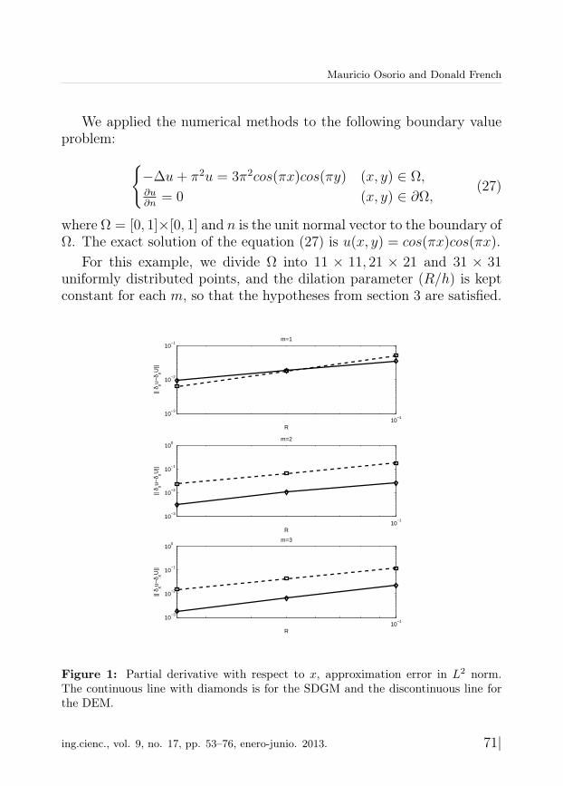
We applied the numerical methods to the following boundary valueproblem:

−∆u+ π2u = 3π2cos(πx)cos(πy) (x, y) ∈ Ω,∂u∂n

= 0 (x, y) ∈ ∂Ω,(27)

where Ω = [0, 1]×[0, 1] and n is the unit normal vector to the boundary ofΩ. The exact solution of the equation (27) is u(x, y) = cos(πx)cos(πx).

For this example, we divide Ω into 11 × 11, 21 × 21 and 31 × 31uniformly distributed points, and the dilation parameter (R/h) is keptconstant for each m, so that the hypotheses from section 3 are satisfied.

10−1

10−3

10−2

10−1

R

|| δ xu−

δ xU||

m=1

10−1

10−3

10−2

10−1

100

R

|| δ xu−

δ xU||

m=2

10−1

10−3

10−2

10−1

100

R

|| δ xu−

δ xU||

m=3

Figure 1: Partial derivative with respect to x, approximation error in L2 norm.The continuous line with diamonds is for the SDGM and the discontinuous line forthe DEM.



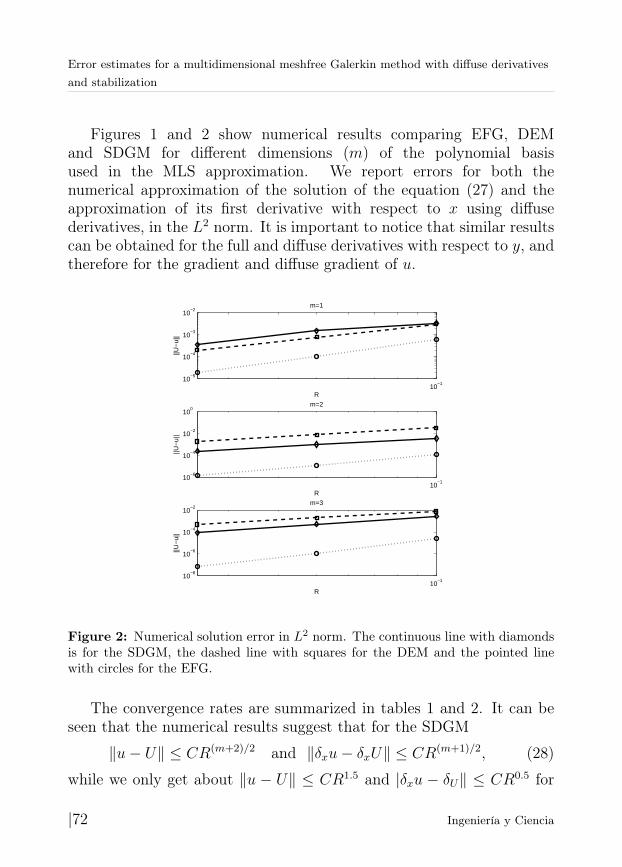
Figures 1 and 2 show numerical results comparing EFG, DEMand SDGM for different dimensions (m) of the polynomial basisused in the MLS approximation. We report errors for both thenumerical approximation of the solution of the equation (27) and theapproximation of its first derivative with respect to x using diffusederivatives, in the L2 norm. It is important to notice that similar resultscan be obtained for the full and diffuse derivatives with respect to y, andtherefore for the gradient and diffuse gradient of u.

10−1

10−5

10−4

10−3

10−2

R

||U−

u||

m=1

10−1

10−6

10−4

10−2

100

R

||U−

u||

m=2

10−1

10−8

10−6

10−4

10−2

R

||U−

u||

m=3

Figure 2: Numerical solution error in L2 norm. The continuous line with diamondsis for the SDGM, the dashed line with squares for the DEM and the pointed linewith circles for the EFG.

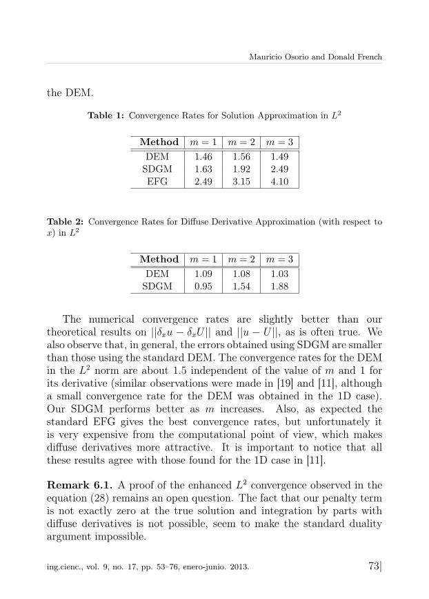
The convergence rates are summarized in tables 1 and 2. It can beseen that the numerical results suggest that for the SDGM

∥u− U∥ ≤ CR(m+2)/2 and ∥δxu− δxU∥ ≤ CR(m+1)/2, (28)

while we only get about ∥u − U∥ ≤ CR1.5 and |δxu − δU∥ ≤ CR0.5 for



the DEM.

Table 1: Convergence Rates for Solution Approximation in L2

Method m = 1 m = 2 m = 3

DEM 1.46 1.56 1.49SDGM 1.63 1.92 2.49EFG 2.49 3.15 4.10

Table 2: Convergence Rates for Diffuse Derivative Approximation (with respect tox) in L2

Method m = 1 m = 2 m = 3

DEM 1.09 1.08 1.03SDGM 0.95 1.54 1.88

The numerical convergence rates are slightly better than ourtheoretical results on ||δxu − δxU || and ||u − U ||, as is often true. Wealso observe that, in general, the errors obtained using SDGM are smallerthan those using the standard DEM. The convergence rates for the DEMin the L2 norm are about 1.5 independent of the value of m and 1 forits derivative (similar observations were made in [19] and [11], althougha small convergence rate for the DEM was obtained in the 1D case).Our SDGM performs better as m increases. Also, as expected thestandard EFG gives the best convergence rates, but unfortunately itis very expensive from the computational point of view, which makesdiffuse derivatives more attractive. It is important to notice that allthese results agree with those found for the 1D case in [11].

Remark 6.1. A proof of the enhanced L2 convergence observed in theequation (28) remains an open question. The fact that our penalty termis not exactly zero at the true solution and integration by parts withdiffuse derivatives is not possible, seem to make the standard dualityargument impossible.



7 Conclusions

A modification to the traditional DEM, the stabilized diffuse Galerkinmethod (SDGM) has been proposed, in which a stabilization term isintroduced to improve the overall accuracy and stability. The newscheme, like DEM, does not require the evaluation of full derivatives.This method is shown to give better results than DEM and convergesto the true solution as the dilation parameter (R) goes to zero, or theorder of the polynomial basis is increased, as demonstrated numericallyand proved theoretically. The procedure described in this paper can beapplied to more general multidimensional problems (see [15]).

We see SDGM as enhancing the viability of the diffuse derivativeapproach. Again, as suggested in Huerta et al [6], we think the versatilityof the diffuse derivative could be helpful in fluid flows or mixed methodcomputations.

Acknowledgements

We thank the University of Cincinnati and the Universidad Nacional deColombia, for the support to this project . D. A. French was partiallysupported by a Charles Phelps Taft Summer Fellowship at the Universityof Cincinnati.

References

[1] T. Belytschko, Y. Krongauz, M. Fleming, D. Organ, and W. K. Liu, “Smoothingand accelerated computations in the element free Galerkin method,” J. Comput.Appl. Math, vol. 74, pp. 111–126, 1996. 54

[2] P. Breitkopf, A. Rassineux, G. Touzot, and P. Villon, “Explicit form and efficientcomputations of MLS shape functions and their derivatives,” Int. J. Numer.Meth. Engrg., vol. 48, pp. 451–466, 2000. 54

[3] B. Nayroles, G. Touzot, and O. Villon, “Generating the finite element method:diffuse approximation and diffuse elements,” Comput. Mech., vol. 10, pp. 307–318, 1992. 54, 61



[4] T. Belytschko, Y. Y. Lu, and L. Gu, “Element-free Galerkin methods,” Int. J.Numer. Methods Engrg., vol. 37, pp. 229–256, 1994. 54

[5] Y. Krongauz and T. Belytschko, “A Petrov-Galerkin diffuse element method(PG DEM) and its comparison to EFG,” Computational Mechanics, vol. 19, pp.327–333, 1997. 54

[6] A. Huerta, Y. Vidal, and P. Villon, “Pseudo-divergence-free element freeGalerkin method for incompressible fluid flow,” Comput. Methods Appl. Mech.Engrg., vol. 193, pp. 1119–1136, 2004. 54, 57, 74

[7] I. Babuska, U. Banerjee, and J. Osborn, “Survey of meshless and generalizedfinite element methods: A unified approach,” Acta Numerica, pp. 1–125, 2003.55

[8] W. Han and X. Meng, “Error analysis of the reproducing kernel particlemethod,” Comput. Methods Appl. Mech. Engrg., vol. 190, pp. 6157–6181, 2001.55, 60

[9] M. Armentano, “Error estimates in Sobolev spaces for moving least squareapproximations,” SIAM J. Numer. Anal., vol. 39, pp. 38–51, 2001. 55, 60,62, 66

[10] D. W. Kim and W. K. Liu, “Maximum principle and convergence analysis forthe meshfree point collocation method,” SIAM J. Numer. Anal., vol. 44, pp.515–539, 2006. 55

[11] D. A. French and M. Osorio, “A Galerkin Meshfree Method with DiffuseDerivatives and Stabilization,” Computational Mechanics., vol. 50, pp. 657–664,2012. 55, 62, 65, 68, 73

[12] O. C. Zienkiewicz, “Constrained variational principles and penalty functionmethods in the finite element analysis,” Lecture Notes in Mathematics, vol. 363,pp. 207–214, 1974. 55

[13] T. Hughes, L. Franca, and G. Hulbert, “A new finite element formulation forcomputational fluid dynamics: VIII. The Galerkin/least-squares method foradvective-diffusive equations,” Comput. Methods Appl. Mech. Engrg., vol. 73,pp. 173–189, 1989. 55

[14] S. Beissel and T. Belytschko, “Nodal integration of the element-free Galerkinmethod,” Comput. Methods Appl. Mech. Engrg., vol. 139, pp. 49–74, 1996. 55

[15] M. Osorio, “Error analysis of a Meshfree method with diffuse derivatives andpenalty stabilization,” Ph.D. dissertation, University of Cincinnati, 2010. 58,60, 65, 66, 74



[16] M. Armentano and R. Duran, “Error estimates for moving least squareapproximations,” Applied Numerical Mathematics, vol. 37, pp. 397–416, 2001.60

[17] W. K. Liu and T. Belytschko, “Moving least-square reproducing kernel methods.Part I: Methodology and convergence,” Comput. Methods Appl. Mech. Engrg.,vol. 143, pp. 113–154, 1997. 60

[18] D. Kim and Y. Kim, “Point collocation methods using the fast moving leastsquare reproducing kernel approximation,” Int. J. Numer. Meth. Engrg., vol. 56,pp. 1445–1464, 2003. 61

[19] P. Breitkopf, A. Rassineux, and P. Villon, An introduction to moving leastsquares meshfree methods. In: Meshfree and particle based approaches incomputational mechanics. Edited by P. Breitkopf and A. Huerta, 2004. 73


Documents

Error estimates for a multidimensional meshfree Galerkin method with diﬀuse derivatives and stabilization