Environmental Assessment of AromaticHydrocarbons-Contaminated Sediments of the MexicanSalina Cruz Bay

C. González-Macías & I. Schifter &

D. B. Lluch-Cota & L. Méndez-Rodríguez &

S. Hernández-Vázquez

Received: 26 June 2006 /Accepted: 30 October 2006 / Published online: 13 February 2007# Springer Science + Business Media B.V. 2007

Abstract Concentrations of total aromatic hydro-carbons and extractable organic matter in the watercolumn and sediment were determined in samplescollected in the course of the last 20 years from theSalina Cruz Harbor, México, to assess the degree oforganic contamination. In sediments, organic com-pounds accumulate in shallow areas mostly associatedwith extractable organic matter and fine fractions.Calculated geocumulation index and enrichmentfactors suggest that contamination could be derivedfrom anthropogenic activities attributed to harbor andship scrapping activities, as well as transboundarysource. Concentration of total aromatic hydrocarbons(as chrysene equivalents) ranged from 0.01 to 534 μgl−1 in water, and from 0.10 to 2,160 μg g−1 insediments. Total aromatic concentration of 5 μg g−1 isproposed as background concentration.

Keywords Total aromatic hydrocarbon . Surfacesediments . Bay of Salina Cruz . Geoaccumulation .

Enrichment factors

1 Introduction

The study of trace organic contaminants in coastalmarine environments and especially in estuarinesystems is of great importance since these areas arebiologically productive and receive considerablepollutant inputs from land-based sources via riverrunoff and sewage outfalls. Therefore, estuaries act asa transit zone in which contaminants are transportedfrom rivers to oceans (Karichknoff et al. 1979; Kot-Wasik et al. 2004; Means et al. 1980).

Chronic spillages from land-based facilities, ves-sels, effluent discharges, and accidental spills intro-duce large amounts of petroleum hydrocarbons tourbanized coastal areas. Depending on the partition-ing properties of hydrocarbons, a large fractionadsorbs to suspended particles and accumulates inunderlying sediments which becomes long termreservoirs and secondary sources.

The Salina Cruz Bay located at the Ventosa Bay,State of Oaxaca, has undergone considerable devel-opment, and consequently urbanization, industrializa-tion. Ship scrapping industry and oil processing in thearea has become potential source of contamination tothe marine environment.

Environ Monit Assess (2007) 133:187–207DOI 10.1007/s10661-006-9572-3

C. González-Macías : I. Schifter (*)Dirección de Seguridad y Medio Ambiente,Instituto Mexicano del Petróleo,Eje Central Lázaro Cárdenas No. 152,San Bartolo Atepehuacan, México,México, D.F. 07730, Mexicoe-mail: ishifter@imp.mx

D. B. Lluch-Cota : L. Méndez-Rodríguez :S. Hernández-VázquezCentro de Investigaciones Biológicas del Noroeste,S.C. Mar Bermejo No. 195. Playa Palo de Santa Rita,La Paz, BCS 23090, Mexico

The Bay receives continental runoff from theVentosa Estuary System – which runs perpendicularto the coast- and freshwater from the TehuantepecRiver flowing into the Ventosa Bay. Municipal wastedischarges are also an important source of petroleumhydrocarbons which has been estimated to accountroughly for 5% of the total global input per year inother regions of the world (Barrick 1982; Eganhouseand Kaplan 1982; Latimer and Quinn 1996).

Organic pollution from anthropogenic sources toaquatic environments has been an area of greatconcern. In terms of “unpolluted” intertidal andestuarine sediments, concentrations generally rangefrom sub- μg g−1 to approximately 10 μg g−1

(Bouloubassi and Saliot 1993; Volkman et al. 1992).For example, Tolosa et al. (2005) found concen-

tration levels <15 μg g−1, as chrysene equivalents, forbottom sediments of the Gulf of Oman, that wereproposed to reflect background levels in this region.

To calculate approximately the severity of oilcontamination, a number of indicators have beenproposed, among them: (a) high concentrations(>100 μg g−1) of total hydrocarbons; (b) C21–C35n-alkanes having no odd over even predominance; (c)complex distributions; (d) an unresolved complexmixture which produces a raised baseline in the gas-chromatogram of the hydrocarbon fraction; (e) bio-markers (Volkman et al. 1992).

Massoud et al. (1996) recognized chronic moder-ately (50–89 μg g−1) and heavily hydrocarbonspolluted areas (266–1,448 μg g−1) in bottomsediments of the Arabian Gulf, concluding thatthe grain-size distribution and the hydrocarbonscontent were positively correlated.

Readman et al. (2002) reported concentrations ofpetroleum hydrocarbons from surface sediment in theBlack Sea (2–310 μg g−1) comparable to thoseencountered in the Mediterranean, but lower thanthose found by others in highly contaminated areassuch as Saudi Arabia Gulf (11–6,900 μg g−1) orTaiwan (869–10,300 μg g−1) (Jeng and Han 1994;Readman et al. 1996).

In the literature scarce information exists concerningthe impact of the anthropogenic activities around thecoastal waterways and estuarine environments of theGulf of Tehuantepec.

Botello et al. (1998) reported for the Salina CruzBay levels of total polycyclic aromatic hydrocarbons(PAH) of 3.21 μg g−1 in the inner port sediments,

while in the outer harbor, the concentrations were inthe order of 0.22 μg g−1. Moreover, García-Ruelas etal. (2004) reported PAH concentrations in sedimentsalong the coasts of Mexican Pacific within a range ofvalues between 0.2 and 55.3 μg g−1.

High lead enrichment factor in sediment collect-ed during the last two decades at the Salina CruzBay was reported in a previous work (González-Macías et al. 2006). Geoaccumulation and enrich-ment factors for Cr, Cu, Fe, Ni, V, and Zn showedvalues similar to those found worldwide for siteswith analogous industrial activities (Readman et al.2002).

The major objective of the current study was toestimate the spatial patterns and historical trends inorganic contamination of the surface sediments fromthe inner shelf and coastal areas of the Salina CruzHarbor. For that purpose, evaluation of total aromatichydrocarbon (TAH) and extractable organic matter(EOM) in the water column and sediment wasassessed for samples collected by our group in thecourse of the last 20 years.

Normalization was performed for backgroundcontributions, with the aim of differentiate anypotential site contaminant releases from backgroundsources (both naturally occurring and anthropogenic).

2 Materials and Methods

2.1 Study area

The Salina Cruz (SC) Bay is located at the North sideof the Tehuantepec Golf in the Mexican Pacific Ocean(16°06′–16°11′ N and 95°15′–95°07′ W). A high-energy oceanographic condition prevails in the areawhich generates dispersal of the different inputs(Trasviña et al. 1995). The study area, 30 km alongthe coast, includes the Salina Cruz city (population230,000), and harbor.

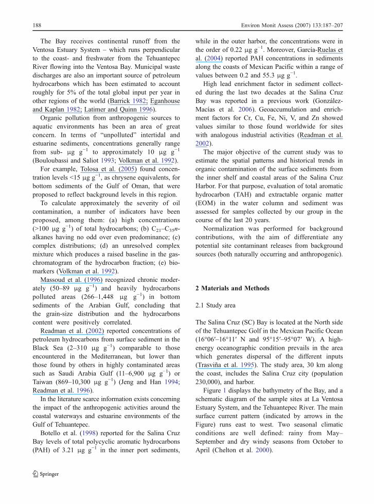
Figure 1 displays the bathymetry of the Bay, and aschematic diagram of the sample sites at La VentosaEstuary System, and the Tehuantepec River. The mainsurface current pattern (indicated by arrows in theFigure) runs east to west. Two seasonal climaticconditions are well defined: rainy from May–September and dry windy seasons from October toApril (Chelton et al. 2000).

188 Environ Monit Assess (2007) 133:187–207

One of the six major oil processing facilities in thecountry is located 5 km NE from the harbor with andoff-shore outfalls diffusor that discharges the treatedsewage effluents to the Bay. The large oil refinerysupplies most oil and by-products required by thePacific Coastal region of Mexico.

Three buoys are located for oil exports in the outerharbor, and the Salinas de Marquez evaporation pondsare sited at 5 km SW of the harbor. The TehuantepecRiver release approximately 1,400 million m3 year−1

of water to the Bay, while the La Ventosa EstuarineSystem discharges are not constant and arise mostlyduring the rainy seasons.

A total of 365 samples were collected at 24 sitesbetween October 1982, and September 2002 atdifferent seasons of the year, aboard chartered

oceanographic vessel. A global positioning system,Micro logic ML-150, was used to locate the sites.Between December 1995 and May 2002 sites sam-pled, using small boats, accomplished 241 stationsfrom La Ventosa Estuarine System and TehuantepecRiver (coded as “Continental”).

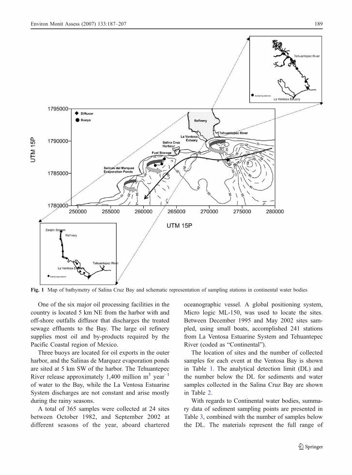
The location of sites and the number of collectedsamples for each event at the Ventosa Bay is shownin Table 1. The analytical detection limit (DL) andthe number below the DL for sediments and watersamples collected in the Salina Cruz Bay are shownin Table 2.

With regards to Continental water bodies, summa-ry data of sediment sampling points are presented inTable 3, combined with the number of samples belowthe DL. The materials represent the full range of

Fig. 1 Map of bathymetry of Salina Cruz Bay and schematic representation of sampling stations in continental water bodies

Environ Monit Assess (2007) 133:187–207 189

sediment textures, i.e., from fine-grained mud tocoarse-grained sand.

2.2 Sampling

A total of 326 one gallon water samples werecollected from −50 cm depth in each site using pre-cleaned amber glass bottles with screw cap narrowneck and aluminum foil lid liners. The extraction wasperformed on site and samples transported back to thelaboratory on ice, and stored at 4°C before analysis. Adelay between sampling and extraction of greater than4 h required sampling preservation by the addition of5 ml HCl.

Samples of surface sediment (10–15 cm depth)from the continental shelf of the SC Bay werecollected using a Smith-McIntyre grab. At each site,the top 1–5 cm of surface sediment was carefullyremoved with a stainless steel spoon. Sediments werehomogenized into a stainless steal bowl, and 250 g.

later transferred into acid soak/solvents precleanedamber frozen glass jars with aluminum foil-lined lids.

Total suspended solids in water were measured bycalculating the difference between the initial and finalweight of a standard glass-fiber filter after filtration of a250 ml well-mixed water sub-sample (APHA 1995).

Grain analysis was performed to establish theparticle size distribution of the sediment, which cancontribute in defining the origin and depositionenvironment. Sediments grain size was estimated bya combination of wet sieving (2 mm–63 μm) andpipette analysis (<63 μm) (Folk 1974).

2.3 Extraction

Water samples were extracted three times into 30 ml ofspectrophotometer grade carbon tetrachloride, usingfresh solvent, and combining all solvent into thevolumetric flask. The combined extracts were filteredtrough glass fiber wool, transferred to an acid-soak

Table 1 Salina Cruz Bay: sampling period data matrix composition

Sampling event Date Season Geographical limits

UTMa northing UTM easting Number of samples

1 Oct-1982 dry/windy 1,783,063–1,788,875 261,570–273,263 242 Dec-1982 dry/windy 1,783,063–1,788,875 261,570–273,263 243 Apr-1983 dry/windy 1,783,063–1,788,875 261,570–273,263 244 May-1984 rainy 1,779,753–1,788,806 253,817–284,524 245 May-1985 rainy 1,784,118–1,788,630 262,397–271,895 36 Jul-1985 rainy 1,783,254–1,788,630 262,655–271,895 37 Oct-1985 dry/windy 1,782,755–1,783,017 261,820–272,132 38 Mar-1988 dry/windy 1,782,260–1,788,639 261,699–272,229 249 Jul-1988 rainy 1,782,260–1,788,639 261,699–272,229 2410 Sep-1988 rainy 1,782,253–1,788,639 261,699–272,229 2411 Mar-1989 dry/windy 1,782,260–1,788,639 261,699–272,229 2412 Aug-1990 rainy 1,780,656–1,788,092 259,034–273,727 1913 Dec-1995 dry/windy 1,784,479–1,790,709 271,079–276,903 1814 Jul-1997 rainy 1,782,290–1,789,499 262,214–272,821 1115 Dec-1997 dry/windy 1,783,322–1,787,818 262,214–272,821 216 Feb-1998 dry/windy 1,783,322–1,789,470 263,705–272,821 617 May-1998 rainy 1,787,133–1,789,954 269,826–274,472 1018 Jun-1999 rainy 1,783,771–1,787,921 259,487–267,998 919 Sep-1999 rainy 1,783,771–1,787,921 259,487–267,998 920 Aug-2000 rainy 1,783,708–1,790,158 259,575–273,304 1721 Aug-2001 rainy 1,779,824–1,790,158 249,579–273,304 2122 Dec-2001 dry/windy 1,779,824–1,790,158 249,579–273,304 2123 May-2002 rainy 1,788,699–1,789,833 263,999–264,805 724 Sept-2002 rainy 1,779,824–1,790,158 249,579–273,304 14Total 365

a Universal Transverse Mercator Zone 15P

190 Environ Monit Assess (2007) 133:187–207

precleaned amber glass, and stored at 4°C untilanalysis. Previous to analysis, extracts were reducedto 2 ml by rotary evaporation under soft flowingnitrogen gas at ambient temperature.

Frozen sediments were dried at 40°C to constantweight, and 50 g of the dry material was digestedunder reflux with 100 ml of methanol and 3 g ofKOH. The non-saponificable fraction was obtainedby extracting twice with 25 ml of spectrophotometergrade hexane. The combined extracts were dried withanhydrous sodium sulfate, and reduced to 2 ml byrotary evaporation under soft flowing nitrogen gas atambient temperature.

2.4 Analysis

Instruments calibrations were performed against purereference standards; blank samples were analyzed witheach sample batch and positive peaks were negligible.

Total EOM was quantified by infrared spectrometryin a FT-IR Thermo Electron Corporation NicoletModel 710, or a Perkin Elmer UNICAM Model SP-2000, base on the United States EnvironmentalProtection Agency (USEPA) Method 418.1 (Chesleret al. 1976; USEPA 1978, 1996). The acid sulfur pre-treatment was excluded in order to recover all materialsoluble in CCl4 (lipids, chlorinated hydrocarbons,

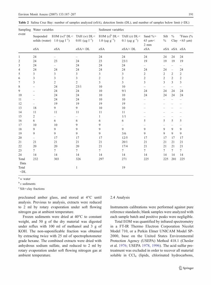
Table 2 Salina Cruz Bay: number of samples analyzed (nSA), detection limits (DL), and number of samples below limit (<DL)

Samplingevent

Water variables Sediment variables

Suspendedsolids (water)

EOM (w)a DL<1.0 (μg l−1)

TAH (w) DL<0.01 (μg l−1)

EOM (s)b DL<1.0 (μg g−1)

TAH (s) DL<0.1 (μg g−1)

Sand %>63 μm<2 mm

Silt%

%Clay

cFines (%<63 μm)

nSA nSA nSA/< DL nSA nSA/< DL nSA nSA nSA nSA

1 24 – – 24 24 24 24 24 242 24 23 24 23 23/1 19 19 19 193 24 – 24 24 24 – – – –4 24 24 24 24 24 24 24 – 245 3 3 3 3 3 2 2 2 26 3 3 3 2 2 2 2 2 27 3 2 2 3 3 3 3 3 38 – 24 23/1 10 10 – – – –9 – 24 24 10 9/1 24 24 24 2410 – 24 24 10 10 24 24 24 2411 – 24 24 10 10 – – – –12 – 19 19 19 19 – – – –13 18 9 9 10 10 – – – –14 11 11 11 11 11 – – – –15 2 – – 1 1/1 – – – –16 6 6 6 6 6 5 5 5 517 10 10 9 9 – – – – –18 9 9 9 9 9 9 9 9 919 9 9 9 9 3/6 9 9 9 920 – 17 17 17 12/5 17 17 17 1721 21 21 21 21 20/1 21 21 21 2122 20 20 20 21 17/4 21 21 21 2123 7 7 7 7 7 7 7 7 724 14 14 14 14 14 14 14 14 14TotalData

232 303 326 297 271 225 225 201 225

Total<DL

1 19

aw waterb s sedimentsc Silt+clay fractions

Environ Monit Assess (2007) 133:187–207 191

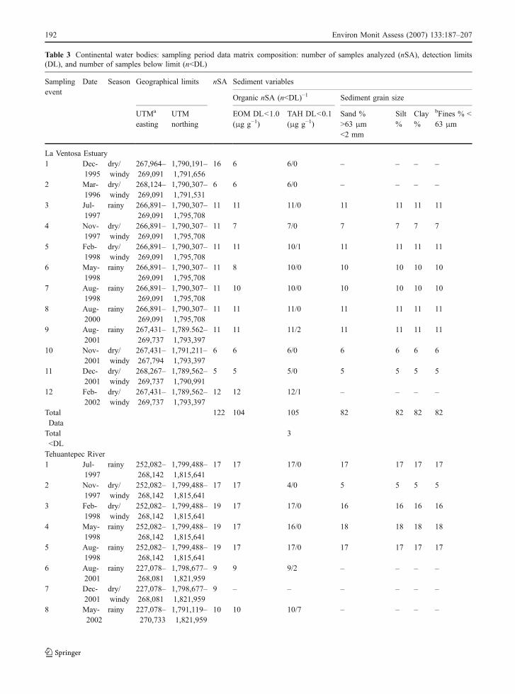
Table 3 Continental water bodies: sampling period data matrix composition: number of samples analyzed (nSA), detection limits(DL), and number of samples below limit (n<DL)

Samplingevent

Date Season Geographical limits nSA Sediment variables

Organic nSA (n<DL)−1 Sediment grain size

UTMa

eastingUTMnorthing

EOM DL<1.0(μg g−1)

TAH DL<0.1(μg g−1)

Sand %>63 μm<2 mm

Silt%

Clay%

bFines % <63 μm

La Ventosa Estuary1 Dec-

1995dry/windy

267,964–269,091

1,790,191–1,791,656

16 6 6/0 – – – –

2 Mar-1996

dry/windy

268,124–269,091

1,790,307–1,791,531

6 6 6/0 – – – –

3 Jul-1997

rainy 266,891–269,091

1,790,307–1,795,708

11 11 11/0 11 11 11 11

4 Nov-1997

dry/windy

266,891–269,091

1,790,307–1,795,708

11 7 7/0 7 7 7 7

5 Feb-1998

dry/windy

266,891–269,091

1,790,307–1,795,708

11 11 10/1 11 11 11 11

6 May-1998

rainy 266,891–269,091

1,790,307–1,795,708

11 8 10/0 10 10 10 10

7 Aug-1998

rainy 266,891–269,091

1,790,307–1,795,708

11 10 10/0 10 10 10 10

8 Aug-2000

rainy 266,891–269,091

1,790,307–1,795,708

11 11 11/0 11 11 11 11

9 Aug-2001

rainy 267,431–269,737

1,789.562–1,793,397

11 11 11/2 11 11 11 11

10 Nov-2001

dry/windy

267,431–267,794

1,791,211–1,793,397

6 6 6/0 6 6 6 6

11 Dec-2001

dry/windy

268,267–269,737

1,789,562–1,790,991

5 5 5/0 5 5 5 5

12 Feb-2002

dry/windy

267,431–269,737

1,789,562–1,793,397

12 12 12/1 – – – –

TotalData

122 104 105 82 82 82 82

Total<DL

3

Tehuantepec River1 Jul-

1997rainy 252,082–

268,1421,799,488–1,815,641

17 17 17/0 17 17 17 17

2 Nov-1997

dry/windy

252,082–268,142

1,799,488–1,815,641

17 17 4/0 5 5 5 5

3 Feb-1998

dry/windy

252,082–268,142

1,799,488–1,815,641

19 17 17/0 16 16 16 16

4 May-1998

rainy 252,082–268,142

1,799,488–1,815,641

19 17 16/0 18 18 18 18

5 Aug-1998

rainy 252,082–268,142

1,799,488–1,815,641

19 17 17/0 17 17 17 17

6 Aug-2001

rainy 227,078–268,081

1,798,677–1,821,959

9 9 9/2 – – – –

7 Dec-2001

dry/windy

227,078–268,081

1,798,677–1,821,959

9 – – – – – –

8 May-2002

rainy 227,078–270,733

1,791,119–1,821,959

10 10 10/7 – – – –

192 Environ Monit Assess (2007) 133:187–207

fatty acids, soaps, fats, waxes), accounting then forthe organic and mineral extractable matter.

TAH was evaluated in sub samples of the extractssuspended again in spectrophotometer grade, methy-lene chloride by fluorescence spectroscopy in PerkinElmer models MPF-44B, and LS-3B spectrofluorom-eters (Gordon and Keizer 1976). The sedimentsamples were maintained frozen until analysis, andfor extraction, we followed the methods and recom-mendations suggested in UNESCO (1982, 1984), andGold et al. (1987).

The “chrysene equivalent” concentration of TAHwas calculated by comparison with the fluorescenceof known concentrations of chrysene in hexane(Mzoughi et al. 2005). For EOM analysis, thestandard was composed of a mixture of spectropho-

tometer grade n-hexadecane, isooctane, and chloro-benzene.

Appropriate blanks analyzed were always at orbelow the DL. The precision for multiple analysis, asexpressed by the relative standard deviation, wasusually <10% for TAH. Recovery rates were deter-mined by spiking duplicate sediments samples with amixture of standard solution. The relative recoveries ofTAH into seawater ranged from 90 to 110%, and insediments from 70 to 110%.

2.5 Statistical analysis

Statistical analysis of the data was performed withStatistica (1998), and Surfer-8 software to draw thespatial distribution of the TAH (Surfer 2002). SC

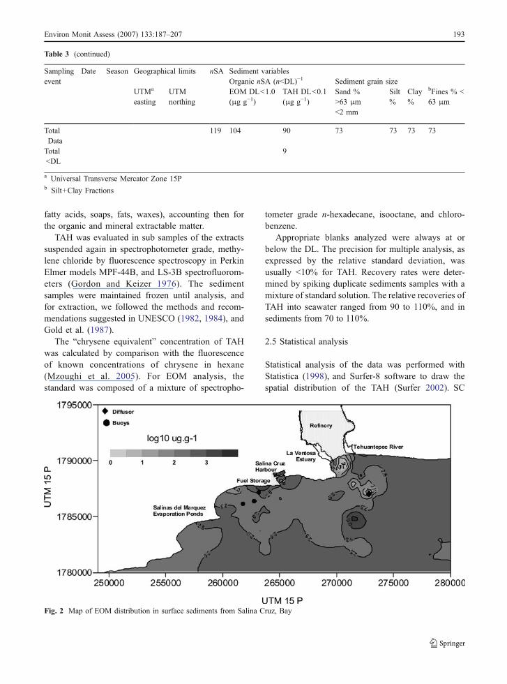
Fig. 2 Map of EOM distribution in surface sediments from Salina Cruz, Bay

Table 3 (continued)

Samplingevent

Date Season Geographical limits nSA Sediment variablesOrganic nSA (n<DL)−1 Sediment grain size

UTMa

eastingUTMnorthing

EOM DL<1.0(μg g−1)

TAH DL<0.1(μg g−1)

Sand %>63 μm<2 mm

Silt%

Clay%

bFines % <63 μm

TotalData

119 104 90 73 73 73 73

Total<DL

9

a Universal Transverse Mercator Zone 15Pb Silt+Clay Fractions

Environ Monit Assess (2007) 133:187–207 193

Bay data matrix without outliers was employed toperform the t Student test, Pearson correlationcoefficient, Tukey variance and scatter plots. Outliersare identified as those outside the range of ±2standard deviations around the mean.

A similar procedure was followed for the raw dataof the Continental water bodies (Tehuantepec Riverand La Ventosa Estuary). Outliers were not removedin order to select typical values to be use innormalization; enrichment factors, and geoaccumula-tion index calculations, thus the coded Global set isnot represented.

Central tendency analysis of the SC Bay raw datawas performed grouping the variables in three setscoded as: Dry, Rainy and Global. To evaluate ifdifferences prevail among the data subset, Student’s ttest for independent samples with different variancewas performed (Statistica 1998).

According to the Kolmogorov–Sminorv analysis,none of the resultant variables tested (without extremevalues) were normally distributed (Massey 1951).

Moreover, Log Normal transformations wereapplied to correct for non constant variance andthe non-normality of the data, ensuring that in themultiple regression test, normality is applied to theresiduals, instead of the raw data. Extreme valueswere kept to evaluate quality of sediments.

The inference method appears to be well-suitedto temperature and other environmental reconstruc-tions (Holmström and Erästö 2001).

Therefore, the non-parametric SiZer methoddescribed by Chaudhuri and Marron (1999) wasapplied to assess the statistical significance of thereconstructed organic compounds variation alongthe time. SiZer enables meaningful statistical infer-ence, while doing exploratory data analysis usingstatistical smoothing methods.

Consequently, a collection of scatter plot smooth-ers of the reconstructed TAH concentrations areconsidered, and inferences about the significance ofthe TAH trends made along time (Godtliebsen et al.2003).

2.6 Normalization

In order to differentiate the TAH originating fromhuman activities from those resulting from naturalweathering, a ‘normalization’ technique is usually

applied, i.e., the TAH concentrations are normalizedto a textural or compositional characteristic ofsediments (NFESC 2003).

The organic matter content of sediments, quan-tified by the concentration of total organic carbon(TOC), is thought to play an important role in theaccumulation and release of different micro pollu-tants. Moreover, some studies of marine sedimentshave reported a progressive increase in TOCcontent concomitant with the decrease in grain-size(Karichknoff et al. 1979). Therefore, since grain size<63 μm, tend to co-vary with the EOM; the use ofa single normalizer can often represent severalunderlying geochemical relationships.

First, Pearson coefficients were used to check ifa positively correlation exists between normalizerand contaminants of concern. Later TAH werenormalized to fine-grained fractions and EOM, andlastly scatter plots were draw to search correlationsbetween the TAH, EOM, and fines fraction.

2.7 Enrichment factors (EF) and indexof geoaccumulation (Igeo)

When comparison of metals content in sedimentsis performed between different regions, normaliza-tion with respect to crusted average is usuallyapplied to determine EF (Nolting et al. 1999;Taylor 1964). Therefore, a TAH enrichment factorwas calculated as a quotient of the ratio of thenormalizing element (i.e., EOM and percent of finefractions) by the ratio found in the chosen baseline(i.e., Tehuantepec River continental water bodieswhich discharge to the Bay):

EF ¼ðTAH=EOMÞsediments Bay:

ðTAH=EOMÞ�1sediments Tehuantepec River:

According to the work of Zsefer et al. (1996),we associate EFs close to unity with TAH continentalorigin, while those less than 1.0 would suggests apossible mobilization or depletion of the hydro-carbons. If EF>1.0 is found, then TAH could be ofanthropogenic origin, and EF greater than 10 shouldsuggest TAH arising from non-continental runoffsources.

194 Environ Monit Assess (2007) 133:187–207

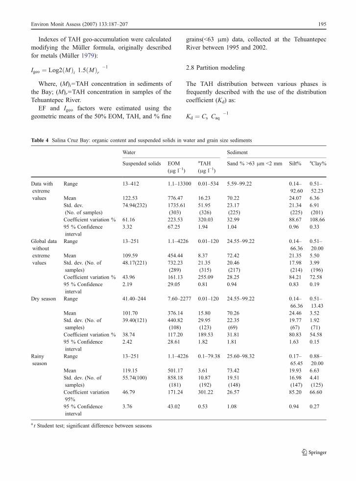
Indexes of TAH geo-accumulation were calculatedmodifying the Müller formula, originally describedfor metals (Müller 1979):

Igeo ¼ Log2 Mð Þi 1:5 Mð Þr� ��1

Where, (M)i=TAH concentration in sediments ofthe Bay; (M)r=TAH concentration in samples of theTehuantepec River.

EF and Igeo factors were estimated using thegeometric means of the 50% EOM, TAH, and % fine

grains(<63 μm) data, collected at the TehuantepecRiver between 1995 and 2002.

2.8 Partition modeling

The TAH distribution between various phases isfrequently described with the use of the distributioncoefficient (Kd) as:

Kd ¼ Cs Caq

� ��1

Table 4 Salina Cruz Bay: organic content and suspended solids in water and grain size sediments

Water Sediment

Suspended solids EOM(μg l−1)

aTAH(μg l−1)

Sand % >63 μm <2 mm Silt% aClay%

Data withextremevalues

Range 13–412 1.1–13300 0.01–534 5.59–99.22 0.14–92.60

0.51–52.23

Mean 122.53 776.47 16.23 70.22 24.07 6.36Std. dev.(No. of samples)

74.94(232) 1735.61(303)

51.95(326)

23.17(225)

21.34(225)

6.91(201)

Coefficient variation % 61.16 223.53 320.03 32.99 88.67 108.6695 % Confidenceinterval

3.32 67.25 1.94 1.04 0.96 0.33

Global datawithoutextremevalues

Range 13–251 1.1–4226 0.01–120 24.55–99.22 0.14–66.36

0.51–20.00

Mean 109.59 454.44 8.37 72.42 21.35 5.50Std. dev. (No. ofsamples)

48.17(221) 732.23(289)

21.35(315)

20.46(217)

17.98(214)

3.99(196)

Coefficient variation % 43.96 161.13 255.09 28.25 84.21 72.5895 % Confidenceinterval

2.19 29.05 0.81 0.94 0.83 0.19

Dry season Range 41.40–244 7.60–2277 0.01–120 24.55–99.22 0.14–66.36

0.51–13.43

Mean 101.70 376.14 15.80 70.26 24.46 3.52Std. dev. (No. ofsamples)

39.40(121) 440.82(108)

29.95(123)

22.35(69)

19.77(67)

1.92(71)

Coefficient variation % 38.74 117.20 189.53 31.81 80.83 54.5895 % Confidenceinterval

2.42 28.61 1.82 1.81 1.63 0.15

Rainyseason

Range 13–251 1.1–4226 0.1–79.38 25.60–98.32 0.17–65.45

0.88–20.00

Mean 119.15 501.17 3.61 73.42 19.93 6.63Std. dev. (No. ofsamples)

55.74(100) 858.18(181)

10.87(192)

19.51(148)

16.98(147)

4.41(125)

Coefficient variation95%

46.79 171.24 301.22 26.57 85.20 66.60

95 % Confidenceinterval

3.76 43.02 0.53 1.08 0.94 0.27

a t Student test; significant difference between seasons

Environ Monit Assess (2007) 133:187–207 195

Tab

le5

SalinaCruzBay

andCon

tinentalwater

bodies:surfacesedimentsorganics

andfine

grains

content

EOM

(μgg−

1)

TAH

(μgg−

1)

c Fines

(%<63

μm

)

Salina

CruzBay

a Con

tinental

bodies

La

Ventosa

system

a Tehuantepec

River

a Salina

CruzBay

Con

tinental

bodies

LaVentosa

System

Tehuantepec

River

Salina

CruzBay

Con

tinental

bodies

LaVentosa

System

Tehuantepec

River

Total

data

with

extrem

evalues

Range

1.54

–10

,105

28.65–

30,401

28.65–

30,401

33.31–

1,66

50.10

–2,16

00.11–

3,09

40.14

–3,09

40.11–

196.54

0.78

–94

.41

0.55

–94

.09

0.75–

94.09

0.55–

66.59

Geometric

mean

(data

50%)

209.62

255.36

172.76

1.00

2.20

0.63

2.63

16.82

1.18

Mean

563.90

978.03

b1,41

8.48

b46

9.06

52.84

90.92

b15

1.44

b15

.46

29.76

26.61

b44

.13

b6.93

Std.dev.

(No.

ofsamples)

1,15

7.56

(297

)2,64

6.03

(194

)3,54

8.97

(104

)34

3.28

(90)

177.87

(271

)29

2.58

(182

)38

2.10

(101

)27

.98

(81)

23.18

(225

)27

.52

(155

)25

.66

(82)

11.72

(73)

Coefficient

variation

%

205.28

270.55

250.20

73.18

336.59

321.78

252.31

189.97

77.91

103.42

58.15

168.98

95%

Con

fidence

interval

45.30

128.14

234.73

24.41

7.29

14.63

25.64

2.10

1.04

1.49

1.91

0.93

Global

data

with

out

extrem

evalues

Range

1.54

–2,55

30.10

–36

50.78

–75

.45

Mean

348.73

31.79

27.55

Std.dev.

(No.

ofsamples)

394.29

(284

)61

.73

(265

)20

.47

(217

)

Coefficient

variation

%

113.07

194.18

74.30

95%

Con

fidence

interval

15.78

2.56

0.94

Dry season

Range

22.80–

2,55

328

.65–

11,803

26.85–

11,803

294–

1,35

60.12

–36

50.11–

3,09

40.15

–3,09

40.11–

197

0.78

–75

.45

0.55

–85

.84

2.14–

85.84

0.55–

26.21

Geometric

mean

(data

50%)

440.67

375.74

628.58

1.24

3.47

0.68

3.02

21.81

1.30

196 Environ Monit Assess (2007) 133:187–207

Tab

le5

(con

tinued)

EOM

(μgg−

1)

TAH

(μgg−

1)

c Fines

(%<63

μm

)Salina

CruzBay

a Con

tinental

bodies

La

Ventosa

system

a Tehuantepec

River

a Salina

CruzBay

Con

tinental

bodies

LaVentosa

System

Tehuantepec

River

Salina

CruzBay

Con

tinental

bodies

LaVentosa

System

Tehu

antepec

River

Mean

318.56

1,12

6.65

1,31

0.25

768.19

40.47

139.47

b20

5.51

b16

.82

29.75

27.24

b43

.2b5.2

Std.dev.

(No.

of samples)

374.54

(126

)1,78

9.33

(62)

2,18

1.94

(41)

198.62

(21)

63.56

(126

)43

3.73

(60)

527.49

(39)

44.76

(21)

22.37

(69)

27.70

(50)

26.17

(29)

6.49

(21)

Coefficient

variation

%

117.57

158.82

166.53

25.86

157.07

310.99

256.67

266.14

75.20

101.70

60.59

12.78

95%

Con

fidence

interval

22.51

153.27

229.84

29.23

3.82

37.77

56.97

6.59

1.82

2.64

3.28

0.96

Rainy

season

Range

1.54–

2,37

233

.31–

30,401

59.94–

30,401

33.31–

1,66

50.1– 360

0.13–

1,23

30.14–

1,23

30.13–

80.07

1.68

–74

.40

0.58

–94

.09

0.75–

94.09

0.58–

66.59

Geometric

mean

(data

50%)

171.52

220.72

142.78

0.92

1.70

0.62

2.47

17.61

1.18

Mean

372.79

908.22

b1,48

8.92

b37

8.02

23.92

67.05

b117.43

b14

.99

26.53

26.31

b44

.63

b7.63

Std.dev.

(No.

of samples)

408.94

(158

)2,96

7.98

(132

)4,22

3.74

(63)

426.47

(69)

59.16

(139

)18

5.94

(122

)25

0.93

(62)

19.54

(60)

19.52

(148

)27

.56

(105

)25

.61

(53)

13.25

(52)

Coefficient

variation

%

109.70

326.79

284.68

86.36

247.26

277.33

213.69

130.37

73.58

104.75

57.38

173.57

95%

Con

fidence

interval

21.94

174.24

358.92

26.51

3.38

11.35

21.49

1.70

1.08

1.81

2.37

1.24

atStudent

test;sign

ificantdifference

betweenseason

sbtStudent

test;sign

ificantdifference

betweensites

cSilt+clay

fractio

ns

Environ Monit Assess (2007) 133:187–207 197

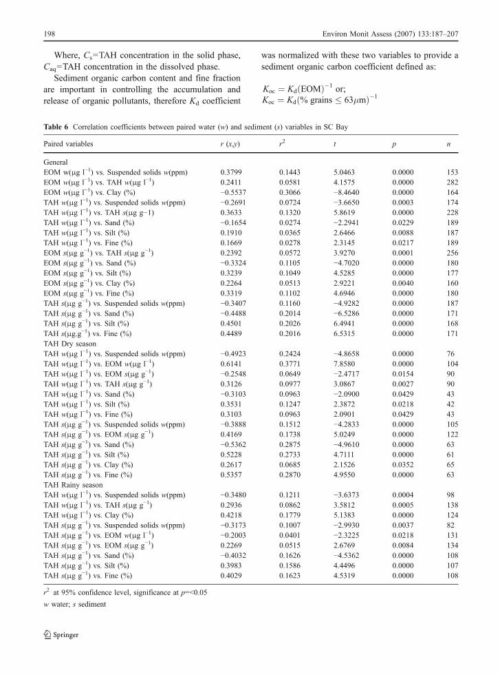
Where, Cs=TAH concentration in the solid phase,Caq=TAH concentration in the dissolved phase.

Sediment organic carbon content and fine fractionare important in controlling the accumulation andrelease of organic pollutants, therefore Kd coefficient

was normalized with these two variables to provide asediment organic carbon coefficient defined as:

Koc ¼ Kd EOMð Þ�1 or;Koc ¼ Kd % grains � 63μmð Þ�1

Table 6 Correlation coefficients between paired water (w) and sediment (s) variables in SC Bay

Paired variables r (x,y) r2 t p n

GeneralEOM w(μg l−1) vs. Suspended solids w(ppm) 0.3799 0.1443 5.0463 0.0000 153EOM w(μg l−1) vs. TAH w(μg l−1) 0.2411 0.0581 4.1575 0.0000 282EOM w(μg l−1) vs. Clay (%) −0.5537 0.3066 −8.4640 0.0000 164TAH w(μg l−1) vs. Suspended solids w(ppm) −0.2691 0.0724 −3.6650 0.0003 174TAH w(μg l−1) vs. TAH s(μg g−1) 0.3633 0.1320 5.8619 0.0000 228TAH w(μg l−1) vs. Sand (%) −0.1654 0.0274 −2.2941 0.0229 189TAH w(μg l−1) vs. Silt (%) 0.1910 0.0365 2.6466 0.0088 187TAH w(μg l−1) vs. Fine (%) 0.1669 0.0278 2.3145 0.0217 189EOM s(μg g−1) vs. TAH s(μg g−1) 0.2392 0.0572 3.9270 0.0001 256EOM s(μg g−1) vs. Sand (%) −0.3324 0.1105 −4.7020 0.0000 180EOM s(μg g−1) vs. Silt (%) 0.3239 0.1049 4.5285 0.0000 177EOM s(μg g−1) vs. Clay (%) 0.2264 0.0513 2.9221 0.0040 160EOM s(μg g−1) vs. Fine (%) 0.3319 0.1102 4.6946 0.0000 180TAH s(μg g−1) vs. Suspended solids w(ppm) −0.3407 0.1160 −4.9282 0.0000 187TAH s(μg g−1) vs. Sand (%) −0.4488 0.2014 −6.5286 0.0000 171TAH s(μg g−1) vs. Silt (%) 0.4501 0.2026 6.4941 0.0000 168TAH s(μg.g−1) vs. Fine (%) 0.4489 0.2016 6.5315 0.0000 171TAH Dry seasonTAH w(μg l−1) vs. Suspended solids w(ppm) −0.4923 0.2424 −4.8658 0.0000 76TAH w(μg l−1) vs. EOM w(μg l−1) 0.6141 0.3771 7.8580 0.0000 104TAH w(μg l−1) vs. EOM s(μg g−1) −0.2548 0.0649 −2.4717 0.0154 90TAH w(μg l−1) vs. TAH s(μg g−1) 0.3126 0.0977 3.0867 0.0027 90TAH w(μg l−1) vs. Sand (%) −0.3103 0.0963 −2.0900 0.0429 43TAH w(μg l−1) vs. Silt (%) 0.3531 0.1247 2.3872 0.0218 42TAH w(μg l−1) vs. Fine (%) 0.3103 0.0963 2.0901 0.0429 43TAH s(μg g−1) vs. Suspended solids w(ppm) −0.3888 0.1512 −4.2833 0.0000 105TAH s(μg g−1) vs. EOM s(μg g−1) 0.4169 0.1738 5.0249 0.0000 122TAH s(μg g−1) vs. Sand (%) −0.5362 0.2875 −4.9610 0.0000 63TAH s(μg g−1) vs. Silt (%) 0.5228 0.2733 4.7111 0.0000 61TAH s(μg g−1) vs. Clay (%) 0.2617 0.0685 2.1526 0.0352 65TAH s(μg g−1) vs. Fine (%) 0.5357 0.2870 4.9550 0.0000 63TAH Rainy seasonTAH w(μg l−1) vs. Suspended solids w(ppm) −0.3480 0.1211 −3.6373 0.0004 98TAH w(μg l−1) vs. TAH s(μg g−1) 0.2936 0.0862 3.5812 0.0005 138TAH w(μg l−1) vs. Clay (%) 0.4218 0.1779 5.1383 0.0000 124TAH s(μg g−1) vs. Suspended solids w(ppm) −0.3173 0.1007 −2.9930 0.0037 82TAH s(μg g−1) vs. EOM w(μg l−1) −0.2003 0.0401 −2.3225 0.0218 131TAH s(μg g−1) vs. EOM s(μg g−1) 0.2269 0.0515 2.6769 0.0084 134TAH s(μg g−1) vs. Sand (%) −0.4032 0.1626 −4.5362 0.0000 108TAH s(μg g−1) vs. Silt (%) 0.3983 0.1586 4.4496 0.0000 107TAH s(μg g−1) vs. Fine (%) 0.4029 0.1623 4.5319 0.0000 108

r2 at 95% confidence level, significance at p=<0.05

w water; s sediment

198 Environ Monit Assess (2007) 133:187–207

Tab

le7

Correlatio

ncoefficientsbetweenpaired

sedimentvariablesin

Con

tinentalwater

bodies

Pairedvariables

r(x,y)

r2t

pn

r(x,y)

r2t

pn

r(x,y)

r2t

pn

Con

tinentalwater

bodies

LaVentosa

Estuary

System

Tehuantepec

River

General

EOM

s(μgg−

1)vs.TA

Hs(μgg−

1)

0.65

620.43

0711.603

50.00

0018

00.66

650.44

428.80

410.00

0099

0.55

450.30

755.92

210.00

0081

EOM

s(μgg−

1)vs.Silt

(%)

0.20

320.04

132.52

410.01

2715

0EOM

s(μgg−

1)vs.Fine(%

)0.17

950.03

222.22

040.02

7915

0TA

Hs(μgg−

1)vs.Silt

(%)

0.26

750.07

163.35

490.00

1014

8TA

Hs(μgg−

1)vs.Clay(%

)0.24

830.06

173.09

730.00

2314

8TA

Hs(μgg−

1)vs.Fine(%

)0.27

390.07

503.44

100.00

0814

8TA

HDry

season

TAH

s(μgg−

1)vs.EOM

s(μgg−

1)

0.52

060.27

104.64

370.00

0060

0.63

220.39

974.96

310.00

0039

0.55

090.30

352.87

710.00

9721

TAH

s(μgg−

1)vs.Silt

(%)

0.31

200.09

732.20

270.03

2847

TAH

s(μgg−

1)vs.Clay(%

)0.33

210.1103

2.36

170.02

2647

TAH

s(μgg−

1)vs.Fine(%

)0.33

980.1154

2.42

340.01

9547

TAH

Rainy

season

TAH

s(μgg−

1)vs.EOM

s(μgg−

1)

0.72

550.52

6411.452

50.00

0012

00.69

070.47

717.27

390.00

0060

0.74

890.56

098.60

720.00

0060

TAH

s(μgg−

1)vs.Silt

(%)

0.24

870.06

192.55

480.01

2110

1TA

Hs(μgg−

1)vs.Clay(%

)0.20

440.04

182.07

720.04

0410

1TA

Hs(μgg−

1)vs.Fine(%

)0.24

330.05

922.49

600.01

4210

1

r2at

95%

C.I.,sign

ificance

atp=<0.05

Environ Monit Assess (2007) 133:187–207 199

3 Results and Discussion

3.1 Physical and chemical characterization

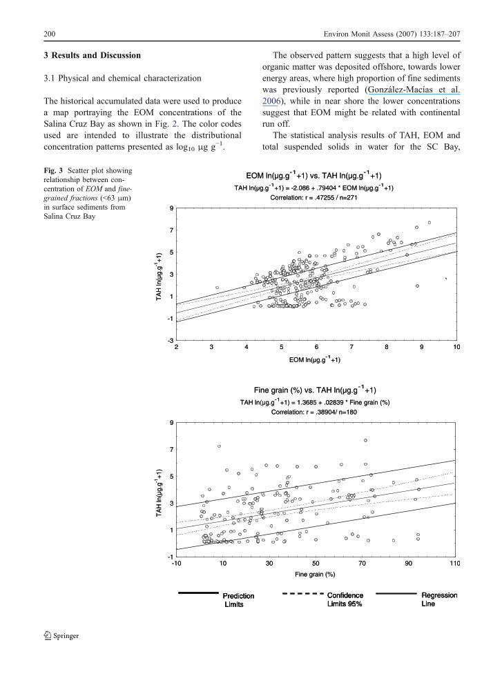
The historical accumulated data were used to producea map portraying the EOM concentrations of theSalina Cruz Bay as shown in Fig. 2. The color codesused are intended to illustrate the distributionalconcentration patterns presented as log10 μg g−1.

The observed pattern suggests that a high level oforganic matter was deposited offshore, towards lowerenergy areas, where high proportion of fine sedimentswas previously reported (González-Macías et al.2006), while in near shore the lower concentrationssuggest that EOM might be related with continentalrun off.

The statistical analysis results of TAH, EOM andtotal suspended solids in water for the SC Bay,

PredictionLimits

ConfidenceLimits 95%

RegressionLine

EOM ln(µg.g-1+1) vs. TAH ln(µg.g-1+1)

TAH ln(µg.g-1+1) = -2.086 + .79404 * EOM ln(µg.g-1+1)

Correlation: r = .47255 / n=271

EOM ln(µg.g-1+1)

TA

H ln

(µg.

g-1+

1)

-3

-1

1

3

5

7

9

2 3 4 5 6 7 8 9 10

Fine grain (%) vs. TAH ln(µg.g-1+1)

TAH ln(µg.g-1+1) = 1.3685 + .02839 * Fine grain (%)

Correlation: r = .38904/ n=180

Fine grain (%)

TA

H ln

(µg.

g-1+

1)

-1

1

3

5

7

9

-10 10 30 50 70 90 110

PredictionLimits

ConfidenceLimits 95%

RegressionLine

PredictionLimits

PredictionLimits

ConfidenceLimits 95%ConfidenceLimits 95%

RegressionLine

EOM ln(µg.g-1+1) vs. TAH ln(µg.g-1+1)

TAH ln(µg.g-1+1) = -2.086 + .79404 * EOM ln(µg.g-1+1)

Correlation: r = .47255 / n=271

EOM ln(µg.g-1+1)

TA

H ln

(µg.

g-1+

1)

-3

-1

1

3

5

7

9

2 3 4 5 6 7 8 9 10

Fine grain (%) vs. TAH ln(µg.g-1+1)

TAH ln(µg.g-1+1) = 1.3685 + .02839 * Fine grain (%)

Correlation: r = .38904/ n=180

Fine grain (%)

TA

H ln

(µg.

g-1+

1)

-1

1

3

5

7

9

-10 10 30 50 70 90 110

Fig. 3 Scatter plot showingrelationship between con-centration of EOM and fine-grained fractions (<63 μm)in surface sediments fromSalina Cruz Bay

200 Environ Monit Assess (2007) 133:187–207

along with the original matrix including outliers,and global data set are shown in Table 4. Moreover,the Table includes sediments grain size distributionthat prevails during the two dominant climaticperiods in the Bay.

Mean average TAH values in water ranged from0.01 to 120 μg l−1. Student t test for independentsamples, with different variance was tested for Dry(D) and Rainy (R) season sets.

The means are significantly different for TAH inwater (t=35.8343, df=298, p=0.0000, nD=108, nR=192) and for the grain fractions: i.e. clay (t=−5.6264,df=194, p=0.0000, nD=71, nR=125).

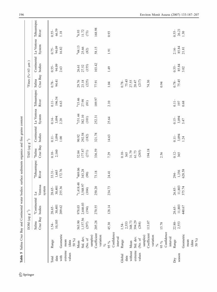
Mean average values of TAH, EOM, and percentagefine grains distribution in sediments of the SC Bay andContinental water bodies are presented in Table 5 forthe two dominant climatic periods of the area. TAHvalues from SC Bay vary between 0.10 to 2,160 μgg−1 while in Continental water bodies the meanaverage vary between 0.11 to 3,094 μg g−1.

Student t test for independent samples showedsignificantly differences in TAH concentrations forSC Bay sediments between seasons (t=16.1520, df=316, p=0.0000, nD=126, nR=192), while no season-al differences were found for TAH and fine fractionsin Continental water bodies sets, although differenceswere found between La Ventosa Estuary system andthe Tehuantepec River.

EOM values in sediments from Salina Cruz Bayvary from 1.54 to 10,105.0 μg g−1, and from 28.65 to30,401.0 μg g−1 in Continental water bodies. Nodifferences were found during dry season for EOMbetween La Ventosa Estuary System (V) and Tehuan-tepec River (T) (t=−0.0798, df=60, p=0.9367, nV=42, nT=21), there were no seasonal differences eitherin Salina Cruz Bay.

There are EOM seasonal differences Dry (D) andRainy (R) in Tehuantepec river (t =13.0877, df=57,p=0.0000, nD=21, nR=38) and Continental waterbodies analyzed together (t=9.3658, df=161, p=0.0000, nD=62, nR=101).

EOM shows differences also between La VentosaEstuary System and Tehuantepec River during rainyseason (t=3.6884, df=192, p=0.0002, nV=104,nT=90) (t=5.9800, df=99, p=0.0000, nV=63,nT=38).

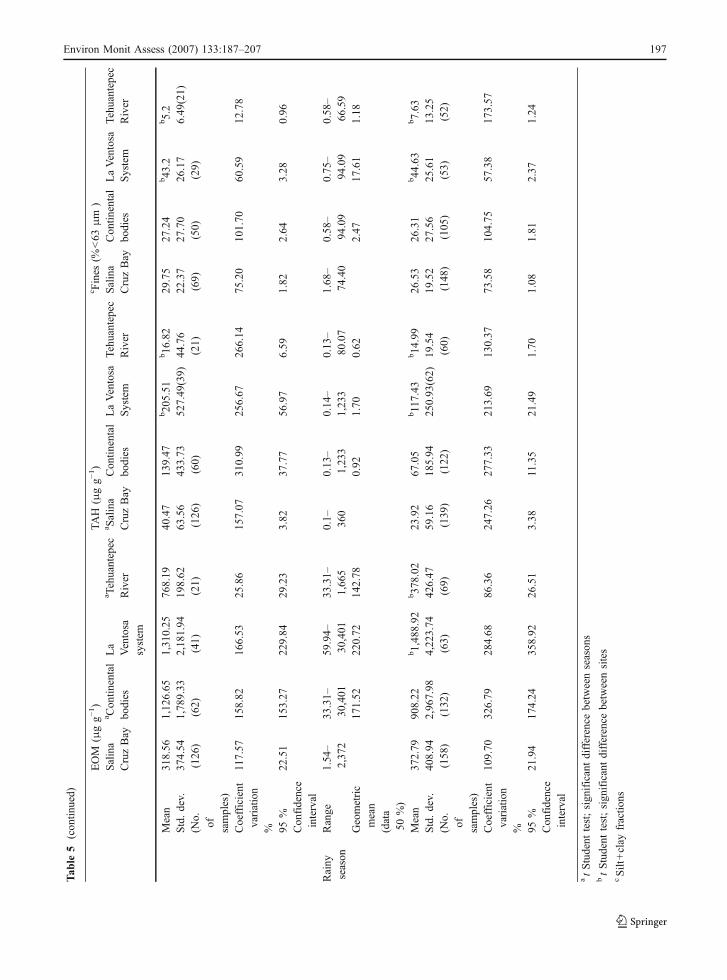
Significantly different coefficients between pairedwater and sediment variables were found in the SCBay, see Table 6. TAH in water and sediments relate

positive each other and both relate negative tosuspended solids in water and sands.

TAH content in water relates with EOM in waterand with the fine fractions of sediment while insediments TAH content is related with EOM and fineparticles. These patterns are present in both seasons,excluding the pair TAH in water vs. EOM in water,which is not followed during rainy season.

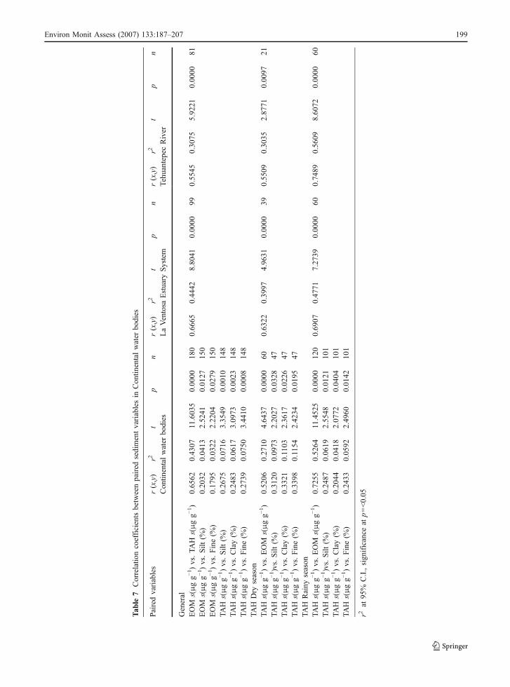
Table 7 shows grain sizes and TAH correlationcoefficients obtained for significant paired variablesfrom Continental water bodies. TAH relates positivelywith EOM, and fine grains, in both seasons whenContinental body waters are considered together. Ifseparate correlations for La Ventosa Estuary and theRiver are made, TAH correlates positive only withEOM in both seasons.

Briefly, EOM concentrations in Tehuantepec Riverare influenced by seasonal conditions with highvalues during dry season when water flow decreases.Pearson coefficients suggest that TAH are associatedpreferentially to EOM instead to fine particles, anddon’t settle down in the sediment.

TAH and fine grains in continental water bodies arenot influenced by seasonal conditions, low concen-trations of them are present in the River, accumulatingin the sediments of the Bay during dry season.Regression analyses suggest that TAH in water andsediments compartments of Salina Cruz Bay aremostly associated to EOM and sediment fine fractions.

3.2 Normalization with EOM and fine-grainedfraction <63 μm.

Scatter plots of TAH concentrations vs. EOM andfine-grained fractions, found in the sediments of SCBay are shown in Fig. 3. Likewise, correlation valuesat the 95% probability level, defined as ± the standarderror of estimate (n=>30), could constitute thenaturally occurring background of the SC Bay.Samples where TAH plot is above backgroundrelationship have an additional source contributionnot present in the background samples.

3.3 TAH enrichment factors and geo-accumulationindex of the sediment

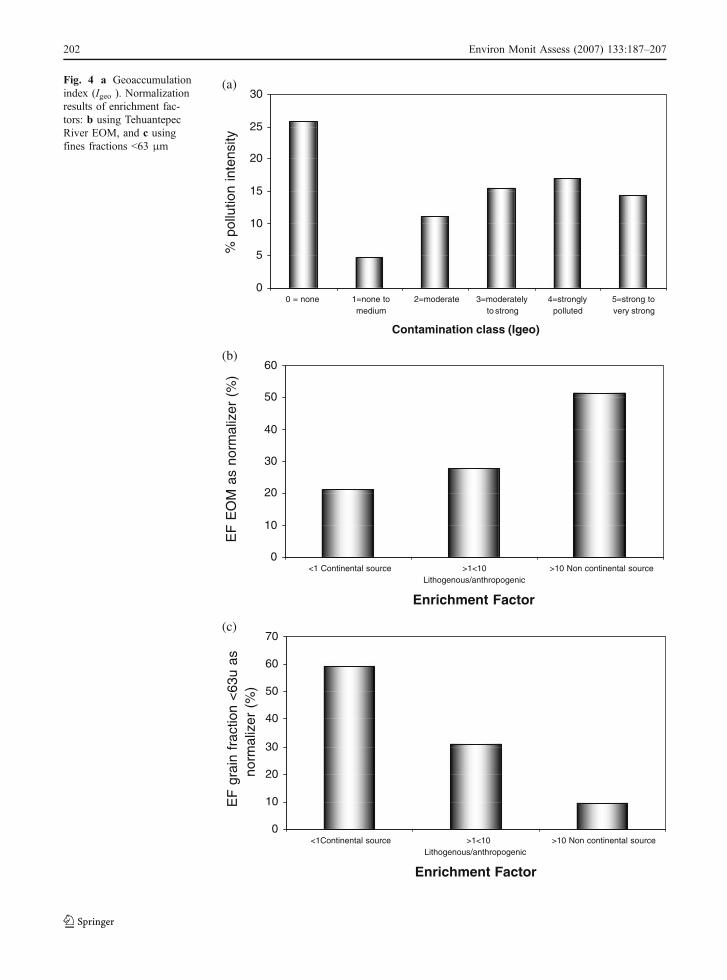
Figure 4a shows calculated Igeo factors while Fig. 4band c illustrate the enrichment factors using EOM andgrain fraction as normalizer respectively.

Environ Monit Assess (2007) 133:187–207 201

0

5

10

15

20

25

30

0 = none 1=none tomedium

2=moderate 3=moderatelyto strong

4=stronglypolluted

5=strong tovery strong

Contamination class (Igeo)

% p

ollu

tion

inte

nsity

(a)

0

10

20

30

40

50

60

<1 Continental source >1<10Lithogenous/anthropogenic

>10 Non continental source

Enrichment Factor

EF

EO

M a

s no

rmal

izer

(%

)

(b)

0

10

20

30

40

50

60

70

<1Continental source >1<10Lithogenous/anthropogenic

>10 Non continental source

Enrichment Factor

EF

gra

in f

ract

ion

<63

u as

no

rmal

izer

(%

)

(c)

Fig. 4 a Geoaccumulationindex (Igeo ). Normalizationresults of enrichment fac-tors: b using TehuantepecRiver EOM, and c usingfines fractions <63 μm

202 Environ Monit Assess (2007) 133:187–207

Approximately 70% of Igeo values range frommoderately to strong contaminated classes. Accordingto Müller (1979), concentrations of contaminants maybe separated into ranges from 0 to 6 (0=none, 1=none to medium, 2=moderate, 3=moderately tostrong, 4=strongly polluted, 5=strong to very strong,6=very strong). The higher range expresses a totalaromatic hydrocarbon concentration 100 times greaterthan that of the reference ambient.

Total aromatic hydrocarbons are depleted withrespect to continental baseline in view that 21% ofTAH data are below the baseline concentration (EF=<1) when normalized with respect to EOM (Fig. 4b)and 60% if fine grains size is employed (Fig. 4c).Thirty % of the data in Fig. 4b and c are above thebaseline (EF=>1≤10) using either normalizer, pointedout to an enrichment of lithogenous or anthropogenicorigin.

Pertaining to the non continental sources (EF≥10),50% of the data shown in Fig. 4b are above the baseline

concentration when EOM is the normalizer, and 10% ofdata are also above if normalized with respect to grainsize fraction, Fig. 4c.

Organic carbon and grain size are employed inparticular cases as geochemical normalizers. Theywill often shows strong relationships with site con-taminants, and to varying degrees they covarytogether with sediment texture. This seems to be thecase of the Salina Cruz, Bay site, but not of theTehuantepec River, where the only significant posi-tive relationship is observed between TAH and EOM(Tables 6 and 7).

View that both normalizers are positively correlat-ed with TAH in the Bay (Table 6), and no seasonaldifferences influence the results with grain size fractionof the Tehuantepec River (Table 5), differences can beexplained taking into account that each baselinerepresents unlike TAH sources, in accordance withFig. 3 in which higher concentrations above the back-ground using EOM as normalizer are found.

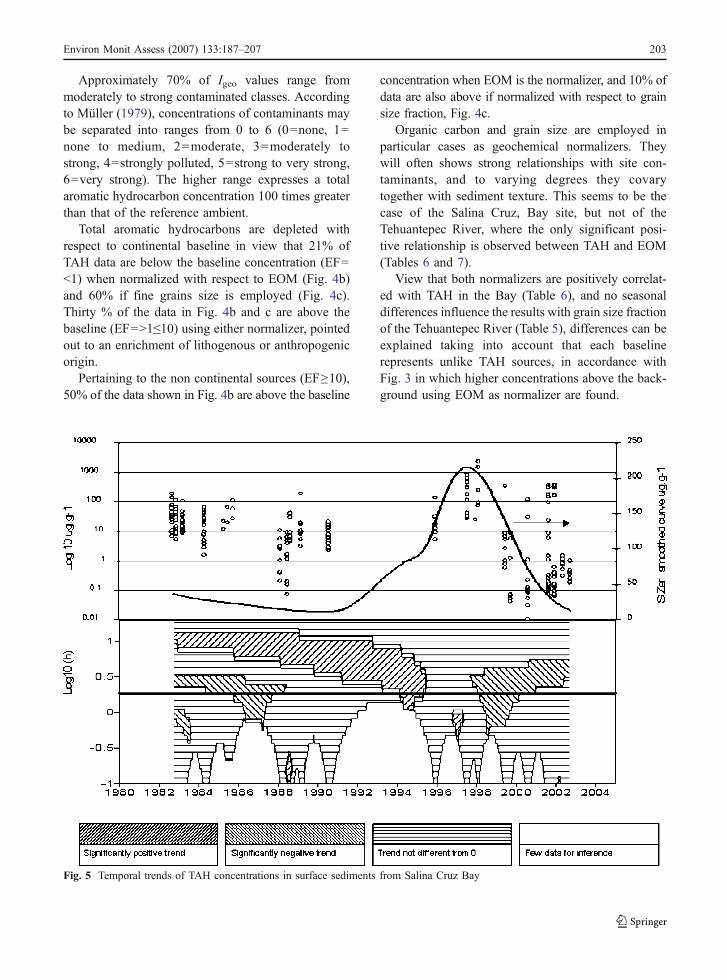
Fig. 5 Temporal trends of TAH concentrations in surface sediments from Salina Cruz Bay

Environ Monit Assess (2007) 133:187–207 203

3.4 Temporal and spatial trends

The historical accumulated data portraying the TAHconcentrations in sediments of the SC Bay is shownin Fig. 5. The lower part of the graph shows a SiZerplot which relates time and concentration trends whilethe upper part shows the inferred values of thesmoothed line (continuous line, secondary Y scale)graphed along the raw data (dotted data, Y left scale).

In the plot, the entire point wise straight lines areshown. The bold lines illustrate the first inferencestraight line that uses all the data set to perform the timetrend inference. The slope of the dashed lines is relatedwith increasing or decreasing tendency as well as themagnitude and significance of the inference. Horizon-tal dashed lines indicate that for a specific timeframe,significant difference from 0 can not be ascertained forthe smoothed line. The non-dashed areas indicate thatfew data are available to do inference.

TAH concentrations in surface sediments shows adecrease (negative slope at log10(h)=0.25 ) in theperiod 1984–1992, follows by an increase from 1992to 1996 (dashed lines positive slope), and a significantdecrease again from 1998 to 2002. Reconstruction ofthe temporal tendencies seems to indicate that TAHdecrease continued to present days.

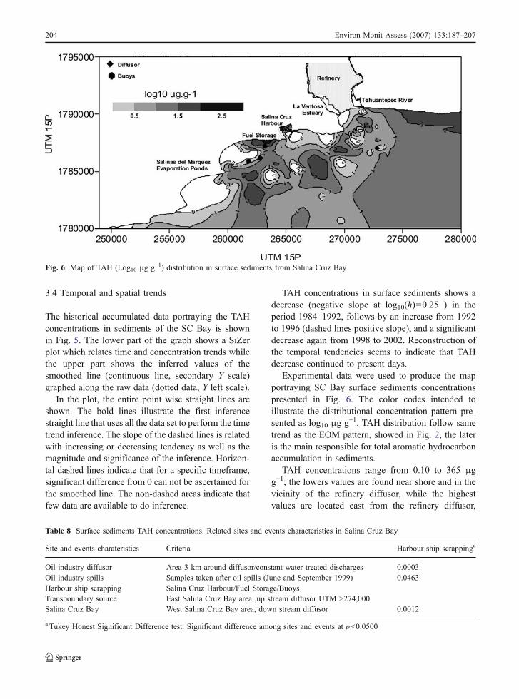
Experimental data were used to produce the mapportraying SC Bay surface sediments concentrationspresented in Fig. 6. The color codes intended toillustrate the distributional concentration pattern pre-sented as log10 μg g−1. TAH distribution follow sametrend as the EOM pattern, showed in Fig. 2, the lateris the main responsible for total aromatic hydrocarbonaccumulation in sediments.

TAH concentrations range from 0.10 to 365 μgg−1; the lowers values are found near shore and in thevicinity of the refinery diffusor, while the highestvalues are located east from the refinery diffusor,

Table 8 Surface sediments TAH concentrations. Related sites and events characteristics in Salina Cruz Bay

Site and events charateristics Criteria Harbour ship scrappinga

Oil industry diffusor Area 3 km around diffusor/constant water treated discharges 0.0003Oil industry spills Samples taken after oil spills (June and September 1999) 0.0463Harbour ship scrapping Salina Cruz Harbour/Fuel Storage/BuoysTransboundary source East Salina Cruz Bay area ,up stream diffusor UTM >274,000Salina Cruz Bay West Salina Cruz Bay area, down stream diffusor 0.0012

a Tukey Honest Significant Difference test. Significant difference among sites and events at p<0.0500

Fig. 6 Map of TAH (Log10 μg g−1) distribution in surface sediments from Salina Cruz Bay

204 Environ Monit Assess (2007) 133:187–207

close to the fuels dispatch and at the evaporationponds, suggesting that a transboundary source forTAH must influence the observed trends.

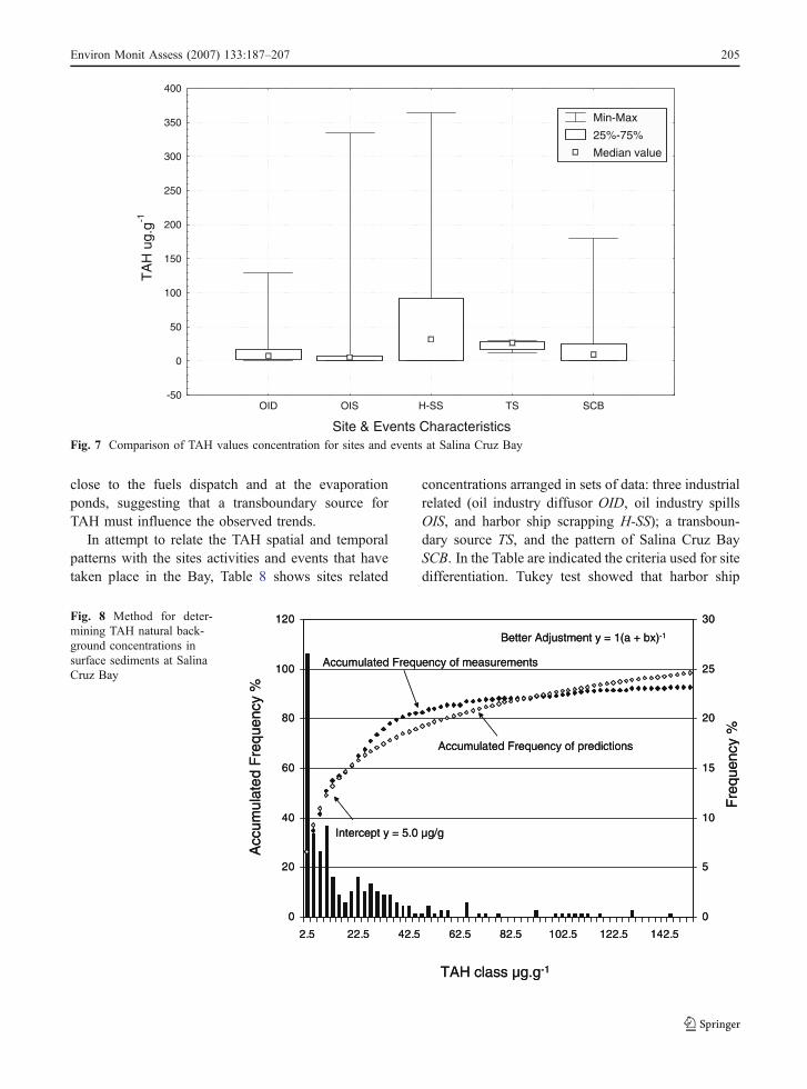
In attempt to relate the TAH spatial and temporalpatterns with the sites activities and events that havetaken place in the Bay, Table 8 shows sites related

concentrations arranged in sets of data: three industrialrelated (oil industry diffusor OID, oil industry spillsOIS, and harbor ship scrapping H-SS); a transboun-dary source TS, and the pattern of Salina Cruz BaySCB. In the Table are indicated the criteria used for sitedifferentiation. Tukey test showed that harbor ship

Site & Events Characteristics

TA

H u

g.g-1

-50

0

50

100

150

200

250

300

350

400

OID OIS H-SS TS SCB

Min-Max

25%-75%

Median value

Fig. 7 Comparison of TAH values concentration for sites and events at Salina Cruz Bay

0

20

40

60

80

100

120

2.5 22.5 42.5 62.5 82.5 102.5 122.5 142.5

0

5

10

15

20

25

30

Better Adjustment y = 1(a + bx)-1

Accumulated Frequency of measurements

Accumulated Frequency of predictions

Intercept y = 5.0 µg/g

Acc

umul

ated

Fre

quen

cy %

TAH class µg.g-1

Fre

quen

cy %

0

20

40

60

80

100

120

2.5 22.5 42.5 62.5 82.5 102.5 122.5 142.5

0

5

10

15

20

25

30

Better Adjustment y = 1(a + bx)-1

Accumulated Frequency of measurements

Accumulated Frequency of predictions

Intercept y = 5.0 µg/g

Acc

umul

ated

Fre

quen

cy %

TAH class µg.g-1

Fre

quen

cy %

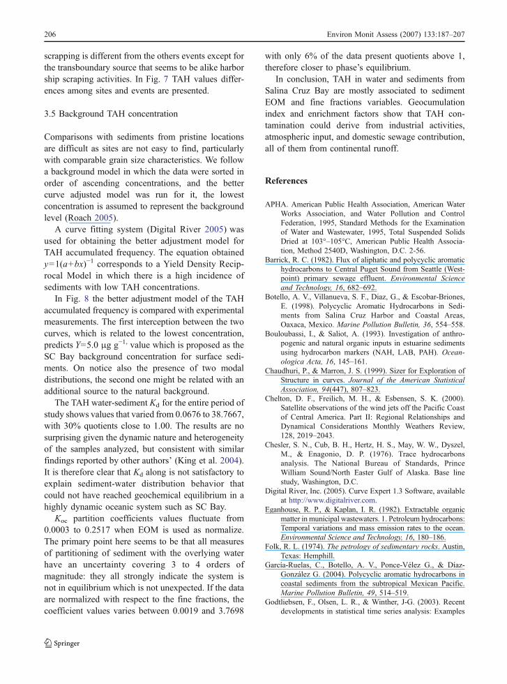
Fig. 8 Method for deter-mining TAH natural back-ground concentrations insurface sediments at SalinaCruz Bay

Environ Monit Assess (2007) 133:187–207 205

scrapping is different from the others events except forthe transboundary source that seems to be alike harborship scraping activities. In Fig. 7 TAH values differ-ences among sites and events are presented.

3.5 Background TAH concentration

Comparisons with sediments from pristine locationsare difficult as sites are not easy to find, particularlywith comparable grain size characteristics. We followa background model in which the data were sorted inorder of ascending concentrations, and the bettercurve adjusted model was run for it, the lowestconcentration is assumed to represent the backgroundlevel (Roach 2005).

A curve fitting system (Digital River 2005) wasused for obtaining the better adjustment model forTAH accumulated frequency. The equation obtainedy=1(a+bx)−1 corresponds to a Yield Density Recip-rocal Model in which there is a high incidence ofsediments with low TAH concentrations.

In Fig. 8 the better adjustment model of the TAHaccumulated frequency is compared with experimentalmeasurements. The first interception between the twocurves, which is related to the lowest concentration,predicts Y=5.0 μg g−1, value which is proposed as theSC Bay background concentration for surface sedi-ments. On notice also the presence of two modaldistributions, the second one might be related with anadditional source to the natural background.

The TAH water-sediment Kd for the entire period ofstudy shows values that varied from 0.0676 to 38.7667,with 30% quotients close to 1.00. The results are nosurprising given the dynamic nature and heterogeneityof the samples analyzed, but consistent with similarfindings reported by other authors’ (King et al. 2004).It is therefore clear that Kd along is not satisfactory toexplain sediment-water distribution behavior thatcould not have reached geochemical equilibrium in ahighly dynamic oceanic system such as SC Bay.

Koc partition coefficients values fluctuate from0.0003 to 0.2517 when EOM is used as normalize.The primary point here seems to be that all measuresof partitioning of sediment with the overlying waterhave an uncertainty covering 3 to 4 orders ofmagnitude: they all strongly indicate the system isnot in equilibrium which is not unexpected. If the dataare normalized with respect to the fine fractions, thecoefficient values varies between 0.0019 and 3.7698

with only 6% of the data present quotients above 1,therefore closer to phase’s equilibrium.

In conclusion, TAH in water and sediments fromSalina Cruz Bay are mostly associated to sedimentEOM and fine fractions variables. Geocumulationindex and enrichment factors show that TAH con-tamination could derive from industrial activities,atmospheric input, and domestic sewage contribution,all of them from continental runoff.

References

APHA. American Public Health Association, American WaterWorks Association, and Water Pollution and ControlFederation, 1995, Standard Methods for the Examinationof Water and Wastewater, 1995, Total Suspended SolidsDried at 103°–105°C, American Public Health Associa-tion, Method 2540D, Washington, D.C. 2-56.

Barrick, R. C. (1982). Flux of aliphatic and polycyclic aromatichydrocarbons to Central Puget Sound from Seattle (West-point) primary sewage effluent. Environmental Scienceand Technology, 16, 682–692.

Botello, A. V., Villanueva, S. F., Diaz, G., & Escobar-Briones,E. (1998). Polycyclic Aromatic Hydrocarbons in Sedi-ments from Salina Cruz Harbor and Coastal Areas,Oaxaca, Mexico. Marine Pollution Bulletin, 36, 554–558.

Bouloubassi, I., & Saliot, A. (1993). Investigation of anthro-pogenic and natural organic inputs in estuarine sedimentsusing hydrocarbon markers (NAH, LAB, PAH). Ocean-ologica Acta, 16, 145–161.

Chaudhuri, P., & Marron, J. S. (1999). Sizer for Exploration ofStructure in curves. Journal of the American StatisticalAssociation, 94(447), 807–823.

Chelton, D. F., Freilich, M. H., & Esbensen, S. K. (2000).Satellite observations of the wind jets off the Pacific Coastof Central America. Part II: Regional Relationships andDynamical Considerations Monthly Weathers Review,128, 2019–2043.

Chesler, S. N., Cub, B. H., Hertz, H. S., May, W. W., Dyszel,M., & Enagonio, D. P. (1976). Trace hydrocarbonsanalysis. The National Bureau of Standards, PrinceWilliam Sound/North Easter Gulf of Alaska. Base linestudy, Washington, D.C.

Digital River, Inc. (2005). Curve Expert 1.3 Software, availableat http://www.digitalriver.com.

Eganhouse, R. P., & Kaplan, I. R. (1982). Extractable organicmatter in municipal wastewaters. 1. Petroleum hydrocarbons:Temporal variations and mass emission rates to the ocean.Environmental Science and Technology, 16, 180–186.

Folk, R. L. (1974). The petrology of sedimentary rocks. Austin,Texas: Hemphill.

García-Ruelas, C., Botello, A. V., Ponce-Vélez G., & Díaz-González G. (2004). Polycyclic aromatic hydrocarbons incoastal sediments from the subtropical Mexican Pacific.Marine Pollution Bulletin, 49, 514–519.

Godtliebsen, F., Olsen, L. R., & Winther, J-G. (2003). Recentdevelopments in statistical time series analysis: Examples

206 Environ Monit Assess (2007) 133:187–207

of use in climate research. Journal Geophysical Research,30(12), 1654–1657.

Gold, G., Acuña, J, & Morell, J. (1987). Manual CARIPOL/IOCARIBE para el análisis de hidrocarburos de petróleo ensedimentos y organismos marinos. Cartagena de Indias,Colombia.

González-Macías, C., Schifter, I., Lluch-Cota, D. B. Méndez-Rodríguez, L., & Hernández-Vázquez, S. (2006). Distri-bution, enrichment and accumulation of heavy metals incoastal sediments of Salina Cruz Bay, México. Environ-mental Monitoring and Assessment, 118, 1–3.

Gordon, D. C., & Keizer, P. D. (1976). Estimation of petroleumhydrocarbons in sea water by fluorescence spectroscopy.Improved sampling and analytical methods. TechnicalReport No. 481. Canada: Fisheries and Marine Service.

Holmström, L., & Erästö, P. (2001). Using the SiZer method inHolocene temperature reconstruction. Research Reports A36,Rolf Nevanlinna Institute. Finland: University of Helsinki.

Jeng, W. L., & Han, B. C. (1994). Sedimentary coprostanol inKaohsiung harbor and the Tan-Shui estuary, Taiwan.Marine Pollution Bulletin, 28, 494–499.

Karichknoff, S. W., Brown, D. S., & Scott, T. A. (1979).Sorption of hydrophobic pollutants on natural sediments.Water Research, 13, 241–248.

King, A. J., Readman, J. W., & Zhou, J. L. (2004). Dynamicbehavior of polycyclic hydrocarbons in Brighton marina,UK. Marine Pollution Bulletin, 48, 229–239.

Kot-Wasik, A., Dbska, J., & Namienik, J. (2004). Monitoring oforganic pollutants in coastal waters of the Gulf of Gdansk,Southern Baltic. Marine Pollution Bulletin, 49, 264–276.

Latimer, J. S., & Quinn, J. G. (1996). Historical trends andcurrent inputs of hydrophobic organic compounds in anurban estuary: The sedimentary record. EnvironmentalScience and Technology, 30, 623–633.

Massey, Jr., F. J. (1951). The Kolmogorov–Smirnov test for goodnessof fit. Journal of the American Statistical Association, 46, 68–78.

Massoud, M. S., Al-Abdali, F., Al-Ghadban, A. N., & Al-Sarawi, M. (1996). Botton Sediments of the Arabian Gulf-II.TPH and TOC contents as indicators of oil pollution andimplications for the effect and fate of the Kuwait Oil Slick.Environmental Pollution, 93, 271–284.

Means, J. C., Wood, S. G., Hassett, J. I., & Banwart, W. L.(1980). Sorption of polynuclear aromatic hydrocarbons bysediments and soils. Environmental Science and Technol-ogy, 14, 1524–1528.

Müller, G. (1979). Schwermetalle in den sediments des Rheins-Veranderungen seitt 1971. Umschan, 79, 778–783.

Mzoughi, N., Dachraoui, M., & Villeneuve, J. P. (2005).Evaluation of aromatic hydrocarbons by spectrofluorometryin marine sediments and biological matrix: What referenceshould be considered? Comptes Rendus Chimie, 8, 97–102.

NFESC (2003). Final implementation guide for assessing andmanaging contaminated sediment at navy facilities. User’sGuide UG-2053-ENV. Naval Facilities Engineering Com-mand. Washington, DC 20374-5065.

Nolting, R. F., Ramkema, A., & Everaats, J. M. (1999). Thegeochemistry of Cu, Cd, Zn, Ni and Pb in sediment cores

from the continental slope of the Banc d’Arguin (Maur-itania). Continental Shelf Research, 19, 665–691.

Readman, J. W., Bartocci, J., Tolosa, I., Fowler, S. W., Oregioni,B., & Abdulraheem, M. Y. (1996). Recovery of the coastalmarine environment in the Gulf following 1991 the warrelated oil spills. Marine Pollution Bulletin, 32, 493–498.

Readman, J. W., Fillmann, G., Tolosa, I., Bartocci, J.Villeneuve, J. P., Catinni, C., et al. (2002). Petroleumand PAH contamination of the Black Sea. MarinePollution Bulletin, 44, 48–62.

Roach, A. C. (2005). Assessment of metals in sediments fromLake Macquarie, New South Wales, Australia, usingnormalization models and sediment quality guidelines.Marine Environmental Research, 59, 453–472.

Statistica (1998). Statistica for windows (Vol I). GeneralConventions General Conventions ands Statistics I (2nded.). StatSoft, Inc., Tulsa OK, USA.

Surfer® version 8.01 (2002). Golden Software, Inc., CO, USA.Taylor, S. R. (1964). Abundance of chemical elements in the

continental crust; a new table. Geochimica CosmochimicaActa, 28, 1273–1285.

Tolosa, I., de Mora S. J., Fowler, S. W., Villeneuve, J. P.,Bartocci, J., & Cattini, C. (2005). Aliphatic and aromatichydrocarbons in marine biota and coastal sediments fromthe Gulf and the Gulf of Oman. Marine Pollution Bulletin,50, 1619–1633.

Trasviña, A., Barton, E. D., Brown, J.,Velez, H. S., Kosro, P.M., & Smith, R. L. (1995). Offshore wind forcing in theGulf of Tehuantepec, México. The asymmetric circulation.Journal of Geophysical Research, 100(20), 649–663.

United States Environmental Protection Agency (USEPA) (1978).Test method for evaluating total recoverable petroleumhydrocarbon, method 418.1 (spectrophotometric, infrared).Washington, DC: U.S. Government Printing Office.

United States Environmental Protection Agency (USEPA) (1996).Method 8440, total recoverable petroleum hydrocarbon byinfrared spectrophotometry. SW-846 (3rd edn.). Revision-0.Washington, DC: U.S.Government Printing Office.

UNESCO (1982). Comisión Oceanográfica IntergubernamentalDeterminación de los hidrocarburos de petróleo en lossedimentos. Manuales y Guías, 11, 1–35. Place deFontenoy, París, Francia.

UNESCO (1984). Comisión Oceanográfica IntergubernamentalManual para la vigilancia del aceite y de los hidrocarburosdel petróleo disueltos o dispersos en el agua del mar y enlas playas. Procedimientos para el componente petróleodel sistema de vigilancia de la contaminación del mar(MARPOL-MON-P). Manuales y Guías, 13, 1–37. Placede Fontenoy, París, Francia.

Volkman, J. K., Holdswoeth, D. G., Neill, G. P., & Bavor, H. J.(1992). Identification of natural, anthropogenic and petro-leum hydrocarbons in aquatic sediments. The Science ofTotal Environment, 112, 203–219.

Zsefer, P., Glasby, G. P., Sefer, K., Pempkowiak, J., & Kaliszan,R. (1996). Heavy-metal pollution in superficial sedimentsfrom the southern Baltic Sea off Poland. Journal ofEnvironmental Science and Health, 31A, 2723–2754.

Environ Monit Assess (2007) 133:187–207 207