Embed Size (px)
Citation preview

Energy-saving potential ofAramid-based conveyor belts
S. Drenkelford
Mas
tero
fScie
nce
Thes
is
Department of Maritime and Transportation Technology
Energy-saving potential ofAramid-based conveyor belts
Master of Science Thesis
For the degree of Master of Science in Mechanical Engineering at DelftUniversity of Technology
S. Drenkelford
March 5, 2015
Faculty of Mechanical, Maritime and Materials Engineering (3mE) · Delft University ofTechnology
Delft University of Technology
FACULTY MECHANICAL, MARITIME AND
MATERIALS ENGINEERING Department Marine and Transport Technology
Mekelweg 2 2628 CD Delft the Netherlands Phone +31 (0)15-2782889 Fax +31 (0)15-2781397 www.mtt.tudelft.nl
This report consists of 90 pages and 3 appendices. It may only be reproduced literally and as a whole. For commercial purposes only with written authorization of Delft University of Technology. Requests for consult are only taken into consideration under the condition that the applicant denies all legal rights on liabilities concerning the contents of the advice.
Specialization: Transport Engineering and Logistics Report number: 2014.TEL.7928 Title: Energy-saving potential of
aramid-based conveyor belts Author: S. Drenkelford
Title (in Dutch) Energie besparende potentie van aramide transportbanden
Assignment: Graduation
Confidential: Yes
Initiator (university): prof.dr.ir. G. Lodewijks
Initiator (company): - H. Van De Ven
- Drs. A.M. Beers
Supervisor: MSc M. Zamiralova
Date: January 23, 2015

Delft University of Technology
FACULTY OF MECHANICAL, MARITIME AND MATERIALS ENGINEERING Department of Marine and Transport Technology
Mekelweg 2 2628 CD Delft the Netherlands Phone +31 (0)15-2782889 Fax +31 (0)15-2781397 www.mtt.tudelft.nl
Student: Assignment type: Graduation Mentor: Prof. dr. ir. G. Lodewijks Report number: 2014.TEL.xxxx Specialization: TEL Confidential: Creditpoints (EC): 35 Subject: Energy consumption of aramid conveyor belts The bulk material handling industry uses mile after mile of rubber conveyor belts to transport ore and minerals around dry bulk material processing facilities. Research has shown that using aramid materials in conjunction with an NR/BR rubber drastically reduces the energy consumption of conveyor belts. In particular, the overall maximum energy saving could be as much as 60% depending on the conveyor belt system used. Currently, data are available to estimate the energy consumption of aramid conveyor belts. However, the estimation is based on specific conveyor belt applications. In order to predict the energy saving more generally, this assignment will improve currently available datasheets and establish the fundamental estimation of energy consumption towards general conveyor belt applications, when aramid conveyor belts are in use. The study and analysis will be based on the norm of DIN 22101. One of the outputs of the assignment will be a GUI application allows users to investigate the energy consumption with respect to general belt conveyor configurations. The report should comply with the guidelines of the section. Details can be found on blackboard. The professor, Prof. dr. ir. G. Lodewijks
Summary
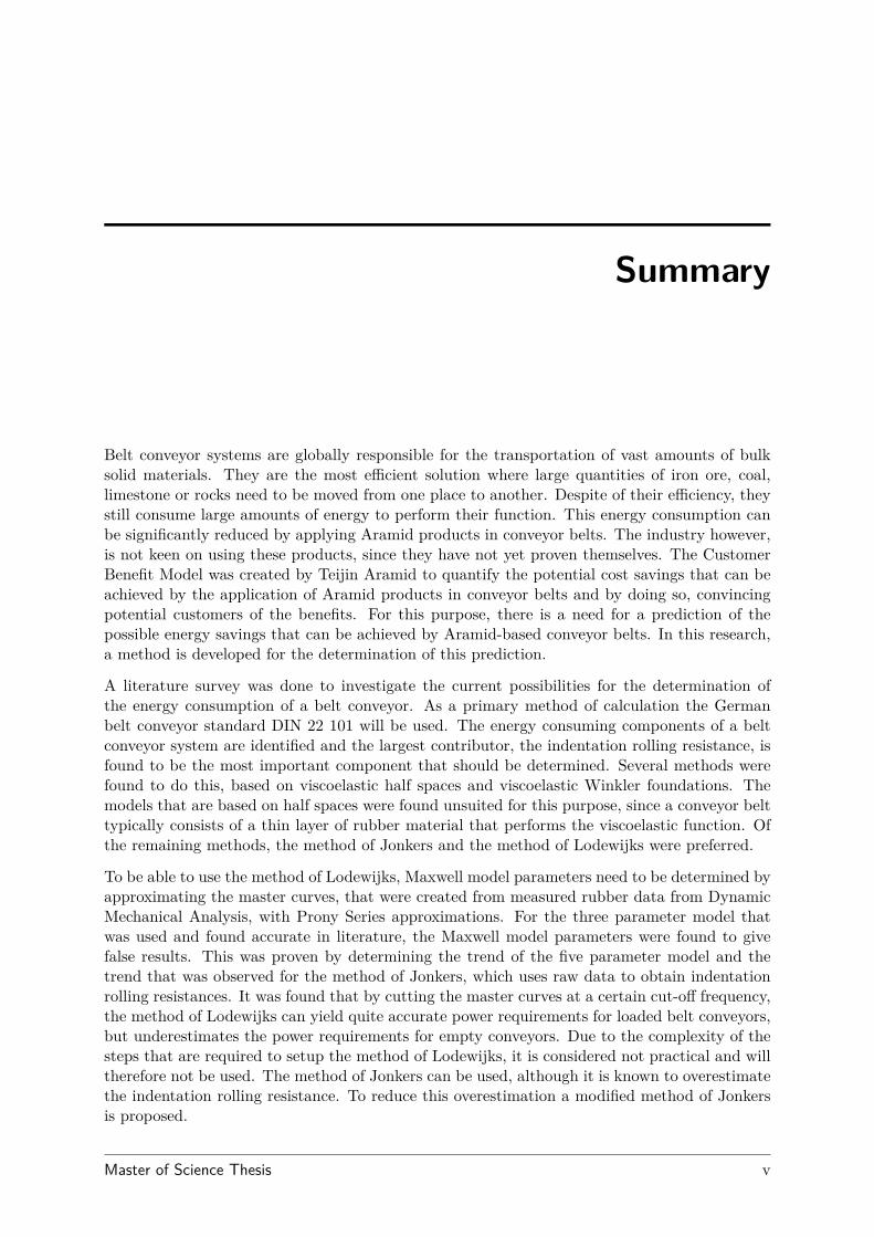
Belt conveyor systems are globally responsible for the transportation of vast amounts of bulksolid materials. They are the most efficient solution where large quantities of iron ore, coal,limestone or rocks need to be moved from one place to another. Despite of their efficiency, theystill consume large amounts of energy to perform their function. This energy consumption canbe significantly reduced by applying Aramid products in conveyor belts. The industry however,is not keen on using these products, since they have not yet proven themselves. The CustomerBenefit Model was created by Teijin Aramid to quantify the potential cost savings that can beachieved by the application of Aramid products in conveyor belts and by doing so, convincingpotential customers of the benefits. For this purpose, there is a need for a prediction of thepossible energy savings that can be achieved by Aramid-based conveyor belts. In this research,a method is developed for the determination of this prediction.
A literature survey was done to investigate the current possibilities for the determination ofthe energy consumption of a belt conveyor. As a primary method of calculation the Germanbelt conveyor standard DIN 22 101 will be used. The energy consuming components of a beltconveyor system are identified and the largest contributor, the indentation rolling resistance, isfound to be the most important component that should be determined. Several methods werefound to do this, based on viscoelastic half spaces and viscoelastic Winkler foundations. Themodels that are based on half spaces were found unsuited for this purpose, since a conveyor belttypically consists of a thin layer of rubber material that performs the viscoelastic function. Ofthe remaining methods, the method of Jonkers and the method of Lodewijks were preferred.
To be able to use the method of Lodewijks, Maxwell model parameters need to be determined byapproximating the master curves, that were created from measured rubber data from DynamicMechanical Analysis, with Prony Series approximations. For the three parameter model thatwas used and found accurate in literature, the Maxwell model parameters were found to givefalse results. This was proven by determining the trend of the five parameter model and thetrend that was observed for the method of Jonkers, which uses raw data to obtain indentationrolling resistances. It was found that by cutting the master curves at a certain cut-off frequency,the method of Lodewijks can yield quite accurate power requirements for loaded belt conveyors,but underestimates the power requirements for empty conveyors. Due to the complexity of thesteps that are required to setup the method of Lodewijks, it is considered not practical and willtherefore not be used. The method of Jonkers can be used, although it is known to overestimatethe indentation rolling resistance. To reduce this overestimation a modified method of Jonkersis proposed.
Master of Science Thesis v

The performance of the proposed method and that of the original Jonkers method were assessedin a case study in which the energy consumptions of four belt conveyor systems were evaluatedand compared against the results from external research. The modified method of Jonkers givesa better approximation of the power requirements for loaded conveyor belts, but underestimatesthe power requirements of empty conveyor belts. It is concluded that the modified method ofJonkers should be used to estimate the power requirements for loaded conveyor belts and theoriginal method of Jonkers for the empty conveyor belts. Since the proposed methods and thegenerated results are all based on theoretical models, it is recommended that a pilot belt isinstalled, on which actual measurements can be done. These measurements can then be used toimprove the proposed modification to Jonkers method.
To make this method usable for employees of Teijin Aramid, a software application has beendeveloped that incorporates both the original and the modified Jonkers method. The softwareapplication was tested and is able to perform the analysis that is shown in this study.
vi Master of Science Thesis
Samenvatting
Transportbanden zijn wereldwijd verantwoordelijk voor het transport van grote hoeveelhedenstortgoederen. Ze zijn de meest efficiÃńnte oplossing op plaatsen waar grote hoeveelheden ijz-ererts, kolen, kalksteen of steen verplaatst moet worden. Ondanks hun efficiÃńntie verbruikendeze installaties toch grote hoeveelheden energie. Deze energieconsumptie kan significant wordenverminderd door het toepassen van Aramide producten in de transportbanden. Deze technolo-gie wordt echter niet met open armen ontvangen door de bestaande industrie, doordat dezenieuwe types transportbanden zichzelf nog niet bewezen hebben. Het Customer Benefit Modelis gemaakt door Teijin Aramid om de potentiÃńle kostenbesparing te kwantificeren die mogelijkzijn door de toepassing van deze transportbanden en hiermee klanten te overtuigen van de vo-ordelen. De input van dit model zijn de energieverbruiken van de verschillende types Aramidetransportbanden. Dit rapport beschrijft de bepaling en de ontwikkeling van een methode omdeze energieverbruiken te berekenen. Deze methode moet precies genoeg zijn om betrouwbareresultaten te leveren die de ordergrootte van de potentiÃńle energiebesparingen tonen die doorhet toepassen van Aramide producten mogelijk zijn.
De huidige bestaande methodes voor het bepalen van de energieconsumptie van transportban-den zijn onderzocht door middel van een literatuuronderzoek. De Duitse norm DIN 22 101 zalworden gebruikt als basis voor de energieberekeningen. De componenten van het totale energie-verbruik van een transportband zijn geÃŕdentificeerd en de indrukrolweerstand, die het grootsteaandeel heeft in het totale energieverbruik, is het belangrijkste component om te berekenen.De literatuur beschrijft verscheidene methoden om de indrukrolweerstand te bepalen, gebaseerdop viscoelastische half-ruimten en viscoelastische Winkler matrasmodellen. De methoden diezijn gebaseerd op een half-ruimtemodel blijken minder bruikbaar, aangezien een transportbandgebruikelijk bestaat uit dunne lagen viscoelastisch materiaal. Van de overgebleven methodenzijn de methode van Lodewijks en de methode van Jonkers geselecteerd voor dit onderzoek.
Om de methode van Lodewijks te kunnen gebruiken moeten eerst de Maxwell model parametersbepaald worden door met Prony series de master curves te benaderen. Deze master curveszijn gebaseerd op gemeten materiaaleigenschappen die zijn bepaald met Dynamic MechanicalAnalysis. Met deze Maxwell model parameters is de methode van Lodewijks doorgerekend en deresultaten bleken het tegenovergestelde te vertonen dan was verwacht, namelijk dat de toevoeg-ing van Sulfron een negatieve invloed zou hebben op de roleigenschappen van het rubber. Dehypothese dat het drie-parameter model onjuiste resultaten geeft is bevestigd door de berekeningvan het vijf-parameter model en de berekening van de methode van Jonkers. Het drie-parametermodel kan wel gebruikt worden door de master curves af te snijden boven een bepaalde frequen-
Master of Science Thesis vii
tie. De op deze manier behaalde resultaten zijn vrij accuraat voor de beladen transportbanden,maar onderschatten het benodigde vermogen voor de lege transportband. Doordat deze meth-ode erg complex is om op te zetten, wat niet gewenst is voor de industriÃńle toepassing waardit rapport op doelt, is besloten om de methode van Jonkers verder te gebruiken. Het is echterbekend dat deze methode de vermogensbehoeftes overschat, dus een aangepaste methode vanJonkers is voorgesteld om dit gedrag tegen te gaan.
De prestaties van de aangepaste methode van Jonkers en die van de originele methode vanJonkers zijn getoetst aan de resultaten die zijn gepresenteerd door Lodewijks voor een casusbetreffende de Optimum Collieries in Zuid-Afrika. Voor beladen transportbanden geldt datde aangepaste methode van Jonkers een betere benadering van de vermogensbehoeften geeftdan de originele methode van Jonkers. Voor lege transportbanden is dit niet het geval enzorgt de aanpassing van de methode voor een onderschatting van de vermogensbehoeften. Deconclusie is dat de vermogensbehoeften voor de beladen transportbanden dus het beste berekendkunnen worden met de aangepaste methode van Jonkers en de vermogensbehoeften van de legetransportbanden met de originele methode van Jonkers.
Gezien de voorgestelde aangepaste methode van Jonkers en de gegenereerde resultaten enkelzijn gebaseerd op theorie, is het van belang dat er metingen worden gedaan aan een echtetransportband, zodat de aangepaste methode van Jonkers indien nodig bijgesteld kan worden.
Een software applicatie is ontwikkeld, tegelijkertijd met dit rapport, zodat de medewerkersvan Teijin Aramid de originele en de aangepaste methode van Jonkers kunnen gebruiken omvermogensbehoeften en dus energieverbruiken van transportbanden te kunnen bepalen. Dezeapplicatie is getest en is in staat om de analyse naar behoren uit te voeren.
viii Master of Science Thesis

List of symbols
Capital lettersA First part contact length of idler and belt mC Secondary resistance factor -C’ Last part contact length of idler and belt mCV Correction factor for the Jonkers method -D Diameter idler roll mE’ Storage modulus PaE” Loss modulus PaE* Complex modulus PaE1 First Maxwell model parameter PaE2 Second Maxwell model parameter PaF Total motional resistance NFAuf Load/belt friction in loading zone NFGr Belt/belt cleaner resistance NFGb Belt bending resistance at pulley NFH Main resistance NFHi Main resistance of section i NFN Secondary resistances NFS Special resistances NFSchb Load/chute resistance in loading zone NFSt Gradient resistance NFTri Pulley bearing resistance NFz Gravitational force of mass NH Conveyor lifting height mL Conveying lenght mLi Conveying length section i mP Required drive power WU’ Idler bearing resistance NU ′′B Belt flexure resistance NU ′′E Indentation rolling resistance NU ′′F Bulk flexure resistance N

Small lettersf Friction factor carry strand and return strand combined -fi Friction factor indentation rolling resistance -fb Friction factor idler bearing resistance -fbe Friction factor belt flexure resistance -fbu Friction factor bulk flexure resistance -fij Friction factor Jonkers method -f ′ij Friction factor modified Jonkers method -fo Friction factor carry strand -fu Friction factor return strand -g Gravitational acceleration m/s2
h Cover layer thickness mm′G Mass belt kg/mm′L Mass load kg/mm′R Mass rotating parts kg/mm′Ro Mass rotating parts (Carry strand) kg/mm′Ru Mass rotating parts (Return strand) kg/mqR Distributed load on an idler roll N/mv Belt speed m/s
Greek lettersα Wrap angle radiansδ Phase loss angle o or radiansε0 Maximum strain -η Damping coefficient Pa sθ Inclination angle (total system) o
θi Inclination angle of section i o
λ Trough angle o
µ Friction factor pulley/belt -σ Applied stress Paσ0 Maximum applied stress Paω Harmonic excitation frequency of indentation Hz
x Master of Science Thesis

List of abbreviations
BEM Boundary Element ModelBR Butadiene RubberCEMA Conveyor Equipment Manufacturers AssociationDIN Deutsche Institut fÃijr NormungFEM Finite Element ModelMRC Maximum Rolling CoefficientMTPH Metric Tonnes Per HourNR Natural Rubberphr Parts per Hundred RubberSBR Styrene-Butadiene RubberSLS Standard Lineair Solid (model)tan-delta Tangent Delta
Master of Science Thesis xi

Contents
List of symbols ix
List of abbreviations xi
1 Introduction 1
1.1 Energy reduction in belt conveyors . . . . . . . . . . . . . . . . . . . . . . . . . . 2
1.2 Research goal and scope . . . . . . . . . . . . . . . . . . . . . . . . . . . . . . . . 3
1.3 Report structure . . . . . . . . . . . . . . . . . . . . . . . . . . . . . . . . . . . . 3
2 Aramid conveyor belts 5
2.1 Twaron . . . . . . . . . . . . . . . . . . . . . . . . . . . . . . . . . . . . . . . . . 5
2.2 Sulfron . . . . . . . . . . . . . . . . . . . . . . . . . . . . . . . . . . . . . . . . . . 8
3 The energy consumption of belt conveyors 9
3.1 Belt conveyor basics . . . . . . . . . . . . . . . . . . . . . . . . . . . . . . . . . . 9
3.1.1 Basic setup of a generic belt conveyor . . . . . . . . . . . . . . . . . . . . 9
3.1.2 Conveyor belt composition . . . . . . . . . . . . . . . . . . . . . . . . . . 10
3.1.3 Other components of a belt conveyor system . . . . . . . . . . . . . . . . 11
3.2 Energy calculations of DIN 22 101 . . . . . . . . . . . . . . . . . . . . . . . . . . 13
3.2.1 Total motional resistance . . . . . . . . . . . . . . . . . . . . . . . . . . . 13
3.2.2 Resulting power consumption . . . . . . . . . . . . . . . . . . . . . . . . . 16
3.3 Energy consumption distribution . . . . . . . . . . . . . . . . . . . . . . . . . . . 16
4 Indentation rolling resistance 21
Master of Science Thesis xiii
4.1 General theory . . . . . . . . . . . . . . . . . . . . . . . . . . . . . . . . . . . . . 21
4.1.1 Viscoelasticity . . . . . . . . . . . . . . . . . . . . . . . . . . . . . . . . . 21
4.1.2 Dynamic Mechanical Analysis . . . . . . . . . . . . . . . . . . . . . . . . . 22
4.1.3 Material models . . . . . . . . . . . . . . . . . . . . . . . . . . . . . . . . 23
4.1.4 Modelling the belt backing layer . . . . . . . . . . . . . . . . . . . . . . . 24
4.2 Theoretical methods . . . . . . . . . . . . . . . . . . . . . . . . . . . . . . . . . . 26
4.2.1 May et al. . . . . . . . . . . . . . . . . . . . . . . . . . . . . . . . . . . . . 26
4.2.2 Hunter . . . . . . . . . . . . . . . . . . . . . . . . . . . . . . . . . . . . . . 27
4.2.3 Jonkers . . . . . . . . . . . . . . . . . . . . . . . . . . . . . . . . . . . . . 28
4.2.4 Spaans . . . . . . . . . . . . . . . . . . . . . . . . . . . . . . . . . . . . . . 28
4.2.5 Lodewijks . . . . . . . . . . . . . . . . . . . . . . . . . . . . . . . . . . . . 29
4.3 Numerical methods . . . . . . . . . . . . . . . . . . . . . . . . . . . . . . . . . . . 32
4.3.1 Wheeler . . . . . . . . . . . . . . . . . . . . . . . . . . . . . . . . . . . . . 32
4.3.2 Qui . . . . . . . . . . . . . . . . . . . . . . . . . . . . . . . . . . . . . . . 32
4.4 Selected method . . . . . . . . . . . . . . . . . . . . . . . . . . . . . . . . . . . . 33
5 Rubber rheology 35
5.1 Experimental setup . . . . . . . . . . . . . . . . . . . . . . . . . . . . . . . . . . . 35
5.2 Creating master curves . . . . . . . . . . . . . . . . . . . . . . . . . . . . . . . . . 36
5.3 Maxwell model parameters . . . . . . . . . . . . . . . . . . . . . . . . . . . . . . 38
5.4 Cutting the master curves . . . . . . . . . . . . . . . . . . . . . . . . . . . . . . . 44
5.5 Jonkers method . . . . . . . . . . . . . . . . . . . . . . . . . . . . . . . . . . . . . 47
5.5.1 Jonkers method with master curve data . . . . . . . . . . . . . . . . . . . 47
5.5.2 Jonkers method without master curve data . . . . . . . . . . . . . . . . . 48
6 Proposed method 49
6.1 Analysis . . . . . . . . . . . . . . . . . . . . . . . . . . . . . . . . . . . . . . . . . 49
6.2 Set-up . . . . . . . . . . . . . . . . . . . . . . . . . . . . . . . . . . . . . . . . . . 51
7 Verification 57
7.1 Optimum Collieries . . . . . . . . . . . . . . . . . . . . . . . . . . . . . . . . . . . 57
7.2 Results . . . . . . . . . . . . . . . . . . . . . . . . . . . . . . . . . . . . . . . . . . 59
7.2.1 Verification power requirements for loaded conveyors . . . . . . . . . . . . 59
7.2.2 Verification power requirements for empty conveyors . . . . . . . . . . . . 62
xiv Master of Science Thesis
7.2.3 Discussion results Optimum Collieries verification . . . . . . . . . . . . . 65
8 Case study 67
8.1 Case study: stockpile conveyor . . . . . . . . . . . . . . . . . . . . . . . . . . . . 67
8.2 Calculation of the energy consumptions with master curve data . . . . . . . . . . 69
8.3 Calculation of the energy consumptions without master curve data . . . . . . . . 74
9 Software application 77
9.1 System of requirements . . . . . . . . . . . . . . . . . . . . . . . . . . . . . . . . 77
9.2 System architecture . . . . . . . . . . . . . . . . . . . . . . . . . . . . . . . . . . 78
9.2.1 Calculation . . . . . . . . . . . . . . . . . . . . . . . . . . . . . . . . . . . 78
9.2.2 Calculation of a conveyor belt . . . . . . . . . . . . . . . . . . . . . . . . . 79
9.3 Recalculation of the case study . . . . . . . . . . . . . . . . . . . . . . . . . . . . 81
9.4 Extra options . . . . . . . . . . . . . . . . . . . . . . . . . . . . . . . . . . . . . . 85
10 Conclusions 87
11 Recommendations 89
Appendix A: research paper 91
Appendix B: draft of research paper for BeltCon 2015 97
Appendix C: results DMA tests 107
11.1 Control sample, 3Hz . . . . . . . . . . . . . . . . . . . . . . . . . . . . . . . . . . 107
11.2 Sulfron sample, 3Hz . . . . . . . . . . . . . . . . . . . . . . . . . . . . . . . . . . 109
11.3 Control sample, 6Hz . . . . . . . . . . . . . . . . . . . . . . . . . . . . . . . . . . 111
11.4 Sulfron sample, 6Hz . . . . . . . . . . . . . . . . . . . . . . . . . . . . . . . . . . 114
11.5 Control sample, 10Hz . . . . . . . . . . . . . . . . . . . . . . . . . . . . . . . . . 116
11.6 Sulfron sample, 10Hz . . . . . . . . . . . . . . . . . . . . . . . . . . . . . . . . . . 119
11.7 Control sample, 20Hz . . . . . . . . . . . . . . . . . . . . . . . . . . . . . . . . . 122
11.8 Sulfron sample, 20Hz . . . . . . . . . . . . . . . . . . . . . . . . . . . . . . . . . . 125
Bibliography 129
Master of Science Thesis xv

xvi Master of Science Thesis
Chapter 1
Introduction
Since the industrial revolution, mankind has had an ever-growing need for raw materials, suchas iron ore and coal. To fulfil this need, large logistical networks have grown all over the worldto move these materials from one place to another. One of the backbones of these networks isthe belt conveyor, which can move large quantities of bulk solid material, often with a greaterefficiency than for instance trucks or trains. Despite of this great efficiency, they still consumevast amounts of energy. Due to the rapid depletion of fossil fuels around the world and theimplied impact on the environment, the urge to reduce this energy consumption keeps increasing.
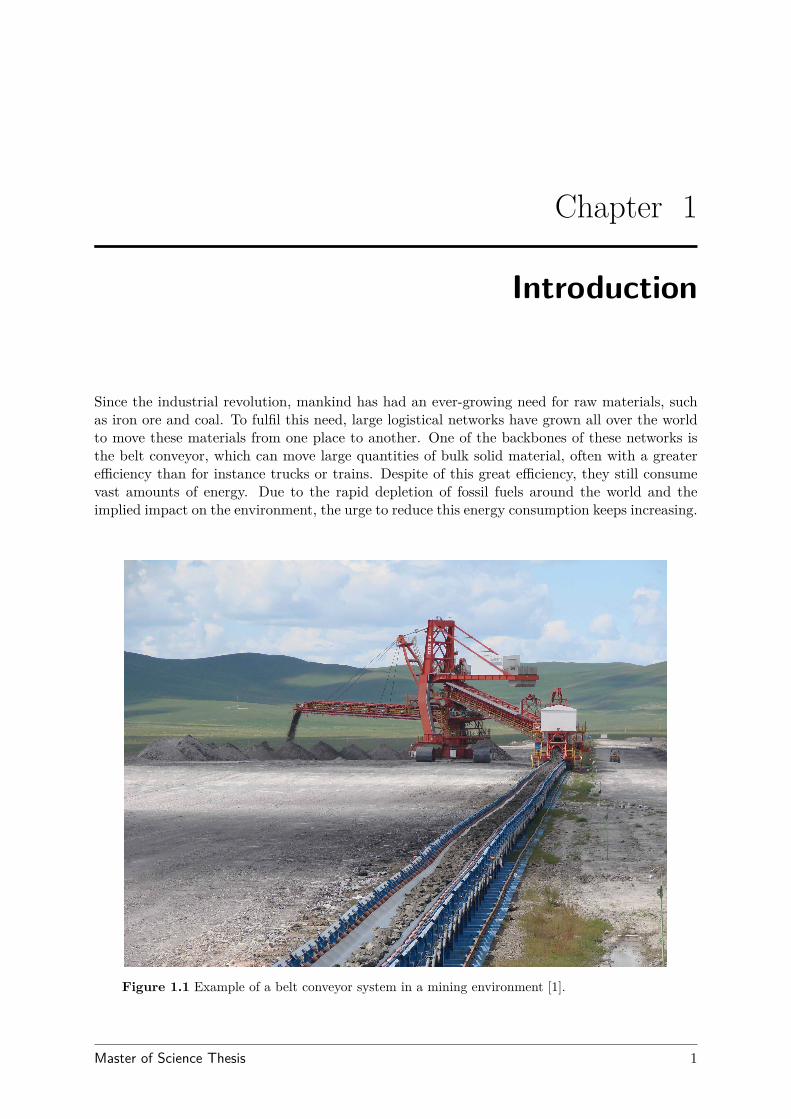
Figure 1.1 Example of a belt conveyor system in a mining environment [1].
Master of Science Thesis 1
1.1 Energy reduction in belt conveyors
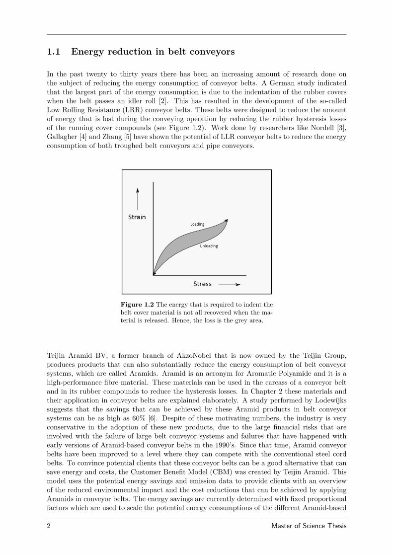
In the past twenty to thirty years there has been an increasing amount of research done onthe subject of reducing the energy consumption of conveyor belts. A German study indicatedthat the largest part of the energy consumption is due to the indentation of the rubber coverswhen the belt passes an idler roll [2]. This has resulted in the development of the so-calledLow Rolling Resistance (LRR) conveyor belts. These belts were designed to reduce the amountof energy that is lost during the conveying operation by reducing the rubber hysteresis lossesof the running cover compounds (see Figure 1.2). Work done by researchers like Nordell [3],Gallagher [4] and Zhang [5] have shown the potential of LLR conveyor belts to reduce the energyconsumption of both troughed belt conveyors and pipe conveyors.
Figure 1.2 The energy that is required to indent thebelt cover material is not all recovered when the ma-terial is released. Hence, the loss is the grey area.
Teijin Aramid BV, a former branch of AkzoNobel that is now owned by the Teijin Group,produces products that can also substantially reduce the energy consumption of belt conveyorsystems, which are called Aramids. Aramid is an acronym for Aromatic Polyamide and it is ahigh-performance fibre material. These materials can be used in the carcass of a conveyor beltand in its rubber compounds to reduce the hysteresis losses. In Chapter 2 these materials andtheir application in conveyor belts are explained elaborately. A study performed by Lodewijkssuggests that the savings that can be achieved by these Aramid products in belt conveyorsystems can be as high as 60% [6]. Despite of these motivating numbers, the industry is veryconservative in the adoption of these new products, due to the large financial risks that areinvolved with the failure of large belt conveyor systems and failures that have happened withearly versions of Aramid-based conveyor belts in the 1990’s. Since that time, Aramid conveyorbelts have been improved to a level where they can compete with the conventional steel cordbelts. To convince potential clients that these conveyor belts can be a good alternative that cansave energy and costs, the Customer Benefit Model (CBM) was created by Teijin Aramid. Thismodel uses the potential energy savings and emission data to provide clients with an overviewof the reduced environmental impact and the cost reductions that can be achieved by applyingAramids in conveyor belts. The energy savings are currently determined with fixed proportionalfactors which are used to scale the potential energy consumptions of the different Aramid-based
2 Master of Science Thesis
conveyor belt types in comparison with a conventional steel cord conveyor belt.
1.2 Research goal and scope
The scaling factors for the energy consumption that are used in the CBM are based on a singlecase study, which can result in varying results when applied to generic belt conveyor systems.In this research, a method is developed to estimate the energy consumption of a generic beltconveyor system under steady state operating conditions that is more accurate than the currentsolution and therefore yields a more realistic result. With the focus on its usability in a non-technical environment, this study is about finding the balance between the ease-of-use and thetechnical accuracy. To reach this goal, the following research questions will be answered:
- Which factors are responsible for the energy consumption of a conveyor belt and to whatextent?
- What methods to determine the energy consumption of belt conveyors are available inliterature and how are they applicable for this topic?
- What is the desired accuracy of this estimation?
- What should be used as comparison to quantify these energy savings?
To make this method usable with the CBM, a user-friendly software application will be developedalongside of this method, that will allow Teijin employees to calculate the first approximationof the energy consumption of a generic belt conveyor system, in order to use it in the CustomerBenefit Model to determine the potential cost savings and reductions in emissions. By compar-ison with field test results and calculations by consultancy firms, the results of this method canbe verified.
This study is done as a graduation project at the Delft University of Technology for the facultyof Mechanical, Maritime and Materials Engineering (3me) and Teijin Aramid BV. As stated bythe assignment (as showed at the start of this report) this research will be based on the Germanstandard DIN 22 101, in which a methodology is stated for the calculation and design of beltconveyor systems.
1.3 Report structure
In Chapter 2 the Aramid products are explained that are used by Teijin to reduce the energyconsumption of conveyor belts. Chapter 3 will show how belt conveyors in general consumeenergy and how this energy consumption is distributed. In Chapter 4 the details of the inden-tation rolling resistance are explained, along with the methods that were found in literature todetermine this resistance. The limitations of the rubber data that is used in this report is shownin Chapter 5, after which a proposal is done to modify the only remaining method in Chapter6.
Chapter 7 shows the verification of this modified method by comparing it with a case study frompublic literature. Chapter 8 shows a case study of a fictive belt conveyor system that illustratesthe function of this method and the performance of the Aramid-based conveyor belts.
Master of Science Thesis 3

In Chapter 9 the software application that has been developed alongside of this method is shown,which will be able to estimate the energy consumption of a generic belt conveyor system. Finally,conclusions and recommendations are stated in Chapters 10 and 11.
4 Master of Science Thesis
Chapter 2
Aramid conveyor belts
Teijin Aramid produces two types of aramid that can reduce the energy consumption of beltconveyors: Twaron and Sulfron. They are engineered to focus on two different aspects of energylosses in belt conveyors, respectively the reduction of belt weight and the reduction of the runningresistance.
2.1 Twaron
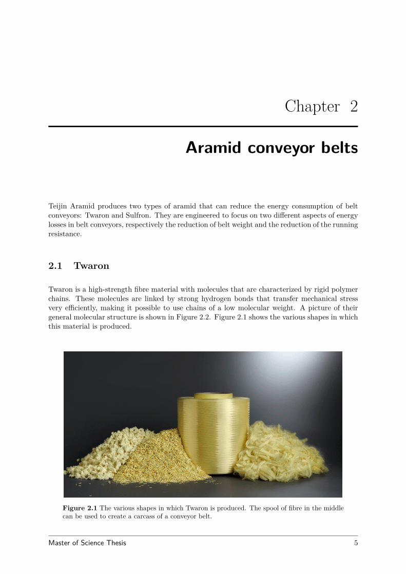
Twaron is a high-strength fibre material with molecules that are characterized by rigid polymerchains. These molecules are linked by strong hydrogen bonds that transfer mechanical stressvery efficiently, making it possible to use chains of a low molecular weight. A picture of theirgeneral molecular structure is shown in Figure 2.2. Figure 2.1 shows the various shapes in whichthis material is produced.
Figure 2.1 The various shapes in which Twaron is produced. The spool of fibre in the middlecan be used to create a carcass of a conveyor belt.
Master of Science Thesis 5
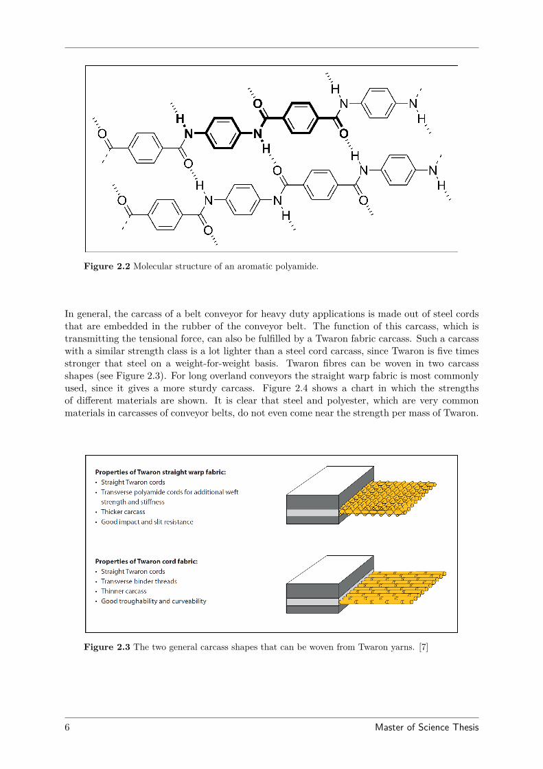
Figure 2.2 Molecular structure of an aromatic polyamide.
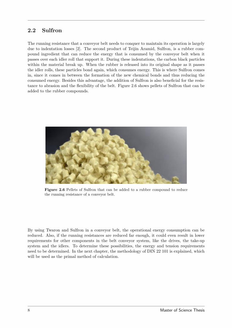
In general, the carcass of a belt conveyor for heavy duty applications is made out of steel cordsthat are embedded in the rubber of the conveyor belt. The function of this carcass, which istransmitting the tensional force, can also be fulfilled by a Twaron fabric carcass. Such a carcasswith a similar strength class is a lot lighter than a steel cord carcass, since Twaron is five timesstronger that steel on a weight-for-weight basis. Twaron fibres can be woven in two carcassshapes (see Figure 2.3). For long overland conveyors the straight warp fabric is most commonlyused, since it gives a more sturdy carcass. Figure 2.4 shows a chart in which the strengthsof different materials are shown. It is clear that steel and polyester, which are very commonmaterials in carcasses of conveyor belts, do not even come near the strength per mass of Twaron.
Figure 2.3 The two general carcass shapes that can be woven from Twaron yarns. [7]
6 Master of Science Thesis
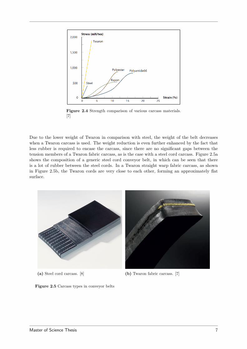
Figure 2.4 Strength comparison of various carcass materials.[7]
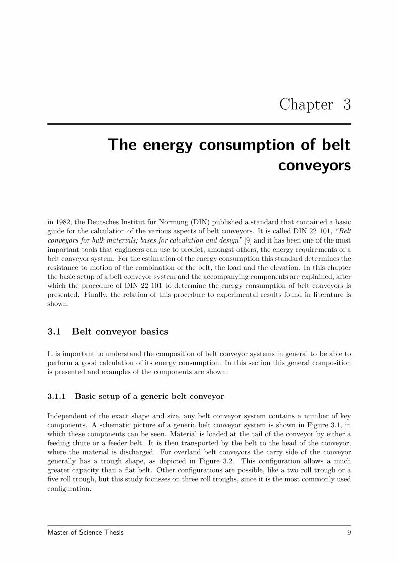
Due to the lower weight of Twaron in comparison with steel, the weight of the belt decreaseswhen a Twaron carcass is used. The weight reduction is even further enhanced by the fact thatless rubber is required to encase the carcass, since there are no significant gaps between thetension members of a Twaron fabric carcass, as is the case with a steel cord carcass. Figure 2.5ashows the composition of a generic steel cord conveyor belt, in which can be seen that thereis a lot of rubber between the steel cords. In a Twaron straight warp fabric carcass, as shownin Figure 2.5b, the Twaron cords are very close to each other, forming an approximately flatsurface.
(a) Steel cord carcass. [8] (b) Twaron fabric carcass. [7]
Figure 2.5 Carcass types in conveyor belts
Master of Science Thesis 7
2.2 Sulfron
The running resistance that a conveyor belt needs to conquer to maintain its operation is largelydue to indentation losses [2]. The second product of Teijin Aramid, Sulfron, is a rubber com-pound ingredient that can reduce the energy that is consumed by the conveyor belt when itpasses over each idler roll that support it. During these indentations, the carbon black particleswithin the material break up. When the rubber is released into its original shape as it passesthe idler rolls, these particles bond again, which consumes energy. This is where Sulfron comesin, since it comes in between the formation of the new chemical bonds and thus reducing theconsumed energy. Besides this advantage, the addition of Sulfron is also beneficial for the resis-tance to abrasion and the flexibility of the belt. Figure 2.6 shows pellets of Sulfron that can beadded to the rubber compounds.
Figure 2.6 Pellets of Sulfron that can be added to a rubber compound to reducethe running resistance of a conveyor belt.
By using Twaron and Sulfron in a conveyor belt, the operational energy consumption can bereduced. Also, if the running resistances are reduced far enough, it could even result in lowerrequirements for other components in the belt conveyor system, like the drives, the take-upsystem and the idlers. To determine these possibilities, the energy and tension requirementsneed to be determined. In the next chapter, the methodology of DIN 22 101 is explained, whichwill be used as the primal method of calculation.
8 Master of Science Thesis
Chapter 3
The energy consumption of beltconveyors
in 1982, the Deutsches Institut für Normung (DIN) published a standard that contained a basicguide for the calculation of the various aspects of belt conveyors. It is called DIN 22 101, “Beltconveyors for bulk materials; bases for calculation and design” [9] and it has been one of the mostimportant tools that engineers can use to predict, amongst others, the energy requirements of abelt conveyor system. For the estimation of the energy consumption this standard determines theresistance to motion of the combination of the belt, the load and the elevation. In this chapterthe basic setup of a belt conveyor system and the accompanying components are explained, afterwhich the procedure of DIN 22 101 to determine the energy consumption of belt conveyors ispresented. Finally, the relation of this procedure to experimental results found in literature isshown.
3.1 Belt conveyor basics
It is important to understand the composition of belt conveyor systems in general to be able toperform a good calculation of its energy consumption. In this section this general compositionis presented and examples of the components are shown.
3.1.1 Basic setup of a generic belt conveyor
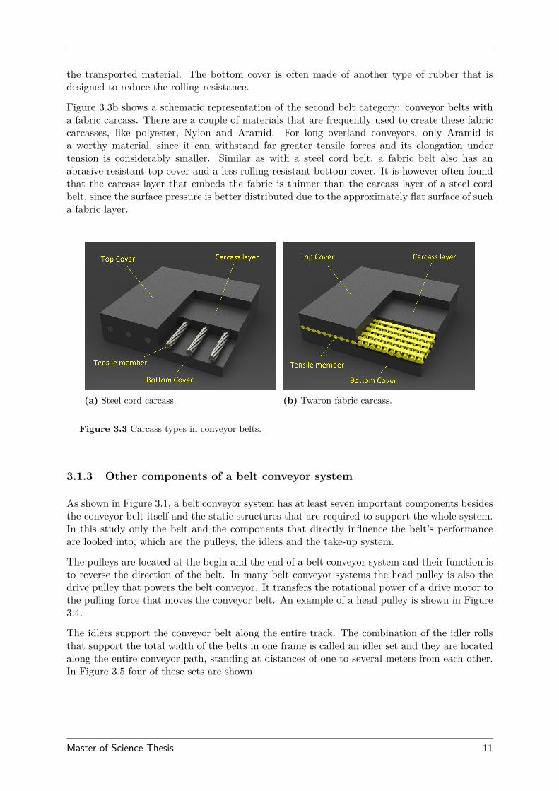
Independent of the exact shape and size, any belt conveyor system contains a number of keycomponents. A schematic picture of a generic belt conveyor system is shown in Figure 3.1, inwhich these components can be seen. Material is loaded at the tail of the conveyor by either afeeding chute or a feeder belt. It is then transported by the belt to the head of the conveyor,where the material is discharged. For overland belt conveyors the carry side of the conveyorgenerally has a trough shape, as depicted in Figure 3.2. This configuration allows a muchgreater capacity than a flat belt. Other configurations are possible, like a two roll trough or afive roll trough, but this study focusses on three roll troughs, since it is the most commonly usedconfiguration.
Master of Science Thesis 9
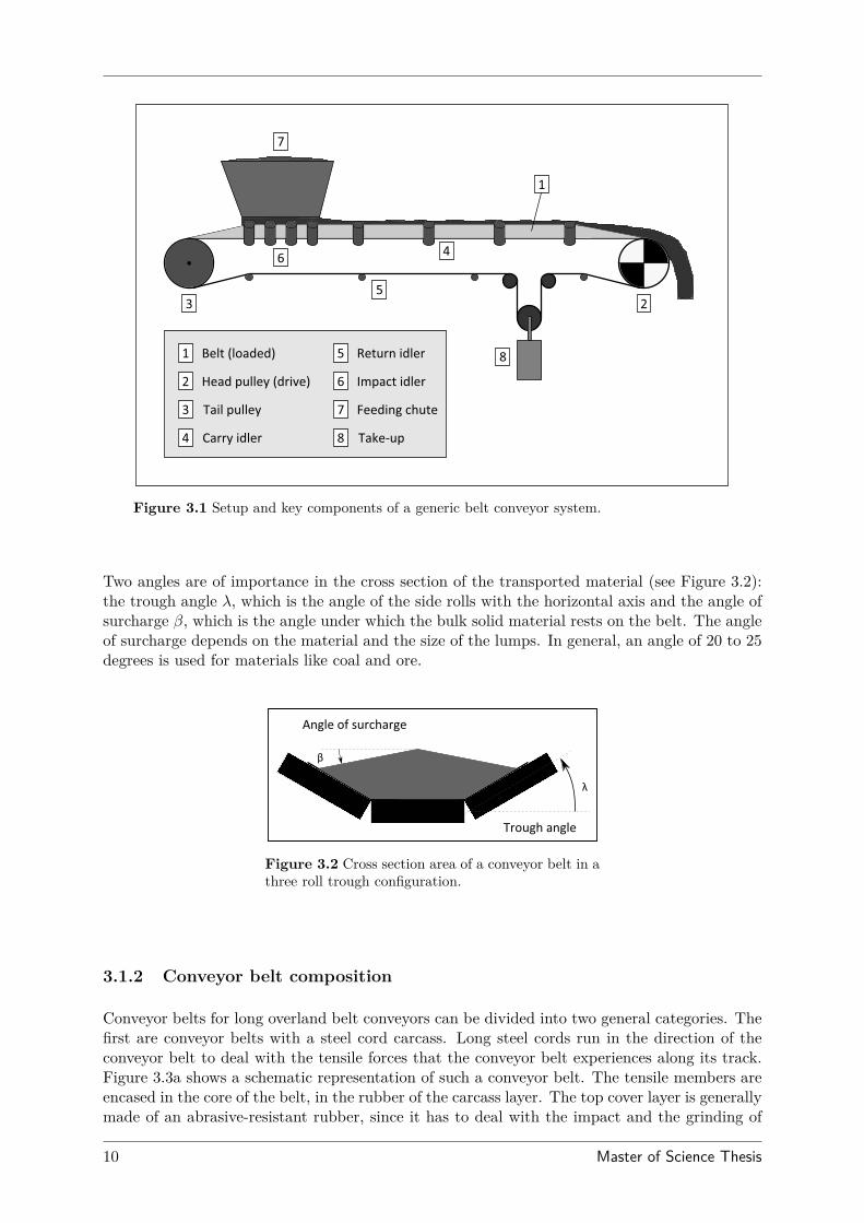
Figure 3.1 Setup and key components of a generic belt conveyor system.
Two angles are of importance in the cross section of the transported material (see Figure 3.2):the trough angle λ, which is the angle of the side rolls with the horizontal axis and the angle ofsurcharge β, which is the angle under which the bulk solid material rests on the belt. The angleof surcharge depends on the material and the size of the lumps. In general, an angle of 20 to 25degrees is used for materials like coal and ore.
Figure 3.2 Cross section area of a conveyor belt in athree roll trough configuration.
3.1.2 Conveyor belt composition
Conveyor belts for long overland belt conveyors can be divided into two general categories. Thefirst are conveyor belts with a steel cord carcass. Long steel cords run in the direction of theconveyor belt to deal with the tensile forces that the conveyor belt experiences along its track.Figure 3.3a shows a schematic representation of such a conveyor belt. The tensile members areencased in the core of the belt, in the rubber of the carcass layer. The top cover layer is generallymade of an abrasive-resistant rubber, since it has to deal with the impact and the grinding of
10 Master of Science Thesis
the transported material. The bottom cover is often made of another type of rubber that isdesigned to reduce the rolling resistance.
Figure 3.3b shows a schematic representation of the second belt category: conveyor belts witha fabric carcass. There are a couple of materials that are frequently used to create these fabriccarcasses, like polyester, Nylon and Aramid. For long overland conveyors, only Aramid isa worthy material, since it can withstand far greater tensile forces and its elongation undertension is considerably smaller. Similar as with a steel cord belt, a fabric belt also has anabrasive-resistant top cover and a less-rolling resistant bottom cover. It is however often foundthat the carcass layer that embeds the fabric is thinner than the carcass layer of a steel cordbelt, since the surface pressure is better distributed due to the approximately flat surface of sucha fabric layer.
(a) Steel cord carcass. (b) Twaron fabric carcass.
Figure 3.3 Carcass types in conveyor belts.
3.1.3 Other components of a belt conveyor system
As shown in Figure 3.1, a belt conveyor system has at least seven important components besidesthe conveyor belt itself and the static structures that are required to support the whole system.In this study only the belt and the components that directly influence the belt’s performanceare looked into, which are the pulleys, the idlers and the take-up system.
The pulleys are located at the begin and the end of a belt conveyor system and their function isto reverse the direction of the belt. In many belt conveyor systems the head pulley is also thedrive pulley that powers the belt conveyor. It transfers the rotational power of a drive motor tothe pulling force that moves the conveyor belt. An example of a head pulley is shown in Figure3.4.
The idlers support the conveyor belt along the entire track. The combination of the idler rollsthat support the total width of the belts in one frame is called an idler set and they are locatedalong the entire conveyor path, standing at distances of one to several meters from each other.In Figure 3.5 four of these sets are shown.
Master of Science Thesis 11
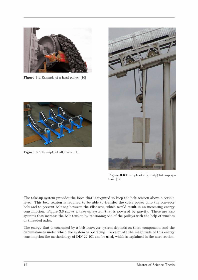
Figure 3.4 Example of a head pulley. [10]
Figure 3.5 Example of idler sets. [11]
Figure 3.6 Example of a (gravity) take-up sys-tem. [12]
The take-up system provides the force that is required to keep the belt tension above a certainlevel. This belt tension is required to be able to transfer the drive power onto the conveyorbelt and to prevent belt sag between the idler sets, which would result in an increasing energyconsumption. Figure 3.6 shows a take-up system that is powered by gravity. There are alsosystems that increase the belt tension by tensioning one of the pulleys with the help of winchesor threaded axles.
The energy that is consumed by a belt conveyor system depends on these components and thecircumstances under which the system is operating. To calculate the magnitude of this energyconsumption the methodology of DIN 22 101 can be used, which is explained in the next section.
12 Master of Science Thesis
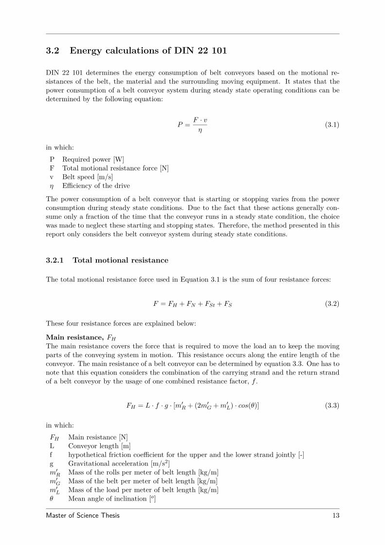
3.2 Energy calculations of DIN 22 101
DIN 22 101 determines the energy consumption of belt conveyors based on the motional re-sistances of the belt, the material and the surrounding moving equipment. It states that thepower consumption of a belt conveyor system during steady state operating conditions can bedetermined by the following equation:
P = F · vη
(3.1)
in which:P Required power [W]F Total motional resistance force [N]v Belt speed [m/s]η Efficiency of the drive
The power consumption of a belt conveyor that is starting or stopping varies from the powerconsumption during steady state conditions. Due to the fact that these actions generally con-sume only a fraction of the time that the conveyor runs in a steady state condition, the choicewas made to neglect these starting and stopping states. Therefore, the method presented in thisreport only considers the belt conveyor system during steady state conditions.
3.2.1 Total motional resistance
The total motional resistance force used in Equation 3.1 is the sum of four resistance forces:
F = FH + FN + FSt + FS (3.2)
These four resistance forces are explained below:
Main resistance, FHThe main resistance covers the force that is required to move the load an to keep the movingparts of the conveying system in motion. This resistance occurs along the entire length of theconveyor. The main resistance of a belt conveyor can be determined by equation 3.3. One has tonote that this equation considers the combination of the carrying strand and the return strandof a belt conveyor by the usage of one combined resistance factor, f .
FH = L · f · g · [m′R + (2m′G +m′L) · cos(θ)] (3.3)
in which:FH Main resistance [N]L Conveyor length [m]f hypothetical friction coefficient for the upper and the lower strand jointly [-]g Gravitational acceleration [m/s2]m′R Mass of the rolls per meter of belt length [kg/m]m′G Mass of the belt per meter of belt length [kg/m]m′L Mass of the load per meter of belt length [kg/m]θ Mean angle of inclination [o]
Master of Science Thesis 13
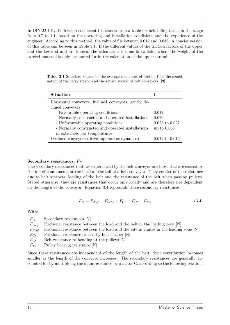
In DIN 22 101, the friction coefficient f is chosen from a table for belt filling ratios in the rangefrom 0.7 to 1.1, based on the operating and installation conditions and the experience of theengineer. According to this method, the value of f is between 0.012 and 0.035. A concise versionof this table can be seen in Table 3.1. If the different values of the friction factors of the upperand the lower strand are known, the calculation is done in twofold, where the weight of thecarried material is only accounted for in the calculation of the upper strand.
Table 3.1 Standard values for the average coefficient of friction f for the combi-nation of the carry strand and the return strand of belt conveyors. [9]
Situation f
Horizontal conveyors, inclined conveyors, gently de-clined conveyors
- Favourable operating conditions 0.017- Normally constructed and operated installations 0.020- Unfavourable operating conditions 0.023 to 0.027- Normally constructed and operated installations up to 0.035in extremely low temperatures
Declined conveyors (drives operate as dynamos) 0.012 to 0.016
Secondary resistances, FNThe secondary resistances that are experienced by the belt conveyor are those that are caused byfriction of components at the head an the tail of a belt conveyor. They consist of the resistancedue to belt scrapers, loading of the belt and the resistance of the belt when passing pulleys.Stated otherwise, they are resistances that occur only locally and are therefore not dependenton the length of the conveyor. Equation 3.4 represents these secondary resistances.
FN = FAuf + FSchb + FGr + FGb + FTri (3.4)
With:FN Secondary resistances [N]FAuf Frictional resistance between the load and the belt in the loading zone [N]FSchb Frictional resistance between the load and the lateral chutes in the loading zone [N]FGr Frictional resistance caused by belt cleaner [N]FGb Belt resistance to bending at the pulleys [N]FTri Pulley bearing resistance [N]
Since these resistances are independent of the length of the belt, their contribution becomessmaller as the length of the conveyor increases. The secondary resistances are generally ac-counted for by multiplying the main resistance by a factor C, according to the following relation:
14 Master of Science Thesis
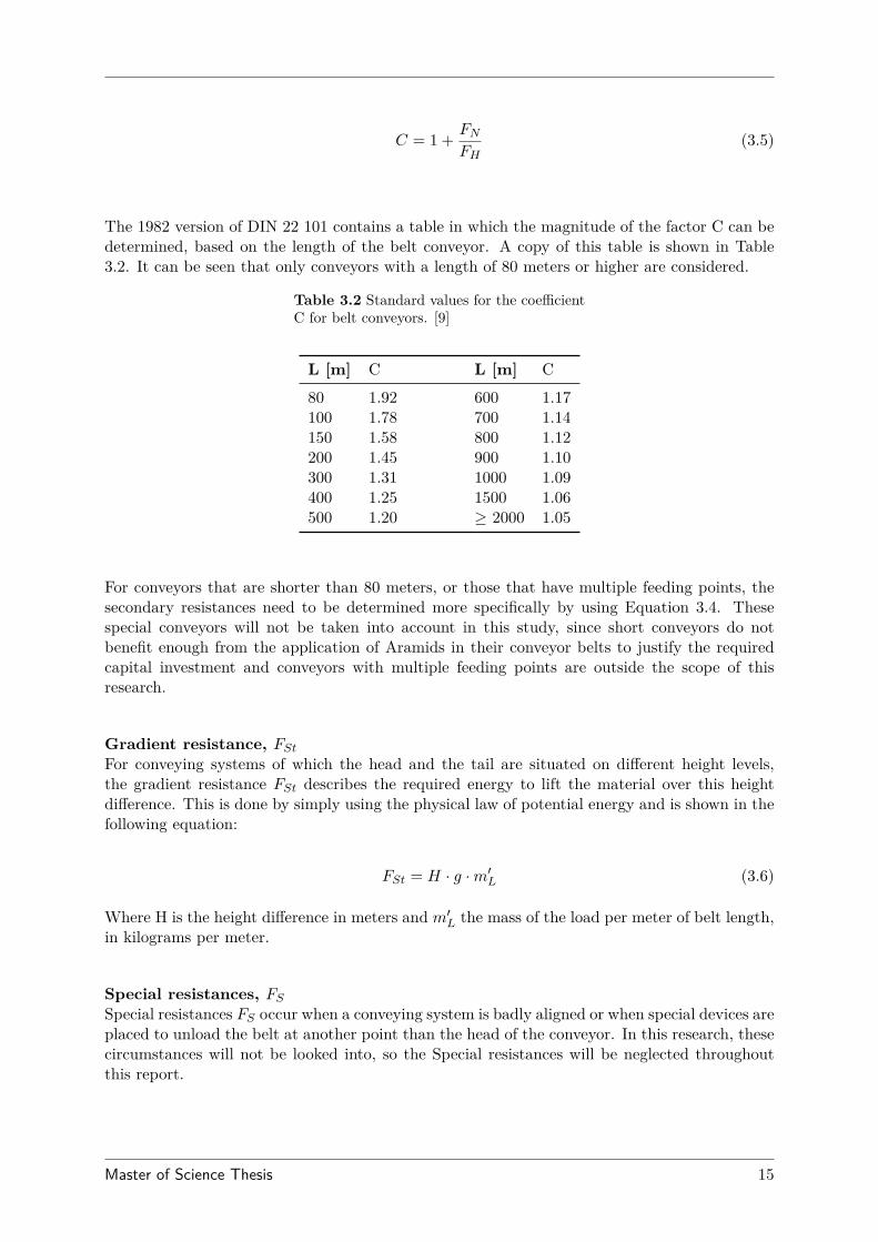
C = 1 + FNFH
(3.5)
The 1982 version of DIN 22 101 contains a table in which the magnitude of the factor C can bedetermined, based on the length of the belt conveyor. A copy of this table is shown in Table3.2. It can be seen that only conveyors with a length of 80 meters or higher are considered.
Table 3.2 Standard values for the coefficientC for belt conveyors. [9]
L [m] C L [m] C
80 1.92 600 1.17100 1.78 700 1.14150 1.58 800 1.12200 1.45 900 1.10300 1.31 1000 1.09400 1.25 1500 1.06500 1.20 ≥ 2000 1.05
For conveyors that are shorter than 80 meters, or those that have multiple feeding points, thesecondary resistances need to be determined more specifically by using Equation 3.4. Thesespecial conveyors will not be taken into account in this study, since short conveyors do notbenefit enough from the application of Aramids in their conveyor belts to justify the requiredcapital investment and conveyors with multiple feeding points are outside the scope of thisresearch.
Gradient resistance, FStFor conveying systems of which the head and the tail are situated on different height levels,the gradient resistance FSt describes the required energy to lift the material over this heightdifference. This is done by simply using the physical law of potential energy and is shown in thefollowing equation:
FSt = H · g ·m′L (3.6)
Where H is the height difference in meters and m′L the mass of the load per meter of belt length,in kilograms per meter.
Special resistances, FSSpecial resistances FS occur when a conveying system is badly aligned or when special devices areplaced to unload the belt at another point than the head of the conveyor. In this research, thesecircumstances will not be looked into, so the Special resistances will be neglected throughoutthis report.
Master of Science Thesis 15
3.2.2 Resulting power consumption
The sum of the four resistances can be reduced to a more tidy formula (Equation 3.7), in whichthe secondary resistances are taken into account by the earlier mentioned factor C and thespecial resistances are neglected. This formula can then be inserted into Equation 3.1, whichyields the equation of the power consumption of a belt conveyor during steady state operatingconditions (Equation 3.8).
F = C · L · f · g · [m′R + (2m′G +m′L)cos(θ)] +H · g ·m′L (3.7)
P = v · (C · L · f · g · [m′R + (2m′G +m′L)cos(θ)] +H · g ·m′L)η
(3.8)
It is clear that DIN 22 101 does not contain explicit information about the belt’s materialproperties. These properties can be accounted for by the friction factor f, which is also known asthe rolling resistance factor. As stated earlier, this rolling resistance factor is a fictional factorof the upper and the lower strand of the belt conveyor combined and is derived from empiricallyfilled tables. In the next section, the most important components of this rolling resistance factorare identified, which give insight in the possibilities reducing the energy consumption of conveyorbelt systems.
3.3 Energy consumption distribution
In 1993 two German researchers, Hager and Hintz, did an extensive study to determine theenergy consumption of belt conveyors and the distribution of its components. They identifiedseven components that together form the total motional resistance of belt conveyor systems [2]:
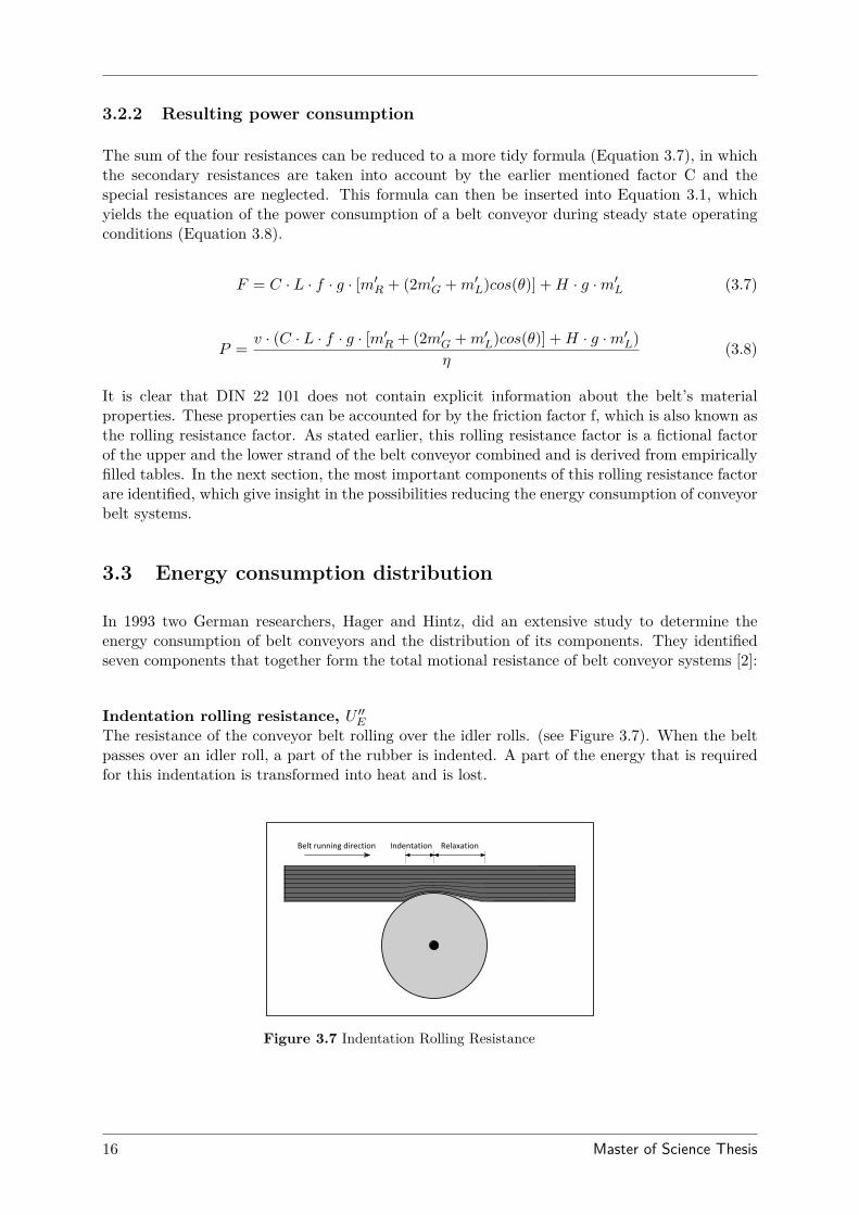
Indentation rolling resistance, U ′′EThe resistance of the conveyor belt rolling over the idler rolls. (see Figure 3.7). When the beltpasses over an idler roll, a part of the rubber is indented. A part of the energy that is requiredfor this indentation is transformed into heat and is lost.
Figure 3.7 Indentation Rolling Resistance
16 Master of Science Thesis
Belt flexure resistance, U ′′BThe internal friction in the conveyor belt due to the deformation of the belt in between idlersets, which is shown in Figure 3.8. Energy is required to reform the belt into its original shapewhen it approaches the next idler set.
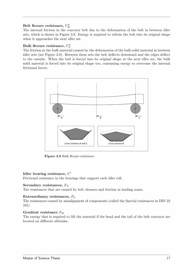
Bulk flexure resistance, U ′′FThe friction in the bulk material caused by the deformation of the bulk solid material in betweenidler sets (see Figure 3.8). Between these sets the belt deflects downward and the edges deflectto the outside. When the belt is forced into its original shape at the next idler set, the bulksolid material is forced into its original shape too, consuming energy to overcome the internalfrictional forces.
Figure 3.8 Bulk flexure resistance
Idler bearing resistance, U ′Frictional resistance in the bearings that support each idler roll.
Secondary resistances, FNThe resistances that are caused by belt cleaners and friction in loading zones.
Extraordinary resistances, FSThe resistances caused by misalignment of components (called the Special resistances in DIN 22101)
Gradient resistance FStThe energy that is required to lift the material if the head and the tail of the belt conveyor arelocated on different altitudes.
Master of Science Thesis 17
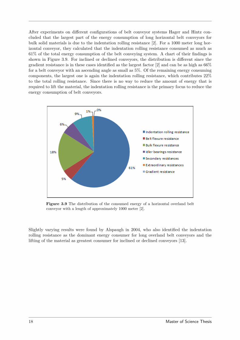
After experiments on different configurations of belt conveyor systems Hager and Hintz con-cluded that the largest part of the energy consumption of long horizontal belt conveyors forbulk solid materials is due to the indentation rolling resistance [2]. For a 1000 meter long hor-izontal conveyor, they calculated that the indentation rolling resistance consumed as much as61% of the total energy consumption of the belt conveying system. A chart of their findings isshown in Figure 3.9. For inclined or declined conveyors, the distribution is different since thegradient resistance is in these cases identified as the largest factor [2] and can be as high as 66%for a belt conveyor with an ascending angle as small as 5%. Of the remaining energy consumingcomponents, the largest one is again the indentation rolling resistance, which contributes 22%to the total rolling resistance. Since there is no way to reduce the amount of energy that isrequired to lift the material, the indentation rolling resistance is the primary focus to reduce theenergy consumption of belt conveyors.
Figure 3.9 The distribution of the consumed energy of a horizontal overland beltconveyor with a length of approximately 1000 meter [2].
Slightly varying results were found by Alspaugh in 2004, who also identified the indentationrolling resistance as the dominant energy consumer for long overland belt conveyors and thelifting of the material as greatest consumer for inclined or declined conveyors [13].
18 Master of Science Thesis
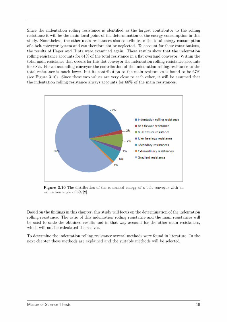
Since the indentation rolling resistance is identified as the largest contributor to the rollingresistance it will be the main focal point of the determination of the energy consumption in thisstudy. Nonetheless, the other main resistances also contribute to the total energy consumptionof a belt conveyor system and can therefore not be neglected. To account for these contributions,the results of Hager and Hintz were examined again. These results show that the indentationrolling resistance accounts for 61% of the total resistance in a flat overland conveyor. Within thetotal main resistance that occurs for this flat conveyor the indentation rolling resistance accountsfor 68%. For an ascending conveyor the contribution of the indentation rolling resistance to thetotal resistance is much lower, but its contribution to the main resistances is found to be 67%(see Figure 3.10). Since these two values are very close to each other, it will be assumed thatthe indentation rolling resistance always accounts for 68% of the main resistances.
Figure 3.10 The distribution of the consumed energy of a belt conveyor with aninclination angle of 5% [2].
Based on the findings in this chapter, this study will focus on the determination of the indentationrolling resistance. The ratio of this indentation rolling resistance and the main resistances willbe used to scale the obtained results and in that way account for the other main resistances,which will not be calculated themselves.
To determine the indentation rolling resistance several methods were found in literature. In thenext chapter these methods are explained and the suitable methods will be selected.
Master of Science Thesis 19

20 Master of Science Thesis
Chapter 4
Indentation rolling resistance
Chapter 3 concluded that the largest part of the energy consumption of a belt conveyor systemis consumed by the indentation rolling resistance. To be able to make a decent prediction ofthe energy consumption of a conveyor belt, the indentation rolling resistance factor needs to bedetermined. In literature, several methods were found that determine the indentation rollingresistance. In this chapter the most influencing methods are explained. The first section of thischapter provides general theory that is required to use the theoretical models that are shown inSection 2. In Section 3 the numerical methods to determine the indentation rolling resistanceare explained, after which the methods are selected that will be used in this study.
4.1 General theory
In this section the general theory is presented that will be the basis for the determination of theindentation rolling resistance. It will show the fundamental basis of the material and a numberof material models that will be used to describe the material and its behaviour.
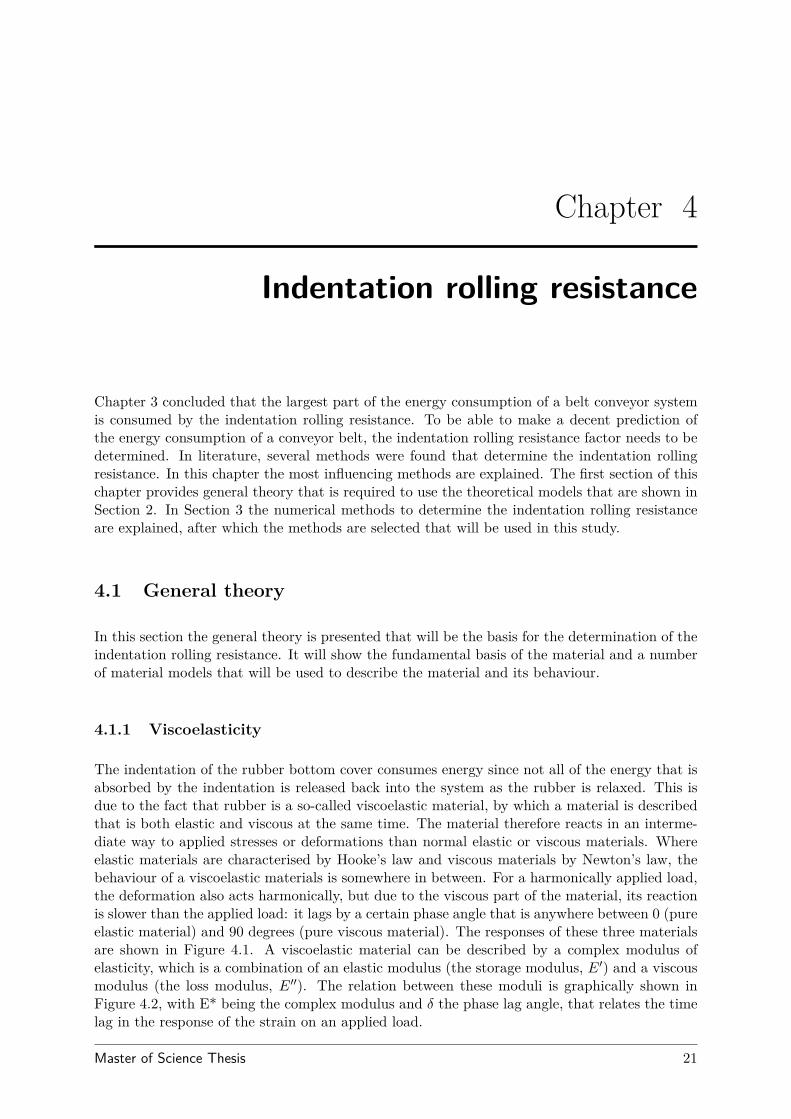
4.1.1 Viscoelasticity
The indentation of the rubber bottom cover consumes energy since not all of the energy that isabsorbed by the indentation is released back into the system as the rubber is relaxed. This isdue to the fact that rubber is a so-called viscoelastic material, by which a material is describedthat is both elastic and viscous at the same time. The material therefore reacts in an interme-diate way to applied stresses or deformations than normal elastic or viscous materials. Whereelastic materials are characterised by Hooke’s law and viscous materials by Newton’s law, thebehaviour of a viscoelastic materials is somewhere in between. For a harmonically applied load,the deformation also acts harmonically, but due to the viscous part of the material, its reactionis slower than the applied load: it lags by a certain phase angle that is anywhere between 0 (pureelastic material) and 90 degrees (pure viscous material). The responses of these three materialsare shown in Figure 4.1. A viscoelastic material can be described by a complex modulus ofelasticity, which is a combination of an elastic modulus (the storage modulus, E′) and a viscousmodulus (the loss modulus, E′′). The relation between these moduli is graphically shown inFigure 4.2, with E* being the complex modulus and δ the phase lag angle, that relates the timelag in the response of the strain on an applied load.
Master of Science Thesis 21
Figure 4.1 Response to strain of an elastic material, a viscous material and a vis-coelastic material.
From Figure 4.2 it can be seen that the storage modulus and the loss modulus are related bythe following equation:
E′′
E′= tan(δ) (4.1)
The tangent of the phase loss angle δ (tan-delta) is a frequently used parameter to describe theperformance of a viscoelastic material, since it relates the stored energy to the lost energy in aload cycle. In general: a lower tan-delta represents a material with lower energy losses.
4.1.2 Dynamic Mechanical Analysis
The exact properties of a viscoelastic material are dependent on its composition and the cir-cumstances in which it operates. To determine these properties a technique called DynamicMechanical Analysis (DMA) is used. In this technique, a sample of the material is exposed to a
22 Master of Science Thesis
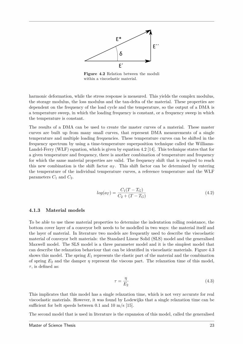
Figure 4.2 Relation between the moduliwithin a viscoelastic material.
harmonic deformation, while the stress response is measured. This yields the complex modulus,the storage modulus, the loss modulus and the tan-delta of the material. These properties aredependent on the frequency of the load cycle and the temperature, so the output of a DMA isa temperature sweep, in which the loading frequency is constant, or a frequency sweep in whichthe temperature is constant.
The results of a DMA can be used to create the master curves of a material. These mastercurves are built up from many small curves, that represent DMA measurements of a singletemperature and multiple loading frequencies. These temperature curves can be shifted in thefrequency spectrum by using a time-temperature superposition technique called the Williams-Landel-Ferry (WLF) equation, which is given by equation 4.2 [14]. This technique states that fora given temperature and frequency, there is another combination of temperature and frequencyfor which the same material properties are valid. The frequency shift that is required to reachthis new combination is the shift factor aT . This shift factor can be determined by enteringthe temperature of the individual temperature curves, a reference temperature and the WLFparameters C1 and C2.
log(aT ) = C1(T − TG)C2 + (T − TG) (4.2)
4.1.3 Material models
To be able to use these material properties to determine the indentation rolling resistance, thebottom cover layer of a conveyor belt needs to be modelled in two ways: the material itself andthe layer of material. In literature two models are frequently used to describe the viscoelasticmaterial of conveyor belt materials: the Standard Linear Solid (SLS) model and the generalisedMaxwell model. The SLS model is a three parameter model and it is the simplest model thatcan describe the relaxation behaviour that can be identified in viscoelastic materials. Figure 4.3shows this model. The spring E1 represents the elastic part of the material and the combinationof spring E2 and the damper η represent the viscous part. The relaxation time of this model,τ , is defined as:
τ = η
E2(4.3)
This implicates that this model has a single relaxation time, which is not very accurate for realviscoelastic materials. However, it was found by Lodewijks that a single relaxation time can besufficient for belt speeds between 0.1 and 10 m/s [15].
The second model that is used in literature is the expansion of this model, called the generalised
Master of Science Thesis 23
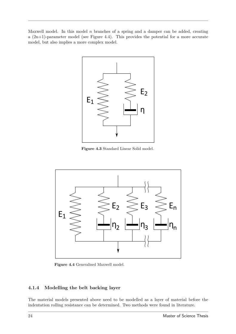
Maxwell model. In this model n branches of a spring and a damper can be added, creatinga (2n+1)-parameter model (see Figure 4.4). This provides the potential for a more accuratemodel, but also implies a more complex model.
Figure 4.3 Standard Linear Solid model.
Figure 4.4 Generalised Maxwell model.
4.1.4 Modelling the belt backing layer
The material models presented above need to be modelled as a layer of material before theindentation rolling resistance can be determined. Two methods were found in literature.
24 Master of Science Thesis
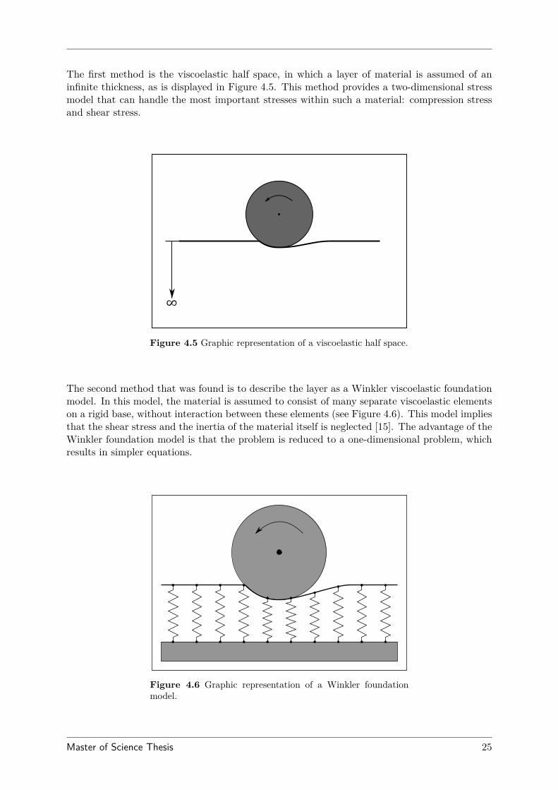
The first method is the viscoelastic half space, in which a layer of material is assumed of aninfinite thickness, as is displayed in Figure 4.5. This method provides a two-dimensional stressmodel that can handle the most important stresses within such a material: compression stressand shear stress.
Figure 4.5 Graphic representation of a viscoelastic half space.
The second method that was found is to describe the layer as a Winkler viscoelastic foundationmodel. In this model, the material is assumed to consist of many separate viscoelastic elementson a rigid base, without interaction between these elements (see Figure 4.6). This model impliesthat the shear stress and the inertia of the material itself is neglected [15]. The advantage of theWinkler foundation model is that the problem is reduced to a one-dimensional problem, whichresults in simpler equations.
Figure 4.6 Graphic representation of a Winkler foundationmodel.
Master of Science Thesis 25
4.2 Theoretical methods
The following researchers have made use of the above material models to derive the indentationrolling resistance forces.
4.2.1 May et al.
In 1959, May et al. laid out the first brick in this field of research with a paper called “Rollingfriction of a hard cylinder over a visco-elastic material" [16]. They defined the viscoelastic layeras a two-dimensional viscoelastic half space. To describe the behaviour of the material, theSLS model was chosen. The rolling resistance force was determined through the asymmetricalstress pattern that is caused by the stress relaxation within the viscoelastic material. This stresspattern causes a moment around the cylinder’s axis. The rolling resistance force that counteractsthis moment was found to be dependent on the belt speed and has a maximum for a certainbelt speed. This specific speed corresponded to a peak in the relaxation time distribution,which is material-dependent. The analysis was performed by keeping the indentation depth ata constant level by increasing the load. They concluded that the load to maintain this depthwas also dependent on the belt speed, where the load was required to increase for an increasingvelocity.
In 1995 Lodewijks rearranged this method so that the vertical load was pre-described, insteadof the indentation depth, which is more convenient for evaluating belt conveyor systems. Hearrived at the following indentation rolling resistance factor [15]:
f∗im = F ∗iF ∗z
(4.4)
In which F ∗z is the pre-described vertical load and F ∗i the resulting rolling resistance force, whichare defined by:
F ∗z = E1a30
6Rh
[2 −
(b
a0
)3+ 3
(b
a0
)]+ 2E2ka
30
Rh
[1 −
(b
a0
)2](4.5)
F ∗i = E1a40
8R2h
[1 − 2
(b
a0
)2+(b
a0
)4]
+ E2a40k
R2h
k3 − k
2
(1 +
(b
a0
)2)+ 1
3
(1 +
(b
a0
)3)− k(1 + k)
(k + b
a0
)e
−1k
(a0 + ba0
) (4.6)
E1, E2 are the Maxwell model parameters that follow from the SLS model. R is the radius ofthe roll in meters, h is the thickness of the belt’s bottom cover layer and b is the length of thesecond part of the contact zone between the belt and the roll. k is the Deborah number, whichis defined by:
k = V τ
a0(4.7)
a0 is the first part of the contact length between the belt and the roll and is given by:
26 Master of Science Thesis
a30 = 3FzDh
4E1(4.8)
Where D is equal to 2R. Due to the pre-description of the indentation depth, which is generallynot the case in the situation of a belt conveyor, this method is not directly applicable in thisstudy.
4.2.2 Hunter
Hunter followed in 1961 with “The rolling contact of a rigid cylinder with a viscoelastic halfspace" [17]. Like May et al, he models the belt backing material as a viscoelastic half space andthe material itself conform the SLS model. He uses a more analytical approach than May et al byusing integral equations that allow shear stresses. Hunter also relates the rolling resistance forceto the asymmetrical stress distribution within the rolling contact. He approaches the problemfrom another angle: the retardation instead of the relaxation. For the three parameter Maxwellmodel the following equations can be stated [15]:
f = E2E1
(4.9)
µD = E1 + E2 (4.10)
Which represent the retardation coefficient and the dynamic shear modulus. The semi-contactlength of the indentation at zero velocity, a0, is defined by Hunter as:
a20 = 2(1 − ν)(1 + f)RFz
πµD(4.11)
The ratio between a and a0, the contact length when the belt has a non-zero speed, can bedetermined by:
(a0a
)2= 1 +
2f∗h∗
K0(k)K1(k) + I0(h)
I1(h)
(4.12)
With k = a/V τ and h = (1 + f)k. K0, K1, I0 and I1 are modified Bessel functions of the zerothand first order. Through the entering pressure distribution function Hunter finally reaches theindentation rolling resistance factor:
Γ1 = a
(− 1h
− 12
[(a0a
)2− 1
]I0(h)I1(h)
)(4.13)
b = V τ − Γ1 (4.14)
f∗ih = 1R
(b− V τ
1 + f− Γ1
(a
a0
)2)
(4.15)
Master of Science Thesis 27
Like May et al, Hunter too reaches the conclusion that the rolling friction coefficient is de-pendent on the belt speed and that it reaches a certain maximum value for a belt speed thatcorresponds with the relaxation time of the belt material. The usability of the method of Hunteris questionable, since he assumes that the indentation depth is independent of the belt speed[15].
4.2.3 Jonkers
In 1980, Jonkers used a different approach to model the indentation rolling resistance [18].Instead of using the asymmetrical stress distribution, he uses the rubber hysteresis losses thatare caused by the indentation of the viscoelastic material. Jonkers also models the belt’s backingmaterial with the SLS model, but he uses a Winkler model to describe the material layer witha finite thickness [15]. It is assumed that the indentation can be described as half a sinusoidalcurve and that the pressure distribution also follows this geometry, with the maximum pressureat the centreline of the roll. Although not correct for typical belt conveying speeds [19], thischoice of geometry allowed Jonkers to express the indentation rolling resistance force as a conciseequation that is quick and easy in use. The implication is that it overestimates the indentationrolling resistance, which has been shown by, among others, Wheeler [19]. Also, the method ofJonkers does not take the influence of the belt speed on the contact length into account [15].Despite these downsides, the Jonkers method is still widely used to make a quick comparison oftwo different belt materials, since it requires very little parameters.
Jonkers defines the indentation rolling resistance force of a single roll as:
Fij = f(δ)[
h
E′D2
] 13F
43Z (4.16)
In which h and D are respectively the thickness of the bottom cover layer and the diameter ofthe idler roll and f(δ) is:
fδ = 12πtan(δ)
[(π + 2δ)cos(δ)4√
1 + sin(δ)
] 43
(4.17)
If the friction factor is defined as in DIN 22 101 - like a Coulomb friction, the method of Jonkersyields the following equation:
f ′ij = FWFZ
= 12πtan(δ)
[(π + 2δ)cos(δ)4√
1 + sin(δ)
] 43 [ FZhE′D2
] 13
(4.18)
An adaptation of the method of Jonkers was used by Lodewijks to be able to compare it withother methods. This adaptation uses the contact length as determined by Lodewijks’ adaptationof the method of May (which will be shown in Section 4.2.5). In this adaptation, the influenceof the belt speed on the contact length is taken into account.
4.2.4 Spaans
Spaans also used the Winkler foundation model for the belt’s backing layer and the SLS modelfor the material itself. He therefore also neglects the shear forces within the material. Similar
28 Master of Science Thesis
to the approach of Jonkers, he established the indentation rolling resistance by determining thehysteresis losses for the belt travelling over a roll and assumes the maximum pressure at thecentre line of the roll. The indentation friction factor was determined by Spaans to be [15]:
fis = 0.5ηiF
1/3z
(2/3)4/3E∗1/3D2/30 (1 + (1 − ηi)3/4)4/3
(4.19)
The indentation damping factor ηi and the lateral stiffness E∗ need to be determined from aharmonic deformation test that is performed on a sample of the total belt [15]. D0 is a diameterin which both the diameter of the roll and the curvature of the belt at the roll are accountedfor.
The method of Spaans is less useful than methods presented earlier, since he uses the lateralstiffness and the indentation damping coefficient of the total belt, which cannot be determinedproperly without fabricating a piece of the total belt. More drawbacks to use this model arethat it neglects the belt speed dependence of the contact length and that the hysteresis lossfactor δ is assumed to be a material constant, which is generally not a valid assumption [15].To still be able to compare this method with those of Hunter, May and Jonkers, an adaptationwas provided by Lodewijks through which only the belt’s backing layer is modelled [15].
By using the three parameter Maxwell model, the damping factor ηi of the damping layer isgiven as a function of the loss factor tan-delta by [15]:
ηi(δ) = 2πtan(δ)2 + (π + 2δ)tan(δ) (4.20)
In which the loss factor tan-delta is given by [15]:
tan(δ) = ωηE22
E1E22 + ω2η2(E1 + E2) (4.21)
If the assumption is made that the lateral stiffness is only caused by the belt’s backing layer,the Winkler model provides the following expression for this stiffness [15]:
E∗ = E1h
(4.22)
The adapted indentation rolling resistance factor of Spaans’ methods can now be expressed:
f∗is = 0.5ηi(δ)F
1/3z h1/3
(2/3)4/3E1/31 D
2/30 (1 + (1 − ηi(δ))3/4)4/3
(4.23)
A final assumption needs to be made in order to compare this method with those of Hunter,May and Jonkers, which is that under normal circumstances, D0 will practically be the same asthe idler roll diameter D.
4.2.5 Lodewijks
In 1995 Lodewijks created a method for the calculation of the indentation rolling resistance inwhich he partly follows the method of May et al [19]. The material is modelled by using the
Master of Science Thesis 29
SLS model, but different from May et al., the Winkler foundation model is used to describethe backing layer. An iterative process was established to determine the contact length and theSLS model parameters, by beginning with a simple predictor for the contact length that followsfrom the Winkler foundation model [15] and is given by equation 4.8. With these SLS modelparameters the indentation resistance force is determined and with that, the indentation rollingresistance factor.
The stress distribution for the SLS model can be written as:
σ(x) = a2[E1
2Rh
(a− x
a
)(a+ x
a
)+ E2k
Rh
[(1 + k)
(1 − e( −1(a−x)
ka))
−(a− x
a
)]](4.24)
In which k is defined as in equation 4.7.
a = F1/3z[
E16Rh
(2 −
(ba
)3+ 3
(ba
))+ 2E2k
Rh
(1 −
(ba
)2)](1/3) (4.25)
The formula for the rolling resistance force Fi is almost equal to that of May et al., but thecontact length is different.
Fi = E1a4
8R2h
[1 − 2
(b
a
)2+(b
a
)4]
+ E2a4k
R2h
[k3 − k
2
(1 +
(b
a
)2)+ 1
3
(1 +
(b
a
)3)− k(1 + k)
(k + b
a
)e
−1k ( a+b
a )]
(4.26)
For the use in the procedure of DIN 22 101, the following relation can be used:
fim = FiFz
(4.27)
To compensate for the neglecting of the shear forces by the Winkler foundation, Lodewijksdetermined a correction factor fs, based on the method of Hunter, which does incorporate theshear forces, and the method of May, which also neglects them.
fs = f∗ihf∗im
(4.28)
Which allows the calculation of the corrected indentation rolling resistance:
fi = fsfim (4.29)
The graphical relation between the method of May et al., Hunter and the modified method ofMay et al. can be seen in Figure 4.7, which were generated for the parameters from Table 4.1.As can be seen, the modified method of May et al. proposed by Lodewijks yields a lower valuefor the indentation rolling resistance than its original method and the method of Hunter. Thecorrection factor fs shifts the results in the direction of those of May et al.
30 Master of Science Thesis
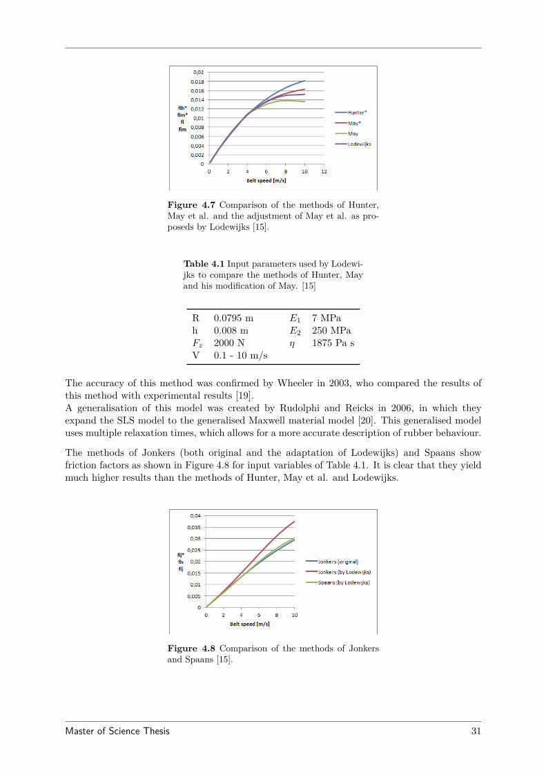
Figure 4.7 Comparison of the methods of Hunter,May et al. and the adjustment of May et al. as pro-poseds by Lodewijks [15].
Table 4.1 Input parameters used by Lodewi-jks to compare the methods of Hunter, Mayand his modification of May. [15]
R 0.0795 m E1 7 MPah 0.008 m E2 250 MPaFz 2000 N η 1875 Pa sV 0.1 - 10 m/s
The accuracy of this method was confirmed by Wheeler in 2003, who compared the results ofthis method with experimental results [19].A generalisation of this model was created by Rudolphi and Reicks in 2006, in which theyexpand the SLS model to the generalised Maxwell material model [20]. This generalised modeluses multiple relaxation times, which allows for a more accurate description of rubber behaviour.
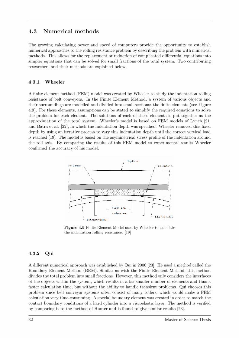
The methods of Jonkers (both original and the adaptation of Lodewijks) and Spaans showfriction factors as shown in Figure 4.8 for input variables of Table 4.1. It is clear that they yieldmuch higher results than the methods of Hunter, May et al. and Lodewijks.
Figure 4.8 Comparison of the methods of Jonkersand Spaans [15].
Master of Science Thesis 31
4.3 Numerical methods
The growing calculating power and speed of computers provide the opportunity to establishnumerical approaches to the rolling resistance problem by describing the problem with numericalmethods. This allows for the replacement or reduction of complicated differential equations intosimpler equations that can be solved for small fractions of the total system. Two contributingresearchers and their methods are explained below.
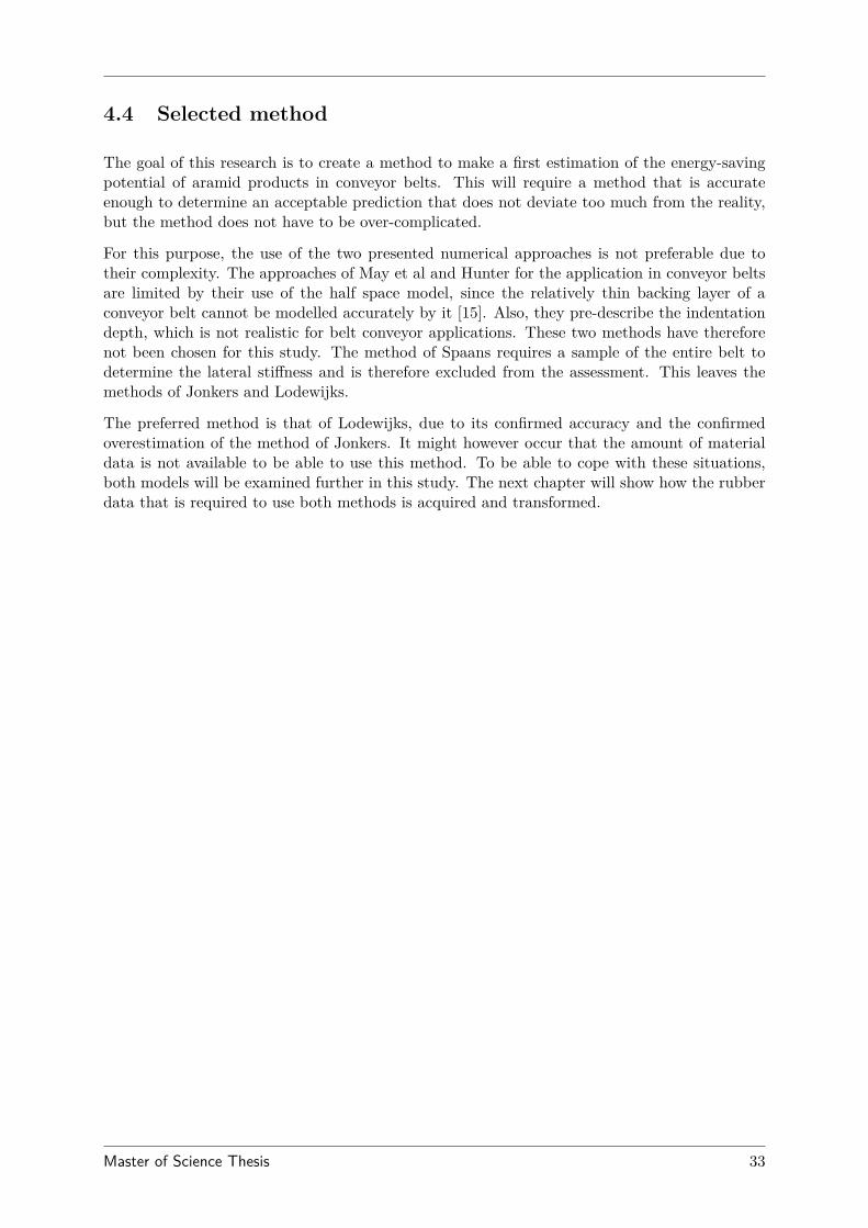
4.3.1 Wheeler
A finite element method (FEM) model was created by Wheeler to study the indentation rollingresistance of belt conveyors. In the Finite Element Method, a system of various objects andtheir surroundings are modelled and divided into small sections: the finite elements (see Figure4.9). For these elements, assumptions can be stated to simplify the required equations to solvethe problem for each element. The solutions of each of these elements is put together as theapproximation of the total system. Wheeler’s model is based on FEM models of Lynch [21]and Batra et al. [22], in which the indentation depth was specified. Wheeler removed this fixeddepth by using an iterative process to vary this indentation depth until the correct vertical loadis reached [19]. The model is based on the asymmetrical stress profile of the indentation aroundthe roll axis. By comparing the results of this FEM model to experimental results Wheelerconfirmed the accuracy of his model.
Figure 4.9 Finite Element Model used by Wheeler to calculatethe indentation rolling resistance. [19]
4.3.2 Qui
A different numerical approach was established by Qui in 2006 [23]. He used a method called theBoundary Element Method (BEM). Similar as with the Finite Element Method, this methoddivides the total problem into small fractions. However, this method only considers the interfacesof the objects within the system, which results in a far smaller number of elements and thus afaster calculation time, but without the ability to handle transient problems. Qui chooses thisproblem since belt conveyor systems often consist of many rollers, which would make a FEMcalculation very time-consuming. A special boundary element was created in order to match thecontact boundary conditions of a hard cylinder into a viscoelastic layer. The method is verifiedby comparing it to the method of Hunter and is found to give similar results [23].
32 Master of Science Thesis
4.4 Selected method
The goal of this research is to create a method to make a first estimation of the energy-savingpotential of aramid products in conveyor belts. This will require a method that is accurateenough to determine an acceptable prediction that does not deviate too much from the reality,but the method does not have to be over-complicated.
For this purpose, the use of the two presented numerical approaches is not preferable due totheir complexity. The approaches of May et al and Hunter for the application in conveyor beltsare limited by their use of the half space model, since the relatively thin backing layer of aconveyor belt cannot be modelled accurately by it [15]. Also, they pre-describe the indentationdepth, which is not realistic for belt conveyor applications. These two methods have thereforenot been chosen for this study. The method of Spaans requires a sample of the entire belt todetermine the lateral stiffness and is therefore excluded from the assessment. This leaves themethods of Jonkers and Lodewijks.
The preferred method is that of Lodewijks, due to its confirmed accuracy and the confirmedoverestimation of the method of Jonkers. It might however occur that the amount of materialdata is not available to be able to use this method. To be able to cope with these situations,both models will be examined further in this study. The next chapter will show how the rubberdata that is required to use both methods is acquired and transformed.
Master of Science Thesis 33

34 Master of Science Thesis
Chapter 5
Rubber rheology
Before the selected methods can be used to evaluate the performance of the aramid-based con-veyor belts, the properties of the belt cover materials need to be examined. In the first sectionof this chapter the experiments that were performed to measure these properties are described.In Section 5.2 the procedure to transform these measurements into the so-called master curves isexplained, after which the model parameters are determined from these master curves in Section5.3. Finally, an alternative way to use the master curves for the method of Jonkers is presentedin Section 5.5
5.1 Experimental setup
For this study two rubber compound types were prepared at the Teijin Aramid rubber labora-tory: a control sample of NR/BR rubber and a sample of the same rubber but with the additionof 2 phr Sulfron D3515. Phr stands for parts per hundred rubber and this is evaluated on aweight-base, D3515 is the Sulfron type that was used. The rubber compound formulations ofboth rubbers is shown in Table 5.1.
Table 5.1 Rubber compound formulations for both rubber samples pro-duced by the Teijin Aramid rubber laboratory. All values in Parts perHundred Rubber (phr).
Control sample Sulfron sample
Natural rubber (NR) 86 86Polybutadiene rubber (BR) 14 14Carbon black 49 49Sulfron D3515 0 2
Cylindrical samples were taken from both rubber compounds with a height of 18 mm and adiameter of 12 mm. A GABO Eplexor 500N machine was used to perform compression DMAon all samples, which is shown in Figure 5.1.
Master of Science Thesis 35
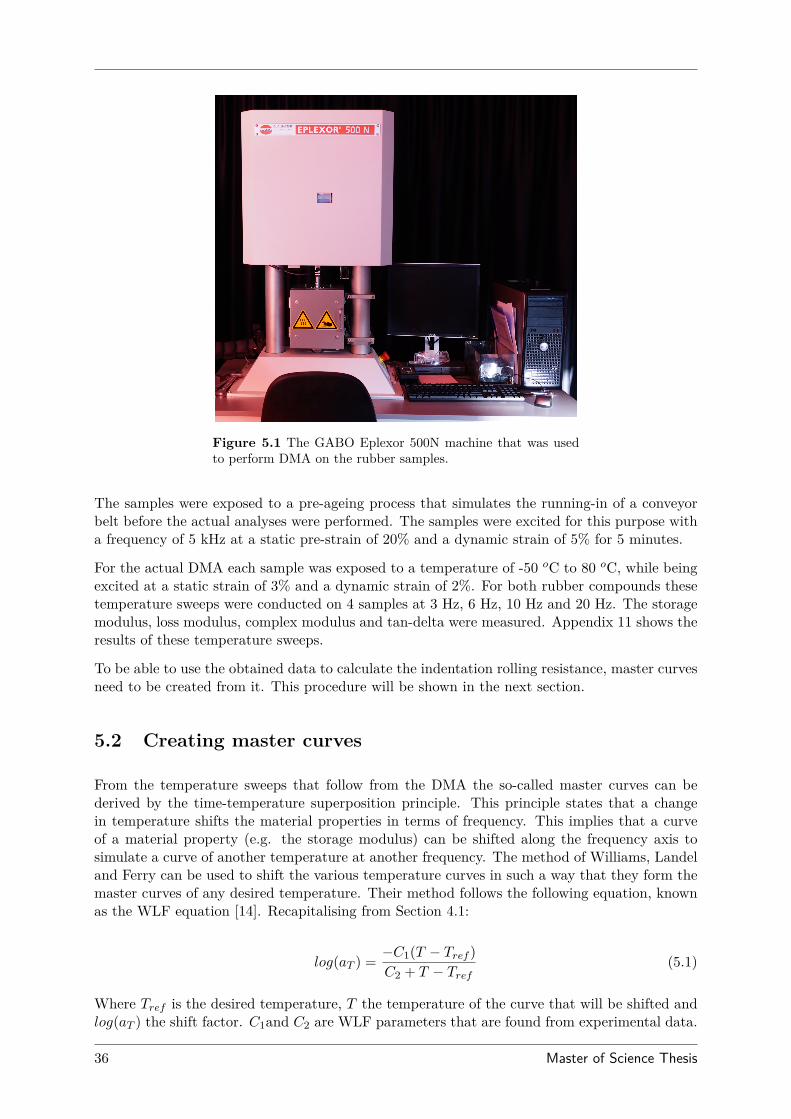
Figure 5.1 The GABO Eplexor 500N machine that was usedto perform DMA on the rubber samples.
The samples were exposed to a pre-ageing process that simulates the running-in of a conveyorbelt before the actual analyses were performed. The samples were excited for this purpose witha frequency of 5 kHz at a static pre-strain of 20% and a dynamic strain of 5% for 5 minutes.
For the actual DMA each sample was exposed to a temperature of -50 oC to 80 oC, while beingexcited at a static strain of 3% and a dynamic strain of 2%. For both rubber compounds thesetemperature sweeps were conducted on 4 samples at 3 Hz, 6 Hz, 10 Hz and 20 Hz. The storagemodulus, loss modulus, complex modulus and tan-delta were measured. Appendix 11 shows theresults of these temperature sweeps.
To be able to use the obtained data to calculate the indentation rolling resistance, master curvesneed to be created from it. This procedure will be shown in the next section.
5.2 Creating master curves
From the temperature sweeps that follow from the DMA the so-called master curves can bederived by the time-temperature superposition principle. This principle states that a changein temperature shifts the material properties in terms of frequency. This implies that a curveof a material property (e.g. the storage modulus) can be shifted along the frequency axis tosimulate a curve of another temperature at another frequency. The method of Williams, Landeland Ferry can be used to shift the various temperature curves in such a way that they form themaster curves of any desired temperature. Their method follows the following equation, knownas the WLF equation [14]. Recapitalising from Section 4.1:
log(aT ) = −C1(T − Tref )C2 + T − Tref
(5.1)
Where Tref is the desired temperature, T the temperature of the curve that will be shifted andlog(aT ) the shift factor. C1and C2 are WLF parameters that are found from experimental data.
36 Master of Science Thesis
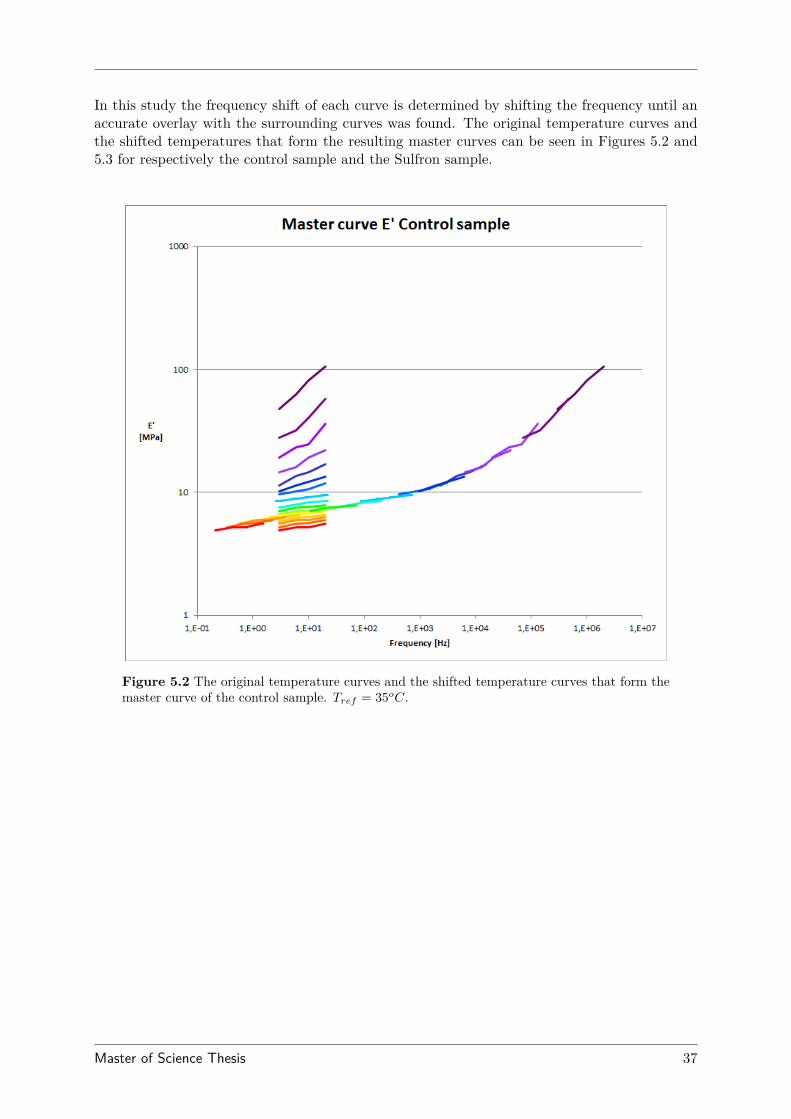
In this study the frequency shift of each curve is determined by shifting the frequency until anaccurate overlay with the surrounding curves was found. The original temperature curves andthe shifted temperatures that form the resulting master curves can be seen in Figures 5.2 and5.3 for respectively the control sample and the Sulfron sample.
Figure 5.2 The original temperature curves and the shifted temperature curves that form themaster curve of the control sample. Tref = 35oC.
Master of Science Thesis 37
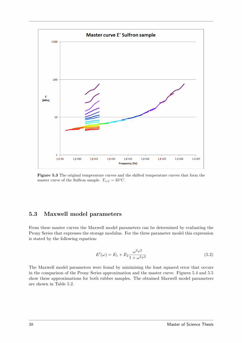
Figure 5.3 The original temperature curves and the shifted temperature curves that form themaster curve of the Sulfron sample. Tref = 35oC.
5.3 Maxwell model parameters
From these master curves the Maxwell model parameters can be determined by evaluating theProny Series that expresses the storage modulus. For the three parameter model this expressionis stated by the following equation:
E′(ω) = E1 + E2ω2τ2
1 + ω2τ2 (5.2)
The Maxwell model parameters were found by minimising the least squared error that occursin the comparison of the Prony Series approximation and the master curve. Figures 5.4 and 5.5show these approximations for both rubber samples. The obtained Maxwell model parametersare shown in Table 5.2.
38 Master of Science Thesis
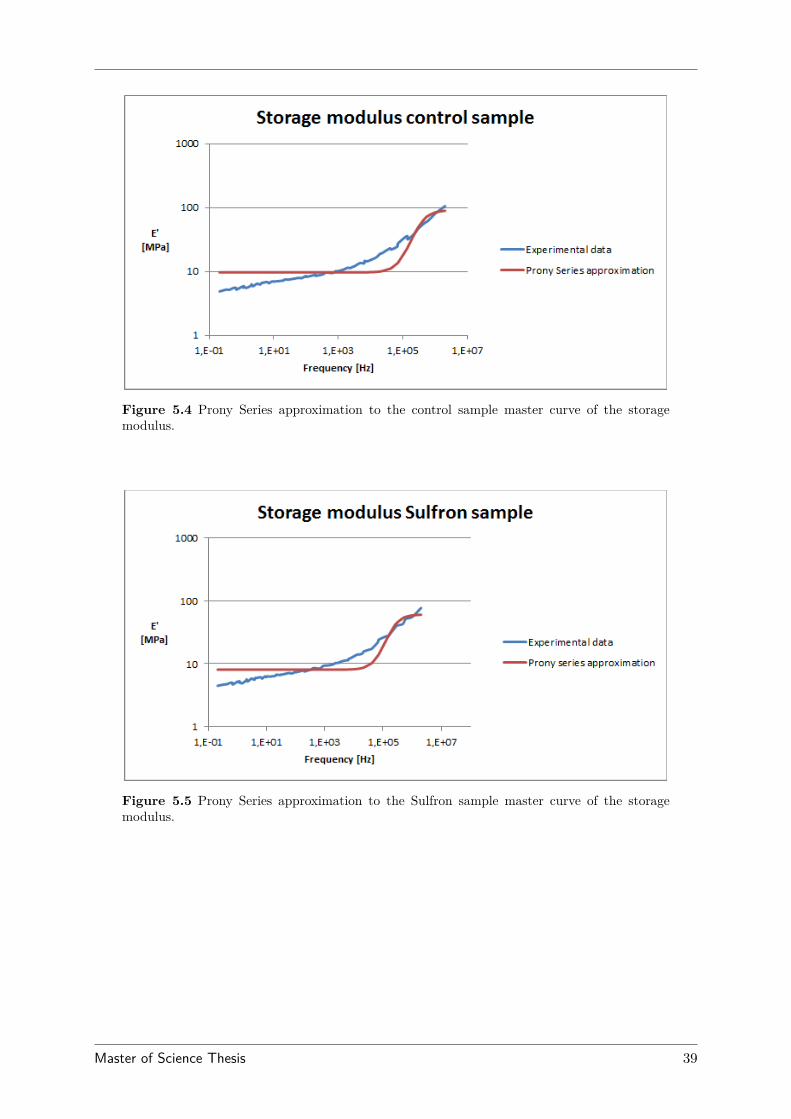
Figure 5.4 Prony Series approximation to the control sample master curve of the storagemodulus.
Figure 5.5 Prony Series approximation to the Sulfron sample master curve of the storagemodulus.
Master of Science Thesis 39
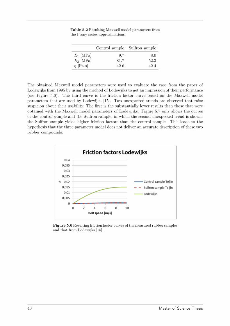
Table 5.2 Resulting Maxwell model parameters fromthe Prony series approximations.
Control sample Sulfron sample
E1 [MPa] 9.7 8.0E2 [MPa] 81.7 52.3η [Pa s] 42.6 42.4
The obtained Maxwell model parameters were used to evaluate the case from the paper ofLodewijks from 1995 by using the method of Lodewijks to get an impression of their performance(see Figure 5.6). The third curve is the friction factor curve based on the Maxwell modelparameters that are used by Lodewijks [15]. Two unexpected trends are observed that raisesuspicion about their usability. The first is the substantially lower results than those that wereobtained with the Maxwell model parameters of Lodewijks. Figure 5.7 only shows the curvesof the control sample and the Sulfron sample, in which the second unexpected trend is shown:the Sulfron sample yields higher friction factors than the control sample. This leads to thehypothesis that the three parameter model does not deliver an accurate description of these tworubber compounds.
Figure 5.6 Resulting friction factor curves of the measured rubber samplesand that from Lodewijks [15].
40 Master of Science Thesis
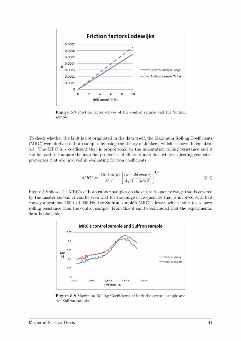
Figure 5.7 Friction factor curves of the control sample and the Sulfronsample.
To check whether the fault is not originated in the data itself, the Maximum Rolling Coefficients(MRC) were derived of both samples by using the theory of Jonkers, which is shown in equation5.3. The MRC is a coefficient that is proportional to the indentation rolling resistance and itcan be used to compare the material properties of different materials while neglecting geometricproperties that are involved in evaluating friction coefficients.
MRC = 0.5πtan(δ)E′1/3
[(π + 2δ)cos(δ)4√
1 + sin(δ)
]4/3
(5.3)
Figure 5.8 shows the MRC’s of both rubber samples on the entire frequency range that is coveredby the master curves. It can be seen that for the range of frequencies that is involved with beltconveyor systems, 100 to 1,000 Hz, the Sulfron sample’s MRC is lower, which indicates a lowerrolling resistance than the control sample. From this it can be concluded that the experimentaldata is plausible.
Figure 5.8 Maximum Rolling Coefficients of both the control sample andthe Sulfron sample.
Master of Science Thesis 41
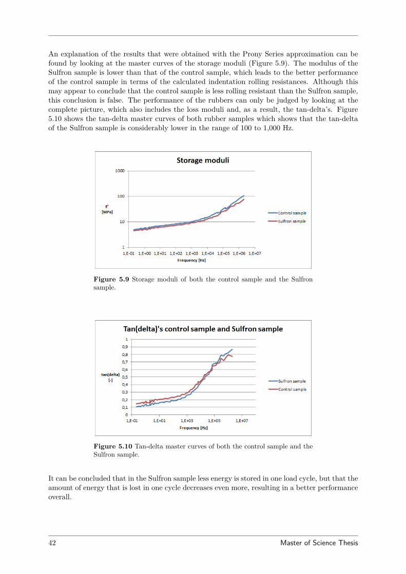
An explanation of the results that were obtained with the Prony Series approximation can befound by looking at the master curves of the storage moduli (Figure 5.9). The modulus of theSulfron sample is lower than that of the control sample, which leads to the better performanceof the control sample in terms of the calculated indentation rolling resistances. Although thismay appear to conclude that the control sample is less rolling resistant than the Sulfron sample,this conclusion is false. The performance of the rubbers can only be judged by looking at thecomplete picture, which also includes the loss moduli and, as a result, the tan-delta’s. Figure5.10 shows the tan-delta master curves of both rubber samples which shows that the tan-deltaof the Sulfron sample is considerably lower in the range of 100 to 1,000 Hz.
Figure 5.9 Storage moduli of both the control sample and the Sulfronsample.
Figure 5.10 Tan-delta master curves of both the control sample and theSulfron sample.
It can be concluded that in the Sulfron sample less energy is stored in one load cycle, but that theamount of energy that is lost in one cycle decreases even more, resulting in a better performanceoverall.
42 Master of Science Thesis
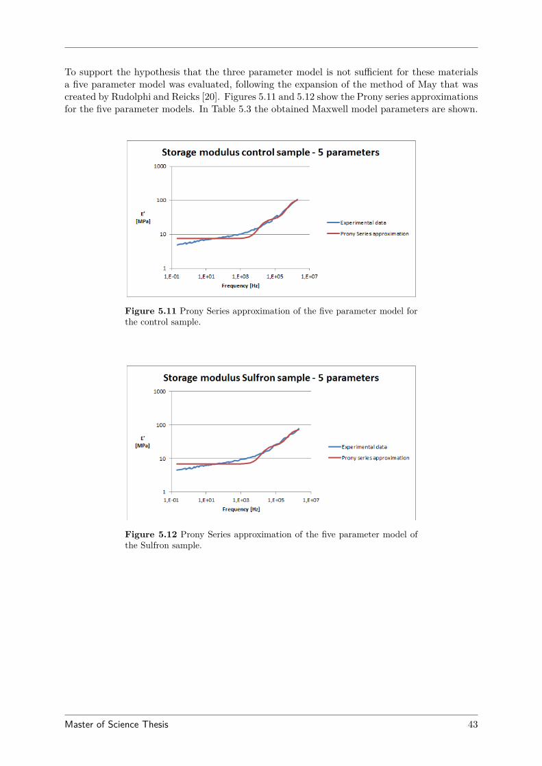
To support the hypothesis that the three parameter model is not sufficient for these materialsa five parameter model was evaluated, following the expansion of the method of May that wascreated by Rudolphi and Reicks [20]. Figures 5.11 and 5.12 show the Prony series approximationsfor the five parameter models. In Table 5.3 the obtained Maxwell model parameters are shown.
Figure 5.11 Prony Series approximation of the five parameter model forthe control sample.
Figure 5.12 Prony Series approximation of the five parameter model ofthe Sulfron sample.
Master of Science Thesis 43
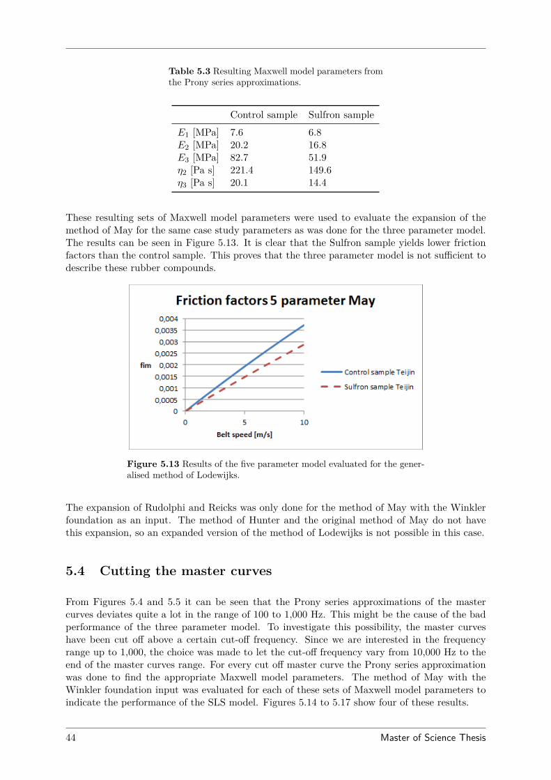
Table 5.3 Resulting Maxwell model parameters fromthe Prony series approximations.
Control sample Sulfron sample
E1 [MPa] 7.6 6.8E2 [MPa] 20.2 16.8E3 [MPa] 82.7 51.9η2 [Pa s] 221.4 149.6η3 [Pa s] 20.1 14.4
These resulting sets of Maxwell model parameters were used to evaluate the expansion of themethod of May for the same case study parameters as was done for the three parameter model.The results can be seen in Figure 5.13. It is clear that the Sulfron sample yields lower frictionfactors than the control sample. This proves that the three parameter model is not sufficient todescribe these rubber compounds.
Figure 5.13 Results of the five parameter model evaluated for the gener-alised method of Lodewijks.
The expansion of Rudolphi and Reicks was only done for the method of May with the Winklerfoundation as an input. The method of Hunter and the original method of May do not havethis expansion, so an expanded version of the method of Lodewijks is not possible in this case.
5.4 Cutting the master curves
From Figures 5.4 and 5.5 it can be seen that the Prony series approximations of the mastercurves deviates quite a lot in the range of 100 to 1,000 Hz. This might be the cause of the badperformance of the three parameter model. To investigate this possibility, the master curveshave been cut off above a certain cut-off frequency. Since we are interested in the frequencyrange up to 1,000, the choice was made to let the cut-off frequency vary from 10,000 Hz to theend of the master curves range. For every cut off master curve the Prony series approximationwas done to find the appropriate Maxwell model parameters. The method of May with theWinkler foundation input was evaluated for each of these sets of Maxwell model parameters toindicate the performance of the SLS model. Figures 5.14 to 5.17 show four of these results.
44 Master of Science Thesis
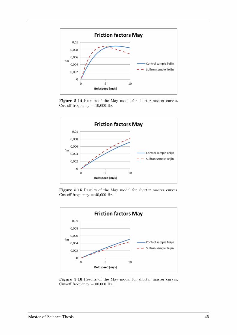
Figure 5.14 Results of the May model for shorter master curves.Cut-off frequency = 10,000 Hz.
Figure 5.15 Results of the May model for shorter master curves.Cut-off frequency = 40,000 Hz.
Figure 5.16 Results of the May model for shorter master curves.Cut-off frequency = 80,000 Hz.
Master of Science Thesis 45
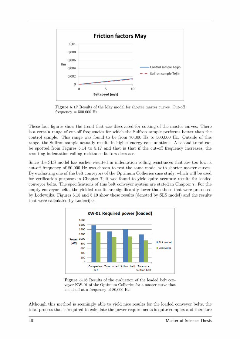
Figure 5.17 Results of the May model for shorter master curves. Cut-offfrequency = 500,000 Hz.
These four figures show the trend that was discovered for cutting of the master curves. Thereis a certain range of cut-off frequencies for which the Sulfron sample performs better than thecontrol sample. This range was found to be from 70,000 Hz to 500,000 Hz. Outside of thisrange, the Sulfron sample actually results in higher energy consumptions. A second trend canbe spotted from Figures 5.14 to 5.17 and that is that if the cut-off frequency increases, theresulting indentation rolling resistance factors decrease.
Since the SLS model has earlier resulted in indentation rolling resistances that are too low, acut-off frequency of 80,000 Hz was chosen to test the same model with shorter master curves.By evaluating one of the belt conveyors of the Optimum Collieries case study, which will be usedfor verification purposes in Chapter 7, it was found to yield quite accurate results for loadedconveyor belts. The specifications of this belt conveyor system are stated in Chapter 7. For theempty conveyor belts, the yielded results are significantly lower than those that were presentedby Lodewijks. Figures 5.18 and 5.19 show these results (denoted by SLS model) and the resultsthat were calculated by Lodewijks.
Figure 5.18 Results of the evaluation of the loaded belt con-veyor KW-01 of the Optimum Collieries for a master curve thatis cut-off at a frequency of 80,000 Hz.
Although this method is seemingly able to yield nice results for the loaded conveyor belts, thetotal process that is required to calculate the power requirements is quite complex and therefore
46 Master of Science Thesis
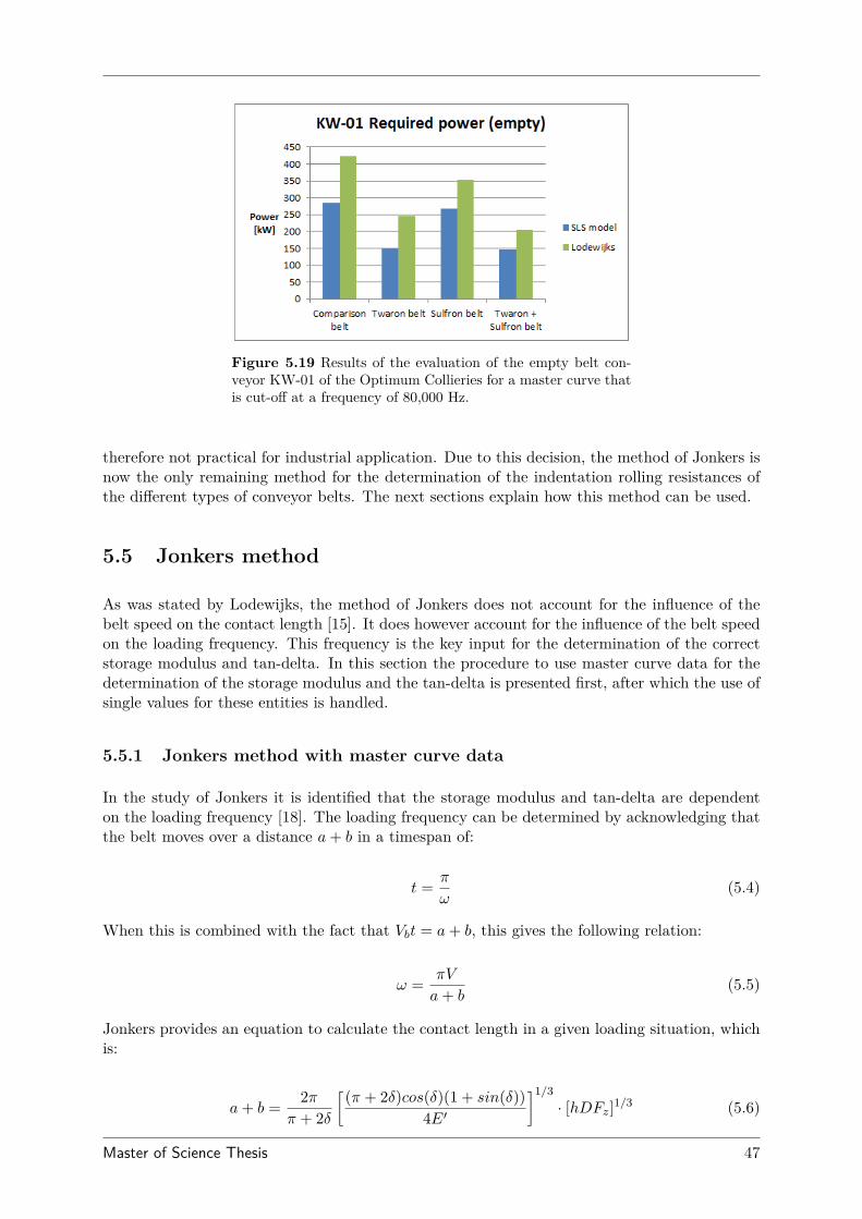
Figure 5.19 Results of the evaluation of the empty belt con-veyor KW-01 of the Optimum Collieries for a master curve thatis cut-off at a frequency of 80,000 Hz.
therefore not practical for industrial application. Due to this decision, the method of Jonkers isnow the only remaining method for the determination of the indentation rolling resistances ofthe different types of conveyor belts. The next sections explain how this method can be used.
5.5 Jonkers method
As was stated by Lodewijks, the method of Jonkers does not account for the influence of thebelt speed on the contact length [15]. It does however account for the influence of the belt speedon the loading frequency. This frequency is the key input for the determination of the correctstorage modulus and tan-delta. In this section the procedure to use master curve data for thedetermination of the storage modulus and the tan-delta is presented first, after which the use ofsingle values for these entities is handled.
5.5.1 Jonkers method with master curve data
In the study of Jonkers it is identified that the storage modulus and tan-delta are dependenton the loading frequency [18]. The loading frequency can be determined by acknowledging thatthe belt moves over a distance a+ b in a timespan of:
t = π
ω(5.4)
When this is combined with the fact that Vbt = a+ b, this gives the following relation:
ω = πV
a+ b(5.5)
Jonkers provides an equation to calculate the contact length in a given loading situation, whichis:
a+ b = 2ππ + 2δ
[(π + 2δ)cos(δ)(1 + sin(δ))4E′
]1/3· [hDFz]1/3 (5.6)
Master of Science Thesis 47
So the contact length that is required to determine the loading frequency depends on the loadingfrequency. Thus, these equations form a loop that can be solved by using an iterative procedure,for which an initial guess for one of the entities is required. In this study an initial guess ofthe loading frequency will be used. It was found that only two or three steps were requiredto obtain a converged solution. The master curves that were created in the previous sectionsare used here to determine the values of the storage modulus and tan-delta for the calculatedloading frequencies.
It is also possible that master curve data is not present. The following section describes thepossibilities and pitfalls that arise in those occasions.
5.5.2 Jonkers method without master curve data
An advantage of the method of Jonkers is that it works with single values of the storage modulusand tan-delta. This allows for the comparison of two different rubbers even when no completemaster curves are available. A common test to compare two different viscoelastic materials isa temperature sweep at 10 Hz and 2% strain for both materials [24]. It has to be noted thatthe indentation rolling resistance and thus the energy consumption of a conveyor belt basedon such test results can deviate from realistic values. This is due to the fact that the loadingfrequencies that are found in belt conveyor applications are generally between 100 and 1,000 Hz.This results in deviations in the values of the storage modulus and tan-delta.
The variation of the indentation rolling resistance that are caused by the different materialproperties at the incorrect loading frequency can be determined by evaluating the MRC at thegiven frequencies. The deviations were determined for both the control sample and the Sulfronsample by looking up the values of the storage modulus and tan-delta for 10 Hz, 100 Hz and1,000 Hz. By using equation 5.3, the variation of the friction factors were determined. For thecontrol sample the indentation rolling resistance factor was found to be 7% to 26% higher thanthat found for the 10 Hz input values. For the Sulfron sample these values are 8% to 39% higher.
It can be concluded that if the method of Jonkers is evaluated with values of the storage modulusand tan-delta that are measured at 10Hz, the yielded results will be lower than the results ofthe method of Jonkers when master curve data is used.
Besides this side note, the method of Jonkers is still capable of delivering a comparison betweentwo different rubber compounds. It is however known that it overestimates the indentationrolling resistance. In the next chapter the indentation rolling phenomenon as modelled byJonkers will be studied, to explore the possibilities to gain more accurate results with it.
48 Master of Science Thesis
Chapter 6
Proposed method
In the previous section the methods of Jonkers was selected to be used in this study to determinethe indentation rolling resistance. As stated earlier, Jonkers’ method overestimates the inden-tation rolling resistance, since it does not take the effect of the belt speed on the contact lengthinto account. A possible solution to reduce this shortcomings could be found in the creation of amodified Jonkers method, in which the influence of the belt speed on the contact length is takeninto account. It is preferable that this new method does not require more rubber property data,since that would require expensive and time-consuming experiments. The modification to theJonkers method is based on the following analysis of a single roller, with a belt that is alwaysloaded to the same degree.
6.1 Analysis
Confidential content removed
Master of Science Thesis 49

Confidential content removed
50 Master of Science Thesis

Confidential content removed
6.2 Set-up
Master of Science Thesis 51

Confidential content removed
52 Master of Science Thesis

Confidential content removed
Master of Science Thesis 53

Confidential content removed
54 Master of Science Thesis

Confidential content removed
Master of Science Thesis 55

56 Master of Science Thesis
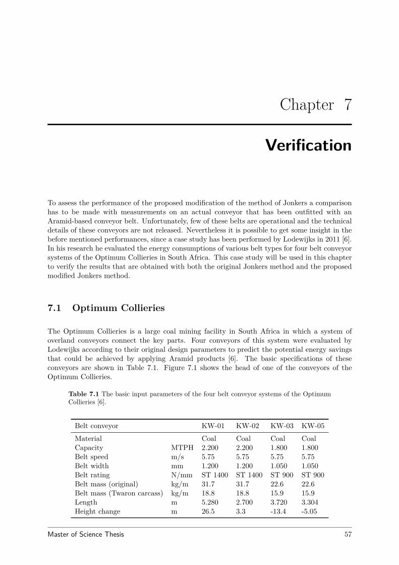
Chapter 7
Verification
To assess the performance of the proposed modification of the method of Jonkers a comparisonhas to be made with measurements on an actual conveyor that has been outfitted with anAramid-based conveyor belt. Unfortunately, few of these belts are operational and the technicaldetails of these conveyors are not released. Nevertheless it is possible to get some insight in thebefore mentioned performances, since a case study has been performed by Lodewijks in 2011 [6].In his research he evaluated the energy consumptions of various belt types for four belt conveyorsystems of the Optimum Collieries in South Africa. This case study will be used in this chapterto verify the results that are obtained with both the original Jonkers method and the proposedmodified Jonkers method.
7.1 Optimum Collieries
The Optimum Collieries is a large coal mining facility in South Africa in which a system ofoverland conveyors connect the key parts. Four conveyors of this system were evaluated byLodewijks according to their original design parameters to predict the potential energy savingsthat could be achieved by applying Aramid products [6]. The basic specifications of theseconveyors are shown in Table 7.1. Figure 7.1 shows the head of one of the conveyors of theOptimum Collieries.
Table 7.1 The basic input parameters of the four belt conveyor systems of the OptimumCollieries [6].
Belt conveyor KW-01 KW-02 KW-03 KW-05
Material Coal Coal Coal CoalCapacity MTPH 2.200 2.200 1.800 1.800Belt speed m/s 5.75 5.75 5.75 5.75Belt width mm 1.200 1.200 1.050 1.050Belt rating N/mm ST 1400 ST 1400 ST 900 ST 900Belt mass (original) kg/m 31.7 31.7 22.6 22.6Belt mass (Twaron carcass) kg/m 18.8 18.8 15.9 15.9Length m 5.280 2.700 3.720 3.304Height change m 26.5 3.3 -13.4 -5.05
Master of Science Thesis 57
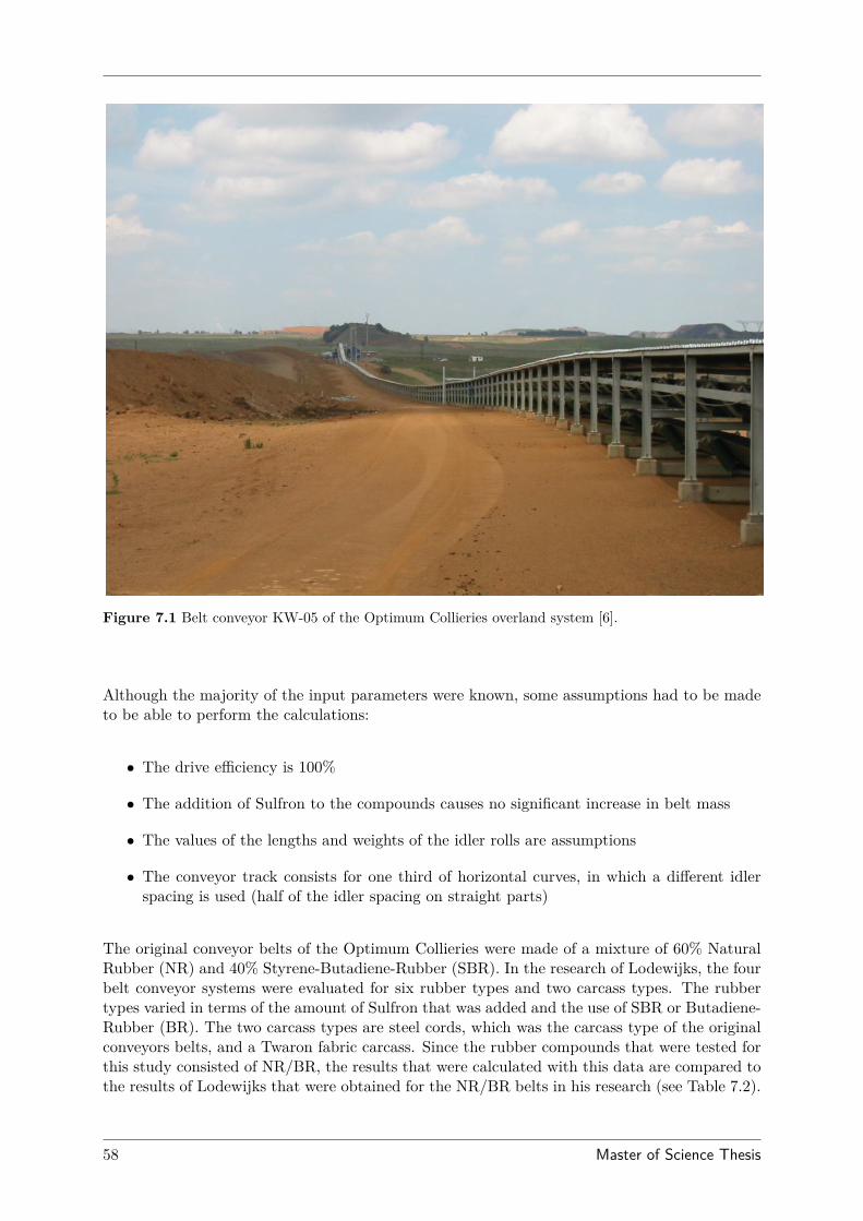
Figure 7.1 Belt conveyor KW-05 of the Optimum Collieries overland system [6].
Although the majority of the input parameters were known, some assumptions had to be madeto be able to perform the calculations:
• The drive efficiency is 100%
• The addition of Sulfron to the compounds causes no significant increase in belt mass
• The values of the lengths and weights of the idler rolls are assumptions
• The conveyor track consists for one third of horizontal curves, in which a different idlerspacing is used (half of the idler spacing on straight parts)
The original conveyor belts of the Optimum Collieries were made of a mixture of 60% NaturalRubber (NR) and 40% Styrene-Butadiene-Rubber (SBR). In the research of Lodewijks, the fourbelt conveyor systems were evaluated for six rubber types and two carcass types. The rubbertypes varied in terms of the amount of Sulfron that was added and the use of SBR or Butadiene-Rubber (BR). The two carcass types are steel cords, which was the carcass type of the originalconveyors belts, and a Twaron fabric carcass. Since the rubber compounds that were tested forthis study consisted of NR/BR, the results that were calculated with this data are compared tothe results of Lodewijks that were obtained for the NR/BR belts in his research (see Table 7.2).
58 Master of Science Thesis
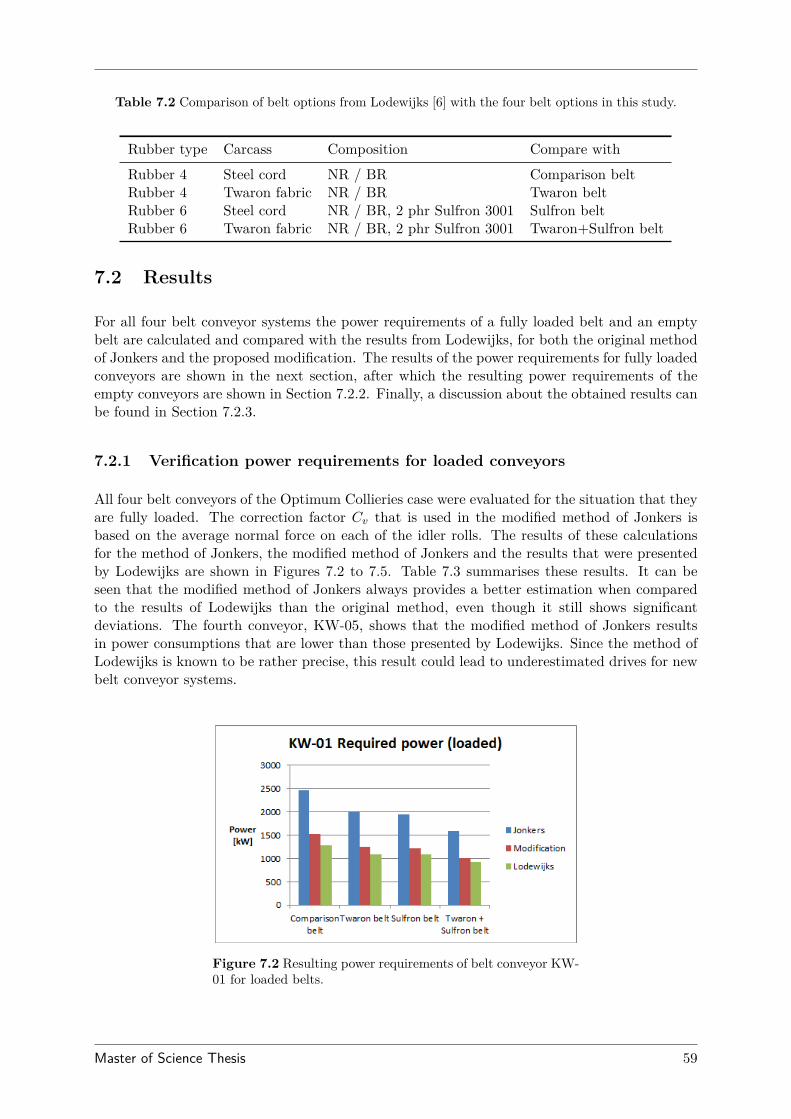
Table 7.2 Comparison of belt options from Lodewijks [6] with the four belt options in this study.
Rubber type Carcass Composition Compare with
Rubber 4 Steel cord NR / BR Comparison beltRubber 4 Twaron fabric NR / BR Twaron beltRubber 6 Steel cord NR / BR, 2 phr Sulfron 3001 Sulfron beltRubber 6 Twaron fabric NR / BR, 2 phr Sulfron 3001 Twaron+Sulfron belt
7.2 Results
For all four belt conveyor systems the power requirements of a fully loaded belt and an emptybelt are calculated and compared with the results from Lodewijks, for both the original methodof Jonkers and the proposed modification. The results of the power requirements for fully loadedconveyors are shown in the next section, after which the resulting power requirements of theempty conveyors are shown in Section 7.2.2. Finally, a discussion about the obtained results canbe found in Section 7.2.3.
7.2.1 Verification power requirements for loaded conveyors
All four belt conveyors of the Optimum Collieries case were evaluated for the situation that theyare fully loaded. The correction factor Cv that is used in the modified method of Jonkers isbased on the average normal force on each of the idler rolls. The results of these calculationsfor the method of Jonkers, the modified method of Jonkers and the results that were presentedby Lodewijks are shown in Figures 7.2 to 7.5. Table 7.3 summarises these results. It can beseen that the modified method of Jonkers always provides a better estimation when comparedto the results of Lodewijks than the original method, even though it still shows significantdeviations. The fourth conveyor, KW-05, shows that the modified method of Jonkers resultsin power consumptions that are lower than those presented by Lodewijks. Since the method ofLodewijks is known to be rather precise, this result could lead to underestimated drives for newbelt conveyor systems.
Figure 7.2 Resulting power requirements of belt conveyor KW-01 for loaded belts.
Master of Science Thesis 59
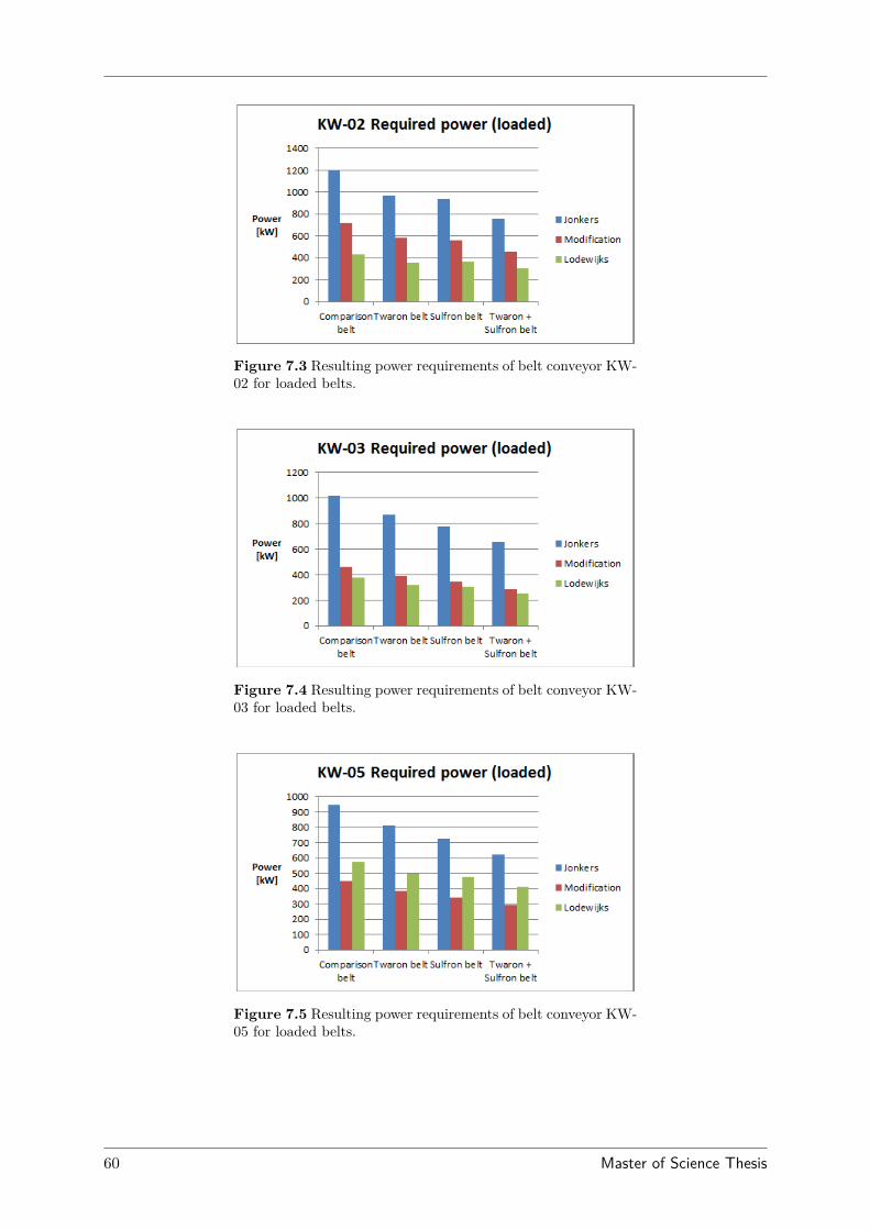
Figure 7.3 Resulting power requirements of belt conveyor KW-02 for loaded belts.
Figure 7.4 Resulting power requirements of belt conveyor KW-03 for loaded belts.
Figure 7.5 Resulting power requirements of belt conveyor KW-05 for loaded belts.
60 Master of Science Thesis
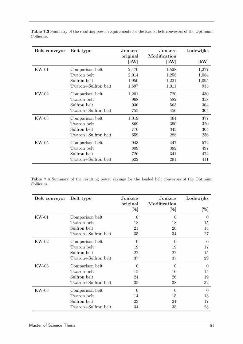
Table 7.3 Summary of the resulting power requirements for the loaded belt conveyors of the OptimumCollieries.
Belt conveyor Belt type Jonkers Jonkers Lodewijksoriginal Modification
[kW] [kW] [kW]KW-01 Comparison belt 2,470 1,528 1,277
Twaron belt 2,014 1,258 1,084Sulfron belt 1,950 1,221 1,095Twaron+Sulfron belt 1,597 1,011 933
KW-02 Comparison belt 1,201 720 430Twaron belt 968 582 358Sulfron belt 936 563 364Twaron+Sulfron belt 755 456 304
KW-03 Comparison belt 1,019 464 377Twaron belt 869 390 320Sulfron belt 776 345 304Twaron+Sulfron belt 659 288 256
KW-05 Comparison belt 943 447 572Twaron belt 809 382 497Sulfron belt 726 341 474Twaron+Sulfron belt 622 291 411
Table 7.4 Summary of the resulting power savings for the loaded belt conveyors of the OptimumCollieries.
Belt conveyor Belt type Jonkers Jonkers Lodewijksoriginal Modification
[%] [%] [%]KW-01 Comparison belt 0 0 0
Twaron belt 18 18 15Sulfron belt 21 20 14Twaron+Sulfron belt 35 34 27
KW-02 Comparison belt 0 0 0Twaron belt 19 19 17Sulfron belt 22 22 15Twaron+Sulfron belt 37 37 29
KW-03 Comparison belt 0 0 0Twaron belt 15 16 15Sulfron belt 24 26 19Twaron+Sulfron belt 35 38 32
KW-05 Comparison belt 0 0 0Twaron belt 14 15 13Sulfron belt 23 24 17Twaron+Sulfron belt 34 35 28
Master of Science Thesis 61
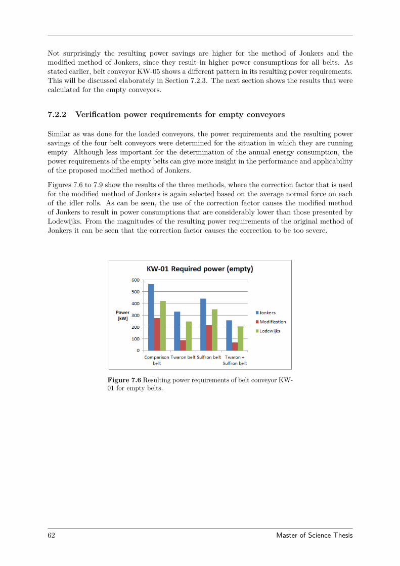
Not surprisingly the resulting power savings are higher for the method of Jonkers and themodified method of Jonkers, since they result in higher power consumptions for all belts. Asstated earlier, belt conveyor KW-05 shows a different pattern in its resulting power requirements.This will be discussed elaborately in Section 7.2.3. The next section shows the results that werecalculated for the empty conveyors.
7.2.2 Verification power requirements for empty conveyors
Similar as was done for the loaded conveyors, the power requirements and the resulting powersavings of the four belt conveyors were determined for the situation in which they are runningempty. Although less important for the determination of the annual energy consumption, thepower requirements of the empty belts can give more insight in the performance and applicabilityof the proposed modified method of Jonkers.
Figures 7.6 to 7.9 show the results of the three methods, where the correction factor that is usedfor the modified method of Jonkers is again selected based on the average normal force on eachof the idler rolls. As can be seen, the use of the correction factor causes the modified methodof Jonkers to result in power consumptions that are considerably lower than those presented byLodewijks. From the magnitudes of the resulting power requirements of the original method ofJonkers it can be seen that the correction factor causes the correction to be too severe.
Figure 7.6 Resulting power requirements of belt conveyor KW-01 for empty belts.
62 Master of Science Thesis
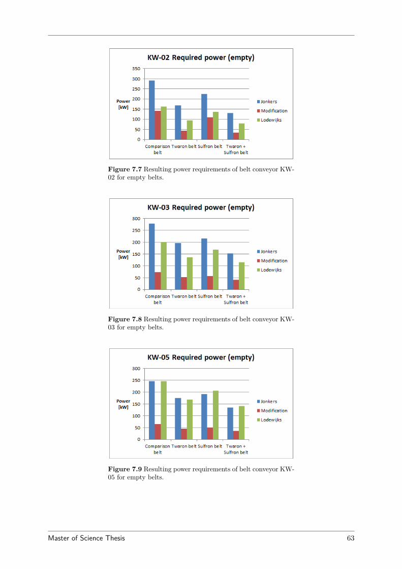
Figure 7.7 Resulting power requirements of belt conveyor KW-02 for empty belts.
Figure 7.8 Resulting power requirements of belt conveyor KW-03 for empty belts.
Figure 7.9 Resulting power requirements of belt conveyor KW-05 for empty belts.
Master of Science Thesis 63
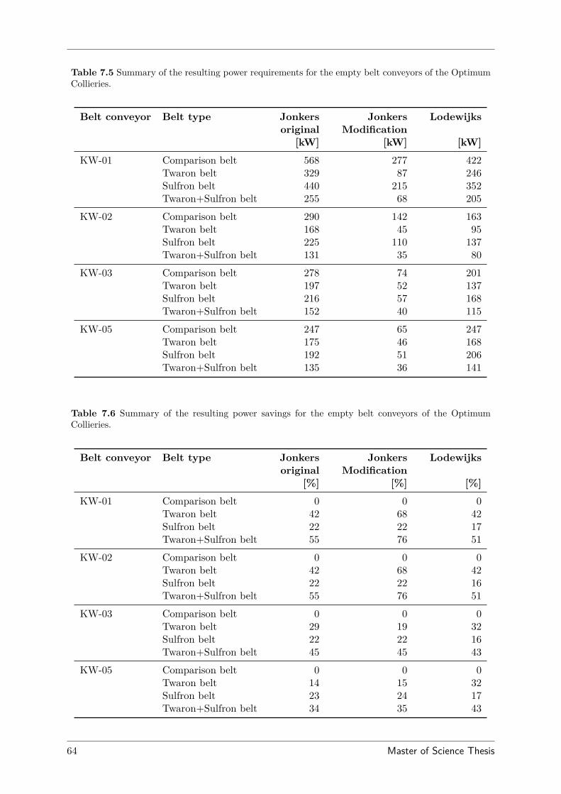
Table 7.5 Summary of the resulting power requirements for the empty belt conveyors of the OptimumCollieries.
Belt conveyor Belt type Jonkers Jonkers Lodewijksoriginal Modification
[kW] [kW] [kW]KW-01 Comparison belt 568 277 422
Twaron belt 329 87 246Sulfron belt 440 215 352Twaron+Sulfron belt 255 68 205
KW-02 Comparison belt 290 142 163Twaron belt 168 45 95Sulfron belt 225 110 137Twaron+Sulfron belt 131 35 80
KW-03 Comparison belt 278 74 201Twaron belt 197 52 137Sulfron belt 216 57 168Twaron+Sulfron belt 152 40 115
KW-05 Comparison belt 247 65 247Twaron belt 175 46 168Sulfron belt 192 51 206Twaron+Sulfron belt 135 36 141
Table 7.6 Summary of the resulting power savings for the empty belt conveyors of the OptimumCollieries.
Belt conveyor Belt type Jonkers Jonkers Lodewijksoriginal Modification
[%] [%] [%]KW-01 Comparison belt 0 0 0
Twaron belt 42 68 42Sulfron belt 22 22 17Twaron+Sulfron belt 55 76 51
KW-02 Comparison belt 0 0 0Twaron belt 42 68 42Sulfron belt 22 22 16Twaron+Sulfron belt 55 76 51
KW-03 Comparison belt 0 0 0Twaron belt 29 19 32Sulfron belt 22 22 16Twaron+Sulfron belt 45 45 43
KW-05 Comparison belt 0 0 0Twaron belt 14 15 32Sulfron belt 23 24 17Twaron+Sulfron belt 34 35 43
64 Master of Science Thesis
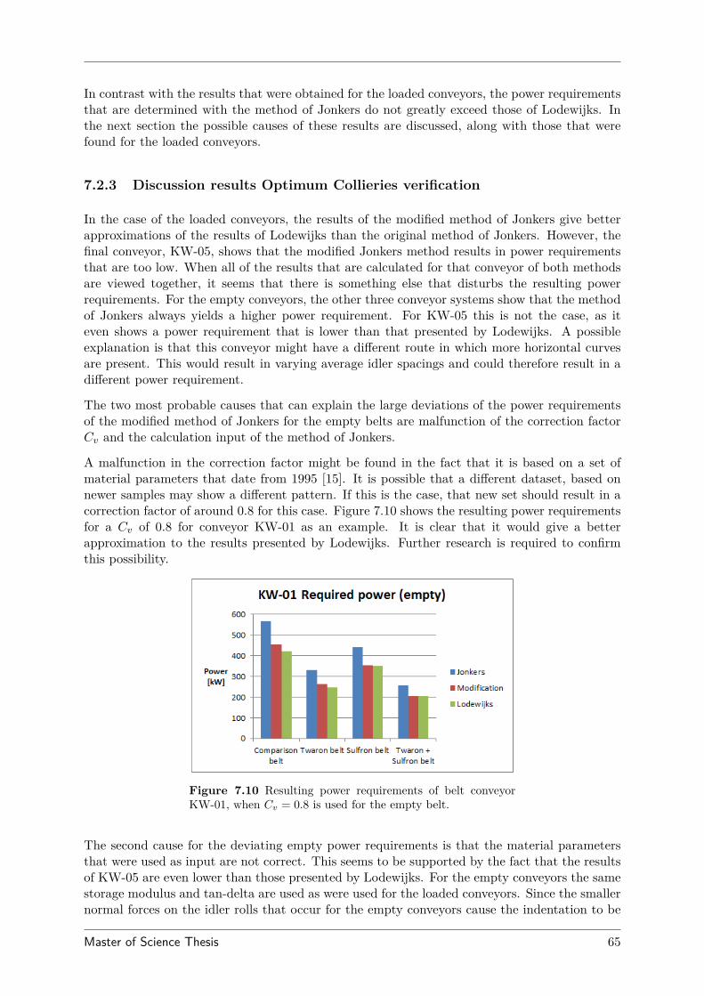
In contrast with the results that were obtained for the loaded conveyors, the power requirementsthat are determined with the method of Jonkers do not greatly exceed those of Lodewijks. Inthe next section the possible causes of these results are discussed, along with those that werefound for the loaded conveyors.
7.2.3 Discussion results Optimum Collieries verification
In the case of the loaded conveyors, the results of the modified method of Jonkers give betterapproximations of the results of Lodewijks than the original method of Jonkers. However, thefinal conveyor, KW-05, shows that the modified Jonkers method results in power requirementsthat are too low. When all of the results that are calculated for that conveyor of both methodsare viewed together, it seems that there is something else that disturbs the resulting powerrequirements. For the empty conveyors, the other three conveyor systems show that the methodof Jonkers always yields a higher power requirement. For KW-05 this is not the case, as iteven shows a power requirement that is lower than that presented by Lodewijks. A possibleexplanation is that this conveyor might have a different route in which more horizontal curvesare present. This would result in varying average idler spacings and could therefore result in adifferent power requirement.
The two most probable causes that can explain the large deviations of the power requirementsof the modified method of Jonkers for the empty belts are malfunction of the correction factorCv and the calculation input of the method of Jonkers.
A malfunction in the correction factor might be found in the fact that it is based on a set ofmaterial parameters that date from 1995 [15]. It is possible that a different dataset, based onnewer samples may show a different pattern. If this is the case, that new set should result in acorrection factor of around 0.8 for this case. Figure 7.10 shows the resulting power requirementsfor a Cv of 0.8 for conveyor KW-01 as an example. It is clear that it would give a betterapproximation to the results presented by Lodewijks. Further research is required to confirmthis possibility.
Figure 7.10 Resulting power requirements of belt conveyorKW-01, when Cv = 0.8 is used for the empty belt.
The second cause for the deviating empty power requirements is that the material parametersthat were used as input are not correct. This seems to be supported by the fact that the resultsof KW-05 are even lower than those presented by Lodewijks. For the empty conveyors the samestorage modulus and tan-delta are used as were used for the loaded conveyors. Since the smallernormal forces on the idler rolls that occur for the empty conveyors cause the indentation to be
Master of Science Thesis 65

less deep, the contact length will also be smaller. This results in a loading frequency that ishigher and will therefore lead to different material properties and probably higher results.
Based on the obtained results it is advised that the modified method of Jonkers is only usedto determine the power consumptions of the loaded conveyor belts. For the empty belts theoriginal method of Jonkers should be used. In the next section a case study of a fictive beltconveyor will be shown that uses this conclusion.
66 Master of Science Thesis
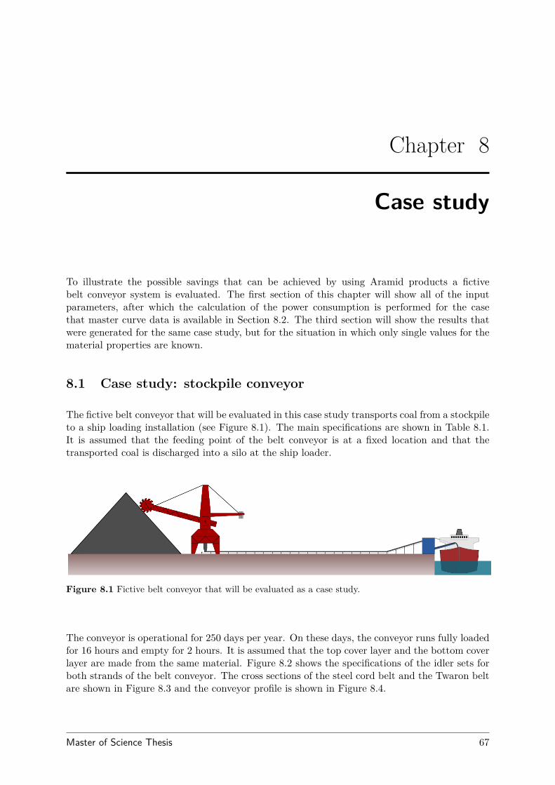
Chapter 8
Case study
To illustrate the possible savings that can be achieved by using Aramid products a fictivebelt conveyor system is evaluated. The first section of this chapter will show all of the inputparameters, after which the calculation of the power consumption is performed for the casethat master curve data is available in Section 8.2. The third section will show the results thatwere generated for the same case study, but for the situation in which only single values for thematerial properties are known.
8.1 Case study: stockpile conveyor
The fictive belt conveyor that will be evaluated in this case study transports coal from a stockpileto a ship loading installation (see Figure 8.1). The main specifications are shown in Table 8.1.It is assumed that the feeding point of the belt conveyor is at a fixed location and that thetransported coal is discharged into a silo at the ship loader.
Figure 8.1 Fictive belt conveyor that will be evaluated as a case study.
The conveyor is operational for 250 days per year. On these days, the conveyor runs fully loadedfor 16 hours and empty for 2 hours. It is assumed that the top cover layer and the bottom coverlayer are made from the same material. Figure 8.2 shows the specifications of the idler sets forboth strands of the belt conveyor. The cross sections of the steel cord belt and the Twaron beltare shown in Figure 8.3 and the conveyor profile is shown in Figure 8.4.
Master of Science Thesis 67
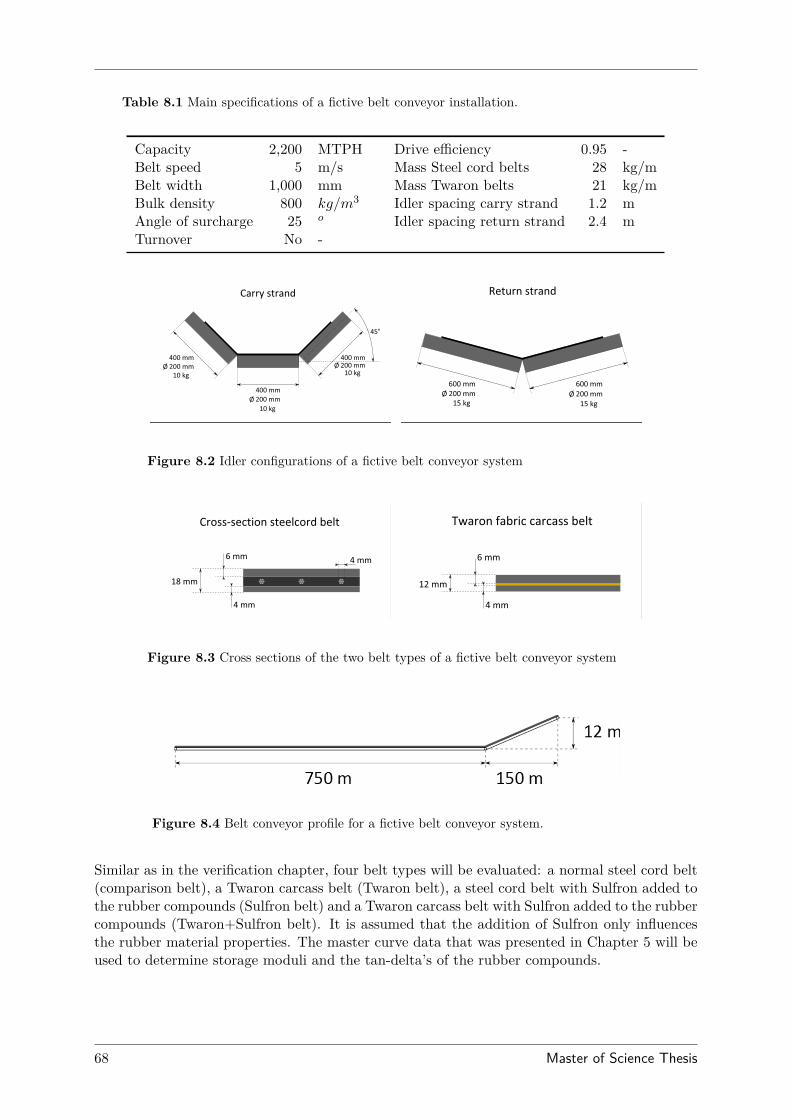
Table 8.1 Main specifications of a fictive belt conveyor installation.
Capacity 2,200 MTPH Drive efficiency 0.95 -Belt speed 5 m/s Mass Steel cord belts 28 kg/mBelt width 1,000 mm Mass Twaron belts 21 kg/mBulk density 800 kg/m3 Idler spacing carry strand 1.2 mAngle of surcharge 25 o Idler spacing return strand 2.4 mTurnover No -
Figure 8.2 Idler configurations of a fictive belt conveyor system
Figure 8.3 Cross sections of the two belt types of a fictive belt conveyor system
Figure 8.4 Belt conveyor profile for a fictive belt conveyor system.
Similar as in the verification chapter, four belt types will be evaluated: a normal steel cord belt(comparison belt), a Twaron carcass belt (Twaron belt), a steel cord belt with Sulfron added tothe rubber compounds (Sulfron belt) and a Twaron carcass belt with Sulfron added to the rubbercompounds (Twaron+Sulfron belt). It is assumed that the addition of Sulfron only influencesthe rubber material properties. The master curve data that was presented in Chapter 5 will beused to determine storage moduli and the tan-delta’s of the rubber compounds.
68 Master of Science Thesis
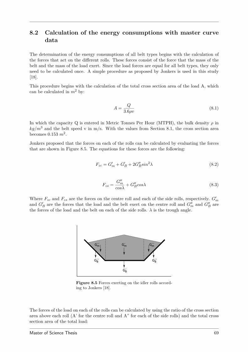
8.2 Calculation of the energy consumptions with master curvedata
The determination of the energy consumptions of all belt types begins with the calculation ofthe forces that act on the different rolls. These forces consist of the force that the mass of thebelt and the mass of the load exert. Since the load forces are equal for all belt types, they onlyneed to be calculated once. A simple procedure as proposed by Jonkers is used in this study[18].
This procedure begins with the calculation of the total cross section area of the load A, whichcan be calculated in m2 by:
A = Q
3.6ρv (8.1)
In which the capacity Q is entered in Metric Tonnes Per Hour (MTPH), the bulk density ρ inkg/m3 and the belt speed v in m/s. With the values from Section 8.1, the cross section areabecomes 0.153 m2.
Jonkers proposed that the forces on each of the rolls can be calculated by evaluating the forcesthat are shown in Figure 8.5. The equations for these forces are the following:
Fzc = G′m +G′B + 2G′′Bsin2λ (8.2)
Fzs = G′′mcosλ
+G′′Bcosλ (8.3)
Where Fzc and Fzs are the forces on the centre roll and each of the side rolls, respectively. G′mand G′B are the forces that the load and the belt exert on the centre roll and G′′m and G′′B arethe forces of the load and the belt on each of the side rolls. λ is the trough angle.
Figure 8.5 Forces exerting on the idler rolls accord-ing to Jonkers [18].
The forces of the load on each of the rolls can be calculated by using the ratio of the cross sectionarea above each roll (A’ for the centre roll and A” for each of the side rolls) and the total crosssection area of the total load:
Master of Science Thesis 69
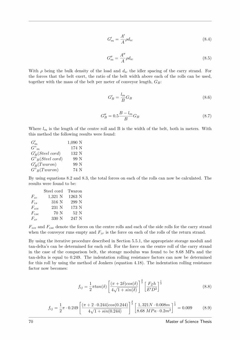
G′m = A′
Aρdic (8.4)
G′′m = A′′
Aρdic (8.5)
With ρ being the bulk density of the load and dic the idler spacing of the carry strand. Forthe forces that the belt exert, the ratio of the belt width above each of the rolls can be used,together with the mass of the belt per meter of conveyor length, GB:
G′B = lmBGB (8.6)
G′′B = 0.5B − lmB
GB (8.7)
Where lm is the length of the centre roll and B is the width of the belt, both in meters. Withthis method the following results were found:
G′m 1,090 NG”m 174 NG′B(Steel cord) 132 NG”B(Steel cord) 99 NG′B(Twaron) 99 NG”B(Twaron) 74 N
By using equations 8.2 and 8.3, the total forces on each of the rolls can now be calculated. Theresults were found to be:
Steel cord TwaronFzc 1,321 N 1263 NFzs 316 N 299 NFzce 231 N 173 NFzse 70 N 52 NFzr 330 N 247 N
Fzce and Fzse denote the forces on the centre rolls and each of the side rolls for the carry strandwhen the conveyor runs empty and Fzr is the force on each of the rolls of the return strand.
By using the iterative procedure described in Section 5.5.1, the appropriate storage moduli andtan-delta’s can be determined for each roll. For the force on the centre roll of the carry strandin the case of the comparison belt, the storage modulus was found to be 8.68 MPa and thetan-delta is equal to 0.249. The indentation rolling resistance factors can now be determinedfor this roll by using the method of Jonkers (equation 4.18). The indentation rolling resistancefactor now becomes:
fij = 12πtan(δ)
[(π + 2δ)cos(δ)4√
1 + sin(δ)
] 43 [ FZhE′D2
] 13
(8.8)
fij = 12π · 0.249
[(π + 2 · 0.244)cos(0.244)
4√
1 + sin(0.244)
] 43 [ 1, 321N · 0.008m
8.68 MPa · 0.2m2
] 13
= 0.009 (8.9)
70 Master of Science Thesis
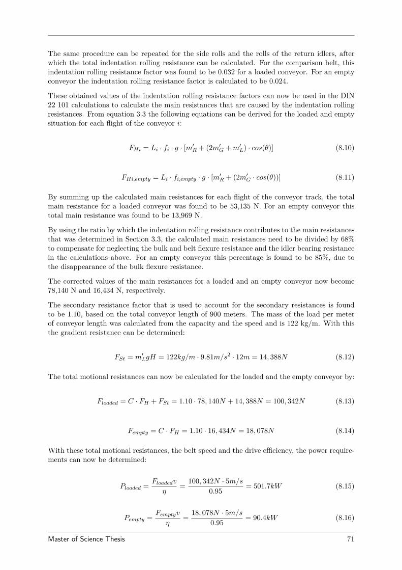
The same procedure can be repeated for the side rolls and the rolls of the return idlers, afterwhich the total indentation rolling resistance can be calculated. For the comparison belt, thisindentation rolling resistance factor was found to be 0.032 for a loaded conveyor. For an emptyconveyor the indentation rolling resistance factor is calculated to be 0.024.
These obtained values of the indentation rolling resistance factors can now be used in the DIN22 101 calculations to calculate the main resistances that are caused by the indentation rollingresistances. From equation 3.3 the following equations can be derived for the loaded and emptysituation for each flight of the conveyor i:
FHi = Li · fi · g · [m′R + (2m′G +m′L) · cos(θ)] (8.10)
FHi,empty = Li · fi,empty · g · [m′R + (2m′G · cos(θ))] (8.11)
By summing up the calculated main resistances for each flight of the conveyor track, the totalmain resistance for a loaded conveyor was found to be 53,135 N. For an empty conveyor thistotal main resistance was found to be 13,969 N.
By using the ratio by which the indentation rolling resistance contributes to the main resistancesthat was determined in Section 3.3, the calculated main resistances need to be divided by 68%to compensate for neglecting the bulk and belt flexure resistance and the idler bearing resistancein the calculations above. For an empty conveyor this percentage is found to be 85%, due tothe disappearance of the bulk flexure resistance.
The corrected values of the main resistances for a loaded and an empty conveyor now become78,140 N and 16,434 N, respectively.
The secondary resistance factor that is used to account for the secondary resistances is foundto be 1.10, based on the total conveyor length of 900 meters. The mass of the load per meterof conveyor length was calculated from the capacity and the speed and is 122 kg/m. With thisthe gradient resistance can be determined:
FSt = m′LgH = 122kg/m · 9.81m/s2 · 12m = 14, 388N (8.12)
The total motional resistances can now be calculated for the loaded and the empty conveyor by:
Floaded = C · FH + FSt = 1.10 · 78, 140N + 14, 388N = 100, 342N (8.13)
Fempty = C · FH = 1.10 · 16, 434N = 18, 078N (8.14)
With these total motional resistances, the belt speed and the drive efficiency, the power require-ments can now be determined:
Ploaded = Floadedv
η= 100, 342N · 5m/s
0.95 = 501.7kW (8.15)
Pempty = Femptyv
η= 18, 078N · 5m/s
0.95 = 90.4kW (8.16)
Master of Science Thesis 71
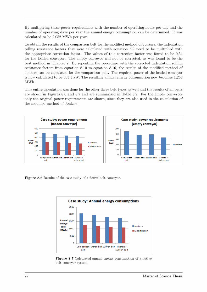
By multiplying these power requirements with the number of operating hours per day and thenumber of operating days per year the annual energy consumption can be determined. It wascalculated to be 2,052 MWh per year.
To obtain the results of the comparison belt for the modified method of Jonkers, the indentationrolling resistance factors that were calculated with equation 8.9 need to be multiplied withthe appropriate correction factor. The values of this correction factor was found to be 0.54for the loaded conveyor. The empty conveyor will not be corrected, as was found to be thebest method in Chapter 7. By repeating the procedure with the corrected indentation rollingresistance factors from equation 8.10 to equation 8.16, the results of the modified method ofJonkers can be calculated for the comparison belt. The required power of the loaded conveyoris now calculated to be 303.3 kW. The resulting annual energy consumption now becomes 1,258MWh.
This entire calculation was done for the other three belt types as well and the results of all beltsare shown in Figures 8.6 and 8.7 and are summarised in Table 8.2. For the empty conveyorsonly the original power requirements are shown, since they are also used in the calculation ofthe modified method of Jonkers.
Figure 8.6 Results of the case study of a fictive belt conveyor.
Figure 8.7 Calculated annual energy consumption of a fictivebelt conveyor system.
72 Master of Science Thesis
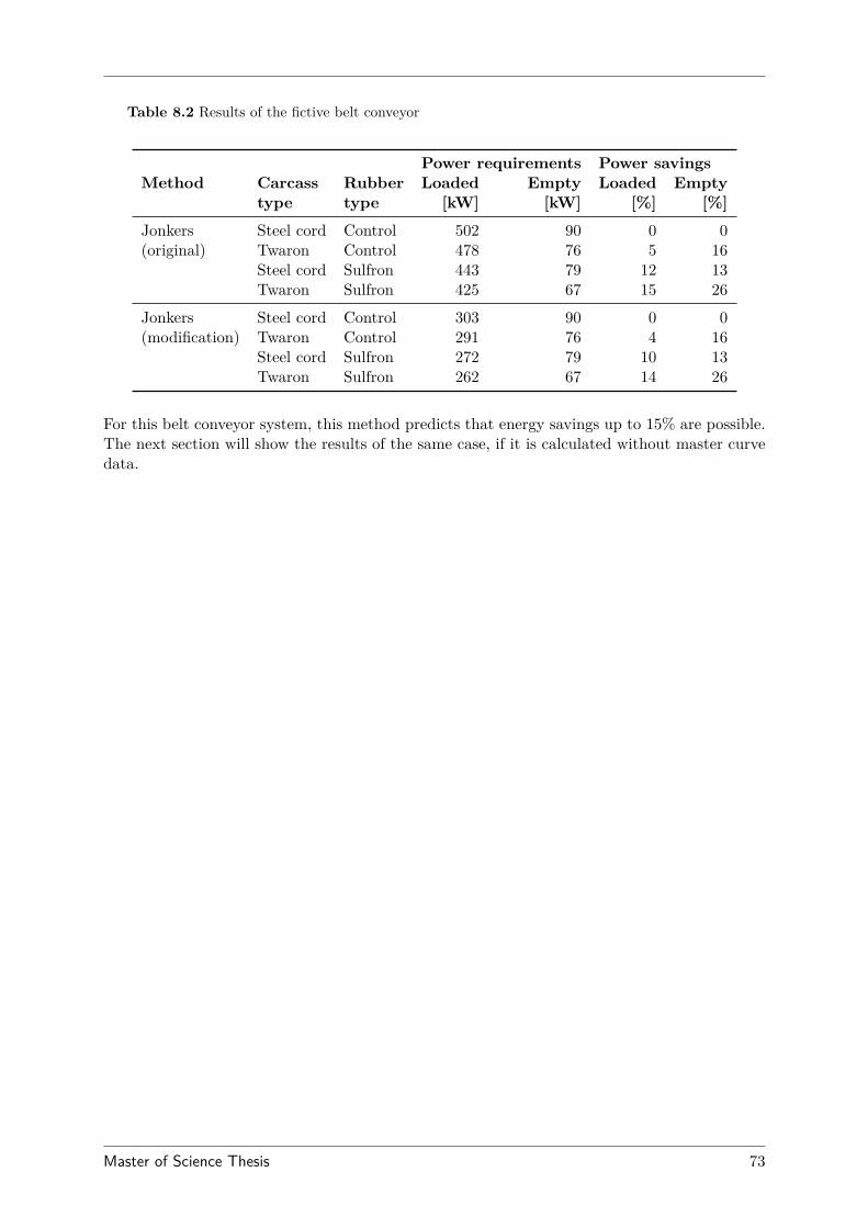
Table 8.2 Results of the fictive belt conveyor
Power requirements Power savingsMethod Carcass Rubber Loaded Empty Loaded Empty
type type [kW] [kW] [%] [%]Jonkers Steel cord Control 502 90 0 0(original) Twaron Control 478 76 5 16
Steel cord Sulfron 443 79 12 13Twaron Sulfron 425 67 15 26
Jonkers Steel cord Control 303 90 0 0(modification) Twaron Control 291 76 4 16
Steel cord Sulfron 272 79 10 13Twaron Sulfron 262 67 14 26
For this belt conveyor system, this method predicts that energy savings up to 15% are possible.The next section will show the results of the same case, if it is calculated without master curvedata.
Master of Science Thesis 73
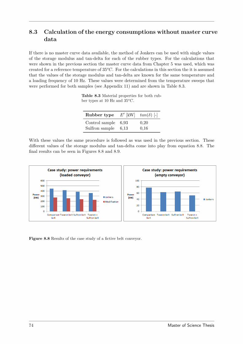
8.3 Calculation of the energy consumptions without master curvedata
If there is no master curve data available, the method of Jonkers can be used with single valuesof the storage modulus and tan-delta for each of the rubber types. For the calculations thatwere shown in the previous section the master curve data from Chapter 5 was used, which wascreated for a reference temperature of 35oC. For the calculations in this section the it is assumedthat the values of the storage modulus and tan-delta are known for the same temperature anda loading frequency of 10 Hz. These values were determined from the temperature sweeps thatwere performed for both samples (see Appendix 11) and are shown in Table 8.3.
Table 8.3 Material properties for both rub-ber types at 10 Hz and 35oC.
Rubber type E′ [kW] tan(δ) [-]
Control sample 6,93 0,20Sulfron sample 6,13 0,16
With these values the same procedure is followed as was used in the previous section. Thesedifferent values of the storage modulus and tan-delta come into play from equation 8.8. Thefinal results can be seen in Figures 8.8 and 8.9.
Figure 8.8 Results of the case study of a fictive belt conveyor.
74 Master of Science Thesis
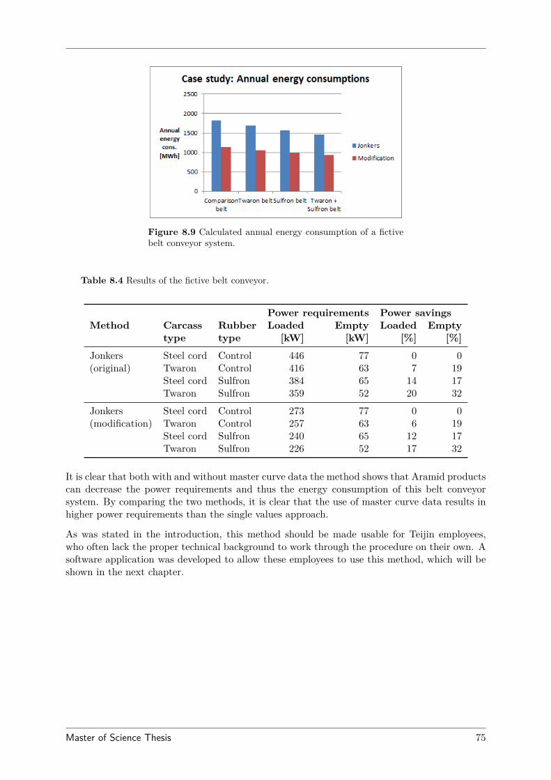
Figure 8.9 Calculated annual energy consumption of a fictivebelt conveyor system.
Table 8.4 Results of the fictive belt conveyor.
Power requirements Power savingsMethod Carcass Rubber Loaded Empty Loaded Empty
type type [kW] [kW] [%] [%]Jonkers Steel cord Control 446 77 0 0(original) Twaron Control 416 63 7 19
Steel cord Sulfron 384 65 14 17Twaron Sulfron 359 52 20 32
Jonkers Steel cord Control 273 77 0 0(modification) Twaron Control 257 63 6 19
Steel cord Sulfron 240 65 12 17Twaron Sulfron 226 52 17 32
It is clear that both with and without master curve data the method shows that Aramid productscan decrease the power requirements and thus the energy consumption of this belt conveyorsystem. By comparing the two methods, it is clear that the use of master curve data results inhigher power requirements than the single values approach.
As was stated in the introduction, this method should be made usable for Teijin employees,who often lack the proper technical background to work through the procedure on their own. Asoftware application was developed to allow these employees to use this method, which will beshown in the next chapter.
Master of Science Thesis 75

76 Master of Science Thesis
Chapter 9
Software application
To make the solution from the previous chapters usable for Teijin employees, an application wasdeveloped, in which both the original and the modified Jonkers method can be used to predictthe energy savings of an existing or a new belt conveyor system. A system of requirements wascreated for the application, which will be shown in the following section. Section 9.2 explainsthe system architecture that was used and the various components. Section 9.3 shows the resultsof the case study from Chapter 8, which are recalculated with this software application.
9.1 System of requirements
Confidential content removed
Master of Science Thesis 77

9.2 System architecture
Confidential content removed
9.2.1 Calculation
78 Master of Science Thesis

Confidential content removed
9.2.2 Calculation of a conveyor belt
Master of Science Thesis 79

Confidential content removed
80 Master of Science Thesis

9.3 Recalculation of the case study
Confidential content removed
Master of Science Thesis 81

Confidential content removed
82 Master of Science Thesis

Confidential content removed
Master of Science Thesis 83

Confidential content removed
84 Master of Science Thesis

Confidential content removed
9.4 Extra options
Confidential content removed
Master of Science Thesis 85

86 Master of Science Thesis
Chapter 10
Conclusions
The following conclusions can be drawn from the results of this report:
The indentation rolling resistance was found to be the most important cause of the energyconsumptions of belt conveyor systems. It has therefore been chosen to be the primary targetfor the determination of the total energy consumption of belt conveyor systems.
In literature it is found that the method of Lodewijks yields accurate results for the calculationof the indentation rolling resistance. However, the transformation of the measured materialproperties into the required Maxwell model parameters is not always successful. The threeparameter model that was given by Lodewijks showed results that showed the opposite effectof what can be expected. A verification with a five parameter expansion of this model didshow the expected trend in the indentation rolling resistance of a normal rubber compound anda compound that has been made low rolling resistant by the addition of Sulfron. From thisit can be concluded that the three parameter model cannot describe the material behaviourproperly by using the total master curves that were created for the two rubber types. It hasbeen shown that by cutting these master curves above a certain frequency, the three parametermodel can yield quite accurate results for loaded conveyor belts, but significantly underestimatesthe power requirements for the empty conveyor belts. Due to the complexity of the total processof determining the energy consumption of a belt conveyor system with the method of Lodewijks,this method is considered not practical for this study.
The proposed modification to the method of Jonkers can significantly improve the estimationof the indentation rolling resistance for loaded belt conveyors. For empty conveyor belts, themodified method shows a correction of the original Jonkers method that is too severe andtherefore yields power requirements that are too low. From these results it can be concludedthat for the purpose of generating a first estimation of the energy consumption of a belt conveyorsystem, the modified method of Jonkers should be used for the loaded conveyor belts and theoriginal method of Jonkers for the empty conveyor belts. The accuracy of this approach needsto be verified by comparing it with experimental results.
Regardless of the method that is used, the performance of the different Aramid-based conveyorbelts follow the trend that was observed by Lodewijks [6]. The application of these Aramidproducts can significantly reduce the energy consumption of a belt conveyor system. On anannual basis, the energy consumption of a belt conveyor system can be reduced by 40%.
The software application that has been developed to create a usable version of the modifiedmethod of Jonkers and the original method of Jonkers has showed that it is capable to deliver
Master of Science Thesis 87

the right results as were calculated for the case study in this report.
88 Master of Science Thesis
Chapter 11
Recommendations
Based on the conclusions of this report and the findings that were done during the study, somerecommendations can be stated:
Since this developed method and software application are based on theoretical models, validationof both is required. This is also true for the real performance of Aramid-based conveyor belts.For this purpose, measurements on an actual conveyor of which the belt type will be changedare required. With the outcome of those measurements, the modified method of Jonkers can beadjusted, if required, to obtain a better method for the estimation of the energy consumptionof generic belt conveyor systems.
It was found that the Prony series approximation of the measured material properties did notyield plausible Maxwell model parameters. In previous studies it has been reported to do thisproperly, so a future study is required to determine for what circumstances this approach worksand for which it does not. Sequently, if this is determined, the method of Lodewijks could beapplied instead of the modified Jonkers method to estimate the energy consumption of genericbelt conveyor systems.
The variation of the energy consumptions that can be obtained with the iterative process ofthe method of Jonkers in comparison with the use of single values for the storage modulus andtan-delta has been estimated roughly in this report, with variations of 7% to 40%. A moreaccurate study of these variations could be valuable for the interpretation of the results that canbe obtained by single values.
The developed software application is based on Visual Basic and Microsoft Excel, which impliesthat it is a computer-based application. If the frequency of use of this software applicationbecomes significant, a conversion step to a web-based application is advised, so it can be accessedmore easily.
Master of Science Thesis 89

90 Master of Science Thesis

Appendix A: research paper
Master of Science Thesis 91
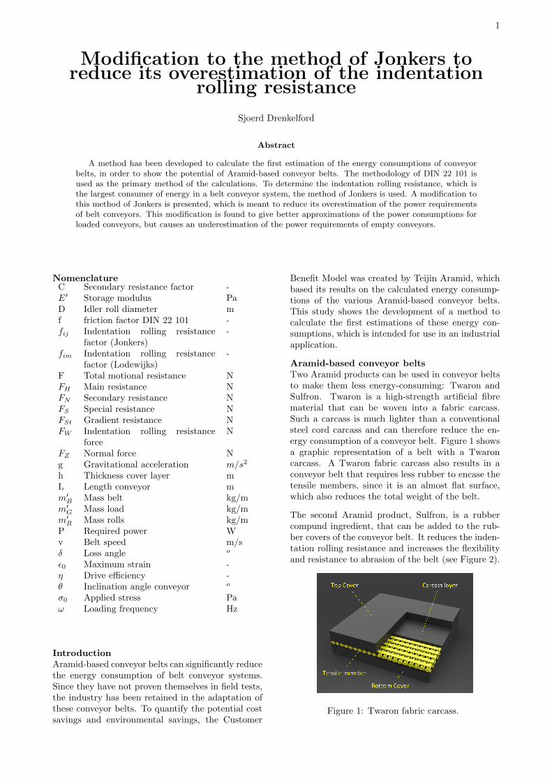
1
Modification to the method of Jonkers toreduce its overestimation of the indentation
rolling resistance
Sjoerd Drenkelford
Abstract
A method has been developed to calculate the first estimation of the energy consumptions of conveyorbelts, in order to show the potential of Aramid-based conveyor belts. The methodology of DIN 22 101 isused as the primary method of the calculations. To determine the indentation rolling resistance, which isthe largest consumer of energy in a belt conveyor system, the method of Jonkers is used. A modification tothis method of Jonkers is presented, which is meant to reduce its overestimation of the power requirementsof belt conveyors. This modification is found to give better approximations of the power consumptions forloaded conveyors, but causes an underestimation of the power requirements of empty conveyors.
NomenclatureC Secondary resistance factor -E′ Storage modulus PaD Idler roll diameter mf friction factor DIN 22 101 -fij Indentation rolling resistance
factor (Jonkers)-
fim Indentation rolling resistancefactor (Lodewijks)
-
F Total motional resistance NFH Main resistance NFN Secondary resistance NFS Special resistance NFSt Gradient resistance NFW Indentation rolling resistance
forceN
FZ Normal force Ng Gravitational acceleration m/s2
h Thickness cover layer mL Length conveyor mm′
B Mass belt kg/mm′
G Mass load kg/mm′
R Mass rolls kg/mP Required power Wv Belt speed m/sδ Loss angle o
ε0 Maximum strain -η Drive efficiency -θ Inclination angle conveyor o
σ0 Applied stress Paω Loading frequency Hz
IntroductionAramid-based conveyor belts can significantly reducethe energy consumption of belt conveyor systems.Since they have not proven themselves in field tests,the industry has been retained in the adaptation ofthese conveyor belts. To quantify the potential costsavings and environmental savings, the Customer
Benefit Model was created by Teijin Aramid, whichbased its results on the calculated energy consump-tions of the various Aramid-based conveyor belts.This study shows the development of a method tocalculate the first estimations of these energy con-sumptions, which is intended for use in an industrialapplication.
Aramid-based conveyor beltsTwo Aramid products can be used in conveyor beltsto make them less energy-consuming: Twaron andSulfron. Twaron is a high-strength artificial fibrematerial that can be woven into a fabric carcass.Such a carcass is much lighter than a conventionalsteel cord carcass and can therefore reduce the en-ergy consumption of a conveyor belt. Figure 1 showsa graphic representation of a belt with a Twaroncarcass. A Twaron fabric carcass also results in aconveyor belt that requires less rubber to encase thetensile members, since it is an almost flat surface,which also reduces the total weight of the belt.
The second Aramid product, Sulfron, is a rubbercompund ingredient, that can be added to the rub-ber covers of the conveyor belt. It reduces the inden-tation rolling resistance and increases the flexibilityand resistance to abrasion of the belt (see Figure 2).
Figure 1: Twaron fabric carcass.
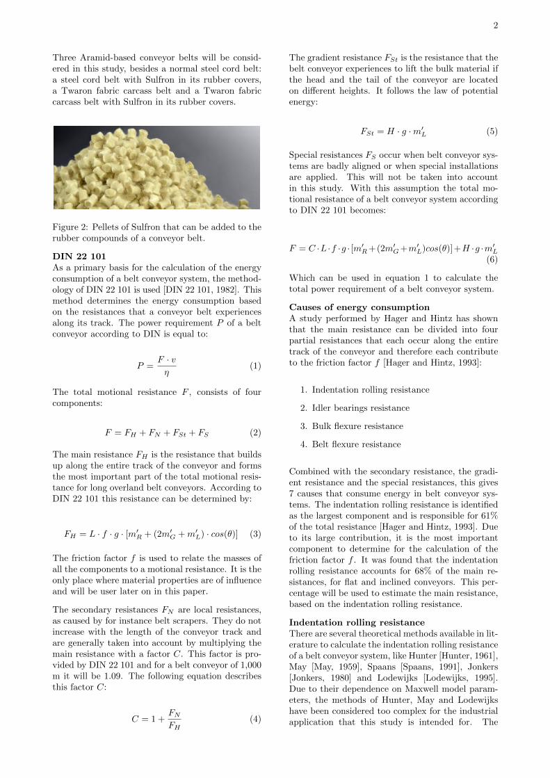
2
Three Aramid-based conveyor belts will be consid-ered in this study, besides a normal steel cord belt:a steel cord belt with Sulfron in its rubber covers,a Twaron fabric carcass belt and a Twaron fabriccarcass belt with Sulfron in its rubber covers.
Figure 2: Pellets of Sulfron that can be added to therubber compounds of a conveyor belt.
DIN 22 101As a primary basis for the calculation of the energyconsumption of a belt conveyor system, the method-ology of DIN 22 101 is used [DIN 22 101, 1982]. Thismethod determines the energy consumption basedon the resistances that a conveyor belt experiencesalong its track. The power requirement P of a beltconveyor according to DIN is equal to:
P =F · vη
(1)
The total motional resistance F , consists of fourcomponents:
F = FH + FN + FSt + FS (2)
The main resistance FH is the resistance that buildsup along the entire track of the conveyor and formsthe most important part of the total motional resis-tance for long overland belt conveyors. According toDIN 22 101 this resistance can be determined by:
FH = L · f · g · [m′R + (2m′
G +m′L) · cos(θ)] (3)
The friction factor f is used to relate the masses ofall the components to a motional resistance. It is theonly place where material properties are of influenceand will be user later on in this paper.
The secondary resistances FN are local resistances,as caused by for instance belt scrapers. They do notincrease with the length of the conveyor track andare generally taken into account by multiplying themain resistance with a factor C. This factor is pro-vided by DIN 22 101 and for a belt conveyor of 1,000m it will be 1.09. The following equation describesthis factor C:
C = 1 +FN
FH(4)
The gradient resistance FSt is the resistance that thebelt conveyor experiences to lift the bulk material ifthe head and the tail of the conveyor are locatedon different heights. It follows the law of potentialenergy:
FSt = H · g ·m′L (5)
Special resistances FS occur when belt conveyor sys-tems are badly aligned or when special installationsare applied. This will not be taken into accountin this study. With this assumption the total mo-tional resistance of a belt conveyor system accordingto DIN 22 101 becomes:
F = C ·L ·f ·g · [m′R +(2m′
G +m′L)cos(θ)]+H ·g ·m′
L
(6)
Which can be used in equation 1 to calculate thetotal power requirement of a belt conveyor system.
Causes of energy consumptionA study performed by Hager and Hintz has shownthat the main resistance can be divided into fourpartial resistances that each occur along the entiretrack of the conveyor and therefore each contributeto the friction factor f [Hager and Hintz, 1993]:
1. Indentation rolling resistance
2. Idler bearings resistance
3. Bulk flexure resistance
4. Belt flexure resistance
Combined with the secondary resistance, the gradi-ent resistance and the special resistances, this gives7 causes that consume energy in belt conveyor sys-tems. The indentation rolling resistance is identifiedas the largest component and is responsible for 61%of the total resistance [Hager and Hintz, 1993]. Dueto its large contribution, it is the most importantcomponent to determine for the calculation of thefriction factor f . It was found that the indentationrolling resistance accounts for 68% of the main re-sistances, for flat and inclined conveyors. This per-centage will be used to estimate the main resistance,based on the indentation rolling resistance.
Indentation rolling resistanceThere are several theoretical methods available in lit-erature to calculate the indentation rolling resistanceof a belt conveyor system, like Hunter [Hunter, 1961],May [May, 1959], Spaans [Spaans, 1991], Jonkers[Jonkers, 1980] and Lodewijks [Lodewijks, 1995].Due to their dependence on Maxwell model param-eters, the methods of Hunter, May and Lodewijkshave been considered too complex for the industrialapplication that this study is intended for. The
3
method of Spaans requires a sample of the totalbelt to be able to function correctly, so it is alsoconsidered not practical. This leaves the method ofJonkers, which is
Jonkers considers the indentation to follow a sinu-soidal pattern and because of this assumption, heis able to express the indentation rolling resistanceforce in a very concise equation. For the use in themethod of DIN 22 101, this force needs to be dividedby the normal force, after which the friction factoraccording to Jonkers is described by:
f ′ij =FW
FZ=
1
2πtan(δ)
[(π + 2δ)cos(δ)
4√
1 + sin(δ)
] 43 [
FZh
E′D2
] 13
(7)
Since the method of Jonkers is known to overesti-mate the indentation rolling resistance [Lodewijks,1995], it will yield energy consumptions that are toohigh and will therefore give a less realistic predictionof the potential savings that can be achieved withthe application of Aramids in conveyor belts. To re-duce this overestimation, an empiric modification isproposed, based on the following analysis.
Proposed modification
Verification and resultsThe performance of this modified method of Jonkersis assessed by comparing the results with a casestudy of four belt conveyors of the Optimum Col-lieries, that was performed by Lodewijks [Lodewi-jks, 2011]. This case considers four conveyors thattransport coal and all have the same belt speed of5.75 m/s. The specifications of the four conveyorsare shown below:
Belt conveyor KW-01:Capacity 2,200 MTPHBelt width 1,2 mBelt mass (Steel cord) 31.7 kg/mBelt mass (Twaron fabric) 18.8 kg/mLenght 5,280 mHeight change 26.5 m
Belt conveyor KW-02:
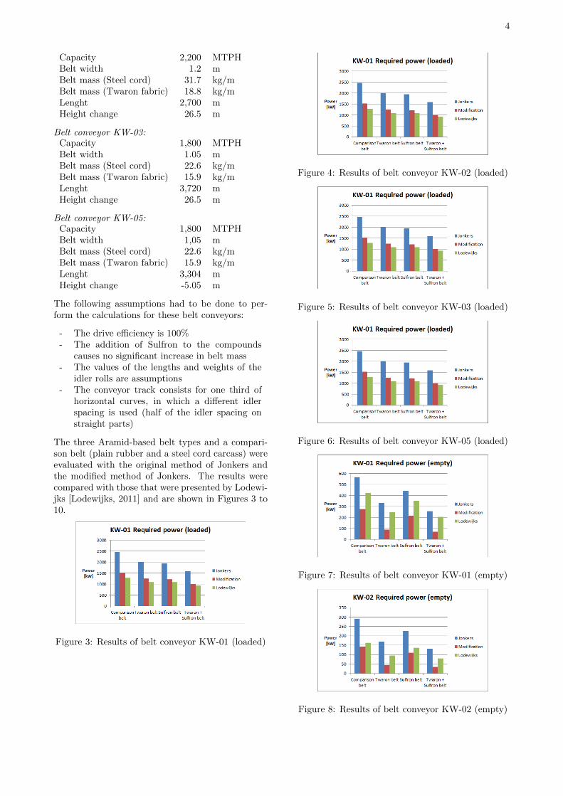
4
Capacity 2,200 MTPHBelt width 1.2 mBelt mass (Steel cord) 31.7 kg/mBelt mass (Twaron fabric) 18.8 kg/mLenght 2,700 mHeight change 26.5 m
Belt conveyor KW-03:Capacity 1,800 MTPHBelt width 1.05 mBelt mass (Steel cord) 22.6 kg/mBelt mass (Twaron fabric) 15.9 kg/mLenght 3,720 mHeight change 26.5 m
Belt conveyor KW-05:Capacity 1,800 MTPHBelt width 1,05 mBelt mass (Steel cord) 22.6 kg/mBelt mass (Twaron fabric) 15.9 kg/mLenght 3,304 mHeight change -5.05 m
The following assumptions had to be done to per-form the calculations for these belt conveyors:
- The drive efficiency is 100%- The addition of Sulfron to the compounds
causes no significant increase in belt mass- The values of the lengths and weights of the
idler rolls are assumptions- The conveyor track consists for one third of
horizontal curves, in which a different idlerspacing is used (half of the idler spacing onstraight parts)
The three Aramid-based belt types and a compari-son belt (plain rubber and a steel cord carcass) wereevaluated with the original method of Jonkers andthe modified method of Jonkers. The results werecompared with those that were presented by Lodewi-jks [Lodewijks, 2011] and are shown in Figures 3 to10.
Figure 3: Results of belt conveyor KW-01 (loaded)
Figure 4: Results of belt conveyor KW-02 (loaded)
Figure 5: Results of belt conveyor KW-03 (loaded)
Figure 6: Results of belt conveyor KW-05 (loaded)
Figure 7: Results of belt conveyor KW-01 (empty)
Figure 8: Results of belt conveyor KW-02 (empty)
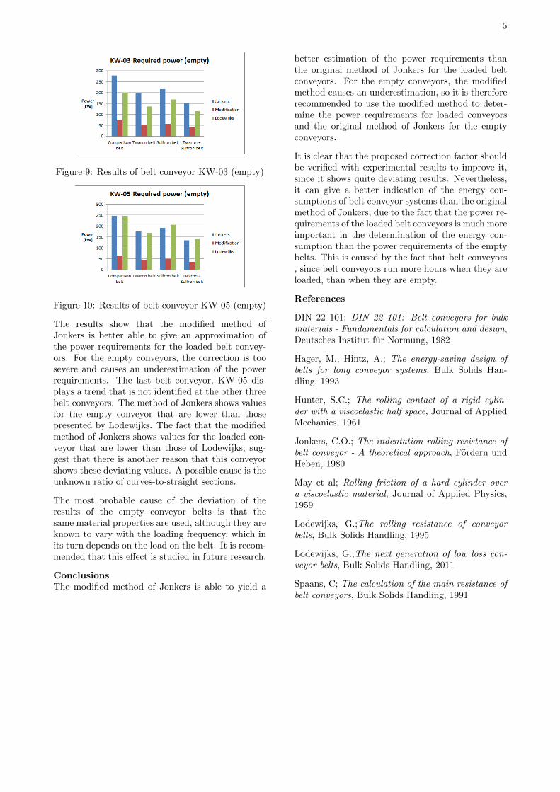
5
Figure 9: Results of belt conveyor KW-03 (empty)
Figure 10: Results of belt conveyor KW-05 (empty)
The results show that the modified method ofJonkers is better able to give an approximation ofthe power requirements for the loaded belt convey-ors. For the empty conveyors, the correction is toosevere and causes an underestimation of the powerrequirements. The last belt conveyor, KW-05 dis-plays a trend that is not identified at the other threebelt conveyors. The method of Jonkers shows valuesfor the empty conveyor that are lower than thosepresented by Lodewijks. The fact that the modifiedmethod of Jonkers shows values for the loaded con-veyor that are lower than those of Lodewijks, sug-gest that there is another reason that this conveyorshows these deviating values. A possible cause is theunknown ratio of curves-to-straight sections.
The most probable cause of the deviation of theresults of the empty conveyor belts is that thesame material properties are used, although they areknown to vary with the loading frequency, which inits turn depends on the load on the belt. It is recom-mended that this effect is studied in future research.
ConclusionsThe modified method of Jonkers is able to yield a
better estimation of the power requirements thanthe original method of Jonkers for the loaded beltconveyors. For the empty conveyors, the modifiedmethod causes an underestimation, so it is thereforerecommended to use the modified method to deter-mine the power requirements for loaded conveyorsand the original method of Jonkers for the emptyconveyors.
It is clear that the proposed correction factor shouldbe verified with experimental results to improve it,since it shows quite deviating results. Nevertheless,it can give a better indication of the energy con-sumptions of belt conveyor systems than the originalmethod of Jonkers, due to the fact that the power re-quirements of the loaded belt conveyors is much moreimportant in the determination of the energy con-sumption than the power requirements of the emptybelts. This is caused by the fact that belt conveyors, since belt conveyors run more hours when they areloaded, than when they are empty.
References
DIN 22 101; DIN 22 101: Belt conveyors for bulkmaterials - Fundamentals for calculation and design,Deutsches Institut fur Normung, 1982
Hager, M., Hintz, A.; The energy-saving design ofbelts for long conveyor systems, Bulk Solids Han-dling, 1993
Hunter, S.C.; The rolling contact of a rigid cylin-der with a viscoelastic half space, Journal of AppliedMechanics, 1961
Jonkers, C.O.; The indentation rolling resistance ofbelt conveyor - A theoretical approach, Fordern undHeben, 1980
May et al; Rolling friction of a hard cylinder overa viscoelastic material, Journal of Applied Physics,1959
Lodewijks, G.;The rolling resistance of conveyorbelts, Bulk Solids Handling, 1995
Lodewijks, G.;The next generation of low loss con-veyor belts, Bulk Solids Handling, 2011
Spaans, C; The calculation of the main resistance ofbelt conveyors, Bulk Solids Handling, 1991

Appendix B: draft of research paper forBeltCon 2015
Master of Science Thesis 97
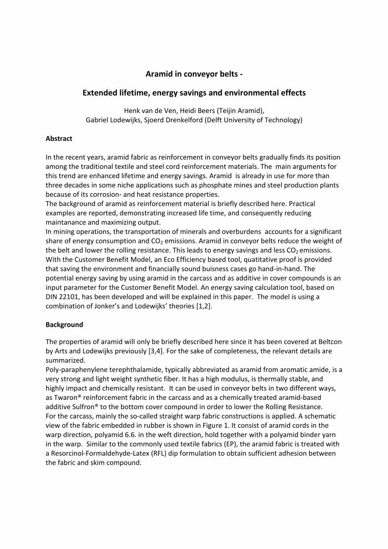
Aramid in conveyor belts -
Extended lifetime, energy savings and environmental effects
Henk van de Ven, Heidi Beers (Teijin Aramid), Gabriel Lodewijks, Sjoerd Drenkelford (Delft University of Technology)
Abstract In the recent years, aramid fabric as reinforcement in conveyor belts gradually finds its position among the traditional textile and steel cord reinforcement materials. The main arguments for this trend are enhanced lifetime and energy savings. Aramid is already in use for more than three decades in some niche applications such as phosphate mines and steel production plants because of its corrosion- and heat resistance properties. The background of aramid as reinforcement material is briefly described here. Practical examples are reported, demonstrating increased life time, and consequently reducing maintanance and maximizing output. In mining operations, the transportation of minerals and overburdens accounts for a significant share of energy consumption and CO2 emissions. Aramid in conveyor belts reduce the weight of the belt and lower the rolling resistance. This leads to energy savings and less CO2 emissions. With the Customer Benefit Model, an Eco Efficiency based tool, quatitative proof is provided that saving the environment and financially sound buisness cases go hand-in-hand. The potential energy saving by using aramid in the carcass and as additive in cover compounds is an input parameter for the Customer Benefit Model. An energy saving calculation tool, based on DIN 22101, has been developed and will be explained in this paper. The model is using a combination of Jonker’s and Lodewijks’ theories [1,2]. Background
The properties of aramid will only be briefly described here since it has been covered at Beltcon by Arts and Lodewijks previously [3,4]. For the sake of completeness, the relevant details are summarized. Poly-paraphenylene terephthalamide, typically abbreviated as aramid from aromatic amide, is a very strong and light weight synthetic fiber. It has a high modulus, is thermally stable, and highly impact and chemically resistant. It can be used in conveyor belts in two different ways, as Twaron® reinforcement fabric in the carcass and as a chemically treated aramid-based additive Sulfron® to the bottom cover compound in order to lower the Rolling Resistance. For the carcass, mainly the so-called straight warp fabric constructions is applied. A schematic view of the fabric embedded in rubber is shown in Figure 1. It consist of aramid cords in the warp direction, polyamid 6.6. in the weft direction, hold together with a polyamid binder yarn in the warp. Similar to the commonly used textile fabrics (EP), the aramid fabric is treated with a Resorcinol-Formaldehyde-Latex (RFL) dip formulation to obtain sufficient adhesion between the fabric and skim compound.
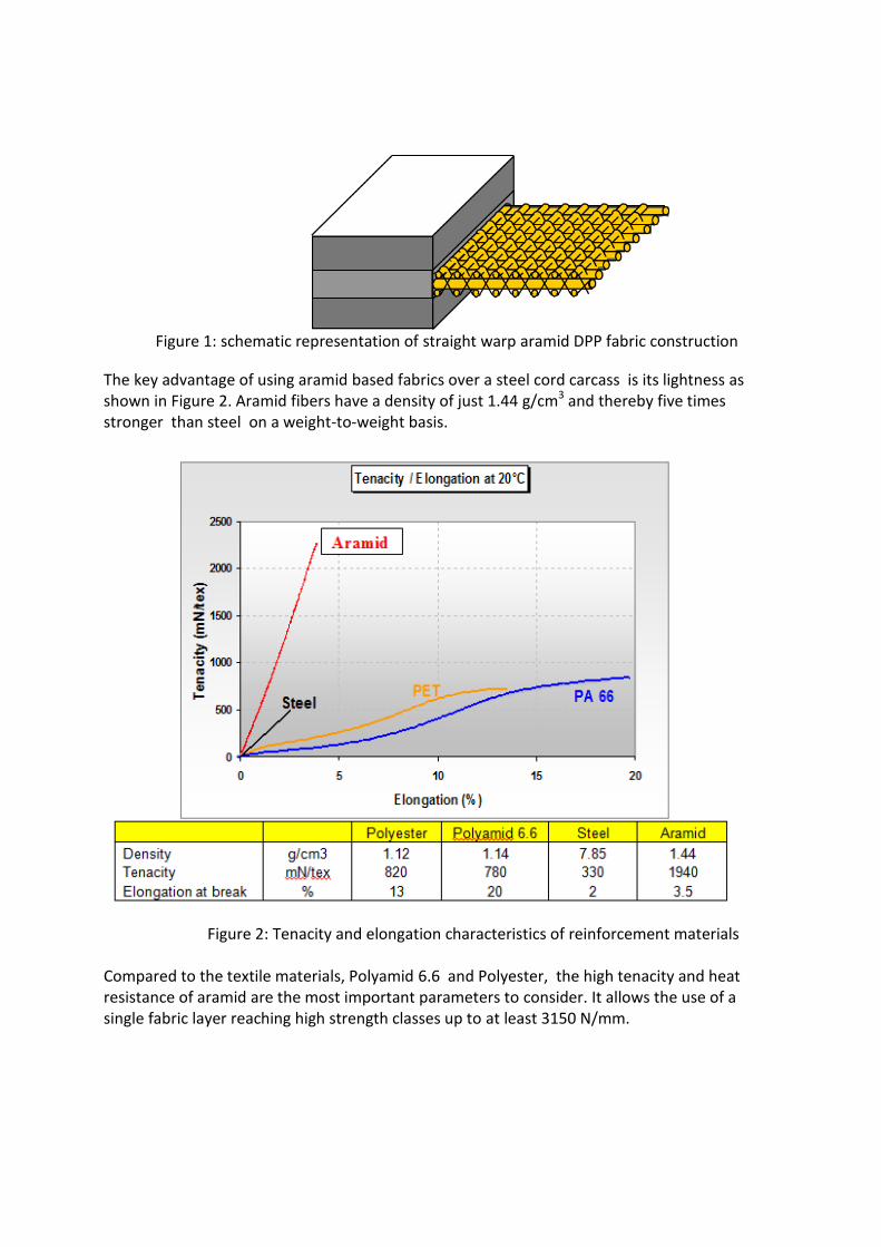
Figure 1: schematic representation of straight warp aramid DPP fabric construction
The key advantage of using aramid based fabrics over a steel cord carcass is its lightness as shown in Figure 2. Aramid fibers have a density of just 1.44 g/cm3 and thereby five times stronger than steel on a weight-to-weight basis.
Figure 2: Tenacity and elongation characteristics of reinforcement materials Compared to the textile materials, Polyamid 6.6 and Polyester, the high tenacity and heat resistance of aramid are the most important parameters to consider. It allows the use of a single fabric layer reaching high strength classes up to at least 3150 N/mm.
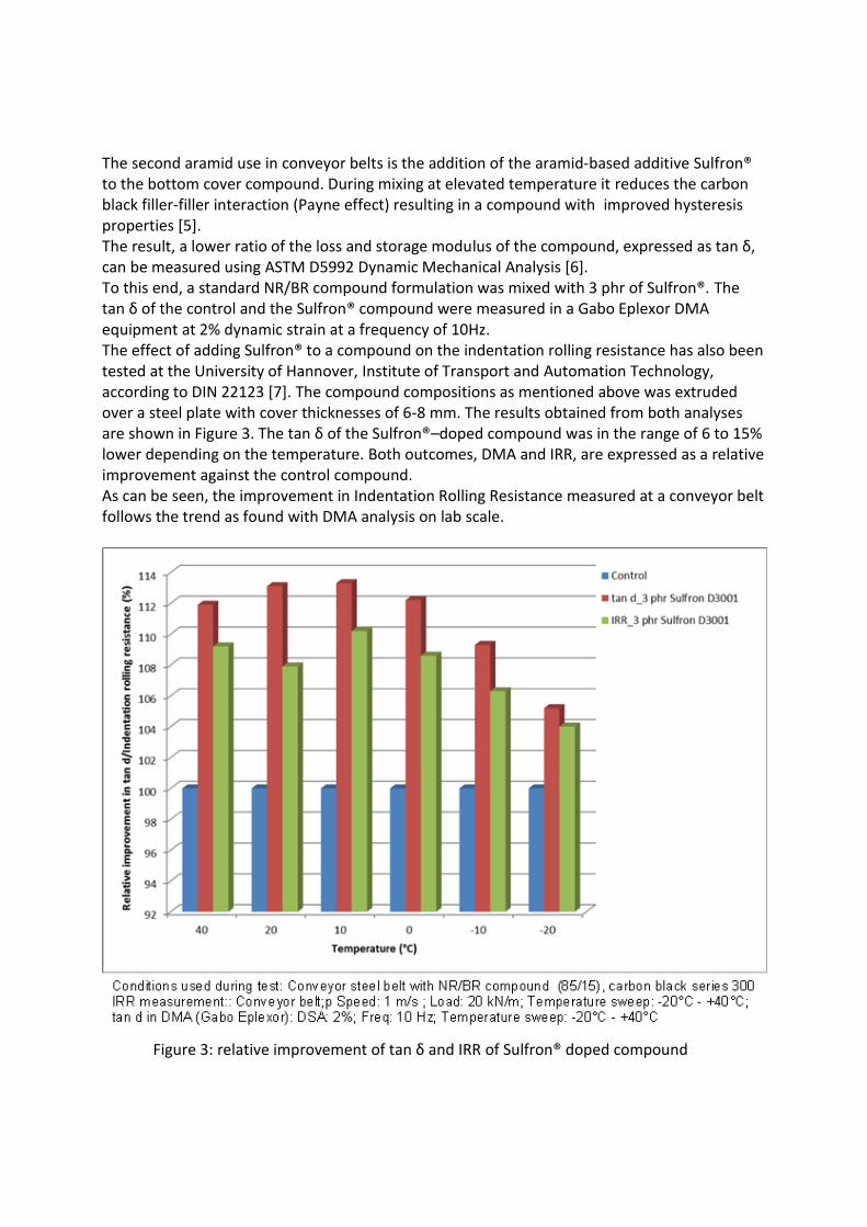
The second aramid use in conveyor belts is the addition of the aramid-based additive Sulfron® to the bottom cover compound. During mixing at elevated temperature it reduces the carbon black filler-filler interaction (Payne effect) resulting in a compound with improved hysteresis properties [5]. The result, a lower ratio of the loss and storage modulus of the compound, expressed as tan δ, can be measured using ASTM D5992 Dynamic Mechanical Analysis [6]. To this end, a standard NR/BR compound formulation was mixed with 3 phr of Sulfron®. The tan δ of the control and the Sulfron® compound were measured in a Gabo Eplexor DMA equipment at 2% dynamic strain at a frequency of 10Hz. The effect of adding Sulfron® to a compound on the indentation rolling resistance has also been tested at the University of Hannover, Institute of Transport and Automation Technology, according to DIN 22123 [7]. The compound compositions as mentioned above was extruded over a steel plate with cover thicknesses of 6-8 mm. The results obtained from both analyses are shown in Figure 3. The tan δ of the Sulfron®–doped compound was in the range of 6 to 15% lower depending on the temperature. Both outcomes, DMA and IRR, are expressed as a relative improvement against the control compound. As can be seen, the improvement in Indentation Rolling Resistance measured at a conveyor belt follows the trend as found with DMA analysis on lab scale.
Figure 3: relative improvement of tan δ and IRR of Sulfron® doped compound
Extended life time and additional advantages of using aramid
One of the traditional applications of aramid fabrics in conveyor belts has been in corrosive environments. Good examples are in Tunesia at the CPG (Gafsa) phosphate mine where a 4,6-km aramid belt was in operation for 9 years before being replaced again with aramid. Another aramid belt in a phosphate mine in Tampa (Florida, US) has been replaced last year after 13 years in operation. The aramid fabric retained about 85% of its original strength [8]. Rubber cover wear and tear were the reason for replacement in both cases. With its unique set of properties, aramid can be a solution for belts applied under extreme conditions having short life time. It should be studied case-by case. Some design parameters like transition length should be taken into account before replacing textile belts for example. The flexibility of the aramid fabric compared to steel cord has proven its functionality in a 110-m reclaimer belt in the Chinese Zhanjiang Port. This class St1600 belt had an average life time of six months because of the high turning frequency around the pulleys. The aramid belts have reached an average life time of fifteen months. Because of its dense and strong weft (the weaving threads in transversal direction), the aramid fabric also acts as an integrated breaking layer. This means that in the conveying of sharp and heavy rocks, like in copper mining, there is intrinsic protection against belt slitting, and no costly additional breaking layer or slitting detection is needed. An example in a copper mine, where a short steel belts typically had a very limited service life – typically as little as one month – an aramid belt recently ran for a full six months, which is well beyond the expected life expectancy of the previous non-aramid belts in this installation. After six months, the belt, which was still working fine, was taken out for residual testing by a Polish Mining University [9]. In Table 1, a St2500 and aramid DPP 2500 belt having typical dimensions are listed. The roll diameters have been calculated for both. It can be seen that at equal diameter of 2.71 m, the roll length of the aramid belt exceeds the length of the steel cord belt by far. Consequently, the number of splices in a long haul conveying system can be reduced considerably. For a 5-km belt to be installed, the number of splices is reduced from 17 to 12 in the example shown. It certainly contributes to limit downtime of the system and saves installation costs.
Steel cord belt St2500 Aramid belt DPP2500
Cord/fabric thickness [mm] 6,7 3
Min Cover [mm] 6 x 6 6 x 4
Width [mm] 1200 1200
Belt weight [kg/m] 38,3 20,5
300m roll 425 m roll 300m roll 425 m roll
Diameter [m] 2,71 3,23 2,28 2,71
Total belt weight [kg] 11488 16274 6153 8718
Table 1: belt weights and roll diameters of typical St2500 and DPP2500 belts
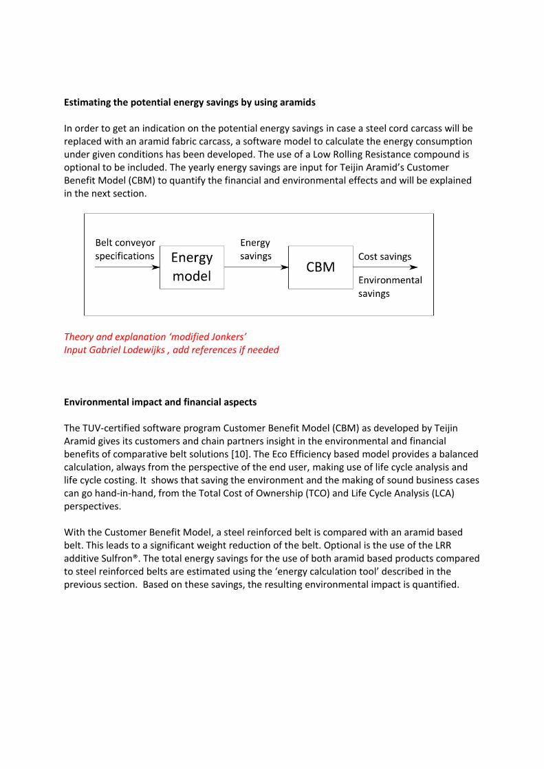
Estimating the potential energy savings by using aramids In order to get an indication on the potential energy savings in case a steel cord carcass will be replaced with an aramid fabric carcass, a software model to calculate the energy consumption under given conditions has been developed. The use of a Low Rolling Resistance compound is optional to be included. The yearly energy savings are input for Teijin Aramid’s Customer Benefit Model (CBM) to quantify the financial and environmental effects and will be explained in the next section.
Theory and explanation ‘modified Jonkers’ Input Gabriel Lodewijks , add references if needed
Environmental impact and financial aspects The TUV-certified software program Customer Benefit Model (CBM) as developed by Teijin Aramid gives its customers and chain partners insight in the environmental and financial benefits of comparative belt solutions [10]. The Eco Efficiency based model provides a balanced calculation, always from the perspective of the end user, making use of life cycle analysis and life cycle costing. It shows that saving the environment and the making of sound business cases can go hand-in-hand, from the Total Cost of Ownership (TCO) and Life Cycle Analysis (LCA) perspectives. With the Customer Benefit Model, a steel reinforced belt is compared with an aramid based belt. This leads to a significant weight reduction of the belt. Optional is the use of the LRR additive Sulfron®. The total energy savings for the use of both aramid based products compared to steel reinforced belts are estimated using the ‘energy calculation tool’ described in the previous section. Based on these savings, the resulting environmental impact is quantified.
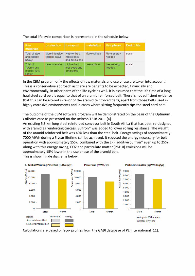
The total life cycle comparison is represented in the schedule below:
In the CBM program only the effects of raw materials and use phase are taken into account. This is a conservative approach as there are benefits to be expected, financially and environmentally, in other parts of the life cycle as well. It is assumed that the life time of a long haul steel cord belt is equal to that of an aramid reinforced belt. There is not sufficient evidence that this can be altered in favor of the aramid reinforced belts, apart from those belts used in highly corrosive environments and in cases where slitting frequently rips the steel cord belt. The outcome of the CBM software program will be demonstrated on the basis of the Optimum Collories case as presented on the Beltcon 16 in 2011 [4]. An existing 5,3 km long steel reinforced conveyor belt in South Africa that has been re-designed with aramid as reinforcing carcass. Sulfron® was added to lower rolling resistance. The weight of the aramid reinforced belt was 40% less than the steel belt. Energy savings of approximately 7000 MWh during a 5 year lifetime can be achieved. It reduced the energy necessary for belt operation with approximately 15%, combined with the LRR additive Sulfron® even up to 25% . Along with this energy saving, CO2 and particulate matter (PM10) emissions will be approximately 15% lower in the use phase of the aramid belt. This is shown in de diagrams below:
Calculations are based on eco- profiles from the GABI database of PE International [11].
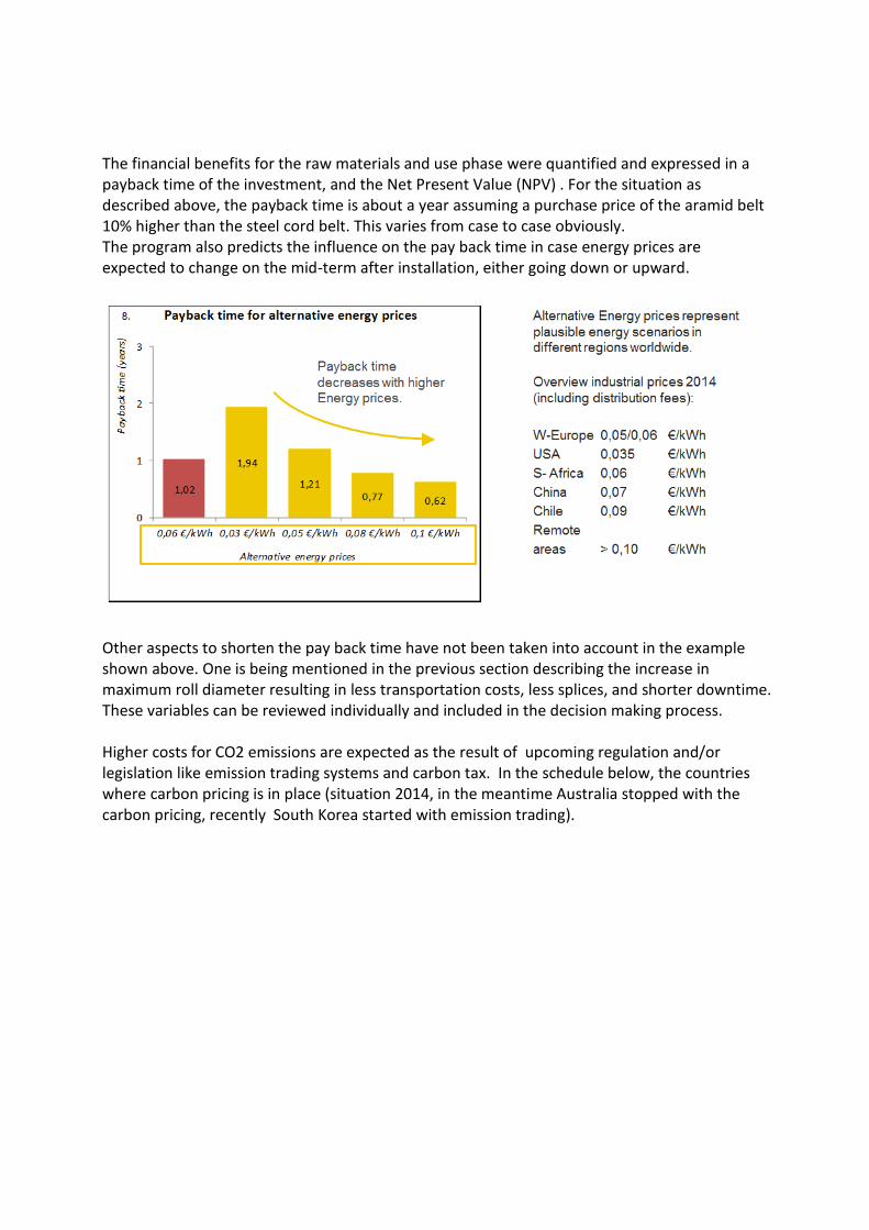
The financial benefits for the raw materials and use phase were quantified and expressed in a payback time of the investment, and the Net Present Value (NPV) . For the situation as described above, the payback time is about a year assuming a purchase price of the aramid belt 10% higher than the steel cord belt. This varies from case to case obviously. The program also predicts the influence on the pay back time in case energy prices are expected to change on the mid-term after installation, either going down or upward.
Other aspects to shorten the pay back time have not been taken into account in the example shown above. One is being mentioned in the previous section describing the increase in maximum roll diameter resulting in less transportation costs, less splices, and shorter downtime. These variables can be reviewed individually and included in the decision making process. Higher costs for CO2 emissions are expected as the result of upcoming regulation and/or legislation like emission trading systems and carbon tax. In the schedule below, the countries where carbon pricing is in place (situation 2014, in the meantime Australia stopped with the carbon pricing, recently South Korea started with emission trading).

The Customer Benefit Model is a next step on Eco Efficiency Analysis (EAA) as TUV certified tool. Variables and scenarios are implemented in the program making it possible to adapt to changing situations: belt prices, energy prices, raw material prices, eco-profiles etc. In sum, a business case for every specific situation. Conclusions Gabriel : conclusie nodig om te eindigen??
References
1. Jonkers C.O. (1980), “The indentation rolling resistance of belt conveyor - a theoretical
approach”, Fordern und Heben.
2. Lodewijks G. (1995), “The rolling resistance of conveyor belts”, Bulk Solids Handling 15,
pp.15-22.
3. Arts K. (2009), “Case study: aramid reinforced conveyor belt in Maritsa Istok power
plant”, Proceedings of the Beltcon 15 conference, Johannesburg, Republic of South
Africa, September 2-3, 2009
4. Lodewijks G. (2011), “The Next Generation Low Loss Conveyor Belts”, Proceedings of
the Beltcon 16 conference, Johannesburg, Republic of South Africa, August 3-4, 2011.
5. Huntink N. (2011), “Using Sulfron to Improve Rolling Resistance and Durability of Tires”,
Fall 180th Technical Meeting of the Rubber Division of the American Chemical Society,
Cleveland, Ohio.
6. ASTM D5992 -96 (re-approved 2006), “Standard Guide for Dynamic Testing of
Vulcanized Rubber and Rubber-Like Materials Using Vibratory Methods.”
7. ITA University Hannover, “Test Rig for Determination of Indentation Rolling Resistance
of Conveyor Belts according to DIN 22123.”
8. Info from bilateral discussions with Fenner Dunlop USA, October 2014.
9. Moore P. (Jan. 2015) , “Conveying cost down”, International Mining magazine.
10. Xxxxxxxxx references for Lodewijks
11. TUV EEA certificate nr. CO 600948550001, TUV Rheinland Nurnberg 2014
12. GaBi LCA Database v.6.3, 2013 PE International Stuttgart
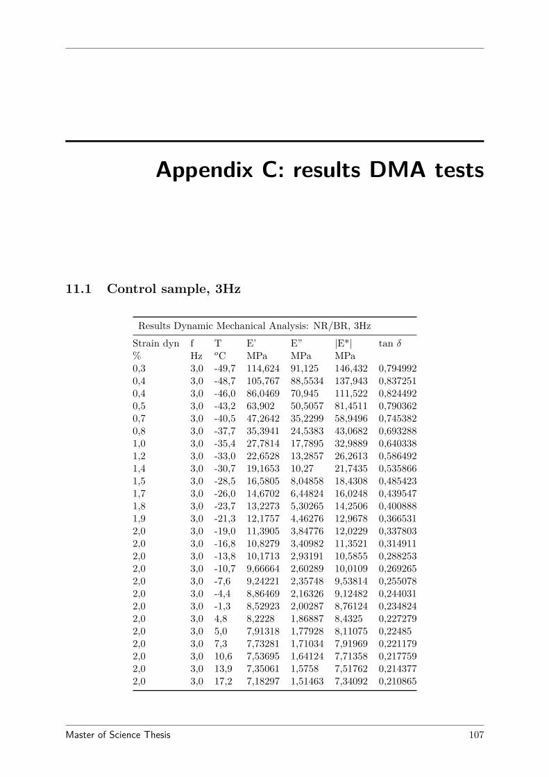
Appendix C: results DMA tests
11.1 Control sample, 3Hz
Results Dynamic Mechanical Analysis: NR/BR, 3Hz
Strain dyn f T E’ E” |E*| tan δ% Hz oC MPa MPa MPa0,3 3,0 -49,7 114,624 91,125 146,432 0,7949920,4 3,0 -48,7 105,767 88,5534 137,943 0,8372510,4 3,0 -46,0 86,0469 70,945 111,522 0,8244920,5 3,0 -43,2 63,902 50,5057 81,4511 0,7903620,7 3,0 -40,5 47,2642 35,2299 58,9496 0,7453820,8 3,0 -37,7 35,3941 24,5383 43,0682 0,6932881,0 3,0 -35,4 27,7814 17,7895 32,9889 0,6403381,2 3,0 -33,0 22,6528 13,2857 26,2613 0,5864921,4 3,0 -30,7 19,1653 10,27 21,7435 0,5358661,5 3,0 -28,5 16,5805 8,04858 18,4308 0,4854231,7 3,0 -26,0 14,6702 6,44824 16,0248 0,4395471,8 3,0 -23,7 13,2273 5,30265 14,2506 0,4008881,9 3,0 -21,3 12,1757 4,46276 12,9678 0,3665312,0 3,0 -19,0 11,3905 3,84776 12,0229 0,3378032,0 3,0 -16,8 10,8279 3,40982 11,3521 0,3149112,0 3,0 -13,8 10,1713 2,93191 10,5855 0,2882532,0 3,0 -10,7 9,66664 2,60289 10,0109 0,2692652,0 3,0 -7,6 9,24221 2,35748 9,53814 0,2550782,0 3,0 -4,4 8,86469 2,16326 9,12482 0,2440312,0 3,0 -1,3 8,52923 2,00287 8,76124 0,2348242,0 3,0 4,8 8,2228 1,86887 8,4325 0,2272792,0 3,0 5,0 7,91318 1,77928 8,11075 0,224852,0 3,0 7,3 7,73281 1,71034 7,91969 0,2211792,0 3,0 10,6 7,53695 1,64124 7,71358 0,2177592,0 3,0 13,9 7,35061 1,5758 7,51762 0,2143772,0 3,0 17,2 7,18297 1,51463 7,34092 0,210865
Master of Science Thesis 107
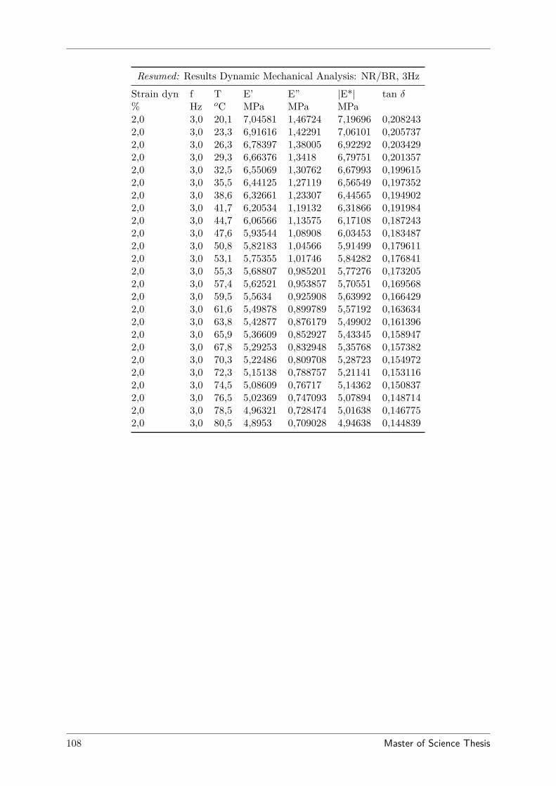
Resumed: Results Dynamic Mechanical Analysis: NR/BR, 3Hz
Strain dyn f T E’ E” |E*| tan δ% Hz oC MPa MPa MPa2,0 3,0 20,1 7,04581 1,46724 7,19696 0,2082432,0 3,0 23,3 6,91616 1,42291 7,06101 0,2057372,0 3,0 26,3 6,78397 1,38005 6,92292 0,2034292,0 3,0 29,3 6,66376 1,3418 6,79751 0,2013572,0 3,0 32,5 6,55069 1,30762 6,67993 0,1996152,0 3,0 35,5 6,44125 1,27119 6,56549 0,1973522,0 3,0 38,6 6,32661 1,23307 6,44565 0,1949022,0 3,0 41,7 6,20534 1,19132 6,31866 0,1919842,0 3,0 44,7 6,06566 1,13575 6,17108 0,1872432,0 3,0 47,6 5,93544 1,08908 6,03453 0,1834872,0 3,0 50,8 5,82183 1,04566 5,91499 0,1796112,0 3,0 53,1 5,75355 1,01746 5,84282 0,1768412,0 3,0 55,3 5,68807 0,985201 5,77276 0,1732052,0 3,0 57,4 5,62521 0,953857 5,70551 0,1695682,0 3,0 59,5 5,5634 0,925908 5,63992 0,1664292,0 3,0 61,6 5,49878 0,899789 5,57192 0,1636342,0 3,0 63,8 5,42877 0,876179 5,49902 0,1613962,0 3,0 65,9 5,36609 0,852927 5,43345 0,1589472,0 3,0 67,8 5,29253 0,832948 5,35768 0,1573822,0 3,0 70,3 5,22486 0,809708 5,28723 0,1549722,0 3,0 72,3 5,15138 0,788757 5,21141 0,1531162,0 3,0 74,5 5,08609 0,76717 5,14362 0,1508372,0 3,0 76,5 5,02369 0,747093 5,07894 0,1487142,0 3,0 78,5 4,96321 0,728474 5,01638 0,1467752,0 3,0 80,5 4,8953 0,709028 4,94638 0,144839
108 Master of Science Thesis
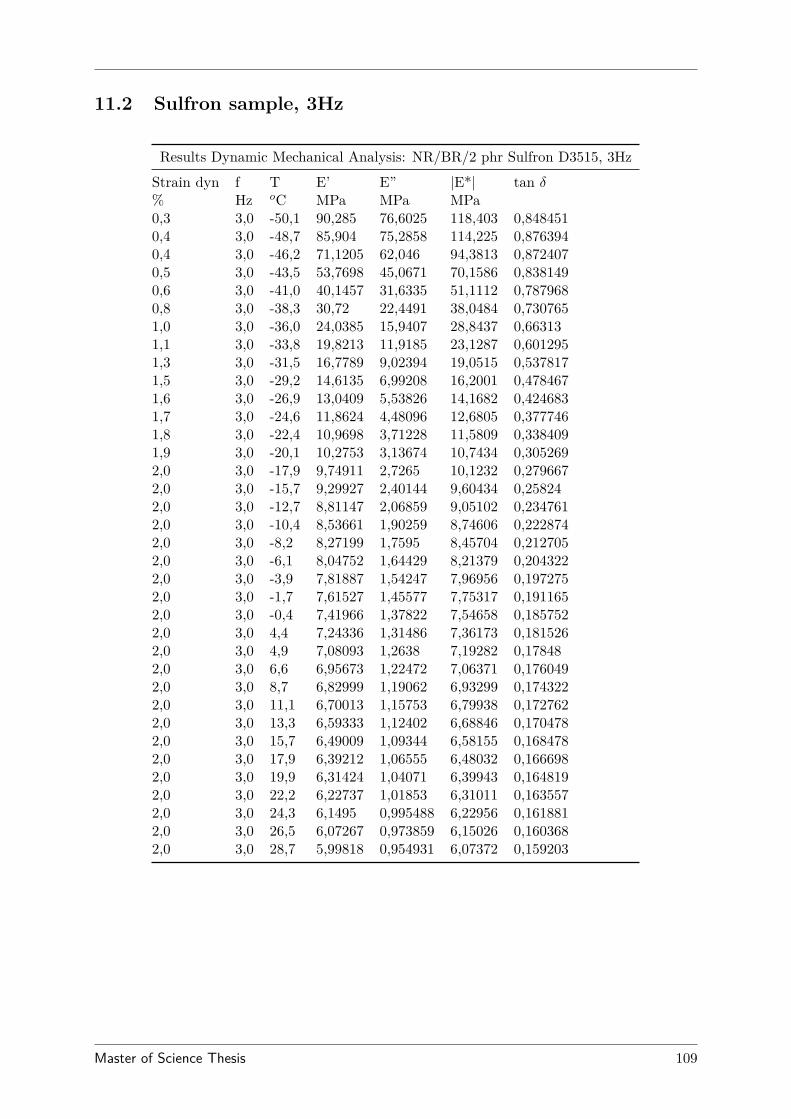
11.2 Sulfron sample, 3Hz
Results Dynamic Mechanical Analysis: NR/BR/2 phr Sulfron D3515, 3Hz
Strain dyn f T E’ E” |E*| tan δ% Hz oC MPa MPa MPa0,3 3,0 -50,1 90,285 76,6025 118,403 0,8484510,4 3,0 -48,7 85,904 75,2858 114,225 0,8763940,4 3,0 -46,2 71,1205 62,046 94,3813 0,8724070,5 3,0 -43,5 53,7698 45,0671 70,1586 0,8381490,6 3,0 -41,0 40,1457 31,6335 51,1112 0,7879680,8 3,0 -38,3 30,72 22,4491 38,0484 0,7307651,0 3,0 -36,0 24,0385 15,9407 28,8437 0,663131,1 3,0 -33,8 19,8213 11,9185 23,1287 0,6012951,3 3,0 -31,5 16,7789 9,02394 19,0515 0,5378171,5 3,0 -29,2 14,6135 6,99208 16,2001 0,4784671,6 3,0 -26,9 13,0409 5,53826 14,1682 0,4246831,7 3,0 -24,6 11,8624 4,48096 12,6805 0,3777461,8 3,0 -22,4 10,9698 3,71228 11,5809 0,3384091,9 3,0 -20,1 10,2753 3,13674 10,7434 0,3052692,0 3,0 -17,9 9,74911 2,7265 10,1232 0,2796672,0 3,0 -15,7 9,29927 2,40144 9,60434 0,258242,0 3,0 -12,7 8,81147 2,06859 9,05102 0,2347612,0 3,0 -10,4 8,53661 1,90259 8,74606 0,2228742,0 3,0 -8,2 8,27199 1,7595 8,45704 0,2127052,0 3,0 -6,1 8,04752 1,64429 8,21379 0,2043222,0 3,0 -3,9 7,81887 1,54247 7,96956 0,1972752,0 3,0 -1,7 7,61527 1,45577 7,75317 0,1911652,0 3,0 -0,4 7,41966 1,37822 7,54658 0,1857522,0 3,0 4,4 7,24336 1,31486 7,36173 0,1815262,0 3,0 4,9 7,08093 1,2638 7,19282 0,178482,0 3,0 6,6 6,95673 1,22472 7,06371 0,1760492,0 3,0 8,7 6,82999 1,19062 6,93299 0,1743222,0 3,0 11,1 6,70013 1,15753 6,79938 0,1727622,0 3,0 13,3 6,59333 1,12402 6,68846 0,1704782,0 3,0 15,7 6,49009 1,09344 6,58155 0,1684782,0 3,0 17,9 6,39212 1,06555 6,48032 0,1666982,0 3,0 19,9 6,31424 1,04071 6,39943 0,1648192,0 3,0 22,2 6,22737 1,01853 6,31011 0,1635572,0 3,0 24,3 6,1495 0,995488 6,22956 0,1618812,0 3,0 26,5 6,07267 0,973859 6,15026 0,1603682,0 3,0 28,7 5,99818 0,954931 6,07372 0,159203
Master of Science Thesis 109
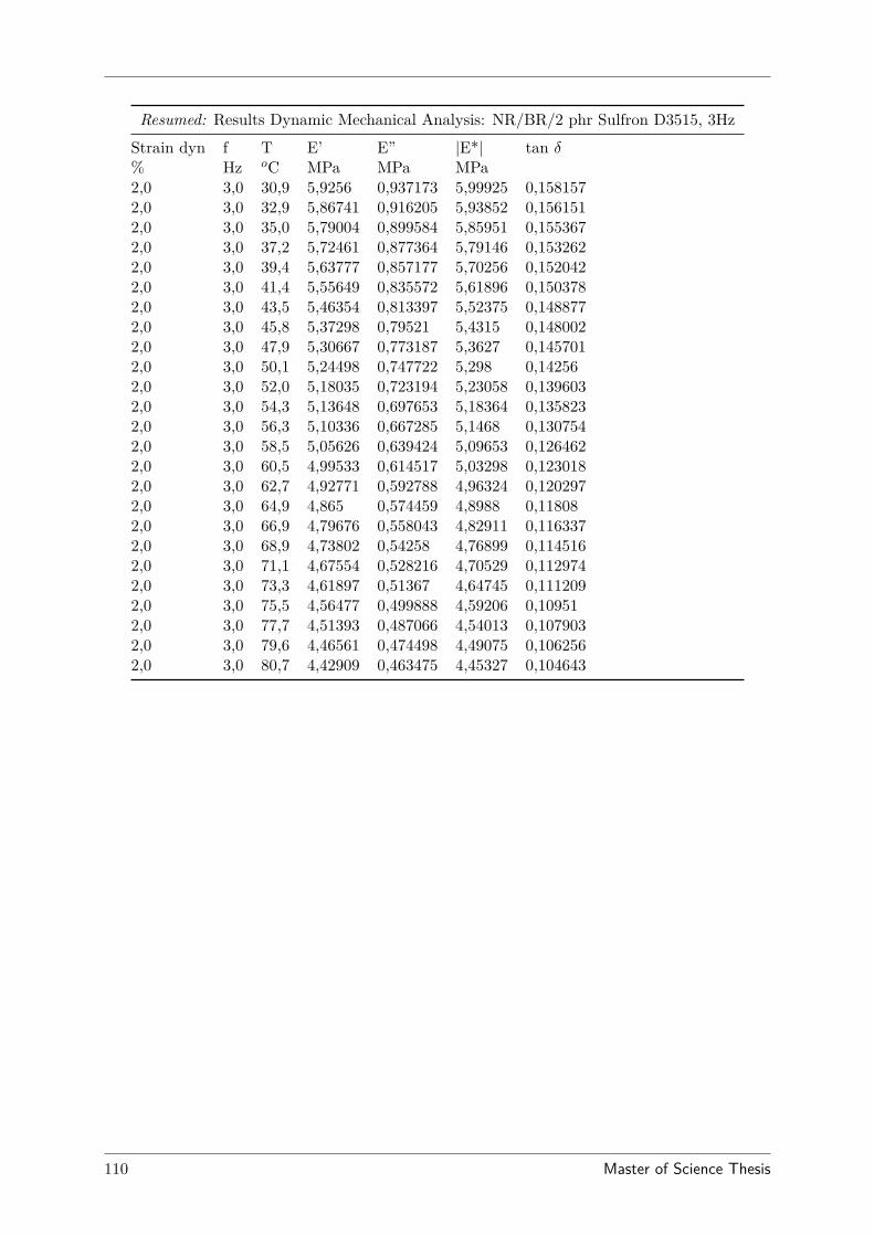
Resumed: Results Dynamic Mechanical Analysis: NR/BR/2 phr Sulfron D3515, 3Hz
Strain dyn f T E’ E” |E*| tan δ% Hz oC MPa MPa MPa2,0 3,0 30,9 5,9256 0,937173 5,99925 0,1581572,0 3,0 32,9 5,86741 0,916205 5,93852 0,1561512,0 3,0 35,0 5,79004 0,899584 5,85951 0,1553672,0 3,0 37,2 5,72461 0,877364 5,79146 0,1532622,0 3,0 39,4 5,63777 0,857177 5,70256 0,1520422,0 3,0 41,4 5,55649 0,835572 5,61896 0,1503782,0 3,0 43,5 5,46354 0,813397 5,52375 0,1488772,0 3,0 45,8 5,37298 0,79521 5,4315 0,1480022,0 3,0 47,9 5,30667 0,773187 5,3627 0,1457012,0 3,0 50,1 5,24498 0,747722 5,298 0,142562,0 3,0 52,0 5,18035 0,723194 5,23058 0,1396032,0 3,0 54,3 5,13648 0,697653 5,18364 0,1358232,0 3,0 56,3 5,10336 0,667285 5,1468 0,1307542,0 3,0 58,5 5,05626 0,639424 5,09653 0,1264622,0 3,0 60,5 4,99533 0,614517 5,03298 0,1230182,0 3,0 62,7 4,92771 0,592788 4,96324 0,1202972,0 3,0 64,9 4,865 0,574459 4,8988 0,118082,0 3,0 66,9 4,79676 0,558043 4,82911 0,1163372,0 3,0 68,9 4,73802 0,54258 4,76899 0,1145162,0 3,0 71,1 4,67554 0,528216 4,70529 0,1129742,0 3,0 73,3 4,61897 0,51367 4,64745 0,1112092,0 3,0 75,5 4,56477 0,499888 4,59206 0,109512,0 3,0 77,7 4,51393 0,487066 4,54013 0,1079032,0 3,0 79,6 4,46561 0,474498 4,49075 0,1062562,0 3,0 80,7 4,42909 0,463475 4,45327 0,104643
110 Master of Science Thesis
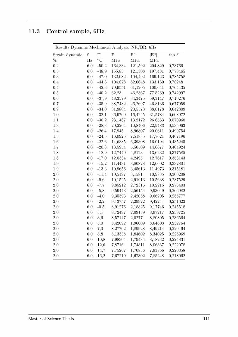
11.3 Control sample, 6Hz
Results Dynamic Mechanical Analysis: NR/BR, 6Hz
Strain dynamic f T E’ E” |E*| tan δ% Hz oC MPa MPa MPa0,2 6,0 -50,2 164,834 121,592 204,829 0,737660,3 6,0 -48,9 155,83 121,308 197,481 0,7784650,3 6,0 -47,0 132,982 104,492 169,123 0,7857580,4 6,0 -44,6 104,878 82,0648 133,169 0,782480,4 6,0 -42,3 79,9551 61,1205 100,641 0,7644350,5 6,0 -40,2 62,23 46,2367 77,5269 0,7429970,6 6,0 -37,9 48,3579 34,3475 59,3147 0,7102760,7 6,0 -35,9 38,7482 26,2697 46,8136 0,6779590,9 6,0 -34,0 31,9804 20,5573 38,0178 0,6428091,0 6,0 -32,1 26,9709 16,4245 31,5784 0,6089721,1 6,0 -30,2 23,1487 13,2172 26,6563 0,5709681,3 6,0 -28,3 20,2264 10,8406 22,9483 0,5359631,4 6,0 -26,4 17,945 8,96807 20,0611 0,4997541,5 6,0 -24,5 16,0925 7,51835 17,7621 0,4671961,6 6,0 -22,6 14,6885 6,39308 16,0194 0,4352451,7 6,0 -20,8 13,5954 5,50509 14,6677 0,4049241,8 6,0 -18,9 12,7449 4,8123 13,6232 0,3775851,8 6,0 -17,0 12,0334 4,2495 12,7617 0,3531431,9 6,0 -15,2 11,4431 3,80828 12,0602 0,3328011,9 6,0 -13,3 10,9656 3,45613 11,4973 0,3151812,0 6,0 -11,4 10,5197 3,1581 10,9835 0,3002082,0 6,0 -9,6 10,1525 2,91913 10,5638 0,2875292,0 6,0 -7,7 9,85212 2,72316 10,2215 0,2764032,0 6,0 -5,8 9,59443 2,56154 9,93049 0,2669822,0 6,0 -4,0 9,35393 2,42058 9,66205 0,2587772,0 6,0 -2,2 9,13757 2,29922 9,4224 0,2516222,0 6,0 -0,5 8,91276 2,18825 9,17746 0,2455182,0 6,0 3,1 8,72497 2,09159 8,97217 0,2397252,0 6,0 3,6 8,57147 2,0277 8,80805 0,2365642,0 6,0 5,0 8,42092 1,96009 8,64603 0,2327642,0 6,0 7,0 8,27702 1,89928 8,49214 0,2294642,0 6,0 8,8 8,13338 1,84602 8,34025 0,2269692,0 6,0 10,8 7,98304 1,79484 8,18232 0,2248312,0 6,0 12,6 7,8716 1,74811 8,06337 0,2220782,0 6,0 14,7 7,75267 1,70836 7,93866 0,2203582,0 6,0 16,2 7,67219 1,67302 7,85248 0,218062
Master of Science Thesis 111
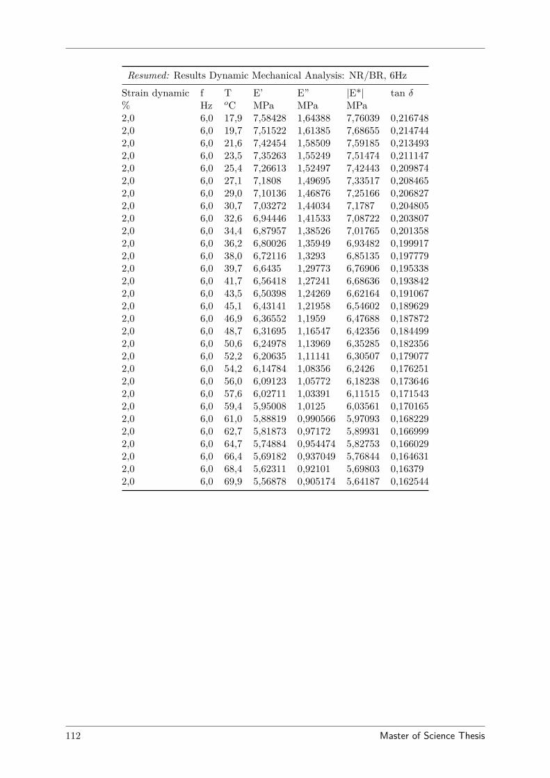
Resumed: Results Dynamic Mechanical Analysis: NR/BR, 6Hz
Strain dynamic f T E’ E” |E*| tan δ% Hz oC MPa MPa MPa2,0 6,0 17,9 7,58428 1,64388 7,76039 0,2167482,0 6,0 19,7 7,51522 1,61385 7,68655 0,2147442,0 6,0 21,6 7,42454 1,58509 7,59185 0,2134932,0 6,0 23,5 7,35263 1,55249 7,51474 0,2111472,0 6,0 25,4 7,26613 1,52497 7,42443 0,2098742,0 6,0 27,1 7,1808 1,49695 7,33517 0,2084652,0 6,0 29,0 7,10136 1,46876 7,25166 0,2068272,0 6,0 30,7 7,03272 1,44034 7,1787 0,2048052,0 6,0 32,6 6,94446 1,41533 7,08722 0,2038072,0 6,0 34,4 6,87957 1,38526 7,01765 0,2013582,0 6,0 36,2 6,80026 1,35949 6,93482 0,1999172,0 6,0 38,0 6,72116 1,3293 6,85135 0,1977792,0 6,0 39,7 6,6435 1,29773 6,76906 0,1953382,0 6,0 41,7 6,56418 1,27241 6,68636 0,1938422,0 6,0 43,5 6,50398 1,24269 6,62164 0,1910672,0 6,0 45,1 6,43141 1,21958 6,54602 0,1896292,0 6,0 46,9 6,36552 1,1959 6,47688 0,1878722,0 6,0 48,7 6,31695 1,16547 6,42356 0,1844992,0 6,0 50,6 6,24978 1,13969 6,35285 0,1823562,0 6,0 52,2 6,20635 1,11141 6,30507 0,1790772,0 6,0 54,2 6,14784 1,08356 6,2426 0,1762512,0 6,0 56,0 6,09123 1,05772 6,18238 0,1736462,0 6,0 57,6 6,02711 1,03391 6,11515 0,1715432,0 6,0 59,4 5,95008 1,0125 6,03561 0,1701652,0 6,0 61,0 5,88819 0,990566 5,97093 0,1682292,0 6,0 62,7 5,81873 0,97172 5,89931 0,1669992,0 6,0 64,7 5,74884 0,954474 5,82753 0,1660292,0 6,0 66,4 5,69182 0,937049 5,76844 0,1646312,0 6,0 68,4 5,62311 0,92101 5,69803 0,163792,0 6,0 69,9 5,56878 0,905174 5,64187 0,162544
112 Master of Science Thesis
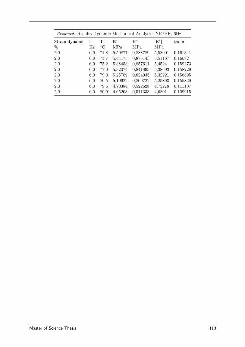
Resumed: Results Dynamic Mechanical Analysis: NR/BR, 6Hz
Strain dynamic f T E’ E” |E*| tan δ% Hz oC MPa MPa MPa2,0 6,0 71,8 5,50877 0,888789 5,58001 0,1613412,0 6,0 73,7 5,44175 0,875143 5,51167 0,160822,0 6,0 75,2 5,38453 0,857611 5,4524 0,1592732,0 6,0 77,0 5,32074 0,841893 5,38693 0,1582292,0 6,0 79,0 5,25789 0,824935 5,32221 0,1568952,0 6,0 80,5 5,19622 0,809722 5,25893 0,1558292,0 6,0 79,6 4,70384 0,522628 4,73278 0,1111072,0 6,0 80,9 4,65208 0,511333 4,6801 0,109915
Master of Science Thesis 113
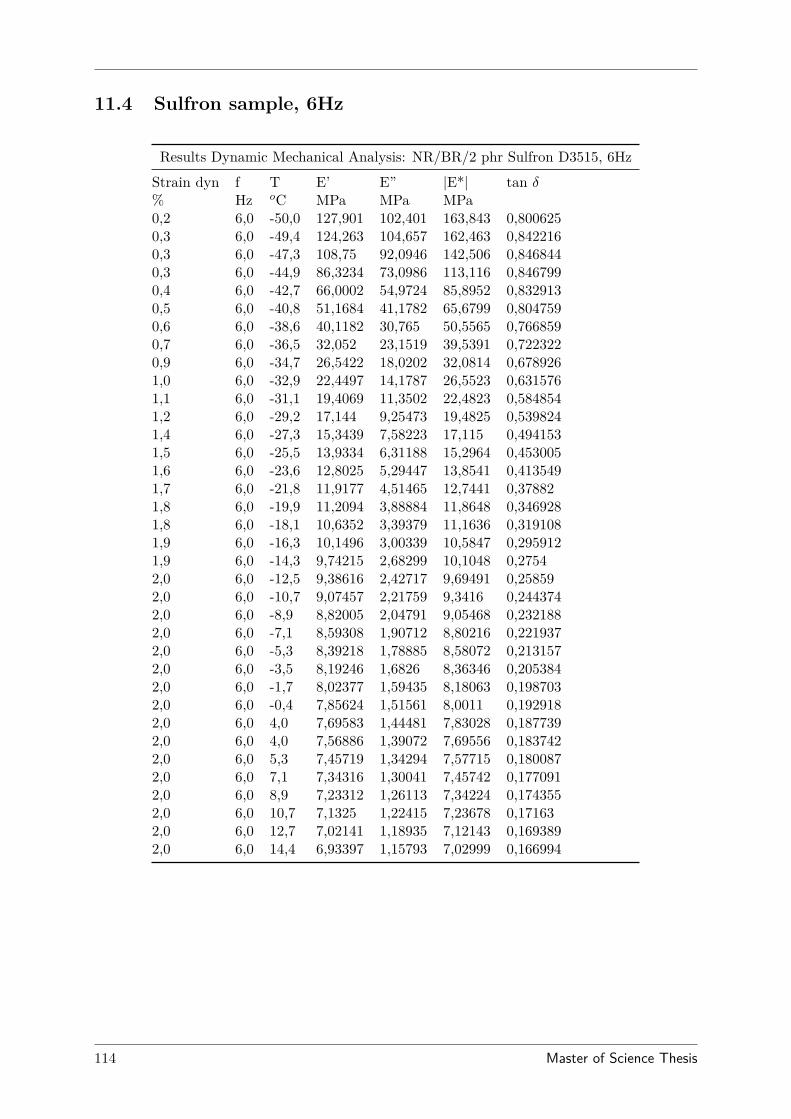
11.4 Sulfron sample, 6Hz
Results Dynamic Mechanical Analysis: NR/BR/2 phr Sulfron D3515, 6Hz
Strain dyn f T E’ E” |E*| tan δ% Hz oC MPa MPa MPa0,2 6,0 -50,0 127,901 102,401 163,843 0,8006250,3 6,0 -49,4 124,263 104,657 162,463 0,8422160,3 6,0 -47,3 108,75 92,0946 142,506 0,8468440,3 6,0 -44,9 86,3234 73,0986 113,116 0,8467990,4 6,0 -42,7 66,0002 54,9724 85,8952 0,8329130,5 6,0 -40,8 51,1684 41,1782 65,6799 0,8047590,6 6,0 -38,6 40,1182 30,765 50,5565 0,7668590,7 6,0 -36,5 32,052 23,1519 39,5391 0,7223220,9 6,0 -34,7 26,5422 18,0202 32,0814 0,6789261,0 6,0 -32,9 22,4497 14,1787 26,5523 0,6315761,1 6,0 -31,1 19,4069 11,3502 22,4823 0,5848541,2 6,0 -29,2 17,144 9,25473 19,4825 0,5398241,4 6,0 -27,3 15,3439 7,58223 17,115 0,4941531,5 6,0 -25,5 13,9334 6,31188 15,2964 0,4530051,6 6,0 -23,6 12,8025 5,29447 13,8541 0,4135491,7 6,0 -21,8 11,9177 4,51465 12,7441 0,378821,8 6,0 -19,9 11,2094 3,88884 11,8648 0,3469281,8 6,0 -18,1 10,6352 3,39379 11,1636 0,3191081,9 6,0 -16,3 10,1496 3,00339 10,5847 0,2959121,9 6,0 -14,3 9,74215 2,68299 10,1048 0,27542,0 6,0 -12,5 9,38616 2,42717 9,69491 0,258592,0 6,0 -10,7 9,07457 2,21759 9,3416 0,2443742,0 6,0 -8,9 8,82005 2,04791 9,05468 0,2321882,0 6,0 -7,1 8,59308 1,90712 8,80216 0,2219372,0 6,0 -5,3 8,39218 1,78885 8,58072 0,2131572,0 6,0 -3,5 8,19246 1,6826 8,36346 0,2053842,0 6,0 -1,7 8,02377 1,59435 8,18063 0,1987032,0 6,0 -0,4 7,85624 1,51561 8,0011 0,1929182,0 6,0 4,0 7,69583 1,44481 7,83028 0,1877392,0 6,0 4,0 7,56886 1,39072 7,69556 0,1837422,0 6,0 5,3 7,45719 1,34294 7,57715 0,1800872,0 6,0 7,1 7,34316 1,30041 7,45742 0,1770912,0 6,0 8,9 7,23312 1,26113 7,34224 0,1743552,0 6,0 10,7 7,1325 1,22415 7,23678 0,171632,0 6,0 12,7 7,02141 1,18935 7,12143 0,1693892,0 6,0 14,4 6,93397 1,15793 7,02999 0,166994
114 Master of Science Thesis
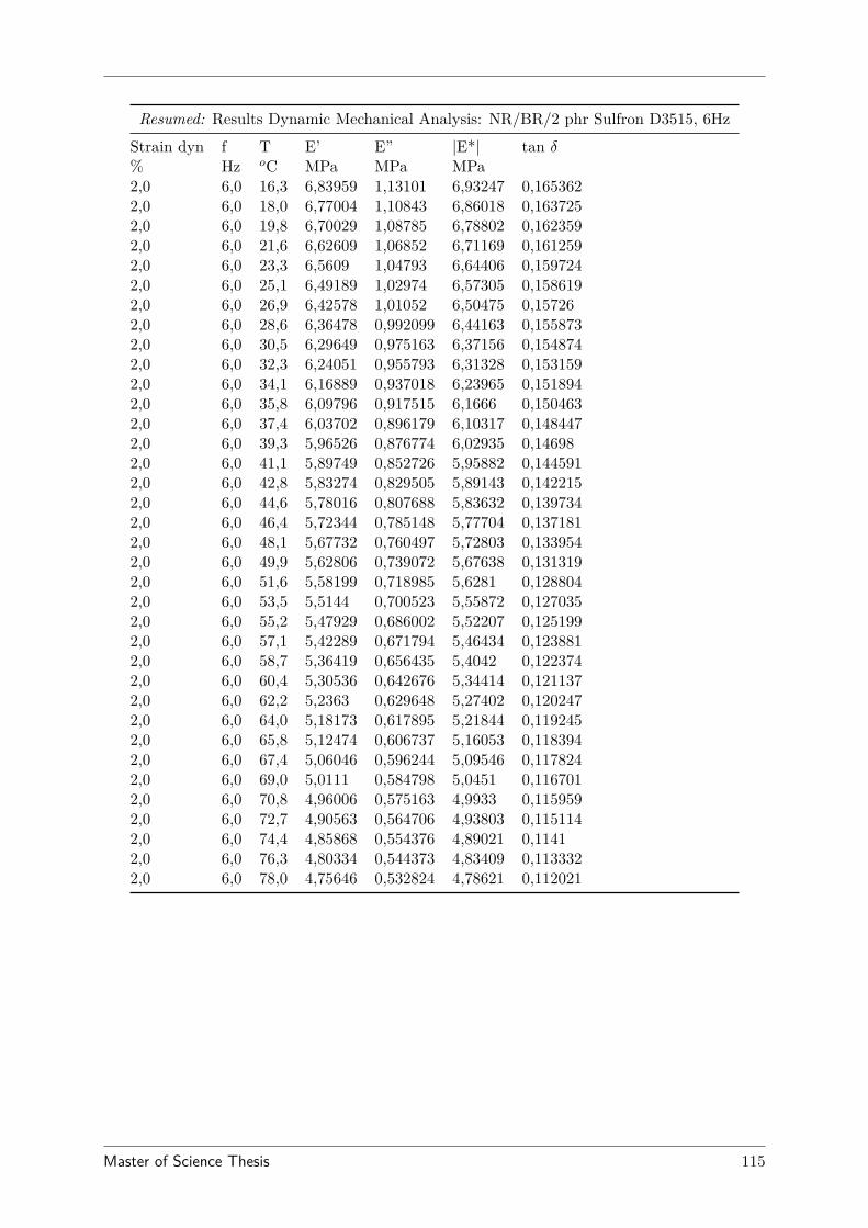
Resumed: Results Dynamic Mechanical Analysis: NR/BR/2 phr Sulfron D3515, 6Hz
Strain dyn f T E’ E” |E*| tan δ% Hz oC MPa MPa MPa2,0 6,0 16,3 6,83959 1,13101 6,93247 0,1653622,0 6,0 18,0 6,77004 1,10843 6,86018 0,1637252,0 6,0 19,8 6,70029 1,08785 6,78802 0,1623592,0 6,0 21,6 6,62609 1,06852 6,71169 0,1612592,0 6,0 23,3 6,5609 1,04793 6,64406 0,1597242,0 6,0 25,1 6,49189 1,02974 6,57305 0,1586192,0 6,0 26,9 6,42578 1,01052 6,50475 0,157262,0 6,0 28,6 6,36478 0,992099 6,44163 0,1558732,0 6,0 30,5 6,29649 0,975163 6,37156 0,1548742,0 6,0 32,3 6,24051 0,955793 6,31328 0,1531592,0 6,0 34,1 6,16889 0,937018 6,23965 0,1518942,0 6,0 35,8 6,09796 0,917515 6,1666 0,1504632,0 6,0 37,4 6,03702 0,896179 6,10317 0,1484472,0 6,0 39,3 5,96526 0,876774 6,02935 0,146982,0 6,0 41,1 5,89749 0,852726 5,95882 0,1445912,0 6,0 42,8 5,83274 0,829505 5,89143 0,1422152,0 6,0 44,6 5,78016 0,807688 5,83632 0,1397342,0 6,0 46,4 5,72344 0,785148 5,77704 0,1371812,0 6,0 48,1 5,67732 0,760497 5,72803 0,1339542,0 6,0 49,9 5,62806 0,739072 5,67638 0,1313192,0 6,0 51,6 5,58199 0,718985 5,6281 0,1288042,0 6,0 53,5 5,5144 0,700523 5,55872 0,1270352,0 6,0 55,2 5,47929 0,686002 5,52207 0,1251992,0 6,0 57,1 5,42289 0,671794 5,46434 0,1238812,0 6,0 58,7 5,36419 0,656435 5,4042 0,1223742,0 6,0 60,4 5,30536 0,642676 5,34414 0,1211372,0 6,0 62,2 5,2363 0,629648 5,27402 0,1202472,0 6,0 64,0 5,18173 0,617895 5,21844 0,1192452,0 6,0 65,8 5,12474 0,606737 5,16053 0,1183942,0 6,0 67,4 5,06046 0,596244 5,09546 0,1178242,0 6,0 69,0 5,0111 0,584798 5,0451 0,1167012,0 6,0 70,8 4,96006 0,575163 4,9933 0,1159592,0 6,0 72,7 4,90563 0,564706 4,93803 0,1151142,0 6,0 74,4 4,85868 0,554376 4,89021 0,11412,0 6,0 76,3 4,80334 0,544373 4,83409 0,1133322,0 6,0 78,0 4,75646 0,532824 4,78621 0,112021
Master of Science Thesis 115
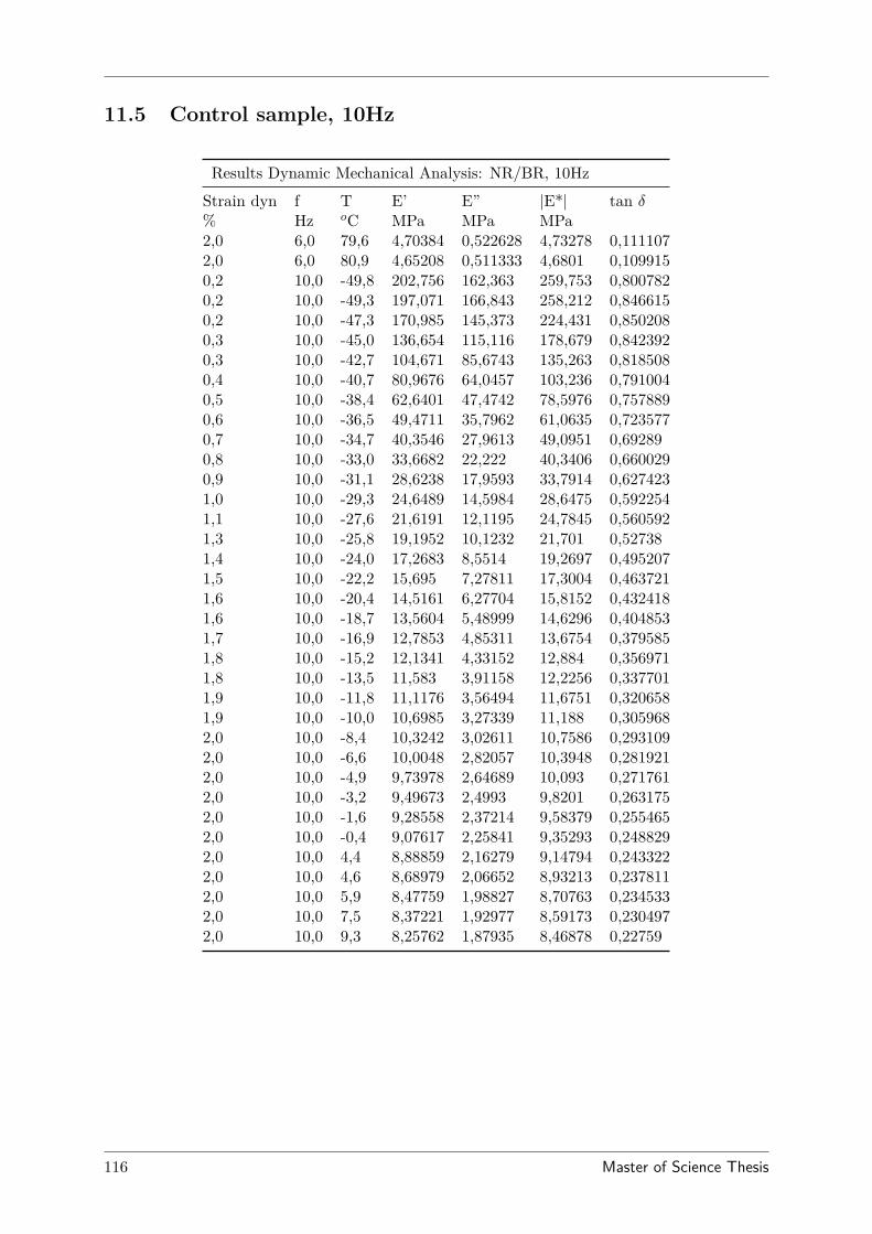
11.5 Control sample, 10Hz
Results Dynamic Mechanical Analysis: NR/BR, 10Hz
Strain dyn f T E’ E” |E*| tan δ% Hz oC MPa MPa MPa2,0 6,0 79,6 4,70384 0,522628 4,73278 0,1111072,0 6,0 80,9 4,65208 0,511333 4,6801 0,1099150,2 10,0 -49,8 202,756 162,363 259,753 0,8007820,2 10,0 -49,3 197,071 166,843 258,212 0,8466150,2 10,0 -47,3 170,985 145,373 224,431 0,8502080,3 10,0 -45,0 136,654 115,116 178,679 0,8423920,3 10,0 -42,7 104,671 85,6743 135,263 0,8185080,4 10,0 -40,7 80,9676 64,0457 103,236 0,7910040,5 10,0 -38,4 62,6401 47,4742 78,5976 0,7578890,6 10,0 -36,5 49,4711 35,7962 61,0635 0,7235770,7 10,0 -34,7 40,3546 27,9613 49,0951 0,692890,8 10,0 -33,0 33,6682 22,222 40,3406 0,6600290,9 10,0 -31,1 28,6238 17,9593 33,7914 0,6274231,0 10,0 -29,3 24,6489 14,5984 28,6475 0,5922541,1 10,0 -27,6 21,6191 12,1195 24,7845 0,5605921,3 10,0 -25,8 19,1952 10,1232 21,701 0,527381,4 10,0 -24,0 17,2683 8,5514 19,2697 0,4952071,5 10,0 -22,2 15,695 7,27811 17,3004 0,4637211,6 10,0 -20,4 14,5161 6,27704 15,8152 0,4324181,6 10,0 -18,7 13,5604 5,48999 14,6296 0,4048531,7 10,0 -16,9 12,7853 4,85311 13,6754 0,3795851,8 10,0 -15,2 12,1341 4,33152 12,884 0,3569711,8 10,0 -13,5 11,583 3,91158 12,2256 0,3377011,9 10,0 -11,8 11,1176 3,56494 11,6751 0,3206581,9 10,0 -10,0 10,6985 3,27339 11,188 0,3059682,0 10,0 -8,4 10,3242 3,02611 10,7586 0,2931092,0 10,0 -6,6 10,0048 2,82057 10,3948 0,2819212,0 10,0 -4,9 9,73978 2,64689 10,093 0,2717612,0 10,0 -3,2 9,49673 2,4993 9,8201 0,2631752,0 10,0 -1,6 9,28558 2,37214 9,58379 0,2554652,0 10,0 -0,4 9,07617 2,25841 9,35293 0,2488292,0 10,0 4,4 8,88859 2,16279 9,14794 0,2433222,0 10,0 4,6 8,68979 2,06652 8,93213 0,2378112,0 10,0 5,9 8,47759 1,98827 8,70763 0,2345332,0 10,0 7,5 8,37221 1,92977 8,59173 0,2304972,0 10,0 9,3 8,25762 1,87935 8,46878 0,22759
116 Master of Science Thesis
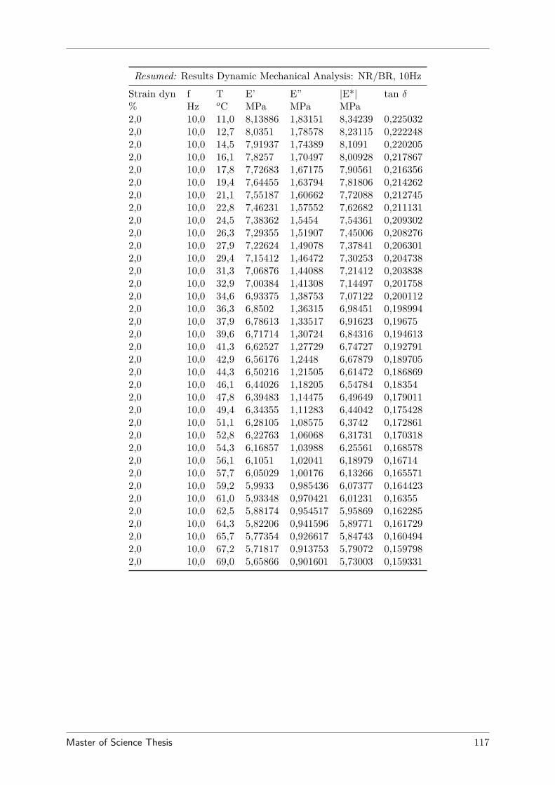
Resumed: Results Dynamic Mechanical Analysis: NR/BR, 10Hz
Strain dyn f T E’ E” |E*| tan δ% Hz oC MPa MPa MPa2,0 10,0 11,0 8,13886 1,83151 8,34239 0,2250322,0 10,0 12,7 8,0351 1,78578 8,23115 0,2222482,0 10,0 14,5 7,91937 1,74389 8,1091 0,2202052,0 10,0 16,1 7,8257 1,70497 8,00928 0,2178672,0 10,0 17,8 7,72683 1,67175 7,90561 0,2163562,0 10,0 19,4 7,64455 1,63794 7,81806 0,2142622,0 10,0 21,1 7,55187 1,60662 7,72088 0,2127452,0 10,0 22,8 7,46231 1,57552 7,62682 0,2111312,0 10,0 24,5 7,38362 1,5454 7,54361 0,2093022,0 10,0 26,3 7,29355 1,51907 7,45006 0,2082762,0 10,0 27,9 7,22624 1,49078 7,37841 0,2063012,0 10,0 29,4 7,15412 1,46472 7,30253 0,2047382,0 10,0 31,3 7,06876 1,44088 7,21412 0,2038382,0 10,0 32,9 7,00384 1,41308 7,14497 0,2017582,0 10,0 34,6 6,93375 1,38753 7,07122 0,2001122,0 10,0 36,3 6,8502 1,36315 6,98451 0,1989942,0 10,0 37,9 6,78613 1,33517 6,91623 0,196752,0 10,0 39,6 6,71714 1,30724 6,84316 0,1946132,0 10,0 41,3 6,62527 1,27729 6,74727 0,1927912,0 10,0 42,9 6,56176 1,2448 6,67879 0,1897052,0 10,0 44,3 6,50216 1,21505 6,61472 0,1868692,0 10,0 46,1 6,44026 1,18205 6,54784 0,183542,0 10,0 47,8 6,39483 1,14475 6,49649 0,1790112,0 10,0 49,4 6,34355 1,11283 6,44042 0,1754282,0 10,0 51,1 6,28105 1,08575 6,3742 0,1728612,0 10,0 52,8 6,22763 1,06068 6,31731 0,1703182,0 10,0 54,3 6,16857 1,03988 6,25561 0,1685782,0 10,0 56,1 6,1051 1,02041 6,18979 0,167142,0 10,0 57,7 6,05029 1,00176 6,13266 0,1655712,0 10,0 59,2 5,9933 0,985436 6,07377 0,1644232,0 10,0 61,0 5,93348 0,970421 6,01231 0,163552,0 10,0 62,5 5,88174 0,954517 5,95869 0,1622852,0 10,0 64,3 5,82206 0,941596 5,89771 0,1617292,0 10,0 65,7 5,77354 0,926617 5,84743 0,1604942,0 10,0 67,2 5,71817 0,913753 5,79072 0,1597982,0 10,0 69,0 5,65866 0,901601 5,73003 0,159331
Master of Science Thesis 117
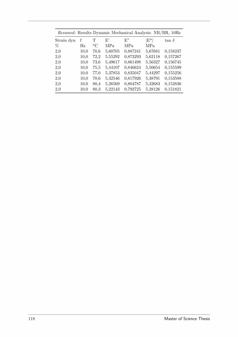
Resumed: Results Dynamic Mechanical Analysis: NR/BR, 10Hz
Strain dyn f T E’ E” |E*| tan δ% Hz oC MPa MPa MPa2,0 10,0 70,6 5,60705 0,887241 5,67681 0,1582372,0 10,0 72,2 5,55292 0,873293 5,62118 0,1572672,0 10,0 73,6 5,49617 0,861498 5,56327 0,1567452,0 10,0 75,5 5,44107 0,846624 5,50654 0,1555992,0 10,0 77,0 5,37853 0,835047 5,44297 0,1552562,0 10,0 78,6 5,32546 0,817926 5,38791 0,1535882,0 10,0 80,4 5,26569 0,804787 5,32683 0,1528362,0 10,0 80,3 5,22143 0,792725 5,28126 0,151821
118 Master of Science Thesis
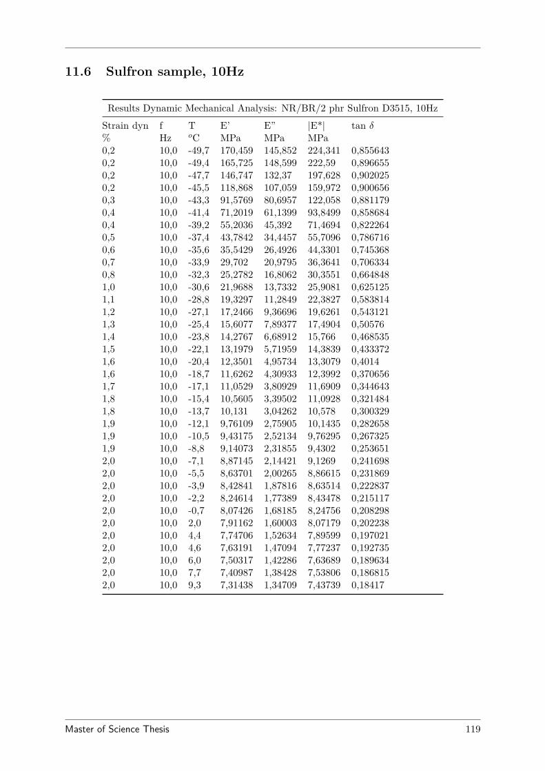
11.6 Sulfron sample, 10Hz
Results Dynamic Mechanical Analysis: NR/BR/2 phr Sulfron D3515, 10Hz
Strain dyn f T E’ E” |E*| tan δ% Hz oC MPa MPa MPa0,2 10,0 -49,7 170,459 145,852 224,341 0,8556430,2 10,0 -49,4 165,725 148,599 222,59 0,8966550,2 10,0 -47,7 146,747 132,37 197,628 0,9020250,2 10,0 -45,5 118,868 107,059 159,972 0,9006560,3 10,0 -43,3 91,5769 80,6957 122,058 0,8811790,4 10,0 -41,4 71,2019 61,1399 93,8499 0,8586840,4 10,0 -39,2 55,2036 45,392 71,4694 0,8222640,5 10,0 -37,4 43,7842 34,4457 55,7096 0,7867160,6 10,0 -35,6 35,5429 26,4926 44,3301 0,7453680,7 10,0 -33,9 29,702 20,9795 36,3641 0,7063340,8 10,0 -32,3 25,2782 16,8062 30,3551 0,6648481,0 10,0 -30,6 21,9688 13,7332 25,9081 0,6251251,1 10,0 -28,8 19,3297 11,2849 22,3827 0,5838141,2 10,0 -27,1 17,2466 9,36696 19,6261 0,5431211,3 10,0 -25,4 15,6077 7,89377 17,4904 0,505761,4 10,0 -23,8 14,2767 6,68912 15,766 0,4685351,5 10,0 -22,1 13,1979 5,71959 14,3839 0,4333721,6 10,0 -20,4 12,3501 4,95734 13,3079 0,40141,6 10,0 -18,7 11,6262 4,30933 12,3992 0,3706561,7 10,0 -17,1 11,0529 3,80929 11,6909 0,3446431,8 10,0 -15,4 10,5605 3,39502 11,0928 0,3214841,8 10,0 -13,7 10,131 3,04262 10,578 0,3003291,9 10,0 -12,1 9,76109 2,75905 10,1435 0,2826581,9 10,0 -10,5 9,43175 2,52134 9,76295 0,2673251,9 10,0 -8,8 9,14073 2,31855 9,4302 0,2536512,0 10,0 -7,1 8,87145 2,14421 9,1269 0,2416982,0 10,0 -5,5 8,63701 2,00265 8,86615 0,2318692,0 10,0 -3,9 8,42841 1,87816 8,63514 0,2228372,0 10,0 -2,2 8,24614 1,77389 8,43478 0,2151172,0 10,0 -0,7 8,07426 1,68185 8,24756 0,2082982,0 10,0 2,0 7,91162 1,60003 8,07179 0,2022382,0 10,0 4,4 7,74706 1,52634 7,89599 0,1970212,0 10,0 4,6 7,63191 1,47094 7,77237 0,1927352,0 10,0 6,0 7,50317 1,42286 7,63689 0,1896342,0 10,0 7,7 7,40987 1,38428 7,53806 0,1868152,0 10,0 9,3 7,31438 1,34709 7,43739 0,18417
Master of Science Thesis 119
Resumed: Results Dynamic Mechanical Analysis: NR/BR/2 phr Sulfron D3515, 10Hz
Strain dyn f T E’ E” |E*| tan δ% Hz oC MPa MPa MPa2,0 10,0 11,0 7,21081 1,31401 7,32956 0,1822282,0 10,0 12,7 7,11594 1,28242 7,23058 0,1802182,0 10,0 14,5 7,01204 1,25284 7,12308 0,1786692,0 10,0 15,9 6,93178 1,22905 7,03989 0,1773062,0 10,0 17,5 6,85423 1,2065 6,9596 0,1760222,0 10,0 19,3 6,76934 1,18285 6,87191 0,1747362,0 10,0 21,0 6,709 1,16045 6,80862 0,1729692,0 10,0 22,6 6,64006 1,13899 6,73704 0,1715332,0 10,0 24,3 6,5608 1,11862 6,65548 0,1705012,0 10,0 25,9 6,50121 1,09721 6,59315 0,1687712,0 10,0 27,5 6,43703 1,07801 6,52667 0,167472,0 10,0 29,2 6,36446 1,05991 6,45211 0,1665352,0 10,0 30,8 6,31231 1,04043 6,39748 0,1648262,0 10,0 32,3 6,25134 1,02259 6,33443 0,1635792,0 10,0 34,0 6,18573 1,0051 6,26686 0,1624862,0 10,0 35,5 6,13014 0,98585 6,20891 0,160822,0 10,0 37,3 6,06088 0,967621 6,13764 0,159652,0 10,0 38,7 6,01409 0,945687 6,08799 0,1572452,0 10,0 40,4 5,95971 0,924039 6,03092 0,1550482,0 10,0 42,2 5,89025 0,899757 5,95858 0,1527542,0 10,0 43,8 5,84041 0,875851 5,90572 0,1499642,0 10,0 45,4 5,78826 0,856003 5,85121 0,1478862,0 10,0 47,1 5,73538 0,83561 5,79594 0,1456942,0 10,0 48,7 5,69063 0,814342 5,7486 0,1431022,0 10,0 50,2 5,65141 0,792007 5,70664 0,1401432,0 10,0 51,6 5,60552 0,772247 5,65846 0,1377662,0 10,0 53,4 5,56386 0,750365 5,61423 0,1348642,0 10,0 55,1 5,50712 0,731581 5,5555 0,1328432,0 10,0 56,6 5,45727 0,712418 5,50358 0,1305452,0 10,0 58,2 5,39132 0,695881 5,43605 0,1290742,0 10,0 59,9 5,34119 0,682245 5,38459 0,1277332,0 10,0 61,4 5,2873 0,668125 5,32935 0,1263642,0 10,0 63,2 5,22333 0,655469 5,2643 0,1254892,0 10,0 64,5 5,17363 0,644094 5,21357 0,1244952,0 10,0 66,2 5,11805 0,63328 5,15708 0,1237342,0 10,0 68,0 5,06615 0,621822 5,10416 0,122741
120 Master of Science Thesis
Resumed: Results Dynamic Mechanical Analysis: NR/BR/2 phr Sulfron D3515, 10Hz
Strain dyn f T E’ E” |E*| tan δ% Hz oC MPa MPa MPa2,0 10,0 69,6 5,01764 0,612115 5,05484 0,1219932,0 10,0 71,0 4,96916 0,601964 5,00549 0,121142,0 10,0 72,6 4,92372 0,591811 4,95915 0,1201962,0 10,0 74,2 4,87236 0,581573 4,90695 0,1193622,0 10,0 75,9 4,82868 0,572053 4,86245 0,118472,0 10,0 77,5 4,78235 0,561974 4,81526 0,117512,0 10,0 79,0 4,73377 0,551401 4,76578 0,1164822,0 10,0 80,5 4,68887 0,540792 4,71995 0,1153352,0 10,0 80,9 4,64963 0,532194 4,67999 0,114459
Master of Science Thesis 121
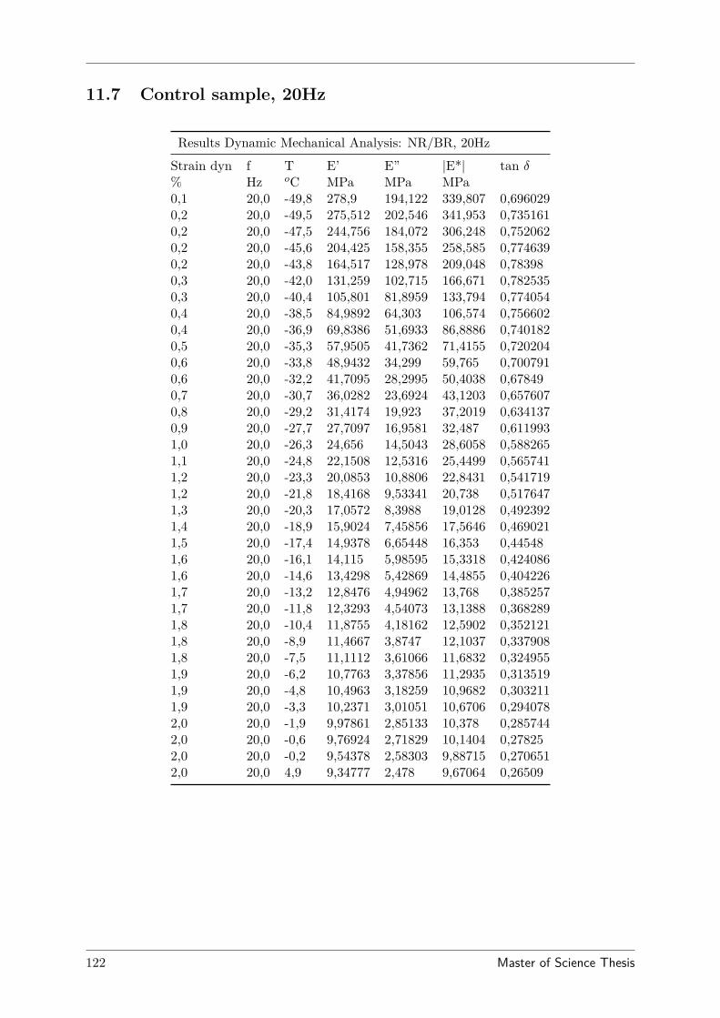
11.7 Control sample, 20Hz
Results Dynamic Mechanical Analysis: NR/BR, 20Hz
Strain dyn f T E’ E” |E*| tan δ% Hz oC MPa MPa MPa0,1 20,0 -49,8 278,9 194,122 339,807 0,6960290,2 20,0 -49,5 275,512 202,546 341,953 0,7351610,2 20,0 -47,5 244,756 184,072 306,248 0,7520620,2 20,0 -45,6 204,425 158,355 258,585 0,7746390,2 20,0 -43,8 164,517 128,978 209,048 0,783980,3 20,0 -42,0 131,259 102,715 166,671 0,7825350,3 20,0 -40,4 105,801 81,8959 133,794 0,7740540,4 20,0 -38,5 84,9892 64,303 106,574 0,7566020,4 20,0 -36,9 69,8386 51,6933 86,8886 0,7401820,5 20,0 -35,3 57,9505 41,7362 71,4155 0,7202040,6 20,0 -33,8 48,9432 34,299 59,765 0,7007910,6 20,0 -32,2 41,7095 28,2995 50,4038 0,678490,7 20,0 -30,7 36,0282 23,6924 43,1203 0,6576070,8 20,0 -29,2 31,4174 19,923 37,2019 0,6341370,9 20,0 -27,7 27,7097 16,9581 32,487 0,6119931,0 20,0 -26,3 24,656 14,5043 28,6058 0,5882651,1 20,0 -24,8 22,1508 12,5316 25,4499 0,5657411,2 20,0 -23,3 20,0853 10,8806 22,8431 0,5417191,2 20,0 -21,8 18,4168 9,53341 20,738 0,5176471,3 20,0 -20,3 17,0572 8,3988 19,0128 0,4923921,4 20,0 -18,9 15,9024 7,45856 17,5646 0,4690211,5 20,0 -17,4 14,9378 6,65448 16,353 0,445481,6 20,0 -16,1 14,115 5,98595 15,3318 0,4240861,6 20,0 -14,6 13,4298 5,42869 14,4855 0,4042261,7 20,0 -13,2 12,8476 4,94962 13,768 0,3852571,7 20,0 -11,8 12,3293 4,54073 13,1388 0,3682891,8 20,0 -10,4 11,8755 4,18162 12,5902 0,3521211,8 20,0 -8,9 11,4667 3,8747 12,1037 0,3379081,8 20,0 -7,5 11,1112 3,61066 11,6832 0,3249551,9 20,0 -6,2 10,7763 3,37856 11,2935 0,3135191,9 20,0 -4,8 10,4963 3,18259 10,9682 0,3032111,9 20,0 -3,3 10,2371 3,01051 10,6706 0,2940782,0 20,0 -1,9 9,97861 2,85133 10,378 0,2857442,0 20,0 -0,6 9,76924 2,71829 10,1404 0,278252,0 20,0 -0,2 9,54378 2,58303 9,88715 0,2706512,0 20,0 4,9 9,34777 2,478 9,67064 0,26509
122 Master of Science Thesis
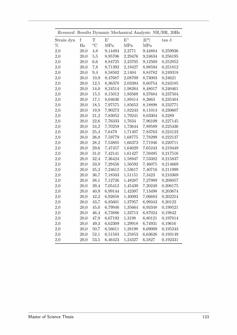
Resumed: Results Dynamic Mechanical Analysis: NR/BR, 20Hz
Strain dyn f T E’ E” |E*| tan δ% Hz oC MPa MPa MPa2,0 20,0 4,8 9,14494 2,3771 9,44884 0,2599362,0 20,0 5,5 8,95706 2,29476 9,24634 0,2561952,0 20,0 6,6 8,84725 2,23705 9,12569 0,2528522,0 20,0 7,8 8,71392 2,19427 8,98594 0,2518122,0 20,0 9,4 8,58502 2,1404 8,84782 0,2493182,0 20,0 10,9 8,47687 2,08709 8,73003 0,246212,0 20,0 12,5 8,36378 2,03394 8,60754 0,2431852,0 20,0 14,0 8,24514 1,98264 8,48017 0,2404612,0 20,0 15,5 8,15012 1,93569 8,37684 0,2375042,0 20,0 17,1 8,04636 1,89414 8,2663 0,2354042,0 20,0 18,5 7,97575 1,85653 8,18898 0,2327712,0 20,0 19,9 7,90273 1,82243 8,11014 0,2306072,0 20,0 21,2 7,83052 1,79241 8,03304 0,22892,0 20,0 22,6 7,76333 1,7634 7,96109 0,2271452,0 20,0 24,2 7,70259 1,73644 7,89589 0,2254362,0 20,0 25,4 7,6479 1,71407 7,83763 0,2241232,0 20,0 26,8 7,59779 1,68775 7,78299 0,2221372,0 20,0 28,2 7,53805 1,66373 7,71946 0,2207112,0 20,0 29,6 7,47457 1,64029 7,65243 0,2194492,0 20,0 31,0 7,42141 1,61427 7,59495 0,2175162,0 20,0 32,4 7,36424 1,58947 7,53382 0,2158372,0 20,0 33,9 7,29456 1,56592 7,46075 0,2146692,0 20,0 35,2 7,24612 1,53617 7,40716 0,2119992,0 20,0 36,7 7,18503 1,51151 7,3423 0,2103692,0 20,0 38,1 7,12726 1,48287 7,27989 0,2080572,0 20,0 39,4 7,05412 1,45439 7,20249 0,2061752,0 20,0 40,9 6,99144 1,42397 7,13498 0,2036742,0 20,0 42,2 6,92658 1,40093 7,06683 0,2022542,0 20,0 43,7 6,85601 1,37957 6,99343 0,201222,0 20,0 45,0 6,79946 1,35664 6,93348 0,1995212,0 20,0 46,4 6,73886 1,33713 6,87024 0,198422,0 20,0 47,9 6,67192 1,3198 6,80121 0,1978142,0 20,0 49,3 6,62309 1,29918 6,74931 0,196162,0 20,0 50,7 6,56611 1,28198 6,69009 0,1952432,0 20,0 52,1 6,51583 1,25853 6,63626 0,1931492,0 20,0 53,5 6,46423 1,24327 6,5827 0,192331
Master of Science Thesis 123
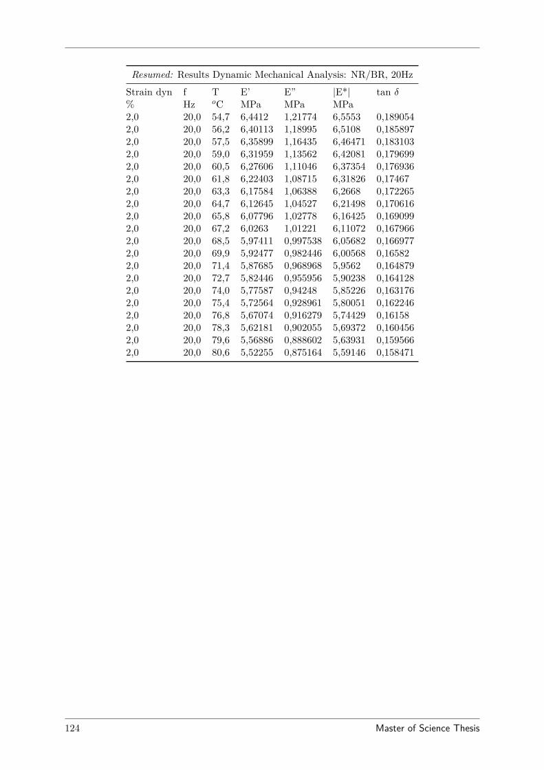
Resumed: Results Dynamic Mechanical Analysis: NR/BR, 20Hz
Strain dyn f T E’ E” |E*| tan δ% Hz oC MPa MPa MPa2,0 20,0 54,7 6,4412 1,21774 6,5553 0,1890542,0 20,0 56,2 6,40113 1,18995 6,5108 0,1858972,0 20,0 57,5 6,35899 1,16435 6,46471 0,1831032,0 20,0 59,0 6,31959 1,13562 6,42081 0,1796992,0 20,0 60,5 6,27606 1,11046 6,37354 0,1769362,0 20,0 61,8 6,22403 1,08715 6,31826 0,174672,0 20,0 63,3 6,17584 1,06388 6,2668 0,1722652,0 20,0 64,7 6,12645 1,04527 6,21498 0,1706162,0 20,0 65,8 6,07796 1,02778 6,16425 0,1690992,0 20,0 67,2 6,0263 1,01221 6,11072 0,1679662,0 20,0 68,5 5,97411 0,997538 6,05682 0,1669772,0 20,0 69,9 5,92477 0,982446 6,00568 0,165822,0 20,0 71,4 5,87685 0,968968 5,9562 0,1648792,0 20,0 72,7 5,82446 0,955956 5,90238 0,1641282,0 20,0 74,0 5,77587 0,94248 5,85226 0,1631762,0 20,0 75,4 5,72564 0,928961 5,80051 0,1622462,0 20,0 76,8 5,67074 0,916279 5,74429 0,161582,0 20,0 78,3 5,62181 0,902055 5,69372 0,1604562,0 20,0 79,6 5,56886 0,888602 5,63931 0,1595662,0 20,0 80,6 5,52255 0,875164 5,59146 0,158471
124 Master of Science Thesis
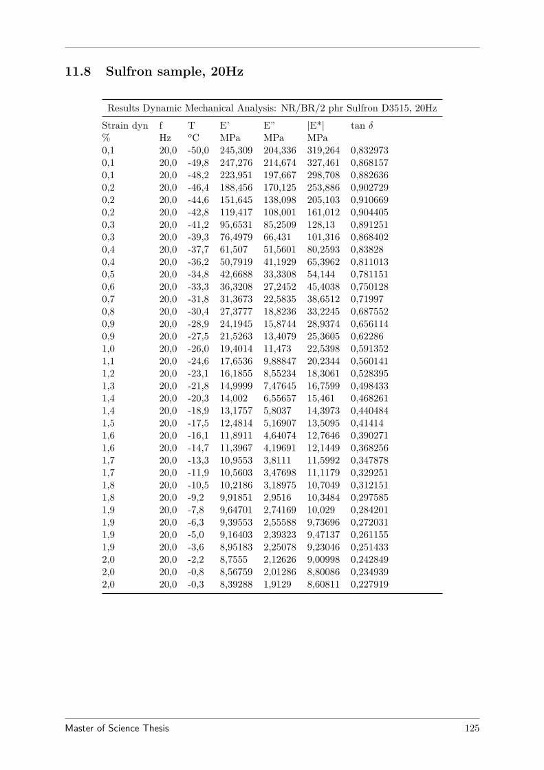
11.8 Sulfron sample, 20Hz
Results Dynamic Mechanical Analysis: NR/BR/2 phr Sulfron D3515, 20Hz
Strain dyn f T E’ E” |E*| tan δ% Hz oC MPa MPa MPa0,1 20,0 -50,0 245,309 204,336 319,264 0,8329730,1 20,0 -49,8 247,276 214,674 327,461 0,8681570,1 20,0 -48,2 223,951 197,667 298,708 0,8826360,2 20,0 -46,4 188,456 170,125 253,886 0,9027290,2 20,0 -44,6 151,645 138,098 205,103 0,9106690,2 20,0 -42,8 119,417 108,001 161,012 0,9044050,3 20,0 -41,2 95,6531 85,2509 128,13 0,8912510,3 20,0 -39,3 76,4979 66,431 101,316 0,8684020,4 20,0 -37,7 61,507 51,5601 80,2593 0,838280,4 20,0 -36,2 50,7919 41,1929 65,3962 0,8110130,5 20,0 -34,8 42,6688 33,3308 54,144 0,7811510,6 20,0 -33,3 36,3208 27,2452 45,4038 0,7501280,7 20,0 -31,8 31,3673 22,5835 38,6512 0,719970,8 20,0 -30,4 27,3777 18,8236 33,2245 0,6875520,9 20,0 -28,9 24,1945 15,8744 28,9374 0,6561140,9 20,0 -27,5 21,5263 13,4079 25,3605 0,622861,0 20,0 -26,0 19,4014 11,473 22,5398 0,5913521,1 20,0 -24,6 17,6536 9,88847 20,2344 0,5601411,2 20,0 -23,1 16,1855 8,55234 18,3061 0,5283951,3 20,0 -21,8 14,9999 7,47645 16,7599 0,4984331,4 20,0 -20,3 14,002 6,55657 15,461 0,4682611,4 20,0 -18,9 13,1757 5,8037 14,3973 0,4404841,5 20,0 -17,5 12,4814 5,16907 13,5095 0,414141,6 20,0 -16,1 11,8911 4,64074 12,7646 0,3902711,6 20,0 -14,7 11,3967 4,19691 12,1449 0,3682561,7 20,0 -13,3 10,9553 3,8111 11,5992 0,3478781,7 20,0 -11,9 10,5603 3,47698 11,1179 0,3292511,8 20,0 -10,5 10,2186 3,18975 10,7049 0,3121511,8 20,0 -9,2 9,91851 2,9516 10,3484 0,2975851,9 20,0 -7,8 9,64701 2,74169 10,029 0,2842011,9 20,0 -6,3 9,39553 2,55588 9,73696 0,2720311,9 20,0 -5,0 9,16403 2,39323 9,47137 0,2611551,9 20,0 -3,6 8,95183 2,25078 9,23046 0,2514332,0 20,0 -2,2 8,7555 2,12626 9,00998 0,2428492,0 20,0 -0,8 8,56759 2,01286 8,80086 0,2349392,0 20,0 -0,3 8,39288 1,9129 8,60811 0,227919
Master of Science Thesis 125
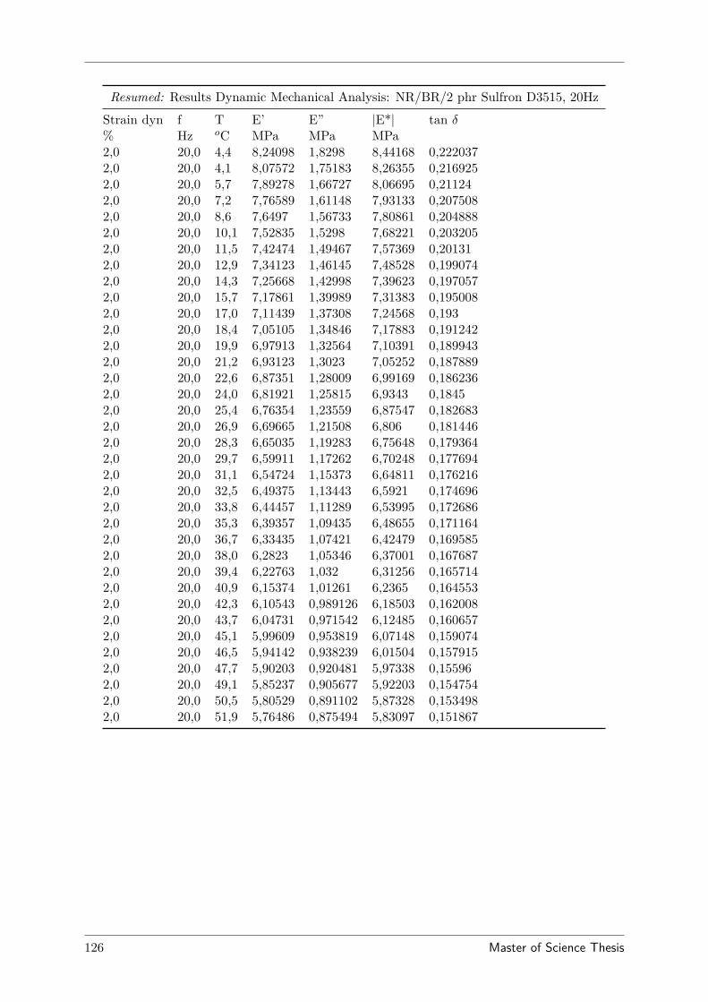
Resumed: Results Dynamic Mechanical Analysis: NR/BR/2 phr Sulfron D3515, 20Hz
Strain dyn f T E’ E” |E*| tan δ% Hz oC MPa MPa MPa2,0 20,0 4,4 8,24098 1,8298 8,44168 0,2220372,0 20,0 4,1 8,07572 1,75183 8,26355 0,2169252,0 20,0 5,7 7,89278 1,66727 8,06695 0,211242,0 20,0 7,2 7,76589 1,61148 7,93133 0,2075082,0 20,0 8,6 7,6497 1,56733 7,80861 0,2048882,0 20,0 10,1 7,52835 1,5298 7,68221 0,2032052,0 20,0 11,5 7,42474 1,49467 7,57369 0,201312,0 20,0 12,9 7,34123 1,46145 7,48528 0,1990742,0 20,0 14,3 7,25668 1,42998 7,39623 0,1970572,0 20,0 15,7 7,17861 1,39989 7,31383 0,1950082,0 20,0 17,0 7,11439 1,37308 7,24568 0,1932,0 20,0 18,4 7,05105 1,34846 7,17883 0,1912422,0 20,0 19,9 6,97913 1,32564 7,10391 0,1899432,0 20,0 21,2 6,93123 1,3023 7,05252 0,1878892,0 20,0 22,6 6,87351 1,28009 6,99169 0,1862362,0 20,0 24,0 6,81921 1,25815 6,9343 0,18452,0 20,0 25,4 6,76354 1,23559 6,87547 0,1826832,0 20,0 26,9 6,69665 1,21508 6,806 0,1814462,0 20,0 28,3 6,65035 1,19283 6,75648 0,1793642,0 20,0 29,7 6,59911 1,17262 6,70248 0,1776942,0 20,0 31,1 6,54724 1,15373 6,64811 0,1762162,0 20,0 32,5 6,49375 1,13443 6,5921 0,1746962,0 20,0 33,8 6,44457 1,11289 6,53995 0,1726862,0 20,0 35,3 6,39357 1,09435 6,48655 0,1711642,0 20,0 36,7 6,33435 1,07421 6,42479 0,1695852,0 20,0 38,0 6,2823 1,05346 6,37001 0,1676872,0 20,0 39,4 6,22763 1,032 6,31256 0,1657142,0 20,0 40,9 6,15374 1,01261 6,2365 0,1645532,0 20,0 42,3 6,10543 0,989126 6,18503 0,1620082,0 20,0 43,7 6,04731 0,971542 6,12485 0,1606572,0 20,0 45,1 5,99609 0,953819 6,07148 0,1590742,0 20,0 46,5 5,94142 0,938239 6,01504 0,1579152,0 20,0 47,7 5,90203 0,920481 5,97338 0,155962,0 20,0 49,1 5,85237 0,905677 5,92203 0,1547542,0 20,0 50,5 5,80529 0,891102 5,87328 0,1534982,0 20,0 51,9 5,76486 0,875494 5,83097 0,151867
126 Master of Science Thesis
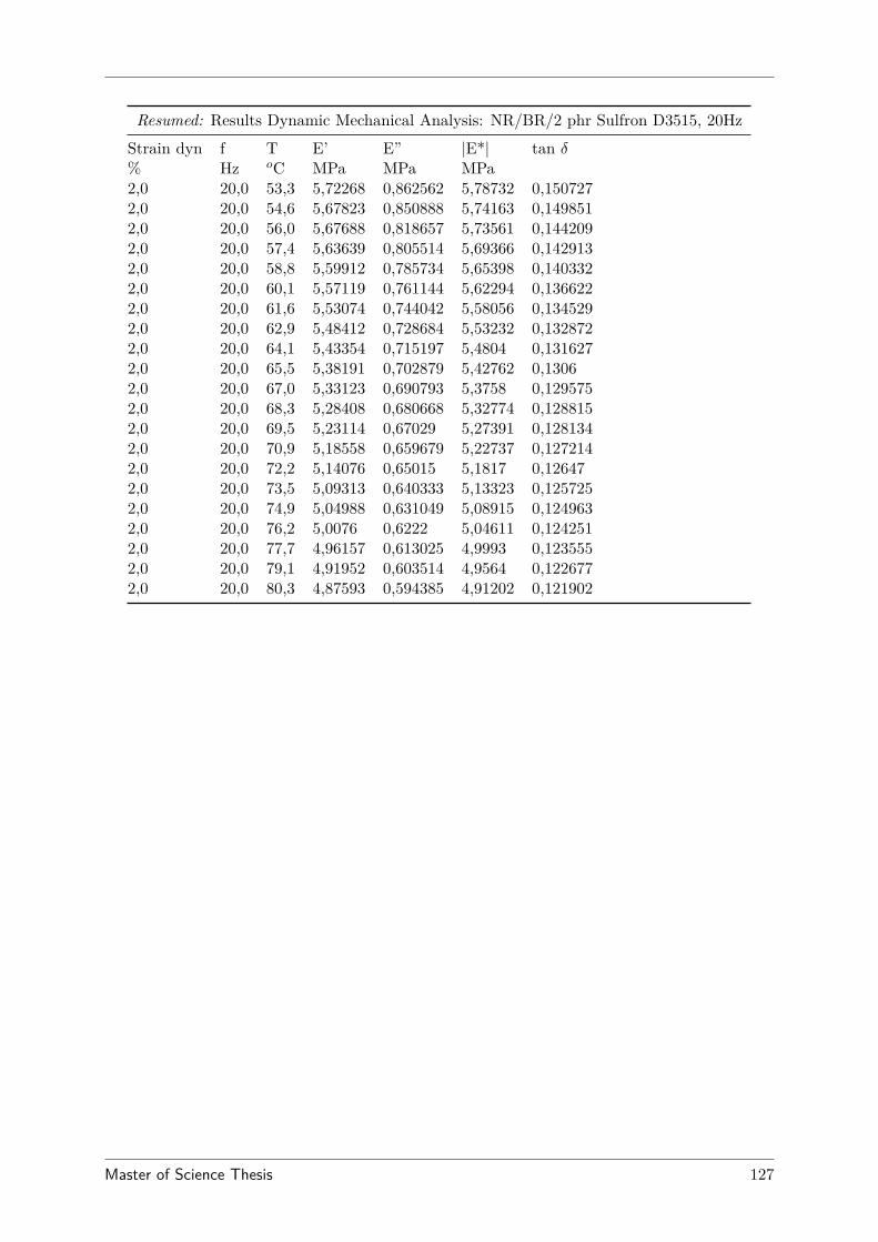
Resumed: Results Dynamic Mechanical Analysis: NR/BR/2 phr Sulfron D3515, 20Hz
Strain dyn f T E’ E” |E*| tan δ% Hz oC MPa MPa MPa2,0 20,0 53,3 5,72268 0,862562 5,78732 0,1507272,0 20,0 54,6 5,67823 0,850888 5,74163 0,1498512,0 20,0 56,0 5,67688 0,818657 5,73561 0,1442092,0 20,0 57,4 5,63639 0,805514 5,69366 0,1429132,0 20,0 58,8 5,59912 0,785734 5,65398 0,1403322,0 20,0 60,1 5,57119 0,761144 5,62294 0,1366222,0 20,0 61,6 5,53074 0,744042 5,58056 0,1345292,0 20,0 62,9 5,48412 0,728684 5,53232 0,1328722,0 20,0 64,1 5,43354 0,715197 5,4804 0,1316272,0 20,0 65,5 5,38191 0,702879 5,42762 0,13062,0 20,0 67,0 5,33123 0,690793 5,3758 0,1295752,0 20,0 68,3 5,28408 0,680668 5,32774 0,1288152,0 20,0 69,5 5,23114 0,67029 5,27391 0,1281342,0 20,0 70,9 5,18558 0,659679 5,22737 0,1272142,0 20,0 72,2 5,14076 0,65015 5,1817 0,126472,0 20,0 73,5 5,09313 0,640333 5,13323 0,1257252,0 20,0 74,9 5,04988 0,631049 5,08915 0,1249632,0 20,0 76,2 5,0076 0,6222 5,04611 0,1242512,0 20,0 77,7 4,96157 0,613025 4,9993 0,1235552,0 20,0 79,1 4,91952 0,603514 4,9564 0,1226772,0 20,0 80,3 4,87593 0,594385 4,91202 0,121902
Master of Science Thesis 127

128 Master of Science Thesis
Bibliography
[1] Jiaozuo Creation Machinery Company. Example of a belt conveyor system, 2009.http://www.jzcreation.cc/files/2013/02/mining-conveyor01.jpg.
[2] M. Hager and A. Hintz. The energy-saving design of belts for long conveyor systems. BulkSolids Handling, pages 749–758, 1993.
[3] L.K. Nordell. The power of rubber part 1. Bulk Solids Handling, 16, 1996.
[4] D. Gallagher. Low rolling resistance for conveyor belts. Presented at the InternationalRubber Conference Melbourne, 2000.
[5] Y. Zhang. Overland pipe conveyor with low rolling resistance belt. Bulk Solids Handling,33:16–21, 2013.
[6] G. Lodewijks. The next generation of low loss conveyor belts. Bulk Solids Handling, 32:52–56, 2011.
[7] Teijin Aramid. Sustainable performance for conveyor belts. Conveyor belts leaflet, 2012.
[8] Phoenix Conveyor Belt Systems GmbH. Example of a steel cord belt,2007. http://www.phoenix-conveyorbelts.com/pages/press-themes/press/2007-01_century_en.html.
[9] Deutsches Institut Für Normung. Belt conveyors for bulk materials - fundamentals forcalculation and design. 1982.
[10] Martin Engineering. Example of a drive pulley, 2014. https://www.martin-eng.com/press-release/conveyor-belt-cleaner-designed-aggregates-handling.
[11] Universal Roll. Example idler sets, 2012. http://www.universalroll.com/blog/.
[12] G. Lodewijks. Example of a (gravity) take-up system. Lecture sheets "Introduction TransportEngineering and Logistics", 2011.
[13] M.A. Alspaugh. Latest developments in belt conveyor technology. Presented at MINExpo,2004.
[14] M.L. Williams et al. The temperature dependence of relaxation mechanisms in amorphouspolymers and other glass-forming liquids. Journal of Applied Science, 77:3701–3707, 1955.
Master of Science Thesis 129
[15] G. Lodewijks. The rolling resistance of conveyor belts. Bulk Solids Handling, pages 15–22,1995.
[16] W.D. et al May. Rolling friction of a hard cylinder over a viscoelastic material. Journal ofApplied Physics, 30:1713–1724, 1959.
[17] S.C. Hunter. The rolling contact of a rigid cylinder with a viscoelastic half space. Journalof Applied Mechanics, pages 612–617, 1961.
[18] C.O. Jonkers. The indentation rolling resistance of belt conveyor - a theoretical approach.Fordern und Heben, 1980.
[19] C. Wheeler. Analysis of the main resistance of belt conveyors. PhD thesis, University ofNewcastle, Australia, 2003.
[20] T.J. Rudolphi and A.V. Reicks. Viscoelastic indentation and resistance to motion of con-veyor belts using a generalised maxwell model of the backing material. Journal rubberchemistry and technology, 2006.
[21] F. Lynch. A finite element method of viscoelastic stress analysis with application to rollingcontact problems. International Journal for Numerical Methods in Engineering, 1:379–394,1969.
[22] R. et al Batra. Rubber covered rolls - the thermoviscoelastic problem. a finite elementsolution. International Journal for Numerical Methods in Engineering, 10:767–785, 1976.
[23] X. Qui. Full two-dimensional model for rolling resistance: hard cylinder on viscoelasticfoundation of finite thickness. Journal of Engineering Mechanics, pages 1241–1251, 2006.
[24] J.I. O’Shea et al. The influence of viscoelastic property measurements on the predictedrolling resistance of belt conveyors. Journal of Applied Polymer Science, 2014.
130 Master of Science Thesis