Embed Size (px)
Citation preview
energies
Article
Energy Efficiency Comparison of HydraulicAccumulators and Ultracapacitors
Jorge Leon-Quiroga 1, Brittany Newell 1, Mahesh Krishnamurthy 2,Andres Gonzalez-Mancera 3 and Jose Garcia-Bravo 1,*
1 Purdue Polytechnic School of Engineering Technology, Purdue University, West Lafayette, IN 47907, USA;[email protected] (J.L.-Q.); [email protected] (B.N.)
2 Department of Electrical and Computer Engineering, Illinois Institute of Technology, Chicago, IL 60616, USA;[email protected]
3 Department of Mechanical Engineering, Universidad de los Andes, Bogota 111711, Colombia;[email protected]
* Correspondence: [email protected]
Received: 21 February 2020; Accepted: 20 March 2020; Published: 2 April 2020
Abstract: Energy regeneration systems are a key factor for improving energy efficiency inelectrohydraulic machinery. This paper is focused on the study of electric energy storage systems(EESS) and hydraulic energy storage systems (HESS) for energy regeneration applications. Two testbenches were designed and implemented to compare the performance of the systems under similaroperating conditions. The electrical system was configured with a set of ultracapacitors, and thehydraulic system used a hydraulic accumulator. Both systems were designed to have the sameenergy storage capacity. Charge and discharge cycle experiments were performed for the two systemsin order to compare their power density, energy density, cost, and efficiency. According to theexperimentally obtained results, the power density in the hydraulic accumulator was 21.7% higherwhen compared with the ultracapacitors. Moreover, the cost/power ($/Watt) ratio in the hydraulicaccumulator was 2.9 times smaller than a set of ultracapacitors of the same energy storage capacity.On the other hand, the energy density in the set of ultracapacitors was 9.4 times higher, and thecost/energy ($/kWh) ratio was 2.9 times smaller when compared with the hydraulic accumulator.Under the tested conditions, the estimated overall energy efficiency for the hydraulic accumulatorwas 87.7%, and the overall energy efficiency for the ultracapacitor was 78.7%.
Keywords: efficiency; energy storage systems; electrical power systems; hydraulic power systems;hydraulic accumulator; ultracapacitor
1. Introduction
Energy consumption in the transportation and the industrial sector represented 72% of the totalenergy consumption during 2018 in the United States. Most of this energy (around 87%) comes frompetroleum-based sources and natural gas [1]. In the industrial sector, around 24% of the energy isspent by the agriculture, construction, and mining sectors. Many applications within these sectors usehydraulic equipment and hydraulic machinery, so improving the energy efficiency of the hydraulicsystems that are already in use could have a large impact on the reduction of energy consumptionand emissions. If the energy efficiency of the hydraulic machinery used in industrial applicationsis improved by 5%, based on the data provided by the U.S. Energy Department [1], it is possible toestimate an overall annual reduction of 1% in energy consumption in the US.
Over the last 20 years, there has been interest in developing and improving systems for energyregeneration in hydraulic machinery [2–5]. Some of the options for energy storage in energy regeneration
Energies 2020, 13, 1632; doi:10.3390/en13071632 www.mdpi.com/journal/energies
Energies 2020, 13, 1632 2 of 23
devices include flywheels, compressed air, electrical energy storage systems (EESS), and hydraulicenergy storage systems (HESS). In the electrical energy regeneration system, an electric accumulator orcapacitor is used to store energy [6]. This kind of system is used in electric hybrid machinery. The returnline of a boom mechanism in an excavator is connected to a hydraulic motor that is used to move anelectric generator that produces electrical energy that is stored in an electric accumulator (ultracapacitoror battery) [2,3,7]. The main benefit of this system is an improvement in energy efficiency, but thecomplexity that is added to the baseline hydraulic system is evident. Ultracapacitors are mostly used inelectric applications that require a high power density such as wind turbines in remote areas [8], energyregeneration and engine size reduction in rubber wheeled gantry cranes [9], and even biomedicalapplications [10].
The hydraulic energy regeneration system is similar to its electric counterpart. Instead of havingan electric accumulator (ultracapacitor or battery), the hydraulic energy regeneration system uses ahydraulic accumulator that works as the energy storage device [6]. One of the main benefits when usinga hydraulic regenerative system is the relative ease of installation, since the baseline application alreadyuses a hydraulic system. Moreover, no complex power controls are needed, which is a significantadvantage. On the other hand, the energy storage density in hydraulic accumulators can be a drawbackwhen compared to a traditional electric system. Hydraulic regenerative systems have been studiedfor applications in relief valves [11], where the flow in the return line of the valve is used to chargea hydraulic accumulator. Alternatives like digital hydraulics have been studied to improve energyefficiency in hydraulic systems [12,13]. In these studies, a network of valves is used to change the flowrate in the actuator and to reconfigure the system in order to use the flow from assistive loads to moveactuators with resistive loads.
2. Relevance of This Work
Most of the previous studies regarding EESS and HESS have focused on the characteristics ofeach energy storage system separately. Some studies have focused on the study of the performanceof ultracapacitors [14–17] and others have focused on hydraulic accumulators. [18,19], but verylittle research has been done to compare the two storage systems (hydraulic accumulators andultracapacitors) side by side. The main purpose of this study was to have a direct comparison of theperformance characteristics of ultracapacitors and hydraulic accumulators when used as energy storagedevices. Previous studies concerning EESS and HESS for hybrid applications have not compared thebenefits and drawbacks of both systems under similar operating conditions; these studies have beenfocused on each system individually. For this work, an experimental procedure was developed formeasuring the charging and discharging cycles of a hydraulic accumulator. Likewise, a test benchusing ultracapacitors of similar energy storage capabilities was tested. The estimated energy capacityof each system was modeled with the equations shown in the following section. The experimentalprocedure and experimental equipment are also described in that section.
The results of this research can be used to stablish a control strategy to optimize systems that usehydraulic accumulators as energy storage systems or as a design strategy to select one over the other.
3. Test Bench Description
The main purpose of the test benches developed in this study was to compare an electrical and ahydraulic energy storage system under similar operating conditions in order to determine the efficiency,power density, energy density, and cost by energy capacity. The main characteristics of the hydraulicaccumulator and the ultracapacitor used are shown below in Tables 1 and 2.
Energies 2020, 13, 1632 3 of 23
Table 1. Characteristics of the hydraulic accumulator used in this study.
Hydraulic AccumulatorManufacturer Parker Hannifin
Reference A2N0058D1KMass (kg) 4.53
Vol. Capacity (cm3) 950Max. Pressure (Bar) 207
Table 2. Characteristics of the ultracapacitor used in this study.
UltracapacitorManufacturer Maxwell Technologies
Reference BCAP0050 P270 S01Mass (g) 12.2
Energy Capacity (mWh) 50.6Max. Voltage (V) 2.7Max. Current (A) 6.1
To compare both devices in a similar way, two test benches were designed and built. Both testbenches were designed to measure charge and discharge response of the systems, which in a hydraulicsystem are the pressure and flow rate and in the electric system are the voltage and current.
3.1. Hydraulic Test Bench
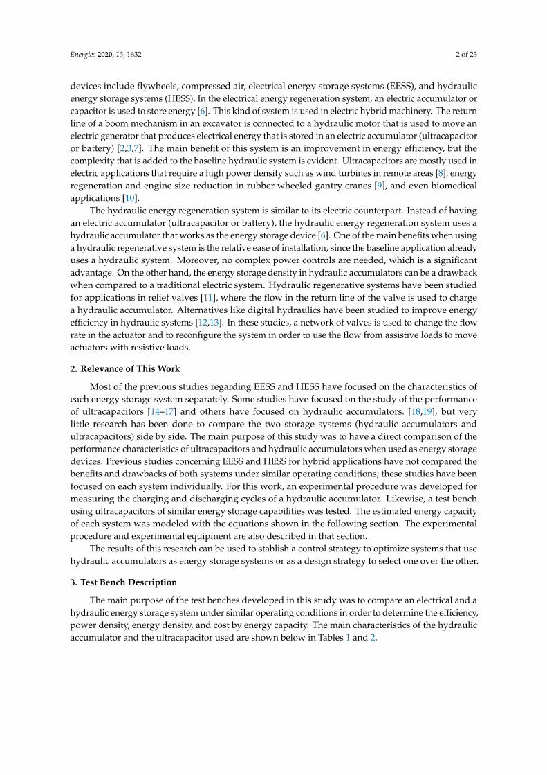
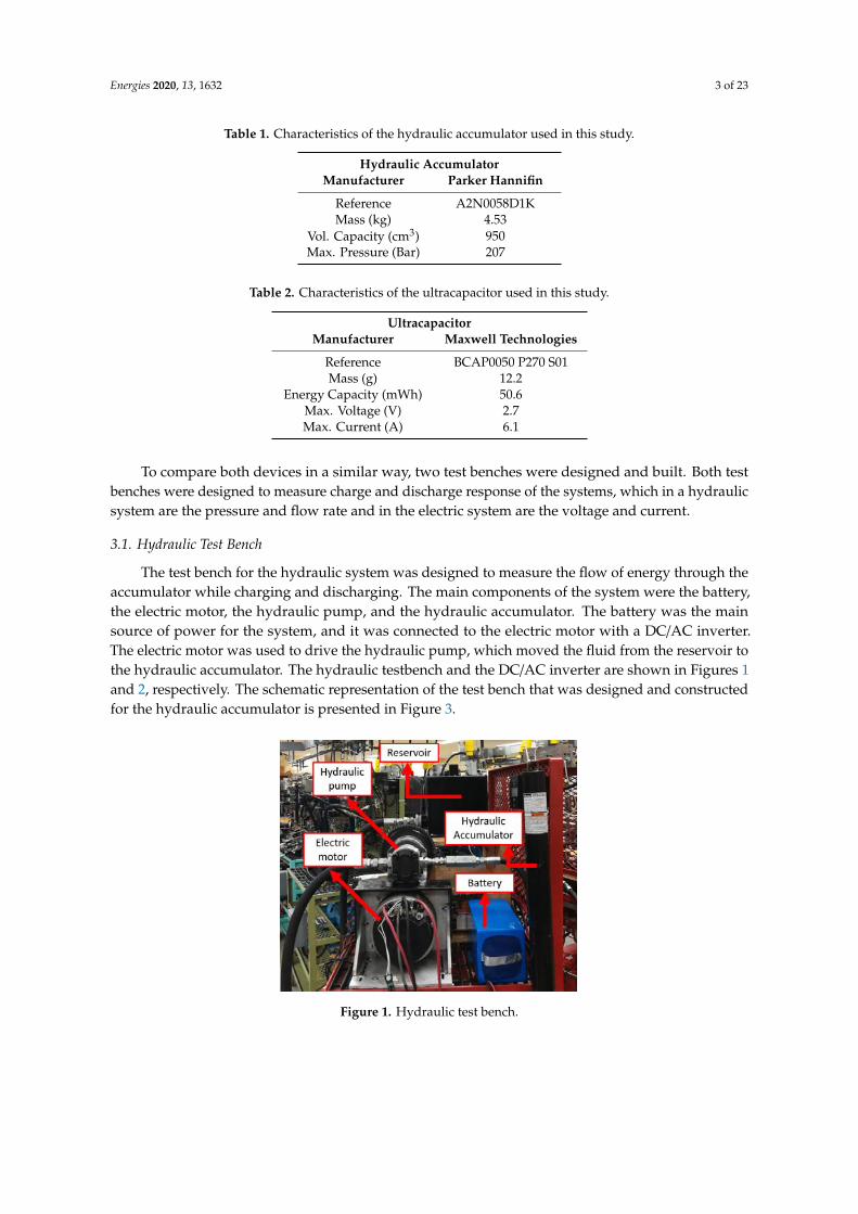
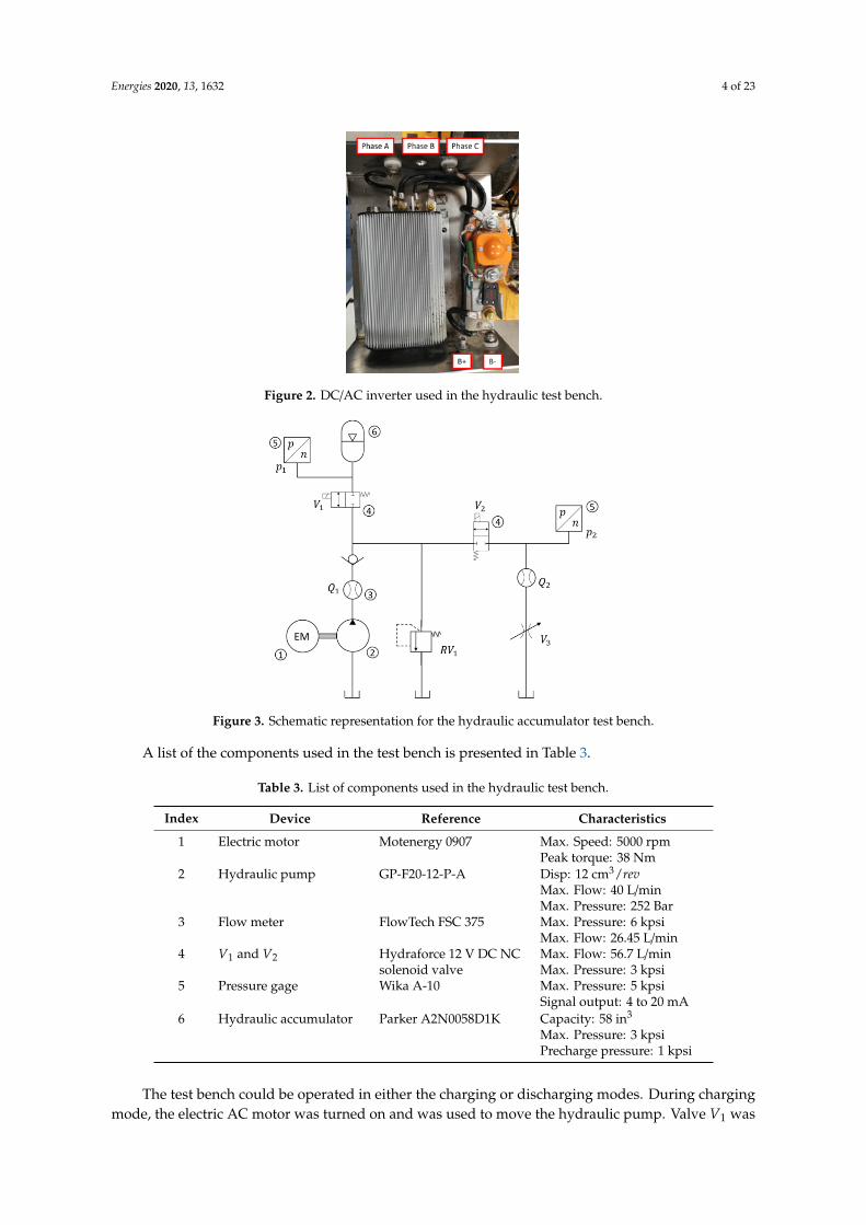
The test bench for the hydraulic system was designed to measure the flow of energy through theaccumulator while charging and discharging. The main components of the system were the battery,the electric motor, the hydraulic pump, and the hydraulic accumulator. The battery was the mainsource of power for the system, and it was connected to the electric motor with a DC/AC inverter.The electric motor was used to drive the hydraulic pump, which moved the fluid from the reservoir tothe hydraulic accumulator. The hydraulic testbench and the DC/AC inverter are shown in Figures 1and 2, respectively. The schematic representation of the test bench that was designed and constructedfor the hydraulic accumulator is presented in Figure 3.
Energies 2020, 13, x FOR PEER REVIEW 3 of 23
Table 1. Characteristics of the hydraulic accumulator used in this study.
Hydraulic Accumulator
Manufacturer Parker Hannifin
Reference A2N0058D1K
Mass (kg) 4.53
Vol. Capacity( ) 950
Max. Pressure (Bar) 207
Table 2. Characteristics of the ultracapacitor used in this study.
Ultracapacitor
Manufacturer Maxwell Technologies
Reference BCAP0050 P270 S01
Mass (g) 12.2
Energy Capacity (mWh) 50.6
Max. Voltage (V) 2.7
Max. Current (A) 6.1
3.1. Hydraulic Test Bench
The test bench for the hydraulic system was designed to measure the flow of energy through the
accumulator while charging and discharging. The main components of the system were the battery,
the electric motor, the hydraulic pump, and the hydraulic accumulator. The battery was the main
source of power for the system, and it was connected to the electric motor with a DC/AC inverter.
The electric motor was used to drive the hydraulic pump, which moved the fluid from the reservoir
to the hydraulic accumulator. The hydraulic testbench and the DC/AC inverter are shown in Figures
1 and 2, respectively. The schematic representation of the test bench that was designed and
constructed for the hydraulic accumulator is presented in Figure 3.
Figure 1. Hydraulic test bench. Figure 1. Hydraulic test bench.
Energies 2020, 13, 1632 4 of 23Energies 2020, 13, x FOR PEER REVIEW 4 of 23
Figure 2. DC/AC inverter used in the hydraulic test bench.
.
Figure 3. Schematic representation for the hydraulic accumulator test bench.
A list of the components used in the test bench is presented in Table 3.
Table 3. List of components used in the hydraulic test bench.
Index Device Reference Characteristics
1 Electric motor Motenergy 0907 Max. Speed: 5000 rpm
Peak torque: 38 Nm
2 Hydraulic pump GP‐F20‐12‐P‐A Disp: 12 cm ⁄
Max. Flow: 40 L/min
Max. Pressure: 252 Bar
3 Flow meter FlowTech FSC 375 Max. Pressure: 6 kpsi
Max. Flow: 26.45 L/min
4 V1 and V2 Hydraforce 12 V DC NC
solenoid valve
Max. Flow: 56.7 L/min
Max. Pressure: 3 kpsi
5 Pressure gage Wika A‐10 Max. Pressure: 5 kpsi
Signal output: 4 to 20 mA
6 Hydraulic
accumulator
Parker A2N0058D1K Capacity: 58in Max. Pressure: 3 kpsi
Precharge pressure: 1 kpsi
Figure 2. DC/AC inverter used in the hydraulic test bench.
Energies 2020, 13, x FOR PEER REVIEW 4 of 23
Figure 2. DC/AC inverter used in the hydraulic test bench.
.
Figure 3. Schematic representation for the hydraulic accumulator test bench.
A list of the components used in the test bench is presented in Table 3.
Table 3. List of components used in the hydraulic test bench.
Index Device Reference Characteristics
1 Electric motor Motenergy 0907 Max. Speed: 5000 rpm
Peak torque: 38 Nm
2 Hydraulic pump GP‐F20‐12‐P‐A Disp: 12 cm ⁄
Max. Flow: 40 L/min
Max. Pressure: 252 Bar
3 Flow meter FlowTech FSC 375 Max. Pressure: 6 kpsi
Max. Flow: 26.45 L/min
4 V1 and V2 Hydraforce 12 V DC NC
solenoid valve
Max. Flow: 56.7 L/min
Max. Pressure: 3 kpsi
5 Pressure gage Wika A‐10 Max. Pressure: 5 kpsi
Signal output: 4 to 20 mA
6 Hydraulic
accumulator
Parker A2N0058D1K Capacity: 58in Max. Pressure: 3 kpsi
Precharge pressure: 1 kpsi
Figure 3. Schematic representation for the hydraulic accumulator test bench.
A list of the components used in the test bench is presented in Table 3.
Table 3. List of components used in the hydraulic test bench.
Index Device Reference Characteristics
1 Electric motor Motenergy 0907 Max. Speed: 5000 rpmPeak torque: 38 Nm
2 Hydraulic pump GP-F20-12-P-A Disp: 12 cm3/revMax. Flow: 40 L/minMax. Pressure: 252 Bar
3 Flow meter FlowTech FSC 375 Max. Pressure: 6 kpsiMax. Flow: 26.45 L/min
4 V1 and V2 Hydraforce 12 V DC NCsolenoid valve
Max. Flow: 56.7 L/minMax. Pressure: 3 kpsi
5 Pressure gage Wika A-10 Max. Pressure: 5 kpsiSignal output: 4 to 20 mA
6 Hydraulic accumulator Parker A2N0058D1K Capacity: 58 in3
Max. Pressure: 3 kpsiPrecharge pressure: 1 kpsi
The test bench could be operated in either the charging or discharging modes. During chargingmode, the electric AC motor was turned on and was used to move the hydraulic pump. Valve V1 was
Energies 2020, 13, 1632 5 of 23
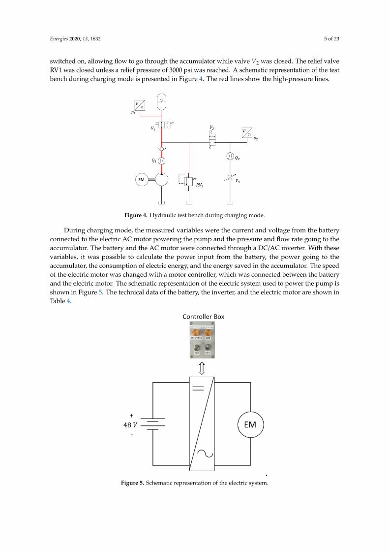
switched on, allowing flow to go through the accumulator while valve V2 was closed. The relief valveRV1 was closed unless a relief pressure of 3000 psi was reached. A schematic representation of the testbench during charging mode is presented in Figure 4. The red lines show the high-pressure lines.
Energies 2020, 13, x FOR PEER REVIEW 5 of 23
The test bench could be operated in either the charging or discharging modes. During charging
mode, the electric AC motor was turned on and was used to move the hydraulic pump. Valve V1 was
switched on, allowing flow to go through the accumulator while valve V2 was closed. The relief valve
RV1 was closed unless a relief pressure of 3000 psi was reached. A schematic representation of the
test bench during charging mode is presented in Figure 4. The red lines show the high‐pressure lines.
.
Figure 4. Hydraulic test bench during charging mode.
During charging mode, the measured variables were the current and voltage from the battery
connected to the electric AC motor powering the pump and the pressure and flow rate going to the
accumulator. The battery and the AC motor were connected through a DC/AC inverter. With these
variables, it was possible to calculate the power input from the battery, the power going to the
accumulator, the consumption of electric energy, and the energy saved in the accumulator. The speed
of the electric motor was changed with a motor controller, which was connected between the battery
and the electric motor. The schematic representation of the electric system used to power the pump
is shown in Figure 5. The technical data of the battery, the inverter, and the electric motor are shown
in Table 4.
.
Figure 5. Schematic representation of the electric system.
Table 4. Technical data of the electric system.
Device Reference Characteristics
Figure 4. Hydraulic test bench during charging mode.
During charging mode, the measured variables were the current and voltage from the batteryconnected to the electric AC motor powering the pump and the pressure and flow rate going to theaccumulator. The battery and the AC motor were connected through a DC/AC inverter. With thesevariables, it was possible to calculate the power input from the battery, the power going to theaccumulator, the consumption of electric energy, and the energy saved in the accumulator. The speedof the electric motor was changed with a motor controller, which was connected between the batteryand the electric motor. The schematic representation of the electric system used to power the pump isshown in Figure 5. The technical data of the battery, the inverter, and the electric motor are shown inTable 4.
Energies 2020, 13, x FOR PEER REVIEW 5 of 23
The test bench could be operated in either the charging or discharging modes. During charging
mode, the electric AC motor was turned on and was used to move the hydraulic pump. Valve V1 was
switched on, allowing flow to go through the accumulator while valve V2 was closed. The relief valve
RV1 was closed unless a relief pressure of 3000 psi was reached. A schematic representation of the
test bench during charging mode is presented in Figure 4. The red lines show the high‐pressure lines.
.
Figure 4. Hydraulic test bench during charging mode.
During charging mode, the measured variables were the current and voltage from the battery
connected to the electric AC motor powering the pump and the pressure and flow rate going to the
accumulator. The battery and the AC motor were connected through a DC/AC inverter. With these
variables, it was possible to calculate the power input from the battery, the power going to the
accumulator, the consumption of electric energy, and the energy saved in the accumulator. The speed
of the electric motor was changed with a motor controller, which was connected between the battery
and the electric motor. The schematic representation of the electric system used to power the pump
is shown in Figure 5. The technical data of the battery, the inverter, and the electric motor are shown
in Table 4.
.
Figure 5. Schematic representation of the electric system.
Table 4. Technical data of the electric system.
Device Reference Characteristics
Figure 5. Schematic representation of the electric system.
Energies 2020, 13, 1632 6 of 23
Table 4. Technical data of the electric system.
Device Reference Characteristics
Electric motor Motenergy 0907 Max. Speed: 5000 rpmPeak torque: 38 NmContinuous current of 80 Amps ACInductance phase to phase: 0.1 millihenry
Inverter KEB48600 Max. Power: 6 kWMax. voltage: 48 VMax. Current: 125 A
Battery SUN-CYCLELiFePO4 48 V24 Ah
Max. Voltage: 48 VMax. discharge current: 60 AWeight: 9.8 kg
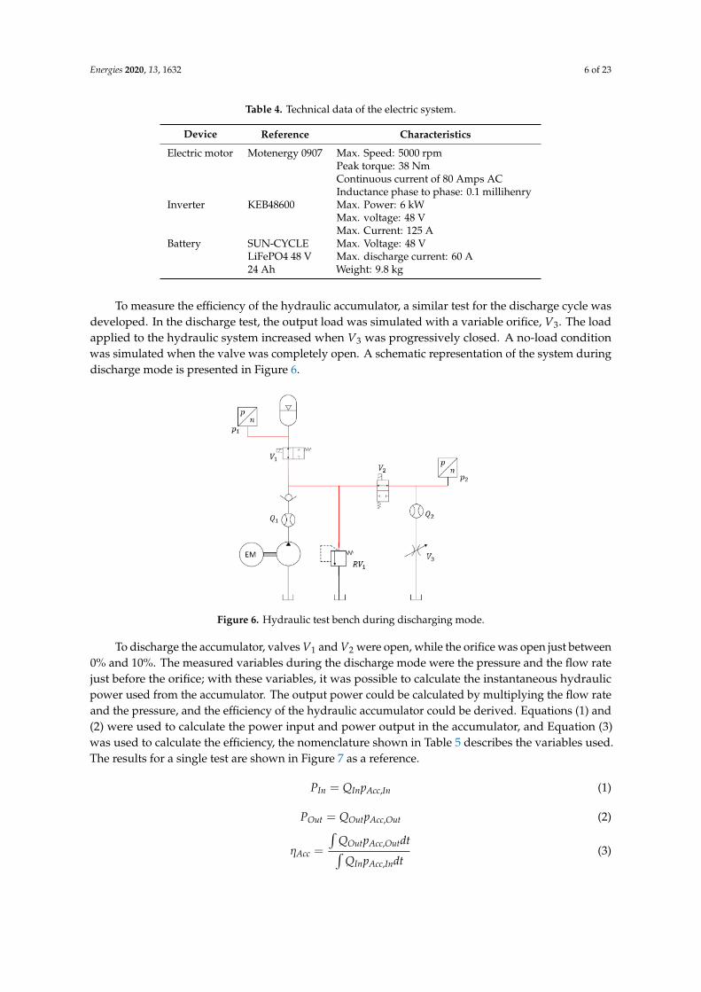
To measure the efficiency of the hydraulic accumulator, a similar test for the discharge cycle wasdeveloped. In the discharge test, the output load was simulated with a variable orifice, V3. The loadapplied to the hydraulic system increased when V3 was progressively closed. A no-load conditionwas simulated when the valve was completely open. A schematic representation of the system duringdischarge mode is presented in Figure 6.
Energies 2020, 13, x FOR PEER REVIEW 6 of 23
Electric motor Motenergy 0907 Max. Speed: 5000 rpm
Peak torque: 38 Nm
Continuous current of 80 Amps AC
Inductance phase to phase: 0.1 millihenry
Inverter KEB48600 Max. Power: 6 kW
Max. voltage: 48 V
Max. Current: 125 A
Battery SUN‐CYCLE LiFePO4 48 V 24 Ah Max. Voltage: 48 V
Max. discharge current: 60 A
Weight: 9.8 kg
To measure the efficiency of the hydraulic accumulator, a similar test for the discharge cycle was
developed. In the discharge test, the output load was simulated with a variable orifice, V3. The load
applied to the hydraulic system increased when V3 was progressively closed. A no‐load condition
was simulated when the valve was completely open. A schematic representation of the system during
discharge mode is presented in Figure 6.
Figure 6. Hydraulic test bench during discharging mode.
To discharge the accumulator, valves V1 and V2 were open, while the orifice was open just
between 0% and 10%. The measured variables during the discharge mode were the pressure and the
flow rate just before the orifice; with these variables, it was possible to calculate the instantaneous
hydraulic power used from the accumulator. The output power could be calculated by multiplying
the flow rate and the pressure, and the efficiency of the hydraulic accumulator could be derived.
Equations (1) and (2) were used to calculate the power input and power output in the accumulator,
and Equation (3) was used to calculate the efficiency, the nomenclature shown in Table 5 describes
the variables used. The results for a single test are shown in Figure 7 as a reference.
, (1)
, (2)
,
, (3)
Table 5. Variables used for determining the instantaneous efficiency of the accumulator.
Variable Description
(W) Power charging the accumulator
(W) Power discharging the accumulator
(gal/min) Volumetric flow charging the accumulator
Figure 6. Hydraulic test bench during discharging mode.
To discharge the accumulator, valves V1 and V2 were open, while the orifice was open just between0% and 10%. The measured variables during the discharge mode were the pressure and the flow ratejust before the orifice; with these variables, it was possible to calculate the instantaneous hydraulicpower used from the accumulator. The output power could be calculated by multiplying the flow rateand the pressure, and the efficiency of the hydraulic accumulator could be derived. Equations (1) and(2) were used to calculate the power input and power output in the accumulator, and Equation (3)was used to calculate the efficiency, the nomenclature shown in Table 5 describes the variables used.The results for a single test are shown in Figure 7 as a reference.
PIn = QInpAcc,In (1)
POut = QOutpAcc,Out (2)
ηAcc =
∫QOutpAcc,Outdt∫
QInpAcc,Indt(3)
Energies 2020, 13, 1632 7 of 23
Table 5. Variables used for determining the instantaneous efficiency of the accumulator.
Variable Description
PIn (W) Power charging the accumulatorPOut (W) Power discharging the accumulator
QIn (gal/min) Volumetric flow charging the accumulatorQOut (gal/min) Volumetric flow discharging the accumulator
pAcc,In (psi) Pressure charging the accumulatorpAcc,Out (psi) Pressure discharging the accumulatorηAcc Efficiency of the accumulator
Energies 2020, 13, x FOR PEER REVIEW 7 of 23
(gal/min) Volumetric flow discharging the accumulator
, (psi) Pressure charging the accumulator
, (psi) Pressure discharging the accumulator
Efficiency of the accumulator
Figure 7. Pressure in the accumulator during the charging and discharging process.
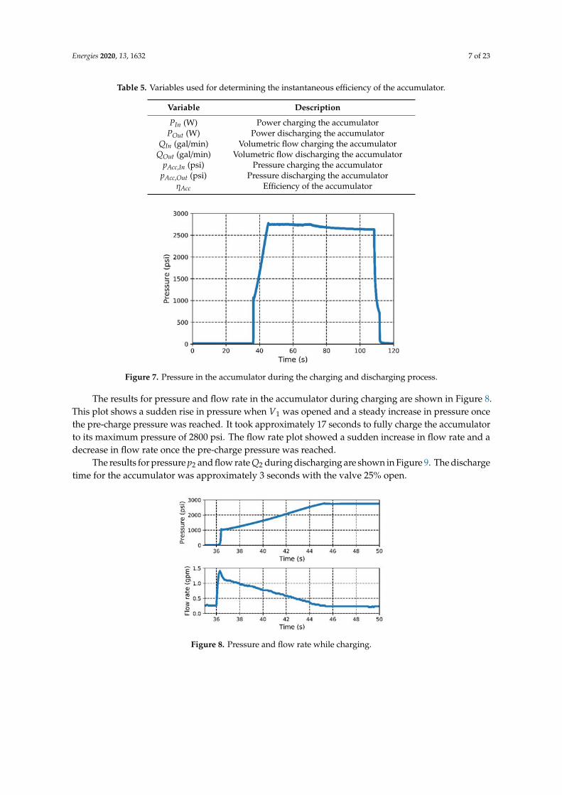
The results for pressure and flow rate in the accumulator during charging are shown in Figure
8. This plot shows a sudden rise in pressure when V1 was opened and a steady increase in pressure
once the pre‐charge pressure was reached. It took approximately 17 seconds to fully charge the
accumulator to its maximum pressure of 2800 psi. The flow rate plot showed a sudden increase in
flow rate and a decrease in flow rate once the pre‐charge pressure was reached.
The results for pressure and flow rate during discharging are shown in Figure 9. The
discharge time for the accumulator was approximately 3 seconds with the valve 25% open.
Figure 8. Pressure and flow rate while charging.
Figure 7. Pressure in the accumulator during the charging and discharging process.
The results for pressure and flow rate in the accumulator during charging are shown in Figure 8.This plot shows a sudden rise in pressure when V1 was opened and a steady increase in pressure oncethe pre-charge pressure was reached. It took approximately 17 seconds to fully charge the accumulatorto its maximum pressure of 2800 psi. The flow rate plot showed a sudden increase in flow rate and adecrease in flow rate once the pre-charge pressure was reached.
The results for pressure p2 and flow rate Q2 during discharging are shown in Figure 9. The dischargetime for the accumulator was approximately 3 seconds with the valve 25% open.
Energies 2020, 13, x FOR PEER REVIEW 7 of 23
(gal/min) Volumetric flow discharging the accumulator
, (psi) Pressure charging the accumulator
, (psi) Pressure discharging the accumulator
Efficiency of the accumulator
Figure 7. Pressure in the accumulator during the charging and discharging process.
The results for pressure and flow rate in the accumulator during charging are shown in Figure
8. This plot shows a sudden rise in pressure when V1 was opened and a steady increase in pressure
once the pre‐charge pressure was reached. It took approximately 17 seconds to fully charge the
accumulator to its maximum pressure of 2800 psi. The flow rate plot showed a sudden increase in
flow rate and a decrease in flow rate once the pre‐charge pressure was reached.
The results for pressure and flow rate during discharging are shown in Figure 9. The
discharge time for the accumulator was approximately 3 seconds with the valve 25% open.
Figure 8. Pressure and flow rate while charging. Figure 8. Pressure and flow rate while charging.
Energies 2020, 13, 1632 8 of 23Energies 2020, 13, x FOR PEER REVIEW 8 of 23
Figure 9. Pressure and flow rate while discharging.
Several experiments like the one described in this section were carried out to calculate the
efficiency and performance of the hydraulic accumulator. Load conditions were changed in all the
experiments by changing the orifice area. A list of the experiments is shown in Table 6. The 100%
value for the orifice area was 11.7mm .
Table 6. List of experiments performed in the hydraulic test bench.
Orifice Area While
Charging
Orifice Area While
Discharging
Orifice Area While
Charging
Orifice Area While
Discharging
3.1%
3.1%
12.5%
3.1%
6.2% 6.2%
9.4% 9.4%
12.5% 12.5%
25.0% 25.0%
100.0% 100.0%
6.2%
3.1%
25.0%
3.1%
6.2% 6.2%
9.4% 9.4%
12.5% 12.5%
25.0% 25.0%
100.0% 100.0%
9.4%
3.1%
100.0%
3.1%
6.2% 6.2%
9.4% 9.4%
12.5% 12.5%
25.0% 25.0%
100.0% 100.0%
3.2. Electric Test Bench
To compare the hydraulic accumulator with the ultracapacitor set, an electric test bench was
designed and constructed. A schematic representation of the test bench is presented in Figure 10.
Figure 9. Pressure and flow rate while discharging.
Several experiments like the one described in this section were carried out to calculate the efficiencyand performance of the hydraulic accumulator. Load conditions were changed in all the experimentsby changing the orifice area. A list of the experiments is shown in Table 6. The 100% value for theorifice area was 11.7 mm2.
Table 6. List of experiments performed in the hydraulic test bench.
Orifice Area WhileCharging
Orifice Area WhileDischarging
Orifice Area WhileCharging
Orifice Area WhileDischarging
3.1%
3.1%
12.5%
3.1%6.2% 6.2%9.4% 9.4%
12.5% 12.5%25.0% 25.0%
100.0% 100.0%
6.2%
3.1%
25.0%
3.1%6.2% 6.2%9.4% 9.4%
12.5% 12.5%25.0% 25.0%
100.0% 100.0%
9.4%
3.1%
100.0%
3.1%6.2% 6.2%9.4% 9.4%
12.5% 12.5%25.0% 25.0%
100.0% 100.0%
3.2. Electric Test Bench
To compare the hydraulic accumulator with the ultracapacitor set, an electric test bench wasdesigned and constructed. A schematic representation of the test bench is presented in Figure 10.
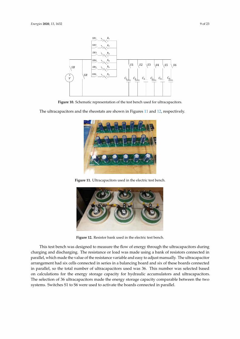
Energies 2020, 13, 1632 9 of 23Energies 2020, 13, x FOR PEER REVIEW 9 of 23
Figure 10. Schematic representation of the test bench used for ultracapacitors.
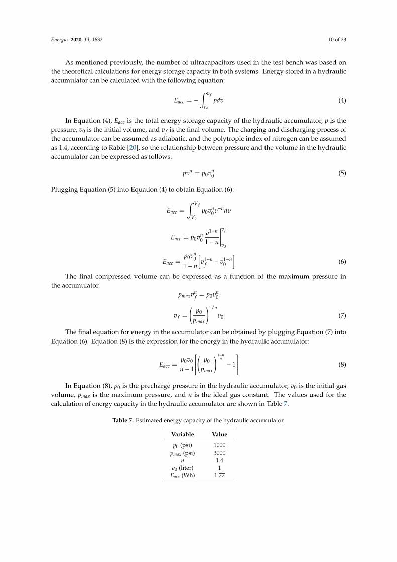
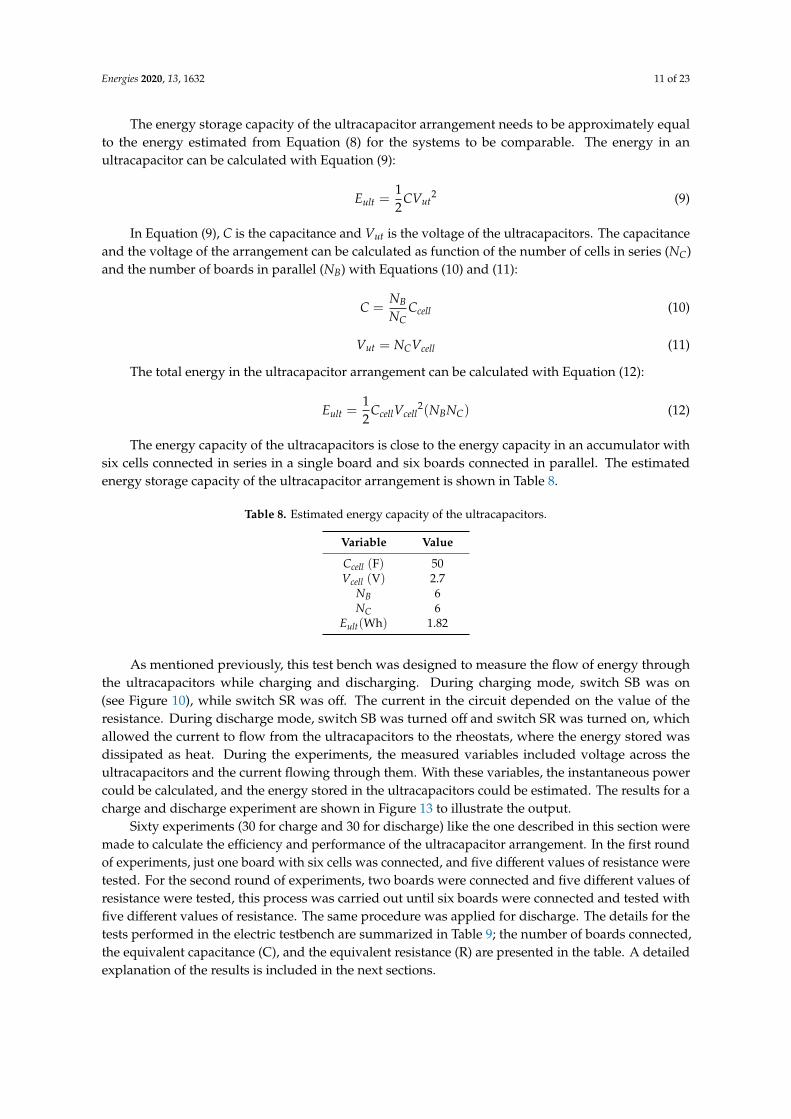
The ultracapacitors and the rheostats are shown in Figures 11 and 12, respectively.
Figure 11. Ultracapacitors used in the electric test bench.
Figure 12. Resistor bank used in the electric test bench.
This test bench was designed to measure the flow of energy through the ultracapacitors during
charging and discharging. The resistance or load was made using a bank of resistors connected in
parallel, which made the value of the resistance variable and easy to adjust manually. The
ultracapacitor arrangement had six cells connected in series in a balancing board and six of these
boards connected in parallel, so the total number of ultracapacitors used was 36. This number was
selected based on calculations for the energy storage capacity for hydraulic accumulators and
ultracapacitors. The selection of 36 ultracapacitors made the energy storage capacity comparable
between the two systems. Switches S1 to S6 were used to activate the boards connected in parallel.
As mentioned previously, the number of ultracapacitors used in the test bench was based on the
theoretical calculations for energy storage capacity in both systems. Energy stored in a hydraulic
accumulator can be calculated with the following equation:
Figure 10. Schematic representation of the test bench used for ultracapacitors.
The ultracapacitors and the rheostats are shown in Figures 11 and 12, respectively.
Energies 2020, 13, x FOR PEER REVIEW 9 of 23
Figure 10. Schematic representation of the test bench used for ultracapacitors.
The ultracapacitors and the rheostats are shown in Figures 11 and 12, respectively.
Figure 11. Ultracapacitors used in the electric test bench.
Figure 12. Resistor bank used in the electric test bench.
This test bench was designed to measure the flow of energy through the ultracapacitors during
charging and discharging. The resistance or load was made using a bank of resistors connected in
parallel, which made the value of the resistance variable and easy to adjust manually. The
ultracapacitor arrangement had six cells connected in series in a balancing board and six of these
boards connected in parallel, so the total number of ultracapacitors used was 36. This number was
selected based on calculations for the energy storage capacity for hydraulic accumulators and
ultracapacitors. The selection of 36 ultracapacitors made the energy storage capacity comparable
between the two systems. Switches S1 to S6 were used to activate the boards connected in parallel.
As mentioned previously, the number of ultracapacitors used in the test bench was based on the
theoretical calculations for energy storage capacity in both systems. Energy stored in a hydraulic
accumulator can be calculated with the following equation:
Figure 11. Ultracapacitors used in the electric test bench.
Energies 2020, 13, x FOR PEER REVIEW 9 of 23
Figure 10. Schematic representation of the test bench used for ultracapacitors.
The ultracapacitors and the rheostats are shown in Figures 11 and 12, respectively.
Figure 11. Ultracapacitors used in the electric test bench.
Figure 12. Resistor bank used in the electric test bench.
This test bench was designed to measure the flow of energy through the ultracapacitors during
charging and discharging. The resistance or load was made using a bank of resistors connected in
parallel, which made the value of the resistance variable and easy to adjust manually. The
ultracapacitor arrangement had six cells connected in series in a balancing board and six of these
boards connected in parallel, so the total number of ultracapacitors used was 36. This number was
selected based on calculations for the energy storage capacity for hydraulic accumulators and
ultracapacitors. The selection of 36 ultracapacitors made the energy storage capacity comparable
between the two systems. Switches S1 to S6 were used to activate the boards connected in parallel.
As mentioned previously, the number of ultracapacitors used in the test bench was based on the
theoretical calculations for energy storage capacity in both systems. Energy stored in a hydraulic
accumulator can be calculated with the following equation:
Figure 12. Resistor bank used in the electric test bench.
This test bench was designed to measure the flow of energy through the ultracapacitors duringcharging and discharging. The resistance or load was made using a bank of resistors connected inparallel, which made the value of the resistance variable and easy to adjust manually. The ultracapacitorarrangement had six cells connected in series in a balancing board and six of these boards connectedin parallel, so the total number of ultracapacitors used was 36. This number was selected basedon calculations for the energy storage capacity for hydraulic accumulators and ultracapacitors.The selection of 36 ultracapacitors made the energy storage capacity comparable between the twosystems. Switches S1 to S6 were used to activate the boards connected in parallel.
Energies 2020, 13, 1632 10 of 23
As mentioned previously, the number of ultracapacitors used in the test bench was based onthe theoretical calculations for energy storage capacity in both systems. Energy stored in a hydraulicaccumulator can be calculated with the following equation:
Eacc = −
∫ v f
vo
pdv (4)
In Equation (4), Eacc is the total energy storage capacity of the hydraulic accumulator, p is thepressure, v0 is the initial volume, and v f is the final volume. The charging and discharging process ofthe accumulator can be assumed as adiabatic, and the polytropic index of nitrogen can be assumedas 1.4, according to Rabie [20], so the relationship between pressure and the volume in the hydraulicaccumulator can be expressed as follows:
pvn = p0vn0 (5)
Plugging Equation (5) into Equation (4) to obtain Equation (6):
Eacc =
∫ V f
Vo
p0vn0v−ndv
Eacc = p0vn0
v1−n
1− n
∣∣∣∣∣∣v f
v0
Eacc =p0vn
0
1− n
[v1−n
f − v1−n0
](6)
The final compressed volume can be expressed as a function of the maximum pressure inthe accumulator.
pmaxvnf = p0vn
0
v f =
(p0
pmax
)1/n
v0 (7)
The final equation for energy in the accumulator can be obtained by plugging Equation (7) intoEquation (6). Equation (8) is the expression for the energy in the hydraulic accumulator:
Eacc =p0v0
n− 1
( p0
pmax
) 1−nn
− 1
(8)
In Equation (8), p0 is the precharge pressure in the hydraulic accumulator, v0 is the initial gasvolume, pmax is the maximum pressure, and n is the ideal gas constant. The values used for thecalculation of energy capacity in the hydraulic accumulator are shown in Table 7.
Table 7. Estimated energy capacity of the hydraulic accumulator.
Variable Value
p0 (psi) 1000pmax (psi) 3000
n 1.4v0 (liter) 1
Eacc (Wh) 1.77
Energies 2020, 13, 1632 11 of 23
The energy storage capacity of the ultracapacitor arrangement needs to be approximately equalto the energy estimated from Equation (8) for the systems to be comparable. The energy in anultracapacitor can be calculated with Equation (9):
Eult =12
CVut2 (9)
In Equation (9), C is the capacitance and Vut is the voltage of the ultracapacitors. The capacitanceand the voltage of the arrangement can be calculated as function of the number of cells in series (NC)and the number of boards in parallel (NB) with Equations (10) and (11):
C =NB
NCCcell (10)
Vut = NCVcell (11)
The total energy in the ultracapacitor arrangement can be calculated with Equation (12):
Eult =12
CcellVcell2(NBNC) (12)
The energy capacity of the ultracapacitors is close to the energy capacity in an accumulator withsix cells connected in series in a single board and six boards connected in parallel. The estimatedenergy storage capacity of the ultracapacitor arrangement is shown in Table 8.
Table 8. Estimated energy capacity of the ultracapacitors.
Variable Value
Ccell (F) 50Vcell (V) 2.7
NB 6NC 6
Eult(Wh) 1.82
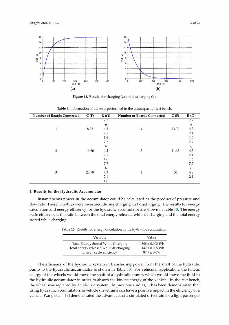
As mentioned previously, this test bench was designed to measure the flow of energy throughthe ultracapacitors while charging and discharging. During charging mode, switch SB was on(see Figure 10), while switch SR was off. The current in the circuit depended on the value of theresistance. During discharge mode, switch SB was turned off and switch SR was turned on, whichallowed the current to flow from the ultracapacitors to the rheostats, where the energy stored wasdissipated as heat. During the experiments, the measured variables included voltage across theultracapacitors and the current flowing through them. With these variables, the instantaneous powercould be calculated, and the energy stored in the ultracapacitors could be estimated. The results for acharge and discharge experiment are shown in Figure 13 to illustrate the output.
Sixty experiments (30 for charge and 30 for discharge) like the one described in this section weremade to calculate the efficiency and performance of the ultracapacitor arrangement. In the first roundof experiments, just one board with six cells was connected, and five different values of resistance weretested. For the second round of experiments, two boards were connected and five different values ofresistance were tested, this process was carried out until six boards were connected and tested withfive different values of resistance. The same procedure was applied for discharge. The details for thetests performed in the electric testbench are summarized in Table 9; the number of boards connected,the equivalent capacitance (C), and the equivalent resistance (R) are presented in the table. A detailedexplanation of the results is included in the next sections.
Energies 2020, 13, 1632 12 of 23
Energies 2020, 13, x FOR PEER REVIEW 11 of 23
(10)
(11)
The total energy in the ultracapacitor arrangement can be calculated with Equation (12):
12
(12)
The energy capacity of the ultracapacitors is close to the energy capacity in an accumulator with
six cells connected in series in a single board and six boards connected in parallel. The estimated
energy storage capacity of the ultracapacitor arrangement is shown in Table 8.
Table 8. Estimated energy capacity of the ultracapacitors.
Variable Value
F 50
V 2.7
6
6
Wh 1.82
As mentioned previously, this test bench was designed to measure the flow of energy through
the ultracapacitors while charging and discharging. During charging mode, switch SB was on (see
Figure 10), while switch SR was off. The current in the circuit depended on the value of the resistance.
During discharge mode, switch SB was turned off and switch SR was turned on, which allowed the
current to flow from the ultracapacitors to the rheostats, where the energy stored was dissipated as
heat. During the experiments, the measured variables included voltage across the ultracapacitors and
the current flowing through them. With these variables, the instantaneous power could be calculated,
and the energy stored in the ultracapacitors could be estimated. The results for a charge and discharge
experiment are shown in Figure 13 to illustrate the output.
(a) (b)
Figure 13. Results for charging (a) and discharging (b).
Sixty experiments (30 for charge and 30 for discharge) like the one described in this section were
made to calculate the efficiency and performance of the ultracapacitor arrangement. In the first round
of experiments, just one board with six cells was connected, and five different values of resistance
were tested. For the second round of experiments, two boards were connected and five different
values of resistance were tested, this process was carried out until six boards were connected and
tested with five different values of resistance. The same procedure was applied for discharge. The
details for the tests performed in the electric testbench are summarized in Table 9; the number of
boards connected, the equivalent capacitance (C), and the equivalent resistance (R) are presented in
the table. A detailed explanation of the results is included in the next sections.
Figure 13. Results for charging (a) and discharging (b).
Table 9. Information of the tests performed in the ultracapacitor test bench.
Number of Boards Connected C (F) R (Ω) Number of Boards Connected C (F) R (Ω)
1 8.33
7.7
4 33.32
7.76 6
4.3 4.32.1 2.11.6 1.6
2 16.66
7.7
5 41.65
7.76 6
4.3 4.32.1 2.11.6 1.6
3 24.99
7.7
6 50
7.76 6
4.3 4.32.1 2.11.6 1.6
4. Results for the Hydraulic Accumulator
Instantaneous power in the accumulator could be calculated as the product of pressure andflow rate. These variables were measured during charging and discharging. The results for energycalculation and energy efficiency for the hydraulic accumulator are shown in Table 10. The energycycle efficiency is the ratio between the total energy released while discharging and the total energystored while charging.
Table 10. Results for energy calculation in the hydraulic accumulator.
Variable Value
Total Energy Stored While Charging 1.308± 0.003 WhTotal energy released while discharging 1.147± 0.005 Wh
Energy cycle efficiency 87.7± 0.6%
The efficiency of the hydraulic system in transferring power from the shaft of the hydraulicpump to the hydraulic accumulator is shown in Table 10. For vehicular application, the kineticenergy of the wheels would move the shaft of a hydraulic pump, which would move the fluid tothe hydraulic accumulator in order to absorb the kinetic energy of the vehicle. In the test bench,the wheel was replaced by an electric system. In previous studies, it has been demonstrated thatusing hydraulic accumulators in vehicle drivetrains can have a positive impact in the efficiency of avehicle. Wang et al. [19] demonstrated the advantages of a simulated drivetrain for a light passenger
Energies 2020, 13, 1632 13 of 23
vehicle, where, although the energy used for the simulated drive cycle was better using the pureelectric drivetrain, the acceleration performance was better for the hydraulic drivetrain thanks to itshigher power density. Moreover, Hui et al. [18] studied the effect of using a hydraulic accumulator forextending the state of charge of a battery when hybridizing an electric drivetrain with a hydraulicregeneration with positive results due to the high efficiency of hydraulic accumulators. The power inthe hydraulic pump shaft was calculated as the product of the shaft torque and the rotational speed.The torque was estimated based on the pressure at outlet of the pump. The pressure and the torquewere correlated according to the next expression.
T =D∆pηm
(13)
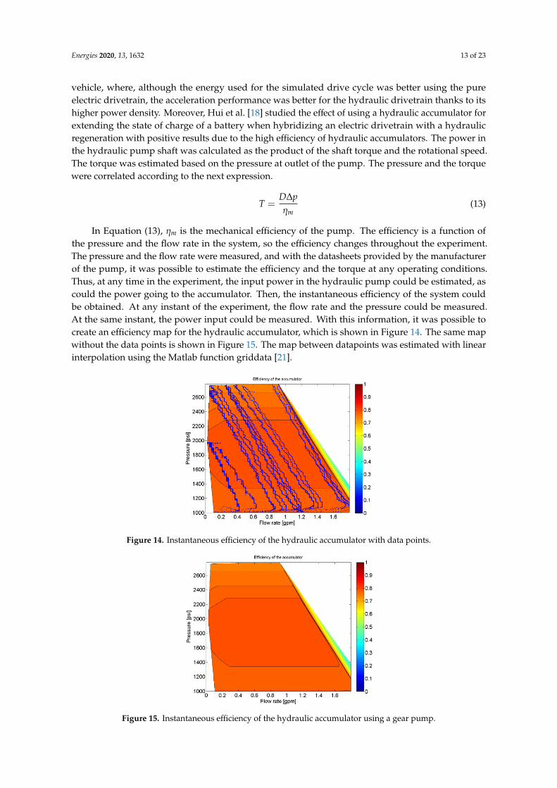
In Equation (13), ηm is the mechanical efficiency of the pump. The efficiency is a function ofthe pressure and the flow rate in the system, so the efficiency changes throughout the experiment.The pressure and the flow rate were measured, and with the datasheets provided by the manufacturerof the pump, it was possible to estimate the efficiency and the torque at any operating conditions.Thus, at any time in the experiment, the input power in the hydraulic pump could be estimated, ascould the power going to the accumulator. Then, the instantaneous efficiency of the system couldbe obtained. At any instant of the experiment, the flow rate and the pressure could be measured.At the same instant, the power input could be measured. With this information, it was possible tocreate an efficiency map for the hydraulic accumulator, which is shown in Figure 14. The same mapwithout the data points is shown in Figure 15. The map between datapoints was estimated with linearinterpolation using the Matlab function griddata [21].
Energies 2020, 13, x FOR PEER REVIEW 13 of 23
𝑇 =𝐷∆𝑝
𝜂𝑚
(13)
In Equation (13), 𝜂𝑚 is the mechanical efficiency of the pump. The efficiency is a function of the
pressure and the flow rate in the system, so the efficiency changes throughout the experiment. The
pressure and the flow rate were measured, and with the datasheets provided by the manufacturer of
the pump, it was possible to estimate the efficiency and the torque at any operating conditions. Thus,
at any time in the experiment, the input power in the hydraulic pump could be estimated, as could
the power going to the accumulator. Then, the instantaneous efficiency of the system could be
obtained. At any instant of the experiment, the flow rate and the pressure could be measured. At the
same instant, the power input could be measured. With this information, it was possible to create an
efficiency map for the hydraulic accumulator, which is shown in Figure 14. The same map without
the data points is shown in Figure 15. The map between datapoints was estimated with linear
interpolation using the Matlab function griddata [21].
Figure 14. Instantaneous efficiency of the hydraulic accumulator with data points.
Figure 15. Instantaneous efficiency of the hydraulic accumulator using a gear pump.
The map presented in Figures 14 and 15 is important in identifying operating conditions that
would be optimal for a system like the one proposed in this study. According to these plots, the
highest efficiency was around 80% and was obtained for flow rates of approximately 1 gpm and
pressures of approximately 1800 psi.
The current and voltage of the electric system were also measured during the experiment. A
similar map of efficiency could be made for the conversion of electric power to hydraulic power. The
map is shown in Figure 16.
Figure 14. Instantaneous efficiency of the hydraulic accumulator with data points.
Energies 2020, 13, x FOR PEER REVIEW 13 of 23
𝑇 =𝐷∆𝑝
𝜂𝑚
(13)
In Equation (13), 𝜂𝑚 is the mechanical efficiency of the pump. The efficiency is a function of the
pressure and the flow rate in the system, so the efficiency changes throughout the experiment. The
pressure and the flow rate were measured, and with the datasheets provided by the manufacturer of
the pump, it was possible to estimate the efficiency and the torque at any operating conditions. Thus,
at any time in the experiment, the input power in the hydraulic pump could be estimated, as could
the power going to the accumulator. Then, the instantaneous efficiency of the system could be
obtained. At any instant of the experiment, the flow rate and the pressure could be measured. At the
same instant, the power input could be measured. With this information, it was possible to create an
efficiency map for the hydraulic accumulator, which is shown in Figure 14. The same map without
the data points is shown in Figure 15. The map between datapoints was estimated with linear
interpolation using the Matlab function griddata [21].
Figure 14. Instantaneous efficiency of the hydraulic accumulator with data points.
Figure 15. Instantaneous efficiency of the hydraulic accumulator using a gear pump.
The map presented in Figures 14 and 15 is important in identifying operating conditions that
would be optimal for a system like the one proposed in this study. According to these plots, the
highest efficiency was around 80% and was obtained for flow rates of approximately 1 gpm and
pressures of approximately 1800 psi.
The current and voltage of the electric system were also measured during the experiment. A
similar map of efficiency could be made for the conversion of electric power to hydraulic power. The
map is shown in Figure 16.
Figure 15. Instantaneous efficiency of the hydraulic accumulator using a gear pump.
Energies 2020, 13, 1632 14 of 23
The map presented in Figures 14 and 15 is important in identifying operating conditions thatwould be optimal for a system like the one proposed in this study. According to these plots, the highestefficiency was around 80% and was obtained for flow rates of approximately 1 gpm and pressures ofapproximately 1800 psi.
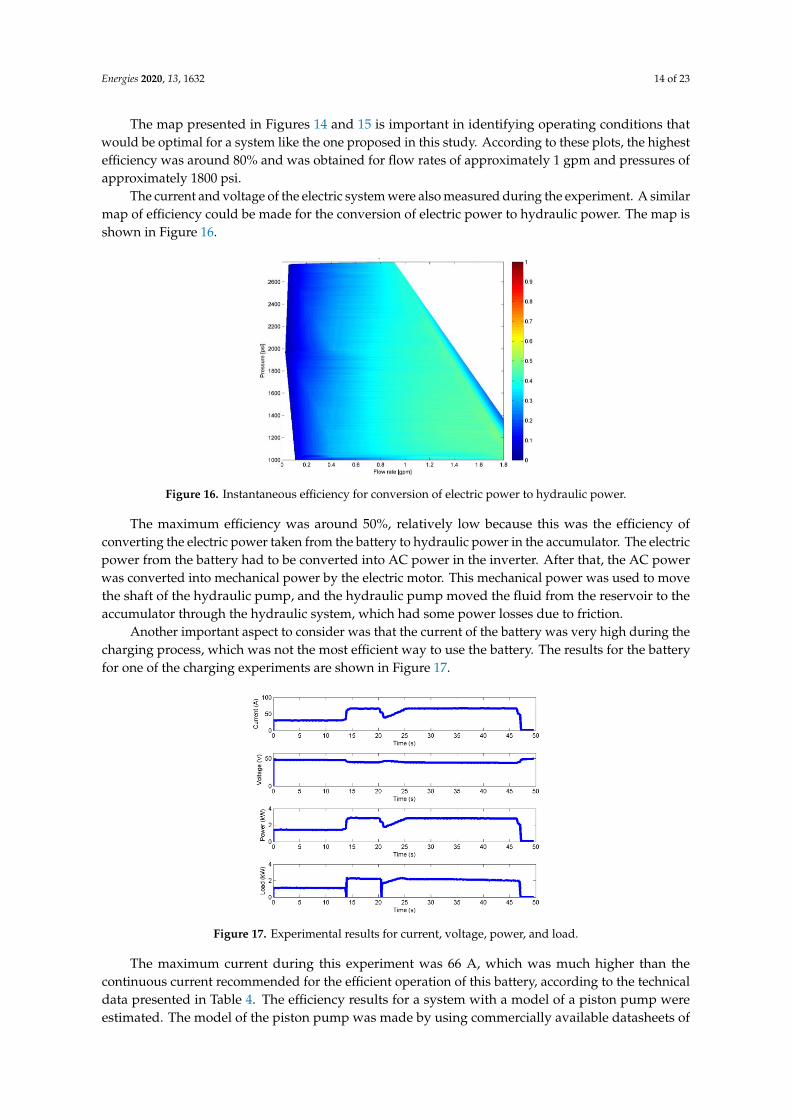
The current and voltage of the electric system were also measured during the experiment. A similarmap of efficiency could be made for the conversion of electric power to hydraulic power. The map isshown in Figure 16.Energies 2020, 13, x FOR PEER REVIEW 14 of 23
Figure 16. Instantaneous efficiency for conversion of electric power to hydraulic power.
The maximum efficiency was around 50%, relatively low because this was the efficiency of
converting the electric power taken from the battery to hydraulic power in the accumulator. The
electric power from the battery had to be converted into AC power in the inverter. After that, the AC
power was converted into mechanical power by the electric motor. This mechanical power was used
to move the shaft of the hydraulic pump, and the hydraulic pump moved the fluid from the reservoir
to the accumulator through the hydraulic system, which had some power losses due to friction.
Another important aspect to consider was that the current of the battery was very high during
the charging process, which was not the most efficient way to use the battery. The results for the
battery for one of the charging experiments are shown in Figure 17.
Figure 17. Experimental results for current, voltage, power, and load.
The maximum current during this experiment was 66 A, which was much higher than the
continuous current recommended for the efficient operation of this battery, according to the technical
data presented in Table 4. The efficiency results for a system with a model of a piston pump were
estimated. The model of the piston pump was made by using commercially available datasheets of
different piston pumps and then estimated with interpolation for a piston pump with a volumetric
displacement of 0.73 𝑖𝑛3 𝑟𝑒𝑣⁄ , which was 11.9 𝑐𝑐/𝑟𝑒𝑣. The results of the numerical estimation are
shown in Figure 18.
Figure 16. Instantaneous efficiency for conversion of electric power to hydraulic power.
The maximum efficiency was around 50%, relatively low because this was the efficiency ofconverting the electric power taken from the battery to hydraulic power in the accumulator. The electricpower from the battery had to be converted into AC power in the inverter. After that, the AC powerwas converted into mechanical power by the electric motor. This mechanical power was used to movethe shaft of the hydraulic pump, and the hydraulic pump moved the fluid from the reservoir to theaccumulator through the hydraulic system, which had some power losses due to friction.
Another important aspect to consider was that the current of the battery was very high during thecharging process, which was not the most efficient way to use the battery. The results for the batteryfor one of the charging experiments are shown in Figure 17.
Energies 2020, 13, x FOR PEER REVIEW 14 of 23
Figure 16. Instantaneous efficiency for conversion of electric power to hydraulic power.
The maximum efficiency was around 50%, relatively low because this was the efficiency of
converting the electric power taken from the battery to hydraulic power in the accumulator. The
electric power from the battery had to be converted into AC power in the inverter. After that, the AC
power was converted into mechanical power by the electric motor. This mechanical power was used
to move the shaft of the hydraulic pump, and the hydraulic pump moved the fluid from the reservoir
to the accumulator through the hydraulic system, which had some power losses due to friction.
Another important aspect to consider was that the current of the battery was very high during
the charging process, which was not the most efficient way to use the battery. The results for the
battery for one of the charging experiments are shown in Figure 17.
Figure 17. Experimental results for current, voltage, power, and load.
The maximum current during this experiment was 66 A, which was much higher than the
continuous current recommended for the efficient operation of this battery, according to the technical
data presented in Table 4. The efficiency results for a system with a model of a piston pump were
estimated. The model of the piston pump was made by using commercially available datasheets of
different piston pumps and then estimated with interpolation for a piston pump with a volumetric
displacement of 0.73 𝑖𝑛3 𝑟𝑒𝑣⁄ , which was 11.9 𝑐𝑐/𝑟𝑒𝑣. The results of the numerical estimation are
shown in Figure 18.
Figure 17. Experimental results for current, voltage, power, and load.
The maximum current during this experiment was 66 A, which was much higher than thecontinuous current recommended for the efficient operation of this battery, according to the technicaldata presented in Table 4. The efficiency results for a system with a model of a piston pump wereestimated. The model of the piston pump was made by using commercially available datasheets of
Energies 2020, 13, 1632 15 of 23
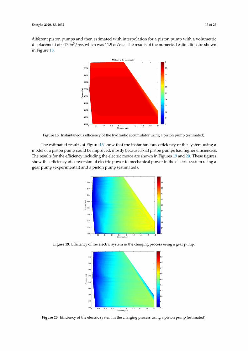
different piston pumps and then estimated with interpolation for a piston pump with a volumetricdisplacement of 0.73 in3/rev, which was 11.9 cc/rev. The results of the numerical estimation are shownin Figure 18.Energies 2020, 13, x FOR PEER REVIEW 15 of 23
Figure 18. Instantaneous efficiency of the hydraulic accumulator using a piston pump (estimated).
The estimated results of Figure 16 show that the instantaneous efficiency of the system using a
model of a piston pump could be improved, mostly because axial piston pumps had higher
efficiencies. The results for the efficiency including the electric motor are shown in Figures 19 and 20.
These figures show the efficiency of conversion of electric power to mechanical power in the electric
system using a gear pump (experimental) and a piston pump (estimated).
Figure 19. Efficiency of the electric system in the charging process using a gear pump.
Figure 20. Efficiency of the electric system in the charging process using a piston pump (estimated).
Figure 18. Instantaneous efficiency of the hydraulic accumulator using a piston pump (estimated).
The estimated results of Figure 16 show that the instantaneous efficiency of the system using amodel of a piston pump could be improved, mostly because axial piston pumps had higher efficiencies.The results for the efficiency including the electric motor are shown in Figures 19 and 20. These figuresshow the efficiency of conversion of electric power to mechanical power in the electric system using agear pump (experimental) and a piston pump (estimated).
Energies 2020, 13, x FOR PEER REVIEW 15 of 23
Figure 18. Instantaneous efficiency of the hydraulic accumulator using a piston pump (estimated).
The estimated results of Figure 16 show that the instantaneous efficiency of the system using a
model of a piston pump could be improved, mostly because axial piston pumps had higher
efficiencies. The results for the efficiency including the electric motor are shown in Figures 19 and 20.
These figures show the efficiency of conversion of electric power to mechanical power in the electric
system using a gear pump (experimental) and a piston pump (estimated).
Figure 19. Efficiency of the electric system in the charging process using a gear pump.
Figure 20. Efficiency of the electric system in the charging process using a piston pump (estimated).
Figure 19. Efficiency of the electric system in the charging process using a gear pump.
Energies 2020, 13, x FOR PEER REVIEW 15 of 23
Figure 18. Instantaneous efficiency of the hydraulic accumulator using a piston pump (estimated).
The estimated results of Figure 16 show that the instantaneous efficiency of the system using a
model of a piston pump could be improved, mostly because axial piston pumps had higher
efficiencies. The results for the efficiency including the electric motor are shown in Figures 19 and 20.
These figures show the efficiency of conversion of electric power to mechanical power in the electric
system using a gear pump (experimental) and a piston pump (estimated).
Figure 19. Efficiency of the electric system in the charging process using a gear pump.
Figure 20. Efficiency of the electric system in the charging process using a piston pump (estimated).
Figure 20. Efficiency of the electric system in the charging process using a piston pump (estimated).
Energies 2020, 13, 1632 16 of 23
From Figures 19 and 20, it can be observed that the electric system worked better when usinga gear pump. The difference in the results was due to the input torque needed to turn the shaft ofthe hydraulic pump, which in this case is lower for the gear pump than for the piston pump used.The overall efficiency of the system was highly dependent on pump efficiency.
5. Results for the Ultracapacitors
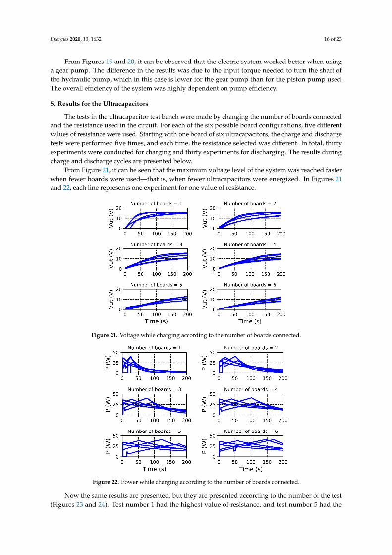
The tests in the ultracapacitor test bench were made by changing the number of boards connectedand the resistance used in the circuit. For each of the six possible board configurations, five differentvalues of resistance were used. Starting with one board of six ultracapacitors, the charge and dischargetests were performed five times, and each time, the resistance selected was different. In total, thirtyexperiments were conducted for charging and thirty experiments for discharging. The results duringcharge and discharge cycles are presented below.
From Figure 21, it can be seen that the maximum voltage level of the system was reached fasterwhen fewer boards were used—that is, when fewer ultracapacitors were energized. In Figures 21and 22, each line represents one experiment for one value of resistance.
Energies 2020, 13, x FOR PEER REVIEW 16 of 23
From Figures 19 and 20, it can be observed that the electric system worked better when using a
gear pump. The difference in the results was due to the input torque needed to turn the shaft of the
hydraulic pump, which in this case is lower for the gear pump than for the piston pump used. The
overall efficiency of the system was highly dependent on pump efficiency.
5. Results for the Ultracapacitors
The tests in the ultracapacitor test bench were made by changing the number of boards
connected and the resistance used in the circuit. For each of the six possible board configurations, five
different values of resistance were used. Starting with one board of six ultracapacitors, the charge
and discharge tests were performed five times, and each time, the resistance selected was different.
In total, thirty experiments were conducted for charging and thirty experiments for discharging. The
results during charge and discharge cycles are presented below.
From Figure 21, it can be seen that the maximum voltage level of the system was reached faster
when fewer boards were used—that is, when fewer ultracapacitors were energized. In Figures 21 and
22, each line represents one experiment for one value of resistance.
Figure 21. Voltage while charging according to the number of boards connected.
Figure 22. Power while charging according to the number of boards connected.
Figure 21. Voltage while charging according to the number of boards connected.
Energies 2020, 13, x FOR PEER REVIEW 16 of 23
From Figures 19 and 20, it can be observed that the electric system worked better when using a
gear pump. The difference in the results was due to the input torque needed to turn the shaft of the
hydraulic pump, which in this case is lower for the gear pump than for the piston pump used. The
overall efficiency of the system was highly dependent on pump efficiency.
5. Results for the Ultracapacitors
The tests in the ultracapacitor test bench were made by changing the number of boards
connected and the resistance used in the circuit. For each of the six possible board configurations, five
different values of resistance were used. Starting with one board of six ultracapacitors, the charge
and discharge tests were performed five times, and each time, the resistance selected was different.
In total, thirty experiments were conducted for charging and thirty experiments for discharging. The
results during charge and discharge cycles are presented below.
From Figure 21, it can be seen that the maximum voltage level of the system was reached faster
when fewer boards were used—that is, when fewer ultracapacitors were energized. In Figures 21 and
22, each line represents one experiment for one value of resistance.
Figure 21. Voltage while charging according to the number of boards connected.
Figure 22. Power while charging according to the number of boards connected. Figure 22. Power while charging according to the number of boards connected.
Now the same results are presented, but they are presented according to the number of the test(Figures 23 and 24). Test number 1 had the highest value of resistance, and test number 5 had the
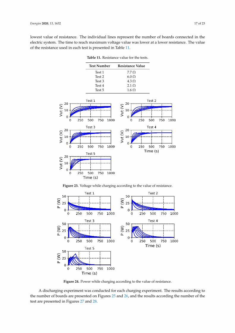
Energies 2020, 13, 1632 17 of 23
lowest value of resistance. The individual lines represent the number of boards connected in theelectric system. The time to reach maximum voltage value was lower at a lower resistance. The valueof the resistance used in each test is presented in Table 11.
Table 11. Resistance value for the tests.
Test Number Resistance Value
Test 1 7.7 ΩTest 2 6.0 ΩTest 3 4.3 ΩTest 4 2.1 ΩTest 5 1.6 Ω
Energies 2020, 13, x FOR PEER REVIEW 17 of 23
Now the same results are presented, but they are presented according to the number of the test
(Figures 23 and 24). Test number 1 had the highest value of resistance, and test number 5 had the
lowest value of resistance. The individual lines represent the number of boards connected in the
electric system. The time to reach maximum voltage value was lower at a lower resistance. The value
of the resistance used in each test is presented in Table 11.
Table 11. Resistance value for the tests.
Test Number Resistance Value
Test 1 7.7 Ω
Test 2 6.0 Ω
Test 3 4.3 Ω
Test 4 2.1 Ω
Test 5 1.6 Ω
Figure 23. Voltage while charging according to the value of resistance.
Figure 24. Power while charging according to the value of resistance.
Figure 23. Voltage while charging according to the value of resistance.
Energies 2020, 13, x FOR PEER REVIEW 17 of 23
Now the same results are presented, but they are presented according to the number of the test
(Figures 23 and 24). Test number 1 had the highest value of resistance, and test number 5 had the
lowest value of resistance. The individual lines represent the number of boards connected in the
electric system. The time to reach maximum voltage value was lower at a lower resistance. The value
of the resistance used in each test is presented in Table 11.
Table 11. Resistance value for the tests.
Test Number Resistance Value
Test 1 7.7 Ω
Test 2 6.0 Ω
Test 3 4.3 Ω
Test 4 2.1 Ω
Test 5 1.6 Ω
Figure 23. Voltage while charging according to the value of resistance.
Figure 24. Power while charging according to the value of resistance. Figure 24. Power while charging according to the value of resistance.
A discharging experiment was conducted for each charging experiment. The results according tothe number of boards are presented on Figures 25 and 26, and the results according the number of thetest are presented in Figures 27 and 28.
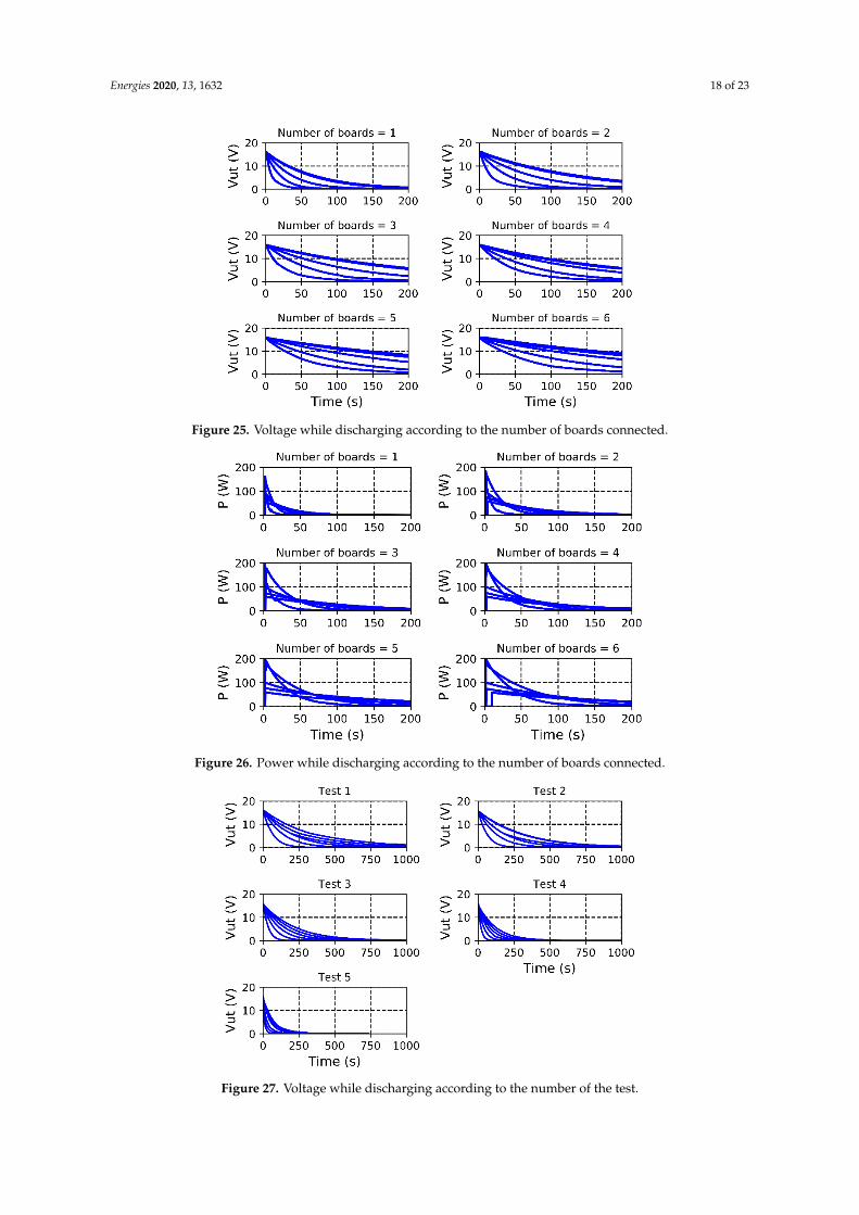
Energies 2020, 13, 1632 18 of 23
Energies 2020, 13, x FOR PEER REVIEW 18 of 23
A discharging experiment was conducted for each charging experiment. The results according
to the number of boards are presented on Figures 25 and 26, and the results according the number of
the test are presented in Figures 27 and 28.
Figure 25. Voltage while discharging according to the number of boards connected.
Figure 26. Power while discharging according to the number of boards connected.
Figure 25. Voltage while discharging according to the number of boards connected.
Energies 2020, 13, x FOR PEER REVIEW 18 of 23
A discharging experiment was conducted for each charging experiment. The results according
to the number of boards are presented on Figures 25 and 26, and the results according the number of
the test are presented in Figures 27 and 28.
Figure 25. Voltage while discharging according to the number of boards connected.
Figure 26. Power while discharging according to the number of boards connected. Figure 26. Power while discharging according to the number of boards connected.
Energies 2020, 13, x FOR PEER REVIEW 19 of 23
Figure 27. Voltage while discharging according to the number of the test.
Figure 28. Power while discharging grouped according to the number of the test.
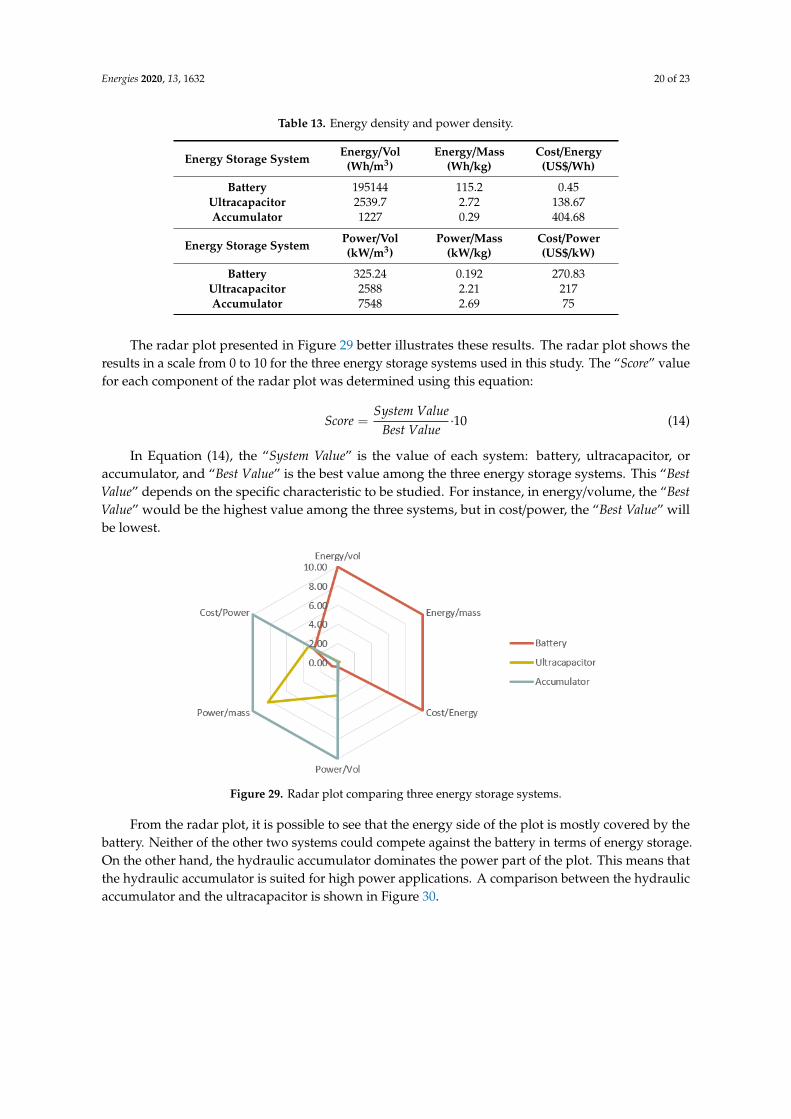
Using results presented in Figures 21–28, it was possible calculate the energy stored in the
ultracapacitors and the efficiency. The results for energy calculations in the ultracapacitors are
presented in Table 12.
Table 12. Results for energy calculation in the ultracapacitors.
Variable Number of Boards Connected in Parallel
1 2 3
Value Error Value Error Value Error
Energy stored while
charging (Wh) 0.31 0.01 0.63 0.02 0.92 0.03
Energy stored while
discharging (Wh) 0.25 0.01 0.50 0.01 0.76 0.02
Energy efficiency 77.46 2.33 77.2 2.7 80.75 3.3
Figure 27. Voltage while discharging according to the number of the test.
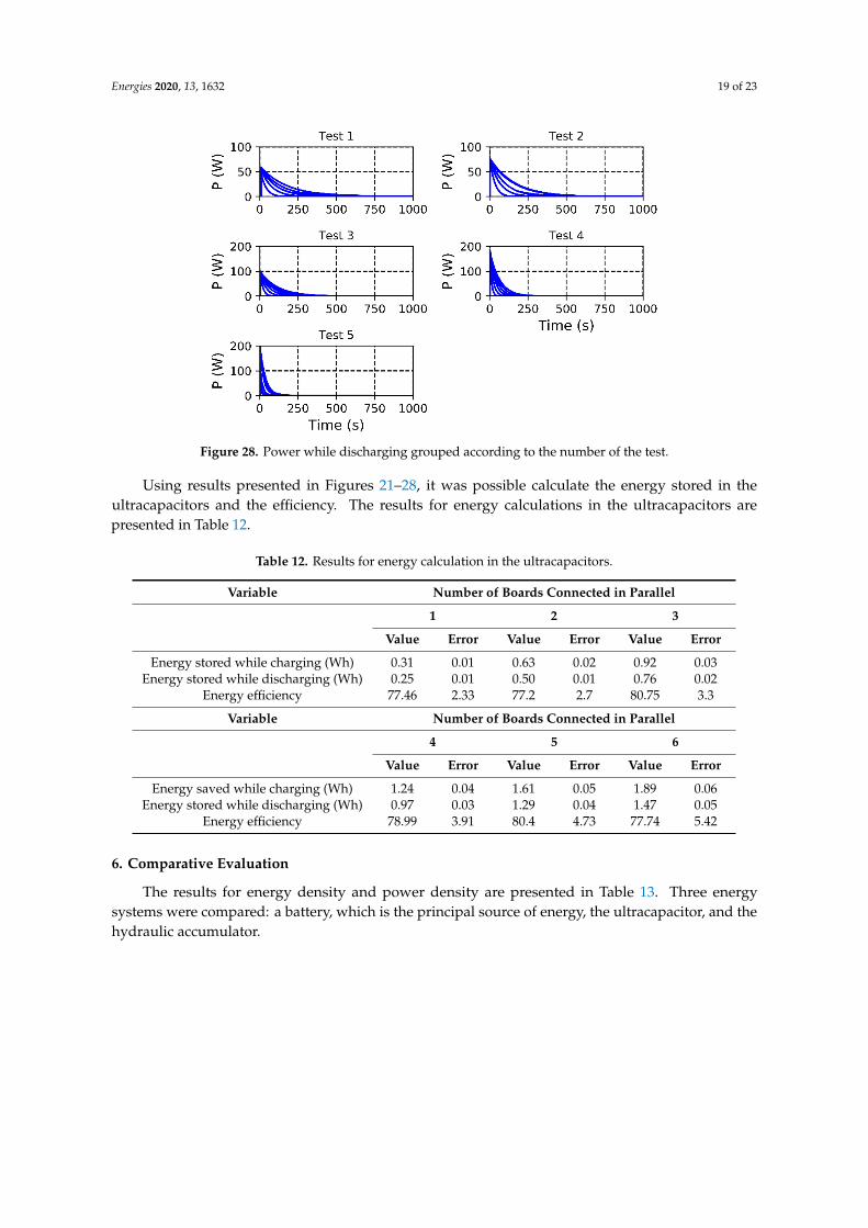
Energies 2020, 13, 1632 19 of 23
Energies 2020, 13, x FOR PEER REVIEW 19 of 23
Figure 27. Voltage while discharging according to the number of the test.
Figure 28. Power while discharging grouped according to the number of the test.
Using results presented in Figures 21–28, it was possible calculate the energy stored in the
ultracapacitors and the efficiency. The results for energy calculations in the ultracapacitors are
presented in Table 12.
Table 12. Results for energy calculation in the ultracapacitors.
Variable Number of Boards Connected in Parallel
1 2 3
Value Error Value Error Value Error
Energy stored while
charging (Wh) 0.31 0.01 0.63 0.02 0.92 0.03
Energy stored while
discharging (Wh) 0.25 0.01 0.50 0.01 0.76 0.02
Energy efficiency 77.46 2.33 77.2 2.7 80.75 3.3
Figure 28. Power while discharging grouped according to the number of the test.
Using results presented in Figures 21–28, it was possible calculate the energy stored in theultracapacitors and the efficiency. The results for energy calculations in the ultracapacitors arepresented in Table 12.
Table 12. Results for energy calculation in the ultracapacitors.
Variable Number of Boards Connected in Parallel
1 2 3
Value Error Value Error Value Error
Energy stored while charging (Wh) 0.31 0.01 0.63 0.02 0.92 0.03Energy stored while discharging (Wh) 0.25 0.01 0.50 0.01 0.76 0.02
Energy efficiency 77.46 2.33 77.2 2.7 80.75 3.3
Variable Number of Boards Connected in Parallel
4 5 6
Value Error Value Error Value Error
Energy saved while charging (Wh) 1.24 0.04 1.61 0.05 1.89 0.06Energy stored while discharging (Wh) 0.97 0.03 1.29 0.04 1.47 0.05
Energy efficiency 78.99 3.91 80.4 4.73 77.74 5.42
6. Comparative Evaluation
The results for energy density and power density are presented in Table 13. Three energysystems were compared: a battery, which is the principal source of energy, the ultracapacitor, and thehydraulic accumulator.
Energies 2020, 13, 1632 20 of 23
Table 13. Energy density and power density.
Energy Storage System Energy/Vol(Wh/m3)
Energy/Mass(Wh/kg)
Cost/Energy(US$/Wh)
Battery 195144 115.2 0.45Ultracapacitor 2539.7 2.72 138.67Accumulator 1227 0.29 404.68
Energy Storage System Power/Vol(kW/m3)
Power/Mass(kW/kg)
Cost/Power(US$/kW)
Battery 325.24 0.192 270.83Ultracapacitor 2588 2.21 217Accumulator 7548 2.69 75
The radar plot presented in Figure 29 better illustrates these results. The radar plot shows theresults in a scale from 0 to 10 for the three energy storage systems used in this study. The “Score” valuefor each component of the radar plot was determined using this equation:
Score =System Value
Best Value·10 (14)
In Equation (14), the “System Value” is the value of each system: battery, ultracapacitor, oraccumulator, and “Best Value” is the best value among the three energy storage systems. This “BestValue” depends on the specific characteristic to be studied. For instance, in energy/volume, the “BestValue” would be the highest value among the three systems, but in cost/power, the “Best Value” willbe lowest.Energies 2020, 13, x FOR PEER REVIEW 21 of 23
Figure 29. Radar plot comparing three energy storage systems.
From the radar plot, it is possible to see that the energy side of the plot is mostly covered by the
battery. Neither of the other two systems could compete against the battery in terms of energy
storage. On the other hand, the hydraulic accumulator dominates the power part of the plot. This
means that the hydraulic accumulator is suited for high power applications. A comparison between
the hydraulic accumulator and the ultracapacitor is shown in Figure 30.
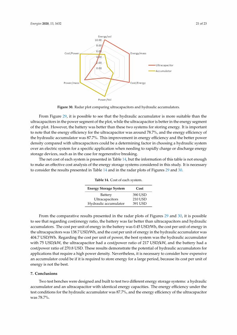
Figure 30. Radar plot comparing ultracapacitors and hydraulic accumulators.
From Figure 29, it is possible to see that the hydraulic accumulator is more suitable than the
ultracapacitors in the power segment of the plot, while the ultracapacitor is better in the energy
segment of the plot. However, the battery was better than these two systems for storing energy. It is
important to note that the energy efficiency for the ultracapacitor was around 78.7%, and the energy
efficiency of the hydraulic accumulator was 87.7%. This improvement in energy efficiency and the
better power density compared with ultracapacitors could be a determining factor in choosing a
hydraulic system over an electric system for a specific application when needing to rapidly charge or
discharge energy storage devices, such as in the case for regenerative breaking.
The net cost of each system is presented in Table 14, but the information of this table is not
enough to make an effective cost analysis of the energy storage systems considered in this study. It
is necessary to consider the results presented in Table 14 and in the radar plots of Figures 29 and 30.
Table 14. Cost of each system.
Energy Storage System Cost
Battery 390 USD
Figure 29. Radar plot comparing three energy storage systems.
From the radar plot, it is possible to see that the energy side of the plot is mostly covered by thebattery. Neither of the other two systems could compete against the battery in terms of energy storage.On the other hand, the hydraulic accumulator dominates the power part of the plot. This means thatthe hydraulic accumulator is suited for high power applications. A comparison between the hydraulicaccumulator and the ultracapacitor is shown in Figure 30.
Energies 2020, 13, 1632 21 of 23
Energies 2020, 13, x FOR PEER REVIEW 21 of 23
Figure 29. Radar plot comparing three energy storage systems.
From the radar plot, it is possible to see that the energy side of the plot is mostly covered by the
battery. Neither of the other two systems could compete against the battery in terms of energy
storage. On the other hand, the hydraulic accumulator dominates the power part of the plot. This
means that the hydraulic accumulator is suited for high power applications. A comparison between
the hydraulic accumulator and the ultracapacitor is shown in Figure 30.
Figure 30. Radar plot comparing ultracapacitors and hydraulic accumulators.
From Figure 29, it is possible to see that the hydraulic accumulator is more suitable than the
ultracapacitors in the power segment of the plot, while the ultracapacitor is better in the energy
segment of the plot. However, the battery was better than these two systems for storing energy. It is
important to note that the energy efficiency for the ultracapacitor was around 78.7%, and the energy
efficiency of the hydraulic accumulator was 87.7%. This improvement in energy efficiency and the
better power density compared with ultracapacitors could be a determining factor in choosing a
hydraulic system over an electric system for a specific application when needing to rapidly charge or
discharge energy storage devices, such as in the case for regenerative breaking.
The net cost of each system is presented in Table 14, but the information of this table is not
enough to make an effective cost analysis of the energy storage systems considered in this study. It
is necessary to consider the results presented in Table 14 and in the radar plots of Figures 29 and 30.
Table 14. Cost of each system.
Energy Storage System Cost
Battery 390 USD
Figure 30. Radar plot comparing ultracapacitors and hydraulic accumulators.
From Figure 29, it is possible to see that the hydraulic accumulator is more suitable than theultracapacitors in the power segment of the plot, while the ultracapacitor is better in the energy segmentof the plot. However, the battery was better than these two systems for storing energy. It is importantto note that the energy efficiency for the ultracapacitor was around 78.7%, and the energy efficiency ofthe hydraulic accumulator was 87.7%. This improvement in energy efficiency and the better powerdensity compared with ultracapacitors could be a determining factor in choosing a hydraulic systemover an electric system for a specific application when needing to rapidly charge or discharge energystorage devices, such as in the case for regenerative breaking.
The net cost of each system is presented in Table 14, but the information of this table is not enoughto make an effective cost analysis of the energy storage systems considered in this study. It is necessaryto consider the results presented in Table 14 and in the radar plots of Figures 29 and 30.
Table 14. Cost of each system.
Energy Storage System Cost
Battery 390 USDUltracapacitors 210 USD
Hydraulic accumulator 391 USD
From the comparative results presented in the radar plots of Figures 29 and 30, it is possibleto see that regarding cost/energy ratio, the battery was far better than ultracapacitors and hydraulicaccumulators. The cost per unit of energy in the battery was 0.45 USD/Wh, the cost per unit of energy inthe ultracapacitors was 138.7 USD/Wh, and the cost per unit of energy in the hydraulic accumulator was404.7 USD/Wh. Regarding the cost per unit of power, the best system was the hydraulic accumulatorwith 75 USD/kW, the ultracapacitor had a cost/power ratio of 217 USD/kW, and the battery had acost/power ratio of 270.8 USD. These results demonstrate the potential of hydraulic accumulators forapplications that require a high power density. Nevertheless, it is necessary to consider how expensivean accumulator could be if it is required to store energy for a large period, because its cost per unit ofenergy is not the best.
7. Conclusions
Two test benches were designed and built to test two different energy storage systems: a hydraulicaccumulator and an ultracapacitor with identical energy capacities. The energy efficiency under thetest conditions for the hydraulic accumulator was 87.7%, and the energy efficiency of the ultracapacitorwas 78.7%.
Energies 2020, 13, 1632 22 of 23
The efficiency map from this study can be used to determine a control strategy for a regenerativesystem with hydraulic accumulators. This efficiency map can be replicated for different hydraulicpumps by using numerical models for a pump. In addition, the analysis of the efficiency map for apiston pump shows that a hydraulic accumulator would be more efficient if a piston pump is usedinstead of a gear pump.
This study also shows that energy segments of the radar plot were dominated by the ultracapacitor,while the power segments were dominated by the hydraulic accumulator. It is interesting to notethat there were segments in the radar plot that were not covered by either of the three energy storagesystems. In other words, none of the systems showed a good score in cost/power and energy/volume.This means that energy storage systems with high energy density can provide high power but at a highcost. Moreover, there was no system with a high score in power/volume and cost/energy, which meansthat the energy storage systems with good power density can be used to store energy but at a high cost.
The higher energy efficiency in the hydraulic accumulator and the better power density comparedwith ultracapacitors could be determining factors in choosing a hydraulic system over an electricsystem for a specific application, where there is a need to rapidly charge or discharge energy storagedevices, such as in the case of regenerative breaking.
Author Contributions: Conceptualization, J.L.-Q., J.G.-B. and M.K.; methodology, J.L.-Q., J.G.-B. and M.K.;software, J.L.-Q.; validation, J.L.-Q., B.N., M.K., A.G.-M., and J.G.-B.; formal analysis, J.L.-Q., and J.G.-B.;investigation, J.L.-Q., M.K., A.G.-M., and J.G.-B.; resources, B.N., and J.G.-B.; data curation, J.L.-Q.; writing—originaldraft preparation, J.L.-Q.; writing—review and editing, J.L.-Q., B.N., M.K., A.G.-M., and J.G.-B.; visualization,J.L.-Q., B.N., M.K., A.G.-M., and J.G.-B.; supervision, B.N., M.K., A.G.-M., and J.G.-B.; project administration, B.N.,and J.G.-B.; funding acquisition, B.N., and J.G.-B. All authors have read and agreed to the published version ofthe manuscript.
Funding: This research was funded by the Purdue Polytechnic, office of the vice dean of research, and the schoolof Engineering Technology at Purdue University.
Acknowledgments: Special thanks for Sun Hydraulics for providing testing components.
Conflicts of Interest: The authors declare no conflict of interest.
References
1. U.S. Energy Information Administration. Monthly Energy Review; U.S. Energy Information Administration:Washington, DC, USA, 2019.
2. Lin, T.; Wang, Q.; Hu, B.; Gong, W. Development of hybrid powered hydraulic construction machinery.Autom. Constr. 2010, 19, 11–19. [CrossRef]
3. Kwon, T.S.; Lee, S.W.; Sul, S.K.; Park, C.G.; Kim, N.I.; Kang, B.I.; Hong, M.S. Power Control Algorithm forHybrid Excavator with Supercapacitor. IEEE Trans. Ind. Appl. 2010, 46, 1447–1455. [CrossRef]
4. Xiao, Q.; Wang, Q.; Zhang, Y. Control strategies of power system in hybrid hydraulic excavator—ScienceDirect.Autom. Constr. 2018, 17, 361–367. [CrossRef]
5. Wang, T.; Wang, Q.; Lin, T. Improvement of boom control performance for hybrid hydraulic excavator withpotential energy recovery—ScienceDirect. Autom. Constr. 2013, 30, 161–169. [CrossRef]
6. Lin, T.; Chen, Q.; Ren, H.; Huang, W.; Chen, Q.; Fu, S. Review of boom potential energy regenerationtechnology for hydraulic construction machinery. Renew. Sustain. Energy Rev. 2017, 79, 358–371. [CrossRef]
7. Lin, T.; Huang, W.; Ren, H.; Fu, S.; Liu, Q. New compound energy regeneration system and control strategyfor hybrid hydraulic excavators. Autom. Constr. 2016, 68, 11–20. [CrossRef]
8. Tan, Y.; Ciufo, P.; Meegahapola, L.; Muttaqi, K.M. Enhanced Frequency Response Strategy for a PMSG-BasedWind Energy Conversion System Using Ultracapacitor in Remote Area Power Supply Systems. IEEE Trans.Ind. Appl. 2016, 53, 549–558. [CrossRef]
9. Kim, S.M.; Sul, S.K. Control of Rubber Tyred Gantry Crane with Energy Storage Based on SupercapacitorBank. IEEE Trans. Power Electron. 2006, 21, 1420–1427. [CrossRef]
10. Pandey, A.; Allos, F.; Hu, A.P.; Budgett, D. Integration of supercapacitors into wirelessly charged biomedicalsensors. In Proceedings of the 2011 6th IEEE Conference on Industrial Electronics and Applications, Beijing,China, 21–23 June 2011; pp. 56–61. [CrossRef]
Energies 2020, 13, 1632 23 of 23
11. Lin, T.; Zhou, S.; Chen, Q.; Fu, S. A Novel Control Strategy for an Energy Saving Hydraulic System WithNear-Zero Overflowing Energy-Loss. IEEE Access 2018, 6, 33810–33818. [CrossRef]
12. Wang, B. High Speed On-Off Valve Self-adapting Clamping System. J. Appl. Sci. 2014, 14, 279–284. [CrossRef]13. Andruch, J.; Lumkes, J.H. Regenerative Hydraulic Topographies using High Speed Valves. SAE Tech. Pap.
Ser. 2009. [CrossRef]14. Fouda, M.; Elwakil, A.S.; Radwan, A.G.; Allagui, A. Power and energy analysis of fractional-order electrical
energy storage devices. Energy 2016, 111, 785–792. [CrossRef]15. Hartley, T.T.; Veillette, R.J.; Adams, J.L.; Lorenzo, C.F. Energy storage and loss in fractional-order circuit
elements. IET Circuits Devices Syst. 2015, 9, 227–235. [CrossRef]16. Allagui, A.; Freeborn, T.J.; Elwakil, A.S.; Maundy, B.J. Reevaluation of Performance of Electric Double-layer
Capacitors from Constant-current Charge/Discharge and Cyclic Voltammetry. Sci. Rep. 2016, 6, 38568.[CrossRef] [PubMed]
17. Freeborn, T.J. Estimating supercapacitor performance for embedded applications using fractional-ordermodels. Electron. Lett. 2016, 52, 1478–1480. [CrossRef]
18. Hui, S.; Lifu, Y.; Junqing, J.; Yanling, L. Control strategy of hydraulic/electric synergy system in heavy hybridvehicles. Energy Convers. Manag. 2011, 52, 668–674. [CrossRef]
19. Wang, F. Comparison between Hydraulic Hybrid and Electric Hybrid Passenger Vehicles using ADVISOR2004. In Proceedings of the 52nd National Conference on Fluid Power, Las Vegas, NV, USA, 23–25 March2011; pp. 31–40.
20. Rabie, M.G. Fluid Power Engineering; McGraw-Hill: New York, NY, USA, 2009; Volume 28.21. Interpolate 2-D or 3-D Scattered Data—MATLAB Griddata. Available online: https://www.mathworks.com/
help/matlab/ref/griddata.html (accessed on 15 January 2020).
© 2020 by the authors. Licensee MDPI, Basel, Switzerland. This article is an open accessarticle distributed under the terms and conditions of the Creative Commons Attribution(CC BY) license (http://creativecommons.org/licenses/by/4.0/).


