PROGRAM ON THE GLOBAL DEMOGRAPHY OF AGING

Working Paper Series

Endogenous Longevity and Economic Growth

Jocelyn Finlay¤† School of Economics

Faculty of Economics and Commerce HW Arndt Building 25A

Australian National University 0200 Australia

fax: +61 2 612 55124 email: Jocelyn.Finlay@anu.edu.au

July 24, 2006

PGDA Working Paper No. 7: http://www.hsph.harvard.edu/pgda/working.htm The views expressed in this paper are those of the author(s) and not necessarily those of the Harvard Initiative for Global Health. The Program on the Global Demography of Aging receives funding from the National Institute on Aging, Grant No. 1 P30 AG024409-01.

Endogenous Longevity and Economic Growth

Jocelyn Finlay∗†

School of EconomicsFaculty of Economics and Commerce

HW Arndt Building 25AAustralian National University 0200

Australiafax: +61 2 612 55124

email: Jocelyn.Finlay@anu.edu.au

July 24, 2006

Abstract

In a two period overlapping generations model of endogenous longevity and economicgrowth, individuals choose to invest in health and education. The investments are costlyin terms of foregone first period consumption and the benefit is in the second periodwhere health has the effect of increasing the probability of survival, and educationinvestment will bring higher income. These investments are risky as survival throughperiod two, when the payoffs can be had, is not certain. Individuals with varying degreesof risk aversion will choose the ordering in which they invest in health and education.It is only when investment in education is achieved that an economy will experienceendogenous growth.

Keywords: Endogenous Longevity, Endogenous Growth, Health, Risk

∗Address for correspondence: School of Economics, Faculty of Economics and Commerce, Aus-tralian National University, Canberra ACT 0200, AUSTRALIA, fax: +61 2 612 55124, email: Joce-lyn.Finlay@anu.edu.au

†I would like to thank Steve Dowrick whose comments have strongly influenced the direction of thispaper. Thanks also goes to Guillaume Rocheteau. I am much obliged for the comments from partic-ipants of the seminar series at Institut de Recherches Economiques et Sociales, Universite Catholiquede Louvain, Belgium, especially those from David de la Croix and Raouf Boucekkine. Finally I wouldlike to thank Pierre Pestieau and Izabela Jelovac of the University of Liege for their support. All errorsare my own.

1

Endogenous Longevity and Economic Growth

1 Introduction

The relationship between life expectancy and economic growth is a newly contested

field. Economic growth models that treat longevity as an exogenous parameter show

that an increase in life expectancy will increase the time horizon over which returns

to education can be realised, thereby encouraging investment in human capital and

driving endogenous growth. Existing models of endogenous life expectancy, where the

survival probability is a function of a choice variable within the model, also show this

same positive relationship between life expectancy and economic growth. Moreover,

models of endogenous longevity can explain a persistent low level of per capita income.

By making not only education levels a choice of the individual, but also allowing the

individual to invest in their health and influence their own life expectancy adds a new

dimension to the analysis as an individual has control over the level of investment in

the risky asset and also the probability of achieving that asset.

In this chapter, the relationship between health and education, and thus the nexus

with economic growth, is explored in detail. Investment in schooling has the effect

of increasing income in the second period of life, but an individual will only live into

this period probabilistically. Thus lifetime income is state contingent — a person lives

through the second period or dies prematurely at the end of the first period. If the

individual lives through the second period then they are able to enjoy the higher income

from skilled wages, but if they die they will have forgone current consumption to invest

in schooling and are not alive to enjoy the benefit. Investment in education has the

effect of increasing the return on the risky asset, but with health also a choice variable,

the individual can determine the probability of achieving the risky asset (second period

consumption). An individual will compare this ‘gamble’ with a position of certainty,

where investment in health and education remains at zero, when making decisions over

whether to invest in the two choice variables.

Investment in schooling is sufficient for long run growth to prevail even when the

productivity of human capital is low, however it is costly in terms of forgone first period

2

income and the individual will not invest in schooling unless the expected utility of this

investment is higher than the expected utility of zero investment in schooling. That

the individual has command over the probability of living through the second period

by investing in health, elucidates the effects of variable life expectancy on investment

in schooling and thus economic growth. Understanding that with uncertain lifetimes

individuals make decisions with state contingent outcomes, in which they not only con-

trol how much to invest in the risky asset but also make a choice over the probability

of gaining the risky asset, sheds new light on our analysis of the incentives to invest in

health and education and their flow on effects to economic growth.

In a survey of the literature pertaining to demographic change and economic growth,

Ehrlich and Lui (1997) emphasise the next logical advancement is to develop models of

endogenous longevity. Although Grossman (1972), Ehrlich and Chuma (1990), Black-

burn and Cipriani (2002), Chakraborty (2004), Chakraborty and Das (2005) explore

some aspects of the dynamic characteristics of longevity and per capita income, the

relationship with fully endogenous longevity is not analysed systematically. This paper

aims to clarify the relationship between life expectancy and economic growth using a two

period overlapping generations model similar in form to that of Blackburn and Cipriani

(2002), Chakraborty (2004) and Chakraborty and Das (2005). The particular focus of

this paper is the interaction between health investment and schooling investment under

different degrees of risk aversion and their roles in economic development.

This chapter is structured as follows, in the next section a brief review of the literature

on economic growth using exogenous life expectancy is given, followed by a more detailed

review of two of the key papers using endogenous life expectancy. The model used in this

chapter is then developed, and the first order conditions lead to analysis of the corner

solutions in health and schooling investment, and the Euler equations are analysed in

the the context of a full interior solution with differing degrees of risk aversion. The

payoff between health and schooling investment is analysed by simulating the model.

Concluding comments are then made.

3

2 Models of Longevity and Growth

2.1 Exogenous Longevity

Theoretical models proposed by authors such as Zhang et al. (2001), de la Croix and Li-

candro (1999), Rosenzweig (1990), Kalemli-Ozcan et al. (2000), Boucekkine et al. (1999),

Kalemli-Ozcan (2002) construct an overlapping generations model and demonstrate that

an exogenous increase in life expectancy lengthens the time horizon over which returns

to human capital investment can be earned, thereby influencing an increase in the latter.

The enhanced accumulation of human capital drives endogenous growth. However, their

analysis suffers from two limitations: the assumed direction of causality and neglect of

the role of costly investment in health and thus life expectancy.

In models of exogenous longevity the unidirectional causal link between life ex-

pectancy and income severely restricts the scope for analysis and policy application.

The imposition of this restrictive assumption regarding the causal direction leads to

the conclusion that a universal increase in life expectancy, by exogenously determined

means, will boost economic growth in all countries from low to high per capita income.

Here we argue that life expectancy may increase as a result of deliberate and costly

investment. Unlike other exogenous variables in these models, for example, the rate of

time preference, life expectancy is not a feature of an individual’s preferences, but is

achieved by way of the allocation of resources to goods and services that will enhance

the individual’s health and probability of survival. Investing in health increases the

probability of gaining utility over second period consumption. The source of these

resources can be government provision or private investment. Either avenue requires

individuals to forgo current consumption in favour of investment in health that will

enhance the probability of survival. To model investment in health and longevity, it

must be a choice variable with resource costs.

Incorporating the opportunity cost of investing in health (in addition to that of

schooling) into the lifetime consumption decision does not lead to the same policy con-

clusion as models of exogenous longevity, rather at low levels of income zero investment

in health can be optimal, and actively increasing investment in life extension may be

4

sub-optimal. The model developed in this chapter explores in greater detail the inter-

action between life expectancy and economic growth by allowing for the endogeneity of

life expectancy, where health is a choice variable of the expected utility maximising in-

dividual. The individual makes the choice over investing in schooling to increase second

period consumption (the risky asset) or increasing the probability of achieving the risky

asset through investment in health.

2.2 Endogenous Longevity

Models of endogenous longevity are currently in their infancy, although they are increas-

ingly the focus of analysis relating demographic variables to economic growth. Seminal

works by Grossman (1972) and the more refined paper by Ehrlich and Chuma (1990)

introduce the concept of the demand for health and longevity. The rigor of the Ehrlich

and Chuma (1990) paper is impressive, and the development of the value of health cap-

ital, that is lacking in models of exogenous longevity, is articulated convincingly. The

opportunity cost of forgone consumption for the provision of resources for investment

in health is identified in these two papers. Ehrlich and Chuma (1990) only briefly dis-

cuss the relationship between endogenous longevity and economic growth (Ehrlich and

Chuma, 1990), the focus of their work is the demand for health rather than the dynamic

economic growth effects.

The modelling framework adopted in the current paper extends works by Black-

burn and Cipriani (2002) and Chakraborty (2004) who attempt to model endogenous

longevity and economic growth. Both models feature endogenous growth driven by hu-

man capital accumulation; Blackburn and Cipriani (2002) augment their model with

variable labour supply and Chakraborty (2004) opts for augmentation with physical

capital accumulation. The Blackburn and Cipriani (2002) paper is used in developing

the core framework of this chapter where individuals are both consumers and producers.

In drawing on their foundation, the model in this chapter incorporates their production

functions for output and human capital accumulation.

Blackburn and Cipriani (2002) and Chakraborty (2004) endogenise longevity in dif-

ferent ways. Both are discrete time models, and analyse the endogeneity of the proba-

5

bility of survival into the final period of life. In Blackburn and Cipriani (2002), the life

expectancy of a child is pre-determined by the choice of human capital accumulation of

their parents. Chakraborty (2004) endogenises the probability of survival through an

optimally chosen health tax. The concept of an optimally chosen proportion of income

devoted to health as in Chakraborty (2004), is adopted in this chapter, although it is

treated as a matter of individual choice rather than public choice.

Blackburn and Cipriani (2002) find in their model of development with dynamically

endogenous life expectancy, that a higher probability of survival is associated with a

higher steady state level of human capital, and potentially endogenous growth (Black-

burn and Cipriani, 2002, p. 194). The mechanism by which a higher life expectancy is

achieved is through a higher level of human capital investment by the parent, not of the

current utility maximising individual. Chakraborty (2004) also finds that a higher life

expectancy is associated with a faster rate of convergence from the same initial condi-

tions (other than life expectancy). The steady state level of income increases with the

increase in life expectancy and the economy is now further away from the steady state

and hence transitional dynamics dictate that the growth rate will be faster.

A feature of these two papers which endogenise life expectancy is the existence of

poverty traps, or economic stagnation. Blackburn and Cipriani (2002) show that if the

initial level of human capital is below the threshold level then the economy will stagnate,

and as life expectancy depends on the level of development of the economy, persistent

low income translates to a persistent low life expectancy. Economies that are above the

threshold of initial human capital stock experience endogenous growth and rising life

expectancy. Chakraborty (2004) explains that in their model, development traps are

possible, and in high mortality economies the incentive to invest (in physical or human

capital) is low, and hence growth stagnates.

Despite the merits of these two papers of endogenous longevity and economic growth,

they have serious drawbacks, and there is scope to develop the modelling. The Black-

burn and Cipriani (2002) paper’s use of parents’ human capital implies a dynamically

endogenous probability of survival, but life expectancy is not a control variable of the

utility maximising agent. As longevity is not a choice variable of the agent, parents’ util-

ity function remains additively separable (see Equation (1) in Blackburn and Cipriani,

6

2002) and a closed form solution is proposed. Ignoring the opportunity cost of extend-

ing life expectancy affords a modelling simplification, but restricts the value added of

this model over models of exogenous longevity. The differences between exogenous and

endogenous models of longevity are driven by the recognition of this opportunity cost,

and skirting this important aspect detracts from the value of endogenising longevity.

Chakraborty (2004) does address the opportunity cost of investment in health through

the health tax chosen optimally by the utility maximising individual (see Appendix B

Chakraborty, 2004). The fundamental problem with the analysis of Chakraborty (2004)

is that he does not utilise the endogeneity of the survival probability and the associated

opportunity cost to address key conclusions; rather, he conducts the analysis assuming

a fixed health tax. In the development of Proposition 1 (see page 126), the discussion

reverts to endogenous longevity even though the preceding analysis was conducted as-

suming exogenous longevity. On closer inspection, this proposition pertaining to the

mechanism by which differences in productivity drive cross country differences in life

expectancy can be attained with exogenous longevity — endogeneity of longevity is not

required as is asserted by Chakraborty (2004). Appendix 1 of this chapter details this

criticism.

Each of the above models explores the relationship between endogenous longevity

and economic growth. The relationship between life expectancy, human capital ac-

cumulation, and endogenous life expectancy feature in all of these models. However,

the model in this chapter offers a comparison of human capital investment and health

capital investment and the role each plays in their contribution to economic growth.

Moreover, decisions over these investments consider the individuals’ attitude towards

risk, as decisions are made under uncertainty.

3 A Model of Endogenous Longevity and

Economic Growth

In a two period overlapping generations model, the fertility rate is predetermined with

one child born to each individual at the end of period one, and the individual will max-

7

imise their lifetime expected utility over consumption in the current and future periods.

In the first period of life, the individual makes decisions over labour supply and invest-

ment in schooling, the latter contributes to the accumulation of the stock of human

capital. Consumption in this period is increasing in labour supply, but investment in

schooling will increase second period consumption. This investment, however, is con-

sidered risky as the individual will only survive into the second period probabilistically

depending on their health status. If the individual survives into the second period they

supply labour and are awarded a wage depending on their accumulated level of human

capital. Human capital accumulation is the engine of growth, and an economy can

stagnate if investment in schooling is non-existent or insufficient.

The probability of survival into the second period is endogenised. In the first period,

individuals not only make decisions over how much to invest in the risky investment

(schooling), but also how much to invest in health which determines the probability of

attaining the risky asset (period two consumption). From a situation where investment

in schooling and health is zero, which investment the individual will make first (health

or schooling) will depend on the individual’s degree of risk aversion. For example, as

the simulation results show, an individual who is highly risk averse will first invest in

health to increase the probability of a payoff, before taking the gamble by investing in

schooling.

The model in this chapter extends the model of exogenous longevity above on two

fronts: firstly, and obviously, life expectancy is endogenous, and secondly, schooling is

split into a compulsory and voluntary level. The reason for the latter is to show that an

individual’s willingness to voluntarily invest in health, or schooling, will depend on the

degree of risk aversion. Without the compulsory schooling component this cannot be

determined as the marginal utility of schooling investment is infinite at zero investment

if compulsory schooling is not in the model.

To summarise, the model is a two period overlapping generations model of endoge-

nous survival probability, and exogenous fertility, where economic growth is driven by

human capital accumulation. The individual aims to maximise their expected lifetime

utility over current and future consumption, and in the first period of life, the individual

has the choice over current consumption, investment in schooling to raise second period

8

consumption, and investment in health to increase survival probability1. In the second

period of life, the individual consumes all that is produced. Individuals make the choice

of investing in either health or schooling, both, or neither, depending on their degree of

risk aversion as income accumulates.

3.1 Expected Utility

Individuals born in period t maximise their expected lifetime utility over consumption

in the first period of life, ctt, and that in the second period, ct

t+1. The expected utility

of death is zero.

U tt = u

(

ctt

)

+ πt+1u(

ctt+1

)

(1)

It is assumed that utility is increasing and concave in consumption, u′ (c) > 0 and

u′′ (c) < 0.

The probability of survival, πt+1, acts as an effective discount rate, and is a choice

variable (via health investment, htt) within the individual’s maximisation problem. The

rate of time preference is set at zero in this example, and as this exogenous parame-

ter plays no role in the analysis, this assumption has no limiting consequences. Even

though the rate of time preference is set to zero, the individual is not strictly indifferent

between consumption in the first and second periods as survival through period two is

probabilistic, πt+1 ∈ (0, 1). Survival through the first period is certain and hence the

notation of πt = 1 could be included. To this end, this is a model of adult mortality.

A felicity function with a constant relative risk aversion has the properties required

of the expected utility function in Equation (1), and takes the form,

U tt =

(ctt)

1−γ

1 − γ+ π(ht, z)

(ctt+1)

1−γ

1 − γ, γ ∈ (0, 1) (2)

Where γ = 1

σ. Being a model with uncertainty, the familiar constant intertemporal

elasticity of substitution is better termed as a constant relative risk aversion in ctt and

ctt+1

2, where σ is the measure of risk aversion. An individual with constant relative

1The terms survival probability, longevity and life expectancy are used interchangeably.2The measure of constant relative risk aversion, rR(ct+i, u) = ct+iu

′′(c)u′(c) = −γ is constant and not

influenced by the endogenous probability of survival.

9

risk aversion (as opposed to increasing or decreasing) will have no greater willingness

to accept a gamble (invest in period two consumption) with an increase in wealth. The

higher is the relative risk aversion (the higher is γ, σ → 0), the more risk averse is

the individual and they will require a greater risk premium to encourage investment

in second period consumption where the length of time over which returns to such

investment is uncertain. A value of γ > 1 will yield a negative felicity function in

consumption, hence γ < 1 is assumed so that consumption has the intuitive effect of

positive expected utility even at very low levels of consumption3. Note that γ = 0 gives

a risk neutral person, and as γ → 1 the degree of risk aversion increases. γ = 1 will give

a felicity function logarithmic in consumption.

3.2 Survival Function

The probability of survival, πt+1, is determined in part by the level of investment in

health as chosen by the individual in period one, ht, and in part by factors historically

determined or existing public health measures, z. The survival function has the following

properties:

πt+1 = π (ht, z) ; πt+1 (0, z) > 0; πt+1(∞,∞) ≤ 1

πh (ht, z) > 0; πz (ht, z) > 0; πhh (ht, z) < 0;

πh(0, z) ∈ (0,∞); πh(0, 0) = ∞ (3)

There is a baseline probability of survival that is a function of an exogenously determined

level of health, z. Investment in health could be directed towards public goods such

as closed sewerage system, access to clean water or a public hospital system, or private

health benefits such as private medical insurance, healthy food, and exercise, all of which

are assumed to increase life expectancy beyond the baseline level. Health investment,

ht, contributes positively to the probability of survival through the second period. An

individual lives with certainty through the first period, and with probability πt+1 lives

3In this model of uncertainty, expected utility is interpreted as cardinal utility and not ordinal utility,hence the value of utility matters. Moreover, in this OLG model the implicit expected utility of deathis zero, so when expected utility of consumption is negative then the individual will always prefer dyingto living no matter how high consumption is, if γ > 1, in this situation strictly positive investment inhealth and schooling will never eventuate.

10

into the second period, otherwise the individual dies with probability 1 − πt+1 at the

end of the first period. Disinvestment in health, for example smoking cigarettes, is

not modelled here, but zero investment in health is a feasible decision of the utility

maximising individual. Note that the survival probability is not a function of education,

as is done in Blackburn and Cipriani (2002). Although it is reasonable to expect that

higher levels of education promote longevity, insofar as on average individuals who are

more highly educated have greater decision making capabilities over choices that include

life extending behaviour. However, in this model the role of education and health are

considered separate, and further extensions may include both health and education

investment (or stock) in the survival function.

3.3 Human Capital Accumulation and Transmission

In the first period of life, individuals divide their time between compulsory schooling, s,

voluntary schooling, st, and labour supply. Schooling augments inherited human capital

in a multiplicative fashion, reflecting the hypothesis that the higher the level of initial

human capital, the greater the benefit of schooling. Thus a person born in period t

enters the second period of life with human capital. ett+1, given by,

ett+1 = Bet

t (st + s) , B > 1 (4)

Human capital is linked across generations by the assumption that children are not only

born with a biological level of human capital, e, but they also inherit4 their parents’

acquired level of human capital

ett = et−1

t + e (5)

Equations (4) and (5) together describe the evolution of human capital as a first order

difference equation which can be rewritten as,

ett+1 = B(s + st)e

t−1t + Be(s + st) (6)

4This inheritance might be acquired through informal education in the home which is treated ascostless for the purpose of this paper.

11

Being a linear autonomous first order difference equation, Equation (6) solves to be,

et = e{1 − 2B(st + s)

1 − B(st + s)}{B(st + s)}t +

Be(st + s)

1 − B(st + s)(7)

For endogenous growth, et must grow exponentially. For this to be such, restrictions on

the parameter values are required.

The economy will stagnate to the steady state of human capital if, B(st + s) < 1, in

which case the growth component of equation (7) will approach zero in the limit,

lim t → ∞ {B(st + s)}t = 0 if B(st + s) < 1 (8)

Endogenous growth requires,

B(st + s) > 1

which then ensures, e{1 − 2B(st + s)

1 − B(st + s)} > 0 (9)

High productivity of human capital in human capital production, B, must be coupled

with a high rate of schooling investment (voluntary or compulsory) to ensure that en-

dogenous growth ensues5.

3.4 Production Function

Output in each period, ytT where T = t, t + 1, is a multiplicative function of inherited

human capital, etT , labour supply, ltT , and a productivity parameter, A. Per capita

income is essentially a function of productive labour.

ytT = Aet

T ltT , where T=t, t+1 (10)

This is the same form adopted by Blackburn and Cipriani (2002). There is no physical

capital, and savings is in the form of schooling and it is the avenue by which income is

5The simulation results conducted later in the chapter indicate that it is the low productivityof human capital in human capital reproduction that causes the poverty traps, not low compulsoryschooling levels. In running the simulations with parameter values as those defined later, but withB = 9, s = 0.1 then stagnation does not occur, but with B = 3 and s = 0.3 the economy will be caughtin a poverty trap even though in both cases B < 1

s.

12

transferred from period one to period two. Increasing the level of schooling will require

the individual to supply less labour in period one which will lower ytt, but increase the

stock of human capital taken into the second period and subsequently increase ytt+1.

The labour productivity effect of health, for example At+1 = At(1 + g + θht), where

g ≥ 0 is technological change, and θ > 0, is not modelled here as this model is meant

as a baseline model of endogenous longevity and identifying health with a single role —

extending life expectancy — makes for a clear interpretation.

3.5 Budget Constraints

The individual is constrained by time and income. In the first period, an individual

must divide their unit of time between labour supply (ltt), compulsory schooling (s), and

voluntary schooling (st).

ltt ≤ 1 − s − st (11)

In the first period, income is divided between consumption and investment in health.

In the second period, however, consumption of goods and services is the only avenue of

expenditure.

ctt ≤ yt

t − ht (12)

ctt+1 ≤ yt

t+1 (13)

Non-satiation of expected utility in consumption and the assumption of no leisure imply

that the constraints in Equations (11), (12), and (13), hold with equality.

13

3.6 Problem of the Agent

Given that Equations (11) to (13) can be written as equalities, the problem of the utility

maximising individual can be reduced to a problem over (st, ht)6.

Maximise U tt (st, ht) =u

(

Aett(1 − s − st) − ht

)

+ π (ht, z) u(

ABett

(

s + stt

))

(14)

Subject to st ≥ 0; ht ≥ 0 (15)

Where corner solutions in health and schooling are feasible.

The Lagrangian is then expressed as

L (st, ht, λ, µ) =u(Aett(1 − s − st) − ht)

+ π(ht, z)u(ABett(s + st

t)) + λst + µht (16)

The first order necessary conditions are

∂L

∂st

⇒ u′(ctt)Aet

t = π(ht, z)u′(ctt+1)ABet

t + λ (17)

∂L

∂ht

⇒ u′(ctt) = πh(ht, z)u(ct

t+1) + µ (18)

λst = 0; st ≥ 0; λ ≥ 0 (19)

µht = 0; ht ≥ 0; µ ≥ 0 (20)

The first order conditions and Euler equations are used to conduct analysis as a closed

form solution cannot be deduced with this utility function which is not additively sepa-

rable. Threshold incomes at which schooling and health become positive, and the payoff

between health and schooling are analysed in the following sections.

6As labour supply is normalised to one, then schooling investment which represents a proportion oftime is bound between zero and one, whereas investment in health is represented in the level and withthe non-negativity constraint then health is bound between zero and the level of first period income.

14

3.7 Threshold Incomes for Strictly Positive

Investment in Schooling

Recalling that the utility function is expressed in a functional form with constant relative

risk aversion in consumption in Equation (2), the first order condition in Equation (17)

can be expressed as,

π(ht, z)ABet

(ABet(st + s))γ+ λ =

Aet

(Aet(1 − st − s) − ht)γ(21)

At the threshold level of income where an individual will switch from zero to positive

investment in schooling, the constraint on st in Equation (15) is binding and schooling

investment is zero and so too is the complementary slackness variable, λ7. This gives,

π(ht, z)ABet

(ABets)γ=

Aet

(Aet(1 − s) − ht)γ(22)

Rearranging this, the first period income at which this switch from zero to positive

investment in schooling can be determined8,

Aet(1 − s) =ABets

π(ht, z)1

γ B1

γ

+ ht (23)

This level of income represents the level of income required to encourage strictly positive

investment in schooling. Given that schooling investment is a risky investment, the

payoff of higher second period consumption is not certain as survival through the second

period of life is probabilistic, then we expect that an individual with a higher degree of

risk aversion will require a higher threshold income at which investment in the risky asset

becomes strictly positive. This is indeed confirmed by the simulation results presented

later in the chapter.

Given the term for risk aversion, γ, is in the exponent of Equation (23), taking the

7To satisfy the Kuhn Tucker conditions of constrained optimisation with inequalities, if the constraintis binding so that it holds with an equality, in this case st = 0, then the multiplier, λ, must be ≥ 0.When the constraint is not binding, and st > 0, then the multiplier must be zero, λ = 0. Hence at thethreshold where the constraint is binding with zero investment in schooling, and the indifference curveassociated with the expected utility function is tangent to the constraint at st = 0 and the multiplieris also zero, λ = 0 (Simon and Blume, 1994).

8A corner solution in health is not assumed as this imposes zero investment in health when schoolingswitches when indeed there is no reason for it not to be positive as the simulation results indicate.

15

log of both sides and then taking the derivative with respect to γ gives,

∂ ln{Aet(1 − s) − ht}

∂γ=

1

γ2ln{π(ht, z)B} (24)

This will be strictly positive, if π(ht, z) > 1

Band thus the level of income required before

schooling is strictly positive is increasing in the degree of risk aversion. This positive

relationship between the threshold first period income and the degree of risk aversion

can be examined by looking at three cases,

Case 1: γ = 1, the highest degree of risk aversion in this model (log utility), the

threshold income is thus,

Aet(1 − s) =ABets

π(ht, z)B+ ht (25)

Case 2: γ ∈ (0, 1) risk averse,

Aet(1 − s) =ABets

π(ht, z)1

γ B1

γ

+ ht (26)

Case 3: γ = 0, risk neutral,

Aet(1 − s) =ABets

π(ht, z)1

0 B1

0

+ ht = ht (27)

with,

ht <ABets

π(ht, z)1

γ B1

γ

+ ht <ABets

π(ht, z)B+ ht (28)

which requires, π(ht, z) > 1

Bas the derivative above also shows.

Thus, the level of income that is required at the threshold of an individual switching

from zero to positive investment in schooling is increasing in the degree of risk aversion.

Column 4 of Table of the simulation results presented in the Appendix on page 26

confirms this. In the next chapter, we hold the degree of risk aversion constant, and

analyse changes in exogenous health and schooling.

16

3.8 Threshold Incomes for Strictly Positive

Investment in Health

Turning now to the first order condition with respect to health, Equation (18), and

using the functional form of constant relative risk aversion in consumption, then the

first order condition can be expressed as,

πh(ht, z)(ABet(s + st))

1−γ

1 − γ+ µ = (Aet(1 − s − st) − ht)

−γ (29)

Again, the income threshold at which investment in health switches from zero to positive,

health investment is zero, and the constraint on ht in Equation (15) is binding with

ht = 0, and µ is also zero. Using this condition and rearranging the level of income at

which investment in health switches from zero to positive is,

Aet(1 − s − st) = {1 − γ

πh(0, z)(ABet(s + st))1−γ}

1

γ (30)

Comparative static shows that,

∂ ln(Aet(1 − st − s))

∂γ=

1

γ2ln((1 − γ)πh(0, z)ABet(st + s)) (31)

where

∂

∂γ< 0 if (1 − γ)πh(0, z)ABet(st + s) < 1

∂

∂γ> 0 if (1 − γ)πh(0, z)ABet(st + s) > 1 (32)

Where ∂∂γ

> 0 implies that the income required before health investment is strictly

positive is increasing in the degree of risk aversion. Given the different degrees of risk

aversion are expressed in terms of the value γ takes on, looking at three cases helps us

understand how attitudes towards health investment differ according to the degree of

risk aversion.

Case 1: γ = 1, log utility and the highest degree of risk aversion in this study.

Aet(1 − s − st) =1

πh(0, z) ln(ABet(st + s))(33)

17

Case 2: γ ∈ (0, 1), the individual is risk averse.

Aet(1 − s − st) = {1 − γ

πh(0, z)(ABet(s + st))1−γ}

1

γ (34)

Case 3: γ = 0, the individual is risk neutral.

Aet(1 − s − st) = 0 if 1 − γ < πh(0, z)(ABet(s + st))

= ∞ if 1 − γ > πh(0, z)(ABet(s + st)) (35)

Looking at these three cases then we can see that the income required to encourage

strictly positive investment in health is increasing in the degree of risk aversion if 1−γ <

πh(0, z)(ABet(s + st)) and γ ∈ [0, 1). Simulation results presented later in the chapter

articulate this relationship as the threshold income is not clearly increasing or decreasing

in the degree of risk aversion is shown in Column 2 of Table in the Appendix, page 26

as the inequality condition in (35) does not hold with the chosen parameter values.

This analysis tells us the threshold levels of income required to switch to strictly

positive investment in health and/or schooling. The nature of the two types of invest-

ment are quite different, both are costly in terms of forgoing first period consumption,

but schooling has the effect of increasing the value of period two consumption, while

health has the effect of increasing the probability of achieving period two consumption.

3.9 Optimal Payoff Between Health and Schooling

The Euler equations show the optimal payoff between the two choice variables, schooling

and health. With a full interior solution, the first order conditions can be written as,

wrt s:π(ht, z)ABet

(ABet(st + s)γ=

Aet

(Aet(1 − st − s) − ht)γ(36)

wrt h:πh(ht, z)(ABet(st + s))1−γ

1 − γ=

1

(Aet(1 − st − s) − ht)γ(37)

Using these two first order conditions, the Euler equation can be deduced as,

1 − γ

Aet(st + s)=

πh(ht, z)

π(ht, z)(38)

18

Totally differentiating this Euler equation to determine the relationship between health

and schooling investment, we get,

−(1 − γ)Aet

(Aet(st + s))2ds =

πhh(ht, z)π(ht, z) − πh(ht, z)2

π(ht, z)2dh (39)

Recalling the properties of the survival function, it can be seen that both sides are neg-

ative, indicating the health and schooling change in the same direction and thus shows

that the two investments are complements. Thus if education investment increases,

health investment will increase. If an individual is willing to bare the cost of investing

in education, they will also invest in health to increase the probability that they will live

to earn the returns on the investment in education. Similarly, if an individual invests

in health, thereby increasing their life expectancy, they have an improved incentive to

invest in education as the probability of living to enjoy the returns to education is now

higher.

3.10 Simulation Results

So far we have shown that from the first order conditions the level of income required

to encourage strictly positive investment in schooling is increasing in the level of risk

aversion, and this is also the case for health investment under given parameter restric-

tions. Moreover, the Euler equation shows that investment in health and schooling are

complements. Simulation results are used to show the dynamic process and how invest-

ment decisions over health and schooling are made as human capital accumulates (and

therefore, as income accumulates) over the generations.

The following demonstrates the conditions required to determine which investment

comes first as income increases with human capital accumulation (which is always pos-

sible even when voluntary investment in schooling is zero as there is an element of

compulsory schooling). In conducting the simulations, assumptions over parameter val-

ues, initial conditions, and the functional form of the survival function need to be made.

Given that the production functions are based on the paper by Blackburn and Cipri-

ani (2002), where possible, parameter values used by these authors are adopted in this

chapter. In this case, A = 1, B = 9, e = 0.1, π = 0.3 (minimum exogenous probability

19

of survival), π = 0.95 (maximum probability of survival), Φ = 0.01. The choice of the

initial human capital stock parameter value, e = 0.1, is brought from Blackburn and

Cipriani (2002) and is this small value albeit greater than zero as we are attempting to

model an economy from the initial stages of development. If the initial human capital

stock is large, then the individual’s lifetime income would be beyond the thresholds re-

quired for positive investment in health and education. Hence with a high initial human

capital stock, we cannot analyse the payoff between health and education investment,

and potential zero investment in either or both of these variables, as the individual be-

gins with a lifetime income where both investment will be strictly positive. In addition

to these parameter value assumptions, we assume, φ = 0.5, and compulsory schooling

is s = 0.3. The functional form of the survival function used in this chapter is also an

adaptation of Blackburn and Cipriani (2002). The functional form of the probability of

survival is,

π(ht, z) =π + πΦ(ht)

φ

1 + Φ(ht)φ(40)

With these parameter values, simulations are run over fifty generations. Income ac-

cumulates each successive generation according to the equation for human capital in

Equation (4), and with B > 1

s, the condition for endogenous growth is satisfied (ac-

cording to requirements for exponential accumulation in Equation (9)) even without

voluntary investment in schooling. Hence, with the above chosen parameter values, a

poverty trap is not a threat (B = 9 > 1

s= 10

3). In conducting the simulations, different

levels of risk aversion are assumed, γ = [0, 0.1, 0.2, ..., 0.9], and each time the simula-

tions are run, the generation in which health and schooling become strictly positive is

observed, and the associated level of first period income and expected lifetime utility

are also noted. The ordering of these investments differs as the degree of risk aversion

changes, so too does the level of income required to encourage investment in either

health or schooling.

Figure 1 on page 27 illustrates that the proportion of time invested in schooling

decreases as risk aversion increases. At low levels of risk aversion, (γ → 0), an individual

will invest strongly in schooling thereby taking resources from first period income and

then earn a skilled wage in the second period. This decision to invest in the risky asset

(second period consumption) stems from the fact that a risk neutral individual (where

γ = 0) will base their decisions under uncertainty on expected value, and for a risk

20

neutral individual expected value and expected utility are the same.

Not only is the rate of investment in schooling decreasing in the degree of risk

aversion, but the generation at which this investment initially occurs is increasing in the

degree of risk aversion. This is representative of the fact that the higher the degree of

risk aversion, the greater the first period income must be before an individual is willing

to switch from zero to strictly positive investment in schooling.

Figure 2 shows the level of health investment is decreasing in the degree of risk aver-

sion. Health investment has the effect of increasing life expectancy, thereby increasing

the probability of achieving second period income. But as an individual becomes more

risk averse, their willingness to invest in health will decline, for as with schooling returns,

health investment will not be enjoyed if the individual dies at the end of the first period.

The willingness of the individual to invest in health and schooling can be thought

of in a risk analysis setting. Individuals who are risk averse will base their decisions on

expected utility, not expected value as a risk neutral person would, and to encourage an

individual to take a gamble then they must be awarded an appropriate risk premium

(an amount the individual receives with certainty when taking the gamble) to do so.

Comparing two degrees of risk aversion, say high and low, an individual with a high

degree of risk aversion will require a higher risk premium for the same gamble as an

individual with a lower degree of risk aversion. Alternatively, we can interpret this

comparison as for a given initial income an individual with the higher degree of risk

aversion will gamble less than the individual with a lower degree or risk aversion. So,

for a given level of income, the amount an individual is willing to gamble falls as the

degree or risk aversion increases. This results is observed in the simulation results

presented in Figures 1 and 2.

Table in page 26 shows that as the degree of risk aversion increases so too does the

threshold level of income required before an individual will switch to strictly positive

investment in schooling. With the degree of risk aversion γ ∈ [0, 0.2] schooling and

health investment switch to strictly positive simultaneously at the beginning of the first

generation. With mid levels of risk aversion, γ ∈ [0.3, 0.7], investment in schooling

precedes investment in health. For example with γ = 0.6 schooling investment occurs

from the first generation, but health investment does not switch to strictly positive

21

until the forth generation. At high degrees of risk aversion, γ ∈ [0.8, 1.0], investment

in schooling occurs after investment in health, as an example when, γ = 0.8 initial

investment in health occurs at the third generation but investment in schooling does

not commence until the 11th generation. The ordering of the investments depends on

the return each investment offers at different degrees of risk aversion.

The ordering of the investments changes as the degree of risk aversion changes be-

cause each investment plays a different role in decision making under uncertainty. In-

vestment in schooling has the effect of increasing the expected value of the risky asset,

and investment in health increases the probability of achieving the risky asset. When

risk aversion is high, an individual will invest in health first, increasing the probability

of achieving the risky asset, before they take the gamble on the risky asset by investing

in schooling.

4 Conclusion

Prior to this paper, models of endogenous longevity did not explore the dynamic rela-

tionship between investment in health, life expectancy, schooling and economic growth.

Using a two period overlapping generations model where both schooling and health in-

vestment are choice variables of the individual, interactions between health and schooling

can be analysed more thoroughly than in models of exogenous longevity. Both health

and schooling are costly in terms of forgone first period consumption, but the payoffs are

different for each investment. Schooling investment has the effect of increasing the return

to labour in the second period thus increasing second period consumption. However,

the individual only lives through the second period probabilistically and this probability

is determined by the level of investment in health. Investment in schooling is thus risky,

and health investment has the effect of increasing the probability of achieving the payoff

for this risky investment in schooling.

In further exploring the relationship between health and schooling and their effects

on economic growth, the first order conditions reveal that threshold levels of income exist

where schooling and health switch to strictly positive levels. For schooling investment,

the threshold level of income is increasing the the degree of risk aversion. As risk

22

aversion increases the individual must secure a higher income with certainty before they

are willing to take the gamble of investing in schooling. The threshold income for health

investment does not monotonically increase with the degree of risk aversion.

The Euler equations show that health and schooling investments are complements. In

this model there is no quality/quantity trade off of length of life and higher consumption.

The two investments move together.

The first order conditions show that thresholds exist, but we are not able to decipher

from these alone when investment in health and schooling occur relative to the other as

income accumulates. Simulation results show that when the degree of risk aversion is low

then the individual will invest in schooling first and then as income further accumulates,

they invest in health. For individuals who are more risk averse, they will invest in health

first to increase the probability of achieving the risky asset before investing in schooling.

The key contribution of this model of endogenous life expectancy over other mod-

els of exogenous life expectancy is to show that the relationship between health and

schooling is highly interactive and depends on the degree of risk aversion. The pol-

icy prescription of increasing life expectancy to boost economic growth does not hold

when considering the endogeneity of both health and schooling as it does in models

of exogenous longevity. Encouraging individuals to devote resources to increase in life

expectancy may be suboptimal when income levels are low. The next chapter explores

the economic growth effects of schooling and health programs in more detail.

23

5 Appendices

Chakraborty (2004) asserts that using his specified Equations (1), (2) and (6) it can be

shown that differences in productivity, A, lead to differences in the capital to output

ratio, because for any given capital stock, a lower A will reduce longevity through lower

income and health investment. The endogeneity of life expectancy is implied through

a chosen health tax, τt. But it is not the endogeneity of life expectancy that is driving

differences in productivity as Proposition 1 of Chakraborty (2004) claims.

From Equation (1) in Chakraborty (2004):

φt = φ (ht) (41)

From Equation (2) in Chakraborty (2004):

(ht) = g (τt, wt) = τtwt (42)

From Equation (6) in Chakraborty (2004):

wt = w (kt) = (1 − α) Akαt (43)

To identify the relationship between productivity and life expectancy from these three

equations, the first derivative of each is take with respect to the shared arguments. From

equation (41),∂wt

∂A> 0 (44)

From equation (42),∂ht

∂wt

> 0 (45)

From equation (43),∂φt

∂ht

> 0 (46)

These first derivatives show that if productivity falls, the wage rate will fall, which

in turn lowers health and life expectancy. Differences in life expectancy implied by a

change in productivity are generated by changes in the wage rate, not a variable health

tax rate. It is not the endogeneity of the health tax that is driving this relationship

24

between productivity and life expectancy as asserted by Chakraborty (2004, p. 126),

rather the proposition can be achieved with either endogenous or exogenous health tax.

25

Table 1: Threshold incomes, expected utility and generation at which investmentswitches from zero to strictly positive.

γ yht Uh

t yst U s

t Gen. th Gen. ts

0 0.003 0.265 0.003 0.265 1 1

0.1 0.003 0.301 0.003 0.301 1 1

0.2 0.006 0.349 0.006 0.349 1 1

0.3 0.194 1.818 0.025 0.433 2 1

0.4 1.395 4.739 0.043 0.587 3 1

0.5 1.180 3.941 0.055 0.851 3 1

0.6 3.298 6.383 0.063 1.310 4 1

0.7 2.297 6.230 0.069 2.176 4 1

0.8 0.769 6.609 2256.284 35.273 3 11

0.9 0.259 11.736 114696.807 58.281 2 15

1 5.867 2.706 319065.732 23.571 5 16

γ degree of risk aversion; yht threshold level of first period income where investment in health becomes

positive; yst threshold level of first period income when investment in schooling becomes positive; Uh

t

expected lifetime utility when health switches to strictly positive; Ust expected lifetime utility when

schooling switches to strictly positive; Gen. th generation when investment in health switches tostrictly positive; Gen. ts generation when investment in schooling switches to strictly positive.

.

26

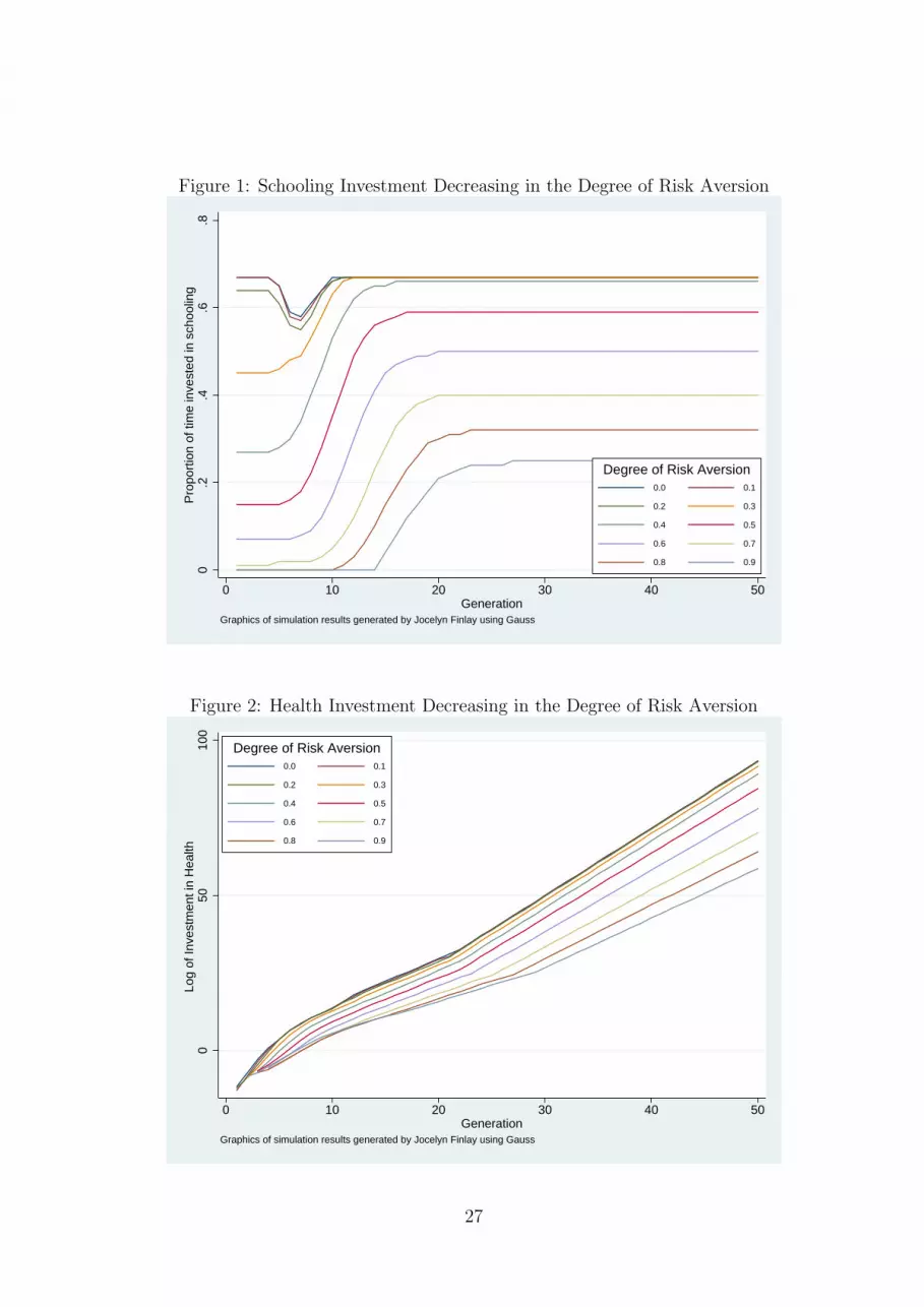
Figure 1: Schooling Investment Decreasing in the Degree of Risk Aversion0

.2.4

.6.8

Pro

port

ion

of ti

me

inve

sted

in s

choo

ling

0 10 20 30 40 50Generation

0.0 0.1

0.2 0.3

0.4 0.5

0.6 0.7

0.8 0.9

Degree of Risk Aversion

Graphics of simulation results generated by Jocelyn Finlay using Gauss

Figure 2: Health Investment Decreasing in the Degree of Risk Aversion

050

100

Log

of In

vest

men

t in

Hea

lth

0 10 20 30 40 50Generation

0.0 0.1

0.2 0.3

0.4 0.5

0.6 0.7

0.8 0.9

Degree of Risk Aversion

Graphics of simulation results generated by Jocelyn Finlay using Gauss

27

References

Blackburn, K. and Cipriani, G. P. (2002). A model of longevity, fertility and growth.Journal of Economic Dynamics and Control, 26(2):187–204.

Boucekkine, R., del Riob, F., and Licandro, O. (1999). Endogenous vs exogenouslydriven fluctuations in vintage capital models. Journal of Economic Theory, 88(1):161–187.

Chakraborty, S. (2004). Endogenous lifetime and economic growth. Journal of Economic

Theory, 116:119–137.

Chakraborty, S. and Das, M. (2005). Mortality, fertility and child labour. Economics

Letters, 86(2):273–278.

de la Croix, D. and Licandro, O. (1999). Life expectancy and endogenous growth.Economic Letters, 65:255–263.

Ehrlich, I. and Chuma, H. (1990). A model of the demand for longevity and the valueof life extenstion. The Journal of Political Economy, 98(4):761–782.

Ehrlich, I. and Lui, F. (1997). The problem of population and growth: A review ofthe literature from malthus to contemporary models of endogenous population andendogenous growth. Journal of Dynamics and Control, 21(1):205–242.

Grossman, M. (1972). On the concept of health capital and the demand for health. The

Journal of Political Economy, 80(2):223–255.

Kalemli-Ozcan, S. (2002). Does the mortality decline promote economic growth? Jour-

nal of Economic Growth, 7:411–439.

Kalemli-Ozcan, S., Ryder, H. E., and Weil, D. N. (2000). Mortality decline, human capi-tal investment, and economic growth. Journal of Development Economics, 62(1):1–23.

Rosenzweig, M. R. (1990). Population growth and human capital investments: Theoryand evidence. The Journal of Political Economy, 98(5.2):S38–S70.

Simon, C. P. and Blume, L. (1994). Mathematics for Economists. W.W. Norton andCompany.

Zhang, J., Zhang, J., and Lee, R. (2001). Mortality decline and long-run economicgrowth. Journal of Public Economics, 80(3):485–507.

28