Embed Size (px)
Citation preview
EMPIRICALECONOMICS( Springer-Verlag 1999
Empirical Economics (1999) 24:599±619
The role of labour demand elasticities in tax incidenceanalysis with heterogeneous labour*
Keshab Bhattarai1, John Whalley1,2,3
1 Department of Economics, University of Warwick, Coventry, CV4 7AL, UK(e-mail: [email protected])2 Department of Economics, University of Western Ontario, London Ontario, ONT N6A 5C2,Canada (e-mail: [email protected])3 National Bureau of Economic Research, 1050 Mass. Ave., Cambridge, MA 02138-5318, USA
First version received: March 1998/Final version received: April 1999
Abstract. Whether labour bears full burden of household level income andconsumption taxes ultimately depends on the degree of substitutability amongdi¨erent types of labour in production. We ®nd more variation in incidencepatterns across households with less than perfectly substitutable heteroge-neous labour than with perfectly substitutable homogeneous labour in pro-duction. This ®nding is based on results obtained from homogeneous andheterogeneous labour general equilibrium tax models calibrated to decile levelincome and consumption distribution data of UK households for the year1994. We use labour supply elasticities implied by the substitution elasticity inhouseholds' utility functions and derive labour demand elasticities from thesubstitution elasticity in the production function.
Key words: Elasticities, labour demand, labour supply, welfare, tax incidence,redistribution
JEL classi®cations: J20, H22, C68
1. Introduction
This paper builds on the observation that existing empirically based incidenceanalyses drawing either on shifting assumptions1, or on general equilibriumtax models treat labour as bearing the burden of its own income and payroll
* Bhattarai and Whalley acknowledge ®nancial support from the ESRC under an award for aproject on General Equilibrium Modelling of UK Policy Issues. We are thankful to Baldev Rajand two referees for comments on earlier versions of this paper.1 See Pechman and Okner (1974), and Gillespie (1965) as examples of this approach.

taxes2. The implicit assumption is that labour is a homogenous input which isperfectly mobile across industries and yields leisure which is consumed byhouseholds. A key set of parameters in incidence analyses conducted withthese models have been presumed to be the labour supply elasticities whichare the subject of some attention in both calibration and sensitivity analysis.Labour demand elasticities do not enter these analyses.
We argue that with homogeneous labour in production, the implicitlabour demand function facing each household is highly elastic since, if smallrelative to the aggregate, each is a price taker in labour markets. The impli-cation is that labour will bear most of the burden of its own labour taxes, in-dependently of labour supply elasticities used. Conventional sensitivity analy-sis on labour supply elasticities will show little variation in tax incidencepro®les. On the other hand, varying labour demand elasticities will allow forthe shifting of tax burdens to other groups or households.
We investigate di¨erences in model analyses of tax incidence using com-parable nested models in which labour is either homogenous or heterogeneousin production, so that labour demand elasticities also enter. Each model iscalibrated to a ten decile household data set containing data on consumption,taxes, and leisure for the UK for 1994. Labour supply elasticity calibration isbased on estimates from Killingsworth (1983), with the labour demand elas-ticity used in calibration in the heterogeneous labour model drawing on esti-mates from Hamermesh (1993). Signi®cant di¨erences in incidence pro®les arefound across the two models. The heterogeneous model shows signi®cantvariations in incidence pro®les as labour demand elasticities change, while thehomogeneous good model shows little sensitivity to labour supply elasticities.The implication drawn is the need to more carefully specify labour demandelasticities in tax incidence analyses.
II. Tax incidence models with heterogeneous and homogeneous labour supply
It seems clear that if labour supplied by household groups is heterogeneouswith imperfect substitutability in production across skill levels, then bothlabour demand and labour supply elasticities are needed in tax incidenceanalyses. If labour is treated as homogeneous across households, then if eachhousehold is small and a taker of wage rates, they implicitly face a perfectlyelastic labour demand function. In this case, varying the labour supply elas-ticity will not change the conclusion that labour bears the burden of their ownincome taxes, even if tax rates di¨er across households.
If the labour demand elasticity is less than in®nite, as labour supply func-tions shift due to household speci®c taxes, some of the burden of the taxis shifted elsewhere. The implication is that if heterogeneous labourmodels are used for tax incidence analysis and model parameters calibrated toboth labour demand and labour supply elasticities, tax incidence results can
2 See Shoven and Whalley (1972) for a simple 2 sector 2 household Harberger tax model; Piggottand Whalley (1985) for a 100 household model of the UK; Ballard, Fullerton, Shoven andWhalley (1985) for a 15 household model of the US; and Auerbach and Kotliko¨ (1987) for a 55overlapping generations dynamic structure applied to US data.
600 K. Bhattarai, J. Whalley

di¨er3 (and potentially sharply so) from those generated by the homogenouslabour model conventionally used.
We choose the household as the basic unit of tax incidence analysis notonly because consumption and labour-leisure choice decisions are made at thehousehold level, but also it is adapted in the data on income and consumptionused in the empirical analysis of incidence pro®les in the paper.
A heterogeneous labour household tax model
We consider an economy with households di¨erentiated according to theirskill levels, which, for our empirical application, we take to be collinear withincome ranges. Each household is endowed with a ®xed amount of time,which it can divide between leisure and work. A production function speci®eshow the various labour types combine to yield a single consumption good.Each of them buys the consumption good using income earned by selling itslabour on the market along with transfers received from government, e¨ec-tively buying back its leisure at its net of tax wage. Households maximizeutility by choosing bundles of consumption goods and leisure subject to theirbudget constraint. Hours of work (labour supply), consumption and leisureare thus obtained by solving each household's optimization problem.
Taxes distort the consumption-leisure choice of households. Tax rates arehousehold speci®c, and government budget balance holds with transfers thesole expenditure item. In empirical implementation, we use a single tax rate onlabour income for each household to represent the composite of income andpayroll taxes, and a composite indirect tax rate for each household which re-¯ects sales (VAT) and excise taxes. These latter rates di¨er by household dueto di¨ering consumption patterns in the data.
More speci®cally, we assume CES preferences for each household as
U h � �ahCh�s hÿ1�=sh � �1ÿ ah�Lh�shÿ1�=s h �s h=�s hÿ1� �1�
where U h is utility, ah is the share of income spent on the consumption good,
�1ÿ ah� is the share parameter on leisure, C h and Lh are consumption and
leisure respectively of household h, and sh is the elasticity of substitution be-tween consumption and leisure of household h.
The income for household h equals the time endowment valued at the netof tax wage plus transfers received from government, i.e.
I h � �1ÿ t hI �whL
h � RH h �2�
where I h is the full income of household h;wh is the gross of tax wage rate for
household h, and thI is the household speci®c income tax rate. L
his the time
endowment of household h to be divided between labour supply and leisure,and RH h are transfers received by household h.
3 One reason for the relative absence of heterogeneous labour models in empirically based generalequilibrium work is the seeming di½culty of solution in the non-nested production function case.We solve it using the new PATH algorithm developed and employed with GAMS by MichaelFerris (see Appendix 2 for details).
Labour demand elasticities in tax incidence analysis with heterogeneous labour 601

Maximization of utility (1), subject to (2), yields demand functions forconsumption and leisure for each household as,
C h � ah
P�1� thC�
� �sh
I h
ah�P�1� thC��1ÿs h � �1ÿ ah��wh�1ÿ th
I ��1ÿs h
" #�3�
Lh � �1ÿ ah�wh�1ÿ th
I �� �s h
I h
ah�P�1� thC��1ÿs h � �1ÿ ah��wh�1ÿ th
I ��1ÿs h
" #�4�
where wh is the gross of tax wage rate for labor of type h (supplied by house-
hold h), P is the price of the consumption good, and thC is the consumption (or
indirect) tax rate faced by household h. The budget balance condition forhouseholds implies that on the expenditure side
I h � P�1� thc �C h � wh�1ÿ th
l �Lh �5�
Each household supplies labour to the market which re¯ects the di¨erencebetween its labour endowment and its demand for leisure,
LS h � Lh ÿ Lh �6�
where LS h is labour supplied by household h. The economy wide laboursupply is the sum of labour supplied across the individual households. Inequilibrium, equation (6) is also the labour market clearing condition forlabour of type h.
In the model, we assume that the labour each household supplies is di¨er-entiated by skill level from the labour supplied by all other households, andwe represent this through a CES production technology for the single outputY in which all labour types enter, i.e.
Y � lX
h
dhLS h�spÿ1�=sp
!sp=�spÿ1��7�
where LS h is the input (labour supply) of type h; dh is the share parameter inproduction on each category of labour, l is a units term and sp is the elasticityof substitution among labour types in production.
Producers pay the gross of tax wage rate when hiring labour from eachhousehold, and households receive the net of income tax wage. For simplicity,we assume that only one consumption good is produced in this economy, andproducers maximize pro®t,
Q, given byY
� PY ÿX
h
whLS h �8�
where the P is price of the consumption good, and LS h is the labour input oftype h.
602 K. Bhattarai, J. Whalley
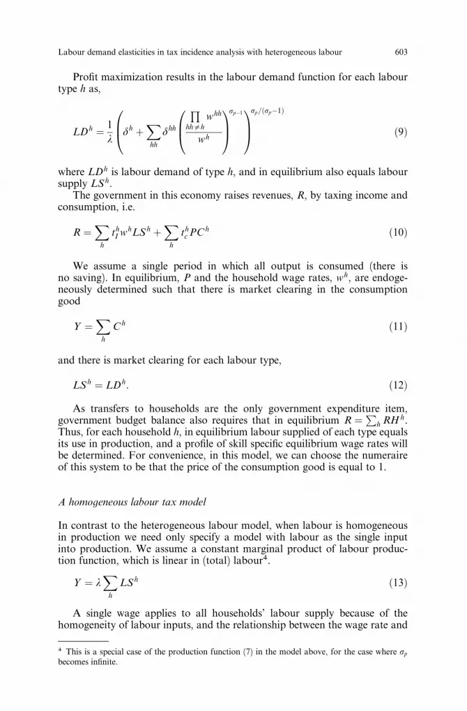
Pro®t maximization results in the labour demand function for each labourtype h as,
LDh � 1
ldh �
Xhh
dhh
Qhh0h
whh
wh
0B@1CA
spÿ10B@
1CAsp=�spÿ1�
�9�
where LDh is labour demand of type h, and in equilibrium also equals laboursupply LS h.
The government in this economy raises revenues, R, by taxing income andconsumption, i.e.
R �X
h
thI whLS h �
Xh
thc PC h �10�
We assume a single period in which all output is consumed (there isno saving). In equilibrium, P and the household wage rates, wh, are endoge-neously determined such that there is market clearing in the consumptiongood
Y �X
h
C h �11�
and there is market clearing for each labour type,
LS h � LDh: �12�
As transfers to households are the only government expenditure item,government budget balance also requires that in equilibrium R �Ph RH h.Thus, for each household h, in equilibrium labour supplied of each type equalsits use in production, and a pro®le of skill speci®c equilibrium wage rates willbe determined. For convenience, in this model, we can choose the numeraireof this system to be that the price of the consumption good is equal to 1.
A homogeneous labour tax model
In contrast to the heterogeneous labour model, when labour is homogeneousin production we need only specify a model with labour as the single inputinto production. We assume a constant marginal product of labour produc-tion function, which is linear in (total) labour4.
Y � lX
h
LS h �13�
A single wage applies to all households' labour supply because of thehomogeneity of labour inputs, and the relationship between the wage rate and
4 This is a special case of the production function (7) in the model above, for the case where sp
becomes in®nite.
Labour demand elasticities in tax incidence analysis with heterogeneous labour 603

the price of the consumption good is given by
P � w
l: �14�
Households still di¨er in their preferences as in (1), still face householdspeci®c income and consumption tax rates, but unlike in the heteogeneouslabour model face a common wage rate. Equilibrium in this case is given bymarket clearing for the single labour type in the model; with, in this case, onesingle wage rate endogenously determined.
This homogeneous labour model is thus a special case of the model pre-sented above, and nests into the more general heterogeneous labour model.
III. Implementation of homogeneous and heterogeneous labour tax incidencemodels
We perform tax incidence analyses using two models above by calibrating5each to a base year data set, specifying labour demand and labour supplyelasticity values, and performing counterfactual equilibrium analyses. Thebase case data set we use re¯ects the UK economy for the UK tax year 1994/956. We use data on incomes, taxes and bene®ts by household decile compiledby the UK Treasury and reported in the UK government statistical publica-tion Economic Trends (1996). This source reports data for non retired house-holds grouped by income7 decile, bene®ts received both in cash and in kind,and direct and indirect taxes paid by each household decile.
Base case data
For modelling purposes, we require a base case data set which is fully modeladmissible. This means that all variables which appear in each model shouldbe identi®ed in the data set, and all of the model equilibrium conditions needto be satis®ed. Among these are conditions that the value of consumptionacross households should equal the value of production (a zero pro®t condi-tion in production implies that income received from supplying labour equalsthe value of production). All households should also be represented by datawhich satis®es household budget balance, and government expenditures equalgovernment receipts (government budget balance).
The basic data we use, while having most of the information we need, isde®cient for our purposes in number of respects. Household leisure consump-
5 Calibration, here, denotes the exact calibration of each model to a model admissible data setwhich is constructed from unadjusted data from a variety of statistical sources. This is the sense ofcalibration discussed by Mansur and Whalley (1984) and di¨ers from the calibration proceduresused by real business cycles researchers (see Kydland and Prescott (1982)). In this latter work, noreadjustments are made to data, and model parameter values chosen by reference to literaturesources with a view to seeing how close model solution can be made to actual data. See alsoWatson (1993).6 April 5th 1994 to April 4th 1995. This is the year used in recording tax and household incomedata by the UK tax authorities.7 The income concept used in the published data is ``household equivalized disposable income''.
604 K. Bhattarai, J. Whalley

tion is not identi®ed. Government budget balance is violated in the data, sinceall taxes paid by households are identi®ed but only those government expendi-tures leading directly to direct household bene®ts (cash transfers, education,and health care appear, but defence, for instance, is missing). In the basicdata, government expenditures in aggregate are thus substantially less thantax revenues. Also, individual household budget constraints do not automati-cally hold.
A series of adjustments and modi®cations are therefore necessary to thebasic data set before it can be used for model calibration. These are set outin more detail in Appendix 1, but can be summarised as follows. We scale thein kind portion of government bene®ts for each decile such that governmentexpenditures equal taxes collected. Transfers received by each decile in themodel are thus the sum of cash and in kind bene®ts provided by government.We use wage rate data by household and UK time use survey data to con-struct data on the value of leisure time by household for each decile, valuingtime at the net of tax wage. We then make further adjustments to ensure fullconsistency of the data set to the model, including modi®cations such thathousehold budget constraints hold in the data.
The resulting model admissible data set across ten UK households is dis-played in Table 1. In this data, gross income is concentrated in the higherdeciles, with transfers concentrated in the lower deciles. The household pro®leof leisure consumption re¯ects the interaction of hours (falling as we move tothe higher income ranges) and wage rates at which leisure is valued (rising byincome range). The two tax rate pro®les are for average (not marginal) taxrates. For income taxes they rise by income range, but not by as much asmight be thought from an examination of tax rate schedules. This is becauseof income tax allowances, caps on social (national) insurance contributions,untaxed housing capital income, and UK tax shelters (pensions, savings intax sheltered vehicles), all of which have a major in¯uence on the average taxrate pro®le. The indirect tax rates fall by income range due to the in¯uence ofexcise taxes, particularly on petrol, but also on drink, both of which are aconsiderably larger fraction of expenditures for the poor than the rich.
Using information on elasticities, we calibrate both the homogeneousand heterogeneous labour models to this benchmark equilibrium data set. Todo this, we ®rst take the benchmark data set from Table 1 in value terms,and decompose it into separate price and quantity observations. FollowingHarberger (1962), and Shoven and Whalley (1992) we choose units both forlabour by type, and for consumption, as those amounts which sell for £1 in thebase case equilibrium. Using this convention all prices and wages are one inthe base case, and all quantities are as given by the base case observations inTable 1. The calibrated versions of each model replicate this base case data asa model solution.
Elasticities
The elasticity parameters needed for the models are the ten household speci®csubstitution elasticities in consumption (CES preferences) which are used inboth models, and the substitution elasticity in production (in the CES pro-duction function) in the heterogeneous labour model. Direct estimates of theseelasticities are not available in the literature. Elasticities in consumption over
Labour demand elasticities in tax incidence analysis with heterogeneous labour 605

Tab
le1
.M
od
elad
mis
sib
leh
ou
seh
old
data
set
by
dec
iles
of
inco
me
for
no
n-r
etir
edh
ou
seh
old
s,U
K1994/
958
Ho
use
ho
lds9
(a)
(b)
(c)
(d)
(e)
(f)
(g)
(h)
Gro
sso
fta
xla
bo
rin
com
ea
Tra
nsf
ersa
Inco
me
an
do
ther
dir
ect
taxes
paid
a,10
Ind
irec
tta
xes
paid
a,11
Co
nsu
mp
tio
ngro
sso
fin
dir
ect
taxes
a,12
Lei
sure
a,13
Inco
me
tax
rate
14
Ind
irec
tta
xra
te15
Dec
ile
1(P
oo
r)3079
14638
930
2139
16787
14491
0.0
50.1
3
Dec
ile
25918
12880
1194
2183
17604
17085
0.0
60.1
2
Dec
ile
311021
11040
1880
2759
20181
14076
0.0
90.1
4
Dec
ile
416111
9867
2815
3213
23163
11934
0.1
10.1
4
Dec
ile
521184
8559
3831
3572
25912
10895
0.1
30.1
4
Dec
ile
626161
8205
4745
3957
29621
10455
0.1
40.1
3
Dec
ile
730140
6858
5531
4266
31467
12293
0.1
50.1
4
Dec
ile
834614
5645
6576
4362
33683
13895
0.1
60.1
3
Dec
ile
941918
5166
8175
4537
38909
15449
0.1
70.1
2
Dec
ile
10
(Ric
h)
71147
4440
15082
5551
60505
6871
0.2
00.0
9
No
tes:
All
®gu
res
inth
ista
ble
no
ted
wit
hsu
per
scri
pt
aare
mil
lio
ns
of
£,
for
the
tax
yea
r1994/9
5.
606 K. Bhattarai, J. Whalley

goods and leisure must be inferred from literature estimates of labour supplyelasticities. Elasticities of substitution in production between labour typesmust be inferred from literature estimates of labour demand elasticities forvarious types of labour.
From the production function (7), we can use the ®rst order conditionsfor pro®t maximization and the derived labour demand function (9). The
elasticity of labour demand in production is given by ehLD �
qLDh
qwh
wh
LDhand
di¨erentiating (9) w.r.t. wh gives
ehLD �
ÿsp
Phh0h
dhh Qh0h
whh
!spÿ1
whs
pÿ1dh �P
hh
dhh
Qh0h
whh
wh
0B@1CA
spÿ1264375
�15�
In the base case all gross of tax wage rates are unity, and if, in addition,household labour shares are small, eh
LD e¨ectively collapses to ÿsp. We choosethe elasticity of substitution between labour types in production which, from(15), we can calibrate numerically to values of labour demand elasticitiesfound in the literature (Hamermesh (1993)), and use other sensitivity casesdiscussed below to re¯ect ranges around a central case value. As there are tenhousehold demand elasticities in the model around the base case equilibrium,and only one free parameter, sp, in calibration we choose sp such that elas-ticities across households (which do not vary that much) are within a desiredrange.
Labour supply elasticities, in contrast, are found using the leisure demandfunction (4). Point estimates of labour supply elasticities for each household inthe neighbourhood of the benchmark equilibrium can be generated by notingthat
qLS h
qwh
wh
LS h� qLS h
qLh
qLh
qwh
wh
Lh
Lh
LS h� �ÿ1�hLE
Lh
LS h�16�
We use the leisure demand function (4) to derive the leisure demand elasticity,hLE which is given by
hhLE � ÿ sh � �sh ÿ 1��1ÿ ah�wh1ÿs h
ahP1ÿsh � �1ÿ ah�wh1ÿs h
!�17�
8 See Appendix 1 for more detail.9 These households are grouped by ``original'' household income as in Economic Trends (1995).Original income is pre tax/pre transfer income.10 This includes all social insurance contributions.11 This includes VAT and all excises (especially on petrol, tobacco, drink).12 This is gross of indirect taxes.13 This is from UK time use survey data; leisure time is valued at the net of tax wage.14 This includes income tax and social insurance contributions.15 This includes the VAT plus speci®c excise taxes.
Labour demand elasticities in tax incidence analysis with heterogeneous labour 607
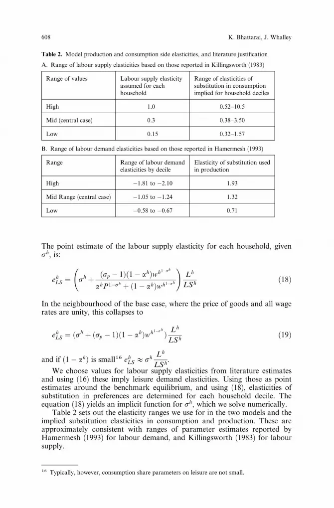
The point estimate of the labour supply elasticity for each household, givensh, is:
ehLS � sh � �sp ÿ 1��1ÿ ah�wh1ÿs h
ahP1ÿs h � �1ÿ ah�wh1ÿs h
!Lh
LS h�18�
In the neighbourhood of the base case, where the price of goods and all wagerates are unity, this collapses to
ehLS � �sh � �sp ÿ 1��1ÿ ah�wh1ÿs h � Lh
LS h�19�
and if �1ÿ ah� is small16 ehLS A sh Lh
LS h.
We choose values for labour supply elasticities from literature estimatesand using (16) these imply leisure demand elasticities. Using those as pointestimates around the benchmark equilibrium, and using (18), elasticities ofsubstitution in preferences are determined for each household decile. Theequation (18) yields an implicit function for sh, which we solve numerically.
Table 2 sets out the elasticity ranges we use for in the two models and theimplied substitution elasticities in consumption and production. These areapproximately consistent with ranges of parameter estimates reported byHamermesh (1993) for labour demand, and Killingsworth (1983) for laboursupply.
16 Typically, however, consumption share parameters on leisure are not small.
Table 2. Model production and consumption side elasticities, and literature justi®cation
A. Range of labour supply elasticities based on those reported in Killingsworth (1983)
Range of values Labour supply elasticityassumed for eachhousehold
Range of elasticities ofsubstitution in consumptionimplied for household deciles
High 1.0 0.52±10.5
Mid (central case) 0.3 0.38±3.50
Low 0.15 0.32±1.57
B. Range of labour demand elasticities based on those reported in Hamermesh (1993)
Range Range of labour demandelasticities by decile
Elasticity of substitution usedin production
High ÿ1.81 to ÿ2.10 1.93
Mid Range (central case) ÿ1.05 to ÿ1.24 1.32
Low ÿ0.58 to ÿ0.67 0.71
608 K. Bhattarai, J. Whalley
In the model, there are 10 separate labour demand elasticities for eachlabour type. These elasticities vary, and hence we calibrate the model to pointestimates of these elasticities in the neighbourhood of the benchmark equilib-rium. In addition, there is only one free model parameter (the elasticity ofsubstitution among labour types in production) so that exact calibration foreach household type labour demand elasticity is not feasible. We thus vary thesingle production side elasticity until the household labour demand elasticities,which are similar across households, are within the desired range.
IV. Results
We have used the heterogeneous and homogeneous labour models describedabove and calibrated to UK data for the 1995/96 tax year to investigatethe behaviour of tax incidence results across models. We do this for di¨erenttax experiments, di¨erent labour supply elasticity (consumption/leisure sub-stitution) con®gurations, freezing the labour demand elasticity speci®cation;and for di¨erent labour demand elasticity speci®cations, freezing the laboursupply elasticity speci®cation.
The essence of tax policy analysis lies in comparing welfare changes be-tween benchmark and counterfactual equilibria. How much a typical house-hold has gained or lost because of changes in policy in money metric terms, orhow much money is required to bring him/her back to their original welfarecan be measured at either original or new prices. The Hicksian equivalentvariation �EV� is a money metric measure of the welfare change betweenbenchmark and counterfactual scenarios using benchmark (old) prices. It isthe di¨erence in money metric utility at old prices corresponding to bench-mark and counterfactual model solutions; i.e.
EV � E�U N ;P0� ÿ E�U 0;P0� �20�
where superscripts N and O represent new and old values for the variable onwhich they appear, U is the utility, and E is the expenditure function whichdepends on prices and utility level.
If utility functions are of the linear homogeneous type, then original andnew equilibria can be thought of in terms of a radial expansion of the utilitysurface. In this case the change in money metric welfare between benchmarkand counterfactual solutions of the model is proportional to the change inutility or the percentage change along the radial projection between the twoconsumption points.
EV � U N ÿU 0
U 0I 0 �21�
where N and O represent new and old values of the variables as before, and Irepresents the income.
In Table 3 we report tax incidence calculations for a case where we replacethe pre existing pattern of labour income tax rates by household by a yieldpreserving uniform rate income tax across households. We consider caseswhere we freeze labour supply elasticities ®rst at 0.3, and then at 1.0, and varythe ranges we use for labour demand elasticities in the heterogeneous labour
Labour demand elasticities in tax incidence analysis with heterogeneous labour 609

Table 3. Comparing homogeneous and heterogeneous labour models
Speci®cation. Experiment: replacing existing labour income taxes by yield preserving uniform rate. Elasticity speci®cation: Labour supply elasticity 0.3 and 1.0 in two cases, labour
demand elasticities range from ÿ0.58 to ÿ2.1.
Results:Welfare gains/losses by decile in terms of Hicksian EV as a fraction of base income(with low labour supply elasticity (0.3))
Decile HomogeneousLabour model
Heterogeneous Labour modelLabour demand elasticities rangesas speci®ed in Table 2
Low Middle High(ÿ0.58 to ÿ0.67) (ÿ1.05 to ÿ1.24) (ÿ1.8 to ÿ2.1)
1 poor ÿ0.0581 ÿ0.0134 ÿ0.0501 ÿ0.0591
2 ÿ0.0485 ÿ0.0173 ÿ0.0434 ÿ0.0493
3 ÿ0.0424 ÿ0.0334 ÿ0.0401 ÿ0.0430
4 ÿ0.0299 ÿ0.0306 ÿ0.0296 ÿ0.0303
5 ÿ0.0143 ÿ0.0211 ÿ0.0153 ÿ0.0146
6 ÿ0.0064 ÿ0.0159 ÿ0.0078 ÿ0.0066
7 0.0044 ÿ0.0059 0.0028 0.0042
8 0.0173 0.0060 0.0155 0.0171
9 0.0272 0.0154 0.0253 0.0270
10 rich 0.0670 0.0562 0.0660 0.0666
Results:Welfare gains/losses by decile in terms of Hicksian EV as a fraction of base income(with high labour supply elasticity (1.0))
Decile HomogeneousLabour model
Heterogeneous Labour modelLabour demand elasticities rangesas speci®ed in Table 2
Low Middle High(ÿ0.58 to ÿ0.67) (ÿ1.05 to ÿ1.24) (ÿ1.8 to ÿ2.1)
1 poor ÿ0.0577 ÿ0.0376 ÿ0.0503 ÿ0.0585
2 ÿ0.0481 ÿ0.0709 ÿ0.0442 ÿ0.0486
3 ÿ0.042 ÿ0.2191 ÿ0.0420 ÿ0.0421
4 ÿ0.0295 ÿ0.2944 ÿ0.0312 ÿ0.0294
5 ÿ0.014 ÿ0.3300 ÿ0.0150 ÿ0.0140
6 ÿ0.0061 ÿ0.1114 ÿ0.0060 ÿ0.0061
7 0.0047 0.3908 0.0066 0.0045
8 0.0176 0.0739 0.0221 0.0172
9 0.0276 0.1476 0.0349 0.0270
10 rich 0.0676 ÿ0.0025 0.0737 0.0670
model. We compare model results across the homogeneous labour model andthe various speci®cations of the heterogeneous model for these labour supplyelasticities.
Results in Table 3 show the redistribution across households in thesecases. Richer households gain because their taxes fall, and poorer householdslose since the replacement tax is at a uniform rate and their taxes rise. How-ever, there is considerable variation in the redistribution pro®le across thetwo elasticity cases for the heterogeneous labour model. Considerably moreredistribution occurs in the high elasticity case since wage rate changes in re-sponse to the tax replacement are small; low income households bear most ofthe burden of their higher taxes, and high income households gain by mostof their tax saving.
As one moves across labour demand elasticity speci®cations the redis-tributive e¨ects from the tax changes become larger, with wage changes lesspronounced. Labour demand elasticities have a signi®cant in¯uence on theperceived tax incidence e¨ects from the tax replacement. From various sensi-tivity analyses, we ®nd that as labour demand elasticities increase, the incometax incidence pro®le in the heterogeneous labour model approaches that of thehomogeneous labour model for any given value of the labour supply elasticity.
In Table 4 we explore how the model comparisons change as we varylabour supply elasticities. We consider the same tax replacement, i.e. replacingthe existing pro®le of income tax rates by a uniform rate income tax acrosshouseholds, but only consider the mid range speci®cation of labour demandelasticities, changing labour supply elasticities in both homogeneous and het-erogeneous labour models.
Results in Table 4 show that the incidence pro®le changes relatively littlebetween heterogeneous and homogeneous labour models as labour supplyelasticities increase. The low income households lose about 5±6 percent ofthe base year income in both heterogeneous and homogeneous labour modelsirrespective of di¨erent values of labour supply elasticities. For middle rangevalues of labour demand elasticities (irrespective to any speci®c value oflabour supply elasticity), income tax incidence pro®les of replacing base caselabour income taxes by yield preserving labour income tax rates becomecomparable across two models.
As ®nal sets of results in Table 5 we present incidence results for threedi¨erent yield preserving tax changes; the ®rst one only involves income taxes,the second one involves income and sales taxes, and the last one involves onlysales taxes. We use a 0.3 labour supply elasticity and mid range labour de-mand elasticities.
In both the income tax case and the combined income and sales tax casewe ®nd low income households lose and high incomes households gain whenbase case taxes are replaced by yield preserving tax rates, but the pattern ofgains is di¨erent in the upper tail of the distribution across heterogeneous andhomogeneous models.
V. Conclusions
In this paper we analyze how labour demand elasticities, long neglected inempirically based tax incidence analysis, a¨ect incidence conclusions. Using adata set for the UK for tax year 1994/95 covering 10 household deciles we
Labour demand elasticities in tax incidence analysis with heterogeneous labour 611

Table
4.
Imp
act
so
fvary
ing
lab
ou
rsu
pp
lyel
ast
icit
ies
on
inci
den
cep
ro®
leco
mp
ari
son
s
Sp
eci®
cati
on
.E
xper
imen
t:re
pla
cin
gex
isti
ng
lab
ou
rin
com
eta
xes
by
yie
ldp
rese
rvin
gu
nif
orm
rate
.E
last
icit
ysp
eci®
cati
on
:Lab
ou
rsu
pp
lyel
ast
icit
y0.3
,mid
ran
ge
dem
an
del
ast
icit
ies
inth
eh
eter
ogen
eou
sla
bo
ur
mo
del
.
Res
ult
s:W
elfa
regain
s/lo
sses
by
ho
use
ho
lds,
Hic
ksi
an
EV
as
afr
act
ion
of
base
inco
me
Dec
ile
Lab
ou
rsu
pp
lyel
ast
icit
yL
ab
ou
rsu
pp
lyel
ast
icit
yL
abo
ur
sup
ply
elast
icit
y(0
.15)
(0.3
)(1
.0)
Ho
mo
gen
eou
sla
bo
ur
Mo
del
Het
ero
gen
eou
sla
bo
ur
mo
del
Ho
mo
gen
eou
sla
bo
ur
Mo
del
Het
ero
gen
eou
sla
bo
ur
mo
del
Ho
mo
gen
eou
sla
bo
ur
Mo
del
Het
ero
gen
eou
sla
bo
ur
mo
del
1p
oo
rÿ0
.0582
ÿ0.0
500
ÿ0.0
581
ÿ0.0
501
ÿ0.0
577
ÿ0.0
585
2ÿ0
.0486
ÿ0.0
431
ÿ0.0
485
ÿ0.0
434
ÿ0.0
481
ÿ0.0
486
3ÿ0
.0426
ÿ0.0
395
ÿ0.0
424
ÿ0.0
401
ÿ0.0
420
ÿ0.0
421
4ÿ0
.0300
ÿ0.0
290
ÿ0.0
299
ÿ0.0
296
ÿ0.0
295
ÿ0.0
294
5ÿ0
.0144
ÿ0.0
149
ÿ0.0
143
ÿ0.0
153
ÿ0.0
140
ÿ0.0
140
6ÿ0
.0065
ÿ0.0
075
ÿ0.0
064
ÿ0.0
078
ÿ0.0
061
ÿ0.0
061
70.0
043
0.0
028
0.0
044
0.0
028
0.0
047
0.0
045
80.0
172
0.0
150
0.0
173
0.0
155
0.0
176
0.0
172
90.0
270
0.0
244
0.0
272
0.0
253
0.0
276
0.0
270
10
rich
0.0
668
0.0
650
0.0
670
0.0
660
0.0
676
0.0
670
612 K. Bhattarai, J. Whalley

Table
5.
Inci
den
ceco
mp
ari
son
for
di¨
eren
tta
xch
an
ges
for
the
het
ero
gen
eou
sla
bo
ur
an
dh
om
ogen
eou
sla
bo
ur
mo
del
s
Sp
eci®
cati
on
.L
abo
ur
sup
ply
elast
icit
yse
tat
0.3
.L
abo
ur
dem
an
del
ast
icit
ies
set
at
mid
ran
ge
valu
esin
the
het
ero
gen
eou
sla
bo
ur
mo
del
.
Res
ult
s:W
elfa
regain
s/lo
sses
by
ho
use
ho
lds,
Hic
ksi
an
EV
as
afr
act
ion
of
base
inco
me
On
lyin
com
eta
xIn
com
ean
dsa
les
tax
On
lysa
les
tax
Dec
ile
Ho
mo
gen
eou
sla
bo
ur
Mo
del
Het
ero
gen
eou
sla
bo
ur
mo
del
Ho
mo
gen
eou
sla
bo
ur
Mo
del
Het
ero
gen
eou
sla
bo
ur
mo
del
Ho
mo
gen
eou
sla
bo
ur
Mo
del
Het
ero
gen
eou
sla
bo
ur
mo
del
1p
oo
rÿ0
.0581
ÿ0.0
501
ÿ0.0
551
ÿ0.0
489
0.0
029
0.0
026
2ÿ0
.0485
ÿ0.0
434
ÿ0.0
478
ÿ0.0
434
0.0
006
0.0
006
3ÿ0
.0424
ÿ0.0
401
ÿ0.0
324
ÿ0.0
307
0.0
101
0.0
096
4ÿ0
.0299
ÿ0.0
296
ÿ0.0
167
ÿ0.0
166
0.0
132
0.0
129
5ÿ0
.0143
ÿ0.0
153
ÿ0.0
008
ÿ0.0
014
0.0
134
0.0
134
6ÿ0
.0064
ÿ0.0
078
0.0
039
0.0
032
0.0
100
0.0
102
70.0
044
0.0
028
0.0
164
0.0
155
0.0
116
0.0
118
80.0
173
0.0
155
0.0
235
0.0
225
0.0
058
0.0
061
90.0
272
0.0
253
0.0
217
0.0
208
ÿ0.0
057
ÿ0.0
054
10
rich
0.0
670
0.0
660
0.0
314
0.0
307
ÿ0.0
337
ÿ0.0
338
Labour demand elasticities in tax incidence analysis with heterogeneous labour 613

use two models to evaluate the incidence e¨ect of various tax changes, spe-cially the replacement of the existing pattern of income tax rates by a uniformrate yield preserving alternative. We consider two models, one with labourheterogeneous in production, i.e. 10 di¨erent labour types (one for each dec-ile) in production; and the other with labour homogeneous across householdsi.e. only one type of labour in production. The substitution elasticity amonglabour types in production determines labour demand elasticities. Our resultssuggest that labour demand elasticities do indeed matter for tax incidenceconclusions.
Appendix 1. Data sources
This appendix presents details on various data sources and adjustments thatunderlie Table 1. The main data sources are Table 3A (Appendix 1) ofEconomic Trends, 1995/96, p. 36, New Earnings Survey 1995 and Time UseSurvey reported in Dex et al. (1995).
The gross income in column (a) of Table 1 in the text comprises originalincome and direct taxes (see Table A1 below). Original income includes wagesand salaries, imputed income from bene®ts in kind, self-employment income,occupational pensions, annuities and other income. Direct taxes includeemployees' national insurance (NI) contributions. The household averagedirect tax rate to be income and other taxes divided by gross of tax incomeplus transfers.
The UK Economic Trends data distinguishes ®ve di¨erent concepts of in-come: original, income, gross income, disposable income, post tax incomeand ®nal income. Original income plus cash bene®ts equal gross income,disposable income is gross income minus direct taxes. Post tax income is dis-posable income minus indirect taxes Final income equals post tax income plusin kind bene®ts.
The transfers presented in column (b) of Table 1 in the text include directcash bene®ts, in kind transfers, and consumption of publicly provided goodsservices such as national defence. Direct cash bene®ts consist of retirementpension contributions, unemployment bene®t, invalidity pension and allow-ance, sickness and industrial injury bene®t, widow's bene®ts, and statutorymaternity pay/allowance. Non-contributory bene®ts include income support,child bene®t, housing bene®t, invalid care allowances, attendance allowance,disability living allowance, industrial injury disablement bene®t, studentmaintenance awards, government training schemes, family credit and othernon-contributory bene®ts. Bene®ts in kind consist of education, nationalhealth service, housing subsidy, rail travel subsidy, bus travel subsidy, schoolmeals and welfare milk.
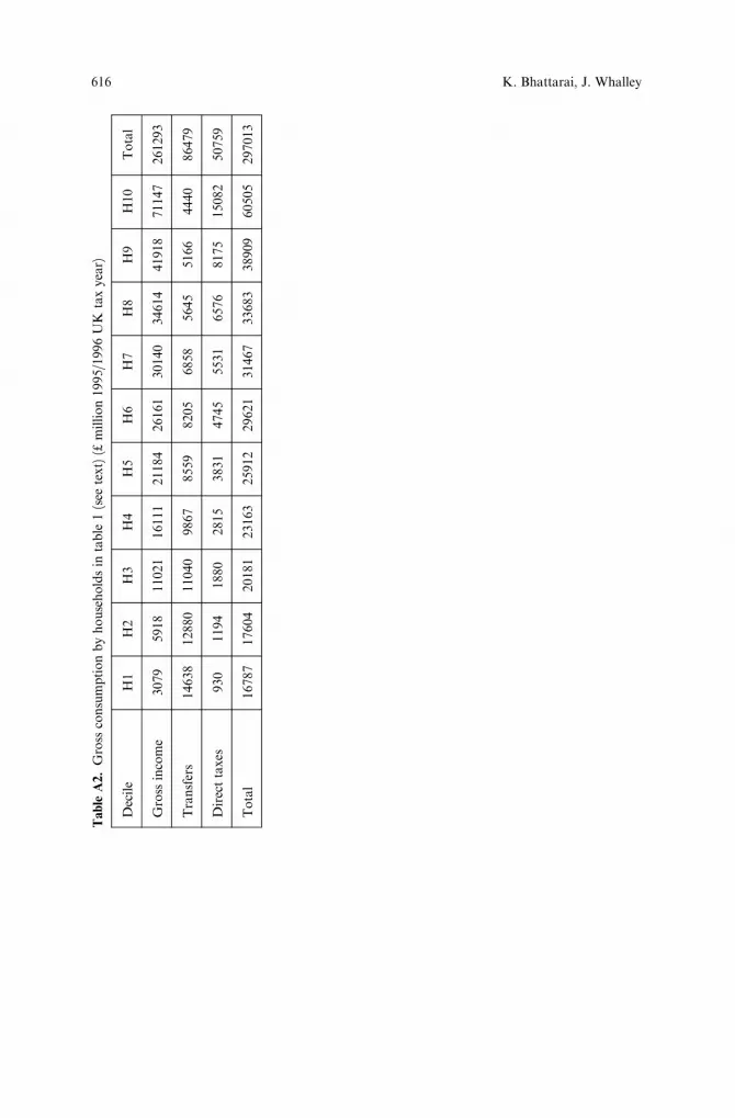
The gross consumption of each household, included in column (e) ofTable 1 in the text, is derived by adding cash, in kind and non-contributorybene®ts to original income and subtracting the direct and indirect taxes paidby the household. Consumption thus is gross of indirect taxes that includetaxes on ®nal goods and services, VAT, duty on tobacco, beer and cider,wines and spirits, hydrocarbon oils, vehicle excise duty, TV licences, stampduty on house purchase, customs duties, betting taxes, fossil fuel levy, andCamelot national lottery fund. It also includes intermediate taxes such as
614 K. Bhattarai, J. Whalley
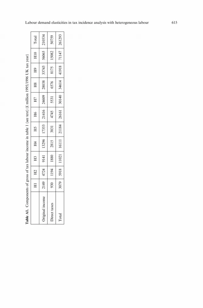
Ta
ble
A1.
Co
mp
on
ents
of
gro
sso
fta
xla
bo
ur
inco
me
inta
ble
1(s
eete
xt)
(£m
illi
on
1995/
1996
UK
tax
yea
r)
H1
H2
H3
H4
H5
H6
H7
H8
H9
H10
To
tal
Ori
gin
al
inco
me
2149
4724
9141
13296
17353
21416
24609
28038
33743
56065
21053
4
Dir
ect
taxes
930
1194
1880
2815
3831
4745
553
16576
8175
15082
50759
To
tal
3079
5918
11021
16111
21184
26161
3014
034614
41918
71147
26129
3
Labour demand elasticities in tax incidence analysis with heterogeneous labour 615
Tab
leA
2.
Gro
ssco
nsu
mp
tio
nb
yh
ou
seh
old
sin
tab
le1
(see
text)
(£m
illi
on
1995/1
996
UK
tax
yea
r)
Dec
ile
H1
H2
H3
H4
H5
H6
H7
H8
H9
H10
To
tal
Gro
ssin
com
e3079
5918
11021
16111
21184
26161
30140
34614
41918
71147
26129
3
Tra
nsf
ers
14638
12880
11040
9867
8559
8205
6858
5645
5166
4440
86479
Dir
ect
taxes
930
1194
1880
2815
3831
4745
5531
6576
8175
15082
50759
To
tal
16787
17604
20181
23163
25912
29621
31467
33683
38909
60505
29701
3
616 K. Bhattarai, J. Whalley

Ta
ble
A3
.T
he
valu
eo
fle
isu
reco
nsu
mp
tio
nb
yh
ou
seh
old
sin
tab
le1
(see
text)
H1
H2
H3
H4
H5
H6
H7
H8
H9
H10
To
tal
Ear
nin
gs/
wee
k/
ho
use
ho
lds
(£)
160
210
223
243
272
306
35
5403
473
543
319
Wo
rkin
gw
eek
s13
23
41
55
64
70
69
70
71
91
57
Lei
sure
wee
ks
91
81
63
49
40
34
35
34
33
13
47
Va
lue
of
leis
ure
by
ho
use
ho
ld(£
mil
lio
n)
14491
17085
14076
11934
10895
10455
122
9313895
15449
6871
12744
4
Labour demand elasticities in tax incidence analysis with heterogeneous labour 617

commercial and industrial rates, employer's NI contributions, duty on hy-drocarbon oils, vehicle excise and other duties.
The value of leisure reported in Table 1 in the text has been obtained bymultiplying nonworking weeks by the weekly earnings rate. The number ofnon-working weeks is the di¨erence between the working weeks and 104weeks. The total working week represents the total labour endowment perhousehold with two working members. Earnings per week for top and bottomdeciles, and ®rst and third quartiles are taken from the New Earnings Survey1995. These are interpolated for other deciles. Working weeks are derived bydividing the original income by the weekly earnings.
Appendix 2. Solution method of the model
Both homogeneous and heterogeneous labour models discussed in this paperare set up as a mixed complementarity problems and solved in GAMS soft-ware using the PATH solver.
Dirkse and Ferris (1995) state the basic idea behind the PATH solver interms of a ``zero ®nding problem''. For any function F : Rn ! Rn with lowerbound ÿyU l and an upper boundU uU�y the problem is to ®nd z A Rn
such that
either zi � li and Fi�z�V 0
or zi � li and Fi�z�U 0
or li U zi U uI and Fi�z� � 0
PATH constructs a solution using a damped Newton method such as
0 � FB�x� � Fx�B� � �xÿ xB�where xB is the Euclidean projection of x onto the Box B :� �l; u�. A vectorx solves this nonlinear equation only if z � xB solves the MCP. A moredetailed explanation of this algorithm is beyond the scope of this paper,many technical papers on the topic are available in Ferris's homepage:http://www.cs.wisc.edu/�ferris/.
GAMS syntax (Brook, Kendrick and Meeraus (1992)) permits us to gen-erate a non linear mixed complemetarity model by declaring and assigningsets, data, parameters, variables, equations in the model. PATH is invoked bythe ``OPTION MCP � PATH'' statement in the GAMS code and a commandline ``solve hmodel namei using MCP'' instructs GAMS to solve the modelusing the PATH solver. We use batch ®les to compute incidence pro®lesacross various scenarios for di¨erent values of elasticities and tax rates forhouseholds.
References
Auerbach AJ, Kotliko¨ LJ (1987) Dynamic ®scal policy. Cambridge University PressBallard CL, Fullerton D, Shoven JB, Whalley J (1985) A general equilibrium model for tax
policy evaluation. University of Chicago Press, Chicago
618 K. Bhattarai, J. Whalley
Dirkse SP, Ferris MC (1995) CCPLIB: A collection of nonlinear mixed complementarityproblems. Optimization Methods and Software 5:319±345
Dex S, Clark A, Taylor M (1995) Household labour supply employment. Department ResearchSeries No. 43, ESRC Center for Micro-social Change, University of Essex
Economic Trends (1996) O½ce of National Statistics. LondonGillespie W (1965) E¨ect of public expenditure in distribution of income. In Musgrave R (ed.)
Essays in ®scal federalism, Brookings, Washington DC, pp. 122±186Hamermesh DS (1993) Labour demand. Princeton University Press, New JerseyHarberger AC (1962) The incidence of the corporation income tax. Journal of Political Economy
70:215±40Killingsworth M (1983) Labour supply. Cambridge University PressKydland FE, Prescott EC (1982) Time to build and aggregate ¯uctuations. Econometrica
50:1345±70Mansur A, Whalley J (1986) Numerical speci®cation of applied general equilibrium models:
Estimation, calibration and data. In: Scarf HE, Shoven JB (eds.) Applied general equilibriumanalysis, Cambridge University Press
Pechman JA, Okner BA (1974) Who bears the burden of taxes? Brookings Institute, WashingtonD.C.
Piggott J, Whalley J (1985) UK tax policy and applied general equilibrium analysis. CambridgeUniversity Press
Shoven JB, Whalley J (1992) Applying general equilibrium. Cambridge University PressShoven JB, Whalley J (1972) A general equilibrium calculation of the e¨ects of di¨erential taxa-
tion of income from capital in the U.S.. Journal of Public Economics 1:281±322Watson MW (1993) Measures of ®t for calibrated models. Journal of Political Economy
101:1011±1041
Labour demand elasticities in tax incidence analysis with heterogeneous labour 619


